Possible representation errors in inversions of satellite CO2 retrievals

Katherine D. Corbin,1 A. Scott Denning,1 Lixin Lu,1 Jih-Wang Wang,1,2 and Ian T. Baker1

Received 28 March 2007; revised 20 July 2007; accepted 2 October 2007; published 16 January 2008.

[1] Owing to global spatial sampling and sheer data volume, satellite CO2 concentrationscan be used in inverse models to enhance our understanding of the carbon cycle. Usingcolumn measurements to represent a transport model grid column may introduce spatial,local clear-sky, and temporal sampling errors into inversions: the footprint is smaller than agrid cell, total column concentrations are only retrieved in clear skies, and the mixingratios are only sampled at one time. To investigate these errors, we used a coupledecosystem-atmosphere cloud-resolving model to create CO2 fields over fine (�1�� 1�) andcoarse (�4� � 4�) grid columns from 1 km2 and 25 km2 pixels that utilized explicitmicrophysics. We performed two simulations in August 2001: one in central NorthAmerica and one in the Brazilian Amazon. Differences between satellite and grid columnconcentrations were calculated by subtracting the domain mean column concentration from10-km-wide simulated satellite measurements. Spatial and local clear-sky errors wereless than 0.5 ppm for the fine grid column; however, these errors became large and biasedover the coarse grid column in North America. To avoid these errors, transport modelsshould be run at high resolution. Using satellite measurements to represent bimonthlyaverages created large (>1 ppm) errors for all cases. The errors were negatively biased(approximately �0.4 ppm) in the North American simulation, indicating that inversemodels cannot use satellite measurements to represent temporal averages. Simulatedrepresentation errors did not arise because of differences in ecosystem metabolism incloudy versus sunny conditions; rather, they reflected large-scale CO2 gradients inmidlatitudes that were organized along frontal boundaries and masked under regional cloudcover. Such boundaries were not found in the dry-season tropical simulation presentedhere and may be less prevalent in the tropics in general. To avoid incurring errors,inversions must accurately model synoptic-scale atmospheric transport and CO2

concentrations must be assimilated at the time and place observed.

Citation: Corbin, K. D., A. S. Denning, L. Lu, J.-W. Wang, and I. T. Baker (2008), Possible representation errors in inversions of

satellite CO2 retrievals, J. Geophys. Res., 113, D02301, doi:10.1029/2007JD008716.

1. Introduction

[2] Variations of atmospheric CO2 concentrations containinformation about sources and sinks which air interacts withas it is transported from place to place. Using atmospherictracer transport models, inverse modelers can quantitativelyestimate the strengths and spatial distribution of sources andsinks around the world from concentration data [Gurney etal., 2002; Rodenbeck et al., 2003; Baker et al., 2006]. Theseflux estimates are still highly uncertain in many regionsbecause of sparse data coverage [Gurney et al., 2003].Satellite CO2 measurements have the potential to helpinverse modeling studies by improving the data constraintbecause of their global spatial sampling and sheer data

volume. Previous studies have indicated that using spatiallyresolved, global measurements of the column-integrated dryair mole fraction (XCO2) with precisions of �1 ppm willreduce the uncertainties in regional estimates of sources andsinks of atmospheric CO2 [Rayner and O’Brien, 2001;Miller et al., 2007; Chevallier et al., 2007].[3] Two existing satellites, the Atmospheric Infrared

Sounder (AIRS) and the Scanning Imaging Absorption Spec-trometer for Atmospheric Chartography (SCIAMACHY),provide information about CO2 concentrations. AIRS, onthe Aqua platform launched in May 2002, measures 2378spectral channels in the infrared (IR) from 3.74 to 15.4 mm[Aumann et al., 2003]. AIRS has a 1330 LSTequator crossingtime, nine 1.1� by 0.6� footprints in a single FOV, and scans±48.95� from nadir, making 90 measurements per scan. Astudy by Engelen et al. [2004] demonstrated the feasibility ofglobal CO2 estimation using AIRS data in a numericalweather prediction data assimilation system. Since AIRSmeasures IR radiances rather than reflected sunlight, itcan be used to measure upper tropospheric-weighted CO2

concentrations during the day and at night; however, atmo-spheric mixing makes the upper tropospheric CO2 concen-

JOURNAL OF GEOPHYSICAL RESEARCH, VOL. 113, D02301, doi:10.1029/2007JD008716, 2008ClickHere

for

FullArticle

1Department of Atmospheric Science, Colorado State University, FortCollins, Colorado, USA.

2Now at Cooperative Institute for Research in the EnvironmentalSciences and Department of Atmospheric and Oceanic Sciences, Universityof Colorado, Boulder, Colorado, USA.

Copyright 2008 by the American Geophysical Union.0148-0227/08/2007JD008716$09.00

D02301 1 of 11

trations rather zonal, indicating that AIRS data can onlyinform about very broad features of the surface fluxes[Chevallier et al., 2005]. SCIAMACHY, which embarkedon board the European Space Agency (ESA) Envisat satellitein 2001, is a polar-orbiting nadir looking instrument thatmeasures reflected sunlight in the UV, visible, and near IRregions from 240 to 2400 nm. SCIAMACHY has a 30 �60 km2 footprint that scans across a 960-km-wide swath and a35 d repeat cycle with global coverage in �6 d. Studies byHouweling et al. [2004] and Buchwitz et al. [2005] indicatethat SCIAMACHY measurements may be capable of detect-ing regional CO2 surface source/sink regions; however,accurate SCIAMACHY CO2 retrievals are limited to landregions because of low surface reflectivity over the oceanand are difficult because of calibration issues and spectraland spatial resolution [Houweling et al., 2004; Buchwitz etal., 2005].[4] Two satellites designed specifically to measure XCO2

with �0.3–0.5% (1–2 ppm) precision are scheduled tolaunch in late 2008: the Orbiting Carbon Observatory(OCO) [Crisp et al., 2004; Miller et al., 2007] and theGreenhouse gases Observing Satellite (GOSAT) [NationalInstitute for Environmental Studies, 2006]. Both satelliteswill collect high-resolution spectra of reflected sunlight inthe 0.76 mm O2 A-band and the CO2 bands at 1.61 mm and2.06 mm. A single sounding will consist of simultaneousobservations from all three bands. OCO and GOSATwill flyin a polar Sun-synchronous orbit to provide global coveragewith an equator crossing time �1300 LST. OCO will orbitjust ahead of the Earth Observing System (EOS) Aquaplatform in the A-train, which has a 16-d repeat cycle. Toobtain an adequate number of soundings on regional scaleseven in the presence of patchy clouds, OCO will have a 10-km-wide cross-track field of view (FOV) that is divided intoeight 1.25-km-wide samples with a 2.25 km down-trackresolution at nadir. GOSAT will orbit at an altitude of666 km with a 3-d recurrence. GOSAT is designed withcross-track pointing ability and will sample points with avariable width from 88 to 800 km.[5] CO2 concentration fields retrieved from satellites will

be used as inputs to synthesis inversion and data assimila-tion models to help reduce uncertainties in flux estimates;however, to utilize these measurements, care must be takento sample the models following the satellite samplingstrategy as closely as possible. Spatial representativenesserrors may be introduced into inversions that compare CO2

concentrations from a model grid column to satellite con-centrations sampled over only a fraction of the domain.Local clear-sky errors may exist in inversions that compareconcentrations in a grid column that may be partially cloudyto total-column CO2 concentrations sampled at the sametime but only over clear areas. Temporal sampling errorscan result from comparing satellite measurements to tem-porally averaged concentrations. Incorrectly accounting forthese errors could lead to errors in the flux estimates,particularly if they are biased. Spatially coherent biases assmall as 0.1 ppm will alter flux estimates and must beaccounted for [Miller et al., 2007]. Chevallier et al. [2007]simulated the impact of undetected biases and showed thatregional biases of only a few tenths of a ppm in columnaveraged CO2 can bias the inverted yearly subcontinentalfluxes by a few tenths of a gigaton of carbon. To avoid

incurring errors in inversions, the spatial, clear-sky, andtemporal sampling errors need to be investigated andquantified.[6] Spatial representation errors are determined by the

spatial variability: as horizontal spatial heterogeneityincreases, observations characterize smaller areas and rep-resentation errors increase [Gerbig et al., 2003; Wofsy andHarriss, 2002]. Gerbig et al. [2003] used aircraft data toinvestigate spatial representation errors of mixed layeraveraged CO2 mixing ratios and concluded that spatialrepresentation errors reach 1–2 ppm for a typical 200–400 km horizontal resolution grid cell. Expanding onGerbig’s analysis, Lin et al. [2004] found column CO2

spatial representation errors of �0.6–0.7 ppm over NorthAmerica and �0.2–0.3 ppm over the Pacific Ocean. Con-sistent with the results from Lin et al. [2004], an analysis ofregional XCO2 variability using coarsely modeled (5.5� �5.5�) total column CO2 shows that the spatial variability issmaller over oceans than over land and reveals that thespatial variability varies seasonally as well as geographically,with higher variability during the northern hemisphere sum-mer and lower variability in winter [Miller et al., 2007].[7] Although studies have investigated the spatial vari-

ability and associated representation errors of total columnCO2, little research has been focused on clear-sky andtemporal representation errors. This study analyzes spatial,local clear-sky and temporal sampling errors using a cloudresolving, coupled ecosystem-atmosphere model, SiB2-RAMS. We performed simulations over a temperate forestregion and a tropical region, and we investigated theseerrors for both fine (�1� � 1�) and coarse (�4� � 4�) gridcolumns by simulating CO2 concentrations over theseregions using explicit microphysics and grid cell incrementsof 1 km and 5 km, respectively.

2. Methods

2.1. Model Description, SiB2-RAMS

[8] The Simple Biosphere Model (SiB2) calculates thetransfer of energy, mass, and momentum between theatmosphere and the vegetated surface of the earth [Sellerset al., 1996a, 1996b]. The coupled meteorological model isthe Brazilian version of the Colorado State Regional Atmo-spheric Modeling System (RAMS) [Freitas et al., 2006].RAMS is a comprehensive mesoscale meteorological mod-eling system designed to simulate atmospheric circulationsspanning in scale from hemispheric scales down to largeeddy simulations of the planetary boundary layer [Pielke etal., 1992; Cotton et al., 2002]. Details of the coupled modelare given by Denning et al. [2003], Nicholls et al. [2004],Wang et al. [2007], and L. Lu et al. (Simulating the two-wayinteractions between vegetation biophysical processes andmesoscale circulations during the 2001 Santarem FieldCampaign, submitted to Journal of Geophysical Research,2007, hereinafter referred to as Lu et al., submitted manu-script, 2007).[9] This study focuses on two simulations, one in North

America (NA) and one in South America (SA). Bothsimulations consist of four levels of nested grids down toa fine domain of 97 km by 97 km with a grid increment of1 km (Figures 1 and 2). The NA simulation has 45 verticallevels extending up to 23.5 km, and the SA simulation has

D02301 CORBIN ET AL.: CO2 REPRESENTATION ERRORS

2 of 11

D02301

32 vertical levels up to 24 km. To simulate cloud andprecipitation processes explicitly, both simulations use thebulk microphysical parameterization in RAMS [Meyers etal., 1997; Walko et al., 1995]. We use the Mellor andYamada [1982] scheme for vertical diffusion, theSmagorinsky [1963] scheme for horizontal diffusion, andthe two-stream radiation scheme developed by Harrington[1997]. At the lateral boundaries we utilize the radiationcondition discussed by Klemp and Wilhelmson [1978].

2.2. Input Data

[10] The vegetation cover is derived from the 1-kmAVHRR land cover classification data [Hansen et al.,2000], and this study used 1-km resolution NormalizedDifference Vegetation Index (NDVI) data from SPOT-4(Systeme Probatoire d’Observation de la Terre polar orbit-ing satellite; United States Department of Agriculture/Foreign Agriculture Service and Global Inventory Modelingand Mapping Studies). The meteorological fields in NA areinitialized by and the lateral boundaries are nudged every 3 hby the National Center for Environmental Prediction(NCEP) mesoscale Eta–212 grid reanalysis with 40-kmhorizontal resolution (AWIPS 40-km). The SA simulationis initialized and driven by 6-hourly lateral boundary con-ditions derived from Centro de Previsao de Tempo eEstudos Climaticos (CPTEC) analysis products.[11] Surface carbon fluxes due to fossil fuel combustion,

cement production, and gas flaring are prescribed from the1995 CO2 emission estimates of Andres et al. [1996], with a1.112 scaling factor applied to adjust the strength for August2001 [Marland et al., 2005; Wang et al., 2007]. The air-sea

CO2 fluxes are the monthly 1995 estimates from Takahashiet al. [2002]. The initial CO2 field and the lateral bound-aries in SiB2-RAMS are set to 370 ppm for NA and360 ppm for SA. A more detailed description of the inputdata and initialization can be found in Wang et al. [2007]and Lu et al. (submitted manuscript, 2007) for NA and SA,respectively.

2.3. Case Descriptions

[12] The NA simulation was centered on the WLEF towerin Wisconsin (Figure 1) (see Davis et al. [2003], Bakwin etal. [1998] and Ricciuto et al. [2007] for a description ofthe site and measurements). We analyzed the third grid(Figure 1, bottom left), which will be referred to as thecoarse grid column and the fourth grid (Figure 1, bottomright), which we denote as the fine grid column. The coarsegrid column was 450 km by 450 km with a 5 km gridincrement. The northeastern portion of the domain includedLake Superior, the upper and middle regions are dominatedby mixed forest, and the southern third contained significantareas of agriculture and cropland. The fine grid column,which was 97 km � 97 km with a 1 km grid increment, wasprimarily mixed forest and broadleaf deciduous trees with afew patches of evergreens. This grid had several smalllakes, with one of the larger lakes just north of the WLEFtower.[13] This case ran from 0000 UT 11 August to 0000 UT

21 August 2001. During this 10-d time period, threecold fronts passed over the WLEF tower. The first simulatedfront passed at 0200 local standard time (LST) on12 August, the second front passed at 2300 LST the nightof 15 August, and the third front passed over the tower at1800 LST on 17 August. During the simulation, the windwas light and southwesterly except during the fontal pas-

Figure 1. Grid setup over North America, with the nestedgrids outlined in red. The vegetation classifications for thecoarse grid column (grid 3) and the fine grid column (grid4) are shown in the bottom left and right images,respectively. The red cross indicates the location of theWLEF tower.

Figure 2. Grid setup in the South American simulation.The four grids in the simulation are outlined in red. The redcross displays the Tapajos Km 67 tower.

D02301 CORBIN ET AL.: CO2 REPRESENTATION ERRORS

3 of 11

D02301

sages, when the wind strengthened and rotated clockwise tonortherly flow. For a more complete description of this caseand the meteorological conditions, see Wang et al. [2007].[14] This 10-d time period was chosen to capture the front

on 15–16 August, which caused the most significant CO2

concentration variation seen at the WLEF tower that sum-mer. Investigating the representation errors over a timeperiod when the concentration at 396 m varied by morethan 40 ppm in 36 h provides an estimate of the errorsduring a significant synoptic event. Since the simulation ischaracterized by considerable CO2 variability, the errorestimates from this case are likely to be the maximumerrors associated with this site.[15] The simulation in SA was centered over the Tapajos

River in Brazil (Figure 2), and ran from 0000 UT 1 Augustto 0000 UT 16 August 2001. Similar to the NA case, weanalyzed the third (Figure 2, bottom left) and fourth(Figure 2, bottom right) grids, denoted as the coarse andfine grid columns, respectively. The coarse column was335 km by 335 km with a 5-km grid increment. The TapajosRiver flowed northward through the center of the domain,and the region was covered primarily by broadleaf ever-green forest and short vegetation, which consisted of pastureand mixed farming. The fine domain was 97 � 97 km, witha 1-km grid increment. The dominant land type for thisregion was pasture and mixed farming, inland water com-prised �30% of the domain, and the remaining vegetationwas broadleaf evergreen forest. On the east side of theTapajos River, the Km-67 eddy covariance flux towermeasured heat, moisture and trace gas fluxes, CO2 concen-trations, and radiation profiles [Saleska et al., 2003]. Thiscase occurred during the dry season and was characterizedby calm conditions without fronts or squall lines. During thesimulation, intense trade winds blew almost constantly, littleprecipitation fell over most of the domain, and the cloudswere predominantly cumulus. Lu et al. [2005, alsosubmitted manuscript, 2007] provide a further discussionof this simulation.[16] The unique physical setting of the SA case with

respect to the topography and the Tapajos River produces aunique mesoscale and micrometeorological environment[Lu et al., 2005]. This time period was chosen to avoidsquall lines and organized weather patterns, highlightingCO2 variability due to the heterogeneous river and vegeta-tion cover and mesoscale circulations. Analyzing this sim-ulation will provide estimates of the representation errorsexpected from water-vegetation interactions including alow-level convergence line. The error estimates from thissimulation represent estimates from local circulation pat-terns rather than from large-scale features, and these errorsprovide the expected maximum error of CO2 due to surfaceheterogeneity.

2.4. Model Evaluation

[17] The two simulations analyzed in this study areevaluated against observations in complementary publica-tions. Wang et al. [2007] focused on the 15 August frontalpassage in the North American simulation to analyze theimpact of fronts and synoptic events on the CO2 concen-tration. A high CO2 air mass built up in the southern GreatPlains on 14–15 August because of the slow photosynthesisrate caused by hot and dry air over Oklahoma and Texas and

strong nighttime respiration in the southeast. This air masstraveled north and was primarily responsible for the highconcentrations just prior to the front on 15 August, althoughweak local photosynthesis on 15 August and strong night-time respiration under overcast sky conditions also contrib-uted to the accumulation of CO2. Wang et al. [2007]concluded that the atmospheric CO2 variations during thistime period were dominated by coherent regional anomaliesthat were advected by synoptic-scale systems. In the study,Wang et al. [2007] compared the near-surface meteorolog-ical fields between observations and SiB2-RAMS for theperiod 11 August 2001 through 20 August 2001, includingevaluations of temperature, water vapor mixing ratio, windspeed, wind direction, net ecosystem exchange (NEE), andCO2 concentration anomalies.[18] Lu et al. (submitted manuscript, 2007) analyzed the

SA simulation depicted here to investigate mesoscale cir-culations and atmospheric CO2 variations over a heteroge-neous landscape during the Santarem Mesoscale Campaign(SMC) of August 2001. They evaluated the modeled CO2

concentrations and fluxes, sensible and latent heat fluxes,temperature, and winds compared to observations, showingthat the model captured the temperatures, winds, NEE, anddaytime CO2 concentrations reasonably well. Lu et al.(submitted manuscript, 2007) found that the topography,the differences in roughness length between water and land,the juxtaposition of the Amazon and Tapajos Rivers, and theresulting horizontal and vertical wind shears all facilitatedthe generation of local mesoscale circulations and a low-level convergence line.[19] To evaluate the effect of clouds on the carbon flux

and CO2 concentration, we compared modeled NEE andCO2 to the observations sampled at the towers located in thedomains (see section 2.3 for the tower descriptions). For theNA case, we sampled the model at the WLEF towerlocation and compared hourly net radiation, CO2 concen-trations at 396 m, and NEE over the 10-d simulation to thecorresponding hourly observations at the WLEF tower. Weperformed a similar comparison for the SA simulation: wesampled the model at the location of the Km-67 tower andcompared the modeled shortwave radiation, the CO2 con-centration sampled at 60 m, and NEE over the simulation tothe corresponding hourly data sampled at the flux tower.[20] To investigate the response of the carbon flux to

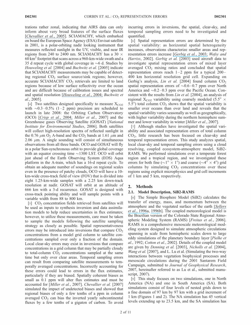
various cloud conditions, we compared the modeled andobserved NEE to incoming radiation and overlaid a 2-harmonic function fit to both the model output and thetower observations (Figure 3). At both locations for con-ditions with radiation values higher than 650 W m�2, whichcorresponds primarily to clear or mostly clear conditions,the fits to both the model and the in situ observations have aconstant uptake of �10 mmol m�2 s�1 and �13.5 mmolm�2 s�1 for NA and SA, respectively. As the radiationdecreases from 650 W m�2 the carbon uptake alsodecreases; however, the observed decrease occurs at higherradiation values. Simulated uptake remains relatively con-stant until the radiation decreases to �400 W m�2, while theobserved uptake has a higher light saturation and thusbegins decreasing at higher radiation values. SiB2.5 calcu-lates photosynthesis for a single sun leaf and uses anempirical adjustment to extinction law in conjunction withsatellite information to adjust carbon flux up to canopy scale

D02301 CORBIN ET AL.: CO2 REPRESENTATION ERRORS

4 of 11

D02301

[Baker et al., 2005]. Using this technique is known to resultin model photosynthesis reaching light saturation too soon,resulting in enhanced uptake for moderate radiation values[e.g., Dai et al., 2003; Dickinson et al., 1998]. Theenhanced uptake in the model could decrease the surfaceCO2 concentrations during moderately cloudy to overcastconditions and just after sunrise and before sunset.[21] To investigate the relationship between cloud cover

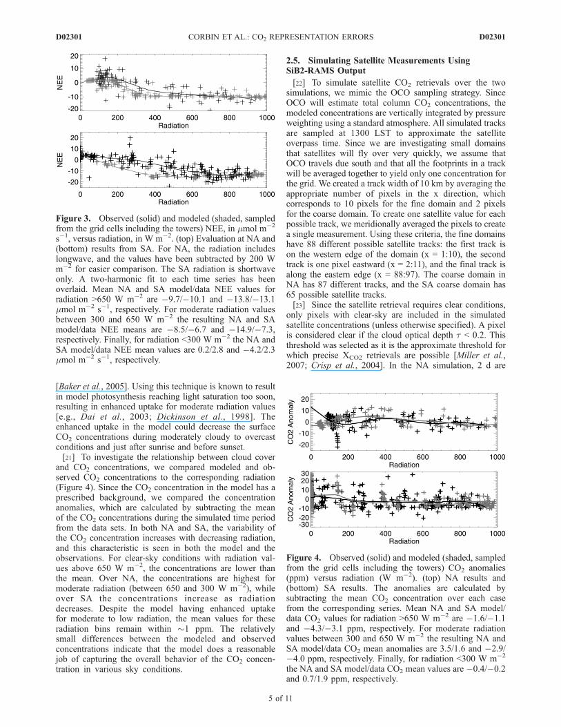
and CO2 concentrations, we compared modeled and ob-served CO2 concentrations to the corresponding radiation(Figure 4). Since the CO2 concentration in the model has aprescribed background, we compared the concentrationanomalies, which are calculated by subtracting the meanof the CO2 concentrations during the simulated time periodfrom the data sets. In both NA and SA, the variability ofthe CO2 concentration increases with decreasing radiation,and this characteristic is seen in both the model and theobservations. For clear-sky conditions with radiation val-ues above 650 W m�2, the concentrations are lower thanthe mean. Over NA, the concentrations are highest formoderate radiation (between 650 and 300 W m�2), whileover SA the concentrations increase as radiationdecreases. Despite the model having enhanced uptakefor moderate to low radiation, the mean values for theseradiation bins remain within �1 ppm. The relativelysmall differences between the modeled and observedconcentrations indicate that the model does a reasonablejob of capturing the overall behavior of the CO2 concen-tration in various sky conditions.

2.5. Simulating Satellite Measurements UsingSiB2-RAMS Output

[22] To simulate satellite CO2 retrievals over the twosimulations, we mimic the OCO sampling strategy. SinceOCO will estimate total column CO2 concentrations, themodeled concentrations are vertically integrated by pressureweighting using a standard atmosphere. All simulated tracksare sampled at 1300 LST to approximate the satelliteoverpass time. Since we are investigating small domainsthat satellites will fly over very quickly, we assume thatOCO travels due south and that all the footprints in a trackwill be averaged together to yield only one concentration forthe grid. We created a track width of 10 km by averaging theappropriate number of pixels in the x direction, whichcorresponds to 10 pixels for the fine domain and 2 pixelsfor the coarse domain. To create one satellite value for eachpossible track, we meridionally averaged the pixels to createa single measurement. Using these criteria, the fine domainshave 88 different possible satellite tracks: the first track ison the western edge of the domain (x = 1:10), the secondtrack is one pixel eastward (x = 2:11), and the final track isalong the eastern edge (x = 88:97). The coarse domain inNA has 87 different tracks, and the SA coarse domain has65 possible satellite tracks.[23] Since the satellite retrieval requires clear conditions,

only pixels with clear-sky are included in the simulatedsatellite concentrations (unless otherwise specified). A pixelis considered clear if the cloud optical depth t < 0.2. Thisthreshold was selected as it is the approximate threshold forwhich precise XCO2 retrievals are possible [Miller et al.,2007; Crisp et al., 2004]. In the NA simulation, 2 d are

Figure 3. Observed (solid) and modeled (shaded, sampledfrom the grid cells including the towers) NEE, in mmol m�2

s�1, versus radiation, in W m�2. (top) Evaluation at NA and(bottom) results from SA. For NA, the radiation includeslongwave, and the values have been subtracted by 200 Wm�2 for easier comparison. The SA radiation is shortwaveonly. A two-harmonic fit to each time series has beenoverlaid. Mean NA and SA model/data NEE values forradiation >650 W m�2 are �9.7/�10.1 and �13.8/�13.1mmol m�2 s�1, respectively. For moderate radiation valuesbetween 300 and 650 W m�2 the resulting NA and SAmodel/data NEE means are �8.5/�6.7 and �14.9/�7.3,respectively. Finally, for radiation <300 W m�2 the NA andSA model/data NEE mean values are 0.2/2.8 and �4.2/2.3mmol m�2 s�1, respectively.

Figure 4. Observed (solid) and modeled (shaded, sampledfrom the grid cells including the towers) CO2 anomalies(ppm) versus radiation (W m�2). (top) NA results and(bottom) SA results. The anomalies are calculated bysubtracting the mean CO2 concentration over each casefrom the corresponding series. Mean NA and SA model/data CO2 values for radiation >650 W m�2 are �1.6/�1.1and �4.3/�3.1 ppm, respectively. For moderate radiationvalues between 300 and 650 W m�2 the resulting NA andSA model/data CO2 mean anomalies are 3.5/1.6 and �2.9/�4.0 ppm, respectively. Finally, for radiation <300 W m�2

the NA and SA model/data CO2 mean values are �0.4/�0.2and 0.7/1.9 ppm, respectively.

D02301 CORBIN ET AL.: CO2 REPRESENTATION ERRORS

5 of 11

D02301

primarily clear, 5 d are partly cloudy, and 2 d are overcast.Over SA, 6 d are completely clear and 9 d are partly cloudy.

3. Results

3.1. Total Column CO2 Concentrations

[24] In the NA simulation, the main driver of total columnCO2 temporal variability is synoptic-scale systems(Figure 5). A Fourier analysis of the CO2 concentrationsreveals a significant spectral peak at �3.5 d (at the 95%confidence level using an F test), which indicates thedominant timescale of variability is the fronts in the simu-lation. The diurnal cycle also has a significant spectral peak,although it is much smaller. Rather than displaying a strongdiurnal cycle, the simulated total column concentrationsampled from the grid cell that includes the WLEF towerhas three spikes associated with the three frontal passages.The column CO2 range is �6 ppm and the standarddeviation is �1 ppm. The fronts, which are associated withclouds, advect high concentrations from the southwest,where a heat wave reduces carbon uptake causing highCO2 anomalies [Wang et al., 2007]. The lowest concen-trations during the simulation occur in clear conditions,when the main influence on CO2 is the local vegetationrather than advection.[25] The NA total column CO2 spatial variability is also

predominantly affected by the weather via the frontalpassages. The range of column CO2 at 1300 LST over thefine grid column varies from 0.2 to 1.8 ppm, with anaverage of 0.8 ppm (Table 1). Over the coarse grid column,the CO2 range at 1300 LST varies from 1 ppm to 13.7 ppm,with an average range of 3.5 ppm across the domain and amean standard deviation of 0.6 ppm. Although the surfaceheterogeneity of the coarse domain contributes to increasedCO2 variability, the greatest concentration ranges occurwhen the southwestern portion of the domain has highconcentrations from advection while the northeastern halfof the domain has low concentrations. Optically thickclouds that are associated with the fronts contribute to

higher concentrations by reducing photosynthesis due tolight limitation.[26] Ground-based measurements of total column CO2

are being made at the WLEF tall tower site [Washenfelder etal., 2006]. The observatory utilizes a similar technique asOCO, GOSAT, and SCIAMACHY to measure XCO2 usingan upward looking Fourier Transform Spectrometer (FTS).The observatory has been measuring XCO2 since May 2004.At WLEF, XCO2 is minimally influenced by the diurnalrectifier effect. Washenfelder et al. [2006] present resultsfrom a validation study involving aircraft data wherecolumn observations were measured on five dates in Julyand August of 2004. The column average concentrationvaries �7 ppm between these samples, which is similar inmagnitude to the column variations seen in the SiB-RAMSsimulations due to the frontal passages. A plot of theseasonal cycle of daytime daily averaged XCO2 showsday-to-day variability of �6–7 ppm during the summer[Washenfelder et al., 2006].[27] The dominant cause of column CO2 temporal vari-

ability in SA is the diurnal cycle and mesoscale circulations(Figure 6), since this simulation occurs in the dry seasonand is characterized by steady trade winds, nocturnaldecoupling, river breezes, boundary layer cumulus clouds,and no air masses or fronts. A power spectrum of this seriesshows the only significant spectral peak is at 1 d. Thetemporal CO2 variability in SA is smaller than in NA, as therange and standard deviation of the simulated columnconcentrations sampled at the Tapajos tower is only3.1 ppm and 0.7 ppm, respectively. The amplitude of themean diurnal cycle is 1.1 ppm. Unlike in NA, there is nocorrelation between cloud cover and mixing ratios. Sincethis simulation was selected to isolate the influence of localvegetation and circulations, the clouds are midafternooncumulus clouds primarily seen on the east bank of theTapajos River due to the low-level convergence line [Lu etal., 2005, also submitted manuscript, 2007].[28] Since the SA case has significant surface heteroge-

neity due to the rivers, the spatial variability in thissimulation is larger for the fine grid column compared tothe NA simulation; however, the spatial variability over thecoarse domain is smaller, which is due to the lack ofsynoptic-scale features which advected high CO2 in NA.The average total column spatial range at 1300 LST is1.46 ppm and 2.15 ppm for the fine and coarse gridcolumns, respectively (Table 1). The CO2 spatial patternat 1300 LST was similar for all days, with a low concen-tration on the eastern half of the domain and higherconcentrations in the northwest corner, which is primarilydue to the topography and surface cover [Lu et al., 2005].

Table 1. Range and Standard Deviation (s) of the Simulated Grid

Columns at 1300 LSTa

Range s

Mean Max Mean Max

NA Fine 0.76 1.81 0.15 0.4NA Coarse 3.53 13.71 0.64 1.9SA Fine 1.46 2.1 0.4 0.53SA Coarse 2.15 2.91 0.44 0.58

aBoth the mean values over the entire simulation and the maximumvalues are displayed. Unit is ppm.

Figure 5. Simulated total column CO2 concentrations atthe WLEF tower (solid line) and the sky conditions (shadedline), where 0 indicates clear sky and 1 indicates the towerwas cloud covered. The vertical dashed lines indicate thethree frontal passages.

D02301 CORBIN ET AL.: CO2 REPRESENTATION ERRORS

6 of 11

D02301

[29] The total column measurements in SiB-RAMS areconsistent with results presented by Olsen and Randerson[2004]. Using the Model of Atmospheric Transport andChemistry (MATCH) three-dimensional atmospheric trans-port model, Olsen and Randerson [2004] investigated thetotal column CO2 concentrations. They found that at WLEFthe greatest variability of column CO2 was linked tosynoptic events on the order of 2 to 6 d. In order toinfluence the column, CO2 flux anomalies had to accumu-late in the lower troposphere over a period of several days orthere had to be a large-scale replacement of air in thecolumn. Day-to-day variations of up to �8 ppm can beseen at the WLEF tower during the summer because ofsynoptic events. Similar to SiB-RAMS, results from Olsenand Randerson [2004] show the main driver of column CO2

variability over WLEF during the summer is synoptic-scalesystems, as midlatitude air masses with distinct CO2 con-centrations develop in response to surface fluxes and areseparated by fronts [Parazoo, 2007].[30] In the Amazon, modeled vertical CO2 profiles were

qualitatively similar to the observed profiles near thesurface, but did not exhibit the same degree of variability[Olsen and Randerson, 2004]. The amplitude of the averagediurnal cycle within the Amazon basin was 0.9 ppm in July,which is slightly weaker than the diurnal cycle from SiB-RAMS; however, comparison of MATCH column CO2 tocolumn CO2 profiles from aircraft data revealed thatMATCH tended to have lower diurnal variability thanobserved. In the tropics, the dominant cause of CO2

variability is the diurnal cycle because of the productiveecosystems and the lack of synoptic-scale features.

3.2. Spatial Representativeness Errors

[31] Since satellite track widths are not the same size asan inverse model grid column, using satellite concentrationsto optimize a grid column may introduce spatial represen-tativeness errors into the inversion. In this study, the size ofthe coarse and fine domains in both NA and SA correspondroughly to a global model grid size. We calculated thespatial errors that inversions would incur from using satel-lite measurements to represent grid columns in central NAand in the Amazon by subtracting the domain-averaged

1300 LST total column concentrations from the simulatedsatellite concentrations, which use only clear-sky pixels.The daily results are compiled into a single samplingdistribution for each domain and location (Figure 7). Themean and standard deviation of the sampling distributionsfor the fine and coarse domains for both NA and SA areprovided in Table 2.[32] The spatial errors for both fine grid columns are

unbiased, as the mean of the distributions are close to 0.Over NA, all of the errors are within 0.3 ppm; however,over SA only 13% of the simulated satellite concentrationswere within 0.3 ppm of the mean. The standard deviationfor SA is 0.2 ppm and the maximum error is �0.72 ppm.97% of the simulated SA tracks are within 0.5 ppm, whichis only half of the expected spectroscopic retrieval error[Miller et al., 2007]. The larger errors over SA are due to theheterogeneity in that domain and cloud masking in NA,since the greatest NA variability occurred when there wereclouds and hence no satellite retrievals. The relatively smallmagnitude of the errors is due to the limited total columnCO2 variability in the domains.[33] The errors that would be introduced into inversions

that use satellite measurements to represent coarse gridcolumns are larger than the errors for a fine grid column,which is not surprising since the total column CO2 is morevariable. The spatial errors over SA remain unbiased andhave a standard deviation similar to that of the fine domain.95% of the satellite tracks capture the domain mean within0.5 ppm. The errors for the NA coarse domain are muchlarger and negatively biased, with a mean of �0.13 ppm anda standard deviation of 0.43 ppm. Although nearly 25% ofthe tracks are within 0.1 of the mean, 18% of the tracks haveerrors larger than 0.5 ppm and 6% of the tracks have errorslarger than 1 ppm, which is larger than the expectedretrieval error. The large and negatively biased spatial errorsare due to the large gradients of CO2 due to the frontalpassages and the cloud masking of the higher concentrationsassociated with the fronts.

3.3. Local Clear-Sky Errors

[34] We define local clear-sky errors as errors that areintroduced into inversions that use clear-sky satellite con-centrations to represent a transport model grid column thatincludes clouds. These errors are calculated by subtractingthe simulated satellite concentrations at 1300 LST using allpixels from the simulated satellite concentrations using onlyclear-sky pixels. The resulting errors are smaller than theretrieval error and are unbiased for the fine domains

Figure 6. Simulated total column CO2 concentrations atthe Tapajos tower (solid line) and the modeled skyconditions (shaded line), where 0 indicates clear sky and1 indicates the tower was cloud covered.

Table 2. Mean (m) and Standard Deviation (s) of the Sampling

Distributions of the Spatial Representation Errors, the Local Clear-

Sky Errors, the Diurnal Sampling Errors, and the Temporal

Sampling Errors for All Four Casesa

SpatialLocal Clear-

Sky Diurnal Temporal

m s m s m s m s

NA fine �0.01 0.06 �0.02 0.06 �0.19 0.33 �0.44 0.31NA coarse �0.13 0.43 �0.12 0.51 �0.25 0.51 �0.42 0.5SA fine �0.04 0.21 �0.04 0.18 0.1 0.26 0.06 0.66SA coarse �0.04 0.24 �0.03 0.19 0 0.25 �0.01 0.64

aUnit is ppm.

D02301 CORBIN ET AL.: CO2 REPRESENTATION ERRORS

7 of 11

D02301

(Figure 8). All the NA satellite tracks over the fine gridcolumn that only use clear-sky footprints capture the truemean track value within 0.3 ppm. For the SA case, thestandard deviation is larger and 87% of the tracks are within0.3 ppm of the true mean. The largest error is 0.7 ppm. TheSA coarse domain errors are very similar to the errors in thefine domain, with 85% of the errors less than 0.3 ppm. Thesimilarity between the fine and coarse sampling distribu-tions indicates that differences in carbon uptake due to localcloud cover has a minimal impact on the concentration at asingle snapshot in time. The local clear-sky errors over theNA coarse grid column are negatively biased with asampling distribution mean of �0.12 ppm. The negativebias is due to a few tracks that have large negative errors.Although 80% of the simulated satellite concentrationsusing only clear footprints have errors less than 0.3 ppm,3% of the tracks have errors greater than 1 ppm, with errorsas large as 4 ppm. Similar to the spatial errors, large andnegatively biased local clear-sky errors are due to cloudmasking of high frontal CO2.[35] To further examine the clear-sky errors, we analyzed

local clear minus all-sky differences in net ecosystemexchange (NEE), which were calculated in a similar mannerby subtracting the mean NEE value in a satellite track

containing all pixels from the corresponding satellite trackNEE mean utilizing only clear-sky pixels. The resultingerrors are very small (<1 mmol m�2 s�1). For the finedomains, the errors are shifted toward enhanced uptake inclear conditions due to reduced photosynthesis underclouds; however, the errors in the coarse domains aresymmetrical about 0. Since the clear-sky NEE errors aresmall, their effect on the column CO2 concentration isminimal, indicating that the main driver of the large errorsseen in the clear-sky CO2 is the organization of regionalCO2 gradients along frontal boundaries, which are maskedby large-scale cloud systems and not observed by satellites.

3.4. Temporal Sampling Errors

[36] Temporal sampling errors can occur in inversionsthat use satellite concentrations to optimize temporallyaveraged concentrations in the model. We calculated tem-poral errors that arise from using satellite measurements torepresent diurnal averages and bimonthly averages.3.4.1. Diurnal Sampling Errors[37] To calculate the diurnal errors, we subtracted the

domain average diurnal mean (0000 UT to 0000 UT) fromthe simulated 1300 LST satellite tracks (Figure 9). All thestandard deviations for the diurnal errors are larger than thestandard deviations seen for both spatial and local clear-skyerrors. Over SA, the mean of the sampling distribution ispositively biased by a tenth of a ppm, and the entiredistribution is positively shifted, indicating that on a fine

Figure 7. Sampling distributions of the spatial representa-tiveness errors in NA (solid) and SA (shaded) at 1300 LSTcompiled from all days of the simulations. The x axis is thedifference between the simulated satellite concentration andthe domain mean concentration, and the y axis is the numberof satellite tracks that correspond to each difference.Negative values indicate an underestimation by thesimulated satellite measurements and positive valuesindicate an overestimation. (top) Results from the fine gridcolumns and (bottom) distribution of the errors from thecoarse grid columns.

Figure 8. Local clear-sky total column CO2 errors for NA(solid) and SA (shaded), which are the differences betweenthe simulated satellite concentrations at 1300 LST usingonly clear-sky pixels and the simulated satellite concentra-tions at the same time using all the pixels in the satellitetrack. (top) Errors from the fine grid and (bottom) resultsfrom the coarse grid.

D02301 CORBIN ET AL.: CO2 REPRESENTATION ERRORS

8 of 11

D02301

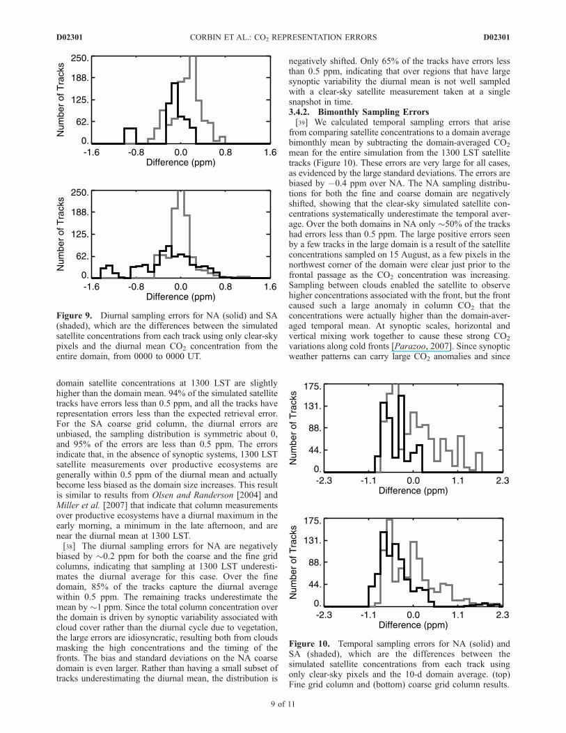
domain satellite concentrations at 1300 LST are slightlyhigher than the domain mean. 94% of the simulated satellitetracks have errors less than 0.5 ppm, and all the tracks haverepresentation errors less than the expected retrieval error.For the SA coarse grid column, the diurnal errors areunbiased, the sampling distribution is symmetric about 0,and 95% of the errors are less than 0.5 ppm. The errorsindicate that, in the absence of synoptic systems, 1300 LSTsatellite measurements over productive ecosystems aregenerally within 0.5 ppm of the diurnal mean and actuallybecome less biased as the domain size increases. This resultis similar to results from Olsen and Randerson [2004] andMiller et al. [2007] that indicate that column measurementsover productive ecosystems have a diurnal maximum in theearly morning, a minimum in the late afternoon, and arenear the diurnal mean at 1300 LST.[38] The diurnal sampling errors for NA are negatively

biased by �0.2 ppm for both the coarse and the fine gridcolumns, indicating that sampling at 1300 LST underesti-mates the diurnal average for this case. Over the finedomain, 85% of the tracks capture the diurnal averagewithin 0.5 ppm. The remaining tracks underestimate themean by �1 ppm. Since the total column concentration overthe domain is driven by synoptic variability associated withcloud cover rather than the diurnal cycle due to vegetation,the large errors are idiosyncratic, resulting both from cloudsmasking the high concentrations and the timing of thefronts. The bias and standard deviations on the NA coarsedomain is even larger. Rather than having a small subset oftracks underestimating the diurnal mean, the distribution is

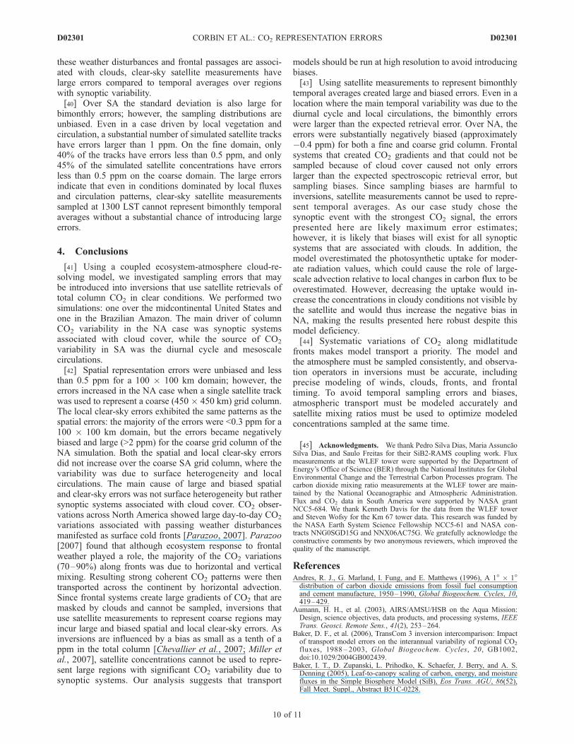
negatively shifted. Only 65% of the tracks have errors lessthan 0.5 ppm, indicating that over regions that have largesynoptic variability the diurnal mean is not well sampledwith a clear-sky satellite measurement taken at a singlesnapshot in time.3.4.2. Bimonthly Sampling Errors[39] We calculated temporal sampling errors that arise

from comparing satellite concentrations to a domain averagebimonthly mean by subtracting the domain-averaged CO2

mean for the entire simulation from the 1300 LST satellitetracks (Figure 10). These errors are very large for all cases,as evidenced by the large standard deviations. The errors arebiased by �0.4 ppm over NA. The NA sampling distribu-tions for both the fine and coarse domain are negativelyshifted, showing that the clear-sky simulated satellite con-centrations systematically underestimate the temporal aver-age. Over the both domains in NA only �50% of the trackshad errors less than 0.5 ppm. The large positive errors seenby a few tracks in the large domain is a result of the satelliteconcentrations sampled on 15 August, as a few pixels in thenorthwest corner of the domain were clear just prior to thefrontal passage as the CO2 concentration was increasing.Sampling between clouds enabled the satellite to observehigher concentrations associated with the front, but the frontcaused such a large anomaly in column CO2 that theconcentrations were actually higher than the domain-aver-aged temporal mean. At synoptic scales, horizontal andvertical mixing work together to cause these strong CO2

variations along cold fronts [Parazoo, 2007]. Since synopticweather patterns can carry large CO2 anomalies and since

Figure 9. Diurnal sampling errors for NA (solid) and SA(shaded), which are the differences between the simulatedsatellite concentrations from each track using only clear-skypixels and the diurnal mean CO2 concentration from theentire domain, from 0000 to 0000 UT.

Figure 10. Temporal sampling errors for NA (solid) andSA (shaded), which are the differences between thesimulated satellite concentrations from each track usingonly clear-sky pixels and the 10-d domain average. (top)Fine grid column and (bottom) coarse grid column results.

D02301 CORBIN ET AL.: CO2 REPRESENTATION ERRORS

9 of 11

D02301

these weather disturbances and frontal passages are associ-ated with clouds, clear-sky satellite measurements havelarge errors compared to temporal averages over regionswith synoptic variability.[40] Over SA the standard deviation is also large for

bimonthly errors; however, the sampling distributions areunbiased. Even in a case driven by local vegetation andcirculation, a substantial number of simulated satellite trackshave errors larger than 1 ppm. On the fine domain, only40% of the tracks have errors less than 0.5 ppm, and only45% of the simulated satellite concentrations have errorsless than 0.5 ppm on the coarse domain. The large errorsindicate that even in conditions dominated by local fluxesand circulation patterns, clear-sky satellite measurementssampled at 1300 LST cannot represent bimonthly temporalaverages without a substantial chance of introducing largeerrors.

4. Conclusions

[41] Using a coupled ecosystem-atmosphere cloud-re-solving model, we investigated sampling errors that maybe introduced into inversions that use satellite retrievals oftotal column CO2 in clear conditions. We performed twosimulations: one over the midcontinental United States andone in the Brazilian Amazon. The main driver of columnCO2 variability in the NA case was synoptic systemsassociated with cloud cover, while the source of CO2

variability in SA was the diurnal cycle and mesoscalecirculations.[42] Spatial representation errors were unbiased and less

than 0.5 ppm for a 100 � 100 km domain; however, theerrors increased in the NA case when a single satellite trackwas used to represent a coarse (450 � 450 km) grid column.The local clear-sky errors exhibited the same patterns as thespatial errors: the majority of the errors were <0.3 ppm for a100 � 100 km domain, but the errors became negativelybiased and large (>2 ppm) for the coarse grid column of theNA simulation. Both the spatial and local clear-sky errorsdid not increase over the coarse SA grid column, where thevariability was due to surface heterogeneity and localcirculations. The main cause of large and biased spatialand clear-sky errors was not surface heterogeneity but rathersynoptic systems associated with cloud cover. CO2 obser-vations across North America showed large day-to-day CO2

variations associated with passing weather disturbancesmanifested as surface cold fronts [Parazoo, 2007]. Parazoo[2007] found that although ecosystem response to frontalweather played a role, the majority of the CO2 variations(70–90%) along fronts was due to horizontal and verticalmixing. Resulting strong coherent CO2 patterns were thentransported across the continent by horizontal advection.Since frontal systems create large gradients of CO2 that aremasked by clouds and cannot be sampled, inversions thatuse satellite measurements to represent coarse regions mayincur large and biased spatial and local clear-sky errors. Asinversions are influenced by a bias as small as a tenth of appm in the total column [Chevallier et al., 2007; Miller etal., 2007], satellite concentrations cannot be used to repre-sent large regions with significant CO2 variability due tosynoptic systems. Our analysis suggests that transport

models should be run at high resolution to avoid introducingbiases.[43] Using satellite measurements to represent bimonthly

temporal averages created large and biased errors. Even in alocation where the main temporal variability was due to thediurnal cycle and local circulations, the bimonthly errorswere larger than the expected retrieval error. Over NA, theerrors were substantially negatively biased (approximately�0.4 ppm) for both a fine and coarse grid column. Frontalsystems that created CO2 gradients and that could not besampled because of cloud cover caused not only errorslarger than the expected spectroscopic retrieval error, butsampling biases. Since sampling biases are harmful toinversions, satellite measurements cannot be used to repre-sent temporal averages. As our case study chose thesynoptic event with the strongest CO2 signal, the errorspresented here are likely maximum error estimates;however, it is likely that biases will exist for all synopticsystems that are associated with clouds. In addition, themodel overestimated the photosynthetic uptake for moder-ate radiation values, which could cause the role of large-scale advection relative to local changes in carbon flux to beoverestimated. However, decreasing the uptake would in-crease the concentrations in cloudy conditions not visible bythe satellite and would thus increase the negative bias inNA, making the results presented here robust despite thismodel deficiency.[44] Systematic variations of CO2 along midlatitude

fronts makes model transport a priority. The model andthe atmosphere must be sampled consistently, and observa-tion operators in inversions must be accurate, includingprecise modeling of winds, clouds, fronts, and frontaltiming. To avoid temporal sampling errors and biases,atmospheric transport must be modeled accurately andsatellite mixing ratios must be used to optimize modeledconcentrations sampled at the same time.

[45] Acknowledgments. We thank Pedro Silva Dias, Maria AssuncaoSilva Dias, and Saulo Freitas for their SiB2-RAMS coupling work. Fluxmeasurements at the WLEF tower were supported by the Department ofEnergy’s Office of Science (BER) through the National Institutes for GlobalEnvironmental Change and the Terrestrial Carbon Processes program. Thecarbon dioxide mixing ratio measurements at the WLEF tower are main-tained by the National Oceanographic and Atmospheric Administration.Flux and CO2 data in South America were supported by NASA grantNCC5-684. We thank Kenneth Davis for the data from the WLEF towerand Steven Wofsy for the Km 67 tower data. This research was funded bythe NASA Earth System Science Fellowship NCC5-61 and NASA con-tracts NNG0SGD15G and NNX06AC75G. We gratefully acknowledge theconstructive comments by two anonymous reviewers, which improved thequality of the manuscript.

ReferencesAndres, R. J., G. Marland, I. Fung, and E. Matthews (1996), A 1� � 1�distribution of carbon dioxide emissions from fossil fuel consumptionand cement manufacture, 1950–1990, Global Biogeochem. Cycles, 10,419–429.

Aumann, H. H., et al. (2003), AIRS/AMSU/HSB on the Aqua Mission:Design, science objectives, data products, and processing systems, IEEETrans. Geosci. Remote Sens., 41(2), 253–264.

Baker, D. F., et al. (2006), TransCom 3 inversion intercomparison: Impactof transport model errors on the interannual variability of regional CO2

fluxes, 1988 – 2003, Global Biogeochem. Cycles, 20, GB1002,doi:10.1029/2004GB002439.

Baker, I. T., D. Zupanski, L. Prihodko, K. Schaefer, J. Berry, and A. S.Denning (2005), Leaf-to-canopy scaling of carbon, energy, and moisturefluxes in the Simple Biosphere Model (SiB), Eos Trans. AGU, 86(52),Fall Meet. Suppl., Abstract B51C-0228.

D02301 CORBIN ET AL.: CO2 REPRESENTATION ERRORS

10 of 11

D02301

Bakwin, P. S., P. P. Tans, D. F. Hurst, and C. Zhao (1998), Measurements ofcarbon dioxide on very tall towers: Results of the NOAA/CMDL pro-gram, Tellus, Ser. B, 50(5), 401–415.

Buchwitz, M., et al. (2005), Carbon monoxide, methane and carbon dioxidecolumns retrieved from SCIAMACHY by WFM-DOAS: Year 2003 in-itial data set, Atmos. Chem. Phys., 5, 3313–3329.

Chevallier, F., R. J. Engelen, and P. Peylin (2005), The contribution ofAIRS data to the estimation of CO2 sources and sinks, Geophys. Res.Lett., 32, L23801, doi:10.1029/2005GL024229.

Chevallier, F., F.-M. Breon, and P. J. Rayner (2007), Contribution of theOrbiting Carbon Observatory to the estimation of CO2 sources and sinks:Theoretical study in a variational data assimilation framework, J. Geo-phys. Res., 112, D09307, doi:10.1029/2006JD007375.

Cotton, W. R., et al. (2002), RAMS 2001: Current status and future direc-tions, Meteorol. Atmos. Phys., 82(1–4), 5–29, doi:10.1007/s00703-001-0584-9.

Crisp, D., et al. (2004), The Orbiting Carbon Observatory (OCO) mission,Adv. Space Res., 34, 700–709.

Dai, Y., et al. (2003), The Common Land Model (CLM), Bull. Am. Meteor-ol. Soc., 84(8), 1013–1023.

Davis, K. J., P. S. Bakwin, C. Yi, B. W. Berger, C. Zhao, R. M. Teclaw, andJ. G. Isebrands (2003), The annual cycle of CO2 and H2O exchange overa northern mixed forest as observed from a very tall tower, GlobalChange Biol., 9, 1278–1293.

Denning, A. S., M. Nicholls, L. Prihodko, I. Baker, P. L. Vidale, K. Davis,and P. Bakwin (2003), Simulated variations in atmospheric CO2 over aWisconsin forest using a coupled ecosystem-atmosphere model, GlobalChange Biol., 9, 1–10.

Dickinson, R. E., M. Shaikh, R. Bryant, and L. Graumlich (1998), Inter-active canopies for a climate model, J. Clim., 11, 2823–2836.

Engelen, R. J., E. Andersson, F. Chevallier, A. Hollingsworth,M. Matricardi, A. P. McNally, J.-N. Thepaut, and P. D. Watts (2004),Estimating atmospheric CO2 from advanced infrared satellite radianceswithin an operational 4D-Var data assimilation system: Methodology andfirst results, J. Geophys. Res., 109, D19309, doi:10.1029/2004JD004777.

Freitas, S. R., K. Longo, M. Silva Dias, P. Silva Dias, R. Chatfield,A. Fazenda, and L. F. Rodrigues (2006), The Coupled Aerosol and TracerTransport model to the Brazilian developments on the Regional Atmo-spheric Modeling System: Validation Using direct and remote sensingobservations, paper presented at 8th International Conference on South-ern Hemisphere Meteorology and Oceanography, Am. Meteorol. Soc.,Foz do Iguacu, Brazil.

Gerbig, C., J. C. Lin, S. C. Wofsy, B. C. Daube, A. E. Andrews, B. B.Stephens, P. S. Bakwin, and C. A. Grainger (2003), Toward constrainingregional-scale fluxes of CO2 with atmospheric observations over a con-tinent: 1. Observed spatial variability from airborne platforms, J. Geo-phys. Res., 108(D24), 4756, doi:10.1029/2002JD003018.

Gurney, K. R., et al. (2002), Towards robust regional estimates of CO2

sources and sinks using atmospheric transport models, Nature, 415,626–630.

Gurney, K. R., et al. (2003), TransCom 3 CO2 inversion intercomparison:1. Annual mean control results and sensitivity to transport and prior fluxinformation, Tellus, Ser. B, 55, 555–579.

Hansen, M., R. DeFries, J. R. G. Townshend, and R. Sohlberg (2000),Global land cover classification at 1 km resolution using a decision treeclassifier, Int. J. Remote Sens., 21, 1331–1365.

Harrington, J. Y. (1997), The effects of radiative and microphysical pro-cesses on simulated warm and transition season Arctic stratus, Atmos. Sci.Pap. 637, 289 pp., Dep. of Atmos. Sci., Colo. State Univ., Fort Collins,Colo.

Houweling, S., F. M. Breon, I. Aben, C. Rodenbeck, M. Gloor,M. Heimann, and P. Ciais (2004), Inverse modeling of CO2 sourcesand sinks using satellite data: A synthetic inter-comparison of measure-ment techniques and their performance as a function of space and time,Atmos. Chem. Phys., 4, 523–538.

Klemp, J. B., and R. B. Wilhelmson (1978), The simulation of three-dimensional convective storm dynamics, J. Atmos. Sci., 35, 1070–1096.

Lin, J. C., C. Gerbig, B. C. Daube, S. C. Wofsy, A. E. Andrews, S. A. Vay,and B. E. Anderson (2004), An empirical analysis of the spatial varia-bility of atmospheric CO2: Implications for inverse analyses and space-borne sensors, Geophys. Res. Lett., 31, L23104, doi:10.1029/2004GL020957.

Lu, L., A. S. Denning, M. A. Silva-Dias, P. Silva-Dias, M. Longo, S. R.Frietas, and S. Saatchi (2005), Mesoscale circulations and atmospheric

CO2 variations in the Tapajos Region, Para, Brazil, J. Geophys. Res., 110,D21102, doi:10.1029/2004JD005757.

Marland, G., T. A. Boden, and R. J. Andres (2005), Global, regional, andnational CO2 emissions, in Trends: A Compendium of Data on GlobalChange, Carbon Dioxide Inf. Anal. Cent., Oak Ridge Natl. Lab., U.S.Dep. of Energy, Oak Ridge, Tenn. (Available at http://cdiac.ornl.gov/trends/emis/em_cont.htm)

Mellor, G. L., and T. Yamada (1982), Development of a turbulence closuremodel for geophysical fluid problems, Rev. Geophys., 20, 851–875.

Meyers, M. P., R. L. Walko, J. Y. Harrington, and W. R. Cotton (1997),New RAMS cloud microphysics parameterization, Part II: The two-moment scheme, Atmos. Res., 45, 3–39.

Miller, C. E., et al. (2007), Precision requirements for space-based XCO2

data, J. Geophys. Res., 112, D10314, doi:10.1029/2006JD007659.National Institute for Environmental Studies (2006), GOSAT pamphlet,Greenhouse Gases Obs. Satell. Proj., Cent. for Global Environ. Res.,Natl. Inst. for Environ. Stud., Tsukuba, Japan.

Nicholls, M. E., A. S. Denning, L. Prihodko, P.-L. Vidale, I. Baker,K. Davis, and P. Bakwin (2004), A multiple-scale simulation of variationsin atmospheric carbon dioxide using a coupled biosphere-atmosphericmodel, J. Geophys. Res., 109, D18117, doi:10.1029/2003JD004482.

Olsen, S. C., and J. T. Randerson (2004), Differences between surfaceand column atmospheric CO2 and implications for carbon cycle research,J. Geophys. Res., 109, D02301, doi:10.1029/2003JD003968.

Parazoo, N. C. (2007), Investigating synoptic variations in atmosphericCO2 using continuous observations and a global transport model, MastersThesis, 101 pp., Colo. State Univ., Fort Collins.

Pielke, R. A., et al. (1992), A comprehensive meteorological modelingsystem RAMS, Meteorol. Atmos. Phys., 49, 69–91.

Rayner, P. J., and D. M. O’Brien (2001), The utility of remotely sensed CO2

concentration data in surface source inversions, Geophys. Res. Lett.,28(1), 175–178.

Ricciuto, D. M., M. P. Butler, K. J. Davis, B. D. Cook, P. S. Bakwin, A. E.Andrews, and R. M. Teclaw (2007), Causes of interannual variability inecosystem-atmosphere CO2 exchange in a northern Wisconsin forestusing a Bayesian synthesis inversion, Agric. For. Meteorol., in press.

Rodenbeck, C., S. Houweling, M. Gloor, and M. Heimann (2003), CO2 fluxhistory 1982–2001 inferred from atmospheric data using a global inver-sion of atmospheric transport, Atmos. Chem. Phys., 3, 1919–1964.

Saleska, S. R., et al. (2003), Carbon in Amazon forests: Unexpected sea-sonal fluxes and disturbance-induced losses, Science, 302, 1554–1557.

Sellers, P. J., D. A. Randall, G. J. Collatz, J. A. Berry, C. B. Field, D. A.Dazlich, C. Zhang, G. D. Collelo, and L. L. Bounoua (1996a), A revisedland surface parameterization (SiB2) for atmospheric GCMs, Part I:Model formulation, J. Clim., 9, 676–705.

Sellers, P. J., S. O. Los, C. J. Tucker, C. O. Justice, D. A. Dazlich, G. J.Collatz, and D. A. Randall (1996b), A revised land surface parameteriz-tion (SiB2) for atmospheric GCMs. Part II: The generation of globalfields of terrestrial biophysical parameters from satellite data, J. Clim.,9, 706–737.

Smagorinsky, J. (1963), General circulation experiments with the primitiveequations. Part I: The basic experiment, Mon. Weather Rev., 91, 99–164.

Takahashi, T., et al. (2002), Global sea-air CO2 flux based on climatologicalsurface ocean pCO2, and seasonal, biological, and temperature effects,Deep Sea Res., Part II, 49, 1601–1622.

Walko, R. L., W. R. Cotton, M. P. Meyers, and J. Y. Harrington (1995),New RAMS cloud microphysics parameterization: Part I. The singlemoment scheme, Atmos. Res., 38, 29–62.

Wang, J.-W., A. S. Denning, L. Lu, I. T. Baker, K. D. Corbin, and K. J.Davis (2007), Observations and simulations of synoptic, regional, andlocal variations in atmospheric CO2, J. Geophys. Res., 112, D04108,doi:10.1029/2006JD007410.

Washenfelder, R. A., G. C. Toon, J.-F. Blavier, Z. Yang, N. T. Allen, P. O.Wennberg, S. A. Vay, D. M. Matross, and B. C. Daube (2006), Carbondioxide column abundances at the Wisconsin Tall Tower site, J. Geophys.Res., 111, D22305, doi:10.1029/2006JD007154.

Wofsy, S. C., and R. C. Harriss (2002), The North American Carbon Pro-gram (NACP), U.S. Global Change Res. Program, Washington, D. C.

�����������������������I. T. Baker, K. D. Corbin, A. S. Denning, and L. Lu, Department of

Atmospheric Science, Colorado State University, Fort Collins, CO 80525-1371, USA. (kdcorbin@atmos.colostate.edu)J.-W. Wang, Cooperative Institute for Research in the Environmental

Sciences, University of Colorado, Boulder, CO 80309, USA.

D02301 CORBIN ET AL.: CO2 REPRESENTATION ERRORS

11 of 11

D02301