materials

Article

Johnson Cook Material and Failure Model ParametersEstimation of AISI-1045 Medium Carbon Steel forMetal Forming Applications

Mohanraj Murugesan † and Dong Won Jung *,†

Department of Mechanical Engineering, Jeju National University, Jeju-Do 63243, Korea; mohanaero45@gmail.com* Correspondence: jdwcheju@jejunu.ac.kr† These authors contributed equally to this work.

Received: 23 December 2018; Accepted: 12 February 2019; Published: 18 February 2019�����������������

Abstract: Consistent and reasonable characterization of the material behavior under the coupled effectsof strain, strain rate and temperature on the material flow stress is remarkably crucial in order to design aswell as optimize the process parameters in the metal forming industrial practice. The objective of this workwas to formulate an appropriate flow stress model to characterize the flow behavior of AISI-1045 mediumcarbon steel over a practical range of deformation temperatures (650–950 ◦C) and strain rates (0.05–1.0 s−1).Subsequently, the Johnson-Cook flow stress model was adopted for modeling and predicting the materialflow behavior at elevated temperatures. Furthermore, surrogate models were developed based on theconstitutive relations, and the model constants were estimated using the experimental results. As a result,the constitutive flow stress model was formed and the constructed model was examined systematicallyagainst experimental data by both numerical and graphical validations. In addition, to predict thematerial damage behavior, the failure model proposed by Johnson and Cook was used, and to determinethe model parameters, seven different specimens, including flat, smooth round bars and pre-notchedspecimens, were tested at room temperature under quasi strain rate conditions. From the results, it canbe seen that the developed model over predicts the material behavior at a low temperature for all strainrates. However, overall, the developed model can produce a fairly accurate and precise estimationof flow behavior with good correlation to the experimental data under high temperature conditions.Furthermore, the damage model parameters estimated in this research can be used to model the metalforming simulations, and valuable prediction results for the work material can be achieved.

Keywords: AISI-1045 medium carbon steel; flow stress; surrogate modeling; Johnson–Cook material anddamage model; metal forming simulations

1. Introduction

Understanding the damage caused by plastic deformation in the metal forming process is essentialto make safe the operation of structures in the working field as well as to reduce the cost and timeconsumption of the experiments. In industrial practice, the Johnson–Cook (JC) material and damagemodel is extensively incorporated into most of the available finite element (FE) tools to model metalforming simulations because of its ability to predict the model parameters with less effort. It is undeniablethat the well-made and reliable proposed flow stress model is more supportive over a wide range ofstrain rates and elevated temperatures for product design in terms of predicting the material ductilitybehavior efficiently. Even though the flow stress models are broken down into different categories, such as

Materials 2019, 12, 609; doi:10.3390/ma12040609 www.mdpi.com/journal/materials

Materials 2019, 12, 609 2 of 18

physically-based, empirical, and semi-empirical, the aim of these models to achieve accurate predictionof the material behavior for a specific material remains the same [1]. So, developing a proper flow stressmodel for the design process is essential to predict material deformation behavior at high strain ratesand deformation temperatures, and, as a result, reasonable research has been performed consideringvarious materials.

Aviral Shrot et al. [2] proposed a method using the Levenberg-Marquardt search algorithm for theinverse identification of JC material parameters. A set of JC parameters was used to develop an idealizedFE model for the machining process. Then, the inverse identification method was used to estimate theJC by looking at the chip morphology and the cutting force during the process. They concluded that itis possible to re-identify the model parameters by inverse methods; however the estimated parametersfrom the simulation results were almost identical to the original set. Luca Gambirasio et al. [3] adoptedvarious procedures for calibrating the JC model parameters under the high strain rate phenomenonby expressing the deviatoric behavior of elasto-plastic materials. In addition, the Taylor impact testexperimental data was also included for the evaluation of the JC strength model parameters. The sameauthors, Luca Gambirasio et al. [4], introduced a new strength model, named split JC, for the flowstress prediction of three real materials. They stated that the split JC model provides a much moreimproved coherence on the plastic material description and the capability to predict the material behavioris remarkably better that the original JC. Ravindranadh Bobbili et al. [5] employed an artificial neuralnetwork (ANN) constitutive model and the JC model to predict the material’s behavior at a high strainrate generated from split Hopkinson pressure bar (SHPH) experiments at various temperatures for 7017aluminium alloy. It was reported that the predictions of the ANN model were observed to be moreconsistent with the experimental data than the JC model for all strain rates and temperatures.

A. S. Milani et al. [6] used a weighted multi-objective identification strategy to estimate JC materialparameters of two materials, Nitronic 33 super alloy and Ti-6Al-4V, which are often used in modelsof FE tools. The proposed framework was found to be admirable in terms of reducing the number ofexperiments necessary for the identification of model parameters. G. H. Majzoobi et al. [7] adoptedan optimization approach instead of conducting conventional experiments which are time and costconsuming. They concluded that JC material and failure model parameters were estimated, and a goodagreement between experimental and FE predictions was observed. A. Banerjee et al. [8] investigated thetypical behavior of armour steel material to analyze and predict its response to various dynamic loadingconditions. The developed JC constitutive and damage model displayed a reasonable agreement betweenthe Charpy impact test simulation and experimental results. A. E. Buzyurkin et al. [9] investigated thefracture behaviour of titanium alloys based on the available experimental data obtained from variousdynamic loading conditions. The model parameters of the JC model were determined and incorporatedinto the FE simulations to solve a case of an aircraft engine fan problem. The simulation results of thefan case provided better agreement with the experimental data. Xueping Zhang et al. [10] examined thehard turning process to predict the effects of cutting parameters and tool geometry using the JC damagemodel, and the results showed better agreement with the experiments. Jian Liu et al. [11] evaluated a metalcutting process with six ductile fracture models to identify the appropriate fracture model. They statedthat suitable damage prediction was obtained from the Bao-Wierzbicki fracture model, including ratedependency, temperature effect and damage evolution.

From a literature survey, it was identified that constructing a proper FE model typically requiresexpensive experimental effort, and appropriate modeling of fracture behavior is necessary, and the damagemodel should consider both damage initiation and damage evolution. Even though many researcherswere worked with the original JC model, only very few researchers were reported about the strategyto optimize the JC model constants to improve the model predictability. Furthermore, so far, there hasbeen no attempt to develop a detailed JC material and damage model for AISI-1045 medium carbon steel

Materials 2019, 12, 609 3 of 18

material. The aim of this research was to identify the most consistent JC constitutive and damage modelparameters for AISI-1045 medium carbon steel material, and, in addition, to exploit an empirical modelapproach in order to fit the constitutive equation using experimental data. Isothermal tensile tests werecarried out at elevated temperatures (650–950 ◦C) and at low strain rates (0.05–1.0 s−1) to determine themodel properties. To improve the predictability of the JC material model, an optimization procedurebased on the nonlinear programming solver, find minimum of constrained nonlinear multivariablefunction (fmincon), was employed, considering the strain rate hardening and the thermal softeningparameters. Also, an extensive series of experiments, including un-notched and pre-notched flat andround bar specimens, were conducted at quasi-static strain rates (0.0001–0.05 s−1) to estimate the damagemodel parameters of the JC model.

2. Experimental Procedures

The AISI-1045 medium carbon steel material was investigated in the present research work, and thechemical composition (in wt.%) of the steel is listed in Table 1. The specimens were prepared by thewater jet cutting process from the AISI-1045 steel plates and were further used in uniaxial tensile tests toobtain the flow stress-strain data to characterize the hot deformation flow behavior. In detail, the tensiletest specimens were prepared with a gauge length of 25 mm and a thickness of 3 mm, according tothe ASTM-E8M-subsize standard. Tensile tests were performed at elevated deformation temperatures(650–950 ◦C) and high strain rates (0.05–1.0 s−1) on a computer-controlled servo-hydraulic testing machine,as shown in Figure 1a, which can heat the specimen to a maximum of 950 ◦C. From Figure 1a, it canbe seen that the clamped tensile specimen was covered with the isolation part to achieve isothermalconditions, and, in addition, a detailed view of the prepared tensile specimen, which was inside the testingmachine, is shown in Figure 1b. Before conducting the tests, as displayed in Figure 1b, the calibrationswere done using the thermocouples to determine the heating time to obtain an approximately uniformtemperature distribution for the specific temperature value, and then, the noted details were used toconduct the experiments. During the experiment, two specimens were tested for each case, and theaveraged load-stroke data were converted into the true stress-strain data using the standard equations ofthe simple tensile tests. The fractured specimens and the obtained flow stress-strain data are displayed inFigure 2. Subsequently, the elastic region was removed from the flow stress-strain curve in order to get thetrue plastic flow stress-strain data for the purpose of estimation of the constitutive model parameters.

(a) (b)

Figure 1. Experimental set-up. (a) Test machine; (b) Specimen with thermocouples.

Materials 2019, 12, 609 4 of 18

Table 1. Chemical composition of AISI-1045 medium carbon steel (in wt.%).

C Fe Mn P S

0.42–0.50 98.51–98.98 0.60–0.90 ≤0.04 ≤0.05

(a) Fractured specimens at 950 ◦C and 0.1 s−1

0 0.05 0.1 0.15 0.2 0.25 0.30

50

100

150

200

250

300

350

400

True strainFl

ow st

ress

(MPa

)

1.0 s-1

0.5 s-1

0.1 s-1

0.05 s-1

(b) T = 650 ◦C

0 0.05 0.1 0.15 0.2 0.25 0.30

20

40

60

80

100

120

140

160

180

200

True strain

Flow

stre

ss (M

Pa)

1.0 s-1

0.5 s-1

0.1 s-1

0.05 s-1

(c) T = 850 ◦C

0 0.05 0.1 0.15 0.2 0.25 0.30

20

40

60

80

100

120

140

160

True strain

Flow

stre

ss (M

Pa)

1.0 s-1

0.5 s-1

0.1 s-1

0.05 s-1

(d) T = 650 ◦C

Figure 2. True strain-true stress data obtained from hot tensile tests at various temperatures under differentstrain rates.

3. Johnson-Cook Model

The metallic material relationships between stress and strain can be described by the Johnson-Cookmodel under the conditions of large deformation, high strain rate and elevated temperatures. Being ina simple form and as it requires less effort to estimate the material constants, it has been widely employedby many researchers to predict the flow behavior of materials. The flow stress model is expressedas follows [12–17]:

σ = (A + Bεn)(1 + C lnε̇∗)(1− T∗m), (1)

Materials 2019, 12, 609 5 of 18

where σ is the equivalent stress, and ε is the equivalent plastic strain. The material constants are A, B, n,C and m. A is the yield stress of the material under reference conditions, B is the strain hardening constant,n is the strain hardening coefficient, C is the strengthening coefficient of strain rate, and m is the thermalsoftening coefficient [18].

The three parenthesis components in Equation (1) represent, from left to right, the strain hardeningeffect, the strain rate strengthening effect and the temperature effect, which influences the flow stressvalues [19]. In the flow stress model, ε̇∗ and T∗ are

ε̇∗ =ε̇

ε̇ref, T∗ =

T − TrefTm − Tref

,

where ε̇∗ is the dimensionless strain rate, T∗ is the homologous temperature, Tm is the melting temperatureof the material, and T is the deformation temperature. ε̇ref and Tref are the reference strain rate and thereference deformation temperature, respectively [19]. In the present study, regarding the experimentalconditions, the reference strain rate, ε̇ref, and the reference temperature, Tref, were taken as 1223 K and1 s−1, respectively. In accordance with the reference conditions, the material constant, A, was determinedto be 50.103 MPa for further calculations.

3.1. Determination of Material Constants B and n

When the deformation temperature is T = Tre f = 1223 K, and the deformation strain rate isε̇ = ε̇re f = 1 s−1, Equation (1) is modified as follows [19]:

σ = (A + Bεn). (2)

Here, the influences of strain rate strengthening and thermal softening effects are neglected.By rearranging Equation (2) and taking the natural logarithm on both sides of Equation (2), the modifiedequation can be obtained as shown below [19]:

ln(σ− A) = n lnε + lnB. (3)

By substituting the flow stress and strain values at the reference deformation conditions intoEquation (3), the linear relationship plot between ln(σ− A) and lnε was drawn, and then the first-orderregression model was used to fit the data points as depicted in Figure 3. From Figure 3, it is noted thatmore than 96 percent of the data lies very close to the regression line, which shows the better predictabilityof the data distribution. As a result, the material constants B and n were estimated to be 176.09 MPa and0.5176 from the slope and intercept of the fitted curve.

Materials 2019, 12, 609 6 of 18

−4 −3.5 −3 −2.5 −2 −1.5 −13

3.2

3.4

3.6

3.8

4

4.2

4.4

4.6

lnε

ln(σ

−A)

Datalinear fit

Figure 3. Relationship between ln(σ− A) and lnε under the reference conditions.

3.2. Determination of Material Constant C

When the deformation temperature is T = Tre f = 1223 K, Equation (1) can be remodeled asshown below [19]:

σ = (A + Bεn)(1 + C lnε̇∗), (4)

whereas, the influences of thermal softening effects are ignored. Rearranging Equation (4) will result in thefollowing form:

σ

(A + Bεn)= (1 + C lnε̇∗). (5)

Initially, the values of material constants A, B and n, obtained in Section 3.1, were substituted intoEquation (5); then, σ

(A+Bεn)∼ lnε̇∗ was drawn as a curve, as shown in Figure 4. Subsequently, linear fitting

was carried out using the first-order regression model with an intercept value of 1, considering flowstress values at four strain rates (0.05 s−1, 0.1 s−1, 0.5 s−1 and 1 s−1). Finally, the slope of the fittingcurve, the material constant value, C, was estimated to be 0.1056. Here, it is important to mention thatat first, the material constant, C, was estimated based on the traditional method considering all strainvalues. However, in this research, the optimization procedure was adopted to find out the optimumC value in order to reduce the prediction error compared with the experimental data. For this purpose,the material constant, C, was estimated at ten discrete strain values, and, as a result, ten different values ofC were obtained from the fitted linear model. Thereafter, the estimated values were further used in theoptimization calculations.

Materials 2019, 12, 609 7 of 18

−3.5 −3 −2.5 −2 −1.5 −1 −0.5 0 0.50.4

0.5

0.6

0.7

0.8

0.9

1

1.1

lnε̇∗

σ

(A+Bεn)

Data points

Figure 4. Relationship between σ(A+Bεn)

and lnε̇∗ under the reference conditions.

3.3. Determination of the Material Constant, m

When the deformation strain rate is ε̇ = ε̇re f = 1 s−1, Equation (1) can be simplified as [19]:

σ = (A + Bεn)(1− T∗m). (6)

Here, the influences of the strain rate strengthening effect are neglected. Equation (6) is rearrangedinto the following form:

1− σ

(A + Bεn)= T∗m. (7)

Taking the natural logarithm on both sides of Equation (7), the following equation can be obtained as:

ln[

1− σ

(A + Bεn)

]= m lnT∗. (8)

Substituting the values of material constants A, B and n into Equation (8) and fitting the data pointsusing the first-order regression model, as shown in Figure 5, the material constant, m, was determinedto be 0.5655 from the slope of fitted curve considering the conventional method. As with the materialconstant, C, from the estimation at ten discrete strain points, ten different m values were obtained fromthe flow stress values of two different temperatures (923 K, 1123 K) for optimization purposes. Hereafter,a bounds constrained optimization procedure (Figure 6) was used to find the optimum solution of thematerial constants C and m, and the optimization formulation used in the present work is expressed below:

Minimize:x

AARE = 1n

n∑

i=1

∣∣∣∣ σiexp−σi

predσexp

∣∣∣∣× 100%,

where, σpred = (A + Bεn)(1 + x(1)lnε̇∗)(1− T∗x(2))

subjected to

{Cmin ≤ x(1) ≤ Cmax

mmin ≤ x(2) ≤ mmax

Materials 2019, 12, 609 8 of 18

−1.5 −1 −0.5 0−1.5

−1

−0.5

0

0.5

1

1.5

lnT∗

ln[1

−σ

(A+Bεn)]

Data points

Figure 5. Relationship between ln[1− σ

(A+Bεn)

]and lnT∗ under the reference conditions.

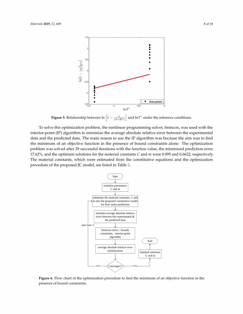
To solve this optimization problem, the nonlinear programming solver, fmincon, was used with theinterior-point (IP) algorithm to minimize the average absolute relative error between the experimentaldata and the predicted data. The main reason to use the IP algorithm was because the aim was to findthe minimum of an objective function in the presence of bound constraints alone. The optimizationproblem was solved after 29 successful iterations with the function value, the minimized prediction error,17.62%, and the optimum solutions for the material constants C and m were 0.095 and 0.6622, respectively.The material constants, which were estimated from the constitutive equations and the optimizationprocedure of the proposed JC model, are listed in Table 2.

Start

initialize parameters

C and m

estimate average absolute relative

error between the experimental &

the predicted data

Converged ? YES

substitute the material constants, C and

m into the proposed constitutive model

for flow stress prediction

fmincon solver : bounds

constraints, interior-point

algorithm

NO

iter=iter+1

End

Optimal solutions

C and m

Find the minimum of an objective function in the presence of bound

constraints.

average absolute relative error

minimization

Figure 6. Flow chart of the optimization procedure to find the minimum of an objective function in thepresence of bound constraints.

Materials 2019, 12, 609 9 of 18

Table 2. Johnson-Cook material model parameters of AISI-1045 steel.

Regular JC Model Optimized JC Model

A (MPa) B (MPa) n C m A (MPa) B (MPa) n C m

50.103 176.091 0.5176 0.1056 0.5655 50.103 176.091 0.5176 0.095 0.6622

Thus, the material constants were substituted into Equation (1) to form a final flow stress model.Thereafter, the relations among stress, σ, strain, ε, the deformation strain rate, ε̇, and the deformationtemperature, T, were established according to the JC model, as follows:

σ̂pred = (50.103 + 176.09ε0.518)

(1 + 0.095 ln

(ε̇

1.0

))(1−

(T − 1223

1623− 1223

)0.662)

(MPa). (9)

3.4. Johnson-Cook Damage Model

Johnson and Cook proposed that fracture strain typically depends on the stress triaxiality ratio,the strain rate and the temperature. The JC fracture model can be written as follows [8,20]:

ε f =

[D1 + D2exp

(D3

(σm

σeq

))] [1 + D4ln

(˙εp∗)] [1 + D5T∗] (10)

where D1 to D5 are the damage model constants, σm is the mean stress, and σeq is the equivalent stress [19].The damage of an element is defined based on a cumulative damage law, and it can be represented ina linear way as shown below [9,19]:

D = ∑(

∆ε

ε f

), (11)

where ∆ε is the equivalent plastic strain increment, and ε f is the equivalent strain to fracture under thepresent conditions of stress, strain rate and temperature. Due to the fracture occurrence, the materialstrength reduces during deformation, and the constitutive relation of stress for the damage evolution canbe expressed as [8]

σD = (1− D)σeq. (12)

In Equation (12), σD is the damaged stress state, and D is the damage parameter, (0 ≤ D < 1).Furthermore, the stress triaxiality [21–25] and the equivalent stress can be obtained from undamagedmaterial considering the plastic behavior until the necking formation [19].

At first, the un-notched and pre-notched specimens were fabricated using the machine cutting process,and more than one sample was used to obtain the flow curve to get a better outcome in terms of themechanical properties of the material in order to control the experimental error. A series of experimentsincluding un-notched and pre-notched round bar, flat specimens were carried out simultaneously, as shownin Figure 7, at room temperature considering a wide range of quasi-static strain rate conditions toinvestigate the effect of stress triaxiality on the damage behavior of AISI-1045 medium carbon steel material.The flow curves accomplished from the tests were decomposed into elastic and plastic regions untilnecking for the identification of material properties as well as for the numerical model inputs. In addition,the mechanical properties of the material were determined carefully from performed experiments, becausethese properties needed to replicate the material’s behavior in the real situations as accurately as possible.blue Furthermore, the estimated properties were incorporated into commercial tools, and the workhardening behavior was simulated by considering the multi-linear isotropic hardening model for the

Materials 2019, 12, 609 10 of 18

assessment of stress triaxiality. The FE models were modeled using half symmetry conditions andmeshed by different mesh sizes to reduce the computational time without affecting the accuracy, as shownin Figure 8a. From the outcome, a good correlation between experimental observations and the FE modelwas achieved in the elastic and plastic range until necking, as depicted in Figure 9. From Figure 9,it is evident that the estimation of mechanical properties from the experiments was done perfectly and canbe further used to perform the estimation of stress triaxiality without any barrier. Subsequently, the stresscomponents, such as, σ1, σ2, and σ3, were chosen from the center of the cross-section of the specimen.Ductile damage mostly tends to occur at this region due to maximum stresses, as displayed in Figure 8b.Thus, the stress components were substituted into Equation (13) to determine the mean stress, σm, and theequivalent stress, σeq, and the set of stress triaxialities estimated for an entire specimens is listed in Table 3.

σ∗ =(σ1 + σ2 + σ3)

3×√

0.5× [(σ21 − σ2

2 ) + (σ22 − σ2

3 ) + (σ23 − σ2

1 )](13)

(a) (b)

Figure 7. Experimental set-up to perform tension test at room temperature. (a) Test machine; (b) Un-notchedand pre-notched specimens.

B

B'

B

B'

(a)

A A'

A A'

(b)

Figure 8. Finite element models. (a) Fine mesh in notching region; (b) Stress estimation region.

Materials 2019, 12, 609 11 of 18

Table 3. Different stress triaxiality data determined from numerical simulations using experimental datafrom round bar, flat un-notched and pre-notched specimens.

T ε̇ (s−1) Flat 6w N-R0 N-R1 N-R2 N-R3

27 ◦C

0.001 0.3345 – 0.8523 0.7756 –0.005 0.3337 – 0.9017 0.7782 –0.010 0.3332 – 0.8961 0.7852 –0.050 0.3333 – 0.9015 0.7829 –

0.0001 – 0.3359 0.5082 0.6070 0.74730.001 – 0.3299 0.4989 0.6152 0.76410.010 – – 0.4897 0.5983 0.7438

To verify the FE results of the flat specimens, Bao and co-workers’ formula was used asgiven below [26]:

η =13+√

2 ln(

1 +t

4R

). (14)

As depicted in Figure 9c, various stress triaxilities were calculated with respect to different thickness toradius ratios. From the comparison results, the estimated stress triaxialities from the numerical simulationswere found to be considerably consistent with the analytical solutions. Also, stress triaxiality statesaccording to Bridgman’s analytical model for the round bar specimens were employed to cross check thenumerical data as follows [27]:

σ∗ =13+ ln

(1 +

a2R

)(15)

where σ∗, R and a are the stress triaxiality, the radius of the circumferential notch and the minimum crosssection of the radius, respectively. From the data plotted in Figure 9d, it is evident that the numerical resultsaligned well with the analytical data. This aspect shows that the un-notched and pre-notched, and theround bar and flat shape specimen results are adequate for the estimation of JC damage model parameters.

Rearranging Equation (10) by neglecting the effects of strain rate and temperature, the failure modelequation can be rewritten only in terms of the stress triaxiality effect with respect to fracture strainas follows [19]:

ε f = D1 + D2 exp (D3σ∗) . (16)

By substituting the stress triaxialities and corresponding fracture strain values into Equation (16),the relationship plot, ε f ∼ σ∗, was developed, and from the coefficients of the fitted equation, as shownin Figure 10, the model parameters D1, D2 and D3 were computed. Subsequently, the strain rate and thetemperature dependent damage parameters D4 and D5 were obtained from two sets of high temperatureand strain rate data by interpreting the failure strain variation [19]. The estimated JC fracture modelparameters are outlined in Table 4, and the model parameters can be used in the metal forming applicationsto predict the ductile fracture behavior.

Materials 2019, 12, 609 12 of 18

0 0.02 0.04 0.06 0.08 0.1 0.12 0.14 0.160

100

200

300

400

500

600

700

800

900

1000

True strain

Tru

e st

ress

(M

Pa)

necking region

failure point

ExperimentSimulation

(a)

0 0.005 0.01 0.015 0.02 0.025 0.03 0.035 0.040

100

200

300

400

500

600

700

800

900

1000

True strain

Tru

e st

ress

(M

Pa)

necking region

failure point

ExperimentSimulation

(b)

0 0.5 1 1.5 2 2.5 3 3.50.2

0.3

0.4

0.5

0.6

0.7

0.8

0.9

1

1.1

1.2

t/R

η

simulationanalytical

(c)

−0.1 0 0.1 0.2 0.3 0.4 0.5 0.6 0.70.1

0.2

0.3

0.4

0.5

0.6

0.7

0.8

0.9

a/R

σ∗

simulationanalytical

(d)

Figure 9. Flow stress curve at room temperature for AISI-1045 steel. (a) Comparison plot of the stress∼straincurve between experimental results and simulation results of the round bar specimen; (b) Comparisonplot of the stress∼strain curve between experimental results and simulation results of the round barnotched specimen; (c) Comparison results of Bao and co-workers’ equation and numerical simulation;(d) Comparison results of the Bridgman equation and numerical simulation.

0.3 0.4 0.5 0.6 0.7 0.8 0.9 1 1.1 1.2 1.30.02

0.04

0.06

0.08

0.1

0.12

0.14

0.16

0.18

0.2

0.22

Triaxiality

Fracture

strain

unnotched flat specimen

notched−R1

notched−R2

R2=0.9907

Data pointsfitted curve

(a)

0.3 0.4 0.5 0.6 0.7 0.8 0.9

0.02

0.04

0.06

0.08

0.1

0.12

0.14

0.16

0.18

Triaxiality

Fracture

strain

unnotched round bar

notched−R1

notched−R2notched−R3

R2=0.9969

Data pointsfitted curve

(b)

Figure 10. Relationship plot of strain to fracture and stress triaxiality. (a) Flat specimens; (b) Roundbar specimens.

Materials 2019, 12, 609 13 of 18

Table 4. Johnson-Cook fracture model parameters of AISI-1045 steel.

Round Bar and Notched Specimens Flat and Notched Specimens

D1 D2 D3 D4 D5 D1 D2 D3 D4 D50.025 16.93 −14.8 0.0214 0 0.04 1.519 −6.905 −0.023 1.302

4. Discussion

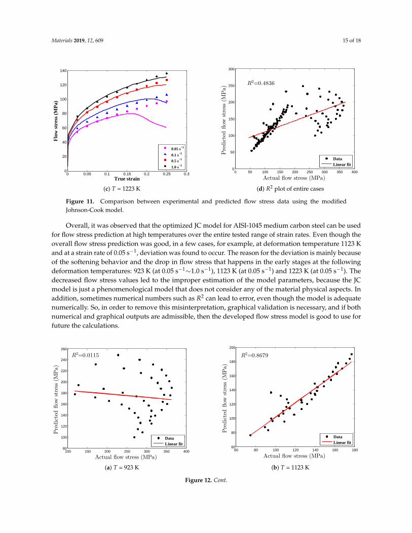
Numerous isothermal experiments were conducted over a practical range of deformationtemperatures (650–950 ◦C) and strain rates (0.05–1.0 s−1) to develop the JC material model to predictthe flow stress data of AISI-1045 medium carbon steel. In addition, the experimental data obtainedfrom the quasi-static strain rate tensile tests at room temperature were employed for the evaluation ofdamage model parameters. To verify the model adequacies and predictability, the proposed constitutivemodel predictions were compared with the experimental observations and were also incorporated intothe numerical simulations for inverse calibrations. Figure 11 depicts the comparison of experimentalstress-strain flow curves with the predicted flow curves by using the proposed JC model, whereas themodel parameters were estimated from the optimization method. The data plotted in Figure 11 andthe numerical data outlined in Table 5 clearly display that the presented optimized JC model is in goodagreement with the experimental observations at higher temperatures for all strain rates, and on thecontrary, the model cannot offer a better prediction of flow stress at the deformation temperature, 650 ◦C,for all tested strain rates. Thus, from the prediction error comparison, the flow stress data obtained in theoptimized JC model were found to be more consistent with the experimental data than the conventionalJC model.

Table 5. Different stress triaxiality data obtained from experiments.

Conditions R2 Overall-R2 AARE (%) Overall-AARE (%)

923 K 0.01150.4836

40.934117.61121123 K 0.8679 5.9313

1223 K 0.8419 5.9689

To perform the model evaluation, standard statistical measurements such as coefficient ofdetermination (R2) and an average absolute relative error (AARE) were adopted to quantify theproposed JC model predictability at discrete strains with an interval of 0.025 for all strain rates andtemperatures. The R2 provides information about the prediction strength of the linear relationshipbetween the experimental observations and the predicted values, whereas AARE was estimated througha term-by-term comparison of the relative error. To perform this quantification, the following expressionswere employed [28,29]:

R2 = 1−

n∑

i=1(σi

exp − σipred)

2

n∑

i=1(σi

exp − σ̄exp)2, (17)

AARE =1n

n

∑i=1

∣∣∣∣∣σiexp − σi

pred

σiexp

∣∣∣∣∣× 100%, (18)

where σexp, σpred, σ̄exp are the experimental flow stress, the predicted flow stress, and the mean flow stress,respectively, and n is the total number of data points.

Materials 2019, 12, 609 14 of 18

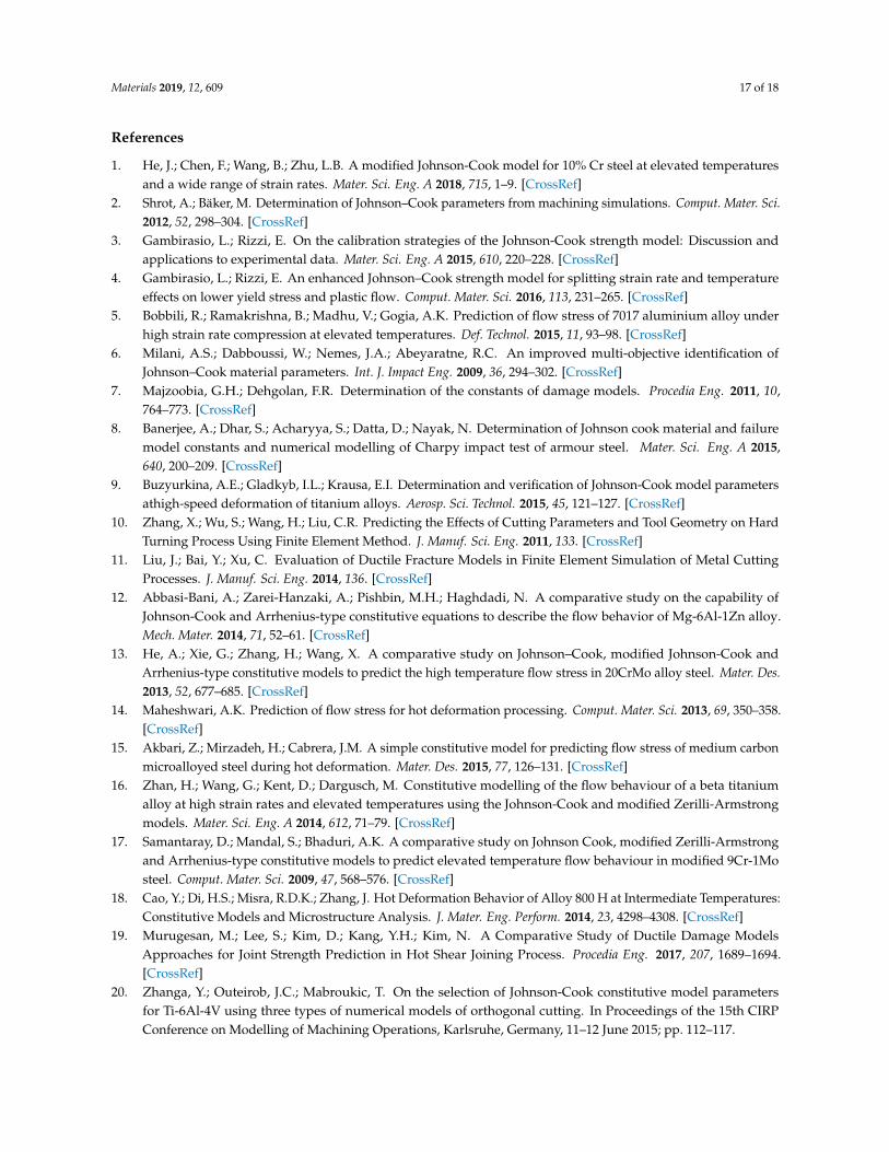
In this research, each test condition was examined by estimating the values of R2 and AARE for eachcase rather than the traditional method, in which the entire data set was used to compute the statisticalparameters as mentioned in Table 5. In this way, the prediction strength of the proposed JC model canbe discussed in detail in terms of each and every test condition. The predicted flow curves and thegraphical validation of the optimized JC model are shown in Figure 11 for all strain rates and deformationtemperatures. Figure 11a depicts the comparison plot between predicted flow curves and experimentaldata and it shows that the developed model overpredicts the flow stress data. The numerical values R2 andAARE were found to be 0.0012, lacking the prediction of the linear relationship as illustrated in Figure 12a,and 40.9341, respectively. From these numbers, it is clear that the optimized JC model cannot predict thematerial behavior at a deformation temperature of 923 K for all strain rate conditions. However, somehow,as shown in Figure 12a, there is some abnormal behavior in the distribution of data points. To verify thisphenomenon, the residual plot, decomposed into three parts—low, exact, and high predictions—is plottedin Figure 12d. From Figure 12d, it is clearly shown that the proposed model mostly under predicts theflow stress, as the most of the data points were distributed linearly, somehow in exponential form, abovethe exact prediction line. This phenomenon explains that by adding some noise function into a negativelinear or exponential form to the original flow stress model, this prediction error can be avoided. Likewise,Figure 11b shows that at a deformation temperature of 1123 K for all strain rates, it is evident that most ofthe predicted flow stress data are close to the experimental observations, whereas Figure 12b exhibits agood correlation between actual and predicted data. In addition, the computed corresponding values of thestatistical parameters, R2, 0.8679, and AARE, 5.9313%, show that the proposed JC model has considerablepotential to predict the flow stress under the tested conditions. Furthermore, Figures 11c and 12c illustratethe good correlation between experimental and predicted data under the tested conditions. R2 andAARE were found to be 0.8419 and 5.9689%, respectively. Besides, it is noted that the prediction errorminimization considering the material parameters, c and m using the optimization procedure led tosignificant improvement in the JC model prediction. For all test conditions, the overall AARE reducedfrom 18.12% to 17.61%. The differences between the models may be small but this small error can causethe false estimation of flow stress which leads to the inaccurate prediction of material behavior.

0 0.05 0.1 0.15 0.2 0.25 0.30

50

100

150

200

250

300

350

400

True strain

Flo

w s

tres

s (M

Pa)

0.05 s−1

0.1 s−1

0.5 s−1

1.0 s−1

(a) T = 923 K

0 0.05 0.1 0.15 0.2 0.25 0.30

20

40

60

80

100

120

140

160

180

200

True strain

Flo

w s

tres

s (M

Pa)

0.05 s−1

0.1 s−1

0.5 s−1

1.0 s−1

(b) T = 1123 K

Figure 11. Cont.

Materials 2019, 12, 609 15 of 18

0 0.05 0.1 0.15 0.2 0.25 0.30

20

40

60

80

100

120

140

True strain

Flo

w s

tres

s (M

Pa)

0.05 s−1

0.1 s−1

0.5 s−1

1.0 s−1

(c) T = 1223 K

0 50 100 150 200 250 300 350 4000

50

100

150

200

250

300

R2=0.4836

Actual flow stress (MPa)

Predictedflow

stress

(MPa)

DataLinear fit

(d) R2 plot of entire cases

Figure 11. Comparison between experimental and predicted flow stress data using the modifiedJohnson-Cook model.

Overall, it was observed that the optimized JC model for AISI-1045 medium carbon steel can be usedfor flow stress prediction at high temperatures over the entire tested range of strain rates. Even though theoverall flow stress prediction was good, in a few cases, for example, at deformation temperature 1123 Kand at a strain rate of 0.05 s−1, deviation was found to occur. The reason for the deviation is mainly becauseof the softening behavior and the drop in flow stress that happens in the early stages at the followingdeformation temperatures: 923 K (at 0.05 s−1∼1.0 s−1), 1123 K (at 0.05 s−1) and 1223 K (at 0.05 s−1). Thedecreased flow stress values led to the improper estimation of the model parameters, because the JCmodel is just a phenomenological model that does not consider any of the material physical aspects. Inaddition, sometimes numerical numbers such as R2 can lead to error, even though the model is adequatenumerically. So, in order to remove this misinterpretation, graphical validation is necessary, and if bothnumerical and graphical outputs are admissible, then the developed flow stress model is good to use forfuture the calculations.

100 150 200 250 300 350 40080

100

120

140

160

180

200

220

240

260

R2=0.0115

Actual flow stress (MPa)

Predictedflow

stress

(MPa)

DataLinear fit

(a) T = 923 K

60 80 100 120 140 160 18060

80

100

120

140

160

180

200

R2=0.8679

Actual flow stress (MPa)

Predictedflow

stress

(MPa)

DataLinear fit

(b) T = 1123 K

Figure 12. Cont.

Materials 2019, 12, 609 16 of 18

50 60 70 80 90 100 110 120 130 14050

60

70

80

90

100

110

120

130

140

R2=0.8419

Actual flow stress (MPa)

Predictedflow

stress

(MPa)

DataLinear fit

(c) T = 1223 K (d) Residual plot (T = 923 K)

Figure 12. Relationship plots.

5. Conclusions

In this paper, numerous isothermal hot tensile tests at elevated temperatures (650–950 ◦C) and strainrates (0.05–1.0 s−1) were carried out to identify the Johnson-Cook material model parameters for AISI 1045medium carbon steel. The nonlinear programming solver fmincon-based optimization procedure wasemployed for minimizing the prediction error between the experiments and the predictions to improvethe ability of the proposed JC constitutive model. Overall, the results obtained from the optimized JCmodel showed better agreement with the experimental observations than those of the traditional method.However, more computational time is required to achieve the JC material constants while performing theoptimization procedures than with the conventional method. Besides, the developed model predictabilitywas evaluated in terms of the metrics R2 and AARE. In addition, using the commercial tool, the numericalsimulations were modeled extensively in order to develop the damage model using the experimentalobservations obtained from the quasi-static tensile tests with smooth and notched specimens at roomtemperature. The numerical results displayed a good agreement with the corresponding experimentaldata. From the discussion, it was found that the JC material model requires less effort to predict the modelparameters and, on the contrary, the JC damage model requires numerous experimental data to find themodel parameters, which necessitates extensive time and cost efforts. Besides, the prediction error betweenthe experimental and predicted data ensures that the proposed constitutive model is credible at elevatedtemperatures and higher strain rates. Based on these research outcomes, the detailed identification of theJC material and damage model can be devised using the procedure presented here to predict materialductile fracture behavior.

Author Contributions: In this research, the parts such as conceptualization, methodology, numerical modeling,programming, investigation and validation, original draft preparation is done by the author, M.M. and the supervisionis carried out by D.W.J.

Funding: This research received no external funding.

Conflicts of Interest: The authors declare no conflict of interest.

Materials 2019, 12, 609 17 of 18

References

1. He, J.; Chen, F.; Wang, B.; Zhu, L.B. A modified Johnson-Cook model for 10% Cr steel at elevated temperaturesand a wide range of strain rates. Mater. Sci. Eng. A 2018, 715, 1–9. [CrossRef]

2. Shrot, A.; Bäker, M. Determination of Johnson–Cook parameters from machining simulations. Comput. Mater. Sci.2012, 52, 298–304. [CrossRef]

3. Gambirasio, L.; Rizzi, E. On the calibration strategies of the Johnson-Cook strength model: Discussion andapplications to experimental data. Mater. Sci. Eng. A 2015, 610, 220–228. [CrossRef]

4. Gambirasio, L.; Rizzi, E. An enhanced Johnson–Cook strength model for splitting strain rate and temperatureeffects on lower yield stress and plastic flow. Comput. Mater. Sci. 2016, 113, 231–265. [CrossRef]

5. Bobbili, R.; Ramakrishna, B.; Madhu, V.; Gogia, A.K. Prediction of flow stress of 7017 aluminium alloy underhigh strain rate compression at elevated temperatures. Def. Technol. 2015, 11, 93–98. [CrossRef]

6. Milani, A.S.; Dabboussi, W.; Nemes, J.A.; Abeyaratne, R.C. An improved multi-objective identification ofJohnson–Cook material parameters. Int. J. Impact Eng. 2009, 36, 294–302. [CrossRef]

7. Majzoobia, G.H.; Dehgolan, F.R. Determination of the constants of damage models. Procedia Eng. 2011, 10,764–773. [CrossRef]

8. Banerjee, A.; Dhar, S.; Acharyya, S.; Datta, D.; Nayak, N. Determination of Johnson cook material and failuremodel constants and numerical modelling of Charpy impact test of armour steel. Mater. Sci. Eng. A 2015,640, 200–209. [CrossRef]

9. Buzyurkina, A.E.; Gladkyb, I.L.; Krausa, E.I. Determination and verification of Johnson-Cook model parametersathigh-speed deformation of titanium alloys. Aerosp. Sci. Technol. 2015, 45, 121–127. [CrossRef]

10. Zhang, X.; Wu, S.; Wang, H.; Liu, C.R. Predicting the Effects of Cutting Parameters and Tool Geometry on HardTurning Process Using Finite Element Method. J. Manuf. Sci. Eng. 2011, 133. [CrossRef]

11. Liu, J.; Bai, Y.; Xu, C. Evaluation of Ductile Fracture Models in Finite Element Simulation of Metal CuttingProcesses. J. Manuf. Sci. Eng. 2014, 136. [CrossRef]

12. Abbasi-Bani, A.; Zarei-Hanzaki, A.; Pishbin, M.H.; Haghdadi, N. A comparative study on the capability ofJohnson-Cook and Arrhenius-type constitutive equations to describe the flow behavior of Mg-6Al-1Zn alloy.Mech. Mater. 2014, 71, 52–61. [CrossRef]

13. He, A.; Xie, G.; Zhang, H.; Wang, X. A comparative study on Johnson–Cook, modified Johnson-Cook andArrhenius-type constitutive models to predict the high temperature flow stress in 20CrMo alloy steel. Mater. Des.2013, 52, 677–685. [CrossRef]

14. Maheshwari, A.K. Prediction of flow stress for hot deformation processing. Comput. Mater. Sci. 2013, 69, 350–358.[CrossRef]

15. Akbari, Z.; Mirzadeh, H.; Cabrera, J.M. A simple constitutive model for predicting flow stress of medium carbonmicroalloyed steel during hot deformation. Mater. Des. 2015, 77, 126–131. [CrossRef]

16. Zhan, H.; Wang, G.; Kent, D.; Dargusch, M. Constitutive modelling of the flow behaviour of a beta titaniumalloy at high strain rates and elevated temperatures using the Johnson-Cook and modified Zerilli-Armstrongmodels. Mater. Sci. Eng. A 2014, 612, 71–79. [CrossRef]

17. Samantaray, D.; Mandal, S.; Bhaduri, A.K. A comparative study on Johnson Cook, modified Zerilli-Armstrongand Arrhenius-type constitutive models to predict elevated temperature flow behaviour in modified 9Cr-1Mosteel. Comput. Mater. Sci. 2009, 47, 568–576. [CrossRef]

18. Cao, Y.; Di, H.S.; Misra, R.D.K.; Zhang, J. Hot Deformation Behavior of Alloy 800 H at Intermediate Temperatures:Constitutive Models and Microstructure Analysis. J. Mater. Eng. Perform. 2014, 23, 4298–4308. [CrossRef]

19. Murugesan, M.; Lee, S.; Kim, D.; Kang, Y.H.; Kim, N. A Comparative Study of Ductile Damage ModelsApproaches for Joint Strength Prediction in Hot Shear Joining Process. Procedia Eng. 2017, 207, 1689–1694.[CrossRef]

20. Zhanga, Y.; Outeirob, J.C.; Mabroukic, T. On the selection of Johnson-Cook constitutive model parametersfor Ti-6Al-4V using three types of numerical models of orthogonal cutting. In Proceedings of the 15th CIRPConference on Modelling of Machining Operations, Karlsruhe, Germany, 11–12 June 2015; pp. 112–117.

Materials 2019, 12, 609 18 of 18

21. Bai, Y.; Wierzbicki, T. A new model of metal plasticity and fracture with pressure and Lode dependence.Int. J. Plast. 2008, 24, 1071–1096. [CrossRef]

22. Brunig, M.; Chyra, O.; Albrecht, D.; Driemeier, L.; Alves, M. A ductile damage criterion at various stresstriaxialities. Int. J. Plast. 2008, 24, 1731–1755. [CrossRef]

23. Mirone, G.; Corallo, D. A local viewpoint for evaluating the influence of stress triaxiality and Lode angle onductile failure and hardening. Int. J. Plast. 2010, 26, 348–371. [CrossRef]

24. Cao, T.S.; Gachet, J.M.; Montmitonnet, P.; Bouchard, P.O. A Lode-dependent enhanced Lemaitre model forductile fracture prediction at low stress triaxiality. Eng. Fract. Mech. 2014, 124–125, 80–96. [CrossRef]

25. Bao, Y. Dependence of ductile crack formation in tensile tests on stress triaxiality, stress and strain ratios.Eng. Fract. Mech. 2005, 72, 505–522. [CrossRef]

26. Bao, Y. Prediciton of Ductile Crack Formation in Uncracked Bodies. Ph.D. Thesis, Massachusetts Institute ofTechnology, Cambridge, MA, USA, 2003.

27. Bridgman, P.W. Studies in Large Plastic Flow and Fracture; McGraw-Hill Book Company, Inc.: New York,NY, USA, 1952.

28. Lee, K.; Murugesan, M.; Lee, S.M.; Kang, B.S. A Comparative Study on Arrhenius-Type Constitutive Modelswith Regression Methods. Trans. Mater. Process. 2017, 26, 18–27. [CrossRef]

29. Murugesan, M.; Kang, B.S.; Lee, K. Multi-Objective Design Optimization of Composite Stiffened Panel UsingResponse Surface Methodology. J. Compos. Res. 2015, 28, 297–310. [CrossRef]

c© 2019 by the authors. Licensee MDPI, Basel, Switzerland. This article is an open accessarticle distributed under the terms and conditions of the Creative Commons Attribution (CCBY) license (http://creativecommons.org/licenses/by/4.0/).