DISCUSSION PAPER SERIES

ABCD

www.cepr.org

Available online at: www.cepr.org/pubs/dps/DP4147.asp www.ssrn.com/xxx/xxx/xxx

No. 4147

JOB TENURE, WAGES AND TECHNOLOGY: A REASSESSMENT USING MATCHED WORKER-FIRM

PANEL DATA

Pauline Givord and Eric Maurin

LABOUR ECONOMICS

ISSN 0265-8003

JOB TENURE, WAGES AND TECHNOLOGY: A REASSESSMENT USING MATCHED WORKER-FIRM

PANEL DATA

Pauline Givord, INSEE, Paris Eric Maurin, Center for Research in Economics and Statistics (CREST) and CEPR

Discussion Paper No. 4147 December 2003

Centre for Economic Policy Research 90–98 Goswell Rd, London EC1V 7RR, UK

Tel: (44 20) 7878 2900, Fax: (44 20) 7878 2999 Email: cepr@cepr.org, Website: www.cepr.org

This Discussion Paper is issued under the auspices of the Centre’s research programme in LABOUR ECONOMICS. Any opinions expressed here are those of the author(s) and not those of the Centre for Economic Policy Research. Research disseminated by CEPR may include views on policy, but the Centre itself takes no institutional policy positions.

The Centre for Economic Policy Research was established in 1983 as a private educational charity, to promote independent analysis and public discussion of open economies and the relations among them. It is pluralist and non-partisan, bringing economic research to bear on the analysis of medium- and long-run policy questions. Institutional (core) finance for the Centre has been provided through major grants from the Economic and Social Research Council, under which an ESRC Resource Centre operates within CEPR; the Esmée Fairbairn Charitable Trust; and the Bank of England. These organizations do not give prior review to the Centre’s publications, nor do they necessarily endorse the views expressed therein.

These Discussion Papers often represent preliminary or incomplete work, circulated to encourage discussion and comment. Citation and use of such a paper should take account of its provisional character.

Copyright: Pauline Givord and Eric Maurin

CEPR Discussion Paper No. 4147

December 2003

ABSTRACT

Job Tenure, Wages and Technology: A Reassessment Using Matched Worker-Firm Panel Data*

This Paper presents new estimates of the impact of job tenure on wages using a new French matched worker-firm dataset. We develop an identification strategy that relies on one specific feature of the French labour laws. They stipulate that firms, when firing workers, must include as one of their criteria the number of dependent children of their employees. Our dataset confirms that workers with a relatively large number of dependent children at the entry in the firm are, ceteris paribus, less likely to be laid-off and have on average higher job tenure than their co-workers with a relatively small number of dependent children. Within this framework, the relative number of children at entry in the firm represents a plausibly valid instrumental variable for identifying the impact of job tenure on wages. Our new IV estimate of the return to job tenure (3.1% per year) is much larger than the OLS estimate (1%). This result holds true regardless of whether we focus on educated or non-educated workers, men or women. The downward bias which affects OLS estimates suggests that workers who receive relatively high wage offers tend to change firms more rapidly: they tend to have relatively high wages and low job tenure. Regarding trends, our new IV estimator suggests that the returns to job tenure have declined over the 1990s in the industries where the share of educated workers is the largest. The technologies that complement highly-skilled labour seem to drive a decline in the incentive to keep workers over long periods of time and, as a consequence, a decline in the impact of tenure on wages.

JEL Classification: J31, J53 and O33 Keywords: job tenure, technological change and wages

Pauline Givord INSEE 18 boulevard Pinard 75014 Paris FRANCE Tel: (33 1) 4117 5448 Fax: (33 1) 4117 6045 Email: pauline.givord@insee.fr For further Discussion Papers by this author see: www.cepr.org/pubs/new-dps/dplist.asp?authorid=158784

Eric Maurin CREST - DR 15 boulevard Gabriel Péri 92245 Malakoff FRANCE Tel: (33 1) 4117 6035 Fax: (33 1) 4117 6046 Email: maurin@ensae.fr For further Discussion Papers by this author see: www.cepr.org/pubs/new-dps/dplist.asp?authorid=131502

*We would like to thank participants at the conference on matched employer-employee data in Bergen (2002), the conference on the dynamics of European labour markets in Berlin (2002) and seminar participants at Timbergen Institute (Amsterdam, 2003), CREST (Paris, 2002) and INSEE (Paris, 2003).

Submitted 22 October 2003

1 Introduction

The idea that job seniority has a large effect on wages has been the subject of

much controversy in the recent economic literature1 . At stake is the view that

speciÞc human capital is an important ingredient of wage growth and workers�

turnover, as well as the assumption that deferred compensation (in the form of

rising wages) encourages workers� effort and induces proÞtable self-selection of

heterogenous workers. Whether or not seniority has a large impact on earnings

is also very important in assessing the costs of job dislocation and the relevance

of public policy targeted at increasing labor market ßexibility.

In this paper, we try to shed some light on these issues and provide new

estimates of the returns to seniority and of their variations across industries

and over time. We use new French matched worker-Þrm panel data and new

identiÞcation techniques, relying on some of the unique features of our database

and of French institutions.

The basic problem for identifying the returns to job tenure comes from the

fact that job tenure, like wage, is an outcome of optimisation by employers and

workers. As such, job tenure cannot be considered as an exogenous determinant

of wages. Workers with different level of seniority receive different wages, but

it does not necessarily mean that seniority affect wages. It may also simply

reßect the fact that job tenure and wages are both determined by some similar

unobserved factors.

To overcome this problem and identify the true effect of seniority on wages,

one possibility is to construct instrumental variables that affect wages only in-

sofar as they affect seniority. When laying workers off, French Þrms are con-

strained by labor laws to take into account the number of dependent children

of their workers (see article L. 321-1-1 of the French labor laws). One interest-

ing feature of our matched worker-Þrm dataset is that it makes it possible to

rank workers within their Þrm according to the number of dependent children.

1See e.g. Abraham and Farber (1987), Altonji and Shakotko (1987), Topel (1991), Altonjiand Williams (1997).

2

Our dataset conÞrms that workers with a relatively large number of dependent

children are less likely to be laid off and have on average higher job tenure than

their co-workers with a relatively small number of dependent children regardless

of whether we control for the absolute number of children or not. Assuming that

the relative number of children has no direct effect on wages, this variable pro-

vides us with a new interesting instrumental variable for identifying the returns

to job tenure. The Þrst basic goal of this paper is actually to reevaluate the

average returns to job tenure using this new instrument.

The second purpose of this paper is to explore the extent in which returns

to job tenure vary across industries and over time. On the one hand, we can

plausibly speculate that contemporary technological change is increasing the

returns to skills that are acquired on the job, exactly the same way it is increas-

ing the returns to education (see e.g. Katz and Autor, 1999). On the other

hand, given that routine tasks are those for which senior workers may have the

strongest comparative advantage -they have had time for learning them on the

job- and given that the dissemination of new technologies is mostly destroying

these routine tasks2 , we can also expect that technological change is decreasing

the demand for high-seniority workers and, as a consequence, decreasing the

returns to seniority.

To shed some light on these issues, we will analyze whether the returns to job

tenure are larger in the sectors with the highest employment share of educated

workers at the beginning of the period under consideration (which we interpret

as an indicator of the dissemination of the technologies that complement skilled

labor). Besides, we will explore whether this link between the returns to job

tenure and the employment share of educated workers varies over time. One

of the interesting feature of our dataset is indeed that it provides matched

worker-Þrm information over a relatively long period of time (i.e., 1991-2002).

The last decade has witnessed dramatic technological change in France, while

labor laws remained stable. If contemporary technological change is actually

2See e.g. Autor et al. (2003), Maurin and Thesmar (2003).

3

increasing the degree of substituability between high and low seniority workers,

we can plausibly expect a decline in the return to tenure across the last decade,

especially in sectors with the highest dissemination of new technologies.

Our main empirical results may be summarized as follows:

(a) our new IV estimate suggests an average return to job tenure of about

3.1% per year. Most interestingly, this new IV estimate is much larger than the

estimate obtained with standard OLS speciÞcation (1% per year). This result

holds true regardless of whether we focus on educated or less educated workers,

men or women. Generally speaking, our IV estimates are closer from Topel

(1991) or Dustman and Meghir (2003) than from Altonji and Shakotko (1987)

or Abraham and Farber (1989).

The downward bias which affects OLS estimates reßects a negative corre-

lation between the unobserved determinants of wages and job tenure. One

possible explanation is that workers who tend to receive high-wage offers also

tend to change job more often and, as a consequence, are over-represented in

the population of low-seniority workers. This explanation is consistent with the

fact that the downward biases affecting OLS estimates are more important for

the most educated workers, i.e. the most mobile workers and, as a consequence,

those whose seniority is the most likely to be correlated with the quality of the

job offers.

(b) According to our IV estimation techniques, the average return to job

tenure is actually less signiÞcant in the industries with highest share of educated

workers at the beginning of the period under consideration. Also we observe a

decline in the returns to job tenure in these industries over the last decade. The

technologies that complement skilled labor seem to be associated with a decline

in the incentive to keep workers for long period of time and, as a consequence,

seem to be driving a decline in the returns to job tenure.

All in all, we end up with an array of Þndings suggesting that the average

returns to tenure are actually more signiÞcant than what standard OLS speci-

Þcations suggest and that the technologies which complement skilled labor are

4

driving a decline in the average returns to job tenure in France.

The paper is organized as follows. Section 2 provides an overlook of the

litterature. Section 3 presents our matched worker-Þrm dataset and our econo-

metric models. Section 4 shows the results.

2 Existing Litterature

There is an old literature on estimating the returns to job tenure using standard

earnings function. Typical OLS regression Þnds an average return of about 1%-

2% per year depending on the speciÞcation.

There exists also a substantial literature which has worried about the biases

that may affect simple OLS estimates of returns to job tenure because of the

endogeneity of seniority. Job tenure, like the wage, is an outcome of Þrms� and

workers� behaviors, and, as such, cannot be assumed to represent an independant

source of wage variation.

Altonji and Shakotko (1987) and Abraham and Farber (1987) argue that the

standard OLS estimated returns to tenure are upward biased due to the fact that

job tenure depends on the same unobserved individual and job speciÞc variables

as wages. To overcome this problem, Abraham and Farber (1987) construct for

each worker-job pair an indicator of the completed duration of the match. They

add this indicator as a supplementary control variable to capture the effect of

the unobserved quality of the match on wages. Altonji and Shakotko (1987)

use an instrumental variable (IV) version of this strategy. For each worker-job

pair and each year, they construct the deviation of current job tenure from the

mean observed job tenure of this speciÞc match. They use this deviation as an

instrumental variable for identifying the true effect of job tenure on wages. In

both papers, job tenure and wages are assumed to be linear function of the same

unobserved individual and match-speciÞc components. It is the reason why the

available information on mean tenure or completed tenure make it possible to

purge out the effect of the unobserved factors. Both Altonji and Shakotko (1987)

and Abraham and Farber (1987) Þnd a substantial reduction in the estimated

5

effect of job tenure (i.e., about 0.5% per year of job tenure as opposed to the

2% OLS effect).

In an other inßuential paper, Topel (1991) takes a different approach. Firstly,

he uses the average within-job wage growth of workers who do not change jobs

(stayers) as an unbiased estimated of the total wage growth due to both labor

market experience and job tenure. He assumes that biases that could arise from

endogenous selection in the subsample of stayers can be neglected. This Þrst

stage provides Topel with an estimate of the wage that workers receive when

they got hired. By regressing this estimated wage at the start of the job on an

indicator of the labor market experience at the start of the job, he gets what

he interprets as an upward bound of the impact of labor market experience

on wages. The difference between the Þrst-stage and second-stage estimates

provides him with a lower bound for true return to tenure of about 2.5% per

year. All in all, Topel argues that there exists a substantial return to job tenure.

One issue in Topel�s analysis is his assuming that the wage dynamics of

stayers provide an unbiased evaluation of the wage dynamics for all workers had

they changed jobs or not. This assumption does not allow for the possibility

that workers change jobs for reasons related to wage.

Altonji and Williams (1997) revisit the question and argue that Topel�s use

of lagged wages with a current measure of job tenure (due to the design of the

PSID) results in an upward bias in the return to tenure in his sample. They

conclude from their analysis that the return to tenure is about 1% per year, i.e.

substantially smaller than Topel�s Þnding.

As emphasized by Farber (1999), the assumptions under which Altonji and

Williams or Abraham and Farber estimators are valid remain not perfectly

clear. Controlling for current tenure, the completed or mean tenure depends

plausibly on factors that also determine the current wage and this may cause

some biases. Besides it is not clear why job tenure should be a linear function of

the unobserved determinant of wages and why the difference between observed

tenure and complete tenure should purge the endogenous unobserved effects

6

out. Assume for instance that (a) quits occur when current wages are lower

than a given exogenous threshold, (b) the unobserved determinant of current

wages affect tenure only insofar as they affect quits. In such a case, job tenure

is clearly a highly non-linear function of any unobserved determinant of wages.

Buchinski et al. (2002) have recently tried to address these issues by es-

timating jointly a participation equation, a job mobility equation and a wage

equation. Using the PSID and assuming a normal distribution for the joint

distribution of their residuals, they Þnd returns to job tenure which are signif-

icantly higher than Altonji and Williams (1997) and almost as high as Topel

(1991).

Another approach to evaluating returns to tenure relies on examining the

wage dynamics of workers who change jobs for reasons exogenous to their own

decisions or to the decisions of employers with regard to their wages or per-

formances. Addison and Portugal (1989) present an analysis of data from the

January 1984 Displaced Workers Survey which Þnds that earnings losses are

larger for workers with more pre-displacement tenure. Farber (1999) presents

similar evidence using the DWS from 1984 to 1996 suggesting a return to tenure

of about 1.2% per year. Using the DWS from 1984 to 1986, Gibbons and Katz

(1991) present an analysis of workers who are displaced due to plant closing.

The idea is that the other displaced workers may be selected by their employers

on the basis of relatively poor performance (or relatively high pay). To avoid

the bias that may arise from endogenous selection, the idea is to focus on a sam-

ple of more exogenous job losers. Gibbons and Katz (1991) report similar links

between wage losses and pre-displacement tenure across the different categories

of job losers.

One issue with focusing on plant closure is that workers who are still em-

ployed in a plant when this plant closes represent a plausibly endogenously

selected population. Put differently, plant closing is a long process and one

may speculate that the population of workers at the end of the process is not

representative of the population at the beginning (see Pfann, 2002).

7

In a recent paper on German data, Dustman and Meghir (2003) circumvent

the problem by assuming that workers cannot predict a closure if the closure is

more than a year away and by deÞning displaced workers as workers who are in

the Þrm one year before the closure. Assuming that age affects the probability of

Þnding a post displacement job, but not the level of the wage offer, they are able

to identify the return to experience and the return to sector tenure. From there,

using a two-step approach in the spirit of Topel (1991), they can recover the

return to seniority. They Þnd very signiÞcant average return to tenure (from 2%

for skilled workers to 3.5% for unskilled workers). Of course, the most debatable

assumption in Dustman and Meghir (2003) is their exclusion restriction. If the

impact of age on labor force participation reßects the impact of family situation

(as suggested by the authors), it is not very clear why it should not also affect

the intensity of job search and, as a consequence, the quality of the available

job offers.

3 Data

The data in this study come from the recent annual Labor Force Surveys (LFS)

conducted by the French national statistical office (INSEE) between 1991 and

2001. The survey takes place in March of every year. The survey samples

are representative of the population aged 15 and up. The sampling fraction is

approximately 1/300. The following standard information is compiled for each

interviewee: education, age, labor market status (in employment, unemploy-

ment, not in the labor force), industry, job tenure. We also have an information

on whether the worker wants to change job and (if yes) whether this is because

s/he expects to be soon laid off. Further, we have an information on the family

situation of each worker. In particular, we know the number and the age of the

dependent children in his/her household.

Using the information on the seniority of the worker and the age of his/her

children, we can evaluate the number of dependent children when s/he got hired

by his/her current Þrm. For instance, a ten-years seniority worker with a Þve-

8

years old child is a worker who had no dependent children when s/he got hired

by his/her current Þrm.

Regarding wages, we have information on actual net monthly earnings and

on the corresponding number of hours worked. Respondents are asked to state

their actual wage for the month prior to the survey - or the latest month of

regular activity if the previous month was too atypical. The study focuses on

hourly wages. Generally speaking, we Þnd qualitatively similar results when

we focus on monthly-earnings rather than hourly wages and this is the reason

why we do not report the monthly-earning regressions. Notice that our wage

measure refers to the same month as our job tenure measure3.

One interesting characteristics of the LFS is that workers are asked their

Þrms� identiÞcation number (SIREN). This information is collected and cap-

tured in several stages (for more details, see appendix A). The information is

available for about 80% of the workers surveyed. As it turns out, about 45% of

the private-sector workers surveyed in a typical LFS have at least one co-worker

surveyed in the same LFS and about 20% have four co-workers or more in the

same survey (see table A1). This feature of the LFS makes possible to construct

large samples of workers with detailed information on one or more other workers

in the same Þrm. In this paper we will mostly focus on the sample of respon-

dents who are less than 50 years old, who are employed in the private sector,

for whom we know the SIREN identiÞcation number of the Þrm and who have

at least one co-worker in the sample. The size of this sample is 71,698 when

we focus on male respondents and 48,500 when we focus on women. Table A2

provides some basics statistics of the sample.

Another interesting feature of the LFS is that only one third of the sample is

renewed each year. One can thus track the career of portion of the sample for 2

or 3 years. In this paper, we have extracted from the main sample a subsample

of about 40,260 workers who are surveyed two years consecutively t and t + 1.

3The American studies that are regarded as authoritative used the PSID where job tenurerefers to the date of the survey whereas the wage measure is annual earnings in the previouscalendar year. When there is a job change, all measures of earnings are mixture of the oldand the new compensation (see Altonji&Williams, 1997).

9

About 5% are employed at t and unemployed at t+ 1, but were not willing to

Þnd another job at t or were willing to Þnd another job only because they were

expecting to be laid off. We will interpret this subsample as a subsample of

involuntary job losers.

3.0.1 Instrumental variables

Regarding instrumental variables, we will use a variable describing workers�

family situation at the entry in the Þrm relative to the family situation of their

co-workers at the entry in the Þrm.

The rationale for using this variable as an instrument comes from the fact

that French labor laws stipulate that Þrms -when laying workers off- must take

into account the family situation of their employees. The Article L 321-1-1 of

the French Code du Travail stipulates that (a) the employer must negotiate

with workers� representatives the criteria that are used for determining who is

laid off when some layoffs are decided and (b) these criteria should take into

account the number of dependent children of the worker, whether the worker

is a single parent, his/her seniority within the Þrm, the age of the worker,

whether the worker has handicaps that make it more difficult to Þnd another

job. The employer must take these criteria into account regardless of the number

of layoffs.

Among the compulsory criteria (number of dependent children, age, senior-

ity, handicaps) the number of dependent children is the only one that does not

correspond to a personal characteristic of the worker and, in this sense, it is a

priori the most exogenous one, .i.e. the least correlated with the unobserved

abilities which may affect wages. It is the reason why we will focus on this

speciÞc criterium to construct our instrument.

SpeciÞcally, we will evaluate for each worker the rank within his/her Þrm

according to the number of dependent children in his/her household at the

entry in the current Þrm. We will focus on the relative number of children at

the entry in the Þrm rather than on the current relative number of children,

because the current number of children is plausibly a consequence of the quality

10

of the current job-worker match4 and, as such, less exogenous. Dividing this

rank variable by its mean value within the Þrm, we obtain a normalized rank

variable which is by construction uncorrelated with the number of co-workers

and with the size of the Þrm. This normalized rank variable will be used as

our basic instrument for identifying the effect of seniority on wages. As shown

below, these instruments are correlated with involuntary job loss and job tenure,

even after controlling for the absolute number of children. Appendix B proposes

a very simple model of job mobility and wage formation which may justify our

identifying strategy.

4 Results

Holding workers� education, experience and number of children constant, Table

1 shows that the relative number of children at the entry in the Þrm z has a

signiÞcant negative effect on the probability of being laid off and a signiÞcant

positive impact on job tenure. These results are the same regardless of whether

we control for Þrm size or not. These Þndings are consistent with the French

institutional context and conÞrm that z is a potentially valid instrument for

identifying the effect of job tenure on wages.

Model (3) in table 2 shows the results of the basic OLS regression of wages on

workers� seniority and basic characteristics (education, experience and number

of children). According to this model, the return to job tenure is about 1.1%

per year5 . This Þnding is consistent with typical OLS estimates of the average

return to job tenure in France (see e.g. Goux and Maurin, 1994).

Model (4) shows the results of our basic IV regression. Most interestingly,

the IV estimated average return to job tenure is signiÞcantly larger than the

OLS estimate, namely 3.1% per year. The downward bias which affects OLS

estimates suggest that high-seniority workers have on average lower wage po-

tential than low-seniority workers. One plausible interpretation is that workers

4Some parents may plausibly wait for good, stable jobs before having children.5We Þnd exactly the same OLS results when we use the whole LFS sample rather than the

sample of workers with at least one co-worker.

11

who receive relatively high-wage offers tend to change Þrm more rapidly than

workers with low wage offers: they tend to have (ceteris paribus) higher wage

and less job tenure.

Models (5) and (6) show the OLS and IV results for the subsample of high-

school dropouts while models (7) and (8) focus on high-school graduates. In

both cases, the IV estimates are larger than the OLS estimates. The downward

bias which affects OLS estimates is, however, larger for educated workers than

for non-educated ones. This result suggests that the correlation between job

tenure and the quality of wage offers is stronger for educated workers than non-

educated workers, which is consistent with the fact that job mobility is more

often voluntary for educated workers than for non-educated workers.

4.1 Robustness

Holding the absolute number of children constant, the relative number of chil-

dren of any given worker is correlated with the distribution of the absolute

number of children in his/her Þrm. Given that the absolute number of chil-

dren is correlated with age, the distribution of the absolute number of children

at the entry in a Þrm is plausibly correlated with the distribution of workers�

age at the entry in this Þrm. Hence, our identiÞcation strategy relies upon

the assumption that the unobserved components of Þrms� wage policies are not

correlated with the distributions of age at the entry. To test this hypothesis

and probe the robustness of our results, we have replicated our analysis using

the average age at the entry of co-workers as a supplementary control variable

(Table A3). Comfortingly, this variable has a negligible effect on wages and

the basic diagnosis are the same regardless of whether we use it as a control

variable or not. We have also replicated our analysis on the sample of women

(N = 48, 500). Comfortingly the OLS estimate are very similar for women and

men (Table 2b). The IV estimates are also much larger than the OLS estimates.

The IV estimates are however somewhat less well estimated in the women case.

12

4.2 Seniority biased technological change

As argued by Farber (1999), an appropriate estimate of the returns to job tenure

measures the compensation structure used by Þrms to discourage voluntary

turnover and achieve appropriate performance from their workers. Such an

interpretation suggests that the relationship between tenure and earning is not

a market-determined constant, but is likely to vary across Þrms with different

technologies6.

More speciÞcally, technologies may vary with respect to the quantity of pro-

ductive skills that can be acquired on the job. But they may also vary with

respect to the degree in which the (transferable) skills that can be found on

the labor market are easy to substitute for the (speciÞc) skills that are acquired

on the job. Generally speaking, the incentive to reduce voluntary turnover and

to offer steeply sloped earning proÞles increases when (a) workers acquire a lot

of new skills on the job and when (b) low-seniority workers cannot be easily

substituted for high-seniority ones.

Given this fact, contemporary technological change may plausibly have two

opposit effects on the compensation structure used by employers. Its Þrst po-

tential effect is throught destruction of routine tasks (Autor et al. 2003, Maurin

and Thesmar, 2003). Given that routine tasks are those for which high-seniority

workers may have a signiÞcant comparative advantage (they have had time to

learn them on then job), technological progress plausibly makes low-seniority

workers easier to substitute for high-seniority ones. As a consequence, turnover

may become less costly to the Þrms and the link between seniority and wages

may weaken7.

On the other hand, technological change plausibly increases the productivity

of the skills that are acquired on the job exactly the same way it increases

the productivity of the skills that are acquired at school (Katz and Autor,

1999). As a consequence, it may also increase the incentive to reduce voluntary6Margolis (1996) provides a detailed description of the huge variations in earning proÞles

across Þrms.7Givord and Maurin (2002) Þnd that the recent increase in involuntary turnover in France

is more pronounced in sectors with the highest proportion of new technologies� users.

13

turnover. In this section we are going to examine empirically how these two

effects combine.

To begin with, Table 3 provides an analysis of the returns to job tenure when

one allows these returns to vary across sectors. We distinguish sectors according

to the employment share of high-school graduates at the beginning of the period

(i.e. 1991). The question is whether the returns to job tenure depend on the

presence of technologies that complement skilled labor8. Model (16) provides

IV estimates showing that the returns to job tenure are less signiÞcant in the

sectors with the highest share of educated workers. According to model (18)

and (20), this result holds true regardless of whether we focus on educated or

non-educated workers. As discussed above, one possible interpretation is that

new technologies are destroying the very tasks for which job tenure provides a

comparative advantage, which reduces the incentive to keep workers for long

period of time.

Regarding the estimated effect of tenure and its variation across sectors, the

comparison of models (16), (18) and (20) with models (15), (17) and (19) shows

that the downward bias which affects OLS is larger in �low-tech� sector, i.e.

sectors with the lowest proportion of educated workers. This Þnding suggests

the concentration of high-wage workers in low-tenure jobs is relatively more

important in �low-tech� than in �high-tech� sectors. One plausible explanation

is that the ßows of voluntary job mobility go mostly from �low-tech� to �high-

tech� sectors.

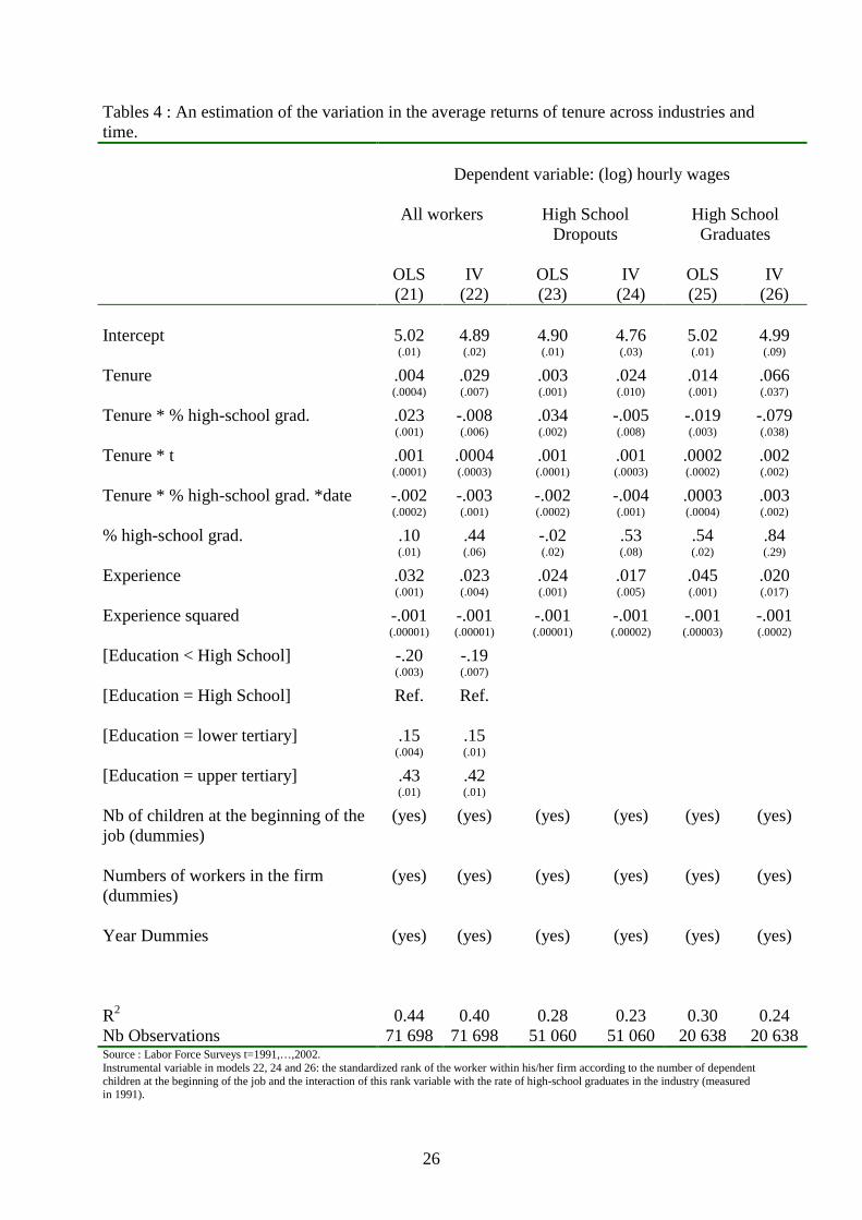
To probe the robustness of these results, Table 4 provides an analysis of

the variation in the average return to seniority over time. Model (22) provides

an IV analysis showing that the differences between the returns to job tenure

in low-tech and high-tech sectors tend to increase over time. SpeciÞcally, the

returns to tenure are becoming increasingly larger in the low-tech sectors, i.e.

8The mean employment share of high-school gradute is 0.28 and the standard deviationis 0.17. Using the recent survey on Working Conditions (conducted in 1998 as a supplementof the French LFS), we have checked that the employment share of high-school graduates ishighly correlated with the employment share of internet users (the correlation coefficient is0.70) or with the employment share of R&D workers (0.63). More details can be found inGivord and Maurin (2003).

14

the sectors with the lowest share of educated workers. These results conÞrm that

the diffusion of technologies that complement skilled workers is driving a decline

in the average return to tenure. Models (24) and (26) suggest that this trend

is signiÞcant for non-educated workers only. The impact of new technologies

on the distribution of tasks across senior and junior workers would be more

signiÞcant for non-educated workers than for educated workers. Assuming that

new technologies affect the returns to job tenure mostly through destroying

routine tasks, this last Þnding plausibly reßects that routine tasks are mostly

allocated to non-educated workers.

5 Conclusion

French Þrms, when laying workers off, have to take into account the number

of dependent children of their employees. Using a unique French dataset with

information on the family situation of a representative sample of workers and

co-workers, we conÞrm that workers with a relatively large number of depen-

dent children are less likely to be laid off and have - ceteris paribus - higher job

tenure than their co-workers with a relatively small number of dependent chil-

dren. Given these facts, the variable measuring the relative number of children

provides us with a potentially interesting new instrumental variable for identify-

ing the impact of job tenure on wages. Our new IV estimate of the return to job

tenure (3.1% per year) is much larger than the OLS estimate (1.1 %). Also, it is

signiÞcantly larger in the industries with the lowest share of educated workers

and the differences across sectors tend to increase over time. We interpret these

variations in the returns to tenure across sectors and over time as reßecting

the emergence of a new seniority-biased technological change. The technologies

that complement skilled labor seem to drive a decline in the incentive to keep

workers over long period of time and, as a consequence, a decline in the impact

of job tenure on wages.

This paper focuses on the average returns to tenure and on their distribu-

tion across industries. The identiÞcation of other aspects of the distribution of

15

returns to tenure would require supplementary instrumental variables. Further

researches are needed to better explore how the marginal returns to tenure vary

with age and also with tenure itself.

References[1] Abraham, K.G. and H. S. Farber (1987), �Job Duration, Seniority, and

Earnings�, The American Economic Review, 77(3), 278-297.

[2] Abraham K.G. and H.S. Farber (1988) �Returns to Seniority in Unionand Non-Union Jobs: A New Look at the Evidence�, Industrial and LaborRelation Review, 42 (1), pp:3-19.

[3] Addison J. T.and P. Portugal (1989), �Job Displacement, Relative WageChanges, and Duration of Unemployment,� Journal of Labor Economics,7(3), 281-302.

[4] Altonji J. G. and Shakotko R. (1997), �Do Wages Rise With Job Senior-ity?�, Review of Economic Studies, Vol. LIV (3) No. 179 (July 1987), 437-460.

[5] Altonji J. G. and Williams (1997),�Do Wages Rise With Job Seniority? AReassessment�, NBER Working Paper, n◦W6010.

[6] Autor D. H., F. Levy and R.J. Murname (2003), �The Skill Content of Re-cent Technological Change: An Empirical Exploration�, Quarterly Journalof Economics, forthcoming.

[7] Buchinski M., Fougère D., Kramarz F., and R. Tchernis (2002), �InterÞrmMobility, Wages and the Returns to Seniority and Experience in the US�,CREST WP n◦2002− 29.

[8] Dustman C. and C. Meghir (2003), �Wages, Experience and Seniority�,IFS working paper W01/23.

[9] Farber H. S. (1993), �The incidence and Costs of Job Loss�, BrookingsPapers on Economics Activities : Microeconomics, 73-119.

[10] Farber H. S. (1999), ”Mobility and Stability: The Dynamics of Job Changein Labor Markets”, Handbook on Labor Economics, Orley Ashenfelter andDavid Card (eds.) Vol 3, Amsterdam North Holland.

[11] Gibbons R. S. and L. F. Katz (1991), �Layoffs and Lemons�, Journal ofLabor Economics, 9, 351-80.

[12] Givord P. and E. Maurin (2003), �Changes in Job Security and theirCauses: an Empirical Analysis for France 1982-2002�, European EconomicReview, forthcoming.

[13] Goux D. and E. Maurin (1994), �Education Expérience et Salaire: Ten-dances Récentes et Evolutions de Long Terme�, Economie et Prévision,n◦116, pp: 155-178.

16

[14] Katz L. F. and D. H. Autor (1999) �Changes in the Wage Structure andEarnings Inequality�, Handbook of Labor Economics, Vol. 3A, chap.26,1463-1555.

[15] Kletzer L.G. (1989), �Returns to Seniority after Permanent Job Loss�, TheAmerican Economic Review, 79(3), 536-543.

[16] Margolis D. N. (1996), �Cohort Effects and Returns to Seniority in France,�Annales d’Economie et de Statistique, 41/42, 433-63.

[17] Maurin E. and D. Thesmar (2003), �Changes in the Functional Structureof Firms and the Demand for Skills�, Journal of Labor Economics, forth-coming.

[18] Pfann G.A. (2002), �Downsizing�, IZA Working Paper n◦307.

[19] Topel R. (1991), �SpeciÞc Capital, Mobility, and Wages : Wages Rise withJob Seniority�, Journal of Political Economy, 99(1), 145-175.

Appendix A

Employer identification

During the interview, the LFS respondents furnish the actual address of

the establishment where they work and its SIREN identiÞcation number (they

know it by looking at their pay slip). The data are entered into a computer

and assembled at a national computing center for collation with the official

national business register (SIRENE). In nearly 60% of the cases, the information

gathered from the respondents offers an instant straightforward match with

single establishment in the official register. For all these cases, the national

center extracts the relevant information on the employer from SIRENE and it is

this information that is used to enhance the Þnal LFS Þle. In other words, the

information on establishments and Þrms that appears in the Þnal Þle (including

industry and SIRET number) is taken from the legal register, not from survey

respondents.

In about 20% of cases, the information obtained from the respondent matches

two possible establishments in the SIRENE register. Typically, they are estab-

lishments of the same Þrm, but with nearby or identical adresses. For these

occurences, the coding center list the two possible responses and it is up to

the INSEE survey local manager to choose the most likely one. Here as well,

17

the employer information incorporated into the survey Þle is derived from the

official register, not from statements of the surveyed workers.

In the 20% or so remaining cases, the address given by the respondent is

incorrect or incomplete, preventing an identiÞcation of the employer establish-

ment. In such instances, the information on Þrms� industry and size included

in the survey Þle is the information reported by respondents.

It should be pointed out that the LFS annual codings in year t take into

account the codings in year t − 1. Consequently, when the official register

suggests two alternative codes in year t − 1 (i.e., in 20% of cases) and when

two identical options reoccur in year t, the INSEE survey local manager checks

whether the choices in both year are consistent. This procedure offers additional

protection against the spurious mobility that could be construed from the coding

of problematic responses.

Appendix B

Wages, seniority and mobility: the model and the econometric

strategy

This section proposes a simple illustrative model that captures the key con-

cepts and identiÞcation problems. Consider worker i at date t and denote,

wit ≡ the (log) wage paid to the worker by the current Þrm ,

wAit ≡ the best alternative (log) wage available to the worker,w0

it ≡the (log) wage that the worker received when s/he got hired by thecurrent Þrm,

Qit ≡ a dummy indicating whether the worker experiences a voluntary Þrmchange between t and t+ 1.

Fit ≡ a dummy indicating whether the worker experiences an unvoluntary

Þrm change between t and t+ 1.

With these notations, we assume the following very simple model of wage

determination and mobility decision,

wit = w0it + αsit + ²it,

wAit = βXit + γ expit +νit,

18

Qit = (wAit −wit−1 > 0) and Fit = (θZit + ηit > 0),

where sit is the seniority of the worker and expit the labor market experience

of the worker. TheXit represents observed variables that affect the quality of the

job offers received by i, typically his/her education. Since the family situation

is a plausible determinant of the job search quality, these variables plausibly

include the number of dependent children. The Zit represents observed variables

that determine the layoff probability of worker i.

The α parameter describes the average wage growth within Þrms while εit

represents the unobserved factors that makes observed wages deviates from the

average within-Þrm trajectory. The εit variable can be deÞned as to be un-

correlated with w0it and sit. The γ parameter describes the average growth of

wage offers as workers become more experienced. The νit variable represents -

for each job offer - the corresponding quality of the job-worker match while ηit

captures unobserved shocks to the Þrms�demand for labor.

The timing is assumed the following. At the beginning of the period [t, t+ 1],

the worker discovers the new situation of the Þrm and the quality of the new job

offers, i.e. ηit and νit. The new ηit determines Fit while the new νit determines

wAit and, as a consequence, determinesQit. Taken together, ηit and νit determine

whether the worker changes Þrm or not at the beginning of [t, t+ 1].

All in all, after substituting wAit−sit

to w0it in the wage equation, we obtain,

wit = (α− γ)sit + γexpit + βXit−sit+ εit + νit−sit , (1)

The parameter φ = α − γ in equation 1 corresponds to the true returns toseniority, namely the extent in which wages rise relative to alternatives as job

seniority accumulates. This is the main parameter of interest. The identiÞcation

problem comes from the fact that sit is generated by the same unobserved shocks

as wit.More speciÞcally, the dynamics of seniority is given by,

sit = 1(wAit −wit−1 ≤ 0 and θZit + ηit ≤ 0)(sit−1 + 1).

where 1(x) is dummy indicating whether x holds true. Given that (wAit −

wit−1 = γ+β(Xit−Xit−sit−1)+(γ−α) sit−1 +(νit−νit−sit−1)−εit−1), wAit−wit−1

19

depends plausibly on all the present and past values of Xit1− X1it−1, εit−1 and

vit − vit−1. Hence, the reduced form of sit can be rewritten,

sit = S(Zit−k, ηit−k,Xit−k+1 −Xit−k, νit−k+1 − νit−k, εit−1−k; k = 0, ..., expit).

In other words, sit is a function of (i) all the present and past unobserved and

observed determinant of involuntary job loss since the entry in the labor market

(i.e., all the Zit−k and ηit−k experienced by the worker) (ii) all the observed and

unobserved of determinants of voluntary job mobility since the entry in the labor

market (i.e.,all the Xit−k+1− X1it−k, εit−1−k and νit−k+1 − νit−k experienced

by the worker).

This model makes clear that an OLS regression of wages on seniority levels

may provide us with biased estimates of φ because both wages and seniority

depend on νit−sit . Generally speaking, the sign of the bias is difficult to predict.

It depends on the sign of the correlation between νit − νit−s and νit−s, i.e. on

the dynamics of the potential matches. Assume for instance that νit = νi0 +uit

where the uit are i.i.d serially uncorrelated random shocks. In such a case,

νit−νit−s and vit−s are negatively correlated. People who move tend to be those

holding low-quality jobs, people who stay tend to hold high-quality jobs and

OLS are typically downward biased. In contrast, assume that νit = νit−1 + vit

where the vit are serially correlated. In such a case, νit − νit−s and νit−s are

negatively correlated. People who move the most are those holding the highest

quality jobs and OLS are typically upward biased.

To address this issue, we need a variable which belongs to the set of determi-

nants of involuntary mobility and seniority, but is uncorrelated with the current

unobserved determinant of wages (i.e., εit and νit−sit). In this paper, we use

a measurement of Zit−sit where Zit represents at each period the number of

children of worker i relative to the number of children at entry in the Þrm who

proposes the best job offer at t. Given French labor laws, this variable plausibly

belongs to the set of determinants of involuntary mobility and, as such, belongs

to the set of determinant of seniority. Empirically, one checks that this vari-

able actually belongs to the set of determinants of both involuntary mobility

20

and seniority. Within this context, the identifying assumption is that -holding

education and age constant- there exists no correlation between the quality of

the job offered to a worker and his/her number of children at the entry relative

to the number of children of the other workers in the Þrm which makes the

best offer. Under this assumption, our measurement for the relative number

of children is uncorrelated with the quality that characterizes the current jobs,

and affects wage only insofar as it affects seniority.

21

22

Table 1 : First stage regressions: the determinants of job tenure and involuntary job loss. Job tenure Involuntary

job loss (1) (2) Intercept

1.42 (0.11)

-1.15 (0.06)

Z=Rank according to nb children at the entry in the firm

.19 (.02)

-.03 (.01)

Experience

.63 (.01)

-.10 (.01)

Experience squared

.0003 (.0002)

.018 (.0001)

[Education < High School]

-.94 (.06)

.29 (.04)

[Education = High School]

Ref. Ref.

[Education = lower tertiary]

-.41 (.09)

-.15 (.06)

[Education = upper tertiary]

-.37 (.10)

-.38 (.07)

[Nb of children at the beginning of the job = 0]

Ref. Ref.

[Nb of children at the beginning of the job = 1]

-4.76 (0.07)

.31 (0.04)

[Nb of children at the beginning of the job = 2]

-7.16 (0.08)

.42 (0.04)

[Nb of children at the beginning of the job > 2]

-8.34 (0.10)

.53 (0.05)

Numbers of workers in the firm (4 dummies)

(yes) (yes)

Year Dummies

(yes) (yes)

R2 0.59 Nb Observations 71 712 40 260 Source : Labor Force Surveys t=1991,…,2002. Field: Male respondants aged less than 50 employed in private sector. Standard deviations are in brackets. Note: Model 1 is a linear regression where the dependent variable is job tenure at t. Models 2 is a probit regression where the dependent variable is a dummy indicating an involuntary job loss between t and t+1.

23

Table 2: An estimation of the average returns to tenure using the relative number of children at the entry in the firm as an instrumental variable (men only).

Dependent variable : (log) hourly wages

All workers High School Dropouts

High School Graduates

OLS

(3) IV (4)

OLS (5)

IV (6)

OLS (7)

IV (8)

Intercept

5.03 (.01)

5.00 (.01)

4.89 (.01)

4.87 (.02)

5.15 (.01)

5.10 (.01)

Tenure

.011 (.0002)

.031 (.007)

.011 (.0002)

.024 (.009)

.009 (0.001)

.071 (0.031)

Experience

.033 (0.001)

.020 (.004)

.024 (.001)

.016 (.005)

.048 (0.001)

.016 (0.016)

Experience squared

-.001 (.00001)

-.001 (.00001)

-.001 (.00001)

-.001 (.00002)

-.001 (.00003)

-.002 (.0002)

[Education < High School]

-.22 (.003)

-.20 (.01)

[Education = High School]

Ref. Ref.

[Education = lower tertiary diploma]

.15 (0.004)

.16 (.01)

[Education > upper tertiary diploma]

.48 (0.01)

.46 (.01)

[Nb of children at the beginning of the job = 0]

Ref. Ref. Ref. Ref. Ref. Ref.

[Nb of children at the beginning of the job = 1]

.03 (.003)

.12 (0.03)

.03 (.004)

.10 (.05)

.03 (0.01)

.22 (0.09)

[Nb of children at the beginning of the job = 2]

.05 (0.004)

.18 (0.05)

.04 (.004)

.14 (.07)

.06 (0.01)

.39 (0.17)

[Nb of children at the beginning of the job > 2]

-.004 (0.01)

.16 (0.05)

-.02 (.01)

.09 (.08)

.06 (0.01)

.44 (0.19)

Numbers of workers in the firm (4 dummies)

(yes) (yes) (yes) (yes) (yes) (yes)

Year Dummies

(yes) (yes) (yes) (yes) (yes) (yes)

R2 0.43 0.38 0.26 0.22 0.27 0.18 Nb Observations 71 712 71 712 51 072 51 072 20 638 20 638 Source : Labor Force Surveys t=1991,…,2002. Field: Male respondent, aged less than 50, private sector. Standard deviations are in brackets. Instrumental variable in models 4, 6 and 8: the standardized rank of the worker within his/her firm according to the number of dependent children at the entry in the firm.

24

Table 2 b: An estimation of the average returns to tenure using the relative number of children at the entry in the firm as an instrumental variable (women only).

Dependent variable : (log) hourly wages

All workers High School Dropouts

High School Graduates

OLS

(9) IV

(10) OLS (11)

IV (12)

OLS (13)

IV (14)

Intercept

4.94 (.01)

4.92 (.01)

4.84 (.01)

4.84 (.01)

5.05 (.01)

5.00 (.06)

Tenure

.012 (.0002)

.053 (.0076)

.012 (.0002)

.049 (.008)

.011 (.001)

.22 (.20)

Experience

.026 (.001)

-.01 (.01)

.014 (.001)

-.019 (.007)

.034 (.001)

-.10 (.13)

Experience squared

-.001 (.00001)

-.0003 (.00006)

-.0003 (.00002)

-.00001 (.00007)

-.001 (.00004)

-.001 (.001)

[Education < High School]

-.19 (.003)

.17 (.007)

[Education = High School]

Ref. Ref.

[Education = lower tertiary]

.19 (.004)

.21 (.01)

[Education = upper tertiary]

.41 (0.01)

.43 (0.01)

[Nb of children at the beginning of the job = 0]

Ref. Ref. Ref. Ref. Ref. Ref.

[Nb of children at the beginning of the job = 1]

-.007 (.004)

.25 (.05)

.002 (.004)

.25 (.05)

-.03 (.01)

.91 (.86)

[Nb of children at the beginning of the job = 2]

-.02 (.004)

.31 (.06)

-.013 (.01)

.30 (.07)

-.04 (.02)

1.34 (.27)

[Nb of children at the beginning of the job > 2]

-.055 (.01)

.34 (.07)

-.053 (.01)

.33 (.08)

-.08 (.01)

1.46 (1.42)

Numbers of workers in the firm (4 dummies)

(yes) (yes) (yes) (yes) (yes) (yes)

Year Dummies

(yes) (yes) (yes) (yes) (yes) (yes)

R2 0.42 0.28 0.28 0.15 0.24 0.03 Nb Observations 48 532 48 532 31 512 31 512 17 020 17 020 Source : Labor Force Surveys t=1991,…,2002. Field: Male respondent, aged less than 50, private sector. Standard deviations are in brackets. Instrumental variable in models 10, 12 and 14: the standardized rank of the worker within his/her firm according to the number of dependent children at the entry in the firm.

25

Table 3: An estimation of the variation in the average returns to tenure across industries (men).

Dependent variable : (log) hourly wages

All workers High School Dropouts

High School Graduates

OLS

(15) IV

(16) OLS (17)

IV (18)

OLS (19)

IV (20)

Intercept

5.00 (.01)

4.90 (.02)

4.89 (.01)

4.77 (0.03)

5.00 (0.01)

4.87 (0.11)

Tenure

.008 (.0003)

.031 (.007)

.006 (.0003)

.026 (.010)

.015 (.001)

.073 (.041)

Tenure * % high-school graduates.

.014 (.001)

-.021 (.001)

.025 (.001)

-.021 (.007)

-.018 (.002)

-.066 (.040)

% high-school graduates.

.097 (.012)

.434 (.059)

-.011 (.017)

.522 (.082)

.538 (.019)

.867 (.282)

Experience

.032 (.0004)

.023 (.004)

.024 (.001)

.017 (.005)

.045 (.001)

.023 (.015)

Experience squared

-.001 (.00001)

-.001 (.00001)

-.001 (.00001)

-.001 (.00002)

-.001 (.00003)

-.001 (.0002)

[Education < High School]

-.20 (.003)

-.19 (.007)

[Education = High School]

Ref. Ref.

[Education = lower tertiary]

.15 (.004)

.15 (.01)

[Education = upper tertiary]

.43 (.01)

.42 (.01)

Nb of children at the beginning of the job (4 dummies)

(yes) (yes) (yes) (yes) (yes) (yes)

Numbers of workers in the firm (4 dummies)

(yes) (yes) (yes) (yes) (yes) (yes)

Year Dummies

(yes) (yes) (yes) (yes) (yes) (yes)

R2 0.44 0.40 0.28 0.23 0.30 0.24 Nb Observations 71 698 71 698 51 060 51 060 20 638 20 638 Source : Labor Force Surveys t=1991,…,2002. Instrumental variable in models 16, 18 and 20: the standardized rank of the worker within his/her firm according to the number of dependent children at the beginning of the job and the interaction of this rank variable with the rate of high-school graduates in the industry (measured in 1991).

26

Tables 4 : An estimation of the variation in the average returns of tenure across industries and time.

Dependent variable: (log) hourly wages

All workers High School Dropouts

High School Graduates

OLS

(21) IV

(22) OLS (23)

IV (24)

OLS (25)

IV (26)

Intercept

5.02 (.01)

4.89 (.02)

4.90 (.01)

4.76 (.03)

5.02 (.01)

4.99 (.09)

Tenure

.004 (.0004)

.029 (.007)

.003 (.001)

.024 (.010)

.014 (.001)

.066 (.037)

Tenure * % high-school grad.

.023 (.001)

-.008 (.006)

.034 (.002)

-.005 (.008)

-.019 (.003)

-.079 (.038)

Tenure * t

.001 (.0001)

.0004 (.0003)

.001 (.0001)

.001 (.0003)

.0002 (.0002)

.002 (.002)

Tenure * % high-school grad. *date

-.002 (.0002)

-.003 (.001)

-.002 (.0002)

-.004 (.001)

.0003 (.0004)

.003 (.002)

% high-school grad.

.10 (.01)

.44 (.06)

-.02 (.02)

.53 (.08)

.54 (.02)

.84 (.29)

Experience

.032 (.001)

.023 (.004)

.024 (.001)

.017 (.005)

.045 (.001)

.020 (.017)

Experience squared

-.001 (.00001)

-.001 (.00001)

-.001 (.00001)

-.001 (.00002)

-.001 (.00003)

-.001 (.0002)

[Education < High School]

-.20 (.003)

-.19 (.007)

[Education = High School]

Ref. Ref.

[Education = lower tertiary]

.15 (.004)

.15 (.01)

[Education = upper tertiary]

.43 (.01)

.42 (.01)

Nb of children at the beginning of the job (dummies)

(yes) (yes) (yes) (yes) (yes) (yes)

Numbers of workers in the firm (dummies)

(yes) (yes) (yes) (yes) (yes) (yes)

Year Dummies

(yes) (yes) (yes) (yes) (yes) (yes)

R2 0.44 0.40 0.28 0.23 0.30 0.24 Nb Observations 71 698 71 698 51 060 51 060 20 638 20 638 Source : Labor Force Surveys t=1991,…,2002. Instrumental variable in models 22, 24 and 26: the standardized rank of the worker within his/her firm according to the number of dependent children at the beginning of the job and the interaction of this rank variable with the rate of high-school graduates in the industry (measured in 1991).

27

Data Appendix

Table A1: Workers and Co-workers in a typical French LFS.

Nb of workers with

0 coworker 20 527

Only 1 coworker 5 092

2 coworkers 2 214

3 coworkers 1 552

more than 3 coworkers 7 215

Total 36,600

Numbers of firms with at least two co workers 4 354Source : Labor Force Surveys t=2000. Field: Workers employed in private sector in 2000. Table A2: Descriptive statistics.

Mean

SD

(log) hourly wages 5,37 0,36

Tenure 9,88 8,38

Experience 17,70 9,24 [Education < High School] 0,71 0,45 [Education = High School] 0,54 0,77 [Education = lower tertiary] 0,10 0,25 [Education = upper tertiary] 0,07 0,25

Nb of children at the beginning of the job 0,47 0,95

Standardized Rank (Z) 1,00 1,06

Involuntary Job change 0,044 0,205 Source : Labor Force Surveys t=1991,…,2002. Field: Men aged less than 50, private sector.

28

Table A3: The average returns of tenure : a reestimation using coworkers’ mean age as a supplementary control variable.

Dependent variable : (log) hourly wages

All workers High School Dropouts

High School Graduates

OLS (27)

IV (28)

OLS (29)

IV (30)

OLS (31)

IV (32)

Intercept

4.98 (0.01)

5.02 (0.02)

4.85 (0.01)

4.88 (0.02)

5.05 (0.02)

5.15 (0.06)

Tenure

0.011 (0.0002)

0.031 (0.007)

0.011 (0.0002)

0.024 (0.010)

0.009 (0.001)

0.072 (0.033)

Experience

0.033 (0.001)

0.020 (0.004)

0.024 (0.001)

0.016 (0.005)

0.047 (0.001)

0.016 (0.016)

Experience squared

-0.001 (0.00001)

-0.001 (0.00001)

-0.001 (0.00001)

-0.001 (0.00002)

-0.001 (0.00003)

-0.002 (0.0002)

[Education < High School]

-0.22 (0.003)

-0.20 (0.007)

[Education = High School]

Ref. Ref.

[Education = lower tertiary]

0.15 (0.004)

0.16 (0.005)

[Education = upper tertiary]

0.45 (0.005)

0.46 (0.006)

[Nb of children at the beginning of the job = 0]

Ref. Ref. Ref. Ref. Ref. Ref.

[Nb of children at the beginning of the job = 1]

0.03 (0.003)

0.12 (0.03)

0.03 (0.003)

0.10 (0.05)

0.03 (0.008)

0.22 (0.10)

[Nb of children at the beginning of the job = 2]

0.04 (0.004)

0.18 (0.05)

0.04 (0.004)

0.14 (0.07)

0.05 (0.009)

0.40 (0.17)

[Nb of children at the beginning of the job > 2]

-0.007 (0.005)

0.16 (0.06)

-0.02 (0.005)

0.09 (0.08)

0.05 (0.003)

0.45 (0.18)

Numbers of workers in the firm (4 dummies)

(yes) (yes) (yes) (yes) (yes) (yes)

Year Dummies

(yes) (yes) (yes) (yes) (yes) (yes)

Mean age of coworkers

0.001 (0.0001)

-0.001 (0.001)

0.001 (0.0001)

-0.0001 (0.001)

0.003 (0.0003)

-0.001 (0.002)

R2 0.43 0.38 0.26 0.22 0.27 0.18 Nb Observations 71 712 71 712 51 072 51 072 20 638 20 638 Source : Labor Force Surveys t=1991,…,2002. Field: Male respondent, aged less than 50, private sector. Standard deviations are in brackets. Instrumental variable in models 28, 30 and 32: the standardized rank of the worker within his/her firm according to the number of dependent children at the entry in the firm.