Issues, progress and new results in robust adaptive control

INTERNATIONAL JOURNAL OF ADAPTIVE CONTROL AND SIGNAL PROCESSINGInt. J. Adapt. Control Signal Process. 2006; 20:000–000Published online in Wiley InterScience (www.interscience.wiley.com). DOI: 10.1002/acs.912

Issues, progress and new results in robust adaptive control**

Sajjad Fekri*,y,, Michael Athansz,k and Antonio Pascoal

Institute of Systems and Robotics (ISR), Instituto Superior Tecnico (IST), Lisbon, Portugal

SUMMARY

We overview recent progress in the field of robust adaptive control with special emphasis on methodologiesthat use multiple-model architectures. We argue that the selection of the number of models, estimators andcompensators in such architectures must be based on a precise definition of the robust performancerequirements. We illustrate some of the concepts and outstanding issues by presenting a new methodologythat blends robust non-adaptive mixed m-synthesis designs and stochastic hypothesis-testing conceptsleading to the so-called robust multiple model adaptive control (RMMAC) architecture. A numericalexample is used to illustrate the RMMAC design methodology, as well as its strengths and potentialshortcomings. The later motivated us to develop a variant architecture, denoted as RMMAC/XI, that canbe effectively used in highly uncertain exogenous plant disturbance environments. Copyright # 2006 JohnWiley & Sons, Ltd.

Received 21 October 2005; Revised 17 April 2006; Accepted 12 May 2006

KEY WORDS: multiple model adaptive control; adaptive control; robust control; robust adaptive control;robust m-synthesis

1. INTRODUCTION

The solution to the so-called ‘adaptive control’ [1, 2] problem is akin to the elusive search for the‘Holy Grail’ in the context of feedback control system design. In spite of 40 years of research,

*Correspondence to: Sajjad Fekri, Department of Engineering, Control & Instrumentation Research Laboratory,University of Leicester, University Road, Leicester LE1 7RH, U.K.yE-mail: [email protected], [email protected]: [email protected]: [email protected] Associate in Department of Engineering, Control & Instrumentation Research Laboratory, University ofLeicester, Leicester, U.K.kProfessor (emeritus) of the Department of EE&CS, MIT, Cambridge, MA, U.S.A.

**An earlier version of this paper was based on a plenary talk by M. Athans and published in the Proceedings of the

2005 IFACWorld Congress, Prague, Czech Republic, 2005 [1]. This work is based upon S. Fekri’s doctoral thesis [2] and

was supported in part by the Portuguese FCT POSI programme under framework QCA III and by project MAYA-Sub

of the AdI.

Copyright # 2006 John Wiley & Sons, Ltd.

Int. Journal of Adaptive Control and Signal Processing, Vol. 20, Issue 10, Dec. 2006, pp 519-579

several books and hundreds of articles we still lack, in our view, a universally accepted designmethodology for adaptive control which is based on sound theoretical issues and suitable forengineering implementations in real-life control systems. In this paper we overview some recentprogress in adaptive designs that employ multiple-models. Currently available results seem to bevery promising, but still require a great deal of theoretical and pragmatic research to arrive atthe ‘Holy Grail’ of adaptive control. Thus in our view, the solution to the adaptive controlproblem is still not available.

We first discuss a general philosophy for designing ‘robust’ adaptive multivariable feedbackcontrol systems for linear time-invariant (LTI) plants that include both unmodelled dynamicsand uncertain real parameters in the plant state-space description. The adjective ‘adaptive’ refersto the fact that the real parameter uncertainty and performance requirements require theimplementation of a feedback architecture with better performance and greater complexity thanthat of the best possible fixed non-adaptive controller. The word ‘robust’ refers to the desire thatthe adaptive control system remains stable and also meets the posed performance specificationsfor all-possible ‘legal’ parameter values and unmodelled dynamics.

In order to place our remarks in a proper perspective and motivate the development of ournew RMMAC method we pose a set of basic engineering questions that naturally arise when wedeal with adaptive control:

(1) What do we gain by using adaptive control?(2) How do we fairly predict and compare performance improvements (if any) of a proposed

adaptive design vis-a-vis the ‘best non-adaptive’ one?(3) How do we design adaptive controllers with guaranteed robust-stability and robust-

performance in the presence of unmodelled dynamics and unmeasurable plantdisturbances and sensor noises?

(4) Is the increased complexity of an adaptive controller justified by the performanceimprovement? What should be the level of complexity for designer-specified adaptivesystem performance guarantees?

Even though there is no precise universally accepted definition of ‘adaptive control’ the abovequestions are (or should be) at the heart of adaptive control research; they have motivated theperspective adopted in this paper.

It is important to stress at this point that the vast majority of approaches to adaptive controldeal with the case of constant uncertain real parameters. Furthermore, they invariably focusupon stability without explicit quantitative specifications for the desired adaptive systemperformance. However, from an engineering perspective, the true value of an adaptive systemcan only be judged by its performance when the uncertain real parameters change ‘slowly withtime’, within their predefined limits.

Thus, one designs and tests an adaptive system for constant real parameters, using whatevertheoretical approaches developed, but it should be also tested, and its performance evaluated,for time-varying parameters as well.

The current accepted concept of a robust (non-adaptive) feedback control system, for LTIplants, is that the designed compensator must be such so as to guarantee (if possible) closed-loop stability and to also meet posed performance specifications, most often reflecting superiordisturbance-rejection. This attribute is often referred to as ‘stability- and performance-robustness’. The physical plant is assumed to belong to a ‘legal family’ of possible plants,where the nominal plant together with frequency-dependent upper bounds on unmodelled

S. FEKRI, M. ATHANS AND A. PASCOAL2

Copyright # 2006 John Wiley & Sons, Ltd. Int. J. Adapt. Control Signal Process. 2006; 20:000–000

DOI: 10.1002/acs

dynamics and upper- and lower-bounds on key uncertain real parameters defines this ‘legalfamily’ of plants. The performance specifications are explicitly stated in the frequency domain;they typically require superior disturbance-rejection in the lower frequency region whilesafeguarding for excessive control action at higher frequencies. Such robust non-adaptivecompensators can be designed, more or less in a routine manner, using the so-called mixed-msynthesis methodology and associated Matlab software. At present, robust synthesis cannotdeal with slowly-varying parameters, from a theoretical perspective, although some recentresearch in ‘linear parameter varying (LPV)’ systems shows some promise.

It is highly desirable that the above attributes of non-adaptive robust feedback systems bealso reflected in the design of robust adaptive controllers as well. Thus, in our view, an adaptivecontrol design must explicitly yield stability- and performance-robustness guarantees, not juststability (which has been the central focus of almost all adaptive control methodologies).

1.1. Brief historical perspective

Early approaches to adaptive control, such as the model-reference adaptive control (MRAC)method and its variants, were concerned with real-time parameter identification andsimultaneous adjustment of the loop-gain. Representative references are [3–7]. In the classicalMRAC method the emphasis was on proving global convergence to the uncertain realparameter, while using deterministic Lyapunov (hyperstability) arguments for inferring closed-loop stability. However, the assumptions required for stability and convergence (such as relativedegree, positive-realness, knowledge of the high-frequency gain) did not include the presence ofunmodelled dynamics, unmeasurable disturbances and sensor noise. Moreover, no explicit andquantifiable performance requirement was posed for the adaptive system; rather the ‘goodness’of the MRAC design was judged by the nature of the command-following error based uponsimulations. It turned out that classical MRAC systems can become unstable in the presence ofplant disturbances, sensor noise and high-frequency unmodelled dynamics [8]. In Reference [9]‘averaging analysis’ was used to partially overcome the problems identified in Reference [8].Moreover the MRAC methodology was limited to single-input single-output (SISO) plants;attempts to extend the MRAC methodology to the multi-input multi-output (MIMO) case wereextremely cumbersome. Because of these shortcomings, we shall not further address the MRACmethodology in the sequel.

Later, and the more recent, approaches to the adaptive control problem involved multiple-model techniques which, in principle, are also applicable to the MIMO case. The (large) real-parameter uncertainty set was subdivided into smaller parameter subsets; each parameter subsetgives rise to a different ‘plant model set’ with reduced real-parameter uncertainty. One thendesigned a set of control gains or dynamic compensators for each model set so that, if indeed thetrue parameter was ‘close’ to a specific model, then a ‘satisfactory’ performance was obtained.

In most of the multiple-model approaches, the identification of the most likely model iscarried out by a ‘supervisor’ which switches into the feedback loop different controllers, basedprimarily on deterministic concepts [10–18]. These proofs and results were presented for the caseof SISO systems. The second approach relied upon stochastic designs that generated on-lineposterior probabilities reflecting which of the models is more likely. In the latter approach thecontrollers could be designed either by classical LQG methods [19–26] or by more sophisticatedrobust multiple-model adaptive control methods [2, 27–29] which can deal with MIMO designs.A philosophically different, more direct approach, called unfalsified control, also merits attention

NEW RESULTS IN ROBUST ADAPTIVE CONTROL 3


DOI: 10.1002/acs

[30–35] and we shall briefly discuss it in the sequel. Finally, we do not discuss numerousapproaches to adaptive control utilizing ‘intelligent’ methods, such as neuro-fuzzy designs, sincethey are void of any analytical insights.

In all the proposed multiple-model adaptive methods the complexity of the adaptive feedbacksystem directly depends on the number of models employed, N: By decreasing the size of theparametric subsets one obtains more models. Thus, all multiple model approaches must addressthe following:

(a) how to divide the initial large parameter uncertain set into N smaller parameter subsets,(b) how to determine the ‘size’ or ‘boundary’ of each parameter subset, and(c) how large should N be? Presumably the ‘larger’ the N; the ‘better’ the performance of the

adaptive system should be.

Although not commonly considered as an ‘adaptive’ design, the widely used engineeringdesigns utilizing gain-scheduling can be viewed as multiple-model methods. Gain scheduling isactually used to control non-linear systems, such as aircraft and jet engines, where an exogenousmeasured variable, such as dynamic pressure, defines a family of LTI models over the operatingenvelope [36–41]. A set of control gains is defined for each LTI model. The measured dynamicpressure (or equivalent) is used to interpolate between the control gains.

The basic difference between the adaptive multiple-model approaches discussed above and thegain-scheduled methods is the fact that in adaptive multiple-model approaches there is noexternally measured variable to accomplish the equivalent of gain-scheduling. Rather, theinformation of which model is most likely (and what controller to use) must be obtained fromorganic plant measurements.

1.2. The RMMAC design philosophy

In this paper we shall stress the use of ‘robust performance’ requirements on the adaptive systemimplemented by one of the available multiple-model methods. We follow our recent research on‘robust multiple-model adaptive control (RMMAC),’ [1, 2, 27–29, 42], which will be discussed andevaluated in much more detail in the sequel.

If we turn our attention to the non-adaptive literature there exists a well-documented designmethodology, and associated Matlab design software, for LTI multivariable plants (both SISOand MIMO) that addresses simultaneously both robust-stability and robust-performance in thepresence of unmodelled dynamics and parametric uncertainty as well as unmeasurable plantdisturbances and sensor noise. This methodology, pioneered by J.C. Doyle and his colleagues, isoften called the mixed-m design method [43–50]. We assume that the reader is familiar with thisrobust design methodology and associated software. The mixed-m design method incorporatesthe state-of-the-art in non-adaptive multivariable robust control synthesis and exploits theproper use of frequency-domain weights to quantify desired performance. Typically, using themixed-m design method, one finds that as the size of the parametric uncertainty is reduced theguaranteed desired performance, say superior disturbance-rejection, increases. Unfortunately,very little has been done in integrating the non-adaptive mixed-m design methodology with thatof robust adaptive control studies; even though it should be apparent that the mixed-m designmethod should provide us guidance on the selection and number, N; of the models to be used inany multiple-model adaptive control scheme. Notable exceptions are References [2, 16,27–29, 32, 51,].



DOI: 10.1002/acs

We now summarize our design philosophy regarding adaptive control designs that employmultiple models. We assume that:

(1) Independent of the size of uncertainty for the plant real parameter(s), the plant alwayscontains unmodelled dynamics whose size must be bounded a priori only in the frequencydomain. Therefore, the adaptive design must explicitly reflect these frequency-domain boundson the unmodelled dynamics. The presence of unmodelled dynamics immediately brings intosharp focus the fact that we must use the state-of-the-art in non-adaptive robust controlsynthesis, i.e. mixed-m synthesis [43–47, 50]; and associated Matlab software [48, 49].

(2) The plant is subject to unmeasurable plant disturbances whose impact upon the chosenperformance variables (error signals) must be minimized, i.e. we must have superior‘disturbance-rejection’. The modern trend is to use frequency-dependent weights to emphasizeand define superior disturbance-rejection performance. This design objective can also beaccommodated by the mixed-m design methodology.

(3) The plant measurements are not perfect; thus sensor measurements are corrupted byunmeasurable sensor noise. The performance variables must be ‘insensitive’, to the degreepossible, to such sensor noise.

(4) Performance requirements must be explicitly defined, up to constants whose values can beoptimized for superior performance. In the mixed-m design methodology these ‘disturbance-rejection’ performance requirements are explicitly quantified by frequency-domain weightstypically involving the selected ‘error signals’ and the control variables.

(5) Given the information in (1)–(4), we can design what we call the best ‘global non-adaptiverobust compensator (GNARC)’ for the entire (large) uncertain real-parameter set and by takinginto account both the unmodelled dynamics and the performance requirements. This non-adaptive feedback design must be optimized so as to yield the best possible performance, i.e.superior disturbance-rejection with reasonable control effort. The GNARC design then providesa yardstick (lower-bound) for performance, so that any performance improvements by morecomplex adaptive designs can be quantified. The GNARC is designed using the mixed-msynthesis methodology.

(6) An upper-bound for adaptive performance can be obtained by optimizing the performanceunder the assumption that the real-parameter values are known exactly, but still reflecting thepresence of complex-valued unmodelled dynamics and frequency-dependent performancerequirements. This implies that we compute for a large number of grid points in the originalparameter uncertainty set what we call a ‘fixed non-adaptive robust compensator (FNARC)’which defines the best possible performance for each parameter value. The FNARC design iscarried out using the complex-m synthesis methodology, since we still must take into account theunmodelled dynamics and frequency-dependent performance specifications. We use the samequantitative performance requirements as in part (5) above. The set of the FNARCscorresponds to having an infinite number of models in the multiple-model implementation.

The difference between the lower-bound on performance defined by the GNARC in part (5)and the FNARC upper-bound from part (6) provides a valuable quantitative decision aid to thedesigner on what performance improvements are possible by some multiple-model adaptive controlmethod. The designer must then make a quantifiable choice on the degree of performanceimprovement that he/she desires from the adaptive system. As we shall show in the sequel, thisapproach will then define the number of models (parameter subsets) required, N; and theirnumerical specification (boundary of parameter subsets) in a natural manner.



DOI: 10.1002/acs

One possible approach is that the designer demands that the adaptive performance equals orexceeds a certain percentage, say 75%; of the (best possible) FNARC performance for eachparameter value. Another possible approach is to demand that the adaptive system yield aperformance that equals a certain multiple, say 10; of the (lower-bound) GNARC performance,if possible (there may be inherent limitations due to non-minimum phase zeros and/or unstablepoles) and consistent with the FNARC upper-bound. Yet another approach is to fix the numberN of the models, i.e. specify the complexity of a multiple-model scheme, and maximize theperformance for each model. Many other approaches are also possible which use both theGNARC lower-bound and the FNARC upper-bound for performance.

By following the above performance-driven methodology one directly arrives at the number,N; of required models in the adaptive multiple-model system, as well as the quantification ofeach model. The robust synthesis method requires that each ‘model’ is represented by aparameter-subset which must be a hyperparallelpiped. In general, the more stringent theperformance requirements on any adaptive implementationconsistent, of course, with theFNARC upper-boundthe larger the number of models and the greater the complexity of themultiple-model adaptive system.We stress that such a systematic definition of the required modelsand numerical specification would not be possible if we did not explicitly pose the performancespecifications and optimized performance to the extent possible.

The procedure summarized above can be used with any of the adaptive multiple-modelmethods. We shall illustrate its detailed design and properties by using the multiple-modelmethod in the context of dynamic hypothesis-testing, which involves generating the posteriorprobability for each model, the so-called RMMAC architecture. However, it can also be used inconjunction with the ‘switching’ supervisory controllers developed by Morse, Anderson,Hespanha and others, as well as by the unfalsified-control approaches (although in theunfalsified-control methods one does not assume any models for the plant to be controlled, nolower- and upper-bounds on the real uncertain parameters, no frequency-domain bounds onunmodelled dynamics nor explicit performance requirements in the sense of (4)–(6) above). Theimportant point to remember is that all multiple-model adaptive schemes require the definitionof the minimum number of models required to achieve both robust-stability and robust-performance, and these can only be defined after we pose realistic performance requirements forthe adaptive system as discussed above.

In Section 2 we present an overview of four different multiple-model architectures foradaptive estimation, identification and control. In Section 3 we discuss the designs of the robustdynamic compensators, such as the GNARC and FNARC discussed above, and how todetermine the number N of models in the multiple-model architectures, as well as the collectionof the compensators. In Section 4 we focus upon the ‘identification’ aspect of the RMMAC. InSection 5 we define a variant of the RMMAC architecture, denoted by RMMAC/XI. TheRMMAC/XI was developed because of possible performance degradation of the standardRMMAC when the plant disturbances had very wide variability [2]. We shall demonstrate thatsuch performance degradations are eliminated by the RMMAC/XI architecture. In Section 6 wepresent numerous results and simulations using the RMMAC and RMMAC/XI architectures.These results provide a concrete illustration of our design philosophy as well as severalperformance evaluations and comparisons of the RMMAC design, even when we violate thetheoretical assumptions to a significant degree. Section 7 discusses the commonalties anddifferences of the supervisory switching multiple model adaptive control (SMMAC) andRMMAC architectures and we summarize our conclusions in Section 8.



DOI: 10.1002/acs

2. MULTIPLE-MODEL ARCHITECTURES IN ADAPTIVE CONTROL

In this section we shall discuss the architectures that utilize multiple-models. We follow ahistorical development that traces the concepts over the past 40 years or so. First we shalldiscuss the architecture associated with multiple-model adaptive estimation (MMAE). Second, wediscuss the early extension of the MMAE concepts to classical multiple-model adaptive control(CMMAC). Third, we present architectures associated with SMMAC. Next, we discuss thearchitecture associated with robust multiple-model adaptive control (RMMAC). Finally, wecomment briefly on the unfalsified control concept.

2.1. Multiple-model adaptive estimation (MMAE)

One of the earliest uses of multiple-models was motivated by the need for accurate stochasticstate-estimation for dynamic systems subject to significant parameter uncertainty. In many suchapplications the estimation accuracy provided by standard Kalman filters (KF) was notadequate. For some early references regarding MMAE see References [52–56]. We remark thatthe MMAE algorithms were also referred to as ‘partitioned estimation’, especially in theresearch by Lainiotis. We also remark that a similar adaptive estimation architecture, the so-called ‘Sum of Gaussians’ method, utilizing a bank of extended KF, was used for non-linearfiltering problems [57–59].

Figure 1 shows the architecture of the MMAE system. It is assumed that a discrete-time TIplant is driven by white process noise, as well as a known deterministic input signal, andgenerates measurements that are corrupted by white measurement noise. If there is noparameter uncertainty in the plant, then the KF is the optimal state-estimation algorithm in awell-defined sense; see, for example References [57, 60]. Moreover, under the usual linear-Gaussian assumptions, the KF state-estimate is the true conditional mean of the state, given the

ˆ( )x t

(t)θ(t)ξ

1( )P t

2 ( )P t

( )NP t

1S

2S

NS

( )u t ( )y t

)(1 tr

)(2 tr

)(trN

1ˆ ( )x t

2ˆ ( )x t

ˆ ( )Nx t

Posteriorhypothesesprobabilities(PPE)

Figure 1. The MMAE architecture for adaptive estimation.



DOI: 10.1002/acs

past controls and observations. If the plant has an uncertain real-parameter vector, p; one canimagine that it is ‘close’ to one of the elements of a finite discrete parameter set, PD ¼fp1; p2; . . . ; pNg: One can then design a bank of standard KFs where each KF uses one of thediscrete parameters pk in its implementation, k ¼ 1; 2; . . . ;N: It turns out that, if indeed the trueplant parameter is identical to one of its discrete valuesand this is modelled by the hypothesisH ¼ Hk; then the conditional probability density of the state is the sum of Gaussian densities.Then, the MMAE of Figure 1 will indeed generate the true conditional mean of the state and onecan calculate the true conditional covariance matrix; see, for example, Reference [54; 57, Chapter10]. Appendix A summarizes the notation and formulas associated with the MMAE algorithmfor the discrete-time case.

From a technical point of view the MMAE system of Figure 1 blends optimal estimationconcepts (i.e. Kalman filtering) and dynamic hypothesis-testing concepts that lead to a systemidentification algorithm. As explained in Appendix A, each KF generates a ‘local’ state estimate,#xkðt j tÞ and a residual (or innovations) signal, rkðtÞ; which is the difference between the actualmeasurement and the predicted measurement (the residual is precisely the prediction errorcommon to all adaptive systems). Furthermore, the (steady state) residual covariance matrix, Sk;k ¼ 1; 2; . . . ;N; associated with each KF can be computed off-line. The key to the MMAEalgorithm is the so-called ‘posterior probability evaluator (PPE)’ which calculates, in real time,the posterior conditional probability that each model generates the data, i.e. PkðtÞ ¼ ProbfH ¼Hk j YðtÞg; k ¼ 1; 2; . . . ;N; see Equation (4). Thus, the PPE represents an identificationsubsystem. The ‘global’ state-estimate is then obtained by the probabilistic weighting of thelocal state-estimates as shown in Figure 1; this ‘global’ state estimate is precisely the trueconditional mean of the state given the set YðtÞ of past measurements and controls. The trueconditional covariance can also be calculated on-line; see Appendix A for mathematical details.

The key property of the MMAE algorithm is that, under suitable assumptions, one of theposterior probabilities, say Pj ;PjðtÞ ! 1; where j indexes the model that is ‘closest’ to the correcthypothesis H ¼ Hj ; even though the actual plant parameter is different than pj ; as t!1: Theseasymptotic convergence results hinge upon information-theoretic arguments and involve non-trivial stationarity and ergodicity assumptions. The detailed convergence proofs involve eitherthe so-called ‘Baram proximity measure (BPM)’ [61–63], as discussed in Appendix B, or theKullback information metric [57, pp. 267–279]. The detailed proofs are beyond the scope of thispaper. These (asymptotic) convergence results to the ‘nearest probabilistic neighbour’ using theBPM represent the key ‘system-identification’ algorithms associated with both the CMMACand the RMMAC algorithms discussed in the sequel.

It should be noted that the MMAE architecture is essentially identical to that of the ‘sum ofGaussians’ estimators used extensively in non-linear filtering [57–59] which utilize banks ofextended KFs. Furthermore, it is important to stress that the blend of dynamic hypothesis-testing concepts and optimal estimation theory is the workhorse of all modern defense andcivilian surveillance and fusion algorithms that deal with several sensors and several targets(crossing, manoeuvring, disappearing, re-appearing, etc.)

2.2. Classical multiple-model adaptive control (CMMAC)

The intriguing convergence properties of the MMAE algorithm, coupled with the robustnessshortcomings of MRAC systems to disturbances and sensor noise, gave rise to what we call theclassical MMAC (CMMAC) algorithms which simply integrated design concepts from linear-



DOI: 10.1002/acs

quadratic-Gaussian (LQG) control system design [64, 65] with the MMAE architecture ofSection 1.1 in a purely ad hocmanner. The classical MMAC architecture (CMMAC) is shown inFigure 2. Each ‘local’ state-estimate of the (steady-state) KF, #xkðt j tÞ; k ¼ 1; 2; . . . ;N; ismultiplied by the associated linear-quadratic (LQ) optimal control-gain matrix, Gk; to generatea ‘local’ control signal ukðtÞ by

ukðtÞ ¼ Gk #xkðt j tÞ; k ¼ 1; 2; . . . ;N ð1Þ

Using precisely the same MMAE calculation by the PPE of the posterior probabilities PkðtÞ;Equation (4), the ‘global’ control applied to the plantand to the bank of KFsis obtained byprobabilistic weighting of the local controls, i.e.

uðtÞ ¼XNk¼1

PkðtÞukðtÞ ð2Þ

The CMMAC algorithm of Figure 2 represented a purely ad hoc approach to adaptive control.It is not optimal in a stochastic LQG sense [19]. However, several adaptations, extensions andsimulations have been reported [20–26]. In the context of this paper it is important to stress thatno robustness to unmodelled dynamics was considered in early CMMAC designs (suchrobustness issues were unknown in the 1970s) and that performance specifications weregenerated by LQG ‘tricks’ and not with the frequency-weight concepts andH2 andH1 designswidely adopted at present.

From a high-level philosophical perspective, the CMMAC represents, in our view, a form of‘probabilistic gain-scheduling.’ As we remarked earlier in classical gain-scheduling de-signs[10, 36–41] an exogenous measured signal is used to ‘schedule’ or ‘interpolate’ from afinite-set of gains. In the CMMAC no such exogenous signal is available; rather, it is the

)(tr

)(tr

)(trx

ˆ ( )x

x

u

u

u

t

ˆ ( )t

ˆ ( )t

( )t

( )t

( )t

( )u t

( )tP

P

P

( )t

( )t

S

S

S

(t)θ(t)ξ

( )u t ( )y t

(PPE)

Unknown plant

KFs

ResidualPosterior

ProbabilityEvaluator

Posterior

LQ-gains

-GN

-G2

-G1

probabilitieshypotheses

convariances

KF #1

KF #2

KF #N

Figure 2. The CMMAC algorithm where the ‘local’ KF state estimates are multiplied by ‘local’ LQ gainsto form ‘local’ controls which, in turn, generate a probabilistically weighted ‘global’ control.



DOI: 10.1002/acs

posterior probabilities in Figure 2 that are used to accomplish this ‘probabilistic gain-scheduling’. As we shall see, the same situation happens in the RMMAC architecture(s)discussed in the sequel.

It is also noteworthy to mention that a ‘switching’ version of the CMMAC can be readily(and naturally) implemented in which the ‘local’ control with the largest posterior probability isused as the ‘global’ control; such switching versions of the CMMAC are much more sensitive tothe stochastic signals. Finally, in retrospect, the fact that both the ‘local’ KF state estimates andtheir residuals, via the posterior probabilities, were combined in the generation of the ‘global’adaptive control has certain shortcomings, because one mixes state-estimation and feedbackcontrol generation. Thus, errors in the local state-estimates will directly impact the localcontrols. In the CMMAC architecture no clear-cut ‘separation-principle’ of an ‘identificationsubsystem’ and a ‘control subsystem’ is made.

2.3. Supervisory switching multiple-model adaptive control (SMMAC)

During the past decade a different, with a strong deterministic flavour, approach to adaptivecontrol using multiple models has been initiated [11–18] and active research along these lines isstill in progress. We refer to these methodologies as SMMAC. The basic architecture of thedifferent SMMAC algorithms is shown in Figure 3 (which is an adaptation of Figure 1 inReference [18], so that comparisons with the CMMAC and RMMAC become easier). Weremark that in all versions of the SMMAC architectures there exists a ‘separation’ betweenidentification and control (unlike the CMMAC). In other words, the state-estimates inside eachmulti-estimator do not directly influence the associated local control signal.

( )t

( )e t

( )t

(t)θ(t)ξ

( )tµ

( )tµ

( )tµ

( )u t

( )u t

( )t

( )u t

( )u t ( )y t

( )σ µ

Disturbances Sensor errors

: Measurements

Predictionerrors

Multi-Controllers

...

Controls

Multi-estimators

E1(s)

E2(s)

CN(s)

C2(s)

C1(s)

EN(s)

Monitoring Switching

Switchingindicator

logic anddwell time

signalgenerator

Unknown plant:

Figure 3. The SMMAC architecture.



DOI: 10.1002/acs

We briefly discuss the SMMAC architecture to point out some similarities and differencesto the CMMAC of Figure 2 and the RMMAC architecture to be discussed belowseeFigure 4. The approach is deterministic and the goal is to prove ‘local’ bounded-input bounded-output stability of the SMMAC system under certain assumptions. The plant-disturbance andsensor-noise signals are assumed bounded rather than being characterized as stochasticprocesses as in the CMMAC and RMMAC. The presence of unmodelled dynamics is alsoconsidered, although the bound on the unmodelled dynamics is simply an H1 bound. Thetheoretical results to date are restricted to SISO systems, although research is underway toextend them to the MIMO case [10].

In reference to Figure 3, the SMMAC employs a finite number of stable deterministicestimators (Luenberger observers), called multi-estimators and denoted by EkðsÞ; k ¼ 1; 2; . . . ;N;designed for a grid of distinct known parameter values pk 2 P; where P is the compact real-parameter set. The output of each estimator ykðtÞ is compared with the measured (true plant)output yðtÞ to form the estimation (prediction) errors ekðtÞ ¼ ykðtÞ yðtÞ; k ¼ 1; 2; . . . ;N: Weremark that the errors ekðtÞ in Figure 3 are completely analogous to the residuals rkðtÞ in theMMAE (Figure 1), the CMMAC (Figure 2) and the RMMAC (Figure 4). The monitoring signalgenerator, MðsÞ; is a dynamical system that generates monitoring signals mkðtÞ; these are suitablydefined integral norms of the estimation errors ekðtÞ: The size of these monitoring signalsindicates which of the multi-estimators is ‘closer’ to the true plant. In addition to the bank ofmulti-estimators, it is assumed that a family of multi-controllers, CkðsÞ; k ¼ 1; 2; . . . ;N; has beendesigned so that each provides satisfactory stable feedback performance for at least one discreteparameter pk 2 PD: However, no quantitative design performance specifications are defined for

1( )K s)(1 tr

)(2 tr

)(trN

(t)θ(t)ξ

2 ( )K s

( )NK s

1( )P t

2 ( )P t

( )NP t

1S

2S

NS

1( )u t

2 ( )u t

( )Nu t

( )u t

( )u t ( )y t

Process noises Sensor noises

Measurements

LNARCsKFs

KF #1

KF #2

KF #N

Residualcovariances

Posterior

Posterior probabilities

ProbabilityEvaluator

(PPE)

Unknown plant

Controls

Figure 4. The RMMAC architecture.



DOI: 10.1002/acs

the CMMAC system. The basic idea is to use the monitoring signals mkðtÞ to ‘switch-in’ thesuitable controller. This is accomplished (see Figure 3) by a switching logic S which generates asignal sðtÞ 2 PD that can be used to switch-in the appropriate controller. A key property of theswitching logic S is that it keeps its output sðtÞ constant over some suitably long ‘dwell time’; thisavoids rapid switching of the controllers and allows most transients to die-out between controllerswitchings. The details of the switching logic algorithms differ in the cited SMMAC references.

The basic structural difference between the CMMAC and the SMMACcompare Figures 2and 3is that in the SMMAC the ‘identification’ process is completely separated from the‘control’ process. Even in the case of the ‘switching’ CMMAC, where the largest posteriorprobability switches the corresponding LQ control gain, the identification and control getmixed-up. The separation of the identification and control processes in the SMMAC seems tohave an advantage, coupled with the idea of infrequent controller-switching. Otherwise, the KFsin the CMMAC serve the same objective as the multi-estimators of the SMMAC. Moreover, themulti-controllers in the SMMAC can be more complex than the simple LQ-gains in theCMMAC. Some potential shortcomings of the SMMAC methodology will be discussed after wepresent the RMMAC approach below. Unfortunately, SMMAC numerical simulations havebeen reported for only a couple of (very) academic SISO plants.

2.4. Robust multiple-model adaptive control (RMMAC)

We now overview the newest multiple-model architecture which we call RMMAC, Figure 4, toemphasize the fact that both stability-robustness and performance-robustness are addressedfrom the start. Our preliminary results on RMMAC can be found in References [1, 28, 29, 42]and a more complete treatment is available in Fekri’s PhD thesis [2]. We note that the RMMACarchitecture has a ‘separation’ between identification and control, like the SMMAC and unlikethe CMMAC.

As in the CMMAC, the RMMAC uses a bank of (steady state) KFs and relies on stochasticprocesses for the disturbance signals and the sensor noise measurements. The stochastic plantdisturbances provide the necessary ‘sufficient excitation’ for identification [66]. However, unlikeCMMAC the ‘local’ KF state-estimates (the #xkðt j tÞ in Figure 2) are not used in generating thecontrol signals. Only the KF residuals, rkðtÞ; k ¼ 1; 2; . . . ;N; generated on-line and their pre-computed residual covariance matrices, Sk; are utilized by the PPE to generate the posteriorprobability signals PkðtÞ: The calculation of the posterior probabilities is identical to that in theMMAE or CMMAC (see Appendix A); see also Equation (4) below. A crucial difference is thatthe ‘nominal’ KF design is based upon explicit use of the BPM to ensure asymptoticconvergence of the posterior probabilities. Another key difference lies in the construction of thebank of the ‘local’ robust compensators, KjðsÞ; j ¼ 1; 2; . . . ;N; in Figure 4, which are designedusing the state-of-the-art in robust mixed-m synthesis [43–49]. These compensators, KjðsÞ; j ¼1; 2; . . . ;N; referred to as the ‘local non-adaptive robust compensators (LNARC)’, are designed soas to guarantee ‘local’ stability- and performance-robustness, as will be explained in detail inSection 3. Each ‘local’ compensator KjðsÞ generates a ‘local’ control signal ujðtÞ: The ‘global’control is then generated, as in the CMMAC case, by the probabilistic weighting of the localcontrols ujðtÞ by the posterior probability PjðtÞ

uðtÞ ¼XNj¼1

PjðtÞujðtÞ ð3Þ



DOI: 10.1002/acs

A switching version of RMMAC can also be implemented by finding the largestprobability PjðtÞ; at each instant of time, and using the corresponding ‘local’ ujðtÞ as the‘global’ control uðtÞ: Moreover, a ‘dwell-time’ could be incorporated to avoid frequentswitching.

One relies upon the convergence properties of the posterior probabilities to thenearest probabilistic neighbour, using the BPM [61–63], to ensure that the RMMACoperates in a superior manner, so as to ensure correct asymptotic identification. SeeAppendix B. This requires careful design of the KFs, perhaps robustified through the use of‘fake-white-plant-noise’a time-honoured design trick in linear and non-linear estimationpractice [67].

One of the key algorithms in the RMMAC architecture is the PPE in Figure 4. Since we areconcerned with both robust-stability and robust-performanceand the LNARCs K1ðsÞ; . . . ;KNðsÞ are designed with this objective in mindit is imperative that one of the posteriorprobabilities converges to the right model. We repeat from Appendix A (Equations (A20)–(A22)) the recursive formula by which the posterior probabilities PkðtÞ; k ¼ 1; 2; . . . ;N aregenerated:

Pkðtþ 1Þ ¼bkðe

12r0kðtþ1ÞS1

krkðtþ1ÞÞPN

j¼1 bjðe12r0jðtþ1ÞS1

jrjðtþ1ÞÞ PjðtÞ

24

35PkðtÞ ð4Þ

where rjðtÞ; j ¼ 1; 2; . . . ;N is the residual of the jth KF, Sj; j ¼ 1; 2; . . . ;N is the steady-stateconstant residual covariance matrix of rjðtÞ and bj 1=ð2pÞm=2

ffiffiffiffiffiffiffiffiffiffiffiffidet Sj

pis a constant scaling

factor.Notice that the propagation of the posterior probabilities involves the quadratic forms

r0jðtÞS1j rjðtÞ: If the residuals are, in a sense, ‘regular’, i.e. their size and correlation is more-or-less

consistent with that predicted by their associated covariance matrix (say within 3–4 sigmalevels), then the posterior probabilities will behave in a smooth manner and will result in correctidentification (convergence to the nearest probabilistic neighbour in the BPM sense). This isaccomplished by the very careful design of the KFs as explained in Section 4. If the theoreticalassumptions of Appendix B are valid or mildly violated, the RMMAC yields excellentperformance, as evidenced by thousands of simulations [2]. If, however, the theoreticalassumptions are severely violated, then the residuals can become very large compared with theirpredicted size inherent in their covariances Sj ; the posterior probabilities can get ‘confused’ andthe inaccurate identification can cause the RMMAC to yield degraded performance and, in rarecircumstances, break into instability. These issues will be discussed further in the sequel; it isimportant to state explicitly the potential shortcomings of any adaptive method (a rarity in theadaptive literature).

2.5. Unfalsified control

As we have remarked the recent unfalsified control method developed by M.G. Safonov andcolleagues [30–35] is a promising approach to the control of uncertain plants. We stress that inthat methodology there are no assumptions about the plant to be controlled; one appliescontrol(s) and makes real-life measurements. It is assumed that there exists a collection of Nprecomputed compensators and that at least one of them will stabilize the actual plant. Thus,the emphasis is on stability (which is certainly robust since it involves the actual plant). It can be



DOI: 10.1002/acs

argued that the availability of N compensators makes unfalsified control a multiple-modelscheme.

When one of the available compensators is connected to the plant and it does not stabilize theplant, then a safe algorithm should recognize rapidly in real-time this instability and discard thiscompensator. Next, another compensator is tried and so on. By assumption, eventually one willfind one of the stabilizing compensators.

Since there are absolutely no assumptions on the plant, we cannot make any directcomparisons with the architectures discussed above. It is hard to say how one can design for thismethod the required family of compensators to achieve not only robust-stability but alsorobust-performance based upon explicit specification of closed-loop performance specifications.

For these reasons, we will not comment any further on this potentially useful methodology.

2.6. Discussion

The three adaptive multiple-model algorithms (CMMAC, SMMAC, and RMMAC) presentedabove have the following common characteristics.

(a) One must design a set of N multi-controllers or dynamic compensators.(b) One must design a set of N KF or multi-estimators (observers).(c) One must implement an identification process by which the actual (global) adaptive

control is generated.

Clearly, the complexity of the adaptive system will depend on the number, N; of models thatare required to implement. Ideally, N should be as small as possible. However, it should beintuitively obvious that if N is too small the performance of the adaptive system may not be verygood. On the other hand, if N is very large, one may reach the point of diminishing returns asfar as adaptive performance improvement is concerned. It follows that we need a more-or-lesssystematic procedure by which, starting from a compact parameter set p 2 P; to define a finiteset, N; of discrete values (models), PD ¼ fp1; p2; . . . ; pNg P; that are used subsequently indesigning the KFs in the CMMAC and RMMAC, the multi-estimators in SMMAC as well asthe compensators. The following section summarizes our suggested methodology which hingesupon the recent developments in robust feedback control synthesis using the so-called mixed-mmethodology and associated software.

Even though all MMAC architectures are made by piecing together LTI systems, theprobabilistic weighting in the RMMAC as well as the supervisory switching logic of theSMMAC result in a highly non-linear and time-varying closed loop MIMO feedback system.Hence, it is naıve to expect foolproof global asymptotic stability results in the near future, becausethere does not, as yet, exist a solid mathematical theory for global (stochastic) non-linear time-varying stability which can be readily adapted to the multiple-model architectures discussed inthis paper. Even in the simpler CMMAC, involving LQG controllers, attempts to prove globalstability were not successful [20, 22, 23]. Thus, it is the opinion of the authors, what is needed inthe short run is additional pragmatic understanding of the different multiple-model approaches,their similarities and differences and consistent fair comparisons on performance improvementover non-adaptive designs. Thus, there are numerous opportunities for future theoreticalresearch to investigate such global stability-robustness and performance-robustness issues,especially in the MIMO case.



DOI: 10.1002/acs

3. DESIGNING ROBUST COMPENSATORS IN THE RMMAC ARCHITECTURE

3.1. Introduction

During the past several years a very sophisticated and complete non-adaptive designmethodology, accompanied by Matlab design software, has been developed for the robustfeedback control of MIMO LTI uncertain dynamic systems with simultaneous dynamic andparametric errors. This design methodology is often called the ‘mixed-m synthesis’ method,which involves the so-called D,G-K iteration, and it requires the design of different H1

compensators at each iteration. The outcome of the ‘mixed-m synthesis’ process is the definitionof a non-adaptive LTI MIMO dynamic compensator with fixed parameters, which guaranteesthat the closed-loop feedback system enjoys stability-robustness and performance-robustness,i.e. it meets the posed performance specifications in the frequency domain (if such acompensator exists). The ‘mixed-m synthesis’, loosely speaking, de-tunes an optimal H1

nominal design, that meets more stringent performance specifications, to reflect the presence ofinevitable dynamic and parameter errors. In particular, if the bounds on key parameter errorsare large, then the ‘mixed-m synthesis’ yields a robust LTI design albeit with inferiorperformance guarantees as compared to the H1 nominal design. So the price for stability-robustness is poorer performance. Experience has shown that if the bounds on the parametererrors decrease, then the mixed-m synthesis yields a design with better guaranteed performance.Two recent applications [68, 69] illustrate this uncertainty/performance trade-off in a clearmanner. We cannot provide details about this elegant methodology in this paper.

Whether we are dealing with non-adaptive or adaptive feedback designs we must take intoaccount the following engineering issues:

(a) Complex-valued plant unmodelled dynamics (e.g. unmodelled time-delays, plant-orderreduction, parasitic high-frequency poles and zeros, high-frequency bending and torsionalmodes, etc).

(b) Errors in key real-valued plant parameters in its state-space realization.(c) Explicit definition of performance requirements typically in the frequency-domain (rather

than just the shape of step responses, location of dominant closed-loop poles etc); thesereflect the common objective to have small tracking errors in the low-frequency regionand small control signals in the high-frequency region.

(d) Unmeasurable plant disturbances, perhaps with information on their power spectraldensities.

(e) Unmeasurable sensor noises, perhaps with information on their power spectral densities.

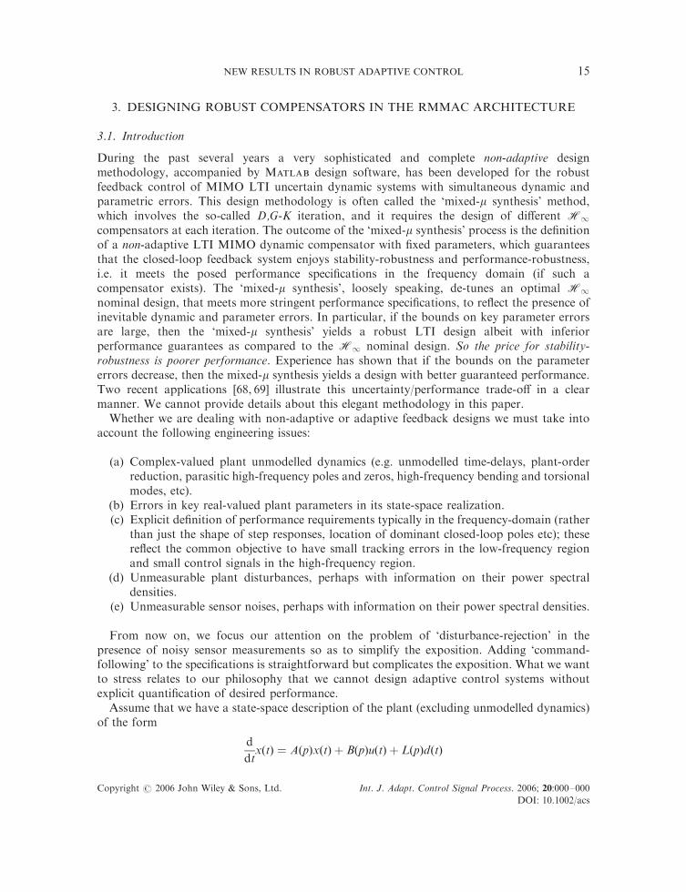
From now on, we focus our attention on the problem of ‘disturbance-rejection’ in thepresence of noisy sensor measurements so as to simplify the exposition. Adding ‘command-following’ to the specifications is straightforward but complicates the exposition. What we wantto stress relates to our philosophy that we cannot design adaptive control systems withoutexplicit quantification of desired performance.

Assume that we have a state-space description of the plant (excluding unmodelled dynamics)of the form

d

dtxðtÞ ¼ AðpÞxðtÞ þ BðpÞuðtÞ þ LðpÞdðtÞ



DOI: 10.1002/acs

yðtÞ ¼ C1ðpÞxðtÞ þDðpÞnðtÞ

zðtÞ ¼ CðpÞxðtÞ ð5Þ

where xðtÞ is the state vector, uðtÞ the control vector, dðtÞ the plant-disturbance vector, yðtÞ the(noisy) measurement vector, nðtÞ the sensor noise and zðtÞ the performance (output or error)vector, i.e. the vector for which we wish to minimize the effects of the disturbance dðtÞ and noisenðtÞ; i.e. have superior disturbance-rejection. The system matrices depend upon a real-valuedparameter vector p; where p is constrained to be in a (hyper) parallelepiped, p 2 Pp; this is arequired m-synthesis constraint. Thus, we must have a lower- and an upper-bound (real-valued)for each independent uncertain parameter. The disturbances, dðtÞ; can be either deterministictime-functions or stochastic processes. In either case, the robust m-synthesis requires adisturbance frequency weight for superior performance. If dðtÞ is a stochastic process, its power-spectral density naturally defines this weight.

From a performance point of view, in order to achieve superior disturbance-rejection, thedesigner specifies a frequency weight on zðtÞ: Typically, to achieve superior disturbance-rejectionin the low-frequency region, the designer specifies, in the m-synthesis methodology, a frequency-weight, say of the form

%zðsÞ ¼ Apa

sþ a

m

I zðsÞ ð6Þ

which implies that superior disturbance-rejection is most important in the frequency range04o4a: The larger the performance-gain parameter Ap; the better the desired performance-rejection.

To complete the robust design synthesis the designer must provide frequency-dependentbounds for all (structured or unstructured) unmodelled dynamics, and frequency weights for thecontrol, disturbance and sensor noise vectors. The control and sensor-noise weights, togetherwith the bound(s) on the unmodelled dynamics, safeguard against very high-bandwidthfeedback designs.

3.2. The GNARC design

Before a wise designer can make a decision on whether or not to implement an adaptive system,he/she must have a solid knowledge on what is the best robust non-adaptive design. We called thebest ‘global non-adaptive robust compensator’ GNARC-based design. The GNARC iscomputed via mixed-m synthesis and it takes into account the frequency-domain bounds onunmodelled dynamics, the various frequency weights that quantify disturbance-rejectionrequirements, control effort and, perhaps, power spectral densities for the plant-disturbancesand sensor-noises.

We certainly do not intend to provide here a tutorial exposition of the mixed-m synthesismethod. To compute the GNARC, one fixes the performance gain Ap in Equation (6) to someinitial value and exercises the Matlab software which, after a sequence of the so-called DG-Kiterations, determines a compensator KðsÞ and generates an upper-bound mubðoÞ: If

mubðoÞ518o ð7Þ

then the resulting feedback design is guaranteed to be stable for all ‘legal’ unmodelled dynamicsand the entire parameter uncertainty p 2 Pp:Moreover, in addition to stability-robustness, we are



DOI: 10.1002/acs

guaranteed that we meet or exceed the posed performance requirements. Therefore, in order tofind the ‘best’ GNARC we must maximize the performance-parameter Ap in Equation (6) untilthe m-upper bound is just below unity, say 0:9954mubðoÞ418o:

The GNARC is a single dynamic (SISO or MIMO) compensator that can be used by thedesigner to fully understand what is the best possible robust performance in the absence ofadaptation. Since the feedback system is LTI a whole variety of performance evaluations arepossible, using representative values of the uncertain real-parameter vector p 2 Pp for the plant,as summarized in Table I.

We believe that such a thorough understanding of the non-adaptive GNARC is essentialprior to making a design decision on using some sort of multiple-model adaptive control. It hasbeen our experience that such GNARC analyses point out which parameter uncertainty is mostcritical; this can be used to eliminate from further consideration non-critical parameters.Moreover, the performance of the GNARC, say for a SISO system, can change drastically if oneadds more measurements and/or controls. Thus, an unacceptable performance for a SISOGNARC non-adaptive system may, indeed, become acceptable if more controls and/or sensorsare introduced [2] and a MIMO GNARC analyzed, thereby eliminating the need for complexadaptive control.

3.3. The FNARC design

If the GNARC analyses discussed above indicate the need for adaptive control, they provide alower-bound upon robust performance. The ‘fixed non-adaptive robust compensators (FNARC)’

Table I. List of performance evaluation tools.

(1) Magnitude (or singular-value) Bode plot of the closed-loop transfer function from the plantdisturbance, d; to output, z; which measures the quality of disturbance-rejection vs frequency.Assuming that the plant has no integrators, the magnitude of this transfer function, in the lowfrequency region, will be approximately 1=Ap: This is why we must maximize the performance parameterAp for superior disturbance-rejection

(2) Magnitude (or singular-value) Bode plot of the closed-loop transfer function from the sensor noise, n; tooutput, z; which measures the quality of insensitivity to sensor noise vs frequency

(3) Magnitude (or singular-value) Bode plot of the closed-loop transfer function from the plantdisturbance, d; to control, u; which measures the impact of the plant-disturbance on the control vsfrequency

(4) Magnitude (or singular-value) Bode plot of the closed-loop transfer function from the sensor noise, n; tocontrol, u; which measures the impact of the sensor noise on the control vs frequency

(5) Root-mean-square (RMS) tables assuming that the plant-disturbance, d; and the sensor noise, n; arestationary stochastic processes. Such RMS values are readily evaluated via the solution of Lyapunovequations. Individual or combined RMS tables for the output, z; and the control, u; as a function of theplant-disturbance, d; and the sensor noise, n; can be computed.

(6) Time-domain responses, e.g. step- or sinusoidal-disturbance, stochastic signals, etc for different valuesof the uncertain constant parameters and for slowly time-varying parameters (within their predefinedranges)



DOI: 10.1002/acs

provide the means for quantifying an upper-bound on robust performance. ‘Ideally’, the FNARCanalyses assumes an infinite number of models, N !1; in any multiple-model adaptivescheme. Thus, we understand what is the best possible performance if we knew the realparameter(s) exactly.

In practice, to determine the FNARC one uses a dense grid of parameters pj ; j !1; in Pp

and determines the associated robust compensator for each pj using exactly the same bounds onunmodelled dynamics and frequency weights employed in the GNARC design. Thus, we canmake fair and meaningful comparisons. For each pj we use the complex-m design methodologyand Matlab software [49], because both the performance weights and bounds on unmodelleddynamics are complex-valued and there are no real parameter uncertainties. For each pj ; weagain maximize the performance-parameter Ap in Equation (6) until the complex-m upper-bound, mcubðoÞ is just below unity for all frequencies, say mcubðoÞ 0:995 8o; to be consistentwith the GNARC lower-bound.

One can then again analyse each FNARC design using the six techniques outlined inTable I. Our experience indicates that detailed analyses, especially at the corners and facesof the hyper-parallelepiped Pp; provide useful insights regarding the impact of the subset of theuncertain real parameters upon performance; this determines the need for sophisticatedadaptive control.

3.4. The potential benefit of adaptive control

Recall that we had posed the following question: do we need adaptive control? The GNARC andFNARC results provide the designer with the means to answer this question.

In Figure 5 we visualize a hypothetical plot of the outcome of the GNARC and FNARCdesigns by plotting the (maximized) performance parameter Ap; see Equation (6), as a functionof a scalar uncertain real parameter, p; pL4p4pU : We denote the (constant) value associatedwith the GNARC design by AG

p : We denote the parameter-dependent value associated with theFNARC by AF

p ðpÞ; pL4p4pU : The difference, AFp ðpÞ AG

p50 quantifies the impact of theuncertain parameter p 2 ½pL; pU upon performance. The FNARC process indicates that if theparameter p were known exactly, then the (low-frequency) disturbance-rejection is approxi-mately 1=AF

p ðpÞ: The GNARC process indicates that if the parameter p were unknown, then the(low-frequency) disturbance-rejection is approximately 1=AG

p : Note that to obtain the FNARCbenefits we must implement a multiple-model architecture with an infinite number of models. In this

Up

pA

pLp

( )FpA

A

p

Gp

FNARC design

GNARC design

: Scalar parameter

Per

form

ance

par

amet

er

Figure 5. Hypothetical comparison of the performance parameter, Ap; for the GNARC and FNARCfor the case of a scalar uncertain real parameter, p; pL4p4pU :



DOI: 10.1002/acs

manner we have quantified the potential performance benefits of adaptive control; the non-adaptive (single-model) GNARC provides the lower-bound upon expected performance, whilethe adaptive (infinite-model) FNARC provides the performance upper-bound. This informationis critical in deciding whether to implement an adaptive control system or not.

The shapes of the curves in Figure 5 provide additional valuable information. In thehypothetical case of Figure 5, we should expect the benefit of using adaptive control to begreatest if the true parameter was near its upper-bound, i.e. p pU : The benefits decrease if theunknown parameter is closer to its lower-bound, i.e. p pL: Indeed it may well happen thatAF

p ðpLÞ ¼ AGp : This can occur, for example, if the parameter p; in rad/s, represents the value of a

non-minimum phase zero which places inherent restrictions upon disturbance-rejection (see, e.g.Reference [70]). Such a non-minimum phase system has been analysed, using the RMMAC, inReference [27].

If we have an uncertain m-dimensional parameter vector, constrained in a hyper-parallelepiped, i.e. p 2 Pp Rm; the calculations are more complex to construct the twohypersurfaces along the lines suggested by Figure 5 [2]. However, the same philosophy stillapplies. In Reference [42] a two-input two-output RMMAC system with two uncertain realparameters is designed and analysed.

3.5. Determining the number of models and designing the LNARCs

Let us suppose that we have decided that there is a substantial benefit in using adaptive controland that we wish to use a multiple-model architecture. As we remarked before, the adaptivecomplexity is directly related to the number N of models in either the SMMAC or RMMACimplementation. Recall that the non-adaptive GNARC requires N ¼ 1 model while theFNARC requires N ¼ 1 models. Clearly, there must be a happy medium.

3.5.1. A ‘Brute-Force’ approach.. A ‘brute-force’ approach is to decide on the number ofmodels, say N ¼ 4; and their parameter variation as illustrated in the hypothetical visualizationof Figure 6.

Essentially, in this approach, the designer fixes the ‘adaptive complexity’, quantified by N; ofthe multiple-model system. Each model, denoted by M#k (k ¼ 1; 2; 3; 4) requires definition of its

pA

p

p p= p p= p p= p p= p p=

1A

2A

3A

4A

Figure 6. Illustration of a ‘brute-force’ selection of four models. An ad hoc decision is made on the numberof models, N ¼ 4; and the specification of their ‘boundaries’, ½pkL; pkU ; k ¼ 1; 2; 3; 4; for each model M#k:

The Akp denote the maximized value of the performance parameter in Equation (6).



DOI: 10.1002/acs

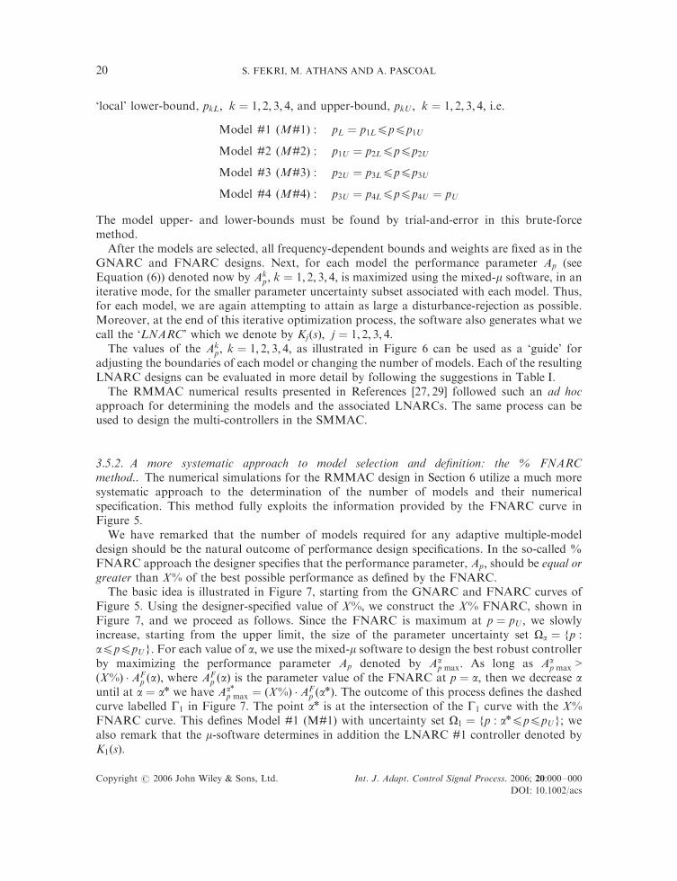
‘local’ lower-bound, pkL; k ¼ 1; 2; 3; 4; and upper-bound, pkU ; k ¼ 1; 2; 3; 4; i.e.

Model #1 ðM#1Þ : pL ¼ p1L4p4p1U

Model #2 ðM#2Þ : p1U ¼ p2L4p4p2U

Model #3 ðM#3Þ : p2U ¼ p3L4p4p3U

Model #4 ðM#4Þ : p3U ¼ p4L4p4p4U ¼ pU

The model upper- and lower-bounds must be found by trial-and-error in this brute-forcemethod.

After the models are selected, all frequency-dependent bounds and weights are fixed as in theGNARC and FNARC designs. Next, for each model the performance parameter Ap (seeEquation (6)) denoted now by Ak

p; k ¼ 1; 2; 3; 4; is maximized using the mixed-m software, in aniterative mode, for the smaller parameter uncertainty subset associated with each model. Thus,for each model, we are again attempting to attain as large a disturbance-rejection as possible.Moreover, at the end of this iterative optimization process, the software also generates what wecall the ‘LNARC’ which we denote by KjðsÞ; j ¼ 1; 2; 3; 4:

The values of the Akp; k ¼ 1; 2; 3; 4; as illustrated in Figure 6 can be used as a ‘guide’ for

adjusting the boundaries of each model or changing the number of models. Each of the resultingLNARC designs can be evaluated in more detail by following the suggestions in Table I.

The RMMAC numerical results presented in References [27, 29] followed such an ad hocapproach for determining the models and the associated LNARCs. The same process can beused to design the multi-controllers in the SMMAC.

3.5.2. A more systematic approach to model selection and definition: the % FNARCmethod.. The numerical simulations for the RMMAC design in Section 6 utilize a much moresystematic approach to the determination of the number of models and their numericalspecification. This method fully exploits the information provided by the FNARC curve inFigure 5.

We have remarked that the number of models required for any adaptive multiple-modeldesign should be the natural outcome of performance design specifications. In the so-called %FNARC approach the designer specifies that the performance parameter, Ap; should be equal orgreater than X% of the best possible performance as defined by the FNARC.

The basic idea is illustrated in Figure 7, starting from the GNARC and FNARC curves ofFigure 5. Using the designer-specified value of X%; we construct the X% FNARC, shown inFigure 7, and we proceed as follows. Since the FNARC is maximum at p ¼ pU ; we slowlyincrease, starting from the upper limit, the size of the parameter uncertainty set Oa ¼ fp :a4p4pUg: For each value of a; we use the mixed-m software to design the best robust controllerby maximizing the performance parameter Ap denoted by Aa

p max: As long as Aap max >

ðX%Þ AFp ðaÞ; where AF

p ðaÞ is the parameter value of the FNARC at p ¼ a; then we decrease auntil at a ¼ an we have Aan

p max ¼ ðX%Þ AFp ða

nÞ: The outcome of this process defines the dashedcurve labelled G1 in Figure 7. The point an is at the intersection of the G1 curve with the X%FNARC curve. This defines Model #1 (M#1) with uncertainty set O1 ¼ fp : an4p4pUg; wealso remark that the m-software determines in addition the LNARC #1 controller denoted byK1ðsÞ:



DOI: 10.1002/acs

The process is repeated from the (right) boundary of M#1; an: Starting at p ¼ an; we definethe set Ob ¼ fp : b4p4ang: For each value of b; we use the mixed-m software to design the bestrobust controller by maximizing the performance parameter Ap denoted by Ab

p max: As long asAb

p max > ðX%Þ AFp ðbÞ; where AF

p ðbÞ is the parameter value of the FNARC at p ¼ b; then b isdecreased until at b ¼ bn we have Abn

p max ¼ ðX%Þ AFp ðb

nÞ: The outcome of this process definesthe dashed curve labelled G2 in Figure 7. The point bn is at the intersection of the G2 curve withthe X% FNARC curve. This defines Model #2 (M#2) with uncertainty set O2 ¼ fp : b

n4p4ang: It is noted that the m-software also determines the LNARC #2 controller denoted by K2ðsÞ:The process is repeated until the parameter lower-bound is reached.

The % FNARC method is straightforward for systems involving a single scalaruncertain real parameter. In the case of two, or more, uncertain parameters the procedurehas to be modified. For the case of two or more uncertain parameters, the GNARC, FNARCand % FNARC become surfaces. The above process yields intersection of surfaces (theequivalent of G1;G2; . . . are also surfaces). Unfortunately, the intersection of these surfacesdoes not occur along rectangular (or parallelepiped) parameter subsets. However, recallthat the mixed-m software requires rectangular (or parallelepiped) constraints for uncertainparameter sets. Suggested modifications to the % FNARC concept are discussed inReference [2].

3.6. Discussion

In this section we presented an overview of what we believe is the proper way of designingcompensators or multi-controllers for the RMMAC and SMMAC architectures. We are drivenby the desire that we must guarantee (local) robust-stability and robust-performance. Thisimplies that we must exploit the state-of-the-art of the mixed-m synthesis methodology andsoftware. We also stressed the value of having optimized performance lower-bounds (via theGNARC) and upper-bounds (via the FNARC) to aid the control system designer in theselection of the models, their number and their numerical specification (and hence complexity ofthe adaptive system). We presented two methods (there are more) for defining the models andthe associated compensators (the LNARCs) driven by designer-specified performance orcomplexity specifications.

Up

pA

pLp

( )FpA p

1Ω2ΩM #2 M #1

*β *α

Figure 7. Visualization of the % FNARC model definition process.



DOI: 10.1002/acs

4. DESIGNING THE BANK OF KALMAN FILTERS FOR THE RMMACARCHITECTURE

4.1. Introduction

In this section we discuss the critical issues related to the design of the KFs in the RMMACarchitecture. We remark that the design of the bank of KFs is much more systematic (andcomplex) that the ad hoc multi-estimators employed in SMMAC architectures.

The proper design of each KF in the RMMAC architecture of Figure 4 is crucial in order tosatisfy the theoretical assumptions [61–63] which will imply that the PPE will yield the correctmodel identification. The KF design explicitly utilizes the BPM Appendix B presents thesummary concepts leading to the on-line generation of the posterior probabilities and containsthe key equations for calculating the BPM.

The design of the KFs is done after the number of models and their boundaries have beenestablished using the procedures in Section 3.5. Recall that the original parameter set, p 2 Pp (aparallelepiped) is subdivided into N subsets (parallelepipeds) denoted by Ok; k ¼ 1; 2; . . . ;N;such that

[Nk¼1

Ok ¼ Pp ð8Þ

and each Ok defines the associated Model #k:We need to design a discrete-time steady-state KFfor each Ok: To accomplish this we need to specify the ‘nominal’ value of the parameter, denotedby pnk 2 Ok; which will be used to design the kth KF. Each KF requires specification of theintensity matrices of the plant white noise and of the sensor white noise.

The ‘naıve’ point of view would be to choose pnk at the center of Ok: Unfortunately, this maylead to unpredictable behaviour in the convergence of the posterior probabilities. The correctway is to select the pnk using the BPM.

The presence of unmodelled dynamics (and their frequency-domain bounds) is neglected inthe design of the KFs. Unfortunately, we are not aware of any theory that is currently availableto help us design KFs that are ‘robust’ in the presence of unmodelled dynamics. Thus, torobustify the KFs we often use ‘fake plant white noise’. This engineering trick [67] is extremelycommon in engineering estimation applications. It causes the KF gains to increase and pay moreattention to the measurements, which after all contain the actual information about theuncertain plant.

4.2. The Baram proximity measure (BPM)

Let p 2 O and let pn denote the nominal value used to implement a KF. If p ¼ pn; then thesteady-state KF residual, rnðtÞ; would be a stationary white-noise sequence with a specificcovariance matrix Sn: If the data were generated by a different LTI system, with p=pn; then theKF residual rðtÞ would no longer be white. The BPM is a real-valued function, denoted byLðp; pnÞ which measures how large is the ‘stochastic distance’ between the residuals rðtÞ and rnðtÞ:See Appendix B for details.

Now suppose that p 2 O; as above, but we have designed two different KFs, one (KF #1) withnominal value pn1 2 O and another (KF #2) with pn2 2 O: Now we can calculate two BPMs,L1 Lðp; pn1Þ and L2 Lðp; pn2Þ:



DOI: 10.1002/acs

Figure 8 illustrates this idea for a scalar parameter, p; where we visualize the BPMs L1 and L2

for all p 2 O: For the specific value p ¼ pA shown, we can see that LðpA; pn1Þ5LðpA; pn2Þ: Theimplication of this is that for a 2-model MMAE, when the true value is p ¼ pA; the posteriorprobabilities P1ðtÞ ! 1; P2ðtÞ ! 0; so that we have convergence to Model #1 (defined by KF#1), even though the Euclidean distances would indicate the opposite (jpA pn1 j > jpA pn2 j).

Fundamental convergence result: In Reference [61] this result was generalized and proved foran arbitrary number of stable KFs designed for the nominal values pn1 ; p

n2 ; . . . ; p

nN : If the BPM

satisfies the inequality

Lðp; pnj Þ5Lðp; pnkÞ 8k=j ¼ 1; 2; . . . ;N ð9Þ

then, under some additional stationarity and ergodicity assumptions (see Appendix B) theposterior probabilities converge almost surely to the correct model, i.e.

limt!1

PjðtÞ ! 1 ð10Þ

4.3. Integrating probability convergence results for the RMMAC

The outcome of the controller design of Section 3 yielded the number of models, N; and theirboundaries, in terms of the parallelepipeds O1;O2; . . . ;ON which define the models M#1; M#2; . . . ;M#N: The question now is: how do we select the nominal values pn1 ; p

n2 ; . . . ; p

nN to design the

KFs?The idea, illustrated for three models in Figure 9 for a scalar parameter, is to use an iterative

algorithm to calculate the nominal KF values pn1 ; pn2 ; p

n3 ; so that the BPMs are equal at the

boundary of adjacent Os:In this manner, the fundamental probability convergence result will guarantee that p 2 Oj )

PjðtÞ ! 1 a.s. This, is the method we use in the numerical RMMAC simulations of Section 6.This method becomes more complicated when we have two, or more, uncertain parameters. It

becomes necessary to use some sort of genetic algorithm to determine the optimized nominalKF design points so that the BPM surfaces agree at the model boundaries [2, 42].

4.4. Discussion

We have presented a brief summary on how to optimize the design of the KFs in the RMMACarchitecture using the BPM, so as to ensure ‘correct model identification’ by the posterior

iL

p

*2 ( , )L L p p=

*1p *

2p

*1 ( , )L L p p=

Ap

Figure 8. Illustration of Baram proximity measures (BPM).



DOI: 10.1002/acs

probabilities. We stress that a KF is optimal if indeed the data is generated by the same model asthat used to design the KF. In adaptive control, however, the true parameter is NOT identical tothat of the ‘closest’ KF in the sense of Section 4.3. Also, the unmodelled dynamics are not takeninto account in the design of the KF. Moreover, the KFs and the PPE must perform well evenwhen some of the stochastic assumptions are violated. Thus, we may need to ‘robustify’ the KFto be tolerant of such ‘errors’. The engineering practice of using suitable ‘fake plant white noise’is a very useful tool. We have found [2, 42] that judicious use of ‘fake plant white noise’ (whichcauses the KF gains to increase and pay more attention to the measurements [67]) can be a veryvaluable tool in improving the quality and speed of probability convergence. We believe thatfuture fundamental studies of robustifying KFs, in the context of multiple-model adaptivecontrol, are very relevant. Also, the identification must work when the parameters change‘slowly’ as a function of time.

It is also important to note that similar probability convergence results for the MMAE can befound in Reference[57, pp. 267–279] and (cited references therein) which used the so-calledKullback information metric. The Kullback metric, however, is not a true norm (it violates thetriangle inequality). Nonetheless, it would be highly desirable that future research examines in-depth the relationship of the BPM and the Kullback metric, especially with respect to posteriorprobability convergence behaviour.

5. THE RMMAC/XI ARCHITECTURE

The simulations in Section 6 will demonstrate that the RMMAC works quite well even if weviolate the theoretical assumptions for MMAE convergence in a ‘mild’ manner. This fact issupported by hundreds of different simulations in Fekri’s PhD thesis [2]. Nonetheless, we mustalways remember that: theories have limitations, stupidity does not!

Obviously, the superior performance of the RMMAC hinges upon the rapid convergence ofthe posterior probabilities to the correct model (see Equation (4) and Appendices A and B). Aswe remarked in Section 2.5 such a convergence critically depends upon the ‘regularity’ of theresiduals generated by the bank of KFs in Figure 4. Each KF is designed for a particularcovariance matrix cov½xðtÞ; xðtÞ ¼ EfxðtÞx0ðtÞg ¼ Xdðt tÞ of the continuous-time zero-mean

iL

p

2L

*1p*

2p

3L

1L

*3p

1Ω2Ω3Ω

ΩFigure 9. Optimizing the KF nominal design points using the BPMs so that they are equal at the

boundaries of adjacent models.



DOI: 10.1002/acs

plant white noise xðtÞ; where X is the plant-noise intensity matrix. The numerical value of theintensity noise X will determine the size of the KF gains and the residual covariance matrices Sk:These will determine the size of the coloured stochastic disturbances applied to the plant.

Under normal operating conditions these exogenous plant disturbances will fall within aspecific range. It may very well happen that once-in-a-while the actual plant disturbancesbecome very much larger than the normal onesyy. During these ‘abnormal’ time-intervals, theactual KF residuals will be much larger than those predicted by their associated ‘normal’residual covariances, Sk: Our experience has been that during these ‘abnormal’ time intervals [2],the posterior probabilities generated by Equation (4) can undergo rapid oscillations andfrequent switching among the models and, as a consequence, the RMMAC performancedeteriorates; often it is worse than that of the non-adaptive GNARC design. A numericalexample in Section 6 will provide concrete evidence of this phenomenon.

In short, the RMMAC can behave poorly when the true stochastic plant disturbances, asquantified by the intensity matrix Xact of the actual plant white noise, are very different fromthose associated with the intensity Xd used to design the linear KFs. If XactcXd ; then the actualresiduals are much higher than, say, the 3-sigma values expected by the residual covariancematrices Sk (see Equation (4)) and this can lead to rapid switching of the posterior probabilities,‘confused identification’ and poor RMMAC performance.

If, on the other hand, XactXd ; then the actual residuals are much lower than, say, the 3-sigma values expected by the residual covariance matrices Sk and this can also lead to rapidswitching of the posterior probabilities, or slow convergence, ‘confused identification’ and poorRMMAC performance. In this case, the smaller actual plant disturbance may not indeedprovide sufficient persistent excitation, required by the identifiability conditions, to generatesignals that are not masked by the measurement noise.

These pragmatic considerations led us to develop the so-called RMMAC/XI architectureillustrated in Figure 10. By increasing the complexity of the RMMAC we can mitigate theRMMAC performance deterioration problems. The basic idea in RMMAC/XI is to introduceadditional models, i.e. increase the number of hypotheses, to reflect different ranges of the plantnoise intensity matrix X: Let us assume that the number, N; of models and their size has beendetermined by the required adaptive performance specifications and that we have alreadycalculated the N LNARCs denoted by KkðsÞ; k ¼ 1; 2; . . . ;N: Let us further suppose that theplant noise intensity X is bounded by

X 2 ½XL;XH

and that, for the sake of simplicity, we decide to select two intermediate values, X1 and X2; suchthat

XL5X15X25XH

Then we design two sets of linear KFs, one set indexed by k ¼ 1; 2; . . . ;N using the noiseintensity X1 and the second set indexed by k ¼ N þ 1;N þ 2; . . . ; 2N using the noise intensity X2:It is important to stress that the nominal points for designing each KF, as determined bythe BPM method of Section 4 will be different (and must be recomputed) for each value of

yyFlight load-alleviation automatic control systems are often designed for different levels of turbulence and the pilot can‘switch-in’ the appropriate control system. However, in case of extreme turbulence (not anticipated in the design phase)the pilot typically disconnects the control system and flies the aircraft himself.



DOI: 10.1002/acs

X1 and X2: Essentially, we have doubled the number of hypotheses in the associated MMAE;but we can still apply the MMAE-based identification methodology. This allows us to define theRMMAC/XI architecture shown in Figure 10.

Note that each of the 2N KFs will now generate a different residual, rkðtÞ; k ¼ 1; 2; . . . ; 2N:Also, we pre-compute the 2N residual covariance matrices Sk: These are introduced to the PPEof Figure 10 which will generate 2N posterior probabilities, PkðtÞ; k ¼ 1; 2; . . . ; 2N; one for eachof the 2N hypotheses. Note, however, that the bank, and number, of the N LNARCs isunchanged, since their design does not depend on X; the LNARCs are only influenced bythe disturbance frequency weight that is independent of X: Thus, it is important to note inFigure 10 that each LNARC control signal ukðtÞ; k ¼ 1; 2; . . . ;N; is multiplied by the twodifferent associated posterior probabilities, PkðtÞ and PkþNðtÞ; to generate the overall adaptivecontrol uðtÞ:

It is obvious how to generalize this idea for more than two values of X: It remains an openresearch question on how to select ‘intelligently’ the values of X; other than by brute-force andtrial-and-error.

Figure 10. The RMMAC/XI architecture.



DOI: 10.1002/acs

The advantages of implementing the RMMAC/XI architecture will be clearly demonstratedin the numerical simulations of Section 6. There we will compare the performance of thestandard RMMAC with that of the RMMAC/XI during ‘abnormal’ disturbance conditions.

6. RMMAC SIMULATIONS

We described above how the RMMAC architecture combines the state-of-the-art in mixed-mrobust synthesis and MMAE system identification. Furthermore, we described the step-by-stepdesign process required to implement a RMMAC design.

In this section we test and evaluate the disturbance-rejection performance of the RMMACfeedback system as compared to the ‘best’ GNARC non-adaptive design. We also illustrate, in aconcrete way, the step-by-step design methodology of Sections 3–5.

We present the outcome of several Monte Carlo (MC) simulations, which demonstrate theRMMAC performance improvements, as compared to that of the best non-adaptive GNARCsystem. Overall, for the example considered, the proposed RMMAC design yields significantperformance improvements over the non-adaptive GNARC, thereby confirming the positiveaspects of this adaptive control method.

We present simulation results when we satisfy or ‘mildly violate’ the theoretical assumptionsfor both a constant as well as a slowly time-varying uncertain scalar parameter. We also discusswhat happens when we ‘severely violate’ the theoretical assumptions and compare theperformance of the standard RMMAC and RMMAC/XI in ‘abnormal’ disturbanceenvironments.

6.1. The two-cart example dynamics

The RMMAC was tested and evaluated using the two-cart mass–spring–damper (MSD) system,shown in Figure 11. A different topology of the two-cart system was analysed by the RMMACin Reference [29].

The system in Figure 11 includes a random coloured disturbance force, dðtÞ; acting on massm2 and sensor noise on the only measurement of the position of mass m2: The control force uðtÞacts upon the mass m1: The disturbance force dðtÞ is a stationary first-order (coloured) stochasticprocess generated by driving a low-pass filter, WdðsÞ; with continuous-time white noise xðtÞ; withzero mean and unit intensity, i.e X ¼ 1; as follows:

dðsÞ ¼a

sþ a|fflzfflWd ðsÞ

xðsÞ ð11Þ

Figure 11. The two-cart MSD system. The spring-constant k1 is uncertain. Also, the time-delay, t; isuncertain; it represents unmodelled dynamics.



DOI: 10.1002/acs

The overall state-space representation, including the disturbance dynamics via the state variablex5ðtÞ; is:

’xðtÞ ¼ AxðtÞ þ BuðtÞ þ LxðtÞ

yðtÞ ¼ CxðtÞ þ yðtÞ ð12Þ

where the state vector is

xTðtÞ ¼ ½x1ðtÞ x2ðtÞ ’x1ðtÞ ’x2ðtÞ dðtÞ

and

A ¼

0 0 1 0 0

0 0 0 1 0

k1

m1

k1

m1b1

m1

b1

m10

k1

m2ðk1 þ k2Þ

m2

b1

m2ðb1 þ b2Þ

m2

1

m2

0 0 0 0 a

26666666666664

37777777777775

BT ¼ 0 01

m10 0

; C ¼ ½0 1 0 0 0

LT ¼ ½0 0 0 0 a

The following parameters in Equation (12) are fixed and known:

m1 ¼ m2 ¼ 1; k2 ¼ 0:15; b1 ¼ b2 ¼ 0:1; a ¼ 0:1 ð13Þ

The upper and lower-bounds for the uncertain spring constant, k1; are:

O ¼ fk1 : 0:254k141:75g ð14Þ

The performance variable (output) zðtÞ is the position of mass m2;

zðtÞ x2ðtÞ ð15Þ

All feedback loops utilize a single measurement yðtÞ; that includes additive white sensor noiseyðtÞ; independent of xðtÞ defined by

yðtÞ x2ðtÞ þ yðtÞ

EfyðtÞg ¼ 0; EfyðtÞyðtÞg ¼ 106dðt tÞ ð16Þ

The desired disturbance-rejection requires that the effects of dðtÞ and yðtÞ be minimized at theoutput, so that zðtÞ 0:

RemarkThe control problem is hard even if the spring, k1; is known. Clearly, the control problembecomes much harder in our adaptive design, because the control uðtÞ is applied via the



DOI: 10.1002/acs

uncertain spring, so we are not sure how much force is exerted through the uncertain spring tothe mass m2: Thus, we have a non-collocated actuator problem because the control is not appliedto the mass m2 whose position we wish to regulate.

In addition to the uncertain spring stiffness, we assume that there is, in the control channel, anunmodelled time-delay t whose maximum possible value is 0.05 s, i.e.

t40:05 s ð17Þ

The frequency-domain upper-bound for the unmodelled time-delay, which serves, for thisexample, as a surrogate for unmodelled dynamics, is required by the mixed-m synthesis designand is the magnitude of the first-order transfer function

WunmodðsÞ ¼2:1s

sþ 40ð18Þ

6.2. Designing the global non-adaptive robust compensator (GNARC)

In this section we discuss the details behind the mixed-m design of the GNARC system, whichguarantees the ‘best’ robust-stability and robust-performance for the entire large springuncertainty of Equation (14). As explained in Section 3, the GNARC system will define what wecan best expect in the absence of adaptation.

As it is common inH2 orH1 designs, we use the following frequency domain weights on thecontrol and measurement noise:

Control weight :WuðsÞ ¼10ðsþ 10Þsþ 103

Measurement noise weight :Wn ¼ 103ðconstantÞ ð19Þ

These, together with the unmodelled dynamics weight as in Equation (18), limit the bandwidthof the closed-loop system by penalizing large high-frequency control signals. The control weightWuðsÞ allows large controls at lower frequencies, where we desired superior disturbance-rejection, while penalizing controls at higher frequencies. The frequency weights of Equations(18) and (19) are incorporated in the definition of the nominal generalized plant, together withEquation (12) with k1 ¼ 1:0: The weights of Equations (11), (18), and (19) will not change in anyof the subsequent designs.

To carry out the mixed-m synthesis, the parameter uncertainty of Equation (14) is representedby

0:254k141:75 ) k1 ¼ 1:0þ 0:75 dk1 ; jdk1 j41 ð20Þ

In order to design the ‘best possible’ non-adaptive feedback system the following type ofperformance weight upon the output zðtÞ is used:

WpðsÞ ¼ Ap0:1

sþ 0:1ð21Þ

which reflects our specification for good disturbance-rejection for the frequency range o40:1rad=s where the disturbance dðtÞ has most of its power; see Equation (11). Notice that theperformance weight WpðsÞ penalizes the output error in the same frequency range as the



DOI: 10.1002/acs

disturbance dynamics WdðsÞ; while the gain parameter Ap in WpðsÞ specifies our desired level ofdisturbance-rejection. The larger Ap; the greater the penalty on the effect of the disturbances onthe position. As we described in Section 3, for superior disturbance-rejection Ap should be aslarge as possible; how large it can be is only limited by the required guarantees on robust-stability and performance inherent in the mixed-m synthesis methodology.

Figure 12 shows the MSD plant with weights as required by mixed-m synthesis. One can notethat there are two frequency-weighted ‘errors’ *zðtÞ and *uðtÞ: This figure is in fact a block diagramof the uncertain closed-loop MSD system illustrating the disturbance-rejection performanceobjective namely the closed-loop transfer function from xðtÞ ! zðtÞ; or dðtÞ ! zðtÞ:

The ‘position error’ *z is our main performance variable for evaluating the quality of thedisturbance-rejection. Since

*zðsÞ ¼WpðsÞ zðsÞ ¼ Ap0:1

sþ 0:1

zðsÞ ð22Þ

we communicate to the m-design that position errors are most important below the ‘cornerfrequency’ 0:1 rad=s: The larger the ‘performance parameter’ Ap; the more one cares aboutposition errors at all frequencies.

The ‘control error’ *uðtÞ is defined by

*uðsÞ ¼WuðsÞuðsÞ ¼ 10sþ 10

sþ 103

uðsÞ ð23Þ

Thus, WuðsÞ is a high-pass filter that penalizes the system for using large controls at highfrequencies.

Using the mixed-m software [48] the performance parameter Ap in Equation (21) is increased,as much as possible, until the upper-bound on the mixed-m; mubðoÞ; satisfies the inequality

mubðoÞ41 8o ð24Þ

which is only a sufficient condition for both stability- and performance-robustness. The largestvalue of the performance parameter Ap in Equation (21) was to be

AGp ¼ 50:75 ðwith mub 0:995Þ ð25Þ

δ

( )tξ ( )tθ

( )u t ( )y t

( )z t

( )d tun∆

z(t)

( )u(

s

αα+

Figure 12. The MSD system with weights for mixed-m synthesis.



DOI: 10.1002/acs

which leads to the GNARC design, i.e. the ‘best’ LTI non-adaptive compensator KðsÞ thatguarantees stability- and performance-robustness for the entire parameter uncertainty intervalas in Equation (14). As explained in Section 3, the performance characteristics of the GNARCare to be used as the comparison-basis for evaluating performance improvement (if any) of ourproposed RMMAC design. See Section 3.2.

6.3. Designing the local non-adaptive robust compensators (LNARCs)

Following the procedure presented in Section 3, the plots of the maximized performanceparameter Ap for the GNARC design and the FNARC designs (requiring an infinite number ofmodels) is shown in Figure 13. This figure shows that there is a potential 20-fold improvement inperformance by using adaptive control.

RemarkIn Figure 13, the GNARC and FNARC look flat for all values of k1: Actually, the FNARCbecomes a little smaller as we approach small values of k1; but this cannot be noticed in thefigure. This ‘flatness’ disappears if we change our control specifications [2].

Next, we specify a desired level of adaptive performance to be 70% of the FNARC, i.e.X ¼ 70%; following the discussion of Section 3.5.2.

Figure 14 shows how four models (subintervals) are determined to be used for the RMMACbased upon the required performance level of X ¼ 70%:

Their characteristics are summarized in Table II. Explanation. We now provide a bit moredetail on how the four models of Figure 14 are obtained. Starting at the North–East cornerlabelled F1; k1 ¼ 1:75; (because the FNARC is maximum there) we slowly open-up the uncertaininterval denoted by Ob ¼ fk1 : b4k141:75g: For each interval, we iterate (using the mixed-msoftware [48]) to calculate the maximum performance parameter Ab

p which results in the dashedcurve, labelled G1 in Figure 14. When the curve G1 intersects the 70% FNARC curve we stop. Inthis example, this occurs at k1 ¼ 1:02 which yields the subset O1 ¼ ½1:02; 1:75; i.e. 1:024k141:75;Model M#1; and LNARC #1: The left boundary of M#1 defines the point labelled F2 onthe FNARC. Starting from this point we slowly open up the interval denoted by Oc ¼ fk1 :c4k141:02g: Once more, we iterate using the mixed-m software to calculate the maximumperformance parameter Ac

p which results in the dashed curve, labelled G2 in Figure 14. When thecurve G2 intersects the 70% FNARC curve we stop. In this example, this occurs at k1 ¼ 0:64

0.25 0.75 1.25 1.7510

1

102

103

k1

Ap

FNARCGNARC

Figure 13. Best GNARC and FNARC performance gains for spring-stiffness uncertainty interval inEquation (14); note the log scale along the vertical axis.



DOI: 10.1002/acs

which yields the subset O2 ¼ ½0:64; 1:02; i.e. 0:644k141:02; Model #2; and LNARC #2:Repeating this process leads to the curves labelled G3 and G4 in Figure 14 and the four modelssummarized in Table II.

As a result, the entire initial uncertainty set of Equation (14) is covered by four modelsrequiring four local compensators. Clearly, the reduction in parameter uncertainty allows largerperformance gains for designing the LNARCs, resulting into guaranteed both stability- andperformance robustness over the corresponding subintervals of Table II. Note that we shouldexpect, on the average, about 20 times better performance from the RMMAC as compared tothe GNARC (694.5/50.75)

The above model selection procedure also generates four ‘local’ robust compensators,K1ðsÞ; . . . ;K4ðsÞ; designed for each subinterval (model) defined in Table II; these are referred toas LNARCs. In the mixed-m synthesis, the weights of Equations (11), (18) and (19) were thesame as in the GNARC design of Section 6.2. However, for each LNARC design, theperformance parameter Ap in Equation (21) is maximized until the mixed-m bound of Equation(24) is achieved, and their optimized values are shown in the last column of Table II.

0.25 0.5 0.75 1 1.25 1.5 1.750

200

400

600

800

1000

k1

Ap

Model #1(M #1)M#2M#3M#4

GNARC

70% of FNARC

FNARC

Ω1Ω2Ω3Ω4

Γ2 Γ1

Γ3Γ4

F1F2F3F4

Figure 14. Construction of the four models using the performance requirement X ¼ 70% of the FNARC.

Table II. Summary of models and performance parameters.

Compensator O X (%) Anp

GNARC O ¼ ½0:25; 1:75 5.1 AGp ¼ 50:75

LNARC 1 O1 ¼ ½1:02; 1:75 70 A1p ¼ 694:5

LNARC 2 O2 ¼ ½0:64; 1:02 70 A2p ¼ 694:5

LNARC 3 O3 ¼ ½0:40; 0:64 70 A3p ¼ 694:5

LNARC 4 O4 ¼ ½0:25; 0:40 70 A4p ¼ 694:5

nBest performance gains for the GNARC and each of the four LNARCs used insubsequent designs vs ‘FNARC’



DOI: 10.1002/acs

Figure 15 compares the GNARC compensator KðsÞ with the four LNARCs, namely K1ðsÞ;. . . ; K4ðsÞ by examining their Bode magnitude plots; it is clear that at low frequencies theLNARCs generate a loop-gain about 20 times as large compared to the GNARC and this,naturally, leads to the performance improvements in disturbance-rejection discussed below,especially in the specified frequency region o50:1 rad=s: We emphasize that each individualLNARC closed-loop design has guaranteed performance- and stability-robustness over itsassociated parameter subinterval of Table II. These also confirm the ‘rough’ predictions impliedby Table II. These also confirm the ‘rough’ predictions implied by Table II.

RemarkIn the design philosophy adopted in this paper we have stressed that the adaptive controllercomplexity, as measured by the number of models in the RMMAC should be the naturalby-product of the performance requirements. We have just demonstrated that if we demand thatthe performance equals or exceeds X ¼ 70% of the FNARC, we require the four modelssummarized in Table II.

If we are willing to accept a somewhat inferior performance and select, say, X ¼ 50% then theprocedure outlined yields only two models. If we wish to have much better performance andselect, say, X ¼ 90%; then the outlined procedure yields nine models. Therefore, as we demandbetter and better performance we must increase the RMMAC complexity, and this agrees withengineering intuition. If explicit performance requirements were used in the design of theSMMAC, the same philosophy could be applied for those architectures as well.

6.4. Predicting potential RMMAC performance benefits

Testing the RMMAC requires significant computation using multiple MC runs under differentscenarios. It is highly desirable, as explained in Section 3, to use the LTI feedback designs, usingthe GNARC and LNARCs, to quantify the potential benefits of using adaptive control ingeneral, and the RMMAC in particular. From a pragmatic engineering perspective we must have

102

100

102

104

101

100

101

102

103

104

Freq. (rad /sec)

Mag

.

LNARCs

GNARC

Figure 15. Compensator frequency-domain characteristics (Bode plot) of the GNARC andthe four LNARCs.



DOI: 10.1002/acs

trade-offs that contrast the performance improvements (if any) of the very sophisticated RMMACvis-a-vis the much simpler non-adaptive GNARC design. To the best of our knowledge, suchperformance trade-offs have not been explicitly quantified in other adaptive control studies.

Referring to Figure 4, the RMMAC requires the on-line computation of its four KFs as wellas of its four dynamic LNARCs, K1ðsÞ; . . . ;K4ðsÞ; in addition to the calculation of the fourposterior probabilities, P1ðsÞ; . . . ;P4ðsÞ; by the PPEa lot of computations!

In order to understand how one can easily predict the potential RMMAC performancecharacteristics, assume that one of the posterior probabilities converges to its nearestprobabilistic neighbour (which it does, as we demonstrate in the sequel); it follows that, aftera transient time, a specific LNARC is used. After the probability convergence, the RMMACessentially operates as an LTI stochastic feedback system!

In the spirit of Table I, this allows us to calculate two key transfer functions for disturbance-rejection and control signal characteristics

Disturbance-rejection :

MxzðsÞ zðsÞxðsÞ

or MdzðsÞ zðsÞdðsÞ

Control-signal :

MxuðsÞ uðsÞxðsÞ

or MduðsÞ uðsÞdðsÞ

ð26Þ

for different values of the uncertain spring stiffness of Equation (14), for the GNARC and foreach LNARC design.

Figure 16 illustrates the above using the different spring constants quantifying the potentialRMMAC improvement in disturbance-rejection in the frequency domain. Figure 16 predictsthat the RMMAC has the potential to significantly improve disturbance-rejection on the orderof 1=Ap: These predictions will be again validated in the sequel.

Similar plots for control signal characteristics can be made for other values of the uncertainspring constant. Other transfer functions could also be computed (not shown) from the plantdisturbance xðtÞ and the sensor noise yðtÞ to the control uðtÞ:

Figure 17 evaluates the potential performance improvement of using RMMAC by usingstochastic metrics, namely by comparing the steady-state RMS errors of the output z and thecontrol u; for different values of k1: Assuming that x and y are indeed white noises, these RMSresults are readily computed by solving standard covariance algebraic Lyapunov equations forstochastic LTI systems, e.g. Reference [60]. The graphs of Figure 17 vividly suggest thatRMMAC has the potential of decreasing the output RMS by a factor of 2–5 over that obtainedfrom the GNARC system. Note that the potential improvement in output RMS requirescontrols with higher RMS values, as expected. Note also that, since we are using m-synthesis, theGNARC, FNARCs and LNARCs we design are H1 compensators. These H1 compensatorsdo not necessarily minimize RMS errors, unlike H2 controllers. Nonetheless, RMS metrics areimportant in engineering analyses and complement the frequency-domain plots of Figure 16.

Finally, it is important to construct what we call the ‘Mismatch Model/LNARC’ table shownin Table III.

The interpretation of Table III answers the question: what happens to closed-loop stability ifwe use the LNARC #KjðsÞ when the true spring constant is in subinterval (or model) #i?



DOI: 10.1002/acs

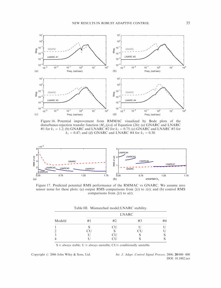
0.25 0.75 1.25 1.750

2

4

6

8

RM

S o

f z(t

)

0.25 0.75 1.25 1.750

1

2

3

RM

S o

f u(t

)

LNARC#4

LNARC#2LNARC#3 LNARC#1

GNARC

uncertain k1

LNARC#4

LNARC#2

LNARC#3

LNARC#1

GNARC

×10 2

(a) (b)

Figure 17. Predicted potential RMS performance of the RMMAC vs GNARC. We assume zerosensor noise for these plots: (a) output RMS comparisons from xðtÞ to zðtÞ; and (b) control RMS

comparisons from xðtÞ to uðtÞ:

10210110010−110−210−3

10−4

10−3

10−2

10−1

100

101

Freq. (rad /sec)

Mag

.

10210110010−110−210−3

10−4

10−3

10−2

10−1

100

101

Freq. (rad /sec)

Mag

.10210110010−110−2

10−310−4

10−3

10−2

10−1

100

101

Freq. (rad /sec)M

ag.

10210110010−110−210−3

10−4

10−3

10−2

10−1

100

101

Freq. (rad /sec)

Mag

.

GNARC

LNARC #1 LNARC #2

GNARC

LNARC #3

GNARC

LNARC #4

GNARC

(a) (b)

(c) (d)

Figure 16. Potential improvement from RMMAC visualized by Bode plots of thedisturbance-rejection transfer function jMxzðjoÞj of Equation (26): (a) GNARC and LNARC#1 for k1 ¼ 1:2; (b) GNARC and LNARC #2 for k1 ¼ 0:75; (c) GNARC and LNARC #3 for

k1 ¼ 0:47; and (d) GNARC and LNARC #4 for k1 ¼ 0:30:

Table III. Mismatched model/LNARC stability.

LNARC

Model# #1 #2 #3 #4

1 S CU U U2 CU S CU U3 U CU S S4 U CU S S

S always stable; U always unstable; CU conditionally unstable.



DOI: 10.1002/acs

The diagonal entries in this table are always robustly stable, by construction. Examining the firstrow in Table III it is observed that for Model #1; i.e. for all k1 2 ½1:20; 1:75; if we use theLNARC #4 we always have instability (U); if we use the LNARC #2 we have instability forsmaller values of k1; but have stability for larger values (CU). This is due to the fact that themixed-m upper-bound inequality of Equation (24) is only a sufficient condition for both robust-stability and robust-performance and, hence, each LNARC design will actually have a widerrobust-stability region. It turns out that for this example, LNARC #1 maintains stability for allk1 2 ½0:69; 1:75; LNARC #2 for all k1 2 ½0:43; 1:58; LNARC #3 for all k1 2 ½0:25; 1:01; andLNARC #4 for all k1 2 ½0:25; 0:73: Of course, performance-robustness is only guaranteed forthe models defined in Table II.

6.5. Designing the MMAE and RMMAC identification subsystem

We now follow the process described in Section 4 to design the four KFs outlined in theRMMAC architecture of Figure 4.

As explained in Section 4, a great deal of care must be exercised in designing the KFs in theRMMAC architecture, since the convergence of the appropriate posterior probability to itsnearest probabilistic neighbour is at the heart of the RMMAC identification process (seeAppendices A and B). The basic decision in designing the KFs in Figure 4 is how to select thenominal value of the uncertain spring stiffness, k1; denoted by kn

1i; i ¼ 1; 2; 3; 4; which must beused for designing each of the four KFs.We stress that these nominal values are not at the centresof the sets Oj defined in Table II. Rather, as explained in Section 4, the KF design points, kn

1i;i ¼ 1; 2; 3; 4; must be determined by an iterative optimization process so that the BPMs agreeat the boundaries of adjacent sets Oj : The outcome of this optimization process is shown inFigure 18 using the optimized KF nominal values.

In Figure 18 the curves show the BPM, denoted by Li; for any value 0:254k141:75 for eachof the four optimized KFs. This process is required so that for any k1 2 Oj ; the correspondingposterior probability Pj ! 1; Pk ! 0 8k=j: The specific nominal KF numerical values for thisexample were obtained by iteration and are

Kn

1 ¼ ½1:2 0:75 0:47 0:30 ð27Þ

0.25 0.5 0.75 1 1.25 1.5 1.758.13

8.1

k1

BP

M

Model # 1Model # 2Model # 3Model # 4

M#4 M#3 M#2 M#1

Figure 18. Baram proximity measures (BPM) for the optimized four KFs. Note that the BPMs arethe same at the boundaries of adjacent model pairs.



DOI: 10.1002/acs

where kn1i ¼Kn

1 ½i is the nominal spring constant k1 used in Model #i associated with KF #i: InFigure 18 the numerical values (27) are shown as ‘diamonds’ on the k1 axis.

Although the GNARC and LNARC compensators are designed in continuous time, allsimulations for this example were implemented in discrete-time using a zero-order hold with asampling time of Ts ¼ 0:01 s: The KFs in the MMAE algorithm were designed in discrete-timeusing the sampling interval Ts:; all continuous-time dynamics (plant, frequency weights, etc)were transformed to their discrete-time equivalents. In addition, the correct covarianceintensities of the discrete-time white noise sequences, xð:Þ and yð:Þ; defined in (11) and (16), werecalculated [60] and used to design the four steady-state discrete-time KFs as well as the PPE inFigure 4; these discrete-time numerical results were used in all MC simulations that arepresented in the sequel.

As explained in Section 2.4, the real-time KF residual sequences in Figure 4, rjðtÞ; j ¼1; . . . ; 4; t ¼ 0; 1; 2; . . . ; are used by the PPE to generate on-line the four posterior probabilities,PjðtÞ; j ¼ 1; . . . ; 4; t ¼ 1; 2; . . . ; which are next used to generate the overall RMMAC controlsignal uðtÞ by probabilistic weighting, i.e.

uðtÞ ¼X4j¼1

PjðtÞ ujðtÞ ð28Þ

where the ujðtÞ are the ‘local’ controls generated by each LNARC, KjðsÞ; designed in Section 6.3.

6.6. RMMAC stochastic simulations and performance evaluations

Unless stated otherwise:

(a) all simulations use a plant-stochastic disturbance and white measurement noise generatedaccording to (11) and (16). The true system includes an actual (but unmodelled) ‘legal’time-delay of 0:01 s in the control channel.

(b) all initial model probabilities are initialized to be Pkð0Þ ¼ 0:25 ðk ¼ 1; . . . ; 4Þ at t ¼ 0 s:(c) we present numerical averages for 5 MC simulations.

In the sequel some representative stochastic simulations are shown using the completeRMMAC closed-loop system. Due to space limitations, we only show ‘typical’ plots; however,our conclusions are based on thousands of other MC runs not explicitly shown in this paper [2].

6.6.1. ‘Easy’ identification, I. The dynamic evolution of the four posterior probabilities whenthe true k1 ¼ 1:65; well inside the Model #1 subinterval, and the corresponding outputs for theRMMAC and the GNARC systems are shown in Figure 19. The correct model (Model #1) isidentified quickly in about 2 s: The significant improvement in disturbance-rejection by theRMMAC vis-a-vis that of the GNARC is evident as shown in Figure 19(b).

6.6.2. ‘Easy’ identification, II. The dynamic evolution of the four posterior probabilities whenthe true k1 ¼ 0:3; well inside the Model #4 subinterval, and the corresponding outputs for theRMMAC and the GNARC systems are shown in Figure 20(a). The correct model (Model #4) isidentified quickly in about 10 s: The improvement in disturbance-rejection by the RMMAC isagain evident as shown in Figure 20(b).



DOI: 10.1002/acs

6.6.3. ‘Harder’ identification. When the actual spring constant is near the boundary betweentwo models, it takes longer (more data) to resolve the true hypothesis. In this example, k1 ¼0:405 is selected which belongs to Model #3 but is also very ‘close’ to Model #4; see Figure 18.The probabilities vs time as well as output comparisons are shown in Figure 21. It takes about50 s to resolve the ambiguity between Models #3 and #4:

Figure 21(a) shows that the probabilistic weighting of the control according to Equation (28)persists for about 50 s: However, as evidenced by Figure 21(b), there is no significantdegradation of the RMMAC disturbance-rejection as compared to the GNARC.

In order to demonstrate that the probabilistic weighting (28) works very well we present thefollowing result. In Figure 22 the performance of the non-adaptive system is shown when we fixP3ðtÞ ¼ 1 8t ¼ 0; 1; 2; . . . ; i.e. when we have ‘perfect’ identification from the start, with that of theRMMAC and compare the resulting output response. The results shown in Figure 21

0 2 4 6 8 100

0.5

1P 1

(t)

0 2 4 6 8 100

0.5

1

P 2(t

)

0 2 4 6 8 100

0.5

1

P 3(t

)

0 2 4 6 8 100

0.2

0.4

time(sec)

P 4(t

)

0 20 40 60 80 100−0.06

−0.04

−0.02

0

0.02

0.04

0.06

time (sec)

z(t)

RMMACGNARC

(a) (b)

Figure 19. Simulation results for k1 ¼ 1:65 in Model #1: (a) RMMAC posterior probabilities;and (b) output performance comparisons.

0 5 10 15 20 25 300

0.5

1

P 1(t

)

0 5 10 15 20 25 300

0.5

1

P 2(t

)

0 5 10 15 20 25 300

0.5

1

P 3(t

)

0 5 10 15 20 25 300

0.5

1

time (sec)

P 4(t

)

0 20 40 60 80−0.1

−0.05

0

0.05

0.1

time (sec)

z(t)

RMMAC

GNARC

(a) (b)

Figure 20. Simulation results for k1 ¼ 0:3 in Model #4: (a) RMMAC posterior probabilities;and (b) output performance comparisons.



DOI: 10.1002/acs

demonstrate that the probabilistic averaging results in insignificant performance deterioration.Hence our ‘probabilistic gain-scheduling’ works well.

6.6.4. Mismatch model/LNARC instability. In Section 6.4 we raised the critical issue of Model/LNARC mismatch instability. In Table III the mismatch-stability properties of the LNARCdesigns are summarized. We discuss this important issue by some simulations.

First, we evaluate the RMMAC response when we force it to be unstable at time t ¼ 0:Figure 23 illustrates a typical result selected from several different MC simulations. In Figure 23the true value of k1 is 1:75 in Model #1: From Table III we know that if we use LNARC #4;K4ðsÞ; with Model #1 we have an unstable closed-loop system. In order to force this initial

0 20 40 60 800

0.5

1P 1

(t)

0 20 40 60 800

0.5

1

P 2(t

)

0 20 40 60 800

0.5

1

P 3(t

)

0 20 40 60 800

0.5

1

time (sec)

P 4(t

)

0 20 40 60 80 100−0.04

−0.02

0

0.02

0.04

time (sec)

z(t)

GNARCRMMAC

(a) (b)

Figure 21. Simulation results for k1 ¼ 0:405 (in Model #3), but also close to Model #4: (a) RMMACposterior probabilities; and (b) output performance comparisons.

0 10 20 30 40 50−0.025

0

0.025

time(sec)

z(t)

LNARC #3RMMAC

Figure 22. LNARC #3 (perfect identification) and RMMAC output comparisons for k1 ¼ 0:405: Notethe insignificant deterioration in disturbance rejection by the RMMAC.



DOI: 10.1002/acs

instability, the initial values of the probability vector are selected to be

P1ð0Þ ¼ P2ð0Þ ¼ P3ð0Þ ¼ 0:01; P4ð0Þ ¼ 0:97

so that initially, at least at t ¼ 0; the RMMAC system is forced to be unstable. However, asillustrated in Figure 23, the RMMAC rapidly recovers to a stable configuration. Figure 23(a)shows that the ‘correct probability’ P1ðtÞ ! 1 within 1:3 s; starting from its initial valueP1ð0Þ ¼ 0:01; the other three probabilities converge to zero within 1:3 s as well. Figure 23(b)shows the output response in which, after an initial period of brief ‘instability’, the RMMACrecovers and returns to its predictable superior disturbance-rejection.

Figure 24 illustrates another mismatch-instability result, similar to the above case with k1 ¼1:75 in Model #1: This test was suggested by Anderson. To force this instability, using LNARC

0 1 2 3 4 50

0.5

1P 1

(t)

0 1 2 3 4 50

0.5

1

P 2(t

)

0 1 2 3 4 50

0.5

1

P 3(t

)

0 1 2 3 4 50

0.5

1

time (sec)

P 4(t

)

0 20 40 60 80 100−0.15

−0.05

0.05

0.15

time (sec)

z(t)

RMMAC

GNARC

(a) (b)

Figure 23. The RMMAC recovers from forced unstable configuration at t ¼ 0; when k1 ¼ 1:75 in Model#1: (a) posterior probabilities transients; and (b) output response.

0 50 100 1500

0.5

1

P 1(t

)

0 50 100 1500

0.5

1

P 2(t

)

0 50 100 1500

0.5

1

P 3(t

)

0 50 100 1500

0.5

1

time (sec)

P 4(t

)

0 50 100 150−0.06

−0.03

0

0.03

0.06

time (sec)

z(t)

GNARCRMMAC

(a) (b)

Figure 24. The RMMAC recovers from a forced unstable configuration at T ¼ 60 secs with k1 ¼ 1:75 inModel #1: (a) posterior probabilities transients; and (b) output response.



DOI: 10.1002/acs

#4 as above, we force the posterior probabilities starting at time t ¼ 60 s to be

P1ðTÞ ¼ P2ðTÞ ¼ P3ðTÞ ¼ 0:01; P4ðTÞ ¼ 0:97 for T ; 605T560:1 s

This forces the RMMAC system to be unstable at time t ¼ 60 for 0.1 s which corresponds to 10discrete-time measurements. Figure 24 shows that the RMMAC rapidly recovers to a stableexpected configuration. Figure 24(a) shows that initially P1ðtÞ ! 1 so that the correct Model #1is identified. Then it is forced to P1ð60Þ ¼ 0:01: Figure 24(b) shows the output response in whichthe RMMAC quickly recovers, following some oscillations induced by the forced instability, re-identifies the correct Model #1 and returns to its predictable superior disturbance-rejection.

Comments on instability: The RMMAC is designed to operate in a stochastic environment.Thus, it is conceivable that very unlikely events of very small probability can infrequently occur.Such an event may occur by having at the same instant of time a plant noise and sensor noise,say, at the 10+ sigma-level of their associated Gaussian distributions and this would lead to anunstable RMMAC mismatch configuration of the type shown in Figures 23 and 24. In the caseof Figure 24 the same unlikely event must persist for 10 consecutive measurements and since thewhite noises are independent this event has truly infinitesimal probability of occurrence. Evenso, as long as the remainder of the theoretical assumptions are valid, Figures 23 and 24demonstrate that the RMMAC can rapidly recover as long as the forced temporary instabilitydoes not make the KF residuals to be completely inconsistent with their precomputedcovariancessee Equation (4). This fact is supported by numerous similar simulations [2] notshown here.

For the system discussed in this subsection, a forced instability starting at t ¼ 60 s and lastinguntil t ¼ 62:6 s (a total of 260 discrete-time consecutive measurements) caused one out of 10Monte Carlo runs to be completely unstable, while nine recovered and eventually identified thecorrect model after a prolonged period of violent oscillations (as expected). A forced instabilityfor the time interval 604t463:4 (a total of 340 consecutive measurements) caused all 10 MCRMMAC simulations to be unstable. Clearly, the probability of such events is immenselyinfinitesimal!

Future adaptive simulations, especially those involving multiple-models, should explicitlyreport upon such mismatch-instability simulations. After all, the more models we use the higherthe performance and loop-gain and of the associated local compensators, i.e. LNARCs. Thisfact will certainly imply that a large subset of the N local compensators can potentially lead tosevere mismatch-unstable combinations.

6.7. Mild violations of the RMMAC convergence assumptions

The theory which guarantees the convergence of the posterior probabilities [61, 62] assumes thatall MMAE signals are stochastic stationary random processes. With some additional ergodicityconditions, all results presented in Section 6.6 satisfied those assumptions, and we have indeedobserved convergence to a nearest probabilistic neighbour. In this section we evaluate theRMMAC performance when we intentionally ‘mildly violate’ some of the above assumptions,because this will always happen for real systems. We shall show that the RMMAC still performsquite well; in a sense it appears ‘robust’ to mild violations of the theoretical assumptions. Weevaluated the RMMAC performance over a wide variety of operating conditions, for differentvalues of the uncertain spring stiffness [2]. In all the RMMAC worked well and no instabilitieswere observed. The following representative cases are presented.



DOI: 10.1002/acs

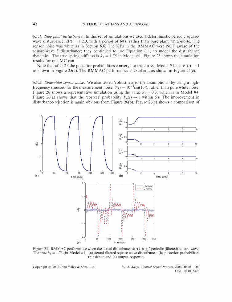
6.7.1. Step plant disturbance. In this set of simulations we used a deterministic periodic square-wave disturbance, xðtÞ ¼ 2:0; with a period of 60 s, rather than pure plant white-noise. Thesensor noise was white as in Section 6.6. The KFs in the RMMAC were NOT aware of thesquare-wave x disturbance; they continued to use Equation (11) to model the disturbancedynamics. The true spring stiffness is k1 ¼ 1:75 in Model #1: Figure 25 shows the simulationresults for one MC run.

Note that after 2 s the posterior probabilities converge to the correct Model #1; i.e. P1ðtÞ ! 1as shown in Figure 25(a). The RMMAC performance is excellent, as shown in Figure 25(c).

6.7.2. Sinusoidal sensor noise. We also tested ‘robustness to the assumptions’ by using a high-frequency sinusoid for the measurement noise, yðtÞ ¼ 103sinð10tÞ; rather than pure white noise.Figure 26 shows a representative simulation using the value k1 ¼ 0:3; which is in Model #4:Figure 26(a) shows that the ‘correct’ probability P4ðtÞ ! 1 within 5 s. The improvement indisturbance-rejection is again obvious from Figure 26(b). Figure 26(c) shows a comparison of

0 60 120 180 240 300 350−2

−1

0

1

2

time (sec)

d(t)

0 2 4 6 8 100

0.5

1

P 1(t

)

0 2 4 6 8 100

0.5

1

P 2(t

)

0 2 4 6 8 100

0.5

1

P 3(t

)

0 2 4 6 8 100

0.5

1

time (sec)

P 4(t

)

0 60 120 180 240 300 350−0.2

−0.1

0

0.1

0.2

time (sec)

z(t)

RMMACGNARC

(a) (b)

(c)

Figure 25. RMMAC performance when the actual disturbance dðtÞ is a2 periodic (filtered) square-wave.The true k1 ¼ 1:75 (in Model #1): (a) actual filtered square-wave disturbance; (b) posterior probabilities

transients; and (c) output response.



DOI: 10.1002/acs

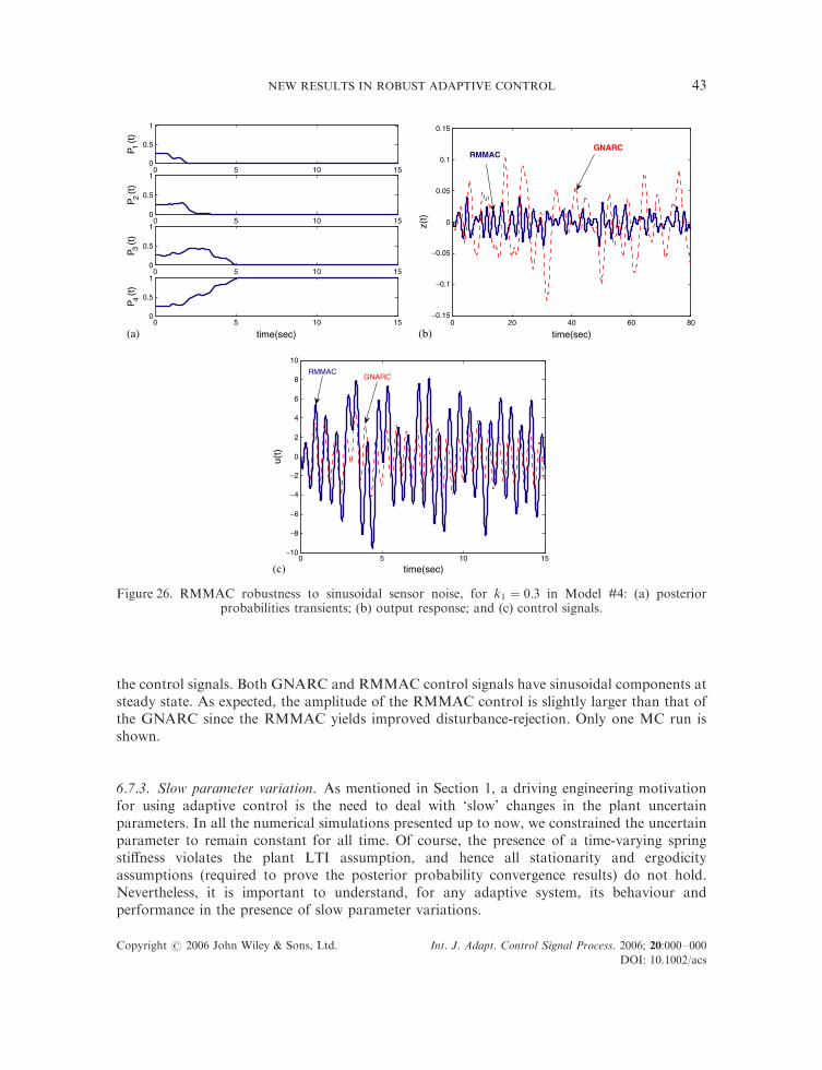
the control signals. Both GNARC and RMMAC control signals have sinusoidal components atsteady state. As expected, the amplitude of the RMMAC control is slightly larger than that ofthe GNARC since the RMMAC yields improved disturbance-rejection. Only one MC run isshown.

6.7.3. Slow parameter variation. As mentioned in Section 1, a driving engineering motivationfor using adaptive control is the need to deal with ‘slow’ changes in the plant uncertainparameters. In all the numerical simulations presented up to now, we constrained the uncertainparameter to remain constant for all time. Of course, the presence of a time-varying springstiffness violates the plant LTI assumption, and hence all stationarity and ergodicityassumptions (required to prove the posterior probability convergence results) do not hold.Nevertheless, it is important to understand, for any adaptive system, its behaviour andperformance in the presence of slow parameter variations.

0 5 10 150

0.5

1P 1

(t)

0 5 10 150

0.5

1

P 2(t

)

0 5 10 150

0.5

1

P 3(t

)

0 5 10 150

0.5

1

time(sec)

P 4(t

)

0 20 40 60 80−0.15

−0.1

−0.05

0

0.05

0.1

0.15

time(sec)

z(t)

RMMACGNARC

0 5 10 15−10

−8

−6

−4

−2

0

2

4

6

8

10

time(sec)

u(t)

RMMACGNARC

(c)

(a) (b)

Figure 26. RMMAC robustness to sinusoidal sensor noise, for k1 ¼ 0:3 in Model #4: (a) posteriorprobabilities transients; (b) output response; and (c) control signals.



DOI: 10.1002/acs

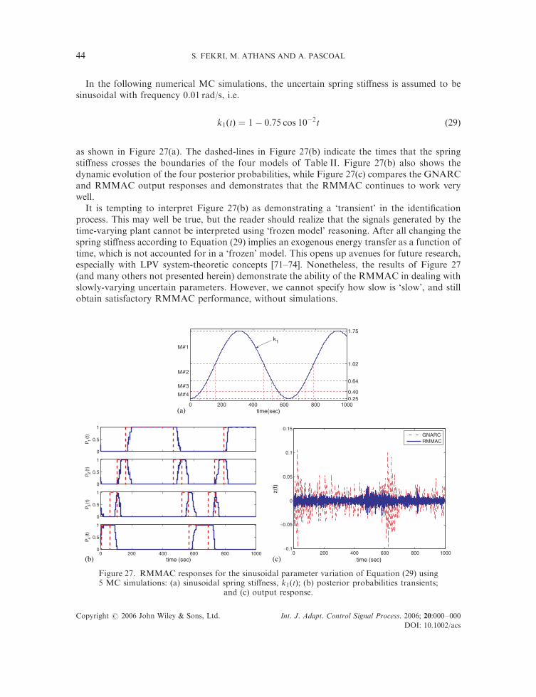
In the following numerical MC simulations, the uncertain spring stiffness is assumed to besinusoidal with frequency 0.01 rad/s, i.e.

k1ðtÞ ¼ 1 0:75 cos 102t ð29Þ

as shown in Figure 27(a). The dashed-lines in Figure 27(b) indicate the times that the springstiffness crosses the boundaries of the four models of Table II. Figure 27(b) also shows thedynamic evolution of the four posterior probabilities, while Figure 27(c) compares the GNARCand RMMAC output responses and demonstrates that the RMMAC continues to work verywell.

It is tempting to interpret Figure 27(b) as demonstrating a ‘transient’ in the identificationprocess. This may well be true, but the reader should realize that the signals generated by thetime-varying plant cannot be interpreted using ‘frozen model’ reasoning. After all changing thespring stiffness according to Equation (29) implies an exogenous energy transfer as a function oftime, which is not accounted for in a ‘frozen’ model. This opens up avenues for future research,especially with LPV system-theoretic concepts [71–74]. Nonetheless, the results of Figure 27(and many others not presented herein) demonstrate the ability of the RMMAC in dealing withslowly-varying uncertain parameters. However, we cannot specify how slow is ‘slow’, and stillobtain satisfactory RMMAC performance, without simulations.

0 200 400 600 800 10000.250.40

0.64

1.02

1.75

time(sec)

M # 1

M # 3

M # 2

M # 4

k1

0

0.5

1

P(t

)

0

0.5

1

P(t

)

0

0.5

1

P(t

)

0 200 400 600 800 10000

0.5

1

time (sec)

P(t

)

0 200 400 600 800 1000−0.1

−0.05

0

0.05

0.1

0.15

time (sec)

z(t)

GNARCRMMAC

(a)

(b) (c)

Figure 27. RMMAC responses for the sinusoidal parameter variation of Equation (29) using5 MC simulations: (a) sinusoidal spring stiffness, k1ðtÞ; (b) posterior probabilities transients;

and (c) output response.



DOI: 10.1002/acs

6.8. Widely varying disturbance environments and the RMMAC/XI architecture

We shall now demonstrate the poor performance of the standard RMMAC when the plantdisturbance environment is highly uncertain; this represents a severe violation of the underlyingassumptions. We shall also demonstrate how the RMMAC/XI architecture, developed inSection 5, overcomes these shortcomings and yields outstanding disturbance-rejection.

First, let us suppose that the N ¼ 4 model standard RMMAC, designed for unit intensity,X ¼ 1; of the plant white noise xðtÞ (see Equation (11)) has been implemented as in the previoussimulations of this section. Let us now suppose that the actual plant white noise xðtÞ is generatedby the square-wave intensity sequence, shown in Figure 28(a), which changes from the ‘normalintensity’ X ¼ 1 to the ‘abnormal intensity’ X ¼ 100: Thus, periodically, every 100 s the standardRMMAC is subjected to the very large (an unanticipated) disturbance dðtÞ shown in Figure28(b) generated by Equation (11). Figure 28(c) shows the evolution of the four posterior

0 50 150 250 350 4001

100

time (sec)

Ξ(t)

0 50 150 250 350 400−8

−4

0

4

8

time (sec)

d(t)

0

0.5

1

P 1(t

)

0

0.5

1

P 2(t

)

0

0.5

1

P 3(t

)

0 50 150 250 350 4000

0.5

1

time (sec)

P 4(t

)

0 50 150 250 350 400−1.5

−1

−0.5

0

0.5

1

1.5

time (sec)

z(t)

RMMACGNARC

(a) (b)

(c) (d)

Figure 28. The standard RMMAC performance when we have a periodic severe violation of thetheoretical assumptions. The KFs are designed for the ‘normal’ intensity X ¼ 1; but the actual noiseintensity is a periodic square-wave with Xact 2 f1; 100g: The true spring stiffness is k1 ¼ 1:5 in Model #1:Only a single Monte Carlo simulation is shown: (a) square-wave intensity of the plant disturbance; (b)

plant disturbance noise; (c) posterior probabilities; and (d) the output zðtÞ:



DOI: 10.1002/acs

probabilities using the value k1 ¼1.5 in Model #1: It is evident from Figure 28(c) that during thetime-intervals associated with the ‘normal’ disturbance, P1ðtÞ ! 1 so that the correct model #1is identified. However, during the time-intervals of the ‘abnormal’ disturbance all posteriorprobabilities switch rapidly and exhibit ‘model-identification confusion’. The impact upon thestandard RMMAC performance is shown in Figure 28(d). There is no long-term instability;however, during the ‘abnormal’ time-intervals the disturbance-rejection of the RMMAC isabout the same as that of the (non-adaptive) GNARC. Hence, we conclude that this severeviolation of the theoretical assumptions drastically degrades the RMMAC performance. Similarbehaviour was observed in many other ‘abnormal’ simulations [2] (not shown here).

We next demonstrate how the use of the RMMAC/XI architecture of Figure 10 with N ¼ 4alleviates the performance-deterioration noted above. We implement eight KFs. The first fourKFs ðk ¼ 1; 2; 3; 4Þ are designed for the noise intensity X ¼ 1 and are identical to those usedbefore. The last four KFs ðk ¼ 5; 6; 7; 8Þ are designed for the noise intensity X ¼ 100; for thesethe BPM procedure discussed in Section 6.5 was repeated to design KF #5; 6; 7; 8 (results notshown). The four LNARCs remain the same since they do not depend upon the value of theintensity X:

We show simulations for the same spring constant k1 ¼ 1:5 as in Figure 28. In this case, thetrue model is Model #1 when X ¼ 1 but changes to Model #5 when X ¼ 100: Figure 29 showsthe results obtained from simulations using the same square-wave X intensity as in Figure 28(a),repeated in Figure 29(a). The time-evolution of the eight posterior probabilities is shown inFigure 29(c); note that the posterior probabilities identify the correct models almostimmediately, i.e.

P1ðtÞ ! 1 for t 2 ½0; 50 [ ½150; 250 [ ½350; 400

P5ðtÞ ! 1 for t 2 ½50; 150 [ ½250; 350

Figure 29(b) compares the disturbance rejection of the standard RMMAC (from Figure28(d)) with that of the RMMAC/XI. It is clear that in this example the RMMAC/XI yields trulyoutstanding disturbance-rejection; similar conclusions were arrived at in Reference [2] fromnumerous other similar simulations.

6.9. Discussion of numerical results

The stochastic simulation results presented in this paper demonstrate the excellent performanceof the RMMAC system. Compared to the ‘best’ non-adaptive design, GNARC, the RMMACand RMMAC/XI consistently had superior disturbance-rejection. No closed-loop instabilitieswere noted in thousands of MC simulations, with the exception of forced prolonged mismatchinstabilities as noted in Section 6.6.4.

The example illustrated how to predict (and then validate) the potential performancecharacteristics of the RMMAC. This was done by analysing the corresponding LTI feedbackloops involving the GNARC and each of the four LNARCs so as to generate RMS predictions,frequency-domain visualizations for disturbance-rejection, etc. We emphasize that thisconstructive capability is critical so that quantitative trade-offs can be carried out, before oneconstructs and tests the full-blown RMMAC design with numerous MC simulations.

The RMMAC performance conclusions reported here validate earlier simulations by theauthors. In Reference [27] we analysed, using a five-model RMMAC, an academic SISO



DOI: 10.1002/acs

non-minimum phase (NMP) plant with a single uncertain right-half plane zero which posesfundamental limits to superior disturbance-rejection near its frequency; see, for example,Reference [70]. In that example, the GNARC ‘hedged’ for the minimum value of the NMP zero.If the true zero was near its minimum value, the RMMAC performance was essentially the sameas for the GNARC (no magic properties). The true value of the RMMAC shows when the trueNMP zero is large; then the RMMAC produces truly superior performance vis-a-vis theGNARC. The interested reader may also review the RMMAC results reported in Reference [29]for a different two-cart mass–spring–dashpot non-collocated system with a mass uncertainty.However, the previous results [27–29] did not use the systematic FNARC based approach fordefining the models (in the spirit of Figure 14) nor the optimized KF design using the BPM (in

0 50 150 250 350 4001

100

time(sec)

Ξ(t)

0 50 150 250 350 400−1.5

−1

−0.5

0

0.5

1

1.5

time(sec)

z(t)

RMMAC/XIRMMAC

0

0.5

1

P 1(t

)

0

0.5

1

P 2(t

)

0

0.5

1

P 3(t

)

0 50 150 250 350 4000

0.5

1

time(sec)

P 4(t

)

0

0.5

1

P 5(t

)

0

0.5

1P 6

(t)

0

0.5

1

P 7(t

)

0 50 150 250 350 4000

0.5

1

time(sec)

P 8(t

)

(c)

(a) (b)

Figure 29. The RMMAC/XI performance for varying plant noise intensity. The true spring constant isk1 ¼ 1:5 in Model #1 when X ¼ 1 but in Model #5 when X ¼ 100:Note that the correct probabilities, P1ðtÞand P5ðtÞ; almost instantaneously go to unity whenever X changes. Only a single Monte Carlo run, with thesame seed as in Figure 29, is shown: (a) square-wave intensity of the plant disturbance; (b) the RMMAC

output zðtÞ; and (c) posterior probabilities.



DOI: 10.1002/acs

the spirit of Figure 18). Several other SISO and MIMO results and examples can be found in thedoctoral dissertation of Fekri [2].

The computation time required by the RMMAC is modest for the numerical exampleconsidered in this section. In a single Monte Carlo simulation we carry out, in real-time, therequired on-line calculations and simulations for the four KFs, the PPE and the four LNARCsusing a sampling time of 0.01 s. These were done 13 times faster than real-time using a ToshibaSatellite Pro laptop with an Intel Pentium M 1.5GHz processor, running under Windows XPPro (SP2) and Matlab 7.0.

We also carried out several simulations using the ‘switched version’ of the RMMAC discussedin Section 2.4 [2]. Our experience is that the ‘switched RMMAC’ leads to larger RMS errorsduring the identification transient interval for constant uncertain parameters. After the posteriorprobability converges, of course both RMMAC versions behave in the same manner. This is thereason that we focused upon the RMMAC architecture of Figure 4 that utilizes probabilisticweighting of the control signals via Equation (3).

Finally, we stress that all mixed-m computations to determine the GNARC and LNARCswere carried out by the (as yet non-commercially available) software provided to us by Balas[48]. If we had designed these compensators with the commercial version of Matlab [49], whichuses only the D-K scales in the iterative design of the H1 compensators, they would be muchmore conservative and the performance improvements would be inferior [69].

7. DISCUSSION AND FUTURE RESEARCH DIRECTIONS

We have presented a brief overview of different approaches to adaptive control that utilizemultiple-model architectures. Recent research in the area of the CMMAC and RMMACarchitectures seems most promising, but we still have no widely accepted solution to the robustadaptive control problem. As a consequence, there is still a great deal of work that needs to bedone, both theoretical and applied, to fully understand the similarities and difference among thetwo architectures and the variants within each one, and suitable extensions.

Any future theoretical research must adopt a design methodology. We strongly believe thatthe adaptive problem formulation should always include unmodelled dynamics, unknown plantdisturbances and sensor noise, in addition to the (slowly-varying) uncertain real parameters.Furthermore, the design methodology should contain explicit performance specifications andperformance-robustness should be an integral part of the adaptive problem formulation. Thus,closed loop-stability arguments are not enough. This implies that the ‘local’ compensators, theLNARCs, must be designed to exhibit both local robust-stability and robust-performance,following the ideas presented in Section 3 and as utilized in our RMMAC architectures. In theunfalsified control methodologies, if robust-performance is to be considered, the availableresults must be significantly extended; most probably, the family of robust compensatorsavailable for unfalsified and safe control will also have to be designed using the methodologysuggested in Section 3. Recent results in unfalsified control [30, 31] claim stability, butperformance is not addressed (after all, an open-loop stable highly uncertain plant remainsrobustly stable with no feedback, albeit with lousy performance).

The structure of the multi-controllers used in the SMMAC architecture does not explicitlyreflect a robust-performance requirement. Indeed, for the most part, the SMMAC multi-controllers have a common Ac-matrix (so all controllers have the same poles). This was done for



DOI: 10.1002/acs

the purpose of computational simplicity and ‘bump less transfer’ to avoid control transients.However, such controller structures are not appropriate if performance-robustness isdesired. A recent exception [75] uses multi-controllers that have an LQG structure, butthey use pole-placement ideas, which are also notorious for their lack-of-robustnessproperties. On the other hand, the RMMAC architecture deals directly with such robust-performance issues and the dynamic characteristics of the RMMAC compensators are quitedifferent.

We believe that, as stressed in Section 3, one cannot arrive at a systematic procedure fordefining the number of models required in any multiple-model scheme without explicitperformance specifications. Specification of complexity requires fixing the number, N; ofmodels; however, one still needs to properly calculate their ‘boundaries’. Specification of therequired performance, such as in the % FNARC method, would naturally lead to the requirednumber of models and their boundaries. In either case, one needs to utilize the mixed-mmethodology to maximize performance and derive the LNARCs.

We note that for many industrial applications, where ‘tuned’ PID controllers are judged toyield satisfactory performance, designing the LNARCs may be an overkill. Based upon operatorexperience, one can define the N models in an ad hoc manner as opposed to systematicprocedures of Section 3. In such cases, one can still design the KFs, using the BPMmethodologyof Section 4 and obtain and implement the ‘identification subsystem’ of the resulting RMMAC.

We now consider the ‘system identification’ part of the SMMAC and RMMAC architectures.In the RMMAC architecture the approach is stochastic and relies on the residuals generated bythe bank of KFs. These must be designed very carefully so as to meet the probabilityconvergence results, as explained in Section 4 and Appendices A and B. In the SMMACarchitectures the approach is deterministic and relies upon the prediction errors generated by abank of multi-estimators, which are a special class of Luenberger observers. In all citedSMMAC references, with the exception of Reference [75], each estimator uses the same ‘AE ’matrix, i.e. all observers have identical stable poles. This was done to minimize on-linecomputation. An integral norm of the prediction errors is used for the system identificationfunction. Research should be done to remove the common ‘AE ’ matrix assumption and usemore general observers. Also, the assumption of scalar prediction errors must be removed tomake the SMMAC architectures extendable to the MIMO case. In Reference [75] this was done,but the problem of designing suitable deterministic MIMO Luenberger observers, say byeigenstructure assignment, becomes quite complex.

Our experience has shown that the RMMAC can effectively deal with ‘slowly time-varying’parameters. It may be interesting to examine if one can integrate the RMMAC philosophy andmethodology with the evolving theory of LPV systems [36–41, 71–74, 76].

A weakness of the MMAE algorithm is that the BPMsee Appendix Bcannot be definedor calculated for open-loop unstable plants. Thus, if in an RMMAC application the plant isunstable one would not be able to use the ideas of Section 4, which are based on the BPM, todesign the KFs. One can still design KFs (and RMMACs) for unstable plants, but one wouldmost likely have to use trial-and-error methods in designing the KFs and ensuring convergenceof the posterior probabilities. This defines a key and very important area for future research.

With respect to the RMMAC and RMMAC/XI architectures, if one or more of the LNARCsis unstable (but leads to a stable feedback loop) remains an open question. All the LNARCs thatwe have designed [2] were stable. However, if the open-loop plant is both unstable and non-minimum phase then some of the LNARCs may be unstable. Since we cannot define the BPM



DOI: 10.1002/acs

for unstable open-loop plants noted above, this remains a very important future research areafor RMMAC architectures.

Finally, we need to stress that in all available SMMAC and RMMAC results we cannotproveas yetglobal robust-stability, because a suitable theory is lacking for handling the non-linear time-varying (stochastic) closed loop dynamics arising from these architectures. Needlessto say, any advances in stability theory along these directions would be welcomed. At present,the promise of the SMMAC and RMMAC architectures is in their ‘local’ and ‘asymptotic’results related to stability and performance. With respect to the RMMAC one can design real-time monitoring systems for the ‘regularity’ of the residuals. If ‘abnormal’ situations areobserved (see the discussion in Sections 2 and 6), which may lead to long-term instability, oneshould be able to design a ‘fail-safe’ logic that disconnects the LNARCs and uses the GNARCuntil the residuals return to a ‘regular’ behaviour and the LNARCs are reconnected.

Equally important to the theoretical research investigations would be to fairly compare thedifferent adaptive methods using a variety of common ‘test-bed examples’, with identicalperformance requirements.

8. CONCLUDING REMARKS

We have witnessed the development and evolution of a variety of novel multiple-modelarchitectures for robust adaptive control during the past decade. In order to compare them in afair manner we have suggested that all should utilize the available results and softwareassociated with mixed-m synthesis. If we explicitly state the specifications for required stability-and performance-robustness for the adaptive closed-loop system, then we can evolve the presentarchitectures so that they can be confidently used in real applications.

We view our RMMAC architecture and design methodology as a potential contribution toadaptive feedback engineering system design. As we have remarked, we cannot prove globalstability results and we only have numerous simulation studies that demonstrate its excellentperformance. Thus, a reader may ask an important question: why should one pay attention to theRMMAC procedure in the absence of solid theoretical guarantees?

The best way to view our perspective is by an analogy. Thousands of real engineering systemsare operating using methods that also lack a solid theoretical foundation, but are based uponcommon-sense integration of rigorous results. We list just three, all of them involving non-linearsystems:

(a) gain-scheduling feedback control system designs (with no global stability guarantees),(b) surveillance, tracking and other estimation systems that utilize the extended KF (which

may diverge), and(c) surveillance, tracking systems and other estimation systems that are based on the sum-of-

Gaussian multiple model estimation method, when the extended KF performance is notgood enough (but they still may not always work well).

None of the above ‘practical’ design methods is backed by a complete body of solidtheory. Their extensive engineering utility is based upon exhaustive simulations, engineeringinsight and know-how to inevitably ‘tune’ certain parameters in the algorithms. However,all utilize reasonable extensions of theoretical results valid for linear systems, e.g. the KF. The



DOI: 10.1002/acs

gain-scheduling method also pieces together linear feedback control results in a common sensemanner. Since almost all real applications involve non-linear systems the engineering utility of(a)–(c) is extensive. Our perspective is that the highly non-linear proposed RMMAC method isakin to the above. Maybe we are nearing the end of the search for the adaptive ‘Holy Grail’.

APPENDIX A: SUMMARY OF THE MMAE FILTER

In this appendix, the equations of the MMAE algorithm, shown in Figure 1, and some of itsproperties are summarized. Here we shall restrict our attention to linear systems driven by whiteGaussian inputs having time-invariant statistics. It is also assumed that the system has attainedsteady state, i.e. that all signals of interest are stationary.

Consider the discrete-time (unknown) system

xðnþ 1Þ ¼ F*xðnÞ þ J

*uðnÞ þ G

*wðnÞ

yðnÞ ¼ H*xðnÞ þ vðnÞ ðA1Þ

where fuðnÞg is the deterministic (control) input and wðnÞ and vðnÞ are zero-mean whiteGaussian sequences, mutually independent with

EfwðnÞwðnÞTg ¼ Q*

EfvðnÞvðnÞTg ¼ R*

ðA2Þ

Let us assume that N discrete-time stochastic LTI models are given that include disturbancedynamics (if any). These models blend a finite set of families of models

¼ fM :Mk ¼ ðFk; Jk;Gk;Hk;Qk;RkÞ; k ¼ ð1; 2; . . . ;NÞg ðA3Þ

The kth model is then described by the state-space dynamics

xkðnþ 1Þ ¼ FkxkðnÞ þ JkuðnÞ þ GkwðnÞ

ykðnÞ ¼ HkxkðnÞ þ vðnÞ ðA4Þ

where the time index is n ¼ 0; 1; 2; . . . and the model index is k ¼ 1; 2; . . . ;N:It is assumed that the true system that generates the data is one of the models in Equation

(A4). The set of past controls, uð0Þ; uð1Þ; uð2Þ; . . . ; uðn 1Þ; and the set of past noisymeasurements, including the one at the present time n; yð1Þ; yð2Þ; . . . ; yðn 1Þ; yðnÞ; are alsoknown at time n: We want to determine the true steady-state conditional mean of the presentstate vector, xðnÞ; i.e. as n!1

#xðnjnÞ ¼ EfxðnÞj uð0Þ; uð1Þ; . . . ; uðn 1Þ; yð1Þ; . . . ; yðn 1Þ; yðnÞ|fflfflfflfflfflfflfflfflfflfflfflfflfflfflfflfflfflfflfflfflfflfflfflfflfflfflfflfflfflfflfflfflfflfflfflfflfflfflfflfflfflfflzfflfflfflfflfflfflfflfflfflfflfflfflfflfflfflfflfflfflfflfflfflfflfflfflfflfflfflfflfflfflfflfflfflfflfflfflfflfflfflfflfflfflYðnÞ

g

and the true steady-state conditional covariance matrix of xðnÞ; i.e.

SðnjnÞ ¼ E½ðxðnÞ #xðnjnÞÞðxðnÞ #xðnjnÞÞ0jYðnÞ ðA5Þ



DOI: 10.1002/acs

The MMAE filter shown in Figure 1 is driven by the sequence of past controls and noisy sensormeasurements while it generates both a state-estimate vector and a corresponding error-covariance matrix. Let us first establish some notation for the discrete-time steady-state KF.

Predict-cycle:

#xkðnþ 1jnÞ ¼ Fk #xkðnÞ þ JkuðnÞ

#ykðnþ 1jnÞ ¼ Hk #xkðnþ 1jnÞ ðA6Þ

Update-cycle:

#xkðnþ 1jnþ 1Þ ¼ #xkðnþ 1jnÞ þ Kkrkðnþ 1Þ ðA7Þ

The residual rkðÞ; residual covariance matrix Sk; and the constant steady-state KF gain matrix,Kk; are, respectively, defined as follows:

Residual:

rkðnþ 1Þ ¼ yðnþ 1Þ #ykðnþ 1jnÞ ðA8Þ

Residual covariance:

Sk ¼ cov½rkðnþ 1Þ; rkðnþ 1Þ ¼ HkSpkH

Tk þ Rk ðA9Þ

KF gain:

Kk ¼ SpkH

Tk S1k ðA10Þ

The constant steady-state covariance equations arePredict-cycle covariance Sp

k:

Spk ¼ FkSkA

Tk þ GkQkG

Tk ðA11Þ

Update-cycle covariance Sk:

Sk ¼ Spk Sp

kHTk S1k HkS

pk ðA12Þ

We stress that both the MMAE state-estimate and state-covariance matrix in Equation (A5)represent true conditional state estimate and its conditional covariance at steady state [54, 57].This is because, one can explicitly calculate the conditional probability density function pðxðnÞjYðnÞÞ; which turns out to be a weighted sum of Gaussian densities, where the weights arefound from the PPE; see Figure 1.

The problem reduces to a combination of a hypothesis-testing problem and a state-estimationproblem. The fact that one of the N models is the true one is modelled by a hypothesis randomvariable that must belong to a discrete set of hypothesis fH1;H2; . . . ;HNg: It turns out thatonline generation of the posterior conditional probabilities determines which hypothesis is true.Let suppose that H indicates the hypothesis random variable (scalar) which can attain only oneof N possible values,

H 2 fH1;H2; . . . ;HNg ðA13Þ

The event H ¼Hk means that the kth system is the true one, i.e. the one that is generating thedata. The prior probabilities at initial time n ¼ 0; Pkð0Þ ProbðH ¼HkÞ; are assumed known



DOI: 10.1002/acs

(typically Pkð0Þ ¼ 1=N), and

Pkð0Þ50;XNk¼1

Pkð0Þ ¼ 1 ðA14Þ

The posterior probabilities, PkðnÞ ¼ ProbðH ¼HkjYðnÞÞ; must also satisfy

PkðnÞ50;XNk¼1

PkðnÞ ¼ 1 ðA15Þ

and can be calculated on-line by the PPE in the MMAE system. It turns out that the conditionalPDF, pðyðnþ 1ÞjuðnÞ;Hk;YðnÞÞ; is Gaussian with mean

Efyðnþ 1ÞjuðnÞ;Hk;YðnÞg ¼ Hk #xkðnþ 1jnÞ ðA16Þ

and steady-state covariance

cov½yðnþ 1Þ; yðnþ 1ÞjuðnÞ;Hk;YðnÞ ¼ HkSpkH

Tk þ Rk¼

4Sk ðA17Þ

Furthermore,

pðyðnþ 1ÞjuðnÞ;Hk;YðnÞÞ ¼1

ð2pÞm=2ffiffiffiffiffiffiffiffiffiffiffiffiffidet Sk

p e12rTkðnþ1ÞS1

krkðnþ1Þ ðA18Þ

By using Bayes rule we deduce that

Pkðnþ 1Þ ¼pðyðnþ 1Þ jHk; uðnÞ;YðnÞÞPN

j¼1 PjðnÞpðyðnþ 1Þ jHj ; uðnÞ;YðnÞÞ PkðnÞ ðA19Þ

For notational simplicity, define

wjðnþ 1Þ ¼ r0jðnþ 1Þ S1j rjðnþ 1Þ ðA20Þ

bj ¼ ðð2pÞm=2

ffiffiffiffiffiffiffiffiffiffiffiffidet Sj

pÞ1 ðA21Þ

where m is the number of measurements. Then, from Equations (A19)–(A22) the posteriorprobabilities can be computed on-line by the PPE using the recursive formula

Pkðnþ 1Þ ¼bke

12wkðnþ1ÞPN

j¼1 bj e12wjðnþ1ÞPjðnÞ

PkðnÞ ðA22Þ

where Pkð0Þ are the prior model probabilities as in Equation (A4).Thus, at steady-state the MMAE generates the state estimate (exact conditional mean) by

#xðnjnÞ ¼XNk¼1

PkðnÞ #xkðnjnÞ ðA23Þ

and the exact conditional covariance matrix

SðnjnÞ ¼XNk¼1

PkðnÞ ½SkðnjnÞ þ ð #xkðnjnÞ #xðnjnÞÞð #xkðnjnÞ #xðnjnÞÞ0 ðA24Þ

We stress that the above results hold when the true (unknown) plant is assumed to belong tothe model set of Equation (A4).



DOI: 10.1002/acs

APPENDIX B: BARAM PROXIMITY MEASURE (BPM)

The purpose of this appendix is to summarize the underlying results from probability andestimation theory that yield the identification procedure which converges to a model in the setwhich is closest to the true model in an information-theoretic sense, as proved by Baram [61].The posterior probabilities will converge if certain ergodicity and stationarity assumptions ofresiduals (innovation signals) are true. These conditions are briefly discussed in this appendix;see Reference [61] for more details.

B.1. Stationarity and ergodicity

In this section we provide definitions and convergence results for ergodic sequences used in thepaper. It is not intended to provide an elaborate presentation of the ergodicity concept. For aprecise development of ergodicity theory the reader is referred to, e.g. References [77, 78].

Definitions1. Consider a probability space ðO;U;PÞ: A transformation T from O to U is said to be measurepreserving if

PðT1AÞ ¼ PðAÞ

for all A 2 U:2. A stochastic sequence fxðnÞg on ðO;U;PÞ is said to converge almost everywhere (a.e.) or

almost surely (a.s.) to a random variable x on ðO;U;PÞ if

limn!1

xðnÞ ¼ x a:e:

3. Given a measure preserving transformation T ; a U-measurable event A is said to beinvariant if

T1A ¼ A

4. Let fxðnÞg be a stochastic sequence on ðO;U;PÞ with values in ðR‘;B‘Þ; where ðR‘Þ is thel-dimensional Euclidean space and ðB‘Þ is the s algebra of Borel sets of Rl; see Reference[79, Chapter 3]. Let B‘1 be the s-algebra of Borel sets of R‘

1 where R‘1 ¼ R‘ R‘ : Then

fxðnÞg is said to be stationary if for each k51 and for every C 2 B‘1

P½fxð1Þ; xð2Þ; . . . ;xðnÞg 2 C ¼ P½fxðkþ 1Þ;xðkþ 2Þ; . . . ;xðkþ nÞg 2 C ðB1Þ

5. The covariance matrix defined by

RðkÞ EfxðnÞ xTðnþ kÞg

plays a fundamental role in the study of stationary processes in the wide sense [77]. A zero meanstationary Gaussian process is ergodic if and only if [80, pp. 257–260; 77, p. 494]

limn!1

1

nþ 1

Xnk¼0

jRðkÞj2 ¼ 0 ðB2Þ

where jRðkÞj denotes the determinant of RðkÞ:



DOI: 10.1002/acs

B.2. Calculating the Baram proximity measure (BPM) [61]

Consider a bank of N discrete KF, and a set of N models for the system of Equation (A1)described by

xjðnþ 1Þ ¼ FjxjðnÞ þ GjwðnÞ

yjðnÞ ¼ HjxjðnÞ þ vðnÞ ðB3Þ

in the absence of deterministic inputs but with the assumption of a stationary processes. Notethat these results can be extended to the case where the system of Equation (B3) is driven by anadditional deterministic (known) stationary random sequence.

Let Mn ¼ f* [g denotes the model set that also includes the true model, denoted by * :For each i; j 2 let

Sj Ef½yðnÞ #yjðnÞ½yðnÞ #yjðnÞTjHi ¼Hjg

denote the residual covariance matrix generated by the jth KF and

Gij Ef½yðnÞ #yjðnÞ½yðnÞ #yjðnÞTjHi=Hjg

according to Mj ; when Mi is the correct model.We shall use the following condition [61, p. 77] in addition to the other stationarity and

ergodicity conditions.Condition B1 (C.B1): For each j 2Mn; the residual covariance Sj exists and has a finite

positive definite value.A sufficient condition for B1 is that each model corresponding to j 2Mn is detectable and

controllable. For each j 2Mn; Sj is generated by the discrete KF #j corresponding to the modelMj ¼ ðFj ;Gj ;Hj ;Qj ;RjÞ:

Assuming that index ‘i’ denotes the true parameter in Mn; the augmented dynamic equationgenerating simultaneously the state xðnÞ and its updated estimate generated by the jth KF, #xjðnÞ;is

xiðnþ 1Þ

#xjðnþ 1Þ

" #¼

Fi 0

FjKjHi FjðI KjHjÞ

" #xiðnÞ

#xjðnÞ

" #þ

Gi 0

0 FjKj

" #wðnÞ

vðnÞ

" #ðB4Þ

where Kj is the (steady state) KF gain corresponding to the model Mj : The KF gain matrix isgiven by

Kj ¼ SjHTj ðHjSjH

Tj þ RjÞ

1

where Sj denote the prediction error covariance matrix according to Mj :For notational purposes, define:

Fij

Fi 0

FjKjHi FjðI KjHjÞ

" #

Gij

Gi 0

0 FjKj

" #



DOI: 10.1002/acs

Qi Qi 0

0 Ri

" #

Hij ½Hi j Hj

Then the matrix

Cijðnþ 1Þ E

xiðnþ 1Þ

#xjðnþ 1Þ

" #xiðnþ 1Þ

#xjðnþ 1Þ

" #T8<:

9=;

is generated by the dynamic Lyapunov equation

Cijðnþ 1Þ ¼ Fi

jCijðnÞF

iT

j þ GijQ

iGiT

j ðB5Þ

The (steady-state) limit of the Lyapunov equation of Equation (B5) is computed by

Cij ¼ lim

n!1Ci

jðnÞ ðB6Þ

It exists and is finite if and only if the augmented state matrix Fij has all its eigenvalues inside

the unit circle, i.e. the spectral radius satisfies

rðFij Þ51 ðB7Þ

This is the case if for each j 2Mn; Fj has all its eigenvalues inside the unit circle and ðFj ;HjÞ isobservable.

Therefore, to calculate the limit matrix Cij of Equation (B5) we simply solve, using Matlab,

the discrete-time algebraic Lyapunov equation

Cij ¼ Fi

jCijF

iT

j þ GijQ

iGiT

j ðB8Þ

It can be shown that

Gij ¼ Hi

jCijH

iT

j þ Ri ðB9Þ

where Cij is the steady-state solution of Equation (B5).

It can also be shown that the state covariance matrix can be calculated as follows:

RðkÞ ¼Hi

jCijH

iT

j þ Ri ¼ Gij ; k ¼ 0

HijC

ijðF

iT

j ÞkHiT

j ; k > 0

8<: ðB10Þ

This is shown in Reference [61, pp. 80–81]. However, note that the stability and observabilityof the models are only sufficient, and not necessary. In fact, Reference [61, Theorem 5.1] hasproved ergodicity of the state residuals fxðnÞ #xjðnÞg; which is not necessary, to show theergodicity of fyðnÞ #yjðnÞg: Thus, in the sequel we shall directly use the following assumption.

Condition B2 (C.B2): For each j 2Mn the residual sequence fyðnÞ #yjðnÞg is ergodic.The ergodicity condition of (C.B2) is important and must be checked. If it is not satisfied, one

might use a ‘fake-white-plant-noise’ as mentioned in Section 2.4; see Reference [67, Chapter 7]for more details.



DOI: 10.1002/acs

The conditional probability density function corresponding to Model #j ðj 2MnÞ is

pjðyðnÞjYðn 1ÞÞ ¼ ½ð2pÞm j Sj j12 expf1

2½yðnÞ #yjðnÞTS1j ½yðnÞ #yjðnÞg ðB11Þ

where m is the dimension of yðnÞ; i.e. the number of measurements.For each j; k 2Mn the mean information in yðnÞ favouring ‘model’ k against j is defined by

[61–63]

%Inðk; jÞ ¼ E logpkðyðnÞjYðn 1Þ;H ¼HkÞpjðyðnÞjYðn 1Þ;H ¼HjÞ

and the distance measure is defined as

dnðk; jÞ ¼ j%Inðk; jÞj

For each j 2Mn; using * to denote the true plant in Mn; we have

E log pjðyðnÞjYðn 1Þ;H ¼HjÞ ¼ m

2log 2p

1

2log jSj j

1

2trfS1j Gn

j g ðB12Þ

and for each pair j; k 2Mn

%Inðk; jÞ ¼ %Inðj; kÞ ¼ 12log jSj j þ 1

2trfS1j Gn

j g 12log jSkj 1

2trfS1k Gn

kg ðB13Þ

The BPM of the jth filter denoted by Lij is generated by

Lij logjSj j þ trfS1j Gi

jg; i; j 2Mn ðB14Þ

Therefore,

%Inðk; jÞ ¼ 12ðLn

j Ln

kÞ; i; j 2M ðB15Þ

Also,

%Inð* ; jÞ5 0; j 2M ðB16Þ

It is easy to check that

dð* ; jÞ5 dð* ; kÞ

if and only if

Ln

j 5 Ln

k

for which the following condition is essential.Condition B3 (C.B3): There exists some parameter k 2M such that

Ln

k5Ln

j for all j 2M; j= k ðB17Þ

If the convergence conditions hold for the MMAE to converge, i.e. Equation (B2) andconditions (C.B1)–(C.B3), then it will converge to the jth filter (corresponding to theappropriate plant model) governed by

Ln

j ¼ minifLi

jg; i ¼ 1; . . . ;N

where Lij is the BPM of the models as in Equation (B14).

In conclusion, the BPM, is an appropriate distance metric between the true model and each ofthe other models that form the bank of KF.



DOI: 10.1002/acs

Remarks

The application of deterministic inputs, rather than stationary random sequences, to thedynamic system, for the purpose of identification and their optimal selection, is not addressed inthis paper. Generally speaking, the convergence analysis in the presence of deterministic inputsrequires a more elaborate analysis, a topic for future research.

Reference [61, Chapter 6] discusses a case that any deterministic input sequence, that satisfiesa suitable assumption of Reference [61, Theorem 6.3], will provide convergence in the mean ofthe identification procedures at a certain rate; see References [61, 81] for more details.

Reference [66] uses the prediction error parameter estimate obtained by minimizing a scalarfunction of the matrix Xt

t¼0

½R1=2ðtÞ rðt; pÞ½R1=2ðtÞ rðt; pÞT ðB18Þ

where RðtÞ is some positive definite weighting matrix, and shows that under general conditionsof bounded fourth moments of the residuals rðt; pÞ; by searching over models leading to stableKFs and overall system stability, this prediction error estimate converges into the set of modelsthat yield the same output prediction as the true system in the following sense:

limt!1

inf1

tþ 1

Xtt¼0

j#yðt; p0Þ #yðt; pÞj2 ¼ 0 ðB19Þ

which is similar to the ergodicity condition as in Equation (B2). This set depends in general onthe input signal and will be contained in the set of all models with the same input–outputrelation as the true model, if the input is general enough to excite all modes of the system. It isshown in Reference [66] that a sufficient condition would be for uðtÞ to be independent of theprocess noise and persistently exciting. The input uðtÞ is persistently exciting if, for all M; thereexists dðMÞ and N0ðMÞ such that

dI51

N

XN1

uMðtÞu0MðtÞ51

dI

for N > N0 and where

u0MðtÞ ½u0ðtÞ . . . u0ðtMÞ

ACKNOWLEDGEMENTS

We thank Profs B. D. O. Anderson and J. Hespanha for their frequent suggestions, discussions andcriticisms throughout the course of our research. We also are grateful to Prof. G. J. Balas for providing uswith the latest non-commercial version of the mixed-m software [48] and Prof. Y. Baram for providing us acopy of his PhD thesis [61]. We are also indebted to the four anonymous reviewers whose comments andcriticisms greatly improved the final version of this paper.

REFERENCES

1. Athans M, Fekri S, Pascoal A. Issues on robust adaptive feedback control, Preprints 16th IFAC World Congress,Invited Plenary Paper, Prague, Czech Republic, July 2005; 9–39.



DOI: 10.1002/acs

2. Fekri S. Robust adaptive MIMO control using multiple-model hypothesis testing and mixed-m synthesis. Ph.D.Dissertation, Instituto Superior Tecnico, Lisbon, Portugal, 2005.

3. Landau I. Adaptive Control: The Model Reference Approach. Marcel Dekker: New York, U.S.A., 1979.4. Narendra KS, Annaswamy A. Stable Adaptive Systems. Prentice-Hall: Englewood Cliffs, NJ, U.S.A., 1988.5. Sastry S, Bodson M. Adaptive Control: Stability, Convergence and Robustness. Prentice-Hall: Englewood Cliffs, NJ,

U.S.A., 1989.6. Astrom K, Wittenmark B. Adaptive Control (2nd edn). Addison-Wesley: MA, U.S.A., 1995.7. Ioannou P, Sun J. Robust Adaptive Control. Prentice-Hall: NJ, U.S.A., 1996.8. Rohrs C et al. Robustness of continuous-time adaptive control algorithms in the presence of unmodelled dynamics.

IEEE Transactions on Automatic Control 1985; 30(9):881–889.9. Anderson BDO et al. Stability of Adaptive Systems: Passivity and Averaging Analysis. MIT Press: Cambridge, MA,

1986.10. Mosca E et al. Designing predictors for MIMO switching supervisory control. International Journal of Adaptive

Control and Signal Processing 2001; 15:265–286.11. Morse A. Supervisory control of families of linear set-point controllerspart 1: exact matching. IEEE Transactions

on Automatic Control 1996; 41(10):1413–1431.12. Morse A. Supervisory control of families of linear set-point controllerspart 2: robustness. IEEE Transactions on

Automatic Control 1997; 42(11):1500–1515.13. Morse A. A bound for the disturbance-to-tracking-error gain of a supervised set point control system, ser.

In Perspectives in Control Theory and Applications, Normand-Cyrot D (ed.). Springer: Berlin, 1998.14. Morse A. Analysis of a supervised set-point control containing a compact continuum of finite-dimensional linear

controllers. Proceedings of MTNS, Belgium, 2004.15. Narendra KS, Balakrishnan J. Adaptive control using multiple models. IEEE Transactions on Automatic Control

1997; 42(2):171–187.16. Anderson BDO et al. Multiple model adaptive control. part 1: finite controller coverings. International Journal of

Robust and Nonlinear Control 2000; 10(11–12):909–929.17. Anderson BDO et al. Multiple model adaptive control with safe switching. International Journal of Adaptive Control

and Signal Processing 2001; 15(5):445–470.18. Hespanha J et al. Multiple model adaptive controlpart 2: switching. International Journal of Robust and Nonlinear

Control 2001; 11(5):479–496.19. Willner D. Observation and control of partially unknown systems. Ph.D. Dissertation, MIT, Cambridge, MA,

U.S.A., June 1973.20. Greene C. An analysis of the multiple model adaptive control algorithm. Ph.D. Dissertation, MIT, Cambridge, MA,

U.S.A., 1978.21. Athans M et al. The stochastic control of the F-8C aircraft using the multiple model adaptive control (MMAC)

methodpart I: equilibrium flight. IEEE Transactions on Automatic Control 1977; 22(5):768–780.22. Shomber H. An extended analysis of the multiple model adaptive control algorithm. Ph.D. Dissertation, MIT,

Cambridge, MA, U.S.A., 1980.23. Greene C, Willsky A. An analysis of the multiple model adaptive control algorithm. Proceedings of the IEEE

Conference on Decision and Control, 1980; 1142–1145.24. Schiller G, Maybeck P. Control of a large space structure using MMAE/MMAC techniques. IEEE Transactions on

Aerospace and Electronic System 1997; 33(4):1122–1130.25. Maybeck P, Griffin J. MMAE/MMAC control for bending with multiple uncertain parameters. IEEE Transactions

on Aerospace and Electronic System 1997; 33(3):903–912.26. Schott K, Bequette B. Multiple model adaptive control, ser. In Multiple Model Approaches to Modeling and Control,

Chapter 11, Murray-Smith R, Johnsen TA (eds). Taylor & Francis: London, 1997; 269–292.27. Fekri S, Athans M, Pascoal A. A new robust adaptive control method using multiple-models. Proceedings of the 12th

IEEE Mediterranean Conference on Control and Automation (MED’04), Kusadasi, Turkey, June 2004.28. Fekri S, Athans M, Pascoal A. RMMAC: a novel robust adaptive control schemepart I: architecture. Proceedings

of the IEEE Conference on Decision and Control, Paradise Island, Bahamas, December 2004; 1134–1139.29. Fekri S, Athans M, Pascoal A. RMMAC: a novel robust adaptive control schemepart II: performance evaluation.

In Proceedings of the IEEE Conference on Decision and Control, Paradise Island, Bahamas, December 2004, 1140–1145.

30. Wang C et al. Cost-detectability and stability of adaptive control systems. Proceedings of the Joint IEEE Conferenceon Decision and Control/European Control Conference, Seville, Spain, December 2005.

31. Stefanovic M et al. Stability and convergence in adaptive systems. Proceedings of the American Control Conference,Boston, MA, 2004.

32. Wang R et al. Unfalsified direct adaptive control using multiple controllers. Proceedings of the AIAA GNCConference, No. AIAA-2004-5223, Providence, RI, 2004.

33. Safonov M, Tsao T-C. The unfalsified control concept: a direct path from experiment to controller, ser. In FeedbackControl, Nonlinear Systems, and Complexity, Francis BA, Tannenbaum AR (eds). Springer: Berlin, 1995; 196–214.



DOI: 10.1002/acs

34. Safonov M, Tsao T-C. The unfalsified control concept and learning. IEEE Transactions on Automatic Control 1997;42(6):843–847.

35. Jun M, Safonov M. Automatic PID tuning: an application of unfalsified control. Proceedings of the IEEE CCA/CACSD, 1999; 328–333.

36. Shamma S. Analysis and design of gain scheduled control systems. Ph.D. Dissertation, Department of MechanicalEngineering, MIT, Cambridge, 1988.

37. Shamma J, Athans M. Analysis of gain scheduled control for nonlinear plants. IEEE Transactions on AutomaticControl 1990; 35(8):898–907.

38. Rugh W. Analytical framework for gain scheduling. IEEE Control Systems Magazine 1991; 11(1):79–84.39. Nichols R et al. Gain scheduling for H1 controllers: a flight control example. IEEE Transactions on Control

Systems Technology 1993; 1(2):69–79.40. Stilwell D, Rugh W. Interpolation of observer state feedback controllers for gain scheduling. IEEE Transactions on

Automatic Control 1999; 44(6):1225–1229.41. Blanchini F. The gain scheduling and the robust state feedback stabilization problems. IEEE Transactions on

Automatic Control 2000; 45(11):2061–2070.42. Fekri S, Athans M, Pascoal A. A two-input two-output robust multiple model adaptive control (RMMAC) case

study. Proceedings of the American Control Conference, Minneapolis, MN, U.S.A., June 2006.43. Young PM et al. Practical computation of the mixed-m problem. Proceedings of the American Control Conference,

Chicago, IL, June 1992; 2190–2194.44. Young PM et al. Computing bounds for the mixed-m problem. International Journal of Robust and Nonlinear Control

1995; 5:573–590.45. Young PM. Controller design with mixed uncertainties. Proceedings of the American Control Conference, Baltimore,

MD, June 1994; 2333–2337.46. Zhou K et al. Robust and Optimal Control. Prentice-Hall: Englewood Cliffs, NJ, U.S.A., 1996.47. Zhou K, Doyle JC. Essentials of Robust Control. Prentice-Hall: Englewood Cliffs, NJ, U.S.A., 1998.48. Balas GJ. Private communication re mixed-m software, 2003.49. Balas GJ et al. m-Analysis and Synthesis Toolbox of Matlab, User’s Guide. The MathWorks Inc., January 2001.50. Skogestad S, Postlethwaite I. Multivariable Feedback ControlAnalysis and Design (2nd edn). Wiley: New York,

2005.51. Kosut RL, Anderson BDO. Adaptive control via finite modeling and robust control. IFAC Workshop on Robust

Adaptive Control, August 1988; 91–95.52. Magill DT. Optimal adaptive estimation of sampled stochastic processes. IEEE Transactions on Automatic Control

1965; 10(4):434–439.53. Lainiotis DG. Optimal adaptive estimation: structure and parameter adaptation. IEEE Transactions on Automatic

Control 1971; 16(2):160–170.54. Athans M, Chang CB. Adaptive estimation and parameter identification using multiple model estimation

algorithms. Technical Report 28, MIT Lincoln Laboratory, Lexington, MA, U.S.A., June 1976.55. Hawkes RM, Moore J. Performance of Bayesian parameter estimators for linear signal models. IEEE Transactions

on Automatic Control 1976; 21(4):523–527.56. Chang CB, Athans M. State estimation for discrete systems with switching parameters. IEEE Transactions on

Aerospace and Electronic System 1978; 14(3):418–425.57. Anderson BDO, Moore JB. Optimal Filtering. Prentice-Hall: Englewood Cliffs, NJ, U.S.A., 1979.58. Sorenson HW, Alspach DL. Recursive Bayesian estimation using Gaussian sums. Automatica 1971; 7:465–479.59. Alspach DL, Sorenson HW. Nonlinear Bayesian estimation using Gaussian sum approximations. IEEE

Transactions on Automatic Control 1972; AC-17:439–448.60. Gelb A. Applied Optimal Estimation. MIT Press: MA, U.S.A., 1974.61. Baram Y. Information, consistent estimation and dynamic system identification. Ph.D. Dissertation, MIT,

Cambridge, MA, U.S.A., November 1976.62. Baram Y, Sandell NR. An information theoretic approach to dynamical systems modeling and identification. IEEE

Transactions on Automatic Control 1978; 23(1):61–66.63. Baram Y, Sandell NR. Consistent estimation on finite parameter sets with application to linear systems

identification. IEEE Transactions on Automatic Control 1978; 23(3):451–454.64. Kwakernaak H, Sivan R. Linear Optimal Control Systems. Wiley: NY, U.S.A., 1972.65. Anderson BDO, Moore JB. Optimal ControlLinear Quadratic Methods. Prentice-Hall: Englewood Cliffs, NJ,

U.S.A., 1990.66. Ljung L. On the consistency of prediction error identification methods, ser. In System Identification: Advances and

Case Studies, Mehra RK, Lainiotis DG (eds). Academic Press: New York, 1976; 121–164.67. Grewal MS et al. Global Positioning Systems, Inertial Navigation, and Integration. Wiley: New York, 2001.68. Barros D, Fekri S, Athans M. Robust mixed-m synthesis performance for a mass–spring system with stiffness

uncertainty. Proceedings of the IEEE International Symposium on Intelligent Control, 2005, MediterraneanConference on Control and Automation, Limassol, Cyprus, June 2005; 743–748.



DOI: 10.1002/acs

69. Vasconcelos JF et al. Uncertainty and performance tradeoffs in robust feedback control: a mimo case study.Proceedings of the IEEE Conference on Decision and Control, December 2006, submitted.

70. Astrom KJ. Limitations on control system performance. European Journal of Control 2000; 6(1):1–19.71. Bokor J, Balas G. Linear parameter varying systems: a geometric theory and applications. Preprints 16th IFAC

World Congress, Prague, Czech Republic, July 2005; 69–79.72. Sun X-D, Postlethwaite I. Affine LPV modeling and its use in gain-scheduled helicopter control. UKACC

International Conference on Control (Conference Publication No. 455), vol. 2, September 1998; 1504–1509.73. Bara GI et al. State estimation for affine LPV systems. Proceedings of the IEEE Conference on Decision and Control

2000; 5:4565–4570.74. Szaszi I et al. LPV detection filter design for a Boeing 747-100/200 aircraft. AIAA Journal of Guidance, Dynamics and

Control 2005; 18(3):461–470.75. Corradini ML et al. Robust stabilization of multivariable uncertain plants via switching control. IEEE Transactions

on Automatic Control 2004; 49(1):107–114.76. Mehendale CS, Grigoriadis KM. A new approach to LPV gain-scheduling design and implementation. Proceedings

of the IEEE Conference on Decision and Control, vol. 3. Paradise Island, Bahamas, December 2004; 2942–2947.77. Doob JL. Stochastic Processes. Wiley: New York, 1953.78. Halmos PR. Lectures on Ergodic Theory. Chelsea Publ. Co.: New York, 1956.79. Gray RM. Probability, Random Processes, and Ergodic Properties. Springer: Berlin, 2001.80. Grenander U. Stochastic Processes and Statistical Inference. Arkiv fur Matematik, vol. 1. 1950.81. Yared KI. Maximum likelihood identification of state space models for linear dynamic systems. Ph.D. Dissertation,

MIT, Cambridge, MA, U.S.A., 1979.



DOI: 10.1002/acs

Issues, progress and new results in robust adaptive control

Documents

Transcript of Issues, progress and new results in robust adaptive control