ISIKD IS

IS EXERCISED WHEN YOU REPLENISH MATERIAL

IF YOU DO A POOR JOB THEN,

EVERYTHING DONE AFTERWARD IS

COST OF CARRYING INVENTORY

The Cost of Carrying Inventory is expressed as a percentage of each dollar carried on the average in inventory throughout a full year. What comprises the Cost of Carrying Inventory, besides the money invested?

space is tied up

insurance premiums must be paid

tax levies are set by the state

material is stolen

products become obsolete

people are hired to receive inventory, put it up, move it around, look for it, and count it.

The above list are all “hidden” costs to a degree because no one ever sees a dollar amount listed separately on a financial statement. These expenses are mixed in with a lot of others. Every company needs to be aware that a Cost of Carrying Inventory exists and how large it has become. It must be considered in nearly every inventory decision. The Cost of Carrying Inventory changes when the prime rate changes.

2

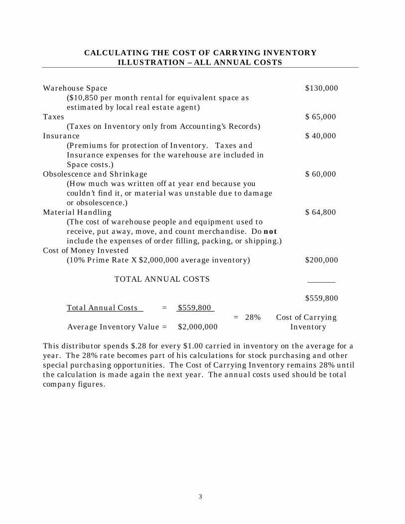
CALCULATING THE COST OF CARRYING INVENTORY ILLUSTRATION – ALL ANNUAL COSTS

Warehouse Space $130,000 ($10,850 per month rental for equivalent space as estimated by local real estate agent) Taxes $ 65,000 (Taxes on Inventory only from Accounting’s Records) Insurance $ 40,000 (Premiums for protection of Inventory. Taxes and Insurance expenses for the warehouse are included in Space costs.) Obsolescence and Shrinkage $ 60,000 (How much was written off at year end because you couldn’t find it, or material was unstable due to damage or obsolescence.) Material Handling $ 64,800 (The cost of warehouse people and equipment used to receive, put away, move, and count merchandise. Do not include the expenses of order filling, packing, or shipping.) Cost of Money Invested (10% Prime Rate X $2,000,000 average inventory) $200,000 TOTAL ANNUAL COSTS _______ $559,800

Total Annual Costs = $559,800 = 28% Cost of Carrying Average Inventory Value = $2,000,000 Inventory This distributor spends $.28 for every $1.00 carried in inventory on the average for a year. The 28% rate becomes part of his calculations for stock purchasing and other special purchasing opportunities. The Cost of Carrying Inventory remains 28% until the calculation is made again the next year. The annual costs used should be total company figures.

3

Cost of Carrying Inventory cont’d

The shortcut method of calculating the Cost of Carrying Inventory is to add 20% to the current prime rate for borrowing money. Example: Prime Rate = 10% Cost of Carrying Inventory: 10% (prime rate) + 20 = 30%. When prime rate goes up or down by 2 points you should recalculate. Once you have established the company’s Cost of Carrying Inventory, you need to put it into SUCCESS 2000 + so that it can by used in EOQ purchasing.

1) Go into Purchasing Parameters <POP>.

2) Select #2 Constants.

3) Return down to field #4 Cost of Carrying Inventory, and enter the percentage as a 2 digit whole number with a 1 decimal if needed. For example, 28% would be entered as 28. It will display as 28.0.

4) Return through the rest of the fields until you get back to a menu.

4

COST OF PURCHASING

The Cost of Purchasing is expressed in a dollar amount per purchase order line written. What goes into the Cost of Purchasing?

* Half of the computer time expense which processes all the transactions necessary to track an item’s condition; all sales, transfers, receipts, returns, cycle counts, etc. These together tell you availability of an item.

There are two primary purposes for maintaining a stock balance and an availability in the computer for each item. 1) to be able to commit material (allocate) to a new customer order. (sales) 2) to start the stock replenishment steps early enough to maintain a continuous supply – no unintentional stockout. (purchasing)

* purchasing effort and costs * expediting work when needed * receiving * A/P work generated with each purchase

The company should set a value on time and effort to bring an item in.

5

COST OF A REPLENISHMENT/PURCHASING CYCLE ILLUSTRATION – ALL ANNUAL COSTS

One half the total annual expense of the computer’s time needed to maintain accurate balances of merchandise available for sale on all stock items. $ 60,000 The portion of the Purchasing Department’s annual expense spent looking at reports, making buying decisions, entering purchase orders or transfers. For most distributors, this is between 50% and 75% of the department’s total annual budget, since stock purchases account for those percentages of total effort. Be sure to include the cost of office space, telephones, etc. $120,000 The annual expense of expediting stock items. $ 6,000 That portion of Account Payables annual budget (including office space, telephones, etc.) that represents how much of their total time is expended in clearing, processing, writing or calling suppliers about invoices for stock merchandise. It could be 50% of their expense. $194,000 The Fixed portion of Receiving’s annual expense devoted to Filing paperwork, keying in purchase order receipts, etc. Receiving must perform some steps with every purchase order regardless of the number of items or quantities involved. $ 21,000 TOTAL ANNUAL COSTS $400,000

1. Number of purchase orders created per year for stock = 10,000 2. Average number of different stock items per order = 8

Total number of times stock items were ordered (1 X 2) = 80,000

Total Annual Costs $400,000 = $5.00 Cost Total Times Stock Items Were Ordered 80,000 of Purchasing

This distributor has spent or will spend a total of $5.00 each time a buyer decides to replenish a stock item OR each time a single PO line is written.

6

Cost of Purchasing cont’d

In the example the Cost of Purchasing is $5.00, which means $5.00 of cost spent per item per purchase order. I f purchase order listed 20 stock items, the Cost of Purchasing in total is $100.00. The Cost of Purchasing is an integral part of EOQ calculation. It sets a value on the time and trouble necessary to buy an item and bring it in. The logic for doing this becomes clear when you consider how many items you now have in stock that sell no more than $5.00 to $15.00 at cost during an entire year! If is costs $5.00 to go through a buying cycle, how many times a year does it make sense to do that on such items? To head for 4 turns or more a year on these items wouldn’t make much sense. Therefore, the Cost of Purchasing number used in proposed purchasing helps you allocate efforts and expenses annually across the stock items in a cost effective way. An accurate Cost of Purchasing is very difficult to calculate. The cost elements are gray in nature and very hard to search out. If you were to go through the effort you should end up in the $4.00 to $6.00 range in today’s market. Therefore, a recommended shortcut is to use $5.00 as the calculation. Once you have established the company’s Cost of Purchasing, you need to put it into SUCCESS 2000 + so that it can be used in EOQ purchasing.

1) Go into Purchasing Parameters <POP>. 2) Select #2 Constants.

3) Return down to field #3 Cost of Ordering Goods, and enter the dollar

figure.

7

4) Return through the rest of the fields until you get back to a menu.

THE OUTGOING COST CONCEPT

The Outgoing Cost is the total amount of cost an average unit of stock carries with it as it goes out the warehouse door to your customer. The Outgoing Cost is rarely considered as a distributor decides how much of an item to buy. It isn’t calculated, it isn’t found on a financial statement, but it is real! What makes up Outgoing Cost?

* Incoming Cost – what you paid the manufacturer per unit for the item, including freight if that was a significant percentage of the cost paid.

* Cost of Carrying Inventory

* Cost of Purchasing

8

Outgoing Cost Calculation – Illustration

Incoming Cost $1.00 Cost of Carrying Inventory .17 | Cost of Purchasing .05 Gross Profit computed on difference between Outgoing Cost $1.22 Incoming Cost and Selling Price. | Selling Price $1.22 | Gross Profit .22 Commission to Salesman .02 The $1.00 was what was paid to the supplier. To get the $1.00 cost, enough had to be purchased to get freight paid. It’s a good seller so they went extra heavy on it. Therefore, it was around long enough to accumulate $.17 worth of Inventory Carrying Costs. They bought 100 units, so the Cost of Purchasing, $5.00, spread over 100 units is $.05 per piece. Competition on this item is tough so sales managed to get only $1.22 for it. 10% commission ($.02) was paid on the gross profit of $.22. When all costs were considered they just broke even on the item and then paid a commission on it. The Outgoing Cost is actually the sum of the two costs (Cost of Carrying Inventory and Cost of Purchasing) that work on an item as you bring it in and then hold it in stock, added to what was paid to the supplier. The chart shows how the two costs accumulate as you buy more and more of a stock item. The Cost of Carrying Inventory has a direct relationship. The more you buy, the longer the stock sits before it is sold, so the more Carrying Costs are incurred. The Cost of Purchasing isn’t that direct. All $5.00 would have to be assigned to a single unit in stock if just that one piece were purchased. When 100 of the item is purchased, then the $5.00 is spread over the 100 units. As you go from 1 unit purchased on up, the total of these two costs starts high, dips to a low point, then climbs again. The Lowest Outgoing Cost results when you purchase a quantity that balances exactly the incremental Cost of Purchasing. Any purchased quantity lower or higher than this ideal results in a higher total cost when the average piece of stock leaves your warehouse. That ideal buying target for the item is called the Economic Order Quantity.

9

FINDING THE LOWEST TOTAL COST

COST

ACCEPTABLE ORDER TOTAL RANGE COST COST OF CARRYING COST INVENTORY OF PURCHASING

EOQ QUANTITY PURCHASED

10

ECONOMIC ORDER QUANTITY CALCULATION

24 x Cost of Purchasing x Usage Rate

Cost of Carrying Inventory x Unit Cost

24 is a constant that helps to solve mathematically the problem of finding the Lowest Total Cost, which was graphed earlier. Cost of Purchasing is a constant. Monthly Usage Rate is the monthly quantity of sales averaged over 4 months. Non-seasonal – averaged over the last 4 months. Seasonal – average of the upcoming 4 months from last year. Cost of Carrying Inventory is a constant. Unit Cost is the item’s Replacement Cost from the product detail file. Lead-time is the time between the date the purchase order is entered and the date of the first receipt of material on an item. When Lead-Time is used in the Order Point formula it must be expressed in months for the calculation to come out correctly because the Usage Rate is expressed in months. 1 week = .25 months 4 weeks = 1.0 months 2 week = .5 months 5 weeks = 1.25 months 3 week = .75 months 6 weeks = 1.5 months etc.

Assume a 4 week month (28 days) rather than a 4.333 weeks. This has the effect of building a small amount of extra safety into the system.

An Order Point is the basic for replenishment timing on most stocked items in a distributor’s inventory when he replenishes stock from sources outside the company. An order Point is a reference point. It’s an amount of material below, which you should not go – on hand plus on order already with the supplier – without starting the replenishing cycle.

11

EXAMPLE 1

Usage Rate = 20 per month Unit Cost = $7.00 Cost of Carrying Inventory = $5.00 Cost of Purchasing = $ .30

| 24 x 5.00 x 20

| | .30 x 7.00

| 120 x 20 | | 2.1

| 2400 | | 2.1

| 1142.86

EOQ = 34 (rounded off to even units) 34 units are about 1 and ¾ month’s supply. This would get about 8 turns a year. It would be purchased about every 6 weeks. Actual turns would be somewhat lower because you must carry some zero turn merchandise in the order timing safety allowance. Still, 6 or 7 turns are acceptable on an item with a 20% to 30% gross margin. At this rate GMROI would be between 120 = 6 turns x 20% to 210 = 7 turns x 30%.

12

EXAMPLE 2 A cheaper item

Usage Rate = 20 per month Unit Cost = $.10 Cost of Carrying Inventory $ 5.00 Cost of Purchasing = $.30 | 24 x 5.00 x 20 | | .30 x .10 | 120 x 20 | | .03 | 2400 | | .03 | 80,000

EOQ = 283 (rounded off to even units)

283 units are about 14-month’s supply. Turns would be less than 1 per year. Can you afford turns like that? YES! A year’s supply of this item is only 20 x 12 x .10 = $2.40. A year’s supply of the item in Example 1 is 20 x 12 x 7.00 = $1,680.00 These two examples demonstrate EOQ in action. It recommends a quantity to buy related to how much money moves through your inventory on the item each month or each year. Lots of money … a low quantity in terms of month’s supply and high turnover per year. Not much money… a higher month’s supply, lower turns.

WHERE AND WHEN TO USE EOQ

13

Use EOQ for the fastest moving, high dollar items. You may want order quantities of only 2 weeks to 1 month. “When” replenishment is triggered has the greatest impact on service. “How many” ordered at a time largely controls turnover. A BALANCE must be maintained between service and turnover objectives. Conditions for a stock item that should be present for EOQ to be effective:

1. The price paid to the supplier does not vary when you buy more of this item. You may have a “total order” economic advantage for buying more, but the price quoted by the manufacturer for this item does not improve when you purchase more of this single item. No price breaks.

2. The usage rate of the item is higher than ½ unit per month. You move

at least one piece every other month.

3. The supplier’s lowest permissible purchasing quantity on the item is reasonable for you to obtain … it does not represent 3 or 4 times the calculated EOQ amount.

There’s a range of usage for an item when formulas work. Very high or very low usage rates throw any formula for a loop. Arbitrary ordering controls should be set on items like these and then the reorder points “frozen” until a person changes them purposefully. Most hard goods distributors have as many as 25% of their stock items in this category. Don’t make the mistake of attempting to handle all stock items under the same rules and formulas. The system will yield lousy results. There are items where the supplier packs them in too large quantities (for you). The EOQ might come out at 6 but you can only buy in quantities of 24. In nearly every case you should discontinue stocking the item or try to get it down the street from a competitor and pay what you must because it just isn’t economical to buy from the supplier.

ROUNDING REQUIREMENTS FOR EOQ

14

1. Round the EOQ answer off to the nearest standard package quantity.

2. Round the EOQ answer up to at least 2 weeks’ supply if it’s lower than that.

For a few expensive items that sell very well, the EOQ concept recommends a very high turnover achieved by buying maybe only 3 or 4 days’ supply. Don’t do it. 20 or more turns per year are good enough on anything. You do not want to fool with any item any more frequently than once every 2 weeks, unless there is a severe space limitation in storing the item.

3. Round the EOQ answer back to a limit of one year’s supply if it calculates out

higher than that.

The risk of damage, obsolescence, shrinkage, and theft increases when material sits in a warehouse longer than a year. EOQ assumes a fixed inventory carrying cost and it is relatively fixed until you go out beyond a year’s supply. Then it begins to climb exponentially.

4. Check the EOQ against the product line’s Review Cycle, times the monthly

usage rate of the item: Review Cycle: 1 month Usage Rate per Month: 100 Calculation: 1 X 100 = 100 EOQ must be raised to 100 if it calculates out less.

EOQ SUMMATION

EOQ encourages ordering cost effective quantities and will cause some 65% of your stock items (that sell) to come up for reordering only once or twice a year.

15

You can afford to buy 6 months’ to a year’s supply of over half your stock items, if you restrict it to the proper half as EOQ does. The other 35% of inventory will turn much faster than before … and that is where most of the dollars move that offsetting what happens on the 65% that move poorly. If you buck up for it and deal with your dead stock, you should get between 5 and 6 turns per year on your total inventory investment. Another great benefit happens – purchasing agents see the majority of items only once or twice a year. This gives them more time to handle the other items, the big money through the inventory items; more time to check out unusual orders with sales; more time to look into iffy lead times; more time to be thinkers, planners, analyzers, rather than clerks.

--------------------Screen 1--------------------

Branch INC 1 PROPOSED PURCHASE ORDER NO. 2050 Weight Cost Purchasing Selects %%%-%%% ABC Selects AA%-BB% This Order 1860 3000 Seasonal Adjustment 1.00 Group 000300-000300 Best Buy 2000 0 Vendor 1540 SUCCESS MANUFACTURING Bal Needed 140 3000 Created: 6/01/93

16

Group 300 Avail Cust Unpkgd Proposed

Item BR Description ABC NOW B/O Qty Qty 00070 1 ¼” Black Malleable Tee BB 512 0 512 512 Y 00080 1 ½” Black Malleable Tee AA 317 0 312 312 Y 00100 1 1” Black Malleable Tee CB 572 0 204 204 Y 00210 1 ½” Black Malleable 90 Ell AB 190 0 475 480 Y 00231 1 ¾” Black Malleable 90 Ell AA 233 0 260 264 Y When the cursor is on the line for which you wish to see stock status information or product history, press “F7”. The following screen will display. Example: line 2.

--------------------Screen 2--------------------

Group 300 Avail Cust Unpkgd Proposed Item Br Description ABC NOW B/O Qty Pkg Qty 00080 1 ½” Black Malleable Tee BB 572 0 312 312 Y PPO Type E Reorder Point 737 Pkg Qty 12 Stock Sales YTD 4781 B/O Qty YTD 0 Item Weight 0.250 Stock Freq YTD 143 B/O Freq YTD 0 Repl Cost 0.500 Date Last Sold 6/07/93 Lost Sale YTD 0 In-Trans Qty 0 Stock On Order 0 Lost Freq YTD 0 Begin Date 10/25/82

SUPPLEMENTAL INFORMATION --------------------------------------------------

SS – Stock Sales RV – Stock Receive DD – Direct Sales DT – Delivery Times TI – Transfer EQ – EOQ Analysis TO – Transfer Out LB – Line Buy Analysis LS – Lost Sales FO – Future Order Analysis Please Select A Task_____

- - - - - - - - - - - - - - - - - - - - Screen 3 - - - - - - - - - - - - - - - - - - - -

Group 300 Avail Cust Unpkgd Proposed Item Br Description ABC Now B/O Qty Pkg Qty 00080 1 ½” Black Malleable Tee AA 572 0 312 312 Y PPO Type E Recorder Point 737 Pkg Qty 12 Stock Sales YTD 4781 B/O Qty YTD 0 Item Weight 0.250

17

Stock Freq YTD 143 B/O Freq YTD 0 Repl Cost 0.500

Date Last Sold 6/07/93 Lost Sale YTD 0 In-Trans Qty 0 Stock On Order 0 Lost Freq YTD 0 Begin Date 10/25/82

YEAR 19XX YEAR 19XX YEAR 19XX YEAR 19XX Jan Jan Jan 874 20 Jan 832 25 Feb Feb Feb 875 21 Feb 889 22 Mar Mar Mar 869 23 Mar 954 33 Apr Apr Apr 792 18 Apr 927 36 May NO May NO May 816 26 May 876 28 Jun Jun Jun 822 25 Jun 0 0 Jul DATA Jul DATA Jul 785 22 Jul 0 0 Aug Aug Aug 665 17 Aug 0 0 Sep Sep Sep 865 31 Sep 0 0 Oct Oct Oct 823 24 Oct 0 0 Nov Nov Nov 754 22 Nov 0 0 Dec Dec Dec 730 17 Dec 0 0

Stock Sales History

-------------------- Screen 4 --------------------

Group 300 Avail Cust Unpkgd Proposed Item Br Description ABC Now B/O Qty Pkg Qty 00080 1 ½”Black Malleable Tee AA 572 0 312 312 Y PPO Type E Reorder Point 737 Pkg Qty 12 Stock Sales YT D 4781 B/O Qty YTD 0 Item Weight 0.250

18

Stock Freq YT 143 B/O Freq YTD 0 Repl Cost 0.500

Date Last Sol 6/07/93 Lost Sale YTD 0 In-Trans Qty 0 Stock On Order 0 Lost Freq YTD 0 Begin Date 10/25/82 YEAR 19XX YEAR 19XX YEAR 19XX YEAR 19XX Jan Jan Jan 25 13 Jan 14 12 Feb Feb Feb 24 15 Feb 20 20 Mar Mar Mar 18 1 Mar 20 20 Apr Apr Apr 20 16 Apr 12 15 May NO May NO May 17 15 May 18 18 Jun Jun Jun 16 1 Jun 0 14 Jul DATA Jul DATA Jul 14 13 Jul 0 19 Aug Aug Aug 19 13 Aug 0 15 Sep Sep Sep 16 12 Sep 0 17 Oct Oct Oct 21 15 Oct 0 21 Nov Nov Nov 23 14 Nov 0 22 Dec Dec Dec 20 16 Dec 0 16 Delivery Time History Longest receipt for the month ------------- Last 12 receipts for the year ------------------------ Group 300 Avail Cust Unpkgd Proposed Item Br Description ABC Now B/O Qty Pkg Qty 00080 1 ½” Black Malleable Tee AA 572 0 312 312 Y PPO Type E Recorder Point 737 Pkg Qty 12 Stock Sales YTD 4781 B/O Qty YTD 0 Item Weight 0.250 Stock Freq YTD 143 B/O Freq YTD 0 Repl Cost 0.500 Date Last Sold 6/07/93 Lost Sale YTD 0 In-Trans Qty 0 Stock On Order 0 Lost Freq YTD 0 Begin Dat 10/25/82

19

DELV 1992 1993 Last 12 DELV EOQ PARAMETERS Jan 25 14 1 12 Stock Code Feb 24 20 2 20 Cost of Ordering Stock 5.00 Mar 18 25 3 20 Cost of Carrying Inventory (%) 28.00 Apr 20 12 4 15 Seasonal Adjustment Factor 1.000 May 17 18 5 18 Monthly Usage 889 954 927 876 Jun 16 0 6 14 Monthly Usage Rate 912 Jul 14 0 7 19 Average Lead Time (Days) 17 Aug 19 0 8 15 Average Lead Time (Months) 0.607 Sep 16 0 9 17 Maximum Lead Time (Days) 25 Oct 21 0 10 21 Safety Stock 183 Nov 23 0 11 22 Order Point 737 Dec 20 0 12 16 EOQ Quantity 884 EOQ QTY ( 884) = SR (24 * 5.00 * 912 / .280 * 0.500) Monthly Usage – the appropriate 4 months from stock sales product history. Monthly Usage Rate is the monthly quantity of sales averaged over 4 months. Non-seasonal – averaged over the last 4 months. Seasonal – average of the upcoming 4 months from last year. Average Lead Time (Days) – average of the last 3 receipts. Average Lead Time (Months) – expressed as a percent. Average Lead Time (Days) ________________________ (fixed number of days for a week month) 28 Maximum Lead Time (Days) – highest lead time in the last 12 months. Safety Stock Max Lead Time – Avg Lead Time Monthly Usage Rate x Avg Lead Time (Month) x .7 x Average Lead Time Order Point - Monthly Usage Rate x Average Lead Time + Safety Stock

20

MINIMUM REQUIREMENTS FOR USING EOQ TYPE PPO’S 1. Product Detail <PD> - Primary Vendor

PPO flag = “E” 2. PPO Specifications <PPOS> - one must be set up for every primary vendor and his product groups. 3. Purchasing Parameters <POP> - Cost of Ordering

21

Cost of Carrying Inventory

4. Product History <PHF> or <WLPH> - Stock Sales Quantity

Delivery Times

For non-seasonal items a minimum of 4 months of history. For seasonal items a minimum of 16 months of history.

OPTIONAL FIELDS 1. Product Detail <PD> - Item Weight

Package Quantity Package Weight Purchasing Selects ABC selects Stock Code.

2. Vendor <V> - Best Buy Weight

Best Buy Cost

PPO FORMULAS

TYPE RECORDER POINT ORDER UP TO QUANTITY I (min/max) SS + LT SS + LT + OC (independent items) S (super A line buy items) SS + LT + OC SS + LT + OC R (regular line buy items) SS + LT + OC SS + LT + OC

22

M (Wittock’s version of min/max) SS OC + PQA (PQA = on hand + on order + transfer in intransit – allocated – backorder – & hold) _____________________________________ E (economic order quantity) 24 x Cost of Purchasing x Usage Rate ____ | _____________________________________ \ |

\ | Cost of Carrying Inventory x Unit Cost

Recalculating Reorder Points can be done either of 2 ways.

1. Recalculate Reorder Points from YTD Sales. <RRPY>

Safety Stock and Order Cycle quantities are recalculated using fiscal YTD Stock Sales quantities.

23

2. Recalculate Reorder Points from Product History. <RRPH>

Safety Stock and Order Cycle quantities are recalculated using the Product History for the item.

When running the program you select how many months of history to use. If an item is flagged as non-seasonal the system will use the most recent number of months. If the item is flagged as seasonal, the system uses the upcoming number of months from last year.