International risk sharing is better than you think, or exchange ...

ARTICLE IN PRESS

Journal of Monetary Economics 53 (2006) 671–698

0304-3932/$ -

doi:10.1016/j

$We than

Erzo Luttme

Chris Telme

acknowledge

School of the

Research in

NBER.�CorrespoE-mail ad

www.elsevier.com/locate/jme

International risk sharing is better than you think, orexchange rates are too smooth$

Michael W. Brandta, John H. Cochraneb,�, Pedro Santa-Clarac

aFuqua School of Business, Duke University, Durham, NC 27708, USAbGraduate School of Business, University of Chicago, Chicago, IL 60637, USA

cAnderson Graduate School of Management, UCLA, Los Angeles, CA 90095, USA

Received 17 November 2004; received in revised form 22 February 2005; accepted 25 February 2005

Available online 17 April 2006

Abstract

Exchange rates depreciate by the difference between domestic and foreign marginal utility growth

or discount factors. Exchange rates vary a lot, as much as 15% per year. However, equity premia

imply that marginal utility growth varies much more, by at least 50% per year. Therefore, marginal

utility growth must be highly correlated across countries: international risk sharing is better than you

think. Conversely, if risks really are not shared internationally, exchange rates should vary more than

they do: exchange rates are too smooth. We calculate an index of international risk sharing that

formalizes this intuition. We treat carefully the realistic case of incomplete capital markets. We

contrast our estimates with the poor risk sharing suggested by consumption data and home-bias

portfolio calculations.

r 2006 Elsevier B.V. All rights reserved.

JEL classification: G12; G15; F31

Keywords: International risk sharing; Exchange rate volatility; Discount factor

see front matter r 2006 Elsevier B.V. All rights reserved.

.jmoneco.2005.02.004

k David Backus, Ravi Bansal, Bernard Dumas, Lars Hansen, Ravi Jagannathan, Urban Jerman,

r, Maurice Obstfeld, Monika Piazzesi, Helene Rey, Roberto Rigobon, Richard Roll, John Romalis,

r, Paul Willen, and many seminar participants for comments and suggestions. Brandt gratefully

s financial support from the Weiss Center for International Financial Research at the Wharton

University of Pennsylvania. Cochrane gratefully acknowledges financial support from the Center for

Securities Prices at the Graduate School of Business and from an NSF grant administered by the

nding author. Tel.: +1773 702 3059; fax: +1 773 834 2031.

dress: [email protected] (J.H. Cochrane).

www.elsevier.com/locate/jme

dx.doi.org/10.1016/j.jmoneco.2005.02.004

mailto:[email protected]

ARTICLE IN PRESSM.W. Brandt et al. / Journal of Monetary Economics 53 (2006) 671–698672

1. Introduction

Exchange rates etþ1 are linked to domestic and foreign marginal utility growth ordiscount factors md

tþ1 and mftþ1 by the equation1

lnetþ1

et

¼ lnmftþ1 � lnmd

tþ1. (1)

Take variances of both sides of the equation. Exchange rates vary a lot, as much as 15%per year. However, equity premia imply that marginal utility growth varies much more, byat least 50% per year.2 For Eq. (1) to hold, therefore, marginal utility growth must behighly correlated across countries: international risk sharing is better than you think.Conversely, if risks are not shared internationally—if marginal utility growth isuncorrelated across countries—exchange rates should vary by

ffiffiffi2p� 50% ¼ 71% or more:

exchange rates are too smooth.To quantify this idea, we compute the following index of international risk sharing:

1�s2ðlnm

ftþ1 � lnmd

tþ1Þ

s2ðlnmftþ1Þ þ s2ðlnmd

tþ1Þ¼ 1�

s2 lnetþ1

et

� �

s2ðlnmftþ1Þ þ s2ðlnmd

tþ1Þ. (2)

The numerator measures how different marginal utility growth is across the twocountries—how much risk is not shared. The denominator measures the volatility ofmarginal utility growth in the two countries—how much risk there is to share. A 10%exchange rate volatility and a 50% marginal utility growth volatility in each country implya risk sharing index of 1� 0:12=ð2� 0:52Þ ¼ 0:98: Our detailed calculations in Table 2 givesimilar results. It seems that a lot of risk is shared.Our index is not quite the same as a correlation. Like a correlation, our index is equal to

one if lnmf ¼ lnmd , it is equal to zero if lnmf and lnmd are uncorrelated, and it is equal tominus one if (pathologically) lnmf ¼ � lnmd . However, risk sharing requires thatdomestic and foreign marginal utility growth are equal, not just perfectly correlated, andour index detects violations of scale as well as of correlation. For example, iflnmf ¼ 2� lnmd , risks are not perfectly shared despite perfect correlation. In this caseour index is 0:8. Like the correlation of discount factors or of consumption growth, ourindex is a statistical description of how far we are from perfect risk sharing. Higher risksharing indices do not necessarily imply higher welfare.The risk sharing index is essentially an extension of Hansen–Jagannathan (1991) bounds

to include exchange rates. Hansen and Jagannathan showed that marginal utility growthsmust be highly volatile in order to explain the equity premium. We show that marginal

1We discuss this equation in detail below, including the case of incomplete markets. For now, you can regard it

as a change of units from the marginal utility of domestic goods to the marginal utility of foreign goods. It can

also apply to nominal discount factors and nominal exchange rates. Among many others, Backus et al. (2001) and

Brandt and Santa-Clara (2002) exploit this equation to relate the dynamics of the exchange rate to the dynamics of

the domestic and foreign discount factors. A working paper version of Backus et al. (2001) (Backus et al., 1996, p.

7) discusses briefly the link between the variance of the exchange rate and the variances and covariance of

domestic and foreign discount factors, and notes the high correlation between discount factors across countries

when discount factors are chosen to satisfy Eq. (1).2From 0 ¼ EðmReÞ with Re denoting the excess return of stocks over bonds, it follows that

sðmÞ=EðmÞXEðReÞ=sðReÞ (Hansen and Jagannathan, 1991). An 8% mean excess return EðReÞ and 16% standard

deviation sðReÞ with a gross risk-free rate 1=EðmÞ near one lead to sðmÞX0:5.

ARTICLE IN PRESSM.W. Brandt et al. / Journal of Monetary Economics 53 (2006) 671–698 673

utility growths must also be highly correlated across countries in order to explain therelative smoothness of exchange rates.

Like the equity premium, we regard this result as a puzzle. Common intuition andcalculations based on consumption data or observed portfolios suggest much less risksharing. For example, if agents in each country have the same power utility function over aconsumption composite,

Pbtcð1�gÞt =ð1� gÞ, then the discount factors are

lnmdtþ1 ¼ ln b� g lnðDcd

tþ1Þ and lnmftþ1 ¼ ln b� g lnðDcftþ1Þ. (3)

Consumption growth is correlated across countries—we find correlations as large as 0.41below—but both the correlation and risk sharing indices as in Eq. (2) come nowhere nearthose implied by asset-market data.

Yet the conclusion is hard to escape. Our calculation uses only price data, and noquantity data or economic modeling (utility functions, income or productivity shockprocesses, and so forth). A large degree of international risk sharing is an inescapablelogical conclusion of Eq. (1), a reasonably high equity premium (over 1%, as we showbelow), and the basic economic proposition that price ratios measure marginal rates ofsubstitution.

If the puzzle is eventually resolved following the path of the equity premium literature,with utility functions and environments that deliver high equity premia and relativelysmooth exchange rates (volatile and highly correlated marginal rates of substitution), thenthe puzzle will be resolved in favor of the asset market view that international risk sharingis, in fact, better than we now think. The only way it can be resolved in favor of poorinternational risk sharing is if the vast majority of consumers are far from their first orderconditions, further off than can be explained by observed financial market imperfections,so that measurements of marginal rates of substitution from price ratios are wrong byorders of magnitude. However, like the equity premium, our contribution is to articulatethe puzzle, not to opine on which underlying view will have to be modified in order toresolve the puzzle.

What exactly does the calculation mean? To start a more careful interpretation of thecalculation, we discuss two major potential impediments to risk sharing: transport costsand incomplete asset markets. In the remainder of the paper we also consider the poorcorrelation of consumption across countries, the home bias puzzle, frictions that separatemarginal utility from prices, and the possibility that the equity premium is a lot lower thanpast average returns.

1.1. Transport costs

Risk sharing requires frictionless goods markets. The container ship is a risk sharinginnovation as important as 24 hour trading.3 Suppose that Earth trades assets with Marsby radio, in complete and frictionless capital markets. If Mars enjoys a positive shock,Earth-based owners of Martian assets rejoice in anticipation of their payoffs. But tradewith Mars is still impossible, so the real exchange rate between Mars and Earth must

3Obstfeld and Rogoff (2000) emphasize the importance of transport costs for understanding a wide range of

puzzles in international economics. Alesina et al. (2003) find that real exchange rate volatility increases with

distance between two countries. Ravn (2001) emphasizes the importance of real exchange rate movements in risk

sharing measurements.


adjust exactly to offset any net payoff. In the end, Earth marginal utility growth mustreflect Earth resources, and the same for Mars. Risk sharing is impossible. If theunderlying shocks are uncorrelated, the exchange rate variance is the sum of the variancesof Earth and Mars marginal utility growth, and we measure a zero risk sharing indexdespite perfect capital markets.At the other extreme, if there is costless trade between the two planets (teletrans-

portation), and the real exchange rate is therefore constant, marginal utilities canmove in lockstep. With constant exchange rates, we measure a perfect risk sharing indexof one.Actual economies produce a mix of tradeable and non-tradeable goods, and transport

costs vary by good and country-pair. Thus, actual economies lie somewhere between thetwo extremes. If there is a positive shock in one country, asset holdings by the othercountries should lead to an outflow of goods. But it is costly to ship goods, and those costsincrease with the volume being shipped. Therefore, real exchange rates move and theirfluctuations blunt risk sharing. Our index lies below one.Thus, our index answers the question: How much do exchange rate movements blunt the

risk sharing opportunities offered by capital markets? Since exchange rates vary so muchless than marginal utility growth (as revealed by asset markets), our answer is ‘‘not much’’.

1.2. Incomplete asset markets

Incomplete asset markets are the second reason that risk sharing may be imperfect. If nostate-contingent payments are promised, marginal utilities can diverge across countries,even without transport costs and with constant exchange rates.With incomplete asset markets, the discount factors md

tþ1 and mftþ1 that we can recover

from asset market data are not unique. Given a discount factor mtþ1, that generates theprices pt of payoffs xtþ1 by pt ¼ Etðmtþ1xtþ1Þ, any discount factor of the form mtþ1þ etþ1

also prices the payoffs, where etþ1 is any random variable with Etðetþ1xtþ1Þ ¼ 0: Therefore,Eq. (1) does not hold for arbitrary pairs of domestic and foreign discount factors. If Eq. (1)holds for one choice of md and mf , then it will not hold for another, e.g., md þ e. Inparticular Eq. (1) need not hold between domestic and foreign marginal utility growth inan incomplete market. Of course, there always exist pairs of discount factors for which (1)holds; Eq. (1) can be used to construct a valid discount factor mf from a discount factor md

and the exchange rate.To think about incomplete markets and multiple discount factors, start by considering a

single economy with many agents. In an incomplete market, individuals’ marginal utilitygrowths may not be equal. However, the projection of each individual’s marginal utilitygrowth on the set of available asset payoffs should still be the same.4 In this sense,individuals should use the available assets to share risks as much as possible. For example,we should not see one consumer heavily invested in tech stocks and another in blue chipstocks, so that one is more affected than the other when tech stocks fall (unless, of course,

4The projection is the fitted value of a regression of marginal utility growth on the asset payoffs, and the

‘‘mimicking portfolio’’ for marginal utility growth. Each individual’s first order conditions state that his marginal

utility growth mi satisfies pt¼ Etðmitþ1xtþ1Þ, and thus (since residuals are orthogonal to fitted values) pt ¼

Et½projðmitþ1jX Þxtþ1� where X denotes the payoff space of all traded assets. There is a unique discount factor

xn 2 X such that pt ¼ Etðxntþ1xtþ1Þ for all x 2 X . Since this discount factor is unique, projðmi

tþ1jX Þ ¼ xn is the

same for all individuals. See Cochrane (2004, p. 68) for elaboration.


the consumers differ significantly in preferences or exposures to non-marketed risks, i.e. ifthe first consumer works in the old economy and the second in tech). We could imaginerunning regressions of individual marginal utility growth on asset market returns. Thecorrelation between the fitted values of those regressions would tell us how well individualsuse existing markets to share risk.

With this example in mind, we evaluate Eqs. (1) and (2) using the unique discountfactors md

tþ1 and mftþ1 that are in the space of domestic and foreign asset payoffs (evaluated

in units of domestic and foreign goods, respectively). These discount factors are theprojections of any possible domestic and foreign discount factors onto the relevant spacesof asset payoffs, and they are also the minimum-variance discount factors. We show thatEq. (1) continues to hold with this particular choice of discount factors. If we start withmd

tþ1 2 X , form mftþ1 ¼ md

tþ1 � etþ1=et to satisfy (1), we can quickly see that mftþ1 is in the

payoff space available to the foreign investor.In an incomplete markets context, then, our international risk sharing index

answers the questions: How well do countries share risks spanned by existing assetmarkets? How much do exchange rate changes blunt risk sharing using existing assetmarkets?

Marginal utility growth is equal to the minimum-variance discount factors mdtþ1 and

mftþ1 that we examine, plus additional risks that are orthogonal to, and hence uninsurable

by, asset markets. Overall risk sharing—the risk sharing index computed using truemarginal utility growth—can be better or worse than our asset-based measure. It can bebetter if the additional risks, not spanned by asset markets, generate a component ofmarginal utility growth that is positively correlated across countries. It can be worse if theunspanned risks generate a component of marginal utility growth that is negativelycorrelated across countries. However, to have a quantitatively important effect on therisk sharing measure, additional non-spanned risks would have to be a good deallarger than the already puzzling 50% volatility of marginal utility growth implied by theequity premium. Ruling out such huge numbers, our asset-based measure implies thatoverall risks are also well shared. We make detailed calculations to address this pointbelow.

2. Calculation

2.1. Discount factors and the risk sharing index

We adopt a continuous time formulation, which allows us to translate more easilybetween logs and levels. We first describe how to recover the minimum-variance discountfactor from asset markets in general, and then we specialize the discussion to ourinternational setting.

2.1.1. Discount factors and asset returns

Suppose that a vector of assets has the following instantaneous excess return process:

dR ¼ mdtþ dz with Eðdzdz0Þ ¼ Sdt. (4)

(An excess return is the difference between any two value processes, e.g., dR ¼

dS=S � dV=V . We often use a risk-free asset dV=V ¼ rdt, but this is notnecessary.) We will keep the expressions simple by specifying that a risk-free asset


is traded,

dB

B¼ rdt. (5)

With this notation, the discount factor

dLL¼ �rdt� m0S�1 dz (6)

prices the assets, i.e., it satisfies the basic pricing conditions

rdt ¼ �EdLL

� �and mdt ¼ �E

dLL

dR

� �. (7)

In this formulation, dL=L plays the role of m in the introduction.We can construct the log discount factor5 required in Eqs. (1) and (2) via Ito’s lemma:

d lnL ¼dLL�

1

2

dL2

L2¼ � rþ

1

2m0S�1m

� �dt� m0S�1 dz. (8)

We can then evaluate the variance of the discount factor as

1

dts2ðd lnLÞ ¼ m0S�1m. (9)

Eqs. (6) and (9) show why mean asset returns determine the volatility of marginal utilitygrowth. Holding constant S, the higher m is, the more dL=L loads on the shocks dz in Eq.(6), and the more volatile is dL=L in Eq. (9).

2.1.2. International discount factors and the risk sharing index

We now specialize these formulas to our international context. We write the real returnson the domestic risk-free asset Bd , domestic stocks Sd , exchange rate e (in units of foreigngoods/domestic goods), foreign risk-free asset Bf , and foreign stocks Sf as

dBd

Bd¼ rd dt;

dSd

Sd¼ yd dtþ dzd ,

de

e¼ ye dtþ dze,

5The discrete-time versions of these calculations condition down. Starting with 1 ¼ Etðmtþ1Rtþ1Þ we can

condition down to 1 ¼ EðmRÞ and hence EðRÞ ¼ 1=EðmÞ � covðm;RÞ where E and cov are unconditional

moments. We can represent these unconditional moments analogously to (6) with the discount factor mtþ1 ¼

1=Rf � ðEðRÞ � Rf Þ0covðR;R0ÞðRtþ1 � EðRÞÞ=Rf where Rf � 1=EðmÞ. These constructions go through even if

there is arbitrary variation in the conditional moments of returns. This conditioning down property does not go

through in the continuous time formulation. While 0 ¼ Et½dðLPÞ� conditions down to 0 ¼ E½dðLPÞ�, we cannot

apply Ito’s lemma to the latter expression. Thus, the covariance on the right-hand side of Eq. (7) must be the

conditional covariance. To estimate using sample averages as we do, we must assume constant conditional

covariances. With constant conditional covariances, the means in (7) do condition down, so our calculation based

on unconditional moments is still correct if there is variation in conditional means. One can derive the same

formulas for log discount factors from the discrete time formulas that do condition down, but approximations are

required to translate from levels to logs. The approximations are essentially that conditional variances do not

change too much.


dBf

Bf¼ rf dt;

dSf

Sf¼ yf dtþ dzf . (10)

We collect the shocks in a vector dz and write their covariance matrix as

dz ¼

dzd

dze

dzf

264

375 and S ¼

1

dtEðdzdz0Þ ¼

Sdd 0 Sde Sdf 0

Sed 0 See Sef 0

Sfd 0 Sfe Sff 0

264

375. (11)

(We use the notation Sdd 0 etc. because there may be several risky assets in each economy.)We show in the Appendix that the vector of expected excess returns on domestic stock,

exchange rate, and foreign stock are, for the domestic investor,

md ¼

yd� rd

yeþ rf � rd

yf� rf þ Sef

264

375 (12)

and for the foreign investor,

mf ¼

yd� rd � Sed

yeþ rf � rd � See

yf� rf

264

375. (13)

The covariance matrix of these returns is S for both investors.The discount factors are, as in Eq. (6),

dLi

Li¼ �ri dt� mi0S�1 dz; i ¼ d; f . (14)

By Ito’s lemma we then have

d lnLi ¼ � ri þ 12mi0S�1mi

� �dt� mi0S�1 dz; i ¼ d; f (15)

and

1

dts2ðd lnLiÞ ¼ mi0S�1mi; i ¼ d; f . (16)

Our risk sharing index from Eq. (2) is therefore

1�s2ðd lnLd � d lnLf Þ

s2ðd lnLdÞ þ s2ðd lnLf Þ¼ 1�

See

md0S�1md þ mf 0S�1mf. (17)

As one might expect, the domestic and foreign discount factors load equally on thedomestic and foreign stock return shocks, and their loadings on the exchange rate shockdiffer by exactly one. To see this result, note from the definitions (12) and (13) that we canwrite

mf ¼ md �

Sed

See

Sef

264

375 ¼ md � Se, (18)


where Se denotes the middle column of S. Thus, we can relate the domestic and foreignminimum-variance discount factors by

dLf

Lf¼

dLd

Ldþ ðrd � rf Þdtþ Se0S�1 dz

¼dLd

Ldþ ðrd � rf Þdtþ dze. ð19Þ

2.2. Incomplete markets

When markets are incomplete, the discount factors recovered from asset markets asabove are not the only possible ones. If we add noise to the discount factor that is meanzero (to price the interest rate) and uncorrelated with the asset return shocks, the pricingimplications are not affected. So long as EtðdwiÞ ¼ 0 and Etðdwi dzÞ ¼ 0,

dLin

Lin¼

dLi

Liþ dwi (20)

satisfies the pricing conditions (7) and is hence a valid discount factor.Since dwi is orthogonal to dz and dLi=Li is driven only by dz, we have three properties

of the discount factors dLi=Li that we recover from asset markets by Eq. (14): (i) they arethe minimum variance discount factors; (ii) they are the unique domestic and foreigndiscount factors formed as a linear combination of shocks to assets dz; (iii) they are thediscount factors formed by the projection of any valid discount factor dLin=Lin on thespace of asset returns.In an incomplete market, there exist pairs of discount factors that satisfy the relation

d ln e ¼ d lnLf � d lnLd , (21)

but not all pairs of discount factors do so. Existence follows by construction. A domesticdiscount factor satisfies 0 ¼ E½dðLdSÞ�, for any asset S, and a foreign discount factorsatisfies 0 ¼ E½dðLf ðS=eÞÞ�. Given any domestic discount factor Ld that satisfies the firstrelation, the choice Lf ¼ keLd (with any constant k) obviously satisfies the second relationand the identity (21). But another foreign discount factor formed by adding dwf no longersatisfies the identity (21).The basic identity (21) does hold for the minimum-variance discount factors. To see this

result, start with the minimum-variance discount factor Ld , and form a candidateLf ¼ keLd . As above, this is a valid foreign discount factor. To check that this is theminimum-variance foreign discount factor, we can check any of the three properties above.It is easiest to check the second. d lnLd is driven only by the shocks dz, and dze is one ofthe shocks dz, so d lnLf and hence dLf is also driven only by the shocks dz. (TheAppendix also includes a more explicit but algebraically more intensive proof.)

3. Results

3.1. Data and summary statistics

We implement the continuous time formulas in Section 2 with straightforward discretetime approximations and monthly data. We start with domestic excess stock returns Rd

tþD,


foreign excess stock returns RftþD, the exchange rate et (in units of foreign currency per

dollar), and domestic and foreign interest rates rdtþD and r

ftþD, where D ¼

112years. Denoting

sample mean by ET (where T is the sample size), we estimate the instantaneous risk premiaand variances required in the risk sharing measure (17) by the obvious sample counterpartsto the continuous time moments:

yd� rd ¼

1

DET Rd

tþD; yf� rf ¼

1

DET R

ftþD,

yeþ rf � rd ¼

1

DET

etþD � et

et

þ rftþD � rd

tþD

� �,

dzd ¼ RdtþD � ET Rd

tþD; dzf ¼ Rf � ET RftþD,

dze ¼etþD � et

et

� �� ET

etþD � et

et

� �,

S ¼1

DET ðdzdz0Þ. (22)

We use real returns, real interest rates, and a real exchange rate, each adjusted ex post byrealized inflation. Since the risk sharing index is based entirely on excess returns, thecalculation is fairly insensitive to how one handles interest rates and inflation. However,excess nominal returns are not quite the same as excess real returns, so we start with realreturns to keep the calculation as pure as possible.

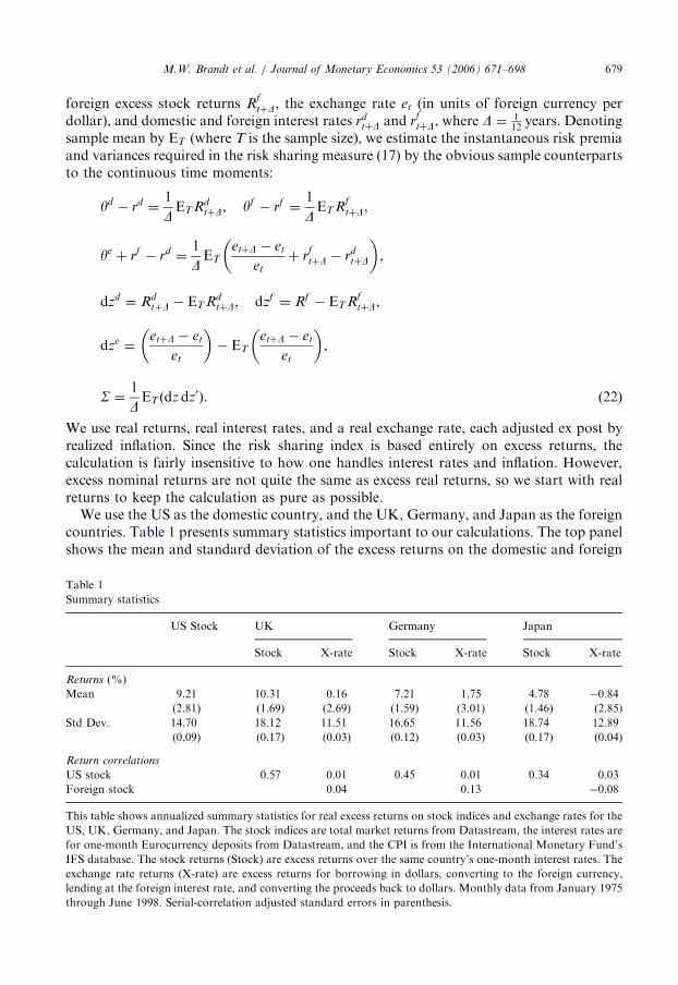
We use the US as the domestic country, and the UK, Germany, and Japan as the foreigncountries. Table 1 presents summary statistics important to our calculations. The top panelshows the mean and standard deviation of the excess returns on the domestic and foreign

Table 1

Summary statistics

US Stock UK Germany Japan

Stock X-rate Stock X-rate Stock X-rate

Returns (%)

Mean 9.21 10.31 0.16 7.21 1.75 4.78 �0.84

(2.81) (1.69) (2.69) (1.59) (3.01) (1.46) (2.85)

Std Dev. 14.70 18.12 11.51 16.65 11.56 18.74 12.89

(0.09) (0.17) (0.03) (0.12) (0.03) (0.17) (0.04)

Return correlations

US stock 0.57 0.01 0.45 0.01 0.34 0.03

Foreign stock 0.04 0.13 �0.08

This table shows annualized summary statistics for real excess returns on stock indices and exchange rates for the

US, UK, Germany, and Japan. The stock indices are total market returns from Datastream, the interest rates are

for one-month Eurocurrency deposits from Datastream, and the CPI is from the International Monetary Fund’s

IFS database. The stock returns (Stock) are excess returns over the same country’s one-month interest rates. The

exchange rate returns (X-rate) are excess returns for borrowing in dollars, converting to the foreign currency,

lending at the foreign interest rate, and converting the proceeds back to dollars. Monthly data from January 1975

through June 1998. Serial-correlation adjusted standard errors in parenthesis.


stock indices and the exchange rate (annualized and reported in percent). The bottompanel shows correlations between the returns. Autocorrelation-corrected standard errorsare in parentheses.6

The table reminds us of the high equity risk premium, not only in the US but alsoabroad. The mean excess stock index returns range from 4.78% in Japan to 10.31% in theUK and are all statistically significant. The standard deviation ranges from 14.70% inthe US to 18.74% in Japan, resulting in annualized Sharpe ratios of 0.63 in the US, 0.57 inthe UK, 0.43 in Germany, and 0.26 in Japan. The estimates of the exchange rate riskpremium ye

þ rf � re are positive for the UK and Germany and negative for Japan, but areall small and statistically indistinguishable from zero. The volatility of the exchange rates isabout 2

3that of stocks, ranging from 11.51% to 12.89%. Suggestively, this is about the

same as the volatility of long-term nominal bond returns. The stock returns are positivelycorrelated across countries, with correlations ranging from 0.34 to 0.57. The exchangerates are poorly correlated with stock returns both in the US and abroad, with correlationsless than 0.15.Table 1 also reminds us of how difficult it is to estimate equity risk premia. For example,

the US risk premium of 9.21% is measured with a 2.81% standard error. The reason is, ofcourse, the high volatility of stock returns relative to the size of the mean return. Thestandard error of the mean return sðRtþDÞ=

ffiffiffiffiTp

, and its more precise incarnation in ourGMM standard errors, dooms precise measurement of the risk premium. This is thecentral source of uncertainty in the risk sharing index.

3.2. Risk sharing index

Table 2 presents our central result, estimates of the risk sharing index (17). The numbersare all at or above 0.98, implying a very high level of international risk sharing.The high risk sharing indices are driven by the relatively low volatilities of the exchange

rates compared to the volatilities of the discount factors. To see this fact, Table 2 calculatesthe volatilities of the minimum-variance domestic and foreign discount factors. We see thatdiscount factor volatilities are between 0.63 and 0.69, much higher than the 0.11–0.12exchange rate volatilities of Table 1. The discount factor volatilities are very similar forinvestors in each pair of countries, despite the quite different equity premia in eachcountry. Remember that the discount factor volatility has the interpretation of themaximum Sharpe ratio obtainable by trading in all of the international assets, not just theassets in each investor’s home country. Thus, all investors essentially face the same set ofassets, distorted only by exchange rate volatility. For the observed exchange ratevolatilities, this distortion is small. If exchange rates were more volatile, the discount factorvolatilities would differ more across countries.The standard errors on the discount factor volatilities are quite high, ranging from 0.13

to 0.21. This is because the variance of the discount factor depends on mean excess returnsmd and mf (see Eq. (16)), which, as we saw in Table 1, are difficult to estimate precisely.However, the standard errors on the risk sharing index are very small. The risk sharingindex of 0.98 is measured with a standard error of about 0.01. The index is so close to one

6To obtain standard errors, we stack Eqs. (22) into a vector of moment conditions and treat that vector in the

framework of GMM estimation (Hansen, 1982). We use Newey and West’s (1987) estimator of the moment

covariance matrix with a six-month correction for serial correlation.

ARTICLE IN PRESS

Table 3

Discount factor loadings

US vs. UK US vs. Germany US vs. Japan

Domestic Foreign Domestic Foreign Domestic Foreign

dzd 3.13 3.13 3.77 3.77 4.22 4.22

dze 0.31 �0.69 1.05 0.05 �0.76 �1.76

dzf 1.73 1.73 1.13 1.13 0.14 0.14

This table shows the loading of the discount factors md0S�1 and mf 0S�1 on the domestic stock return shocks dzd ,

the exchange rate shocks dze and the foreign stock return shocks dzf . The risk premium vectors md and mf are

given in Eqs. (12) and (13).

Table 2

Risk sharing index


Risk sharing index

0.986 0.985 0.980

(0.005) (0.007) (0.016)

Standard Deviation of marginal utility growth

Domestic 0.69 0.67 0.64

(0.18) (0.18) (0.21)

Foreign 0.69 0.66 0.67

(0.13) (0.19) (0.16)

This table shows the risk sharing index and annualized standard deviations of the discount factors recovered from

asset markets. The domestic country is the US and the foreign country is the UK, Germany, or Japan. The

investable assets are the domestic interest rate, the domestic stock market, the foreign interest rate, and the foreign

stock market. The risk sharing index is defined in Eq. (17),

1�See

md0S�1md þ mf 0S�1mf.

Discount factor volatility is calculated by mi0S�1mi. Serial-correlation adjusted standard errors in parenthesis.

M.W. Brandt et al. / Journal of Monetary Economics 53 (2006) 671–698 681

that even substantial uncertainty about the discount factor volatility does not much affectits value. Even if the variance of discount factors were 20% lower, the risk sharing indexwould still be 0.96.

3.3. Discount factor loadings and plots

To get a better sense of the discount factors recovered from asset markets, we show inTable 3 the loadings md0S�1 and mf 0S�1 of the domestic and foreign discount factors on theexcess return shocks dz. As Eq. (19) shows, the discount factor loadings on the stock returnshocks are exactly the same, and the foreign discount factor loads by minus one more onthe exchange rate shock, so that the difference between the two discount factors is exactlyequal to the exchange rate. Also sensibly, the loadings on the stock market shocks are allpositive, which, together with the minus sign in Eq. (14), means that marginal utility


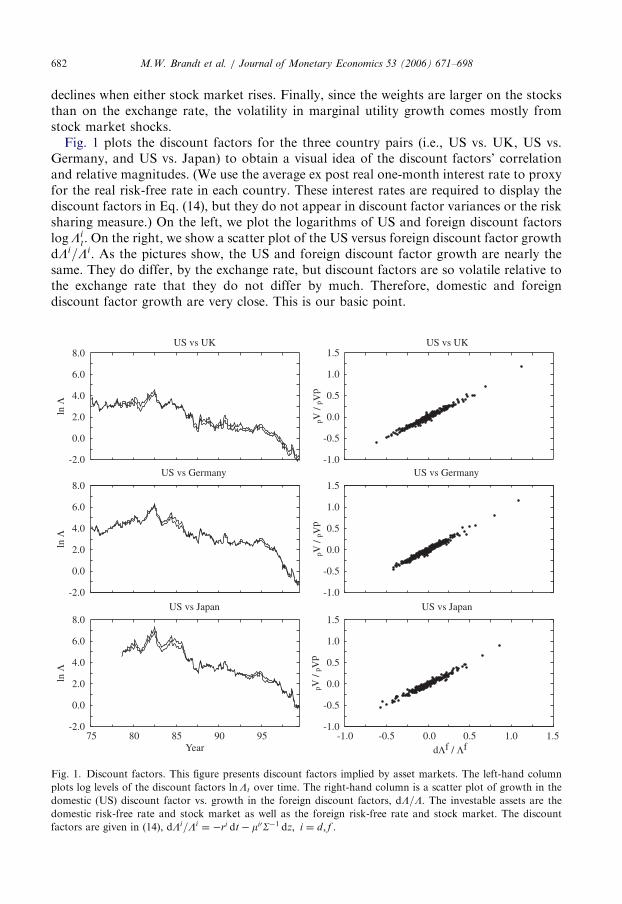
declines when either stock market rises. Finally, since the weights are larger on the stocksthan on the exchange rate, the volatility in marginal utility growth comes mostly fromstock market shocks.Fig. 1 plots the discount factors for the three country pairs (i.e., US vs. UK, US vs.

Germany, and US vs. Japan) to obtain a visual idea of the discount factors’ correlationand relative magnitudes. (We use the average ex post real one-month interest rate to proxyfor the real risk-free rate in each country. These interest rates are required to display thediscount factors in Eq. (14), but they do not appear in discount factor variances or the risksharing measure.) On the left, we plot the logarithms of US and foreign discount factorslogLi

t. On the right, we show a scatter plot of the US versus foreign discount factor growthdLi=Li. As the pictures show, the US and foreign discount factor growth are nearly thesame. They do differ, by the exchange rate, but discount factors are so volatile relative tothe exchange rate that they do not differ by much. Therefore, domestic and foreigndiscount factor growth are very close. This is our basic point.

-2.0

0.0

2.0

4.0

6.0

8.0

ln Λ

US vs UK

-1.0

-0.5

0.0

0.5

1.0

1.5

dΛd / Λ

d

US vs UK

-2.0

0.0

2.0

4.0

6.0

8.0

ln Λ

US vs Germany

-1.0

-0.5

0.0

0.5

1.0

1.5

dΛd / Λ

d

US vs Germany

75 80 85 90 95-2.0

0.0

2.0

4.0

6.0

8.0

Year

ln Λ

US vs Japan

-1.0 -0.5 0.0 0.5 1.0 1.5-1.0

-0.5

0.0

0.5

1.0

1.5

dΛf / Λf

dΛd / Λ

d

US vs Japan

Fig. 1. Discount factors. This figure presents discount factors implied by asset markets. The left-hand column

plots log levels of the discount factors lnLt over time. The right-hand column is a scatter plot of growth in the

domestic (US) discount factor vs. growth in the foreign discount factors, dL=L: The investable assets are the

domestic risk-free rate and stock market as well as the foreign risk-free rate and stock market. The discount

factors are given in (14), dLi=Li ¼ �ri dt� mi0S�1 dz; i ¼ d ; f .

ARTICLE IN PRESS

Table 4

Risk sharing index from consumption data


Standard Deviation of log consumption growth (%)

Quarterly

Domestic 1.44 1.44 1.44

Foreign 3.11 1.66 2.65

Annual

Domestic 1.80 1.80 1.80

Foreign 3.14 2.09 1.58

Log consumption growth correlations

Quarterly 0.31 0.17 0.27

Annual 0.42 0.24 0.35

Risk sharing index

Quarterly 0.245 0.166 0.265

Annual 0.361 0.233 0.350

This table shows annualized summary statistics for domestic and foreign log consumption growth and the

corresponding risk sharing index. Consumption is real per-capita consumption of non-durables and services from

the International Monetary Fund’s IFS database. Quarterly and annual data from Q1 1975 through Q2 1998.

Quarterly standard deviations are annualized. The domestic country is the US and the foreign country is the UK,

Germany, or Japan. The risk sharing index is calculated according to Eq. (23),

1�s2ðd ln cd � d ln cf Þ

s2ðd ln cd Þ þ s2ðd ln cf Þ.


3.4. Consumption data

Consumption growth is poorly correlated across countries, so studies based onconsumption data typically find that international risks are poorly shared. This finding is amajor puzzle of international economics.7 Consumption growth is also not very volatile, sowhen it is multiplied by reasonable risk aversion to produce marginal utility growth,consumption-based models do not produce the observed volatility of the exchange rate viaEq. (1). By this standard, exchange rates seem too volatile.8 The low volatility ofconsumption growth, and hence marginal utility growth, is also the heart of the equitypremium puzzle.

To examine quantitatively the discrepancy between the asset market view of risk sharingand the view based on consumption data, we calculate marginal utility growth and risksharing measures implied by consumption data and standard power utility. Table 4presents the results.

Table 4 starts with annualized standard deviations and correlations of log consumptiongrowth for the three country pairs. Since high-frequency consumption data is notoriouslynoisy, we consider both quarterly and annual data. (Temporally aggregating consumption

7Important contributions include Backus et al. (1992), Backus and Smith (1993), Brennan and Solnik (1989),

Davis et al. (2001), Lewis (1996, 2000), Obstfeld (1992, 1994) and Tesar (1993).8See Flood and Rose (1995), Mark (1995), Meese and Rogoff (1983), Obstfeld and Rogoff (2000), and Rogoff

(1999).


data is likely to reduce the effect of measurement errors. See Bell and Wilcox, 1993, andWilcox, 1992.) The table confirms the usual results. Consumption growth is relativelysmooth, with standard deviations of 1.4% to 3.1%. Using CRRA utility with u0ðcÞ ¼ c�g,the variance of log marginal utility growth is s2ðd lnLÞ ¼ s2ðgd ln cÞ. As is well knownfrom the equity risk premium literature, we therefore need a very large g, at least 20, togenerate the 60% volatility of marginal utility growth implied by asset markets from suchsmooth consumption growth.Table 4 also shows that consumption growth is imperfectly correlated across countries,

with correlations ranging from 0.17 to 0.42. The correlations are highest between the USand UK and lowest between the US and Germany. Although nicely above zero, these arewell below one, and surprisingly lower than the correlations of output growth acrosscountries (Backus et al., 1992). This is the heart of the usual observation that internationalrisks do not seem to be well shared.Assuming for simplicity that the domestic and foreign representative investors have the

same level of relative risk aversion, we can compute the risk sharing index based onconsumption data as

1�s2ðd lnLd � d lnLf Þ

s2ðd lnLdÞ þ s2ðd lnLf Þ¼ 1�

s2ðd ln cd � d ln cf Þ

s2ðd ln cdÞ þ s2ðd ln cf Þ. (23)

(In incomplete markets, marginal utility growth does not necessarily obey Eq. (21), so wecannot use exchange rates in the numerator of the risk sharing index. The risk aversioncoefficients conveniently drop out of the index when both countries have the same level ofrisk aversion.) As shown in Table 4, this calculation results in risk sharing indices of0.17–0.36. These numbers are much lower than the risk sharing indices implied by assetmarkets in Table 2, and they capture in our index the usual conclusion that risks are poorlyshared internationally. (The index is lower than the consumption growth correlationbecause the index penalizes size as well as correlation. The greater standard deviation offoreign consumption growth would count against risk sharing even if consumptiongrowths were perfectly correlated.)These consumption-based results do not contradict our calculations, in the sense of

pointing out an error. We measure marginal utility growth directly from asset markets,ignoring quantity data. The consumption-based calculations measure marginal utilitygrowth from quantity data via a utility function, ignoring asset prices. Since the results areso different, the quantity-based and price-based calculations need to be reconciled ofcourse, and we discuss this reconciliation below.Consumption-based calculations also measure overall risk sharing, while we only

measure that component of risk sharing achieved through incomplete asset markets. Ifthere are substantial additional risks, one could see good risk sharing in asset marketsdespite poor risk sharing in total consumption. As we quantify in the next section, though,this view falls apart on the required magnitude of the additional risks.

3.5. Non-market risks and bounds on overall risk sharing

What does the asset market-based risk sharing index tell us about overall risk sharing—the risk sharing index computed using marginal utility growth—in incomplete markets?

ARTICLE IN PRESS

Table 5

Risk sharing index with incomplete markets

rðdwd ;dwf Þ sðdwd Þ ¼ sðdwf Þ

0% 10% 20% 30% 50% 100%

�1.0 0.975 0.909 0.735 0.507 0.060 �0.557

�0.8 0.975 0.916 0.760 0.554 0.152 �0.402

�0.4 0.975 0.929 0.808 0.649 0.338 �0.091

0.0 0.975 0.943 0.857 0.744 0.523 0.219

0.4 0.975 0.956 0.905 0.839 0.710 0.529

0.8 0.975 0.969 0.954 0.934 0.894 0.839

1.0 0.975 0.976 0.978 0.981 0.987 0.994

This table shows the risk sharing index in the case of incomplete markets for different levels of the volatility and

correlation of additional risks. The domestic and foreign mean excess stock returns yd� rd and yf

� rf are 8%.

The volatility of both stock returns is 18%. The volatility of the exchange rate is 12%. The correlation between the

stock returns is 0.4 and the stock returns are both uncorrelated with the exchange rate. The domestic foreign

exchange risk premium yeþ rf � rd is zero. The implied standard deviation of the minimum-variance discount

factors is 56.7%. The risk sharing index is calculated as in Eq. (27),

1�See þ s2ðdwd � dwf Þ

md0S�1md þ mf 0S�1mf þ s2ðdwd Þ þ s2ðdwf Þ.


How much and what kind of non-market risk would it take to drive the asset market-basedrisk sharing index down to the values suggested by consumption data and power utility?

Overall risk sharing can be better or worse than the asset market-based risk sharingindex. Marginal utility growth equals the minimum-variance discount factor, plus theeffects of additional non-spanned risks.

The additional risks9 are orthogonal to asset payoffs, but they may be arbitrarilycorrelated across countries. If the additional risks are highly correlated across countries,marginal utility growths can move together more closely than the asset market-baseddiscount factors, and the risk sharing index for marginal utility growth can be higher thanwe calculate. If additional risks are uncorrelated across countries, marginal utility growthis less correlated than the asset-based discount factors, and overall risk sharing is lowerthan our calculation. Finally, if the unspanned risks are somehow negatively correlatedacross countries, they will drive down the risk sharing index more quickly, and ultimatelydrive it to negative values. In each of these cases, there must be more risk as well. The non-traded risks are orthogonal to asset market-based discount factors, so to be less correlatedacross countries, marginal utility growth must be even more volatile than the alreadyhighly volatile asset-based discount factors.

To make this discussion quantitative and explicit, Table 5 presents some calculations.Consider a pair of candidates for marginal utility growth d ~L

i= ~L

iformed from the

minimum-variance discount factors dLi=Li by the addition of noises dwi with

9Precisely, we mean here and below ‘‘the effects on marginal utility growth of the additional risks’’. If utility is

power and the additional risks take the form of endowment shocks, the consumption risk translates directly to

marginal utility growth risk. Under other circumstances, additional risks affect marginal utility growth in more

complex ways.


Eðdwi dzÞ ¼ 0. The risk sharing index for these marginal utility growths is

1�s2ðd ln ~L

d� d ln ~L

fÞ

s2ðd ln ~LdÞ þ s2ðd ln ~L

fÞ. (24)

To calculate this index and to relate this expression to the risk sharing index using theminimum-variance discount factors, note that

s2ðd ln ~LiÞ ¼ s2ðd lnLiÞ þ s2ðdwiÞ; i ¼ d; f , (25)

and

s2ðd ln ~Ld� d ln ~L

fÞ ¼ s2ðd lnLd � d lnLf Þ þ s2ðdwd � dwf Þ. (26)

Substituting the last two expressions into Eq. (24), the risk sharing index using candidatesfor marginal utility growth is

1�s2ðd lnLd � d lnLf Þ þ s2ðdwd � dwf Þ

s2ðd lnLdÞ þ s2ðd lnLf Þ þ s2ðdwdÞ þ s2ðdwf Þ

¼ 1�See þ s2ðdwd � dwf Þ

md0S�1md þ mf 0S�1mf þ s2ðdwd Þ þ s2ðdwf Þ. ð27Þ

There is no point in redoing the calculations for all three countries, so we use a simple setof representative numbers for Table 5 and following experiments. We use a 8% mean stockexcess return and 18% standard deviation of stock excess returns in both countries. We setthe exchange rate volatility to 12%. We assume a correlation of 0.4 between the stockindex returns and zero correlation between the stock index returns and the exchange rate.We set the domestic exchange rate risk premium to zero.10 In the notation of the formulas,our assumptions for the sensitivity analysis are

yeþ rf � re ¼ 0; yd

� rd ¼ yf� rf ¼ 0:08,

sðdzdÞ ¼ sðdzf Þ ¼ 0:18; sðdzeÞ ¼ 0:12,

rðdzd ;dzf Þ ¼ 0:4; rðdzd dzeÞ ¼ rðdzf dzeÞ ¼ 0. (28)

The risk sharing index for these parameter values is 0.975, typical of Table 2. We then varythe volatility of the additional risks dwd and dwf from zero to 100% and their correlationbetween �1 and 1. Table 5 reports the corresponding values of the risk sharing index,calculated from Eq. (27).Table 5 and Eq. (27) verify the above intuition about additional risk. The risk sharing

index rises if the additional risks are more highly correlated than the asset market-baseddiscount factors, as shown in the r ¼ 1 row. In this case, the numerator of (27) isunchanged and the denominator increases. If additional risks are uncorrelated, the risksharing index declines towards zero as the size of the additional risks increases. Here,s2ðdwd � dwf Þ ¼ s2ðdwd Þ þ s2ðdwf Þ. The extra terms in the numerator and denominator of(27) are the same, which increases the ratio (since it starts below one) and pulls the risksharing index towards zero. For intermediate positive correlations, the risk sharing index

10This assumption gives foreigners a currency risk premium of �See � 0:12 ¼ 1%. However, the results are

insensitive to the assumed exchange rate risk premium.


declines as one adds additional risks, but more slowly than for the r ¼ 0 case. Finally, ifthe additional risks are somehow negatively correlated, the risk sharing index declinesquickly, and eventually becomes negative, reflecting the now negative correlation ofmarginal utility growth across countries.

Most importantly, Table 5 shows how much risk must be added to the discount factor tohave a quantitatively important impact on the risk sharing index. We find some positivecorrelation of additional risks to be the most plausible case. One reason is that we omit awide variety of assets from the analysis. Additional assets make discount factors morevolatile, but typically do so in the same way for domestic and foreign investors. Theyprovide additional risk-sharing opportunities. Non-traded insurance mechanisms such asinternational remittances, government aid, insurance and reinsurance, etc. have the sameeffect. Finally, many shocks, such as international business cycles, commodity prices, etc.have common effects across countries, making uninsured marginal utility growths movetogether. Table 5 shows that if the additional risks have only a r ¼ 0:4 correlation, similarto that of consumption or GDP growth across countries, then additional risks with asmuch as 50% volatility leave the risk sharing index above 0.70. Even additional risks with100% volatility do not bring the risk sharing index down to the maximum 0.35 risk sharingindex obtained from consumption growth. Keep in mind that 50% discount factorvolatility launched the entire equity premium puzzle literature.

If we assume instead that the extra risks are completely uncorrelated across countries,the r ¼ 0 line of Table 5 shows that the volatility of extra risks still has to be more than30% to reduce the risk sharing index to below 0.75, and we need additional risks withvolatility on the order of 100% to reach values of 0.2–0.3 suggested by consumption-basedcalculations in Table 4.

It is hard to think of quantitatively important negatively correlated shocks. Beggar-thy-neighbor policies are a possibility, though changes in such policies pale relative to 10%exchange rate volatility, let alone 50% marginal utility growth volatility. Commodity (oil)price changes might affect certain country pairs, but not US vs. Germany, for example.Still, even with a correlation of negative one, shocks with 30% volatility only bring downthe risk sharing index to 0.5.

In sum, additional risks of plausible magnitude and correlation do not have a largeimpact on the asset market based risk sharing measures. Additional risks have to be largerthan the 50% volatility of the minimum-variance discount factor to seriously affect the risksharing index. It is difficult enough to understand the 50% volatility of the minimum-variance discount factor; do we really believe that there are other country risks, orthogonalto asset market returns, that add up to an additional 50–100% volatility of marginal utilitygrowth? Without huge additional risks, we can conclude that overall risk sharing,measured from marginal utility growth, is large as well.11

For this reason, additional risks also do not offer a reconciliation between the asset market-based risk sharing measure and that derived from consumption data. The consumption-basedcalculations predict marginal utility growth that is poorly correlated, but they also predictthat marginal utility growth has a low volatility, typically below 20% for risk aversion g lessthan 10. If we add enough additional risks to our calculation to bring the correlation of

11If one imposes an a priori upper limit on the volatility of marginal utility growth as in Cochrane and Saa-

Requejo (2000), one can obtain lower and upper bounds on overall risk sharing from the asset market-based index

to formalize this observation.


marginal utility growth down to the consumption-based levels, we increase the volatility ofmarginal utility growth from 50% to well over 100%, doubling the equity premium puzzle.This is a sideways move, not one that brings the two calculations closer together.

3.6. A lower equity premium?

Can we avoid the puzzles altogether? Perhaps the ex ante equity premium is a lot lowerthan sample averages suggest. It is attractive to view the exchange rate from Eq. (1) as adirect measure of marginal utility growth, one that gives much lower volatility than theHansen–Jagannathan (1991) calculation coming from the mean equity premium. If so, thispaper adds to the view that a lot of the historical equity premium was luck.To explore in quantitative detail the effect of uncertainty about the equity premium, we

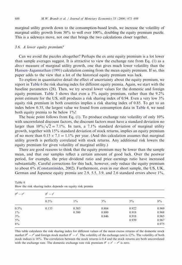
report in Table 6 the risk sharing index for different equity premia. Again, we start with thebaseline parameters (28). Then, we try several lower values for the domestic and foreignequity premium. Table 3 shows that even a 5% equity premium, rather than the 9.2%point estimate for the US, still produces a risk sharing index of 0.94. Even a very low 3%equity risk premium in both countries implies a risk sharing index of 0.85. To get to anindex below 0.35, the largest value we found from consumption data in Table 4, we needboth equity premia to be below 1%!The basic point follows from Eq. (1). To produce exchange rate volatility of only 10%

with uncorrelated discount factors, the discount factors must have a standard deviation nolarger than 10%=

ffiffiffi2p¼ 7:1%. In turn, a 7.1% standard deviation of marginal utility

growth, together with 15% standard deviation of stock returns, implies an equity premiumof no more than 0:15� 7:1 ¼ 1:1% per year. (And this calculation assumes that marginalutility growth is perfectly correlated with stock returns. Any additional risk lowers theequity premium for given volatility of marginal utility.)There are good reasons to think that the equity premium may be lower than the sample

mean, and that our samples reflect a certain amount of good luck. Over the postwarperiod, for example, the price–dividend ratio and price–earnings ratio have increasedsubstantially. Careful corrections for this luck, however, only reduce the equity premiumto about 6% (Constantinides, 2002). Furthermore, even in our short sample, the US, UK,German and Japanese equity premia are 2.9, 5.5, 3.9, and 2.6 standard errors above 1%,

Table 6

How the risk sharing index depends on equity risk premia

yd� rd yf

� rf

0.5% 1% 3% 5% 8%

0.5% 0.133 0.303 0.804 0.922 0.969

1% 0.380 0.800 0.918 0.968

3% 0.846 0.918 0.965

5% 0.939 0.967

8% 0.975

This table calculates the risk sharing index for different values of the mean excess returns of the domestic stock

market yd� rd and foreign stock market yf

� rf . The volatility of the exchange rate is 12%. The volatility of both

stock indices is 18%. The correlation between the stock returns is 0.4 and the stock returns are both uncorrelated

with the exchange rate. The domestic exchange rate risk premium yeþ rf � rd is zero.


and the significance grows in longer samples. If the true equity premium is below 1%, thelast century was extraordinarily lucky.

Table 6 also shows that the risk sharing index is driven by the larger of the domestic andforeign equity risk premia. As long as one of the risk premia is high, the risk sharing indexis also high. Only when both premia drop does the risk sharing index decreasesubstantially. The risk sharing index is driven by the maximum Sharpe ratio in portfoliosof the domestic and international assets. This fact contributes to the small standard errorsof our risk sharing index in Table 2, relative to the standard errors of the individualcountry equity premia. Since stock returns are not perfectly correlated, cross-country dataadds to the statistical evidence against very small equity premia.

3.7. . . .Or exchange rates are too smooth

Suppose that risks are in fact not well shared internationally. Then, the exchange rateswe observe are surprisingly smooth. To make this point quantitatively, in Table 7 we solveEq. (27) for the exchange rate volatility See that is consistent with a risk sharing index of0.35, the highest value implied by the consumption data in Table 4. As in Table 5 andTable 6, we start with baseline parameters (28). The result, in the 8% row and 0% columnof Table 7, is that exchange rates should have a standard deviation of 102.4%!

As above, perhaps the equity premium is lower than 8%. Table 7 considers a reasonablerange of equity risk premia by varying yd

� rd and yf� rf from 4% to 8%. (Since our index

is driven by the maximum risk premium, we set yd� rd ¼ yf

� rf .) The implied exchange

Table 7

Exchange rate volatility implied by a risk sharing index of 0.35

md ¼ mf sðdwd Þ ¼ sðdwf Þ

0% 10% 20% 30% 40%

r ¼ 0:44% 51.2 51.5 52.3 53.6 55.5

6% 76.8 77.0 77.5 78.4 79.7

8% 102.4 102.5 102.9 103.6 104.6

r ¼ 0:04% 51.2 49.2 42.7 28.6 0.1

6% 76.8 75.5 71.4 70.0 51.9

8% 102.4 101.4 98.4 93.2 85.3

This table shows the exchange rate volatility implied by a risk sharing index of 0.35 in the case of incomplete

markets for different levels of the domestic and foreign mean excess stock returns yd� rd and yf

� rf and different

levels of the volatility and correlation of additional risks. The volatility of both stock returns is 18%. The

correlation between the stock returns is 0.4 and the stock returns are both uncorrelated with the exchange rate.

The domestic foreign exchange risk premium yeþ rf � rd is zero. The implied standard deviations of the

minimum-variance discount factors for the three different equity risk premia are 28.3%, 42.5%, and 56.7%. The

implied exchange rate volatility is computed by setting Eq. (27) equal to 0.35, i.e. we solve

0:35 ¼ 1�See þ s2ðdwd � dwf Þ

md0S�1md þ mf 0S�1mf þ s2ðdwd Þ þ s2ðdwf Þ

for See. (Note See is an element of S.)


rate volatility declines to 76.8% and then 51.2%. Cutting the equity premium in half stillleaves a prediction that exchange rates should be four times as volatile as they are in fact.As unspanned risks dwd and dwf lower risk sharing for a given exchange rate volatility,

they can also lower the predicted exchange rate volatility for a given risk sharing index.Thus, Table 7 also considers additional unspanned risks with volatilities ranging from zeroto 40% and a correlation of either zero or 0.4.When the additional risks are positively correlated, they raise the predicted volatility of

exchange rates; numbers increase across the columns of Table 7 in the r ¼ 0:4 panel.Marginal utility growth equals the asset-market discount factor plus the extra risks. If theextra risks are more correlated than is marginal utility growth, then the asset-marketdiscount factors must be even less correlated than marginal utility growth. The ratio ofasset-market discount factors generates the exchange rate, and the less correlated the asset-market discount factors, the more volatile the exchange rate. We can also digest this resultby looking at Eq. (27). We can solve (27) approximately for exchange rate volatility See

given a risk sharing index r as

See � 2½ð1� rÞm0S�1mþ ðr� rÞs2ðdwÞ�. (29)

(This is only an approximate solution since See also appears in S�1, though its effect thereis minor.) Extra risks that are more correlated than the presumed risk sharing index r4rincrease the predicted volatility of exchange rates.With uncorrelated extra risks, the addition of extra risks does help to predict smoother

exchange rates given a view that overall risk sharing is only 0.35. Numbers decline acrosscolumns of Table 7 in the r ¼ 0 rows. But again, this specification is not quantitativelyplausible. Only by simultaneously assuming an equity premium of 4% or less (less than halfthe sample value), additional risks with a huge 40% volatility, and extra risks completelyuncorrelated with each other, do we produce exchange rates with volatility less than orequal to sample values of about 12%, as seen in the top right corner of the r ¼ 0 panel.

4. Interpreting the calculation

4.1. Clarifications and misconceptions

Domestic and foreign discount factors each price the full set of assets: domestic andforeign stocks and bonds. One might derive a ‘‘domestic discount factor’’ that only pricesdomestic stocks and bonds. Such a discount factor is a different object, and an uninterestingone in our context. In the continuous-time limit, in fact, the domestic and foreign discountfactors lie in the same space, diffusions driven by the three shocks dzd ;dze;dzf .For this reason, the correlation of international stock markets has little bearing on the

risk sharing index. The risk sharing index is driven by the mean returns, through themaximum Sharpe ratio. It also is not directly related to the question, how much do meanvariance frontiers expand by the inclusion of international stocks?12 We always allowinvestors to trade in both domestic and foreign stocks.Do not confuse the discount factor with the optimal portfolio. The optimal portfolio,

together with a utility function and a driving process for income, supports a marginalutility growth process, and the discount factor is the projection of that marginal utility

12For example, Chen and Knez (1995) and De Santis and Gerard (1997).


growth process on the space of asset returns. The beginning and the end of this trail aretotally different objects. The discount factor is not the optimal portfolio, the ‘‘market’’portfolio, or the portfolio held by any investor. The minimum-variance discount factor isproportional to the minimum second-moment portfolio, which is on the bottom of themean—variance frontier, and is therefore a portfolio nobody wants to hold. In a mean—variance setting, the optimal, tangency, and market portfolios are all on the top of themean—variance frontier. With more general utility functions and non-marketed incomeprocesses, asset portfolios are not even on the mean—variance frontier. Discount factorscan be highly correlated, even when portfolios are not correlated.

Although the index has the above interpretation as the ratio of risk not shared to overallrisk, so country pairs with lower risk sharing indices have greater scope to reduce overallrisk (variance of discount factor) if capital markets can be opened or transport costslowered, we do not connect the risk sharing index to a measure of welfare. Also, a high risksharing index does not mean that further risk sharing through the introduction of newassets or institutions, or the lowering of transport costs, is not possible or desirable. Therisk sharing index is high in large part because the denominator is high. Improvements inthe numerator can have substantial welfare benefits, even when the index is already high.

One might ask, ‘‘If two countries fix their exchange rates, will this not lead to a perfectrisk sharing index?’’ The answer is no. Two countries can fix their nominal exchange rates,but they cannot fix their real exchange rates, except by allowing and enjoying perfectshipment of goods, which of course is the perfect risk-sharing case.

The notion of risk-sharing measured by our index does not respect transport costs. Forexample, we would measure poor risk sharing between Earth and Mars, or betweencountries with integrated capital markets, free trade, but a preponderance of locallyprovided non-tradeable goods. Yet the allocations between countries in these examplesmay be Pareto optimal if the planning problem respects the costs of transport. Ourmeasure does not say anything about this concept of risk sharing. Our measure asks towhat extent real exchange rate variability, which is the shadow price of transport costs,blunts risk sharing, defined relative to costless trade in all goods. Whether removing thetransport cost is a physical impossibility (haircuts) or a result of government policy (tariffs)is not relevant to our question. Also for this reason we do not complicate the analysis withmultiple (tradeable and non-tradeable) goods.

4.2. Home bias

US investors largely hold US securities, Japanese investors largely hold Japanesesecurities, and so forth. This observation is the ‘‘home bias puzzle’’.13

Exchange rate volatility blunts optimal risk sharing, so it implies that optimal portfoliosshould display some home bias. Once Earth-based investors understand that exchange rate

13The home bias puzzle goes back a long way, for example Solnik (1974). French and Poterba (1991) observe

that Americans held 94% of their equity wealth in the US stock market. The analogous figure for Japan was 98%.

Lewis (1999) surveys the home bias puzzle. Baxter and Jermann (1997) argue that human capital is a domestic

asset, so adding labor income risk worsens the puzzle. Tesar and Werner (1995) show that foreign portfolios

turned over much faster than domestic portfolios, and argue that this suggests that transactions costs do not drive

the home bias. ‘‘Home bias’’ puzzles include the propensity of people and managers to hold stocks in companies

near them or in their industries. For example, Coval and Moskowitz (1999) find that fund managers hold stocks of

companies that are on average somewhat closer to them than the market as a whole.


movements will offset any gains from holding Martian securities, their optimal portfolioswill ignore those securities. In mean—variance portfolio calculations, exchange rates arevolatile, poorly correlated with stock returns, and offer virtually no risk premium. As aresult, foreign stocks are less desirable to domestic investors than similar domestic stocks.However, neither observation has yet generated the amount of home bias that weobserve.14

In one sense, the home bias calculations complement ours: the home bias literatureagrees that exchange rates do not move enough to blunt the risk-sharing possibilitiesof asset markets. On the other hand, it suggests that risks are not in fact that wellshared since people do not hold as many foreign stocks as the portfolio calculationsrecommend.Like the consumption-based evidence, the home bias puzzle does not contradict our

calculation. The home bias puzzle refers to an optimal portfolio calculation for a specificutility function, and underlying risky income and asset return process or productionfunction and technology shock specification. Portfolios do not need to be similar acrosscountries for marginal utilities to be similar. (Again, do not confuse the discount factor withthe optimal portfolio.) For example, we can see volatile and highly correlated marginalutility growth despite very little asset cross-holding if the underlying income shocks arehighly correlated, if risk sharing is achieved by other means (e.g., government transfers,direct payments to relatives abroad, assets not included in the analysis such asinternational reinsurance), or if preferences are not the simple one-period quadraticutility over wealth envisioned by mean–variance calculations, or the simple forms used ingeneral-equilibrium models. It is possible to see large amounts of risk sharing in marginalutility growth, but still to be puzzled by the underlying economic model and the portfoliopositions that support it. It is an open question whether the home bias puzzle represents afailure of portfolio models to capture the right utility function and the right incomeprocess, or whether it represents a systematic and dramatic failure of people to follow theirfirst order conditions for portfolio optimization.Still, like the consumption-based evidence, one is uncomfortable that two independent

ways of calculating risk sharing lead to such different results, so some thoughts onreconciling the calculations are in order.

4.3. Reconciliation of asset-market, consumption, and home-bias calculations

Asset prices give a quite different picture of marginal utility growth from that painted byconsumption or portfolio data, using standard utility functions, environments, andparameters. Based on asset prices, it appears that there is a lot of risk (sðlnmd Þ andsðlnmf Þ are large) and that risk is shared well across countries (md and mf move together),since exchange rates are surprisingly smooth (sðD ln eÞ is a lot smaller than sðlnmÞ). Basedon consumption data and power utility with low risk aversion, it appears that there is littlerisk, that risk is poorly shared across countries, and that exchange rates are surprisinglyvolatile. Based on portfolio calculations with standard utility functions and simple incomeprocesses, it appears that people do not share risks through asset markets as much as theycould.

14For example, see Baxter et al. (1995) for a dynamic general equilibrium model with non-tradeable goods, and

Black and Litterman (1992) for mean-variance calculations.


As a result, we present our calculations as a contribution to a puzzle, rather than adefinitive answer to the risk sharing question. Our contribution is to tie together the asset-market evidence on the equity premium, exchange rate volatility, and risk-sharing aspectsof the puzzle, not to reconcile all three phenomena with consumption and portfolio data.We knew that asset markets present more volatile exchange rates than are implied byconsumption data and standard utility functions; we knew that asset markets presenthigher equity premia than are implied by consumption data and standard utility functions.Now we know that asset markets imply substantially higher risk sharing than are impliedby consumption data and standard utility functions as well. Furthermore, we see that risksharing, the equity premium, and exchange rate volatility are all tied together.

Which view of risk sharing will prevail in the end? We cannot be sure until the asset-market and quantity-based views are reconciled. One cannot take the quantity-basedmeasures of risk-sharing at face value while the quantity-based models remain completelyat odds with basic facts such as the observed equity premium and exchange rate volatility.While the asset-price measures do not suffer the same internal inconsistency becausethey are not based on models that make counterfactual predictions, one isjustifiably uncomfortable in believing their results with no economic model in hand thatcan generate the measured pattern of volatility and high correlation of marginal utilitygrowth.

How will the asset-market and quantity-based calculations eventually be resolved? Ourasset-market calculations are like the observation that the relative price of apples andoranges is pretty much the same across supermarkets in Los Angeles. We conclude thatshoppers’ marginal rates of substitution for apples and oranges must be pretty much thesame. We do not look inside shopping baskets to make this observation. The quantity-based calculations look into shopping baskets, ignoring prices. Shoppers bring homegrocery bags with vastly different apple/orange ratios. Translated through standard utilityfunctions, this quantity data implies that marginal rates of substitution vary a lot acrosspeople.

There are two ways to resolve such contrasting calculations: either the specification ofthe utility function or environment needs modification, or some friction causes marginalrates of substitution not to equal price ratios. In the former category, we can considerdifferent functional forms for preferences, including non-separabilities (habits, durability,non-state-separable preferences), preference heterogeneity (some like oranges better thanapples; preference shocks in our one-good intertemporal context), heterogeneity inendowments (people who have apple trees at home buy more oranges; different income orproduction processes in our context).

The first path is familiar from the equity premium literature. Reconciling the equitypremium with consumption data seems to require dramatic departures from theconventional power utility setup.15 Since these departures generate large discount factorvolatility, they will generate volatile exchange rates as well. If they are not to generate too

volatile exchange rates, they will have to imply good international risk sharing as well, bythe inescapable logic of Eq. (1). Thus, a reconciliation along these lines will bring thequantity-based risk sharing measures up to what we measure from asset markets, not theother way around.

15For example, habits as in Campbell and Cochrane (1999), or countercyclical idiosyncratic non-traded risk as

in Constantinides and Duffie (1996).


The second path is also familiar. If it costs me $10 to get to the grocery store, mymarginal rate of substitution for apples vs. oranges may deviate substantially from theprice ratio. A large literature has tried quantitatively to explain the equity premium,exchange rate volatility, poor risk sharing, and home bias puzzles by explicit frictions suchas transactions costs, taxes, legal portfolio constraints, asymmetric information, borrowingconstraints, participation constraints and so forth,16 and the implication that manyconsumers do not participate in asset markets.17 Alas, this literature has not yet beenentirely successful—which is equivalent to saying the puzzles are still puzzles rather thanex-puzzles. The frictions are just not large enough to keep people far from frictionless firstorder conditions. The equity premium implies that contingent claims prices (discountfactors) vary by 50% or more. Marginal rates of substitution inferred from consumptiongrowth, standard utility functions and low risk aversion vary by 10% or less. That meansthe wedge between them must vary by 40% or more. Observed transactions costs of a fewpercent or any reasonable information and adverse selection costs, or taxes just do notvary this much. Furthermore, if some consumers are in fact disconnected from assetmarkets by transactions costs, the puzzles all remain intact for the investors who do obeytheir first order conditions. If limited participation becomes the resolution, we willconclude that risks are surprisingly well shared among people who do hold any stocks.

5. Conclusion

We present a calculation of international risk sharing based on asset market data. Thehigh Sharpe ratios obtainable in international asset markets imply that marginal utilitygrowth is very volatile—there is a lot of risk to share. Compared to this volatility, thevolatility of exchange rates is very small. We conclude that there is a surprisingly high levelof international risk sharing. Alternatively, if risks really are poorly shared, exchange ratesare much too smooth. Both conclusions are in stark contrast to the standard findings fromconsumption data, general equilibrium models, or portfolio calculations.Since markets are incomplete, our risk sharing index answers the question, ‘‘to what

extent do exchange rate movements blunt the risk-sharing possibilities of existing assetmarkets?’’ The answer is ‘‘not much’’. Additional risks uncorrelated with asset movementscan lower overall risk sharing, but they simultaneously raise the total amount of risk.Therefore, we argue that reasonably sized and correlated risks cannot lower overall risksharing by much, and we conclude that the asset-based results indicate a surprisingly largeamount of overall risk sharing as well.The large equity premium drives the large volatility of marginal utility growth, so

perhaps a lower equity premium can resolve the puzzle. Like additional risks, this is not aquantitatively plausible resolution however. The equity premium needs to be below 1% inboth countries for our risk sharing measure to go down to conventional levels, or,equivalently, for the smoothness of exchange rates to be explained.We conduct our analysis only for country pairs and two assets in each country—the

stock market and a risk-free asset. Taking into account more countries or more assets willmake our results even stronger, since the maximum Sharpe ratio obtainable ininternational asset markets can only increase. Adding conditioning information is likely

16Some examples include Heaton and Lucas (1997), Lewis (1996, 1999), Luttmer (1999), and Davis et al. (2003).17For example Mankiw and Zeldes (1991) and Vissing-Jorgenson (2002).


to increase the implied level of risk sharing as well, since the presence of conditioninginformation is just like the presence of additional assets (managed portfolios) that can onlyincrease unconditional Sharpe ratios. Conditioning information may however give time-variation in the amount of risk that is shared. For example, Brandt and Santa-Clara (2002)find that the volatility of exchange rates drops at times very significantly, which suggestseven higher values of the risk sharing index at those times.

We interpret our results as a puzzle. Asset markets allow the potential of a great deal ofrisk sharing. To conclude that risks are in fact well shared, all we need to believe is thatinvestors obey first order conditions for portfolio allocation. Even approximately optimalportfolios will do, as the magnitudes are so large. This conclusion needs no statementabout preferences, technology, endowments, shocks, etc. It is just the conclusion thatconsumer’s marginal rates of substitution are equated once we observe a common priceratio. To conclude that risks are well shared overall, all we need believe is that additionalrisks, orthogonal to asset returns, are of reasonable magnitude, i.e. they contribute lessthan 100% per year to the volatility of marginal utility growth. These conclusions arecounterintuitive, and they contradict calculations made with quantity data and simpleutility functions, as do a wide range of asset price phenomena. Still, they are a simple andinescapable logical result of Eq. (1) and an equity premium above one percent.

Appendix A

Here, we go through the algebra to find the excess returns in Eqs. (12), (13) given theprocesses for stock and bond returns and the exchange rate in (10). The excess domesticstock return is

dSd

Sd�

dBd

Bd¼ ðyd

� rdÞdtþ dzd . (A.1)

To invest in the foreign risk-free bond, the domestic investor also faces currency risk.Hence, the excess return is

dðeBf Þ

eBf�

dBd

Bd¼

de

eþ rf dt� rd dt ¼ ðye

þ rf � rdÞdtþ dze. (A.2)

The foreign excess return to foreign stocks is

dSf

Sf�

dBf

Bf¼ ðyf

� rf Þdtþ dzf . (A.3)

Accounting for exchange risk, the domestic returns to holding a foreign stock and risk-freeasset are dðeSf Þ=eSf and dðeBf Þ=eBf , respectively. Thus, the corresponding domestic excessreturn is

dðeSf Þ

eSf�

dðeBf Þ

eBf¼

dSf

Sf�

dBf

Bfþ

de

e

dSf

Sf�

dBf

Bf

� �

¼ 1þde

e

� �dSf

Sf�

dBf

Bf

� �

¼ ð1þ ye dtþ dzeÞ½ðyf� rf Þdtþ dzf �


¼ ðyf� rf Þdtþ dze dzf þ dzf

¼ ðyf� rf þ Sef Þdtþ dzf . ðA:4Þ

(This excess return differences two risky assets, foreign stock less foreign bond, rather thanforeign stock over domestic bond. This choice gives slightly simpler formulas with nochange in results.)Stacking the three excess returns (A.1), (A.2), and (A.4), the vector of mean excess

returns to a domestic investor is (12) and the covariance matrix of excess returns is just S.The foreign excess return from holding foreign stocks is already given by Eq. (A.3). The

foreign excess return from borrowing at the domestic interest rate and investing at theforeign interest rate is18

�dð1=eÞ

ð1=eÞ� ðrd � rf Þdt ¼ ðrf � rdÞdtþ

de

e�

de2

e2

¼ ðyeþ rf � rd � SeeÞdtþ dze. ðA:5Þ

The foreign returns to holding a domestic stock and risky bond are dðSd=eÞ=ðSd=eÞ anddðBd=eÞ=ðBd=eÞ, respectively. Therefore, the excess return to a foreign investor is

dðSd=eÞ

Sd=e�

dðBd=eÞ

Bd=e¼

dSd

Sd�

de

eþ

de2

e2�

de

e

dSd

Sd

� ��

dBd

Bd�

de

eþ

de2

e2�

de

e

dBd

Bd

� �

¼dSd

Sd�

dBd

Bd�

de

e

dSd

Sd�

dBd

Bd

� �

¼ ð1� ye dt� dzeÞ½ðyd� rdÞdtþ dzd �

¼ ðyd� rdÞdt� dze dzd þ dzd

¼ ðyd� rd � Sed Þdtþ dzd . ðA:6Þ

Stacking the excess returns (A.3), (A.5), and (A.6), the vector of mean excess returns facedby foreign investors is given in (13) and the covariance matrix is again S.Next, we prove directly that the minimum-variance discount factors satisfy the identity

(21). Starting from the definitions (12) and (13) and using (19),

d lnLf ¼ � ðrf þ 12mf 0S�1mf Þdt� mf 0S�1dz

¼ � ðrf þ 12ðmd � SeÞ

0S�1ðmd � SeÞÞdt� ðmd � SeÞS�1 dz

¼ � ðrf þ 12m

d0S�1md � md0S�1Se þ 12S

e0S�1SeÞdt� md0S�1 dzþ dze

¼ � ðrf þ 12md0S�1md � ðye

þ rf � rd Þ þ 12SeeÞdt� md0S�1 dzþ dze

¼ � ðrd þ 12m

d0S�1md � yeþ 1

2SeeÞdt� md0S�1 dzþ dze

¼ d lnLd � ð�yeþ 1

2SeeÞdtþ dze

¼ d lnLd þ d ln e. ðA:7Þ

18Note that dð1=eÞ ¼ �ð1=e2Þdeþ ð1=e3Þde2 and dð1=eÞ1=e¼ � de

eþ de2

e2. We write the foreign excess return slightly

unconventionally as the return to borrowing domestically to invest in foreign assets. This specification highlights

the symmetry between domestic and foreign investors. Of course, the sign of an excess return makes no difference

to the volatility of the discount factor (see Eq. (9)).


References

Alesina, A., Barro, R., Tenreyro, S., 2003. Optimal currency areas. NBER Macroeconomics Annual, 2002, 2003,

Vol. 17, pp. 301–345. MIT Press, Cambridge and London.

Backus, D.K., Smith, G.W., 1993. Consumption and real exchange rates in dynamic economies with non-traded

goods. Journal of International Economics 35, 297–316.

Backus, D.K., Kehoe, P.J., Kydland, F.E., 1992. International real business cycles. Journal of Political Economy

100, 745–755.

Backus, D.K., Foresi, S., Telmer, C.I., 1996. Affine models of currency pricing. Working paper, NBER #5623.

Backus, D.K., Foresi, S., Telmer, C.I., 2001. Affine term structure models and the forward premium anomaly.

Journal of Finance 56, 279–304.

Baxter, M., Jermann, U.J., 1997. The international diversification puzzle is worse than you think. American

Economic Review 87, 170–191.

Baxter, M., Jermann, U.J., King, R., 1995. Nontraded goods, nontraded factors, and international

nondiversification. Journal of International Economics 46, 211–229.

Bell, W.R., Wilcox, D.W., 1993. The effect of sampling error on the time series behavior of consumption data.

Journal of Econometrics 55, 235–265.

Black, F., Litterman, R., 1992. Global portfolio optimization. Financial Analysts Journal 48, 28–43.

Brandt, M.W., Santa-Clara, P., 2002. Simulated likelihood estimation of diffusions with an application to

exchange rate dynamics in incomplete markets. Journal of Financial Economics 63, 161–210.

Brennan, M.J., Solnik, B., 1989. International risk sharing and capital mobility. Journal of International Money

and Finance 8, 359–373.

Campbell, J.Y., Cochrane, J.H., 1999. By force of habit: a consumption-based explanation of aggregate stock

market behavior. Journal of Political Economy 107, 205–251.

Chen, Z., Knez, P.J., 1995. Measurement of market integration and arbitrage. Review of Financial Studies 8,

287–325.

Cochrane, J.H., 2004. Asset Pricing, revised edition. Princeton University Press, Princeton, NJ.

Cochrane, J.H., Saa-Requejo, J., 2000. Beyond arbitrage: good-deal asset price bounds in incomplete markets.

Journal of Political Economy 108, 79–119.

Constantinides, G.M., 2002. Rational asset prices. Journal of Finance 57, 1567–1591.

Constantinides, G.M., Duffie, D., 1996. Asset pricing with heterogeneous consumers. Journal of Political

Economy 104, 219–240.

Coval, J.D., Moskowitz, T.J., 1999. Home bias at home: local equity preference in domestic portfolios. Journal of

Finance 54, 2045–2074.

Davis, S., Kubler, F., Willen, P., 2003. Borrowing costs and the demand for equity over the life cycle. Working

paper, University of Chicago.

Davis, S.J., Nalewaik, J., Willen, P., 2001. On the gains to international trade in risky financial assets. Working

paper, University of Chicago.

De Santis, G., Gerard, B., 1997. International asset pricing and portfolio diversification with time-varying risk.

Journal of Finance 52, 1881–1912.

Flood, R.P., Rose, A.K., 1995. Fixing the exchange rate regime: a virtual quest for fundamentals. Journal of

Monetary Economics 36, 3–37.

French, K., Poterba, J., 1991. Investor diversification and international equity markets. American Economic

Review 81, 222–226.

Hansen, L.P., 1982. Large sample properties of generalized method of moments estimators. Econometrica 50,

1029–1054.

Hansen, L.P., Jagannathan, R., 1991. Implications of security market data for models of dynamic economies.


Heaton, J., Lucas, D., 1997. Market frictions, savings behavior, and portfolio choice. Macroeconomic Dynamics

1, 76–101.

Lewis, K.K., 1996. What can explain the lack of international consumption risk sharing? Journal of Political

Economy 104, 267–297.

Lewis, K.K., 1999. Trying to explain home bias in equities and consumption. Journal of Economic Literature 37,

571–608.


Lewis, K.K., 2000. Why do stocks and consumption imply such different gains from international risk sharing?

Journal of International Economics 52, 1–35.

Luttmer, E.G.J., 1999. What level of fixed costs can reconcile consumption and stock returns. Journal of Political

Economy 107, 969–997.

Mankiw, N.G., Zeldes, S.P., 1991. The consumption of stockholders and non-stockholders. Journal of Financial

Economics 29, 97–112.

Mark, N., 1995. Exchange rates and fundamentals: evidence on long horizon predictability. American Economic

Review 85, 201–218.

Meese, R., Rogoff, K., 1983. Empirical exchange rate models of the seventies: do they fit out of sample. Journal of

International Economics 14, 3–24.

Newey, W.K., West, K.D., 1987. A simple, positive semi-definite, heteroscedasticity and autocorrelation

consistent covariance matrix. Econometrica 55, 703–708.

Obstfeld, M., 1992. International risk sharing and capital mobility: another look. Journal of International Money

and Finance 11, 115–121.

Obstfeld, M., 1994. Are industrial-country consumption risks globally diversified? In: Leiderrman, L., Razin, A.

(Eds.), Capital Mobility: The Impact on Consumption, Investment, and Growth. Cambridge University Press,

Cambridge, MA.

Obstfeld, M., Rogoff, K., 2000. The six major puzzles in international macroeconomics: is there a common cause.

In: Bernanke, B., Rogoff, K. (Eds.), NBER Macroeconomics Annual. MIT Press, Cambridge, MA.

Ravn, M., 2001. Consumption dynamics and real exchange rates. Working paper, London Business School.

Rogoff, K., 1999. Perspectives on exchange rate volatility. In: Feldstein, M. (Ed.), International Capital Flows.

University of Chicago Press, Chicago.

Solnik, B.H., 1974. Why not diversify internationally rather than domestically. Financial Analysts Journal 30,

48–54.

Tesar, L.L., 1993. International risk sharing and non-traded goods. Journal of International Economics 35,

69–89.

Tesar, L.L., Werner, I.M., 1995. Home bias and high turnover. Journal of International Money and Finance 14,

467–492.

Vissing-Jorgenson, A., 2002. Limited asset market participation and the elasticity of intertemporal substitution.


Wilcox, D.W., 1992. The construction of US consumption data: some facts and their implications for empirical

work. American Economic Review 82, 922–941.

International risk sharing is better than you think, or exchange ...

Documents

Transcript of International risk sharing is better than you think, or exchange ...