Research Division Federal Reserve Bank of St. Louis Working Paper Series

Investing for the Long-Run in European Real Estate

Carolina Fugazza Massimo Guidolin

and Giovanna Nicodano

Working Paper 2006-028A http://research.stlouisfed.org/wp/2006/2006-028.pdf

May 2006

FEDERAL RESERVE BANK OF ST. LOUIS Research Division

P.O. Box 442 St. Louis, MO 63166

______________________________________________________________________________________

The views expressed are those of the individual authors and do not necessarily reflect official positions of the Federal Reserve Bank of St. Louis, the Federal Reserve System, or the Board of Governors.

Federal Reserve Bank of St. Louis Working Papers are preliminary materials circulated to stimulate discussion and critical comment. References in publications to Federal Reserve Bank of St. Louis Working Papers (other than an acknowledgment that the writer has had access to unpublished material) should be cleared with the author or authors.

Investing for the Long-Run in European Real Estate∗

Carolina FUGAZZA

Center for Research on Pensions and Welfare Policies (CERP)

Massimo GUIDOLIN

Federal Reserve Bank of St. Louis and CERP

Giovanna NICODANO†

CERP, Fondazione Collegio Carlo Alberto and University of Turin

This draft: April 2006

Abstract

We calculate optimal portfolio choices for a long-horizon, risk-averse investor who diversifies among

European stocks, bonds, real estate, and cash, when excess asset returns are predictable. Simulations are

performed for scenarios involving different risk aversion levels, horizons, and statistical models capturing

predictability in risk premia. Importantly, under one of the scenarios, the investor takes into account the

parameter uncertainty implied by the use of estimated coefficients to characterize predictability. We find

that real estate ought to play a significant role in optimal portfolio choices, with weights between 12 and

44 percent. Under plausible assumptions, the welfare costs of either ignoring predictability or restricting

portfolio choices to traditional financial assets only are found to be in the order of 150-300 basis points

per year. These results are robust to changes in the benchmarks and in the statistical framework.

JEL Classification Codes: G11, L85.

Keywords: Optimal asset allocation, real estate, predictability, parameter uncertainty.

1. Introduction

Predictability of asset returns is known to have powerful effects on the structure and dynamics of optimal

portfolio weights for long-horizon investors. This conclusion holds across alternative models for predictabil-

ity, different data sets and asset allocation frameworks (e.g. Brennan, Schwartz, and Lagnado,1997, and

Campbell, Chan and Viceira, 2003). However, most of this evidence has been obtained in asset menus lim-

ited to traditional financial portfolios only, i.e. stocks, bonds, and short-term liquid assets.1 On the contrary,

∗We thank Piet Eicholtz (the editor), Richard Buttimer and Mario Padula (two discussants), Kanak Patel, one anonymous

referee, and all seminar participants at the Fourth Maastricht-Cambridge Real Estate Finance and Investment Symposium

Symposium 2005, CeRP, EFMA Meetings 2005 in Milan, Ente Einaudi Roma, Enquire Europe Seminar in Wien and RTN

Conference at Goethe Universitat in Frankfurt for helpful comments. Jeroen Beimer kindly provided us the real estate data.

Financial support from MIUR is gratefully acknowledged by Giovanna Nicodano.†Corresponding Author. Address: University of Turin, Faculty of Economics, Corso Unione Sovietica, 218bis - 10134 Turin,

ITALY. Tel: +39-011.6706073, Fax: +39-011.67060621Flavin and Yamashita (2002) represent an exception, although their focus is on life-cycle effects at the household level.

contributions available to asset managers with long horizons − such as pension fund managers − are investednot only in equity and bonds, but in real estate assets too.

For instance, as of the mid-1990s, in the UK 75.0 and 7.8 percent of managed pension fund assets

were held in stocks and real estate, respectively; the corresponding percentage weights were 6.6 and 4.2 in

Germany, and 26.9 and 2.2 in France. In the last two countries, long-term bonds represented 42.3 and 59.0

percent of long term portfolios (see Miles, 1996, p.23), while bonds were given a negligible weight in the

UK.2 So it appears that considerable heterogeneity exists in the relative weights assigned to stocks, bonds

and real estate. Although our paper aims at tracing out the normative implications of predictability for

optimal portfolio composition, we report results that shed light on the preferences, investment horizons and

predictability models under which one may obtain rational choices consistent with either the German-French

pattern (dominated by bonds) or with the British one (dominated by stocks). Additionally − since the

evidence is for real estate weights between 2 and 8 percent − in this paper we ask whether existing datasupport the notion that real estate ought to be included in long-horizon portfolios.

Our paper provides evidence on the effects of predictability on long-run portfolio choice when the asset

menu includes real estate assets. Furthermore, our asset allocation results are based on predictability pat-

terns characterizing a European data set that has been left unexplored thus far. On the one hand, both

extensions are crucial to make the results found in the literature relevant to the operational goals of long-

horizon asset managers that commonly employ asset menus not limited to financial securities only, and that

fail to circumscribe their portfolio choices to North American assets only. Obviously, among them, Euro-

pean institutional investors occupy a leading position. On the other hand, our results allow us to perform

comparisons to parallel findings obtained from comparable U.S. data on stocks, bonds and cash.

We use a simple vector autoregressive framework to capture predictable time variations in the investment

opportunity set (similarly to Campbell, Chan, and Viceira, 2003, Geltner and Mei, 1995, and Glascock, Lu

and So, 2001) and solve a standard portfolio problem with power utility of terminal wealth. In most cases,

the optimal long-run weight to be assigned to real estate is large, between 23 and 44 percent of the initial

wealth. It falls to 12 − 16 percent when we take into account the (sometimes considerable) estimationuncertainty concerning the coefficients characterizing the predictability model. The inclusion of real estate

does not alter the finding that predictable time variation in risk premia has first-order effects for the optimal

allocation between equities and bonds. Predictability in risk premia also changes the attractiveness of real

estate, by making it relatively less risky than bonds but riskier than stocks as the horizon grows, as well

as increasingly more profitable than the other assets. Thus its portfolio share increases the more with the

investment horizon, the lower the investor coefficient of risk aversion. Consideration of parameter uncertainty

together with predictability confirms that the share of bonds falls while that of real estate grows with the

investment horizon (see Barberis, 2000). Additionally, short-term securities (deposits, T-bills) become less

risky and increasingly substitute stock holdings, because their own lagged returns, realized inflation and the

term spread predict their return precisely.

Thus long-run investors with an interest in European assets ought to consider the effects of time-varying

risk premia because estimates of optimal portfolio weights are structurally different when predictability is

omitted. This result applies especially when parameter uncertainty, which plagues our estimates based on a

monthly frequency, is taken into account. In fact, the estimated welfare costs from ignoring predictability

2At the end of 2004 TIAA-CREF, one of the largest U.S. pension funds, invested about 17% of assets in real estate (source:

www.tiaa-cref.org).

2

are large, in excess of 150 basis points per year for a long-run (10-year) investor with a plausible coefficient

of relative risk aversion of 5.

The costs of restricting the available asset menu to financial securities only, thus ignoring real estate, are

large as maintained with different arguments by Hudson-Wilson, Fabozzi and Gordon (2003). We find that

for long-horizon investors the resulting damage would be substantial, once more in the approximate order

of 200 basis points per year for a long-run, intermediate risk-averse investor. Such a figure may however

climb up to more than 400 basis points under some configurations of the predictability model and assuming

a higher coefficient of relative risk aversion of 10.

Our paper contributes to three literatures. Several studies have compared the risk and return charac-

teristics of stocks, bonds, and cash to real estate, and analyzed optimal portfolio choice in a mean variance

framework (see e.g. Li and Wang, 1995, and Ross and Zisler, 1991), at times considering the value of housing

services provided to households (Pellizzon and Weber, 2003). However, considerable uncertainty still exists

regarding optimal weight one should assign to real estate. Among the others, Hudson-Wilson, Fabozzi, and

Gordon (2003), Karlberg, Liu, and Greig (1996), Liang, Myer, and Webb (1996), and Ziobrowski, Caines, and

Ziobrowski (1999) calculate optimal mean-variance US portfolios when the asset menu comprises property

whose return is measured by direct (appraisal-based) indices. They find that property ought to have a rather

negligible weight, although its importance increases when bootstrap methods are employed to account for

the uncertainty surrounding the distribution of returns (Gold, 1993). On the opposite, Brounen and Eicholtz

(2003), Chandrashakaran (1999), and de Roon, Eichholtz, and Koedijk (2002) find much larger weights using

longer time series and/or different data (e.g. hedged REITs).

Geltner and Rodriguez (1995) allow for both public and private real estate assets in portfolios, showing

that the portfolio share of public (private) ones increases (decreases) with the investor’s risk tolerance. They

also recognize that pension funds have longer horizons than other investors, thus computing mean-variance

portfolios on the basis of 5-year return statistics. We further develop this latter insight, and explicitly

examine the joint predictability of all return series affecting both risk premia and variance of cumulative

returns and hence their desirability in a multi-period setting. This is of major importance to long run

investors, as it is well known that when returns are predictable the mean-variance asset allocation may differ

substantially from the long-term one (see e.g. Bodie, 1995) while the investor’s planning horizon is irrelevant

for portfolio choice when returns are independently and identically distributed (Samuelson, 1969, Merton,

1969). Therefore, by taking predictability into account, our paper departs from the earlier literature on

portfolio management when real estate is available.

Secondly, the literature on strategic asset allocation has shown that stock return predictability may affect

long-term portfolio choice in two ways (e.g. Campbell, Chan, and Viceira, 2003). First, an investor would

have powerful incentives to regularly rebalance his portfolio as he receives new information on the conditional

risk premium of the available assets, even accounting for transaction costs at the rebalancing points (Balduzzi

and Lynch, 1999). Secondly (and assuming preferences differ from log-utility), even a buy and hold investor

would modify his asset holdings in order to exploit changes in the relative risk of assets brought about

by predictability. When the asset menu is restricted to financial assets and a vector autoregressive (VAR)

system captures return predictability in US data, Campbell and Viceira (1999) and Barberis (2000) have

shown that mean-reversion in stock returns implies that average stock holdings generally increase with the

investors’ horizon. In our paper, we mostly focus on buy and hold strategies and confirm that these results

are not altered by the inclusion of real estate.

3

Hoovernaars, Molenaar, Schotman, and Steenkamp (2005) also study long-run, buy-and-hold, mean-

variance asset allocation on US quarterly data that includes NAREITs, hedge funds, commodities and

credits returns. After detecting predictability patterns with a restricted VAR on stocks and bonds, they

find that public real estate is very similar to stocks, in that it is a poor inflation hedge in the short run,

and becomes less risky once the investor horizon exceeds four years. In line with earlier results by Froot

(1995), they argue that listed real estate does not add much value to a well-diversified portfolio. Our analysis

focuses instead on European, monthly data and employs an unrestricted VAR (as in Campbell, Chan, and

Viceira (2003)) on real estate as well.3 The unrestricted nature of our predictability model implies that real

estate excess returns are not simply driven by a mixture of stock and bond market performances. In our

model/data, the risk of stocks declines with the investment horizon, while real estate becomes both riskier

and more profitable than stocks. In this sense, it is not simply the “term structure” of risk that makes

real estate different from stocks, but the entire structure of the reward-to-risk trade-off. Consequently, we

find that European real estate should play a major role in optimal portfolios and that the utility loss from

preventing an investor from holding it is substantial.

Two other papers closely related to ours are Barberis (2000) and Bharati and Gupta (1992). Barberis

investigates the portfolio choice effects of predictability when the latter is characterized through parametric

VAR models that are subject to estimation uncertainty. The uncertainty about parameters is taken into

account when solving long-run portfolio problems by adopting a Bayesian approach and integrating over the

posterior density of the parameters to obtain the (multivariate) predictive density of future asset returns.

We adopt the same approach here because, given the monthly frequency of our data, we face considerable

estimation uncertainty. At least to our knowledge, our paper is the first attempt at taking parameter

uncertainty into account by using an explicit Bayesian framework in a realistic asset menu that includes real

estate.

Bharati and Gupta (1992) model predictability in US asset returns − including real estate, measured byreturns on REITs − by using predictive regressions that employ typical variables such as the 1-month T-billrate, the term spread, the default spread, monthly dummies, etc. (see Pesaran and Timmermann, 2000, for

a discussion of possible predictors). Long-horizon portfolio models are used to calculate optimal portfolio

choices. They find that predictability and real estate as an asset class are both important, in the sense that

active strategies involving real estate holdings outperform passive ones, even in the presence of transaction

costs. Their paper uses a predictability framework that maximizes predictive R-squares by increasing the

number of state variables that make it difficult to apply the dynamic portfolio optimization methods we use.

The plan of the paper is as follows. Section 2 briefly outlines the methodology of the paper. Section 3

describes the data and reports results on their statistical properties, revealing the existence of exploitable

predictable patterns in the dynamics of the investment opportunity set. Section 4 is the core section of

the paper. We characterize optimal portfolios including real estate, and compare them to the case without

predictability and parameter uncertainty. In Section 5, we calculate welfare costs of ignoring either pre-

dictability or real estate. Section 6 contains a few robustness checks involving both the asset allocation

model and the choice of the benchmarks for welfare cost calculations. Section 7 concludes. A final Appendix

collects further details on the statistical models and solution methods employed in the paper.

3Additionally, since our focus on long-run asset allocation is hardly compatible with approximation results (i.e. mean-variance

becomes a poor approximation over larger and larger supports for final wealth), we use numerical methods to compute optimal

portfolio choices for an investor endowed with standard, power utility preferences.

4

2. Asset Allocation Models

Long run portfolio strategies may be calculated under two alternative assumptions: either the investor takes

classical estimates of the coefficients characterizing the statistical model for asset returns as if they correspond

to (yet unknown) true parameters, what is normally called a classical (or plug-in) approach; or the investor

takes the uncertainty surrounding the coefficients into account. In the latter case, the approach is usually

a Bayesian one, in which conditional expectations are calculated employing the predictive density of future

asset returns. In the following we distinguish between these two different asset allocation frameworks.

2.1. Classical Portfolio Choice

Consider the time t problem of an investor who maximizes expected utility from terminal wealth over a

planning horizon of T months by choosing optimal portfolio weights (ωt), when preferences are described by

a power utility function:4

maxωt

Et

"W 1−γ

t+T

1− γ

#γ > 1.

Wealth can be invested in three risky asset classes: stocks, bonds, and real estate. The menu is completed by

a cash, short-term investment (1-month deposits). Although some of the previous literature (e.g. Barberis

(2000) and Campbell and Viceira (1999)) has assumed that the continuously compounded monthly real

return on the risk free asset, rft , is simply constant over time, this assumption is clearly counter-factual:

short-term bond (deposit) returns are time-varying. Therefore in what follows we model rft as random.5

The continuously compounded excess returns between month t − 1 and t on stocks, bonds and real estate

are denoted by rst , rbt , and rrt , respectively. The fraction of wealth invested in stocks, in bonds, and in real

estate are ωst , ωbt , and ωrt , respectively, so that ωt ≡ [ωst ωbt ω

rt ]0. When initial wealth Wt is normalized to

one, the investor’s terminal wealth is given by:

Wt+T = ωst exp(Rst,T ) + ωbt exp(R

bt,T ) + ωrt exp(R

rt,T ) + (1− ωst − ωbt − ωrt ) exp(R

ft,T ),

where Rst,T , R

bt,T , R

rt,T , and Rf

t,T denote the cumulative returns on the three portfolios between t and T :

Rst,T ≡

TXk=1

(rst+k + rft+k) Rbt,T ≡

TXk=1

(rbt+k + rft+k) Rrt,T ≡

TXk=1

(rrt+k + rft+k) Rst,T ≡

TXk=1

(rft+k)

4Since Samuelson (1969) and Merton (1969), it is well known that except for the case of logarithmic preferences (i.e. γ = 1),

predictability gives rise to an intertemporal hedging demand. In this paper we limit our attention to the empirically most

plausible case of γ > 1.5The notation rft is meant to signal that on [t − 1, t] a short-term deposit investment is free of risk. This is clearly a

simplification since on [t− 1, t] realized inflation remains random (although its volatility is only 0.025% per month).

5

Call n the number of asset classes. Our baseline experiment concerns n = 4. Furthermore, we follow the

bulk of the literature imposing no-short sale constraints. The buy-and-hold problem is:6

maxωt

Et

⎡⎢⎣nωst exp(R

st,T ) + ωbt exp(R

bt,T ) + ωrt exp(R

rt,T ) + (1− ωst − ωbt − ωrt ) exp(R

ft,T )o1−γ

1− γ

⎤⎥⎦ (1)

s.t. 1 > ωst ≥ 0 1 > ωbt ≥ 0 1 > ωrt ≥ 0.

Time-variation in (excess) returns is modeled using a Gaussian VAR(1) framework:7

zt = μ+Φzt−1 + ²t, (2)

where ²t is i.i.d. N(0,Σ), zt ≡ [rst rbt rrt rft x0t]0, and xt represents a vector of economic variables able to

forecast future asset returns. Model (2) implies that

Et−1[zt] = μ+Φzt−1,

i.e. the conditional risk premia on the assets are time-varying and function of past excess asset returns, past

short-term interest rates, as well as lagged values of the predictor variable xt−1. The Appendix shows that

the problem can be then solved by employing simulation methods similar to Kandel and Stambaugh (1996),

Barberis (2000), and Guidolin and Timmermann (2005):

maxωt

1

N

NXi=1

"{ωst exp(R

s,it,T ) + ωbt exp(R

b,it,T ) + ωrt exp(R

r,it,T ) + (1− ωst − ωbt − ωrt ) exp(R

f,it,T )}1−γ

1− γ

#. (3)

In the results that follow, we employ N = 100, 000 Monte Carlo trials in order to minimize (essentially

eradicate) any residual random errors in optimal weights induced by simulations.

2.2. Bayesian Portfolio Choice

Since the true values of the coefficients in (2) are unknown, the uncertainty on the actual strength of

predictability induced by estimation risk may substantially affect portfolio rules, especially over the long

run, by increasing the variance of cumulative future returns. As in Barberis (2000), parameter uncertainty is

incorporated in the model by using a Bayesian framework that relies on the principle that portfolio choices

ought to be based on the multivariate predictive distribution of future asset returns. Such a predictive

distribution is obtained by integrating the joint distribution of θ and returns p(zt,T ,θ|Zt) with respect tothe posterior distribution of θ, p(θ|Zt):

p(zt,T ) =

Zp(zt,T ,θ|Zt)dθ =

Zp(zt,T |Zt,θ)p(θ|Zt)dθ,

6We also impose a further upper bound, ωst + ωbt + ωrt < 1 (j = s, b, r). This means that we allow ωjt and ωst + ωbt + ωrt to

go up to 0.9999 but prevent it from reaching 1. These restrictions are required to ensure that expected utility is defined when

solving the Bayesian portfolio problem.7We also experiment relaxing the first-order VAR constraint but find that for all exercises performed in this paper, a first-order

VAR provides the best trade-off between fit and parsimony, i.e. it minimizes standard information criteria (AIC and BIC).

6

where Zt collects the time series of observed values for asset returns and the predictor, Zt ≡ {zi}ti=1. Whenparameter uncertainty is taken into account, the maximization problem becomes:8

maxωt

ZW 1−γ

t+T

1− γp(zt,T |Zt,θ)p(θ|Zt) · dzt,T .

In this case, Monte Carlo methods require drawing a large number of times from p(zt,T ) and then ‘extracting’

cumulative returns from the resulting vector. The Appendix provides further details on methods and on

the Bayesian prior densities, which we simply assume to be of a standard uninformative diffuse type.9 In

particular, since applying Monte Carlo methods implies a double simulation scheme, in the following N is set

to a relatively large value of 300,000 independent trials that are intended to approximate the joint predictive

density of excess returns and predictors.10

3. Estimation Results

3.1. The Data

Since one of the contributions of this paper is to expand the asset menu to real estate, we start by providing

a sense for what the related data issues may be. Real estate performance can be measured using two types of

indices. Direct indices are derived from either transaction prices or the appraised value of properties, while

indirect indices are inferred from the behavior of the stock price of property companies that are listed on

public exchanges. Indirect real estate index returns normally show higher volatility than direct returns, and

− being subject to similar common market factors − tend to display higher correlations with standard stockindex returns. In this sense, indirect indices are biased towards a finding of simultaneous correlation of real

estate returns with financial returns. On the other hand, the reliability of transaction-based, direct indices

is often made problematic both by the fact that properties may be wildly heterogeneous and by the poor

transparency of transaction conditions. Additionally, direct, appraisal-based data are known to be affected

by many biases. For instance, the standard deviation of appraisal indices has been shown to represent a

downward biased estimate of the true value.11

8As it is well known from the Bayesian econometrics literature, integrating the joint posterior for zt,T and θ with respect to

the posterior for θ delivers a density for returns with fatter tails which simply reflect the additional (estimation) uncertainty

implied by θ being random.9Hoovernaars, Molenaar, Schotman, and Steenkamp (2006) show that the priors may have important effects on optimal

portfolio choices. While our paper uses the standard uninformative type to minimize these effects, Hoovernaars et al. (2006)

develop the concept of robust portfolio: the portfolio of an investor with a prior that has minimal welfare costs when evaluated

under a wide range of alternative priors.10Furthermore, we approximate the (marginal) predictive density of the real short-term rate by applying a truncation that

corresponds to the minimum realized value of Rft,T over each set of N simulated path. As illustrated by Kandel and Stambaugh

(1996, p. 402) when 100% of wealth is invested in any of the risky assets , say the j−th one, then Et (1− γ)−1W 1−γt+T = (1−γ)−1

Et exp((1− γ)Rjt,T ) which is not finite because the t-student implied by our prior set-up does not have a moment generating

function. The problem is that wealth can be arbitrarily close to zero when ωjt = 1 is allowed, so that utility is unbounded from

below. In that case, the lower tail of the predictive density does not shrink rapidly enough as utility approaches −∞, a property

that reflects the fat tails that characterize the t distribution. Our assumption on the upper bounds characterizing the weights

in (1) and the truncation are equivalent to forcing the agent to invest at least some small fraction of her wealth in short-term

deposits which are assumed not to imply any probability of a 100% loss; as a result wealth is kept positive and existence of

expected utility is guaranteed.11A comparison of direct appraisal-based vs. indirect indices is provided by Brounen and Eicholtz (2003) and Geltner and

Rodriguez (1995).

7

Confronted with these pros and cons of direct vs. indirect real estate indices, our paper employs an

indirect index that reflects the price behavior of property companies for which the market capitalization is

over 50 million US dollar for two consecutive months, the monthly Global Property Research General Quoted

Index Europe. The GPR General Quoted Index (henceforth, GPRGQIE) is value-weighted and its purpose is

to reflect the performance of the universe of listed property companies. Companies are included when at least

75% of operational turnover is derived from investment activities or investment and development activities

combined. The GPRGQIE is based on a broad definition of real estate and includes office, residential, retail,

industrial, health care, hotel and diversified property companies. Importantly, the values of the GPRGQIE

are based on total return calculations, that is both price and dividend returns. Thus, our simulations are

by construction meaningful for investors that choose real estate vehicles, such as property companies and

listed real estate funds, rather than direct property holdings. We select the GPRGQIE index among the

many indirect alternatives available with the intent of maximizing the homogeneity of the asset classes under

analysis in terms of transaction costs − in the sense that only for the most liquid real estate property

companies an assumption of homogeneous frictions vs. stocks and bonds is a sensible one. Our choice is also

motivated by the current growth of real estate funds in Europe that is going to increase the availability of

stock based, hence more liquid and better diversified, real estate assets. Data on the GPR Quoted European

index are available to us for the period January 1986 - October 2005, for a total of 238 observations.

The remaining assets entering the investment opportunity set are European short-term deposits, long-

term bonds, and stocks. Also in this case, we collect monthly data for the period January 1986 - October

2005. The sample period is well-balanced, including several, complete bull (1986, the late 1990s, 2004-2005)

and bear (1988-1991, 2000-2002) market cycles. Stock returns are calculated from the Datastream European

price index. The Merrill-Lynch European Government Bond index returns (for maturities of 10 years or

longer) is used to capture the behavior of European bond returns for maturities exceeding ten years. This

is a constant maturity index. Money-market yields are proxied by the 1-month Euribor provided by the

European Central Bank (before 1999 it is a GDP-weighted average of national Interbank euro rates).12

All indices are continuously compounded total return market-capitalization indices, including both capital

gains and income return components, expressed in euros. Excess returns are calculated by deducting short-

term cash returns from total returns. The short-term investment yield is expressed in real terms as the

difference between the nominal yield and the monthly rate of change in a Euro-zone total monthly inflation

rate (covering an average of wholesale and retail prices) provided by the European Central Bank.

Finally, the set of predictor variables xt is identified with three indicators that have received considerable

attention in the literature (see Ling, Naranjo, and Ryngaert, 2000). First, similarly to Campbell and

Shiller (1988), Fama and French (1989), and Kandel and Stambaugh (1996), we use the dividend yield on

the Datastream stock price index as a predictor of future excess asset returns.13 Second, following the

12In terms of coverage, the GPRGQIE is based on prices of European quoted property company shares in the following

countries: Austria, Belgium, Finland, France, Germany, Italy, the Netherlands, Norway, Portugal, Sweden, Switzerland, and the

United Kingdom. The Merrill-Lynch Government Bond Index Europe is a market-capitalization weighted portfolio that tracks

the performance of bonds issued in the countries above as well as Greece, Ireland, Luxembourg, and Spain. The Datastream

equity index covers the stock markets in the countries above as well as Prague, Budapest, Bucarest, Moscow, and Instanbul.13Due to its high persistence coupled with the strong negative correlation between shocks to returns and shocks to the dividend

yield, Campbell, Chan, and Viceira (2003) find that the dividend yield generates the largest hedging demand among a wider set

of predictor variables. Among others, Ling, Naranjo and Ryngaert (2000), Karolyi and Sanders (1998) Liu and Mei (1992) find

that the dividend yield also helps predicting REIT returns.

8

empirical asset allocation studies by Brandt (1999) and Campbell, Chan, and Viceira (2003), we also employ

a term structure slope index — “term”— as a predictor. This is defined as the difference between a Euro-zone

yield on long-term government bonds (10 year benchmark maturity) and the 1-month nominal Euribor rate,

both expressed in annualized terms The slope of the yield curve is a well-known predictor of business cycle

dynamics and as such ought to be able to predict asset returns as well, in particular excess bond returns.

Third, we also employ the ex-post, realized inflation rate as a further predictor. This will allow to add to

the debate in the literature (e.g. Fama and Schwert, 1977, and Ritter and Warr, 2002) concerning whether

stocks, bonds and/or real estate may represent good hedges against inflation risk. Finally, also past values

of asset returns may forecast both future returns as well as values of the three economic predictors.

In Table 1 we present summary statistics for the variables discussed above. Over our sample period,

the European real estate market fails to be ‘dominated’ (in mean-variance terms) by the stock market, in

spite of the euphoria characterizing the so-called New Economy period of 1995-2000: real estate investments

performed slightly less than to equities in mean terms (4.7 and 5.7 percent per year in excess of short-term

deposits, respectively), but were less volatile than stocks (their annualized standard deviation is 13% vs.

17% for equities).14 As one would expect, bonds have been less profitable (4.5%) but also less volatile (6.9%)

than stocks and real estate. However an annualized real return of approximately 4.5% remains remarkable

for bonds and is explained by the declining short-term interest rates during the 1990s.

Table 2 provides simultaneous correlations. The table shows that the performance across the four asset

markets is only weakly correlated, with a peak correlation coefficient of 0.64 between excess stock and real

estate returns. Under these conditions, there is wide scope for portfolio diversification across financial and

real assets. Excess bond returns are characterized by insignificant correlations vs. both stock and real estate,

and therefore we expect a large demand for bonds for hedging reasons. As in much of the existing literature

(see e.g. Fama, 1981, and Balduzzi, 1995), the contemporaneous correlation between excess asset returns

and inflation is negative.

3.2. Predictability in Excess Asset Returns

The estimation of the VAR model (2) reveals the extent of predictability in risk premia. Results are reported

in Table 3 for the case in which classical estimation methods are employed; robust t-stats are reported in

parenthesis, under the corresponding point estimates. We highlight p-values equal to or below 0.1 since the

previous literature has shown that sometimes economically important predictability structure may produce

rather weak statistical p-values (see e.g. Kandel and Stambaugh, 1996).15 There is strong statistical evidence

that a time t increase in stock returns predicts a time t + 1 increase in real estate returns. There is also

some indication that lagged excess bond returns forecast subsequent excess real estate returns. Therefore,

real estate returns seems already rather predictable employing past returns on the European bond and stock

markets as forecasting variables.16 This is consistent with stories by which real estate markets adjust to the

14Most earlier papers report lower mean returns for real estate appraisal-based returns coupled with lower volatility relative

to stocks in both in the US (Ibbotson and Siegel,1984), the UK, and Germany (Maurer, Reiner and Sebastian, 2004). A similar

pattern emerges in Hovenaars et al. (2005) using US real estate returns.15We check that the estimated VAR(1) satisfies standard stability conditions for stationarity. Similarly to most of the related

literature (see e.g. Campbell, Chan, and Viceira, 2003) we do not correct for small sample biases induced by persistence of a

few of the predictors.16The effects are economically important: a one standard deviation increase in monthly excess equity returns forecasts a 66

basis points increase in excess real estate returns; a one standard deviation increase in monthly excess bond returns predicts an

9

equity and bond market swings (e.g., booming prices of financial assets cause wealth effects that spread over

the real estate market), see e.g. Li, Mooradian and Yang (2003). Real estate performance is also negatively

related to the lagged short term real rate. The latter, in turn, appears to respond to its own lagged value,

previous inflation and previous term spread, confirming the patterns found on U.S. data (Campbell, Chan

and Viceira, 2003).

We also find remarkable evidence of forecasting power of the dividend yield for all excess return series

and the real one-month T-bill. The resulting t-stats are all in the neighborhood of 2 and the coefficients

relating returns to past values of the dividend yield are especially large for excess stock and real estate

returns. A one standard deviation decline in the dividend yield (say, caused by increasing valuation ratios in

the European stock market) forecasts a reduction of 140 and 76 basis points in the equity and real estate risk

premia, respectively. Thus, while on US data the dividend yield is mainly known to forecast stock returns,

such evidence extends to bond and real estate excess returns on our sample of European data.

Other predictor variables seem to play an important role. Excess stock returns can be predicted, with

negative sign, by lagged inflation, supporting the view that mispricings prevail in the short run causing

stocks to be a poor hedge of inflation risk (see Ritter and Warr, 2002).17 Real estate excess returns also show

an interesting negative (partial) correlation with lagged inflation. Although the corresponding coefficient

is economically small, one wonders what assets may provide a satisfactory inflation hedge in the light of

this structure of the predictability patterns we have uncovered. Section 6.2 further investigates this point

drawing a distinction between short- and long-run hedges.

Contrary to the US evidence, bond risk premia are not related to the term spread. Bonds thus represent

the asset class with the lowest apparent degree of predictability. Finally, the real short term interest rate

appears somewhat predictable, although the coefficients are economically small. There is trace of a failure

of the ‘Fisher effect’, in the sense that rising inflation increases the (subsequent) real interest rate.

One last remark concerns the MLE estimates of the covariance matrix of the VAR residuals, reported

in the third panel of Table 3. The panel has a peculiar structure, in the sense that the elements on and

below the main diagonal are volatilities and pairwise covariances, while the elements above the main diagonal

are pairwise correlations. Notice the relatively high correlation (0.62) between excess stock and real estate

returns residuals, an indication that shocks unexplained by the VAR(1) model tend to appear simultaneously

for the stock and real estate markets. Moreover, the simultaneous sample correlations between news affecting

stock and real estate markets and news involving the dividend yields are negative and significant (−0.94 and−0.62, respectively): when shocks hit the dividend yield, our estimates imply a contemporaneous negativeeffect on excess stock and real estate returns. Such findings are ubiquitous in the literature analyzing US

equity data (see e.g. Barberis, 2000), but they are novel with reference to European and − more important −real estate markets. As we will see in Section 4, these features may have major portfolio choice implications

because they imply that stocks and − to a lesser extent − real estate are a good hedge against adverse

future dividend yield news. However, there are other contemporaneous links among shocks with opposite

implications for portfolio shares. For instance, the lower panel of Table 3 shows that inflation surprises

42 basis point increase in excess real estate returns.17Interestingly, the term spread and the real short-term rate fail to forecast the equity risk premium. In the North-American

literature, Avramov (2002) finds that the term premium predicts U.S. stock returns, with a positive sign. Since Keim and

Stambaugh (1986) it has been noticed that US real interest rates forecast excess stock returns with a negative sign, even though

the statistical significance of the finding is normally borderline.

10

are negatively correlated with real estate return innovations, while in the panel reporting VAR estimates, a

higher inflation rate to day predicts lower future returns on real estate. This suggests once again that real

estate may not represent a good (short-term) hedge against inflation risks.18

Given the relatively large standard errors around some of our point parameter estimates in Table 3, we

repeat the econometric analysis employing Bayesian estimation techniques that − as stressed in Section 2.2− allow us to derive a joint posterior density for the ‘coefficients’ collected in θ. The tails of this densityalso measure the amount of estimation risk present in the data. In fact, Table 4 reports the means of the

marginal posteriors of each of the coefficients inC (see the Appendix for a definition) along with the standard

deviation of the corresponding marginal posterior, which gives an idea of its spread and therefore a measure

of the uncertainty involved. As typically found in the finance literature, the posterior means in Table 4 only

marginally depart from the MLE point estimates in Table 3. However, the additional variance of the slope

coefficients caused by the existence of estimation uncertainty reduces the predictive power of many economic

variables, as in Avramov (2002).

A few standard errors become relatively high, confirming the presence of important amounts of estimation

risk in this application. However, it remains clear that the effects of lagged excess stock returns on real estate

returns and of lagged inflation on stock returns are characterized by tight posteriors which suggest a non-zero

effect. Also in this case, the effect of the dividend yield on subsequent returns seems to be rather strong

in terms of location of the posterior density, although the tails are thick enough — in the case of bonds and

real estate — to cast some doubts on the precision with which effects can be disentangled. Interestingly,

the real short term rate remains precisely predicted by its own lagged value. Moreover, an increase in the

term spread and in inflation precisely forecast a higher subsequent real short-term rate. For completeness,

we also report in the last panel of Table 4 the posterior means and standard deviations (in parenthesis) for

the covariance matrix Σ. Most elements of Σ have very tight posteriors and all the implied correlations are

identical (to the fourth decimal) to those found under MLE.

4. Optimal Asset Allocation with Real Estate

4.1. Classical Portfolio Weights

We start with the simplest of the portfolio allocation exercises: we consider an investor who commits her

initial, unit wealth for T years and who ignores parameter uncertainty. Initially, we set zt−1 to the full-sample

mean values for excess returns, the real short-term rate, and the three predictors.

Figure 1 reports optimal portfolio weights for horizons between 1 month and 10 years, which is assumed

to represent a typical long-horizon objective. The exercise is repeated for two alternative values of the

coefficient of relative risk aversion, γ = 5 and 10, values typical in the empirical portfolio choice literature.

We experiment with a lower coefficient of risk aversion in Section 6.1. The importance of predictability in

determining portfolio choice can be assessed by comparing the results in Figure 1 with those one calculates

assuming no predictability, i.e.

zt = μ+ ²t ²t i.i.d. N(0,Σ), (4)

with constant covariances as well as risk premia. We find that the long-run asset allocations in the presence

18This result differs from the one in Fama and Schwert (1977), who however focus on private residential property and find

favourable inflation hedging properties.

11

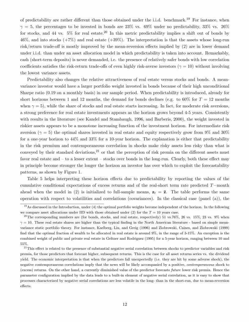
of predictability are rather different than those obtained under the i.i.d. benchmark.19 For instance, when

γ = 5, the percentages to be invested in bonds are 23% vs. 69% under no predictability, 33% vs. 26%

for stocks, and 44 vs. 5% for real estate.20 In this metric predictability implies a shift out of bonds by

46%, and into stocks (+7%) and real estate (+39%). The interpretation is that the assets whose long-run

risk/return trade-off is mostly improved by the mean-reversion effects implied by (2) are in lower demand

under i.i.d. than under an asset allocation model in which predictability is taken into account. Remarkably,

cash (short-term deposits) is never demanded, i.e. the presence of relatively safer bonds with low correlation

coefficients satisfies the risk-return trade-offs of even highly risk-averse investors (γ = 10) without involving

the lowest variance assets.

Predictability also changes the relative attractiveness of real estate versus stocks and bonds. A mean-

variance investor would have a larger portfolio weight invested in bonds because of their high unconditional

Sharpe ratio (0.19 on a monthly basis) in our sample period. When predictability is introduced, already for

short horizons between 1 and 12 months, the demand for bonds declines (e.g. to 60% for T = 12 months

when γ = 5), while the share of stocks and real estate starts increasing. In fact, for moderate risk aversions,

a strong preference for real estate investments appears as the horizon grows beyond 4-5 years. Consistently

with results in the literature (see Kandel and Stambaugh, 1996, and Barberis, 2000), the weight invested in

riskier assets appears to be a monotone increasing function of the investment horizon. For intermediate risk

aversion (γ = 5) the optimal shares invested in real estate and equity respectively grow from 9% and 30%

for a one-year horizon to 44% and 33% for a 10-year horizon. The explanation is either that predictability

in the risk premium and contemporaneous correlation in shocks make risky assets less risky than what is

conveyed by their standard deviations,21 or that the perception of risk premia on the different assets must

favor real estate and — to a lesser extent — stocks over bonds in the long-run. Clearly, both these effect may

in principle become stronger the longer the horizon an investor has over which to exploit the forecastability

patterns, as shown by Figure 1.

Table 5 helps interpreting these horizon effects due to predictability by reporting the values of the

cumulative conditional expectations of excess returns and of the real-short term rate predicted T−monthahead when the model in (2) is initialized to full-sample means, zt = z. The table performs the same

operation with respect to volatilities and correlations (covariances). In the classical case (panel (a)), the

19As discussed in the Introduction, under (4) the optimal portfolio weights become independent of the horizon. In the following

we compare asset allocations under IID with those obtained under (2) for the T = 10 years case.20The corresponding numbers are (for bonds, stocks, and real estate, respectively) 51 vs.76%, 26 vs. 15%, 23 vs. 9% when

γ = 10. These real estate shares are higher than the typical finding in the North American literature - based on simple mean-

variance static portfolio theory. For instance, Karlberg, Liu, and Greig (1996) and Ziobrowski, Caines, and Ziobrowski (1999)

find that the optimal fraction of wealth to be allocated in real estate is around 9%, in the range of 3-15%. An exception is the

combined weight of public and private real estate in Geltner and Rodriguez (1995) for a 5-year horizon, ranging between 10 and

55%.21This effect is related to the presence of substantial negative serial correlation between shocks to predictor variables and risk

premia, for those predictors that forecast higher, subsequent returns. This is the case for all asset returns series vs. the dividend

yield. The economic interpretation is that when the predictors fall unexpectedly (i.e. they are hit by some adverse shock), the

negative contemporaneous correlations imply that the news will be likely accompanied by a positive, contemporaneous shock to

(excess) returns. On the other hand, a currently diminished value of the predictor forecasts future lower risk premia. Hence the

parameter configuration implied by the data leads to a built-in element of negative serial correlation, as it is easy to show that

processes characterized by negative serial correlations are less volatile in the long- than in the short-run, due to mean-reversion

effects.

12

formulas employed are the standard ones for sums of (conditionally) multivariate normal returns (T ≥ 1):

Et

"TX

k=1

zt+k

#= Tμ+ (T − 1)Φμ+ (T − 2)Φ2μ+ ...+ΦT−1μ+ (Φ+Φ2 + ...+ΦT )zt−1

V art

"TX

k=1

zt+k

#= Σ+ (I+Φ)Σ(I+Φ)0+(I+Φ+Φ2)Σ(I+Φ+Φ2)0+

...+(I+Φ+ ...+ΦT−1)Σ(I+Φ+ ...+ΦT−1)0,

where I is the identity matrix of dimension n and Φk ≡Qk

i=1Φ.22 For comparison, panel (b) reports

moments under the null of no predictability, i.e. when

Et

"TX

k=1

zt+k

#= Tμ V art

"TX

k=1

zt+k

#= TΣ.

Therefore the table reports the “term structure” of the reward-to-risk trade-off, in the sense recently stressed

by Guidolin and Timmermann (2006) and Campbell and Viceira (2005). Careful inspection of the table

reveals that the horizon effects in portfolio weights previously reported cannot be explained by changing,

time-varying volatility: the annualized variance of excess real estate returns grows with the horizon much

faster in the presence of predictability, as effects associated with inflation and the short-term real rate produce

mean aversion in real estate returns. For instance, at a 10-year horizon, real estate volatility is 64% (i.e.

20% per year) under (2) vs. 39% (12% per year) in a misspecified IID framework. On the contrary, the

risk of stocks grows considerably slower than what would happen in the absence of predictability, consistent

with mean reverting stock returns. Thus, the predicted volatility of cumulative excess real estate returns is

larger than the volatility of excess stock returns for horizons exceeding 2 years.23 Furthermore, conditional

correlations between long-term bonds and real estate cumulative excess returns increase from 0.18 to 0.60

(they are constant vs. T in the no-predictability case). On the opposite, the correlation between bonds and

stocks remains below 0.15 despite an increasing trend. Therefore it is unlikely that correlations involving

real estate excess returns may explain the steep upward sloping schedule found in the case of intermediate

risk aversion (γ = 5).24

As a matter of fact, Table 5 shows that the horizon effects in portfolio weights can be traced back to

forecasts of future long-run risk premia that are steeply increasing in the time horizon for real estate and

— to a lesser extent — for equities. The expected 1-month risk premia implied by (2) are approximately

equal for stocks and real estate (at roughly 5% per annum), while the 10-year cumulative conditional risk

premium on real estate (9.9% per annum) exceeds the equity premium (6.8% per annum). Real estate is

simply anticipated to provide higher excess returns over long-horizons. This effect explains why the upward

sloping shape for real estate is also found for highly risk averse investors (γ = 10), although in this case

22In the Bayesian case (panel (c)), we use the simulation method described in Appendix A to obtain long-horizon returns and

approximate risk premia, variances, and covariances simply by computing these moments over a large numbers of Monte Carlo

trials (N = 300, 000). These results are described in Section 4.2.23The real short term rate is strongly mean averting, i.e. rolling over 1-month deposits is much riskier in the long run than it

is in the short run.24The correlation between real estate excess returns and real short-term rate subtiantially drops (from -0.03 to -0.84) as T

increases. However, the same patterns can be observed for stocks and especially bonds. Moreover, correlation patters are the

more important, the more the assets involved are volatile, which is hardly the case for 1-month cash deposits.

13

the equity portfolio share remains higher than the real estate share at all horizons. Overall, it seems that

ignoring predictability altogether would lead to grossly inappropriate asset allocations, with the bias growing

with the investment horizon. Section 5.1 further investigates the welfare losses resulting from disregarding

predictability.

Finally, Figure 1 shows another key result: the optimal allocation to bonds is generally monotone de-

creasing with T . This is explained by the statistical properties of the vector zt in Table 3. In particular,

notice that bonds display a negligible covariance with the dividend yield (with correlation of −0.15 only).This means that news affecting the dividend yield will essentially leave current, realized bond returns un-

changed and forecast future changes in risk premia of the opposite sign as the news. Therefore bonds will be

characterized by a variance that grows approximately as a linear function of T . Combined with increasing

correlations with both stocks and real estate (see Table 5, panels (a) and (c)), this makes bonds increasingly

riskier — relative to stocks and real estate — as the horizon lengthens. At the same time, cumulative bond

excess returns fail to increase as fast as those on real estate, thus reducing the relative attractiveness of

bonds especially for the least risk averse investors, like in the upper panel of Figure 1.

In conclusion, a classical analysis implies that real estate ought to have an important role in buy-and-

hold portfolio choices. Depending on the assumed coefficient of relative risk aversion, we have found optimal

long-run real estate weights between 23 and 44 percent of the available wealth for sensible risk aversion

parameters. Predictability makes demand schedules for the most risky assets a monotone increasing function

of the investment horizon and makes real estate more attractive than stocks as the horizon grows.

4.2. Parameter Uncertainty

We calculate optimal portfolios for the case in which the investor adopts a Bayesian approach. Figure 2

reports portfolio weights as a function of T . The effects of estimation risk manifest themselves with varying

intensity at two levels. The first major difference obtains for T ≥ 4 years, and consists in the appearance ofpositive weights invested in short-term deposits, as much as 45% for high risk aversion. Indeed, a strategy

that roll over “cash” investments is not only the safest among the available assets in terms of its overall

variance, but also the one that remains predictable with high precision from its own lagged value, the term

premium as well as the inflation rate. As a matter of fact, the volatility of such a strategy does increase

in T (see Table 5, panel (c)), as the mean averting effect induced by persistence is stronger than the mean

reversion induced by links with both inflation and the term premium. However it remains as small as 31%

(i.e. 3.1% per annum) for T = 10; this is almost four times smaller than long-term bonds, and 7 to 9

times smaller than real estate and equities. Therefore — even if the real short term rate becomes risky in

our framework and overall risk is non-negligible over long horizons — short term deposits preserve their role

of safe assets in relative terms. This is a strong incentive to risk-averse investors to develop a substantial

demand for short-term deposits, especially in the long-run.25

On the other hand, important modifications occur in the structure of the investment schedules as a

function of the horizon: while a classical investor will be characterized by weights to riskier assets increasing

with the investment horizon, when parameter uncertainty is taken into account the schedule for real estate

becomes flatter and that for stocks non-monotonic. For instance, when γ = 5 the allocation to real estate

25Notice that a strategy rolling over short-term deposits yields only 1.9% per annum over a 10-year horizon. Such a cumulative

return is actually inferior to the one that would be made under no predictability (3.3% per annum).

14

increases from 9% at 1-month to 16% at 10 years, while the allocation to stocks decreases from 23% to 20%

and describes an S-shaped behavior. When γ = 10, the equity demand schedule turns essentially monotone

decreasing. These flattening effects concerning the portfolio share schedules of the riskier assets is well

explained by the fact that the uncertainty deriving from estimation risk compounds over time, implying that

the difficulty to predict is magnified over longer planning periods. This means that the contrasting effects of

the reduction in long-run risk resulting from predictability − which would cause the investment schedules tobe upward sloping − and of estimation risk roughly cancel out for a long-horizon investor, with the result ofeither flat or weakly monotonically decreasing schedules. For instance, the cumulative excess equity return

volatility for a long-horizon investor is 283% (84% per annum), while the corresponding perceived volatility

is 214% for real estate excess returns (68% per annum). These numbers can be contrasted both to perceived

volatilities at shorter horizons (e.g. they are both 16% for T = 2 years) and to the long-run perceived

volatility of long-term bonds (37% per annum), which in fact attract a considerable share when parameter

uncertainty is accounted for.

We provide a measure of the importance of predictability under parameter uncertainty by calculating

optimal portfolio weights under the no-predictability benchmark (4), thus quantifying the effects of parameter

uncertainty alone on optimal portfolio weights.26 Figure 3 displays results through the usual set of plots.

Without predictability but with parameter uncertainty, the investment schedules for both stocks and real

estate are slightly monotonically decreasing, because estimation risk is compounded and magnified by longer

and longer investment horizons. Interestingly, the demand for cash is completely absent, also for investors

with high risk aversion. Moreover, the bond investment schedules turn now upward sloping, which confirms

that there exists a differential of estimation risk that favors bonds over riskier instruments. Comparing

Figures 2 and 3, predictability appears to induce several changes. There is a change in the slope of the demand

for bonds, which becomes decreasing in the investor horizon, and a positive demand for cash investments

appears. Furthermore, the real estate weight is equal to or exceeds the equity weight at all investment horizons

and for all risk aversion parameters, when predictability is ignored in Figure 3. On the contrary, investment

in stocks exceeds that in real estate for horizons shorter than 6 years when predictability is considered in

Figure 2. Finally, the portfolio shares allocated to the riskier assets are considerably lower when predictability

is accounted for. This is consistent with larger degrees of parameter uncertainty plaguing the VAR model (2)

vs. the IID. one (4), with high posterior standard errors characterizing many of the coefficients concerning

real estate and excess equity returns.

In conclusion, adding parameter uncertainty to the asset allocation problem changes a few of the results

found in Section 4.1, but leaves the overall picture intact: real estate is an important class that − whenpredictability is measured and put to use through a Bayesian approach− ought to receive an optimal long-runweight between 12 and 16%, depending on the assumed coefficient of relative risk-aversion.

5. Welfare Cost Analysis

Even though Section 4 has provided evidence that real estate enters optimal long-run portfolios with non-

negligible weights when asset returns are predictable, and that predictability affects portfolio weights, it

remains important to evaluate the effects of real estate on the expected utility of an investor. Therefore

we follow and Guidolin and Timmermann (2005), and obtain estimates of the welfare cost of restricting the

26Details on the posterior distribution of the coefficients are available upon request.

15

problem in both the breadth of the asset menu and the richness of the statistical model used to describe the

multivariate process of asset returns.

Call ωRt the vector of portfolio weights obtained imposing restrictions on the problem. For instance,

ωRt may be the vector of optimal asset demands when the investor is precluded from investing in real

estate. Define V (Wt, zt; ωt) the optimal value function of the unconstrained problem, and V (Wt, zt; ωRt ) the

constrained value function. Since a restricted model is by construction a special case of the unrestricted

model:

V (Wt, zt; ωRt ) ≤ V (Wt, zt; ωt).

We compute the compensatory premium, πRt , that an investor with relative risk aversion coefficient γ is

willing to pay to obtain the same expected utility from the constrained and unconstrained problems as:

πRt =

∙V (Wt, zt; ωt)

V (Wt, zt; ωRt )

¸ 11−γ− 1. (5)

The interpretation is that an investor endowed with an initial wealth of (1 + πRt ) would tolerate to be

constrained to solve a restricted problem For simplicity, we only consider simple buy-and-hold strategies

that provide lower bounds to the implied welfare costs, see e.g. Guidolin and Timmermann (2005).27

5.1. Cost of Ignoring Predictability

We first calculate the πRt implied by forcing an investor to ignore predictability altogether, i.e. to pretend

that (4) is correctly specified. As observed in Section 4, this would lead to ‘incorrect’ portfolio choices. We

present the annualized percentage compensation that an investor would require to ignore the evidence of

predictability in Figure 4. In particular, panel (a) refers to the classical case. The implied welfare costs

from model misspecifications are higher the higher is γ. The implied annualized welfare costs are far from

negligible, and in the case of long-horizon investors with moderate risk aversion they range between 2 and 4

percent in riskless, annualized terms. Predictability is clearly most useful to a short horizon investor, that

is able to time the market. Thus, the annualized cost of disregarding it tops 12% for T = 1 month. This

means that a rational investor with γ = 5 would require a (riskless) annual increase in the returns generated

by her portfolio in the order of approximately up to 95 basis points, for him to accept portfolio decisions

based on a misspecified IID model that disregards predictability altogether.

Panel (b) of Figure 4 presents results for the Bayesian portfolio choice case, when estimation risk is

incorporated in optimal decisions. For long horizons, the implied utility loss is slightly lower. The reasons of

the lower utility losses under parameter uncertainty are related to the fact that for large T portfolio choices

imply substantial cash investments that are not found when predictability is ignored. On the contrary, in

the classical case departures from the IID benchmark involve a higher demand for more profitable assets

- especially real estate. All in all, we interpret the evidence in Figure 4 as consistent with the idea that

ignoring predictability is associated with welfare losses of substantial magnitude.

27Under rebalancing (see Section 6.2) predictability gives an investor a chance to aggressively act upon the information on

zt; therefore ignoring predictability when rebalancing is possible implies higher utility costs. A similar reasoning applies to

restrictions on the asset menu: depriving investors of useful assets hurts them the most the highest is the frequency with which

they can switch in and out of the assets themselves.

16

5.2. Cost of Excluding Real Estate

The recent growth of the real estate fund market in several continental European countries is likely to provide

institutional investors with increasing possibilities to access this asset class. Here we offer an estimate of the

welfare gains brought about by this development. Given that ignoring predictability is suboptimal, especially

when estimation risk is taken into account, we estimate the welfare costs of ignoring real estate investment

opportunities when the investor exploits predictability.

As a first step, Table 6 presents classical MLE estimates for the case in which the asset menu is limited

to stock, bonds, and short term deposits. In a restricted asset menu, the evidence of predictability remains

strong especially for excess stock returns, that can be precisely predicted by the dividend yield, inflation and

lagged stock returns. The left column of plots in Figure 5 shows ‘classical’ asset allocation results under this

restricted asset menu. Results are consistent with the general patterns isolated in Section 4: the demand for

stocks increases with the investment horizon as their riskiness declines thanks to their predictability; on the

opposite, the bond investment schedule is downward sloping. There is no demand for cash independently of

the degree of relative risk aversion. Real estate therefore crowds out stocks at longer investment horizons,

because of its higher profitability.

Figure 6, panel (a), shows the implied welfare costs from excluding real estate from the portfolio problem.

Also in this case, we report the annualized, riskless compensation that an investor would require to make

portfolio decisions using a restricted asset menu. The welfare cost of excluding real estate from the asset

menu is not monotone increasing in the coefficient of risk aversion: the compensatory variation is the highest

at short investment horizons for intermediate risk aversion. This is intuitive as predictability is relatively

strong at short horizons, and it will be more risk-tolerant investors who will better exploit it. For highly risk

averse investors the compensatory variation is instead highest at long horizons, because it mostly reflects

foregone diversification opportunities. In other words, the welfare gains from accessing real estate originate

from improvement in both diversification and predictability. In the case of moderate risk aversion (γ = 5)

the welfare loss at a short horizon of one year only is approximately equal to 7 percent of initial wealth. The

yearly welfare loss naturally declines with T, although this implies that a roughly constant portion of initial

wealth would be sacrificed to obtain the possibility to invest in real estate. For instance, the annualized

riskless compensatory variation is 73 basis points per year at T = 10 years, although this corresponds to a

7.5 percent of time t wealth. Such figure more than doubles if one considers a highly risk-averse investor

under a 10-year horizon. This means that, especially under long planning horizons, including real estate in

the asset menu should represent a primary concern for all portfolio managers.

Table 7 and Figures 5-6 complete the picture by reporting results for the case in which parameter

uncertainty is kept into consideration. Table 7 gives Bayesian posterior means and standard deviations for

the restricted VAR model that excludes real estate excess returns. Posterior means are very close to MLE

estimates, and standard errors confirm the results in Table 6: the evidence of predictability is once more

particularly strong for excess stock returns and the real short term rate. Figure 5 plots instead optimal

asset allocations and obtains differences between classical and Bayesian portfolio weights consistent with

our comments in Section 4: positive weights on liquid investments appear under parameter uncertainty,

as a protective measure against the additional estimation risk deriving from the fact the coefficients are

perceived to be random. Moreover, while the equity investment schedule is generally upward sloping in

a classical framework (an effect of predictability), the Bayesian allocation to stocks tends to decline with

17

the investment horizon. Finally, Figure 6 displays the annualized percentage compensatory variation from

excluding real estate from the asset menu. In this case, results are different from the classical ones, i.e.

the loss from ignoring real estate remains below 5 percent per year for either highly risk-averse and/or for

long-horizon investors. This is because the real estate portfolio share, and hence its potential for enhancing

returns and lowering risk, is modest, at least when compared to the classical case.

6. Robustness Checks

We conclude by performing a number of additional exercises to corroborate our results and show that they

scarcely depend on specific assumptions concerning the coefficient of relative risk aversion, how the state

variables are initialized, the frequency with which portfolio re-shuffling is admitted, and the measurement

of the welfare loss implied by solving ‘standard’ portfolio problems in which the predictable nature of risk

premia is ignored and the attention is focused on a standard mean-variance benchmark. For all experiments,

wherever results are not fully reported in the paper, further details are available upon request.

6.1. Low Risk Aversion

Although the equity premium literature points to the use of relatively high relative risk aversion in portfolio

choice applications (such as γ = 5, 10), part of the literature (e.g. Brennan, Schwartz and Lagnado (1997)

and Barberis (2000)) has experimented with lower coefficients, typically γ = 2. Figure 7 reports a few results

under this assumption, focussing on the simple case of a buy-and-hold investor. The two panels of the figure

show that not only our results on the importance of real estate as an asset class are robust to using lower risk

aversion levels, but also that as a matter of fact a relative risk-insensitive investor ought to aggressively invest

in real estate, thus exploiting its high Sharpe ratio. For instance, a long run classic portfolio optimizer (panel

(a)) ought to invest 88% in real estate, 12% in stocks, and nothing in bonds. When parameter uncertainty is

taken into account (panel (b)), the structure of portfolio weights is not radically changed at short horizons;

for instance, the 1-month allocation is identical to the one derived ignoring parameter uncertainty as an

investor who is not strongly risk averse will not be greatly affected by additional estimation risk. The

10-year Bayesian allocation is instead 45% in real estate, 24% in stocks, and 31% in bonds, closer to an

equally-weighted portfolio. In any event, under low risk aversion, it is clear that real estate plays a much

bigger role, with weights above 30 percent for horizons longer than two years.

6.2. Sensitivity of Optimal Weights to the Predictors

With limited exceptions, all of our simulation experiments have been based on initializing the variables with

a strong predictive content (i.e. the dividend yield, the term spread, the inflation rate, and the 1-month real

rate) to their full-sample means (see Table 1). Under this assumption, we have found that under predictable

risk premia, real estate represents an important asset class in optimal long-run portfolios. However, it

is natural to ask whether this conclusion is robust to different assumptions concerning the starting value

assigned to the predictors in our simulations, especially because Table 1 implies that a wide range of values

for the term spread (between -0.015 and 0.033 on a yearly basis) and the dividend yield (between 1.74 and

18

3.76 percent in annualized terms) have to be considered ‘plausible’ as they fall in a 90% confidence interval.28

Figure 8 plots the resulting optimal asset allocation choices as the initial values of the predictors are changed

over a wide range of possible initial values in simulation experiments. In each experiment, we set the values

of all variables in the model (2) to correspond to their sample means and change the target predictor variable

over a wide range of values. For each predictor variable, two exercises are performed, in correspondence to

a short (T = 12) vs. a long (T = 120) horizon. To simplify calculations, we only report classical results that

ignore parameter uncertainty. The qualitative insights are similar for the Bayesian case.

Over short horizons, real estate optimal portfolio holdings are scarcely sensitive to the starting value of

the dividend yield (apart from the sub-interval 1.3 - 1.8%, characterized by very low dividend yields), while

they are strongly monotonically decreasing in the value for the term spread, the inflation rate, and the real

short term rate. This finding matches the negative signs of the coefficients on these three predictors in the

MLE results reported in Table 3: higher values of the predictors forecast lower real estate risk premia over

horizons of 1 year or less. In particular, the effect is quantitatively strong for the term spread and the inflation

rate, implying that over short intervals, real estate presents a risk-return trade-off which is (comparatively)

worsened by both increasing inflation and by a steepening yield curve. Consistent with standard intuition,

the investment in real estate declines as real interest rates grow, also because short-term deposits represent

a competing asset class. Over a 10-year horizon, the real estate holdings are strongly increasing in both

the real short and the inflation rates. The latter finding may be interpreted as a consequence of the ability

of real estate to offer a long-term hedge against inflation: the slope of the real estate demand curve is

particularly steep when current inflation moves from very low (0.2% a year) to intermediate levels (2.1%).

All in all, unless one focuses on rather extreme configurations (of zero inflation, negative real interest rates,

and inverted yield curve) of the economic predictors, we obtain again that the real estate weight is always is

approximately 20 percent, while values of the predictors exist for which the weight approaches 40 percent.

Over short horizons, the sensitivity patterns of equity holdings to changes of the predictors is similar to

real estate, although the equity schedules are generally flatter. In the long-run however, the equity holdings

behave rather differently than real estate: they monotonically increase in the dividend yield, and they

strongly decrease in the term spread, the real short term rate, and inflation. The first two results illustrate

the standard logic that an increasing real cost of capital (especially as measured by long-term interest rates)

forecasts declining firm values and therefore an adverse risk-return trade-off for equities. The shape of the

schedule as a function of inflation stresses that stocks are hardly a good long-term hedge against inflation,

to the point that a rational long-run investor progressively reduces the equity weight as current inflation

increases and anticipating (notice that inflation is a persistent process) future, higher inflation.

Finally, the schedules characterizing bonds are opposite to those for real estate and equity over a one-year

horizon; in particular, they are strongly upward sloping as a function of the term spread, the real short rate,

and inflation. While the first two findings are hardly surprising — even ignoring predictability, it is clear

that increasing real short term rates (given the shape of the yield curve) or a steeper term structure (given

the short real rate) increase the expected return on long-term bonds — the sensitivity to inflation shows that

over short horizons it is bonds that manage to provide the best protection against inflation. This means

that already in the first year following an inflation shock the returns to a basket of constant maturity bonds

suffer of the inflation shock less than equities and real estate do. However, for long-horizon investors, bond

28The range of plausible values is narrower for the inflation rate (from 2.12 to 3.08 percent) and real short term rate (from

2.44 to 4.36 percent), both in annualized terms.

19

holdings are generally flat and display moderate sensitivity to the predictors.

6.3. Dynamic Rebalancing

An investor who follows a buy-and-hold strategy chooses the optimal allocation at the beginning of the

planning horizon (t) and does not modify it until the end-point (t + T ) is reached. Clearly, when T is

large, this represents a strong commitment not to revise the portfolio weights despite the receipt of news

characterizing the investment opportunity set. Under a rebalancing strategy, the investor chooses the asset

allocation at the beginning of the planning horizon taking into account that it shall be optimal to modify

the portfolio weights at intermediate dates (rebalancing points), t+ ϕ, t+ 2ϕ, ..., t+ T − ϕ. Appendix A.3

reports details on the implied dynamic programming problem and related solution methods.

We assess the effects of dynamic rebalancing by computing portfolio allocations when adjustment to the

allocation is admitted every year. Initially, we use J = 6 discretization points for each of the predictor

variables employed in our study. For simplicity, we ignore parameter uncertainty. Also in this case to obtain

a “representative” calibration, we set the predictors to their full-sample means. Panel (a) of Figure 9 shows

optimal portfolio weights as a function of the investment horizon when the coefficient of relative risk aversion

(γ) is set to 5. A comparison with Figure 1 reveals two important changes. First, rebalancing flattens the

portfolio investment schedules for horizons T exceeding the rebalancing frequency ϕ. Careful analysis of the

plots reveals that differences between optimal weights at T = 4 and at T = 10 years are negligible. This

makes sense as two investors with either a four or a ten-year horizon who anticipate unrestricted changes to

their optimal portfolios in only 12 months are unlikely to drastically differ in their current portfolio choices.

The fact that rebalancing tends to flatten optimal investment schedules for T >> ϕ has been observed already

by Brandt (1999) and Guidolin and Timmermann (2004, 2005) in related applications. Second, differences

between the rebalancing and buy-and-hold cases are modest but visible: rebalancing opportunities tend to

increase the long-run optimal weight of stocks and bonds, while reducing the weight of real estate.29 Overall,

setting the predictors to their sample means may suggest some caution to a rational investor, who then

waits for an improvement in the investment opportunities by going longer in the relatively safe (especially

over a relatively short period) bonds. In general, even when rebalancing is admitted, real estate remains

an important asset class, receiving a weight always in excess of 20% for all horizons that exceed the annual

rebalancing frequency.

Panel (b) of Figure 9 reports the results of robustness checks that use J = 12 grid points to achieve a

higher degree of discretization accuracy. Since double-digit values of J translate into millions of combined

discretization points (their number equals Jn), in this case we fix the value of excess asset returns and of

the term premium to their sample means and simply discretize the support of the dividend yield, the real

short term rate, and of inflation (for a total of 123 = 1, 728 discretization points).30 The results on portfolio

weights are qualitatively identical to those in panel (a) and confirm that real estate plays an important role

in long-run portfolio choices even assuming that regular rebalancing is admitted.

29For instance, at T = 10 years, the optimal weights in real estate under rebalancing is 36% (vs. 44% under no buy and hold)

while the weights of stocks and bonds are 35 and 29% (vs. 33 and 23% under buy and hold).30Fixing the term premium to its mean is clearly arbitrary and we justify this choice on the basis of the weak predictability

results involving this instrument in Table 3. Further robustness checks with a 2-year horizon but 125 = 248, 832 grid points

(i.e. in which the term premium and excess real estate returns are discretized as well) confirm that our insights are qualitatively

robust.

20

6.4. Welfare Costs of Excluding Real Estate Under Constant Investment Opportunities

In Section 5 the long-run welfare costs of ignoring predictability exceeds 200 basis points per year, i.e. a

rational investor should request a riskless increase in returns of the order of 2 percent a year, or more. A

similar result was obtained for the compensatory variation that should be required to ignore real estate as an

asset class in addition to stocks, bonds, and cash. However, this last estimate has been obtained assuming

that predictability should and would not be ignored by a rational portfolio manager. Even though the

statistical evidence in favor of the existence of predictability patterns in mean excess returns is strong and a

welfare cost exceeding 2% a year ought to be a major incentive for investors not to ignore predictability, it

remains interesting to repeat the calculations of Section 5 when predictability is ignored and excess returns

are generated by the simple model (4).

In the classical case, we obtain a picture that is very similar to figure 4(a): in the long-run, the cost of

excluding real estate grows with the coefficient of risk aversion; for long-run investor with γ = 5, the cost is

in the order of 240 basis points a year, and this estimate grows to exceed 400 basis points when γ = 10 is

considered. This implies that the cost of ignoring real estate scarcely depends on the whether predictability

is modeled or not, although it is clear that the welfare gains from doing so remain substantial.

Similar calculations are performed in the Bayesian case. We find that welfare costs of ignoring real

estate are actually higher when predictability is ignored altogether.31 In fact, Figure 3 has shown that the

optimal real estate weight is higher by 10-15 percent vs. the case in which predictability is taken into account

(Figure 2). This is easily explained by the fact that real estate excess returns were characterized by weaker

predictability patterns than stocks so that the demand for real estate is hurt.32 In this sense, restricting

our exercise to the case of i.i.d. excess asset returns may bring − when parameter uncertainty is taken intoaccount − to a higher estimate of the utility loss deriving from ignoring real estate. In conclusion, the welfarelosses reported and discussed in Section 5 represent a lower bound for the utility costs of omitting real estate

when choosing optimal European portfolios.

7. Conclusions

In this paper we have documented the existence of linear predictability patterns − described by a simpleVAR(1) framework − in an asset menu that involves both financial and real estate excess returns. In

particular, excess stock and bond returns predict subsequent real estate excess returns. Moreover, real

estate performance is negatively related to the lagged short term real rate and to past inflation, while the

dividend yield has predictive power for all excess return series and the real one-month T-bill. These facts

cause the risk-return trade-off characterizing real estate to improve as the investment horizon lengthens,

in the sense that its expected annualized risk premia grows even faster. As a result, when we calculate

optimal portfolio weights based on the MLE estimates of the VAR coefficients, we find portfolio weights

for real estate that are increasing in the planning horizon. Stocks, bonds, and real estate do not appear

excessively risky (once their risk premia are taken into account) to a long-run investor, so that the demand

for cash is rather limited or even absent. These findings are qualitatively robust to the adoption of a Bayesian

approach that incorporates estimation risk into the formal portfolio problem, although the trade-off between

31For instance, assuming γ = 5, the cost for a 10-year horizon investor exceeds 310 basis points a year.32For instance, in Table 3 the coefficients with which real excess returns load on lagged dividend yields and inflation rates are

characterized by sensibly lower t-ratios.

21

predictability and parameter uncertainty makes for flatter — often non-monotonic — investment schedules,

while at the longest horizon some demand for short-term deposits appears. Finally, real estate appears as a

poor instrument to cover inflation risk in the short run, while in the long run it is the best inflation hedge

as suggested by its long run optimal portfolio share being strongly upward sloping in the current rate of

inflation.

We find that real estate should play a considerable role, both in terms of portfolio weights and in welfare

terms: the compensatory variation required by an investor to do without real estate is easily in excess of 200

basis points per year. This conclusion echoes recent findings by Chun Sa-Aadu and Shilling (2004) on the

asset pricing properties of real estate. Although the welfare costs deriving from ignoring predictability would

be of similar importance, the conclusions above concerning the utility loss from expelling real estate from the

asset menu do not depend on the finding of predictability. As a matter of fact, our robustness checks suggest

that our estimates for the optimal real estate weights and welfare losses from restricting the asset menu are

probably only a lower bound for higher estimates obtainable under alternative assumptions. It would be

interesting to perform some of the calculations in this paper using indirect indices, that traditionally imply

a much smaller correlation with stock and bond returns and hence offer greater diversification opportunities.

The observed divergence in asset holdings of European pension funds mentioned in the Introduction can

be dictated by institutional reasons. However, our paper implies that preferences and horizons exist that

justify both the British and the continental European patterns. In particular, the German-French pattern

is consistent with the rational choices of portfolio managers that display high risk aversion, worry about

estimation risk, and have investment horizons between 1 and 4 years. On the contrary, investing four-fifths

of one’s wealth in (highly) risky assets − as in the Anglo-Saxon pattern − may be optimal for long-horizoninvestors with low risk aversion and who disregard parameter uncertainty. However, in this case real estate

ought to receive a weight at least as important as stocks, which is not the case in practice. This can be due to

our consideration of stock-based indices, while most European institutions routinely confine their portfolios

to real property. While this observation calls for replicating this analysis on indirect indices, it should be

stressed that developments in the real estate funds industry justify our current choice.

There are many issues that this paper merely touches upon. In particular, we have ignored transaction

costs. On one hand, this is consistent with our use of an indirect real estate index based on the market price of

the equity issued by companies involved in real estate operations: it makes sense to entertain the assumption

that the frictions associated in trading in these companies may not be structurally different from the market

average. Furthermore, even assuming that publicly-traded real estate vehicles imply higher transaction costs

than other securities, it is difficult to think that such a differential exceeds a full one-to-two percent of total

initial wealth of the investor. On the other hand, recent papers (e.g. Balduzzi and Lynch (1999)) have shown

how dynamic portfolio choices may be computed in the presence of transaction costs. Such an effort seems to

be particularly appropriate for addressing direct property investments. Finally, recent work by Hoevenaars,

Molenaar, Schotman, and Steenkamp (2005) reports a high welfare cost from ignoring liabilities when solving

the strategic asset allocation problem faced by institutional investors. Under the condition that real estate

holdings may be useful hedges against the interest rate and inflation risks of a given stock of liabilities, our

estimate of the utility loss from excluding real estate from portfolio choices may be biased downwards. We

leave these further explorations for future research.

22

References

[1] Avramov, D., 2002, “Stock Return Predictability and Model Uncertainty”, Journal of Financial Eco-

nomics, 64, 423-458

[2] Balduzzi, P., 1995, “Stock Returns, Inflation, and the ‘Proxy Hypothesis’: A New Look at the Data”,

Economics Letters, 48, 47-53.

[3] Balduzzi, P., and A., Lynch, 1999, “Transaction Costs and Predictability: Some Utility Cost Calcula-

tions”, Journal of Financial Economics, 52, 47-78.

[4] Barberis, N., 2000, “Investing for the Long Run When Returns Are Predictable”, Journal of Finance,

55, 225-64.

[5] Bharati, R., and M., Gupta, 1992, “Asset Allocation and Predictability of Real Estate Returns”, Journal

of Real Estate Research, 7, 469-484.

[6] Black, A., and P., Fraser, 1995, “U.K. Stock Returns: Predictability and Business Conditions”,

Manchester School, 63, 85-102.

[7] Bodie, Z., 1995, “On the Risk of Stocks in the Long Run”, Financial Analysts Journal, 51, 18-22.

[8] Brandt, M., 1999, “Estimating Portfolio and Consumption Choice: A Conditional Euler Equations

Approach”, Journal of Finance, 54, 1609-1645.

[9] Brennan, M., E., Schwartz, and R., Lagnado, 1997, “Strategic Asset Allocation”, Journal of Economic

Dynamics and Control, 21, 1377-1403.

[10] Brounen, D., and P., Eicholtz, 2003, “Property, Common Stock and Property Shares”, Journal of

Portfolio Management, Special Issue, 129-137.

[11] Campbell, J., Y., Chan, and L., Viceira, 2003, “A Multivariate Model of Strategic Asset Allocation”,

Journal of Financial Economics, 67, 41-80.

[12] Campbell, J., and R., Shiller, 1988, “Stock Prices, Earnings, and Expected Dividends”, Journal of

Finance, 43, 661-676.

[13] Campbell, J., and L., Viceira, 1999, “Consumption and Portfolio Decisions When Expected Returns

Are Time Varying”, Quarterly Journal of Economics, 114, 433-495.

[14] Campbell, J., and L., Viceira, 2005, “The Term Structure of the Risk-Return Tradeoff”, Financial

Analysts Journal, 61, 34-44 .

[15] Chandrashakaran, V., 1999, “The Time Series Properties and Diversification Benefits of REIT Returns”,

Journal of Real Estate Research, 17, 91-112.

[16] Chun, G., J., Sa-Aadu, and J., Shilling, 2004, “The Role of Real Estate in an Institutional Investor’s

Portfolio Revisited ”, Journal of Real Estate Finance and Economics, 29, 295-320.

23

[17] de Roon, F., P., Eichholtz, and K., Koedijk, 2002, “The Portfolio Implications of Home Ownership”,

CEPR discussion paper 3501.

[18] Fama, E., 1981, “Stock Returns, Real Activity, Inflation, and Money”, American Economic Review, 71,

201-231.

[19] Fama, E., and K., French, 1989, “Business Conditions and Expected Returns on Stocks and Bonds”,

Journal of Financial Economics, 25, 23-49.

[20] Fama, E., and G., Schwert, 1977, “Asset Returns and Inflation”, Journal of Financial Economics, 5,

115-146

[21] Flavin, M., and T., Yamashita, 2002, “Owner-Occupied Housing and the Consumption of the Household

Portfolio Over the Life Cycle”, American Economic Review, 92, 345-362.

[22] Froot, K., 1995, “Hedging Portfolios with Real Assets”, Journal of Portfolio Management, Summer,

60-77.

[23] Geltner, D., and J., Rodriguez, 1995, “The Similar Genetics of Public & Private Real Estate And the

Optimal Long-Horizon Portfolio Mix”, Real Estate Finance, 12, 71-81

[24] Geltner, D., and J., Mei, 1995, “The Present Value Model with Time-Varying Discount Rates: Impli-

cation for Commercial Property Valuation and Investment Decisions”, Journal of Real Estate Finance

and Economics, 11, 119-135.

[25] Glascock, J., C., Lu, and R., So, 2001, “Further Evidence on the Integration of REIT, Bond, and Stock

Returns”, Journal of Real Estate Finance and Economics, 20, 177-194.

[26] Gold, R., 1993, “Why the efficient frontier for real estate is ‘Fuzzy,”, Journal of Real Estate Portfolio

Management, 1, 59-66.

[27] Guidolin, M. and A., Timmermann, 2004, “Strategic Asset Allocation and Consumption Decisions under

Multivariate Regime Switching”, Federal Reserve Bank of St. Louis working paper No. 2005-002A.

[28] Guidolin, M. and A., Timmermann, 2005, “Economic Implications of Bull and Bear Regimes in UK

Stock and Bond Returns”, Economic Journal, 115, 111-143.

[29] Guidolin, M. and A., Timmermann, 2006, “Term Structure of Risk under Alternative Econometric

Specifications”, Journal of Econometrics, 131, 285-308.

[30] Hudson-Wilson, S., F., Fabozzi, and J., Gordon, 2003, “Why Real Estate? An Expanding Role for

Institutional Investors”, The Journal of Portfolio Management, Special Real Estate Issue.

[31] Hoevenaars R., R. Molenaar, P. Schotman, and T. Steenkamp, 2005, “Strategic Asset Allocation with

Liabilities: Beyond Stock and Bonds”, mimeo, Maastricht University.

[32] Hoevenaars R., R. Molenaar, P. Schotman, and T. Steenkamp, 2006, “Strategic Asset Allocation for

Long-Term Investors: Parameter Uncertainty and Prior Information”, mimeo, Maastricht University.

24

[33] Ibbotson, R., and L., Siegel, 1984, “Real Estate Returns: A Comparison with Other Investments”,

American Real Estate and Urban Economics Association Journal, 12, 219-242.

[34] Kandel, S., and R., Stambaugh, 1996, “On the Predictability of Stock Returns: An Asset-Allocation

Perspective”, Journal of Finance, 51, 385-424.

[35] Karlberg, J., C., Liu, and W., Greig, 1996, “The Role of Real Estate in the Portfolio Allocation Process”,

Real Estate Economics, 24, 359-377.

[36] Karolyi, G. A., and A. B., Sanders, (1998), “The Variation of Economic Risk Premiums in Real Estate

Returns”, Journal of Real Estate Financial Economics, 17, 245-262.

[37] Keim, D. and R., Stambaugh, 1986, “Predicting Returns in Stock and Bond Markets”, Journal of

Financial Economics, 17, 357-390.

[38] Li, Y., and K., Wang, 1995, “The Predictability of Real Estate Returns and Market Segmentation”,

Journal of Real Estate Research, 10, 471-482.

[39] Li, J., R., Mooradian and S., Yang, 2003, “Economic Forces, Asset Pricing, and REIT Returns”, mimeo,

Northeastern University.

[40] Liang, Y., N., Myer, and J., Webb, 1996, “The Boostrap Efficient Frontier for Mixed-Asset Portfolios”,

Real Estate Economics, 24, 247-256.

[41] Ling, D. C., A. Naranjo and M. D., Ryngaert (2000), “The Predictability of Equity REIT Returns: Time

Variation and Economic Significance”, Journal of Real Estate Finance and Economics, 20, 117-136.

[42] Liu, C., and J. Mei. (1992). “The Predictability of Returns on Equity REITs and Their Co-movement

with Other Assets”, Journal of Real Estate Financial Economics 5, 401- 418.

[43] Maurer R., F., Reiner, and S., Sebastian, 2004, “Characteristics of German Real Estate Return Dis-

tributions: Empirical Evidence from Germany and Comparison to the U.S. and U.K,” Working Paper

Series: Finance and Accounting 108, Department of Finance, Goethe University, Frankfurt.

[44] Merton, R., 1969, “Lifetime Portfolio Selection under Uncertainty: the Continuous Time Case”, Review

of Economics and Statistics, 51, 247-257.

[45] Miles D., 1996, Housing, Financial Markets and the Wider Economy, John Wiley.

[46] Pellizzon, L. and G., Weber, 2003, “Are Households Portfolios Efficient: An Analysis Conditional on

Housing”, mimeo, University of Padua.

[47] Pesaran, M. H. and A. Timmermann, 2000, “A Recursive Modelling Approach to Predicting UK Stock

Returns”, Economic Journal, 110, 646-668.

[48] Ritter, J., and R., Warr, 2002,“The Decline of Inflation and the Bull Market of 1982-1999”, Journal of

Financial and Quantitative Analysis, 37, 29-61.

[49] Ross, S., and R., Zisler, 1991, “Risk and Return in Real Estate”, Journal of Real Estate Finance and

Economics, 4, 175-190.

25

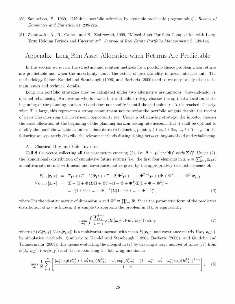
[50] Samuelson, P., 1969, “Lifetime portfolio selection by dynamic stochastic programming”, Review of

Economics and Statistics, 51, 239-246.

[51] Ziobrowski, A., R., Caines, and B., Ziobrowski, 1999, “Mixed-Asset Portfolio Composition with Long-

Term Holding Periods and Uncertainty”, Journal of Real Estate Portfolio Management, 2, 139-144.

Appendix: Long Run Asset Allocation when Returns Are Predictable

In this section we review the structure and solution methods for a portfolio choice problem when returns

are predictable and when the uncertainty about the extent of predictability is taken into account. The

methodology follows Kandel and Stambaugh (1996) and Barberis (2000) and so we only briefly discuss the

main issues and technical details.

Long run portfolio strategies may be calculated under two alternative assumptions: buy-and-hold vs.

optimal rebalancing. An investor who follows a buy-and-hold strategy chooses the optimal allocation at the

beginning of the planning horizon (t) and does not modify it until the end-point (t+ T ) is reached. Clearly,

when T is large, this represents a strong commitment not to revise the portfolio weights despite the receipt

of news characterizing the investment opportunity set. Under a rebalancing strategy, the investor chooses

the asset allocation at the beginning of the planning horizon taking into account that it shall be optimal to

modify the portfolio weights at intermediate dates (rebalancing points), t+ ϕ, t+ 2ϕ, ..., t+ T − ϕ. In the

following we separately describe the relevant methods distinguishing between buy-and-hold and rebalancing.

A1. Classical Buy-and-Hold Investor

Call θ the vector collecting all the parameters entering (2), i.e. θ ≡ [μ0 vec(Φ)0 vech(Σ)0]0. Under (2),the (conditional) distribution of cumulative future returns (i.e. the first four elements in zt,T ≡

PTk=1 zt+k)

is multivariate normal with mean and covariance matrix given by the appropriately selected elements of:

Et−1[zt,T ] = Tμ+ (T − 1)Φμ+ (T − 2)Φ2μ+ ...+ΦT−1μ+ (Φ+Φ2+...+ΦT )zt−1

V art−1[zt,T ] = Σ+ (I+Φ)Σ(I+Φ)0+(I+Φ+Φ2)Σ(I+Φ+Φ2)0+

...+(I+Φ+ ...+ΦT−1)Σ(I+Φ+ ...+ΦT−1)0, (6)

where I is the identity matrix of dimension n and Φk ≡Qk

i=1Φ. Since the parametric form of the predictive

distribution of zt,T is known, it is simple to approach the problem in (1), or equivalently

maxωt

ZW 1−γ

t+T

1− γφ (Et[zt,T ], V art[zt,T ]) · dzt,T (7)

where (φ (Et[zt,T ], V art[zt,T ]) is a multivariate normal with mean Et[zt,T ] and covariance matrix V art[zt,T ]),

by simulation methods. Similarly to Kandel and Stambaugh (1996), Barberis (2000), and Guidolin and

Timmermann (2005), this means evaluating the integral in (7) by drawing a large number of times (N) from

φ (Et[zt,T ], V art[zt,T ]) and then maximizing the following functional:

maxωt

1

N

NXi=1

"{ωst exp(R

s,it,T ) + ωbt exp(R

b,it,T ) + ωrt exp(R

r,it,T ) + (1− ωst − ωbt − ωrt ) exp(R

f,it,T )}1−γ

1− γ

#, (8)

26

where [Rs,it,T Rb,i

t,T Rr,it,T Rf,i

t,T ]0 represent the first four elements of zit,T along a sample path i = 1, ..., N. At

this stage, the portfolio weight non-negativity constraints are imposed by maximizing (8) using a simple

two-stage grid search algorithm that sets ωjt to 0, 0.01, 0.02, ..., 0.99, 0.9999 for j = s, b, r.

A2. Bayesian Buy-and-Hold Investor

Given the problem

maxωt

ZW 1−γ

t+T

1− γp(zt,T |Zt,θ)p(θ|Zt) · dzt,T ,

the task is somewhat simplified by the fact that predictive draws can be obtained by drawing from the

posterior distribution of the parameters and then, for each set of parameters drawn, by sampling one point

from the distribution of returns conditional on past data and the parameters. At this point, (2) can be

re-written as: ⎡⎢⎢⎢⎢⎣z02z03...

z0t

⎤⎥⎥⎥⎥⎦ =⎡⎢⎢⎢⎢⎣1 z011 z02...

...

1 z0t−1

⎤⎥⎥⎥⎥⎦"μ0

Φ0

#+

⎡⎢⎢⎢⎢⎣²02²03...

²0t

⎤⎥⎥⎥⎥⎦ ,or simply Z = XC+E, where Z is a (t−1, n+1) matrix with the observed vectors as rows, X is a (t−1, n+2)matrix of regressors, and E a (t−1, n+1) matrix of error terms, respectively. All the coefficients are insteadcollected in the (n+ 2, n+ 1) matrix C. If we consider the following standard uninformative diffuse prior:

p(C,Σ) ∝ |Σ|−n+22 ,

then the posterior distribution for the coefficients in θ, p(C,Σ−1|Zt) can be characterized as:

Σ−1|Zt ∼ Wishart(t− n− 2, S−1)vec(C)|Σ−1, Zt ∼ N

³vec(C),Σ⊗ (X0X)−1

´where S = (Z−XC)0(Z−XC) and C = (X0X)−1X0Z, i.e. the classical OLS estimators for the coefficientsand covariance matrix of the residuals.

Also for the Bayesian case, we adopt a simulation method that: First, draws N independent variates from

p(C,Σ−1|Zt). This is done by first sampling from a marginal Wishart for Σ−1 and then (after calculating

Σ) from the conditional N³vec(C),Σ⊗ (X0X)−1

´, where C is easily calculated. Second, for each set

(C,Σ) obtained, the algorithm samples cumulated returns from a multivariate normal with mean vector and

covariance matrix given by (6). Given the double simulation scheme, in this case N is set to a relatively

large value of 300,000 independent trials.

A3. Dynamic Rebalancing Strategies

The solution method is in this case based on standard dynamic programming principles and on a dis-

cretization of the state space. Divide the interval [t, T ] into B ≥ 1 intervals [t, t + ϕ], [t + ϕ, t + 2ϕ], ...,

[t+ (B − 1)ϕ, t+Bϕ], where B = T/ϕ and assume the rebalancing occurs at regular intervals B times over

[t, T ]. The problem is then similar to (1), with the only difference that the objective has to be maximized

27

by choosing the entire sequence {ωt+ϕ}B−1ϕ=0 :

max{ωt+kϕ}B−1k=0

Et

"W 1−γ

t+T

1− γ

#s.t. Wt+(k+1)ϕ =Wt+kϕ[ω

st+kϕ exp(R

st+kϕ,t+(k+1)ϕ) + ωbt+kϕ exp(R

bt+kϕ,t+(k+1)ϕ)+

+ωrt+kϕ exp(Rrt+kϕ,t+(k+1)ϕ) + (1− ωst+kϕ − ωbt+kϕ − ωrt+kϕ) exp(R

ft+kϕ,t+(k+1)ϕϕ)]

where cumulated returns Rjt+kϕ,t+(k+1)ϕ ≡

Pϕi=1(r

jt+i + rft+i) (j = s, b, r) are defined similarly to Section

2.1. Standard arguments show that under a power utility function the value function of the problem is

homogeneous in wealth, i.e.

V (Wt+kϕ, zt+kϕ) ≡ max{ωt+kϕ}B−1k=0

Et+kϕ

"W 1−γ

t+T

1− γ

#=

W 1−γt+kϕ

1− γQ(zt+kϕ).

This fact suggests solving the problem by backward induction, starting at time t + (B − 1)ϕ and workingto time t. The solution is approximate in the sense that it is based on a discretization of the space for the

state vector z on a discrete grid of J points, say zj , j = 1, ..., J. In fact, at time t + (B − 1)ϕ the problemsimplifies as Q(zjt+(B−1)ϕ) = 1 ∀j, i.e. at the end of the investment horizon the investor ought to solve

maxωt+(B−1)ϕ

Et+(B−1)ϕ

"W 1−γ

t+T

1− γ

#, (9)

which is a simple buy-and-hold problem with horizon ϕ. If the process of excess asset returns is de-

scribed by (2) and parameter uncertainty is ignored, then (9) has a simple solution that can be found

using the results in Section 2.1, as the multivariate density for z remains normal p(Et+(B−1)ϕ[zt+(B−1)ϕ,T ],

V art+(B−1)ϕ[zt+(B−1)ϕ,T ]) with moments given by (6) when zt+(B−1)ϕ = zjt+(B−1)ϕ, j = 1, ..., J. For instance,

provided N is large enough, an approximate solution will be found by maximizing N−1 PNi=1

¡W i

t+T

¢1−γ/(1−γ), whereW i

t+T is found on the simulated path i.Define thenQ(zjt+(B−1)ϕ) as maximized expected utility

ϕ periods before terminal time T when p(Et+(B−1)ϕ[zt,T ], V art+(B−1)ϕ[zt,T ]) is conditional on zt+(B−1)ϕ =

zjt+(B−1)ϕ. Then for j = 1, ..., J, ωjt+(B−2)ϕ will be found by solving (by simulation, using a multivariate

normal conditional on zjt+(B−2)ϕ)

maxωjt+(B−2)ϕ

Et+(B−2)ϕ

"W 1−γ

t+(B−1)ϕ1− γ

Q(zjt+(B−1)ϕ)

#,

thus yielding J new values, Q(zjt+(B−2)ϕ) j = 1, ..., J. The process is to be continued until t+ (B −B)ϕ = t,

i.e. until a vector ωjt j = 1, ..., J emerges from expected utility maximization. By construction, each ωj

t

is matched to a zjt . Although in general the observed zt differs from zjt on the grid, simple interpolation

algorithm will then be used to determine ωt using the two closest values of ωjt . For the calculations that

follow, we use two alternative values of J , 6 and 12 discretization points, and a number of Monte Carlo trials

N = 100, 000.

28

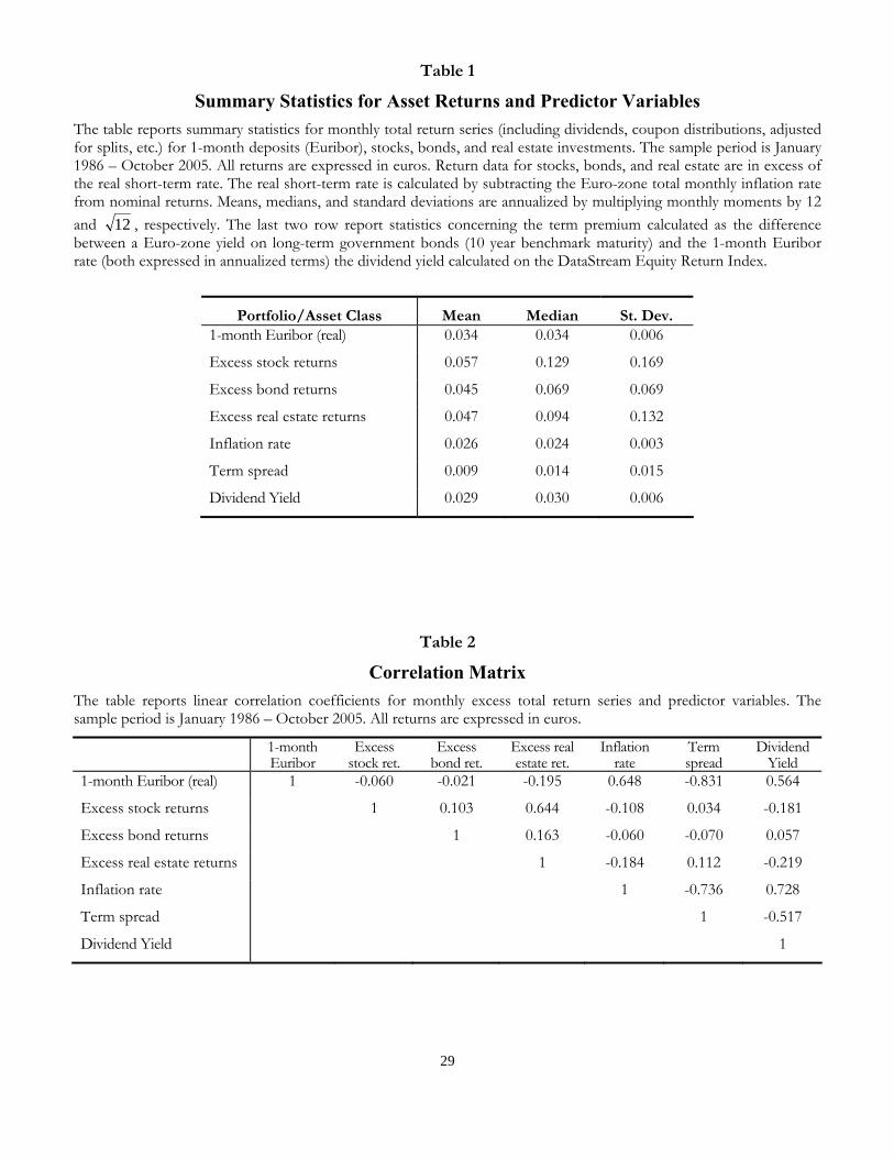
29

Table 1

Summary Statistics for Asset Returns and Predictor Variables The table reports summary statistics for monthly total return series (including dividends, coupon distributions, adjusted for splits, etc.) for 1-month deposits (Euribor), stocks, bonds, and real estate investments. The sample period is January 1986 – October 2005. All returns are expressed in euros. Return data for stocks, bonds, and real estate are in excess of the real short-term rate. The real short-term rate is calculated by subtracting the Euro-zone total monthly inflation rate from nominal returns. Means, medians, and standard deviations are annualized by multiplying monthly moments by 12 and 12 , respectively. The last two row report statistics concerning the term premium calculated as the difference between a Euro-zone yield on long-term government bonds (10 year benchmark maturity) and the 1-month Euribor rate (both expressed in annualized terms) the dividend yield calculated on the DataStream Equity Return Index.

Portfolio/Asset Class Mean Median St. Dev. 1-month Euribor (real) 0.034 0.034 0.006

Excess stock returns 0.057 0.129 0.169

Excess bond returns 0.045 0.069 0.069

Excess real estate returns 0.047 0.094 0.132

Inflation rate 0.026 0.024 0.003

Term spread 0.009 0.014 0.015

Dividend Yield 0.029 0.030 0.006

Table 2

Correlation Matrix The table reports linear correlation coefficients for monthly excess total return series and predictor variables. The sample period is January 1986 – October 2005. All returns are expressed in euros.

1-month Euribor

Excess stock ret.

Excess bond ret.

Excess real estate ret.

Inflation rate

Term spread

Dividend Yield

1-month Euribor (real) 1 -0.060 -0.021 -0.195 0.648 -0.831 0.564

Excess stock returns 1 0.103 0.644 -0.108 0.034 -0.181

Excess bond returns 1 0.163 -0.060 -0.070 0.057

Excess real estate returns 1 -0.184 0.112 -0.219

Inflation rate 1 -0.736 0.728

Term spread 1 -0.517

Dividend Yield 1

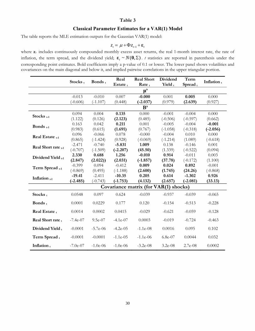
30

Table 3

Classical Parameter Estimates for a VAR(1) Model The table reports the MLE estimation outputs for the Gaussian VAR(1) model:

ttt zz ε+Φ+= −1μ where zt includes continuously compounded monthly excess asset returns, the real 1-month interest rate, the rate of inflation, the term spread, and the dividend yield; ),( ~ Σ0ε Nt . t statistics are reported in parenthesis under the corresponding point estimates. Bold coefficients imply a p-value of 0.1 or lower. The lower panel shows volatilities and covariances on the main diagonal and below it, and implied pairwise correlations in the upper triangular portion.

Stocks t Bonds t Real

Estate t Real Short

Rate t Dividend

Yield t Term

Spread t Inflation t

μ’ -0.013

(-0.606) -0.010

(-1.107) 0.007

(0.448) -0.000

(-2.037) 0.001

(0.979) 0.005

(2.639) 0.000

(0.927) B’

Stocks t-1 0.094

(1.122) 0.004

(0.126) 0.135

(2.123) 0.000

(0.485) -0.001

(-0.506) -0.004

(-0.597) 0.000

(0.662)

Bonds t-1 0.163

(0.983) 0.042

(0.615) 0.211

(1.691) 0.001

(0.767) -0.005

(-1.058) -0.004

(-0.318) -0.001

(-2.056)

Real Estate t-1 0.096

(0.865) -0.066

(-1.424) 0.078

(0.928) -0.000

(-0.069) -0.004

(-1.214) 0.010

(1.089) 0.000

(-0.618)

Real Short rate t-1 -2.471

(-0.707) -0.740

(-1.509) -5.831

(-2.207) 1.009

(45.50) 0.138

(1.339) -0.146

(-0.522) 0.001

(0.094)

Dividend Yield t-1 2.330

(2.847) 0.688

(2.022)) 1.256

(2.031) -0.010

(-1.857) 0.914

(37.78) -0.011

(-0.172) 0.003

(1.100)

Term Spread t-1 -0.399

(-0.869) 0.094

(0.495) -0.412

(-1.188) 0.009

(2.600) 0.024

(1.745) 0.892

(24.26) -0.001

(-0.868)

Inflation t-1 -19.41

(-2.485) -2.411

(-0.743) -10.35

(-1.753) 0.205

(4.132) 0.614

(2.657) -1.302

(-2.081) 0.926

(33.13) Covariance matrix (for VAR(1) shocks) Stocks t 0.0548 0.097 0.624 -0.039 -0.937 -0.039 -0.065

Bonds t 0.0001 0.0229 0.177 0.120 -0.154 -0.513 -0.228

Real Estate t 0.0014 0.0002 0.0415 -0.029 -0.621 -0.059 -0.128

Real Short rate t -7.4e-07 9.5e-07 -4.1e-07 0.0003 -0.019 -0.724 -0.463

Dividend Yield t -0.0001 -5.7e-06 -4.2e-05 -1.1e-08 0.0016 0.095 0.102

Term Spread t -0.0001 -0.0001 -1.1e-05 -1.1e-06 6.8e-07 0.0044 0.032

Inflation t -7.0e-07 -1.0e-06 -1.0e-06 -3.2e-08 3.2e-08 2.7e-08 0.0002

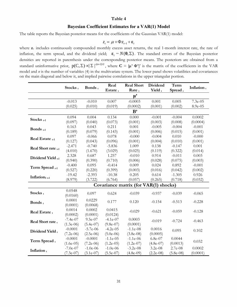
31

Table 4

Bayesian Coefficient Estimates for a VAR(1) Model The table reports the Bayesian posterior means for the coefficients of the Gaussian VAR(1) model:

ttt zz ε+Φ+= −1μ where zt includes continuously compounded monthly excess asset returns, the real 1-month interest rate, the rate of inflation, the term spread, and the dividend yield; ),( ~ Σ0ε Nt . The standard errors of the Bayesian posterior densities are reported in parenthesis under the corresponding posterior means. The posteriors are obtained from a standard uninformative prior, 2)/2-(n||)p(C, +Σ∝Σ , where C = [μ’ Φ’]’ is the matrix of the coefficients in the VAR model and n is the number of variables (4) in the multivariate system. The lower panel shows volatilities and covariances on the main diagonal and below it, and implied pairwise correlations in the upper triangular portion.

Stocks t Bonds t Real

Estate t Real Short

Rate t Dividend

Yield t Term

Spread t Inflation t

μ’ -0.013

(0.025) -0.010 (0.010)

0.007 (0.019)

-0.0003 (0.0002)

0.001 (0.001)

0.005 (0.002)

7.3e-05 8.9e-05

B’

Stocks t-1 0.094

(0.097) 0.004

(0.040) 0.134

(0.073) 0.000

(0.001) -0.001 (0.003)

-0.004 (0.008)

0.0002 (0.0004)

Bonds t-1 0.163

(0.189) 0.043

(0.079) 0.211

(0.143) 0.001

(0.001) -0.005 (0.006)

-0.004 (0.015)

-0.001 (0.001)

Real Estate t-1 0.097

(0.127) -0.066 (0.043)

0.078 (0.096)

-0.000 (0.001)

-0.004 (0.004)

0.010 (0.010)

-0.000 (0.001)

Real Short rate t-1 -2.471 (4.010)

-0.740 (1.670)

-5.836 (3.029)

1.009 (0.025)

0.138 (0.119)

-0.147 (0.322)

0.001 (0.014)

Dividend Yield t-1 2.328

(0.940) 0.687

(0.390) 1.257

(0.710) -0.010 (0.006)

0.914 (0.028)

-0.011 (0.075)

0.003 (0.003)

Term Spread t-1 -0.400 (0.527)

0.095 (0.220)

-0.414 (0.399)

0.009 (0.003)

0.024 (0.016)

0.892 (0.042)

-0.001 (0.002)

Inflation1 t-1 -19.42 (8.979)

-2.393 (3.722)

-10.38 (6.764)

0.205 (0.057)

0.614 (0.265)

-1.305 (0.718)

0.926 (0.032)

Covariance matrix (for VAR(1) shocks)

Stocks t 0.0548

(0.0160) 0.097 0.624 -0.039 -0.937 -0.039 -0.065

Bonds t 0.0001

(0.0001) 0.0229

(0.0068) 0.177 0.120 -0.154 -0.513 -0.228

Real Estate t 0.0014

(0.0002) 0.0002

(0.0001) 0.0415

(0.0124) -0.029 -0.621 -0.059 -0.128

Real Short rate t -7.4e-07 (1.3e-06)

9.5e-07 (5.4e-07)

-4.1e-07 (9.8e-07)

0.0003 (0.0001)

-0.019 -0.724 -0.463

Dividend Yield t -0.0001

(7.2e-06) -5.7e-06(2.5e-06)

-4.2e-05 (5.0e-06)

-1.1e-08 (3.8e-08)

0.0016 (0.0005)

0.095 0.102

Term Spread t -0.0001

(1.6e-05) -0.0001

(7.2e-06)-1.1e-05 (1.2e-05)

-1.1e-06 (1.2e-07)

6.8e-07 (4.8e-07)

0.0044 (0.0013) 0.032

Inflation t -7.0e-07 (7.3e-07)

-1.0e-06(3.1e-07)

-1.0e-06 (5.5e-07)

-3.2e-08 (4.8e-09)

3.2e-08 (2.2e-08)

2.7e-08 (5.8e-08)

0.0002 (0.0001)

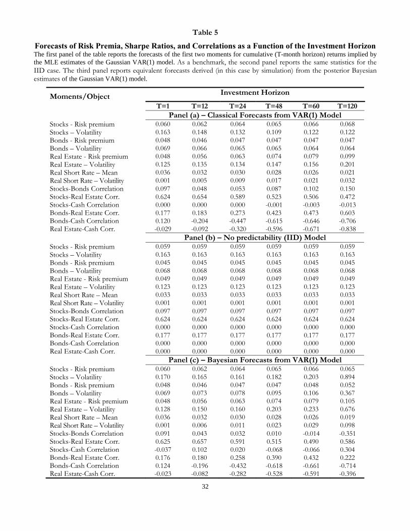
32

Table 5

Forecasts of Risk Premia, Sharpe Ratios, and Correlations as a Function of the Investment Horizon The first panel of the table reports the forecasts of the first two moments for cumulative (T-month horizon) returns implied by the MLE estimates of the Gaussian VAR(1) model. As a benchmark, the second panel reports the same statistics for the IID case. The third panel reports equivalent forecasts derived (in this case by simulation) from the posterior Bayesian estimates of the Gaussian VAR(1) model.

Moments/Object Investment Horizon

T=1 T=12 T=24 T=48 T=60 T=120 Panel (a) – Classical Forecasts from VAR(1) Model Stocks - Risk premium 0.060 0.062 0.064 0.065 0.066 0.068 Stocks – Volatility 0.163 0.148 0.132 0.109 0.122 0.122 Bonds - Risk premium 0.048 0.046 0.047 0.047 0.047 0.047 Bonds – Volatility 0.069 0.066 0.065 0.065 0.064 0.064 Real Estate - Risk premium 0.048 0.056 0.063 0.074 0.079 0.099 Real Estate – Volatility 0.125 0.135 0.134 0.147 0.156 0.201 Real Short Rate – Mean 0.036 0.032 0.030 0.028 0.026 0.021 Real Short Rate – Volatility 0.001 0.005 0.009 0.017 0.021 0.032 Stocks-Bonds Correlation 0.097 0.048 0.053 0.087 0.102 0.150 Stocks-Real Estate Corr. 0.624 0.654 0.589 0.523 0.506 0.472 Stocks-Cash Correlation 0.000 0.000 0.000 -0.001 -0.003 -0.013 Bonds-Real Estate Corr. 0.177 0.183 0.273 0.423 0.473 0.603 Bonds-Cash Correlation 0.120 -0.204 -0.447 -0.615 -0.646 -0.706 Real Estate-Cash Corr. -0.029 -0.092 -0.320 -0.596 -0.671 -0.838 Panel (b) – No predictability (IID) Model Stocks - Risk premium 0.059 0.059 0.059 0.059 0.059 0.059 Stocks – Volatility 0.163 0.163 0.163 0.163 0.163 0.163 Bonds - Risk premium 0.045 0.045 0.045 0.045 0.045 0.045 Bonds – Volatility 0.068 0.068 0.068 0.068 0.068 0.068 Real Estate - Risk premium 0.049 0.049 0.049 0.049 0.049 0.049 Real Estate – Volatility 0.123 0.123 0.123 0.123 0.123 0.123 Real Short Rate – Mean 0.033 0.033 0.033 0.033 0.033 0.033 Real Short Rate – Volatility 0.001 0.001 0.001 0.001 0.001 0.001 Stocks-Bonds Correlation 0.097 0.097 0.097 0.097 0.097 0.097 Stocks-Real Estate Corr. 0.624 0.624 0.624 0.624 0.624 0.624 Stocks-Cash Correlation 0.000 0.000 0.000 0.000 0.000 0.000 Bonds-Real Estate Corr. 0.177 0.177 0.177 0.177 0.177 0.177 Bonds-Cash Correlation 0.000 0.000 0.000 0.000 0.000 0.000 Real Estate-Cash Corr. 0.000 0.000 0.000 0.000 0.000 0.000 Panel (c) – Bayesian Forecasts from VAR(1) Model Stocks - Risk premium 0.060 0.062 0.064 0.065 0.066 0.065 Stocks – Volatility 0.170 0.165 0.161 0.182 0.203 0.894 Bonds - Risk premium 0.048 0.046 0.047 0.047 0.048 0.052 Bonds – Volatility 0.069 0.073 0.078 0.095 0.106 0.367 Real Estate - Risk premium 0.048 0.056 0.063 0.074 0.079 0.105 Real Estate – Volatility 0.128 0.150 0.160 0.203 0.233 0.676 Real Short Rate – Mean 0.036 0.032 0.030 0.028 0.026 0.019 Real Short Rate – Volatility 0.001 0.006 0.011 0.023 0.029 0.098 Stocks-Bonds Correlation 0.091 0.043 0.032 0.010 -0.014 -0.351 Stocks-Real Estate Corr. 0.625 0.657 0.591 0.515 0.490 0.586 Stocks-Cash Correlation -0.037 0.102 0.020 -0.068 -0.066 0.304 Bonds-Real Estate Corr. 0.176 0.180 0.258 0.390 0.432 0.222 Bonds-Cash Correlation 0.124 -0.196 -0.432 -0.618 -0.661 -0.714 Real Estate-Cash Corr. -0.023 -0.082 -0.282 -0.528 -0.591 -0.396

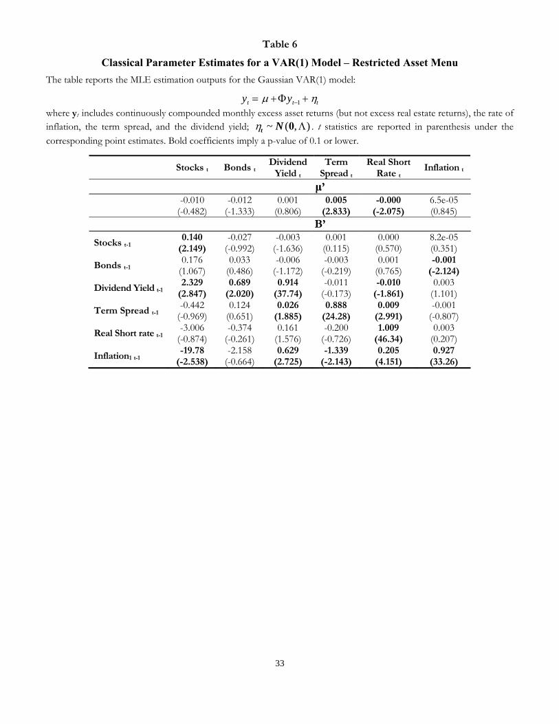
33

Table 6

Classical Parameter Estimates for a VAR(1) Model – Restricted Asset Menu The table reports the MLE estimation outputs for the Gaussian VAR(1) model:

ttt yy ημ +Φ+= −1 where yt includes continuously compounded monthly excess asset returns (but not excess real estate returns), the rate of inflation, the term spread, and the dividend yield; ),( ~ Λ0Ntη . t statistics are reported in parenthesis under the corresponding point estimates. Bold coefficients imply a p-value of 0.1 or lower.

Stocks t Bonds t Dividend

Yield t Term

Spread t Real Short

Rate t Inflation t

μ’ -0.010

(-0.482) -0.012

(-1.333) 0.001

(0.806) 0.005

(2.833) -0.000

(-2.075) 6.5e-05 (0.845)

B’

Stocks t-1 0.140

(2.149) -0.027

(-0.992) -0.003

(-1.636) 0.001

(0.115) 0.000

(0.570) 8.2e-05 (0.351)

Bonds t-1 0.176

(1.067) 0.033

(0.486) -0.006

(-1.172) -0.003

(-0.219) 0.001

(0.765) -0.001

(-2.124)

Dividend Yield t-1 2.329

(2.847) 0.689

(2.020) 0.914

(37.74) -0.011

(-0.173) -0.010

(-1.861) 0.003

(1.101)

Term Spread t-1 -0.442

(-0.969) 0.124

(0.651) 0.026

(1.885) 0.888

(24.28) 0.009

(2.991) -0.001

(-0.807)

Real Short rate t-1 -3.006

(-0.874) -0.374

(-0.261) 0.161

(1.576) -0.200

(-0.726) 1.009

(46.34) 0.003

(0.207)

Inflation1 t-1 -19.78

(-2.538) -2.158

(-0.664) 0.629

(2.725) -1.339

(-2.143) 0.205

(4.151) 0.927

(33.26)

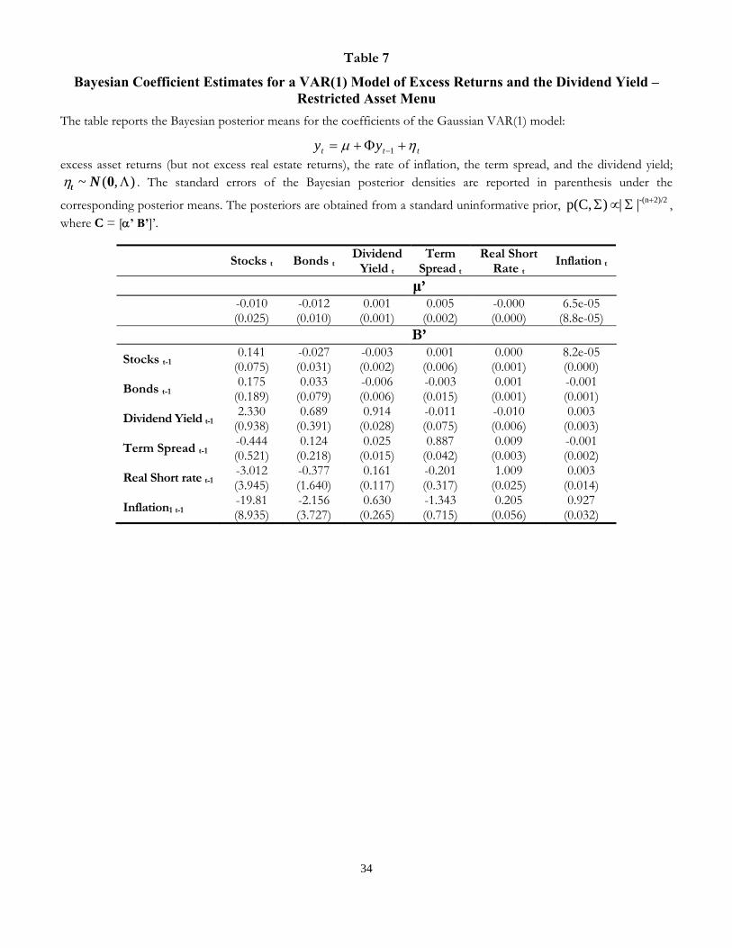
34

Table 7

Bayesian Coefficient Estimates for a VAR(1) Model of Excess Returns and the Dividend Yield – Restricted Asset Menu

The table reports the Bayesian posterior means for the coefficients of the Gaussian VAR(1) model:

ttt yy ημ +Φ+= −1 excess asset returns (but not excess real estate returns), the rate of inflation, the term spread, and the dividend yield;

),( ~ Λ0Ntη . The standard errors of the Bayesian posterior densities are reported in parenthesis under the

corresponding posterior means. The posteriors are obtained from a standard uninformative prior, 2)/2-(n||)p(C, +Σ∝Σ , where C = [α’ B’]’.

Stocks t Bonds t Dividend

Yield t Term

Spread t Real Short

Rate t Inflation t

μ’ -0.010

(0.025) -0.012 (0.010)

0.001 (0.001)

0.005 (0.002)

-0.000 (0.000)

6.5e-05 (8.8e-05)

B’

Stocks t-1 0.141

(0.075) -0.027 (0.031)

-0.003 (0.002)

0.001 (0.006)

0.000 (0.001)

8.2e-05 (0.000)

Bonds t-1 0.175

(0.189) 0.033

(0.079) -0.006 (0.006)

-0.003 (0.015)

0.001 (0.001)

-0.001 (0.001)

Dividend Yield t-1 2.330

(0.938) 0.689

(0.391) 0.914

(0.028) -0.011 (0.075)

-0.010 (0.006)

0.003 (0.003)

Term Spread t-1 -0.444 (0.521)

0.124 (0.218)

0.025 (0.015)

0.887 (0.042)

0.009 (0.003)

-0.001 (0.002)

Real Short rate t-1 -3.012 (3.945)

-0.377 (1.640)

0.161 (0.117)

-0.201 (0.317)

1.009 (0.025)

0.003 (0.014)

Inflation1 t-1 -19.81 (8.935)

-2.156 (3.727)

0.630 (0.265)

-1.343 (0.715)

0.205 (0.056)

0.927 (0.032)

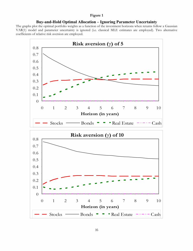
35

Figure 1

Buy-and-Hold Optimal Allocation – Ignoring Parameter Uncertainty The graphs plot the optimal portfolio weights as a function of the investment horizons when returns follow a Gaussian VAR(1) model and parameter uncertainty is ignored (i.e. classical MLE estimates are employed). Two alternative coefficients of relative risk aversion are employed.

Risk aversion (γ) of 5

00.10.20.30.40.50.60.70.8

0 1 2 3 4 5 6 7 8 9 10Horizon (in years)

Stocks Bonds Real Estate Cash

Risk aversion (γ) of 10

00.10.20.30.40.50.60.70.8

0 1 2 3 4 5 6 7 8 9 10Horizon (in years)

Stocks Bonds Real Estate Cash

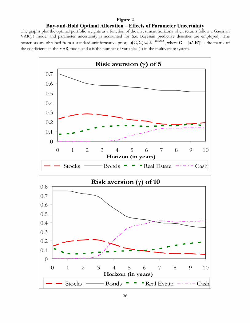
36

Figure 2 Buy-and-Hold Optimal Allocation – Effects of Parameter Uncertainty

The graphs plot the optimal portfolio weights as a function of the investment horizons when returns follow a Gaussian VAR(1) model and parameter uncertainty is accounted for (i.e. Bayesian predictive densities are employed). The posteriors are obtained from a standard uninformative prior, 2)/2-(n||)p(C, +Σ∝Σ , where C = [α’ B’]’ is the matrix of the coefficients in the VAR model and n is the number of variables (4) in the multivariate system.

Risk aversion (γ) of 5

0

0.1

0.2

0.3

0.4

0.5

0.6

0.7

0 1 2 3 4 5 6 7 8 9 10Horizon (in years)

Stocks Bonds Real Estate Cash

Risk aversion (γ) of 10

00.1

0.20.3

0.40.5

0.60.7

0.8

0 1 2 3 4 5 6 7 8 9 10Horizon (in years)

Stocks Bonds Real Estate Cash

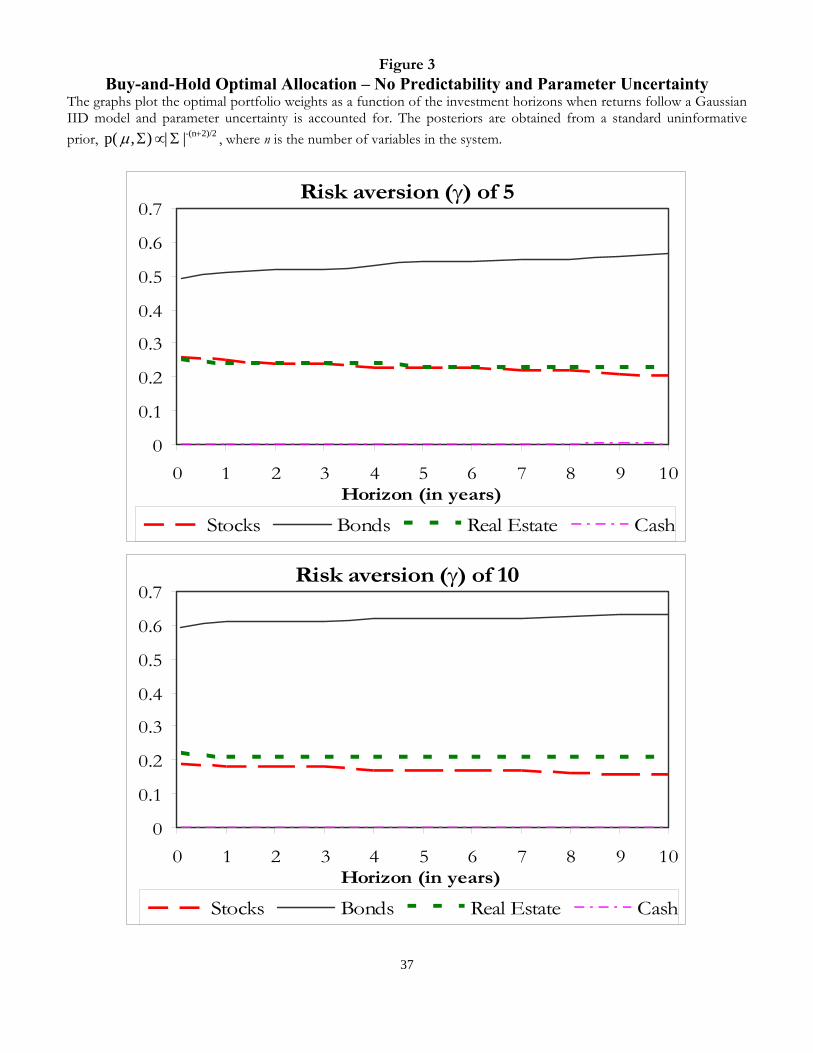
37

Figure 3 Buy-and-Hold Optimal Allocation – No Predictability and Parameter Uncertainty

The graphs plot the optimal portfolio weights as a function of the investment horizons when returns follow a Gaussian IID model and parameter uncertainty is accounted for. The posteriors are obtained from a standard uninformative prior, 2)/2-(n||),p( +Σ∝Σμ , where n is the number of variables in the system.

Risk aversion (γ) of 5

0

0.1

0.2

0.3

0.4

0.5

0.6

0.7

0 1 2 3 4 5 6 7 8 9 10Horizon (in years)

Stocks Bonds Real Estate Cash

Risk aversion (γ) of 10

0

0.1

0.2

0.3

0.4

0.5

0.6

0.7

0 1 2 3 4 5 6 7 8 9 10Horizon (in years)

Stocks Bonds Real Estate Cash

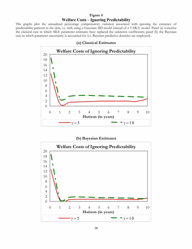
38

Figure 4 Welfare Costs – Ignoring Predictability

The graphs plot the annualized percentage compensatory variation associated with ignoring the existence of predictability patterns in the data, i.e. with using a Gaussian IID model instead of a VAR(1) model. Panel (a) concerns the classical case in which MLE parameter estimates have replaced the unknown coefficients; panel (b) the Bayesian case in which parameter uncertainty is accounted for (i.e. Bayesian predictive densities are employed).

(a) Classical Estimates

Welfare Costs of Ignoring Predictability

02468

101214161820

0 1 2 3 4 5 6 7 8 9 10Horizon (in years)

γ = 5 γ = 10

(b) Bayesian Estimates

Welfare Costs of Ignoring Predictability

02468

101214161820

0 1 2 3 4 5 6 7 8 9 10Horizon (in years)

γ = 5 γ = 10

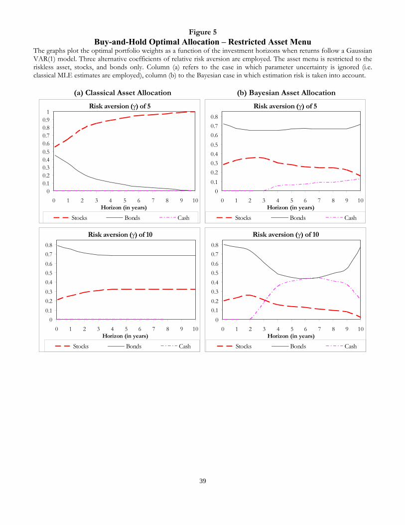
39

Figure 5 Buy-and-Hold Optimal Allocation – Restricted Asset Menu

The graphs plot the optimal portfolio weights as a function of the investment horizons when returns follow a Gaussian VAR(1) model. Three alternative coefficients of relative risk aversion are employed. The asset menu is restricted to the riskless asset, stocks, and bonds only. Column (a) refers to the case in which parameter uncertainty is ignored (i.e. classical MLE estimates are employed), column (b) to the Bayesian case in which estimation risk is taken into account.

(a) Classical Asset Allocation (b) Bayesian Asset Allocation

Risk aversion (γ) of 5

00.10.20.30.40.50.60.70.80.9

1

0 1 2 3 4 5 6 7 8 9 10Horizon (in years)

Stocks Bonds Cash

Risk aversion (γ) of 5

00.10.20.30.40.50.60.70.8

0 1 2 3 4 5 6 7 8 9 10Horizon (in years)

Stocks Bonds Cash

Risk aversion (γ) of 10

00.10.20.30.40.50.60.70.8

0 1 2 3 4 5 6 7 8 9 10Horizon (in years)

Stocks Bonds Cash

Risk aversion (γ) of 10

00.10.20.30.40.50.60.70.8

0 1 2 3 4 5 6 7 8 9 10Horizon (in years)

Stocks Bonds Cash

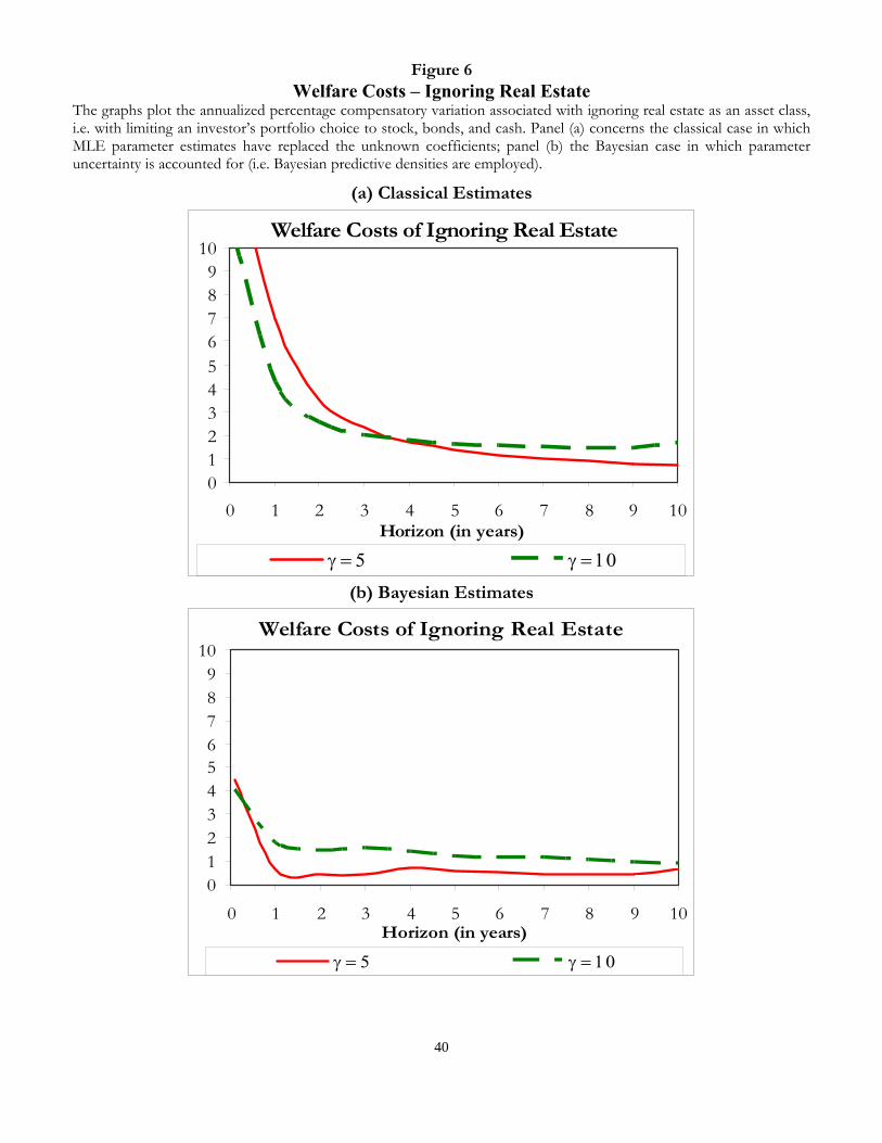
40

Figure 6 Welfare Costs – Ignoring Real Estate

The graphs plot the annualized percentage compensatory variation associated with ignoring real estate as an asset class, i.e. with limiting an investor’s portfolio choice to stock, bonds, and cash. Panel (a) concerns the classical case in which MLE parameter estimates have replaced the unknown coefficients; panel (b) the Bayesian case in which parameter uncertainty is accounted for (i.e. Bayesian predictive densities are employed).

(a) Classical Estimates

Welfare Costs of Ignoring Real Estate

0123456789

10

0 1 2 3 4 5 6 7 8 9 10Horizon (in years)

γ = 5 γ = 10

(b) Bayesian Estimates

Welfare Costs of Ignoring Real Estate

0123456789

10

0 1 2 3 4 5 6 7 8 9 10Horizon (in years)

γ = 5 γ = 10

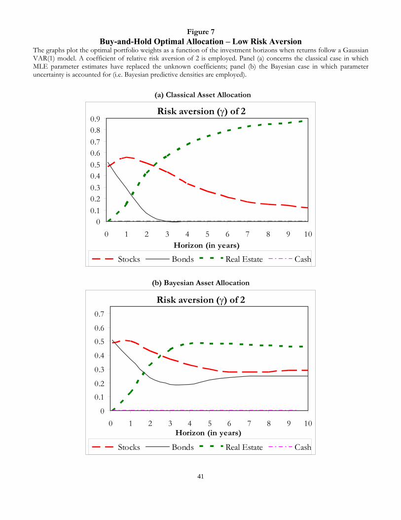
41

Figure 7 Buy-and-Hold Optimal Allocation – Low Risk Aversion

The graphs plot the optimal portfolio weights as a function of the investment horizons when returns follow a Gaussian VAR(1) model. A coefficient of relative risk aversion of 2 is employed. Panel (a) concerns the classical case in which MLE parameter estimates have replaced the unknown coefficients; panel (b) the Bayesian case in which parameter uncertainty is accounted for (i.e. Bayesian predictive densities are employed).

(a) Classical Asset Allocation

Risk aversion (γ) of 2

00.10.20.30.40.50.60.70.80.9

0 1 2 3 4 5 6 7 8 9 10Horizon (in years)

Stocks Bonds Real Estate Cash

(b) Bayesian Asset Allocation

Risk aversion (γ) of 2

0

0.1

0.2

0.3

0.4

0.5

0.6

0.7

0 1 2 3 4 5 6 7 8 9 10Horizon (in years)

Stocks Bonds Real Estate Cash

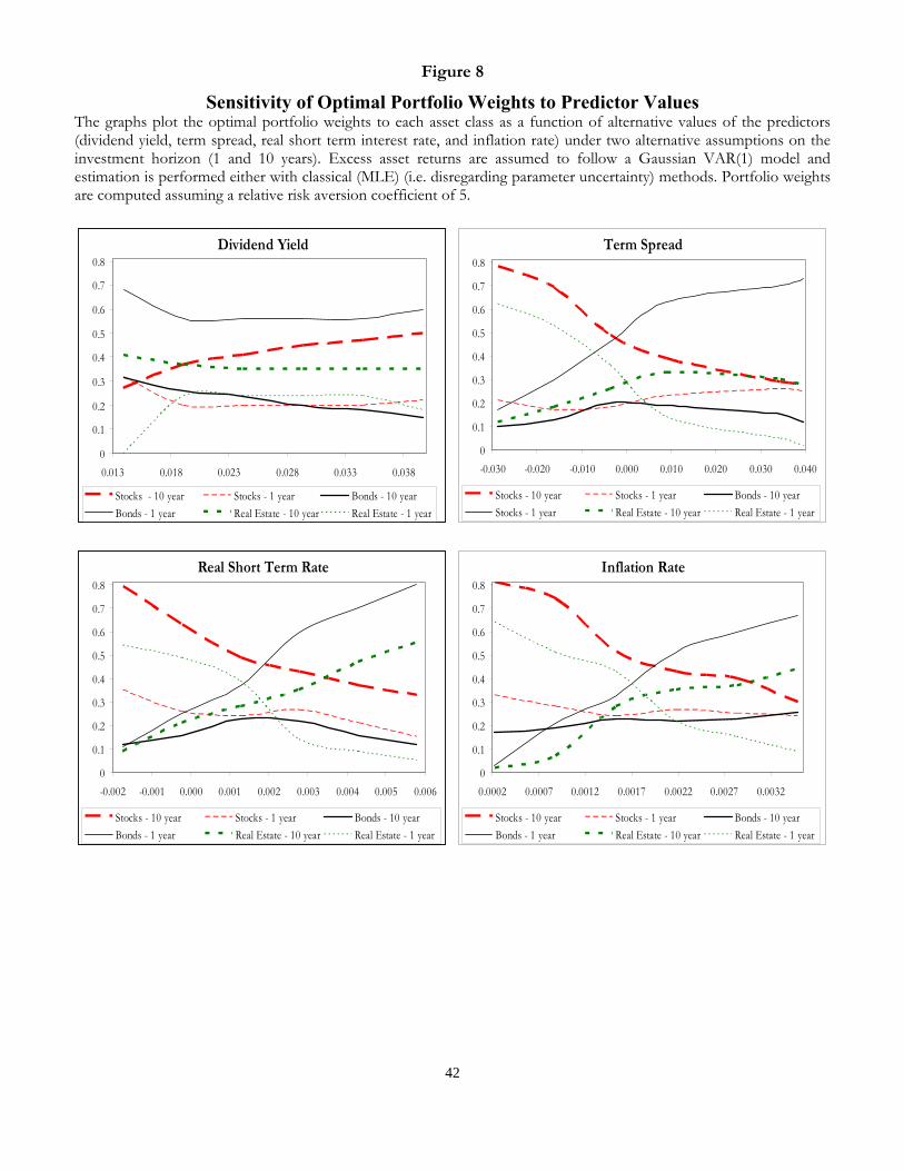
42

Figure 8

Sensitivity of Optimal Portfolio Weights to Predictor Values The graphs plot the optimal portfolio weights to each asset class as a function of alternative values of the predictors (dividend yield, term spread, real short term interest rate, and inflation rate) under two alternative assumptions on the investment horizon (1 and 10 years). Excess asset returns are assumed to follow a Gaussian VAR(1) model and estimation is performed either with classical (MLE) (i.e. disregarding parameter uncertainty) methods. Portfolio weights are computed assuming a relative risk aversion coefficient of 5.

Dividend Yield

0

0.1

0.2

0.3

0.4

0.5

0.6

0.7

0.8

0.013 0.018 0.023 0.028 0.033 0.038

Stocks - 10 year Stocks - 1 year Bonds - 10 yearBonds - 1 year Real Estate - 10 year Real Estate - 1 year

Term Spread

0

0.1

0.2

0.3

0.4

0.5

0.6

0.7

0.8

-0.030 -0.020 -0.010 0.000 0.010 0.020 0.030 0.040

Stocks - 10 year Stocks - 1 year Bonds - 10 yearStocks - 1 year Real Estate - 10 year Real Estate - 1 year

Real Short Term Rate

0

0.1

0.2

0.3

0.4

0.5

0.6

0.7

0.8

-0.002 -0.001 0.000 0.001 0.002 0.003 0.004 0.005 0.006

Stocks - 10 year Stocks - 1 year Bonds - 10 yearBonds - 1 year Real Estate - 10 year Real Estate - 1 year

Inflation Rate

0

0.1

0.2

0.3

0.4

0.5

0.6

0.7

0.8

0.0002 0.0007 0.0012 0.0017 0.0022 0.0027 0.0032

Stocks - 10 year Stocks - 1 year Bonds - 10 yearBonds - 1 year Real Estate - 10 year Real Estate - 1 year

43

Figure 9 Optimal Dynamic Portfolio Allocation under Predictable Returns

The graphs plot the optimal portfolio weights as a function of the investment horizons when returns follow a Gaussian VAR(1) model and the investor rebalances her portfolio once a year. The variables are initialized at their sample mean. Panel (a) refers to the case in which all of the predictors are considered but a coarse (5-point) grid is employed, panel (b) to the case in which the term spread is held at its sample mean but a finer 12-point grid is used. When the horizon T is inferior or is equal to the rebalancing frequency φ = 12 months, optimal weights coincide with those obtained under buy-and-hold.

(a) Coarse grid – all predictors

Risk aversion (γ) = 5

0.000.100.200.300.40

0.500.600.700.80

0 1 2 3 4 5 6 7 8 9 10Horizon (in years)

Stocks Bonds Real Estate Cash

(b) Fine grid – Term spread fixed at sample mean

Risk aversion (γ) = 5

0.000.100.200.300.40

0.500.600.700.80

0 1 2 3 4 5 6 7 8 9 10Horizon (in years)

Stocks Bonds Real Estate Cash