Investigations of marine aerosols over the tropical Indian Ocean

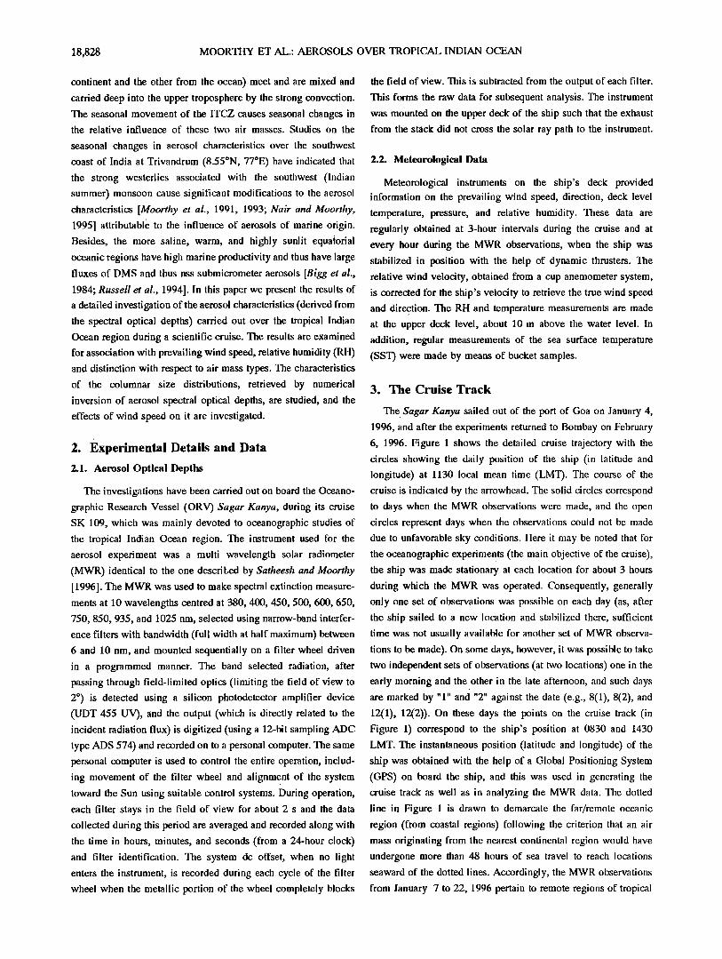
JOURNAL OF GEOPHYSICAL RESEARCH, VOL. 102, NO. D15, PAGES 18,827-18,842, AUGUST 20, 1997

Investigations of marine aerosols over the tropical Indian Ocean

K. Krishna Moorthy, S.K. Satheesh, and B.V. Krishna Murthy Space Physics Laboratory, Vikram Sarabhai Space Centre, Trivandrum, India

Abstract. Results of the studies on the characteristics of marine aerosol optical depths made in remote regions of the tropical Indian Ocean using a multiwavelength solar radiometer, taken on a scientific cruise, are presented. The dependence of the aerosol optical depths on prevailing winds in marine boundary layer and on deck level relative humidity (RH) are examined. Aerosol optical depths (xp) in far oceanic regions with marine air mass prevailing, in general, are found to increase nearly exponentially with average wind speed (Ua) as xp = x o exp(a Ua), where a = 0.16 _+ 0.04. No association is seen with deck level relative humidity, as the effects of wind appear to offset the effects due to RH. The columnar size distributions retrieved from aerosol spectral optical depths reveal two modes, one at ~0.04/m• and a secondary mode at ~0.8/•m. The columnar mass loading estimated from the size distributions increases exponentially with wind speed and has a wind independent value of ~28 mg m '2.

1. Introduction

Oceans constitute one of the single largest sources of atmos-

pheric aerosols. Several estimates have shown that about one third

of the total natural aerosol flux to the atmosphere is of oceanic

(marine) origin and is estimated to be in the range 1000 to 2000

Tg l•r year [Prost•ero et al., 1983; Jaenicke, 1984; Andreae,

1995]. Marine aerosols have broadly two components: the sea salt

component, comprising aerosols produced mechanically over the

sea surface by breaking of bubbles and whitecaps (through the

combinations of bubble jet action and film droplets) and the non-

sea-salt (nss) sulphate aerosols produced mainly by the photolytic decomposition of dimethyl sulfide (DMS) secreted b•/ marine

phytoplankton. The abundance and size spectrum of sea salt

aerosol are strongly influenced by the wind speed [e.g., Wood-

cock, 1953; Blanchard, 1963; Monahan, 1968; Lovett, 1978;

Kulkarni et al., 1982] while that of the nss component strongly

depends on the DMS flux [e.g., Charlson et al., 1987; Hegg et al., 1991g Pandis et al., 1•4]. The tropical oceans are known to be

conducive to DMS generation [Russell et al., 1994; Pandis et al., 1904]. In the submicrometer size range, bursting of whitecap

bubbles produces substantial amounts of sea salt aerosols [Cipr-

iano et al. 1987], while the photolytic reactions involving DMS are mainly responsible for the nss component [Pandis' et al., 1994] of marine aerosols. The submicrometer aerosols are believed to

form condensation nuclei in the marine Stratocumulus clouds and

cause increase in cloud albedo [Charlson et al., 1987]. Mineral

aerosols from continental (and arid) regions are found to be

Copyright 1997 by the American Geophysical Union

Paper number 97JD01121. 0148-0227/97/97JD-01121 $09.00

transported by winds over to remote ocean regions and signifi- o

cantly influence the aerosol characteristics there [e.g., Prospero,

1979; Hoppel et al., 1990]. Advection of sea spray aerosols to

coastal regions by favorable and sufficiently strong winds to cause

distinct signature in the size distribution, composition, and optical

depths at coastal regions is also observed [Kulkarni et al., 1982;

Suzuki and Tsunogai, 1988; Moorthy et al., 1991]. Marine aerosols strongly influence the radiative coupling between ocean

and atmosphere by scattering and absorbing solar radiation. They

also lead to the formation of (stratocumulus) clouds in the marine

boundary layer (MBL) and influence the droplet size distribution and cloud albedo, thereby playing an important role in remote

sensing of oceans and affecting visibility in the atmosphere over

oceans [e.g., Fitzgerald, 1991]. Thus the study of aerosol

characteristics and optical effects over the oceanic region assumes

significance. Extensive studies have been carried out on marine aerosols

[Woodcock, 1953; Blanchard and Woodcock, 1957; Blanchard,

1963; Hoppel et al., 1990; Fitzgerald, 1091; Smirnov et al.,

1905] in laboratory simulations [e.g., Monaban et al., 1986;

Cipriano et al. 1987] as well as field experiments on board ships

[e.g., Lovett, 1978; Prosl•ero, 1070; Hoppel et al., 1985, 1990]

and air craft [e.g., Woodcock, 1953; Patterson et al., 1980;

Blanchard et al., 1984] using various instruments. However, most

studies have investigated the generation and fate of marine

aerosols over the Atlantic and Pacific Ocean regions, while

observations have been quite scanty over the tropical Indian

Ocean region. This region is quite important, as far as aerosol

studies are concerned, as it experiences seasonally varying air

mass types associated with the In:tian monsoon. Moreover, the

Intertropical Convergence Zone (ITCZ) constitutes a zone where the two distinct contrasting air masses (one originating from the

18,827

18,828 MOORTHY ET AL.: AEROSOLS OVER TROPICAL INDIAN OCEAN

continent and the other from the ocean) meet and are mixed and

carried deep into the upper troposphere by the strong convection. The seasonal movement of the ITCZ causes seasonal changes in the relative influence of these two air masses. Studies on the

seasonal changes in aerosol characteristics over the southwest

coast of India at Trivandrum (8.55øN, 77øE) have indicated that the strong westerlies associated with the southwest (Indian

summer) monsoon cause significant modifications to the aerosol characteristics [Moorthy et al., 1001, 1993; Nair and Moorthy,

1995] attributable to the influence of aerosols of marine origin. Besides, the more saline, warm, and highly sunlit equatorial

oceanic regions have high marine productivity and thus have large fluxes of DMS and thus nss submicrometer aerosols [Bigg et al.,

1984; Russell et al., 1994]. In this paper we present the results of

a detailed investigation of the aerosol characteristics (derived from the spectral optical depths) carried out over the tropical Indian Ocean region during a scientific cruise. The results are examined for association with prevailing wind speed, relative humidity (RH) and distinction with respect to air mass types. The characteristics

of the columnar size distributions, retrieved by numerical

inversion of aerosol spectral optical depths, are studied, and the

effects of wind speed on it are investigated.

2. Experimental Details and Data

2.1. Aerosol Optical Depths

The investigations have been carried out on board the Oceano-

graphic Research Vessel (ORV) Sagar Kanya, during its cruise

SK 109, which was mainly devoted to oceanographic studies of

the tropical Indian Ocean region. The instrument used for the

aerosol experiment was a multi wavelength solar radiometer

(MWR) identical to the one described by Satheesh and Moorthy [1996]. The MWR was used to make spectral extinction measure-

ments at 10 wavelengths centred at 380, 400, 450, 500, 600, 650, 750, 850, 935, and t025 nm, selected using narrow-band interfer-

ence filters with bandwidth (full width at half maximum) between 6 and 10 nm, and mounted sequentially on a filter wheel driven

in a programmed manner. The band selected radiation, after passing through field-limited optics (limiting the field of view to 2 ø) is detected using a silicon photodetector amplifier device

(UDT 455 UV), and the output (which is directly related to the incident radiation flux) is digitized (using a 12-bit sampling ADC

type ADS 574) and recorded on to a personal computer. The same personal computer is used to control the entire operation, includ-

ing movement of the filter wheel and alignment of the system

toward the Sun using suitable control systems. During operation,

each filter stays in the field of view for about 2 s and the data

collected during this period are averaged and recorded along with

the time in hours, minutes, and seconds (from a 24-hour clock)

and filter identification. The system dc offset, when no light

enters the instrument, is recorded during each cycle of the filter

wheel when the metallic portion of the wheel completely blocks

the field of view. This is subtracted from the output of each filter.

This forms the raw data for subsequent analysis. The instrument

was mounted on the upper deck of the ship such that the exhaust

from the stack did not cross the solar ray path to the instrument.

2.2. Meteorological Data

Meteorological instruments on the ship's deck provided information on the prevailing wind speed, direction, deck level

temperature, pressure, and relative humidity. These data are

regularly obtained at 3-hour intervals during the cruise and at

every hour during the MWR observations, when the ship was

stabilized in position with the help of dynamic thrusters. The relative wind velocity, obtained from a cup anemometer system,

is corrected for the ship's velocity to retrieve the true wind speed

and direction. The RH and temperature measurements are made

at the upper deck level, about 10 m above the water level. In

addition, regular measurements of the sea surface temperature

(SST) were made by means of bucket samples.

3. The Cruise Track

The Sagar Kanya sailed out of the port of Goa on January 4,

1996, and after the experiments returned to Bombay on February

6, 1996. Figure 1 shows the detailed cruise trajectory with the

circles showing the daily position of the ship (in latitude and

longitude) at 1130 local mean time (LMT). The course of the cruise is indicated by the arrowhead. The solid circles correspond

to days when the MWR observations were made, and the open

circles represent days when the observations could not be made due to unfavorable sky conditions. Here it may be noted that for

the oceanographic experiments (the main objective of the cruise),

the ship was made stationary at each location for about 3 hours

during which the MWR was operated. Consequently, generally

only one set of observations was possible on each day (as, after

the ship sailed to a new location and stabilized there, sufficient

time was not usually available for another set of MWR observa-

tions to be made). On some days, however, it was possible to take two independent sets of observations (at two locations) one in the

early morning and the other in the late afternoon, and such days

are marked by "1" and "2" against the date (e.g., 8(1), 8(2), and 12(1), 12(2)). On these days the points on the cruise track (in

Figure 1) correspond to the ship's position at 0830 and 1430

LMT. The instantaneous position (latitude and longitude) of the ship was obtained with the help of a Global Positioning System

(GPS) on board the ship, and this was used in generating the cruise track as well as in analyzing the MWR data. The dotted

line in Figure 1 is drawn to demarcate the tar/remote oceanic

region (from coastal regions) following the criterion that an air mass originating from the nearest continental region would have

undergone more than 48 hours or' sea travel to reach locations

seaward of the dotted lines. Accordingly, the MWR observations

from January 7 to 22, 1906 pertain to remote regions of tropical

MOORTHY ET AL.: AEROSOLS OVER TROPICAL INDIAN OCEAN 18,829

3O

25

2O

15

c• lO

o '•

• .lO

0 .15

16

10

6

0

.6

.10

.16

.30

0 5 10 15 20 25 30 35 40 45 60 '55 60 •5 70 75 I0 15 I0 16 100 110

GEOGRAPHIC LON•ITUDfi

Figure 1. The cruise track of SK 109. The points correspond to the ship's position at 1130 LMT (details are given in the text).

Indian Ocean bounded approximately between latitudes 5øN and

5øS and longitudes 60øE and 75øE.

4. Analysis of Data

Of the total cruise duration of 32 days, aerosol optical depths

were estimated on 20 days including 2 sets each on January 8 and

12, 1996. Each set of raw data has been analyzed following the

Langley plot method [e.g., Shaw et al., 1973; Moorthy et al.,

1989] to deduce total optical depths -rx. A typical Langley plot

obtained for the data on January 12, 1996 is shown in Figure 2 as

an illustrative example. The wavelength X, xx, and correlation

coefficient p are marked above each plot. From -rx the aerosol

optical depths -rpx have been deduced after accounting for the optical depths due to Rayleigh scattering and absorption by ozone, NO2, and water vapor; tollowing the procedure described else-

where [Moorthy et al., 1080, 1906]. A detailed error analysis,

considering instrumental and model uncertainties, puts the typical

error on the estimate of-rpx in the range 0.009 to 0.011 at the different wavelengths.

Of the various meteorological parameters obtained at regular

intervals from the on board instruments, the (true) wind speed and direction showed significant fluctuations both within a day as well

as from day to day during the cruise. Thus for inferring the mean

trends in speed and direction of arrival, the average wind characteristics have been used. For this, the values of wind speed

and directions are averaged over the day, and the mean speed U, and direction and their standard deviations have also been

estimated.

5. Presentation of Results and Discussion

5.1. Chronological Variations of Meteorological Parameters

During the period covered by the cruise, the synoptic scale winds are such that the regions northward of the equator are

generally under the influence of a nearly steady northeasterly trade wind [Rao, 1976; Das, 1986] associated with the Indian

winter monsoon. The day to day variations in the mean (true) wind speed U and direction are shown in Figure 3. The vertical

lines through the points are the standard deviations indicative of

the variations in the parameter concerned within a day. It may be noticed that the wind speed generally showed fairly large

fluctuations (barring the days January 7 to 9 and 15 to 18). Moreover, U increased fairly steadily from ~6 m s '• on January 5 to reach ~10 m s '• on January 14. Thereafter it decreased sharply for the next 4 days before sharply increasing again. The wind on subsequent days shows large fluctuations both within a

day and from day to day until January 29, after which it

decreased steadily. The top panel of Figure 3 shows that the wind

direction was fairly steady (within a day) up to January 20 (except for January 17), after which it showed large fluctuations, (like U), both within the day and from day to day. Considering the wind over the open ocean to be characteristic of the prevailing wind in the MBL (and perhaps in the lower troposphere too), it can be seen that as the cruise proceeded away from the coast the wind

gradually shifted from a northerly/northeasterly (N/NE) direction to northwesterly (NW), westerly (W), southwesterly (SW) and nearly southerly (S) direction by January 16. Subsequently also, even though there were large variations, the winds are mainly


1

-2

2

SK 109 12JAN 1996

1 0rim 1--0.13 0/- -- I ---'•'"""•' -•

, 1.• 1 0 , =- . =- .

1.• 1.• i

=- . =- .

.

Z • 1.e 1 1,• z.o

1

o • o 1.• 0 1.0 2.0

REL. AIR MASS

Figure 2. A typical Langley plot obtained on January 12, 1996.

from the southwest / west till January 21, 1996. After that, wind was from the N/NE and continued so until the end of the cruise.

This changing pattern in the direction is significant, as the N and NE winds would have their origin from the continent (the Indian

subcontinent and the adjoining regions; see Figure 1) while the

NW, W, and SW winds represent pure or so-called "pristine"

marine air mass. These distinctive air mass regions are marked by

the pair of dotted lines in the top panel (in Figure 3) such that the

portion of the direction curve I•tween these lines represents days

during which the prevailing winds indicate possible presence of

continental air mass (and thus a continental aerosol component),

while the days outside these lines represent possibly pristine

marine aerosol environment. Figure 4 shows (from top to bottom)

the variations of SST, RH, and temperature at the deck level. It

is seen that the SST remained nearly steady, with a mean value

of 28.2øC (marked by the dashed horizontal line in the figure) and a standard deviation of 0.41øC. The ambient temperature also

remained nearly steady at ~28øC (except for the regular diurnal variations of about +_2 ø about the mean), particularly from January 7 to 28, when the ship was cruising in far marine areas. The RH

did not reveal any remarkable tree, ds during this period being

mostly in the range 7(} to 85%. The steady nature of all these

parameters without any sharp or abrupt discontinuity indicates the

absence of any strong localized weather fronts influencing the

environments of MWR observations. Furthermore, an examination

of the regional weather charts, for the peninsular Indian and

adjoining regions upto the equator, available at the meteorological

center, Trivandrum (TVM in Figure 1) revealed no major weather

systems during the entire cruise period.

5.2. Variations in Aerosol Optical Depths

The top panel of Figure 5 shows the chronological variation of

aerosol optical depths (at a representative wavelength of 50(} nm),

270

-- 180 - e,... T

c 90

i• 270

, I , I , I , I , I , I œ I ß I , I i I , sl , I • I , I , I , i

16

lo

/+ 6 8 10 12 1/+ 16 18 20 22 2/+ 26 28 30 1 3

.JAN FEB ,..,

Figure :3. Variation of the daily mean wind speed U and direction durin• the cruise. The vertical bars are the •tandard deviations.

MOORTHY ET AL.' AEROSOLS OVER TROPICAL INDIAN OCEAN 18,831

31

30

•g

ro •8

• •6 Z5

I0C•

90

•o, 80

• 7o

31

ß 30 •) a 29

• 28

• 27

ß 25

24

I

6 8 tO 12 14 16 18 20 22 24 26 28 30 I 3

Jan Feb

Figure 4. Chronological variations of (top) SST, (middle) RH, and (bottom) deck level temperature.

0.8 500 nm

-

•. 0.2 0.0 • I , I • I • I , I , • , • , I , • , • . I , I , I , , I , I

'• o JAN FEB ..._

o

o

(• 0.6 -

0.t•-

0.2- tt , o.o i I I I

0 $00 1000 1500 2000 2•00 Dlkm)

Figure 5. (Top) Temporal and (bottom) spatial variation of '[p at 500 nm. Points marked by solid circles correspond to far oceanic locations.


from January 5, 1996. The vertical bars drawn through the points represent the total error, arising out of the errors from various

system parameters (described earlier) and the variance of the Langley fit. The former is the same for all days, whereas the latter

showed day to day variations arising from the scatter of the

individual measurement points about the least squares fitted line.

In the bottom panel of Figure 5, the same -rp data are shown but as a function of the approximate distance D from the continent to

the MWR observation point along the mean wind direction. The

following features are seen clearly from the figure.

1. As the ship moves away from the coast, -rp decreases rapidly, and it increases as the ship approaches the coast, indicat-

ing the increased aerosol loading prevailing in the coastal regions,

due to the proximity to !and.

2. In the remote oceanic regions, where the air mass is purely

marine in nature, the aerosol optical depths are very low.

Examining these figures, along with the wind history plotted

in Figure 3, the following picture emerges. Close to the coast, the

aerosols of continental origin dominate and the loading is

expected to be generally high. As the continental air leaves the

coast and advects over the sea, most of' the heavy and large

mineral aerosols would be lost from it by sedimentation, and with

no new input from oceans of' such aerosols the air mass rapidly

loses its pure continental characteristics. Consequently, -rp also decreases rapidly. As the air mass travels sufficiently over the ocean, the aerosol environment becomes a mixture with more and

more marine aerosol component. At distances over ~1000 km

(from the continent), •:p attains a nearly steady level (bottom panel of Figure 5). A mean speed o• 5 m s 'x takes the air mass more than 50 hours of sea travel to cover this distance, and by then the

Table 1. Aerosol Optical Depths Over Indian Ocean Region

No. Date Ship Position 'rp at (Jan. 1996) 500 nm

Latitude, øN Longitude, øE

1 7 8.83 65.00 0.22

2 8(1) 7.40 63.34 0.19 3 8(2) 6.81 62.42 0.21 4 9 5.13 60.18 0.14

5 11 -0.15 60.00 0.11

6 12(1) -2.70 60.00 0.12 7 12(2) -3.50 60.00 0.14 8 13 -5.00 60.80 0.13

9 14 -4.85 65.00 0.52

10 15 -3.40 65.00 0.16

I1 17 -0.88 65.00 0.16

12 19 1.78 65.00 0.14

13 20 4.03 65.00 0.12

14 21 5.07 66.78 0.16

15 22 4.67 69.00 0.27

Mean 0.186

s.d. 0.10

1025nm

75Ohm

50Ohm

oo • c• c•

RANGE OF •'p

Figure 6. Histogram of the frequency of occurrence of various 'r v values at four wavelengths (4(X), 500, 750 and 1025 nm). The hatched portions represent values obtained during high (>7 m s 4) wind speed conditions.

aerosols can be considered to be old enough to be treated as

far/remote oceanic aerosols [Hoppel et al., 1000]. The values of

-rv satisfying the above criterion are marked by solid circles in Figure 5 and consist of 15 sets of data obtained from January 7 to 22, 1996. Only these sets are considered further in the study.

These values of -rp (at 500 nm) are listed in Table 1, along with the date and geographical location pertinent to them. The last two

entries in the rightmost column of Table 1 give the mean and

standard deviation of -r,,, which are 0.186 and 0.10, respectively. These values are in general agreement with those reported by various investigators for the Indian Ocean, the Mediterranean

regions and the Atlantic Ocean under the influence of tropical air

masses [e.g., Smirnov et al., 1095, Table 1].

5.3. Distribution of XpX

We have examined the frequency distribution of'rp over remote oceanic regions using the aforementioned 15 sets of data and show the results at four representative wavelengths, two in the

visible range (400 and 500 nm) and the other two in the near-IR

(750 and 1025 nm), in Figure 6 which is a histogram representa-

tion of the frequency of occurrence of -rp. It is seen that the distribution has the least spread at 500 nm, with a sharp peak for

'% in the range 0.10 to 0.20, while at the other wavelengths the spread is much larger. It is also seen that the peak of the

distribution (i.e., the most frequent value of-rp) shifts slowly toward lower values of -r, as one moves toward longer wavelengths.


Table 2. Effect of U on Distribution of

Aerosol Optical Depth

X, nm U•7 m s a (7 samples) U>7 m s -1 (8 samples)

Mean s.d. Mean s.d.

400 0.19 0.09 0.27 0.12

500 0.16 0.03 0.21 0.14

750 0.15 0.03 0.23 0.14

1025 0.14 0.04 0.32 0.21

In order to examine the effects of changes in wind speed on

the distribution of xpx, the individual day xp values are examined along with the daily mean wind speed U. The distribution of U

for the period January 7 to 22 revealed a median value of 7 m s 4, and the x• values associated with U exceeding this median value are represented by the hatched portion in the histogram plots in

Figure 6. It is interesting to note that many of the occurrences

(and at 500 nm all the occurrences) of xp>0.2 are associated with higher wind speeds (U>7 m s4). The mean values and the standard deviations are given for both the low (U_<7 m s 4) and high (U>7 m s 4) wind speed regimes in Table 2. It is seen that in the low wind regime, the mean xp values are generally low and the statistical fluctuations are small. There is also a gradual

decrease in the mean value of x•, toward longer wavelengths. But at higher wind speeds, the xp values are generally higher and are spread over a wider range; the spread tends to increase toward longer wavelengths.

5.4. Dependence of Xp on Wind Speed

The dependence of aerosol abundance and size distribution in the MBL on wind speed over the sea has been a subject of intense

investigation over the years [Woodcock, 1053; Junge, 1963; Blanchard 1963; Lovett, 1978; Monahah et al., 1083; Exton et al.,

1985, Hoppel et al, 1090; Taylor and Wu, 1092]. All these

observations have indicated that an increase in wind speed causes

an increase in abundance of aerosols, particularly of the super-

micrometer sized aerosols in the marine boundary layer. As xp depends both on the abundance of particles and on the size

distributions, it is logical to expect that the optical depth would

show an association with wind speed.

We have investigated this aspect by using the wind speed and

optical depth data obtained during the cruise by considering three

successively more constrained data groups; G1, consisting of the

entire data obtained during the cruise (20 sets); G2, data pertain-

ing to the far oceanic regions (15 sets) consisting of data collected on dates when the ship was seaward of the dotted line in Figure

i (irrespective of the wind direction); and G3, consisting only of

10 sets of xpx data collected during the period January 10 to 22, 1996 when the prevailing winds were from the sea. As evident from the earlier discussions on the direction of arrival of wind, it is clear that the data in G2 will include both oceanic and conti-

nental contributions, where as the data under G3 can be con-

sidered to be purely of oceanic character as far as the aerosol features are concerned. With this in mind, the correlation coeffi-

dents p have been estimated between the average wind speed U s

and In (x•) for all the wavelengths. The average wind speed for this purpose has been computed as the average of (wind speed) measurements made from 6 hours prior to the start of MWR

measurements on the day until the end of MWR measurements

and thus typically consist of observations over about a 9-hdur long period. The results are summarized in Table 3. Considering

the number of data pairs (U s and xpx) in each group, values of p exceeding 0.38, 0.44, and 0.55 are significant at a significance

level P=0.1 (i.e., at 90%) or higher [Fisher, 1970]. As can readily be seen from Table 3, when the entire data sets are

considered, the coefficients p are very low and generally insignifi-

cant. The correlation, however, improves substantially for the data

sets in G2 and G3, at all the wavelengths.

The values of p are highest for G3, when points influenced by

the marine air mass alone are considered, with a mean value (over the entire spectral range) of 0.65 and standard deviation 0.07, and

the increase is statistically significant. The different values of p

at different wavelengths may be the consequence of the changes

in the size distribution of aerosols (with change in wind character-

istics) and also may be due to statistical uncertainties. The values

of p appear to be generally higher at the longer wavelengths

(*_>600 nm) as compared to the shorter wavelengths (involved in this investigation). The very low value of p for G1 may be due to the influence of the coastal region when the entire data set is

considered. It is quite likely that coastal aerosol characteristics

are highly influenced by the proximity to the continent and thus

the prevailing wind speed would be only one among many

processes that influence xp; in contrast to the far oceanic regions

Table 3. Correlation Between U s and

Group

Correlation Coefficient p Mean p

380nm 400nm 450nm 500nm 600nm 650nm 750nm 850nm 935nm 1025nm

G1 0.10 0.02 0.09 0.06 0.05 0.30 0.19 0.28 0.42 0.27

G2 0.53 0.33 0.43 0.34 0.52 0.53 0.53 0.51 0.65 0.65

G3 0.69 0.63 0.54 0.51 0.73 0.73 0.65 0.69 0.64 0.69

0.18 _ 0.13

0.50 _ 0.11

0.65 _ 0.07


where winds are the only main perturbations to the otherwise aged

background aerosols. It is also noted that the values of p are quite low (even for G2 and G3) if the instantaneous wind speeds only are considered, instead of the average value (Ua). For example, for

the data in G2, the values of p dropped substantially and lay in

the range 0.05 to 0.40 with a mean value of 0.26+_0.14, when the instantaneous wind speeds (during the MWR observations) only are corisidered. Highest correlation was observed for average wind speed obtained using wind speed history starting from up to 6 hours before the start and continuing to the end of the MWR

observations. Going back farther than 6 hours was not found to

produce any improvement in the correlations. It may be noted that, studying the effect of wind speed on aerosol concentration from shipborne measurements over north Atlantic, Lovett [1078] reported that even though there is an instantaneous increase in the concentration with increase in wind speed, the decrease was not

simultaneous, and wind histories 6 to 12 hours prior to the measurements are found to influence the concentration, because

of the longer residence time of the particles. Studying the correlation between wind speed and aerosol concentrations from

shipborne measurements over the Atlantic, Hoppel et al., [1990] reported that in addition to the instantaneous wind speeds, the wind characteristics prevailing several hours (12 to 24 hours) prior to the measurements also play a dominant role in production of

large aerosols (with radius r > 0.5/,tm). They also observed that the correlation with wind speed is higher for supermicrometer

particles (r > 1/an) while in the submicrometer ranges (0.02 to 0.5/,tm) the correlations were poor. This might be attributed to the longer residence time of submicrometer aerosols in the marine atmosphere, due to their smaller gravitational and turbulent deposition velocities, compared to that of the larger particles [Monahah et al., 1983]. As a result, during the calm periods following a major (wind associated) generation episode, the concentration of small particles is depleted more slowly than that

of larger particles. However, these observations are mainly based on measurements and estimates of particle concentration at levels

varying from ~10 to 600 m above the water level. Our results on

-[p, which is the integrated effect of aerosols in the vertical atmospheric column (mainly in the MBL), also indicate that wind speed histories (extending back as hr as 6 hours before) signifi- cantly influence the aerosol optical depth in remote marine environments.

In Figure 7 we show the scatterplot of ln(x,,x) against Ua for all 10 wavelengths for the data covered under G3. A fairly good linear dependence is apparent at all the wavelengths, indicating a relationship of the form

x = x 0 exp (a/:5) (1)

where x 0 represents the wind independent quiescent hackground level of aerosol optical depth and a (in seconds per meter), the index for wind speed dependence. Linear regression fitted lines are drawn through the points (in Figure 7) and the index a (from

ß ß

ß ß ß ß

._. o.1 ,•,, • i Ol ß • O0 0 01 I, I, ,, ', I, , , .•, -

-r 1ø0 F I--- /,SOnm ß 1 0 L 8SOnm ß ,., 01 ' '. '. ,_, 0 1

-< 001 001 • , ,, •, ,,,, •. , .

•_ ; 0 . 0 L • ]Snm ß ß ' _. • 010 10 ...... "• • 001 01! , I, I, I,', I ,

,,, o I . ß • ' 1025nm

0 10 10• ' .. . 0 O1 .01i, I, I, I, I, I ,

0 2 /, 6 8 10 12 0 2 /, 6 8 10 12

Wind spePd (Ua m•l) Figure 7. Variation of up with Ua. The points correspond to MWR measurements, and the line is the least squares fit to equation (1).


Table 4. Regression Coefficients

Group Regression 380nm 400nm 450nm 500nm coefficient

600nm 650nm 750nm 850nm 935nm 1025nm Mean

G2 a s m 4 0.15 0.09 0.11 0.07 0.11

% 0.08 0.11 0.07 0.10 0.06

G3 a s m 4 0.18 0.12 0.13 0.12 0.19

% 0.06 0.11 0.06 0.06 0.04

0.17 0.13 0.18 0.19 0.21 0.14-_.04

0.04 0.07 0.04 0.04 0.04 0.07__..03

0.24 0.14 0.17 0.17 0.18 0.16__..04

0.02 0.07 0.05 0.06 0.05 0.06_.*.02

the slope) and % (from the Y intercept for Ua=0 ) are determined

for each wavelength. Similar estimates are made for the data in

group G2 also. These values of a and x0, for the 10 wavelengths,

are given in Table 4 separately for G2 and G3. The last column

in Table 4 gives the mean (for the entire wavelength range) and standard deviation of a and x 0. The mean value of x 0 is 0.06 for

G3 and 0.07 for G2, and the index a is 0.16 and 0.14, respective-

ly. The wind independent component of the aerosol optical depth

which lies in the range 0.05 to 0.07 may be considered as arising

out of the aged background aerosols in the remote marine

environment (in the MBL and in the marine free troposphere and

stratosphere).

Extensive studies on the functional form of the dependence of

aerosol (mass and number) concentrations, optical depth, and

extinction coefficient on (average) wind speed (over the ocean

surface) at different marine locations, have indicated a wind dependence of the form given by equation (1). From shipborne measurements over the North Atlantic, Lovett [1078] reported an

exponential increase of the mass concentration of sea salt aerosols

(at ~15 m above water level) with average wind speed, similar in

form to equation (1). He obtained a mean value of 0.16 (_ 0.07) for the index. From inland measurements close to the west coast

(Bombay) in India, Kulkarni et al. [1982] reported a value of 0.27 for the index of wind dependence. From measurements of sea salt

at the island of South Uist, off the north coast of Scotland (at ~14

m above water level), Exton et al. [1985] found the index to vary from ~0.07 to 0.24 s m 4 as the size range of aerosols considered increased from 0.1-0.3 •m to 8-16 •m, with a value of 0.16 for

a typical mixture of all these sizes. Deducing the volume

scattering coefficients [•sc from measured size distri butions, Hoppel

et al. [1990] reported a value of 0.17 s m 4 for the wind index a, relating lSsc at 550 nm and the average wind speed. They also

found the index to be higher at near-IR wavelengths. Using 19

months of continuous wave Ar* lidar measurements of mixing

region (from ground to 1100 m) aerosols at the coastal station

Trivandrum (~200 m t¾om the coast),Parameswaran et al. [1995] observed that the retrieved aerosol number densities vary expo-

nentially with wind speed (at the 10-m level) with an average

index of 0.12__.0.02 s m 4. They also reported that the index remains nearly steady in the mixing region. The optical depths

due to the mixing region aerosols also correlated well with the

mean (surface) wind speed [Pararneswaran et al., 1005]. Our

results compare well with most of the above observations with the

exception ofKulkarni et al. [1982] who used the data collected at

a site ~1.8 km inland from the Bombay coast in their studies.

5.5. Dependence of Up on Deck Level Relative Humidity

As marine aerosols are typically hygroscopic, they can undergo

size changes with changes in RH, which in turn may cause

changes in up. We have plotted in Figure 8, a scatter diagram of xp•. against mean RH at four representative wavelengths, 400, 500, 750, and 1025 nm. For the purpose of obtaining the mean value

of RH, the measurements made during the daytime period from 0830 LMT to the end of MWR observations on that day are considered because even though the aerosols may react instantaneous-

ly to an increase in RH, the reverse process will not be instantaneous. For this study, we have considered only the far ocean

points (G2). The scatter of points in Figure 8 is quite large and clearly indicates the absence of any significant association

between RH and xpx, for the range of RH values (70 to 85%) encountered. There was no improvement in the situation even if

data in G3 alone are considered. This is rather puzzling, as the marine aerosols, being hygroscopic, are expected to be sensitive

to changes in RH, and this should be reflected in up also (particularly because a major share of up is contributed by aerosols in MBL). Thus the scatter of points in Figure 8 is suggestive of some other processes which might be overriding the effects

caused by the changes in RH. We have examined the role of Ua

in this context by plotting in Figure 9 the average RH against the

simultaneous values of U• for the data period covered under G2.

A clear negative correlation can be seen indicating that an increase in the mean wind speed results, on an average, in a decrease in the mean RH at deck level. The value of the correla-

tion coefficient is -0.46 and is significant at P-0.1 level. The

mean trend is indicated by the regression-fitted line in Figure 9.

This, when viewed with the findings from Figure 8, indicates that

the changes in up associated with those of /• would be strong enough to offset or even overcompensate the effects caused by changes in RH, at least over the range of RH encountered in our

study.

We compare our result with the results of similar studies made

by several investigators in the past [e.g., Lovett, 1978; Exton et

al., 1985; Srnirnov and Shifrin, 1989; Srnirnov et al., 1995], over


0.8

0.6

0.4

0.2

0.0

RELATIVE HUMIDITY

60 70 80 90 60 70 80 90 ! I I i I I I I

- •00nm - - 750nm

! I I I

50Ohm

ß

ß ß

I I ß e ß

e ß

• eee ß ß ß

I I I • 60 70 80 90

I I

60 70

RELATIVE HUMIDITY {%)

I I

1025nm

ß

ß ß

ß e•

I i

80 90

0.8

0.6

0.4

'0.2

Figure 8. Scatterplot of xv against mean RH at four representative wavelengths.

different oceanic environments. All of them have reported a lack

of association with RH. Exton et al. [ 1085] suggested a dynamical

equilibrium between the particles growing (due to increase in RH) into a given size range and those growing out of it to account for

lOO

90

80

70

6o

50 i I I I I I , ,

t+ 6 8 lO 12

Wind speed (Uca,rn •') Figure 9. Variation of average RH (at deck level) with Ua. The line is least squares fitted.

the absence of association between aerosol characteristics and RH.

Stairnov et al. [1995] in fact observed a negative association

between RH and aerosol optical depth (at 550 nm) for RH <80%

and a positive correlation for RH >85%. They attributed the anticorrelation to the contrasting effects of turbulent exchange (by

the prevailing winds) on x,, and RH. An increase in turbulent exchange due to an increase in wind speed causes a decrease in

surhce (deck level) RH, which is also borne out by our results shown in Figure 9. However, increase in turbulence leads to

increase in the upward flux of sea spray droplets (from near the

sea surface) into higher elevations in the MBL [Smirnov et al., 1095]. However, the decrease in RH (in the MBL) as the aerosols

(sea spray) are transported vertically in the MBL by turbulence would lead to a shrinking of the particles. The observed results

would be a consequence of all these processes.

5.6. Wavelength Variation of Xp and Retrieved Size Distributions

The wavelength variation of aerosol optical depth is indicative

of the columnar size distribution (CSD) and has been used to

retrieve the CSDs [King, 1082; Moorthy et al., 1001, 1006]. The

retrieved CSDs can be thought of as a broad characterisation of

the aerosols inasmuch as the optical properties are concerned and

are useful for deducing parameters such as the effective radius

and mass loading [Moorthy et al., 1906]. We have employed


numerical inversion techniques to retrieve the CSDs from spectral optical depths and examined their characteristics. For retrieving the CSDs, the inversion of the integral equation for scattering, given by

Table 5. Parameters of the Retrieved CSDs

Case

Date

(Jan. 1996)

Parameters

Fml (•1 Fro2 C•2

r b

• = f •r2 Qe•t (m,•.,r) n½ (r) dr (2)

(where n•(r) is the CSD, giving the number of particles in a small size range dr centered around r, and Q•xt is the Mie extinction efficiency factor depending on r, •., and the refractive index m of

aerosols, and r• and % are the lower and upper radii limits (of aerosols) considered relevant for the estimates of xp at multiple wavelengths) has been carried out following the constrained inversion technique described by King [1982] and adapted for the MWR studies [Moorthy et al., 1991, 1993, 1996]. For evaluating Qext in equation (2) the wavelength dependent refractive indices of oceanic aerosols at 70% RH, as given by Shettle and Fenn

[1979] have been used. A value of 0.05/xn• is used for r• and 5/•m for %, based on the extreme wavelengths in the MWR, and the CSDs are retrieved for all the 15 sets of data covered under

G2.

One such retrieved CSD, obtained tbr January 12, 1996, is shown in Figure 10 on a log-log scale. The figure reveals a steep fall in n,(r) as r increases from 0.05 3tin followed by a well- defined (secondary) mode at ~0.5 ,urn. At still larger sizes, n,(r) decreases rapidly. For the smaller particle sizes (r<0.4/m•), no mode is explicitly seen. Nevertheless, the slanting nature of the distribution is suggestive of the occurrence of a (primary) mode at a value of r lower than the lower limit (r•) considered in the

i I I I I 0.05 o.1 o.5 1.o 5

Radius lure)

Figure 10. A typical columnar size distribution of aerosols over far oceanic regions, retrieved from the spectral optical depth on January 12, 1996

1 7 0.049 0.45 0.83 0.23

2 8(1) 0.040 0.36 0.56 0.17 3 8(2) 0.020 0.39 0.69 0.18 4 9 0.150 0.51 0.69 0.20

S 11 0.029 0.40 0.69 0.16

6* 12(1) 0.025 0.46 0.53 0.27 7 12(2) 0.058 0.45 0.99 0.23 8 13 0.026 0.43 0.83 0.22 9 14 0.047 0.40 0.99 0.25

10 15 0.068 0.62 0.83 0.20 11 17 0.250 0.52 0.83 0.30

12 19 0.049 0.75 0.55 0.36 13 20 0.040 0.52 0.83 0.26

14 21 0.048 0.46 0.69 0.13 15 22 0.044 0.48 0.69 0.17

* Corresponds to the distribution shown in Figure 10.

inversion. The occurrence of such a mode is to be expected from physical considerations, as (at locations away from strong sources) the microphysical processes (such as coagulation and cloud cycling) would rapidly transform smaller particles to larger ones, leading to the formation of an accumulation mode [e.g., tloppel et al., 1990]. Coagulation is known to be quite efficient at submicrometer sizes and is an accepted process in limiting the concentration of the submicrometer aerosols [Junge, 1963]. Moreover examination of all 15 CSDs (obtained from the Xp data sets pertaining to G2) revealed that the primary mode is well developed in some cases and partly developed in some other cases. The secondary large-particle mode was consistently present in all the cases. The position of the modes and their relative amplitudes varied from distribution to distribution.

In order to quantity the CSDs in terms of the mode radii and

to locate the primary mode where it is not explicitly seen, we have characterized them using a combination of two lognormal distributions given by

n½(r) -- Z exp - '•' (3) i-• V•-•:o, r

where, rmi and o' i are respectively the mode radii and standard

deviations with i= 1 representing the primary (small particle) mode and i=2 r•presenting the secondary (large particle) mode, following the procedure given by Moorthy et al. [1996]. By evolving a

10 fit between the retrieved CSDs and equation (3) with minimum rms error, the mode radii and standard deviations are deduced.

The values of the parameters thus deduced are given in Table 5. From Table 5 it is seen that except for two high values, rm• generally varies from 0.02 to 0.06 •m, while r,• 2 lies in the range

18,838 MOORTHY ET AL.- AEROSOLS OVER TROPICAL INDIAN OCEAN

~0.5 to 0.9 btm. Excluding the extreme two values, rmx has a mean

value of 0.042+-0.01 and rm2 has a mean of 0.74+_0.15. The

corresponding values of ox and o 2 are 0.48+_0.1 and 0.22+_0.06. On average, the primary mode is much broader than the secondary mode. In view of this feature, we consider the CSDs as bimodal

in nature for the radius range considered here. The values of rm•

and rm2 did not show any clear dependence on wind speed.

From the retrieved distributions, the effective radius Raf and

columnar mass loading rnt. (in milligrams per square meter) have been estimated following

f r 3 n½(r) dr R = •' (4)

r

m L

r b

= _•rd r n½(r)dr 3

ra

(5)

where d is the density of marine aerosols and has been taken to

be 2.2 g cm 4. The values of rn L thus estimated appeared to increase with increase in wind speed Ua, similar to that case with

a:p values. In Figure 11 the natural logarithm of rnt. is plotted against Ua. Irrespective of the scatter of points, a linear trend is

apparent. A regression analysis yields a relation of the form

27.7 exp (0.21 U• ) (6)

with a correlation coefficient of +0.64 which is statistically

significant at level P=0.02 [Fisher, 1970]. This shows that the

overall aerosol loading increases exponentially with increase in

U,. As the mass loading is influenced more by large-sized

particles, this result implies a relative increase in the abundance

of large particles with increase in wind speed. The wind indepen-

dent components of aerosol mass loading given by the Y intercept of the regression fitted line in Figure 11 is 27.7 mg m '2. This value is, in general, consistent with aerosol mass concentration measurements made over sea surface at remote marine locations

[e.g.,Prospero, 1979], if we assume a well-mixed MBL of ~1 km

(which would yield an aerosol mass concentration of 27.7 btg m4). This scatterplot of Ra• (estimated from the CSDs following

equation (3)) against U• shown in of Figure lib, shows no clear association with U•.

Almost all the measurements of aerosol size distributions in the

MBL have revealed the existence of bimodai size distribution.

From extensive measurements, Hoppel et al. [1990] have shown that the bimodal nature is a consistent feature in the MBL of far

ocean regions. They attributed the primary (submicrometer) small- particle mode to the combined effects of various processes such

as nonprecipitating cloud cycling of the gas to particle conversion

products followed by coagulation and condensation growth of

these aerosols, while the secondary mode is associated with direct

lOOO

500

100 so

lO I I t [ t I t I t I t

0 2 t, 6 8 10 12

2.00

1.00

0.50

0.10

(b)

ß

ß

o. ß .

• t I I I t I I I , I ,

0 2 t, 6 8 10 12

Wind speed Figure 11. Variation of (a) columnar mass loading and (b) the effective radius with wind speed U•.


production of sea spray aerosols over the sea surface. As this component is more sensitive to wind speed, and an increase in the larger sized particles will lead to an increase in aerosol mass loading, the mass loading also increases with U,.

Table 6. Characteristics of the Size Distributions

Param eters

Group /'ml (211 /'m2 (212

5.7. Characteristics of the CSDs of

Wind Independent Component

G2 0.20 0.29 0.82 0.21 0.39

G3 0.05 0.39 0.80 0.17 0.16

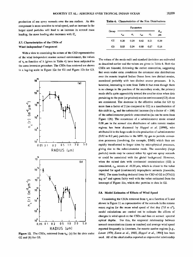
With a view to examining the nature of the CSD representative

of the wind independent marine aerosol environment, the values of % as function of • (given in Table 4) have been subjected to the same inversion procedure. The CSDs thus retrieved are shown

in a log-log scale in Figure 12a for G2 and Figure 12b for G3.

11,

0 05 0 1 0 2 0.5 10 2 0

RADIUS (urn

50

16

1 -

10 •

10

,.

10 •' • O. OS 0.1

(hi

02 0.5 10 20

RADIUS (urn)

5.0

Figure 12. The CSDs, retrieved from x0x: (a) for the data under G2 and (b) for G3.

The values of the mode radii and standard deviation are estimated

as described earlier and the values are given in Table 6. Both the

CSDs are bimodal, to!lowing the earlier convention, suggesting that even under calm conditions the columnar size distributions

over the remote tropical Indian Ocean have two distinct modes,

associated probably with two distinct source processes. It is,

however, interesting to note from Table 6 that even though there

is no change in the position of the secondary mode, the primary

mode shifts quite appreciably toward the smaller sizes when data

pertaining to the pure (or pristine) marine environment (G3) alone are considered. The decrease in the effective radius for G3 by

more than a factor of 2 (as compared to G2) is a manifestation of

this shift in r,,• and the substantial increase (by a factor of ~ 100)

of the submicrometer particle concentration (as can be seen from

Figure 12b). The occurrence of a submicrometer mode around

0.08/an in the aerosol size distribution of calm remote marine

regions has been discussed by Hoppel et al. [1990], who

attributed it to the large-scale in situ production of submicrometer

(0.02 to 0.2/an) particles in the MBL by gas to particle conver-

sion processes (involving, for example, DMS) which then are rapidly transformed to larger sizes by microphysical processes,

giving rise to the submicrometer mode. The secondary (large

particle) mode may be caused either by aged sea spray aerosols

or could be associated with the global background. ltowever,

when the mixed data with continental contamination (G2) is considered, rmi occurs at ~0.20 3tin, which is closer to the value

expected for aged (continental) tropospheric aerosols [Jaenicke,

1984]. The mass loading deduced from the CSD of G2 is (37__.11) mg m '2 and agrees fairly well with the value estimated from the intercept of Figure 11a, which also pertains to data in G2.

5.8. Model Estimates of Effects of Wind Speed

Considering the CSDs retrieved from xp as a function of ),. and shown in Figure 11 as representative of the aerosols in the remote

ocean region for the mean wind speed of that day (7.0 m s4), model calculations are carried out to estimate the effects of

changes in wind speed on the CSDs and thus on aerosol spectral

optical depths. For this, the empirical relationship between

aerosol concentrations (mass or number) and average wind speed

reported frequently in literature, for remote marine regions [e.g.,

Lovett 1978; Exton et al., 1085; Hoppel et al., 1990] has been

used. All of the cited studies reported an exponential relationship


1.00

0.50

0.10

0.05

001 '

100 ,

0.50

_ 50Ohm

• , I , ! , I , I , I

0 2 /, 6 8 10 12

0.10

0.05

OOl i • ! , I , I

/+ 6 8 lO -1

Wind speed (U m s j

12

Figure 13. Wind speed dependence of a:p from model calculations at two representative wavelengths.

between aerosol concentration S and mean wind speed (Ua) of the

form

In(S) = !n(S 0) + bU• (7)

with a value of b lying in the range 0.16 to 0.18. Considering this value of b to be applicable for the size range (0.05 to 5 htm) considered in our study, and the CSD shown in Figure 10, the CSDs are computed for Ua = 0 to 12 m s 'l in steps of 1 m s 4. Using the CSDs thus generated (using the empirical relationship of equation (7)), a:px has been estimated using the direct Mie scattering equation (2) for two typical wavelengths 400 and 750 nm, using the same refractive index as was used for the retrieval of CSDs. The results, shown in Figure 13 (for b=0.16), show that

'cp (estimated from the CSDs modified by wind speed according to equation (7) also increases with the same slope b. Though this is not very surprising because in generating the CSDs using equation (7) the aerosol concentration in the entire size range (from 0.05 to 5 htm) is considered to change by the same rate, this observation is important inasmuch as it corroborates the fact that the CSDs, retrieved from spectral optical depths, are indicative of

the general aerosol characteristics prevailing in the MBL and reproduce the optical effects. In the actual situation, however, the increase in wind speed would have different influence on particles of different sizes as different mechanisms lead to generation of

aerosols in different size regimes. For example, in addition to the

film droplets and jet droplets, large-sized droplets are also

produced associated with spume production when the wind speed exceeds ~7 m s 4 [Andreas et al., 1005]. The abundance of these particles in the MBL again depends on various atmospheric processes which determine their lifetime and this may lead to the observed scatter of points.

6. Conclusions

The main conclusions of our study are as follows:

1. Aerosol optical depth decreases rapidly as the distance from the coast increases. The influence of coastal characteristics are

found to prevail upto about 1000 km offshore. 2. In the remote ocean regions the optical depths are generally

low, usually in the range 0.1 to 0.2, when the wind speed is low. During high wind conditions the optical depths show significant increase both in the mean value and in the standard deviation.

3. Aerosol optical depths over remote oceanic regions are well correlated with mean wind speed and increase exponentially with increase in the average wind speed, with a mean value in the range 0.14 to 0.16 (_+0.04) for the index. The association is stronger when the prevailing winds are purely of marine origin. It is seen that the wind histories that prevailed about 6 to 9 hours

prior to estimate of a:p are important in influencing a:p. 4. The aerosol optical depths are found to be insensitive to

changes in the deck level RH for RH <~85%. 5. Columnar size distributions retrieved from aerosol spectral

optical depths indicated two modes at ~0.04/zm and 0.7 htm. The


columnar mass loading estimated from the distributions increased

exponentially with mean wind speed. 6. The CSDs retrieved from wind independent (background)

optical depths show a large particle mode at ~0.8/•m and a small

particle mode at ~0.05 •m for the pristine marine data set. When the marine environment has a continental contamination, the

primary mode occurs at a higher value (~0.2 •m).

Acknowledgments. This study forms part of the marine aerosol

characterization work undertaken as a part of the INDOEX precampaign,

and the authors are thankful to A.P. Mitra, FRS, who spearheaded the

program. The authors are grateful to the Department of Ocean Develop- ment, Delhi, and Director, National Institute of Oceanography (NIO), Goa,

for providing the shipboard facilities. We are also thankful to N. Bahu-

leyan (NIO), Chief Scientist of the cruise, and to the captain and officers on board the ORV Sagar Kanya for facilitating the experiments. The

authors also thank the reviewer for the useful suggestions.

References

Andreae, M.O., Climate effects of changing atmospheric aerosol levels, in Worm Survey of Climatology, Vol. 16, Future Climate of the World, edited by A. Henderson - Sellers, pp 341-392, Elsevier, New York, 1995.

Andreas, E.L, J.B. Edson, E.C. Monahah, M.P. Rouault, and S.D. Smith,

The sea spray contribution to net evaporation from the sea: A review of recent progress, Boundary Layer Meteorol., 72, 3-52, 1995.

Bigg, E.K., J.L. Gras, and C. Evans, Origin of Aitken particles in remote marine region of the southern hemisphere, J. Atrnos. Chern., 1, 203- 214, 1984.

Blanchard, D.C., The electrification of the atmosphere by particles from bubbles in the sea, Prog. Oceanogr., 1, 71-202, 1963.

Blanchard, D.C., and A.H. Woodcock, Bubble formation and modification

in the sea and its meteorological significance, Tellus, 9, 145-157, 1957. Blanchard, D.C., A.H. Woodcock, and R.J. Cipriano, The vertical

distribution of sea salt in the marine atmosphere near Hawaii, Tellus, Ser. B, 36, 118-125, 1984.

Charlson, R.J., J.E., Lovelock, M.O. Andreae, and S.G. Warren, Oceanic

Phytoplankton, atmospheric sulfur, cloud albedo and climate, Nature, 326, 655-661, 1987.

Cipriano, R.J., E.C. Monahah, P.A. Bowyer, and D.K. WooIf, Marine condensation nucleus generation inferred from whitecap simulation tank results, J. Geophys. Res'., 92, 6569-6576, 1987.

Das, P.K., Monsoons, Fifth IMO Lecture, WMO 613, World Meteorol.

Organ., Geneva, 1986. Exton, H.J., J. Latham, P.M. Park, S.J. Perry, M.H. Smith, and R.R. Allan,

The production and dispersal of marine aerosol, Q. J. R. Meteorol. Soc., 111, 817-837, 1985.

Fisher, R.A., Statistical Methods' for Research Workers', Oliver ,and Boyd,

Edinburgh, Scotland, 1970. Fitzgerald, J.W., Marine aeroso Is - A review, Atrnos. Environ., Part A, 25,

533-545, 1991.

Hegg, D.A., L.F. Radke, and P.V. Hobbs, Measurement of Aitken nuclei and cloud condensation nuclei in the marine atmosphere and their relation to the DMS-cloud-climate hypothesis, J. Geophys. Res'., 96, 8727-8733, 1991.

Hoppel, W.A., J.W. Fitzgerald, and R.E. Larson, Aerosol size distributions in air masses advecting off the east coast of the United States, J. Geophys. Res., 90, 2365-2379, 1985.

Hoppel, W.A., J.W. Fitzgerald, G.M. Frick, and R.E. Larson, Aerosol size distribution and optical properties found in the marine boundary layer over the Atlantic Ocean, J. Geophys. Res., 05, 3659-3686, 1990.

Jaenicke, R., Physical aspects of atmospheric aerosol, in Aerosols and Their Climatic Effects, edited by H.E. Gerhard and A. Deepak, pp 7-34, A. Deepak, Hampton, Va., 1984.

Junge, C.E., Air Chemistry and Radioactivity, 382 pp., Academic, San Diego, Calif., 1963.

Junge, C.E., Our knowledge of the physico-chemistry of aerosols in the undisturbed marine environment, J. Geophys. Res'., 77, 5183-5200, 1972.

King, M.D., Sensitivity of constrained linear inversion to the selection of Lagrange multiplier, J. Atrnos. Sci., 39, 1356-1369, 1982.

Kulkarni, M.R., B.B. Adiga, R.K. Kapoor, and V.V. Shirvaikar, Sea salt in coastal air and its deposition on porcelain insulators, J. Appl. Meteorol., 21, 350-354, 1982.

Lovett, R.F., Quantitative measurement of airborne sea-salt in the North

Atlantic, Tellus, Ser. B, 30, 358-364, 1978. Monahan, E.C., Sea spray as a function of low elevation wind speed, J.

Geophys. Res., 73, 1127-1137, 1968. Monahah, E. C., C.W. Fairall, K.L. Davidson, and P.J. Boyle, Observed

interrelation between 10m winds, ocean whitecaps and marine aerosols, Q. J. R. Meteorol. Soc., 109, 379-392, 1983.

Monahah, E.C., D.E. Spiel, and K.L. Davidson, A model of marine aerosol generation via whitecaps and wave disruption, in Oceanic Whitecaps, edited by E.C. Monahan and G. Mac Niocaill, pp 167-174, D. Reidel, Norwell, Mass., 1986.

Moorthy, K.K., P.R. Nair, and B.V. Krishna Murthy, Multiwavelength solar radiometer network and features of aerosol spectral optical depth at Trivandrum, Indian J. Radio Space Phys., 18, 194-201, 1989.

Moorthy, K.K., P.R. Nair, and B.V. Krishna Murthy, Size distribution of coastal aerosols: Effects of local sources and sinks, J. Appl. Meteorol., 30, 844-852, 1991.

Moorthy, K.K., B.V.Krishna Murthy, and P.R. Nair, Sea-breeze front effects on boundary layer aerosols at a tropical coastal station, J. Appl. Meteorol., 32, 1196-1205, 1993.

Moorthy, K.K., P.R. Nair, B.V. Krishna Murthy, and S.K. Satheesh, Time evolution of the optical effects and aerosol characteristics of Mr. Pinatubo origin from ground-based observation, J. Atrnos. Terr. Phys., 58, 1101-1116, 1996.

Nair P.R., and K.K. Moorthy, On the association between aerosol optical depths and surface meteorological condition in a tropical coastal environment, Mausam, 46, 427-434, 1995.

Pandis, S.N., L.M. Russell, and J.H. Seinfeld, The relationship between DMS flux and CCN concentration in remote marine regions, J. Geophys. Res., O0, 16,945-16,957, 1994.

Parameswaran, K., G. Vijayakumar, B.V. Krishna Murthy, and K.K. Moorthy, Effect of wind speed on mixing region aerosol concentrations in a tropical coastal environment, J. Appl. Meteorol., 34, 1392-1397, 1995.

Patterson, E.M., C.S. Kiang, A.C. Delany, A.F. Wartburg, A.C.D. Leslie, and B.J. Huebert, Global measurements of aerosols in remote continen-

tal and marine regions: Concentrations, size distributions and optical properties, J. Geophys. Res'., 85, 7361-7376, 1980

Prospero, J.M., Mineral and sea salt aerosol concentrations in various ocean regions, J. Geophys. Res'., 84, 725-731, 1979.

Prospero, J.M., R.J. Charlson, B. Mohnen, R Jaenicke, A.C. Delany, J. Mayers, W Zoller and K. Rahn, The atmospheric aerosol system - An overview, Rev. Geophys., 21, 1607-1629, 1983.

Rao, Y.P., South west monsoon, Meteorol. rnonogr., 1/06, India Meteorol.

Dep., New Delhi, June 1976. Russell, L.M., S.N. Pandis, and J.H. Seinfeld, Aerosol production and


growth in marine boundary layer, J. Geophys. Res., 09, 20,989-21,003, 1994.

Satheesh, S.K., and K.K. Moorthy, Atmospheric total ozone content from spectral extinction measurements, Indian J. Radio Space Phys., 25, 204-210, 1996.

Shaw, G.E., J.A. Regan, and B.M. Herman, Investigations of atmospheric extinctions using direct solar radiation measurements made with a multiple wavelength radiometer, J. Appl. Meteorol., 12, 374-380, 1973.

Shettle, E.P., and R.W. Fenn, Models for the aerosols of the lower

atmosphere and the effects of humidity variations on th•/ir optical properties, AFGL-TR-79-0214, Environ. Res. pap. 676, 26 pp, Phillips Lab., Hanscorn Air Force Ba•, Mass., 1979.

Smirnov, A.V., and K.S. Shifrin, Relationship of optical thickness to humidity of air above the ocean, Izv. Acad. Sci., USSR Atmos. Oceanic Phys., Engi. Transl. 25, 374-379, 1989.

Smirnov, A.V., Y. Villevalde, N.T.O'NeilI, A. Royer, and A. Tarussov,

Aerosol optical depth over the oceans: Analysis in terms of synoptic air mass types, J. Geophys. Res., 100, 16,639-16,650, 1995.

Suzuki, T., and S. Tsunogai, Daily variation of aerosols of marine and continental origin in the surface air over a small island Okushin in Japan Sea, Tellus, Ser. B, 40, 42-49, 1988.

Taylor, N.J., and J. Wu, Simultaneous measurements of spray and sea salt, J. Geophys. Res., 97, 7355-7360, 1992.

Woodcock, A.H., Salt nuclei in marine air as a function of altitude and

wind force, J. Meteorol., 10, 362-371, 1953.

K. K. Moorthy, B. V. K. Murthy, and S. K. Satheesh, Space Physics Laboratory, Vikram Sarabhai Space Centre, Trivandrum 695022, India.

(Received October 4, 1996; revised April 9, 1997; accepted April 11, 1997.)

Investigations of marine aerosols over the tropical Indian Ocean

Documents

Transcript of Investigations of marine aerosols over the tropical Indian Ocean