Investigation of the performance of single and multi-drop hydraulic structures

48 Int. J. Hydrology Science and Technology, Vol. 2, No. 1, 2012

Copyright © 2012 Inderscience Enterprises Ltd.

Investigation of the performance of single and multi-drop hydraulic structures

Mohamed Farouk* Faculty of Engineering, Ain Shams University, EL-Sarayat Street, Abdo Basha Square, P.O. Box 11517, Abbassia, Cairo, Egypt E-mail: [email protected] *Corresponding author

Mohamed Elgamal Irrigation and Hydraulics Department, Faculty of Engineering, Cairo University, Gamaet El Qahera St., Giza, 12613, Egypt E-mail: [email protected]

Abstract: In this paper, the work is divided into two parts. First, the hydraulic performance of single and multi-drop structures is investigated and compared using two approaches. In the first approach, the empirical equations found in the literature are summarised and reanalysed to compare the dissipation of energy of single drop and multi-drop structures. The demarcation condition at which multi-drop structure behaves as a single drop is identified. In the second approach, a numerical investigation of the hydraulic performance of single vertical drop and multi-stepped channel has been conducted via the computational fluid dynamic (CFD) fluent package using the volume of fluid (VOF) technique. It is found that the CFD package is able to simulate the hydraulic performance of both structures (single and multi-drop) reasonably well; however, it has been noted that in some situations the CFD package did not detect the presence of air cavities underneath the nappe for the napped flow case. Second, an Excel solver called HSMD has been developed. The objective of this solver is to work as an expert system for the design of drop structures and to facilitate the use of the large number of the available empirical formulas for practicing engineers. A comparison between the previous laboratory empirical formula (adopted in HSMD model) and numerical simulations has been also carried out.

Keywords: vertical drop; brink depth; toe depth; impinging point; pool water depth; critical depth; multi-drop; stepped chutes; napped flow; skimming flow; volume of fluid; VOF; computational fluid dynamic; CFD; Fluent.

Reference to this paper should be made as follows: Farouk, M. and Elgamal, M. (2012) ‘Investigation of the performance of single and multi-drop hydraulic structures’, Int. J. Hydrology Science and Technology, Vol. 2, No. 1, pp.48–74.

Biographical notes: Mohamed Farouk received his PhD in Civil Engineering from University of Manchester, UK. He is currently an Associate Professor in the Irrigation and Hydraulics Department, Ain Shams University, Egypt. His

Investigation of the performance of single and multi-drop hydraulic structures 49

research interest includes numerical simulation of different environmental and hydraulics problems such as air and water quality problems, wind environmental effects on the pedestrian, aerodynamics, wind loads on the structures, multiphase flow such as oil separator, flow through highway culverts, flow over spillways, flow through dam inlet, flow under gates, and outlet structures.

Mohamed Elgamal received his PhD in Civil and Environmental Engineering from University of Alberta, Canada. He is currently an Assistant Professor in the Irrigation and Hydraulics Department, Cairo University, Egypt. His research interest includes surface and subsurface flow modelling.

1 Introduction

Vertical as well as multi-drop structures are currently used as energy dissipators where the local topography is steeply-sloping. Although stepped chutes have been used since antiquity, they have recently regained popularity and interest among storm drainage engineers besides dam engineers partly due to the technical advances in the construction techniques and more importantly due to the significant role that steps play in the dissipation of energy (Khatsuria, 2005). Recently, road drainage engineers have shown strong interest in stepped ditches while dealing with some applications including scour problems related to steep ditches. In many cases, road drainage engineers have to deal with ditches of steep slopes that might exceed 10%. In such cases, stepped ditches might be plausible and practical solution for many reasons which include: the capability of steps for dissipating energy (it has been found that the friction factor in stepped channel flow is considerably greater than that in smooth channel flow) and thus avoiding the necessity of having the conventional energy dissipators; the possibility of using conventional concrete grades rather than high concrete grades that might be necessary in case of no steps; moreover, steps could provide better soil erosion control.

Studying the hydraulic performance of stepped spillway has been an active area of research for the last three decades. Different tools have been adopted for this regard starting from the development of downscale models in laboratories and ending at using state of the art CFD numerical tools and commercial packages (Xiangju et al., 2006) and (Musavi et al., 2008) to develop two-phase flow numerical models to simulate the complexity of air-water and free surface interactions.

The paper is structured as follow: in the next section, we describe the important design parameters of the single drop structure and compile the empirical formulas commonly used to determine the key design parameters of the hydraulic structure then we carry out a number of CFD numerical experiments (via Fluent) and compare the numerical results against the empirical formulas. In Section 3, the design parameters of the multi-drop structures are presented and the corresponding empirical design formulas are compiled. Moreover, the energy dissipation for single and multi-drop structures is compared. After reanalysing the empirical equation, the demarcation condition at which multi-drop structure behaves as a single drop is identified. In Section 4, a number of CFD numerical experiments is conducted for the multi-drop structures and a comparison of the numerical and empirical results is presented. In Section 5, an excel solver based on the empirical formulas is presented. The excel solver could be used for both of the single and multi-drop structures.

50 M. Farouk and M. Elgamal

2 Single drop structure

2.1 Previous research works and investigations

The hydraulic characteristics and performance at the base of a straight drop spillway have been extensively studied by different researchers throughout the last seven decades. Most of the studies were empirical such as: Moore (1943), Bakhmeteff and Feodoroff (1943), and Rand (1955).

Several decades after, Chanson (1994) and Rajaratnam and Chamani (1995) have analysed the empirical data of Moore (1943) and Rand (1955), and their own data with respect to energy dissipation and proposed new energy loss relationships. In parallel to lab studies, few studies were analytical such as that of White (1943), Gill (1979) and Moghaddam (1999).

A wide spectrum of numerical analysis concepts for studying the flow over single hydraulic drops are found in the literature. The available numerical concepts range from simple to more complex concepts. These concepts include: 1D models (such as HEC-RAS model), 2D depth averaged models, and the more complicated models which include: the 2D vertical and the 3D models. In these models, the location of the free water surface is identified after solving a multi-phase air-water problem via some techniques such as the volume of fluid (VOF) technique or what is alike. The common practice in solving the vertical drop structure while adopting the simple 1D or 2D horizontal model concept is to increase the Manning’s roughness to some relatively high values (to compensate the energy dissipation due to jet-pool impingement) for the approach, basin/apron and the outlet sections (relative to the drop locations) (HEC-RAS, 2010). The typical n value reported is of the order of 0.05 (US ACE, 1994). An example for the 2D-horizontal models is the work of Stockstill et al. (2010) where they modelled the flow over a number of single drop structures in a manmade channel reach to a river. The developed model is based on a two-dimensional depth-averaged module of the adaptive hydraulics (ADH) finite element flow solver.

Few numerical studies (based on 2D vertical or 3D CFD models) have been found in the literature to simulate the flow structure and the hydraulic performance over a single drop structure. An example of these numerical studies is the work of Cook and Richmond (2001) where they numerically examined the hydraulic performance of the single drop structure while validating the Flow-3D CFD package.

2.2 Important design parameters

The major design elements in the single drop structure include the following parameters:

Hd = h the drop height for single drop case

yc critical depth

yb brink depth

y1 toe depth

yp pool water depth

Ld horizontal length from the brink of the drop to the impinging point (length of the drop).


Table 1 Formulas for single vertical drop

# Au

thor

To

e wa

ter d

epth

(y1)

Re

sidu

al e

nerg

y (H

r) Po

ol w

ater

dep

th (y

p) L d

and

β

1 W

hite

(194

3)*

12

31.

062

co c

y yz y

=Δ

++

2

1.06

1.5

24

1.06

1.5

cr c

c

h

y

H

y

h

y

⎛⎞

++

⎜⎟

⎜⎟

⎝⎠

=+

++

2

1

1

.

23

p

p

pc

y

cy

c

yy

Fh

h

yy

Fy

y

=

⎛⎞

⎛⎞

=+

−⎜

⎟⎜

⎟⎝

⎠⎝

⎠

1.5

.cot

dby

L hh

β⎛

⎞=

+⎜

⎟⎝

⎠

2 R

and

(195

5)**

1.

275

10.

54c

yy

hh

⎛⎞

=⎜

⎟⎝

⎠

Hr /

Hm

ax =

1 –

0.1

1039

7 (y

c / h

) – 0

.572

18

0.66

pc

yy

hh

⎛⎞

=⎜

⎟⎝

⎠

0.81

4.30

dcy

L

hh

⎛⎞

=⎜

⎟⎝

⎠

3 G

ill (1

979)

0.

283

10.

524

0.00

53c

cy

yy

h

hh

⎛⎞

=−

⎜⎟

⎝⎠

0.69

7

1.06

70.

0016

pc

yy

h

h⎛

⎞=

−⎜

⎟⎝

⎠

1.5

.cot

dby

L hh

β⎛

⎞=

+⎜

⎟⎝

⎠ 0.

305

cos

0.96

80.

0058

cy

hβ

⎛⎞

=−

⎜⎟

⎝⎠

4

Cha

nson

(199

4)

1.32

61

0.62

5c

yy

hh

⎛⎞

=⎜

⎟⎝

⎠

0.

675

0.99

8p

cy

y

h

h⎛

⎞=

⎜⎟

⎝⎠

0.

525

2.17

1c

dy

Lh

⎛⎞

=⎜

⎟⎝

⎠

5 R

ajar

atna

m a

nd

Cha

man

i (19

95)

H

r / H

max

= 1

– 0

.089

6 (y

c / h

) – 0

.766

0.

719

1.10

7p

cy

y

h

h⎛

⎞=

⎜⎟

⎝⎠

6 M

ogha

ddam

(1

999)

1.

222

10.

505

cy

y

h

h⎛

⎞=

⎜⎟

⎝⎠

H

r / H

max

= 1

– 0

.077

(yc /

h) –

0.8

13

0.59

8

1.02

60.

03p

cy

y

h

h⎛

⎞=

−⎜

⎟⎝

⎠

0.46

6

cos

0.99

cy

h

β⎛

⎞=

⎜⎟

⎝⎠

7 C

ham

ani a

nd

Bei

ram

i (20

02)

H

r / H

max

= 1

– 0

.056

2F1

– 0.

559

(yc /

h) –

1.0

32

Not

es: *

The

pool

wat

er d

epth

equ

atio

n an

d Ld

equ

atio

n ha

ve b

een

deriv

ed b

y th

e au

thor

s of

the

pape

r in-

hand

[ref

er to

equ

atio

n (1

)] u

sing

Whi

te’s

equ

atio

n fo

r the

toe

wat

er d

epth

and

bas

ed o

n th

e de

finiti

on sk

etch

show

n in

Fig

ure

1.

**R

esid

ual e

nerg

y eq

uatio

n ha

s bee

n ob

tain

ed a

fter b

est f

ittin

g Ra

nd’s

dat

a by

cur

rent

aut

hors

.


Table 1 presents the list of equations that have been developed by different researchers. The table includes analytical equations such as those of White (1943), Gill (1979) and Moghaddam (1999). It also includes the empirical equations that have been developed based on several lab experiments within the last six decades. It should be mentioned that the most crucial design parameter in the single vertical drop structure is the water depth at the toe (y1). The pool water depth (yp) is also needed so as to make sure that the lower (underside/nappe) edge of the falling jet is aerated (ventilated) or not (if yp / h is less than one; it is aerated).

If the toe water depth is known, the other geometric design parameters could be easily estimated on analytical basis. For instance, White has formulated his toe water depth analytical formula as shown in Table 1. However White did not present analytical expressions for the pool water depth (yp) or the drop jet length (Ld). For this regard, the authors have derived an analytical expression for yp based on the control volume shown in Figure 1 and using the momentum conservation law. The following assumptions have been considered in the aforementioned derivation:

• the adopted distance between the critical depth section and the brink section is 3.5yc (which is the average value of the range given from previous laboratory observations documented in the literature)

• the water surface between the two aforementioned sections is assumed parabolic accordingly the local water depth between these two sections is defined as: y = yc – (0.0233 / yc).x2

• the bed shear stress forces could be estimated as:

( )( )

3.5

2 22* 0

21

1

*2*

.1 0.0233 /

.

2 3

8.8008 ,

c

p

p

yc

b

c

p cy

cy

c

gy dxFC x y

y yF

h h

yyF

y y

CCC g

ρτ

ε

ε

=−

=

⎛ ⎞⎛ ⎞= + + −⎜ ⎟⎜ ⎟⎝ ⎠⎝ ⎠

= =

∫

(1)

where

Fτb bed shear forces from the critical section to the brink

x downstream distance, taking the origin at the critical section

ρ water density

g acceleration of gravity

Fyp modification factor for the pool water depth

ε dimensionless friction parameter

C* dimensionless Chezy coefficient (typically ranges from 10–20).


It has been noted that the frictional forces of the approaching channel (from the critical depth section to the brink) is relatively small and it does not exceed 3.5% of the pressure force at the upstream critical depth section (for the case of C* = 17).

Figure 1 Design parameters for single vertical drop structure

h

yc yb

y1 yp

Ld

Legend: Control volume Water surface

Note: Hd = h in single vertical drop

2.3 Numerical experiments

2.3.1 Fluent package and VOF method

Fluent is one of the CFD commercial packages that are commonly used for studying the hydrodynamics of complicated flow fields including multiphase flow applications. In the study in-hand, Fluent package is adopted for carrying out all numerical simulations. In CFD literature, several methods have been used to approximate free-surface flows. A simple, but powerful method is the VOF method. This method is found to be more flexible and efficient than other methods for treating complicated free-surface flows (ANSYS, 2009). It was designed for two or more immiscible fluids where the position of the interface between the fluids is of interest.

The VOF model theory was used in this research. The model formulation relies on the fact that both fluids ‘water and air’ are not interpenetrating. Thus for each phase, a variable is introduced as the volume fraction of the phase in the computational cell. In each control volume, the volume fractions of all phases sum up to unity. The fields for all variables and properties are shared by the phases and represent volume-averaged values, as long as the volume fraction of each of the phases is known at each location.

If qth fluid’s volume fraction in the cell is denoted as αq, then the following three conditions are possible:

αq = 0 the cell is empty (of the qth fluid)

αq = 1 the cell is full (of the qth fluid)

0 < αq < 1 the cell contains the interface between the qth fluid and other fluid.

Based on the local value of αq, the appropriate properties and variables will be assigned to each control volume within the domain (ANSYS, 2009).


Conservation of mass: the tracking of the interface(s) between the phases is accomplished by the solution of a continuity equation (2) for the volume fraction of air and water phases. For the qth phase, this equation has the following form:

( ) ( ) ( )2

1

1q q q q q q pq qp

q p

S m mt αα ρ α ρ υ

ρ =

⎡ ⎤∂+∇ ⋅ = +⎢ ⎥

∂⎢ ⎥⎣ ⎦∑ (2)

where

pqm the mass transfer from phase ‘q’ to phase ‘p’

pqm the mass transfer from phase ‘p’ to phase ‘q’,

Sαq the source term, assumed zero in this research

qυ the velocity of phase q

ρ the fluid density.

From the general conservation of mass equation for phases q and p, one can obtain that:

pq qpm m= (3)

0ppm = (4)

Conservation of momentum: a single momentum equation is solved throughout the domain, and the resulting velocity field is shared among the phases. The momentum equation, shown below, is dependent on the volume fractions of all phases through the properties ‘ρ’ and the dynamic viscosity ‘µ’.

( ) ( ) [ ]Tp g Ftρυ ρυυ ν ν α∂

+∇ ⋅ = ∇ +∇ ∇ +∇ + +∂

(5)

where

F force vector

g gravitational acceleration

t time.

2.3.2 Numerical simulations for single drop

For the case of single hydraulic drop, a set of numerical experiments have been conducted. In all the numerical experiments, the model length is equal 80 m. The model length upstream of the drop is 20 m and 60 m is set downstream the drop. The depth of the drop for all runs is 3 m. Five cases (numerical experiments) are conducted in this study.

• in the first case: yc equals 0.75 m (i.e., yc / h = 0.25)

• in the second case: yc equals 1.5 m (yc / h = 0.5)


• in the third case: yc equals 3 m (yc / h = 0.75)

• in the fourth case: yc equals 3 m (yc / h = 0.95)

• in the fifth case: yc equals 4.5 m (yc / h = 1.5).

It should be mentioned that in all of the aforementioned single drop models, the number of quadrilateral cells used is about 462,500 cells. The boundary conditions are similar to the one adopted for the multi drops (Figure 13) (it is presented in Section 4).

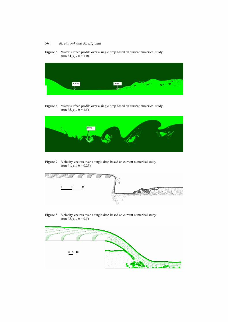
Figure 2 to Figure 6 present the water surface profiles of the five cases as per the Fluent package. It has been noted that the numerical model estimated the existence of hydraulic hump downstream of the hydraulic drop. It has been also noted that clinging nappe or no aeration condition exists for the case of (yc / h = 0.25) whereas free nappe (i.e., aerated nappe) conditions exists for the cases of (yc / h = 0.5 and yc / h = 0.75).

Figure 7 and Figure 8 present two samples of the velocity vectors corresponding to the first two runs. The velocity vectors show how the flow is accelerating at the drop location. It also describes the mixing and eddy structure that are taking place at the nappe impinging point, at the pool just underneath the drop and at the hydraulic jump.

Figure 2 Water surface profile over a single drop (clinging nappe) based on current numerical study

Figure 3 Water surface profile over a single drop based on current numerical study (run #2, aerated nappe, yc / h = 0.5)

Figure 4 Water surface profile over a single drop based on current numerical study (run #3, aerated nappe, yc / h = 0.75)


Figure 5 Water surface profile over a single drop based on current numerical study (run #4, yc / h = 1.0)

Figure 6 Water surface profile over a single drop based on current numerical study (run #5, yc / h = 1.5)

Figure 7 Velocity vectors over a single drop based on current numerical study (run #1, yc / h = 0.25)

Figure 8 Velocity vectors over a single drop based on current numerical study (run #2, yc / h = 0.5)


2.4 Comparison and discussion

Figure 9 presents the normalised toe water depth as a function of the critical depth to drop height ratio based on previous empirical and analytical analysis. The same figure shows also how the numerical results of the current study are compared with the aforementioned empirical and analytical analysis. It has been noted that the numerical results agree well with the previous empirical and analytical trends.

Figure 9 Comparison of the normalised toe water depth (single vertical drop)

0

0.2

0.4

0.6

0.8

1

1.2

1.4

1.6

1.8

0 0.5 1 1.5 2

y 1/h

yc/h

White(1943)

Rand (1955)

Gill (1979)

Chanson (1994)

Moghaddam (1997)

Current Numerical Study

Figure 10 Comparison of the normalised pool water depth (single vertical drop)


Figure 10 presents the normalised pool water depth (yp/h) as per the newly derived analytical equation [equation (1)]. The figure also shows how equation (1) is compared with the empirical equation that is given by Rand (1955). The same figure also shows the numerical results of runs no. 2, 3 and 4 (yc / h = 0.5, 0.75 and 0.95). It should be noted that the numerical simulations for run # 1 (yc / h = 0.25) produces no aeration conditions (i.e., clinging nappe).

Figure 11 Comparison of normalised residual energy (single vertical drop)

Figure 11 presents the normalised residual energy (E1 / Hmax) as a function of yc / h where

E1 is the residual energy at the toe (E1 = y1 + v12 / 2g)

Hmax is the energy upstream the drop at the critical section (Hmax = 1.5yc + h).

It has been noted that the numerical results generally match well with the empirical equations given by Rand (1955) and Moghaddam (1999). It has been noted also that White equation tends to overestimate the residual energy (compared to other formulas) for the cases of yc / h > 1.1 and it gives erroneous values (E1 / Hmax should be less than one) for the cases of yc / h >1.5.

3 Multi-stepped chute or channel

3.1 Types of flow regime over stepped chute

Flow over the stepped channel is an important and complicated hydraulic phenomenon. Stepped channel flow is a two-phase flow with free surface. The flow conditions on a stepped chute are governed by some geometric and kinematic design parameters including: the step height (h), step length (l) or implicitly the chute slope (tanθ = h / l), and the unit discharge (q) (Figure 12). Most investigators have developed empirical relationships with parameters (yc / h) and (h / l).


Figure 12 Definition sketch of stepped chute

Figure 13 Flow conditions on a stepped chute, (a) nappe flow (b) transitional flow (c) skimming flow

Source: Modified after Hanbay et al. (2009)

The first classification of stepped flow regime has been given by Essery and Horner (1971). Based on their classification, the stepped flow regime is categorised into three types: skimming flow, napped flow and transition flow. Figure 13 presents the different flow conditions on stepped chute.

For a given stepped channel setting and geometry, it has been noted that as the flow increases, the flow regime over steps is converted from nappe to transition and eventually to skimming flow. The nappe flow exists when the dimensionless critical ratio yc / h is small and it is characterised by a succession of free-falling jets (nappes) at each step edge, followed by nappe impingement on the downstream step. After the nappe impingement on the step floor, a hydraulic jump might form partially or fully within the remaining length of the step floor especially for the cases of small to relatively medium flow rates.

In case of relatively high flow rates, the jump may not occur but the nappe hits the step directly and falls on to the next step. In such flow regime, energy dissipation occurs


by jet break up in air and jet mixing on the step with or without formation of a hydraulic jump on the step (Khatsuria, 2005).

The next flow regime is the transition flow which is observed for intermediate discharges or intermediate dimensionless critical ratio yc/h. When the flow rate starts to increase above the nappe threshold (refer to Table 2), the air cavity underneath the falling nappe starts to disappear.

The transition flow regime is characterised by strong flow instabilities and fluctuations with significant splashing, spray and air entrainment near the free surface with chaotic appearance [Figure 13(b)].

It has been noted that numerous droplet ejections were seen to reach heights of up to three to eight times the step height. Accordingly, reduced ability for accurate prediction of transition flow properties is expected (Chanson and Tombes, 2004).

The last type of flow regime is the skimming flow which takes place for large discharges. The name of such flow regime has been so derived because the water skims over a pseudo-bottom that is formed by the step edges. As water skims over the steps, transmission of energy from the main skimming flow stream and the trapped (cornered) water volumes with each step boundaries takes place resulting in the formation of internal clockwise re-circulating eddies within the steps cavities (Chamani and Rajaratnam, 1999).

In order to clearly differentiate between the transition and the skimming flow patterns, some researchers (De Marinis et al., 2000) have indicated that the skimming flow conditions are defined when the air cavities beneath the falling jet disappear in all steps of the spillway, while a transition flow regime is assumed when some cavities along the stepped channel are still observed.

Table 2 presents a summary of the empirical flow classification formula and the demarcation limit between different flow regimes for the case of stepped chutes.

Figure 14 presents a flow classification chart for the stepped chute as a function of two parameters: the steepness ratio (h/l) and the critical depth to step height ratio (yc / h).

Figure 14 Flow type and classification for multi-steps channels

0

0.2

0.40.6

0.8

1

1.2

1.41.6

1.8

2

0 0.5 1 1.5 2

h/l

yc /

h

Nappe with FHJ-Chanson 1994 U.L.Nappe (Yasuda 1999)

U.L. Nappe (Yasuda 2001) U.L. Nappe (Chanson 2001)

U.L. Nappe (Chinnarasri 2002) L.L. Transition (Chanson 2004)

Skimming (Chanson 1994) Skimming (Chamani and Raj, 1999)

Skimming (Yasuda 1999) Skimming (Boes 2000)

U.L.Transition (Chanson 2004)


Table 2 Flow classification formulas for stepped chutes

# Au

thor

D

emar

catio

n lim

it Eq

uatio

n/m

etho

dolo

gy

Con

strai

nts

Rem

ark

1 C

hans

on (1

994)

N

appe

flow

with

fu

lly d

evel

oped

H.J.

y c

/ h ≤

0.09

16 (h

/ l)–1

.276

0.

2 ≤

h / l

≤ 0

.6

Bas

ed o

n R

and

(195

5) e

xper

imen

tal d

ata

2 Y

asud

a an

d

Oht

su (1

999)

U

pper

lim

it of

na

ppe

flow

y c

/ h ≤

[1.4

– (h

/ l)]

0.26

/ 1.

4 h

/ l ≤

tan

(55)

3 Y

asud

a et

al.

(200

1)

Nap

pe fl

ow

y c /

h ≤

1 / [

0.57

(h /

l)3 + 1

.3]

0.1 ≤

h / l

≤ 1

.43;

0 ≤

h / y

c ≤ 1

.37

This

equ

atio

n w

as d

evel

oped

to g

ive

the

low

er li

mit

of th

e st

ep h

eigh

t for

the

form

atio

n of

nap

pe fl

ow

4 C

ham

ani a

nd

Raj

arat

nam

(199

9)

Upp

er li

mit

of

napp

e flo

w

y c /

h ≤

4.29

7 (h

/ l)1.

613

D

e M

arin

is e

t al.

(200

0) o

bser

ved

that

the

give

n eq

uatio

n un

dere

stim

ates

the

thre

shol

d sl

ope

that

de

term

ines

the

uppe

r lim

it of

nap

pe fl

ow

5 C

hans

on (2

001)

U

pper

lim

it of

na

ppe

flow

y c

/ h ≤

0.89

– 0

.4(h

/ l)

0.05

≤ h

/ l ≤

1.7

Th

is re

latio

n is

val

id fo

r uni

form

or q

uasi

-uni

form

flo

w (n

ot v

alid

for r

apid

ly v

arie

d flo

w)

6 C

hinn

aras

ri (2

002)

U

pper

lim

it of

na

ppe

flow

y c

/ h ≤

0.98

(0.5

5)(h

/ l)

7 C

hans

on a

nd

Tom

bes

(200

4)

Low

er li

mit

of

trans

ition

zon

e y c

/ h

> 0.

9174

– 0

.381

(h /

l) 0 ≤

h / l

≤ 1

.7

8 C

hans

on a

nd

Tom

bes

(200

4)

Upp

er li

mit

of

trans

ition

zon

e y c

/ h

< 0.

9821

/[(h

/ l) +

0.3

88]0.

384

0 ≤

h / l

≤ 1

.5

9 R

ajar

atna

m (1

990)

O

nset

of

skim

min

g flo

w

y c /

h >

0.8

0.4 ≤

h / l

≤ 0

.9

10

Cha

nson

(199

4)

Ons

et o

f sk

imm

ing

flow

y c

/ h ≥

1.05

7 –

0.46

5(h

/ l)

0.2 ≤

h / l

≤ 1

.25

11

Mon

dard

o an

d Fa

bian

i (19

95)

Ons

et o

f sk

imm

ing

flow

y c

/ h ≥

1.19

74 –

0.5

9501

(h /

l)

12

Cha

man

i and

R

ajar

atna

m (1

999)

O

nset

of

skim

min

g flo

w

(h /

l) ≥

SQR

T

(0.8

9 [(

y c /

h)–1

– (y

c / h

)–0.3

4 + 1

.5] –

1)

1 ≤

h / l

13

Yas

uda

and

Oht

su

(199

9)

Low

er li

mit

of

skim

min

g flo

w

y c /

h ≥

0.86

2 (h

/ l)–

0.16

5 h

/ l ≤

tan

(55)

14

Boe

s (2

000)

O

nset

of

skim

min

g flo

w

y c /

h ≥

0.91

– 0

.14

(h /

l) 0.

47 ≤

h /

l ≤ 1

.43

15

Han

bay

et a

l. (2

009)

Id

entif

icat

ion

of ty

pe

of fl

ow

Ada

ptiv

e ne

twor

k ba

sed

fuzz

y in

fere

nce

syst

em (A

NFI

S)

0.2 ≤

h / y

c ≤ 2

.7

15°

< sl

ope

< 50

° B

ased

on

Bay

lar e

t al.

(200

3, 2

006)


Table 3 Energy dissipation formula for stepped chute

# Au

thor

D

emar

catio

n lim

it Eq

uatio

n/m

etho

dolo

gy

Con

stra

ints

Re

mar

ks

1 C

hans

on

(199

4)

Nap

pe fl

ow

with

fully

de

velo

ped

H.J.

()

()

()

0.27

50.

55

max

0.54

/1.

715

/1.

5/

cc

r

dc

yh

yh

H HH

y

−+

=+

0.

2/

6h

l≤

≤

No.

of s

teps

is su

ffici

ent

Bas

ed o

n R

and

(195

5)

expe

rimen

tal d

ata

for f

ully

dev

elop

ed q

uasi

un

iform

flow

2

Frat

ino

et a

l. (2

000)

N

appe

flow

2

max

1 2.

3 2

r

d c

HH

Hy

λλ−

+=

+

0.12

/0.

48

23

3 22

2c

hl

h y

λ

≤≤

=+

+

fo

r ful

ly d

evel

oped

qua

si

unifo

rm fl

ow

3 C

ham

ani a

nd

Raj

arat

nam

(1

994)

Nap

pe fl

ow

()

()

1 1

max

(1)

11.

5/

(1)

1.5

/

ni

ci

r

c

yh

H Hn

yh

αα

− =

⎡⎤

−+

+−

⎣⎦

=+

∑

0.74

6log

(/

)0.

5481

log(

/)

0.04

55cy

hh

lα=−

−−

4 R

ajar

atna

m

(199

0)

Skim

min

g flo

w

0.05

0.18

fC

=−

0.

4/

0.9

hl

≤≤

V

alid

for R

eyno

lds

No.

(R

n) in

the

rang

e of

: 5,

000 ≤

R n ≤

10E

+ 0

6,

base

d on

Sor

ense

n (1

985)

da

ta

5 C

ham

ani a

nd

Raj

arat

nam

(1

999)

Skim

min

g flo

w

13.

85lo

g3.

53f

y kC

⎛⎞

=+

⎜⎟

⎝⎠

()

22

./

kh

lsq

rth

l=

+

0.7

/4.

40.

6 /

0.8

cyh

hl

≤≤

≤≤


Table 3 Energy dissipation formula for stepped chute (continued)

# Au

thor

D

emar

catio

n lim

it Eq

uatio

n/m

etho

dolo

gy

Con

stra

ints

Re

mar

ks

6 C

hinn

aras

ri (2

002)

Sk

imm

ing

flow

0

12.

01.

19lo

g.

y kf=

+

01

/2.

1an

d=1

5to

59k

yθ

≤≤

°°

7 Bo

es a

nd

Min

or (2

002)

Sk

imm

ing

flow

qu

asi u

nifo

rm

11

1.0

0.25

log

0.5

0.42

(2)

hwu

kD

fSi

nθ

⎡⎤

⎛⎞

=−

⎢⎥

⎜⎟

−⎝

⎠⎣

⎦

()1/

30.

86si

nhw

uc

Dy

θ−

=

Fo

r uni

form

flo

w

8 Y

asud

a et

al.

(200

1)

Skim

min

g flo

w

1/3

2/3

max

1.c

os8.

sin

28.

sin

3 2

aa

r

d c

ff

HH

Hy

θθ

θ

−⎛

⎞⎛

⎞+

⎜⎟

⎜⎟

⎝⎠

⎝⎠

=+

Fo

r uni

form

flo

w c

ondi

tions

9 G

hare

et a

l. (2

002)

Sk

imm

ing

flow

max

1(0

.905

5.0

209

)r

ce

yH

Log

hH

=−

−

()2/

3W

hen

24

sin

dc

Hy

θ≥

V

alid

onl

y

for a

spec

ified

ch

ute

slop

e 10

Bo

es a

nd

Min

or (2

002)

Sk

imm

ing

flow

no

n-un

iform

(

)0.

10.

80.

045

sin

max

kH

dD

y cr

He

H

θ⎛

⎞⎛

⎞−

⎜⎟

−⎜

⎟⎜

⎟⎝

⎠⎝

⎠=

(

)2/3

Whe

n 2

4si

nd

cH

yθ

<

Non

-uni

form

flo

w


3.2 Comparison of energy dissipation in vertical drop and stepped chute

Steps in stepped chutes play an important rule in energy dissipation. The general understanding is that significant energy dissipation exists in case of stepped chute compared to vertical drops (of the same total vertical drop height). It was also concluded that the relative energy loss in the stepped spillway was in the range of 48% to 63% (Chamani and Rajaratnam, 1999).

Figure 15 compares the normalised residual energy (Hr / Hmax) for a single drop with the corresponding value for the case of stepped chute.

Figure 15 Comparison of residual energy head for single drop and stepped chute

Notes: hd = h for single drop case and hd = n.h for n drops in a stepped chute. Dashed curves indicate trends outside its validity range.

Figure 15 indicates that as long as the ratio yc / Hd is small (generally yc / Hd < 0.2), the residual energy head for the stepped chute is significantly less than the corresponding value for the vertical drop. It is also noted that for a given design value of yc / Hd (ex: yc / Hd = 0.14), the residual energy for a stepped chute at skimming flow condition (n = 10 steps) is larger than a stepped chute at nappe flow condition (n = 5 steps).

One could also notice that as the ratio yc / Hd gets bigger, the energy dissipation performance of stepped chute asymptotically approaches that of a single drop. In other words, the efficiency of energy dissipation for stepped chute in this case (i.e., large value of yc / Hd) is very close to that of single vertical drop. Despite the aforementioned behaviour is thoroughly discussed in the literature while differentiating skimming and nappe flow, no discussions are found in the literature (to the authors knowledge) related to the demarcation (limit) condition at which multi-drop structure behaves as a single drop. For this regard, Rand energy dissipation equation (for a single vertical drop) and Boes and Minor equation (for multiple steps) have been used to identify the demarcation condition as per Figure 16.


Figure 16 Demarcation chart for the most recommended (single or multi-) drop structure (see online version for colours)

4 Numerical experiments for stepped chutes

4.1 Previous numerical investigations

Studying numerically the hydraulic performance of stepped spillway has been an active area of research for the last decade. Different numerical tools have been adopted for this regard including 1D and 2D depth averaged models and CFD packages. Examples of the developed models by CFD (Fluent and/or CFX) packages are: Xiangju et al. (2006), Dong and Lee (2006), Musavi et al. (2008) and Rad and Teimouri (2010). Such models make use of the state of the art CFD numerical tools to develop two-phase flow numerical models to simulate the complexity of air-water and free surface interactions. Adopting the k-ε turbulence model, the mixture flow model for air-water two-phase flow is commonly used to simulate the flow field over stepped spillway using the PISO numerical technique.

In the paper in-hand, a number of numerical experiments is conducted via Fluent package. The objective is to investigate the capabilities of CFD Fluent package in simulating the hydraulic performance of flow over stepped chutes with different geometric parameters.

4.2 Boundary conditions

The adopted boundary conditions for the stepped chute are as follows (refer to Figure 17):

• pressure inlet is assumed at the inlet section

• atmospheric pressure at the upper boundary


• pressure outlet is considered at the outlet section

• wall condition is assumed at the bottom bed boundary.

Figure 17 Boundary conditions for stepped channel

4.3 Numerical experiments

For the case of stepped chute, four numerical experiments have been conducted. The number of chute steps ranges from five to ten steps with a steepness ratio (h / l) from 0.25 to 1.0. On the other hand, the normalised critical depth to step height ratio (yc / h) ranges from 0.467 to 1.01 according to Table 4: Table 4 List of numerical experimental runs for stepped chute

Numerical run

Q (m3/s)

Channel width, W (m)

dW/dx* No. of steps (n) h(m) l(m) h/l yc/h # Cells

1 2.7 1 0 5 1 1 1 0.467 80,000

2 3.5 2 0 10 1 2 0.5 0.467 560,000

3 1.7 1 0 10 1 4 0.25 0.467 1,024,000

4 7 2.2: 4.7 0.06 10 1 4 0.25 1.01: 0.61 1,029,111

In the first three runs (run #1 to run #3), the width (W) of the multi-drop structure is constant throughout the channel length. In run #4, the stepped channel width is diverging with a start width of 2.2 m and an end width of 4.7 m (dW / dx = 0.06).

According to the flow classification formulas given in Table 2, the flow type is identified for each run as shown in Table 5: Table 5 Comparison of flow type for different numerical experimental runs

Numerical run dW/dx Flow type based on Table 2

classification formula Flow type based on numerical package

1 0 Skimming Skimming

2 0 Rippled Rippled

3 0 Rippled Rippled with partial H.J.

4 0.06 Start with transition – end by rippled Start with transition – end by rippled


Figure 18 Water surface profile over a stepped chute based on current numerical study (run #1)

Figure 19 Velocity vectors and eddy patterns over a stepped chute based on current numerical study (run #1)

Figure 20 Velocity vectors over a stepped chute based on current numerical study (run #1)

m/s

Zoom in (Figure 19)




Figure 23 Velocity vectors over a stepped chute based on current numerical study (run #3)


Zoom in (Figure 23)


4.4 Results of numerical runs

Figure 18 to Figure 24 show the water surface profiles produced by Fluent package for the four numerical runs. In Figure 18 to Figure 20 (i.e., run #1), the stream lines above the virtual bed are nearly parallel and the water surface is almost parallel to the virtual bed surface which suggests that the flow might be classified as skimming flow, which agrees with the empirical flow classification formula given in Table 2.

In Figure 21 (i.e., Run #2), the stream lines are not straight but rather follow a path ‘carved’ by the steps geometry which suggests that the flow is nappe flow. This run’s result also matches with the empirical flow classification formula given in Table 2 however it has been noted that the air cavities underneath the steps almost do not exist, which means that the numerical model reflects unventilated nappe flow condition.

In Figure 22 and Figure 23 (i.e., run #3), the stream lines are not straight but it rather follows a path ‘carved’ by the steps geometry which suggests that the flow is nappe flow. It has been also noted that downstream of the impinging point of the falling jet, there is a decelerated supercritical flow zone where the local water depth is rising however the water depth did not reach its critical value before the brink of the next step and thus the numerical model reflects the case of nappe flow with partial development of a hydraulic jump. It has been also noted that the numerical model has produced some dispersed air cavities underneath the steps. On the other hand the empirical flow classification formula shows also a rippled jump condition.

In the last run, (run #4) a 3D numerical model has been developed to simulate a more complicated flow condition where the width of the multi-drop structure increases downstream. Based on the classification formulas (Table 2), the flow type is transitional at the start channel sections and changes to nappe at the drop structure end. It is interesting to note that the numerical model (Figure 24) shows that the water surface becomes more nappe (or less skimming) along the course of the channel.

5 Hydraulics of single and multi-drop solver

Based on the literature review in Section 2 and Section 3, it has been noted that there is a need for developing an integrated system or model that is based on the previously published empirical as well as analytical formulas. The purpose of that model is to work as an ‘expert system’ to facilitate the use of all the empirical equations mentioned in Table 1 to Table 3 and thus to enhance the design of the related hydraulic structures. For this regard, an excel sheet called the hydraulics of single and multi-drop (HSMD) solver has been developed. The model deals with both single and multiple drops and it includes two modules. The first module is the flow classifier module where the flow type is obtained based on the flow classification formulas given in Table 2. In this module the flow type is identified based on the drop geometry and the design flow (Q or yc) values. The second module is the flow solver module. In this module, the water depth (ytoe) and the average velocity (Vtoe) at the toe of the single drop or the multi-drop structure are calculated based on the different formulas listed in Table 3 and results are presented.


The model is fully dynamic and it is provided with a set of dynamic warning messages that are useful to the design engineer, such as the existence of transitional flow so that the designer could avoid; recommendations for step sizes; existence of inception of aeration or not (in case of streaming flow regime). HSMD also includes a number of self checks such as the applicability of formulas. The model also provides some other information such as air entrainment (not covered in this study), existence of nappe aeration for a single drop. The excel sheet also provides a comparison between the required multi-drop chute and the case of having one single drop with a comparison of the energy lost in both cases. The model could also be used to solve the case of a single drop in case of supercritical approaching flow.

Figure 25 and Figure 26 give snapshots of HSMD interface and its results while solving run #1 and run #3.

Figure 25 Snapshot of HSMD solver interface and results of run #1

Figure 26 Snapshot of HSMD solver interface and results of run #3


6 Conclusions

The study in hand focuses on investigating the hydraulic performance of single and multi-drop structures. After reanalysing the empirical formulas of energy dissipation in both structure types, it has been noted that multi-drop structures are significantly efficient in energy dissipation compared to single drop structures as long as yc / Hd is less than 0.2. Moreover, a demarcation chart has been created that identify the limiting condition at which multi-drop structure behaves as a single drop. This demarcation chart could help practicing engineer to select the best structure type and to avoid constructing steps (in some cases) that will not contribute much in the enhancement of energy dissipation. In addition to that, a numerical investigation using Fluent CFD package has been conducted to simulate the flow over single as well as multi-drop structures. It has been noted that the numerical results were generally satisfactory except for some situations where the numerical model could not detect the presence of air cavities underneath the nappe for the nappe flow case (i.e., clinging nappe).

An excel solver, HSMD, for simulating the HSMDs has been also presented. The solver is based on the empirical and analytical formulas previously published. The objective of the developed solver is to work as an expert system that helps in preliminary design stages. It is expected that the developed model (despite its simplicity) will enhance the capabilities of practicing engineers in choosing the most relevant values of the different design parameters.

Acknowledgements

The authors would like to thank Dar Al-Handasah, ‘Shair and partners’, Resource and Environment Department, for their great and continuous support.

References ANSYS (2009) ‘Fluent 12.1.4 User Guide Manual’, ANSYS Inc. Bakhmeteff, B.A. and Feodoroff, N.V. (1943) ‘Discussion on the paper energy loss at the base of

free overfall by Moore’, Trans ASCE, Vol. 108, No. HY, pp.1364–1373. Boes, R.M. (Ed.) (2000) Zweiphasenstromung und Energieumsetzungan Grosskaskaden (Two-

Phase-Flow and Energy Dissipation at Cascades), VAW, Zurich (in German). Chamani, M.R. and Rajaratnam, N. (1994) ‘Jet flow on stepped spillways’, J. Hydr. Engg.,

Vol. 120, No. 2, pp.254–259. Boes, R.M. and Minor, H.E. (2002) ‘Hydraulic design of stepped spillways for RCC dams’, Intnl.

Jnl of Hydropower and Dams, Vol. 9, No. 3, pp.87–91. Chamani, M.R. and Rajaratnam, N. (1999) ‘Characteristics of skimming flow over stepped

spillways’, J. of Hyd. Engrg., ASCE, Vol. 125, No. 4, pp. 361–368, Discussion: Vol. 126, No. 11, pp.860–872, Closure: Vol. 126, No. 11, pp.872–873.

Chamani, M.R. and Beirami, M.K. (2002) ‘Flow characteristics at drops’, ASCE Journal of Hyd Engg., August, Vol. 128, No. 8, pp.788–791.

Chanson, H. (1994) ‘Hydraulics of nappe flow regime above stepped chutes and spillways’, Australian Civil Engineering Transactions, IEAust., Vol. CE36, No. 1, pp.69–76.

Chanson, H. (2001) The Hydraulics of Stepped Chutes and Spillways, Balkema, Lisse, The Netherlands, 418pp.


Chanson, H. and Tombes, L. (2004) ‘Hydraulics of stepped chutes: the transition flow’, Jl of Hyd. Res., IAHR, Vol. 42, No. 1, pp.43–54.

Chinnarasri, C. (2002) ‘Assessing the flow resistance of skimming flow on the step faces of stepped spillways’, Dam Engineering, Vol. 12, No. 4, pp.303–321.

Cook, C.B. and Richmond, M. (2001) ‘Simulation of tailrace hydrodynamics using computational fluid dynamics models’, Report, Pacific Northwest National Laboratory, US Army Corps of Engineers, Portland District.

De Marinis, G., Fratino, U. and Piccinni, A.F. (2000) Dissipation Efficiency of Stepped Spillways: Hydraulics of Stepped Spillways, Minor and Hager (Eds.), pp.103–110, Balkema, Rotterdam.

Dong, Z. and Lee, H.J. (2006) ‘Numerical simulation of skimming flow over mild stepped channel’, Journal of Hydrodynamics, Vol. 18, No. 3, pp.367–371.

Essery, I.T.S. and Horner, M.W. (1971) ‘The hydraulic design of stepped spillways’, Report 33, Constr. Indus. Res. and Inform. Assoc., London.

Fratino, U., Piccinni, A.F. and de Marinis, G. (2000) Dissipation Efficiency of Stepped Spillways, Hydraulics of Stepped Spillways, Swets & Zeitlinger, Netherlands.

Ghare, A.D., Porey, P.D. and Ingle, R.N. (2002) ‘Experimental studies on energy dissipation over stepped spillways’, Proc Hydro, Indian Society for Hydraulics, Mumbai.

Gill, M.A. (1979) ‘Hydraulics of rectangular vertical drop’, Journal of Hydraulic Research, Vol. 17, No. 4, pp.289–302.

Hanbay, D., Baylar, A. and Ozpolat, E. (2009) ‘Predicting flow conditions over stepped chutes based on ANFIS’, Soft Comput, Vol. 13, No. 7, pp.701–707.

HEC-RAS, Hydrologic Engineering Center, River Analysis System (2010) ‘User Guide and Design Manual’, US Corps of Engineers, Version 4.1, January.

Khatsuria, R.M. (2005) Hydraulics of Spillways and Energy Dissipators, Marcel Dekker, New York.

Moghaddam, M.A.A. (1999) ‘Modified theory for rectangular vertical drop structures’, Unpublished report.

Mondardo, J.M. and Fabiani, A.L. (1995) ‘Comparison of energy dissipation between nappe and skimming flow regimes on stepped chutes’, IAHR Journal of Hydraulic Research, Vol. 33, No. 1, pp.119–122.

Moore, W.L. (1943) ‘Energy loss at the base of a free overfall’, Trans ASCE, Vol. 108, No. HY, pp.1343–1360.

Musavi, H., Bina, M. and Salmasi, F. (2008) ‘Physical and numerical modeling of the nappe flow in the stepped spillways’, Journal of Applied Sciences, Vol. 8, No. 9, pp.1720–1725.

Rad, I. and Teimouri, M. (2010) ‘An investigation of flow energy dissipation in simple stepped spillways by numerical model’, European Journal of Scientific Research, Vol. 47, No. 4, pp.544–553, ISSN 1450-216X.

Rajaratnam, N. (1990) ‘Skimming flow in stepped spillways’, Journal of Hyd. Engg., Vol. 116, No. 4, pp.587–591.

Rajaratnam, N. and Chamani, M.R. (1995) ‘IAHR energy loss at drops’, Journal of Hyd. Research, Vol. 33, No. 3, pp.373–384.

Rand, W. (1955) ‘Flow geometry at straight drop soillways’, Trans. ASCE, Proceeding, September, Vol. 81, No. 791, pp.1–13.

Stockstill, R.L., Vaughan, J.M. and Martin, K. (2010) ‘Numerical model of the hoosic river flood-control channel’, Adams, MA, Report No. ERDC/CHL TR-10-1, US Army Corps of Engineers.

US ACE (1994) ‘Technical report’, US Army Corps of Engineers, HL-94-4. White, M.P. (1943) ‘Discussion to Moore’, W., Trans. ASCE, Vol. 10, No. HY10, pp.1361–1364.


Xiangju, C., Yongcan, C. and Lin, L. (2006) ‘Numerical simulation of air-water two-phase flow over stepped spillways’, Science in China Series E: Technological Sciences, Vol. 49, No. 6, pp.674–684.

Yasuda, Y. and Ohtsu, I. (1999) ‘Flow resistance of skimming flow in stepped channels’, Proc. 28th IAHR Congress, Graz (OS), B14.

Yasuda, Y., Takahashi, M. and Ohtsu, I. (2001) ‘Energy dissipation of skimming flows on stepped-channel chutes’, 29th IAHR Congress, Beijing, China.

Nomenclature

C* dimensionless Chezy coefficient = C / g0.5 [1]

C Chezy coefficient [L0.5 / T]

Cf friction coefficient (Cf = f / 4) [1]

Dhuw hydraulic mean depth for uniform flow [L]

Fyp the modification factor for the pool water depth

Fτb the bed shear stress force for the reach from the critical depth to the brink depth in a single vertical drop structure

f Darcy-Weisbach friction coefficient (f = 4Cf) [1]

fa Darcy-Weisbach friction factor for uniform aerated flow (fa = 0.18) [1]

g the acceleration of gravity [L / T2]

h height of a single drop [L]

Hd total height of a single drop (Hd = h) or multi-drop (Hd = n.h) structures

Hmax Hmax = Hd + 1.5yc [L]

Hr residual head at the toe of the drop structure [L]

k roughness height of steps (k = h.l / sqrt(h2 + l2)) [L]

l length of step or drop in multi-drop structure [L]

Ld horizontal length from the brink of single drop to the impinging point (length of single vertical drop) [L]

n number of drops in a multi-drop structures [dimensionless]

Q flow discharge [L3 / T]

Rn Reynolds no. [1]

W width of the drop structure [L]

dW / dx longitudinal variation of drop structure width with the downstream distance x [1]

yb the brink depth in a single drop structure [L]


yc the critical depth [L]

yp the pool water depth in a single drop structure [L]

y1 the toe water depth in a single drop structure [L]

ε friction factor = 8.8008 / C*2 [1]

θ slope of multi-drop structure [1]

CFD computational fluid dynamics

HSMD hydraulics of single and multi-drop solver

VOF volume of fluid.

Investigation of the performance of single and multi-drop hydraulic structures

Documents

Transcript of Investigation of the performance of single and multi-drop hydraulic structures