University of Windsor University of Windsor

Scholarship at UWindsor Scholarship at UWindsor

Electronic Theses and Dissertations Theses, Dissertations, and Major Papers

7-11-2015

Investigation of the Formability Enhancement of DP600 Steel Investigation of the Formability Enhancement of DP600 Steel

Sheets in Electrohydraulic Die Forming Sheets in Electrohydraulic Die Forming

Jia Cheng University of Windsor

Follow this and additional works at: https://scholar.uwindsor.ca/etd

Recommended Citation Recommended Citation Cheng, Jia, "Investigation of the Formability Enhancement of DP600 Steel Sheets in Electrohydraulic Die Forming" (2015). Electronic Theses and Dissertations. 5306. https://scholar.uwindsor.ca/etd/5306

This online database contains the full-text of PhD dissertations and Masters’ theses of University of Windsor students from 1954 forward. These documents are made available for personal study and research purposes only, in accordance with the Canadian Copyright Act and the Creative Commons license—CC BY-NC-ND (Attribution, Non-Commercial, No Derivative Works). Under this license, works must always be attributed to the copyright holder (original author), cannot be used for any commercial purposes, and may not be altered. Any other use would require the permission of the copyright holder. Students may inquire about withdrawing their dissertation and/or thesis from this database. For additional inquiries, please contact the repository administrator via email (scholarship@uwindsor.ca) or by telephone at 519-253-3000ext. 3208.

Investigation of the Formability Enhancement of DP600 Steel Sheets in

Electrohydraulic Die Forming

By

Jia Cheng

A Thesis

Submitted to the Faculty of Graduate Studies

through the Department of Mechanical, Automotive & Materials Engineering

in Partial Fulfillment of the Requirements for

the Degree of Master of Applied Science

at the University of Windsor

Windsor, Ontario, Canada

2015

© 2015 Jia Cheng

Investigation of the Formability Enhancement of DP600 Steel Sheets in

Electrohydraulic Die Forming

By

Jia Cheng

APPROVED BY:

______________________________________________

Dr. S. Cheng

Civil & Environmental Engineering

______________________________________________

Dr. W. Altenhof

Mechanical, Automotive & Materials Engineering

______________________________________________

Dr. D. Green, Advisor

Mechanical, Automotive & Materials Engineering

May 7th

, 2015

III

Declaration of Originality

I hereby certify that I am the sole author of this thesis and that no part of this thesis has

been published or submitted for publication.

I certify that, to the best of my knowledge, my thesis does not infringe upon anyone’s

copyright nor violate any proprietary rights and that any ideas, techniques, quotations, or

any other material from the work of other people included in my thesis, published or

otherwise, are fully acknowledged in accordance with the standard referencing practices.

Furthermore, to the extent that I have included copyrighted material that surpasses the

bounds of fair dealing within the meaning of the Canada Copyright Act, I certify that I

have obtained a written permission from the copyright owner(s) to include such

material(s) in my thesis and have included copies of such copyright clearances to my

appendix.

I declare that this is a true copy of my thesis, including any final revisions, as approved

by my thesis committee and the Graduate Studies office, and that this thesis has not been

submitted for a higher degree to any other University or Institution.

IV

Abstract

The objectives of this thesis are to quantify the increase in formability of DP600 steel

sheets in electrohydraulic die forming (EHDF) and describe the mechanisms that lead to

a formability enhancement. Marciniak tests and EHDF tests were conducted to obtain the

conventional and EHDF forming limit curves of this sheet material, respectively. EHDF

tests with a V-shaped die indicated that, globally, there was no formability improvement;

however a 100% improvement was achieved locally near the apex of the specimen. A

formability enhancement of over 75% can be achieved in EHDF with a conical die,

provided the discharge energy is sufficient ( kV). Numerical simulations of these

tests showed that the combination of high strain rate and inertial effects helps to delay the

onset of necking prior to the sheet contacting the die. But contact phenomena play an

even more significant role to improve sheet formability by decreasing the stress

triaxiality.

V

Acknowledgements

First and foremost I would like to thank my supervisor Dr. Daniel Green, Canada

Research Chair for the Development & Optimization of Metal Forming Processes. It has

been an honour to be his graduate student. I appreciate all his contributions of time, ideas

and funding to make my Master’s experience productive and stimulating. I am also

thankful for the excellent example he has provided as a successful man in work and

personal life.

Secondly, I would like to thank Alan Gillard who provided invaluable help in

electrohydraulic die forming tests at Ford Research &Advanced Engineering. I also thank

Andy Jenner for his work of machining the test blanks and the water chamber for the V-

shaped die. In addition, I would like to thank Lucian Blaga, from CANMET Materials

Technology Laboratory, who conducted all the Marciniak tests. During this collaboration,

he also gave me some precious suggestions.

Lastly, I would like thank my family for all their love and encouragement. I appreciate

the great financial support from my parents to send me to Canada to further my studies. I

would also like to thank David and Barbara Pratt, my Canadian parents who gave me lots

of care and help in my daily life. It is they who changed the way I live.

VI

Table of Contents

Declaration of Originality ..................................................................................................III

Abstract ............................................................................................................................. IV

Acknowledgements ............................................................................................................. V

List of Tables ...................................................................................................................... X

List of Figures ................................................................................................................... XI

List of Abbreviations ..................................................................................................... XIX

Nomenclature ................................................................................................................... XX

1. Introduction ..................................................................................................................1

1.1 Background ................................................................................................................1

1.2 Motivation ..................................................................................................................2

1.3 Objectives ...................................................................................................................2

2. Literature Review .........................................................................................................4

2.1 High-Speed Forming ..................................................................................................4

2.1.1 Categories of High Speed Forming .....................................................................4

2.1.2 Description of the EHF Process ...........................................................................6

2.1.3 Advantages of EHF .............................................................................................7

2.2 Observations of Improved Formability in High Speed Forming ...............................8

2.3 Mechanisms of Formability Improvement in High Speed Forming ........................16

3. Experimental Methodology ........................................................................................26

3.1 Sheet Material Selection...........................................................................................26

3.2 Grid Etching .............................................................................................................27

3.3 Strain Measurements and Formability Analysis ......................................................28

VII

3.4 Marciniak Test (Conventional Forming)..................................................................29

3.4.1 Marciniak Test Setup .........................................................................................29

3.4.2 Carrier and Test Blanks .....................................................................................31

3.4.3 Lubricant Condition ...........................................................................................33

3.4.4 Experimental testing procedure .........................................................................33

3.5 Electrohydraulic Die Forming ..................................................................................34

3.5.1 Electrohydraulic Die Forming Setup .................................................................35

3.5.2 Impulse-current Generator .................................................................................37

3.5.3 Forming Chamber Assembly .............................................................................38

3.5.4 Electrical Insulation and Water Control ............................................................40

3.5.5 Energy Measurements .......................................................................................40

3.5.6 Die and Specimen Geometries ..........................................................................41

4. Numerical Methodology .............................................................................................44

4.1 Meshing Technique and Choice of Solver ...............................................................44

4.2 Boundary Conditions and Contact Definition ..........................................................48

4.3 Mesh Sensitivity Analysis ........................................................................................49

4.4 Material Characterization .........................................................................................53

4.4.1 Water .................................................................................................................53

4.4.2 TNT ...................................................................................................................54

4.4.3 Die .....................................................................................................................55

4.4.4 Workpiece ..........................................................................................................55

4.5 Generating a Pressure Pulse .....................................................................................60

4.5.1 Empirical Equations ..........................................................................................61

VIII

4.5.2 Determination of the Energy Discharged between the Electrodes ....................63

4.5.3 Determination of k .............................................................................................64

4.6 Validation of the Numerical Model .........................................................................66

4.6.1 Numerical Model with the V-shaped die ...........................................................66

4.6.2 Numerical Model with the Conical Die .............................................................69

5. Results and Discussion ...............................................................................................71

5.1 Quasi-static Forming (Marciniak Test) ....................................................................71

5.1.1 Strain Localization and Fracture........................................................................71

5.1.2 Forming Limit Diagram .....................................................................................73

5.2 EHDF with the V-shaped Die ..................................................................................74

5.2.1 Overview of Experimental Results ....................................................................74

5.2.2 Progressive deformation of a V-shaped specimen ............................................80

5.2.3 Investigation of the mechanisms resulting in formability enhancement ...........81

5.3 EHDF with the Conical Die ...................................................................................101

5.3.1 Overview of Experimental Results ..................................................................101

5.3.2 Overview of Numerical results ........................................................................103

5.3.3 Investigation of the mechanisms resulting in formability enhancement .........115

5.3.4. Comparison with EHFF specimens ................................................................120

6. Summary and Conclusions .......................................................................................128

6.1 Increase in formability of DP600 sheets ................................................................128

6.2 The Mechanisms of Formability Improvement ......................................................129

Bibliography ....................................................................................................................131

Appendices .......................................................................................................................134

IX

Appendix A ..................................................................................................................134

Appendix B ..................................................................................................................134

VITA AUCTORIS ...........................................................................................................135

X

List of Tables

Table 3.1. Mechanical properties and chemical composition of the as-received DP600

steel sheets ........................................................................................................................ 26

Table 4.1. Mesh sensitivity of underwater explosion model ............................................ 50

Table 4.2. Material properties of water ............................................................................. 53

Table 4.3. Gruneisen parameters for water ....................................................................... 54

Table 4.4. Material properties of TNT .............................................................................. 54

Table 4.5. JWL parameters of TNT .................................................................................. 54

Table 4.6. J-C constitutive model for DP600 ................................................................... 58

Table 4.7. Corresponding k values at different voltage levels .......................................... 66

Table 4.8. Determination of the k value for the voltage range of interest ........................ 66

Table 5.1. EHDF V-shaped specimens that exhibit safe strains that exceed the FLC ...... 76

XI

List of Figures

Figure 2.1. Schematic of simplified electrohydraulic forming process .............................. 6

Figure 2.2. Forming limit diagram using strain data from 1mm AA5754 strain samples

formed at three voltages (Oliveira et al., 2005) ................................................................ 10

Figure 2.3. Formability improvements in EMF of AA 6111-T4 and AA5754

(Golovashchenko, 2007) ................................................................................................... 11

Figure 2.4. Evolution of strain at three locations during EHF of 5182-O specimen

(Rohatgi et al., 2011) ........................................................................................................ 12

Figure 2.5. Strain-rate vs. strain (local coordinate system) at three locations on a sheet

(Rohatgi et al., 2011) ........................................................................................................ 13

Figure 2.6. Combined LDH and EHF formability results for DP500, 0.65mm

(Golovashchenko et al., 2013) .......................................................................................... 14

Figure 2.7. Combined LDH and EHF formability results for DP780, 1.0mm

(Golovashchenko et al., 2013) .......................................................................................... 15

Figure 2.8. Transmission and reflection of shock waves (Wood, 1967) .......................... 17

Figure 2.9. Effects of the velocity of the oncoming wave transmitted through the water

(Wood, 1967) .................................................................................................................... 18

Figure 2.10. Influence of velocity on and for solutionized 6061 Al, 6061-T6 Al

and Cu. (Altynova et al., 1996) ......................................................................................... 19

Figure 2.11. Microhardness as a function of expansion velocity for 6061 T6 Al and Cu.

Microhardness of materials before deformation: 6061-T6 Al: 101 HV and Cu:56 HV.

(Altynova et al., 1996) ...................................................................................................... 20

XII

Figure 2.12. Comparison of void volume fraction histories for the case of 5% nucleation

strain in the top and bottom layers of the sheet specimen (Imbert et al., 2005) ............... 21

Figure 2.13. Predicted hydrostatic stress and void volume fraction histories in the top

layer of the sheet at 5% nucleation strain during EMF into a conical die (Imbert et al.,

2005) ................................................................................................................................. 22

Figure 2.14. Predicted through-thickness stresses and plastic strains during EMF for

elements in contact with the die (Imbert et al., 2006) ....................................................... 23

Figure 2.15. Predicted stress triaxiality during EMF of free-formed and conical parts

(Imbert et al., 2006) .......................................................................................................... 24

Figure 2.16. Predicted shear stresses and strains for an outside element during EMF

(Imbert et al., 2006) .......................................................................................................... 24

Figure 3.1. Schematic of electrochemical marking .......................................................... 27

Figure 3.2. Strain measurements in FMTI system (Sklad, 2004) ..................................... 28

Figure 3.3. Schematic diagram of the Marciniak test tooling set up ................................ 30

Figure 3.4. Corresponding specimen and washer geometries for different strain paths ... 32

Figure 3.5. Magnepress power supply module ................................................................. 37

Figure 3.6. Chamber assembly with the conical die ......................................................... 38

Figure 3.7. Chamber assembly with the V-shaped die ..................................................... 39

Figure 3.8. Section view of the 34º conical die ................................................................ 42

Figure 3.9. Octagonal-shaped specimen for use in the conical dies ................................. 42

Figure 3.10. Drawing of the V-shaped die ........................................................................ 43

Figure 4.1. Numerical model of EHDF with the V-shaped die ........................................ 46

Figure 4.2. Numerical model of EHDF with the conical die ............................................ 46

XIII

Figure 4.3. Underwater explosion model for element size determination ........................ 50

Figure 4.4. Through-thickness stress history predicted by the model with three layers of

solid elements through the thickness of the blank ............................................................ 51

Figure 4.5. Through-thickness stress history predicted by the model with five layers of

solid elements through the thickness of the blank ............................................................ 52

Figure 4.6. Through-thickness stress history predicted by the model with seven layers of

solid elements through the thickness of the blank ............................................................ 52

Figure 4.7. Determination of constant A in Equation 4.3 for DP600 ............................... 56

Figure 4.8. Determination of initial constant B and n for DP600 ..................................... 57

Figure 4.9. Determination of initial constant C for DP600............................................... 58

Figure 4.10. Predicted flow curves of DP600 with initial J-C model parameters ............ 59

Figure 4.11. Predicted flow curves of DP600 with corrected J-C model parameters ....... 60

Figure 4.12. Comparison of TNT and underwater exploding wire pressure histories

(McGrath, 1965) ............................................................................................................... 61

Figure 4.13. Energy measured at the electrodes and at the Magnepress at different voltage

levels (adapted from Maris, 2014) .................................................................................... 64

Figure 4.14. Numerical model of EHFF with the open window ...................................... 65

Figure 4.15. Locations where strains were measured across the DP600 V-shaped

specimen formed using a 13 kV pulse in order to validate the numerical model ............. 67

Figure 4.16. Comparison of predicted and measured strains across both sidewalls of

DP600 V-shaped EHDF specimens formed at 11 kV ....................................................... 68

Figure 4.17. Comparison of predicted and measured strains across both sidewalls of

DP600 V-shaped EHDF specimens formed at 13 kV ....................................................... 68

XIV

Figure 4.18. Location and orientation of strain measurements on the conical EHDF

specimen used to validate the numerical model ............................................................... 69

Figure 4.19. Comparison of predicted and measured major strain in the RD and TD of the

DP600 conical specimen formed with 12.2kV ................................................................. 70

Figure 5.1. Strain localization and fracture of DP600, 1.5mm in Marciniak tests ........... 72

Figure 5.2. Forming limit diagram for DP600, 1.5mm ..................................................... 73

Figure 5.3. Elongated neck observed in the 1.5 mm DP600 specimen formed into the 38°

V-shaped die using a 13 kV pulse..................................................................................... 74

Figure 5.4. Crack in a 1.5 mm DP600 specimen formed into the 38° V-shaped die using a

14 kV pulse ....................................................................................................................... 75

Figure 5.5. Necked and maximum safe strain regions of the DP600 EHDF specimen

formed into the 38° V-shaped die using a 13 kV pulse .................................................... 76

Figure 5.6. Engineering strains of necked points for DP600, 1.5 mm, formed into the 38°

V-shaped die ..................................................................................................................... 77

Figure 5.7. Maximum engineering strains measured in safe grids in DP600 EHDF

specimens formed into the 38° V-shaped die ................................................................... 77

Figure 5.8. Comparison of the appearance of necks in the Marciniak and V-shaped EHDF

specimens .......................................................................................................................... 79

Figure 5.9. Forming limit diagram of DP600 combining necked data from V-shaped

EHDF specimens and cracked data from Marciniak specimens. ...................................... 80

Figure 5.10. Step-by-step sequence of deformation of DP600 sheet during EHDF into the

38° V-shaped die (front view) .......................................................................................... 81

XV

Figure 5.11. Two locations of interest on the upper surface of the sidewall of the V-

shaped EHDF specimen .................................................................................................... 82

Figure 5.12. Strain paths for the two locations of interest on the DP600 V-shaped EHDF

specimen formed with a 13 kV pulse ................................................................................ 83

Figure 5.13. Sequence of deformation for the DP600 EHDF specimen formed into the

38° V-shaped die with a 13 kV pulse. The location where necking occurs (X=16 mm) is

identified in each step. ...................................................................................................... 84

Figure 5.14. Sequence of deformation for the DP600 EHDF specimen formed into the

38° V-shaped die with a 13 kV pulse. .............................................................................. 85

Figure 5.15. True major strain & through-thickness stress vs. time at the location where

necking occurs (X=16 mm) .............................................................................................. 86

Figure 5.16. True major strain & through-thickness stress vs. time at the location of

maximum safe strains (X=4.25 mm) ................................................................................ 86

Figure 5.17. True major strain & effective strain rate vs. time at the location where

necking occurs (X=16 mm) .............................................................................................. 90

Figure 5.18. True major strain & effective strain rate vs. time at the location of maximum

safe strains (X=4.25 mm) .................................................................................................. 90

Figure 5.19. Right hand side of the sample with associated velocity and force profiles,

from Balanethiram and Daehn (1994) .............................................................................. 93

Figure 5.20. Position of the grid that necks at two distinct moments during the

deformation of a V-shaped specimen ............................................................................... 94

Figure 5.21. Evolution of the velocities at different locations above the necked grid (V-

shaped die) ........................................................................................................................ 95

XVI

Figure 5.22. Position of the grid that reaches the maximum safe strain at distinct moments

during the deformation of the V-shaped specimen ........................................................... 96

Figure 5.23. Velocity history of the apex of the specimen formed in the V-shaped die .. 96

Figure 5.24. Through-thickness stress & stress triaxiality histories at the location that

develops a neck ................................................................................................................. 99

Figure 5.25. Through-thickness stress & stress triaxiality histories at the location of

maximum safe strain ......................................................................................................... 99

Figure 5.26. DP600 conical specimens formed into the 34° conical die at different energy

levels ............................................................................................................................... 101

Figure 5.27. Maximum safe strains in the DP600 specimen formed into the 34° conical

die .................................................................................................................................... 103

Figure 5.28. Step-by-step sequence of deformation of the specimen formed into the 34°

conical die with 12.2 kV ................................................................................................. 104

Figure 5.29. Locations of interest in the conical specimen formed with 12.2 kV that are

identified by the horizontal distance from the apex (measured in mm) ......................... 105

Figure 5.30. Strain paths at locations of interest along the sidewall of the conical

specimen formed with 12.2 kV (position X is measured horizontally in mm from the

apex) ................................................................................................................................ 105

Figure 5.31. The influence of discharge energy on the strain path of selected points .... 107

Figure 5.32.Influence of the impact against the die on the strain path for a point near the

apex of the conical specimen formed with high energy ................................................. 108

Figure 5.33. Strain paths predicted at locations of maximum strain measured on conical

EHDF specimens formed at different energy levels ....................................................... 111

XVII

Figure 5.34. Shift in the FLC of DP600 at a low voltage (12kV)................................... 112

Figure 5.35. Shifted FLC and estimated increase in formability ( ) for the point of

maximum safe strain on the conical specimen formed at medium voltage (12.2kV)..... 113

Figure 5.36. Shifted FLC and estimated increase in formability ( ) for the point of

maximum safe strain on the conical specimen formed at medium voltage (12.5kV)..... 114

Figure 5.37. Major strain and through-thickness stress histories near the apex (X=7mm)

of the conical specimen formed at 12.2 kV .................................................................... 116

Figure 5.38. True major strain & effective strain rate histories near the apex (X=7mm) of

the conical specimen formed at 12.2 kV ......................................................................... 117

Figure 5.39. Velocity history of the apex of the conical specimen formed with 12.2 kV

......................................................................................................................................... 118

Figure 5.40. Through-thickness stress & stress triaxiality histories near the apex

(X=7mm) of the conical die formed with 12.2 kV ......................................................... 119

Figure 5.41. EHFF specimen formed in balanced biaxial tension using 13.6kV ........... 120

Figure 5.42. Necked strain data measured in different DP600 EHFF specimens (courtesy

of Maris, 2014)................................................................................................................ 122

Figure 5.43. Predicted true major strain history for the most deformed point in mode #1

cluster of data in the EHFF balanced biaxial specimen .................................................. 123

Figure 5.44. Predicted effective strain rate and vertical velocity histories of the most

stretched point (mode #1 cluster) at the pole of the EHFF balanced biaxial specimen .. 124

Figure 5.45. Predicted true major strain history of a necked point in the mode #2 cluster

of data away from the pole of the EHFF balanced biaxial specimen ............................. 125

XVIII

Figure 5.46. Predicted effective strain rate and vertical velocity histories of a necked

point in the mode #2 cluster of data away from the pole of the EHFF balanced biaxial

specimen ......................................................................................................................... 126

Figure 5.47. Predicted effective strain rate and vertical velocity histories at the point of

maximum safe strain located near the apex (X=7mm) of the conical EHDF specimen . 127

XIX

List of Abbreviations

The following table defines various abbreviations and acronyms used throughout the

thesis.

Abbreviation Explanation

AHSS Advanced High Strength Steels

ALE Arbitrary Lagrange-Eulerian

CAFE Corporate Average Fuel Economy

EF Explosive Forming

EHF Electrohydraulic Forming

EHDF Electrohydraulic Die Forming

EHFF Electrohydraulic Free Forming

EMF Electromagnetic Forming

FEA Finite Element Analysis

FLC Forming Limit Curve

FLC0 Plane Strain Intercept of the Forming Limit Curve

FLD Forming Limit Diagram

FMTI Forming Measurement Tool Innovations

IF Interstitial Free

J-C Johnson-Cook Material Model

QS Quasi-Static

RMSE Root Mean Squared Error

SGA Square Grid Analysis

XX

Nomenclature

The following table defines some of the more significant terms used throughout the thesis.

Term Meaning

DP600 A grade of dual phase steel with a minimum tensile

strength of 600 MPa.

Formability The ability of sheet metal to be formed into a desired

without necking or cracking.

Forming limit curve

A curve in principal strain space, below which there is no

risk that a combination of strains will exhibit evidence of

necking.

Forming limit diagram A plot of major strain versus minor strain which typically

contains at least one forming limit curve.

Neck A failure mechanism attributed to the reduction of

thickness due to strain localization.

Quasi-static A process which happens so slowly that strain rate and

inertial effects are negligible.

1

1. Introduction

1.1 Background

The United States government has set the corporate average fuel economy (CAFE) of

cars and light-duty trucks to 54.5 miles per gallon by 2025. Therefore vehicle weight

reduction has now become the automotive industry’s top priority to achieve this CAFE

standard, according to Evans (2013). Vehicle weight reduction not only improves fuel

efficiency but also reduces carbon emissions and protects the environment.

As was reported by the U.S. department of energy in 2011, U.S. automotive

manufacturers produce approximately 17 million vehicles annually which contain each

about 400 kg of stamped steel sheet metal components. The technology predominantly

used to manufacture automotive sheet metal parts is conventional stamping, which

generally includes deep drawing, stretch-forming, flanging and hemming operations.

These forming processes utilize two-sided tooling and rely on metal-to-metal contact

between the dies and the workpiece to achieve the desired parts.

The common strategy to produce lightweight, crash-resistant vehicles is to replace mild

steel with either advanced high strength steel (AHSS) or low-density aluminum alloys.

Due to their superior strength compared to mild steel, the thickness of AHSS sheet

components can be reduced and still meet, or exceed, the strength, stiffness and crash-

resistance requirements. For aluminum alloys, although an increase in sheet thickness is

necessary in order to satisfy stiffness and crash-performance standards, the final weight

can still be decreased due to their lower density. Therefore, the overall weight of a

vehicle can be significantly reduced by using AHSS with reduced gauge and low-density

aluminum into its body and structure components.

2

1.2 Motivation

The main difficulty with these alternative sheet materials, however, is their lower

formability in conventional, room-temperature stamping operations as compared to mild

steel. And because of the considerable costs and challenges associated with conventional

stamping of high-strength or low-density sheet materials, alternate forming processes are

being investigated and developed for the production of car body parts.

One approach to overcoming the reduced formability of high strength steel sheets is to

form them at very high velocity. Indeed, high strain rate forming has the potential to

achieve increased formability compared to quasi-static forming. For instance,

electromagnetic forming, explosive forming and electrohydraulic forming have been

investigated in recent years as they exhibit the potential of increasing the formability of

automotive sheet materials. The implementation of such novel technologies could

revolutionize the way car body parts are manufactured, increase the competitiveness of

the local automotive industry, reduce the consumption of fossil-fuels and help to reduce

carbon emissions.

1.3 Objectives

The general objectives of this work are to quantify the increase in formability of DP600

steel sheets in electrohydraulic die forming and achieve a better understanding of the

mechanisms that lead to a formability enhancement. To achieve these objectives, the

following methodology has been followed:

Conduct Marciniak tests on DP600 steel sheets in different strain paths.

Conduct electrohydraulic die forming (EHDF) tests on DP600 steel sheets with

both conical and V-shaped dies.

3

Measure strains in necked regions and severely deformed regions of the

Marciniak specimens and the conical and V-shaped EHDF specimens using an

FMTI optical strain measuring system.

Determine the corresponding quasi-static and EHDF forming limits.

Quantify the improvement in formability of DP600 in EHDF compared to the

quasi-static forming limits, considering the actual, linear and non-linear strain

paths.

Develop and validate a simplified FE model (using ALE formulation) of the

different EHDF tests, simulate the EHDF of DP600 and investigate the

mechanisms that lead to an increase in formability.

Analyze the experimental and numerical data to develop a better understanding of

the conditions and mechanisms that are required to achieve an increase in

formability.

This thesis first presents a review of the pertinent literature on high-speed forming

processes and the current understanding of formability improvement in these processes

(Chapter 2). The third chapter of the thesis describes the experimental work that was

done. Chapter 4 outlines the development and validation of the finite element model used

to simulate the various forming tests. The experimental and numerical results are then

presented and discussed in Chapter 5, and a summary and conclusions of this work are

given in Chapter 6.

4

2. Literature Review

2.1 High-Speed Forming

High-speed forming is also named as high energy rate forming, high velocity forming or

pulsed forming. High-speed forming processes have the common feature that energy is

released very rapidly to the workpiece, typically in a few microseconds. The workpiece is

therefore accelerated to velocities (20 to 300 m/s) that are substantially greater than in

conventional forming (0.3 to 5 m/s).

2.1.1 Categories of High Speed Forming

High speed forming processes are mainly classified under the following categories:

1. Explosive forming (EF)

In this process, the punch is replaced by an explosive charge. The process derives its

name from the fact that the energy released from detonation of an explosive is used

to form the workpiece into the desired configuration. Depending on the position of

the explosive charge relative to the workpiece, explosive forming is usually divided

into two groups: standoff and contact forming. In the standoff method, the explosive

charge is located at some predetermined distance from the workpiece and the energy

is transmitted through a medium such as air or water. The peak pressure on the

workpiece varies from 10 MPa to several hundred MPa and depends on the process

parameters. In the contact method, the explosive charge is held in direct contact with

the workpiece and the peak pressure on the surface of the metal is much greater than

in the previous method: it can reach several GPa.

5

2. Electrohydraulic forming (EHF)

In electrohydraulic forming, electric energy is stored in a capacitor bank and

suddenly discharged between two electrodes that are submerged in a water-filled

forming chamber. In some cases, the spark gap is connected with a straight wire or

coil, which leads to a more repeatable and reliable process. Due to ionization and

steam produced during the discharge, a high-pressure wave develops and propagates

through the water and forms the sheet metal at high velocity into a die cavity.

3. Electromagnetic forming (EMF)

In this process, the electric energy stored in the capacitors of a pulsed power

generator is discharged into an electromagnetic coil. Consequently, a damped

sinusoidal current pulse flows through the inductor, and the time-dependent current

induces a corresponding magnetic field. If there is an electrically conductive

workpiece in close proximity to the inductor, the energy density of the pulsed

magnetic field generates a force that acts upon work piece, and as a consequence of

this force the workpiece can be accelerated up to a strain rate of approximately

10,000 .

EF is not generally regarded for mass production due to safety concerns and its limited

efficiency. The usefulness of EMF as a production process is also restricted by the need

for expensive electromagnetic coils that must be discarded after only a few cycles and for

highly-conductive driver material that complicates the process. In contrast,

electrohydraulic forming (EHF) is a very promising technology that has been developed

6

to the point where it could almost be implemented into low-volume production of

automotive parts. Therefore this study focuses on investigating the formability

improvement that can be achieved using EHF.

2.1.2 Description of the EHF Process

EHF is a high-energy rate forming process that directly converts electrical energy into

work. In typical EHF, a pair of electrodes is submerged in a water-filled chamber and a

high-voltage discharge between those two electrodes creates a high-energy plasma

channel which vaporizes a small volume of the liquid and generates a high-intensity

shock wave that propagates through the water at the speed of sound towards the blank.

The shockwave simultaneously transforms the metal workpiece into a visco-plastic state

(rate-dependent plastic behaviour of solids) and accelerates it onto a die, enabling

forming of complex shapes at high speeds at room-termperature. The entire forming

process takes place within milliseconds.

Figure 2.1. Schematic of simplified electrohydraulic forming process

7

The electric equipment for carrying out the electrohydraulic process consists of three

functional groups of components: 1) Charging equipment with transformer, rectifier and

charging resistances, 2) Parallel connected capacitors for capacitive energy storage;

discharging unit equipped with spark gaps and 3) Coaxial cables and spark heads. Figure

2.1 shows a schematic of the main components in a typical EHF process.

2.1.3 Advantages of EHF

One of the interesting advantages of EHF is that only single-sided dies are required,

which significantly reduces the cost of dies as compared to the mating dies required in

conventional stamping. Because the solid punch is replaced by water, the friction that

results from contact between the punch and the workpiece is eliminated on one side of

the part. Therefore, the forming force is more evenly distributed over the surface of the

workpiece, which helps to avoid stress concentrations and failure initiation sites.

Moreover, EHF is a single-step process compared to stamping which is usually a multi-

step progressive process that requires a series of die sets: this simplifies the

manufacturing process and reduces costs. One of the most interesting advantages of this

technology is that EHF can lead to improved formability, thus enabling greater draw

depths than can be achieved with conventional drawing. Golovashchenko, Gillard, &

Mamutov (2013) indicated that the significant improvement in formability that is

observed has a practical application in corner filling for automotive panels. In addition,

the high forming speeds achieved in this process result in minimal springback of formed

parts. Finally, the improvement in formability will allow higher strength sheet materials

to be used, which signifies that sheet thickness can be further reduced. Therefore this

8

technology is very promising for use in low-volume, commercial and defense

applications, such as the production of automotive and aerospace components.

2.2 Observations of Improved Formability in High Speed Forming

In some of the earliest research on high speed forming, Wood (1967) carried out

experimental tests at very high strain rates using explosive forming and capacitor-

discharge energy. These tests included tensile testing, tube bulging and dome bulging for

a wide variety of materials. As Wood indicated, the maximum ductility of 17-7 PH was

enhanced by a factor of almost two compared to the original ductility. Balanethiram &

Daehn (1994) investigated the formability of a BCC sheet material (interstitial free iron)

and two FCC materials (annealed and quenched 6061 aluminum and annealed oxygen-

free high-conductivity (OFHC) copper) formed by electrohydraulic discharge and found

that the forming limits of these three materials increased by a factor of well over two

compared to their conventional FLC. Imbert, Winkler, Worswick, & Golovashchenko

(2004) investigated EMF of AA5754 and AA6111 sheet formed into conical dies with

either 40º or 45º side angles and observed that the greatest safe true major strain reached

0.67 for AA5754 and 0.425 for AA6111, which was double the strain of the as-received

FLC for the same level of minor strain. Two failure modes were observed with different

materials: significant thinning prior to fracture for AA5754 and a combination of plastic

collapse and ductile fracture for AA6111. El-Magd & Abouridouane (2004) investigated

the deformation and fracture behavior of AA7075, AZ80 and a Ti-6Al-4V alloys in

quasi-static and dynamic uniaxial compression and tension tests at strain rates in the

range of 0.001 to 5000 and temperatures between 20 ºC and 500 ºC. Also, both

quasi-static and dynamic shear tests of AZ80 were performed in the range of 0.01 to

9

116,000 at 20 ºC. They observed that the ductility of AA7075 and AZ80 increased

dramatically with strain rate due to a high strain-rate sensitivity. In contrast, Ti-6Al-4V

showed a drop in formability due to the dominating rate dependence of the damage

process. Seth, Vohnout, & Daehn (2005) performed electromagnetic impact tests with a

curved punch. They reported that in these tests, the increase of high-velocity formability

of five low-alloy cold-rolled steels with different quasi-static ductility varied from a

factor of 4 to a factor of 20. Regardless of large differences in quasi-static ductility of

those materials, the strain distribution lay in the same range of 20-55%. However, only

strain measurements from uniaxial tensile tests were selected as the quasi-static reference

forming limit. Oliveira, Worswick, Finn, & Newman (2005) used two different dies, a

flat-bottom die and the other one with a hemispherical protrusion at the bottom of the die

cavity, to perform a series of high strain-rate electromagnetic forming tests. They

measured maximum engineering strains of ~ 40-50% when forming AA5754 by EMF

into a rectangular die, which is almost twice the level of strain of the conventional

forming limit.

10

Figure 2.2. Forming limit diagram using strain data from 1mm AA5754 strain samples

formed at three voltages (Oliveira et al., 2005)

Golovashchenko (2007) conducted EMF tests with a round, open window, a V-shaped

die and a conical die, which provided information on the change in formability for

different strain paths. As indicated in Figure 2.3, specimens formed into a V-shaped die

or into a conical die exhibited a significant increase in formability: the maximum true

major strain for AA6111-T4 increased to about 0.63 while that of the quasi-static FLC

was only around 0.25. However, the maximum strains obtained from free forming

showed only a slight increase in formability as compared to a quasi-static process.

11

Figure 2.3. Formability improvements in EMF of AA 6111-T4 and AA5754

(Golovashchenko, 2007)

Dariani, Liaghat, & Gerdooei (2009) investigated sheet metal formability under

conditions of quasi-static, low impact and explosive free forming. Substantial

improvements in high strain-rate formability were observed as compared to quasi-static

deformation, which was displayed as almost parallel FLCs on the FLD. Similarly, Kim,

12

Huh, Bok & Moon (2011) performed uniaxial tensile tests and high-speed crash tests at

high strain-rates, which showed that the strain rate had a noticeable influence on the

formability of steel sheets. Rohatgi, Stephens, Soulami, Davies & Smith (2011)

developed a novel experimental technique which combines high-speed imaging and

digital image correlation techniques. They applied this technology to electrohydraulic

free forming to observe the high strain-rate deformation behavior of AA5182-O sheets. A

very detailed description of sheet deformation evolution in high strain-rate forming

process was given in this paper. As shown in Figure 2.4, the further an element was

located from the apex, the more non-linear the strain path was.

Figure 2.4. Evolution of strain at three locations during EHF of 5182-O specimen

(Rohatgi et al., 2011)

Also, the strain-rate vs. strain in Figure 2.5 indicates that the strain accumulated at any

given location on the formed specimen is achieved through a range of strain rates, from 0

to the highest value and then back to 0.

13

Figure 2.5. Strain-rate vs. strain (local coordinate system) at three locations on a sheet

(Rohatgi et al., 2011)

Rohatgi et al. (2012) compared and contrasted the electrohydraulic free forming and

electrohydraulic conical-die forming behavior of 1 mm thick AA5182-O and DP600 steel

sheets employing the DIC technique. They found the use of the conical die was of

significant benefit to amplify the apex velocity, strain rates and strains relative to free

forming. They insisted that the die geometry focused the energy to deform the sheet when

the sheet is contracted into the tip of die cavity. Also, they noted that the die helped to

increase the strain rate more effectively than the increase of capacitor voltage. Another

fact they discovered is that the strain path at the apex was generally linear for both free

forming and conical-die forming. Golovashchenko et al. (2013) made a comparison of

maximum strains of dual phase steels resulting from EHF into a conical die and a V-

shaped die to those from quasi-static limiting dome height testing. Considerable increase

of deformation was observed in the EHF process, especially for the plane-strain path. As

14

is shown in Figure 2.6, a 37.5% relative increase in major strain was observed for DP500

in biaxial stretching at 20% minor strain, and above 100% relative improvement in plane

strain. As for DP590 shown in Figure 2.7, both major strains obtained in EHF

corresponding to the minor strain of 0% and 21% almost doubled that achieved in as-

received FLC at the same levels of minor strain respectively. Golovashchenko et al.

thought that high strain-rates accompanied by a high hydrostatic stress contributed to the

maximum increase in formability with EHF technology. Only a very slight improvement

in formability was achieved if the sheet did not reach the apex of the die. Also, these

authors developed a complex, multi-physics numerical model with detailed exploding

wire model to predict the sheet metal behavior during EHF process.

Figure 2.6. Combined LDH and EHF formability results for DP500, 0.65mm

(Golovashchenko et al., 2013)

15

Figure 2.7. Combined LDH and EHF formability results for DP780, 1.0mm

(Golovashchenko et al., 2013)

Gillard, Golovashchenko & Mamutov (2013) developed a hybrid forming process

consisting of a quasi-static hydroforming preforming step and followed by a single EHF

pulse. They compared the improvements achieved in this hybrid forming with those in

one-pulse EHF and found that the amount of increase in formability decreased in the

hybrid forming process although it was still significant. Recently, Rohatgi, Soulami,

Stephens, Davies & Smith (2014) quantified the improvement in formability of AA5182-

O at high strain-rates using EHF, and DIC technology was used to record the deformation

history. As was shown, the formability of AA5182-O aluminum alloy sheets locally

increased by about 2.5 times and 6.5 times at minor strains of about –0.1 and 0.05,

respectively, relative to the corresponding quasi-static forming limit. Hassannejadasl,

Green, Golovashchenko, Samei & Maris (2014) used the Johnson-Cook (JC) damage

16

model in numerical simulations to predict the circumferential damage accumulation near

the apex of the specimen in EHDF. Numerical results showed that the maximum effective

strain rates in EHDF were in the order of 10,000 , which is much higher than those

observed in EHFF (3000 ). It was also pointed out in this work that the sheet/die

impact can lead to an abrupt change in strain path from biaxial to plane strain during

EHDF.

2.3 Mechanisms of Formability Improvement in High Speed Forming

Wood (1967) concluded that the increase in formability mainly resulted from the fact that

the material’s constitutive behaviour changes at high strain rate. The increasing rate of

strain hardening has a positive effect to forestall the unstable neck and fracture. Also, he

discovered that the negligible increase in ductility observed in samples deformed beyond

critical velocities was limited by the strain wave propagation. Figure 2.8 shows the

transmission and reflection of shock waves. When a shock wave propagating through

water reaches a metal workpiece, two waves are generated from the front water-metal

interface: one propagates through the metal and the other is reflected back through the

water. This reflected wave is compressive due to the low (water) to high (metal)

impedance. This compressive reflected wave is the most important reactive force of the

initial shock wave, and makes a dominant contribution to the deformation of the blank. A

tensile rarefaction wave will also form due to high (metal) to low (vacuum) impedance as

the incident wave reaches the back side of the blank and is reflected.

Figure 2.9 shows the effect of a shock wave on the forming process. √ ⁄ is the

tension-shock-wave velocity moving at the speed of sound in the blank towards its center,

17

which shows C is determined by the material properties of the medium. The author

investigated the condition that the metal is firmly clamped around the edge. The solution

to the wave equation with proper boundary condition is ( ⁄ ) , where 0V is

the velocity of the on-coming wave transmitted through the water and LV is the average

velocity at which the cup wall elongates. As is indicated, when 0V far exceeds C in the

metal, the wave velocity is insufficient to propagate through the metal into the center, and

most deformation is produced in the area near the clamped edge, which leads to a

different failure mode than at lower speed.

Figure 2.8. Transmission and reflection of shock waves (Wood, 1967)

18

Figure 2.9. Effects of the velocity of the oncoming wave transmitted through the water

(Wood, 1967)

Besides the change in the material constitutive behaviour at high strain rate, Balanethiram

& Daehn (1994) concluded that it was material inertial effects that stabilize the

development of a neck in the sample. The inertial force helps to diffuse the deformation

throughout the sample by increasing the stress at the gripped end. Also, they defined the

term “hyperplasticity” as the plasticity of the workpiece when it is deformed at velocities

in excess of 175 m/s; this found to be the critical velocity for most materials. In an effort

to better understand how ductility was affected by inertia, Altynova, Hu, & Daehn (1996)

conducted the electromagnetic expansion of thin ring tests along with quasi-static tensile

tests and established a simple one-dimensional model. In axisymmetric ring expansion,

the authors did not need to consider the complications that arose from the shock wave

propagation because of the symmetry of the problem. The authors analyzed two separate

factors: inertial effects and changes in material constitutive behaviour at high strain-rates.

The hardness at various velocities was measured to indicate the material behaviour

19

change at high strain-rates. Figure 2.11 indicated the change in constitutive behaviour

only made a minor contribution to the increase in ductility that was seen. Therefore, it is

the inertial effect that mainly accounts for the formability improvement. As is shown in

Figure 2.10, ductility measured in the form of the reduction in the cross section of the

uniform parts of the samples can exceed the quasi-static value by 60, 150 and 250% for

Cu, solutionized 6061 Al, and 6061-T6 Al, respectively when the expansion rate was

greater than 200 m/s.

Figure 2.10. Influence of velocity on and for solutionized 6061 Al, 6061-T6 Al

and Cu. Solid symbols represent the measured total elongation and open symbols the

average uniform elongation. Solid lines are simulated results. (Altynova et al., 1996)

20

Figure 2.11. Microhardness as a function of expansion velocity for 6061 T6 Al and Cu.

Microhardness of materials before deformation: 6061-T6 Al: 101 HV and Cu:56 HV.

(Altynova et al., 1996)

El-Magd & Abouridouane (2004) indicated that increased strain rate sensitivity and the

adiabatic character of the deformation process mainly characterized the mechanical

behaviour of materials. They observed that the ductility of AA7075 and AZ80 increased

dramatically with strain rate due to high strain-rate sensitivity. In contrast, Ti-6Al-4V

showed a decreasing trend due to the dominating rate-dependence of the damage process.

It was found that the damage of three materials was caused by the deformation

localization and shear bands. Imbert, Winkler, Worswick, Oliveira & Golovashchenko

(2005) studied the effect of tool-workpiece interaction on formability in electromagnetic

forming of aluminum alloy sheets. Tool-workpiece interaction consists of the inertial

ironing, as well as the bending-unbending which the sheet undergoes when it is deformed

into the die. Compressive hydrostatic stresses result from the interaction between the tool

21

and sheet, which reduces the amount of damage. As a result, the formability improves

significantly. As is shown in Figure 2.12 and 2.13, an element in the top layer reaches a

peak void volume fraction before impact. Upon impact, the sheet straightens and

rebounds and large negative hydrostatic stresses are generated in the top layer so that the

porosity is suppressed. Meanwhile, the bottom layer deforms in tension and the material

sees a sudden increase in porosity upon impact, which causes the highest amount of

damage. It was concluded, therefore that the increased formability is mainly attributed to

tool-sheet interaction during EMF.

Figure 2.12. Comparison of void volume fraction histories for the case of 5% nucleation

strain in the top and bottom layers of the sheet specimen (Imbert et al., 2005)

22

Figure 2.13. Predicted hydrostatic stress and void volume fraction histories in the top

layer of the sheet at 5% nucleation strain during EMF into a conical die (Imbert et al.,

2005)

Imbert, Worswick & Golovashchenko (2006) analyzed the factors that contribute to the

increased formability observed in AA5754 aluminum alloy sheets during EMF. They

concluded that high hydrostatic stresses, through-thickness compression and shear

stresses contributed to the overall improvement in formability of AA5754. High

hydrostatic stresses induced by tool-sheet impact suppress the damage and change the

failure mode of the material. Shear stresses and strains due to friction during the tool-

sheet contact help the material achieve additional deformation. Also the non-linear strain

paths lead to greater strains when the sheet is formed into a conical die. Figure 2.14

shows the evolution of the predicted through-thickness stresses and strains of an element

during the contact with the die. A very high compressive hydrostatic stress is created by

the extremely high through-thickness stress. Also, the closer the element is to the die, the

greater the through-thickness stresses and strains are.

23

Figure 2.14. Predicted through-thickness stresses and plastic strains during EMF for

elements in contact with the die (Imbert et al., 2006)

Figure 2.15 compares the stress triaxiality history predicted for elements in free-formed

and conical specimens. The stress triaxiality is defined as the ratio of the hydrostatic

stress or mean stress to the effective stress. As it can be seen in this figure, the triaxiality

of the free-formed elements undergoes a steady increase throughout the forming process

whereas the conical specimen is characterized by a considerably negative triaxiality

caused by the existence of the high through-thickness stress. The triaxiality of the stress

state is known to greatly influence the amount of plastic strain which a material may

withstand before ductile failure takes place.

24

Figure 2.15. Predicted stress triaxiality during EMF of free-formed and conical parts

(Imbert et al., 2006)

Figure 2.16 shows the predicted shear stress and strain for an element on the outside layer

of the conical specimen. Imbert et al., (2006) noted that the shear stress cannot be

neglected due to its magnitude being in the same order as the yield stress. This shear

stress makes a positive contribution to the improvement in formability.

Figure 2.16. Predicted shear stresses and strains for an outside element during EMF

(Imbert et al., 2006)

25

In conclusion, much more formability enhancement can be achieved in EHDF compared

to EHFF. But the traditional method to quantify the improvement in formability in EHDF

is neither accurate nor acceptable because the change in strain path is not taken into

account. The mechanisms of this improvement are still being investigated. Generally, the

increase in formability can be attributed to three mechanistic factors: strain rate effects,

inertial effects and contact effects. However, there is a contradiction in terms of the

understanding of strain rate effects on formability improvement among previous

researchers. In addition, these factors are not linked with each other dependent on

deforming time history in previous explanations.

In this research, the actual increase in formability in EHF will be quantified by

comparing the strains attained in EHDF experiments with the conventional FLC

determined by quasi-static formability tests. Moreover, the effect of non-linear strain

paths on the as-received FLC will also be considered and a better understanding of the

mechanistic factors that lead to formability improvement in EHDF will be discussed.

26

3. Experimental Methodology

The experimental tests carried out in this research and presented in this chapter fall into

two main categories. The first type of test consisted of typical sheet forming tests:

Marciniak tests were carried out at room temperature and under quasi-static loading

conditions. The main goal for conducting these tests was to determine the forming limit

curve of DP600 under conventional forming conditions. The second type of test consisted

of EHDF into either a 34º conical die or a 38º V-shaped die in order to achieve biaxial

and plane-strain stretching, respectively, at high strain rates.

3.1 Sheet Material Selection

DP600 steel was selected for this study due to its common usage in the automotive

industry. The sheet material used in the experimental program was 1.5mm thick. The

microstructure of DP600 consists of hard martensite, and soft formable ferrite. The

ultimate tensile strength of this material is greater than 600 MPa. To avoid any

inconsistencies, all sheet specimens were from the same batch. The material properties of

this DP600 steel are listed in Table 3.1.

Table 3.1. Mechanical properties and chemical composition of the as-received DP600

steel sheets

t

(mm) o

(MPa)

uts

(MPa)

unif

(%)

tot

(%)

Chemical Composition (wt%)

C Mn Si Cr Mo Cu Al

1.5 345 617 17.4 25.5 0.107 1.50 0.18 0.18 0.21 0.06 0.04

27

3.2 Grid Etching

In order to measure the strains on deformed specimens, a 2.54 mm-square grid pattern

was etched onto flat blanks before forming. Electrochemical etching has long been

regarded as the best method for gridding blanks, in terms of accuracy, durability and cost.

Also, electrochemical marking is uniformly deep. The surrounding metal will not be

influenced and strain concentrations will not be introduced either.

As is shown in Figure 3.1, a calibrated stencil is placed onto a blank. The stencil has a

non-conducting coating applied across its surface except for those locations where

markings are desired. A wick pad saturated with electrolyte is placed above the stencil,

and both a metallic roller marker and the blank are connected to a power unit. As the

roller marker is rolled back and forth across the wick with a moderate pressure, the

electric current flows through the electrolyte and the blank under the stencil is

electroetched. Each sheet material requires a specific electrolyte and its own power

settings for optimum markings.

Figure 3.1. Schematic of electrochemical marking

28

3.3 Strain Measurements and Formability Analysis

The FMTI grid analysis system was utilized to measure strains deformed in sheet metal

specimens produced by forming processes, as shown in Figure 3.2. The system consists

of a special grid analyzer and the grid analysis software installed on a personal computer.

The grid analyzer captures images of a grid marked on the sheet surface by a specialized

digital camera connected to the computer. And the computer displays and analyzes these

images further through the installed software.

Figure 3.2. Strain measurements in FMTI system (Sklad, 2004)

The scale factor that normalizes the image to the unit space is determined by an

automated square grid analysis (SGA) system which compares each image to the initial

undeformed square grid image. Following this step, the SGA system calculates the

direction and magnitude of each of the principal strains. The algorithm assumes the

direction normal to the image plane is one of the principal strain directions.

In the process of strain analysis, strains were categorized into three types (safe,

questionable and necked) according to a consistent standard. If the neck cannot be

observed by naked eye or detected by the touch of a finger, the strain at this location is

29

considered “safe”. But if a neck can be detected, and if it lies inside the grid, the strain is

considered “necked”. If a neck does not clearly lie within a single grid but is distributed

across two grids, the strain is considered “questionable” or “neck affected”.

3.4 Marciniak Test (Conventional Forming)

In order to determine the quasi-static forming limit curves of DP600, Marciniak tests

were conducted at CanMet Materials Laboratory. The basic set-up and experimental

procedures for these formability tests will be fully described in the following sections.

The main advantages of the Marciniak test are that the severe strain gradients developed

by the traditional dome test are eliminated and variability due to friction between the

punch face and the test piece is removed as well.

3.4.1 Marciniak Test Setup

The distinguishing feature of the Marciniak test is the use of a carrier blank with a central

hole, as is shown in Figure 3.3. The test piece is stacked together with the carrier blank

and the two blanks are placed in the open die and clamped in the press with a clamping

force of 70Kip (311kN) so that no material can flow out of the die. The Marciniak test is

designed to simply convert a vertical force into a biaxial force in the horizontal plane.

And this is achieved by a flat punch deforming a test piece indirectly via a carrier blank

with a central hole. The speed of the punch was set to 0.1mm/s throughout all the tests.

30

Figure 3.3. Schematic diagram of the Marciniak test tooling set up

The carrier blank, or washer, is peened (sand blasted) on the side facing the specimen to

increase the friction between the carrier blank and specimen. The central hole in the

carrier blank expands as it is formed under the moving punch. Meanwhile, the test blank

is stretched with the carrier blank over the flat punch. The radial friction forces in the

contact region between the carrier blank and the test blank prevent the sheet from

fracturing near the punch profile radius. Also, a layer of Teflon is placed between the

punch and carrier blank to reduce the strains in the specimens around the punch profile

radius. The maximum strain in the test blank develops in the center of the test piece and

is proportional to the travelling distance of the punch. It is noted that all Marciniak tests

were carried out at room temperature under quasi-static loading conditions and

displacement control.

31

Two digital cameras were installed in the press so that the operator could view the

surface of the test piece throughout the whole deformation process and determine the

moment at which necking begins. Lighting for the test was provided by ambient light and

diffused LED light.

3.4.2 Carrier and Test Blanks

The Marciniak test was designed so that the carrier blank prevents any contact between

the test piece and the surface of the punch. This ensures an in-plane, homogeneous strain

distribution in the test piece, and leads to the maximum stress being located at the centre

of the test piece. Carrier blanks should have greater ductility compared to the material

being tested; this prevents the carrier blank from fracturing before the test piece. Hence, it

is common to use IF steel to make the carrier blanks. The minimum thickness of the

carrier blank should be approximately 0.8 times the thickness of the test piece. In this

work, the thickness of IF steel carrier blanks was 1.6 mm for tests in plane strain and

balanced-biaxial tension, and 0.93 mm for tests in uniaxial tension. In addition, the hole

size of carrier blanks is an important parameter that has an influence on the results.

Quaak (2008) mentioned that the Marciniak test has same results as a deep drawing test if

the hole size of the carrier blank is infinitesimal under certain conditions. While a larger

hole size of carrier blanks can lead to the washer sliding off the punch and thereby

initiating a cutting type of failure. In this research, a 2-in. diameter hole was used in plane

strain and balanced-biaxial stretching, and a 1.5-in. diameter hole was used in uniaxial

tension.

32

Figure 3.4. Corresponding specimen and washer geometries for different strain paths

By varying the shape and width of the test piece, any strain path from uniaxial to

balanced-biaxial tension can be achieved. The position of the carrier and test blanks used

in the test are shown in Figure 3.3 and the range of test piece geometries and

corresponding strain paths are shown in Figure 3.4.

33

3.4.3 Lubricant Condition

In Marciniak tests, no lubrication is used between the carrier blank and the test piece

since friction at this interface should be maximized. However, a lubricant is typically

used between the punch and the carrier blank to ensure that the carrier blank easily

stretches over the punch face and that rupture starts in the flat central region of the test

piece immediately below the hole in the carrier blank (see Figure 3.3). In these tests, a

circular Teflon membrane was used to minimize punch friction.

3.4.4 Experimental testing procedure

The following testing procedure was followed in this work:

1) Stack a carrier blank onto a test specimen and place them together on the lower

die (carrier blank facing up), ensuring that the double-blank assembly is centered

in the die.

2) Place a 0.1mm-thick layer of PTFE (Teflon) onto the carrier blank, between the

punch and the carrier blank.

3) Adjust the focus of the camera, the orientation of the lighting system and ensure

the camera is capturing a clear image of the specimen surface, as seen in the

monitor.

4) Set the prescribed clamping force to 70Kip (311kN) to make sure the bead will be

formed and the double blank will be locked.

5) Set the prescribed punch speed to 0.1 mm/s

6) Prescribe the maximum punch stroke and start the test. The punch load and stroke

are continuously recorded in real time throughout the test.

34

7) Carefully observe the image of the test piece on the monitor and the recorded

punch load throughout the test.

8) Allow the test to continue until the maximum punch stroke is reached, or

manually interrupt the test at the onset of necking (appearing as a shaded band

parallel with the sheet rolling direction) which usually occurs just before the

maximum punch load on the load vs. time graph that is displayed.

9) After the punch retracts to its original position and the die opens, remove the

formed double blank specimen.

10) Visually observe the necked specimen, or touch the necked region with the tip of

a sensitive finger, in order to determine the severity of the neck. Record the

maximum punch stroke and determine by what amount to modify the prescribed

maximum punch stroke for the next test.

11) Write specific test conditions on the specimen using a permanent marker.

It is not always straightforward to obtain a specimen with a suitable incipient neck. The

ideal specimen for determination of forming limits is one which exhibits a neck that is

just barely detectable. Steps 6 to 8 of the above procedure are therefore repeated until at

least five specimens have been formed with suitable incipient necks.

3.5 Electrohydraulic Die Forming

Electrohydraulic forming tests were conducted at Ford Research & Advanced

Engineering’s facility using various conical dies and a V-shaped die in order to achieve

different strain paths for specimens. The only difference between these two types of

EHDF tests is the design of the chamber and corresponding dies.

35

3.5.1 Electrohydraulic Die Forming Setup

`

Figure 3.5. Electrohydraulic forming equipment

A schematic diagram of the equipment used in electrohydraulic forming tests is shown in

Figure 3.5. This equipment consists of three main systems: the impulse-current generator

system, the hydraulic press system and the chamber-die system. In these tests, an adapter

ring was bolted above the water chamber to increase the volume of the chamber. The

following test procedure was followed:

1) The water chamber is filled with tap water up to the upper rim of the adapter ring.

2) The prepared test blank is placed on top of the chamber filled with water,

ensuring that the blank touches the water closely.

3) The selected die is placed on the blank in such a way that the blank is contained

within the die periphery.

4) Four steel cylindrical blocks are placed above the die and a square garolite

insulating plate is placed above the cylindrical blocks.

Water Chamber

Upper die

Hydraulic

Circuit

Draining Tube

Bottom Insulation

Electric Lead

Impulse-current

Generator

Press

Busbar

Coaxial Cable

36

5) The press is then activated to firmly clamp the upper die onto the water chamber

and the operators are required to leave the room for safety reasons.

6) From the test-control room, a vacuum pump is activated for several minutes to

create a sufficient vacuum in the die cavity prior to the high-voltage discharge.

7) The discharge energy is prescribed by the operator by setting a specified voltage,

and the electrical discharge takes place when the prescribed voltage in the

capacitor bank is reached.

The set-up for electrohydraulic forming with the V-shaped die is similar to that with a

conical die. The only difference between them is the replacement of the lower chamber-

conical die assembly with the lower chamber-V-shaped die assembly. Since the range of

discharged voltage set for tested specimens is hard to determine and the impulse-current

generator system needs to “warm up” to generate a stable discharge between electrodes,

several low-voltage trials were carried out with dummy blanks.

In this electrohydraulic forming process, electrical energy charges the capacitors through

the charging equipment which consists of a transformer, rectifier and charging resistances.

Each of the capacitors is connected to the discharge circuit through their individual

vacuum switches. Once these vacuum switches close, the high energy stored in the

capacitors will instantly flow into two electrodes that protrude inside the water-filled

chamber through a coaxial cable. As a result of the discharge, a high-pressure shock wave

is generated in the water and it travels through the chamber toward the test blank and

pushes it into the die cavity at high velocity.

37

3.5.2 Impulse-current Generator

The Impulse current generator is an electrical apparatus which produces very short, high-

amperage current surges. As is shown in Figure 3.5, a Magnepress power supply module

was employed as the pulse generator in these experiments. The specifications of this

module are as follows: the maximum capacity is 22.5 kJ, the peak voltage is 15 kV and

the peak current is 100 kA.

Figure 3.5. Magnepress power supply module

This impulse-current generator has a total capacitance of 200 , consisting of 4

capacitors, of 50 each. The input voltage ranges from 6kV to 15 kV, therefore the

nominal stored energy varies from 3.6 kJ to 22.5kJ according to Equation 3.1:

21

2U CV (Equation 3.1)

where U is the nominal electrical energy stored in the capacitors, C is the capacitance and

V is the input voltage.

38

It should be noted that there are slight variations of energy output even when the same

discharge voltage is specified. For instance, the energy that remains in the capacitors after

a discharge is a variable that is difficult to determine.

3.5.3 Forming Chamber Assembly

Figure 3.6. Chamber assembly with the conical die

The water chamber used for conical-die forming is a hemispherical bowl, as shown in

Figure 3.6. This shape allows the pressure pulse to reflect off the chamber walls with

minimal energy loss. The volume of the water chamber was designed to be 0.45L. This

chamber size proved to be very efficient in terms of flushing the water from the chamber

after each pulse. But in order to increase the impact of the shock wave on the blank under

the limited energy output by the Magnepress pulse generator, an adapter ring was added.

This adapter ring was placed immediately above the water chamber and served to

increase the volume of water in the chamber and to optimize the distance between the

electrodes and the blank. In order to prevent the corrosion of tools due the water and the

electricity, the water chamber and the dies were all made of stainless steel.

The two electrodes protruding inside the water chamber are positioned to be diametrically

opposite each other, and the standoff distance from the top of the chamber without a ring

Water chamber

Electrode insulation

Adapter ring

Copper coil

Electrode

Sealing ring

Busbar

39

is 30 mm. Electrode insulation (see Figure 3.7) ensures that there is no electricity leakage

between the electrodes and the water chamber. Even though the gap between the

electrodes would allow the high-voltage discharge to occur consistently, a copper coil

bridge wire was still used in all the electrohydraulic die forming tests. The use of a bridge

wire helps to obtain a more repeatable discharge with more consistent electrical

parameters.

Figure 3.7. Chamber assembly with the V-shaped die

An elongated EHF chamber was used with the V-shaped die to form specimens in a state

of plane strain. This chamber makes use of a “pass through” electrode design with

exposed thread steel at the center of each electrode, in order to facilitate the placement of

a bridge wire, which is shown in Figure 3.7. This wire is made of aluminum with a

diameter of 1.8mm. The bridge wire is mounted in the 130 mm gap between the two

electrodes, with a little bit of tension to ensure the repeatability of tests. Lock beads were

machined at the edges of the chamber to tightly hold the blank and to prevent any flow of

material into the die cavity during the forming process.

Sealing

ring

Electrode

Water

chamber Aluminum

wire Draining

hole

Busb

ar

40

3.5.4 Electrical Insulation and Water Control

Electrical insulation here mainly means to isolate the electrodes from the water chamber

and from the press itself. The insulation material that was used is garolite: a high-

performance fiberglass composite with very high electrical resistance. As is shown in

Figure 3.7, the lower insulation plate sits between the chamber and the press bed. This

prevents electricity from flowing into the press bed if electricity leakage occurs. A pair of

bus-bars is used to connect electrodes so that a substantial current of electricity is

conducted. A layer of insulation completely encloses the bus-bars except for the

connecting ends. Also, the energized electrode must be insulated from the steel chamber

by materials with high insulation capability and good mechanical resilience.

Water control is another important issue in these tests. Prior to the discharge of high-

voltage electricity, the water chamber is filled with fresh tap water without the

contamination from the disintegrated bridge wire in the previous test. After the discharge,

the water is drained out through a draining hole in the bottom of the chamber. If the

specimen is split, the water in the chamber will spray into the upper die cavity. In this

case, it is necessary to remove the water remaining in the die cavity and vacuum tube.

Only then will the vacuum pump be able to effectively evacuate the air from the die

cavity. Any residual water and air would prevent the specimen from completely filling

the die cavity.

3.5.5 Energy Measurements

In order to quantify the actual amount of energy delivered to the electrodes at different

input voltages, a number of experimental measurements of voltage and current were

carried out. A voltage probe was used to measure the voltage difference between two

41

electrodes and a Rogowski coil was used to measure the current flowing through the bus-

bar and Magnepress equipment, respectively. Digital data was displayed on an

oscilloscope. The actual energy generated at the Magnepress and electrodes is calculated

by equations:

(Equation 3.2)

∫ (Equation 3.3)

Equation 3.2 describes the electrical power that depends on the voltage and current. U

represents the voltage and I represents the current. The integration of the electrical power

P during a certain period is the electrical energy E generated in total, as seen in Equation

3.3.

3.5.6 Die and Specimen Geometries

The overall features of the conical dies were the same from one die to another, except for

the side angle. For DP600, conical dies with a side angle of 34º or 40º were used,

however, specimens could not fill the 40º conical die even with the maximum discharge

voltage that was achievable with the Magnepress. Hence, only specimens deformed into

the 34º conical die will be discussed in this thesis. A drawing of this conical die is shown

in Figure 3.8.

The specimens were initially square blanks measuring 200mm × 200mm. The four

corners were then sheared off to ensure that the blanks would fit inside the adapter ring,

resulting in octagonal-shaped blanks (Figure 3.9).

42

Figure 3.8. Section view of the 34º conical die

Figure 3.9. Octagonal-shaped specimen for use in the conical dies

In order to form specimens in plane strain, the V-shaped die was used in conjunction with

the elongated water chamber. The side angle of the V-shaped die was 38º, which allowed

the 1.5 mm-thick specimens to fill the die cavity without failure under the optimum

electrohydraulic forming conditions. The detailed dimensions of the V-shaped die are

shown in Figure 3.10. This drawing shows that there are two small-diameter vacuum

43

ports located along the centre plane of the die which allow the air in the die cavity to be

removed and a vacuum created prior to the high-voltage discharge.

The specimens used with the V-shaped die are rectangular blanks measuring 270mm

200 mm, with a thickness of up to 1.5mm.

Figure 3.10. Drawing of the V-shaped die

Section view A-A Section view B-B

44

4. Numerical Methodology

The numerical model developed to simulate the laboratory-scale electrohydraulic die

forming of DP600 steel sheets is presented in this chapter. The model was developed for

the commercial explicit finite element code LS-DYNA and simulation results are

expected to assist in better understanding the mechanistic factors that operate in this high-

energy rate forming process.

4.1 Meshing Technique and Choice of Solver

In this finite element model, the surfaces of the dies in the laboratory electrohydraulic

forming tests were discretized using rigid shell elements. In order to ensure the accuracy

of computation, the average element size was set to approximately 1.0 mm. The sheet

metal blank was modelled using solid elements so that the through-thickness stresses can

be accurately predicted. Moreover, in view of the significant deformation of the blank

prior to contact with the die in electrohydraulic forming, the element size for the blank

was defined to be a little smaller size (maximum length of 0.8 mm) than the elements for

the die. After conducting a series of simulations with different numbers of elements

through the thickness of the sheet and analyzing the results the blank was finally

modelled using five layers of solid elements (ELFORM=1) through the thickness; this

provided adequate accuracy without significantly increasing the computation time. In

consideration of substantial deformation at the central region of the blank, the mesh near

the centre of the blank was locally refined so that the maximum aspect ratio of the

elements making up the blank would not exceed 2.67 in the case of the V-shaped die and

2.5 in the case of the conical die.

45

The electrical discharge was modelled as a TNT explosive charge which mixes with, and

propagates through, the water in a space discretized by an Eulerian mesh. The TNT and

water share common nodes within this mesh that was built with eight-node hexahedrons.

Four-node tetrahedrons and ten-node tetrahedrons were also considered to model the

space occupied by the water, but it was found that eight-node hexahedrons lead to more

reliable and accurate results, for the following reasons:

1. The eight-node hexahedral element is linear with a strain variation

displacement mode, whereas tetrahedral elements generally yield greater

discretization error because they predict a constant strain.

2. Lower-order tetrahedral elements tend to cause volumetric locking and

excessive stiffness in bending.

3. The reaction of hexahedral elements to body loads more precisely corresponds

to the response observed under actual loading conditions.

Furthermore, it is easier to visualize the mesh when it is comprised of hexahedral

elements compared to tetrahedrons. Specifically, in the numerical model with the V-

shaped die shown in Figure 4.1, the blank was discretized with a mesh of 555,000

elements having a maximum length of 0.8 mm. The mesh of the TNT and water consisted

of 57,160 8-noded hexahedral elements of identical size (1.25mm). In the numerical

model with the conical die shown in Figure 4.2, the blank was discretized with a mesh of

22,735 hexahedral elements having a size of 0.8mm, and the TNT and water contain

29,660 8-noded hexahedral elements of identical size (1.5mm).

46

Figure 4.1. Numerical model of EHDF with the V-shaped die

Figure 4.2. Numerical model of EHDF with the conical die

47

The TNT explosion, the propagation of the pressure wave in the water and the interaction

of the fluid with the tool surfaces were simulated using the Arbitrary Lagrange-Eulerian

(ALE) solver with Multi-Material capability available in LS-DYNA. In consideration of

the multiple materials in each element and the severe distortions caused by the explosive,

single point ALE multi-material element formulation (ELFORM=11) was applied in this

simulation.

Before describing the ALE formulation, it is necessary to first explain the Eulerian

formulation. The Eulerian mesh in fact consists of two overlapping meshes: one is a

background reference mesh which is fixed in space and the other is a virtual mesh

attached to the material (i.e. the water in this case) which flows through the reference

mesh. In each time step, the material deforms according to a Lagrangian formulation (i.e.

the virtual mesh deforms with the material), then state variables in the virtual Lagrangian

elements are remapped, or advected, back onto the fixed reference Eulerian mesh.

The primary difference between the ALE and Eulerian formulations is that an ALE mesh

can deform rather than remain fixed in space, which leads to different amounts of

material advected to reference meshes. Hence, the Eulerian method is simply a subset of

the more general ALE method. In this model for simulating electrohydraulic forming,

either Eulerian or ALE formulations could be applied, however, the ALE method was

adopted here. As indicated, the ALE method utilizes the operator split technique to

perform a 2-step computational cycle:

1. A Lagrangian step is taken first.

2. Then the state variables of the deformed material configuration are mapped

back onto the moving reference mesh (advection step).

48

Generally, there are two possible advection schemes in LS-DYNA: the Van Leer and the

Donor Cell advection schemes. The Donor Cell is a first order accurate scheme (meth=1

&3) whereas the Van Leer advection is a second order monotonic scheme. The main

advantage of second order advection algorithms is that new spurious oscillations or the

peak values (either minimum or maximum) for the variables created during the transport

calculations can be prevented. Also, the monotonic property of second order scheme

provides stability to the code. Therefore the Van Leer advection scheme (meth=2) was

utilized in this model. Default number (1) of cycles between advections was set in this

model.

4.2 Boundary Conditions and Contact Definition

In the physical model, the forming system consists of TNT, water, an adapter ring, a

chamber, the vacuum space above the sheet, the workpiece and the die. Because the

combined volume of the chamber and adapter ring is filled with water, the chamber and

ring was simplified as a virtual slip boundary condition. The vacuum in the die

theoretically could be defined as a void, however, both the TNT and the water flow into

the void and LS-DYNA does not allow the use of a void in this case. Therefore, the

vacuumed space was defined as very low-density air and thus the influence of the air was

eliminated. In this model, both the TNT-water and the water-air interfaces were defined

as ALE interfaces and share common nodes in the mesh. The Lagrangian mesh for the

workpiece intersects the ALE mesh, but nodes are not shared between the Lagrangian and

ALE meshes.

This electrohydraulic forming process is described as a process with fluid-structure

interactions (FSI). The impact of the workpiece against the die signifies that one

49

Lagrangian material contacts another Lagrangian material, which is modelled by using an

automatic-surface-to-surface contact definition. Moreover, when the TNT explodes into

the water and both media mix together to interact with the air, the model simulates one

ALE material interacting with another ALE material. The ALE-Multi-Material meshes

were defined such that they use merged nodes on their shared boundaries, and the

advection process is performed on each material to the same reference mesh. Finally, the

contact of the mixed materials (water + TNT + low-density air) with the workpiece was

modelled as ALE materials in contact with a Lagrangian material; the contact between

these two types of materials was defined by the keyword * CONSTRAINED

LAGRANGE IN SOLID. In this contact model, the coupling forces are computed based

on a Penalty Method, similar to that used for standard penalty-based Lagrangian contact.

If a coupled Lagrangian surface is detected inside an ALE element, the Lagrangian-

Eulerian coupling points (NQUAD=2) is marked and coupling forces are calculated

based on the penetration distance of the ALE materials across the Lagrangian surface.

4.3 Mesh Sensitivity Analysis

In order to determine the proper element size for the water and TNT, an isolated

underwater explosion model was established. All parameters in this model were identical

except for the element size. In Figure 4.3, and the blue block (6mm×6mm×6mm)

represents the TNT explosive positioned 60 mm away from the location of interest at the

intersection of the symmetry planes at the top surface of the water. The top and outside

boundaries, excluding the two symmetry planes, were assigned a slip condition, and

symmetry boundary conditions were applied to the other two side planes.

50

The underwater explosion was simulated and the peak pressure at the location of interest

and the calculation time were recorded. Table 4.1 shows the results of simulations with

different element sizes. It can be seen that these simulation results are not very sensitive

to the element size for the water and TNT. Therefore, in consideration of both accuracy

and computation cost, an element size of 1.5 mm was selected for simulations of EHF.

Figure 4.3. Underwater explosion model for element size determination

Table 4.1. Mesh sensitivity of underwater explosion model

Element size (mm) Calculation time Peak Pressure at certain

location (MPa)

3.0 14 seconds 46

2.0 2 minutes 4 seconds 43

1.5 5 minutes 18 seconds 47

1.0 32 minutes 10 seconds 45

0.75 1 hour 14 minutes 48

Since the die is modelled with rigid shell elements, the only factor to be considered is the

mesh size. In order to ensure the accuracy of computation, an element size of 1.0 mm for

the die and of 0.8 mm for the blank were selected, as indicated in Section 4.1.The number

51

of layers of solid elements through the thickness of the blank is a significant factor that

will influence the accuracy of the predicted through-thickness compressive stress.

Blanks with different odd numbers of layers were employed in the same test model to

determine the most appropriate number of layers through the thickness of the blank. The

compression stress at both the top and bottom surfaces of the blank were recorded and

compared, as shown in Figures 4.4-4.6. In each figure, curve A represents an element on

the top surface which impacts the die directly and curve B represents an element on the

bottom surface which is in contact with the water. Practically, the peak pressure predicted

at the top surface should be greater than that at the bottom surface. The through-thickness

stress history shown in Figure 4.5 is more accurate than that in Figures 4.4 and 4.6

because of the increased aspect ratio of the elements caused by the increased number of

layers. Considering the computation time required, the EHDF model was constructed

with five layers of solid elements through the thickness of the blank.

Figure 4.4. Through-thickness stress history predicted by the model with three layers of

solid elements through the thickness of the blank

52

Figure 4.5. Through-thickness stress history predicted by the model with five layers of

solid elements through the thickness of the blank

Figure 4.6. Through-thickness stress history predicted by the model with seven layers of

solid elements through the thickness of the blank

53

4.4 Material Characterization

4.4.1 Water

The water in the electrohydraulic chamber was modelled by the MAT_NULL material

model in LS-Dyna. Deviatoric stresses are not considered in the equations of state of this

material. Optionally, the viscosity of water can be specified. Also, the cut-off pressure (–

0.1MPa) of water was defined to allow for this material to numerically cavitate. The

properties of water are summarized in Table 4.2

Table 4.2. Material properties of water

Water

Density

( )⁄

Pressure cutoff

( ) Dynamic viscosity coefficient

1.0E-6 1.0E-4 1.0E-9

Note: All values are derived from basic units: Kg, mm, ms

The equation of state adopts the Gruneisen equation with cubic shock velocity-particle

velocity which defines pressure for water. The pressure in the water is computed by using

the following Mie-Gruneisen equation of state:

0

2

0

021

21

Cp e

s

(Equation 4.1)

where 0 is the initial density, e is the energy, is the Gruneisen parameter, 01

and 0C and s are material constants. The values of the parameters in this model are given

in Table 4.3.

54

Table 4.3. Gruneisen parameters for water

Water 0C s

1480 1.79 1.65

Note. All values are derived from basic units: Kg, mm, ms

4.4.2 TNT

The MAT_HIGH_EXPLOSIVE_BURN model which simulates the detonation of a TNT

explosive charge was used to model the electrohydraulic pulse. The material properties of

TNT are listed in Table 4.4.

Table 4.4. Material properties of TNT

TNT

Density

( )⁄

Detonation speed

(m/s)

Chapman-Jouget pressure

(GPa)

1.63E-6 6930 21

Note. All values are derived from basic units: Kg, mm, ms

The pressure in the explosive was calculated using the JWL (Jones-Wilkins-Lee)

equation of state:

1 2

1 2

(1 )exp( R ) (1 )exp( R ) eep A V B VRV R V V

(Equation 4.2)

where A, B, 1R , 2R , C, and e are JWL parameters. V is the ratio of the volume of

gaseous products to the initial volume of the undetonated explosive. For TNT explosive,

these constants were obtained from the literature and are given in Table 4.5.

Table 4.5. JWL parameters of TNT

TNT A(GPa) B(GPa) 1R 2R e(GPa)

371.2 3.23 4.15 0.95 0.3 7

Note. All values are derived from basic units: Kg, mm, ms.

55

4.4.3 Die

Since the deformation of the die is not the focus of these simulations, the dies were

modelled using the MAT_RIGID material model. The rigid element type is very efficient

in terms of computation time because the storage of state variables is not required.

4.4.4 Workpiece

The definition of material properties for the workpiece directly influences the accuracy of

the simulation results. Since electrohydraulic forming is a high velocity process,

extensive experimental testing was conducted by Professor Worswick’s research team at

the University of Waterloo to obtain the hardening behaviour of these sheet materials at

different strain rates. And therefore different strain-rate dependent material models were

employed to describe the behaviour of these sheet materials.

The Johnson-Cook (MAT_JOHNSON_COOK) model (Gladman, 2001) was employed to

model the DP600 steel sheet steel which has a moderate strain rate sensitivity. Moreover

the DP600 steel was assumed to be an isotropic material.

According to the Johnson-Cook model, the equivalent von Mises flow stress is defined as

* *[ ][1 ln ][1 ]mn

pA B C T (Equation 4.3)

where p is the equivalent plastic strain, *

0/ is the dimensionless plastic strain rate

for 1

0 0.001s . Constant A is the yield stress corresponding to a 0.2% offset strain;

constant B and exponent n represent the work hardening effects of the material. The

expression in the second term accounts for the strain rate effect through constant C.

Exponent m in the third term models the thermal softening effect.

* ( ) / ( / )test room melt roomT T T T T (Equation 4.4)

56

In this numerical model, the temperature effects were ignored since no temperature

change was recorded in the electrohydraulic forming experiments. The constants in

Equation 4.3 were determined by using the least squares method to fit the experimental

true stress versus true strain curve.

Figure 4.7. Determination of constant A in Equation 4.3 for DP600

An offset of 0.2% strain was plotted on the true stress versus true strain curve at a strain

rate of 0.001 to determine constant A, as is shown in Figure 4.7. The value of constant

A is 344.9 MPa.

Constants B and n of for this DP600 steel were determined from the experimental data by

plotting the ratio of the true stress to yield stress versus the true strain on a log-log chart

(see Figure 4.8): n was obtained by linear regression of the data between 0.1 strain and

uniform elongation (strain at maximum load).

57

0log( ) logB nlog (Equation 4.5)

As shown in Figure 4.8, the slope of the linear fit determines the value of the strain

hardening exponent n = 0.3702, and constant B can be deduced as follows:

2.838510 689.45B MPa

Figure 4.8. Determination of initial constant B and n for DP600

The strain rate sensitivity constant C for DP600 was determined as the slope of the linear

fit of ln (relative strain rate) versus (dynamic stress/static stress) using the high strain-rate

data corresponding to a strain rate of 0.1, as shown in Figure 4.9. The value of this

constant was found to be C= 0.0146. The J-C constants thus determined are summarized

as the initial values in Table 4.6, and the root mean squared error (RMSE) between the

flow curves predicted with these constants and the experimental data was 18.07.

58

Figure 4.9. Determination of initial constant C for DP600

Table 4.6. J-C constitutive model for DP600

A(MPa) B(MPa) n C

Initial Value 344.9 689.5 0.3702 0.0146

Corrected

Value 323 650 0.33 0.015

Note. All values are derived from basic units: Kg, mm, ms

As shown in Figure 4.10, the flow-stress curves predicted for DP600 according to the

fitting procedure above are generally in agreement with the experimental data, especially

for a strain rate of 0.001 1s . However, the predicted curves for strain rates of 0.1, 1 and

10 1s show some discrepancy with the experimental data. Therefore, an additional manual

fitting operation was performed, which yielded a better overall description of the stress-

59

strain curves at all strain rates. This manual adjustment of Johnson-Cook parameters was

based on minimizing the RMSE between the predicted flow curves and the experimental

data. The specific aim of this subsequent manual fitting was to improve the fit of the flow

curves at large strains (0.07~0.14 mm/mm). The RMSE calculated from the predicted

flow curves with corrected J-C parameters decreased to 11.41. The corrected values of

the J-C constants are listed in Table 4.6 and the corresponding flow curves are shown in

Figure 4.11.

Figure 4.10. Predicted flow curves of DP600 with initial J-C model parameters

60

Figure 4.11. Predicted flow curves of DP600 with corrected J-C model parameters

4.5 Generating a Pressure Pulse

The chemical explosive TNT was used to model the underwater exploding wire

phenomenon in the simulations of electrohydraulic die forming. The use of TNT is not

only able to generate a pressure pulse caused by the underwater exploding wire, but it is

also able to simulate the influence of reflected waves on the workpiece. The most

important consideration is to quantify the weight or volume of chemical explosive TNT

in order to generate an equivalent shock wave effect on the workpiece as that which is

caused by the underwater exploding wire.

61

4.5.1 Empirical Equations

McGrath (1965) carried out some early research on exploding-wire phenomenon (EWP)

and chemical underwater explosions (CUE). In this work, McGrath compared underwater

EWP pressure-time profiles with those of TNT explosions, and Figure 4.12 shows both

normalized pressure histories plotted on the same chart. It is evident from McGrath’s

work that the general profiles of these two events are almost the same, especially during

the pressure rise up to the peak pressure. Knowing that the most significant effect of the

pressure wave on the workpiece depends on the peak pressure, the period of decay is not

considered to have a significant influence on the process. Moreover, experimental

measurements of explosion time constants are restricted by limited facilities.

Figure 4.12. Comparison of TNT and underwater exploding wire pressure histories

(McGrath, 1965)

62

In the work of McGrath (1965), the peak pressure at any distance R from the exploding

source is related to the weight of charge and the gauge distance R by the law of similarity.

For TNT:

1

1/3

1( )CUEm

Wp k

R

(Equation 4.7)

where 1k is a constant for TNT, CUEW is the charge weight of TNT, R is the gauge

distance, 1 is a constant slightly greater than unity and mp is the peak pressure at a

certain distance.

For underwater exploding wire:

2

2

1/3

( )EWPm

Wp k

R

(Equation 4.8)

where 2k is a constant for TNT, W is the equivalent weight of the TNT charge for EWP, R

is the gauge distance, 2 is a constant slightly greater than unity and mp is the peak

pressure at a certain distance. EWPW is defined as:

EWP

D

EW

H (Equation 4.9)

where E is the actual energy delivered to the chamber, DH is the heat of detonation of

TNT. Combining Equations 4.7 and 4.8, the relation between CUEW and EWPW is:

2

1 2

1

( )1/31

2

( ) *REWP

CUE

Wkk

k W

(Equation 4.10)

In the literature from McGrath (1965), it was found that 1 =1.13 and 2 =1.08. Since

both these factors are close to 1 and have almost the same value, and in an attempt to

63

simplify the model, both 1 and 2 were set to 1.0 and thus Equation 4.10 can be

rewritten as:

1/3( )EWP

CUE

Wk

W (Equation 4.11)

or

3

CUE EWPW k W (Equation 4.12)

In the literature from McGrath (1965), it was found that k≈1.4. However, k in this

simulation should be re-evaluated because of the different configurations of exploding

wire and equipment, and this will be discussed in more detail in Section 4.5.3.

4.5.2 Determination of the Energy Discharged between the Electrodes

A large number of voltage and current measurements were carried out by Maris (2014)

with the same testing equipment as used in this work. Maris measured the electric current

using a Rogowski gauge and the voltage was measured across the ends of the electrodes

outside the EHF chamber.

64

Figure 4.13. Energy measured at the electrodes and at the Magnepress at different voltage

levels (adapted from Maris, 2014)

The author calculated the energy at the Magnepress pulse generator and at the electrodes

for different levels of input voltage. As is shown in Figure 4.13, the energy at the

electrodes can be approximated by a linear function that describes the relation between

the output energy and the input voltage. The figure indicates that there is a significant

energy loss between the Magnepress and the electrodes at the chamber.

4.5.3 Determination of k

Ideally, the determination of k should be based on the comparison between peak

pressures measured in the experimental test at a specific location with that generated in

the simulation at the same location. However, this was not actually done due to the cost

and experimental difficulties associated with such measurements.

65

In this work, the value of k was determined by correlating the predicted and measured

height at the apex of deformed EHFF specimens. The following observations are listed in

support of this approach:

1. The deformation of specimen is primarily attributed to the peak pressure

generated by the underwater exploding wire.

2. The effect of underwater exploding wire in EHFF is the same as that in EHDF at

the same voltage, regardless of the sheet material used in the test.

3. The constitutive model used in the numerical simulation perfectly describes the

work hardening behavior of the sheet material.

4. All the parameters in the finite element simulations of EHFF and EHDF tests

were exactly the same except for the difference in the tooling (i.e. an open

window for EHFF and a closed die for EHDF), as shown in Figure 4.14.

Figure 4.14. Numerical model of EHFF with the open window

66

The k values were adjusted to ensure the predicted and the measured heights at the apex

of the specimen were identical for the EHFF test at a given voltage. Since the k values

varied for different energy levels, the k value was finally determined as an average value

in a given range of energy (see Tables 4.7 and 4.8).

Table 4.7. Corresponding k values at different voltage levels

Voltage(kV)

Experimental

apex height@

EHFF (mm)

Predicted apex

height @EHFF

(mm)

Errors (%) k

12 31.11 31.71 1.93% 1.134

13 32.32 32.33 0.03% 1.100

13.3 33.77 33.15 -1.84% 1.100

13.7 35.45 35.70 0.71% 1.130

Table 4.8. Determination of the k value for the voltage range of interest

Range of Voltage (kV) Average of k

12~13.7 1.116

4.6 Validation of the Numerical Model

4.6.1 Numerical Model with the V-shaped die

The validation of the finite element model described in this chapter is a critical step prior

to analyzing the results of numerical simulations of EHDF. The reliability of the model

was established by comparing the predicted and measured major strains across the V-

shaped EHDF specimen along its central plane of symmetry, as shown in Figure 4.15.

67

Figure 4.15. Locations where strains were measured across the DP600 V-shaped

specimen formed using a 13 kV pulse in order to validate the numerical model

Figures 4.16 and 4.17 show a comparison of the predicted and measured major strains

across the front and rear sidewalls and along the central symmetry plane of the V-shaped

specimens formed using pulses of 11 kV and 13 kV, respectively. It can be seen that the

predicted strains correlate very well with the measured strains in the two sidewalls of the

V-shaped specimen formed with 11 kV (Figure 4.12). For the specimen formed with a

13 kV pulse, the predicted strains generally correlate well with the measured strain data,

except in the region where a local neck was observed (at a horizontal distance X=16.5

mm from the apex, or mid-plane of the specimen). Since the numerical model does not

include a strain localization criterion, the model was not able to predict the local thinning

and the corresponding increase in major strain across the neck. Nevertheless, these results

show that this finite element model is able to accurately predict the strains in EHDF

specimens.

68

Figure 4.16. Comparison of predicted and measured strains across both sidewalls of

DP600 V-shaped EHDF specimens formed at 11 kV

Figure 4.17. Comparison of predicted and measured strains across both sidewalls of

DP600 V-shaped EHDF specimens formed at 13 kV

69

4.6.2 Numerical Model with the Conical Die

The reliability of numerical results directly depends on the validation of the numerical

model. Since the specimen completely filled the die cavity at high energy levels,

comparing the predicted and experimental profile or height of the specimen is not

adequate to validate the model. Instead, the comparison was made for the distribution of

major strains along a section that passes through the apex of the specimen. Since the

material anisotropy was not considered in the numerical model, it is necessary to confine

the comparison to data measured or predicted along the rolling direction (RD) and

transverse direction (TD), as shown in Figure 4.18. And Figure 4.19 shows that the

distribution of major strains predicted by the numerical model agrees very well with that

which was measured along the RD and TD of the conical specimen.

Figure 4.18. Location and orientation of strain measurements on the conical EHDF

specimen used to validate the numerical model

70

Figure 4.19. Comparison of predicted and measured major strain in the RD and TD of the

DP600 conical specimen formed with 12.2kV

71

5. Results and Discussion

This chapter presents the results of formability analysis for both quasi-static and EHDF

specimens as well as the results of the numerical simulations of these tests.

5.1 Quasi-static Forming (Marciniak Test)

5.1.1 Strain Localization and Fracture

Figure 5.1 shows representative DP600 Marciniak specimens after they were formed

under quasi-static conditions. It is interesting to observe that the necked bands and cracks

in every tested specimen are consistently parallel with the sheet rolling direction.

The final condition of each Marciniak specimen, whether safe, necked or fractured, is

dependent on the prescribed punch displacement prior to the termination of the test. It can

be seen in Figure 5.1, that it was possible to interrupt Marciniak tests just at the onset of

necking for uniaxial and plane-strain tension tests because the localization of strains in

DP600 sheet material is a gradual process. However, it was not possible to interrupt the

Marciniak tests in equi-biaxial tension at the onset of necking because fracture occurred

so suddenly, without any evidence of strain localization. It could be observed, however,

that the entire gauge area of equi-biaxial tension specimens exhibited, first an increasing

surface roughness, then a very shallow rippled appearance (specimen in Figure 5.1.C);

but these specimens always fractured abruptly without any evidence of localized necking.

72

Figure 5.1. Strain localization and fracture of DP600, 1.5mm in Marciniak tests

The Marciniak specimens were analyzed and surface strains were measured according to

the procedure outlined in Section 3.3. The evaluation of whether a grid was necked or not

was determined on the basis of both visual observation and the touch of a sensitive finger

(the “Keeler” tactile method (Green & Black, 2002)). The measured strain data were

plotted on a diagram of major versus minor strains and each data point was labeled

according to whether the grid at that location was safe or necked. In some cases, when an

incipient neck passed through the side or the corner of a grid, it was difficult to judge

whether the grid was clearly necked or not, and therefore it was labeled as

“questionable”.

73

5.1.2 Forming Limit Diagram

Figure 5.2 is the forming limit diagram (FLD) of the DP600 sheet material, as determined

from the Marciniak specimens in three different strain paths. The red open circles

represent the strain data for grids that were clearly necked, whether they were incipient

necks or deeper necks. The yellow solid triangles represent the strain data for grids which

only partially contain a neck. And the forming limit curve (FLC) was determined by

plotting the lower bound of all necked data (open circles).

Figure 5.2. Forming limit diagram for DP600, 1.5mm

It can be seen that the lowest point on the FLC, the plane strain intercept, is located at

about 17% major strain. This FLC is somewhat lower than is typically observed for this

grade of dual phase steel, but discussions with the steel supplier confirmed that this FLC

74

is consistent with their internal FLC data considering the conservative nature of the

formability analysis methodology that was consistently adopted in this work.

5.2 EHDF with the V-shaped Die

5.2.1 Overview of Experimental Results

A series of EHDF tests was carried out with the V-shaped die in which the discharge

voltage was gradually increased. It was observed that with increasing voltage the DP600

specimens would increasingly fill the V-shaped die cavity. Once 12 kV was reached, a

long neck appeared in the region near the clamped edge, as seen in Figure 5.3. Moreover,

this neck was deeper near the central symmetry plane of the specimen and gradually

became shallower towards the two ends of the specimen. Another important observation

is that this elongated neck became flattened on the upper, outside surface of the specimen

due to the high-velocity impact against the die wall, whereas the neck was deeper on the

inside of the specimen.

Figure 5.3. Elongated neck observed in the 1.5 mm DP600 specimen formed into the 38°

V-shaped die using a 13 kV pulse

Outside surface Inside surface

75

When the discharged voltage was increased beyond 13.5 kV, a fracture appeared on one

of the sidewalls near the end of the V-shaped specimen (Figure 5.4). This fracture

developed after severe strain localization.

Figure 5.4. Crack in a 1.5 mm DP600 specimen formed into the 38° V-shaped die using a

14 kV pulse

It was also found that the strains measured in the necks of V-shaped specimens were not

the greatest strains that developed in the specimen. Indeed, strains were measured in safe

grids on both sidewalls near the top edge of the specimen that exceeded the strains

measured in the necks; the location of these two distinct areas is indicated in Figure 5.5.

76

Figure 5.5. Necked and maximum safe strain regions of the DP600 EHDF specimen

formed into the 38° V-shaped die using a 13 kV pulse

The strains in the neck and the greatest safe strains were carefully measured in all V-

shaped specimens and plotted along with the FLC of the DP600 steel that was determined

from Marciniak tests. Figure 5.6 shows the strain data measured in the neck, consisting of

necked strains from specimen #5 formed with 13 kV, specimen #6 formed with 14 kV,

specimen #7 formed with 13.5 kV. Figure 5.7 shows the greatest safe strains recorded

near the apex of the V-shaped specimen and specimens involved in this group are

indicated in Table 5.1. More details on the EHDF tests with the V-shaped die are

provided in Appendix A.

Table 5.1. EHDF V-shaped specimens that exhibit safe strains that exceed the FLC

Specimen # #3 #4 #5 #6 #7 #9

Voltage 11 kV 12 kV 13 kV 14 kV 13.5kV 12.3 kV

77

Figure 5.6. Engineering strains of necked points for DP600, 1.5 mm, formed into the 38°

V-shaped die

Figure 5.7. Maximum engineering strains measured in safe grids in DP600 EHDF

specimens formed into the 38° V-shaped die

78

Both Figure 5.6 and 5.7 show that all the strain data recorded from the V-shaped

specimens lie close to the vertical axis (i.e. 0% minor strain) which indicates that these

specimens are approximately loaded in a mode of plane strain. It can also be seen in

Figure 5.6, that the necked data lie on the FLC and above it; and the greater the depth of

the neck (as detected on the inside surface of the specimen) the greater was the

corresponding major strain measured in the neck. And therefore it is evident that the

necked data in the V-shaped EHDF specimen are perfectly consistent with the quasi-

static FLC of the DP600 sheet, as determined from the Marciniak tests. And therefore,

globally, the EHDF process does not lead to any formability improvement for specimens

formed in the V-shaped die.

In Figure 5.7, however, there are safe strains recorded near the apex of the V-shaped

EHDF specimen that lie well above the quasi-static FLC. In fact, the greatest of these

safe strains reaches approximately 46% major engineering strain, which is more than

double of the major strain on the quasi-static FLC at the same level of minor strain. It is

evident therefore that local conditions near the apex of the V-shaped die are such that this

EHDF process can yield approximately 100% increase in formability.

It is also interesting to notice the difference in the appearance of the necks in the

Marciniak and V-shaped EHDF specimens, as shown in Figure 5.8. Using the “Keeler”

tactile method to detect necks, the sensitivity of the operator’s finger was able to

distinguish that the width of a neck in V-shaped EHDF specimens was somewhat greater

than that of a neck in Marciniak specimens. The wider neck on the inside surface, as well

as the flattened neck on the outside surface of V-shaped EHDF specimens, are no doubt

79

two characteristics that result from the high-speed impact of the sheet against the die

wall.

Figure 5.8. Comparison of the appearance of necks in the Marciniak and V-shaped EHDF

specimens

Furthermore, it is interesting to compare the necking strain data measured in V-shaped

EHDF specimens and the fracture strain data determined from fractured plane-strain

Marciniak specimens, as shown in Figure 5.9. This figure shows that EHDF can lead to

strains in necked grids that exceed the strains measured across cracked grids in Marciniak

specimens. This would indicate that the fracture limit of this DP600 steel sheet can be

extended under EHDF conditions beyond that of conventional forming. Since the onset of

necking in V-shaped EHDF specimens occurs at the same strain level as the quasi-static

FLC (i.e. no formability improvement as seen in Figure 5.6), the post-uniform

deformation of this sheet material must therefore increase in EHDF in order to allow the

fracture limit to increase.

Schematic of a neck in DP600

Marciniak specimens deformed

in plane strain

Schematic of a neck in

DP600 V-shaped EDHF

specimens deformed in plane

strain

80

Figure 5.9. Forming limit diagram of DP600 combining necked data from V-shaped

EHDF specimens and cracked data from Marciniak specimens. Open circles represent

strains of all necked grids in V-shaped EHDF specimens; solid diamonds represent

strains across cracked grids in plane strain Marciniak specimens determined by

“stitching” the cracked grids with the FMTI software

5.2.2 Progressive deformation of a V-shaped specimen

Since the actual EHDF process is extremely fast (approximately 200 µs), the numerical

model was used to simulate the process and break it down into a sequence of progressive

deformation steps that are helpful to understand how the sheet material deforms in the V-

shaped die.

81

Figure 5.10. Step-by-step sequence of deformation of DP600 sheet during EHDF into the

38° V-shaped die (front view)

Once the high voltage is discharged, cylindrical-shaped shock waves are produced by the

exploding wire submerged in the water. These shock waves expand and propagate

through the water pushing the blank into the V-shaped die cavity. As is shown in Figure

5.10, the sheet metal first contacts the apex of the die in the middle of the specimen

(around 127 μs) and the contact area progressively increases toward the two ends until

the entire die cavity is filled (around 200 μs).

5.2.3 Investigation of the mechanisms resulting in formability enhancement

In order to investigate the mechanistic factors that affect the formability of the DP600

sheet in EHDF, two locations of interest on the upper surface of the sidewall of the V-

shaped specimen formed with a 13 kV pulse were selected in accordance with the

experimental observations made in Section 5.2.1 (specifically Figure 5.5), and are

indicated in Figure 5.11. This figure shows a section view of a half-model, in which the

vertical plane of symmetry that divides the V-shaped specimen in half lengthways is

82

identified in the figure. The values of X shown in Figure 5.11 indicate the horizontal

distance in millimeters from this vertical symmetry plane to the elements of interest:

X=16 mm corresponds with the location where a neck developed, and X=4.25 mm

corresponds with the region near the apex of the V-shaped specimen where safe strains

well in excess of the strains in the neck were recorded.

Figure 5.11. Two locations of interest on the upper surface of the sidewall of the V-

shaped EHDF specimen

The deformation of any material point (i.e. one node in the finite element mesh) on the

surface of the specimen can be typically divided into two stages:

Stage 1: The material stretches as it moves toward the die surface; however it has not yet

contacted the die wall. This stage is similar to electrohydraulic free forming.

Stage 2: The material contacts the die wall and continues to stretch until it reaches a

maximum surface strain; during this stage the through-thickness stress increases

significantly. The through-thickness stress will oscillate rapidly due to fluctuations in

Vertical

plane of

symmetry

that divides

the V-shaped

specimen

lengthways

X

83

pressure as shock waves propagate through the water and the sheet material rebounds

against the die wall.

5.2.3.1 Occurrence of necking

It can be seen in Figure 5.12 that the strain path of each point of interest on the V-shaped

specimen is approximately linear and very close to plane strain (the maximum true minor

strain is only 0.016). The strain path for location X=16 mm just barely goes beyond the

conventional forming limit, and the actual formed specimen shows a neck at this location.

Once again, the existence of a neck confirms that, at this location, the EHDF process did

not yield any increase in formability. The strain path for location X=4.25 mm extends

well past the FLC, as was observed earlier in Figure 5.7.

Figure 5.12. Strain paths for the two locations of interest on the DP600 V-shaped EHDF

specimen formed with a 13 kV pulse

84

Figure 5.13 shows the step-by-step sequence of deformation of the sheet material inside

the die cavity. It appears that the moment of first contact for the necked point (X=16

mm), that is the beginning of stage 2, occurs approximately at t=88 μs.

Figure 5.13. Sequence of deformation for the DP600 EHDF specimen formed into the

38° V-shaped die with a 13 kV pulse. The location where necking occurs (X=16 mm) is

identified in each step.

In order to determine the moment at which the sheet metal contacts the die wall, it is

useful to consider the evolution of the through-thickness stress, as predicted by the

numerical model and shown in Figures 5.15 and 5.16 for the two locations of interest

X=16 mm and X=4.25 mm, respectively. It should be mentioned that in these and all

subsequent figures that show numerical results (i.e. strain, strain rate, stress, stress

triaxiality and velocity histories), 1000 data points per millisecond were output to ensure

the predicted curves are plotted with adequate details. As these figures show, the increase

in major strain with time follows a similar trend for both points of interest.

85

Figure 5.14. Sequence of deformation for the DP600 EHDF specimen formed into the

38° V-shaped die with a 13 kV pulse. The safe grid of maximum strain (X=4.25 mm) is

identified in each step.

The major strain increases with time throughout stage 1 and reaches a certain value

before stage 2 begins. Without considering the minor strain, the true major strain at the

conventional forming limit curve in a mode of plane strain is 0.157, as shown in

Figure 5.12. For the necked point (X=16 mm), the value of the major strain at the end of

stage 1 (t<0.88 μs) is much less than the forming limit, and therefore necking should not

occur during stage 1 (see Figure 5.15). However, the true major strain at the location of

the maximum safe strain (X=4.25 mm) has already reached about 0.21 at the moment

contact occurs (at t = 115 μs, as seen in Figure 5.14 and Figure 5.16), which exceeds the

major limit strain of 0.157. This means that certain factors help to enhance the

formability of the sheet material during stage 1. No doubt inertial effects and the positive

strain rate sensitivity of the material combine to delay the onset of necking during this

free-forming stage. However, these mechanisms still need to be investigated in more

detail.

86

Figure 5.15. True major strain & through-thickness stress vs. time at the location where

necking occurs (X=16 mm)

Figure 5.16. True major strain & through-thickness stress vs. time at the location of

maximum safe strains (X=4.25 mm)

87

In stage 2, the compressive through-thickness stress increases as the material contacts the

die. However, contact between the sheet and the die is not a single event in time but

occurs in a series of cycles: indeed, the sheet material is severely compressed when it first

hits the die, but then it rebounds. However the shock waves in the water push it back

against the die, and the contact pressure continues to oscillate until the kinetic energy

decays to a certain value. The major strain in the sheet increases after the first impact

against the die for both locations, but the increase in major strain is far more significant

near the apex of the V-shaped specimen (X=4.25 mm) compared to that in the neck

(X=16 mm).

Figure 5.15 and Figure 5.16 indicate that the material is subject to different dynamic

effects at these two locations because the compressive stress history caused by successive

shock waves differs at each location. Nevertheless, at any given location, after the

through-thickness stress has increased and then decreased, the momentary decrease in

compressive stress allows the pressure wave to continue stretching the sheet and to

further fill the die cavity. Therefore the major strain will continue to increase so long as

there is sufficient energy in the pressure wave and empty space in the die cavity

remaining to be filled.

For the location where a neck develops (X=16 mm), Figure 5.15 shows that after the first

significant increase in through-thickness compressive stress (88 μs<t<104 μs), it rapidly

decreases to about ‒120 MPa. The sheet then rebounds somewhat allowing the major

strain to increase up to the conventional forming limit. At this moment (at t=104 µs)

necking begins. The deformed V-shaped specimen shows that necking occurs at this level

of strain at this location. But since the constitutive model does not include any plastic

88

instability criterion, the simulation results do not reveal any evidence of necking in the

major strain history.

For the location near the apex where maximum safe strains were measured (X=4.25 mm),

Figure 5.16 shows that the through-thickness compressive stress increases in magnitude

to approximately ‒400 MPa after the initial contact and then decreases in magnitude to

approximately ‒80 MPa at which moment (t=128 μs) the sheet material reaches its

greatest major strain ( 0.32). After this, the shock wave once again pushes the

material into a state of high compression (‒270 MPa). It appears therefore that other

mechanisms act to impede the onset of necking.

It can be seen that in these EHDF tests necking occurred during stage 2, after the sheet

initially contacted the die and at a moment when the through-thickness stresses relaxed

sufficiently to allow the material to rebound and continue to stretch. After the material

has been formed up to the quasi-static forming limit, a neck will develop unless

conditions exist to further suppress the onset of necking. For the location where safe

strains were recorded well above the FLC, two different mechanisms operate during each

stage: in stage 1 before the sheet contacts the die, the inertial effect and the positive

strain-rate sensitivity act to increase the formability. In stage 2, the contact effects have a

significant influence on the formability enhancement. Further investigation of these

contact effects will be presented in the following section.

5.2.3.2 Strain Rate Effects

It is well known that high strain rates will modify the constitutive behaviour of most

metals. Emmens (2011) discussed two categories of strain rate effects in materials:

1. work hardening and strain rate hardening effects can be multiplicative:

89

1 2( , ) ( ). ( )f f (Equation 5.1)

2. work hardening and strain rate hardening effects can be additive:

1 2( , ) ( ) ( )f f (Equation 5.2)

The Johnson-Cook material model used in the simulation of EHDF consists of the

multiplicative terms and shows a good fit with the experimental data.

Emmens (2011) concluded that the ability to work harden will postpone or suppress the

onset of necking. But strain rate hardening does not delay the onset of necking, it only

slows down or retards the development of a neck once strain has started to localize. In

fact, a greater strain rate accelerates work hardening.

According to the current experimental results, strains in the necks of V-shaped EHDF

specimens lie on or above the quasi-static FLC. Since these simulation results represent

the EHDF of a specimen that necked, Figure 5.17 indicates that the onset of strain

localization should occur at t=104µs when the material reaches the conventional forming

limit in plane strain, and that failure should occur at t=110 µs when the major strain

reaches its maximum value in this simulation. And therefore the entire strain localization

takes place within the interval 104 μs<t<110 μs.

90

Figure 5.17. True major strain & effective strain rate vs. time at the location where

necking occurs (X=16 mm)

Figure 5.18. True major strain & effective strain rate vs. time at the location of maximum

safe strains (X=4.25 mm)

91

Figure 5.17 shows how the strain rate of the material in the neck fluctuates during the

EHDF process. The strain rate reached a maximum value of about 9000 s-1

early in the

process, then reached another peak of about 4500 s-1

at the moment of initial contact

(t=88 μs), then decreased so that the lowest strain rate during the period of strain

localization (104 µs<t<110 µs) was about 1100 . Since experimental results showed

that the onset of necking in this V-shaped EHDF specimen was consistent with the quasi-

static FLC, it is evident that even a relatively high strain rate of 1100 in a DP600

sheet material with positive strain rate sensitivity was not able to delay the onset of

necking. Therefore, a high strain rate alone is not sufficient to enhance the

formability of a sheet material with positive strain rate sensitivity. This is consistent

with the conclusions of Emmens (2011) who wrote that it is work hardening that

determines the onset of necking, and high strain rates only speed up the work hardening

process.

Figure 5.18 shows the major strain and effective strain rate histories at the region of

maximum safe strain. The material is deformed in a state of free forming without contact

in the period of 99.5 µs<t<115 µs, where only inertial effects and strain rate sensitivity

have an influence on formability. The minimum strain rate during this period is about

620 which is less than that observed in the neck. Therefore, inertial effects must

play a dominant role in retarding the onset of necking in the free forming stage

prior to the sheet contacting the die.

92

5.2.3.3 Inertial Effects

In mechanics, inertia is the resistance of any physical object to any change of its original

state of motion. The severity of inertial effects on the material can be estimated by the

level of acceleration which is generated by the material’s flow stress.

(Equation 5.3)

According to Newton’s second law:

( ) (Equation 5.4)

Substituting Equation 5.3 into Equation 5.4 yields:

(Equation 5.5)

where is the material’s density and L is the dimension of the part in the direction of

acceleration. Emmens (2011) demonstrated that the maximum acceleration is in the order

of ⁄ This agrees well with the numerical results of resultant acceleration

observed in EHDF. Generally, additional stress in the material caused by inertial effects

may locally reduce the formability. However, secondary inertial effects acting on global

materials can improve the formability significantly.

Previous understanding:

Balanethiram & Daehn (1994) investigated how inertial effects work to improve

formability in a tensile test at high velocity. During uniform deformation, the local

velocity in the tensile specimen increases linearly with the distance from the fixed end of

the specimen. Once strain localization occurs, the velocity distribution along the

specimen will change abruptly, becoming somewhat like a step function. This change in

velocity along the specimen over time (acceleration) generates inertial forces acting in the

material around the neck.

93

Figure 5.19. Right hand side of the sample with associated velocity and force profiles,

from Balanethiram and Daehn (1994)

The total inertial force, acting in the specimen was determined by Balanethiram &

Daehn (1994) and is written as:

∫

(

)

(Equation 5.6)

where are the material density, change in local velocity, specimen cross-

sectional area and half-gauge length, respectively; and V is the velocity of the mobile end

of the specimen.

As can be seen, inertial effects are a linear function of the velocity at the moving end of

the specimen rather than the strain rate. The additional stress caused by inertial effects

acting in the uniform part of the specimen will lead to a corresponding extra strain

increment in the safe regions. Therefore, the strain gradient between the region of

94

uniform strain and the neck will decrease, which in turn retards the progression of the

neck.

It is noted that secondary inertial effects are based on the occurrence of necking (at the

onset of post-uniform elongation). In fact, inertial effects retard the onset of necking

because when necking is about to start, inertial effects will work to diffuse the

deformation throughout the specimen and delay the onset of plastic instability.

Current observations:

Necked grids:

Figure 5.20. Position of the grid that necks at two distinct moments during the

deformation of a V-shaped specimen

In Figure 5.20, when t=104 µs the major strain in the grid element that will eventually

neck just begins to exceed the FLC. The material at this location has already come into

contact with the die. As deformation progresses, the material above this location

progressively comes into contact with the die, and when t=110 µs the material at this

same location safely reaches the greatest level of strain, prior to the onset of necking.

95

Figure 5.21. Evolution of the velocities at different locations above the necked grid (V-

shaped die)

In Figure 5.21, curve A represents the velocity history at the grid that eventually necks.

The other curves represent grids located above the grid that necks, and the farther along

the identification letter is in alphabetical order from letter A, the farther the location is

above the necked grid. In general, the velocity trend and gradient across the specimen is

quite uniform before the sheet contacts the die wall. At the moment of impact, the

velocity at each point of contact suddenly drops and then oscillates. Inertial effects

become suppressed because the velocity history around the neck is disrupted by the

contact effects. As is shown in Figure 5.21, the velocity histories of material points above

the necked grid intersect each other after contact takes place. This will negatively

influence the significant change in velocities of materials around this region once the

strain localization starts to occur somewhere outside this region. Therefore, after contact

has taken place, inertial effects may only have a minor influence on the distribution of

96

deformation throughout the specimen and on delaying the development of the neck, even

though the sheet material that hasn’t yet contacted the die is still moving at high velocity.

Maximum safe strain grid:

Figure 5.22. Position of the grid that reaches the maximum safe strain at distinct moments

during the deformation of the V-shaped specimen

In Figure 5.22, when t=99.5 µs the major strain in the grid element where the maximum

safe strain will occur just surpasses that on the FLC in a deformation mode near to plane

strain; at t=115 µs: the material at this location starts to impact the die; and at t=128 µs

the major strain at this same location safely reaches its greatest magnitude without any

evidence of necking.

Figure 5.23. Velocity history of the apex of the specimen formed in the V-shaped die

97

The velocity at the apex (i.e. at the center of the top edge) of the deformed V-shaped

specimen is shown in Figure 5.23. In this figure, the three vertical lines correspond with

the significant times identified in Figure 5.22 for the location where the maximum safe

strain in the V-shaped specimen was recorded. As is shown in Figure 5.23, the velocity of

the sheet material at the apex remains extremely high (around 180 m/s) during the period

when the material at the location of maximum strain safe point, which is just below the

apex, stretches beyond the conventional forming limit. Since inertial effects are a linear

function of the speed of the moving end of the specimen, this forming speed is

sufficiently high to generate significant inertial effects. When plastic instability is about

to occur, inertial effects work to diffuse the deformation throughout the specimen

and decrease the strain gradient. As a result, the onset of necking is delayed and the

formability of the material is locally improved during the period prior to the sheet

contacting the die.

Moreover, the material just above this location will contact the die immediately after the

material at this grid contacts the die, as is observed in Figure 5.22. Considerable friction

forces will be generated between the sheet and the die due to the high velocity impact

against the die. These friction forces will cause a sudden decrease in the velocity of

material that is already in contact with the die. In addition, the rebounding of the sheet

after the initial impact will interrupt the movement of the material, thereby decreasing the

change of velocities along the major strain direction. As a result of these two factors,

inertial effects are suppressed during the period of contact.

98

5.2.3.4 Contact Effects

Current observations:

The stress triaxiality factor η is defined as the ratio of the hydrostatic stress to the

equivalent stress. In prior research on structural steel, Hopperstad et al., 2003 pointed out

that the fracture strain increases (i.e. the rate of damage accumulation decreases) with

decreasing stress triaxiality. As is seen in Figure 5.24 and Figure 5.25 for both locations

of interest, after several fluctuations caused by the first shock wave the stress triaxiality

factor increases to approximately η=0.6 (the theoretical value for plane strain is η=0.577)

and remains at this level during the period prior to initial contact. It can also be seen that

the trend of the stress triaxiality factor follows that of the through-thickness stress in both

figures; this shows that the stress triaxiality is largely affected by the through-thickness

stress. Then, as the sheet contacts the die at high velocity, the negative compressive stress

causes the stress triaxiality factor to decrease, and this contact effect momentarily

decreases the risk of necking. But at the location where a neck develops, Figure 5.24

shows that the stress triaxiality goes back up to around 0.577 when the sheet rebounds,

and the risk of necking increases once again because the contact effect becomes

insufficient to suppress strain localization. Necking begins at t=104 μs when the strain in

the sheet exceeds the conventional forming limit. In conclusion, low impact velocity

and rebounding of the sheet material allow the stress triaxiality factor to increase,

and once the contact effects dissipate strains begin to localize consistent with the

forming limit curve, as they would in any conventional forming process.

99

Figure 5.24. Through-thickness stress & stress triaxiality histories at the location that

develops a neck

Figure 5.25. Through-thickness stress & stress triaxiality histories at the location of

maximum safe strain

100

For the location where safe strains significantly exceed the quasi-static forming limit, the

initial contact causes the stress triaxiality factor to decrease much further (down to

η=0.13) compared to the previous location. And although the sheet rebounds, the stress

triaxiality factor remains below 0.45 for some time, thus allowing the strain to safely

increase until the specimen has completely filled the die cavity. The lower stress

triaxiality factor caused by a more significant and prolonged impact delays the onset of

strain localization more noticeably and allows the sheet material to safely deform well

beyond the conventional forming limit.

In conclusion, significant and prolonged contact effects suppress the onset of

necking and enhance the formability.

5.2.3.5 Summary

The strain rate (~1100 ) in this EHDF process appears to not have an influence

on the onset of strain localization, even though the material has a positive strain

rate sensitivity.

Inertial effects help to delay the onset of necking prior to the sheet contacting the

die.

Inertial effects are suppressed during the period of contact due to the presence of

friction forces and dynamic oscillations.

Contact effects (i.e. a significant compressive through-thickness stress and an

increased stress triaxiality factor) lead to a less damaging stress state and the

greater the contact effect, the longer necking is delayed.

101

5.3 EHDF with the Conical Die

5.3.1 Overview of Experimental Results

In general, the level of deformation of DP600 specimens in the conical die was

proportional to the discharge voltage. As is shown in Figure 5.26, the specimen formed

with an input voltage lower than 12 kV does not completely fill the die cavity whereas

the specimens formed with a voltage greater than 12 kV do. The greater the input energy,

the harder the material hits the die wall, and in particular at the apex of the die. This is

confirmed by the damage that is visible at the apex of the specimen. For this experimental

setup, the greatest voltage that was possible was 15 kV. But regardless of the energy used

to form these conical specimens, none of them exhibited a neck. More details on the

conical EHDF specimens can be found in Appendix B.

Figure 5.26. DP600 conical specimens formed into the 34° conical die at different energy

levels

102

The specimen that was EH formed with 12 kV is of particular interest since there was no

evidence of damage near the apex. This shows that there is an optimum level of input

energy which enables the sheet to safely and completely fill the die cavity without

inducing impact forces that are unnecessarily hard and damaging to the sheet and the die.

Furthermore, when a conical specimen is formed with the optimum discharge voltage, the

electro-etched grid remains sufficiently clear to be able to measure strains near the apex

of the specimen (the grid at the very apex of conical specimens that completely filled the

die were always erased due to the severe impact against the die). It was observed that the

strain state in the readable grids near the apex was not always one of balanced biaxial

strain. But the specimen formed with 12 kV did exhibit balanced biaxial strains at the

apex. In order to analyze the experimental strain data, grids were identified by their

horizontal distance from the center, or apex, of the specimen.

Figure 5.27 shows the results of DP600 steel formed into the 34° conical die at different

energy levels. All the strain data shown in this diagram are the maximum safe strains

measured in the conical specimens. These data are grid-dependent and the distribution of

data points results from the different distance from the center. The observed improvement

in formability in biaxial stretching can be quantified in the following way: at 25.4%

minor strain, the relative improvement in major strain is 35.8%; at 47.4% minor strain,

the relative increase in major strain is 34.5%; and at 54% minor strain, the relative

improvement is 42.5%.

103

Figure 5.27. Maximum safe strains in the DP600 specimen formed into the 34° conical

die

5.3.2 Overview of Numerical results

5.3.2.1 Strain paths generated in the conical specimen

The objective of this section is to determine the strain paths that are generated in the

conical specimen. Figure 5.28 shows a step-by-step sequence of the deformation of the

sheet metal as it is EH formed into the conical die. It can be seen that the central region of

the specimen exhibits somewhat of a delay relative to the peripheral region as it

progressively fills the die cavity.

104

Figure 5.28. Step-by-step sequence of deformation of the specimen formed into the 34°

conical die with 12.2 kV

Figure 5.29 indicates five points of interest located along a radial section of the cone and

whose position is determined by the horizontal distance X from the apex of the cone.

Figure 5.30 shows the predicted strain path for each of the five locations identified in

Figure 5.29. As indicated in Figure 5.30, the grid located at the apex of the conical

specimen (X=0.5 mm) follows a linear, balanced-biaxial strain path. However, the strain

path deviates and the ratio of the major to minor strain gradually increases as the distance

from the grid to the apex increases. However, at the end of the forming process, the strain

path at each location of interest tends to go back to the mode of balanced-biaxial strain.

105

Figure 5.29. Locations of interest in the conical specimen formed with 12.2 kV that are

identified by the horizontal distance from the apex (measured in mm)

Figure 5.30. Strain paths at locations of interest along the sidewall of the conical

specimen formed with 12.2 kV (position X is measured horizontally in mm from the

apex)

106

5.3.2.2 Influence of forming energy on predicted strain paths

The strain paths predicted by the numerical model for the different locations identified in

Figure 5.29 (i.e. X=0.5, X=7, X=14.02, X=29.78 and X=44.58 mm) are shown in Figure

5.30, and the final strain states in Figure 5.30 can be seen to correspond with those

measured experimentally and shown in Figure 5.27. However, the maximum strains

measured (from readable grids) in conical specimens are located no closer than 7 mm

(horizontally) from the symmetry axis of the specimen.

Figure 5.31 shows that the strain path of a point at the apex (X=0.5) of a conical

specimen formed with low energy closely follows the path of balanced biaxial tension.

The decrease in strain at the end of the test comes from the rebound and correlates very

well with the strains measured near the apex of the specimen formed with 12 kV (Figure

5.27). As the discharge energy is increased, the strain path at the apex becomes

shortened. Because the higher discharge energy causes the material around the periphery

of the cone to stretch farther up the sidewall, it leaves insufficient space in the apex of the

conical die for the material in the centre to stretch as much as it could.

In general, strain paths of locations near the apex of specimens formed with high energy

tend to deviate to the left of balanced biaxial strain as compared with those that are

formed with lower energy. For example, the strain path of the point at X=7 formed with

high energy starts to deviate from the linear strain path at t=0.21 ms, as is shown in

Figure 5.31 and Figure 5.32. And then right at the moment of impact (t=0.24ms), the

major strain increases significantly compared to the minor strain, which causes the strain

path to suddenly change to plane strain (vertical strain path) as is shown in Figures 5.31

and 5.32. After this change to plane strain, the strain path briefly appears to follow a

107

horizontal path where the major strain no longer changes but the minor strain increases

somewhat. The deformation is greater in the major strain direction than in the minor

strain direction due to shape of the die cavity and the rapid reduction in space remaining

to be filled. In addition, the sheet material experiences bending and unbending as the die

cavity is filled, and this will also influence the strain path.

Figure 5.31. The influence of discharge energy on the strain path of selected points

108

Figure 5.32.Influence of the impact against the die on the strain path for a point near the

apex of the conical specimen formed with high energy

The change in strain path at high energy can be divided into two periods: the period

before contact and the period after initial contact. In the period before contact, the change

of strain path is caused by the energy concentration in the limited free space and bending

effects in the sidewall. In the period dominated by contact, the change of strain path is

attributed to the high-velocity impact and the development of significant through-

thickness stresses. The through-thickness compression becomes sufficiently severe that

the material deforms in plane strain.

It should also be pointed out that the non-linearity of the strain path at certain locations

may also affect the forming limit at these locations. And consequently, the actual increase

in formability may be different from what it appears to be.

109

5.3.2.3 Estimation of the increase in formability

It has been shown that the strain path in the conical EHDF specimen is not only location-

dependent but also energy-dependent. Indeed, grids located at different distances from

the apex actually experience different strain paths. Moreover, grids in specimens

deformed with different voltages will also exhibit different strain paths even though they

are located at the same distance from the apex. The consequence is that each location in

the conical specimen experiences a different non-linear strain path, and therefore the FLC

at each location is expected to translate in strain space simply as a result of the non-linear

loading (Stoughton, 2000). Hence, it is necessary to investigate how the FLC will

translate in strain space after a known non-linear strain path at a specific location since

the actual formability improvement due to EHDF should be determined relative to the

shifted FLC rather than the as-received FLC.

Three typical cases are discussed in this section. Each case considers the strain path of a

single point near the apex of a conical specimen, where the greatest apparent increase in

formability was recorded (i.e. the maximum strains measured in visible grids), and each

specimen was formed at a different energy level. The strain path for each location of

interest was predicted using the finite element model. Another software program was

used to calculate the theoretical shifted FLC of a material point that was subjected to

successive linear strain increments that closely approximate the predicted strain path.

This program predicts how the FLC will shift in strain space using Stoughton’s model

(2000) which assumes that the FLC in stress space is unique and independent of strain

path. Finally, the actual increase in formability due to the EHDF process will be

determined by comparing strain data to the shifted FLC rather than the as-received FLC.

110

The increase in formability due to the EHDF process can be determined by comparing the

effective strain at two different points: 1) the location of interest where the maximum

strains are attained and 2) the point in strain space where the actual strain path first

crosses the shifting FLC. The shifted FLC was determined after each linear pre-strain

step in order to determine the strain state at which the strain path actually crosses the

shifted FLC. This intersection point on the shifted FLC then becomes the reference point

from which to evaluate the actual increase in formability.

The effective strain can be determined by (Hill, 1948):

2 2

1 2 1 2

1 2( )

11 2

R R

RR

(Equation 5.7)

and when the sheet material is isotropic ( 1R ), Equation 5.7 simplifies to

2 2

1 2 1 2

2

3 (Equation 5.8)

Since the strain path at any given location may not be linear, in general, it is necessary to

calculate the effective strain as the sum of each increment of effective strain along the

actual strain path ( ̅ ∑ ̅). And finally, the relative improvement in formability can

be determined by:

(̅ ) ( ̅ ̅ ) ̅ ⁄ (Equation 5.9)

where ̅ is the effective strain at the location of interest where the maximum safe strain

was recorded, and FLC is the effective strain at the intersection point where the strain

path first crossed the shifted FLC.

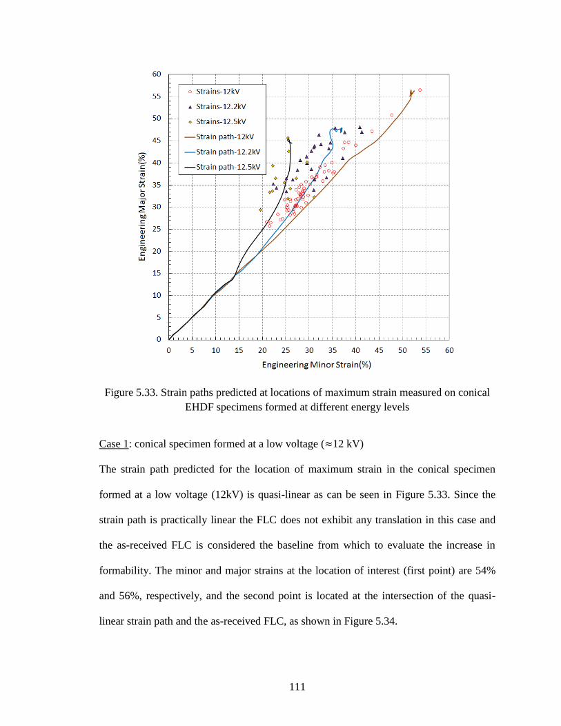
111

Figure 5.33. Strain paths predicted at locations of maximum strain measured on conical

EHDF specimens formed at different energy levels

Case 1: conical specimen formed at a low voltage ( 12 kV)

The strain path predicted for the location of maximum strain in the conical specimen

formed at a low voltage (12kV) is quasi-linear as can be seen in Figure 5.33. Since the

strain path is practically linear the FLC does not exhibit any translation in this case and

the as-received FLC is considered the baseline from which to evaluate the increase in

formability. The minor and major strains at the location of interest (first point) are 54%

and 56%, respectively, and the second point is located at the intersection of the quasi-

linear strain path and the as-received FLC, as shown in Figure 5.34.

112

Figure 5.34. Shift in the FLC of DP600 at a low voltage (12kV)

In the case of this conical specimen formed with 12 kV, the greatest relative increase in

formability in terms of effective strain due to EHDF is calculated to be ̅= 41.1%.

However, this is only considered to be an estimate since the strains at the onset of

necking in EHDF are not actually known.

Case 2: conical specimen formed at a medium voltage ( 12.2 kV)

The strain path at the location of maximum strain on the conical specimen formed with a

medium voltage (12.2kV) does not follow a linear strain path, as shown in Figure 5.33.

The strain path deviates slightly from a linear strain path toward the vertical axis (plane

strain) after a first prestrain in balanced biaxial tension. After the first prestrain the FLC

113

shifts in strain space as shown in Figure 5.35. And the strain path first intersects the

shifted FLC at the intersection point identified in Figure 5.35. The greatest relative

increase in formability was once again determined according to Equation 5.9 and was

found to be ̅= 53.3%.

Figure 5.35. Shifted FLC and estimated increase in formability ( )̅ for the point of

maximum safe strain on the conical specimen formed at medium voltage (12.2kV)

Case 3: conical specimen formed at a high voltage ( 12.5 kV)

As the discharge voltage is increased beyond 12.5 kV, the predicted strain path for the

point of maximum safe strain starts to deviate from the balance biaxial strain path earlier

and shows a more significant deviation from linearity. This indicates that the strain path

turns more rapidly toward plane strain. The earlier deviation from a linear path, followed

114

by the steeper slope of the strain path cause the actual strain path to intersect the shifted

FLC earlier than in Case 2. And even though the effective strain attained at the maximum

safe strain point (second point) is less than it was in Case 2, the relative increase in

formability, determined according to Equation 5.9, was found to be ̅= 75.6%, which is

much greater than in Case 2.

Figure 5.36. Shifted FLC and estimated increase in formability ( )̅ for the point of

maximum safe strain on the conical specimen formed at medium voltage (12.5kV)

3. Conclusion

The lowest increase in formability among these three conical specimens was found to be

in that formed at low energy (≈12 kV); in this case, the strain path is practically linear in

balanced biaxial strain. The baseline from which to quantify the formability improvement

115

is the point where the balanced biaxial strain path crosses the FLC. An increase in

formability of 41.1% was achieved in this case even though the maximum safe strain lies

significantly above the FLC.

The greatest increase in formability among these three conical specimens was found to be

in that formed with a relatively greater input energy (≈12.5 kV). In this case, the strain

path starts to deviate from balanced biaxial strain and crosses the shifted FLC quite early

in the process which leads to a significant formability improvement (75.6%).

5.3.3 Investigation of the mechanisms resulting in formability enhancement

This investigation is based on the results of the numerical simulation of EHDF of DP600

sheet specimen formed into the 34 conical die with a discharge voltage of 12.2 kV. At

this energy level, the specimen completely fills the die cavity. The location of interest in

the numerical model is the same location as the measured grid on the conical specimen

formed with the same level of energy: X = 7mm, measured horizontally from the center

of the specimen. Figure 5.37 indicates that the material at this location reaches the

conventional forming limit at a true major strain of 0.31 and at t=248 µs.

Considering the history of the through-thickness stress, Figure 5.37 shows that the sheet

begins to contact the die at t=267 µs, and that the major strain reaches its greatest value

( 0.40) 10μs later at t=277 µs, just when the through-thickness compression reaches

its greatest magnitude (~400 MPa).

Focussing more particularly on the events that occur after the material exceeds the

conventional forming limit (after t=248 µs), two different periods can be distinguished

(see Figure 5.37). During the first period (248 µs < t < 267 µs), the sheet deforms without

the influence of contact effects. The second period begins the moment the sheet contacts

116

the die (at t=267 µs) and ends when the major strain safely reaches its maximum value

(when t=277 µs). The remainder of this investigation will examine the strain rate effects,

the inertial effects and the contact effects during these two periods.

Figure 5.37. Major strain and through-thickness stress histories near the apex (X=7mm)

of the conical specimen formed at 12.2 kV

5.3.3.1 Strain Rate Effects

As is shown in Figure 5.38, the effective strain rate remains greater than 3700 1s

throughout the period without contact effects (248 µs < t < 267 µs). In the case of the V-

shaped specimen, it was seen that when the strain rate remained above 1100 1s there was

relatively little effect on formability improvement. Hoµwever in the case of the conical

117

specimen the strain rate ( >3700 1s ) is somewhat greater and therefore may have a

greater ability to prevent the onset of necking.

Figure 5.38. True major strain & effective strain rate histories near the apex (X=7mm) of

the conical specimen formed at 12.2 kV

When t > 267 µs, the contact causes the strain rate to significantly decrease. However,

while the major strain is increasing toward its greatest value the strain rate

simultaneously drops to approximately 1000 1s . This relatively low strain rate is unable

to prevent the onset of necking. Also, inertial effects are supressed during the period with

contact, therefore the contact effects must play a dominant role in the later period.

5.3.3.2 Inertial effects

Figure 5.39 shows that during the period of free forming prior to contact (248 µs < t <

267 µs) when the major strain already exceeds the conventional forming limit, the

velocity of the apex of the specimen remains between 50 m/s and 190 m/s, although it

118

had reached a peak velocity of 330 m/s earlier in the process. Although the average

velocity at the apex is somewhat lower than that observed in the V-shaped die

(~ 180 m/s), it appears to be sufficient to delay the onset of necking. When strain is about

to localize, the inertia of the material tends to diffuse the strains and suppresses the onset

of necking. After the sheet contacts the die, the velocity of the material rapidly decreases

because of frictional forces and consequently inertial effects become minimized.

Figure 5.39. Velocity history of the apex of the conical specimen formed with 12.2 kV

5.3.3.3 Contact effects

The stress triaxiality factor and the through-thickness stress histories near the apex of the

conical specimen (X=7 mm) follow a very similar trend, as seen in Figure 5.40. The

theoretical value of the stress triaxiality factor in balanced biaxial stretching is η=0.667,

and it is interesting to observe that the stress triaxiality factor remains almost constant at

119

approximately this level throughout the entire period before t=248 µs, as is shown in

Figure 5.40. During the period just prior to contact (248 µs < t < 267 µs), the stress

triaxiality continues to maintain this same value although it dips down slightly. This

confirms that the strain rate and inertial effects combine to improve the formability

during this period prior to contact. In the later period, the stress triaxiality drops sharply

to η=0.29 due to the impact against the die. This low stress triaxiality changes the stress

state of the material and further impedes the formation of a neck.

Figure 5.40. Through-thickness stress & stress triaxiality histories near the apex

(X=7mm) of the conical die formed with 12.2 kV

5.3.3.4 Summary

During the period just prior to contact, the combination of strain rate and inertial

effects prevent the formation of a neck, thereby enhancing the formability.

120

During the period just after the initial impact of the sheet against the die, the stress

triaxiality factor decreases to further impede the onset of strain localization.

5.3.4. Comparison with EHFF specimens

Both EHDF and EHFF tests were carried out on DP600 sheet specimens using the same

pulse unit, press, EHF chamber and lower die; the only difference between the two types

of tests was the upper die. In the case of EHDF, the upper die consisted of either a conical

die or a V-shaped die, whereas in EHFF the upper die was open. Results of EHFF tests

were taken from Maris (2014) and further analyzed and compared with results from

EHDF tests in order to shed additional light on the mechanisms that lead to a formability

enhancement in EHDF. Moreover, since it is difficult to distinguish the relative

contributions of strain rate effects and inertial effects during the period just prior to the

sheet contacting the die in EHDF, these two effects are combined in the following

analysis.

Figure 5.41. EHFF specimen formed in balanced biaxial tension using 13.6kV

121

Figure 5.41 shows a local neck that extends across the pole of an EHFF specimen formed

with 13.6 kV. It was observed that the neck was not detectable at the pole of the

specimen, but was deeper at some distance from the pole.

Figure 5.42 shows strain data measured in necked grids on a number of EHFF DP600

specimens. It is apparent that, globally, the EHFF process shows no formability

improvement compared to the quasi-static as-received FLC, however, some increase in

formability can still be achieved when local conditions allow it. For instance, the necked

strain data obtained from biaxial specimens can be seen to fall into two clusters. The

cluster of data closer to the vertical axis is identified as mode #2 and the other cluster of

data that lie above the as-received FLC and closer to balanced biaxial tension is identified

as mode #1. The most significant increase in formability in the mode #1 cluster was

obtained at a location where the minor and major engineering strains were 50% and 53%,

respectively. No neck was detectable at this location. This represents a relative increase

in major strain measured vertically above the as-received FLC of approximately 32.5%.

The formability improvement can also be quantified in terms of the increase in effective

strain beyond that at the FLC, and assuming the strain path at this location was quasi-

linear, the increase in effective strain was also found to be approximately 32.5%.

122

Figure 5.42. Necked strain data measured in different DP600 EHFF specimens (courtesy

of Maris, 2014); * deformed in plane strain (PS), biaxial tension (B), uniaxial tension (U)

and in and intermediate draw (UPS) mode; strain data in mode #1 come from necked

grids right at, or less than 3 grids from, the pole; strain data in mode #2 come from

necked grids at least 3 grids away from the pole of the specimen.

Mode #1 cluster:

Figure 5.43 shows the predicted true major strain history of the element at the pole of the

EHFF balanced biaxial specimen where the greatest strains were recorded (

and in the mode #1 cluster of data). Since the neck was not detectable at the

pole, the location is considered safe. This figure shows that, at the pole, the material starts

to stretch beyond the as-received forming limit at t=251 µs and reaches the maximum

level of major strain at t=269 µs. Figure 5.44 shows the predicted effective strain rate and

vertical velocity histories for the same point at the pole of the specimen. It appears in this

123

figure that a peak of effective strain rate reaching approximately 30,000 coinciding

with a peak in vertical velocity of about 160 m/s at the apex combined just before

t=251 µs to cause this significant increase in major strain beyond the FLC.

Figure 5.43. Predicted true major strain history for the most deformed point in mode #1

cluster of data in the EHFF balanced biaxial specimen

During the period 251 µs < t < 269 µs, the combination of the strain rate and vertical

velocity, even though they were both in decline, was able to delay the strain localization

at the pole of the specimen. After t=251 µs, both the strain rate and the vertical velocity

(i.e. inertial effect) decline, and by the time t=269 µs they have practically decreased to

zero. Once the combination of these two factors is no longer able to prevent necking

(11000 s and 20m/s at t 269 µs), the strain can start to localize. However, at

this extreme point on the pole of the EHFF specimen, the strain has not yet localized.

124

Figure 5.44. Predicted effective strain rate and vertical velocity histories of the most

stretched point (mode #1 cluster) at the pole of the EHFF balanced biaxial specimen

Mode #2 cluster:

Figure 5.45 shows the predicted true major strain history of one of the necked points

( ) in the mode #2 cluster of data seen in Figure 5.42. The material

starts to locally deform beyond the as-received forming limit at t=268 µs. It can be

assumed that the strain path at this location was quasi-linear. The sheet material in this

grid began to neck at a true major strain of approximately 0.29 ( , see

Figure 5.42) and at t= 268 µs (see Figure 5.45). This lowest point next to the FLC was

selected because the numerical model without consideration of an instability criterion can

better predict the material behavior right up to the onset of necking.

125

Figure 5.45. Predicted true major strain history of a necked point in the mode #2 cluster

of data away from the pole of the EHFF balanced biaxial specimen

Figure 5.46 shows the predicted effective strain rate and the vertical velocity histories for

this point in the mode #2 cluster. This figure shows that both the strain rate and inertial

effects have already decreased to very low levels by the time the FLC is reached at

t=268 µs: at this time the effective strain rate has reached approximately 3,000 and

the vertical velocity has dropped to 20 m/s. Therefore, these two effects combined were

not able to prevent the strain from localizing. After this, the effective strain rate and the

vertical velocity rapidly decrease to zero.

The analysis of strain rate and velocity histories at these two locations on a balanced

biaxial EHFF specimens shows that although there is globally no increase in formability

in the EHFF process, yet there can be local conditions that do lead to an increase in

formability. And it is the combination of high strain rate (up to 130,000s ) and

126

vertical velocity (inertial effects) that contribute to delay the onset of strain localization

and locally improve the formability by up to 32.5%.

Figure 5.46. Predicted effective strain rate and vertical velocity histories of a necked

point in the mode #2 cluster of data away from the pole of the EHFF balanced biaxial

specimen

Numerical analysis for EHDF:

Figure 5.47 shows the predicted effective strain rate and the vertical velocity histories of

the point located near the apex (X=7mm) of the conical EHDF specimen where the

maximum safe strains were measured. Compared to EHFF, Figure 5.47 shows that both

the strain rate and vertical velocity (inertial effects) maintain high levels which combine

to extend the formability of the sheet material in the period just prior to contact (248 µs <

t < 267 µs). Once the combination of strain rate and inertial effects declines to a certain

level, contact effects become predominant and prevent the occurrence of necking, as seen

127

in Figure 5.40. Hence, with the addition of contact effects, the formability in EHDF can

improve significantly more than in EHFF.

Figure 5.47. Predicted effective strain rate and vertical velocity histories at the point of

maximum safe strain located near the apex (X=7mm) of the conical EHDF specimen

128

6. Summary and Conclusions

Consistent with the objectives of this thesis, the major results of this research are

summarized in two sections:

6.1 Increase in formability of DP600 sheets

EHDF with 38º V-shaped die (near plane strain):

No formability improvement was observed for the global plane strain EHDF

operation since the necked data lie on and above the quasi-static FLC.

The greatest safe strains can reach around 46% major strain under local

conditions, i.e. almost double the major strain on the FLC (for the same level of

minor strain). This represents approximately 100% increase in formability.

EHDF with 34º conical die (near balanced biaxial tension):

The non-linear strain paths that are mainly caused by severe impact of the sheet against

the die must be taken into account when estimating the increase in formability. Since the

shift in the FLC is dependent on the position relative to the specimen’s symmetry axis

and the electrical discharge energy, only the material that exhibited the greatest level of

safe strains was considered at each level of energy.

Low energy level (~12kV)

The strain path was quasi-linear and the greatest relative increase in formability was 41%

in terms of effective strain under local conditions.

Medium energy level (~12.2kV)

The strain path was non-linear and the greatest relative increase in formability was 53%

in terms of effective strain under local conditions.

129

In high energy level (≥12.5kV)

The quasi-static FLC was shown to translate significantly in strain space as a result of the

local change in strain path due to the severe impact against the die wall. Comparing the

safe strain data in the conical EHDF specimen with this quasi-static FLC, more than 75%

formability improvement was observed.

6.2 The Mechanisms of Formability Improvement

This research has also led to a better understanding of the mechanisms that lead to

formability improvement in electrohydraulic forming. Three major factors were found to

have the potential to enhance the formability of the sheet: a high strain rate as well as

inertial and contact effects.

EHDF with a V-shaped die:

Strain rate effects were not sufficient to delay the onset of necking in this case. But

inertial effects were shown to play a dominant role to impede the occurrence of necking

in the period prior to the sheet coming into contact with the die. However, inertial effects

become suppressed during the period of contact due to the presence of friction forces and

the occurrence of dynamic oscillations. Contact effects become significant upon impact

against the die wall, which helps to locally decrease the stress triaxiality factor. A lower

stress triaxiality factor can significantly improve the sheet formability.

130

EHDF with a conical die:

During the period prior to contact, the combination of strain rate and inertial

effects can potentially prevent the formation of the necking and enhance the

formability.

During the period with contact, the stress triaxiality factor decreases (i.e. the

compressive through-thickness stress increases in magnitude) as the impact

energy increases. This low stress triaxiality helps to decrease the damage caused

by further deformation and impedes the formation of a neck. Because of the

participation of contact effects, the formability of the sheet can locally improve

much more in EHDF than in EHFF.

131

Bibliography

Altynova, M., Hu, X., & Daehn, G. S. (1996). Increased Ductility in High Velocity

Electromagnetic Ring Expansion. Metallurgical and Materials Transactions A,

27A(July), 1837–1844.

Balanethiram, V. S., & Daehn, G. S. (1994). Hyperplasticity:increased forming limits at

high workpiece velocity. In Scripta Metallurgica Vol. 30, 515–520. Pergamon Press

Ltd.

Dariani, B. M., Liaghat, G. H., & Gerdooei, M. (2009). Experimental investigation of

sheet metal formability under various strain rates. Proceedings of the Institution of

Mechanical Engineers, Part B: Journal of Engineering Manufacture, 223(6), 703–

712.

El-Magd, E., & Abouridouane, M. (2004). High Speed Forming of the Light-Weight

Wrought Alloys. 1st International Conference on High Speeding Forming, 3–12.

Emmens, W. C. (2011). Formability. SpringerBriefs in Applied Sciences and Technology,

57–65.

Evans, C. (2013). Vehicle lightweighting as an eco solution. Retrieved from

http://www.innovationintextiles.com/vehicle-lightweighting-as-an-eco-solution/

Gillard, A. J., Golovashchenko, S. F., & Mamutov, A. V. (2013). Effect of quasi-static

prestrain on the formability of dual phase steels in electrohydraulic forming. Journal

of Manufacturing Processes, 15(2), 201–218.

Gladman, B. (2001). LS-DYNA keyword user’s manual 971 R4 beta. Livermore Software

Technology Corporation (Vol. I).

Golovashchenko, S. F. (2007). Material Formability and Coil Design in Electromagnetic

Forming. Journal of Materials Engineering and Performance, 16(3), 314–320.

Golovashchenko, S. F., Gillard, A. J., & Mamutov, A. V. (2013). Formability of dual

phase steels in electrohydraulic forming. Journal of Materials Processing

Technology, 213(7), 1191–1212.

Green, D. E., & Black, K. C. (2002). A Visual Technique to Determine the Forming

Limit for Sheet Materials. Society of Automotive Engineers, 01(1062).

Hassannejadasl, A., Green, D. E., Golovashchenko, S. F., Samei, J., & Maris, C. (2014).

Numerical modelling of electrohydraulic free-forming and die-forming of DP590

steel. Journal of Manufacturing Processes, 16(3), 391–404.

Hill, R. (1948a). A Theory of the Yielding and Plastic Flow of Anisotropic Materials.

Proceedings of the Royal Society of London, A193, 281–297.

132

Hopperstad, O. S., Børvik, T., Langseth, M., Labibes, K., & Albertini, C. (2003). On the

influence of stress triaxiality and strain rate on the behaviour of a structural steel.

Part I. Experiments. European Journal of Mechanics, A/Solids, 22, 1–13.

Imbert, J. M., Winkler, S. L., Worswick, M. J., & Golovashchenko, S. (2004).

Formability and Damage in Electromagnetically Formed AA5754 and AA6111. 1st

International Conference on High Speed Forming, 201–210.

Imbert, J. M., Winkler, S. L., Worswick, M. J., Oliveira, D. a., & Golovashchenko, S.

(2005). The Effect of Tool–Sheet Interaction on Damage Evolution in

Electromagnetic Forming of Aluminum Alloy Sheet. Journal of Engineering

Materials and Technology, 127(1), 145.

Imbert, J. M., Worswick, M. J., & Golovashchenko, S. (2006). Contributing Factors to

the Increased Formability Observed in Electromagnetically Formed Aluminum

Alloy Sheet. 2nd International Conference on High Speed Forming.

Kim, S. B., Huh, H., Bok, H. H., & Moon, M. B. (2011). Forming limit diagram of auto-

body steel sheets for high-speed sheet metal forming. Journal of Materials

Processing Technology, 211(5), 851–862.

Maris, C. (2014). Experimental determination of the forming limits of DP600 and

AA5182 sheets in electrohydraulic free forming. Master's Thesis. University of

Windsor.

McGrath, J. R. (1965). Scaling Underwater Exploding Wires. Washington, D.C.

Oliveira, D. A., Worswick, M. J., Finn, M., & Newman, D. (2005). Electromagnetic

forming of aluminum alloy sheet: Free-form and cavity fill experiments and model.

Journal of Materials Processing Technology, 170(1-2), 350–362.

Quaak, G. (2008). Biaxial Testing of Sheet Metal : An Experimental-Numerical Analysis.

Master's Thesis. Eindhoven University of Technology.

Rohatgi, A., Soulami, A., Stephens, E. V., Davies, R. W., & Smith, M. T. (2014). An

investigation of enhanced formability in AA5182-O Al during high-rate free-

forming at room-temperature: Quantification of deformation history. Journal of

Materials Processing Technology, 214(3), 722–732.

Rohatgi, A., Stephens, E. V., Davies, R. W., Smith, M. T., Soulami, A., & Ahzi, S.

(2012). Electro-hydraulic forming of sheet metals: Free-forming vs. conical-die

forming. Journal of Materials Processing Technology, 212(5), 1070–1079.

Rohatgi, A., Stephens, E. V., Soulami, A., Davies, R. W., & Smith, M. T. (2011).

Experimental characterization of sheet metal deformation during electro-hydraulic

forming. Journal of Materials Processing Technology, 211(11), 1824–1833.

133

Seth, M., Vohnout, V. J., & Daehn, G. S. (2005). Formability of steel sheet in high

velocity impact. Journal of Materials Processing Technology, 168(3), 390–400.

Sklad, M. P. (2004). Aspects of automated measurement of proportional and non-

proportional deformation in sheet metal forming. Journal of Materials Processing

Technology, 145(3), 377–384.

Stoughton, T. B. (2000). General forming limit criterion for sheet metal forming.

International Journal of Mechanical Sciences, 42(1), 1–17.

Wood, W. W. (1967). Experimental Mechanics at Velocity Extremes -Very High Strain

Rates and cylindrical bulging for a wide variety of materials. Experimental

Mechanics, 441–446.

134

Appendices

Appendix A

EHDF formability results with the V-shaped die for DP600

Gauge

(mm)

Sample

NO.

Die

Angle

(°)

Voltage

(kV)

Number

of

Capacitor

Banks

Die Filled

Condition Note

1.5 #1 38 8 4 Completely

Unfilled Safe

1.5 #2 38 9 4 Completely

Unfilled Safe

1.5 #3 38 11 4 Partially Unfilled Safe

1.5 #4 38 12 4 Partially Unfilled Safe

1.5 #5 38 13 4 Partially Unfilled Necked

1.5 #6 38 14 4 Completely Filled Necked and Cracked

1.5 #7 38 13.5 4 Completely Filled Necked and Cracked

1.5 #8 38 12.5 4 Partially Unfilled Safe

1.5 #9 38 12.3 4 Partially Unfilled Safe

1.5 #10 38 12.5 4 Partially Unfilled Safe

1.5 #11 38 12.8 4 Partially Unfilled Safe

Appendix B

EHDF formability results with the conical die for DP600

Gauge

(mm)

Sample

NO.

Die

Angle

(°)

Voltage

(kV)

Number

of

Capacitor

Banks

Die Filled

Condition Note

1.5 #9 34 13.2 4 Completely Filled Damages at the Apex

1.5 #10 34 12.5 4 Completely Filled Damages at the Apex

1.5 #11 34 11 4 Partially Unfilled Safe

1.5 #12 34 12.2 4 Completely Filled Safe

1.5 #13 34 12 4 Almost Completely

Filled Damages at the Apex

135

VITA AUCTORIS

NAME: JIA CHENG

PLACE OF BIRTH:

Changzhou, Jiangsu, China

YEAR OF BIRTH:

1990

EDUCATION:

Qianhuang High School, Changzhou, Jiangsu,

China, 2008

China University of Petroleum (East China),

B.A.Sc., Qingdao, Shandong, China, 2012

University of Windsor, M.A.Sc., Windsor, ON,

Canada, 2015