Applied Research and Innovation Branch

INVESTIGATION OF SEISMIC PERFORMANCE AND DESIGN OF TYPICAL CURVED AND SKEWED

BRIDGES IN COLORADO

Suren Chen Hussam Mahmoud

Thomas Wilson Robert Johnson

Guangyang Houuthors

Report No. CDOT-2018-08 January 2018

The contents of this report reflect the views of the

author(s), who is(are) responsible for the facts and

accuracy of the data presented herein. The contents

do not necessarily reflect the official views of the

Colorado Department of Transportation or the Federal

Highway Administration. This report does not

constitute a standard, specification, or regulation.

Technical Report Documentation Page 1. Report No.

CDOT-2018-082. Government Accession No. 3. Recipient's Catalog No.

4. Title and Subtitle

INVESTIGATION OF SEISMIC PERFORMANCE AND DESIGN OF

TYPICAL CURVED AND SKEWED BRIDGES IN COLORADO

5. Report Date

1/15/2018

6. Performing Organization Code

7. Author(s)

Suren Chen, Hussam Mahmoud, Thomas Wilson, Robert Johnson,

Guangyang Hou

8. Performing Organization Report No.

CDOT-2018-08

9. Performing Organization Name and Address

Colorado State University

Fort Collins, CO

10. Work Unit No. (TRAIS)

11. Contract or Grant No.

12. Sponsoring Agency Name and Address

Colorado Department of Transportation - Research4201 E. Arkansas Ave.Denver, CO 80222

13. Type of Report and Period Covered

Final: 2/15/12 to 10/1/15

14. Sponsoring Agency Code

087-00

15. Supplementary Notes

Prepared in cooperation with the US Department of Transportation, Federal Highway Administration

16. Abstract

This report summarizes the analytical studies on the seismic performance of typical Colorado concrete bridges, particularly

those with curved and skewed configurations. A set of bridge models with different geometric configurations derived from

a prototype bridge selected in Denver area were studied. Some discussions about the connection modeling are carried out in

terms of the interior bent support. For the displacement-based and force-based designs, due to the lack of design details that

may be adopted for different Colorado bridges, some specific recommendations cannot be made at this point without

detailed analyses of all possible detailing options. Therefore, some general observations of these two design concepts are

summarized in the end of the report. In the appendices, the design examples of 2-span and 3-span bridges are listed to help

the engineers to conduct bridge seismic analysis in Colorado.

The SAP2000 modeling example and four design examples are included in the appendices of this report.

Implementation

17. Keywords

Denver Area, Colorado, 2-span, 3-span, SAP2000,connection detail, bent support

18. Distribution Statement

This document is available on CDOT’s websitehttp://www.coloradodot.info/programs/research/pdfs

19. Security Classif. (of this report)

Unclassified 20. Security Classif. (of this page)

Unclassified 21. No. of Pages

187 22. Price

Form DOT F 1700.7 (8-72) Reproduction of completed page authorized

1

INVESTIGATION OF SEISMIC PERFORMANCE AND DESIGN OF

TYPICAL CURVED AND SKEWED BRIDGES IN COLORADO

by

Suren Chen

Hussam Mahmoud

Thomas Wilson

Robert Johnson

Guangyang Hou

Sponsored by the

Colorado Department of Transportation

Colorado Department of Transportation

Applied Research & Innovation Branch

4201 E. Arkansas Ave.

Denver, CO 80222

2

Acknowledgement

The authors wish to thank the CDOT Applied Research and Innovation Branch for funding this

study. The authors like to acknowledge the project panel for providing valuable technical

discussion and guidance throughout the project period. The time, participation and feedback

provided by the project panel members: Richard Osman, Derrell Manceaux, Trever Wang, Mac

Hasan, Steve Yip, David Thomas and Su Cheng, is greatly appreciated.

3

Executive Summary

This report presents the results of a study conducted on the seismic behavior of select RC

bridges in Colorado with a focus on curved and skewed configurations. Numerical models of

bridges with different geometric configurations were derived from a typical prototype bridge in

Colorado. Detailed nonlinear time-history analyses with SAP2000 are conducted on these bridge

models with a seismic site hazard for Denver, Colorado.

In the first part of the report, detailed background information is provided that relates to

earthquake engineering and the Colorado hazard. A review of the seismic hazard is presented

with documentation on the AASHTO LRFD Design Specification and AASHTO Guide

Specifications, including different types of computational modeling, structural analysis and

ground motion-scaling methodologies. Secondly, a 2 and 3-span RC bridges were selected for

use in the seismic investigation with the intention of being representative of the general Colorado

bridge inventory. The 3-span bridge was independently modified to explore the effects of skew

and curvature under seismic loads, in addition to loading constraints and support alternatives.

Modal and non-linear time-history analyses were performed on 9 different bridge models in

SAP2000 using two sets of two seismic hazard levels from the AASHTO codes. An evaluation

of major structural components using SAP2000 and a section analysis is included, in addition to

an extensive study on the impact and behavior of skew and curvature. The effects of support

condition, earthquake input direction and soil stiffness are also included. The discussions are also

made in terms of different modeling options of interior bent connections for the specific designs

of the prototype bridge based on comparative study results. Due to the lack of site-specific

design detail alternatives of major connections, the general discussion about the difference

between displace-based and force-based approaches is made.

4

Lastly, design examples for creating the numerical models constructed in SAP2000 are also

provided with detailed steps on model construction, seismic analyses and post-processing of

results as appendices of the report. This is supplemented with comprehensive details on seismic

design procedures for SDC A and SDC B using the AASHTO LRFD Bridge Design

Specifications and AASHTO Guide Specifications for LRFD Bridge Design, Zones 1 & 2.

5

Table of Contents (Organization)

Acknowledgement .......................................................................................................................... 2

Executive Summary ........................................................................................................................ 3

Table of Contents (Organization) ................................................................................................... 5

1. Background Information .......................................................................................................... 8

1.1. Introduction ................................................................................................................... 8

1.2. Colorado Seismic Hazard ............................................................................................. 9

1.3. AASHTO LRFD Specifications and Guide Specifications ........................................ 13

1.4. Review of Different Structural Modeling Methods .................................................... 16

1.5. Review of Demand Analysis Methods ....................................................................... 17

1.5.1. Introduction .............................................................................................................. 17

1.5.2. Response Spectrum Method .................................................................................... 18

1.5.3. Time-history Analysis .............................................................................................. 19

1.6. Ground Motion Scaling............................................................................................... 20

2. Bridge Plans and Specifications............................................................................................. 22

2.1. Structural Components of the 2- Span Bridge ............................................................ 22

2.2. Structural Components of the 3- Span Bridge ............................................................ 23

2.3. Configuration of 3-Span Bridges ................................................................................ 24

2.3.1. Part I - Baseline bridge model configuration (Radius: 4500 ft; Skew: 30) ............. 24

2.3.2. Geometric Configurations of Bridges ...................................................................... 25

3. Numerical Modeling Method ................................................................................................. 27

3.1. Development of the Finite Element Models ............................................................... 27

3.2. SAP2000: Advantages for Structural Design and Analysis ........................................ 27

6

3.3. SAP2000: Disadvantages and Limitations.................................................................. 28

3.4. Details of the Finite Element Modeling Process ......................................................... 28

3.5. Alternative Modeling Capacity Software: KSU_RC .................................................. 34

4. Ground Motion Scaling and Analytical Method .................................................................... 36

4.1. Ground Motion Selection and Scaling ........................................................................ 36

4.2. Applied Analysis Method: Nonlinear Time-history Analysis .................................... 38

5. Numerical Analysis of Representative Bridges ..................................................................... 40

5.1. Introduction ................................................................................................................. 40

5.2. Modal Analysis Results .............................................................................................. 40

5.3. Evaluation Criteria ...................................................................................................... 42

5.4. Time-history Analysis Results of the 2-span Baseline Model .................................... 43

5.5. Time-history Analysis Results of the 3-span Baseline Model .................................... 45

5.6. Effect of Earthquake Input Direction .......................................................................... 47

5.7. Effect of Support Condition ........................................................................................ 48

5.8. Effect of Soil Stiffness ................................................................................................ 49

5.9. 3-Span Parametric Study Results – Curved and Skewed Bridge Configurations ....... 51

5.9.1. Drift Ratios of Pier-Columns ................................................................................... 52

5.9.2. Soil Resistance ......................................................................................................... 53

5.9.3. Shearing Forces in the Pier-Columns ...................................................................... 53

5.9.4. Axial Force and Moment Demand on Pier-Columns .............................................. 54

5.10. Section Analysis of Bridge Components .................................................................. 58

5.11. Summary of Analytical Results ................................................................................ 61

6. Comparative Study on Different Girder-bent Connections ................................................... 65

7

6.1. Bridge configuration ................................................................................................... 65

6.2. SAP modeling and three connection types ................................................................. 67

6.3. Ground motion record and earthquake scaling ........................................................... 68

6.4. Analytical results ........................................................................................................ 69

6.5. Discussions ................................................................................................................. 75

6.6. Summary ..................................................................................................................... 78

7. Discussion about displacement-based and force-based designs for bridges .......................... 81

8. Conclusion ............................................................................................................................. 85

9. Sources Cited ......................................................................................................................... 86

Appendices A-C: SAP 2000 Modeling Example and four design examples…………….. 89 - 184

8

1. Background Information

1.1. Introduction

Earthquakes are a present-day hazard to the expanding infrastructure in the United States and

are currently responsible for approximately $5.3 billion in annual economic losses (FEMA 366,

2008). An earthquake can cause damage to, and in cases collapse of buildings, railways, and

bridges. In the case of a severely damaged or collapsed bridge the consequences can be

substantial in terms of financial losses from cost of repair or replacement and socioeconomic

losses through the value of lost time to the public by a longer travel time. Bridges are typically

designed for life loss prevention under large seismic demand, which requires a design that

prevents structural collapse under large cyclic demands. The response of bridges subjected to

earthquake ground motion, however is difficult to predict and often requires rigorous analyses.

All states, independent of the seismic hazard, are required to conduct seismic design

following the American Association of State Highway and Transportation Officials (AASHTO)

LRFD Bridge Design Specifications (called “LRFD Specifications” hereafter) or the AASHTO

Guide Specifications for LRFD Seismic Bridge Design (called “Guide Specifications” or “GS”

hereafter). Each code presents a methodology of design against earthquakes following force-

based methods or displacement-based design practices. In this study, both specifications will be

reviewed in the following sections.

Structural codes typically classify bridges into seismic Zones or Categories based on site-

specific ground acceleration and site classification. Mountainous states in the central U.S. are

typically classified as low seismic regions and incorporate little to no seismic design or analyses

into their bridge practices. Colorado, as reviewed in the following section, is classified as a low

seismic state. According to seismologists, however, Colorado may be exposed to a higher

9

seismic risk than currently considered by structural codes. In this report, the following chapters

document studies primarily based on nonlinear time-history analyses to investigate the dynamic

response of representative Colorado bridges and provide insight on the effects of geometric and

structural configurations. Prior to conducting the time-history simulations, a review of Colorado

seismic hazard is provided; followed by classification of the bridges according to current bridge

specifications and an overview of state-of-the-art modeling and analysis methods of bridges

under earthquake excitations.

1.2. Colorado Seismic Hazard

Earthquakes pose an on-going threat to society and infrastructure in the United States and

around the world. Improper design of infrastructure against seismic events can result in collapse

or extensive damage to roads, bridges, buildings, and utility lines. The AASHTO codes utilize

the United States Geological Survey (USGS) hazard maps (Fig. 1.1) that assign representative

horizontal accelerations based on geography and tectonic activity across the United States. Based

on the ground acceleration coefficient and the site classification for the location of interest, the

level of seismic analysis required can be determined. Colorado is classified state wide as either

Seismic Design Category A or B (Zones 1 & 2) and requires minimal to limited seismic analysis

according to the AASHTO LRFD Specifications and Guide Specifications.

10

Figure 1.1 Seismic Hazard Maps for AASHTO Guide Specifications, Peak Ground Acceleration

(PGA) (7% in 75-year) (2011)

The seismicity of Colorado is still uncertain according to seismologists and the state may be

more active than currently presumed (Charlie et al. 2006; Sheehan et al. 2003). Generally,

Colorado is thought to be a low seismic region; it has a low number of previously recorded

seismic events in the area and is located a far distance from major inter-plate fault lines. Inter-

plate faults are typically characterized by the junction and interaction of two tectonic plates.

Present at these junctions are large tectonic forces that result in fracturing of the lithosphere-

asthenosphere complex generating frequent and larger magnitude earthquakes. Therefore, the

seismic activity present in Colorado is rather characterized by intra-plate tectonic interaction and

the occurrence of intra-plate earthquakes is attributed to internal fractures of the lithosphere on

the tectonic plate. The generation of earthquakes across the lithosphere may be attributed to

anomalies in temperature, strength or by the nature of the geological site conditions. Colorado

has 58 mountain peaks of elevation higher than 14,000 feet, apparent Neogene and active

quaternary deformation, and the second to largest heat flow anomaly, which all point towards an

active tectonic area (Charlie et al., 2002). In addition, there are ninety-two potentially active

11

quaternary faults documented. Of the ninety two faults, thirteen have a maximum credible

earthquake (MCE) of higher than 6.25 ML (Fig. 2.2) on the Richter Scale (Widmann et al. 1998).

The maximum credible earthquake scale is based on a 2500-year return period, and is utilized to

assess the highest magnitude earthquake that a fault line may produce. In light of the inherent

impracticalities of design and construction of bridges using the MCE, the design based

earthquake (DBE) is utilized for most designs of bridges and represents a 1000 year return

period.

Figure 1.2 (Matthews, 2002) Quaternary Fault Lines with Assigned Maximum Credible

Earthquake Magnitudes for the State of Colorado

The focal point of recorded seismic activity has been centered just west of the Rocky

Mountain Front Range and in Southern Colorado near Trinidad. The largest earthquake to date

was recorded on November 7, 1882 with magnitude of 6.6 ± 0.6 ML on the Richter Scale

(Spence et al. 1996; Kirkham & Rogers 2000). The ground motion was observed throughout

12

several neighboring states, as shown in Figure 1.3, and is estimated to have affected an area of

330,000 mi2 (Spence 1999). The unified estimate on the Modified Mercalli Intensity (MMI) scale

was assessed by seismologists at an intensity of VII ( Kirkham 1986). In fact, Colorado is one of

only fourteen states across the country to have documented an earthquake of magnitude 6.0 or

greater (Stover & Coffman 1993).

Figure 1.3 (Stover & Coffman, 1993) Isoseismal Map for November 7th, 1882 Earthquake in

Colorado

A total of 570 earthquakes have also been recorded from 1870 to 2005 of Moment

Magnitude (Mw) 2.0 or higher. Of these 570 earthquakes, 82 earthquakes have been recorded at a

MMI scale of V or higher. Colorado’s highest probability for a seismic event measure using the

MCE scale, is estimated at magnitude 7.5 ML on the Richter scale (Kirkham & Rogers, 1985).

According to Charlie et al. (2006), data collected from independent earthquakes yields a mean

recurrence interval of 420 years for an earthquake of magnitude 6.5 ML or larger. Applying a

Gutenberg-Richter magnitude-recurrence relation developed by Charlie et al. (2002) yields that a

13

magnitude 6.6 ML or larger earthquake will have a corresponding return period of 500 years.

Applying the same relationship, a 1000-year return period corresponds to a 7.0 ML event, and a

2500-year return period corresponds to a 7.5 ML event. In comparison, by current AASHTO

design criteria, most of Colorado falls into a Seismic Design Category A for a 1000 year return

period, which dictates that seismic design is not required. Comparing the estimated earthquake

magnitudes by seismologists and AASHTO seismic hazard maps for comparable return periods,

one can find that there appears to be a significantly larger estimated hazard by seismologists than

what is estimated by the AASHTO bridge codes in Colorado.

1.3. AASHTO LRFD Specifications and Guide Specifications

Prior to the moment that the magnitude 6.6 Mw earthquake struck the San Fernando Valley in

the state of California in 1971, guidelines on seismic design were fairly rudimentary. A fraction

of the dead load from the structure was used to estimate the lateral seismic loads, based on which

the members of the structural system were designed. Following the earthquake in 1971, a group

of experts in the field of seismology and structural engineering wrote a document, which was

published in 1981 by the Applied Technology Council (ATC), titled “Seismic Design Guidelines

for Highway Bridges” (ATC-6 1981). ATC-6 was later adopted as a Guide Specification and a

required Specification for seismic design in the AASHTO Standard Specification Division 1-A.

Since then, further development and updates have followed in the AASHTO LRFD Bridge

Design Specification (AASHTO 2007). In 2007, AASHTO introduced the LRFD Guide

Specifications for Seismic Design of Highway Bridges in addition to updates to the existing

specifications. Life safety performance dictated that a bridge would be designed such that it has

low probability of collapse, although it may sustain significant amounts of damage such that

partial or complete rehabilitation may be required following a high magnitude seismic event.

14

Supplementing this change was an increase in the return period of the design event from 475

years to 1000 years in both specifications, which was also motivated by the AASHTO’s desire to

stay current with the building design codes.

The AASHTO LRFD Bridge Design Specifications is based on traditional force-based

seismic design and relies on the strength capacity of the specified structural members to perform

in the inelastic range through an elastic analysis. To determine the level of analysis required, the

AASHTO Bridge Specifications differentiates all bridge sites into four Seismic Zones (SZ)

partitioned by acceleration coefficient ranges and site (soil) conditions. The acceleration

coefficients are determined from the 1-second seismic hazard maps developed by the USGS.

Based on the seismic zone and bridge importance classification, the minimum analysis

requirements are determined. For SZ 1, applicable to most of Colorado, no seismic analysis is

required. However a fraction of the vertical reaction is applied horizontally to determine the

required connection strength and ensure that minimum requirements for deck unseating are met.

In contrast, critical bridges in SZ 4 require time history analysis as the minimum analysis

requirement. The general method for analyses requires developing a unique response spectrum

using spectral maps and site-specific soil classifications. Following calculation of elastic forces

using the response spectrum, a response modification factor (R-factor) (Fig. 1.4) was utilized to

modify the seismic forces in recognition that it is uneconomical to design bridges to resist large

earthquake forces elastically (AASHTO 2007). The structural components of the bridge are then

designed based on the modified load, which varies for different substructure components and

importance categories. By modifying the elastic forces with the Response Modification Factor,

“R”, it is recognized that yielding of the structure may occur.

15

Figure 1.4 Response Modification Factors in AASHTO LRFD Bridge Design Specifications

(2007) (Table 3.10.7.1-1 & 2)

The AASHTO Guide Specifications (GS) was developed under the guidance of the

AASHTO T-3 Committee as part of a National Cooperative Highway Research Program

(NCHRP) task. The method of identifying seismic hazard utilizes identical USGS ground motion

hazard maps and life safety performance criteria as the existing specifications. The Guide

Specification also determines the demand on the structure by placing it into Seismic Design

Categories (SDC). The SDC is synonymous to the AASHTO LRFD Bridge Specifications

Seismic Zones. The Guide Specifications, however, employs ductility-based design after the

realization that this method of design is significantly less sensitive to sharp increases in the

uncertain and variable seismic loading (Elnashai & Di Sarno, 2008). Ductility-based design

evaluates the performance of a structural system based on the displacement capacity of the

system and applies detailing requirements to provide ductility with inelastic deformation. The

first steps required by the Guide Specifications (GS) are similar to the existing LRFD

16

Specifications; analysis requirements are determined through the use of hazard maps and site

coefficients, and SDC classification. The extent of the analysis includes determination of

connection requirements similar to the LRFD Specifications, a check against minimum criteria

for unseating at supports, along with column detailing and foundation design. For SDC B, C and

D, the GS incorporate more rigorous analysis and design methods. SDC B suggests an implicit

displacement capacity check or pushover analysis. SDC C and D involve the engineer’s choice

of a design strategy referred to as the Earthquake Resisting System (ERS) and development of

earthquake resisting elements (ERE). This is ensured by detailing specified components to yield

using specified procedures in the code to “capacity protect” all other elements connecting the

yielding component. The capacity protection method is employed where the individual

component resistances should have the ability to avoid that connecting components reach their

overstrength capacity (American Association of State and Highway Transportation Officials,

2011).

1.4. Review of Different Structural Modeling Methods

Once the method of analysis is established, a model that approximates the response of the

bridge structure is often required. There are several model types that are applicable for providing

a representation of the structural characteristics of bridges, although they have varying degrees of

accuracy and time efficiency. These include single-degree-of-freedom (SDOF) systems,

multiple-degree-of-freedom (MDOF) models, and detailed finite element (FE) models. SDOF

models have the advantages of minimum computational demand and yielding a fair

representation of the global behavior. SDOF models are limited primarily to standard structures

and do not account for tridimensional effects and local behavior (Elnashai & Di Sarno, 2008).

Stick models accounting for multiple degrees of freedom, are applicable to all regular structures,

17

and accommodate tridimensional effects. But similar to SDOF models, stick models only

account for the global response. In a recent publication by Abdel-Mohti and Pekan (2008) on the

comparison between detailed finite element models and beam stick models for skewed bridges in

SAP2000, it was concluded that for bridge decks with skew angles larger than 30 degrees,

detailed finite element models should be utilized in order to correctly represent higher mode

effects. For practicing Engineers, the preferred methods are always the simplest models that

provide adequate results. Therefore, to hit the optimal balance between more accurate results

from complex models and the simplicity of the analytical procedure still remains a topic worthy

discussion for engineering community.

In recent years, finite element models using SAP2000 have been extensively developed

by many researchers in seismic engineering. Mwafy and Elnashai (2007) investigated the seismic

integrity of multi-span curved bridges using SAP2000. Itani and Pekcan (2011) investigated the

seismic performance of steel plate girder bridges with integral-abutments using SAP2000.

Kappos et al. (2005) utilized the analysis program to show that modal-pushover analysis can be

effectively employed for seismic assessment of bridges. SAP2000 is also currently used in

several design offices of State Departments of Transportation (DOT) for seismic analysis around

the country. For example, Washington DOT utilizes SAP2000 and the AASHTO Guide

specifications as the basis for evaluation of bridge structures and have developed guidelines and

design examples (Washington Department of Transportation 2011). In addition to Washington,

SAP2000 is also used for seismic analysis by other State Departments of Transportations, such

as Indiana, Nevada and California DOTs.

1.5. Review of Demand Analysis Methods

1.5.1. Introduction

18

There are several available methods for estimating the demand imposed by earthquakes on

bridges. The conventional analysis methods adopted in research and structural codes are

discussed in the following section. The methods covered include: response spectrum method and

time history analysis.

1.5.2. Response Spectrum Method

The response spectrum analysis (RSA) method is an elastic seismic analysis approach, which

usually can give reasonable response prediction for ordinary standard bridges under seismic

excitation. Based on modal properties of the structure, a response spectrum method reduces the

dynamic analysis to a series of static analyses to assess the peak response of a structure. As a

type of popular and efficient approach adopted in structural codes such as the AASHTO LRFD,

and Guide Specifications, the response spectrum method is often used when the basic equivalent

static analysis (ESA) is not sufficient. The analytical method is governed by the following

dynamic equations to ground motions:

𝑀 �̈�(𝑡) + 𝐶�̇�(𝑡) + 𝐾𝑥(𝑡) = 𝑚𝑥�̈�𝑔𝑥(𝑡) + 𝑚𝑦�̈�𝑔𝑦(𝑡) + 𝑚𝑧�̈�𝑔𝑧(𝑡)

where K represents the stiffness matrix, M represents the diagonal mass matrix and C represents

the proportional damping matrix; The variables of x(t) represent the motion with respect to the

ground, �̈�𝑔𝑥,𝑦,𝑧 represents the components of uniform ground acceleration, and lastly 𝑚𝑥,𝑦,𝑧

represents the unit acceleration loads (CSI 2011). Response spectrum analysis evaluates the

model at the maximum response to the dynamic equilibrium equation at the fundamental period

of vibration. The input is a response spectrum curve of spectral acceleration versus structural

period. This is developed using the guidelines provided in the structural codes. The computed

dynamic response of the bridge represents a statistical calculation of the maximum magnitude for

19

that measure. Response-spectrum analysis is generally based upon superposition with modes

computed using Ritz-vector analysis. With the modal analyses results, single-mode spectral

method and multimode spectral method can be used. In the following, the multimode spectral

method, which is popular in engineering practice, is briefly introduced. Typically, a multi-

degree-of-freedom (MDOF) structural model is excited by a transient signal and decomposed

analytically into a series of single degree of freedom (SDOF) systems. Modal dynamic response

is firstly calculated for each mode, which is combined to yield the global response of the MDOF

system using mode superposition concept. Such a method is typically limited to linear-elastic

systems with very little nonlinearity due to mode-superposition nature. Although MDOF

approach offers a convenient and valid tool to predict global response of most standard bridges

with little nonlinearities, time-history analysis is usually recommended for non-ordinary bridges

or scenarios with high nonlinearity.

1.5.3. Time-history Analysis

Due to the known limitations of the response spectrum method, nonlinear time history analysis

(NLTHA) is usually recommended for non-ordinary bridges and/or when considerable

nonlinearities are expected on bridge structures subjected to seismic. Although it usually requires

advanced modeling skills and high computational cost, NLTHA is recognized as the most

accurate and rigorous analysis method in both open-source and commercial finite element

software (Burdetteet al. 2008; Mwafy & Elnashai, 2007). NLTHA is a step function analysis and

evaluates the dynamic response of the bridge structure due to a specific earthquake loading at

discrete time steps and iteration is often required. When nonlinear behaviors are developed in the

20

structure, the stiffness of the bridge needs to be recalculated due to degradation of strength as

well as redistribution of forces (Aviram et. al. 2008).

The equations of motion defining this type of analysis are as follows:

𝑀�̈�(𝑡) + 𝐶�̈�(𝑡) + 𝐾𝑥(𝑡) = 𝐹(𝑡)

where K, M, and C, represent the stiffness matrix, the mass matrix, and the damping matrix,

respectively and x(t) and 𝐹(𝑡) represent the displacement increment at a specified time increment

and the forcing function, respectively. The forcing function is typically represented by an

earthquake record, scaled to the level of seismic hazard at the location of the bridge, which will

be discussed in the following section.

In the present study with SAP2000, direct integration utilizing the Hilber-Hughes-Taylor method

is selected as the method of calculating the equations of motion for each time step (Hilber et al.

1979). Direct integration offers the advantages of displaying full damping properties of coupled

modes, and more efficient integration of wave and impact propagation of higher modes. The

Hilber-Hughes-Taylor method is optimal for nonlinear analysis where the reduction in stiffness

may lead to excitation of higher modes in later time steps (CSI 2011).

1.6. Ground Motion Scaling

In nonlinear time-history analysis, the numerical models are subjected to an array of ground

motion records. Code requirements for ground motions call for utilization of a minimum of three

time histories to represent the design earthquakes (two horizontal and one vertical motion). Prior

to conducting the analysis, however, the ground motion records require scaling to match the

seismic exposure of the area. There are several methods that can be used to scale ground motion

21

records. In addition, the earthquake records should be obtained from geological conditions

representing similar shear wave velocity characteristics and have similar magnitudes and

distances as to reduce the scaling factor.

The scaling of spectral accelerations at single spectral periods, has also been widely utilized

in research fields (e.g. Kunnath et al. 2006; among others). Kurama and Farrow (2003)

introduced a method of scaling based on the maximum incremental velocity. Baker and Cornell

(2006), proposed that if earthquake records are selected with appropriate spectral shapes, the

structural response reduction and amplifications are comparable to the variation in earthquake

intensity. The most recent developments in ground motion scaling came from Kalkan and

Chopra (2010) and Kalkan and Kwong (2010), who developed modal-pushover-based scaling

approaches. Other methods of scaling have been shown to produce inaccuracy and large

variances in response. For example, scaling based on the peak ground acceleration (PGA) has

been shown to produce widely scattered results (Vidic et al. 1994, Shome& Cornell 1998).

Kuruma and Farrow (2003) summarized that scalar intensity measures such as effective peak

acceleration and effective peak velocity can be inaccurate and insufficient for analysis. A

comprehensive evaluation of the scaling methods including those listed above can be found in a

National Science Foundation (NSF) report authored by Donnell et al. (2011).

22

2. Bridge Plans and Specifications

2.1. Structural Components of the 2- Span Bridge

The 2-span bridge selected by CDOT as a representative bridge is constructed of eight

parallel I-girders that support concrete deck with 8” thickness. The girders utilize the BT42 type

detailing and are 5’-7” overall depth, and 2’- 3” base width. The superstructure is supported at

either end by integral abutments, creating a rigid connection to the foundation. The substructure

is composed of four circular pier-columns that are tied to the superstructure through an integrated

bent cap. Each pier column is 3’ in diameter and is confined by transverse hoop reinforcement

with 1’ spacing. The columns are supported by 3’-7” caissons that are embedded into the soil.

Figure 2.1 Plan View of 2-Span Bridge – Radius 4500 ft Skew 400

23

2.2. Structural Components of the 3- Span Bridge

A series of 3-span bridges analyzed are of varying geometric configurations but are all

constructed with the same structural components as a straight prototype one. Due to the

similarities of the structural components, one curved and skewed bridge (Radius 4500 ft. Skew

450) is selected to demonstrate the structural components. The bridge superstructure (Fig.2.2a) is

composed of 8-in concrete slab deck supported by eight, 5’-8” deep, parallel pre-stressed

concrete I-girders (Fig. 2.2c). The girders are reinforced longitudinally at the tops of the cross

sections and are braced with stirrups at 18-in intervals. The junctions between adjacent girders,

supported by the pier cap, are embedded in a concrete diaphragm creating an integral, fixed

connection. Supporting the concrete diaphragms are rectangular pier caps of 5’ depth, each

supported by an interior and exterior columns with constant average depths (Fig. 2.2b). Each

column contains standard longitudinal reinforcement, and transverse confinement at spacing of

2’-9”. The abutments and piers are parallel and skewed at the same angle to the transverse axis.

The integral abutment is adopted for these bridges. So it encases the contiguous I-girders, and is

also tied by reinforcement to the adjacent deck.

(a) Plan View

24

Figure 2.2 (a) Plan View of Bridge – Radius 4500 ft. Skew 450 (b) Pier X-Section and (c) I-

Girder X-section

2.3. Configuration of 3-Span Bridges

2.3.1. Part I - Baseline bridge model configuration (Radius: 4500 ft; Skew: 30)

Part one of the analysis examines a baseline bridge model with a single degree of skew and

radii of curvature in great detail, and identifies critical areas of interest that will be the focus

points later in the geometric variation portion of the study. In addition, it also examines the

impact of typical design decisions such as the abutment support condition, and the directional

components of the loading (Table 2.1). The baseline bridge model includes a radius of curvature

of 4500 feet, a skew angle of 30 degrees, and a super elevation of 4 degrees. A plan view and an

elevation view of the baseline bridge configuration used for comparative purposes is shown in

Figure 2.3a and 2.3b, respectively,

Table 2.1 Bridge Components for Baseline Comparison

Scenario Skew (degrees) Curvature Radius (ft) Component

1 30 4500 Baseline Model

2 30 4500 Reversed Directional Loading

3 30 4500 Bearing Support

Elevation View

(b) (c)

25

2.3.2. Geometric Configurations of Bridges

Eight RC bridges of varying curvature and skew are constructed from the baseline model for

comparison of geometric effects. Each bridge consists of three spans, with two identical side

spans and a middle span kept at consistent lengths of 72’–6” and 96’-8”, respectively.

Characteristics that would otherwise affect the structural response such as the member material

properties, deck width, mean pier height, and member cross-section are identical to the baseline

bridge. Characteristics such as the skewed length of support piers and abutments are subject to

changes in accordance to the variations of skew angles and curvature and other realistic design

considerations. The superelevation of the bridges follows the typical values as defined in the

AASHTO (2007) design guidelines. The geometries selected for the parametric study are

summarized in Table 2.2.

Bridge #1 is a representation of a regular, straight bridge serving as a benchmark case for

comparison purposes. Bridges #2 – 5 were constructed for evaluating independent effects of

skew and curvature, as well as studying the effects of the parameter. Bridges #6 – 8 incorporate

both skew and curvature, and Bridge #6 serves as the baseline model as described above.

Table 2.2 3-Span Bridge Configurations

Note: * Benchmark model and ** Baseline model

Bridge # Skew (degrees) Curvature Radius (ft) Super Elevation (degrees)

1* 0 0 0

2 30 0 0

3 45 0 0

4 0 4500 4

5 0 3000 6

6** 30 4500 4

7 45 4500 4

8 30 3000 6

26

Figure 2.3 (a) Plan View (b) Elevation View of Bridge – Radius 4500 ft. Skew 300

(a)

(b)

27

3. Numerical Modeling Method

3.1. Development of the Finite Element Models

The structural performance of the bridges being studied is evaluated using 3-D finite element

(FE) models (Fig. 3.1) constructed in SAP2000 (CSI 2011). The model was constructed

following the practices developed by authors in previous research studies who have utilized

SAP2000, guidelines utilized used for analysis of bridges in high seismic regions, and

recommendations made by the software developer (Kappos et al. 2005, Mwafy and Elnashai

2007; Itani and Pekcan 2011; WSDOT 2011; CSI 2011).

*Location 1 – Circled

Figure 3.1 SAP2000 Finite Element Model of the Bridge

3.2. SAP2000: Advantages for Structural Design and Analysis

As popular commercial FEM software primarily targeting at Civil Structures, SAP2000 has

some advantages in terms of conducting structural design and analysis. For example, SAP2000

can provide an accurate representation of the global response of a bridge to dead loads, traffic

28

loads and seismic conditions. It can also calculate the axial, shear and bending demand on frame

and shell elements, which can represent the deck, as well as major super and substructure

components. SAP2000 also offers a range of flexibility for engineers to build the analytical

model: the structural designer can choose to build a more simplified 2-D beam-stick type model

or a more complex 3-D model depending on the needs. Furthermore, the designer can perform a

variety of analyses, from a simple static linear dead load analysis, to a seismic pushover analysis,

or a nonlinear time-history analysis, depending on the software version.

3.3. SAP2000: Disadvantages and Limitations

The limitations to SAP2000 are that the construction of detailed models, like the one shown

in Figure 3.1, can be time consuming. However, if sets of guidelines or design examples are

followed, and a step-by-step process that includes recommendations on construction and analysis

techniques, the time spent could be considerably reduced. Another limitation to SAP2000 is that

it does not handle connections and complex local nonlinear performance very well. Idealized

elements such as rigid links are often used which approximates the behavior of the connection.

3.4. Details of the Finite Element Modeling Process

Details of the modeling process are discussed in this section. The model construction method

is more detailed than required in most designs. However, such a model is required as an accurate

depiction of the global and local behavior of the bridge is crucial to the research conducted in

this study. The modeling methods described in the following sections were utilized in the

development of both the 2-span and 3-span bridges; however the exact details are specific to the

3-span bridges. A more in depth review of the modeling can be found in Design Example No. 3 –

SAP 2000.

29

A spine structure of the overall dimensions and 3-D layout of the bridge is first constructed in

AutoCAD. Dimensions of the bridge and basic orientation of the superstructure and substructure

are established using the centroids of each section to construct spine model. Once developed, the

spine layout is exported as a DXF file and imported into SAP2000. After this step is completed,

the finite element member properties are modeled as summarized in the following:

Major structural components

The bridge deck was modeled using shell elements that span intermediate nodes of the girder

and are further meshed into quadrants. Due to minimal contribution to the structural response,

reinforcing in the deck was neglected. The girders are modeled using linear beam elements and

divided into 5 segments per span in accordance with AASHTO Guide Specifications (5.4.3)

(AASHTO 2011). Prestressing components are modeled using lumped tendons at each girder,

and the prestressing force (after losses) is applied as end-wise point loads. Beam elements are

connected to shell elements through the adoption of fully constrained rigid links. The

substructure is modeled using beam elements representing the columns and pier caps. The

columns are fixed at the spread footing in six rotational and translational directions. The columns

are connected directly to the pier cap and the lengths are adjusted by the use of end length

offsets. In order to account for inelastic column behavior, plastic hinges were assigned at a

specific distance from the top and bottom of the columns. The hinging mechanism follows the

established details by Caltrans, and the locations are developed in accordance with WashDOT

procedures (Caltrans 2004; WSDOT 2011).

The integral abutment is modeled using beam elements representative of the abutment

cross section. The abutment-girder connection is modeled using a rigid link, characteristic of the

30

integral fixity between the abutment and girder (CSI 2011). The abutment is considered to have

fixity from the surrounding soil and pile foundation in all degrees of freedom except the

longitudinal direction. The backing soil behind the abutment is represented by the use of a tri-

linear, longitudinal, compressive spring (Fig. 3.2) following the Caltrans design procedures for

backing soil behind an integral abutment (Caltrans 2004).

Figure 3.2 Abutment Spring and Force-Displacement Relationship

Connection modeling

Connection modeling is important for bridge seismic assessment since the way these connections

are modeled not only affects the seismic performance due to the different FE modeling details

required, but also due to the possible damage outcomes of the connections themselves. Similar to

the prototype bridge evaluated in this study, many multi-span bridges are often constructed with

simple-span girders made continuous for live load to increase efficiency and redundancy. CIP

Diaphragms, often adopted for these bridges, are very important components that are used to

connect adjacent girders and also pier caps. During seismic events, the continuity of

superstructure of the simple-made-continuous bridges is usually maintained. This continuity is

31

usually preferred and can be implemented in the construction phase by developing appropriate

details.

Comparatively, the connection between diaphragm and the interior pier cap for multi-span

bridges is more complex to model for seismic analysis. According to the study by NCHRP

(NCHRP 2004), there are three types of typical connections between the diaphragm and pier cap:

(1) isolated connections. The continuous girders and diaphragm are placed on bearing pads

without physical connections with the substructure. As a result, no moment, and sometimes no

horizontal force as well, is transferred from the ground motion to the superstructure in the

longitudinal or transverse directions. In practice, the connections between the girders and the pier

caps are often molded as idealized pin or roller supports and there are also many variations of

this type of design across the U.S. (2) Integral continuity with full rigid connection between the

superstructure and pier cap, which is popular in California. (3) Similar to Type 1, however, the

diaphragm is connected to the pier cap with limited shear and moment transferred during ground

motion. Popular in states like Washington, this type of connection often requires the diaphragm

to be partially casted before the composite deck is built. Studies on Type 3 connections are found

limited and more studies along this direction were found needed as future topics (NCHRP 2004).

For the CIP Diaphragms of the prototype bridge as shown in Figure 3.3a, the two girders sit on

thin bearing pads connected with CIP concrete diaphragms on an intermediate pier, including a

steel anchor projected into the pier cap. This detail is similar to the old hinged design (not used

on new bridges at WA any more) by WSDOT (Figure 3.3.b) except that the diaphragm of the

prototype bridge shares the same width as the intermediate bent cap, thin bearing pads are used

32

and no recessed space to allow relative rotation. For low seismic zone like Colorado, some

limited moment resistance capacity about the transverse axis exists for this specific design

details. With respect to the longitudinal axis, two-column design makes the corresponding

rotational stiffness significantly large so that the connection is acting rigidly about the

longitudinal axis for piers with more than one column, as suggested by Priestley et al. (2007). In

respect to the transverse axis, the specific detail of the connection as shown in Fig. 3.3a will

allow very limited relative rotation first before the compressed thin bearing pad and the pier cap

stops further relative rotation. So the actual performance of the connection is mostly likely in a

semi-rigid and time-variant style when subjected to seismic, somewhere between an idealized

pin support and an idealized fixed support. It is typically known that the rigid connection

assumption usually gives more conservative results for the substructures. This is of course the

case assuming low seismic demand where the connection rigidity is maintained during an

earthquake event. For higher levels of excitations, however, plastic hinges could develop which

could cause softening in the connection. Given the discussed considerations, the following study

will focus on the assumption of an idealized rigid connection between the continuous girders and

the intermediate pier cap. To provide more insights about the effect of different connection

assumptions on bridge behavior, a comparative study of pinned and also roller connections are

conducted and some discussions are made in Chapter 6.

33

Cl. Pier

Pier Cap:

(2)x6-#11 Bott.

6-#11 Top

4-#5 Each Side

(2) Sets #5 Ties

(Spacing Varies)

Support Column:

2'-0"x12'-0"

11-#10 V Each Side

3-#10 V Each End

14-#5 Ties

Elastomeric Bearing

Pad, Typ.

Precast I

3'-2"

2'-0"

8"

4"

Hau

nch

Deck Slab

Diaphragm:

5-#5 Each Side

8-#5 Ties

Between Girders

5-#9 Dowels Between

Girders

SECTION AT PIER

(a) CDOT prototype bridge

(b) WSDOT(WSDOT Design Manual 2015)

Figure 3.3 CIP Diaphragms details

34

3.5. Alternative Modeling Capacity Software: KSU_RC

SAP2000, as well as some other FEM software, can provide accurate capacity modeling, which

can be incorporated into time-history analyses. In consideration of time and design-efficiency for

the construction of detailed FEM models, a simplified program is available to estimate section

capacities. KSU_RC is open source section analysis software that specializes in estimating

moment-curvature and force-deflection of reinforced concrete members with monotonic and

hysteresis response. It was developed by Asad Esmaeily at Kansas State University and is

currently in an ongoing stage of development. Figure 3.4 show the basic interface and stress

strain relationship, of a typical member developed through KSU_RC.

Link to KSU_RC: http://www.ce.ksu.edu/faculty/esmaeily/KSU_RC.htm

(a) KSU_RC Input Parameters Page

35

(b) Output Stress- Strain Diagram

Figure 3.4 KSU_RC interface

KSU_RC is easy to use with friendly interface and can provide an accurate, detailed estimate

of the capacity of structural members. This can be used by a structural designer to check or

analyze members against structural demand in an efficient manner. The disadvantage of the

software is that the current version (ver. 1.0.11) has a limited number of typical sections and is

limited to reinforced concrete members. However, if the demands are estimated through hand

calculations using code-based procedures (e.g. AASHTO 2011), rather than FEM-based

integrated software or through alternative software, capacities can be checked through this

program.

36

4. Ground Motion Scaling and Analytical Method

4.1. Ground Motion Selection and Scaling

Ground motion scaling can be conducted through several different methods as reviewed in

Section 1.7: Ground Motion Scaling. The approach taken to scale the ground motion used in the

evaluation of the Colorado bridges uses response spectrum based scaling. This method is often

employed in research and design and provides a simplified yet accurate representation of the

ground motion hazard level of a state. The steps involved include selection of ground motion

records, development of a design response spectrum and scaling of time histories using the

difference in spectrums at the fundamental period of the bridge. The exact details of the method

used are described in the following section.

Seven sets of earthquake records are first selected from the Pacific Earthquake Engineering

Research (PEER) Center strong motion database (Table 4.1). To simulate typical earthquake

motion for Colorado, Denver is chosen as a site location. A stiff soil profile for Denver is

selected, and a design response spectrum is developed using the USGS database and AASHTO

Guide Specifications (2011). Strong motion records were chosen based on a moment magnitude

range between Mw 6.5 and 7.0, a stiff soil condition with shear wave velocity range of 650 -

1200 mi/h, and a 14 - 19 mi range for the Joyner-Boore distance of the fault to the site (Rjb). The

characteristics of the selected ground motions are listed in Table 4.1. Figures 4.1and 4.2 show a

representation of the fault normal response spectra for the selected records, and the design

response spectrum developed for the site condition spectrum, respectively. The scaling factor is

computed for the fault normal and parallel directions by matching the AASHTO design response

spectrum (AASHTO 2011) to the average of the seven earthquake response spectrums at the

fundamental period of the bridge structure.

37

Figure 4.1 Earthquake Time-Histories Used in the Analysis

Table 4.1 Earthquake Characteristics

Record # Event Year Station

Mag.

(Mw)

Significant Duration

(5-95%, s)

Rjb

(mi)

Vs30

(mi/h)

1 San

Fernando

1971 LA - Hollywood Stor

FF

6.61 11.9 14.2 1038

2 Imperial

Valley

1979 Calipatria Fire Station 6.53 25.1 14.4 675

3 Superstition

Hills

1987 Wildlife Liquef. Array 6.54 29.1 14.9 681

4 Irpinia, Italy 1980 Mercato San. Severino 6.9 28.4 18.5 1148

5 Loma Prieta 1989 Agnews State Hospital 6.93 18.4 15.1 787

6 Northridge 1994 LA - Baldwin Hills 6.69 17.6 14.6 975

7 Kobe, Japan 1995 Kakogawa 6.9 17.6 14.0 1024

Figure 4.2 Earthquake and AASHTO Design Response Spectrum

0 10 20 30 40-0.1

-0.05

0

0.05

0.1

Time (s)

Acc

eler

atio

n (

g)

0 5 10 15 20 25-0.2

-0.1

0

0.1

0.2

Time (s)

Acc

eler

atio

n (

g)

0 10 20 30 40

-0.1

-0.05

0

0.05

0.1

Time (s)

Acc

eler

atio

n (

g)

0 10 20 30 40-0.2

-0.1

0

0.1

0.2

Time (s)

Acc

eler

atio

n (

g)

0 10 20 30 40-0.2

-0.1

0

0.1

0.2

Time (s)A

ccel

erat

ion (

g)

0 10 20 30 40-0.2

-0.1

0

0.1

0.2

Time (s)

Acc

eler

atio

n (

g)

0 10 20 30 40-0.2

-0.1

0

0.1

0.2

Time (s)

Acc

eler

atio

n (

g)

San Fernando, CA Superstion Hills, CA

Irpania, Italy Loma Prieta, CA Northridge, CA

Kobe, Japan

Imperial Vally, CA

0 0.5 1 1.5 2 2.5 3 3.5 40

0.2

0.4

0.6

0.8

1

1.2

Period (sec)

Sp

ectr

al A

ccel

erat

ion

(g

)

San Fernando, CA

Imperial Valley, CA

Superstition Hills, CA

Irpania, Italy

Loma Prieta, CA

Northridge, CA

Kobe, Japan

Average

Design Reponse Spectrum

38

4.2. Applied Analysis Method: Nonlinear Time-history Analysis

Nonlinear time-history dynamic analysis is selected as the primary method for evaluating the

seismic performance of the Colorado bridges. As stated in Section 1.7, nonlinear time-history

analysis is the most rigorous and accurate method of analyzing a structure since it provides

realistic simulation of structural response through considering various nonlinearities or strength

degradation of different members when subjected to earthquake ground motions. Less rigorous

analysis methods that are commonly employed in the evaluation of the performance of structures

are the response spectrum method using uniform load, single mode, or multi-mode analysis

methods, which are essentially all linear analysis without considering nonlinearities. The

inherent limitation of time-history analysis method lies on the fact that typically a set of

representative ground motion records are employed that are targeted at representing the realistic

ground motion that the bridge might observe. In cases where ground records in the area are

lacking, existing ground motion from other areas or synthetic ground motion records need to be

used. The method of time-step integration and damping was based on recommendations by

existing research studies and also the software developer of SAP2000.

In the present study, time-history dynamic analysis is conducted with SAP2000 by adopting

the direct integration method to consider both material and geometric nonlinearities. Fixed

Rayleigh damping coefficients are used that represent 2% damping in the first and second

modes. The method of time integration follows the Hilber-Hughes-Taylor method with alpha,

beta and gamma values at 0, 0.25, and 0.5. The integration time step is kept constant at 0.01 sec

and a standard iteration convergence tolerance of 0.0001 is used following a sensitivity study.

Vertical ground motion is typically incorporated into the analysis of bridges in high seismic

regions and bridges in close proximity to active faults (Button et al. 2002, Caltrans 2006). Given

39

the geographic nature of mountain states and seismic classification, the study considers effects of

horizontal ground motions only. Two orthogonal components of the ground motion set were

applied in each analysis. The fault normal component of the ground motion is applied to the

global longitudinal direction, while 40 percent of the fault parallel component is applied in the

global transverse direction. In a study conducted by Bisadi and Head (2011), it was found the

adoption of 40% in perpendicular direction produced the lowest probability of underestimation

of seismic demand. Although it is also common for a design engineer to utilize a 30%

participation in the perpendicular direction, 40% participation in the perpendicular direction is

adopted in the evaluation of the Colorado bridges for the sake of conservatism.

40

5. Numerical Analysis of Representative Bridges

5.1. Introduction

The seismic performance evaluation of the Colorado bridges was conducted in a series of

stages. First, a modal analysis was conducted to identify the primary modes of vibration and the

corresponding fundamental periods of vibrations. Next, a detailed time-history analysis was

carried out on the 2-span bridge and the 3-span baseline bridges with configurations as discussed

in section 4.2. Impacts of varying structural and geometric components on the seismic

vulnerability of the bridge are included. Last, the effects of skew and curvature are evaluated

through a comparison of several different 3-span bridge configurations, and a section analysis is

performed for member capacity.

5.2. Modal Analysis Results

A modal analysis is conducted on each of the 2 and 3-span bridges configurations for

participations in the first 25 modes. Ritz vectors are utilized for determining the mode shapes,

and the target dynamic participation mass ratios are set at 99% in the local longitudinal and

transverse directions. Scaled depictions of the resulting mode shapes and tabulated summaries of

the periods of vibration for the first three modes are shown in Fig. 5.1 and Table 5.1,

respectively.

The 2-Span bridge (#9 in Table 5.1) induces a longitudinal mode of vibration with a first

mode period of 0.45 sec (Fig 5.1). The second and third modes of vibration have vertical and

transverse mode shapes and have periods of 0.15 and 0.09 sec respectively.

Of the 3-Span bridges, the benchmark model (#1 in Table 5.1), which contains no skew or

curvature, induces a longitudinal fundamental mode of vibration with a period of 0.21 sec (Fig.

41

5.1). Transverse and vertical modes follow with lesser periods and contain negligible rotational

participation. The curved bridge configurations (#4 and #5) show comparable mode shapes and

translational participation ratios to the benchmark bridge. The curved bridges differ from the

benchmark bridge since torsional rotation was introduced into the mode shapes, as seen for

example in the primary longitudinal mode that incurs twist about the vertical DOF. Higher

contributions from rotational DOF are also observed in the mode shapes for transverse and

vertical directions, as seen in Table #4. In skewed bridges (#2 and #3), participation in secondary

translational directions of the first two modes is observed. This is reflected in the fundamental

longitudinal modes shape, where torsional vibration occurs about the primary axis. In the skewed

and curved bridges, independent geometric effects are superposed. The alternate translational

participation associated with skew is observed in combination with increased rotational

participation associated with curvature.

Table 5.1 Modal Participation Factors of Bridges

Bridge

#

Skew

(deg.)

Curv.

Radius

(m)

Mode Period

(Sec)

UX

(kip-s2)

UY

(kip-s2)

UZ

(kip-

s2)

RX

(kip-ft-s2)

RY

(kip-ft-s2)

RZ

(kip-ft-s2)

1* 0 0 1 0.21 10 0 0 0 -10 0

2 0.13 0 -8 0 22 0 0

3 0.11 0 0 -8 0 1 2

2 30 0 1 0.19 10 -3 0 -18 6 0

2 0.11 -4 -8 0 27 -25 0

3 0.10 0 0 7 0 0 -35

3 45 0 1 0.19 9 -4 0 -20 1 69

2 0.12 4 7 0 -15 72 -119

3 0.10 0 0 -7 0 -128 55

4 0 4500 1 0.20 10 0 0 40 3030 -43315

2 0.13 0 8 0 -2064 50 -1518

3 0.10 0 0 7 33201 893 5

5 0 3000 1 0.21 10 0 0 89 3141 -29850

2 0.13 0 -7 0 2556 -22 1288

3 0.10 0 1 6 18499 667 -25

6** 30 4500 1 0.20 9 -3 0 1901 2829 -39736

2 0.12 -4 -7 0 1852 -1207 17656

3 0.10 0 0 -7 -29514 -749 -549

7 45 4500 1 0.19 9 -4 0 3712 2722 -37483

42

2 0.12 -5 -6 0 1660 -1606 22543

3 0.10 0 0 7 32996 945 297

8 30 3000 1 0.20 9 -4 0 2146 2905 -27126

2 0.13 -4 -7 0 3280 -1363 14078

3 0.11 0 0 7 21793 965 -392

9 40 4500 1 0.43 10 0 0 -32 2809 -19724

2 0.15 0 -1 6 12021 398 -51

3 0.09 0 8 1 49 127 -867 Note: * Benchmark model and ** Baseline model

5.3. Evaluation Criteria

The seven earthquake records previously described are applied to each of the bridge models

through non-linear dynamic time-history analysis. The demand is compared to the component

section capacity using demand-deformation relationships based on a fiber model for member

sections (CSI 2011). Demand/capacity (D/C) ratios for the column section are calculated for

column sections using axial force-uniaxial moment relationships, and further investigated using

an axial force, biaxial moment surface interaction, shown in Fig. 5.1. Using strain relationships

for axial forces and moments in any two orthogonal directions in the horizontal plane, 3-

dimensional curves representing the capacity are developed and plotted together to generate a

surface. The section capacity is also heavily dependent on the axial load; for higher axial loads

both directional components positively increase moment for structures below the balance point

on the moment interaction diagram as shown below.

43

Figure 5.1 Axial Force, Biaxial Moment Interaction Surface for the Pier-column Section

5.4. Time-history Analysis Results of the 2-span Baseline Model

Time-history analysis is first performed on the 2-span bridge for the seven earthquake

records previously described. Ground motion excitation at supports of the bridge induces, among

other responses, planar torsion about the superstructure and large demands imposed on the pier-

columns. The largest response across the earthquake records is induced by the Loma Prieta

earthquake record, which causes both higher demands and deformations. Longitudinal drift in the

pier-columns is the largest at the exterior column with respect to the center of curvature,

followed by the interior column. The drift at these locations reaches a maximum of 0.213% in

the longitudinal direction, and 0.03% in the transverse direction. At the abutments, the resistance

of the soil ranges from 303.9 kips to 1605.1 kips. Significant demands are generated in the

substructure of the bridge under ground motion excitation. The highest moment demand is

generated under the Loma Prieta earthquake and about the interior column. The generated

44

demand and relative capacity are summarized in Table 5.1 below. The axial and shear demands

in the longitudinal and transverse directions generated in the pier-column are 494.1, 74.3 and

164.4 kips respectively and do not exceed the capacity of the section. In terms of bending forces,

the section resists the moments in the transverse direction of the column safely. In the

longitudinal direction, the moment generated at the bases of the pier-columns induces plastic

hinging behavior (Figure 5.2). The hinge capacity per FEMA-356 guidelines is estimated at

0.137 radians and is shown for positive rotations in Figure 5.2 (FEMA 2000). Plastic hinges are

not observed at the top of the pier-columns, and the induced rotation at the base is reduced for

columns further from the interior.

Table 5.2 Maximum Demand on Bridge Pier –at Interior Column for the 2-Span Bridge (Local

Coordinates)

Axial

Force

Shear

(long.)

Shear

(trans.)

Uniaxial Moment

(long.)

Uniaxial

Moment

(trans.)

(kips) (kips) (kips) (kip-ft) (kip-ft)

Maximum Demand 494.1 74.3 164.4 1328 442.3

Demand/Capacity 0.64 0.29 0.65 1.08 0.36

Figure 5.2 Plastic Hinge Rotation for Interior Column w/ FEMA-356 Ultimate Capacity

45

5.5. Time-history Analysis Results of the 3-span Baseline Model

Nonlinear time-history analysis is conducted on the 3-span baseline bridge model. The

baseline bridge configuration (#6 in Table 2.2) consists of a 4500 ft radius of curvature and a 30-

degree skew. Under seven sets of dynamic time-history earthquake loading, ground motion

excitation of supports induces: longitudinal drift at the top of the piers (Fig. 5.3a); concentrated

actions at the column bases (Table 5.2); and concentrated loads on the abutments in the

transverse and longitudinal directions. Among the earthquake records, deformations are more

notably observed when the bridge is excited by the San Fernando, Loma Prieta, or Kobe

earthquake records. The San Fernando earthquake time-history induces the highest demands

observed in the substructure, and is therefore used as a basis for evaluation of triaxial capacity

against axial and bending forces.

The highest drift ratios in the pier-columns are observed at the tops of the interior column,

and undergo peak excitations of 0.18% and 0.037% in the local longitudinal and transverse

directions, respectively. Resistance of the soil across the back of the abutment ranges from no

observed resistance to 1104.7 kips. The large variance is attributed to the level of deformation

induced in the superstructure and the consequent impact on the soil. Under dead load, the bridge

is pulled towards the center of mass, and away from the backing soil. If the excitation of the

bridge does not cause a large enough deformation to close the gap and induce impact on the soil,

no resistance is observed.

Coupling effects are observed between diagonally opposite pier-columns as an effect of the

skewed substructure and abutments. Although the relative deformation is limited in the

superstructure, significant actions are developed in the substructure (Table 5.2). Uniaxial

analysis shows column shear and moment in the local longitudinal (weak) axis to be controlling

46

the design. The longitudinal shear generated in the columns reaches 92.3% of the nominal

capacity, while the longitudinal moment reaches 69.2% of its capacity. In addition to the

unidirectional analysis, the demand on the critical interior column for the San Fernando

earthquake is plotted against the triaxial surface capacity (Figs. 5.3a-b). The section cut of the

triaxial surface shows that the section capacity is exceeded by the demand in several instances of

the earthquake excitation, and that subsequent damage may be expected.

Table 5.3 Maximum Demand on Bridge Pier –at Location 1 for the Baseline Bridge (Local

Coordinates)

Axial Force (kips)

Shear

(long.) (kips)

Shear (trans.) (kips)

Uniaxial

Moment

(long.) (kip-ft)

Uniaxial

Moment

(trans.) (kip-ft)

Maximum

Demand 870.6 440.0 158.8 1749 6852.5

Demand/Capacity 0.076 0.923 0.289 0.692 0.465

(a) (b)

Figure 5.3 (a) Triaxial Capacity Demand and (b) Drift Ratio - Loma Prieta Time-history

47

5.6. Effect of Earthquake Input Direction

In the analysis of the baseline model above, the earthquake input hereafter referred to as the

Primarily Longitudinal Combination, is applied (100%) in the global longitudinal and partially

(40%) in the global transverse direction. To study the effect of a different earthquake input

direction, a new seismic input combination is defined. The new combination consists of a full

(100%) load contribution to the global transverse direction and a partial (40%) contribution to

the longitudinal direction. This input is referred to as the Primarily Transverse Combination,

with which the structural model of the baseline bridge is reanalyzed.

In comparison to the analysis using the Primarily Longitudinal Combination, the drift ratios

at the pier cap for the Primarily Transverse Combination are reduced in both the longitudinal and

transverse directions (Figs. 5.4a and b). Comparatively, maximum D/C ratios developed in the

pier-columns for the Primarily Transverse Combination are also on average 55.5% smaller. This

is predominantly attributed to the asymmetrical strength and rigidity of the column sections in

the global transverse direction, and the added resistance derived from the abutments in the

transverse direction. The abutment reactions are also lower in all six degrees of freedom for the

transverse combination in comparison to the longitudinal combination. The column critical

locations do match for both combinations and those critical locations are the focus points for the

analyses to follow.

48

Figure 5.4(a) Longitudinal and (b) Transverse Drift Ratios of Baseline Bridge with Reversed

Input Direction - Top of Pier - Loma Prieta Time-history (Location 1)

5.7. Effect of Support Condition

Another parameter investigated is the effect of a non-integral abutment support. The analysis

showed that small variations in support condition significantly affect the excitation and

subsequent distribution of actions in the bridge model. Imposing a typical abutment support, the

integral abutments are replaced with bearing pads and reinforced with shear keys. The support

connection is modeled by restraining translation in the vertical and transverse directions and

rotation about the vertical and longitudinal axes. In addition, a three-inch gap spring is used to

represent the typical longitudinal expansion allowed between the superstructure and abutment.

The results from the analysis show that the use of a bearing type connection releases the structure

in the longitudinal direction, increasing the period of vibration and subsequently reducing the

demand on the structure. Modal analysis yields an increased period of 0.394 sec and induces

equivalent modes of vibration to the baseline model.

(a) (b)

49

The dynamic time-history analyses results show that with the change in abutment condition,

a lower demand is generated across the piers. In fact, a very low demand is generated that

induces little to no additional strain on the pier columns. In addition the bearing supports develop

significantly smaller forces, with transverse force and moment 12.3% and 33.6% lower than

those of the integral abutment, respectively. At the pier connection, actions developed across all

DOFs were 53.7% lower than those developed with an integral abutment. This may infer that

there are significant advantages for CDOT to employ bearing type (or longitudinally released)

supports at the abutments for curved and skewed bridges where seismic performance is a

concern. On the other hand, if bearing supports are adopted, bridge designers should make

appropriate considerations to potential pounding effects, as well as the strength of transverse

support components such as shear keys, despite it not being a concern for this specific bridge

configuration and loading scenario.

5.8. Effect of Soil Stiffness

A series of models were constructed to specifically investigate the effect of a varied spring

soil condition around the abutments. To achieve this 5 additional models were constructed with

varying soil stiffness’s, as shown in Table 5.3. Each model varies the spring force by the

resistance factor that is the ratio between the new spring force and the spring force for the

benchmark model.

50

Figure 5.5 Abutment Spring and Force-Displacement Relationship

Table 5.4 Soil stiffness

Model 1 Model 2 Model 3 (BM) Model 4 Model 5 Model 6

Soil Stiffness (kN/m) 15 75 150 225 300 6000

Soil Resistance

Factor 0.01 0.5 1 1.5 2 4

Time-history analysis of various soil conditions impacts the dynamics of the structure and

consequent distribution of forces. With an increase in soil stiffness, the bridges dynamic

response is reduced (Table 5.4). This in turn leads to a lower displacement in the longitudinal

direction, which is characterized by a lower column drift. It also diminishes effects of torsion

from skew, reducing the transverse column displacement and rotation. This is accompanied by a

reduction in both shear and bending forces in the substructure (Figure 5.6). An increase in soil

stiffness also leads to an increase in the axial compression forces developed. This has both

positive and negative effects by increasing the section capacity in bending, but decreasing the

capacity of the section to resist shear forces.

51

Table 5.5 Soil Stiffness Results

Model

#

Soil Force

Abutment (kips)

Drift

Ratio

(long.)

Drift

Ratio

(transv.)

Axial

Force

(kip)

Long.

Shear

(kip)

Trans.

Shear

(kip)

Long.

Moment

(kip-ft)

Trans.

Moment

(kip-ft)

1 78.7 0.18% 0.058% 816.5 408.7 129.3 1596 6757

2 316.2 0.17% 0.056% 804.6 366.0 121.4 1492 6050

3 505.7 0.16% 0.055% 821.2 371.8 114.9 1401 6167

4 641.2 0.16% 0.054% 827.8 372.7 114.2 1398 6201

5 730.4 0.16% 0.051% 830.4 373.4 112.9 1375 6164

6 898.4 0.15% 0.048% 837.4 357.9 107.0 1283 5890

Figure 5.6 Soil Effects on Pier Column

5.9. 3-Span Parametric Study Results – Curved and Skewed Bridge Configurations

The analyses described above evaluate the impacts of design considerations for the base line

model. In this section, the effects of curvature and skew are further analyzed. The results of the

Lo

ng

. M

om

(kip

-ft)

Tra

ns.

Mo

m (

kip

-ft)

52

baseline models are used as a reference for comparison of trends, while the benchmark model

(no skew or curvature) is used as a control for evaluating geometric effects.

5.9.1. Drift Ratios of Pier-Columns

The excitation of the bridges induces relatively low deformation, regardless of geometric

configuration (Fig. 5.7). The displacements in both directions are observed to be minimal, with

relatively higher longitudinal displacements observed in the primary axis of loading. The bridge

configurations are composed of non-slender reinforced concrete members that are connected

integrally to abutments and piers. Subsequently, large deformations are not easily incurred

without significant damage to members or connections. Behavioral effects observed in the model

sets would likely be amplified in less structurally rigid bridges with more flexible supports.

Planar rotation in the substructure is observed in skewed bridges, characterized by higher

percentages of translational drift and lower percentages of longitudinal drift, measured at pier

caps. Effects from curvature on the bridge translational motion are not observed due to the

constraining nature of the abutments. Despite the limited deformation observed, the bridge

geometries incorporating skew and curvature result in trends of higher resisting forces in the

substructure and abutment.

Figure 5.7 Longitudinal and Transverse Drift Ratios at Pier

53

5.9.2. Soil Resistance

The resistance of the soil at the abutment is a function of the induced vibration from effects

of geometry, and the resultant displacement in the longitudinal direction. The non-skewed bridge

configurations induce primarily longitudinal vibration and therefore, yield the highest resistance

from soil springs (Fig. 5.8). Skewed bridges induce more planar rotational motion about the

center of the superstructure. This causes substantially higher forces on the transverse supports of

the abutments, and less stress longitudinally on the backing soil. Alternative abutment

configurations where initial transverse resistances are comparable, such as shear keys or wing

walls, would be heavily loaded in the scenarios involving skewed geometries and may exceed

expected capacities.

Figure 5.8 Reaction Force at Abutment – (Global)

5.9.3. Shearing Forces in the Pier-Columns

The shear capacity of the pier-columns was calculated using section 5.8.3.3 of the

AASHTO LRFD Bridge Specifications for determination of nominal shear resistance of concrete

54

members (American Association of State and Highway Transportation Officials, 2007). The

shear capacity of the section is heavily dependent on axial, moment and shear demand, thus a

comparison of the capacity to the longitudinal and transverse shear loading over the span of the

time history is made (Critical long. direction shown in Fig. 5.10). A summary of the critical shear

D/C ratios for each of the configurations is also made, as presented in Fig. 5.11. The shear force

observed in the substructure of skewed bridges shows significant dependence on the angle of

skew. In both skewed bridges, skew causes a reduction in the transverse column shear, and a

substantial increase in longitudinal shear. The longitudinal shear in the 45 degree skewed bridge

is the highest at 650.2 kips, and exceeds the capacity of the section at the two boxed intervals

shown in Fig. 5.9. The longitudinal and transverse shear observed in the pier-columns of curved

bridges decrease for higher radii of curvature. In the combined geometries, the shearing forces

are comparatively higher in the transverse directions and varied in the longitudinal direction.

The longitudinal shear forces observed in all the skewed bridge configurations are near or exceed

1.

Figure 5.9 Pier Shear Force/ Nominal Capacity – Northridge Time-history

5.9.4. Axial Force and Moment Demand on Pier-Columns

55

In comparison to the benchmark model (of no skew or curvature) the bridge

configurations with skew and curvature independently yield higher D/C ratios in the

substructure. An evaluation of the pier-columns is conducted first through force-uniaxial moment

D/C ratios, then by use of force-biaxial moment surface interaction. The D/C ratios represented

in Figs. 5.10a-b are for the time-history and column location yielding the highest demand,

although the analysis and discussion is equally accurate for the average behavioral trends. In all

model sets, the distribution throughout the pier-columns shows the highest concentration of

demand at the bases of pier-columns.

Imposing skew on the bridge structure directs bending in the substructure away from the

weak axis of the columns and also causes cross coupling of actions between adjacent columns. In

the longitudinal (weak) axis of the pier-columns: the normally critical longitudinal moment

decreases proportional to the skew angle (Fig. 5.10a). This is accompanied by an amplification

of the moment in the strong axis, which becomes critical in the 45-degree skew configuration. In

the curved bridge configurations, although equivalent deformation is observed, longitudinal

moment increases proportional to higher degrees of curvature, and is substantially more critical

than transverse moments. In the combined geometries, interaction between skew and curvature

leads to a stacking effect where higher moments are observed in both the longitudinal and

transverse directions. This results in the longitudinal and translational moment reaching 87.9 %

and 66.6 % of nominal capacity respectively in combined configurations.

To evaluate the pier-column capacities for axial forces with bidirectional moments, the

column demand was evaluated with respect to the force-biaxial moment surface capacity. For

each bridge configuration the most critical time-point is selected from the time history, and the

resulting demand is plotted against the triaxial surface capacity (Fig. 5.10b). The plot of the

56

analysis shows the demand exceeding the capacity of the pier-column sections in 3 out of 8

bridge configurations, primarily attributed to moment in the longitudinal moment direction.

Some damage may occur in the curved bridge configuration of lowest radii (3000 ft.), due to

higher induced longitudinal moment from curvature in combination with induced transverse

moment and low axial compression. In the combined curved and skewed bridge configurations,

higher longitudinal moments (caused by curvature) combined with higher transverse moment

(caused by skew) lead to exceedance of capacity in both 3000 ft and 4500 ft curved, 30-degree

skew bridges. Exceedance of capacity does not occur in the 4500 ft curved, 45-degree skew

bridge configuration due to reduced longitudinal moment attributed to the skew angle. The

triaxial analysis performed on the range of geometric configurations illustrates the importance of

examining combined loadings, particularly in complex geometries where demands are high in

both directions.

Figure 5.1 (a) Section Analysis – Unidirectional Moment Demand/Nominal Section Capacity at

Critical Pier (b)Triaxial D/C Ratios of Pier-Columns in Various Bridge Configurations

Analysis of the different geometries also identifies critical locations for higher seismic

demand and locations where damage may occur (Fig. 5.11). For the curved configurations, the

57

two interior columns consistently display higher D/C ratios compared to exterior columns, where

the separation is proportionally larger for higher degrees of curvature. For the curved bridge

model of highest curvature, this effect leads to exceedance of nominal capacity in interior

columns. For skewed bridge configurations, coupling of actions in diagonally opposite pier-

columns is observed. Higher force and moment demand in skewed bridges is higher, and focused

in front interior and back exterior locations due to coupling and planar rotational. The

separations between column sets are also more apparent for higher degrees of skew. The

behavior observed in curved and skewed bridges is evident in combined geometries and a

stacking effect is observed. Both skew and curvature have in common the interior front column

location as a focus point for high concentrations of demand. This location yields higher shearing

forces as well as higher axial and moment demands, which in two of the three combined

geometries leads to exceedance of nominal capacity.

Figure 5.2 Normalized Triaxial Demand Ratios at Critical Pier-Columns

0.000

0.100

0.200

0.300

0.400

0.500

0.600

0.700

0.800

0.900

1.000

R0 S0 R0 S30 R0 45 R4500 S0 R3000 S0 R4500 S30 R4500 S45 R3000 S30

Dem

and

/Cap

acit

y (

No

rmal

ized

)

Interior Column A Exterior Column B

Interior Column C Exterior Column D

Column B

Column A Column C

Column D

58

5.10. Section Analysis of Bridge Components

In order to evaluate the remaining structural components of the bridge against seismic based

loading, a section analysis is performed for the integral abutments, bent-caps and girder

components. In the section analyses, each section is subject to a large range of axial stresses. To

be consistent, the axial force used to determine the section capacity is taken conservatively as

zero for each section. For the 3-span bridges, the demand is determined from the critical

geometry and time-history from the entire set of geometries. Based on the section performance,

insight is provided on the impact of geometrical effects.

Table 5.6 Section Analysis of Integral Abutment: 2-Span Bridge

Peak Demand Nominal Section Capacity D/C

Axial Kip -119.4 635.4, -7005.1 0.02

V2 Kip -112.0 659.1 0.17

V3 Kip -11.7 448.9 0.03

T Kip-ft -270.3 299.3 0.90

M2 Kip-ft 13.8 2537.1 0.01

M3 Kip-ft 363.2 739.2 0.49

Table 5.7 Section Analysis of Integral Abutment: 3-Span Bridges

Peak Demand Nominal Section Capacity D/C

Axial Kip -192.3 597.6, -7549.9 0.03

V2 Kip 46.2 786.6 0.06

V3 Kip -251.8 457.4 0.55

T Kip-ft -1489.2 533.6 2.79

M2 Kip-ft 447.2 3327.5 0.13

M3 Kip-ft 154.9 637.9 0.24

The integral abutment is analyzed across the x-section that spans between girders. The

highest demand was observed at interior and exterior span locations. The main issue with the

abutment is its resistance to the torsional moment created by the skew of the bridge

59

superstructure. This is particularly of concern for the 3-span bridges with larger skew angles that

result in larger torsional moments. The SAP models do utilize full fixity in this DOF as a

representation of the integral abutment support provided by the pile foundation and backing soil.

Although beyond the scope of this project, a soil-interaction study at this location may be helpful

on providing more accurate insights, which is recommended for future study.

Table 5.8 Section Analysis of Bent Cap: 2-Span Bridge

Peak Demand Nominal Section Capacity D/C

Axial Kip -192.3 1459.2, -10179.0 -0.04

V2 Kip -362.57 682.9 0.48

V3 Kip 326.27 1246.3 -0.04

T Kip-ft -49.97 876.1 0.65

M2 Kip-ft 566.76 3487.2 0.08

M3 Kip-ft 282.99 2884.4 -0.28

Table 5.9 Section Analysis of Bent Cap: 3-Span Bridges

Peak Demand Nominal Section Capacity D/C

Axial Kip -684.41 1755.89, -9728.7 0.07

V2 Kip 497.37 680.20 0.73

V3 Kip 97.90 580.46 0.17

T Kip-ft 1181.82 1145.00 1.03

M2 Kip-ft 549.01 2322.50 0.24

M3 Kip-ft -2589.77 6404.43 0.40

In the analysis of the bent cap under seismic ground motion, the section is exposed to large

moment and torsional demand. In bending, the section capacity is large enough that the integrity

of the member is unscathed. Under seismic loading, an integral diaphragm connection between

the pier-columns and the superstructure can create large torsional moments on the bent cap

section. This could potentially be alleviated by using a bearing type connection, or strengthening

the cross-section for larger torsional forces. Of the various bridge geometries, these demands

60

were observed to be the largest on bridges incorporating larger degrees of skew and curvature.

Peak torsional demand was observed in bridge sets that involved both components together.

Table 5.10 Section Analysis of Girder: 2-Span Bridges

Peak Demand Nominal Section Capacity D/C

Axial Kip -921.11 -3715.7 0.25

V2 Kip 102.03 712.59 0.14

V3 Kip -6.12 681.59 0.01

T Kip-ft 15.69 52.00 0.30

M2 Kip-ft 43.57 233.36 0.19

M3 Kip-ft -1122.91 3734.89 0.30

Table 5.11 Section Analysis of Girder: 3-Span Bridges

Peak Demand Nominal Section Capacity D/C

Axial Kip -842.31 -3196.90 0.26

V2 Kip -83.92 1056.99 0.08

V3 Kip -8.35 671.67 0.01

T Kip-ft 3.69 69.45 0.05

M2 Kip-ft 57.80 67.37 0.86

M3 Kip-ft -1221.89 5542.25 0.22

In the analysis of the seismic demand on the superstructures girders, no exceedance of the

nominal section capacity was observed. Some lateral bending moments were induced due to

skewed and curved plan geometries. However, they were not large enough to exceed the girder

member’s capacity. The highest concentration of bending forces and demand were observed at

the ends of the span, and particularly at the connection to the integral abutment.

61

5.11. Summary of Analytical Results

Over the course of this study, two and three-span RC bridge configurations were subjected to

7 different earthquake ground motions. The geometric and support configurations of the three-

span bridges were varied to include different components of skew and curvature, as well as the

effects of support boundary conditions and soil conditions. FE bridge models were created for

each configuration and subjected to nonlinear time-history-analysis. The following summarizes

the results from the numerical analyses conducted:

Analysis of 2-Span Bridge J-17-AA:

In the pier-columns of the substructure, the 2-span bridge with a radius of 2000’ and 40

degree skew performs well under axial and shear demands imposed by the earthquake sets. The

axial forces reach a peak D/C ratio of 0.64, and the shear demand reaches a peak in the

translational direction of 0.65. In bending, the column is not vulnerable in the translational

direction (about the weak axis). The moment demand in the longitudinal direction of the column

exceeds the bending capacity by D/C of 1.08. Through the section analysis, it was found that the

integral abutment may also encounter some issues with torsional demand as the D/C ratio for the

section reached a peak of 0.9. Analysis of the bent cap and I-girders yielded no major issues

under seismic loading.

Analysis of 3-Span Configurations

Similar to the 2-Span bridge model, large deformations are not observed on the 3-span

bridges due to the rigid nature of abutment supports and integral pier connections. Generalizing

62

all geometric configurations analyzed, peak drift ratios are measured at a 0.21% and 0.05% in the

longitudinal and transverse directions, respectively.

Under axial and bending forces, a biaxial demand section analysis indicates high D/C ratios,

but none exceeds unity. Triaxial demand analysis shows potential bending damage in the bridge

of lowest curvature (3000 ft) due to higher induced longitudinal moments in the interior column.

Similarly, capacity exceedance is also observed in the two 3000 ft and 4500 ft radius curved, 30

degree skewed bridges. This is attributed to higher longitudinal moments caused by curvature,

combined with higher transverse moments caused by the skew angle. The lengthwise shear

demand induced in the pier-columns of the substructure also yields a potential damage point for

all bridges involving skew levels of 45 degrees, and also in the 910 m radius, 30 degree skew

bridge.

Through the section analysis conducted, it is observed that some damage may be sustained to

the integral abutment under the torsional demands induced by the superstructure. Although the

demand may be significantly alleviated by the displacement of the foundations (not included in

the model), analysis of FE models yields peak D/C ratio of 2.8. Similarly, analysis of the bent

cap section yields that the torsional demand exceeds section capacity by a marginally higher ratio

of 1.03. The girder section capacities do not yield any particular vulnerability to seismic loads,

which is consistent with most observations in other earthquake studies.

Effect of Earthquake Input Direction

Ground motion applied primarily in the global longitudinal direction (100/40) was confirmed

to control the design and analysis. Loading shifted to (100/40) in the transverse axes yielded a

55.5% reduction in the column D/C ratios, lower deformations at pier caps, and lower resistance

63

forces generated at supports. Dynamic time-history analysis per the AASHTO codes utilizes a

(100/30) ratio for applied earthquake time-histories. If a single direction is applied; a primarily

longitudinal combination is likely to induce larger demands on the bridge.

Effect of Support Condition

Integral abutments were found to induce substantially higher actions and deformations in the

structural model compared to a bearing support. A standard bearing support if adopted and

properly designed, can increase the period of vibration, reduce bridge excitation, and

substantially lower the demand on columns, abutments and pier cap connections.

Effect of Soil Stiffness

The bridge displacement is reduced as the resistance force and soil stiffness increase. The

increase of soil stiffness also reduces the effects of torsion, characterized by a reduction in

column rotation. With a reduction in the displacement of the deck and superstructure, a trend of

reduction in both shear and bending forces is observed in the substructure. It also leads to an

increase in the axial compression forces developed which can have a net positive effect by

increasing the section capacity in bending, but reduces shear capacity.

Analysis of 3-Span Bridge D-17-DJ Geometric Configurations:

Effect of Skew

Skewed bridge geometries induced coupling effects between diagonally opposite columns

and directed seismic induced actions away from the primary axes. The result exhibits a sharp

increase in the observed longitudinal shear and transverse moment in the local axes of the

64

substructure, supplementing a decrease in longitudinal moment and transverse shear. The effect

of skew was observed to be directly proportional to the skew angle and an established difference

was readily visible at the supposed conservative skew level of 30 degrees. The increase in

longitudinal shear attributed to skew exceeded the capacity of pier-column members in the 45-

degree skew bridges and 30-degree skewed bridges with low radii.

Effect of Curvature

Curved bridge models induced higher longitudinal moments and overall lower shear demand

in the substructure compared to the benchmark model. The interior columns of the bridge with

respect to the center of curvature experienced the highest longitudinal moment demand and

exceeded the capacity of the member in the analysis of triaxial demand. The demand on the

interior, in contrast to exterior, pier-columns was observed to be much higher and increase

proportionally to the level of curvature.

Effect of Curvature and Skew in Combined Geometries

Curved and skewed bridge models exhibited mixed effects proportional to the influence of

each geometric parameter. The result is higher observed D/C ratios in the columns, and higher

transverse deformation of the superstructure. In some cases mixed effects were observed to

counteract each other leading to more conservative behavior than the single geometrical

contribution. Bridges incorporating both geometrical components should be evaluated more

rigorously, because they develop larger actions in the substructure with concentrations at specific

column locations (shown in previous parts).

65

6. Comparative Study on Different Girder-bent Connections

As discussed earlier, depending on the actual design and construction of the connection details,

the connection between the interior bent and the girder may be modeled in different ways for

seismic analysis. Regardless of the design intention, how an actual connection would behave is

more complex than people typically thought. In previous sections, the connection between the

continuous superstructure and the interior bent cap was modeled as fixed connection. In

engineering practices, similar connection is often chosen to be modeled as pin or roller supports

by ignoring the moment resistance and even shear resistance of the connection details. Such

seemingly over simplification of the connection representation (i.e. ignoring moment resistance)

sometimes may lead to non-conservative results. In this section, a comparative study is carried

out to investigate the influence of different connection modeling choices on the seismic response

of the prototype bridge.

6.1. Bridge configuration

Among all the bridge configurations studied previously, four three-span bridges with varying

curvature and skew are examined in this section (Table 6.1). Other geometric and material

parameters are the same for the four bridges. The plan view of a bridge with skew of 30 degrees

and curved radius of 3000-ft is shown in Figure 6.1. Each bridge has the same side span and

middle span length of 72’-6” and 96’-8”, respectively. A typical cross section of a bridge is

shown in Figure 6.2. The superstructure consists of 8-in concrete slab deck and eight 5’-8” deep

66

pre-stressed concrete I-girders. The substructure is composed of 5-ft deep pier caps, 12-ft×3-ft

interior piers, integral abutments and 3’-7” caissons.

Table 6.1 Bridge configurations

Figure 6.1 Plan view of bridge R3000S30

Figure 6.2 Typical cross section

Bridge Name Skew (degrees) Curvature Radius (ft) Super Elevation (degrees)

R0S0 0 0 0

R0S30 30 0 0

R3000S0 0 3000 6

R3000S30 30 3000 6

67

6.2. SAP modeling and three connection types

SAP2000 is used to model and analyze the bridges. The finite element model of bridge

R3000S30 is shown in Figure 6.3. Frame elements are used to model the I-girders, pier caps,

piers and abutments. The deck slab is modeled using shell elements. The girders and deck are

connected by rigid link elements. Prestressing tendons are simulated with equivalent load which

follow the geometry of the tendons at each girder. The columns are fully constrained at the

bottom. To consider the plastic behavior of columns, plastic hinges are assigned at the two ends

of columns. The connections between the integral abutments and girders are modeled as fixed.

The abutments are assumed as fixed by the surrounding soil and pile foundation in all

translational and rotational directions. A tri-linear, longitudinal, compressive spring is used to

model the stiffness of backing soil behind the abutment.

After the cast-in-place diaphragm and bridge deck are made, the original simple-supported

girders become continuous on the superstructure. The focus of this study is on the connection

between the continuous girder-diaphragm superstructure and the bent cap. In order to examine

different connection assumptions, three types of support conditions are studied, including fixed,

pin and roller supports as shown in Figure 6.4. These support conditions are modeled by link

elements. The fixed support implies that the bent cap and girder are rigidly connected in all

directions. After releasing rotations about the transverse axis and longitudinal axis based on the

assumption that rotational constraint will be failed during earthquake due to concrete crushing, a

pin support is formed. Additionally, if the translational constraints in the transverse and

68

longitudinal directions are also assumed to have failed during an earthquake, the connection

would essentially become a roller support (Figure 6.4).

Figure 6.3 Finite element model in SAP2000

Figure 6.4 Support conditions at intermediate pier

6.3. Ground motion record and earthquake scaling

In order to carry out seismic analysis of the selected bridges, seven earthquake records are

selected from the Pacific Earthquake Engineering Research (PEER) Center strong motion

69

database. Response spectrum-based scaling method is used to scale the ground motions. A stiff

soil profile for Denver is selected, and a design response spectrum is developed using the USGS

database and AASHTO Guide Specifications. Response spectrums of the seven earthquake

records are obtained by using software SeismoSignal.

For the three different connections as shown in Figure 6.4, three different SAP analytical models

are developed for each bridge configuration. After the modal analyses are conducted for each

bridge, the corresponding fundamental frequencies are obtained. By matching the design

response spectrum as specified by AASHTO LRFD design specification to the average of the

response spectrums of the seven earthquake records at the fundamental period of the bridge

structure, the scaling factors are computed for both fault normal direction and fault parallel

direction.

6.4. Analytical results

Modal results

Modal analyses are carried out for three different bridges, each with three different girder-bent

connections and the fundamental modal properties are shown in Table 6.1.

Table 6.1 Fundamental modal property (Unit: s)

Bridge

/support

R0S0 R0S30 R3000S0 R3000S30

Period

(s)

Mode type Period

(s)

Mode type Period

(s)

Mode type Period

(s)

Mode type

Fixed

support 0.206

Deck

longitudinal

translation 0.186

Deck

longitudinal

translation &

torsion

0.205

Deck

longitudinal

translation 0.199

Deck

longitudinal

& torsion

Pin

Support 0.198

Deck

longitudinal

translation

0.193

Deck

longitudinal

translation &

0.339

Deck

vertical

bending

0.474

Deck

vertical

bending

70

torsion

Roller

Support 0.294

Pier bending

about

transverse

axis

0.312

Pier bending

about

transverse

axis

0.368

Deck

vertical

bending 0.542

Deck

vertical

bending

As shown in Table 6.1, after the rotational constraint is released from fixed connection for the

straight bridge (R0S0), the fundamental period of the longitudinal movement remains almost the

same with a very slight reduction. Given the fact that the bridge has integral abutments, the

rotational release does not affect the longitudinal stiffness considerably. When the translational

constraints of the straight bridge are also released, the fundamental mode shifts from longitudinal

translation of superstructure to pier bending with an increased period (0.198 s to 0.294 s). The

skewed-only bridge (R0S30) exhibits similar modal properties as the straight bridge (R0S0) and

the fundamental modes are mostly controlled by longitudinal movements, mixed with torsional

movement because of the skew nature. Slightly different from straight bridges, the rotational

release of the intermediate support for the skew-only bridge (R0S30) causes an increase of the

fundamental period from 0.186 s to 0.193 s for the translation and torsion modes, respectively.

Further release of translational constraints at the superstructure-bent cap connection causes the

fundamental mode to shift from longitudinal translation of superstructure to pier bending about

the transverse axis with an increased period from 0.193 s to 0.312 s.

For curved bridges (R3000S0 and R3000S30), the fundamental periods generally increase to

varying extents for different bridges. For bridges with curvature, the release of rotational

constraints causes considerable increase of fundamental periods and shifts the fundamental mode

shape from longitudinal translation to vertical bending. For curved bridge, rotation release of the

superstructure-bent connection causes the deck to lose local rotational restraint from the

71

bearings, shifting the fundamental mode shape from longitudinal translation of deck to a coupled

local vibration of bending and torsion of deck. Meanwhile, the fundamental period is increased

by 65.4% and 138.2% for bridge R3000S0 and R3000S30, respectively. Translational release of

the support causes the substructure to fully lose longitudinal restraint from superstructure.

Because the ratio of average spectrum acceleration to design spectrum acceleration decreases as

the fundamental periods increases, the earthquake scaling factors increase with the increase of

fundamental periods. Thus, the release causes larger increases in both scaling factors and

earthquake loads for curved bridges (30.4% and 51.8%) in comparison to the non-curved bridges

(0.8% and 15.8%).

Moment Demand at pier base

The results of the moment demand at the base of the intermediate pier for different bridges and

constraints are listed in Figure 6.5. For the straight bridge, the release of rotational constraint can

considerably decrease the longitudinal moment demand from that of the fixed connection. The

release of translational constraint will further reduce the longitudinal demand. However for the

transverse moment, the release of rotational constraint does not cause much change from that of

the fixed support, which also confirms the rationality of fixed connection assumption in

transverse directions for multi-column bent recommended by Priestley et al. (2007).

As shown in Figure 6.5, there is a general trend for both longitudinal (about transverse axis) and

transverse moments (about longitudinal axis) for other three curved and/or skewed bridges. The

general trend is that the longitudinal and transverse moment demands of the “pin support” model

are typically smaller than those of the “fixed support” models. The release of translational

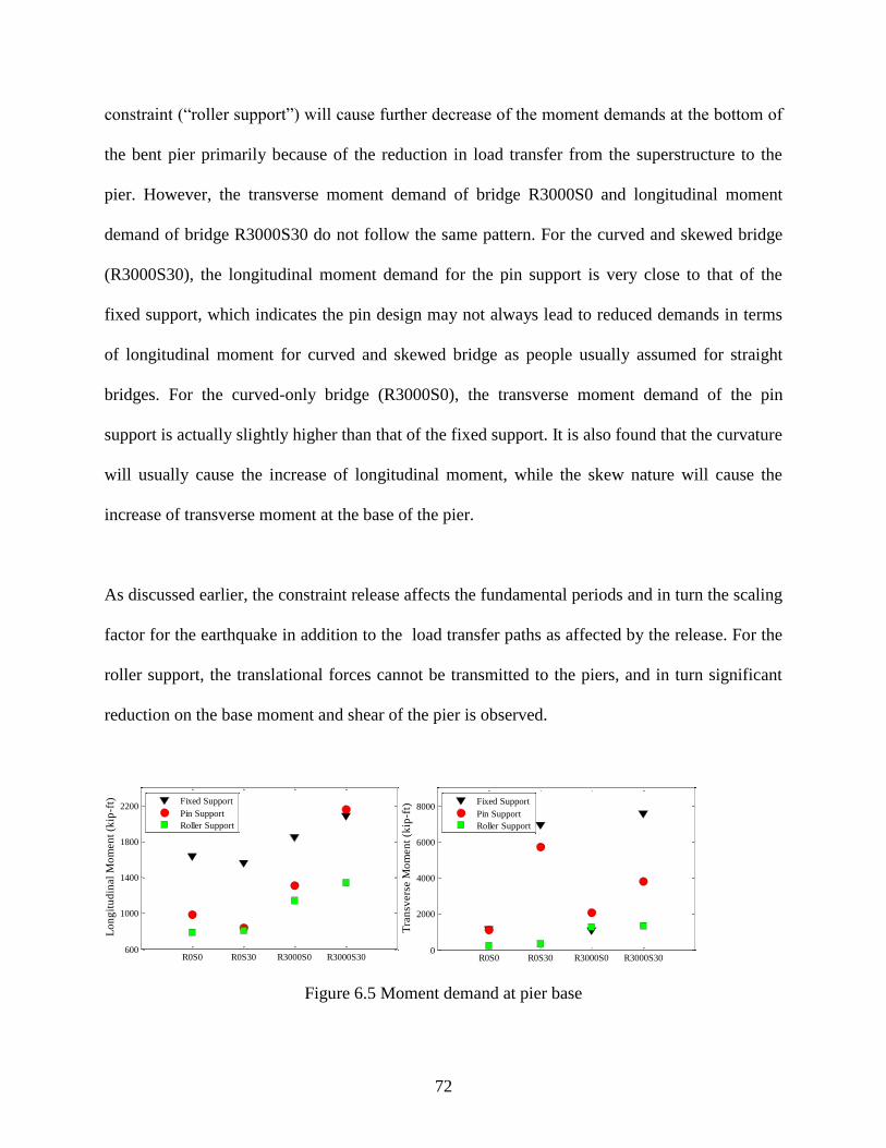
72

constraint (“roller support”) will cause further decrease of the moment demands at the bottom of

the bent pier primarily because of the reduction in load transfer from the superstructure to the

pier. However, the transverse moment demand of bridge R3000S0 and longitudinal moment

demand of bridge R3000S30 do not follow the same pattern. For the curved and skewed bridge

(R3000S30), the longitudinal moment demand for the pin support is very close to that of the

fixed support, which indicates the pin design may not always lead to reduced demands in terms

of longitudinal moment for curved and skewed bridge as people usually assumed for straight

bridges. For the curved-only bridge (R3000S0), the transverse moment demand of the pin

support is actually slightly higher than that of the fixed support. It is also found that the curvature

will usually cause the increase of longitudinal moment, while the skew nature will cause the

increase of transverse moment at the base of the pier.

As discussed earlier, the constraint release affects the fundamental periods and in turn the scaling

factor for the earthquake in addition to the load transfer paths as affected by the release. For the

roller support, the translational forces cannot be transmitted to the piers, and in turn significant

reduction on the base moment and shear of the pier is observed.

Figure 6.5 Moment demand at pier base

R0S0 R0S30 R3000S0 R3000S30600

1000

1400

1800

2200

Lo

ng

itu

din

al

Mo

men

t (k

ip-f

t)

Fixed Support

Pin Support

Roller Support

R0S0 R0S30 R3000S0 R3000S300

2000

4000

6000

8000

Tra

nsv

ers

e M

om

en

t (k

ip-f

t)

Fixed Support

Pin Support

Roller Support

73

Shear forces at pier base

The shear forces at pier base follow similar patterns as the moment demands (Figure 6.6).

However, the transverse shear of bridge R3000S0 does not follow the same pattern. This is also

the result of the complex outcome, both advantageous and disadvantageous, from constraint

release. In this case, increased transverse shear force due to the increased earthquake loads

exceeds reduced shear force due to modified load path, as a result, leading to a resultant increase.

Moreover, the variation of shear forces corresponds well to that of moment demand in two

directions. Similarly, it is found that fully fixed support may result in non-conservative result for

curved bridges. In-plane rotation also causes larger transverse shear for skewed baseline and “pin

support” bridges.

Figure 6.6 Shear forces at pier base

Drift ratio of pier

For the non-curved bridges, the drift ratios remain unchanged or slightly reduced after rotation

release and translation release in general (Figure 6.7). For the curved bridges, the drift ratios

increase first after rotation release and then decrease after translation release. It can also be

explained by the combined effect from both earthquake loads and also modified structure and

load path. Rotation release affect bridge R3000S30 the most, causing 82% increase in

R0S0 R0S30 R3000S0 R3000S300

50

100

150

200

250

Lo

ng

itu

din

al

Sh

ear

(kip

s)

Fixed Support

Pin Support

Roller Support

R0S0 R0S30 R3000S0 R3000S300

100

200

300

400

500

Tra

nsv

ers

e S

hear

(kip

s)

Fixed Support

Pin Support

Roller Support

74

longitudinal drift ratio and 169% increase in transverse drift ratio. This is because rotation

release leads to relatively large seismic demand increase for bridge R3000S30, and the resulted

negative effect is much larger than the positive effect. Lager transverse drift ratio in skewed

bridges is also partially due to the planar rotation of superstructure. For curved and skewed

bridges, the increased drift ratio at the pier top for the pin-support may cause some design issue.

Figure 6.7 Drift ratio of pier

Resistance behind integral abutment

Figure 6.8 summarizes the results of the resistance force behind integral abutments of bridges

with different connections. After rotation release and translation release, the longitudinal force

acting on the abutment from soil springs increases in general as compared to the “fixed” model.

Due to the loss of longitudinal restraint from girder and deck after translation release, most

longitudinal earthquake load acting on the superstructure is shifted from the piers to the

abutments. Translation release leads to an increase in longitudinal force and a reduction in

transverse force on the abutments for skewed bridges. Planar rotation in skewed bridges also

causes significant larger transverse reaction at abutment. For abutments, fixed support conditions

always lead to non-conservative design as expected. Particularly, for curved bridges (R3000S0

and R3000S30), those with pin–support connections will generate considerably larger

R0S0 R0S30 R3000S0 R3000S300.1

0.2

0.3

Lo

ng

itu

din

al

Dri

ft R

ati

o (

%)

Fixed Support

Pin Support

Roller Support

R0S0 R0S30 R3000S0 R3000S300

0.05

0.1

0.15

Tra

nsv

ers

e D

rift

Rati

o (

%)

Fixed Support

Pin Support

Roller Support

75

longitudinal forces on the abutments, which may pose some design challenges on the abutment

depending on the actual soil conditions. For skewed bridges (R0S0 and R3000S30), the

transverse reaction forces are much larger than those non-skewed bridges.

Figure 6.8 Resistance force behind the abutment

6.5. Discussions

Joint effect of scaled earthquake loads and structural system

It is found that support release causes both advantageous and disadvantageous effects in terms of

seismic performance. In order to quantify the respective contributions, three time-history

analysis cases for bridge R3000S0 under San Fernando earthquake are compared (Figure 6.9).

Case 1 uses the fixed-support model and the corresponding scaling factor. Case 2 uses the same

scaling factor as Case 1 but with the pin support. Case 3 uses the pin support model and the

corresponding scaling factor. It is can be seen from Figure 6.9 that under same earthquake load,

moment demand of Case 2 is 48.2% less than that of Case 1 because of the modified structure

connection. In other words, by only considering the structure with released constraints, the

moment demands at the pier base can be reduced by about a half. Comparing Case 2 and Case 3,

the moment demand of Case 3 is 58.2% greater than that of Case 2 (equivalent to an increase

about 30% of the Case 1 demand), and such an increase is attributable to the seismic load change

due to the updated fundamental period, scaling factor, and in turn earthquake loads. In other

R0S0 R0S30 R3000S0 R3000S300

500

1000

1500

2000

Lo

ng

itu

din

al

Fo

rce (

kip

s)

Fixed Support

Pin Support

Roller Support

R0S0 R0S30 R3000S0 R3000S300

500

1000

1500

Tra

nsv

ers

e F

orc

e (

kip

s)

Fixed Support

Pin Support

Roller Support

76

words, for the exactly same structure, by using the updated earthquake load, the moment

demands increase more than 50%. As a summary, for the R3000S0 bridge, it was found that the

constraint releasing alone and the seismic load change alone cause about 52% reduction and 30%

increase from the longitudinal moment demand of the fixed support (Case 1) respectively,

resulting in about 22% total reduction by considering the combined effects. For any bridge with

released constraints, the ultimate structural response is approximately the superposition of two

types of effects. For a particular bridge, depending on which part of influence (advantageous one

or disadvantageous one), the resultant effect from constraint releasing can be complex and a

general trend cannot be made at this point.

For this particular study, fixed support condition overall gives more conservative results for the

base moment and shear for the most part. In some cases such as curved bridges, fixed support

condition may lead to non-conservative estimation. If the displacement at the pier top is of

concern, pin support may actually cause the largest response particularly for both curved and

skewed bridge.

Figure 6.9 Time-history of moment demand at pier base of bridge R3000S0

0 5 10 15 20 25-2000

-1500

-1000

-500

0

500

1000

1500

Time (sec)

Lo

ng

itu

din

al

Mo

men

t (k

ip-f

t)

Case 1

Case 2

Case 3

77

Support assumptions

In order to further analyze the support assumptions, internal demands of some critical

connections are quantified. For the fixed support, the moment demand at the fixed connection is

evaluated, which may be used to assess the assumption rationality of any specific connection

detail. Because of the adoption of rigid link element, the moment at the element on the top of the

bridge pier, rather than the link itself, is shown in Figure 6.10. The peak moments in longitudinal

and transverse directions are about 1000 and 450 kip-ft, respectively. Similarly, the shear forces

of the element on the top of the pier are also assessed to provide information in terms of whether

translational constraints would fail, causing a constraint release. As shown in Figure 6.11, for the

pin support, the shear forces are about 25 and 40 kips in longitudinal and transverse directions,

respectively. For the given connection detail one can determine the capacity of the connection

and evaluate whether or not failure (i.e. release) of the detail is really expected. The detailed

capacity analysis of the specific connection details is not conducted here.

0 5 10 15 20 25

-1000

-500

0

500

1000

Lo

ng

itu

din

al M

om

ent

M2

(K

ip-f

t)

Time (sec)

Fixed Support

Pin Support

0 5 10 15 20 25

0

200

400

600

Tra

nsv

erse

Mo

men

t M

3 (

Kip

-ft)

Time (sec)

Fixed Support

Pin Support

Figure 6.10 Moment demand at the top of the pier of bridge R0S0

78

0 5 10 15 20 25

-100

-50

0

50

100

Longit

udin

al S

hea

r V

3 (

Kip

)

Time (sec)

Fixed Support

Pin Support

0 5 10 15 20 25

-40

0

40

80 Fixed Support

Pin Support

Tra

nsv

erse

Shea

r V

2 (

Kip

)

Time (sec)

Figure 6.11 Shear force at the top of the pier of bridge R0S0

6.6. Summary

The comparative study of four different bridge models was made by appropriately scaling the

respective time-history earthquake records. The main findings from this comparative study are

summarized below:

1) In terms of bridge pier base shear and moment response, fixed connection usually gives

the most conservative results for straight bridges and also most scenarios of curved

and/or skewed bridge. For curved bridges, releasing the rotation at the girder-pier

connection may not always reduce the shear and moment demands at the base of the

bridge pier. For the both curved and skewed bridge, the rotation constraint release also

considerably influences the transverse moment and shear for multi-column pier, which is

very different from the straight bridge.

2) Release of constraints usually does not cause much difference on the pier top

displacement for the straight bridge. However, such release can cause considerable

79

increase of the top displacement for the curved and skewed bridge. This observation

suggests that the constraint release may increase the risk of excessive drift ratio for

curved and skewed bridge.

3) It was found that the release of constraints at the connection part may affect the

fundamental period, scaling actor and in turn earthquake loads. In addition, the constraint

release will also modify structural load path and the response. The resultant influence on

the bridge response will depend on the combined effects from both factors, which are

specific to bridge configurations. For the R3000S0 bridge as an example, it was found

that the constraint releasing alone and the earthquake load adjustment alone cause about

52% reduction and 30% increase from the longitudinal moment demand of the fixed

support (Case 1) respectively, resulting in about 22% total reduction by considering the

combined effects.

4) For straight bridge with multi-column piers, to model the connection between the top of

the interior pier and diaphragm support with a pin may have some advantages such as

reduced longitudinal moment and shear demands on the pier end at the cost of the

increased pier top longitudinal displacement. For curved and skewed bridge, releasing

rotation constraints will reduce transverse moment even for multi-column piers, however

the pier top displacement will be considerably increased along with large abutment

reaction forces, which may cause some design challenges.

5) For the pier-diaphragm connection of the prototype bridge, the realistic scenario is

probably a type of semi-rigid connection during earthquake with limited capacity of some

constraints regardless of what was the design intention. This is more critical to low

seismic region than to high seismic region because of limited demands acting on those

80

connections. An accurate capacity analysis is needed for those connections in order to

assess what is the more realistic connection assumption based on how the bridge actually

behaves during earthquakes.

81

7. Discussion about displacement-based and force-based designs for bridges

The underlying design philosophy for designing bridge against seismic demands, known as

Capacity Design, is to design a bridge with sufficient ductility and deformability to resist the

expected demand. The deformability in the system is typically achieved through ensuring

adequate movement in the bridge joints which the ductility is ensured through the formation of

plastic hinges in the piers or possibly through components of the superstructure such as steel

cross bracings and end diaphragms connecting two adjacent girders. It is important to note that

typically an engineer would have to determine the joints and components that can be utilized to

achieve the required deformability and ductility, respectively. The remaining components are

then designed to remain elastic without losing their strength such that they can provide the

required load path and accommodate the expected actions (forces and moments) and

deformations (displacements and rotations) imposed on the joints and components that are

utilized to achieved the desired deformation and ductility.

Traditionally, seismic provisions have relied on force-based capacity approach to resist the

earthquake effects expressed as a set of horizontal actions defined as a proportion of the weight

of the structure. In the past two to three decades, there has been a shift towards using ductility

instead of strength as the main approach for seismic design of structures. The motivation of

utilizing the ductility-based methods, also called displacement-based method, is due to the

significant uncertainty in estimating the seismic demand using the force-based method. On the

other hand, the ductility method is much less sensitive to unexpected increase in the force

demand imposed on it than its strength-designed counterpart. In addition, the use of the ductility-

82

based method is likely to result in less material being required and hence produce lighter

structures. However, the ductility method typically requires extensive detailing to ensure proper

energy dissipation as manifested by plastic hinge formation. Therefore, more workmanship is

expected and could drive the fabrication cost higher. Both the force-based method and the

displacement-based methods are adopted by the AASHTO Specification. Specifically, the force-

based method is included in the AASHTO LRFD Specification while the displacement-based

method has recently been adopted by the AASHTO Guide Specification for Seismic Bridge

Design.

Both methods hinge on the determination of the demand through seismic analysis, designing the

bridge elements to meet the required demand, and finally comparing and evaluating the

demand/capacity ratio. Various analysis methods and techniques can be used to determine the

expected demand on the bridge include both static and dynamic analysis. The static analysis

include 1) equivalent static, 2) conventional pushover, and 3) adaptive pushover, while dynamic

analysis could be conducted using 1) multi-modal spectral analysis, response time-history

analysis, and 3) incremental dynamic analysis. Performing the analysis requires the generation of

the numerical model, selecting the analysis method, and acquiring the forces and displacements

from the analytical results for which elements and component will be designed to withstand.

Undoubtedly, the complexity of the numerical analysis process is governed by the required level

of geometrical representation of the bridge when generating the models and the level of seismic

input hazard which can affect the ability of models to achieve convergence.

83

Force-based Method: The force-based method is customarily used in the ASHTO LRFD Bridge

Design Specifications. In this method, yielding in specified elements is ensured through

computing the elastic forces from an elastic demand analysis then reducing the forces, for which

the element is to be designed, to ensure the development and progression of yielding in these

elements. The reduction in forces is achieved through the use of Response Modification Factors

(R). In other words, the yield force is equal to the peak elastic force divided by a force

modification factor, R. In Figure 7.1 below, the elastic response line represents the response of

the bridge when no yielding occurs. The elastic force is then reduced using the R factor to ensure

the presence of ductile behavior. However, as indicated previously estimating the inelastic force

is rather challenging due to the large uncertainty associated with estimating the R factor and

often times the displacements are accurately predicted as opposed to member forces.

Figure 7.1 Calculation of Design Force Level and Displacement Demand in Force-Based Method

(FHWA-NHI-15-004, 2014)

Displacement-based Method: Used in the AASHTO Guide Specification, the displacement-based

method essentially seeks to provide the needed performance requirements of those of force-based

design; that is deformability and ductility. In this method design forces for the yielded elements

84

are not computed. Instead, the system can be proportioned by the designer such that the

displacement demand on the bridge is less than the displacement capacity at each pier while

ensuring that minimum lateral strength, typically represented by base shear and overturning

moment, is provided. This is depicted in Figure 7.2 where the displacement capacity is larger

than the displacement demand. In this method the required displacement is ensured through

specific detailing requirements that are with specific guidelines provided to avoid brittle failure.

Figure 7.2 Calculation of Design Force Level and Displacement Demand in Displacement-Based

Method (FHWA-NHI-15-004, 2014)

85

8. Conclusion

This report summarizes the analytical studies on the seismic performance of typical Colorado

concrete bridges, particularly those with curved and skewed configurations. A set of bridge

models with different geometric configurations derived from a prototype bridge selected in

Denver area were studied. Some discussions about the connection modeling are carried out in

terms of the interior bent support. For the displacement-based and force-based designs, due to the

lack of design details that may be adopted for different Colorado bridges, some specific

recommendations cannot be made at this point without detailed analyses of all possible detailing

options. Therefore, some general observations of these two design concepts are summarized in

the end of the report. In the appendices, the design examples of 2-span and 3-span bridges are

listed to help the engineers to conduct bridge seismic analysis in Colorado.

The SAP2000 modeling example and four design examples are included in the Appendices of

this report.

86

9. Sources Cited

Abdel-Mohti, A., & Pekcan, G. (2008). Seismic Response of Skewed RC Box-Girder Bridges.

Earthquake Engineering and Engineering Vibration, 7(4),

American Association of State and Highway Transportation Officials. (2007). AASHTO LRFD

Bridge Design Specifications (4th ed.). Washington, DC: AASHTO.

American Association of State and Highway Transportation Officials. (2011). AASHTO Guide

Specifications for LRFD Seismic Bridge Design (2nd ed.). Washington, DC: AASHTO.

American Society of Civil Engineers. (n.d.). FEMA 356-Prestandard and Commentary for the

Seismic Rehabilitation of Buildings. Washington DC: Federal Emergency Management ….

Washington, DC.

Aviram, A., Mackie, K., Stojadinovic, B. (2008). Guidelines for Nonlinear Analysis of Bridge

Structures in California. Pacific Earthquake Engineering Research Center Report (PEER

2008/03).

Baker, J. W., & Allin Cornell, C. (2006). Spectral shape, epsilon and record selection.

Earthquake Engineering & Structural Dynamics, 35(9), 1077–1095. doi:10.1002/eqe.571

Berman, E. (2008). Estimated Annualized Earthquake Losses for the United States. FEMA 366.

Bignell, J. L., LaFave, J. M., & Hawkins, N. M. (2005). Seismic vulnerability assessment of wall

pier supported highway bridges using nonlinear pushover analyses. Engineering Structures,

27(14), 2044–2063. doi:10.1016/j.engstruct.2005.06.015

Bisadi, V., Asce, S. M., Head, M., & Asce, A. M. (2011). Evaluation of Combination Rules for

Orthogonal Seismic Demands in Nonlinear Time History Analysis of Bridges, (December),

711–717. doi:10.1061/(ASCE)BE.1943-5592.0000241.

Burdette, N. J., Elnashai, A. S., Lupoi, A., & Sextos, A. G. (2008). Effect of Asynchronous

Earthquake Motion on Complex Bridges. I: Methodology and Input Motion. Journal of

Bridge …, (April), 158–165.

Button, M., Cronin, C., & Mayes, R. (2002). Effect of vertical motions on seismic response of

highway bridges. Journal of Structural Engineering, (December), 1551–1564.

California Department of Transportation. (2006). Caltrans Seismic Design Criteria, (1.6), 161.

Charlie, W. A., Battalora, R. J., Siller, T. J., & Doehring, D. O. (2002). Magnitude Recurrence

Relations for Colorado Earthquakes. Earthquake Spectra, 18(2), 233.

doi:10.1193/1.1490546

87

Charlie, W., Battalora, R., Siller, T., & Doehring, D. (2006). Colorado Earthquakes and Active

Faults, 20–34.

Computers and Structures Inc. (2011). CSI Analysis Reference Manual. Berkeley, California,

USA.

Cooper, J., Sharpe, R. L., Fox, G. F., Gates, J. H., Goins, V. M., Hourigan, E. V, … Martin, G.

A. (1981). ATC- 6 Seismic Design Guidelines for Highway Bridges. Berkeley, California,

USA.

Donnell, A. P. O., Beltsar, O. A., Kurama, Y. C., & Taflanidis, A. (2011). Evaluation of Ground

Motion Scaling Methods for Nonlinear Analysis of Structural Systems Erol Kalkan Unites

States Geological Survey. In Proceedings of 2011 NSF Engineering Research and

Innovation Confernence. Atlanta, Georgia.

Elnashai, A. S., & Luigi Di Sarno. (2008). Fundamentals of Earthquake Engineering (1st ed., p.

347). John Wiley & Sons, Ltd.

Housner, G. W. (1952). Spectrum Intensities of strong-motion earthquakes. Proceedings of the

1st World Conference on Earthquake Engineering,, 1.

Itani, A. M., & Pekcan, G. (2011). Seismic Performance of Steel Plate Girder Bridges with

Integral Abutments. Federal Highway Administatrion.

Kalkan, B. E., & Kwong, N. S. (2010). Documentation for Assessment of Modal Pushover-

Documentation for Assessment of Modal Pushover-Based Scaling Procedure for Nonlinear

Response History Analysis of “Ordinary Standard” Bridges.

Kalkan, E., & Chopra. (2010). Practical guidelines to select and scale earthquake records for

nonlinear response history analysis of structures. US Geological Survey Open-File Report.

Kappos, A. J., Paraskeva, T. S., & Sextos, A. G. (2005). Modal pushover analysis as a means for

the seismic assessment of bridge structures. In 4th European Workshop on the Seismic

Behaviour of Irregular and Complex Structures. Thessaloniki, Greece.

Kirkham, R. (1986). An interpretation of the November 7, 1882 Colorado earthquake. Colorado

Geological Survey, (Open File Report 86-8).

Kirkham, R. M., & Rogers, W. P. (1985). Colorado Earthquake Data and Interpretations 1857 to

1985. Colorado Geological Survey, 46, 94.

Krawinkler, H., & Seneviratna, G. D. P. K. (1998). Pros and cons of a pushover analysis of

seismic performance evaluation. Engineering Structures, 20(4-6), 452–464.

doi:10.1016/S0141-0296(97)00092-8

88

Kunnath, S. K., Larson, L., & Miranda, E. (2006). Modelling considerations in probabilistic

performance-based seismic evaluation: case study of the I-880 viaduct. Earthquake

Engineering & Structural Dynamics, 35(1), 57–75. doi:10.1002/eqe.531

Kurama, Y. C., & Farrow, K. T. (2003). Ground motion scaling methods for different site

conditions and structure characteristics. Earthquake Engineering & Structural Dynamics,

32(15), 2425–2450. doi:10.1002/eqe.335

Marsh, L., Buckle, I., Kavazanjian, E. (2014). LRFD seismic analysis and design of bridges

reference manual: NHI course no. 130093 and 130093a.

Mwafy, A. M., & Elnashai, A. S. (2007). Assessment of seismic integrity of multi-span curved

bridges in mid-America, (April). Retrieved from

http://www.ideals.illinois.edu/handle/2142/8782

NCHRP (2004). Connection of Simple-Span Precast Concrete Girders for Continuity. NCHRP

Report 519.

Sheehan, A. F., Godchaux, J. D., & Hughes, N. (2003). COLORADO FRONT RANGE

SEISMICITY AND SEISMIC HAZARD. Colorado Geological Survey Special Publication

55, (15), 1–21.

Spence, W. (1999). Colorado’s Largest Historical Earthquake. USGS Fact Sheet 098-99, (098-

99).

Spence, W., Langer, C. J., & George, L. C. (1996). Rare , Large Earthquakes at the Laramide

Deformation Front Colorado ( 1882 ) and Wyoming ( 1984 ), 86(6), 1804–1819.

Stover, C. W., & Coffman, J. L. (1993). Seismicity of the United States, 1968-1989 (Revised).

U.S. Geological Survey Professional Paper 1527, 418.

Washington Department of Transportation. (2011). WSDOT Bridge Design Manual.

Widmann, B. L., Kirkham, R. M., & Rogers, W. P. (1998). Preliminary Quaternary Fault and

Fold Map and Database of Colorado. Colorado Geological Survey (Vol. Open-File ).

Denver, Colorado.

89

INVESTIGATION OF SEISMIC PERFORMANCE AND DESIGN OF

TYPICAL CURVED AND SKEWED BRIDGES IN COLORADO

Appendix

The appendices A-C include the SAP modeling example and four design examples.

DISCLAIMER

In order to provide related specification requirements for engineers to follow the design

examples, some formulas and graphs from AASHTO LRFD and Guide Specifications are

directly cited. The copyrights of the cited information belong to the original owner.

90

Table of Contents

DISCLAIMER .............................................................................................................................. 89

Table of Contents .......................................................................................................................... 90

Appendix A: SAP 2000 Modeling Example ................................................................................. 91

Appendix B: Design Examples 1 and 2 for SZ I & SDC A ........................................................ 118

Appendix C: Design Examples 3 and 4 for SZ II & SDC B....................................................... 137

91

Appendix A: SAP 2000 Modeling Example

The following section describes the detailed steps taken to develop the 3-span bridge. The

dimension and other information about the 3-span bridge can be found in Appendix B (B.1). The

steps describe the general procedures taken, with additional information and guidelines that are

specific to Colorado bridge design and seismic hazard. The FE models described have been used

for research purposes and may be more detailed than required.

A.1 AutoCAD data input into SAP2000

It is often difficult to develop the geometries for the bridge models using the drawing tools

provided in the analysis software. It is preferable to develop a spine structure in a drafting

program that can be further built upon in SAP2000. AutoCAD is widely used in engineering as a

drafting program and is compatible with most FE software to deal with complex structures. For

non-complex structures, a model can be constructed more quickly through the templates and

drawing tools found in SAP2000. The steps taken to developing the spine model for the 3-Span

bridge using AutoCAD is discussed below.

Step A.1.1

In AutoCAD, the coordinates for the centroid of the bridge girders are calculated from the bridge

plans and drawn in a 2-D plane.

Step A.1.2

Next, the outside edges of the deck, and centerlines of the abutments and bent caps are added to

the drawing, again in the 2-D plane.

92

Step A.1.3

The super-elevation is added by rotating the plan geometry of the bridge to the super-elevation

specified about the (0,0,0) coordinates.

Step A.1.4

While very simple, the basic spine used for SAP is shown in Figure 10; Additional bridge

components may be added as to the spine model as necessary. The file is saved as a “*.dxf”,

which is easily imported with most FE software.

Figure A.1 AutoCAD Spine Model

Step A.1.5

A super elevation may be added by rotating the plan of the bridge about the (0,0,0) global

coordinate. This assumes that each curve is drawn a distance equal to the radius of curvature

from the (0,0,0) coordinate.

93

A.2 Model Construction in SAP 2000

Step A.2.1

A new blank model is created in SAP2000; the default units are always kip-ft when the model is

opened. The units can only be permanently changed in the file by using the Excel interactive

database.

Step A.2.2

The .dxf file created in AutoCAD is imported into the blank model space. A check is made to

ensure that the imported geometries and unit lengths are consistent with the CAD model. There

should be a line element for each of the girders. The curved AutoCAD lines that span the outside

of the deck will not import into SAP, however the nodes on each end of those lines are available

and may be used for developing curved shapes.

Step A.2.3

The girder elements need to first be divided into 5 separate segments. This is done by selecting

the frame element and selecting Edit>Edit Lines>Divide Lines>Divide Into Specified Number of

Frames = 5.

Step A.2.4

The next step is to construct nodes for the deck. From the bridge plans, the distance between the

centroid of the girders and the centroid of the deck (Call this distance Z*) is measured. Using the

“draw special joint” tool, nodes are constructed that are offset by Z* in the positive global z-

direction. The nodes are created at an offset from all of the imported girder, abutment and bent-

cap nodes.

94

Step A.2.5

The outside edges of the deck also need to be drawn. Using the tool for a curved frame element,

the abutment and pier nodes are connected in each span at the exterior and interior edge of the

deck; for this the two-point and radius tool should be selected. The default section (FSEC1) may

be used, as this will be a place holder for the shell elements. The curved frame element is

discretized into 5 straight sections, per span. SAP does not support curved frame elements but

will discretize a curve into a number of straight line elements.

Once the elements are discretized, construction nodes for the abutment and bent cap sections are

added; using the “draw special joint” tool, nodes are constructed at the centroid of the bent cap

and abutment members. The model then resembles Figure A.2.

Figure A.2 SAP2000 Model – Early Stages

Step A.2.6

Subsequently, a check is made to ensure that the nodes of the deck are discretized into equivalent

quadrants. To model the deck slab, shell elements using the default section are drawn in each

quadrant created. A sample model at this point is shown in

95

Figure A.3.

Figure A.3 SAP Model with Girder Elements, Shell Elements, and Nodes for Abutment and Bent

Cap

Frame elements are then drawn through the construction nodes at the bent cap and abutment,

again using the default FSEC1 section. Specific sections will be assigned to members in a later

step.

Step A.2.7

Following the same procedure as illustrated in Step 7, nodes are added at the intersections

between the column and the bent cap and the column and the footing. The adjacent nodes are

connected using frame elements to represent the pier-column.

96

A.3 Materials

Material definitions are created for the structural components of the bridge. A new material is

defined by using the following steps.

Step A.3.1

A custom material is defined by Define>Materials>Add New Material

Step A.3.2

Enter the properties of the material in the dialogue boxes for other material properties under

“Advanced Property Display”. (See Figure A.4a)

Step A.3.3

Alternatively a predefined material may be used by adding a “New Material Quick”. Figure A.4b

shows the characteristics of predefined A992 steel.

Step A.3.4

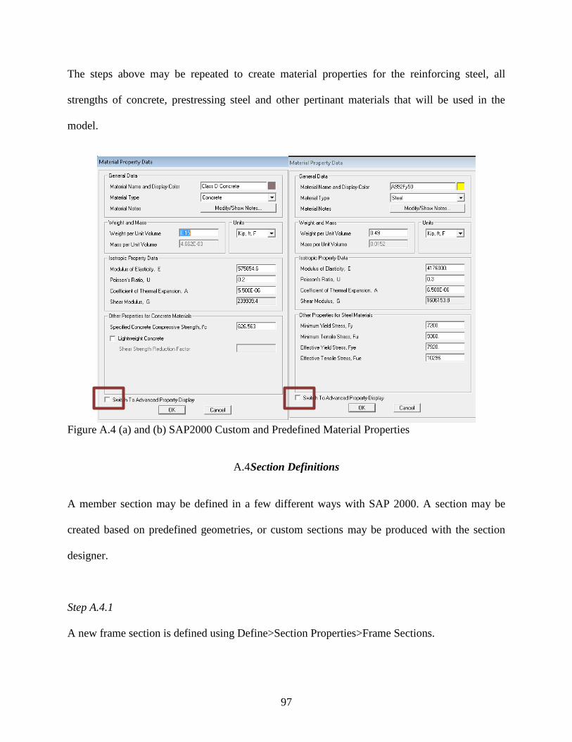
97

The steps above may be repeated to create material properties for the reinforcing steel, all

strengths of concrete, prestressing steel and other pertinant materials that will be used in the

model.

Figure A.4 (a) and (b) SAP2000 Custom and Predefined Material Properties

A.4 Section Definitions

A member section may be defined in a few different ways with SAP 2000. A section may be

created based on predefined geometries, or custom sections may be produced with the section

designer.

Step A.4.1

A new frame section is defined using Define>Section Properties>Frame Sections.

98

Step A.4.2

Under “Other”, “Section Designer” is selected and the “Section Designer” tab is selected to

begin drawing a custom section.

Step A.4.3

Custom sections may be created by using the drawing tools to create the structural shapes and to

add the layout of the reinforcement. In addition, the properties of the section may be modified

under the C-model to add stirrups and confined properties of the concrete section. (See Fig. 6.5)

Step A.4.4

With variable geometry members as shown in Figure A.5, two tools become useful. The first is

the guideline tool, where the outline of a shape may be drawn with guidelines using coordinates.

The next is the polyshape tool that can create a shape from the nodes of the guidelines. Using

these two tools, a non-typical shape may be created as shown below. While non-linear material

properties for the concrete have been provided to SAP, it is unlikely that they will be invoked in

the SAP analysis.

99

Figure A.5 Custom Girder Section

Step A.4.5

Following the preceding steps, sections for the remaining structural members are created. After

material properties and sections have been created, the corresponding members are selected and

using the Assign>Frame Sections command, a frame section is assigned to each of the frame

elements as applicable. Assigning different colors to different frame sections and setting the Set

Display Options to displaying by section color allows for easy differentiation between various

member sections of the model; this can reduce clutter and avoid errors in the structural model.

100

Figure A.6 SAP2000 Bridge Model with Bent Cap and Abutment Sections

A.5 Links

In FE models, links are useful to model connections between adjacent nodes where a connection

or interaction exists but cannot be modeled using frames or constraints. In the example shown,

the superstructure is integral so fixed connections are used. At the abutments, the soil in the

longitudinal direction is represented by nonlinear springs that are also modeled using link

elements. The method of employing both links is described below

Step A.5.1

101

In order to model the connections between integral parts of the bridge, rigid links are used to

connect adjacent frame elements.

Step A.5.2

A new link section is defined by selecting Define>Section Properties>Link/Support Properties

and adding a new property.

Step A.5.3

Linear is selected under Link/Support Type and the “fix all” option is selected at the bottom of

the dialogue box. This restrains displacement and rotation in all degrees of freedom between the

two nodes of the link. The newly defined link will be used to model the integral behavior

described above.

Step A.5.4

Using the ‘rigid link’ defined in the previous step, the girder nodes are connected to the deck at

each intermediate node. This is done using the Draw>Draw 2 Joint Link – and selecting the rigid

link section defined in the previous step. In addition a fixed connection is made between the

nodes of the bent cap and girders, and the girders and the abutment. The configuration of the

links should resemble the model shown below (ignore the links behind the abutment as they are

added in a later step).

102

Figure A.7 SAP2000 Link Elements Implemented

A.6 Support Condition

Step A.6.1

103

Next the support conditions of the bridge need to be defined. This is achieved through

implementing nodal constraints at the appropriate locations of the bridge. The bridge modeled in

this study utilizes integral abutments and a spread footing beneath each pier column. For the

intent of this study and simplified representation of the global dynamic behavior, the spread

footing support is modeled as a fixed support in all 6 DOF. The integral abutment is modeled as

fixed in 5 DOF, while the backing soil in longitudinal (UX) direction is represented by a multi-

linear spring.

The spread footings are modeled by selecting the nodes at the base of each column. Using the

Assign>Joint>Restraints option – restrained displacement is implemented at the base of the

member in all translational and rotational degrees of freedom.

Step A.6.2

The previous step is repeated for the nodes that support the abutment; however, translation in the

global longitudinal direction (corresponding to UX) is not restrained. Note that it is also possible

to change the local axes of the nodes by using the Assign>Joint>Local Axes

Step A.6.3

The next step involves creating a multi-linear spring for the backfill. This method is based on

section 7.8.1 of the CALTRANS Seismic Design Criteria for the longitudinal abutment response

for a stiff soil condition (SDC 1.6, 2010). The completed model is shown in Figure A.8.

104

72'-6" 96'-8" 72'-6"

Figure A.8 Global SAP Models

A.7 Analysis Methods

105

Once the model has been created, a series of different analyses may be performed. The analysis

methods covered in this example include a dead load analysis, modal seismic analysis, seismic

response spectrum analysis, and seismic time-history analysis.

A.7.1 Dead Load Analysis

Step A.7.1.1

To perform a dead load analysis, a load case must be created for the dead load, however, prior to

defining the load case, the load pattern must be defined.( Define>Load Patterns>Add New Load

Pattern) is selected and a new load pattern is defined.

Figure A.9 Defining Load Pattern

Step A.7.1.2

Following creating the dead load pattern, a load case is created. (Define>Load Cases>Add New

Load Case). The new load case is named DEAD and static and nonlinear is chosen under the

106

load case and analysis type. Load Pattern is chosen under Load Type and DEAD is selected

under Load Name and a scale factor of 1 is applied.

Figure A.10 Load Case Data - Dead Loads

Step A.7.1.3

Due to limitations of this study, the effects of bridge live load were not considered. A traffic

loading may be considered at this stage however, SAP no longer has this capability and it would

be necessary to use CSI Bridge or a similar product. Additionally, AASHTO does not have any

firm requirements for the value of EQ, the load factor for live load in the Extreme Event I

(Earthquake) Load combination.

A.7.2 Modal Analysis

107

Step A.7.2.1

Another load case named MODAL is created. Modal is selected under Load Case Type and Ritz

Vectors are employed. The maximum number of modes specified is 30, which may vary

depending on model complexity; at a minimum, enough modes must be considered to capture

95% of the structure mass and in this case, 30 modes are sufficient. Depending on the intent of

the analysis, the stiffness used in the analysis may be selected as an unstressed state or using the

stiffness at end of nonlinear case and selecting dead. It is the recommended that the stiffness at

the end of the dead load analysis be used, thus the dead loads will be applied during the

nonlinear case.

Step A.7.2.2

Under “Loads Applied”, add a load with an Acceleration Load Type, UX direction and maintain

the 99 % participation ratio as shown in Figure A.11.

Step A.7.2.3

Repeat Step 2 for the UY direction in the same load case.

108

Figure A.11 Modal Load Case

109

A.8 Response Spectrum Analysis

Although it is not employed in the analysis performed in this study, Response Spectrum analysis

provides a quick way to estimate the seismic demand on a structure. The following steps describe

a quick method of conducting this type of analysis per the AASHTO 2011 Guide Specifications.

In order to estimate the seismic demand, a response spectrum must be created for the geographic

location and site condition. This can alternatively be created directly in SAP2000 through their

tool, on the USGS website, or through the hazard maps in either AASHTO Bridge Design

specification. This example utilizes a USGS tool developed for the AASHTO 2011 Guide

Specification with a return period of 1000 years.

Step A.8.1

Using the tool below, a response spectrum for Site Class D - a stiff soil is assumed for site for

Denver, Colorado using the AASHTO Guide Specification (2011) as the base design code.

http://earthquake.usgs.gov/designmaps/us/application.php

Step A.8.2

The report that is generated using the link above contains information on the site class definitions

in conjunction with the articles of the code. The report also develops a Design Response

Spectrum and partitions which Seismic Design Category that specific site falls into.

Step A.8.3

110

Using the data supplied in the report and the equations given in section 3.4.1 of the GS, the

design response spectrum in tabular form can be generated. This can be readily computed in a

program like Microsoft Excel.

Step A.8.4

Once the periods and corresponding spectral accelerations have been generated, the data is

copied and pasted into a .txt file (notepad preferable) and saved. The response spectrum can now

either be used to analyze a frame directly or be indirectly used in a time-history analysis.

Step A.8.5

The response spectrum curve is input into SAP 2000 by using the. Define>Functions>Response

Spectrum> select "From File" under "Choose Function Type to Add" and click Add New

Function.

Step A.8.6

“Browse” is selected and the text file containing the response spectrum is selected. "Time and

Function Values” under "Values are:" are used and a check box is selected. So the parameters

"Header Lines to Skip" match the data imported. "Display Graph" is used as a final check to

ensure the correct RS is generated.

Alternatively, one can add a new function directly by going to Define>Functions>Response

Spectrum and manually input the data

111

Step A.8.7

In the SAP model, a new load case is created and named RS. A new Response Spectrum type

load case is defined and the defaults are left as is. Under Loads Applied, a U1 load case is

applied with the response spectrum function and original scale factors multiplied by 32.2 (ft/s2)

to account that the spectrum is input as a percentage of gravity.

Step A.8.8

This step is repeated for another load case with the applied load in the U2 direction.

Alternatively, a load case should be used for comparative purposes, which applies 100% load in

the U2 direction, and 30% in the orthogonal U1 direction. This simulates the fact that the

direction of the earthquake is unknown. In addition a load case to consider 100% U1 plus 30%

U2 analyzed.

112

A.9 Nonlinear Time-History Analysis

Time-history analysis is the most rigorous and accurate analysis method used by code standards

and researchers alike. It can be used in both linear and nonlinear structural models, and typically

requires large computational demand depending on the complexity of the model. The general

steps to performing a generic time-history analysis are described below.

Step A.9.1

Earthquake records should be selected to simulate earthquake ground motion loading on the

bridge. The AASHTO specifications require a minimum of three records for a suitable analysis

(two horizontal and one vertical ground motion). The records should be characteristic of the

tectonic setting and site characteristics. For Colorado, this is not feasible because of the limited

seismic data in Colorado and records with similar tectonic characteristics. It is typically

recommended (not per code) that records be selected based on a low PGA, similar to that of the

DRS developed, a medium site distance, and from a primarily inter-plate database where records

are generally more reliable. The PEER database (the link to which is shown below) is widely

utilized in research and design and provides a strong motion database for earthquake selection.

http://peer.berkeley.edu/gmsm/documentation/

Step A.9.2

Once three records have been chosen, the ground motions must be scaled. Although different

scaling methods provide various advantages and disadvantages (Section 4.1) a response spectrum

based scaling approach is often used due to its accuracy, efficiency and code based origins.

113

Step A.9.3

Construct a design response spectrum using guidelines from the AASHTO Bridge or Guide

Specifications.

Step A.9.4

Determine the fundamental period of vibration of the bridge by running a modal analysis,

developed in 6.3.7. The fundamental period is determined by searching for the mass participation

being excited in the direction of interest,

Step A.9.5

In an Excel spreadsheet, tabulate the response spectra from the structural code (ex. USGS -

AASHTO 2011) as well as the fault normal and fault parallel components of the ground motion

records. When using the PEER database, the response spectra are available through the "Save

Search Spectra" option for the marked search results. Alternatively, a program like Seismosignal

developed by Seismosoft, (http://www.seismosoft.com/en/seismosignal.aspx) provides a quick

and free solution for processing earthquake signals.

Step A.9.6

The scaling factor is determined as the differential factor between the spectral acceleration of the

DRS and the earthquake record at the fundamental period of the bridge. This factor is computed

for the fault normal and fault parallel components. The scale factor is multiplied by 0.3* per

design codes for the fault parallel (or smaller ground motion component).

114

*In the analyses described in the previous chapter, the perpendicular scaling factor used to

evaluate bridge performances was multiplied by 0.4. A higher scaling factor was used for

research purposes as to limit the probability of underestimation of seismic demand imposed by

the earthquake ground motion. This was adopted from the following study (Bisadi and Head,

2011).

Step A.9.7

After the scaling factors are computed, the records need to be processed and imported into

SAP2000. Each record is imported into Seismosignal and a baseline correction is applied.

115

Figure A.12 Seismosignal Forms for Signal Processing

The time-history record in the dual column format is shown in the “Baseline Correction

Filtering” tab under “Corrected” and can be copied and pasted into a .txt file. An independent

text file is created for both the fault normal and fault parallel component of each earthquake. The

response spectrum can also be found under the “Elastic/Inelastic Response Spectra” tab, this may

be useful for Step A.9.6.

Step A.9.8

In SAP, a new load function is added through the Define>Functions>Time History>Add New

Function (From File). Under browse, the text file is added and the parameters are completed to

match the format of the record.

Step A.9.9

After the earthquakes have been processed, scaled and imported into SAP2000, a load case can

be created. The important parameters of the load case are that it is Time History, Nonlinear,

116

Direct Integration, and considers P-Delta effects. It is also important to "Continue from State at

End of Nonlinear Case: Dead" (Figure A.13).

Step A.9.10

The earthquake records are added as shown in the picture below and the time step and total

number of output time steps matches that of the original earthquake record. Damping is defined

by a 2% proportional Rayleigh damping of dynamic vibration for the first and second modes of

vibration. The method of direct time integration is conducted through Hilber-Hughes-Taylor

method.

Figure A.13 Load Case Data - NLTH

117

A.10 Post Processing Methods

A few different tools are available to easily post process the SAP models. Each of the following

options has their advantages based on information provided and computation time.

I. Use the display options to display forces and displacements as shown below

The advantages to this option are that it is easily accessible, and can show a visual representation

of the forces and moment diagram on the actual frame. It is also easy to right click on the frame

to obtain action diagrams once it is displayed. The disadvantages are that for time-history

analysis it necessitates large amounts of time to compute. It also has difficulties panning through

the model to find results (i.e. it needs to update each time step).

II. Use the “Show Plot Functions” option.

The “Show Plot Function” allows a time-history plot of various components, such as a single

nodal result (i.e. displacement or force). It is best used for further investigating components of

the model once a global demand has been calculated. For example, in this study it was useful for

finding a particular peak demand and the corresponding actions that develop at that time for a

specific point in the earthquake time-history. Additional post processing is easiest computed by

exporting the results from this section to a .txt file and subsequently importing into MATLAB,

Excel or other software for further processing. Alternative select step-by-step under the “Show

Tables” option discussed below.

III. Utilizing the “Show Tables” option

118

Most of the post processing can be conducted using this option. It is recommended that the

engineer select the frames or nodes that are of interest – select “Show Tables” and select the

results that are desired from the analyses in order to avoid being overloaded with data. This

method is the recommended option as it provides the maximum developed actions and

displacements in a clean format that can be formatted and post processed directly in Excel.

Figure A.14 Display Tables

For time-history analysis, the output will only display the largest demand observed over the

entire earthquake. For analyses that require more than one demand component, this can lead to

conservative and un-conservative design values. Therefore option B is recommended for

identifying particular critical time points.

119

Appendix B: Design Examples 1 and 2 for SZ I & SDC A

AASHTO Bridge Design Code Examples 1 & 2 are based on LRFD and Guide Specification

respectively for the 3-span bridge in SZ I & SDC A. The basic information of the 3-D bridge

(referred to “D-17-DJ bridge” in some following text) is shown below.

B1. 3-span bridge Information

Three-span bridge layout and construction information is shown in Figures B1-B5.

120

Figure B.1 - Three Span Bridge - Plans and Elevation (D-17-DJ bridge)

121

EL 4850.96 ft.

EL 4865.67 ft.

EL 4850.96 ft.EL 4864.75 ft.

17'-6"x10'-0"x4'-3" Pile cap, typ.

12'-0"x2'-0" Pier, typ.Detail:

4'-3"x3'-3" Girder

EL 4870.84 ft.

EL 4869.59 ft.

59'-0"

7 spaces @ 8'-0 ½” = 56'-3 ½"

Figure B.2 – Three Span Bridge Section at Pier

6 1

/2"

3 1

/2"

4'-

1 1

/4"

1 5

/8"

1 5

/8" 5

5/8

"

2'-0"

2'-4"

1'-4"

3 7/8" 3 7/8"

1 5/8"1'-8 1/2"

1 5/8"

Interior of Span Bearing Ends

5"

Figure B.3 – Three Span Bridge - Precast I Sections

122

1'-

0"

HP12x84 Pile

Pile Cap:

4-#11 Each Side

#5 Ties @ 12"

Abutment

Cl. Bearing Abutment

Elastomeric Bearing Pad

At Girders, Typ.

1'-

0"

6 1/2"

1'-3" 1'-3"

5"3

'-6

"

Precast I

Deck Slab 8"

4"

Ha

un

ch

#5 @ 6 Top, 2 1/2” Clear

#5 Bottom, 1” Clear (Spcg. Varies)

#5 @ 12 Each Side

1'-

9"

(Typ

.)

Figure B.4 – Three Span Bridge - Section at Abutment

123

Cl. Pier

Pier Cap:

(2)x6-#11 Bott.

6-#11 Top

4-#5 Each Side

(2) Sets #5 Ties

(Spacing Varies)

Support Column:

2'-0"x12'-0"

11-#10 V Each Side

3-#10 V Each End

14-#5 Ties

Elastomeric Bearing

Pad, Typ.

Precast I

3'-2"

2'-0"

8"

4"

Hau

nch

Deck Slab

Diaphragm:

5-#5 Each Side

8-#5 Ties

Between Girders

5-#9 Dowels Between

Girders

SECTION AT PIER

Figure B.5 – Three Span Bridge - Section at Pier

124

B2. Design Example No.1 (LRFD Design Specification-SZ I)

This design example is based on AASHTO LRFD Bridge Design Specifications – Customary

U.S. Units (2012)

The following section describes the seismic design procedures required for bridges in Seismic

Zone 1. The bridge selected for the design example carries the northbound and southbound lanes

of Interstate Highway I25 over State Highway 119 at Del Camino (Firestone, Colorado). The

bridge layout and construction are shown in Figures B.1 to B.5. The example is not

comprehensive for all bridges in SZ-1 but rather serves as a general example for a typical bridge

design with a few additional comments and insights.

The flowchart presented in Chapter 3, Appendix A3 of the AASHTO LRFD Code is the easiest

way to follow the seismic design procedure and is thus followed herein. The organization of the

design example is categorized by article title and follows the general structure of the design

flowcharts.

B2.1 Earthquake Demand:

B.2.1.1 AASHTO Article 3.10 Earthquake Effects: EQ

AASHTO Article 3.10.1 introduces the general methodology of the seismic design, and also

describes the applicability of the specifications.

There are two possible options for determination of the seismic hazard factors:

125

Option A. Use the articles and procedures presented in AASHTO subsections 3.10.2,

3.10.4, and 3.10.6 to identify the seismic hazard factors from hazard maps ,

develop a design response spectrum, make adjustments with respect to the soil

condition, and select the seismic performance zone (SZ).

Option B. (Recommended):Use the USGS-AASHTO web-based tool to determine

the same parameters but through an automated process available at the following

address:

http://earthquake.usgs.gov/designmaps/us/application.php

This example uses AASHTO Option A for determination of the seismic hazard factors to provide

a basis for comparison with Option B, which is used in a subsequent example. From AASHTO

Article 3.10.2 for the D-17-DJ bridge and a site location in Firestone near Denver, Colorado,

accelerations are determined from Figures B.6-8 and are equal to PGA=0.06g, Ss = 0.12g, S1 =

0.035g, respectively. Linear interpolation is used for locations that are between contour lines; the

red circle indicates the location of the bridge in Firestone.

Figure B.6 - AASHTO Bridge Spec.: 3.10.2-1 Acceleration Coefficient for Conterminous

United States (PGA) with Seven Percent Probability of Exceedance in 75 yr. (Approx. 1000-yr

Return Period)

126

Figure B.7 – AASHTO Bridge Spec.: 3.10.2-2 Horizontal Response Spectral Acceleration

Coefficient for the Conterminous United States at Period of 0.2 s (Ss) with Seven Percent

Probability of Exceedance in 75 yr. (Approx. 100-yr. Return Period) and Five Percent Critical

Damping

Figure B.8- AASHTO Bridge Spec.: 3.10.2-3 Horizontal Response Spectral Acceleration

Coefficient for the Conterminous United States at Period of 1.0 s (Sl) with Seven Percent

Probability of Exceedance in 75 yr. (Approx. 100-yr. Return Period) and Five Percent Critical

Damping

127

B.2.1.2 AASHTO Article 3.10.3 Site Class

A site class is chosen based on the properties of the soil defined in AASHTO Table 3.10.3.1-1.

For the prototype location in Firestone, Site Class D is selected for a stiff soil. Typically, the site

class would be provided in the report of geotechnical investigation.

AASHTO Article 3.10.3.2 Site Factor

Based on AASHTO Tables 3.10.3.2-1, 2 and 3 and the acceleration coefficients determined

from the hazard maps, the following site factors were determined:

FPGA = 1.6, Fa = 1.6, Fv = 2.4

B.2.1.3 AASHTO Article 3.10.4 Seismic Hazard Characterization

Using the equations and guidelines presented in AASHTO Article 3.10.4, a design response

spectrum (DRS) was developed. Based on the equations, the following factors were calculated

for the DRS:

As = Fpga*PGA = 1.6*0.06g = 0.96g

SDS=FA*SS = 1.6*.12g = 0.192g

SD1 = FvS1 = 2.4 * 0.035g = 0.084g

Ts= SD1/ SDS = 0.084/0.192 = 0.438s

T0 = 0.2*Ts = 0.2 * 0.4375 = 0.875s

B.2.1.4 AASHTO Article 3.10.5 Operational Classification

The owner shall determine the operational category of the bridge as Critical, Essential or Other.

The operational category is used for determination of the appropriate response modification

factor for the design of the substructure from AASHTO Table 3.10.7.1-1 and from AASHTO

128

Table 3.10.7.1-2 for the connections. For the subject bridge supporting an interstate highway,

the Critical category is chosen for which the response modification factor is 1.5 for vertical steel

piles.

B.2.1.5 AASHTO Article 3.10.6 Seismic Performance Zones

Using the Seismic Hazard Parameters determined, the bridge may be assigned to a seismic

performance zone. The Seismic Zone is determined from AASHTO Table 3.10.6-1 (Table B.1).

Table B.1 - AASHTO Table 3.10.6-1 Seismic Zones

Acceleration Coefficient,

SD1

Seismic Zone

SD1≤ 0.15 1

0.15 < SD1≤ 0.30 2

0.30 < SD1≤ 0.50 3

0.50 < SD1≤ 4

SD1 = 0.084 ≤ 0.15 which places the D-17-DJ bridge in Firestone, Colorado in Seismic Zone 1.

B.2.1.6 AASHTO Article 3.10.7 Response Modification Factors

The response modification factors for the connections are the same regardless of the response

modification factor and are 0.8 for the superstructure to the abutment and 1.0 for columns to cap

beam and columns to foundations.

B.2.1.7 AASHTO Article 4.7.4 Analysis for Earthquake Loads

Based on the Seismic Zone to which the bridge is assigned, this section is utilized to determine

which analysis method is required. AASHTO Table 4.7.4.3 (Table B.2) presents each of the

general analysis requirements. Based on a multi-span bridge type and seismic zone; for SZ-1, no

seismic analysis is required.

129

Table B.2 - AASHTO Table 4.7.4.3

Seismic

Zone

Single-Span

Bridges

Multispan Bridges

Other Bridges Essential Bridges Critical Bridges

regular irregular regular irregular regular irregular

1

No seismic

analysis

required

* * * * * *

2 SM/UL SM SM/UL MM MM MM

3 SM/UL MM MM MM MM TH

4 SM/UL MM MM MM TH TH

* = no seismic analysis required

UL = uniform load elastic method

SM = single-mode elastic method

MM = multimode elastic method

TH = time history method

For SZ-1 the next step is to meet the minimum requirements in AASHTO Articles 4.7.4.4 and

3.10.9. Starting with 4.7.4.4, the minimum support length requirements must be satisfied. The

support length, N, is determined from:

2(8 0.02 0.08 )(1 0.000125 )N L H S AASHTO Eqn. 4.7.4.4-1

:

minimum support length measured normal to the centerline of bearing (in.)

length of the bridge deck to the adjacent expansion joint, or to the end of the bridge deck;

for single -spa

Where

N

L

n bridge, L equals the length of the bridge deck (ft)

for abutments, average height of columns supporting the bridge deck from the abutment to

the next expansion joint (ft)

for columns

H

and/or piers, column, or pier height (ft)

skew of support measured from line normal to span (degrees)S

In this case:

130

2

241.6 ft., 14 ft., 0

(8 0.02 241.6 0.08 14)(1 0.000125 5 ) 13.99 in. Say 14 in. minimum

L H S

N

o;

AASHTO Article 3.10.9.2

Subsequently, the connection design forces are calculated per AASHTO Article 3.10.9.2 for a

bridge in Seismic Zone 1.

Calculate the unit dead load of the bridge deck for determination of tributary vertical reactions in

order to calculate resulting horizontal seismic forces at the piers and abutments.

Table B.3 – Unit weights for bridge superstructure components

Element Weight Factor Unit Load (psf)

Precast I Beams 637 lb/ft. 8’-0 ½” Spacing 127.5

Slab + Haunches 6760 lb/ft (total) 59’-0” Width 59

Wearing Course 24 psf 1 24

Deck Forms 5 psf 1 5

Total - - 216

If As<0.05:

0.15 (Vert. Reaction based on influence area)

0.5 0.15 (Vert. Reaction based on tributary area)

long

lat long

F

F F

If As <0.15:

0.25 (Vert. Reaction based on influence area)

0.5 0.25 (Vert. Reaction based on tributary area)

long

lat long

F

F F

The next step is to calculate the influence area dead load of each span:

2

1,3

2

2

(72.5 ft)(59.1 ft) 4,285 ft

(72.5 ft 96.8 ft)(59.1 ft) 10,006 ft

span

span

A

A

2

1,3

2

2

(0.216 ksf )(4,285 ft ) 926 kips - Abutments

(0.216 ksf)(10,006 ft ) 2161 kips - Piers

W

W

Next calculating the minimum connection force on the integral abutments and piers:

131

2

1,3

2

2

(0.216 ksf )(4,285 ft ) 926 kips - Abutments

(0.216 ksf)(10,006 ft ) 2161 kips - Piers

W

W

Lastly calculating the minimum connection force on the center pier:

(0.25)(2161 kips) 540 kips

(0.5)(540 kips) 270 kips

Long

Lat

F

F

B.2.1.8 AASHTO Section 5: Concrete Structures

5.10.11 Provisions for Seismic Design

AASHTO Section 5.10.11.2 states that “For bridges in Seismic Zone 1 where the response

acceleration coefficient, SD1, specified in Article 3.10.4.2 is less than 0.10, no consideration of

seismic forces shall be required for the design of structural components, except that the design of

the connection of the superstructure to the substructure shall be as specified in 3.10.9.2.”

For bridges in Seismic Zone 1 where 0.10< SD1 0.15 , the transverse reinforcement

requirements at the top and bottom of a column shall be as specified in AASHTO Articles

5.10.11.4.1 d and 4.10.11.4.1e. For this design example, SD1=0.08 > 0.1, thus this section is not

applicable.

B.2.1.9 AASHTO Section 10: Foundations

According to AASHTO Appendix A10 a site specific investigation should be performed for

sites with SD1>0.1g, since SD1<0.1g, no significant earthquake design factors need be considered

B.2.1.10 AASHTO Section 11: Abutments, Piers and Walls

The abutments are essentially concrete structures as they are caps supported by piles and thus,

should be subject to the same design requirements, specifically, since SD1<0.1g, no significant

earthquake design factors need be considered.

The abutment walls carry no bridge load, vertical or horizontal and thus will not be subject to

excitation from the bridge.

132

133

B3. Design Example No.2 (Guide Specification-SDC A)

This design example is based on AASHTO Guide Specifications for LRFD Seismic Bridge Design

2nd Edition (2011)

The following section describes the seismic design procedures required for bridges subject to the

design requirements of Seismic Design Category A (SDC A) using the AASHTO Guide

Specifications (GS). The same bridge as used in design example No. 1 (D-17-DJ bridge) is

selected, which carries the northbound and southbound lanes of Interstate Highway I25 over

State Highway 119 at Del Camino (Firestone, Colorado) is considered. The center of the bridge

is at coordinates 40.160654, -104.978964 based on Google.

B.3.1 Earthquake Demand:

B.3.1.1 GS 3.4 Seismic Ground Shaking Hazard

Option A. Use the articles and procedures presented in 3.4 Seismic Ground Shaking

Hazard to develop a design response spectrum based on hazard maps, and make

adjustments with respect to the soil condition.

Option B. (Recommended). Use the USGS-AASHTO tool to determine the same

parameters but through an automated process.

http://earthquake.usgs.gov/designmaps/us/application.php

Using Option B, the following parameters were determined and may be used with the

specifications in Section 3.4.1-1 or taken directly from the USGS-AASHTO document to

determine the design response spectrum:

134

Parameter Value

PGA 0.058g As =FPGA*PGA 0.093g

Ss 0.124g SDS=Fa*Ss 0.198g

S1 0.033g SD1 = Fv*S1 0.079g

Fpga 1.60

Fa 1.60

Fv 2.40

Figure B.6 - Design response spectrum – Origin: USGS – AASHTO 2014 Guide Spec. Seismic

Hazard Tool

B.3.1.2 AASHTO Article 3.5 Selection of Seismic Design Category (SDC)

a. Utilize the specifications below and the SD1 parameter to determine the Seismic

Design Category

AASHTO Table 3.5.-1 - Partitions for Seismic Design Categories A, B, C, and D

135

Based on the value of 0.079g for the SD1 parameter developed in the previous step, the Seismic

Design Category is determined as SDC A. A review of the requirements for each step is shown

below:

SDC A Requirements from AASHTO Article 3.5 – Selection of Seismic Design Category

(SDC)

a. No identification of ERS according to Article 3.3

b. No demand analysis

c. No implicit capacity check needed

d. No capacity design required

e. Minimum detailing requirements for support length, superstructure/substructure

connection design force, and column transverse steel

f. No liquefaction evaluation required

B.3.1.3 AASHTO Article 4.6 – Design Requirements for Seismic Design Category A

Based on the requirements, determine the minimum design requirements that need to be met

through Article 4.6. The acceleration coefficient As is the critical factor for calculation of the

seismic forces on the connections in the restrained directions; for the subject connection As =

0.093.

For the 3-Span Bridge,

If As<0.05:

, ,

, , ,

0.15 (Vert. Reaction base on influence area)

0.15 (Vert. Reaction base on tributary area) 0.5

min conn long

min,conn trans min conn long

F

F F

136

If As <0.15:

, ,

, , , ,

0.25 (Vert. Reaction base on influence area)

0.25 (Vert. Reaction base on tributary area) 0.5

min conn long

min conn trans min conn long

F

F F

This second case will be used since 0.05 0.093 0.15 .

Subsequently, the influence area dead load of each span is calculated (refer to Table B.3 for unit

values of component dead loads). The longitudinal loads should first be determined based on the

influence areas:

2

1,3

2

2

(60.17 ft)(59.1 ft) 3,556 ft

(60.17 ft 115.42 ft)(59.1 ft) 10,377 ft

span

span

A

A

2

1,3

2

2

(0.216 ksf )(3,556 ft ) 768 kips - Abutments

(0.216 ksf)(10,377 ft ) 2241 kips - Piers

W

W

Next calculating the minimum connection force on the integral abutment:

2

1,3

2

2

(0.216 ksf )(3,556 ft ) 768 kips - Abutments

(0.216 ksf)(10,377 ft ) 2241 kips - Piers

W

W

Lastly, calculating the minimum connection force at the pier:

(0.25)(2241 kips) 560 kips

(0.5)(560 kips) 280 kips

Long

Lat

F

F

B.3.1.4 AASHTO Article 4.12 Minimum Support Length Requirements

The minimum required support lengths are specified in AASHTO Article 4.12. These

specifications typically apply for bridges in Seismic Design Category A; however, the subject

bridge has integral abutments and thus, does not need to satisfy this requirement.

B.3.1.5 AASHTO Section 8: Reinforced Concrete Members

8.2 – Seismic Design Category (SDC) A

For SD1values equal to or exceeding 0.10, but less than 0.15 in SDC A, minimum shear

reinforcement is required to meet the SDC B requirements for concrete members per AASHTO

Article 8.6.5. In addition “When such transverse reinforcement is provided, the provisions of

137

AASHTO Article 8.8.9 should apply. The length over which this reinforcement shall extend

shall be the plastic hinge region defined in AASHTO Article 4.11.7. Alternatively, this length

may be that defined in Article 5.10.11.4 of the AASHTO LRFD Bridge Specifications”

For the bridge under consideration, SD1= 0.079 <0.1 and thus, does not need to satisfy these

requirements.

B.3.1.6 AASHTO Section 6: Foundation and Abutment Design

Per AASHTO Article 6.2.3, “there are no special seismic foundation investigation requirements

for SDC A”.

138

Appendix C: Design Examples 3 and 4 for SZ II & SDC B

Design examples 3 & 4 are for both 2-span (J-17-AA bridge) and 3-span bridges (D-17-DJ

bridge) in SZ II and SDC seismic zones based on the AASHTO LRFD Standard and Guide

Specifications. The 3-span bridge information can be found at Appendix B (B.1). The 2-span

bridge information is introduced in the below.

C1. 2-span bridge (J-17-AA bridge) Information

Two Span Bridge Layout and Construction (J-17-AA bridge)

139

Figure C.1 - Two Span Bridge Plan and Elevation (J-17-AA bridge)

148'-4.9"

74'-2.45"

38'-

6"

38'-

6"

5'-

0"

5'-

0"

3 @

10

'-0

"3

@ 1

0'-

0"

CL. Brg. CL. Pier CL. Brg.

2'-6"

13'-

1"

ELEVATION

Abutment Grade Beam

CaissonPierPier ColumnCaisson

Pier Diaphragm

PLAN

4'-

0"

74'-2.45"

140

10'-0" 10'-0"20'-0" 20'-0"

8 in. Slab with

3 1/2 in. Haunches

3'-

11

"

3'-

0"

12

'-9

"

7 Spaces @ 10'-0"

36" Dia. Column on

42" Dia. Caisson, Typ.

Figure C.2 - Two Span Bridge - Section at Pier

1'-4" 2"

6 1/

2"

6"

3'-7"

3 1/

2"

2"

2"

1'-

10"

2'-3"

7"

10"

3'-

6"

Figure C.3 - Two Span Bridge - I-Girder Cross Section

141

1'-5"

4'-0"

8"

3"

3'-

6"

Var

ies

3'-

0"

to 3

'-11

"

Typ.

8-#11 Top & Bott.

4-#5 Each Side

#5 U at 6" O.C.

3-#11 Cont.

(Mechanically Spliced)

I-Girder

36" Dia. Column:

15-#8 Vert.

#5 Hoops @ 12" O.C.

15-#8 Dowels

Extended 5'-3" into

Column

42" Dia. Caisson:

15-#9 Vert.

#5 Hoops @ 12" O.C.20

'-0

" +/

-

#6 x 48" @24"+/- O.C.

#5@6 (omit at girders)

6-#5 Between Girders

5-#5 Typ.

Elastomeric Bearing, Typ.

Figure C.4 - Two Span Bridge - Section at Pier

142

30" Dia. Caisson:

8-#9 Vert., Extend

fully into abutment

#5 Hoops @ 12" O.C.

6 1/2"

2'-6"

1'-

0"

3'-

6"

3'-

6"

3-#5 Each Side

#5 U at 6" O.C.

Elastomeric Bearing, Typ.

I-Girder

6-#5 Between Girders

#5@6 (omit at girders)

3-#5

4-#5

#5@6"

#5@6"

Figure C.5 - Two Span Bridge - Section at Abutment

143

C2. SAP Analysis Results for the 2-span and 3-span bridges

The portion of Colorado that falls into SDC B and SZ II in the AASHTO specifications is limited

to a finite portion of the map, for a select soil condition. The select geographic area that falls in

the higher seismic zone is limited to the portions of the South and West of Colorado, and for a

softer (Site Class E and lower) soil condition. For this region and condition described a DRS is

developed per the AASHTO Guide Specifications. The ground motion is then scaled and the

imposed seismic demand is analyzed using the 2-span bridge, and a select 3-span bridge. The

bridge geometry selected for the three-span bridge is Bridge #6 which has a radius of 4500 ft and

skew angle of 30 degrees. Table C.1 shows the increased deformation of the model resulting

from using SDC B/SZ II compared to SCC A/SZ I. Tables C.2 through C.7 present the increased

structural demand of the model resulting from SDC B/SZ II.

Table C.1 Jt. Displacement: 2-Span & 3-Span Bridges

3-Span Bridge Jt. Displacements 2-Span Bridge Jt. Displacements

U1

(Longitudinal)

U2

(Transverse)

U1

(Longitudinal)

U2

(Transverse)

Minimum 38% 49% Minimum 18% 2%

Maximum 122% 164% Maximum 87% 62%

Table C.2 Jt. SDC B: 2-Span Bridge: Column Demand

Peak Demand % Increase from SDC A D/C Ratio

Axial Kip -537.7 18.1% 0.12

V2 Kip -83.51 52.8% 0.18

V3 Kip 181.3 62.8% 0.60

T Kip-ft 20.15 34.4% 0.11

M2 Kip-ft 1376.6 63.4% 1.24

M3 Kip-ft -503.8 49.7% 0.45

144

Table C.3 SDC B: 3-Span Bridge: Column Demand

Peak Demand % Increase from SDC A D/C Ratio

Axial Kip -987.9 18.1% 0.07

V2 Kip -843.0 73.9% 0.51

V3 Kip -276.3 117% 1.74

T Kip-ft 101.7 77.8% 0.53

M2 Kip-ft 2930 103% 1.13

M3 Kip-ft -12460 78.0% 0.82

Nominal section capacities are not shown for components that are strongly influenced by

fluctuating axial loads.

Table C.4 SDC B: 2-Span Bridge: Bent Cap Demand

Peak Demand % Increase from SDC A Nominal Section Capacity D/C

Axial Kip -643.1 52% -9728.7 0.07

V2 Kip 385.8 26% 680.2 0.57

V3 Kip 82.5 92% 580.46 0.14

T Kip-ft 700.2 131% 1145 0.61

M2 Kip-ft 393.2 99% 2322.5 0.17

M3 Kip-ft -1274 36% 6404.43 0.20

Table C.5 SDC B: 3-Span Bridge: Bent Cap Demand

Peak Demand % Increase from SDC A Nominal Section Capacity D/C

Axial Kip -1014 52% X,-10179 0.10

V2 Kip 583.7 26% 682.9 0.85

V3 Kip -148.6 92% 1246 -0.12

T Kip-ft 1848 131% 876.1 2.11

M2 Kip-ft 770.7 99% 3487 0.22

M3 Kip-ft -3077 36% 2884 -1.07

Table C.6 SDC B: 2-Span Bridge: Girder Demand

Peak Demand % Increase from SDC A Nominal Section Capacity D/C

Axial Kip -959.4 12% -3715.7 0.26

V2 Kip -115.7 23% 712.59 0.16

V3 Kip -7.21 29% 681.59 0.01

T Kip-ft 17.0 33% 52 0.33

M2 Kip-ft 52.2 34% 233.36 0.22

M3 Kip-ft -1216 15% 3734.89 0.33

Table C.7 SDC B: 3-Span Bridge: Girder Demand

Peak Demand % Increase from SDC A Nominal Section Capacity D/C

145

Axial Kip -948.7 29% -3196.9 0.30

V2 Kip -96.00 32% 1056.99 0.09

V3 Kip -8.67 149% 671.67 0.01

T Kip-ft -4.69 104% 69.45 0.07

M2 Kip-ft -85.3 165% 67.37 1.27*

M3 Kip-ft -1301 49% 5542.25 0.23

*It is unlikely that a significant compromise in structural integrity would result in this case.

There are components of the superstructure such as the integral diaphragms between the girders

that would increase the lateral moment (M2) capacity and were not included in the structural

model.

Table C.8 SDC B: 2-Span Bridge: Integral Abutment Demand

Peak Demand Nominal Section Capacity D/C

Axial Kip -40.26 -7005.1 0.01

V2 Kip 84.49 659.1 0.13

V3 Kip -157.2 448.9 0.35

T Kip-ft -416.8 299.3 1.39

M2 Kip-ft 277.2 2537.1 0.11

M3 Kip-ft 253.3 739.2 0.34

Table C.9 SDC B: 3-Span Bridge: Integral Abutment Demand

Peak Demand Nominal Section Capacity D/C

Axial Kip -378.6 7549.9 0.05

V2 Kip 67.0 786.6 0.09

V3 Kip -417.0 457.4 0.91

T Kip-ft -2140 533.6 4.01

M2 Kip-ft -613.7 3327.5 0.18

M3 Kip-ft 267.2 637.9 0.42

146

With the increase in seismic excitation from the SDC B (SZ II) load case, the structural

demand on the model increases significantly. The results exceed nominal capacities in shear and

bending in the pier-columns, bent caps and girders. A large torsional demand is also observed on

the integral abutment where damage is likely to occur. This is observed for both the 2 and 3-span

bridge models. A suggestion for an improvement in cases where a Colorado bridge is exposed to

either similar or higher seismic demand than imposed above, would be to implement bearing

type supports. Allowing translation specifically in the longitudinal direction elongates the

fundamental period and can dramatically reduce the excitation from seismic loads. In addition, it

may be necessary to implement an Earthquake Resisting System (ERS) in the bridge, as

discussed in the AASHTO Guide specifications. An ERS allows for concentrated yielding and

energy dissipation to occur in targeted areas while maintain the structural integrity of the bridge.

Further information on ERS details are provided in the AASHTO Guide Specifications.

147

C3. Design Example No. 3: LRFD design specification and SZ II

This design example is based on AASHTO LRFD Bridge Design Specifications – Customary U.S.

Units (2012) a selected bridge in Seismic Zone (SZ) II.

The easiest way to maneuver through the bridge design specifications and complete a

comprehensive seismic design is through the flow charts provided in Appendix A3 of the LRFD

specification. The organization of Design Example 3 follows the structure of the flow chart.

C.3.1 Earthquake Demand:

C.3.1.1 AASHTO Article 3.10 Earthquake Effects: EQ

AASHTO Article 3.10.1 General

Applicability of the AASHTO Bridge Spec. to the seismic design of this bridge, along with

supplemental information and is provided in this section

AASHTO Article 3.10.2 Seismic Hazard

Option 1: Use the articles and procedures presented in AASHTO Articles 3.10.2-

4,6 to develop a design response spectrum based on hazard maps, make

adjustments with respect to soil condition, and determine seismic zone.

Option 2: (Recommended) Use the USGS-AASHTO tool to determine the same

parameters but through an automated process.

http://earthquake.usgs.gov/designmaps/us/application.php

Through Option 2, the following parameters were determined and can be used with the

specifications in AASHTO Article 3.4.1-1 or taken directly from the USGS-AASHTO document

to determine the design response spectrum:

148

Parameter Value

PGA 0.088g As =FPGA*PGA 0.219

Ss 0.117g SDS=Fa*SS 0.443

S1 0.045g SD1 = FV*S1 0.156

FPGA 2.50

Fa 2.50

Fv 3.50

Figure C.6 – Origin: USGS – AASHTO 2011 Guide Spec. Seismic Hazard Tool

C.3.1.2 AAHSTO Article 3.10.6 - Selection of Seismic Zone

b. Utilize the specifications below and the SD1 parameter to determine the Seismic

Design Category

Using the Seismic Hazard Parameters developed a DRS can be constructed and

the Seismic Zone can be identified per Table 3.10.6-1

149

AASHTO Table 3.10.6-1 Seismic Zones

Acceleration Coefficient,

SD1

Seismic Zone

SD1≤ 0.15 1

0.15 < SD1≤ 0.30 2

0.30 < SD1≤ 0.50 3

0.50 < SD1≤ 4

SD1 = 0.156 ≥ 0.15 which places the D-17-DJ bridge, for soft soil condition in Denver, Colorado,

in Seismic Zone 2.

C.3.1.3 AASHTO Article 3.10.5 Operational Classification

“For the purpose of Article 3.10, the Owner or those having jurisdiction shall classify the bridge

into one of three operational categories as follows:

i) Critical bridges

ii) Essential bridges, or

iii) Other bridges

For purposes of providing an example that is applicable to most designs, this bridge is

designated as “Other” bridges

C.3.1.4 AASHTO Article 3.10.7 Determine Response Modification Factors

To apply the response modification factors, the structural details shall satisfy the provisions of

Articles 5.10.2.2, 5.10.11, and 5.13.4.6.

AASHTO Table 3.10.7.1-1 Response Modification Factors Substructures

Substructure

Operational Category

Critical Essential Other

Wall-type piers-larger dimension 1.5 1.5 2.0

Reinforced concrete pile bents

Vertical piles only

With Batter piles

1.5

1.5

2.0

1.5

3.0

2.0

150

Single Columns 1.5 2.0 3.0

Steel or composite steel and concrete pile bents

Vertical pile only

With batter piles

1.5

1.5

3.5

2.0

5.0

3.0

Multiple column bents 1.5 3.5 3.0

It is evident that the substructure of the 3-span bridge has vertical steel piles (R = 5.0) supporting

multiple concrete columns bents (R = 5.0).

AASHTO Table 3.10.7.1-2 Response Modification Factors – Connections Connection All Operation Categories

Superstructure to abutment 0.8

Expansion joints within a span of the superstructure 0.8

Columns, piers, or pile bents to cap beam or superstructure 1.0

Columns or piers to foundations 1.0

C.3.1.5 Section 5: Concrete Structures

C.3.1.5.1 AASHTO Article 5.10.2.2 –Seismic Hooks (Section 5: Concrete Structures)

“Seismic hooks shall consist of a 135 degree bend, plus an extension of not less than the larger of

6.0db or 3.0 in. Seismic hooks shall be used for transverse reinforcement in regions of expected

plastic hinges. Such hooks and their required locations shall be detailed in the contract

documents.”

C.3.1.5.2 AASHTO Article 5.10.11 Provisions for Seismic Design (Section 5: Concrete

Structures)

AASHTO Article 5.10.11.1 –General

Support length requirements as specified in Article 4.7.4.4 shall be met, otherwise longitudinal

restrainers as specified in Article 3.10.9.5 shall be provided. The support length requirements

are determined as follows:

151

28 0.02 0.08 1 0.000125 (AASHTO 4.7.4.4-1)

where:

minimum support length measured normal to the centerline of bearing (in.)

length of the bridge deck to the adjacent expansion joint, or to the

N L H S

N

L

end

of the bridge deck; for hinges within a span, shall be the sum of the

distances to either side of the hinge; for single-span bridges, equals

the length of the bridge

L

L

deck (ft)

for abutments, average height of columns supporting the bridge deck

from the abutment to the next expansion joint (ft).

for columns and/or piers, column, or pier height (ft)

H

for hinges within a span, average height of the adjacent two columns or piers (ft)

skew of support measured from line normal to span (degrees)S

For the three-span bridge, the required bearing length calculated in accordance with AASHTO

Eqn. 4.7.4.4.1 is:

2

8 0.02 169.4 0.08 14.25 1 0.000125 45 15.7 in. 16 in.<20 in. OK

Therefore, no restrainers are required.

N

For the two-span bridge, the required bearing length is:

2

8 0.02 145.5 0.08 12.75 1 0.000125 40 14.3 in. 15 in.<18 in. OK

Therefore, no restrainers are required.

N

Bridge structures located in SZ 2 shall also satisfy the requirements of AASHTO Article

5.10.11.3.

C.3.1.5.2 AASHTO Article 5.10.11.3 – Seismic Zone 2

“The requirements of Article 5.10.11.4 shall be taken to apply to bridges in SZ 2 except that the

area of longitudinal reinforcement shall not be less than 0.01 or more than 0.06 times the gross

cross-section area, Ag.”

AASHTO Article 5.10.11.4.1 – Column Requirements

This article allows columns to be considered as piers for analysis and design if the ratio of the

clear height to the maximum plan dimension of the support is less than 2.5.

152

For the three-span bridge, the columns are 24 in. x 144 in. x 14.7 ft. high.

The minimum ratio is 14.7/12 = 1.23 <2.5, thus, for design, these columns shall be considered as

piers for the long direction and columns for the short direction.

For the two-span bridge, the columns are 24 in. diameter x 13.08 ft. high.

The ratio is 13.08/2 = 6.5>2.5, thus these supports shall be considered as columns for design.

C.3.2 Flexible Resistance:

AASHTO Article 5.10.11.4.1b Flexural Resistance

According to this section, biaxial strength in flexure should not to be taken as less than specified

in AASHTO Article 3.10.9.4, however, this is contradicted by AASHTO Article 3.10.9.3 –

Seismic Zone 2, which indicates that the appropriate response modification factor, R, be used.

Thus, it seems logical that the biaxial strength should be evaluated based on the latter in

accordance with AASHTO Article 3.10.8. Review of AASHTO commentary C3.10.9.3

recommends that foundations of critical and essential bridges in SZ 2 use forces determined in

AASHTO Article 3.10.9.4.3f; however, both bridges have been considered to be “Other

Bridges” and thus AASHTO Article 3.10.9.3 shall be used for calculation of design forces,

which “shall be determined by dividing the elastic seismic forces obtained from AASHTO

Article 3.10.8 by the appropriate response modification factor, R, specified in AASHTO Table

3.10.7.10.1”; in this case, R = 5.0 (multiple column bents, other).

For the extreme event limit state (earthquake), resistance factors as dictated in AASHTO Article

5.5.4.2 for columns shall be 0.9 for columns with either spiral or tie reinforcement.

C.3.3 Column shear and transverse reinforcement:

AASHTO Article 5.10.11.4.1c Column Shear and Transverse Reinforcement

153

Factored shear force, Vu, in each principal axis and pile bent shall be determined using

AASHTO Article 3.10.9.4 and, specifically, AASHTO Article 3.10.9.4.3c as it regards

determination of elastic hinging forces, as follows:

The steps involved in the determination of forces at the pier bents are presented in the following

paragraphs. Note that the force effects must not only be determined in the plane of the bent, but

also perpendicular to the plane of the bent (AASHTO Table 3.10.7.1-1)

The following procedure is for a two column bent:

Step 1

Determine the column overstrength resistances (AASHTO Table 3.10.7.1-1). Resistance factor,

= 1.3 for reinforced concrete. The overstrength moment, Mos = 1.3 Mn.

Step 2

Determine the column overstrength shear forces (Vos) based on the overstrength moment

determined in step 1, Vos = Mos /Lcol = 1.3Mn/Lcol, where Lcol = Column length.

Step 3

Apply Vos to the center of the mass of the superstructure above the pier and determine the

corresponding axial forces in the pier. For two columns, Aos = Vos/Scol(Lcol), where Aos =

overstrength axial load and Lcol = column length.

Step 4

Use Aos determined in step 3 as EQ in the Extreme Event Load Combination I to determine the

revised column moment overstrength resistance. On the basis of the revised moment resistance

calculate the column shear forces and the maximum shear force for the bent. If the maximum

154

shear force is not within 10% of the value determined in Step 2, return to Step 3 with maximum

shear force and repeat Steps 3 and 4.

The forces in the individual columns in the plane of a bent corresponding to column hinging

shall be taken as:

“Axial Forces – The maximum and minimum axial loads determined using Extreme

Event Load Combination I, with the axial load determined from the final iteration of Step

3 taken as EQ and treated as plus and minus.

Moments – The column overstrength moment resistances corresponding to the maximum

compressive axial load specified above.

Shear Force – The shear force corresponding to the column overstrength moment

resistances specified above, noting the provisions in Step 2 above”

Transverse reinforcement should not less than specified in AASHTO Article 5.8.3.

Specific to end regions Vc should be taken per the requirements in AASHTO Article 5.8.3

unless axial force component < 0.1f’c*Ag. Here Vc shall decrease linearly to zero with zero

compression force.

The end regions (top and bottom) shall be taken as the greater of: 18”, diameter of the column,

and maximum cross section of column.

AASHTO Article 5.11.4.1d Transverse Reinforcement for Confinement at Plastic Hinges

Rectangular columns shall satisfy in each principal direction:

𝐴𝑠ℎ ≥ 0.30𝑠 ℎ𝑐

𝑓𝑐′

𝑓𝑦[𝐴𝑔

𝐴𝑐− 1]

155

Or

𝐴𝑠ℎ ≥ 0.12𝑠 ℎ𝑐

𝑓𝑐′

𝑓𝑦

where:

Ash = total cross-sectional area of tie reinforcement, including supplementary cross-ties having a

vertical spacing of s and crossing a section having a core dimension of hc.

s = vertical spacing of hoops, not exceeding 4.0 in.

hc = core dimension of tied column in direction of consideration

f’c = 28 day compressive strength

fy = yield strength of reinforcing bars

Ac= area of column core

Ag = gross area of column

All cross-ties shall have seismic hooks as specified in Article 5.10.2.2

AASHTO Article 5.10.11.4.1e – Spacing of Transverse Reinforcement for Confinement

Short provisions on minimum detailing requirements for transverse reinforcement are provided

in this section.

AASHTO 5.10.11.4.1f – Splices

Provisions for splice lengths types are provided in this section.

C.3.4 Column reinforcement design:

The column and resultant factored forces for the 3-span bridge are shown in Figure . The

columns are 12’-0” long and 2’-0” wide. For preliminary purposes, the following assumptions

are made:

Reinforcing clear distance = 2 in.

Vertical bars = 28 - #10

Ties = #5@16

Vertical cross ties = #5@16

156

x

z

y

Mz = 12460 k-ft

Mx = 2930 k-ft

My (T)= 101.7 k-ft

Fz = 276 k

Fx = 843 k

Fy = 988 k

Figure C.7 - Resultant Factored Column Forces

Design and details of the column/pier reinforcing and shown following:

AASHTO 3.10.

This article specifies that for bending, two load cases must be considered based on combinations

as follows:

“100 percent of the absolute value of the force effects in one of the perpendicular

directions combined with 30 percent of the absolute value of the force effects in the

second perpendicular direction

100 percent of the absolute value of the force effects in the second perpendicular

direction combined with 30 percent of the absolute value of the force effects in the first

perpendicular direction.

157

When column connection forces are determined with plastic hinging of the column

connection occurring, the resulting force effects may be considered individually without

consideration of the combined effects above.

In this example these two load combinations become:

Case 1.

2,930 k-ft

0.3(12,460 k-ft) 3,738 k-ft

x

z

M

M

Case 2

0.3(2,930 k-ft) 879 k-ft

12,460 k-ft

x

z

M

M

The design of the bending reinforcing would determine the required size and spacing of bars on

the longitudinal faces and at the ends to resist both cases.

AASHTO Article 5.8.3 – Sectional Design Model

This article discusses shear design where permitted in accordance with the provisions of

AASHTO Article 5.8.1.

AASHTO Article 5.8.3.3 – Nominal Shear Resistance

Nominal shear resistance Vn, shall be the lesser of the following, which are modified for this

example :

'

'

(AASHTO 5.8.3.3-1)

0.25 (AASHTO 5.8.3.3-2)

0.0316

(cot cot )sin

Where variables used are defined in AASHTO Article 5.8.3.3

c s

n c v v

c c v v

v y v

s

V V V

V f b d

V f b d

A f dV

s

158

AASHTO Article 5.8.6.3 – Regions Requiring Consideration of Torsional Effects

Torsional effects need not be investigated if

'

'

1 3 (5.8.6.3-1)

in which:

0.0632 2 (5.8.6.3-2)

1 2.0 (5.8.6.3-3)00632

where:

factored torsional moment (kip-in.)

torsional cracking momen

u cr

cr c o e

pc

c

u

cr

T T

T K f A b

fK

f

T

T

t (kip-in.)

stress variable shall not be taken greater than 1.0 for any section where the stress in the

extreme tension fiber, calculated on the basis of gross section properties, due to fa

K K

'

0

2

ctored

load and effective prestress force after losses exceeds 0.18 in tension

area enclosed by the shear flow path of a closed box section, including any holes

theein (in. )

e

c

e

f

A

b

ffective width of the shear flow path, but not exceeding the minimum thickness of the

webs or flanges comprising the closed box section (in.). shall be adjusted to account for

the pr

eb

esence of ducts

the length of the outside perimeter of the concrete section (in.)

unfactored compressive stress in concrete after prestress losses have occurred

resistance factor for shear sp

c

pc

p

f

ecified in AAHSTO Article 5.5.4.2

For the bridge being considered, the values of the variables are as follows:

Tu

=My

=101.7 k-ft. = 1220 k-in.

fc

' = 4.50 ksi

K = 1+0

0.0632 fc

'=1.0 £1.0 Okay

Ao

= 2 120 in.(24 in.) + 2(12 in.)2p 2éë

ùû= 6665 in.2

be= 24 in.

fpc

= 0

f = 0.90

fTcr

= 0.90 .0632(1.0) 4.5(2)(6665)(24)éëê

ùûú= 38,600 k-in

159

On the basis of the preceding:

1/ 3 0.9(38,600) / 3 11,580 k-in.

1220 k-in.<11,580 k-in., Okay

cr

u

T

T

Thus, torsional effects need not be investigated.

C.3.5 Seismic design load calculation:

AASHTO Article 4.7.4.3 Multispan Bridges

For Seismic Zone II, either a single-mode or uniform load method may be applied to other

regular bridges. The requirements for geometries of regular bridges are specified in AASHTO

Table 4.7.4.3.1-2.

AASHTO Table 4.7.4.3.1-2 Regular Bridge Requirements Parameter Value

Number of Spans 2 3 4 5 6

Maximum subtended angle for a

curved bridge

900 900 900 900 900

Maximum span length ratio from span

to span

3 2 2 1.5 1.5

Maximum bent/pier stiffness ratio from

span to span excluding abutments

- 4 4 3 2

The subtended angle for all geometries evaluated of the D-17-DJ bridge ≤ 4.6 deg.

The span to length ratio: 29.5/22.1m = 1.33

The piers at all supports are the same dimensions and thus will have the same cross section

properties ergo the pier stiffness ratio from span-to-span: 1:1

D-17-DJ bridges meet all requirements for regular bridges; and a Single-Mode Spectral Method

is selected for analysis. The guidelines for the analysis methods are presented in the remaining

sections of 4.7.4.3. The spectral method and other analysis methods are presented in 4.7.4.3.2-4.

160

C.3.5.1 AASHTO Article 4.7.4.3.2b Single Mode Spectral Method

I. LONGITUDINAL RESPONSE

1. Calculate the static displacements vs(x) due to an assumed uniform loading po

𝛼 = ∫ 𝜈𝑠(𝑥)𝑑𝑥 (𝑓𝑡.2 )

(area under the deflection curve)

𝛽 = ∫ 𝑤(𝑥)𝜈𝑠(𝑥)𝑑𝑥(𝑘 − 𝑓𝑡. )

(area under the deflection curve x weight curve)

𝛾 = ∫ 𝑤(𝑥)𝑣𝑠2(𝑥)𝑑𝑥 (𝑘 − 𝑓𝑡2)

(area under the deflection curve squared x weight curve)

where:

po = arbitrary uniform load equal to 1.0 kip/ft

vs(x) = deformation corresponding to po (ft)

w(x) = nominal, unfactored dead load of the bridge superstructure and tributary substructure

Using the SAP2000 structural model, a 1 kip/ft load is applied in the longitudinal direction.

vs(x) =0 .0019 ft

L = 241’ 8”

161

w(x)= 16.26 kip/ft

𝛼 = ∫ 0.0019241.667 𝑓𝑡

0

(𝑓𝑡) 𝑑𝑥

𝛼 = 0.45917 𝑓𝑡2

𝛽 = ∫ 𝑤(𝑥)𝜈𝑠(𝑥)𝑑𝑥

𝛽 = ∫ 16.256 𝑘𝑖𝑝/𝑓𝑡 ∗ 0.0019 (𝑓𝑡)𝑑𝑥241.667 𝑓𝑡

0

𝛽 = 7.464 (𝑘𝑖𝑝 − 𝑓𝑡)

𝛾 = ∫ 𝑤(𝑥)𝑣𝑠2(𝑥)𝑑𝑥

𝛾 = ∫ 16.256 𝑘𝑖𝑝/𝑓𝑡 ∗ (0.0019)2241.667 𝑓𝑡

0

𝑑𝑥

𝛾 = 0.01418(𝑘𝑖𝑝 − 𝑓𝑡2)

𝑇𝑚 = 2𝜋√𝛾

𝑃𝑜𝑔𝛼

𝑇𝑚 = 2𝜋√0.01418

1 ∗ 32.17 ∗ 0.45917

𝑇𝑚 = 0.195 𝑠𝑒𝑐𝑜𝑛𝑑𝑠

This period matches the estimated period generated in SAP2000.

Tm = period of vibration of the mth mode (sec.)

Csm = dimensionless elastic seismic resonance coefficient (3.10.6.1-1)

Tm= period of vibration of mth modes (s) = 0.195 sec

T0 = reference period used to define spectral shape

162

T0 = 0.2 Ts (s) = 0.070

Calculate Csm using the 3.10.4.2-4 since 0 = 0.070 sec. and 0.352 sec.m m ST T T T (on linear

portion of spectrum)

0.443sm DSC S

Ts = corner period at which spectrum changes from being independent of period to being

inversely proportional to period

𝑝𝑒(𝑥) =𝛽𝐶𝑠𝑚

𝛾𝑤(𝑥)𝑣𝑠(𝑥)

𝑝𝑒(𝑥) =7.464 ∗ 0.443

0.01418∗ 16.256 ∗ 0.0019

𝒑𝒆(𝒙) = 𝟕. 𝟐𝟎 (𝒌𝒊𝒑𝒔/𝒇𝒕)

The resultant loading can be applied to the structural model and yield the seismic response.

II. TRANSVERSE RESPONSE

Calculate the static displacements vs(x) due to an assumed uniform loading po

𝛼 = ∫ 𝜈𝑠(𝑥)𝑑𝑥

𝛽 = ∫ 𝑤(𝑥)𝜈𝑠(𝑥)𝑑𝑥

𝛾 = ∫ 𝑤(𝑥)𝑣𝑠2(𝑥)𝑑𝑥

vs(x) =0 .0015 ft

L = 241.667 ft

163

w(x)= 16.256 kip/ft

𝛼 = ∫ 0.0015241.667 𝑓𝑡

0

(𝑓𝑡) 𝑑𝑥

𝛼 = 0.363 𝑓𝑡2

𝛽 = ∫ 𝑤(𝑥)𝜈𝑠(𝑥)𝑑𝑥

𝛽 = ∫ 16.256 𝑘𝑖𝑝/𝑓𝑡 ∗ 0.0015 (𝑓𝑡)𝑑𝑥241.667 𝑓𝑡

0

𝛽 = 5.893 (𝑘𝑖𝑝 − 𝑓𝑡)

𝛾 = ∫ 𝑤(𝑥)𝑣𝑠2(𝑥)𝑑𝑥

𝛾 = ∫ 16.256 𝑘𝑖𝑝/𝑓𝑡 ∗ (0.015)2241.667 𝑓𝑡

0

𝑑𝑥

𝛾 = 0.00884(𝑘𝑖𝑝 − 𝑓𝑡2)

𝑇𝑚 = 2𝜋√𝛾

𝑃𝑜𝑔𝛼

𝑇𝑚 = 2𝜋√0.00884

1 ∗ 32.17 ∗ 0.363

𝑇𝑚 = 0.173 𝑠𝑒𝑐𝑜𝑛𝑑𝑠

Actual modal period accounting for 60% transverse mass participation is 0.128 sec from

SAP2000.

Calculate Csm using the 3.10.4.2-4 since 0 and m m ST T T T (on linear portion of spectrum)

0.443sm DSC S

164

𝑝𝑒(𝑥) =𝛽𝐶𝑠𝑚

𝛾𝑤(𝑥)𝑣𝑠(𝑥)

𝑝𝑒(𝑥) =5.893 ∗ 0.443

0.00884∗ 16.256 ∗ 0.0015

𝒑𝒆(𝒙) = 𝟕. 𝟐𝟎(𝒌𝒊𝒑𝒔/𝒇𝒕)

The resultant loading can be applied to the structural model and yield the structural response.

C.3.5.2 AASHTO Article 3.10.9.3 – Seismic Zone 2

This section states “Structures in Seismic Zone 2 shall be analyzed according to the minimum

requirements specified in Articles 4.7.4.1 and 4.7.4.3. Except for foundations (AASHTO Article

3.10.9.3), seismic design forces for all components, including pile bents and retaining walls,

shall be determined by dividing the elastic seismic forces, obtained from Article 3.10.8, by the

appropriate response modification factor, R, specified in Table 3.10.7.1-1.

C.3.6 Seismic force combination:

AASHTO Article 3.10.8 Combination of Seismic Force Effects

The specifications require two separate load cases to account for the uncertainty of the EQ

direction:

Load Case 1: “100 percent of the absolute value of the force effects in one of the perpendicular

directions combined with 30 percent of the absolute value of the force effects in the second

perpendicular direction.”

Load Case 1: pe(x) (longitudinal) applied 100% = 7.20 kips/ft

pe(x) (transverse) applied 30% = 2.16 kips/ft

Load Case 2: “100 percent of the absolute value of the force effects in the second perpendicular

directions combined with 30 percent of the absolute value of the force effects in the first

perpendicular direction.”

Load Case 2 pe(x) (longitudinal) applied 30% = 2.16 kips/ft

165

pe(x) (transverse) applied 100% = 7.20 kips/ft

The loading developed is then applied to the structural model and evaluated using resistance

factors and elastic response factors to verify capacities of the bridge structural elements.

C.3.7 Minimum support length:

AASHTO Article 4.7.4.4 – Minimum Support Length Requirements

The minimum support length to accommodate displacements is specified in Article 4.7.4.4.

These specifications typically apply to bridges in SDC B; however the bridges analyzed in this

scenario are integral abutment type and have integrally restrained displacement.

C.3.8 Foundation:

Foundations (AASHTO Section 10)

Foundations were not included in this design example. However the following sections are useful

in aiding the seismic design portion if needed.

Settlement: 10.5.2.4 & 10.6.2.4

Battered Piles: 10.7.1.4

Concrete shafts and Piles: 10.5.2.4, 10.8.3.9.4 & 5.13.4.6

C.3.9 Abutment and piers:

Abutments, Piers and Walls (AASHTO Section 11)

AASHTO Article 11.6.5 covers seismic design for abutments and conventional retaining walls,

however the abutments for the subject bridge are supported by piles and thus, non-conventional

requiring advanced analysis, which is beyond the scope of this study.

166

C4. Design Example No. 4: Guide specification and SDC B

This design example is based on AASHTO Guide Specifications for LRFD Seismic Bridge Design

2nd Edition (2011)

The design example presented below utilizes the AASHTO Guide Specifications for seismic

design and analysis of a select bridge in Seismic Design Category (SDC) B. The example is not

comprehensive of all SDC B bridge design requirements and rather supplies only a guideline for

a select seismic bridge design. The organization of Design Example No. 4 follows the structure

of the flow chart. The bridges to which the GS are applicable are discussed in AASHTO GS

Article 3.1.

C.4.1 Earthquake Demand:

C4.1.1 AASHTO GS Article 3.4 - Seismic Ground Shaking Hazard

Option 1: Use the articles and procedures presented in 3.4 Seismic Ground

Shaking Hazard to develop a design response spectrum based on hazard maps,

and make adjustments with respect to the soil condition.

Option 2: (Recommended) Use the USGS-AASHTO tool to determine the same

parameters but through an automated process.

http://earthquake.usgs.gov/designmaps/us/application.php

Through Option 2 the following parameters were determined and can be used with the

specifications in AASHTO GS Article 3.4.1-1 or taken directly from the USGS-AASHTO

document to determine the design response spectrum:

167

Parameter Value

PGA 0.088g As =FPGA*PGA 0.219

Ss 0.117g SDS=Fa*SS 0.443

S1 0.045g SD1 = FV*S1 0.156

FPGA 2.50

Fa 2.50

Fv 3.50

Figure C.8 Design response spectrum – Origin: USGS – AASHTO 2011 Guide Spec. Seismic

Hazard Tool

C4.1.2 AASHTO Article GS 3.5- Selection of Seismic Design Category (SDC)

c. Utilize the specifications below and the SD1 parameter to determine the Seismic

Design Category

AASHTO GS Table 3.5.1 - Partitions for Seismic Design Categories A, B, C, and D

168

Based on the SD1 = 0.156 developed in the previous step, the Seismic Design Category is

determined as category B. A review of the generalized requirements for each step is shown

below.

SDC B Requirements taken from AASHTO GS Article 3.6 – Selection of Seismic Design

Category (SDC)

g. Identification of ERS according to Article 3.3 should be considered

h. Demand analysis

i. Implicit capacity check required (displacement, P-∆, support length)

j. Capacity design should be considered for column shear; checks should be

considered to avoid weak links in the ERS

k. SDC B level of detailing

l. Liquefaction check should be considered for certain conditions

Figure C.9 AASHTO Bridge Spec. General Requirements

C4.1.3 AASHTO GS Article 3.3 - Earthquake-Resisting Systems (ERS) Requirements for

SDCSs C and D

169

“For SDC C or D (see AASHTO GS Article 3.5), all bridges and their foundations shall have a

clearly identifiable earthquake resisting system (ERS) selected to achieve the life safety criteria

defined in AASHTO GS Article 3.2. For SDC B, identification of an ERS should be considered.”

AASHTO GS Commentary C.3.3

“For SDC B, it is suggested that the ERS be identified. The displacement checks for SDC B are

predicated on the existence of a complete lateral load resisting system; thus, the Designer should

ensure that an ERS is present and that no unintentional weak links exist. Additionally,

identifying the ERS helps the Designer ensure that the model used to determine displacement

demands is compatible with the drift limit calculation.”

C4.1.4 AASHTO GS Article 4.2 –Selection of Analysis Procedure to Determine Seismic

Demand

To determine the seismic demands, the minimum analysis requirements are determined through

AASHTO GS Section 4.2 and through use of the tables shown below.

For the D-17-DJ Bridge, the following specifications are determined:

AASHTO GS Table 4.2-1 Analysis Procedures

AASHTO GS Table 4.2-2 Description of Analysis Procedures

170

The requirements for geometries of regular bridges are specified in Table 4.2.3.

171

AASHTO GS Table 4.2-3 Requirements for Regular Bridges

The maximum subtended angle for the three span bridge may be determined by using the

smallest bridge radius, 3000 ft. The chord length of the bridge and the radial length of the bridge

may be considered approximately equal for the determination of the subtended angle, thus, based

on the equation for angle from chord length, 180 (arc length) / ( )oA r . Based on a radius of

3000 ft., which will provide the largest angle, and an arc length of 241’-8” (241.67 ft.), the

subtended angle is 4.6o. All other subtended angles will be smaller due to the larger radii.

To determine the maximum span length ratio from span to span, an end span, 72.6 ft.L and

the center span, 96.7 ft.L of the three span bridge are considered. The span length ratio then

becomes 96.7 ft. 72.6 ft. 1.33 . All piers for the bridge are identical, thus, the bent/pier stiffness

ratio is 1.33. D-17-DJ bridges meet all requirements for regular bridges, thus analysis Procedure

1 may be used, which involves Equivalent Static Analysis per section 5.4.3.

C4.1.5 AASHTO GS Article 4.3.2 - Displacement Modification for Other than Five Percent

Damped Bridges

A list of criteria herein is provided for using alternative damping ratios.

172

AASHTO GS Article 4.3.3 - Displacement Magnification for Short-Period Bridges

𝑅𝑑 = (1 −1

𝜇𝐷)

𝑇 ∗

𝑇+

1

𝜇𝐷≥ 1.0 for

𝑇∗

T> 1

𝑅𝑑 = 1.0 𝑓𝑜𝑟 𝑇∗

T≤ 1.0

In which T* = 1.25Ts

where:

μD= maximum local member displacement ductility demand

= 2 for SDC B

Ts = period determined from Article 3.4.1 (sec.)

Ts = SD1/SDS (s) = 0.156/0.443 = 0.352

T* = 1.25Ts = 1.25*.352 = 0.44

The fundamental period may be developed using analysis procedures in AASHTO GS Article

5.4.3 (shown below) or developed from the model. Using the numerical model developed, the

fundamental period is found to be T= 0.195

T*/T = 0.44/.195 = 2.26

𝑅𝑑 = (1 −1

𝜇𝐷)

𝑇 ∗

𝑇+

1

𝜇𝐷≥ 1.0 for

𝑇∗

T> 1

𝑅𝑑 = (1 −1

2) 2.2 +

1

2

𝑅𝑑 = 1.6

C4.2 Seismic load analysis

AASHTO GS Article 5.4.3 – Procedure 1: Equivalent Static Analysis (ESA)

173

ESA should be considered to estimate displacement demands for structures where a more

involved dynamic analyses will not provide additional information or insight on the performance

of the bridge. Per the AASHTO GS Commentary C5.4.2, “Long bridges, or those with

significant skew or horizontal curvature, have dynamic characteristics that should be assessed

using multimode dynamic analyses.”

Acceptable methods for ESA are the following:

A. Uniform Load Method – This method is based on calculating the longitudinal or

transverse fundamental period of vibration, through a simplified representation of the

bridge using a single spring and mass oscillator. The spring stiffness is found by applying

an arbitrary uniform load and obtaining the corresponding maximum displacement. Per

the commentary, the method is best suited for bridges that respond in their principally in

their fundamental period of vibration. Displacements are estimated with reasonable

accuracy, but can overstate transverse shear in the abutments by up to 100 percent.

Consequently the columns may have inadequate lateral strength.

Procedure: Found in AASHTO GS C5.4.2

B. Single-mode Spectral Analysis Method (Recommended) – This method is similarly based

on longitudinal or transverse fundamental mode of vibration. The mode shape is

developed by applying of a uniform horizontal load and calculating the resultant

deformed shape. The natural period of vibration is subsequently obtained by equating

maximum potential and kinetic energy. This method is recommended to avoid an

improbable redistribution of seismic demand.

Procedure: Found in AASHTO Bridge Spec. Article 4.7.4.3.2b

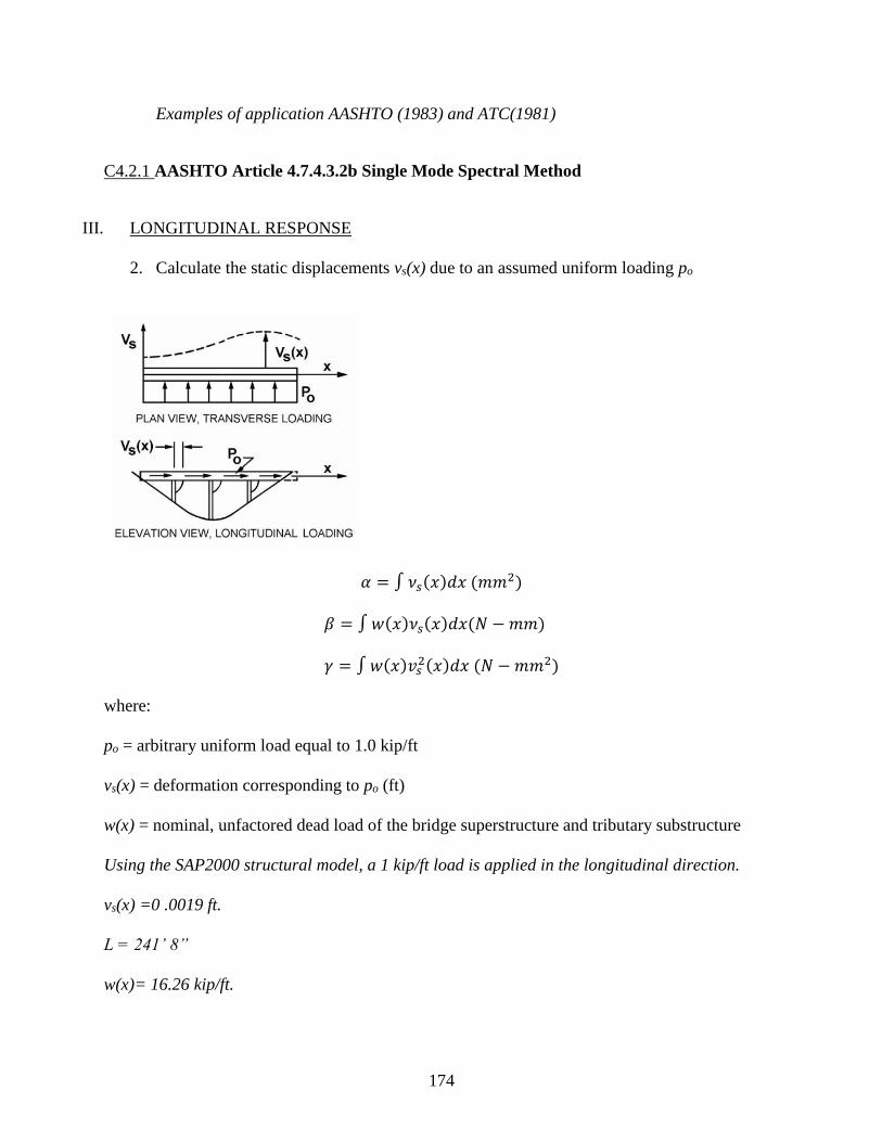
174

Examples of application AASHTO (1983) and ATC(1981)

C4.2.1 AASHTO Article 4.7.4.3.2b Single Mode Spectral Method

III. LONGITUDINAL RESPONSE

2. Calculate the static displacements vs(x) due to an assumed uniform loading po

𝛼 = ∫ 𝜈𝑠(𝑥)𝑑𝑥 (𝑚𝑚2)

𝛽 = ∫ 𝑤(𝑥)𝜈𝑠(𝑥)𝑑𝑥(𝑁 − 𝑚𝑚)

𝛾 = ∫ 𝑤(𝑥)𝑣𝑠2(𝑥)𝑑𝑥 (𝑁 − 𝑚𝑚2)

where:

po = arbitrary uniform load equal to 1.0 kip/ft

vs(x) = deformation corresponding to po (ft)

w(x) = nominal, unfactored dead load of the bridge superstructure and tributary substructure

Using the SAP2000 structural model, a 1 kip/ft load is applied in the longitudinal direction.

vs(x) =0 .0019 ft.

L = 241’ 8”

w(x)= 16.26 kip/ft.

175

𝛼 = ∫ 0.0019241.667 𝑓𝑡

0

(𝑓𝑡) 𝑑𝑥

𝛼 = 0.45917 𝑓𝑡2

𝛽 = ∫ 𝑤(𝑥)𝜈𝑠(𝑥)𝑑𝑥

𝛽 = ∫ 16.256 𝑘𝑖𝑝/𝑓𝑡 ∗ 0.0019 (𝑓𝑡)𝑑𝑥241.667 𝑓𝑡

0

𝛽 = 7.464 (𝑘𝑖𝑝 − 𝑓𝑡)

𝛾 = ∫ 𝑤(𝑥)𝑣𝑠2(𝑥)𝑑𝑥

𝛾 = ∫ 16.256 𝑘𝑖𝑝/𝑓𝑡 ∗ (0.0019)2241.667 𝑓𝑡

0

𝑑𝑥

𝛾 = 0.01418(𝑘𝑖𝑝 − 𝑓𝑡2)

𝑇𝑚 = 2𝜋√𝛾

𝑃𝑜𝑔𝛼

𝑇𝑚 = 2𝜋√0.01418

1 ∗ 32.17 ∗ 0.45917

𝑇𝑚 = 0.195 𝑠𝑒𝑐𝑜𝑛𝑑𝑠

This period matches the estimated period generated in SAP2000.

Tm = period of vibration of the mth mode (sec.)

Calculate Csm using AASHTO equation 3.10.4.2-4 since

0 = 0.070 sec. and 0.352 sec.m m ST T T T (on linear portion of spectrum)

0.443sm DSC S

Csm = dimensionless elastic seismic resonance coefficient

176

Tm= period of vibration of mth modes (s) = 0.195 sec

T0 = reference period used to defined spectral shape

T0 = 0.2 Ts (s) = 0.070

Ts = corner period at which spectrum changes from being independent of period to being

inversely proportional to period

Ts = SD1/SDS (s) = 0.156/0.443 = 0.352

𝐶𝑠𝑚 = 0.30

𝑝𝑒(𝑥) =𝛽𝐶𝑠𝑚

𝛾𝑤(𝑥)𝑣𝑠(𝑥)

𝑝𝑒(𝑥) =7.464 ∗ 0.443

0.01418∗ 16.256 ∗ 0.0019

𝒑𝒆(𝒙) = 𝟕. 𝟐𝟎 (𝒌𝒊𝒑𝒔/𝒇𝒕)

The resultant loading can be applied to the structural model and yield the seismic response.

IV. TRANSVERSE RESPONSE

Calculate the static displacements vs(x) due to an assumed uniform loading po

𝛼 = ∫ 𝜈𝑠(𝑥)𝑑𝑥 (𝑚𝑚2)

𝛽 = ∫ 𝑤(𝑥)𝜈𝑠(𝑥)𝑑𝑥(𝑁 − 𝑚𝑚)

𝛾 = ∫ 𝑤(𝑥)𝑣𝑠2(𝑥)𝑑𝑥 (𝑁 − 𝑚𝑚2)

vs(x) =0 .0015 ft

L = 241.667 ft

177

w(x)= 16.256 kip/ft

𝛼 = ∫ 0.0015241.667 𝑓𝑡

0

(𝑓𝑡) 𝑑𝑥

𝛼 = 0.363 𝑓𝑡2

𝛽 = ∫ 𝑤(𝑥)𝜈𝑠(𝑥)𝑑𝑥

𝛽 = ∫ 16.256 𝑘𝑖𝑝/𝑓𝑡 ∗ 0.0015 (𝑓𝑡)𝑑𝑥241.667 𝑓𝑡

0

𝛽 = 5.893 (𝑘𝑖𝑝 − 𝑓𝑡)

𝛾 = ∫ 𝑤(𝑥)𝑣𝑠2(𝑥)𝑑𝑥

𝛾 = ∫ 16.256 𝑘𝑖𝑝/𝑓𝑡 ∗ (0.015)2241.667 𝑓𝑡

0

𝑑𝑥

𝛾 = 0.00884(𝑘𝑖𝑝 − 𝑓𝑡2)

𝑇𝑚 = 2𝜋√𝛾

𝑃𝑜𝑔𝛼

𝑇𝑚 = 2𝜋√0.00884

1 ∗ 32.17 ∗ 0.363

𝑇𝑚 = 0.173 𝑠𝑒𝑐𝑜𝑛𝑑𝑠

Actual modal period accounting for 60% transverse participation is 0.128 sec from SAP2000.

Calculate Csm using the 3.10.4.2-4 since 0 = 0.070 sec. and 0.352 sec.m m ST T T T (on linear

portion of spectrum)

0.443sm DSC S

178

𝑝𝑒(𝑥) =𝛽𝐶𝑠𝑚

𝛾𝑤(𝑥)𝑣𝑠(𝑥)

𝑝𝑒(𝑥) =5.893 ∗ 0.443

0.00884∗ 16.256 ∗ 0.0015

𝒑𝒆(𝒙) = 𝟕. 𝟐𝟎(𝒌𝒊𝒑𝒔/𝒇𝒕)

The resultant loading can be applied to the structural model and yield the structural response.

AASHTO Figure C4.7.4.3.2b-1 Bridge Deck Subjected to Assumed Transverse and Longitudinal

Loading

C4.2.2 Multimode Dynamic Analysis (Recommended for large skew angles and high

curvatures)

This method can be used to estimate displacement demands where ESA is considered

inadequate. A multi modal spectral analysis can be performed on a numerical (FE) model using

the demand obtained from an appropriate response spectrum (5 percent damping should be used).

Further details on the procedure can be obtained in section 5.4.3 and the Commentary included.

For development of the numerical model, specifications are provided in “5.5 - Mathematical

Modeling Using EDA (Procedure 2)” and “5.6-Effective Section Properties”. These guidelines

include improvements to the structural model, as to assimilate a near as possible representation

of the bridge response using a linear elastic analysis.

For development of a mathematical model: effective section properties can be found in Article

5.6, modeling provisions can be found on abutments in Articles 5.3 and foundations 6.8 (if

liquefaction is present) and guidelines for the global model can be found in article 5.1.2.

179

C4.2.3 AASHTO GS Article 4.4 - Combination of Orthogonal Seismic Displacement

Demands

Per the specifications two load cases are formulated including:

Load Case 1: 100 (%) of the absolute value of the seismic displacements resulting from the

analysis of the longitudinal direction plus 30 (%) of the absolute value of the seismic

displacements corresponding to analysis of the transverse direction

Load Case 2: 100 (%) of the absolute value of the seismic displacements resulting from the

analysis of the transverse direction plus 30 (%) of the absolute value of the seismic

displacements corresponding to analysis of the longitudinal direction

C.4.3 Displacement demand/capacity ratio and connection design

C.4.3.1 AASHTO GS Article 4.8 - Structure Displacement Demand/Capacity for SDCS B,

C, and D

∆𝐷𝐿 ≤ ∆𝐶

𝐿

∆𝐷𝐿 = displacement demand taken along the local principal axis of the ductile member. The

displacement demand may be conservatively taken as the bent displacement inclusive of

flexibility contribution from the foundations, superstructure or both.

The displacement demand is obtained by imposing the demand from then ESA Single mode

spectral method on the structural model. This estimate does not include any flex from the

foundation.

Longitudinal Load: ∆LDL = 0.1068 in, ∆T

DL = 0.037 in

180

Transverse Load: ∆LDT = 0.03 in, ∆T

DT = 0.116 in

Combining load cases and using RD = 1.6 for the longitudinal direction and RD = 1.77 for the

transverse direction.

Load Case 1: ∆LD1 = 0. 185 in, ∆T

D1 = 0. 1152

Load Case 2: ∆LD2 = 0.10 in, ∆T

D2= 0. 203

∆LC = displacement capacity taken along the local principal axis corresponding to ∆L

D of the

ductile member as determined in accordance with Article 4.8.1 for SDC’s B and C.”

AASHTO GS Article 4.8.1 – Local Displacement Capacity for SDCs B

For SDC B:

Δ𝐶𝐿 = 0.12𝐻0(−1.27 ln(𝑥) − 0.32) ≥ 0.12𝐻0

𝑥 =Λ𝐵0

𝐻0

where:

H0 = clear height of the column (ft)

B0 = column diameter or width measured parallel to the direction of displacement under

consideration (ft)

Λ = factor for column end restraint condition

= 1 for fixed-free (pinned on one end)

= 2 for fixed top and bottom

LONGITUDINAL

𝑥 =1 ∗ 2

20.94= 0.096

Δ𝐶𝐿 = 0.12 ∗ 20.94(−1.27 ln(0.096) − 0.32) ≥ 0.12 ∗ 20.94

181

Δ𝐶𝐿 = 6.67 ≥ 2.513(𝑖𝑛. )

∆𝐷𝐿 ≤ ∆𝐶

𝐿

0.185 𝑖𝑛. ≤ 6.67 𝑖𝑛.

TRANSVERSE

𝑥 =1 ∗ 12

20.94= 0.573

Δ𝐶𝐿 = 0.12 ∗ 20.94(−1.27 ln(0.573) − 0.32) ≥ 0.12 ∗ 20.94

0.973 2.5127 2.5127L L

C C

∆𝐷𝐿 ≤ ∆𝐶

𝐿

0.203 𝑖𝑛. ≤ 2.513 𝑖𝑛.

C.4.3.2 AASHTO GS Article 4.12 - Minimum Support Length Requirements

Since integral sub-to-superstructure connections and integral abutments are used, there are no

applicable support length requirements to meet.

C.4.3.3 AASHTO GS Article 4.14 – Superstructure Shear Keys

This bridge does employ shear keys in the longitudinal direction however, dowels are present

between the pier cap concrete and the pier and between the pier and the pile cap, which will also

act as shear keys, thus the requirements of this section apply. The overstrength shear capacity

shall be taken as 1.5ok nV V , where:

overstrength shear key capacity

nominal interface shear capacity of shear key (AASHTO Spec. 5.8.4)

ok

n

V

V

C.4.3.4AASHTO GS Article 4.10 - Column Shear Requirements for SDCs B, C, and D

182

For SDCs B, C, or D, shear demand requirements for reinforced concretes columns (Vu) shall

satisfied to the requirements of AASHTO GS Article 8.6. For columns in SDC B, the force

shall be determined on the basis of the lesser of:

- “The force obtained from a linear elastic seismic analysis, or

- The force Vpo corresponding to plastic hinging of the column including an

overstrength factor” (recommended whenever practical)

The maximum forces obtained from elastic analysis are shown in Figure C.7 - Resultant Factored

Column Forces; these forces will be used for verification of the capacity of the dowels to

adequately transfer the shear loads. The longitudinal shear load is 276 kips and the transverse

shear load is 843 kips. Since the same dowels will be required to resist either the load at a time,

the controlling (maximum) load of 843 kips should be used for verification.

C.4.4 Design Requirements

AASHTO GS Article 4.7 – Design Requirements for Seismic Design Categories B, C, and D

C.4.4.1 AASHTO GS Article 4.7-1 Design methods for Lateral Seismic Displacement

Demands

“Dictates which displacement resisting system can be used. The most applicable is Limited-

Ductility Response in which a plastic mechanism is activated in the pier-columns but the

ductility demands are reduced (µD ≤ 4.0). Intended yielding should be restricted to locations that

can be readily accessed for damage inspection following a design earthquake.”

183

AASHTO GS Commentary 4.7.1

“A key element in the design procedure is the flexural capacity of the columns. Philosophically,

the lower the flexural capacity of the column, the more economical will be the seismic design

because the overstrength flexural capacity of a column drives the cost and capacity of both the

foundations and connections to the superstructure. For SDC B, the capacity of the column design

for non seismic loads is considered to be acceptable for this lower seismic hazard level.”

C.4.4.2 AASHTO GS Article 4.11 Capacity Design Requirement for SDCs B, C, and D

“Capacity design principles require that those components not participating as part of the

primary energy dissipating system, typically flexural hinging in columns above ground or in

some cases flexural hinging of drilled shafts, solid wall encased pile bents, etc., below ground,

shall be capacity protected. The components include the superstructure, joints and cap beams,

spread footings, pile caps, and foundations. This is achieved by ensuring the maximum moment

and shear from plastic hinges in the column, considering overstrength can be resisted elastically

by adjoining elements.”

“For SDC B, forces obtained from capacity design principles should be used when the plastic

hinging forces are less than the forces obtained from an elastic analysis. In lieu of full capacity

design using overstrength forces, capacity checks should be made to ensure that no weak links

exist in the ERS. Joint shear checks are required.”

AASHTO GS Commentary 4.11

“For SDC B, full capacity design is not required. However, it is good practice to ensure that no

portions of load path are weaker than the elements that establish the plastic capacity of the

184

substructure (e.g., plastic hinging in the columns). Therefore checks of the load path are

suggested, but full capacity design using plastic overstrength forces is not required. “

“The design of substructures using the elastic forces associated with the design ground motion is

permitted in SDC B, although not encouraged, because potentially larger ground motions could

produce undesirable performance, including collapse or partial collapse of the bridge.”

C.4.4.3 AASHTO GS Article 6.2 - Foundation Investigation

AASHTO GS Article 6.2.4 – “In addition to the normal site investigation, potential hazards and

seismic design requirements related to (1) liquefaction potential, (2) seismic –induced settlement,

(3) lateral spreading, (4) slope instability, and (5) increases in lateral earth pressure, all as a result

of earthquake motions, should be evaluated. The seismic hazards evaluation shall also consider

the potential for and influence of:

Surface rupture due to faulting if an active fault has been identified within 1 mi of the bridge

site (see Article 3.4 for the definition of an active fault),

Differential ground displacement (lurching), and

Cyclic loading on the deformation and strength characteristics of foundation soils.”

C.4.4.4 AASHTO GS Article 6.8 - Liquefaction Assessment

Given the local seismic hazard, site location and soil condition liquefaction was not considered

in this study. Some basic information about liquefaction which applies to SDC B is cited below.

“Where loose to very saturated sands are within the subsurface profile such that liquefaction of

these soils could impact the stability of the structure, the potential for liquefaction in SDC B

should also be considered as discussed in the commentary.”