Corrosion protection of carbon steel by an epoxy resin containing organically modified clay
Upload
khangminh22Category
view
1download
0
Investigation of resin and steelreinforced resin behaviour un-der quasi-static and cyclic load-ing in oversized IBCs
Aravind Ramkumar
Chair of thesis committee- Prof. Dr. M. Veljkovic, TU DelftThesis Supervisors- Dr. F. Kavoura, TU DelftDaily Supervisor - Ir. B. Pedrosa, University of Coimbra

Investigation of resin and steel reinforcedresin behaviour under quasi-static and
cyclic loading in oversized IBCsby
Aravind Ramkumarto obtain the degree of Master of Science
at the Delft University of Technology,to be defended publicly on Thursday August 24, 2021 at 10:00 AM.
Student number: 4744713Project duration: September 1, 2019 – August 24, 2021Thesis committee: Prof. dr. ir. M. Veljkovic, TU Delft, Chair of thesis committee
Dr. F. Kavoura, TU DelftAssistant Prof. dr. B. Savija, TU DelftIr. B. Pedrosa, University of Coimbra
An electronic version of this thesis is available at http://repository.tudelft.nl/.

Abstract
With the world moving towards a sustainable economy, it becomes important for the construction industryto shift from a linear to a circular economy. This has given rise to various topics of interest, one being the useof bolted shear connectors in the form of oversized injection bolted connections which replaces the weldedstuds in the composite structures.
Injection Bolted Connections (IBC) are connections in which the cavity between the bolts and the plates(hole clearance) is filled with two-component epoxy resin. These connections must be slip-resistant for theseconnections to be used in bridges and storm barriers. Due to a larger hole clearance, the stiffness of the con-nection is compromised. To avoid this, a new material called Steel Reinforced Resin (SRR) was developed atTU Delft. Steel shots are injected into the resin not only to improve their stiffness but also to decrease the slipof the connection.
This study aims to analyse the behaviour of the resin and SRR subjected to compression-compressioncyclic loading conditions. A custom made setup that replicates the nominal bearing stress experienced bythe resin in a double lap shear joint is used to study the behaviour of the resin under cyclic loading. Twodifferent test specimens which corresponded to 3 mm and 6 mm hole clearance were used for the tests. Thetests are conducted at three different nominal bearing stress ranges with a constant test ratio. The test con-sists of two stages, initially, the test specimens were tested under quasi-static loading for 20 cycles at 0.05 Hzto determine the initial stiffness and the second stage is cyclic loading stages where the specimens are testedtill 400,000 cycles at 2.5 Hz to determine the slip. The slip obtained from cyclic loading is extrapolated for 5million cycles to check if maximum slip exceeds failure criterion of 0.3 mm and slip range exceeds the failurecriterion of 0.1 mm over 5 million cycles.
Numerical modelling was done using the material model obtained by Nijgh et al. [36] and Xin et al. [25]to determine if the stresses experienced by the resin in the current test setup is similar to the stresses expe-rienced by the resin of under double lap shear joint. Numerical modelling was also done to see if the results(initial stiffness) obtained from the experiments can be replicated by the material models for static and onecycle loading with the help of a reasonable friction coefficient between the steel and resin surfaces.
The results obtained from the experiments showed that the initial stiffness increased about 51.5% for 3mm hole clearance and 92.1% increase for 6 mm hole clearance when SRR were used over conventional resin.A common trend of increase in stiffness from the first cycle to 400,000 cycles was observed due to densifica-tion of the material under loading and thus a common trend of decrease in slip range over number of cyclesfor all the tested specimens was observed. Ratcheting behaviour where progressive accumulation of defor-mation of the resin with an increase in the number of cycles was observed and this behaviour was about 3times higher for resin specimens over SRR specimens. On extrapolating to 5 million cycles, resin specimenswith 3 mm hole clearance failed at a stress range of 200 MPa and resin specimens with 6 mm hole clearancefailed at stress range of 150 MPa. SRR specimens with 6 mm hole clearance failed at a stress range of 200 MPa.
From the numerical model, it was seen that the bearing stresses acting on the resin in the current testsetup was similar to the bearing stresses acting on the resin in a double lap shear joint. The friction coeffi-cient for the resin to steel interaction was found to be 0.05 and for SRR to steel interaction, it was found to be0.1. A good correlation was found between the force vs displacement curve obtained from the experiments tothe curve obtained from the numerical model. The material model with the modulus of elasticity for a resin-hardener mixture of RenGel© SW 404 + HY 5159 was found to be more closer to the results obtained from theexperiments with a reasonable friction coefficient rather than the material model with the modulus of elas-ticity for a resin-hardener mixture of RenGel© SW 404 + HY 2404. Hence, it was concluded that the modulusof elasticity is different when these two different hardeners are used which is contrary to the properties givenby the manufacturer.
iii


Preface
This thesis has been submitted at Delft University of Technology as a partial requirement to obtain Master ofScience in Structural Engineering (Civil Engineering). It was been an incredible yet tough journey with reallygood highs and horrible lows. I would like to express my gratitude for the people who have been me in thesetesting times.
I would like to thank my master thesis supervisor Prof. Milan Veljkovic for guiding me with my thesisand understanding my eye condition during my surgeries. I would like to thank my daily supervisor BurnoPedrosa who guided me throughout the numerical modelling and my report with meetings every week forabout three months. I would like to thank Dr. Florentia Kavoura for being a part of my thesis committeeand providing valuable comments in my report. I would like to thank Dr. Martin Nijgh for his guidance andassisting me in the experiments and analysis of results. I would like to thank Kevin Mouthaan for helping mewith the conduction of experiments.My academic counsellor Karel Karsen has been a huge pillar of supportduring my tough times where he would give appointments two days a week just to take care of my mentalhealth.
Firstly, I would like to thank my parents and my sister for their constant support throughout the course ofmy study and for understanding my situation and for patiently being a part of this unexpectedly long journeyat TU Delft. Finally, I would like to thank my friends who are like a family away from home. I would like tothank Manojna Vedula for always being there for me especially during my most difficult times where I hadself-doubt. I believe that without her this journey would have been next to impossible to complete. I alsothank her for helping me to understand and work with Latex document. I would like to thank Riya Maanand Manoj Subramanian Sankari for their continuous support throughout my study. I would like to thankthe above mentioned three people who are my support system for taking care of me during my eye surgerywhere I needed help even to walk from my house to the hospital. I would like to extend my sincerer thanksto Raghavendran Raman for his constant support and valuable insights during my thesis and also for givingfeedback on my numerical model. I would like to thank Arvind Vijayakumar for his support and the banterswhich we had while playing cricket or football which helped me get out of few bad days along the way. Iwould like to thank Karishma Kumar for her words of encouragement time and again that I needed. I wouldlike to thank Aishwarya Shastry and Sharadhi Soorambail for their support. Last but certainly not the least, Iwould like to thank all my friends back home for their prayers and well wishes with special mention to TejasSomashekhar and Lalith Badigar who have remained my pillar of support.
Aravind RamkumarDelft, August 2021
v

Contents
Abstract iii
List of Figures ix
List of Tables xiii
1 Introduction 11.1 Motivation and problem statement . . . . . . . . . . . . . . . . . . . . . . . . . . . . . . . . 1
1.2 Main objective . . . . . . . . . . . . . . . . . . . . . . . . . . . . . . . . . . . . . . . . . . 2
1.3 Research question . . . . . . . . . . . . . . . . . . . . . . . . . . . . . . . . . . . . . . . . 2
1.4 Outline of the report . . . . . . . . . . . . . . . . . . . . . . . . . . . . . . . . . . . . . . . 3
2 State of the art 52.1 Injection bolted connection. . . . . . . . . . . . . . . . . . . . . . . . . . . . . . . . . . . . 5
2.2 Application of injection bolted connection . . . . . . . . . . . . . . . . . . . . . . . . . . . . 6
2.3 Behaviour of injection bolted connection under static loading . . . . . . . . . . . . . . . . . . 7
2.4 Behaviour of injection bolted connection under fatigue loading . . . . . . . . . . . . . . . . . 8
2.5 Bolted shear connectors with standard and oversized holes in composite structures . . . . . . . 11
2.6 Types of epoxy resins and hardeners . . . . . . . . . . . . . . . . . . . . . . . . . . . . . . . 13
2.7 Static behaviour of epoxy resin and steel reinforced resin . . . . . . . . . . . . . . . . . . . . . 14
2.8 Fatigue testing parameters . . . . . . . . . . . . . . . . . . . . . . . . . . . . . . . . . . . . 17
2.8.1 Basic terminologies of fatigue loading . . . . . . . . . . . . . . . . . . . . . . . . . . . 17
2.8.2 Hysteresis loop and frequency of fatigue loading. . . . . . . . . . . . . . . . . . . . . . 17
2.9 Fatigue behaviour of epoxy resins . . . . . . . . . . . . . . . . . . . . . . . . . . . . . . . . . 18
2.9.1 Ratcheting behaviour of resin . . . . . . . . . . . . . . . . . . . . . . . . . . . . . . . 21
3 Experimental setup and procedure 233.1 Geometry of test setup . . . . . . . . . . . . . . . . . . . . . . . . . . . . . . . . . . . . . . 23
3.1.1 Top plate . . . . . . . . . . . . . . . . . . . . . . . . . . . . . . . . . . . . . . . . . . 24
3.1.2 Bottom plate . . . . . . . . . . . . . . . . . . . . . . . . . . . . . . . . . . . . . . . . 25
3.1.3 Side/Cover plates and Hex bolts . . . . . . . . . . . . . . . . . . . . . . . . . . . . . . 25
3.2 Materials . . . . . . . . . . . . . . . . . . . . . . . . . . . . . . . . . . . . . . . . . . . . . 26
3.2.1 Epoxy resin. . . . . . . . . . . . . . . . . . . . . . . . . . . . . . . . . . . . . . . . . 26
3.2.2 Steel Reinforced Resin . . . . . . . . . . . . . . . . . . . . . . . . . . . . . . . . . . . 27
3.2.3 Steel . . . . . . . . . . . . . . . . . . . . . . . . . . . . . . . . . . . . . . . . . . . . 28
3.2.4 Release agent . . . . . . . . . . . . . . . . . . . . . . . . . . . . . . . . . . . . . . . 28
3.3 Preparation of test specimen . . . . . . . . . . . . . . . . . . . . . . . . . . . . . . . . . . . 29
3.3.1 Assembly of test specimens . . . . . . . . . . . . . . . . . . . . . . . . . . . . . . . . 29
3.3.2 Geometrical imperfections. . . . . . . . . . . . . . . . . . . . . . . . . . . . . . . . . 30
3.3.3 Injection of resin . . . . . . . . . . . . . . . . . . . . . . . . . . . . . . . . . . . . . . 32
3.3.4 Correction and finalization of specimen . . . . . . . . . . . . . . . . . . . . . . . . . . 33
3.4 Testing of specimens . . . . . . . . . . . . . . . . . . . . . . . . . . . . . . . . . . . . . . . 33
3.4.1 Loading method and control. . . . . . . . . . . . . . . . . . . . . . . . . . . . . . . . 34
3.4.2 Stress range . . . . . . . . . . . . . . . . . . . . . . . . . . . . . . . . . . . . . . . . 35
3.4.3 Naming of specimens and number of tests. . . . . . . . . . . . . . . . . . . . . . . . . 35
3.4.4 Quasi-static and cyclic loading. . . . . . . . . . . . . . . . . . . . . . . . . . . . . . . 36
vii
viii Contents
4 Experimental results 374.1 Calculation of initial stiffness from quasi-static loading. . . . . . . . . . . . . . . . . . . . . . 374.2 Results and interpretation of initial stiffness and final stiffness . . . . . . . . . . . . . . . . . . 374.3 Failure criterion for cyclic loading. . . . . . . . . . . . . . . . . . . . . . . . . . . . . . . . . 414.4 Results of cyclic loading. . . . . . . . . . . . . . . . . . . . . . . . . . . . . . . . . . . . . . 424.5 Failure of specimen . . . . . . . . . . . . . . . . . . . . . . . . . . . . . . . . . . . . . . . . 474.6 Defects in specimen . . . . . . . . . . . . . . . . . . . . . . . . . . . . . . . . . . . . . . . 514.7 Summary of experimental results . . . . . . . . . . . . . . . . . . . . . . . . . . . . . . . . . 52
5 Numerical modelling 535.1 Modelling of test setup . . . . . . . . . . . . . . . . . . . . . . . . . . . . . . . . . . . . . . 535.2 Static loading and calibration of friction coefficient . . . . . . . . . . . . . . . . . . . . . . . . 54
5.2.1 Verification of test setup with double lap shear joint . . . . . . . . . . . . . . . . . . . . 585.3 Loading and unloading of the test setup . . . . . . . . . . . . . . . . . . . . . . . . . . . . . 605.4 Summary of numerical modelling. . . . . . . . . . . . . . . . . . . . . . . . . . . . . . . . . 61
6 Discussion 63
7 Conclusions and future recommendation 657.1 Conclusions. . . . . . . . . . . . . . . . . . . . . . . . . . . . . . . . . . . . . . . . . . . . 65
7.1.1 Conclusion from experiments . . . . . . . . . . . . . . . . . . . . . . . . . . . . . . . 657.1.2 Conclusions from numerical modelling . . . . . . . . . . . . . . . . . . . . . . . . . . 66
7.2 Future recommendations . . . . . . . . . . . . . . . . . . . . . . . . . . . . . . . . . . . . . 677.2.1 Future works on experiments . . . . . . . . . . . . . . . . . . . . . . . . . . . . . . . 677.2.2 Future works on numerical modelling . . . . . . . . . . . . . . . . . . . . . . . . . . . 67
Bibliography 69
A Product description of RenGel© SW 404 / Ren© HY 2404 or HY 5159 73
B Input parameters for ABAQUS model 77
C Graphs obtained from quasi-static loading phase of the experiments 79
D Values of maximum slip obtained for quasi-static and cyclic loading 87
E Comparison of associative flow model and non-dilatant flow model 91
List of Figures
1.1 Injection bolted connection [23] . . . . . . . . . . . . . . . . . . . . . . . . . . . . . . . . . . . . . 11.2 Reader’s guide for this thesis . . . . . . . . . . . . . . . . . . . . . . . . . . . . . . . . . . . . . . . 3
2.1 Injection of resin into the bolt head [21] . . . . . . . . . . . . . . . . . . . . . . . . . . . . . . . . . 52.2 Installation of injection bolts in progress and view of web reinforced with injection bolts [3] 62.3 Storm surge barrier when closed and injection preloaded bolts used in the connection [44] 62.4 Stress distribution he resin when length of the bolt is three times larger than its diameter[17] 82.5 Comparison of S-N fatigue data from the single shear connections made of the material
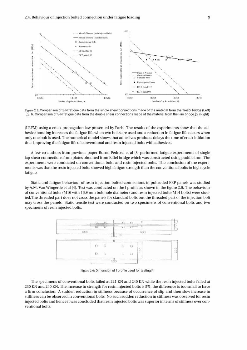
from the Trezói bridge (Left) [5]. b. Comparison of S-N fatigue data from the double shearconnections made of the material from the Fão bridge.[5] (Right) . . . . . . . . . . . . . . . . 9
2.6 Dimension of I profile used for testing[4] . . . . . . . . . . . . . . . . . . . . . . . . . . . . . . . . 92.7 RIBJ test configurations: (a) Type 1; (b) Type 2.[6] . . . . . . . . . . . . . . . . . . . . . . . . . . 102.8 Load-slip curves for: (Left) M16 18HL (Joint 1); (Right) M16 16HL (Joint 1).[6] . . . . . . . . . 112.9 Demountable shear connector with resin in its oversized hole clearance [39](left); Embed-
ded bolts with embedded coupler [58] (right) . . . . . . . . . . . . . . . . . . . . . . . . . . . . . 122.10 Novel bolted shear connector proposed by Fei Yang et. al. [60] . . . . . . . . . . . . . . . . . 132.11 Different geometry details for the top washer under the bolt head of IBC [47] . . . . . . . . . 142.12 Geometry of the confined compression configuration by K.Ravi-Chandar [49] . . . . . . . . . 152.13 Stress-strain relationship of Sikadur 30 under uniaxial tension and compression [16][10][44] 152.14 Stress-strain relationship of unconfined resin specimens[25] (left). Stress-strain relation-
ship of unconfined steel reinforced resin specimens [25] (right) . . . . . . . . . . . . . . . . . 162.15 Stress-strain relationship of confined resin specimens[25] (left). Stress-strain relationship
of confined steel reinforced resin specimens [25] (right) . . . . . . . . . . . . . . . . . . . . . . 162.16 Basic terminologies of fatigue loading [51] . . . . . . . . . . . . . . . . . . . . . . . . . . . . . . 172.17 Energy dissipation under hysteresis curve [61] [9] . . . . . . . . . . . . . . . . . . . . . . . . . . 172.18 Geometry of a cylindrical specimen used in fatigue test (right)[54]. Photo of the specimen
(left)[57] . . . . . . . . . . . . . . . . . . . . . . . . . . . . . . . . . . . . . . . . . . . . . . . . . . . . 192.19 Evolution ofmodulus during the fatigue life period. The lines with fluctuations are from ex-
periments and the smoothed lines are simulations[57] (Left) (b) Evolution of stress rangesduring the entire fatigue life period under the same strain amplitude butwith differentmeanstrain ratios [57] (Right) . . . . . . . . . . . . . . . . . . . . . . . . . . . . . . . . . . . . . . . . . . 20
2.20 Ratcheting strain vs number of cycles at different loading rates (left)[11]; Ratcheting strainvs number of cycles at the same stress amplitude and different mean stresses (right)[11] . 21
2.21 (a) Stress-strain relationship of epoxy resin under tensile loading [13];(b) Progression ofthe isotropic hardening variable vs accumulation of plastic strain [13]; (c) Progression ofkinematic hardening variable vs accumulation of plastic strain [13] . . . . . . . . . . . . . . . 22
3.1 Test specimen . . . . . . . . . . . . . . . . . . . . . . . . . . . . . . . . . . . . . . . . . . . . . . . . 233.2 Test specimen used in the experimental setup . . . . . . . . . . . . . . . . . . . . . . . . . . . . 243.3 Top/male plate . . . . . . . . . . . . . . . . . . . . . . . . . . . . . . . . . . . . . . . . . . . . . . . . 243.4 Bottom/Female plate . . . . . . . . . . . . . . . . . . . . . . . . . . . . . . . . . . . . . . . . . . . . 253.5 Side Plates . . . . . . . . . . . . . . . . . . . . . . . . . . . . . . . . . . . . . . . . . . . . . . . . . . 253.6 Epoxy resin Araldite/RenGel SW 404 . . . . . . . . . . . . . . . . . . . . . . . . . . . . . . . . . . 263.7 Spherical steel shots (S330) with diameter of 0.84 mm . . . . . . . . . . . . . . . . . . . . . . 273.8 Releasing agent ACMOS 82-2405 . . . . . . . . . . . . . . . . . . . . . . . . . . . . . . . . . . . . 283.9 Support structure for preparing the specimen . . . . . . . . . . . . . . . . . . . . . . . . . . . . 293.10 Possible misalignment that could occur when specimen is placed on the ground . . . . . . 303.11 Bolt at the center of hole diameter . . . . . . . . . . . . . . . . . . . . . . . . . . . . . . . . . . . . 303.12 Assembly of specimen before injecting resin . . . . . . . . . . . . . . . . . . . . . . . . . . . . . 31
ix
x List of Figures
3.13 Geometrical imperfections due to manufacturing tolerances . . . . . . . . . . . . . . . . . . . 313.14 Critical dimensions of top plate . . . . . . . . . . . . . . . . . . . . . . . . . . . . . . . . . . . . . 313.15 a.Injection of resin into the hole clearance. b. Indication of completely filled hole clearance 323.16 a. Hole clearance not completely filled by resin b. Further addition of resin into the hole
clearance . . . . . . . . . . . . . . . . . . . . . . . . . . . . . . . . . . . . . . . . . . . . . . . . . . . 333.17 Completed specimen ready to be tested . . . . . . . . . . . . . . . . . . . . . . . . . . . . . . . . 333.18 a. Testing of specimen in Hydraulic Wedge Grip Machine. b. Schematic representation of
Hydraulic Wedge Grip Machine [51] . . . . . . . . . . . . . . . . . . . . . . . . . . . . . . . . . . . 343.19 Stress distribution on resin in double lap shear joint in IBCs . . . . . . . . . . . . . . . . . . . . 343.20 Graphical representation of loading cycles . . . . . . . . . . . . . . . . . . . . . . . . . . . . . . 36
4.1 Force vs displacement curve obtained after Quasi static loading of resin specimen . . . . . 374.2 Initial stiffness vs stress range for resin specimens (Left). Initial stiffness vs stress range
for SRR specimens (Right). . . . . . . . . . . . . . . . . . . . . . . . . . . . . . . . . . . . . . . . . 384.3 Variation of initial stiffness vs diameter of the specimen . . . . . . . . . . . . . . . . . . . . . 384.4 Difference in stiffness of first and last cycle of quasi-static loading in resin (Left). Differ-
ence in initial stiffness of quasi-static loading and final stiffness of cyclic loading in resin(Right) . . . . . . . . . . . . . . . . . . . . . . . . . . . . . . . . . . . . . . . . . . . . . . . . . . . . . 39
4.5 Difference in stiffness of first and last cycle of quasi-static loading in SRR (Left). Differencein initial quasi-static stiffness of quasi-static loading and final stiffness of cyclic loadingin SRR (Right) . . . . . . . . . . . . . . . . . . . . . . . . . . . . . . . . . . . . . . . . . . . . . . . . . 40
4.6 Initial stiffness fromquasi-static loading and progression of stiffness during cyclic loadingfor SRR_D26_100_1 specimen . . . . . . . . . . . . . . . . . . . . . . . . . . . . . . . . . . . . . . . 40
4.7 Initial stiffness fromquasi-static loading and progression of stiffness during cyclic loadingfor (i)R_D32_200_1 (left) and (ii)SRR_D32_200_1 (right) specimen . . . . . . . . . . . . . . . . 40
4.8 (a) Failure criterion for creep loading according to EN 1090-2 [21]. (b) Fatigue strengthcurve for direct stress range according to EN 1993-1-9 [20] . . . . . . . . . . . . . . . . . . . . 41
4.9 (a) Maximum slip vs number of cycles for R_D26_100 and SRR_D26_100; (b) Slip range vsnumber of cycles for R_D26_100 and SRR_D26_100; (c) Slip remaining after unloading atspecific cycles for SRR specimens (Right) . . . . . . . . . . . . . . . . . . . . . . . . . . . . . . . 42
4.10 (a) Maximum slip vs number of cycles for R_D32_100 and SRR_D32_100; (b) Slip range vsnumber of cycles for R_D32_100 and SRR_D32_100; (c) Slip remaining after unloading atspecific cycles for SRR specimens) . . . . . . . . . . . . . . . . . . . . . . . . . . . . . . . . . . . 43
4.11 (a) Maximum slip vs number of cycles for R_D26_150 and SRR_D26_150; (b) Slip range vsnumber of cycles for R_D26_150 and SRR_D26_150; (c) Slip remaining after unloading atspecific cycles for resin and SRR specimens . . . . . . . . . . . . . . . . . . . . . . . . . . . . . 44
4.12 (a) Maximum slip vs number of cycles for R_D32_150 and SRR_D32_150; (b) Slip range vsnumber of cycles for R_D32_150 and SRR_D32_150; (c) Slip remaining after unloading atspecific cycles for resin and SRR specimens . . . . . . . . . . . . . . . . . . . . . . . . . . . . . 45
4.13 (a) Maximum slip vs number of cycles for R_D26_200 and SRR_D26_200; (b) Slip range vsnumber of cycles for R_D26_200 and SRR_D26_200; (c) Slip remaining after unloading atspecific cycles for resin and SRR specimens . . . . . . . . . . . . . . . . . . . . . . . . . . . . . 45
4.14 (a) Maximum slip vs number of cycles for R_D32_200 and SRR_D32_200; (b) Slip range vsnumber of cycles for R_D32_200 and SRR_D32_200; (c) Slip remaining after unloading atspecific cycles for resin and SRR specimens . . . . . . . . . . . . . . . . . . . . . . . . . . . . . 46
4.15 Extrapolation of slip range of resin specimens to 5 million cycles for failure criterion of 0.3mm . . . . . . . . . . . . . . . . . . . . . . . . . . . . . . . . . . . . . . . . . . . . . . . . . . . . . . . 48
4.16 Extrapolation of slip range of SRR specimens to 5 million cycles for failure criterion of 0.3mm . . . . . . . . . . . . . . . . . . . . . . . . . . . . . . . . . . . . . . . . . . . . . . . . . . . . . . . 48
4.17 Extrapolation of slip range of resin specimens to 5 million cycles for failure criterion of 0.1mm . . . . . . . . . . . . . . . . . . . . . . . . . . . . . . . . . . . . . . . . . . . . . . . . . . . . . . . 49
4.18 Extrapolation of slip range of SRR specimens to 5 million cycles for failure criterion of 0.1mm . . . . . . . . . . . . . . . . . . . . . . . . . . . . . . . . . . . . . . . . . . . . . . . . . . . . . . . 50
4.19 Quasi static loading of defected specimen . . . . . . . . . . . . . . . . . . . . . . . . . . . . . . 514.20 Cyclic loading of defected specimen . . . . . . . . . . . . . . . . . . . . . . . . . . . . . . . . . . 514.21 Voids in resin . . . . . . . . . . . . . . . . . . . . . . . . . . . . . . . . . . . . . . . . . . . . . . . . . 52
List of Figures xi
5.1 (a) Top plate (b) Resin/SRR (c) Side plate (d) M8 Hex bolts (e) Bottom plate (f) Assembledmodel of test setup . . . . . . . . . . . . . . . . . . . . . . . . . . . . . . . . . . . . . . . . . . . . . 54
5.2 Comparison of associative flowand non-dilatant flowmodelswith 0.05 friction co-efficientfor resin specimen models and 0.1 friction co-efficient for SRR specimen models . . . . . . 55
5.3 Comparison of force-displacement curve between experiments and numerical model ofdifferent friction coefficients for R D26 200 (Left); Comparison of stiffness between ex-periments and numerical models for resin specimens with 26 mm diameter (Right) . . . . 56
5.4 Comparison of force-displacement curve between experiments and numerical model ofdifferent friction coefficients for R D32 200 (Left); Comparison of stiffness between ex-periments and numerical models for resin specimens with 32 mm diameter (Right) . . . . 57
5.5 Comparison of force-displacement curve between experiments and numerical model ofdifferent friction coefficients for SRR D26 200 (Left); Comparison of stiffness betweenexperiments and numerical models for SRR specimens with 26 mm diameter (Right) . . . 57
5.6 Comparison of force-displacement curve between experiments and numerical model ofdifferent friction coefficients for SRR D32 200 (Left); Comparison of stiffness betweenexperiments and numerical models for SRR specimens with 32 mm diameter (Right) . . . 57
5.7 Comparison of stiffness between numerical models for hardener HY 2404, HY 5159 andexperiments for resin specimens with 26 mm diameter (Left); resin specimens with 32mm diameter (Right) . . . . . . . . . . . . . . . . . . . . . . . . . . . . . . . . . . . . . . . . . . . . 58
5.8 Comparison of stiffness between numerical models for hardener HY 2404, HY 5159 andexperiments for steel reinforced resin specimens with 26 mm diameter (Left); SRR speci-mens with 32 mm diameter (Right) . . . . . . . . . . . . . . . . . . . . . . . . . . . . . . . . . . . 58
5.9 Double-lap shear test cf. EN 1090-2 Annex G/K [18] [45] (Left); Test setup used in this study(Right) . . . . . . . . . . . . . . . . . . . . . . . . . . . . . . . . . . . . . . . . . . . . . . . . . . . . . 59
5.10 Comparison of longitudinal bearing stresses along the curvature of resin between doublelap shear joint and the test setup used in this study(Left); Counter plot of stress S22 andthe path along the curvature of resin (Right) . . . . . . . . . . . . . . . . . . . . . . . . . . . . . 59
5.11 Comparison of longitudinal bearing stresses along the bolt length of resin between doublelap shear joint and the test setup used in this study(Left); Counter plot of stress S22 andthe path along the bolt length of resin (Right) . . . . . . . . . . . . . . . . . . . . . . . . . . . . 60
5.12 (a) and (b) Comparison of hysteresis loop obtained from 2nd cycle of quasi-static loadingfrom experiments and one loading cycle of associative and non-dilatant flow from numer-ical for R D26 200 and R D32 200 specimens respectively; (c) Comparison of dissipatedenergy from the obtained hysteresis loop . . . . . . . . . . . . . . . . . . . . . . . . . . . . . . . 60
5.13 (a) and (b) Comparison of hysteresis loop obtained from 2nd cycle of quasi-static load-ing from experiments and one loading cycle of associative and non-dilatant flow from nu-merical for SRR D26 200 and SRR D32 200 specimens respectively; (c) Comparison ofdissipated energy from the obtained hysteresis loop . . . . . . . . . . . . . . . . . . . . . . . . 61
6.1 (a) Graphs from experiments on resin under monotonic loading indicating stress plateauand graph obtained from FEM modelling [9]; (b) Graph obtained from quasi static experi-ments from this study . . . . . . . . . . . . . . . . . . . . . . . . . . . . . . . . . . . . . . . . . . . 63
C.1 Graphs from quasi-static loading for R_D26_100 . . . . . . . . . . . . . . . . . . . . . . . . . . . 79C.2 Graphs from quasi-static loading for R_D32_100 . . . . . . . . . . . . . . . . . . . . . . . . . . . 80C.3 Graphs from quasi-static loading for R_D26_150 . . . . . . . . . . . . . . . . . . . . . . . . . . . 80C.4 Graphs from quasi-static loading for R_D32_150 . . . . . . . . . . . . . . . . . . . . . . . . . . . 81C.5 Graphs from quasi-static loading for R_D26_150 . . . . . . . . . . . . . . . . . . . . . . . . . . . 81C.6 Graphs from quasi-static loading for R_D32_200 . . . . . . . . . . . . . . . . . . . . . . . . . . . 82C.7 Graphs from quasi-static loading for SRR_D26_100 . . . . . . . . . . . . . . . . . . . . . . . . . 82C.8 Graphs from quasi-static loading for SRR_D32_100 . . . . . . . . . . . . . . . . . . . . . . . . . 83C.9 Graphs from quasi-static loading for SRR_D26_150 . . . . . . . . . . . . . . . . . . . . . . . . . 83C.10 Graphs from quasi-static loading for SRR_D32_150 . . . . . . . . . . . . . . . . . . . . . . . . . 84C.11 Graphs from quasi-static loading for SRR_D26_200 . . . . . . . . . . . . . . . . . . . . . . . . . 84C.12 Graphs from quasi-static loading for SRR_D32_200 . . . . . . . . . . . . . . . . . . . . . . . . . 85

xii List of Figures
E.1 Comparison of associative flow and non-dilatant flow models for a stress range of 100MPa with 0.05 friction co-efficient for resin specimen models and 0.1 friction co-efficientfor SRR specimen models . . . . . . . . . . . . . . . . . . . . . . . . . . . . . . . . . . . . . . . . . 91
E.2 Comparison of associative flow and non-dilatant flow models for a stress range of 150MPa with 0.05 friction co-efficient for resin specimen models and 0.1 friction co-efficientfor SRR specimen models . . . . . . . . . . . . . . . . . . . . . . . . . . . . . . . . . . . . . . . . . 92
List of Tables
2.1 Values of β and tb , resin as a function of ratio t1/t2 in double lap shear connections[18][51] . . . 72.2 Fatigue detail categories for double lap and single lap connections for preloaded, non-preloaded,
and injected, non-injected according to EN 1993-1-9[20] [51] . . . . . . . . . . . . . . . . . . . . . 8
3.1 Steel grades and quantities of plates used in experiments . . . . . . . . . . . . . . . . . . . . . . . 283.2 Material proprieties of steel . . . . . . . . . . . . . . . . . . . . . . . . . . . . . . . . . . . . . . . . . 283.3 Stress ranges adapted for testing the specimens . . . . . . . . . . . . . . . . . . . . . . . . . . . . . 353.4 Number of specimens tested . . . . . . . . . . . . . . . . . . . . . . . . . . . . . . . . . . . . . . . . 35
4.1 Fatigue life of specimens which exceeds the failure criterion of maximum slip greater than 0.3mm . . . . . . . . . . . . . . . . . . . . . . . . . . . . . . . . . . . . . . . . . . . . . . . . . . . . . . . 47
4.2 Fatigue life of resin specimens which exceeds the failure criterion of slip range greater than 0.1mm . . . . . . . . . . . . . . . . . . . . . . . . . . . . . . . . . . . . . . . . . . . . . . . . . . . . . . . 49
4.3 Fatigue life of SRR specimens which exceeds the failure criterion of slip range greater than 0.1mm . . . . . . . . . . . . . . . . . . . . . . . . . . . . . . . . . . . . . . . . . . . . . . . . . . . . . . . 50
5.1 Comparison of stiffness obtained experiments and from material models of associative andnon-dilatant flow . . . . . . . . . . . . . . . . . . . . . . . . . . . . . . . . . . . . . . . . . . . . . . . 56
B.1 Material properties of the resin, steel-reinforced resin and steel . . . . . . . . . . . . . . . . . . . . 77B.2 Drucker Prager yield criterion for resin and steel-reinforced resin . . . . . . . . . . . . . . . . . . 77B.3 Drucker Prager Hardening for resin and steel-reinforced resin . . . . . . . . . . . . . . . . . . . . 77
D.1 Presentation of slip obtained for D26 specimens before and after each loading stages for resinand SRR at stress range of -25 MPa to -125 MPa . . . . . . . . . . . . . . . . . . . . . . . . . . . . . 87
D.2 Presentation of slip obtained for D32 specimens before and after each loading stages for resinand SRR at stress range of -25 MPa to -125 MPa . . . . . . . . . . . . . . . . . . . . . . . . . . . . . 88
D.3 Presentation of slip obtained for D26 specimens before and after each loading stages for resinand SRR at stress range of -25 MPa to -175 MPa . . . . . . . . . . . . . . . . . . . . . . . . . . . . . 88
D.4 Presentation of slip obtained for D32 specimens before and after each loading stages for resinand SRR at stress range of -25 MPa to -175 MPa . . . . . . . . . . . . . . . . . . . . . . . . . . . . . 88
D.5 Presentation of slip obtained for D26 specimens before and after each loading stages for resinand SRR at stress range of -25 MPa to -225 MPa . . . . . . . . . . . . . . . . . . . . . . . . . . . . . 89
D.6 Presentation of slip obtained for D32 specimens before and after each loading stages for resinand SRR at stress range of -25 MPa to -225 MPa . . . . . . . . . . . . . . . . . . . . . . . . . . . . . 89
xiii


List of Abbreviations
IBC Injection Bolted Connections
SRR Steel Reinforced Resin
FRP Fiber-Reinforced Polymers
LCF Low Cycle Fatigue
LVDT Linear Variable Differential Transformer
CO2 Carbon dioxide
DLSJ Double Lap Shear Joint
ULS Ultimate Limit State
SLS Serviceability Limit State
fc friction coefficient
SN Stress vs Number of cycles
QS Quasi-static
HSFG bolts High Strength Friction Grip Bolts
xv


Symbols
Ki ni Initial stiffness
K f i n Final stiffness
Fv ,R d Shear resistance of the bolt
Fb ,R b ,r e s i n Bearing resistance of the resin
Fs ,R d Design slip resistance
tb ,r e s i n effective bearing stiffness of the resin
fb ,r e s i n Bearing strength of the resin
fb ,r e s i n ,L T Long term bearing stress of resin
fb ,r e s i n ,S T Short term bearing stress of resin
σmax Maximum bearing stress
σmi n Minimum bearing stress
∆σ Stress range
σa Alternating stress
σm Mean stress
σb Equivalent bearing stress
ε Strain
Fmax Maximum force
Fmi n Minimum force
Fb external load
db bolt diameter
tp thickness of the plate
fy Nominal yield strength
A Amplitude ratio
R Stress ratio
E Modulus of elasticity
β friction angle
ψ dilation angle
xvii

1Introduction
1.1. Motivation and problem statementThe need for a more sustainable environment is growing in today’s world. As of 2011, over 1500 million tons ofsteel were being produced each year, and half of those produced steel were used in the construction industry[41].The construction industry accounts for 40% consumption of primary energy thus producing 36% of CO2
emissions[46]. With the world moving towards a more sustainable environment, there is a need for the con-struction sector to move forward in the same direction. Thus, there is a need to shift from a linear economyto a circular economy by recycling and reusing the existing material. According to Addis [2], the followingthree criteria must be satisfied for the reuse of structural elements. The elements must not be worn, yielded,or corroded, it can still interact with new elements and the elements must not be subjected to fire, seismic,or other external loading’s such that their standard sizes have not changed over 50 years. With this need fora circular economy, a new field of research has opened up in which the welded shear connectors in compos-ite structures have been replaced by injection bolted shear connectors which facilitate the reuse of concretedeck and the steel beam by having higher tolerances during (dis)assembling of composite structures. Thusthe lifetime of the structure is not controlled by its functional lifetime rather than its technical lifetime [39]
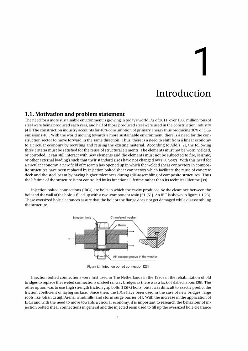
Injection bolted connections (IBCs) are bolts in which the cavity produced by the clearance between thebolt and the wall of the hole is filled up with a two-component resin [21][51]. An IBC is shown in figure 1.1[23].These oversized hole clearances assure that the bolt or the flange does not get damaged while disassemblingthe structure.
Figure 1.1: Injection bolted connection [23]
Injection bolted connections were first used in The Netherlands in the 1970s in the rehabilitation of oldbridges to replace the riveted connections of steel railway bridges as there was a lack of skilled labour[36]. Theother option was to use High strength friction grip bolts (HSFG bolts) but it was difficult to exactly predict thefriction coefficient of laying surface. Since then, the IBCs have been used in the case of new bridges, largeroofs like Johan Cruijff Arena, windmills, and storm surge barrier[51]. With the increase in the application ofIBCs and with the need to move towards a circular economy, it is important to research the behaviour of in-jection bolted shear connections in general and the injected resin used to fill up the oversized hole clearance
1

2 1. Introduction
in particular especially in quasi-static and cyclic loading conditions.
A new injection material that could be added to the resin was developed at the TU Delft laboratory. Theinjection material is a spherical steel shot that can be injected into the hole clearance before the injectionof the resin and this is called Steel Reinforced Resin (SRR). SRR provides better strength and stiffness to theconnection when compared to normal epoxy resin. As the existing research on SRR is limited, it is importantto further study its behaviour when combined with the resin.
1.2. Main objectiveThe main objective of this work is to investigate the behaviour of conventional resin and steel-reinforcedresin in oversized hole clearance to provide a slip resistant connection. Experiments has to be done undercompression-compression cyclic loading using a custom-made test setup that replicates the bearing stressesacting on the resin of injection bolted shear connections under double lap shear joints. Additionally, to val-idate the test setup against the double lap shear joint and the results obtained for one cycle loading fromthe experiments with numerical modelling of resin and SRR using reasonable friction coefficients for steel toresin/SRR interactions.
1.3. Research questionThe research questions can be classified into experiments and numerical modelling. The following are theresearch questions that have been answered in this thesis.
ExperimentsThe main aim of the experiments are to investigate the behaviour of resin and steel reinforced resin (SRR)
in oversized hole clearances under quasi-static and cyclic loading. This broader research question can bebroken down into the following research objectives which can be achieved from the experiments.
• How does the oversized hole clearance affect the initial stiffness Ki ni of resin and steel-reinforced resin?
• How does the cyclic loading affects the progression of stiffness for conventional resin/ SRR and what isfinal stiffness K f i n obtained at the end of cyclic loading for resin/ SRR?
• What is the slip obtain during the cyclic loading of the two materials and thus determine at what stressrange the failure occurs according to the failure criterion given in EN 1090-2 [21] and ECCS recommen-dations for bolted connections with injection bolts [17] ?
• What kind of deformations are obtained on the unloading of resin and SRR at certain fixed intervals ofcyclic loading?
Numerical modellingThe main objective of numerical modelling is to validate the stresses obtained in the test setup with the
double lap shear joint and to validate the experimentally obtained results for one cycle using the materialmodels by means of the following research objectives.
• Will the resin experience stresses from the current test setup that is similar to the stresses experiencedby the resin in a double lap shear joint?
• Can the numerical material model reproduce force vs displacement curve after one loading cycle asobtained from experiment and thus validate the initial stiffness Ki ni obtained?
• What are the friction coefficient of interaction between steel and resin/ SRR in the current test setup?
• Does modulus of elasticity change when resin mixture of RenGel© SW 404 / Ren© HY 5159 is used overRenGel© SW 404 / Ren© HY 2404?
1.4. Outline of the report 3
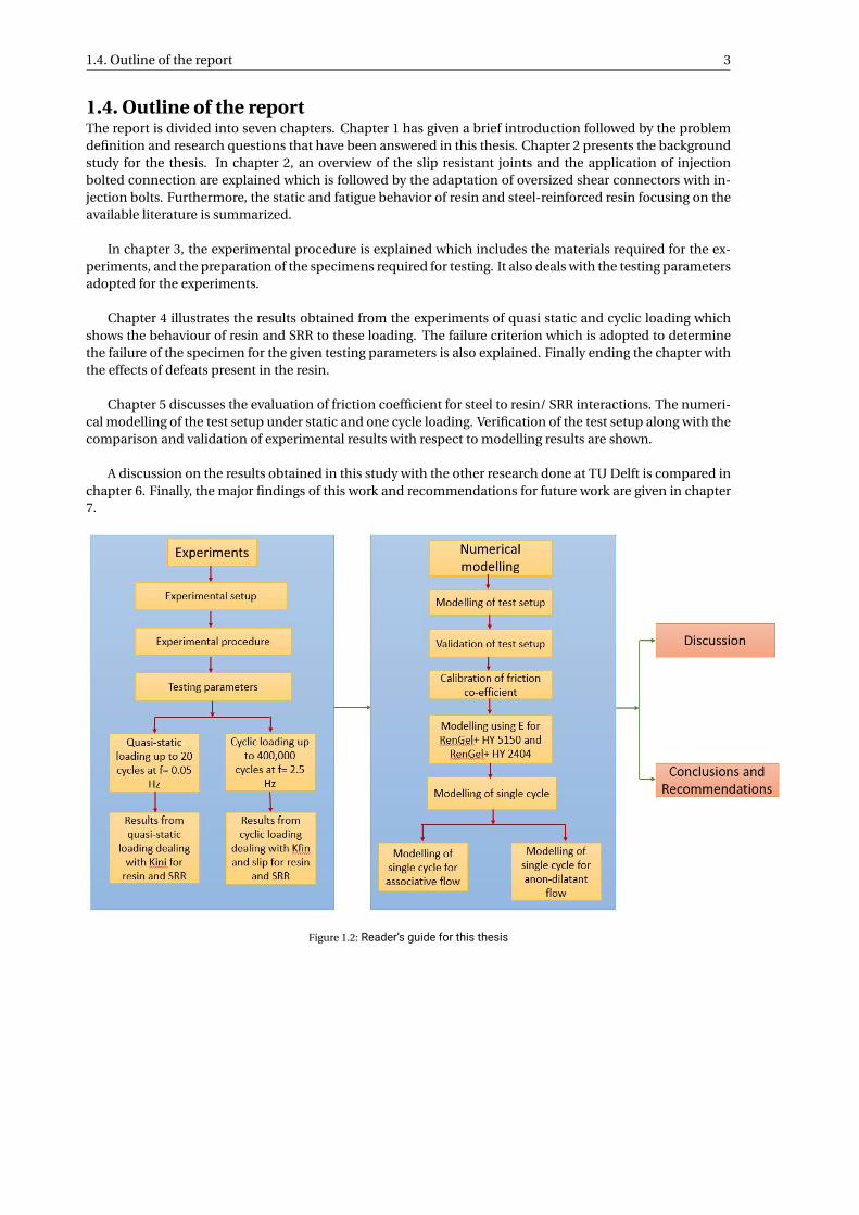
1.4. Outline of the reportThe report is divided into seven chapters. Chapter 1 has given a brief introduction followed by the problemdefinition and research questions that have been answered in this thesis. Chapter 2 presents the backgroundstudy for the thesis. In chapter 2, an overview of the slip resistant joints and the application of injectionbolted connection are explained which is followed by the adaptation of oversized shear connectors with in-jection bolts. Furthermore, the static and fatigue behavior of resin and steel-reinforced resin focusing on theavailable literature is summarized.
In chapter 3, the experimental procedure is explained which includes the materials required for the ex-periments, and the preparation of the specimens required for testing. It also deals with the testing parametersadopted for the experiments.
Chapter 4 illustrates the results obtained from the experiments of quasi static and cyclic loading whichshows the behaviour of resin and SRR to these loading. The failure criterion which is adopted to determinethe failure of the specimen for the given testing parameters is also explained. Finally ending the chapter withthe effects of defeats present in the resin.
Chapter 5 discusses the evaluation of friction coefficient for steel to resin/ SRR interactions. The numeri-cal modelling of the test setup under static and one cycle loading. Verification of the test setup along with thecomparison and validation of experimental results with respect to modelling results are shown.
A discussion on the results obtained in this study with the other research done at TU Delft is compared inchapter 6. Finally, the major findings of this work and recommendations for future work are given in chapter7.
Figure 1.2: Reader’s guide for this thesis


2State of the art
2.1. Injection bolted connectionAs previously stated in section 1.1, injection bolted connections are the ones in which the hole clearance isfilled by a two component epoxy resin. The two component epoxy resin consist of resin and hardener. Thisprovides a slip resistant connections, the cured and hardened resin acts as a solid mass thus preventing theslip of connection. Slip resistant connections are essential when the connections are subjected to load rever-sals of shear loading or when they are subjected to cyclic shear loading to improve the fatigue resistance[43].Injection bolts can also be used where the corrosion of the bolts has to be prevented (for example: Stormsurge barriers). They prevent corrosion by concealing the hole clearance and not allowing the water to comeinto with the bolts. In addition, sudden slip due to over loading is not possible in case of IBC but the suddenslip can occur in high friction strength bolts[3]. In protruded fiber reinforced polymers (FRP), the resin sealsthe welded edges of FRP profiles which eases the erection process[4] and acts as a slip resistant connectionas prestressed bolts cannot be used in FRP panels because of the loss of prestress due to relaxation.
Injection bolted connections commonly have 2 or 3 mm larger hole diameter than nominal diameter ofbolt similar to conventional bolt systems. So, the hole diameter which are used for conventional bolted con-nection can also be used for injection bolted connections [21]. The resin is injected into the hole clearancewith a hole on the head section of the bolt using an injection gun. The dimensions are as shown in the figure2.1. A special washer should be used under the bolt head [21]. The bolts can be either non-preloaded orpreloaded bolts. For non-preloaded bolts, the resin acts as load bearing as the load is transferred through thebearing of plates and shear of bolts. In preloaded bolts, load is transferred by friction between two plates andthe resin need not be load bearing as the stresses around the hole are less.
Figure 2.1: Injection of resin into the bolt head [21]
In steel to steel connection, the stiffness of oversized IBC is less than the connection stiffness of conven-tional fitted bolts. Due to the oversized hole, the stiffness of the connection decreases as larger area of steel inreplaced by the resin which has lesser stiffness when compared to steel [32]. Hence, to increase the strengthand stiffness of the connection, steel reinforced resin was developed at TU Delft [44] which on addition to
5
6 2. State of the art
the resin, increases its strength and stiffness. However, in fibre reinforced polymers, IBC provide improvedstiffness and better fatigue performance are observed for load reversal[4].
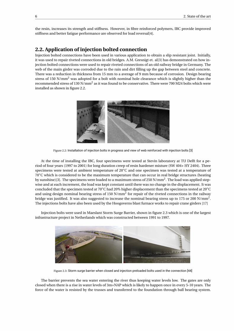
2.2. Application of injection bolted connectionInjection bolted connections have been used in various application to obtain a slip resistant joint. Initially,it was used to repair riveted connections in old bridges. A.M. Gresnigt et. al[3] has demonstrated on how in-jection bolted connections were used to repair riveted connections of an old railway bridge in Germany. Theweb of the main girder was corroded due to the rain and dirt filling up the gap between steel and concrete.There was a reduction in thickness from 15 mm to a average of 9 mm because of corrosion. Design bearingstress of 150 N/mm2 was adopted for a bolt with nominal hole clearance which is slightly higher than therecommended stress of 130 N/mm2 as it was found to be conservative. There were 700 M24 bolts which wereinstalled as shown in figure 2.2.
Figure 2.2: Installation of injection bolts in progress and view of web reinforced with injection bolts [3]
At the time of installing the IBC, four specimens were tested at Stevin laboratory at TU Delft for a pe-riod of four years (1997 to 2001) for long duration creep of resin hardener mixture (SW 404+ HY 2404). Threespecimens were tested at ambient temperature of 20◦C and one specimen was tested at a temperature of70◦C which is considered to be the maximum temperature that can occur in real bridge structures (heatingby sunshine)[3]. The specimens were loaded to a maximum stress of 250 N/mm2. The load was applied step-wise and at each increment, the load was kept constant until there was no change in the displacement. It wasconcluded that the specimen tested at 70◦C had 20% higher displacement than the specimens tested at 20◦Cand using design nominal bearing stress of 150 N/mm2 for repair of the riveted connections in the railwaybridge was justified. It was also suggested to increase the nominal bearing stress up to 175 or 200 N/mm2.The injections bolts have also been used by the Hoogoverns blast furnace works to repair crane girders [17]
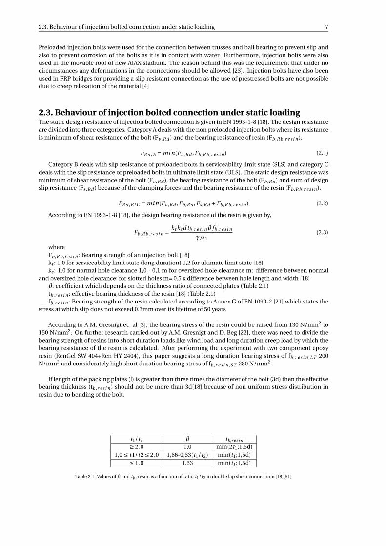
Injection bolts were used in Maeslant Storm Surge Barrier, shown in figure 2.3 which is one of the largestinfrastructure project in Netherlands which was constructed between 1991 to 1997.
Figure 2.3: Storm surge barrier when closed and injection preloaded bolts used in the connection [44]
The barrier prevents the sea water entering the river thus keeping water levels low. The gates are onlyclosed when there is a rise in water levels of 3m+NAP which is likely to happen once in every 5-10 years. Theforce of the water is resisted by the trusses and transferred to the foundation through ball bearing system.
2.3. Behaviour of injection bolted connection under static loading 7
Preloaded injection bolts were used for the connection between trusses and ball bearing to prevent slip andalso to prevent corrosion of the bolts as it is in contact with water. Furthermore, injection bolts were alsoused in the movable roof of new AJAX stadium. The reason behind this was the requirement that under nocircumstances any deformations in the connections should be allowed [23]. Injection bolts have also beenused in FRP bridges for providing a slip resistant connection as the use of prestressed bolts are not possibledue to creep relaxation of the material [4]
2.3. Behaviour of injection bolted connection under static loadingThe static design resistance of injection bolted connection is given in EN 1993-1-8 [18]. The design resistanceare divided into three categories. Category A deals with the non preloaded injection bolts where its resistanceis minimum of shear resistance of the bolt (Fv ,R d ) and the bearing resistance of resin (Fb ,R b ,r e s i n).
FR d , A = mi n(Fv ,R d ,Fb ,R b ,r e s i n) (2.1)
Category B deals with slip resistance of preloaded bolts in serviceability limit state (SLS) and category Cdeals with the slip resistance of preloaded bolts in ultimate limit state (ULS). The static design resistance wasminimum of shear resistance of the bolt (Fv ,R d ), the bearing resistance of the bolt (Fb ,R d ) and sum of designslip resistance (Fs ,R d ) because of the clamping forces and the bearing resistance of the resin (Fb ,R b ,r e s i n).
FR d ,B /C = mi n(Fv ,R d ,Fb ,R d ,Fs ,R d +Fb ,R b ,r e s i n) (2.2)
According to EN 1993-1-8 [18], the design bearing resistance of the resin is given by,
Fb ,R b ,r e s i n = kt ks d tb ,r e s i nβ fb ,r e s i n
γM 4(2.3)
whereFb ,R b ,r e s i n : Bearing strength of an injection bolt [18]kt : 1,0 for serviceability limit state (long duration) 1,2 for ultimate limit state [18]ks : 1.0 for normal hole clearance 1,0 - 0,1 m for oversized hole clearance m: difference between normal
and oversized hole clearance; for slotted holes m= 0.5 x difference between hole length and width [18]β: coefficient which depends on the thickness ratio of connected plates (Table 2.1)tb ,r e s i n : effective bearing thickness of the resin [18] (Table 2.1)fb ,r e s i n : Bearing strength of the resin calculated according to Annex G of EN 1090-2 [21] which states the
stress at which slip does not exceed 0.3mm over its lifetime of 50 years
According to A.M. Gresnigt et. al [3], the bearing stress of the resin could be raised from 130 N/mm2 to150 N/mm2. On further research carried out by A.M. Gresnigt and D. Beg [22], there was need to divide thebearing strength of resins into short duration loads like wind load and long duration creep load by which thebearing resistance of the resin is calculated. After performing the experiment with two component epoxyresin (RenGel SW 404+Ren HY 2404), this paper suggests a long duration bearing stress of fb ,r e s i n ,L T 200N/mm2 and considerately high short duration bearing stress of fb ,r e s i n ,S T 280 N/mm2.
If length of the packing plates (l) is greater than three times the diameter of the bolt (3d) then the effectivebearing thickness (tb ,r e s i n) should not be more than 3d[18] because of non uniform stress distribution inresin due to bending of the bolt.
t1/t2 β tb,r esi n
≥ 2,0 1,0 min(2t1;1,5d)1,0 ≤ t1/t2 ≤ 2,0 1,66-0,33(t1/t2) min(t1;1,5d)
≤ 1,0 1.33 min(t1;1,5d)
Table 2.1: Values of β and tb , resin as a function of ratio t1/t2 in double lap shear connections[18][51]
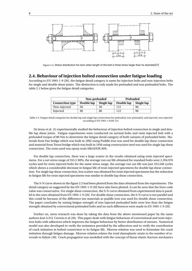
8 2. State of the art
Figure 2.4: Stress distribution he resin when length of the bolt is three times larger than its diameter[17]
2.4. Behaviour of injection bolted connection under fatigue loadingAccording to EN 1993-1-9 [20], the fatigue detail category is same for injection bolts and non-injection boltsfor single and double shear joints. The distinction is only made for preloaded and non preloaded bolts. Thetable 2.1 below gives the fatigue detail categories.
Non-preloaded PreloadedConnection type Double lap Single lap Double lap Single lapNon-injected 50 50 112 90Injected 90 80 112 90
Table 2.2: Fatigue detail categories for double lap and single lap connections for preloaded, non-preloaded, and injected, non-injectedaccording to EN 1993-1-9[20] [51]
De Jesus et al. [5] experimentally studied the behaviour of injection bolted connection in single and dou-ble lap shear joints. Fatigue experiments were conducted on normal bolts and resin injected bolt with apreloaded torque of 80 Nm to determine the fatigue detail category of both variants of preloaded bolts. Ma-terials from Fao bridge which was built in 1892 using Puddle iron was used for double lap shear connectionand material from Trezoi bridge which was built in 1956 using construction steel was used for single lap shearconnection. The resin used was epoxy resin SIKADUR 30®.
For double lap connection, there was a large scatter in the results obtained using resin injected speci-mens. For a net stress range of 355.5 MPa, the average run out life obtained for standard bolts were 2,394,976cycles and for resin injected bolts for the same stress range, the average run out life was just 333,548 cycleswhich shows a considerable decrease in fatigue life of resin injected specimens for double lap shear connec-tion. For single lap shear connection, less scatter was obtained for resin injected specimens but the reductionin fatigue life for resin injected specimens was similar to double lap shear connection.
The S-N curve shown in the figure 2.5 had been plotted from the data obtained from the experiments. Thedetail category as suggested by the EN 1993-1-9 [20] have also been plotted. It can be seen that the Euro codevalue was conservative. For single shear connection, the S-N curve obtained from experimental data is paral-lel to the ones obtained from EN 1993-1-9 [20]. For double shear connection, the S-N curve is not parallel andthis could be because of the difference inn materials as puddle iron was used for double shear connection.The paper concludes by stating fatigue strength of rein injected preloaded bolts were less than the fatiguestrength obtained by convectional preloaded bolts and no such differences were made in EN 1993-1-9 [20].
Further on, more research was done by taking the data from the above mentioned paper by the sameauthors José A.F.O. Correia et al [30]. This paper deals with fatigue behaviour of conventional and resin injec-tion bolts with adhesives which improves the fatigue behaviour by better distribution of stresses. Numericalmodel was also developed to verify the resistance provided by the adhersives and to verify the contributionof crack initiation in bolted connection to its fatigue life. Morrow relation was used to formulate the crackinitiation through fatigue damage. Morrow relation relates the total elastoplastic strain to the number of re-versals to failure [30]. Crack propagation was modelled with the concept of linear elastic fracture mechanics
2.4. Behaviour of injection bolted connection under fatigue loading 9
Figure 2.5: Comparison of S-N fatigue data from the single shear connections made of the material from the Trezói bridge (Left)[5]. b. Comparison of S-N fatigue data from the double shear connections made of the material from the Fão bridge.[5] (Right)
(LEFM) using a crack propagation law presented by Paris. The results of the experiments show that the ad-hesive bonding increases the fatigue life when two bolts are used and a reduction in fatigue life occurs whenonly one bolt is used. The numerical model shows that adhesives products delays the time of crack initiationthus improving the fatigue life of conventional and resin injected bolts with adhesives.
A few co-authors from previous paper Burno Pedrosa et al [8] performed fatigue experiments of singlelap shear connections from plates obtained from Eiffel bridge which was constructed using puddle iron. Theexperiments were conducted on conventional bolts and resin injected bolts. The conclusion of the experi-ments was that the resin injected bolts showed high fatigue strength than the conventional bolts in high cyclefatigue.
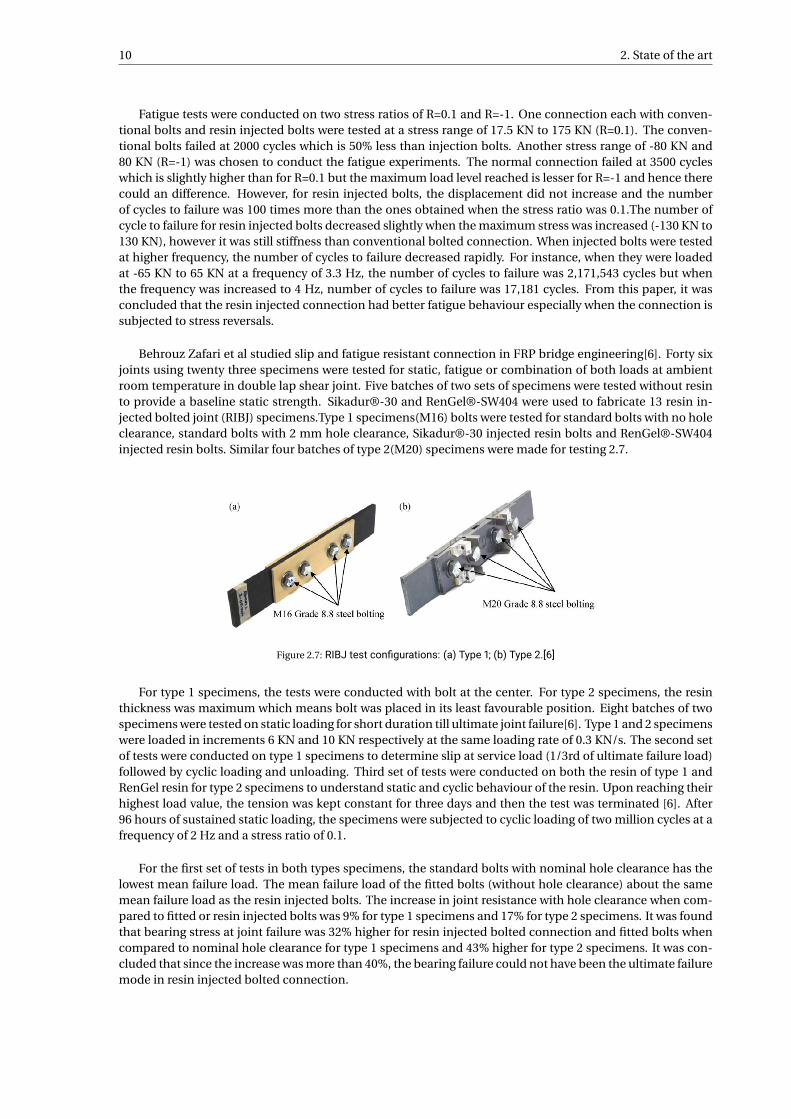
Static and fatigue behaviour of resin injection bolted connections in pultruded FRP panels was studiedby A.M. Van Wingerde et al [4]. Test was conducted on the I profile as shown in the figure 2.6. The behaviourof conventional bolts (M16 with 16.9 mm bolt hole diameter) and resin injected bolts(M14 bolts) were stud-ied.The threaded part does not cross the panels for standard bolts but the threaded part of the injection boltmay cross the panels. Static tensile test were conducted on two specimens of conventional bolts and twospecimens of resin injected bolts.
Figure 2.6: Dimension of I profile used for testing[4]
The specimens of conventional bolts failed at 221 KN and 240 KN while the resin injected bolts failed at230 KN and 240 KN. The increase in strength for resin injected bolts is 5%, the difference is too small to havea firm conclusion. A sudden reduction in stiffness because of occurrence of slip and then slow increase instiffness can be observed in conventional bolts. No such sudden reduction in stiffness was observed for resininjected bolts and hence it was concluded that resin injected bolts was superior in terms of stiffness over con-ventional bolts.
10 2. State of the art
Fatigue tests were conducted on two stress ratios of R=0.1 and R=-1. One connection each with conven-tional bolts and resin injected bolts were tested at a stress range of 17.5 KN to 175 KN (R=0.1). The conven-tional bolts failed at 2000 cycles which is 50% less than injection bolts. Another stress range of -80 KN and80 KN (R=-1) was chosen to conduct the fatigue experiments. The normal connection failed at 3500 cycleswhich is slightly higher than for R=0.1 but the maximum load level reached is lesser for R=-1 and hence therecould an difference. However, for resin injected bolts, the displacement did not increase and the numberof cycles to failure was 100 times more than the ones obtained when the stress ratio was 0.1.The number ofcycle to failure for resin injected bolts decreased slightly when the maximum stress was increased (-130 KN to130 KN), however it was still stiffness than conventional bolted connection. When injected bolts were testedat higher frequency, the number of cycles to failure decreased rapidly. For instance, when they were loadedat -65 KN to 65 KN at a frequency of 3.3 Hz, the number of cycles to failure was 2,171,543 cycles but whenthe frequency was increased to 4 Hz, number of cycles to failure was 17,181 cycles. From this paper, it wasconcluded that the resin injected connection had better fatigue behaviour especially when the connection issubjected to stress reversals.
Behrouz Zafari et al studied slip and fatigue resistant connection in FRP bridge engineering[6]. Forty sixjoints using twenty three specimens were tested for static, fatigue or combination of both loads at ambientroom temperature in double lap shear joint. Five batches of two sets of specimens were tested without resinto provide a baseline static strength. Sikadur®-30 and RenGel®-SW404 were used to fabricate 13 resin in-jected bolted joint (RIBJ) specimens.Type 1 specimens(M16) bolts were tested for standard bolts with no holeclearance, standard bolts with 2 mm hole clearance, Sikadur®-30 injected resin bolts and RenGel®-SW404injected resin bolts. Similar four batches of type 2(M20) specimens were made for testing 2.7.
Figure 2.7: RIBJ test configurations: (a) Type 1; (b) Type 2.[6]
For type 1 specimens, the tests were conducted with bolt at the center. For type 2 specimens, the resinthickness was maximum which means bolt was placed in its least favourable position. Eight batches of twospecimens were tested on static loading for short duration till ultimate joint failure[6]. Type 1 and 2 specimenswere loaded in increments 6 KN and 10 KN respectively at the same loading rate of 0.3 KN/s. The second setof tests were conducted on type 1 specimens to determine slip at service load (1/3rd of ultimate failure load)followed by cyclic loading and unloading. Third set of tests were conducted on both the resin of type 1 andRenGel resin for type 2 specimens to understand static and cyclic behaviour of the resin. Upon reaching theirhighest load value, the tension was kept constant for three days and then the test was terminated [6]. After96 hours of sustained static loading, the specimens were subjected to cyclic loading of two million cycles at afrequency of 2 Hz and a stress ratio of 0.1.
For the first set of tests in both types specimens, the standard bolts with nominal hole clearance has thelowest mean failure load. The mean failure load of the fitted bolts (without hole clearance) about the samemean failure load as the resin injected bolts. The increase in joint resistance with hole clearance when com-pared to fitted or resin injected bolts was 9% for type 1 specimens and 17% for type 2 specimens. It was foundthat bearing stress at joint failure was 32% higher for resin injected bolted connection and fitted bolts whencompared to nominal hole clearance for type 1 specimens and 43% higher for type 2 specimens. It was con-cluded that since the increase was more than 40%, the bearing failure could not have been the ultimate failuremode in resin injected bolted connection.

2.5. Bolted shear connectors with standard and oversized holes in composite structures 11
The graph below 2.8 shows the results from second set of tests to determine the slip load. The load at0.15mm of slip was considered to be the slip load. From the graph, it can be observed that the slip load fortype 1 specimen with 2 mm hole clearance was 11.5 KN for joint 1. Once the load exceeded, the slip increasedsignificantly with final value of 3 mm. The slip load for fitted bolt was 19 KN for the first joint and the max-imum slip obtained was 0.3 mm. For RIBJs, their slip load(0.08 mm) was more than there service load of 25KN. Slip load of specimen with RenGel was 39 KN for joint 1 and 42 KN for Sikadur-30 specimen.This confirmsthat resin injected bolts offer better slip resistance for FRP structures.
Figure 2.8: Load-slip curves for: (Left) M16 18HL (Joint 1); (Right) M16 16HL (Joint 1).[6]
Third set of tests deals with the static and fatigue behaviour of both the resins. From type 1 specimenwith Sikadur-30, the final displacement obtained after 96 hours was 0.1 mm and 0.5 mm for the load of 25 KNand 56 KN respectively. On linear interpolation, the value of displacement at a load of 40 KN was 0.29 mm.RenGel resin with type 1 joint offer better stiffness when compared to Sikadur-30 resin. For a load of 48 KN,the stiffness was 1.5 times higher and the slip was 72% lesser. RenGel type 1 specimen failed at 60 KN afterthree static load levels and six million cycles of testing. For type 2 RenGel specimens, the displacement at 32KN was 0.13 mm and at 66 KN was 0.64 mm and the specimen failed at 82 KN after two static load levels andfour million cycles. It was concluded that all the three resin injected specimens had a displacement <0.15mm when they were loaded at their service loads.
The displacement values were extrapolated for 50 years to check if the slip exceeded the failure criterionof 0.3 mm. Type 1 Sikadur-30 specimens at 32 KN had a slip of 0.19 mm but at 48 KN, the slip was 0.45 mmwhich exceeded the limits. For type 1 RenGel specimens, the slip is 0.13 and 0.3 mm for the same tensionloads. For type 2 RenGel specimens, the displacement was 0.24 mm for 32 KN and 0.5 mm for 66 KN. It wasconcluded that the displacement limits of 0.3 mm for 50 years is too low for FRP structures because of itsviscoelastic material properties. Rather a 0.75 mm displacement for 100 years is proposed as the alternativefailure criterion for FRP structures. For the cyclic loading of the specimens, it was observed that after theinitial shakedown of 200,000 cycles, the displacement was found be constant till the end of the experiment.It was concluded that with this low amount of slip, resin injected bolts joints can be successfully used in FRPstructures.
2.5. Bolted shear connectors with standard and oversized holes in com-posite structures
There is a need for the construction section to move towards a circular economy, which can be achieved mydismounting and reusing existing structures. With this need, it becomes important to have hole clearanceslightly larger than the nominal hole clearance which accounts for larger fabrication and execution toler-ances during (dis)assembling of composite beams. At TU Delft, research have been made to use oversizedinjection bolts as shear connectors for composite structures which enables the the reuse of concrete as theoversize clearance prevent the damage of concrete during dissembling.
12 2. State of the art
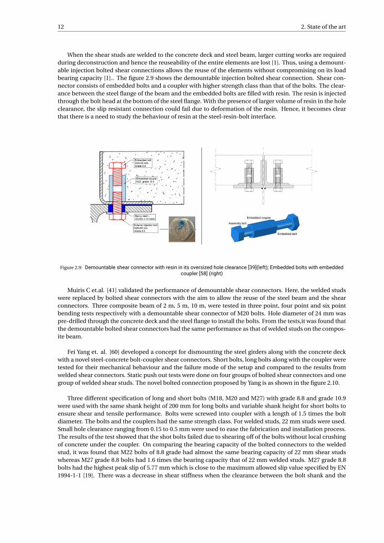
When the shear studs are welded to the concrete deck and steel beam, larger cutting works are requiredduring deconstruction and hence the reuseability of the entire elements are lost [1]. Thus, using a demount-able injection bolted shear connections allows the reuse of the elements without compromising on its loadbearing capacity [1].. The figure 2.9 shows the demountable injection bolted shear connection. Shear con-nector consists of embedded bolts and a coupler with higher strength class than that of the bolts. The clear-ance between the steel flange of the beam and the embedded bolts are filled with resin. The resin is injectedthrough the bolt head at the bottom of the steel flange. With the presence of larger volume of resin in the holeclearance, the slip resistant connection could fail due to deformation of the resin. Hence, it becomes clearthat there is a need to study the behaviour of resin at the steel-resin-bolt interface.
Figure 2.9: Demountable shear connector with resin in its oversized hole clearance [39](left); Embedded bolts with embeddedcoupler [58] (right)
Muiris C et.al. [41] validated the performance of demountable shear connectors. Here, the welded studswere replaced by bolted shear connectors with the aim to allow the reuse of the steel beam and the shearconnectors. Three composite beam of 2 m, 5 m, 10 m, were tested in three point, four point and six pointbending tests respectively with a demountable shear connector of M20 bolts. Hole diameter of 24 mm waspre-drilled through the concrete deck and the steel flange to install the bolts. From the tests,it was found thatthe demountable bolted shear connectors had the same performance as that of welded studs on the compos-ite beam.
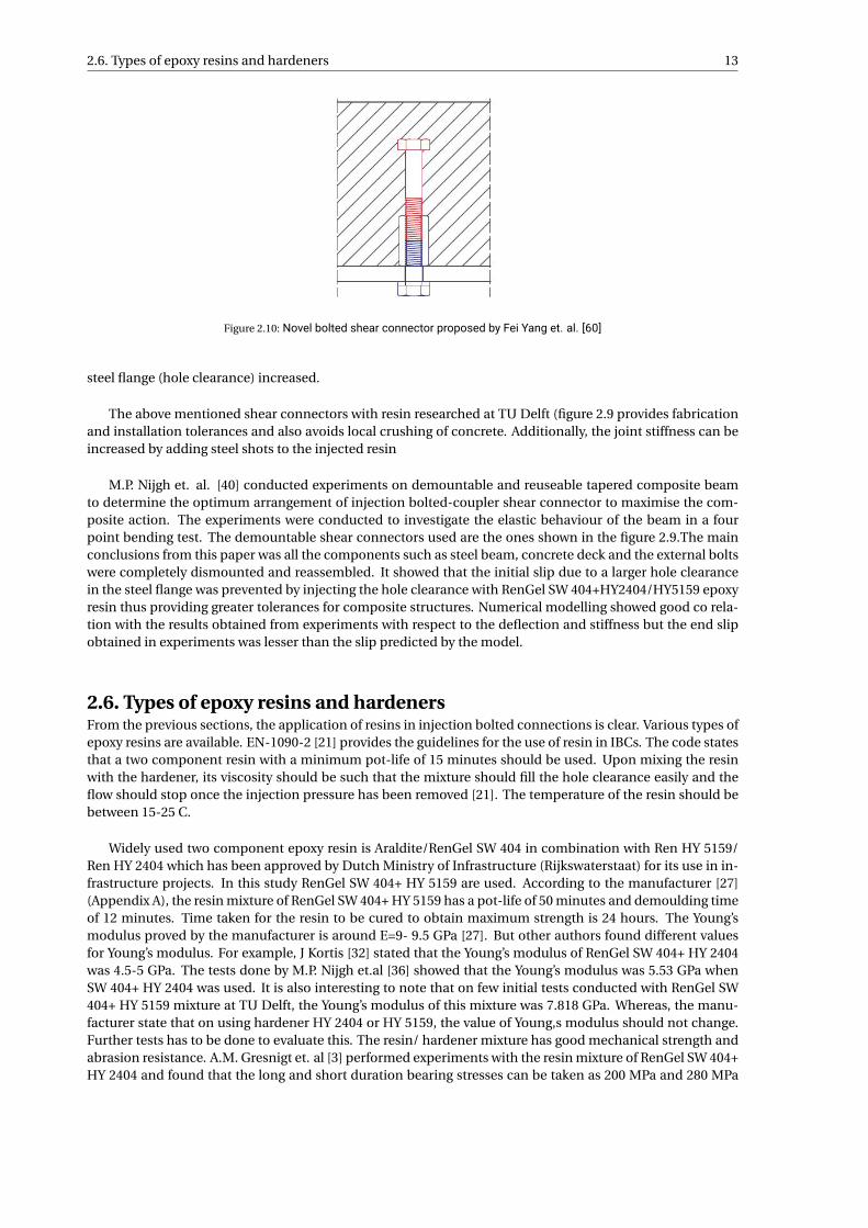
Fei Yang et. al. [60] developed a concept for dismounting the steel girders along with the concrete deckwith a novel steel-concrete bolt-coupler shear connectors. Short bolts, long bolts along with the coupler weretested for their mechanical behaviour and the failure mode of the setup and compared to the results fromwelded shear connectors. Static push out tests were done on four groups of bolted shear connectors and onegroup of welded shear studs. The novel bolted connection proposed by Yang is as shown in the figure 2.10.
Three different specification of long and short bolts (M18, M20 and M27) with grade 8.8 and grade 10.9were used with the same shank height of 200 mm for long bolts and variable shank height for short bolts toensure shear and tensile performance. Bolts were screwed into coupler with a length of 1.5 times the boltdiameter. The bolts and the couplers had the same strength class. For welded studs, 22 mm studs were used.Small hole clearance ranging from 0.15 to 0.5 mm were used to ease the fabrication and installation process.The results of the test showed that the shot bolts failed due to shearing off of the bolts without local crushingof concrete under the coupler. On comparing the bearing capacity of the bolted connectors to the weldedstud, it was found that M22 bolts of 8.8 grade had almost the same bearing capacity of 22 mm shear studswhereas M27 grade 8.8 bolts had 1.6 times the bearing capacity that of 22 mm welded studs. M27 grade 8.8bolts had the highest peak slip of 5.77 mm which is close to the maximum allowed slip value specified by EN1994-1-1 [19]. There was a decrease in shear stiffness when the clearance between the bolt shank and the
2.6. Types of epoxy resins and hardeners 13
Figure 2.10: Novel bolted shear connector proposed by Fei Yang et. al. [60]
steel flange (hole clearance) increased.
The above mentioned shear connectors with resin researched at TU Delft (figure 2.9 provides fabricationand installation tolerances and also avoids local crushing of concrete. Additionally, the joint stiffness can beincreased by adding steel shots to the injected resin
M.P. Nijgh et. al. [40] conducted experiments on demountable and reuseable tapered composite beamto determine the optimum arrangement of injection bolted-coupler shear connector to maximise the com-posite action. The experiments were conducted to investigate the elastic behaviour of the beam in a fourpoint bending test. The demountable shear connectors used are the ones shown in the figure 2.9.The mainconclusions from this paper was all the components such as steel beam, concrete deck and the external boltswere completely dismounted and reassembled. It showed that the initial slip due to a larger hole clearancein the steel flange was prevented by injecting the hole clearance with RenGel SW 404+HY2404/HY5159 epoxyresin thus providing greater tolerances for composite structures. Numerical modelling showed good co rela-tion with the results obtained from experiments with respect to the deflection and stiffness but the end slipobtained in experiments was lesser than the slip predicted by the model.
2.6. Types of epoxy resins and hardenersFrom the previous sections, the application of resins in injection bolted connections is clear. Various types ofepoxy resins are available. EN-1090-2 [21] provides the guidelines for the use of resin in IBCs. The code statesthat a two component resin with a minimum pot-life of 15 minutes should be used. Upon mixing the resinwith the hardener, its viscosity should be such that the mixture should fill the hole clearance easily and theflow should stop once the injection pressure has been removed [21]. The temperature of the resin should bebetween 15-25 C.
Widely used two component epoxy resin is Araldite/RenGel SW 404 in combination with Ren HY 5159/Ren HY 2404 which has been approved by Dutch Ministry of Infrastructure (Rijkswaterstaat) for its use in in-frastructure projects. In this study RenGel SW 404+ HY 5159 are used. According to the manufacturer [27](Appendix A), the resin mixture of RenGel SW 404+ HY 5159 has a pot-life of 50 minutes and demoulding timeof 12 minutes. Time taken for the resin to be cured to obtain maximum strength is 24 hours. The Young’smodulus proved by the manufacturer is around E=9- 9.5 GPa [27]. But other authors found different valuesfor Young’s modulus. For example, J Kortis [32] stated that the Young’s modulus of RenGel SW 404+ HY 2404was 4.5-5 GPa. The tests done by M.P. Nijgh et.al [36] showed that the Young’s modulus was 5.53 GPa whenSW 404+ HY 2404 was used. It is also interesting to note that on few initial tests conducted with RenGel SW404+ HY 5159 mixture at TU Delft, the Young’s modulus of this mixture was 7.818 GPa. Whereas, the manu-facturer state that on using hardener HY 2404 or HY 5159, the value of Young,s modulus should not change.Further tests has to be done to evaluate this. The resin/ hardener mixture has good mechanical strength andabrasion resistance. A.M. Gresnigt et. al [3] performed experiments with the resin mixture of RenGel SW 404+HY 2404 and found that the long and short duration bearing stresses can be taken as 200 MPa and 280 MPa
14 2. State of the art
respectively.
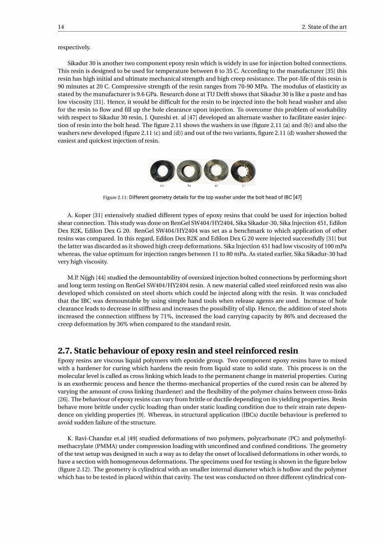
Sikadur 30 is another two component epoxy resin which is widely in use for injection bolted connections.This resin is designed to be used for temperature between 8 to 35 C. According to the manufacturer [35] thisresin has high initial and ultimate mechanical strength and high creep resistance. The pot-life of this resin is90 minutes at 20 C. Compressive strength of the resin ranges from 70-90 MPa. The modulus of elasticity asstated by the manufacturer is 9.6 GPa. Research done at TU Delft shows that Sikadur 30 is like a paste and haslow viscosity [31]. Hence, it would be difficult for the resin to be injected into the bolt head washer and alsofor the resin to flow and fill up the hole clearance upon injection. To overcome this problem of workabilitywith respect to Sikadur 30 resin, J. Qureshi et. al [47] developed an alternate washer to facilitate easier injec-tion of resin into the bolt head. The figure 2.11 shows the washers in use (figure 2.11 (a) and (b)) and also thewashers new developed (figure 2.11 (c) and (d)) and out of the two variants, figure 2.11 (d) washer showed theeasiest and quickest injection of resin.
Figure 2.11: Different geometry details for the top washer under the bolt head of IBC [47]
A. Koper [31] extensively studied different types of epoxy resins that could be used for injection boltedshear connection. This study was done on RenGel SW404/HY2404, Sika Sikadur-30, Sika Injection 451, EdilonDex R2K, Edilon Dex G 20. RenGel SW404/HY2404 was set as a benchmark to which application of otherresins was compared. In this regard, Edilon Dex R2K and Edilon Dex G 20 were injected successfully [31] butthe latter was discarded as it showed high creep deformations. Sika Injection 451 had low viscosity of 100 mPawhereas, the value optimum for injection ranges between 11 to 80 mPa. As stated earlier, Sika Sikadur-30 hadvery high viscosity.
M.P. Nijgh [44] studied the demountability of oversized injection bolted connections by performing shortand long term testing on RenGel SW404/HY2404 resin. A new material called steel reinforced resin was alsodeveloped which consisted on steel shorts which could be injected along with the resin. It was concludedthat the IBC was demountable by using simple hand tools when release agents are used. Increase of holeclearance leads to decrease in stiffness and increases the possibility of slip. Hence, the addition of steel shotsincreased the connection stiffness by 71%, increased the load carrying capacity by 86% and decreased thecreep deformation by 36% when compared to the standard resin.
2.7. Static behaviour of epoxy resin and steel reinforced resinEpoxy resins are viscous liquid polymers with epoxide group. Two component epoxy resins have to mixedwith a hardener for curing which hardens the resin from liquid state to solid state. This process is on themolecular level is called as cross linking which leads to the permanent change in material properties. Curingis an exothermic process and hence the thermo-mechanical properties of the cured resin can be altered byvarying the amount of cross linking (hardener) and the flexibility of the polymer chains between cross-links[26]. The behaviour of epoxy resins can vary from brittle or ductile depending on its yielding properties. Resinbehave more brittle under cyclic loading than under static loading condition due to their strain rate depen-dence on yielding properties [9]. Whereas, in structural application (IBCs) ductile behaviour is preferred toavoid sudden failure of the structure.
K. Ravi-Chandar et.al [49] studied deformations of two polymers, polycarbonate (PC) and polymethyl-methacrylate (PMMA) under compression loading with unconfined and confined conditions. The geometryof the test setup was designed in such a way as to delay the onset of localised deformations in other words, tohave a section with homogeneous deformations. The specimens used for testing is shown in the figure below(figure 2.12). The geometry is cylindrical with an smaller internal diameter which is hollow and the polymerwhich has to be tested in placed within that cavity. The test was conducted on three different cylindrical con-
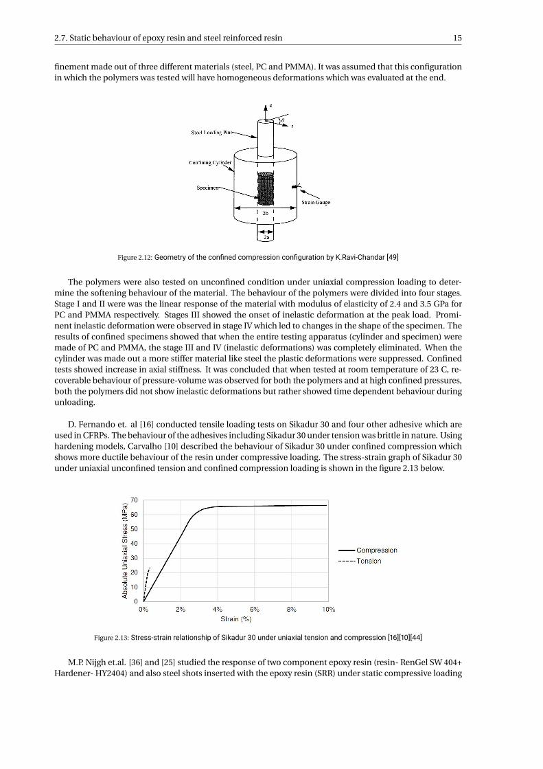
2.7. Static behaviour of epoxy resin and steel reinforced resin 15
finement made out of three different materials (steel, PC and PMMA). It was assumed that this configurationin which the polymers was tested will have homogeneous deformations which was evaluated at the end.
Figure 2.12: Geometry of the confined compression configuration by K.Ravi-Chandar [49]
The polymers were also tested on unconfined condition under uniaxial compression loading to deter-mine the softening behaviour of the material. The behaviour of the polymers were divided into four stages.Stage I and II were was the linear response of the material with modulus of elasticity of 2.4 and 3.5 GPa forPC and PMMA respectively. Stages III showed the onset of inelastic deformation at the peak load. Promi-nent inelastic deformation were observed in stage IV which led to changes in the shape of the specimen. Theresults of confined specimens showed that when the entire testing apparatus (cylinder and specimen) weremade of PC and PMMA, the stage III and IV (inelastic deformations) was completely eliminated. When thecylinder was made out a more stiffer material like steel the plastic deformations were suppressed. Confinedtests showed increase in axial stiffness. It was concluded that when tested at room temperature of 23 C, re-coverable behaviour of pressure-volume was observed for both the polymers and at high confined pressures,both the polymers did not show inelastic deformations but rather showed time dependent behaviour duringunloading.
D. Fernando et. al [16] conducted tensile loading tests on Sikadur 30 and four other adhesive which areused in CFRPs. The behaviour of the adhesives including Sikadur 30 under tension was brittle in nature. Usinghardening models, Carvalho [10] described the behaviour of Sikadur 30 under confined compression whichshows more ductile behaviour of the resin under compressive loading. The stress-strain graph of Sikadur 30under uniaxial unconfined tension and confined compression loading is shown in the figure 2.13 below.
Figure 2.13: Stress-strain relationship of Sikadur 30 under uniaxial tension and compression [16][10][44]
M.P. Nijgh et.al. [36] and [25] studied the response of two component epoxy resin (resin- RenGel SW 404+Hardener- HY2404) and also steel shots inserted with the epoxy resin (SRR) under static compressive loading
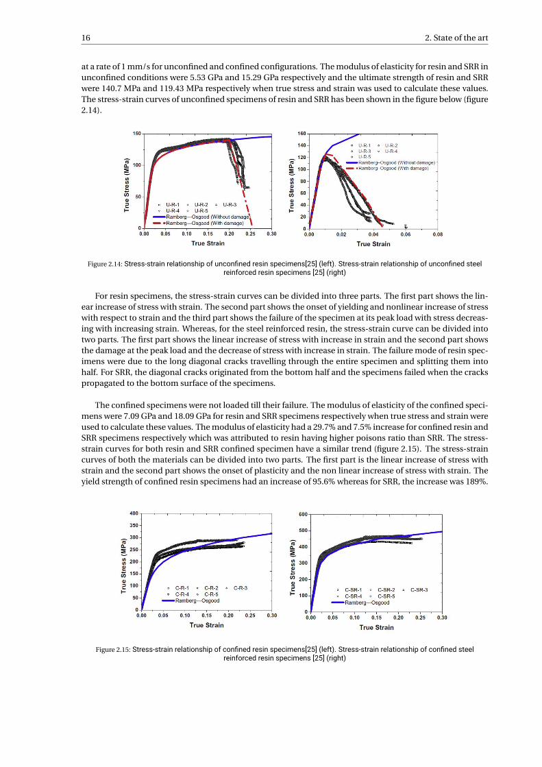
16 2. State of the art
at a rate of 1 mm/s for unconfined and confined configurations. The modulus of elasticity for resin and SRR inunconfined conditions were 5.53 GPa and 15.29 GPa respectively and the ultimate strength of resin and SRRwere 140.7 MPa and 119.43 MPa respectively when true stress and strain was used to calculate these values.The stress-strain curves of unconfined specimens of resin and SRR has been shown in the figure below (figure2.14).
Figure 2.14: Stress-strain relationship of unconfined resin specimens[25] (left). Stress-strain relationship of unconfined steelreinforced resin specimens [25] (right)
For resin specimens, the stress-strain curves can be divided into three parts. The first part shows the lin-ear increase of stress with strain. The second part shows the onset of yielding and nonlinear increase of stresswith respect to strain and the third part shows the failure of the specimen at its peak load with stress decreas-ing with increasing strain. Whereas, for the steel reinforced resin, the stress-strain curve can be divided intotwo parts. The first part shows the linear increase of stress with increase in strain and the second part showsthe damage at the peak load and the decrease of stress with increase in strain. The failure mode of resin spec-imens were due to the long diagonal cracks travelling through the entire specimen and splitting them intohalf. For SRR, the diagonal cracks originated from the bottom half and the specimens failed when the crackspropagated to the bottom surface of the specimens.
The confined specimens were not loaded till their failure. The modulus of elasticity of the confined speci-mens were 7.09 GPa and 18.09 GPa for resin and SRR specimens respectively when true stress and strain wereused to calculate these values. The modulus of elasticity had a 29.7% and 7.5% increase for confined resin andSRR specimens respectively which was attributed to resin having higher poisons ratio than SRR. The stress-strain curves for both resin and SRR confined specimen have a similar trend (figure 2.15). The stress-straincurves of both the materials can be divided into two parts. The first part is the linear increase of stress withstrain and the second part shows the onset of plasticity and the non linear increase of stress with strain. Theyield strength of confined resin specimens had an increase of 95.6% whereas for SRR, the increase was 189%.
Figure 2.15: Stress-strain relationship of confined resin specimens[25] (left). Stress-strain relationship of confined steelreinforced resin specimens [25] (right)
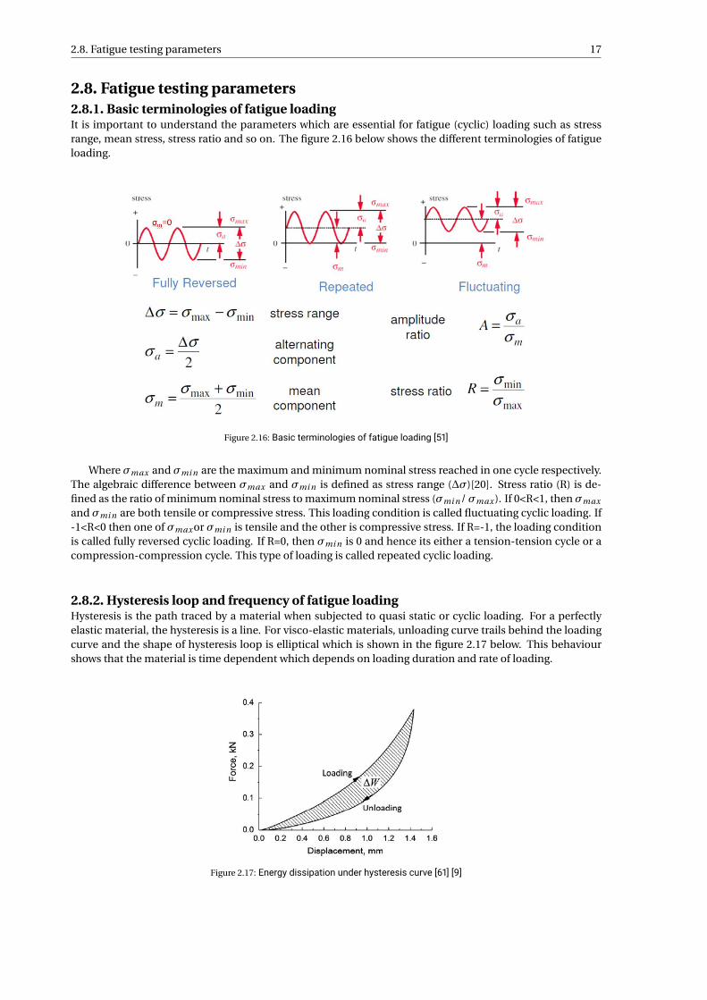
2.8. Fatigue testing parameters 17
2.8. Fatigue testing parameters2.8.1. Basic terminologies of fatigue loadingIt is important to understand the parameters which are essential for fatigue (cyclic) loading such as stressrange, mean stress, stress ratio and so on. The figure 2.16 below shows the different terminologies of fatigueloading.
Figure 2.16: Basic terminologies of fatigue loading [51]
Where σmax and σmi n are the maximum and minimum nominal stress reached in one cycle respectively.The algebraic difference between σmax and σmi n is defined as stress range (∆σ)[20]. Stress ratio (R) is de-fined as the ratio of minimum nominal stress to maximum nominal stress (σmi n/ σmax ). If 0<R<1, then σmax
and σmi n are both tensile or compressive stress. This loading condition is called fluctuating cyclic loading. If-1<R<0 then one of σmax or σmi n is tensile and the other is compressive stress. If R=-1, the loading conditionis called fully reversed cyclic loading. If R=0, then σmi n is 0 and hence its either a tension-tension cycle or acompression-compression cycle. This type of loading is called repeated cyclic loading.
2.8.2. Hysteresis loop and frequency of fatigue loadingHysteresis is the path traced by a material when subjected to quasi static or cyclic loading. For a perfectlyelastic material, the hysteresis is a line. For visco-elastic materials, unloading curve trails behind the loadingcurve and the shape of hysteresis loop is elliptical which is shown in the figure 2.17 below. This behaviourshows that the material is time dependent which depends on loading duration and rate of loading.
Figure 2.17: Energy dissipation under hysteresis curve [61] [9]
18 2. State of the art
The area under the hysteresis curve gives the energy dissipated by the material. In materials with time-dependent properties and low thermal conductivity, the energy released in the form of heat cannot escapeinto the environment rather ends up heating the material itself. Due to this reason, unlike in metals the ex-periments cannot be accelerated by using higher frequency as these materials are temperature dependent[9]. On exposing the polymers to a temperature above its threshold temperature, they tend to have reductionin their ultimate strength and stiffness properties thus negatively affecting the fatigue life [48]. This thermalsoftening could results in failure under fatigue loading even without crack propagation [48]. ASTM D7791-12[28] proposes a test frequency of 1 to 25 Hz for plastics but strongly recommends the test frequency to be 5Hz or below [37]. This adaption of test frequency can be observed throughout the literature. For example, J.Correia et al [30] adopted a frequency of 4 to 6 Hz for single lap shear joint and 2.5 Hz for double lap shearjoint. M. Rodrigues et.al [37] adopted a frequency of 5 and 2.5 Hz for testing Sikadur®-30 and Sikadur®-52resins. B. Zafari et.al [6] adopted a frequency of 2 Hz for testing injection bolted connections for FRP bridges.With the help of these literature, in this study a test frequency of 2.5 Hz was adopted for the cyclic loading ofresin and steel reinforced resin specimens.
2.9. Fatigue behaviour of epoxy resinsWith the application of resin in composite structures and fibre reinforced polymers, it becomes importantto understand the behaviour of resin under cyclic (fatigue) loading conditions which further helps to un-derstand the behaviour of connection or the structure itself. Fatigue is defined as loss of strength or otherimportant property as the result of stressing over a period of time [38][9]. Polymers fail at much lower stresslevels under fluctuating loading when compared to monotonic loading and they fail quicker under alternat-ing stress amplitude when compared to creep loading which is applied at a constant stress for a long time[52]. Epoxy resins are strain-rate dependent and yielding depends on the speed at which the forces impactthe body (loading rate) [34]. Loading rates are higher on fatigue loading rather than static loading. Hence,epoxy resins tends to be more brittle under cyclic loading[34].
Like in metals, the fatigue life of polymers can be expressed in terms of SN curves and it decreases with in-crease in number of cycles. The failure modes of the polymers are defined in [29] with the common one beingthe micro cracks on the specimen [9]. According to W. Cooper [12], fatigue of resin followed three differentstages which were: nucleation of a crack, propagation of cracks and final failure. However, for the confinedtest setup used in this thesis and the specimens being tested in compression-compression cycle does not al-low for initiation or propagation of cracks like in metals using which the SN curves are plotted. Thus, failuredue to fracture of resin under the loading conditions is not possible to define using SN curves for these set ofexperiments. Hence, the failure of resin and steel reinforced resin under cyclic loading is defined accordingto Annex G of EN 1090-2 [21] which defines the failure criterion in terms of relative displacement (slip) of thematerial under creep loading. According to EN 1090-2 [21], the applied load should not cause a slip of morethan 0.3 mm over the design life of the structure which is taken as 50 years. However, this criterion is onlyvalid for creep loading but in this study, the specimens are loaded under cyclic loading and hence accordingto EN 1993-1-9 [20], a connection detail will have infinite fatigue life if it does not not fail under 5 millioncycles and hence this criterion is used in this study.
Fatigue tests on two sets of resin (Epon 815/ Versamid 140-Ductile resin and Epon 828/Epon Z-Brittleresin) under tensile-tensile cyclic loading was conducted by L. Lorenzo et.al. [34]. Fatigue response of theepoxy resins were evaluated on the bases of duality and fracture of the resin specimens. The specimens ranout at lower stresses with Epon 815 running out at 25% of its static strength and Epon 828 running out at 21%of its static strength. The fatigue strain for ductile resin was 27% higher than of brittle resin. Plastic defor-mations were observed for both the resin specimens with the permanent strain being three times larger forductile resin when compared to the brittle resin. However, it was still within the visco-elastic range of Epon815 resin. Creep strain accumulation decreased over time and this decrease was higher for brittle resin overductile resin. The brittle resin failed at once without any stable crack growth patterns with lesser micro-cracksnucleating to form a larger crack. ductile resin showed patterns of crack initiation, propagation of crack andfailure of specimens by nucleation of micro-cracks.
M. Nagasawa et.al. [42] studied the mechanical behaviour of resin under fatigue loading. They stated that
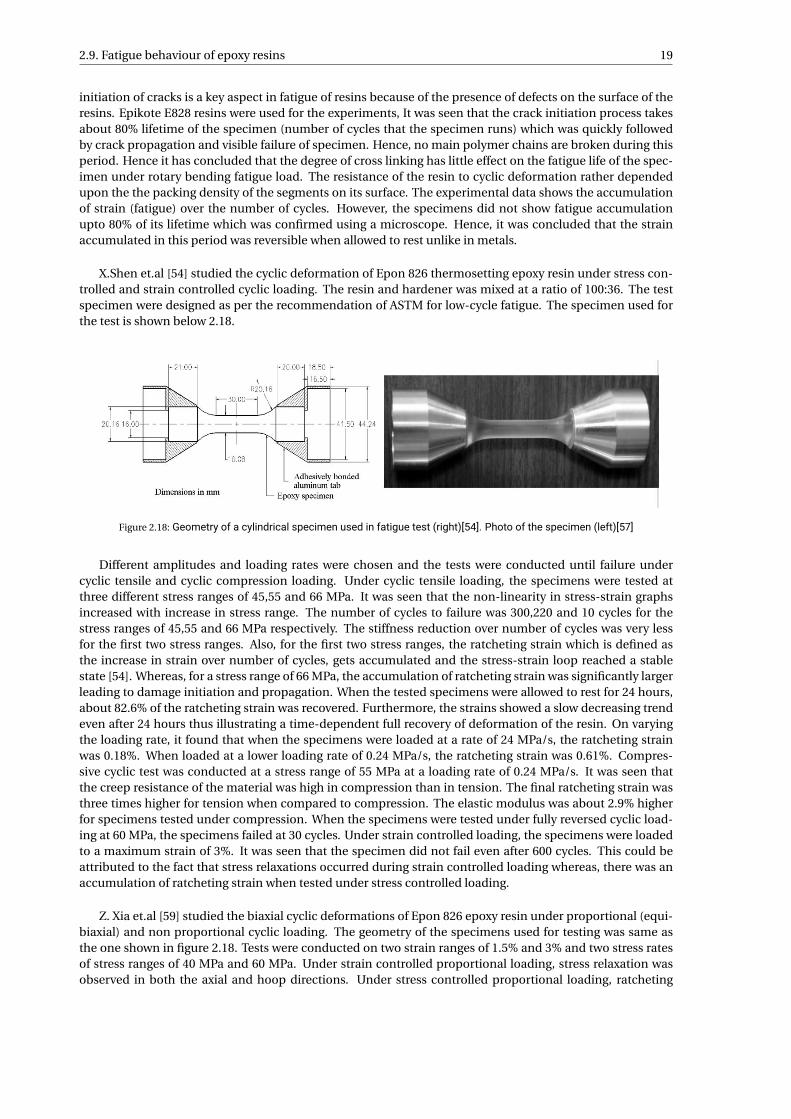
2.9. Fatigue behaviour of epoxy resins 19
initiation of cracks is a key aspect in fatigue of resins because of the presence of defects on the surface of theresins. Epikote E828 resins were used for the experiments, It was seen that the crack initiation process takesabout 80% lifetime of the specimen (number of cycles that the specimen runs) which was quickly followedby crack propagation and visible failure of specimen. Hence, no main polymer chains are broken during thisperiod. Hence it has concluded that the degree of cross linking has little effect on the fatigue life of the spec-imen under rotary bending fatigue load. The resistance of the resin to cyclic deformation rather dependedupon the the packing density of the segments on its surface. The experimental data shows the accumulationof strain (fatigue) over the number of cycles. However, the specimens did not show fatigue accumulationupto 80% of its lifetime which was confirmed using a microscope. Hence, it was concluded that the strainaccumulated in this period was reversible when allowed to rest unlike in metals.
X.Shen et.al [54] studied the cyclic deformation of Epon 826 thermosetting epoxy resin under stress con-trolled and strain controlled cyclic loading. The resin and hardener was mixed at a ratio of 100:36. The testspecimen were designed as per the recommendation of ASTM for low-cycle fatigue. The specimen used forthe test is shown below 2.18.
Figure 2.18: Geometry of a cylindrical specimen used in fatigue test (right)[54]. Photo of the specimen (left)[57]
Different amplitudes and loading rates were chosen and the tests were conducted until failure undercyclic tensile and cyclic compression loading. Under cyclic tensile loading, the specimens were tested atthree different stress ranges of 45,55 and 66 MPa. It was seen that the non-linearity in stress-strain graphsincreased with increase in stress range. The number of cycles to failure was 300,220 and 10 cycles for thestress ranges of 45,55 and 66 MPa respectively. The stiffness reduction over number of cycles was very lessfor the first two stress ranges. Also, for the first two stress ranges, the ratcheting strain which is defined asthe increase in strain over number of cycles, gets accumulated and the stress-strain loop reached a stablestate [54]. Whereas, for a stress range of 66 MPa, the accumulation of ratcheting strain was significantly largerleading to damage initiation and propagation. When the tested specimens were allowed to rest for 24 hours,about 82.6% of the ratcheting strain was recovered. Furthermore, the strains showed a slow decreasing trendeven after 24 hours thus illustrating a time-dependent full recovery of deformation of the resin. On varyingthe loading rate, it found that when the specimens were loaded at a rate of 24 MPa/s, the ratcheting strainwas 0.18%. When loaded at a lower loading rate of 0.24 MPa/s, the ratcheting strain was 0.61%. Compres-sive cyclic test was conducted at a stress range of 55 MPa at a loading rate of 0.24 MPa/s. It was seen thatthe creep resistance of the material was high in compression than in tension. The final ratcheting strain wasthree times higher for tension when compared to compression. The elastic modulus was about 2.9% higherfor specimens tested under compression. When the specimens were tested under fully reversed cyclic load-ing at 60 MPa, the specimens failed at 30 cycles. Under strain controlled loading, the specimens were loadedto a maximum strain of 3%. It was seen that the specimen did not fail even after 600 cycles. This could beattributed to the fact that stress relaxations occurred during strain controlled loading whereas, there was anaccumulation of ratcheting strain when tested under stress controlled loading.
Z. Xia et.al [59] studied the biaxial cyclic deformations of Epon 826 epoxy resin under proportional (equi-biaxial) and non proportional cyclic loading. The geometry of the specimens used for testing was same asthe one shown in figure 2.18. Tests were conducted on two strain ranges of 1.5% and 3% and two stress ratesof stress ranges of 40 MPa and 60 MPa. Under strain controlled proportional loading, stress relaxation wasobserved in both the axial and hoop directions. Under stress controlled proportional loading, ratcheting
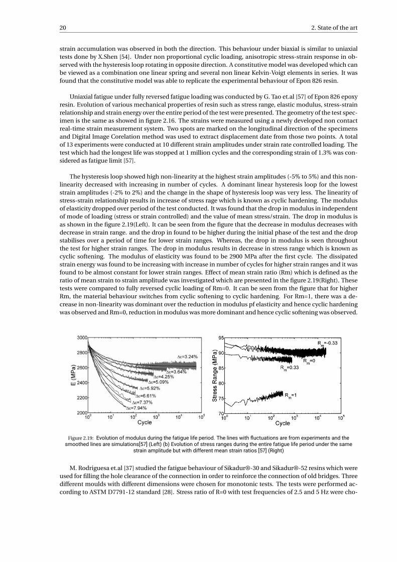
20 2. State of the art
strain accumulation was observed in both the direction. This behaviour under biaxial is similar to uniaxialtests done by X.Shen [54]. Under non proportional cyclic loading, anisotropic stress-strain response in ob-served with the hysteresis loop rotating in opposite direction. A constitutive model was developed which canbe viewed as a combination one linear spring and several non linear Kelvin-Voigt elements in series. It wasfound that the constitutive model was able to replicate the experimental behaviour of Epon 826 resin.
Uniaxial fatigue under fully reversed fatigue loading was conducted by G. Tao et.al [57] of Epon 826 epoxyresin. Evolution of various mechanical properties of resin such as stress range, elastic modulus, stress-strainrelationship and strain energy over the entire period of the test were presented. The geometry of the test spec-imen is the same as showed in figure 2.16. The strains were measured using a newly developed non contactreal-time strain measurement system. Two spots are marked on the longitudinal direction of the specimensand Digital Image Corelation method was used to extract displacement date from those two points. A totalof 13 experiments were conducted at 10 different strain amplitudes under strain rate controlled loading. Thetest which had the longest life was stopped at 1 million cycles and the corresponding strain of 1.3% was con-sidered as fatigue limit [57].
The hysteresis loop showed high non-linearity at the highest strain amplitudes (-5% to 5%) and this non-linearity decreased with increasing in number of cycles. A dominant linear hysteresis loop for the loweststrain amplitudes (-2% to 2%) and the change in the shape of hysteresis loop was very less. The linearity ofstress-strain relationship results in increase of stress rage which is known as cyclic hardening. The modulusof elasticity dropped over period of the test conducted. It was found that the drop in modulus in independentof mode of loading (stress or strain controlled) and the value of mean stress/strain. The drop in modulus isas shown in the figure 2.19(Left). It can be seen from the figure that the decrease in modulus decreases withdecrease in strain range. and the drop in found to be higher during the initial phase of the test and the dropstabilises over a period of time for lower strain ranges. Whereas, the drop in modulus is seen throughoutthe test for higher strain ranges. The drop in modulus results in decrease in stress range which is known ascyclic softening. The modulus of elasticity was found to be 2900 MPa after the first cycle. The dissipatedstrain energy was found to be increasing with increase in number of cycles for higher strain ranges and it wasfound to be almost constant for lower strain ranges. Effect of mean strain ratio (Rm) which is defined as theratio of mean strain to strain amplitude was investigated which are presented in the figure 2.19(Right). Thesetests were compared to fully reversed cyclic loading of Rm=0. It can be seen from the figure that for higherRm, the material behaviour switches from cyclic softening to cyclic hardening. For Rm=1, there was a de-crease in non-linearity was dominant over the reduction in modulus pf elasticity and hence cyclic hardeningwas observed and Rm=0, reduction in modulus was more dominant and hence cyclic softening was observed.
Figure 2.19: Evolution of modulus during the fatigue life period. The lines with fluctuations are from experiments and thesmoothed lines are simulations[57] (Left) (b) Evolution of stress ranges during the entire fatigue life period under the same
strain amplitude but with different mean strain ratios [57] (Right)
M. Rodriguesa et.al [37] studied the fatigue behaviour of Sikadur®-30 and Sikadur®-52 resins which wereused for filling the hole clearance of the connection in order to reinforce the connection of old bridges. Threedifferent moulds with different dimensions were chosen for monotonic tests. The tests were performed ac-cording to ASTM D7791-12 standard [28]. Stress ratio of R=0 with test frequencies of 2.5 and 5 Hz were cho-
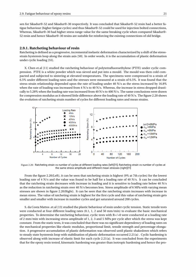
2.9. Fatigue behaviour of epoxy resins 21
sen for Sikadur®-52 and Sikadur®-30 respectively. It was concluded that Sikadur®-52 resin had a better fa-tigue behaviour (higher fatigue cycles) and thus Sikadur®-52 could be used for injection bolted connections,Whereas, Sikadur®-30 had higher stress range value for the same breaking cycle when compared Sikadur®-52 resin and hence Sikadur®-30 resins are suitable for reinforcing the existing connections of old bridge.
2.9.1. Ratcheting behaviour of resinRatcheting is defined as a progressive, incremental inelastic deformation characterized by a shift of the stress-strain hysteresis loop along the strain axis [50]. In order words, it is the accumulation of plastic deformationunder cyclic loading [55].
X. Chen et.al [11] studied the ratcheting behaviour of polytetrafluoroethylene (PTFE) under cyclic com-pression. PTFE is a white powder which was sieved and put into a mould. The mould was then cold com-pacted and subjected to sintering at elevated temperatures. The specimens were compressed to a strain of6.5% under different loading rates and the stresses were measured at a strain of 6.5%. It was found that thestress-strain relationship depended upon the rate of loading under 40 N/s as the stress increased by 16.8%when the rate of loading was increased from 4 N/s to 40 N/s. Whereas, the increase in stress dropped drasti-cally to 5.28% when the loading rate was increased from 40 N/s to 400 N/s. The same conclusions were drawnfor compression modulus as it showed little difference above the loading rate of 40 N/s. The figure 2.20 showsthe evolution of ratcheting strain number of cycles for different loading rates and mean strains.
Figure 2.20: Ratcheting strain vs number of cycles at different loading rates (left)[11]; Ratcheting strain vs number of cycles atthe same stress amplitude and different mean stresses (right)[11]
From the figure 2.20(Left), it can be seen that ratcheting strain is highest (9% at 7th cycles) for the lowestloading rate of 4 N/s and the value was found to be half for a loading rate of 40 N/s. It can be concludedthat the ratcheting strain decreases with increase in loading and it is sensitive to loading rate below 40 N/sas the reduction in ratcheting strain over 40 N/s becomes less. Stress amplitude of 6 MPa with varying meanstresses are shown in figure 2.20(Right). It can be seen that the ratcheting strain increases with increase inmean stress. The value of ratcheting strain is highest for the first cycle and this value of ratcheting strain getssmaller and smaller with increase in number cycles and get saturated around 200 cycles.
S. da Costa Mattos .et.al [13] studied the plastic behaviour of resin under cyclic tension. Static tensile testswere conducted at four different loading rates (0.1, 1, 2 and 50 mm/min) to evaluate the basic mechanicalproperties. To determine the ratcheting behaviour, cyclic tests with R=/=0 were conducted at a loading rateof 2 mm/min with increasing stress amplitude of 1, 2, 3 and 5 MPa per cycle after which the stress was keptconstant. From the static tests, it was concluded that there was no significant dependency of loading rates onthe mechanical properties like elastic modulus, proportional limit, tensile strength and percentage elonga-tion. A progressive accumulation of plastic deformation was observed until plastic shakedown which refersto steady state hysteresis loop with stabilisation of plastic deformation occurred 2.21(a) . Cyclic hardening isobserved along with increase of elastic limit for each cycle 2.21(a). It was concluded from the experimentsthat for the epoxy resin tested, kinematic hardening was greater than isotropic hardening and hence the pro-
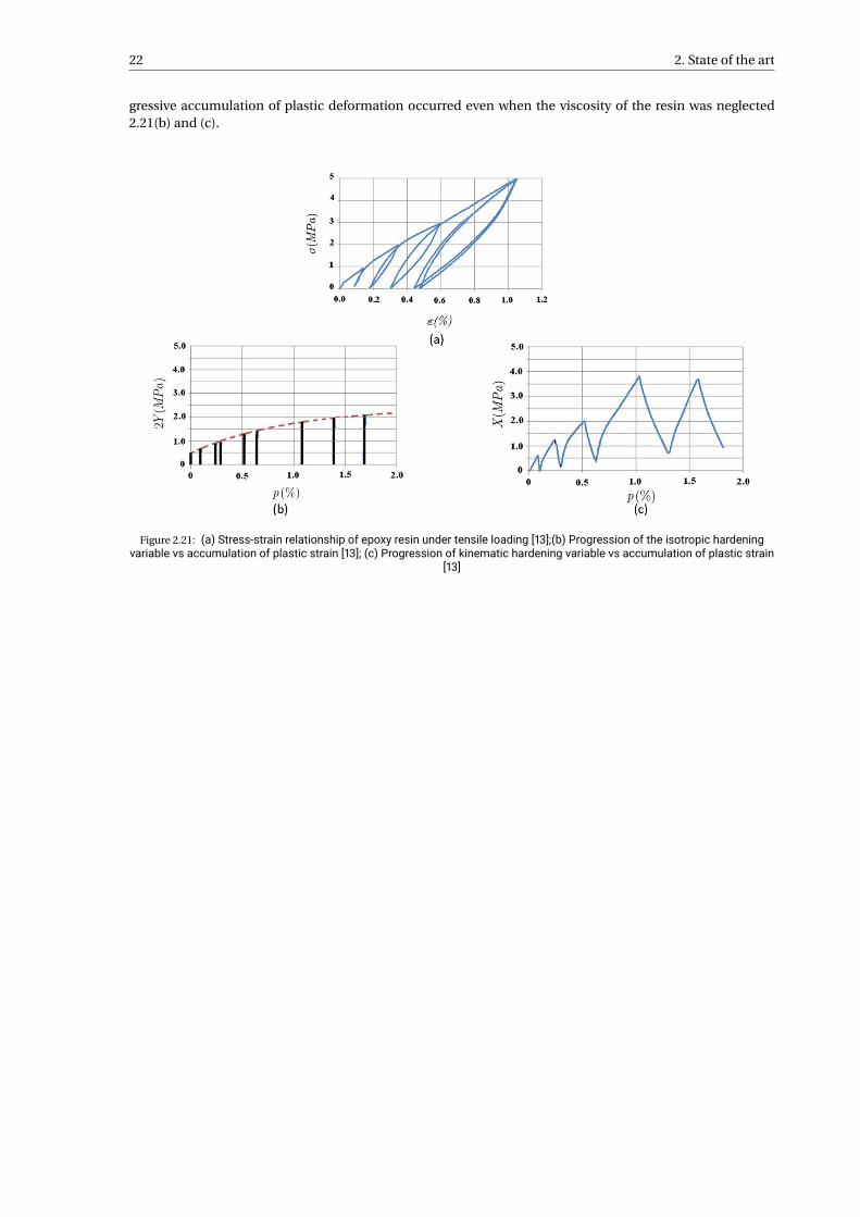
22 2. State of the art
gressive accumulation of plastic deformation occurred even when the viscosity of the resin was neglected2.21(b) and (c).
Figure 2.21: (a) Stress-strain relationship of epoxy resin under tensile loading [13];(b) Progression of the isotropic hardeningvariable vs accumulation of plastic strain [13]; (c) Progression of kinematic hardening variable vs accumulation of plastic strain
[13]
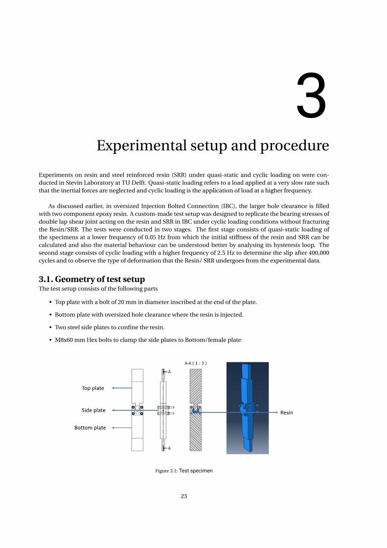
3Experimental setup and procedure
Experiments on resin and steel reinforced resin (SRR) under quasi-static and cyclic loading on were con-ducted in Stevin Laboratory at TU Delft. Quasi-static loading refers to a load applied at a very slow rate suchthat the inertial forces are neglected and cyclic loading is the application of load at a higher frequency.
As discussed earlier, in oversized Injection Bolted Connection (IBC), the larger hole clearance is filledwith two component epoxy resin. A custom-made test setup was designed to replicate the bearing stresses ofdouble lap shear joint acting on the resin and SRR in IBC under cyclic loading conditions without fracturingthe Resin/SRR. The tests were conducted in two stages. The first stage consists of quasi-static loading ofthe specimens at a lower frequency of 0.05 Hz from which the initial stiffness of the resin and SRR can becalculated and also the material behaviour can be understood better by analysing its hysteresis loop. Thesecond stage consists of cyclic loading with a higher frequency of 2.5 Hz to determine the slip after 400,000cycles and to observe the type of deformation that the Resin/ SRR undergoes from the experimental data.
3.1. Geometry of test setupThe test setup consists of the following parts
• Top plate with a bolt of 20 mm in diameter inscribed at the end of the plate.
• Bottom plate with oversized hole clearance where the resin is injected.
• Two steel side plates to confine the resin.
• M8x60 mm Hex bolts to clamp the side plates to Bottom/female plate
Figure 3.1: Test specimen
23
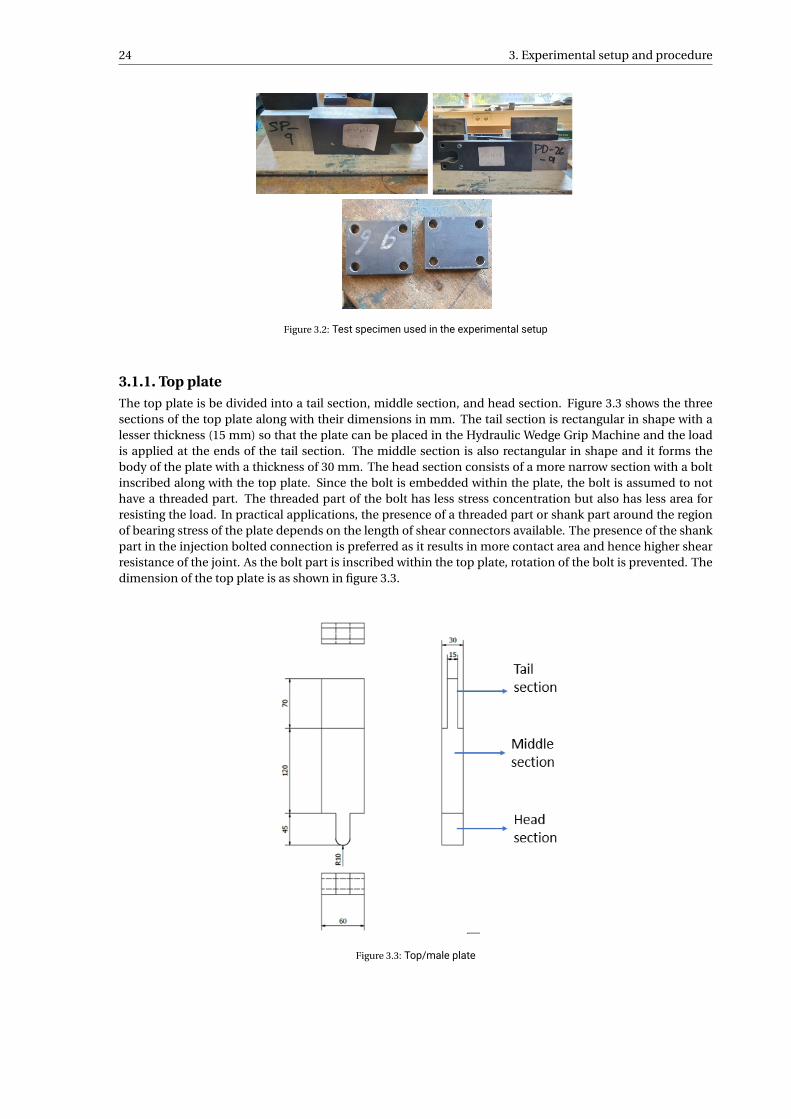
24 3. Experimental setup and procedure
Figure 3.2: Test specimen used in the experimental setup
3.1.1. Top plateThe top plate is be divided into a tail section, middle section, and head section. Figure 3.3 shows the threesections of the top plate along with their dimensions in mm. The tail section is rectangular in shape with alesser thickness (15 mm) so that the plate can be placed in the Hydraulic Wedge Grip Machine and the loadis applied at the ends of the tail section. The middle section is also rectangular in shape and it forms thebody of the plate with a thickness of 30 mm. The head section consists of a more narrow section with a boltinscribed along with the top plate. Since the bolt is embedded within the plate, the bolt is assumed to nothave a threaded part. The threaded part of the bolt has less stress concentration but also has less area forresisting the load. In practical applications, the presence of a threaded part or shank part around the regionof bearing stress of the plate depends on the length of shear connectors available. The presence of the shankpart in the injection bolted connection is preferred as it results in more contact area and hence higher shearresistance of the joint. As the bolt part is inscribed within the top plate, rotation of the bolt is prevented. Thedimension of the top plate is as shown in figure 3.3.
Figure 3.3: Top/male plate
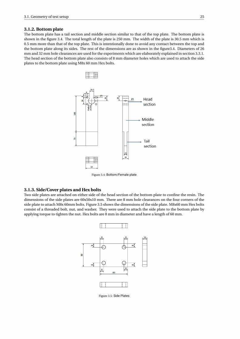
3.1. Geometry of test setup 25
3.1.2. Bottom plateThe bottom plate has a tail section and middle section similar to that of the top plate. The bottom plate isshown in the figure 3.4. The total length of the plate is 250 mm. The width of the plate is 30.5 mm which is0.5 mm more than that of the top plate. This is intentionally done to avoid any contact between the top andthe bottom plate along its sides. The rest of the dimensions are as shown in the figure3.4. Diameters of 26mm and 32 mm hole clearances are used for the experiments which are elaborately explained in section 3.3.1.The head section of the bottom plate also consists of 8 mm diameter holes which are used to attach the sideplates to the bottom plate using M8x 60 mm Hex bolts.
Figure 3.4: Bottom/Female plate
3.1.3. Side/Cover plates and Hex boltsTwo side plates are attached on either side of the head section of the bottom plate to confine the resin. Thedimensions of the side plates are 60x50x10 mm. There are 8 mm hole clearances on the four corners of theside plate to attach M8x 60mm bolts. Figure 3.5 shows the dimensions of the side plate. M8x60 mm Hex boltsconsist of a threaded bolt, nut, and washer. They were used to attach the side plate to the bottom plate byapplying torque to tighten the nut. Hex bolts are 8 mm in diameter and have a length of 60 mm.
Figure 3.5: Side Plates
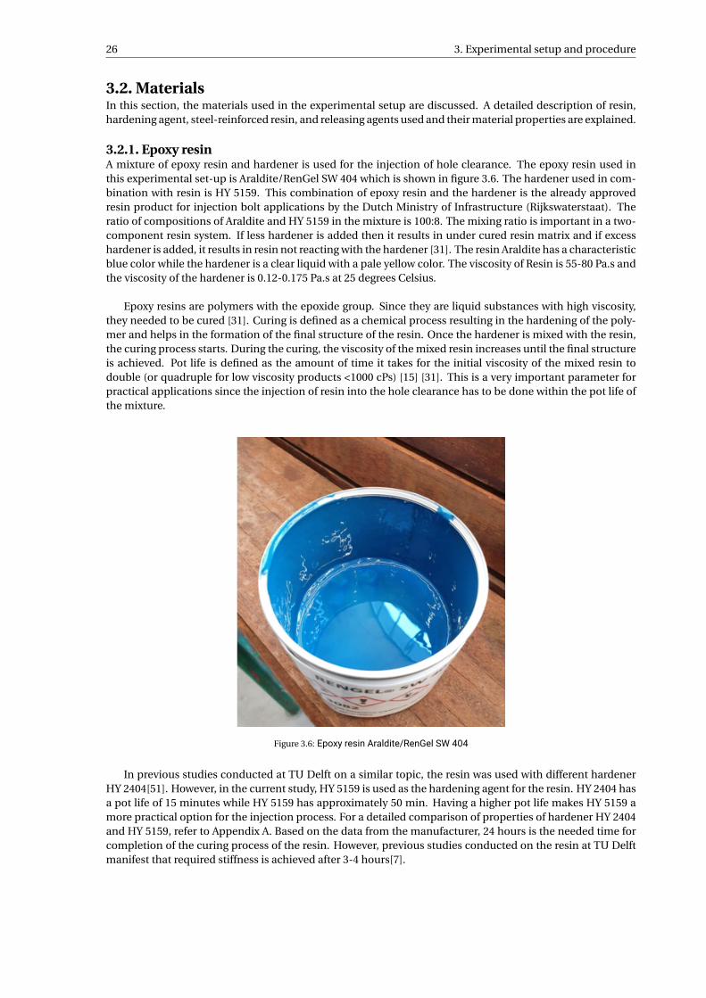
26 3. Experimental setup and procedure
3.2. MaterialsIn this section, the materials used in the experimental setup are discussed. A detailed description of resin,hardening agent, steel-reinforced resin, and releasing agents used and their material properties are explained.
3.2.1. Epoxy resinA mixture of epoxy resin and hardener is used for the injection of hole clearance. The epoxy resin used inthis experimental set-up is Araldite/RenGel SW 404 which is shown in figure 3.6. The hardener used in com-bination with resin is HY 5159. This combination of epoxy resin and the hardener is the already approvedresin product for injection bolt applications by the Dutch Ministry of Infrastructure (Rijkswaterstaat). Theratio of compositions of Araldite and HY 5159 in the mixture is 100:8. The mixing ratio is important in a two-component resin system. If less hardener is added then it results in under cured resin matrix and if excesshardener is added, it results in resin not reacting with the hardener [31]. The resin Araldite has a characteristicblue color while the hardener is a clear liquid with a pale yellow color. The viscosity of Resin is 55-80 Pa.s andthe viscosity of the hardener is 0.12-0.175 Pa.s at 25 degrees Celsius.
Epoxy resins are polymers with the epoxide group. Since they are liquid substances with high viscosity,they needed to be cured [31]. Curing is defined as a chemical process resulting in the hardening of the poly-mer and helps in the formation of the final structure of the resin. Once the hardener is mixed with the resin,the curing process starts. During the curing, the viscosity of the mixed resin increases until the final structureis achieved. Pot life is defined as the amount of time it takes for the initial viscosity of the mixed resin todouble (or quadruple for low viscosity products <1000 cPs) [15] [31]. This is a very important parameter forpractical applications since the injection of resin into the hole clearance has to be done within the pot life ofthe mixture.
Figure 3.6: Epoxy resin Araldite/RenGel SW 404
In previous studies conducted at TU Delft on a similar topic, the resin was used with different hardenerHY 2404[51]. However, in the current study, HY 5159 is used as the hardening agent for the resin. HY 2404 hasa pot life of 15 minutes while HY 5159 has approximately 50 min. Having a higher pot life makes HY 5159 amore practical option for the injection process. For a detailed comparison of properties of hardener HY 2404and HY 5159, refer to Appendix A. Based on the data from the manufacturer, 24 hours is the needed time forcompletion of the curing process of the resin. However, previous studies conducted on the resin at TU Delftmanifest that required stiffness is achieved after 3-4 hours[7].
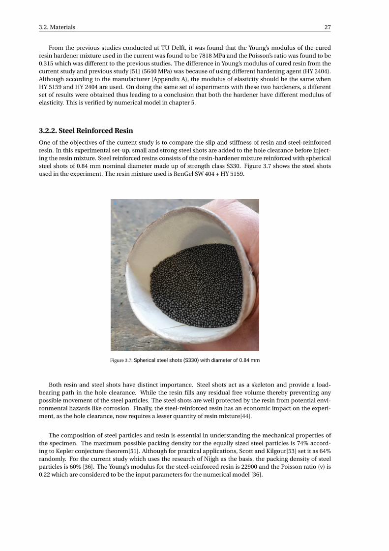
3.2. Materials 27
From the previous studies conducted at TU Delft, it was found that the Young’s modulus of the curedresin hardener mixture used in the current was found to be 7818 MPa and the Poisson’s ratio was found to be0.315 which was different to the previous studies. The difference in Young’s modulus of cured resin from thecurrent study and previous study [51] (5640 MPa) was because of using different hardening agent (HY 2404).Although according to the manufacturer (Appendix A), the modulus of elasticity should be the same whenHY 5159 and HY 2404 are used. On doing the same set of experiments with these two hardeners, a differentset of results were obtained thus leading to a conclusion that both the hardener have different modulus ofelasticity. This is verified by numerical model in chapter 5.
3.2.2. Steel Reinforced Resin
One of the objectives of the current study is to compare the slip and stiffness of resin and steel-reinforcedresin. In this experimental set-up, small and strong steel shots are added to the hole clearance before inject-ing the resin mixture. Steel reinforced resins consists of the resin-hardener mixture reinforced with sphericalsteel shots of 0.84 mm nominal diameter made up of strength class S330. Figure 3.7 shows the steel shotsused in the experiment. The resin mixture used is RenGel SW 404 + HY 5159.
Figure 3.7: Spherical steel shots (S330) with diameter of 0.84 mm
Both resin and steel shots have distinct importance. Steel shots act as a skeleton and provide a load-bearing path in the hole clearance. While the resin fills any residual free volume thereby preventing anypossible movement of the steel particles. The steel shots are well protected by the resin from potential envi-ronmental hazards like corrosion. Finally, the steel-reinforced resin has an economic impact on the experi-ment, as the hole clearance, now requires a lesser quantity of resin mixture[44].
The composition of steel particles and resin is essential in understanding the mechanical properties ofthe specimen. The maximum possible packing density for the equally sized steel particles is 74% accord-ing to Kepler conjecture theorem[51]. Although for practical applications, Scott and Kilgour[53] set it as 64%randomly. For the current study which uses the research of Nijgh as the basis, the packing density of steelparticles is 60% [36]. The Young’s modulus for the steel-reinforced resin is 22900 and the Poisson ratio (v) is0.22 which are considered to be the input parameters for the numerical model [36].
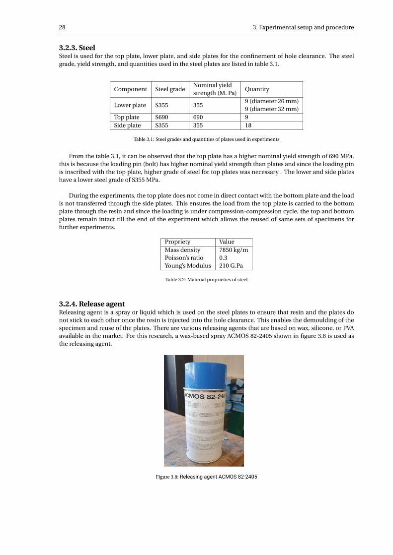
28 3. Experimental setup and procedure
3.2.3. SteelSteel is used for the top plate, lower plate, and side plates for the confinement of hole clearance. The steelgrade, yield strength, and quantities used in the steel plates are listed in table 3.1.
Component Steel gradeNominal yieldstrength (M. Pa)
Quantity
Lower plate S355 3559 (diameter 26 mm)9 (diameter 32 mm)
Top plate S690 690 9Side plate S355 355 18
Table 3.1: Steel grades and quantities of plates used in experiments
From the table 3.1, it can be observed that the top plate has a higher nominal yield strength of 690 MPa,this is because the loading pin (bolt) has higher nominal yield strength than plates and since the loading pinis inscribed with the top plate, higher grade of steel for top plates was necessary . The lower and side plateshave a lower steel grade of S355 MPa.
During the experiments, the top plate does not come in direct contact with the bottom plate and the loadis not transferred through the side plates. This ensures the load from the top plate is carried to the bottomplate through the resin and since the loading is under compression-compression cycle, the top and bottomplates remain intact till the end of the experiment which allows the reused of same sets of specimens forfurther experiments.
Propriety ValueMass density 7850 kg/mPoisson’s ratio 0.3Young’s Modulus 210 G.Pa
Table 3.2: Material proprieties of steel
3.2.4. Release agentReleasing agent is a spray or liquid which is used on the steel plates to ensure that resin and the plates donot stick to each other once the resin is injected into the hole clearance. This enables the demoulding of thespecimen and reuse of the plates. There are various releasing agents that are based on wax, silicone, or PVAavailable in the market. For this research, a wax-based spray ACMOS 82-2405 shown in figure 3.8 is used asthe releasing agent.
Figure 3.8: Releasing agent ACMOS 82-2405

3.3. Preparation of test specimen 29
3.3. Preparation of test specimenThis section describes the procedure followed in the preparation of the test specimens and the issues facedduring the preparation. The following are the procedures that were followed for the preparation of the testspecimen.
• Assembly of specimens
• Geometrical imperfections in the specimens
• Injection of steel reinforcements and resin
• Curing of resin
• Correction and finalisation of the specimen
3.3.1. Assembly of test specimensA support structure was designed to keep both the plate as straight as possible and to avoid any eccentricitiesin both horizontal and vertical planes during the preparation of specimens which could have a significantimpact on the test results. The support structure is placed on a flat level on the working platform. The topand bottom plates are aligned horizontally on a support structure. The bottom plate is placed such that thehole through which the air escapes is faced upwards. The support structure shown in figure 3.9 is L-shapedwith a flat base and a backrest on either end with a gap at the center to facilitate injection of resin.
Figure 3.9: Support structure for preparing the specimen
The top and bottom plates were placed on the flat base and were pushed against the backrest using aclamp. This arrangement proved to be vital to avoid any movement of the top and bottom plates during thepreparation stage of the specimen. Figure 3.10 show the misalignment that could occur if the specimen isplaced on the ground. In the figure, it can be seen that the bottom plate is not straightly aligned which couldgive inaccurate results.
The release agent ACMOS 82-2405 was sprayed on the head section top and bottom plates which are incontact with the resin. The top and bottom plates are assembled in such a way that the bolt which is em-bedded in the top plate is at the center position of the hole clearance. This results in a 3 mm gap betweenthe bolt and hole (hole clearance) for a bottom plate with a 26 mm diameter and a hole clearance of 6 mmfor a bottom plate with a diameter of 32 mm. By choosing these hole clearances, a comparison can be madebetween an oversize clearance which is barely 1 mm larger than the conventional hole clearance and to anoversize hole clearance which is substantially larger of about 3 to 4 mm than the conventional hole clearance.This is shown in figure 3.11
According to EN 1090-2 [21], the nominal hole clearance for a bolt diameter of 20 mm is 2 mm. In thisstudy, an attempt was made to study the behaviour of resin/SRR under larger hole clearance than the stan-dard value as higher hole clearance increases the ease of dismounting of the connection. The bottom plate
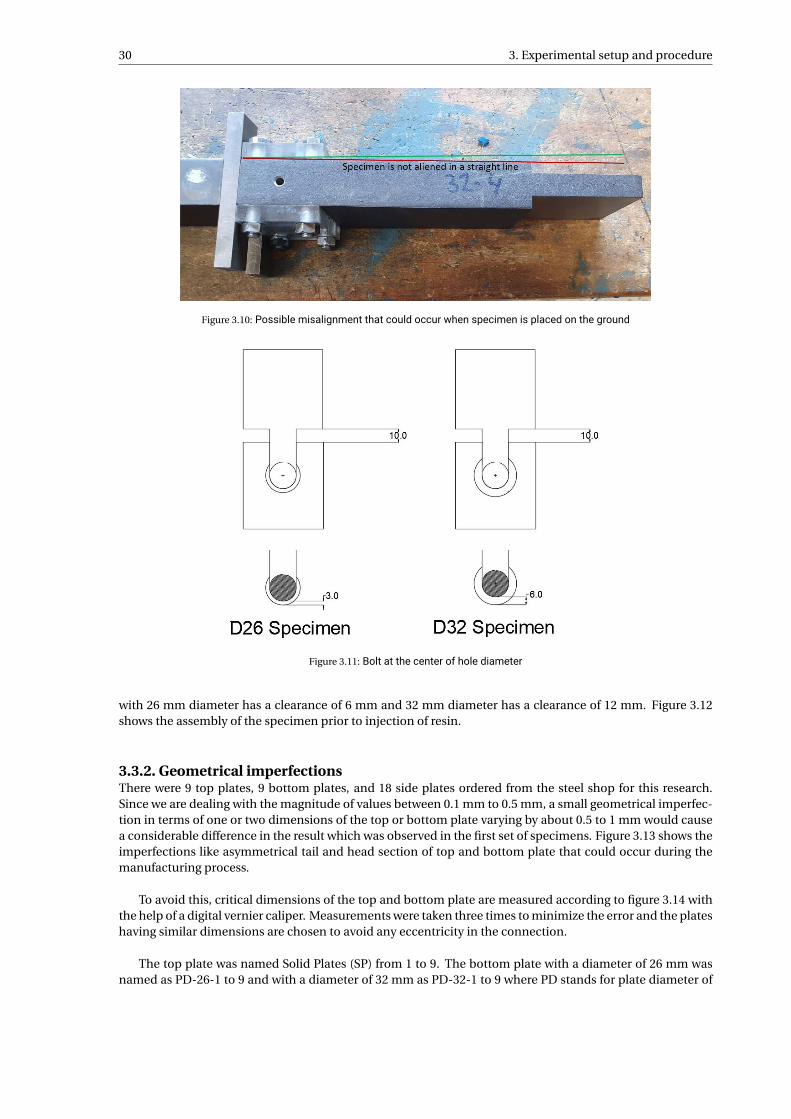
30 3. Experimental setup and procedure
Figure 3.10: Possible misalignment that could occur when specimen is placed on the ground
Figure 3.11: Bolt at the center of hole diameter
with 26 mm diameter has a clearance of 6 mm and 32 mm diameter has a clearance of 12 mm. Figure 3.12shows the assembly of the specimen prior to injection of resin.
3.3.2. Geometrical imperfectionsThere were 9 top plates, 9 bottom plates, and 18 side plates ordered from the steel shop for this research.Since we are dealing with the magnitude of values between 0.1 mm to 0.5 mm, a small geometrical imperfec-tion in terms of one or two dimensions of the top or bottom plate varying by about 0.5 to 1 mm would causea considerable difference in the result which was observed in the first set of specimens. Figure 3.13 shows theimperfections like asymmetrical tail and head section of top and bottom plate that could occur during themanufacturing process.
To avoid this, critical dimensions of the top and bottom plate are measured according to figure 3.14 withthe help of a digital vernier caliper. Measurements were taken three times to minimize the error and the plateshaving similar dimensions are chosen to avoid any eccentricity in the connection.
The top plate was named Solid Plates (SP) from 1 to 9. The bottom plate with a diameter of 26 mm wasnamed as PD-26-1 to 9 and with a diameter of 32 mm as PD-32-1 to 9 where PD stands for plate diameter of

3.3. Preparation of test specimen 31
Figure 3.12: Assembly of specimen before injecting resin
Figure 3.13: Geometrical imperfections due to manufacturing tolerances
Figure 3.14: Critical dimensions of top plate
32 3. Experimental setup and procedure
26 or 32 mm diameters and the specimen numbers. The top and bottom plates having similar measurementsto each other were matched and the same specimens were used to conduct all the tests.
3.3.3. Injection of resinOnce the plates are positioned horizontally such that the bolt is at the center of the hole clearance andclamped to the support structure, the resin has to be injected. For injecting the resin, two Perspex glassside plates were used. Perspex plates had the same dimension as that of the steel plates (60x50x10) and wereplaced on either side of the head region of the bottom plate to confine the resin. On the perspex side platewhich was placed on one side of the bottom plate, a hole of 5 mm in diameter was drilled on the bottom rightcorner such that the resin was injected directly into the hole clearance. On the perspex plate which was seton the other side of bottom plate, a hole of 1 mm diameter was drilled on the left top corner such that theresin overflow through the hole of 1 mm diameter once the entire hole clearance is filled up with resin.
These side plates were fixed to the bottom plate with the help of M8x60 mm bolts and tightened such thatthere was no possibility of any air gaps (voids) between the side plate and the head region of the top plate andthus resin is completely confined.
For specimens where only resin has to be injected, it can be done right away. For specimens with SteelReinforced Resin, steel shots are added before injecting the resin. Steel shots are added to the hole clearancethrough the air escape path of 5 mm diameter on top of the bottom plate with the help of a funnel and thesteel shots were compacted with a stick such that the entire hole clearance is occupied by the steel shots.
Figure 3.15: a.Injection of resin into the hole clearance. b. Indication of completely filled hole clearance
Steel shots must be added till the hole clearance (the gap between top and bottom plate) is covered by thesteel shots. The 5 mm diameter hole on one of the perspex plates is covered with clay till the hole clearanceis completely covered with the steel shots.
Resin RenGel SW 404 and hardener HY 5159 were weighed and then mixed using a stirrer. The mixture ispoured into a plastic tube with a nozzle of 4 mm diameter and the tube is closed with a cap and is assembledinto a handheld caulking gun.
The resin mixture is injected into the hole clearance through the perspex glass plate of 5 mm diameterwith the help of the caulking gun. The hole clearance is completely filled with resin when the resin overflowsthrough the 1 mm hole on the perspex plate on the other side and also through the air escape path on top ofthe bottom plate.
3.4. Testing of specimens 33
Injection of resin should be done at a slow pace to avoid any formation of voids (air gaps) within the holeclearance as it would lead to incorrect results. Once the hole clearance is completely filled with resin, a 5 mmhole on the side plate was closed using artificial clay. The specimens were allowed to cure for about 24 hoursbefore removing the perspex glass side plates.
3.3.4. Correction and finalization of specimenAfter 24 hours of curing, the perspex glass side plates were removed. If the resin does not cover the entire holeclearance as shown in figure 3.16a, the resin mixture is added around the region where the resin is missingand the excess resin is skimmed off to form a smooth and uniform surface as shown in figure 3.16b.This isallowed to cure for 3 to 4 hours as the strength and stiffness are obtained within that time.
Figure 3.16: a. Hole clearance not completely filled by resin b. Further addition of resin into the hole clearance
Once the hole clearance is completely covered by the resin without any imperfection, metal side platesare attached on either side of the head region of the bottom plates. The specimens are named and kept fortesting. This marks the end of the preparation stage of the specimens and the specimens can be tested asshown in figure 3.17
Figure 3.17: Completed specimen ready to be tested
3.4. Testing of specimensHydraulic Wedge Grip Machine in Stevin Laboratory at TU Delft was used to test the specimens in quasi-staticand cyclic loading conditions. Tests are conducted to evaluate the initial stiffness of the joint in quasi-staticloading, the slip obtained in cyclic loading, and the deformation of resin and steel-reinforced resin during the
34 3. Experimental setup and procedure
cyclic loading. Two LVDTs (Linear Variable Displacement Transducers), one on the sides of the top plate andone on the sides of the bottom plate were positioned using a quick setting strong glue to measure the relativedisplacements of the top and bottom plates (slip).
The specimens were placed vertically such that the lower end of the bottom plate is clamped by the lowerwedge and the force is applied by the upper wedge on the upper end of the top plate as shown in figure 3.18a.
3.4.1. Loading method and controlThe specimens were tested under constant amplitude compression loading, i.e the stress ratio (R =σmi n/σmax )< 1 (for example, R= -10/-100= 0.1 < 1). In a double lap shear connection of injection bolted connections, theresin is always under compression as shown in figure 3.19 and hence the resin is tested under pure compres-sion.
Figure 3.18: a. Testing of specimen in Hydraulic Wedge Grip Machine. b. Schematic representation of Hydraulic Wedge GripMachine [51]
This test setup enables the transfer of forces from the top plate through the resin to the bottom plate.This allows the resin to act as a load bearing component. However, the resin cannot be tested in tension asit would lead to separation of the top and bottom plate. This setup also facilitates the resin/SRR to be testedunder cyclic loading without the formation of cracks as top and bottom plate do not come in direct contactwith each other.
Figure 3.19: Stress distribution on resin in double lap shear joint in IBCs
3.4. Testing of specimens 35
Force-controlled loading mode was adapted to test the specimens on the hydraulic wedge grip machine.Displacement controlled loading is used for static loading to represent the failure of the specimens. However,here the focus was on the behaviour of resin and steel-reinforced resin under cyclic loading. Hence undercyclic loading, it is important to control the stress applied.
3.4.2. Stress rangeIn this research, specimens are tested for three different bearing stress ranges (Table ) to determine the slipat the given stress range. The long term bearing stress of the resin was taken as fb,r esi n,LT = 200 MPa [24].Stress ranges (∆σ=σmax −σmi n) of 100, 150 and 200 MPa were adopted for testing of the specimen. Since theloading of the specimen is done using the force-controlled setting, these bearing stresses have to be convertedinto equivalent force and it can be done using the following formula.
σb = Fb
db .tp(3.1)
Where σb is Equivalent bearing stress [N /mm2], Fb is external load [N], db is bolt diameter [mm] tp isthickness of the plate [mm].
Max bearing stress(σmax ) MPa
Min bearing stress(σmi n) MPa
Stress range(∆σ) MPa
Fmax
KNFmi n
KNR =σmi n/σmax
125 25 100 75 15 0.2175 25 150 105 15 0.14225 25 200 135 15 0.11
Table 3.3: Stress ranges adapted for testing the specimens
The value of R=0 which relates to minimum nominal bearing stress being 0 is avoided as any small errorin the machine would results in a tensile force on the specimens which would result in separation of top andbottom plates.
3.4.3. Naming of specimens and number of testsThere are two different hole diameters (26 mm and 32 mm), two different types of injection material (Resinand Steel Reinforced Resin), three different stress ranges, it was important to have a different name for eachspecimen so that it becomes easy to identify the results from each specimen. The name of the specimen startswith the date on which it was made, followed by if the specimens injected with resin (R) or steel-reinforcedresin (SRR), followed by the hole diameter (D26 or D32), followed by the stress range (100, 150 or 200 MPa)and finally by the specimen number (1,2 or 3).
Injectionmaterial
Nominal holeclearance (mm)
Nominal bearingstress range (MPa)
No of specimens
Resin
26100 3150 3200 3
32100 3150 3200 3
SRR
26100 3150 3200 3
32100 3150 3200 3
Total= 36
Table 3.4: Number of specimens tested
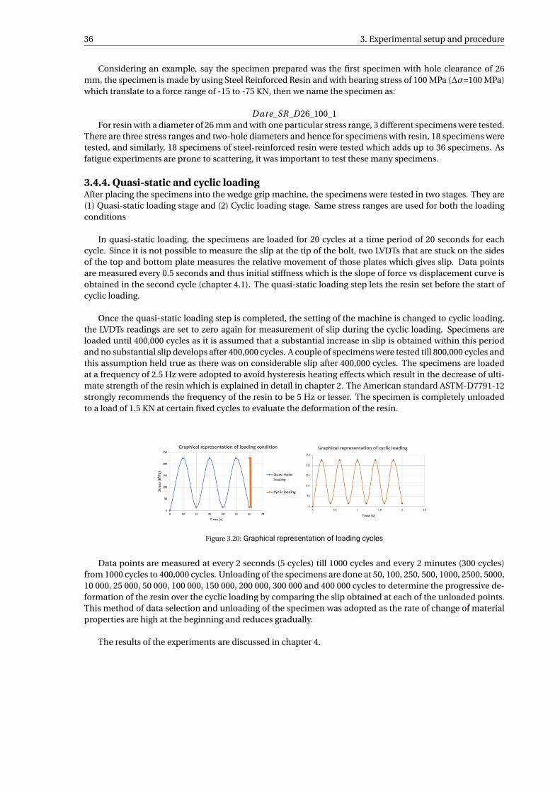
36 3. Experimental setup and procedure
Considering an example, say the specimen prepared was the first specimen with hole clearance of 26mm, the specimen is made by using Steel Reinforced Resin and with bearing stress of 100 MPa (∆σ=100 MPa)which translate to a force range of -15 to -75 KN, then we name the specimen as:
Date_SR_D26_100_1For resin with a diameter of 26 mm and with one particular stress range, 3 different specimens were tested.
There are three stress ranges and two-hole diameters and hence for specimens with resin, 18 specimens weretested, and similarly, 18 specimens of steel-reinforced resin were tested which adds up to 36 specimens. Asfatigue experiments are prone to scattering, it was important to test these many specimens.
3.4.4. Quasi-static and cyclic loadingAfter placing the specimens into the wedge grip machine, the specimens were tested in two stages. They are(1) Quasi-static loading stage and (2) Cyclic loading stage. Same stress ranges are used for both the loadingconditions
In quasi-static loading, the specimens are loaded for 20 cycles at a time period of 20 seconds for eachcycle. Since it is not possible to measure the slip at the tip of the bolt, two LVDTs that are stuck on the sidesof the top and bottom plate measures the relative movement of those plates which gives slip. Data pointsare measured every 0.5 seconds and thus initial stiffness which is the slope of force vs displacement curve isobtained in the second cycle (chapter 4.1). The quasi-static loading step lets the resin set before the start ofcyclic loading.
Once the quasi-static loading step is completed, the setting of the machine is changed to cyclic loading,the LVDTs readings are set to zero again for measurement of slip during the cyclic loading. Specimens areloaded until 400,000 cycles as it is assumed that a substantial increase in slip is obtained within this periodand no substantial slip develops after 400,000 cycles. A couple of specimens were tested till 800,000 cycles andthis assumption held true as there was on considerable slip after 400,000 cycles. The specimens are loadedat a frequency of 2.5 Hz were adopted to avoid hysteresis heating effects which result in the decrease of ulti-mate strength of the resin which is explained in detail in chapter 2. The American standard ASTM-D7791-12strongly recommends the frequency of the resin to be 5 Hz or lesser. The specimen is completely unloadedto a load of 1.5 KN at certain fixed cycles to evaluate the deformation of the resin.
Figure 3.20: Graphical representation of loading cycles
Data points are measured at every 2 seconds (5 cycles) till 1000 cycles and every 2 minutes (300 cycles)from 1000 cycles to 400,000 cycles. Unloading of the specimens are done at 50, 100, 250, 500, 1000, 2500, 5000,10 000, 25 000, 50 000, 100 000, 150 000, 200 000, 300 000 and 400 000 cycles to determine the progressive de-formation of the resin over the cyclic loading by comparing the slip obtained at each of the unloaded points.This method of data selection and unloading of the specimen was adopted as the rate of change of materialproperties are high at the beginning and reduces gradually.
The results of the experiments are discussed in chapter 4.
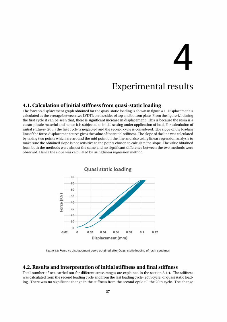
4Experimental results
4.1. Calculation of initial stiffness from quasi-static loadingThe force vs displacement graph obtained for the quasi static loading is shown in figure 4.1. Displacement iscalculated as the average between two LVDT’s on the sides of top and bottom plate. From the figure 4.1 duringthe first cycle it can be seen that, there is significant increase in displacement. This is because the resin is aelasto-plastic material and hence it is subjected to initial setting under application of load. For calculation ofinitial stiffness (Ki ni ) the first cycle is neglected and the second cycle is considered. The slope of the loadingline of the force-displacement curve gives the value of the initial stiffness. The slope of the line was calculatedby taking two points which are around the mid point on the line and also using linear regression analysis tomake sure the obtained slope is not sensitive to the points chosen to calculate the slope. The value obtainedfrom both the methods were almost the same and no significant difference between the two methods wereobserved. Hence the slope was calculated by using linear regression method.
Figure 4.1: Force vs displacement curve obtained after Quasi static loading of resin specimen
4.2. Results and interpretation of initial stiffness and final stiffnessTotal number of test carried out for different stress ranges are explained in the section 3.4.4. The stiffnesswas calculated from the second loading cycle and from the last loading cycle (20th cycle) of quasi static load-ing. There was no significant change in the stiffness from the second cycle till the 20th cycle. The change
37
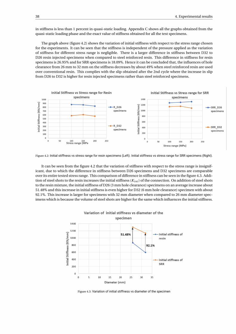
38 4. Experimental results
in stiffness is less than 1 percent in quasi-static loading. Appendix C shows all the graphs obtained from thequasi-static loading phase and the exact value of stiffness obtained for all the test specimens.
The graph above (figure 4.2) shows the variation of initial stiffness with respect to the stress range chosenfor the experiments. It can be seen that the stiffness is independent of the pressure applied as the variationof stiffness for different stress range is negligible. There is a larger difference in stiffness between D32 toD26 resin injected specimens when compared to steel reinforced resin. This difference in stiffness for resinspecimens is 26.95% and for SRR specimens is 18.09%. Hence it can be concluded that, the influences of holeclearance from 26 mm to 32 mm on the stiffness decreases by about 49% when steel reinforced resin are usedover conventional resin. This complies with the slip obtained after the 2nd cycle where the increase in slipfrom D26 to D32 is higher for resin injected specimens rather than steel reinforced specimens.
Figure 4.2: Initial stiffness vs stress range for resin specimens (Left). Initial stiffness vs stress range for SRR specimens (Right).
It can be seen from the figure 4.2 that the variation of stiffness with respect to the stress range is insignif-icant, due to which the difference in stiffness between D26 specimens and D32 specimens are comparableover its entire tested stress range. This comparison of difference in stiffness can be seen in the figure 4.3. Addi-tion of steel shots to the resin increases the initial stiffness (Ki ni ) of the connection. On addition of steel shotsto the resin mixture, the initial stiffness of D26 (3 mm hole clearance) specimens on an average increase about51.48% and this increase in initial stiffness is even higher for D32 (6 mm hole clearance) specimen with about92.1%. This increase is larger for specimens with 32 mm diameter when compared to 26 mm diameter spec-imens which is because the volume of steel shots are higher for the same which influences the initial stiffness.
Figure 4.3: Variation of initial stiffness vs diameter of the specimen
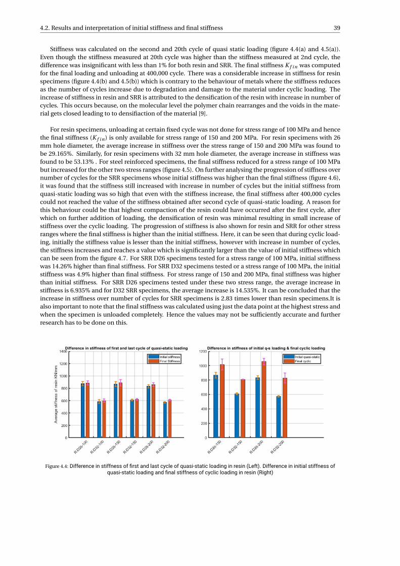
4.2. Results and interpretation of initial stiffness and final stiffness 39
Stiffness was calculated on the second and 20th cycle of quasi static loading (figure 4.4(a) and 4.5(a)).Even though the stiffness measured at 20th cycle was higher than the stiffness measured at 2nd cycle, thedifference was insignificant with less than 1% for both resin and SRR. The final stiffness K f i n was computedfor the final loading and unloading at 400,000 cycle. There was a considerable increase in stiffness for resinspecimens (figure 4.4(b) and 4.5(b)) which is contrary to the behaviour of metals where the stiffness reducesas the number of cycles increase due to degradation and damage to the material under cyclic loading. Theincrease of stiffness in resin and SRR is attributed to the densification of the resin with increase in number ofcycles. This occurs because, on the molecular level the polymer chain rearranges and the voids in the mate-rial gets closed leading to to densifiaction of the material [9].
For resin specimens, unloading at certain fixed cycle was not done for stress range of 100 MPa and hencethe final stiffness (K f i n) is only available for stress range of 150 and 200 MPa. For resin specimens with 26mm hole diameter, the average increase in stiffness over the stress range of 150 and 200 MPa was found tobe 29.165%. Similarly, for resin specimens with 32 mm hole diameter, the average increase in stiffness wasfound to be 53.13% . For steel reinforced specimens, the final stiffness reduced for a stress range of 100 MPabut increased for the other two stress ranges (figure 4.5). On further analysing the progression of stiffness overnumber of cycles for the SRR specimens whose initial stiffness was higher than the final stiffness (figure 4.6),it was found that the stiffness still increased with increase in number of cycles but the initial stiffness fromquasi-static loading was so high that even with the stiffness increase, the final stiffness after 400,000 cyclescould not reached the value of the stiffness obtained after second cycle of quasi-static loading. A reason forthis behaviour could be that highest compaction of the resin could have occurred after the first cycle, afterwhich on further addition of loading, the densification of resin was minimal resulting in small increase ofstiffness over the cyclic loading. The progression of stiffness is also shown for resin and SRR for other stressranges where the final stiffness is higher than the initial stiffness. Here, it can be seen that during cyclic load-ing, initially the stiffness value is lesser than the initial stiffness, however with increase in number of cycles,the stiffness increases and reaches a value which is significantly larger than the value of initial stiffness whichcan be seen from the figure 4.7. For SRR D26 specimens tested for a stress range of 100 MPa, initial stiffnesswas 14.26% higher than final stiffness. For SRR D32 specimens tested or a stress range of 100 MPa, the initialstiffness was 4.9% higher than final stiffness. For stress range of 150 and 200 MPa, final stiffness was higherthan initial stiffness. For SRR D26 specimens tested under these two stress range, the average increase instiffness is 6.935% and for D32 SRR specimens, the average increase is 14.535%. It can be concluded that theincrease in stiffness over number of cycles for SRR specimens is 2.83 times lower than resin specimens.It isalso important to note that the final stiffness was calculated using just the data point at the highest stress andwhen the specimen is unloaded completely. Hence the values may not be sufficiently accurate and furtherresearch has to be done on this.
Figure 4.4: Difference in stiffness of first and last cycle of quasi-static loading in resin (Left). Difference in initial stiffness ofquasi-static loading and final stiffness of cyclic loading in resin (Right)
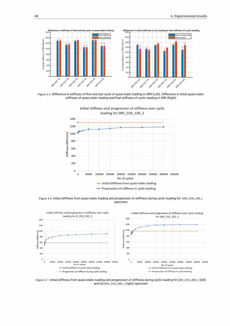
40 4. Experimental results
Figure 4.5: Difference in stiffness of first and last cycle of quasi-static loading in SRR (Left). Difference in initial quasi-staticstiffness of quasi-static loading and final stiffness of cyclic loading in SRR (Right)
Figure 4.6: Initial stiffness from quasi-static loading and progression of stiffness during cyclic loading for SRR_D26_100_1specimen
Figure 4.7: Initial stiffness from quasi-static loading and progression of stiffness during cyclic loading for (i)R_D32_200_1 (left)and (ii)SRR_D32_200_1 (right) specimen
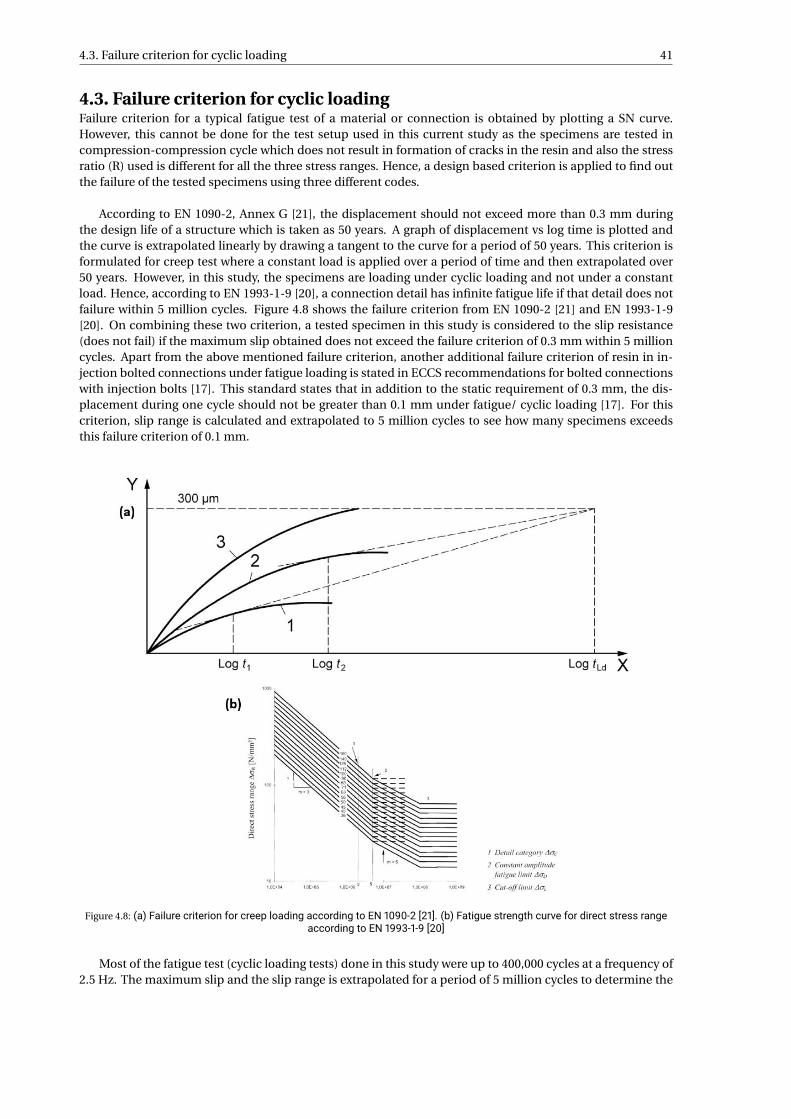
4.3. Failure criterion for cyclic loading 41
4.3. Failure criterion for cyclic loadingFailure criterion for a typical fatigue test of a material or connection is obtained by plotting a SN curve.However, this cannot be done for the test setup used in this current study as the specimens are tested incompression-compression cycle which does not result in formation of cracks in the resin and also the stressratio (R) used is different for all the three stress ranges. Hence, a design based criterion is applied to find outthe failure of the tested specimens using three different codes.
According to EN 1090-2, Annex G [21], the displacement should not exceed more than 0.3 mm duringthe design life of a structure which is taken as 50 years. A graph of displacement vs log time is plotted andthe curve is extrapolated linearly by drawing a tangent to the curve for a period of 50 years. This criterion isformulated for creep test where a constant load is applied over a period of time and then extrapolated over50 years. However, in this study, the specimens are loading under cyclic loading and not under a constantload. Hence, according to EN 1993-1-9 [20], a connection detail has infinite fatigue life if that detail does notfailure within 5 million cycles. Figure 4.8 shows the failure criterion from EN 1090-2 [21] and EN 1993-1-9[20]. On combining these two criterion, a tested specimen in this study is considered to the slip resistance(does not fail) if the maximum slip obtained does not exceed the failure criterion of 0.3 mm within 5 millioncycles. Apart from the above mentioned failure criterion, another additional failure criterion of resin in in-jection bolted connections under fatigue loading is stated in ECCS recommendations for bolted connectionswith injection bolts [17]. This standard states that in addition to the static requirement of 0.3 mm, the dis-placement during one cycle should not be greater than 0.1 mm under fatigue/ cyclic loading [17]. For thiscriterion, slip range is calculated and extrapolated to 5 million cycles to see how many specimens exceedsthis failure criterion of 0.1 mm.
Figure 4.8: (a) Failure criterion for creep loading according to EN 1090-2 [21]. (b) Fatigue strength curve for direct stress rangeaccording to EN 1993-1-9 [20]
Most of the fatigue test (cyclic loading tests) done in this study were up to 400,000 cycles at a frequency of2.5 Hz. The maximum slip and the slip range is extrapolated for a period of 5 million cycles to determine the
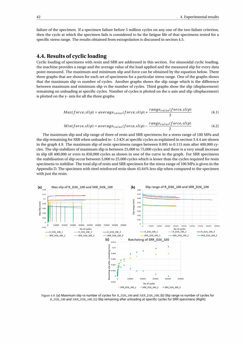
42 4. Experimental results
failure of the specimen. If a specimen failure before 5 million cycles on any one of the two failure criterion,then the cycle at which the specimen fails is considered to be the fatigue life of that specimens tested for aspecific stress range. The results obtained from extrapolation is discussed in section 4.5.
4.4. Results of cyclic loadingCyclic loading of specimens with resin and SRR are addressed in this section. For sinusoidal cyclic loading,the machine provides a range and the average value of the load applied and the measured slip for every datapoint measured. The maximum and minimum slip and force can be obtained by the equation below. Therethree graphs that are shown for each set of specimens for a particular stress range. One of the graphs showsthat the maximum slip vs number of cycles. Another graphs shows the slip range which is the differencebetween maximum and minimum slip vs the number of cycles. Third graphs show the slip (displacement)remaining on unloading at specific cycles. Number of cycles is plotted on the x-axis and slip (displacement)is plotted on the y- axis for all the three graphs.
M ax( f or ce, sl i p) = aver ag ev a l u e ( f or ce, sl i p)+ r ang ev a l u e ( f or ce, sl i p)
2(4.1)
Mi n( f or ce, sl i p) = aver ag ev a l u e ( f or ce, sl i p)− r ang ev a l u e ( f or ce, sl i p)
2(4.2)
The maximum slip and slip range of three of resin and SRR specimens for a stress range of 100 MPa andthe slip remaining for SRR when unloaded to -1.5 KN at specific cycles as explained in section 3.4.4 are shownin the graph 4.9. The maximum slip of resin specimens ranges between 0.095 to 0.115 mm after 400,000 cy-cles. The slip stabilizes of maximum slip is between 25,000 to 75,000 cycles and there is a very small increasein slip till 400,000 or even to 850,000 cycles as shown in one of the curve in the graph. For SRR specimensthe stabilisation of slip occur between 5,000 to 25,000 cycles which is lesser than the cycles required for resinspecimens to stabilise. The total slip of resin and SRR specimen for the stress range of 100 MPa is given in theAppendix D. The specimen with steel reinforced resin show 45.64% less slip when compared to the specimenwith just the resin.
Figure 4.9: (a) Maximum slip vs number of cycles for R_D26_100 and SRR_D26_100; (b) Slip range vs number of cycles forR_D26_100 and SRR_D26_100; (c) Slip remaining after unloading at specific cycles for SRR specimens (Right)
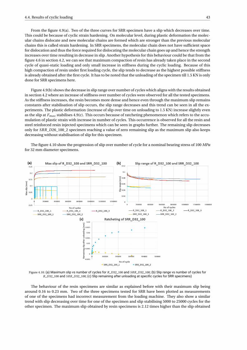
4.4. Results of cyclic loading 43
From the figure 4.9(a). Two of the three curves for SRR specimen have a slip which decreases over time.This could be because of cyclic strain hardening. On molecular level, during plastic deformation the molec-ular chains dislocate and new molecular chains are formed which are stronger than the previous molecularchains this is called strain hardening. In SRR specimens, the molecular chain does not have sufficient spacefor dislocation and thus the force required for dislocating the molecular chain goes up and hence the strengthincreases over time resulting in decrease in slip. Another hypothesis for this behaviour could be that from thefigure 4.6 in section 4.2, we can see that maximum compaction of resin has already taken place in the secondcycle of quasi-static loading and only small increase in stiffness during the cyclic loading. Because of thishigh compaction of resin under first loading cycle, the slip tends to decrease as the highest possible stiffnessis already obtained after the first cycle. It has to be noted that the unloading of the specimen till 1.5 KN is onlydone for SRR specimens here.
Figure 4.9(b) shows the decrease in slip range over number of cycles which aligns with the results obtainedin section 4.2 where an increase of stiffness over number of cycles were observed for all the tested specimens.As the stiffness increases, the resin becomes more dense and hence even through the maximum slip remainsconstants after stabilisation of slip occurs, the slip range decreases and this trend can be seen in all the ex-periments. The plastic deformation (increase of slip over time on unloading to 1.5 KN) increase slightly evenas the slip at Fmax stabilises 4.9(c). This occurs because of ratcheting phenomenon which refers to the accu-mulation of plastic strain with increase in number of cycles. This occurrence is observed for all the resin andsteel reinforced resin injected specimens which can be seen in graphs further. The remaining slip decreasesonly for SRR_D26_100_2 specimen reaching a value of zero remaining slip as the maximum slip also keepsdecreasing without stabilisation of slip for this specimen.
The figure 4.10 show the progression of slip over number of cycle for a nominal bearing stress of 100 MPafor 32 mm diameter specimens.
Figure 4.10: (a) Maximum slip vs number of cycles for R_D32_100 and SRR_D32_100; (b) Slip range vs number of cycles forR_D32_100 and SRR_D32_100; (c) Slip remaining after unloading at specific cycles for SRR specimens)
The behaviour of the resin specimens are similar as explained before with their maximum slip beingaround 0.16 to 0.23 mm. Two of the three specimens tested for SRR have been plotted as measurementsof one of the specimens had incorrect measurement from the loading machine. They also show a similartrend with slip decreasing over time for one of the specimen and slip stabilising 5000 to 25000 cycles for theother specimen. The maximum slip obtained by resin specimens is 2.12 times higher than the slip obtained
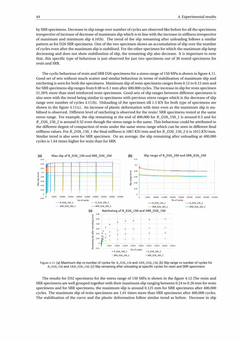
44 4. Experimental results
by SRR specimens. Decrease in slip range over number of cycles are observed like before for all the specimensirrespective of increase of decrease of maximum slip which is in line with the increase in stiffness irrespectiveof maximum and minimum slip 4.10(b). The trend of the slip remaining after unloading follows a similarpattern as for D26 SRR specimens. One of the two specimen shows an accumulation of slip over the numberof cycles even after the maximum slip is stabilised. For the other specimen for which the maximum slip keepdecreasing and does not show stabilisation of slip, the remaining slip also decrease. It is important to notethat, this specific type of behaviour is just observed for just two specimens out of 36 tested specimens forresin and SRR.
The cyclic behaviour of resin and SRR D26 specimens for a stress range of 150 MPa is shown in figure 4.11.Good set of sets without much scatter and similar behaviour in terms of stabilisation of maximum slip andratcheting is seen for both the specimens. Maximum slip of resin specimens ranges from 0.12 to 0.15 mm andfor SRR specimens slip ranges from 0.08 to 0.1 mm after 400,000 cycles. The increase in slip for resin specimen31.26% more than steel reinforced resin specimens. Good sets of slip ranges between different specimens isalso seen with the trend being similar to specimens with previous stress ranges which is the decrease of sliprange over number of cycles 4.11(b). Unloading of the specimen till 1.5 KN for both type of specimens areshown in the figure 4.11(c). An increase of plastic deformation with time even as the maximum slip is sta-bilised is observed. Different level of ratcheting is observed for the resin/ SRR specimens tested at the samestress range. For example, the slip remaining at the end of 400,000 for R_D26_150_1 is around 0.5 and forR_D26_150_2 is around 0.32 even though the stress range is the same. This behaviour could be attributed tothe different degree of compaction of resin under the same stress range which can be seen in different finalstiffness values. For R_D26_150_1 the final stiffness is 1067 KN/mm and for R_D26_150_2 it is 1015 KN/mm.Similar trend is also seen for SRR specimen. On an average, the slip remaining after unloading at 400,000cycles is 1.64 times higher for resin than for SRR.
Figure 4.11: (a) Maximum slip vs number of cycles for R_D26_150 and SRR_D26_150; (b) Slip range vs number of cycles forR_D26_150 and SRR_D26_150; (c) Slip remaining after unloading at specific cycles for resin and SRR specimens
The results for D32 specimens for the stress range of 150 MPa is shown in the figure 4.12.The resin andSRR specimens are well grouped together with their maximum slip ranging between 0.24 to 0.26 mm for resinspecimens and for SRR specimens, the maximum slip is around 0.125 mm for SRR specimens after 400,000cycles. The maximum slip of resin specimens are 1.61 times more than SRR specimens after 400,000 cycles.The stabilisation of the curve and the plastic deformation follow similar trend as before. Decrease in slip
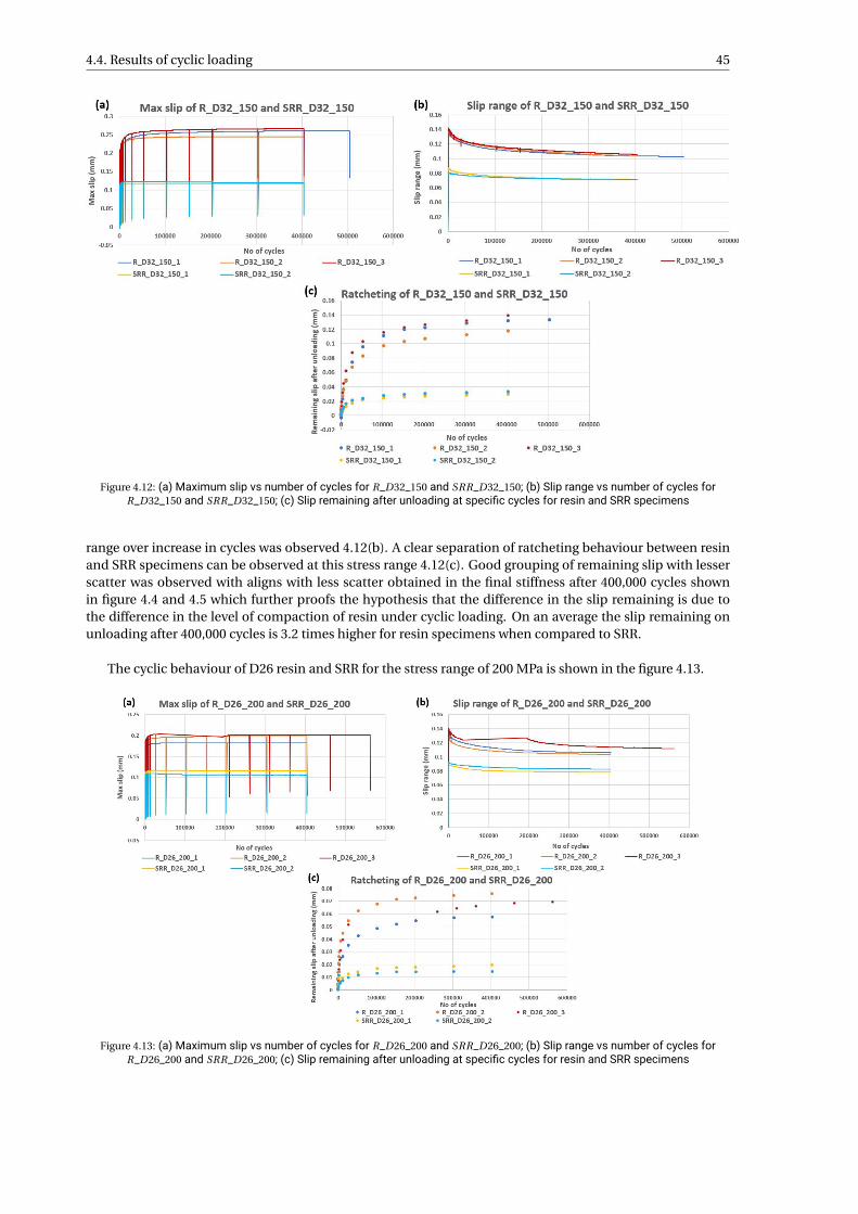
4.4. Results of cyclic loading 45
Figure 4.12: (a) Maximum slip vs number of cycles for R_D32_150 and SRR_D32_150; (b) Slip range vs number of cycles forR_D32_150 and SRR_D32_150; (c) Slip remaining after unloading at specific cycles for resin and SRR specimens
range over increase in cycles was observed 4.12(b). A clear separation of ratcheting behaviour between resinand SRR specimens can be observed at this stress range 4.12(c). Good grouping of remaining slip with lesserscatter was observed with aligns with less scatter obtained in the final stiffness after 400,000 cycles shownin figure 4.4 and 4.5 which further proofs the hypothesis that the difference in the slip remaining is due tothe difference in the level of compaction of resin under cyclic loading. On an average the slip remaining onunloading after 400,000 cycles is 3.2 times higher for resin specimens when compared to SRR.
The cyclic behaviour of D26 resin and SRR for the stress range of 200 MPa is shown in the figure 4.13.
Figure 4.13: (a) Maximum slip vs number of cycles for R_D26_200 and SRR_D26_200; (b) Slip range vs number of cycles forR_D26_200 and SRR_D26_200; (c) Slip remaining after unloading at specific cycles for resin and SRR specimens
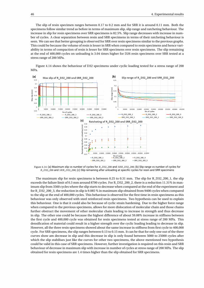
46 4. Experimental results
The slip of resin specimen ranges between 0.17 to 0.2 mm and for SRR it is around 0.11 mm. Both thespecimens follow similar trend as before in terms of maximum slip, slip range and ratcheting behaviour. Theincrease in slip for resin specimens over SRR specimens is 82.5%. Slip range decreases with increase in num-ber of cycles. A clear separation between resin and SRR specimens in terms of their ratcheting behaviour isseen. We can see that better grouping is observed for SRR over resin specimens similar to the previous graphs.This could be because the volume of resin is lesser in SRR when compared to resin specimens and hence vari-ability in terms of compaction of resin is lesser for SRR specimens over resin specimens. The slip remainingat the end of 400,000 cycles on unloading is 3.04 times higher for D26 resin specimens over SRR tested at astress range of 200 MPa.
Figure 4.14 shows the behaviour of D32 specimens under cyclic loading tested for a stress range of 200MPa.
Figure 4.14: (a) Maximum slip vs number of cycles for R_D32_200 and SRR_D32_200; (b) Slip range vs number of cycles forR_D32_200 and SRR_D32_200; (c) Slip remaining after unloading at specific cycles for resin and SRR specimens
The maximum slip for resin specimens is between 0.25 to 0.31 mm. The slip for R_D32_200_1, the slipexceeds the failure limit of 0.3 mm around 8700 cycles. For R_D32_200_2, there is a reduction 11.31% in max-imum slip from 3560 cycles where the slip starts to decrease when compared at the end of the experiment andfor R_D32_200_3, the reduction in slip is 9.085 % in maximum slip obtained from 9400 cycles when comparedto the slip at the end of 400,000 cycles. This behaviour is observed for the first time in resin specimens as thisbehaviour was only observed with steel reinforced resin specimens. Two hypothesis can be used to explainthis behaviour. One is that it could also be because of cyclic strain hardening. Due to the higher force rangewhen compared to the previous specimens, allows for more dislocation of molecular chain and those chainsfurther obstruct the movement of other molecular chain leading to increase in strength and thus decreasein slip. The other one could be because the highest difference of about 59.08% increase in stiffness betweenthe first cycle and 400,000 cycle was obtained for resin specimens tested at stress range of 200 MPa. Thisdensification of material could result in a higher strength over the cyclic loading leading to decrease in slip.However, all the three resin specimens showed about the same increase in stiffness from first cycle to 400,000cycle. For SRR specimens, the slip ranges between 0.13 to 0.15 mm. It can be that for only one out of the threecurves show am decrease in slip and this decrease in slip is only found between 5000 to 25000 cycles afterwhich the slip stabilises just like the curves for other two specimens, the above mentioned two hypothesiscould be valid in this case of SRR specimens. However, further investigation is required on this resin and SRRbehaviour of decrease in maximum slip with increase in number of cycles at stress range of 200 MPa. The slipobtained for resin specimens are 1.4 times higher than the slip obtained for SRR specimens.
4.5. Failure of specimen 47
The progression of slip range over number of cycles is shown in the figure 4.14(b). Here, it is interest-ing to note that the decrease in slip range over number of cycles is more steeper for the two sets of resinspecimens which show a decreasing trend of maximum slip. On analysing the stiffness for all the three resinspecimens, a lesser increase in stiffness were observed for specimen whose slip decreased steeply. Here itcan be concluded that the decrease in maximum slip results in a steeper decrease of slip range for the resinspecimens. This behaviour is just observed for these two resin specimens (R_D32_200_2 and R_D32_200_2.Figure 4.14(c) shows the slip remaining after unloading to 1.5 KN over number of cycles. Good sets of resultsare obtained for SRR specimens with very minimal scatter. Whereas, for resin specimens, since there is adecrease in slip for two out of three tested specimens, there is a significant difference between the remainingslip of R_D32_200_1 which is around 0.17 mm when compared to R_D32_200_2 and R_D32_200_3 where theslip remaining is around 0.08 mm after 400,000 cycles. Because of this, a comparison of slip remaining after400,000 cycles between resin and SRR cannot be done in this particular case.
The cyclic loading of resin and SRR specimens show good co relation between the three tested specimenwithout showing much scatter in the results which was on the drawback in K. Roupakas [51] work. Two out offive SRR specimens tested for a stress range of 100 MPa showed a drastically decreasing slip with increase innumber of cycle which was only found for those two SRR specimens 4.9 and 4.10. Further studies are requiredto analysis and understand the decrease in slip with increase in number of cycles for resin and SRR. A com-mon trend of decrease in slip range over number of cycles was observed for all the tested specimens which isin agreement with the conclusion made on analysing the stiffness over number of cycles, where increase instiffness over number of cycles were observed for all the tested specimens irrespective of their diameters andthe tested stress ranges. The slip remaining on loading to -1.5 KN showed a similar behaviour of increase of(accumulation) of slip even after the stabilisation of the maximum slip which can be attributed to the ratch-eting behaviour of resin and SRR. The slip remaining on unloading at the end of 400,000 cycles was 2.36 timeshigher for 26 mm resin specimens over SRR specimens and 3.16 times higher for 32 mm resin specimens overSRR specimens.
4.5. Failure of specimenIt can be seen from the previous section that the failure criteria of 0.3 mm for maximum slip and 0.1 mm forslip range was not reached by all the specimens up to 400,000 cycles. In this section, graphs are extrapolatedfor 5 million cycles to see if the tested specimens exceed a maximum slip of 0.3 mm and slip range for 0.1mm for the design life of 5 million cycles. Many specimens have exceeded 0.1 mm during the cyclic loadingand hence the cycles at which the specimens exceeds these failure limits and thus their fatigue life has beenaddressed below.
The graph above (figure 4.15) shows the extrapolation of resin specimens. It can be seen that one speci-mens for a stress range of 200 MPa has failed. The other two specimens which are tested at 200 MPa has itsslip decreasing drastically over time. More tests has to be done at this stress range to see if the same behaviouroccurs as explained in the previous section. It can be concluded that the resin specimens with 26 mm diam-eter has infinite fatigue life for all the tested stress ranges and for resin specimens with 32 mm diameter, justone specimen tested at the stress range of 200 MPa failed at 3009 cycles (R_D32_200_1) and none of the otherspecimen exceeded the failure criterion of 0.3 mm.
Failure criterion of maximum slip exceeding 0.3 mmFailed specimen Stress range (MPa) Fatigue life of the specimenR_D32_200_1 200 (-25 to -225) 3009 cycles
Table 4.1: Fatigue life of specimens which exceeds the failure criterion of maximum slip greater than 0.3 mm
For steel reinforced resin specimens (figure 4.16), the maximum slip obtained over a span of 5 million cy-cle is much lesser than resin specimens so much so that the slip at maximum stress range is about 0.15 mm.There is a drastic reduction in slip for the lower stress range of -25 to -125 MPa. For the other two stress ranges,the slip is almost stable and does not show rapid increase or decrease when extrapolated over its lifetime. It
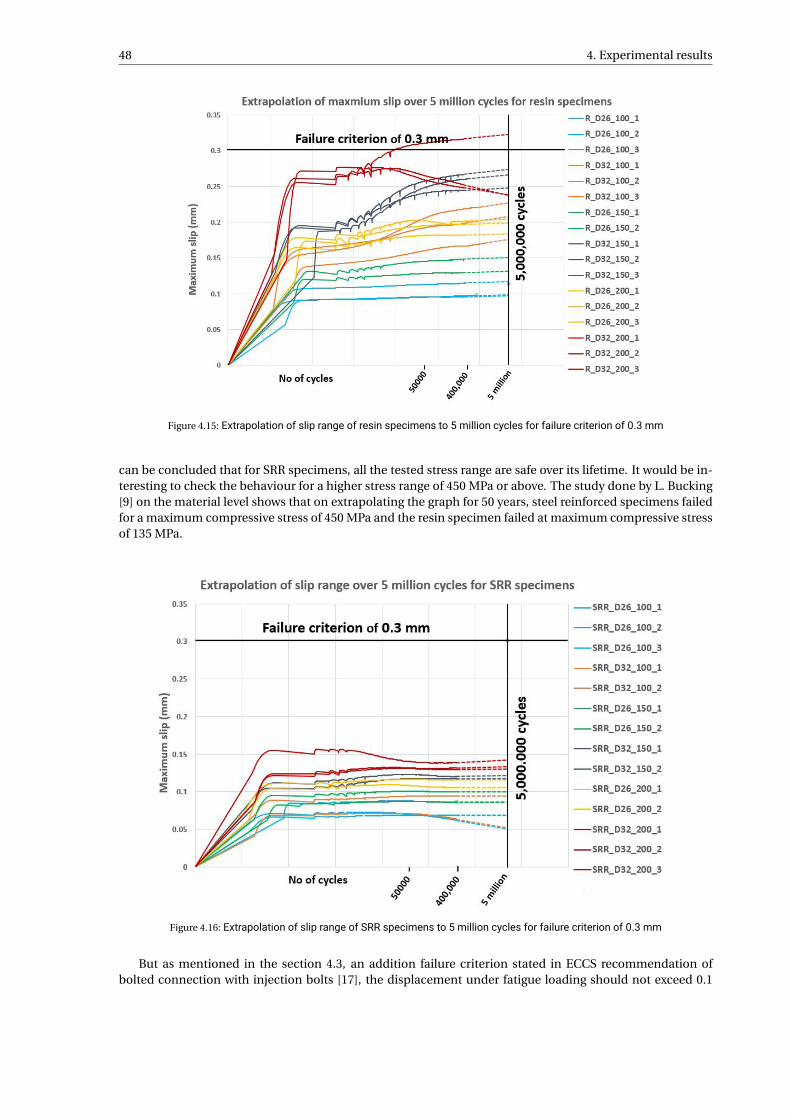
48 4. Experimental results
Figure 4.15: Extrapolation of slip range of resin specimens to 5 million cycles for failure criterion of 0.3 mm
can be concluded that for SRR specimens, all the tested stress range are safe over its lifetime. It would be in-teresting to check the behaviour for a higher stress range of 450 MPa or above. The study done by L. Bucking[9] on the material level shows that on extrapolating the graph for 50 years, steel reinforced specimens failedfor a maximum compressive stress of 450 MPa and the resin specimen failed at maximum compressive stressof 135 MPa.
Figure 4.16: Extrapolation of slip range of SRR specimens to 5 million cycles for failure criterion of 0.3 mm
But as mentioned in the section 4.3, an addition failure criterion stated in ECCS recommendation ofbolted connection with injection bolts [17], the displacement under fatigue loading should not exceed 0.1
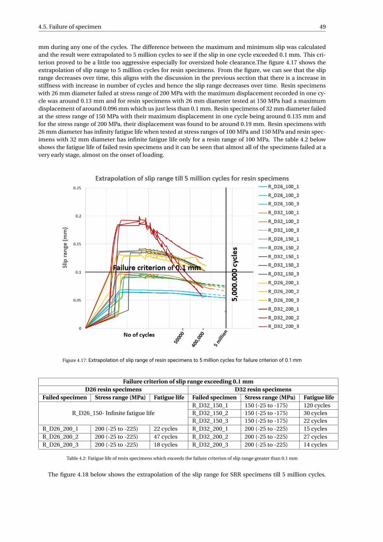
4.5. Failure of specimen 49
mm during any one of the cycles. The difference between the maximum and minimum slip was calculatedand the result were extrapolated to 5 million cycles to see if the slip in one cycle exceeded 0.1 mm. This cri-terion proved to be a little too aggressive especially for oversized hole clearance.The figure 4.17 shows theextrapolation of slip range to 5 million cycles for resin specimens. From the figure, we can see that the sliprange decreases over time, this aligns with the discussion in the previous section that there is a increase instiffness with increase in number of cycles and hence the slip range decreases over time. Resin specimenswith 26 mm diameter failed at stress range of 200 MPa with the maximum displacement recorded in one cy-cle was around 0.13 mm and for resin specimens with 26 mm diameter tested at 150 MPa had a maximumdisplacement of around 0.096 mm which us just less than 0.1 mm. Resin specimens of 32 mm diameter failedat the stress range of 150 MPa with their maximum displacement in one cycle being around 0.135 mm andfor the stress range of 200 MPa, their displacement was found to be around 0.19 mm. Resin specimens with26 mm diameter has infinity fatigue life when tested at stress ranges of 100 MPa and 150 MPa and resin spec-imens with 32 mm diameter has infinite fatigue life only for a resin range of 100 MPa. The table 4.2 belowshows the fatigue life of failed resin specimens and it can be seen that almost all of the specimens failed at avery early stage, almost on the onset of loading.
Figure 4.17: Extrapolation of slip range of resin specimens to 5 million cycles for failure criterion of 0.1 mm
Failure criterion of slip range exceeding 0.1 mmD26 resin specimens D32 resin specimens
Failed specimen Stress range (MPa) Fatigue life Failed specimen Stress range (MPa) Fatigue life
R_D26_150- Infinite fatigue lifeR_D32_150_1 150 (-25 to -175) 120 cyclesR_D32_150_2 150 (-25 to -175) 30 cyclesR_D32_150_3 150 (-25 to -175) 22 cycles
R_D26_200_1 200 (-25 to -225) 22 cycles R_D32_200_1 200 (-25 to -225) 15 cyclesR_D26_200_2 200 (-25 to -225) 47 cycles R_D32_200_2 200 (-25 to -225) 27 cyclesR_D26_200_3 200 (-25 to -225) 18 cycles R_D32_200_3 200 (-25 to -225) 14 cycles
Table 4.2: Fatigue life of resin specimens which exceeds the failure criterion of slip range greater than 0.1 mm
The figure 4.18 below shows the extrapolation of the slip range for SRR specimens till 5 million cycles.
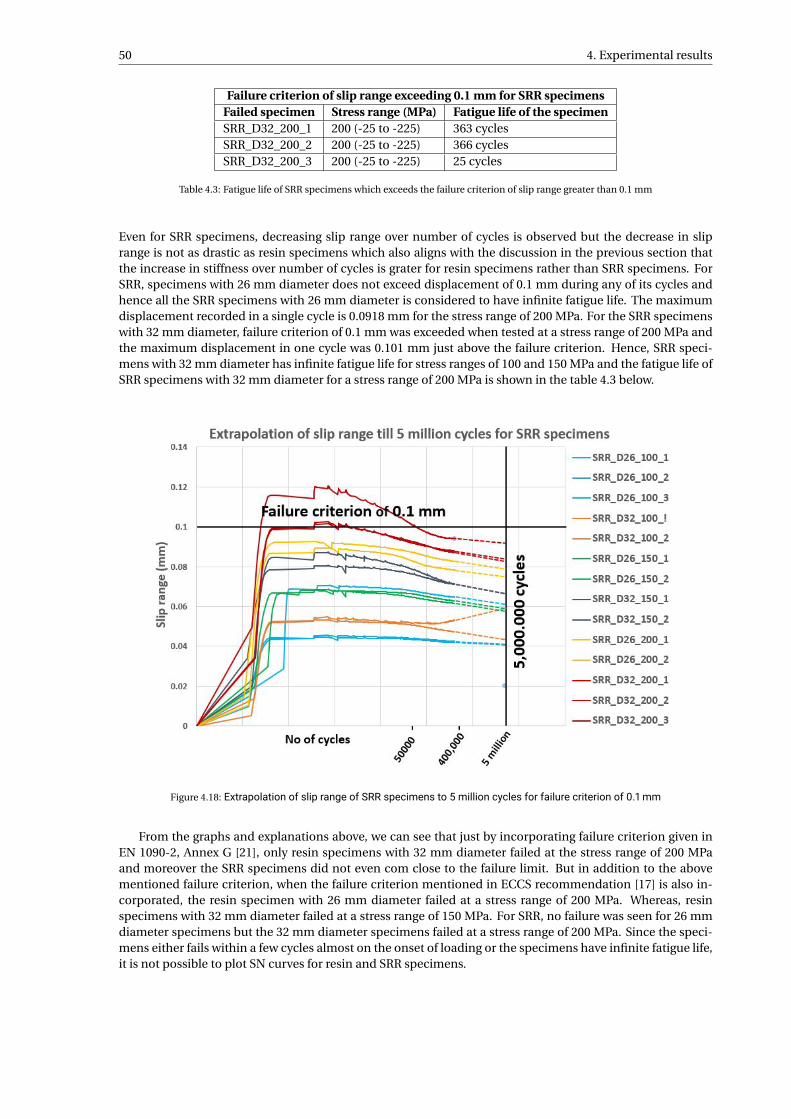
50 4. Experimental results
Failure criterion of slip range exceeding 0.1 mm for SRR specimensFailed specimen Stress range (MPa) Fatigue life of the specimenSRR_D32_200_1 200 (-25 to -225) 363 cyclesSRR_D32_200_2 200 (-25 to -225) 366 cyclesSRR_D32_200_3 200 (-25 to -225) 25 cycles
Table 4.3: Fatigue life of SRR specimens which exceeds the failure criterion of slip range greater than 0.1 mm
Even for SRR specimens, decreasing slip range over number of cycles is observed but the decrease in sliprange is not as drastic as resin specimens which also aligns with the discussion in the previous section thatthe increase in stiffness over number of cycles is grater for resin specimens rather than SRR specimens. ForSRR, specimens with 26 mm diameter does not exceed displacement of 0.1 mm during any of its cycles andhence all the SRR specimens with 26 mm diameter is considered to have infinite fatigue life. The maximumdisplacement recorded in a single cycle is 0.0918 mm for the stress range of 200 MPa. For the SRR specimenswith 32 mm diameter, failure criterion of 0.1 mm was exceeded when tested at a stress range of 200 MPa andthe maximum displacement in one cycle was 0.101 mm just above the failure criterion. Hence, SRR speci-mens with 32 mm diameter has infinite fatigue life for stress ranges of 100 and 150 MPa and the fatigue life ofSRR specimens with 32 mm diameter for a stress range of 200 MPa is shown in the table 4.3 below.
Figure 4.18: Extrapolation of slip range of SRR specimens to 5 million cycles for failure criterion of 0.1 mm
From the graphs and explanations above, we can see that just by incorporating failure criterion given inEN 1090-2, Annex G [21], only resin specimens with 32 mm diameter failed at the stress range of 200 MPaand moreover the SRR specimens did not even com close to the failure limit. But in addition to the abovementioned failure criterion, when the failure criterion mentioned in ECCS recommendation [17] is also in-corporated, the resin specimen with 26 mm diameter failed at a stress range of 200 MPa. Whereas, resinspecimens with 32 mm diameter failed at a stress range of 150 MPa. For SRR, no failure was seen for 26 mmdiameter specimens but the 32 mm diameter specimens failed at a stress range of 200 MPa. Since the speci-mens either fails within a few cycles almost on the onset of loading or the specimens have infinite fatigue life,it is not possible to plot SN curves for resin and SRR specimens.

4.6. Defects in specimen 51
4.6. Defects in specimenA few specimens showed inappropriate increase in displacement (slip) as early as the first loading cycle inQuasi static loading phase and thus an increased level of slip during their cycle loading Figure 4.19 and 4.20.On visual inspection of the specimen after the test, it was seen that there were large air inclusions (voids) inthe resin 4.21. These voids have a significant impact on the strength and stiffness of the resin.
Figure 4.19: Quasi static loading of defected specimen
Figure 4.20: Cyclic loading of defected specimen
Voids could occur during injecting the resin into the specimen due to mechanical trapping of air and thepressure of injecting the resin or they can be formed due to shrinkage of resin during the curing process.When resin is injected in an confined environment and left for curing, the void then moves up to to the topdue to buoyancy effects and relatively low viscosity of the resin [14]. The void that was observed here, was alarge one at the middle of the resin. This could be because the air was trapped because of high pressure whileinjecting the resin into the specimen with the help of a hand held injecting gun. Care was taken to inject theresin slowly and in fixed intervals so that the resin can flow smoothly and the air inclusions could be avoided.Skilled labour or standard injecting procedure is required for the injection of resin into the hole clearance aslittle amount of air inclusion within the resin could cause a significantly influence the slip of the connection.On injecting the resin, it is not possible to know if there are any air inclusion within the resin by visual inspec-tion and an X-ray scan would be needed to check this and hence it becomes important that sufficient care istaking while injecting the resin.
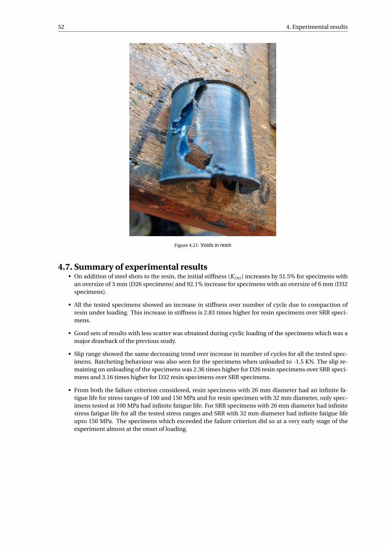
52 4. Experimental results
Figure 4.21: Voids in resin
4.7. Summary of experimental results• On addition of steel shots to the resin, the initial stiffness (Ki ni ) increases by 51.5% for specimens with
an oversize of 3 mm (D26 specimens( and 92.1% increase for specimens with an oversize of 6 mm (D32specimens).
• All the tested specimens showed an increase in stiffness over number of cycle due to compaction ofresin under loading. This increase in stiffness is 2.83 times higher for resin specimens over SRR speci-mens.
• Good sets of results with less scatter was obtained during cyclic loading of the specimens which was amajor drawback of the previous study.
• Slip range showed the same decreasing trend over increase in number of cycles for all the tested spec-imens. Ratcheting behaviour was also seen for the specimens when unloaded to -1.5 KN. The slip re-maining on unloading of the specimens was 2.36 times higher for D26 resin specimens over SRR speci-mens and 3.16 times higher for D32 resin specimens over SRR specimens.
• From both the failure criterion considered, resin specimens with 26 mm diameter had an infinite fa-tigue life for stress ranges of 100 and 150 MPa and for resin specimen with 32 mm diameter, only spec-imens tested at 100 MPa had infinite fatigue life. For SRR specimens with 26 mm diameter had infinitestress fatigue life for all the tested stress ranges and SRR with 32 mm diameter had infinite fatigue lifeupto 150 MPa. The specimens which exceeded the failure criterion did so at a very early stage of theexperiment almost at the onset of loading.
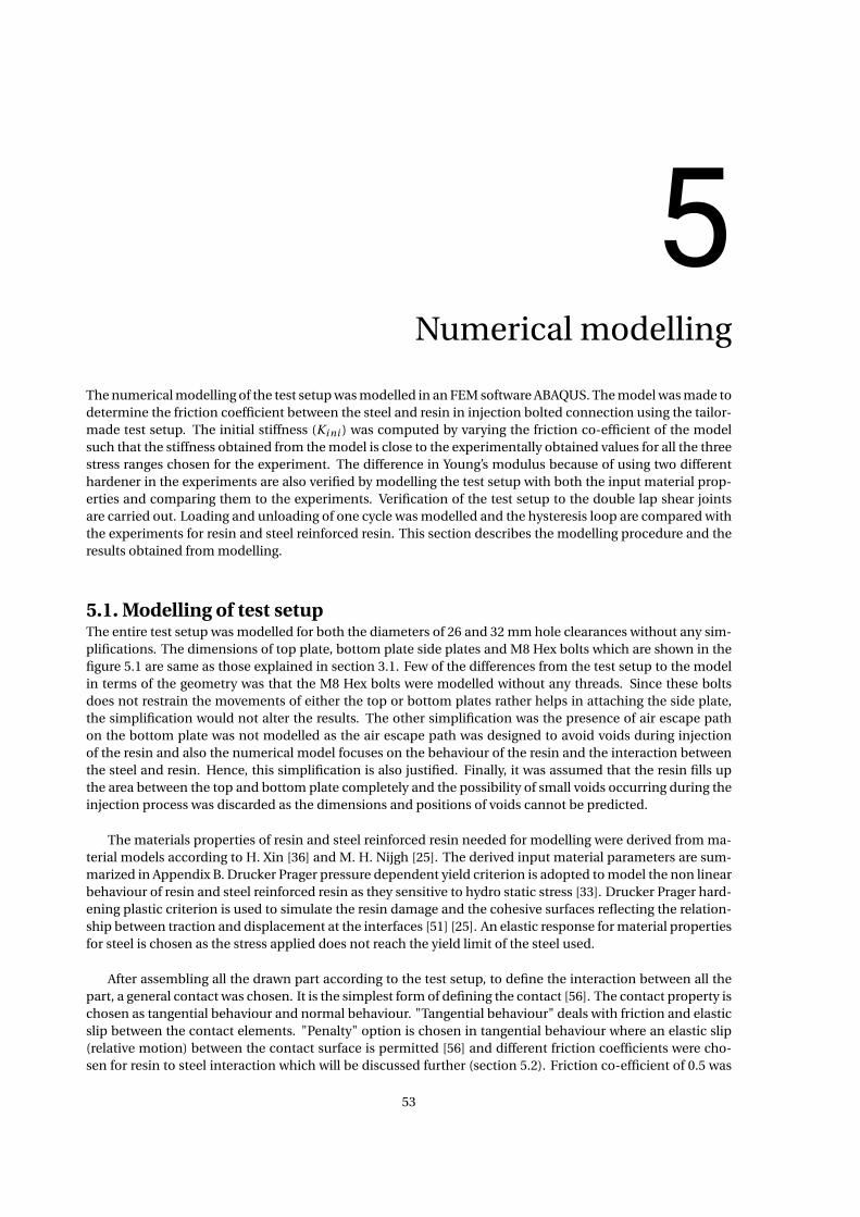
5Numerical modelling
The numerical modelling of the test setup was modelled in an FEM software ABAQUS. The model was made todetermine the friction coefficient between the steel and resin in injection bolted connection using the tailor-made test setup. The initial stiffness (Ki ni ) was computed by varying the friction co-efficient of the modelsuch that the stiffness obtained from the model is close to the experimentally obtained values for all the threestress ranges chosen for the experiment. The difference in Young’s modulus because of using two differenthardener in the experiments are also verified by modelling the test setup with both the input material prop-erties and comparing them to the experiments. Verification of the test setup to the double lap shear jointsare carried out. Loading and unloading of one cycle was modelled and the hysteresis loop are compared withthe experiments for resin and steel reinforced resin. This section describes the modelling procedure and theresults obtained from modelling.
5.1. Modelling of test setupThe entire test setup was modelled for both the diameters of 26 and 32 mm hole clearances without any sim-plifications. The dimensions of top plate, bottom plate side plates and M8 Hex bolts which are shown in thefigure 5.1 are same as those explained in section 3.1. Few of the differences from the test setup to the modelin terms of the geometry was that the M8 Hex bolts were modelled without any threads. Since these boltsdoes not restrain the movements of either the top or bottom plates rather helps in attaching the side plate,the simplification would not alter the results. The other simplification was the presence of air escape pathon the bottom plate was not modelled as the air escape path was designed to avoid voids during injectionof the resin and also the numerical model focuses on the behaviour of the resin and the interaction betweenthe steel and resin. Hence, this simplification is also justified. Finally, it was assumed that the resin fills upthe area between the top and bottom plate completely and the possibility of small voids occurring during theinjection process was discarded as the dimensions and positions of voids cannot be predicted.
The materials properties of resin and steel reinforced resin needed for modelling were derived from ma-terial models according to H. Xin [36] and M. H. Nijgh [25]. The derived input material parameters are sum-marized in Appendix B. Drucker Prager pressure dependent yield criterion is adopted to model the non linearbehaviour of resin and steel reinforced resin as they sensitive to hydro static stress [33]. Drucker Prager hard-ening plastic criterion is used to simulate the resin damage and the cohesive surfaces reflecting the relation-ship between traction and displacement at the interfaces [51] [25]. An elastic response for material propertiesfor steel is chosen as the stress applied does not reach the yield limit of the steel used.
After assembling all the drawn part according to the test setup, to define the interaction between all thepart, a general contact was chosen. It is the simplest form of defining the contact [56]. The contact property ischosen as tangential behaviour and normal behaviour. "Tangential behaviour" deals with friction and elasticslip between the contact elements. "Penalty" option is chosen in tangential behaviour where an elastic slip(relative motion) between the contact surface is permitted [56] and different friction coefficients were cho-sen for resin to steel interaction which will be discussed further (section 5.2). Friction co-efficient of 0.5 was
53
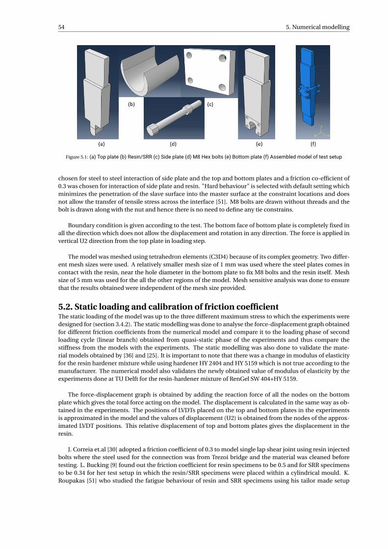
54 5. Numerical modelling
Figure 5.1: (a) Top plate (b) Resin/SRR (c) Side plate (d) M8 Hex bolts (e) Bottom plate (f) Assembled model of test setup
chosen for steel to steel interaction of side plate and the top and bottom plates and a friction co-efficient of0.3 was chosen for interaction of side plate and resin. "Hard behaviour" is selected with default setting whichminimizes the penetration of the slave surface into the master surface at the constraint locations and doesnot allow the transfer of tensile stress across the interface [51]. M8 bolts are drawn without threads and thebolt is drawn along with the nut and hence there is no need to define any tie constrains.
Boundary condition is given according to the test. The bottom face of bottom plate is completely fixed inall the direction which does not allow the displacement and rotation in any direction. The force is applied invertical U2 direction from the top plate in loading step.
The model was meshed using tetrahedron elements (C3D4) because of its complex geometry. Two differ-ent mesh sizes were used. A relatively smaller mesh size of 1 mm was used where the steel plates comes incontact with the resin, near the hole diameter in the bottom plate to fix M8 bolts and the resin itself. Meshsize of 5 mm was used for the all the other regions of the model. Mesh sensitive analysis was done to ensurethat the results obtained were independent of the mesh size provided.
5.2. Static loading and calibration of friction coefficientThe static loading of the model was up to the three different maximum stress to which the experiments weredesigned for (section 3.4.2). The static modelling was done to analyse the force-displacement graph obtainedfor different friction coefficients from the numerical model and compare it to the loading phase of secondloading cycle (linear branch) obtained from quasi-static phase of the experiments and thus compare thestiffness from the models with the experiments. The static modelling was also done to validate the mate-rial models obtained by [36] and [25]. It is important to note that there was a change in modulus of elasticityfor the resin hardener mixture while using hardener HY 2404 and HY 5159 which is not true according to themanufacturer. The numerical model also validates the newly obtained value of modulus of elasticity by theexperiments done at TU Delft for the resin-hardener mixture of RenGel SW 404+HY 5159.
The force-displacement graph is obtained by adding the reaction force of all the nodes on the bottomplate which gives the total force acting on the model. The displacement is calculated in the same way as ob-tained in the experiments. The positions of LVDTs placed on the top and bottom plates in the experimentsis approximated in the model and the values of displacement (U2) is obtained from the nodes of the approx-imated LVDT positions. This relative displacement of top and bottom plates gives the displacement in theresin.
J. Correia et.al [30] adopted a friction coefficient of 0.3 to model single lap shear joint using resin injectedbolts where the steel used for the connection was from Trezoi bridge and the material was cleaned beforetesting. L. Bucking [9] found out the friction coefficient for resin specimens to be 0.5 and for SRR specimensto be 0.34 for her test setup in which the resin/SRR specimens were placed within a cylindrical mould. K.Roupakas [51] who studied the fatigue behaviour of resin and SRR specimens using his tailor made setup
5.2. Static loading and calibration of friction coefficient 55
adopted a frictionless contact between steel and resin as the steel surface was sprayed with a releasing agentwhich prevents adhesive bonding/
Material models for resin and SRR was derived for two types of flows depending on the compressabil-ity in the plastic region of the material- (i) Associative flow (ii) Non-dilatant flow. Non-dilatant flow statesthat the material is not compressable under the influence of the load. In other words, the change in volumeis zero. Static loading of three different stress ranges were modelled for associative and non-dilatant flow.Four different friction coefficients were adopted for interaction between steel and resin for resin specimens-(i) frictionless (ii) 0.05 (iii) 0.1 (iv) 0.2 and three different friction coefficient was chosen for SRR specimens-(i) frictionless (ii) 0.1 (iii) 0.2. These values were adopted on the basics that the release agent was sprayedbefore injecting the resin. This prevents adhesive bonding of the resin and steel. The lower bound valueof frictionless interaction is a theoretical behaviour. Whereas, in the current experimental setup in spite ofadding the release agent, there will be some friction present between the steel plates and the resin. The upperbound value of friction coefficient of 0.2 was adopted in order to have a lesser friction co-efficient than theone chosen for interaction of resin with side plates (friction coefficient of 0.3) where the release agent was notapplied. The load-displacement curve were plotted for all the friction coefficients and the obtained stiffnesswas compared with the experimental results.
Comparison of associative flow and non-dilatant flow models are shown in the figure 5.2 below.
Figure 5.2: Comparison of associative flow and non-dilatant flow models with 0.05 friction co-efficient for resin specimenmodels and 0.1 friction co-efficient for SRR specimen models
The maximum stress applied was chosen for this comparison as the maximum difference in both themodels are seen at the highest stress applied (225 MPa). The models with friction coefficients of 0.05 for resinto steel interaction and 0.1 for steel reinforced resin to steel interaction was chosen for this comparison. Itcan be seen that there is no significant difference in load-displacement curve for associative and non-dilatantmodels for two different diameters of 26 mm and 32 mm upto a maximum stress of 225 MPa (135 KN). Thetable 5.1 shows the stiffness obtained from both the models for three stresses of 125, 175 and 225 MPa fora friction coefficient of 0.05 for resin and 0.1 for SRR which are compared with the stiffness obtained fromexperiments.
The maximum difference between both the models is seen for models with a larger diameter of 32 mm(hole clearance of 12 mm) which can be seem in the stiffness presented in the table 5.1. It is because of thehigher volume of resin in the hole which can be compressed. However, it can be concluded that the differ-ence in associative flow and non-dilatant flow models are negligible for the highest tested maximum stressof 225 MPa. Similar trends were observed for models with different friction coefficients (Appendix E). Larger
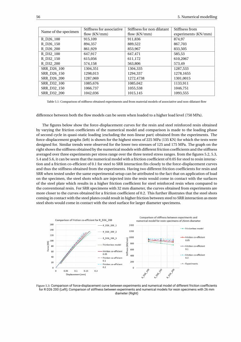
56 5. Numerical modelling
Name of the specimenStiffness for associativeflow (KN/mm)
Stiffness for non dilatantflow (KN/mm)
Stiffness fromexperiments (KN/mm)
R_D26_100 915,109 911,836 874,97R_D26_150 894,357 889,522 867,703R_D26_200 861,929 853,967 833,505R_D32_100 647,917 647,471 585,53R_D32_150 615,056 611,172 610,2067R_D32_200 574,158 563,806 573,49SRR_D26_100 1304,351 1304,335 1287,533SRR_D26_150 1298,013 1294,337 1278,1655SRR_D26_200 1287,069 1272,4738 1301,0015SRR_D32_100 1085,676 1085,042 1133,911SRR_D32_150 1066,737 1055,538 1046,751SRR_D32_200 1042,036 1015,145 1093,555
Table 5.1: Comparison of stiffness obtained experiments and from material models of associative and non-dilatant flow
difference between both the flow models can be seem when loaded to a higher load level (750 MPa).
The figures below show the force-displacement curves for the resin and steel reinforced resin obtainedby varying the friction coefficients of the numerical model and comparison is made to the loading phaseof second cycle in quasi-static loading (excluding the non-linear part) obtained from the experiments. Theforce-displacement graphs (left) is shown for the highest stress of 225 MPa (135 KN) for which the tests weredesigned for. Similar trends were observed for the lower two stresses of 125 and 175 MPa. The graph on theright shows the stiffness obtained by the numerical models with different friction coefficients and the stiffnessaveraged over three experiments per stress range over the three tested stress ranges. from the figures 5.2, 5.3,5.4 and 5.6, it can be seem that the numerical model with a friction coefficient of 0.05 for steel to resin interac-tion and a friction co-efficient of 0.1 for steel to SRR interaction fits closely to the force-displacement curvesand thus the stiffness obtained from the experiments. Having two different friction coefficients for resin andSRR when tested under the same experimental setup can be attributed to the fact that on application of loadon the specimen, the steel shots which are injected into the resin would come in contact with the surfacesof the steel plate which results in a higher friction coefficient for steel reinforced resin when compared tothe conventional resin. For SRR specimens with 32 mm diameter, the curves obtained from experiments aremore closer to the curves obtained for a friction coefficient of 0.2. This further illustrates that the steel shotscoming in contact with the steel plates could result in higher friction between steel to SRR interaction as moresteel shots would come in contact with the steel surface for larger diameter specimens.
Figure 5.3: Comparison of force-displacement curve between experiments and numerical model of different friction coefficientsfor R D26 200 (Left); Comparison of stiffness between experiments and numerical models for resin specimens with 26 mm
diameter (Right)
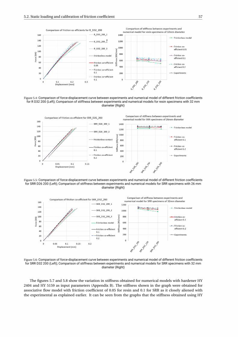
5.2. Static loading and calibration of friction coefficient 57
Figure 5.4: Comparison of force-displacement curve between experiments and numerical model of different friction coefficientsfor R D32 200 (Left); Comparison of stiffness between experiments and numerical models for resin specimens with 32 mm
diameter (Right)
Figure 5.5: Comparison of force-displacement curve between experiments and numerical model of different friction coefficientsfor SRR D26 200 (Left); Comparison of stiffness between experiments and numerical models for SRR specimens with 26 mm
diameter (Right)
Figure 5.6: Comparison of force-displacement curve between experiments and numerical model of different friction coefficientsfor SRR D32 200 (Left); Comparison of stiffness between experiments and numerical models for SRR specimens with 32 mm
diameter (Right)
The figures 5.7 and 5.8 show the variation in stiffness obtained for numerical models with hardener HY2404 and HY 5159 as input parameters (Appendix B). The stiffness shown in the graph were obtained forassociative flow model with friction coefficient of 0.05 for resin and 0.1 for SRR as it closely aliened withthe experimental as explained earlier. It can be seen from the graphs that the stiffness obtained using HY
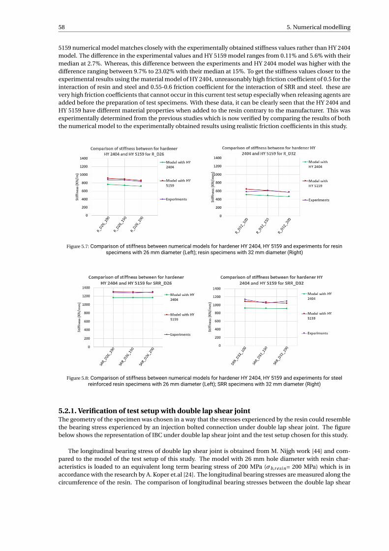
58 5. Numerical modelling
5159 numerical model matches closely with the experimentally obtained stiffness values rather than HY 2404model. The difference in the experimental values and HY 5159 model ranges from 0.11% and 5.6% with theirmedian at 2.7%. Whereas, this difference between the experiments and HY 2404 model was higher with thedifference ranging between 9.7% to 23.02% with their median at 15%. To get the stiffness values closer to theexperimental results using the material model of HY 2404, unreasonably high friction coefficient of 0.5 for theinteraction of resin and steel and 0.55-0.6 friction coefficient for the interaction of SRR and steel. these arevery high friction coefficients that cannot occur in this current test setup especially when releasing agents areadded before the preparation of test specimens. With these data, it can be clearly seen that the HY 2404 andHY 5159 have different material properties when added to the resin contrary to the manufacturer. This wasexperimentally determined from the previous studies which is now verified by comparing the results of boththe numerical model to the experimentally obtained results using realistic friction coefficients in this study.
Figure 5.7: Comparison of stiffness between numerical models for hardener HY 2404, HY 5159 and experiments for resinspecimens with 26 mm diameter (Left); resin specimens with 32 mm diameter (Right)
Figure 5.8: Comparison of stiffness between numerical models for hardener HY 2404, HY 5159 and experiments for steelreinforced resin specimens with 26 mm diameter (Left); SRR specimens with 32 mm diameter (Right)
5.2.1. Verification of test setup with double lap shear jointThe geometry of the specimen was chosen in a way that the stresses experienced by the resin could resemblethe bearing stress experienced by an injection bolted connection under double lap shear joint. The figurebelow shows the representation of IBC under double lap shear joint and the test setup chosen for this study.
The longitudinal bearing stress of double lap shear joint is obtained from M. Nijgh work [44] and com-pared to the model of the test setup of this study. The model with 26 mm hole diameter with resin char-acteristics is loaded to an equivalent long term bearing stress of 200 MPa (σb,r esi n= 200 MPa) which is inaccordance with the research by A. Koper et.al [24]. The longitudinal bearing stresses are measured along thecircumference of the resin. The comparison of longitudinal bearing stresses between the double lap shear
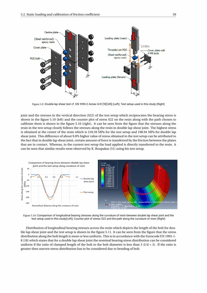
5.2. Static loading and calibration of friction coefficient 59
Figure 5.9: Double-lap shear test cf. EN 1090-2 Annex G/K [18] [45] (Left); Test setup used in this study (Right)
joint and the stresses in the vertical direction (S22) of the test setup which reciprocates the bearing stress isshown in the figure 5.10 (left) and the counter plot of stress S22 on the resin along with the path chosen tocalibrate them is shown in the figure 5.10 (right). It can be seen from the figure that the stresses along theresin in the test setup closely follows the stresses along the resin in double lap shear joint. The highest stressis obtained at the center of the resin which is 218.59 MPa for the test setup and 198.94 MPa for double lapshear joint. This difference of about 9.8% higher value of stress obtained in the test setup can be attributed tothe fact that in double lap shear joint, certain amount of force is transferred by the friction between the platesthat are in contact. Whereas, in the current test setup the load applied is directly transferred to the resin. itcan be seen that similar results were observed by K. Roupakas [51] using his test setup.
Figure 5.10: Comparison of longitudinal bearing stresses along the curvature of resin between double lap shear joint and thetest setup used in this study(Left); Counter plot of stress S22 and the path along the curvature of resin (Right)
Distribution of longitudinal bearing stresses across the resin which depicts the length of the bolt for dou-ble lap shear joint and the test setup is shown in the figure 5.11. It can be seen from the figure that the stressdistribution along the bolt length is more or less uniform. This is in accordance with the Eurocode EN 1993-1-8 [18] which states that for a double lap shear joint the nominal bearing stress distribution can be considereduniform if the ratio of clamped length of the bolt to the bolt diameter is less than 3 (l/d < 3). If the ratio isgreater then uneven stress distribution has to be considered due to bending of bolt.
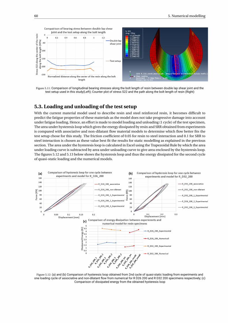
60 5. Numerical modelling
Figure 5.11: Comparison of longitudinal bearing stresses along the bolt length of resin between double lap shear joint and thetest setup used in this study(Left); Counter plot of stress S22 and the path along the bolt length of resin (Right)
5.3. Loading and unloading of the test setupWith the current material model used to describe resin and steel reinforced resin, it becomes difficult topredict the fatigue properties of these materials as the model does not take progressive damage into accountunder fatigue loading, Hence, an effort is made to model loading and unloading (1 cycle) of the test specimen,The area under hysteresis loop which gives the energy dissipated by resin and SRR obtained from experimentsis compared with associative and non-dilatant flow material models to determine which flow better fits thetest setup chose for this study. The friction coefficient of 0.05 for resin to steel interaction and 0.1 for SRR tosteel interaction is chosen as these value best fit the results for static modelling as explained in the previoussection. The area under the hysteresis loop is calculated in Excel using the Trapezoidal Rule by which the areaunder loading curve is subtracted by area under unloading curve to give area enclosed by the hysteresis loop.The figures 5.12 and 5.13 below shows the hysteresis loop and thus the energy dissipated for the second cycleof quasi-static loading and the numerical models.
Figure 5.12: (a) and (b) Comparison of hysteresis loop obtained from 2nd cycle of quasi-static loading from experiments andone loading cycle of associative and non-dilatant flow from numerical for R D26 200 and R D32 200 specimens respectively; (c)
Comparison of dissipated energy from the obtained hysteresis loop
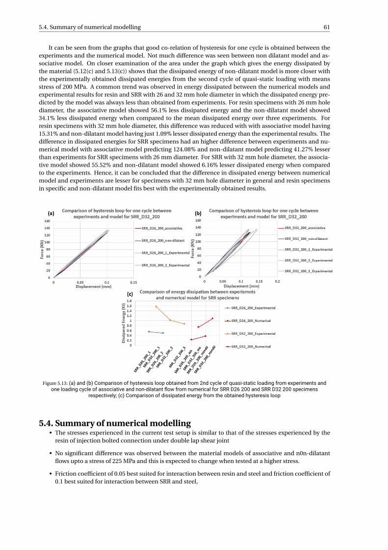
5.4. Summary of numerical modelling 61
It can be seen from the graphs that good co-relation of hysteresis for one cycle is obtained between theexperiments and the numerical model. Not much difference was seen between non dilatant model and as-sociative model. On closer examination of the area under the graph which gives the energy dissipated bythe material (5.12(c) and 5.13(c)) shows that the dissipated energy of non-dilatant model is more closer withthe experimentally obtained dissipated energies from the second cycle of quasi-static loading with meansstress of 200 MPa. A common trend was observed in energy dissipated between the numerical models andexperimental results for resin and SRR with 26 and 32 mm hole diameter in which the dissipated energy pre-dicted by the model was always less than obtained from experiments. For resin specimens with 26 mm holediameter, the associative model showed 56.1% less dissipated energy and the non-dilatant model showed34.1% less dissipated energy when compared to the mean dissipated energy over three experiments. Forresin specimens with 32 mm hole diameter, this difference was reduced with with associative model having15.31% and non-dilatant model having just 1.09% lesser dissipated energy than the experimental results. Thedifference in dissipated energies for SRR specimens had an higher difference between experiments and nu-merical model with associative model predicting 124.08% and non-dilatant model predicting 41.27% lesserthan experiments for SRR specimens with 26 mm diameter. For SRR with 32 mm hole diameter, the associa-tive model showed 55.52% and non-dilatant model showed 6.16% lesser dissipated energy when comparedto the experiments. Hence, it can be concluded that the difference in dissipated energy between numericalmodel and experiments are lesser for specimens with 32 mm hole diameter in general and resin specimensin specific and non-dilatant model fits best with the experimentally obtained results.
Figure 5.13: (a) and (b) Comparison of hysteresis loop obtained from 2nd cycle of quasi-static loading from experiments andone loading cycle of associative and non-dilatant flow from numerical for SRR D26 200 and SRR D32 200 specimens
respectively; (c) Comparison of dissipated energy from the obtained hysteresis loop
5.4. Summary of numerical modelling• The stresses experienced in the current test setup is similar to that of the stresses experienced by the
resin of injection bolted connection under double lap shear joint
• No significant difference was observed between the material models of associative and n0n-dilatantflows upto a stress of 225 MPa and this is expected to change when tested at a higher stress.
• Friction coefficient of 0.05 best suited for interaction between resin and steel and friction coefficient of0.1 best suited for interaction between SRR and steel,
62 5. Numerical modelling
• On comparing the dissipated energy on modelling one cycle using associative and non-dilatant mate-rial models to the second cycle of quasi-static loading from experiments, even though the differencewas small, non-dilatant flow model had a better fit with the experimental results,
• Numerical model using material properties of hardeners HY 2404 and HY 5259 obtained experimentallyfrom previous studies was modelled and it was found that the results obtained in from the experimentsconducted in this study resembled close to the material model with HY 5159 and unrealistically higherfriction coefficients were needed when to get similar results from using numerical model of HY 2404.Hence, it was verified that modulus of elasticity does change when using two different hardener whichwas experimentally shown in the previous studies.
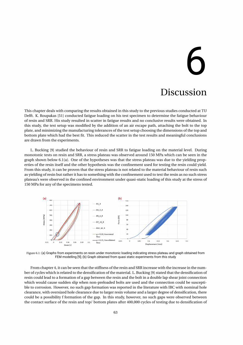
6Discussion
This chapter deals with comparing the results obtained in this study to the previous studies conducted at TUDelft. K. Roupakas [51] conducted fatigue loading on his test specimen to determine the fatigue behaviourof resin and SRR. His study resulted in scatter in fatigue results and no conclusive results were obtained. Inthis study, the test setup was modified by the addition of an air escape path, attaching the bolt to the topplate, and minimizing the manufacturing tolerances of the test setup choosing the dimensions of the top andbottom plate which had the best fit. This reduced the scatter in the test results and meaningful conclusionsare drawn from the experiments.
L. Bucking [9] studied the behaviour of resin and SRR to fatigue loading on the material level. Duringmonotonic tests on resin and SRR, a stress plateau was observed around 150 MPa which can be seen in thegraph shown below 6.1(a). One of the hypotheses was that the stress plateau was due to the yielding prop-erties of the resin itself and the other hypothesis was the confinement used for testing the resin could yield.From this study, it can be proven that the stress plateau is not related to the material behaviour of resin suchas yielding of resin but rather it has to something with the confinement used to test the resin as no such stressplateau’s were observed in the confined environment under quasi-static loading of this study at the stress of150 MPa for any of the specimens tested.
Figure 6.1: (a) Graphs from experiments on resin under monotonic loading indicating stress plateau and graph obtained fromFEM modelling [9]; (b) Graph obtained from quasi static experiments from this study
From chapter 4, it can be seen that the stiffness of the resin and SRR increase with the increase in the num-ber of cycles which is related to the densification of the material. L. Bucking [9] stated that the densification ofresin could lead to a formation of a gap between the resin and the bolt in a double lap shear joint connectionwhich would cause sudden slip when non-preloaded bolts are used and the connection could be suscepti-ble to corrosion. However, no such gap formation was reported in the literature with IBC with nominal holeclearance, with oversized hole clearance due to larger resin volume and a larger degree of densification, therecould be a possibility f formation of the gap. In this study, however, no such gaps were observed betweenthe contact surface of the resin and top/ bottom plates after 400,000 cycles of testing due to densification of
63
64 6. Discussion
the resin. This could change if the stress range was increased or the size of the hole clearance e was furtherincreased or if tensile stresses appear on the resin which would lead to detachment of the resin from the bolt.As it is an important phenomenon to be considered while dealing with double lap shear joints using oversizedhole clearances, further studies have to be done on this to form a more concrete conclusion.
In this study, there was no significant abrasion of steel shots on the top or the bottom plates after 400,000cycles. The top plate is made of mild steel S690 and the bottom plate is made of S355. The lack of significantimpact due to mechanical abrasion of steel shots can also be seen in the test results as no difference in thetrend of results was observed in spite of using the same sets of specimens for all tests conducted. However, indouble lap shear joints, steel shots could be mechanical abrasion on the bolt or on the plate when the jointis subjected to higher loading cycles or at higher stress ranges. Abrasion on bolt could lead to localized stressconcentrations which could lead to initiation and propagation of cracks under cyclic loading. Indentation onthe steel plates could affect its reusability. Hence, furthermore, experiments on double lap shear joint withsteel reinforced resin should be performed to check the effect of mechanical abrasion.
The presence of air inclusions (voids) within the resin when injected using a handheld injecting gun byA. Koper [31] and K. Roupakas [51] led to scatter in their experimental results. In general, it is important tolead the air which is trapped inside the hole clearance is allowed to escape through an air escape path whichwas done in this thesis. In this study, it was seen that when the resin was injected at a slower rate and lowerpressure, allowing the resin to settle and injecting the resin in short intervals within its pot life resulted intest specimens with lesser air inclusions. It was also seen that with a better experience of injecting the resin,the air inclusions were considerably reduced. However, air inclusions were seen in a few of the experiments.When there were air inclusions, the experiments resulted in a slip that was two to three times higher than thespecimens without the air inclusions. Hence, injection of resin into the hole clearance is an important aspectand hence further research is needed to standardize the injection process and to make sure no air inclusionsare presented within the resin.
7Conclusions and future recommendation
7.1. ConclusionsThis section presents the conclusions that can be drawn from the sets of experiments conducted on resin andsteel reinforced resin and the numerical modelling of static and single cycle loading of the test setup
7.1.1. Conclusion from experiments• Addition of steel shots into the resin (SRR) had a significant increase in the initial connection stiffness
(Ki ni ) with 51.5% increase for specimens with hole diameter of 26 mm and 92.1% increase for speci-mens with hole diameter of 32 mm.
• The drop in stiffness from 26 mm hole diameter to 32 mm hole diameter is larger for resin injectedspecimens when compared to steel reinforced resin specimens. This drop in stiffness for resin speci-mens is 26.95% and for SRR it is 18.09%. Hence, it can be concluded that, the drop in stiffness between26 mm hole diameter and 32 hole diameter reduces by 49% when SRR are used over convectional resin.
• The stiffness obtained for all the three tested stress ranges were almost constant. Hence, it can be con-cluded that in the current test setup the stiffness of the resin and steel reinforced resin is independentof the hydrostatic pressure applied.
• There was an increase in stiffness between first cycle of quasi-static loading and 400,000 cycles of cyclicloading when measured after 400,000 cycles for both resin and SRR specimens which is contrary tometals. This increase in stiffness is due to densification of resin with increase in number of loadingand unloading cycles the microscopic voids in the material gets closed. For resin specimens with 26mm hole diameter, the final stiffness (K f i n) was 29.165% higher than initial stiffness (Ki ni ) and forresin specimens with 32 mm hole diameter, this difference was 53.13%. For SRR specimens tested for astress range of 100 MPa contrary to the above mentioned behaviour was seen where the initial stiffnesswas 14.26 higher than final stiffness for SRR specimens with 26 mm hole diameter and 4.9% higherfor SRR specimens with 32 mm hole diameter resulting in decrease of stiffness over number of cycles.However, on closer examination, it was seen that the stiffness still increased with increase in numberof cycle but the initial stiffness was so high that the final stiffness did not reach the value of the initialstiffness. This could be because of higher initial compaction of the resin under the first loading cycle.For SRR specimens tested for stress range of 150 and 200 MPa, normal trend was seen with averageinitial stiffness being 6.935% lower than final stiffness for specimens with 26 mm hole diameter and14.535% lower for 32 mm hole diameter specimens.
• The difference between the initial stiffness from final stiffness for resin specimens is 2.83 times higherwhen compared to the difference between initial stiffness from final stiffness for steel reinforced resin.
• The increase in stiffness between the second cycle of quasi static loading to the 20th cycle of quasiloading was minimal with the increase being less than 1%
65
66 7. Conclusions and future recommendation
• Good sets of results with less scatter was obtained for both resin and SRR specimens when tested undercyclic loading upto 400,000 cycles at a frequency of 2.5 Hz. The stabilisation of slip occurred between25000 to 75000 cycles for resin specimens and 5000 to 25000 cycles for SRR specimens after which theslip became almost constant.
• For a stress range of 100 MPa, addition of steel shots to the resin reduces the slip obtained after 400,000cycles of cyclic loading by 42.32% for 26 mm hole diameter specimens and 166.033% for 32 mm di-ameter specimens. For stress range of 150 MPa, the final slip was reduced by 49.46% for 26 mm holediameter specimens and 145.187% for hole diameter of 32 mm hole diameter by the addition of steelshots into the resin. For stress range of 200 MPa, the reduction was 75.203% for 26 mm hole diameterspecimens and 104.048% for 32mm hole diameter specimens. In total it can be concluded that addi-tion of steel shots into the resin reduces the slip by 55.66% for 26 mm hole diameter specimens and thereduction is 1.385 times for with specimens with the larger hole clearance of 32 mm.
• A common trend of decrease in slip range over increase in number of cycles during the cyclic loadingwas observed for all the tested specimens irrespective to their hole diameter and the stress ranges whichaligns with the finding that the stiffness increased with increase in number of cycles for all the testedspecimens.
• Ratcheting behaviour was observed for all the tested specimens on unloading to -1.5 KN. The slip re-maining on unloading at the end of the experiment (400,000 cycles) showed that the resin specimenswith 26 mm diameter had 2.36 times higher remaining slip when compared to SRR specimens with 26mm diameter. This difference was even higher for D32 specimens with the remaining slip being 3.16times higher for resin specimens with 32 mm diameter when compared to SRR specimens with 32 mmdiameter.
• When the values of maximum slip and slip range were extrapolated for 5 million cycles which gives thefailure criterion for the resin and SRR which was formulated using three codes, EN 1090-2, Annex G [21],EN 1993-1-9 [20] and ECCS recommendations of bolted connections with injection bolts [17], it wasfound that the failure criterion of 0.3 mm was never reached by SRR specimens of both the diameter.For conventional resin specimens, this failure criterion was exceeded by one of these specimens testedwith 32 mm hole diameter for a stress range of 200 MPa (stress range of -25 to -225 MPa). Hence itcan be concluded that conventional resin specimens with 32 mm hole diameter fails for a stress rangeof 200 MPa. However, according to ECCS recommendations [17], in addition to the failure criterionmentioned in EN 1090-2, it states that slip obtained in a single cycle should not be more than 0.1 mm.On considering this criterion, it was found that the resin specimen with 26 mm diameter failed at astress range of 200 MPa and the resin specimens with 32 mm diameter failed at a stress ranges of 150and 200 MPa. For SRR specimens, this failure criterion was just exceeded by 32 mm diameter specimensat the stress range of 200 MPa. The specimens which exceeded the failure criterion did so at a very earlystage of the experiments almost on the onset of loading.
7.1.2. Conclusions from numerical modelling• Verification of the test setup to resemble the stresses experienced by the resin of injection bolted con-
nection under double lap shear joint was conducted successfully with the difference in longitudinalbearing stress experienced by the test setup and double lap shear joint being around 9.8%.
• For static modelling with maximum applied stress of 225 MPa, no significant difference was observedbetween associative and non-dilatant material models. However seeing the trend of the graph, thisconclusion is expected to change when higher stresses are applied.
• The friction coefficients between steel and resin/ SRR were determined by comparing the force vs dis-placement curve (stiffness) obtained in second cycle of quasi-static loading to the curve (stiffness) ob-tained from static loading of the model. It was found that friction coefficient of 0.05 best suited the steelto resin interactions and friction coefficient of 0.1 best suited the steel to SRR interaction.
• Study conducted at TU Delft through experiments showed that on using hardener HY 5159+ resin re-sulted in different modulus of elasticity of the resin-hardener mixture when hardener HY 2404+ resinwas used which is contrary to the manufacturer. For the experiments in this study, HY 5159+ resin wasused. On modelling the test setup with both the experimentally obtained material properties, it was

7.2. Future recommendations 67
seen that the stiffness obtained by using the material properties of HY 5159+ resin was closer to the ex-perimentally obtained stiffness with an error of 2.7%. Whereas, when material properties of HY 2404+resin was used, this difference in stiffness ranged between 9.7% and 23.02%. A very higher friction coef-ficient of 0.5 for resin-steel interaction and 0.55-0.6 for SRR-steel interaction was required to obtainedthe stiffness similar to experiments when model with HY 2404+resin was used. This high friction coeffi-cient is not possible especially when releasing agents are added while the preparation of the specimens.Hence it can be concluded that modulus of elasticity changes from HY 2404 and HY 5159 hardener areused.
• The dissipated energy from modelling of one cycle and comparing the modelling results to the secondcycle of quasi-static loading from experiments showed that the non-dilatant model fits best to the ex-perimentally obtained results even though the difference in associative and non-dilatant models weresmall.
7.2. Future recommendations7.2.1. Future works on experiments
• Further experiments should be done in order to understand the decrease in slip with increase in num-ber of cycles.
• Fatigue detail class for injection bolted connections should be derived from experiments on IBCs.
• Injecting procedure of resins into the oversized hole clearances would be standardise in such a way asto avoid formation of air inclusions which compromises the slip resistant characteristics of IBCs.
• Higher stress ranges must be tested especially with steel reinforced resin to find out the stress range forwhich SRR fails. Experiments could be extend till 2 million cycles to further analyse the behaviour ofresin and SRR
• Reduction in volume of the resin under cyclic loading and impact of mechanical abrasion of steel shotson the plates and bolts have to be further investigated,
7.2.2. Future works on numerical modelling• Material models of resin and SRR to predict the cyclic loading should be derived based on the cyclic
hardening/ softening behaviour and the damage mechanism of resin and SRR under cyclic loadingcondition.
• The entire double lap shear joint with oversized IBC should be modelled under static and cyclic loadingto find the contribution of deformations in resin to the total deformation of the connection itself.
• The possibility of formation of gap in over-sized hole clearance due to reduction in volume of resin indouble lap shear joint could be checked using the numerical model.

RenGel© SW404 HY2404 HY5159 Page 1 of 3 11/5/2012
Advanced Materials
RenGel© SW 404 / Ren© HY 2404 or HY 5159
GELCOAT RESIN FILLED EPOXY SYSTEM, WITH OUTSTANDING ABRASION RESISTANCE
KEY PROPERTIES
• Outstanding mechanical strength and qualities
• Good chemical resistance
• Very hard, abrasion-resistant surfaces
APPLICATIONS • Foundry patterns
• Copy-milling models
• Foaming and concrete-casting moulds
• Tools and tooling aids
PRODUCT DATA
Property Unit RenGel
©
SW 404
Ren©
HY 2404
Ren©
HY 5159
Appearance Colour
visual Paste Blue
Clear liquid Pale yellow
Clear liquid Pale yellow
Viscosity at 25ºC *
mPas 70’000-110’000** 3400-5000** 120-175**
Density
g/cm3 1.85-1.95 1.0-1.05 0.98
** Specified data are on a regular basis analysed. Data which is described in this document as ‘typical’ is not analysed on a regular basis and is given for information purpose only. Data values are not guaranteed or warranted unless if specifically mentioned.
TYPICAL SYSTEM DATAS
PROCESSING
Mix ratio Parts by weight
RenGel©
SW 404 100 100
Ren©
HY 2404
10
-
Ren©
HY 5159
-
8
Mix the two components thoroughly in the ratio indicated. Apply in thin layers with a brush or spatula, wait until gelcoat has gelled, but ensure that it is still slightly tacky before proceeding. Post-curing will improve final properties.

Bibliography
[1] M.V. Braun M. Veljkovic A. Kozma, C. Odenbreit and M.P. Nijgh. "push-out tests on demountable shearconnectors of steel-concrete composite structures". 12th International Conference on Advances in Steel-Concrete Composite Structures (ASCCS), 2018.
[2] Bill Addis. "building with reclaimed components and materials: A design handbook for recycle andreuse". Earthscan, London, 2007.
[3] M. Paschen A.M. Gresnigt, G. Sedlacek. "injection bolts to repair old bridges". Connections in steelstructures, pages 349–360, 2000.
[4] E.S Knudsen A.M van Wingerde, D.R.V van Delft. "fatigue behaviour of bolted connections in pultrudedfrp panels". Plastic, Rubber and Composites, 2003.
[5] M.V. Figueiredo A.S. Ribeiro A.A. Fernandes J.A.F.O. Correia A.L.L. da Silva J.M.C. Maeiro A.M.P. de Jesus,J.F.N. da Silva. "fatigue behaviour of resin-injected bolts: An experimental approach". Iberian Conferenceon Fracture and Structural Integrity, 2010.
[6] J. TobyMottramc Rusi Rusev Behrouz Zafari, Jawed Qureshi. "static and fatigue performance of resininjected bolts for a slip and fatigue resistant connection in frp bridge engineering". Structures, 2016.
[7] L. P. Bouman. "de invloed van de dikteverhoudingen van hoofd- en stuikplaten op de toelaatbarestuikspanning bij verbindingen met injectie-bouten,". 1974.
[8] A.M.P. de Jesus C. Rebelo Luís Simões da Silva Bruno Pedrosa, José A.F.O. Correia. "experimental fa-tigue tests of resin-injected and standard single bolted connections combining s355 mild steel and oldmaterial from eiffel bridge". Institute for Sustainability and Innovation in Structural Engineering, 2017.
[9] Linda Bucking. "behaviour of steel-reinforced epoxy resin exposed to compressive-compressive cyclicloading in confined conditions". 2019.
[10] B. J. P. M. Carvalho. "modelação por elementos finitos do comportamento de ligações aparafusadas seme com resina injetada". Universidade de Trás-os-Montes e Alto Douro.
[11] Xu Chen and Shucai Hui. Ratcheting behavior of ptfe under cyclic compression. Polymer testing, 24(7):829–833, 2005.
[12] W Cooper. Developments in polymer fracture—1: Edited by eh andrews. applied science publishers ltd,london. 348 pp. 1979. price:£ 23· 00, 1980.
[13] Heraldo S da Costa Mattos and Silvana de Abreu Martins. Plastic behaviour of an epoxy polymer undercyclic tension. Polymer testing, 32(1):1–8, 2013.
[14] Yongsung Eom, Louis Boogh, Véronique Michaud, Paul Sunderland, and Jan-Anders Månson. Dynamicsof void formation upon curing of epoxy resin. In 12th International Conference on Composite Materials,1999.
[15] Epotek. "pot life, working life and gel time of epoxies". 2016.
[16] Dilum Fernando, T Yu, Jin-Guang Teng, and Xiao Ling Zhao. Cfrp strengthening of rectangular steeltubes subjected to end bearing loads: Effect of adhesive properties and finite element modelling. Thin-Walled Structures, 47(10):1020–1028, 2009.
[17] European Committee for Standardization. "european recommendations for bolted connections withinjection bolts". ECCS Publication, 1994.
69

70 Bibliography
[18] European Committee for Standardization. "nen-en 1993-1-8 eurocode 3: Design of steel structures -part 1-8: Design of joints". 2003.
[19] European Committee for Standardization. "en 1994-eurocode 4: Design of composite steel and concretestructures", 2004.
[20] European Committee for Standardization. "nen-en 1993-1-9 eurocode 3: Design of steel structures -part 1-9: Fatigue". 2005.
[21] European Committee for Standardization. "nen-en 1090-2 execution of steel structures and aluminiumstructures - part 2: Technical requirements for steel structures". 2019.
[22] A.M. (Nol) Gresnigt and D. (Darko) Beg. "design bearing stresses for injection bolts with short and longduration high loads". Taylor Francis Group, 2013.
[23] A.M. (Nol) Gresnigt and J.W.B. (Jan) Stark. "design of bolted connections with injection bolts". pages77–87.
[24] A. Koper W. Gard M. H. Nijgh M. Veljkovic H. Kolstein, J. Li. "behaviour of double shear connections withinjection bolts". Steel Construction, 10(4), 2017.
[25] Milan Veljkovic Haohui Xin*, Martin Nijgh. "computational homogenization simulation on steel rein-forced resin used in the injected bolted connections". Composite Structures, pages 942–957, 2019.
[26] Jin Sang Hwang, Myung Jin Yim, and Kyung Wook Paik. Effects of epoxy functionality on the proper-ties and reliability of the anisotropic conductive films for flip chips on organic substrates. Journal ofelectronic materials, 35(9):1722–1727, 2006.
[27] Inter-Composite. "gelcoat resin: Araldite sw 404 resin with hy 2404 hardener [online]". http://inter-composite.com/wp-content/uploads/2012/12/Araldite-SW-404-a-HY-2404.pdf.
[28] ASTM International. Astm d7791-12: Standard test method for uniaxial fatigue properties of plastics,2012.
[29] ASTM International. Astm e606/e606m-12: Standard test method for strain-controlled fatigue testing,2012.
[30] Rui Calçada Bruno Pedrosa José A.F.O. Correia, A.M.P. de Jesus. "fatigue behaviour of single and doubleshear connections with resin-injected preloaded bolts". 19th Congress of IABSE Stockholm, 2016.
[31] A. Koper. "assessment of epoxy resins for injected bolted shear connections". 2017.
[32] J Kortis. "the numerical solution of the bolted connection with the low-quality injected bolts". Proceed-ings of the 9th International Conference on new trends in statics and dynamics of buildings, 2011.
[33] Frédéric Lani, Xavier Morelle, Christian Bailly, and Thomas Pardoen. Characterization and model-ing of the strainrate, temperature and pressure dependence of the deformation of a highly crosslinkedaerospace grade epoxy resin. In 20th International Conference on Composite Materials ICCM20, 2015.
[34] Luis Lorenzo and H Thomas Hahn. Effect of ductility on the fatigue behavior of epoxy resins. PolymerEngineering & Science, 26(4):274–284, 1986.
[35] Sika Ltd. "sikadur 30 - adhesive for bonding carbon fibre steel reinforcement, [online]".https://www.resapol.com/images/sikadur-30-tds.pdf.
[36] H. Xin M. P. Nijgh and M. Veljkovic. "non-linear hybrid homogenization method for steel-reinforcedresin". Constr. Build. Mater, 182:324–333, 2018.
[37] B. Pedrosab J.A.F.O. Correiaa S. Blasónc M. Calventec A.M.P. Jesusa C. Rebelob R.A.B. Calçadaa A.Fernández-Cantelic M. Rodriguesa, P.C. Raposoa. Fatigue characterization of structural resins used inreinforcement of old steel bridges. XI Congresso de Construção Metálica e Mista, 2017.
[38] J Manson and RW Hertzberg. Fatigue of engineering plastics. Academic Pr2SS, 1980.
Bibliography 71
[39] Milan Veljkovic Martin Paul Nijgh. "requirements for oversized holes for reusable steel-concrete com-posite floor systems". Institution of Structural Engineers, 2020.
[40] Milan Veljkovic Martin Paul Nijgh, Ioan Andrei Gîrbacea. "elastic behaviour of a tapered steel-concretecomposite beam optimized for reuse". Engineering Structures, 2019.
[41] Julian M. Allwood Muiris C. Moynihan. "viability and performance of demountable composite connec-tors". Journal of Constructional Steel Research, 2014.
[42] M Nagasawa, H Kinuhata, H Koizuka, K Miyamoto, T Tanaka, H Kishimoto, and T Koike. Mechanicalfatigue of epoxy resin. Journal of materials science, 30(5):1266–1272, 1995.
[43] Peter de Vries Erik Schedin Johan Pilhagen Simon Cardwe Natalie Stranghöner, Nariman Afzali. "slip-resistant bolted connections of stainless steel". Steel Construction, 2017.
[44] M. P. Nijgh. "new materials for injected bolted connections a feasibility study for demountable connec-tions". 2017.
[45] Martin P Nijgh, Haohui Xin, Milan Veljkovic, et al. Mechanical properties of (steel-reinforced) resinsused in injected bolted connections. ICCM22 2019, page 2825, 2019.
[46] Intergovernmental Panel on Climate Change (IPCC). "mitigation, contribution of working group iii tothe third assessment report of the intergovernmental panel on climate chang". United States of America:Cambridge University Press, 2001.
[47] Jawed Qureshi and J Toby Mottram. Resin injected bolted connections: a step towards achieving slip-resistant joints in frp bridge engineering. Proceedings FRP bridges, pages 56–66, 2012.
[48] SB Ratner and VI Korobov. Self-heating of plastics during cyclic defformation. Polymer Mechanics, 1(3):63–68, 1965.
[49] K. RAVI-CHANDAR? and Z. MA. Inelastic deformation in polymers under multiaxial compression. Me-chanics of Time-Dependent Materials, 4:333–357, 2000.
[50] Joachim Rösler, Harald Harders, and Martin Bäker. Mechanical behaviour of engineering materials: met-als, ceramics, polymers, and composites. Springer Science & Business Media, 2007.
[51] K. Roupakas. "fatigue behavior of resin and steel reinforced resin used in ibcs". 2019.
[52] JA Sauer and GC Richardson. Fatigue of polymers. International journal of fracture, 16(6):499–532, 1980.
[53] G. D. Scott and D. M. Kilgour. "the density of random close packing of spheres". Applied physics, 2(6),1969.
[54] Xinghe Shen, Zihui Xia, and Fernand Ellyin. Cyclic deformation behavior of an epoxy polymer. part i:experimental investigation. Polymer Engineering & Science, 44(12):2240–2246, 2004.
[55] publisher=Cambridge University Press Suresh Subro, year=2004. Fatigue of Materials.
[56] Dassault Systemes et al. Abaqus 6.14: Abaqus/cae user’s guide, 2014.
[57] Gang Tao and Zihui Xia. An experimental study of uniaxial fatigue behavior of an epoxy resin by a newnoncontact real-time strain measurement and control system. Polymer Engineering & Science, 47(6):780–788, 2007.
[58] M. von Arnim. "demountable composite steel-concrete flooring system for reuse". Delft University ofTechnology,Karlsruhe Institute of Technology, 2017.
[59] Z Xia, X Shen, and F Ellyin. Biaxial cyclic deformation of an epoxy resin: experiments and constitutivemodeling. Journal of materials science, 40(3):643–654, 2005.
[60] Fei Yang, Yuqing Liu, Zhibo Jiang, and Haohui Xin. Shear performance of a novel demountable steel-concrete bolted connector under static push-out tests. Engineering Structures, 160:133–146, 2018.
[61] Dayi Zhang, Fabrizio Scarpa, Yanhong Ma, Katarzyna Boba, Jie Hong, and Hongwei Lu. Compressionmechanics of nickel-based superalloy metal rubber. Materials Science and Engineering: A, 580:305–312,2013.


AProduct description of RenGel© SW 404 /
Ren© HY 2404 or HY 5159
73
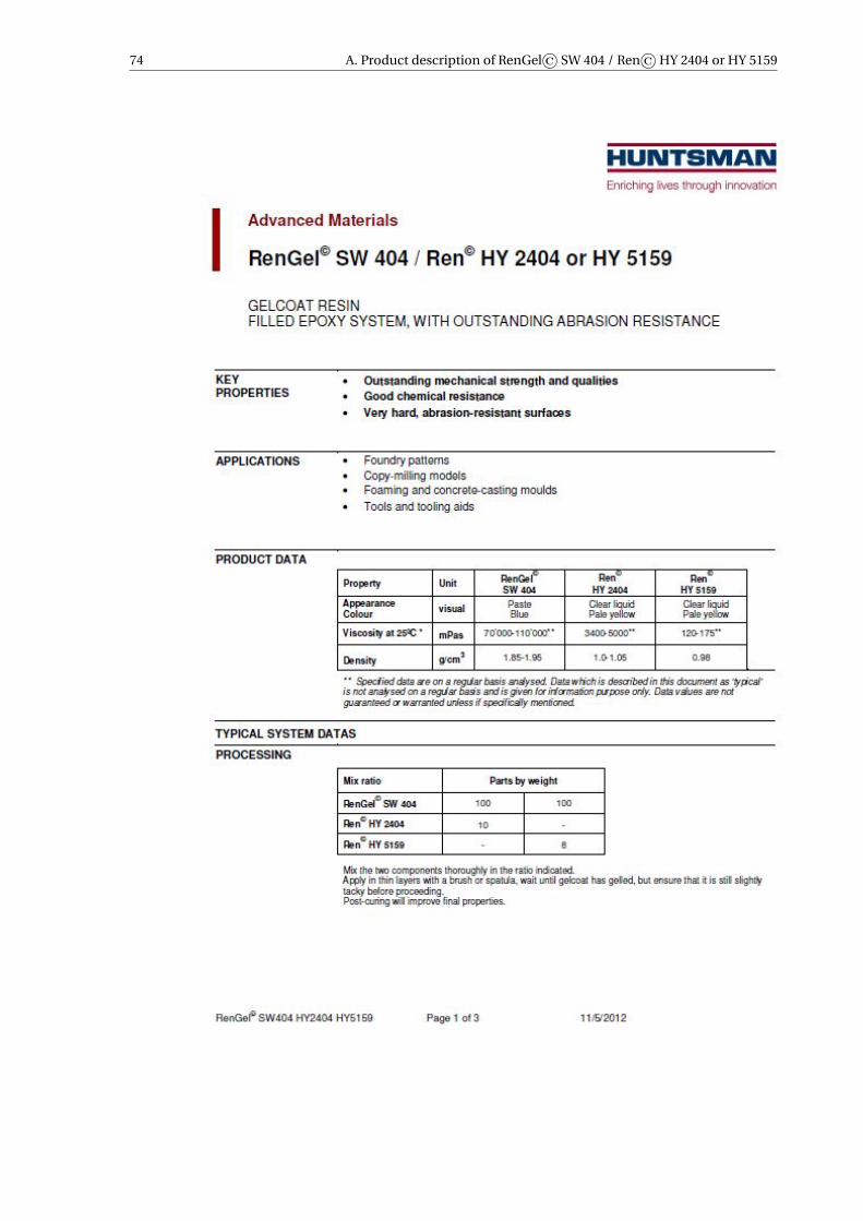
74 A. Product description of RenGel© SW 404 / Ren© HY 2404 or HY 5159
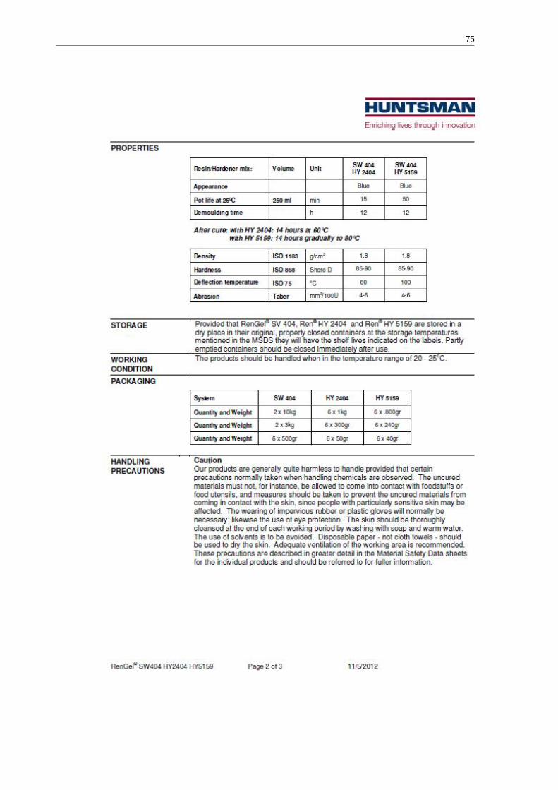
75
76 A. Product description of RenGel© SW 404 / Ren© HY 2404 or HY 5159
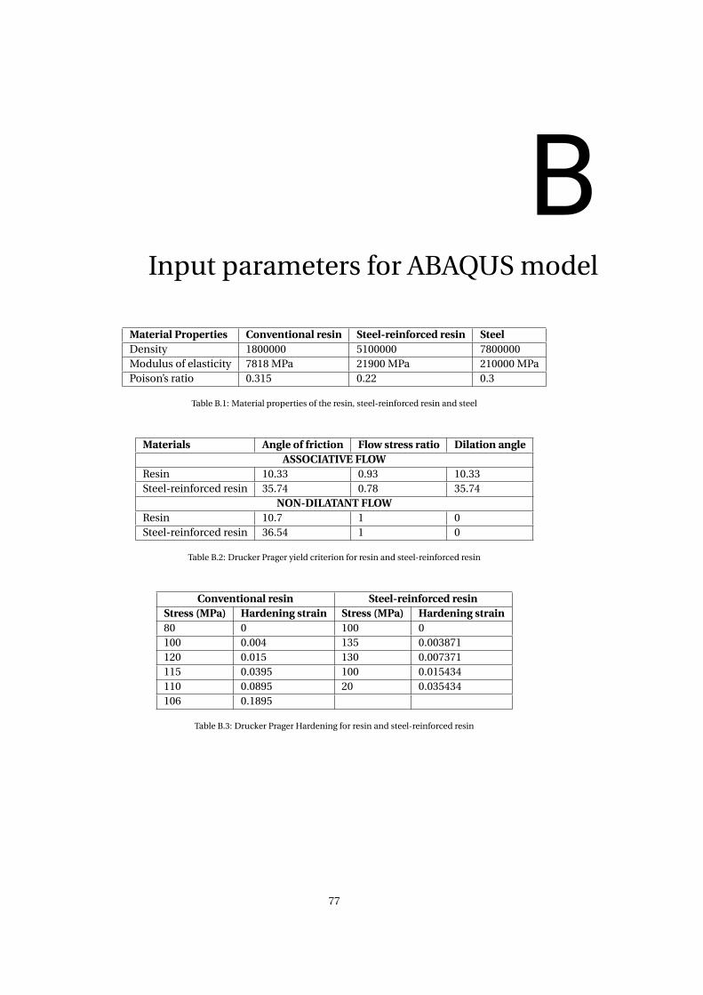
BInput parameters for ABAQUS model
Material Properties Conventional resin Steel-reinforced resin SteelDensity 1800000 5100000 7800000Modulus of elasticity 7818 MPa 21900 MPa 210000 MPaPoison’s ratio 0.315 0.22 0.3
Table B.1: Material properties of the resin, steel-reinforced resin and steel
Materials Angle of friction Flow stress ratio Dilation angleASSOCIATIVE FLOW
Resin 10.33 0.93 10.33Steel-reinforced resin 35.74 0.78 35.74
NON-DILATANT FLOWResin 10.7 1 0Steel-reinforced resin 36.54 1 0
Table B.2: Drucker Prager yield criterion for resin and steel-reinforced resin
Conventional resin Steel-reinforced resinStress (MPa) Hardening strain Stress (MPa) Hardening strain80 0 100 0100 0.004 135 0.003871120 0.015 130 0.007371115 0.0395 100 0.015434110 0.0895 20 0.035434106 0.1895
Table B.3: Drucker Prager Hardening for resin and steel-reinforced resin
77


CGraphs obtained from quasi-static loading
phase of the experiments
Figure C.1: Graphs from quasi-static loading for R_D26_100
The graphs in the figure C.1 represents the graph obtained during the quasi-static loading for resin spec-imens with 26 mm diameter at the stress range of 100 MPa. R_D26_100_1 shows some irregularities in themeasurement during the test.
• Stiffness obtained by R_D26_100_1 is 877.90 KN/mm
• Stiffness obtained by R_D26_100_2 is 908.3 KN/mm
• Stiffness obtained by R_D26_100_3 is 838.7 KN/mm
The graphs in the figure C.2 represents the graph obtained during the quasi-static loading for resin spec-imens with 32 mm diameter at the stress range of 100 MPa. R_D32_100_1 shows an higher non-linearity dueto presence of voids in the tested specimen.
• Stiffness obtained by R_D32_100_1 is 621.63 KN/mm
• Stiffness obtained by R_D32_100_2 is 576.64 KN/mm
79
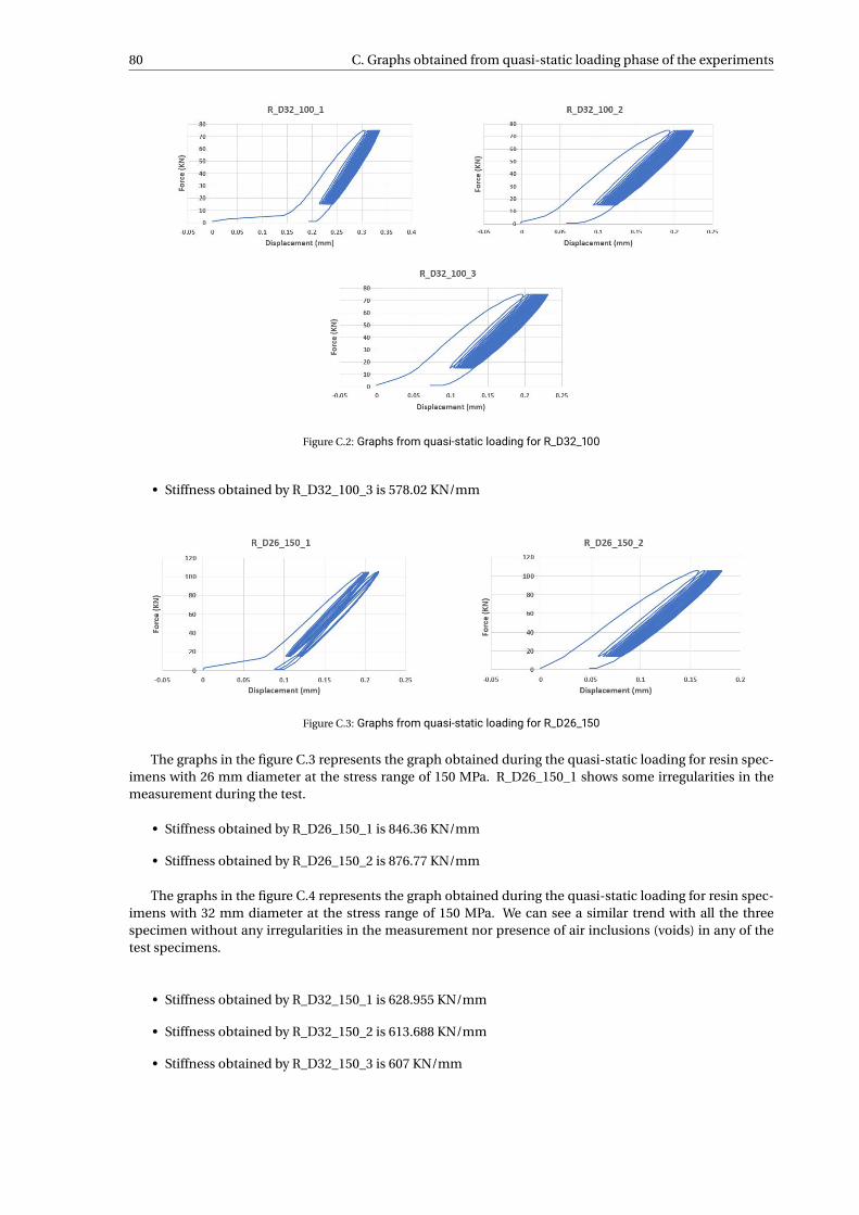
80 C. Graphs obtained from quasi-static loading phase of the experiments
Figure C.2: Graphs from quasi-static loading for R_D32_100
• Stiffness obtained by R_D32_100_3 is 578.02 KN/mm
Figure C.3: Graphs from quasi-static loading for R_D26_150
The graphs in the figure C.3 represents the graph obtained during the quasi-static loading for resin spec-imens with 26 mm diameter at the stress range of 150 MPa. R_D26_150_1 shows some irregularities in themeasurement during the test.
• Stiffness obtained by R_D26_150_1 is 846.36 KN/mm
• Stiffness obtained by R_D26_150_2 is 876.77 KN/mm
The graphs in the figure C.4 represents the graph obtained during the quasi-static loading for resin spec-imens with 32 mm diameter at the stress range of 150 MPa. We can see a similar trend with all the threespecimen without any irregularities in the measurement nor presence of air inclusions (voids) in any of thetest specimens.
• Stiffness obtained by R_D32_150_1 is 628.955 KN/mm
• Stiffness obtained by R_D32_150_2 is 613.688 KN/mm
• Stiffness obtained by R_D32_150_3 is 607 KN/mm
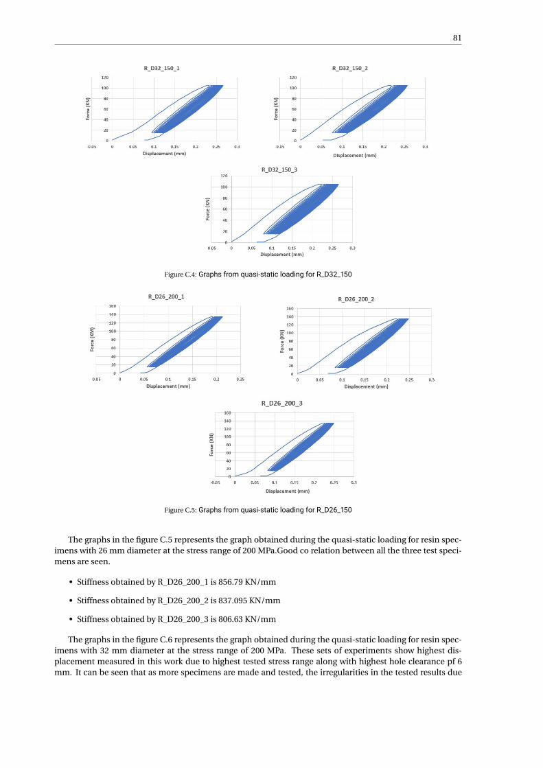
81
Figure C.4: Graphs from quasi-static loading for R_D32_150
Figure C.5: Graphs from quasi-static loading for R_D26_150
The graphs in the figure C.5 represents the graph obtained during the quasi-static loading for resin spec-imens with 26 mm diameter at the stress range of 200 MPa.Good co relation between all the three test speci-mens are seen.
• Stiffness obtained by R_D26_200_1 is 856.79 KN/mm
• Stiffness obtained by R_D26_200_2 is 837.095 KN/mm
• Stiffness obtained by R_D26_200_3 is 806.63 KN/mm
The graphs in the figure C.6 represents the graph obtained during the quasi-static loading for resin spec-imens with 32 mm diameter at the stress range of 200 MPa. These sets of experiments show highest dis-placement measured in this work due to highest tested stress range along with highest hole clearance pf 6mm. It can be seen that as more specimens are made and tested, the irregularities in the tested results due
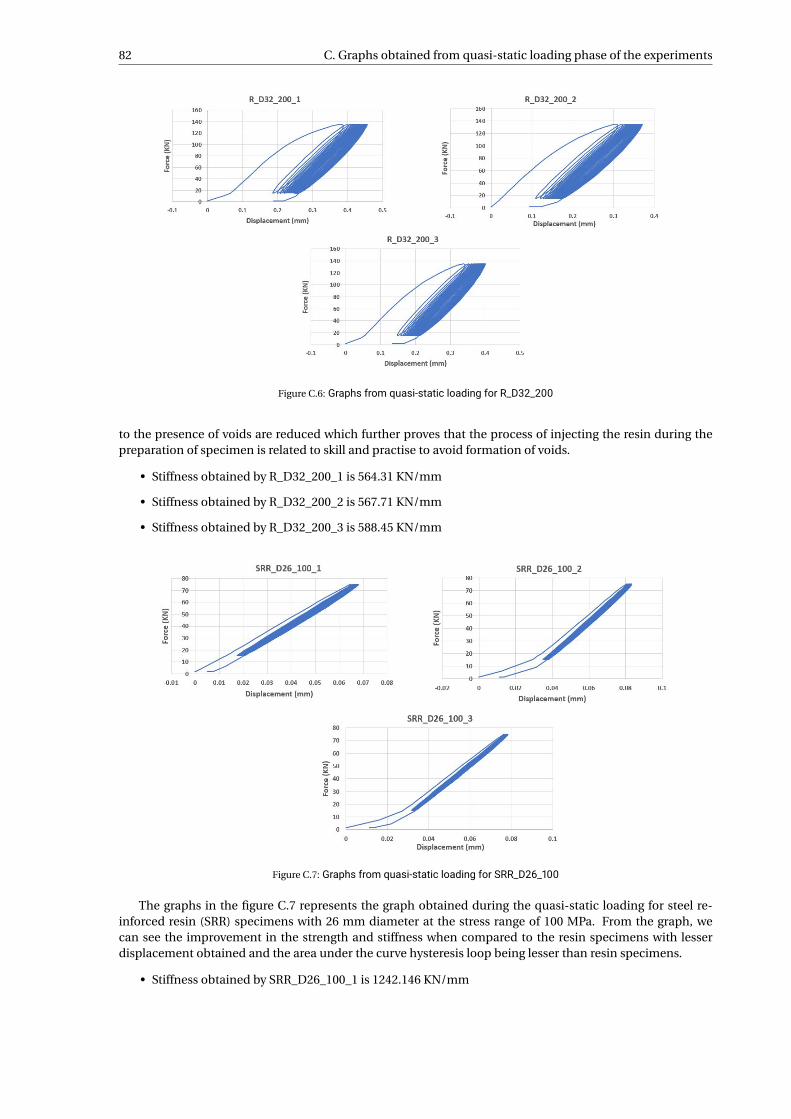
82 C. Graphs obtained from quasi-static loading phase of the experiments
Figure C.6: Graphs from quasi-static loading for R_D32_200
to the presence of voids are reduced which further proves that the process of injecting the resin during thepreparation of specimen is related to skill and practise to avoid formation of voids.
• Stiffness obtained by R_D32_200_1 is 564.31 KN/mm
• Stiffness obtained by R_D32_200_2 is 567.71 KN/mm
• Stiffness obtained by R_D32_200_3 is 588.45 KN/mm
Figure C.7: Graphs from quasi-static loading for SRR_D26_100
The graphs in the figure C.7 represents the graph obtained during the quasi-static loading for steel re-inforced resin (SRR) specimens with 26 mm diameter at the stress range of 100 MPa. From the graph, wecan see the improvement in the strength and stiffness when compared to the resin specimens with lesserdisplacement obtained and the area under the curve hysteresis loop being lesser than resin specimens.
• Stiffness obtained by SRR_D26_100_1 is 1242.146 KN/mm
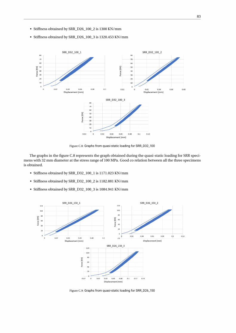
83
• Stiffness obtained by SRR_D26_100_2 is 1300 KN/mm
• Stiffness obtained by SRR_D26_100_3 is 1320.453 KN/mm
Figure C.8: Graphs from quasi-static loading for SRR_D32_100
The graphs in the figure C.8 represents the graph obtained during the quasi-static loading for SRR speci-mens with 32 mm diameter at the stress range of 100 MPa. Good co relation between all the three specimensis obtained.
• Stiffness obtained by SRR_D32_100_1 is 1171.023 KN/mm
• Stiffness obtained by SRR_D32_100_2 is 1182.881 KN/mm
• Stiffness obtained by SRR_D32_100_3 is 1084.941 KN/mm
Figure C.9: Graphs from quasi-static loading for SRR_D26_150
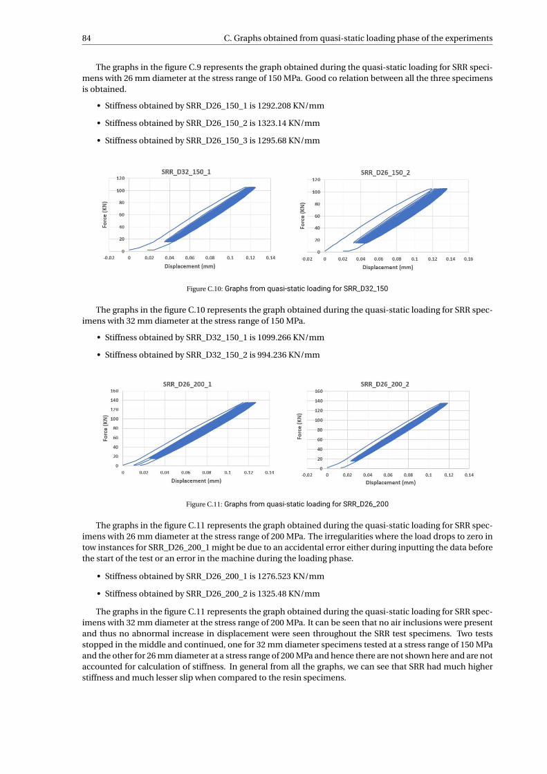
84 C. Graphs obtained from quasi-static loading phase of the experiments
The graphs in the figure C.9 represents the graph obtained during the quasi-static loading for SRR speci-mens with 26 mm diameter at the stress range of 150 MPa. Good co relation between all the three specimensis obtained.
• Stiffness obtained by SRR_D26_150_1 is 1292.208 KN/mm
• Stiffness obtained by SRR_D26_150_2 is 1323.14 KN/mm
• Stiffness obtained by SRR_D26_150_3 is 1295.68 KN/mm
Figure C.10: Graphs from quasi-static loading for SRR_D32_150
The graphs in the figure C.10 represents the graph obtained during the quasi-static loading for SRR spec-imens with 32 mm diameter at the stress range of 150 MPa.
• Stiffness obtained by SRR_D32_150_1 is 1099.266 KN/mm
• Stiffness obtained by SRR_D32_150_2 is 994.236 KN/mm
Figure C.11: Graphs from quasi-static loading for SRR_D26_200
The graphs in the figure C.11 represents the graph obtained during the quasi-static loading for SRR spec-imens with 26 mm diameter at the stress range of 200 MPa. The irregularities where the load drops to zero intow instances for SRR_D26_200_1 might be due to an accidental error either during inputting the data beforethe start of the test or an error in the machine during the loading phase.
• Stiffness obtained by SRR_D26_200_1 is 1276.523 KN/mm
• Stiffness obtained by SRR_D26_200_2 is 1325.48 KN/mm
The graphs in the figure C.11 represents the graph obtained during the quasi-static loading for SRR spec-imens with 32 mm diameter at the stress range of 200 MPa. It can be seen that no air inclusions were presentand thus no abnormal increase in displacement were seen throughout the SRR test specimens. Two testsstopped in the middle and continued, one for 32 mm diameter specimens tested at a stress range of 150 MPaand the other for 26 mm diameter at a stress range of 200 MPa and hence there are not shown here and are notaccounted for calculation of stiffness. In general from all the graphs, we can see that SRR had much higherstiffness and much lesser slip when compared to the resin specimens.
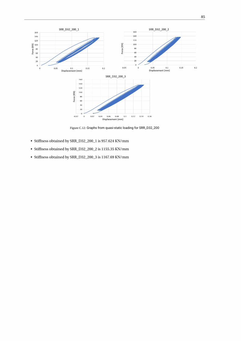
85
Figure C.12: Graphs from quasi-static loading for SRR_D32_200
• Stiffness obtained by SRR_D32_200_1 is 957.624 KN/mm
• Stiffness obtained by SRR_D32_200_2 is 1155.35 KN/mm
• Stiffness obtained by SRR_D32_200_3 is 1167.69 KN/mm

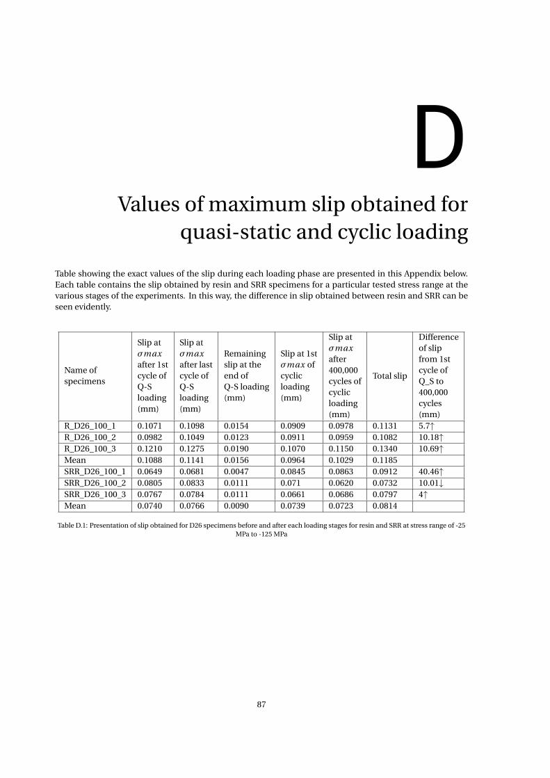
DValues of maximum slip obtained for
quasi-static and cyclic loading
Table showing the exact values of the slip during each loading phase are presented in this Appendix below.Each table contains the slip obtained by resin and SRR specimens for a particular tested stress range at thevarious stages of the experiments. In this way, the difference in slip obtained between resin and SRR can beseen evidently.
Name ofspecimens
Slip atσmaxafter 1stcycle ofQ-Sloading(mm)
Slip atσmaxafter lastcycle ofQ-Sloading(mm)
Remainingslip at theend ofQ-S loading(mm)
Slip at 1stσmax ofcyclicloading(mm)
Slip atσmaxafter400,000cycles ofcyclicloading(mm)
Total slip
Differenceof slipfrom 1stcycle ofQ_S to400,000cycles(mm)
R_D26_100_1 0.1071 0.1098 0.0154 0.0909 0.0978 0.1131 5.7↑R_D26_100_2 0.0982 0.1049 0.0123 0.0911 0.0959 0.1082 10.18↑R_D26_100_3 0.1210 0.1275 0.0190 0.1070 0.1150 0.1340 10.69↑Mean 0.1088 0.1141 0.0156 0.0964 0.1029 0.1185SRR_D26_100_1 0.0649 0.0681 0.0047 0.0845 0.0863 0.0912 40.46↑SRR_D26_100_2 0.0805 0.0833 0.0111 0.071 0.0620 0.0732 10.01↓SRR_D26_100_3 0.0767 0.0784 0.0111 0.0661 0.0686 0.0797 4↑Mean 0.0740 0.0766 0.0090 0.0739 0.0723 0.0814
Table D.1: Presentation of slip obtained for D26 specimens before and after each loading stages for resin and SRR at stress range of -25MPa to -125 MPa
87
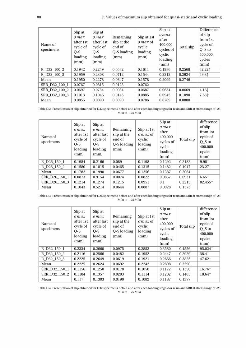
88 D. Values of maximum slip obtained for quasi-static and cyclic loading
Name ofspecimens
Slip atσmaxafter 1stcycle ofQ-Sloading(mm)
Slip atσmaxafter lastcycle ofQ-Sloading(mm)
Remainingslip at theend ofQ-S loading(mm)
Slip at 1stσmax ofcyclicloading(mm)
Slip atσmaxafter400,000cycles ofcyclicloading(mm)
Total slip
Differenceof slipfrom 1stcycle ofQ_S to400,000cycles(mm)
R_D32_100_2 0.1942 0.2249 0.0582 0.1611 0.1986 0.2568 32.22↑R_D32_100_3 0,1959 0.2308 0.0712 0.1544 0.2212 0.2924 49.3↑Mean 0.1950 0.2278 0.0647 0.1578 0.2099 0.2746SRR_D32_100_1 0.0767 0.0815 0.0123 0.0762SRR_D32_100_2 0.0697 0.0734 0.0034 0.0687 0.0634 0.0669 4.16↓SRR_D32_100_3 0.1013 0.1046 0.0145 0.0885 0.0945 0.1090 7.63↑Mean 0.0855 0.0890 0.0090 0.0786 0.0789 0.0880
Table D.2: Presentation of slip obtained for D32 specimens before and after each loading stages for resin and SRR at stress range of -25MPa to -125 MPa
Name ofspecimens
Slip atσmaxafter 1stcycle ofQ-Sloading(mm)
Slip atσmaxafter lastcycle ofQ-Sloading(mm)
Remainingslip at theend ofQ-S loading(mm)
Slip at 1stσmax ofcyclicloading(mm)
Slip atσmaxafter400,000cycles ofcyclicloading(mm)
Total slip
differenceof slipfrom 1stcycle ofQ_S to400,000cycles(mm)
R_D26_150_1 0.1984 0.2166 0.089 0.1198 0.1292 0.2182 9.98↑R_D26_150_2 0.1580 0.1815 0.0465 0.1315 0.1482 0.1947 23.27↑Mean 0.1782 0.1990 0.0677 0.1256 0.1387 0.2064SRR_D26_150_1 0.0873 0.9154 0.0074 0.0822 0.0857 0.0931 6.65↑SRR_D26_150_3 0.1214 0.1274 0.1215 0.0951 0.1 0.2215 82.455↑Mean 0.1043 0.5214 0.0644 0.0887 0.0928 0.1573
Table D.3: Presentation of slip obtained for D26 specimens before and after each loading stages for resin and SRR at stress range of -25MPa to -175 MPa
Name ofspecimens
Slip atσmaxafter 1stcycle ofQ-Sloading(mm)
Slip atσmaxafter lastcycle ofQ-Sloading(mm)
Remainingslip at theend ofQ-S loading(mm)
Slip at 1stσmax ofcyclicloading(mm)
Slip atσmaxafter400,000cycles ofcyclicloading(mm)
Total slip
differenceof slipfrom 1stcycle ofQ_S to400,000cycles(mm)
R_D32_150_1 0.2334 0.2660 0.0975 0.2852 0.3580 0.4556 95.024↑R_D32_150_2 0.2116 0.2566 0.0482 0.1952 0.2447 0.2929 38.4↑R_D32_150_3 0.2225 0.2649 0.0619 0.1921 0.2666 0.3825 47.62↑Mean 0.2225 0.2624 0.0692 0.2242 0.2898 0.3590SRR_D32_150_1 0.1156 0.1250 0.0178 0.1050 0.1172 0.1350 16.76↑SRR_D32_150_2 0.1184 0.1357 0.0203 0.1114 0.1202 0.1405 18.64↑Mean 0.117 0.1303 0.0190 0.1082 0.1187 0.1377
Table D.4: Presentation of slip obtained for D32 specimens before and after each loading stages for resin and SRR at stress range of -25MPa to -175 MPa
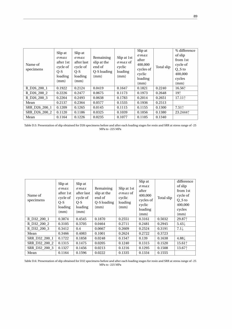
89
Name ofspecimens
Slip atσmaxafter 1stcycle ofQ-Sloading(mm)
Slip atσmaxafter lastcycle ofQ-Sloading(mm)
Remainingslip at theend ofQ-S loading(mm)
Slip at 1stσmax ofcyclicloading(mm)
Slip atσmaxafter400,000cycles ofcyclicloading(mm)
Total slip
% differenceof slipfrom 1stcycle ofQ_S to400,000cycles(mm)
R_D26_200_1 0.1922 0.2124 0.0419 0.1647 0.1821 0.2240 16.56↑R_D26_200_2 0.2226 0.2477 0.0675 0.1173 0.1973 0.2648 19↑R_D26_200_3 0.2264 0.2493 0.0638 0.1783 0.2014 0.2651 17.11↑Mean 0.2137 0.2364 0.0577 0.1535 0.1936 0.2513SRR_D26_200_1 0.1209 0.1265 0.0145 0.1115 0.1155 0.1300 7.51↑SRR_D26_200_2 0.1120 0.1186 0.0325 0.1039 0.1056 0.1380 23.2444↑Mean 0.1164 0.1226 0.0235 0.1077 0.1105 0.1340
Table D.5: Presentation of slip obtained for D26 specimens before and after each loading stages for resin and SRR at stress range of -25MPa to -225 MPa
Name ofspecimens
Slip atσmaxafter 1stcycle ofQ-Sloading(mm)
Slip atσmaxafter lastcycle ofQ-Sloading(mm)
Remainingslip at theend ofQ-S loading(mm)
Slip at 1stσmax ofcyclicloading(mm)
Slip atσmaxafter400,000cycles ofcyclicloading(mm)
Total slip
differenceof slipfrom 1stcycle ofQ_S to400,000cycles(mm)
R_D32_200_1 0.3874 0.4545 0.1870 0.2551 0.3161 0.5032 29.87↑R_D32_200_2 0.3105 0.3705 0.0464 0.2711 0.2481 0.2945 5.43↓R_D32_200_3 0.3412 0.4 0.0667 0.2609 0.2524 0.3191 7.1↓Mean 0.3466 0.4083 0.1001 0.2624 0.2722 0.3723SRR_D32_200_1 0.1722 0.1858 0.0248 0.1547 0.139 0.1638 4.88↓SRR_D32_200_2 0.1315 0.1475 0.0205 0.1240 0.1315 0.1520 15.61↑SRR_D32_200_3 0.1327 0.1456 0.0213 0.1216 0.1295 0.1508 13.67↑Mean 0.1164 0.1596 0.0222 0.1335 0.1334 0.1555
Table D.6: Presentation of slip obtained for D32 specimens before and after each loading stages for resin and SRR at stress range of -25MPa to -225 MPa


EComparison of associative flow model and
non-dilatant flow model
Figure E.1: Comparison of associative flow and non-dilatant flow models for a stress range of 100 MPa with 0.05 frictionco-efficient for resin specimen models and 0.1 friction co-efficient for SRR specimen models
From the graphs E.1 and E.2, it can be seen that there is hardly any difference between the force vs dis-placement graphs obtained by the numerical models of associative flow and non-dilatant flow. For the stressrange of 100 MPa, this difference is the smallest with lines from both the models overlapping with each other.For the stress range of 150 MPa, the lines are very close to each other (almost overlapping) to have any signifi-cant difference. For the stress range of 200 MPa which is shown in the chapter 5, distinct force vs displacementlines for both types of flow models are seen but do not cause any significant difference in stiffness nor in thechosen friction coefficients. But we can see hat as the force applied increases, the difference between the as-sociative flow models and non-dilatant flow models increases. Hence, these graphs further proves that if thespecimens are tested for higher stress ranges, then there could be a significant difference between associative
91
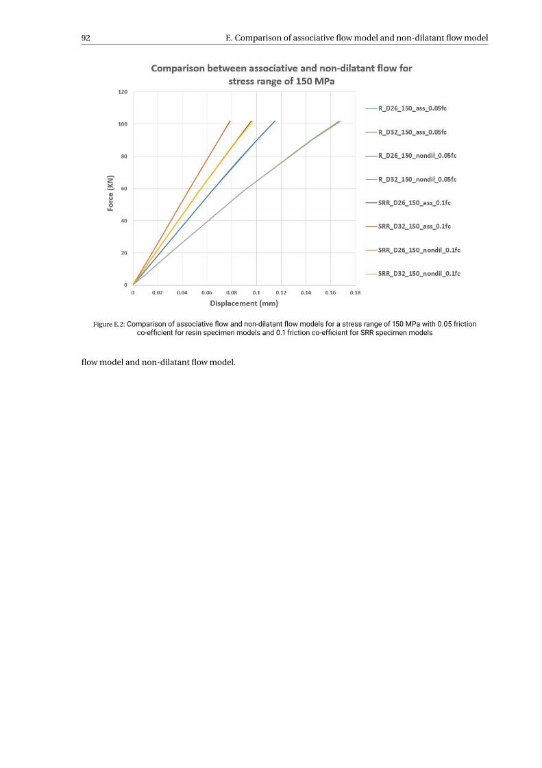
92 E. Comparison of associative flow model and non-dilatant flow model
Figure E.2: Comparison of associative flow and non-dilatant flow models for a stress range of 150 MPa with 0.05 frictionco-efficient for resin specimen models and 0.1 friction co-efficient for SRR specimen models
flow model and non-dilatant flow model.
Copyright © 2022 FDOKUMEN