This article was published in an Elsevier journal. The attached copyis furnished to the author for non-commercial research and

education use, including for instruction at the author’s institution,sharing with colleagues and providing to institution administration.

Other uses, including reproduction and distribution, or selling orlicensing copies, or posting to personal, institutional or third party

websites are prohibited.

In most cases authors are permitted to post their version of thearticle (e.g. in Word or Tex form) to their personal website orinstitutional repository. Authors requiring further information

regarding Elsevier’s archiving and manuscript policies areencouraged to visit:

http://www.elsevier.com/copyright

Investigating RaDAR–LiDAR synergy in a North Carolina pine forest

Ross F. Nelson a,⁎, Peter Hyde b, Patrick Johnson c, Bomono Emessiene c, Marc L. Imhoff a,Robert Campbell d, Wilson Edwards d

a Biospheric Sciences Branch, Code 614.4, NASA-Goddard Space Flight Center, Greenbelt, MD 20771, United Statesb Science Systems and Applications, Inc., 10210 Greenbelt Road, Suite 600, Lanham, MD 20706, United States

c Zimmerman Associates, Inc., 9302 Lee Highway, Suite 600, Vienna, VI 22031, United Statesd Weyerhaeuser, Inc., P.O. Box 1391, New Bern, NC 28563, United States

Received 11 October 2006; received in revised form 29 January 2007; accepted 3 February 2007

Abstract

A low frequency (80–120 MHz) VHF RaDAR, BioSAR, specifically designed for forest biomass estimation and a profiling LiDAR, PALS,were flown over loblolly pine plantations in the southeastern United States. LiDAR-only, RaDAR-only, and joint LiDAR–RaDAR linear modelswere developed to determine if returns from two sensors could be used to estimate pine biomass more accurately and precisely than returns fromeither sensor alone. The best five-variable RaDAR model explained 81.8% (R2) of the stem green biomass variability, with a regression RMSE of57.5 t/ha. The best one-variable LiDAR model explained 93.3% of the biomass variation (RMSE=33.9 t/ha). Combining the RaDAR normalizedvolumetric returns with the profiling LiDAR ranging measurements did little to improve the best LiDAR-only model. The best LiDAR–RaDARmodel explained 93.8% of the biomass variation (RSME=32.7 t/ha). Cross-validation and training/test validation procedures demonstrated (1)that all models are unbiased and (2) the increased precision of the LiDAR-only and LiDAR–RaDAR models. The results of this investigation anda companion study indicate that there is little to be gained combining VHF–RaDAR volumetric returns and profiling LiDAR rangingmeasurements in pine forests; a LiDAR ranging system is sufficient for accurate, precise biomass estimation.© 2007 Elsevier Inc. All rights reserved.

Keywords: VHF RaDAR; Profiling LiDAR; Biomass; RaDAR–LiDAR synergy

1. Introduction

Numerous investigators in the airborne RaDAR and LiDARremote sensing field have indicated that both portions of theelectromagnetic spectrum (EMS) can be used to estimateaboveground forest volume and biomass. RaDAR sensorsemployed in more recent forestry-related studies have typicallyrecorded volumetric, low-frequency VHF returns or higherfrequency UHF measurements. Low frequency systems emitpulsed radio waves in the 20 to 120 MHz range, e.g.,CARABAS (20–90 MHz, Fransson et al., 2000), BioSAR(80–120 MHz, Imhoff et al., 2001). UHF signals in the250MHz (P-band) to 9800MHz (X-band) range, in conjunctionwith interferometric SAR techniques, are used to measure range

to the forest canopy and to ground, e.g., GeoSAR (Hensleyet al., 2001), AirSAR (Lucas et al., 2006). Vegetation LiDARs,due to the physics of laser construction and the reflectivity ofvegetation, typically work in the visible green and near-infraredportions of the EMS to measure forest canopy height and crownclosure.

Early work with RaDAR sensors indicated that UHFvolumetric returns tended to saturate at forest biomass levelsexceeding 200 t/ha (Dobson et al., 1992; Imhoff, 1995). Dobsonet al. (1992) reported a P-band (440 MHz, λ=0.7 m) biomasssaturation limit of 200 t/ha and an L-band (1250 MHz,λ=0.24 m) limit of 100 t/ha. Imhoff (1995) reported asaturation limit of 100 t/ha for P-band radars, 40 t/ha for L-band radars, and 20 t/ha for C-band radars (5300 MHz,λ=0.05 m). Imhoff concluded that use of such space-basedUHF systems would exclude 38% of the Earth's vegetatedsurface containing 81% of the terrestrial biomass from an

Remote Sensing of Environment 110 (2007) 98–108www.elsevier.com/locate/rse

⁎ Corresponding author. Tel.: +1 301 614 6632.E-mail address: Ross.F.Nelson@nasa.gov (R.F. Nelson).

0034-4257/$ - see front matter © 2007 Elsevier Inc. All rights reserved.doi:10.1016/j.rse.2007.02.006

accurate global biomass assessment. Asymptotic limits similarto those reported by Imhoff are noted in Lucas et al. (2006),their Figs. 7 and 8.

Subsequent studies have found that lower frequency, longerwavelength RaDARs in the VHF range (20 to 120 MHz,λ=15.0 m to 2.5 m, respectively) do not run up against thisphytomass limit and, in fact, biomass discrimination improvesas the radio frequency decreases (Imhoff et al., 1998).Magnusson and Fransson (2004a,b) used the CARABASVHF wide-band RaDAR (20–90 MHz, λ=15.0 m to 3.3 m,respectively) in conjunction with Landsat TM and SPOTmultispectral data to estimate stem volume in southern Sweden.Stem volumes ranged from 15 to 585 m3/ha. In both studies,they found that the combined optical-RaDAR data sets werebest for predicting stand-level volume. Interestingly, they foundthat the CARABAS data predicted stem volume most accuratelyin high-volume situations, whereas the optical data were moreaccurate in low-volume circumstances. Smith et al. (2002),working with the CARABAS VHF system and scanningLiDAR data at the individual tree crown level, concluded thatthe VHF radar returns provided a more direct measure of treevolume than the LiDAR.

Vegetation measurements can also be obtained usinginterferometric processing techniques in conjunction withsynthetic aperture RaDAR systems, InSAR, in order to gatherposition information, e.g., range to top-of-canopy (X band) orrange to ground (P band). Though discussion of interferometrictechniques is beyond the scope of this paper, researchers havedemonstrated that biomass saturation limits can be increased byemploying interferometry. Papathanassiou and Cloude (2001)used polarized L-band interferometry to measure tree heights on8 coniferous and 6 deciduous forest stands in Germany. Theyfound that the standard deviation of the difference betweenground-measured height and RaDAR estimates was 2.5 m.Santoro et al. (2002) employed multi-baseline, i.e., repeat-pass,C-band SAR interferometry to infer stem volumes up to 200 m3/ha. Above that, C-band sensitivity to increasing stem volumedecreased, though they were able to estimate stem volumes upto 350 m3/ha. They noted that changes in rainfall, temperature,and wind between overpasses degraded volume retrievals.Treuhaft et al. (2003) fused C-band InSAR and airbornehyperspectral data to estimate biomass on 11 stands in Oregon.The standard deviation of the difference between ground andRaDAR estimates of biomass was 25 t/ha on stands rangingfrom ∼25 t/ha up to ∼270 t/ha. Askne et al. (2003) employedspace-based C- and L-band, multi-baseline InSAR to retrievestem volumes on boreal forest stands up to 335 m3/ha with anRMSE of ∼10 m3/ha for C-band and ∼30–35 m3/ha for L-band. Like Santoro et al. (2002), they note that unstable weatherconditions between overpasses exacerbate volume retrievals.

Airborne LiDAR researchers, over the last two decades, haveempirically related small-footprint (b1 m spot size) LiDARranging measurements of tree heights, height variability, intra-crown canopy densities, and/or crown closure to forest volume(e.g., Holmgren, 2004; Maclean & Krabill, 1986; Maltamoet al., 2006; Næsset, 1997; Nelson et al., 1988; Nilsson, 1996),biomass (e.g., Nelson et al., 1988, 2004), basal area (e.g.,

Gobakken & Næsset, 2004; Holmgren, 2004), and stem counts(e.g., Maltamo et al., 2004; Næsset & Bjerknes, 2001). Forinstance, Næsset (2002) used small-footprint scanning LiDARto predict various plot heights, basal area, and volume ofNorway spruce and Scots pine stands in Norway. Log–logvolume model R2 values ranged from 0.80 to 0.93, withnonsignificant difference between ground and LiDAR estimates(RMSE=18.3 to 31.9 m3/ha). Holmgren et al. (2003) obtainedsimilar results working in spruce/pine stands in Sweden. Meanset al. (2000), working in the northwestern U.S., reported a linearvolume model with an R2 =0.95 and an RMSE of 73 m3/ha instands ranging up to 2500 m3/ha. Nelson et al. (1988) used aprofiling LiDAR in conjunction with linear models to estimatepine biomass in southwestern Georgia, USA — R2 ∼ 0.5,RMSEs ∼70 t/ha. No LiDAR research known to the currentstudy's authors have noted any saturation effect or asymptoticlimit to volume or biomass estimation. LiDAR forestry hasmatured to the point where small-footprint airborne scanningLiDAR is routinely used in Norway and Sweden for foreststructural measurement and management planning (Næsset,2004; Næsset et al., 2004; T. Aasland 2006, personalcommunication).

Recent North American studies have demonstrated that (1)forest volume or biomass can be estimated across extensiveregions using generic, airborne LiDAR-based equations and (2)low density scanning LiDAR data sets (post spacingsNN1 mapart) can be used to acquire those regionalmeasurements. Lefskyet al. (2005b) reported robust biomass and LAI equationsapplicable across five diverse sites in the Pacific Northwest.Rooker Jensen et al. (2006) demonstrated that regression modelsrelating ground-measured height, basal area, and wood volume toLiDAR heights could be generalized across structurally andtopographically variable coniferous sites in Idaho. Thomas et al.(2006) compared low density (5 m post spacing) and high density(0.5 m) LiDAR datasets. While concerns were expressed aboutthe use of low density LiDAR for regional estimation, nodegradation in predictive capacity was found.

Both technologies have demonstrated a capacity to senseforest structure which scientists exploit to estimate the amountof aboveground wood. But can RaDAR and LiDAR measure-ments, considered jointly, be used to predict forest biomassbetter than either separately? Previous studies comparing and/orjointly considering RaDAR and LiDAR data sets are somewhatsparse, though interest in sensor synergy is increasing. Slattonet al. (2001) used systematically sampled strips of scanningLiDAR measurements as ground reference data to calibrateground and vegetation height measurements made by ainterferometric SAR. Slatton et al.'s Figs. 13–15 directlycompare C-band InSAR and LiDAR vegetation heightmeasurements. Lucas et al. (2005) did not directly compareLiDAR and SAR data sets, but they did employ the LiDARmeasurements to help understand AirSAR C, L, and P bandreturns. They employed field data, scanning LiDAR data, aerialphotography, and CASI (Compact Airborne SpectrographicImager) multispectral observations to create 3-D forest canopiesin order to develop an AirSAR simulation model. Breidenbachet al. (2006) compared scanning LiDAR and InSAR ranging

99R.F. Nelson et al. / Remote Sensing of Environment 110 (2007) 98–108

measurements to see which best estimated tree heights on 250poly-areal forest inventory plots in beech-spruce-oak forestsnear Stuttgart, Germany. In this study, the LiDAR last-pulseground returns were used to create a digital terrain model(DTM). The LiDAR first returns and the InSAR X-band top-of-canopy returns were combined with the LiDAR DTM to seewhich data source best-predicted tree heights. The RMSE of theplot-level InSAR height estimates was 2.69 m (CV=9.5%),whereas the comparable LiDAR RMSE was 1.85 m(CV=6.6%). The authors concluded that “The use of laserscanner data is more appropriate when a high level of accuracyfor the estimation of tree height or vegetation height structure isrequired.” As noted above (Askne et al., 2003; Santoro et al.,2002), multi-baseline interferometry may improve performanceof the X-band height estimates.

The current study is a follow-on to work reported by Hydeet al. (2007)who found no practical, exploitable LiDAR–RaDARsynergy in the ponderosa pine forests (Pinus ponderosa Laws.) ofthe southwestern United States. Hyde et al. investigated the use ofan extremely low frequency U.S. Defense Department RaDAR–FOPEN (FOliage PENetrating RaDAR), λ=7.8 m- and GeoSARX and P-band ranging data in conjunction with LiDAR scanningdata. They concluded that scanning LiDAR was the sensor ofchoice to predict pine biomass. More importantly, RaDAR didlittle to improve LiDAR biomass estimates, though they pointedout that the RaDAR acquisitions were not ideal from thestandpoint of polarization availability (GeoSAR) or sensorwavelength (FOPEN).

The current investigation augments the Hyde et al. (2007)study by looking at eastern U.S. rather than western U.S. pinestands using significantly different RADAR and LiDARtechnology. Hyde et al. investigated low-frequency RADARdata at a wavelengthmuch longer than the wavelength consideredin the current study. They also looked at P and X band InSAR(GeoSAR) to get ranging information to the top and bottom of thecanopy.We employed a low-frequencyVHFRaDAR–BioSAR–which acquiredmulti-angle volumetric returns in the 80–120MHz(λ=3.7 m to 2.5 m, respectively) range. BioSARwas specificallydesigned to retrieve forest biomass estimates without saturating.With respect to LiDAR, the Hyde study, much like Thomas et al.(2006), looked at small footprint, low density, e.g., 5 mpost spacing, scanning LiDAR. We employed a small profilingLiDAR called PALS — the Portable Airborne Laser System(Nelson et al., 2003a). PALS was specifically designed as asampling tool to estimate forest volume, biomass, and carbonacross regions (e.g., 1000–5000 km2, Nelson et al., 2003b, 2004;27,000 km2, Gobakken et al., 2006). Though both studies in-vestigate RaDAR–LiDAR synergy, they do so using markedlydifferent RaDAR and LiDAR technology.

The overall objective of this study is to determine if there isany sort of VHF RaDAR-profiling, small-footprint LiDARsynergy that might be exploited to better predict forest biomass.Specific subobjectives follow:

(1) Identify those BioSAR volumetric variables that bestpredict stand-level stem green biomass. Identify thoseRaDAR look angles most useful for pine biomass

prediction. Likewise identify the best PALS height,height variability, and canopy closure predictors. DevelopBioSAR-only and PALS-only models.

(2) Consider BioSAR and PALS variables jointly, select thebest biomass predictors, and develop a joint model toestimate stem green biomass.

(3) Assess the accuracy and precision of these models usingcross-validation and training/testing procedures.

2. Materials

BioSAR RaDAR and PALS LiDAR returns were acquiredover 32 Weyerhaeuser loblolly pine (Pinus taeda L.) stands nearNewBern, North Carolina (Fig. 1). TheWeyerhaeuser plantationsare located in the southern pine region of the United States, aregion that extends from southern New Jersey across the CoastalPlain and Piedmont regions of the southeastern US to easternTexas (Fig. 1). Loblolly pine is the most important of the fourcommercially valuable pines found throughout the area, an areawhich supplies 59% of the nation's roundwood (Haynes, 2003).These even-aged pine plantations, growing on flat, sandy soils ofthe southeastern U.S. coastal plain, presented ideal, simple targetsfor the two sensors — relatively open canopy, flat terrain, littleunderstory, uniform height, crown closure, and stem spacing. Atotal of 76 aircraft transects were made across these 32 stands onFebruary 17 and 18, 2005.

The two sensors were carried aboard a Twin Otter twin-engine turboprop aircraft that nominally flew at 300 m AGL at130 knots (240 km/h, or 66.7 m/s). Wings were, to the best ofthe pilots' abilities, kept flat and level during the simultaneousBioSAR and PALS data collection transects. The pilots drovethe aircraft across the centroids of the forest stands on magneticeast–west or north–south transects using the course deviationindicator on a WAAS-enabled Garmin GPSMap 296.

2.1. Weyerhaeuser ground reference data

The stands are, for the most part, pure loblolly pine. The standwith the largest deciduous component, which was leaf-off at thetime of the data collection, contained only 6% hardwood, byvolume. Weyerhaeuser supplied estimates of merchantable stemvolume, inside bark, to a 10 cm (4 in.) top for each of the 32stands overflown. A simple, proprietary, multiplicative trans-formation was employed to calculate stem green biomass, insidebark, from the field-measured volume estimates. The averagecanopy height of those stands transected by the BioSAR-PALSsystem ranged from 0.3 m to 22.7 m (as measured by PALS),with a mean height of 13.0 m±7.5 m (one standard deviation).Stem green biomass values ranged from 0 t/ha to 416.9 t/ha onthese 32 stands, with a mean value of 199.5 t/ha±127.5 t/ha.Across the entire study area, stand sizes ranged from 0.3 to 249.4ha; while the stands actually flown range in size from 32.7 ha to112.5 ha. Larger plantations were preferentially selected forstudy to accommodate the relatively large size of the BioSARpixels.

100 R.F. Nelson et al. / Remote Sensing of Environment 110 (2007) 98–108

2.2. RaDAR data

BioSAR was developed as a VHF SAR specifically tomitigate biomass saturation problems noted in UHF RaDARsystems. BioSAR was originally conceived as an instrument tomeasure aboveground biomass in tropical forests, where drybiomass values may be in excess of 500 t/ha. BioSAR, as

configured for this experiment, acquired volumetric returns on a600 m radius circle directly beneath the aircraft in the 80–100 MHz range. The size of the area illuminated by the radiopulse is determined by the beam width and flight altitude,nominally 300 m AGL. The wavelength of the emitted pulse isadjustable and is set prior to a specific mission so that local FMradio station signals do not contaminate target returns. On this

Fig. 1. (A) Range map for loblolly pine (from Gaby, 1985, his Fig. 1), with study area location annotated. (B) Seventy-six BioSAR-PALS flight lines crossing 32Weyerhaeuser loblolly pine stands near New Bern, North Carolina, February 17 and 18, 2005.

101R.F. Nelson et al. / Remote Sensing of Environment 110 (2007) 98–108

mission, the pulse repetition rate was 166 kHz, the pulse widthwas 1.52 μs, and the pulse frequency was 85 MHz (λ=3.5 m).

As explained and illustrated in Imhoff et al. (2000), the returnsfrom the 600 m target area were range-gated (across-track) andDoppler-sorted (along-track) to produce 300 m across-track×30 m along-track pixels. The high repetition rate andDoppler sorting permitted the instrument to acquire multipleobservations at multiple angles on a particular 30m×300m patchof ground up to 45 degrees in front of the aircraft and 45 degreesbehind. In this study, the RaDAR returns were sorted into 64forward- and rearward-looking angle bins, ±45° (Table 1). InTable 1, zero is the nadir look angle, directly beneath the aircraft.Plus (+) indicates a forward look angle, minus (−) indicates areturn acquired looking back toward the rear of the aircraft, and ±indicates an average of the forward and backward look angleresponses. All angles reported in Table 1 aremidpoints, in degreesfrom nadir, of 1.42° Doppler angle bins.

The angular volumetric BioSAR responses were furtherprocessed into Normalized RaDAR Cross Sections (NRCS).The RaDAR cross-section (RCS) for a given incidence angle isthe ratio of the received power to the transmitted power, adjustedfor receiver and antenna gains. The RCS was then normalized toproduce the NRCS responses by dividing this RCS return by theeffective target area. Given the flight speed and RaDAR samplingrate, the along-track post spacing of the BioSAR pixels was 10m,so sequentially-acquired BioSAR pixels overlapped ∼67%.

Preliminary work with other data sets by ZAI personnelsuggested that certain simple linear transformations of the 64NRCS angle bin responses might prove useful for predicting theamount of wood on the ground. As noted in Table 1, the post-processed NRCS angle bin responses ranged from approxi-mately+45° (forward-looking) to −45° (backward-looking).The preliminary studies by ZAI personnel suggested that thefollowing transformations be considered:

– Average forward- and backward-looking NRCS values. Forinstance, calculate an 11.4° NRCS as the average of the+11.4° and −11.4° responses.

– Average 5°, 10°, and 15° ±angle bin responses. For instance,calculate a mean NRCS response for all bins between ±30°and 40°.

The additional BioSAR variables which resulted from thecalculation of these simple means are listed in Table 1.

2.3. Profiling LiDAR data

The PALS data were acquired coincidentally with the BioSARdata. The laser used in the acquisition was a Riegl LD90-3800VHS FLP, a near-infrared LiDAR (λ=0.905 μm), programmed tosupply sequential, alternating first and last returns. The 2000 Hzdata stream was subsampled 5:1, providing a effective samplingrate of 400 Hz. At a nominal flight speed of ∼67 m/s, a flyingaltitude of 300mAGL, and a laser divergence of 1.7mr, the PALSspot sizewas 60 cm at target, and the along-track post spacingwas16.7 cm. Since first and last returns are sequentially acquired, thetop of the canopy is described by pulses spaced 33.4 cm apart. The

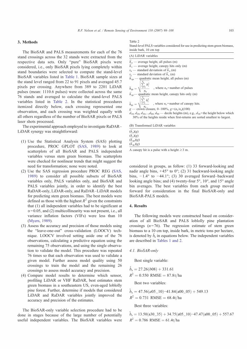
interleaved last returns were used to identify ground beneathforest canopy by identifying local minima and connecting theseminima with a spline function. Once the ground line was defined,a tree height was calculated for each first return pulse. The PALSvariables developed frommeasurements acquired over each standare reported in Table 2.

Table 1Stand-level BioSAR variables considered for use in models predicting stemgreen biomass, inside bark, 10 cm top

(A) Forward (f), nadir (p0), and backward (b) look angles; 64 variables

Midpoint(deg)

Variablename

Midpoint(deg)

Variablename

Midpoint(deg)

Variablename

0.0 p0 15.6 f15,b15 31.3 f31,b311.4 f01,b01 17.1 f17,b17 32.7 f32,b322.8 f02,b02 18.5 f18,b18 34.1 f34,b344.3 f04,b04 19.9 f19,b19 35.6 f35,b355.7 f05,b05 21.3 f21,b21 37.0 f37,b377.1 f07,b07 22.8 f22,b22 38.4 f38,b388.5 f08,b08 24.2 f24,b24 39.8 f39,b3910.0 f10,b10 25.6 f25,b25 41.3 f41,b4111.4 f11,b11 27.0 f27,b27 42.7 f42,b4212.8 f12,b12 28.4 f28,b28 44.1 f44,b4414.2 f14,b14 29.9 f29,b29 45.5 f45

(B) Averaged forward–backward angle bin responses; 31 transformations

Transformation Variable name

mean [+/−1.4°] a01mean [+/−2.8°] a02mean [+/−4.3°] a04mean [+/−5.7°] a05mean [+/−7.1°] a07

••••••••••mean [+/−42.7°] a42mean [+/−44.1°] a44

(C) 5° groups; 9 transformations

Transformation Variable name

mean [+/−0.0°–4.3°] a00_05mean [+/−5.7°–10.0°] a05_10mean [+/−11.4°–14.2°] a10_15

••••••••••mean [+/−35.6°–39.8°] a35_40mean [+/−41.3°–45.5°] a40_45

(D) 10° groups; 8 transformations

Transformation Variablename

Transformation Variablename

mean [±0.0°–10.0°] a00_10 mean [±21.3°–29.9°] a20_30mean [±5.7°–14.2°] a05_15 mean [±25.6°–34.1°] a25_35mean [±11.4°–19.9°] a10_20 mean [±31.3°–39.8°] a30_40mean [±15.6°–24.2°] a15_25 mean [±35.6°–45.5°] a35_45

(E) 15° groups; 7 transformations

Transformation Variablename

Transformation Variablename

mean [±0.0°–14.2°] a00_15 mean [±21.3°–34.1°] a20_35mean [±5.7°–19.9°] a05_20 mean [±25.6°–39.8°] a25_40mean [±11.4°–24.2°] a10_25 mean [±31.3°–45.5°] a30_45mean [±15.6°–29.9°] a15_30

Table entries report the midpoint of 1.42° look angle bins and the associatedvariable names.

102 R.F. Nelson et al. / Remote Sensing of Environment 110 (2007) 98–108

3. Methods

The BioSAR and PALS measurements for each of the 76stand crossings across the 32 stands were extracted from therespective data sets. Only “pure” BioSAR pixels wereconsidered, i.e., only BioSAR pixels lying completely withinstand boundaries were selected to compute the stand-levelBioSAR variables listed in Table 1. BioSAR sample sizes atthe stand level ranged from 22 to 91 pixels and averaged 45.7pixels per crossing. Anywhere from 389 to 2201 LiDARpulses (mean: 1110.6 pulses) were collected across the same76 stands and averaged to calculate the stand-level PALSvariables listed in Table 2. In the statistical proceduresitemized directly below, each crossing represented oneobservation, and each crossing was weighted equally withall others regardless of the number of BioSAR pixels or PALSlaser shots processed.

The experimental approach employed to investigate RaDAR–LiDAR synergy was straightforward:

(1) Use the Statistical Analysis System (SAS) plottingprocedure, PROC GPLOT (SAS, 1989) to look atscatterplots of all BioSAR and PALS independentvariables versus stem green biomass. The scatterplotswere checked for nonlinear trends that might suggest theneed for transformation; none were noted.

(2) Use the SAS regression procedure PROC REG (SAS,1989) to consider all possible subsets of BioSARvariables only, PALS variables only, and BioSAR andPALS variables jointly, in order to identify the bestRaDAR-only, LiDAR-only, and RaDAR–LiDAR modelsfor predicting stem green biomass. The best models weredefined as those with the highest R2 given the constraintsthat (1) all independent variables had to be significant atα=0.05, and (2) multicollinearity was not present, i.e., allvariance inflation factors (VIFs) were less than 10(Myers, 1989).

(3) Assess the accuracy and precision of those models usingthe “leave-one-out” cross-validation (LOOCV) tech-nique. LOOCV involved setting aside one of the 76observations, calculating a predictive equation using theremaining 75 observations, and using the single observa-tion to validate the model. This procedure was repeated76 times so that each observation was used to validate agiven model. Further assess model quality using 50crossings to train the model and the remaining 26crossings to assess model accuracy and precision.

(4) Compare model results to determine which sensor,profiling LiDAR or VHF RaDAR, best estimates stemgreen biomass in a southeastern US, even-aged loblollypine forest. Further, determine if models that consideredLiDAR and RaDAR variables jointly improved theaccuracy and precision of the estimates.

The BioSAR-only variable selection procedure had to bedone in stages because of the large number of potentiallyuseful independent variables. The BioSAR variables were

considered in groups, as follow: (1) 33 forward-looking andnadir angle bins, +45° to 0°; (2) 31 backward-looking anglebins, −1.4° to −44.1°; (3) 30 averaged forward–backwardlooking angle bins; and (4) twenty-four 5°, 10°, and 15° anglebin averages. The best variables from each group movedforward for consideration in the final BioSAR-only andBioSAR-PALS models.

4. Results

The following models were constructed based on consider-ation of all BioSAR and PALS loblolly pine plantationcrossings (n=76). The regression estimate of stem greenbiomass to a 10 cm top, inside bark, in metric tons per hectare,is denoted by b̂s in equations below. The independent variablesare described in Tables 1 and 2.

4.1. BioSAR-only

Best single variable:

b̂s ¼ 27:26ðb08Þ þ 331:61

R2 ¼ 0:550 RMSE ¼ 87:8t=ha

Best two variables:

b̂s ¼ 47:56ða05−10Þ−41:84ða00−05Þ þ 549:13

R2 ¼ 0:731 RMSE ¼ 68:4t=ha

Best three variables:

b̂s ¼ 13:50ða30−35Þ þ 34:75ða05−10Þ−47:47ða00−05Þ þ 557:67

R2 ¼ 0:786 RMSE ¼ 61:4t=ha

Table 2Stand-level PALS variables considered for use in predicting stem green biomass,inside bark, 10 cm top

(A) LiDAR variables

h̄ a — average height, all pulses (m)h̄ c — average height, canopy hits only (m)sa — standard deviatioin of h̄ a (m)sc — standard deviation of h̄ c (m)h̄ qa — quadratic mean height, all pulses (m)

h̄qa ¼

ffiffiffiffiffiffiffiffiffiffiffiffiPnai¼1

h2i

na

vuut, where na=number of pulses

h̄ qc— quadratic mean height, canopy hits only (m)

h̄qc ¼

ffiffiffiffiffiffiffiffiffiffiffiffiPnci¼1

h2i

nc

vuut, where nc=number of canopy hits.

g — crown closure, 0–100%, g=(nc/na)(100)d10, d20, d30,…,d80, d90 — decile heights (m), e.g., d30= the height below which30% of the heights reside when first-returns are sorted smallest to largest.

(B) Transformed LiDAR variables

(h̄ a)(g)(h̄ c)(g)(h̄ qa)(g)(h̄ qc)(g)

A canopy hit is a pulse with a height ≥3 m.

103R.F. Nelson et al. / Remote Sensing of Environment 110 (2007) 98–108

Best four variables:

b̂s ¼ ð−13:43Þðp0Þ−27:81ða02Þ þ 28:45ða05−10Þþ13:58ða30−35Þ þ 551:21R2 ¼ 0:802 RMSE ¼ 59:5t=ha

Best five variables:

b̂s ¼ ð−11:95Þðp0Þ−6:92ðb41Þ−23:80ða02Þ þ 28:08ða07Þþ 15:13ða30−35Þ þ 495:38

R2 ¼ 0:818 RMSE ¼ 57:5t=ha

In all five models, every independent variable was significantat pb0.0001 with the exception of b41 (p=0.008) in the 5-variable model. All five models had y-intercepts significantlydifferent from zero. The largest VIF recorded for any of theindependent variables in any of these five models was 3.4, wellbelow 10, the threshold that connotes multicollinearity (Myers,1989). The best BioSAR-only model with 6 variables included anonsignificant independent variable, and models with 7 or morevariables had multicollinearity problems with three or moreVIFsN10.

4.2. PALS-only

Best model:

b̂s ¼ 0:17ðh̄qcÞðgÞ−11:86 R2 ¼ 0:933RMSE ¼ 33:9t=ha

Additional LiDAR-only variable entries lead to multi-collinearity problems, i.e., VIFsN10. The y-intercept was notsignificantly different from zero at the 95% level of confidence(p=0.149).

4.3. BioSAR-PALS

Best model:

b̂s ¼ 0:15ðh̄qaÞðgÞ þ 4:40ðb08Þ þ 41:02R2 ¼ 0:938 RMSE ¼ 32:7 t=ha

(h̄ qa)(g) is significant at pb0.0001; b08 is significant atp=0.0047; VIF=2.0. The y-intercept was significantly differentfrom zero at the 95% level of confidence (p=0.0069).Consideration of BioSAR-PALS models with three or morevariables lead to multicollinearity problems due to the additionof highly correlated LiDAR height metrics.

These results suggest the following:

(1) LiDAR height observations are more useful for predictingstem green biomass in southeastern U.S. pine plantationsthan VHF RaDAR normalized cross sectional returns.

(2) Multiplicative LiDAR variables that combine quadraticmean height measurements with crown closure wereconsistently selected as the best profiling LiDARvariables for pine biomass prediction. However thesecomposite variables, in this setting, do little better than a

simple average height predictor. For instance, a simplelinear model using the average height of all pulses (h̄ a) asthe independent variable, produced an R2 =0.929,RMSE=34.9 t/ha.

(3) The backward-looking BioSAR NRCS response at −8.5°was selected as the best single BioSAR predictor of stemgreen biomass and as the best BioSAR variable in theLiDAR–RaDAR model. This empirical observation is atodds with previous BioSAR research in the oak/pineforests of the Big Thicket Forest Preserve in eastern Texas(Imhoff et al., 2000). Using 5° Doppler bins rather thanthe 1.4° bins considered in this study, they identifiedRaDAR returns at a 25° look angle as best for predictingforest dry biomass up to∼270 t/ha at RaDAR frequenciesbetween 80.0 and 88.5 MHz.

(4) The PALS-only model has a y-intercept not significantlydifferent from zero. The BioSAR-only and joint BioSAR-PALS models all have y-intercepts significantly differentfrom zero. Zero height should align with zero biomass, somodels with significantly positive or negative y-interceptsare, intuitively, less reasonable than models with smallintercepts.

(5) Preliminary work with the BioSAR responses suggestedthat strong RaDAR returns were frequently observed onclearcuts. Analysis of the coincident video imageryindicated the presence of logging slash, debris piles, andcoarse, downed, woody debris in recently harvestedstands. Attempts were made to formulate RaDAR andRaDAR–LiDAR regressions based on ground observa-tions where ground-measured biomass was greater than100 t/ha, excluding all of the zero biomass sites, butthese regressions proved to be much weaker than thosereported above. BioSAR did, apparently, interact withslash left over after a harvesting operation, but exclusionof these harvested sites did not improve regressionresults.

(6) A five-variable BioSAR-only model explained 82% ofthe southern pine biomass variability on a study areawhere ground-based biomass estimates ranged from 0 to417 t/ha. No “plateau-ing” or biomass saturation effectwas noted in scatterplots of biomass versus each of the 5independent BioSAR variables.

(7) Based on these regression metrics alone, i.e., R2 andRMSE, a statistically significant though marginally usefulsynergy may be realized by considering RaDAR andLiDAR measurements jointly. The inclusion of theBioSAR NRCS response at −8.5° increased R2 by0.005 and decreased the regression RMSE by 1.1 t/harelative to the best PALS model.

These results are consistent with those reported by Hyde et al.(2007) who investigated RaDAR–LiDAR synergy for predictionof ponderosa pine total aboveground dry biomass. Theydeveloped a best LiDAR-only simple linear model based on h̄awith an R2=0.822, RMSE=26.1 t/ha. h̄qa was also highlysignificant when used as the solo predictor in a linearmodel. Theirbest RaDAR-only models reported R2 values less than half the

104 R.F. Nelson et al. / Remote Sensing of Environment 110 (2007) 98–108

size of the LiDARmodels and RMSE values twice as large. As inthe current study, Hyde et al. (2007) observed that, thoughRaDAR–LiDAR synergy may be statistically significant, inpractical terms the small improvements may not merit theincreased cost of the RaDAR acquisition and processing.

4.4. Model cross-validation and training/test results

Cross-validation results are illustrated in Fig. 2 and, alongwith training/test results, summarized in Table 3. Table 3 resultsclosely track the initial regression results. All of the models

Fig. 2. Best RaDAR-only (A), LiDAR-only (B), and LiDAR–RaDAR (C) cross-validated results. The y-axis, total above-ground stem green biomass, in metric tonsper hectare is plotted as a function of one of the independent predictors. Ground-measured stem green biomass (blue) and predicted stem green biomass (red) aredisplayed for each of the 76 loblolly pine stands. The equations reported above each figure are identical to those reported in the text for the best BioSAR-only model, 5variables, the best PALS-only model, and the best PALS-BioSAR model. The y-axis in each graph is the predicted stem green biomass (tot_sgb), in tons/ha.

105R.F. Nelson et al. / Remote Sensing of Environment 110 (2007) 98–108

considered appear to be unbiased; the largest difference betweenthe average predicted versus actual biomass value was only0.5 t/ha. However, model precision as characterized by thecross-validation RMSE, and the range of the predicted versusactual biomass differences, are quite dissimilar. Both theLiDAR-only and LiDAR–RaDAR models are more precisethan the best RaDAR-only model. The best RaDAR-only modelhas an error standard deviation 1.8 times larger than the bestLiDAR-only model and a range of errors 1.6 times as large.

The LiDAR–RaDAR model improves the precision of theLiDAR-only model by ±0.55 t/ha, a 1.6% improvement (i.e.,(34.38 t/ha–33.83 t/ha)/(33.83 t/ha)). In short, practicallyspeaking, little is gained by combining BioSAR and PALSdata to predict southeastern U.S. pine plantation stem greenbiomass. An airborne laser profiler, on its own, is, for mostpurposes, probably adequate, at least in a southern pine setting.

5. Discussion

To date, two studies have specifically looked for RaDAR–LiDAR synergy to improve forest biomass estimation. In bothstudies, Hyde et al. (2007) and the current investigation, siteswere considered that were near-optimal with respect to bothRaDAR and LiDAR acquisitions, i.e., flat topography, little/nounderstory vegetation, relatively open canopies, large contigu-ous forest stands supporting one predominant species of pine.Results from both studies are consistent. LiDAR, whetherscanning or profiling, estimated pine biomass more accuratelyand precisely than any of the RaDARs considered in the twostudies. Further, consideration of LiDAR and RaDAR jointlydid not, for all practical purposes, improve forest biomassestimation even though the addition of a RaDAR variable to thebest LiDAR model was statistically significant. The addition ofthe best RaDAR variable to the best LiDAR model decreasedcross-validated biomass RMSEs by 0.6 t/ha (this study), or0.3% of the average stem green biomass, and 1.9 t/ha (Hydeet al., 2007), or 1.9% of the average total aboveground drybomass. Given the magnitude of the improvement, it is fair toask if this marginal synergy is worth exploiting.

Why did a simple profiling LiDAR provide substantiallymore accurate and precise estimates of stem green biomass inNorth Carolina? Though simple, these industrial plantationforests favor LiDAR remote sensing. Airborne LiDARsmeasure height, and the more highly correlated the relationshipbetween canopy height and biomass, the better the accuracy andprecision of the LiDAR-based biomass estimates. Even-aged,monospecific, closed canopy forests with an apically dominantgrowth form and little or no understory are, from a LiDARstandpoint, the ideal remote sensing situation. BioSAR recordsreturns from physical corner reflectors sized at roughly thewavelength of the RaDAR system, in this case, 3.5 m. Thecorner reflectors in this case are the tree stems, with larger stemsand higher stem densities producing brighter (or louder) returns.Downed wood left from harvesting activities also reflects radioenergy, adding noise to the RaDAR return signal. The effects ofsuch corner reflectors are noted in Fig. 2A; stands with zeroground-measured stem green biomass have a wide range ofnonzero RaDAR responses, and these nonzero responses arecorrelated with the presence of ground clutter. Similar effectsare noted in the PALS plots (Fig. 2B, C), but the effects aremuch reduced because the height components of these debrisfeatures are small. We also note the presence of drainage ditchesin some of the stands; these too might act as corner reflectors.

RaDAR systems have their strong points relative to LiDARsystems. Currently, perhaps their greatest strength is that therehave been and are numerous space-based RaDARs operationallycollecting UHF returns; they have a truly global perspective.They can “see” through clouds and, with their side-lookingcapabilities and rapid data acquisition rates, airborne and spaceRaDARs cover large areas quickly. But space and airborneRaDARs have significant drawbacks that limit their utility foraboveground biomass estimation. Returns from low frequencyairborne RaDARs such as CARABAS and BioSAR are affectedby slope (Fransson et al., 2004), aspect, possibly target moisturecontent, and certainly ground clutter. Higher frequency, UHFvolumetric systems run up against well-documented saturationlimits. Multi-baseline interferometric SARs seem, at this point,to have the greatest potential for estimating regional biomass,but these systems have their own limiting factors. Weatherchanges – temperature, wind, atmospheric moisture – and soilmoisture changes between baseline acquisitions lead to temporaldecorrelation, compromising biomass sensitivity (Askne et al.,2003; Santoro et al., 2002).

Small footprint airborne LiDAR profilers and scanners, whilenot constrained by saturation limits, downedwoody debris, and/orthe effects changing weather on target characteristics, have theirown set of problems. Problems specific to LiDAR platformsinclude a lack of an operational space-based LiDAR, the expenseand limited spatial coverage of the small-footprint LiDARs, and apotential problem associated with accurately and preciselyestimating volume and biomass in hardwood and mixedwoodstands. We note that a space-based profiling LiDAR, theGeosciences Laser Altimeter System (GLAS), is currentlyoperating onboard the ICESat platform. But this system isexperimental, with variable spot sizes, laser power, pointing/positioning accuracies, and orbital tracks. GLAS is a large-

Table 3Cross-validation and training/test results for the best BioSAR-only, PALS-only,and BioSAR-PALS models

Model Cross-validation test

R2 b̂s error (t/ha) R2

Mean St. dev. Min Max

BioSAR-onlyBest 1 var. 0.532 −0.14 88.99 −214.3 231.1 0.494Best 2 var. 0.711 0.21 70.08 −225.4 126.9 0.686Best 3 var. 0.760 0.50 63.64 −194.9 135.5 0.755Best 4 var. 0.773 0.13 62.01 −184.8 121.9 0.760Best 5 var. 0.790 0.49 59.72 −177.3 104.2 0.799

PALS-onlyBest 1 var. 0.929 0.08 34.38 −95.2 99.0 0.939

BioSAR-PALSBest model 0.932 0.17 33.83 −97.7 92.5 0.941

The table R2 values report the strength of the linear relationship betweenpredicted and actual stem green biomass.

106 R.F. Nelson et al. / Remote Sensing of Environment 110 (2007) 98–108

footprint system, ∼120m×70 m spot size, designed for ice sheetanalyses, not for vegetation, and the large footprint convolvestopography and forest structure. Despite these limitations andbecause of its near-global coverage, forestry LiDAR researchersare trying to develop techniques to utilize these waveform rangingdata for forest volume, biomass, and carbon estimation (Lefskyet al., 2005a; Ranson et al., 2004).

To mitigate the limited spatial coverage and expenseassociated with small-footprint LiDARs, research is currentlyunderway to further refine techniques whereby small-footprintprofiling and scanning systems can be used as sampling toolsfor regional (Nelson et al., 2003b, 2004; Tickle et al., 2006) andnational forest biomass measurement and, eventually, monitor-ing. An ongoing study headed by E. Næsset and involving theprimary author in southeastern Norway will assess the accuracyand precision of profiling LiDAR and scanning LiDAR sampleestimates relative to ground-based estimates to refine LIDAR-based sampling techniques.

Previous LiDAR research has suggested that biomassestimation in hardwoods may be more problematic thanconiferous biomass estimation (Nelson et al., 2004; Popescuet al., 2003). It has been hypothesized, though not proven, thatthe LiDAR “hardwood problem” may be due to the hardwood'sdeliquescent growth form. Deliquescent trees tend to place morebiomass, relative to the total biomass of the tree, in the lateralbranches, weakening the height–biomass relationshipsexploited by laser researchers. It is possible that a volumetricVHF system such as BioSAR may, in fact, respond morepredictably than LiDAR measurements to hardwood biomass. Ifsynergistic LiDAR–RaDAR responses are to be found, theyshould most noticeably manifest themselves in high biomassforests with deliquescent growth forms.

Evergreen broadleaf, deciduous broadleaf, and mixedwoodforests comprise 17.2% of the Earth's land surface (Lovelandet al., 2000). The tremendous biomass reserves of these tropicaland temperate forests and the speeds at which the tropical forestsespecially are being converted, provides impetus to conductadditional LiDAR–RaDAR research. We suggest that futurestudies be done on more complex sites to directly compare small-footprint scanning LiDAR, low-frequency volumetric RaDAR,and UHF InSAR data sets to look for exploitable synergies in all-aged temperate and tropical hardwood and mixedwood forests.We recommend that these studies be done on extensive siteswhich are topographically challenging, varied with respect tospecies composition, but not so remote so as to preclude fieldaccess. Potentially interesting western hemisphere sites mightinclude forest reserves in the Appalachian Mountains (easternU.S.), forests in the Sierra Madre's of western and southwest-ern Mexico, and the volcanic areas of central Costa Rica.

References

Askne, J., Santoro, M., Smith, G., & Fransson, J. E. S. (2003). MultitemporalRepeat-Pass SAR Interferometry of Boreal Forests. IEEE Transactions onGeoscience and Remote Sensing, 41(7), 1540−1550.

Breidenbach, J., Koch, B., Kändler, G., & Kleusberg, A. (2006). Comparison ofLiDAR and InSAR Data to Estimate Tree Height in Forest Inventories.

Workshop on 3D Remote Sensing in Forestry — Session 4b, Feb. 14–15,2006, Vienna, Austria (pp. 124−134).

Dobson, M. C., Ulaby, F. T., LeToan, T., Beaudoin, A., Kasischke, E. S., &Christensen, N. (1992). Dependence of radar backscatter on coniferousforest biomass. IEEE Transactions on Geoscience and Remote Sensing, 30(2), 412−415.

Fransson, J. E. S., Smith, G., Walter, F., Gustavsson, A., & Ulander, L. M. H.(2004). Estimation of forest stem volume in sloping terrain using CARABAS-II VHFSAR data. Canadian Journal of Remote Sensing, 30(4), 651−660.

Fransson, J. E. S., Walter, F., & Ulander, L. M. H. (2000). Estimation of forestparameters using CARABAS-II VHFSAR data. IEEE Transactions onGeoscience and Remote Sensing, 38, 720−727.

Gaby, L. I. (1985). The Southern Pines. USDA-Forest Service Tech. Rpt. FS-256, Southeastern Forest Experiment Station, Athens, Georgia 10 pgs.

Gobakken, T., & Næsset, E. (2004). Estimation of diameter and basal areadistributions in coniferous forest by means of airborne laser scanner data.Scandinavian Journal of Forest Research, 19, 529−542.

Gobakken, T., Næsset, E., & Nelson, R. (2006). Developing regional forestinventory procedures based on scanning LiDAR. Proc., Silvilaser 2006,Nov. 7–10, 2006, Matsuyama, Japan, Shikoku Research Center, Kohchi,Japan (pp. 99−104).

Haynes R. W. [Technical Coordinator]. (2003). An analysis of the timber situationin theUnitedStates: 1952 to 2050.General Tech. Rpt. PNW-GTR-560,USDA-Forest Service, Pacific NW Research Station, Portland, OR. 254 pgs.

Hensley, S., Chapin, E., Freedman, A., Le, C., Madsen, S., Michel, T., et al.(2001). First P-band results using the GeoSAR mapping system. IGARSS2001. Proc. IEEE International Geoscience and Remote Sensing Sympo-sium. Sydney, Australia, July 9–13, 2001, Vol. 1 (pp. 126−128).

Holmgren, J. (2004). Prediction of tree height, basal area, and stem volume inforest stands using airborne laser scanning. Scandinavian Journal of ForestResearch, 19, 543−553.

Holmgren, J., Nilsson, M., & Olsson, H. (2003). Estimation of tree height andstem volume on plots using airborne laser scanning. Forest Science, 49(3),419−428.

Hyde, P., Nelson, R., Kimes, D., & Levine, E. (2007). Exploring LiDAR–RaDAR Synergy — Predicting Aboveground Biomass in a Southwesternponderosa pine forest using LiDAR, SAR, and InSAR. Remote Sensing ofEnvironment, 106(1), 28−38.

Imhoff, M. (1995). Radar backscatter and biomass saturation: Ramifications forglobal biomass inventory. IEEE Transactions on Geoscience and RemoteSensing, 33, 511−518.

Imhoff, M. L., Carson, S., & Johnson, P. (1998). A low-frequency radarexperiment for measuring vegetation biomass. IEEE Transactions onGeoscience and Remote Sensing, 36(6), 1988−1991.

Imhoff, M. L., Johnson, P., Carson, S., Lawrence, W., Condit, R., Stutzer, D.,et al. (2001). VHF radar mapping of forest biomass in Panama. IGARSS2001. Proc. IEEE International Geoscience and Remote Sensing Symposium.Sydney, Australia, July 9–13, 2001, Vol. 1 (pp. 121−122).

Imhoff, M. L., Johnson, P., Holford, W., Hyer, J., May, L., Lawrence, W., et al.(2000). BioSAR™: An inexpensive airborne VHF multiband SAR systemfor vegetation biomass measurement. IEEE Transactions on Geoscience andRemote Sensing, 38(3), 1458−1462.

Lefsky, M. A., Harding, D. J., Keller, M., Cohen, W. B., Carabajal, C. C., Del BomEspirito-Santo, F., et al. (2005). Estimates of forest canopy height andaboveground biomass using ICESat.Geophysical Research Letters, 32(22). 4 pp.

Lefsky, M. A., Hudak, A. T., Cohen, W. B, & Acker, S. A. (2005). Geographicvariability in LiDAR predictions of forest stand structure in the PacificNorthwest. Remote Sensing of Environment, 95, 532−548.

Loveland, T. R., Reed, B. C., Brown, J. F., Ohlen, D. O., Zhu, Z., Yang, L., et al.(2000). Global Land Cover Characteristics Database (GLCCD) Vers. 2.0.http://earthtrends.wri.org/searchable_db/index.php?theme=9, or http://edcsns17.cr.usgs.gov/glcc/, last accessed Jan. 29, 2007.

Lucas, R. M., Cronin, N., Lee, A., Moghaddam, M., Witte, C., & Tickle, P.(2006). Empirical relationships between AIRSAR backscatter and LiDAR-derived forest biomass, Queensland, Australia. Remote Sensing of Environ-ment, 100, 407−425.

Lucas, R. M., Lee, A., & Williams, M. (2005). The role of LiDAR data inunderstanding the relation between forest structure and SAR imagery.

107R.F. Nelson et al. / Remote Sensing of Environment 110 (2007) 98–108

IGARSS 2005. Proc., 25th IEEE International Geoscience and RemoteSensing Symposium, Seoul, South Korea, July 25–29, 2005, Vols. 1–8(pp. 2101−2104).

Maclean, G., & Krabill, W. (1986). Gross-merchantable timber volumeestimation using an airborne LiDAR system. Canadian Journal of RemoteSensing, 12, 7−18.

Magnusson, M., & Fransson, J. E. S. (2004). Combining airborne CARABAS-IIVHFSAR and Landsat TM satellite data for estimation of forest stemvolume. IGARSS 2004. Proc., 2004 IEEE International Geoscience andRemote Sensing Symposium, Anchorage, Alaska, Sept. 20–24, 2004, Vol. 4(pp. 2327−2331).

Magnusson, M., & Fransson, J. E. S. (2004). Combining airborne CARABAS-IIVHFSAR data and optical SPOT-4 satellite data for estimation of forest stemvolume. Canadian Journal of Remote Sensing, 30(4), 661−670.

Maltamo, M., Malinen, J., Packalén, P., Suvanto, A., & Kangas, J. (2006).Nonparametric estimation of stem volume using airborne laser scanning,aerial photography, and stand-register data. Canadian Journal of ForestResearch, 36, 426−436.

Maltamo, M., Mustonen, K., Hyyppä, J., Pitkänen, J., & Yu, X. (2004). Theaccuracy of estimating individual tree variables with airborne laser scanningin a boreal nature reserve. Canadian Journal of Forest Research, 34,1791−1801.

Means, J. E., Acker, S. A., Fitt, B. J., Renslow, M., Emerson, L., & Hendrix,C. J. (2000). Predicting forest stand characteristics with airborne scanningLiDAR. Photogrammetric Engineering and Remote Sensing, 66(11),1367−1371.

Myers, R. (1989).Classical andModern Regression with Applications (2nd Ed.).Boston, MA: PWS-Kent Publishing Co. 488 pp.

Næsset, E. (1997). Estimating timber volume of forest stands using airbornelaser scanner data. Remote Sensing of Environment, 61, 246−253.

Næsset, E. (2002). Predicting forest stand characterisitics with airborne scanninglaser using a practical two-stage procedure and field data. Remote Sensing ofEnvironment, 80, 88−99.

Næsset, E. (2004). Accuracy of forest inventory using airborne laser scanning:Evaluating the first Nordic full-scale operational project. ScandinavianJournal of Forest Research, 19, 554−557.

Næsset, E., & Bjerknes, K. -O. (2001). Estimating tree heights and number ofstems in young forest stands using airborne laser scanner data. RemoteSensing of Environment, 78, 328−340.

Næsset, E., Gobakken, T., Holmgren, J., Hyyppä, H., Hyyppä, J., Maltamo, M.,et al. (2004). Laser scanning of forest resources: The Nordic experience.Scandinavian Journal of Forest Research, 19, 482−499.

Nelson, R. F., Krabill, W., & Tonelli, J. (1988). Estimating forest biomass andvolume using airborne laser data. Remote Sensing of Environment, 24,247−267.

Nelson, R., Parker, G., & Hom, M. (2003). A portable airborne laser system forforest inventory. Photogrammetric Engineering and Remote Sensing, 69(3),267−273.

Nelson, R. F., Short, E. A., & Valenti, M. A. (2003). A multiple resource inventoryof Delaware using airborne laser data. Bioscience, 53(10), 981−992.

Nelson, R., Short, A., & Valenti, M. (2004). Measuring biomass and carbon inDelaware using an airborne profiling LiDAR. Scandinavian Journal ofForest Research, 19, 500−511 (Erratum. 2005, 20: 283–284).

Nilsson, M. (1996). Estimation of tree heights and stand volume using anairborne LiDAR system. Remote Sensing of Environment, 56, 1−7.

Papathanassiou, K. P., & Cloude, S. R. (2001). Single-baseline polarimetricSAR interferometry. IEEE Transactions on Geoscience and Remote Sensing,39(11), 2352−2363.

Popescu, S. C., Wynne, R. H., & Nelson, R. F. (2003). Measuring individual treecrown diameter with LiDAR and assessing its influence on estimating forestvolume and biomass. Canadian Journal of Remote Sensing, 29(5),564−577.

Ranson, K. J., Sun, G., Kovacs, K., & Kharuk, V. I. (2004). Landcover attributesfrom IceSat GLAS data in central Siberia. IGARSS 2004. Proc., 2004 IEEEInternational Geoscience and Remote Sensing Symposium, Anchorage,Alaska, Sept. 20–24, 2004, Vol. 6 (pp. 753−756).

Rooker Jensen, J. L., Humes, K. S., Conner, T., Williams, C. J., & DeGroot, J.(2006). Estimation of biophysical characteristics for highly variable mixed-conifer stands using small-footprint lidar. Canadian Journal of ForestResearch, 36, 1129−1138.

Santoro, M., Askne, J., Smith, G., & Fransson, J. E. S. (2002). Stem volumeretrieval in boreal forests from ERS-1/2 interferometry. Remote Sensing ofEnvironment, 81, 19−35.

SAS (1989). SAS/STAT User's Guide, Ver.6, 4th Ed., Vol. 1 and 2. Cary, NC,USA: SAS Institute.

Slatton, K. C., Crawford, M. M., & Evans, B. L. (2001). Fusing interferometricradar and laser altimeter data to estimate surface topography and vegetationheights. IEEE Transactions on Geoscience and Remote Sensing, 39(11),2470−2482.

Smith, G., Persson, A., Holmgren, J., Hallberg, B., Fransson, J. E. S., & Ulander,L. M. H. (2002). Forest stem volume estimation using high-resolution lidarand SAR data. IGARSS 2002. Proc., 2002 IEEE International Geoscienceand Remote Sensing Symposium, Toronto, Ontario, Canada, June 24–28,2002, Vol. 4 (pp. 2084−2086).

Thomas, V., Treitz, P., McCaughey, J. H., &Morrison, I. (2006). Mapping stand-level forest biophysical variables for a mixedwood boreal forest using lidar:An examination of scanning density. Canadian Journal of Forest Research,36, 34−47.

Tickle, P. K., Lee, A., Lucas, R. M., Austin, J., & Witte, C. (2006). QuantifyingAustralian forest floristics and structure using small footprint LiDAR andlarge scale aerial photography. Forest Ecology and Management, 223(1–3),379−394.

Treuhaft, R. N., Asner, G. P., & Law, B. E. (2003). Structure-based forestbiomass from fusion of radar and hyperspectral observations. GeophysicalResearch Letters, 30(9), 25-1−25-4.

108 R.F. Nelson et al. / Remote Sensing of Environment 110 (2007) 98–108