Master thesis, 30 hp

Master of science in energy technology, 300 hp

Department of applied physics and electronics. Spring term 2018

EN1819

Investigating an electroplating method of

Co-Cr alloys

A design of experiment approach to determine the impact of key factors on the electroplating

process

Andreas Nordenström

AbstractSolar energy is increasingly being considered a promising solution to reduce theemissions of CO2 and green house gas. The performance of solar collectors largelydepends on the ability to absorb incoming solar radiation with minimal thermalradiation losses. To weigh the potential absorbed energy to thermal losses, theperformance criterion (PC) can be used, calculated as PC = α − xε, where α isabsorptance, ε is emittance and x is a scaling factor < 1. It has been shown by G.Vargas et al. [1] that Co-Cr alloys excibit great potential (α = 0.98 and ε = 0.03)for use in solar concentrators. The main goal of this project is to quantify theimpact of key factors (controlled input variables) on an electroplating process ofCo-Cr alloys, using the design of experiment (DOE) methodology. It is part ofan ongoing collaboration between Absolicon and the physics department at Umeåuniversity.

Six factors were investigated using a fractional factorial (FrF) design. Datawas collected through a series of experiments where stainless steel substrates wereelectroplated with Co-Cr alloys. The resulting samples were analyzed in terms ofα and ε as well as the quality of deposition (QD). Using the experimental results,three models were made in a DOE-software called MODDE. Models are used tocorrelate the factors with each response, i.e. α, ε and QD. Ideally the predictivepower of the models (Q2) should be as high as possible, and at least > 0.5 [2].The analysis of variance (ANOVA) test was used to determine the significance ofthe models. Based on the models, the ’Optimizer’ tool in MODDE was used topredict two set of optimum factor settings, producing two samples, S1 and S2. S1and S2 were evaluated in terms of α, ε and QD as well as chemical compositionand structural properties of the coatings.

The predictive power of the models was 0.49 for α, 0.38 for ε and 0.53 for QD.The predictive power of the models were therefore limited. ANOVA-test showedthat the models for α and QD were statistically significant. For all three responsesthe significant effects were mostly two factor interactions. All three models showedsignificant lack of fit (model error) as a result of high reproducibility. S1 hadthe best PCAbsolicon (performance criterion for Absolicons solar collectors) of allsamples with 0.858. S2 was not as good, even though it was predicted to have ahigher value of PCAbsolicon by MODDE.

EDS, XPS and SEM measurements of samples S1 and S2 showed that the twosamples were very similar in terms of chemical composition. The main differencewas that the coating of S1 was more porous, and also thicker than S2, 0.81 µmcompared to 0.26 µm.

Even though the models showed some predictive capabilities, the impact of thefactors could not be fully determined. That is due to the nature of the FrF-design,which cannot accurately determine two-factor interactions.

i

AcknowledgementsFirst of all I would like to thank Absolicon, and especially my supervisor Erik Zällfor providing me with an interesting and challenging project. Erik has been veryhelpful throughout my project and has provided great support and guidance. Hismaster’s thesis has been of great help and is frequently cited in this report.

I would also like to thank Thomas Wågberg and the Nano for energy groupfor allowing me to carry out my work as part of the research group. It has been agreat experience, and given me valuable insights into the work in academia.

Thanks to Gireesh Nair, my supervisor from the university, for providing inputand comments on my report as well as answering questions when needed.

I also want to express my gratitude to Rickard Sjögren for helping me withDOE-related problems, and especially for his assistance in the refinement of themodels.

Finally I would like to thank Andrey Shchukarev who performed the XPSmeasurements, and Cheng Choo Lee for helping out with SEM and FIB as well asEDS measurements.

ii

Abbreviations and nomenclature

Abbreviations

PTC Parabolic trough collectorCSC Concentrating solar collectorSTE Solar thermal energyDOE Design of experimentFrF Fractional factorialFFD Full factorial designEG Ethylene glycolChCl Choline ChlorideDES Deep eutectic solventSEM Scanning electron microscopeEDS Energy-dispersive spectroscopyFIB Focused ion beamXPS X-ray photoelectron spectroscopyNomenclature

α Absorptanceε EmittanceQ2 Goodness of prediction parameterR2 Goodness of fit parameterQD Quality of deposition

iii

Contents1 Introduction 1

1.1 Background . . . . . . . . . . . . . . . . . . . . . . . . . . . . . . . 11.2 Previous research . . . . . . . . . . . . . . . . . . . . . . . . . . . . 31.3 Purpose and goals . . . . . . . . . . . . . . . . . . . . . . . . . . . . 41.4 Limitations . . . . . . . . . . . . . . . . . . . . . . . . . . . . . . . 4

2 Theory 52.1 Multivariate fitting methods . . . . . . . . . . . . . . . . . . . . . . 5

2.1.1 Multiple Linear Regression (MLR) . . . . . . . . . . . . . . 52.1.2 Partial Least Squares (PLS) . . . . . . . . . . . . . . . . . . 5

2.2 Design of Experiment . . . . . . . . . . . . . . . . . . . . . . . . . . 62.2.1 Fundamental experimental designs . . . . . . . . . . . . . . 72.2.2 Defining relation, generators and resolution . . . . . . . . . . 92.2.3 Design- and experimental matrix . . . . . . . . . . . . . . . 102.2.4 Mathematical models and effects . . . . . . . . . . . . . . . 11

2.3 DOE software - MODDE . . . . . . . . . . . . . . . . . . . . . . . . 122.4 Analyzing data in MODDE . . . . . . . . . . . . . . . . . . . . . . 12

2.4.1 Analysis of variance (ANOVA) . . . . . . . . . . . . . . . . . 122.4.2 Statistical parameters . . . . . . . . . . . . . . . . . . . . . 132.4.3 Replicate plot . . . . . . . . . . . . . . . . . . . . . . . . . . 152.4.4 Histogram of response . . . . . . . . . . . . . . . . . . . . . 15

2.5 Electroplating . . . . . . . . . . . . . . . . . . . . . . . . . . . . . . 152.6 Electrolyte . . . . . . . . . . . . . . . . . . . . . . . . . . . . . . . . 172.7 Optical properties . . . . . . . . . . . . . . . . . . . . . . . . . . . . 172.8 Selective surfaces . . . . . . . . . . . . . . . . . . . . . . . . . . . . 182.9 Basic concepts in chemistry . . . . . . . . . . . . . . . . . . . . . . 19

2.9.1 Molar . . . . . . . . . . . . . . . . . . . . . . . . . . . . . . 192.9.2 Molar proportion and atomic percentage . . . . . . . . . . . 19

2.10 Optical efficiency of concentrating solar collectors . . . . . . . . . . 192.11 Performance criterion . . . . . . . . . . . . . . . . . . . . . . . . . . 202.12 Measurement equipment . . . . . . . . . . . . . . . . . . . . . . . . 21

3 Methodology 213.1 Preparations . . . . . . . . . . . . . . . . . . . . . . . . . . . . . . . 22

3.1.1 Electrolyte . . . . . . . . . . . . . . . . . . . . . . . . . . . . 233.1.2 Factors . . . . . . . . . . . . . . . . . . . . . . . . . . . . . . 243.1.3 Responses . . . . . . . . . . . . . . . . . . . . . . . . . . . . 253.1.4 Experimental design . . . . . . . . . . . . . . . . . . . . . . 25

3.2 Data collection . . . . . . . . . . . . . . . . . . . . . . . . . . . . . 26

iv

3.2.1 Experimental Matrix . . . . . . . . . . . . . . . . . . . . . . 263.2.2 Electroplating setup and procedure . . . . . . . . . . . . . . 273.2.3 Measuring responses . . . . . . . . . . . . . . . . . . . . . . 29

3.3 Analysis of raw data . . . . . . . . . . . . . . . . . . . . . . . . . . 303.3.1 Collected data . . . . . . . . . . . . . . . . . . . . . . . . . . 303.3.2 Model 1 - Absorptance . . . . . . . . . . . . . . . . . . . . . 323.3.3 Model 2 - Emittance . . . . . . . . . . . . . . . . . . . . . . 353.3.4 Model 3 - Quality of deposition . . . . . . . . . . . . . . . . 38

3.4 Performance criterion calculation . . . . . . . . . . . . . . . . . . . 403.5 Optimal factor settings . . . . . . . . . . . . . . . . . . . . . . . . . 41

4 Results 424.1 Refined models . . . . . . . . . . . . . . . . . . . . . . . . . . . . . 42

4.1.1 Model 1 - Absorptance . . . . . . . . . . . . . . . . . . . . . 424.1.2 Model 2 - Emittance . . . . . . . . . . . . . . . . . . . . . . 434.1.3 Model 3 - Quality of deposition . . . . . . . . . . . . . . . . 44

4.2 Optimal factor settings . . . . . . . . . . . . . . . . . . . . . . . . . 454.3 Chemical and structural properties . . . . . . . . . . . . . . . . . . 47

4.3.1 Scanning electron microscopy . . . . . . . . . . . . . . . . . 474.3.2 Energy dispersive X-ray spectroscopy - Cross section . . . . 494.3.3 Energy dispersive X-ray spectroscopy - Surface . . . . . . . . 514.3.4 X-ray photoelectron spectroscopy . . . . . . . . . . . . . . . 51

5 Discussion 525.1 Results . . . . . . . . . . . . . . . . . . . . . . . . . . . . . . . . . . 525.2 General . . . . . . . . . . . . . . . . . . . . . . . . . . . . . . . . . 545.3 Electroplating procedure . . . . . . . . . . . . . . . . . . . . . . . . 57

6 Conclusions 58

7 Future work 59

References 60

Appendices i

A Electropolishing i

B Python script for randomizing experiments ii

v

C Matlab scripts for calculating absorptance iiiC.1 Main script . . . . . . . . . . . . . . . . . . . . . . . . . . . . . . . iiiC.2 2D-interpolant for Lambda 35 . . . . . . . . . . . . . . . . . . . . . ivC.3 Total absorptance . . . . . . . . . . . . . . . . . . . . . . . . . . . . v

D ANOVA vi

E Energy-dispersive X-ray spectroscopy - raw spectral data viiE.1 Surface . . . . . . . . . . . . . . . . . . . . . . . . . . . . . . . . . . viiE.2 Cross section . . . . . . . . . . . . . . . . . . . . . . . . . . . . . . viii

vi

1 IntroductionThere is an increasing interest in renewable technologies. Solar thermal energy(STE) is widely used across the world, and has increased by more than 368 %since 2006. However, STE is far from meeting its full potential, and research isbeing done to increase the efficiency and lower the cost of production. Absoliconis a Swedish company which specialize in parabolic trough collectors (PTCs).Together with Umeå University, Absolicon has been developing an electroplatingmethod to create selective surfaces. Selective surfaces are ideal for use in solarcollectors, and could increase the thermal efficiency of the solar collectors comparedto the commercial alternative they currently use. This project is a continuation ofAbsolicons research and aims to increase the understanding of the electroplatingprocess of selective surfaces. This main goal of this project is to quantify the effectof six (6) factors in terms of absorptance and emittance, as well as the overallquality of the coating. Increased understanding of the electroplating process can beused to optimize the electroplating process, and ultimately increase the efficiencyof solar collectors.

1.1 Background

Depleting fossil fuel reserves, increased concentration of greenhouse gases, climatechanges and growing public awareness of CO2-emissions has led to an upswing inrenewable technologies. For the last five consecutive years, the global investmentsin renewable power capacity has been approximately double that of fossil fuelgenerating capacity [3]. The world now adds more renewable power capacityannually than net capacity from all fossil fuels combined [4]. Year 2016 marked aturning point in CO2-emissions in that, for the first time since 1991, CO2-emissionsfrom fossil fuels and industry did not increase but stayed nearly flat from theprevious two years [4]. The renewable technology trends are the result of manyfactors such as the declining coal use worldwide, great improvements in energyefficiency and sharp cost reductions [3]. However, fossil fuels still accounts formost of the global total final energy consumption (78.4 % as of 2016) [4]. Thecountries with the most CO2-emissions are, in descending order, China, USA,India, Russia and Japan. Together they accounted for 58 % of the world totalin 2016. Out of the five countries, USA had the highest emissions per capitawith 15.56 ton CO2. For reference, that same year the global average was 4.8ton CO2/capita and for Sweden it was 4.5 ton CO2/capita [5]. In 2016, the Parisagreement was signed by countries from all over the world in an effort to limit theglobal warming to well below 2 °C [6]. In order to meet these goals, the amount ofgreenhouse gas (of which CO2 is one of the most abundant) has to be reduced 40% by 2030 [6]. To reduce greenhouse emissions, efficient utilization of renewable

1

energy resources, and especially solar energy, is being considered as a promisingsolution. The power from the sun received by the earth is approximately 1.8×1011

MW [7], which is many times more than the present consumption rate [8]. Datafrom 2016 shows that solar power was the number one new investment for bothdeveloped, and developing countries followed by wind power [4]. The same year,solar photo-voltaics (PV) accounted for more additional power capacity than anyother generating technology for the first time ever [3]. Apart from solar PV thereis an increasing demand for another solar technology, namely solar thermal energy(STE) [4]. STE is widely used across the world and between 2006 and 2016 theglobal capacity increased by 368 %, from 124 GW to 456 GW [4]. China is by farthe most expansive country in STE, and in 2016 they held 71 % of the total globalcapacity in operation [3]. STE is far from meeting its economic and technicalpotential, and research is being done world wide to increase the efficiency andlower production cost [4]. One of the most common types of solar concentratorsfor STE is the parabolic trough collector (PTC), shown schematically in Fig. 1.

Figure 1 – Schematic illustration of a parabolic trough collector [9].

PTCs have multiple distinctive features and advantages over other types ofsolar systems. For example, they are easily scalable, and also they only needtwo-dimensional tracking compared to other types of solar collectors (such asdish-engine collectors) which usually require three-dimensional tracking systems[7]. The overall efficiency of the PTCs largely depend on the optical properties ofthe parabolic reflector and reciever tube. Two important factors for the recievertube surface is absorptance (α) and emittance (ε) [10]. The absorptance is theratio of the absorbed to the incident radiant power [11]. Emittance is the ratio of

2

the emitted thermal radiation to that of a black body at the same temperature [11].For efficient photothermal conversion, α must be high and ε low at the operationaltemperature, which is around 160 °C for Absolicons PTCs [1,12]. High absorptance(α ≈ 1) for wavelengths (λ) ≤ 3 µm and low absorptance (α ≈ 0) for λ ≥ 3µm charactarize a (spectrally) selective surface, and is ideal for use in solarcollectors [13].

In Sweden, one of the companies working with STE is Absolicon. Theymanufacture and develop solar concentrators and specializes in PTCs. Researchon selective surfaces has been conducted by Absolicon, in collaboration with UmeåUniversity, since early 2017. The ultimate goal is to develop a selective surfacewhich is optimized for use in their own solar collectors, more specifically their PTCmodel T160. This report is part of that effort, and aims to quantify the impact ofsix (6) key factors in an electroplating process of Co-Cr alloys. By doing so, theelectroplating process can be optimized and be used to create selective surfaces.

1.2 Previous research

There has been a lot of research on PTCs which have contributed to increasedoverall efficiency and stability. One of the milestones was the development of solartracking devices, which was shown by G. E. Bakos to improve the efficiency by46.46 % compared to a fixed PTC [14,15]. There has also been great improvementsin terms of optical efficiency by means of simulation and finite element analysis,for example the work of M. K. Islam et al. [9,15]. As absorbers are generally madeof metal pipe, it is understood that better coating around the absorber will reducethermal losses and increase the thermal efficiency [16]. Therefore, there has beenan increasing interest in selective surfaces for use as a coating for absorbers, forexample the work of Dr. Md. G. M. Choudhury [10] and many others [1, 12, 15].In late 2016, a promising study was conducted by G. Vargas et al. claimingthat optical properties of α = 0.98 and ε = 0.03 was achieved by electroplatingCo-Cr on a stainless steel substrate [1]. This was better than the best availablecommercial reciever tubes (α = 0.95 and ε = 0.04) and better than the currentcommercial technology in Absolicons T160 (α = 0.95 and ε = 0.15) [12]. In 2017a master thesis project, conducted at Umeå University, attempted to reproducethe results of G. Vargas et al. and investigate if the produced surface could bepotential improvement over the receiver tube used by Absolicon. The result ofthat project was a strongly selective surface with optical properties of α = 0.95and ε = 0.32 [12]. On the back of these promising results, research continuedthroughout 2017, focusing on the method of electroplating Co-Cr on stain lesssteel substrate. One of the main obstacles to optimize the process further is thelack of understanding for the Co-Cr electroplating process in terms of cause andeffect relationships between factors and the outcome. To identify, and quantify

3

the impact of certain factors a method known as design of experiment (DOE)has been used successfully on other electroplating processes such as Ni, and Fe-Nielectroplating by for example R. Katırcı [17] and M. Poroch et al. [18,19]. The DOEapproach can be used both for determining the influence of a given set of factors ona process, as well as a tool for optimization [2]. By using the DOE approach, thisproject will try to determine the influence of key factors in the Co-Cr electroplatingprocess, thus making it possible to optimize the process further.

1.3 Purpose and goals

The main goal of this project is to quantify the impact of several key factors on anelectroplating process of Co-Cr alloys. To do so, design of experiment (DOE) willbe used along with a DOE-software called MODDE. DOE is a systematic methodto determine cause-and-effect relationships between factors and responses (output)of a given process. Six (6) factors will be investigated and three (3) responses.Three models will be created in MODDE, one for each response. Models are usedto describe the impact of the factors on each response. Ideally, the predictivecapabilities of the models should be high. The optimal factor settings will bepredicted using the three models and the ’Optimizer’ tool in MODDE. Experimentswill be performed using the optimal factor settings, and the resulting samples willbe evaluated in terms of responses as well as chemical and structural properties.If the models are good, i.e. have good predictive capabilities, the optimal factorsettings should produce the best samples in terms of the responses.

1.4 Limitations

This report will not analyze why factors affect the electroplating process in acertain way. Instead, the focus will be to quantify the impact of the factors.

This project will not investigate pH as a controlled factor, even though it hasbeen found to have a significant effect on other electroplating-processes [17–19].At the time of this report not enough research has been done and the side-effectsof using pH regulatory solutions such as KOH (Potassium hydroxide) and HCl(Hydrochloric acid) are unclear. However, pH will still be measured at eachexperiment, which will give some information about the effect it may have onthe output. However, pH will only be investigated in a small spectrum, namelythe natural level of pH in the electrolyte. It is therefore not possible to make anyconclusions regarding the effect it has on the Co-Cr electroplating-process outsideof this small spectrum.

This report will not analyze the electropolishing method, which is apreparation-process for all samples before they are electroplated. This is becausethe method is well established and works sufficiently well already [12].

4

2 TheoryIn design of experiment, statistical models are used to plan experiments in such away that maximum information is achieved in the least number of experimentalruns. Once data has been collected according to the chosen model, it is fittedusing multivariate fitting methods such as partial least squares (PLS) or multiplelinear regression (MLR). The fitted data result in a model which can be analyzed,in terms of statistical parameters, and what is known as the analysis of variance(ANOVA) test. The model can then be refined in terms of predictive ability andother.

The process which the DOE-approach was applied to was the electroplating ofCo-Cr alloys on a substrate of stainless steel. Electroplating is a process wheremetal is deposited onto a substrate by using electricity as a driving force.

2.1 Multivariate fitting methods

Two commonly used methods for fitting of multivariate data is multiple linearregression (MLR) and partial least squares (PLS).

2.1.1 Multiple Linear Regression (MLR)

Multiple linear regression (MLR) is a linear regression model in multiple variables.The residual sum of squares is minimized to fit a series of factors (independentvariables) to describe a response (dependent variable) on the form

y = β0 + β1x1 + β2x2 + · · ·+ βNxN + ε, (1)

where y is the response, x are factors and ε is the unexplained error. In order touse MLR, the factors must be linearly independent from each other. Note thatMLR can only be used for one response at a time.

2.1.2 Partial Least Squares (PLS)

Partial least squares is a multivariate method of estimating many responses at thesame time. For the purpose of this report it is not necessary to go into great detailabout how it works, and for that reason this section is somewhat simplified. PLSfinds the relationship between a matrix Y (responses) and X (factors) expressedas

Y = XB+ E,

where B is a matrix of coefficients and E are the residuals [2]. It is an alternative toMLR, and in fact MLR is covered by PLS in the special case of linearly independentfactors and one response. PLS does not assume linear independency among factors

5

or responses making it a more general method than MLR. PLS is a regressionextension of what is known as principle component analysis (PCA) [2]. PCA isa multivariate projection method designed to extract and display the systematicvariation in a data matrix. It works by creating a new coordinate system wherethe axes, called principle components (PC) are defined according to the greatestvariation of the data. For K factors, the first principle component (PC1) is a line inK-dimensional space representing the greatest variation in the data. PC2 representthe second most variation and so on. The principle components are orthogonal(linearly independent) to each other in order to extract maximum informationwith each new component [2]. PLS works by maximizing the covariance betweenprinciple components in X-space (factors) and Y-space (responses).

2.2 Design of Experiment

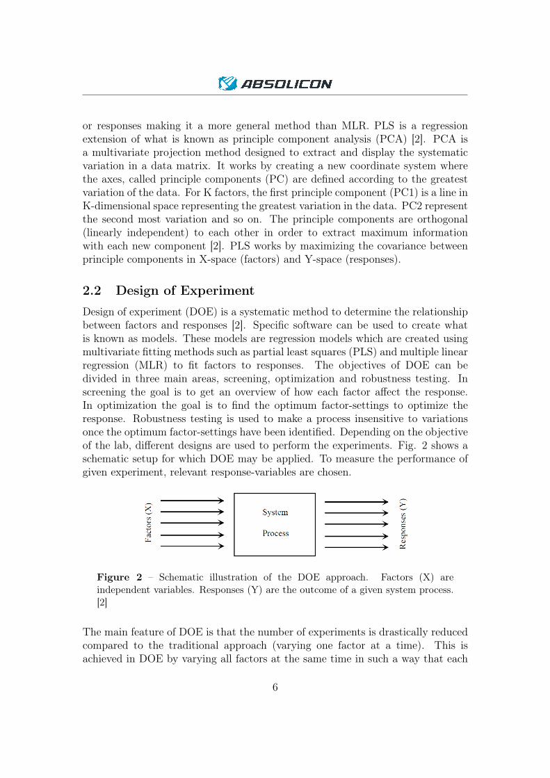
Design of experiment (DOE) is a systematic method to determine the relationshipbetween factors and responses [2]. Specific software can be used to create whatis known as models. These models are regression models which are created usingmultivariate fitting methods such as partial least squares (PLS) and multiple linearregression (MLR) to fit factors to responses. The objectives of DOE can bedivided in three main areas, screening, optimization and robustness testing. Inscreening the goal is to get an overview of how each factor affect the response.In optimization the goal is to find the optimum factor-settings to optimize theresponse. Robustness testing is used to make a process insensitive to variationsonce the optimum factor-settings have been identified. Depending on the objectiveof the lab, different designs are used to perform the experiments. Fig. 2 shows aschematic setup for which DOE may be applied. To measure the performance ofgiven experiment, relevant response-variables are chosen.

Figure 2 – Schematic illustration of the DOE approach. Factors (X) areindependent variables. Responses (Y) are the outcome of a given system process.[2]

The main feature of DOE is that the number of experiments is drastically reducedcompared to the traditional approach (varying one factor at a time). This isachieved in DOE by varying all factors at the same time in such a way that each

6

experiment is linearly independent from all others in terms of factor-settings, hencegetting the maximum amount of information from each experiment.

2.2.1 Fundamental experimental designs

The set of experiments to perform are chosen based on the objective of the laband are generated using statistical models. These models are called experimentaldesigns and they constitute a design space which is defined within the boundaries ofthe design. Compared to traditional methods, the DOE-approach covers a greaterdesign space. The experimental designs can be seen as maps as they show whichfactor-settings to use to carry out a given design. The most common design iscalled two-level design, in which each factor is investigated at one low and one highlevel. The low setting is denoted (-), the high setting (+) and the centre-point (0).Two-level designs are denoted 2k, where k is the number of factors. If nothing elseis stated, it is understood that 2k is a so called full factorial design (FFD), meaningthat all corners of the design space is investigated. The FFD forms the basis for alldesigns, and other designs are derived by adding or omitting experiments. Fig. 3shows a geometrical interpretation of a 23-design (two-level full factorial design forthree factors). Since it is a two-level design, each factor has one low and one highsetting. By definition the centre-point is at 0,0,0 in the geometrical interpretation.The corners of the geometrical interpretation each represent a unique combinationof factors, i.e. a specific factor setting. Together all factor settings form a set ofexperiments associated with the design.

Figure 3 – Geometrical interpretation of a 23-design for factors A, B, C. The setof experiments are defined by the corners (black circles) of the experimental space.The centre-point is indicated by a star.

Notice that for three factors the 23-design forms a cube in the design space. Since

7

the design in Fig. 3 is a FFD, all corners of the experimental space is investigated,resulting in 23 = 16 experimental runs (one for each corner). This may be areasonable number of experiments, but that is not the case when the numberof investigated factors increases. For example, a FFD for eight factors requires28 = 256 experimental runs, which is not realistic. For this reason there are otherdesigns which require fewer experiments, enabling the investigation of more factors.Such designs are called fractional factorial (FrF) designs as they require only afraction of the experiments, compared to the corresponding FFD. FrF-designs aredenoted 2k−n for a two-level design, where k is the number of factors and n isthe number of steps reduced from the corresponding FFD. Table 1 illustrates howeffective the FrF-designs are at reducing the number of experiments, as opposedto using a FFD.

Table 1 – Required number of experimental runs for full factorial design andfractional factorial design, given different numbers of investigated factors.

No. of investigatedfactors (k)

No. of runsFull factorial

No. of runsFractional factorial

2 4 —3 8 44 16 85 32 166 64 167 128 168 256 169 512 3210 1024 32

As can be seen in Table 1 the number of experiments increases dramatically withmore than five (5) factors, making the FrF-designs the only realistic choice whenfive or more factors are to be investigated [2]. Apart from FFD and FrF-designs,there are other designs, such as the central composite design (CCD). Regardlessof design it is common to make replicated experiments of the centre-point, whichis usually indicated by a star in experimental designs. Replicated experimentsbecomes important when distinguishing between the model error and pure error,as will be explained further in the ANOVA-section. Fig. 4 shows three differentdesigns, namely the FFD, FrF-design and CCD (from top to bottom in Fig. 4)for two, three and more than three factors. Note that it is difficult visualize thedesigns when the number of factors are greater than three, as the designs arehyper cubes spanning more than three dimensions. From top to bottom are FFD,

8

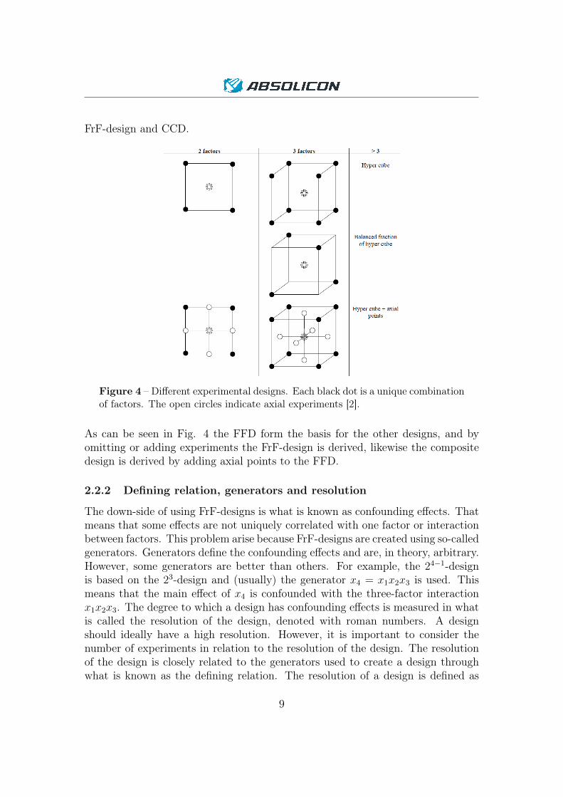
FrF-design and CCD.

Figure 4 – Different experimental designs. Each black dot is a unique combinationof factors. The open circles indicate axial experiments [2].

As can be seen in Fig. 4 the FFD form the basis for the other designs, and byomitting or adding experiments the FrF-design is derived, likewise the compositedesign is derived by adding axial points to the FFD.

2.2.2 Defining relation, generators and resolution

The down-side of using FrF-designs is what is known as confounding effects. Thatmeans that some effects are not uniquely correlated with one factor or interactionbetween factors. This problem arise because FrF-designs are created using so-calledgenerators. Generators define the confounding effects and are, in theory, arbitrary.However, some generators are better than others. For example, the 24−1-designis based on the 23-design and (usually) the generator x4 = x1x2x3 is used. Thismeans that the main effect of x4 is confounded with the three-factor interactionx1x2x3. The degree to which a design has confounding effects is measured in whatis called the resolution of the design, denoted with roman numbers. A designshould ideally have a high resolution. However, it is important to consider thenumber of experiments in relation to the resolution of the design. The resolutionof the design is closely related to the generators used to create a design throughwhat is known as the defining relation. The resolution of a design is defined as

9

”the shortest word in the defining relation” [2]. The defining relation (I) is definedfrom the generators of a design using two rules:

i) I = x · x = x2

ii) x = I · x

As an example, for the 24−1-design with generator x4 = x1x2x3 the defining relationis obtained by multiplying both sides by x4, resulting in I = x4 · x4 = x1x2x3x4.For I = x1x2x3x4 the resolution would be IV (four) since that is the length of”x1x2x3x4”. In this example only one generator was used, but the true power ofthe defining relation is that it can be used to define several generators implicitly.Also, the definition of resolution makes more sense when there are more than oneword as in the example above.

2.2.3 Design- and experimental matrix

It is often convenient to use a tabular representation of the factor-settings, insteadof a geometrical interpretation as the one in Fig. 3 and Fig. 4. This is calleddesign matrix. As an example, the design matrix of a 23-design is shown in Table2. By definition, the set of experiments shown in the table is exactly the same asthe corners of the geometrical interpretation, seen in Fig. 3.

Table 2 – Design matrix for 23-design. Standard notation is used to indicate lowor high level.

Run Factor A Factor B Factor C

1 + + +2 - + +3 + - +4 - - +5 + + -6 - + -7 + - -8 - - -

As an example, lets assume that factor A, B and C are temperature, time andstirring. The last row in Table 2 (-,-,-) would mean low temperature, short timeand low stirring rate. That combination of factors corresponds to the bottom leftcorner of Fig. 3. For each row in the experimental matrix, there is a correspondingpoint in the geometrical interpretation.

10

Design matrices makes it possible to get an overview of the set of experiments toperform, especially when the number of factors are greater than three in which caseit is impossible to visualize geometrically. Note that confounded effects have thesame sign in the design matrix, which is another way of visualizing the problem ofconfounded effects. In the easiest example, let’s assume that a (very poorly chosen)generator is used as Factor D = Factor A. Since the two factors are equal it meansthat Factor D would have the exact same signs as Factor A in the experimentalmatrix. Since every time a low setting of Factor A is used, a low setting of FactorD is used (and the same for high setting) the effect it may have on the system orprocess is impossible to attribute to either Factor. In other words, Factor A andFactor D are confounded, they cannot be separated.

A similar tool to the design matrix is the experimental matrix, which usesactual values of factors instead of standard notation, and also includes thecentre-point of the design. Experimental matrices are used when performingexperiments, as opposed to the design matrix which is more of a tool duringpreparation.

2.2.4 Mathematical models and effects

Each experimental design have corresponding mathematical models and morecomplex designs makes for more comprehensive mathematical models. Simpledesigns can be used to estimate linear effects while slightly more complex designscan estimate interaction effects between factors and even more complex designscan estimate quadratic and higher order effects. The reason why complex designsare not used all the time is because they require a lot more experiments (forexample compare the FrF-design to the CCD shown in Fig. 4). Regardless ofthe experimental design, some sort of method of fitting the data to a model isused such as MLR or PLS. This result in a regression model which correlatesfactors and responses based on the experimental results. Eq. (1) is an exampleof a mathematical model which only deals with linear effects. The effect ofeach factor is indicated by the absolute value of its coefficient (β1 . . . βN). Alarge absolute value on βi indicate that factor xi has a significant effect on theresponse. A coefficient which has a confidence interval spanning zero is said to benon-significant. The models used in DOE are semi-empirical, meaning that anyfactor can be transformed (logarithmic, or otherwise). Transforming factors andremoving non-significant factors are tools which can be used to improve the modeland is called refining [2]. Creating experimental designs and refining models isusually done using some sort of DOE-software.

11

2.3 DOE software - MODDE

MODDE is a design of experiment software created by Umetrics. It is widelyused both in academia and industries. The software is used to create experimentaldesigns, analyze and evaluate raw data as well as creating (regression) models.MODDE supports both MLR and PLS for fitting the model to the data. Thesoftware comes with a great number of experimental designs for all applicationsof DOE, whether it may be screening, optimization or robustness testing. Italso includes a set of tools for refining data, such as linear, logarithmic orpower-transformation. The software calculates statistical parameters such as R2,Q2, model validity and reproducibility. This is makes it easier to refine models asone can get direct feedback if the refining measures did in fact improve the modelor not. To evaluate the overall significance (performance) of a model, MODDEuses analysis of variance (ANOVA).

2.4 Analyzing data in MODDE

Analyzing data is an integral part of DOE. To get a good model, it is oftennecessary to make changes such as transformation of data and adding and removingeffects such as quadratic and two-factor interactions. It is also important to detectoutliers and remove them if they are in fact experimental errors. Note that byexcluding experiments it is easy to get a ”better” model in terms of statisticalparameters. However, it is important that the reason for excluding the experimentis valid, otherwise the model is falsifying the reality of the experiment, resultingin a nice looking, but inaccurate model. Excluding data from the model alsodecreases the amount of data used for the model, which makes for a weaker modelin some sense. Therefore, excluding data should only be done when real mistakeshappened during the experiment and there is a good chance that the measurementis wrong.

2.4.1 Analysis of variance (ANOVA)

Analysis of variance (ANOVA) is used to validate statistical parameters of a model.In statistical analysis the term significance is used to describe meaningful. SoANOVA is used to determine if the obtained model is meaningful (significant) ornot. This is done by a so-called F-test which test if the variance in the model issignificantly larger than variance of the residuals. The following hypotheses arepostulated

H0 : σ2Regression ≤ σ2

Residuals

HA : σ2Regression > σ2

Residuals,

12

where H0 is the null-hypothesis, which is the one that will be tested and HA is thealternative hypothesis which can be accepted or rejected in favor of H0. σ2

Regression

and σ2Residuals is the variance of the model and residuals respectively. Note that

variance is simply standard deviation squared, hence the symbol σ2. The varianceis calculated from the degrees of freedom (DF) and the sum of squares (SS) as

σ2 =SSDF

.

A F-value is calculated as the ratio between the variances, as

FCalculated =σ2Regression

σ2Residuals

.

To determine which hypothesis to accept, FCalculated is compared to a tabulatedvalue FCritical. If FCalculated > FCritical this means that H0 is rejected in favor ofHA. A second F-test can be done if replicates (repeated experiments) have beenmade. In this test the goal is to determine whether there is significant Lack ofFit (LoF) in the model. The variance of LoF is compared to the variance of thepure error (PE) and the procedure is exactly the same as in the first F-test. Amodel with significant LoF means that the model predicts a bigger error than theobserved replicate error, thus a model with LoF is not desirable. For each F-test aso-called p-value is obtained which can be viewed as the probability of HA beingfalse. For a significance of 95 % the p-value should be < 0.05 in order to reject H0.Ideally the p-value of the first F-test, concerning the model regression, should beas low as possible, and for the second F-test, testing for LoF, it should be as highas possible. In MODDE the p-values are presented in tabular form in the so-calledANOVA table.

2.4.2 Statistical parameters

Models can be evaluated in terms of statistical parameters such as goodness offit (R2), goodness of prediction (Q2), model validity and reproducibility [2]. Eachparameter is presented below, as described in the book ”Design of Experiments -Principles and applications” [2], followed by a general discussion.

R2 is the goodness of fit. It is an indicator how well a regression model can bemade to fit a set of data. If R2 = 1 that means a perfect fit, and R2 = 0means no fit at all.

Q2 is the goodness of prediction. It is used to estimate the predictive power of amodel. Q2 = 1 means perfect predictive power, Q2 = 0 means no predictivepower.

13

Model validity reflects whether a model is appropriate in a general sense.Ideally, the model validity should be as high as possible as that would indicatethat the ”right” kind of effects were chosen for investigation (linear, quadratic,interaction effects etc) and can be used to describe a system well. A low valueindicates that many effects, which are needed to describe a system, are notcovered by the chosen model. Model validity is calculated as

Model Validity = 1 + 0.57647× log pLof , (2)

where pLof is the p-value for lack of fit, as calculated by the ANOVA-test.Note that if the variance in the replicates is zero it is not possible for theANOVA-test to calculate FCalculated (division by zero) and hence pLof cannotbe determined. If pLof can’t be determined that means that the modelvalidity can’t be calculated, according to Eq. (2).

Reproducibility has to do with the overall control of the experimental procedure.It is determined based on the consistency of replicated experiments (usuallythe centre-point in DOE). It should ideally be high as that indicatesconsistency in the experiments. If the reproducibility is too low it isimpossible to separate real effects from experimental error.

In general, the most important parameter for the usefulness of a model is Q2.When refining a model, Q2 can generally be used as a compass to see if the model isgetting better or not. R2 is generally not considered as good as Q2 when measuringthe performance of a model. That is because R2 can always be made arbitrarilyhigh by adding more effects to a model. Model validity can be tricky since itis difficult to know beforehand what kind of effects will be important in a givensystem. Also, if the reproducibility of the model is high that will result in verylow model validity [2]. It is therefore possible to have a good model even if modelvalidity is low. Lastly, reproducibility is used to separate pure error (errors whichhave to do with the experimental procedure) from model error. Note that if thereproducibility is high it may cause considerable lack of fit in the model, which issomething to keep in mind when analyzing a model.

For a model to be considered good, the statistical parameters should complywith the reference values presented in Table 3.

14

Table 3 – Reference values for a DOE model to be considered good [2].

Parameter Benchmark

Q2 > 0.5R2 - Q2 < 0.3

Model validity > 0.25Reproducibility > 0.5

Note that it is possible to have a valid model even if it does not comply with thevalues in Table 3. However, it is useful to compare the statistical parameters of amodel to the reference values to get a sense of the overall performance.

2.4.3 Replicate plot

To get an overview of the overall variation of data and detect outliers, the replicateplot is useful. The x and y-axis are replicate index and response. Replicate indexcan be seen as a way of adding dimensions to the plot so that data points do notall lie on top of each other in a straight line. By looking at the replicate plotthe overall variation can be compared to the variation of the centre-points (calledreplicates) in a design. Ideally the variation in the replicates should be muchsmaller than the overall variation [2]. If the variation of the replicates is greater,or comparable to, the overall variation that will lead to a very bad model, as itwould be impossible to distinguish real effects from pure error.

2.4.4 Histogram of response

The histogram is a powerful graphical tool for determining if a transformation ofresponses is needed [2]. In such a plot response values are grouped in ”bins” (x-axis)and counted (y-axis). It is advantageous if the response is normally distributed,or nearly so. By transforming the response it may increase the model validity andgoodness of fit of a model. To determine which transformation to use, if any, thegoodness of fit parameter, Q2 can be used as a compass. If Q2 increase that is anindication that the transformation improved the model.

2.5 Electroplating

Electrochemical deposition of metals is called electroplating. It is a form ofelectrolysis meaning that electric current (DC) is used to drive an otherwisenon-spontaneous chemical reaction. Electroplating is used for coating metalobjects with a thin coherent layer of a different metal. It is widely used in a rangeof industries because of convenience and cost-effectiveness. For example, in the

15

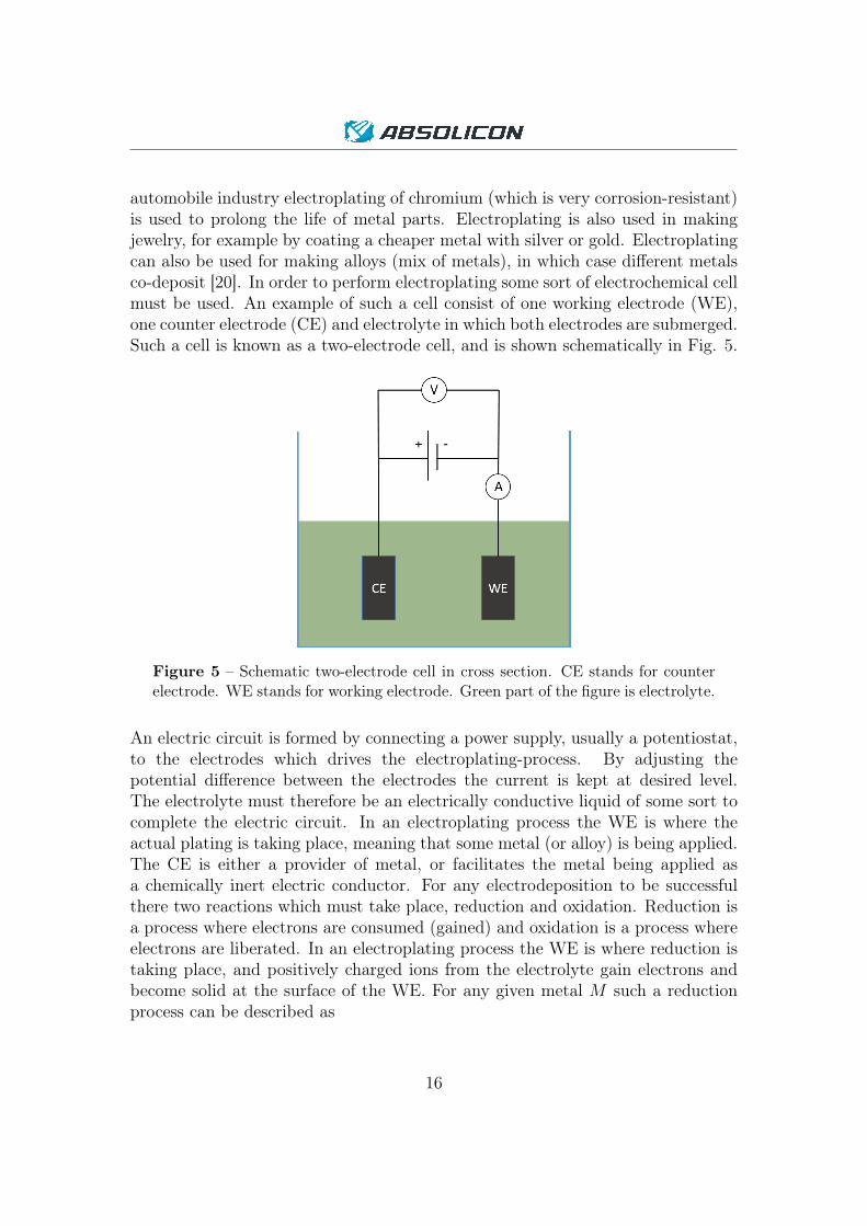
automobile industry electroplating of chromium (which is very corrosion-resistant)is used to prolong the life of metal parts. Electroplating is also used in makingjewelry, for example by coating a cheaper metal with silver or gold. Electroplatingcan also be used for making alloys (mix of metals), in which case different metalsco-deposit [20]. In order to perform electroplating some sort of electrochemical cellmust be used. An example of such a cell consist of one working electrode (WE),one counter electrode (CE) and electrolyte in which both electrodes are submerged.Such a cell is known as a two-electrode cell, and is shown schematically in Fig. 5.

Figure 5 – Schematic two-electrode cell in cross section. CE stands for counterelectrode. WE stands for working electrode. Green part of the figure is electrolyte.

An electric circuit is formed by connecting a power supply, usually a potentiostat,to the electrodes which drives the electroplating-process. By adjusting thepotential difference between the electrodes the current is kept at desired level.The electrolyte must therefore be an electrically conductive liquid of some sort tocomplete the electric circuit. In an electroplating process the WE is where theactual plating is taking place, meaning that some metal (or alloy) is being applied.The CE is either a provider of metal, or facilitates the metal being applied asa chemically inert electric conductor. For any electrodeposition to be successfulthere two reactions which must take place, reduction and oxidation. Reduction isa process where electrons are consumed (gained) and oxidation is a process whereelectrons are liberated. In an electroplating process the WE is where reduction istaking place, and positively charged ions from the electrolyte gain electrons andbecome solid at the surface of the WE. For any given metal M such a reductionprocess can be described as

16

M+zelectrolyte + ze −→Msurface, (3)

where z is the number of electrons involved in the process, which depends on themetal.

2.6 Electrolyte

As mentioned before, the electrolyte must be some sort of conducting liquid. Themost popular alternatives are ionic liquids (ILs), aqueous liquids (ALs) and deepeutectic solvents (DESs). For industrial applications, ALs are the most popular[21]. However, with new legislation some widely used metals such as hexavalentChromium (CrVI) are phased out and replaced with more environmental-friendlyalternatives such as trivalent Chromium (CrIII) [12]. ALs have proved unsuccessfulfor use with CrIII, and ALs are generally not as good as ILs or DESs [21]. ILsare well established and effective, and have been studied extensively. The maindrawback is that they are expensive. DESs are relatively new to the marketcompared to other alternatives, and the first report was published in 2001. DESsshare many of the properties of ILs but are relatively inexpensive. Therefore itis a promising alternative for the future, and the scale-up and commercializationof DES based processes have been, and still are, the subject of a number of EUfunded projects [21].

2.7 Optical properties

As mentioned before, absorptance and emittance are both used to measure theperformance of absorber materials such as reciever tubes in solar collectors [10].Absorptance is defined as the ratio of absorbed to incident radiant power [11].Emittance is defined as the ratio of the emitted thermal radiation to that of ablack body at the same temperature [11]. As both absorptance and emittance areratios, they range between 0 and 1.

According to Kirchoff’s law, the absorptance (α) at a specific wavelength (λ)can be expressed as

α(λ) = 1− ρ(λ), (4)

where ρ is the reflectance [13]. Also, for a given temperature T

α(λ, T ) = ε(λ, T ). (5)

Note that Eq. (4) and (5) are only valid for opaque materials, i.e. materials whichdo not allow for light to pass through it [13].

17

To calculate the total absorptance the following relation can be used

αtot =

∑α(λ)IAM1.5(λ)∑IAM1.5(λ)

, (6)

where the summation should ideally cover the entire solar spectrum (280 ≤ λ ≤4000 nm) [12,22].

2.8 Selective surfaces

A (spectrally) selective surface is characterized by a selective response to incominglight depending on its wavelength [10]. Such surfaces offer a cost effective way toincrease the efficiency of solar collectors by reducing the thermal losses [10,22]. Anideal absorber (reciever tube for PTCs) should have an absorptance of 1 in the solarspectrum and emittance of 0 in the infrared spectrum [13]. Also, the transitionbetween high absorptance and low emittance should be as sharp as possible [10].An ideal absorber exhibiting these properties is shown in Fig. 6.

Figure 6 – Ideal selective surface for working temperature of 160 °C, indicatedby the black dotted line in terms of reflectance. Both the blackbody radiation andsolar radiation have been normalized [12].

In reality, a perfectly selective surface is not possible. Instead the degree ofselectivity, which is defined as the ratio between low and high absorptance, shouldbe as high as possible [12]. For a perfectly selective surface the selectivity is 1.

18

2.9 Basic concepts in chemistry

To measure the concentration of a constituent in a mixture, molar (M), molarproportion (mol%) or atomic percentage (at%) can be used.

2.9.1 Molar

Molar (M) is synonymous with amount concentration and molarity. It is theamount of a constituent divided by the total volume of the mixture [11]. Thecommon unit is mole per cubic dm (mol dm-3).

2.9.2 Molar proportion and atomic percentage

Molar proportion (mol%) is closely related to molar fraction (xi). In chemistry, xiis used to describe the amount of a constituent i (in number of moles) in relationto the total amount of all constituents in a solution [11]. It is calculated as

xi =ni

nTot

, (7)

where n is the number of moles. The same concept expressed with a denominatorof 100 is the molar proportion (mol%), i.e. mol% = 100 · xi.

A similar concept to the molar proportion is atomic proportion, in which caseEq. (7) is used, but instead of the number of moles, the number of atoms are usedas

ai =Ni

NTot

, (8)

where ai is the atomic proportion [11]. To get the atomic percentage (at%), adenominator of 100 is used, i.e. at% = 100 · a. To clarify, if constituent i isconcentrated with at% = 23 % that means that 23 % of all total atoms are thatof constituent i.

2.10 Optical efficiency of concentrating solar collectors

To determine the overall performance of a concentrating solar collector (CSC),the optical efficiency can be used. The most important parameters for the opticalefficiency is the absorptance (α) and emittance (ε) of the receiver tube in theCSC (see Fig. 1 for schematic CSC). However, these two parameters are not ofequal importance, which is important to keep in mind when optimizing the CSCsperformance with regard to its optical efficiency [23]. To understand the opticalefficiency it is important to realize that there is a protective glass in front ofthe receiver tube, and a reflector behind the reciever tube, which both affect theamount of energy received by solar radiation. The optical efficiency (η) is defined

19

as the ratio between actual energy received by the receiver tube to the maximumenergy available, as

η =Q̇a − Q̇l

˙Qtot

. (9)

Where Q̇a is the energy received by the receiver tube, Q̇l is the energy loss fromthe receiver tube due to radiation, and ˙Qtot is the available, or maximum, energyreceived by the solar collector [23]. Q̇a, Q̇l and ˙Qtot are calculated as follows [24].

Q̇a = τηrαAgI0, (10)

Q̇l = εσAt(T4s − T 4

amb), (11)˙Qtot = I0Ag. (12)

Where τ is the transmittance of the protective glass, ηr is the efficiency of thereflector, α is the absorptance of the receiver tube, Ag is the surface area of theprotective glass, I0 is the incoming solar radiation in W/m2, ε is the emittance ofthe receiver tube, σ is the Stefan-Boltzmann constant, At is the surface area of thereceiver tube, Ts is the surface temperature of the receiver tube and Tamb is theambient temperature. Inserting Eq. (10), Eq. (11) and Eq. (12) in Eq. (9) yieldsthe expression

η =τηrαAgI0 − εσAt(T

4s − T 4

amb)

I0Ag

. (13)

2.11 Performance criterion

The performance criterion (PC) is a useful tool which is derived from the opticalefficiency. It is defined as

PC = α− xε, (14)

where x is a constant [23]. Both α and ε are properties of the reciever tube. Bymultiplying Eq. (13) with (τηr)

−1 the following expression is obtained

PC = α− Atσ(T4s − T 4

amb)

AgI0τηrεt. (15)

Combining Eq. (14) and (15) gives the following expressions for x

x =Atσ(T

4s − T 4

amb)

AgI0τηr, (16)

which can be calculated for the solar concentrator to be evaluated and then insertin Eq. (14) to get the PC. Note that it is clear from Eq. (15) that the absorptanceand emittance is not of equal importance. That is not obvious from the opticalefficiency expression Eq. (13).

20

2.12 Measurement equipment

The following techniques and equipment will be used to analyze the optical,structural and chemical properties of selected samples.

Spectrophotometry is a branch of spectroscopy used to measure the radiantenergy transmitted or reflected by a body. The intensity of monochromaticlight is measured at different wavelengths before and after the samplebeing tested and compared to some reference sample with known properties(usually 0 % reflectance) [25]. By measuring the reflectance the absorptancecan be determined implicitly.

Scanning Electron Microscope (SEM) works by scanning a surface with afocused beam of electrons. The electrons interact with the sample, producinginformation about the surface topography and composition [26].

X-ray Photoelectron Spectroscopy (XPS) is a technique based on thephotoelectric effect and one of the most widely used surfaces analysistechniques. By bombarding a solid surface with X-rays a photoelectronspectra is obtained. By analyzing the spectral information about thechemical composition and chemical states of the surface constituents can bedetermined [27]. XPS is used to determine the environment of the elementsrather than the amount of each element.

Energy-Dispersive X-ray Spectroscopy (EDS) is a mapping method. It isused to estimate the quantitative amounts of different elements in a solidsurface as well distribution mapping of the elements across the surface. Abeam of electrons is used and the number, and energy, of the X-rays emittedfrom the sample are registered [28]. EDS is performed by equipping a SEMwith sensors which can register X-rays.

3 MethodologyFor DOE applications it is essential to know and understand the system orprocess to be investigated to get good data and model. Therefore, a lot oftime was spen initially on preparatory work, described in 3.1. Based on thethe preparatory work, factors and responses were chosen, presented in 3.1.2 and3.1.3 respectively. An experimental design (3.1.4) was chosen based on previousresearch, and an experimental matrix (3.2.1) was created in MODDE to facilitatethe data collection. A total of 20 experiments were made for the DOE model,including four (4) centre-points. The data was analyzed and refined to createa model for each response using the MODDE software (3.3). Using the refined

21

models, the optimal factor settings could be found using MODDE to maximizethe optical efficiency according to Eq. (13). Experiments were performed to testthe optimal factor settings, and the results was analyzed in terms of optical andmaterial properties of the samples. Fig. 7 shows a flowchart with arrows indicatingthe workflow.

Figure 7 – Flowchart for the project with arrows indicating the workflow, startingin the top left. Subcategories in yellow. Main categories in blue.

3.1 Preparations

The preparatory work was used as the foundation for decisions regarding factors,responses, centre-point and design. The main goals were as follows.

• Familiarization of the electroplating process

• Investigation of appropriate factors and responses

• Gathering of data regarding the centre-point of design

• Test the range of factors

22

• Investigation of pH

The system in this project was an electroplating process, more specifically theelectroplating process of Co-Cr alloys used by E. Zäll [12] in his research forAbsolicon. Quite a lot of time (∼ 60 h) was spent learning that electroplatingprocess, as described in full in 3.2.2. Partly to determine which factors to use,partly to minimize random errors associated with the experimental procedure.

To determine the centre-point of the design and test the appropriate rangeof each factor a series of experiments was made. As it is important that thecentre-point can be reproduced a lot of time (∼ 80 h) was spent making replicatedexperiments until the results were satisfactory. No optical measurements weremade during this process and the general quality of the sample QD was deemed asa sufficiently good indicator.

The range of each factor was tested in a series of experiments. For the DOEmodel to be good, it is important that the factors are varied in such a way thatthey disturb the process, but at the same time they should not be too extreme.In the electroplating process extreme would be if the sample is blank, i.e. QD =0. A lot of time (∼ 80 h) was spent testing the ranges to avoid poor results andsubsequently a bad model.

Based on previous research, pH seems to have an important effect on someelectroplating processes [17–19]. It is therefore an interesting factor which wouldbe good to include in the model. For the electroplating process at hand, the pH hadnot previously been regulated. Therefore there was no established method availableand a trial and error approach was used in an attempt to succesfully adjust thepH of the electrolyte. This was done in a series of experiments (∼ 40 h) by addingaqueous solutions of potassium hydroxide (KOH) and hydrochloric acid (HCl) tothe electrolyte at a concentration of ∼5 M. The results showed that it was possibleto regulate the pH of the electrolyte, but due inconsistent results and inaccurateequipment it was impossible to make any conclusions regarding the appropriaterange. Also, the potential side effects of adding pH regulatory solutions to theelectrolyte would have to be further investigated in a future project. Based oninitial testing, it was determined that pH would not be one of the factors in thedesign.

3.1.1 Electrolyte

Electrolyte was prepared according to E. Zäll [12]. The electrolyte consistedof four components. These were choline cloride (ChCl), ethylene glycol(EG), chromium trichloride hexahydrate (CrCl3·6H2O) and cobalt dichloridehexahydrate (CoCl2·6H2O). EG and ChCl together form a solvent, morespecifically a deep eutectic solvent (DES). CrCl3·6H2O and CoCl2·6H2O form a

23

metal salt (MS). The electrolyte can thus be said to consist of DES and MS.Henceforth, DES refers to the mixture of ChCl and EG, and MS refers to themixture of CrCl3·6H2O and CoCl2·6H2O.

3.1.2 Factors

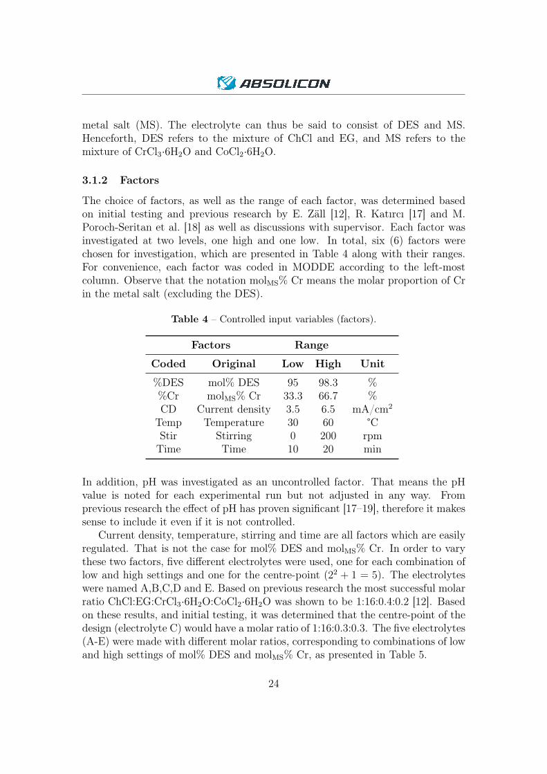
The choice of factors, as well as the range of each factor, was determined basedon initial testing and previous research by E. Zäll [12], R. Katırcı [17] and M.Poroch-Seritan et al. [18] as well as discussions with supervisor. Each factor wasinvestigated at two levels, one high and one low. In total, six (6) factors werechosen for investigation, which are presented in Table 4 along with their ranges.For convenience, each factor was coded in MODDE according to the left-mostcolumn. Observe that the notation molMS% Cr means the molar proportion of Crin the metal salt (excluding the DES).

Table 4 – Controlled input variables (factors).

Factors Range

Coded Original Low High Unit

%DES mol% DES 95 98.3 %%Cr molMS% Cr 33.3 66.7 %CD Current density 3.5 6.5 mA/cm2

Temp Temperature 30 60 °CStir Stirring 0 200 rpmTime Time 10 20 min

In addition, pH was investigated as an uncontrolled factor. That means the pHvalue is noted for each experimental run but not adjusted in any way. Fromprevious research the effect of pH has proven significant [17–19], therefore it makessense to include it even if it is not controlled.

Current density, temperature, stirring and time are all factors which are easilyregulated. That is not the case for mol% DES and molMS% Cr. In order to varythese two factors, five different electrolytes were used, one for each combination oflow and high settings and one for the centre-point (22 + 1 = 5). The electrolyteswere named A,B,C,D and E. Based on previous research the most successful molarratio ChCl:EG:CrCl3·6H2O:CoCl2·6H2O was shown to be 1:16:0.4:0.2 [12]. Basedon these results, and initial testing, it was determined that the centre-point of thedesign (electrolyte C) would have a molar ratio of 1:16:0.3:0.3. The five electrolytes(A-E) were made with different molar ratios, corresponding to combinations of lowand high settings of mol% DES and molMS% Cr, as presented in Table 5.

24

Table 5 – Molar ratios for each electrolyte.

Electrolyte Molar ratio

A 1:16:0.3:0.6B 1:16:0.1:0.2C 1:16:0.3:0.3D 1:16:0.6:0.3E 1:16:0.2:0.1

Ideally, the order of the experiments should be as random as possible to avoidsystematic errors. However, because of the different electrolytes it would beimpractical and time consuming. Therefore, a small program was created whichrandomizes the experimental order as much as possible, while making sure thatexperiments with the same electrolyte are made in succession. Based on initialtesting, it was also decided that another restriction be implemented in the programto ensure that experiments with the same electrolyte and temperature were carriedout in succession. The program was written in Python is available in Appendix B.

3.1.3 Responses

Three (3) response-variables were chosen. These were absorptance (α), emittance(ε) and quality of deposition (QD). Ideally the absorptance should be high,emittance low and QD high. QD is not strictly a scientific measure, but it isan attempt to characterize the overall homogeneity of the plating.

3.1.4 Experimental design

Based on the results of the initial testing, six (6) factors were chosen forinvestigation. For that, a fractional factorial (FrF) design was determined tobe the most suitable design. Such a design allows for linear (main) effects tobe determined, which is usually enough for screening-purposes [2, 29]. By usinga FrF-design the number of experiments is reduced considerably compared to aFFD. For six factors the number of experiments is reduced from 26 = 64 to26−2 = 16, thus making it possible to investigate the factors in a reasonable numberof experiments. The design has resolution IV, which allows for good estimationof main effects. The drawback is that two-factor interactions are confounded.At a later stage, it may be necessary to unconfound the two-factor interactions.However, that is only of interest if there are significant two-factor interactions. Thedesign matrix of the 26−2 experimental design can be seen in Table 6. Note that itis based on the 24-design with the generators x5 = x1x2x3 and x6 = x2x3x4. Thedefining relation of the design is I = x1x2x3x5 + x2x3x4x6. From the definition of

25

resolution as ”length of shortest word in I”, it is clear that the resolution is indeedIV.

Table 6 – Design matrix for 26−2-design. Minus (-) indicate low level, plus (+)indicate high level.

Run x1 x2 x3 x4 x5 x6

1 - - - - - -2 + - - - + -3 - + - - + +4 + + - - - +5 - - + - + +6 + - + - - +7 - + + - - -8 + + + - + -9 - - - + - +10 + - - + + +11 - + - + + -12 + + - + - -13 - - + + + -14 + - + + - -15 - + + + - +16 + + + + + +

Note that the centre-point is not included in Table 6 as it is arbitrary how manycentre-point measurements to use.

3.2 Data collection

The data collection was done through an electroplating process, described in 3.2.2.To facilitate the data collection an experimental matrix was used which combinesthe chosen FrF-design with the actual factor settings (not coded) of the factors.

3.2.1 Experimental Matrix

The chosen FrF-design resulted in four (4) experimental runs for each electrolyte.Subsequently, the experiments were named A1,A2,A3,A4 ... E1,E2,E3,E4. Theletters indicate which electrolyte to use and the number gives a unique identifierfor the experiment. It was also determined that four (4) centre-points should beused. To combine the 26−2-design with the chosen factors and ranges presented inTable 4, an experimental matrix was created in MODDE presented in Table 7.

26

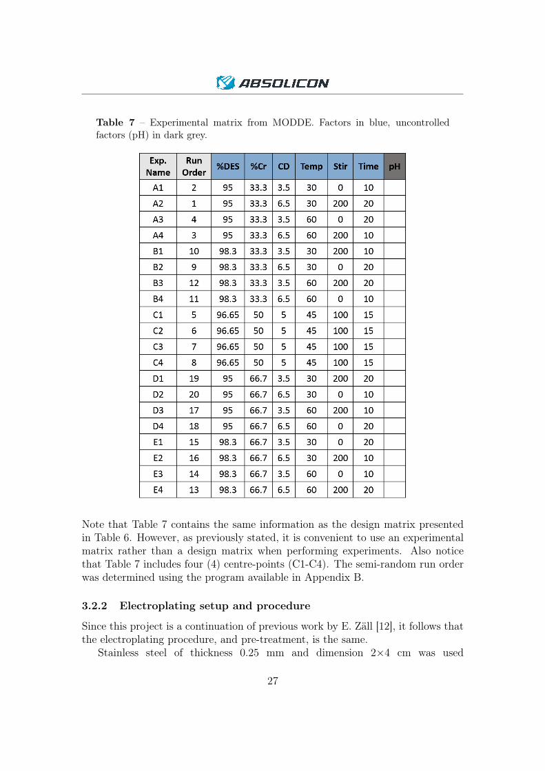
Table 7 – Experimental matrix from MODDE. Factors in blue, uncontrolledfactors (pH) in dark grey.

Note that Table 7 contains the same information as the design matrix presentedin Table 6. However, as previously stated, it is convenient to use an experimentalmatrix rather than a design matrix when performing experiments. Also noticethat Table 7 includes four (4) centre-points (C1-C4). The semi-random run orderwas determined using the program available in Appendix B.

3.2.2 Electroplating setup and procedure

Since this project is a continuation of previous work by E. Zäll [12], it follows thatthe electroplating procedure, and pre-treatment, is the same.

Stainless steel of thickness 0.25 mm and dimension 2×4 cm was used

27

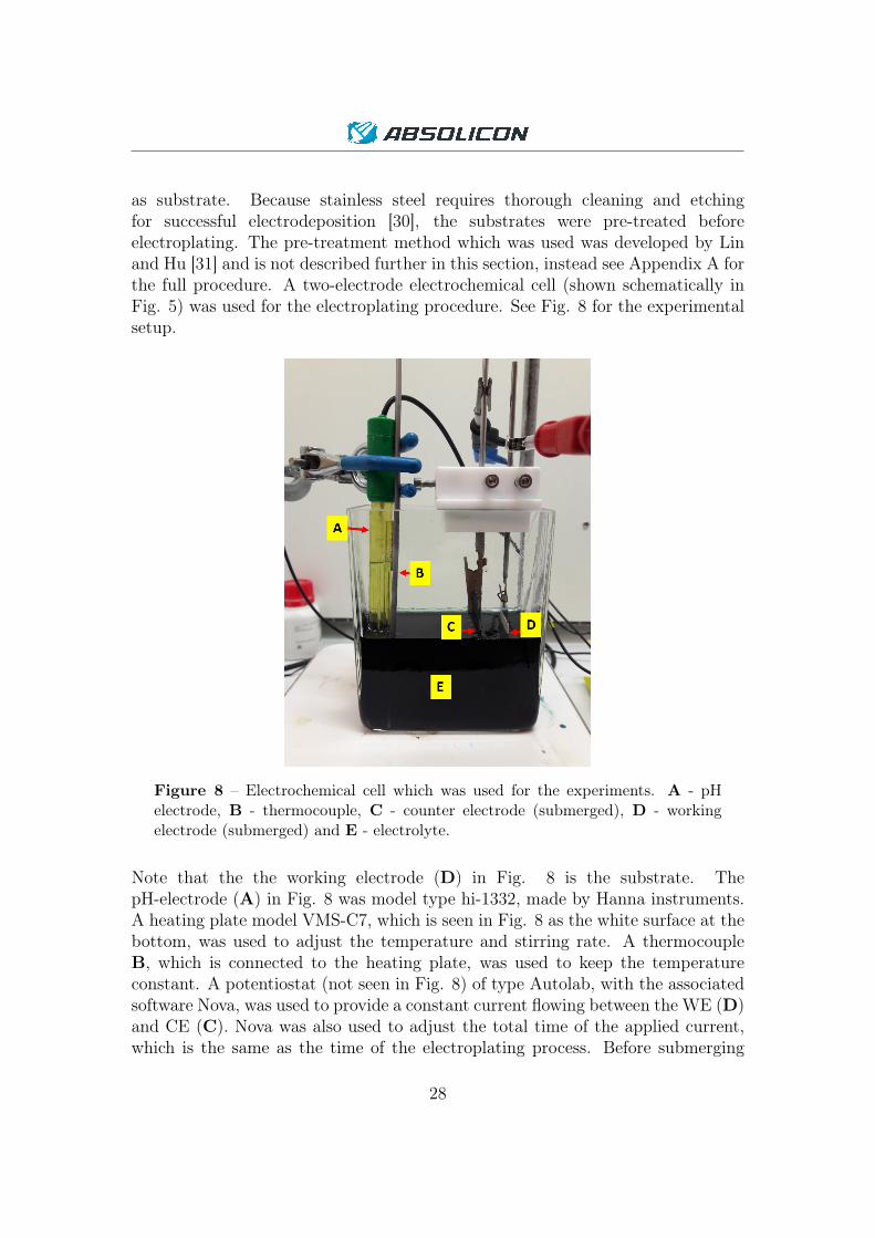
as substrate. Because stainless steel requires thorough cleaning and etchingfor successful electrodeposition [30], the substrates were pre-treated beforeelectroplating. The pre-treatment method which was used was developed by Linand Hu [31] and is not described further in this section, instead see Appendix A forthe full procedure. A two-electrode electrochemical cell (shown schematically inFig. 5) was used for the electroplating procedure. See Fig. 8 for the experimentalsetup.

Figure 8 – Electrochemical cell which was used for the experiments. A - pHelectrode, B - thermocouple, C - counter electrode (submerged), D - workingelectrode (submerged) and E - electrolyte.

Note that the the working electrode (D) in Fig. 8 is the substrate. ThepH-electrode (A) in Fig. 8 was model type hi-1332, made by Hanna instruments.A heating plate model VMS-C7, which is seen in Fig. 8 as the white surface at thebottom, was used to adjust the temperature and stirring rate. A thermocoupleB, which is connected to the heating plate, was used to keep the temperatureconstant. A potentiostat (not seen in Fig. 8) of type Autolab, with the associatedsoftware Nova, was used to provide a constant current flowing between the WE (D)and CE (C). Nova was also used to adjust the total time of the applied current,which is the same as the time of the electroplating process. Before submerging

28

the substrate (D) in the electrolyte (E) it was cleaned in HCl solution (13 %)for approximately 30 seconds, rinsed with deionoized water and air-dried. Thereason for this is that that the HCl solution helps remove any oxide films that mayhave formed, which is favorable for successful electrodeposition [31]. To controlthe area of the substrate teflon tape was used, seen in Fig. 8 as the small whitepart just above the electrolyte surface at D. The total area (front and back) underthe tape was noted using a standard ruler and the information was later used toconvert current density to current. After the area had been noted, the substratewas then submerged in the electrolyte and the current and time was adjusted inNova. When the time expired the substrate was removed from the electrolyte,rinsed in distilled water and air-dried. A successful electrodeposition will result ina black coating on the stainless steel substrate, consisting of a Co-Cr alloy.

3.2.3 Measuring responses

The absorptance was measured indirectly through the reflectance (Eq. (4)) using aspectrophotometer, which is a well established approach. Emittance was measuredusing an IR-thermometer, which is not ideal, but works for the purposes of thisreport. The quality of deposition response was determined by looking at thesamples and each sample was rated on a scale 0-5, where 0 is no plating and 5 isvery homogeneous plating.

Absorptance The absorptance was measured indirectly by using a Lambda35 spectrophotometer to measure the reflectance of the samples in the spectra280 ≤ λ ≤ 1100 nm. For full step by step instructions how to operate thespectrophotometer and which settings to use in the assosciated software, thatwill not be described here as it is already well described in previous work by E.Zäll [12]. The reflectance had to be corrected for each wavelength for the specificspectrophotometer, i.e. ρtrue(λ) = ρtrue(ρmeasured(λ), λ), where ρ is reflectance.The true reflectance (ρtrue) was found using a table from the manufacturer [32].A Matlab script (available in Appendix C.2) was used to create a 2D-interpolantbased on the values of that table. The script returns a 2D-interpolant which canbe used to calculate ρtrue for a specific wavelength, given ρmeasured and λ. Once thereflectance had been corrected, Eq. (4) was used to calculate the absorptance foreach wavelength. In order to get the total absorptance, Eq. (6) was used togetherwith the relevant solar spectrum (280 ≤ λ ≤ 1100 nm) found at the website ofthe National Renewable Energy Lab (NREL) [22]. To facilitate the calculationof absorptance another Matlab script was used, provided in Appendix C.1. Formore accurate results, two rounds of measurements was made for each sample andaveraged.

29

Emittance The emittance was measured using an IR-thermometer. The sampleof interest was placed on a heating plate along with a reference sample of thesame material. The reference sample, and the unplated (area not subject toelectroplating) part of the sample of interest was covered in teflon tape withknown emittance of 0.95. Both samples were heated to 160 °C because that isthe working temperature of Absolicons concentrating solar collectors [12]. Whenthe temperature of the reference sample reached the desired temperature, theemittance-setting of the IR-thermometer was adjusted until it showed the sametemperature for the electroplated area, as for the reference sample. To verify thatthe two samples were the same temperature, a second measurement was made withthe samples in shifted placements, e.g. the reference sample shifted place with thesample of interest. Step by step instructions are available in the previous work byE. Zäll [12].

Quality of deposition Quality of deposition was judged on a scale from one tofive by looking at each sample. Zero (0) is no plating (blank surface), one (1) is verynon-homogeneous, two (2) is non-homogeneous, three (3) is decent homogeneity,four (4) is good homogeneity and five (5) is very good homogeneity.

3.3 Analysis of raw data

The data was collected in MODDE by using the experimental matrix (Table 7)as a foundation. Three models were then created, one for each response. Foreach model, the raw data was analyzed using a replicate plot and histogramof the response. These tools are useful to get an overview of the data, as wellas identifying outliers. The histogram is especially useful to determine whethertransformation of the response is needed. By analyzing the raw data it gets easierto refine the models at a later stage. A summary of fit plot was used for eachresponse, which is a graphical interpretation of the statistical parameters presentedin 2.4.2. The statistical parameters of a model tells whether it needs to be refined,which is more often than not. Finally, for each model the so-called coefficient plotwas used to get an initial overview of which factors are the most influential foreach response. To avoid confusion, the models are presented in separate sectionsbelow and analyzed separately.

3.3.1 Collected data

The raw data from the experiments was collected in MODDE, seen in Table 8. Notethat it is the experimental matrix (Table 7) with added pH-values and responses.

30

Table 8 – Raw data from experiments. Controlled factors in blue, uncontrolled ingrey. Responses in green. Abs. stands for absorptance, Emi. stands for emittance.QD stands for quality of deposition.

Take note of column ’Exp. Name’ and ’pH’ in Table 8. Remember that the letterin the sample-ID (seen in ’Exp. Name’) indicates which electrolyte to be used (aspresented in Table 5). It is clear from Table 8 that the pH values differ between theelectrolytes, for example electrolyte B in general have higher pH than electrolyte D.This is somewhat expected due to the difference in chemical composition. Ideallythe electrolytes should be tested at the same pH values to better see the effect ofthe other factors, but this is one of the drawbacks of using uncontrolled factors.Also note in Table 8 that the absorptance (Abs.) was measured with greaterprecision than emittance (Emi.). That is because the measurement technique forabsorptance was more precise. The data for the absorptance was very consistent,i.e. small standard deviation between measurements, as seen Fig. 9. The figure

31

shows an output from the Matlab script ’Absorptance_all’, available in AppendixC.3. Two measurements were made for each sample and the averaged value iswhat is displayed as the absorptance (Abs). The standard deviation (Std) wascalculated between these two samples.

Figure 9 – Output from ’Absorptance_all’ Matlab script (Appendix C.3). Absstands for Absorptance, Std stands for the standard deviation.

As can be seen in Fig. 9 the standard deviation (Std) is very low for all samples,especially A2, E4 and D1. Since the Std is so small it is reasonable to includethree digits in the absorptance response. When measuring the emittance it wasnot possible to be as precise, and therefore two digits were used.

3.3.2 Model 1 - Absorptance

A replicate plot of the response is shown in Fig. 10.

32

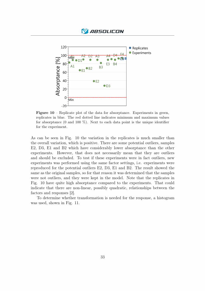
Figure 10 – Replicate plot of the data for absorptance. Experiments in green,replicates in blue. The red dotted line indicates minimum and maximum valuesfor absorptance (0 and 100 %). Next to each data point is the unique identifierfor the experiment.

As can be seen in Fig. 10 the variation in the replicates is much smaller thanthe overall variation, which is positive. There are some potential outliers, samplesE2, D3, E1 and B2 which have considerably lower absorptance than the otherexperiments. However, that does not necessarily mean that they are outliersand should be excluded. To test if these experiments were in fact outliers, newexperiments was performed using the same factor settings, i.e. experiments werereproduced for the potential outliers E2, D3, E1 and B2. The result showed thesame as the original samples, so for that reason it was determined that the sampleswere not outliers, and they were kept in the model. Note that the replicates inFig. 10 have quite high absorptance compared to the experiments. That couldindicate that there are non-linear, possibly quadratic, relationships between thefactors and responses [2].

To determine whether transformation is needed for the response, a histogramwas used, shown in Fig. 11.

33

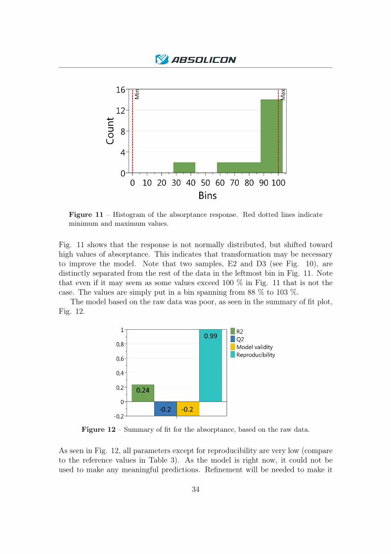
Figure 11 – Histogram of the absorptance response. Red dotted lines indicateminimum and maximum values.

Fig. 11 shows that the response is not normally distributed, but shifted towardhigh values of absorptance. This indicates that transformation may be necessaryto improve the model. Note that two samples, E2 and D3 (see Fig. 10), aredistinctly separated from the rest of the data in the leftmost bin in Fig. 11. Notethat even if it may seem as some values exceed 100 % in Fig. 11 that is not thecase. The values are simply put in a bin spanning from 88 % to 103 %.

The model based on the raw data was poor, as seen in the summary of fit plot,Fig. 12.

Figure 12 – Summary of fit for the absorptance, based on the raw data.

As seen in Fig. 12, all parameters except for reproducibility are very low (compareto the reference values in Table 3). As the model is right now, it could not beused to make any meaningful predictions. Refinement will be needed to make it

34

useful. The model fails to explain the process using the main effects investigatedby the FrF-design, i.e. effects such as interactions and quadratic effects are mostlikely present. This is indicated in the low model validity (-0.2). Note that thereproducibility of the model is very high (0.99). That is because the variationbetween the replicates is very small (as seen in Fig. 10). High reproducibilityindicate small experimental error (pure error), and reliable results. However, it willmost certainly result in significant lack of fit (model error) in a future ANOVA-testfor the refined model. That is because the ANOVA-test compares the pure errorto the model error, and if the pure error is very small the model error appears verylarge in comparison.

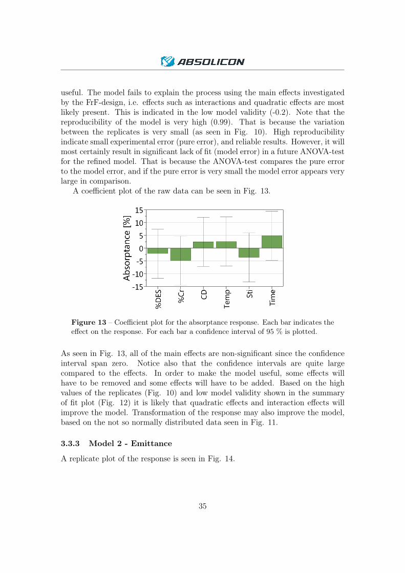
A coefficient plot of the raw data can be seen in Fig. 13.

Figure 13 – Coefficient plot for the absorptance response. Each bar indicates theeffect on the response. For each bar a confidence interval of 95 % is plotted.

As seen in Fig. 13, all of the main effects are non-significant since the confidenceinterval span zero. Notice also that the confidence intervals are quite largecompared to the effects. In order to make the model useful, some effects willhave to be removed and some effects will have to be added. Based on the highvalues of the replicates (Fig. 10) and low model validity shown in the summaryof fit plot (Fig. 12) it is likely that quadratic effects and interaction effects willimprove the model. Transformation of the response may also improve the model,based on the not so normally distributed data seen in Fig. 11.

3.3.3 Model 2 - Emittance

A replicate plot of the response is seen in Fig. 14.

35

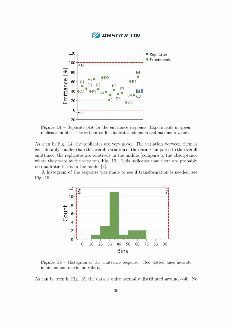
Figure 14 – Replicate plot for the emittance response. Experiments in green,replicates in blue. The red dotted line indicates minimum and maximum values.

As seen in Fig. 14, the replicates are very good. The variation between them isconsiderably smaller than the overall variation of the data. Compared to the overallemittance, the replicates are relatively in the middle (compare to the absorptancewhere they were at the very top, Fig. 10). This indicates that there are probablyno quadratic terms in the model [2].

A histogram of the response was made to see if transformation is needed, seeFig. 15.

Figure 15 – Histogram of the emittance response. Red dotted lines indicateminimum and maximum values.

As can be seen in Fig. 15, the data is quite normally distributed around ∼40. No

36

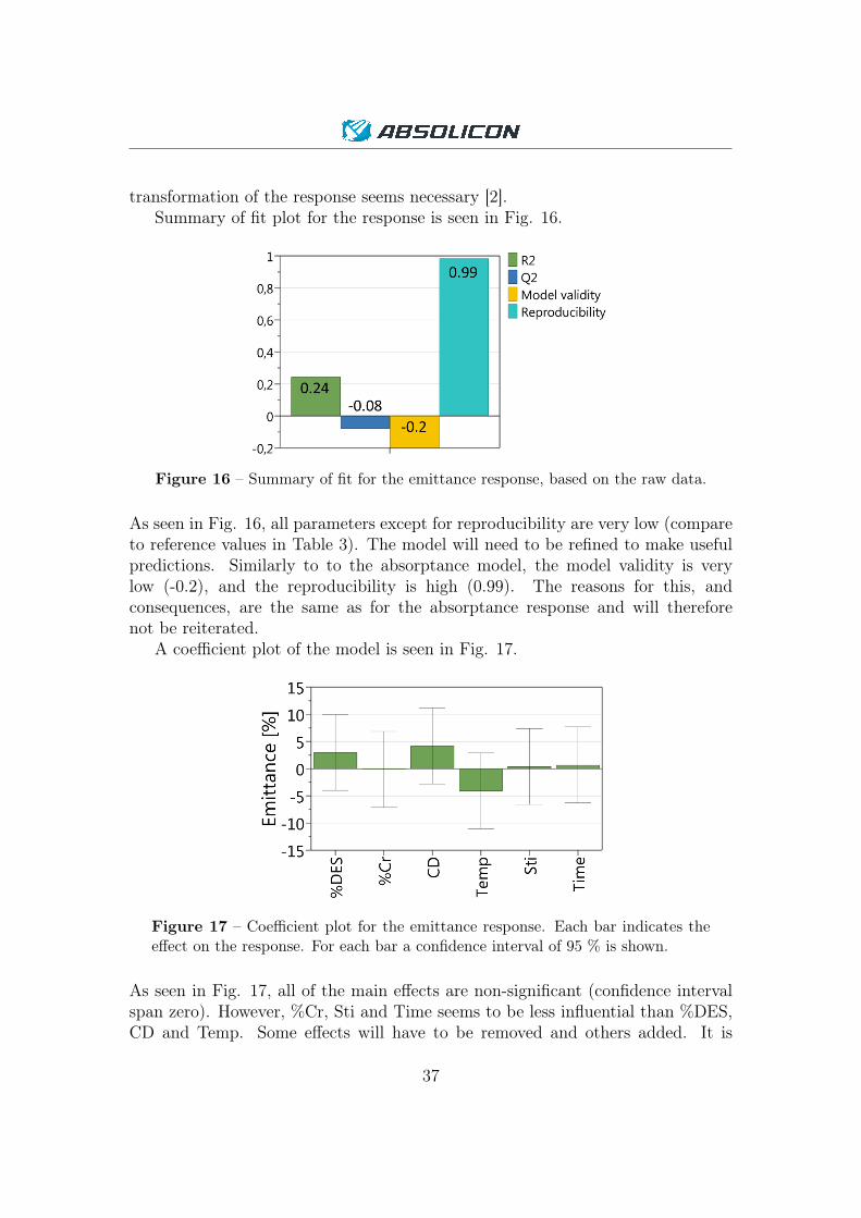
transformation of the response seems necessary [2].Summary of fit plot for the response is seen in Fig. 16.

Figure 16 – Summary of fit for the emittance response, based on the raw data.

As seen in Fig. 16, all parameters except for reproducibility are very low (compareto reference values in Table 3). The model will need to be refined to make usefulpredictions. Similarly to to the absorptance model, the model validity is verylow (-0.2), and the reproducibility is high (0.99). The reasons for this, andconsequences, are the same as for the absorptance response and will thereforenot be reiterated.

A coefficient plot of the model is seen in Fig. 17.

Figure 17 – Coefficient plot for the emittance response. Each bar indicates theeffect on the response. For each bar a confidence interval of 95 % is shown.

As seen in Fig. 17, all of the main effects are non-significant (confidence intervalspan zero). However, %Cr, Sti and Time seems to be less influential than %DES,CD and Temp. Some effects will have to be removed and others added. It is

37

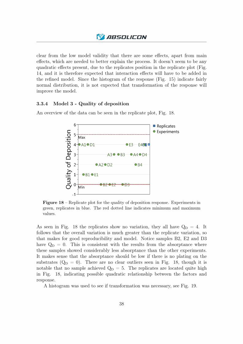
clear from the low model validity that there are some effects, apart from maineffects, which are needed to better explain the process. It doesn’t seem to be anyquadratic effects present, due to the replicates position in the replicate plot (Fig.14, and it is therefore expected that interaction effects will have to be added inthe refined model. Since the histogram of the response (Fig. 15) indicate fairlynormal distribution, it is not expected that transformation of the response willimprove the model.

3.3.4 Model 3 - Quality of deposition

An overview of the data can be seen in the replicate plot, Fig. 18.

Figure 18 – Replicate plot for the quality of deposition response. Experiments ingreen, replicates in blue. The red dotted line indicates minimum and maximumvalues.

As seen in Fig. 18 the replicates show no variation, they all have QD = 4. Itfollows that the overall variation is much greater than the replicate variation, sothat makes for good reproducibility and model. Notice samples B2, E2 and D3have QD = 0. This is consistent with the results from the absorptance wherethese samples showed considerably less absorptance than the other experiments.It makes sense that the absorptance should be low if there is no plating on thesubstrates (QD = 0). There are no clear outliers seen in Fig. 18, though it isnotable that no sample achieved QD = 5. The replicates are located quite highin Fig. 18, indicating possible quadratic relationship between the factors andresponse.

A histogram was used to see if transformation was necessary, see Fig. 19.

38

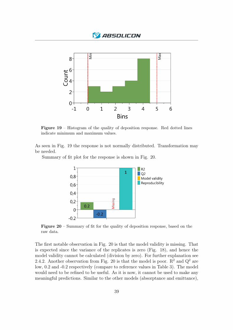
Figure 19 – Histogram of the quality of deposition response. Red dotted linesindicate minimum and maximum values.

As seen in Fig. 19 the response is not normally distributed. Transformation maybe needed.

Summary of fit plot for the response is shown in Fig. 20.

Figure 20 – Summary of fit for the quality of deposition response, based on theraw data.

The first notable observation in Fig. 20 is that the model validity is missing. Thatis expected since the variance of the replicates is zero (Fig. 18), and hence themodel validity cannot be calculated (division by zero). For further explanation see2.4.2. Another observation from Fig. 20 is that the model is poor. R2 and Q2 arelow, 0.2 and -0.2 respectively (compare to reference values in Table 3). The modelwould need to be refined to be useful. As it is now, it cannot be used to make anymeaningful predictions. Similar to the other models (absorptance and emittance),

39

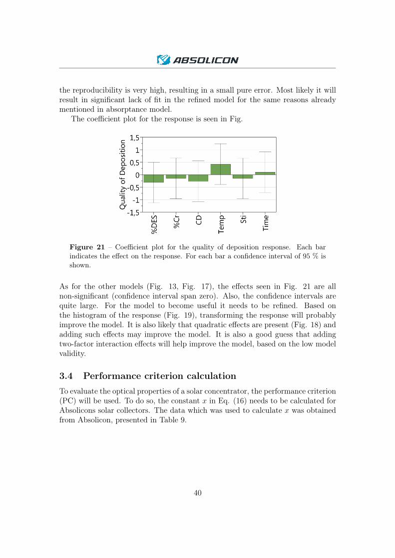
the reproducibility is very high, resulting in a small pure error. Most likely it willresult in significant lack of fit in the refined model for the same reasons alreadymentioned in absorptance model.

The coefficient plot for the response is seen in Fig.

Figure 21 – Coefficient plot for the quality of deposition response. Each barindicates the effect on the response. For each bar a confidence interval of 95 % isshown.

As for the other models (Fig. 13, Fig. 17), the effects seen in Fig. 21 are allnon-significant (confidence interval span zero). Also, the confidence intervals arequite large. For the model to become useful it needs to be refined. Based onthe histogram of the response (Fig. 19), transforming the response will probablyimprove the model. It is also likely that quadratic effects are present (Fig. 18) andadding such effects may improve the model. It is also a good guess that addingtwo-factor interaction effects will help improve the model, based on the low modelvalidity.

3.4 Performance criterion calculation

To evaluate the optical properties of a solar concentrator, the performance criterion(PC) will be used. To do so, the constant x in Eq. (16) needs to be calculated forAbsolicons solar collectors. The data which was used to calculate x was obtainedfrom Absolicon, presented in Table 9.

40

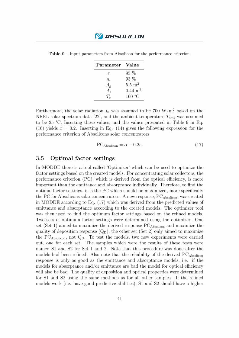
Table 9 – Input parameters from Absolicon for the performance criterion.

Parameter Value

τ 95 %ηr 93 %Ag 5.5 m2

At 0.44 m2

Ts 160 °C

Furthermore, the solar radiation I0 was assumed to be 700 W/m2 based on theNREL solar spectrum data [22], and the ambient temperature Tamb was assumedto be 25 °C. Inserting these values, and the values presented in Table 9 in Eq.(16) yields x = 0.2. Inserting in Eq. (14) gives the following expression for theperformance criterion of Absolicons solar concentrators

PCAbsolicon = α− 0.2ε. (17)

3.5 Optimal factor settings

In MODDE there is a tool called ’Optimizer’ which can be used to optimize thefactor settings based on the created models. For concentrating solar collectors, theperformance criterion (PC), which is derived from the optical efficiency, is moreimportant than the emittance and absorptance individually. Therefore, to find theoptimal factor settings, it is the PC which should be maximized, more specificallythe PC for Absolicons solar concentrators. A new response, PCAbsolicon, was createdin MODDE according to Eq. (17) which was derived from the predicted values ofemittance and absorptance according to the created models. The optimizer toolwas then used to find the optimum factor settings based on the refined models.Two sets of optimum factor settings were determined using the optimizer. Oneset (Set 1) aimed to maximize the derived response PCAbsolicon and maximize thequality of deposition response (QD), the other set (Set 2) only aimed to maximizethe PCAbsolicon, not QD. To test the models, two new experiments were carriedout, one for each set. The samples which were the results of these tests werenamed S1 and S2 for Set 1 and 2. Note that this procedure was done after themodels had been refined. Also note that the reliability of the derived PCAbsolicon

response is only as good as the emittance and absorptance models, i.e. if themodels for absorptance and/or emittance are bad the model for optical efficiencywill also be bad. The quality of deposition and optical properties were determinedfor S1 and S2 using the same methods as for all other samples. If the refinedmodels work (i.e. have good predictive abilities), S1 and S2 should have a higher

41

PCAbsolicon than the other samples A1-E4. The PCAbsolicon for samples A1-E4can be calculated using the data for absorptance and emittance in Table 8 andEq. (17). The structural properties of S1 and S2 were analyzed using scanningelectron microscope (SEM), and the chemical composition was analyzed usingenergy-dispersive X-ray spectroscopy (EDS), X-ray photoelectron spectroscopy(XPS). A focused ion beam (FIB) was used to carve out a piece of the sampleto get a better look at the cross sectional area. By analyzing the cross section, thethickness of the coating could be determined.

4 ResultsThe models were refined to increase the predictive power (Q2). The refined modelswere then used together with the optimizer tool in MODDE to predict two sets ofoptimum factor settings. Experiments were carried out using these factor settingsand the results are presented in terms of absorptance, emittance and quality ofdeposition. The optimized samples were also analyzed in terms of chemical andstructural properties.

4.1 Refined models

The models based on the raw data were poor for all three responses, as seen in thesummary of fit plots (Fig. 12, Fig. 16 and Fig. 20). It was necessary to refine allthree models to achieve an acceptable level of predictive power (ideally Q2 > 0.5).Based on the analysis of the raw data, improvement of the models could be madeusing the goodness of fit parameter Q2 as a compass. To determine the significanceof each model, ANOVA was used. The complete data for the ANOVA-tests arepresented in Appendix D. The final model for each response is presented in thissection. Note that two-factor interaction effects are confounded in the FrF-design,and therefore the observed two-factor interactions may as well be a result of twoother factors, e.g. the effect of Temp*%Cr is indistinguishable from %DES*CDand so on.

4.1.1 Model 1 - Absorptance

The final model for absorptance can be seen in Fig. 22 in terms of coefficientplot and summary of fit plot. The raw data was refined by removing main effects%DES, CD, Temp, adding the interaction effects %Cr*Time, Sti*Time, %Cr*Sti,and the quadratic term Time*Time. The response was also power-transformed,which is what ∼ indicates in Fig. 22.

42

Figure 22 – Coefficient plot (a), and summary of fit plot (b) for the refinedabsorptance model. In the coefficient plot, # indicates that the effect isconfounded.

The refined model is considerably better than the raw model, especially in termsof Q2, 0.49 compared to -0.2. As can be seen in Fig. 22a, the main effects in therefined model (%Cr, Sti, Time) are technically non-significant since the confidenceinterval span zero. The only significant effects are the two-factor interactions#%Cr*Sti, #%Cr*Time and #%Sti*Time. According to the reference values inTable 3, the refined model is good except for the model validity which is -0.2,compared to the recommended > 0.25.

Regarding the significance of the model, the ANOVA-test gives a p-value of0.012, meaning that the probability of the model being non-significant is 1.2 %.It is therefore possible to say that the model is in fact significant at a significancelevel of 0.95. The lack of fit ANOVA-test scored poorly, p = 0.000, indicating thatthere is significant lack of fit in the model. This is expected since the pure erroris so small due to the very high reproducibility.

4.1.2 Model 2 - Emittance

The final model for emittance can be seen in Fig. 23 in terms of coefficient plotand summary of fit plot. The raw data was refined by removing main effect %Cr,and adding the interaction effects %DES*Temp, CD*Sti and Sti*Time, as well asthe quadratic term Temp*Temp. No transformation of the response was needed,i.e. did not improve Q2. This was expected from the analysis of the raw data (Fig.15).

43

Figure 23 – Coefficient plot (a), and summary of fit plot (b) for the refinedemittance model. In the coefficient plot, the # indicates that the effect isconfounded.

The refined model seen in Fig. 23 is better than the raw model, Q2 = 0.38compared to Q2 = -0.08. However, the refined model is still quite poor since Q2

is only 0.38 compared to the reference minimum value of 0.5 (Table 3). Thismeans that the model has limited predictive ability. The reproducibility of themodel is high (0.98), as seen in Fig. 23b. The model validity is low (-0.2), whichis a consequence of the high reproducibility. Notice in Fig. 23a that there areno confidence intervals. That is because the number of coefficients are too highcompared to the total number of observations [2]. The lack of confidence intervalsmakes it impossible to tell which effects are significant.

Regarding the significance of the model, the ANOVA-test gives a p-value of0.117. At a significance level of 0.95 the model is not significant. This is expecteddue to the low goodness of fit Q2, and confirms the limited predictive power ofthe model. The lack of fit ANOVA-test scored poorly, p = 0.004, indicating thatthere is most certainly significant lack of fit in the model. This is expected sincethe pure error is so small due to the high reproducibility.

4.1.3 Model 3 - Quality of deposition

The final model for quality of deposition can be seen in Fig. 24 in termsof coefficient plot and summary of fit plot. The raw data was refined byremoving main effects Sti and CD, and adding interaction effects %DES*Tempand %Cr*Time as well as the quadratic effect Temp*Temp. The response was nottransformed, even though analysis of the raw data suggested that it may improve

44

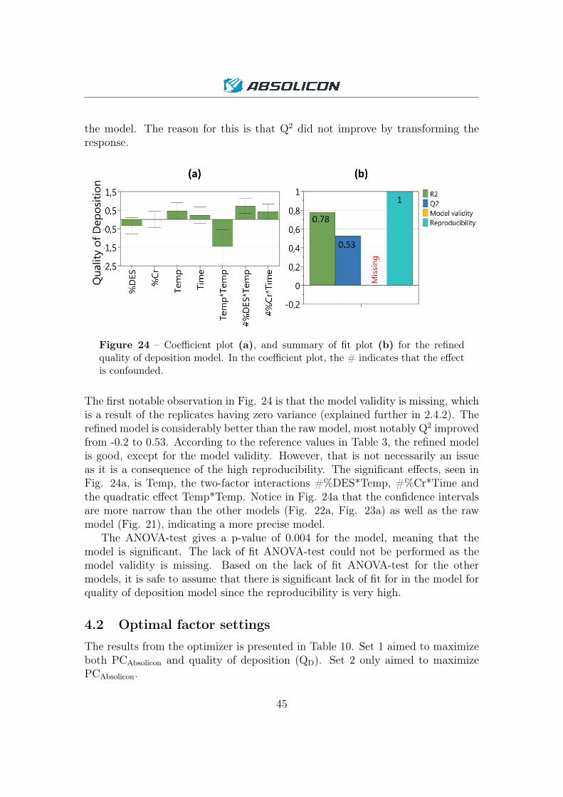
the model. The reason for this is that Q2 did not improve by transforming theresponse.

Figure 24 – Coefficient plot (a), and summary of fit plot (b) for the refinedquality of deposition model. In the coefficient plot, the # indicates that the effectis confounded.

The first notable observation in Fig. 24 is that the model validity is missing, whichis a result of the replicates having zero variance (explained further in 2.4.2). Therefined model is considerably better than the raw model, most notably Q2 improvedfrom -0.2 to 0.53. According to the reference values in Table 3, the refined modelis good, except for the model validity. However, that is not necessarily an issueas it is a consequence of the high reproducibility. The significant effects, seen inFig. 24a, is Temp, the two-factor interactions #%DES*Temp, #%Cr*Time andthe quadratic effect Temp*Temp. Notice in Fig. 24a that the confidence intervalsare more narrow than the other models (Fig. 22a, Fig. 23a) as well as the rawmodel (Fig. 21), indicating a more precise model.

The ANOVA-test gives a p-value of 0.004 for the model, meaning that themodel is significant. The lack of fit ANOVA-test could not be performed as themodel validity is missing. Based on the lack of fit ANOVA-test for the othermodels, it is safe to assume that there is significant lack of fit for in the model forquality of deposition model since the reproducibility is very high.

4.2 Optimal factor settings

The results from the optimizer is presented in Table 10. Set 1 aimed to maximizeboth PCAbsolicon and quality of deposition (QD). Set 2 only aimed to maximizePCAbsolicon.

45

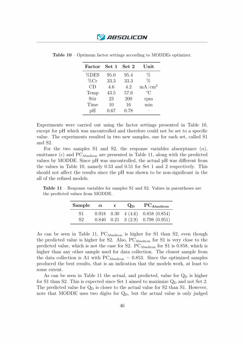
Table 10 – Optimum factor settings according to MODDEs optimizer.

Factor Set 1 Set 2 Unit

%DES 95.0 95.4 %%Cr 33.3 33.3 %CD 4.6 4.2 mA/cm2

Temp 43.5 57.6 °CStir 23 200 rpmTime 10 16 minpH 0.67 0.78 –

Experiments were carried out using the factor settings presented in Table 10,except for pH which was uncontrolled and therefore could not be set to a specificvalue. The experiments resulted in two new samples, one for each set, called S1and S2.

For the two samples S1 and S2, the response variables absorptance (α),emittance (ε) and PCAbsolicon are presented in Table 11, along with the predictedvalues by MODDE. Since pH was uncontrolled, the actual pH was different fromthe values in Table 10, namely 0.53 and 0.51 for Set 1 and 2 respectively. Thisshould not affect the results since the pH was shown to be non-significant in theall of the refined models.

Table 11 – Response variables for samples S1 and S2. Values in parentheses arethe predicted values from MODDE.

Sample α ε QD PCAbsolicon

S1 0.918 0.30 4 (4.6) 0.858 (0.854)S2 0.840 0.21 3 (2.9) 0.798 (0.951)

As can be seen in Table 11, PCAbsolicon is higher for S1 than S2, even thoughthe predicted value is higher for S2. Also, PCAbsolicon for S1 is very close to thepredicted value, which is not the case for S2. PCAbsolicon for S1 is 0.858, which ishigher than any other sample used for data collection. The closest sample fromthe data collection is A1 with PCAbsolicon = 0.853. Since the optimized samplesproduced the best results, that is an indication that the models work, at least tosome extent.

As can be seen in Table 11 the actual, and predicted, value for QD is higherfor S1 than S2. This is expected since Set 1 aimed to maximize QD and not Set 2.The predicted value for QD is closer to the actual value for S2 than S1. However,note that MODDE uses two digits for QD, but the actual value is only judged

46

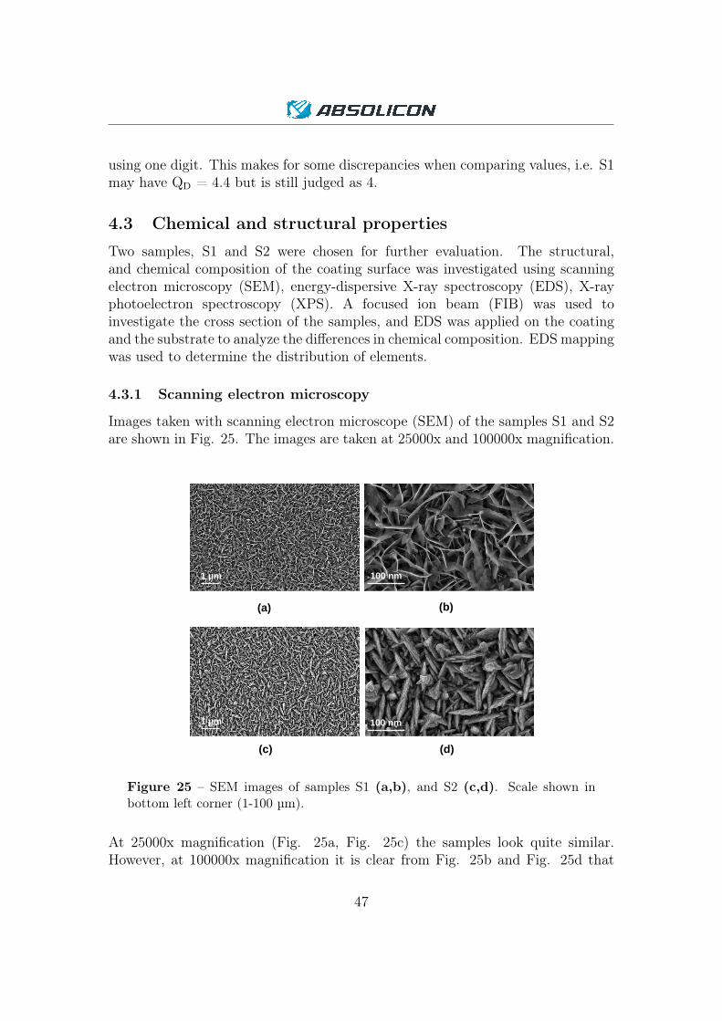
using one digit. This makes for some discrepancies when comparing values, i.e. S1may have QD = 4.4 but is still judged as 4.

4.3 Chemical and structural properties

Two samples, S1 and S2 were chosen for further evaluation. The structural,and chemical composition of the coating surface was investigated using scanningelectron microscopy (SEM), energy-dispersive X-ray spectroscopy (EDS), X-rayphotoelectron spectroscopy (XPS). A focused ion beam (FIB) was used toinvestigate the cross section of the samples, and EDS was applied on the coatingand the substrate to analyze the differences in chemical composition. EDS mappingwas used to determine the distribution of elements.

4.3.1 Scanning electron microscopy

Images taken with scanning electron microscope (SEM) of the samples S1 and S2are shown in Fig. 25. The images are taken at 25000x and 100000x magnification.

100 nm

100 nm1 µm

1 µm

(a) (b)

(c) (d)

Figure 25 – SEM images of samples S1 (a,b), and S2 (c,d). Scale shown inbottom left corner (1-100 µm).

At 25000x magnification (Fig. 25a, Fig. 25c) the samples look quite similar.However, at 100000x magnification it is clear from Fig. 25b and Fig. 25d that

47

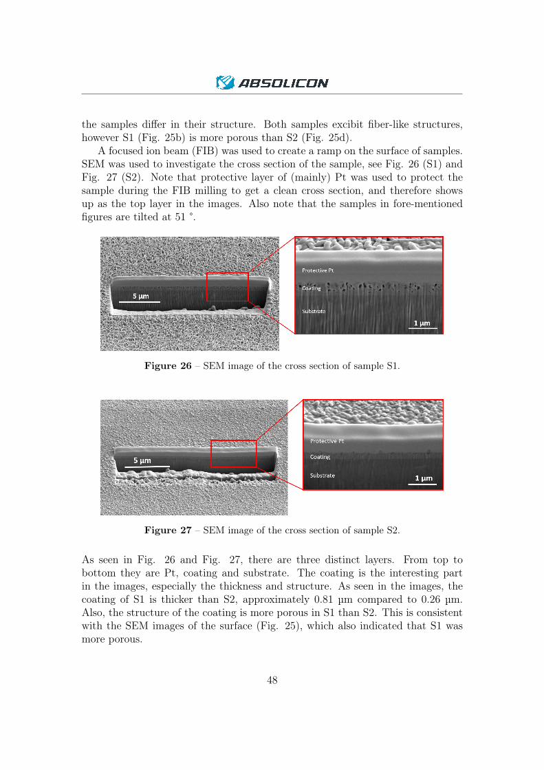
the samples differ in their structure. Both samples excibit fiber-like structures,however S1 (Fig. 25b) is more porous than S2 (Fig. 25d).

A focused ion beam (FIB) was used to create a ramp on the surface of samples.SEM was used to investigate the cross section of the sample, see Fig. 26 (S1) andFig. 27 (S2). Note that protective layer of (mainly) Pt was used to protect thesample during the FIB milling to get a clean cross section, and therefore showsup as the top layer in the images. Also note that the samples in fore-mentionedfigures are tilted at 51 °.

Figure 26 – SEM image of the cross section of sample S1.

Figure 27 – SEM image of the cross section of sample S2.

As seen in Fig. 26 and Fig. 27, there are three distinct layers. From top tobottom they are Pt, coating and substrate. The coating is the interesting partin the images, especially the thickness and structure. As seen in the images, thecoating of S1 is thicker than S2, approximately 0.81 µm compared to 0.26 µm.Also, the structure of the coating is more porous in S1 than S2. This is consistentwith the SEM images of the surface (Fig. 25), which also indicated that S1 wasmore porous.

48

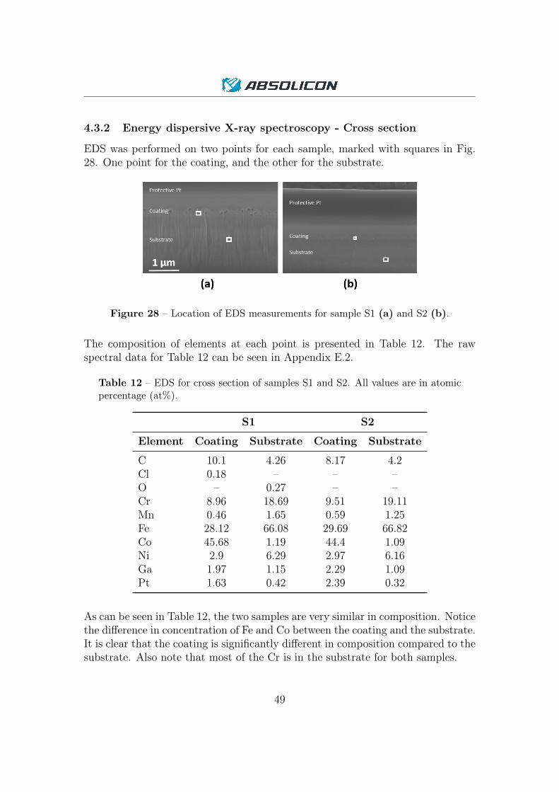
4.3.2 Energy dispersive X-ray spectroscopy - Cross section

EDS was performed on two points for each sample, marked with squares in Fig.28. One point for the coating, and the other for the substrate.

Figure 28 – Location of EDS measurements for sample S1 (a) and S2 (b).

The composition of elements at each point is presented in Table 12. The rawspectral data for Table 12 can be seen in Appendix E.2.

Table 12 – EDS for cross section of samples S1 and S2. All values are in atomicpercentage (at%).

S1 S2

Element Coating Substrate Coating Substrate

C 10.1 4.26 8.17 4.2Cl 0.18 – – –O – 0.27 – –Cr 8.96 18.69 9.51 19.11Mn 0.46 1.65 0.59 1.25Fe 28.12 66.08 29.69 66.82Co 45.68 1.19 44.4 1.09Ni 2.9 6.29 2.97 6.16Ga 1.97 1.15 2.29 1.09Pt 1.63 0.42 2.39 0.32

As can be seen in Table 12, the two samples are very similar in composition. Noticethe difference in concentration of Fe and Co between the coating and the substrate.It is clear that the coating is significantly different in composition compared to thesubstrate. Also note that most of the Cr is in the substrate for both samples.

49

To get a better idea of how the elements are distributed, EDS mappingwas made on the cross section of S1, presented in Fig. 29. The elements arecolour-coded. Fig. 29a shows approximately the same area as Fig. 26. Fig. 29bshows the same area as Fig. 29a but colour-coded by element. Fig. 29a - k showsthe individual elements.

Figure 29 – Cross section for S1 (a), all elements (b), carbon (c), oxygen (d),chromium (e), manganese (f), iron (g), cobalt (h), nickel (i), gallium (j) andplatinum (k).

50

As can be seen in Fig. 29, some elements (C, Cr, Fe, Co, Ga, Pt) are confined to aspecific layer, and others (Ni, Mn, O) are more evenly distributed. It is clear fromFig. 29 that there are distinct differences in chemical composition between thelayers. The only element which is specific to the coating is Co (Fig. 29h), whichis also clear from the low concentration of Co seen in Table 12. C, Pt and Ga areall specific to the protective layer, while Fe and most of the Cr is confined to thesubstrate.

Note that there is no need to display the corresponding EDS mapping for S2, asthere will be no distinguishable differences in terms of layering. The only differencewould be a less distinct coating.

4.3.3 Energy dispersive X-ray spectroscopy - Surface

Energy dispersive X-ray spectroscopy (EDS) was performed on the surface ofsamples S1 and S2 to determine the chemical composition. The results from thesemeasurements are shown in Table 13. Raw spectral data for Table 13 is availablein Appendix E.1.

Table 13 – Chemical composition of the surface of samples S1 and S2. All valuesare in atomic percentage (at%).

Element S1 S2

C 12.52 13.32O 9.87 5.19Cl 0.50 0.34Cr 6.94 3.29Fe 20.17 6.71Co 47.37 70.59Ni 2.1 0.55Mn 0.53 –

Notice in Table 13 that there is more of the substrate-specific elements (Fe, Ni,Mn) in S1 than S2. Especially notice the difference in at% Co and Fe between thesamples.

4.3.4 X-ray photoelectron spectroscopy

XPS was applied to the samples to determine the compounds (environments)rather than individual elements. The results are shown in Table 14. Noticethat the Co2O3 and Co(OH)2 rows in Table 14 are merged because it wasnot possible to determine the amount of each environment. Also note that

51

an asterix (*) indicate uncertainty, i.e. it is not certain that it is the correctenvironment. XPS-measurements also found traces of N and Cl in both samples,but the concentration of these elements were so low the environments could notbe determined.

Table 14 – Result of XPS measurements for samples S1 and S2. All values are inatomic percentage (at%).

Environment S1 S2

C-(C,H) 11.02 7.88C-O,C-N 3.28 2.59COOH 2.99 2.54carbonate 0.9 0.54Co=O 29.42 30.24Co-OH 18.68 20.49C=O,C-O 4.85 2.43*Co2O3 28.85 33.3*Co(OH)2

The samples are very similar in composition, as seen in Table 14. No Cr was foundat the surface of either sample. Most of the deposited Co has formed Co-OH andCo=O. A large part of the Co could potentially be in Co2O3 and/or Co(OH)2environments, but the uncertainty of these are high as well as the distributionbetween them.

5 DiscussionThe results of this project is discussed in a separate section, followed by a generaldiscussion and a section specifically about the electroplating process.

5.1 Results

The refined models were significantly better than the models based on the rawdata. In general, the reproducibility was high for all three models causing themodel validity to appear artificially low. Because of the high reproducibility, themodel validity is of limited interest in the evaluation of the models. A directconsequence of the high reproducibility is significant lack of fit in the models, asseen in the ANOVA-tests (Appendix D). The model for emittance was the worst interms of Q2, and the coefficient plot (Fig. 23a) for the model also failed to calculateconfidence intervals. Even without confidence intervals, conclusions can be made

52

that main effects %DES, CD and Temp probably have a greater impact than Stiand Time, as seen by the size of coefficients in Fig. 23a. Also, based on the modelsfor absorptance and QD it is likely that the interaction effects are significant.Note that it would have been possible to reduce the number of coefficients in theemittance model, thus enabling coefficient intervals to be calculated. However,since adding effects (coefficients) improved Q2 it was prioritized over confidenceintervals, especially since the value of Q2 was so low for the model. Ideally Q2

should be > 0.5 but for the emittance it was only 0.38. This was likely a limitingfactor for the derived response PCAbsolicon. The predicted PCAbsolicon for S2 wasvery high compared to the actual value (0.951 compared to 0.798). The reasonwhy these values differ may have to do with the fact that Set 2 only use the derivedresponse to optimize the results, as opposed to Set 1 which also uses the model forquality of deposition (QD). The model for QD was relatively good (Q2 = 0.53), andhigher QD helps improve the optical properties of the samples (as seen in Table8). Had the goodness of fit been higher for emittance, the predictive capabilitiesof the derived response would be better, and the optimized S2 would likely havecloser to the predicted value of PCAbsolicon. Since the derived response is limitedin its predictive capabilities as a result of the bad model for emittance it may bethat the model for QD helps Set 1 to increase the performance, and Set 2 is notas reliable as it only uses the derived response. Nevertheless, the PCAbsolicon forS1 was the highest of all samples, indicating that the models have at least somepredictive capabilities.

In the refined models, almost no main effects were shown to be significant,with the exception being Temp in the QD response. The significant effects for allof the refined models were shown to be two-factor interactions. Since two-factorinteractions are confounded in the FrF-design, no conclusions can be made aboutthem except that two-factor interactions are important to describe the process. Itis not possible to attribute any two-factor interactions to specific factors due toconfounded effects, i.e. it may as well be two other factors causing any observedtwo-factor interaction effect. This indicates that another experimental designwould be necessary instead of the FrF-design. Ideally, the experimental designshould be able to accurately determine two-factor interactions as well as quadraticeffects. For example the Box-Behnken design may be appropriate [2]. However,using such a design does not allow for as many factors to be investigated.

Neither of the refined models showed pH as a significant factor. That is abit surprising, given the results of other publications showing that pH is in factone of the most significant factors for electroplating processes [17–19]. The reasonwhy pH was not found to be significant may be because the interval which wasinvestigated was very limited, approximately 0.3 to 0.8. The reason why such asmall range was investigated was because pH was an uncontrolled factor. Had it

53

been a controlled factor, a greater range could have been investigated. In thatcase it is likely that it would have been shown to be a significant factor, based onprevious research.

SEM images of the samples (Fig. 25, Fig. 26 and Fig. 27) showed that S1had a more porous surface than S2. It has been shown that a porous surface ispreferable to achieve high absorptance in selective surfaces [33], which is consistentwith the fact that S1 had higher absorptance than S2 (0.92 compared to 0.84).Interestingly the emittance of S2 was better (lower) than the emittance of S1.However, when calculating PCAbsolicon, S1 was better (0.858 compared to 0.798).

EDS of the cross section (Table 12) showed that S1 and S2 were very similar incomposition. It is not surprising that the substrate is similar since it is the samestainless steel, but regarding the composition of the coating it was not as clear whatto expect. The coating measurements in Table 12 can be compared to the EDSsurface measurements in Table 13. Both of the EDS measurements were used toinvestigate the coating, but one was performed on the cross section while the otherwas performed on the surface. There were higher concentrations of Fe and lowerconcentrations of Co in S1 than S2 in the surface measurements. This indicatesthat the electron beam used in the measurements have penetrated the coating forS1 and the substrate is what is contributing to the high concentration of Fe. Thisis a bit surprising since the coating of S1 was thicker than S2. It may be a result ofthe structure of S1 being more porous, as seen in SEM images. A porous surfacewould have a thinner coating at certain spots, while a non-porous surface wouldbe more homogeneous in terms of thickness. There seems to be a similar effect inreverse for S2. The cross section measurements show higher concentrations of Feand lower concentrations of Co compared to the surface measurements. The reasonfor this may be that the dense coating limit the depth at which the electron beamcan penetrate the coating, hence the measurements are comparatively shallow.The thickness of S2 was less than a third of S1, and it is therefore possible thatmore of the substrate contributed to the cross section measurements.

XPS measurements showed that no Cr was found at the surface. Thatindicates that it was almost exclusively Co which was been deposited duringthe electroplating process. It is possible that the Cr which showed up in EDSmeasurements are from the substrate. This problem of poor co-deposition of Coand Cr is the same as E. Zäll experienced during his project [12].

5.2 General

In general, the time-planning for this project was a bit optimistic. The initialtesting took a lot of time, especially because I wanted to include pH as a controlledfactor. This led to some time pressure in the later stages of the project, especiallyaffecting the data collection. Had there been more time/better time planning,

54

the data would be better, meaning that the ranges of the factors would be moreappropriate, and hence produce better samples, mainly in terms of coating quality(QD). To better determine the ranges of the factors, more time would be neededfor initial testing and preparations. Due to the lack of time the range of thefactors was too extreme, resulting in some bad samples (QD = 0 or QD = 1). Inhindsight, the factors should have been chosen in such a way that no samplewas below QD = 2. That is because samples with low quality of deposition(QD < 2) are considerably more specular than samples with higher quality ofdeposition (QD > 2). The specularity is the degree to which light is directly ordiffusely scattered from a surface [34]. If a surface has high specularity, that meansthat incoming light is very sharply reflected (incoming reflection angle is equal tooutgoing reflection angle). The opposite is true for samples with low specularity(a.k.a. diffuse surface). Since samples with low quality of deposition are a lot morespecular, that means that a new random error is introduced unnecessarily. It isunclear how the degree of specularity affected the measurement of the absorptanceand emittance responses. Especially the absorptance measurements are likely tobe affected of this, as the spectrophotometer uses different reference samples fordiffuse and specular measurements. For all the measurements a diffuse referencesample was used. It would of course be possible to use a specular reference sampleas well, but that would introduce yet another random error. The best would beto avoid the problem all together and choose the ranges of factors in such a waythat QD > 1. As it is now, the samples with low QD also had low absorptance,especially the samples E2 and D3. These samples were difficult to account for, andwere marked as outliers by MODDE. However, it would not be justified to removethe samples simply because the quality of deposition was low. These two samplesaffected the model for absorptance in a negative way. By removing these samplesas well as E1 and B2 (which also had low QD) in the absorptance model, it waspossible to get a better model (Q2 = 0.51), and also get significant main effects%Cr and CD. The samples E2, D3, E1, and B2 all had QD < 2, which reinforcesmy earlier point that better results would be achieved if all samples had QD >1. However, one sample B1 has QD = 1, and α = 0.89, which is an exceptionto the other samples with QD < 2. This may have to do with the specularitygiving random errors in the absorptance measurements. It is also another reasonfor not excluding the samples E1, B2, D3 and E2, as it is apparent that it ispossible to have low QD and relatively high absorptance from sample B1. It isalso, of course, possible that the absorptance measurements of samples E1, B2, D3and E2 are correct. Looking at the standard deviation (Fig. 9) of these samples,they do not have significantly higher standard deviation than the other samples,which could indicate that they are in fact correct. But, then again it is difficult tosay how the specularity of the samples affect the measurements. It may be that

55

they are consistent (low standard deviation), but inaccurate at the same time.If the measurements are correct, a different experimental design which includesinteraction effects and quadratic effects would be better suited. However, suchan approach would not be able to investigate the same number of factors as theFrF-design which was chosen for this project, due to the large number experimentsneeded.

The chosen FrF-design enabled many factors to be investigated, but therewere some factors which were left out. One factor which was initially consideredwas the distance between working electrode (sample) and the counter electrode.However, it was deemed unlikely that it would be a significant factor since the useof a potentiostat regulate the potential difference in such a way that the currentflowing between the electrodes is constant, no matter the distance. Also, the cellwhich was used (Fig. 8) was quite small so it would not be possible to adjust thedistance between the electrodes more than a few centimeters at max. Another,more important factor, which was not tested was the pH. It was included as anuncontrolled factor, but that does not enable the factor to be investigated in thesame way that a controlled factor can be investigated. Though considerable timewas spent on regulating the pH of the electrolyte in the initial testing, it wasnot possible to get consistent results. Had there been more time, I am quite surethat the pH could be regulated. Another factor which was not investigated was theconcentration of Co in the electrolyte. The reason for this is that previous researchby E. Zäll [12] has shown that it is almost exclusively Co which is depositedin the electroplating procedure, and therefore it makes no sense to increase theconcentration of Co. Also, the concentration of Co is indirectly regulated byincreasing or decreasing the concentration of Cr (which was one of the factors).

The run order for the data collection was determined using a Python script(Appendix B), which produced a semi-random run order. Randomizing the runorder is tool to avoid systematic errors due to external influences (such as ambienttemperature etc.). By restricting the randomness, this could introduce systematicerrors in the data collection. However, it would take a lot of time to gather thedata had the run order been completely random, and therefore it was deemedappropriate to put restrictions on the randomization process. One example of aproblem which may arise from the semi-random run order is that the experimentswithin the same electrolyte consistently deteriorate. Looking at the raw data inTable 8 that does not seem to be the case. There does not seem to be any otherobvious consequences of the semi-random run order either, and it is unlikely thatit affected the data collection in a significant way.

56

5.3 Electroplating procedure

The electroplating procedure was quite sensitive to variations in the setup. That isbecause the magnetic stirring device in the heating plate is located in the middle,and the electrochemical cell (see Fig. 8) therefore needs to be placed in such a waythat the stirring occurs at the same place in the cell. If the stirring occurs close tothe sample, that means that greater turbulence is caused in the electrolyte thanif the stirring occurs further away from the sample, even if the stirring rate is thesame. This caused a random error in the experiments for the experiments withstirring. This caused the experiments with stirring to have one more random errorthan experiments without. It is unclear how this affected the results. Even thoughthe procedure was sensitive to variations, the reproducibility of the experimentswas proven to be high, as seen in the replicate samples C1 - C4 (Table 8, Fig. 9).The reason being that during the initial testing, many of the potential problemswere identified and could be managed.

Using the same electrolyte numerous times can cause the electrolyte todeteriorate over time, as observed by E. Zäll [12]. He claimed that the causefor this may be the change in pH. This is not an issue for this project since eachelectrolyte (Table 5) was used only for a short period of time, and only for a fewsamples. Also, no significant change in pH was observed. Hence, problems relatedto degrading electrolytes were limited, and it is unlikely that it affected the results.

The spectrophotometer which was used did not cover the entire solar spectrum,280 - 1100 nm as opposed to 280 - 4000 nm [22]. This is not an issue for this projectsince it affects all samples equally, but it may cause inaccurate results comparedthe measurements taken in the full solar spectrum.

The method which was used to measure the emittance was not ideal. TheIR-thermometer which was used is not intended to be used for emittancemeasurements and therefore it has some understandable shortcomings. Oneproblem is radiation from the surroundings, which inevitably will affect themeasurements. The surrounding surfaces have higher emittance than the actualsample, which will affect the results in such a way that the emittance of the sampleappears to be higher than it is. Also, the IR-thermometer assumes that the samplehave a gray surface [12], meaning that the emittance is the same for all wavelengths.That is certainly not the case for spectrally selective surfaces. Also, the accuracyof the IR-thermometer is limited to ± 1 °C + 2 %, which means that the accuracydecrease with temperature. At the measuring temperature 160 °C the error is ±4.2 °C, which is potentially significant error. However, since the errors are thesame for all samples, they are still comparable.

57

6 ConclusionsThe impact which the investigated factors have on the electroplating method couldnot be fully determined. The FrF-design which was used only covers main effectsand the significant effects were shown to be mostly interaction effects and quadraticeffects. The FrF-design was therefore not sufficient for the electroplating method.

Out of the three responses, acceptable models were produced for two of them,namely absorptance and quality of deposition. For these two models the goodnessof fit parameter Q2 was 0.49 and 0.53 respectively. That is sufficient to make validpredictions, according to the available reference values (Table 3). The model foremittance was poor, Q2 = 0.38. The ANOVA-test showed that the absorptanceand quality of deposition model were significant at a significance level of 0.95,while the emittance was not. All three models showed significant lack of fit as aresult of high reproducibility.

Using the optimizer tool in MODDE, two sets of factor settings was predictedby the software (Table 10), resulting in samples S1 and S2 (one for each set). S1had PCAbsolicon = 0.858, which was the highest of all samples. It was also very closeto the predicted value of 0.854, indicating that the optimization was successful. S2was predicted to produce even better results by MODDE in terms of PCAbsolicon,but the actual PCAbsolicon was only 0.798 compared to a predicted value of 0.951.The reason why S2 was less successful may have to do with the poor model foremittance, limiting the derived response model.

The optimized samples S1 and S2 were very similar in chemical composition,as shown by EDS and XPS measurements of the surface and cross section of thecoatings. The greatest difference between the samples was that the coating wasmore porous for S1 than S2, as seen in SEM images of the surface (Fig. 25) andcross section (Fig. 26 and Fig. 27). The coating was also thicker for S1 than S2,0.81 µm compared to 0.26 µm.

58

7 Future workThe optimized factor settings in Set 1 may be used as a centre-point for futureprojects. A different design would be needed which accounts for quadratic andinteraction effects between factors. For example the Box-Behnken design could beused. To apply a more complex design such as Box-Behnken, a smaller number offactors would need to be selected due to the reqired number of experiments. Carefulselection of these factors must be made, using this report and other research as afoundation.

The effect of pH has been shown by others to be significant for the electroplatingprocess. It would therefore be interesting to investigate pH as a controlled factor.However, to do so there would need to be some experimenting as well as literaturestudy on how pH regulatories affect the electrolyte.

Once the electroplating process is well understood, the next step would beto optimize the process. When the optical properties of the coating have beenoptimized, the durability of the coating would have to be investigated, for exampleby the lifetime qualification test presented by E. Zäll [12].

When the optimized process can produce samples which pass thedurability-tests, the optimized electroplating method could be implemented onlarger samples and pipes, and eventually be used by Absolicon in the productionof their solar collectors.

59

References[1] G. Vargas, A.P. García, J. Lopez and J. Cerda, “Electrodeposition of Co-Cr

Black Coatings on Steel in Deep Eutectic Solvents, for Solar CollectionApplications,” in Proceedings of 11th ISES EuroSun Conference, 2016.

[2] L. Eriksson, E. Johansson, N. Kettaneh-Wold, C. Wikström and S. Wold,Design of Experiments - Principles and Applications. Umeå: UmetricsAcadamy, third ed., 2008.

[3] Angus McCrone et al., “Global trends in renewable energy investment 2017,”tech. rep., Frankfurt School-UNEP, apr 2017.

[4] REN21, Renewables 2017 Global Status Report, vol. 978-3-9818107-6-9, 2017.

[5] G. Janssens-Maenhout, M. Crippa, D. Guizzardi, D, M. Muntean, E. Schaaf,J.G.J. Olivier, J.A.H.W. Peters and K.M. Schure, “Fossil CO2 and GHGemissions of all world countries,” 2017.

[6] European Comission, “EU climate action.” https://ec.europa.eu/clima/citizens/eu_en, 2018. [Online; Accessed 29-Jan-2018].

[7] Y. Tian and C.Y. Zhao, “A review of solar collectors and thermal energystorage in solar thermal applications,” Applied Energy, vol. 104, pp. 538 –553, 2013.

[8] J.A. Duffie and W.A. Beckman, Solar engineering of thermal processes. JohnWiley & Sons, 2013.

[9] M.K. Islam, M. Hasanuzzaman and N.A. Rahim, “Modelling and analysis ofthe effect of different parameters on a parabolic-trough concentrating solarsystem,” RSC Adv., vol. 5, pp. 36540 – 36546, apr 2015.

[10] Dr. Md. GolamMowla Choudhury, “Selective surface for efficient solar thermalconversion,” Bangladesh Renewable Energy Newsletter, vol. 1, pp. 1 – 3, 2003.

[11] E.R. Cohen, I. Mills, IUPAC Quantities, Units and Symbols in PhysicalChemistry. Second Edition. Oxford: Blackwell Scientific Publications„second ed., 1993.

[12] E. Zäll, “Electroplating of selective surfaces for concentrating solar collectors,”Master’s thesis, Umeå University, 2017.

60

[13] C.E. Kennedy, “Review of mid-to high-temperature solar selective absorbermaterials,” tech. rep., National Renewable Energy Lab., Golden, CO.(US),2002.

[14] G.C. Bakos, “Design and construction of a two-axis Sun tracking system forparabolic trough collector (PTC) efficiency improvement,” Renewable Energy,vol. 31, no. 15, pp. 2411 – 2421, 2006.

[15] V.K. Jebasingh and G.M. Joselin Herbert, “A review of solar parabolic troughcollector,” Renewable and Sustainable Energy Reviews, vol. 54, pp. 1085 –1091, 2016.

[16] S.A. Kalogirou, “Solar thermal collectors and applications,” Progress inEnergy and Combustion Science, vol. 30, no. 3, pp. 231 – 295, 2004.

[17] R. Katırcı, “Statistical optimisation of trivalent chromium bath andcharacterisation of coating defects,” Surface Engineering, vol. 31, pp. 1 – 3,jan 2015.

[18] M. Poroch-Seritan, S. Gutt, G. Gutt, I. Cretescu, C. Cojocaru and T.Severin, “Design of experiments for statistical modeling and multi-responseoptimization of nickel electroplating process,” Chemical Engineering Researchand Design, vol. 89, pp. 136 – 147, feb 2011.

[19] M. Poroch - Seritan , I. Cretescu, C. Cojocaru, S. Ameriei and C. Suciu,“Experimental design for modelling and multi-response optimization of fe–nielectroplating process,” Chemical Engineering Research and Design, vol. 96,pp. 138 – 149, apr 2015.

[20] M. Schlesinger and M. Paunovic, Fundamentals of electrochemical deposition.Wiley, second ed., 2006.

[21] E.L. Smith, A.P. Abbott and K.S. Ryder, “Deep Eutectic Solvents (DESs) andTheir Applications,” Chemical Reviews, vol. 114, no. 21, pp. 11060 – 11082,2014.

[22] C. National Renewable Energy Lab., Golden, “Reference Solar SpectralIrradiance: Air Mass 1.5.” http://rredc.nrel.gov/solar/spectra/am1.5/, 2017. [Online; Accessed 11-Apr-2018].

[23] B. Carlsson and M. Köhl, “Recommended qualification test procedure for solarabsorber surface durability,” IEA SHC Task, vol. 27, 2005.

[24] Y.A. Çengel, A.J. Ghajar and M. Kanoglu, Heat and mass transfer:fundamentals & applications, vol. 4. McGraw-Hill New York, 2011.

61

[25] Encyclopædia Britannica, “Spectrophotometry.” academic.eb.com.proxy.ub.umu.se/levels/collegiate/article/spectrophotometry/69038, jan2009. [Online; Accessed 4-Feb-2018].

[26] Nanoscience Instruments, “Scanning electron microscopy.” https://www.nanoscience.com/technology/sem-technology. [Online; Accessed4-Feb-2018].

[27] N.H. Turner and J.A. Schreifels, “Surface Analysis: X-ray PhotoelectronSpectroscopy and Auger Electron Spectroscopy,” Analytical Chemistry,vol. 66, no. 12, pp. 163 – 185, 1994.

[28] J.J. Friela and C.E. Lyman, “Tutorial Review: X-ray Mapping inElectron-Beam Instruments,” Microscopy and Microanalysis, vol. 12, no. 1,pp. 2 – 25, 2006.

[29] C.C. Hu and A. Bai, “Composition control of electroplated nickel–phosphorusdeposits,” Surface and Coatings Technology, vol. 137, no. 2, pp. 181 – 187,2001.

[30] J. Edwards, “Electroplating–a guide for designers and engineers,” TheCommittee for the Promotion of Electroplating,, p. 72, 1983.

[31] C.C. Lin and C.C. Hu, “Electropolishing of 304 stainless steel: Surfaceroughness control using experimental design strategies and a summarizedelectropolishing model,” Electrochimica Acta, vol. 53, no. 8, pp. 3356 – 3363,2008.

[32] Labsphere, RSA-PE-20. AQ-00073-000, Rev. 7.

[33] C. Atkinson, C.L. Sansom, H.J. Almond and C.P. Shaw, “Coatings forconcentrating solar systems–a review,” Renewable and Sustainable EnergyReviews, vol. 45, pp. 113 – 122, 2015.

[34] M. Fox, Optical properties of solids, vol. 3. Oxford university press, 2010.

[35] D. Ensminger and F.B. Stulen, Ultrasonics: data, equations and their practicaluses. CRC press, 2008.

62

AppendicesA ElectropolishingEach sample was pre-treated using an ultrasonic cleaner (sonicator) and anelectropolishing method developed by Lin and Hu [31]. A sonicator is a toolwhich can be used to smoothen surfaces of samples using energy from ultrasonicwaves [35]. Each sample was sonicated during 15 minutes using a VWR ultrasoniccleaner. After the sonication, the samples were subjected to the electropolishingprocess. The electropolishing method is very similar to the electroplating method,and the schematic two-electrode cell in Fig. 5 is valid representation of the setup.Each sample, acting as the working electrode, was submerged in an electrolyte anda potentiostat was used to apply the desired current between the sample and acounter-electrode for 10 minutes. The electrolyte consisted of phosphoric acid (85%), sulphuric acid (97 %), and glycerol at a volume ratio of 2:1:1. The appliedvoltage was calculated using 0.2 A/cm2. The area of the submerged samples weredetermined using a ruler, and the area was controlled using teflon tape. After theelectropolishing was finished, each sample was cleaned using deionized water, airdried and then stored in a acetone. The effect of the pre-treatment is illustratedin in Fig. A.1, showing close up images (taken with scanning electron microscope(SEM)) of a substrate before and after pre-treatment.

Figure A.1 – Untreated substrate (a), and substrate with pre-treatment applied(b) [12].

As can be seen in Fig. A.1, the treated substrate is considerably smoother.

i

B Python script for randomizing experimentsThe following script was used to randomize the experiments with constraints. Thescript needs data from MODDE separating the samples according to electrolyteand temperature. The script returns a list of the samples along with a semi-randomrunorder.import random

# Data from MODDE, sepera t ed in low and high temperature .# A,B,C,D,E i nd i c a t e which e l e c t r o l y t e to be used f o r experimentA_low = [ 'A1 ' , 'A2 ' ] ; D_low = [ 'D1 ' , 'D2 ' ]A_high = [ 'A3 ' , 'A4 ' ] ; D_high = [ 'D3 ' , 'D4 ' ]

B_low = [ 'B1 ' , 'B2 ' ] ; E_low = [ 'E1 ' , 'E2 ' ]B_high = [ 'B3 ' , 'B4 ' ] ; E_high = [ 'E3 ' , 'E4 ' ]

# Shu f f l e data wi th same temperaturerandom . s h u f f l e (A_low ) ; random . s h u f f l e (A_high)random . s h u f f l e (B_low ) ; random . s h u f f l e (B_high )random . s h u f f l e (D_low ) ; random . s h u f f l e (D_high)random . s h u f f l e (E_low ) ; random . s h u f f l e (E_high )

# Combine low and high temperatureA = [A_low , A_high ]B = [B_low , B_high ]C = [ [ 'C1 ' ] , [ 'C2 ' ] , [ 'C3 ' ] , [ 'C4 ' ] ]D = [D_low , D_high ]E = [E_low , E_high ]

# Shu f f l e data w i th in same type o f e l e c t r o l y t erandom . s h u f f l e (A) ; random . s h u f f l e (D)random . s h u f f l e (B) ; random . s h u f f l e (E)

# Combine a l l e l e c t r o l y t e sorder = [A,B,C,D,E]random . s h u f f l e ( order )

# Print r e s u l t sprint ( " {0:^10}{1:^10} " . format ( "Sample" , "Run␣Order" ) )

k = 1for i in order :

for j in i :for l in j :

print ( " {0:^10}{1:^10} " . format ( l , k ) )k = k + 1

ii

C Matlab scripts for calculating absorptanceA Matlab script, ’Absorptance’ was created to calculate the absorptance for eachsample from the raw CSV-data (Appendix C.1. To facilitate the calculations,another Matlab script (Appendix C.3) was created which uses the ’Absorptance’script to calculate the final absorptance for each sample, which is the average of twomeasurements, and print the results in a table showing the sample-ID, absorptanceand standard deviation between measurements.

C.1 Main script

The following script was used to calculate the absorptance of each sample.

function A = Absorptance(filename)% Returns the total absorptance of a sample, given% the reflection data taken in the range 280 - 1100 nm

% Import solar spectrum data (in range 1100nm to 280nm)I = xlsread('SolarSpectrum.xlsx');

% Import 2D-interpolant for data-correctionF = Reflectance_correction;

% Import csv-file with reflection data of the sampleStart_row = 2;End_row = 822;[Wavelengths,R_measured] = importfile(filename,Start_row, End_row);

% Calculate actual reflectanceR_actual = zeros(length(R_measured),1);for i = 1:821

R_actual(i,1) = F(Wavelengths(i),0.01*R_measured(i));end

% Calculate absorptanceA = (1-R_actual)'*flipud(I)/sum(I);end

In order for the script to run, it needs to import ’SolarSpectrum.xlsx’, a2D-interpolant and reflection data for each sample. ’SolarSpectrum.xlsx’ is solarspectrum data, available from NREL website [22]. To import the 2D-interpolant(which is used to correct the reflectance) a separate function is used called

iii

’Reflectance_correction’, available in Appendix C.2. To import the reflectancedata (in CSV-format) an auto generated script was used called ’importfile’. Theimportfile is specific for the data taken with Lambda 35 and can easily be adjustedto suit other types of data.

C.2 2D-interpolant for Lambda 35

The following Matlab code was used to create a 2D-interpolant. A 2D-interpolantis simply a tool to interpolate in two dimensions (variables). The interpolant wasmade based on a data sheet for the integrated sphere used in the spectrophotometer(Lambda 35) [32].

function F = Reflectance_correction

% x-values (wavelengths)wavelengths = [300:25:1100];x = [repelem(wavelengths,6)]';

% y-values (measured reflectance)y = [0.009 0.053 0.099 0.192 0.337 0.378...

0.009 0.050 0.095 0.188 0.329 0.371...0.009 0.050 0.093 0.184 0.323 0.366...0.009 0.049 0.092 0.182 0.319 0.362...0.010 0.048 0.091 0.181 0.316 0.360...0.010 0.048 0.091 0.181 0.314 0.359...0.010 0.048 0.091 0.182 0.313 0.358...0.010 0.049 0.091 0.183 0.313 0.359...0.010 0.049 0.092 0.184 0.313 0.359...0.010 0.050 0.092 0.186 0.313 0.360...0.010 0.050 0.093 0.187 0.313 0.361...0.010 0.050 0.093 0.188 0.314 0.362...0.010 0.051 0.094 0.190 0.315 0.364...0.010 0.051 0.095 0.191 0.316 0.365...0.011 0.052 0.095 0.193 0.317 0.366...0.011 0.052 0.096 0.194 0.317 0.367...0.011 0.053 0.097 0.195 0.318 0.368...0.011 0.054 0.098 0.196 0.319 0.369...0.011 0.054 0.099 0.198 0.320 0.370...0.012 0.055 0.100 0.199 0.321 0.371...0.012 0.056 0.101 0.200 0.323 0.372...0.012 0.057 0.102 0.202 0.324 0.374...0.013 0.057 0.102 0.203 0.325 0.375...0.013 0.058 0.104 0.204 0.326 0.376...0.013 0.059 0.104 0.206 0.327 0.377...0.014 0.059 0.105 0.207 0.328 0.378...0.014 0.060 0.106 0.208 0.329 0.379...0.014 0.061 0.107 0.209 0.331 0.380...0.014 0.061 0.108 0.210 0.332 0.381...0.014 0.062 0.108 0.210 0.333 0.382...0.014 0.062 0.109 0.211 0.334 0.383...0.014 0.062 0.110 0.212 0.334 0.383...0.015 0.063 0.110 0.213 0.336 0.385]';

% v-values (actual reflectance)v = [0.011 0.065 0.123 0.231 0.394 0.436...

0.011 0.064 0.121 0.230 0.392 0.434...0.012 0.064 0.121 0.230 0.388 0.432...0.011 0.064 0.122 0.229 0.387 0.431...0.011 0.064 0.122 0.230 0.386 0.431...0.011 0.064 0.122 0.231 0.385 0.431...0.011 0.064 0.122 0.232 0.385 0.432...0.011 0.064 0.122 0.233 0.385 0.433...0.011 0.064 0.123 0.235 0.385 0.433...0.011 0.065 0.123 0.236 0.385 0.434...0.011 0.065 0.123 0.238 0.385 0.435...0.011 0.066 0.124 0.239 0.386 0.436...0.011 0.066 0.124 0.240 0.386 0.436...0.011 0.066 0.125 0.241 0.386 0.436...0.011 0.067 0.125 0.243 0.386 0.437...0.011 0.067 0.126 0.243 0.386 0.437...0.011 0.068 0.126 0.245 0.387 0.438...0.011 0.068 0.127 0.245 0.388 0.439...0.011 0.068 0.127 0.246 0.388 0.440...0.011 0.069 0.128 0.247 0.388 0.440...0.011 0.069 0.129 0.249 0.391 0.440...0.011 0.070 0.130 0.249 0.391 0.442...0.011 0.071 0.131 0.251 0.391 0.442...0.012 0.072 0.132 0.251 0.391 0.442...0.012 0.072 0.133 0.252 0.391 0.441...0.012 0.072 0.133 0.252 0.391 0.441...0.012 0.072 0.134 0.252 0.391 0.442...0.013 0.073 0.134 0.254 0.392 0.443...0.012 0.073 0.135 0.255 0.392 0.443...0.012 0.075 0.135 0.256 0.393 0.443...0.012 0.075 0.135 0.256 0.392 0.444...0.012 0.075 0.136 0.257 0.394 0.444...0.012 0.076 0.138 0.257 0.396 0.445]';

% Create 2D-interpolantF = scatteredInterpolant(x,y,v);

iv

C.3 Total absorptance

This script was used to get the absorptance for each sample by averaging themeasurements made for each sample.

A1 = Absorptance('A1.Sample.Raw.csv');A2 = Absorptance('A2.Sample.Raw.csv');A3 = Absorptance('A3.Sample.Raw.csv');A4 = Absorptance('A4.Sample.Raw.csv');A12 = Absorptance('A12.Sample.Raw.csv');A22 = Absorptance('A22.Sample.Raw.csv');A32 = Absorptance('A32.Sample.Raw.csv');A42 = Absorptance('A42.Sample.Raw.csv');B1 = Absorptance('B1.Sample.Raw.csv');B2 = Absorptance('B2.Sample.Raw.csv');B3 = Absorptance('B3.Sample.Raw.csv');B4 = Absorptance('B4.Sample.Raw.csv');B12 = Absorptance('B12.Sample.Raw.csv');B22 = Absorptance('B22.Sample.Raw.csv');B32 = Absorptance('B32.Sample.Raw.csv');B42 = Absorptance('B42.Sample.Raw.csv');C1 = Absorptance('C1.Sample.Raw.csv');C2 = Absorptance('C2.Sample.Raw.csv');C3 = Absorptance('C3.Sample.Raw.csv');C4 = Absorptance('C4.Sample.Raw.csv');

C12 = Absorptance('C12.Sample.Raw.csv');C22 = Absorptance('C22.Sample.Raw.csv');C32 = Absorptance('C32.Sample.Raw.csv');C42 = Absorptance('C42.Sample.Raw.csv');D1 = Absorptance('D1.Sample.Raw.csv');D2 = Absorptance('D2.Sample.Raw.csv');D3 = Absorptance('D3.Sample.Raw.csv');D4 = Absorptance('D4.Sample.Raw.csv');D12 = Absorptance('D12.Sample.Raw.csv');D22 = Absorptance('D22.Sample.Raw.csv');D32 = Absorptance('D32.Sample.Raw.csv');D42 = Absorptance('D42.Sample.Raw.csv');E1 = Absorptance('E1.Sample.Raw.csv');E2 = Absorptance('E2.Sample.Raw.csv');E3 = Absorptance('E3.Sample.Raw.csv');E4 = Absorptance('E4.Sample.Raw.csv');E12 = Absorptance('E12.Sample.Raw.csv');E22 = Absorptance('E22.Sample.Raw.csv');E32 = Absorptance('E32.Sample.Raw.csv');E42 = Absorptance('E42.Sample.Raw.csv');

% Calculate statisticsSample = {'A1','A2','A3','A4','B1','B2','B3','B4','C1','C2','C3','C4'...

'D1','D2','D3','D4','E1','E2','E3','E4'}';Abs = [mean([A1 A12]),mean([A2 A22]),mean([A3 A32]),mean([A4 A42])...

mean([B1 B12]),mean([B2 B22]),mean([B3 B32]),mean([B4 B42])...mean([C1 C12]),mean([C2 C22]),mean([C3 C32]),mean([C4 C42])...mean([D1 D12]),mean([D2 D22]),mean([D3 D32]),mean([D4 D42])...mean([E1 E12]),mean([E2 E22]),mean([E3 E32]),mean([E4 E42])]';

Std = [std([A1 A12]),std([A2 A22]),std([A3 A32]),std([A4 A42])...std([B1 B12]),std([B2 B22]),std([B3 B32]),std([B4 B42])...std([C1 C12]),std([C2 C22]),std([C3 C32]),std([C4 C42])...std([D1 D12]),std([D2 D22]),std([D3 D32]),std([D4 D42])...std([E1 E12]),std([E2 E22]),std([E3 E32]),std([E4 E42])]';

Results = table(Sample, Abs, Std)

The script uses the main absorptance script (Appendix C.1) to calculate theabsorptance for each sample from the raw data and stores the result as A1 ...E42. The first letter and digit is the sample-ID. When there is a 2 at the end,e.g. E42, that means that sample is the second measurement of sample E4. Inthe end of the script, the results are compiled in a table showing the sample-ID,absorptance and standard deviation between measurements.

v

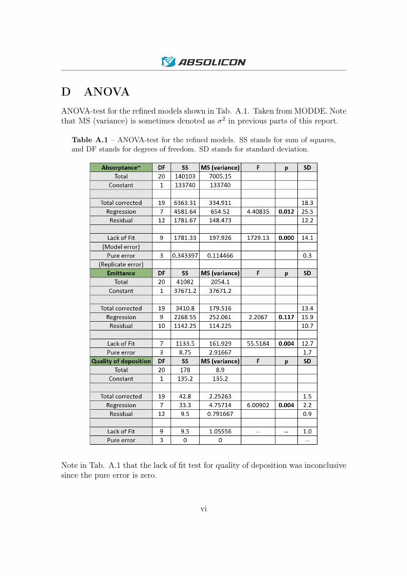
D ANOVAANOVA-test for the refined models shown in Tab. A.1. Taken from MODDE. Notethat MS (variance) is sometimes denoted as σ2 in previous parts of this report.

Table A.1 – ANOVA-test for the refined models. SS stands for sum of squares,and DF stands for degrees of freedom. SD stands for standard deviation.

Note in Tab. A.1 that the lack of fit test for quality of deposition was inconclusivesince the pure error is zero.

vi

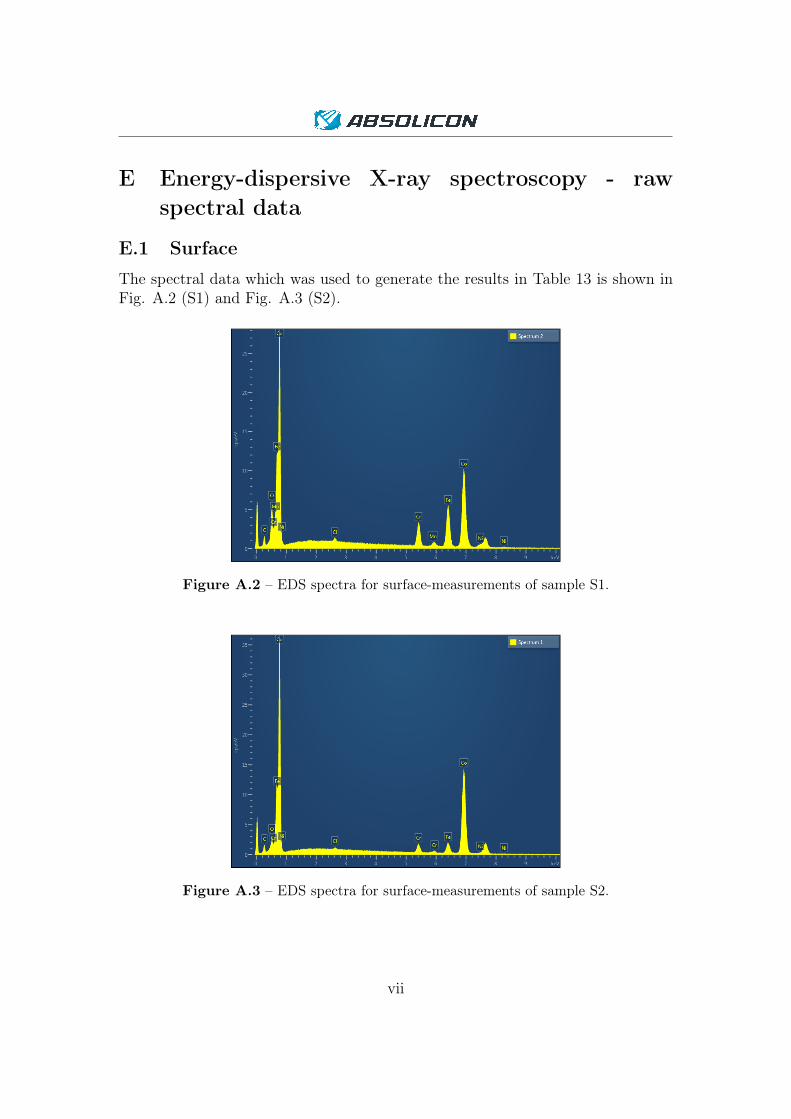
E Energy-dispersive X-ray spectroscopy - rawspectral data

E.1 Surface

The spectral data which was used to generate the results in Table 13 is shown inFig. A.2 (S1) and Fig. A.3 (S2).

Figure A.2 – EDS spectra for surface-measurements of sample S1.

Figure A.3 – EDS spectra for surface-measurements of sample S2.

vii

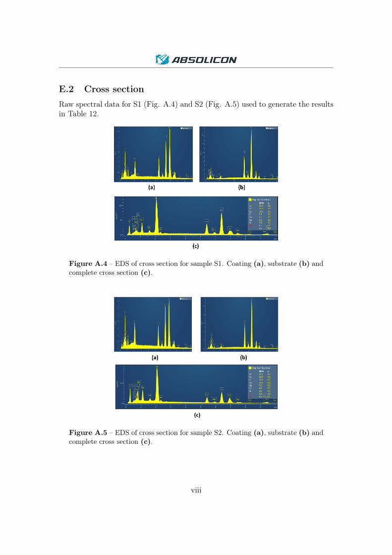
E.2 Cross section

Raw spectral data for S1 (Fig. A.4) and S2 (Fig. A.5) used to generate the resultsin Table 12.

Figure A.4 – EDS of cross section for sample S1. Coating (a), substrate (b) andcomplete cross section (c).

Figure A.5 – EDS of cross section for sample S2. Coating (a), substrate (b) andcomplete cross section (c).

viii