Inversion of helicopter electromagnetic data to a magnetic conductive layered earth

GEOPHYSICS, VOL. 68, NO. 4 (JULY-AUGUST 2003); P. 1211–1223, 13 FIGS., 1 TABLE.10.1190/1.1598113

Inversion of helicopter electromagnetic datato a magnetic conductive layered earth

Haoping Huang∗ and Douglas C. Fraser‡

ABSTRACT

Inversion of airborne electromagnetic (EM) data fora layered earth has been commonly performed underthe assumption that the magnetic permeability of thelayers is the same as that of free space. The resistivity in-verted from helicopter EM data in this way is not reliablein highly magnetic areas because magnetic polarizationcurrents occur in addition to conduction currents, caus-ing the inverted resistivity to be erroneously high.

A new algorithm for inverting for the resistivity, mag-netic permeability, and thickness of a layered modelhas been developed for a magnetic conductive layeredearth. It is based on traditional inversion methodolo-gies for solving nonlinear inverse problems and mini-mizes an objective function subject to fitting the data ina least-squares sense. Studies using synthetic helicopter

EM data indicate that the inversion technique is reason-ably dependable and provides fast convergence. Whensix synthetic in-phase and quadrature data from threefrequencies are used, the model parameters for two- andthree-layer models are estimated to within a few percentof their true values after several iterations. The analysisof partial derivatives with respect to the model parame-ters contributes to a better understanding of the relativeimportance of the model parameters and the reliabilityof their determination.

The inversion algorithm is tested on field dataobtained with a Dighem helicopter EM system atMt. Milligan, British Columbia, Canada. The outputmagnetic susceptibility-depth section compares favor-ably with that of Zhang and Oldenburg who inverted forthe susceptibility on the assumption that the resistivitydistribution was known.

INTRODUCTION

A number of interpretation methods exist for helicopterelectromagnetic (EM) data that are designed to provide im-ages that mimic the distribution of the true parameter(s) in thegeologic section. Generally, the methods fall into two classes:(1) direct transform of data to a generalized model such as ahalf-space, and (2) inversion of data to a specific model suchas a layered earth, where a starting model is employed, fol-lowed by iterative fitting of the data to yield a best fit in theleast-squares sense.

Transform methods (e.g., Fraser, 1978; Huang and Fraser,2001) have the advantage of yielding a single robust solutionfor the given output parameter, and the disadvantage that theoutput parameter may provide a poorly resolved image of thegeology.

Inversion methods (e.g., Fitterman and Deszcz-pan, 1998;Sengpiel and Siemon, 2000) have the advantage of yielding a

Published on Geophysics Online January 30, 2003. Manuscript received by the Editor April 27, 2001; revised manuscript received December 2, 2002.∗Formerly Geoterrex-Dighem, Unit 2, 2270 Argentia Road, Mississauga, Ontario L5N 6A6, Canada; presently Geophex, Ltd., 605 Mercury Street,Raleigh, North Carolina 27603. E-mail: [email protected].‡Formerly Geoterrex-Dighem, Unit 2, 2270 Argentia Road, Mississauga, Ontario L5N 6A6, Canada; presently consultant, 1294 GatehouseDr., Mississauga, Ontario L5H 1A5, Canada. E-mail: [email protected]© 2003 Society of Exploration Geophysicists. All rights reserved.

much superior resolution for the given output parameter andthe disadvantage that the output parameter may vary with thestarting model, so this lack of robustness is always a concernwhen evaluating an interpretive output. The starting modelis a common problem for all inversions and is not a topicof this paper. We use damped least-squares inversion basedon singular value decomposition, where the starting modelis determined directly from the resistivity-depth algorithm ofHuang and Fraser (1996) and the apparent permeability algo-rithm of Huang and Fraser (2000), both of which are multi-frequency transforms from a half-space model. Sengpiel andSiemon (2000) show examples for determining starting modelsfrom transforms. Such starting models are often sufficient fora successful inversion of airborne EM data.

Inversion methods for the interpretation of electromagnetic(EM) data for a layered earth are being employed more com-monly for helicopter-borne surveys as the data quality is im-proved and as both the number of frequencies and computer

1211

1212 Huang and Fraser

speed are increased. Numerous papers have been published onthe methods used to invert for the resistivity of a layered earthmodel under the assumption that the magnetic permeabilityand dielectric permittivity are the same as those of free space(Holladay et al., 1986; Paterson and Reford, 1986; Huang andPalacky, 1991; Qian et al., 1997; Fitterman and Deszcz-Pan,1998; Sengpiel and Siemon, 2000). However, EM data may beaffected by the permeability in magnetic areas (Fraser, 1981;Huang and Fraser, 2000) which is the subject matter of thispaper. EM data at frequencies above 10000 Hz may also be af-fected by the dielectric permittivity (Fraser et al., 1990; Huangand Fraser, 2002), but this is beyond the scope of this paper.

The resistivity derived from helicopter EM data, based ona nonmagnetic earth, is not reliable in highly magnetic areasbecause magnetic polarization currents occur in addition toconduction currents. The effect of a magnetic permeability µgreater than the free space µ0 is that the response at low fre-quencies may be dominated by a magnetization effect that isin-phase with, and in the same direction as, the primary field.As the frequency approaches zero, the in-phase response froma magnetic conductive earth becomes negative (in accordancewith the normal signing convention) and frequency indepen-dent, and the quadrature response goes to zero. At higher fre-quencies, the magnetization effect and conductive effect aremixed, and the EM response becomes frequency dependent.The in-phase response is suppressed, although it may retaina positive value, and the positive quadrature response is in-creased. In this case, the magnetic effect on the data may go un-noticed, and an inversion can produce an overestimate, some-times large, in the earth’s resistivity when using a nonmagneticearth model. See Beard and Nyquist (1998) for a discussion onthe so-called in-phase shift due to magnetic polarization.

Magnetic permeability is one of the EM parameters of theearth. Ignoring it may not only cause the interpretation to beerroneous, but may also result in the loss of potentially usefulinformation about the earth (Zhang and Oldenburg, 1999).

Some researchers have reported on the computation of mag-netic permeability and resistivity from airborne EM data us-ing noninversion methods. Lodha and West (1976) and Huangand Zhu (1984) presented methods for determining the mag-netic susceptibility, conductivity, size, and depth of a magneticconductive sphere in a dipole source field. Fraser (1973) de-scribed a technique for the estimation of the amount of mag-netite contained in a nonconductive vertical dike. Fraser (1981)also presented a magnetite mapping method for helicopter EMsystems, yielding the apparent weight-percent magnetite basedon a nonconductive homogeneous half-space. He showed thata magnetite content of 0.25% can be recognized in the data.Huang and Fraser (2000) developed a resistivity and magneticpermeability mapping technique that yielded the relative mag-netic permeability and resistivity of a magnetic conductive half-space.

Inversion of airborne multifrequency EM data for the mag-netic permeability and resistivity of a layered earth has re-ceived limited attention. Beard and Nyquist (1998) invertedhelicopter-borne EM data from five frequencies for a half-space resistivity and identified hazardous waste sites whenmagnetic permeability was included as an inversion parameter.Otherwise, the waste sites were almost invisible on a resistivitymap. Zhang and Oldenburg (1997) describe a method to in-vert for the magnetic permeability of a layered earth under the

assumption that the resistivity distribution is known. The inver-sion technique may produce a good representation of the truemagnetic susceptibility if the true conductivity-depth model isobtained by other methods. They also developed an inversionalgorithm to simultaneously recover 1D distributions of electri-cal conductivity and magnetic permeability given the thicknessof each layer (Zhang and Oldenburg, 1999).

In this paper, we invert for the magnetic permeability, resis-tivity, and thickness simultaneously for a layered earth underthe quasi-static assumption that the dielectric permittivity isignored. The inversion method is tested on synthetic data andon three-frequency data from a Dighem survey at Mt. Milligan,British Columbia, Canada. The results are compared to thoseobtained by Zhang and Oldenburg (1997).

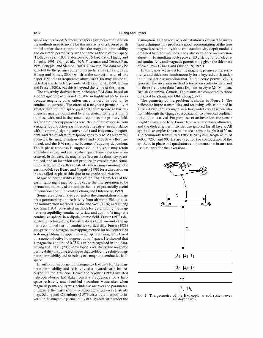
The geometry of the problem is shown in Figure 1. Thehelicopter-borne transmitting and receiving coils, contained ina towed bird, are arranged in a horizontal coplanar orienta-tion, although the change to a coaxial or to a vertical coplanarorientation is trivial. For purposes of an inversion, the sensorheight h is assumed to be known from a radar or laser altimeter,and the dielectric permittivities are ignored for all layers. Allsynthetic examples shown below use a sensor height h of 30 m.The commonly transmitted DIGHEM system frequencies of56000, 7200, and 900 Hz are used for the computation of thesynthetic in-phase and quadrature components that in turn areused as input for the inversions.

FIG. 1. The geometry of the EM coplanar coil system overa L-layer earth.

Helicopter Resistivity and Permeability Inversion 1213

THE FORWARD PROBLEM

The EM response of a layered half-space for dipole sourceexcitation is given by Frischknecht (1967), Ward (1967), andWard and Hohmann (1988), among many others. If a horizon-tal coplanar system is at a height h above the layered half-space, the secondary magnetic field Hs, normalized against theprimary field H0 at the receiving coil, is

Hs

H0= s3

∫ ∞0

R(λ)λ2exp(−2u0h)J0(λs)dλ, (1)

where s is the coil separation, λ is the variable of integration,and J0 the Bessel function of the first kind of order zero. Theterm R(λ) can be written as

R(λ) = Y1 − Y0

Y1 + Y0, (2)

where Y0= u0/ iωµ0 is the intrinsic admittance of free space,Y1 is the surface admittance, i is the imaginary number, ω isthe angular frequency, µ0 is the magnetic permeability of freespace, and u0 is equal to (λ2+ k2

0)1/2, where k0 is the wave num-ber of free space. For a L-layer earth, Y1 can be obtained bythe following recurrence relation:

Yl = Yl

Yl+1 + Yl tanh(ultl)

Yl + Yl+1 tanh(ultl), l = 1, 2, . . . ,L− 1, (3)

where

Yl= ul

iωµ0µl

(4)

and

ul=(λ2 + k2

l

)1/2, (5)

where kl is the wave number of l-th layer given by

kl =(iωσlµ0µl − ω2ε0µ0µl

)1/2, (6)

and where tl is the thickness, µl is the relative magnetic per-meability, σl is the conductivity of the lth layer, and ε0 is thedielectric permittivity of free space. In practice, the reciprocalof the conductivity, the resistivity ρl, is commonly used. Here,for convenience, we note the lth layer relative permeabilityas µl instead of µr l. Further, since we employ the quasi-staticassumption, equation (6) becomes

kl = (iωσlµ0µl)1/2. (7)

In the half-space at the bottom of the electrical section,

YL = YL . (8)

Y1 is a complex function of an integral variable λ, the angularfrequencyω, the magnetic permeabilityµ, the resistivity ρ, andthe thickness t of the layers. For a given model, Y1 can be calcu-lated by using the recurrence relationship in equations (3)–(5).Then, Y1 can be substituted into equations (2) and then into (1)to yield the responses of the system over the model.

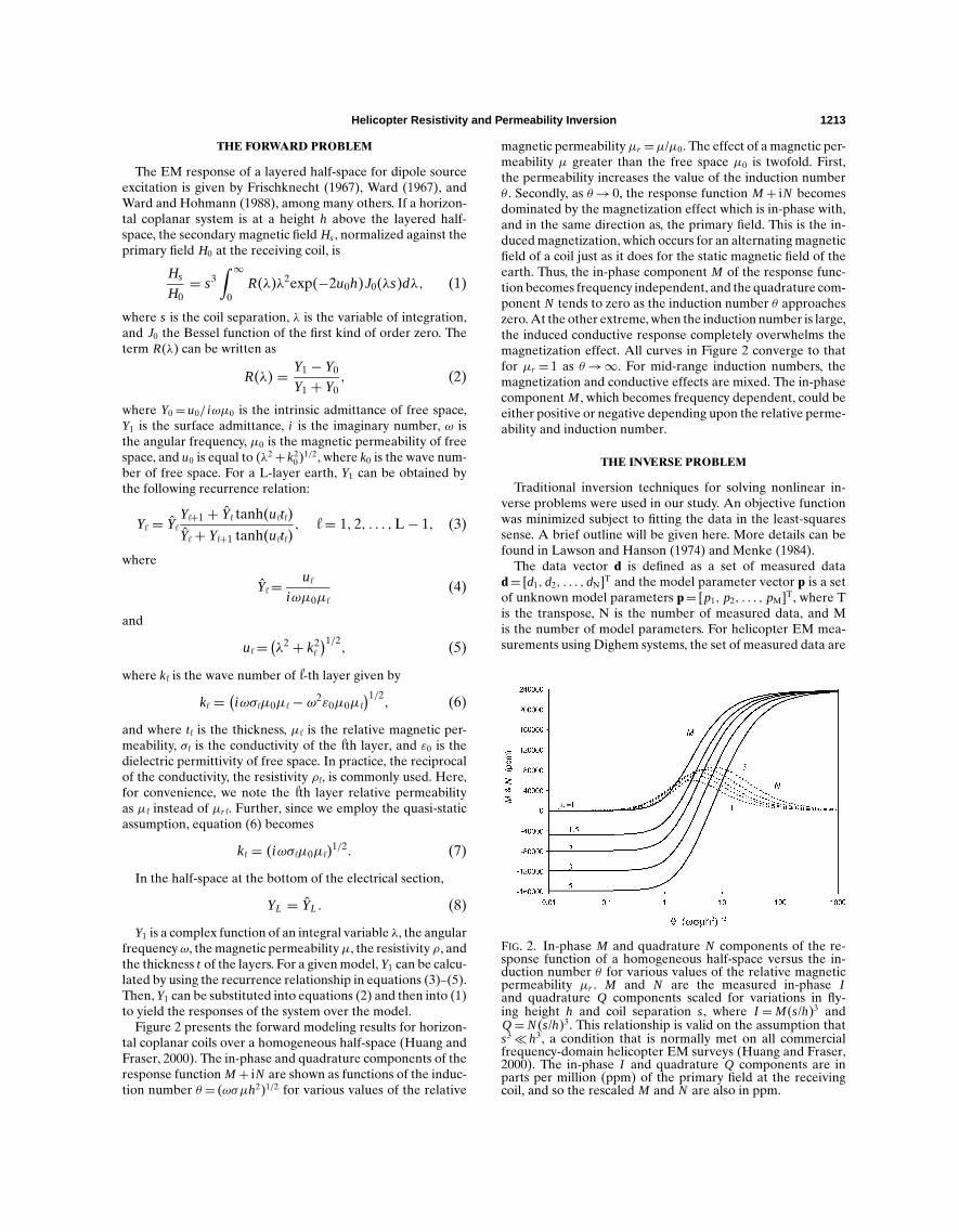
Figure 2 presents the forward modeling results for horizon-tal coplanar coils over a homogeneous half-space (Huang andFraser, 2000). The in-phase and quadrature components of theresponse function M + iN are shown as functions of the induc-tion number θ = (ωσµh2)1/2 for various values of the relative

magnetic permeabilityµr =µ/µ0. The effect of a magnetic per-meability µ greater than the free space µ0 is twofold. First,the permeability increases the value of the induction numberθ . Secondly, as θ→ 0, the response function M + iN becomesdominated by the magnetization effect which is in-phase with,and in the same direction as, the primary field. This is the in-duced magnetization, which occurs for an alternating magneticfield of a coil just as it does for the static magnetic field of theearth. Thus, the in-phase component M of the response func-tion becomes frequency independent, and the quadrature com-ponent N tends to zero as the induction number θ approacheszero. At the other extreme, when the induction number is large,the induced conductive response completely overwhelms themagnetization effect. All curves in Figure 2 converge to thatfor µr = 1 as θ→∞. For mid-range induction numbers, themagnetization and conductive effects are mixed. The in-phasecomponent M , which becomes frequency dependent, could beeither positive or negative depending upon the relative perme-ability and induction number.

THE INVERSE PROBLEM

Traditional inversion techniques for solving nonlinear in-verse problems were used in our study. An objective functionwas minimized subject to fitting the data in the least-squaressense. A brief outline will be given here. More details can befound in Lawson and Hanson (1974) and Menke (1984).

The data vector d is defined as a set of measured datad= [d1, d2, . . . ,dN]T and the model parameter vector p is a setof unknown model parameters p= [p1, p2, . . . , pM]T, where Tis the transpose, N is the number of measured data, and Mis the number of model parameters. For helicopter EM mea-surements using Dighem systems, the set of measured data are

FIG. 2. In-phase M and quadrature N components of the re-sponse function of a homogeneous half-space versus the in-duction number θ for various values of the relative magneticpermeability µr . M and N are the measured in-phase Iand quadrature Q components scaled for variations in fly-ing height h and coil separation s, where I =M(s/h)3 andQ= N(s/h)3. This relationship is valid on the assumption thats3¿ h3, a condition that is normally met on all commercialfrequency-domain helicopter EM surveys (Huang and Fraser,2000). The in-phase I and quadrature Q components are inparts per million (ppm) of the primary field at the receivingcoil, and so the rescaled M and N are also in ppm.


the in-phase and quadrature components at each frequencyfor the given altimeter. For a layered earth described here, theset of unknown model parameters are the resistivity, magneticpermeability, and thickness of each layer.

The functional relationship between the model parametersand the EM responses defined in equation (1) can be rewrittenas

di = Fi(p), i = 1, 2, . . . ,N. (9)

For the helicopter EM problem, the function Fi(p) is highlynonlinear. To linearize the problem locally, we expand Fi(p) ina Taylor series around an initial model parameter vector p0 forthe first iteration and neglect the higher-order terms. Thus, weobtain1p=A1d, where1d is a vector of differences betweenthe measured data and the response of the initial model, and1p is an unknown vector to be solved, consisting of differencesbetween the updated and initial model parameters p and p0,respectively. A is an N×M matrix referred to as the Jacobianpartial derivative or sensitivity matrix. Its elements are givenby

ai j = ∂Fi

∂pi, i = 1, 2, . . . , N, j = 1, . . . ,M. (10)

Using singular value decomposition (SVD), we have A=U3VT , where U is an N×N data eigenvector matrix, V isan M×M parameter eigenvector, and3 is an N×M diagonalmatrix whose elements λ j are the singular values. Then, themodel parameter vector correction 1p can be approximatelycalculated by

1p = V3−1UT 1d, (11)

where elements in 3−1 are 1/λj. A small singular value tendsto yield a large contribution to 1p. This may place a new so-lution outside the region where the Taylor series expansionis valid, and therefore make the inversion unstable. To stabi-lize the inverse procedure, we use Marquardt’s method, andequation (11) can be modified as

1p = V3(32 + e2I)−1UT1d, (12)

where I is the identity matrix and e2 is the damping parameter.The damping factor is defined as a percentage of the largestsingular value λ1. The percentage is larger in the beginning ofthe iteration procedure and gradually decreases as the modelparameters are improved.

Then, an updated model parameter vector at the kth iterationis given by pk= pk−1+1p. The misfit χ 2, given by

χ2 = 1N

N∑i=1

[di − Fi

si

]2

, (13)

will be minimized in the least-squares sense; si is the uncer-tainty in the i th datum, assuming data errors to be uncorre-lated. In the case of nonlinear problems, several iterations arerequired before an acceptable solution is obtained in termsof minimizing the misfit between the measured data and themodel responses.

CALCULATION OF THE JACOBIAN MATRIX

Inversion methods based on the linearization of nonlin-ear functions depend critically on the ability to estimate the

Jacobian matrix. The most generally applicable way of comput-ing the partial derivatives is to use a finite-difference technique.However, it is only accurate to the second order for the centraldifference and to the first order for the forward difference. Thedisadvantage of finite-difference schemes is not only that theyproduce errors, but also that they are computationally inten-sive. Errors in the computation of the partial derivatives leadto instabilities during the inversion. To avoid these problems,an analytic method will be used here to compute the partialderivatives.

The partial derivatives in equation (10) can be computedanalytically from equations (2) and (3), where the derivativeswith respect to the model parameters involves only the termR(λ) in equation (1). Thus, we can write

∂R

∂pl

= ∂R

∂Y1

∂Y1

∂pl

= 2Y0

(Y1 + Y0)2

∂Y1

∂pl

, (14)

where pl represents a model parameter in lth layer, which canbe resistivity, permeability or thickness.

From equation (3), we can write

∂Y1

∂pl

= ∂Y1

∂Y2

∂Y2

∂Y3· · · ∂Yl−1

∂Yl

∂Yl

∂pl

. (15)

Differentiating equation (3), we have

∂Yl

∂Yl+1= (Yl)2

[1− tanh2(ultl)

][Yl + Yl+1 tanh(ul tl)]2

, (16)

The derivatives of Yl with respect to each model parameterpl in the lth layer can be easily obtained from equation (3).Finally, the partial derivatives of the response with respect tothe earth parameters can be obtained by replacing R(λ) byequation (14) in equation (1).

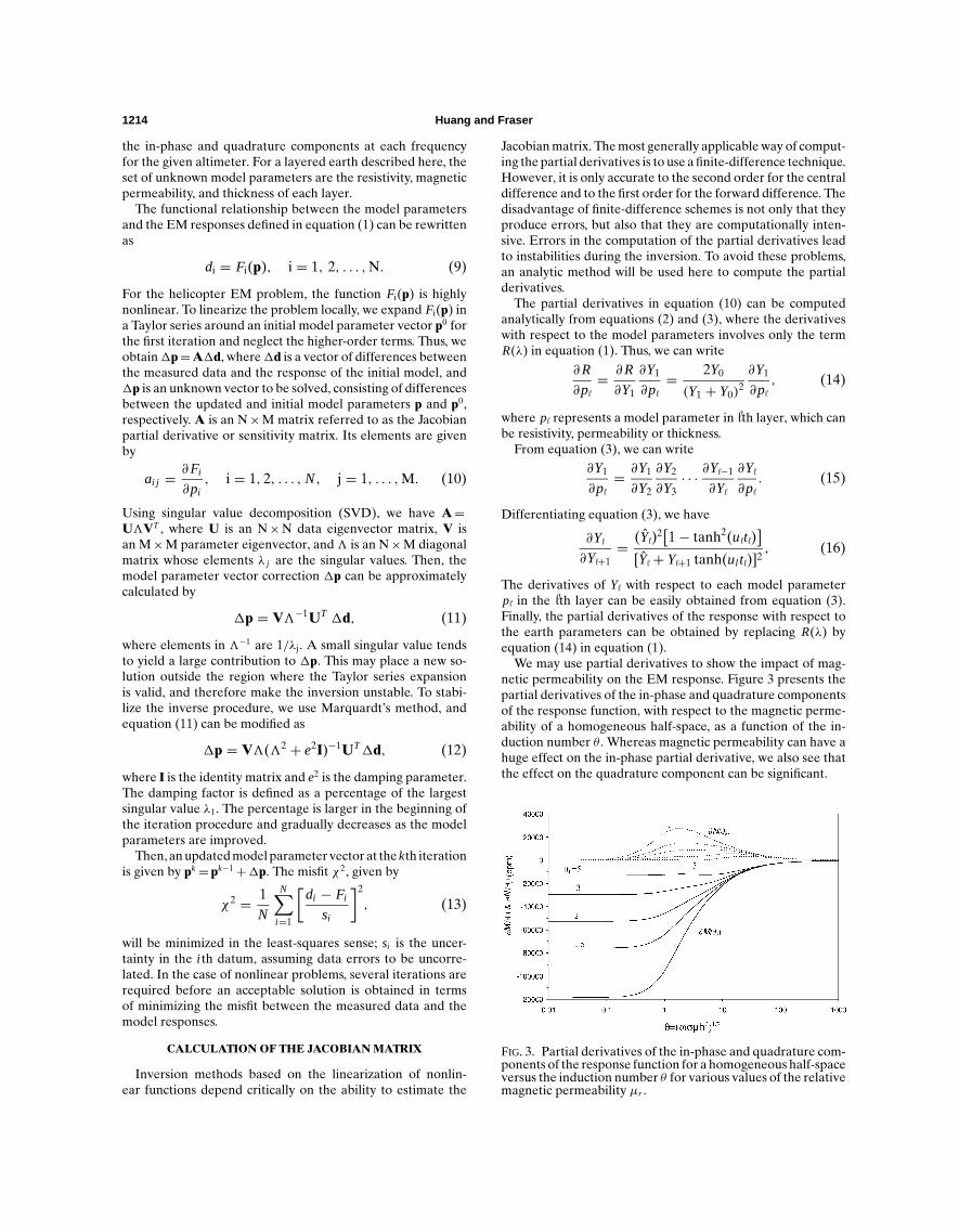
We may use partial derivatives to show the impact of mag-netic permeability on the EM response. Figure 3 presents thepartial derivatives of the in-phase and quadrature componentsof the response function, with respect to the magnetic perme-ability of a homogeneous half-space, as a function of the in-duction number θ . Whereas magnetic permeability can have ahuge effect on the in-phase partial derivative, we also see thatthe effect on the quadrature component can be significant.

FIG. 3. Partial derivatives of the in-phase and quadrature com-ponents of the response function for a homogeneous half-spaceversus the induction number θ for various values of the relativemagnetic permeability µr .


Large absolute values of the partial derivatives of Figure 3 in-dicate good resolvability in parameter determination, whereasvalues close to zero indicate poor reliability. When theinduction number θ¿ 1, the partial derivatives of the in-phaseare frequency independent, whereas those of the quadratureare almost zero. A small variation in magnetic permeabilitycauses a large change in the partial derivative of the in-phasecomponent, indicating that the magnetic permeability can bewell determined from the in-phase data at low induction num-ber. The absolute value of the in-phase derivative decreases asthe magnetic permeability increases. This means that the re-solvability may be better for materials of low magnetic perme-ability than for highly magnetic materials. For the mid-rangevalues of the induction number θ , the derivatives of the in-phase component become frequency dependent, and their ab-solute values decrease. Those of the quadrature componentincrease as θ increases, until they reach local maxima, and thenthey decrease. The resolvability of the magnetic permeabilitydecreases at the higher induction numbers, but the use of boththe in-phase and quadrature data aids in the resolution of themagnetic permeability. As θ→∞, the derivatives for differentmagnetic permeabilities tend to be identical and approach zero,whereupon permeability determinations become impossible.

INVERSION OF SYNTHETIC DATA

Detection of magnetic basement

The inversion technique is demonstrated on synthetic, noise-free data using three typical Dighem frequencies of 56000,

FIG. 4. The results of an inversion for a two-layer model, where ρ1= 50 ohm-m, ρ2= 500 ohm-m,µ1= 1,µ2= 1.05and t1 = 15 m. The model parameters for (a) ρ1 and ρ2, (b) t1, (c) µ2, and (d) the associated misfit are shownas a function of the number of iterations. The input data comprised the in-phase and quadrature componentscomputed at frequencies of 56000, 7200, and 900 Hz for a sensor height of 30 m.

7200, and 900 Hz, each with a transmitting-receiving coil sep-aration of 8 m. Our first example employs a two-layer model(insert to Figure 4a) to simulate the common situation of mod-erately conductive, nonmagnetic overburden overlying a mod-erately resistive and magnetically permeable basement. Theupper layer has a resistivity ρ1 of 50 ohm-m, a relative mag-netic permeability µ1 of 1 (free space) and a thickness t1 of15 m. The basement has a resistivity ρ2 of 500 ohm-m and a rel-ative magnetic permeability µ2 of 1.05. The goal is to resolvemodel parameters ρ1, ρ2, µ2, and t1 given our knowledge thatthe overburden is nonmagnetic and so µ1 is fixed at the freespace value.

The inversion results for the model are shown in Figure 4.Figures 4a, 4b, and 4c respectively illustrate how the modelparameters of resistivity, thickness, and permeability changeafter each iteration. The starting model (iteration = 0) is deter-mined directly from the resistivity-depth transform of Huangand Fraser (1996) and the apparent permeability transformof Huang and Fraser (2000). The upper-layer resistivity ρ1 andbasement permeabilityµ2 reach their correct values after threeand four iterations, respectively. The basement resistivity ρ2

converges more slowly, yielding the correct value at the 6thiteration. Figure 4d presents the decrease in the misfit χ 2 asdefined in equation (13), which is normalized by the misfit atthe 0th iteration. The misfit is reduced by more than five ordersof magnitude in six iterations.

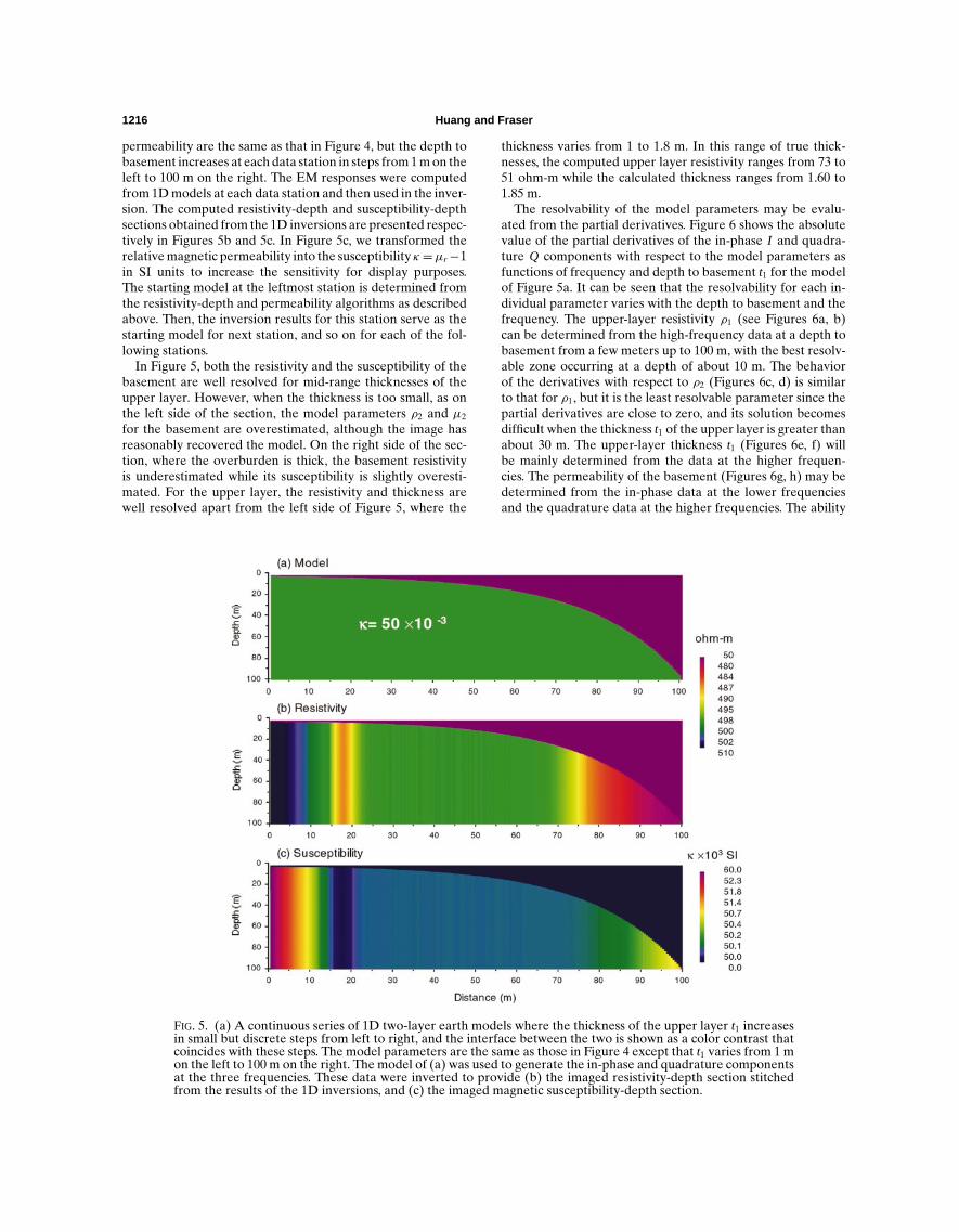
We now examine the same model but with a varying depthto basement. Figure 5a presents a two-layer model where thethickness t1 of the upper layer is variable. Its resistivity and


permeability are the same as that in Figure 4, but the depth tobasement increases at each data station in steps from 1 m on theleft to 100 m on the right. The EM responses were computedfrom 1D models at each data station and then used in the inver-sion. The computed resistivity-depth and susceptibility-depthsections obtained from the 1D inversions are presented respec-tively in Figures 5b and 5c. In Figure 5c, we transformed therelative magnetic permeability into the susceptibility κ =µr−1in SI units to increase the sensitivity for display purposes.The starting model at the leftmost station is determined fromthe resistivity-depth and permeability algorithms as describedabove. Then, the inversion results for this station serve as thestarting model for next station, and so on for each of the fol-lowing stations.

In Figure 5, both the resistivity and the susceptibility of thebasement are well resolved for mid-range thicknesses of theupper layer. However, when the thickness is too small, as onthe left side of the section, the model parameters ρ2 and µ2

for the basement are overestimated, although the image hasreasonably recovered the model. On the right side of the sec-tion, where the overburden is thick, the basement resistivityis underestimated while its susceptibility is slightly overesti-mated. For the upper layer, the resistivity and thickness arewell resolved apart from the left side of Figure 5, where the

FIG. 5. (a) A continuous series of 1D two-layer earth models where the thickness of the upper layer t1 increasesin small but discrete steps from left to right, and the interface between the two is shown as a color contrast thatcoincides with these steps. The model parameters are the same as those in Figure 4 except that t1 varies from 1 mon the left to 100 m on the right. The model of (a) was used to generate the in-phase and quadrature componentsat the three frequencies. These data were inverted to provide (b) the imaged resistivity-depth section stitchedfrom the results of the 1D inversions, and (c) the imaged magnetic susceptibility-depth section.

thickness varies from 1 to 1.8 m. In this range of true thick-nesses, the computed upper layer resistivity ranges from 73 to51 ohm-m while the calculated thickness ranges from 1.60 to1.85 m.

The resolvability of the model parameters may be evalu-ated from the partial derivatives. Figure 6 shows the absolutevalue of the partial derivatives of the in-phase I and quadra-ture Q components with respect to the model parameters asfunctions of frequency and depth to basement t1 for the modelof Figure 5a. It can be seen that the resolvability for each in-dividual parameter varies with the depth to basement and thefrequency. The upper-layer resistivity ρ1 (see Figures 6a, b)can be determined from the high-frequency data at a depth tobasement from a few meters up to 100 m, with the best resolv-able zone occurring at a depth of about 10 m. The behaviorof the derivatives with respect to ρ2 (Figures 6c, d) is similarto that for ρ1, but it is the least resolvable parameter since thepartial derivatives are close to zero, and its solution becomesdifficult when the thickness t1 of the upper layer is greater thanabout 30 m. The upper-layer thickness t1 (Figures 6e, f) willbe mainly determined from the data at the higher frequen-cies. The permeability of the basement (Figures 6g, h) may bedetermined from the in-phase data at the lower frequenciesand the quadrature data at the higher frequencies. The ability


to resolve the permeability of the basement is reduced as theoverburden becomes deeper, as expected.

The narrow low-amplitude features in Figure 6 show that thederivatives cross zero. Zero derivatives indicate that the EMdata are insensitive to changes in the model parameter. Forexample, the quadrature data in Figure 2 have amplitude peaksat the middle values of the induction number θ . The derivativeof the quadrature data with respect to conductivity σ will bezero at these peaks. Therefore, the quadrature data at the peakamplitudes would be not useful in resolving the conductivity.

Detection of magnetic middle layer

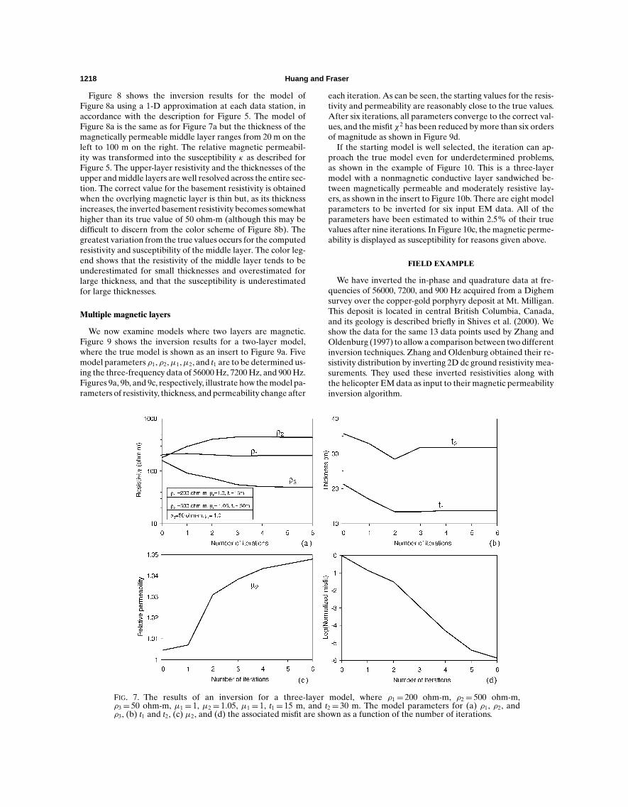
We will use a three-layer model (insert to Figure 7a) tosimulate the situation of a magnetic layer sandwiched between

FIG. 6. Absolute magnitude of the partial derivatives of the in-phase I and quadrature Q components withrespect to model parameters of (a, b) ρ1, (c, d) ρ2, (e, f) t1, and (g, h) µ2 for the 2D model in Figure 5. Valuesclose to zero indicate poor reliability in parameter determination.

nonmagnetic layers. The nonmagnetic upper layer of Figure 7ahas a resistivity ρ1 of 200 ohm-m and a thickness t1 of 15 m. Thevariable-thickness middle layer has a resistivity ρ2 of 500 ohm-m and a permeability µ2 of 1.05. The nonmagnetic basementhas a resistivity ρ3 of 50 ohm-m. The model parameters tobe resolved are ρ1, ρ2, ρ3, µ2, t1, and t2 using three-frequencydata under the assumption that the upper and lower layers arenon-magnetic. First, we examine how the iterations convergefor a single model with t2= 30 m, as shown in Figure 7a. Thevalues for resistivity and thickness almost reach the true valuesafter five and four iterations, respectively. The permeabilityneeds six iterations to approach the correct value because thestarting value is far from the true value. The normalized misfitχ2 is reduced by more than five orders of magnitude in sixiterations as seen in Figure 7d.


Figure 8 shows the inversion results for the model ofFigure 8a using a 1-D approximation at each data station, inaccordance with the description for Figure 5. The model ofFigure 8a is the same as for Figure 7a but the thickness of themagnetically permeable middle layer ranges from 20 m on theleft to 100 m on the right. The relative magnetic permeabil-ity was transformed into the susceptibility κ as described forFigure 5. The upper-layer resistivity and the thicknesses of theupper and middle layers are well resolved across the entire sec-tion. The correct value for the basement resistivity is obtainedwhen the overlying magnetic layer is thin but, as its thicknessincreases, the inverted basement resistivity becomes somewhathigher than its true value of 50 ohm-m (although this may bedifficult to discern from the color scheme of Figure 8b). Thegreatest variation from the true values occurs for the computedresistivity and susceptibility of the middle layer. The color leg-end shows that the resistivity of the middle layer tends to beunderestimated for small thicknesses and overestimated forlarge thickness, and that the susceptibility is underestimatedfor large thicknesses.

Multiple magnetic layers

We now examine models where two layers are magnetic.Figure 9 shows the inversion results for a two-layer model,where the true model is shown as an insert to Figure 9a. Fivemodel parameters ρ1, ρ2,µ1,µ2, and t1 are to be determined us-ing the three-frequency data of 56000 Hz, 7200 Hz, and 900 Hz.Figures 9a, 9b, and 9c, respectively, illustrate how the model pa-rameters of resistivity, thickness, and permeability change after

FIG. 7. The results of an inversion for a three-layer model, where ρ1= 200 ohm-m, ρ2= 500 ohm-m,ρ3= 50 ohm-m, µ1= 1, µ2= 1.05, µ1= 1, t1= 15 m, and t2= 30 m. The model parameters for (a) ρ1, ρ2, andρ3, (b) t1 and t2, (c) µ2, and (d) the associated misfit are shown as a function of the number of iterations.

each iteration. As can be seen, the starting values for the resis-tivity and permeability are reasonably close to the true values.After six iterations, all parameters converge to the correct val-ues, and the misfit χ 2 has been reduced by more than six ordersof magnitude as shown in Figure 9d.

If the starting model is well selected, the iteration can ap-proach the true model even for underdetermined problems,as shown in the example of Figure 10. This is a three-layermodel with a nonmagnetic conductive layer sandwiched be-tween magnetically permeable and moderately resistive lay-ers, as shown in the insert to Figure 10b. There are eight modelparameters to be inverted for six input EM data. All of theparameters have been estimated to within 2.5% of their truevalues after nine iterations. In Figure 10c, the magnetic perme-ability is displayed as susceptibility for reasons given above.

FIELD EXAMPLE

We have inverted the in-phase and quadrature data at fre-quencies of 56000, 7200, and 900 Hz acquired from a Dighemsurvey over the copper-gold porphyry deposit at Mt. Milligan.This deposit is located in central British Columbia, Canada,and its geology is described briefly in Shives et al. (2000). Weshow the data for the same 13 data points used by Zhang andOldenburg (1997) to allow a comparison between two differentinversion techniques. Zhang and Oldenburg obtained their re-sistivity distribution by inverting 2D dc ground resistivity mea-surements. They used these inverted resistivities along withthe helicopter EM data as input to their magnetic permeabilityinversion algorithm.


Figures 11a and 11b respectively show the Dighem sen-sor height and the three-frequency EM data for the 13 datapoints, and Figure 11c shows the apparent susceptibility ob-tained from the transform technique developed by Huangand Fraser (2000). As discussed above, a magnetic perme-ability that is greater than free space may cause the in-phase data at the lower frequencies to become negative.Figure 11b shows that the in-phase data at 900 Hz are neg-ative across the center part of the profile, with the maxi-mum negative value occurring at station 12.9 km. This stationcorresponds to the computed apparent susceptibility high inFigure 11c.

The inversion was performed using a three-layer model.Eight parameters ρ1, ρ2, ρ3, µ1, µ2, µ3, t1, and t2 were invertedusing the six in-phase and quadrature data of Figure 11b and thesensor height of Figure 11a. Figures 12a and 12b respectivelyshow the inverted and imaged resistivity and susceptibility. Theinversion results from Zhang and Oldenburg (1997) are shownin Figure 13 for comparison.

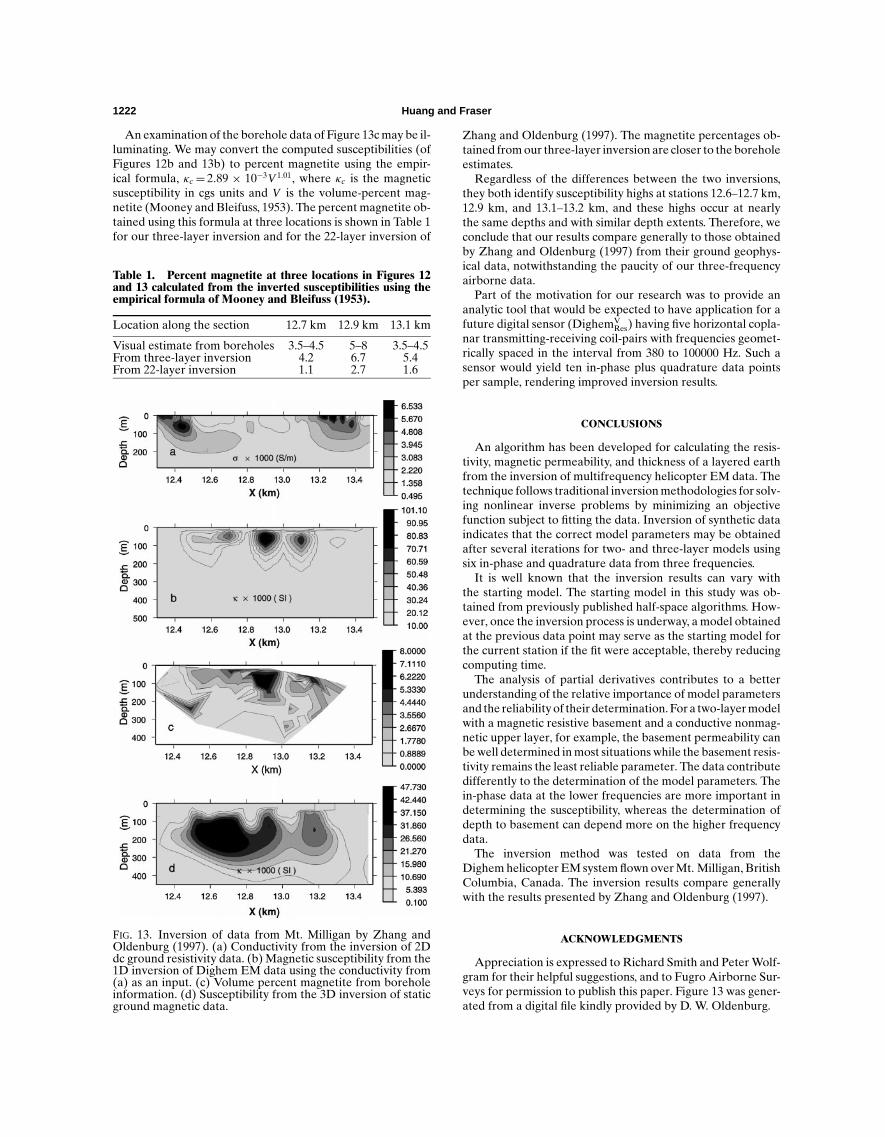
The conductivity model in Figure 13a was obtained by Zhangand Oldenburg (1997) from their inversion of 2D dc groundresistivity data using 22 layers. This conductivity model wasused as an input, along with the helicopter EM data, to invertfor the susceptibility. Their susceptibility inversion was per-formed using the same 22 layers as used in their inversion ofthe dc ground resistivity data. The magnetite concentration,

FIG. 8. (a) Two-dimensional model simulated by a number of 1D models, (b) the imaged resistivity-depth sectionstitched from the results of the 1D inversions, and (c) the magnetic susceptibility-depth section. The modelparameters are the same as those in Figure 7 except for t2, which ranges from 20 m on the left to 100 m on theright.

visually estimated from borehole samples over the same sec-tion, is shown in Figure 13c, and the susceptibility obtainedfrom the 3D inversion of static ground magnetic data is shownin Figure 13d. The authors have explained the discrepanciesbetween Figures 13b, c, and d. Our discussion will be focusedon a comparison of our inversion results of Figure 12 with theirinversion results of Figures 13a and 13b.

A comparison of the resistivity section in Figure 12a to theconductivity (= 1/resistivity) section in Figure 13a shows thatsimilar conductive features appear at both ends of the pro-file on both sections. However, the conductivity section ofFigure 13a has a different appearance because the inversionis based on a 22-layer model with a smoothly varying presen-tation across the layers versus the discrete three-layer presen-tation of Figure 12a, and also because different data sets wereused.

There are three susceptibility highs in Figure 13b. The largesthas an amplitude of 0.1 SI and occurs at station 12.9 km at adepth of about 20 m. This body has a thickness of 100 m or more.The susceptibility section from the three-layer inversion ofFigure 12b has a magnetic middle layer with the strongest sus-ceptibility occurring at this same station, but the amplitude of0.247 SI is much larger than in Figure 13b. The thickness of themagnetic layer at this station is about 70 m in Figure 12b, whichis thinner than that from the 22-layer inversion of Figure 13band from the ground magnetic inversion of Figure 13d.


FIG. 9. The results of an inversion for a two-layer model, where ρ1= 500 ohm-m, ρ2= 50 ohm-m, µ1= 1.2,µ2= 1.05 and t1= 50 m. The model parameters for (a) ρ1 and ρ2, (b) t1, (c) µ1 and µ2, and (d) the associatedmisfit are shown as a function of the number of iterations.

FIG. 10. The results of an inversion for a three-layer model, where ρ1= 500 ohm-m, ρ2= 20 ohm-m, ρ3= 100ohm-m, µ1= 1.02, µ2= 1.0, µ3= 1.5, t1= 30 m, and t2= 15 m. The model parameters for (a) ρ1, ρ2, and ρ3, (b) t1and t2, (c) µ1, µ2, and µ3, and (d) the associated misfit are shown as a function of the number of iterations. Themagnetic permeability parameter is plotted as susceptibility to show the smaller values more clearly.


The second strongest susceptibility high occurs at station13.1 km in Figure 13b and at 13.2 km in Figure 13d. It is lo-cated at 13.1–13.2 km according to our inversion of Figure 12b.The 0.2-SI susceptibility from our inversion of Figure 12b islarger than the 0.06 SI of Figure 13b.

The third susceptibility feature in Figure 13b occurs at sta-tions 12.5–12.7 km, and this location correlates with our inver-sion in Figure 12b. Again, the 0.05–0.18-SI susceptibility fromour inversion in Figure 12b is larger than the 0.005–0.015 SI ofFigure 13b.

There is a disagreement between the two inversions with re-spect to the amplitude of the magnetic susceptibility. Values

FIG. 11. Dighem data from Mt. Milligan. (a) The EM sensor height, (b) the three-frequency EM data, and(c) the computed apparent susceptibility.

FIG. 12. (a) Resistivity and (b) susceptibility sections from inversion of the Dighem data of Figures 11a and 11busing a three-layer model.

obtained from our inversion are 2–10 times higher than thoseobtained from the 22-layer inversion of Zhang and Oldenburg(1997). The discrepancy may be caused in part by the differentresistivity sections. Resistivities rang from 120 to 2000 ohm-m in Figure 13a (derived from their ground dc data) versus80 to 1500 ohm-m in our section of Figure 12a (from thehelicopter EM data). In our case, inverting for the resistiv-ity and the susceptibility simultaneously using the same dataset may improve the quality of the inversion. On the otherhand, our use of a single data set may increase the likeli-hood of nonuniqueness in the inversion, resulting in a poorersolution.


An examination of the borehole data of Figure 13c may be il-luminating. We may convert the computed susceptibilities (ofFigures 12b and 13b) to percent magnetite using the empir-ical formula, κc= 2.89 × 10−3V1.01, where κc is the magneticsusceptibility in cgs units and V is the volume-percent mag-netite (Mooney and Bleifuss, 1953). The percent magnetite ob-tained using this formula at three locations is shown in Table 1for our three-layer inversion and for the 22-layer inversion of

Table 1. Percent magnetite at three locations in Figures 12and 13 calculated from the inverted susceptibilities using theempirical formula of Mooney and Bleifuss (1953).

Location along the section 12.7 km 12.9 km 13.1 km

Visual estimate from boreholes 3.5–4.5 5–8 3.5–4.5From three-layer inversion 4.2 6.7 5.4From 22-layer inversion 1.1 2.7 1.6

FIG. 13. Inversion of data from Mt. Milligan by Zhang andOldenburg (1997). (a) Conductivity from the inversion of 2Ddc ground resistivity data. (b) Magnetic susceptibility from the1D inversion of Dighem EM data using the conductivity from(a) as an input. (c) Volume percent magnetite from boreholeinformation. (d) Susceptibility from the 3D inversion of staticground magnetic data.

Zhang and Oldenburg (1997). The magnetite percentages ob-tained from our three-layer inversion are closer to the boreholeestimates.

Regardless of the differences between the two inversions,they both identify susceptibility highs at stations 12.6–12.7 km,12.9 km, and 13.1–13.2 km, and these highs occur at nearlythe same depths and with similar depth extents. Therefore, weconclude that our results compare generally to those obtainedby Zhang and Oldenburg (1997) from their ground geophys-ical data, notwithstanding the paucity of our three-frequencyairborne data.

Part of the motivation for our research was to provide ananalytic tool that would be expected to have application for afuture digital sensor (DighemV

Res) having five horizontal copla-nar transmitting-receiving coil-pairs with frequencies geomet-rically spaced in the interval from 380 to 100000 Hz. Such asensor would yield ten in-phase plus quadrature data pointsper sample, rendering improved inversion results.

CONCLUSIONS

An algorithm has been developed for calculating the resis-tivity, magnetic permeability, and thickness of a layered earthfrom the inversion of multifrequency helicopter EM data. Thetechnique follows traditional inversion methodologies for solv-ing nonlinear inverse problems by minimizing an objectivefunction subject to fitting the data. Inversion of synthetic dataindicates that the correct model parameters may be obtainedafter several iterations for two- and three-layer models usingsix in-phase and quadrature data from three frequencies.

It is well known that the inversion results can vary withthe starting model. The starting model in this study was ob-tained from previously published half-space algorithms. How-ever, once the inversion process is underway, a model obtainedat the previous data point may serve as the starting model forthe current station if the fit were acceptable, thereby reducingcomputing time.

The analysis of partial derivatives contributes to a betterunderstanding of the relative importance of model parametersand the reliability of their determination. For a two-layer modelwith a magnetic resistive basement and a conductive nonmag-netic upper layer, for example, the basement permeability canbe well determined in most situations while the basement resis-tivity remains the least reliable parameter. The data contributedifferently to the determination of the model parameters. Thein-phase data at the lower frequencies are more important indetermining the susceptibility, whereas the determination ofdepth to basement can depend more on the higher frequencydata.

The inversion method was tested on data from theDighem helicopter EM system flown over Mt. Milligan, BritishColumbia, Canada. The inversion results compare generallywith the results presented by Zhang and Oldenburg (1997).

ACKNOWLEDGMENTS

Appreciation is expressed to Richard Smith and Peter Wolf-gram for their helpful suggestions, and to Fugro Airborne Sur-veys for permission to publish this paper. Figure 13 was gener-ated from a digital file kindly provided by D. W. Oldenburg.


REFERENCES

Beard, L. P., and Nyquist, J. E., 1998, Simultaneous inversion of air-borne electromagnetic data for resistivity and magnetic permeabil-ity: Geophysics, 63, 1556–1564.

Fitterman, D. V., and Deszcz-pan, M., 1998, Helicopter EM mappingof saltwater intrusion in Everglades National Park, Florida: Explor.Geophys., 29, 240–243.

Fraser, D. C., 1973, Magnetite ore tonnage estimates from an aerialelectromagnetic survey: Geoexploration, 11, 97–105.

———1978, Resistivity mapping with an airborne multicoil electro-magnetic system: Geophysics, 43, 144–172.

———1981, Magnetite mapping with a multicoil airborne electromag-netic system: Geophysics, 46, 1579–1593.

Fraser, D. C., Stodt, J. A., and Ward, S. H., 1990, The effect of dis-placement currents on the response of a high-frequency helicopterelectromagnetic system, in Ward, S. H., Ed., Geotechnical and en-vironmental geophysics: II, Environmental and groundwater: Soc.Expl. Geophys., 89–96.

Frischknecht, F. C., 1967, Fields about an oscillating magnetic dipoleover a two-layer earth and application to ground and airborne elec-tromagnetic surveys: Quarterly of the Colorado School of Mines, 62,No. 1.

Holladay, S. J., Valleau, N., and Morrison, E., 1986, Application ofmultifrequency helicopter electromagnetic survey to mapping ofsea-ice thickness and shallow-water bathymetry, in Palacky, G. J.,Ed., Airborne resistivity mapping: Geol. Surv. Canada Paper 86-22,91–98.

Huang, H., and Fraser, D. C., 1996, The differential parameter methodfor multifrequency airborne resistivity mapping: Geophysics, 61,100–109.

———2000, Airborne resistivity and susceptibility mapping in mag-netically polarizable areas: Geophysics, 65, 502–511.

———2001, Mapping of the resistivity, susceptibility, and permittivityof the earth using a helicopter-borne electromagnetic system: Geo-physics, 66, 148–157.

———2002, Dielectric permittivity and resistivity mapping using high-frequency helicopter-borne EM data: Geophysics, 67, 727–738.

Huang, H., and Palacky, G. J., 1991, Damped least-squares inver-sion of time-domain airborne EM data based on singular value

decomposition: Geophys. Prosp., 39, 827–844.Huang, H., and Zhu, R., 1984, Interpretation method of the time-

domain airborne electromagnetic response above a magnetic con-ductive sphere model, J. Changchun College of Geology, 1, 107–116.

Lawson, C. L., and Hanson, R. J., 1974, Solving least-squares problems:Prentice Hall, Inc.

Lodha, G. S., and West, G. F., 1976, Practical airborne EM (AEM)interpretation using a sphere model: Geophysics, 41, 1157–1169.

Menke, W., 1984, Geophysical data analysis—Discrete inverse theory:Academic Press, Inc.

Mooney, H. M., and Bleifuss, R., 1953, Magnetic susceptibility mea-surements in Minnesota, Part II, Analysis of field results: Geo-physics, 18, 383–393.

Paterson, N. R., and Reford, S. W., 1986, Inversion of airborne elec-tromagnetic data for overburden mapping and groundwater explo-ration, in Palacky, G. J., Ed., Airborne resistivity mapping: Geol.Surv. Canada Paper 86-22, 39–48.

Qian, W., Gamey, J. T., Holladay, S. J., Lewis, R., and Abernathy, D.,1997, Inversion of airborne electromagnetic data using an Occamtechnique to resolve a variable number of layers, in Proceedings ofhigh-resolution geophysics workshop, SAGEEP, 97,735–744.

Sengpiel, K. P., and Siemon, B., 2000, Advanced inversion methods forairborne electromagnetic exploration, Geophysics, 65, 1983–1992.

Shives, R. B. K., Charbonneau, B. W., and Ford, K. L., 2000, Thedetection of potassic alteration by gamma-ray spectrometry—Recognition of alteration related to mineralization: Geophysics, 65,2001–2011.

Ward, S. H., 1967, Electromagnetic theory for geophysical applications,in Ward, S. H., Ed., Mining geophysics, 2, Theory: Soc. Expl. Geo-phys., 13–196.

Ward, S. H., and Hohmann, G. W., 1988, Electromagnetic theory forgeophysical applications, in Nabighian, M. N., Ed., Electromagneticmethods in applied geophysics, 1, Theory: Soc. Expl. Geophys., 130–311.

Zhang, Z., and Oldenburg, D. W., 1997, Recovering magnetic suscepti-bility from electromagnetic data over a one-dimensional earth: Geo-phys. J. Internat., 130, 422–434.

———1999, Simultaneous reconstruction of 1-D susceptibility andconductivity from electromagnetic data: Geophysics, 64, 33–47.

Inversion of helicopter electromagnetic data to a magnetic conductive layered earth

Documents

Transcript of Inversion of helicopter electromagnetic data to a magnetic conductive layered earth