HAL Id: hal-03188300https://hal.archives-ouvertes.fr/hal-03188300

Submitted on 6 Apr 2021

HAL is a multi-disciplinary open accessarchive for the deposit and dissemination of sci-entific research documents, whether they are pub-lished or not. The documents may come fromteaching and research institutions in France orabroad, or from public or private research centers.

L’archive ouverte pluridisciplinaire HAL, estdestinée au dépôt et à la diffusion de documentsscientifiques de niveau recherche, publiés ou non,émanant des établissements d’enseignement et derecherche français ou étrangers, des laboratoirespublics ou privés.

Introduction to stress and strain analysisMichael Fagan, Michiel Postema

To cite this version:Michael Fagan, Michiel Postema. Introduction to stress and strain analysis. The University of Hull,63 p., 2007, 978-90-812588-1-4. �hal-03188300�

Introduction to stress and strain analysis

Dr. Michael J. FaganDr. Michiel Postema

Department of EngineeringThe University of Hull

2

ISBN 978-90-812588-1-4

c©2007 M.J. Fagan, M. Postema.All rights reserved. No part of this publication may be reproduced, stored in aretrieval system or transmitted in any form or by any means, electronic, mechan-ical, photocopying, recording or otherwise, without the prior written permissionof the authors.

Publisher: Michiel Postema, BergschenhoekPrinted in England by The University of Hull

Typesetting system: LATEX2ε

Contents

1 The uniform state of stress 5

2 Stress on an inclined plane 7

3 Transformation of stresses for rotation of axes 11

4 Principal stresses 13

5 Stationary values of shear stress 17

6 Octahedral stresses 21

7 Hydrostatic (dilational) and deviatoric stress tensors 23

8 Strains and displacements 25

9 Generalized Hooke’s law 29

10 Equilibrium equations for three dimensions 33

11 Strain compatibility equations 35

12 Plane strain 37

13 Plane stress 39

14 Polar coordinates 41

15 Stress functions 45

16 Stress functions in polar coordinates 47

3

4

17 Torsion of non-circular prisms 51

18 Prandtl’s membrane analogy 57

19 Torsion of thin-walled members — open sections 59

20 Torsion of thin-walled members — closed sections 61

21 Bibliography 63

1The uniform state of stress

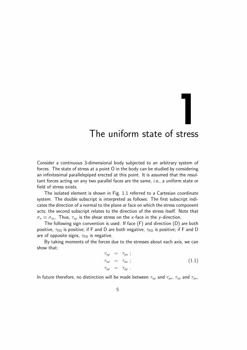
Consider a continuous 3-dimensional body subjected to an arbitrary system offorces. The state of stress at a point O in the body can be studied by consideringan infinitesimal parallelepiped erected at this point. It is assumed that the resul-tant forces acting on any two parallel faces are the same, i.e., a uniform state orfield of stress exists.

The isolated element is shown in Fig. 1.1 referred to a Cartesian coordinatesystem. The double subscript is interpreted as follows: The first subscript indi-cates the direction of a normal to the plane or face on which the stress componentacts; the second subscript relates to the direction of the stress itself. Note thatσx ≡ σxx . Thus, τxy is the shear stress on the x-face in the y -direction.

The following sign convention is used: If face (F) and direction (D) are bothpositive, τFD is positive; if F and D are both negative, τFD is positive; if F and Dare of opposite signs, τFD is negative.

By taking moments of the forces due to the stresses about each axis, we canshow that:

τxy = τyx ;

τxz = τzx ;

τyz = τzy .

(1.1)

In future therefore, no distinction will be made between τxy and τyx , τxz and τzx ,

5

6

x

σx

τxy

τyx

y

τxz

σy

τyz

τzx

τzy

σz

zx

σz

τzy

τyz

τzx

y

σy

τxz

τyx

τxy

σx

z

Figure 1.1: Stresses acting on the positive (left) and negative (right)faces of an infinitesimal body.

or τyz and τzy . This means that only 6 Cartesian components are necessary forthe complete specification of the state of stress at any point in the body. Theseterms can be conveniently assembled into the so-called stress tensor:

[σ] =

σx τxy τxz

τyx σy τyz

τzx τzy σz

. (1.2)

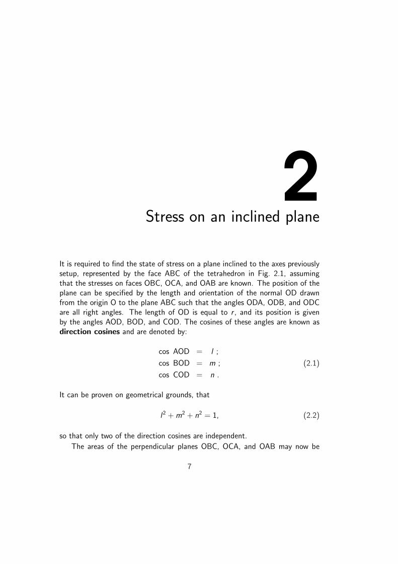
2Stress on an inclined plane

It is required to find the state of stress on a plane inclined to the axes previouslysetup, represented by the face ABC of the tetrahedron in Fig. 2.1, assumingthat the stresses on faces OBC, OCA, and OAB are known. The position of theplane can be specified by the length and orientation of the normal OD drawnfrom the origin O to the plane ABC such that the angles ODA, ODB, and ODCare all right angles. The length of OD is equal to r , and its position is givenby the angles AOD, BOD, and COD. The cosines of these angles are known asdirection cosines and are denoted by:

cos AOD = l ;

cos BOD = m ;

cos COD = n .

(2.1)

It can be proven on geometrical grounds, that

l2 + m2 + n2 = 1, (2.2)

so that only two of the direction cosines are independent.

The areas of the perpendicular planes OBC, OCA, and OAB may now be

7

8

x

A

zC

D

y

O

B

Figure 2.1: Plane inclined to the axes, represented by the face ABC of atetrahedron.

found in terms of these direction cosines:

OA =r

l;

OB =r

m;

OC =r

n.

(2.3)

Let the area of face ABC be A, and that of OCA be Ay . The volume of thetetrahedron can be written as 1

3Ar = 1

3AyOB = 1

3Ay

rm

, from which it followsthat Ay = A m. Hence,

Ax

l=

Ay

m=

Az

n= A. (2.4)

9

These are the relationships between the areas of the four faces of the tetrahedron.With the stress on the inclined plane represented by its three Cartesian com-

ponents sx , sy , and sz , the general state of stress on the tetrahedron is shown inFig. 2.2. The equilibrium of the element can be examined by resolving the forces

x

σz

τzy

sx

τyz

τzx

y

σy

sy

τxz

τyx

τxy

sz

σx

z

Figure 2.2: State of stress on a tetrahedron.

acting on it in the directions of the three axes. For example, in the x-direction,

sxA− σxAx − τyxAy − τzxAz = 0. (2.5)

Hence,

sx = σx l + τyxm + τzxn. (2.6)

Similar expressions exist for sy and sz . These three equations can be expressed

10

in matrix form:

sx

sy

sz

=

σx τxy τxz

τyx σy τyz

τzx τzy σz

l

m

n

. (2.7)

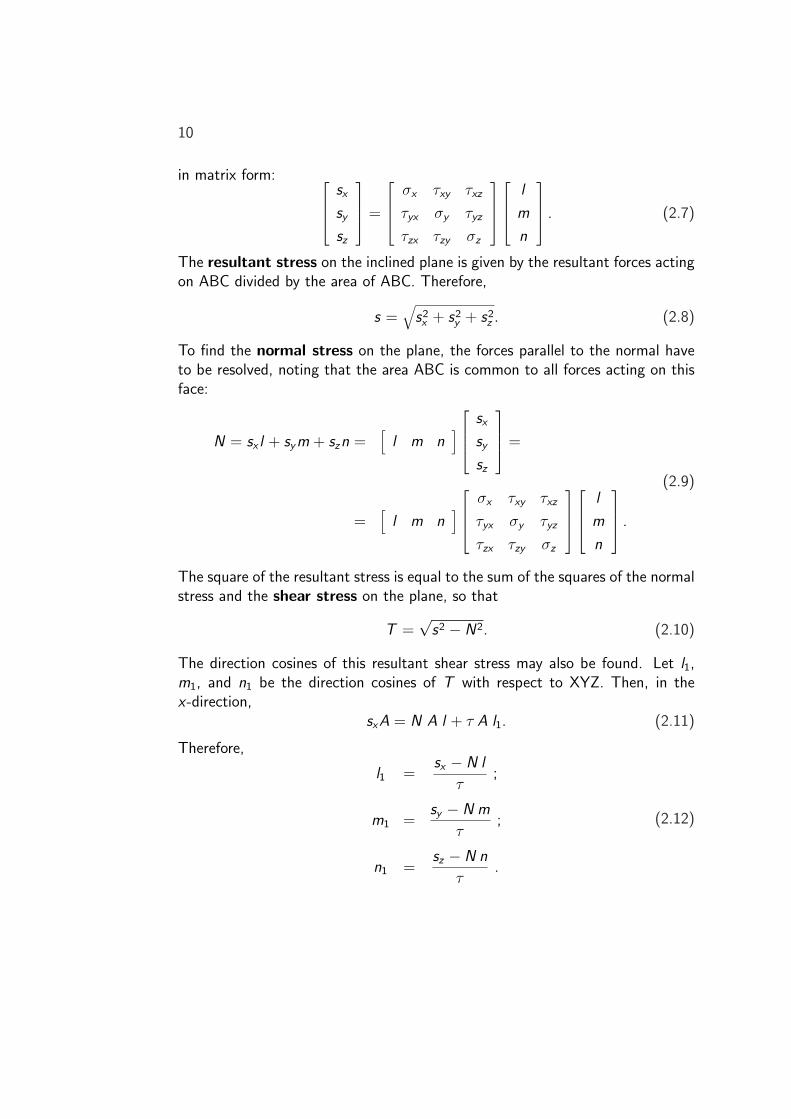
The resultant stress on the inclined plane is given by the resultant forces actingon ABC divided by the area of ABC. Therefore,

s =√

s2x + s2

y + s2z . (2.8)

To find the normal stress on the plane, the forces parallel to the normal haveto be resolved, noting that the area ABC is common to all forces acting on thisface:

N = sx l + sym + szn =[

l m n]

sx

sy

sz

=

=[

l m n]

σx τxy τxz

τyx σy τyz

τzx τzy σz

l

m

n

.

(2.9)

The square of the resultant stress is equal to the sum of the squares of the normalstress and the shear stress on the plane, so that

T =√

s2 − N2. (2.10)

The direction cosines of this resultant shear stress may also be found. Let l1,m1, and n1 be the direction cosines of T with respect to XYZ. Then, in thex-direction,

sxA = N A l + τ A l1. (2.11)

Therefore,

l1 =sx − N l

τ;

m1 =sy − N m

τ;

n1 =sz − N n

τ.

(2.12)

3Transformation of stresses for rotation

of axes

By extending the theory developed in the previous Chapter, it is possible totransform the tensor of a given state of stress known for one set of axes to thetensor of the same state in a second set of axes. For example, if the stress tensorin the (x , y , z) coordinate system is [σ], it is possible to determine the stresstensor [σ′] in another coordinate system (x ′, y ′, z ′).

The relative rotation of the second system to the first is defined by 9 directioncosines, where for example l1 is the angle between the x ′-axis and the x-axis, m1

is the angle between the x ′-axis and the y -axis, and l2 is the angle between they ′-axis and the x-axis.

The full set of cosines is:

[L] =

l1 m1 n1

l2 m2 n2

l3 m3 n3

. (3.1)

Consider a second Cartesian system (x ′, y ′, z ′) and the set used in the previousChapter. Let the x ′-axis be coincident with the normal of the plane that was

11

12

examined: σx ′ = N . The normal stress on the plane follows from (2.9):

σx ′ = N =[

l1 m1 n1

]

σx τxy τxz

τyx σy τyz

τzx τzy σz

l1

m1

n1

. (3.2)

By using the same method for the other axes, the other components of the stresstensor [σ′] can be determined:

[σ′] = [L][σ][L]T. (3.3)

Using this equation, a tensorial state of stress in one coordinate system can beeasily converted into another system.

4Principal stresses

A principal plane is defined as one on which the shear stress is zero. The normalstress on this plane is known as the principal stress and is denoted by p. If thedirection cosines of the plane are l , m, and n, then resolving stresses on the planein the coordinate directions gives:

sx

sy

sz

=

p l

p m

p n

=

p 0 0

0 p 0

0 0 p

l

m

n

. (4.1)

Rearranging this with (2.7) gives:

σx − p τxy τxz

τyx σy − p τyz

τzx τzy σz − p

l

m

n

= 0. (4.2)

This matrix represents three linear equations in l , m, and n, which will havenon-trivial solutions if and only if

det |[σ]− [p]| = 0. (4.3)

13

14

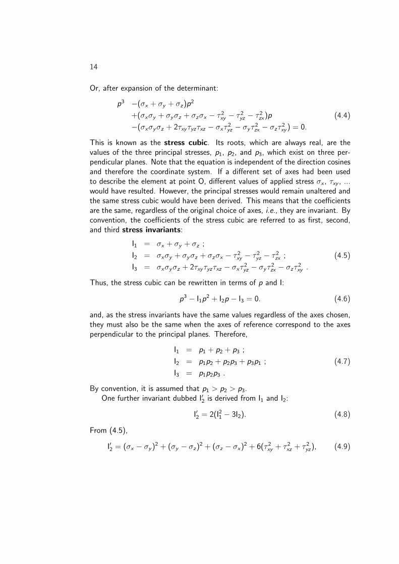
Or, after expansion of the determinant:

p3 −(σx + σy + σz)p2

+(σxσy + σyσz + σzσx − τ 2xy − τ 2

yz − τ 2zx)p

−(σxσyσz + 2τxyτyzτxz − σxτ2yz − σyτ

2zx − σzτ

2xy ) = 0.

(4.4)

This is known as the stress cubic. Its roots, which are always real, are thevalues of the three principal stresses, p1, p2, and p3, which exist on three per-pendicular planes. Note that the equation is independent of the direction cosinesand therefore the coordinate system. If a different set of axes had been usedto describe the element at point O, different values of applied stress σx , τxy , ...would have resulted. However, the principal stresses would remain unaltered andthe same stress cubic would have been derived. This means that the coefficientsare the same, regardless of the original choice of axes, i.e., they are invariant. Byconvention, the coefficients of the stress cubic are referred to as first, second,and third stress invariants:

I1 = σx + σy + σz ;

I2 = σxσy + σyσz + σzσx − τ 2xy − τ 2

yz − τ 2zx ;

I3 = σxσyσz + 2τxyτyzτxz − σxτ2yz − σyτ

2zx − σzτ

2xy .

(4.5)

Thus, the stress cubic can be rewritten in terms of p and I:

p3 − I1p2 + I2p − I3 = 0. (4.6)

and, as the stress invariants have the same values regardless of the axes chosen,they must also be the same when the axes of reference correspond to the axesperpendicular to the principal planes. Therefore,

I1 = p1 + p2 + p3 ;

I2 = p1p2 + p2p3 + p3p1 ;

I3 = p1p2p3 .

(4.7)

By convention, it is assumed that p1 > p2 > p3.One further invariant dubbed I′2 is derived from I1 and I2:

I′2 = 2(I21 − 3I2). (4.8)

From (4.5),

I′2 = (σx − σy )2 + (σy − σz)

2 + (σz − σx)2 + 6(τ 2

xy + τ 2xz + τ 2

yz), (4.9)

15

or in terms of principal stresses

I′2 = (p1 − p2)2 + (p2 − p3)

3 + (p3 − p1)2. (4.10)

The so-called Von Mises yield stress σys is related to I′2 as follows:

σ2ys =

I′22

. (4.11)

I1 and I′2 are of particular interest to us because they are related to the octahedralnormal and octahedral shear stress, respectively.

The directions of the principal stresses can be found by substituting each ofthe three values of p in turn into (4.2) and, using (2.2), solving for each set ofl , m, and n.

16

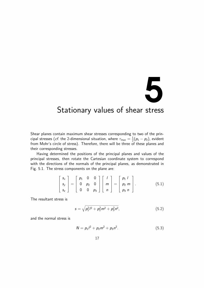
5Stationary values of shear stress

Shear planes contain maximum shear stresses corresponding to two of the prin-cipal stresses (cf. the 2-dimensional situation, where τmax = 1

2(p1 − p2), evident

from Mohr’s circle of stress). Therefore, there will be three of these planes andtheir corresponding stresses.

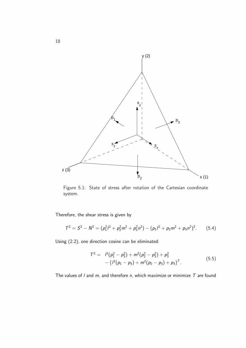
Having determined the positions of the principal planes and values of theprincipal stresses, then rotate the Cartesian coordinate system to correspondwith the directions of the normals of the principal planes, as demonstrated inFig. 5.1. The stress components on the plane are:

sx

sy

sz

=

p1 0 0

0 p2 0

0 0 p3

l

m

n

=

p1 l

p2 m

p3 n

. (5.1)

The resultant stress is

s =√

p21 l

2 + p22m

2 + p23n

2, (5.2)

and the normal stress is

N = p1l2 + p2m

2 + p3n2. (5.3)

17

18

x (1)

p3

sx

y (2)

p2

sy

sz

p1

z (3)

Figure 5.1: State of stress after rotation of the Cartesian coordinatesystem.

Therefore, the shear stress is given by

T 2 = S2 − N2 = (p21 l

2 + p22m

2 + p23n

2)− (p1l2 + p2m

2 + p3n2)2. (5.4)

Using (2.2), one direction cosine can be eliminated:

T 2 = l2(p21 − p2

3) + m2(p22 − p2

3) + p23

−{l2(p1 − p3) + m2(p2 − p3) + p3}2.

(5.5)

The values of l and m, and therefore n, which maximize or minimize T are found

19

by differentiating (5.5) with respect to l and m and equating to zero.

T∂T

∂l= l(p1 − p3)

{(p1 + p3)− 2

[l2(p1 − p3) + m2(p2 − p3) + p3

]}= 0;

T∂T

∂m= m(p2 − p3)

{(p2 + p3)− 2

[l2(p1 − p3) + m2(p2 − p3) + p3

]}= 0.

(5.6)Clearly, these equations vanish if l = m = 0 and n = 1, but this locates theplane on which p3 acts, which by definition is a principal plane on which the shearstress T = 0. The other minima can similarly be found on the other principalplanes. The maxima are found as follows. Assume l = 0. This satisfies the firstequation in (5.6). The second will vanish if

(p2 + p3)− 2[m2(p2 − p3) + p3

]= 0, (5.7)

or, simplified, if(p2 − p3)(1− 2m2) = 0. (5.8)

This holds for

m = ± 1√2. (5.9)

Thus,

n = ± 1√2. (5.10)

Substituting back into (5.4), the shear is found to be

T =1

2(p2 − p3). (5.11)

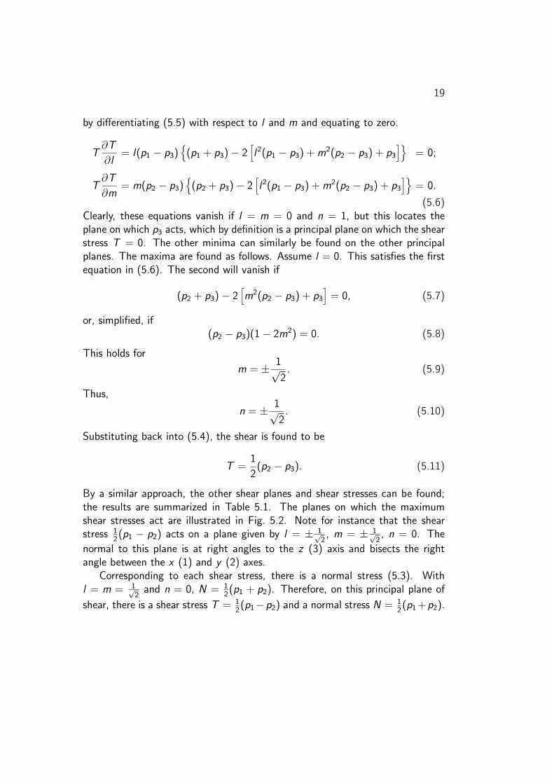
By a similar approach, the other shear planes and shear stresses can be found;the results are summarized in Table 5.1. The planes on which the maximumshear stresses act are illustrated in Fig. 5.2. Note for instance that the shearstress 1

2(p1 − p2) acts on a plane given by l = ± 1√

2, m = ± 1√

2, n = 0. The

normal to this plane is at right angles to the z (3) axis and bisects the rightangle between the x (1) and y (2) axes.

Corresponding to each shear stress, there is a normal stress (5.3). Withl = m = 1√

2and n = 0, N = 1

2(p1 + p2). Therefore, on this principal plane of

shear, there is a shear stress T = 12(p1−p2) and a normal stress N = 1

2(p1 +p2).

20

Table 5.1: Minimal and maximal shear stresses and corresponding directioncosines.

Tmin Tmax

l 0 0 ±1 0 ± 1√2

± 1√2

m 0 ±1 0 ± 1√2

0 ± 1√2

n ±1 0 0 ± 1√2

± 1√2

0

T 0 0 0 12(p2 − p3)

12(p1 − p3)

12(p1 − p2)

x (1)

(p1−p

2)/2

y (2)

(p1−p

3)/2

(p2−p

3)/2

z (3)

Figure 5.2: Planes of maximum shear stresses.

6Octahedral stresses

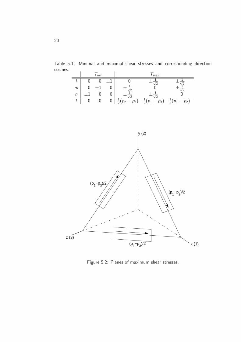
It is possible to find a more meaningful indication of the state of stress, ratherthan the tensorial description, by considering the octahedral sections of the el-ement. These are planes equally inclined to the principle stress axes. Fromconsideration of Fig. 6.1 it is obvious that each of the eight planes will be sub-jected to the same value of direct stress and the same value of shear stress. Thismeans that whereas it took six parameters to describe the state of stress in aset of rectangular sections, it takes only to describe the magnitudes (though notdirections) of the stresses on octahedral sections. Note that octahedral normaland shear stresses correspond to two fundamental effects of uniform dilation anduniform shear.

The magnitudes of the octahedral stresses are easily obtained. If the directioncosines of the normal to the octahedral plane are l , m, and n, their values mustbe l2 = m2 = n2 = 1

3. Also,

σ0 =1

3(p1 + p2 + p3) =

I13

(6.1)

and

τ0 =1

3

√(p1 − p2)2 + (p1 − p3)2 + (p2 − p3)2 =

1

3

√I′2. (6.2)

21

22

p1

σ0

σ0

τ0

p2

p2

τ0

τ0

p3

σ0

p1

Figure 6.1: State of stress on octahedral sections of an element. σ0 isthe octahedral normal stress, τ0 is the octahedral shear stress.

The octahedral stresses can obviously be quoted in terms of the components ofany tensor of the state:

σ0 =1

3(σx + σy + σz), (6.3)

and

τ0 =1

3

√(σx − σy )2 + (σy − σz)2 + (σz − σx)2 + 6(τ 2

xy + τ 2xz + τ 2

yz). (6.4)

The octahedral shear stress is related to the Von Mises yield stress. Failureoccurs when

τ0 =

√2

3σys. (6.5)

7Hydrostatic (dilational) and deviatoric

stress tensors

It is sometimes necessary to take account of the directions of the octahedralshear stresses as well as their magnitudes. In this Chapter, it is shown that anygeneral stress tensor can be split into two, where one part describes the effectof the direct stress on the octahedral section, whereas the other describes theeffect of the octahedral shear stress.

The octahedral normal stress may be expressed in tensor form as

[σ0] =

σ0 0 0

0 σ0 0

0 0 σ0

. (7.1)

This is called the hydrostatic of dilational stress tensor. It describes a state ofstress without shearing present. The value of σ0 is the average of the directstresses on the leading diagonal of the general stress tensor [σ]. The remainderof the tensor, [σ]−[σ0], must describe the effect of the uniform octahedral shearsand is called the deviatoric tensor of the state.

Note that the dilational tensor produces a change in volume without changein shape, while the deviatoric tensor produces a change in shape without changein volume.

23

24

8Strains and displacements

To examine the relationship between strain and displacement, in the first instanceonly a 2-dimensional case will be considered. The displacements are assumed tobe small, so that the strains are small compared to unity.

For the element ABCD in Fig. 8.1, stressing the element will result in adisplacement of the element in addition to straining. Direct strains are responsiblefor increases in length of the sides of the element, while shear strains producerotation of the lines, i.e., change of shape. The increase in length of AB to A′B′

is dx × (the variation of u with respect to x) = ∂u∂x

dx .Therefore, the direct strain in the x-direction is

εx =(dx + ∂u

∂xdx)− dx

dx=

∂u

∂x. (8.1)

Similarly, in the y -direction

εy =∂u

∂y. (8.2)

Because of shear, AB and AD rotate through small angles θ and λ. For smallstrains (dx À ∂u

∂xdx),

θ ≈ tan θ =∂v∂x

dx + ∂u∂x

dx=

∂v

∂x, (8.3)

25

26

y

x

x u

y

v

dx

dy

A

D

B

C

A’ B’

C’D’

∂u__∂x dx

∂v__∂x dx

∂u__∂y dy

∂v__∂y dy

Figure 8.1: Stressing an element.

and

λ ≈ tan λ =∂u

∂y. (8.4)

The shear strain is the change in angle between two lines originally at right angles:

γxy = θ + λ =∂v

∂x+

∂u

∂y. (8.5)

Clearly, γyx = γxy .

In the case of a 3-dimensional rectangular prism with sides dx , dy , and dz ,

27

a similar analysis will give

εx =∂u

∂x; εy =

∂v

∂y; εz =

∂w

∂z;

γxy =∂u

∂y+

∂v

∂x; γyz =

∂v

∂z+

∂w

∂y; γxz =

∂w

∂x+

∂u

∂z.

(8.6)

Like stress, strain is a tensor quantity. It may be stored in a matrix

εx12γyx

12γzx

12γxy εy

12γzy

12γxz

12γyz εz

. (8.7)

A strain tensor has all the properties of a stress tensor, and the same conceptsderived in previous Chapters will apply to it:

1. Strain resolutionThe normal strain on a plane with direction cosines l , m, and n is given by

εN = [ l m n ]

εx12γyx

12γzx

12γxy εy

12γzy

12γxz

12γyz εz

l

m

n

. (8.8)

2. Transformation of axesThe state of strain [ε′] can be found in any second coordinate systemdefined by the direction cosine matrix [L] with respect to the first systemby the equation

[ε′] = [L][ε][L]T. (8.9)

3. Principal strainsIn any pattern of deformation there is one set of rectangular directionswhich suffer no relative rotation and are therefore free of shear. The linearstrains of these lines are called principal strains. They are found by solving

εx − εp12γyx

12γzx

12γxy εy − εp

12γzy

12γxz

12γyz εz − εp

l

m

n

= 0. (8.10)

In an isotropic material the principal axes of strain will coincide with theprincipal axes of stress.

28

4. Stationary values of shear strainThe same technique can be applied to small strains to derive those planeswhere the maximum and minimum values of the shear strain exist: 1

2γ13 =

12(εp1 − εp3).

5. Volumetric and octahedral stainsThe linear strain along each of the four octahedral axes which are equallyinclined to the three principal axes is

ε0 =1

3(εp1 + εp2 + εp3) =

1

3(εx + εy + εz), (8.11)

which is related to the volumetric strain ∆ = εp1 +εp2 +εp3 . This is provedby considering the volumetric strain of a prism with sides parallel to theprincipal axes. If the sides are a1, a2, a3 and increase to a1 + εp1 , a2 + εp2 ,a3 + εp3 , the volumetric strain

∆ = change in volumeoriginal volume

=a1a2a3(1 + εp1)(1 + εp2)(1 + εp3)− a1a2a3

a1a2a3.

(8.12)

Ignoring second order terms,

∆ = εp1 + εp2 + εp3 = 3ε0. (8.13)

6. Hydrostatic and deviatoric strain tensorsAs for the stress tensor, the strain tensor can be split into its dilational anddeviatoric parts. The following relationships apply, which will be discussedin the next Chapter:

σ0[U] = κ∆[U] (8.14)

for the hydrostatic terms, and

[σ]− σ0[U] = 2G

([ε]− ∆

3[U]

)(8.15)

for the deviatoric terms. Here, κ is the Bulk modulus and G is the shearmodulus.

9Generalized Hooke’s law

Hooke’s law states that the strain produced in an elastic material is proportionalto the applied stress. For a linear elastic material the principle of superpositionapplied, so that the deformations may be determined independently and added.Remember that a normal stress only produces a normal strain, while a shear stressonly produces a shear strain. Therefore, the strain due to σx in the x-direction isσx

E(extension), with the Poisson effect producing a strain of −νσx

Ein the y - and

z-directions. Hence, for a triaxial stress, the total normal strains are given by

εx =σx

E− νσy

E− νσz

E=

1

E(σx − ν (σy + σz)) ;

εy =σy

E− νσx

E− νσz

E=

1

E(σy − ν (σz + σx)) ;

εz =σz

E− νσx

E− νσy

E=

1

E(σz − ν (σx + σy)) ,

(9.1)

where E is Young’s modulus. Alternatively, in matrix form,

εx

εy

εz

=

1

E

1 −ν −ν

−ν 1 −ν

−ν −ν 1

σx

σy

σz

. (9.2)

29

30

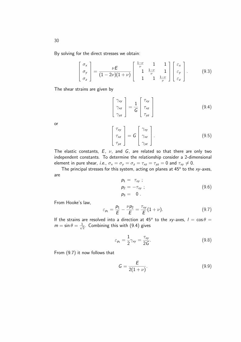
By solving for the direct stresses we obtain:

σx

σy

σz

=

νE

(1− 2ν)(1 + ν)

1−νν

1 1

1 1−νν

1

1 1 1−νν

εx

εy

εz

. (9.3)

The shear strains are given by

γxy

γxz

γyz

=

1

G

τxy

τxz

τyz

(9.4)

or

τxy

τxz

τyz

= G

γxy

γxz

γyz

. (9.5)

The elastic constants, E , ν, and G , are related so that there are only twoindependent constants. To determine the relationship consider a 2-dimensionalelement in pure shear, i.e., σx = σy = σz = τxz = τyz = 0 and τxy 6= 0.

The principal stresses for this system, acting on planes at 45o to the xy -axes,are

p1 = τxy ;

p2 = −τxy ;

p3 = 0 .

(9.6)

From Hooke’s law,

εp1 =p1

E− νp2

E=

τxy

E(1 + ν). (9.7)

If the strains are resolved into a direction at 45o to the xy -axes, l = cos θ =m = sin θ = 1√

2. Combining this with (9.4) gives

εp1 =1

2γxy =

τxy

2G. (9.8)

From (9.7) it now follows that

G =E

2(1 + ν). (9.9)

31

The Bulk modulus

Summing the three equations in (9.1) gives

εx + εy + εz =1− 2ν

E(σx + σy + σz). (9.10)

The sum on the left is the invariant which determines the volumetric strain(8.13), while the right-hand term is the invariant which is equal to three timesthe hydrostatic stress (6.3). Therefore,

∆ =3(1− 2ν)

Eσ0 =

σ0

κ, (9.11)

where κ = E3(1−2ν)

is an elastic constant called the bulk modulus.The relationship between the deviatoric tensors can easily be determined.

From (9.3), by subtracting the second and third equation from twice the first,we obtain

σx − σ0 =E

1 + ν

(εx − ∆

3

)= 2G

(εx − ∆

3

). (9.12)

Thus, each direct stress of the deviatoric tensor, like each shear component, isrelated by 2G to the corresponding element of the deviatoric strain tensor.

Lame’s constant

It has been shown that the total stress tensor can be split into its hydrostaticand deviatoric parts. Each of these effects may then be described as a simpleproportion of the corresponding strain effect. This is advantageous since wecan often ignore the hydrostatic effect. In other cases, however, it may bemore convenient to retain the total tensors intact. Here we show that the splitrelationship can be recombined to describe the total stress tensor as a linearfunction of the total strain tensor and the volumetric strain:

[σ] = 2G [ε] +

(κ− 2G

3

)∆[U]. (9.13)

Because κ and G are constants,

[σ] = 2G [ε] + λ∆[U], (9.14)

32

where λ is Lame’s constant

λ = κ− 2G

3=

Eν

(1 + ν)(1− 2ν). (9.15)

10Equilibrium equations for three

dimensions

Consider a small cuboid of finite size ∆x×∆y×∆z , with stresses acting on eachcoordinate plane and their variations on opposite faces. Resolving the forces inthe x-direction and equating to zero for equilibrium, ignoring body forces, yields

σx ∆z ∆y −(σx +

∂σx

∂x∆x

)∆z ∆y

+τyx ∆x ∆z −(τyx +

∂τyx

∂y∆y

)∆x ∆z

+τzx ∆x ∆y −(τzx +

∂τzx

∂z∆z

)∆x ∆y = 0,

(10.1)

which after simplifying becomes

∂σx

∂x+

∂τyx

∂y+

∂τzx

∂z= 0. (10.2)

33

34

Resolving in the other directions similarly gives

[σ]

∂∂x∂∂y∂∂z

=

0

0

0

. (10.3)

These equations ensure that equilibrium of the material is maintained.In two dimensions they can be simplified to

∂σx

∂x+

∂τyx

∂y= 0 ;

∂τxy

∂x+

∂σy

∂y= 0 .

(10.4)

11Strain compatibility equations

The fundamental equations (8.6) relate the six components of strain in a 3-dimensional system to only three components of displacement. The strainstherefore cannot be independent of one another.

Consider a 2-dimensional case. Since

εx =∂u

∂x(11.1)

and

εy =∂v

∂y, (11.2)

it follows that∂2εx

∂y 2=

∂3u

∂x∂y 2(11.3)

and∂2εy

∂x2=

∂3v

∂x2∂y. (11.4)

Also,∂γxy

∂x∂y=

∂3u

∂x∂y 2+

∂3v

∂x2∂y. (11.5)

35

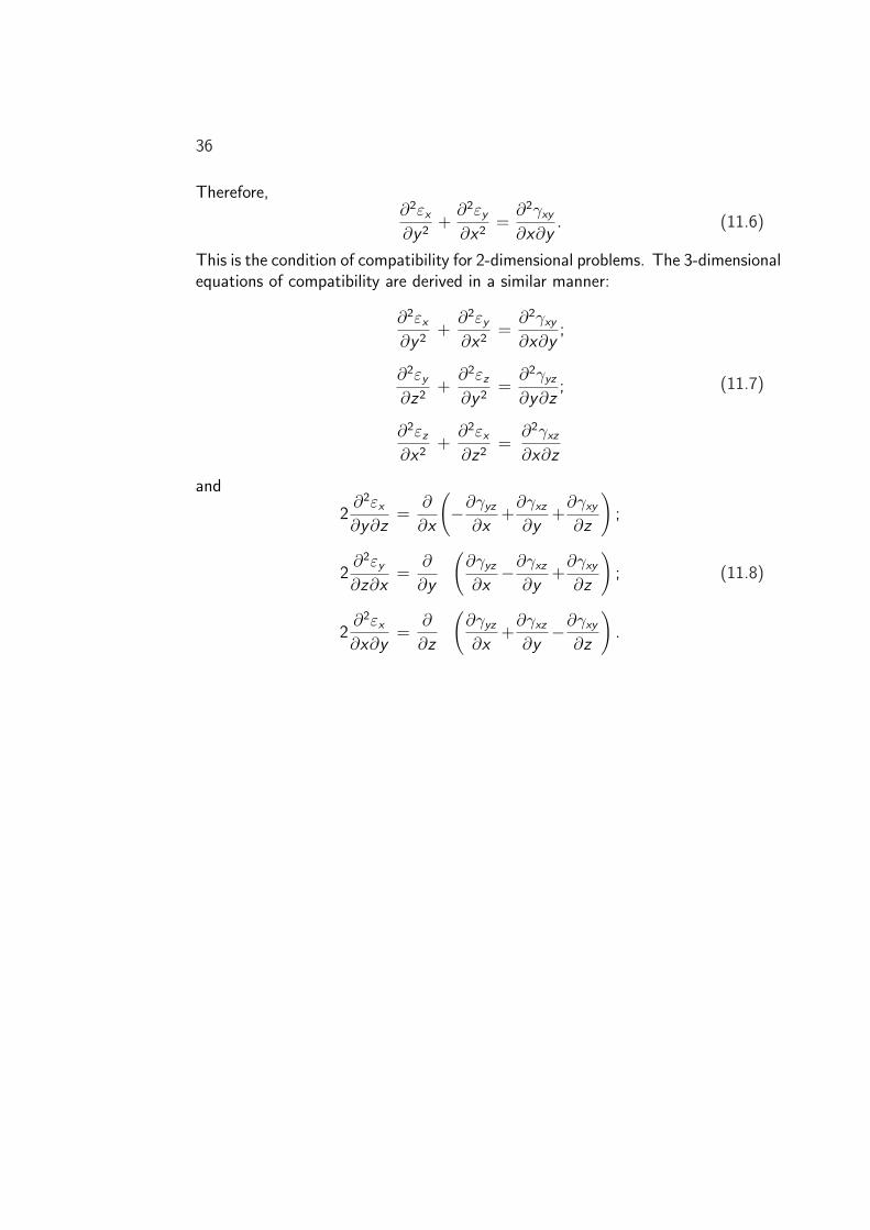
36

Therefore,∂2εx

∂y 2+

∂2εy

∂x2=

∂2γxy

∂x∂y. (11.6)

This is the condition of compatibility for 2-dimensional problems. The 3-dimensionalequations of compatibility are derived in a similar manner:

∂2εx

∂y 2+

∂2εy

∂x2=

∂2γxy

∂x∂y;

∂2εy

∂z2+

∂2εz

∂y 2=

∂2γyz

∂y∂z;

∂2εz

∂x2+

∂2εx

∂z2=

∂2γxz

∂x∂z

(11.7)

and

2∂2εx

∂y∂z=

∂

∂x

(−∂γyz

∂x+

∂γxz

∂y+

∂γxy

∂z

);

2∂2εy

∂z∂x=

∂

∂y

(∂γyz

∂x−∂γxz

∂y+

∂γxy

∂z

);

2∂2εx

∂x∂y=

∂

∂z

(∂γyz

∂x+

∂γxz

∂y−∂γxy

∂z

).

(11.8)

12Plane strain

Consider a long cylinder held between fixed, rigid end plates. It is subjected toan internal pressure, i.e., a purely lateral load. The cylinder can only deform inthe x and y directions. So, w = 0 along the length of the cylinder. From (8.6),

εz = γxz = γyz = 0 (12.1)

and

εx =∂u

∂x;

εy =∂v

∂y;

γxy =∂u

∂y+

∂v

∂x.

(12.2)

This is a state of plain strain, where each point remains within its transverseplane following application of the load. Since εz = 0,

εz =1

E(σx − ν(σx + σy )) = 0, (12.3)

37

38

so that

εx =1− ν2

E

(σx − ν

1− νσy

);

εy =1− ν2

E

(σy − ν

1− νσx

);

γxy =1

Gτxy .

(12.4)

The compatibility equation must also be satisfied by this stressing regime, fortwo dimensions that is:

∂2εx

∂y 2+

∂2εy

∂x2=

∂2γxy

∂x∂y. (12.5)

Differentiating (12.4) and using (10.4) with (12.5) gives

(∂2

∂x2+

∂2

∂y 2

)(σx + σy ) = 0. (12.6)

This is the equation of compatibility in terms of stress. Therefore, we now havethree equations defining three unknowns:

∂σx

∂x+

∂τyx

∂y= 0 ;

∂τxy

∂x+

∂σy

∂y= 0 ;

∇2(σx + σy ) = 0 .

(12.7)

13Plane stress

Consider a thin plate whose loading is evenly distributed over the thickness par-allel to the plane of the plate. On the faces of the plate, σz = τzx = τzy = 0.Since the plate is thin, it can be assumed the same is true through its thickness.The stress–strain relationships are therefore

εx =1

E(σx − νσy ) ;

εy =1

E(σy − νσz) ;

εz = − ν

E(σx + σy ) ;

γxy =1

Gτxy .

(13.1)

Again, using the same strain compatibility equation with the equations for equi-librium, it can be proven that

∇2(σx + σy ) = 0, (13.2)

which is the same equation of compatibility as for the plane strain case.

39

40

14Polar coordinates

Where axial symmetry exists, it is much more convenient to use polar coordinates.The polar coordinate system (r , θ) and the Cartesian coordinate system (x , y)are related by the expressions

x = r cos θ;

y = r sin θ;

r 2 = x2 + y 2;

θ = tan−1 yx.

(14.1)

Strain components in polar coordinates

Consider a pure radial strain, where the internal face of the element with originallength dr is displaced by a radial distance u and a tangential distance v . Thestrained length of the element is dr + ∂u

∂rdr . Therefore, the radial strain

εr =∂u∂r

dr

dr=

∂u

∂r. (14.2)

The tangential strain arises from the radial displacement

εθr =(r + u) dθ − r dθ

r dθ=

u

r(14.3)

41

42

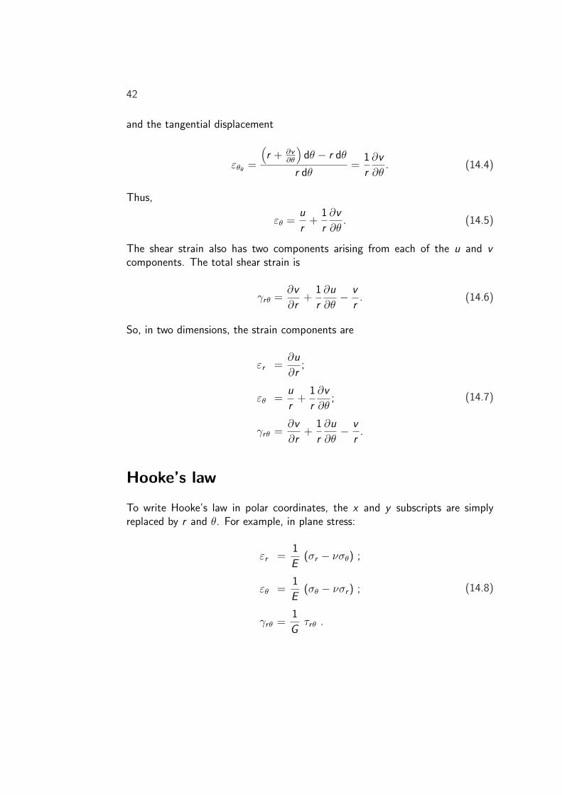
and the tangential displacement

εθθ=

(r + ∂v

∂θ

)dθ − r dθ

r dθ=

1

r

∂v

∂θ. (14.4)

Thus,

εθ =u

r+

1

r

∂v

∂θ. (14.5)

The shear strain also has two components arising from each of the u and vcomponents. The total shear strain is

γrθ =∂v

∂r+

1

r

∂u

∂θ− v

r. (14.6)

So, in two dimensions, the strain components are

εr =∂u

∂r;

εθ =u

r+

1

r

∂v

∂θ;

γrθ =∂v

∂r+

1

r

∂u

∂θ− v

r.

(14.7)

Hooke’s law

To write Hooke’s law in polar coordinates, the x and y subscripts are simplyreplaced by r and θ. For example, in plane stress:

εr =1

E(σr − νσθ) ;

εθ =1

E(σθ − νσr ) ;

γrθ =1

Gτrθ .

(14.8)

43

Equilibrium equations

By considering equilibrium of the radial and circumferential forces acting on anelement of unit thickness, we obtain

r∂σr

∂r+

∂τrθ

∂θ+ σr − σθ = 0 ;

∂σθ

∂θ+

r∂τrθ

∂r+ 2τrθ = 0 .

(14.9)

Strain compatibility equation

The three compatibility equations (14.7) defining the strain components can becombined to give the equation of compatibility

∂2εθ

∂r 2+

1

r 2

∂2εr

∂θ2+

2

r

∂εθ

∂r− 1

r

∂εr

∂r=

1

r

∂2γrθ

∂r∂θ+

1

r 2

∂γrθ

∂θ. (14.10)

Stress compatibility equation

Substituting (14.8) into (14.10) yields

(∂2

∂r 2+

1

r

∂

∂r+

1

r 2

∂2

∂θ2

)(σr + σθ) = 0. (14.11)

For axially symmetrical problems, this may be further simplified to

(∂2

∂r 2+

1

r

∂

∂r

)(σr + σθ) = 0. (14.12)

44

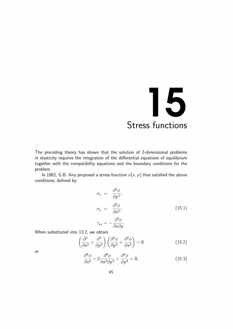
15Stress functions

The preceding theory has shown that the solution of 2-dimensional problemsin elasticity requires the integration of the differential equations of equilibriumtogether with the compatibility equations and the boundary conditions for theproblem.

In 1862, G.B. Airy proposed a stress function φ(x , y) that satisfied the aboveconditions, defined by:

σx =∂2φ

∂y 2;

σy =∂2φ

∂x2;

τxy = − ∂2φ

∂x∂y.

(15.1)

When substituted into 13.2, we obtain(∂2

∂x2+

∂2

∂y 2

) (∂2φ

∂y 2+

∂2φ

∂x2

)= 0 (15.2)

or∂4φ

∂x4+ 2

∂4φ

∂x2∂y 2+

∂4φ

∂y 4= 0, (15.3)

45

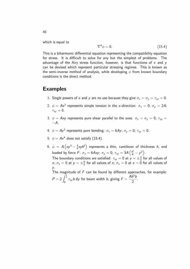
46

which is equal to∇4φ = 0. (15.4)

This is a biharmonic differential equation representing the compatibility equationfor stress. It is difficult to solve for any but the simplest of problems. Theadvantage of the Airy stress function, however, is that functions of x and ycan be devised which represent particular stressing regimes. This is known asthe semi-inverse method of analysis, while developing φ from known boundaryconditions is the direct method.

Examples

1. Single powers of x and y are no use because they give σx = σy = τxy = 0.

2. φ = Ax2 represents simple tension in the x-direction: σx = 0; σy = 2A;τxy = 0.

3. φ = Axy represents pure shear parallel to the axes: σx = σy = 0; τxy =−A.

4. φ = Ay 3 represents pure bending: σx = 6Ay ; σy = 0; τxy = 0.

5. φ = Ax4 does not satisfy (15.4).

6. φ = A(xy 3 − 3

4xyh2

)represents a thin, cantilever of thickness h, end

loaded by force F : σx = 6Axy ; σy = 0; τxy = 3A(

h2

4− y 2

).

The boundary conditions are satisfied: τxy = 0 at y = ±h2

for all values ofx ; σy = 0 at y = ±h

2for all values of x ; σx = 0 at x = 0 for all values of

y .The magnitude of F can be found by different approaches, for example:

P = 2∫ h

2

0τxyb dy for beam width b, giving F =

Ah3b

2.

16Stress functions in polar coordinates

The Airy stress function may also be used in polar coordinates:

σr =1

r 2

∂2φ

∂θ2+

1

r

∂φ

∂r;

σθ =∂2φ

∂r 2;

τrθ = − ∂

∂r

(1

r

∂φ

∂θ

).

(16.1)

The biharmonic equation then becomes

∇4φ =

(∂2

∂r 2+

1

r

∂

∂r+

1

r 2

∂2

∂θ2

) (∂2φ

∂r 2+

1

r

∂φ

∂r+

1

r 2

∂2φ

∂θ2

)= 0. (16.2)

Hole in a plate subjected to pure tension

Consider the stress function φ = 12σ0y

2, which defines a plate under tensionin the x-direction. To analyse the stresses in a plate with a hole, it is moreconvenient to use polar coordinates, and therefore replace y by r sin θ, so that

φ =σ0

2r 2 sin2 θ (16.3)

47

48

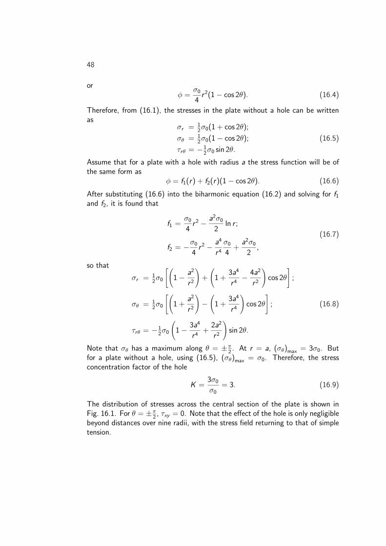
orφ =

σ0

4r 2(1− cos 2θ). (16.4)

Therefore, from (16.1), the stresses in the plate without a hole can be writtenas

σr = 12σ0(1 + cos 2θ);

σθ = 12σ0(1− cos 2θ);

τrθ = −12σ0 sin 2θ.

(16.5)

Assume that for a plate with a hole with radius a the stress function will be ofthe same form as

φ = f1(r) + f2(r)(1− cos 2θ). (16.6)

After substituting (16.6) into the biharmonic equation (16.2) and solving for f1and f2, it is found that

f1 =σ0

4r 2 − a2σ0

2ln r ;

f2 = −σ0

4r 2 − a4

r 4

σ0

4+

a2σ0

2,

(16.7)

so that

σr = 12σ0

[(1− a2

r 2

)+

(1 +

3a4

r 4− 4a2

r 2

)cos 2θ

];

σθ = 12σ0

[(1 +

a2

r 2

)−

(1 +

3a4

r 4

)cos 2θ

];

τrθ = −12σ0

(1− 3a4

r 4+

2a2

r 2

)sin 2θ.

(16.8)

Note that σθ has a maximum along θ = ±π2. At r = a, (σθ)max = 3σ0. But

for a plate without a hole, using (16.5), (σθ)max = σ0. Therefore, the stressconcentration factor of the hole

K =3σ0

σ0= 3. (16.9)

The distribution of stresses across the central section of the plate is shown inFig. 16.1. For θ = ±π

2, τxy = 0. Note that the effect of the hole is only negligible

beyond distances over nine radii, with the stress field returning to that of simpletension.

49

0 1 2 3 4 5 6 7 8 90

0.5

1

1.5

2

2.5

3

σθ / σ0

σr / σ

0

r / a

σ r / σ 0

Figure 16.1: Variation of σr and σθ across the central cross-section of aplate containing a small hole of diameter 2a.

For an elliptical hole with width 2a in the x-direction and length 2b in they -direction, at θ = ±π

2,

(σθ)max = σ0

(1 +

2b

a

). (16.10)

Thus, if b : a = 20 : 1, K = 41. Therefore, a crack, which can be considered asa very long ellipse, has a very high stress concentration factor.

50

17Torsion of non-circular prisms

For circular bars under torsion,

Mt

J=

τ

r=

Gθ

l, (17.1)

where G is the shear modulus, J is the polar moment of inertia, i.e., 12πa4 for

a circular cross-section of radius a, l is the length of the bar, Mt is the appliedtorque, r is the radius at which the stress is required, θ is the angle of twist, andτ is the shear stress.

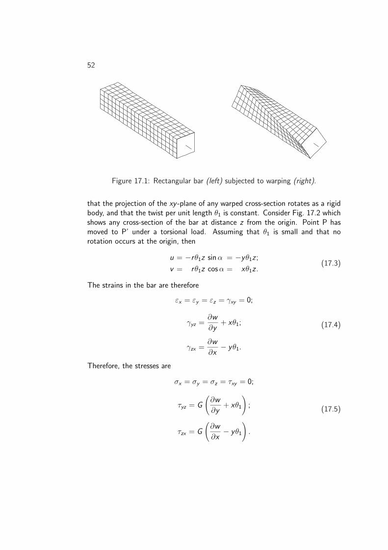
We may assume that all transverse sections remain plain after twisting andthat the cross-sections are undistorted in their individual planes, i.e., the shearstrain is a linear function of r . Initially plane cross-sections experience out-of-plane deformation or warping (cf. Fig. 17.1).

General solution of the torsion problem

Consider a bar of arbitrary cross-section. The origin of the coordinate system isat the centre of twist, where the displacements, u and v , are zero. It is assumedthat the warping deformation is independent of the axial position:

w = f (x , y), (17.2)

51

52

Figure 17.1: Rectangular bar (left) subjected to warping (right).

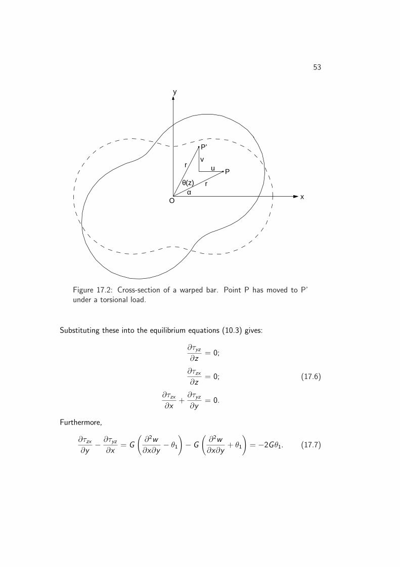
that the projection of the xy -plane of any warped cross-section rotates as a rigidbody, and that the twist per unit length θ1 is constant. Consider Fig. 17.2 whichshows any cross-section of the bar at distance z from the origin. Point P hasmoved to P’ under a torsional load. Assuming that θ1 is small and that norotation occurs at the origin, then

u = −rθ1z sin α = −yθ1z ;

v = rθ1z cos α = xθ1z .(17.3)

The strains in the bar are therefore

εx = εy = εz = γxy = 0;

γyz =∂w

∂y+ xθ1;

γzx =∂w

∂x− yθ1.

(17.4)

Therefore, the stresses are

σx = σy = σz = τxy = 0;

τyz = G

(∂w

∂y+ xθ1

);

τzx = G

(∂w

∂x− yθ1

).

(17.5)

53

αθ(z)

uv

P

P’

r

r

y

xO

Figure 17.2: Cross-section of a warped bar. Point P has moved to P’under a torsional load.

Substituting these into the equilibrium equations (10.3) gives:

∂τyz

∂z= 0;

∂τzx

∂z= 0;

∂τzx

∂x+

∂τyz

∂y= 0.

(17.6)

Furthermore,

∂τzx

∂y− ∂τyz

∂x= G

(∂2w

∂x∂y− θ1

)− G

(∂2w

∂x∂y+ θ1

)= −2Gθ1. (17.7)

54

Equations (17.6) and (17.7) are usually solved by using a stress function φ(x , y),called the Prandtl stress function, such that

τyz = −∂φ

∂x;

τzx =∂φ

∂y.

(17.8)

Equation (17.7) therefore becomes

∇2φ = −2Gθ1 = constant. (17.9)

Boundary conditions

1. The load-free sides of the barφ may be considered as a surface defined by x and y , so that τxy is theslope of the φ-surface in the x-direction. At a free edge of any section, thenormal shear stress, and therefore the slope of φ, must be equal to zero.Thus φ is a constant around the boundary. We may arbitrarily chooseφ = 0.

2. The loaded ends of the barThe total torque at the end surface with area A is

Mt = −∫

Ay τzx dx dy +

∫

Ax τyz dx dy

= −∫

Ay

(∂φ

∂y

)dx dy +

∫

Ax

(∂φ

∂x

)dx dy .

(17.10)

Let’s concentrate on the first term of (17.10): − ∫A y

(∂φ∂y

)dx dy . For

constant x , ∂φ∂y

dy = dφ, so that integrating by parts from C to D (cf.

Fig. 17.3) gives

−∫∫ D

Cy dφ dx = −

∫ {[yφ

]D

C−

∫ D

Cφ dy

}dx . (17.11)

Because φ is constant around the edge, φC = φD, and

−∫∫ D

Cy dφ dx =

∫∫ D

Cφ dy dx =

∫

Aφ dA. (17.12)

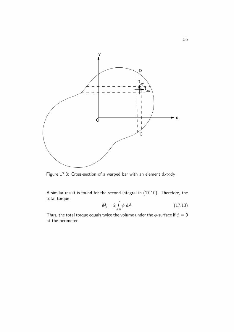
55

C

D

y

xO

y

xO

τzx

τzy

Figure 17.3: Cross-section of a warped bar with an element dx×dy .

A similar result is found for the second integral in (17.10). Therefore, thetotal torque

Mt = 2∫

Aφ dA. (17.13)

Thus, the total torque equals twice the volume under the φ-surface if φ = 0at the perimeter.

56

18Prandtl’s membrane analogy

Consider an edge-supported membrane (soap film) spanning a hole cut in a plate.The shape of the hole is the same as that of the twisted bar to be studied. Letthe membrane be blown-up by a small pressure p, so that all deflections are small.Let the tensile force per unit length in the membrane be S (cf. Fig. 18.1).

Considering the normal equilibrium of an element dx×dy , we obtain

p dx dy = S dy∂z

∂x− S dy

d

dx

(z +

∂z

∂xdx

)

+S dx∂z

∂y− S dx

d

dy

(z +

∂z

∂ydy

),

(18.1)

which leads to

∇2z = −p

S. (18.2)

This may be compared to (17.9), taking into account a scaling factor:

φ =2Gθ1

p/Sz , (18.3)

57

58

z z + dx ∂z ∂x

x

z

membrane

dx

dy S

plate

x

y

Figure 18.1: Edge-supported membrane spanning a hole in a plate.

so that

τxz =∂φ

∂y=

2Gθ1

p/S

∂z

∂y;

τyz = −∂φ

∂x= −2Gθ1

p/S

∂z

∂x,

(18.4)

and

Mt = 2∫

Aφ dA =

2Gθ1

p/S

∫

Az dA. (18.5)

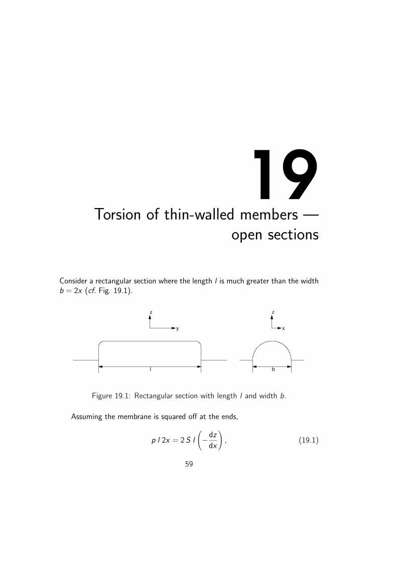
19Torsion of thin-walled members —

open sections

Consider a rectangular section where the length l is much greater than the widthb = 2x (cf. Fig. 19.1).

l b

zz

xy

Figure 19.1: Rectangular section with length l and width b.

Assuming the membrane is squared off at the ends,

p l 2x = 2 S l

(−dz

dx

), (19.1)

59

60

ordz

dx= −p

Sx , (19.2)

giving

z = −p

S

x2

2+ constant. (19.3)

At x = b2, z = 0. Therefore,

constant =p

S

b2

8, (19.4)

so that

z =p

2S

(b2

4− x2

). (19.5)

Rephrasing (18.5),

Mt =4Gθ1

p/s× volume under the membrane. (19.6)

The volume under the membrane

∫

Az dA = 2

b2∫

0

z l dx =p l

S

b2∫

0

(b2

4− x

)dx =

p

S

lb3

12. (19.7)

Therefore, the torque transmitted by a rectangular section

Mt =Gθ1lb

3

3, (19.8)

and the shear stress

τ =2Gθ1

p/S

dz

dx= −2Gθ1x . (19.9)

20Torsion of thin-walled members —

closed sections

The membrane analogy can also be applied to closed sections if care is takendefining the shape of the membrane.

Consider a hollow thin-walled member with wall thickness b. The membranesurface is approximated by a flat surface of thickness h, as shown in Fig. 20.1.The slope of the membrane h

bis taken constant over the thin wall. If L is the

perimeter length,

p A =∫ L

0

h

bS dL, (20.1)

orp

S=

h

A

∫ L

0

1

bdL. (20.2)

Also,

τ =∂φ

∂r=

2Gθ1

p/S

dz

dr=

2Gθ1

p/S

h

b. (20.3)

Therefore,

τ =2Gθ1

h

A

∫ L

0

1

bdL

h

b=

2Gθ1A

b∫ L

0

1

bdL

. (20.4)

61

62

x

z

x

y

b

h

Figure 20.1: Closed section approximated by a flat surface and constantslopes over the thin wall.

For a constant the wall thickness,

τ =2Gθ1A

L. (20.5)

The torque carried by the section

Mt =4Gθ1

p/S

∫

Az dA =

4Gθ1

p/ShA =

4Gθ1hAh

A

∫ L

0

1

bdL

=4Gθ1A

2

∫ L

0

1

bdL

. (20.6)

For a constant the wall thickness, the total torque transmitted

Mt =4Gθ1A

2b

L, (20.7)

so that

τ =Mt

2Ab. (20.8)

21Bibliography

1. Gere JM. Mechanics of Materials. 6th ed. Toronto: Thomson 2006.

2. Landau LD, Lifshitz EM. Theory of Elasticity. 3rd ed. Oxford: Butterworth-Heinemann 1986.

3. Renny JN. Theory and Analysis of Elastic Plates and Shells. 2nd ed. BocaRaton: CRC Press 2007.

63