
Governing Automated Vehicle Behavior - Archive ouverte HAL
195
HAL Id: tel-03680555 https://hal.archives-ouvertes.fr/tel-03680555 Submitted on 28 May 2022 HAL is a multi-disciplinary open access archive for the deposit and dissemination of sci- entific research documents, whether they are pub- lished or not. The documents may come from teaching and research institutions in France or abroad, or from public or private research centers. L’archive ouverte pluridisciplinaire HAL, est destinée au dépôt et à la diffusion de documents scientifiques de niveau recherche, publiés ou non, émanant des établissements d’enseignement et de recherche français ou étrangers, des laboratoires publics ou privés. Governing Automated Vehicle Behavior Nelson de Moura To cite this version: Nelson de Moura. Governing Automated Vehicle Behavior. Computer Science [cs]. Sorbonne Univer- sites, UPMC University of Paris 6, 2021. English. tel-03680555
-
Upload
khangminh22 -
Category
Documents
-
view
2 -
download
0
Transcript of Governing Automated Vehicle Behavior - Archive ouverte HAL

HAL Id: tel-03680555https://hal.archives-ouvertes.fr/tel-03680555
Submitted on 28 May 2022
HAL is a multi-disciplinary open accessarchive for the deposit and dissemination of sci-entific research documents, whether they are pub-lished or not. The documents may come fromteaching and research institutions in France orabroad, or from public or private research centers.
L’archive ouverte pluridisciplinaire HAL, estdestinée au dépôt et à la diffusion de documentsscientifiques de niveau recherche, publiés ou non,émanant des établissements d’enseignement et derecherche français ou étrangers, des laboratoirespublics ou privés.
Governing Automated Vehicle BehaviorNelson de Moura
To cite this version:Nelson de Moura. Governing Automated Vehicle Behavior. Computer Science [cs]. Sorbonne Univer-sites, UPMC University of Paris 6, 2021. English. tel-03680555

SORBONNE UNIVERSITÉÉcole doctorale 130: Informatique, Télécommunications et Électronique
Institut des Systèmes Intelligents et de Robotique
Thèse de Doctorat
Pour obtenir le grade de
DOCTEUR en informatique
Soutenance présenté par
Nelson DE MOURA MARTINS GOMES
GOVERNING AUTOMATED VEHICLE BEHAVIOR
Soutenue le 29 juin 2021 devant le jury composé de :
Dr. Fawzi NASHASHIBI Rapporteur INRIADr. Catherine TESSIER Rapporteur OneraPr. Stéphane CHAUVIER Examinateur Sorbonne Université
Pr. Véronique CHERFAOUI Examinateur Université de Technologiede Compiègne
Dr. Ebru BURCU DOGAN Examinateur Institut VEDECOMPr. Jean-Gabriel GANASCIA Examinateur Sorbonne UniversitéPr. Alan WINFIELD Examinateur UWE BristolPr. Raja CHATILA Directeur de thèse Sorbonne Université

Abstract
From a societal point of view, automated vehicles (AV) can bring many benefits, suchas an increase of road safety and a decrease of congestion (Fagnant and Kockelman, 2015;Schwarting et al., 2018). However, due to the highly dynamic environments these vehicles canencounter, technical concerns about their feasibility and ethical concerns about their actions’deliberation, explainability and consequences (Lin, 2016; Gerdes and Thornton, 2016) seems todamper the enthusiasm and optimism that once ruled the automotive sector and the public opinion(Boudette, 2019).
This thesis addresses the core questions surrounding autonomous vehicles today: howthey should account the road users sharing the same environment in their decision making andalso how they should deliberate to act in dilemma situations. Firstly, a decision making process forthe autonomous vehicle under general situations is proposed, and then, as a particular situation,the deliberation under certain collision, with other vehicles, pedestrians or static objects, isimplemented.
The discussion focus on an hypothetical AV implementation in urban environments,where velocity is limited and many road users might interact with each other. Therefore, thebehavior from other road users is a significant source of uncertainty for the AV (Madigan et al.,2019). In a first attempt to propose a decision making algorithm for the AV that contemplateboth generic and dilemma situations, the behavior of road users was considered static during theexecution of an AV policy.
A finite horizon MDP, with states representing only the AV’s configuration, was im-plemented, leaving the road users’ configuration to be accounted in the reward function as anevaluation of how much risk and performance each action would bring. With this state definitionthe transition probability was defined as static scalar constant, given that it would represent onlythe probability of the AV reaching an expected next state given a current one and an action. Adilemma scenario was defined as when all available actions for the AV would result in an accident,which is predicted by the outcome calculated in the reward function estimation. The results ofthis implementation can be seen in (de Moura et al., 2020).
In the aforementioned article and also in (Evans et al., 2020), a measure of the risk in anaccident, called harm, was proposed. It accounts for the difference of velocity produced by thecollision and for the vulnerability between the involved road users. This last parameter is proposedto be calculated via a statistical accidentology study from a region or a country, classifying theseverity of a collision according to the difference of velocity between the concern road users.The harm represents a scaled measure of risk for each road user due to a collision and is used todeliberate on which action the AV should execute in a dilemma scenario situation.
On the subject of ethical deliberation, (de Moura et al., 2020) and (Evans et al., 2020)take different approaches. The former adapts the general idea of certain ethical theories (ralwsiancontractualism, utilitarianism and egalitarianism) into a mathematical formulation to choose theaction based on the expected harm it would produce, which is then used as a deliberation methodby the MDP for a state that presents a dilemma situation, instead of the usual value iterationcriteria for general situations. The method proposed by (Evans et al., 2020) adds to the harm theconcept of ethical valence, which represents the degree of social acceptability that is attached tothe claims of the road users in the environment. Then both measures are used by defined moralprofiles to deliberate on an action.
Coming back to the question about other road users’ behaviors uncertainty, a differentapproach was considered for such parameter to the AV’s decision making. Using an intersectionas use case, a multi-agent simulation was implemented, with each decision making from otherroad users (pedestrians and vehicles) being executed by a set of deterministic rules, to representthe behavior of a standard driver/pedestrian. To estimate the intentions of other users, the AVcompares its predictions by assuming an intention vector and updating an instance of a Kalmanfilter for each user. The distance between the estimate and the observation defines the probabilitythat a user has the assumed intention. To take into account the interactions between the differentusers, we adopt a game theoretic approach with incomplete information (Harsanyi, 1967; Harsanyi,1968b) to then calculate the Nash’s equilibrium, giving the final AV’s strategy.
Keywords: automated vehicles, decision-making, ethical decision-making, artificialmoral agents, game theory, behavior prediction

Résumé
D’un point de vue sociétal, le véhicule à conduite automatisée (VA) peut nous offrirplusieurs avantages par rapport au trafic constitué seulement de véhicules avec conducteur, commeune augmentation de la sécurité routière et une diminution de la congestion routière (Fagnantand Kockelman, 2015; Schwarting et al., 2018). Cependant, à cause de l’environnent dynamiqueet complexe où ces systèmes doivent opérer, des questionnements concernant leur sûreté defonctionnement et leur comportement vis-à-vis des autres utilisateurs se posent, en particuliersur la capacité du VA de délibérer sous dilemme éthique, d’expliquer ses choix et de mesurerles conséquences de ses actions (Lin, 2016; Gerdes and Thornton, 2016). Ces questions ontfinalement ralenti l’enthousiasme naïf et inouï qui avait conquis l’opinion publique et une partiedes constructeurs automobiles (Boudette, 2019).
Deux sujets sont abordés dans cette thèse concerant les défis du déploiement du VAdans le monde réel: comment prendre en compte les autres utilisateurs de la route dans leprocessus de prise de décision du VA dans un environnent urbain, et comment le VA doit délibérersous une situation de dilemme éthique. D’abord un algorithme de prise de décision conçu pourtraiter des situations génériques est proposé; ensuite, à partir de cet algorithme et dans le cadred’une situation spécifique, quand une collision avec des autres véhicules ou des piétons devientinévitable, la délibération éthique est traitée.
La discussion concernant la prise de décision du VA est limitée à l’environnent urbain, oùla vitesse est limitée et plusieurs utilisateurs, protégés par des coques de métal (véhicules) ou pas(piétons, cyclistes, etc.) interagissent les uns avec les autres. Le comportement des autres usagersest une source majeure d’incertitude pour le VA. Dans une premiere proposition d’un algorithmede prise de décision pour le VA, le comportement des autres utilisateurs a été considéré commestatique.
Un processus de décision Markovien (Markov Decision Process, MDP) fini avec des étatsqui représentent seulement la configuration du VA a été implémenté, avec la prise en compte de laposition des autres utilisateurs dans l’évaluation de chaque action action. Cette évaluation permetaussi de détecter les situations de dilemme éthique, qui sont traités de deux façons différentes:avec une optimisation (minimisation) du dommage (harm en anglais) prévu pour une collision

dans le cadre d’un processus délibération défini à partir d’une théorie éthique (de Moura et al.,2020) ou en considérant des profils moraux qui prennent en compte la valence éthique de chaqueutilisateur et le dommage prévu (Evans et al., 2020).
La probabilité de transition entre états a été considérée comme statique pour le processusde prise de décision proposé. Cependant elle est en réalité dépendante du comportement de chaqueutilisateur individuellement et de ses interactions avec les autres. Dans une généralisation de ladémarche précédente, nous avons introduit une modélisation pour prédire ces comportements.
Une simulation multi-agents est nécessaire pour que l’interaction avec les autres usagerssoit bien représentée. Pour estimer les intentions des autres usagers, le VA compare ses prédictionsen utilisant un vecteur d’intentions et en mettant à jour un filtre de Kalman pour chaque usager.L’écart entre l’estimation et l’observation définit la probabilité qu’un utilisateur ait l’intentionprédite. Pour tenir compte des ineractions entre les usagers, nous adoptons une formulationthe théorie des jeux avec informations incomplètes qui permet de fournir le comportement del’ensemble des agents (Harsanyi, 1967; Harsanyi, 1968b). Le point d’équilibre de Nash permetd’obtenir la stratégie finale du VA.
Mots-clés: véhicule automatisé, prise de decision, prise de decision éthique, agentsmoraux artificiel, théorie des jeux, prédiction de comportement

Remerciements
Primeiro eu gostaria de agrader meus pais, Nelson e Daisy, pela confiança que eles sempreme deram e pelo apoio incondicional, em todos os momentos, desde os tempos da natação comtreinos às 4:00, passando pela poli e pelas duas mudanças para o exterior. Tenho que agradecertambém minha família aqui na Europa, tia Marilda e tio Henk, Tanja, Carol, Dennis, Janwillen,Mats e Louis pelas páscoas, natais, aniversários e por me ajudar em todos os momentos aqui.Sem todos vocês eu nunca teria chegado aonde cheguei.
Je veux remercier aussi Amanda, pour m’avoir eu comme co-loc pendant quatre mois etpour être toujours là quand je besoin. Et Bruno, Jero, Ale et Lucas pour tous les weekends, lesfêtes et les invitations que j’ai refusés car je devrais travailler. Ebru, merci pour m’avoir choisipour travailler dans votre projet et pour me donner la possibilité d’être dans MOB02. Mercedes,Elsa, Franck, JB, Jessy, Jean-Louis et Céline, je suis très content d’avoir appris un peu sur ledomaine de chacun de vous, qui sont très éloignés de tout ce que j’ai étudié auparavant et de nosdiscussions autour des cafés dans les matins et des bières dans les après-midis. Merci beaucouppour m’avoir reçu de manière si chaleureuse au sein de l’équipe. Le même est aussi vrai pourle VEH08, DT et Guillaume, Mohamed, Nicolas, Laurène, Florent, Flavie, Floriane et Marie,merci pour les cafés, les discussions et pour me soutenir pendant les trois années à VEDECOM.Je remercie aussi le CSE, pour l’expérience quasi-syndicale et le D1 pour la camaraderie et lesafters.
Katherine, merci pour avoir facilité mon introduction à l’éthique, sujet avec lequel je n’aijamais eu de contact avant le début de la thèse; sans ton aide toute le développement de cettethèse aura été beaucoup plus difficile. Merci pour les innombrables révisions de notre article(vraiment innombrables) et pour ta patience et compréhension quand je faisais des remarques surles aspects fonctionnels dans tes raisonnements (c’est-à-dire tout le temps).
Et en dernier, et certainement le plus important, je remercie Raja. Au long des trois ansde thèse j’ai écouté plusieurs histoires de thésards qu’ont eu des difficultés avec ces directeurs dethèse. Je n’ai jamais compris ces histoires car pendant tout ma thèse tu m’as donné le support,le temps et la confiance que j’avais besoin. Merci beaucoup pour avoir eu la patience avec moimême quand je ne l’avais pas et pour le soutien indéfectible pendant ces derniers mois de thèse.
vii

Chapter 0. Remerciements
This research has been conducted as part of the AVEthics Project funded by the French National Agencyfor Research, grant agreement number ANR-16-C22-008 and Horizon 2020 program AI4EU under grant
agreement 825619.
viii

Contents
Abstract iii
Résumé v
Remerciements vii
List of Figures xv
List of Tables xviii
1 Introduction 1
1.1 Automated driving vehicles in society . . . . . . . . . . . . . . . . . . . . . . 1
1.1.1 A note on terminology . . . . . . . . . . . . . . . . . . . . . . . . . . 1
1.1.2 History . . . . . . . . . . . . . . . . . . . . . . . . . . . . . . . . . . 2
1.1.3 Current research status . . . . . . . . . . . . . . . . . . . . . . . . . . 9
1.2 Motivation of the thesis . . . . . . . . . . . . . . . . . . . . . . . . . . . . . . 12
1.3 Contributions of the thesis . . . . . . . . . . . . . . . . . . . . . . . . . . . . 14
1.4 Structure of the document . . . . . . . . . . . . . . . . . . . . . . . . . . . . . 15
ix

Contents Contents
2 State of the Art 17
2.1 Decision Making . . . . . . . . . . . . . . . . . . . . . . . . . . . . . . . . . 18
2.1.1 Related works . . . . . . . . . . . . . . . . . . . . . . . . . . . . . . . 20
2.2 Ethical decision-making . . . . . . . . . . . . . . . . . . . . . . . . . . . . . 25
2.2.1 Normative Ethics . . . . . . . . . . . . . . . . . . . . . . . . . . . . . 25
2.2.2 Artificial moral agents . . . . . . . . . . . . . . . . . . . . . . . . . . 27
2.3 Behavior prediction . . . . . . . . . . . . . . . . . . . . . . . . . . . . . . . . 32
2.3.1 Vehicle prediction . . . . . . . . . . . . . . . . . . . . . . . . . . . . 33
2.3.2 Pedestrian prediction . . . . . . . . . . . . . . . . . . . . . . . . . . . 38
2.4 Game theory . . . . . . . . . . . . . . . . . . . . . . . . . . . . . . . . . . . . 40
2.4.1 Related works . . . . . . . . . . . . . . . . . . . . . . . . . . . . . . . 42
2.5 Conclusion . . . . . . . . . . . . . . . . . . . . . . . . . . . . . . . . . . . . 45
3 MDP for decision making 47
3.1 Theoretical background . . . . . . . . . . . . . . . . . . . . . . . . . . . . . . 47
3.1.1 AV’s Architecture . . . . . . . . . . . . . . . . . . . . . . . . . . . . . 48
3.1.2 Markov Decision Process . . . . . . . . . . . . . . . . . . . . . . . . 50
3.2 AV decision-making model . . . . . . . . . . . . . . . . . . . . . . . . . . . . 55
3.2.1 State and action sets . . . . . . . . . . . . . . . . . . . . . . . . . . . 55
3.2.2 Transition function . . . . . . . . . . . . . . . . . . . . . . . . . . . . 57
3.2.3 Reward function . . . . . . . . . . . . . . . . . . . . . . . . . . . . . 59
3.3 Results and discussion . . . . . . . . . . . . . . . . . . . . . . . . . . . . . . 66
x

Contents Contents
3.3.1 Value iteration . . . . . . . . . . . . . . . . . . . . . . . . . . . . . . 66
3.3.2 Simulation . . . . . . . . . . . . . . . . . . . . . . . . . . . . . . . . 68
3.3.3 MDP policy results . . . . . . . . . . . . . . . . . . . . . . . . . . . . 70
3.4 Conclusion . . . . . . . . . . . . . . . . . . . . . . . . . . . . . . . . . . . . 74
4 Dilemma Deliberation 77
4.1 Dilemma situations . . . . . . . . . . . . . . . . . . . . . . . . . . . . . . . . 78
4.2 The definition of harm . . . . . . . . . . . . . . . . . . . . . . . . . . . . . . 79
4.2.1 ∆v for collision . . . . . . . . . . . . . . . . . . . . . . . . . . . . . . 82
4.2.2 Vulnerability constant . . . . . . . . . . . . . . . . . . . . . . . . . . 83
4.3 Ethical deliberation process . . . . . . . . . . . . . . . . . . . . . . . . . . . . 86
4.3.1 Ethical Valence Theory . . . . . . . . . . . . . . . . . . . . . . . . . . 86
4.3.2 Ethical Optimization . . . . . . . . . . . . . . . . . . . . . . . . . . . 90
4.3.3 Value iteration for dilemma scenarios . . . . . . . . . . . . . . . . . . 94
4.4 Results and discussion . . . . . . . . . . . . . . . . . . . . . . . . . . . . . . 98
4.4.1 Using EVT as ethical deliberation . . . . . . . . . . . . . . . . . . . . 98
4.4.2 Using the Ethical Optimization profiles to deliberate . . . . . . . . . . 102
4.5 Conclusion . . . . . . . . . . . . . . . . . . . . . . . . . . . . . . . . . . . . 104
5 Road User Intent Prediction 107
5.1 Broadening the scope . . . . . . . . . . . . . . . . . . . . . . . . . . . . . . . 108
5.2 Intent estimation . . . . . . . . . . . . . . . . . . . . . . . . . . . . . . . . . 109
5.2.1 Simulated Environment . . . . . . . . . . . . . . . . . . . . . . . . . . 109
xi
Contents Contents
5.2.2 Agent’s decision model . . . . . . . . . . . . . . . . . . . . . . . . . . 112
5.2.3 Estimating other agents’ intent . . . . . . . . . . . . . . . . . . . . . . 119
5.3 Incomplete game model . . . . . . . . . . . . . . . . . . . . . . . . . . . . . . 125
5.3.1 Nash equilibrium . . . . . . . . . . . . . . . . . . . . . . . . . . . . . 125
5.3.2 Harsanyi’s Bayesian game . . . . . . . . . . . . . . . . . . . . . . . . 126
5.3.3 Decision making procedure . . . . . . . . . . . . . . . . . . . . . . . 129
5.4 Simulation results . . . . . . . . . . . . . . . . . . . . . . . . . . . . . . . . . 133
5.4.1 Multi-agent simulation . . . . . . . . . . . . . . . . . . . . . . . . . . 134
5.5 Final remarks . . . . . . . . . . . . . . . . . . . . . . . . . . . . . . . . . . . 138
6 Conclusion 141
6.1 Final remarks . . . . . . . . . . . . . . . . . . . . . . . . . . . . . . . . . . . 141
6.2 Future research perspectives . . . . . . . . . . . . . . . . . . . . . . . . . . . 144
A Simulation set-up 147
A.1 Webots simulation structure . . . . . . . . . . . . . . . . . . . . . . . . . . . . 147
A.2 Controlling a car-like vehicle . . . . . . . . . . . . . . . . . . . . . . . . . . . 149
A.3 Controlling the pedestrian . . . . . . . . . . . . . . . . . . . . . . . . . . . . . 153
A.4 Necessary modifications . . . . . . . . . . . . . . . . . . . . . . . . . . . . . 154
Bibliography 157
xii

List of Figures
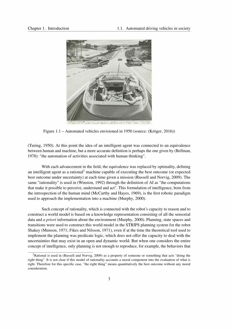
1.1 Automated vehicles envisioned in 1950 (source: (Kröger, 2016)) . . . . . . . . 3
1.2 Interior of the vehicle used to test the machine vision component proposed in(Dickmanns and Zapp, 1987) (source: (Daimler, 2016)) . . . . . . . . . . . . . 5
1.3 Argo vehicle (source: (Parma, 1999)) . . . . . . . . . . . . . . . . . . . . . . . 6
1.4 Sandstorm vehicle in its final accident (source: Urmson, Anhalt, Clark, et al., 2004) 7
1.5 Stanley vehicle in 2005 DARPA Grand Challenge (source: (Thrun et al., 2006)) 8
1.6 Boss vehicle in 2007 DARPA Urban Challenge (source: (Urmson, Anhalt, Bag-nell, et al., 2008)) . . . . . . . . . . . . . . . . . . . . . . . . . . . . . . . . . 9
1.7 Definitions of levels of automation (source: (SAE, 2018)) . . . . . . . . . . . . 10
2.1 Possible structures for the AV’s decision-making . . . . . . . . . . . . . . . . 19
2.2 Hierarchy of possible significations for behavior . . . . . . . . . . . . . . . . . 33
3.1 Three tiered (3T) architecture . . . . . . . . . . . . . . . . . . . . . . . . . . . 49
3.2 AV architecture adopted . . . . . . . . . . . . . . . . . . . . . . . . . . . . . . 49
3.3 Simplified example of an MDP . . . . . . . . . . . . . . . . . . . . . . . . . . 52
3.4 AV’s kinematic model . . . . . . . . . . . . . . . . . . . . . . . . . . . . . . . 56
3.5 Example of state space discovery . . . . . . . . . . . . . . . . . . . . . . . . . 57
xiii

List of Figures List of Figures
3.6 State transition uncertainty for a0 and a3 . . . . . . . . . . . . . . . . . . . . . 58
3.7 Performance reward parameters . . . . . . . . . . . . . . . . . . . . . . . . . 60
3.8 AV with all the proximity limits . . . . . . . . . . . . . . . . . . . . . . . . . 61
3.9 Calculation of velocity projections . . . . . . . . . . . . . . . . . . . . . . . . 63
3.10 Workflow for sprox calculation . . . . . . . . . . . . . . . . . . . . . . . . . . 64
3.11 Calculating the separation line . . . . . . . . . . . . . . . . . . . . . . . . . . 65
3.12 Initial simulation setup (other road users’ configuration is represented by (x,y,θ ,v),not in scale) . . . . . . . . . . . . . . . . . . . . . . . . . . . . . . . . . . . . 69
3.13 Simulation environment . . . . . . . . . . . . . . . . . . . . . . . . . . . . . . 69
3.14 AV’s behavior for xveh = 100, 80, 40m . . . . . . . . . . . . . . . . . . . . . . 71
3.15 AV’s behavior for xveh = 80,40m with 5 transitions . . . . . . . . . . . . . . . 72
3.16 AV’s velocity, direction and trajectory for xveh = 80m . . . . . . . . . . . . . . 72
3.17 AV’s behavior for xveh = 100, 40m and θped = 3π
4 rad . . . . . . . . . . . . . . 74
3.18 Trajectory for xveh=40m, θped= 3π
4 rad for 5 transitions . . . . . . . . . . . . . . 74
4.1 Projection of future collision into previous states . . . . . . . . . . . . . . . . 97
4.2 Possible dilemma situation . . . . . . . . . . . . . . . . . . . . . . . . . . . . 99
4.3 Initial simulation setup (other road users’ configuration is represented by (x,y,θ ,v),not in scale) . . . . . . . . . . . . . . . . . . . . . . . . . . . . . . . . . . . . 99
4.4 Collision simulation for situation 1 . . . . . . . . . . . . . . . . . . . . . . . . 100
4.5 Second simulation setup (other road users’ configuration is represented by(x,y,θ ,v), not in scale) . . . . . . . . . . . . . . . . . . . . . . . . . . . . . . 101
4.6 Collision simulation for situation 2 . . . . . . . . . . . . . . . . . . . . . . . . 102
4.7 Trajectories for contractarian, utilitarian and egalitarian methods . . . . . . . . 103
xiv

List of Figures List of Figures
5.1 New simulation environment . . . . . . . . . . . . . . . . . . . . . . . . . . . 111
5.2 Road environment graph structure . . . . . . . . . . . . . . . . . . . . . . . . 115
5.3 Decision tree for vehicles . . . . . . . . . . . . . . . . . . . . . . . . . . . . . 117
5.4 Decision tree for pedestrians . . . . . . . . . . . . . . . . . . . . . . . . . . . 118
5.5 Illustration of the intersection interaction . . . . . . . . . . . . . . . . . . . . . 135
5.6 Strategies used during situation 1 . . . . . . . . . . . . . . . . . . . . . . . . . 135
5.7 Strategies used during situation 2 . . . . . . . . . . . . . . . . . . . . . . . . . 136
5.8 Strategies used during situation 3 . . . . . . . . . . . . . . . . . . . . . . . . . 137
5.9 Modified vehicle decision for the no collision sub-tree . . . . . . . . . . . . . . 138
A.1 Main window of the simulator . . . . . . . . . . . . . . . . . . . . . . . . . . 148
A.2 Longitudinal control for the vehicle . . . . . . . . . . . . . . . . . . . . . . . 150
A.3 Vehicle’s acceleration sampling distribution . . . . . . . . . . . . . . . . . . . 151
A.4 The pedestrian object . . . . . . . . . . . . . . . . . . . . . . . . . . . . . . . 154
A.5 Pedestrian supervisor field . . . . . . . . . . . . . . . . . . . . . . . . . . . . 155
xv


List of Tables
3.1 Parameters used in the state space discovery . . . . . . . . . . . . . . . . . . . 58
3.2 MDP parameters used . . . . . . . . . . . . . . . . . . . . . . . . . . . . . . . 66
3.3 Road users’ physical properties . . . . . . . . . . . . . . . . . . . . . . . . . . 70
4.1 ∆v threshold used for fatality collisions . . . . . . . . . . . . . . . . . . . . . . 80
4.2 Possible valence hierarchy . . . . . . . . . . . . . . . . . . . . . . . . . . . . 87
4.3 Possible moral profiles for an AV . . . . . . . . . . . . . . . . . . . . . . . . . 87
4.4 Optimization procedure based on the moral profile chosen . . . . . . . . . . . 88
4.5 Valence hierarchy . . . . . . . . . . . . . . . . . . . . . . . . . . . . . . . . . 100
4.6 AV’s harm for each possible collision for situation 1 . . . . . . . . . . . . . . . 101
4.7 Road users’s harm for each possible collision for situation 1 . . . . . . . . . . 101
4.8 AV’s harm for each possible collision for situation 2 . . . . . . . . . . . . . . . 102
4.9 Road users’s harm for each possible collision for situation 2 . . . . . . . . . . 102
4.10 Expected harms and σhexp for contractarian policy . . . . . . . . . . . . . . . . 103
4.11 Expected harms and Σhexp for utilitarian policy . . . . . . . . . . . . . . . . . 104
4.12 Expected harms and total cost for egalitarian policy . . . . . . . . . . . . . . . 104
xvii

List of Tables List of Tables
5.1 Example of reward table for a specific intent vector c . . . . . . . . . . . . . . 130
5.2 Rewards for player x . . . . . . . . . . . . . . . . . . . . . . . . . . . . . . . 132
5.3 Intent probabilities . . . . . . . . . . . . . . . . . . . . . . . . . . . . . . . . 132
5.4 Conditional probabilities for cx = i1 . . . . . . . . . . . . . . . . . . . . . . . 132
5.5 Conditional payoffs for cx = i1 . . . . . . . . . . . . . . . . . . . . . . . . . . 133
xviii

Chapter 1
Introduction
Contents1.1 Automated driving vehicles in society . . . . . . . . . . . . . . . . . . . . 1
1.1.1 A note on terminology . . . . . . . . . . . . . . . . . . . . . . . . . 1
1.1.2 History . . . . . . . . . . . . . . . . . . . . . . . . . . . . . . . . . 2
1.1.3 Current research status . . . . . . . . . . . . . . . . . . . . . . . . . 9
1.2 Motivation of the thesis . . . . . . . . . . . . . . . . . . . . . . . . . . . . 121.3 Contributions of the thesis . . . . . . . . . . . . . . . . . . . . . . . . . . 141.4 Structure of the document . . . . . . . . . . . . . . . . . . . . . . . . . . 15
1.1 Automated driving vehicles in society
1.1.1 A note on terminology
The expression "automated driving vehicles" or "automated vehicles", will be preferablyused in this manuscript instead of autonomous vehicles. The technical meaning of an "autonomousmachine" is a machine that operates on its own, once programmed and started, without humanintervention. This is also the meaning of "automated machine"(Dictionary, 1989). Only environ-ment and task complexity lead researchers in robotics to use "autonomous robots" in place of"automated" because the necessary capacities in terms of perception, decision making, learning,etc., are more diverse, and the tasks are more complex. However, "autonomous" and "autonomy"in the general language, in philosophy and in law carry the meaning of deciding one’s owngoals and making one’s own decisions - including moral decisions - independently from otheragents’ influence, (Christman, 2008): "...to govern itself, to be directed by considerations, desires,
1
Chapter 1. Introduction 1.1. Automated driving vehicles in society
conditions and characteristics that are not simply imposed externally upon one but are part ofwhat can somehow be considered one’s authentic self". The decision-making algorithms proposedand discussed in this thesis account for usual vehicle behavior control but also for decisionshaving ethical stakes. This invalidates the use of autonomy as descriptive of such vehicles, sincemachines do not have morality on their own. Automated driving vehicles accomplish compu-tations as programmed in their algorithms, designed by humans - including through machinelearning methods - and are constrained by what these algorithms compute. It’s therefore importantto avoid any misleading terminology and to use the proper terms.
1.1.2 History
To explain from where the decision-making algorithms that govern automated vehicles(AV) originated, a short history about the development of artificial intelligence (AI) in general,with focus on mobile robotics, will be given, together with the past and current developments forautomated vehicles. A picture about the current deployment of automated driving technologies onroads will also be presented, with the most popular use cases and main actors in the domain. Thisoverview will situate the motivations and contributions of this thesis and help to put the researchdiscussed in the next chapters into context.
The history of automated vehicles (AVs) is one that starts long before this century, andin fact even before the well known DARPA challenges (2005 Grand challenge and 2007 Urbanchallenge), that brought AVs into the public spotlight as a real and imminent innovation. The firstinteraction between the wide public and cars that can drive themselves was in the New York’sworld fair in 1939. At that time, GM imagined a trench-like system build into highways to keepvehicles separated. Then the driver could enable the automatic driving system and relax. All suchvehicles based their autonomy in mechanical systems (Kröger, 2016) since any kind of computingmachine technology was still in its beginnings.
Only in 1960’s, with the development of computational systems, semiconductors andthe establishment of artificial intelligence (AI), researchers start working towards reproducingsome sort of intelligence embedded in a vehicle. By introspection, what makes an agent1 becomean intelligent agent (which hypothetically receives some sort of authorization from society tofunction with less or even without human supervision) is the possession of a model for the world,which can be used to draw conclusion about how a task can be accomplished using computationalreasoning, can be enriched with additional information and allow the agent to execute tasksnecessary to complete a goal (McCarthy and Hayes, 1969). However the exigence towards theperformance level of said intelligent agent changed through the years. The first definition ofartificial intelligence for an inanimate agent, the Turing Test, verify if some sort of machineis capable of producing an output indistinguishable from one originated from a human being
1Which are considered by the literal provenance of the word, from the latin agere, or to do, disregarding itsphilosophical meaning.
2
Chapter 1. Introduction 1.1. Automated driving vehicles in society
Figure 1.1 – Automated vehicles envisioned in 1950 (source: (Kröger, 2016))
(Turing, 1950). At this point the idea of an intelligent agent was connected to an equivalencebetween human and machine, but a more accurate definition is perhaps the one given by (Bellman,1978): "the automation of activities associated with human thinking".
With each advancement in the field, the equivalence was replaced by optimality, definingan intelligent agent as a rational2 machine capable of executing the best outcome (or expectedbest outcome under uncertainty) at each time given a mission (Russell and Norvig, 2009). Thesame "rationality" is used in (Winston, 1992) through the definition of AI as "the computationsthat make it possible to perceive, understand and act". This formulation of intelligence, born fromthe introspection of the human mind (McCarthy and Hayes, 1969), is the first robotic paradigmused to approach the implementation into a machine (Murphy, 2000).
Such concept of rationality, which is connected with the robot’s capacity to reason and toconstruct a world model is based on a knowledge representation consisting of all the sensorialdata and a priori information about the environment (Murphy, 2000). Planning, state spaces andtransitions were used to construct this world model in the STRIPS planning system for the robotShakey (Munson, 1971; Fikes and Nilsson, 1971), even if at the time the theoretical tool used toimplement the planning was predicate logic, which does not offer the capacity to deal with theuncertainties that may exist in an open and dynamic world. But when one considers the entireconcept of intelligence, only planning is not enough to reproduce, for example, the behaviors that
2Rational is used in (Russell and Norvig, 2009) as a property of someone or something that acts "doing theright thing". It is not clear if this model of rationality accounts a moral component into the evaluation of what isright. Therefore for this specific case, "the right thing" means quantitatively the best outcome without any moralconsideration.
3

Chapter 1. Introduction 1.1. Automated driving vehicles in society
can be observed in animals given its complexity and the need for real-time execution (Brooks,1986).
Intelligence as only defined by reason, and therefore with an artificial implementationbased on a top-down approach like the hierarchical paradigm, practically limits a robot’s capa-bilities to some aspects of what one would expect from an intelligent agent (Brooks, 1991). Forexample, the necessity for a real-time capacity to respond to stimulus can be in opposition tothe execution of a planning routine at every iteration (and it certainly was in the 1960s, whencomputational capacity was much lower). It is from the search of a more "animal-like" responsesthat the reactive paradigm came about. The seminal paper of (Brooks, 1986) defines the maincharacteristics of this bottom-up approach (using a subsumption architecture): many distributedcomponents, each one emulating a kind of behavior, interact with each other and with othercomponents in different layers of increasing complex behavior. No planning is involved in thisapproach, thus the agents do not have a model of the environment or any type of memory, insteadthey react to what is perceived from the environment.
However, given the desire to implement an intelligent agent that has at least an equivalentcapacity to a human (if not more) to execute some specific task, the reactive paradigm also fallsshort on finding a viable implementation (even though it produced many successful demonstratorsof animal behaviors, as (Brooks, 1989) or even other models of reactive behavior, as (Firby,1989)). Having no capacity to plan is not realistically possible, since some kind of high-levelplanning is necessary to execute long-term missions, map the environment and check the robot’sperformance (Murphy, 2000). So because of this outcome the planning step was added on top ofa deliberative process proposed by the reactive approach, in a hybrid configuration. The reactiveapproach was a functional way to model the low-level real-time behavior for an agent but someknowledge representation of the world is always necessary to plan, as it is shown in (Payton,1986), (Arkin, 1990), (Giralt et al., 1990) and (Noreils and Chatila, 1995).
From the 1990s forward, two other modules started to appear and compose roboticssystems with perception, deliberation and action: communicate and learn (and given the dif-fuse nature of the behavioral approach, these two functions where implemented by specificcomponents). The former is an essential source of information about other agents in the sameenvironment, allowing a more predictable interaction to optimize the main goal of both. Learn-ing, and more specifically reinforcement learning presented itself as an alternative to the fixedbehaviors proposed by the reactive paradigm while using planning to find the best actions to beexecuted (Sutton, 1990). Perception will also adopt learning for machine vision (Brauckmannet al., 1994).
Throughout the development of the techniques, concepts and demonstrators of AI inrobotics, AV research (in this context AV refers to the domain of mobile robotics concerned intoproducing vehicles for transportation) also took part in such progress from the 1980s. Given thehighly dynamical environment they should be able to operate, they touch the main problem ofhierarchical architectures, the need for a closed world assumptions, but an reactive approach is
4

Chapter 1. Introduction 1.1. Automated driving vehicles in society
also not completely adapted a priori to the problem, since planning and representation is stillessential. Thus, since the beginning an hybrid approach was taken to build an AV architecture.Some of the main demonstrators of self-driving AVs will be discussed bellow3.
One of the first implementation of camera-based perception for AVs was done by (Tsug-awa et al., 1979). Two cameras were used in a stereo mount to detect and avoid objects, witha maximum cruise velocity of 30km/h on private tracks. In 1987 (Dickmanns and Zapp, 1987)successfully tested an AV capable of lateral and longitudinal guidance by computer vision in apublic highway for 20km with a maximal velocity of 96km/h. Such implementation extracted theroad boundary markings from images produced by a CCD TV-camera to determine an estimationof the road geometry (curvature). Then this measure was updated at each iteration with the vehiclestate using a Kalman filter and used to calculate the longitudinal and lateral control.
The progress of self-driving continued from 1987 to 1995 due to the Prometheus project,an European project that assembled car manufactures and research organizations to improve roadtraffic safety from a vehicle perspective and from an infrastructure perspective. At the same timethe machine vision applied to AVs also was focus of research in the US and in Japan (Dickmanns,2002). In (Dickmanns, Behringer, et al., 1994) a vision system composed of two platforms oftwo cameras with different focal points was used to interpret the situation ahead and behindthe vehicle, with traffic sign detection, moving humans identification, obstacles and road lanesfinding. In the same project, (Brauckmann et al., 1994) proposed a vision system of sixteencameras, capable of detecting road vehicles all around, with a neural network capable of detectingthe rear of vehicles, a lateral blind spot surveillance and a short range visual object detection toautomate stop and go situations.
Figure 1.2 – Interior of the vehicle used to test the machine vision component proposed in(Dickmanns and Zapp, 1987) (source: (Daimler, 2016))
3A more exhaustive list of projects can be found in (Claussmann, 2019)
5

Chapter 1. Introduction 1.1. Automated driving vehicles in society
All of the developments cited were finally concentrated in the VITA II demonstrator(Ulmer, 1994), which had the following capacities: lane, distance and speed keeping, lane change,overtaking and collision avoidance. For the collision avoidance, two subsystems co-exist in thevehicle: one that calculate controls based in a potential field approach and another that uses a statetransition model to represent all possible situations that may arise in traffic, invoking vehicle’smaneuvers when necessary. Another European project, ARGO, also demonstrated a AV prototypecapable to drive long distances without a driver only with passive sensors (two cameras anda speedometer) (Broggi, Bertozzi, et al., 1999). The road was reconstructed using monocularimages while detection and tracking of other vehicles was done with pattern matching. For thevehicle control, a variable gain proportional controller with a non-holonomic bicycle model and aquintic polynomial approximation produced the final trajectory. This demonstrator drove 2000kmin Italian highway network (not continuously). Problems related to illumination sensibility inimage acquisition and some control instability in high speeds were observed along during tests.
Figure 1.3 – Argo vehicle (source: (Parma, 1999))
Then it came the DARPA (Defense Advanced Research Projects Agency) challenges. Therace consisted in completing a 143 miles (approx. 230 km) route in the Mojave desert. No teamwere able to complete the very first challenge in 2004, with the Red team from Carnegie MellonUniversity traveling the farthest. The course route were given only 3 hours before the start ofthe race, so the trajectory could not be calculated beforehand and since it is a off-road challenge(thus no traffic infrastructure were available) the number of sensors needed to assure high speedautomated driving increased in number and complexity in comparison with the previous attemptsin highway environments. An effort from Red team was made to build a detailed map from theentire region were the race could take place, with possible routes, geographic characteristics,elevation and satellite images before the race. All this information was used, with the coursewaypoints, to calculate a pre-established path, which should be tracked by the vehicle duringexecution based on sensor readings (GPS for position and LIDAR and stereo vision for terrainperception). Many incidents were reported, some related to the inability to modified the pre-planned trajectory to avoid obstacles, but the one that provoked the final accident was due to an
6

Chapter 1. Introduction 1.1. Automated driving vehicles in society
excessive sharpness in the pre-planned trajectory, tendency to cut corners from the pure pursuitcontrol and measurement errors in the GPS readings (Urmson, Anhalt, Clark, et al., 2004).
Figure 1.4 – Sandstorm vehicle in its final accident (source: Urmson, Anhalt, Clark, et al., 2004)
Since no team was able to finish the event, it was repeated in 2005. Five teams successfullyfinished the course this time, with the Stanford team as first. The winner vehicle also possessed arich array of sensors as previously, from lasers, radars and cameras for environmental detectionto IMU, GPS and wheel encoders for position measurements. The Red team vehicle alreadyimplemented an architecture close to the hierarchical paradigm, but the Stanford’s vehicle wentbeyond and based its software in the three-layer architecture (will be detailed in the next chapter).All position estimation measures were calculated using an UKF with a modified estimation forGPS outages situations, where accurate vehicle modeling is necessary to maintain pose errorscontained. No environment a priori map was used, with the vehicle executing the obstacledetection online and with laser measurements. Such detection is based on a probabilistic gridapproach with parameters tuned by a discriminative machine learning algorithm. For road finding,since the laser range was insufficient given the speed necessary to complete the challenge, allreadings of safe terrain from laser origin were projected into the perceived pixels of the cameraimage. Then, using a mixture of Gaussians the image pixels were classified and the drivablesurface was determined. The base trajectory was pre-calculated and modified online to avoidobstacles while staying inside the course limits (Thrun et al., 2006).
As one can see, the complexity of the perception systems increased substantially since thedays of (Dickmanns and Zapp, 1987; Brooks, 1986) in terms of price and capacity. The other mainadvancement that allowed such gain of performance is the availability of more capable computers.Most of the machine vision processing done in (Dickmanns and Zapp, 1987) was done in specifichardware; in (Thrun et al., 2006) the embedded processing unit had 6 processors. Advancesin machine learning were also capitalized in machine vision for the road and object detection(although neural networks were already present in (Dickmanns, Behringer, et al., 1994)).
In 2007 the Urban Challenge took place, which consisted in a course of 97km through
7

Chapter 1. Introduction 1.1. Automated driving vehicles in society
Figure 1.5 – Stanley vehicle in 2005 DARPA Grand Challenge (source: (Thrun et al., 2006))
an urban environment. This time it was the Carnegie Mellon University team that won the firstplace. Their vehicle, called Boss, used a similar architecture from Stanley but with a focus onactive sensing. Given the nature of the challenge two different navigation modules existed: oneto generate a trajectory for road environments and another for non-structured zones (parkingzones). In roads multiple trajectories were generated from the middle of the current lane, allowingthe vehicle to choose the best lane to avoid static or dynamic obstacles. Outside roads, wherethere was no nominal orientation, the vehicle model was used to generate offline a set of possiblemaneuvers available for each state (in this case the state is composed by (x,y,θ ,v)4 ). Then thisspace was searched online to form a trajectory, from the goal pose to the current position. Movingobstacles were tracked using or a fixed-body hypothesis or a point-based estimation and thenclassified as moving or not, while static objects first were identified in a instantaneous map tothen be filtered out or added into the temporally map (Urmson, Anhalt, Bagnell, et al., 2008).
But the real differential with the previous challenge was the mission planning. Theenvironment now had intersections, that needed to be managed in addition to the structuredand unstructured environment. Thus three behaviors were available: lane driving, intersectionhandling and goal selection (for unstructured road). Each one of these behaviors had functionalcomponents that could be used if necessary, in a reactive structure (Urmson, Anhalt, Bagnell,et al., 2008).
From this point on there have been some initiatives from institutional projects, but theprivate initiative took hold from the domain and started to develop real applications with thetechnology displayed until this point (Anderson, Kalra, et al., 2016). Research beyond the 2010sstarted to focus on the study of V2X communications combined with automated driving, as shownby The Grand Cooperative Driving Challenge (Englund et al., 2016), an event in the molds ofthe DARPA Challenge about wireless communication usage in traffic. Two other examples areBroggi, Cerri, et al., 2015, a test in open street without driver in Parma, and Ziegler et al., 2014,an automated driving test in the same route where the first cross-country automobile journey tookplace, between Mannheim and Pforzhein in 1888.
4position in 2D, direction and velocity
8

Chapter 1. Introduction 1.1. Automated driving vehicles in society
Figure 1.6 – Boss vehicle in 2007 DARPA Urban Challenge (source: (Urmson, Anhalt, Bagnell,et al., 2008))
1.1.3 Current research status
Many applications for limited domain of operation are already present in the real worldtoday. The most popular system deployed are small shuttles operating in closed environmentsand with limited velocity. For example, university campuses are very interesting environmentsto test such technology and also to inquire the users about the service’s quality and its socialacceptability (Berrada et al., 2020; Nordhoff et al., 2021). Even if from a technical standpoint theydo not deliver what is expected – fully automated driving; Nordhoff et al., 2021 and Mouratidisand Cobeña Serrano, 2021 had maximal velocity of 18km/h with automatic longitudinal controlbut any obstacle avoidance needed to be executed by the operator and Berrada et al., 2020 had amaximal velocity of 30km/h – their deployment in specific domains is useful to start studyingthe societal effects that the automated driving can have in our society, which can vary from anacceleration of urban sprawl (Soteropoulos et al., 2019) to an improvement of public transportcoverage in urban zones with few or infrequent buses (Mouratidis and Cobeña Serrano, 2021).
Usual car manufacturers already adopted level 1 or level 2 autonomy solutions. Accordingto the definition given by (SAE, 2018), level 1 automation is characterized by longitudinal orlateral automatic control and level 2 both directions are controlled by the vehicle, but alwaysunder de strict driver supervision. The latter is the frontier between having the driver in the loop5,since from level 3 it is the machine that takes over – although in case of accidents or any typeof failure the driver must be ready to take over. For example, a very common system nowadays
5To be more precise, the difference between both levels is that level 2 assumes that no object or event detection,recognition, classification, response preparation and response execution will be done by the vehicle, while level 3internalize such tasks while maintaining the option to cede control for the driver (SAE, 2018)
9

Chapter 1. Introduction 1.1. Automated driving vehicles in society
is the adaptive cruise control (ACC), which controls the velocity of a vehicle when engaged,always checking ahead for obstacles. Another popular feature is the automatic emergency braking(AEB), a system capable of detecting obstacles in front of the vehicle and break under dangerof collision. Its efficacy to reduce rear-end vehicle to vehicle (V2V) collision by was shown inFildes et al., 2015 for low speed (30km/h to 50km/h), but these systems still have difficulty toprevent collisions with pedestrians in straight roads and in left and right turns (AAA, 2019).
Figure 1.7 – Definitions of levels of automation (source: (SAE, 2018))
Both aforementioned systems are classified as level 1. A level 2 system could be composedfor example by an ACC and a lane keeping system functioning at the same time, which is acombination done by some brands (Toyota, Tesla and Mercedes, for example). No examples ofcomplete level 3 automation for open road usage6 exist in commercial cars today due to the lackof regulatory legislation up to 2020, since level 3, often called conditional autonomy, is the firststage of automated driving, thus, a priori, manufacturers could be liable for accidents duringexecution of the given system, even in misuse cases.
6The open road usage was added to exclude parking assistants from the comparison, given that they are classifiedas level 4 but they have a very specific raison d’être.
10

Chapter 1. Introduction 1.1. Automated driving vehicles in society
From January 2021 forward, 60 countries (including the EU, Japan and Canada) adopteda UN resolution that sets up the regulation of automated lane keeping systems (ALKS)7, limitedto 60km/h and roads with separation between opposite directions and without pedestrians orcyclists. The regulation considers the system as primary driver and sets safety requirements foremergency maneuvers, transition demands and minimal risk maneuvers. With level 3 capabilitiesalso comes two mandatory hardware components: a driver availability recognition system, whichdetects the driver’s presence and readiness to take back control, and a data storage system, sort ofa black box for the automated system (UNECE, 2020). Thus, level 3 capable vehicles should beexpected in the near future.
Differently from the established car manufacturers, that avoid taking considerable risks,some companies are working in level 4 urban AVs. Two of them already have automated demon-strators working in the streets: Waymo and Cruise. The first, a spin-off from Google, is thecompany with the most experience and mileage concerning simulation and real kilometers drivenin automated mode. It even created its own LIDAR sensor, which is used to give the vehicle a360° vision of the environment. Cruise, a start-up that has as investors GM, Honda and Microsoft,has a automated taxi service in central San Francisco without backup driver since October 2020,after years of tests in the suburbs. Zoox, bought by Amazon in 2020, does not have vehiclesretrofitted with sensors to be autonomous, it has taken the approach to design a vehicle (in thiscase a shuttle) from the ground up to be autonomous, with 4-wheel steering and bidirectionaldriving.
The case of Tesla for automated driving is more complex. Tesla’s Autopilot has beenpresent in the streets since 2014 and it has generated controversy given its array of accidents andproblems, since its first accident in 2016 (Yadron and Tynan, 2016), when a Tesla drove under aperpendicular lorry after failing to distinguish the latter from the bright sky (Tesla, 2016), untilanother one in 2018 when a Model X hit a previously damaged median barrier at approximately114km/h (Chokshi, 2020). In this last accident the National Transportation Safety Board, thefederal agency that investigated the incident pointed that the accident was caused by the driverwho has not paying attention to the road and that in 19 minutes of automated driving the driverkept its hands on the wheel for a total of 34 seconds (Chokshi, 2020).
In 2017, as the result of an investigation of the 2016 accident (BBC, 2017), the sameagency had already issued two specific recommendations, for Tesla and all other manufacturers:to limit the use of automated systems to the conditions accounted during design and to make suredriver keep the focus on the road and their hands on the wheel (Chokshi, 2020). More recentlyit was announced that US federal regulators investigate 23 accidents involving Tesla’s vehicles,potentially using AutoPilot (it is not clear yet if the system was enable and functioning at themoment of accident in all accounts). In these accidents there are instances when the Tesla crashedinto a stopped police vehicle without decreasing its velocity, another rear-ended a police vehicleand one, which happened in February 2021, very similar to the 2016 lorry accident (Boudette,2021).
7Despite the name, longitudinal control is also executed by the system
11

Chapter 1. Introduction 1.2. Motivation of the thesis
Tesla’s new automated lane change system is the main focus of attention now. Since 2019the Autopilot function can deliberate if a lane change is possible and necessary, and dependingon the settings used, it can executed or ask the driver permission to execute. Up until 2019 thedriver itself had to initiate the lane change. According to Barry, 2019, the functionality can cut offcars in a way that drivers do not usually do. Other problems are mentioned, like the difficulty tointeract with high-speed vehicles coming from the rear during lane change and problems to mergeinto traffic. Thus, one of the characteristics that an AV should have (or at least some vehicle withadvanced ADAS), the predictability of its actions by other drivers, sometimes is not present. Byhindsight, maybe the system executes such maneuvers because it has a greater analytical capacitythan a common driver, but there is no way to know since the inner works of the system are secret.
This privacy problem is also present in all other automated systems from other manufac-turers, throwing all the responsibility to policymakers, that will need to establish the homologationprocess for automated driving systems. This secrecy also prevents the inspection or the investi-gation of these systems by the scientific community (or the public in general) at large. Despitean expected re-calibration on the hopes and dreams about deploying fully functional AVs in theroads at the beginning of this decade (Boudette, 2019), the technological development in theprivate domain has already solidified and it is advancing towards a real prototype.
1.2 Motivation of the thesis
Simply put, the biggest selling point for the deployment of automated vehicles a possibledecrease in the number of accidents, given that that approximately 93.1% of them in the USare due to human error (NHTSA, 2008). Such decrease is taken as a condition for the licensingof automated systems according to guidelines from regulators (Luetge, 2017; Bonnefon et al.,2020). Automated driving is estimated to represent a significant decrease in the number of deathsin road accidents per year, which would be a gain for society as a whole, even if the gains ofsuch revolution would be felt in its majority in high-income countries, where the average rateof death per 100.000 is 8.3 in comparison with 27.5 for low-income countries8 (WHO, 2018).There are other reasons to study and push for AVs in the streets, for example to reduce trafficand congestion (Narayanan et al., 2020), improve transportation efficiency (and therefore reducepollution) (Wadud et al., 2016), increase accessibility to the elderly and the disable (Fagnant andKockelman, 2015), but spare lives is the most urgent issue.
It is undeniable that an automated system can, a priori, have a better analytical capacitythan a human. This is even more evident if one considers afflictions that only affect humans, forexample alcoholic intoxication, lack of attention, disregard towards signalization or the trafficcode, drowsiness and many others. So, on the account of accidents involving these situationsan AV can make a difference. However, the interaction between AV and other drivers can itself
8It is also important to mention that road traffic injuries are the eight leading cause of death for all age groups andthe leading cause for the range of 5-29 years according to WHO, 2018.
12

Chapter 1. Introduction 1.2. Motivation of the thesis
introduce new sources of accidents. This interaction between machine and human is even morecritical considering that it is expected from the AV the capacity to solve situations that wouldresult in an accident, thus possibly producing a non-obvious behavior for the other road users.The AV’s ability to account for these interactions and predict the reaction of all other road usersis important and, by nature, these reactions are uncertain.
The AV itself also has some shortcomings. For example, every perception source has aninherent noise, maximal range and other specficities related to each type of sensor (for exampleGPS do not work well in dense urban areas and LIDAR measurements are disturbed by rain),there is a limited time for reasoning and hardware failures are always possible. But even if oneassume that all the AV system and the infrastructure function at an ideal performance level, theunpredictability about the other road users remain (considering situations were there is an humancomponent in the environment). Thus, even in an ideal world some uncertainty always exists and,because of that, the possibility of an accident happening cannot be disregarded (Goodall, 2014).According to Teoh and Kidd, 2017, in 2016, Google’s AV registered 3 reportable incidents in testsat Mountain View, California. The comparison with real drivers shows that the AV is safer than anormal driver, but without statistical certainty (95% confidence interval). Looking the numbers ofdisengagement initiated by the backup driver, out of 13, 10 would have caused a contact. A moredetailed study is done in Blanco et al., 2016, which also does not have enough data to reach aconclusion but observes the same tendency, this time adjusted by US national statistics9.
It is clear from this point that a probabilistic approach needs to be adopted at the planningcomponent of the AV, to account the behavior of other road users and all the related uncertainty.But if an ethical dilemma situation presents itself in the planning, how the AV should deliberate?Firstly, an ethical dilemma is defined as a situation where harm will be inflicted by the AV towardother road users for every possible action executed (Evans et al., 2020). If the planning for somenon-dilemma situation predicts a possible collision (i.e., there is a risk of harm for some ofthe users), the simple imperative that the AV must not cause accidents can be used to avoidcompletely this situation, and in this normal situation other parameters would be used to drivethe decision, as for example the AV’s performance given the chosen action, proximity to otherroad users, etc. But this imperative is invalid in a dilemma situation, and the other ones are notpertinent, since deliberation about the harm distribution must be the priority, which is dependenton how one thinks it is pertinent, fair, moral to distribute the risk of harm between each one in theenvironment. Such deliberation is necessarily an ethical one (Evans et al., 2020).
Considering the predicament mentioned, this is the main motivation of the thesis: to inves-tigate how an automated vehicle should deliberate under normal situation and in dilemmasituations. From a defined decision process for normal situations an additional component mustbe integrated, to enable the AV to reproduce some sort of moral deliberation, given a pre-definedethical theory, to determine how the distribution of risk needs to be done if the planned situation
9Another interesting problem with a direct comparison of accidents is that all accidents are reported by AVs, whichis not true for human drivers, creating a bias against the AV. Even so, the final conclusion in Blanco et al., 2016 saysthat only for the least severe crashes the AV is safer at a statistically significant level.
13

Chapter 1. Introduction 1.3. Contributions of the thesis
manifest itself in the real world.
The reasoning to argue that ethics is necessary in the decision-making component ofan AV presented above might be classified as a top-down justification, since it starts discussingthe general capabilities of an AV to them point where the need for ethical reasoning arises. Theinverse direction could also be used to justify the same need: assuming that during the life-cycleof an AV and that because of the highly dynamic environment characterized by urban areas, atleast once it might face a dilemma situation, maybe only in planning, but if it is predicted itmight materialize itself. In this case, how it should deliberate? Should it choose at random, orshould it beforehand have some capacity to choose one action over the other (Lin, 2016)? Thisconsideration also assumes that it is improbable that an AV could be treated as a perfect implicitethical machine, i.e. a system capable to avoid any type of ethical issues at all times (Moor, 2006).
1.3 Contributions of the thesis
The following contributions were implemented and tested through a multi-agent simula-tion of an environment containing vehicles, pedestrians and AV.
• Definition of a harm measure for collisions: Defined by the difference os velocity be-tween the two road users involved in the collision and scaled using a constant that representsthe inherent fragility of a road user.
• Ethical deliberation according to different moral theories: Rawlsian contractualism,utilitarianism and egalitarianism were used to inspire three different optimization criteriafor the risk of harm in an accident.
• Reward function combined with ethical consideration: An ethical component assumesthe role as reward function when necessary, projecting future dilemma situations into thepresent to actively avoid it.
• Model of interaction between road users using an probabilistic game theory ap-proach: Accommodation of other road users probable behavior into the AV’s decision-making structure using a game with incomplete information to model expected rewardgiven each possible action for the AV.
Results from the ideas and propositions during this thesis are presented in the followingpublications:
14

Chapter 1. Introduction 1.4. Structure of the document
Peer-Reviewed JournalsTitle: Ethical Decision Making In Autonomous Vehicles: The AVEthics ProjectAuthors: Katherine Evans, Nelson de Moura, Stéphane Chauvier, Raja Chatila & Ebru DoganJournal: Science and Engineering Ethics, SpringerVolume: 26, Pages: 3285-3312, Year: 2020, Reference: Evans et al., 2020
Peer-Reviewed ConferencesTitle: Ethical decision making for autonomous vehiclesAuthors: Nelson de Moura, Raja Chatila, Katherine Evans, Stéphane Chauvier & Ebru DoganConference: IEEE Intelligent Vehicles SymposiumPlace: Las Vegas, US (virtual), Date: October 2020, Reference: de Moura et al., 2020
1.4 Structure of the document
Chapter 2 presents the state of the art in the most relevant domains addressed in this thesis,decision-making, ethical decision-making, behavior prediction and game theory. Commentsabout the structure and types of methods inside each domain is followed by the mention ofa set of representative publications about the methods discussed.
Chapter 3 proposes the decision-making algorithm to process normal situations. Before divinginto the implementation details, a discussion about the architecture used and the theoreticaldefinition of a Markov decision process are done. Next, the details about the implementationof a MDP are given, which is followed by the policy determination procedure and theresults obtained in simulation.
Chapter 4 proposes two possible deliberation procedures to determine an action to be executedin a dilemma situation. The chapter starts with the definition of what is a dilemma situation,to then propose a severity measure of an accident. The two deliberation methods are treatednext and to finish the chapter, the simulation results are discussed.
Chapter 5 ’s main goal is to relax the assumption about the invariability of the other roadusers behaviors during the execution of the AV’s policy. Starting from the determinationof the errors that might drive the AV into a dilemma situation, the a new use-case andthe definition of the deterministic decision process for other agents in the simulation isaddressed. The AV’s estimation of the other road users intent and the game theoretic modelare proposed, in a first moment only considering pure strategies and then modifying theproposed framework to account for mixed strategies.
Chapter 6 closes this document with the final remarks and future research perspectives concern-ing this thesis thematic.
15

Chapter 1. Introduction 1.4. Structure of the document
Appendix A includes a presentation of the simulation environment and set-up, based on Webots,to which we have made some adaptations.
16

Chapter 2
State of the Art
Contents2.1 Decision Making . . . . . . . . . . . . . . . . . . . . . . . . . . . . . . . . 18
2.1.1 Related works . . . . . . . . . . . . . . . . . . . . . . . . . . . . . . 20
2.2 Ethical decision-making . . . . . . . . . . . . . . . . . . . . . . . . . . . . 252.2.1 Normative Ethics . . . . . . . . . . . . . . . . . . . . . . . . . . . . 25
2.2.2 Artificial moral agents . . . . . . . . . . . . . . . . . . . . . . . . . 27
2.3 Behavior prediction . . . . . . . . . . . . . . . . . . . . . . . . . . . . . . 322.3.1 Vehicle prediction . . . . . . . . . . . . . . . . . . . . . . . . . . . 33
2.3.2 Pedestrian prediction . . . . . . . . . . . . . . . . . . . . . . . . . . 38
2.4 Game theory . . . . . . . . . . . . . . . . . . . . . . . . . . . . . . . . . . 402.4.1 Related works . . . . . . . . . . . . . . . . . . . . . . . . . . . . . . 42
2.5 Conclusion . . . . . . . . . . . . . . . . . . . . . . . . . . . . . . . . . . . 45
To propose a decision-making system capable to deal with the situations mentioned inChapter 1 it is necessary to consider two main subjects. The first is the algorithms that reasonabout the world around the AV and allow it to make decisions in place of the driver during themission. They usually consider criteria about the consequences of actions towards achieving agoal as the only (or the most important) measure to find the best action. Three domains from thisfirst subject are explored in this thesis: how to predict the behavior of other agents, how to modelinteraction between agents and how to account for uncertainty.
The second subject concerns the fusion between ethical considerations and normaldecision making. The resulting methods from this domain are grouped on what is called ethicaldecision-making methods; their imperative is to determine the best action according to someethical theory of what is right, good or fair. A discussion about the scope of ethics needed toimplement these methods and the one used in the algorithms that are proposed in subsequent
17
Chapter 2. State of the Art 2.1. Decision Making
chapters will be followed by a report of the past and current state of the art in the field of artificialmoral agents.
Two other domains are of importance, this time for the questions addressed in chapter 5.To relax the assumption that no interaction between road users happens during the AV’s missionit is necessary to, first estimate the intention of each road user and then account for possibleinteractions. Therefore, a discussion about behavior prediction is due, as is one concerning gametheory, the most appropriate tool to model interaction between agents that present some form ofrationality.
2.1 Decision Making
As the title clearly states a decision making system uses its input, that may be sensorinformation, a priori data or any sort of exploitable data, with its decision structure to deliberateon what the automated1 system (AS) should do, given a mission or an objective. Considering thehierarchical paradigm, decision-making is the embodiment of the plan step (for mobile vehiclesmotion planning2 is also a part of the plan step, if it is not handle by the decision-making itself),and for the reactive paradigm the decision is indirectly implemented by the sum of all componentsin all layers.
There is a wide range of methods for decision making in many tasks and situations.Autonomous systems cover a wide range of applications, from the automated vehicles (aerial,terrestrial or aquatic) to robotic manipulators, but the discussion here will be centered in thedecision making methods for automated vehicles. In the AV domain, the organization establishedby the hierarchical paradigm is often used to define the AV’s architecture (more details on thispoint will be given in chapter 3), with the sense-plan-act layers. These three layers can also bedivided in sub-components, which is typically the case of the planning layer: its task can beseparated in strategic, tactic and operation procedures. Such classification is used in (Gonzálezet al., 2016) and (Sharma et al., 2021) and in most of the AV published research, although withdifferent names. Decision-making methods concerns exactly the planning layer, with the tacticalcomponent (path planner in the former and behavioral planner in the latter) being of specialinterest since it is where the global path is adapted to the environment constraints and the behaviorof other road users.
The realization of this architecture can be done in different ways. One notable difference1The same reasoning as for the discussion between automated and autonomous vehicles is valid here; the term
more commonly known is autonomous systems, but automated systems will be used.2There might be some confusion related to the frontier between motion planning and decision-making. It will be
considered that decision-making is more general than motion planning and thus can refer to decisions about othervariables than the trajectory to be executed, which the output of each motion planning method necessarily refers to; forexample, considering the AV context, the decision-making can reason about the necessity to adopt some general profileof defensive driving in certain situations, which does not have a direct relation with the trajectory to be followed.
18

Chapter 2. State of the Art 2.1. Decision Making
concerns the flow of information inside an AV. According to (Schwarting et al., 2018), theseorganizations can be resumed to three representations, shown in figure 2.1 (they are fairly similarto the usual architecture for an AV, as it will be explored in section 3.1). The first and thesecond approaches have the perception and control components well defined, having as differencethe separation or not from the motion planning and the higher decision-making process. Suchdifference depends upon the characteristics of the model, for example, if some internal motivationor long-term strategy is calculated as a separate process, then this result necessarily becomesthe input for the motion planning, that may deal not only with the geometric constraints of thetrajectory but also with the interaction with other road users. On the other hand, methods asMarkov Decision Process (MDP) can fuse both procedures in one only component, even if someinternal variable needs to be calculated as to guide the trajectory determination.
Input Output
SequentialPerception Decision making Motion planning Control
IntegratedPerception Behavior-aware planning Control
UniqueEnd-to-end planning
Figure 2.1 – Possible structures for the AV’s decision-making
The third option has recently being in the spotlight due to the advancements delivered bydeep-learning methods, which enables the learning procedure to be executed directly from theinput data mass without any type of separation, rule abstraction or clear hierarchy. However, thefirst application of end-to-end driving was proposed years before, by (Pomerleau, 1988), whichused an neural network to teach a vehicle how to keep driving in the same lane. Given the criticalcharacteristic of automated driving, this implementation philosophy is somewhat contentious,since these systems function as black-boxes and that they are approximate methods without ameasure of limits to which the output values can assume.
Considering the frameworks of possible methods and proposed organization for the flowof information, some examples of decision-making application into for AVs will be discussednext. A preference will be given for MDP-inspired decision-making algorithms, since it directlyrelates to all the methods proposed here, and, together with end-to-end learning based on neuralnetworks, constitutes the two most used approaches for AVs decision-making implementation.
19

Chapter 2. State of the Art 2.1. Decision Making
2.1.1 Related works
Given the importance of the uncertainties involved in automated driving, finite statemachines are not commonly used to embody the decision-making of an AV. Markov decisionprocesses are much more adapted to this task, which is observed by the number of publicationsthat propose such methods. Aiming to solve a partially observable Markov decision process(POMDP) in real time, (Ulbrich and Maurer, 2013) organized the entire decision system usingtwo levels: one that detects if a lane change is possible and/or beneficial, using two differentsignal processing networks, and a POMDP that has as input these networks and chooses theaction to take the AV to a state from a defined set of eight possible states. These are defined bythree boolean variables, that represents if the lane change is possible, if it is beneficial and if itis in progress, while the action set is composed by continue in lane, change lane and abort lanechange. The main idea is to encapsulate into the POMDP all the sensor noise handling whilemaintaining a low complexity so as to allow real-time execution.
Still in the lane change use-case, (Wei et al., 2011) uses a point-based Markov decisionprocess (QMDP) to implement a decision-making capable to account for three types of uncertain-ties: sensor noise, perception limitations and other vehicles’ behaviors. Such interpretation of theusual MDP algorithm uses Monte Carlo sampling from the sensor readings to define the stateswhich will have the reward calculated, instead of using a POMDP. The sensor uncertainty and theperception range limitation also modifies the transition probability calculation during the policyevaluation.
In (Brechtel et al., 2011) an MDP with a Dynamic Bayesian Network (DBN) as atransition model is proposed. The state space is discretized in rectangles of equal size so asto allow the definition of a finite set of states, while the use of an DBN gives the possibilityto express multiple abstraction levels. The model resolution is obtained by applying a MonteCarlo approximation, that is solved partially offline and then refined online, allowing a real-timeexecution.
Two types of uncertainty are the focus of (Brechtel et al., 2014) proposed POMDPmodel: the environment evolution uncertainty and the limitation of sensor. In order to addressthese parameters, the transition probability function is defined by a DBN, similar to (Brechtelet al., 2011) but without the state space discretization, where the current state is related to theenvironment context, the planned trajectory and the action, transitioning to a new state witha certain probability. Finally, the model is solved using the Monte Carlo Value Iteration, analgorithm proposed in (Brechtel et al., 2013) which determines a discrete representation of thestate space and calculates the α-vectors; such representation is formed offline and then used inreal time for a T-intersection use-case.
Addressing the same two uncertainty sources, (Hubmann et al., 2018) defines a POMDPwith a limited number of parameters, searching to determine the longitudinal acceleration neces-sary for the AV to cross an intersection. The lateral motion is considered to be extracted from
20

Chapter 2. State of the Art 2.1. Decision Making
the road geometry. Each vehicle in the environment is represented in the state by its position,longitudinal velocity and its assumed path, which is not observable as the other two variables,but it is determined from the current state of the vehicle in question and it has its predictionuncertainty calculated by a naive Bayes instance. This POMDP is solves using an adaptive belieftree (ABT) proposed in (Kurniawati and Yadav, 2016), a method that uses an unweighted particlefilter-like approach to create a belief tree while selecting with actions should be favored in theparticle sampling using an upper confidence bound determination (UCB).
Bayesian change-point detection is used in (Galceran et al., 2017) to classify observedstates from other vehicles based on predefined action-policies, or intentions, which are formedby low-level commands. These distributions are then sample to determine the possible actionsthat need to be evaluated, for the entire environment (AV and other vehicles). Then the expectedreward for each possible state are maximized to find the best policy to be executed.
Without a high penetration of automated vehicles in the real world vehicle-to-vehiclecommunication will remain based on non-verbal signals between drivers, as is today. The work in(Lenz et al., 2016) offers a method to participate in such exchange using Monte Carlo Tree Search(MCTS). It is defined that two vehicles are interacting if their respective reward functions areinfluenced by each other, which means that changes in the value function (the expected rewardconsidering some fixed horizon) happen due to the behavior from another vehicle. In the definedcontext it is also assumed that all vehicles act in a rational manner, i.e. they try to maximizetheir reward function. The MCTS proposed is similar the ABT algorithm of (Kurniawati andYadav, 2016) in the sense that it also uses a tree structure and the UCB algorithm to select whichaction should be used to expand the tree during its evaluation process. For each vehicle thereward function (in this case a cost function) is defined by the cost for the considered vehicle,itself defined by typical parameters like lane change cost or acceleration cost, calculated using aweighted sum, and a cooperative cost function defined as the sum of the vehicle cost and all othervehicles’ cost multiplied by the cooperation factor. The first one is used in the tree expansion andthe second updates the cost in the back-propagation. Multiple scenarios are tested, with differentcooperation levels.
The starting ideal used in (Broadhurst et al., 2005) is to reason about the road usersfuture paths and to assess the related danger from the combination of all of then. Pedestriansand vehicles were given geometric bodies (squares and rectangles respectively), with the latterfollowing a front-wheel steering single track model. Two different goals are considered, straightline following and road following, so as to determine the future control inputs, which has its riskmeasured by a conditional probability, dependent of these control inputs. The integral resultingfrom the conditional probability is calculated using a Monte Carlo random sampling, whichsamples behaviors from different trajectories defined by different intentions (as stop, turn andstop, change lane, etc.). The end result allows the algorithm to detect intersections in the path ofeach road users, and according to the probability of this intersections to raise a warning of unsafebehavior in the environment.
21

Chapter 2. State of the Art 2.1. Decision Making
Focusing in the intersection problem, (Barbier et al., 2018) proposes an POMDP to modelthe uncertainty related to sensor readings and other vehicle behavior but also key performanceindicators to measure the calculated policy quality. The state evaluates is defined by the distance tothe intersection and the speed of the ego-vehicle and the other vehicle together with the calculatedintention from the other vehicle and the expectation for both vehicles in regards to each other.These three last variables, intention and expectations are calculated as proposed in (Lefèvre,Laugier, et al., 2012), which motivates the Bayesian network representation of the transitionprobability. A method known as POMCP, proposed in (Silver and Veness, 2010), solves thePOMDP model using a combination of Monte Carlo update of the belief state and a MCTSrepresentation. The key performance indicators are divided in four categories: safety, navigation,trust and comfort; they were used to evaluate two different policies calculated using differentweights for the rewards’ component terms. The set of indicators were able to represent theperformance of the policy related to each of the categories and the trade-off available betweenthen to improve the performance.
Decision-making can also be implemented using fuzzy logic; (Claussmann et al., 2018)employs a multi-criteria decision-making based on fuzzy logic to select the most appropriatetrajectory to be executed by the AV in an highway scenario. A wide range of criteria is considered,from vehicle and passenger safety to passenger comfort and energy savings, to select whichtrajectory has the best behavior (if the AV should change lane or stay in the same one) and themost desirable acceleration/deceleration profile. The usefulness of such approach becomes cleardue to the capacity to mix a fairly big number of criteria (eight in this publication) and reach adecision concerning multiple candidates of trajectories. Another application of fuzzy methods isthe estimation of risk during driving. Using a two-level architecture (Derbel and Landry Jr., 2018)uses a fuzzy approach to measure the global risk of a situation.
Any type of negotiation between humans, that inevitably will fall under the AV’s purview,can be focus of a learning method. Using the lane swap that might happen in an highwayenvironment as an use-case, (Schmerling et al., 2018) proposed a learning algorithm capable ofdetermine probability distributions over possible behaviors from human to human training data(obtained experimentally), to then determine a policy using conditional variational auto-encoders.Using as input the history of the interacting driver and the optimal response from the AV, thisnetwork is capable of estimating the future response of the driver, from a Gaussian mixturemodels used to evaluate the probability to observe some specific answer from the driver.
Lane changes are recurrently target of decision-making implementations, given its com-plexity in a highway scenario. Having as an objective the evaluation of a lane change desirability,(Scheel et al., 2018) adopted a bidirectional recurrent neural network (RNN), which can processinformation in both directions of time. According to the results, such arrangement allows thealgorithm to improve its performance in detection when a lane change is possible in comparisonwith the same network exploring only the future and also in comparison with the results of anSVM-based risk assessment.
22

Chapter 2. State of the Art 2.1. Decision Making
Markov decision processes, and particularly the partially observable variation, can takea prohibitive amount of time and computational effort to be solve, without even pointing outthe necessity of variable discretization. One of the applications of deep learning has been thepolicy representation of such problems using a neural network, facilitating the applicationof reinforcement learning methods. (Qiao et al., 2018) compared the results of policies forcrossing intersections from three different methods: one based on time-to-collision, another whichimplements calculates a POMDP via a long short-term memory (LSTM) neural network and aMDP model with hierarchical decisions. This structure divides the possible policies in differentcategories restricted only to certain states, and in the experiments conducted produces the safestpolicy, in comparison with the other two implementations.
Every learning method so far dealt with the decision-making component of the automateddriving, always having the control as a separate piece of the pipeline, consisting on the informationflows named sequential or integrated, in figure 2.1. The first example of end-to-end drivinghere comes from (Jaritz et al., 2018), with a deep reinforcement learning algorithm for racedriving. Using a realistic rally game to extract the training data and a state decoder composedby convolutional neural networks (CNN) plus LSTM with a asynchronous actor critic (A3C)framework, which allows the network escape from local minima at training, the end result is apolicy capable of driving the AV, although still with some crashes. The calculated policy alsoshown some generalization with tested in unseen tracks.
One of the main problems with black-box type learning methods is the lack of assurancesabout the existence of unsafe outputs, given the definition of safe for a specific context. To avoidthis inconvenient (Mirchevska et al., 2018) coupled a reinforcement learning formulation with asafety verification of the next state given the action to be executed, allowing the end policy toguide the AV through a highway scenario, executing a target velocity and navigating throughmultiple vehicles, which sometimes demand lane change operations. The state used in the modelcorresponds to only thirteen variables, the AV’s velocity itself and the relative velocities anddistance towards other six vehicles considered in the policy calculation. Such limited set offeatures also favors a faster convergence rate than larger implementations.
Targeting pedestrian collision-free automated driving, (Pusse and Klusch, 2019) usedan hybrid POMDP resolution method, combining the deep reinforcement learning and theapproximated POMDP planning. The approximated belief tree built during the POMDP planningoperation has its construction guided by the neural network, for each leaf expansion the newbelief distribution is given by the network’s output. As training data the collision history recordedin project GIDAS (German in-depth road accident study) are used, resulting in a policy capableof avoiding such collisions while remaining competitive in terms of performance and smoothnessof driving.
Reinforcement learning does not restrain itself only to the use of deep learning methodsto calculate the policies. In an application of inverse reinforcement learning to obtain drivingstyles from human drivers, (Kuderer et al., 2015) tried to determine parameters from real data
23

Chapter 2. State of the Art 2.1. Decision Making
to improve the comfort during the automated driving. Features like longitudinal and normalacceleration, jerks, following distance and curvature were used to learn the closest policy thatresults in a behavior compatible to the one demonstrated by the driver.
24

Chapter 2. State of the Art 2.2. Ethical decision-making
2.2 Ethical decision-making
In more common applications an instance of decision making tries to emulate reasoningbased on objective quantifiable concepts that are connected by logical relationships. Every bit ofcare is taken for ASs in general to adhere to strict limitations on performance, comfort, safety andso forth. However, as the number of applications where robots are employed without supervisionincreases, they get closer and closer to situations in which not only economical and scientificfactors are important, but also certain moral features3 the consequences of an automated system’sactions should be another parameter in its decision-making (Arkin, Ulam, and Wagner, 2012;Allen et al., 2000). The automated vehicle is an emblematic case, since controlling a one thousandto two thousand kilogram vehicle at 40km/h with unprotected humans around clearly demandsan evaluation of the risk that actions might pose to multiple parties. Many other such morallysalient cases exist and will continue to crop up in the future, such as the helper robot which willinteract with the elderly, or more topically, the level of independence of "autonomous" weapons.As the point of depart of the discussion about artificial moral agents, the three main domains ofnormative ethics will be discussed to then detail some of the implementations of artificial moralagents proposed throughout the years.
2.2.1 Normative Ethics
Consequentialism
Consequentialist ethics can be defined by the idea that an action is morally acceptable,desirable or necessary in virtue of the results it produces (Gips, 1995; Alexander and Moore,2020), rather than the nature of the action (or agent) themselves. Of course, before any type ofevaluation can occur, what is of value needs to be defined. It is generally agreed upon that "theGood" is the value that must be targeted, i.e. an action is more morally justifiable if it increases "theGood". The definition of goodness varies according to the flavor of consequentialism considered.Taking the example of utilitarianism, the ’Good’ which ought to be considered is underpinned bya monistic account of value, which implies that utilitarians hold that only one factor in a decisionhas moral salience, namely happiness or pleasure(Brink, 2018). Other consequentialist theories,on the other hand, may be underpinned by a pluralistic account of value, implying that multiplevalues ought to be seen as morally relevant in decision making: John Rawls, for instance, believedthat the desirability of an action should also be connected with questions of justice, such as whoreceives this "Good", and how this effects inequalities in society.
Two main currents of thought from this domain of normative ethics will be discussedlater on: utilitarianism, where the Good should simply be maximized; and egalitarianism, whichdefends that an equal distribution of the Good is morally preferable to its simple maximisation.
3The terms ethics and morals will be used interchangeably.
25

Chapter 2. State of the Art 2.2. Ethical decision-making
Two main critiques may be levelled against consequentialist theories. The first is thatmany consequentialist theories, by for instance focusing exclusively on the maximization ofhappiness, do not capture enough about what is seen to matter morally. Other features that manypeople might find important in moral decision making, such as the motivations of the agent, thecircumstances of the action, or any pertinent rights or entitlements are often disregarded. Thereis no list of a priori forbidden actions, everything boils down to the consequences produced bythe action, however apparently abhorrent it may be. In the AV context, this would represent theact of targeting an older person to save two younger ones for example, considering only thegeneral maximisation of utility. From this conclusion came the idea of relaxing the maximizationrequirement, allowing the consideration that only a certain amount of utility may be sufficient.To this end, the second critique addresses the practical feasability of these more monistic typesof consequentialist theories, which compel an agent to consistently and categorically maximizeutility, leaving little room for individual goals or preferences, or any weakness of the will on thepart of the agent.
Deontology
This domain of ethics defends that an action should be considered good or evil accordingto its nature, denying the justification of an action based on its results and imposing a rigidand immutable constraint that cannot be changed, a norm, which is the case of the categoricalimperative from Kant. For an action to be good, it needs to obey a categorical imperative, i.e.the rightness of an action is assessed by its adherence to a universal maxim or law which allrational agents autonomously accept (Allen et al., 2000). One clear consequence of this approachaligns with the second critique of consequentialist theories, namely, that the uncompromisingrecommendations that deontology may yield are too much for many human beings to live upto. Some other lines of thought consider more flexible interpretation of the pre-defined norms,allowing exceptions to be made according to the situation.
One of these interpretations, proposed by W.D. Ross, consider the norms to act morallyas prima facie duties. Such an interpretation is useful in the case of a conflict between the duties,were it is argued that a stronger duty can supersede another. It also offers a list of basic dutiesthat a person should observe and a priority list, that creates an hierarchical order between themin case of conflict. Asimov’s three laws of robotics is also an example of normative frameworkbased on the essential premise of deontological ethics.
Another class of interpretations about how to use norms to define if an action is morallyacceptable is the contractarian deontological theories. An act would be immoral if it violates aframework of norms defined by a social contract and accepted by society. The origins of Rawls’theory of justice resides in deontology, since the two imperatives which ground his theory– thatinequalities are not acceptable and if they exist, they should benefit the worse off–are basicallynorms. Later on, a version of these two laws will be adapted to the AV context.
26

Chapter 2. State of the Art 2.2. Ethical decision-making
One of the main critics of this type of moral reasoning is that sets of norms resemblemore heuristic attempts to capture a deliberation process that would be better represented with anutilitarian approach (Gips, 1995). Another is the lack of consideration of information uncertaintyand uncertainty in actions’ consequences into the definition of the normative framework, althoughsome recent works address this question (Alexander and Moore, 2020).
Virtue Ethics
Virtue ethics predates both previous ethical schools and departs from a focus on bothactions and consequences. Its origins can be placed in ancient Greece, when ethical behaviour wasunderstood in terms of an agent’s virtues and dispositions, rather than an action’s consequences orits rightness according to some normative framework. Thus, if an agent has a virtuous disposition–acting with wisdom, courage, temperance and justice (the four cardinal values proposed byPlato)–then right action would be a consequence of his reasoning and deliberation process.
One can already understand that such theory is based on highly symbolic values held bypersons, the concept of a virtue, which can be defined as human excellence embodied in a list ofcharacter traits (Hursthouse and Pettigrove, 2016). Naturally, the substantive definition of thesevirtuous traits is the point of contention for this approach. Some, as Aristotle, argue that virtuesare divided into intellectual virtues and moral virtues, with the first type has the possibility tobe taught, while the second set must be learned practically through experience. This learning inpractice is one of the main tenets of virtue ethics, allowing the agent to discern what to do toaccomplish its intention through an action in any situation, and thus developing indirectly thevirtue connected to this action.
2.2.2 Artificial moral agents
Artificial moral agents (AMA) is a qualifier that represents every application that triesto implement some sort of ethical reasoning. This goes from simple applications, like the onesproposed in (McLaren, 2003) and (Anderson, Anderson, and Armen, 2005) that are basicallyprograms have ethical recommendations as an output, to (Thornton et al., 2017) and (de Mouraet al., 2020) who propose ethical components close to real robotic applications. It should alsobe pointed out that in most cases, the aim of these approaches is to approximate human moralreasoning, able to consider a universal set of problems, using some form of generic formalism totranslate the world into comprehensible data.
Another choice is to focus on specific applications, which is the case of the methodsproposed in the next chapters, where the entire ethical deliberation process is designed to solveproblems having a specific format and constant properties. Therefore, the question is not whetherthe agent is morally good or bad, since the approach itself does not aim to simulate moral agency.
27

Chapter 2. State of the Art 2.2. Ethical decision-making
Instead, what is important is that the artificial moral agent is capable of making ethical choiceswhich align or coincide with what a human moral agent might decide in a similar context, usingthe same tools and available information. This argumentation is what motivates the use of theword automated instead of autonomous. Both cases, AMA for generic and specific cases, wouldbe classified as explicit ethical agents using the classification proposed by (Moor, 2006), giventhat the ethical deliberation are coded into their systems, for more generic that they may be.
The role that uncertainty in information acquisition and processing has within any ethicaldeliberation (Anderson and Anderson, 2007) must also not be forgotten, because it can directlyimpact the end decision or invalidate the entire reasoning method. This is one of the maindifficulties of the implementation of AMAs, since uncertainty is always present in measurementand most of the time it is not easy to estimate. Most of the works in the domain assume that theinformation received from other parts of the system is exact, avoiding this concern.
The three domains of normative ethics are viable options to be implemented into an AMA.Deontological and consequentialist approaches are ever present (Gips, 1995; Allen et al., 2000)with the Kantian categorical imperative and the utilitarian maximization principle respectivelymost of the time. Virtue based methods are less popular, and considering that an AMA doesnot have agency, an ethical reasoning method based on this approach could be proposed ashaving some sort of variables that represent virtues that might evolve through time, accordingto the success, failure and observed consequences of its actions. Another way to implementa virtue-based approach is to use the role morality concept (as is done in (Thornton et al.,2017)). According to (Gips, 1995), virtue-based systems are usually translated as deontologicalapproaches for an application. The other two are the focus of much of the published works on thearea, as we will explain shortly.
AMAs can be employed in a wide range of applications, from counseling a human’sethical decision to deciding whether a lethal action from a drone is ethically permissible. In theautomated vehicle domain the ethical component is most of the time connected to the safety claimof the road users, meaning that there is always a risk of death involved. Therefore the domain isposed to be the first one that presents to laypeople an application that can present ethical behaviorin some situations, given that it was already established that braking and relinquishing controlfrom the AV to the driver is not always the best option (Lin, 2016).
Related works
Since the advent of autonomous systems and our expectations for their deploymentin the real world, certain ethical concerns related to these systems have become well known.In (McLaren, 2006), two implementations of the casuistry approach, were a real problem iscompared to an instance of a similar case so as to guide the decision-making, are reported one.The first compares ethical dilemmas questioning if the truth or a lie should be told. Adopting thepoint of view from the person that ponders what to do in a dilemma, the algorithm points out the
28
Chapter 2. State of the Art 2.2. Ethical decision-making
motivations as to why the truth should be told that are valid for the current situation and the basesituation (the one loaded a priori in the machine to serve as a comparison point), that are morestrongly connected to one case or that it is only valid in one instance.
The second program, proposed in (McLaren, 2003), operates as an ethical board reviewwould, comparing past instances of deliberated cases and ethical codes. Then, given a new caseto be analyzed, the system would give a list of possible pertinent codes, a list of pertinent casesand additional suggestions concerning the relationships that may exist between the cited ethicalcodes. Its deliberation procedure involves a two-step graph-mapping algorithm, where in the firsteach of the cases in the database are given a score according to the similarity to the one beingevaluated, which is used with a A∗ algorithm to establish the most similar cases.
Taking a similar approach, using recorded cases of ethical decisions as the baseline tothe resolution of new ones, (Anderson, Anderson, and Armen, 2005) implements the principlesof Biomedical Ethics (that are prima facie duties) into a program, which extract principles fromsome cases and use these to solve new cases. The implementation is divided in three components:a knowledge-based interface, that manages the selection of principles to be applied, a advisormodule, that make the decision and a learning module, that abstract principles from particularcases. This last one uses inductive logic programming to generate the decision rules that arerepresentative from the problems given as training and that might passed undetected given that anreflection of multiple cases is necessary to detect them.
Ethical constraints for autonomous weapons were addressed by (Arkin, Ulam, andDuncan, 2009) through the definition of a framework that contains a ethical governor, proposedin (Arkin, Ulam, and Duncan, 2009) and an ethical adaptor, proposed in (Arkin and Ulam, 2009).The first module restrains the lethal actions that a robot can take given constraints defined bythe Laws of War and the rules of engagement, which are grouped in obligations and forbiddenconstraints for the current mission. Such constraints are applied to the robotic response calculatedby the system, and if it is not a permissible action another one is selected and then executed.Two components define the action selection: one deals with evidential reasoning, extracting fromperception, a priori information, target data and current behavior the logical assertions that willconfront the current constraints; and the constraint applicator, that process such logical assertions,composed by the constraint interpreter, that translated the general language used to restrictionsthat should be applied in the current situations and the damage estimator, that estimates theconsequences of an action in an utilitarian fashion, accounting for structural damage and loss oflife. However it is assumed that accurate targeting with precise uncertainty correction is employed,which may be too optimistic to consider.
The ethical adaptor acts in the level of the constraints used to evaluate the chosenbehavior, and more generally tries to modify the robot’s behavior so as to insert an emotion-likedeliberation during the behavior selection. It functions both as a reviewer of the robot’s actionsafter the fact and it measures the effect of a violation of the LOW or ROE using emotion-basedfunctions; both mechanisms have as objective the evolution of the robot’s procedures so as to
29
Chapter 2. State of the Art 2.2. Ethical decision-making
prevent another violation of its constraints. As such, it works only by increasing the intensity ofrestrictions, never on the other direction. In (Arkin and Ulam, 2009), it is the second functionthat is discussed. It employs a measure of guilt towards violations of the restrictions, whichcan accumulate throughout the mission and result in then necessity to disable temporarily orpermanently the lethal actions available to the robot until an after-action review is completed. Inthis context the guilt "feeling" works as a representation of the overall ability of the machine tobehave ethically.
(Berreby et al., 2015) proposes a formal language to model a generic ethical dilemma,allowing the artificial agent to reason about an ethical choice during its occurrence using theinformation at hand. Taking the trolley dilemma as an example, a model of causality is establishedas an Event Calculus model, which enables the program to reason about responsibility of actionswhile taking into consideration the actual state of the world and also account prevented situations.This framework then uses the deliberation given by the formalization of the Doctrine of theDouble effect (DDE), represented here by the nature-of-the-action, that measures if an actionis appropriate from its inherent nature, the means-end and right-intention condition, that avoidsnegative intentions and instances that use negative actions to achieve positive ends, and theproportionality condition, that demands that positive and negative effects be proportional.
On the same line, trying to give the machine the capacity to deliberate similarly as anperson might do in ethical dilemma situations, (Bonnemains et al., 2018) propose formal tools todescribe a situation and some models of ethical principles that can be used with this descriptionsto achieve an ethically motivated decision. Three ethical frameworks are proposed, based onutilitarian and deontological ethics and another inspired by the Doctrine of Double effect. Givena particular situation, it is described as logical facts which are taken into account to deliberate ona decision by a respective profile; the utilitarian approach chooses the decision that present thegreater good having also the lesser evil; the deontological approach judges the decision by itsnature; the DDE is implemented with the same formalization than the proposed in (Berreby et al.,2015). The same assumption made in (Arkin, Ulam, and Wagner, 2012) and in (Berreby et al.,2015) is present here: all decisions and facts are considered to be certain, hence no uncertainty istaken into account inside the deliberation process.
Using a new approach to decide under ethical dilemma, (Leben, 2017) proposes a criteriabased on Rawls’ Maximin principle as an alternative to an utilitarian approach or the usage of theDoctrine of the Double effect, outlining an algorithm to implement such a principle while usinga "veil of ignorance" to conceal information that could create a bias. The procedure applied ina dilemma, using an automated vehicle in a inevitable collision as an example, is to put everyinvolved road user in an original bargaining position of fairness to find the final decision. Thebiggest difference from the utilitarian approach if that the proposed decision procedure operatestrying to increase the worst possible option that might happen, while the utilitarian approachalways based its decision in maximizing its expected criteria in uncertain situations, withoutlooking to what might happen in the worst possible option.
30

Chapter 2. State of the Art 2.2. Ethical decision-making
But one can only go so far with hypothetical situations. Parameters such as dynamicinteractions between agents and uncertain action consequences must be taken into account toproduce fair, realistic, and acceptable ethical deliberation. Focusing on a situation when an AVmust decide between a collision with pedestrians or a physical barrier, (Pickering et al., 2019)used an estimation of the AV’s deformation against the barrier and statistical data to define a riskvelocity for the pedestrian collision. A bi-linear model of the deformation is tuned to be similarto a finite element analysis (FEA) instance of a full-frontal collision, and from that model themaximum deformation that can be produced so as the injuries involved are minor is obtained. Thepedestrian injury severity is then represented by the vehicle’s velocity obtained by a statisticalanalysis of collisions in another study. Then the deliberation becomes clear if one or the otherpossible decision, collide with the barrier or with the pedestrian results in minor injuries, but thecase when it is equally bad to do either is not treated.
Taking a design approach to infuse ethical constraints in the control component of anAV, (Thornton et al., 2017) uses concepts from deontology, consequentialism and virtue ethicsto define a Model Predictive Control (MPC) that respect ethical constraints by design. SuchMPC is proposed in an straight road, with shoulder and an obstacle ahead of the vehicle. Everychoice that may be taken in this scenario have an ethical component: if the vehicle uses the otherlane while there is a double solid yellow line it will break the traffic code; if it uses the shouldlane then it needs to be unoccupied and can only be used for brief periods of time; and if thestop behavior is chosen then the mobility property of the vehicle is affected. Firstly, the pathtracking cost is dependent to the necessity to deviate from the reference trajectory while thesteering angle have two constraints from different philosophic origins: a limit on the steeringangle limits (in a deontological sense) and a cost function connected to its rate of change (in aconsequentialist sense), a process to avoid the obstacle with absolute certainty and the adherenceto the traffic code, which is treated as a soft constraint that can be set with a high weight(thus approach a deontological behavior) or with a low weight (approaching a consequentialistbehavior). Two different experiences are made, one with different weight values from each of thereward parameters and another simulating a form of role morality connected to an emergencyvehicle goal.
31

Chapter 2. State of the Art 2.3. Behavior prediction
2.3 Behavior prediction
An essential role of the AV during execution is the capacity to predict other road users’behaviors, given the environment that they are in. Multiple information sources can be used topredict what road users intent to do next, from the road structure itself to wireless communicationsand traffic rules, without forgetting the road users’ dynamics itself. The most immediate use ofthese methods are in advanced driving assistance systems (ADAS) to detect possible dangersto the driver and passengers, but without the need to deliberate on an action based on thisinformation.
Different types of road users are present and interact between themselves in urbanenvironments. A useful classification of this environment is the definition of vulnerable road users(VRU), which assemble pedestrians, cyclists and two-wheeled drivers into one single categorythat distinguishes itself for the lack of protective "shell" (WHO, 2018) surrounding the user.Every one of these groups is the focus of multiple studies to predict the behaviors of each specificroad users type, but the two most studied groups are pedestrians and car-like vehicles, given that66% of deaths in EU roads in 2018 were pedestrians or vehicle passengers (Commission, 2018).Pedestrians and car-like vehicle passengers are the only two types of road users considered in thisthesis.
According to (Rudenko et al., 2020), motion prediction procedures contain three mainelements:
• Stimuli: represents the agent’s motivation to execute the trajectory observed. It can bedivided in two parameters, the agent motion intent and other influences, exerted by theenvironment itself (and in this case the road infrastructure) or by other road users.
• Modeling approach: encodes the agent’s reasoning; given a stimuli composed of an intentand the environment influence, it produced as output what the agent will do in the future toaccomplish its intent.
• Prediction: the format of the output from the previous element; it can be the a trajectoryitself to a probability distribution given some possible maneuvers for example.
The reasoning model is the main component of the behavior prediction. Three differentapproaches may be taken to reason about an agent behavior: focus on a physical description ofthe agent to predict on a short-term basis, try to learn these behaviors from data and reproduceit generically or reason about each agent motivations to then find the correct behavior. In thesethree options the term behavior represents a different quantity being estimated. Figure 2.2 showswhich is the meaning of behavior in a short ∆t, a mid-range ∆t and a long-term ∆t prediction4.
4Roughly speaking, one can consider a short ∆t as less than 1 second, and a long-term ∆t as more than 4 seconds
32

Chapter 2. State of the Art 2.3. Behavior prediction
This structure can be identified in the survey done in (Rudenko et al., 2020), where physics-basedmethods predict short-term movements, pattern-based methods try to learn features and cues frompast agents’ trajectories and planning-based methods that reason about the agent’s motivation.
IntentLong ∆t
Maneuver∆t
TrajectorySmall ∆t
Behavior
Figure 2.2 – Hierarchy of possible significations for behavior
A different classification is proposed by (Lefèvre, Vasquez, et al., 2014), where threedifferent types of behavior prediction are also proposed, with the first pertaining to the physicalprediction, short-term models that takes into account the mechanical properties of the agent. Thedifference between both classifications comes from the other two categories, maneuver basedprediction and interaction based prediction, which represents the capacity to observe a specificmaneuver being executed, already accounting the possible intention determination that lead theagent to choose a maneuver and, lastly, changes in behavior during interactions between roadusers. What becomes clear from this classification is that the three levels as defined are notdisjoint, they can complement each other, going from prediction close to the seconds scale toaccounting interactions between agents, as to plan and execute a mission.
In comparison between the classification proposed by (Rudenko et al., 2020) the learningmethod does not need to restrain itself only to a maneuver abstraction level, it can determine theintent of a road user using the data available, that usually is also composed by interactions withother road users. Clearly, the proposed organization it is not completely rigid in its definition.But, since it is more pragmatic, it considers the implementation method for behavior prediction,thus interactions between agents are considered at every level. To understand the body of workin behavior prediction (which is also present in some decision-making methods too, since theformer frequency is a part of the latter) it is important to consider the type of method being usedto implement the prediction model and what is really being observed as a behavior.
2.3.1 Vehicle prediction
Methods that use the physical prediction approach usually search the minimization ofmeasurement errors while predicting the position of the vehicle in the near future. Aligned withthe ability to predict the behavior in short-term periods of time, one the main use cases of suchapproach is to estimate risk of collision given a specific situation. Considering a cooperativegroup of vehicles in a road with the possible presence of cyclists and pedestrians, (Batz et al.,
33

Chapter 2. State of the Art 2.3. Behavior prediction
2009) uses unscented Kalman filters (UKFs) to predict trajectories during a specified ∆t andthus monitor the distance between pairs of agents, taking into account the physical dimensionsof each road user. The distance is calculated from a set of vectors defined by the Minkowskisum between the uncertainty ellipsis, calculated from the covariance estimated by the UKF, thepossible rotations of the rectangle that represents the body of the road user, which also considersa range of values extracted from the covariance matrix, and the mean position. Inside a groupof vehicles, one of them is designated as leader, which will execute the probabilistic prediction,check if all vehicles are at a minimal distance from each other, and if there are not then signalthat the situation is dangerous.
The trigger time of AEB systems is a critical parameter that might prevent a collision oreven reduce its severity. It is in the short term that the real need of activation needs to be checked,which is proposed in (Kaempchen et al., 2009) to be determined considering the trajectories ofall road users involved. Only if all possible trajectories evaluated result in a collision that thevehicle must trigger the braking (reason why only the maximal acceleration is considered todetermine the trajectory). One sensible point is the determination of which trajectories shouldbe checked, which is done by sampling the Kamm’s circle5 to obtain the different values oflongitudinal and cross accelerations that might be applied in a short period of time. Given theinfinite number of possible trajectories, a search through the circle is done using the approximatecollision intersection area between the involved parties. When no zero area is detected after agradient descent search, the AEB must be triggered.
In (Brännström et al., 2010) a linear bicycle model is used to model vehicles in nearaccident scenarios and assess the risk of collisions. These models are then tested to verify ifthere are possible collisions in the future, and if there is, to determine and execute differentpolicies according to the driver’s preferences and the other vehicle’s actions. Observations that,for example, drivers tend to use constant steering angle velocity followed by a constant steeringangle (Godthelp, 1986) during normal driving or in evasive situations, specially in the moosetest6, that the steering velocity is correlated with the posterior steering angle (Breuer, 1998)were used to model possible maneuvers to be tested. They are a combination of swerving andacceleration or braking, always determined to avoid contact with other road users, given that eachone of them are considered as rectangles. The system is triggered if no possible safe maneuverthat respects the driver’s preferences (orientation position and its rate of change and accelerationvalue and its rate of change) and proceeds to a two-step verification: considering the other roaduser as deterministic, it finds the maneuvers that the ego-vehicle should execute, and also doesthe opposite for the other vehicle. As such, it can improve the timing of AEB activation as assesshow the driver can avoid collisions.
Following the same line of (Brännström et al., 2010), the uncertainties connected toroad geometry detection and measurement are accounted in the sampling of possible trajectories
5Encompass all possible direction of the forces between the interaction of the tires and the road.6The moose test is a high-speed avoidance maneuver test that tries to emulate a vehicle avoiding an obstacle ahead
maintaining its velocity constant during a lane change and going back afterwards
34

Chapter 2. State of the Art 2.3. Behavior prediction
by (Petrich et al., 2013). Each lane center-line is approximated by a cubic Hermite curve, andthe mean value of the vehicle’s state (estimated by an EKF) is projected into this center-line,defining a way-point. Since there is also uncertainty in the lane’s determination, they are alsoconsidered to be distributed normally, thus making the assignment of a dynamic object to alane by an χ2-test possible. Each lane, to be considered as a viable hypothesis, need to scorehigher than a determined threshold in the test. Then all possible trajectories are predicted by theEKF, considering constant acceleration and that the vehicle always follows the orientation of thecenter-lane. These hypothesis over time are evaluated by a multivariate cumulative sum algorithm,used to detect small and moderate mean shifts in probabilistic distributions, which is adapted toconsider the vehicle’s possible lane change.
As it can be seen, for the physical methods approach the most used implementations tomodel the vehicle are constant models, for example constant velocity (CV), constant acceleration(CA) or constant turn model (CT) with a bicycle model to represent the dynamics. But morecomplexity can be necessary in some contexts, even more in dangerous situations that tend toapproach the vehicle to high lateral accelerations (Polack et al., 2017). Kalman filters are thego to method to account for uncertainties, but there are implementations that use Monte Carlomethods or dynamic Bayesian network (DBN) to relax the Gaussian incertitude assumption(Rudenko et al., 2020). Other methods that can be applied are potential fields derived algorithmsand interaction multiple model (IMM) implementations.
Using maneuver recognition, with pre-determined maneuvers, and a constant yaw rateand acceleration (CYRA), (Houenou et al., 2013) achieves an improved prediction accuracy incomparison if only the physical model was used to predict the trajectory. Three types of maneuvers,keep lane, change lane and turn at intersection, are used to generate different trajectories usingthe current state and the road’s parameters. A Malahanobis distance between the current positionand the center-lane is used to define the correct lane and, by consequence, the maneuver beingexecuted. The selection of the most appropriate one is done by a cost function that accounts forthe comfort during the execution of the trajectory (which means no high normal accelerations)and a time parameter to punish longer maneuvers. The physical prediction is done using theCYRA model, as if the vehicle was a determinist agent. This physical prediction and one of thesampled trajectories are fused using a pre-defined weight function.
Also considering maneuvers, but this time taking an offline learning approach to learnfollowing, overtaking and flanking maneuvers, (Firl and Tran, 2011) uses a Hiden MarkovModel (HMM) to represent each one of them. The learning method chosen is an expectation-maximization-type (EM) algorithm, with the online recognition being done by calculating thevalue given by argmaxi P(λi|O) ∝ P(O|λi) ·P(λi), with λi being the HMM model and O theobservation vector. The likelihood P(O|λi) is modeled as a mixture of Gaussians (MoG), with isobtained, together with the prior, in training. Still, roads with different spatial disposition andinteraction between more than one vehicle are not considered.
Further improvements came in (Tran and Firl, 2013) where a bi-dimensional Gaussian
35

Chapter 2. State of the Art 2.3. Behavior prediction
process was used to model traffic situations at intersections and an UKF to estimate the trajectory.The parameters of the Gaussian process are obtained by maximizing the log marginal likelihoodgiven some training data, which classify the behavior of other vehicles as turn left, turn right orgo straight. With the most probable maneuver identified, the correct Gaussian process is used inthe update step of the UKF to correct the prediction. In another implementation, (Tran and Firl,2014), the same structure is used, but this time the algorithm combines 3-dimensional Gaussianprocesses with a particle filter, instead of the previous UKF. Another dimension was added to theprocesses to allow training the model with data that originated from different intersections andsimilarly, the process that correctly represents the situation is used to calculate the weight of eachparticle in the filter.
The road structure configuration exert an important influence into the behavior of allroad users. Together with distances to surrounding vehicles and road characteristics, (Gindeleet al., 2010) employs a dynamic Bayesian network (DBN) to model the relationship betweenposition, context, behavior and trajectory. Using a bicycle model without slip to model vehiclesand six possible maneuvers (free ride, following, acceleration, sheer out, overtake and sheer in),it predicts the most probable trajectory, which is approximated by a cubic Bézier curve. Theresulting filter is solved using a particle filter approach to calculate the update equation. Themodel is further improved in (Gindele et al., 2013) adding a learning step to determine the correctpolicy model for other road users given a specific context.
Up until now probabilistic methods composed the entirety of algorithms discussed, but inpattern approach and also later, in planning-based methods , two other type of methods will startto appear. The use of logical reasoning is one of them. in (Hummel et al., 2008), it descriptionlogic is used to describe all the possible different forms and configurations of intersections thatmay exist in a city. A case-based approach is taken by (Vacek et al., 2007) to interpret situationsand deliberate on a maneuver to be executed. Each case is composed by a description of a situationthat might occur and the correct behavior that needs to be executed. During the execution newknowledge can be added, possibly modifying a case solution.
Deep learning is the other technique that is increasingly popular in behavior prediction.Long short-term memory (LSTM) is used as a recurrent neural network (RNN) in (Cho et al.,2019) in the implementation of the encoder, interaction and prediction components. The firstmodels patterns of trajectory of other vehicles, the second measures both multi-modality (howmany situation can occur) and robustness slackness related to a rule (exclude situations that cannotoccur) while the third effectively predicts the trajectory and the robustness of a rule. Maneuversare considered as a logical relation, formalized by a signal temporal logic (STL) approach, whichhas a the robustness slackness measure defined to create an order of priority in a set of rules. Thelast component of the algorithm is a controller, implemented by an MPC.
Another work that uses deep learning is (Messaoud et al., 2021), which considers theenvironment surrounding the ego-vehicle as a grid, to encode drivable areas and all vehicle presentinto the input vector to the encoder layer. Then a middle layer, called attention layer, decides
36

Chapter 2. State of the Art 2.3. Behavior prediction
which vehicles must be prioritized when the trajectory is being defined. The output of this layeris fed to the decoder layer, that executes the trajectory prediction, formed by two networks: theLSTM decoder and two fully connected layers separated by a leaky rectified linear unit (ReLU).Each output of this last network represents the probability of the predicted trajectories.
Pattern approaches can use pre-defined maneuvers or offline learning methods but with adefined set of maneuvers. Popular methods are GPs, HMMs, DBNs, neural networks (Rudenkoet al., 2020). But there are also methods that use learning to model and detect the intention ofother road users. Intersections are one of the most dangerous road environments, given the numberof accidents that are observed in them. The work in (Lefèvre, Laugier, et al., 2012) proposedto use the difference between what is expected from road users from what they intent to do asa measure of risk. A DBN model is used to estimate the vehicles’ motion while the behaviorintention and expectation is estimated jointly. Both the context at the moment of estimation andthe interaction between road users, through the jointly estimation, are considered to measure therisk. An RNN with LSTMs is used in (Zyner et al., 2018) to predict the intent of other road usersin non-signalized intersections. The proposed method is applied in tangential roundabouts7, withlidar data as input.
In an implementation of a system capable to predict vehicle behavior in generic envi-ronments, (Bonnin et al., 2012) proposes the use of an hierarchy of cases, where each noderepresents a specific behavior that might be detected in different locations. Inside each node thereis multiple models, itself defined by a set of features and classifiers. A node is activated based onGPS readings and road infrastructure information collected from an a priori map, and it competeswith its children nodes to find the one that better fits the situation.
Uniting physical, pattern and planning based approaches into one single framework,(Lefkopoulos et al., 2021) implemented a predictor that uses an interacting motion model Kalmanfilter (IMM-KF) with 6 different longitudinal and lateral behaviors for each vehicle, which passesthrough an selection based on the detection of collision during prediction, given the size of eachvehicle. Then an hierarchical approach allows the algorithm to define an order of priority, takeninto account the Highway Code, decoupling the multiple prediction of N vehicles into N singleprediction operations.
Focusing on a long horizon prediction of local vehicles in highways, (Xin et al., 2018)used two LSTM networks, one that concentrates into determining the driver’s intention, and asecond dedicated to predict the future trajectory. All the data used in classification and predictionis obtained by the ego vehicle.
7Tangential roundabouts are characterized by higher speeds given that the entry curve is tangential to the centerisland; this configuration differs from the radial approach, adopted mostly in Europe, that ensures the entry into theroundabout through a deliberate turn maneuver to reduce speed.
37

Chapter 2. State of the Art 2.3. Behavior prediction
2.3.2 Pedestrian prediction
The pedestrian’s behavior estimation methods can also be divided into the physical,pattern and planning approaches, with probabilistic and data-driven philosophies being the mostpopular implementations. Since, the trajectory prediction in the algorithms proposed in chapters3, 4 and 5 will be made considering a constant velocity model, only a short state of the art willbe commented here, nonetheless containing the most used approaches in the domain. A moredetailed survey can be found in (Ridel et al., 2018) and for deep learning based approaches,(Ahmed et al., 2019).
Considering the context of an automated vehicle, it is important to determine the behaviorof an pedestrian not only in correspondence with interactions with vehicles but also taking intoaccount the interaction between pedestrians. Using bird-eye images to as support to predict thepedestrian behavior, (Coscia et al., 2018) represents the agent by its position and velocity. Thislast one is the focus of a prediction dependent on four parameters: semantics of the position, ob-servation from training data, constant velocity inertia and a destination probability. The semanticsof a position is supported by measures of desirability of the pixel, according to the number ofpedestrian trajectories that passed close to it and resistivity, which represent the proximity ofobstacles.
In contract to social forces prediction methods, which are usually hand crafted, (Alahiet al., 2016) uses a LSTM network to model not only the constant and predictable movement thatoriginates from attraction and repulsion approaches, but also disruptive behaviors, as for examplethe response of a pedestrian when it perceives a crowded environment. To account the interactionbetween pedestrians the hidden states from an LSTM are shared with neighboring LSTMs.
Taking a probabilistic approach to predict long-term behavior of pedestrians and theirintent was done in (Karasev et al., 2016) by modeling the latter as a function of the goal,considered hidden (but with a goal space known) and the state. This unknown goal is representedby the posterior probability of goal and state given past observations, and it is updated using aRao-Blackwellized particle filter. Then the intent function, which is considered as a sample froman MDP policy, is estimated not by the optimal policy, but by an approximation, since to use theoptimal solution would be to consider the pedestrian completely rational limiting too much thechoices of possible trajectory. In the policy it is considered too traffic signals states, enabling themodel to predict a stop from the pedestrian due to a red light.
As it can be seen, the methods for predicting behavior for vehicles and pedestrians arealmost the same, with the exception that for pedestrians there is another source of informationavailable: the body language, and more importantly for intention estimation, the head orientation.The 3D body language of the pedestrian is modeled in (Quintero et al., 2014) using a Gaussianprocess dynamic model (GPDM), one for each hypothetical behavior, for example starting towalk, stopping and walking combined with left and right. A feature vector for each pedestrian isformed by the 3D coordinates of specific body joints and their velocities, which has the dimension
38

Chapter 2. State of the Art 2.3. Behavior prediction
reduced by the GPDM and used to train the correct model. A naive Bayes classifier is used toclassify an observed pedestrian according to the correct model and a maximum a posteriori(MAP) decision rule determines the correct hypothesis.
39

Chapter 2. State of the Art 2.4. Game theory
2.4 Game theory
Game Theory assembles analytical tools that may be used to model a situation whenan agent’s best action depends on its expectations from the actions executed by other agents,and vice-versa (Ross, 2001). Its first foundations, in the economics context, were established in(Von Neumann and Morgenstern, 1966), with the following definition: They8 have their origin inthe attempts to find an exact description of the endeavor of the individual to obtain a maximumof utility, or, in the case of the entrepreneur, a maximum of profit. In this definition three mainentities can be identified:
• Individual: it represents the agent, the decision-maker that interacts with others.
• Utility: quantify the agent’s preference towards some object or event, expressing thesepreferences into all possible choices of action.
• "Maximum of": what the individual wants from the interaction; corresponds to somedeliberation method to determine the action with the most utility.
The concept of utility came about as a quantity that represented subjectively some formof fulfillment for the agent, thus its main objective is to maximize it. The relationship betweenchoices and utility that emanates from them is represented by the utility function. It allows themathematical formalization for the maximization operation that is executed by every agent. Twoforms of utility function exists, an ordinal9 form, which express a preference order without aparticular meaning for the magnitude of these utilities, and a cardinal one, where magnitudematters (Ross, 2001), such that the utility measures directly the desired property. One example ofa cardinal utility functions is when such function represents a currency.
The definition of a game is the realization of some situation when an agent can onlymaximize some utility if it anticipates the behavior of other agents. Such abstractions allowsdifferent situations to be represented and analyzed by the same set of tools. Examples of differentbackgrounds that may use a game formulation are the economical domain, to study socialinteractions and even in robotic implementations. As for the anticipation towards other agentsdecision, it is based on the rationality model assumed to explain the behavior of the other agents.In normal life, rational behavior means that an agent look for the best mean to achieve a goal(Harsanyi, 1976).
Such definition of rationality is close but not exactly the same as the classical one,that consider not only a set of means but also multiple ends. It is assumed as constraints thatthe decision-maker have perfect access to all relevant knowledge concerning its environment,
8Problems arising from economic behavior9When the type of utility function is not mentioned, it should be considered as an ordinal function.
40

Chapter 2. State of the Art 2.4. Game theory
cognitive capacity to deliberate on an action and clear preferences about its action consequences(Osborne and Rubinstein, 1994; Simon, 1955). Equation 2.1 formulates the usual optimizationexecuted by the classic rationality assumption under certainty, where A is the set of availableactions, g(·) is the action-consequence function and U(·) is the utility function.
a∗ = argmaxa∈A
U(g(a)) (2.1)
However, the classical model of rationality have clear downfalls and approximations.This subject is pointed out in (Simon, 1955), where a number of adjustments are discussed. Forexample, in real situations the perfect information hypothesis is almost never realistic, each agentonly has access to some part of the total information necessary to define the entire situation. Othertwo problems pointed out are the limited cognitive capacity of each agent, which may impede theoptimization of the utility if it needs a complex quantification to be determined and an inabilityof the classical rationality to model situations when utility preferences are not clearly comparable(Simon, 1955). Another practical problem is the limited period of time available to deliberateon an action. Even though these limitations are well known, the classical rational model is stillwidely adopted but sometimes some a priori constraints are relaxed, notably the perfect access toinformation.
The properties below are useful to characterize different types of games and to establishthe conditions in which a game unfolds (Osborne and Rubinstein, 1994).
• Interaction between agents:
– Non-cooperative: games with no communication or enforceable agreements (Nash,1951), where the individuals decide on their own volition (Shoham and Leyton-Brown,2008).
– Cooperative: games with communications and/or enforceable agreements, wherereasoning as a collective is possible.
• Decision time:
– Strategic game: each player makes only one decision, at the beginning of the game;all players decide at the same time.
– Extensive game: each player has the liberty to make a decision and revisit it wheneverit wants.
• Information:
– Perfect information: All agents have access to all information about the other players.
– Imperfect information: Some information might not be accessible for the agents.
41

Chapter 2. State of the Art 2.4. Game theory
Depending on the type of game an analytical solution might exist. Non-cooperativegames are the most studied type of game, since it involves competition between individuals andbecause cooperative games can be remodeled into non-cooperative bargaining games (Harsanyiand Selten, 1992). In this context, a game that considers the classical model of rationality isguaranteed to have an equilibrium point (Nash, 1951).
One of the most important interaction scenarios to be considered is when the decisionmakers do not have knowledge about preferences and motivations of the other with which itinteracts. This incomplete game can be transformed into a complete game according to (Harsanyi,1967) if a joint probability function about these unknown information exists, then the incompletegame is equivalence to a game with complete information and any equilibrium point determinedin this equivalent game represents also an equilibrium point for the original game (Harsanyi,1968b). Chapter 5 will use this transformation to estimate the behavior of other road users, giventhat the AV does not know their motivation.
2.4.1 Related works
As one would expect, all the instances where a game theoretic approach was taken in-volves interaction with other road users. It can be used in physical, pattern or planning approaches.In a racing scenario, where two vehicles try to overtake one another, (Wang et al., 2019) addsa prediction step into the game theoretic controller that is able to estimate how much the othervehicle will yield to the ego-vehicle. Collision is avoided because both vehicles share the samecollision constraint into their controller. One player use the same game-theoretic controller whilethe other uses an MPC, which allows the demonstration of typical racing behaviors, as blockingand overtaking. This game controller was inspired by the implementation in (Spica et al., 2020)for two drones racing, but with the addition of the bicycle model to describe the dynamics of thevehicles involved.
The previous algorithm depends on reliable information about the other player, hence it issusceptible to measurement errors. To fix such vulnerability (Notomista et al., 2020) proposes touse the algorithm proposed in (Wang et al., 2019) as a high-level controller (notably named Senna),while implementing a low-level planning algorithm (this one named Prost) to deal with possibleunreliable information. This second algorithm uses a control barrier function as a constraint tomitigate uncertainties in the opponent’s model or in its state estimation.
In (Turnwald et al., 2016) the Nash equilibrium is used to reason about the interactionsbetween agents. The use-case considered is a robot moving inside a crowed environment. Twogame models are considered, one static, where all players take decision simultaneously, and onedynamic, where decision comes sequentially. The cost functions10 is defined as a sum of two
10Cost function, payoff function and utility function are three names that represent the same entity, the utilityfunction, as explained in the beginning of the section 2.3.
42
Chapter 2. State of the Art 2.4. Game theory
terms, one involving the state of the robot and another accounting for the interaction with otheragents (notably if there is a collision predicted or how close a human pass another). Contrary tothe last two examples, where the utility function to be optimized was the difference in position oftwo racing drivers in reference to how ahead one is from the other, the utility function here isbased more on ordinal preferences.
One simple situation where interaction between agents is vital to achieve an acceptablebehavior is the lane change maneuver. Usually the AV has to "negotiate" with a surroundingvehicle(s) to insert itself into another lane. Vehicle to vehicle communications can help a lot inthis negotiation, but even in a far future there will be manual vehicles in highways. Therefore, in(Meng et al., 2016) a method to evaluate if a change of lane can be executed consists basicallyin a Nash equilibrium calculation, where the actions for the AV are to change or not the lane,and to the other vehicle are to decelerate or accelerate. The payoffs for the AV are the differencebetween the maximal cruise velocity in two situations: if it continues in the current lane (which isthe initial one) and if some safety gap is respected during the lane change operation; otherwisethe payoff if defined as a cost. For the other vehicle the payoffs are defined as the inverse of theacceleration (or the absolute value of deceleration), also if the security criteria is respected.
The lane change use-case is also explored in (Ding et al., 2018) but now using a learningapproach. The maneuver is considered to be composed by two moments, first when one vehicleadjust its state to allow an other vehicle to merge, and second when the merging maneuver happens.Two possible controllers for the operation ae examined; the first one, called asynchronous, controlsthe vehicles with a controller trained using a deep Q-learning algorithm that acts as a singleagent, hence it does not take into account the behavior of other vehicles. The second controller,called synchronous, is implemented using a Markov game11 to account the interaction betweenboth users. The reward function in this case has a cost term connected with the occurrence of acollision, and every Markov game with a stationary policy has at least one Nash equilibrium. It isobserved that the first scheme fails constantly, while the second is successful after a reasonableamount of training episodes.
Interaction between the AV and a human driver is usually treated using an open-loopinformation structure, as was in (Spica et al., 2020) for example. The approach taken in (Fisacet al., 2019) is to consider a fully coupled interaction model, with two levels: a strategic onewhere interactions are treated integrally and dynamics in a simplified way; and a tactical level,which uses the opposite arrangement, since it operates in short time periods. The result of thestrategic level (and the value functions calculated) is used as the best outcome for the tacticallevel, that takes such information in considerations in its planning, solving a high-fidelity modelof each vehicle with a receding horizon approach. A Stackelberg game is used to model the gamein the high-level layer, with the AV as the leader.
It is well known that human drivers make decisions based on experience and emotions,
11Also called stochastic game, is a game defined as a Makov system, with the payoff function equal to the valuefunction.
43

Chapter 2. State of the Art 2.4. Game theory
while most of the proposed methods for implementations in AVs are based on procedural analysisof the environment and prediction of the other assuming that their behavior can be approximatedby another procedural representation. The work done in (Ji and Levinson, 2020) tries to estimatethe behavior difference between the real decision taken during a discretionary lane changesituation and one that is taken using a game theoretic approach with payoff function defined bysafety and time-saving terms with adjusted parameters using real data collected by the NHTSA.The result of simulations with different initial gaps and initial velocities are that greater initialdistances allow the vehicles to pursue more selfish non-cooperative behaviors, while high-velocityallows a fast maneuver but worsens the total payoff since also extends the period in which adangerous choice can be made by one of the drivers.
44

Chapter 2. State of the Art 2.5. Conclusion
2.5 Conclusion
As it was seen in the section about decision-making methods for the automated vehicle,two main approaches dominate the domain: Markov-based application or learning methods. Themethod proposed here is based on the first approach, with a key simplification to avoid consideringthe changes in other road users’ behavior into the decision process. Without such simplificationit would be necessary to consider a complex model to calculate the transition probability, as itis done in (Brechtel et al., 2014) for example, and adopt a sampling-based solving algorithm, acommon resolution method in many MDP and POMDP applications (Ulbrich and Maurer, 2013),(Hubmann et al., 2018), (Wei et al., 2011). The proposed decision-making is designed to work inany type of environment, urban or in highways, and it was tested in an urban scenario.
The literature about ethical decision-making is rich on thought experiments but lessnumerous on real applications. Most works deal with logic rules of some sort, but there areexamples using other approaches such as trajectory control (Thornton et al., 2017) or collisionseverity analysis Pickering et al., 2019. The methods proposed in this thesis to deliberate underethically sensitive situations are based on consequentialist ethics and are specific to situationswhere the ethical consequences need to be accounted for, in opposition to Thornton et al., 2017that includes by design the ethical component of the decision in situations where it is not necessary.Another difference from the literature is that, during the ethical deliberation uncertainties play amain role, differently to the applications proposed by (Bonnemains et al., 2018) and (Berrebyet al., 2015) that relies only in deterministic logical relations for example.
Finally, the last part of the thesis deals with the prediction of other road users’ behaviorand how they should modify its decision accordingly. An incomplete game is then modeled usingthe behavior probabilities for the other road users, applying the Harsanyi’s transformation toenable a resolution via Nash equilibrium. Two main differences from the standard applicationof game theory in the current literature can be pointed out: it is used to make the AV’s decisionmore robust, given the max-min nature of the Nash equilibrium itself and the influence of theuncertainties into the final deliberation; this last one is rarely seen in game-theoretic applications((Meng et al., 2016), for example). The approach, as was used here, is similar to (Turnwald et al.,2016) in that he models the interaction between multiple agents in a higher symbolic level, but theproposition will go beyond since it also accounts for uncertainties; although such use is second tothe most popular application: to model and exploit agent interaction in low symbolic level, as forexample in the control component of agents (Wang et al., 2019), (Notomista et al., 2020).
Each symbolic option of the game is represented by behavior profiles, modeled usingCV (constant velocity) or CA (constant acceleration) policies for pedestrians or vehicles. Thismethod represents a typical physical-based approach application to behavior prediction, giventhat the prediction happens in the dynamic level and that the interval range considered for theimplementation is a small one (Rudenko et al., 2020). A similarity analysis is then executedbased on the expected behavior given the assumed profile, that generates a prediction at each
45

Chapter 2. State of the Art 2.5. Conclusion
iteration using a Kalman filter, and the observation of the environment evolution, typical ofpattern-based approaches such as (Houenou et al., 2013). The behavior probabilities calculatedwith this approach are used by the game model to deliberation on the best strategy.
46

Chapter 3
MDP for decision making
Contents3.1 Theoretical background . . . . . . . . . . . . . . . . . . . . . . . . . . . . 47
3.1.1 AV’s Architecture . . . . . . . . . . . . . . . . . . . . . . . . . . . . 48
3.1.2 Markov Decision Process . . . . . . . . . . . . . . . . . . . . . . . 50
3.2 AV decision-making model . . . . . . . . . . . . . . . . . . . . . . . . . . 553.2.1 State and action sets . . . . . . . . . . . . . . . . . . . . . . . . . . 55
3.2.2 Transition function . . . . . . . . . . . . . . . . . . . . . . . . . . . 57
3.2.3 Reward function . . . . . . . . . . . . . . . . . . . . . . . . . . . . 59
3.3 Results and discussion . . . . . . . . . . . . . . . . . . . . . . . . . . . . . 663.3.1 Value iteration . . . . . . . . . . . . . . . . . . . . . . . . . . . . . 66
3.3.2 Simulation . . . . . . . . . . . . . . . . . . . . . . . . . . . . . . . 68
3.3.3 MDP policy results . . . . . . . . . . . . . . . . . . . . . . . . . . . 70
3.4 Conclusion . . . . . . . . . . . . . . . . . . . . . . . . . . . . . . . . . . . 74
3.1 Theoretical background
This chapter starts with a discussion on the architecture most commonly used for AVs,considering the reactive and hierarchical paradigms approaches presented in chapter 1, which isfollowed by the theoretic definition of a Markov Decision Processes (MDP), from its componentsto the conditions of uniqueness and existence for the policy calculation. Section 3.2 details thespecification of the MDP formulation used in de Moura et al., 2020 and the results obtained insimulation, together with the value iteration procedure used to calculate the resulting policy arediscussed in section 3.3.
47

Chapter 3. MDP for decision making 3.1. Theoretical background
3.1.1 AV’s Architecture
Before talking about the MDP implementation for an AV decision-making, it is necessaryto discuss the architecture used in automated vehicles, which appear after the subsumptionarchitecture, cited in chapter 1, reached its "capacity ceiling". After implementing an airplanecontroller using a subsumption architecture, Hartley and Pipitone, 1991 noted that one flaw insuch organization is the lack of modularity, since each behavior layer interferes with the onebelow only in terms of suppressing it or allowing it to change the output of the controller. Thismeans that complexity scales fast according to the number of layers and changes in one layerneeds to be met with changes in all superior layers.
Since the beginnings of the reactive approach other architectures were proposed, similarto the subsumption although having key differences with respect to it. One common point inthese architectures was the presence of three layers, one containing no internal state, anothercontaining information about the past and one last with predictions about the future, accordingto Gat, 1998. Some examples of such organization are the AuRa robot (Arkin, 1990), the taskcontrol architecture, notably used in (Simmons et al., 1997) and in many robots designed forNASA (Murphy, 2000) and the 3-tiered (3T) architecture (Gat, 1991). Every single one of these,since there are modified the ideas put forth by subsumption to be more modular and to allowplanning, are classified as belonging to the hybrid paradigm (Murphy, 2000).
The three layers mentioned earlier and present in many of the hybrid approach architec-tures can be divided in (using the nomenclature presented in Gat, 1998):
• Controller: It is the layer that communicates with the actuators representing thelow-level algorithms. Usually it does not have any internal states, it deals with theexecution of some behavior passed from higher layers.
• Sequencer: Its role is to choose which behavior the controller must execute, whilereceiving information about the general planning from the upper layer.
• Deliberator: Executes the time consuming strategic planning tasks.
As it can be seen in figure 3.1 the relationship between layers are modified to input andoutput, differently from the suppression relation employed in the reactive paradigm. This structureis curious because it is outdated by the three levels of control during a driver task, presented inMichon, 1979: strategic level, tactical level and operational level (apparently there are no directconnection between the these works). The highest level deals with the global planning of themission, the route determination, traffic level evaluation during the mission and possibly therisks involved in the chosen route. The tactical level deals with local constraints, adapting theroute to interactions with other road users, while the operational level deals with the executionof the trajectory that possibly was modified by the previous layer. The same organization laterappeared in Donges, 1999, with a different nomenclature (navigation, guidance, stabilization)
48
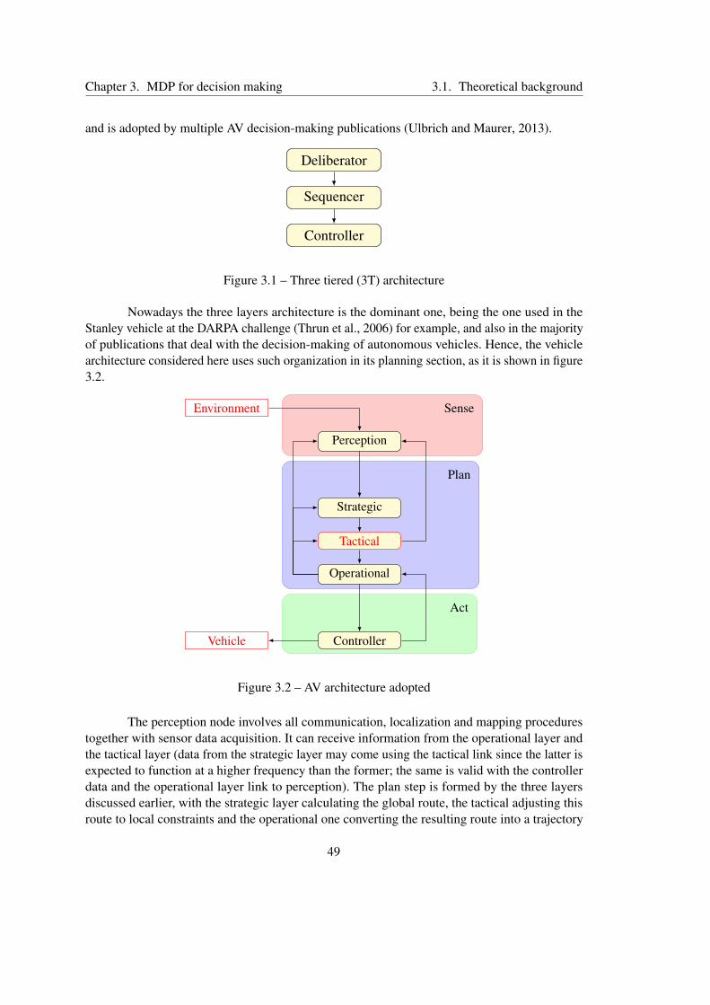
Chapter 3. MDP for decision making 3.1. Theoretical background
and is adopted by multiple AV decision-making publications (Ulbrich and Maurer, 2013).
Deliberator
Sequencer
Controller
Figure 3.1 – Three tiered (3T) architecture
Nowadays the three layers architecture is the dominant one, being the one used in theStanley vehicle at the DARPA challenge (Thrun et al., 2006) for example, and also in the majorityof publications that deal with the decision-making of autonomous vehicles. Hence, the vehiclearchitecture considered here uses such organization in its planning section, as it is shown in figure3.2.
Environment Sense
Perception
Plan
Strategic
Tactical
Operational
Act
ControllerVehicle
Figure 3.2 – AV architecture adopted
The perception node involves all communication, localization and mapping procedurestogether with sensor data acquisition. It can receive information from the operational layer andthe tactical layer (data from the strategic layer may come using the tactical link since the latter isexpected to function at a higher frequency than the former; the same is valid with the controllerdata and the operational layer link to perception). The plan step is formed by the three layersdiscussed earlier, with the strategic layer calculating the global route, the tactical adjusting thisroute to local constraints and the operational one converting the resulting route into a trajectory
49
Chapter 3. MDP for decision making 3.1. Theoretical background
for the controller. The proposed architecture works according to the hybrid approach, since thesense plan act structure is respected, but the tactical and operational layers are not limited by thestrategy layer in their capacity to react to external stimuli.
The discussion in the next sections and next chapters will focus mostly in the tacticallayer, considering the operational layer and the controller component only to explain how theimplementation was done to allow the simulation of the entire system. An a priori route willbe considered as given, and the perception component will be short-circuited by the simulationsupervisor that can detect the configuration of every agent at any time.
3.1.2 Markov Decision Process
About the MDP choice
As it can be seen in the chapter 2, specifically in the section that presents the state of theart for decision-making, two main types of algorithms are used to give a robot, or in our casea vehicle, the capacity to function without supervision and in a flexible way, so as to deal withuncertainties and variations of environment parameters that are common in dynamic scenarios.One is the Markov-based algorithms and another is the deep learning (DL) based methods. Bothhave advantages and inconveniences, but one of them cannot, at least not currently, does not havesome essential properties to be used as a decision-making model for AVs.
To model the deliberation process, in normal and ethical situations, a Markov decisionprocess will be proposed in the rest of this chapter. This was done because this method offers awell defined theoretic framework to deal with uncertainty into action selection and also because ithas tree main characteristics that deep learning does not have (Barredo Arrieta et al., 2020):
• Comprehensability: The ability to represent its learned knowledge in some repre-sentation that is understandable by humans.
• Explainability: The ability to explain in human terms why a decision was taken.
• Transparency: If the model is understandable (there are different levels of trans-parency)a.
aThe important point is that deep learning methods are not transparent, the discussion about differentlevels of transparency is left to Barredo Arrieta et al., 2020
Given that every single decision made by an AV needs to be verified and validated, thethree characteristics are essential, because not only one must be able to explain why an AV didwhat it did. It is also necessary to be certain concerning the limits of operation and which reactions
50

Chapter 3. MDP for decision making 3.1. Theoretical background
might occur in extreme situations, mechanically and ethically to be able to define when dilemmasituations might occur or not; for example, for MDP it is possible to verify the convergence of itspolicy calculation, which theoretically is not possible with DL methods.
And the point of this document is to propose methods of ethical deliberation inspired inethical theories, it is more coherent to do it in an understandable fashion. Of course, this does notmean that any type of ethical oriented decision-making using deep learning is possible, nor that itshould not be researched and implemented, just that considering the points made previously thiswas not the choice made here.
MDP definition
A Markov decision process (MDP) is a stochastic process that has the Markov property,i.e., that is memoryless and that assigns values, positive or negative, to state transitions, accordingto the desirability of such transition (Garcia and Rachelson, 2013).
Definition 1 Markov PropertyLet X(t), t ≥ 0 be a stochastic process defined on a measure space (Ω,F ,P), with Ω
being the sample space, F being the σ -algebra of Ω and P the probability measure on F .X(t), t ≥ 0 is a Markov process if:
P( X( tn+1 ∈ F ) | X(tn), ...,X(t0) ) = P( X( tn+1 ∈ F) | X(tn) ) (3.1)
The 5-tuple (S,A,T,R,γ) defines an MDP. What each component represents is detailedbelow:
Components of an MDP
• State space (si ∈ S): represents all possible process configurations.
• Action set (ai ∈ A): represents the set of all possible actions available; triggers thetransition from one state to another.
• Transition probability (T): represents the probability whether, given a state, execut-ing an action takes the process to some state; formulated as p(st+1|st ,at).
• Reward function (R): quantifies how good or bad the transition to another state wasaccording to a defined criteria.
• Discount constant (γ): represents the factor used to adjust the utility at a timet +n, n ∈ [0,∞] to the present (time t); defined as γ ∈ [0,1].
51

Chapter 3. MDP for decision making 3.1. Theoretical background
What makes an MDP a rather popular method to model stochastic processes is theability to expand on the capacities from a usual Markov chain and add uncertainty into thetransition between states. Figure 3.3 illustrates an MDP with three possible states and two actions.From the state s0, if the action a0 is executed, there is a probability of ptn(s1 | s0, a0) thatthe process at tn+1 will be at the state s1 and ptn(s2 | s0, a0) that it will instead be in s2, withptn(s2 | s0, a0)+ ptn(s1 | s0, a0) = 1.
The reward depends on the current state, the chosen action and the final state. If,from s0, the action a0 is chosen and the process ends up in state s2 the reward would bertn(s0, a0, s2). The expected reward from state s0 and action a0 can be calculated as rtn(s0,a0) =
∑i∈S′(s0) ptn(i | s0 ,a0) · rtn(s0, a0, i), with S′(s0) being the set of possible next states from s0.
tn tn+1
(a)
ptn(s2 | s0, a0)
rtn(s0, a0, s2)
(b)
ptn(s1 | s0, a1)
rtn(s0, a1, s1)
s0
s1
s2
a0
a1
ptn(s1 | s0, a0)
rtn(s0,a0,s1)
(a)
ptn(s2 | s0, a1)
rtn(s0,a1,s2)
(b)
Figure 3.3 – Simplified example of an MDP
The output of an MDP is a policy, a data structure that encloses multiple decision rules,one for each time epoch. Each one of these decision rules give, for each state, the optimal actionto be executed according to the transition probabilities and the reward function chosen (Puterman,1994c). A policy usually is represented by the greek letter π . The decision rules can be Markov-based (the input is the current state) or history-based (the input is a series of past states and actions)and they can also be deterministic (one input gives one action) or stochastic (one input givesa distribution of possible actions). Equation 3.2 shows a policy based in Markov-deterministicdecision rules.
π = (dt(st),dt+1(st+1), ...,dN−1(st+1)) (3.2)
There are multiple criteria to select which action should be executed at each state totransfer the process to another state, supposedly closer to the objective. The criteria that willbe used for the rest of this document is the discounted reward criteria, which uses a discount
52

Chapter 3. MDP for decision making 3.1. Theoretical background
factor to scale down the influence of future rewards into the current decision. This constant alsoallows the convergence of the value function in infinite horizon MDPs. Solving an MDP meansobtaining a policy that has the best reward throughout the entire execution, based on the currenttransition and all the future transitions that the process might choose. Equation 3.3 defines thevalue function, that evaluates the total amount of reward that a policy produces, and equations 3.4show how to calculate the optimal policy can be determined.
V π(st) = E
[∞
∑t=0
γtrt(st ,at) | s0
](3.3)
V ∗(st) = maxa ∈ A E [∑∞
t=0 γ trt(st ,at) | s0]
π∗ ∈ argmaxπ∈ΠHS V π(st)(3.4)
The calculated optimal policy in 3.4 was considered to be the most general possible,having the history-based stochastic type (HS). However, Markov-based deterministic policiesare easier to calculate. The proposition 1 shows that for each history-based stochastic policythere exist a Markov-based stochastic (MS) one with equal value function1, hence allowing theconsideration of a Markov-based stochastic policy as a solution.
Proposition 1 Equivalence of history and Markov based policies:Let π ∈ ΠHS be a stochastic history-based policy; for each initial state there exists aMarkov-based stochastic policy π
′ ∈ΠMS such that:
V π′
γ (s) =V πγ (s) (3.5)
To further verify that the optimal policy can be obtained using a deterministic policy, firstthe optimal equation needs to be determined. An infinite horizon will be considered, since thesimplification for finite horizon can be easily done. The following simplification assumptionswill be adopted:
MDP Optimality Assumptions
• Rewards and transition probabilities are stationary: they do not vary according totime.
• Rewards are bounded: |r(s,a)| ≤M < ∞.
• The state space is discrete.
1The proof of this proposition can be found in Garcia and Rachelson, 2013 or Puterman, 1994b.
53

Chapter 3. MDP for decision making 3.1. Theoretical background
Since rewards and transition probabilities are stationary through time, then the pol-icy itself can be considered stationary, i.e. being composed by only one decision rule, π =(d(st),d(st+1), ...,d(st+1)). All these assumptions are valid regarding the implementation dis-cussed in this and the next chapters. Then, the optimal value equation for infinite horizon MDPsis defined by equation 3.6, called Bellman equation.
V (s) = maxa ∈ A
[r(s,a)+ γ ∑
s j∈Sp(s j | s,a)V (s j)
](3.6)
Transforming equation 3.6 into the vector form the operator L on V can be defined, asshown in equation 3.7 , for ∀π ∈ ΠMS.
LV = maxπ ∈ ΠMS
(rπ + γPπV ) (3.7)
From it the proposition 2 can be established2, stating the equivalence between determin-istic and stochastic policies under the previous assumptions. The space V refers to the space ofall functions V : S → R.
Proposition 2 Equivalence between stochastic and deterministic policies:For all V ∈ V and 0≤ γ ≤ 1
maxπ ∈ ΠMD
(rπ + γPπV ) = maxπ ∈ ΠMS
(rπ + γPπV ) (3.8)
Finally, from the stationary equivalent policy, it is only necessary to prove the existenceof an optimal policy. For that, the next theorem ,13 establishes the existence and uniqueness of anoptimal solution for the Bellman equation, while theorem 24 shows that there is a optimal policyπ∗ connected to such V ∗.
Theorem 1 Existence and uniqueness of Bellman equation solutionIf V = LV , for V ∈ V , then V = V ∗ and is the only optimal solution for the Bellmanequation.
2Proof found in Puterman, 1994a; the proof of this proposition is done during the proof of theorem 1.3The proof of existence can be found in Puterman, 1994a, and of uniqueness in Garcia and Rachelson, 2013.4Proof found in Garcia and Rachelson, 2013.
54
Chapter 3. MDP for decision making 3.2. AV decision-making model
Theorem 2 Existence of optimal policyFor γ < 1:
• π∗ ∈ ΠMS is an optimal policy⇔ V π∗ is a solution of V = LV and V π∗ =V ∗
• Any stationary policy π∗ ∈ argmaxπ∈ΠHA rπ + γPπV ∗ is an optimal policy.
Then, under the conditions assumed earlier, an MDP has a unique optimal value solutionand an optimal policy connected to it. How to determine such policy will be discussed insubsection 3.3.1.
3.2 AV decision-making model
In this section the physical model of the AV will be detailed, together with the definitionof the state set and action set (subsection 3.2.1), the transition probability function (subsection3.2.2) and the reward function (subsection 3.2.3).
3.2.1 State and action sets
State Set
Unlike many MDP (or POMDP) implementations that consider the state as the descriptorof the environment including other road users’ configuration together with the AV’s configurationas the state, the definition used here only includes the AV configuration, as seen in 3.9. All otherroad users are considered through their interaction with the AV in the reward function. The stateis composed by the AV’s middle rear-axis point coordinates (x,y), direction θ , scalar velocity vand steering angle φ .
st = [xt ,yt ,θt ,vt ,φt ] (3.9)
For the AV’s model, a non-holonomic single-track vehicle model without slippage waschosen, as it can be seen in figure 3.4. The correspondent model, using front-wheel driving, isgiven by equation 3.10.
55

Chapter 3. MDP for decision making 3.2. AV decision-making model
~x
~y
~z
G
(x,y)
l~vφ
θ
Figure 3.4 – AV’s kinematic model
xt+1 = vt cosθt cosφt
yt+1 = vt sinθt cosφt
θt+1 = vtl sinφt
vt+1 = at,1
φt+1 = at,2
(3.10)
Action set
Both acceleration and steering angle rate of change are defined as discrete actions for theMDP (3.11). The action set is then defined as the set of pairings considering the possible valuesfor v and φ (values are presented in table 3.1).
at = (vt , φt) (3.11)
State space discovery
Using this finite number of actions, the state space can be determined expanding theinitial state during N transitions using the vehicle model given by 3.10 and each action. Eachtransition is defined to last ∆ttrans. Such expansion is clearly exponential, requiring a limitednumber of transitions to form the state space for the problem. All actions were used at each stateto generate possible next states. Considering Na as the number of possible actions (i.e. size of A),equation 3.12 gives the total number of states. The state space discovery produces a tree of states,
56

Chapter 3. MDP for decision making 3.2. AV decision-making model
with each level corresponding to a specific time epoch and the leafs being the terminal states.
Ns =N
∑i=0
Nia (3.12)
During the propagation of states, each one is checked if it remains in the bounds of theenvironment being simulated. If it is outside, then for this specific state the action chosen is notused and the state is removed from the tree. Another criteria to eliminate possible states is themechanical limit for the steering angle of the AV. It the current state already achieve the maximumangle, then all actions that increase this angle are discarded. The same is valid for null or negativevelocities coupled with actions with negative acceleration, since velocities smaller than zero arenot considered in this implementation.
Figure 3.5 depicts an example of how the state space discovery is done for an hypotheticalMDP with 2 transition and 3 possible actions. Stating from s0, the states s4, s5, s6 and the onesthat remain to be discovered from s1 and s2 are the terminal states of this process.
Time Epoch ts0
Time Epoch t +1s1 s2 s3
Time Epoch t +2s4 s5 s6 · · · · · ·
a0 a1 a2
a0 a1 a2
Figure 3.5 – Example of state space discovery
All constants that concern the state space discovery used in the implementation discussedhere are displayed in table 3.1.
3.2.2 Transition function
The main source of uncertainty in planning for AVs comes from other road users’ behaviorestimation. Since this knowledge is considered to be known during the planning (hence it isalso why the state is defined entirely by the AV’s configuration) the only source of uncertainty
57

Chapter 3. MDP for decision making 3.2. AV decision-making model
Table 3.1 – Parameters used in the state space discovery
Parameter Possible values
v(m/s2) −1,0,1φ(/s) −40,−20,0,20,40
∆ttrans(s) 0.5N (number of transitions) 4
Na (number of actions) 15
becomes the imprecision due to the vehicle model considered. The transition probability wasdefined using the steering angle rate of change, i.e. there are no uncertainty concerning changesin velocity.
In each set of actions with equal acceleration, the chosen action will have a probability of0.8 of being successful, meaning that for state s0, in figure 3.6, the action a3 takes AV to s4 withprobability of 0.8 and to s3 or s5 with probability of 0.1 each. For example, if a3 = (−20,−1),there is an 0.8 probability that the next state will be the correct one, given the model equationsand the current state, 0.1 probability that the process ends up in the next state from (−40,−1) and0.1 that it will arrive in the state from (0,−1). In cases when only one neighbor exists, notablywhen the steering angle is at its mechanical limit, then the transition probabilities become 0.9/0.1(action a0).
s0
s1 s2 s3 s4 s5
a0
0.9 0.1
a3
0.1 0.8 0.1
Figure 3.6 – State transition uncertainty for a0 and a3
The choice of parameters for the transition probability was made arbitrarily. A possibletire slippage, that is not modeled by the single track model presented in figure 3.4, is representedby the incertitude in the AV’s steering angle rate of change with values (0.1 and 0.8) inspired byMDP grid-like applications that are frequently used as an example of Markov processes. Suchdefinition is enough to display the entire AV’s behavior but it is without saying that for a realapplication some form to calculate this probability, including the uncertainty of the other roadusers’ behavior, is necessary (and it will be presented in chapter 5).
58

Chapter 3. MDP for decision making 3.2. AV decision-making model
3.2.3 Reward function
The reward function indicates to the system which actions are preferable in regards toachieve a certain goal. It is based on two parameters: performance (sperf) and action consequences(sconseq), as given by equation 3.13.
R(st ,at ,st+1) = sperf + sconseq (3.13)
Performance term
Performance for the vehicle is measured as lateral distance to the strategic path, directionoffset and time to arrival at goal point. Equation 3.14 calculates the reward using three variables:qlat represents the lateral distance to the trajectory, ∆θ is the offset angle between the direction ofthe AV and the trajectory and qeta represents the approximated time of arrival (ETA).
sperf = wlat ·qlat +wdir ·∆θ +weta ·qeta (3.14)
Both variables qlat and qeat are actually offsets from the real lateral distance (dlat) and theapproximated time to arrival (teta), as equations 3.15 and 3.16 show. For the lateral distance, sincethe ideal is that dlat = 0, the constant rlat sets the reward of this ideal situation. The same idea isapplied with reta, where it represents the maximum allowed ETA before qeta becomes a cost (bothwlat and weta are positive).
qlat = rlat−dlat (3.15)
qeta = teta− reta (3.16)
This approximated ETA is calculated using the projection of the AV’s velocity ontothe direction of the distance between the front axis middle point (pppav
fr ) and the trajectory goal(equation 3.17). More details about how this projection is done will be presented by equation3.21. It is an hypothetical measure, since the vehicle does not necessarily has the same directionthan this distance vector, but is enough to capture some idea of how much time it will take toarrive at the goal given the current speed and direction.
teta =dobj
vproj(dobj)av
(3.17)
59

Chapter 3. MDP for decision making 3.2. AV decision-making model
If the AV has a velocity equal to zero, then equation 3.14 is replaced by a fixed cost ceta.The weights wlat , wdir, weta together with the constants rlat and reta are calibrated heuristically,enabling the AV to arrive at its goal following a trajectory given by the strategic layer of the AV.Since the strategic layer is not of concern here, the trajectory comes from the simulation’s inputand is the same throughout the execution.
pppavfr
dobj
vproj(dobj)av
*
vavθav
dlat
Figure 3.7 – Performance reward parameters
Action consequences term
The action consequences score is measured by two parameters, adherence to the trafficcode (straf) and proximity to other road users (sprox), as equation 3.18 indicates. The values strafand sprox can assume negative values or 0, with the latter approximately 10 times lower than theformer. This difference is necessary since sprox has two functions: evaluate how close the AV isfrom other road users and detect collisions; if no collisions are detected the term straf must alwaysprevail in case of traffic code violation. In case of a collision, as said before, the entire rewardfunction (equation 3.13) is replaces by a negative constant costs.
sconseq = straf +i<Nag
∑i=1
sav,ruiprox (3.18)
However, traffic code violations are not considered to be constitutive of a dilemmasituation event. If, for example, there is one action that violated the traffic code and all others endup in collisions, then the AV will execute the action that violates traffic code to avoid the accident.The objective of this implementation is to focus in unavoidable collisions, not in the ethical andlegal question of a possible trade-off between code violation and possible accidents. A cascade of
60

Chapter 3. MDP for decision making 3.2. AV decision-making model
if-elses emulates some traffic rules into the AV’s decision process by adding the resulting costs. Ifno infringement is detected, straf = 0.
If the AV’s velocity surpasses the legal limit, then the cost cvel is added to straf = 0, but ifthe acceleration is negative, then racc is also added, to favor actions that decrease the velocity inthis context. Five points are considered to analyze a possible AV intrusion in the opposite lane orin the sidewalk: its four corners and the rear axis middle point. If two of these points are in theopposite lane, then straf = straf +2 · coplane (if it is inside the sidewalk and the opposite lane thecost accumulate).
Traffic code evalutation
• Velocity above limit: add the cost cvel to reward.
• AV in opposite lane: add the cost coplane to reward for each point in the oppositelane.
• AV in the sidewalk: add the cost csidewalk to reward for each point in the sidewalk.
To ascertain if the AV is too close to another road user, a minimal distance frontier isdefined in figure 3.8. These security zones are the spaces between the vehicle’s body and thered lines. All positions, orientations and velocities used to evaluate these parameters correspondto the time epoch t, the same as the current state (unless it is said otherwise). These frontiersrepresent an implicit risk measure for the reward function, since their role is to verify if breakingwhile maintaining the same direction is still a valid collision avoidance strategy for this state andaction and if it is not, the action’s reward is negatively impacted.
Frontalzone
Right zone
Left zone
Rearzone dw
dl
dl
dbr d f r
Figure 3.8 – AV with all the proximity limits
The region around the vehicle are divided in front, left, right and back. The front isdefined as the region inside the frontal cone, delimited by the lines formed by the two frontal
61

Chapter 3. MDP for decision making 3.2. AV decision-making model
rectangle’s corners and the frontal axis middle point (blue lines in figure 3.8). The left zoneis defined by the two left corners and the frontal axis middle point; the right zone is definedanalogously, while the rear zone is defined by the rear cone. The frontier checked depends onwith region the closest road user corner is. If it is inside the frontal zone, then the frontier definedby dfr +dbr will be used to verify it there is a potential dangerous situation, while is it is in one ofthe lateral zones, dl is used. No frontier in the rear is defined.
Lateral frontiers are placed at a distance equal to dl from the AV’s body (dw). Equation3.19 gives the calculation of the dl , with all parameters corresponding to the current time epocht. This variable takes into account the lateral security distance dsecl , that is a static input of thesimulation, and the lateral displacement of the other road user during t and t +1, evaluated by∆ttrans · ‖~v
proj(θ⊥av)ru ‖. To calculate this displacement, the velocity of the other road user is projected
perpendicularly to the AV’s direction (equations 3.20 and 3.21), this last defined by 3.22.
dl = ∆ttrans · ‖~vproj(θ⊥av)ru ‖+dsecl (3.19)
~vproj(θ⊥av)ru = ~vru − vproj(θav)
ru (3.20)
vproj(θav)ru = θav · ~vru (3.21)
θav = [cos(θav), sin(θav)] (3.22)
The frontal limit is given by dfr plus dbr, the breaking distance given vav (the AV’s velocityat t) and calculated by equation 3.24. The distance dfr, as dl did, also takes into account thedisplacement of other road users during ∆ttrans, but now using the term ∆ttrans · vproj(θav)
ru to do so,with the velocity calculated previously by equation 3.21. The constant dsec f is the frontal securitydistance, similar to the previous dsecl , while the deceleration constant vbreak is also a static inputof the simulation.
dfr =−∆ttrans · vproj(θav)ru +dsec f (3.23)
dbr =12(vav)
2
vbreak(3.24)
It is assumed as an hypothesis that if an emergency breaking happens the AV will continueat the same direction (φt = 0), thus no term related to the change in direction is necessary inequations 3.19 and 3.23. The behavior of the other road user in the calculation of these equationis that it will continue in the same direction, with the same velocity.
If a road user is predicted to remain outside the security frontiers, then sav,ruiprox = 0;
otherwise the correspondent score becomes a cost, calculated by equation 3.25. To check this
62

Chapter 3. MDP for decision making 3.2. AV decision-making model
condition the position of the road user at t +1 is used. In equation 3.25 there is a static cost, cst ,to punish the next state due to a frontier violation, a static weight wv, defined heuristically and thedifference of velocity variations.
sav,ruiprox = cst +wv ·
[(vproj(dt+1)
rui,t+1 − vproj(dt+1)avt+1
)−(
vproj(dt)rui,t − vproj(dt)
avt
)](3.25)
Each of the difference of velocities refers to a time epoch. Defining the distance vectorbetween the AV and the considered road user (RUi) as the vector from the AV’s front axis middlepoint (pppav
fr ) to the closest corner of the road user’s body, the difference of velocity refers to theprojection of each velocity onto this distance versor.
This measure shows if the AV is converging on (∆v negative) or diverging from (∆vpositive) the road user with the proposed action, while the weight wv (always negative) controlshow important it is to avoid a situation where the AV tends to cross other road user’s immediatedirection while being too close to it. The equation 3.21 is used to calculate the projected velocities,but with the distance versor (dt) instead of the AV’s direction versor. Figure 3.9 given an exampleof the evaluation procedure of this velocity variation for t +1.
dt+1
vavt+1
vproj(dt+1)avt+1 vrui,t+1
vproj(dt+1)rui,t+1
Figure 3.9 – Calculation of velocity projections
Collision detection
To detect collisions during a transition, each road user’s position (including the AV)is predicted ten times during a transition period ∆ttrans. Each road user (including the AV) isrepresented by a rectangle (pedestrians are particularly represented by squared), reflecting theirreal dimensions. This evaluation is done before the verification if the road user is too close to theAV, as it can be seen in the workflow presented by figure 3.10.
63

Chapter 3. MDP for decision making 3.2. AV decision-making model
Evaluate sprox
Compare AVwith RUi
Check if alreadyis in collision
Determine region
Check eq. 3.23 Check eq. 3.19
Inside?
Check collisionin transition
r(st ,at ,st+1) = ccolCalculate sav,ruiprox
sprox+ = sav,ruiprox
End
if i≤ Nru
no
yes
front
lateral
rear
sav,ruiprox = 0
no
yes
no
collision
i = i+1
if i > Nru
Figure 3.10 – Workflow for sprox calculation
In two moments the algorithm checks for collisions involving the AV: at the beginning ofthe procedure to evaluate sprox+= sav,rui
prox in equation 3.18, to determine if the AV already collidedand if the road user i is detected to be inside the safety frontier. In this last case, the collisionis checked during the transition. If it is detected, the algorithm stops and sets 3.18 to ccol. Twodifferent situations can be labeled as a collision, an intersection with the rectangle that representsthe other road user, or if the AV is out of the bounds of the environment being simulated. Thelimits of the state space are considered to be rectangular walls.
According to Gottschalk et al., 1996, one possible way to verify if two convex 2d-
64
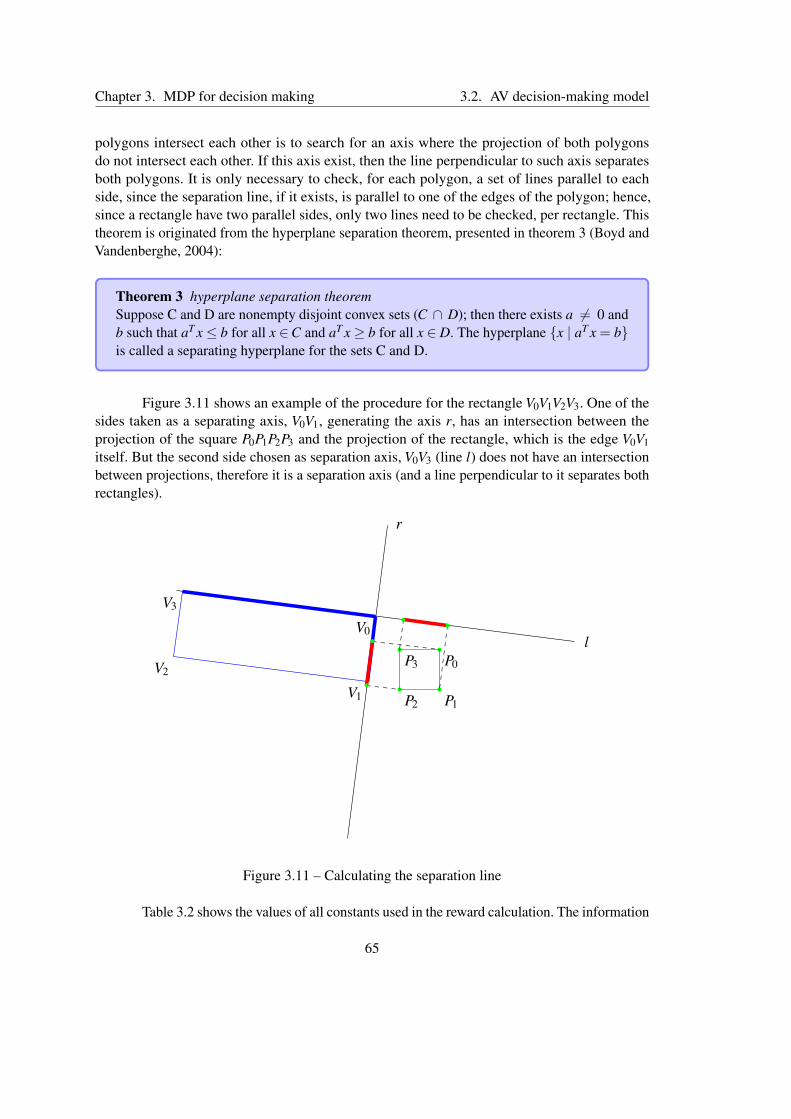
Chapter 3. MDP for decision making 3.2. AV decision-making model
polygons intersect each other is to search for an axis where the projection of both polygonsdo not intersect each other. If this axis exist, then the line perpendicular to such axis separatesboth polygons. It is only necessary to check, for each polygon, a set of lines parallel to eachside, since the separation line, if it exists, is parallel to one of the edges of the polygon; hence,since a rectangle have two parallel sides, only two lines need to be checked, per rectangle. Thistheorem is originated from the hyperplane separation theorem, presented in theorem 3 (Boyd andVandenberghe, 2004):
Theorem 3 hyperplane separation theoremSuppose C and D are nonempty disjoint convex sets (C ∩ D); then there exists a 6= 0 andb such that aT x≤ b for all x ∈C and aT x≥ b for all x ∈ D. The hyperplane x | aT x = bis called a separating hyperplane for the sets C and D.
Figure 3.11 shows an example of the procedure for the rectangle V0V1V2V3. One of thesides taken as a separating axis, V0V1, generating the axis r, has an intersection between theprojection of the square P0P1P2P3 and the projection of the rectangle, which is the edge V0V1itself. But the second side chosen as separation axis, V0V3 (line l) does not have an intersectionbetween projections, therefore it is a separation axis (and a line perpendicular to it separates bothrectangles).
V0
V1
V2
V3
P0
P1P2
P3
l
r
Figure 3.11 – Calculating the separation line
Table 3.2 shows the values of all constants used in the reward calculation. The information
65

Chapter 3. MDP for decision making 3.3. Results and discussion
about the parameters for the AV (mass, acceleration, etc.) and for the other road users in thesimulation will be given in the next section.
Table 3.2 – MDP parameters used
Parameter Value Parameter Value Parameter Value
wlat 60 wθ −50 weta −35rlat 10 reta 30 ceta −1250cvel −1000 racc 750 coplane −50
csidewalk −1500 wv 30 dsec f 5mdsecl 0.5m ∆ttrans 0.5s cst −1000ccol −15000 γ 0.9
In the proposed implementation the γ value was arbitrarily set to 0.9, given that onlyfour transitions are chosen and that the current AV needs to stay aware of future collisions andtransgressions. A lower γ might dampened the costs given to collisions. As for the other constants,they impact the reward and consequently the behavior of the AV in the following manner:
• The parameters related to the proximity term of the reward (cst , wv and ccol) should have ahighly punitive nature to the vehicle with no possibility of generating a positive reward.The decision if it should be calculated is controlled by the frontier around the AV (dsecl ,dsec f ).
• The parameters related to traffic code violations (cvel, racc, coplane and csidewalk) have asimilar nature but they are always verified.
• The parameters related to the performance have the possibility to produce positive re-wards, which are controlled in value by the constants rlat and reta. The cost of not drivingis expressed by ceta. How important each of the parameters related to lateral distance,direction offset and estimated time of arrival is defined by the three weights wlat, wθ , weta,respectively.
3.3 Results and discussion
3.3.1 Value iteration
The output of a MDP algorithm is a policy π∗ which, for each state, yields the optimalaction to be executed, as discussed in section 3.1. It was already determined that this optimal
66

Chapter 3. MDP for decision making 3.3. Results and discussion
policy is Markov-based, deterministic and that it exists. The only remaining piece of the puzzle isa tool to calculate it given an MDP formulation with the assumptions declared before.
V ∗(s) = maxa ∈ A
[r(s,a)+ γ ∑
s j∈Sp(s j | s,a)V (s j)
](3.26)
Equation 3.26 needs to be solved to obtain the policy. There are many ways to solve aBellman equation, but the one adopted here will be the value iteration, where in each iteration thevalue for all states is calculated, until an equilibrium is reached. At this point the value functionwith the selected actions will be the solution, and the optimal policy can be determined by theactions that produced such values (Garcia and Rachelson, 2013). This algorithm is shown in 1.
At each iteration the mean squared error of the difference between each value calculationfor every state is calculated. Such iteration can also be represented using the L operator, as isin equation 3.27. The algorithm is stopped if the calculated error becomes smaller than ε = 0.5(defined heuristically) and the current value iteration is then used by equation 3.28 to obtain thepolicy.
V t+1 = LV t (3.27)
Algorithm 1 convergence is verified by theorem 4 in Puterman, 1994a.
Theorem 4 Optimal solution via value iterationLet V ∈ V , ε > 0 and let V t satisfy 3.27 for n≥ 1; then:
1. V t converges in norm to V ∗
2. The stationary policy defined in equation 3.28 is ε-optimal
67

Chapter 3. MDP for decision making 3.3. Results and discussion
Algorithm 1: Value IterationData: Spaces S and A, functions R and P, constant γ , environment data eResult: Policy π∗(s), Optimal Value V t(s)
1 t = 02 do3 for every si ∈ S do4 V t+1(si) = maxa∈A
[R(si,a,s′,e)+ γ ·∑s′j P(s′j|si,a)V t(s′j)
]5 t = t +16 end7 while MSE(V t+1−V t)> ε
8 for every si ∈ S do9
π∗(si) = argmax
a∈AV t(si) (3.28)
10 end
3.3.2 Simulation
Configuration
Using the WeBots simulator (Michel, 2004), the aforementioned algorithm was tested inthe scenario shown by figure 3.12. A real depiction of the simulation environment is shown infigure 3.13. While the AV is traveling in its lane, two pedestrians, P1 and P2 suddenly cross intothe street (both start moving at tsimul = 4s). Every behavior from other road users are consideredto be known; for example, the other vehicle’s behavior is assumed to be the will to cruise theentirety of the straight road with 10m/s. For the two pedestrians, before they start moving the AVconsider that they will remain stopped. When they start moving, then the AV assumes that theywill cross the road.
All MDP parameters and the physical information of road users’ are shown in table 3.3.
Vehicle control
The obtained policy is used as a one shot fashion. Since the state space has a tree structure,from the current state to all other possible ones, with a fixed number of layers (which is equalto four in this implementation), the policy has the same structure, with an action for each state.Hence, starting from the root, one can determine the sequence of action that should be executed.
68

Chapter 3. MDP for decision making 3.3. Results and discussion
(2,3.25,0,0,0)
AV (100,6.75,π,10)
VEH
(22.5,1.5, π
2 ,1)
P1
(25,0, π
2 ,1)
P2
Figure 3.12 – Initial simulation setup (other road users’ configuration is represented by (x,y,θ ,v),not in scale)
Figure 3.13 – Simulation environment
It is this sequence of actions that is used to command the AV.
Every action sequence originated from a policy is used during one second, consideringthat the four transitions can plan the trajectory for two seconds. After this period the MDP isre-initiated, with a different state space, given that the position of the AV changed, and a newpolicy originates another trajectory. The reason why this two transition buffer is necessary will bemade clear in the next chapter, but it can be said that the AV, at the end of the policy execution,
69

Chapter 3. MDP for decision making 3.3. Results and discussion
Table 3.3 – Road users’ physical properties
AV Pedestrian Vehicle
Mass (kg) 2105+80 80 1065+80Width, Height (m) 4.853,1.65 0.625,0.625 3.475,1.310
Wheelbase (m) 2.933 − 2.55Acceleration (m/s2) 1 − 1Deceleration (m/s2) −7 − −7
Steering angle limits (°) 25 − 25
should be able to known that no collision is predicted before the policy recalculation. Suchjustification accounts for the need to keep one transition as buffer. As it will be explained insubsection 4, two actually need to be kept.
Inside the simulation the velocity of car-like objects are controlled by a cruising control,meaning that they decelerate and accelerate using a constant acceleration value. The steeringangle has a clear mechanical limit, as has its rate of change. For the pedestrians, a constantvelocity is used in its displacement, with the body’s articulation movements being controlled bythe simulator’s controller.
3.3.3 MDP policy results
The AV should not produce accidents or critical situations on its own. Varying the initialposition of the vehicle (xveh) and the velocity direction of one of the pedestrians (θped) relativeto figure 3.12, different AV behaviors can be observed, for this precise road configuration. Eachpolicy predicts two seconds ahead, with one second used for control ((v, φ) are directly fed intothe AV), before the policy being recalculated.
The AV needs at least two transitions to verify if the next action will not cause an accident,and that a state has actions which will not necessarily lead to a dilemma situation. And if itdoes, this fact needs to be signaled to the entire state space to propagate the high cost connectedto a collision to the respective states. It is because of this necessity to look ahead of time thatthe execution of a policy is limited to N−2 (N is given by table 3.1), before the recalculationof the policy. The weights of equations 3.14 and 3.25 were set heuristically to obtain a resultrepresentative of the MDP defined in section 3.2.3.
The first of the AV’s behavior plots shown in figure 3.14, for xveh = 100m is acceptable(but not ideal given that it should have stopped and waited the crossing), avoiding the pedestrianand returning to the other lane afterwards. All road user states are considered observable andknown, therefore at the beginning of a policy calculation the AV can assert correctly all its states
70

Chapter 3. MDP for decision making 3.3. Results and discussion
Figure 3.14 – AV’s behavior for xveh = 100, 80, 40m
and predict changes throughout the decision horizon. But since the AV only has the capacity topredict two seconds ahead of time, it starts the maneuver without knowing how it will end.
This can be seen more clearly in the second plot, for xveh = 80 when after the beginning ofthe maneuver, it reaches a critical situation and simply collides with the wall beyond the sidewalk(every limit of the environment is defined as a static wall). But if five transitions is used to planthe policy the collision is avoided, as it can be seen in figure 3.15. This is because, according tothe Y position graphic at figure 3.16 the vehicle under four transitions do not see clearly the othervehicle approaching and thus places himself ahead of the vehicle in the implementation with fivetransitions. The moment where collision becomes unavoidable is signaled by point 15, where theorientation for the first case takes a turn to the left, while in the second it turns to the right andaccelerates to return to its lane in time.
Adding one mode transition to the policy produces a viable trajectory, but increases thetotal calculation time from t = 60.1s to t = 802.4s, due to the exponential nature of the statespace discovery process.
Starting the other vehicle at xveh = 40m (third plot in figure 3.14) creates a situation inwhich the AV cannot execute the avoidance trajectory. It is perhaps intuitive for a human driver tostop and wait for the pedestrians, but here the AV only reduces its velocity at a certain point andcontinues to move until the path is clear. Even with five transitions (second plot in figure 3.15)
71

Chapter 3. MDP for decision making 3.3. Results and discussion
Figure 3.15 – AV’s behavior for xveh = 80,40m with 5 transitions
Figure 3.16 – AV’s velocity, direction and trajectory for xveh = 80m
the behavior is similar, meaning that it needs more transitions to receive the delayed reward fromthe future and understand that a stop and go behavior is the right one in this context (including inthe cases where it can use the opposite lane without ending up in an accident).
72

Chapter 3. MDP for decision making 3.3. Results and discussion
Some conclusions can be drawn from these three different situations:
I The decision-making horizon needs an appropriate length to anticipate short-termbehaviors from other road users. However, the exponential nature of the state spacediscovery process (subsection 3.2.1) must be avoided.
i One way to do this is to sample the most probable next states given a current stateand an action, focusing only on these discovered next states (as some POMDPsolvers do). In theory, considering a fixed transition function, if a bigger numberof transition were to be used, so as to only eliminate the states inside the decisionhorizon deemed not useful to the AV, the complexity of the resolution might bedecreased. However, the heaviest step to solve this MDP is the evaluation of thereward function, not the iteration in itself, and since it is the reward the indicatorof pertinence, this solution would not accomplish what is expected.
ii Another possible solution involves the inclusion of all other road users into thestate and to evaluate a transition probability function capable to identify the mostpertinent states, given the interaction between all users. This could break theexponential character of the problem if the actions of the AV were subjected tothe same treatment as the states of the other users, i.e. not all actions need to beconsidered, only the ones that somewhat optimize one transition.
II In reality the decision horizon is dependent of the AV’s velocity. If it increases toomuch the capacity to observe sufficiently ahead of time needs to increase, in the casethat transition time (∆ttrans) is fixed. One can see the beginning of this problem inthe situations commented above, but the real problematic becomes evident if oneconsiders high speed limits. Planning should occur in small steps of trajectory, evenmore since the trajectory planned is based on piece-wise linear segments. Withouta small enough transition time it is clear that the maneuver capability of the AVdecreases rapidly.
III Risk evaluation is also necessary to stop the AV from starting a maneuver that cannotbe completed in one policy, as it was done in figure 3.14. Defining the state spacewithout a fixed number of transitions and using the end of a maneuver as a sign ofpolicy termination would allow the AV to start and end in low-risk states.
Changing the direction of the first pedestrian from π
2 rad to 3π
4 rad creates a differentsituation, but the results obtained are similar. Figure 3.17 shows the trajectory at xveh = 100 mand 40 m and figure 3.18 at xveh = 40 m for five transitions.
In comparison with figure 3.14, figure 3.17 produces similar behavior, where an additionaltransition allows the AV to avoid an accident. For xveh = 40 and 5 transitions, it makes the AVchoose to accelerate to avoid an accident, which in turn causes it to invade the sidewalk. With
73

Chapter 3. MDP for decision making 3.4. Conclusion
Figure 3.17 – AV’s behavior for xveh = 100, 40m and θped = 3π
4 rad
Figure 3.18 – Trajectory for xveh=40m, θped= 3π
4 rad for 5 transitions
only four transitions the collision cost was not detected, only the sidewalk invasion cost is, whichfix the future outcome to a collision with the environment’s border.
Another critical point in the implementation is the weights used for the reward function.All the considered weights and constants were defined heuristically for the specific use caseconsidered. Even so, the best values obtained still do not reproduce an ideal trajectory, whichcan be seen in figure 3.14 between [5,15] at the X axis. The small but perceptible change in AV’sdirection, an oscillation in its direction, is not illegal but rather pointless.
3.4 Conclusion
This chapter analyzed an proposition of an MDP algorithm for the decision-making of anAV under normal situations. Before its definition, a discussion about which architecture is used inautomated vehicles in general was addressed and the question of why a Markov-based algorithmwas chosen instead of a deep-learning approach was also answered afterwards. After the MDPmodel was formally defined, from the necessary components to the existence and uniqueness
74

Chapter 3. MDP for decision making 3.4. Conclusion
of its resulting optimal policy to subsequently define all the particularities of the model for thisinstance.
The proposed algorithm was tested in a simulation environment, considering multipleconfigurations from other road users. It was observed that, for the heuristic weights chosenfor the reward function, the AV behaved correctly in most situations, but some problems wereflagrant. The exponential nature of the state set discovery did not allowed the use of an appropriatehorizon prediction to correctly account the behavior of the other road users with the AV’s velocityworsening this problem if the transition time is kept the same. No guarantee is done towards thefinalization of a maneuvers before the end of the prediction horizon, which demands at least arisk assessment to avoid terminating in an unsafe state.
75

Chapter 3. MDP for decision making 3.4. Conclusion
76

Chapter 4
Dilemma Deliberation
Contents4.1 Dilemma situations . . . . . . . . . . . . . . . . . . . . . . . . . . . . . . 78
4.2 The definition of harm . . . . . . . . . . . . . . . . . . . . . . . . . . . . . 79
4.2.1 ∆v for collision . . . . . . . . . . . . . . . . . . . . . . . . . . . . . 82
4.2.2 Vulnerability constant . . . . . . . . . . . . . . . . . . . . . . . . . 83
4.3 Ethical deliberation process . . . . . . . . . . . . . . . . . . . . . . . . . . 86
4.3.1 Ethical Valence Theory . . . . . . . . . . . . . . . . . . . . . . . . . 86
4.3.2 Ethical Optimization . . . . . . . . . . . . . . . . . . . . . . . . . . 90
4.3.3 Value iteration for dilemma scenarios . . . . . . . . . . . . . . . . . 94
4.4 Results and discussion . . . . . . . . . . . . . . . . . . . . . . . . . . . . . 98
4.4.1 Using EVT as ethical deliberation . . . . . . . . . . . . . . . . . . . 98
4.4.2 Using the Ethical Optimization profiles to deliberate . . . . . . . . . 102
4.5 Conclusion . . . . . . . . . . . . . . . . . . . . . . . . . . . . . . . . . . . 104
Up until now dilemma situations were not treated by the algorithm proposed in chapter3, even if when the collision was inevitable, notably the case in graphic 3.14. Two methods totreat such situation will be exposed in this chapter: the ethical valence theory (EVT), proposed byEvans et al., 2020 and the ethical optimization, proposed in de Moura et al., 2020. Both methodsuse to guide its decision the estimated harm that may happen in an accident, while the EVT alsouses the ethical valence with a deliberation procedure to choose the most appropriate action. Thischapter ends with the explanation about how the value iteration, used to obtain the MDP policy, ismodified to account for dilemma scenarios and a discussion about the results of both publications.
77

Chapter 4. Dilemma Deliberation 4.1. Dilemma situations
4.1 Dilemma situations
At each step of its trajectory, the AV should be able to tell whether a situation constitutesa dilemma worthy of moral consideration. This situational classification is necessary to determineif the AV must act according to ethical constraints or simply concrete objectives. Three rules canbe defined to represent the AV’s responsibilities towards the other road users in its environmentand its own passengers and they must be followed at all times. If one or more of these rulesare violated across all possible actions, this indicates that the non-dilemma portion of the AV’sdecision-making cannot cope with the consequences of all possible actions, and thus ethicaldeliberation is required for the AV to act in an acceptable way. Here harm is defined as thenegative consequences suffered by a human after some type of collision with another road user.
AV duties towards other road users
• The lives of the passenger(s) must not be put in harm’s way.
• The lives of the road users in the environment must not be put in harm’s way.
• Traffic regulations must be followed.
Interactions between road users and the AV are covered by the two first rules. If thegeometric representation of two road user (including the AV), during a transition, intercept eachother, a collision is considered to have occurred. As it was done in the last chapter, a safetyfrontier around the AV can be defined to discourage the execution of actions which would removethe possibility of breaking without swerving to avoid an accident. But even so the AV could beexposed to dilemma situation, since the main uncertainty source comes from the behavior ofthe other road users. The general risk of a dilemma can also be minimized with a conservativebehavior from the AV, however it can only go so far if it adopts a precautionary approach since italso must produce a performance capable to justify its existence.
There is a certain antagonism between the two first rules and the third one. One can askhimself if the former should take precedence over the other, so it is certainly desirable that the AVshould also be sensitive to the interplay between ethical and legal behavior. In this sense, whenthere is a conflict in dilemma situations between harm to humans on one hand, and adherenceto the traffic code on the other, the standard behavior adopted will be that the avoidance of theformer should take precedence. As such, the MDP algorithm must be defined so as to expressthis priority in ways independent from the influence of the temporal discount rate. However, afterthe transgression, the AV must return to a ‘safe’ state, guaranteeing that another collision doesnot arise as a direct consequence of its original action choice. If this is the case, then for theAV’s decision-making algorithm all actions, at the first moment, end in collision, considering theproposed policy calculations that will be presented in the next sections.
Make the AV conform to traffic laws by design is not a subject that is widely addressed in
78

Chapter 4. Dilemma Deliberation 4.2. The definition of harm
the literature. Generally, legal conformity presents challenges related to the interpretation of lawswhich can be vague, admit exceptions, or be internally incoherent; the resolution of all of whichmay demand some degree of common sense reasoning in order to be solved (Prakken, 2017).Additionally, with adherence to traffic laws comes the need to embed relatively abstract norms,used in laws to map concrete behavior, into an AV, and more broadly, into an autonomous system(Leenes and Lucivero, 2014). Some authors have already attempted to implement some portionsof various traffic codes — related to circulation and behavior — into an autonomous vehicle,such as Rizaldi et al., 2017 (German legislation). Categorically, these attempts have been madeusing logic-based approaches to emulate constraints, representing only the procedural demandswhich usually compose a traffic code.
Given these considerations, when the duty obliging traffic code adherence is adequatelydefined, the entirety of the given traffic code does not need to be exhaustively implemented. Tosimplify the implementation of this evaluation algorithm, a set of logical rules will represent theprocedural rules present in the specific scenario simulated. This set of rules should almost alwaysallow the AV to cruise in a lawful manner. Exceptions to the code and the resolution of conflictbetween rules will not be covered here, the latter being treated as an ethical decision (even ifideally the procedures to solve conflicts between rules present in traffic codes should be usedwhere possible).
For example, in a straight line domain, without pedestrian strips or semaphores, and witha solid double line the following logic rules can be used:
Simplification of traffic rules
• Do not cross over into the opposite lane.
• Do not drive onto the sidewalk.
• Do not surpass the speed limit.
This simplified rules are the same as the ones used in the last chapter to calculate thecost connection to traffic code infringement, in subsection 3.2.3. In a real implementation, wherethe AV should target full automation (level 4 or more) in specific and generic environments, theactual set of rules will be extended well beyond these three rules and include also the conciliationprocess between these rules.
4.2 The definition of harm
The purpose of considering ’harm’ in ethical deliberation is to measure the risk forAV passengers and other road users involved in a hypothetical collision. For decades, the main
79

Chapter 4. Dilemma Deliberation 4.2. The definition of harm
measurement variable to estimate this property has been the difference of velocity between thetwo implicated road users at the moment of collision (∆v) (Evans, 1994; Jurewicz et al., 2016;Martin and Wu, 2018; Hussain et al., 2019).
Most of the research conducted within the domain of vehicle collisions uses historicalaccident data to analyze the influence of ∆v in collisions. To quantify injury, two metrics arepopular: risk of fatality and the Abbreviated Injury Scale (AIS) (MacKenzie et al., 1985). Thelatter is preferred, since it is important to consider not only fatal collisions but those that caninflict severe damage (referred to as MAIS3+, which indicates that at least one injury in someregion of the body is above AIS3, a scale going from 0 to 6). In the European Union, this metricis used as standard to measure road accidents (Weijermars et al., 2018).
All ∆v used as thresholds for severe injuries are indicated in table 4.1, along with theirsource (typically, an injury is considered as ‘severe’ if it indicates a MAIS3+ injury probabilityof 10%1). For the pedestrian case, the value was obtained from Kröyer, 2015, which considerssevere injury as having an ISS (Injury Severity Score, defined as the squared sum of AIS for thethree most severely injured body regions) larger than 9, which is stricter than MAIS3+. Lateralcrashes are covered by near side (driver’s side) and far side (passenger’s side). For single vehiclecollisions, the same ∆v defined for collisions between vehicles is used.
Table 4.1 – ∆v threshold used for fatality collisions
Collision type Contact ∆v value Taken fromPedestrian collision - 6.94 m/s (Kröyer, 2015)
Vehicle collision
Frontal 7.78 m/s (Jurewicz et al., 2016)Rear 10.56 m/s (Jurewicz et al., 2016)
Near side 5.56 m/s (Jurewicz et al., 2016)Far side 6.39 m/s (Jurewicz et al., 2016)
The data presented in Jurewicz et al., 2016 was collected by the National HighwayTraffic Safety Administration (NHTSA), published in Bahouth et al., 2014, considering injuriesin the front seat, with a seat-belt, without rollover, with a passenger age ranging from 16 to55, involving passenger vehicles and heavy vehicles. In Kröger, 2016 the data comes from theSwedish STRADA database, possessing a complete registry of pedestrian collision between 2004and 2008.
This retrospective analysis of reported accidents has some drawbacks. According toRosén et al., 2011, the data may be biased, since it is only collected across a small set ofcountries. Also, in the pedestrian case, age is an important feature (Kröyer, 2015), therefore theage distribution in the studied population plays a role which is unaccounted for in the resultingcurve. Under-reporting of non-dilemma cases (Martin and Wu, 2018), estimation of collisionvelocities (Rosén et al., 2011), negligence of a vehicle’s mass and geometry (Martin and Wu,
1This is the threshold used by some automotive companies to define an unacceptable risk of collision.
80

Chapter 4. Dilemma Deliberation 4.2. The definition of harm
2018; Mizuno and Kajzer, 1999) and the use of different methodologies to evaluate AIS scores(Weijermars et al., 2018) also reduce the precision of such an approach.
Given that the previous method presents problems when applied to specific situations(despite it generalizing relatively well across a population), accounting for contextual informationis necessary. The collision interaction between vehicles can be approximated by a damper-spring-mass system, where the initial velocity of each vehicle is projected onto the axis nnn (normal tocontact plane between both vehicles) and ttt (tangential to contact plane). One example of suchapproach is Pickering et al., 2019, that uses a sprint bi-linear model to estimate the severityof a frontal collision might have if to avoid a pedestrian the AV needs to collide with a staticobject. The approach that will be considered here should be able to handle any specific situation,being capable to represent multiple collision configurations, from all frontal collisions types tovariations of lateral impacts.
The collision can be divided in two phases: the first is the compression, where thedeformation of each vehicle happens with the transfer of kinetic energy into to the deformationprocess, followed by the restitution, when the vehicles plastic deformation settles, and part of theenergy transferred to deformation returns as kinetic energy (Smit et al., 2019). Given the multiplepossible collision configurations and the objective of having an approximated measure of theseverity, an impact the point-mass collision approach will be adopted (Brach and Brach, 2011),with some simplifications, to model the interaction between road users and the AV in case ofcollision. The following simplification assumptions are adopted:
Collision mechanics simplificatory assumptions
1. No slidding during the collision (when the vehicle skid tangentially the other insteadof deform in the normal direction)
2. Dissipation forces are negligible.
3. Crash interface between vehicles is a point.
4. Duration of the crash is infinitesimal.
With the collision mechanics defined, one can start to reason what "harm" should repre-sent. This should refer to a single road user, during a collision. Thus, a plausible evaluation wouldbe h ∝ ~J, cvul , h representing the road user’s harm, J for the impulse applied during collisionand cvul for a measure of physical vulnerability, which will be explained in subsection 4.2.2.Considering the point-mass approach, the expression then becomes h ∝ ∆~p, cvul , resulting in theequation 4.1, for a road user k:
kh(st ,at ,s′t) =kcvul ·
(‖~v f − k~vi‖
)(4.1)
81

Chapter 4. Dilemma Deliberation 4.2. The definition of harm
The collision velocity is calculated using the conservation of linear momentum, that willbe explained in subsection 4.2.1. The variable v f , represents the collision velocity for both roadusers, k and l. The velocities l~vi and k~vi are measured at the imminence of impact for k and l.
4.2.1 ∆v for collision
To calculate the velocity after collision, v f , used in equation 4.1, both road users (k andl) are considered as punctual masses and all dissipation forces are neglected. From the originalequations of the momentum, given by 4.2 and 4.3 for each road user, which can be broughttogether in one single equation, 4.4, which represents the conservation of linear momentum. Themasses mk and ml correspond to the total mass of each road user (if it is a vehicle, then its massplus the passengers’ mass)
mkk~v f −mk
k~vi =kJ (4.2)
mll~v f −ml
l~vi =lJ =− kJ (4.3)
(mk
k~v f −mkk~vi
)+(
mll~v f −ml
l~vi
)= 0 (4.4)
Usually to solve the system of equations presented by equations 4.2 and 4.3 it is necessaryto "find" two more equations (six variables and only four equations, two for x component andtwo for the y component). Then comes the particular knowledge about the dynamics of collisionrestitution from the coefficient of restitution e and the impulse ratio µ , that is the relation betweenthe normal and tangential impulse (no relation to the friction coefficient, that frequently isrepresented by the same letter) (Brach and Brach, 2011).
Given that it is essential for the harm to estimate the danger that a collision might poseand that such collision can be represented roughly by a spring-mass system (dissipation forcesare negligible, so the presence of the damper is not necessary), it would be interesting to evaluatethe final velocity present at equation 4.1 in the moment of maximal acceleration, which is themost important information to measure injury for passengers/pedestrians. This moment is theend of the compression phase, when the vehicles compose a single structure, right before therestitution takes place and separates them. Thus, this final velocity can be considered equal forboth vehicles, giving the following equation:
(mk
k~vi +mll~vi
)= (mk +mk) ·~v f (4.5)
82

Chapter 4. Dilemma Deliberation 4.2. The definition of harm
With equation 4.5 it is finally possible to calculate the final velocity for each road user~v f
used in the harm equation 4.1, without any particular specificity about the vehicle body properties.For collisions with pedestrians, it is considered that the pedestrian’s~v f is equal to the AV’s~vi,which implicitly means that the linear momentum of the pedestrian is negligible in comparisonwith a vehicle, given the difference in mass, approximately by a factor of 10 and the difference ofvelocity, that can also reach a factor of 10. Thus, the AV’s velocity variation due to the collisioncan be neglected, and its harm is equal to zero.
This simplification was adopted considering that the most common variables used topredict injury for pedestrians, according to the current research about collisions between pedestri-ans and vehicles, are the type of vehicle involved (Mizuno and Kajzer, 1999), specially due tothe height of bonnet leading edge, parameter that can explain why SUVs are more dangerous topedestrians than other vehicle types and the mass of the entire vehicle which usually is biggerthan the average due to its size (Malczyk et al., 2012; Simms and Wood, 2006), along withthe impact velocity. Therefore, this danger that is not captured by the velocity is the focus ofanother parameter, which accounts for the inherent vulnerability of a road user, together withother parameters. This subject comes into discussion with the definition of the vulnerabilityconstant in equation 4.1.
For collisions with static objects, the same reasoning which was used with vehicle tovehicle collisions is applied, but in this case v f is equal to zero. In the last chapter, the borders ofthe simulation environment were defined as static walls (subsection 3.2.3); when the AV leaves thebounds of simulation it considers that the final velocity in a collision (at the end of the respectivetransition) is equal to zero to evaluate its harm in a direct collision with this wall.
4.2.2 Vulnerability constant
A plethora of studies exist in accidentology addressing collisions between vehicles andpedestrians or only between vehicles. The role of vulnerability constant cvul is to represent theinherent physical vulnerability of each road user during a collision using the information capturedby these statistical studies in a way to complete the information given by the velocity variationdescribed in subsection 4.2.1. Lets consider the following scenario: a frontal collision betweentwo vehicles with a ∆v equal to 30km/h and another between a vehicle and a pedestrian with thesame ∆v. Lets first disregard the cvul and define the harm as only being the variation of velocityof a road user due to a collision.
According to equation 4.1 the harm for each vehicle (named l and k, with l~vi = (20,0)and k~vi = (−10,0) and equal mass) would be the norm of the difference between the final velocity,which is the mass weighted sum of their velocities (equation 4.8), and their initial velocity, at thismoment not using cvul. This value, expressed by equations 4.6 and 4.7 needs to be compared withthe same situation happened with the vehicle l but this time with a pedestrian p.
83

Chapter 4. Dilemma Deliberation 4.2. The definition of harm
kh =(‖~v f − k~vi‖
)= ‖(5,0)− (−10,0)‖= 15 (4.6)
lh =(‖~v f − l~vi‖
)= ‖(5,0)− (20,0)‖= 15 (4.7)
~v f =mk
k~vi +mll~vi
(mk +ml)== (5,0) (4.8)
What can be observed from the comparison between the equations 4.6 and 4.7 with 4.9and 4.10 is that for the pedestrian collision the harm would be 25% higher in comparison withthe vehicle case.
ph = (‖~v f − p~vi‖) = (20,0) (4.9)lh = 0 (4.10)
~v f =l~vi (4.11)
One can argue that this conclusion can be interpreted as an evidence that in this case thecollision with the pedestrian can be more severe. But two important details are not included inthis procedure:
• Multiple essential information are left out of the calculation. For example, the typeof vehicle is an important information, giving a hint about the mass and geometry ofthe vehicle; the configuration of collision also is important, since frontal collisionsand lateral collision may present different risks for the passengers.
• The graduation between the harm’s value and the probability of an MAIS3+ injuryis not straightforward either. It cannot be said, for example, that there is a 25%higher change that the collision with the pedestrian result in such injury than incomparison with the vehicle collision.
The objective of the vulnerability constant cvul is to add these information about the roadusers and also scale the harm measure to be an accurate representation of the danger comingfrom the collision, considering all different information. Its determination should come from the∆v curves available in the literature, that connects a certain value of ∆v with a probability of aninjury MAIS3+. However, given the number of parameters the determination of such constant inrather complex. The following parameters should be considered to define the constant:
84

Chapter 4. Dilemma Deliberation 4.2. The definition of harm
Parameters necessary to define the constant of vulnerability
– Type(s) of vehicle(s) involved (minis, SUVs, sedans, etc.).
– Configuration of collision (frontal, oblique, lateral, etc.).
– Homogeneous absolute velocity interval.
Both first and second parameters are self-explanatory. The third refers to the fact that ∆vis only a difference of velocities, therefore to have a ∆v = 30km/h is different when one of thevehicles have v1 = 100km/h and if it have v1 = 30km/h. This parameter guarantees that accidentdata relative to fast corridors in cities does not pollute the set, pushing up the probability of injuryfor a certain ∆v.
For each combination of the three parameters presented above, one curve ∆v versusprobability of MAIS3+ injury would be necessary. If it existed, then, assuming some specificcurve form for the vulnerability constant, it could be fitted to give the harm the same proportionalincrease according to the risk of injury. The necessary offer of graphs do not exist today, all theopen databases concerning traffic accidents usually does not comport the velocity before collisionnor the type of vehicle involved (the french database does not have neither, while the NHTSA hasonly the first, both also without the injury measurement based on the AIS scale).
The choice made to generalize all information about the correlation between the phys-iological impact of an accident into humans, together with the parameters connected with thecompatibility between vehicles (in V2V collisions) and collision configuration, using the statisti-cal data of accidents, tries to simplify the procedure of estimating the harm considering all thesevariables. All different modes of collision could be added into the collision mechanics, but wouldnecessitate a 3D dynamic model of the vehicle to calculate all the forces involved, including aprecise model of the interaction between road and tires. And to account the inherent vulnerabilityof the user would be more difficult, maybe with some relation between acceptable levels of shortpulses of acceleration for humans. As said before, an accidentology approach also has drawbacks,but all the data, in the format proposed, does not need to be validated since it comes from realaccidents.
As the determination of the initial velocity of an vehicle right before a collision andthe aforementioned curves themselves are subject of entire projects and because the necessarydatabases are not open to public, the vulnerability constant was simplified in the implementationpresented at the end of this chapter. As such, the cvul was considered equal to one, given that thevelocities used in simulation where no higher than 10m/s, originating ∆vs that do not signal acritical difference of risk in the collisions studied later on.
85

Chapter 4. Dilemma Deliberation 4.3. Ethical deliberation process
4.3 Ethical deliberation process
Given an hypothetical dilemma situation, the AV must be able to act in an ethical manner,using explainable methods and basing its decision in criteria that is clear and well known. Thissection offers two different methods to achieve such decision procedure: the ethical valence theoryand the ethical optimization. This section ends with an explanation concerning the necessaryadaptation into the value iteration to allow the AV to switch from the reward-value optimizationto one of these ethical deliberation processes.
4.3.1 Ethical Valence Theory
The ethical valence theory was proposed in Evans et al., 2020 as a method to mitigatethe claims that each road user has about the AV’s behavior and also about their right of safety ina public space. It considers two variables to take a decision, the ethical valence, which tries tocapture an hierarchy of protection based on a priori criteria, and the harm, already defined in theprecedent section. Then an ethical deliberation procedure, based on these variables, define whichroad user should be safeguarded against a possible collision.
Valence definition
The purpose of a valence is to represent the degree of social acceptability that is attachedto the claims of the road users in the vehicle’s environment. In this sense, the claims of certain roadusers can be more or less ‘acceptable’ to satisfy via the vehicle’s action selection. The valences,in so far as they are rooted in the phenomenal signature of individuals, then track various physicalcharacteristics which are seen to carry social importance: height, age, gender, helmet-wearing-cyclist, or stroller-pushing-adult, all of which are detectable by the object classification algorithmsof the AV. Importantly, the determination of the strength of these valences is accomplished througha type of ranking or hierarchisation, which associates a road user’s claim with a certain class orcategory of valence, as shown by table 4.2. In this way, depending on the amount or detail of thevalence features under consideration, there can be more or less valence categories.
In this example for instance, two features are used: age and type of road user. Theclassification was created considering recent studies which suggest that western societies preferto spare the young and vulnerable (understood in terms of exposure to injury) in AV collisions(Awad et al., 2018). In the case of multiple people, vehicles or agglomeration of pedestrians, theentity that has the larger number of users with a high classification has the preference. Betweenan AV with passengers C and F and another with C and D, the latter is considered to have a highervalence.
86

Chapter 4. Dilemma Deliberation 4.3. Ethical deliberation process
Table 4.2 – Possible valence hierarchy
Feature 1 Feature 2 ClassificationYoung (0 – 18 years) Pedestrian A
Old (65+ years) Pedestrian BYoung Vehicle passenger C
Old Vehicle passenger D
Adult (18 – 65 years)Pedestrian E
Vehicle passenger F
In cases where the chosen valence features are minimal or simple (such as in the exampleabove) the likelihood that multiple road users will have the same valence, but differing claims,increases. In this sense, there may be certain situations wherein the harm measurement becomesthe decisive factor in action selection. In these cases, the vehicle satisfies the strongest claim inits environment, protecting the person whose welfare is most severely impacted, due either toa dangerous context (high velocity difference) or to an inherent vulnerability (detected by thevulnerability constant). This simple maximization of welfare, however, is complicated by theoperational moral profile, which specifies the claim mitigation process between those passengersinside the car, and those road users outside of it. To this end, two possible moral profiles can beseen in table 4.3. Risk is considered severe if ∆v surpasses the limits defined in table 4.1.
Table 4.3 – Possible moral profiles for an AV
Moral profiles Definition
Risk averse altruismProtects the road user with thehighest valence as long as AVpassenger’s risk is not severe.
Threshold egoismProtects AV passengers as long as risk for
other road users with higher valencethan the AV is not severe.
None of these profiles perfectly resemble any traditional moral theory, or if anything,resemble various positions along the spectrum of egoistic rationality (Parfit, 1984). This isintentional, as these profiles are designed to capture various degrees of compromise betweenthe claims and valences of the AV’s passengers and those of the other agents within the AV’senvironment. These profiles often reinforce the idea that a certain degree of morally admirablepartiality is possible, or perhaps even necessary in AV behavior, in order to best align with userexpectations, or to garner user trust (Gerdes and Thornton, 2016; Keeling et al., 2019). Theprofiles listed in table 4.3 are likewise non-exhaustive and represent somewhat factually opaquerenditions of the profile types the Ethical Valence Theory can accommodate. In these versions,the role of the harm calculation is important, as it is the principal factor which informs the variousconsequences of the AV’s actions, due to trade-offs between the passenger(s) claims and those of
87

Chapter 4. Dilemma Deliberation 4.3. Ethical deliberation process
the other agents in the vehicle’s environment.
Moral deliberation
Once informed by the valences and harms, the AV can deliberate on an action, a step whichis crucially guided by the operational moral profile. Each moral profile indicates a unique form ofdeliberation, as shown in table 4.4. It is perhaps worth restating that the moral profiles—and forthat matter, ethical deliberation itself—is only used if the AV detect a possible dilemma situation.Otherwise, concrete, goal-driven planning is operative, using standard decision-making criteria.
Table 4.4 – Optimization procedure based on the moral profile chosen
Moral profiles Deliberation
Risk averse altruismMinimize the expected harm of the road
user with the highest valence untilthe AV’s collision becomes severe
Threshold egoismMinimize the expected harm of theAV until the risk to a road user with
a higher valence becomes severe
Each profile requires a different implementation. Using the risk-averse altruism case as anexample, to deliberate, the AV’s state (represented with the same variables as in subsection 3.2.1),environment state (e, which contains the position and velocity of all agents in the environment),highest road user valence (η) and maximum ∆v, are the input. The action that should be executed(aη ), is the output. As a first step, all harm measurements for possible actions and the proceedingstates (represented by the state space S′, composed by the states reached after one single transition)need to be calculated. Here the decisional horizon is equal to one transition, since the accidentwill follow immediately afterwards. This is done first by solving equations 4.5 and 4.1. Only oneroad user is implicated with the AV in a collision. The representation of other road users followthe same procedure used in chapter 3: they have a static behavior and their current velocity isused to predict their movements in the future, with no uncertainty involved.
Algorithm 2: Calculation of all possible harms
1 for all ai ∈ A do2 for all s′i ∈ S′ do3 ~v f ← calculate final velocities (equation 4.5)4 kh(si,s′i,at)← calculate harm for all road users (including AV, equation 4.1)5 end6 end
88

Chapter 4. Dilemma Deliberation 4.3. Ethical deliberation process
If all possible outcomes have a velocity difference which is larger than ∆v (the road user’sinitial velocity minus the AV’s velocity), then the collision is severe and the safety of the AV’spassenger is prioritized. In the considered profile, the chosen action minimizes the expected harmfor the AV. It should be pointed out that ∆v changes according to collision type (as can be seen intable 4.1). The transition probability is used to calculate the expected harm (hexp(si,a j), equation4.12), which represents a mean harm value for a road user k, given that for one state si and actiona j different states s′i can be reached, and therefore different collisions can happen. The positionof all road users and the observation of the AV’s state is considered to be perfect (no uncertaintyin these measures).
khexp(si,a j) = ∑s′i∈S′
p(s′i|si,a j)kh(si,s′i,at) (4.12)
If the set of admissible actions according to ∆v, Aη , is not empty, the chosen actionminimizes the road user’s expected harm with the highest valence for the actions ∈ Aη . Otherwisethe action that minimize the harm for the road user with the highest valence is chosen; if multipleminimal actions still exist, then the one that minimizes the AV’s expected harm is chosen. Thisprocess is shown by algorithm 3.
Algorithm 3: Action selection
1 Aη ← all actions in A that (‖RU~vi−AV~vi‖ ≤ ∆v)2 if Aη =∅ then3 aη = argmina∈A
AV hexp(si,a j)4 else5 ac← argmina∈Aη
RU hexp(si,a j)
6 if Multiple ac exists then7 aη = argminac
AV hexp(si,ac)8 else9 aη = ac
10 end11 end
Passing from the AV’s harm minimization to the road user’s harm minimization mayappear to be an extreme position in comparison with other alternatives, such as the possibleminimization of both quantities. An infinite number of compromises can be imagined betweenthe AV and road users, however in our examples here both moral profiles oppose each otherto maximize the safety of only one road user. For the threshold egoism profile, only the actiondeliberation process shown by algorithm 3 would change.
89

Chapter 4. Dilemma Deliberation 4.3. Ethical deliberation process
4.3.2 Ethical Optimization
The original idea behind the optimization procedures discussed in this section is the adap-tation of an ethical reasoning into a mathematical procedure given a specific context. Currentlyand in the close future the existence of some robot capable of capturing all the nuances of humanreasoning and behavior, while being able to reason at all levels, from symbolic to practical sce-narios, is highly improbable. So the legwork from theory to the application of an ethically-drivenform of decision-making must be partly done by the design of the decision-making model itself.
Three ethical principles were chosen to be applied to the collision dilemma situation. Thefirst discussed will be the Rawlsian contractarianism, based on the theory of justice, proposed byRawls, 1971. Then, the more familiar theory of utilitarianism will be considered, subsequentlyfollowed by egalitarianism, an adaptation of the utilitarian idea but also evaluating the scaleof disparity between users. The discussion is concentrated on consequentialism methods, withRawlsian contractarianism and egalitarianism serving as starting points for reflection about thedrawbacks of utilitarianism.
Contractarian optimization
According to Rawls, 1971, justice is an inviolable right of humans, in which the onlycompromise acceptable in the case of an unequal distribution of rights guaranteed upon people byjustice would be the closest possible to equality. The concept of fairness intervenes when two ormore persons are interacting, and fairness should determine which procedures and practices canbe used in their competition or cooperation, or the conditions under which one individual shouldrecognize another individual’s claim without the feeling of being forced or taken advantaged of.These two properties are highly desirable in the context of an AV decision making that mightneed to make decision in ethical dilemma situations.
From Rawls, 1958, the two principles of justice proposed are: "..., each person partici-pating in a practice, or affected by it, has an equal right to the most extensive liberty compatiblewith a like liberty for all; ..., inequalities are arbitrary unless it is reasonable to expect that theywill work out for everyone’s advantage ...". More specifically, the expression "must work outfor everyone’s advantage" excludes the justification of disadvantages for the worst of given theadvantages offered for the most well of.
Translating the generic context used here to the narrow case of justice as is applied todilemma decision scenarios, one can say that every road user must be awarded the most extensiveright to safety as is compatible with the safety of others, and that differences in safety acrossroad users should benefit those road users who are most at risk. In the imminence of a collision,having the same amount of safety means that ideally the harm should be equally distributed forall involved road users (involved here refers to all road users in reach of the AV that might be
90

Chapter 4. Dilemma Deliberation 4.3. Ethical deliberation process
struck by it), if no other action is available that protects the most vulnerable road users.
Practically speaking, starting from the most equal state, when the standard deviation isminimal for an action a that is available to the AV in a dilemma situation (equation 4.13; hexp(a)represents the set ihexp(a), 0≤ i≤ n, n being the number of road users in the scene) an hierarchycan be created, from the road user most protected to the least one. Then the largest expected harm,considering this classification, should be minimized, as long as the harm for all other road usersinvolved does not increase (equation 4.14).
aint = argmina∈A
σhexp(a) (4.13)
Mina
ihexp(a)
, subject to jhexp(a)≤ jhexp(aint) (4.14)
This optimization model is the one used in de Moura et al., 2020, which results arepresented in the later subsection 4.4.2. But this formulation can still be improved to representmore faithfully the ideas of justice proposed by Rawls. The author says that justice is a primitiveconcept, that arises when morality is applied to the negotiation between the involved parties todefine practices that would be acceptable for all parties. It is the sentiment that comes from theenforcement of these practices that configures fairness. If one party holds that some claim is notlegitimate, then to them the decision if unfair. Each one can have a definition of what is legitimateand what is not.
If one considers the traffic code as the practice that deals with the opposing claimsfrom each road user, which in turn would assume that what is just is defined by this code,one has an authentic picture of the relations between users in modern days. Walking backfrom this commitment would certainly create an unjust action (without even discussing thelegal implications of such a decision), hence from this observation comes the first constraint:during the deliberation for an action that will inevitably cause harm, the traffic code mustcontinue to be followed.
So fairness, in a dilemma scenario, would be characterized as the evaluation that aconcerned road user would perform concerning the claim which underpinned an AV’s action.Let’s say that, in such a situation the right for safety is the main parameter to be considered whenan action is selected, since intuitively the claims connected to it are, at least in their majority andassuming an acceptable level of pertinence, legitimate. But it would not be legitimate if to respectsome claim from one road user the AV should risk the safety of other users not involved in thetraffic situation, which means that road users not involved in the interactions that generatedthe dilemma situation cannot be put in harms-way.
For pedestrians this constraint can be described roughly as "the AV must not invade the
91

Chapter 4. Dilemma Deliberation 4.3. Ethical deliberation process
sidewalk as a tactic to decrease the harm in a collision" considering all possible options available,since in doing so it inevitably will put other lives in danger that are not necessarily concerned bythe interaction on the road. The general idea expressed by this limitation was also proposed by theguideline 9 in Luetge, 2017. The interpretation of what is legitimate used here is minimalist andtries to capture a common sense argument since this legitimacy determination has an importantpersonal component involved.
One last modification should be done in the previously proposed deliberation procedure.Given the emphasis that inequalities should only be accepted if the worst off is favored, a searchfor the action that minimizes the greatest expected harm while maintaining the same level ofharm for everybody else was proposed. But such a minimization can be pushed even further:the biggest expected harm should be minimized as long as the expected harm for the otherroad users do not surpass a danger threshold. However, such threshold can only be definedcomparing the harm value before the accident and its consequences; such a comparison is notavailable today.
Lets assume that this threshold can somehow be defined, for each type of road user. Then,three scenarios might appear, for all considered actions, and are displayed below. The set ofactions considered below is formed by the original available actions minus the ones that violatethe traffic code and that brings danger to road users not concerned with the road environmentactivity.
New contractarian deliberation
1. All road users have an expected harm below the threshold: the AV can execute theaction that distributes the harm in the best way possible.
2. Some road users’ expected harm surpass the limit and some do not: the action to beselected must
(a) Reduce the expected harm of the biggest number of road users possible tobelow the threshold.
(b) The action should not send road users above the limit, i.e. the one that arebelow the threshold given the most equal action (determined the same wayas before, the action that has the smallest standard deviation) should remainbelow the limit (but its expected harm can be increased).
(c) Accumulate the biggest reduction of expected harm for the road users abovethe danger limit.
3. All road users’ expected harm surpass the limit: same behavior from the first case.
The proposed deliberation adheres better to the notion of justice expressed by Rawlsthan the first proposition, given the road environment context. But some barriers still exist for its
92

Chapter 4. Dilemma Deliberation 4.3. Ethical deliberation process
implementation, the most notable being the definition of this danger threshold, possibly relatedto the MAIS3+ injury probability level. Somehow, this limit helps to define which claim haspreference in the mitigation process, together with the value of the expected harm itself. Onecould suggest an implementation without this a priori threshold, calculating the median of allexpected harms and setting it to be the limit; in such case every situation would be treated by thesecond item of the new proposition.
Utilitarian optimization
This approach is rooted in the Greatest Happiness Principle, which states that: "actions areright in proportion as they tend to promote happiness, wrong as they tend to produce the reverseof happiness. By happiness is intended pleasure, and the absence of pain; by unhappiness, pain,and the privation of pleasure" Mill, 1859. Happiness, in this definition, refers to the happiness ofall people, not only for the individual that is deliberating about an action. Differently from theprevious theory discussed, which aimed at defining a just framework to arbitrate conflicts andgenerate agreeable compromises, utilitarianism has its origins in trying to explain the motivationof individuals to take actions and as a base to legal and social reform at the time, using thistheory to define what is morally good or right (Driver, 2014); which, according to the theory, isfundamentally connected to the pursuit of pleasure (Brink, 2018).
This idea of the greatest good for everyone embodies the definition of utility, everydecision should be taken according to the maximization of utility, for the common good. Usingthe second formulation of the stated principle, one can minimize the total amount of expectedharm to find the "least wrongful action", as equation 4.15 shows, the definition of the deliberationrule for this criteria is rather straightforward, the minimization of the expected harm.
aeth = argmina
n
∑i=0
ihexp(a) (4.15)
Egalitarian optimization
One of the biggest drawbacks of the utilitarian maximization approach is that everythingrests on general maximization, without any concern towards how the utility is shared among theparticipants. This poses a real problem for the use case discusses here, because the total expectedharm can be minimized for some action while condemning some participants to severe injuriesinstead of allowing a higher total expected harm for a more safe action for everyone. It is alsoclear that there is a need to consider the distribution of harm so as to avoid extreme situations likethe one used previously as an example.
93

Chapter 4. Dilemma Deliberation 4.3. Ethical deliberation process
An approach based on egalitarianism can be used to solve the harm distribution problem.Equality discussion often refers to income distribution, which is an important subject for society,but lets consider that the claim for safety due to each of the road users is more urgent in itsstrength, demanding a stricter representation of equality in dangerous situations. Thus, in acomparison between the two use cases, the latter should have less "tolerance" with possibleinequalities.
One re-interpretation of the utility principle adds how well the utility is distributed asanother parameter of the goodness of an action, besides the total amount of good produced by it.Such a view of distribution and total quantity as equal measures of goodness is called communalegalitarianism by Broome, 2017. One clear conclusion of this approach is that the general goodcan be increased without the need to increase the total amount of good. Such a constraint istranslated into the harm optimization process by the minimization of the cost function composedby the total expected harm and the variance of such expected harm for all involved road users, asequation 4.16 shows. The index i refers to each individual possibly involved in the accident.
aeth = argmina
n
∑i=0
varhexp(i,a) · ihexp(a) (4.16)
The variance is used as weight for each expected harm so as to modulate the propor-tionality of the amount of harm expected for a specific road user and its comparison with thequantity of harm estimated for the other. Another important detail of the proposed criteria is theuse of variance and not standard deviation, with amplifies the importance of inequalities into thedistribution of harm.
4.3.3 Value iteration for dilemma scenarios
The value iteration procedure explained in subsection 3.3.1 is a typical implementationof a method to solve an MDP. But, after all the discussions about how the AV should accountfor collision harm and the ethical consequences an action may present, it is clear that suchimplementation does not support a way to use both methods to calculate the resulting policy.Therefore, some changes in the value maximization need to be made, so as to, when the operationdone by equation 3.27 in algorithm 1 is executed, the action corresponding to the dilemma statebe the one chosen by one of the deliberation methods discussed previously, not by the rewardcalculation proposed in chapter 3.
Some states may have actions that cause collisions and actions that do not. In this casethose that cause accidents are discarded during the iteration procedure, since it should be themain prerogative of the AV the avoidance of any collision every time that it is possible. Only thesafe actions have their value function calculated and consequently, their action considered as the
94

Chapter 4. Dilemma Deliberation 4.3. Ethical deliberation process
optimal solution for a given state. If a dilemma situation arises, then or the ethical value theory isused to deliberate on an action, in which case the valence of all the road users involved is neededas an input of the algorithm; or the ethical optimization might be used, to choose an action thatoptimized the expected harm according to the three optimization measures defined in subsection4.3.2. Algorithm 4 shows the resulting modified value iteration to be used to solve the MDP.
During the value iteration, the switch between a normal evaluation and a dilemmaevaluation happens if the set of actions for a state that do not result in accident, Asi
norm, is empty(line 5). This set is calculated during the estimation of the reward function; it starts having thesame content as A but have actions removed if they end up in accident. If all actions ends up in anaccident, which is the same as saying that Anorm is empty, then the ethical deliberation methodchosen must deliberate on an action (line 6) and the value function correspondent to the currentstate si and the chosen action aeth will receive the collision cost. If there is some action that donot cause a collision, then the value V t+1(si,a j) is calculated normally, only using the actionsinside the set of admissible actions Anorm (line 11).
This abrupt change in the value iteration estimation might raise questions about theassumptions made to guarantee the existence and convergence of the optimal calculation via valueiteration. Such assumptions are still valid (stationary and bounded rewards, subsection 3.1.2),since the value adopted is a constant and establishes unequivocally the action to be executed for astate. Intuitively speaking, the only problem that such approach could induce is a periodical switchbetween both calculation methods, but the convergence theorem also remains valid (theorem 4).
95

Chapter 4. Dilemma Deliberation 4.3. Ethical deliberation process
Algorithm 4: Value iteration including dilemma situationsData: Spaces S and A, functions R and P, constant γ , environment data eResult: Policy π∗(s), Optimal Value V t(s)
1 t = 02 do3 for every si ∈ S do4 Asi
norm determination5 if Asi
norm = /0 then6 aeth = Ethical_deliberation(si,A,e,P)7 V t+1(si,aeth) = ccol8 Asi
select = aeth9 else
10 for every a j ∈ Asinorm do
11 V t+1(si,a j) =[R(si,a j,s′,e)+ γ ·∑s′j P(s′j|si,a)V t(s′j)
]12 end13 Asi
select = Asinorm
14 end15 V t+1(si) = maxa∈Asi
selectV t+1(si,ai)
16 t = t +117 end18 while MSE(V t+1−V t)> ε
19 for every si ∈ S do20
π∗(si) = argmax
a∈AV t(si) (4.17)
21 end
One should also consider the future consequences of these actions that do not provoke anaccident immediately. It is possible that the AV choose an action that currently does not causean accident, but that in the future ends up in a dilemma situation. In such occasions this actionshould be discarded. More serious than that, when the only actions available for the AV arecertain to provoke dilemma situations in the future the AV needs some capacity to compare bothsets of actions from different time epochs. This is done by projecting the parameters (at t +n)used to deliberate ethically on which action must be chosen towards the present (at t). Figure 4.1illustrates how the mechanism works.
Red states show that a collision occurred during the transition, and in such a case the AVbreaks and stops. State s2,2 is critical, since all its actions will cause an accident in all availabletransitions. When the deliberation is done for s1,0, which is not critical per se, it realizes that s2,2is. Thus s1,0 is considered to be critical and the collision information resulting from the chosenaction determined by the ethical deliberation in s2,2 is transferred to s1,0 to be used in its ethical
96

Chapter 4. Dilemma Deliberation 4.3. Ethical deliberation process
s0,0 t = t0
s1,0 s1,1 s1,2 t = t0 +∆tpol
s2,0 s2,1 s2,2 t = t0 +2∆tpol
s3,0 s3,1 s3,2 t = t0 +3∆tpol
a1 a2 a3
a1 a2 a3
a1 a2 a3
Figure 4.1 – Projection of future collision into previous states
deliberation. The deliberation at s1,0 is done with the collision information (expected harm) fora1 and a2 at t +∆ttrans and the information determined by s2,2 at t + 2∆ttrans for a3. The sameprocedure is later done for s0,0, with its information for a1 being the expected harm for the actionchosen in s1,0.
Comments on the effect of the number of people in the ethical deliberation
How the ethical deliberation methods account for the number of persons that participatein the collision while being in the same road user (AV’s passengers or many pedestrians closetogether) is an important detail. In the EVT this is controlled by the moral profile, that uses theexpected harm and the valence to choose an action. In the two examples of moral profiles given bytable 4.4, the risk averse altruism considers only the road user with the highest valence and eachvalence inside the AV, with the maximal valence representing the road user and the others havinga tiebreak function. The expected harm is calculated for the entire vehicle, no consideration ismade concerning differences in passenger placements. This could be done calculating the harmfor each of the passengers, but in this case using their placement as another parameter in thecalculation of the vulnerability constant.
However, the same is not valid for the ethical optimization approach. In the simulationresults that will be presented next, the vehicles (AV and the other vehicle) were assumed to becarrying only one passenger, but lets assume that there are more passengers inside. The correctwould be to give each passenger its own harm and that the total harm for the AV in a collisionwould be the sum of all passengers’ harms, which is compatible with the utilitarian philosophy.This could create a disequilibrium in the deliberation because five medium intensity harms could
97

Chapter 4. Dilemma Deliberation 4.4. Results and discussion
beat one high harm for a pedestrian for example. Another option would be to keep using onlyone harm per road user, even if there is multiple persons inside; such hypothesis would allow abetter account of the harms when the harm baseline is low, for example when the AV’s velocityis low but in high velocities it could favor one individual instead of multiple. Thus, for thecontractarian and egalitarian the most coherent choice is to consider one harm per human beingin the environment but create the constraint that when the action that concerns multiple road usersare evaluated all harms must be evaluated, instead of the one by one basis from the contractarian;the egalitarian would function the same way as the utilitarian, the sum of all expected harms, withthe variance as weights.
4.4 Results and discussion
4.4.1 Using EVT as ethical deliberation
In this publication an example of application of the ethical valence theory was given,starting from a dilemma scenario, to compare the results that each of the deliberation methods(risk-averse altruism and threshold egoism) would produce. The situation is illustrated by figure4.2, where the AV is represented by the red vehicle, the yellow being a vehicle with driver and theperson in the middle of the road a pedestrian. Only three outcomes are possible, depending on theaction that the AV takes: collision with the wall if it turns right, collision with the pedestrian if itcontinues with the same direction and frontal collision with the other vehicle if it turns left. Thedirection is considered the only variable since the acceleration for this case is set to be negative.
The transition probability used to calculate the expected harm is the same proposed inthe last chapter, subsection 3.2.2. Only the changes in direction carry a probability of transition,with the structure 0.1-0.8-0.1 for the action that continues in the same direction and 0.9-0.1 forthe two extremity actions. For the vehicle’s position prediction the same model used previouslywas adopted here, a single-track kinematic non-holonomic model without slippage (figure 3.4),with ∆ttrans = 0.5s.
To calculate the vulnerability constant, cvul , the data available in Kröyer, 2015 andJurewicz et al., 2016 are used in equation 4.18, with ProbMAIS3+(∆v) being the probability ofMAIS3+ injury given a ∆v, difference of initial velocities before the collision. Since the intervalof velocities considered here is small, this curve was chosen to demonstrate how the idea of cvulshould work.
cvul =1
1−ProbMAIS3+(∆v)(4.18)
98

Chapter 4. Dilemma Deliberation 4.4. Results and discussion
Figure 4.2 – Possible dilemma situation
Figure 4.3 shows the collision simulation with all the road users’ initial states in asituation hereby defined as situation 1.
(10,3.25,0,15,0)
AV (25,6.75,π,15)
VEH
(17,3, π
2 ,1.5)
P1
Figure 4.3 – Initial simulation setup (other road users’ configuration is represented by (x,y,θ ,v),not in scale)
Table 4.5 shows the preference order, given the valences for each road user in figure 4.4.
In situation 1, ∆v are equal to 23.1 m/s for the AV-vehicle (frontal collision), 14.1 m/s for
99

Chapter 4. Dilemma Deliberation 4.4. Results and discussion
Table 4.5 – Valence hierarchy
Road User Valences ClassificationAV C, F, F 3
Vehicle C, D 2
Pedestrian A 1
the AV-pedestrian (pedestrian collision) and 14.2 m/s for AV-wall (frontal collision). Comparingthese values with the limits established in table 4.1, one can conclude that all actions pose aserious risk for the AV and all other road users. Following the risk-averse altruism profile wouldentail choosing to run over the pedestrian, since the AV must be prioritized (∆v is above thelimit, therefore the AV’s harm is minimized, selecting the red cell in table 4.6; such a procedurewas seen in algorithm 3). Table 4.6 shows the harm and expected harm calculated for the AVconsidering each possible collision.
Figure 4.4 – Collision simulation for situation 1
If the AV was configured to have threshold egoism as its operational moral profile, thechoice would be to collide with the wall, since the pedestrian’s and vehicle’s valences are higher,according to the table 4.5 (both ∆v are above the limit, thus the road users with valences higherthan the AV have their expected harm minimized, resulting in the blue cell at table 4.7). Table 4.7presents in its first column the nominal road user’s harm, while in the second and third columnsthe vehicle’s expected harm and the pedestrian’s expected harm, obtained using the transitionprobability. Since the wall is a static object, its harm and expected harm is zero (only human safetyis considered; historical, cultural or affective value to a static object like a tree or a monument aredisregarded).
Figure 4.5 shows situation 2, where the initial AV’s state is (10,3.25,0,7.5,0) and theposition and velocity of the other vehicle also are changed. The new consequences of each actionare displayed by figure 4.6, changing the collision with the other vehicle from frontal to lateral.
100

Chapter 4. Dilemma Deliberation 4.4. Results and discussion
Table 4.6 – AV’s harm for each possible collision for situation 1
AV’s harm AV’s exp. harmVeh. col. 8.77 7.02Ped. col. 0 2.46Wall col. 15.80 12.64
Table 4.7 – Road users’s harm for each possible collision for situation 1
Road user’s h Vehicle’s hexp Pedestrian’s hexp
Veh. col. 16.80 15.12 1.57Ped. col. 15.71 1.68 12.57Wall col. 0 0 1.57
There is a change in collision severity, given that the velocity differences ∆v would be 14.87 m/s,5.63 m/s and 6.07 m/s for vehicle to vehicle, to pedestrian and to wall collision, meaning that thetwo last ones do not surpass the severe threshold.
(10,3.25,0,7.5,0)
AV (22,6.75,π,7.5)
VEH
(17,3, π
2 ,1.5)
P1
Figure 4.5 – Second simulation setup (other road users’ configuration is represented by (x,y,θ ,v),not in scale)
Using risk-averse altruism as the operative moral profile results in the wall collisionaction being executed (the road user that has the highest valence has its expected harm minimized),resulting in the action represented by the red cell in table 4.8 (in here, since two action have thesame expected harm the second highest valence had its exp. harm minimized, which is the othervehicle) and for the threshold egoism the chosen action would be collision with the pedestrian(In this case the AV’s expected harm would be minimized), resulting in the blue cell at table 4.9.Tables 4.8 and 4.9 are analogous to tables 4.6 and 4.7, respectively.
101

Chapter 4. Dilemma Deliberation 4.4. Results and discussion
Figure 4.6 – Collision simulation for situation 2
Table 4.8 – AV’s harm for each possible collision for situation 2
AV’s harm AV’s exp. harmVeh. col. 5.10 4.08Ped. col. 0 1.12Wall col. 6.07 4.86
Table 4.9 – Road users’s harm for each possible collision for situation 2
Road user’s h Vehicle’s hexp Pedestrian’s hexp
Veh. col. 10.85 9.76 0.56Ped. col. 5.63 1.08 4.51Wall col. 0 0 0.56
4.4.2 Using the Ethical Optimization profiles to deliberate
Here the simulation presented in subsection 3.3.3 are sightly modified to produce adilemma situation, forcing the AV to use the ethical optimization methods proposed previously.The ethical dilemma scenario is created moving the other vehicle abruptly in just one time step(also, the x coordinate of P1 and P2 are changed to 20 and 22.5, respectively). At this point theAV must deliberate about an action. The velocity difference between each road user (∆v) is notsignificant enough to be identified in the fatality probability versus ∆v graphic given by Hussainet al., 2019 and Richards, 2010, thus the constant cvul used for the collisions will be equal to one.
102

Chapter 4. Dilemma Deliberation 4.4. Results and discussion
As it can be seen in figure 4.7, the result for all cases is a collision with the pedestrian.But each policy chooses a different action, which imposes different collision consequences. Takethe contractarian policy, which has its results displayed in table 4.10: instead of decreasing thevelocity right before the collision (actions 1 through 5), it chooses to maintain it (vAV = 4m/s)to escape a collision with the other vehicle (action a5). The AV ends up colliding with the firspedestrian (in the next calculated policy) with (vAV = 4m/s).
Figure 4.7 – Trajectories for contractarian, utilitarian and egalitarian methods
Table 4.10 – Expected harms and σhexp for contractarian policy
Action (m/s2,/s) AV P1 VEH P2 σhexp
a0 (−1,−40) 3.64 0 6.94 0 2.89a1 (−1,−20) 3.64 0 6.94 0 2.89a2 (−1,0) 3.61 0 6.90 0 2.87a3 (−1,20) 3.54 0 6.77 0 2.82a4 (−1,40) 3.49 0 6.76 0 2.81a5 (0,−40) 0.383 4.38 0.730 4.00 1.83
For the utilitarian policy, (second plot of figure 4.7), action a0 is chosen because itminimizes the total amount of harm, as can be seen in table 4.11. It decreases the velocity tovAV = 3.5m/s and then increases to vAV = 4m/s so as to escape the other vehicle. The finalcollision velocity, in the next calculated policy is vAV = 3.1m/s.
103

Chapter 4. Dilemma Deliberation 4.5. Conclusion
Table 4.11 – Expected harms and Σhexp for utilitarian policy
Action (m/s2,/s) AV P1 VEH P2 Σhexp
a0 (−1,−40) 0.364 3.90 0.694 0 4.96a1 (−1,−20) 3.28 0.433 6.25 0 9.96a2 (−1,0) 3.63 0 6.93 0 10.57a3 (−1,20) 3.58 0 6.83 0 10.40a4 (−1,40) 3.55 0 6.81 0 10.36
The egalitarian policy, trying to achieve a compromise between total expected harmminimization and dispersion minimization, actually increases the velocity right after the ethicaldeliberation, and ends up colliding with the pedestrian with vAV = 4.5m/s. Action a10 predictsthat both pedestrians will be struck by the AV. This policy, in this example, produces morenegative consequences than the other two, but maybe with another formulation, one that calibratesmore the importance of distributing correctly the risks of a collision without allowing the harm beconcentrated in one user, while the other share more of the harm, but only slightly. This methodcan represent a compromise between a contractarian and a utilitarian policy in such formulation.
Table 4.12 – Expected harms and total cost for egalitarian policy
Action (m/s2,/s) AV P1 VEH P2 Total
a0 (−1,−40) 3.77 3.34 7.20 0 95.06a1 (−1,−20) 3.76 3.05 7.18 0 98.07a5 (0,−40) 0.385 4.69 0.735 0 50.00a6 (0,−20) 3.46 2.73 6.61 0 77.50a10 (1,−40) 0.431 4.91 0.824 4.60 46.05
4.5 Conclusion
Two ethical deliberation methods were proposed in this chapter. A formal definition foran ethical dilemma situation in the automated vehicle context was given in the first section, toafterwards proceed to the definition of the harm in a collision, including its main parameters, thedifference of velocity due to the collision and the constant of vulnerability. The harm is then usedby the EVT or by one of the ethical optimization methods to deliberate on an action. From thispoint a small modification for the value iteration algorithm that solves the MDP model from lastchapter is proposed, allowing the AV to switch between deliberation procedures when an ethicalsituation is detected.
104

Chapter 4. Dilemma Deliberation 4.5. Conclusion
The two deliberation methods were then tested in two different scenarios. The EVT wasused in an hypothetical situation where the AV was to decide if it should collide with the vehiclein the other lane, the pedestrian right in from of with the wall in the right. With a higher AVvelocity used in situation 1 the profiles mandated the protection of the AV for the risk-aversealtruism, selecting the collision with the pedestrian; and the road user with the highest valence,the pedestrian, for the threshold egoist profile and therefore selecting a collision with the wall. Insituation 2, when the AV’s velocity was decreased to 7.5m/s the situation inverted concerning thecollision with the pedestrian and the wall, both of which was not considered severe anymore.
All of the profiles for the ethical optimization were tested in the same scenario fromchapter 3, using the MDP model with the modified value iteration. From the three each one chosethe collision with the pedestrians, but with different end velocities, with the utilitarian profilehaving the lowest one. Given the end velocity from all three instances, around 4m/s this was thecorrect choice, not generating severe injuries for the pedestrian, due to the rather low velocity,and avoiding a frontal collision with the vehicle in the other lane, that had a speed of 10m/s.
105

Chapter 4. Dilemma Deliberation 4.5. Conclusion
106

Chapter 5
Road User Intent Prediction
Contents5.1 Broadening the scope . . . . . . . . . . . . . . . . . . . . . . . . . . . . . 108
5.2 Intent estimation . . . . . . . . . . . . . . . . . . . . . . . . . . . . . . . . 109
5.2.1 Simulated Environment . . . . . . . . . . . . . . . . . . . . . . . . . 109
5.2.2 Agent’s decision model . . . . . . . . . . . . . . . . . . . . . . . . . 112
5.2.3 Estimating other agents’ intent . . . . . . . . . . . . . . . . . . . . . 119
5.3 Incomplete game model . . . . . . . . . . . . . . . . . . . . . . . . . . . . 125
5.3.1 Nash equilibrium . . . . . . . . . . . . . . . . . . . . . . . . . . . . 125
5.3.2 Harsanyi’s Bayesian game . . . . . . . . . . . . . . . . . . . . . . . 126
5.3.3 Decision making procedure . . . . . . . . . . . . . . . . . . . . . . 129
5.4 Simulation results . . . . . . . . . . . . . . . . . . . . . . . . . . . . . . . 133
5.4.1 Multi-agent simulation . . . . . . . . . . . . . . . . . . . . . . . . . 134
5.5 Final remarks . . . . . . . . . . . . . . . . . . . . . . . . . . . . . . . . . 138
In the previous chapters the proposed AV decision-making procedure considered thebehavior of other road users as constant throughout the prediction, as if no interaction happenedinside the environment. This kind of assumption can create a planning procedure that is not capableto capture all the variability present in each situation, ignoring an important, if not essential,source of uncertainty. This chapter focuses on correcting this issue using three algorithms: thefirst one to determine the behavior presented by other road users from pre-defined profiles, whichare then used by the AV to estimate the most probable behaviors; and finally, the AV deliberateson which behavior profile it should adopt while at the same time trying to increase its resilienceto errors in the prediction of the other road users’ behaviors.
107

Chapter 5. Road User Intent Prediction 5.1. Broadening the scope
5.1 Broadening the scope
In an ideal world the AV would not encounter any dilemma situations. Given the abundantnumber of sensors one would assume to be embedded in the vehicle and scattered around citiesand highways and fast, reliable and low-latency communication with other road users and thecloud combined with enough processing power to execute all necessary operations, a prioripassengers can be safely driven anywhere, anytime. However, this is a naive assumption sincethe quantity of hardware in a vehicle will always be minimized by car manufacturers due tocost concerns, there will always be some imprecision in sensors measurements and also due tosheer number of possible behaviors that might be originated by the inevitable interaction betweenmanual vehicles (or vehicles that do not have any type of communication capability, i.e., no V2Xcommunication capability), automated ones and vulnerable road users, at least in urban areas.Considering the universe of difficulties that the AV can face, three categories of errors can bedefined:
Possible errors in automated driving
• Material error: due to failure in sensors, processing unit or actuators of the vehicle.
• Design error: represent mostly errors in the software components of the vehicle.
• Interaction error: unexpected behavior and imprecise measurement from other roadusers can create situation that are not accounted for.
The first type of error refers to problems occasioned by the failure of hardware duringthe automated driving task. This risk can be eliminated, and probably will be, with the adoptionof robustness standards and fail-safe strategies to take the vehicle to a safe configuration insuch occasions. Some inspiration can certainly be drawn from the aeronautical industry, that fordecades deals with this type of errors. The critical situation studied in (de Moura et al., 2020) anddiscussed at subsection 4.4.2 was inspired by this type of error since during the simulation anabrupt change in the position of the other vehicle is considered to be caused by a detection errordue to a sensor failure.
Design errors are a real problem in any software component, and even more in complexsystems. This category encompass the errors that originate from bugs and invalid assumptionsmade during the design and implementation of the entire automated system for an AV. Such sourceof problems can also be mitigated with the advancement of programming practices, verificationand validation procedures for the developed software and a robust homologation process, which,as discussed in chapter 1, is not yet set in stone.
This chapter focuses on the third problem: the capacity to predict and correctly accountthe behavior of other road users and their interaction with each other. First, the AV must be capableto predict all possible behaviors of other road users, given the environment constraints that may
108

Chapter 5. Road User Intent Prediction 5.2. Intent estimation
exist, which can be different for each road user, and the influence of interactions between roadusers in the selection of these behaviors; and second, it must be able to estimate the probabilitythat a certain behavior will be adopted for a road user. It is based on this two elements that theAV’s decision-making must work to produce a safe behavior or at least be able to plan beforehandits actions in possible dilemma situations that might appear.
Next section will present the new configuration for the simulation, assuming a multi-agentformulation to enable the study of the possible interactions between agents. The decision-makingprocedure executed independently by each road user will be detailed, followed be the AV’sestimation procedure of each decision taken by other road users. Afterwards, an additionalprocedure to increase the robustness of the AV’s decision is proposed.
5.2 Intent estimation
Given that the scope of the application was enlarged from the original AV’s decision-making proposed in earlier chapters to also include the other road users’ behavior prediction andthe interaction between all agents1 in the environment, a new simulation scenario is necessary,where each road users acts and reacts independently (subsection 5.2.1). To do so, every singleone of them (it will be considered only vehicles and pedestrians) need its own behavior selectionprocedure (subsection 5.2.2). And from the AV’s perspective, it should be able to measure theprobability that each road user is acting according to the AV’s expectation (subsection 5.2.3).
5.2.1 Simulated Environment
Figure 5.1 represents the new environment to be simulated. An intersection is one of themost challenging environments for an AV, because if it does not have any semaphores (which isthe case here) the negotiation between road users might depend on non-verbal communicationor movement cues that are not immediately distinguishable by a machine. Each leg of the T-intersection has 50 meters of length, with an intersection in the form of a square with a 10x10meters of surface. A manual driver is represented by the blue vehicle, that might turn right2 orcontinue straight; the AV is represented by the red vehicle, that might turn left or right; and finallythe pedestrian can cross in any of the two pedestrians strips in the scene.
Each road user behavior is determined by its intent, which is a variable that defineswhat the road user wants to accomplish in the environment. The intent, ci, is composed by twocomponents (gi, fi), where gi represents the goal that the road user has (for example, the vehicle
1From now on agents refers to all the other road users and the AV.2When the turn maneuver is mentioned the frontal direction of the vehicle in question defines the left and right
sides.
109

Chapter 5. Road User Intent Prediction 5.2. Intent estimation
might want to continue straight in the intersection) and fi represents the qualitative behavior thata road user might produce during an interaction with another road user. For the vehicles in figure5.1 for example, this represents if the intersection priority, as defined by the traffic code, will berespected, while for the pedestrian it signals if, in a situations where it does not have the priority,it will nevertheless cross the road.
110

Figure 5.1 – New simulation environment
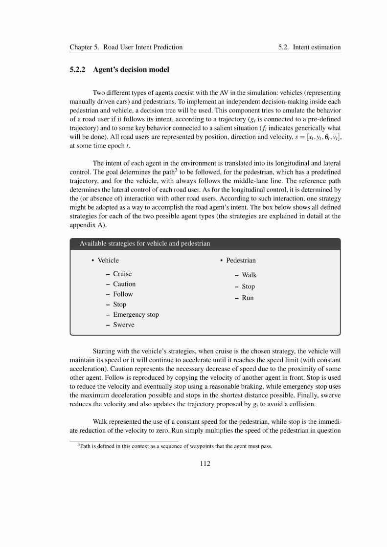
Chapter 5. Road User Intent Prediction 5.2. Intent estimation
5.2.2 Agent’s decision model
Two different types of agents coexist with the AV in the simulation: vehicles (representingmanually driven cars) and pedestrians. To implement an independent decision-making inside eachpedestrian and vehicle, a decision tree will be used. This component tries to emulate the behaviorof a road user if it follows its intent, according to a trajectory (gi is connected to a pre-definedtrajectory) and to some key behavior connected to a salient situation ( fi indicates generically whatwill be done). All road users are represented by position, direction and velocity, s = [xt ,yt ,θt ,vt ],at some time epoch t.
The intent of each agent in the environment is translated into its longitudinal and lateralcontrol. The goal determines the path3 to be followed, for the pedestrian, which has a predefinedtrajectory, and for the vehicle, with always follows the middle-lane line. The reference pathdetermines the lateral control of each road user. As for the longitudinal control, it is determined bythe (or absence of) interaction with other road users. According to such interaction, one strategymight be adopted as a way to accomplish the road agent’s intent. The box below shows all definedstrategies for each of the two possible agent types (the strategies are explained in detail at theappendix A).
Available strategies for vehicle and pedestrian
• Vehicle
– Cruise– Caution– Follow– Stop– Emergency stop– Swerve
• Pedestrian
– Walk
– Stop
– Run
Starting with the vehicle’s strategies, when cruise is the chosen strategy, the vehicle willmaintain its speed or it will continue to accelerate until it reaches the speed limit (with constantacceleration). Caution represents the necessary decrease of speed due to the proximity of someother agent. Follow is reproduced by copying the velocity of another agent in front. Stop is usedto reduce the velocity and eventually stop using a reasonable braking, while emergency stop usesthe maximum deceleration possible and stops in the shortest distance possible. Finally, swervereduces the velocity and also updates the trajectory proposed by gi to avoid a collision.
Walk represented the use of a constant speed for the pedestrian, while stop is the immedi-ate reduction of the velocity to zero. Run simply multiplies the speed of the pedestrian in question
3Path is defined in this context as a sequence of waypoints that the agent must pass.
112

Chapter 5. Road User Intent Prediction 5.2. Intent estimation
by a factor of two.
Each strategy for a road user is determined from a pairwise comparison between theagent in question and all others in the environment, as illustrated by the algorithm 5. Firstly, thetrajectory of all agent is determined during a certain prediction horizon, defined by the variable Nt
(line 1), assuming a default strategy, which for vehicle is cruise and walk for pedestrians. As for themotion models for vehicles and pedestrians, the former uses same one used in previous chapters,represented by equation 3.10, while the latter uses a simple point-mass model. Considering thesepredicted states, the road user in question, indexed by i, is "compared" (how this comparison isdone will be explained shortly) to every other road user, indexed by j, depending on the type ofeach one (lines 6, 8 and 14).
The output of each interaction is the predicted strategy for the agent i in respect to agentj. If there are n road users in the scene, then at the end of all comparisons for agent i there will ben−1 possible strategies (originated from lines 6, 8 or 14). From this set the final strategy ρi iscalculated simply by checking which ρi, j has the higher priority, which grows from top to thebottom, using the previous box as reference. Thus, for the vehicle cruise has the lowest priorityand swerve has the highest; for the pedestrian walk has the lowest and run the highest.
All road users have access to some shared information, that are the environment structure(dimensions of roads and localization of each structure in the global map), the position of eachroad user and the decision procedure in itself, and exclusively for the other road users, the intentof each agent. The AV does not known the others’ intent, only its own. Such choice is justifiedwith the assumption that the driver and the pedestrian can subjectively estimate the intention ofeach other, and to model this subjective process is not the main objective in this chapter. What themethods presented in this section and in the next ones try to achieve is to reproduce the behaviorof real road users in specific situations, to then enable the AV to identify such behaviors, notnecessarily to emulate completely this subjective process of intent estimation.
Next, the comparisons between predicted trajectories for pedestrians and vehicles will beexplained.
113

Chapter 5. Road User Intent Prediction 5.2. Intent estimation
Algorithm 5: Decision procedure for agent iInput: Environment state st = st
i, i ∈ [0,Nt ] time epoch tOutput: Strategy set according to i, ρ j, j ∈ [0,Nt ] for t
1 s = st ,st+1, · · · ,st+Nt = agents_prediction(st)2 for every agent si, i ∈ [0,Nt ] do3 if agent i is a vehicle then4 for every other agent j, j ∈ [0,Nt ]− i do5 if agent j is a vehicle then6 ρi, j = veh_decision(st
i, stj)
7 else8 ρi, j = ped_decision(st
i, stj)
9 end10 end11 else12 for every other agent j, j ∈ [0,Nt ]− i do13 if agent j is a vehicle then14 ρi, j = veh_decision(st
i, stj)
15 end16 end17 end18 ρi = strategy_calculation(ρi, j)19 end
Vehicle model
For a road user that is a vehicle, to compare its trajectory to someone else’s, as done inlines 6 and 14, four logical variables are calculated: if a collision happens, if one vehicle is tooclose to the other, if there is an intersection ahead and who has priority over the other. Collisionsand proximity are checked using the mechanisms proposed in chapter 3, section 3.2, which arethe idea of frontiers for the proximity detection and the hyperplane separation theorem for thecollision detection. To determine the location of each road user inside the simulated environment,a graph-like structure is used to construct the road environment, which is represented by figure5.2. According to the position and the geometrical dimensions of the vehicle, it is placed in oneof the nodes of the road network graph, which automatically determines also the possible nextnodes for vehicles.
With the vehicles placed in one of the nodes, their predicted trajectory can be projectedinto the graph. Each straight road has a reference lane and an opposite one; it is adopted that thereference lane is the one that goes from the extremity not connected to the intersection, whichmakes the opposite lane definition straightforward. The intersection has a more complex set ofpossible destinations.
114

Chapter 5. Road User Intent Prediction 5.2. Intent estimation
Straight road 1 - str1
Straight road 2 - str2 Straight road 3 - str3Intersection - int
Ref. con.: intOpp. con.: -
Ref. con.: intOpp. con.: -
Ref. con.: intOpp. con.: -
From To
Con.:str1 str2, str3str2 str1, str3str3 str1, str2
Figure 5.2 – Road environment graph structure
The priority is calculated according to where the vehicle is. For example, if two vehiclesare in str1 and str2, two roads in the graph-like structure in figure 5.2, the priority to access theintersection node is given to the one in the right side, considering that the right is measured as thesmallest angle between then. If one of them is already inside the intersection it automatically hasthe priority. It was also defined that the pedestrian has priority over the vehicle if both are in thesame node4.
The comparison between agents if i is a vehicle is displayed by algorithm 6. For eachtime epoch predicted (from t to t +Nt) the proximity is verified; if they are close to each other, jmight be in front of i, in which case the latter should follow the former (line 4); or both vehiclesmight collide without being on the same lane. If so, the collision time and the necessary strategyto avoid the collision are registered inside the variable colResult (line 7). Then the priority isdetermined in two specific cases, if j is a vehicle and both are in the imminence of enteringa intersection (line 15) or if j is a pedestrian (line 17). The final strategy is calculated by thefunction in line 19, which uses a decision tree, detailed in figure 5.3, to select the correct strategy.
All leafs in the tree have the final strategies according to the four variables calculated inalgorithm 6, which is case for cruise, caution and stop when there is no collision; if there is acollision, then two specific labels are used: try to stop and dynamic stop. The first one refers to theadoption of the stop strategy if there is enough space and a reasonable deceleration is sufficient todo it and if not the stop degenerates to the emergency stop strategy. Similarly, the dynamic stopchecks by prediction what the vehicle can do to avoid the accident, if stop is enough, which canalso degenerates to a emergency stop or if a swerve strategy is necessary. All these tests are madeby the checkCollision function in line 7.
4A different approach could have been taken, for example defining that the pedestrian has the priority only inside apedestrian strip, while the vehicle has the priority if the pedestrian is crossing outside the strip.
115

Chapter 5. Road User Intent Prediction 5.2. Intent estimation
Algorithm 6: Comparison if i is a vehicleInput: Agent i and j trajectories (si, s j) in [t, t +Nt ], starting time t0Output: Calculated strategy for i, ρi
1 for each time epoch in si and s j do2 if checkProximity(st
i, stj) && type(j)!=pedestrian then
3 isClose = true4 if shouldFollow(st
i, stj, road_graph) then
5 following = true6 end7 if checkCollision(st
i, stj, colResult) then
8 if !following then9 ρi = colResult
10 Break11 end12 end13 end14 end15 if localization(st
i)!=intersection && type(j)!=pedestrian then16 hasPriority = checkV2V_Priority(i, j)17 else if type(j) == pedestrian then18 hasPriority = checkV2P_Priority(st
i, stj, road_graph)
19 ρi = decideStrategy(isClose, following, colResult, hasPriority)
The strategy selection is dependent from the four logical variables calculated in thevehicle comparison (algorithm 6): proximity, collision, placement and priority. This last onecan be modified by the second element of the intent, fi, to create an unexpected behavior. Forexample, if one vehicle should yield in an intersection its fi can say that it should enter it anyway,independently from the other user. The variable fi has the function to reproduce irresponsiblebehavior in the simulation, and the challenge from the AV’s point of view is to anticipate suchbehavior using the cues from the other vehicle’s movement. How this variable affects the decisiontree of a road user will be explained with an application in subsection 5.4.1.
Longitudinal control is defined by the strategy chosen while the lateral control is guidedby the middle-lane line. To calculate the final control for vehicles, given gi and the current positionthe controller shown in equation 5.1 is used. It is the same controller proposed by (Hoffmannet al., 2007) and used in (Thrun et al., 2006), but here the dynamic terms were neglected. It tries tocorrect the direction offset and the lateral distance between the desired trajectory and the currentone and adjusts the steering angle to make the current direction intersects the tangent line fromthe desired trajectory at k/v units of distance (Snider, 2009).
φt+1 = (θtraj−θt)+ atan(
k ·dlat
vlong
)(5.1)
116

Chapter 5. Road User Intent Prediction 5.2. Intent estimation
Col. type
inter. ahead?
Dyn. stop
no
has priority?
Dyn. stopyes
Try stop
no
yes
v2pcol.
inter. ahead?
Dyn. stop
no
has priority?
Cruiseyes
Try stop
no
yes
v2v col.
inter. ahead?
against ped.?
is close?has priority
Cruiseyes
Stop
noyes
Cruiseno
yes
is close?has priority?
Cruiseyes
Stop
noyes
Cruiseno
no
yes
against ped.?
is close?Cruiseyes
Cruiseno
no
is close?Cautionyes
Cruiseno
yes
no
noco
l.
Figure 5.3 – Decision tree for vehicles
Pedestrian model
Pedestrians also have a method to compare the vehicle’s behavior with its own. It isconsidered unnecessary to compare the behavior of two pedestrians, thus it is assumed thatno interaction exclusively between pedestrians cause a change in behavior, leaving only thecomparison with other vehicles to be done. The pedestrian strategy is obtained using the algorithm7 but this time using the current road location of the pedestrian instead of the logical variablerelated to the existence of an intersection ahead, as is done for vehicles. All trajectories consideredfor the pedestrian involves crossing the street according to the environment proposed in figure5.1.
Given that the agent i is a pedestrian, its priority is calculated at line 12 of algorithm 7, in
117

Chapter 5. Road User Intent Prediction 5.2. Intent estimation
the same manner that it is calculated when i is a vehicle and j a pedestrian. The parameter fi alsocontrols this priority decision, where it can overturn the yield if necessary.
Algorithm 7: Comparison is i is a pedestrianInput: Agent i and j trajectories (si, s j) in [t, t +Nt ], starting time t0Output: Calculated strategy for i, ρi
1 for each time epoch in si and s j do2 if checkProximity(st
i, stj) && type(j)!=pedestrian then
3 isClose = true4 if checkCollision(st
i, stj, colResult) then
5 ρi = colResult6 Break7 end8 end9 end
10 placement = find_Place(sti)
11 if placement != sidewalk then12 hasPriority = checkP2V_Priority(i, j)13 end14 ρi = decideStrategy(isClose, placement, colResult, hasPriority)
has col.?
placement
Walksidewalk
has priority?
Walkyes
Stop
no
roadno
placement
Stopsidewalk
has priority?
Walkyes
Run
no
road
yes
Figure 5.4 – Decision tree for pedestrians
The lateral direction of the pedestrian, if its trajectory requires change in direction, isdone instantaneously, as is changes in its nominal speed of 1.5m/s.
118
Chapter 5. Road User Intent Prediction 5.2. Intent estimation
5.2.3 Estimating other agents’ intent
Given the previous decision model, the AV can now make use of it to predict the behaviorof all other road users, assuming an a priori intent for each one and then find the most probableintents. The following information is available for the AV at the beginning of each iteration: theposition of all agents, its own goal gi and the decision process used by other agents. This last oneis considered here as a justified assumption for the AV to have due to the common knowledgeabout the way a human drives or behaves as a pedestrian, based on the traffic code impositions onthe infrastructure and on the behavior of all agents and some introspection.
At the beginning of the simulation the AV faces the question of which intent hypothesisbest matches each agent, making it possible to explain why an agent is behaving as observed.The entire scene is explained by the information vector c, defined by the union of every agentintent as displayed in the expression 5.2 for N agents. Considering that the AV’s intent is alwaysrepresented by the subscription 0 then c = (ci), i ∈ [1,N] is the vector that needs to be estimatedby the AV.
c = (c0, · · · ,cN) = ((g0, f0), · · · ,(gN , fN)) (5.2)
Using all possible values for c the AV tries to predict the next strategy, and consequently,the future trajectories of all other road users. Considering the example given in figure 5.1, wherethere are three road users and assuming that each one of them has 2 possible gi values and 2 fi
values, it totals 64 possible c configurations. One might question why the intention of the AV isconsidered if this estimation about the entire environment is done from the AV’s perspective andas such its intent is known; this is because it is important to understand what the other agentsare thinking or expecting as a behavior from the AV, which does not necessary mean to exploit asituation where the others have a misguided impression about the AV’s intent. To profit from awrong estimation done by another road user is not so straightforward since it is desirable that theAV maintain a defensive stance when driving, although it is a subject that merits more discussionand exploration at a later time.
The proposed road-map of the algorithm consists in the following: from time t to t+Nt theAV predicts the strategies of all road users according to an assumed intent vector c and propagatestheir positions into the future using the prediction step of a Kalman filter. Then, at t +Nt , anobservation is made, which is compared with the predicted result to evaluate the probability of cbeing the right intent vector for the environment. After the calculation of p(zt+1 | ck, st+1), wherezt represents the observation, all the predicted values are modified according to the update stepof the Kalman filter. The algorithm 8 shows how this procedure implemented, being executedat each simulation step, ∆t. Given this short period for the agents to develop their strategies andthat physical cues to become detectable, the update of the EKF and the probability calculationprocedure are only executed after Nt transitions.
119
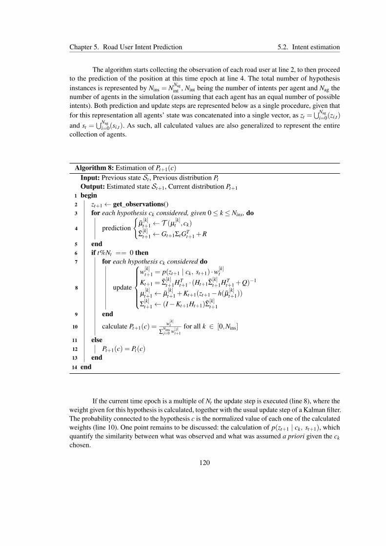
Chapter 5. Road User Intent Prediction 5.2. Intent estimation
The algorithm starts collecting the observation of each road user at line 2, to then proceedto the prediction of the position at this time epoch at line 4. The total number of hypothesisinstances is represented by Nins = NNag
int , Nint being the number of intents per agent and Nag thenumber of agents in the simulation (assuming that each agent has an equal number of possibleintents). Both prediction and update steps are represented below as a single procedure, given thatfor this representation all agents’ state was concatenated into a single vector, as zt =
⋃Nagi=0(zi,t)
and st =⋃Nag
i=0(si,t). As such, all calculated values are also generalized to represent the entirecollection of agents.
Algorithm 8: Estimation of Pt+1(c)Input: Previous state St , Previous distribution Pt
Output: Estimated state St+1, Current distribution Pt+11 begin2 zt+1← get_observations()3 for each hypothesis ck considered, given 0≤ k ≤ Nins, do
4 prediction
µ[k]t+1← T (µ
[k]t ,ck)
Σ[k]t+1← Gt+1ΣtGT
t+1 +R5 end6 if t%Nt == 0 then7 for each hypothesis ck considered do
8 update
w[k]
t+1 = p(zt+1 | ck, st+1) ·w[k]t
Kt+1 = Σ[k]t+1HT
t+1 · (Ht+1Σ[k]t+1HT
t+1 +Q)−1
µ[k]t+1← µ
[k]t+1 +Kt+1(zt+1−h(µ [k]
t+1))
Σ[k]t+1← (I−Kt+1Ht+1)Σ
[k]t+1
9 end
10 calculate Pt+1(c) =w[k]
t
∑Ninsj=0 w[ j]
t+1
for all k ∈ [0,Nins]
11 else12 Pt+1(c) = Pt(c)13 end14 end
If the current time epoch is a multiple of Nt the update step is executed (line 8), where theweight given for this hypothesis is calculated, together with the usual update step of a Kalman filter.The probability connected to the hypothesis c is the normalized value of each one of the calculatedweights (line 10). One point remains to be discussed: the calculation of p(zt+1 | ck, st+1), whichquantify the similarity between what was observed and what was assumed a priori given the ckchosen.
120

Chapter 5. Road User Intent Prediction 5.2. Intent estimation
Kalman filter for agent prediction
This part will focus in the application of the Kalman filter for a single road user, as suchall the formalism used here refers to a single road user, differently from the variables mentionedin algorithm 8. Instead, the respective parts of each vector µt and zt are referenced as si,t and zi,t ,i being the index for the road user. For each agent, one instance of an EKF is used. Following theprediction equations given previously for the vehicle, shown in 5.3, and for pedestrians, 5.4, theKalman matrices Gt and Ht are defined for vehicles in expressions 5.5 and 5.6 and for pedestriansin 5.7 and 5.8.
sveht+1 = sav
t+1 =
xt+1 = xt +∆t · vt cosθt cosφt
yt+1 = yt +∆t · vt sinθt cosφt
θt+1 = θt +∆t · vtl sinφt
vt+1 = vt +∆t ·u1
φt+1 = φt +∆t ·u2
(5.3)
spedt+1 =
xt+1 = xt +∆t · vt cosθt
yt+1 = yt +∆t · vt sinθt
vt+1 = vt +∆t ·u1
θt+1 = θt +∆t ·u2
(5.4)
The state of each other road user that is a vehicle also contains the steering angle, since,due to the strategy estimation, the control using the trajectory defined by gi needs to be calculated.The pedestrian’s state remains being expressed by the previous four variables (x,y,θ ,v).
Gveht =
1 0 −∆t · vt sinθt cosφt ∆t · cosθt cosφt −∆t · vt cosθt sinφt
0 1 ∆t · vt cosθt cosφt ∆t · sinθt cosφt −∆t · vt sinθt sinφt
0 0 1 ∆tl sinφt
∆tvtl cosφt
0 0 0 1 00 0 0 0 1
(5.5)
Hveht = I5 (5.6)
121

Chapter 5. Road User Intent Prediction 5.2. Intent estimation
Gpedt =
1 0 −∆t · cosθt ∆t · vt sinθt
0 1 ∆t · sinθt ∆t · vt cosθt
0 0 1 00 0 0 1
(5.7)
Hpedt = I4 (5.8)
The convergence of an Kalman filter is assured for the systems that obey the pre-requisitesgiven by theorem 5, proved in (Krener, 2003). The system considered is given in the form of5.9, which is uniformly observable if the initial state can be reconstructed with the output and its(n−1) first derivatives, n being the total number of state variables (Gauthier et al., 1992).
x = f (x,u)y = h(x,y)
(5.9)
Continuity of a function f : X → Y can be represented by the Lipschits condition, givenby the expression 5.10. The Euclidean norm is used as the metric for the spaces X and Y , withL ∈ N and x1, x2 ∈ X .
‖ f (x1)− f (x2)‖ ≤ L · ‖x1− x2‖ (5.10)
Finally, the theorem below says that for the conditions assumed the EKF convergesexponentially to the correct result.
Theorem 5 Convergence of EKFsSuppose that:
• The system in question is uniformly observable and satisfies the Lipschitz condition.
• The second derivative of f (x,u) is bounded.
• µt and Σt are the solutions of the extended Kalman filter, where Σ0 is positive definiteand s0−µ0 is sufficiently small
Then ‖st −µt‖ → 0 exponentially as t → ∞.
When a Kalman filter is used to estimate the evolution of some system through time theoutput is a Gaussian distribution. This precise point is used to measure the similarity between
122

Chapter 5. Road User Intent Prediction 5.2. Intent estimation
what is being assumed as an hypothesis for the behavior of the agents and what is really beingobserved.
Mahalanobis distance and similarity estimation
Usually when one wants to measure the similarity between two vectors the Euclideannorm is used, if these two vectors are defined as points in an Euclidean space. For example, ifone have u, v ∈ R5, then the distance between the points is given by expression 5.11, where ui
and vi are the elements of each one of the respective vectors.
d(u,v) =
√4
∑i=0
(ui− vi)2 (5.11)
The same is not valid for the output of the Kalman filter. The distance can be calculatedbetween the observation and the distribution mean, but an importance source of information willbe left out of the measurement, the covariance. Therefore one needs to evaluate the similaritybetween a point, the observation obtained, and a distribution, the prediction of each agent statemaintained using the EKF, which can be done using the Mahalanobis distance expressed byequation 5.12. This type of norm measures the distance between a sample from a distribution andits center.
M(x) =[(x−µ)T ·Σ−1 · (x−µ)
] 12 (5.12)
So, to measure the coherence of an hypothesis ck used to predict the state of each agent,the observation is considered as a sample of the state distribution.
M[k]t =
[(zt −µ
[k]t )T ·
(Σ[k]t
)−1· (zt −µ
[k])
] 12
(5.13)
It is well known that the quadratic form of a Gaussian variable is distributed accordingto the chi-squared distribution (Bensimhoun, 2009). To be more precise, the cumulative sumof squares of n independently normally distributed Gaussian variables, with mean equal to 0(or the null vector) and covariance equal to the identity matrix (In) is called central chi-squareddistribution with n degrees of liberty. This distribution will be used to calculated the probabilityp(zt+1 | ck, st+1). However, as said before, the central chi-squared distribution is only a priorivalid for N (0, In) which is not the case for the distributions treated here.
123

Chapter 5. Road User Intent Prediction 5.2. Intent estimation
If one considers the expression (zt −µ[k]t ) a new variable, called U , it can be assumed
that U ∼ N (0,Σt) since zt is being used as a point of this distribution, thus the difference mustbe zero. Then the theorem 5.1.3 on page 199 of (Mathai and Provost, 1992) can be stated:
Theorem 6 Distribution of M[k]t
If U ∼ N (µu,Σ) and Σ is positive semi-definite, then a set of necessary and sufficientconditions for UT AU ∼ X 2
n (δ2) is:
• trace(AΣ) = n and µT Aµ = δ 2
• ΣAΣAΣ = ΣAΣ
• µT AΣAµ = µT Aµ
• µT (AΣ)2 = µT AΣ
Given that A = Σ−1 and µu = 0 the non-centered chi-squared distribution from thetheorem becomes centered due to δ 2 = µT Aµ = 0 and all the conditions are met. Equation 5.14defines the opposite value of the cumulative probability of the ellipsoid defined between theobservation and the predicted state. Such ellipsoid, if small, shows that the observation is close tothe center of the distribution, meaning that the hypothesis k might be pertinent. The probabilitythat the Mahalanobis distance dM is smaller than the calculated value M[k]
t is the same as thecumulative probability of X 2
n , which value is commonly known.
v[k]t = 1−P(dM ≤M[k]t ) (5.14)
Finally, the probability of an observation given an assumed hypothesis and the currentstate can be defined by equation 5.15.
p(zt | ck, st) =v[k]t
∑Ninsi=0 v[i]t
(5.15)
Using the algorithm 8, that estimates the probability of each possible intent for the agentsbeing true, the AV can now known which strategy it should use if all road users act according tothe decision-making procedure proposed in algorithm 5. One detail was left out of the decisionprocess: the variable fk, which controls the behavior of a road user during the interaction. Suchvariable is used to emulate instances where an agent do not behaves as it should: for example, if avehicle does not yield for a pedestrian crossing the road. The AV might not be able to identifysuch behavior and thus react sub-optimally to it.
124

Chapter 5. Road User Intent Prediction 5.3. Incomplete game model
As such, the AV needs to choose a strategy considering a deviation from normal behaviorcoming from other road users. To maximize the utility of the worst possible scenario is anoperation embodied by the Nash equilibrium in a game theory approach. But the same detail thatcreated the necessity to establish the estimation process of ck is also present if this approach isapplied: the agents do not know which is the intention of the other ones around them. Everythingdone up until now compared these two by two to obtain an expected strategy given an assumedintent; it is necessary now to consider the collective set of calculated strategies and the estimatedagents’ intent and their probabilities of being correct to arrive in a coherent decision for the AV.
Such configuration requires an incomplete game, where part or all the players do nothave access to some essential information. For such cases the method proposed in (Harsanyi,1967) can be used to reach a formulation of the game that has a defined solution.
5.3 Incomplete game model
As discussed in chapter 2, in an incomplete game the players do not have access to someinformation about the other players. Without such information it may be impossible to calculatethe utility of each possible action that might be taken (if the utility function form or some otherparameter is not known) and therefore to find an equilibrium point of the problem, if it exists. Tocounteract the lack of information, this incomplete game can converted into a complete imperfectone in which the Nash equilibrium is applicable.
5.3.1 Nash equilibrium
In a non-cooperative n-player game each player has at its disposal a set of differentstrategies5, which, according to the idea of a game, produces different utilities for the player,each one also depending on the choices of other road users. Every road user tries to anticipate theothers’ decision and maximize its utility and it is from this interaction between every player thatthe notion of equilibrium point emerge.
A pure strategy is defined as a single action that an agent may execute, while a mixedstrategy is represented by a probability distribution over different actions (or similarly, over purestrategies). As one may expect the interaction between agents happens through the choice ofa strategy; if it is assumed that all agents are rational, i.e. that they search to maximize theirpreferences (deterministic reward for pure strategies and expected reward for mixed ones), then
5Used in this sense, strategy here is something more general than the longitudinal control profiles proposed earlier,even though when this theoretical discussion is applied to the problem treated in this chapter, this general sense iscompatible with the definition of strategy used in subsection 5.2.3.
125

Chapter 5. Road User Intent Prediction 5.3. Incomplete game model
each agent tries to anticipate the choice of the other agents and counter it with the best strategyfrom its point of view. This same procedure is repeated inside other agents.
When, for every agent, there is no other better strategy than the one chosen, i.e. thecurrent strategy is self-countering, then an equilibrium point was reached (Nash, 1950). It hasbeen proven in (Nash, 1950) and (Nash, 1951) that every finite game has an equilibrium point,which configures the best collective reward for all the n-players in a non-cooperation game. Thefollowing definition from (Osborne, 2002) resumes the idea of Nash equilibrium:
A Nash equilibrium is an action profile (or a strategy) a∗ with the property that no playeri can do better by choosing an action different from a∗i , given that every other player jadheres to a∗j .
However, the existence of an equilibrium point is only assured in the case of mixedstrategies (Osborne, 2002). This concept is essential to define what each agent does in responseto an interaction and it is the main tool to solve a game model. It assumes that each agent iscapable to predict the behavior of all other agents, which entails that the intent of each agentneeds to be perfectly known by the AV, which is not realist. It is at this point that a Bayesiangame formulation is necessary.
5.3.2 Harsanyi’s Bayesian game
In a n-player game with complete information all agents known the entirety of thenecessary information to predict the choices of the other agents, all their possible strategies andtheir preferences. However, if these details are not accessible one can argue that each agentmaintain a subjective probability distribution over the possible alternatives. The conversion fromincomplete to complete information proposed in (Harsanyi, 1967) uses this concept of probabilityover unknown information to try to find a complete game formulation that has similar propertiesto the original one.
As said before, each player tries to anticipate the behavior of all others. In a incompletegame, this means that player 1 has some expectation over the behavior of player 2, which in turnalso has some expectations about player 1. Such sequence can go on forever, since now player 1also has an expectation over the expectation of player 2 has of him and so on. The Bayesian gameapproach model these expectations as subject6 probability distribution over the behavior of allother players (back later on).
6This probability, differently from the objective definition, refers to the belief of one agent about some phenomenawhich need not be the same for each agent (Savage, 1954), therefore creating a graded belief towards this phenomena(Hajek, 2019). The objective definition, according to (Harsanyi, 1967), refers to the frequentist interpretation ofprobability.
126

Chapter 5. Road User Intent Prediction 5.3. Incomplete game model
One can postulate that all the subjective probability distributions considered by eachagent are the marginal distributions of some original, base probability distribution that has asparameters the information not known by the players, as indicated in expression 5.16, whereR refers to the probability distribution and c to the unknown information (which will be theintent vector for the environment). Then the original game and the complete game formed by thesubstitution of those subjective probability distributions by the marginal probability from thisbase distribution, according to the definition 2, are equivalent, which entails that both have thesame resulting decision rule and the same Nash equilibrium point(s).
R(c)
R(c1, c2, · · · , cn| c0)
R(c0, c2, · · · , cn| c1)...R(c0, c1, · · · , cn−1| cn)
(5.16)
Definition 2 Bayes-equivalencyLet G be an incomplete game and G∗ be a complete one, both in standard form (definedby expression 5.18). Both games are Bayes-equivalent if for a player j:
• The two games must have the same strategy (Si) and information (Ci) spaces (alsocalled intent).
• Both games must have the same expected value function for the payoffs.
• The subjective probability distribution Ri from player i must satisfy the followingrelationship:
Ri(c0, c1, · · · , ci−1, ci+1, · · · | ci) = R∗i (c0, c1, · · · , ci−1, ci+1, · · · | ci) (5.17)
Form of a game
At this point it is necessary to give more details about the standard form of a game and itsnormal form, which will appear subsequently. The standard form of a particular incomplete gameG, defined in (Harsanyi, 1967), has the composition shown in expression 5.18. In this contextSi represents the strategy space, Ci the information space (which space of possible values forthe intent vector), Vi represents the expected value for the payoff7 and Ri the base probability
7In (Harsanyi, 1967), the function V is defined as the common form of the payoff functions of each player, whichis only known by the respective player.
127

Chapter 5. Road User Intent Prediction 5.3. Incomplete game model
distribution.
G∗ = S0, · · · ,Sn ; C0, · · · ,Cn ; V0, · · · ,Vn ; Ri (5.18)
The normal form of a game is presented in definition 3 (Shoham and Leyton-Brown,2008). It is defined directly using actions, but it can also be defined in function of the strategiesthat are available. If these strategies are pure, i.e. they represent only one action, then nothingchanges. But if one needs to consider mixed strategies then the total payoff needs to be calculatedas an expected payoff.
Definition 3 Normal-form gameA finite n-person game in normal form is defined by the following parameters:
• N, the number of players.
• A = A1×A2×·· ·×An, the finite set of actions.
• u = (u1, · · · , un), where ui : A→ R is the payoff function for the player i.
When the game is defined in the normal form, the strategies are also normalized. Thedifference from the usual definition is that the normalized ones are actually functions from theintent space of the road user in question to the strategy space.
Solving the equivalent game
The necessary and sufficient conditions for two games, the original G and the completeone G∗, to be equivalent is enunciated by theorem 7, found in (Harsanyi, 1968b). Basically, it saysthat if two games are equivalent, according to the definition 2, they need to have the same strategyand attribute spaces, the same payoff functions and must respect the relationship described in5.16. Games where the hypothesis that the original distribution exist can be called consistentgames, and those that do not, inconsistent. It will be assumed here that the game involving theinteraction between road users is a consistent one, although even if a game is inconsistent, theequivalency can be extended to this case (Harsanyi, 1968a).
In the theorem below the normal form of the game is cited. This game formulation,differently from the extensive game that exposes all possible outcomes for each player, iscomposed of only three elements: the number of players, the set of available strategies for eachplayer and the combined payoff function, that for each player gives its payoff according to itscurrent strategy, there is not a dependency between players in this calculation.
128

Chapter 5. Road User Intent Prediction 5.3. Incomplete game model
Theorem 7 Bayes-equivalencyLet G be an incomplete game and G∗ be a Bayesian equivalent game to G. To an n-tuplestrategy s∗ of G∗ also be an equilibrium point in G is it necessary and sufficient that in thenormal form N(G∗) of the game G∗, s∗ be an equilibrium point.
The estimated probability by algorithm 8 will serve as the base probability to calculatethe equilibrium points of the equivalent game. This discrete original distribution, calculated by theMahalanobis distance and the chi-square distribution, is itself based on the conclusion obtainedfrom the comparison about what each road user should do in the considered situation.
According to the determination of each strategy proposed in the previous section eachstrategy is a pure one, consisting of a single action possible according to the situation at hand.The Nash equilibrium point is not guaranteed to exist is such situations, but it will be assumedthat it does exists. Its determination, given the implementation specifications of this context, issimilar to the example presented in (Harsanyi, 1968b).
5.3.3 Decision making procedure
The main objective of this procedure is to account for every possible situation in the AV’sdecision-making, so as to avoid instances where the AV is not prepared for a behavior from someroad user. Of course, only the behaviors represented by the considered strategies are involved intothe deliberation, any other behavior that cannot be approximated by them is not considered. Thisis a limitation of the procedure, but if one assumes that such strategies can be extracted from realdata, one can find a sufficient set of strategies to represent all possible reactions during road usersinteractions. From the equivalent game formulation, the Nash equilibrium is calculated the payoffvalues variations according to the intent vector probabilities and the strategies considered.
Each agent will use a reward function that is similar in form to the MDP implementationdisplayed in subsection 3.2.3. For each intent vector hypothesis there will be a table of payoffs.These tables are in turn connected to the probability that such situation is actually happening.Considering the three agents in the scene represented by figure 5.1, the intent vector is formedby three components, c1, c2 and c3 and the normalized strategies are represented by the Greekletters ν , γ and ρ , respectively for each agent. They are functions that take as input the currentvalue of the respective ci and output the strategy that should be used in this given situation.
c = (c1,c2,c3) (ν ,γ,ρ) (5.19)
Then, for each possible value of the c vector, the payoff is calculated, giving differentvalues for each type of strategy, represented by the Greek letters presented earlier with the
129

Chapter 5. Road User Intent Prediction 5.3. Incomplete game model
subscription that indicated the strategy index, as it can be seen in table 5.1. It this table agent one’sstrategy is represented by ν in the row direction while the combination of the possible values forγ and rho are in the column direction. For clarity reasons each agent will be considered to haveonly two possible strategies, even if the vehicles have six possible strategies and pedestrians three.Multiple tables like the one below are calculated for different combinations of the intent vector c.
Table 5.1 – Example of reward table for a specific intent vector c
c = (c1,c2,c3)
ν\γρ γ1ρ1 γ1ρ2 γ2ρ1 γ2ρ2
ν1 r1,11c r1,12
c r1,21c r1,22
c
ν2 r2,11c r2,12
c r2,12c r2,22
c
Table 5.1 exemplifies the reward calculated for each strategy given an intent vector.According to the definition of the Nash equilibrium point, no agent can achieve a better outcome,so if the system is solved from the viewpoint of agent one, it is not necessary to calculate all therewards again and find the equilibrium point for agent two and three.
With the probability distribution Pt+1(c) calculated in algorithm 8, the total estimatedreward is determined by equation 5.20 for a certain combinations of strategies. The functionsf1 : c→ σ , f2 and f3 represent the normalized strategy being evaluated. For example, f1 canassume four possible values according to the number of intents agent one can have (two in thisexample) and the number of possible strategies (also two); if, for agent one f1 = 21 this meansthat for the first intent the agent will choose the strategy 2 and for the other intent, the strategy 1.Using this codification the estimated payoff matrix is formed having as row the possible valuesfor f1 and as column the combination of f2 and f3. Constants Nc1 , Nc2 and Nc3 represent the totalnumber of intents for each agent.
E[rν f1 ,γ f2 ,ρ f3] =
Nc1
∑i=0
Nc2
∑j=0
Nc3
∑k=0
Pt+1(ci,c j,ck) · rν f1(ci),(γ f2(c j)ρ f3(ck))ci,c j,ck (5.20)
But if one considers that the intent of agent one is known a priori, only the conditionalexpected reward is necessary, cutting the number of evaluations needed (equation 5.21). Then,the conditional estimated payoff matrix will have two rows (represented in the equation below bythe index l), one for each of the possible strategies of the agent one, and the columns are all thepossible strategies for agents two and three ((γ11ρ11), (γ11ρ12), (γ11ρ21), · · · , (γ22ρ22), a total
130

Chapter 5. Road User Intent Prediction 5.3. Incomplete game model
of sixteen columns).
E[rν lγ f2 ρ f3 | c1] =
Nc2
∑j=0
Nc3
∑k=0
Pt+1(c j,ck|c1) · rν l ,(γ f2(c j)ρ f3(ck))c j,ck (5.21)
The optimal strategy in a Nash sense is calculated by equation 5.22 using a maxminoperation, consisting of a minimum possible reward in the column, represented by the index h,for each possible normalized strategy for the other agents, and then a maximization operationto find the best strategy overall in the minimized row. Such strategy, as expected, will give thesecurity that at the worst possible situation the payoff is maximized but not necessarily that thehighest possible payoff if obtained in the best scenario.
ν∗ = argmax
lmin
hE[rν lγ f2 ρ f3
] (5.22)
It is the strategy dictated by ν∗ that should be executed by the AV, together with thelateral reference given by its trajectory. This normalized strategy, that depends only on the currentstate of agent one, is a pure strategy since the relationship between current intent and strategy isdeterministic. According to the theorem 7 this equilibrium point will also maximize the payofffrom the original incomplete game.
Example of application
To better explain the calculation of the Nash equilibrium point and the use of equations5.19 to 5.22 an example will be provided below. It will be composed of two players, x and y, thateach can have two different intents i1 and i2 and execute the actions a1 and a2. This example issimilar to the one found in (Harsanyi, 1968b), but it will serve to explain how to apply the methodused to calculate the equilibrium point with more that two players. Table 5.2 gives the reward foreach possible situation for player x, while the rewards for player y are the same but multiplied by−1. The circled numbers are the saddle points for each situation, the rows give the x actions andthe columns the y actions.
The functions ν and γ represent the strategy for agents x and y respectively given theirintent. Table 5.3 gives the intent probability, which is the output of the algorithm 8.
So, with these elements it is already possible to calculate the normalized strategies forthe road user x. There are two possible ways to proceed to the calculation of the Nash equilibriumpoint: or the equation 5.20 can be used to calculate the expected payoffs for all possible intents ofx or, since its intent is known by itself, equation 5.21 can be applied. The second choice will be
131

Chapter 5. Road User Intent Prediction 5.3. Incomplete game model
(a) Reward for intentions c1 = (i1, i1)
x\y γ(i1) = a1 γ(i1) = a2
ν(i1) = a1 r1,1c1 = 5 r1,2
c1 = 10ν(i1) = a2 r2,1
c1 = 3 r2,2c1 = -5
(b) Reward for intentions c2 = (i1, i2)
x\y γ(i2) = a1 γ(i2) = a2
ν(i1) = a1 r1,1c2 = 10 r1,2
c2 = -25
ν(i1) = a2 r2,1c2 = -5 r2,2
c2 = -8
(c) Reward for intentions c3 = (i2, i1)
x\y γ(i1) = a1 γ(i1) = a2
ν(i2) = a1 r1,1c3 = 9 r1,2
c3 = -31
ν(i2) = a2 r2,1c3 = 15 r2,2
c3 = 27
(d) Reward for intentions c = (i2, i2)
x\y γ(i2) = a1 γ(i2) = a2
ν(i2) = a1 r1,1c4 = 1 r1,2
c4 = -4ν(i2) = a2 r2,1
c4 = -24 r2,2c4 = -5
Table 5.2 – Rewards for player x
Table 5.3 – Intent probabilities
x\y c2 = i1 c2 = i2
c1 = i1 0.5 0.1c1 = i2 0.1 0.3
made here and the x intent will be equal to i1, resulting in the conditional probabilities calculatedin table 5.4 (The probabilities Pt+1 are indicated by p).
Table 5.4 – Conditional probabilities for cx = i1
x\y cy = i1 cy = i2
p(cy | cx = i1) 0.833 0.167p(cy | cx = i2) 0.25 0.75
Simplifying the equation 5.21 to two players gives:
E[rν lγ f2 | cx = i1] =Nc2
∑j=0
p(cy = i j|i1) · rν l ,(γ f2(c j))c (5.23)
To determine the conditional payoff table, each row is formed by a possible strategyfor x, ν(i1) = a1 or ν(i1) = a2, while the columns are determined by the possible strategies fory, indicated by γ . The values that it can assume are displayed below. It becomes clear then thedefinition of the function f2 for the general case: if one considers the first item in the box below,
132

Chapter 5. Road User Intent Prediction 5.4. Simulation results
f2(i1) = a1 and f2(i2) = a1, which defines γ11 (the numbers indicate the strategy index for eachintent of y).
• γ(cy = i1) = a1 and γ(cy = i2) = a1 or γ11
• γ(cy = i1) = a1 and γ(cy = i2) = a2 or γ12
• γ(cy = i1) = a2 and γ(cy = i2) = a1 or γ21
• γ(cy = i1) = a2 and γ(cy = i2) = a2 or γ22
The calculation of the conditional payoff for the cell in line one, column one is:
E[rν1γ11 | cx = i1] = p(cy = i1 | cx = i1) · r1,1c1 + p(cy = i2 | cx = i1) · r1,1
c2 == 0.833 ·5+0.167 ·10 = 5.833
And for the cell in line two, column three:
E[rν2γ21 | cx = i1] = p(cy = i1 | cx = i1) · r2,2c1 + p(cy = i2 | cx = i1) · r2,1
c2 == 0.833 · (−5)+0.167 · (−5) =−5
Finally, the conditional payoff table is given by 5.5.
Table 5.5 – Conditional payoffs for cx = i1
x\y γ11 γ12 γ21 γ22
ν1 5.833 0 10 4.167ν2 1.667 1.167 −5 −5.5
To find the best strategy to be adopted, in a Nash sense, it is only necessary to apply theminimal to each row, giving 0 to ν1 and −5.5 to ν2 and then to maximize this result, finding thatthe best strategy is ν1, given that cx = i1.
5.4 Simulation results
Currently only the multi-agent simulation proposed in subsection 5.2.2 is ready to offersome results; the intent estimation procedure proposed in subsection 5.2.3 has been implemented
133

Chapter 5. Road User Intent Prediction 5.4. Simulation results
but not entirely to offer consistent outputs. Therefore, the results presented here will concern onlythe interaction between the multiple independent agents in the simulation. The simulated sceneis given by the figure 5.1, with the same three road users. Given the limitations cited, the twovehicles are implemented as manual drivers with the decision tree component, and the simulationpertains only to the interaction between these road users.
5.4.1 Multi-agent simulation
According to the figure 5.1, there are two possible goals (gi) for each agent. The redvehicle can turn right or left, the blue vehicle can continue straight or turn right and the pedestriancan cross the intersection to the right or continue straight to the other pedestrian strip. Theseoptions are combined with the second element, of the intent, fi, which is the reaction during theinteraction, creating four possible intents for each road user. For each vehicle and in this contextfi indicates if they will obey an yield imperative, since in an intersection without semaphores thevehicle on the right always has priority; and for the pedestrian it defined which is the reaction ofthe pedestrian in a dangerous situation: if it starts to run or if it freezes and stop in the middle ofthe road.
Three different scenes will be displayed as a result:
• Situation 1: Red vehicle turns right, blue vehicle turns right and pedestrian crossesto the right.
• Situation 2: Red vehicle turns right, blue vehicle continues straight and pedestriancrosses to the right.
• Situation 3: Red vehicle turns right, blue vehicle turns right and do not give priorityand pedestrian crosses the pedestrian strip on top.
All the details about the vehicle object implementation, the implementation of eachstrategy and the simulation itself can be found in appendix A.
Situation 1
An image from the output of the simulation when all road users are approaching theintersection can be seen in figure 5.5. The same situation is shown (not exactly the same timeepoch) in figure 5.6, where it can be seen on the right side the three agents moving and on the leftthe trajectory colored with the respective strategy in execution at each position.
134

Chapter 5. Road User Intent Prediction 5.4. Simulation results
Figure 5.5 – Illustration of the intersection interaction
Considering that the pedestrian starts to move at t = 7s, one can clearly see that thered rectangle agent (which represents the red vehicle at figure 5.5) detects that the pedestrianis crossing the road and therefore has the preference. It decreases the velocity to stop in theintersection and avoid a collision, until the point that it can be sure that no collision with thispedestrian can happen, then it resumes the cruise strategy and turns downwards.
Figure 5.6 – Strategies used during situation 1
135
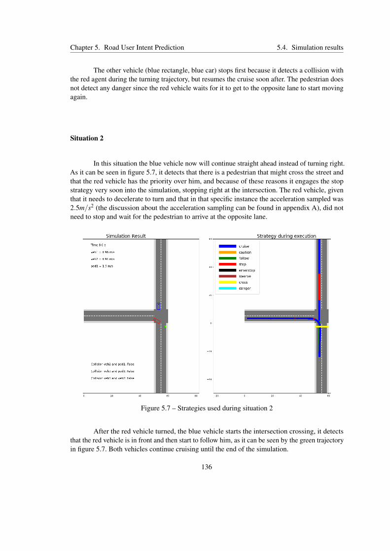
Chapter 5. Road User Intent Prediction 5.4. Simulation results
The other vehicle (blue rectangle, blue car) stops first because it detects a collision withthe red agent during the turning trajectory, but resumes the cruise soon after. The pedestrian doesnot detect any danger since the red vehicle waits for it to get to the opposite lane to start movingagain.
Situation 2
In this situation the blue vehicle now will continue straight ahead instead of turning right.As it can be seen in figure 5.7, it detects that there is a pedestrian that might cross the street andthat the red vehicle has the priority over him, and because of these reasons it engages the stopstrategy very soon into the simulation, stopping right at the intersection. The red vehicle, giventhat it needs to decelerate to turn and that in that specific instance the acceleration sampled was2.5m/s2 (the discussion about the acceleration sampling can be found in appendix A), did notneed to stop and wait for the pedestrian to arrive at the opposite lane.
Figure 5.7 – Strategies used during situation 2
After the red vehicle turned, the blue vehicle starts the intersection crossing, it detectsthat the red vehicle is in front and then start to follow him, as it can be seen by the green trajectoryin figure 5.7. Both vehicles continue cruising until the end of the simulation.
136

Chapter 5. Road User Intent Prediction 5.4. Simulation results
Situation 3
This situation emulates a scenario where one of the vehicles, in this case the blue one,do not abide the priority to the other vehicle and the pedestrian. However, since the idea is torepresent a human driver, the decision making is still sensible to collisions. Looking at the figure5.8 one can see that there is one interval in the blue’s trajectory that is a emergency stop strategy,which is exactly due to a possible collision with the pedestrian and the red vehicle. When thepedestrians freeze in reaction to the proximity of the blue car the red vehicle also engages in acontrolled stop at the intersection, thus avoiding the collision altogether.
Figure 5.8 – Strategies used during situation 3
The parameter fi from the blue vehicle overrides the common decision tree for vehiclesshown in figure 5.3. In the no collision branch, the intermediary nodes related to the priorityare eliminated, since the blue vehicle will not yield in any situation; the new branch taken thesemodifications into account can be seen in figure 5.9. The collision branches continue with thesame structure, which is why the blue vehicle, when it perceives a collision, uses the emergencystop strategy.
137

Chapter 5. Road User Intent Prediction 5.5. Final remarks
Col. type inter. ahead?
against ped.?
is close? Cruiseyes
is close? Cruise
no
yes
against ped.?
is close? Cruiseno
is close? Cruise
yes
no
no col.
Figure 5.9 – Modified vehicle decision for the no collision sub-tree
5.5 Final remarks
In chapter 3, to allow the definition of the MDP state as only the AV’s configuration itwas assumed that, from the start of the policy execution, after is calculation, the intentions ofother road users did not change, which entails that their direction and velocity remains the same.This continuity allows the AV to predict their trajectory only using their current configuration.The main goal of this chapter was to propose a method capable to predict this possible change inintent during the policy execution, so as to relax this assumption made. Three main componentsform the prediction algorithm: the deterministic decision-making that emulate other vehiclesand pedestrians, the probabilistic distance estimation, that calculates the probability of someintent given an observation of the current situation and an incomplete game model to adapt thechoice of strategy to the current interaction between agents. Finally, the results of the multi-agentsimulation using the decision-making models are shown.
However, some considerations about the proposed intent estimation method needs to bemade. During the entire chapter the deterministic decision-making model proposed was suggestedto be used by the AV as a way to predict the other road users strategy and as the decision-makingprocess of the other road users themselves. This would work with the estimation of intent by theAV, but the other capability, the game model to account the interactions between road users, issupposed to close the gap between the simulation and real data. Thus, to test the incomplete gameformulation in a simulation it would be necessary to find another decision-making procedure tobe implemented in the agents, preferably one that mimics real humans using real data.
Another concern related to the game model is that it is based on the assumption that theNash equilibrium point could be reached using a pure strategy, which entails that for each agent,given its state and intent, the strategy taken is deterministic. These agents are human drivers and
138

Chapter 5. Road User Intent Prediction 5.5. Final remarks
pedestrians, that have personalities and different motivations, thus such assumption that everysingle one would act equally is a strong one and must be relaxed. A mixed strategy would bemore suited for the problem, creating an additional degree of liberty according to the specificityof each component that predicts an agent behavior. To allow such consideration it would benecessary to update the proposed intent estimation given by algorithm 8 to a nested particlefilter, capable to consider multiple hypothesis of intent and for each intent multiple hypothesis ofstrategy. Afterwards the proposed Nash equilibrium point determination would also need to bemodifies to deal with mixed strategies.
139

Chapter 5. Road User Intent Prediction 5.5. Final remarks
140

Chapter 6
Conclusion
Contents6.1 Final remarks . . . . . . . . . . . . . . . . . . . . . . . . . . . . . . . . . 141
6.2 Future research perspectives . . . . . . . . . . . . . . . . . . . . . . . . . 144
6.1 Final remarks
In this thesis the question concerning how the automated vehicle should deliberate ondecisions, given its perception information, mission data and the presence of other road usersin its surroundings was treated. Both normal situations for a human driver and the hypotheticalcase of a ethical dilemma situation were addressed. The starting point of the discussion aroundautomated vehicles, and more generally artificial intelligence and automated mobile robots, wasdeveloped in chapter 1, from the early days of artificial intelligence with the definition of theTuring Test, the development of the first automated mobile robots, the paradigms to orient thearchitecture of such robots and the development of driveless vehicles during this process. Someof the most important breakthroughs in the area were cited, for example the works of Dickmannsand Zapp, 1987 and the two prototypes that won the DARPA challenges, Thrun et al., 2006 andUrmson, Anhalt, Bagnell, et al., 2008.
Having done a review of the history of automated systems, the current state of the art inthe domain of automated vehicles was finally described, from most useful advantages that onehopes the AV technology delivers, the current maturity level of the deployment of such robotsin the real world and what is currently being commercialized by the automotive industry. Themost promising prototypes of level four automated driving were also discussed, with an specialattention to the Tesla’s implementation of automated driving.
141

Chapter 6. Conclusion 6.1. Final remarks
Chapter 2 discusses the state of the art of each domain addressed in the theses: decision-making, ethical decision-making, behavior prediction and game theory. Each subject starts withan explanation about the organization of the concepts that define the field of research to thenproceed towards the analysis of a set of representative publications, recent and older, from eachdomain.
The decision-making algorithm for an AV is proposed and explained in chapter 3. Startingfrom the discussion about implementation paradigms from chapter 1, the choice of architectureassumed, so as to model the decision-making process with the correct responsibilities andfunctionalities, was defined to be the 3-tiered architecture Gat, 1998. From the theoretical side,the formulation of a Markov Decision Process has presented next, focusing in the existence anduniqueness of the soon to be calculated policy, given the assumptions made about the system.Finally, the formulation of the MDP is presented, with the hypothesis that the behavior of the otherroad users does not change throughout the execution of the policy, which enabled the definitionof the state to contain only the AV’s configuration while the other road users’ configuration wereaccounted for in the reward function. The results obtained from the simulation are discussednext, not before the definition of the simulation environment and the value iteration method. Thefollowing conclusions could be drawn from such experimentation:
Conclusions from Chapter 3 experiments
• The necessary horizon to sufficiently account for the behaviors of other road usersis in direct conflict with the exponential nature of the defined state space.
• The prediction horizon and the AV’s velocity also have an antagonistic relationship,given that the transition time remains fixed.
• Or some risk evaluation is necessary to stop the AV from starting a maneuver thatends in an unsafe state for the current prediction horizon or the idea of predictionhorizon should be modified to be dependent to the maneuver completion.
Ethical dilemma situations are treated using the methods proposed in chapter 4. First,one needs to define what are dilemma situations, which is done in the first section of chapter 4to then step into the definition of the parameters used to calculate the harm of a collision, thedifference of velocity due to the physical interaction between road users and the vulnerabilityconstant. Using this concepts two types of ethical decision-making procedures are presented:the Ethical Valence theory (EVT), that uses the ethical valence assigned to each road user, incombination to the predicted harm, to deliberate; and the ethical optimization (EO), three differenthandcrafted minimization procedures that are inspired by the utilitarian, egalitarian and Rawlsiancontractarian ethics. Both deliberation methods were tested, with the EVT in an hypotheticalsolution and assuming a specific definition of features for the ethical valences while the ethicaloptimization was tested as an MDP criteria for ethical decision, in the same configuration of thetests executed in the previous chapter. In both implementations the algorithm correctly calculated
142

Chapter 6. Conclusion 6.1. Final remarks
that the collision with the opposite vehicle would be too dangerous, and opted or for the collisionwith the pedestrian or for the collision with the wall in the frontier of the simulated environment.
Conclusions from Chapter 4 experiments
• EVT: According to the moral profile chosen, the deliberation system protected orthe AV’s passengers or the most vulnerable users.
• EO: The three actions produced the same result, a collision with the pedestrian,but with different intensities; the utilitarian approach gives the smallest collisionvelocity for the AV with the pedestrian.
The main subject of the chapter 5 revolves around the relaxation of the assumption madein chapter 3, that the behavior of other road users did not change during the MDP policy execution.To eliminate such assumption it is necessary to account the interaction between each road user,which entails the estimation of their motivations, their intent. To entry in the matter at hand, thetypes of errors that an AV is subject to are discussed, so as to isolate the error that might producean ethical dilemma situation, when other users act in an unforeseen way from the AV’s point ofview. From this point an deterministic decision model for vehicles and pedestrians is proposed,making possible the implementation of a multi-agent simulation and allowing the AV to predictwhat will be the answer of the other road users given some interaction between them. Usingthis prediction the AV can test which intent describes the behavior of the other users the best,according to this deterministic decision model, and then calculate the probability that some roaduser has a determined intent given by the distance between the prediction made by the Kalmanfilter and the observation.
This is only enough to estimate the intent of each road user, not to determine whichaction it will execute next. For such task it is necessary to apply an game theory model of theinteraction, more specifically the interaction at a precise time is modeled as an incomplete game,with the intent of the other agents, that are estimated by the previous algorithm, as the unknowninformation. Calculating the Nash equilibrium point of the equivalent Bayesian game then givesthe adopted strategy for each of the agents in the environment. However, the algorithm describedonly accounts for pure strategies, which does not guarantee the existence of the Nash equilibrium.To allow mixed strategies as an end result of the procedure, it is necessary to modify the intentestimation process so as to account multiple strategies for a single intent being compared, andthen also expand the Nash equilibrium determination procedure as well.
Using this procedure of intent estimation allows the correct evaluation of the transitionprobability for the MDP proposed in chapter 3, which means that a more precise account of theexpected harm and the multiple possible outcomes in a dilemma situation can be determined anddeliberated upon. Not only this but the simulation itself is closer to reality due to the independenceof other road users behaviors from the AV’s controller. All could result in an proposition of adecision-making with ethical deliberation capabilities that accounts for behavior uncertainty, an
143

Chapter 6. Conclusion 6.2. Future research perspectives
implementation yet not studied.
6.2 Future research perspectives
Multiple lines of research can be branched out from the work done in this theses. Someof then are presented and commented below, in no specific order:
New decision-making system using an POMDP Given that, in the intent estimation for otherroad users, their positions are predicted using a Kalman filter there is a probability dis-tribution around the state (which are now defined by the configuration of each road user,including the AV), then it would be more appropriate to consider a partially observableMarkov decision process to model de decision-making, instead of the model proposedin chapter 3. Of course, this comes with more complications since it is harder to calcu-late the optimal policy for such cases, often an approximate solution suffices due to thecomputational cost involved to find the optimal solution. However, the same problemsobserved in the MDP implementation still need to be solved, notably the antagonisticrelationship between the predicted horizon and the capacity to account to other road usersbehavior (which can be better answered by a state space sampling methods, as the one thatKurniawati and Yadav, 2016 proposes) and the addition of some measure to verify thata maneuver, when started, is at least simulated until its end. In this case the structure ofethical and normal decision making deliberation retains the same functionality as before,if a dilemma situation is detected then the ethical deliberation takes place and a highlynegative reward is attached to the situation.
Definition of other road users’ behavior using machine learning In chapter 5 the decisionprocess of other vehicles and pedestrians were defined in a deterministic fashion bydecision trees. One improvement that could be made is to learn a driver or a pedestrianbehavior from real data using a machine learning approach, as Kuderer et al., 2015 did. Theresulting behavioral model could produce simulated agents that reproduce more realisticallythe dynamics of driving, for example acceleration, deceleration, respect to the traffic code,etc. Such method would also allows the test of multiple types of driving profiles, from amore cautious to a more aggressive driver, with the same being valid for the pedestrian.Specifically for pedestrians, there is an entire field of research about the prediction of inten-tions of pedestrians using its pose, head orientation and position. Certainly the capabilitiesof the intent estimation would be improved with more realistic methods.
Fusion between the normal reward criteria and the ethical deliberation The ethical deliber-ation proposed in chapter 4 are only used if a dilemma situation is detected, which mightnot necessarily happen for every real dilemma situation. Detection of some phenomenaalmost always has to deal with false negatives instances of detection and given the gravityof a dilemma situation even the existence of a false negative must be avoided at all times.
144

Chapter 6. Conclusion 6.2. Future research perspectives
Therefore, it would be more suitable to fuse both objective and ethical criteria into onehybrid deliberation process. Both components would be accounted at every action taken,with one predominant in normal situations and the other in ethical dilemmas, so as tominimize the loss of performance given that the other component could influence thesystem towards non-optimal decisions (in the context of a non-dilemma situation) and thesame during ethical deliberation. Another motivation for this modification is that up untilthis point, outside the dilemma situation, the selection criteria for action is entirely basedon an objective regard of the situation, but an argument can be made that some instances innormal driving should involve an ethical component for an AV (even if for a normal driverthis is not the case), so as to encompass possible passive risks due to each AV’s action. Forexample, if there is a cyclist in the same lane as the AV, should it overtake him? From aperformance point of view, yes, but the increase of proximity between both agents wouldmean that the risk of something go wrong and this vulnerable road user end up entangledin a collision increases. Such fact ideally should also be accounted, which is possible usinga hybrid decision process.
Exploration of a virtue ethics approach for ethical learning As established in chapter 2, virtueethics says that morally good actions flows from a good moral character, which is composedby the correct virtues. Implement such an approach in a machine is not as straightforwardas is for deontology or consequentialist based methods, since some sort of character needsto be established and than it must evolve through practice, so as to learn to act ethically.The reason why this is proposed here as a possible research perspective is that such systemwould be interesting to define the weight of each component in a hybrid decision criteria.Using the framework proposed in Arkin and Ulam, 2009 as a model (the emotions consid-ered in the publication is exchanged by the virtues), one could simulate different outcomesfor many dilemma situations and assess the consequences of each action to then backtrackto modify the virtue so as to prevent some actions to be execute while allowing others to.The main question is how to represent a virtue, and to be sure that it represents the same aswe, humans, think it should. Or even some artificial virtues could be proposed specificallyto produce outcomes that could be considered morally correct.
Verification and validation of stochastic decision-making systems One of the key problemswith stochastic models of decision is that certainty cannot be guaranteed. So, to evaluatethe performance of some system and to check its safety operational properties differentindexes are needed. The necessity of such tools increase with the critical aspect of thesystem, which means that decision-making algorithms for automated vehicles should passthrough verification and validation (V&V) using strict measures of performance and safety.One example of V&V for AVs is Barbier et al., 2018 using KPI to evaluate a POMDPperformance.
Real-time implementation and test with a real AV To target a real testing session of the al-gorithm some important modifications are necessary. The first one is the addition of theperception procedure and the delays involved in the extraction of information before thestart of the deliberation process. Also, the measurement uncertainties must be combinedwith the estimation procedures proposed here. The second question to be treated is the
145

Chapter 6. Conclusion 6.2. Future research perspectives
possible real-time execution of the deliberation. Given the computational effort necessary,the limitations of an embedded system (even if it is a vehicle, it has a far less limitationthan a drone for example) and the already observed computation times it is fairly possiblethat real-time performance is off the table. Nonetheless improvements in calculation effortshould be made to increase the responsiveness of the AV. One possible solution is theimplementation of parts of the algorithm using GPU, that can massively decrease theprocessing time of highly parallel tasks. Considering only the evaluation of the reward inchapter 3, it could be parallelized since each calculation is independent from each other.Another algorithm that could take advantage of such operation is the intention estimationnested particle filter structure.
146

Appendix A
Simulation set-up
To test the algorithms proposed in this thesis, the simulator called WeBots was used.It is a 3D simulation environment where dynamic simulations can be done using any type ofobject, the already available modeled ones or personalized structures created using the constructsavailable. Most of its applications are in the field of robotics, as for example industrial robotslike the UR3, UR5 and UR10 arm robots from Universal Robots, Spot, the dog-like robot fromBoston Dynamics and Nao, the humanoid robot from Aldebaran Robotics. It also has pre-modeledvehicles, like the Tesla model 3 and many others. In this appendix it will be presented the mainstructure of simulation, details about the control of vehicles and pedestrians and the modificationsmade in the simulator to unlock new capabilities that were necessary for the simulations proposedin the thesis.
A.1 Webots simulation structure
The simulation structure is similar to other simulators, offering as the main representativeentity nodes, that are any type of object in the 3D scene. In the AV context, the road environmentin the experiments described at chapters three, four and five was constructed with pieces ofstraight roads and an intersection, as the figure A.1 shows. For the physical interaction betweenagents, the Open Dynamics Engine (ODE), an open-source library, is used to calculate rigidbodies dynamics.
The behavior of objects can be controlled externally using a controller, which can bea program written in Python, C++, Matlab or Java. The controllers used, one for the vehicles1
1The AV uses the same control functionalities described here combined with the algorithms proposed throughoutthe thesis.
147

Appendix A. Simulation set-up A.1. Webots simulation structure
Figure A.1 – Main window of the simulator
and another for the pedestrian, were implemented in C++. It is also possible to use perceptionsensors, cameras, LiDARs, radars and wireless communications, but given that in a simulation itis possible to find the positions and velocities of all moving objects, this was the favored option asa method to determine the inputs of the decision-making. Also, the implementation of perceptionroutines would add a complexity level that is outside the scope of this thesis (although it is animportant component that should be considered in a later time).
The controllers for both vehicles and the pedestrians have one component in common:the interface between the control functions and the WeBots objects. This concerns uniquelythe observation acquisition, since the control reference dispatching is specific according to thecontroller (and it will be detailed later on). For the observation acquisition, each object beingcontrolled can access the main node tree of the simulation, where every object in the scene have arespective node, and pull the position and velocities for each moving object at each given time.
Every simulation done in this document uses the time step of 10ms, i.e. the frequency inwhich the simulator calculates all the physical reactions and updates the positions and velocitiesfrom the objects accordingly. Each time step happens synchronously; after the dispatch of acontrol reference each object executes a function called step, that signals to the simulator thatit can execute another iteration. If there are other objects that did not yet execute this function,the controller routine is blocked in this function until all other controllers call the same functionfrom their side. Then, after every controller signaled the simulator it calculates another step andunblocks all the controllers.
In the next sections the particularities about each of the controllers used will be explained,
148

Appendix A. Simulation set-up A.2. Controlling a car-like vehicle
and in the last section the modification of one of the simulator libraries, that consist in the creationof one special function to control the car-like vehicle and a modification of the pedestrian model,will be treated.
A.2 Controlling a car-like vehicle
One of the implemented controllers concerns the car-like vehicles. Apart from theobservation acquisition already described, it builds upon the capabilities of the WeBots librariescalled Driver and Car, the former providing all the functionalities that a human driver usually hasin a vehicle, including functions to steer and to accelerate/brake, and the latter completing theformer library with functions that are not usually available to the common driver, for example tochange the blinking period of the indicator or getting physical parameters of the car.
Two types of longitudinal control are available: speed mode and dynamic mode. The firstone emulates a cruising control system, increasing and decreasing the velocity of the vehicleaccording to a velocity reference, using a constant acceleration value. In this mode the throttleand the brake are not directly used to control the vehicle. This was the function used to changethe vehicle’s velocity during the simulations for chapters 3, 4 and 5 (this last chapter has someparticularities that will be commented in the last section). As for the dynamic mode, it allowsto control the vehicle with the throttle, the gears and the braking directly, according to the typeof engine of the chosen vehicle. Electric vehicles like the Tesla have only two gears, in a 1+1configuration (forward and backward), while the combustion vehicles have six or seven gears, ina 5(6)+1 configuration. Given the needs and limitations of the simulations developed throughoutthe thesis the speed control was enough to model the vehicles’ behavior.
Velocity, acceleration and steering selection
As said in chapter 3, the steering and the velocity of the vehicle are defined by the actionselected by the policy being executed. The pair steering angle / velocity is directly sent to thecontroller using the respective functions from the Car library with the speed mode activated. Thisproduces a cruise control-like behavior, with a constant fixed acceleration. Steering in this case ismanaged by the MDP, given that the reward of each couple state / action depends on the referencetrajectory.
For the simulations in chapter 5, the Stanley controller, given by equation 5.1, takes careof defining the steering angle to correct the vehicle’s trajectory towards the reference, both for theAV and for the other vehicle. For the velocity, it is given according to the strategy chosen, andit is applied to the vehicle using the cruising control from the speed mode, but this time with avariable acceleration between iterations. In figure A.2, each point of a hypothetical trajectory is
149

Appendix A. Simulation set-up A.2. Controlling a car-like vehicle
displayed; for each point the controller calculates a velocity limit, that depends on the curvatureand on the velocity limit imposed by the traffic code considered, together with an acceleration tobe used between the current and the next point, at least until next iteration.
Figure A.2 – Longitudinal control for the vehicle
For all trajectories, the curve trajectory was obtained with a 3rd order Bézier curve, whichwas stitched into the two straight line trajectories at the middle of the road segments. Usingthis curvature, the maximal velocity was calculated, given the friction limits of the vehicle, byequation A.1, where µ is the tire’s friction coefficient, g is gravity and κ the curvature at thetrajectory point being considered. This expression comes from the the equality between thecentripetal force and the lateral friction, simplified so as to be equal to the maximum longitudinalfriction of only one tire where the correct would be to have a dynamic model capable to determinethe lateral force in all four tires given the dynamics of the car’s body and the slippage influencein the friction force. But since the vehicle model used was kinematic, this approximation wasapplied, which did not resulted in slippage during the turning operation.
vl,max =
√gµ
κ(A.1)
The maximal velocity to execute a turn operation was determined to be 5.41m/s, close to
150

Appendix A. Simulation set-up A.2. Controlling a car-like vehicle
−0.5 0 0.5 10
0.5
1
1.5
2
2.5
kacc
Figure A.3 – Vehicle’s acceleration sampling distribution
20km/h, which is a reasonable speed to execute a 90° curve. With this velocity determined, theadjustment for all the trajectory points is done modifying the velocity in the points located beforethe curve start, to arrive in it with the correct velocity. In the straight sectors the maximal velocityis equal to the velocity limit established by the implementation of the traffic rule, 40km/h. Asfor the longitudinal acceleration, a normal distribution given by the figure A.3 is used to definethe factor which multiplies the maximal acceleration from the vehicle used, the Tesla Model 3.Its maximal acceleration is 6.945 m/s2, which is then multiplied by the value sampled from anormal distribution defined as N (0.3,0.15).
But since only positive velocities are used the part of the Gaussian that refers to negativevalues needs to be disregarded. Adding to this the fact that a minimum acceleration is necessaryresults in the definition of the constant kacc, setting the minimal acceleration to be 1m/s2, whichhas a probability of approximately 15% of being drawn (corresponds to the left area of the dashedline in figure A.3). This sampling is useful to test multiple accelerations profiles, and once definedthis acceleration is used throughout the simulation, it is not changed depending on the situationslike the deceleration. Next, each of the available strategies for the vehicle at the chapter 5 will bedetailed.
Cruise, caution and follow strategies
The cruise strategy simply adopts the velocity limit given by the traffic code (or themaximal velocity in curves, vl,max) as the reference for the cruising control. If the vehicle has ahigher velocity before the intersection, it calculates how soon it needs to decelerate to enter the
151

Appendix A. Simulation set-up A.2. Controlling a car-like vehicle
turning trajectory with the correct velocity. The same value to accelerate is used to decelerateinitially, and if it is not enough to arrive at the curve’s entry point with the correct velocity, thenthe necessary deceleration is calculated using the Torricelli’s equation (A.2), that determines theresulting velocity v f ,x according to the initial one vi,x, the acceleration (or deceleration) consideredax and the distance between initial and final points, ∆sx, all in one direction.
v2f ,x = v2
i,x +2ax ·∆sx (A.2)
The caution strategy cuts in half the velocity of the entire trajectory while it is being used,including in curves. And to execute the follow strategy, a vehicle needs to equate its velocity tothe one of the vehicle in front, hence the necessary deceleration is again calculated using equationA.2 to achieve the correct velocity given the distance between both vehicles. This behavior, ifapplied once and not updated during long stretches of time can cause a collision (which thenwould result in a stop strategy), but it is refreshed at every iteration so if the vehicle in frontreduces its velocity the deceleration is again recalculated, allowing the maintenance of a safebuffer distance.
Stop, emergency stop and swerve strategies
Two situations can trigger a stop strategy: when a collision is detected and when thevehicle does not have the priority to access the intersection. In the first case, using the position inwhich the collision was predicted, the deceleration necessary to stop 5 m from this position iscalculated, again using equationA.2. If the deceleration necessary is higher than the one available(and since the speed mode is being used the maximal deceleration possible is equal to the max.acceleration, 6.945 m/s2) then the emergency stop is activated. It simply consists of applying themaximal deceleration until the vehicle stops or when the collision is no longer predicted.
In the second case, given that the environment is always perfectly observable, i.e. theroad graph structure illustrated in 5.2 is always available, so it is always possible to stop beforean intersection. If a vehicle perceives that another is driving to the intersection and that it has thepriority, then the stop procedure starts, with a calculated deceleration until the entry point of theintersection.
The swerve strategy usually refers to the capacity of the vehicle to accelerate and changedirection to avoid a collision that usually cannot be avoided by braking2. Given the environmentused, the strategy of changing direction is never used, and therefore it was not implemented. Onthe other hand, if the stop and the emergency stop are not enough, then an increase of velocity istested; if it works, it is adopted as a swerve, if not then the emergency stop strategy is used.
2If one assumes that the increasing the velocity in a dangerous situation is not allowed, so as to mitigate a possiblecollision severity, the swerve can only happen when braking is not enough to avoid an accident.
152

Appendix A. Simulation set-up A.3. Controlling the pedestrian
A.3 Controlling the pedestrian
Differently from the vehicle case, there is not a special library with control functions forpedestrians, but there is an example of a controller available as an application example preinstalledthat makes the pedestrian "walk". The controller implemented then uses some parameters fromthis application, notably the joint angles. The pedestrian object (figure A.4) in the simulator isdefined by thirteen joints:
• Head angle
• Left shoulder angle, left elbow angle, left hand angle.
• Right shoulder angle, right elbow angle, right hand angle.
• Left hip angle, left knee angle, left foot angle.
• Right hip angle, right knee angle, rights foot angle.
Each one of the joints has eight angle values that are used to give a sense that thepedestrian is moving, when it is actually being displaced at the same time that its joint anglesare being modified. One can even see in figure A.4 that the foot of the pedestrian penetratesthe geometric representation of the sidewalk, since the physical interaction between then is notenabled. These joint angles function in a circular fashion, after eight iterations it start again but ina value that is the natural continuation of the last, creating the illusion of a fluid movement.
As for the pedestrian control, it is rather straightforward; its velocity is changed as it wasa point of mass and the same is valid for its direction. The only feature implemented was thetimer to start, where the controller only starts the movement after certain amount of time.
The trajectory of the pedestrian is defined by five points in simulation (but it could beused many points as needed), that are executed linearly. Its orientation is defined to be the same asthe segment from its position towards the next trajectory point. As it was said in chapter 5, dangerfor a pedestrian is defined as a situation when the vehicle is closer than five meters, triggering achange of strategy from walk to stop or to run. Walk is the behavior mentioned until now, theexecution of the trajectory in a linear piece-wise fashion, with a constant velocity of 1.5 m/s,while the stop strategy is characterized simply by the instantaneous change in velocity to zero.And the run strategy multiplies the pedestrian velocity by two, to 3 m/s.
153

Appendix A. Simulation set-up A.4. Necessary modifications
Figure A.4 – The pedestrian object
A.4 Necessary modifications
During the explanation of the control modes for the vehicle it was said that for the speedmode, which is the one used to control the vehicle in all simulations, the acceleration used bythe cruising control is fixed to be the maximal acceleration possible given the car model used.However, the strategies for the vehicle need to change its acceleration to brake under somemaximal distance and it is also necessary to change the acceleration used in the cruising controlso as to apply the sampled one, for the simulations done in chapter 5. To create this functionalitya modification was made to the Driver library.
All libraries for WeBots are implemented in C, to then be referenced by an C++ interface.In the Driver C file, a call to a new function, that changes the acceleration of the angular motorthat controls the tires depending on the desired linear acceleration (or deceleration) for the vehicle,makes the acceleration change possible. With the library compiled, the effects of the changes inacceleration tested were correctly predicted by equations 3.10.
Another modification done was related to the capacity of the objects to access the nodetree to retrieve positions and velocities from the other objects in the simulated scene. To be ableto access such node tree, a robot should have the status of supervisor. For the vehicle this optionis already available at the simulator interface (which means that it is listed in the parameters fileof this particular car model), but not for the pedestrian. Figure A.5 shows the pedestrian nodewith the already modified field.
154

Figure A.5 – Pedestrian supervisor field
To enable this option one entry was added in the PROTO file of the pedestrian model,which is the file that lists all existent parameters of an object, including motors’ parameters,colors of the object’s parts, name of the object, initial joint values, etc. In this way the pedestriancan obtain the observation from the environment the same way that the vehicle does, directlyfrom the simulator. Apart from these two modifications, the simulator is used as it is available inthe WeBots site.
155

156
Bibliography
AAA (2019). Automatic emercengy braking with pedestrian detection. Report. American Auto-motive Association. URL: https://newsroom.aaa.com/wp-content/uploads/2020/11/Pedestrian- Detection- Full- Research- Report- Oct- 2019.pdf (visited on03/01/2021).
Ahmed, Sarfraz, M. Nazmul Huda, Sujan Rajbhandari, Chitta Saha, Mark Elshaw, and StratisKanarachos (2019). “Pedestrian and Cyclist Detection and Intent Estimation for AutonomousVehicles: A Survey”. In: vol. 9. 11. MDPI. DOI: 10.3390/app9112335.
Alahi, A., K. Goel, V. Ramanathan, A. Robicquet, L. Fei-Fei, and S. Savarese (June 2016). “SocialLSTM: Human Trajectory Prediction in Crowded Spaces”. In: 2016 IEEE Conference onComputer Vision and Pattern Recognition (CVPR), pp. 961–971. DOI: 10.1109/CVPR.2016.110.
Alexander, Larry and Michael Moore (2020). Stanford Encyclopedia of Philosophy: Deontologi-cal Ethics. Stanford University. URL: https://plato.stanford.edu/entries/ethics-deontological/ (visited on 05/08/2021).
Allen, Colin, Gary Varner, and Jason Zinser (2000). “Prolegomena to any future artificial moralagent”. In: Journal of Experimental & Theoretical Artificial Intelligence 12.3, pp. 251–261.DOI: 10.1080/09528130050111428. URL: https://doi.org/10.1080/09528130050111428.
Anderson, James M., Nidhi Kalra, Karlyn D. Stanley, Paul Sorensen, Constantine Samaras, andTobi A. Oluwatola (2016). Autonomous Vehicle Technology: A Guide for Policymakers. SantaMonica, CA: RAND Corporation. DOI: 10.7249/RR443-2.
Anderson, Michael and Susan Leigh Anderson (Dec. 2007). “Machine Ethics: Creating an EthicalIntelligent Agent”. In: AI Magazine 28.4, p. 15. DOI: 10.1609/aimag.v28i4.2065. URL:https://ojs.aaai.org/index.php/aimagazine/article/view/2065.
Anderson, Michael, Susan Leigh Anderson, and Chris Armen (2005). “MedEthEx: Toward aMedical Ethics Advisor.” In: AAAI Fall Symposium: Caring Machines, pp. 9–16.
Arkin, Ronald C, Patrick Ulam, and Brittany Duncan (2009). An ethical governor for constraininglethal action in an autonomous system. Tech. rep. Georgia Institute of Technology.
157

Arkin, Ronald C. (1990). “Integrating behavioral, perceptual, and world knowledge in reactive nav-igation”. In: Robotics and Autonomous Systems 6.1. Designing Autonomous Agents, pp. 105–122. ISSN: 0921-8890. DOI: https://doi.org/10.1016/S0921-8890(05)80031-4. URL:https://www.sciencedirect.com/science/article/pii/S0921889005800314.
Arkin, Ronald C. and Patrick Ulam (2009). “An ethical adaptor: Behavioral modification de-rived from moral emotions”. In: 2009 IEEE International Symposium on ComputationalIntelligence in Robotics and Automation - (CIRA), pp. 381–387. DOI: 10.1109/CIRA.2009.5423177.
Arkin, Ronald Craig, Patrick Ulam, and Alan R. Wagner (2012). “Moral Decision Making inAutonomous Systems: Enforcement, Moral Emotions, Dignity, Trust, and Deception”. In:Proceedings of the IEEE 100.3, pp. 571–589. DOI: 10.1109/JPROC.2011.2173265.
Awad, Edmond, Sohan Dsouza, Richard Kim, Jonathan Schulz, Joseph Henrich, Azim Shariff,Jean-François Bonnefon, and Iyad Rahwan (Aug. 2018). “The Moral Machine experiment”.In: Nature 563.7729, pp. 59–64. ISSN: 1476-4687. DOI: 10.1038/s41586-018-0637-6.URL: https://doi.org/10.1038/s41586-018-0637-6.
Bahouth, George, Jill Graygo, Kennerly Digges, Carl Schulman, and Peter Baur (2014). “TheBenefits and Tradeoffs for Varied High-Severity Injury Risk Thresholds for Advanced Auto-matic Crash Notification Systems”. In: Traffic Injury Prevention 15.sup1. PMID: 25307378,S134–S140. DOI: 10.1080/15389588.2014.936011. URL: https://doi.org/10.1080/15389588.2014.936011.
Barbier, Mathieu, Christian Laugier, Olivier Simonin, and Javier Ibañez-Guzmán (Nov. 2018).“Probabilistic Decision-Making at Road Intersections: Formulation and Quantitative Evalua-tion”. In: ICARCV 2018 - 15th International Conference on Control, Automation, Roboticsand Vision. Singapour, Singapore, pp. 1–8. URL: https://hal.inria.fr/hal-01940392.
Barredo Arrieta, Alejandro, Natalia Díaz-Rodríguez, Javier Del Ser, Adrien Bennetot, SihamTabik, Alberto Barbado, Salvador Garcia, Sergio Gil-Lopez, Daniel Molina, Richard Ben-jamins, Raja Chatila, and Francisco Herrera (2020). “Explainable Artificial Intelligence(XAI): Concepts, taxonomies, opportunities and challenges toward responsible AI”. In: In-formation Fusion 58, pp. 82–115. ISSN: 1566-2535. DOI: https://doi.org/10.1016/j.inffus.2019.12.012. URL: https://www.sciencedirect.com/science/article/pii/S1566253519308103.
Barry, Keith (May 22, 2019). Tesla’s Updated Navigate on Autopilot Requires SignificantDriver Intervention. Consumer Reports. URL: https://www.consumerreports.org/autonomous-driving/tesla-navigate-on-autopilot-automatic-lane-change-requires-significant-driver-intervention/ (visited on 03/04/2021).
Batz, T., K. Watson, and J. Beyerer (June 2009). “Recognition of dangerous situations within acooperative group of vehicles”. In: 2009 IEEE Intelligent Vehicles Symposium, pp. 907–912.DOI: 10.1109/IVS.2009.5164400.
158

BBC (Sept. 12, 2017). Tesla Autopilot ’partly to blame’ for crash. British Broadcast Company.URL: https://www.bbc.com/news/technology-41242884 (visited on 03/01/2021).
Bellman, Richard Ernst (1978). An Introduction to Artificial Intelligence: Can Computers Think?Boyd & Fraser Publishing Company.
Bensimhoun, Michael (2009). “N-dimensional cumulative function, and other useful facts aboutgaussians and normal densities”. In: Jerusalem, Israel, Tech. Rep, pp. 1–8.
Berrada, Jaâfar, Ilyes Mouhoubi, and Zoi Christoforou (2020). “Factors of successful imple-mentation and diffusion of services based on autonomous vehicles: users’ acceptance andoperators’ profitability”. In: Research in Transportation Economics 83. Thredbo 16 con-ference, p. 100902. ISSN: 0739-8859. DOI: https://doi.org/10.1016/j.retrec.2020.100902. URL: https://www.sciencedirect.com/science/article/pii/S0739885920301001.
Berreby, Fiona, Gauvain Bourgne, and Jean-Gabriel Ganascia (2015). “Modelling moral reasoningand ethical responsibility with logic programming”. In: Logic for programming, artificialintelligence, and reasoning. Springer, pp. 532–548.
Blanco, Myra, Jon Atwood, Sheldon M Russell, Tammy Trimble, Julie A McClafferty, andMiguel A Perez (2016). Automated vehicle crash rate comparison using naturalistic data.Tech. rep. Virginia Tech Transportation Institute. URL: https://vtechworks.lib.vt.edu/handle/10919/64420 (visited on 03/08/2021).
Bonnefon, Jean-François, David Cerny, John Danaher, Nathalie Devillier, Veronica Johansson,Tatiana Kovacikova, Marieke Martens, Milos Mladenovic, Paula Palade, Nick Reed, et al.(2020). Ethics of Connected and Automated Vehicles: Recommendations on road safety,privacy, fairness, explainability and responsibility. Tech. rep. European Commision - ExpertGroup on Ethics of Connected and Automated Vehicles. DOI: 10.2777/035239. URL:https://ec.europa.eu/info/news/new-recommendations-for-a-safe-and-ethical-transition-towards-driverless-mobility-2020-sep-18_en (visited on03/08/2021).
Bonnemains, Vincent, Claire Saurel, and Catherine Tessier (2018). “Embedded ethics: sometechnical and ethical challenges”. In: Ethics and Information Technology 20.1, pp. 41–58.
Bonnin, S., F. Kummert, and J. Schmüdderich (Sept. 2012). “A Generic Concept of a System forPredicting Driving Behaviors”. In: 2012 15th International IEEE Conference on IntelligentTransportation Systems, pp. 1803–1808. DOI: 10.1109/ITSC.2012.6338695.
Boudette, Neal E. (July 17, 2019). Despite High Hopes, Self-Driving Cars Are ‘Way in the Future’.The New York Times. URL: https://www.nytimes.com/2019/07/17/business/self-driving-autonomous-cars.html (visited on 03/08/2021).
— (Mar. 23, 2021). Tesla’s Autopilot Technology Faces Fresh Scrutiny. The New York Times.URL: https://www.nytimes.com/2021/03/23/business/teslas- autopilot-safety-investigations.html?smid=url-share (visited on 03/23/2021).
159

Boyd, Stephen and Lieven Vandenberghe (2004). Convex Optimization. USA: Cambridge Univer-sity Press. ISBN: 0521833787.
Brach, Raymond M and R Matthew Brach (2011). Vehicle accident analysis and reconstructionmethods. 2nd. SAE International.
Brännström, M., E. Coelingh, and J. Sjöberg (2010). “Model-Based Threat Assessment forAvoiding Arbitrary Vehicle Collisions”. In: IEEE Transactions on Intelligent TransportationSystems 11.3, pp. 658–669. DOI: 10.1109/TITS.2010.2048314.
Brauckmann, Michael E, Christian Goerick, Jürgen Gross, and Thomas Zielke (1994). “Towardsall around automatic visual obstacle sensing for cars”. In: Proceedings of the IntelligentVehicles’ 94 Symposium. IEEE, pp. 79–84.
Brechtel, Sebastian, Tobias Gindele, and Rüdiger Dillmann (2011). “Probabilistic MDP-behaviorplanning for cars”. In: 2011 14th International IEEE Conference on Intelligent TransportationSystems (ITSC). IEEE, pp. 1537–1542.
— (2013). “Solving Continuous POMDPs: Value Iteration with Incremental Learning of anEfficient Space Representation”. In: Proceedings of the 30th International Conference onInternational Conference on Machine Learning - Volume 28. ICML’13. Atlanta, GA, USA:JMLR.org, III–370–III–378.
— (2014). “Probabilistic decision-making under uncertainty for autonomous driving usingcontinuous POMDPs”. In: 17th International IEEE Conference on Intelligent TransportationSystems (ITSC). IEEE, pp. 392–399.
Breuer, Joerg J (1998). “Analysis of driver-vehicle-interactions in an evasive manoeuvre-resultsof’moose test’studies”. In: Proc. 16th ESV Conf., Paper. 98-S2. NHTSA.
Brink, David (2018). Mill’s Moral and Political Philosophy. Stanford University. URL: https://plato.stanford.edu/entries/mill-moral-political/ (visited on 03/31/2021).
Broadhurst, A., S. Baker, and T. Kanade (2005). “Monte Carlo road safety reasoning”. In: IEEEProceedings. Intelligent Vehicles Symposium, 2005. Pp. 319–324. DOI: 10.1109/IVS.2005.1505122.
Broggi, A., P. Cerri, S. Debattisti, M. C. Laghi, P. Medici, D. Molinari, M. Panciroli, and A.Prioletti (2015). “PROUD—Public Road Urban Driverless-Car Test”. In: IEEE Transactionson Intelligent Transportation Systems 16.6, pp. 3508–3519. DOI: 10.1109/TITS.2015.2477556.
Broggi, Alberto, Massimo Bertozzi, Alessandra Fascioli, C Guarino Lo Bianco, and Aurelio Piazzi(1999). “The ARGO autonomous vehicle’s vision and control systems”. In: InternationalJournal of Intelligent Control and Systems 3.4, pp. 409–441.
Brooks, Rodney A (1986). “A robust layered control system for a mobile robot”. In: IEEE journalon robotics and automation 2.1, pp. 14–23.
160

— (1991). “Intelligence without reason”. In: Artificial intelligence: critical concepts 3, pp. 107–63.
— (1989). “A Robot that Walks; Emergent Behaviors from a Carefully Evolved Network”.In: Neural Computation 1.2, pp. 253–262. DOI: 10.1162/neco.1989.1.2.253. eprint:https://doi.org/10.1162/neco.1989.1.2.253. URL: https://doi.org/10.1162/neco.1989.1.2.253.
Broome, John (2017). “Equality”. In: Weighing Goods. John Wiley & Sons, Ltd. Chap. 9, pp. 174–201. ISBN: 9781119451266. DOI: https://doi.org/10.1002/9781119451266.ch9. URL:https://onlinelibrary.wiley.com/doi/abs/10.1002/9781119451266.ch9.
Cho, K., T. Ha, G. Lee, and S. Oh (2019). “Deep Predictive Autonomous Driving Using Multi-Agent Joint Trajectory Prediction and Traffic Rules”. In: 2019 IEEE/RSJ InternationalConference on Intelligent Robots and Systems (IROS), pp. 2076–2081. DOI: 10.1109/IROS40897.2019.8967708.
Chokshi, Niraj (Feb. 25, 2020). Tesla Autopilot System Found Probably at Fault in 2018 Crash.The New York Times. URL: https://www.nytimes.com/2020/02/25/business/tesla-autopilot-ntsb.html (visited on 03/01/2021).
Christman, John (2008). Autonomy in moral and political philosophy. Tech. rep. URL: https://plato.stanford.edu/entries/autonomy-moral/.
Claussmann, Laurene (2019). “Motion planning for autonomous highway driving: a unifiedarchitecture for decision-maker and trajectory generator”. PhD thesis. Université Paris-Saclay(ComUE).
Claussmann, Lauréne, Marie O’Brien, Sébastien Glaser, Homayoun Najjaran, and DominiqueGruyer (2018). “Multi-Criteria Decision Making for Autonomous Vehicles using FuzzyDempster-Shafer Reasoning”. In: 2018 IEEE Intelligent Vehicles Symposium (IV), pp. 2195–2202. DOI: 10.1109/IVS.2018.8500451.
Commission, European (2018). How is your country doing? Road safety in 2018. Tech. rep. Eu-ropean Union. DOI: 10.2832/39063. URL: https://op.europa.eu/en/publication-detail/ - /publication / 043ee22b - 643b - 11eb - aeb5 - 01aa75ed71a1 (visited on03/20/2021).
Coscia, Pasquale, Francesco Castaldo, Francesco A.N. Palmieri, Alexandre Alahi, Silvio Savarese,and Lamberto Ballan (2018). “Long-term path prediction in urban scenarios using circular dis-tributions”. In: Image and Vision Computing 69, pp. 81–91. ISSN: 0262-8856. DOI: https://doi.org/10.1016/j.imavis.2017.11.006. URL: https://www.sciencedirect.com/science/article/pii/S0262885617301853.
Daimler (2016). The PROMETHEUS project launched in 1986: Pioneering autonomous driving.URL: https://media.daimler.com/marsMediaSite/en/instance/ko.xhtml?oid=13744534&relId=1001&fromOid=13744534&resultInfoTypeId=172&viewType=
161

grid&sortDefinition=PUBLISHED_AT-2&thumbScaleIndex=1&rowCountsIndex=5&fromInfoTypeId=40626#prevId=7408570 (visited on 02/24/2021).
de Moura, N., R. Chatila, K. Evans, S. Chauvier, and E. Dogan (2020). “Ethical decision makingfor autonomous vehicles”. In: 2020 IEEE Intelligent Vehicles Symposium (IV), pp. 2006–2013.DOI: 10.1109/IV47402.2020.9304618.
Derbel, Oussama and René Landry Jr. (Feb. 2018). “Belief and fuzzy theories for driving behaviorassessment in case of accident scenarios”. In: International Journal of Automotive Technology19.1, pp. 167–177. ISSN: 1976-3832. DOI: 10.1007/s12239-018-0016-1. URL: https://doi.org/10.1007/s12239-018-0016-1.
Dickmanns, Ernst D (2002). “The development of machine vision for road vehicles in the lastdecade”. In: Intelligent Vehicle Symposium, 2002. IEEE. Vol. 1. IEEE, pp. 268–281.
Dickmanns, Ernst D and Alfred Zapp (1987). “Autonomous high speed road vehicle guidance bycomputer vision”. In: IFAC Proceedings Volumes 20.5, pp. 221–226.
Dickmanns, Ernst Dieter, Reinhold Behringer, Dirk Dickmanns, Thomas Hildebrandt, MarkusMaurer, Frank Thomanek, and Joachim Schiehlen (1994). “The seeing passenger car’VaMoRs-P’”. In: Proceedings of the Intelligent Vehicles’ 94 Symposium. IEEE, pp. 68–73.
Dictionary, Oxford English (1989). Oxford english dictionary.
Ding, G., S. Aghli, C. Heckman, and L. Chen (2018). “Game-Theoretic Cooperative Lane Chang-ing Using Data-Driven Models”. In: 2018 IEEE/RSJ International Conference on IntelligentRobots and Systems (IROS), pp. 3640–3647. DOI: 10.1109/IROS.2018.8593725.
Donges, Edmund (1999). “A Conceptual Framework for Active Safety in Road Traffic”. In:Vehicle System Dynamics 32.2-3, pp. 113–128. DOI: 10.1076/vesd.32.2.113.2089. URL:https://www.tandfonline.com/doi/abs/10.1076/vesd.32.2.113.2089.
Driver, Julia (2014). The history of Utilitarianism. Stanford University. URL: https://plato.stanford.edu/entries/utilitarianism-history/ (visited on 03/31/2021).
Englund, C., L. Chen, J. Ploeg, E. Semsar-Kazerooni, A. Voronov, H. H. Bengtsson, and J.Didoff (2016). “The Grand Cooperative Driving Challenge 2016: boosting the introductionof cooperative automated vehicles”. In: IEEE Wireless Communications 23.4, pp. 146–152.DOI: 10.1109/MWC.2016.7553038.
Evans, Katherine, Nelson de Moura, Stéphane Chauvier, Raja Chatila, and Ebru Dogan (2020).“Ethical Decision Making in Autonomous Vehicles: The AV Ethics Project”. In: Science andEngineering Ethics 26 (6), pp. 3285–3312. ISSN: 1471-5546. DOI: 10.1007/s11948-020-00272-8. URL: https://doi.org/10.1007/s11948-020-00272-8.
Evans, Leonard (1994). “Driver injury and fatality risk in two-car crashes versus mass ratioinferred using Newtonian mechanics”. In: Accident Analysis & Prevention 26.5, pp. 609–616.
Fagnant, Daniel J. and Kara Kockelman (2015). “Preparing a nation for autonomous vehicles:opportunities, barriers and policy recommendations”. In: Transportation Research Part A:
162
Policy and Practice 77, pp. 167–181. ISSN: 0965-8564. DOI: https://doi.org/10.1016/j.tra.2015.04.003. URL: https://www.sciencedirect.com/science/article/pii/S0965856415000804.
Fikes, Richard E and Nils J Nilsson (1971). “STRIPS: A new approach to the application oftheorem proving to problem solving”. In: Artificial intelligence 2.3-4, pp. 189–208.
Fildes, B., M. Keall, N. Bos, A. Lie, Y. Page, C. Pastor, L. Pennisi, M. Rizzi, P. Thomas,and C. Tingvall (2015). “Effectiveness of low speed autonomous emergency braking inreal-world rear-end crashes”. In: Accident Analysis & Prevention 81, pp. 24–29. ISSN: 0001-4575. DOI: https://doi.org/10.1016/j.aap.2015.03.029. URL: https://www.sciencedirect.com/science/article/pii/S0001457515001116.
Firby, Robert James (1989). “Adaptive execution in complex dynamic worlds”. PhD thesis. YaleUniversity.
Firl, Jonas and Quan Tran (2011). “Probabilistic Maneuver Prediction in Traffic Scenarios”. In:ECMR, pp. 89–94.
Fisac, J. F., E. Bronstein, E. Stefansson, D. Sadigh, S. S. Sastry, and A. D. Dragan (2019).“Hierarchical Game-Theoretic Planning for Autonomous Vehicles”. In: 2019 InternationalConference on Robotics and Automation (ICRA), pp. 9590–9596. DOI: 10.1109/ICRA.2019.8794007.
Galceran, Enric, Alexander G Cunningham, Ryan M Eustice, and Edwin Olson (2017). “Multi-policy decision-making for autonomous driving via changepoint-based behavior prediction:Theory and experiment”. In: Autonomous Robots 41.6, pp. 1367–1382.
Garcia, Frédérick and Emmanuel Rachelson (2013). “Markov Decision Processes”. In: MarkovDecision Processes in Artificial Intelligence. John Wiley & Sons, Ltd. Chap. 1, pp. 1–38.ISBN: 9781118557426. DOI: https://doi.org/10.1002/9781118557426.ch1. URL:https://onlinelibrary.wiley.com/doi/abs/10.1002/9781118557426.ch1.
Gat, Erann (1991). “Reliable Goal-Directed Reactive Control of Autonomous Mobile Robots”.UMI Order No. GAX91-23728. PhD thesis. USA.
— (1998). “Three-Layer Architectures”. In: Artificial Intelligence and Mobile Robots: CaseStudies of Successful Robot Systems. Cambridge, MA, USA: MIT Press, pp. 195–210. ISBN:0262611376.
Gauthier, J.P., H. Hammouri, and S. Othman (1992). “A simple observer for nonlinear systemsapplications to bioreactors”. In: IEEE Transactions on Automatic Control 37.6, pp. 875–880.DOI: 10.1109/9.256352.
Gerdes, J. Christian and Sarah M. Thornton (2016). “Implementable Ethics for AutonomousVehicles”. In: Autonomous Driving: Technical, Legal and Social Aspects. Berlin, Heidelberg:Springer Berlin Heidelberg, pp. 87–102. ISBN: 978-3-662-48847-8. DOI: 10.1007/978-3-662-48847-8_5. URL: https://doi.org/10.1007/978-3-662-48847-8_5.
163
Gindele, T., S. Brechtel, and R. Dillmann (July 2010). “A probabilistic model for estimatingdriver behaviors and vehicle trajectories in traffic environments”. In: 13th International IEEEConference on Intelligent Transportation Systems, pp. 1625–1631. DOI: 10.1109/ITSC.2010.5625262.
— (Oct. 2013). “Learning context sensitive behavior models from observations for predictingtraffic situations”. In: 16th International IEEE Conference on Intelligent TransportationSystems (ITSC 2013), pp. 1764–1771. DOI: 10.1109/ITSC.2013.6728484.
Gips, James (1995). “Towards the Ethical Robot”. In: Android Epistemology. Cambridge, MA,USA: MIT Press, pp. 243–252. ISBN: 0262061848.
Giralt, Georges, Raja Chatila, and Marc Vaisset (1990). “An Integrated Navigation and MotionControl System for Autonomous Multisensory Mobile Robots”. In: Autonomous RobotVehicles. New York, NY: Springer New York, pp. 420–443. ISBN: 978-1-4613-8997-2. DOI:10.1007/978-1-4613-8997-2_31. URL: https://doi.org/10.1007/978-1-4613-8997-2_31.
Godthelp, Hans (1986). “Vehicle Control During Curve Driving”. In: Human Factors 28.2. PMID:3733107, pp. 211–221. DOI: 10.1177/001872088602800209. URL: https://doi.org/10.1177/001872088602800209.
González, David, Joshué Pérez, Vicente Milanés, and Fawzi Nashashibi (2016). “A Review ofMotion Planning Techniques for Automated Vehicles”. In: IEEE Transactions on IntelligentTransportation Systems 17.4, pp. 1135–1145. DOI: 10.1109/TITS.2015.2498841.
Goodall, Noah J (2014). “Ethical decision making during automated vehicle crashes”. In: Trans-portation Research Record 2424.1, pp. 58–65.
Gottschalk, S., M. C. Lin, and D. Manocha (1996). “OBBTree: A Hierarchical Structure forRapid Interference Detection”. In: Proceedings of the 23rd Annual Conference on ComputerGraphics and Interactive Techniques. SIGGRAPH ’96. New York, NY, USA: Association forComputing Machinery, pp. 171–180. ISBN: 0897917464. DOI: 10.1145/237170.237244.URL: https://doi.org/10.1145/237170.237244.
Hajek, Alan (2019). Interpretations of Probability. Tech. rep. URL: https://plato.stanford.edu/archives/win2012/entries/probability-interpret/.
Harsanyi, John C and Reinhard Selten (1992). A general theory of equilibrium selection in games.2nd. The MIT Press. ISBN: 978-0-262-08173-3.
Harsanyi, John C. (1967). “Games with Incomplete Information Played by "Bayesian" Players,I-III. Part I. The Basic Model”. In: Management Science 14.3, pp. 159–182. ISSN: 00251909,15265501. URL: http://www.jstor.org/stable/2628393.
— (1968a). “Games with Incomplete Information Played by ‘Bayesian’ Players, Part III. TheBasic Probability Distribution of the Game”. In: Management Science 14.7, pp. 486–502.DOI: 10.1287/mnsc.14.7.486. URL: https://doi.org/10.1287/mnsc.14.7.486.
164

— (1968b). “Games with Incomplete Information Played by "Bayesian" Players, I-III. Part II.Bayesian Equilibrium Points”. In: Management Science 14.5, pp. 320–334. ISSN: 00251909,15265501. URL: http://www.jstor.org/stable/2628673.
— (1976). “Advances in Understanding Rational Behavior”. In: Essays on Ethics, Social Be-havior, and Scientific Explanation. Dordrecht: Springer Netherlands, pp. 89–117. ISBN:978-94-010-9327-9. DOI: 10.1007/978-94-010-9327-9_6. URL: https://doi.org/10.1007/978-94-010-9327-9_6.
Hartley, R. and F. Pipitone (1991). “Experiments with the subsumption architecture”. In: Proceed-ings. 1991 IEEE International Conference on Robotics and Automation, 1652–1658 vol.2.DOI: 10.1109/ROBOT.1991.131856.
Hoffmann, Gabriel M., Claire J. Tomlin, Michael Montemerlo, and Sebastian Thrun (2007).“Autonomous Automobile Trajectory Tracking for Off-Road Driving: Controller Design,Experimental Validation and Racing”. In: 2007 American Control Conference, pp. 2296–2301. DOI: 10.1109/ACC.2007.4282788.
Houenou, A., P. Bonnifait, V. Cherfaoui, and W. Yao (2013). “Vehicle trajectory prediction basedon motion model and maneuver recognition”. In: 2013 IEEE/RSJ International Conferenceon Intelligent Robots and Systems, pp. 4363–4369. DOI: 10.1109/IROS.2013.6696982.
Hubmann, Constantin, Jens Schulz, Marvin Becker, Daniel Althoff, and Christoph Stiller (2018).“Automated driving in uncertain environments: Planning with interaction and uncertainmaneuver prediction”. In: IEEE Transactions on Intelligent Vehicles 3.1, pp. 5–17.
Hummel, Britta, Werner Thiemann, and Irina Lulcheva (2008). “Scene Understanding of UrbanRoad Intersections with Description Logic”. In: Logic and Probability for Scene Interpretation.Ed. by Anthony G. Cohn, David C. Hogg, Ralf Möller, and Bernd Neumann. DagstuhlSeminar Proceedings 08091. Dagstuhl, Germany: Schloss Dagstuhl - Leibniz-Zentrum fuerInformatik, Germany. URL: http://drops.dagstuhl.de/opus/volltexte/2008/1616.
Hursthouse, Rosalind and Glen Pettigrove (2016). Stanford Encyclopedia of Philosophy: VirtueEthics. Stanford University. URL: https://plato.stanford.edu/entries/ethics-deontological/ (visited on 05/08/2021).
Hussain, Qinaat, Hanqin Feng, Raphael Grzebieta, Tom Brijs, and Jake Olivier (2019). “Therelationship between impact speed and the probability of pedestrian fatality during a vehicle-pedestrian crash: a systematic review and meta-analysis”. In: Accident Analysis & Prevention129, pp. 241–249.
Jaritz, Maximilian, Raoul de Charette, Marin Toromanoff, Etienne Perot, and Fawzi Nashashibi(2018). “End-to-End Race Driving with Deep Reinforcement Learning”. In: 2018 IEEEInternational Conference on Robotics and Automation (ICRA), pp. 2070–2075. DOI: 10.1109/ICRA.2018.8460934.
165

Ji, A. and D. Levinson (2020). “Estimating the Social Gap With a Game Theory Model of LaneChanging”. In: IEEE Transactions on Intelligent Transportation Systems, pp. 1–10. DOI:10.1109/TITS.2020.2991242.
Jurewicz, Chris, Amir Sobhani, Jeremy Woolley, Jeff Dutschke, and Bruce Corben (2016).“Exploration of vehicle impact speed–injury severity relationships for application in saferroad design”. In: Transportation research procedia 14, pp. 4247–4256.
Kaempchen, N., B. Schiele, and K. Dietmayer (2009). “Situation Assessment of an AutonomousEmergency Brake for Arbitrary Vehicle-to-Vehicle Collision Scenarios”. In: IEEE Transac-tions on Intelligent Transportation Systems 10.4, pp. 678–687. DOI: 10.1109/TITS.2009.2026452.
Karasev, V., A. Ayvaci, B. Heisele, and S. Soatto (May 2016). “Intent-aware long-term predictionof pedestrian motion”. In: 2016 IEEE International Conference on Robotics and Automation(ICRA), pp. 2543–2549. DOI: 10.1109/ICRA.2016.7487409.
Keeling, Geoff, Katherine Evans, Sarah M. Thornton, Giulio Mecacci, and Filippo Santoni de Sio(2019). “Four Perspectives on What Matters for the Ethics of Automated Vehicles”. In: RoadVehicle Automation 6. Ed. by Gereon Meyer and Sven Beiker. Cham: Springer InternationalPublishing, pp. 49–60. ISBN: 978-3-030-22933-7.
Krener, Arthur J. (2003). “The Convergence of the Extended Kalman Filter”. In: Directions inMathematical Systems Theory and Optimization. Ed. by Anders Rantzer and Christopher I.Byrnes. Berlin, Heidelberg: Springer Berlin Heidelberg, pp. 173–182. ISBN: 978-3-540-36106-0.
Kröger, Fabian (2016). “Automated Driving in Its Social, Historical and Cultural Contexts”. In:Autonomous Driving: Technical, Legal and Social Aspects. Berlin, Heidelberg: Springer BerlinHeidelberg, pp. 41–68. ISBN: 978-3-662-48847-8. DOI: 10.1007/978-3-662-48847-8_3.URL: https://doi.org/10.1007/978-3-662-48847-8_3.
Kröyer, Höskuldur R.G. (2015). “Is 30km/h a ‘safe’ speed? Injury severity of pedestrians struckby a vehicle and the relation to travel speed and age”. In: IATSS Research 39.1, pp. 42–50.ISSN: 0386-1112. DOI: https://doi.org/10.1016/j.iatssr.2014.08.001. URL:https://www.sciencedirect.com/science/article/pii/S0386111214000235.
Kuderer, Markus, Shilpa Gulati, and Wolfram Burgard (2015). “Learning driving styles forautonomous vehicles from demonstration”. In: 2015 IEEE International Conference onRobotics and Automation (ICRA), pp. 2641–2646. DOI: 10.1109/ICRA.2015.7139555.
Kurniawati, Hanna and Vinay Yadav (2016). “An Online POMDP Solver for Uncertainty Planningin Dynamic Environment”. In: Robotics Research: The 16th International Symposium ISRR.Ed. by Masayuki Inaba and Peter Corke. Cham: Springer International Publishing, pp. 611–629. ISBN: 978-3-319-28872-7. DOI: 10.1007/978-3-319-28872-7_35. URL: https://doi.org/10.1007/978-3-319-28872-7_35.
166

Leben, Derek (2017). “A Rawlsian algorithm for autonomous vehicles”. In: Ethics and Informa-tion Technology 19.2, pp. 107–115.
Leenes, Ronald and Federica Lucivero (2014). “Laws on Robots, Laws by Robots, Laws inRobots: Regulating Robot Behaviour by Design”. In: Law, Innovation and Technology 6.2,pp. 193–220. DOI: 10.5235/17579961.6.2.193. URL: https://doi.org/10.5235/17579961.6.2.193.
Lefèvre, S., C. Laugier, and J. Ibañez-Guzmán (June 2012). “Risk assessment at road intersec-tions: Comparing intention and expectation”. In: 2012 IEEE Intelligent Vehicles Symposium,pp. 165–171. DOI: 10.1109/IVS.2012.6232198.
Lefèvre, Stéphanie, Dizan Vasquez, and Christian Laugier (2014). “A survey on motion predictionand risk assessment for intelligent vehicles”. In: ROBOMECH Journal 1.1. DOI: 10.1186/s40648-014-0001-z.
Lefkopoulos, V., M. Menner, A. Domahidi, and M. N. Zeilinger (Jan. 2021). “Interaction-Aware Motion Prediction for Autonomous Driving: A Multiple Model Kalman FilteringScheme”. In: IEEE Robotics and Automation Letters 6.1, pp. 80–87. ISSN: 2377-3766. DOI:10.1109/LRA.2020.3032079.
Lenz, David, Tobias Kessler, and Alois Knoll (2016). “Tactical cooperative planning for au-tonomous highway driving using Monte-Carlo Tree Search”. In: 2016 IEEE IntelligentVehicles Symposium (IV), pp. 447–453. DOI: 10.1109/IVS.2016.7535424.
Lin, Patrick (2016). “Why Ethics Matters for Autonomous Cars”. In: Autonomous Driving:Technical, Legal and Social Aspects. Berlin, Heidelberg: Springer Berlin Heidelberg, pp. 69–85. ISBN: 978-3-662-48847-8. DOI: 10.1007/978-3-662-48847-8_4. URL: https://doi.org/10.1007/978-3-662-48847-8_4.
Luetge, Christoph (2017). “The German ethics code for automated and connected driving”. In:Philosophy & Technology 30.4, pp. 547–558.
MacKenzie, Ellen J, Sam Shapiro, and James N Eastham (1985). “The Abbreviated Injury Scaleand Injury Severity Score: levels of inter-and intrarater reliability”. In: Medical care, pp. 823–835.
Madigan, Ruth, Sina Nordhoff, Charles Fox, Roja Ezzati Amini, Tyron Louw, Marc Wilbrink,Anna Schieben, and Natasha Merat (2019). “Understanding interactions between AutomatedRoad Transport Systems and other road users: A video analysis”. In: Transportation ResearchPart F: Traffic Psychology and Behaviour 66, pp. 196–213. ISSN: 1369-8478. DOI: https://doi.org/10.1016/j.trf.2019.09.006. URL: https://www.sciencedirect.com/science/article/pii/S1369847819300531.
Malczyk, Axel, Gerd Müller, and Tina Gehlert (2012). “The increasing role of SUVs in crashinvolvement in Germany”. In: Ireland: IRCOBI.
Martin, Jean-Louis and Dan Wu (2018). “Pedestrian fatality and impact speed squared: Cloglogmodeling from French national data”. In: Traffic injury prevention 19.1, pp. 94–101.
167

Mathai, A. M. and S. Provost (1992). Quadratic forms in random variables : theory and applica-tions. 1st. Dekker. ISBN: 0-8247-8691-2.
McCarthy, John and Patrick J Hayes (1969). “Some philosophical problems from the standpointof artificial intelligence”. In: Machine Intelligence 4, pp. 463–504.
McLaren, Bruce M (2006). “Computational models of ethical reasoning: Challenges, initial steps,and future directions”. In: IEEE intelligent systems 21.4, pp. 29–37.
— (2003). “Extensionally defining principles and cases in ethics: An AI model”. In: ArtificialIntelligence 150.1. AI and Law, pp. 145–181. ISSN: 0004-3702. DOI: https://doi.org/10.1016/S0004-3702(03)00135-8. URL: https://www.sciencedirect.com/science/article/pii/S0004370203001358.
Meng, F., J. Su, C. Liu, and W. Chen (2016). “Dynamic decision making in lane change: Gametheory with receding horizon”. In: 2016 UKACC 11th International Conference on Control(CONTROL), pp. 1–6. DOI: 10.1109/CONTROL.2016.7737643.
Messaoud, K., I. Yahiaoui, A. Verroust-Blondet, and F. Nashashibi (Mar. 2021). “Attention BasedVehicle Trajectory Prediction”. In: IEEE Transactions on Intelligent Vehicles 6.1, pp. 175–185.ISSN: 2379-8904. DOI: 10.1109/TIV.2020.2991952.
Michel, Olivier (2004). “Cyberbotics Ltd. Webots™: Professional Mobile Robot Simulation”.In: International Journal of Advanced Robotic Systems 1.1, p. 5. DOI: 10.5772/5618. URL:https://doi.org/10.5772/5618.
Michon, John A. (1979). Dealing with danger. Tech. rep. Verkeerskundig Studiecentrum, Rijk-suniversiteit Groningen Haren, The Netherlands. URL: http://www.jamichon.nl/jam_writings/1979_dealing_with_danger.pdf (visited on 04/05/2021).
Mill, John Stuart (1859). “Utilitarianism (1863)”. In: Utilitarianism, Liberty, RepresentativeGovernment, pp. 7–9.
Mirchevska, Branka, Christian Pek, Moritz Werling, Matthias Althoff, and Joschka Boedecker(2018). “High-level Decision Making for Safe and Reasonable Autonomous Lane Chang-ing using Reinforcement Learning”. In: 2018 21st International Conference on IntelligentTransportation Systems (ITSC), pp. 2156–2162. DOI: 10.1109/ITSC.2018.8569448.
Mizuno, Koji and Janusz Kajzer (1999). “Compatibility problems in frontal, side, single carcollisions and car-to-pedestrian accidents in Japan”. In: Accident Analysis & Prevention 31.4,pp. 381–391.
Moor, J. H. (2006). “The Nature, Importance, and Difficulty of Machine Ethics”. In: IEEEIntelligent Systems 21.4, pp. 18–21. DOI: 10.1109/MIS.2006.80.
Mouratidis, Kostas and Victoria Cobeña Serrano (2021). “Autonomous buses: Intentions touse, passenger experiences, and suggestions for improvement”. In: Transportation ResearchPart F: Traffic Psychology and Behaviour 76, pp. 321–335. ISSN: 1369-8478. DOI: https:
168

//doi.org/10.1016/j.trf.2020.12.007. URL: https://www.sciencedirect.com/science/article/pii/S1369847820305921.
Munson, John H (1971). Robot planning, execution, and monitoring in an uncertain environment.Tech. rep. Stanford Research Institute Menlo Park CA.
Murphy, Robin R. (2000). Introduction to AI Robotics. 1st. Cambridge, MA, USA: MIT Press.ISBN: 0262133830.
Narayanan, Santhanakrishnan, Emmanouil Chaniotakis, and Constantinos Antoniou (2020).“Shared autonomous vehicle services: A comprehensive review”. In: Transportation ResearchPart C: Emerging Technologies 111, pp. 255–293. ISSN: 0968-090X. DOI: https://doi.org/10.1016/j.trc.2019.12.008. URL: https://www.sciencedirect.com/science/article/pii/S0968090X19303493.
Nash, John (1951). “Non-Cooperative Games”. In: Annals of Mathematics 54.2, pp. 286–295.ISSN: 0003486X. URL: http://www.jstor.org/stable/1969529.
Nash, John F. (1950). “Equilibrium points in n-person games”. In: Proceedings of the NationalAcademy of Sciences 36.1, pp. 48–49. ISSN: 0027-8424. DOI: 10.1073/pnas.36.1.48.eprint: https://www.pnas.org/content/36/1/48.full.pdf. URL: https://www.pnas.org/content/36/1/48.
NHTSA (2008). National Motor Vehicle Crash Causation Survey. Tech. rep. National HighwayTraffic Safety Administration. URL: https://crashstats.nhtsa.dot.gov/Api/Public/ViewPublication/811059 (visited on 03/05/2021).
Nordhoff, Sina, Victor Malmsten, Bart van Arem, Peng Liu, and Riender Happee (2021). “Astructural equation modeling approach for the acceptance of driverless automated shuttlesbased on constructs from the Unified Theory of Acceptance and Use of Technology and theDiffusion of Innovation Theory”. In: Transportation Research Part F: Traffic Psychologyand Behaviour 78, pp. 58–73. ISSN: 1369-8478. DOI: https://doi.org/10.1016/j.trf.2021.01.001. URL: https://www.sciencedirect.com/science/article/pii/S1369847821000012.
Noreils, Fabrice R and Raja G Chatila (1995). “Plan execution monitoring and control architecturefor mobile robots”. In: IEEE transactions on robotics and automation 11.2, pp. 255–266.
Notomista, G., M. Wang, M. Schwager, and M. Egerstedt (2020). “Enhancing Game-TheoreticAutonomous Car Racing Using Control Barrier Functions”. In: 2020 IEEE InternationalConference on Robotics and Automation (ICRA), pp. 5393–5399. DOI: 10.1109/ICRA40945.2020.9196757.
Osborne, Martin J and Ariel Rubinstein (1994). A course in game theory. MIT press.
Osborne, Martin J. (2002). An Introduction to Game Theory. 1st. Oxford University Press, Inc.ISBN: 0195322487.
169
Parfit, Derek (1984). Reasons and persons. OUP Oxford. ISBN: 978-0-1982-4908-5. DOI: 10.2307/2107444.
Parma, University of (1999). The ARGO project. URL: http://www.argo.ce.unipr.it/ARGO/english/index.html (visited on 02/24/2021).
Payton, David (1986). “An architecture for reflexive autonomous vehicle control”. In: Proceedings.1986 IEEE International Conference on Robotics and Automation. Vol. 3. IEEE, pp. 1838–1845.
Petrich, D., T. Dang, D. Kasper, G. Breuel, and C. Stiller (2013). “Map-based long term motionprediction for vehicles in traffic environments”. In: 16th International IEEE Conference onIntelligent Transportation Systems (ITSC 2013), pp. 2166–2172. DOI: 10.1109/ITSC.2013.6728549.
Pickering, James E., Mateusz Podsiadly, and Keith J. Burnham (2019). “A Model-to-DecisionApproach for the Autonomous Vehicle (AV) Ethical Dilemma: AV Collision with a Bar-rier/Pedestrian(s)”. In: IFAC-PapersOnLine 52.8. 10th IFAC Symposium on Intelligent Au-tonomous Vehicles IAV 2019, pp. 257–264. ISSN: 2405-8963. DOI: https://doi.org/10.1016/j.ifacol.2019.08.080. URL: https://www.sciencedirect.com/science/article/pii/S2405896319304136.
Polack, Philip, Florent Altché, Brigitte d’Andréa-Novel, and Arnaud de La Fortelle (2017). “Thekinematic bicycle model: A consistent model for planning feasible trajectories for autonomousvehicles?” In: 2017 IEEE Intelligent Vehicles Symposium (IV). IEEE, pp. 812–818.
Pomerleau, Dean A. (1988). “ALVINN: An Autonomous Land Vehicle in a Neural Network”. In:Proceedings of the 1st International Conference on Neural Information Processing Systems.NIPS’88. Cambridge, MA, USA: MIT Press, pp. 305–313.
Prakken, Henry (2017). “On the problem of making autonomous vehicles conform to traffic law”.In: Artificial Intelligence and Law 25.3, pp. 341–363. DOI: 10.1007/s10506-017-9210-0.
Pusse, Florian and Matthias Klusch (2019). “Hybrid Online POMDP Planning and Deep Rein-forcement Learning for Safer Self-Driving Cars”. In: 2019 IEEE Intelligent Vehicles Sympo-sium (IV), pp. 1013–1020. DOI: 10.1109/IVS.2019.8814125.
Puterman, Martin L. (1994a). “Discounted Markov Decision Problems”. In: Markov DecisionProcesses. John Wiley & Sons, Ltd. Chap. 6, pp. 142–276. ISBN: 9780470316887. DOI:https://doi.org/10.1002/9780470316887.ch6. URL: https://onlinelibrary.wiley.com/doi/abs/10.1002/9780470316887.ch6.
— (1994b). “Infinite-Horizon Models: Foundations”. In: Markov Decision Processes. John Wiley& Sons, Ltd. Chap. 5, pp. 119–141. ISBN: 9780470316887. DOI: https://doi.org/10.1002/9780470316887.ch5. URL: https://onlinelibrary.wiley.com/doi/abs/10.1002/9780470316887.ch5.
— (1994c). “Model Formulation”. In: Markov Decision Processes. John Wiley & Sons, Ltd.Chap. 2, pp. 17–32. ISBN: 9780470316887. DOI: https://doi.org/10.1002/9780470316887.
170

ch2. URL: https://onlinelibrary.wiley.com/doi/abs/10.1002/9780470316887.ch2.
Qiao, Zhiqian, Katharina Muelling, John Dolan, Praveen Palanisamy, and Priyantha Mudalige(2018). “Pomdp and hierarchical options mdp with continuous actions for autonomous drivingat intersections”. In: 2018 21st International Conference on Intelligent Transportation Systems(ITSC). IEEE, pp. 2377–2382.
Quintero, R., I. Parra, D. F. Llorca, and M. A. Sotelo (Oct. 2014). “Pedestrian path predictionbased on body language and action classification”. In: 17th International IEEE Conferenceon Intelligent Transportation Systems (ITSC), pp. 679–684. DOI: 10.1109/ITSC.2014.6957768.
Rawls, John (1958). “Justice as Fairness”. In: The Philosophical Review 67.2, pp. 164–194. ISSN:00318108, 15581470. URL: http://www.jstor.org/stable/2182612.
— (1971). A Theory of Justice. Rawls. The Belknap.
Richards, DC (2010). “Relationship between speed and risk of fatal injury: pedestrians and caroccupants”. In:
Ridel, D., E. Rehder, M. Lauer, C. Stiller, and D. Wolf (Nov. 2018). “A Literature Reviewon the Prediction of Pedestrian Behavior in Urban Scenarios”. In: 2018 21st InternationalConference on Intelligent Transportation Systems (ITSC), pp. 3105–3112. DOI: 10.1109/ITSC.2018.8569415.
Rizaldi, Albert, Jonas Keinholz, Monika Huber, Jochen Feldle, Fabian Immler, Matthias Althoff,Eric Hilgendorf, and Tobias Nipkow (2017). “Formalising and Monitoring Traffic Rulesfor Autonomous Vehicles in Isabelle/HOL”. In: Integrated Formal Methods. Ed. by NadiaPolikarpova and Steve Schneider. Cham: Springer International Publishing, pp. 50–66. ISBN:978-3-319-66845-1.
Rosén, Erik, Helena Stigson, and Ulrich Sander (2011). “Literature review of pedestrian fatalityrisk as a function of car impact speed”. In: Accident Analysis & Prevention 43.1, pp. 25–33. ISSN: 0001-4575. DOI: https://doi.org/10.1016/j.aap.2010.04.003. URL:https://www.sciencedirect.com/science/article/pii/S0001457510001077.
Ross, Don (2001). Stanford Encyclopedia of Philosophy: Game Theory. Stanford University.URL: https://plato.stanford.edu/entries/game-theory/ (visited on 03/31/2021).
Rudenko, Andrey, Luigi Palmieri, Michael Herman, Kris M Kitani, Dariu M Gavrila, and KaiO Arras (2020). “Human motion trajectory prediction: a survey”. In: The InternationalJournal of Robotics Research 39.8, pp. 895–935. DOI: 10.1177/0278364920917446. URL:https://doi.org/10.1177/0278364920917446.
Russell, Stuart and Peter Norvig (2009). Artificial Intelligence: A Modern Approach. 3rd. USA:Prentice Hall Press. ISBN: 0136042597.
171
SAE, On-Road Automated Driving (ORAD) committee (June 2018). Taxonomy and Definitionsfor Terms Related to Driving Automation Systems for On-Road Motor Vehicles. SAE J3016.Standard. DOI: https://doi.org/10.4271/J3016_201806.
Savage, Leonard J. (1954). The Foundations of Statistics. 1st. John Wiley & Sons. ISBN: 0-486-62349-1.
Scheel, Oliver, Loren Schwarz, Nassir Navab, and Federico Tombari (2018). “Situation Assess-ment for Planning Lane Changes: Combining Recurrent Models and Prediction”. In: 2018IEEE International Conference on Robotics and Automation (ICRA), pp. 2082–2088. DOI:10.1109/ICRA.2018.8462838.
Schmerling, Edward, Karen Leung, Wolf Vollprecht, and Marco Pavone (2018). “MultimodalProbabilistic Model-Based Planning for Human-Robot Interaction”. In: 2018 IEEE Interna-tional Conference on Robotics and Automation (ICRA), pp. 3399–3406. DOI: 10.1109/ICRA.2018.8460766.
Schwarting, Wilko, Javier Alonso-Mora, and Daniela Rus (2018). “Planning and Decision-Makingfor Autonomous Vehicles”. In: Annual Review of Control, Robotics, and Autonomous Systems1.1, pp. 187–210. DOI: 10.1146/annurev-control-060117-105157.
Sharma, Omveer, N.C. Sahoo, and N.B. Puhan (2021). “Recent advances in motion and behaviorplanning techniques for software architecture of autonomous vehicles: A state-of-the-artsurvey”. In: Engineering Applications of Artificial Intelligence 101, p. 104211. ISSN: 0952-1976. DOI: https://doi.org/10.1016/j.engappai.2021.104211. URL: https://www.sciencedirect.com/science/article/pii/S0952197621000580.
Shoham, Yoav and Kevin Leyton-Brown (2008). Multiagent systems: Algorithmic, game-theoretic,and logical foundations. Cambridge University Press.
Silver, David and Joel Veness (2010). “Monte-Carlo Planning in Large POMDPs”. In: Advancesin Neural Information Processing Systems. Ed. by J. Lafferty, C. Williams, J. Shawe-Taylor,R. Zemel, and A. Culotta. Vol. 23. Curran Associates, Inc. URL: https://proceedings.neurips.cc/paper/2010/file/edfbe1afcf9246bb0d40eb4d8027d90f-Paper.pdf.
Simmons, Reid G., Richard Goodwin, Karen Zita Haigh, Sven Koenig, Joseph O’Sullivan, andManuela M. Veloso (Dec. 1997). “Xavier: Experience with a Layered Robot Architecture”.In: SIGART Bull. 8.1–4, pp. 22–33. ISSN: 0163-5719. DOI: 10.1145/272874.272878.
Simms, C K and D P Wood (2006). “Pedestrian Risk from Cars and Sport Utility Vehicles -A Comparative Analytical Study”. In: Proceedings of the Institution of Mechanical Engi-neers, Part D: Journal of Automobile Engineering 220.8, pp. 1085–1100. DOI: 10.1243/09544070JAUTO319. URL: https://doi.org/10.1243/09544070JAUTO319.
Simon, Herbert A. (1955). “A Behavioral Model of Rational Choice”. In: The Quarterly Journalof Economics 69.1, pp. 99–118. ISSN: 00335533, 15314650. URL: http://www.jstor.org/stable/1884852.
172

Smit, Stefan, Ernst Tomasch, Harald Kolk, Michael Alois Plank, Jürgen Gugler, and HannesGlaser (Jan. 2019). “Evaluation of a momentum based impact model in frontal car collisionsfor the prospective assessment of ADAS”. In: European Transport Research Review 11.1,p. 2. ISSN: 1866-8887. DOI: 10.1186/s12544-018-0343-3. URL: https://doi.org/10.1186/s12544-018-0343-3.
Snider, Jarrod M (2009). Automatic steering methods for autonomous automobile path tracking.Report. Carnegie Mellon University. URL: https://www.ri.cmu.edu/pub_files/2009/2/Automatic_Steering_Methods_for_Autonomous_Automobile_Path_Tracking.pdf (visited on 04/23/2021).
Soteropoulos, Aggelos, Martin Berger, and Francesco Ciari (2019). “Impacts of automatedvehicles on travel behaviour and land use: an international review of modelling studies”.In: Transport Reviews 39.1, pp. 29–49. DOI: 10.1080/01441647.2018.1523253. eprint:https://doi.org/10.1080/01441647.2018.1523253. URL: https://doi.org/10.1080/01441647.2018.1523253.
Spica, R., E. Cristofalo, Z. Wang, E. Montijano, and M. Schwager (2020). “A Real-Time GameTheoretic Planner for Autonomous Two-Player Drone Racing”. In: IEEE Transactions onRobotics 36.5, pp. 1389–1403. DOI: 10.1109/TRO.2020.2994881.
Sutton, Richard S. (1990). “Integrated Architectures for Learning, Planning, and Reacting Basedon Approximating Dynamic Programming”. In: Machine Learning Proceedings 1990. Ed. byBruce Porter and Raymond Mooney. San Francisco (CA): Morgan Kaufmann, pp. 216–224. ISBN: 978-1-55860-141-3. DOI: https://doi.org/10.1016/B978- 1- 55860-141-3.50030-4. URL: https://www.sciencedirect.com/science/article/pii/B9781558601413500304.
Teoh, Eric R. and David G. Kidd (2017). “Rage against the machine? Google’s self-drivingcars versus human drivers”. In: Journal of Safety Research 63, pp. 57–60. ISSN: 0022-4375. DOI: https://doi.org/10.1016/j.jsr.2017.08.008. URL: https://www.sciencedirect.com/science/article/pii/S002243751730381X.
Tesla (June 30, 2016). A Traggic Loss. Tesla. URL: https://www.tesla.com/blog/tragic-loss (visited on 03/08/2021).
Thornton, Sarah M., Selina Pan, Stephen M. Erlien, and J. Christian Gerdes (2017). “IncorporatingEthical Considerations Into Automated Vehicle Control”. In: IEEE Transactions on IntelligentTransportation Systems 18.6, pp. 1429–1439. DOI: 10.1109/TITS.2016.2609339.
Thrun, Sebastian, Mike Montemerlo, Hendrik Dahlkamp, David Stavens, Andrei Aron, JamesDiebel, Philip Fong, John Gale, Morgan Halpenny, Gabriel Hoffmann, et al. (2006). “Stanley:The robot that won the DARPA Grand Challenge”. In: Journal of field Robotics 23.9, pp. 661–692.
Tran, Q. and J. Firl (June 2013). “Modelling of traffic situations at urban intersections withprobabilistic non-parametric regression”. In: 2013 IEEE Intelligent Vehicles Symposium (IV),pp. 334–339. DOI: 10.1109/IVS.2013.6629491.
173

Tran, Q. and J. Firl (June 2014). “Online maneuver recognition and multimodal trajectory predic-tion for intersection assistance using non-parametric regression”. In: 2014 IEEE IntelligentVehicles Symposium Proceedings, pp. 918–923. DOI: 10.1109/IVS.2014.6856480.
Tsugawa, Sadayuki, Teruo Yatabe, Takeshi Hirose, and Shuntetsu Matsumoto (1979). “An auto-mobile with artificial intelligence”. In: Proceedings of the 6th international joint conferenceon Artificial intelligence-Volume 2, pp. 893–895.
Turing, Alan Mathison (1950). “Computing machinery and intelligence”. In: Mind 59.236, p. 433.
Turnwald, Annemarie, Daniel Althoff, Dirk Wollherr, and Martin Buss (2016). “Understandinghuman avoidance behavior: interaction-aware decision making based on game theory”. In:International journal of social robotics 8.2, pp. 331–351. DOI: 10.1007/s12369-016-0342-2.
Ulbrich, S. and M. Maurer (2013). “Probabilistic online POMDP decision making for lanechanges in fully automated driving”. In: 16th International IEEE Conference on IntelligentTransportation Systems (ITSC 2013), pp. 2063–2067. DOI: 10.1109/ITSC.2013.6728533.
Ulmer, Berthold (1994). “Vita ii-active collision avoidance in real traffic”. In: Proceedings of theIntelligent Vehicles’ 94 Symposium. IEEE, pp. 1–6.
UNECE (2020). UN Regulation on Automated Lane Keeping Systems is milestone for safe intro-duction of automated vehicles in traffic. Regulation. United Nations Economic Commision forEurope. URL: https://unece.org/transport/press/un-regulation-automated-lane- keeping- systems- milestone- safe- introduction- automated (visited on03/01/2021).
Urmson, Chris, Joshua Anhalt, Drew Bagnell, Christopher Baker, Robert Bittner, M. N. Clark,John Dolan, Dave Duggins, Tugrul Galatali, Chris Geyer, Michele Gittleman, Sam Har-baugh, Martial Hebert, Thomas M. Howard, Sascha Kolski, Alonzo Kelly, Maxim Likhachev,Matt McNaughton, Nick Miller, Kevin Peterson, Brian Pilnick, Raj Rajkumar, Paul Ryb-ski, Bryan Salesky, Young-Woo Seo, Sanjiv Singh, Jarrod Snider, Anthony Stentz, WilliamWhittaker, Ziv Wolkowicki, Jason Ziglar, Hong Bae, Thomas Brown, Daniel Demitrish,Bakhtiar Litkouhi, Jim Nickolaou, Varsha Sadekar, Wende Zhang, Joshua Struble, MichaelTaylor, Michael Darms, and Dave Ferguson (2008). “Autonomous driving in urban environ-ments: Boss and the Urban Challenge”. In: Journal of Field Robotics 25.8, pp. 425–466. DOI:https://doi.org/10.1002/rob.20255. URL: https://www.onlinelibrary.wiley.com/doi/abs/10.1002/rob.20255.
Urmson, Christopher, Joshua Anhalt, Michael Clark, Tugrul Galatali, Juan Pablo Gonzalez,Jay Gowdy, Alexander Gutierrez, Sam Harbaugh, Matthew Johnson-Roberson, Hiroki Kato,et al. (2004). “High speed navigation of unrehearsed terrain: Red team technology for grandchallenge 2004”. In: Robotics Institute, Carnegie Mellon University, Pittsburgh, PA, Tech.Rep. CMU-RI-TR-04-37.
174

Vacek, S., T. Gindele, J. M. Zollner, and R. Dillmann (June 2007). “Situation classificationfor cognitive automobiles using case-based reasoning”. In: 2007 IEEE Intelligent VehiclesSymposium, pp. 704–709. DOI: 10.1109/IVS.2007.4290199.
Von Neumann, John and Oskar Morgenstern (1966). Theory of Games and Economic Behavior.3rd. Princeton University Press. ISBN: 978-0691130613.
Wadud, Zia, Don MacKenzie, and Paul Leiby (2016). “Help or hindrance? The travel, energy andcarbon impacts of highly automated vehicles”. In: Transportation Research Part A: Policyand Practice 86, pp. 1–18. ISSN: 0965-8564. DOI: https://doi.org/10.1016/j.tra.2015.12.001. URL: https://www.sciencedirect.com/science/article/pii/S0965856415002694.
Wang, Mingyu, Zijian Wang, John Talbot, J Christian Gerdes, and Mac Schwager (2019). “GameTheoretic Planning for Self-Driving Cars in Competitive Scenarios.” In: Robotics: Scienceand Systems.
Wei, Junqing, John M Dolan, Jarrod M Snider, and Bakhtiar Litkouhi (2011). “A point-basedmdp for robust single-lane autonomous driving behavior under uncertainties”. In: 2011 IEEEInternational Conference on Robotics and Automation. IEEE, pp. 2586–2592.
Weijermars, Wendy, Niels Bos, Annelies Schoeters, Jean-Christophe Meunier, Nina Nuyttens,Emmanuelle Dupont, Klaus Machata, Robert Bauer, Katherine Perez, Jean-Louis Martin,Heiko Johansson, Ashleigh Filtness, Laurie Brown, and Pete Thomas (2018). “SeriousRoad Traffic Injuries in Europe, Lessons from the EU Research Project SafetyCube”. In:Transportation Research Record 2672.32, pp. 1–9. DOI: 10.1177/0361198118758055. URL:https://doi.org/10.1177/0361198118758055.
WHO (2018). Global status report on road safety 2018. Tech. rep. World Health Organization.URL: https://www.who.int/publications/i/item/9789241565684 (visited on03/05/2021).
Winston, P.H. (1992). Artificial Intelligence. A-W Series in Computerscience. Addison-WesleyPublishing Company. ISBN: 9780201533774.
Xin, L., P. Wang, C. Chan, J. Chen, S. E. Li, and B. Cheng (Nov. 2018). “Intention-aware LongHorizon Trajectory Prediction of Surrounding Vehicles using Dual LSTM Networks”. In:2018 21st International Conference on Intelligent Transportation Systems (ITSC), pp. 1441–1446. DOI: 10.1109/ITSC.2018.8569595.
Yadron, Danny and Dan Tynan (July 1, 2016). Tesla driver dies in first fatal crash while usingautopilot mode. The Guardian. URL: https://www.theguardian.com/technology/2016/jun/30/tesla-autopilot-death-self-driving-car-elon-musk (visited on03/01/2021).
Ziegler, J., P. Bender, M. Schreiber, H. Lategahn, T. Strauss, C. Stiller, T. Dang, U. Franke, N.Appenrodt, C. G. Keller, E. Kaus, R. G. Herrtwich, C. Rabe, D. Pfeiffer, F. Lindner, F. Stein,F. Erbs, M. Enzweiler, C. Knöppel, J. Hipp, M. Haueis, M. Trepte, C. Brenk, A. Tamke, M.
175

Ghanaat, M. Braun, A. Joos, H. Fritz, H. Mock, M. Hein, and E. Zeeb (2014). “Making BerthaDrive—An Autonomous Journey on a Historic Route”. In: IEEE Intelligent TransportationSystems Magazine 6.2, pp. 8–20. DOI: 10.1109/MITS.2014.2306552.
Zyner, A., S. Worrall, and E. Nebot (July 2018). “A Recurrent Neural Network Solution forPredicting Driver Intention at Unsignalized Intersections”. In: IEEE Robotics and AutomationLetters 3.3, pp. 1759–1764. ISSN: 2377-3766. DOI: 10.1109/LRA.2018.2805314.
176