Introduction to Real Analysis
283
Basic Analysis I Introduction to Real Analysis, Volume I by Jiˇ rí Lebl June 8, 2021 (version 5.4) 1
-
Upload
khangminh22 -
Category
Documents
-
view
2 -
download
0
Transcript of Introduction to Real Analysis

Basic Analysis I
Introduction to Real Analysis, Volume I
by Jirí Lebl
June 8, 2021(version 5.4)
1

2
Typeset in LATEX.
Copyright ©2009–2021 Jirí Lebl
This work is dual licensed under the Creative Commons Attribution-Noncommercial-Share Alike4.0 International License and the Creative Commons Attribution-Share Alike 4.0 InternationalLicense. To view a copy of these licenses, visit https://creativecommons.org/licenses/by-nc-sa/4.0/ or https://creativecommons.org/licenses/by-sa/4.0/ or send a letterto Creative Commons PO Box 1866, Mountain View, CA 94042, USA.
You can use, print, duplicate, share this book as much as you want. You can base your own noteson it and reuse parts if you keep the license the same. You can assume the license is either theCC-BY-NC-SA or CC-BY-SA, whichever is compatible with what you wish to do, your derivativeworks must use at least one of the licenses. Derivative works must be prominently marked as such.
During the writing of this book, the author was in part supported by NSF grants DMS-0900885 andDMS-1362337.
The date is the main identifier of version. The major version / edition number is raised only if therehave been substantial changes. Each volume has its own version number. Edition number started at4, that is, version 4.0, as it was not kept track of before.
See https://www.jirka.org/ra/ for more information (including contact information, possibleupdates and errata).
The LATEX source for the book is available for possible modification and customization at github: https://github.com/jirilebl/ra
2

Contents
Introduction 5 0.1 About this book . . . . . . . . . . . . . . . . . . . . . . . . . . . . . . . . . . . . 5 0.2 About analysis . . . . . . . . . . . . . . . . . . . . . . . . . . . . . . . . . . . . 7 0.3 Basic set theory . . . . . . . . . . . . . . . . . . . . . . . . . . . . . . . . . . . . 8
1 Real Numbers 21 1.1 Basic properties . . . . . . . . . . . . . . . . . . . . . . . . . . . . . . . . . . . . 21 1.2 The set of real numbers . . . . . . . . . . . . . . . . . . . . . . . . . . . . . . . . 26 1.3 Absolute value and bounded functions . . . . . . . . . . . . . . . . . . . . . . . . 33 1.4 Intervals and the size of R . . . . . . . . . . . . . . . . . . . . . . . . . . . . . . 38 1.5 Decimal representation of the reals . . . . . . . . . . . . . . . . . . . . . . . . . . 41
2 Sequences and Series 47 2.1 Sequences and limits . . . . . . . . . . . . . . . . . . . . . . . . . . . . . . . . . 47 2.2 Facts about limits of sequences . . . . . . . . . . . . . . . . . . . . . . . . . . . . 56 2.3 Limit superior, limit inferior, and Bolzano–Weierstrass . . . . . . . . . . . . . . . 67 2.4 Cauchy sequences . . . . . . . . . . . . . . . . . . . . . . . . . . . . . . . . . . . 77 2.5 Series . . . . . . . . . . . . . . . . . . . . . . . . . . . . . . . . . . . . . . . . . 80 2.6 More on series . . . . . . . . . . . . . . . . . . . . . . . . . . . . . . . . . . . . . 92
3 Continuous Functions 103 3.1 Limits of functions . . . . . . . . . . . . . . . . . . . . . . . . . . . . . . . . . . 103 3.2 Continuous functions . . . . . . . . . . . . . . . . . . . . . . . . . . . . . . . . . 111 3.3 Min-max and intermediate value theorems . . . . . . . . . . . . . . . . . . . . . . 118 3.4 Uniform continuity . . . . . . . . . . . . . . . . . . . . . . . . . . . . . . . . . . 125 3.5 Limits at infinity . . . . . . . . . . . . . . . . . . . . . . . . . . . . . . . . . . . 131 3.6 Monotone functions and continuity . . . . . . . . . . . . . . . . . . . . . . . . . . 135
4 The Derivative 141 4.1 The derivative . . . . . . . . . . . . . . . . . . . . . . . . . . . . . . . . . . . . . 141 4.2 Mean value theorem . . . . . . . . . . . . . . . . . . . . . . . . . . . . . . . . . . 147 4.3 Taylor’s theorem . . . . . . . . . . . . . . . . . . . . . . . . . . . . . . . . . . . 155 4.4 Inverse function theorem . . . . . . . . . . . . . . . . . . . . . . . . . . . . . . . 159
3

4 CONTENTS
5 The Riemann Integral 163 5.1 The Riemann integral . . . . . . . . . . . . . . . . . . . . . . . . . . . . . . . . . 163 5.2 Properties of the integral . . . . . . . . . . . . . . . . . . . . . . . . . . . . . . . 172 5.3 Fundamental theorem of calculus . . . . . . . . . . . . . . . . . . . . . . . . . . . 180 5.4 The logarithm and the exponential . . . . . . . . . . . . . . . . . . . . . . . . . . 186 5.5 Improper integrals . . . . . . . . . . . . . . . . . . . . . . . . . . . . . . . . . . . 192
6 Sequences of Functions 205 6.1 Pointwise and uniform convergence . . . . . . . . . . . . . . . . . . . . . . . . . 205 6.2 Interchange of limits . . . . . . . . . . . . . . . . . . . . . . . . . . . . . . . . . 212 6.3 Picard’s theorem . . . . . . . . . . . . . . . . . . . . . . . . . . . . . . . . . . . 223
7 Metric Spaces 229 7.1 Metric spaces . . . . . . . . . . . . . . . . . . . . . . . . . . . . . . . . . . . . . 229 7.2 Open and closed sets . . . . . . . . . . . . . . . . . . . . . . . . . . . . . . . . . 237 7.3 Sequences and convergence . . . . . . . . . . . . . . . . . . . . . . . . . . . . . . 246 7.4 Completeness and compactness . . . . . . . . . . . . . . . . . . . . . . . . . . . . 251 7.5 Continuous functions . . . . . . . . . . . . . . . . . . . . . . . . . . . . . . . . . 259 7.6 Fixed point theorem and Picard’s theorem again . . . . . . . . . . . . . . . . . . . 267
Further Reading 271
Index 273
List of Notation 279
4

Introduction
0.1 About this bookThis first volume is a one semester course in basic analysis. Together with the second volume it is ayear-long course. It started its life as my lecture notes for teaching Math 444 at the University ofIllinois at Urbana-Champaign (UIUC) in Fall semester 2009. Later I added the metric space chapterto teach Math 521 at University of Wisconsin–Madison (UW). Volume II was added to teach Math4143/4153 at Oklahoma State University (OSU). A prerequisite for these courses is usually a basicproof course, using for example [ H ], [ F ], or [ DW ].
It should be possible to use the book for both a basic course for students who do not necessarilywish to go to graduate school (such as UIUC 444), but also as a more advanced one-semester coursethat also covers topics such as metric spaces (such as UW 521). Here are my suggestions for whatto cover in a semester course. For a slower course such as UIUC 444:
§0.3, §1.1–§1.4, §2.1–§2.5, §3.1–§3.4, §4.1–§4.2, §5.1–§5.3, §6.1–§6.3
For a more rigorous course covering metric spaces that runs quite a bit faster (such as UW 521):
§0.3, §1.1–§1.4, §2.1–§2.5, §3.1–§3.4, §4.1–§4.2, §5.1–§5.3, §6.1–§6.2, §7.1–§7.6
It should also be possible to run a faster course without metric spaces covering all sections ofchapters 0 through 6. The approximate number of lectures given in the section notes through chapter6 are a very rough estimate and were designed for the slower course. The first few chapters of thebook can be used in an introductory proofs course as is done, for example, at Iowa State UniversityMath 201, where this book is used in conjunction with Hammack’s Book of Proof [ H ].
With volume II one can run a year-long course that also covers multivariable topics. It maymake sense in this case to cover most of the first volume in the first semester while leaving metricspaces for the beginning of the second semester.
The book normally used for the class at UIUC is Bartle and Sherbert, Introduction to RealAnalysis third edition [ BS ]. The structure of the beginning of the book somewhat follows thestandard syllabus of UIUC Math 444 and therefore has some similarities with [ BS ]. A majordifference is that we define the Riemann integral using Darboux sums and not tagged partitions.The Darboux approach is far more appropriate for a course of this level.
Our approach allows us to fit a course such as UIUC 444 within a semester and still spend sometime on the interchange of limits and end with Picard’s theorem on the existence and uniqueness ofsolutions of ordinary differential equations. This theorem is a wonderful example that uses manyresults proved in the book. For more advanced students, material may be covered faster so that wearrive at metric spaces and prove Picard’s theorem using the fixed point theorem as is usual.
5

6 INTRODUCTION
Other excellent books exist. My favorite is Rudin’s excellent Principles of MathematicalAnalysis [ R2 ] or, as it is commonly and lovingly called, baby Rudin (to distinguish it from his othergreat analysis textbook, big Rudin). I took a lot of inspiration and ideas from Rudin. However,Rudin is a bit more advanced and ambitious than this present course. For those that wish to continuemathematics, Rudin is a fine investment. An inexpensive and somewhat simpler alternative to Rudinis Rosenlicht’s Introduction to Analysis [ R1 ]. There is also the freely downloadable Introduction toReal Analysis by William Trench [ T ].
A note about the style of some of the proofs: Many proofs traditionally done by contradiction,I prefer to do by a direct proof or by contrapositive. While the book does include proofs bycontradiction, I only do so when the contrapositive statement seemed too awkward, or whencontradiction follows rather quickly. In my opinion, contradiction is more likely to get beginningstudents into trouble, as we are talking about objects that do not exist.
I try to avoid unnecessary formalism where it is unhelpful. Furthermore, the proofs and thelanguage get slightly less formal as we progress through the book, as more and more details are leftout to avoid clutter.
As a general rule, I use := instead of = to define an object rather than to simply show equality.I use this symbol rather more liberally than is usual for emphasis. I use it even when the context is“local,” that is, I may simply define a function f (x) := x2 for a single exercise or example.
Finally, I would like to acknowledge Jana Maríková, Glen Pugh, Paul Vojta, Frank Beatrous,Sönmez Sahutoglu, Jim Brandt, Kenji Kozai, Arthur Busch, Anton Petrunin, Mark Meilstrup,Harold P. Boas, Atilla Yılmaz, Thomas Mahoney, Scott Armstrong, and Paul Sacks, Matthias Weber,Manuele Santoprete, Robert Niemeyer, Amanullah Nabavi, for teaching with the book and giving melots of useful feedback. Frank Beatrous wrote the University of Pittsburgh version extensions, whichserved as inspiration for many more recent additions. I would also like to thank Dan Stoneham,Jeremy Sutter, Eliya Gwetta, Daniel Pimentel-Alarcón, Steve Hoerning, Yi Zhang, Nicole Caviris,Kristopher Lee, Baoyue Bi, Hannah Lund, Trevor Mannella, Mitchel Meyer, Gregory Beauregard,Chase Meadors, Andreas Giannopoulos, Nick Nelsen, Ru Wang, Trevor Fancher, Brandon Tague,an anonymous reader or two, and in general all the students in my classes for suggestions andfinding errors and typos.
6

0.2. ABOUT ANALYSIS 7
0.2 About analysisAnalysis is the branch of mathematics that deals with inequalities and limits. The present coursedeals with the most basic concepts in analysis. The goal of the course is to acquaint the reader withrigorous proofs in analysis and also to set a firm foundation for calculus of one variable (and severalvariables if volume II is also considered).
Calculus has prepared you, the student, for using mathematics without telling you why whatyou learned is true. To use, or teach, mathematics effectively, you cannot simply know what is true,you must know why it is true. This course shows you why calculus is true. It is here to give you agood understanding of the concept of a limit, the derivative, and the integral.
Let us use an analogy. An auto mechanic that has learned to change the oil, fix brokenheadlights, and charge the battery, will only be able to do those simple tasks. He will be unable towork independently to diagnose and fix problems. A high school teacher that does not understandthe definition of the Riemann integral or the derivative may not be able to properly answer all thestudents’ questions. To this day I remember several nonsensical statements I heard from my calculusteacher in high school, who simply did not understand the concept of the limit, though he could “do”the problems in the textbook.
We start with a discussion of the real number system, most importantly its completeness property,which is the basis for all that comes after. We then discuss the simplest form of a limit, the limit ofa sequence. Afterwards, we study functions of one variable, continuity, and the derivative. Next, wedefine the Riemann integral and prove the fundamental theorem of calculus. We discuss sequencesof functions and the interchange of limits. Finally, we give an introduction to metric spaces.
Let us give the most important difference between analysis and algebra. In algebra, we proveequalities directly; we prove that an object, a number perhaps, is equal to another object. In analysis,we usually prove inequalities, and we prove those inequalities by estimating. To illustrate the point,consider the following statement.
Let x be a real number. If x < ε is true for all real numbers ε > 0, then x≤ 0.
This statement is the general idea of what we do in analysis. Suppose next we really wish toprove the equality x = 0. In analysis, we prove two inequalities: x ≤ 0 and x ≥ 0. To prove theinequality x≤ 0, we prove x < ε for all positive ε . To prove the inequality x≥ 0, we prove x >−ε
for all positive ε .
The term real analysis is a little bit of a misnomer. I prefer to use simply analysis. The othertype of analysis, complex analysis, really builds up on the present material, rather than being distinct.Furthermore, a more advanced course on real analysis would talk about complex numbers often. Isuspect the nomenclature is historical baggage.
Let us get on with the show. . .
7

8 INTRODUCTION
0.3 Basic set theoryNote: 1–3 lectures (some material can be skipped, covered lightly, or left as reading)
Before we start talking about analysis, we need to fix some language. Modern
* analysis uses the
language of sets, and therefore that is where we start. We talk about sets in a rather informal way,using the so-called “naïve set theory.” Do not worry, that is what majority of mathematicians use,and it is hard to get into trouble. The reader has hopefully seen the very basics of set theory andproof writing before, and this section should be a quick refresher.
0.3.1 Sets
Definition 0.3.1. A set is a collection of objects called elements or members. A set with no objectsis called the empty set and is denoted by /0 (or sometimes by {}).
Think of a set as a club with a certain membership. For example, the students who play chessare members of the chess club. However, do not take the analogy too far. A set is only defined bythe members that form the set; two sets that have the same members are the same set.
Most of the time we will consider sets of numbers. For example, the set
S := {0,1,2}
is the set containing the three elements 0, 1, and 2. By “:=”, we mean we are defining what S is,rather than just showing equality. We write
1 ∈ S
to denote that the number 1 belongs to the set S. That is, 1 is a member of S. At times we want tosay that two elements are in a set S, so we write “1,2 ∈ S” as a shorthand for “1 ∈ S and 2 ∈ S.”
Similarly, we write7 /∈ S
to denote that the number 7 is not in S. That is, 7 is not a member of S.The elements of all sets under consideration come from some set we call the universe. For
simplicity, we often consider the universe to be the set that contains only the elements we areinterested in. The universe is generally understood from context and is not explicitly mentioned. Inthis course, our universe will most often be the set of real numbers.
While the elements of a set are often numbers, other objects, such as other sets, can be elementsof a set. A set may also contain some of the same elements as another set. For example,
T := {0,2}
contains the numbers 0 and 2. In this case all elements of T also belong to S. We write T ⊂ S. See Figure 1 for a diagram.
*The term “modern” refers to late 19th century up to the present.
8

0.3. BASIC SET THEORY 9
T
S0
21 7
Figure 1: A diagram of the example sets S and its subset T .
Definition 0.3.2.(i) A set A is a subset of a set B if x ∈ A implies x ∈ B, and we write A⊂ B. That is, all members
of A are also members of B. At times we write B⊃ A to mean the same thing.
(ii) Two sets A and B are equal if A⊂ B and B⊂ A. We write A = B. That is, A and B containexactly the same elements. If it is not true that A and B are equal, then we write A 6= B.
(iii) A set A is a proper subset of B if A⊂ B and A 6= B. We write A ( B.
For S and T defined above T ⊂ S, but T 6= S. So T is a proper subset of S. If A = B, then A andB are simply two names for the same exact set.
To define sets, one often uses the set building notation,{x ∈ A : P(x)
}.
This notation refers to a subset of the set A containing all elements of A that satisfy the propertyP(x). Using S = {0,1,2} as above, {x ∈ S : x 6= 2} is the set {0,1}. The notation is sometimesabbreviated as
{x : P(x)
}, that is, A is not mentioned when understood from context. Furthermore,
x ∈ A is sometimes replaced with a formula to make the notation easier to read.
Example 0.3.3: The following are sets including the standard notations.
(i) The set of natural numbers, N := {1,2,3, . . .}.(ii) The set of integers, Z := {0,−1,1,−2,2, . . .}.
(iii) The set of rational numbers, Q :={m
n : m,n ∈ Z and n 6= 0}
.
(iv) The set of even natural numbers, {2m : m ∈ N}.(v) The set of real numbers, R.
Note that N⊂ Z⊂Q⊂ R.
We create new sets out of old ones by applying some natural operations.
Definition 0.3.4.(i) A union of two sets A and B is defined as
A∪B := {x : x ∈ A or x ∈ B}.
(ii) An intersection of two sets A and B is defined as
A∩B := {x : x ∈ A and x ∈ B}.
9

10 INTRODUCTION
(iii) A complement of B relative to A (or set-theoretic difference of A and B) is defined as
A\B := {x : x ∈ A and x /∈ B}.
(iv) We say complement of B and write Bc instead of A\B if the set A is either the entire universeor is the obvious set containing B, and is understood from context.
(v) We say sets A and B are disjoint if A∩B = /0.
The notation Bc may be a little vague at this point. If the set B is a subset of the real numbers R,then Bc means R\B. If B is naturally a subset of the natural numbers, then Bc is N\B. If ambiguitycan arise, we use the set difference notation A\B.
A∪B
A\B Bc
A∩B
B
A B BA
BA
Figure 2: Venn diagrams of set operations, the result of the operation is shaded.
We illustrate the operations on the Venn diagrams in Figure 2 . Let us now establish one of mostbasic theorems about sets and logic.
Theorem 0.3.5 (DeMorgan). Let A,B,C be sets. Then
(B∪C)c = Bc∩Cc,
(B∩C)c = Bc∪Cc,
or, more generally,
A\ (B∪C) = (A\B)∩ (A\C),
A\ (B∩C) = (A\B)∪ (A\C).
10

0.3. BASIC SET THEORY 11
Proof. The first statement is proved by the second statement if we assume the set A is our “universe.”Let us prove A\ (B∪C) = (A\B)∩ (A\C). Remember the definition of equality of sets. First,
we must show that if x ∈ A\ (B∪C), then x ∈ (A\B)∩ (A\C). Second, we must also show that ifx ∈ (A\B)∩ (A\C), then x ∈ A\ (B∪C).
So let us assume x ∈ A\ (B∪C). Then x is in A, but not in B nor C. Hence x is in A and not inB, that is, x ∈ A\B. Similarly x ∈ A\C. Thus x ∈ (A\B)∩ (A\C).
On the other hand suppose x ∈ (A\B)∩ (A\C). In particular, x ∈ (A\B), so x ∈ A and x /∈ B.Also as x ∈ (A\C), then x /∈C. Hence x ∈ A\ (B∪C).
The proof of the other equality is left as an exercise.
The result above we called a Theorem, while most results we call a Proposition, and a few wecall a Lemma (a result leading to another result) or Corollary (a quick consequence of the precedingresult). Do not read too much into the naming. Some of it is traditional, some of it is stylistic choice.It is not necessarily true that a Theorem is always “more important” than a Proposition or a Lemma.
We will also need to intersect or union several sets at once. If there are only finitely many, thenwe simply apply the union or intersection operation several times. However, suppose we have aninfinite collection of sets (a set of sets) {A1,A2,A3, . . .}. We define
∞⋃n=1
An := {x : x ∈ An for some n ∈ N},
∞⋂n=1
An := {x : x ∈ An for all n ∈ N}.
We can also have sets indexed by two integers. For example, we can have the set of sets{A1,1,A1,2,A2,1,A1,3,A2,2,A3,1, . . .}. Then we write
∞⋃n=1
∞⋃m=1
An,m =∞⋃
n=1
(∞⋃
m=1
An,m
).
And similarly with intersections.It is not hard to see that we can take the unions in any order. However, switching the order of
unions and intersections is not generally permitted without proof. For instance,
∞⋃n=1
∞⋂m=1
{k ∈ N : mk < n}=∞⋃
n=1
/0 = /0.
However,∞⋂
m=1
∞⋃n=1
{k ∈ N : mk < n}=∞⋂
m=1
N= N.
Sometimes, the index set is not the natural numbers. In such a case we require a more generalnotation. Suppose I is some set and for each λ ∈ I, there is a set Aλ . Then we define⋃
λ∈I
Aλ := {x : x ∈ Aλ for some λ ∈ I},⋂λ∈I
Aλ := {x : x ∈ Aλ for all λ ∈ I}.
11

12 INTRODUCTION
0.3.2 InductionWhen a statement includes an arbitrary natural number, a common method of proof is the principleof induction. We start with the set of natural numbers N = {1,2,3, . . .}, and we give them theirnatural ordering, that is, 1 < 2 < 3 < 4 < · · · . By S⊂ N having a least element, we mean that thereexists an x ∈ S, such that for every y ∈ S, we have x≤ y.
The natural numbers N ordered in the natural way possess the so-called well ordering property.We take this property as an axiom; we simply assume it is true.
Well ordering property of N. Every nonempty subset of N has a least (smallest) element.
The principle of induction is the following theorem, which is in a sense
* equivalent to the well
ordering property of the natural numbers.
Theorem 0.3.6 (Principle of induction). Let P(n) be a statement depending on a natural number n.Suppose that
(i) (basis statement) P(1) is true,
(ii) (induction step) if P(n) is true, then P(n+1) is true.
Then P(n) is true for all n ∈ N.
Proof. Suppose S is the set of natural numbers m for which P(m) is not true. Suppose S is nonempty.Then S has a least element by the well ordering property. Let us call m the least element of S.We know 1 /∈ S by assumption. So m > 1 and m− 1 is a natural number as well. Since m isthe least element of S, we know that P(m− 1) is true. But by the induction step we see thatP(m−1+1) = P(m) is true, contradicting the statement that m ∈ S. Therefore, S is empty and P(n)is true for all n ∈ N.
Sometimes it is convenient to start at a different number than 1, all that changes is the labeling.The assumption that P(n) is true in “if P(n) is true, then P(n+ 1) is true” is usually called theinduction hypothesis.
Example 0.3.7: Let us prove that for all n ∈ N,
2n−1 ≤ n! (recall n! = 1 ·2 ·3 · · ·n).
We let P(n) be the statement that 2n−1 ≤ n! is true. By plugging in n = 1, we see that P(1) is true.Suppose P(n) is true. That is, suppose 2n−1 ≤ n! holds. Multiply both sides by 2 to obtain
2n ≤ 2(n!).
As 2≤ (n+1) when n ∈ N, we have 2(n!)≤ (n+1)(n!) = (n+1)!. That is,
2n ≤ 2(n!)≤ (n+1)!,
and hence P(n+1) is true. By the principle of induction, P(n) is true for all n, and hence 2n−1 ≤ n!is true for all n ∈ N.
*To be completely rigorous, this equivalence is only true if we also assume as an axiom that n−1 exists for allnatural numbers bigger than 1, which we do. In this book, we are assuming all the usual arithmetic holds.
12

0.3. BASIC SET THEORY 13
Example 0.3.8: We claim that for all c 6= 1,
1+ c+ c2 + · · ·+ cn =1− cn+1
1− c.
Proof: It is easy to check that the equation holds with n = 1. Suppose it is true for n. Then
1+ c+ c2 + · · ·+ cn + cn+1 = (1+ c+ c2 + · · ·+ cn)+ cn+1
=1− cn+1
1− c+ cn+1
=1− cn+1 +(1− c)cn+1
1− c
=1− cn+2
1− c.
Sometimes, it is easier to use in the inductive step that P(k) is true for all k = 1,2, . . . ,n, not justfor k = n. This principle is called strong induction and is equivalent to the normal induction above.The proof of that equivalence is left as an exercise.
Theorem 0.3.9 (Principle of strong induction). Let P(n) be a statement depending on a naturalnumber n. Suppose that
(i) (basis statement) P(1) is true,
(ii) (induction step) if P(k) is true for all k = 1,2, . . . ,n, then P(n+1) is true.
Then P(n) is true for all n ∈ N.
0.3.3 FunctionsInformally, a set-theoretic function f taking a set A to a set B is a mapping that to each x ∈ Aassigns a unique y ∈ B. We write f : A→ B. An example function f : S→ T taking S := {0,1,2}to T := {0,2} can be defined by assigning f (0) := 2, f (1) := 2, and f (2) := 0. That is, a functionf : A→ B is a black box, into which we stick an element of A and the function spits out an elementof B. Sometimes f is called a mapping or a map, and we say f maps A to B.
Often, functions are defined by some sort of formula, however, you should really think of afunction as just a very big table of values. The subtle issue here is that a single function can haveseveral formulas, all giving the same function. Also, for many functions, there is no formula thatexpresses its values.
To define a function rigorously, first let us define the Cartesian product.
Definition 0.3.10. Let A and B be sets. The Cartesian product is the set of tuples defined as
A×B :={(x,y) : x ∈ A,y ∈ B
}.
For instance, the set [0,1]× [0,1] is a set in the plane bounded by a square with vertices (0,0),(0,1), (1,0), and (1,1). When A and B are the same set we sometimes use a superscript 2 to denotesuch a product. For example, [0,1]2 = [0,1]× [0,1] or R2 = R×R (the Cartesian plane).
13

14 INTRODUCTION
Definition 0.3.11. A function f : A→ B is a subset f of A×B such that for each x ∈ A, there is aunique (x,y) ∈ f . We then write f (x) = y. Sometimes the set f is called the graph of the functionrather than the function itself.
The set A is called the domain of f (and sometimes confusingly denoted D( f )). The set
R( f ) := {y ∈ B : there exists an x such that f (x) = y}
is called the range of f .
It is possible that the range R( f ) is a proper subset of B, while the domain of f is always equalto A. We generally assume that the domain of f is nonempty.
Example 0.3.12: From calculus, you are most familiar with functions taking real numbers to realnumbers. However, you saw some other types of functions as well. The derivative is a functionmapping the set of differentiable functions to the set of all functions. Another example is theLaplace transform, which also takes functions to functions. Yet another example is the function thattakes a continuous function g defined on the interval [0,1] and returns the number
∫ 10 g(x) dx.
Definition 0.3.13. Consider a function f : A→ B and C ⊂ A. Define the image (or direct image) ofC as
f (C) :={
f (x) ∈ B : x ∈C}.
Let D⊂ B. Define the inverse image of D as
f−1(D) :={
x ∈ A : f (x) ∈ D}.
Notice in particular that R( f ) = f (A), the range is the direct image of the domain A.
a1
2
3
4
b
c
d
f f ({1,2,3,4}) = {b,c,d}f ({1,2,4}) = {b,d}f ({1}) = {b}f−1({a,b,c}) = {1,3,4}f−1({a}) = /0f−1({b}) = {1,4}
Figure 3: Example of direct and inverse images for the function f : {1,2,3,4}→ {a,b,c,d} defined byf (1) := b, f (2) := d, f (3) := c, f (4) := b.
Example 0.3.14: Define the function f : R→ R by f (x) := sin(πx). Then f([0,1/2]
)= [0,1],
f−1({0})= Z, etc.
Proposition 0.3.15. Consider f : A→ B. Let C,D be subsets of B. Then
f−1(C∪D) = f−1(C)∪ f−1(D),
f−1(C∩D) = f−1(C)∩ f−1(D),
f−1(Cc) =(
f−1(C))c.
14

0.3. BASIC SET THEORY 15
Read the last line of the proposition as f−1(B\C) = A\ f−1(C).
Proof. Let us start with the union. Suppose x ∈ f−1(C∪D), meaning that x is taken to C or D.Thus f−1(C∪D)⊂ f−1(C)∪ f−1(D). Conversely if x ∈ f−1(C), then x ∈ f−1(C∪D). Similarlyfor x ∈ f−1(D). Hence f−1(C∪D)⊃ f−1(C)∪ f−1(D), and we have equality.
The rest of the proof is left as an exercise.
The proposition does not hold for direct images. We do have the following weaker result.
Proposition 0.3.16. Consider f : A→ B. Let C,D be subsets of A. Then
f (C∪D) = f (C)∪ f (D),
f (C∩D)⊂ f (C)∩ f (D).
The proof is left as an exercise.
Definition 0.3.17. Let f : A→ B be a function. The function f is said to be injective or one-to-oneif f (x1) = f (x2) implies x1 = x2. In other words, for all y ∈ B, the set f−1({y}) is empty or consistsof a single element. We call such an f an injection.
If f (A) = B, then we say f is surjective or onto. We call such an f a surjection.If f is both an surjective and injective, then we say f is bijective or that f is a bijection.
When f : A→ B is a bijection, then the inverse image of a single element, f−1({y}), is always aunique element of A. We then consider f−1 as a function f−1 : B→ A and we write simply f−1(y).In this case, we call f−1 the inverse function of f . For instance, for the bijection f : R→ R definedby f (x) := x3, we have f−1(x) = 3
√x.
Definition 0.3.18. Consider f : A→ B and g : B→C. The composition of the functions f and g isthe function g◦ f : A→C defined as
(g◦ f )(x) := g(
f (x)).
For example, if f : R→R is f (x) := x3 and g : R→R is g(y) = sin(y), then (g◦ f )(x) = sin(x3).
0.3.4 Relations and equivalence classesWe often compare two objects in some way. We say 1 < 2 for natural numbers, or 1/2 = 2/4 forrational numbers, or {a,c} ⊂ {a,b,c} for sets. The ‘<’, ‘=’, and ‘⊂’ are examples of relations.
Definition 0.3.19. Given a set A, a binary relation on A is a subset R ⊂ A×A, which are thosepairs where the relation is said to hold. Instead of (a,b) ∈R, we write aR b.
Example 0.3.20: Take A := {1,2,3}.Consider the relation ‘<’. The corresponding set of pairs is
{(1,2),(1,3),(2,3)
}. So 1 < 2
holds as (1,2) is in the corresponding set of pairs, but 3 < 1 does not hold as (3,1) is not in the set.Similarly, the relation ‘=’ is defined by the set of pairs
{(1,1),(2,2),(3,3)
}.
Any subset of A×A is a relation. Let us define the relation † via{(1,2),(2,1),(2,3),(3,1)
},
then 1 † 2 and 3 † 1 are true, but 1 † 3 is not.
15

16 INTRODUCTION
Definition 0.3.21. Let R be a relation on a set A. Then R is said to be
(i) reflexive if aR a for all a ∈ A,
(ii) symmetric if aR b implies bR a,
(iii) transitive if aR b and bR c implies aR c.
If R is reflexive, symmetric, and transitive, then it is said to be an equivalence relation.
Example 0.3.22: Let A := {1,2,3} as above. The relation ‘<’ is transitive, but neither reflexive norsymmetric. The relation ‘≤’ defined by
{(1,1),(1,2),(1,3),(2,2),(2,3),(3,3)
}is reflexive and
transitive, but not symmetric. Finally, a relation ‘?’ defined by{(1,1),(1,2),(2,1),(2,2),(3,3)
}is
an equivalence relation.
Equivalence relations are useful in that they divide a set into sets of “equivalent” elements.
Definition 0.3.23. Let A be a set and R an equivalence relation. An equivalence class of a ∈ A,often denoted by [a], is the set {x ∈ A : aR x}.
For example, given the relation ‘?’ above, there are two equivalence classes, [1] = [2] = {1,2}and [3] = {3}.
Reflexivity guarantees that a ∈ [a]. Symmetry guarantees that if b ∈ [a], then a ∈ [b]. Finally,transitivity guarantees that if a ∈ [b] and b ∈ [c], then a ∈ [c]. In particular, we have the followingproposition, whose proof is an exercise.
Proposition 0.3.24. If R is an equivalence relation on a set A, then every a ∈ A is in exactly oneequivalence class. In particular, aR b if and only [a] = [b].
Example 0.3.25: The set of rational numbers can be defined as equivalence classes of a pair of aninteger and a natural number, that is elements of Z×N. The relation is defined by (a,b)∼ (c,d)whenever ad = bc. It is left as an exercise to prove that ‘∼’ is an equivalence relation. Usually theequivalence class
[(a,b)
]is written as a/b.
0.3.5 CardinalityA subtle issue in set theory and one generating a considerable amount of confusion among students isthat of cardinality, or “size” of sets. The concept of cardinality is important in modern mathematicsin general and in analysis in particular. In this section, we will see the first really unexpectedtheorem.
Definition 0.3.26. Let A and B be sets. We say A and B have the same cardinality when there existsa bijection f : A→ B. We denote by |A| the equivalence class of all sets with the same cardinalityas A and we simply call |A| the cardinality of A.
For example, {1,2,3} has the same cardinality as {a,b,c} by defining a bijection f (1) := a,f (2) := b, f (3) := c. Clearly the bijection is not unique.
The existence of a bijection really is an equivalence relation. The identity, f (x) := x, is abijection showing reflexivity. If f is a bijection, then so is f−1 showing symmetricity. If f : A→ Band g : B→C are bijections, then g◦ f is a bijection of A and C showing transitivity. A set A hasthe same cardinality as the empty set if and only if A itself is the empty set: If B is nonempty, thenno function f : B→ /0 can exist. In particular, there is no bijection of B and /0.
16

0.3. BASIC SET THEORY 17
Definition 0.3.27. Suppose A has the same cardinality as {1,2,3, . . . ,n} for some n ∈ N. We thenwrite |A| := n. If A is empty, we write |A| := 0. In either case, we say that A is finite.
We say A is infinite or “of infinite cardinality” if A is not finite.
That the notation |A|= n is justified we leave as an exercise. That is, for each nonempty finite setA, there exists a unique natural number n such that there exists a bijection from A to {1,2,3, . . . ,n}.
We can order sets by size.
Definition 0.3.28. We write|A| ≤ |B|
if there exists an injection from A to B. We write |A|= |B| if A and B have the same cardinality. Wewrite |A|< |B| if |A| ≤ |B|, but A and B do not have the same cardinality.
We state without proof that A and B have the same cardinality if and only if |A| ≤ |B| and|B| ≤ |A|. This is the so-called Cantor–Bernstein–Schröder theorem. Furthermore, if A and B areany two sets, we can always write |A| ≤ |B| or |B| ≤ |A|. The issues surrounding this last statementare very subtle. As we do not require either of these two statements, we omit proofs.
The truly interesting cases of cardinality are infinite sets. We will distinguish two types ofinfinite cardinality.
Definition 0.3.29. If |A| = |N|, then A is said to be countably infinite. If A is finite or countablyinfinite, then we say A is countable. If A is not countable, then A is said to be uncountable.
The cardinality of N is usually denoted as ℵ0 (read as aleph-naught)
* .
Example 0.3.30: The set of even natural numbers has the same cardinality as N. Proof: Let E ⊂ Nbe the set of even natural numbers. Given k ∈ E, write k = 2n for some n ∈ N. Then f (n) := 2ndefines a bijection f : N→ E.
In fact, let us mention without proof the following characterization of infinite sets: A set isinfinite if and only if it is in one-to-one correspondence with a proper subset of itself.
Example 0.3.31: N×N is a countably infinite set. Proof: Arrange the elements of N×N as follows(1,1), (1,2), (2,1), (1,3), (2,2), (3,1), . . . . That is, always write down first all the elements whosetwo entries sum to k, then write down all the elements whose entries sum to k+1 and so on. Definea bijection with N by letting 1 go to (1,1), 2 go to (1,2), and so on. See Figure 4 .
Example 0.3.32: The set of rational numbers is countable. Proof: (informal) Follow the sameprocedure as in the previous example, writing 1/1, 1/2, 2/1, etc. However, leave out any fraction(such as 2/2) that has already appeared. So the list would continue: 1/3, 3/1, 1/4, 2/3, etc.
For completeness, we mention the following statements from the exercises. If A⊂ B and B iscountable, then A is countable. The contrapositive of the statement is that if A is uncountable, thenB is uncountable. As a consequence, if |A|< |N|, then A is finite. Similarly, if B is finite and A⊂ B,then A is finite.
*For the fans of the TV show Futurama, there is a movie theater in one episode called an ℵ0-plex.
17

18 INTRODUCTION
(1,1) (1,2) (1,3) (1,4)
(2,1) (2,2) (2,3) . . .
(3,1) (3,2) . . .
(4,1) . . .
Figure 4: Showing N×N is countable.
We give the first truly striking result. First, we need a notation for the set of all subsets of a set.
Definition 0.3.33. The power set of a set A, denoted by P(A), is the set of all subsets of A.
For example, if A := {1,2}, then P(A) ={
/0,{1},{2},{1,2}}
. In particular, |A| = 2 and|P(A)|= 4 = 22. In general, for a finite set A of cardinality n, the cardinality of P(A) is 2n. Thisfact is left as an exercise. Hence, for a finite set A, the cardinality of P(A) is strictly larger than thecardinality of A. What is an unexpected and striking fact is that this statement is still true for infinitesets.
Theorem 0.3.34 (Cantor
* ). |A| < |P(A)|. In particular, there exists no surjection from A onto
P(A).
Proof. There exists an injection f : A→P(A). For any x ∈ A, define f (x) := {x}. Therefore,|A| ≤ |P(A)|.
To finish the proof, we must show that no function g : A→P(A) is a surjection. Supposeg : A→P(A) is a function. So for x ∈ A, g(x) is a subset of A. Define the set
B :={
x ∈ A : x /∈ g(x)}.
We claim that B is not in the range of g and hence g is not a surjection. Suppose for contradictionthat there exists an x0 such that g(x0) = B. Either x0 ∈ B or x0 /∈ B. If x0 ∈ B, then x0 /∈ g(x0) = B,which is a contradiction. If x0 /∈ B, then x0 ∈ g(x0) = B, which is again a contradiction. Thus suchan x0 does not exist. Therefore, B is not in the range of g, and g is not a surjection. As g was anarbitrary function, no surjection exists.
One particular consequence of this theorem is that there do exist uncountable sets, as P(N) mustbe uncountable. A related fact is that the set of real numbers (which we study in the next chapter)is uncountable. The existence of uncountable sets may seem unintuitive, and the theorem causedquite a controversy at the time it was announced. The theorem not only says that uncountable setsexist, but that there in fact exist progressively larger and larger infinite sets N, P(N), P(P(N)),P(P(P(N))), etc.
*Named after the German mathematician Georg Ferdinand Ludwig Philipp Cantor (1845–1918).
18

0.3. BASIC SET THEORY 19
0.3.6 ExercisesExercise 0.3.1: Show A\ (B∩C) = (A\B)∪ (A\C).
Exercise 0.3.2: Prove that the principle of strong induction is equivalent to the standard induction.
Exercise 0.3.3: Finish the proof of Proposition 0.3.15 .
Exercise 0.3.4:
a) Prove Proposition 0.3.16 .
b) Find an example for which equality of sets in f (C∩D)⊂ f (C)∩ f (D) fails. That is, find an f , A, B, C,and D such that f (C∩D) is a proper subset of f (C)∩ f (D).
Exercise 0.3.5 (Tricky): Prove that if A is nonempty and finite, then there exists a unique n ∈ N such thatthere exists a bijection between A and {1,2,3, . . . ,n}. In other words, the notation |A| := n is justified. Hint:Show that if n > m, then there is no injection from {1,2,3, . . . ,n} to {1,2,3, . . . ,m}.
Exercise 0.3.6: Prove:
a) A∩ (B∪C) = (A∩B)∪ (A∩C).
b) A∪ (B∩C) = (A∪B)∩ (A∪C).
Exercise 0.3.7: Let A∆B denote the symmetric difference, that is, the set of all elements that belong to eitherA or B, but not to both A and B.
a) Draw a Venn diagram for A∆B.
b) Show A∆B = (A\B)∪ (B\A).
c) Show A∆B = (A∪B)\ (A∩B).
Exercise 0.3.8: For each n ∈ N, let An := {(n+1)k : k ∈ N}.a) Find A1∩A2.
b) Find⋃∞
n=1 An.
c) Find⋂∞
n=1 An.
Exercise 0.3.9: Determine P(S) (the power set) for each of the following:
a) S = /0,
b) S = {1},c) S = {1,2},d) S = {1,2,3,4}.
Exercise 0.3.10: Let f : A→ B and g : B→C be functions.
a) Prove that if g◦ f is injective, then f is injective.
b) Prove that if g◦ f is surjective, then g is surjective.
c) Find an explicit example where g◦ f is bijective, but neither f nor g is bijective.
Exercise 0.3.11: Prove by induction that n < 2n for all n ∈ N.
Exercise 0.3.12: Show that for a finite set A of cardinality n, the cardinality of P(A) is 2n.
19

20 INTRODUCTION
Exercise 0.3.13: Prove 11·2 +
12·3 + · · ·+ 1
n(n+1) =n
n+1 for all n ∈ N.
Exercise 0.3.14: Prove 13 +23 + · · ·+n3 =(
n(n+1)2
)2for all n ∈ N.
Exercise 0.3.15: Prove that n3 +5n is divisible by 6 for all n ∈ N.
Exercise 0.3.16: Find the smallest n ∈ N such that 2(n+5)2 < n3 and call it n0. Show that 2(n+5)2 < n3
for all n≥ n0.
Exercise 0.3.17: Find all n ∈ N such that n2 < 2n.
Exercise 0.3.18: Prove the well ordering property of N using the principle of induction .
Exercise 0.3.19: Give an example of a countably infinite collection of finite sets A1,A2, . . ., whose union isnot a finite set.
Exercise 0.3.20: Give an example of a countably infinite collection of infinite sets A1,A2, . . ., with A j ∩Akbeing infinite for all j and k, such that
⋂∞j=1 A j is nonempty and finite.
Exercise 0.3.21: Suppose A⊂ B and B is finite. Prove that A is finite. That is, if A is nonempty, construct abijection of A to {1,2, . . . ,n}.
Exercise 0.3.22: Prove Proposition 0.3.24 . That is, prove that if R is an equivalence relation on a set A,then every a ∈ A is in exactly one equivalence class. Then prove that aR b if and only if [a] = [b].
Exercise 0.3.23: Prove that the relation ‘∼’ in Example 0.3.25 is an equivalence relation.
Exercise 0.3.24:
a) Suppose A⊂ B and B is countably infinite. By constructing a bijection, show that A is countable (that is,A is empty, finite, or countably infinite).
b) Use part a) to show that if |A|< |N|, then A is finite.
Exercise 0.3.25 (Challenging): Suppose |N| ≤ |S|, or in other words, S contains a countably infinite subset.Show that there exists a countably infinite subset A⊂ S and a bijection between S\A and S.
20

Chapter 1
Real Numbers
1.1 Basic propertiesNote: 1.5 lectures
The main object we work with in analysis is the set of real numbers. As this set is so fundamental,often much time is spent on formally constructing the set of real numbers. However, we take aneasier approach here and just assume that a set with the correct properties exists. We start with thedefinitions of those properties.
Definition 1.1.1. An ordered set is a set S, together with a relation < such that
(i) For any x,y ∈ S, exactly one of x < y, x = y, or y < x holds.
(ii) If x < y and y < z, then x < z.
We write x≤ y if x < y or x = y. We define > and ≥ in the obvious way.
The set of rational numbers Q is an ordered set by letting x < y if and only if y− x is a positiverational number, that is if y− x = p/q where p,q ∈ N. Similarly, N and Z are also ordered sets.
There are other ordered sets than sets of numbers. For example, the set of countries can beordered by landmass, so India > Lichtenstein. A typical ordered set that you have used sinceprimary school is the dictionary. It is the ordered set of words where the order is the so-calledlexicographic ordering. Such ordered sets often appear, for example, in computer science. In thisbook we will mostly be interested in ordered sets of numbers.
Definition 1.1.2. Let E ⊂ S, where S is an ordered set.
(i) If there exists a b ∈ S such that x≤ b for all x ∈ E, then we say E is bounded above and b isan upper bound of E.
(ii) If there exists a b ∈ S such that x≥ b for all x ∈ E, then we say E is bounded below and b is alower bound of E.
(iii) If there exists an upper bound b0 of E such that whenever b is any upper bound for E we haveb0 ≤ b, then b0 is called the least upper bound or the supremum of E. See Figure 1.1 . Wewrite
sup E := b0.
21

22 CHAPTER 1. REAL NUMBERS
(iv) Similarly, if there exists a lower bound b0 of E such that whenever b is any lower bound forE we have b0 ≥ b, then b0 is called the greatest lower bound or the infimum of E. We write
inf E := b0.
When a set E is both bounded above and bounded below, we say simply that E is bounded.
upper bounds of E
smaller bigger
least upper bound of E
E
Figure 1.1: A set E bounded above and the least upper bound of E.
A simple example: Let S := {a,b,c,d,e} be ordered as a < b < c < d < e, and let E := {a,c}.Then c, d, and e are upper bounds of E, and c is the least upper bound or supremum of E.
Supremum (or infimum) is automatically unique (if it exists): If b and b′ are suprema of E, thenb≤ b′ and b′ ≤ b, because both b and b′ are the least upper bounds, so b = b′.
A supremum or infimum for E (even if they exist) need not be in E. For example, the setE := {x ∈Q : x < 1} has a least upper bound of 1, but 1 is not in the set E itself. The set G := {x ∈Q : x≤ 1} also has an upper bound of 1, and in this case 1 ∈ G. The set P := {x ∈Q : x≥ 0} hasno upper bound (why?) and therefore it cannot have a least upper bound. The set P does have agreatest lower bound: 0.
Definition 1.1.3. An ordered set S has the least-upper-bound property if every nonempty subsetE ⊂ S that is bounded above has a least upper bound, that is sup E exists in S.
The least-upper-bound property is sometimes called the completeness property or the Dedekindcompleteness property
* . As we will note in the next section, the real numbers have this property.
Example 1.1.4: The set Q of rational numbers does not have the least-upper-bound property. Thesubset {x ∈Q : x2 < 2} does not have a supremum in Q. We will see later ( Example 1.2.3 ) that thesupremum is
√2, which is not rational
† . Suppose x ∈Q such that x2 = 2. Write x = m/n in lowest
terms. So (m/n)2 = 2 or m2 = 2n2. Hence, m2 is divisible by 2, and so m is divisible by 2. Writem = 2k and so (2k)2 = 2n2. Divide by 2 and note that 2k2 = n2, and hence n is divisible by 2. Butthat is a contradiction as m/n is in lowest terms.
That Q does not have the least-upper-bound property is one of the most important reasonswhy we work with R in analysis. The set Q is just fine for algebraists. But us analysts requirethe least-upper-bound property to do any work. We also require our real numbers to have manyalgebraic properties. In particular, we require that they are a field.
*Named after the German mathematician Julius Wilhelm Richard Dedekind (1831–1916).†This is true for all other roots of 2, and interestingly, the fact that k
√2 is never rational for k > 1 implies no piano
can ever be perfectly tuned in all keys. See for example: https://youtu.be/1Hqm0dYKUx4 .
22

1.1. BASIC PROPERTIES 23
Definition 1.1.5. A set F is called a field if it has two operations defined on it, addition x+ y andmultiplication xy, and if it satisfies the following axioms:
(A1) If x ∈ F and y ∈ F , then x+ y ∈ F .
(A2) (commutativity of addition) x+ y = y+ x for all x,y ∈ F .
(A3) (associativity of addition) (x+ y)+ z = x+(y+ z) for all x,y,z ∈ F .
(A4) There exists an element 0 ∈ F such that 0+ x = x for all x ∈ F .
(A5) For every element x ∈ F , there exists an element −x ∈ F such that x+(−x) = 0.
(M1) If x ∈ F and y ∈ F , then xy ∈ F .
(M2) (commutativity of multiplication) xy = yx for all x,y ∈ F .
(M3) (associativity of multiplication) (xy)z = x(yz) for all x,y,z ∈ F .
(M4) There exists an element 1 ∈ F (and 1 6= 0) such that 1x = x for all x ∈ F .
(M5) For every x ∈ F such that x 6= 0 there exists an element 1/x ∈ F such that x(1/x) = 1.
(D) (distributive law) x(y+ z) = xy+ xz for all x,y,z ∈ F .
Example 1.1.6: The set Q of rational numbers is a field. On the other hand Z is not a field, as itdoes not contain multiplicative inverses. For example, there is no x ∈ Z such that 2x = 1, so (M5) isnot satisfied. You can check that (M5) is the only property that fails
* .
We will assume the basic facts about fields that are easily proved from the axioms. For example,0x = 0 is easily proved by noting that xx = (0+ x)x = 0x+ xx, using (A4), (D), and (M2). Thenusing (A5) on xx, along with (A2), (A3), and (A4), we obtain 0 = 0x.
Definition 1.1.7. A field F is said to be an ordered field if F is also an ordered set such that:
(i) For x,y,z ∈ F , x < y implies x+ z < y+ z.
(ii) For x,y ∈ F , x > 0 and y > 0 implies xy > 0.
If x > 0, we say x is positive. If x < 0, we say x is negative. We also say x is nonnegative if x≥ 0,and x is nonpositive if x≤ 0.
It can be checked that the rational numbers Q with the standard ordering is an ordered field.
Proposition 1.1.8. Let F be an ordered field and x,y,z,w ∈ F. Then:
(i) If x > 0, then −x < 0 (and vice versa).
(ii) If x > 0 and y < z, then xy < xz.
(iii) If x < 0 and y < z, then xy > xz.
(iv) If x 6= 0, then x2 > 0.
(v) If 0 < x < y, then 0 < 1/y < 1/x.
(vi) If 0 < x < y, then x2 < y2.
(vii) If x≤ y and z≤ w, then x+ z≤ y+w.*An algebraist would say that Z is an ordered ring, or perhaps more precisely a commutative ordered ring.
23

24 CHAPTER 1. REAL NUMBERS
Note that (iv) implies in particular that 1 > 0.
Proof. Let us prove (i) . The inequality x > 0 implies by item (i) of definition of ordered field thatx+(−x) > 0+(−x). Now apply the algebraic properties of fields to obtain 0 > −x. The “viceversa” follows by similar calculation.
For (ii) , first notice that y < z implies 0 < z− y by applying item (i) of the definition of orderedfields. Now apply item (ii) of the definition of ordered fields to obtain 0 < x(z− y). By algebraicproperties we get 0 < xz− xy, and again applying item (i) of the definition we obtain xy < xz.
Part (iii) is left as an exercise.To prove part (iv) first suppose x > 0. Then by item (ii) of the definition of ordered fields we
obtain that x2 > 0 (use y = x). If x < 0, we use part (iii) of this proposition. Plug in y = x and z = 0.Finally, to prove part (v) , notice that 1/x cannot be equal to zero (why?). Suppose 1/x < 0, then
−1/x > 0 by (i) . Then apply part (ii) (as x > 0) to obtain x(−1/x)> 0x or −1 > 0, which contradicts1 > 0 by using part (i) again. Hence 1/x > 0. Similarly, 1/y > 0. Thus (1/x)(1/y)> 0 by definition ofordered field and by part (ii)
(1/x)(1/y)x < (1/x)(1/y)y.
By algebraic properties we get 1/y < 1/x.Parts (vi) and (vii) are left as exercises.
The product of two positive numbers (elements of an ordered field) is positive. However, it isnot true that if the product is positive, then each of the two factors must be positive.
Proposition 1.1.9. Let x,y ∈ F where F is an ordered field. Suppose xy > 0. Then either both xand y are positive, or both are negative.
Proof. Clearly both of the conclusions can happen. If either x and y are zero, then xy is zero andhence not positive. Hence we assume that x and y are nonzero, and we simply need to show that ifthey have opposite signs, then xy < 0. Without loss of generality suppose x > 0 and y < 0. Multiplyy < 0 by x to get xy < 0x = 0. The result follows by contrapositive.
Example 1.1.10: The reader may also know about the complex numbers, usually denoted by C.That is, C is the set of numbers of the form x+ iy, where x and y are real numbers, and i is theimaginary number, a number such that i2 =−1. The reader may remember from algebra that C isalso a field, however, it is not an ordered field. While one can make C into an ordered set in someway, it is not possible to put an order on C that would make it an ordered field: In any ordered field−1 < 0 and x2 > 0 for all nonzero x, but in C, i2 =−1.
Finally, an ordered field that has the least-upper-bound property has the corresponding propertyfor greatest lower bounds.
Proposition 1.1.11. Let F be an ordered field with the least-upper-bound property. Let A⊂ F be anonempty set that is bounded below. Then inf A exists.
Proof. Let B := {−x : x ∈ A}. Let b ∈ F be a lower bound for A: if x ∈ A, then x ≥ b. In otherwords, −x ≤ −b. So −b is an upper bound for B. Since F has the least-upper-bound property,c := sup B exists, and c≤−b. As y≤ c for all y ∈ B, then −c≤ x for all x ∈ A. So −c is a lowerbound for A. As −c≥ b, −c is the greatest lower bound of A.
24

1.1. BASIC PROPERTIES 25
1.1.1 ExercisesExercise 1.1.1: Prove part (iii) of Proposition 1.1.8 . That is, let F be an ordered field and x,y,z ∈ F. ProveIf x < 0 and y < z, then xy > xz.
Exercise 1.1.2: Let S be an ordered set. Let A ⊂ S be a nonempty finite subset. Then A is bounded.Furthermore, inf A exists and is in A and sup A exists and is in A. Hint: Use induction .
Exercise 1.1.3: Prove part (vi) of Proposition 1.1.8 . That is, let x,y ∈ F, where F is an ordered field, suchthat 0 < x < y. Show that x2 < y2.
Exercise 1.1.4: Let S be an ordered set. Let B⊂ S be bounded (above and below). Let A⊂ B be a nonemptysubset. Suppose all the infs and sups exist. Show that
inf B≤ inf A≤ sup A≤ sup B.
Exercise 1.1.5: Let S be an ordered set. Let A⊂ S and suppose b is an upper bound for A. Suppose b ∈ A.Show that b = sup A.
Exercise 1.1.6: Let S be an ordered set. Let A⊂ S be a nonempty subset that is bounded above. Supposesup A exists and sup A /∈ A. Show that A contains a countably infinite subset.
Exercise 1.1.7: Find a (nonstandard) ordering of the set of natural numbers N such that there exists anonempty proper subset A (N and such that sup A exists in N, but sup A /∈ A. To keep things straight it mightbe a good idea to use a different notation for the nonstandard ordering such as n≺ m.
Exercise 1.1.8: Let F := {0,1,2}.a) Prove that there is exactly one way to define addition and multiplication so that F is a field if 0 and 1
have their usual meaning of (A4) and (M4).
b) Show that F cannot be an ordered field.
Exercise 1.1.9: Let S be an ordered set and A is a nonempty subset such that sup A exists. Suppose there is aB⊂ A such that whenever x ∈ A there is a y ∈ B such that x≤ y. Show that sup B exists and sup B = sup A.
Exercise 1.1.10: Let D be the ordered set of all possible words (not just English words, all strings of lettersof arbitrary length) using the Latin alphabet using only lower case letters. The order is the lexicographicorder as in a dictionary (e.g. aa < aaa < dog < door). Let A be the subset of D containing the words whosefirst letter is ‘a’ (e.g. a ∈ A, abcd ∈ A). Show that A has a supremum and find what it is.
Exercise 1.1.11: Let F be an ordered field and x,y,z,w ∈ F.
a) Prove part (vii) of Proposition 1.1.8 . That is, if x≤ y and z≤ w, then x+ z≤ y+w.
b) Prove that if x < y and z≤ w, then x+ z < y+w.
Exercise 1.1.12: Prove that any ordered field must contain a countably infinite set.
Exercise 1.1.13: Let N∞ := N∪{∞}, where elements of N are ordered in the usual way amongst themselves,and k < ∞ for every k ∈ N. Show N∞ is an ordered set and that every subset E ⊂ N∞ has a supremum in N∞(make sure to also handle the case of an empty set).
Exercise 1.1.14: Let S := {ak : k ∈ N}∪{bk : k ∈ N}, ordered such that ak < b j for any k and j, ak < am
whenever k < m, and bk > bm whenever k < m.
a) Show that S is an ordered set.
b) Show that any subset of S is bounded (both above and below).
c) Find a bounded subset of S which has no least upper bound.
25

26 CHAPTER 1. REAL NUMBERS
1.2 The set of real numbersNote: 2 lectures, the extended real numbers are optional
1.2.1 The set of real numbersWe finally get to the real number system. To simplify matters, instead of constructing the realnumber set from the rational numbers, we simply state their existence as a theorem without proof.Notice that Q is an ordered field.
Theorem 1.2.1. There exists a unique
* ordered field R with the least-upper-bound property such
that Q⊂ R.
Note that also N⊂Q. We saw that 1 > 0. By induction (exercise) we can prove that n > 0 forall n ∈ N. Similarly, we verify simple statements about rational numbers. For example, we provedthat if n > 0, then 1/n > 0. Then m < k implies m/n < k/n.
Let us prove one of the most basic but useful results about the real numbers. The followingproposition is essentially how an analyst proves an inequality.
Proposition 1.2.2. If x ∈ R is such that x≤ ε for all ε ∈ R where ε > 0, then x≤ 0.
Proof. If x > 0, then 0 < x/2 < x (why?). Taking ε = x/2 obtains a contradiction. Thus x≤ 0.
Another useful version of this idea is the following equivalent statement for nonnegative numbers:If x ≥ 0 is such that x ≤ ε for all ε > 0, then x = 0. And to prove that x ≥ 0 in the first place, ananalyst might prove that all x≥−ε for all ε > 0. From now on, when we say x≥ 0 or ε > 0, weautomatically mean that x ∈ R and ε ∈ R.
A related simple fact is that any time we have two real numbers a < b, then there is another realnumber c such that a < c < b. Take, for example, c = a+b
2 (why?). In fact, there are infinitely manyreal numbers between a and b. We will use this fact in the next example.
The most useful property of R for analysts is not just that it is an ordered field, but that it has the least-upper-bound property . Essentially, we want Q, but we also want to take suprema (and infima)willy-nilly. So what we do is take Q and throw in enough numbers to obtain R.
We mentioned already that R contains elements that are not in Q because of the least-upper-bound property . Let us prove it. We saw there is no rational square root of two. The set {x ∈Q :x2 < 2} implies the existence of the real number
√2, although this fact requires a bit of work. See
also Exercise 1.2.14 .
Example 1.2.3: Claim: There exists a unique positive r ∈ R such that r2 = 2. We denote r by√
2.
Proof. Take the set A := {x ∈ R : x2 < 2}. We first show that it is bounded above and nonempty.The equation x≥ 2 implies x2 ≥ 4 (see Exercise 1.1.3 ), so if x2 < 2, then x < 2, and A is boundedabove. As 1 ∈ A, the set A is nonempty. We can therefore find the supremum.
Let r := sup A. We will show that r2 = 2 by showing that r2 ≥ 2 and r2 ≤ 2. This is the wayanalysts show equality, by showing two inequalities. We already know that r ≥ 1 > 0.
*Uniqueness is up to isomorphism, but we wish to avoid excessive use of algebra. For us, it is simply enough toassume that a set of real numbers exists. See Rudin [ R2 ] for the construction and more details.
26

1.2. THE SET OF REAL NUMBERS 27
In the following, it may seem we are pulling certain expressions out of a hat. When writing aproof such as this we would, of course, come up with the expressions only after playing aroundwith what we wish to prove. The order in which we write the proof is not necessarily the order inwhich we come up with the proof.
Let us first show that r2 ≥ 2. Take a positive number s such that s2 < 2. We wish to find anh > 0 such that (s+h)2 < 2. As 2− s2 > 0, we have 2−s2
2s+1 > 0. We choose an h ∈ R such that
0 < h < 2−s2
2s+1 . Furthermore, we assume h < 1.
(s+h)2− s2 = h(2s+h)
< h(2s+1)(since h < 1
)< 2− s2 (
since h < 2−s2
2s+1
).
Therefore, (s+h)2 < 2. Hence s+h ∈ A, but as h > 0 we have s+h > s. So s < r = sup A. As swas an arbitrary positive number such that s2 < 2, it follows that r2 ≥ 2.
Now take a positive number s such that s2 > 2. We wish to find an h > 0 such that (s−h)2 > 2.As s2−2 > 0 we have s2−2
2s > 0. Let h := s2−22s .
s2− (s−h)2 = 2sh−h2
< 2sh(since h > 0 so h2 > 0
)≤ s2−2
(since h = s2−2
2s
).
By subtracting s2 from both sides and multiplying by−1, we find (s−h)2 > 2. Therefore, s−h /∈ A.Moreover, if x≥ s−h, then x2 ≥ (s−h)2 > 2 (as x > 0 and s−h > 0) and so x /∈ A. Thus, s−h
is an upper bound for A. However, s−h < s, or in other words, s > r = sup A. Hence, r2 ≤ 2.
Together, r2 ≥ 2 and r2 ≤ 2 imply r2 = 2. The existence part is finished. We still need to handleuniqueness. Suppose s ∈ R such that s2 = 2 and s > 0. Thus s2 = r2. However, if 0 < s < r, thens2 < r2. Similarly, 0 < r < s implies r2 < s2. Hence s = r.
The number√
2 /∈Q. The set R\Q is called the set of irrational numbers. We just saw thatR\Q is nonempty. Not only is it nonempty, we will see later that is it very large indeed.
Using the same technique as above, we can show that a positive real number x1/n exists for alln ∈ N and all x > 0. That is, for each x > 0, there exists a unique positive real number r such thatrn = x. The proof is left as an exercise.
1.2.2 Archimedean property
As we have seen, there are plenty of real numbers in any interval. But there are also infinitelymany rational numbers in any interval. The following is one of the fundamental facts about the realnumbers. The two parts of the next theorem are actually equivalent, even though it may not seemlike that at first sight.
27

28 CHAPTER 1. REAL NUMBERS
Theorem 1.2.4.(i) (Archimedean property)
* If x,y ∈ R and x > 0, then there exists an n ∈ N such that
nx > y.
(ii) (Q is dense in R) If x,y ∈ R and x < y, then there exists an r ∈Q such that x < r < y.
Proof. Let us prove (i) . Divide through by x. Then (i) says that for any real number t := y/x, we canfind n ∈ N such that n > t. In other words, (i) says that N⊂ R is not bounded above. Suppose forcontradiction that N is bounded above. Let b := supN. The number b−1 cannot possibly be anupper bound for N as it is strictly less than b (the least upper bound). Thus there exists an m ∈ Nsuch that m > b−1. Add one to obtain m+1 > b, contradicting b being an upper bound.
m−1n
mn
1n
m+1n
yx
Figure 1.2: Idea of the proof of the density of Q: Find n such that y− x > 1/n, then take the least m suchthat m/n > x.
Let us tackle (ii) . See Figure 1.2 for a picture of the idea behind the proof. First assume x≥ 0.Note that y− x > 0. By (i) , there exists an n ∈ N such that
n(y− x)> 1 or y− x > 1/n.
Again by (i) the set A := {k ∈ N : k > nx} is nonempty. By the well ordering property of N, A has aleast element m, and as m ∈ A, then m > nx. Divide through by n to get x < m/n. As m is the leastelement of A, m−1 /∈ A. If m > 1, then m−1 ∈N, but m−1 /∈ A and so m−1≤ nx. If m = 1, thenm−1 = 0, and m−1≤ nx still holds as x≥ 0. In other words,
m−1≤ nx or m≤ nx+1.
On the other hand from n(y− x)> 1 we obtain ny > 1+nx. Hence ny > 1+nx≥ m, and thereforey > m/n. Putting everything together we obtain x < m/n < y. So let r = m/n.
Now assume x < 0. If y > 0, then just take r = 0. If y ≤ 0, then 0 ≤−y <−x, and we find arational q such that −y < q <−x. Then take r =−q.
Let us state and prove a simple but useful corollary of the Archimedean property .
Corollary 1.2.5. inf{1/n : n ∈ N}= 0.
Proof. Let A := {1/n : n ∈ N}. Obviously A is not empty. Furthermore, 1/n > 0 and so 0 is a lowerbound, and b := inf A exists. As 0 is a lower bound, then b≥ 0. Take an arbitrary a > 0. By the
Archimedean property there exists an n such that na > 1, or in other words a > 1/n ∈ A. Therefore,a cannot be a lower bound for A. Hence b = 0.
*Named after the Ancient Greek mathematician Archimedes of Syracuse (c. 287 BC – c. 212 BC). This property isAxiom V from Archimedes’ “On the Sphere and Cylinder” 225 BC.
28

1.2. THE SET OF REAL NUMBERS 29
1.2.3 Using supremum and infimumSuprema and infima are compatible with algebraic operations. For a set A⊂ R and x ∈ R define
x+A := {x+ y ∈ R : y ∈ A},xA := {xy ∈ R : y ∈ A}.
For example, if A = {1,2,3}, then 5+A = {6,7,8} and 3A = {3,6,9}.Proposition 1.2.6. Let A⊂ R be nonempty.
(i) If x ∈ R and A is bounded above, then sup(x+A) = x+ sup A.
(ii) If x ∈ R and A is bounded below, then inf(x+A) = x+ inf A.
(iii) If x > 0 and A is bounded above, then sup(xA) = x(sup A).
(iv) If x > 0 and A is bounded below, then inf(xA) = x(inf A).
(v) If x < 0 and A is bounded below, then sup(xA) = x(inf A).
(vi) If x < 0 and A is bounded above, then inf(xA) = x(sup A).
Do note that multiplying a set by a negative number switches supremum for an infimum andvice versa. Also, as the proposition implies that supremum (resp. infimum) of x+A or xA exists, italso implies that x+A or xA is nonempty and bounded above (resp. below).
Proof. Let us only prove the first statement. The rest are left as exercises.Suppose b is an upper bound for A. That is, y≤ b for all y ∈ A. Then x+ y≤ x+b for all y ∈ A,
and so x+b is an upper bound for x+A. In particular, if b = sup A, then
sup(x+A)≤ x+b = x+ sup A.
The other direction is similar. If b is an upper bound for x+A, then x+ y≤ b for all y ∈ A andso y≤ b− x for all y ∈ A. So b− x is an upper bound for A. If b = sup(x+A), then
sup A≤ b− x = sup(x+A)− x.
The result follows.
Sometimes we need to apply supremum or infimum twice. Here is an example.
Proposition 1.2.7. Let A,B⊂ R be nonempty sets such that x≤ y whenever x ∈ A and y ∈ B. ThenA is bounded above, B is bounded below, and sup A≤ inf B.
Proof. Any x ∈ A is a lower bound for B. Therefore x ≤ inf B for all x ∈ A, so inf B is an upperbound for A. Hence, sup A≤ inf B.
We must be careful about strict inequalities and taking suprema and infima. Note that x < ywhenever x ∈ A and y ∈ B still only implies sup A ≤ inf B, and not a strict inequality. This is animportant subtle point that comes up often. For example, take A := {0} and take B := {1/n : n ∈ N}.Then 0 < 1/n for all n ∈ N. However, sup A = 0 and inf B = 0.
The proof of the following often used elementary fact is left to the reader. A similar statementholds for infima.
29

30 CHAPTER 1. REAL NUMBERS
Proposition 1.2.8. If S ⊂ R is a nonempty set, bounded above, then for every ε > 0 there existsx ∈ S such that (sup S)− ε < x≤ sup S.
To make using suprema and infima even easier, we may want to write sup A and inf A withoutworrying about A being bounded and nonempty. We make the following natural definitions.
Definition 1.2.9. Let A⊂ R be a set.
(i) If A is empty, then sup A :=−∞.
(ii) If A is not bounded above, then sup A := ∞.
(iii) If A is empty, then inf A := ∞.
(iv) If A is not bounded below, then inf A :=−∞.
For convenience, ∞ and −∞ are sometimes treated as if they were numbers, except we do notallow arbitrary arithmetic with them. We make R∗ := R∪{−∞,∞} into an ordered set by letting
−∞ < ∞ and −∞ < x and x < ∞ for all x ∈ R.
The set R∗ is called the set of extended real numbers. It is possible to define some arithmetic onR∗. Most operations are extended in an obvious way, but we must leave ∞−∞, 0 · (±∞), and ±∞
±∞undefined. We refrain from using this arithmetic, it leads to easy mistakes as R∗ is not a field. Nowwe can take suprema and infima without fear of emptiness or unboundedness. In this book, wemostly avoid using R∗ outside of exercises, and leave such generalizations to the interested reader.
1.2.4 Maxima and minimaBy Exercise 1.1.2 , a finite set of numbers always has a supremum or an infimum that is contained inthe set itself. In this case we usually do not use the words supremum or infimum.
When a set A of real numbers is bounded above, such that sup A ∈ A, then we can use the wordmaximum and the notation max A to denote the supremum. Similarly for infimum: When a set Ais bounded below and inf A ∈ A, then we can use the word minimum and the notation min A. Forexample,
max{1,2.4,π,100}= 100,min{1,2.4,π,100}= 1.
While writing sup and inf may be technically correct in this situation, max and min are generallyused to emphasize that the supremum or infimum is in the set itself.
1.2.5 Exercises
Exercise 1.2.1: Prove that if t > 0 (t ∈ R), then there exists an n ∈ N such that1n2 < t.
Exercise 1.2.2: Prove that if t ≥ 0 (t ∈ R), then there exists an n ∈ N such that n−1≤ t < n.
Exercise 1.2.3: Finish the proof of Proposition 1.2.6 .
30

1.2. THE SET OF REAL NUMBERS 31
Exercise 1.2.4: Let x,y ∈ R. Suppose x2 + y2 = 0. Prove that x = 0 and y = 0.
Exercise 1.2.5: Show that√
3 is irrational.
Exercise 1.2.6: Let n ∈ N. Show that either√
n is either an integer or it is irrational.
Exercise 1.2.7: Prove the arithmetic-geometric mean inequality. That is, for two positive real numbers x,ywe have
√xy≤ x+ y
2.
Furthermore, equality occurs if and only if x = y.
Exercise 1.2.8: Show that for any two real numbers x and y such that x < y, there exists an irrational numbers such that x < s < y. Hint: Apply the density of Q to
x√2
andy√2
.
Exercise 1.2.9: Let A and B be two nonempty bounded sets of real numbers. Let C := {a+b : a ∈ A,b ∈ B}.Show that C is a bounded set and that
sup C = sup A+ sup B and inf C = inf A+ inf B.
Exercise 1.2.10: Let A and B be two nonempty bounded sets of nonnegative real numbers. Define the setC := {ab : a ∈ A,b ∈ B}. Show that C is a bounded set and that
sup C = (sup A)(sup B) and inf C = (inf A)(inf B).
Exercise 1.2.11 (Hard): Given x > 0 and n ∈ N, show that there exists a unique positive real number r suchthat x = rn. Usually r is denoted by x1/n.
Exercise 1.2.12 (Easy): Prove Proposition 1.2.8 .
Exercise 1.2.13: Prove the so-called Bernoulli’s inequality
* : If 1+ x > 0, then for all n ∈ N we have
(1+ x)n ≥ 1+nx.
Exercise 1.2.14: Prove sup{x ∈Q : x2 < 2}= sup{x ∈ R : x2 < 2}.
Exercise 1.2.15:
a) Prove that given any y ∈ R, we have sup{x ∈Q : x < y}= y.
b) Let A ⊂ Q be a set that is bounded above such that whenever x ∈ A and t ∈ Q with t < x, then t ∈ A.Further suppose sup A 6∈ A. Show that there exists a y ∈R such that A = {x ∈Q : x < y}. A set such as Ais called a Dedekind cut.
c) Show that there is a bijection between R and Dedekind cuts.
Note: Dedekind used sets as in part b) in his construction of the real numbers.
Exercise 1.2.16: Prove that if A⊂ Z is a nonempty subset bounded below, then there exists a least elementin A. Now describe why this statement would simplify the proof of Theorem 1.2.4 part (ii) so that you do nothave to assume x≥ 0.
*Named after the Swiss mathematician Jacob Bernoulli (1655–1705).
31

32 CHAPTER 1. REAL NUMBERS
Exercise 1.2.17: Let us suppose we know x1/n exists for every x > 0 and every n ∈ N (see Exercise 1.2.11
above). For integers p and q > 0 where p/q is in lowest terms, define xp/q := (x1/q)p.
a) Show that the power is well-defined even if the fraction is not in lowest terms: If p/q = m/k where m andk > 0 are integers, then (x1/q)
p= (x1/m)
k.
b) Let x and y be two positive numbers and r a rational number. Assuming r > 0, show x < y if and only ifxr < yr. Then suppose r < 0 and show: x < y if and only if xr > yr.
c) Suppose x > 1 and r,s are rational where r < s. Show xr < xs. If 0 < x < 1 and r < s, show that xr > xs.Hint: Write r and s with the same denominator.
d) (Challenging)
* For an irrational z ∈ R\Q and x > 1 define xz := sup{xr : r ≤ z,r ∈Q}, for x = 1 define
1z = 1, and for 0 < x < 1 define xz := inf{xr : r ≤ z,r ∈Q}. Prove the two assertions of part b) for allreal z.
*In §5.4 we will define exponential and the logarithm and define xz := exp(z lnx). We will then have sufficientmachinery to make proofs of these assertions far easier. At this point, however, we do not yet have these tools.
32

1.3. ABSOLUTE VALUE AND BOUNDED FUNCTIONS 33
1.3 Absolute value and bounded functionsNote: 0.5–1 lecture
A concept we will encounter over and over is the concept of absolute value. You want to thinkof the absolute value as the “size” of a real number. Let us give a formal definition.
|x| :={
x if x≥ 0,−x if x < 0.
Let us give the main features of the absolute value as a proposition.
Proposition 1.3.1.(i) |x| ≥ 0, and |x|= 0 if and only if x = 0.
(ii) |−x|= |x| for all x ∈ R.
(iii) |xy|= |x| |y| for all x,y ∈ R.
(iv) |x|2 = x2 for all x ∈ R.
(v) |x| ≤ y if and only if −y≤ x≤ y.
(vi) −|x| ≤ x≤ |x| for all x ∈ R.
Proof. (i) : If x≥ 0, then |x|= x≥ 0. Also |x|= x= 0 if and only if x= 0. If x< 0, then |x|=−x> 0,which is never zero.
(ii) : Suppose x > 0, then |−x|=−(−x) = x = |x|. Similarly when x < 0, or x = 0.
(iii) : If x or y is zero, then the result is immediate. When x and y are both positive, then |x| |y|= xy.xy is also positive and hence xy = |xy|. If x and y are both negative, then xy is still positive andxy = |xy|, and |x| |y|= (−x)(−y) = xy. Next assume x > 0 and y < 0. Then |x| |y|= x(−y) =−(xy).Now xy is negative and hence |xy|=−(xy). Similarly if x < 0 and y > 0.
(iv) : Immediate if x≥ 0. If x < 0, then |x|2 = (−x)2 = x2.
(v) : Suppose |x| ≤ y. If x ≥ 0, then x ≤ y. It follows that y ≥ 0, leading to −y ≤ 0 ≤ x. So−y≤ x≤ y holds. If x < 0, then |x| ≤ y means −x≤ y. Negating both sides we get x≥−y. Againy≥ 0 and so y≥ 0 > x. Hence, −y≤ x≤ y.
On the other hand, suppose −y≤ x≤ y is true. If x≥ 0, then x≤ y is equivalent to |x| ≤ y. Ifx < 0, then −y≤ x implies (−x)≤ y, which is equivalent to |x| ≤ y.
(vi) : Apply (v) with y = |x|.A property used frequently enough to give it a name is the so-called triangle inequality.
Proposition 1.3.2 (Triangle Inequality). |x+ y| ≤ |x|+ |y| for all x,y ∈ R.
Proof. Proposition 1.3.1 gives −|x| ≤ x ≤ |x| and −|y| ≤ y ≤ |y|. Add these two inequalities toobtain
−(|x|+ |y|)≤ x+ y≤ |x|+ |y| .Apply Proposition 1.3.1 again to find |x+ y| ≤ |x|+ |y|.
33

34 CHAPTER 1. REAL NUMBERS
There are other often applied versions of the triangle inequality.
Corollary 1.3.3. Let x,y ∈ R(i) (reverse triangle inequality)
∣∣(|x|− |y|)∣∣≤ |x− y|.(ii) |x− y| ≤ |x|+ |y|.
Proof. Let us plug in x = a−b and y = b into the standard triangle inequality to obtain
|a|= |a−b+b| ≤ |a−b|+ |b| ,
or |a|− |b| ≤ |a−b|. Switching the roles of a and b we find |b|− |a| ≤ |b−a|= |a−b|. Applying Proposition 1.3.1 , we obtain the reverse triangle inequality.
The second version of the triangle inequality is obtained from the standard one by just replacingy with −y, and noting |−y|= |y|.
Corollary 1.3.4. Let x1,x2, . . . ,xn ∈ R. Then
|x1 + x2 + · · ·+ xn| ≤ |x1|+ |x2|+ · · ·+ |xn| .
Proof. We proceed by induction . The conclusion holds trivially for n = 1, and for n = 2 it is thestandard triangle inequality. Suppose the corollary holds for n. Take n+1 numbers x1,x2, . . . ,xn+1and first use the standard triangle inequality, then the induction hypothesis
|x1 + x2 + · · ·+ xn + xn+1| ≤ |x1 + x2 + · · ·+ xn|+ |xn+1|≤ |x1|+ |x2|+ · · ·+ |xn|+ |xn+1|.
Let us see an example of the use of the triangle inequality.
Example 1.3.5: Find a number M such that |x2−9x+1| ≤M for all −1≤ x≤ 5.Using the triangle inequality, write
|x2−9x+1| ≤ |x2|+ |9x|+ |1|= |x|2 +9|x|+1.
The expression |x|2 +9|x|+1 is largest when |x| is largest (why?). In the interval provided, |x| islargest when x = 5 and so |x|= 5. One possibility for M is
M = 52 +9(5)+1 = 71.
There are, of course, other M that work. The bound of 71 is much higher than it need be, but wedidn’t ask for the best possible M, just one that works.
The last example leads us to the concept of bounded functions.
Definition 1.3.6. Suppose f : D→ R is a function. We say f is bounded if there exists a numberM such that | f (x)| ≤M for all x ∈ D.
34

1.3. ABSOLUTE VALUE AND BOUNDED FUNCTIONS 35
inf f (D)
sup f (D)M
−M
f (D)
D
Figure 1.3: Example of a bounded function, a bound M, and its supremum and infimum.
In the example, we proved x2−9x+1 is bounded when considered as a function on D = {x :−1≤ x≤ 5}. On the other hand, if we consider the same polynomial as a function on the wholereal line R, then it is not bounded.
For a function f : D→ R, we write (see Figure 1.3 for an example)
supx∈D
f (x) := sup f (D),
infx∈D
f (x) := inf f (D).
We also sometimes replace the “x ∈ D” with an expression. For example if, as before, f (x) =x2−9x+1, for −1≤ x≤ 5, a little bit of calculus shows
supx∈D
f (x) = sup−1≤x≤5
(x2−9x+1) = 11, infx∈D
f (x) = inf−1≤x≤5
(x2−9x+1) = −77/4.
Proposition 1.3.7. If f : D→ R and g : D→ R (D nonempty) are bounded
* functions and
f (x)≤ g(x) for all x ∈ D,
thensupx∈D
f (x)≤ supx∈D
g(x) and infx∈D
f (x)≤ infx∈D
g(x). (1.1)
Be careful with the variables. The x on the left side of the inequality in ( 1.1 ) is different fromthe x on the right. You should really think of, say, the first inequality as
supx∈D
f (x)≤ supy∈D
g(y).
Let us prove this inequality. If b is an upper bound for g(D), then f (x) ≤ g(x) ≤ b for all x ∈ D,and hence b is also an upper bound for f (D), or f (x)≤ b for all x ∈ D. Take the least upper boundof g(D) to get that for all x ∈ D
f (x)≤ supy∈D
g(y).
*The boundedness hypothesis is for simplicity, it can be dropped if we allow for the extended real numbers.
35

36 CHAPTER 1. REAL NUMBERS
Therefore, supy∈D g(y) is an upper bound for f (D) and thus greater than or equal to the least upperbound of f (D).
supx∈D
f (x)≤ supy∈D
g(y).
The second inequality (the statement about the inf) is left as an exercise ( Exercise 1.3.4 ).
A common mistake is to conclude
supx∈D
f (x)≤ infy∈D
g(y). (1.2)
The inequality ( 1.2 ) is not true given the hypothesis of the proposition above. For this strongerinequality we need the stronger hypothesis
f (x)≤ g(y) for all x ∈ D and y ∈ D.
The proof as well as a counterexample is left as an exercise ( Exercise 1.3.5 ).
1.3.1 ExercisesExercise 1.3.1: Show that |x− y|< ε if and only if x− ε < y < x+ ε .
Exercise 1.3.2: Show: a) max{x,y}= x+y+|x−y|2 b) min{x,y}= x+y−|x−y|
2
Exercise 1.3.3: Find a number M such that |x3− x2 +8x| ≤M for all −2≤ x≤ 10.
Exercise 1.3.4: Finish the proof of Proposition 1.3.7 . That is, prove that given any set D, and two boundedfunctions f : D→ R and g : D→ R such that f (x)≤ g(x) for all x ∈ D, then
infx∈D
f (x)≤ infx∈D
g(x).
Exercise 1.3.5: Let f : D→ R and g : D→ R be functions (D nonempty).
a) Suppose f (x)≤ g(y) for all x ∈ D and y ∈ D. Show that
supx∈D
f (x)≤ infx∈D
g(x).
b) Find a specific D, f , and g, such that f (x)≤ g(x) for all x ∈ D, but
supx∈D
f (x)> infx∈D
g(x).
Exercise 1.3.6: Prove Proposition 1.3.7 without the assumption that the functions are bounded. Hint: Youneed to use the extended real numbers.
Exercise 1.3.7: Let D be a nonempty set. Suppose f : D→ R and g : D→ R are bounded functions.
a) Show
supx∈D
(f (x)+g(x)
)≤ sup
x∈Df (x)+ sup
x∈Dg(x) and inf
x∈D
(f (x)+g(x)
)≥ inf
x∈Df (x)+ inf
x∈Dg(x).
b) Find examples where we obtain strict inequalities.
36

1.3. ABSOLUTE VALUE AND BOUNDED FUNCTIONS 37
Exercise 1.3.8: Suppose f : D→ R and g : D→ R are bounded functions and α ∈ R.
a) Show that α f : D→ R defined by (α f )(x) := α f (x) is a bounded function.
b) Show that f +g : D→ R defined by ( f +g)(x) := f (x)+g(x) is a bounded function.
Exercise 1.3.9: Let f : D→ R and g : D→ R be functions, α ∈ R, and recall what f + g and α f meansfrom the previous exercise.
a) Prove that if f +g and g are bounded, then f is bounded.
b) Find an example where f and g are both unbounded, but f +g is bounded.
c) Prove that if f is bounded but g is unbounded, then f +g is unbounded.
d) Find an example where f is unbounded but α f is bounded.
37

38 CHAPTER 1. REAL NUMBERS
1.4 Intervals and the size of RNote: 0.5–1 lecture (proof of uncountability of R can be optional)
You surely saw the notation for intervals before, but let us give a formal definition here. Fora,b ∈ R such that a < b we define
[a,b] := {x ∈ R : a≤ x≤ b},(a,b) := {x ∈ R : a < x < b},(a,b] := {x ∈ R : a < x≤ b},[a,b) := {x ∈ R : a≤ x < b}.
The interval [a,b] is called a closed interval and (a,b) is called an open interval. The intervals ofthe form (a,b] and [a,b) are called half-open intervals.
The intervals above were all bounded intervals, since both a and b were real numbers. We defineunbounded intervals,
[a,∞) := {x ∈ R : a≤ x},(a,∞) := {x ∈ R : a < x},(−∞,b] := {x ∈ R : x≤ b},(−∞,b) := {x ∈ R : x < b}.
For completeness, we define (−∞,∞) := R. The intervals [a,∞), (−∞,b], and R are sometimescalled unbounded closed intervals, and (a,∞), (−∞,b), and R are sometimes called unboundedopen intervals.
In short, an interval is a set with at least two points that contains all points between any twopoints.
* The proof of the following proposition is left as an exercise.
Proposition 1.4.1. A set I ⊂ R is an interval if and only if I contains at least 2 points and for alla,c ∈ I and b ∈ R such that a < b < c we have b ∈ I.
We have already seen that any open interval (a,b) (where a < b of course) must be nonempty.For example, it contains the number a+b
2 . An unexpected fact is that from a set-theoretic perspective,all intervals have the same “size,” that is, they all have the same cardinality. For example the mapf (x) := 2x takes the interval [0,1] bijectively to the interval [0,2].
Maybe more interestingly, the function f (x) := tan(x) is a bijective map from (−π/2,π/2) toR. Hence the bounded interval (−π/2,π/2) has the same cardinality as R. It is not completelystraightforward to construct a bijective map from [0,1] to (0,1), but it is possible.
And do not worry, there does exist a way to measure the “size” of subsets of real numbers that“sees” the difference between [0,1] and [0,2]. However, its proper definition requires much moremachinery than we have right now.
Let us say more about the cardinality of intervals and hence about the cardinality of R. Wehave seen that there exist irrational numbers, that is R \Q is nonempty. The question is: How
*Sometimes single point sets and the empty set are also called intervals, but in this book, intervals have at least 2points.
38

1.4. INTERVALS AND THE SIZE OF R 39
many irrational numbers are there? It turns out there are a lot more irrational numbers than rationalnumbers. We have seen that Q is countable, and we will show that R is uncountable. In fact, thecardinality of R is the same as the cardinality of P(N), although we will not prove this claim here.
Theorem 1.4.2 (Cantor). R is uncountable.
We give a modified version of Cantor’s original proof from 1874 as this proof requires the leastsetup. Normally this proof is stated as a contradiction proof, but a proof by contrapositive is easierto understand.
Proof. Let X ⊂ R be a countably infinite subset such that for any two real numbers a < b, there isan x ∈ X such that a < x < b. Were R countable, then we could take X = R. If we show that X isnecessarily a proper subset, then X cannot equal R, and R must be uncountable.
As X is countably infinite, there is a bijection from N to X . Consequently, we write X as asequence of real numbers x1,x2,x3, . . ., such that each number in X is given by x j for some j ∈ N.
Let us inductively construct two sequences of real numbers a1,a2,a3, . . . and b1,b2,b3, . . .. Leta1 := x1 and b1 := x1 +1. Note that a1 < b1 and x1 /∈ (a1,b1). For k > 1, suppose ak−1 and bk−1have been defined. Let us also suppose (ak−1,bk−1) does not contain any x j for any j = 1, . . . ,k−1.
(i) Define ak := x j, where j is the smallest j ∈ N such that x j ∈ (ak−1,bk−1). Such an x j existsby our assumption on X .
(ii) Next, define bk := x j where j is the smallest j ∈ N such that x j ∈ (ak,bk−1).
Notice that ak < bk and ak−1 < ak < bk < bk−1. Also notice that (ak,bk) does not contain xk andhence does not contain any x j for j = 1, . . . ,k.
Claim: a j < bk for all j and k in N. Let us first assume j < k. Then a j < a j+1 < · · ·< ak−1 <ak < bk. Similarly for j > k. The claim follows.
Let A = {a j : j ∈ N} and B = {b j : j ∈ N}. By Proposition 1.2.7 and the claim above we have
sup A≤ inf B.
Define y := sup A. The number y cannot be a member of A. If y = a j for some j, then y < a j+1,which is impossible. Similarly, y cannot be a member of B. Therefore, a j < y for all j ∈ N andy < b j for all j ∈ N. In other words y ∈ (a j,b j) for all j ∈ N.
Finally, we must show that y /∈ X . If we do so, then we will have constructed a real number notin X showing that X must have been a proper subset. Take any xk ∈ X . By the construction abovexk /∈ (ak,bk), so xk 6= y as y ∈ (ak,bk).
Therefore, the sequence x1,x2, . . . cannot contain all elements of R and thus R is uncountable.
1.4.1 ExercisesExercise 1.4.1: For a < b, construct an explicit bijection from (a,b] to (0,1].
Exercise 1.4.2: Suppose f : [0,1]→ (0,1) is a bijection. Using f , construct a bijection from [−1,1] to R.
Exercise 1.4.3: Prove Proposition 1.4.1 . That is, suppose I ⊂R is a subset with at least 2 elements such thatif a < b < c and a,c ∈ I, then b ∈ I. Prove that I is one of the nine types of intervals explicitly given in thissection. Furthermore, prove that the intervals given in this section all satisfy this property.
39

40 CHAPTER 1. REAL NUMBERS
Exercise 1.4.4 (Hard): Construct an explicit bijection from (0,1] to (0,1). Hint: One approach is as follows:First map (1/2,1] to (0, 1/2], then map (1/4, 1/2] to (1/2, 3/4], etc. Write down the map explicitly, that is, writedown an algorithm that tells you exactly what number goes where. Then prove that the map is a bijection.
Exercise 1.4.5 (Hard): Construct an explicit bijection from [0,1] to (0,1).
Exercise 1.4.6:
a) Show that every closed interval [a,b] is the intersection of countably many open intervals.
b) Show that every open interval (a,b) is a countable union of closed intervals.
c) Show that an intersection of a possibly infinite family of bounded closed intervals,⋂
λ∈I[aλ ,bλ ], is either
empty, a single point, or a bounded closed interval.
Exercise 1.4.7: Suppose S is a set of disjoint open intervals in R. That is, if (a,b) ∈ S and (c,d) ∈ S, theneither (a,b) = (c,d) or (a,b)∩ (c,d) = /0. Prove S is a countable set.
Exercise 1.4.8: Prove that the cardinality of [0,1] is the same as the cardinality of (0,1) by showing that|[0,1]| ≤ |(0,1)| and |(0,1)| ≤ |[0,1]|. See Definition 0.3.28 . This proof requires the Cantor–Bernstein–Schröder theorem we stated without proof. Note that this proof does not give you an explicit bijection.
Exercise 1.4.9 (Challenging): A number x is algebraic if x is a root of a polynomial with integer coefficients,in other words, anxn +an−1xn−1 + · · ·+a1x+a0 = 0 where all an ∈ Z.
a) Show that there are only countably many algebraic numbers.
b) Show that there exist non-algebraic numbers (follow in the footsteps of Cantor, use uncountability of R).
Hint: Feel free to use the fact that a polynomial of degree n has at most n real roots.
Exercise 1.4.10 (Challenging): Let F be the set of all functions f : R→ R. Prove |R|< |F | using Cantor’s Theorem 0.3.34 .
*
*Interestingly, if C is the set of continuous functions, then |R|= |C|.
40

1.5. DECIMAL REPRESENTATION OF THE REALS 41
1.5 Decimal representation of the reals
Note: 1 lecture (optional)
We often think of real numbers as their decimal representation. For a positive integer n, we findthe digits dK,dK−1, . . . ,d2,d1,d0 for some K, where each d j is an integer between 0 and 9, then
n = dK10K +dK−110K−1 + · · ·+d2102 +d110+d0.
We often assume dK 6= 0. To represent n we write the sequence of digits: n = dKdK−1 · · ·d2d1d0.By a (decimal) digit, we mean an integer between 0 and 9.
Similarly, we represent some rational numbers. That is, for certain numbers x, we can findnegative integer −M, a positive integer K, and digits dK,dK−1, . . . ,d1,d0,d−1, . . . ,d−M, such that
x = dK10K +dK−110K−1 + · · ·+d2102 +d110+d0 +d−110−1 +d−210−2 + · · ·+d−M10−M.
We write x = dKdK−1 · · ·d1d0 .d−1d−2 · · ·d−M.Not every real number has such a representation, even the simple rational number 1/3 does not.
The irrational number√
2 does not have such a representation either. To get a representation for allreal numbers, we must allow infinitely many digits.
Let us consider only real numbers in the interval (0,1]. If we find a representation for these,adding integers to them obtains a representation for all real numbers. Take an infinite sequence ofdecimal digits:
0.d1d2d3 . . . .
That is, we have a digit d j for every j ∈ N. We renumbered the digits to avoid the negative signs.We call the number
Dn :=d1
10+
d2
102 +d3
103 + · · ·+dn
10n .
the truncation of x to n decimal digits. We say this sequence of digits represents a real number x if
x = supn∈N
(d1
10+
d2
102 +d3
103 + · · ·+dn
10n
)= sup
n∈NDn.
Proposition 1.5.1.
(i) Every infinite sequence of digits 0.d1d2d3 . . . represents a unique real number x ∈ [0,1], and
Dn ≤ x≤ Dn +1
10n for all n ∈ N.
(ii) For every x ∈ (0,1] there exists an infinite sequence of digits 0.d1d2d3 . . . that represents x.There exists a unique representation such that
Dn < x≤ Dn +1
10n for all n ∈ N.
41

42 CHAPTER 1. REAL NUMBERS
Proof. We start with the first item. Take an arbitrary infinite sequence of digits 0.d1d2d3 . . .. Usethe geometric sum formula to write
Dn =d1
10+
d2
102 +d3
103 + · · ·+dn
10n ≤9
10+
9102 +
9103 + · · ·+
910n
=9
10(1+ 1/10+(1/10)2 + · · ·+(1/10)n−1)
=9
10
(1− (1/10)n
1− 1/10
)= 1− (1/10)n < 1.
In particular, Dn < 1 for all n. A sum of nonnegative numbers is nonnegative so Dn ≥ 0, and hence
0≤ supn∈N
Dn ≤ 1.
Therefore, 0.d1d2d3 . . . represents a unique number x := supn∈NDn ∈ [0,1]. As x is a supremum,then Dn ≤ x. Take m ∈ N. If m < n, then Dm−Dn ≤ 0. If m > n, then computing as above
Dm−Dn =dn+1
10n+1 +dn+2
10n+2 +dn+3
10n+3 + · · ·+dm
10m ≤1
10n(1− (1/10)m−n)< 1
10n .
Take the supremum over m to find
x−Dn ≤1
10n .
We move on to the second item. Take any x ∈ (0,1]. First let us tackle the existence. Forconvenience let D0 := 0. Then, D0 < x≤ D0 +10−0. Suppose we defined the digits d1,d2, . . . ,dn,and that Dk < x≤ Dk +10−k, for k = 0,1,2, . . . ,n. We need to define dn+1.
By the Archimedean property of the real numbers, find an integer j such that x−Dn≤ j10−(n+1).Take the least such j and obtain
( j−1)10−(n+1) < x−Dn ≤ j10−(n+1). (1.3)
Let dn+1 := j− 1. As Dn < x, then dn+1 = j− 1 ≥ 0. On the other hand since x−Dn ≤ 10−n
we have that j is at most 10, and therefore dn+1 ≤ 9. So dn+1 is a decimal digit. Since Dn+1 =Dn +dn+110−(n+1) add Dn to the inequality ( 1.3 ) above:
Dn+1 = Dn +( j−1)10−(n+1) < x≤ Dn + j10−(n+1)
= Dn +( j−1)10−(n+1)+10−(n+1) = Dn+1 +10−(n+1).
And so Dn+1 < x≤ Dn+1 +10−(n+1) holds. We inductively defined an infinite sequence of digits0.d1d2d3 . . ..
Consider Dn < x ≤ Dn + 10−n. As Dn < x for all n, then sup{Dn : n ∈ N} ≤ x. The secondinequality for Dn implies
x− sup{Dm : m ∈ N} ≤ x−Dn ≤ 10−n.
As the inequality holds for all n and 10−n can be made arbitrarily small (see Exercise 1.5.8 ) wehave x≤ sup{Dm : m ∈ N}. Therefore, sup{Dm : m ∈ N}= x.
42

1.5. DECIMAL REPRESENTATION OF THE REALS 43
What is left to show is the uniqueness. Suppose 0.e1e2e3 . . . is another representation of x. LetEn be the n-digit truncation of 0.e1e2e3 . . ., and suppose En < x≤ En +10−n for all n ∈ N. Supposefor some K ∈ N, en = dn for all n < K, so DK−1 = EK−1. Then
EK = DK−1 + eK10−K < x≤ EK +10−K = DK−1 + eK10−K +10−K.
Subtracting DK−1 and multiplying by 10K we get
eK < (x−DK−1)10K ≤ eK +1.
Similarly,dK < (x−DK−1)10K ≤ dK +1.
Hence, both eK and dK are the largest integer j such that j < (x−DK−1)10K , and therefore eK = dK .That is, the representation is unique.
The representation is not unique if we do not require Dn < x for all n. For example, for thenumber 1/2 the method in the proof obtains the representation
0.49999 . . . .
However, we also have the representation 0.50000 . . ..The only numbers that have nonunique representations are ones that end either in an infinite
sequence of 0s or 9s, because the only representation for which Dn = x is one where all digits pastthe nth digit are zero. In this case there are exactly two representations of x (see the exercises).
Let us give another proof of the uncountability of the reals using decimal representations. This isCantor’s second proof, and is probably better known. This proof may seem shorter, but it is becausewe already did the hard part above and we are left with a slick trick to prove that R is uncountable.This trick is called Cantor diagonalization and finds use in other proofs as well.
Theorem 1.5.2 (Cantor). The set (0,1] is uncountable.
Proof. Let X := {x1,x2,x3, . . .} be any countable subset of real numbers in (0,1]. We will constructa real number not in X . Let
xn = 0.dn1dn
2dn3 . . .
be the unique representation from the proposition, that is, dnj is the jth digit of the nth number. Let
en :=
{1 if dn
n 6= 1,2 if dn
n = 1.
Let En be the n-digit truncation of y = 0.e1e2e3 . . .. Because all the digits are nonzero we getEn < En+1 ≤ y. Therefore
En < y≤ En +10−n
for all n, and the representation is the unique one for y from the proposition. For every n, the nthdigit of y is different from the nth digit of xn, so y 6= xn. Therefore y /∈ X , and as X was an arbitrarycountable subset, (0,1] must be uncountable. See Figure 1.4 for an example.
43

44 CHAPTER 1. REAL NUMBERS
x1 = 0. 1 3 2 1 0 · · ·x2 = 0. 7 9 4 1 3 · · ·x3 = 0. 3 0 1 3 4 · · ·x4 = 0. 8 9 2 5 6 · · ·x5 = 0. 1 6 0 2 4 · · ·
......
......
......
... . . .
Number not in the list:y = 0.21211 . . .
Figure 1.4: Example of Cantor diagonalization, the diagonal digits dnn marked.
Using decimal digits we can also find lots of numbers that are not rational. The followingproposition is true for every rational number, but we give it only for x ∈ (0,1] for simplicity.
Proposition 1.5.3. If x ∈ (0,1] is a rational number and x = 0.d1d2d3 . . ., then the decimal digitseventually start repeating. That is, there are positive integers N and P, such that for all n ≥ N,dn = dn+P.
Proof. Let x = p/q for positive integers p and q. Suppose x is a number with a unique representation,as otherwise we have seen above that both its representations are repeating, see also Exercise 1.5.3 .This also means that x 6= 1 so p < q.
To compute the first digit we take 10p and divide by q. Let d1 be the quotient, and the remainderr1 is some integer between 0 and q−1. That is, d1 is the largest integer such that d1q≤ 10p andthen r1 = 10p−d1q. As p < q, then d1 < 10, so d1 is a digit. Furthermore,
d1
10≤ p
q=
d1
10+
r1
10q≤ d1
10+
110
.
The first inequality must be strict since x has a unique representation. That is, d1 really is the firstdigit. What is left is r1/(10q). This is the same as computing the first digit of r1/q. To compute d2divide 10r1 by q, and so on. After computing n−1 digits, we have p/q = Dn−1 + rn−1/(10nq). To getthe nth digit, divide 10rn−1 by q to get quotient dn, remainder rn, and the inequalities
dn
10≤ rn−1
q=
dn
10+
rn
10q≤ dn
10+
110
.
Dividing by 10n−1 and adding Dn−1 we find
Dn ≤ Dn−1 +rn−1
10nq=
pq≤ Dn +
110n .
By uniqueness we really have the nth digit dn from the construction.The new digit depends only the remainder from the previous step. There are at most q possible
remainders and hence at some step the process must start repeating itself, and P is at most q.
The converse of the proposition is also true and is left as an exercise.
44

1.5. DECIMAL REPRESENTATION OF THE REALS 45
Example 1.5.4: The number
x = 0.101001000100001000001 . . . ,
is irrational. That is, the digits are n zeros, then a one, then n+1 zeros, then a one, and so on and soforth. The fact that x is irrational follows from the proposition; the digits never start repeating. Forevery P, if we go far enough, we find a 1 followed by at least P+1 zeros.
1.5.1 ExercisesExercise 1.5.1 (Easy): What is the decimal representation of 1 guaranteed by Proposition 1.5.1 ? Make sureto show that it does satisfy the condition.
Exercise 1.5.2: Prove the converse of Proposition 1.5.3 , that is, if the digits in the decimal representation ofx are eventually repeating, then x must be rational.
Exercise 1.5.3: Show that real numbers x ∈ (0,1) with nonunique decimal representation are exactly therational numbers that can be written as m
10n for some integers m and n. In this case show that there existexactly two representations of x.
Exercise 1.5.4: Let b≥ 2 be an integer. Define a representation of a real number in [0,1] in terms of base brather than base 10 and prove Proposition 1.5.1 for base b.
Exercise 1.5.5: Using the previous exercise with b = 2 (binary), show that cardinality of R is the same asthe cardinality of P(N), obtaining yet another (though related) proof that R is uncountable. Hint: Constructtwo injections, one from [0,1] to P(N) and one from P(N) to [0,1]. Hint 2: Given a set A⊂ N, let the nthbinary digit of x be 1 if n ∈ A.
Exercise 1.5.6 (Challenging): Construct a bijection between [0,1] and [0,1]× [0,1].
* Hint: Consider even
and odd digits to construct a bijection between [0,1]\A and [0,1]× [0,1] for a countable set A (be carefulabout uniqueness of representation). Then construct a bijection between ([0,1]× [0,1])\B and [0,1]× [0,1]for a countable set B (e.g. use that N and the even natural numbers are bijective).
Exercise 1.5.7: Prove that if x = p/q ∈ (0,1] is a rational number, q > 1, then the period P of repeating digitsin the decimal representation of x is in fact less than or equal to q−1.
Exercise 1.5.8: Prove that if b ∈ N and b ≥ 2, then for any ε > 0, there is an n ∈ N such that we haveb−n < ε . Hint: One possibility is to first prove that bn > n for all n ∈ N by induction.
Exercise 1.5.9: Explicitly construct an injection f : R→ R\Q using Proposition 1.5.3 .
*If you can’t do it, try to at least construct an injection from [0,1]× [0,1] to [0,1].
45
46 CHAPTER 1. REAL NUMBERS
46

Chapter 2
Sequences and Series
2.1 Sequences and limitsNote: 2.5 lectures
Analysis is essentially about taking limits. The most basic type of a limit is a limit of a sequenceof real numbers. We have already seen sequences used informally. Let us give the formal definition.
Definition 2.1.1. A sequence (of real numbers) is a function x : N→R. Instead of x(n), we usuallydenote the nth element in the sequence by xn. We use the notation {xn}, or more precisely
{xn}∞n=1,
to denote a sequence.A sequence {xn} is bounded if there exists a B ∈ R such that
|xn| ≤ B for all n ∈ N.
In other words, the sequence {xn} is bounded whenever the set {xn : n ∈ N} is bounded, orequivalently when it is bounded as a function.
When we need to give a concrete sequence we often give each term as a formula in termsof n. For example, {1/n}∞
n=1, or simply {1/n}, stands for the sequence 1,1/2,1/3,1/4,1/5, . . .. Thesequence {1/n} is a bounded sequence (B = 1 suffices). On the other hand the sequence {n} standsfor 1,2,3,4, . . ., and this sequence is not bounded (why?).
While the notation for a sequence is similar
* to that of a set, the notions are distinct. For example,
the sequence {(−1)n} is the sequence −1,1,−1,1,−1,1, . . ., whereas the set of values, the rangeof the sequence, is just the set {−1,1}. We can write this set as {(−1)n : n ∈ N}. When ambiguitycan arise, we use the words sequence or set to distinguish the two concepts.
Another example of a sequence is the so-called constant sequence. That is a sequence {c}=c,c,c,c, . . . consisting of a single constant c ∈ R repeating indefinitely.
We now get to the idea of a limit of a sequence. We will see in Proposition 2.1.6 that the notationbelow is well-defined. That is, if a limit exists, then it is unique. So it makes sense to talk about thelimit of a sequence.
*[ BS ] use the notation (xn) to denote a sequence instead of {xn}, which is what [ R2 ] uses. Both are common.
47

48 CHAPTER 2. SEQUENCES AND SERIES
Definition 2.1.2. A sequence {xn} is said to converge to a number x ∈ R, if for every ε > 0, thereexists an M ∈ N such that |xn− x|< ε for all n≥M. The number x is said to be the limit of {xn}.We write
limn→∞
xn := x.
A sequence that converges is said to be convergent. Otherwise, we say the sequence diverges orthat it is divergent.
It is good to know intuitively what a limit means. It means that eventually every number in thesequence is close to the number x. More precisely, we can get arbitrarily close to the limit, providedwe go far enough in the sequence. It does not mean we ever reach the limit. It is possible, and quitecommon, that there is no xn in the sequence that equals the limit x. We illustrate the concept in
Figure 2.1 . In the figure we first think of the sequence as a graph, as it is a function of N. Secondlywe also plot it as a sequence of labeled points on the real line.
x
x+ ε
x− ε
1 2 3 4 5 6 7 8 9 10
· · ·
M
x x+ εx− ε
x1x2 x3x4x5x6
x7x8x9x10
Figure 2.1: Illustration of convergence. On top, the first ten points of the sequence as a graph with Mand the interval around the limit x marked. On bottom, the points of the same sequence marked on thenumber line.
When we write lim xn = x for some real number x, we are saying two things. First, that {xn} isconvergent, and second that the limit is x.
The definition above is one of the most important definitions in analysis, and it is necessary tounderstand it perfectly. The key point in the definition is that given any ε > 0, we can find an M.The M can depend on ε , so we only pick an M once we know ε . Let us illustrate this concept on afew examples.
Example 2.1.3: The constant sequence 1,1,1,1, . . . is convergent and the limit is 1. For everyε > 0, we pick M = 1.
48

2.1. SEQUENCES AND LIMITS 49
Example 2.1.4: Claim: The sequence {1/n} is convergent and
limn→∞
1n= 0.
Proof: Given an ε > 0, we find an M ∈ N such that 0 < 1/M < ε ( Archimedean property at work).Then for all n≥M we have that
|xn−0|=∣∣∣∣1n∣∣∣∣= 1
n≤ 1
M< ε.
Example 2.1.5: The sequence {(−1)n} is divergent. Proof: If there were a limit x, then for ε = 12
we expect an M that satisfies the definition. Suppose such an M exists, then for an even n≥M wecompute
1/2 > |xn− x|= |1− x| and 1/2 > |xn+1− x|= |−1− x| .But
2 = |1− x− (−1− x)| ≤ |1− x|+ |−1− x|< 1/2+ 1/2 = 1,
and that is a contradiction.
Proposition 2.1.6. A convergent sequence has a unique limit.
The proof of this proposition exhibits a useful technique in analysis. Many proofs follow thesame general scheme. We want to show a certain quantity is zero. We write the quantity using thetriangle inequality as two quantities, and we estimate each one by arbitrarily small numbers.
Proof. Suppose the sequence {xn} has limits x and y. Take an arbitrary ε > 0. From the definitionfind an M1 such that for all n≥M1, |xn− x|< ε/2. Similarly, find an M2 such that for all n≥M2 wehave |xn− y|< ε/2. Now take an n such that n≥M1 and also n≥M2, and estimate
|y− x|= |xn− x− (xn− y)|≤ |xn− x|+ |xn− y|<
ε
2+
ε
2= ε.
As |y− x|< ε for all ε > 0, then |y− x|= 0 and y = x. Hence the limit (if it exists) is unique.
Proposition 2.1.7. A convergent sequence {xn} is bounded.
Proof. Suppose {xn} converges to x. Thus there exists an M ∈ N such that for all n≥M we have|xn− x|< 1. Let B1 := |x|+1 and note that for n≥M we have
|xn|= |xn− x+ x|≤ |xn− x|+ |x|< 1+ |x|= B1.
The set {|x1| , |x2| , . . . , |xM−1|} is a finite set and hence let
B2 := max{|x1| , |x2| , . . . , |xM−1|}.Let B := max{B1,B2}. Then for all n ∈ N we have
|xn| ≤ B.
49

50 CHAPTER 2. SEQUENCES AND SERIES
The sequence {(−1)n} shows that the converse does not hold. A bounded sequence is notnecessarily convergent.
Example 2.1.8: Let us show the sequence{
n2+1n2+n
}converges and
limn→∞
n2 +1n2 +n
= 1.
Given ε > 0, find M ∈ N such that 1M < ε . Then for any n≥M we have∣∣∣∣n2 +1
n2 +n−1∣∣∣∣= ∣∣∣∣n2 +1− (n2 +n)
n2 +n
∣∣∣∣= ∣∣∣∣ 1−nn2 +n
∣∣∣∣=
n−1n2 +n
≤ nn2 +n
=1
n+1
≤ 1n≤ 1
M< ε.
Therefore, lim n2+1n2+n = 1. This example shows that sometimes to get what you want, you must throw
away some information to get a simpler estimate.
2.1.1 Monotone sequencesThe simplest type of a sequence is a monotone sequence. Checking that a monotone sequenceconverges is as easy as checking that it is bounded. It is also easy to find the limit for a convergentmonotone sequence, provided we can find the supremum or infimum of a countable set of numbers.
Definition 2.1.9. A sequence {xn} is monotone increasing if xn ≤ xn+1 for all n ∈ N. A sequence{xn} is monotone decreasing if xn ≥ xn+1 for all n ∈ N. If a sequence is either monotone increasingor monotone decreasing, we can simply say the sequence is monotone. Some authors also use theword monotonic.
For example, {1/n} is monotone decreasing, the constant sequence {1} is both monotoneincreasing and monotone decreasing, and {(−1)n} is not monotone. First few terms of a samplemonotone increasing sequence are shown in Figure 2.2 .
Proposition 2.1.10. A monotone sequence {xn} is bounded if and only if it is convergent.Furthermore, if {xn} is monotone increasing and bounded, then
limn→∞
xn = sup{xn : n ∈ N}.
If {xn} is monotone decreasing and bounded, then
limn→∞
xn = inf{xn : n ∈ N}.
50

2.1. SEQUENCES AND LIMITS 51
1 2 3 4 5 6 7 8 9 10
Figure 2.2: First few terms of a monotone increasing sequence as a graph.
Proof. Let us suppose the sequence is monotone increasing. Suppose the sequence is bounded, sothere exists a B such that xn ≤ B for all n, that is the set {xn : n ∈ N} is bounded above. Let
x := sup{xn : n ∈ N}.
Let ε > 0 be arbitrary. As x is the supremum, then there must be at least one M ∈ N such thatxM > x− ε (because x is the supremum). As {xn} is monotone increasing, then it is easy to see (by
induction ) that xn ≥ xM for all n≥M. Hence
|xn− x|= x− xn ≤ x− xM < ε.
Therefore, the sequence converges to x. We already know that a convergent sequence is bounded,which completes the other direction of the implication.
The proof for monotone decreasing sequences is left as an exercise.
Example 2.1.11: Take the sequence{ 1√
n
}.
The sequence is bounded below as 1√n > 0 for all n ∈ N. Let us show that it is monotone
decreasing. We start with√
n+1≥√n (why is that true?). From this inequality we obtain
1√n+1
≤ 1√n.
So the sequence is monotone decreasing and bounded below (hence bounded). We apply thetheorem to note that the sequence is convergent and in fact
limn→∞
1√n= inf
{1√n
: n ∈ N}.
We already know that the infimum is greater than or equal to 0, as 0 is a lower bound. Take a numberb≥ 0 such that b≤ 1√
n for all n. We square both sides to obtain
b2 ≤ 1n
for all n ∈ N.
51

52 CHAPTER 2. SEQUENCES AND SERIES
We have seen before that this implies that b2 ≤ 0 (a consequence of the Archimedean property ).As we also have b2 ≥ 0, then b2 = 0 and so b = 0. Hence, b = 0 is the greatest lower bound, andlim 1√
n = 0.
Example 2.1.12: A word of caution: We must show that a monotone sequence is bounded in orderto use Proposition 2.1.10 to conclude a sequence converges. The sequence {1+ 1/2+ · · ·+ 1/n} is amonotone increasing sequence that grows very slowly. We will see, once we get to series, that thissequence has no upper bound and so does not converge. It is not at all obvious that this sequencehas no upper bound.
A common example of where monotone sequences arise is the following proposition. The proofis left as an exercise.
Proposition 2.1.13. Let S⊂ R be a nonempty bounded set. Then there exist monotone sequences{xn} and {yn} such that xn,yn ∈ S and
sup S = limn→∞
xn and inf S = limn→∞
yn.
2.1.2 Tail of a sequenceDefinition 2.1.14. For a sequence {xn}, the K-tail (where K ∈ N) or just the tail of the sequence isthe sequence starting at K +1, usually written as
{xn+K}∞n=1 or {xn}∞
n=K+1.
For example, the 4-tail of {1/n} is 1/5,1/6,1/7,1/8, . . .. The 0-tail of a sequence is the sequenceitself. The convergence and the limit of a sequence only depends on its tail.
Proposition 2.1.15. Let {xn}∞n=1 be a sequence. Then the following statements are equivalent:
(i) The sequence {xn}∞n=1 converges.
(ii) The K-tail {xn+K}∞n=1 converges for all K ∈ N.
(iii) The K-tail {xn+K}∞n=1 converges for some K ∈ N.
Furthermore, if any (and hence all) of the limits exist, then for any K ∈ N
limn→∞
xn = limn→∞
xn+K.
Proof. It is clear that (ii) implies (iii) . We will therefore show first that (i) implies (ii) , and then wewill show that (iii) implies (i) . That is,
(ii)
(i) (iii)
to prove
to prove
In the process we will also show that the limits are equal.Let us start with (i) implies (ii) . Suppose {xn} converges to some x ∈ R. Let K ∈ N be arbitrary,
and define yn := xn+K . We wish to show that {yn} converges to x. Given an ε > 0, there exists an
52

2.1. SEQUENCES AND LIMITS 53
M ∈ N such that |x− xn|< ε for all n≥M. Note that n≥M implies n+K ≥M. Therefore, for alln≥M we have that
|x− yn|= |x− xn+K|< ε.
Consequently, {yn} converges to x.Let us move to (iii) implies (i) . Let K ∈ N be given, define yn := xn+K , and suppose that {yn}
converges to x ∈ R. That is, given an ε > 0, there exists an M′ ∈ N such that |x− yn| < ε for alln≥M′. Let M := M′+K. Then n≥M implies n−K ≥M′. Thus, whenever n≥M we have
|x− xn|= |x− yn−K|< ε.
Therefore {xn} converges to x.
Essentially, the limit does not care about how the sequence begins, it only cares about the tail ofthe sequence. The beginning of the sequence may be arbitrary.
For example, the sequence defined by xn := nn2+16 is decreasing if we start at n = 4 (it is
increasing before). That is: {xn}= 1/17,1/10,3/25,1/8,5/41,3/26,7/65,1/10,9/97,5/58, . . ., and
1/17 < 1/10 < 3/25 < 1/8 > 5/41 > 3/26 > 7/65 > 1/10 > 9/97 > 5/58 > .. . .
If we throw away the first 3 terms and look at the 3-tail, it is decreasing. The proof is left as anexercise. Since the 3-tail is monotone and bounded below by zero, it is convergent, and thereforethe sequence is convergent.
2.1.3 SubsequencesIt is useful to sometimes consider only some terms of a sequence. A subsequence of {xn} is asequence that contains only some of the numbers from {xn} in the same order.
Definition 2.1.16. Let {xn} be a sequence. Let {ni} be a strictly increasing sequence of naturalnumbers, that is ni < ni+1 for all i (in other words n1 < n2 < n3 < · · · ). The sequence
{xni}∞i=1
is called a subsequence of {xn}.
Consider the sequence {1/n}. The sequence {1/3n} is a subsequence. To see how these twosequences fit in the definition, take ni := 3i. The numbers in the subsequence must come fromthe original sequence. So 1,0,1/3,0,1/5, . . . is not a subsequence of {1/n}. Similarly, order must bepreserved. So the sequence 1,1/3,1/2,1/5, . . . is not a subsequence of {1/n}.
A tail of a sequence is one special type of a subsequence. For an arbitrary subsequence, we havethe following proposition about convergence.
Proposition 2.1.17. If {xn} is a convergent sequence, then any subsequence {xni} is also convergentand
limn→∞
xn = limi→∞
xni.
53

54 CHAPTER 2. SEQUENCES AND SERIES
Proof. Suppose limn→∞ xn = x. That means that for every ε > 0 we have an M ∈N such that for alln≥M
|xn− x|< ε.
It is not hard to prove (do it!) by induction that ni ≥ i. Hence i≥M implies ni ≥M. Thus, for alli≥M we have
|xni− x|< ε,
and we are done.
Example 2.1.18: Existence of a convergent subsequence does not imply convergence of the se-quence itself. Take the sequence 0,1,0,1,0,1, . . .. That is, xn = 0 if n is odd, and xn = 1 if n iseven. The sequence {xn} is divergent, however, the subsequence {x2n} converges to 1 and thesubsequence {x2n+1} converges to 0. Compare Proposition 2.3.7 .
2.1.4 ExercisesIn the following exercises, feel free to use what you know from calculus to find the limit, if it exists. But youmust prove that you found the correct limit, or prove that the series is divergent.
Exercise 2.1.1: Is the sequence {3n} bounded? Prove or disprove.
Exercise 2.1.2: Is the sequence {n} convergent? If so, what is the limit?
Exercise 2.1.3: Is the sequence{(−1)n
2n
}convergent? If so, what is the limit?
Exercise 2.1.4: Is the sequence {2−n} convergent? If so, what is the limit?
Exercise 2.1.5: Is the sequence{
nn+1
}convergent? If so, what is the limit?
Exercise 2.1.6: Is the sequence{
nn2 +1
}convergent? If so, what is the limit?
Exercise 2.1.7: Let {xn} be a sequence.
a) Show that lim xn = 0 (that is, the limit exists and is zero) if and only if lim |xn|= 0.
b) Find an example such that {|xn|} converges and {xn} diverges.
Exercise 2.1.8: Is the sequence{
2n
n!
}convergent? If so, what is the limit?
Exercise 2.1.9: Show that the sequence{
13√
n
}is monotone and bounded. Then use Proposition 2.1.10 to
find the limit.
Exercise 2.1.10: Show that the sequence{
n+1n
}is monotone and bounded. Then use Proposition 2.1.10
to find the limit.
Exercise 2.1.11: Finish the proof of Proposition 2.1.10 for monotone decreasing sequences.
54

2.1. SEQUENCES AND LIMITS 55
Exercise 2.1.12: Prove Proposition 2.1.13 .
Exercise 2.1.13: Let {xn} be a convergent monotone sequence. Suppose there exists a k ∈ N such that
limn→∞
xn = xk.
Show that xn = xk for all n≥ k.
Exercise 2.1.14: Find a convergent subsequence of the sequence {(−1)n}.
Exercise 2.1.15: Let {xn} be a sequence defined by
xn :=
{n if n is odd,1/n if n is even.
a) Is the sequence bounded? (prove or disprove)
b) Is there a convergent subsequence? If so, find it.
Exercise 2.1.16: Let {xn} be a sequence. Suppose there are two convergent subsequences {xni} and {xmi}.Suppose
limi→∞
xni = a and limi→∞
xmi = b,
where a 6= b. Prove that {xn} is not convergent, without using Proposition 2.1.17 .
Exercise 2.1.17 (Tricky): Find a sequence {xn} such that for any y ∈ R, there exists a subsequence {xni}converging to y.
Exercise 2.1.18 (Easy): Let {xn} be a sequence and x ∈ R. Suppose for any ε > 0, there is an M such thatfor all n≥M, |xn− x| ≤ ε . Show that lim xn = x.
Exercise 2.1.19 (Easy): Let {xn} be a sequence and x ∈ R such that there exists a k ∈ N such that for alln≥ k, xn = x. Prove that {xn} converges to x.
Exercise 2.1.20: Let {xn} be a sequence and define a sequence {yn} by y2k := xk2 and y2k−1 := xk for allk ∈ N. Prove that {xn} converges if and only if {yn} converges. Furthermore, prove that if they converge,then lim xn = lim yn.
Exercise 2.1.21: Show that the 3-tail of the sequence defined by xn := nn2+16 is monotone decreasing. Hint:
Suppose n≥ m≥ 4 and consider the numerator of the expression xn− xm.
Exercise 2.1.22: Suppose that {xn} is a sequence such that the subsequences {x2n}, {x2n−1}, and {x3n} allconverge. Show that {xn} is convergent.
55

56 CHAPTER 2. SEQUENCES AND SERIES
2.2 Facts about limits of sequencesNote: 2–2.5 lectures, recursively defined sequences can safely be skipped
In this section we go over some basic results about the limits of sequences. We start by lookingat how sequences interact with inequalities.
2.2.1 Limits and inequalitiesA basic lemma about limits and inequalities is the so-called squeeze lemma. It allows us to showconvergence of sequences in difficult cases if we find two other simpler convergent sequences that“squeeze” the original sequence.
Lemma 2.2.1 (Squeeze lemma). Let {an}, {bn}, and {xn} be sequences such that
an ≤ xn ≤ bn for all n ∈ N.
Suppose {an} and {bn} converge and
limn→∞
an = limn→∞
bn.
Then {xn} converges andlimn→∞
xn = limn→∞
an = limn→∞
bn.
Proof. Let x := lim an = lim bn. Let ε > 0 be given. Find an M1 such that for all n≥M1 we havethat |an− x|< ε , and an M2 such that for all n≥M2 we have |bn− x|< ε . Set M := max{M1,M2}.Suppose n≥M. In particular, we have x−an < ε or x− ε < an. Similarly we have that bn < x+ ε .Putting everything together, we find
x− ε < an ≤ xn ≤ bn < x+ ε.
In other words, −ε < xn− x < ε or |xn− x|< ε . So {xn} converges to x. See Figure 2.3 .
x xn bnx− ε an x+ ε
εε
Figure 2.3: Squeeze lemma proof in picture.
Example 2.2.2: One application of the squeeze lemma is to compute limits of sequences usinglimits that we already know. For example, consider the sequence { 1
n√
n}. Since√
n ≥ 1 for alln ∈ N, we have
0≤ 1n√
n≤ 1
n
56

2.2. FACTS ABOUT LIMITS OF SEQUENCES 57
for all n ∈ N. We already know lim 1/n = 0. Hence, using the constant sequence {0} and thesequence {1/n} in the squeeze lemma, we conclude
limn→∞
1n√
n= 0.
Limits, when they exist, preserve non-strict inequalities.
Lemma 2.2.3. Let {xn} and {yn} be convergent sequences and
xn ≤ yn,
for all n ∈ N. Thenlimn→∞
xn ≤ limn→∞
yn.
Proof. Let x := lim xn and y := lim yn. Let ε > 0 be given. Find an M1 such that for all n≥M1 wehave |xn− x| < ε/2. Find an M2 such that for all n ≥M2 we have |yn− y| < ε/2. In particular, forsome n≥max{M1,M2} we have x− xn < ε/2 and yn− y < ε/2. We add these inequalities to obtain
yn− xn + x− y < ε, or yn− xn < y− x+ ε.
Since xn ≤ yn we have 0≤ yn− xn and hence 0 < y− x+ ε . In other words,
x− y < ε.
Because ε > 0 was arbitrary, we obtain x− y≤ 0. Therefore, x≤ y.
The next corollary follows by using constant sequences in Lemma 2.2.3 . The proof is left as anexercise.
Corollary 2.2.4.(i) Let {xn} be a convergent sequence such that xn ≥ 0, then
limn→∞
xn ≥ 0.
(ii) Let a,b ∈ R and let {xn} be a convergent sequence such that
a≤ xn ≤ b,
for all n ∈ N. Thena≤ lim
n→∞xn ≤ b.
In Lemma 2.2.3 and Corollary 2.2.4 we cannot simply replace all the non-strict inequalities withstrict inequalities. For example, let xn := −1/n and yn := 1/n. Then xn < yn, xn < 0, and yn > 0 forall n. However, these inequalities are not preserved by the limit operation as lim xn = lim yn = 0.The moral of this example is that strict inequalities may become non-strict inequalities when limitsare applied; if we know xn < yn for all n, we may only conclude
limn→∞
xn ≤ limn→∞
yn.
This issue is a common source of errors.
57

58 CHAPTER 2. SEQUENCES AND SERIES
2.2.2 Continuity of algebraic operationsLimits interact nicely with algebraic operations.
Proposition 2.2.5. Let {xn} and {yn} be convergent sequences.
(i) The sequence {zn}, where zn := xn + yn, converges and
limn→∞
(xn + yn) = limn→∞
zn = limn→∞
xn + limn→∞
yn.
(ii) The sequence {zn}, where zn := xn− yn, converges and
limn→∞
(xn− yn) = limn→∞
zn = limn→∞
xn− limn→∞
yn.
(iii) The sequence {zn}, where zn := xnyn, converges and
limn→∞
(xnyn) = limn→∞
zn =(
limn→∞
xn
)(limn→∞
yn
).
(iv) If lim yn 6= 0 and yn 6= 0 for all n ∈N, then the sequence {zn}, where zn :=xn
yn, converges and
limn→∞
xn
yn= lim
n→∞zn =
lim xn
lim yn.
Proof. Let us start with (i) . Suppose {xn} and {yn} are convergent sequences and write zn := xn+yn.Let x := lim xn, y := lim yn, and z := x+ y.
Let ε > 0 be given. Find an M1 such that for all n≥M1 we have |xn− x|< ε/2. Find an M2 suchthat for all n≥M2 we have |yn− y|< ε/2. Take M := max{M1,M2}. For all n≥M we have
|zn− z|= |(xn + yn)− (x+ y)|= |xn− x+ yn− y|≤ |xn− x|+ |yn− y|<
ε
2+
ε
2= ε.
Therefore (i) is proved. Proof of (ii) is almost identical and is left as an exercise.Let us tackle (iii) . Suppose again that {xn} and {yn} are convergent sequences and write
zn := xnyn. Let x := lim xn, y := lim yn, and z := xy.Let ε > 0 be given. Let K := max{|x| , |y| , ε/3,1}. Find an M1 such that for all n≥M1 we have
|xn− x|< ε
3K . Find an M2 such that for all n≥M2 we have |yn− y|< ε
3K . Take M := max{M1,M2}.For all n≥M we have
|zn− z|= |(xnyn)− (xy)|= |(xn− x+ x)(yn− y+ y)− xy|= |(xn− x)y+ x(yn− y)+(xn− x)(yn− y)|≤ |(xn− x)y|+ |x(yn− y)|+ |(xn− x)(yn− y)|= |xn− x| |y|+ |x| |yn− y|+ |xn− x| |yn− y|<
ε
3KK +K
ε
3K+
ε
3Kε
3K(now notice that ε
3K ≤ 1 and K ≥ 1)
≤ ε
3+
ε
3+
ε
3= ε.
58

2.2. FACTS ABOUT LIMITS OF SEQUENCES 59
Finally, let us tackle (iv) . Instead of proving (iv) directly, we prove the following simpler claim:Claim: If {yn} is a convergent sequence such that lim yn 6= 0 and yn 6= 0 for all n ∈ N, then
{1/yn} converges and
limn→∞
1yn
=1
lim yn.
Once the claim is proved, we take the sequence {1/yn}, multiply it by the sequence {xn} andapply item (iii) .
Proof of claim: Let ε > 0 be given. Let y := lim yn. As |y| 6= 0, then min{|y|2 ε
2 ,|y|2
}> 0. Find
an M such that for all n≥M we have
|yn− y|< min{|y|2 ε
2,|y|2
}.
For all n≥M we have |y− yn|< |y|2 , and so
|y|= |y− yn + yn| ≤ |y− yn|+ |yn|<|y|2+ |yn| .
Subtracting |y|/2 from both sides we obtain |y|/2 < |yn|, or in other words,
1|yn|
<2|y| .
We finish the proof of the claim: ∣∣∣∣ 1yn− 1
y
∣∣∣∣= ∣∣∣∣y− yn
yyn
∣∣∣∣=|y− yn||y| |yn|
≤ |y− yn||y|
2|y|
<|y|2 ε
2|y|
2|y| = ε.
And we are done.
By plugging in constant sequences, we get several easy corollaries. If c ∈ R and {xn} is aconvergent sequence, then for example
limn→∞
cxn = c(
limn→∞
xn
)and lim
n→∞(c+ xn) = c+ lim
n→∞xn.
Similarly, we find such equalities for constant subtraction and division.As we can take limits past multiplication we can show (exercise) that lim xk
n = (lim xn)k for all
k ∈ N. That is, we can take limits past powers. Let us see if we can do the same with roots.
59

60 CHAPTER 2. SEQUENCES AND SERIES
Proposition 2.2.6. Let {xn} be a convergent sequence such that xn ≥ 0. Then
limn→∞
√xn =
√limn→∞
xn.
Of course to even make this statement, we need to apply Corollary 2.2.4 to show that lim xn ≥ 0,so that we can take the square root without worry.
Proof. Let {xn} be a convergent sequence and let x := lim xn. As we just mentioned, x≥ 0.First suppose x = 0. Let ε > 0 be given. Then there is an M such that for all n≥M we have
xn = |xn|< ε2, or in other words√
xn < ε . Hence∣∣√xn−√
x∣∣=√xn < ε.
Now suppose x > 0 (and hence√
x > 0).∣∣√xn−√
x∣∣= ∣∣∣∣ xn− x√
xn +√
x
∣∣∣∣=
1√xn +√
x|xn− x|
≤ 1√x|xn− x| .
We leave the rest of the proof to the reader.
A similar proof works for the kth root. That is, we also obtain lim x1/kn = (lim xn)
1/k. We leavethis to the reader as a challenging exercise.
We may also want to take the limit past the absolute value sign. The converse of this propositionis not true, see Exercise 2.1.7 part b).
Proposition 2.2.7. If {xn} is a convergent sequence, then {|xn|} is convergent and
limn→∞|xn|=
∣∣∣ limn→∞
xn
∣∣∣ .Proof. We simply note the reverse triangle inequality∣∣ |xn|− |x|
∣∣≤ |xn− x| .Hence if |xn− x| can be made arbitrarily small, so can
∣∣ |xn|− |x|∣∣. Details are left to the reader.
Let us see an example putting the propositions above together. Since lim 1/n = 0, then
limn→∞
∣∣∣√1+ 1/n− 100/n2∣∣∣= ∣∣∣√1+(lim 1/n)−100(lim 1/n)(lim 1/n)
∣∣∣= 1.
That is, the limit on the left hand side exists because the right hand side exists. You really shouldread the equality above from right to left.
On the other hand you must apply the propositions carefully. For example, by rewriting theexpression with common denominator first we find
limn→∞
(n2
n+1−n)=−1.
However,{ n2
n+1
}and {n} are not convergent, so
(lim n2
n+1
)−(lim n
)is nonsense.
60

2.2. FACTS ABOUT LIMITS OF SEQUENCES 61
2.2.3 Recursively defined sequencesNow that we know we can interchange limits and algebraic operations, we can compute the limitsof many sequences. One such class are recursively defined sequences, that is, sequences wherethe next number in the sequence is computed using a formula from a fixed number of precedingelements in the sequence.
Example 2.2.8: Let {xn} be defined by x1 := 2 and
xn+1 := xn−x2
n−22xn
.
We must first find out if this sequence is well-defined; we must show we never divide by zero. Thenwe must find out if the sequence converges. Only then can we attempt to find the limit.
So let us prove xn exists and xn > 0 for all n (so the sequence is well-defined and boundedbelow). Let us show this by induction . We know that x1 = 2 > 0. For the induction step, supposexn > 0. Then
xn+1 = xn−x2
n−22xn
=2x2
n− x2n +2
2xn=
x2n +22xn
.
It is always true that x2n +2 > 0, and as xn > 0, then x2
n+22xn
> 0 and hence xn+1 > 0.Next let us show that the sequence is monotone decreasing. If we show that x2
n−2≥ 0 for all n,then xn+1 ≤ xn for all n. Obviously x2
1−2 = 4−2 = 2 > 0. For an arbitrary n we have
x2n+1−2 =
(x2
n +22xn
)2
−2 =x4
n +4x2n +4−8x2
n4x2
n=
x4n−4x2
n +44x2
n=
(x2
n−2)2
4x2n
.
Since any square is nonnegative, x2n+1−2≥ 0 for all n. Therefore, {xn} is monotone decreasing
and bounded (xn > 0 for all n), and so the limit exists. It remains to find the limit.Write
2xnxn+1 = x2n +2.
Since {xn+1} is the 1-tail of {xn}, it converges to the same limit. Let us define x := lim xn. Take thelimit of both sides to obtain
2x2 = x2 +2,
or x2 = 2. As xn > 0 for all n we get x≥ 0, and therefore x =√
2.
You may have seen the sequence above before. It is Newton’s method
* for finding the square
root of 2. This method comes up often in practice and converges very rapidly. We used the factthat x2
1−2 > 0, although it was not strictly needed to show convergence by considering a tail of thesequence. The sequence converges as long as x1 6= 0, although with a negative x1 we would arriveat x =−
√2. By replacing the 2 in the numerator we obtain the square root of any positive number.
These statements are left as an exercise.You should, however, be careful. Before taking any limits, you must make sure the sequence
converges. Let us see an example.
*Named after the English physicist and mathematician Isaac Newton (1642–1726/7).
61

62 CHAPTER 2. SEQUENCES AND SERIES
Example 2.2.9: Suppose x1 := 1 and xn+1 := x2n + xn. If we blindly assumed that the limit exists
(call it x), then we would get the equation x = x2+x, from which we might conclude x = 0. However,it is not hard to show that {xn} is unbounded and therefore does not converge.
The thing to notice in this example is that the method still works, but it depends on the initialvalue x1. If we set x1 := 0, then the sequence converges and the limit really is 0. An entire branchof mathematics, called dynamics, deals precisely with these issues. See Exercise 2.2.14 .
2.2.4 Some convergence testsIt is not always necessary to go back to the definition of convergence to prove that a sequence isconvergent. We first give a simple convergence test. The main idea is that {xn} converges to x ifand only if {|xn− x|} converges to zero.
Proposition 2.2.10. Let {xn} be a sequence. Suppose there is an x ∈ R and a convergent sequence{an} such that
limn→∞
an = 0
and|xn− x| ≤ an
for all n. Then {xn} converges and lim xn = x.
Proof. Let ε > 0 be given. Note that an ≥ 0 for all n. Find an M ∈ N such that for all n≥M wehave an = |an−0|< ε . Then, for all n≥M we have
|xn− x| ≤ an < ε.
As the proposition shows, to study when a sequence has a limit is the same as studying whenanother sequence goes to zero. In general, it may be hard to decide if a sequence converges, but forcertain sequences there exist easy to apply tests that tell us if the sequence converges or not. Let ussee one such test. First, let us compute the limit of a certain specific sequence.
Proposition 2.2.11. Let c > 0.
(i) If c < 1, thenlimn→∞
cn = 0.
(ii) If c > 1, then {cn} is unbounded.
Proof. First consider c < 1. As c > 0, then cn > 0 for all n ∈ N by induction . As c < 1, thencn+1 < cn for all n. So we have a decreasing sequence that is bounded below. Hence, it isconvergent. Let L := lim cn. The 1-tail {cn+1} also converges to L. Taking the limit of both sides ofcn+1 = c · cn, we obtain L = cL, or (1− c)L = 0. It follows that L = 0 as c 6= 1.
Now consider c > 1. Suppose for contradiction that the sequence is bounded above by B > 0,that is, cn ≤ B for all n ∈ N. Then for all n,(
1c
)n
=1cn ≥
1B> 0.
As 1/c < 1, then{(1/c)n} converges to 0, contradicts the bound above.
62

2.2. FACTS ABOUT LIMITS OF SEQUENCES 63
In the proposition above, the ratio of the (n+1)th term and the nth term is c. We generalize thissimple result to a larger class of sequences. The following lemma will come up again once we getto series.
Lemma 2.2.12 (Ratio test for sequences). Let {xn} be a sequence such that xn 6= 0 for all n andsuch that the limit
L := limn→∞
|xn+1||xn|
exists.
(i) If L < 1, then {xn} converges and lim xn = 0.
(ii) If L > 1, then {xn} is unbounded (hence diverges).
If L exists, but L = 1, the lemma says nothing. We cannot make any conclusion based on thatinformation alone. For example, the sequence {1/n} converges to zero, but L = 1. The constantsequence {1} converges to 1, not zero, and L = 1. The sequence {(−1)n} does not converge at all,and L = 1 as well. Finally, the sequence {n} is unbounded, yet again L = 1. The statement may bestrengthened, see exercises 2.2.13 and 2.3.15 .
Proof. Suppose L < 1. As |xn+1||xn| ≥ 0 for all n, then L≥ 0. Pick r such that L < r < 1. We wish to
compare the sequence {xn} to the sequence {rn}. The idea is that while the ratio |xn+1||xn| is not going
to be less than L eventually, it will eventually be less than r, which is still less than 1. The intuitiveidea of the proof is illustrated in Figure 2.4 .
1L r
Figure 2.4: Proof of ratio test in picture. The short lines represent the ratios |xn+1||xn| approaching L.
As r−L > 0, there exists an M ∈ N such that for all n≥M we have∣∣∣∣ |xn+1||xn|
−L∣∣∣∣< r−L
Therefore, for n≥M,|xn+1||xn|
−L < r−L or|xn+1||xn|
< r.
For n > M (that is for n≥M+1) write
|xn|= |xM||xM+1||xM|
|xM+2||xM+1|
· · · |xn||xn−1|
< |xM|rr · · ·r = |xM|rn−M = (|xM|r−M)rn.
The sequence {rn} converges to zero and hence |xM|r−Mrn converges to zero. By Proposition 2.2.10 ,the M-tail of {xn} converges to zero and therefore {xn} converges to zero.
Now suppose L > 1. Pick r such that 1 < r < L. As L− r > 0, there exists an M ∈ N such thatfor all n≥M ∣∣∣∣ |xn+1|
|xn|−L∣∣∣∣< L− r.
63

64 CHAPTER 2. SEQUENCES AND SERIES
Therefore,|xn+1||xn|
> r.
Again for n > M, write
|xn|= |xM||xM+1||xM|
|xM+2||xM+1|
· · · |xn||xn−1|
> |xM|rr · · ·r = |xM|rn−M = (|xM|r−M)rn.
The sequence {rn} is unbounded (since r > 1), and therefore {xn} cannot be bounded (if |xn| ≤ Bfor all n, then rn < B
|xM |rM for all n, which is impossible). Consequently, {xn} cannot converge.
Example 2.2.13: A simple application of the lemma above is to prove
limn→∞
2n
n!= 0.
Proof: Compute2n+1/(n+1)!
2n/n!=
2n+1
2nn!
(n+1)!=
2n+1
.
It is not hard to see that{ 2
n+1
}converges to zero. The conclusion follows by the lemma.
Example 2.2.14: A more complicated (and useful) application of the ratio test is to prove
limn→∞
n1/n = 1.
Proof: Let ε > 0 be given. Consider the sequence{ n(1+ε)n
}. Compute
(n+1)/(1+ ε)n+1
n/(1+ ε)n =n+1
n1
1+ ε.
The limit of n+1n = 1+ 1
n as n→ ∞ is 1, and so
limn→∞
(n+1)/(1+ ε)n+1
n/(1+ ε)n =1
1+ ε< 1.
Therefore,{ n(1+ε)n
}converges to 0. In particular, there exists an N such that for n≥ N, we have
n(1+ε)n < 1, or n < (1+ ε)n, or n1/n < 1+ ε . As n ≥ 1, then n1/n ≥ 1, and so 0 ≤ n1/n− 1 < ε .
Consequently, lim n1/n = 1.
2.2.5 ExercisesExercise 2.2.1: Prove Corollary 2.2.4 . Hint: Use constant sequences and Lemma 2.2.3 .
Exercise 2.2.2: Prove part (ii) of Proposition 2.2.5 .
64

2.2. FACTS ABOUT LIMITS OF SEQUENCES 65
Exercise 2.2.3: Prove that if {xn} is a convergent sequence, k ∈ N, then
limn→∞
xkn =
(limn→∞
xn
)k.
Hint: Use induction .
Exercise 2.2.4: Suppose x1 := 12 and xn+1 := x2
n. Show that {xn} converges and find lim xn. Hint: You cannotdivide by zero!
Exercise 2.2.5: Let xn := n−cos(n)n . Use the squeeze lemma to show that {xn} converges and find the limit.
Exercise 2.2.6: Let xn := 1n2 and yn := 1
n . Define zn := xnyn
and wn := ynxn
. Do {zn} and {wn} converge? Whatare the limits? Can you apply Proposition 2.2.5 ? Why or why not?
Exercise 2.2.7: True or false, prove or find a counterexample. If {xn} is a sequence such that {x2n} converges,
then {xn} converges.
Exercise 2.2.8: Show that
limn→∞
n2
2n = 0.
Exercise 2.2.9: Suppose {xn} is a sequence and suppose for some x ∈ R, the limit
L := limn→∞
|xn+1− x||xn− x|
exists and L < 1. Show that {xn} converges to x.
Exercise 2.2.10 (Challenging): Let {xn} be a convergent sequence such that xn ≥ 0 and k ∈ N. Then
limn→∞
x1/kn =
(limn→∞
xn
)1/k.
Hint: Find an expression q such that x1/kn −x1/k
xn−x = 1q .
Exercise 2.2.11: Let r > 0. Show that starting with any x1 6= 0, the sequence defined by
xn+1 := xn−x2
n− r2xn
converges to√
r if x1 > 0 and −√r if x1 < 0.
Exercise 2.2.12:
a) Suppose {an} is a bounded sequence and {bn} is a sequence converging to 0. Show that {anbn} convergesto 0.
b) Find an example where {an} is unbounded, {bn} converges to 0, and {anbn} is not convergent.
c) Find an example where {an} is bounded, {bn} converges to some x 6= 0, and {anbn} is not convergent.
65

66 CHAPTER 2. SEQUENCES AND SERIES
Exercise 2.2.13 (Easy): Prove the following stronger version of Lemma 2.2.12 , the ratio test. Suppose {xn}is a sequence such that xn 6= 0 for all n.
a) Prove that if there exists an r < 1 and M ∈ N such that for all n≥M we have
|xn+1||xn|
≤ r,
then {xn} converges to 0.
b) Prove that if there exists an r > 1 and M ∈ N such that for all n≥M we have
|xn+1||xn|
≥ r,
then {xn} is unbounded.
Exercise 2.2.14: Suppose x1 := c and xn+1 := x2n + xn. Show that {xn} converges if and only if −1≤ c≤ 0,
in which case it converges to 0.
Exercise 2.2.15: Prove limn→∞
(n2 +1)1/n= 1.
Exercise 2.2.16: Prove that{(n!)1/n} is unbounded. Hint: Show that
{Cn
n!
}converges to zero for any C > 0.
66

2.3. LIMIT SUPERIOR, LIMIT INFERIOR, AND BOLZANO–WEIERSTRASS 67
2.3 Limit superior, limit inferior, and Bolzano–WeierstrassNote: 1–2 lectures, alternative proof of BW optional
In this section we study bounded sequences and their subsequences. In particular, we definethe so-called limit superior and limit inferior of a bounded sequence and talk about limits ofsubsequences. Furthermore, we prove the Bolzano–Weierstrass theorem
* , which is an indispensable
tool in analysis.We have seen that every convergent sequence is bounded, although there exist many bounded
divergent sequences. For example, the sequence {(−1)n} is bounded, but it is divergent. All is notlost however and we can still compute certain limits with a bounded divergent sequence.
2.3.1 Upper and lower limitsThere are ways of creating monotone sequences out of any sequence, and in this fashion we get theso-called limit superior and limit inferior. These limits always exist for bounded sequences.
If a sequence {xn} is bounded, then the set {xk : k ∈ N} is bounded. For every n, the set{xk : k ≥ n} is also bounded (as it is a subset), so we take its supremum and infimum.
Definition 2.3.1. Let {xn} be a bounded sequence. Define the sequences {an} and {bn} by an :=sup{xk : k ≥ n} and bn := inf{xk : k ≥ n}. Define, if the limits exist,
limsupn→∞
xn := limn→∞
an,
liminfn→∞
xn := limn→∞
bn.
For a bounded sequence, liminf and limsup always exist (see below). It is possible to defineliminf and limsup for unbounded sequences if we allow ∞ and −∞. It is not hard to generalizethe following results to include unbounded sequences, however, we first restrict our attention tobounded ones.
Proposition 2.3.2. Let {xn} be a bounded sequence. Let an and bn be as in the definition above.
(i) The sequence {an} is bounded monotone decreasing and {bn} is bounded monotone increas-ing. In particular, liminfxn and limsupxn exist.
(ii) limsupn→∞
xn = inf{an : n ∈ N} and liminfn→∞
xn = sup{bn : n ∈ N}.
(iii) liminfn→∞
xn ≤ limsupn→∞
xn.
Proof. Let us see why {an} is a decreasing sequence. As an is the least upper bound for {xk : k≥ n},it is also an upper bound for the subset {xk : k ≥ (n+1)}. Therefore an+1, the least upper boundfor {xk : k ≥ (n+1)}, has to be less than or equal to an, that is, an ≥ an+1. Similarly (an exercise),{bn} is an increasing sequence. It is left as an exercise to show that if {xn} is bounded, then {an}and {bn} must be bounded.
The second item in the proposition follows as the sequences {an} and {bn} are monotone.
*Named after the Czech mathematician Bernhard Placidus Johann Nepomuk Bolzano (1781–1848), and the Germanmathematician Karl Theodor Wilhelm Weierstrass (1815–1897).
67

68 CHAPTER 2. SEQUENCES AND SERIES
For the third item, note that bn ≤ an, as the inf of a nonempty set is less than or equal to itssup. The sequences {an} and {bn} converge to the limsup and the liminf respectively. Apply
Lemma 2.2.3 to obtainlimn→∞
bn ≤ limn→∞
an.
limsupn→∞
xn
liminfn→∞
xn
⋄⋄⋄⋄⋄⋄⋄⋄⋄⋄⋄⋄⋄⋄⋄⋄⋄⋄⋄⋄⋄⋄⋄⋄⋄⋄⋄
⋄⋄⋄⋄⋄⋄⋄⋄⋄⋄⋄⋄⋄⋄⋄⋄⋄⋄⋄⋄⋄⋄⋄
Figure 2.5: First 50 terms of an example sequence. Terms xn of the sequence are marked with dots (•),an are marked with circles (◦), and bn are marked with diamonds (�).
Example 2.3.3: Let {xn} be defined by
xn :=
{n+1
n if n is odd,0 if n is even.
Let us compute the liminf and limsup of this sequence. See also Figure 2.6 . First the limit inferior:
liminfn→∞
xn = limn→∞
(inf{xk : k ≥ n}
)= lim
n→∞0 = 0.
For the limit superior, we write
limsupn→∞
xn = limn→∞
(sup{xk : k ≥ n}
).
It is not hard to see that
sup{xk : k ≥ n}={
n+1n if n is odd,
n+2n+1 if n is even.
We leave it to the reader to show that the limit is 1. That is,
limsupn→∞
xn = 1.
Do note that the sequence {xn} is not a convergent sequence.
68
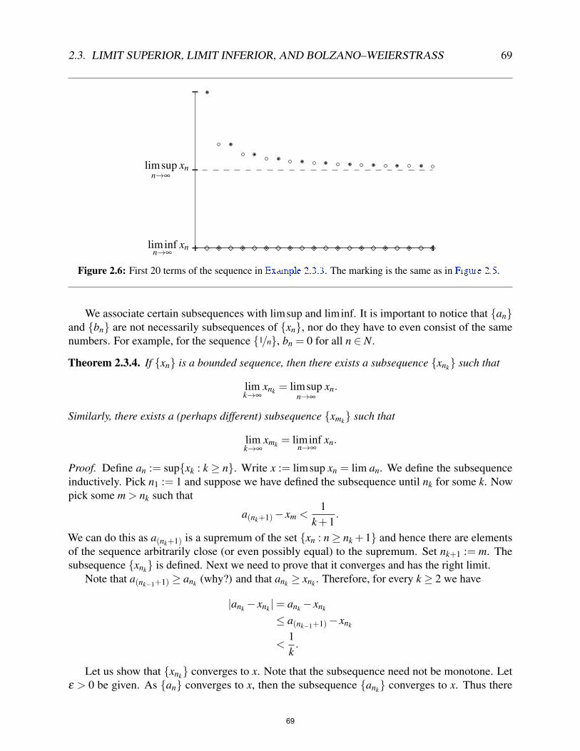
2.3. LIMIT SUPERIOR, LIMIT INFERIOR, AND BOLZANO–WEIERSTRASS 69
limsupn→∞
xn
liminfn→∞
xn ⋄ ⋄ ⋄ ⋄ ⋄ ⋄ ⋄ ⋄ ⋄ ⋄ ⋄ ⋄ ⋄ ⋄ ⋄ ⋄ ⋄ ⋄ ⋄ ⋄
Figure 2.6: First 20 terms of the sequence in Example 2.3.3 . The marking is the same as in Figure 2.5 .
We associate certain subsequences with limsup and liminf. It is important to notice that {an}and {bn} are not necessarily subsequences of {xn}, nor do they have to even consist of the samenumbers. For example, for the sequence {1/n}, bn = 0 for all n ∈ N.
Theorem 2.3.4. If {xn} is a bounded sequence, then there exists a subsequence {xnk} such that
limk→∞
xnk = limsupn→∞
xn.
Similarly, there exists a (perhaps different) subsequence {xmk} such that
limk→∞
xmk = liminfn→∞
xn.
Proof. Define an := sup{xk : k ≥ n}. Write x := limsup xn = lim an. We define the subsequenceinductively. Pick n1 := 1 and suppose we have defined the subsequence until nk for some k. Nowpick some m > nk such that
a(nk+1)− xm <1
k+1.
We can do this as a(nk+1) is a supremum of the set {xn : n≥ nk +1} and hence there are elementsof the sequence arbitrarily close (or even possibly equal) to the supremum. Set nk+1 := m. Thesubsequence {xnk} is defined. Next we need to prove that it converges and has the right limit.
Note that a(nk−1+1) ≥ ank (why?) and that ank ≥ xnk . Therefore, for every k ≥ 2 we have
|ank− xnk |= ank− xnk
≤ a(nk−1+1)− xnk
<1k.
Let us show that {xnk} converges to x. Note that the subsequence need not be monotone. Letε > 0 be given. As {an} converges to x, then the subsequence {ank} converges to x. Thus there
69

70 CHAPTER 2. SEQUENCES AND SERIES
exists an M1 ∈ N such that for all k ≥M1 we have
|ank− x|< ε
2.
Find an M2 ∈ N such that1
M2≤ ε
2.
Take M := max{M1,M2,2} and compute. For all k ≥M we have
|x− xnk |= |ank− xnk + x−ank |≤ |ank− xnk |+ |x−ank |
<1k+
ε
2
≤ 1M2
+ε
2≤ ε
2+
ε
2= ε.
We leave the statement for liminf as an exercise.
2.3.2 Using limit inferior and limit superiorThe advantage of liminf and limsup is that we can always write them down for any (bounded)sequence. If we could somehow compute them, we could also compute the limit of the sequenceif it exists, or show that the sequence diverges. Working with liminf and limsup is a little bit likeworking with limits, although there are subtle differences.
Proposition 2.3.5. Let {xn} be a bounded sequence. Then {xn} converges if and only if
liminfn→∞
xn = limsupn→∞
xn.
Furthermore, if {xn} converges, then
limn→∞
xn = liminfn→∞
xn = limsupn→∞
xn.
Proof. Let an and bn be as in Definition 2.3.1 . In particular, for all n ∈ N,
bn ≤ xn ≤ an.
If liminf xn = limsup xn, then we know that {an} and {bn} both converge to the same limit. By thesqueeze lemma ( Lemma 2.2.1 ), {xn} converges and
limn→∞
bn = limn→∞
xn = limn→∞
an.
Now suppose {xn} converges to x. We know by Theorem 2.3.4 that there exists a subsequence{xnk} that converges to limsup xn. As {xn} converges to x, every subsequence converges to x andtherefore limsup xn = lim xnk = x. Similarly, liminf xn = x.
70

2.3. LIMIT SUPERIOR, LIMIT INFERIOR, AND BOLZANO–WEIERSTRASS 71
Limit superior and limit inferior behave nicely with subsequences.
Proposition 2.3.6. Suppose {xn} is a bounded sequence and {xnk} is a subsequence. Then
liminfn→∞
xn ≤ liminfk→∞
xnk ≤ limsupk→∞
xnk ≤ limsupn→∞
xn.
Proof. The middle inequality has been proved already. We will prove the third inequality, and leavethe first inequality as an exercise.
We want to prove that limsup xnk ≤ limsup xn. Define a j := sup{xk : k ≥ j} as usual. Alsodefine c j := sup{xnk : k≥ j}. It is not true that {c j} is necessarily a subsequence of {a j}. However,as nk ≥ k for all k, we have that {xnk : k ≥ j} ⊂ {xk : k ≥ j}. A supremum of a subset is less than orequal to the supremum of the set and therefore
c j ≤ a j.
Lemma 2.2.3 giveslimj→∞
c j ≤ limj→∞
a j,
which is the desired conclusion.
Limit superior and limit inferior are the largest and smallest subsequential limits. If thesubsequence {xnk} in the previous proposition is convergent, then liminf xnk = lim xnk = limsup xnk .Therefore,
liminfn→∞
xn ≤ limk→∞
xnk ≤ limsupn→∞
xn.
Similarly, we get the following useful test for convergence of a bounded sequence. We leave theproof as an exercise.
Proposition 2.3.7. A bounded sequence {xn} is convergent and converges to x if and only if everyconvergent subsequence {xnk} converges to x.
2.3.3 Bolzano–Weierstrass theoremWhile it is not true that a bounded sequence is convergent, the Bolzano–Weierstrass theorem tells usthat we can at least find a convergent subsequence. The version of Bolzano–Weierstrass that wepresent in this section is the Bolzano–Weierstrass for sequences.
Theorem 2.3.8 (Bolzano–Weierstrass). Suppose a sequence {xn} of real numbers is bounded. Thenthere exists a convergent subsequence {xni}.
Proof. We use Theorem 2.3.4 . It says that there exists a subsequence whose limit is limsup xn.
The reader might complain right now that Theorem 2.3.4 is strictly stronger than the Bolzano–Weierstrass theorem as presented above. That is true. However, Theorem 2.3.4 only applies to thereal line, but Bolzano–Weierstrass applies in more general contexts (that is, in Rn) with pretty muchthe exact same statement.
As the theorem is so important to analysis, we present an explicit proof. The idea of thefollowing proof also generalizes to different contexts.
71

72 CHAPTER 2. SEQUENCES AND SERIES
Alternate proof of Bolzano–Weierstrass. As the sequence is bounded, then there exist two numbersa1 < b1 such that a1 ≤ xn ≤ b1 for all n ∈N. We will define a subsequence {xni} and two sequences{ai} and {bi}, such that {ai} is monotone increasing, {bi} is monotone decreasing, ai ≤ xni ≤ biand such that lim ai = lim bi. That xni converges then follows by the squeeze lemma .
We define the sequences inductively. We will always have that ai < bi, and that xn ∈ [ai,bi]for infinitely many n ∈ N. We have already defined a1 and b1. We take n1 := 1, that is xn1 = x1.Suppose that up to some k ∈ N we have defined the subsequence xn1,xn2, . . . ,xnk , and the sequencesa1,a2, . . . ,ak and b1,b2, . . . ,bk. Let y := ak+bk
2 . Clearly ak < y < bk. If there exist infinitely manyj ∈N such that x j ∈ [ak,y], then set ak+1 := ak, bk+1 := y, and pick nk+1 > nk such that xnk+1 ∈ [ak,y].If there are not infinitely many j such that x j ∈ [ak,y], then it must be true that there are infinitelymany j ∈ N such that x j ∈ [y,bk]. In this case pick ak+1 := y, bk+1 := bk, and pick nk+1 > nk suchthat xnk+1 ∈ [y,bk].
We now have the sequences defined. What is left to prove is that lim ai = lim bi. The limits existas the sequences are monotone. In the construction, bi−ai is cut in half in each step. Therefore,bi+1−ai+1 =
bi−ai2 . By induction ,
bi−ai =b1−a1
2i−1 .
Let x := lim ai. As {ai} is monotone,
x = sup{ai : i ∈ N}.
Let y := lim bi = inf{bi : i ∈ N}. Since ai < bi for all i, then x≤ y. As the sequences are monotone,then for any i we have (why?)
y− x≤ bi−ai =b1−a1
2i−1 .
Because b1−a12i−1 is arbitrarily small and y−x≥ 0, we have y−x= 0. Finish by the squeeze lemma .
Yet another proof of the Bolzano–Weierstrass theorem is to show the following claim, which isleft as a challenging exercise. Claim: Every sequence has a monotone subsequence.
2.3.4 Infinite limitsJust as for infima and suprema, it is possible to allow certain limits to be infinite. That is, we writelim xn = ∞ or lim xn =−∞ for certain divergent sequences.
Definition 2.3.9. We say {xn} diverges to infinity
* if for every K ∈ R, there exists an M ∈ N such
that for all n≥M we have xn > K. In this case we write
limn→∞
xn := ∞.
Similarly, if for every K ∈ R there exists an M ∈ N such that for all n≥M we have xn < K, we say{xn} diverges to minus infinity and we write
limn→∞
xn :=−∞.
*Sometimes it is said that {xn} converges to infinity.
72

2.3. LIMIT SUPERIOR, LIMIT INFERIOR, AND BOLZANO–WEIERSTRASS 73
With this definition and allowing ∞ and −∞, we can write lim xn for any monotone sequence.
Proposition 2.3.10. Suppose {xn} is a monotone unbounded sequence. Then
limn→∞
xn =
{∞ if {xn} is increasing,−∞ if {xn} is decreasing.
Proof. The case of monotone increasing follows from Exercise 2.3.14 part c) below. Let usdo monotone decreasing. Suppose {xn} is decreasing and unbounded, that is, for every K ∈ R,there is an M ∈ N such that xM < K. By monotonicity xn ≤ xM < K for all n ≥ M. Therefore,lim xn =−∞.
Example 2.3.11:limn→∞
n = ∞, limn→∞
n2 = ∞, limn→∞−n =−∞.
We leave verification to the reader.
We may also allow liminf and limsup to take on the values ∞ and −∞, so that we can applyliminf and limsup to absolutely any sequence, not just a bounded one. Unfortunately, the sequences{an} and {bn} are not sequences of real numbers but of extended real numbers. In particular, ancan equal ∞ for some n, and bn can equal −∞. So we have no definition for the limits. But since theextended real numbers are still an ordered set, we can take suprema and infima.
Definition 2.3.12. Let {xn} be an unbounded sequence of real numbers. Define sequences ofextended real numbers by an := sup{xk : k ≥ n} and bn := inf{xk : k ≥ n}. Define
limsupn→∞
xn := inf{an : n ∈ N}, and liminfn→∞
xn := sup{bn : n ∈ N}.
This definition agrees with the definition for bounded sequences whenever liman or limbnmakes sense including possibly ∞ and −∞.
Proposition 2.3.13. Let {xn} be an unbounded sequence. Define {an} and {bn} as above. Then{an} is decreasing, and {bn} is increasing. If an is a real number for every n, then limsup xn =lim an. If bn is a real number for every n, then liminf xn = lim bn.
Proof. As before, an = sup{xk : k ≥ n} ≥ sup{xk : k ≥ n+ 1} = an+1. So {an} is decreasing.Similarly, {bn} is increasing.
If the sequence {an} is a sequence of real numbers, then liman = inf{an : n ∈ N}. This followsfrom Proposition 2.1.10 if {an} is bounded and Proposition 2.3.10 if {an} is unbounded. Weproceed similarly with {bn}.
The definition behaves as expected with limsup and liminf, see exercises 2.3.13 and 2.3.14 .
Example 2.3.14: Suppose xn := 0 for odd n and xn := n for even n. Then an = ∞ for every n, sincefor any M, there exists an even k such that xk = k ≥M. On the other hand, bn = 0 for all n, as forany n, {bk : k ≥ n} consists of 0 and nonnegative numbers. So,
limn→∞
xn does not exist, limsupn→∞
xn = ∞, liminfn→∞
xn = 0.
73

74 CHAPTER 2. SEQUENCES AND SERIES
2.3.5 ExercisesExercise 2.3.1: Suppose {xn} is a bounded sequence. Define an and bn as in Definition 2.3.1 . Show that{an} and {bn} are bounded.
Exercise 2.3.2: Suppose {xn} is a bounded sequence. Define bn as in Definition 2.3.1 . Show that {bn} is anincreasing sequence.
Exercise 2.3.3: Finish the proof of Proposition 2.3.6 . That is, suppose {xn} is a bounded sequence and {xnk}is a subsequence. Prove liminf
n→∞xn ≤ liminf
k→∞xnk .
Exercise 2.3.4: Prove Proposition 2.3.7 .
Exercise 2.3.5:
a) Let xn :=(−1)n
n. Find limsup xn and liminf xn.
b) Let xn :=(n−1)(−1)n
n. Find limsup xn and liminf xn.
Exercise 2.3.6: Let {xn} and {yn} be bounded sequences such that xn ≤ yn for all n. Then show that
limsupn→∞
xn ≤ limsupn→∞
yn
andliminf
n→∞xn ≤ liminf
n→∞yn.
Exercise 2.3.7: Let {xn} and {yn} be bounded sequences.
a) Show that {xn + yn} is bounded.
b) Show that(liminf
n→∞xn)+(liminf
n→∞yn)≤ liminf
n→∞(xn + yn).
Hint: Find a subsequence {xni + yni} of {xn + yn} that converges. Then find a subsequence {xnmi} of
{xni} that converges. Then apply what you know about limits.
c) Find an explicit {xn} and {yn} such that
(liminfn→∞
xn)+(liminfn→∞
yn)< liminfn→∞
(xn + yn).
Hint: Look for examples that do not have a limit.
Exercise 2.3.8: Let {xn} and {yn} be bounded sequences (from the previous exercise we know that {xn +yn}is bounded).
a) Show that(limsup
n→∞xn)+(limsup
n→∞yn)≥ limsup
n→∞(xn + yn).
Hint: See previous exercise.
b) Find an explicit {xn} and {yn} such that
(limsupn→∞
xn)+(limsupn→∞
yn)> limsupn→∞
(xn + yn).
Hint: See previous exercise.
74

2.3. LIMIT SUPERIOR, LIMIT INFERIOR, AND BOLZANO–WEIERSTRASS 75
Exercise 2.3.9: If S⊂R is a set, then x ∈R is a cluster point if for every ε > 0, the set (x−ε,x+ε)∩S\{x}is not empty. That is, if there are points of S arbitrarily close to x. For example, S := {1/n : n ∈ N} has aunique (only one) cluster point 0, but 0 /∈ S. Prove the following version of the Bolzano–Weierstrass theorem:
Theorem. Let S⊂ R be a bounded infinite set, then there exists at least one cluster point of S.
Hint: If S is infinite, then S contains a countably infinite subset. That is, there is a sequence {xn} ofdistinct numbers in S.
Exercise 2.3.10 (Challenging):
a) Prove that any sequence contains a monotone subsequence. Hint: Call n ∈ N a peak if am ≤ an for allm≥ n. There are two possibilities: Either the sequence has at most finitely many peaks, or it has infinitelymany peaks.
b) Conclude the Bolzano–Weierstrass theorem.
Exercise 2.3.11: Prove a stronger version of Proposition 2.3.7 . Suppose {xn} is a sequence such that everysubsequence {xni} has a subsequence {xnmi
} that converges to x.
a) First show that {xn} is bounded.
b) Now show that {xn} converges to x.
Exercise 2.3.12: Let {xn} be a bounded sequence.
a) Prove that there exists an s such that for any r > s there exists an M ∈ N such that for all n≥M we havexn < r.
b) If s is a number as in a), then prove limsup xn ≤ s.
c) Show that if S is the set of all s as in a), then limsup xn = inf S.
Exercise 2.3.13 (Easy): Suppose {xn} is such that liminf xn =−∞, limsup xn = ∞.
a) Show that {xn} is not convergent, and also that neither lim xn = ∞ nor lim xn =−∞ is true.
b) Find an example of such a sequence.
Exercise 2.3.14: Let {xn} be a sequence.
a) Show that lim xn = ∞ if and only if liminf xn = ∞.
b) Then show that lim xn =−∞ if and only if limsup xn =−∞.
c) If {xn} is monotone increasing, show that either lim xn exists and is finite or lim xn = ∞. In either case,lim xn = sup{xn : n ∈ N}.
Exercise 2.3.15: Prove the following stronger version of Lemma 2.2.12 , the ratio test. Suppose {xn} is asequence such that xn 6= 0 for all n.
a) Prove that if
limsupn→∞
|xn+1||xn|
< 1,
then {xn} converges to 0.
b) Prove that if
liminfn→∞
|xn+1||xn|
> 1,
then {xn} is unbounded.
75

76 CHAPTER 2. SEQUENCES AND SERIES
Exercise 2.3.16: Suppose {xn} is a bounded sequence, an := sup{xk : k ≥ n} as before. Suppose that forsome ` ∈ N, a` /∈ {xk : k ≥ `}. Then show that a j = a` for all j ≥ `, and hence limsup xn = a`.
Exercise 2.3.17: Suppose {xn} is a sequence, and an := sup{xk : k≥ n} and bn := sup{xk : k≥ n} as before.
a) Prove that if a` = ∞ for some ` ∈ N, then limsup xn = ∞.
b) Prove that if b` =−∞ for some ` ∈ N, then liminf xn =−∞.
Exercise 2.3.18: Suppose {xn} is a sequence such that both liminf xn and limsup xn are finite. Prove that{xn} is bounded.
Exercise 2.3.19: Suppose {xn} is a bounded sequence, and ε > 0 is given. Prove that there exists an M suchthat for all k ≥M we have
xk−(
limsupn→∞
xn
)< ε and
(liminf
n→∞xn
)− xk < ε.
76

2.4. CAUCHY SEQUENCES 77
2.4 Cauchy sequencesNote: 0.5–1 lecture
Often we wish to describe a certain number by a sequence that converges to it. In this case, it isimpossible to use the number itself in the proof that the sequence converges. It would be nice if wecould check for convergence without knowing the limit.
Definition 2.4.1. A sequence {xn} is a Cauchy sequence
* if for every ε > 0 there exists an M ∈ N
such that for all n≥M and all k ≥M we have
|xn− xk|< ε.
Intuitively it means that the terms of the sequence are eventually all arbitrarily close to eachother. We might expect such a sequence to be convergent, and it turns out that we would be correctbecause R has the least-upper-bound property . Before we prove this, we look at some examples.
Example 2.4.2: The sequence {1/n} is a Cauchy sequence.Proof: Given ε > 0, find M such that M > 2/ε. Then for n,k ≥M we have that 1/n < ε/2 and
1/k < ε/2. Therefore, for n,k ≥M we have∣∣∣∣1n − 1k
∣∣∣∣≤ ∣∣∣∣1n∣∣∣∣+ ∣∣∣∣1k
∣∣∣∣< ε
2+
ε
2= ε.
Example 2.4.3: The sequence {n+1n } is a Cauchy sequence.
Proof: Given ε > 0, find M such that M > 2/ε. Then for n,k ≥M we have that 1/n < ε/2 and1/k < ε/2. Therefore, for n,k ≥M we have∣∣∣∣n+1
n− k+1
k
∣∣∣∣= ∣∣∣∣k(n+1)−n(k+1)nk
∣∣∣∣=
∣∣∣∣kn+ k−nk−nnk
∣∣∣∣=
∣∣∣∣k−nnk
∣∣∣∣≤∣∣∣∣ knk
∣∣∣∣+ ∣∣∣∣−nnk
∣∣∣∣=
1n+
1k<
ε
2+
ε
2= ε.
Proposition 2.4.4. A Cauchy sequence is bounded.
Proof. Suppose {xn} is Cauchy. Pick M such that for all n,k ≥ M we have |xn− xk| < 1. Inparticular, for all n≥M,
|xn− xM|< 1.
*Named after the French mathematician Augustin-Louis Cauchy (1789–1857).
77

78 CHAPTER 2. SEQUENCES AND SERIES
By the reverse triangle inequality, |xn|− |xM| ≤ |xn− xM|< 1. Hence for n≥M,
|xn|< 1+ |xM| .
LetB := max
{|x1| , |x2| , . . . , |xM−1| ,1+ |xM|
}.
Then |xn| ≤ B for all n ∈ N.
Theorem 2.4.5. A sequence of real numbers is Cauchy if and only if it converges.
Proof. Let ε > 0 be given and suppose {xn} converges to x. Then there exists an M such that forn≥M,
|xn− x|< ε
2.
Hence for n≥M and k ≥M,
|xn− xk|= |xn− x+ x− xk| ≤ |xn− x|+ |x− xk|<ε
2+
ε
2= ε.
Alright, that direction was easy. Now suppose {xn} is Cauchy. We have shown that {xn}is bounded. For a bounded sequence, liminf and limsup exist, and this is where we use the
least-upper-bound property . If we show that
liminfn→∞
xn = limsupn→∞
xn,
then {xn} must be convergent by Proposition 2.3.5 .Define a := limsup xn and b := liminf xn. By Theorem 2.3.4 , there exist subsequences {xni}
and {xmi}, such thatlimi→∞
xni = a and limi→∞
xmi = b.
Given an ε > 0, there exists an M1 such that for all i≥M1 we have |xni−a|< ε/3 and an M2 suchthat for all i≥M2 we have |xmi−b|< ε/3. There also exists an M3 such that for all n,k ≥M3 wehave |xn− xk|< ε/3. Let M := max{M1,M2,M3}. If i≥M, then ni ≥M and mi ≥M. Hence
|a−b|= |a− xni + xni− xmi + xmi−b|≤ |a− xni|+ |xni− xmi|+ |xmi−b|<
ε
3+
ε
3+
ε
3= ε.
As |a−b|< ε for all ε > 0, then a = b and the sequence converges.
Remark 2.4.6. The statement of this proposition is sometimes used to define the completenessproperty of the real numbers. We say a set is Cauchy-complete (or sometimes just complete) if everyCauchy sequence converges. Above we proved that as R has the least-upper-bound property , then Ris Cauchy-complete. We can “complete” Q by “throwing in” just enough points to make all Cauchysequences converge (we omit the details). The resulting field has the least-upper-bound property.The advantage of using Cauchy sequences to define completeness is that this idea generalizes tomore abstract settings such as metric spaces, see chapter 7 .
78

2.4. CAUCHY SEQUENCES 79
The Cauchy criterion is stronger than |xn+1− xn| (or∣∣xn+ j− xn
∣∣ for a fixed j) going to zero as ngoes to infinity. When we get to the partial sums of the harmonic series (see Example 2.5.11 in thenext section), we will have a sequence such that xn+1− xn = 1/n, yet {xn} is divergent. In fact, forthat sequence, limn→∞
∣∣xn+ j− xn∣∣= 0 for any j ∈ N (confer Exercise 2.5.12 ). The key point in the
definition of Cauchy is that n and k vary independently and can be arbitrarily far apart.
2.4.1 ExercisesExercise 2.4.1: Prove that {n2−1
n2 } is Cauchy using directly the definition of Cauchy sequences.
Exercise 2.4.2: Let {xn} be a sequence such that there exists a 0 <C < 1 such that
|xn+1− xn| ≤C |xn− xn−1| .
Prove that {xn} is Cauchy. Hint: You can freely use the formula (for C 6= 1)
1+C+C2 + · · ·+Cn =1−Cn+1
1−C.
Exercise 2.4.3 (Challenging): Suppose F is an ordered field that contains the rational numbers Q, such thatQ is dense, that is: Whenever x,y ∈ F are such that x < y, then there exists a q ∈Q such that x < q < y. Saya sequence {xn}∞
n=1 of rational numbers is Cauchy if given any ε ∈Q with ε > 0, there exists an M such thatfor all n,k ≥M we have |xn− xk|< ε . Suppose any Cauchy sequence of rational numbers has a limit in F.Prove that F has the least-upper-bound property .
Exercise 2.4.4: Let {xn} and {yn} be sequences such that lim yn = 0. Suppose that for all k ∈ N and for allm≥ k we have
|xm− xk| ≤ yk.
Show that {xn} is Cauchy.
Exercise 2.4.5: Suppose a Cauchy sequence {xn} is such that for every M ∈ N, there exists a k ≥M and ann≥M such that xk < 0 and xn > 0. Using simply the definition of a Cauchy sequence and of a convergentsequence, show that the sequence converges to 0.
Exercise 2.4.6: Suppose |xn− xk| ≤ n/k2 for all n and k. Show that {xn} is Cauchy.
Exercise 2.4.7: Suppose {xn} is a Cauchy sequence such that for infinitely many n, xn = c. Using only thedefinition of Cauchy sequence prove that lim xn = c.
Exercise 2.4.8: True or false, prove or find a counterexample: If {xn} is a Cauchy sequence, then there existsan M such that for all n≥M we have |xn+1− xn| ≤ |xn− xn−1|.
79

80 CHAPTER 2. SEQUENCES AND SERIES
2.5 SeriesNote: 2 lectures
A fundamental object in mathematics is that of a series. In fact, when the foundations of analysiswere being developed, the motivation was to understand series. Understanding series is importantin applications of analysis. For example, solving differential equations often includes series, anddifferential equations are the basis for understanding almost all of modern science.
2.5.1 Definition
Definition 2.5.1. Given a sequence {xn}, we write the formal object
∞
∑n=1
xn or sometimes just ∑xn
and call it a series. A series converges, if the sequence {sk} defined by
sk :=k
∑n=1
xn = x1 + x2 + · · ·+ xk,
converges. The numbers sk are called partial sums. If x := lim sk, we write
∞
∑n=1
xn = x.
In this case, we cheat a little and treat ∑∞n=1 xn as a number.
If the sequence {sk} diverges, we say the series is divergent. In this case, ∑xn is simply a formalobject and not a number.
In other words, for a convergent series we have
∞
∑n=1
xn = limk→∞
k
∑n=1
xn.
We only have this equality if the limit on the right actually exists. If the series does not converge,the right-hand side does not make sense (the limit does not exist). Therefore, be careful as ∑xnmeans two different things (a notation for the series itself or the limit of the partial sums), and youmust use context to distinguish.
Remark 2.5.2. It is sometimes convenient to start the series at an index different from 1. For instance,we can write
∞
∑n=0
rn =∞
∑n=1
rn−1.
The left-hand side is more convenient to write.
80

2.5. SERIES 81
Remark 2.5.3. It is common to write the series ∑xn as
x1 + x2 + x3 + · · ·with the understanding that the ellipsis indicates a series and not a simple sum. We do not use thisnotation as it is the sort of informal notation that leads to mistakes in proofs.
Example 2.5.4: The series∞
∑n=1
12n
converges and the limit is 1. That is,∞
∑n=1
12n = lim
k→∞
k
∑n=1
12n = 1.
Proof: First we prove the following equality(k
∑n=1
12n
)+
12k = 1.
The equality is immediate when k = 1. The proof for general k follows by induction , which weleave to the reader. See Figure 2.7 for an illustration.
1/2 1/81/4 1/8
1/2+ 1/4+ 1/80 1
Figure 2.7: The equality(∑k
n=112n
)+ 1
2k = 1 illustrated for k = 3.
Let sk be the partial sum. We write
|1− sk|=∣∣∣∣∣1− k
∑n=1
12n
∣∣∣∣∣=∣∣∣∣ 12k
∣∣∣∣= 12k .
The sequence{ 1
2k
}, and therefore
{|1− sk|
}, converges to zero. So, {sk} converges to 1.
Proposition 2.5.5. Suppose −1 < r < 1. Then the geometric series ∑∞n=0 rn converges, and
∞
∑n=0
rn =1
1− r.
Details of the proof are left as an exercise. The proof consists of showingk−1
∑n=0
rn =1− rk
1− r,
and then taking the limit as k goes to ∞. Geometric series is one of the most important series, and infact it is one of the few series for which we can so explicitly find the limit.
We have the following analogue of the tail of a sequence.
81

82 CHAPTER 2. SEQUENCES AND SERIES
Proposition 2.5.6. Let ∑xn be a series. Let M ∈ N. Then∞
∑n=1
xn converges if and only if∞
∑n=M
xn converges.
Proof. We look at partial sums of the two series (for k ≥M)
k
∑n=1
xn =
(M−1
∑n=1
xn
)+
k
∑n=M
xn.
Note that ∑M−1n=1 xn is a fixed number. Use Proposition 2.2.5 to finish the proof.
2.5.2 Cauchy seriesDefinition 2.5.7. A series ∑xn is said to be Cauchy or a Cauchy series, if the sequence of partialsums {sn} is a Cauchy sequence.
A sequence of real numbers converges if and only if it is Cauchy. Therefore, a series isconvergent if and only if it is Cauchy. The series ∑xn is Cauchy if for every ε > 0, there exists anM ∈ N, such that for every n≥M and k ≥M we have∣∣∣∣∣
(k
∑j=1
x j
)−(
n
∑j=1
x j
)∣∣∣∣∣< ε.
Without loss of generality we assume n < k. Then we write∣∣∣∣∣(
k
∑j=1
x j
)−(
n
∑j=1
x j
)∣∣∣∣∣=∣∣∣∣∣ k
∑j=n+1
x j
∣∣∣∣∣< ε.
We have proved the following simple proposition.
Proposition 2.5.8. The series ∑xn is Cauchy if for every ε > 0, there exists an M ∈ N such that forevery n≥M and every k > n we have ∣∣∣∣∣ k
∑j=n+1
x j
∣∣∣∣∣< ε.
2.5.3 Basic propertiesProposition 2.5.9. Let ∑xn be a convergent series. Then the sequence {xn} is convergent and
limn→∞
xn = 0.
Proof. Let ε > 0 be given. As ∑xn is convergent, it is Cauchy. Thus we find an M such that forevery n≥M we have
ε >
∣∣∣∣∣ n+1
∑j=n+1
x j
∣∣∣∣∣= |xn+1| .
Hence for every n≥M+1 we have |xn|< ε .
82

2.5. SERIES 83
Example 2.5.10: If r ≥ 1 or r ≤−1, then the geometric series ∑∞n=0 rn diverges.
Proof: |rn|= |r|n ≥ 1n = 1. So the terms do not go to zero and the series cannot converge.
So if a series converges, the terms of the series go to zero. The implication, however, goes onlyone way. Let us give an example.
Example 2.5.11: The series ∑ 1n diverges (despite the fact that lim 1
n = 0). This is the famousharmonic series
* .
Proof: We will show that the sequence of partial sums is unbounded, and hence cannot converge.Write the partial sums sn for n = 2k as:
s1 = 1,
s2 = (1)+(
12
),
s4 = (1)+(
12
)+
(13+
14
),
s8 = (1)+(
12
)+
(13+
14
)+
(15+
16+
17+
18
),
...
s2k = 1+k
∑j=1
(2 j
∑m=2 j−1+1
1m
).
Notice 1/3+ 1/4≥ 1/4+ 1/4 = 1/2 and 1/5+ 1/6+ 1/7+ 1/8≥ 1/8+ 1/8+ 1/8+ 1/8 = 1/2. More generally
2k
∑m=2k−1+1
1m≥
2k
∑m=2k−1+1
12k = (2k−1)
12k =
12.
Therefore,
s2k = 1+k
∑j=1
(2 j
∑m=2 j−1+1
1m
)≥ 1+
k
∑j=1
12= 1+
k2.
As { k2} is unbounded by the Archimedean property , that means that {s2k} is unbounded, and
therefore {sn} is unbounded. Hence {sn} diverges, and consequently ∑ 1n diverges.
Convergent series are linear. That is, we can multiply them by constants and add them and theseoperations are done term by term.
Proposition 2.5.12 (Linearity of series). Let α ∈ R and ∑xn and ∑yn be convergent series. Then
(i) ∑αxn is a convergent series and
∞
∑n=1
αxn = α
∞
∑n=1
xn.
*The divergence of the harmonic series was known long before the theory of series was made rigorous. The proofwe give is the earliest proof and was given by Nicole Oresme (1323?–1382).
83

84 CHAPTER 2. SEQUENCES AND SERIES
(ii) ∑(xn + yn) is a convergent series and
∞
∑n=1
(xn + yn) =
(∞
∑n=1
xn
)+
(∞
∑n=1
yn
).
Proof. For the first item, we simply write the kth partial sum
k
∑n=1
αxn = α
(k
∑n=1
xn
).
We look at the right-hand side and note that the constant multiple of a convergent sequence isconvergent. Hence, we take the limit of both sides to obtain the result.
For the second item we also look at the kth partial sum
k
∑n=1
(xn + yn) =
(k
∑n=1
xn
)+
(k
∑n=1
yn
).
We look at the right-hand side and note that the sum of convergent sequences is convergent. Hence,we take the limit of both sides to obtain the proposition.
An example of a useful application of the first item is the following formula. Suppose |r|< 1and j ∈ N, then
∞
∑n= j
rn =r j
1− r.
The formula follows by using the geometric series and multiplying by r j:
r j∞
∑n=0
rn =∞
∑n=0
rn+ j =∞
∑n= j
rn.
Multiplying series is not as simple as adding, see the next section. It is not true, of course, that wemultiply term by term. That strategy does not work even for finite sums: (a+b)(c+d) 6= ac+bd.
2.5.4 Absolute convergenceAs monotone sequences are easier to work with than arbitrary sequences, it is usually easier to workwith series ∑xn, where xn ≥ 0 for all n. The sequence of partial sums is then monotone increasingand converges if it is bounded above. Let us formalize this statement as a proposition.
Proposition 2.5.13. If xn ≥ 0 for all n, then ∑xn converges if and only if the sequence of partialsums is bounded above.
As the limit of a monotone increasing sequence is the supremum, then when xn ≥ 0 for all n, wehave the inequality
k
∑n=1
xn ≤∞
∑n=1
xn.
84

2.5. SERIES 85
If we allow infinite limits, the inequality still holds even when the series diverges to infinity, althoughin that case it is not terribly useful.
We will see that the following common criterion for convergence of series has big implicationsfor how the series can be manipulated.
Definition 2.5.14. A series ∑xn converges absolutely if the series ∑ |xn| converges. If a seriesconverges, but does not converge absolutely, we say it is conditionally convergent.
Proposition 2.5.15. If the series ∑xn converges absolutely, then it converges.
Proof. A series is convergent if and only if it is Cauchy. Hence suppose ∑ |xn| is Cauchy. That is,for every ε > 0, there exists an M such that for all k ≥M and all n > k we have
n
∑j=k+1
∣∣x j∣∣= ∣∣∣∣∣ n
∑j=k+1
∣∣x j∣∣∣∣∣∣∣< ε.
We apply the triangle inequality for a finite sum to obtain∣∣∣∣∣ n
∑j=k+1
x j
∣∣∣∣∣≤ n
∑j=k+1
∣∣x j∣∣< ε.
Hence ∑xn is Cauchy and therefore it converges.
If ∑xn converges absolutely, the limits of ∑xn and ∑ |xn| may be different. Computing one doesnot help us compute the other. However the computation above leads to a useful inequality forabsolutely convergent series, a series version of the triangle inequality, a proof of which we leave asan exercise: ∣∣∣∣∣ ∞
∑j=1
x j
∣∣∣∣∣≤ ∞
∑j=1
∣∣x j∣∣ .
Absolutely convergent series have many wonderful properties. For example, absolutely conver-gent series can be rearranged arbitrarily, or we can multiply such series together easily. Conditionallyconvergent series on the other hand often do not behave as one would expect. See the next section.
We leave as an exercise to show that
∞
∑n=1
(−1)n
n
converges, although the reader should finish this section before trying. On the other hand we proved
∞
∑n=1
1n
diverges. Therefore, ∑ (−1)n
n is a conditionally convergent series.
85

86 CHAPTER 2. SEQUENCES AND SERIES
2.5.5 Comparison test and the p-seriesWe noted above that for a series to converge the terms not only have to go to zero, but they have togo to zero “fast enough.” If we know about convergence of a certain series, we can use the followingcomparison test to see if the terms of another series go to zero “fast enough.”
Proposition 2.5.16 (Comparison test). Let ∑xn and ∑yn be series such that 0 ≤ xn ≤ yn for alln ∈ N.
(i) If ∑yn converges, then so does ∑xn.
(ii) If ∑xn diverges, then so does ∑yn.
Proof. As the terms of the series are all nonnegative, the sequences of partial sums are bothmonotone increasing. Since xn ≤ yn for all n, the partial sums satisfy for all k
k
∑n=1
xn ≤k
∑n=1
yn. (2.1)
If the series ∑yn converges, the partial sums for the series are bounded. Therefore, the right-handside of ( 2.1 ) is bounded for all k; there exists some B ∈ R such that ∑k
n=1 yn ≤ B for all k, and so
k
∑n=1
xn ≤k
∑n=1
yn ≤ B.
Hence the partial sums for ∑xn are also bounded. Since the partial sums are a monotone increasingsequence they are convergent. The first item is thus proved.
On the other hand if ∑xn diverges, the sequence of partial sums must be unbounded since it ismonotone increasing. That is, the partial sums for ∑xn are eventually bigger than any real number.Putting this together with ( 2.1 ) we see that for any B ∈ R, there is a k such that
B≤k
∑n=1
xn ≤k
∑n=1
yn.
Hence the partial sums for ∑yn are also unbounded, and ∑yn also diverges.
A useful series to use with the comparison test is the p-series
* .
Proposition 2.5.17 (p-series or the p-test). For p ∈ R, the series
∞
∑n=1
1np
converges if and only if p > 1.
*We have not yet defined xp for x > 0 and an arbitrary p ∈ R. The definition is xp := exp(p lnx). We will definethe logarithm and the exponential in §5.4 . For now you can just think of rational p where xk/m = (x1/m)
k. See also
Exercise 1.2.17 .
86

2.5. SERIES 87
Proof. First suppose p ≤ 1. As n ≥ 1, we have 1np ≥ 1
n . Since ∑ 1n diverges, we see that the ∑ 1
np
must diverge for all p≤ 1 by the comparison test.Now suppose p > 1. We proceed as we did for the harmonic series, but instead of showing that
the sequence of partial sums is unbounded, we show that it is bounded. The terms of the seriesare positive, so the sequence of partial sums is monotone increasing and converges if it is boundedabove. Let sn denote the nth partial sum.
s1 = 1,
s3 = (1)+(
12p +
13p
),
s7 = (1)+(
12p +
13p
)+
(14p +
15p +
16p +
17p
),
...
s2k−1 = 1+k−1
∑j=1
(2 j+1−1
∑m=2 j
1mp
).
Instead of estimating from below, we estimate from above. In particular, as p is positive, then2p < 3p, and hence 1
2p +1
3p <1
2p +1
2p . Similarly, 14p +
15p +
16p +
17p <
14p +
14p +
14p +
14p . Therefore,
s2k−1 = 1+k−1
∑j=1
(2 j+1−1
∑m=2 j
1mp
)
< 1+k−1
∑j=1
(2 j+1−1
∑m=2 j
1(2 j)p
)
= 1+k−1
∑j=1
(2 j
(2 j)p
)
= 1+k−1
∑j=1
(1
2p−1
) j
.
As p > 1, then 12p−1 < 1. Proposition 2.5.5 says that
∞
∑j=1
(1
2p−1
) j
converges. Therefore,
s2k−1 < 1+k−1
∑j=1
(1
2p−1
) j
≤ 1+∞
∑j=1
(1
2p−1
) j
.
As {sn} is a monotone sequence, then sn ≤ s2k−1 for all n≤ 2k−1. Thus for all n,
sn < 1+∞
∑j=1
(1
2p−1
) j
.
The sequence of partial sums is bounded and hence converges.
87

88 CHAPTER 2. SEQUENCES AND SERIES
Neither the p-series test nor the comparison test tell us what the sum converges to. They onlytell us that a limit of the partial sums exists. For instance, while we know that ∑ 1/n2 converges, it isfar harder to find
* that the limit is π2/6. If we treat ∑ 1/np as a function of p, we get the so-called
Riemann ζ function. Understanding the behavior of this function contains one of the most famousunsolved problems in mathematics today and has applications in seemingly unrelated areas such asmodern cryptography.
Example 2.5.18: The series ∑ 1n2+1 converges.
Proof: First, 1n2+1 < 1
n2 for all n ∈ N. The series ∑ 1n2 converges by the p-series test. Therefore,
by the comparison test, ∑ 1n2+1 converges.
2.5.6 Ratio test
Suppose r > 0. The ratio of two subsequent terms in the geometric series ∑rn is rn+1
rn = r, andthe series converges whenever r < 1. Just as for sequences, this fact can be generalized to morearbitrary series as long as we have such a ratio “in the limit.” We then compare the tail of a series tothe geometric series.
Proposition 2.5.19 (Ratio test). Let ∑xn be a series, xn 6= 0 for all n, and such that
L := limn→∞
|xn+1||xn|
exists. Then
(i) If L < 1, then ∑xn converges absolutely.
(ii) If L > 1, then ∑xn diverges.
Proof. If L > 1, then Lemma 2.2.12 says that the sequence {xn} diverges. Since it is a necessarycondition for the convergence of series that the terms go to zero, we know that ∑xn must diverge.
Thus suppose L < 1. We will argue that ∑ |xn| must converge. The proof is similar to that of Lemma 2.2.12 . Of course L≥ 0. Pick r such that L < r < 1. As r−L > 0, there exists an M ∈ Nsuch that for all n≥M ∣∣∣∣ |xn+1|
|xn|−L∣∣∣∣< r−L.
Therefore,|xn+1||xn|
< r.
For n > M (that is for n≥M+1) write
|xn|= |xM||xM+1||xM|
|xM+2||xM+1|
· · · |xn||xn−1|
< |xM|rr · · ·r = |xM|rn−M = (|xM|r−M)rn.
*Demonstration of this fact is what made the Swiss mathematician Leonhard Paul Euler (1707–1783) famous.
88

2.5. SERIES 89
For k > M we write the partial sum as
k
∑n=1|xn|=
(M
∑n=1|xn|)+
(k
∑n=M+1
|xn|)
<
(M
∑n=1|xn|)+
(k
∑n=M+1
(|xM|r−M)rn
)
=
(M
∑n=1|xn|)+(|xM|r−M)
(k
∑n=M+1
rn
).
As 0 < r < 1 the geometric series ∑∞n=0 rn converges, so ∑∞
n=M+1 rn converges as well. We take thelimit as k goes to infinity on the right-hand side above to obtain
k
∑n=1|xn|<
(M
∑n=1|xn|)+(|xM|r−M)
(k
∑n=M+1
rn
)
≤(
M
∑n=1|xn|)+(|xM|r−M)
(∞
∑n=M+1
rn
).
The right-hand side is a number that does not depend on k. Hence the sequence of partial sums of∑ |xn| is bounded and ∑ |xn| is convergent. Thus ∑xn is absolutely convergent.
Example 2.5.20: The series∞
∑n=1
2n
n!
converges absolutely.Proof: We write
limn→∞
2(n+1)/(n+1)!2n/n!
= limn→∞
2n+1
= 0.
Therefore, the series converges absolutely by the ratio test.
2.5.7 Exercises
Exercise 2.5.1: Suppose the kth partial sum of∞
∑n=1
xn is sk =k
k+1 . Find the series, that is find xn, prove that
the series converges, and then find the limit.
Exercise 2.5.2: Prove Proposition 2.5.5 , that is for −1 < r < 1 prove
∞
∑n=0
rn =1
1− r.
Hint: See Example 0.3.8 .
Exercise 2.5.3: Decide the convergence or divergence of the following series.
a)∞
∑n=1
39n+1
b)∞
∑n=1
12n−1
c)∞
∑n=1
(−1)n
n2 d)∞
∑n=1
1n(n+1)
e)∞
∑n=1
ne−n2
89

90 CHAPTER 2. SEQUENCES AND SERIES
Exercise 2.5.4:
a) Prove that if∞
∑n=1
xn converges, then∞
∑n=1
(x2n + x2n+1) also converges.
b) Find an explicit example where the converse does not hold.
Exercise 2.5.5: For j = 1,2, . . . ,n, let {x j,k}∞k=1 denote n sequences. Suppose that for each j
∞
∑k=1
x j,k
is convergent. Then shown
∑j=1
(∞
∑k=1
x j,k
)=
∞
∑k=1
(n
∑j=1
x j,k
).
Exercise 2.5.6: Prove the following stronger version of the ratio test: Let ∑xn be a series.
a) If there is an N and a ρ < 1 such that for all n ≥ N we have |xn+1||xn| < ρ , then the series converges
absolutely.
b) If there is an N such that for all n≥ N we have |xn+1||xn| ≥ 1, then the series diverges.
Exercise 2.5.7 (Challenging): Let {xn} be a decreasing sequence such that ∑xn converges. Show thatlimn→∞
nxn = 0.
Exercise 2.5.8: Show that∞
∑n=1
(−1)n
nconverges. Hint: Consider the sum of two subsequent entries.
Exercise 2.5.9:
a) Prove that if ∑xn and ∑yn converge absolutely, then ∑xnyn converges absolutely.
b) Find an explicit example where the converse does not hold.
c) Find an explicit example where all three series are absolutely convergent, are not just finite sums, and(∑xn)(∑yn) 6= ∑xnyn. That is, show that series are not multiplied term-by-term.
Exercise 2.5.10: Prove the triangle inequality for series, that is if ∑xn converges absolutely, then∣∣∣∣∣ ∞
∑n=1
xn
∣∣∣∣∣≤ ∞
∑n=1|xn| .
Exercise 2.5.11: Prove the limit comparison test. That is, prove that if an > 0 and bn > 0 for all n, and
0 < limn→∞
an
bn< ∞,
then either ∑an and ∑bn both converge or both diverge.
Exercise 2.5.12: Let xn = ∑nj=1 1/j. Show that for every k we have lim
n→∞|xn+k− xn|= 0, yet {xn} is not Cauchy.
Exercise 2.5.13: Let sk be the kth partial sum of ∑xn.
a) Suppose that there exists an m ∈ N such that limk→∞
smk exists and lim xn = 0. Show that ∑xn converges.
b) Find an example where limk→∞
s2k exists and lim xn 6= 0 (and therefore ∑xn diverges).
c) (Challenging) Find an example where lim xn = 0, and there exists a subsequence {sk j} such that limj→∞
sk j
exists, but ∑xn still diverges.
90

2.5. SERIES 91
Exercise 2.5.14: Suppose ∑xn converges and xn ≥ 0 for all n. Prove that ∑x2n converges.
Exercise 2.5.15 (Challenging): Suppose {xn} is a decreasing sequence of positive numbers. The proof ofconvergence/divergence for the p-series generalizes. Prove the so-called Cauchy condensation principle:
∞
∑n=1
xn converges if and only if∞
∑n=1
2nx2n converges.
Exercise 2.5.16: Use the Cauchy condensation principle (see Exercise 2.5.15 ) to decide the convergence of
a) ∑ lnnn2 b) ∑ 1
n lnnc) ∑ 1
n(lnn)2 d) ∑ 1
n(lnn)(ln lnn)2
Hint: Feel free to use the identity ln(2n) = n ln2.
Exercise 2.5.17 (Challenging): Prove Abel’s theorem:
Theorem. Suppose ∑xn is a series whose partial sums are a bounded sequence, {λn} is a sequence withlimλn = 0, and ∑ |λn+1−λn| is convergent. Then ∑λnxn is convergent.
91

92 CHAPTER 2. SEQUENCES AND SERIES
2.6 More on series
Note: up to 2–3 lectures (optional, can safely be skipped or covered partially)
2.6.1 Root test
A test similar to the ratio test is the so-called root test. In fact, the proof of this test is similar andsomewhat easier. Again, the idea is to generalize what happens for the geometric series.
Proposition 2.6.1 (Root test). Let ∑xn be a series and let
L := limsupn→∞
|xn|1/n.
Then
(i) If L < 1, then ∑xn converges absolutely.
(ii) If L > 1, then ∑xn diverges.
Proof. If L > 1, then there exists a subsequence {xnk} such that L = limk→∞ |xnk |1/nk . Let r be suchthat L > r > 1. There exists an M such that for all k ≥M, we have |xnk |1/nk > r > 1, or in otherwords |xnk |> rnk > 1. The subsequence {|xnk |}, and therefore also {|xn|}, cannot possibly convergeto zero, and so the series diverges.
Now suppose L < 1. Pick r such that L < r < 1. By definition of limit supremum, pick M suchthat for all n≥M we have
sup{|xk|1/k : k ≥ n
}< r.
Therefore, for all n≥M we have
|xn|1/n < r, or in other words |xn|< rn.
Let k > M, and let us estimate the kth partial sum
k
∑n=1|xn|=
(M
∑n=1|xn|)+
(k
∑n=M+1
|xn|)≤(
M
∑n=1|xn|)+
(k
∑n=M+1
rn
).
As 0 < r < 1, the geometric series ∑∞n=M+1 rn converges to rM+1
1−r . As everything is positive we have
k
∑n=1|xn| ≤
(M
∑n=1|xn|)+
rM+1
1− r.
Thus the sequence of partial sums of ∑ |xn| is bounded, and the series converges. Therefore, ∑xnconverges absolutely.
92

2.6. MORE ON SERIES 93
2.6.2 Alternating series testThe tests we have seen so far only addressed absolute convergence. The following test gives a largesupply of conditionally convergent series.
Proposition 2.6.2 (Alternating series). Let {xn} be a monotone decreasing sequence of positivereal numbers such that lim xn = 0. Then
∞
∑n=1
(−1)nxn
converges.
Proof. Let sm := ∑mk=1 (−1)kxk be the mth partial sum. Then write
s2n =2n
∑k=1
(−1)kxk = (−x1 + x2)+ · · ·+(−x2n−1 + x2n) =n
∑k=1
(−x2k−1 + x2k).
The sequence {xk} is decreasing and so (−x2k−1 + x2k)≤ 0 for all k. Therefore, the subsequence{s2n} of partial sums is a decreasing sequence. Similarly, (x2k− x2k+1)≥ 0, and so
s2n =−x1 +(x2− x3)+ · · ·+(x2n−2− x2n−1)+ x2n ≥−x1.
The sequence {s2n} is decreasing and bounded below, so it converges. Let a := lim s2n.We wish to show that lim sm = a (and not just for the subsequence). Notice
s2n+1 = s2n + x2n+1.
Given ε > 0, pick M such that |s2n−a|< ε/2 whenever 2n≥M. Since lim xn = 0, we also make Mpossibly larger to obtain x2n+1 < ε/2 whenever 2n≥M. If 2n≥M, we have |s2n−a|< ε/2 < ε , sowe just need to check the situation for s2n+1:
|s2n+1−a|= |s2n−a+ x2n+1| ≤ |s2n−a|+ x2n+1 < ε/2+ ε/2 = ε.
Notably, there exist conditionally convergent series where the absolute values of the terms go tozero arbitrarily slowly. The series
∞
∑n=1
(−1)n
np
converges for arbitrarily small p > 0, but it does not converge absolutely when p≤ 1.
2.6.3 RearrangementsAbsolutely convergent series behave as we imagine they should. For example, absolutely convergentseries can be summed in any order whatsoever. Nothing of the sort holds for conditionally convergentseries (see Example 2.6.4 and Exercise 2.6.3 ).
Consider a series∞
∑n=1
xn.
93

94 CHAPTER 2. SEQUENCES AND SERIES
Given a bijective function σ : N→ N, the corresponding rearrangement is the following series:∞
∑k=1
xσ(k).
We simply sum the series in a different order.
Proposition 2.6.3. Let ∑xn be an absolutely convergent series converging to a number x. Letσ : N→ N be a bijection. Then ∑xσ(n) is absolutely convergent and converges to x.
In other words, a rearrangement of an absolutely convergent series converges (absolutely) to thesame number.
Proof. Let ε > 0 be given. As ∑xn is absolutely convergent, take M such that∣∣∣∣∣(
M
∑n=1
xn
)− x
∣∣∣∣∣< ε
2and
∞
∑n=M+1
|xn|<ε
2.
As σ is a bijection, there exists a number K such that for each n≤M, there exists k ≤ K such thatσ(k) = n. In other words {1,2, . . . ,M} ⊂ σ
({1,2, . . . ,K}
).
For any N ≥ K, let Q := maxσ({1,2, . . . ,N}
). Compute∣∣∣∣∣
(N
∑n=1
xσ(n)
)− x
∣∣∣∣∣=∣∣∣∣∣∣∣ M
∑n=1
xn +N
∑n=1
σ(n)>M
xσ(n)
− x
∣∣∣∣∣∣∣≤∣∣∣∣∣(
M
∑n=1
xn
)− x
∣∣∣∣∣+ N
∑n=1
σ(n)>M
∣∣xσ(n)∣∣
≤∣∣∣∣∣(
M
∑n=1
xn
)− x
∣∣∣∣∣+ Q
∑n=M+1
|xn|
< ε/2+ ε/2 = ε.
So ∑xσ(n) converges to x. To see that the convergence is absolute, we apply the argument above to∑ |xn| to show that ∑
∣∣xσ(n)∣∣ converges.
Example 2.6.4: Let us show that the alternating harmonic series ∑ (−1)n+1
n , which does not convergeabsolutely, can be rearranged to converge to anything. The odd terms and the even terms diverge toplus infinity and minus infinity respectively (prove this!):
∞
∑m=1
12m−1
= ∞, and∞
∑m=1
−12m
=−∞.
Let an := (−1)n+1
n for simplicity, let an arbitrary number L ∈R be given, and set σ(1) := 1. Supposewe have defined σ(n) for all n≤ N. If
N
∑n=1
aσ(n) ≤ L,
94

2.6. MORE ON SERIES 95
then let σ(N +1) := k be the smallest odd k ∈ N that we have not used yet, that is σ(n) 6= k for alln≤ N. Otherwise, let σ(N +1) := k be the smallest even k that we have not yet used.
By construction σ : N→ N is one-to-one. It is also onto, because if we keep adding either odd(resp. even) terms, eventually we pass L and switch to the evens (resp. odds). So we switch infinitelymany times.
Finally, let N be the N where we just pass L and switch. For example, suppose we have justswitched from odd to even (so we start subtracting), and let N′ > N be where we first switch backfrom even to odd. Then
L+1
σ(N)≥
N−1
∑n=1
aσ(n) >N′−1
∑n=1
aσ(n) > L− 1σ(N′)
.
And similarly for switching in the other direction. Therefore, the sum up to N′− 1 is within1
min{σ(N),σ(N′)} of L. As we switch infinitely many times we obtain that σ(N)→ ∞ and σ(N′)→ ∞,and hence
∞
∑n=1
aσ(n) =∞
∑n=1
(−1)σ(n)+1
σ(n)= L.
Here is an example to illustrate the proof. Suppose L = 1.2, then the order is
1+ 1/3− 1/2+ 1/5+ 1/7+ 1/9− 1/4+ 1/11+ 1/13− 1/6+ 1/15+ 1/17+ 1/19− 1/8+ · · · .
At this point we are no more than 1/8 from the limit.
2.6.4 Multiplication of seriesAs we have already mentioned, multiplication of series is somewhat harder than addition. If at leastone of the series converges absolutely, then we can use the following theorem. For this result, it isconvenient to start the series at 0, rather than at 1.
Theorem 2.6.5 (Mertens’ theorem
* ). Suppose ∑∞
n=0 an and ∑∞n=0 bn are two convergent series,
converging to A and B respectively. If at least one of the series converges absolutely, then the series∑∞
n=0 cn where
cn = a0bn +a1bn−1 + · · ·+anb0 =n
∑j=0
a jbn− j,
converges to AB.
The series ∑cn is called the Cauchy product of ∑an and ∑bn.
Proof. Suppose ∑an converges absolutely, and let ε > 0 be given. In this proof instead of pickingcomplicated estimates just to make the final estimate come out as less than ε , let us simply obtainan estimate that depends on ε and can be made arbitrarily small.
Write
Am :=m
∑n=0
an, Bm :=m
∑n=0
bn.
*Proved by the German mathematician Franz Mertens (1840–1927).
95

96 CHAPTER 2. SEQUENCES AND SERIES
We rearrange the mth partial sum of ∑cn:∣∣∣∣∣(
m
∑n=0
cn
)−AB
∣∣∣∣∣=∣∣∣∣∣(
m
∑n=0
n
∑j=0
a jbn− j
)−AB
∣∣∣∣∣=
∣∣∣∣∣(
m
∑n=0
Bnam−n
)−AB
∣∣∣∣∣=
∣∣∣∣∣(
m
∑n=0
(Bn−B)am−n
)+BAm−AB
∣∣∣∣∣≤(
m
∑n=0|Bn−B| |am−n|
)+ |B| |Am−A|
We can surely make the second term on the right hand side go to zero. The trick is to handle thefirst term. Pick K such that for all m≥ K we have |Am−A|< ε and also |Bm−B|< ε . Finally, as∑an converges absolutely, make sure that K is large enough such that for all m≥ K,
m
∑n=K|an|< ε.
As ∑bn converges, then we have that Bmax := sup{|Bn−B| : n = 0,1,2, . . .} is finite. Take m≥ 2K,then in particular m−K +1 > K. So
m
∑n=0|Bn−B| |am−n|=
(m−K
∑n=0|Bn−B| |am−n|
)+
(m
∑n=m−K+1
|Bn−B| |am−n|)
≤(
m
∑n=K|an|)
Bmax +
(K−1
∑n=0
ε |an|)
≤ εBmax + ε
(∞
∑n=0|an|).
Therefore, for m≥ 2K we have∣∣∣∣∣(
m
∑n=0
cn
)−AB
∣∣∣∣∣≤(
m
∑n=0|Bn−B| |am−n|
)+ |B| |Am−A|
≤ εBmax + ε
(∞
∑n=0|an|)+ |B|ε = ε
(Bmax +
(∞
∑n=0|an|)+ |B|
).
The expression in the parenthesis on the right hand side is a fixed number. Hence, we can make theright hand side arbitrarily small by picking a small enough ε > 0. So ∑∞
n=0 cn converges to AB.
Example 2.6.6: If both series are only conditionally convergent, the Cauchy product series need noteven converge. Suppose we take an = bn = (−1)n 1√
n+1. The series ∑∞
n=0 an = ∑∞n=0 bn converges
96

2.6. MORE ON SERIES 97
by the alternating series test, however, it does not converge absolutely as can be seen from the p-test.Let us look at the Cauchy product.
cn = (−1)n
(1√
n+1+
1√2n
+1√
3(n−1)+ · · ·+ 1√
n+1
)= (−1)n
n
∑j=0
1√( j+1)(n− j+1)
.
Therefore,
|cn|=n
∑j=0
1√( j+1)(n− j+1)
≥n
∑j=0
1√(n+1)(n+1)
= 1.
The terms do not go to zero and hence ∑cn cannot converge.
2.6.5 Power seriesFix x0 ∈ R. A power series about x0 is a series of the form
∞
∑n=0
an(x− x0)n.
A power series is really a function of x, and many important functions in analysis can be written asa power series. We use the convention that 00 = 1 (if x = x0 and n = 0).
We say that a power series is convergent if there is at least one x 6= x0 that makes the seriesconverge. If x = x0, then the series always converges since all terms except the first are zero. If theseries does not converge for any point x 6= x0, we say that the series is divergent.
Example 2.6.7: The series∞
∑n=0
1n!
xn
is absolutely convergent for all x ∈ R using the ratio test: For any x ∈ R
limn→∞
(1/(n+1)!
)xn+1
(1/n!)xn = limn→∞
xn+1
= 0.
Recall from calculus that this series converges to ex.
Example 2.6.8: The series∞
∑n=1
1n
xn
converges absolutely for all x ∈ (−1,1) via the ratio test:
limn→∞
∣∣∣∣∣(1/(n+1)
)xn+1
(1/n)xn
∣∣∣∣∣= limn→∞|x| n
n+1= |x|< 1.
The series converges at x = −1, as ∑∞n=1
(−1)n
n converges by the alternating series test. But thepower series does not converge absolutely at x =−1, because ∑∞
n=11n does not converge. The series
diverges at x = 1. When |x|> 1, then the series diverges via the ratio test.
97

98 CHAPTER 2. SEQUENCES AND SERIES
Example 2.6.9: The series∞
∑n=1
nnxn
diverges for all x 6= 0. Let us apply the root test
limsupn→∞
|nnxn|1/n = limsupn→∞
n |x|= ∞.
Therefore, the series diverges for all x 6= 0.
Convergence of power series in general works analogously to one of the three examples above.
Proposition 2.6.10. Let ∑∞n=0 an(x− x0)
n be a power series. If the series is convergent, then eitherit converges at all x ∈ R, or there exists a number ρ , such that the series converges absolutely onthe interval (x0−ρ,x0 +ρ) and diverges when x < x0−ρ or x > x0 +ρ .
The number ρ is called the radius of convergence of the power series. We write ρ = ∞ if theseries converges for all x, and we write ρ = 0 if the series is divergent. At the endpoints, that is ifx = x0 +ρ or x = x0−ρ , the proposition says nothing, and the series might or might not converge.See Figure 2.8 . In Example 2.6.8 the radius of convergence is ρ = 1. In Example 2.6.7 the radius ofconvergence is ρ = ∞, and in Example 2.6.9 the radius of convergence is ρ = 0.
converges absolutely diverges
x0−ρ x0 x0 +ρ
diverges ? ?
Figure 2.8: Convergence of a power series.
Proof. WriteR := limsup
n→∞|an|1/n.
We use the root test to prove the proposition:
L = limsupn→∞
|an(x− x0)n|1/n = |x− x0| limsup
n→∞|an|1/n = |x− x0|R.
In particular, if R = ∞, then L = ∞ for any x 6= x0, and the series diverges by the root test. On theother hand if R = 0, then L = 0 for any x, and the series converges absolutely for all x.
Suppose 0 < R < ∞. The series converges absolutely if 1 > L = R |x− x0|, or in other wordswhen
|x− x0|< 1/R.
The series diverges when 1 < L = R |x− x0|, or
|x− x0|> 1/R.
Letting ρ = 1/R completes the proof.
98

2.6. MORE ON SERIES 99
It may be useful to restate what we have learned in the proof as a separate proposition.
Proposition 2.6.11. Let ∑∞n=0 an(x− x0)
n be a power series, and let
R := limsupn→∞
|an|1/n.
If R = ∞, the power series is divergent. If R = 0, then the power series converges everywhere.Otherwise, the radius of convergence ρ = 1/R.
Often, radius of convergence is written as ρ = 1/R in all three cases, with the understanding ofwhat ρ should be if R = 0 or R = ∞.
Convergent power series can be added and multiplied together, and multiplied by constants. Theproposition has a straight forward proof using what we know about series in general, and powerseries in particular. We leave the proof to the reader.
Proposition 2.6.12. Let ∑∞n=0 an(x− x0)
n and ∑∞n=0 bn(x− x0)
n be two convergent power serieswith radius of convergence at least ρ > 0 and α ∈ R. Then for all x such that |x− x0|< ρ , we have(
∞
∑n=0
an(x− x0)n
)+
(∞
∑n=0
bn(x− x0)n
)=
∞
∑n=0
(an +bn)(x− x0)n,
α
(∞
∑n=0
an(x− x0)n
)=
∞
∑n=0
αan(x− x0)n,
and (∞
∑n=0
an(x− x0)n
)(∞
∑n=0
bn(x− x0)n
)=
∞
∑n=0
cn(x− x0)n,
where cn = a0bn +a1bn−1 + · · ·+anb0.
That is, after performing the algebraic operations, the radius of convergence of the resultingseries is at least ρ . For all x with |x− x0| < ρ , we have two convergent series so their term byterm addition and multiplication by constants follows by what we learned in the last section.For multiplication of two power series, the series are absolutely convergent inside the radius ofconvergence and that is why for those x we can apply Mertens’ theorem. Note that after applying analgebraic operation the radius of convergence could increase. See the exercises.
Let us look at some examples of power series. Polynomials are simply finite power series.That is, a polynomial is a power series where the an are zero for all n large enough. We expanda polynomial as a power series about any point x0 by writing the polynomial as a polynomial in(x− x0). For example, 2x2−3x+4 as a power series around x0 = 1 is
2x2−3x+4 = 3+(x−1)+2(x−1)2.
We can also expand rational functions (that is, ratios of polynomials) as power series, althoughwe will not completely prove this fact here. Notice that a series for a rational function only defines
99

100 CHAPTER 2. SEQUENCES AND SERIES
the function on an interval even if the function is defined elsewhere. For example, for the geometricseries we have that for x ∈ (−1,1)
11− x
=∞
∑n=0
xn.
The series diverges when |x|> 1, even though 11−x is defined for all x 6= 1.
We can use the geometric series together with rules for addition and multiplication of powerseries to expand rational functions as power series around x0, as long as the denominator is notzero at x0. We state without proof that this is always possible, and we give an example of such acomputation using the geometric series.
Example 2.6.13: Let us expand x1+2x+x2 as a power series around the origin (x0 = 0) and find the
radius of convergence.Write 1+2x+ x2 = (1+ x)2 =
(1− (−x)
)2, and suppose |x|< 1. Compute
x1+2x+ x2 = x
(1
1− (−x)
)2
= x
(∞
∑n=0
(−1)nxn
)2
= x
(∞
∑n=0
cnxn
)
=∞
∑n=0
cnxn+1.
Using the formula for the product of series, we obtain c0 = 1, c1 =−1−1 =−2, c2 = 1+1+1 = 3,etc. Hence, for |x|< 1,
x1+2x+ x2 =
∞
∑n=1
(−1)n+1nxn.
The radius of convergence is at least 1. We leave it to the reader to verify that the radius ofconvergence is exactly equal to 1.
You can use the method of partial fractions you know from calculus. For example, to find thepower series for x3+x
x2−1 at 0, write
x3 + xx2−1
= x+1
1+ x− 1
1− x= x+
∞
∑n=0
(−1)nxn−∞
∑n=0
xn.
2.6.6 ExercisesExercise 2.6.1: Decide the convergence or divergence of the following series.
a)∞
∑n=1
122n+1 b)
∞
∑n=1
(−1)n(n−1)n
c)∞
∑n=1
(−1)n
n1/10 d)∞
∑n=1
nn
(n+1)2n
100

2.6. MORE ON SERIES 101
Exercise 2.6.2: Suppose both ∑∞n=0 an and ∑∞
n=0 bn converge absolutely. Show that the product series, ∑∞n=0 cn
where cn = a0bn +a1bn−1 + · · ·+anb0, also converges absolutely.
Exercise 2.6.3 (Challenging): Let ∑an be conditionally convergent. Show that given any number x thereexists a rearrangement of ∑an such that the rearranged series converges to x. Hint: See Example 2.6.4 .
Exercise 2.6.4:
a) Show that the alternating harmonic series ∑ (−1)n+1
n has a rearrangement such that for any x < y, thereexists a partial sum sn of the rearranged series such that x < sn < y.
b) Show that the rearrangement you found does not converge. See Example 2.6.4 .
c) Show that for any x ∈ R, there exists a subsequence of partial sums {snk} of your rearrangement suchthat lim snk = x.
Exercise 2.6.5: For the following power series, find if they are convergent or not, and if so find their radiusof convergence.
a)∞
∑n=0
2nxn b)∞
∑n=0
nxn c)∞
∑n=0
n!xn d)∞
∑n=0
1(2n)!
(x−10)n e)∞
∑n=0
x2n f)∞
∑n=0
n!xn!
Exercise 2.6.6: Suppose ∑anxn converges for x = 1.
a) What can you say about the radius of convergence?
b) If you further know that at x = 1 the convergence is not absolute, what can you say?
Exercise 2.6.7: Expandx
4− x2 as a power series around x0 = 0 and compute its radius of convergence.
Exercise 2.6.8:
a) Find an example where the radius of convergence of ∑anxn and ∑bnxn are 1, but the radius of convergenceof the sum of the two series is infinite.
b) (Trickier) Find an example where the radius of convergence of ∑anxn and ∑bnxn are 1, but the radius ofconvergence of the product of the two series is infinite.
Exercise 2.6.9: Figure out how to compute the radius of convergence using the ratio test. That is, suppose∑anxn is a power series and R := lim |an+1|
|an| exists or is ∞. Find the radius of convergence and prove yourclaim.
Exercise 2.6.10:
a) Prove that lim n1/n = 1. Hint: Write n1/n = 1+bn and note bn > 0. Then show that (1+bn)n ≥ n(n−1)
2 b2n
and use this to show that lim bn = 0.
b) Use the result of part a) to show that if ∑anxn is a convergent power series with radius of convergence R,then ∑nanxn is also convergent with the same radius of convergence.
There are different notions of summability (convergence) of a series than just the one we have seen. Acommon one is Cesàro summability
* . Let ∑an be a series and let sn be the nth partial sum. The series is said
to be Cesàro summable to a ifa = lim
n→∞
s1 + s2 + · · ·+ sn
n.
*Named for the Italian mathematician Ernesto Cesàro (1859–1906).
101

102 CHAPTER 2. SEQUENCES AND SERIES
Exercise 2.6.11 (Challenging):
a) If ∑an is convergent to a (in the usual sense), show that ∑an is Cesàro summable (see above) to a.
b) Show that in the sense of Cesàro ∑(−1)n is summable to 1/2.
c) Let an := k when n = k3 for some k ∈N, an :=−k when n = k3 +1 for some k ∈N, otherwise let an := 0.Show that ∑an diverges in the usual sense, (partial sums are unbounded), but it is Cesàro summable to 0(seems a little paradoxical at first sight).
Exercise 2.6.12 (Challenging): Show that the monotonicity in the alternating series test is necessary. That is,find a sequence of positive real numbers {xn} with lim xn = 0 but such that ∑(−1)nxn diverges.
Exercise 2.6.13: Find a series such that ∑xn converges but ∑x2n diverges. Hint: Compare Exercise 2.5.14 .
Exercise 2.6.14: Suppose {cn} is any sequence. Prove that for any r ∈ (0,1) there exists a strictly increasingsequence {nk} of natural numbers (nk+1 > nk) such that
∞
∑k=1
ckxnk
converges absolutely for all x ∈ [−r,r].
102

Chapter 3
Continuous Functions
3.1 Limits of functionsNote: 2–3 lectures
Before we define continuity of functions, we need to visit a somewhat more general notion of alimit. That is, given a function f : S→ R, we want to see how f (x) behaves as x tends to a certainpoint.
3.1.1 Cluster pointsFirst, let us return to a concept we have previously seen in an exercise.
Definition 3.1.1. Let S ⊂ R be a set. A number x ∈ R is called a cluster point of S if for everyε > 0, the set (x− ε,x+ ε)∩S\{x} is not empty.
That is, x is a cluster point of S if there are points of S arbitrarily close to x. Another way ofphrasing the definition is to say that x is a cluster point of S if for every ε > 0, there exists a y ∈ Ssuch that y 6= x and |x− y|< ε . Note that a cluster point of S need not lie in S.
Let us see some examples.
(i) The set {1/n : n ∈ N} has a unique cluster point zero.
(ii) The cluster points of the open interval (0,1) are all points in the closed interval [0,1].
(iii) For the set Q, the set of cluster points is the whole real line R.
(iv) For the set [0,1)∪{2}, the set of cluster points is the interval [0,1].
(v) The set N has no cluster points in R.
Proposition 3.1.2. Let S ⊂ R. Then x ∈ R is a cluster point of S if and only if there exists aconvergent sequence of numbers {xn} such that xn 6= x and xn ∈ S for all n, and lim xn = x.
Proof. First suppose x is a cluster point of S. For any n ∈ N, we pick xn to be an arbitrary point of(x− 1/n,x+ 1/n)∩S\{x}, which we know is nonempty because x is a cluster point of S. Then xn iswithin 1/n of x, that is,
|x− xn|< 1/n.
103

104 CHAPTER 3. CONTINUOUS FUNCTIONS
As {1/n} converges to zero, {xn} converges to x.On the other hand, if we start with a sequence of numbers {xn} in S converging to x such that
xn 6= x for all n, then for every ε > 0 there is an M such that in particular |xM− x| < ε . That is,xM ∈ (x− ε,x+ ε)∩S\{x}.
3.1.2 Limits of functionsIf a function f is defined on a set S and c is a cluster point of S, then we define the limit of f (x) as xgets close to c. It is irrelevant for the definition if f is defined at c or not. Furthermore, even if thefunction is defined at c, the limit of the function as x goes to c can very well be different from f (c).
Definition 3.1.3. Let f : S→ R be a function and c a cluster point of S⊂ R. Suppose there existsan L ∈ R and for every ε > 0, there exists a δ > 0 such that whenever x ∈ S\{c} and |x− c|< δ ,we have
| f (x)−L|< ε.
We then say f (x) converges to L as x goes to c. We say L is the limit of f (x) as x goes to c. Wewrite
limx→c
f (x) := L,
orf (x)→ L as x→ c.
If no such L exists, then we say that the limit does not exist or that f diverges at c.
Again the notation and language we are using above assumes the limit is unique even though wehave not yet proved uniqueness. Let us do that now.
Proposition 3.1.4. Let c be a cluster point of S⊂ R and let f : S→ R be a function such that f (x)converges as x goes to c. Then the limit of f (x) as x goes to c is unique.
Proof. Let L1 and L2 be two numbers that both satisfy the definition. Take an ε > 0 and finda δ1 > 0 such that | f (x)−L1| < ε/2 for all x ∈ S \ {c} with |x− c| < δ1. Also find δ2 > 0 suchthat | f (x)−L2| < ε/2 for all x ∈ S \ {c} with |x− c| < δ2. Put δ := min{δ1,δ2}. Suppose x ∈ S,|x− c|< δ , and x 6= c. As δ > 0 and c is a cluster point, such an x exists. Then
|L1−L2|= |L1− f (x)+ f (x)−L2| ≤ |L1− f (x)|+ | f (x)−L2|<ε
2+
ε
2= ε.
As |L1−L2|< ε for arbitrary ε > 0, then L1 = L2.
Example 3.1.5: Let f : R→ R be defined as f (x) := x2. Then
limx→c
f (x) = limx→c
x2 = c2.
Proof: First let c be fixed. Let ε > 0 be given. Take
δ := min{
1,ε
2 |c|+1
}.
104

3.1. LIMITS OF FUNCTIONS 105
Take x 6= c such that |x− c|< δ . In particular, |x− c|< 1. By reverse triangle inequality we get
|x|− |c| ≤ |x− c|< 1.
Adding 2 |c| to both sides we obtain |x|+ |c|< 2 |c|+1. We compute∣∣ f (x)− c2∣∣= ∣∣x2− c2∣∣= |(x+ c)(x− c)|= |x+ c| |x− c|≤ (|x|+ |c|) |x− c|< (2 |c|+1) |x− c|< (2 |c|+1)
ε
2 |c|+1= ε.
Example 3.1.6: Define f : [0,1)→ R by
f (x) :=
{x if x > 0,1 if x = 0.
Thenlimx→0
f (x) = 0,
even though f (0) = 1.Proof: Let ε > 0 be given. Let δ := ε . Then for x ∈ [0,1), x 6= 0, and |x−0|< δ we get
| f (x)−0|= |x|< δ = ε.
3.1.3 Sequential limitsLet us connect the limit as defined above with limits of sequences.
Lemma 3.1.7. Let S⊂ R and c be a cluster point of S. Let f : S→ R be a function.Then f (x)→ L as x→ c if and only if for every sequence {xn} of numbers such that xn ∈ S\{c}
for all n, and such that lim xn = c, we have that the sequence { f (xn)} converges to L.
Proof. Suppose f (x)→ L as x→ c, and {xn} is a sequence such that xn ∈ S \{c} and lim xn = c.We wish to show that { f (xn)} converges to L. Let ε > 0 be given. Find a δ > 0 such that ifx ∈ S \ {c} and |x− c| < δ , then | f (x)−L| < ε . As {xn} converges to c, find an M such that forn≥M we have that |xn− c|< δ . Therefore, for n≥M,
| f (xn)−L|< ε.
Thus { f (xn)} converges to L.For the other direction, we use proof by contrapositive. Suppose it is not true that f (x)→ L as
x→ c. The negation of the definition is that there exists an ε > 0 such that for every δ > 0 thereexists an x ∈ S\{c}, where |x− c|< δ and | f (x)−L| ≥ ε .
Let us use 1/n for δ in the statement above to construct a sequence {xn}. We have that thereexists an ε > 0 such that for every n, there exists a point xn ∈ S \ {c}, where |xn− c| < 1/n and| f (xn)−L| ≥ ε . The sequence {xn} just constructed converges to c, but the sequence { f (xn)} doesnot converge to L. And we are done.
105

106 CHAPTER 3. CONTINUOUS FUNCTIONS
It is possible to strengthen the reverse direction of the lemma by simply stating that { f (xn)}converges without requiring a specific limit. See Exercise 3.1.11 .
Example 3.1.8: limx→0
sin(1/x) does not exist, but limx→0
xsin(1/x) = 0. See Figure 3.1 .
Figure 3.1: Graphs of sin(1/x) and xsin(1/x). Note that the computer cannot properly graph sin(1/x) nearzero as it oscillates too fast.
Proof: We start with sin(1/x). Define a sequence by xn := 1πn+π/2
. It is not hard to see thatlim xn = 0. Furthermore,
sin(1/xn) = sin(πn+ π/2) = (−1)n.
Therefore,{
sin(1/xn)}
does not converge. By Lemma 3.1.7 , limx→0 sin(1/x) does not exist.Now consider xsin(1/x). Let {xn} be a sequence such that xn 6= 0 for all n, and such that
lim xn = 0. Notice that |sin(t)| ≤ 1 for any t ∈ R. Therefore,
|xn sin(1/xn)−0|= |xn| |sin(1/xn)| ≤ |xn| .
As xn goes to 0, then |xn| goes to zero, and hence{
xn sin(1/xn)}
converges to zero. By Lemma 3.1.7 ,limx→0
xsin(1/x) = 0.
Keep in mind the phrase “for every sequence” in the lemma. For example, take sin(1/x) andthe sequence given by xn := 1/πn. Then
{sin(1/xn)
}is the constant zero sequence, and therefore
converges to zero, but the limit of sin(1/x) as x→ 0 does not exist.Using Lemma 3.1.7 , we can start applying everything we know about sequential limits to limits
of functions. Let us give a few important examples.
Corollary 3.1.9. Let S⊂ R and let c be a cluster point of S. Suppose f : S→ R and g : S→ R arefunctions such that the limits of f (x) and g(x) as x goes to c both exist, and
f (x)≤ g(x) for all x ∈ S.
Thenlimx→c
f (x)≤ limx→c
g(x).
106

3.1. LIMITS OF FUNCTIONS 107
Proof. Take {xn} be a sequence of numbers in S\{c} that converges to c. Let
L1 := limx→c
f (x), and L2 := limx→c
g(x).
By Lemma 3.1.7 we know { f (xn)} converges to L1 and {g(xn)} converges to L2. We also havef (xn)≤ g(xn). We obtain L1 ≤ L2 using Lemma 2.2.3 .
By applying constant functions, we get the following corollary. The proof is left as an exercise.
Corollary 3.1.10. Let S⊂ R and let c be a cluster point of S. Suppose f : S→ R is a function suchthat the limit of f (x) as x goes to c exists. Suppose there are two real numbers a and b such that
a≤ f (x)≤ b for all x ∈ S.
Thena≤ lim
x→cf (x)≤ b.
Using Lemma 3.1.7 in the same way as above, we also get the following corollaries, whoseproofs are again left as exercises.
Corollary 3.1.11. Let S⊂ R and let c be a cluster point of S. Suppose f : S→ R, g : S→ R, andh : S→ R are functions such that
f (x)≤ g(x)≤ h(x) for all x ∈ S.
Suppose the limits of f (x) and h(x) as x goes to c both exist, and
limx→c
f (x) = limx→c
h(x).
Then the limit of g(x) as x goes to c exists and
limx→c
g(x) = limx→c
f (x) = limx→c
h(x).
Corollary 3.1.12. Let S⊂R and let c be a cluster point of S. Suppose f : S→R and g : S→R arefunctions such that the limits of f (x) and g(x) as x goes to c both exist. Then
(i) limx→c
(f (x)+g(x)
)=(
limx→c
f (x))+(
limx→c
g(x)).
(ii) limx→c
(f (x)−g(x)
)=(
limx→c
f (x))−(
limx→c
g(x)).
(iii) limx→c
(f (x)g(x)
)=(
limx→c
f (x))(
limx→c
g(x)).
(iv) If limx→c
g(x) 6= 0, and g(x) 6= 0 for all x ∈ S\{c}, then
limx→c
f (x)g(x)
=limx→c f (x)limx→c g(x)
.
Corollary 3.1.13. Let S⊂ R and let c be a cluster point of S. Suppose f : S→ R is a function suchthat the limit of f (x) as x goes to c exists. Then
limx→c| f (x)|=
∣∣∣limx→c
f (x)∣∣∣ .
107

108 CHAPTER 3. CONTINUOUS FUNCTIONS
3.1.4 Limits of restrictions and one-sided limitsSometimes we work with the function defined on a subset.
Definition 3.1.14. Let f : S→ R be a function and A⊂ S. Define the function f |A : A→ R by
f |A(x) := f (x) for x ∈ A.
The function f |A is called the restriction of f to A.
The function f |A is simply the function f taken on a smaller domain. The following propositionis the analogue of taking a tail of a sequence.
Proposition 3.1.15. Let S⊂ R, c ∈ R, and let f : S→ R be a function. Suppose A⊂ S is such thatthere is some α > 0 such that (A\{c})∩ (c−α,c+α) = (S\{c})∩ (c−α,c+α).
(i) The point c is a cluster point of A if and only if c is a cluster point of S.
(ii) Supposing c is a cluster point of S, then f (x)→ L as x→ c if and only if f |A(x)→ L as x→ c.
Proof. First, let c be a cluster point of A. Since A⊂ S, then if (A\{c})∩ (c− ε,c+ ε) is nonemptyfor every ε > 0, then (S \ {c})∩ (c− ε,c+ ε) is nonempty for every ε > 0. Thus c is a clusterpoint of S. Second, suppose c is a cluster point of S. Then for ε > 0 such that ε < α we get that(A\{c})∩ (c− ε,c+ ε) = (S\{c})∩ (c− ε,c+ ε), which is nonempty. This is true for all ε < α
and hence (A\{c})∩ (c− ε,c+ ε) must be nonempty for all ε > 0. Thus c is a cluster point of A.Now suppose f (x)→ L as x→ c. That is, for every ε > 0 there is a δ > 0 such that if x ∈ S\{c}
and |x− c|< δ , then | f (x)−L|< ε . Because A⊂ S, if x is in A\{c}, then x is in S\{c}, and hencef |A(x)→ L as x→ c.
Finally suppose f |A(x)→ L as x→ c. For every ε > 0 there is a δ ′> 0 such that if x∈A\{c} and|x− c|< δ ′, then
∣∣ f |A(x)−L∣∣< ε . Take δ := min{δ ′,α}. Now suppose x ∈ S\{c} and |x− c|< δ .
As |x− c|< α , then x ∈ A\{c}, and as |x− c|< δ ′, we have | f (x)−L|=∣∣ f |A(x)−L
∣∣< ε .
The hypothesis of the proposition is necessary. For an arbitrary restriction we generally only getimplication in only one direction, see Exercise 3.1.6 .
The usual notation for the limit is
limx→cx∈A
f (x) := limx→c
f |A(x).
The most common use of restriction with respect to limits are the one-sided limits
* .
Definition 3.1.16. Let f : S→ R be function and let c be a cluster point of S∩ (c,∞). Then if thelimit of the restriction of f to S∩ (c,∞) as x→ c exists, define
limx→c+
f (x) := limx→c
f |S∩(c,∞)(x).
Similarly, if c is a cluster point of S∩ (−∞,c) and the limit of the restriction as x→ c exists, define
limx→c−
f (x) := limx→c
f |S∩(−∞,c)(x).
*There are a plethora of notations for one sided limits. E.g. for limx→c−
f (x) one sees limx→cx<c
f (x), limx↑c
f (x), or limx↗c
f (x).
108

3.1. LIMITS OF FUNCTIONS 109
The proposition above does not apply to one-sided limits. It is possible to have one-sided limits,but no limit at a point. For example, define f : R→ R by f (x) := 1 for x < 0 and f (x) := 0 forx≥ 0. We leave it to the reader to verify that
limx→0−
f (x) = 1, limx→0+
f (x) = 0, limx→0
f (x) does not exist.
We have the following replacement.
Proposition 3.1.17. Let S⊂ R be such that c is a cluster point of both S∩ (−∞,c) and S∩ (c,∞),and let f : S→ R be a function. Then c is a cluster point of S and
limx→c
f (x) = L if and only if limx→c−
f (x) = limx→c+
f (x) = L.
That is, a limit exists if both one-sided limits exist and are equal, and vice versa. The proof is astraightforward application of the definition of limit and is left as an exercise. The key point is that(S∩ (−∞,c)
)∪(S∩ (c,∞)
)= S\{c}.
3.1.5 ExercisesExercise 3.1.1: Find the limit or prove that the limit does not exist
a) limx→c
√x, for c≥ 0 b) lim
x→cx2 + x+1, for any c ∈ R c) lim
x→0x2 cos(1/x)
d) limx→0
sin(1/x)cos(1/x) e) limx→0
sin(x)cos(1/x)
Exercise 3.1.2: Prove Corollary 3.1.10 .
Exercise 3.1.3: Prove Corollary 3.1.11 .
Exercise 3.1.4: Prove Corollary 3.1.12 .
Exercise 3.1.5: Let A ⊂ S. Show that if c is a cluster point of A, then c is a cluster point of S. Note thedifference from Proposition 3.1.15 .
Exercise 3.1.6: Let A⊂ S. Suppose c is a cluster point of A and it is also a cluster point of S. Let f : S→ Rbe a function. Show that if f (x)→ L as x→ c, then f |A(x)→ L as x→ c. Note the difference from
Proposition 3.1.15 .
Exercise 3.1.7: Find an example of a function f : [−1,1]→ R, where for A := [0,1] we have f |A(x)→ 0 asx→ 0, but the limit of f (x) as x→ 0 does not exist. Note why you cannot apply Proposition 3.1.15 .
Exercise 3.1.8: Find example functions f and g such that the limit of neither f (x) nor g(x) exists as x→ 0,but such that the limit of f (x)+g(x) exists as x→ 0.
Exercise 3.1.9: Let c1 be a cluster point of A⊂ R and c2 be a cluster point of B⊂ R. Suppose f : A→ Band g : B→ R are functions such that f (x)→ c2 as x→ c1 and g(y)→ L as y→ c2. If c2 ∈ B, also supposethat g(c2) = L. Let h(x) := g
(f (x)
)and show h(x)→ L as x→ c1. Hint: Note that f (x) could equal c2 for
many x ∈ A, see also Exercise 3.1.14 .
Exercise 3.1.10: Let c be a cluster point of A⊂R, and f : A→R be a function. Suppose for every sequence{xn} in A, such that lim xn = c, the sequence { f (xn)}∞
n=1 is Cauchy. Prove that limx→c f (x) exists.
109

110 CHAPTER 3. CONTINUOUS FUNCTIONS
Exercise 3.1.11: Prove the following stronger version of one direction of Lemma 3.1.7 : Let S⊂ R, c be acluster point of S, and f : S→ R be a function. Suppose that for every sequence {xn} in S \{c} such thatlim xn = c the sequence { f (xn)} is convergent. Then show f (x)→ L as x→ c for some L ∈ R.
Exercise 3.1.12: Prove Proposition 3.1.17 .
Exercise 3.1.13: Suppose S ⊂ R and c is a cluster point of S. Suppose f : S→ R is bounded. Show thatthere exists a sequence {xn} with xn ∈ S\{c} and lim xn = c such that { f (xn)} converges.
Exercise 3.1.14 (Challenging): Show that the hypothesis that g(c2) = L in Exercise 3.1.9 is necessary. Thatis, find f and g such that f (x)→ c2 as x→ c1 and g(y)→ L as y→ c2, but g
(f (x)
)does not go to L as
x→ c1.
Exercise 3.1.15: Show that the condition of being a cluster point is necessary to have a reasonable definitionof a limit. That is, suppose c is not a cluster point of S⊂ R, and f : S→ R is a function. Show that every Lwould satisfy the definition of limit at c without the condition on c being a cluster point.
Exercise 3.1.16:
a) Prove Corollary 3.1.13 .
b) Find an example showing that the converse of the corollary does not hold.
110

3.2. CONTINUOUS FUNCTIONS 111
3.2 Continuous functions
Note: 2–2.5 lectures
You undoubtedly heard of continuous functions in your schooling. A high-school criterion forthis concept is that a function is continuous if we can draw its graph without lifting the pen fromthe paper. While that intuitive concept may be useful in simple situations, we require rigor. Thefollowing definition took three great mathematicians (Bolzano, Cauchy, and finally Weierstrass) toget correctly and its final form dates only to the late 1800s.
3.2.1 Definition and basic properties
Definition 3.2.1. Let S⊂R, c ∈ S, and let f : S→R be a function. We say that f is continuous at cif for every ε > 0 there is a δ > 0 such that whenever x ∈ S and |x− c|< δ , then | f (x)− f (c)|< ε .
When f : S→ R is continuous at all c ∈ S, then we simply say f is a continuous function.
y = f (x)
c
f (c)
ε
ε
δ δ
Figure 3.2: For |x− c|< δ , the graph of f (x) should be within the gray region.
If f is continuous for all c ∈ A, we say f is continuous on A⊂ S. A straightforward exercise( Exercise 3.2.7 ) shows that this implies that f |A is continuous, although the converse does not hold.
Continuity may be the most important definition to understand in analysis, and it is not an easyone. See Figure 3.2 . Note that δ not only depends on ε , but also on c; we need not pick one δ forall c ∈ S. It is no accident that the definition of continuity is similar to the definition of a limit ofa function. The main feature of continuous functions is that these are precisely the functions thatbehave nicely with limits.
Proposition 3.2.2. Let S⊂ R, let f : S→ R be a function, and let c ∈ S be a point. Then
(i) If c is not a cluster point of S, then f is continuous at c.
(ii) If c is a cluster point of S, then f is continuous at c if and only if the limit of f (x) as x→ cexists and
limx→c
f (x) = f (c).
(iii) f is continuous at c if and only if for every sequence {xn} where xn ∈ S and lim xn = c, thesequence { f (xn)} converges to f (c).
111

112 CHAPTER 3. CONTINUOUS FUNCTIONS
Proof. Let us start with the first item. Suppose c is not a cluster point of S. Then there exists aδ > 0 such that S∩ (c−δ ,c+δ ) = {c}. Therefore, for any ε > 0, simply pick this given delta. Theonly x ∈ S such that |x− c|< δ is x = c. Then | f (x)− f (c)|= | f (c)− f (c)|= 0 < ε .
Let us move to the second item. Suppose c is a cluster point of S. Let us first suppose thatlimx→c f (x) = f (c). Then for every ε > 0 there is a δ > 0 such that if x ∈ S\{c} and |x− c|< δ ,then | f (x)− f (c)|< ε . Also | f (c)− f (c)|= 0 < ε , so the definition of continuity at c is satisfied.On the other hand, suppose f is continuous at c. For every ε > 0, there exists a δ > 0 such that forx ∈ S where |x− c| < δ we have | f (x)− f (c)| < ε . Then the statement is, of course, still true ifx ∈ S\{c} ⊂ S. Therefore, limx→c f (x) = f (c).
For the third item, first suppose f is continuous at c. Let {xn} be a sequence such that xn ∈ Sand lim xn = c. Let ε > 0 be given. Find a δ > 0 such that | f (x)− f (c)| < ε for all x ∈ S where|x− c|< δ . Find an M ∈ N such that for n≥M we have |xn− c|< δ . Then for n≥M we have that| f (xn)− f (c)|< ε , so
{f (xn)
}converges to f (c).
Let us prove the other direction of the third item by contrapositive. Suppose f is not continuousat c. Then there exists an ε > 0 such that for all δ > 0, there exists an x ∈ S such that |x− c|< δ and| f (x)− f (c)| ≥ ε . Let us define a sequence {xn} as follows. Let xn ∈ S be such that |xn− c|< 1/n
and | f (xn)− f (c)| ≥ ε . Now {xn} is a sequence of numbers in S such that lim xn = c and suchthat | f (xn)− f (c)| ≥ ε for all n ∈ N. Thus { f (xn)} does not converge to f (c). It may or may notconverge, but it definitely does not converge to f (c).
The last item in the proposition is particularly powerful. It allows us to quickly apply what weknow about limits of sequences to continuous functions and even to prove that certain functions arecontinuous. It can also be strengthened, see Exercise 3.2.13 .
Example 3.2.3: f : (0,∞)→ R defined by f (x) := 1/x is continuous.Proof: Fix c ∈ (0,∞). Let {xn} be a sequence in (0,∞) such that lim xn = c. Then we know that
f (c) =1c=
1lim xn
= limn→∞
1xn
= limn→∞
f (xn).
Thus f is continuous at c. As f is continuous at all c ∈ (0,∞), f is continuous.
We have previously shown limx→c x2 = c2 directly. Therefore the function x2 is continuous. Wecan use the continuity of algebraic operations with respect to limits of sequences, which we provedin the previous chapter, to prove a much more general result.
Proposition 3.2.4. Let f : R→ R be a polynomial. That is
f (x) = adxd +ad−1xd−1 + · · ·+a1x+a0,
for some constants a0,a1, . . . ,ad . Then f is continuous.
Proof. Fix c ∈ R. Let {xn} be a sequence such that lim xn = c. Then
f (c) = adcd +ad−1cd−1 + · · ·+a1c+a0
= ad(lim xn)d +ad−1(lim xn)
d−1 + · · ·+a1(lim xn)+a0
= limn→∞
(adxd
n +ad−1xd−1n + · · ·+a1xn +a0
)= lim
n→∞f (xn).
Thus f is continuous at c. As f is continuous at all c ∈ R, f is continuous.
112

3.2. CONTINUOUS FUNCTIONS 113
By similar reasoning, or by appealing to Corollary 3.1.12 , we can prove the following proposition.The proof is left as an exercise.
Proposition 3.2.5. Let f : S→ R and g : S→ R be functions continuous at c ∈ S.
(i) The function h : S→ R defined by h(x) := f (x)+g(x) is continuous at c.
(ii) The function h : S→ R defined by h(x) := f (x)−g(x) is continuous at c.
(iii) The function h : S→ R defined by h(x) := f (x)g(x) is continuous at c.
(iv) If g(x) 6= 0 for all x ∈ S, the function h : S→ R defined by h(x) := f (x)g(x) is continuous at c.
Example 3.2.6: The functions sin(x) and cos(x) are continuous. In the following computationswe use the sum-to-product trigonometric identities. We also use the simple facts that |sin(x)| ≤ |x|,|cos(x)| ≤ 1, and |sin(x)| ≤ 1.
|sin(x)− sin(c)|=∣∣∣∣2sin
(x− c
2
)cos(
x+ c2
)∣∣∣∣= 2
∣∣∣∣sin(
x− c2
)∣∣∣∣ ∣∣∣∣cos(
x+ c2
)∣∣∣∣≤ 2
∣∣∣∣sin(
x− c2
)∣∣∣∣≤ 2
∣∣∣∣x− c2
∣∣∣∣= |x− c|
|cos(x)− cos(c)|=∣∣∣∣−2sin
(x− c
2
)sin(
x+ c2
)∣∣∣∣= 2
∣∣∣∣sin(
x− c2
)∣∣∣∣ ∣∣∣∣sin(
x+ c2
)∣∣∣∣≤ 2
∣∣∣∣sin(
x− c2
)∣∣∣∣≤ 2
∣∣∣∣x− c2
∣∣∣∣= |x− c|
The claim that sin and cos are continuous follows by taking an arbitrary sequence {xn} converg-ing to c, or by applying the definition of continuity directly. Details are left to the reader.
3.2.2 Composition of continuous functions
You probably already realized that one of the basic tools in constructing complicated functionsout of simple ones is composition. Recall that for two functions f and g, the composition f ◦g isdefined by ( f ◦g)(x) := f
(g(x)
). A composition of continuous functions is again continuous.
Proposition 3.2.7. Let A,B⊂ R and f : B→ R and g : A→ B be functions. If g is continuous atc ∈ A and f is continuous at g(c), then f ◦g : A→ R is continuous at c.
113

114 CHAPTER 3. CONTINUOUS FUNCTIONS
Proof. Let {xn} be a sequence in A such that lim xn = c. As g is continuous at c, then{
g(xn)}
converges to g(c). As f is continuous at g(c), then{
f(g(xn)
)}converges to f
(g(c)
). Thus f ◦g is
continuous at c.
Example 3.2.8: Claim:(sin(1/x)
)2 is a continuous function on (0,∞).Proof: First note that 1/x is a continuous function on (0,∞) and sin(x) is a continuous function
on (0,∞) (actually on all of R, but (0,∞) is the range for 1/x). Hence the composition sin(1/x) iscontinuous. We also know that x2 is continuous on the interval (−1,1) (the range of sin). Thus thecomposition
(sin(1/x)
)2 is also continuous on (0,∞).
3.2.3 Discontinuous functionsWhen f is not continuous at c, we say f is discontinuous at c, or that it has a discontinuity at c. Thefollowing proposition is a useful test and follows immediately from third item of Proposition 3.2.2 .
Proposition 3.2.9. Let f : S→ R be a function and c ∈ S. Suppose there exists a sequence {xn},xn ∈ S, and lim xn = c such that
{f (xn)
}does not converge to f (c). Then f is discontinuous at c.
Again, saying that{
f (xn)}
does not converge to f (c) means that it either does not converge atall, or it converges to something other than f (c).
Example 3.2.10: The function f : R→ R defined by
f (x) :=
{−1 if x < 0,1 if x≥ 0,
is not continuous at 0.Proof: Take the sequence {−1/n}, which converges to 0. Then f (−1/n) =−1 for every n, and
so lim f (−1/n) =−1, but f (0) = 1. Thus the function is not continuous at 0. See Figure 3.3 .
15
14
13
121 · · ·
Figure 3.3: Graph of the jump discontinuity. The values of f (−1/n) and f (0) are marked as black dots.
Notice that f (1/n) = 1 for all n ∈ N. Hence, lim f (1/n) = f (0) = 1. So{
f (xn)}
may convergeto f (0) for some specific sequence {xn} going to 0, despite the function being discontinuous at 0.
Finally, consider f((−1)n
n
)= (−1)n. This sequence diverges.
Example 3.2.11: For an extreme example, take the so-called Dirichlet function
* .
f (x) :=
{1 if x is rational,0 if x is irrational.
*Named after the German mathematician Johann Peter Gustav Lejeune Dirichlet (1805–1859).
114

3.2. CONTINUOUS FUNCTIONS 115
The function f is discontinuous at all c ∈ R.Proof: Suppose c is rational. Take a sequence {xn} of irrational numbers such that lim xn = c
(why can we?). Then f (xn) = 0 and so lim f (xn) = 0, but f (c) = 1. If c is irrational, take a sequenceof rational numbers {xn} that converges to c (why can we?). Then lim f (xn) = 1, but f (c) = 0.
Let us test the limits of our intuition. Can there exist a function continuous at all irrationalnumbers, but discontinuous at all rational numbers? There are rational numbers arbitrarily close toany irrational number. Perhaps strangely, the answer is yes. The following example is called theThomae function
* or the popcorn function.
Example 3.2.12: Define f : (0,1)→ R as
f (x) :=
{1/k if x = m/k, where m,k ∈ N and m and k have no common divisors,0 if x is irrational.
See the graph of f in Figure 3.4 . We claim that f is continuous at all irrational c and discontinuousat all rational c.
Figure 3.4: Graph of the “popcorn function.”
Proof: Suppose c = m/k is rational. Take a sequence of irrational numbers {xn} such thatlim xn = c. Then lim f (xn) = lim 0 = 0, but f (c) = 1/k 6= 0. So f is discontinuous at c.
Now let c be irrational, so f (c) = 0. Take a sequence {xn} in (0,1) such that lim xn = c. Givenε > 0, find K ∈ N such that 1/K < ε by the Archimedean property . If m/k ∈ (0,1) is in lowest terms(no common divisors), then m < k. So there are only finitely many rational numbers in (0,1) whosedenominator k in lowest terms is less than K. Hence there is an M such that for n ≥ M, all thenumbers xn that are rational have a denominator larger than or equal to K. Thus for n≥M,
| f (xn)−0|= f (xn)≤ 1/K < ε.
Therefore, f is continuous at irrational c.
Let us end on an easier example.
Example 3.2.13: Define g : R→ R by g(x) := 0 if x 6= 0 and g(0) := 1. Then g is not continuousat zero, but continuous everywhere else (why?). The point x = 0 is called a removable discontinuity.That is because if we would change the definition of g, by insisting that g(0) be 0, we would obtain
*Named after the German mathematician Carl Johannes Thomae (1840–1921).
115

116 CHAPTER 3. CONTINUOUS FUNCTIONS
a continuous function. On the other hand, let f be the function of Example 3.2.10 . Then f does nothave a removable discontinuity at 0. No matter how we would define f (0) the function would stillfail to be continuous. The difference is that limx→0 g(x) exists while limx→0 f (x) does not.
Let us stay with this example but show another phenomenon. Let A := {0}, then g|A iscontinuous (why?), while g is not continuous on A. Similarly, if B := R \ {0}, then g|B is alsocontinuous.
3.2.4 ExercisesExercise 3.2.1: Using the definition of continuity directly prove that f : R→ R defined by f (x) := x2 iscontinuous.
Exercise 3.2.2: Using the definition of continuity directly prove that f : (0,∞)→ R defined by f (x) := 1/x iscontinuous.
Exercise 3.2.3: Let f : R→ R be defined by
f (x) :=
{x if x is rational,x2 if x is irrational.
Using the definition of continuity directly prove that f is continuous at 1 and discontinuous at 2.
Exercise 3.2.4: Let f : R→ R be defined by
f (x) :=
{sin(1/x) if x 6= 0,0 if x = 0.
Is f continuous? Prove your assertion.
Exercise 3.2.5: Let f : R→ R be defined by
f (x) :=
{xsin(1/x) if x 6= 0,0 if x = 0.
Is f continuous? Prove your assertion.
Exercise 3.2.6: Prove Proposition 3.2.5 .
Exercise 3.2.7: Prove the following statement. Let S⊂R and A⊂ S. Let f : S→R be a continuous function.Then the restriction f |A is continuous.
Exercise 3.2.8: Suppose S⊂ R, such that (c−α,c+α)⊂ S for some c ∈ R and α > 0. Let f : S→ R be afunction and A := (c−α,c+α). Prove that if f |A is continuous at c, then f is continuous at c.
Exercise 3.2.9: Give an example of functions f : R→ R and g : R→ R such that the function h defined byh(x) := f (x)+g(x) is continuous, but f and g are not continuous. Can you find f and g that are nowherecontinuous, but h is a continuous function?
Exercise 3.2.10: Let f : R→ R and g : R→ R be continuous functions. Suppose that for all rationalnumbers r, f (r) = g(r). Show that f (x) = g(x) for all x.
116

3.2. CONTINUOUS FUNCTIONS 117
Exercise 3.2.11: Let f : R→ R be continuous. Suppose f (c)> 0. Show that there exists an α > 0 such thatfor all x ∈ (c−α,c+α) we have f (x)> 0.
Exercise 3.2.12: Let f : Z→ R be a function. Show that f is continuous.
Exercise 3.2.13: Let f : S→R be a function and c∈ S, such that for every sequence {xn} in S with lim xn = c,the sequence { f (xn)} converges. Show that f is continuous at c.
Exercise 3.2.14: Suppose f : [−1,0] → R and g : [0,1] → R are continuous and f (0) = g(0). Defineh : [−1,1]→ R by h(x) := f (x) if x≤ 0 and h(x) := g(x) if x > 0. Show that h is continuous.
Exercise 3.2.15: Suppose g : R→ R is a continuous function such that g(0) = 0, and suppose f : R→ R issuch that | f (x)− f (y)| ≤ g(x− y) for all x and y. Show that f is continuous.
Exercise 3.2.16 (Challenging): Suppose f (x+y) = f (x)+ f (y) for some f : R→R such that f is continuousat 0. Show that f (x) = ax for some a ∈ R. Hint: Show that f (nx) = n f (x), then show f is continuous on R.Then show that f (x)/x = f (1) for all rational x.
Exercise 3.2.17: Suppose S⊂R and let f : S→ R and g : S→ R be continuous functions. Define p : S→ Rby p(x) := max{ f (x),g(x)} and q : S→ R by q(x) := min{ f (x),g(x)}. Prove that p and q are continuous.
Exercise 3.2.18: Suppose f : [−1,1]→ R is a function continuous at all x ∈ [−1,1] \ {0}. Show that forevery ε such that 0 < ε < 1, there exists a function g : [−1,1]→ R continuous on all of [−1,1], such thatf (x) = g(x) for all x ∈ [−1,−ε]∪ [ε,1], and |g(x)| ≤ | f (x)| for all x ∈ [−1,1].
Exercise 3.2.19 (Challenging): A function f : I→ R is convex if whenever a≤ x≤ b for a,x,b in I, we havef (x)≤ f (a) b−x
b−a + f (b) x−ab−a . In other words, if the line drawn between
(a, f (a)
)and
(b, f (b)
)is above the
graph of f .
a) Prove that if I = (α,β ) an open interval and f : I→ R is convex, then f is continuous.
b) Find an example of a convex f : [0,1]→ R which is not continuous.
117

118 CHAPTER 3. CONTINUOUS FUNCTIONS
3.3 Min-max and intermediate value theoremsNote: 1.5 lectures
Continuous functions on closed and bounded intervals are quite well behaved.
3.3.1 Min-max or extreme value theoremRecall a function f : [a,b]→ R is bounded if there exists a B ∈ R such that | f (x)| ≤ B for allx ∈ [a,b]. We have the following lemma.
Lemma 3.3.1. A continuous function f : [a,b]→ R is bounded.
Proof. Let us prove this claim by contrapositive. Suppose f is not bounded. Then for each n ∈ N,there is an xn ∈ [a,b], such that
| f (xn)| ≥ n.
The sequence {xn} is bounded as a ≤ xn ≤ b. By the Bolzano–Weierstrass theorem , there is aconvergent subsequence {xni}. Let x := lim xni . Since a ≤ xni ≤ b for all i, then a ≤ x ≤ b. Thesequence { f (xni)} is not bounded as | f (xni)| ≥ ni ≥ i. Thus f is not continuous at x as
f (x) = f(
limi→∞
xni
), but lim
i→∞f (xni) does not exist.
Recall from calculus that f : S→ R achieves an absolute minimum at c ∈ S if
f (x)≥ f (c) for all x ∈ S.
On the other hand, f achieves an absolute maximum at c ∈ S if
f (x)≤ f (c) for all x ∈ S.
If such a c ∈ S exists, then f achieves an absolute minimum (resp. absolute maximum) on S.
absolute maximum of f = f (c)
absolute minimum of f = f (d)a b
dc
Figure 3.5: f : [a,b]→R achieves an absolute maximum f (c) at c, and an absolute minimum f (d) at d.
If S is a closed and bounded interval, then a continuous f must achieve an absolute minimumand an absolute maximum on S.
Theorem 3.3.2 (Minimum-maximum theorem / Extreme value theorem). A continuous functionf : [a,b]→ R on a closed and bounded interval [a,b] achieves both an absolute minimum and anabsolute maximum on [a,b].
118

3.3. MIN-MAX AND INTERMEDIATE VALUE THEOREMS 119
Proof. The lemma says that f is bounded, and thus the set f([a,b]
)={
f (x) : x ∈ [a,b]}
has asupremum and an infimum. There exist sequences in the set f
([a,b]
)that approach its supremum
and its infimum. That is, there are sequences{
f (xn)}
and{
f (yn)}
, where xn,yn are in [a,b], suchthat
limn→∞
f (xn) = inf f([a,b]
)and lim
n→∞f (yn) = sup f
([a,b]
).
We are not done yet, we need to find where the minima and the maxima are. The problem is that thesequences {xn} and {yn} need not converge. We know {xn} and {yn} are bounded (their elementsbelong to a bounded interval [a,b]). Apply the Bolzano–Weierstrass theorem , to find convergentsubsequences {xni} and {ymi}. Let
x := limi→∞
xni and y := limi→∞
ymi.
As a≤ xni ≤ b, we have a≤ x ≤ b, and similarly a≤ y≤ b. So x and y are in [a,b]. A limit of asubsequence is the same as the limit of the sequence, and we can take a limit past the continuousfunction f :
inf f ([a,b]) = limn→∞
f (xn) = limi→∞
f (xni) = f(
limi→∞
xni
)= f (x).
Similarly,sup f ([a,b]) = lim
n→∞f (yn) = lim
i→∞f (ymi) = f
(limi→∞
ymi
)= f (y).
Therefore, f achieves an absolute minimum at x and f achieves an absolute maximum at y.
Example 3.3.3: The function f (x) := x2 +1 defined on the interval [−1,2] achieves a minimum atx = 0 when f (0) = 1. It achieves a maximum at x = 2 where f (2) = 5. Do note that the domain ofdefinition matters. If we instead took the domain to be [−10,10], then x = 2 would no longer be amaximum of f . Instead the maximum would be achieved at either x = 10 or x =−10.
We show by examples that the different hypotheses of the theorem are truly needed.
Example 3.3.4: The function f (x) := x, defined on the whole real line, achieves neither a minimum,nor a maximum. So it is important that we are looking at a bounded interval.
Example 3.3.5: The function f (x) := 1/x, defined on (0,1) achieves neither a minimum, nor amaximum. The values of the function are unbounded as we approach 0. Also as we approach x = 1,the values of the function approach 1, but f (x)> 1 for all x ∈ (0,1). There is no x ∈ (0,1) such thatf (x) = 1. So it is important that we are looking at a closed interval.
Example 3.3.6: Continuity is important. Define f : [0,1]→ R by f (x) := 1/x for x > 0 and letf (0) := 0. The function does not achieve a maximum. The problem is that the function is notcontinuous at 0.
3.3.2 Bolzano’s intermediate value theoremBolzano’s intermediate value theorem is one of the cornerstones of analysis. It is sometimes onlycalled the intermediate value theorem, or just Bolzano’s theorem. To prove Bolzano’s theorem weprove the following simpler lemma.
119

120 CHAPTER 3. CONTINUOUS FUNCTIONS
Lemma 3.3.7. Let f : [a,b]→ R be a continuous function. Suppose f (a)< 0 and f (b)> 0. Thenthere exists a number c ∈ (a,b) such that f (c) = 0.
Proof. We define two sequences {an} and {bn} inductively:
(i) Let a1 := a and b1 := b.
(ii) If f(
an+bn2
)≥ 0, let an+1 := an and bn+1 := an+bn
2 .
(iii) If f(
an+bn2
)< 0, let an+1 := an+bn
2 and bn+1 := bn.
a1 b1a2 b2a3 b3
a4 b4a5 b5
c
Figure 3.6: Finding roots (bisection method).
See Figure 3.6 for an example defining the first five steps. If an < bn, then an <an+bn
2 < bn. Soan+1 < bn+1. Thus by induction an < bn for all n. Furthermore, an ≤ an+1 and bn ≥ bn+1 for alln, that is the sequences are monotone. As an < bn ≤ b1 = b and bn > an ≥ a1 = a for all n, thesequences are also bounded. Therefore, the sequences converge. Let c := lim an and d := lim bn,where also a≤ c≤ d ≤ b. We need to show that c = d. Notice
bn+1−an+1 =bn−an
2.
By induction ,
bn−an =b1−a1
2n−1 = 21−n(b−a).
As 21−n(b−a) converges to zero, we take the limit as n goes to infinity to get
d− c = limn→∞
(bn−an) = limn→∞
21−n(b−a) = 0.
In other words d = c.
120

3.3. MIN-MAX AND INTERMEDIATE VALUE THEOREMS 121
By construction, for all n we have
f (an)< 0 and f (bn)≥ 0.
Since lim an = lim bn = c and as f is continuous, we may take limits in those inequalities:
f (c) = lim f (an)≤ 0 and f (c) = lim f (bn)≥ 0.
As f (c)≥ 0 and f (c)≤ 0, we conclude f (c) = 0. Thus also c 6= a and c 6= b, so a < c < b.
Theorem 3.3.8 (Bolzano’s intermediate value theorem). Let f : [a,b]→R be a continuous function.Suppose y ∈ R is such that f (a)< y < f (b) or f (a)> y > f (b). Then there exists a c ∈ (a,b) suchthat f (c) = y.
The theorem says that a continuous function on a closed interval achieves all the values betweenthe values at the endpoints.
Proof. If f (a)< y < f (b), then define g(x) := f (x)−y. Then g(a)< 0 and g(b)> 0, and we apply Lemma 3.3.7 to g to find c. If g(c) = 0, then f (c) = y.
Similarly, if f (a)> y > f (b), then define g(x) := y− f (x). Then again g(a)< 0 and g(b)> 0,and we apply Lemma 3.3.7 to find c. Again, if g(c) = 0, then f (c) = y.
If a function is continuous, then the restriction to a subset is continuous; if f : S → R iscontinuous and [a,b] ⊂ S, then f |[a,b] is also continuous. We generally apply the theorem to afunction continuous on some large set S, but we restrict attention to an interval.
The proof of the lemma tells us how to find the root c. The proof is not only useful for uspure mathematicians, but it is a useful idea in applied mathematics, where it is called the bisectionmethod.
Example 3.3.9 (Bisection method): The polynomial f (x) := x3− 2x2 + x− 1 has a real root in(1,2). We simply notice that f (1) =−1 and f (2) = 1. Hence there must exist a point c∈ (1,2) suchthat f (c) = 0. To find a better approximation of the root we follow the proof of Lemma 3.3.7 . Welook at 1.5 and find that f (1.5) =−0.625. Therefore, there is a root of the polynomial in (1.5,2).Next we look at 1.75 and note that f (1.75)≈−0.016. Hence there is a root of f in (1.75,2). Nextwe look at 1.875 and find that f (1.875)≈ 0.44, thus there is a root in (1.75,1.875). We follow thisprocedure until we gain sufficient precision. In fact, the root is at c≈ 1.7549.
The technique above is the simplest method of finding roots of polynomials, which is perhapsthe most common problem in applied mathematics. In general, finding roots is hard to do quickly,precisely, and automatically.
There are often better and faster methods of finding roots of equations, such as Newton’s method.One advantage of the method above is its simplicity. The moment we find an initial interval wherethe intermediate value theorem applies, we are guaranteed to find a root up to a desired precision infinitely many steps. Furthermore, the bisection method finds roots of any continuous function, notjust a polynomial.
The theorem guarantees at least one c such that f (c) = y, but there may be many differentroots of the equation f (c) = y. If we follow the procedure of the proof, we are guaranteed to findapproximations to one such root. We need to work harder to find any other roots.
Polynomials of even degree may not have any real roots. There is no real number x such thatx2 +1 = 0. Odd polynomials, on the other hand, always have at least one real root.
121

122 CHAPTER 3. CONTINUOUS FUNCTIONS
Proposition 3.3.10. Let f (x) be a polynomial of odd degree. Then f has a real root.
Proof. Suppose f is a polynomial of odd degree d. We write
f (x) = adxd +ad−1xd−1 + · · ·+a1x+a0,
where ad 6= 0. We divide by ad to obtain a monic polynomial
*
g(x) := xd +bd−1xd−1 + · · ·+b1x+b0,
where bk = ak/ad. Let us show that g(n) is positive for some large n ∈ N. We first compare thehighest order term with the rest:∣∣∣∣bd−1nd−1 + · · ·+b1n+b0
nd
∣∣∣∣=∣∣bd−1nd−1 + · · ·+b1n+b0
∣∣nd
≤ |bd−1|nd−1 + · · ·+ |b1|n+ |b0|nd
≤ |bd−1|nd−1 + · · ·+ |b1|nd−1 + |b0|nd−1
nd
=nd−1(|bd−1|+ · · ·+ |b1|+ |b0|
)nd
=1n
(|bd−1|+ · · ·+ |b1|+ |b0|
).
Therefore,
limn→∞
bd−1nd−1 + · · ·+b1n+b0
nd = 0.
Thus there exists an M ∈ N such that∣∣∣∣bd−1Md−1 + · · ·+b1M+b0
Md
∣∣∣∣< 1,
which implies−(bd−1Md−1 + · · ·+b1M+b0)< Md.
Therefore, g(M)> 0.Next, consider g(−n) for n ∈ N. By a similar argument, there exists a K ∈ N such that
bd−1(−K)d−1 + · · ·+ b1(−K)+ b0 < Kd and therefore g(−K) < 0 (see Exercise 3.3.5 ). In theproof make sure you use the fact that d is odd. In particular, if d is odd, then (−n)d =−(nd).
We appeal to the intermediate value theorem to find a c ∈ [−K,M], such that g(c) = 0. Asg(x) = f (x)
ad, then f (c) = 0, and the proof is done.
Example 3.3.11: Interestingly, there do exist discontinuous functions that have the intermediatevalue property. The function
f (x) :=
{sin(1/x) if x 6= 0,0 if x = 0,
*The word monic means that the coefficient of xd is 1.
122

3.3. MIN-MAX AND INTERMEDIATE VALUE THEOREMS 123
is not continuous at 0, however, it has the intermediate value property. That is, for any a < b, andany y such that f (a)< y < f (b) or f (a)> y > f (b), there exists a c such that f (y) = c. Proof isleft as Exercise 3.3.4 .
The intermediate value theorem says that if f : [a,b]→ R is continuous, then f([a,b]
)contains
all the values between f (a) and f (b). In fact, more is true. Combining all the results of this sectionone can prove the following useful corollary whose proof is left as an exercise.
Corollary 3.3.12. If f : [a,b]→ R is continuous, then the direct image f ([a,b]) is a closed andbounded interval or a single number.
3.3.3 ExercisesExercise 3.3.1: Find an example of a discontinuous function f : [0,1]→ R where the conclusion of theintermediate value theorem fails.
Exercise 3.3.2: Find an example of a bounded discontinuous function f : [0,1]→ R that has neither anabsolute minimum nor an absolute maximum.
Exercise 3.3.3: Let f : (0,1)→ R be a continuous function such that limx→0
f (x) = limx→1
f (x) = 0. Show that f
achieves either an absolute minimum or an absolute maximum on (0,1) (but perhaps not both).
Exercise 3.3.4: Let
f (x) :=
{sin(1/x) if x 6= 0,0 if x = 0.
Show that f has the intermediate value property. That is, for any a < b, if there exists a y such thatf (a)< y < f (b) or f (a)> y > f (b), then there exists a c ∈ (a,b) such that f (c) = y.
Exercise 3.3.5: Suppose g(x) is a monic polynomial of odd degree d, that is,
g(x) = xd +bd−1xd−1 + · · ·+b1x+b0,
for some real numbers b0,b1, . . . ,bd−1. Show that there exists a K ∈ N such that g(−K) < 0. Hint: Makesure to use the fact that d is odd. You will have to use that (−n)d =−(nd).
Exercise 3.3.6: Suppose g(x) is a monic polynomial of positive even degree d, that is,
g(x) = xd +bd−1xd−1 + · · ·+b1x+b0,
for some real numbers b0,b1, . . . ,bd−1. Suppose g(0)< 0. Show that g has at least two distinct real roots.
Exercise 3.3.7: Prove Corollary 3.3.12 : Suppose f : [a,b]→ R is a continuous function. Prove that thedirect image f ([a,b]) is a closed and bounded interval or a single number.
Exercise 3.3.8: Suppose f : R→ R is continuous and periodic with period P > 0. That is, f (x+P) = f (x)for all x ∈ R. Show that f achieves an absolute minimum and an absolute maximum.
Exercise 3.3.9 (Challenging): Suppose f (x) is a bounded polynomial, in other words, there is an M suchthat | f (x)| ≤M for all x ∈ R. Prove that f must be a constant.
123

124 CHAPTER 3. CONTINUOUS FUNCTIONS
Exercise 3.3.10: Suppose f : [0,1]→ [0,1] is continuous. Show that f has a fixed point, in other words,show that there exists an x ∈ [0,1] such that f (x) = x.
Exercise 3.3.11: Find an example of a continuous bounded function f : R→ R that does not achieve anabsolute minimum nor an absolute maximum on R.
Exercise 3.3.12: Suppose f : R→ R is a continuous function such that x≤ f (x)≤ x+1 for all x ∈ R. Findf (R).
Exercise 3.3.13: True/False, prove or find a counterexample. If f : R→R is a continuous function such thatf |Z is bounded, then f is bounded.
Exercise 3.3.14: Suppose f : [0,1]→ (0,1) is a bijection. Prove that f is not continuous.
Exercise 3.3.15: Suppose f : R→ R is continuous.
a) Prove that if there is a c such that f (c) f (−c)< 0, then there is a d ∈ R such that f (d) = 0.
b) Find a continuous function f such that f (R) = R, but f (x) f (−x)≥ 0 for all x ∈ R.
Exercise 3.3.16: Suppose g(x) is a monic polynomial of even degree d, that is,
g(x) = xd +bd−1xd−1 + · · ·+b1x+b0,
for some real numbers b0,b1, . . . ,bd−1. Show that g achieves an absolute minimum on R.
Exercise 3.3.17: Suppose f (x) is a polynomial of degree d and f (R) = R. Show that d is odd.
124

3.4. UNIFORM CONTINUITY 125
3.4 Uniform continuityNote: 1.5–2 lectures (continuous extension can be optional)
3.4.1 Uniform continuityWe made a fuss of saying that the δ in the definition of continuity depended on the point c. Thereare situations when it is advantageous to have a δ independent of any point, and so we give a nameto this concept.
Definition 3.4.1. Let S ⊂ R, and let f : S→ R be a function. Suppose for any ε > 0 there existsa δ > 0 such that whenever x,c ∈ S and |x− c| < δ , then | f (x)− f (c)| < ε . Then we say f isuniformly continuous.
A uniformly continuous function must be continuous. The only difference in the definitions isthat in uniform continuity, for a given ε > 0 we pick a δ > 0 that works for all c ∈ S. That is, δ
can no longer depend on c, it only depends on ε . The domain of definition of the function makesa difference now. A function that is not uniformly continuous on a larger set, may be uniformlycontinuous when restricted to a smaller set. We will say uniformly continuous on X to mean that frestricted to X is uniformly continuous, or perhaps to just emphasize the domain. Note that x and care not treated any differently in this definition.
Example 3.4.2: f : [0,1]→ R, defined by f (x) := x2 is uniformly continuous.Proof: Note that 0≤ x,c≤ 1. Then∣∣x2− c2∣∣= |x+ c| |x− c| ≤ (|x|+ |c|) |x− c| ≤ (1+1) |x− c| .
Therefore, given ε > 0, let δ := ε/2. If |x− c|< δ , then∣∣x2− c2
∣∣< ε .
On the other hand, g : R→ R, defined by g(x) := x2 is not uniformly continuous.Proof: Suppose it is uniformly continuous, then for all ε > 0, there would exist a δ > 0 such
that if |x− c|< δ , then∣∣x2− c2
∣∣< ε . Take x > 0 and let c := x+ δ/2. Write
ε >∣∣x2− c2∣∣= |x+ c| |x− c|= (2x+ δ/2)δ/2≥ δx.
Therefore, x < ε/δ for all x > 0, which is a contradiction.
Example 3.4.3: The function f : (0,1)→ R, defined by f (x) := 1/x is not uniformly continuous.Proof: Given ε > 0, then ε > |1/x− 1/y| holds if and only if
ε > |1/x− 1/y|= |y− x||xy| =
|y− x|xy
,
or|x− y|< xyε.
Suppose ε < 1, and we wish to see if a small δ > 0 would work. If x∈ (0,1) and y = x+δ/2∈ (0,1),then |x− y| = δ/2 < δ . We plug that into the inequality to get δ/2 < x
(x+ δ/2
)ε . The inequality
implies δ/2 < x. If the definition of uniform continuity is satisfied, then the inequality holds for allx > 0. But then δ ≤ 0. Therefore, there is no single δ > 0 that works for all points.
125

126 CHAPTER 3. CONTINUOUS FUNCTIONS
The examples show that if f is defined on an interval that is either not closed or not bounded,then f can be continuous, but not uniformly continuous. For a closed and bounded interval [a,b],we can, however, make the following statement.
Theorem 3.4.4. Let f : [a,b]→ R be a continuous function. Then f is uniformly continuous.
Proof. We prove the statement by contrapositive. Suppose f is not uniformly continuous. Wewill prove that there is some c ∈ [a,b] where f is not continuous. Let us negate the definition ofuniformly continuous. There exists an ε > 0 such that for every δ > 0, there exist points x,y in[a,b] with |x− y|< δ and | f (x)− f (y)| ≥ ε .
So for the ε > 0 above, we find sequences {xn} and {yn} such that |xn− yn|< 1/n and such that| f (xn)− f (yn)| ≥ ε . By Bolzano–Weierstrass , there exists a convergent subsequence {xnk}. Letc := lim xnk . As a≤ xnk ≤ b, then a≤ c≤ b. Write
|ynk− c|= |ynk− xnk + xnk− c| ≤ |ynk− xnk |+ |xnk− c|< 1/nk + |xnk− c| .
As 1/nk and |xnk− c| both go to zero when k goes to infinity, {ynk} converges and the limit is c. Wenow show that f is not continuous at c. We estimate
| f (xnk)− f (c)|= | f (xnk)− f (ynk)+ f (ynk)− f (c)|≥ | f (xnk)− f (ynk)|− | f (ynk)− f (c)|≥ ε−| f (ynk)− f (c)| .
Or in other words| f (xnk)− f (c)|+ | f (ynk)− f (c)| ≥ ε.
At least one of the sequences { f (xnk)} or { f (ynk)} cannot converge to f (c), otherwise the left handside of the inequality would go to zero while the right-hand side is positive. Thus f cannot becontinuous at c.
3.4.2 Continuous extensionBefore we get to continuous extension, we show the following useful lemma. It says that uniformlycontinuous functions behave nicely with respect to Cauchy sequences. The new issue here is thatfor a Cauchy sequence we no longer know where the limit ends up; it may not end up in the domainof the function.
Lemma 3.4.5. Let f : S→ R be a uniformly continuous function. Let {xn} be a Cauchy sequencein S. Then { f (xn)} is Cauchy.
Proof. Let ε > 0 be given. There is a δ > 0 such that | f (x)− f (y)| < ε whenever x,y ∈ S and|x− y|< δ . Find an M ∈ N such that for all n,k ≥M we have |xn− xk|< δ . Then for all n,k ≥Mwe have | f (xn)− f (xk)|< ε .
An application of the lemma above is the following extension result. It says that a function onan open interval is uniformly continuous if and only if it can be extended to a continuous functionon the closed interval.
126

3.4. UNIFORM CONTINUITY 127
Proposition 3.4.6. A function f : (a,b)→ R is uniformly continuous if and only if the limits
La := limx→a
f (x) and Lb := limx→b
f (x)
exist and the function f : [a,b]→ R defined by
f (x) :=
f (x) if x ∈ (a,b),La if x = a,Lb if x = b,
is continuous.
Proof. One direction is not difficult. If f is continuous, then it is uniformly continuous by Theorem 3.4.4 . As f is the restriction of f to (a,b), then f is also uniformly continuous (easyexercise).
Now suppose f is uniformly continuous. We must first show that the limits La and Lb exist. Letus concentrate on La. Take a sequence {xn} in (a,b) such that lim xn = a. The sequence {xn} isCauchy, so by Lemma 3.4.5 the sequence { f (xn)} is Cauchy and thus convergent. We have somenumber L1 := lim f (xn). Take another sequence {yn} in (a,b) such that lim yn = a. By the samereasoning we get L2 := lim f (yn). If we show that L1 = L2, then the limit La = limx→a f (x) exists.Let ε > 0 be given. Find δ > 0 such that |x− y|< δ implies | f (x)− f (y)|< ε/3. Find M ∈ N suchthat for n ≥ M we have |a− xn| < δ/2, |a− yn| < δ/2, | f (xn)−L1| < ε/3, and | f (yn)−L2| < ε/3.Then for n≥M,
|xn− yn|= |xn−a+a− yn| ≤ |xn−a|+ |a− yn|< δ/2+ δ/2 = δ .
So
|L1−L2|= |L1− f (xn)+ f (xn)− f (yn)+ f (yn)−L2|≤ |L1− f (xn)|+ | f (xn)− f (yn)|+ | f (yn)−L2|≤ ε/3+ ε/3+ ε/3 = ε.
Therefore, L1 = L2. Thus La exists. To show that Lb exists is left as an exercise.Now that we know that the limits La and Lb exist, we are done. If limx→a f (x) exists, then
limx→a f (x) exists (see Proposition 3.1.15 ). Similarly with Lb. Hence f is continuous at a and b.And since f is continuous at c ∈ (a,b), then f is continuous at c ∈ (a,b).
A common application of this proposition (together with Proposition 3.1.17 ) is the following.Suppose f : (−1,0)∪ (0,1)→ R is uniformly continuous, then limx→0 f (x) exists and the functionhas what is called an removable singularity, that is, we can extend the function to a continuousfunction on (−1,1).
3.4.3 Lipschitz continuous functionsDefinition 3.4.7. A function f : S→ R is Lipschitz continuous
* , if there exists a K ∈ R, such that
| f (x)− f (y)| ≤ K |x− y| for all x and y in S.*Named after the German mathematician Rudolf Otto Sigismund Lipschitz (1832–1903).
127

128 CHAPTER 3. CONTINUOUS FUNCTIONS
A large class of functions is Lipschitz continuous. Be careful, just as for uniformly continuousfunctions, the domain of definition of the function is important. See the examples below and theexercises. First, we justify the use of the word continuous.
Proposition 3.4.8. A Lipschitz continuous function is uniformly continuous.
Proof. Let f : S→ R be a function and let K be a constant such that | f (x)− f (y)| ≤ K |x− y| forall x,y in S. Let ε > 0 be given. Take δ := ε/K. For any x and y in S such that |x− y|< δ , we have
| f (x)− f (y)| ≤ K |x− y|< Kδ = Kε
K= ε.
Therefore, f is uniformly continuous.
We interpret Lipschitz continuity geometrically. Let f be a Lipschitz continuous function withsome constant K. We rewrite the inequality to say that for x 6= y we have∣∣∣∣ f (x)− f (y)
x− y
∣∣∣∣≤ K.
The quantity f (x)− f (y)x−y is the slope of the line between the points
(x, f (x)
)and
(y, f (y)
), that is, a
secant line. Therefore, f is Lipschitz continuous if and only if every line that intersects the graph off in at least two distinct points has slope less than or equal to K. See Figure 3.7 .
x y
slope = f (x)− f (y)x−y
Figure 3.7: The slope of a secant line. A function is Lipschitz if |slope|=∣∣∣ f (x)− f (y)
x−y
∣∣∣≤ K for all x and y.
Example 3.4.9: The functions sin(x) and cos(x) are Lipschitz continuous. In Example 3.2.6 wehave seen the following two inequalities.
|sin(x)− sin(y)| ≤ |x− y| and |cos(x)− cos(y)| ≤ |x− y| .
Hence sine and cosine are Lipschitz continuous with K = 1.
Example 3.4.10: The function f : [1,∞)→ R defined by f (x) :=√
x is Lipschitz continuous.Proof: ∣∣√x−√y
∣∣= ∣∣∣∣ x− y√x+√
y
∣∣∣∣= |x− y|√x+√
y.
128

3.4. UNIFORM CONTINUITY 129
As x≥ 1 and y≥ 1, we see that 1√x+√
y ≤12 . Therefore
∣∣√x−√y∣∣= ∣∣∣∣ x− y√
x+√
y
∣∣∣∣≤ 12|x− y| .
On the other hand f : [0,∞)→ R defined by f (x) :=√
x is not Lipschitz continuous. Let us seewhy: Suppose we have ∣∣√x−√y
∣∣≤ K |x− y| ,
for some K. Let y = 0 to obtain√
x ≤ Kx. If K > 0, then for x > 0 we then get 1/K ≤ √x. Thiscannot possibly be true for all x > 0. Thus no such K > 0 exists and f is not Lipschitz continuous.
The last example is a function that is uniformly continuous but not Lipschitz continuous. Tosee that
√x is uniformly continuous on [0,∞) note that it is uniformly continuous on [0,1] by
Theorem 3.4.4 . It is also Lipschitz (and therefore uniformly continuous) on [1,∞). It is not hard(exercise) to show that this means that
√x is uniformly continuous on [0,∞).
3.4.4 Exercises
Exercise 3.4.1: Let f : S→ R be uniformly continuous. Let A ⊂ S. Then the restriction f |A is uniformlycontinuous.
Exercise 3.4.2: Let f : (a,b)→ R be a uniformly continuous function. Finish the proof of Proposition 3.4.6
by showing that the limit limx→b
f (x) exists.
Exercise 3.4.3: Show that f : (c,∞)→ R for some c > 0 and defined by f (x) := 1/x is Lipschitz continuous.
Exercise 3.4.4: Show that f : (0,∞)→ R defined by f (x) := 1/x is not Lipschitz continuous.
Exercise 3.4.5: Let A,B be intervals. Let f : A→ R and g : B→ R be uniformly continuous functions suchthat f (x) = g(x) for x ∈ A∩B. Define the function h : A∪B→R by h(x) := f (x) if x ∈ A and h(x) := g(x) ifx ∈ B\A.
a) Prove that if A∩B 6= /0, then h is uniformly continuous.
b) Find an example where A∩B = /0 and h is not even continuous.
Exercise 3.4.6 (Challenging): Let f : R→ R be a polynomial of degree d ≥ 2. Show that f is not Lipschitzcontinuous.
Exercise 3.4.7: Let f : (0,1)→ R be a bounded continuous function. Show that the function g(x) :=x(1− x) f (x) is uniformly continuous.
Exercise 3.4.8: Show that f : (0,∞)→ R defined by f (x) := sin(1/x) is not uniformly continuous.
Exercise 3.4.9 (Challenging): Let f : Q→ R be a uniformly continuous function. Show that there exists auniformly continuous function f : R→ R such that f (x) = f (x) for all x ∈Q.
129

130 CHAPTER 3. CONTINUOUS FUNCTIONS
Exercise 3.4.10:
a) Find a continuous f : (0,1)→ R and a sequence {xn} in (0,1) that is Cauchy, but such that{
f (xn)}
isnot Cauchy.
b) Prove that if f : R→ R is continuous, and {xn} is Cauchy, then{
f (xn)}
is Cauchy.
Exercise 3.4.11: Prove:
a) If f : S→ R and g : S→ R are uniformly continuous, then h : S→ R given by h(x) := f (x)+ g(x) isuniformly continuous.
b) If f : S→ R is uniformly continuous and a ∈ R, then h : S→ R given by h(x) := a f (x) is uniformlycontinuous.
Exercise 3.4.12: Prove:
a) If f : S→ R and g : S→ R are Lipschitz, then h : S→ R given by h(x) := f (x)+g(x) is Lipschitz.
b) If f : S→ R is Lipschitz and a ∈ R, then h : S→ R given by h(x) := a f (x) is Lipschitz.
Exercise 3.4.13:
a) If f : [0,1]→ R is given by f (x) := xm for an integer m≥ 0, show f is Lipschitz and find the best (thesmallest) Lipschitz constant K (depending on m of course). Hint: (x− y)(xm−1 + xm−2y+ xm−3y2 + · · ·+xym−2 + ym−1) = xm− ym.
b) Using the previous exercise, show that if f : [0,1]→R is a polynomial, that is, f (x) := amxm+am−1xm−1+· · ·+a0, then f is Lipschitz.
Exercise 3.4.14: Suppose for f : [0,1] → R we have | f (x)− f (y)| ≤ K |x− y| for all x,y in [0,1], andf (0) = f (1) = 0. Prove that | f (x)| ≤ K/2 for all x ∈ [0,1]. Further show by example that K/2 is the bestpossible, that is, there exists such a continuous function for which | f (x)|= K/2 for some x ∈ [0,1].
Exercise 3.4.15: Suppose f : R→ R is continuous and periodic with period P > 0. That is, f (x+P) = f (x)for all x ∈ R. Show that f is uniformly continuous.
Exercise 3.4.16: Suppose f : S→ R and g : [0,∞)→ [0,∞) are functions, g is continuous at 0, g(0) = 0,and whenever x and y are in S we have | f (x)− f (y)| ≤ g
(|x− y|
). Prove that f is uniformly continuous.
Exercise 3.4.17: Suppose f : [a,b]→ R is a function such that for every c ∈ [a,b] there is a Kc > 0 andan εc > 0 for which | f (x)− f (y)| ≤ Kc |x− y| for all x and y in (c− εc,c+ εc)∩ [a,b]. In other words, f is
“locally Lipschitz.”
a) Prove that there exists a single K > 0 such that | f (x)− f (y)| ≤ K |x− y| for all x,y in [a,b].
b) Find a counterexample to the above if the interval is open, that is, find an f : (a,b)→ R that is locallyLipschitz, but not Lipschitz.
130

3.5. LIMITS AT INFINITY 131
3.5 Limits at infinity
Note: less than 1 lecture (optional, can safely be omitted unless §3.6 or §5.5 is also covered)
3.5.1 Limits at infinity
As for sequences, a continuous variable can also approach infinity. Let us make this notion precise.
Definition 3.5.1. We say ∞ is a cluster point of S ⊂ R, if for every M ∈ R, there exists an x ∈ Ssuch that x≥M. Similarly, −∞ is a cluster point of S⊂ R, if for every M ∈ R, there exists an x ∈ Ssuch that x≤M.
Let f : S→ R be a function, where ∞ is a cluster point of S. If there exists an L ∈ R such thatfor every ε > 0, there is an M ∈ R such that
| f (x)−L|< ε
whenever x ∈ S and x≥M, then we say f (x) converges to L as x goes to ∞. We call L the limit andwrite
limx→∞
f (x) := L.
Alternatively we write f (x)→ L as x→ ∞.Similarly, if −∞ is a cluster point of S and there exists an L ∈ R such that for every ε > 0, there
is an M ∈ R such that| f (x)−L|< ε
whenever x ∈ S and x≤M, then we say f (x) converges to L as x goes to −∞. We call L the limitand write
limx→−∞
f (x) := L.
Alternatively we write f (x)→ L as x→−∞.
We cheated a little bit again and said the limit. We leave it as an exercise for the reader to provethe following proposition.
Proposition 3.5.2. The limit at ∞ or −∞ as defined above is unique if it exists.
Example 3.5.3: Let f (x) := 1|x|+1 . Then
limx→∞
f (x) = 0 and limx→−∞
f (x) = 0.
Proof: Let ε > 0 be given. Find M > 0 large enough so that 1M+1 < ε . If x ≥ M, then
1x+1 ≤ 1
M+1 < ε . Since 1|x|+1 > 0 for all x the first limit is proved. The proof for −∞ is left to the
reader.
131

132 CHAPTER 3. CONTINUOUS FUNCTIONS
Example 3.5.4: Let f (x) := sin(πx). Then limx→∞ f (x) does not exist. To prove this fact note thatif x = 2n+ 1/2 for some n ∈N, then f (x) = 1, while if x = 2n+ 3/2, then f (x) =−1. So they cannotboth be within a small ε of a single real number.
We must be careful not to confuse continuous limits with limits of sequences. We could say
limn→∞
sin(πn) = 0, but limx→∞
sin(πx) does not exist.
Of course the notation is ambiguous: Are we thinking of the sequence {sin(πn)}∞n=1 or the function
sin(πx) of a real variable? We are simply using the convention that n ∈ N, while x ∈ R. When thenotation is not clear, it is good to explicitly mention where the variable lives, or what kind of limitare you using. If there is possibility of confusion, one can write, for example,
limn→∞n∈N
sin(πn).
There is a connection of continuous limits to limits of sequences, but we must take all sequencesgoing to infinity, just as before in Lemma 3.1.7 .
Lemma 3.5.5. Suppose f : S→ R is a function, ∞ is a cluster point of S⊂ R, and L ∈ R. Then
limx→∞
f (x) = L
if and only iflimn→∞
f (xn) = L
for all sequences {xn} in S such that limn→∞
xn = ∞.
The lemma holds for the limit as x→−∞. Its proof is almost identical and is left as an exercise.
Proof. First suppose f (x)→ L as x→ ∞. Given an ε > 0, there exists an M such that for all x≥Mwe have | f (x)−L|< ε . Let {xn} be a sequence in S such that lim xn = ∞. Then there exists an Nsuch that for all n≥ N we have xn ≥M. And thus | f (xn)−L|< ε .
We prove the converse by contrapositive. Suppose f (x) does not go to L as x→ ∞. This meansthat there exists an ε > 0, such that for every n ∈ N, there exists an x ∈ S, x ≥ n, let us call it xn,such that | f (xn)−L| ≥ ε . Consider the sequence {xn}. Clearly { f (xn)} does not converge to L. Itremains to note that lim xn = ∞, because xn ≥ n for all n.
Using the lemma, we again translate results about sequential limits into results about continuouslimits as x goes to infinity. That is, we have almost immediate analogues of the corollaries in §3.1.3 .We simply allow the cluster point c to be either ∞ or −∞, in addition to a real number. We leave itto the student to verify these statements.
3.5.2 Infinite limitJust as for sequences, it is often convenient to distinguish certain divergent sequences, and talkabout limits being infinite almost as if the limits existed.
132

3.5. LIMITS AT INFINITY 133
Definition 3.5.6. Let f : S→ R be a function and suppose S has ∞ as a cluster point. We say f (x)diverges to infinity as x goes to ∞, if for every N ∈ R there exists an M ∈ R such that
f (x)> N
whenever x ∈ S and x≥M. We write
limx→∞
f (x) := ∞,
or we say that f (x)→ ∞ as x→ ∞.
A similar definition can be made for limits as x→−∞ or as x→ c for a finite c. Also similardefinitions can be made for limits being −∞. Stating these definitions is left as an exercise. Notethat sometimes converges to infinity is used. We can again use sequential limits, and an analogue of
Lemma 3.1.7 is left as an exercise.
Example 3.5.7: Let us show that limx→∞1+x2
1+x = ∞.Proof: For x≥ 1 we have
1+ x2
1+ x≥ x2
x+ x=
x2.
Given N ∈ R, take M = max{2N +1,1}. If x≥M, then x≥ 1 and x/2 > N. So
1+ x2
1+ x≥ x
2> N.
3.5.3 CompositionsFinally, just as for limits at finite numbers we can compose functions easily.
Proposition 3.5.8. Suppose f : A→ B, g : B→ R, A,B⊂ R, a ∈ R∪{−∞,∞} is a cluster point ofA, and b ∈ R∪{−∞,∞} is a cluster point of B. Suppose
limx→a
f (x) = b and limy→b
g(y) = c
for some c ∈ R∪{−∞,∞}. If b ∈ B, then suppose g(b) = c. Then
limx→a
g(
f (x))= c.
The proof is straightforward, and left as an exercise. We already know the proposition whena,b,c ∈ R, see Exercises 3.1.9 and 3.1.14 . Again the requirement that g is continuous at b, if b ∈ B,is necessary.
Example 3.5.9: Let h(x) := e−x2+x. Then
limx→∞
h(x) = 0.
Proof: The claim follows once we know
limx→∞−x2 + x =−∞
andlim
y→−∞ey = 0,
which is usually proved when the exponential function is defined.
133

134 CHAPTER 3. CONTINUOUS FUNCTIONS
3.5.4 ExercisesExercise 3.5.1: Prove Proposition 3.5.2 .
Exercise 3.5.2: Let f : [1,∞)→ R be a function. Define g : (0,1]→ R via g(x) := f (1/x). Using thedefinitions of limits directly, show that limx→0+ g(x) exists if and only if limx→∞ f (x) exists, in which casethey are equal.
Exercise 3.5.3: Prove Proposition 3.5.8 .
Exercise 3.5.4: Let us justify terminology. Let f : R→ R be a function such that limx→∞ f (x) = ∞ (divergesto infinity). Show that f (x) diverges (i.e. does not converge) as x→ ∞.
Exercise 3.5.5: Come up with the definitions for limits of f (x) going to −∞ as x→ ∞, x→−∞, and asx→ c for a finite c ∈ R. Then state the definitions for limits of f (x) going to ∞ as x→−∞, and as x→ c fora finite c ∈ R.
Exercise 3.5.6: Suppose P(x) := xn + an−1xn−1 + · · ·+ a1x+ a0 is a monic polynomial of degree n ≥ 1(monic means that the coefficient of xn is 1).
a) Show that if n is even, then limx→∞ P(x) = limx→−∞ P(x) = ∞.
b) Show that if n is odd, then limx→∞ P(x) = ∞ and limx→−∞ P(x) =−∞ (see previous exercise).
Exercise 3.5.7: Let {xn} be a sequence. Consider S := N⊂ R, and f : S→ R defined by f (n) := xn. Showthat the two notions of limit,
limn→∞
xn and limx→∞
f (x)
are equivalent. That is, show that if one exists so does the other one, and in this case they are equal.
Exercise 3.5.8: Extend Lemma 3.5.5 as follows. Suppose S⊂R has a cluster point c ∈R, c = ∞, or c =−∞.Let f : S→ R be a function and suppose L = ∞ or L =−∞. Show that
limx→c
f (x) = L if and only if limn→∞
f (xn) = L for all sequences {xn} such that lim xn = c.
Exercise 3.5.9: Suppose f : R→ R is a 2-periodic function, that is f (x + 2) = f (x) for all x. Defineg : R→ R by
g(x) := f
(√x2 +1−1
x
)
a) Find the function ϕ : (−1,1)→ R such that g(ϕ(t)
)= f (t), that is ϕ−1(x) =
√x2+1−1
x .
b) Show that f is continuous if and only if g is continuous and
limx→∞
g(x) = limx→−∞
g(x) = f (1) = f (−1).
134

3.6. MONOTONE FUNCTIONS AND CONTINUITY 135
3.6 Monotone functions and continuityNote: 1 lecture (optional, can safely be omitted unless §4.4 is also covered, requires §3.5 )
Definition 3.6.1. Let S ⊂ R. We say f : S→ R is increasing (resp. strictly increasing) if x,y ∈ Swith x < y implies f (x)≤ f (y) (resp. f (x)< f (y)). We define decreasing and strictly decreasing inthe same way by switching the inequalities for f .
If a function is either increasing or decreasing, we say it is monotone. If it is strictly increasingor strictly decreasing, we say it is strictly monotone.
Sometimes nondecreasing (resp. nonincreasing) is used for increasing (resp. decreasing) func-tion to emphasize it is not strictly increasing (resp. strictly decreasing).
If f is increasing, then− f is decreasing and vice versa. Therefore, many results about monotonefunctions can just be proved for, say, increasing functions, and the results follow easily for decreasingfunctions.
3.6.1 Continuity of monotone functionsIt is easy to compute one-sided limits for monotone functions.
Proposition 3.6.2. Let S⊂ R, c ∈ R, f : S→ R be increasing, and g : S→ R be decreasing. If c isa cluster point of S∩ (−∞,c), then
limx→c−
f (x) = sup{ f (x) : x < c,x ∈ S} and limx→c−
g(x) = inf{g(x) : x < c,x ∈ S}.
If c is a cluster point of S∩ (c,∞), then
limx→c+
f (x) = inf{ f (x) : x > c,x ∈ S} and limx→c+
g(x) = sup{g(x) : x > c,x ∈ S}.
If ∞ is a cluster point of S, then
limx→∞
f (x) = sup{ f (x) : x ∈ S} and limx→∞
g(x) = inf{g(x) : x ∈ S}.
If −∞ is a cluster point of S, then
limx→−∞
f (x) = inf{ f (x) : x ∈ S} and limx→−∞
g(x) = sup{g(x) : x ∈ S}.
Namely, all the one-sided limits exist whenever they make sense. For monotone functionstherefore, when we say the left hand limit x→ c− exists, we mean that c is a cluster point ofS∩ (−∞,c), and same for the right hand limit.
Proof. Let us assume f is increasing, and we will show the first equality. The rest of the proof isvery similar and is left as an exercise.
Let a := sup{ f (x) : x < c,x ∈ S}. If a = ∞, then given an M ∈R, there exists an xM ∈ S, xM < c,such that f (xM)> M. As f is increasing, f (x)≥ f (xM)> M for all x ∈ S with x > xM. If we takeδ := c− xM > 0, then we obtain the definition of the limit going to infinity.
Next suppose a < ∞. Let ε > 0 be given. Because a is the supremum and S∩ (−∞,c) isnonempty, a ∈ R and there exists an xε ∈ S, xε < c, such that f (xε)> a− ε . As f is increasing, ifx ∈ S and xε < x < c, we have a− ε < f (xε)≤ f (x)≤ a. Let δ := c− xε . Then for x ∈ S∩ (−∞,c)with |x− c|< δ , we have | f (x)−a|< ε .
135

136 CHAPTER 3. CONTINUOUS FUNCTIONS
Suppose f : S→ R is increasing, c ∈ S, and that both one-sided limits exist. Since f (x) ≤f (c)≤ f (y) whenever x < c < y, taking the limits we obtain
limx→c−
f (x)≤ f (c)≤ limx→c+
f (x).
Then f is continuous at c if and only if both limits are equal to each other (and hence equal to f (c)).See also Proposition 3.1.17 . See Figure 3.8 to get an idea of a what a discontinuity looks like.
Corollary 3.6.3. If I ⊂ R is an interval and f : I→ R is monotone and not constant, then f (I) isan interval if and only if f is continuous.
Assuming f is not constant is to avoid the technicality that f (I) is a single point: f (I) is a singlepoint if and only if f is constant. A constant function is continuous.
Proof. Without loss of generality, suppose f is increasing.First suppose f is continuous. Take two points f (x1) < f (x2) in f (I). As f is increasing,
then x1 < x2. By the intermediate value theorem , given any y with f (x1) < y < f (x2), we find ac ∈ (x1,x2)⊂ I such that f (c) = y, so y ∈ f (I). Hence, f (I) is an interval.
Let us prove the reverse direction by contrapositive. Suppose f is not continuous at c ∈ I, andthat c is not an endpoint of I. Let
a := limx→c−
f (x) = sup{
f (x) : x ∈ I,x < c}, b := lim
x→c+f (x) = inf
{f (x) : x ∈ I,x > c
}.
As c is a discontinuity, a < b. If x < c, then f (x) ≤ a, and if x > c, then f (x) ≥ b. Therefore nopoint in (a,b)\{ f (c)} is in f (I). However there exists x1 ∈ I, x1 < c, so f (x1)≤ a, and there existsx2 ∈ I, x2 > c, so f (x2)≥ b. Both f (x1) and f (x2) are in f (I), but there are points in between themthat are not in f (I). So f (I) is not an interval. See Figure 3.8 .
When c ∈ I is an endpoint, the proof is similar and is left as an exercise.
f (c)
c
I
f (x1)
f (I)
x1 x2
limx→c+
f (x) = b
limx→c−
f (x) = a
f (x2)y = f (x)
Figure 3.8: Increasing function f : I→ R discontinuity at c.
A striking property of monotone functions is that they cannot have too many discontinuities.
136

3.6. MONOTONE FUNCTIONS AND CONTINUITY 137
Corollary 3.6.4. Let I ⊂R be an interval and f : I→R be monotone. Then f has at most countablymany discontinuities.
Proof. Let E ⊂ I be the set of all discontinuities that are not endpoints of I. As there are onlytwo endpoints, it is enough to show that E is countable. Without loss of generality, suppose f isincreasing. We will define an injection h : E →Q. For each c ∈ E the one-sided limits of f bothexist as c is not an endpoint. Let
a := limx→c−
f (x) = sup{
f (x) : x ∈ I,x < c}, b := lim
x→c+f (x) = inf
{f (x) : x ∈ I,x > c
}.
As c is a discontinuity, we have a < b. There exists a rational number q ∈ (a,b), so let h(c) := q.If d ∈ E is another discontinuity, then if d > c, then there exist an x ∈ I with c < x < d, andso limx→d− f (x) ≥ b. Hence the rational number we choose for h(d) is different from q, sinceq = h(c)< b and h(d)> b. Similarly if d < c. So after making such a choice for every c ∈ E, wehave a one-to-one (injective) function into Q. Therefore, E is countable.
Example 3.6.5: By bxc denote the largest integer less than or equal to x. Define f : [0,1]→ R by
f (x) := x+b1/(1−x)c
∑n=0
2−n,
for x < 1 and f (1) := 3. It is left as an exercise to show that f is strictly increasing, bounded, and hasa discontinuity at all points 1− 1/k for k ∈N. In particular, there are countably many discontinuities,but the function is bounded and defined on a closed bounded interval. See Figure 3.9 .
1.5
2
2.5
3
0 1
Figure 3.9: Increasing function with countably many discontinuities.
Similarly, one can find an example of a function discontinuous on a dense set such as the rationalnumbers. See the exercises.
3.6.2 Continuity of inverse functionsA strictly monotone function f is one-to-one (injective). To see this notice that if x 6= y, then wecan assume x < y. Then either f (x)< f (y) if f is strictly increasing or f (x)> f (y) if f is strictlydecreasing, so f (x) 6= f (y). Hence, it must have an inverse f−1 defined on its range.
Proposition 3.6.6. If I ⊂ R is an interval and f : I → R is strictly monotone, then the inversef−1 : f (I)→ I is continuous.
137

138 CHAPTER 3. CONTINUOUS FUNCTIONS
Proof. Let us suppose f is strictly increasing. The proof is almost identical for a strictly decreasingfunction. Since f is strictly increasing, so is f−1. That is, if f (x)< f (y), then we must have x < yand therefore f−1( f (x)
)< f−1( f (y)
).
Take c ∈ f (I). If c is not a cluster point of f (I), then f−1 is continuous at c automatically. Solet c be a cluster point of f (I). Suppose both of the following one-sided limits exist:
x0 := limy→c−
f−1(y) = sup{
f−1(y) : y < c,y ∈ f (I)}= sup
{x ∈ I : f (x)< c
},
x1 := limy→c+
f−1(y) = inf{
f−1(y) : y > c,y ∈ f (I)}= inf
{x ∈ I : f (x)> c
}.
We have x0 ≤ x1 as f−1 is increasing. For all x > x0 with x ∈ I, we have f (x)≥ c. As f is strictlyincreasing, we must have f (x)> c for all x > x0, x ∈ I. Therefore,
{x ∈ I : x > x0} ⊂{
x ∈ I : f (x)> c}.
The infimum of the left hand set is x0, and the infimum of the right hand set is x1, so we obtainx0 ≥ x1. So x1 = x0, and f−1 is continuous at c.
If one of the one-sided limits does not exist, the argument is similar and is left as an exercise.
Example 3.6.7: The proposition does not require f itself to be continuous. Let f : R→ R bedefined by
f (x) :=
{x if x < 0,x+1 if x≥ 0.
The function f is not continuous at 0. The image of I =R is the set (−∞,0)∪ [1,∞), not an interval.Then f−1 : (−∞,0)∪ [1,∞)→ R can be written as
f−1(y) =
{y if y < 0,y−1 if y≥ 1.
It is not difficult to see that f−1 is a continuous function. See Figure 3.10 for the graphs.
Figure 3.10: Graph of f on the left and f−1 on the right.
138

3.6. MONOTONE FUNCTIONS AND CONTINUITY 139
Notice what happens with the proposition if f (I) is an interval. In that case, we could simplyapply Corollary 3.6.3 to both f and f−1. That is, if f : I→ J is an onto strictly monotone functionand I and J are intervals, then both f and f−1 are continuous. Furthermore, f (I) is an intervalprecisely when f is continuous.
3.6.3 ExercisesExercise 3.6.1: Suppose f : [0,1]→ R is monotone. Prove f is bounded.
Exercise 3.6.2: Finish the proof of Proposition 3.6.2 . Hint: You can halve your work by noticing that if g isdecreasing, then −g is increasing.
Exercise 3.6.3: Finish the proof of Corollary 3.6.3 .
Exercise 3.6.4: Prove the claims in Example 3.6.5 .
Exercise 3.6.5: Finish the proof of Proposition 3.6.6 .
Exercise 3.6.6: Suppose S⊂ R, and f : S→ R is an increasing function. Prove:
a) If c is a cluster point of S∩ (c,∞), then limx→c+
f (x)< ∞.
b) If c is a cluster point of S∩ (−∞,c) and limx→c−
f (x) = ∞, then S⊂ (−∞,c).
Exercise 3.6.7: Let I ⊂ R be an interval and f : I→ R a function. Suppose that for each c ∈ I, there exista,b ∈R with a > 0 such that f (x)≥ ax+b for all x ∈ I and f (c) = ac+b. Show that f is strictly increasing.
Exercise 3.6.8: Suppose I and J are intervals and f : I→ J is a continuous, bijective (one-to-one and onto)function. Show that f is strictly monotone.
Exercise 3.6.9: Consider a monotone function f : I→ R on an interval I. Prove that there exists a functiong : I → R such that lim
x→c−g(x) = g(c) for all c in I except the smaller (left) endpoint of I, and such that
g(x) = f (x) for all but countably many x ∈ I.
Exercise 3.6.10:
a) Let S⊂R be any subset. If f : S→R is increasing and bounded, then show that there exists an increasingF : R→ R such that f (x) = F(x) for all x ∈ S.
b) Find an example of a strictly increasing bounded f : S→ R such that an increasing F as above is neverstrictly increasing.
Exercise 3.6.11 (Challenging): Find an example of an increasing function f : [0,1]→ R that has a disconti-nuity at each rational number. Then show that the image f ([0,1]) contains no interval. Hint: Enumerate therational numbers and define the function with a series.
Exercise 3.6.12: Suppose I is an interval and f : I → R is monotone. Show that R \ f (I) is a countableunion of disjoint intervals.
Exercise 3.6.13: Suppose f : [0,1]→ (0,1) is increasing. Show that for any ε > 0, there exists a strictlyincreasing g : [0,1]→ (0,1) such that g(0) = f (0), f (x)≤ g(x) for all x, and g(1)− f (1)< ε .
Exercise 3.6.14: Prove that the Dirichlet function f : [0,1]→ R defined by f (x) := 1 if x is rational andf (x) := 0 otherwise cannot be written as a difference of two increasing functions. That is, there do not existincreasing g and h such that, f (x) = g(x)−h(x).
Exercise 3.6.15: Suppose f : (a,b)→ (c,d) is a strictly increasing onto function. Prove that there exists ag : (a,b)→ (c,d), which is also strictly increasing and onto, and g(x)< f (x) for all x ∈ (a,b).
139

140 CHAPTER 3. CONTINUOUS FUNCTIONS
140

Chapter 4
The Derivative
4.1 The derivativeNote: 1 lecture
The idea of a derivative is the following. If the graph of a function looks locally like a straightline, then we can then talk about the slope of this line. The slope tells us the rate at which the valueof the function is changing at that particular point. Of course, we are leaving out any function thathas corners or discontinuities. Let us be precise.
4.1.1 Definition and basic propertiesDefinition 4.1.1. Let I be an interval, let f : I→ R be a function, and let c ∈ I. If the limit
L := limx→c
f (x)− f (c)x− c
exists, then we say f is differentiable at c, that L is the derivative of f at c, and write f ′(c) := L.
If f is differentiable at all c ∈ I, then we simply say that f is differentiable, and then we obtain afunction f ′ : I→ R. The derivative is sometimes written as d f
dx or ddx
(f (x)
).
The expression f (x)− f (c)x−c is called the difference quotient.
The graphical interpretation of the derivative is depicted in Figure 4.1 . The left-hand plot givesthe line through
(c, f (c)
)and
(x, f (x)
)with slope f (x)− f (c)
x−c , that is, the so-called secant line. Whenwe take the limit as x goes to c, we get the right-hand plot, where we see that the derivative of thefunction at the point c is the slope of the line tangent to the graph of f at the point
(c, f (c)
).
We allow I to be a closed interval and we allow c to be an endpoint of I. Some calculus booksdo not allow c to be an endpoint of an interval, but all the theory still works by allowing it, and itmakes our work easier.
Example 4.1.2: Let f (x) := x2 defined on the whole real line. Let c ∈ R be arbitrary. We find thatif x 6= c,
x2− c2
x− c=
(x+ c)(x− c)x− c
= (x+ c).
141

142 CHAPTER 4. THE DERIVATIVE
c x
slope = f (x)− f (c)x−c
c
slope = f ′(c)
Figure 4.1: Graphical interpretation of the derivative.
Therefore,
f ′(c) = limx→c
x2− c2
x− c= lim
x→c(x+ c) = 2c.
Example 4.1.3: Let f (x) := ax+b for numbers a,b ∈ R. Let c ∈ R be arbitrary. For x 6= c,
f (x)− f (c)x− c
=a(x− c)
x− c= a.
Therefore,
f ′(c) = limx→c
f (x)− f (c)x− c
= limx→c
a = a.
In fact, every differentiable function “infinitesimally” behaves like the affine function ax+b. Youcan guess many results and formulas for derivatives, if you work them out for affine functions first.
Example 4.1.4: The function f (x) :=√
x is differentiable for x > 0. To see this fact, fix c > 0, andtake x 6= c, x > 0. Compute
√x−√cx− c
=
√x−√c
(√
x−√c)(√
x+√
c)=
1√x+√
c.
Therefore,
f ′(c) = limx→c
√x−√cx− c
= limx→c
1√x+√
c=
12√
c.
Example 4.1.5: The function f (x) := |x| is not differentiable at the origin. When x > 0,
|x|− |0|x−0
=x−0x−0
= 1,
When x < 0,|x|− |0|
x−0=−x−0x−0
=−1.
142

4.1. THE DERIVATIVE 143
A famous example of Weierstrass shows that there exists a continuous function that is notdifferentiable at any point. The construction of this function is beyond the scope of this chapter. Onthe other hand, a differentiable function is always continuous.
Proposition 4.1.6. Let f : I→ R be differentiable at c ∈ I, then it is continuous at c.
Proof. We know the limits
limx→c
f (x)− f (c)x− c
= f ′(c) and limx→c
(x− c) = 0
exist. Furthermore,
f (x)− f (c) =(
f (x)− f (c)x− c
)(x− c).
Therefore, the limit of f (x)− f (c) exists and
limx→c
(f (x)− f (c)
)=
(limx→c
f (x)− f (c)x− c
)(limx→c
(x− c))= f ′(c) ·0 = 0.
Hence limx→c
f (x) = f (c), and f is continuous at c.
An important property of the derivative is linearity. The derivative is the approximation ofa function by a straight line. The slope of a line through two points changes linearly when they-coordinates are changed linearly. By taking the limit, it makes sense that the derivative is linear.
Proposition 4.1.7. Let I be an interval, let f : I→ R and g : I→ R be differentiable at c ∈ I, andlet α ∈ R.
(i) Define h : I→ R by h(x) := α f (x). Then h is differentiable at c and h′(c) = α f ′(c).
(ii) Define h : I→R by h(x) := f (x)+g(x). Then h is differentiable at c and h′(c) = f ′(c)+g′(c).
Proof. First, let h(x) := α f (x). For x ∈ I, x 6= c,
h(x)−h(c)x− c
=α f (x)−α f (c)
x− c= α
f (x)− f (c)x− c
.
The limit as x goes to c exists on the right by Corollary 3.1.12 . We get
limx→c
h(x)−h(c)x− c
= α limx→c
f (x)− f (c)x− c
.
Therefore, h is differentiable at c, and the derivative is computed as given.Next, define h(x) := f (x)+g(x). For x ∈ I, x 6= c we have
h(x)−h(c)x− c
=
(f (x)+g(x)
)−(
f (c)+g(c))
x− c=
f (x)− f (c)x− c
+g(x)−g(c)
x− c.
The limit as x goes to c exists on the right by Corollary 3.1.12 . We get
limx→c
h(x)−h(c)x− c
= limx→c
f (x)− f (c)x− c
+ limx→c
g(x)−g(c)x− c
.
Therefore, h is differentiable at c, and the derivative is computed as given.
143

144 CHAPTER 4. THE DERIVATIVE
It is not true that the derivative of a multiple of two functions is the multiple of the derivatives.Instead we get the so-called product rule or the Leibniz rule
* .
Proposition 4.1.8 (Product rule). Let I be an interval, let f : I → R and g : I → R be functionsdifferentiable at c. If h : I→ R is defined by
h(x) := f (x)g(x),
then h is differentiable at c and
h′(c) = f (c)g′(c)+ f ′(c)g(c).
The proof of the product rule is left as an exercise. The key to the proof is the identityf (x)g(x)− f (c)g(c) = f (x)
(g(x)−g(c)
)+(
f (x)− f (c))g(c), which is illustrated in Figure 4.2 .
f (c)g(c)
g(x)
g(c) (f(x)−
f(c) )g(c)
f (x)(g(x)−g(c)
)
f (x)f (c)00
Figure 4.2: The idea of product rule. The area of the entire rectangle f (x)g(x) differs from the areaof the white rectangle f (c)g(c) by the area of the lightly shaded rectangle f (x)
(g(x)−g(c)
)plus the
darker shaded rectangle(
f (x)− f (c))g(c). In other words, ∆( f ·g) = f ·∆g+∆ f ·g.
Proposition 4.1.9 (Quotient Rule). Let I be an interval, let f : I→R and g : I→R be differentiableat c and g(x) 6= 0 for all x ∈ I. If h : I→ R is defined by
h(x) :=f (x)g(x)
,
then h is differentiable at c and
h′(c) =f ′(c)g(c)− f (c)g′(c)(
g(c))2 .
Again, the proof is left as an exercise.
*Named for the German mathematician Gottfried Wilhelm Leibniz (1646–1716).
144

4.1. THE DERIVATIVE 145
4.1.2 Chain ruleMore complicated functions are often obtained by composition, which is differentiated via the chainrule. The rule also tells us how a derivative changes if we change variables.
Proposition 4.1.10 (Chain Rule). Let I1, I2 be intervals, let g : I1→ I2 be differentiable at c ∈ I1,and f : I2→ R be differentiable at g(c). If h : I1→ R is defined by
h(x) := ( f ◦g)(x) = f(g(x)
),
then h is differentiable at c andh′(c) = f ′
(g(c)
)g′(c).
Proof. Let d := g(c). Define u : I2→ R and v : I1→ R by
u(y) :=
{f (y)− f (d)
y−d if y 6= d,
f ′(d) if y = d,v(x) :=
{g(x)−g(c)
x−c if x 6= c,g′(c) if x = c.
Because f is differentiable at d = g(c), we find that u is continuous at d. Similarly, v is continuousat c. For any x and y,
f (y)− f (d) = u(y)(y−d) and g(x)−g(c) = v(x)(x− c).
Plug in to obtain
h(x)−h(c) = f(g(x)
)− f(g(c)
)= u(g(x)
)(g(x)−g(c)
)= u(g(x)
)(v(x)(x− c)
).
Therefore, if x 6= c,h(x)−h(c)
x− c= u(g(x)
)v(x). (4.1)
By continuity of u and v at d and c respectively, we find limy→d u(y) = f ′(d) = f ′(g(c)
)and
limx→c v(x) = g′(c). The function g is continuous at c, and so limx→c g(x) = g(c). Hence thelimit of the right-hand side of ( 4.1 ) as x goes to c exists and is equal to f ′
(g(c)
)g′(c). Thus h is
differentiable at c and the limit is f ′(g(c)
)g′(c).
4.1.3 ExercisesExercise 4.1.1: Prove the product rule. Hint: Prove and use f (x)g(x)− f (c)g(c) = f (x)
(g(x)− g(c)
)+(
f (x)− f (c))g(c).
Exercise 4.1.2: Prove the quotient rule. Hint: You can do this directly, but it may be easier to find thederivative of 1/x and then use the chain rule and the product rule.
Exercise 4.1.3: For n ∈ Z, prove that xn is differentiable and find the derivative, unless, of course, n < 0 andx = 0. Hint: Use the product rule.
Exercise 4.1.4: Prove that a polynomial is differentiable and find the derivative. Hint: Use the previousexercise.
145

146 CHAPTER 4. THE DERIVATIVE
Exercise 4.1.5: Define f : R→ R by
f (x) :=
{x2 if x ∈Q,
0 otherwise.
Prove that f is differentiable at 0, but discontinuous at all points except 0.
Exercise 4.1.6: Assume the inequality |x− sin(x)| ≤ x2. Prove that sin is differentiable at 0, and find thederivative at 0.
Exercise 4.1.7: Using the previous exercise, prove that sin is differentiable at all x and that the derivative iscos(x). Hint: Use the sum-to-product trigonometric identity as we did before.
Exercise 4.1.8: Let f : I→ R be differentiable. Given n ∈ Z, define f n be the function defined by f n(x) :=(f (x)
)n. If n < 0, assume f (x) 6= 0. Prove that ( f n)′(x) = n(
f (x))n−1 f ′(x).
Exercise 4.1.9: Suppose f : R→ R is a differentiable Lipschitz continuous function. Prove that f ′ is abounded function.
Exercise 4.1.10: Let I1, I2 be intervals. Let f : I1→ I2 be a bijective function and g : I2→ I1 be the inverse.Suppose that both f is differentiable at c ∈ I1 and f ′(c) 6= 0 and g is differentiable at f (c). Use the chainrule to find a formula for g′
(f (c)
)(in terms of f ′(c)).
Exercise 4.1.11: Suppose f : I→ R is bounded, g : I→ R is differentiable at c ∈ I, and g(c) = g′(c) = 0.Show that h(x) := f (x)g(x) is differentiable at c. Hint: You cannot apply the product rule.
Exercise 4.1.12: Suppose f : I → R, g : I → R, and h : I → R, are functions. Suppose c ∈ I is such thatf (c)= g(c)= h(c), g and h are differentiable at c, and g′(c)= h′(c). Furthermore suppose h(x)≤ f (x)≤ g(x)for all x ∈ I. Prove f is differentiable at c and f ′(c) = g′(c) = h′(c).
Exercise 4.1.13: Suppose f : (−1,1)→ R is a function such that f (x) = xh(x) for a bounded function h.
a) Show that g(x) :=(
f (x))2 is differentiable at the origin and g′(0) = 0.
b) Find an example of a continuous function f : (−1,1)→ R with f (0) = 0, but such that g(x) :=(
f (x))2
is not differentiable at the origin.
Exercise 4.1.14: Suppose f : I→ R is differentiable at c ∈ I. Prove there exist numbers a and b with theproperty that for every ε > 0, there is a δ > 0, such that |a+b(x− c)− f (x)| ≤ ε |x− c|, whenever x ∈ Iand |x− c|< δ . In other words, show that there exists a function g : I→ R such that limx→c g(x) = 0 and|a+b(x− c)− f (x)| ≤ |x− c|g(x).
Exercise 4.1.15: Prove the following simple version of L’Hôpital’s rule. Suppose f : (a,b) → R andg : (a,b)→ R are differentiable functions whose derivatives f ′ and g′ are continuous functions. Suppose thatat c ∈ (a,b), f (c) = 0, g(c) = 0, and g′(x) 6= 0 for all x ∈ (a,b), and suppose that the limit of f ′(x)/g′(x) as xgoes to c exists. Show that
limx→c
f (x)g(x)
= limx→c
f ′(x)g′(x)
.
146

4.2. MEAN VALUE THEOREM 147
4.2 Mean value theoremNote: 2 lectures (some applications may be skipped)
4.2.1 Relative minima and maximaWe talked about absolute maxima and minima. These are the tallest peaks and lowest valleys inthe whole mountain range. What about peaks of individual mountains and bottoms of individualvalleys? The derivative, being a local concept, is like walking around in a fog; it can’t tell you ifyou’re on the highest peak, but it can help you find all the individual peaks.
Definition 4.2.1. Let S⊂ R be a set and let f : S→ R be a function. The function f is said to havea relative maximum at c ∈ S if there exists a δ > 0 such that for all x ∈ S where |x− c|< δ we havef (x)≤ f (c). The definition of relative minimum is analogous.
Lemma 4.2.2. Suppose f : [a,b]→ R is differentiable at c ∈ (a,b), and f has a relative minimumor a relative maximum at c. Then f ′(c) = 0.
Proof. We prove the statement for a maximum. For a minimum the statement follows by consideringthe function − f .
Let c be a relative maximum of f . In particular, as long as |x− c|< δ we have f (x)− f (c)≤ 0.Then we look at the difference quotient. If x > c we note that
f (x)− f (c)x− c
≤ 0,
and if y < c we havef (y)− f (c)
y− c≥ 0.
See Figure 4.3 for an illustration.
cy
slope = f (y)− f (c)y−c ≥ 0
x
slope =f (x)− f (c)
x−c ≤ 0
Figure 4.3: Slopes of secants at a relative maximum.
As a < c < b, there exist sequences {xn} and {yn}, such that xn > c, and yn < c for all n ∈ N,and such that lim xn = lim yn = c. Since f is differentiable at c we know
0≥ limn→∞
f (xn)− f (c)xn− c
= f ′(c) = limn→∞
f (yn)− f (c)yn− c
≥ 0.
147

148 CHAPTER 4. THE DERIVATIVE
For a differentiable function, a point where f ′(c) = 0 is called a critical point. When f is notdifferentiable at some points, it is common to also say c is a critical point if f ′(c) does not exist.The theorem says that a relative minimum or maximum at an interior point of an interval must be acritical point. As you remember from calculus, finding minima and maxima of a function can bedone by finding all the critical points together with the endpoints of the interval and simply checkingat which of these points is the function biggest or smallest.
4.2.2 Rolle’s theorem
Suppose a function has the same value at both endpoints of an interval. Intuitively it ought to attaina minimum or a maximum in the interior of the interval, then at such a minimum or a maximum, thederivative should be zero. See Figure 4.4 for the geometric idea. This is the content of the so-calledRolle’s theorem
* .
cab
Figure 4.4: Point where the tangent line is horizontal, that is f ′(c) = 0.
Theorem 4.2.3 (Rolle). Let f : [a,b]→ R be continuous function differentiable on (a,b) such thatf (a) = f (b). Then there exists a c ∈ (a,b) such that f ′(c) = 0.
Proof. As f is continuous on [a,b] it attains an absolute minimum and an absolute maximum in[a,b]. We wish to apply Lemma 4.2.2 and so we need to find some c ∈ (a,b) where f attains aminimum or a maximum. Write K := f (a) = f (b). If there exists an x such that f (x) > K, thenthe absolute maximum is bigger than K and hence occurs at some c ∈ (a,b), and therefore we getf ′(c) = 0. On the other hand if there exists an x such that f (x)< K, then the absolute minimumoccurs at some c∈ (a,b) and we have that f ′(c) = 0. If there is no x such that f (x)> K or f (x)< K,then we have that f (x) = K for all x and then f ′(x) = 0 for all x∈ [a,b], so any c∈ (a,b) works.
It is absolutely necessary for the derivative to exist for all x ∈ (a,b). Consider the functionf (x) := |x| on [−1,1]. Clearly f (−1) = f (1), but there is no point where f ′(c) = 0.
*Named after the French mathematician Michel Rolle (1652–1719).
148

4.2. MEAN VALUE THEOREM 149
4.2.3 Mean value theoremWe extend Rolle’s theorem to functions that attain different values at the endpoints.
Theorem 4.2.4 (Mean value theorem). Let f : [a,b]→R be a continuous function differentiable on(a,b). Then there exists a point c ∈ (a,b) such that
f (b)− f (a) = f ′(c)(b−a).
For a geometric interpretation of the mean value theorem, see Figure 4.5 . The idea is that thevalue f (b)− f (a)
b−a is the slope of the line between the points(a, f (a)
)and
(b, f (b)
). Then c is the
point such that f ′(c) = f (b)− f (a)b−a , that is, the tangent line at the point
(c, f (c)
)has the same slope as
the line between(a, f (a)
)and
(b, f (b)
). The theorem follows from Rolle’s theorem , by subtracting
from f the affine linear function with the derivative f (b)− f (a)b−a with the same values at a and b as f .
That is, we subtract the function whose graph is the straight line(a, f (a)
)and
(b, f (b)
). Then we
are looking for a point where this new function has derivative zero.
c
(a, f (a))
(b, f (b))
Figure 4.5: Graphical interpretation of the mean value theorem.
Proof. Define the function g : [a,b]→ R by
g(x) := f (x)− f (b)− f (b)− f (a)b−a
(x−b).
The function g is differentiable on (a,b), continuous on [a,b], such that g(a) = 0 and g(b) = 0.Thus there exists a c ∈ (a,b) such that g′(c) = 0.
0 = g′(c) = f ′(c)− f (b)− f (a)b−a
Or in other words f ′(c)(b−a) = f (b)− f (a).
The proof generalizes. By considering g(x) := f (x)− f (b)− f (b)− f (a)ϕ(b)−ϕ(a)
(ϕ(x)−ϕ(b)
), one can
prove the following version. We leave the proof as an exercise.
149

150 CHAPTER 4. THE DERIVATIVE
Theorem 4.2.5 (Cauchy’s mean value theorem). Let f : [a,b]→R and ϕ : [a,b]→R be continuousfunctions differentiable on (a,b). Then there exists a point c ∈ (a,b) such that(
f (b)− f (a))ϕ′(c) = f ′(c)
(ϕ(b)−ϕ(a)
).
The mean value theorem has the distinction of being one of the few theorems commonly citedin court. That is, when police measure the speed of cars by aircraft, or via cameras reading licenseplates, they measure the time the car takes to go between two points. The mean value theorem thensays that the car must have somewhere attained the speed you get by dividing the difference indistance by the difference in time.
4.2.4 ApplicationsWe now solve our very first differential equation.
Proposition 4.2.6. Let I be an interval and let f : I → R be a differentiable function such thatf ′(x) = 0 for all x ∈ I. Then f is constant.
Proof. Take arbitrary x,y ∈ I with x < y. Then f restricted to [x,y] satisfies the hypotheses of the mean value theorem . Therefore, there is a c ∈ (x,y) such that
f (y)− f (x) = f ′(c)(y− x).
as f ′(c) = 0, we have f (y) = f (x). Hence, the function is constant.
Now that we know what it means for the function to stay constant, let us look at increasing anddecreasing functions. We say f : I→ R is increasing (resp. strictly increasing) if x < y impliesf (x)≤ f (y) (resp. f (x)< f (y)). We define decreasing and strictly decreasing in the same way byswitching the inequalities for f .
Proposition 4.2.7. Let I be an interval and let f : I→ R be a differentiable function.
(i) f is increasing if and only if f ′(x)≥ 0 for all x ∈ I.
(ii) f is decreasing if and only if f ′(x)≤ 0 for all x ∈ I.
Proof. Let us prove the first item. Suppose f is increasing, then for all x,c ∈ I with x 6= c we have
f (x)− f (c)x− c
≥ 0.
Taking a limit as x goes to c we see that f ′(c)≥ 0.For the other direction, suppose f ′(x)≥ 0 for all x ∈ I. Take any x,y ∈ I where x < y. By the
mean value theorem there is some c ∈ (x,y) such that
f (y)− f (x) = f ′(c)(y− x).
As f ′(c)≥ 0, and y− x > 0, then f (y)− f (x)≥ 0 or f (x)≤ f (y) and so f is increasing.We leave the decreasing part to the reader as exercise.
150

4.2. MEAN VALUE THEOREM 151
A similar but weaker statement is true for strictly increasing and decreasing functions.
Proposition 4.2.8. Let I be an interval and let f : I→ R be a differentiable function.
(i) If f ′(x)> 0 for all x ∈ I, then f is strictly increasing.
(ii) If f ′(x)< 0 for all x ∈ I, then f is strictly decreasing.
The proof of (i) is left as an exercise. Then (ii) follows from (i) by considering − f instead.The converse of this proposition is not true. The function f (x) := x3 is strictly increasing, but
f ′(0) = 0.
Another application of the mean value theorem is the following result about location of extrema,sometimes called the first derivative test. The theorem is stated for an absolute minimum andmaximum. To apply it to find relative minima and maxima, restrict f to an interval (c−δ ,c+δ ).
Proposition 4.2.9. Let f : (a,b)→ R be continuous. Let c ∈ (a,b) and suppose f is differentiableon (a,c) and (c,b).
(i) If f ′(x)≤ 0 for x ∈ (a,c) and f ′(x)≥ 0 for x ∈ (c,b), then f has an absolute minimum at c.
(ii) If f ′(x)≥ 0 for x ∈ (a,c) and f ′(x)≤ 0 for x ∈ (c,b), then f has an absolute maximum at c.
Proof. We prove the first item leaving the second to the reader. Take x ∈ (a,c) and {yn} a sequencesuch that x < yn < c and lim yn = c. By the preceding proposition, f is decreasing on (a,c) sof (x)≥ f (yn). As f is continuous at c, we take the limit to get f (x)≥ f (c) for all x ∈ (a,c).
Similarly, take x ∈ (c,b) and {yn} a sequence such that c < yn < x and lim yn = c. The functionis increasing on (c,b) so f (x) ≥ f (yn). By continuity of f we get f (x) ≥ f (c) for all x ∈ (c,b).Thus f (x)≥ f (c) for all x ∈ (a,b).
The converse of the proposition does not hold. See Example 4.2.12 below.
Another often used application of the mean value theorem you have possibly seen in calculus isthe following result on differentiability at the end points of an interval. The proof is Exercise 4.2.13 .
Proposition 4.2.10.
(i) Suppose f : [a,b)→ R is continuous, differentiable in (a,b), and limx→a f ′(x) = L. Then fis differentiable at a and f ′(a) = L.
(ii) Suppose f : (a,b]→ R is continuous, differentiable in (a,b), and limx→b f ′(x) = L. Then fis differentiable at b and f ′(b) = L.
In fact, using the extension result Proposition 3.4.6 , you do not need to assume that f is definedat the end point. See Exercise 4.2.14 .
4.2.5 Continuity of derivatives and the intermediate value theoremDerivatives of functions satisfy an intermediate value property.
Theorem 4.2.11 (Darboux). Let f : [a,b] → R be differentiable. Suppose y ∈ R is such thatf ′(a)< y < f ′(b) or f ′(a)> y > f ′(b). Then there exists a c ∈ (a,b) such that f ′(c) = y.
151

152 CHAPTER 4. THE DERIVATIVE
The proof follows by subtracting f and a linear function with derivative y. The new functiong reduces the problem to the case y = 0, where g′(a) > 0 > g′(b). That is, g is increasing at aand decreasing at b, so it must attain a maximum inside (a,b), where the derivative is zero. See
Figure 4.6 .
a
g′(a)> 0
c
g′(c) = 0
b
g′(b)< 0
Figure 4.6: Idea of the proof of Darboux theorem.
Proof. Suppose f ′(a)< y < f ′(b). Define
g(x) := yx− f (x).
The function g is continuous on [a,b], and so g attains a maximum at some c ∈ [a,b].The function g is also differentiable on [a,b]. Compute g′(x) = y− f ′(x). Thus g′(a)> 0. As
the derivative is the limit of difference quotients and is positive, there must be some differencequotient that is positive. That is, there must exist an x > a such that
g(x)−g(a)x−a
> 0,
or g(x) > g(a). Thus g cannot possibly have a maximum at a. Similarly, as g′(b) < 0, we findan x < b (a different x) such that g(x)−g(b)
x−b < 0 or that g(x)> g(b), thus g cannot possibly have amaximum at b. Therefore, c ∈ (a,b), and Lemma 4.2.2 applies: As g attains a maximum at c wefind g′(c) = 0 and so f ′(c) = y.
Similarly, if f ′(a)> y > f ′(b), consider g(x) := f (x)− yx.
We have seen already that there exist discontinuous functions that have the intermediate valueproperty. While it is hard to imagine at first, there also exist functions that are differentiableeverywhere and the derivative is not continuous.
Example 4.2.12: Let f : R→ R be the function defined by
f (x) :=
{(xsin(1/x)
)2 if x 6= 0,0 if x = 0.
We claim that f is differentiable everywhere, but f ′ : R→ R is not continuous at the origin.Furthermore, f has a minimum at 0, but the derivative changes sign infinitely often near the origin.See Figure 4.7 .
152

4.2. MEAN VALUE THEOREM 153
Figure 4.7: A function with a discontinuous derivative. The function f is on the left and f ′ is on theright. Notice that f (x)≤ x2 on the left graph.
Proof: It is immediate from the definition that f has an absolute minimum at 0: we knowf (x)≥ 0 for all x and f (0) = 0.
The function f is differentiable for x 6= 0, and the derivative is 2sin(1/x)(xsin(1/x)− cos(1/x)
).
As an exercise show that for xn =4
(8n+1)π we have lim f ′(xn) =−1, and for yn =4
(8n+3)π we havelim f ′(yn) = 1. Hence if f ′ exists at 0, then it cannot be continuous.
Let us show that f ′ exists at 0. We claim that the derivative is zero. In other words∣∣∣ f (x)− f (0)
x−0 −0∣∣∣
goes to zero as x goes to zero. For x 6= 0 we have∣∣∣∣ f (x)− f (0)x−0
−0∣∣∣∣= ∣∣∣∣x2 sin2(1/x)
x
∣∣∣∣= ∣∣xsin2(1/x)∣∣≤ |x| .
And, of course, as x tends to zero, then |x| tends to zero and hence∣∣∣ f (x)− f (0)
x−0 −0∣∣∣ goes to zero.
Therefore, f is differentiable at 0 and the derivative at 0 is 0. A key point in the calculation above isthat | f (x)| ≤ x2, see also Exercises 4.1.11 and 4.1.12 .
It is sometimes useful to assume the derivative of a differentiable function is continuous. Iff : I→ R is differentiable and the derivative f ′ is continuous on I, then we say f is continuouslydifferentiable. It is common to write C1(I) for the set of continuously differentiable functions on I.
4.2.6 ExercisesExercise 4.2.1: Finish the proof of Proposition 4.2.7 .
Exercise 4.2.2: Finish the proof of Proposition 4.2.9 .
Exercise 4.2.3: Suppose f : R→R is a differentiable function such that f ′ is a bounded function. Prove thatf is a Lipschitz continuous function.
153

154 CHAPTER 4. THE DERIVATIVE
Exercise 4.2.4: Suppose f : [a,b]→ R is differentiable and c ∈ [a,b]. Show there exists a sequence {xn}converging to c, xn 6= c for all n, such that
f ′(c) = limn→∞
f ′(xn).
Do note this does not imply that f ′ is continuous (why?).
Exercise 4.2.5: Suppose f : R→R is a function such that | f (x)− f (y)| ≤ |x− y|2 for all x and y. Show thatf (x) =C for some constant C. Hint: Show that f is differentiable at all points and compute the derivative.
Exercise 4.2.6: Finish the proof of Proposition 4.2.8 . That is, suppose I is an interval and f : I→ R is adifferentiable function such that f ′(x)> 0 for all x ∈ I. Show that f is strictly increasing.
Exercise 4.2.7: Suppose f : (a,b)→ R is a differentiable function such that f ′(x) 6= 0 for all x ∈ (a,b).Suppose there exists a point c ∈ (a,b) such that f ′(c)> 0. Prove f ′(x)> 0 for all x ∈ (a,b).
Exercise 4.2.8: Suppose f : (a,b)→R and g : (a,b)→R are differentiable functions such that f ′(x) = g′(x)for all x ∈ (a,b), then show that there exists a constant C such that f (x) = g(x)+C.
Exercise 4.2.9: Prove the following version of L’Hôpital’s rule. Suppose f : (a,b)→ R and g : (a,b)→ Rare differentiable functions and c ∈ (a,b). Suppose that f (c) = 0, g(c) = 0, g′(x) 6= 0 when x 6= c, and thatthe limit of f ′(x)/g′(x) as x goes to c exists. Show that
limx→c
f (x)g(x)
= limx→c
f ′(x)g′(x)
.
Compare to Exercise 4.1.15 .
Exercise 4.2.10: Let f : (a,b) → R be an unbounded differentiable function. Show f ′ : (a,b) → R isunbounded.
Exercise 4.2.11: Prove the theorem Rolle actually proved in 1691: If f is a polynomial, f ′(a) = f ′(b) = 0for some a < b, and there is no c ∈ (a,b) such that f ′(c) = 0, then there is at most one root of f in (a,b), thatis at most one x ∈ (a,b) such that f (x) = 0. In other words, between any two consecutive roots of f ′ is atmost one root of f . Hint: Suppose there are two roots and see what happens.
Exercise 4.2.12: Suppose a,b ∈ R and f : R→ R is differentiable, f ′(x) = a for all x, and f (0) = b. Find fand prove that it is the unique differentiable function with this property.
Exercise 4.2.13:
a) Prove Proposition 4.2.10 .
b) Suppose f : (a,b)→ R is continuous, and suppose f is differentiable everywhere except at c ∈ (a,b) andlimx→c f ′(x) = L. Prove that f is differentiable at c and f ′(c) = L.
Exercise 4.2.14: Suppose f : (0,1)→ R is differentiable and f ′ is bounded.
a) Show that there exists a continuous function g : [0,1)→ R such that f (x) = g(x) for all x 6= 0.Hint: Proposition 3.4.6 and Exercise 4.2.3 .
b) Find an example where the g is not differentiable at x = 0.Hint: Consider something based on sin(lnx), and assume you know basic properties of sin and ln fromcalculus.
c) Instead of assuming that f ′ is bounded, assume that limx→0 f ′(x) = L. Prove that not only does g existbut it is differentiable at 0 and g′(0) = L.
Exercise 4.2.15: Prove Theorem 4.2.5 .
154

4.3. TAYLOR’S THEOREM 155
4.3 Taylor’s theoremNote: less than a lecture (optional section)
4.3.1 Derivatives of higher ordersWhen f : I→ R is differentiable, we obtain a function f ′ : I→ R. The function f ′ is called the firstderivative of f . If f ′ is differentiable, we denote by f ′′ : I→R the derivative of f ′. The function f ′′
is called the second derivative of f . We similarly obtain f ′′′, f ′′′′, and so on. With a larger numberof derivatives the notation would get out of hand; we denote by f (n) the nth derivative of f .
When f possesses n derivatives, we say f is n times differentiable.
4.3.2 Taylor’s theoremTaylor’s theorem
* is a generalization of the mean value theorem . Mean value theorem says that up
to a small error f (x) for x near x0 can be approximated by f (x0), that is
f (x) = f (x0)+ f ′(c)(x− x0),
where the “error” is measured in terms of the first derivative at some point c between x and x0.Taylor’s theorem generalizes this result to higher derivatives. It tells us that up to a small error, anyn times differentiable function can be approximated at a point x0 by a polynomial. The error of thisapproximation behaves like (x− x0)
n near the point x0. To see why this is a good approximationnotice that for a big n, (x− x0)
n is very small in a small interval around x0.
Definition 4.3.1. For an n times differentiable function f defined near a point x0 ∈ R, define thenth order Taylor polynomial for f at x0 as
Px0n (x) :=
n
∑k=0
f (k)(x0)
k!(x− x0)
k
= f (x0)+ f ′(x0)(x− x0)+f ′′(x0)
2(x− x0)
2 +f (3)(x0)
6(x− x0)
3 + · · ·+ f (n)(x0)
n!(x− x0)
n.
See Figure 4.8 for the odd degree Taylor polynomials for the sine function at x0 = 0. The evendegree terms are all zero, as even derivatives of sine are again a sine, which are zero at the origin.
Taylor’s theorem says a function behaves like its nth Taylor polynomial. The mean valuetheorem is really Taylor’s theorem for the first derivative.
Theorem 4.3.2 (Taylor). Suppose f : [a,b]→R is a function with n continuous derivatives on [a,b]and such that f (n+1) exists on (a,b). Given distinct points x0 and x in [a,b], we can find a point cbetween x0 and x such that
f (x) = Px0n (x)+
f (n+1)(c)(n+1)!
(x− x0)n+1.
*Named for the English mathematician Brook Taylor (1685–1731). It was first found by the Scottish mathematician James Gregory (1638–1675). The statement we give was proved by Joseph-Louis Lagrange (1736–1813)
155

156 CHAPTER 4. THE DERIVATIVE
y = sin(x)y = P0
1 (x)y = P03 (x)
y = P05 (x) y = P0
7 (x)
Figure 4.8: The odd degree Taylor polynomials for the sine function.
The term Rx0n (x) := f (n+1)(c)
(n+1)! (x− x0)n+1 is called the remainder term. This form of the remainder
term is called the Lagrange form of the remainder. There are other ways to write the remainderterm, but we skip those. Note that c depends on both x and x0.
Proof. Find a number Mx,x0 (depending on x and x0) solving the equation
f (x) = Px0n (x)+Mx,x0(x− x0)
n+1.
Define a function g(s) by
g(s) := f (s)−Px0n (s)−Mx,x0(s− x0)
n+1.
We compute the kth derivative at x0 of the Taylor polynomial (Px0n )
(k)(x0) = f (k)(x0) for k =
0,1,2, . . . ,n (the zeroth derivative of a function is the function itself). Therefore,
g(x0) = g′(x0) = g′′(x0) = · · ·= g(n)(x0) = 0.
In particular, g(x0) = 0. On the other hand g(x) = 0. By the mean value theorem there exists an x1between x0 and x such that g′(x1) = 0. Applying the mean value theorem to g′ we obtain that thereexists x2 between x0 and x1 (and therefore between x0 and x) such that g′′(x2) = 0. We repeat theargument n+1 times to obtain a number xn+1 between x0 and xn (and therefore between x0 and x)such that g(n+1)(xn+1) = 0.
Let c := xn+1. We compute the (n+1)th derivative of g to find
g(n+1)(s) = f (n+1)(s)− (n+1)!Mx,x0.
Plugging in c for s we obtain Mx,x0 =f (n+1)(c)(n+1)! , and we are done.
In the proof we have computed (Px0n )
(k)(x0) = f (k)(x0) for k = 0,1,2, . . . ,n. Therefore, the
Taylor polynomial has the same derivatives as f at x0 up to the nth derivative. That is why the
156

4.3. TAYLOR’S THEOREM 157
Taylor polynomial is a good approximation to f . Notice that in Figure 4.8 the Taylor polynomialsare reasonably good approximations to the sine near x = 0.
We do not necessarily get good approximations by the Taylor polynomial everywhere. Considerexpanding the function f (x) := x
1−x around 0, for x < 1, we get the graphs in Figure 4.9 . The dottedlines are the first, second, and third degree approximations. The dashed line is the 20th degreepolynomial, and yet the approximation only seems to get better with the degree for x >−1, andfor smaller x, it in fact gets worse. The polynomials are the partial sums of the geometric series∑∞
n=1 xn, and the series only converges on (−1,1). See the discussion of power series §2.6 .
Figure 4.9: The function x1−x , and the Taylor polynomials P0
1 , P02 , P0
3 (all dotted), and the polynomialP0
20 (dashed).
If f is infinitely differentiable, that is, if f can be differentiated any number of times, then wedefine the Taylor series:
∞
∑k=0
f (k)(x0)
k!(x− x0)
k.
There is no guarantee that this series converges for any x 6= x0. And even where it does converge,there is no guarantee that it converges to the function f . Functions f whose Taylor series atevery point x0 converges to f in some open interval containing x0 are called analytic functions.Most functions one tends to see in practice are analytic. See Exercise 5.4.11 , for an example of anon-analytic function.
The definition of derivative says that a function is differentiable if it is locally approximated bya line. We mention in passing that there exists a converse to Taylor’s theorem, which we will neitherstate nor prove, saying that if a function is locally approximated in a certain way by a polynomial ofdegree d, then it has d derivatives.
Taylor’s theorem gives us a quick proof of a version of the second derivative test. By a strictrelative minimum of f at c, we mean that there exists a δ > 0 such that f (x) > f (c) for allx ∈ (c−δ ,c+δ ) where x 6= c. A strict relative maximum is defined similarly. Continuity of thesecond derivative is not needed, but the proof is more difficult and is left as an exercise. The proofalso generalizes immediately into the nth derivative test, which is also left as an exercise.
157

158 CHAPTER 4. THE DERIVATIVE
Proposition 4.3.3 (Second derivative test). Suppose f : (a,b)→ R is twice continuously differen-tiable, x0 ∈ (a,b), f ′(x0) = 0 and f ′′(x0)> 0. Then f has a strict relative minimum at x0.
Proof. As f ′′ is continuous, there exists a δ > 0 such that f ′′(c)> 0 for all c ∈ (x0−δ ,x0+δ ), see Exercise 3.2.11 . Take x ∈ (x0−δ ,x0 +δ ), x 6= x0. Taylor’s theorem says that for some c betweenx0 and x,
f (x) = f (x0)+ f ′(x0)(x− x0)+f ′′(c)
2(x− x0)
2 = f (x0)+f ′′(c)
2(x− x0)
2.
As f ′′(c)> 0, and (x− x0)2 > 0, then f (x)> f (x0).
4.3.3 ExercisesExercise 4.3.1: Compute the nth Taylor Polynomial at 0 for the exponential function.
Exercise 4.3.2: Suppose p is a polynomial of degree d. Given any x0 ∈ R, show that the (d +1)th Taylorpolynomial for p at x0 is equal to p.
Exercise 4.3.3: Let f (x) := |x|3. Compute f ′(x) and f ′′(x) for all x, but show that f (3)(0) does not exist.
Exercise 4.3.4: Suppose f : R→ R has n continuous derivatives. Show that for any x0 ∈ R, there existpolynomials P and Q of degree n and an ε > 0 such that P(x) ≤ f (x) ≤ Q(x) for all x ∈ [x0,x0 + ε] andQ(x)−P(x) = λ (x− x0)
n for some λ ≥ 0.
Exercise 4.3.5: If f : [a,b]→ R has n+1 continuous derivatives and x0 ∈ [a,b], prove limx→x0
Rx0n (x)
(x−x0)n = 0.
Exercise 4.3.6: Suppose f : [a,b]→ R has n+1 continuous derivatives and x0 ∈ (a,b). Prove: f (k)(x0) = 0for all k = 0,1,2, . . . ,n if and only if g(x) := f (x)
(x−x0)n+1 is continuous at x0.
Exercise 4.3.7: Suppose a,b,c ∈ R and f : R→ R is differentiable, f ′′(x) = a for all x, f ′(0) = b, andf (0) = c. Find f and prove that it is the unique differentiable function with this property.
Exercise 4.3.8 (Challenging): Show that a simple converse to Taylor’s theorem does not hold. Find a functionf : R→ R with no second derivative at x = 0 such that | f (x)| ≤
∣∣x3∣∣, that is, f goes to zero at 0 faster than
x3, and while f ′(0) exists, f ′′(0) does not.
Exercise 4.3.9: Suppose f : (0,1)→ R is differentiable and f ′′ is bounded.
a) Show that there exists a once differentiable function g : [0,1)→ R such that f (x) = g(x) for all x 6= 0.Hint: See Exercise 4.2.14 .
b) Find an example where the g is not twice differentiable at x = 0.
Exercise 4.3.10: Prove the nth derivative test. Suppose n ∈ N, x0 ∈ (a,b), and f : (a,b)→ R is n timescontinuously differentiable, with f (k)(x0) = 0 for k = 1,2, . . . ,n−1, and f (n)(x0) 6= 0. Prove:
a) If n is odd, then f has neither a relative minimum, nor a maximum at x0.
b) If n is even, then f has a strict relative minimum at x0 if f (n)(x0)> 0 and a strict relative maximum at x0if f (n)(x0)< 0.
Exercise 4.3.11: Prove the more general version of the second derivative test. Suppose f : (a,b)→ R isdifferentiable and x0 ∈ (a,b) is such that, f ′(x0) = 0, f ′′(x0) exists, and f ′′(x0)> 0. Prove that f has a strictrelative minimum at x0. Hint: Consider the limit definition of f ′′(x0).
158

4.4. INVERSE FUNCTION THEOREM 159
4.4 Inverse function theoremNote: less than 1 lecture (optional section, needed for §5.4 , requires §3.6 )
4.4.1 Inverse function theoremWe start with a simple example. Consider the function f (x) := ax for a number a 6= 0. Thenf : R→ R is bijective, and the inverse is f−1(y) = 1
ay. In particular, f ′(x) = a and ( f−1)′(y) = 1a .
As differentiable functions are “infinitesimally like” linear functions, we expect the same behaviorfrom the inverse function. The main idea of differentiating inverse functions is the following lemma.
Lemma 4.4.1. Let I,J ⊂ R be intervals. If f : I → J is strictly monotone (hence one-to-one),onto ( f (I) = J), differentiable at x0 ∈ I, and f ′(x0) 6= 0, then the inverse f−1 is differentiable aty0 = f (x0) and
( f−1)′(y0) =1
f ′(
f−1(y0)) = 1
f ′(x0).
If f is continuously differentiable and f ′ is never zero, then f−1 is continuously differentiable.
Proof. By Proposition 3.6.6 , f has a continuous inverse. For convenience call the inverse g : J→ I.Let x0,y0 be as in the statement. For any x ∈ I write y := f (x). If x 6= x0 and so y 6= y0, we find
g(y)−g(y0)
y− y0=
g(
f (x))−g(
f (x0))
f (x)− f (x0)=
x− x0
f (x)− f (x0).
See Figure 4.10 for the geometric idea.
x = g(y) x0 = g(y0)
f (x) = y
f (x0) = y0
slope = f (x)− f (x0)x−x0
= y−y0g(y)−g(y0)
f (x) = y f (x0) = y0
x = g(y)
x0 = g(y0)
slope = x−x0f (x)− f (x0)
= g(y)−g(y0)y−y0
Figure 4.10: Interpretation of the derivative of the inverse function.
Let
Q(x) :=
{x−x0
f (x)− f (x0)if x 6= x0,
1f ′(x0)
if x = x0 (notice that f ′(x0) 6= 0).
159

160 CHAPTER 4. THE DERIVATIVE
As f is differentiable at x0,
limx→x0
Q(x) = limx→x0
x− x0
f (x)− f (x0)=
1f ′(x0)
= Q(x0),
that is, Q is continuous at x0. As g(y) is continuous at y0, the composition Q(g(y)
)= g(y)−g(y0)
y−y0is
continuous at y0 by Proposition 3.2.7 . Therefore,
1f ′(g(y0)
) = Q(g(y0)
)= lim
y→y0Q(g(y)
)= lim
y→y0
g(y)−g(y0)
y− y0.
So g is differentiable at y0 and g′(y0) =1
f ′(g(y0)).
If f ′ is continuous and nonzero at all x ∈ I, then the lemma applies at all x ∈ I. As g is alsocontinuous (it is differentiable), the derivative g′(y) = 1
f ′(g(y))must be continuous.
What is usually called the inverse function theorem is the following result.
Theorem 4.4.2 (Inverse function theorem). Let f : (a,b)→ R be a continuously differentiablefunction, x0 ∈ (a,b) a point where f ′(x0) 6= 0. Then there exists an open interval I ⊂ (a,b) withx0 ∈ I, the restriction f |I is injective with a continuously differentiable inverse g : J→ I defined onan interval J := f (I), and
g′(y) =1
f ′(g(y)
) for all y ∈ J.
Proof. Without loss of generality, suppose f ′(x0)> 0. As f ′ is continuous, there must exist an openinterval I = (x0−δ ,x0 +δ ) such that f ′(x)> 0 for all x ∈ I. See Exercise 3.2.11 .
By Proposition 4.2.8 f is strictly increasing on I, and hence the restriction f |I is bijective ontoJ := f (I). As f is continuous, then by the Corollary 3.6.3 (or directly via the intermediate valuetheorem ) f (I) is in interval. Now apply Lemma 4.4.1 .
If you tried to prove the existence of roots directly as in Example 1.2.3 , you saw how difficultthat endeavor is. However, with the machinery we have built for inverse functions it becomes analmost trivial exercise, and with the lemma above we prove far more than mere existence.
Corollary 4.4.3. Given any n ∈ N and any x ≥ 0 there exists a unique number y ≥ 0 (denotedx1/n := y), such that yn = x. Furthermore, the function g : (0,∞)→ (0,∞) defined by g(x) := x1/n
is continuously differentiable and
g′(x) =1
nx(n−1)/n=
1n
x(1−n)/n,
using the convention xm/n := (x1/n)m
.
Proof. For x = 0 the existence of a unique root is trivial.Let f : (0,∞)→ (0,∞) be defined by f (y) := yn. The function f is continuously differentiable
and f ′(y) = nyn−1, see Exercise 4.1.3 . For y > 0 the derivative f ′ is strictly positive and soagain by Proposition 4.2.8 , f is strictly increasing (this can also be proved directly). Given any
160

4.4. INVERSE FUNCTION THEOREM 161
M > 1, f (M) = Mn ≥ M, and given any 1 > ε > 0, f (ε) = εn ≤ ε . For any x with ε < x < M,we have by the intermediate value theorem that x ∈ f
([ε,M]
)⊂ f
((0,∞)
). As M and ε were
arbitrary, f is onto (0,∞), and hence f is bijective. Let g be the inverse of f and we obtain theexistence and uniqueness of positive nth roots. Lemma 4.4.1 says g has a continuous derivative andg′(x) = 1
f ′(g(x))= 1
n(x1/n)n−1 .
Example 4.4.4: The corollary provides a good example of where the inverse function theoremgives us an interval smaller than (a,b). Take f : R→ R defined by f (x) := x2. Then f ′(x) 6= 0 aslong as x 6= 0. If x0 > 0, we can take I = (0,∞), but no larger.
Example 4.4.5: Another useful example is f (x) := x3. The function f : R→ R is one-to-one andonto, so f−1(y) = y1/3 exists on the entire real line including zero and negative y. The functionf has a continuous derivative, but f−1 has no derivative at the origin. The point is that f ′(0) = 0.See Figure 4.11 for a graph, notice the vertical tangent on the cube root at the origin. See also
Exercise 4.4.4 .
y = x1/3
y = x3
Figure 4.11: Graphs of x3 and x1/3.
4.4.2 ExercisesExercise 4.4.1: Suppose f : R→ R is continuously differentiable such that f ′(x)> 0 for all x. Show that fis invertible on the interval J = f (R), the inverse is continuously differentiable, and ( f−1)
′(y)> 0 for all
y ∈ f (R).
Exercise 4.4.2: Suppose I,J are intervals and a monotone onto f : I→ J has an inverse g : J→ I. Supposeyou already know that both f and g are differentiable everywhere and f ′ is never zero. Using chain rule butnot Lemma 4.4.1 prove the formula g′(y) = 1
f ′(g(y)).
Exercise 4.4.3: Let n ∈ N be even. Prove that every x > 0 has a unique negative nth root. That is, thereexists a negative number y such that yn = x. Compute the derivative of the function g(x) := y.
Exercise 4.4.4: Let n ∈ N be odd and n≥ 3. Prove that every x has a unique nth root. That is, there exists anumber y such that yn = x. Prove that the function defined by g(x) := y is differentiable except at x = 0 andcompute the derivative. Prove that g is not differentiable at x = 0.
161

162 CHAPTER 4. THE DERIVATIVE
Exercise 4.4.5 (requires §4.3 ): Show that if in the inverse function theorem f has k continuous derivatives,then the inverse function g also has k continuous derivatives.
Exercise 4.4.6: Let f (x) := x+2x2 sin(1/x) for x 6= 0 and f (0) := 0. Show that f is differentiable at all x,that f ′(0)> 0, but that f is not invertible on any open interval containing the origin.
Exercise 4.4.7:
a) Let f : R→ R be a continuously differentiable function and k > 0 be a number such that f ′(x)≥ k forall x ∈ R. Show f is one-to-one and onto, and has a continuously differentiable inverse f−1 : R→ R.
b) Find an example f : R→ R where f ′(x)> 0 for all x, but f is not onto.
Exercise 4.4.8: Suppose I,J are intervals and a monotone onto f : I→ J has an inverse g : J→ I. Supposex ∈ I and y := f (x) ∈ J, and that g is differentiable at y. Prove:
a) If g′(y) 6= 0, then f is differentiable at x.
b) If g′(y) = 0, then f is not differentiable at x.
162

Chapter 5
The Riemann Integral
5.1 The Riemann integralNote: 1.5 lectures
An integral is a way to “sum” the values of a function. There is often confusion among studentsof calculus between integral and antiderivative. The integral is (informally) the area under thecurve, nothing else. That we can compute an antiderivative using the integral is a nontrivial resultwe have to prove. In this chapter we define the Riemann integral
* using the Darboux integral
† ,
which is technically simpler than (but equivalent to) the traditional definition of Riemann.
5.1.1 Partitions and lower and upper integralsWe want to integrate a bounded function defined on an interval [a,b]. We first define two auxiliaryintegrals that are defined for all bounded functions. Only then can we talk about the Riemannintegral and the Riemann integrable functions.
Definition 5.1.1. A partition P of the interval [a,b] is a finite set of numbers {x0,x1,x2, . . . ,xn}such that
a = x0 < x1 < x2 < · · ·< xn−1 < xn = b.
We write∆xi := xi− xi−1.
Let f : [a,b]→ R be a bounded function. Let P be a partition of [a,b]. Define
mi := inf{
f (x) : xi−1 ≤ x≤ xi},
Mi := sup{
f (x) : xi−1 ≤ x≤ xi},
L(P, f ) :=n
∑i=1
mi∆xi,
U(P, f ) :=n
∑i=1
Mi∆xi.
*Named after the German mathematician Georg Friedrich Bernhard Riemann (1826–1866).†Named after the French mathematician Jean-Gaston Darboux (1842–1917).
163

164 CHAPTER 5. THE RIEMANN INTEGRAL
We call L(P, f ) the lower Darboux sum and U(P, f ) the upper Darboux sum.
The geometric idea of Darboux sums is indicated in Figure 5.1 . The lower sum is the area ofthe shaded rectangles, and the upper sum is the area of the entire rectangles, shaded plus unshadedparts. The width of the ith rectangle is ∆xi, the height of the shaded rectangle is mi and the height ofthe entire rectangle is Mi.
x0 x1 x2 x3 x4 x5 x6 x7 x8
∆x5
m5
M5
Figure 5.1: Sample Darboux sums.
Proposition 5.1.2. Let f : [a,b]→R be a bounded function. Let m,M ∈R be such that for all x wehave m≤ f (x)≤M. For any partition P of [a,b] we have
m(b−a)≤ L(P, f )≤U(P, f )≤M(b−a). (5.1)
Proof. Let P be a partition. Then note that m≤ mi for all i and Mi ≤M for all i. Also mi ≤Mi forall i. Finally ∑n
i=1 ∆xi = (b−a). Therefore,
m(b−a) = m
(n
∑i=1
∆xi
)=
n
∑i=1
m∆xi ≤n
∑i=1
mi∆xi ≤
≤n
∑i=1
Mi∆xi ≤n
∑i=1
M∆xi = M
(n
∑i=1
∆xi
)= M(b−a).
Hence we get ( 5.1 ). In particular, the set of lower and upper sums are bounded sets.
Definition 5.1.3. As the sets of lower and upper Darboux sums are bounded, we define∫ b
af (x) dx := sup
{L(P, f ) : P a partition of [a,b]
},
∫ b
af (x) dx := inf
{U(P, f ) : P a partition of [a,b]
}.
We call∫
the lower Darboux integral and∫
the upper Darboux integral. To avoid worrying aboutthe variable of integration, we often simply write∫ b
af :=
∫ b
af (x) dx and
∫ b
af :=
∫ b
af (x) dx.
164
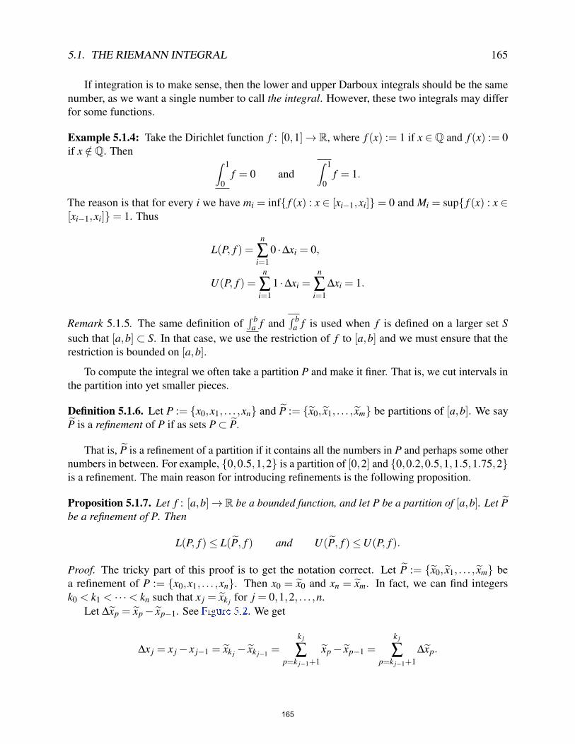
5.1. THE RIEMANN INTEGRAL 165
If integration is to make sense, then the lower and upper Darboux integrals should be the samenumber, as we want a single number to call the integral. However, these two integrals may differfor some functions.
Example 5.1.4: Take the Dirichlet function f : [0,1]→ R, where f (x) := 1 if x ∈Q and f (x) := 0if x /∈Q. Then ∫ 1
0f = 0 and
∫ 1
0f = 1.
The reason is that for every i we have mi = inf{ f (x) : x ∈ [xi−1,xi]}= 0 and Mi = sup{ f (x) : x ∈[xi−1,xi]}= 1. Thus
L(P, f ) =n
∑i=1
0 ·∆xi = 0,
U(P, f ) =n
∑i=1
1 ·∆xi =n
∑i=1
∆xi = 1.
Remark 5.1.5. The same definition of∫ b
a f and∫ b
a f is used when f is defined on a larger set Ssuch that [a,b]⊂ S. In that case, we use the restriction of f to [a,b] and we must ensure that therestriction is bounded on [a,b].
To compute the integral we often take a partition P and make it finer. That is, we cut intervals inthe partition into yet smaller pieces.
Definition 5.1.6. Let P := {x0,x1, . . . ,xn} and P := {x0, x1, . . . , xm} be partitions of [a,b]. We sayP is a refinement of P if as sets P⊂ P.
That is, P is a refinement of a partition if it contains all the numbers in P and perhaps some othernumbers in between. For example, {0,0.5,1,2} is a partition of [0,2] and {0,0.2,0.5,1,1.5,1.75,2}is a refinement. The main reason for introducing refinements is the following proposition.
Proposition 5.1.7. Let f : [a,b]→R be a bounded function, and let P be a partition of [a,b]. Let Pbe a refinement of P. Then
L(P, f )≤ L(P, f ) and U(P, f )≤U(P, f ).
Proof. The tricky part of this proof is to get the notation correct. Let P := {x0, x1, . . . , xm} bea refinement of P := {x0,x1, . . . ,xn}. Then x0 = x0 and xn = xm. In fact, we can find integersk0 < k1 < · · ·< kn such that x j = xk j for j = 0,1,2, . . . ,n.
Let ∆xp = xp− xp−1. See Figure 5.2 . We get
∆x j = x j− x j−1 = xk j − xk j−1 =k j
∑p=k j−1+1
xp− xp−1 =k j
∑p=k j−1+1
∆xp.
165

166 CHAPTER 5. THE RIEMANN INTEGRAL
∆xp−1∆xp−2xpxp−3 xp−1xp−2 ∆xp
∆x j
xk j−1 xk j==
x j−1 x j
· · ·· · ·
Figure 5.2: Refinement of a subinterval. Notice ∆x j = ∆xp−2 +∆xp−1 +∆xp, and also k j−1 +1 = p−2and k j = p.
Let m j be as before and correspond to the partition P. Let m j := inf{ f (x) : x j−1 ≤ x≤ x j}. Now,m j ≤ mp for k j−1 < p≤ k j. Therefore,
m j∆x j = m j
k j
∑p=k j−1+1
∆xp =k j
∑p=k j−1+1
m j∆xp ≤k j
∑p=k j−1+1
mp∆xp.
So
L(P, f ) =n
∑j=1
m j∆x j ≤n
∑j=1
k j
∑p=k j−1+1
mp∆xp =m
∑j=1
m j∆x j = L(P, f ).
The proof of U(P, f )≤U(P, f ) is left as an exercise.
Armed with refinements we prove the following. The key point of this next proposition is thatthe lower Darboux integral is less than or equal to the upper Darboux integral.
Proposition 5.1.8. Let f : [a,b]→ R be a bounded function. Let m,M ∈ R be such that for allx ∈ [a,b] we have m≤ f (x)≤M. Then
m(b−a)≤∫ b
af ≤
∫ b
af ≤M(b−a). (5.2)
Proof. By Proposition 5.1.2 we have for any partition P
m(b−a)≤ L(P, f )≤U(P, f )≤M(b−a).
The inequality m(b− a) ≤ L(P, f ) implies m(b− a) ≤ ∫ ba f . Also U(P, f ) ≤ M(b− a) implies∫ b
a f ≤M(b−a).The middle inequality in ( 5.2 ) is the main point of this proposition. Let P1,P2 be partitions
of [a,b]. Define P := P1∪P2. The set P is a partition of [a,b], which is a refinement of P1 and arefinement of P2. By Proposition 5.1.7 , L(P1, f )≤ L(P, f ) and U(P, f )≤U(P2, f ). So
L(P1, f )≤ L(P, f )≤U(P, f )≤U(P2, f ).
In other words, for two arbitrary partitions P1 and P2, we have L(P1, f ) ≤ U(P2, f ). Recall Proposition 1.2.7 , and take the supremum and infimum over all partitions:∫ b
af = sup
{L(P, f ) : P a partition of [a,b]
}≤ inf
{U(P, f ) : P a partition of [a,b]
}=∫ b
af .
166

5.1. THE RIEMANN INTEGRAL 167
5.1.2 Riemann integralWe can finally define the Riemann integral. However, the Riemann integral is only defined on acertain class of functions, called the Riemann integrable functions.
Definition 5.1.9. Let f : [a,b]→ R be a bounded function such that∫ b
af (x) dx =
∫ b
af (x) dx.
Then f is said to be Riemann integrable. The set of Riemann integrable functions on [a,b] is denotedby R[a,b]. When f ∈R[a,b] we define∫ b
af (x) dx :=
∫ b
af (x) dx =
∫ b
af (x) dx.
As before, we often simply write ∫ b
af :=
∫ b
af (x) dx.
The number∫ b
a f is called the Riemann integral of f , or sometimes simply the integral of f .
By definition, any Riemann integrable function is bounded. By appealing to Proposition 5.1.8
we immediately obtain the following proposition. See also Figure 5.3 .
Proposition 5.1.10. Let f : [a,b]→R be a Riemann integrable function. Let m,M ∈R be such thatm≤ f (x)≤M for all x ∈ [a,b]. Then
m(b−a)≤∫ b
af ≤M(b−a).
a b
m
M
Figure 5.3: The area under the curve is bounded from above by the area of the entire rectangle, M(b−a),and from below by the area of the shaded part, m(b−a).
Often we use a weaker form of this proposition. That is, if | f (x)| ≤M for all x ∈ [a,b], then∣∣∣∣∫ b
af∣∣∣∣≤M(b−a).
167

168 CHAPTER 5. THE RIEMANN INTEGRAL
Example 5.1.11: We integrate constant functions using Proposition 5.1.8 . If f (x) := c for someconstant c, then we take m = M = c. In inequality ( 5.2 ) all the inequalities must be equalities. Thusf is integrable on [a,b] and
∫ ba f = c(b−a).
Example 5.1.12: Let f : [0,2]→ R be defined by
f (x) :=
1 if x < 1,1/2 if x = 1,0 if x > 1.
We claim f is Riemann integrable and∫ 2
0 f = 1.Proof: Let 0 < ε < 1 be arbitrary. Let P := {0,1−ε,1+ε,2} be a partition. We use the notation
from the definition of the Darboux sums. Then
m1 = inf{
f (x) : x ∈ [0,1− ε]}= 1, M1 = sup
{f (x) : x ∈ [0,1− ε]
}= 1,
m2 = inf{
f (x) : x ∈ [1− ε,1+ ε]}= 0, M2 = sup
{f (x) : x ∈ [1− ε,1+ ε]
}= 1,
m3 = inf{
f (x) : x ∈ [1+ ε,2]}= 0, M3 = sup
{f (x) : x ∈ [1+ ε,2]
}= 0.
Furthermore, ∆x1 = 1− ε , ∆x2 = 2ε and ∆x3 = 1− ε . See Figure 5.4 .
0 1− ε 1+ ε 2∆x1 = 1− ε ∆x2 = 2ε ∆x3 = 1− ε
M3 = m2 = m3 = 0
M1 = M2 = m1 = 1
Figure 5.4: Darboux sums for the step function. L(P, f ) is the area of the shaded rectangle, U(P, f ) isthe area of both rectangles, and U(P, f )−L(P, f ) is the area of the unshaded rectangle.
We compute
L(P, f ) =3
∑i=1
mi∆xi = 1 · (1− ε)+0 ·2ε +0 · (1− ε) = 1− ε,
U(P, f ) =3
∑i=1
Mi∆xi = 1 · (1− ε)+1 ·2ε +0 · (1− ε) = 1+ ε.
Thus, ∫ 2
0f −
∫ 2
0f ≤U(P, f )−L(P, f ) = (1+ ε)− (1− ε) = 2ε.
168

5.1. THE RIEMANN INTEGRAL 169
By Proposition 5.1.8 we have∫ 2
0 f ≤ ∫ 20 f . As ε was arbitrary we see
∫ 20 f =
∫ 20 f . So f is Riemann
integrable. Finally,
1− ε = L(P, f )≤∫ 2
0f ≤U(P, f ) = 1+ ε.
Hence,∣∣∫ 2
0 f −1∣∣≤ ε . As ε was arbitrary, we have
∫ 20 f = 1.
It may be worthwhile to extract part of the technique of the example into a proposition.
Proposition 5.1.13. Let f : [a,b]→ R be a bounded function. Then f is Riemann integrable if forevery ε > 0, there exists a partition P such that
U(P, f )−L(P, f )< ε.
Proof. If for every ε > 0 such a P exists, then we have:
0≤∫ b
af −
∫ b
af ≤U(P, f )−L(P, f )< ε.
Therefore,∫ b
a f =∫ b
a f , and f is integrable.
Example 5.1.14: Let us show 11+x is integrable on [0,b] for any b > 0. We will see later that all
continuous functions are integrable, but let us demonstrate how we do it directly.Let ε > 0 be given. Take n ∈ N and pick x j := jb/n, to form the partition P := {x0,x1, . . . ,xn} of
[0,b]. We have ∆x j = b/n for all j. As f is decreasing, for any subinterval [x j−1,x j] we obtain
m j = inf{
11+ x
: x ∈ [x j−1,x j]
}=
11+ x j
, M j = sup{
11+ x
: x ∈ [x j−1,x j]
}=
11+ x j−1
.
Then we have
U(P, f )−L(P, f ) =n
∑j=1
∆x j(M j−m j) =bn
n
∑j=1
(1
1+ ( j−1)b/n− 1
1+ jb/n
)=
=bn
(1
1+ 0b/n− 1
1+ nb/n
)=
b2
n(b+1).
The sum telescopes, the terms successively cancel each other, something we have seen before.Picking n to be such that b2
n(b+1) < ε the proposition is satisfied, and the function is integrable.
Remark 5.1.15. A way of thinking of the integral is that it adds up (integrates) lots of localinformation—it sums f (x) dx over all x. The integral sign was chosen by Leibniz to be the long S,to mean summation. Unlike derivatives, which are “local,” integrals show up in applications whenone wants a “global” answer: total distance travelled, average temperature, total charge, etc.
169

170 CHAPTER 5. THE RIEMANN INTEGRAL
5.1.3 More notationWhen f : S→ R is defined on a larger set S and [a,b]⊂ S, we say f is Riemann integrable on [a,b]if the restriction of f to [a,b] is Riemann integrable. In this case, we say f ∈R[a,b], and we write∫ b
a f to mean the Riemann integral of the restriction of f to [a,b].It is useful to define the integral
∫ ba f even if a 6< b. Suppose b < a and f ∈R[b,a], then define∫ b
af :=−
∫ a
bf .
For any function f , define ∫ a
af := 0.
At times, the variable x may already have some other meaning. When we need to write downthe variable of integration, we may simply use a different letter. For example,∫ b
af (s) ds :=
∫ b
af (x) dx.
5.1.4 ExercisesExercise 5.1.1: Define f : [0,1]→R by f (x) := x3 and let P := {0,0.1,0.4,1}. Compute L(P, f ) and U(P, f ).
Exercise 5.1.2: Let f : [0,1]→ R be defined by f (x) := x. Show that f ∈R[0,1] and compute∫ 1
0 f usingthe definition of the integral (but feel free to use the propositions of this section).
Exercise 5.1.3: Let f : [a,b]→ R be a bounded function. Suppose there exists a sequence of partitions {Pk}of [a,b] such that
limk→∞
(U(Pk, f )−L(Pk, f )
)= 0.
Show that f is Riemann integrable and that∫ b
af = lim
k→∞U(Pk, f ) = lim
k→∞L(Pk, f ).
Exercise 5.1.4: Finish the proof of Proposition 5.1.7 .
Exercise 5.1.5: Suppose f : [−1,1]→ R is defined as
f (x) :=
{1 if x > 0,0 if x≤ 0.
Prove that f ∈ R[−1,1] and compute∫ 1−1 f using the definition of the integral (but feel free to use the
propositions of this section).
Exercise 5.1.6: Let c ∈ (a,b) and let d ∈ R. Define f : [a,b]→ R as
f (x) :=
{d if x = c,0 if x 6= c.
Prove that f ∈R[a,b] and compute∫ b
a f using the definition of the integral (but feel free to use the propositionsof this section).
170

5.1. THE RIEMANN INTEGRAL 171
Exercise 5.1.7: Suppose f : [a,b]→R is Riemann integrable. Let ε > 0 be given. Then show that there existsa partition P = {x0,x1, . . . ,xn} such that if we pick any set of numbers {c1,c2, . . . ,cn} with ck ∈ [xk−1,xk] forall k, then ∣∣∣∣∣
∫ b
af −
n
∑k=1
f (ck)∆xk
∣∣∣∣∣< ε.
Exercise 5.1.8: Let f : [a,b]→ R be a Riemann integrable function. Let α > 0 and β ∈ R. Then defineg(x) := f (αx+β ) on the interval I = [a−β
α, b−β
α]. Show that g is Riemann integrable on I.
Exercise 5.1.9: Suppose f : [0,1]→R and g : [0,1]→R are such that for all x ∈ (0,1] we have f (x) = g(x).Suppose f is Riemann integrable. Prove g is Riemann integrable and
∫ 10 f =
∫ 10 g.
Exercise 5.1.10: Let f : [0,1]→R be a bounded function. Let Pn = {x0,x1, . . . ,xn} be a uniform partition of[0,1], that is, x j := j/n. Is {L(Pn, f )}∞
n=1 always monotone? Yes/No: Prove or find a counterexample.
Exercise 5.1.11 (Challenging): For a bounded function f : [0,1]→R let Rn := (1/n)∑nj=1 f ( j/n) (the uniform
right hand rule).
a) If f is Riemann integrable show∫ 1
0 f = lim Rn.
b) Find an f that is not Riemann integrable, but lim Rn exists.
Exercise 5.1.12 (Challenging): Generalize the previous exercise. Show that f ∈R[a,b] if and only if thereexists an I ∈ R, such that for every ε > 0 there exists a δ > 0 such that if P is a partition with ∆xi < δ for alli, then |L(P, f )− I|< ε and |U(P, f )− I|< ε . If f ∈R[a,b], then I =
∫ ba f .
Exercise 5.1.13: Using Exercise 5.1.12 and the idea of the proof in Exercise 5.1.7 , show that Darbouxintegral is the same as the standard definition of Riemann integral, which you have most likely seen incalculus. That is, show that f ∈R[a,b] if and only if there exists an I ∈ R, such that for every ε > 0 thereexists a δ > 0 such that if P = {x0,x1, . . . ,xn} is a partition with ∆xi < δ for all i, then |∑n
i=1 f (ci)∆xi− I|< ε
for any set {c1,c2, . . . ,cn} with ci ∈ [xi−1,xi]. If f ∈R[a,b], then I =∫ b
a f .
Exercise 5.1.14 (Challenging): Construct functions f and g, where f : [0,1]→ R is Riemann integrable,g : [0,1]→ [0,1] is one-to-one and onto, and such that the composition f ◦g is not Riemann integrable.
171

172 CHAPTER 5. THE RIEMANN INTEGRAL
5.2 Properties of the integralNote: 2 lectures, integrability of functions with discontinuities can safely be skipped
5.2.1 AdditivityAdding a bunch of things in two parts and then adding those two parts should be the same as addingeverything all at once. The corresponding property for integral is called the additive property of theintegral. First, we prove the additivity property for the lower and upper Darboux integrals.
Lemma 5.2.1. Suppose a < b < c and f : [a,c]→ R is a bounded function. Then∫ c
af =
∫ b
af +
∫ c
bf
and ∫ c
af =
∫ b
af +
∫ c
bf .
Proof. If we have partitions P1 = {x0,x1, . . . ,xk} of [a,b] and P2 = {xk,xk+1, . . . ,xn} of [b,c], thenthe set P := P1∪P2 = {x0,x1, . . . ,xn} is a partition of [a,c]. Then
L(P, f ) =n
∑j=1
m j∆x j =k
∑j=1
m j∆x j +n
∑j=k+1
m j∆x j = L(P1, f )+L(P2, f ).
When we take the supremum of the right hand side over all P1 and P2, we are taking a supremumof the left hand side over all partitions P of [a,c] that contain b. If Q is any partition of [a,c] andP = Q∪{b}, then P is a refinement of Q and so L(Q, f )≤ L(P, f ). Therefore, taking a supremumonly over the P that contain b is sufficient to find the supremum of L(P, f ) over all partitions P, see
Exercise 1.1.9 . Finally recall Exercise 1.2.9 to compute∫ c
af = sup
{L(P, f ) : P a partition of [a,c]
}= sup
{L(P, f ) : P a partition of [a,c],b ∈ P
}= sup
{L(P1, f )+L(P2, f ) : P1 a partition of [a,b],P2 a partition of [b,c]
}= sup
{L(P1, f ) : P1 a partition of [a,b]
}+ sup
{L(P2, f ) : P2 a partition of [b,c]
}=∫ b
af +
∫ c
bf .
Similarly, for P, P1, and P2 as above we obtain
U(P, f ) =n
∑j=1
M j∆x j =k
∑j=1
M j∆x j +n
∑j=k+1
M j∆x j =U(P1, f )+U(P2, f ).
We wish to take the infimum on the right over all P1 and P2, and so we are taking the infimumover all partitions P of [a,c] that contain b. If Q is any partition of [a,c] and P = Q∪{b}, then P
172

5.2. PROPERTIES OF THE INTEGRAL 173
is a refinement of Q and so U(Q, f )≥U(P, f ). Therefore, taking an infimum only over the P thatcontain b is sufficient to find the infimum of U(P, f ) for all P. We obtain∫ c
af =
∫ b
af +
∫ c
bf .
Proposition 5.2.2. Let a < b < c. A function f : [a,c]→R is Riemann integrable if and only if f isRiemann integrable on [a,b] and [b,c]. If f is Riemann integrable, then∫ c
af =
∫ b
af +
∫ c
bf .
Proof. Suppose f ∈R[a,c], then∫ c
a f =∫ c
a f =∫ c
a f . We apply the lemma to get∫ c
af =
∫ c
af =
∫ b
af +
∫ c
bf ≤
∫ b
af +
∫ c
bf =
∫ c
af =
∫ c
af .
Thus the inequality is an equality, ∫ b
af +
∫ c
bf =
∫ b
af +
∫ c
bf .
As we also know∫ b
a f ≤ ∫ ba f and
∫ cb f ≤ ∫ c
b f , we conclude∫ b
af =
∫ b
af and
∫ c
bf =
∫ c
bf .
Thus f is Riemann integrable on [a,b] and [b,c] and the desired formula holds.Now assume f is Riemann integrable on [a,b] and on [b,c]. Again apply the lemma to get∫ c
af =
∫ b
af +
∫ c
bf =
∫ b
af +
∫ c
bf =
∫ b
af +
∫ c
bf =
∫ c
af .
Therefore, f is Riemann integrable on [a,c], and the integral is computed as indicated.
An easy consequence of the additivity is the following corollary. We leave the details to thereader as an exercise.
Corollary 5.2.3. If f ∈R[a,b] and [c,d]⊂ [a,b], then the restriction f |[c,d] is in R[c,d].
5.2.2 Linearity and monotonicityA sum is a linear function of the summands. So is the integral.
Proposition 5.2.4 (Linearity). Let f and g be in R[a,b] and α ∈ R.
(i) α f is in R[a,b] and ∫ b
aα f (x) dx = α
∫ b
af (x) dx.
(ii) f +g is in R[a,b] and∫ b
a
(f (x)+g(x)
)dx =
∫ b
af (x) dx+
∫ b
ag(x) dx.
173

174 CHAPTER 5. THE RIEMANN INTEGRAL
Proof. Let us prove the first item for α ≥ 0. Let P be a partition of [a,b]. Let mi := inf{ f (x) : x ∈[xi−1,xi]} as usual. Since α is nonnegative, we can move the multiplication by α past the infimum,
inf{α f (x) : x ∈ [xi−1,xi]}= α inf{ f (x) : x ∈ [xi−1,xi]}= αmi.
Therefore,
L(P,α f ) =n
∑i=1
αmi∆xi = α
n
∑i=1
mi∆xi = αL(P, f ).
Similarly,U(P,α f ) = αU(P, f ).
Again, as α ≥ 0 we may move multiplication by α past the supremum. Hence,∫ b
aα f (x) dx = sup
{L(P,α f ) : P a partition of [a,b]
}= sup
{αL(P, f ) : P a partition of [a,b]
}= α sup
{L(P, f ) : P a partition of [a,b]
}= α
∫ b
af (x) dx.
Similarly, we show ∫ b
aα f (x) dx = α
∫ b
af (x) dx.
The conclusion now follows for α ≥ 0.To finish the proof of the first item, we need to show that − f is Riemann integrable and∫ b
a − f (x) dx =−∫ ba f (x) dx. The proof of this fact is left as Exercise 5.2.1 .
The proof of the second item in the proposition is also left as Exercise 5.2.2 . It is not as trivialas it may appear at first glance.
The second item in the proposition does not hold with equality for the Darboux integrals, butwe do obtain inequalities. The proof of the following proposition is Exercise 5.2.16 . It follows forupper and lower sums on a fixed partition by Exercise 1.3.7 , that is, supremum of a sum is less thanor equal to the sum of suprema and similarly for infima.
Proposition 5.2.5. Let f : [a,b]→ R and g : [a,b]→ R be bounded functions. Then∫ b
a( f +g)≤
∫ b
af +
∫ b
ag, and
∫ b
a( f +g)≥
∫ b
af +
∫ b
ag.
Adding up smaller numbers should give us a smaller result. That is true for an integral as well.
Proposition 5.2.6 (Monotonicity). Let f : [a,b]→R and g : [a,b]→R be bounded, and f (x)≤ g(x)for all x ∈ [a,b]. Then ∫ b
af ≤
∫ b
ag and
∫ b
af ≤
∫ b
ag.
Moreover, if f and g are in R[a,b], then ∫ b
af ≤
∫ b
ag.
174

5.2. PROPERTIES OF THE INTEGRAL 175
Proof. Let P = {x0,x1, . . . ,xn} be a partition of [a,b]. Then let
mi := inf{
f (x) : x ∈ [xi−1,xi]}
and mi := inf{
g(x) : x ∈ [xi−1,xi]}.
As f (x)≤ g(x), then mi ≤ mi. Therefore,
L(P, f ) =n
∑i=1
mi∆xi ≤n
∑i=1
mi∆xi = L(P,g).
We take the supremum over all P (see Proposition 1.3.7 ) to obtain∫ b
af ≤
∫ b
ag.
Similarly, we obtain the same conclusion for the upper integrals. Finally, if f and g are Riemannintegrable all the integrals are equal, and the conclusion follows.
5.2.3 Continuous functionsLet us show that continuous functions are Riemann integrable. In fact, we will show we can evenallow some discontinuities. We start with a function continuous on the whole closed interval [a,b].
Lemma 5.2.7. If f : [a,b]→ R is a continuous function, then f ∈R[a,b].
Proof. As f is continuous on a closed bounded interval, it is uniformly continuous. Let ε > 0 begiven. Find a δ > 0 such that |x− y|< δ implies | f (x)− f (y)|< ε
b−a .Let P = {x0,x1, . . . ,xn} be a partition of [a,b] such that ∆xi < δ for all i = 1,2, . . . ,n. For
example, take n such that b−an < δ and let xi := i
n(b−a)+a. Then for all x,y ∈ [xi−1,xi] we have|x− y| ≤ ∆xi < δ and so
f (x)− f (y)≤ | f (x)− f (y)|< ε
b−a.
As f is continuous on [xi−1,xi], it attains a maximum and a minimum on this interval. Let x be apoint where f attains the maximum and y be a point where f attains the minimum. Then f (x) = Miand f (y) = mi in the notation from the definition of the integral. Therefore,
Mi−mi = f (x)− f (y)<ε
b−a.
And so ∫ b
af −
∫ b
af ≤U(P, f )−L(P, f )
=
(n
∑i=1
Mi∆xi
)−(
n
∑i=1
mi∆xi
)
=n
∑i=1
(Mi−mi)∆xi
<ε
b−a
n
∑i=1
∆xi
=ε
b−a(b−a) = ε.
175

176 CHAPTER 5. THE RIEMANN INTEGRAL
As ε > 0 was arbitrary, ∫ b
af =
∫ b
af ,
and f is Riemann integrable on [a,b].
The second lemma says that we need the function to only be “Riemann integrable inside theinterval,” as long as it is bounded. It also tells us how to compute the integral.
Lemma 5.2.8. Let f : [a,b]→ R be a bounded function, {an} and {bn} be sequences such thata < an < bn < b for all n, with lim an = a and lim bn = b. Suppose f ∈R[an,bn] for all n. Thenf ∈R[a,b] and ∫ b
af = lim
n→∞
∫ bn
an
f .
Proof. Let M > 0 be a real number such that | f (x)| ≤M. As (b−a)≥ (bn−an),
−M(b−a)≤−M(bn−an)≤∫ bn
an
f ≤M(bn−an)≤M(b−a).
Therefore, the sequence of numbers{∫ bn
anf}∞
n=1 is bounded and by Bolzano–Weierstrass has a
convergent subsequence indexed by nk. Let us call L the limit of the subsequence{∫ bnk
ankf}∞
k=1. Lemma 5.2.1 says that the lower and upper integral are additive and the hypothesis says that f
is integrable on [ank ,bnk ]. Therefore∫ b
af =
∫ ank
af +
∫ bnk
ank
f +∫ b
bnk
f ≥−M(ank−a)+∫ bnk
ank
f −M(b−bnk).
We take the limit as k goes to ∞ on the right-hand side,∫ b
af ≥−M ·0+L−M ·0 = L.
Next we use additivity of the upper integral,∫ b
af =
∫ ank
af +
∫ bnk
ank
f +∫ b
bnk
f ≤M(ank−a)+∫ bnk
ank
f +M(b−bnk).
We take the same subsequence {∫ bnkank
f}∞k=1 and take the limit to obtain
∫ b
af ≤M ·0+L+M ·0 = L.
Thus∫ b
a f =∫ b
a f = L and hence f is Riemann integrable and∫ b
a f = L. In particular, no matter whatsubsequence we chose, the L is the same number.
To prove the final statement of the lemma we use Proposition 2.3.7 . We have shown thatevery convergent subsequence
{∫ bnkank
f}
converges to L =∫ b
a f . Therefore, the sequence{∫ bn
anf}
is
convergent and converges to∫ b
a f .
176

5.2. PROPERTIES OF THE INTEGRAL 177
We say a function f : [a,b]→ R has finitely many discontinuities if there exists a finite setS := {x1,x2, . . . ,xn} ⊂ [a,b], and f is continuous at all points of [a,b]\S.
Theorem 5.2.9. Let f : [a,b]→ R be a bounded function with finitely many discontinuities. Thenf ∈R[a,b].
Proof. We divide the interval into finitely many intervals [ai,bi] so that f is continuous on theinterior (ai,bi). If f is continuous on (ai,bi), then it is continuous and hence integrable on [ci,di]whenever ai < ci < di < bi. By Lemma 5.2.8 the restriction of f to [ai,bi] is integrable. By additivityof the integral (and induction ) f is integrable on the union of the intervals.
5.2.4 More on integrable functionsSometimes it is convenient (or necessary) to change certain values of a function and then integrate.The next result says that if we change the values at finitely many points, the integral does not change.
Proposition 5.2.10. Let f : [a,b]→ R be Riemann integrable. Let g : [a,b]→ R be such thatf (x) = g(x) for all x ∈ [a,b]\S, where S is a finite set. Then g is a Riemann integrable function and∫ b
ag =
∫ b
af .
Sketch of proof. Using additivity of the integral, we split up the interval [a,b] into smaller intervalssuch that f (x) = g(x) holds for all x except at the endpoints (details are left to the reader).
Therefore, without loss of generality suppose f (x) = g(x) for all x ∈ (a,b). The proof followsby Lemma 5.2.8 , and is left as Exercise 5.2.3 .
Finally, monotone (increasing or decreasing) functions are always Riemann integrable. Theproof is left to the reader as part of Exercise 5.2.14 .
Proposition 5.2.11. Let f : [a,b]→ R be a monotone function. Then f ∈R[a,b].
5.2.5 ExercisesExercise 5.2.1: Finish the proof of the first part of Proposition 5.2.4 . Let f be in R[a,b]. Prove that − f is inR[a,b] and ∫ b
a− f (x) dx =−
∫ b
af (x) dx.
Exercise 5.2.2: Prove the second part of Proposition 5.2.4 . Let f and g be in R[a,b]. Prove, without using Proposition 5.2.5 , that f +g is in R[a,b] and∫ b
a
(f (x)+g(x)
)dx =
∫ b
af (x) dx+
∫ b
ag(x) dx.
Hint: One way to do it is to use Proposition 5.1.7 to find a single partition P such that U(P, f )−L(P, f )< ε/2
and U(P,g)−L(P,g)< ε/2.
177

178 CHAPTER 5. THE RIEMANN INTEGRAL
Exercise 5.2.3: Let f : [a,b]→ R be Riemann integrable, and g : [a,b]→ R be such that f (x) = g(x) for allx ∈ (a,b). Prove that g is Riemann integrable and that∫ b
ag =
∫ b
af .
Exercise 5.2.4: Prove the mean value theorem for integrals: if f : [a,b]→ R is continuous, then there existsa c ∈ [a,b] such that
∫ ba f = f (c)(b−a).
Exercise 5.2.5: Let f : [a,b]→ R be a continuous function such that f (x)≥ 0 for all x ∈ [a,b] and∫ b
a f = 0.Prove that f (x) = 0 for all x.
Exercise 5.2.6: Let f : [a,b]→ R be a continuous function and∫ b
a f = 0. Prove that there exists a c ∈ [a,b]such that f (c) = 0. (Compare with the previous exercise.)
Exercise 5.2.7: Let f : [a,b]→ R and g : [a,b]→ R be continuous functions such that∫ b
a f =∫ b
a g. Showthat there exists a c ∈ [a,b] such that f (c) = g(c).
Exercise 5.2.8: Let f ∈R[a,b]. Let α,β ,γ be arbitrary numbers in [a,b] (not necessarily ordered in anyway). Prove ∫
γ
α
f =∫
β
α
f +∫
γ
β
f .
Recall what∫ b
a f means if b≤ a.
Exercise 5.2.9: Prove Corollary 5.2.3 .
Exercise 5.2.10: Suppose f : [a,b]→ R is bounded and has finitely many discontinuities. Show that asa function of x the expression | f (x)| is bounded with finitely many discontinuities and is thus Riemannintegrable. Then show ∣∣∣∣∫ b
af (x) dx
∣∣∣∣≤ ∫ b
a| f (x)| dx.
Exercise 5.2.11 (Hard): Show that the Thomae or popcorn function (see Example 3.2.12 ) is Riemannintegrable. Therefore, there exists a function discontinuous at all rational numbers (a dense set) that isRiemann integrable.
In particular, define f : [0,1]→ R by
f (x) :=
{1/k if x = m/k where m,k ∈ N and m and k have no common divisors,0 if x is irrational.
Show∫ 1
0 f = 0.
If I ⊂ R is a bounded interval, then the function
ϕI(x) :=
{1 if x ∈ I,0 otherwise,
is called an elementary step function.
Exercise 5.2.12: Let I be an arbitrary bounded interval (you should consider all types of intervals: closed,open, half-open) and a < b, then using only the definition of the integral show that the elementary stepfunction ϕI is integrable on [a,b], and find the integral in terms of a, b, and the endpoints of I.
178

5.2. PROPERTIES OF THE INTEGRAL 179
A function f is called a step function if it can be written as
f (x) =n
∑k=1
αkϕIk(x)
for some real numbers α1,α2, . . . ,αn and some bounded intervals I1, I2, . . . , In.
Exercise 5.2.13: Using Exercise 5.2.12 , show that a step function is integrable on any interval [a,b]. Fur-thermore, find the integral in terms of a, b, the endpoints of Ik and the αk.
Exercise 5.2.14: Let f : [a,b]→ R be a function.
a) Show that if f is increasing, then it is Riemann integrable. Hint: Use a uniform partition; each subintervalof same length.
b) Use part a) to show that if f is decreasing, then it is Riemann integrable.
c) Suppose
* h = f −g where f and g are increasing functions on [a,b]. Show that h is Riemann integrable.
Exercise 5.2.15 (Challenging): Suppose f ∈R[a,b], then the function that takes x to | f (x)| is also Riemannintegrable on [a,b]. Then show the same inequality as Exercise 5.2.10 .
Exercise 5.2.16: Suppose f : [a,b]→ R and g : [a,b]→ R are bounded.
a) Show∫ b
a ( f +g)≤ ∫ ba f +
∫ ba g and
∫ ba ( f +g)≥ ∫ b
a f +∫ b
a g.
b) Find example f and g where the inequality is strict. Hint: f and g should not be Riemann integrable.
Exercise 5.2.17: Suppose f : [a,b]→ R is continuous and g : R→ R is Lipschitz continuous. Define
h(x) :=∫ b
ag(t− x) f (t) dt.
Prove that h is Lipschitz continuous.
*Such an h is said to be of bounded variation.
179

180 CHAPTER 5. THE RIEMANN INTEGRAL
5.3 Fundamental theorem of calculusNote: 1.5 lectures
In this chapter we discuss and prove the fundamental theorem of calculus. The entirety ofintegral calculus is built upon this theorem, ergo the name. The theorem relates the seeminglyunrelated concepts of integral and derivative. It tells us how to compute the antiderivative of afunction using the integral and vice versa.
5.3.1 First form of the theoremTheorem 5.3.1. Let F : [a,b]→R be a continuous function, differentiable on (a,b). Let f ∈R[a,b]be such that f (x) = F ′(x) for x ∈ (a,b). Then∫ b
af = F(b)−F(a).
It is not hard to generalize the theorem to allow a finite number of points in [a,b] where F is notdifferentiable, as long as it is continuous. This generalization is left as an exercise.
Proof. Let P = {x0,x1, . . . ,xn} be a partition of [a,b]. For each interval [xi−1,xi], use the meanvalue theorem to find a ci ∈ (xi−1,xi) such that
f (ci)∆xi = F ′(ci)(xi− xi−1) = F(xi)−F(xi−1).
See Figure 5.5 , and notice that the area of all three shaded rectangles is F(xi+1)−F(xi−2). Theidea is that by picking small enough subintervals we prove that this area is the integral of f .
area = f (ci)∆xi
= F(xi)−F(xi−1)
area = f (ci−1)∆xi−1
= F(xi−1)−F(xi−2)
area = f (ci+1)∆xi+1
= F(xi+1)−F(xi)
xi−2 xi−1 xi xi+1
f (ci−1)
f (ci)
f (ci+1)
ci−1 ci ci+1
∆xi−1 ∆xi ∆xi+1
y = f (x) = F ′(x)
Figure 5.5: Mean value theorem on subintervals of a partition approximating area under the curve.
Using the notation from the definition of the integral, we have mi ≤ f (ci)≤Mi, and so
mi∆xi ≤ F(xi)−F(xi−1)≤Mi∆xi.
180

5.3. FUNDAMENTAL THEOREM OF CALCULUS 181
We sum over i = 1,2, . . . ,n to getn
∑i=1
mi∆xi ≤n
∑i=1
(F(xi)−F(xi−1)
)≤
n
∑i=1
Mi∆xi.
In the middle sum, all the terms except the first and last cancel and we end up with F(xn)−F(x0) =F(b)−F(a). The sums on the left and on the right are the lower and the upper sum respectively. So
L(P, f )≤ F(b)−F(a)≤U(P, f ).
We take the supremum of L(P, f ) over all partitions P and the left inequality yields∫ b
af ≤ F(b)−F(a).
Similarly, taking the infimum of U(P, f ) over all partitions P yields
F(b)−F(a)≤∫ b
af .
As f is Riemann integrable, we have∫ b
af =
∫ b
af ≤ F(b)−F(a)≤
∫ b
af =
∫ b
af .
The inequalities must be equalities and we are done.
The theorem is used to compute integrals. Suppose we know that the function f (x) is a derivativeof some other function F(x), then we can find an explicit expression for
∫ ba f .
Example 5.3.2: Suppose we are trying to compute∫ 1
0x2 dx.
We notice x2 is the derivative of x3
3 . We use the fundamental theorem to write∫ 1
0x2 dx =
13
3− 03
3=
13.
5.3.2 Second form of the theoremThe second form of the fundamental theorem gives us a way to solve the differential equationF ′(x) = f (x), where f is a known function and we are trying to find an F that satisfies the equation.
Theorem 5.3.3. Let f : [a,b]→ R be a Riemann integrable function. Define
F(x) :=∫ x
af .
First, F is continuous on [a,b]. Second, if f is continuous at c ∈ [a,b], then F is differentiable at cand F ′(c) = f (c).
181
182 CHAPTER 5. THE RIEMANN INTEGRAL
Proof. As f is bounded, there is an M > 0 such that | f (x)| ≤M for all x∈ [a,b]. Suppose x,y∈ [a,b]with x > y. Then
|F(x)−F(y)|=∣∣∣∣∫ x
af −
∫ y
af∣∣∣∣= ∣∣∣∣∫ x
yf∣∣∣∣≤M |x− y| .
By symmetry, the same also holds if x < y. So F is Lipschitz continuous and hence continuous.Now suppose f is continuous at c. Let ε > 0 be given. Let δ > 0 be such that for x ∈ [a,b],
|x− c|< δ implies | f (x)− f (c)|< ε . In particular, for such x we have
f (c)− ε < f (x)< f (c)+ ε.
Thus if x > c, then (f (c)− ε
)(x− c)≤
∫ x
cf ≤
(f (c)+ ε
)(x− c).
When c > x, then the inequalities are reversed. Therefore, assuming c 6= x we get
f (c)− ε ≤∫ x
c fx− c
≤ f (c)+ ε.
AsF(x)−F(c)
x− c=
∫ xa f − ∫ c
a fx− c
=
∫ xc f
x− c,
we have ∣∣∣∣F(x)−F(c)x− c
− f (c)∣∣∣∣≤ ε.
The result follows. It is left to the reader to see why is it OK that we just have a non-strictinequality.
Of course, if f is continuous on [a,b], then it is automatically Riemann integrable, F is differen-tiable on all of [a,b] and F ′(x) = f (x) for all x ∈ [a,b].
Remark 5.3.4. The second form of the fundamental theorem of calculus still holds if we let d ∈ [a,b]and define
F(x) :=∫ x
df .
That is, we can use any point of [a,b] as our base point. The proof is left as an exercise.
Let us look at what a simple discontinuity can do. Take f (x) :=−1 if x < 0, and f (x) := 1 ifx≥ 0. Let F(x) :=
∫ x0 f . It is not difficult to see that F(x) = |x|. Notice that f is discontinuous at 0
and F is not differentiable at 0. However, the converse in the theorem does not hold. Let g(x) := 0if x 6= 0, and g(0) := 1. Letting G(x) :=
∫ x0 g, we find that G(x) = 0 for all x. So g is discontinuous
at 0, but G′(0) exists and is equal to 0.A common misunderstanding of the integral for calculus students is to think of integrals whose
solution cannot be given in closed-form as somehow deficient. This is not the case. Most integralswe write down are not computable in closed-form. Even some integrals that we consider in closed-form are not really such. We define the natural logarithm as the antiderivative of 1/x such thatln1 = 0:
lnx :=∫ x
1
1s
ds.
182

5.3. FUNDAMENTAL THEOREM OF CALCULUS 183
So for example, how does a computer find the value of lnx? One way to do it is to numericallyapproximate this integral. Morally, we did not really “simplify”
∫ x1 1/s ds by writing down lnx. We
simply gave the integral a name. If we require numerical answers, it is possible we end up doing thecalculation by approximating an integral anyway. In the next section, we even define the exponentialusing the logarithm, which we define in terms of the integral.
Another common function defined by an integral that cannot be evaluated symbolically in termsof elementary functions is the erf function, defined as
erf(x) :=2√π
∫ x
0e−s2
ds.
This function comes up often in applied mathematics. It is simply the antiderivative of (2/√
π)e−x2
that is zero at zero. The second form of the fundamental theorem tells us that we can write thefunction as an integral. If we wish to compute any particular value, we numerically approximate theintegral.
5.3.3 Change of variablesA theorem often used in calculus to solve integrals is the change of variables theorem, you mayhave called it u-substitution. Let us prove it now. Recall a function is continuously differentiable ifit is differentiable and the derivative is continuous.
Theorem 5.3.5 (Change of variables). Let g : [a,b]→ R be a continuously differentiable function,let f : [c,d]→ R be continuous, and suppose g
([a,b]
)⊂ [c,d]. Then∫ b
af(g(x)
)g′(x) dx =
∫ g(b)
g(a)f (s) ds.
Proof. As g, g′, and f are continuous, we know f(g(x)
)g′(x) is a continuous function on [a,b],
therefore it is Riemann integrable. Similarly, f is integrable on any subinterval of [c,d].Define
F(y) :=∫ y
g(a)f (s) ds.
By the second form of the fundamental theorem of calculus (see Remark 5.3.4 and Exercise 5.3.4 )F is a differentiable function and F ′(y) = f (y). We apply the chain rule and write(
F ◦g)′(x) = F ′
(g(x)
)g′(x) = f
(g(x)
)g′(x).
We note that F(g(a)
)= 0 and we use the first form of the fundamental theorem to obtain
∫ g(b)
g(a)f (s) ds = F
(g(b)
)= F
(g(b)
)−F
(g(a)
)=∫ b
a
(F ◦g
)′(x) dx =
∫ b
af(g(x)
)g′(x) dx.
The change of variables theorem is often used to solve integrals by changing them to integralsthat we know or that we can solve using the fundamental theorem of calculus.
183

184 CHAPTER 5. THE RIEMANN INTEGRAL
Example 5.3.6: From an exercise, we know that the derivative of sin(x) is cos(x). Therefore, wesolve ∫ √
π
0xcos(x2) dx =
∫π
0
cos(s)2
ds =12
∫π
0cos(s) ds =
sin(π)− sin(0)2
= 0.
However, beware that we must satisfy the hypotheses of the theorem. The following exampledemonstrates why we should not just move symbols around mindlessly. We must be careful thatthose symbols really make sense.
Example 5.3.7: Suppose we write down ∫ 1
−1
ln |x|x
dx.
It may be tempting to take g(x) := ln |x|. Then take g′(x) = 1/x and try to write
∫ g(1)
g(−1)s ds =
∫ 0
0s ds = 0.
This “solution” is incorrect, and it does not say that we can solve the given integral. First problemis that ln|x|
x is not continuous on [−1,1]. It is not defined at 0, and cannot be made continuous bydefining a value at 0. Second, ln|x|
x is not even Riemann integrable on [−1,1] (it is unbounded). Theintegral we wrote down simply does not make sense. Finally, g is not continuous on [−1,1], letalone continuously differentiable.
5.3.4 Exercises
Exercise 5.3.1: Computeddx
(∫ x
−xes2
ds)
.
Exercise 5.3.2: Computeddx
(∫ x2
0sin(s2) ds
).
Exercise 5.3.3: Suppose F : [a,b]→ R is continuous and differentiable on [a,b]\S, where S is a finite set.Suppose there exists an f ∈R[a,b] such that f (x) = F ′(x) for x ∈ [a,b]\S. Show that
∫ ba f = F(b)−F(a).
Exercise 5.3.4: Let f : [a,b]→ R be a continuous function. Let c ∈ [a,b] be arbitrary. Define
F(x) :=∫ x
cf .
Prove that F is differentiable and that F ′(x) = f (x) for all x ∈ [a,b].
Exercise 5.3.5: Prove integration by parts. That is, suppose F and G are continuously differentiable functionson [a,b]. Then prove
∫ b
aF(x)G′(x) dx = F(b)G(b)−F(a)G(a)−
∫ b
aF ′(x)G(x) dx.
184

5.3. FUNDAMENTAL THEOREM OF CALCULUS 185
Exercise 5.3.6: Suppose F and G are continuously
* differentiable functions defined on [a,b] such that
F ′(x) = G′(x) for all x ∈ [a,b]. Using the fundamental theorem of calculus, show that F and G differ by aconstant. That is, show that there exists a C ∈ R such that F(x)−G(x) =C.
The next exercise shows how we can use the integral to “smooth out” a non-differentiable function.
Exercise 5.3.7: Let f : [a,b]→ R be a continuous function. Let ε > 0 be a constant. For x ∈ [a+ ε,b− ε],define
g(x) :=1
2ε
∫ x+ε
x−ε
f .
a) Show that g is differentiable and find the derivative.
b) Let f be differentiable and fix x ∈ (a,b) (let ε be small enough). What happens to g′(x) as ε gets smaller?
c) Find g for f (x) := |x|, ε = 1 (you can assume [a,b] is large enough).
Exercise 5.3.8: Suppose f : [a,b]→ R is continuous and∫ x
a f =∫ b
x f for all x ∈ [a,b]. Show that f (x) = 0for all x ∈ [a,b].
Exercise 5.3.9: Suppose f : [a,b]→ R is continuous and∫ x
a f = 0 for all rational x in [a,b]. Show thatf (x) = 0 for all x ∈ [a,b].
Exercise 5.3.10: A function f is an odd function if f (x)=− f (−x), and f is an even function if f (x)= f (−x).Let a > 0. Assume f is continuous. Prove:
a) If f is odd, then∫ a−a f = 0.
b) If f is even, then∫ a−a f = 2
∫ a0 f .
Exercise 5.3.11:
a) Show that f (x) := sin(1/x) is integrable on any interval (you can define f (0) to be anything).
b) Compute∫ 1−1 sin(1/x) dx. (Mind the discontinuity.)
Exercise 5.3.12 (uses §3.6 ):
a) Suppose f : [a,b]→ R is increasing, by Proposition 5.2.11 , f is Riemann integrable. Suppose f has adiscontinuity at c ∈ (a,b), show that F(x) :=
∫ xa f is not differentiable at c.
b) In Exercise 3.6.11 , you constructed an increasing function f : [0,1]→ R that is discontinuous at everyx ∈ [0,1]∩Q. Use this f to construct a function F(x) that is continuous on [0,1], but not differentiable atevery x ∈ [0,1]∩Q.
*Compare this hypothesis to Exercise 4.2.8 .
185

186 CHAPTER 5. THE RIEMANN INTEGRAL
5.4 The logarithm and the exponentialNote: 1 lecture (optional, requires the optional sections §3.5 , §3.6 , §4.4 )
We now have the tools required to properly define the exponential and the logarithm that youknow from calculus so well. We start with exponentiation. If n is a positive integer, it is obvious todefine
xn := x · x · · · · · x︸ ︷︷ ︸n times
.
It makes sense to define x0 := 1. For negative integers, let x−n := 1/xn. If x > 0, define x1/n as theunique positive nth root. Finally, for a rational number n/m (in lowest terms), define
xn/m :=(x1/m)n
.
It is not difficult to show we get the same number no matter what representation of n/m we use, sowe do not need to use lowest terms.
However, what do we mean by√
2√
2? Or xy in general? In particular, what is ex for all x? And
how do we solve y = ex for x? This section answers these questions and more.
5.4.1 The logarithmIt is convenient to define the logarithm first. Let us show that a unique function with the rightproperties exists, and only then will we call it the logarithm.
Proposition 5.4.1. There exists a unique function L : (0,∞)→ R such that
(i) L(1) = 0.
(ii) L is differentiable and L′(x) = 1/x.
(iii) L is strictly increasing, bijective, and
limx→0
L(x) =−∞, and limx→∞
L(x) = ∞.
(iv) L(xy) = L(x)+L(y) for all x,y ∈ (0,∞).
(v) If q is a rational number and x > 0, then L(xq) = qL(x).
Proof. To prove existence, we define a candidate and show it satisfies all the properties. Let
L(x) :=∫ x
1
1t
dt.
Obviously, (i) holds. Property (ii) holds via the second form of the fundamental theorem ofcalculus ( Theorem 5.3.3 ).
To prove property (iv) , we change variables u = yt to obtain
L(x) =∫ x
1
1t
dt =∫ xy
y
1u
du =∫ xy
1
1u
du−∫ y
1
1u
du = L(xy)−L(y).
186

5.4. THE LOGARITHM AND THE EXPONENTIAL 187
Let us prove (iii) . Property (ii) together with the fact that L′(x) = 1/x > 0 for x > 0, implies thatL is strictly increasing and hence one-to-one. Let us show L is onto. As 1/t ≥ 1/2 when t ∈ [1,2],
L(2) =∫ 2
1
1t
dt ≥ 1/2.
By induction, (iv) implies that for n ∈ N
L(2n) = L(2)+L(2)+ · · ·+L(2) = nL(2).
Given any y > 0, by the Archimedean property of the real numbers (notice L(2)> 0), there is ann ∈ N such that L(2n) > y. By the intermediate value theorem there is an x1 ∈ (1,2n) such thatL(x1) = y. We get (0,∞) is in the image of L. As L is increasing, L(x)> y for all x > 2n, and so
limx→∞
L(x) = ∞.
Next 0 = L(x/x) = L(x)+L(1/x), and so L(x) =−L(1/x). Using x = 2−n, we obtain as above that Lachieves all negative numbers. And
limx→0
L(x) = limx→0−L(1/x) = lim
x→∞−L(x) =−∞.
In the limits, note that only x > 0 are in the domain of L.Let us prove (v) . Fix x > 0. As above, (iv) implies L(xn) = nL(x) for all n ∈ N. We already
found that L(x) =−L(1/x), so L(x−n) =−L(xn) =−nL(x). Then for m ∈ N
L(x) = L((x1/m)
m)= mL
(x1/m).
Putting everything together for n ∈ Z and m ∈ N we have L(xn/m) = nL(x1/m) = (n/m)L(x).Uniqueness follows using properties (i) and (ii) . Via the first form of the fundamental theorem
of calculus ( Theorem 5.3.1 ),
L(x) =∫ x
1
1t
dt
is the unique function such that L(1) = 0 and L′(x) = 1/x.
Having proved that there is a unique function with these properties, we simply define thelogarithm or sometimes called the natural logarithm:
ln(x) := L(x).
Mathematicians usually write log(x) instead of ln(x), which is more familiar to calculus students.For all practical purposes, there is only one logarithm: the natural logarithm. See Exercise 5.4.2 .
187

188 CHAPTER 5. THE RIEMANN INTEGRAL
5.4.2 The exponentialJust as with the logarithm we define the exponential via a list of properties.
Proposition 5.4.2. There exists a unique function E : R→ (0,∞) such that
(i) E(0) = 1.
(ii) E is differentiable and E ′(x) = E(x).
(iii) E is strictly increasing, bijective, and
limx→−∞
E(x) = 0, and limx→∞
E(x) = ∞.
(iv) E(x+ y) = E(x)E(y) for all x,y ∈ R.
(v) If q ∈Q, then E(qx) = E(x)q.
Proof. Again, we prove existence of such a function by defining a candidate and proving that itsatisfies all the properties. The L = ln defined above is invertible. Let E be the inverse function of L.Property (i) is immediate.
Property (ii) follows via the inverse function theorem, in particular Lemma 4.4.1 : L satisfies allthe hypotheses of the lemma, and hence
E ′(x) =1
L′(E(x)
) = E(x).
Let us look at property (iii) . The function E is strictly increasing since E ′(x) = E(x)> 0. As Eis the inverse of L, it must also be bijective. To find the limits, we use that E is strictly increasingand onto (0,∞). For every M > 0, there is an x0 such that E(x0) = M and E(x)≥M for all x≥ x0.Similarly, for every ε > 0, there is an x0 such that E(x0) = ε and E(x)< ε for all x < x0. Therefore,
limn→−∞
E(x) = 0, and limn→∞
E(x) = ∞.
To prove property (iv) , we use the corresponding property for the logarithm. Take x,y ∈ R. AsL is bijective, find a and b such that x = L(a) and y = L(b). Then
E(x+ y) = E(L(a)+L(b)
)= E
(L(ab)
)= ab = E(x)E(y).
Property (v) also follows from the corresponding property of L. Given x ∈ R, let a be such thatx = L(a) and
E(qx) = E(qL(a)
)= E
(L(aq)
)= aq = E(x)q.
Uniqueness follows from (i) and (ii) . Let E and F be two functions satisfying (i) and (ii) .
ddx
(F(x)E(−x)
)= F ′(x)E(−x)−E ′(−x)F(x) = F(x)E(−x)−E(−x)F(x) = 0.
Therefore, by Proposition 4.2.6 , F(x)E(−x) = F(0)E(−0) = 1 for all x ∈ R. Next, 1 = E(0) =E(x− x) = E(x)E(−x). Then
0 = 1−1 = F(x)E(−x)−E(x)E(−x) =(F(x)−E(x)
)E(−x).
188

5.4. THE LOGARITHM AND THE EXPONENTIAL 189
Finally, E(−x) 6= 0
* for all x ∈ R. So F(x)−E(x) = 0 for all x, and we are done.
Having proved E is unique, we define the exponential function as
exp(x) := E(x).
If y ∈Q and x > 0, then
xy = exp(ln(xy)
)= exp
(y ln(x)
).
We can now make sense of exponentiation xy for arbitrary y ∈ R; if x > 0 and y is irrational, define
xy := exp(y ln(x)
).
As exp is continuous, then xy is a continuous function of y. Therefore, we would obtain the sameresult had we taken a sequence of rational numbers {yn} approaching y and defined xy = lim xyn .
Define the number e, sometimes called Euler’s number or the base of the natural logarithm, as
e := exp(1).
Let us justify the notation ex for exp(x):
ex = exp(x ln(e)
)= exp(x).
The properties of the logarithm and the exponential extend to irrational powers. The proof isimmediate.
Proposition 5.4.3. Let x,y ∈ R.
(i) exp(xy) =(exp(x)
)y.
(ii) If x > 0, then ln(xy) = y ln(x).
Remark 5.4.4. There are other equivalent ways to define the exponential and the logarithm. Acommon way is to define E as the solution to the differential equation E ′(x) = E(x), E(0) = 1. See
Example 6.3.3 , for a sketch of that approach. Yet another approach is to define the exponentialfunction by power series, see Example 6.2.14 .
Remark 5.4.5. We proved the uniqueness of the functions L and E from just the properties L(1) = 0,L′(x) = 1/x and the equivalent condition for the exponential E ′(x) = E(x), E(0) = 1. Existencealso follows from just these properties. Alternatively, uniqueness also follows from the laws ofexponents, see the exercises.
*E is a function into (0,∞) after all. However, E(−x) 6= 0 also follows from E(x)E(−x) = 1. Therefore, we canprove uniqueness of E given (i) and (ii) , even for functions E : R→ R.
189

190 CHAPTER 5. THE RIEMANN INTEGRAL
5.4.3 ExercisesExercise 5.4.1: Let y be any real number and b > 0. Define f : (0,∞)→ R and g : R→ R as, f (x) := xy
and g(x) := bx. Show that f and g are differentiable and find their derivative.
Exercise 5.4.2: Let b > 0, b 6= 1 be given.
a) Show that for every y > 0, there exists a unique number x such that y = bx. Define the logarithm base b,logb : (0,∞)→ R, by logb(y) := x.
b) Show that logb(x) =ln(x)ln(b) .
c) Prove that if c > 0, c 6= 1, then logb(x) =logc(x)logc(b)
.
d) Prove logb(xy) = logb(x)+ logb(y), and logb(xy) = y logb(x).
Exercise 5.4.3 (requires §4.3 ): Use Taylor’s theorem to study the remainder term and show that for all x ∈R
ex =∞
∑n=0
xn
n!.
Hint: Do not differentiate the series term by term (unless you would prove that it works).
Exercise 5.4.4: Use the geometric sum formula to show (for t 6=−1)
1− t + t2−·· ·+(−1)ntn =1
1+ t− (−1)n+1tn+1
1+ t.
Using this fact show
ln(1+ x) =∞
∑n=1
(−1)n+1xn
n
for all x ∈ (−1,1] (note that x = 1 is included). Finally, find the limit of the alternating harmonic series∞
∑n=1
(−1)n+1
n= 1− 1/2+ 1/3− 1/4+ · · ·
Exercise 5.4.5: Showex = lim
n→∞
(1+
xn
)n.
Hint: Take the logarithm.Note: The expression
(1+ x
n
)n arises in compound interest calculations. It is the amount of money in a bankaccount after 1 year if 1 dollar was deposited initially at interest x and the interest was compounded n timesduring the year. The exponential ex is the result of continuous compounding.
Exercise 5.4.6:
a) Prove that for n ∈ N,n
∑k=2
1k≤ ln(n)≤
n−1
∑k=1
1k.
b) Prove that the limit
γ := limn→∞
((n
∑k=1
1k
)− ln(n)
)exists. This constant is known as the Euler–Mascheroni constant
* . It is not known if this constant is
rational or not. It is approximately γ ≈ 0.5772.*Named for the Swiss mathematician Leonhard Paul Euler (1707–1783) and the Italian mathematician Lorenzo
Mascheroni (1750–1800).
190

5.4. THE LOGARITHM AND THE EXPONENTIAL 191
Exercise 5.4.7: Show
limx→∞
ln(x)x
= 0.
Exercise 5.4.8: Show that ex is convex, in other words, show that if a≤ x≤ b, then ex ≤ ea b−xb−a + eb x−a
b−a .
Exercise 5.4.9: Using the logarithm findlimn→∞
n1/n.
Exercise 5.4.10: Show that E(x) = ex is the unique continuous function such that E(x+ y) = E(x)E(y) andE(1) = e. Similarly, prove that L(x) = ln(x) is the unique continuous function defined on positive x such thatL(xy) = L(x)+L(y) and L(e) = 1.
Exercise 5.4.11 (requires §4.3 ): Since (ex)′ = ex, it is easy to see that ex is infinitely differentiable (hasderivatives of all orders). Define the function f : R→ R.
f (x) :=
{e−1/x if x > 0,0 if x≤ 0.
a) Prove that for any m ∈ N,
limx→0+
e−1/x
xm = 0.
b) Prove that f is infinitely differentiable.
c) Compute the Taylor series for f at the origin, that is,
∞
∑k=0
f (k)(0)k!
xk.
Show that it converges, but show that it does not converge to f (x) for any x > 0.
191

192 CHAPTER 5. THE RIEMANN INTEGRAL
5.5 Improper integralsNote: 2–3 lectures (optional section, can safely be skipped, requires the optional §3.5 )
Often it is necessary to integrate over the entire real line, or an unbounded interval of the form[a,∞) or (−∞,b]. We may also wish to integrate unbounded functions defined on a open boundedinterval (a,b). For such intervals or functions, the Riemann integral is not defined, but we willwrite down the integral anyway in the spirit of Lemma 5.2.8 . These integrals are called improperintegrals and are limits of integrals rather than integrals themselves.
Definition 5.5.1. Suppose f : [a,b)→ R is a function (not necessarily bounded) that is Riemannintegrable on [a,c] for all c < b. We define∫ b
af := lim
c→b−
∫ c
af ,
if the limit exists.Suppose f : [a,∞)→ R is a function such that f is Riemann integrable on [a,c] for all c < ∞.
We define ∫ ∞
af := lim
c→∞
∫ c
af ,
if the limit exists.If the limit exists, we say the improper integral converges. If the limit does not exist, we say the
improper integral diverges.We similarly define improper integrals for the left-hand endpoint, we leave this to the reader.
For a finite endpoint b, if f is bounded, then Lemma 5.2.8 says that we defined nothing new.What is new is that we can apply this definition to unbounded functions. The following set ofexamples is so useful that we state it as a proposition.
Proposition 5.5.2 (p-test for integrals). The improper integral∫ ∞
1
1xp dx
converges to 1p−1 if p > 1 and diverges if 0 < p≤ 1.
The improper integral ∫ 1
0
1xp dx
converges to 11−p if 0 < p < 1 and diverges if p≥ 1.
Proof. The proof follows by application of the fundamental theorem of calculus . Let us do theproof for p > 1 for the infinite right endpoint and leave the rest to the reader. Hint: You shouldhandle p = 1 separately.
Suppose p > 1. Then using the fundamental theorem,∫ b
1
1xp dx =
∫ b
1x−p dx =
b−p+1
−p+1− 1−p+1
−p+1=
−1(p−1)bp−1 +
1p−1
.
As p > 1, then p− 1 > 0. Take the limit as b→ ∞ to obtain that 1bp−1 goes to 0. The result
follows.
192

5.5. IMPROPER INTEGRALS 193
We state the following proposition on “tails” for just one type of improper integral, though theproof is straight forward and the same for other types of improper integrals.
Proposition 5.5.3. Let f : [a,∞)→R be a function that is Riemann integrable on [a,b] for all b > a.Given any b > a,
∫ ∞b f converges if and only if
∫ ∞a f converges, in which case∫ ∞
af =
∫ b
af +
∫ ∞
bf .
Proof. Let c > b. Then ∫ c
af =
∫ b
af +
∫ c
bf .
Taking the limit c→ ∞ finishes the proof.
Nonnegative functions are easier to work with as the following proposition demonstrates. Theexercises will show that this proposition holds only for nonnegative functions. Analogues of thisproposition exist for all the other types of improper limits and are left to the student.
Proposition 5.5.4. Suppose f : [a,∞)→ R is nonnegative ( f (x) ≥ 0 for all x) and such that f isRiemann integrable on [a,b] for all b > a.
(i) ∫ ∞
af = sup
{∫ x
af : x≥ a
}.
(ii) Suppose {xn} is a sequence with lim xn = ∞. Then∫ ∞
a f converges if and only if lim∫ xn
a fexists, in which case ∫ ∞
af = lim
n→∞
∫ xn
af .
In the first item we allow for the value of ∞ in the supremum indicating that the integral divergesto infinity.
Proof. We start with the first item. As f is nonnegative,∫ x
a f is increasing as a function of x. If thesupremum is infinite, then for every M ∈ R we find N such that
∫ Na f ≥M. As
∫ xa f is increasing,∫ x
a f ≥M for all x≥ N. So∫ ∞
a f diverges to infinity.Next suppose the supremum is finite, say A := sup{∫ x
a f : x≥ a}. For every ε > 0, we find anN such that A− ∫ N
a f < ε . As∫ x
a f is increasing, then A− ∫ xa f < ε for all x ≥ N and hence
∫ ∞a f
converges to A.Let us look at the second item. If
∫ ∞a f converges, then every sequence {xn} going to infinity
works. The trick is proving the other direction. Suppose {xn} is such that lim xn = ∞ and
limn→∞
∫ xn
af = A
converges. Given ε > 0, pick N such that for all n≥ N we have A− ε <∫ xn
a f < A+ ε . Because∫ xa f is increasing as a function of x, we have that for all x≥ xN
A− ε <∫ xN
af ≤
∫ x
af .
193

194 CHAPTER 5. THE RIEMANN INTEGRAL
As {xn} goes to ∞, then for any given x, there is an xm such that m≥ N and x≤ xm. Then∫ x
af ≤
∫ xm
af < A+ ε.
In particular, for all x≥ xN we have |∫ xa f −A|< ε .
Proposition 5.5.5 (Comparison test for improper integrals). Let f : [a,∞)→ R and g : [a,∞)→ Rbe functions that are Riemann integrable on [a,b] for all b > a. Suppose that for all x≥ a we have
| f (x)| ≤ g(x).
(i) If∫ ∞
a g converges, then∫ ∞
a f converges, and in this case |∫ ∞a f | ≤ ∫ ∞
a g.
(ii) If∫ ∞
a f diverges, then∫ ∞
a g diverges.
Proof. Let us start with the first item. For any b and c, such that a ≤ b ≤ c, we have −g(x) ≤f (x)≤ g(x), and so ∫ c
b−g≤
∫ c
bf ≤
∫ c
bg.
In other words, |∫ cb f | ≤ ∫ c
b g.Let ε > 0 be given. Because of Proposition 5.5.3 ,∫ ∞
ag =
∫ b
ag+
∫ ∞
bg.
As∫ b
a g goes to∫ ∞
a g as b goes to infinity,∫ ∞
b g goes to 0 as b goes to infinity. Choose B such that∫ ∞
Bg < ε.
As g is nonnegative, if B≤ b < c, then∫ c
b g < ε as well. Let {xn} be a sequence going to infinity.Let M be such that xn ≥ B for all n≥M. Take n,m≥M, with xn ≤ xm,∣∣∣∣∫ xm
af −
∫ xn
af∣∣∣∣= ∣∣∣∣∫ xm
xn
f∣∣∣∣≤ ∫ xm
xn
g < ε.
Therefore, the sequence {∫ xna f}∞
n=1 is Cauchy and hence converges.We need to show that the limit is unique. Suppose {xn} is a sequence converging to infinity
such that {∫ xna f} converges to L1, and {yn} is a sequence converging to infinity is such that {∫ yn
a f}converges to L2. Then there must be some n such that |∫ xn
a f −L1|< ε and |∫ yna f −L2|< ε . We can
also suppose xn ≥ B and yn ≥ B. Then
|L1−L2| ≤∣∣∣∣L1−
∫ xn
af∣∣∣∣+ ∣∣∣∣∫ xn
af −
∫ yn
af∣∣∣∣+ ∣∣∣∣∫ yn
af −L2
∣∣∣∣< ε +
∣∣∣∣∫ yn
xn
f∣∣∣∣+ ε < 3ε.
As ε > 0 was arbitrary, L1 = L2, and hence∫ ∞
a f converges. Above we have shown that |∫ ca f | ≤ ∫ c
a gfor all c > a. By taking the limit c→ ∞, the first item is proved.
The second item is simply a contrapositive of the first item.
194

5.5. IMPROPER INTEGRALS 195
Example 5.5.6: The improper integral∫ ∞
0
sin(x2)(x+2)x3 +1
dx
converges.Proof: Observe we simply need to show that the integral converges when going from 1 to infinity.
For x≥ 1 we obtain ∣∣∣∣sin(x2)(x+2)x3 +1
∣∣∣∣≤ x+2x3 +1
≤ x+2x3 ≤ x+2x
x3 ≤ 3x2 .
Then ∫ ∞
1
3x2 dx = 3
∫ ∞
1
1x2 dx = 3.
So using the comparison test and the tail test, the original integral converges.
Example 5.5.7: You should be careful when doing formal manipulations with improper integrals.The integral ∫ ∞
2
2x2−1
dx
converges via the comparison test using 1/x2 again. However, if you succumb to the temptation towrite
2x2−1
=1
x−1− 1
x+1and try to integrate each part separately, you will not succeed. It is not true that you can split theimproper integral in two; you cannot split the limit.∫ ∞
2
2x2−1
dx = limb→∞
∫ b
2
2x2−1
dx
= limb→∞
(∫ b
2
1x−1
dx−∫ b
2
1x+1
dx)
6=∫ ∞
2
1x−1
dx−∫ ∞
2
1x+1
dx.
The last line in the computation does not even make sense. Both of the integrals there diverge toinfinity, since we can apply the comparison test appropriately with 1/x. We get ∞−∞.
Now suppose we need to take limits at both endpoints.
Definition 5.5.8. Suppose f : (a,b)→ R is a function that is Riemann integrable on [c,d] for all c,d such that a < c < d < b, then we define∫ b
af := lim
c→a+lim
d→b−
∫ d
cf ,
if the limits exist.
195

196 CHAPTER 5. THE RIEMANN INTEGRAL
Suppose f : R→ R is a function such that f is Riemann integrable on all bounded intervals[a,b]. Then we define ∫ ∞
−∞f := lim
c→−∞limd→∞
∫ d
cf ,
if the limits exist.We similarly define improper integrals with one infinite and one finite improper endpoint, we
leave this to the reader.
One ought to always be careful about double limits. The definition given above says that wefirst take the limit as d goes to b or ∞ for a fixed c, and then we take the limit in c. We will have toprove that in this case it does not matter which limit we compute first.
Example 5.5.9: Let us see an example:∫ ∞
−∞
11+ x2 dx = lim
a→−∞limb→∞
∫ b
a
11+ x2 dx = lim
a→−∞limb→∞
(arctan(b)− arctan(a)
)= π.
In the definition the order of the limits can always be switched if they exist. Let us prove thisfact only for the infinite limits.
Proposition 5.5.10. If f : R→ R is a function integrable on every bounded interval [a,b]. Then
lima→−∞
limb→∞
∫ b
af converges if and only if lim
b→∞lim
a→−∞
∫ b
af converges,
in which case the two expressions are equal. If either of the expressions converges, then the improperintegral converges and
lima→∞
∫ a
−af =
∫ ∞
−∞f .
Proof. Without loss of generality assume a < 0 and b > 0. Suppose the first expression converges.Then
lima→−∞
limb→∞
∫ b
af = lim
a→−∞limb→∞
(∫ 0
af +
∫ b
0f)=
(lim
a→−∞
∫ 0
af)+
(limb→∞
∫ b
0f)
= limb→∞
((lim
a→−∞
∫ 0
af)+∫ b
0f)= lim
b→∞lim
a→−∞
(∫ 0
af +
∫ b
0f).
Similar computation shows the other direction. Therefore, if either expression converges, then theimproper integral converges and∫ ∞
−∞f = lim
a→−∞limb→∞
∫ b
af =
(lim
a→−∞
∫ 0
af)+
(limb→∞
∫ b
0f)
=
(lima→∞
∫ 0
−af)+
(lima→∞
∫ a
0f)= lim
a→∞
(∫ 0
−af +
∫ a
0f)= lim
a→∞
∫ a
−af .
196

5.5. IMPROPER INTEGRALS 197
Example 5.5.11: On the other hand, you must be careful to take the limits independently beforeyou know convergence. Let f (x) = x
|x| for x 6= 0 and f (0) = 0. If a < 0 and b > 0, then
∫ b
af =
∫ 0
af +
∫ b
0f = a+b.
For any fixed a < 0 the limit as b→ ∞ is infinite, so even the first limit does not exist, and hencethe improper integral
∫ ∞−∞ f does not converge. On the other hand if a > 0, then∫ a
−af = (−a)+a = 0.
Therefore,
lima→∞
∫ a
−af = 0.
Example 5.5.12: An example to keep in mind for improper integrals is the so-called sinc function
* .
This function comes up quite often in both pure and applied mathematics. Define
sinc(x) =
{sin(x)
x if x 6= 0,1 if x = 0.
−4π −2π 4π2π
12
1
− 14
Figure 5.6: The sinc function.
It is not difficult to show that the sinc function is continuous at zero, but that is not importantright now. What is important is that∫ ∞
−∞sinc(x) dx = π, while
∫ ∞
−∞|sinc(x)| dx = ∞.
The integral of the sinc function is a continuous analogue of the alternating harmonic series ∑ (−1)n/n,while the absolute value is like the regular harmonic series ∑ 1/n. In particular, the fact that theintegral converges must be done directly rather than using comparison test.
*Shortened from Latin: sinus cardinalis
197

198 CHAPTER 5. THE RIEMANN INTEGRAL
We will not prove the first statement exactly. Let us simply prove that the integral of the sincfunction converges, but we will not worry about the exact limit. Because sin(−x)
−x = sin(x)x , it is enough
to show that ∫ ∞
2π
sin(x)x
dx
converges. We also avoid x = 0 this way to make our life simpler.For any n ∈ N, we have that for x ∈ [π2n,π(2n+1)]
sin(x)π(2n+1)
≤ sin(x)x≤ sin(x)
π2n,
as sin(x)≥ 0. On x ∈ [π(2n+1),π(2n+2)]
sin(x)π(2n+1)
≤ sin(x)x≤ sin(x)
π(2n+2),
as sin(x)≤ 0.Via the fundamental theorem of calculus,
2π(2n+1)
=∫
π(2n+1)
π2n
sin(x)π(2n+1)
dx≤∫
π(2n+1)
π2n
sin(x)x
dx≤∫
π(2n+1)
π2n
sin(x)π2n
dx =1
πn.
Similarly,−2
π(2n+1)≤∫
π(2n+2)
π(2n+1)
sin(x)x
dx≤ −1π(n+1)
.
Adding the two together we find
0 =2
π(2n+1)+
−2π(2n+1)
≤∫ 2π(n+1)
2πn
sin(x)x
dx≤ 1πn
+−1
π(n+1)=
1πn(n+1)
.
See Figure 5.7 .
sin(x)x
sin(x)π(2n+1)
sin(x)π2n
sin(x)x
sin(x)π(2n+1)
sin(x)π(2n+2)
π2n
π(2n+1) π(2n+2)
+
−
Figure 5.7: Bound of∫ 2π(n+1)
2πnsin(x)
x dx using the shaded integral (signed area 1πn +
−1π(n+1) ).
198

5.5. IMPROPER INTEGRALS 199
For k ∈ N, ∫ 2kπ
2π
sin(x)x
dx =k−1
∑n=1
∫ 2π(n+1)
2πn
sin(x)x
dx≤k−1
∑n=1
1πn(n+1)
.
We find the partial sums of a series with positive terms. The series converges as ∑ 1πn(n+1) is a
convergent series. Thus as a sequence,
limk→∞
∫ 2kπ
2π
sin(x)x
dx = L≤∞
∑n=1
1πn(n+1)
< ∞.
Let M > 2π be arbitrary, and let k ∈N be the largest integer such that 2kπ ≤M. For x∈ [2kπ,M]
we have −12kπ≤ sin(x)
x ≤ 12kπ
, and so∣∣∣∣∫ M
2kπ
sin(x)x
dx∣∣∣∣≤ M−2kπ
2kπ≤ 1
k.
As k is the largest k such that 2kπ ≤M, then as M ∈ R goes to infinity, so does k ∈ N.Then ∫ M
2π
sin(x)x
dx =∫ 2kπ
2π
sin(x)x
dx+∫ M
2kπ
sin(x)x
dx.
As M goes to infinity, the first term on the right hand side goes to L, and the second term on theright hand side goes to zero. Hence ∫ ∞
2π
sin(x)x
dx = L.
The double sided integral of sinc also exists as noted above. We leave the other statement—thatthe integral of the absolute value of the sinc function diverges—as an exercise.
5.5.1 Integral test for seriesThe fundamental theorem of calculus can be used in proving a series is summable and to estimateits sum.
Proposition 5.5.13 (Integral test). Suppose f : [k,∞)→ R is a decreasing nonnegative functionwhere k ∈ Z. Then
∞
∑n=k
f (n) converges if and only if∫ ∞
kf converges.
In this case ∫ ∞
kf ≤
∞
∑n=k
f (n)≤ f (k)+∫ ∞
kf .
See Figure 5.8 , for an illustration with k = 1. By Proposition 5.2.11 , f is integrable on everyinterval [k,b] for all b> k, so the statement of the theorem makes sense without additional hypothesesof integrability.
199

200 CHAPTER 5. THE RIEMANN INTEGRAL
0 1 2 3 4 5 6 7 8 9 10· · ·
Figure 5.8: The area under the curve,∫ ∞
1 f , is bounded below by the area of the shaded rectangles,f (2)+ f (3)+ f (4)+ · · · , and bounded above by the area entire rectangles, f (1)+ f (2)+ f (3)+ · · · .
Proof. Let `,m ∈ Z be such that m > ` ≥ k. Because f is decreasing, we have∫ n+1
n f ≤ f (n) ≤∫ nn−1 f . Therefore,
∫ m
`f =
m−1
∑n=`
∫ n+1
nf ≤
m−1
∑n=`
f (n)≤ f (`)+m−1
∑n=`+1
∫ n
n−1f ≤ f (`)+
∫ m−1
`f . (5.3)
Suppose first that∫ ∞
k f converges and let ε > 0 be given. As before, since f is positive, thenthere exists an L ∈N such that if `≥ L, then
∫ m` f < ε/2 for all m≥ `. The function f must decrease
to zero (why?), so make L large enough so that for `≥ L we have f (`)< ε/2. Thus, for m > `≥ L,we have via ( 5.3 ),
m
∑n=`
f (n)≤ f (`)+∫ m
`f < ε/2+ ε/2 = ε.
The series is therefore Cauchy and thus converges. The estimate in the proposition is obtained byletting m go to infinity in ( 5.3 ) with `= k.
Conversely, suppose∫ ∞
k f diverges. As f is positive, then by Proposition 5.5.4 , the sequence{∫ m
k f}∞m=k diverges to infinity. Using ( 5.3 ) with `= k, we find
∫ m
kf ≤
m−1
∑n=k
f (n).
As the left hand side goes to infinity as m→ ∞, so does the right hand side.
Example 5.5.14: The integral test can be used not only to show that a series converges, but toestimate its sum to arbitrary precision. Let us show ∑∞
n=11n2 exists and estimate its sum to within
0.01. As this series is the p-series for p = 2, we already proved it converges (let us pretend we donot know that), but we only roughly estimated its sum.
The fundamental theorem of calculus says that for k ∈ N we have∫ ∞
k
1x2 dx =
1k.
200

5.5. IMPROPER INTEGRALS 201
In particular, the series must converge. But we also have
1k=∫ ∞
k
1x2 dx≤
∞
∑n=k
1n2 ≤
1k2 +
∫ ∞
k
1x2 dx =
1k2 +
1k.
Adding the partial sum up to k−1 we get
1k+
k−1
∑n=1
1n2 ≤
∞
∑n=1
1n2 ≤
1k2 +
1k+
k−1
∑n=1
1n2 .
In other words, 1/k+∑k−1n=1
1/n2 is an estimate for the sum to within 1/k2. Therefore, if we wish tofind the sum to within 0.01, we note 1/102 = 0.01. We obtain
1.6397 . . .≈ 110
+9
∑n=1
1n2 ≤
∞
∑n=1
1n2 ≤
1100
+110
+9
∑n=1
1n2 ≈ 1.6497 . . . .
The actual sum is π2/6≈ 1.6449 . . ..
5.5.2 ExercisesExercise 5.5.1: Finish the proof of Proposition 5.5.2 .
Exercise 5.5.2: Find out for which a ∈ R does∞∑
n=1ean converge. When the series converges, find an upper
bound for the sum.
Exercise 5.5.3:
a) Estimate∞∑
n=1
1n(n+1) correct to within 0.01 using the integral test.
b) Compute the limit of the series exactly and compare. Hint: The sum telescopes.
Exercise 5.5.4: Prove ∫ ∞
−∞|sinc(x)| dx = ∞.
Hint: Again, it is enough to show this on just one side.
Exercise 5.5.5: Can you interpret ∫ 1
−1
1√|x|
dx
as an improper integral? If so, compute its value.
Exercise 5.5.6: Take f : [0,∞)→ R, Riemann integrable on every interval [0,b], and such that there exist M,a, and T , such that | f (t)| ≤Meat for all t ≥ T . Show that the Laplace transform of f exists. That is, for everys > a the following integral converges:
F(s) :=∫ ∞
0f (t)e−st dt.
201

202 CHAPTER 5. THE RIEMANN INTEGRAL
Exercise 5.5.7: Let f : R→ R be a Riemann integrable function on every interval [a,b], and such that∫ ∞−∞ | f (x)| dx < ∞. Show that the Fourier sine and cosine transforms exist. That is, for every ω ≥ 0 the
following integrals converge
Fs(ω) :=1π
∫ ∞
−∞f (t)sin(ωt) dt, Fc(ω) :=
1π
∫ ∞
−∞f (t)cos(ωt) dt.
Furthermore, show that Fs and Fc are bounded functions.
Exercise 5.5.8: Suppose f : [0,∞)→ R is Riemann integrable on every interval [0,b]. Show that∫ ∞
0 fconverges if and only if for every ε > 0 there exists an M such that if M ≤ a < b, then
∣∣∫ ba f∣∣< ε .
Exercise 5.5.9: Suppose f : [0,∞)→ R is nonnegative and decreasing. Prove:
a) If∫ ∞
0 f < ∞, then limx→∞
f (x) = 0.
b) The converse does not hold.
Exercise 5.5.10: Find an example of an unbounded continuous function f : [0,∞)→ R that is nonnegativeand such that
∫ ∞0 f < ∞. Note that limx→∞ f (x) will not exist; compare previous exercise. Hint: On each
interval [k,k+1], k ∈ N, define a function whose integral over this interval is less than say 2−k.
Exercise 5.5.11 (More challenging): Find an example of a function f : [0,∞)→R integrable on all intervalssuch that limn→∞
∫ n0 f converges as a limit of a sequence (so n ∈ N), but such that
∫ ∞0 f does not exist. Hint:
For all n ∈ N, divide [n,n+1] into two halves. On one half make the function negative, on the other make thefunction positive.
Exercise 5.5.12: Suppose f : [1,∞)→ R is such that g(x) := x2 f (x) is a bounded function. Prove that∫ ∞
1 fconverges.
It is sometimes desirable to assign a value to integrals that normally cannot be interpreted even asimproper integrals, e.g.
∫ 1−1
1/x dx. Suppose f : [a,b]→ R is a function and a < c < b, where f is Riemannintegrable on the intervals [a,c− ε] and [c+ ε,b] for all ε > 0. Define the Cauchy principal value of
∫ ba f as
p.v.∫ b
af := lim
ε→0+
(∫ c−ε
af +
∫ b
c+ε
f),
if the limit exists.
Exercise 5.5.13:
a) Compute p.v.∫ 1−1
1/x dx.
b) Compute limε→0+(∫ −ε
−11/x dx+
∫ 12ε
1/x dx) and show it is not equal to the principal value.
c) Show that if f is integrable on [a,b], then p.v.∫ b
a f =∫ b
a f (for an arbitrary c ∈ (a,b)).
d) Suppose f : [−1,1]→R is an odd function ( f (−x) =− f (x)) that is integrable on [−1,−ε] and [ε,1] forall ε > 0. Prove that p.v.
∫ 1−1 f = 0
e) Suppose f : [−1,1]→ R is continuous and differentiable at 0. Show that p.v.∫ 1−1
f (x)x dx exists.
202

5.5. IMPROPER INTEGRALS 203
Exercise 5.5.14: Let f : R→ R and g : R→ R be continuous functions, where g(x) = 0 for all x /∈ [a,b] forsome interval [a,b].
a) Show that the convolution
(g∗ f )(x) :=∫ ∞
−∞f (t)g(x− t) dt
is well-defined for all x ∈ R.
b) Suppose∫ ∞−∞ | f (x)| dx < ∞. Prove that
limx→−∞
(g∗ f )(x) = 0, and limx→∞
(g∗ f )(x) = 0.
203

204 CHAPTER 5. THE RIEMANN INTEGRAL
204

Chapter 6
Sequences of Functions
6.1 Pointwise and uniform convergenceNote: 1–1.5 lecture
Up till now, when we talked about sequences we always talked about sequences of numbers.However, a very useful concept in analysis is to use a sequence of functions. For example, a solutionto some differential equation might be found by finding only approximate solutions. Then the realsolution is some sort of limit of those approximate solutions.
When talking about sequences of functions, the tricky part is that there are multiple notions of alimit. Let us describe two common notions of a limit of a sequence of functions.
6.1.1 Pointwise convergenceDefinition 6.1.1. For every n ∈ N let fn : S→ R be a function. We say the sequence { fn}∞
n=1converges pointwise to f : S→ R, if for every x ∈ S we have
f (x) = limn→∞
fn(x).
As limits of sequences of numbers are unique, given a sequence { fn} that converges pointwise,the limit function f is unique. It is common to say that fn : S→R converges to f on T ⊂ S for somef : T → R. In that case we mean f (x) = lim fn(x) for every x ∈ T . In other words, the restrictionsof fn to T converge pointwise to f .
Example 6.1.2: On [−1,1] the sequence of functions defined by fn(x) := x2n converges pointwiseto f : [−1,1]→ R, where
f (x) =
{1 if x =−1 or x = 1,0 otherwise.
See Figure 6.1 .To see this is so, first take x ∈ (−1,1). Then 0≤ x2 < 1. We have seen before that∣∣x2n−0
∣∣= (x2)n→ 0 as n→ ∞.
Therefore lim fn(x) = 0.
205

206 CHAPTER 6. SEQUENCES OF FUNCTIONS
x2 x4 x6 x16
Figure 6.1: Graphs of f1, f2, f3, and f8 for fn(x) := x2n.
When x = 1 or x = −1, then x2n = 1 for all n and hence lim fn(x) = 1. For all other x, thesequence { fn(x)} does not converge.
Often, functions are given as a series. In this case, we use the notion of pointwise convergenceto find the values of the function.
Example 6.1.3: We write∞
∑k=0
xk
to denote the limit of the functions
fn(x) :=n
∑k=0
xk.
When studying series, we saw that on x ∈ (−1,1) the fn converge pointwise to
11− x
.
The subtle point here is that while 11−x is defined for all x 6= 1, and fn are defined for all x (even
at x = 1), convergence only happens on (−1,1).Therefore, when we write
f (x) :=∞
∑k=0
xk
we mean that f is defined on (−1,1) and is the pointwise limit of the partial sums.
Example 6.1.4: Let fn(x) := sin(nx). Then fn does not converge pointwise to any function on anyinterval. It may converge at certain points, such as when x = 0 or x = π . It is left as an exercise thatin any interval [a,b], there exists an x such that sin(xn) does not have a limit as n goes to infinity.See Figure 6.2 .
Before we move to uniform convergence, let us reformulate pointwise convergence in a differentway. We leave the proof to the reader, it is a simple application of the definition of convergence of asequence of real numbers.
206

6.1. POINTWISE AND UNIFORM CONVERGENCE 207
Figure 6.2: Graphs of sin(nx) for n = 1,2, . . . ,10, with higher n in lighter gray.
Proposition 6.1.5. Let fn : S→ R and f : S→ R be functions. Then { fn} converges pointwise to fif and only if for every x ∈ S, and every ε > 0, there exists an N ∈N such that for all n≥ N we have
| fn(x)− f (x)|< ε.
The key point here is that N can depend on x, not just on ε . That is, for each x we can pick adifferent N. If we can pick one N for all x, we have what is called uniform convergence.
6.1.2 Uniform convergenceDefinition 6.1.6. Let fn : S→ R and f : S→ R be functions. We say the sequence { fn} convergesuniformly to f , if for every ε > 0 there exists an N ∈ N such that for all n≥ N we have
| fn(x)− f (x)|< ε for all x ∈ S.
In uniform convergence, N cannot depend on x. Given ε > 0, we must find an N that works forall x ∈ S. See Figure 6.3 for an illustration.
f − ε
f
f + εfn
Figure 6.3: In uniform convergence, for n≥ N, the functions fn are within a strip of ±ε from f .
Uniform convergence implies pointwise convergence, and the proof follows by Proposition 6.1.5 :
Proposition 6.1.7. Let { fn} be a sequence of functions fn : S→ R. If { fn} converges uniformly tof : S→ R, then { fn} converges pointwise to f .
207

208 CHAPTER 6. SEQUENCES OF FUNCTIONS
The converse does not hold.
Example 6.1.8: The functions fn(x) := x2n do not converge uniformly on [−1,1], even thoughthey converge pointwise. To see this, suppose for contradiction that the convergence is uniform.For ε := 1/2, there would have to exist an N such that x2N =
∣∣x2N−0∣∣< 1/2 for all x ∈ (−1,1) (as
fn(x) converges to 0 on (−1,1)). But that means that for any sequence {xk} in (−1,1) such thatlim xk = 1 we have x2N
k < 1/2 for all k. On the other hand x2N is a continuous function of x (it is apolynomial), therefore we obtain a contradiction
1 = 12N = limk→∞
x2Nk ≤ 1/2.
However, if we restrict our domain to [−a,a] where 0 < a < 1, then { fn} converges uniformlyto 0 on [−a,a]. First note that a2n→ 0 as n→ ∞. Thus given ε > 0, pick N ∈ N such that a2n < ε
for all n≥ N. Then for any x ∈ [−a,a] we have |x| ≤ a. Therefore, for n≥ N∣∣x2n∣∣= |x|2n ≤ a2n < ε.
6.1.3 Convergence in uniform normFor bounded functions there is another more abstract way to think of uniform convergence. To everybounded function we assign a certain nonnegative number (called the uniform norm). This numbermeasures the “distance” of the function from 0. We can then “measure” how far two functions arefrom each other. We then translate a statement about uniform convergence into a statement about acertain sequence of real numbers converging to zero.
Definition 6.1.9. Let f : S→ R be a bounded function. Define
‖ f‖u := sup{| f (x)| : x ∈ S
}.
‖·‖u is called the uniform norm.
To use this notation
* and this concept, the domain S must be fixed. Some authors use the
notation ‖ f‖S to emphasize the dependence on S.
Proposition 6.1.10. A sequence of bounded functions fn : S→R converges uniformly to f : S→R,if and only if
limn→∞‖ fn− f‖u = 0.
Proof. First suppose lim‖ fn− f‖u = 0. Let ε > 0 be given. Then there exists an N such that forn≥ N we have ‖ fn− f‖u < ε . As ‖ fn− f‖u is the supremum of | fn(x)− f (x)|, we see that for allx ∈ S we have | fn(x)− f (x)| ≤ ‖ fn− f‖u < ε .
On the other hand, suppose { fn} converges uniformly to f . Let ε > 0 be given. Then find Nsuch that | fn(x)− f (x)|< ε for all x ∈ S. Taking the supremum we see that ‖ fn− f‖u ≤ ε . Hencelim‖ fn− f‖u = 0.
*The notation nor terminology is not completely standardized. The norm is also called the sup norm or infinitynorm, and in addition to ‖ f‖u and ‖ f‖S it is sometimes written as ‖ f‖∞ or ‖ f‖∞,S.
208

6.1. POINTWISE AND UNIFORM CONVERGENCE 209
Sometimes it is said that { fn} converges to f in uniform norm instead of converges uniformly.The proposition says that the two notions are the same thing.
Example 6.1.11: Let fn : [0,1] → R be defined by fn(x) := nx+sin(nx2)n . Then we claim { fn}
converges uniformly to f (x) := x. Let us compute:
‖ fn− f‖u = sup{∣∣∣∣nx+ sin(nx2)
n− x∣∣∣∣ : x ∈ [0,1]
}= sup
{∣∣sin(nx2)∣∣
n: x ∈ [0,1]
}≤ sup
{1/n : x ∈ [0,1]
}= 1/n.
Using uniform norm, we define Cauchy sequences in a similar way as we define Cauchysequences of real numbers.
Definition 6.1.12. Let fn : S→ R be bounded functions. The sequence is Cauchy in the uniformnorm or uniformly Cauchy if for every ε > 0, there exists an N ∈ N such that for m,k ≥ N we have
‖ fm− fk‖u < ε.
Proposition 6.1.13. Let fn : S→ R be bounded functions. Then { fn} is Cauchy in the uniformnorm if and only if there exists an f : S→ R and { fn} converges uniformly to f .
Proof. Let us first suppose { fn} is Cauchy in the uniform norm. Let us define f . Fix x, then thesequence { fn(x)} is Cauchy because
| fm(x)− fk(x)| ≤ ‖ fm− fk‖u .
Thus { fn(x)} converges to some real number. Define f : S→ R by
f (x) := limn→∞
fn(x).
The sequence { fn} converges pointwise to f . To show that the convergence is uniform, let ε > 0be given. Find an N such that for m,k ≥ N we have ‖ fm− fk‖u < ε/2. In other words for all x wehave | fm(x)− fk(x)| < ε/2. We take the limit as k goes to infinity. Then | fm(x)− fk(x)| goes to| fm(x)− f (x)|. Consequently for all x we get
| fm(x)− f (x)| ≤ ε/2 < ε.
And hence { fn} converges uniformly.For the other direction, suppose { fn} converges uniformly to f . Given ε > 0, find N such that
for all n≥ N we have | fn(x)− f (x)|< ε/4 for all x ∈ S. Therefore for all m,k ≥ N we have
| fm(x)− fk(x)|= | fm(x)− f (x)+ f (x)− fk(x)| ≤ | fm(x)− f (x)|+ | f (x)− fk(x)|< ε/4+ ε/4.
Take supremum over all x to obtain
‖ fm− fk‖u ≤ ε/2 < ε.
209

210 CHAPTER 6. SEQUENCES OF FUNCTIONS
6.1.4 ExercisesExercise 6.1.1: Let f and g be bounded functions on [a,b]. Prove
‖ f +g‖u ≤ ‖ f‖u +‖g‖u .
Exercise 6.1.2:
a) Find the pointwise limitex/n
nfor x ∈ R.
b) Is the limit uniform on R?
c) Is the limit uniform on [0,1]?
Exercise 6.1.3: Suppose fn : S→ R are functions that converge uniformly to f : S→ R. Suppose A ⊂ S.Show that the sequence of restrictions { fn|A} converges uniformly to f |A.
Exercise 6.1.4: Suppose { fn} and {gn} defined on some set A converge to f and g respectively pointwise.Show that { fn +gn} converges pointwise to f +g.
Exercise 6.1.5: Suppose { fn} and {gn} defined on some set A converge to f and g respectively uniformly onA. Show that { fn +gn} converges uniformly to f +g on A.
Exercise 6.1.6: Find an example of a sequence of functions { fn} and {gn} that converge uniformly to somef and g on some set A, but such that { fngn} (the multiple) does not converge uniformly to f g on A. Hint: LetA := R, let f (x) := g(x) := x. You can even pick fn = gn.
Exercise 6.1.7: Suppose there exists a sequence of functions {gn} uniformly converging to 0 on A. Nowsuppose we have a sequence of functions { fn} and a function f on A such that
| fn(x)− f (x)| ≤ gn(x)
for all x ∈ A. Show that { fn} converges uniformly to f on A.
Exercise 6.1.8: Let { fn}, {gn} and {hn} be sequences of functions on [a,b]. Suppose { fn} and {hn} convergeuniformly to some function f : [a,b]→ R and suppose fn(x) ≤ gn(x) ≤ hn(x) for all x ∈ [a,b]. Show that{gn} converges uniformly to f .
Exercise 6.1.9: Let fn : [0,1]→ R be a sequence of increasing functions (that is, fn(x) ≥ fn(y) wheneverx≥ y). Suppose fn(0) = 0 and lim
n→∞fn(1) = 0. Show that { fn} converges uniformly to 0.
Exercise 6.1.10: Let { fn} be a sequence of functions defined on [0,1]. Suppose there exists a sequence ofdistinct numbers xn ∈ [0,1] such that
fn(xn) = 1.
Prove or disprove the following statements:
a) True or false: There exists { fn} as above that converges to 0 pointwise.
b) True or false: There exists { fn} as above that converges to 0 uniformly on [0,1].
Exercise 6.1.11: Fix a continuous h : [a,b]→ R. Let f (x) := h(x) for x ∈ [a,b], f (x) := h(a) for x < a andf (x) := h(b) for all x > b. First show that f : R→ R is continuous. Now let fn be the function g from
Exercise 5.3.7 with ε = 1/n, defined on the interval [a,b]. That is,
fn(x) :=n2
∫ x+1/n
x−1/nf .
Show that { fn} converges uniformly to h on [a,b].
210

6.1. POINTWISE AND UNIFORM CONVERGENCE 211
Exercise 6.1.12: Prove that if a sequence of functions fn : S→ R converge uniformly to a bounded functionf : S→ R, then there exists an N such that for all n≥ N, the fn are bounded.
Exercise 6.1.13: Suppose there is a single constant B and a sequence of functions fn : S→ R that arebounded by B, that is | fn(x)| ≤ B for all x ∈ S. Suppose that { fn} converges pointwise to f : S→ R. Provethat f is bounded.
Exercise 6.1.14 (requires §2.6 ): In Example 6.1.3 we saw ∑∞k=0 xk converges pointwise to 1
1−x on (−1,1).
a) Show that for any 0≤ c < 1, the series ∑∞k=0 xk converges uniformly on [−c,c].
b) Show that the series ∑∞k=0 xk does not converge uniformly on (−1,1).
211

212 CHAPTER 6. SEQUENCES OF FUNCTIONS
6.2 Interchange of limitsNote: 1–2.5 lectures, subsections on derivatives and power series (which requires §2.6 ) optional.
Large parts of modern analysis deal mainly with the question of the interchange of two limitingoperations. When we have a chain of two limits, we cannot always just swap the limits. For instance,
0 = limn→∞
(limk→∞
n/k
n/k+1
)6= lim
k→∞
(limn→∞
n/k
n/k+1
)= 1.
When talking about sequences of functions, interchange of limits comes up quite often. We treattwo cases. First we look at continuity of the limit, and second we look at the integral of the limit.
6.2.1 Continuity of the limitIf we have a sequence { fn} of continuous functions, is the limit continuous? Suppose f is the(pointwise) limit of { fn}. If lim xk = x we are interested in the following interchange of limits. Theequality we have to prove (it is not always true) is marked with a question mark. In fact, the limitsto the left of the question mark might not even exist.
limk→∞
f (xk) = limk→∞
(limn→∞
fn(xk))
?= lim
n→∞
(limk→∞
fn(xk))= lim
n→∞fn(x) = f (x).
We wish to find conditions on the sequence { fn} so that the equation above holds. If we only requirepointwise convergence, then the limit of a sequence of functions need not be continuous, and theequation above need not hold.
Example 6.2.1: Define fn : [0,1]→ R as
fn(x) :=
{1−nx if x < 1/n,
0 if x≥ 1/n.
See Figure 6.4 .Each function fn is continuous. Fix an x ∈ (0,1]. If n≥ 1/x, then x≥ 1/n. Therefore for n≥ 1/x
we have fn(x) = 0, and solimn→∞
fn(x) = 0.
On the other hand if x = 0, thenlimn→∞
fn(0) = limn→∞
1 = 1.
Thus the pointwise limit of fn is the function f : [0,1]→ R defined by
f (x) :=
{1 if x = 0,0 if x > 0.
The function f is not continuous at 0.
If we, however, require the convergence to be uniform, the limits can be interchanged.
212

6.2. INTERCHANGE OF LIMITS 213
1
1/n
Figure 6.4: Graph of fn(x).
Theorem 6.2.2. Let { fn} be a sequence of continuous functions fn : S→ R converging uniformlyto f : S→ R. Then f is continuous.
Proof. Let x ∈ S be fixed. Let {xn} be a sequence in S converging to x.Let ε > 0 be given. As { fk} converges uniformly to f , we find a k ∈ N such that
| fk(y)− f (y)|< ε/3
for all y ∈ S. As fk is continuous at x, we find an N ∈ N such that for m≥ N we have
| fk(xm)− fk(x)|< ε/3.
Thus for m≥ N we have
| f (xm)− f (x)|= | f (xm)− fk(xm)+ fk(xm)− fk(x)+ fk(x)− f (x)|≤ | f (xm)− fk(xm)|+ | fk(xm)− fk(x)|+ | fk(x)− f (x)|< ε/3+ ε/3+ ε/3 = ε.
Therefore{
f (xm)}
converges to f (x) and hence f is continuous at x. As x was arbitrary, f iscontinuous everywhere.
6.2.2 Integral of the limitAgain, if we simply require pointwise convergence, then the integral of a limit of a sequence offunctions need not be equal to the limit of the integrals.
Example 6.2.3: Define fn : [0,1]→ R as
fn(x) :=
0 if x = 0,n−n2x if 0 < x < 1/n,
0 if x≥ 1/n.
213

214 CHAPTER 6. SEQUENCES OF FUNCTIONS
n
1/n
Figure 6.5: Graph of fn(x).
See Figure 6.5 .Each fn is Riemann integrable (it is continuous on (0,1] and bounded), and it is easy to see
∫ 1
0fn =
∫ 1/n
0(n−n2x) dx = 1/2.
Let us compute the pointwise limit of { fn}. Fix an x ∈ (0,1]. For n≥ 1/x we have x≥ 1/n and sofn(x) = 0. Therefore,
limn→∞
fn(x) = 0.
We also have fn(0) = 0 for all n. Therefore the pointwise limit of { fn} is the zero function. Thus
1/2 = limn→∞
∫ 1
0fn(x) dx 6=
∫ 1
0
(limn→∞
fn(x))
dx =∫ 1
00 dx = 0.
But if we again require the convergence to be uniform, the limits can be interchanged.
Theorem 6.2.4. Let { fn} be a sequence of Riemann integrable functions fn : [a,b]→ R converginguniformly to f : [a,b]→ R. Then f is Riemann integrable and
∫ b
af = lim
n→∞
∫ b
afn.
Proof. Let ε > 0 be given. As fn goes to f uniformly, we find an M ∈ N such that for all n≥Mwe have | fn(x)− f (x)| < ε
2(b−a) for all x ∈ [a,b]. In particular, by reverse triangle inequality| f (x)|< ε
2(b−a) + | fn(x)| for all x, hence f is bounded as fn is bounded. Note that fn is integrable
214

6.2. INTERCHANGE OF LIMITS 215
and compute
∫ b
af −
∫ b
af =
∫ b
a
(f (x)− fn(x)+ fn(x)
)dx−
∫ b
a
(f (x)− fn(x)+ fn(x)
)dx
≤∫ b
a
(f (x)− fn(x)
)dx+
∫ b
afn(x) dx−
∫ b
a
(f (x)− fn(x)
)dx−
∫ b
afn(x) dx
=∫ b
a
(f (x)− fn(x)
)dx+
∫ b
afn(x) dx−
∫ b
a
(f (x)− fn(x)
)dx−
∫ b
afn(x) dx
=∫ b
a
(f (x)− fn(x)
)dx−
∫ b
a
(f (x)− fn(x)
)dx
≤ ε
2(b−a)(b−a)+
ε
2(b−a)(b−a) = ε.
The first inequality is Proposition 5.2.5 . The second inequality follows from Proposition 5.1.8 andthe fact that for all x ∈ [a,b] we have −ε
2(b−a) < f (x)− fn(x)< ε
2(b−a) . As ε > 0 was arbitrary, f isRiemann integrable.
Finally we compute∫ b
a f . We apply Proposition 5.1.10 in the calculation. Again, for n ≥M(where M is the same as above) we have∣∣∣∣∫ b
af −
∫ b
afn
∣∣∣∣= ∣∣∣∣∫ b
a
(f (x)− fn(x)
)dx∣∣∣∣
≤ ε
2(b−a)(b−a) =
ε
2< ε.
Therefore {∫ ba fn} converges to
∫ ba f .
Example 6.2.5: Suppose we wish to compute
limn→∞
∫ 1
0
nx+ sin(nx2)
ndx.
It is impossible to compute the integrals for any particular n using calculus as sin(nx2) has no closed-form antiderivative. However, we can compute the limit. We have shown before that nx+sin(nx2)
nconverges uniformly on [0,1] to x. By Theorem 6.2.4 , the limit exists and
limn→∞
∫ 1
0
nx+ sin(nx2)
ndx =
∫ 1
0x dx = 1/2.
Example 6.2.6: If convergence is only pointwise, the limit need not even be Riemann integrable.On [0,1] define
fn(x) :=
{1 if x = p/q in lowest terms and q≤ n,0 otherwise.
The function fn differs from the zero function at finitely many points; there are only finitely manyfractions in [0,1] with denominator less than or equal to n. So fn is integrable and
∫ 10 fn =
∫ 10 0 = 0.
215

216 CHAPTER 6. SEQUENCES OF FUNCTIONS
It is an easy exercise to show that { fn} converges pointwise to the Dirichlet function
f (x) :=
{1 if x ∈Q,
0 otherwise,
which is not Riemann integrable.
Example 6.2.7: In fact, if the convergence is only pointwise, the limit of bounded functions is noteven necessarily bounded. Define fn : [0,1]→ R by
fn(x) :=
{0 if x < 1/n,
1/x else.
For every n we get that | fn(x)| ≤ n for all x ∈ [0,1] so the functions are bounded. However fnconverge pointwise to
f (x) :=
{0 if x = 0,1/x else,
which is unbounded.
6.2.3 Derivative of the limitWhile uniform convergence is enough to swap limits with integrals, it is not, however, enoughto swap limits with derivatives, unless you also have uniform convergence of the derivativesthemselves.
Example 6.2.8: Let fn(x) := sin(nx)n . Then fn converges uniformly to 0. See Figure 6.6 . The
derivative of the limit is 0. But f ′n(x) = cos(nx), which does not converge even pointwise, forexample f ′n(π) = (−1)n. Furthermore, f ′n(0) = 1 for all n, which does converge, but not to 0.
Figure 6.6: Graphs of sin(nx)n for n = 1,2, . . . ,10, with higher n in lighter gray.
Example 6.2.9: Let fn(x) := 11+nx2 . If x 6= 0, then limn→∞ fn(x) = 0 and limn→∞ fn(0) = 1. Hence
{ fn} converges pointwise to a function that is not continuous at 0. We compute
f ′n(x) =−2nx
(1+nx2)2 .
216

6.2. INTERCHANGE OF LIMITS 217
For every x, limn→∞ f ′n(x) = 0, so the derivatives converge pointwise to 0, but the reader can checkthat the convergence is not uniform on any closed interval containing 0. The limit of fn is notdifferentiable at 0, it is not even continuous at 0.
See the exercises for more examples. Using the fundamental theorem of calculus we find ananswer for continuously differentiable functions. The following theorem is true even if we do notassume continuity of the derivatives, but the proof is more difficult.
Theorem 6.2.10. Let I be a bounded interval and let fn : I → R be continuously differentiablefunctions. Suppose { f ′n} converges uniformly to g : I→ R, and suppose
{fn(c)
}∞n=1 is a convergent
sequence for some c ∈ I. Then { fn} converges uniformly to a continuously differentiable functionf : I→ R, and f ′ = g.
Proof. Define f (c) := limn→∞ fn(c). As f ′n are continuous and hence Riemann integrable, then viathe fundamental theorem of calculus, we find that for x ∈ I,
fn(x) = fn(c)+∫ x
cf ′n.
As { f ′n} converges uniformly on I, it converges uniformly on [c,x] (or [x,c] if x < c). Therefore, wefind that the limit on the right hand side exists. Let us define f at the remaining points by this limit:
f (x) := limn→∞
fn(c)+ limn→∞
∫ x
cf ′n = f (c)+
∫ x
cg.
The function g is continuous, being the uniform limit of continuous functions. Hence f is differen-tiable and f ′(x) = g(x) for all x ∈ I by the second form of the fundamental theorem.
It remains to prove uniform convergence. Suppose I has a lower bound a and upper bound b.Let ε > 0 be given. Take M such that for n≥M we have | f (c)− fn(c)|< ε/2, and |g(x)− f ′n(x)|<ε/2(b−a) for all x ∈ I. Then
| f (x)− fn(x)|=∣∣∣∣ f (c)+∫ x
cg− fn(c)−
∫ x
cf ′n
∣∣∣∣≤ | f (c)− fn(c)|+
∣∣∣∣∫ x
cg−
∫ x
cf ′n
∣∣∣∣= | f (c)− fn(c)|+
∣∣∣∣∫ x
c
(g(s)− f ′n(s)
)ds∣∣∣∣
<ε
2+
ε
2(b−a)(b−a) = ε.
The proof goes through without boundedness of I, except for the uniform convergence of fn tof . As an example suppose I = R and let fn(x) := x/n. Then f ′n(x) = 1/n, which converges uniformlyto 0. However, { fn} converges to 0 only pointwise.
6.2.4 Convergence of power seriesIn §2.6 we saw that a power series converges absolutely inside its radius of convergence, so itconverges pointwise. Let us show that it (and all its derivatives) also converges uniformly. This factallows us to swap several types of limits. Not only is the limit continuous, we can integrate andeven differentiate convergent power series term by term.
217

218 CHAPTER 6. SEQUENCES OF FUNCTIONS
Proposition 6.2.11. Let ∑∞n=0 cn(x−a)n be a convergent power series with a radius of convergence
0 < ρ ≤ ∞. Then the series converges uniformly in [a− r,a+ r] for any 0 < r < ρ .In particular, the series defines a continuous function on (a−ρ,a+ρ) (if ρ < ∞), or R (if
ρ = ∞).
Proof. Let I := (a−ρ,a+ρ) if ρ < ∞, or let I :=R if ρ = ∞. Take 0 < r < ρ . The series convergesabsolutely for any x ∈ I, in particular if x = a+ r. Therefore ∑∞
n=0 |cn|rn converges. Given ε > 0,find M such that for all k ≥M,
∞
∑n=k+1
|cn|rn < ε.
For any x ∈ [a− r,a+ r] and any m > k∣∣∣∣∣ m
∑n=0
cn(x−a)n−k
∑n=0
cn(x−a)n
∣∣∣∣∣=∣∣∣∣∣ m
∑n=k+1
cn(x−a)n
∣∣∣∣∣≤
m
∑n=k+1
|cn| |x−a|n ≤m
∑n=k+1
|cn|rn ≤∞
∑n=k+1
|cn|rn < ε.
The partial sums are therefore uniformly Cauchy on [a− r,a+ r] and hence converge uniformly onthat set.
Moreover, the partial sums are polynomials, which are continuous, and so their uniform limit on[a− r,a+ r] is a continuous function. As r < ρ was arbitrary, the limit function is continuous on allof I.
As we said, we will show that power series can be differentiated and integrated term by term.The differentiated or integrated series is again a power series, and we will show it has the sameradius of convergence. Therefore, any power series defines an infinitely differentiable function.
We first prove that we can antidifferentiate, as integration only needs uniform limits.
Corollary 6.2.12. Let ∑∞n=0 cn(x−a)n be a convergent power series with a radius of convergence
0 < ρ ≤ ∞. Let I := (a−ρ,a+ρ) if ρ < ∞ or I := R if ρ = ∞. Let f : I→ R be the limit. Then∫ x
af =
∞
∑n=1
cn−1
n(x−a)n,
where the radius of convergence of this series is at least ρ .
Proof. Take 0 < r < ρ . The partial sums ∑kn=0 cn(x−a)n converge uniformly on [a− r,a+ r]. For
any fixed x ∈ [a− r,a+ r], the convergence is also uniform on [a,x] (or [x,a] if x < a). Hence,∫ x
af =
∫ x
alimk→∞
k
∑n=0
cn(s−a)n ds = limk→∞
∫ x
a
k
∑n=0
cn(s−a)n ds = limk→∞
k+1
∑n=1
cn−1
n(x−a)n.
Corollary 6.2.13. Let ∑∞n=0 cn(x−a)n be a convergent power series with a radius of convergence
0 < ρ ≤ ∞. Let I := (a−ρ,a+ρ) if ρ < ∞ or I := R if ρ = ∞. Let f : I→ R be the limit. Then fis a differentiable function, and
f ′(x) =∞
∑n=0
(n+1)cn+1(x−a)n,
where the radius of convergence of this series is ρ .
218

6.2. INTERCHANGE OF LIMITS 219
Proof. Take 0 < r < ρ . The series converges uniformly on [a− r,a+ r], but we need uniformconvergence of the derivative. Let
R := limsupn→∞
|cn|1/n .
As the series is convergent R < ∞, and the radius of convergence is 1/R (or ∞ if R = 0).Let ε > 0 be given. In Example 2.2.14 we saw lim n1/n = 1. Hence there exists an N such that
for all n≥ N, we have n1/n < 1+ ε .So
R = limsupn→∞
|cn|1/n ≤ limsupn→∞
|ncn|1/n ≤ (1+ ε) limsupn→∞
|cn|1/n = (1+ ε)R.
As ε was arbitrary, limsupn→∞ |ncn|1/n = R. Therefore, ∑∞n=1 ncn(x−a)n has radius of convergence
ρ , and by dividing by (x−a) we find ∑∞n=0(n+1)cn+1(x−a)n has radius of convergence ρ as well.
Consequently, the partial sums ∑kn=0(n+ 1)cn+1(x−a)n, which are derivatives of the partial
sums ∑k+1n=0 cn(x−a)n, converge uniformly on [a−r,a+r]. Furthermore, the series clearly converges
at x = a. We may thus apply Theorem 6.2.10 , and we are done as r < ρ was arbitrary.
Example 6.2.14: We could have used this result to define the exponential function. That is, thepower series
f (x) :=∞
∑n=0
xn
n!
has radius of convergence ρ = ∞. Furthermore, f (0) = 1, and by differentiating term by term wefind that f ′(x) = f (x).
Example 6.2.15: The series∞
∑n=1
nxn
converges to x(1−x)2 on (−1,1).
Proof: On (−1,1), ∑∞n=0 xn converges to 1
1−x . The derivative ∑∞n=1 nxn−1 then converges on the
same interval to 1(1−x)2 . Multiplying by x obtains the result.
6.2.5 ExercisesExercise 6.2.1: While uniform convergence preserves continuity, it does not preserve differentiability. Findan explicit example of a sequence of differentiable functions on [−1,1] that converge uniformly to a functionf such that f is not differentiable. Hint: There are many possibilities, simplest is perhaps to combine |x|and n
2 x2 + 12n , another is to consider
√x2 +(1/n)2. Show that these functions are differentiable, converge
uniformly, and then show that the limit is not differentiable.
Exercise 6.2.2: Let fn(x) = xn
n . Show that { fn} converges uniformly to a differentiable function f on [0,1](find f ). However, show that f ′(1) 6= lim
n→∞f ′n(1).
Note: The previous two exercises show that we cannot simply swap limits with derivatives, even if theconvergence is uniform. See also Exercise 6.2.7 below.
219

220 CHAPTER 6. SEQUENCES OF FUNCTIONS
Exercise 6.2.3: Let f : [0,1]→ R be a Riemann integrable (hence bounded) function. Find limn→∞
∫ 1
0
f (x)n
dx.
Exercise 6.2.4: Show limn→∞
∫ 2
1e−nx2
dx = 0. Feel free to use what you know about the exponential function
from calculus.
Exercise 6.2.5: Find an example of a sequence of continuous functions on (0,1) that converges pointwise toa continuous function on (0,1), but the convergence is not uniform.
Note: In the previous exercise, (0,1) was picked for simplicity. For a more challenging exercise, replace(0,1) with [0,1].
Exercise 6.2.6: True/False; prove or find a counterexample to the following statement: If { fn} is a sequenceof everywhere discontinuous functions on [0,1] that converge uniformly to a function f , then f is everywherediscontinuous.
Exercise 6.2.7: For a continuously differentiable function f : [a,b]→ R, define
‖ f‖C1 := ‖ f‖u +∥∥ f ′∥∥
u .
Suppose { fn} is a sequence of continuously differentiable functions such that for every ε > 0, there exists anM such that for all n,k ≥M we have
‖ fn− fk‖C1 < ε.
Show that { fn} converges uniformly to some continuously differentiable function f : [a,b]→ R.
Suppose f : [0,1]→ R is Riemann integrable. For the following two exercises define the number
‖ f‖L1 :=∫ 1
0| f (x)| dx.
It is true that | f | is integrable whenever f is, see Exercise 5.2.15 . The number is called the L1-norm anddefines another very common type of convergence called the L1-convergence. It is however a bit more subtle.
Exercise 6.2.8: Suppose { fn} is a sequence of Riemann integrable functions on [0,1] that converges uniformlyto 0. Show that
limn→∞‖ fn‖L1 = 0.
Exercise 6.2.9: Find a sequence { fn} of Riemann integrable functions on [0,1] converging pointwise to 0,but
limn→∞‖ fn‖L1 does not exist (is ∞).
Exercise 6.2.10 (Hard): Prove Dini’s theorem: Let fn : [a,b]→ R be a sequence of continuous functionssuch that
0≤ fn+1(x)≤ fn(x)≤ ·· · ≤ f1(x) for all n ∈ N.
Suppose { fn} converges pointwise to 0. Show that { fn} converges to zero uniformly.
Exercise 6.2.11: Suppose fn : [a,b]→ R is a sequence of continuous functions that converges pointwise to acontinuous f : [a,b]→ R. Suppose that for any x ∈ [a,b] the sequence {| fn(x)− f (x)|} is monotone. Showthat the sequence { fn} converges uniformly.
220

6.2. INTERCHANGE OF LIMITS 221
Exercise 6.2.12: Find a sequence of Riemann integrable functions fn : [0,1]→ R such that { fn} convergesto zero pointwise, and such that
a){∫ 1
0 fn}∞
n=1 increases without bound,
b){∫ 1
0 fn}∞
n=1 is the sequence −1,1,−1,1,−1,1, . . ..
It is possible to define a joint limit of a double sequence {xn,m} of real numbers (that is a function fromN×N to R). We say L is the joint limit of {xn,m} and write
limn→∞m→∞
xn,m = L, or lim(n,m)→∞
xn,m = L,
if for every ε > 0, there exists an M such that if n≥M and m≥M, then |xn,m−L|< ε .
Exercise 6.2.13: Suppose the joint limit (see above) of {xn,m} is L, and suppose that for all n, limm→∞
xn,m exists,and for all m, lim
n→∞xn,m exists. Then show lim
n→∞lim
m→∞xn,m = lim
m→∞limn→∞
xn,m = L.
Exercise 6.2.14: A joint limit (see above) does not mean the iterated limits even exist. Consider xn,m :=(−1)n+m
min{n,m} .
a) Show that for no n does limm→∞
xn,m exist, and for no m does limn→∞
xn,m exist. So neither limn→∞
limm→∞
xn,m norlim
m→∞limn→∞
xn,m makes any sense at all.
b) Show that the joint limit of {xn,m} exists and equals 0.
Exercise 6.2.15: We say that a sequence of functions fn : R→ R converges uniformly on compact subsets iffor every k ∈ N, the sequence { fn} converges uniformly on [−k,k].
a) Prove that if fn : R→ R is a sequence of continuous functions converging uniformly on compact subsets,then the limit is continuous.
b) Prove that if fn : R→ R is a sequence of functions Riemann integrable on any closed and boundedinterval [a,b], and converging uniformly on compact subsets to an f : R→ R, then for any interval [a,b],we have f ∈R[a,b], and
∫ ba f = limn→∞
∫ ba fn.
Exercise 6.2.16 (Challenging): Find a sequence of continuous functions fn : [0,1]→ R that converge tothe popcorn function f : [0,1]→ R, that is the function such that f (p/q) := 1
q (if p/q is in lowest terms)and f (x) := 0 if x is not rational (note that f (0) = f (1) = 1), see Example 3.2.12 . So a pointwise limit ofcontinuous functions can have a dense set of discontinuities. See also the next exercise.
Exercise 6.2.17 (Challenging): The Dirichlet function f : [0,1]→ R, that is the function such that f (x) := 1if x ∈Q and f (x) := 0 if x /∈Q, is not the pointwise limit of continuous functions, although this is difficultto show. Prove, however, that f is a pointwise limit of functions that are themselves pointwise limits ofcontinuous functions themselves.
Exercise 6.2.18:
a) Find a sequence of Lipschitz continuous functions on [0,1] whose uniform limit is√
x, which is anon-Lipschitz function.
b) On the other hand, show that if fn : S→ R are Lipschitz with a uniform constant K (meaning all of themsatisfy the definition with the same constant) and { fn} converges pointwise to f : S→ R, then the limit fis a Lipschitz continuous function with Lipschitz constant K.
221

222 CHAPTER 6. SEQUENCES OF FUNCTIONS
Exercise 6.2.19 (requires §2.6 ): If ∑∞n=0 cn(x−a)n has radius of convergence ρ , show that the term by term
integral ∑∞n=1
cn−1n (x−a)n has radius of convergence ρ . Note that we only proved above that the radius of
convergence was at least ρ .
Exercise 6.2.20 (requires §2.6 and §4.3 ): Suppose f (x) := ∑∞n=0 cn(x−a)n converges in (a−ρ,a+ρ).
a) Suppose that f (k)(a) = 0 for all k = 0,1,2,3, . . .. Prove that cn = 0 for all n, or in other words, f (x) = 0for all x ∈ (a−ρ,a+ρ).
b) Using part a) prove a version of the so-called “identity theorem for analytic functions”: If there exists anε > 0 such that f (x) = 0 for all x ∈ (a− ε,a+ ε), then f (x) = 0 for all x ∈ (a−ρ,a+ρ).
Exercise 6.2.21: Let fn(x) := x1+(nx)2 . Notice that fn are differentiable functions.
a) Show that { fn} converges uniformly to 0.
b) Show that | f ′n(x)| ≤ 1 for all x and all n.
c) Show that { f ′n} converges pointwise to a function discontinuous at the origin.
d) Let {an} be an enumeration of the rational numbers. Define
gn(x) :=n
∑k=1
2−k fn(x−ak).
Show that {gn} converges uniformly to 0.
e) Show that {g′n} converges pointwise to a function ψ that is discontinuous at every rational number andcontinuous at every irrational number. In particular, limn→∞ g′n(x) 6= 0 for every rational number x.
222

6.3. PICARD’S THEOREM 223
6.3 Picard’s theoremNote: 1–2 lectures (can be safely skipped)
A first semester course in analysis should have a pièce de résistance caliber theorem. Wepick a theorem whose proof combines everything we have learned. It is more sophisticated thanthe fundamental theorem of calculus, the first highlight theorem of this course. The theorem weare talking about is Picard’s theorem
* on existence and uniqueness of a solution to an ordinary
differential equation. Both the statement and the proof are beautiful examples of what one cando with the material we mastered so far. It is also a good example of how analysis is applied asdifferential equations are indispensable in science of every stripe.
6.3.1 First order ordinary differential equationModern science is described in the language of differential equations. That is, equations involvingnot only the unknown, but also its derivatives. The simplest nontrivial form of a differential equationis the so-called first order ordinary differential equation
y′ = F(x,y).
Generally we also specify an initial condition y(x0) = y0. The solution of the equation is a functiony(x) such that y(x0) = y0 and y′(x) = F
(x,y(x)
).
When F involves only the x variable, the solution is given by the fundamental theorem ofcalculus. On the other hand, when F depends on both x and y we need far more firepower. It is notalways true that a solution exists, and if it does, that it is the unique solution. Picard’s theorem givesus certain sufficient conditions for existence and uniqueness.
6.3.2 The theoremWe need a definition of continuity in two variables. A point in the plane R2 = R×R is denoted byan ordered pair (x,y). For simplicity, we give the following sequential definition of continuity.
Definition 6.3.1. Let U ⊂ R2 be a set, F : U → R a function, and (x,y) ∈U a point. The functionF is continuous at (x,y) if for every sequence
{(xn,yn)
}∞n=1 of points in U such that lim xn = x and
lim yn = y, we havelimn→∞
F(xn,yn) = F(x,y).
We say F is continuous if it is continuous at all points in U .
Theorem 6.3.2 (Picard’s theorem on existence and uniqueness). Let I,J ⊂ R be closed boundedintervals, let I◦ and J◦ be their interiors
† , and let (x0,y0) ∈ I◦× J◦. Suppose F : I× J → R is
continuous and Lipschitz in the second variable, that is, there exists an L ∈ R such that
|F(x,y)−F(x,z)| ≤ L |y− z| for all y,z ∈ J,x ∈ I.
Then there exists an h > 0 and a unique differentiable function f : [x0−h,x0 +h]→ J ⊂ R, suchthat
f ′(x) = F(x, f (x)
)and f (x0) = y0. (6.1)
*Named for the French mathematician Charles Émile Picard (1856–1941).†By interior of [a,b] we mean (a,b).
223

224 CHAPTER 6. SEQUENCES OF FUNCTIONS
Proof. Suppose we could find a solution f . Using the fundamental theorem of calculus we integratethe equation f ′(x) = F
(x, f (x)
), f (x0) = y0, and write ( 6.1 ) as the integral equation
f (x) = y0 +∫ x
x0
F(t, f (t)
)dt. (6.2)
The idea of our proof is that we try to plug in approximations to a solution to the right-hand sideof ( 6.2 ) to get better approximations on the left hand side of ( 6.2 ). We hope that in the end thesequence converges and solves ( 6.2 ) and hence ( 6.1 ). The technique below is called Picard iteration,and the individual functions fk are called the Picard iterates.
Without loss of generality, suppose x0 = 0 (exercise below). Another exercise tells us that F isbounded as it is continuous. Therefore pick some M > 0 so that |F(x,y)| ≤M for all (x,y) ∈ I× J.Pick α > 0 such that [−α,α]⊂ I and [y0−α,y0 +α]⊂ J. Define
h := min{
α,α
M+Lα
}.
Observe [−h,h]⊂ I.Set f0(x) := y0. We define fk inductively. Assuming fk−1([−h,h])⊂ [y0−α,y0 +α], we see
F(t, fk−1(t)
)is a well-defined function of t for t ∈ [−h,h]. Further if fk−1 is continuous on [−h,h],
then F(t, fk−1(t)
)is continuous as a function of t on [−h,h] (left as an exercise). Define
fk(x) := y0 +∫ x
0F(t, fk−1(t)
)dt,
and fk is continuous on [−h,h] by the fundamental theorem of calculus. To see that fk maps [−h,h]to [y0−α,y0 +α], we compute for x ∈ [−h,h]
| fk(x)− y0|=∣∣∣∣∫ x
0F(t, fk−1(t)
)dt∣∣∣∣≤M |x| ≤Mh≤M
α
M+Lα≤ α.
We now define fk+1 and so on, and we have defined a sequence { fk} of functions. We need to showthat it converges to a function f that solves the equation ( 6.2 ) and therefore ( 6.1 ).
We wish to show that the sequence { fk} converges uniformly to some function on [−h,h]. First,for t ∈ [−h,h] we have the following useful bound∣∣F(t, fn(t)
)−F
(t, fk(t)
)∣∣≤ L | fn(t)− fk(t)| ≤ L‖ fn− fk‖u ,
where ‖ fn− fk‖u is the uniform norm, that is the supremum of | fn(t)− fk(t)| for t ∈ [−h,h]. Nownote that |x| ≤ h≤ α
M+Lα. Therefore
| fn(x)− fk(x)|=∣∣∣∣∫ x
0F(t, fn−1(t)
)dt−
∫ x
0F(t, fk−1(t)
)dt∣∣∣∣
=
∣∣∣∣∫ x
0F(t, fn−1(t)
)−F
(t, fk−1(t)
)dt∣∣∣∣
≤ L‖ fn−1− fk−1‖u |x|
≤ Lα
M+Lα‖ fn−1− fk−1‖u .
224

6.3. PICARD’S THEOREM 225
Let C := Lα
M+Lαand note that C < 1. Taking supremum on the left-hand side we get
‖ fn− fk‖u ≤C‖ fn−1− fk−1‖u .
Without loss of generality, suppose n≥ k. Then by induction we can show
‖ fn− fk‖u ≤Ck ‖ fn−k− f0‖u .
For x ∈ [−h,h] we have| fn−k(x)− f0(x)|= | fn−k(x)− y0| ≤ α.
Therefore,‖ fn− fk‖u ≤Ck ‖ fn−k− f0‖u ≤Ck
α.
As C < 1, { fn} is uniformly Cauchy and by Proposition 6.1.13 we obtain that { fn} convergesuniformly on [−h,h] to some function f : [−h,h]→ R. The function f is the uniform limit ofcontinuous functions and therefore continuous. Furthermore, since fn([−h,h])⊂ [y0−α,y0 +α]for all n, then f ([−h,h])⊂ [y0−α,y0 +α] (why?).
We now need to show that f solves ( 6.2 ). First, as before we notice∣∣F(t, fn(t))−F
(t, f (t)
)∣∣≤ L | fn(t)− f (t)| ≤ L‖ fn− f‖u .
As ‖ fn− f‖u converges to 0, then F(t, fn(t)
)converges uniformly to F
(t, f (t)
)for t ∈ [−h,h].
Hence, for x ∈ [−h,h] the convergence is uniform for t ∈ [0,x] (or [x,0] if x < 0). Therefore,
y0 +∫ x
0F(t, f (t)
)dt = y0 +
∫ x
0F(t, lim
n→∞fn(t)
)dt
= y0 +∫ x
0limn→∞
F(t, fn(t)
)dt (by continuity of F)
= limn→∞
(y0 +
∫ x
0F(t, fn(t)
)dt)
(by uniform convergence)
= limn→∞
fn+1(x) = f (x).
We apply the fundamental theorem of calculus ( Theorem 5.3.3 ) to show that f is differentiable andits derivative is F
(x, f (x)
). It is obvious that f (0) = y0.
Finally, what is left to do is to show uniqueness. Suppose g : [−h,h]→ J ⊂R is another solution.As before we use the fact that
∣∣F(t, f (t))−F
(t,g(t)
)∣∣≤ L‖ f −g‖u. Then
| f (x)−g(x)|=∣∣∣∣y0 +
∫ x
0F(t, f (t)
)dt−
(y0 +
∫ x
0F(t,g(t)
)dt)∣∣∣∣
=
∣∣∣∣∫ x
0F(t, f (t)
)−F
(t,g(t)
)dt∣∣∣∣
≤ L‖ f −g‖u |x| ≤ Lh‖ f −g‖u ≤Lα
M+Lα‖ f −g‖u .
As before, C = Lα
M+Lα< 1. By taking supremum over x ∈ [−h,h] on the left hand side we obtain
‖ f −g‖u ≤C‖ f −g‖u .
This is only possible if ‖ f −g‖u = 0. Therefore, f = g, and the solution is unique.
225

226 CHAPTER 6. SEQUENCES OF FUNCTIONS
6.3.3 ExamplesLet us look at some examples. The proof of the theorem gives us an explicit way to find an h thatworks. It does not, however, give us the best h. It is often possible to find a much larger h for whichthe conclusion of the theorem holds.
The proof also gives us the Picard iterates as approximations to the solution. So the proofactually tells us how to obtain the solution, not just that the solution exists.
Example 6.3.3: Considerf ′(x) = f (x), f (0) = 1.
That is, we let F(x,y) = y, and we are looking for a function f such that f ′(x) = f (x). Let us forgetfor the moment that we solved this equation in §5.4 .
We pick any I that contains 0 in the interior. We pick an arbitrary J that contains 1 in itsinterior. We can use L = 1. The theorem guarantees an h > 0 such that there exists a unique solutionf : [−h,h]→ R. This solution is usually denoted by
ex := f (x).
We leave it to the reader to verify that by picking I and J large enough the proof of the theoremguarantees that we are able to pick α such that we get any h we want as long as h < 1/2. We omitthe calculation.
Of course, we know this function exists as a function for all x, so an arbitrary h ought to work.By same reasoning as above, no matter what x0 and y0 are, the proof guarantees an arbitrary h aslong as h < 1/2. Fix such an h. We get a unique function defined on [x0−h,x0 +h]. After definingthe function on [−h,h] we find a solution on the interval [0,2h] and notice that the two functionsmust coincide on [0,h] by uniqueness. We thus iteratively construct the exponential for all x ∈ R.Therefore Picard’s theorem could be used to prove the existence and uniqueness of the exponential.
Let us compute the Picard iterates. We start with the constant function f0(x) := 1. Then
f1(x) = 1+∫ x
0f0(s) ds = 1+ x,
f2(x) = 1+∫ x
0f1(s) ds = 1+
∫ x
0(1+ s) ds = 1+ x+
x2
2,
f3(x) = 1+∫ x
0f2(s) ds = 1+
∫ x
0
(1+ s+
s2
2
)ds = 1+ x+
x2
2+
x3
6.
We recognize the beginning of the Taylor series for the exponential.
Example 6.3.4: Consider the equation
f ′(x) =(
f (x))2 and f (0) = 1.
From elementary differential equations we know
f (x) =1
1− x
226

6.3. PICARD’S THEOREM 227
is the solution. The solution is only defined on (−∞,1). That is, we are able to use h < 1, but nevera larger h. The function that takes y to y2 is not Lipschitz as a function on all of R. As we approachx = 1 from the left, the solution becomes larger and larger. The derivative of the solution grows asy2, and so the L required has to be larger and larger as y0 grows. If we apply the theorem with x0close to 1 and y0 =
11−x0
we find that the h that the proof guarantees is smaller and smaller as x0approaches 1.
The h from the proof is not the best h. By picking α correctly, the proof of the theoremguarantees h = 1−
√3/2≈ 0.134 (we omit the calculation) for x0 = 0 and y0 = 1, even though we
saw above that any h < 1 should work.
Example 6.3.5: Consider the equation
f ′(x) = 2√| f (x)|, f (0) = 0.
The function F(x,y) = 2√|y| is continuous, but not Lipschitz in y (why?). The equation does not
satisfy the hypotheses of the theorem. The function
f (x) =
{x2 if x≥ 0,−x2 if x < 0,
is a solution, but f (x) = 0 is also a solution. A solution exists, but is not unique.
Example 6.3.6: Consider y′ = ϕ(x) where ϕ(x) := 0 if x ∈ Q and ϕ(x) := 1 if x 6∈ Q. In otherwords, the F(x,y) = ϕ(x) is discontinuous. The equation has no solution regardless of the initialconditions. A solution would have derivative ϕ , but ϕ does not have the intermediate value propertyat any point (why?). No solution exists by Darboux’s theorem .
The examples show that without the Lipschitz condition, a solution might exist but not be aunique, and without continuity of F , we may not have a solution at all. It is in fact a theorem, thePeano existence theorem, that if F is continuous a solution exists (but may not be unique).
Remark 6.3.7. It is possible to weaken what we mean by “solution to y′ = F(x,y)” by focusing onthe integral equation f (x) = y0 +
∫ xx0
F(t, f (t)
)dt. For example, let H be the Heaviside function
* ,
that is H(t) := 0 for t < 0 and H(t) := 1 for t ≥ 0. Then y′ = H(t), y(0) = 0, is a common equation.The “solution” is the ramp function f (x) := 0 if x < 0 and f (x) := x if x ≥ 0, since this functionsatisfies f (x) =
∫ x0 H(t)dt. Notice, however, that f ′(0) does not exist, so f is only a so-called weak
solution to the differential equation.
6.3.4 ExercisesExercise 6.3.1: Let I,J ⊂ R be intervals. Let F : I× J→ R be a continuous function of two variables andsuppose f : I→ J be a continuous function. Show that F
(x, f (x)
)is a continuous function on I.
Exercise 6.3.2: Let I,J ⊂R be closed bounded intervals. Show that if F : I×J→R is continuous, then F isbounded.
*Named for the English engineer, mathematician, and physicist Oliver Heaviside (1850–1825).
227

228 CHAPTER 6. SEQUENCES OF FUNCTIONS
Exercise 6.3.3: We proved Picard’s theorem under the assumption that x0 = 0. Prove the full statement ofPicard’s theorem for an arbitrary x0.
Exercise 6.3.4: Let f ′(x) = x f (x) be our equation. Start with the initial condition f (0) = 2 and find thePicard iterates f0, f1, f2, f3, f4.
Exercise 6.3.5: Suppose F : I× J→ R is a function that is continuous in the first variable, that is, for anyfixed y the function that takes x to F(x,y) is continuous. Further, suppose F is Lipschitz in the second variable,that is, there exists a number L such that
|F(x,y)−F(x,z)| ≤ L |y− z| for all y,z ∈ J,x ∈ I.
Show that F is continuous as a function of two variables. Therefore, the hypotheses in the theorem could bemade even weaker.
Exercise 6.3.6: A common type of equation one encounters are linear first order differential equations, thatis equations of the form
y′+ p(x)y = q(x), y(x0) = y0.
Prove Picard’s theorem for linear equations. Suppose I is an interval, x0 ∈ I, and p : I→R and q : I→R arecontinuous. Show that there exists a unique differentiable f : I→ R, such that y = f (x) satisfies the equationand the initial condition. Hint: Assume existence of the exponential function and use the integrating factorformula for existence of f (prove that it works):
f (x) := e−∫ x
x0p(s)ds
(∫ x
x0
e∫ t
x0p(s)dsq(t) dt + y0
).
Exercise 6.3.7: Consider the equation f ′(x) = f (x), from Example 6.3.3 . Show that given any x0 and any y0,and any positive h < 1/2, we can pick α > 0 large enough that the proof of Picard’s theorem guarantees asolution for the initial condition f (x0) = y0 in the interval [x0−h,x0 +h].
Exercise 6.3.8: Consider the equation y′ = y1/3x.
a) Show that for the initial condition y(1) = 1, Picard’s theorem applies. Find an α > 0, M, L, and h thatwould work in the proof.
b) Show that for the initial condition y(1) = 0, Picard’s theorem does not apply.
c) Find a solution for y(1) = 0 anyway.
Exercise 6.3.9: Consider the equation xy′ = 2y.
a) Show that y =Cx2 is a solution for any C.
b) Show that for any x0 6= 0, and any y0, Picard’s theorem applies for the initial condition y(x0) = y0.
c) Show that y(0) = y0 is solvable if and only if y0 = 0.
228

Chapter 7
Metric Spaces
7.1 Metric spacesNote: 1.5 lectures
As mentioned in the introduction, the main idea in analysis is to take limits. In chapter 2 welearned to take limits of sequences of real numbers. And in chapter 3 we learned to take limits offunctions as a real number approached some other real number.
We want to take limits in more complicated contexts. For example, we want to have sequencesof points in 3-dimensional space. We wish to define continuous functions of several variables. Weeven want to define functions on spaces that are a little harder to describe, such as the surface of theearth. We still want to talk about limits there.
Finally, we have seen the limit of a sequence of functions in chapter 6 . We wish to unify all thesenotions so that we do not have to reprove theorems over and over again in each context. The conceptof a metric space is an elementary yet powerful tool in analysis. And while it is not sufficient todescribe every type of limit we find in modern analysis, it gets us very far indeed.
Definition 7.1.1. Let X be a set, and let d : X×X → R be a function such that for all x,y,z ∈ X
(i) d(x,y)≥ 0 (nonnegativity),
(ii) d(x,y) = 0 if and only if x = y, (identity of indiscernibles),
(iii) d(x,y) = d(y,x) (symmetry),
(iv) d(x,z)≤ d(x,y)+d(y,z) (triangle inequality).
The pair (X ,d) is called a metric space. The function d is called the metric or the distance function.Sometimes we write just X as the metric space instead of (X ,d), if the metric is clear from context.
The geometric idea is that d is the distance between two points. Items (i) – (iii) have obviousgeometric interpretation: Distance is always nonnegative, the only point that is distance 0 awayfrom x is x itself, and finally that the distance from x to y is the same as the distance from y to x.The triangle inequality (iv) has the interpretation given in Figure 7.1 .
For the purposes of drawing, it is convenient to draw figures and diagrams in the plane with themetric being the euclidean distance. However, that is only one particular metric space. Just becausea certain fact seems to be clear from drawing a picture does not mean it is true in every metric space.
229

230 CHAPTER 7. METRIC SPACES
xy
z
d(x,y)
d(y,z)d(x,z)
longer
shorter
Figure 7.1: Diagram of the triangle inequality in metric spaces.
You might be getting sidetracked by intuition from euclidean geometry, whereas the concept of ametric space is a lot more general.
Let us give some examples of metric spaces.
Example 7.1.2: The set of real numbers R is a metric space with the metric
d(x,y) := |x− y| .Items (i) – (iii) of the definition are easy to verify. The triangle inequality (iv) follows immediatelyfrom the standard triangle inequality for real numbers:
d(x,z) = |x− z|= |x− y+ y− z| ≤ |x− y|+ |y− z|= d(x,y)+d(y,z).
This metric is the standard metric on R. If we talk about R as a metric space without mentioning aspecific metric, we mean this particular metric.
Example 7.1.3: We can also put a different metric on the set of real numbers. For example, takethe set of real numbers R together with the metric
d(x,y) :=|x− y||x− y|+1
.
Items (i) – (iii) are again easy to verify. The triangle inequality (iv) is a little bit more difficult. Notethat d(x,y) = ϕ(|x− y|) where ϕ(t) = t
t+1 and ϕ is an increasing function (positive derivative).Hence
d(x,z) = ϕ(|x− z|)= ϕ(|x− y+ y− z|)≤ ϕ(|x− y|+ |y− z|)
=|x− y|+ |y− z||x− y|+ |y− z|+1
=|x− y|
|x− y|+ |y− z|+1+
|y− z||x− y|+ |y− z|+1
≤ |x− y||x− y|+1
+|y− z||y− z|+1
= d(x,y)+d(y,z).
230

7.1. METRIC SPACES 231
The function d is thus a metric, and we have an example of a nonstandard metric on R. With thismetric, d(x,y)< 1 for all x,y ∈ R. That is, any two points are less than 1 unit apart.
An important metric space is the n-dimensional euclidean space Rn = R×R×·· ·×R. We usethe following notation for points: x = (x1,x2, . . . ,xn) ∈ Rn. We will not write~x nor x for a vector,we simply give it a name such as x and we will remember that x is a vector. We also write simply0 ∈ Rn to mean the point (0,0, . . . ,0). Before making Rn a metric space, we prove an importantinequality, the so-called Cauchy–Schwarz inequality.
Lemma 7.1.4 (Cauchy–Schwarz inequality
* ). If x = (x1,x2, . . . ,xn) ∈ Rn, y = (y1,y2, . . . ,yn) ∈ Rn,
then ( n
∑j=1
x jy j
)2
≤( n
∑j=1
x2j
)( n
∑j=1
y2j
).
Proof. Any square of a real number is nonnegative. Hence any sum of squares is nonnegative:
0≤n
∑j=1
n
∑k=1
(x jyk− xky j)2
=n
∑j=1
n
∑k=1
(x2
jy2k + x2
ky2j −2x jxky jyk
)=
( n
∑j=1
x2j
)( n
∑k=1
y2k
)+
( n
∑j=1
y2j
)( n
∑k=1
x2k
)−2( n
∑j=1
x jy j
)( n
∑k=1
xkyk
).
We relabel and divide by 2 to obtain
0≤( n
∑j=1
x2j
)( n
∑j=1
y2j
)−( n
∑j=1
x jy j
)2
,
which is precisely what we wanted.
Example 7.1.5: Let us construct the standard metric for Rn. Define
d(x,y) :=√(x1− y1)
2 +(x2− y2)2 + · · ·+(xn− yn)
2 =
√n
∑j=1
(x j− y j)2.
For n = 1, the real line, this metric agrees with what we did above. For n > 1, the only tricky part ofthe definition to check, as before, is the triangle inequality. It is less messy to work with the square
*Sometimes it is called the Cauchy–Bunyakovsky–Schwarz inequality. Karl Hermann Amandus Schwarz (1843–1921) was a German mathematician and Viktor Yakovlevich Bunyakovsky (1804–1889) was a Russian mathematician.What we stated should really be called the Cauchy inequality, as Bunyakovsky and Schwarz provided proofs for infinitedimensional versions.
231

232 CHAPTER 7. METRIC SPACES
of the metric. In the following estimate, note the use of the Cauchy–Schwarz inequality.
(d(x,z)
)2=
n
∑j=1
(x j− z j)2
=n
∑j=1
(x j− y j + y j− z j)2
=n
∑j=1
((x j− y j)
2 +(y j− z j)2 +2(x j− y j)(y j− z j)
)=
n
∑j=1
(x j− y j)2 +
n
∑j=1
(y j− z j)2 +2
n
∑j=1
(x j− y j)(y j− z j)
≤n
∑j=1
(x j− y j)2 +
n
∑j=1
(y j− z j)2 +2
√n
∑j=1
(x j− y j)2
n
∑j=1
(y j− z j)2
=
(√n
∑j=1
(x j− y j)2 +
√n
∑j=1
(y j− z j)2
)2
=(d(x,y)+d(y,z)
)2.
Because the square root is an increasing function, the inequality is preserved when we take thesquare root of both sides, and we obtain the triangle inequality.
Example 7.1.6: The set of complex numbers C is the set of numbers z = x+ iy, where x and y arein R. By imposing i2 =−1, we make C into a field. For the purposes of taking limits, the set C isregarded as the metric space R2, where z = x+ iy ∈C corresponds to (x,y) ∈R2. For any z = x+ iydefine the complex modulus by |z| :=
√x2 + y2. Then for any two complex numbers z1 = x1 + iy1
and z2 = x2 + iy2, the distance is
d(z1,z2) =
√(x1− x2)
2 +(y1− y2)2 = |z1− z2|.
Furthermore, when working with complex numbers it is often convenient to write the metric interms of the so-called complex conjugate: that is, the conjugate of z = x+ iy is z := x− iy. Then|z|2 = x2 + y2 = zz, and so |z1− z2|2 = (z1− z2)(z1− z2).
Example 7.1.7: An example to keep in mind is the so-called discrete metric. For any set X , define
d(x,y) :=
{1 if x 6= y,0 if x = y.
That is, all points are equally distant from each other. When X is a finite set, we can draw a diagram,see for example Figure 7.2 . Of course, in the diagram the distances are not the normal euclideandistances in the plane. Things become subtle when X is an infinite set such as the real numbers.
While this particular example seldom comes up in practice, it gives a useful “smell test.” If youmake a statement about metric spaces, try it with the discrete metric. To show that (X ,d) is indeeda metric space is left as an exercise.
232

7.1. METRIC SPACES 233
1
1 11
1
1
111
1b
c
de
a
Figure 7.2: Sample discrete metric space {a,b,c,d,e}, the distance between any two points is 1.
Example 7.1.8: Let C([a,b],R) be the set of continuous real-valued functions on the interval [a,b].Define the metric on C([a,b],R) as
d( f ,g) := supx∈[a,b]
| f (x)−g(x)| .
Let us check the properties. First, d( f ,g) is finite as | f (x)−g(x)| is a continuous function on aclosed bounded interval [a,b], and so is bounded. It is clear that d( f ,g)≥ 0, it is the supremum ofnonnegative numbers. If f = g, then | f (x)−g(x)|= 0 for all x and hence d( f ,g) = 0. Conversely,if d( f ,g) = 0, then for any x we have | f (x)−g(x)| ≤ d( f ,g) = 0, and hence f (x) = g(x) for allx and f = g. That d( f ,g) = d(g, f ) is equally trivial. To show the triangle inequality we use thestandard triangle inequality.
d( f ,g) = supx∈[a,b]
| f (x)−g(x)|= supx∈[a,b]
| f (x)−h(x)+h(x)−g(x)|
≤ supx∈[a,b]
(| f (x)−h(x)|+ |h(x)−g(x)|
)≤ sup
x∈[a,b]| f (x)−h(x)|+ sup
x∈[a,b]|h(x)−g(x)|= d( f ,h)+d(h,g).
When treating C([a,b],R) as a metric space without mentioning a metric, we mean this particularmetric. Notice that d( f ,g) = ‖ f −g‖u, the uniform norm of Definition 6.1.9 .
This example may seem esoteric at first, but it turns out that working with spaces such asC([a,b],R) is really the meat of a large part of modern analysis. Treating sets of functions as metricspaces allows us to abstract away a lot of the grubby detail and prove powerful results such as
Picard’s theorem with less work.
Example 7.1.9: Another useful example of a metric space is the sphere with a metric usually calledthe great circle distance. Let S2 be the unit sphere in R3, that is S2 := {x ∈ R3 : x2
1 + x22 + x2
3 = 1}.Take x and y in S2, draw a line through the origin and x, and another line through the origin and y,and let θ be the angle that the two lines make. Then define d(x,y) := θ . See Figure 7.3 . The law ofcosines from vector calculus says d(x,y) = arccos(x1y1 + x2y2 + x3y3). It is relatively easy to seethat this function satisfies the first three properties of a metric. Triangle inequality is harder to prove,and requires a bit more trigonometry and linear algebra than we wish to indulge in right now, so letus leave it without proof.
233

234 CHAPTER 7. METRIC SPACES
0y
θ
S2 x
Figure 7.3: The great circle distance on the unit sphere.
This distance is the shortest distance between points on a sphere if we are allowed to travel onthe sphere only. It is easy to generalize to arbitrary diameters. If we take a sphere of radius r, welet the distance be d(x,y) := rθ . As an example, this is the standard distance you would use if youcompute a distance on the surface of the earth, such as computing the distance a plane travels fromLondon to Los Angeles.
Oftentimes it is useful to consider a subset of a larger metric space as a metric space itself. Weobtain the following proposition, which has a trivial proof.
Proposition 7.1.10. Let (X ,d) be a metric space and Y ⊂ X. Then the restriction d|Y×Y is a metricon Y .
Definition 7.1.11. If (X ,d) is a metric space, Y ⊂ X , and d′ := d|Y×Y , then (Y,d′) is said to be asubspace of (X ,d).
It is common to simply write d for the metric on Y , as it is the restriction of the metric on X .Sometimes we say d′ is the subspace metric and Y has the subspace topology.
A subset of the real numbers is bounded whenever all its elements are at most some fixeddistance from 0. When dealing with an arbitrary metric space there may not be some natural fixedpoint 0, but for the purposes of boundedness it does not matter.
Definition 7.1.12. Let (X ,d) be a metric space. A subset S⊂ X is said to be bounded if there existsa p ∈ X and a B ∈ R such that
d(p,x)≤ B for all x ∈ S.
We say (X ,d) is bounded if X itself is a bounded subset.
For example, the set of real numbers with the standard metric is not a bounded metric space. Itis not hard to see that a subset of the real numbers is bounded in the sense of chapter 1 if and only ifit is bounded as a subset of the metric space of real numbers with the standard metric.
On the other hand, if we take the real numbers with the discrete metric, then we obtain a boundedmetric space. In fact, any set with the discrete metric is bounded.
There are other equivalent ways we could generalize boundedness, and are left as exercises.Suppose X is nonempty to avoid a technicality. Then S⊂ X being bounded is equivalent to either
(i) For every p ∈ X , there exists a B > 0 such that d(p,x)≤ B for all x ∈ S.
(ii) diam(S) := sup{
d(x,y) : x,y ∈ S}< ∞.
The quantity diam(S) is called the diameter of a set and is usually only defined for a nonempty set.
234

7.1. METRIC SPACES 235
7.1.1 ExercisesExercise 7.1.1: Show that for any set X, the discrete metric (d(x,y) = 1 if x 6= y and d(x,x) = 0) does give ametric space (X ,d).
Exercise 7.1.2: Let X := {0} be a set. Can you make it into a metric space?
Exercise 7.1.3: Let X := {a,b} be a set. Can you make it into two distinct metric spaces? (define two distinctmetrics on it)
Exercise 7.1.4: Let the set X := {A,B,C} represent 3 buildings on campus. Suppose we wish our distance tobe the time it takes to walk from one building to the other. It takes 5 minutes either way between buildings Aand B. However, building C is on a hill and it takes 10 minutes from A and 15 minutes from B to get to C. Onthe other hand it takes 5 minutes to go from C to A and 7 minutes to go from C to B, as we are going downhill.Do these distances define a metric? If so, prove it, if not, say why not.
Exercise 7.1.5: Suppose (X ,d) is a metric space and ϕ : [0,∞)→ R is an increasing function such thatϕ(t) ≥ 0 for all t and ϕ(t) = 0 if and only if t = 0. Also suppose ϕ is subadditive, that is, ϕ(s+ t) ≤ϕ(s)+ϕ(t). Show that with d′(x,y) := ϕ
(d(x,y)
), we obtain a new metric space (X ,d′).
Exercise 7.1.6: Let (X ,dX) and (Y,dY ) be metric spaces.
a) Show that (X×Y,d) with d((x1,y1),(x2,y2)
):= dX(x1,x2)+dY (y1,y2) is a metric space.
b) Show that (X×Y,d) with d((x1,y1),(x2,y2)
):= max
{dX(x1,x2),dY (y1,y2)
}is a metric space.
Exercise 7.1.7: Let X be the set of continuous functions on [0,1]. Let ϕ : [0,1]→ (0,∞) be continuous.Define
d( f ,g) :=∫ 1
0| f (x)−g(x)|ϕ(x) dx.
Show that (X ,d) is a metric space.
Exercise 7.1.8: Let (X ,d) be a metric space. For nonempty bounded subsets A and B let
d(x,B) := inf{
d(x,b) : b ∈ B}
and d(A,B) := sup{
d(a,B) : a ∈ A}.
Now define the Hausdorff metric as
dH(A,B) := max{
d(A,B),d(B,A)}.
Note: dH can be defined for arbitrary nonempty subsets if we allow the extended reals.
a) Let Y ⊂P(X) be the set of bounded nonempty subsets. Prove that (Y,dH) is a so-called pseudometricspace: dH satisfies the metric properties (i) , (iii) , (iv) , and further dH(A,A) = 0 for all A ∈ Y .
b) Show by example that d itself is not symmetric, that is d(A,B) 6= d(B,A).
c) Find a metric space X and two different nonempty bounded subsets A and B such that dH(A,B) = 0.
Exercise 7.1.9: Let (X ,d) be a nonempty metric space and S⊂ X a subset. Prove:
a) S is bounded if and only if for every p ∈ X, there exists a B > 0 such that d(p,x)≤ B for all x ∈ S.
b) A nonempty S is bounded if and only if diam(S) := sup{d(x,y) : x,y ∈ S}< ∞.
235

236 CHAPTER 7. METRIC SPACES
Exercise 7.1.10:
a) Working in R, compute diam([a,b]
).
b) Working in Rn, for any r > 0, let Br := {x21 + x2
2 + · · ·+ x2n < r2}. Compute diam(Br).
c) Suppose (X ,d) is a metric space with at least two points, d is the discrete metric, and p ∈ X. Computediam({p}) and diam(X), then conclude that (X ,d) is bounded.
Exercise 7.1.11:
a) Find a metric d on N, such that N is an unbounded set in (N,d).b) Find a metric d on N, such that N is a bounded set in (N,d).c) Find a metric d on N such that for any n ∈ N and any ε > 0 there exists an m ∈ N such that d(n,m)< ε .
Exercise 7.1.12: Let C1([a,b],R) be the set of once continuously differentiable functions on [a,b]. Define
d( f ,g) := ‖ f −g‖u +‖ f ′−g′‖u,
where ‖·‖u is the uniform norm. Prove that d is a metric.
Exercise 7.1.13: Consider `2 the set of sequences {xn} of real numbers such that ∑∞n=1 x2
n < ∞.
a) Prove the Cauchy–Schwarz inequality for two sequences {xn} and {yn} in `2:( ∞
∑n=1
xnyn
)2
≤( ∞
∑n=1
x2n
)( ∞
∑n=1
y2n
).
b) Prove that `2 is a metric space with the metric d(x,y) :=√
∑∞n=1 (xn− yn)
2.
236

7.2. OPEN AND CLOSED SETS 237
7.2 Open and closed setsNote: 2 lectures
7.2.1 TopologyBefore we get to convergence, we define the so-called topology. That is, we define closed and opensets in a metric space. Before doing so, let us define two special sets.
Definition 7.2.1. Let (X ,d) be a metric space, x ∈ X , and δ > 0. Define the open ball, or simplyball, of radius δ around x as
B(x,δ ) :={
y ∈ X : d(x,y)< δ}.
Define the closed ball asC(x,δ ) :=
{y ∈ X : d(x,y)≤ δ
}.
When dealing with different metric spaces, it is sometimes vital to emphasize which metricspace the ball is in. We do this by writing BX(x,δ ) := B(x,δ ) or CX(x,δ ) :=C(x,δ ).
Example 7.2.2: Take the metric space R with the standard metric. For x ∈ R and δ > 0,
B(x,δ ) = (x−δ ,x+δ ) and C(x,δ ) = [x−δ ,x+δ ].
Example 7.2.3: Be careful when working on a subspace. Consider the metric space [0,1] as asubspace of R. Then in [0,1],
B(0,1/2) = B[0,1](0,1/2) ={
y ∈ [0,1] : |0− y|< 1/2}= [0,1/2).
This is different from BR(0,1/2) = (−1/2,1/2). The important thing to keep in mind is which metricspace we are working in.
Definition 7.2.4. Let (X ,d) be a metric space. A subset V ⊂ X is open if for every x ∈ V , thereexists a δ > 0 such that B(x,δ )⊂V . See Figure 7.4 . A subset E ⊂ X is closed if the complementEc = X \E is open. When the ambient space X is not clear from context, we say V is open in X andE is closed in X .
If x ∈ V and V is open, then we say V is an open neighborhood of x (or sometimes justneighborhood).
Intuitively, an open set V is a set that does not include its “boundary.” Wherever we are in V , weare allowed to “wiggle” a little bit and stay in V . Similarly, a set E is closed if everything not in Eis some distance away from E. The open and closed balls are examples of open and closed sets (thismust still be proved). But not every set is either open or closed. Generally, most subsets are neither.
Example 7.2.5: The set (0,∞) ⊂ R is open: Given any x ∈ (0,∞), let δ := x. Then B(x,δ ) =(0,2x)⊂ (0,∞).
The set [0,∞) ⊂ R is closed: Given x ∈ (−∞,0) = [0,∞)c, let δ := −x. Then B(x,δ ) =(−2x,0)⊂ (−∞,0) = [0,∞)c.
237

238 CHAPTER 7. METRIC SPACES
x
V
B(x,δ )
δ
Figure 7.4: Open set in a metric space. Note that δ depends on x.
The set [0,1)⊂ R is neither open nor closed. First, every ball in R around 0, B(0,δ ) = (−δ ,δ ),contains negative numbers and hence is not contained in [0,1). So [0,1) is not open. Second, everyball in R around 1, B(1,δ ) = (1−δ ,1+δ ), contains numbers strictly less than 1 and greater than0 (e.g. 1− δ/2 as long as δ < 2). Thus [0,1)c = R\ [0,1) is not open, and [0,1) is not closed.
Proposition 7.2.6. Let (X ,d) be a metric space.
(i) /0 and X are open.
(ii) If V1,V2, . . . ,Vk are open, thenk⋂
j=1
Vj
is also open. That is, a finite intersection of open sets is open.
(iii) If {Vλ}λ∈I is an arbitrary collection of open sets, then⋃λ∈I
Vλ
is also open. That is, a union of open sets is open.
The index set I in (iii) can be arbitrarily large. By⋃
λ∈I Vλ we simply mean the set of all x suchthat x ∈Vλ for at least one λ ∈ I.
Proof. The sets X and /0 are obviously open in X .Let us prove (ii) . If x ∈ ⋂k
j=1Vj, then x ∈ Vj for all j. As Vj are all open, for every j thereexists a δ j > 0 such that B(x,δ j)⊂Vj. Take δ := min{δ1,δ2, . . . ,δk} and notice δ > 0. We haveB(x,δ )⊂ B(x,δ j)⊂Vj for every j and so B(x,δ )⊂⋂k
j=1Vj. Consequently the intersection is open.Let us prove (iii) . If x ∈ ⋃λ∈I Vλ , then x ∈ Vλ for some λ ∈ I. As Vλ is open, there exists a
δ > 0 such that B(x,δ )⊂Vλ . But then B(x,δ )⊂⋃λ∈I Vλ , and so the union is open.
Example 7.2.7: The main thing to notice is the difference between items (ii) and (iii) . Item (ii) isnot true for an arbitrary intersection, for example
⋂∞n=1(−1/n,1/n) = {0}, which is not open.
The proof of the following analogous proposition for closed sets is left as an exercise.
238

7.2. OPEN AND CLOSED SETS 239
Proposition 7.2.8. Let (X ,d) be a metric space.
(i) /0 and X are closed.
(ii) If {Eλ}λ∈I is an arbitrary collection of closed sets, then⋂λ∈I
Eλ
is also closed. That is, an intersection of closed sets is closed.
(iii) If E1,E2, . . . ,Ek are closed, thenk⋃
j=1
E j
is also closed. That is, a finite union of closed sets is closed.
Despite the naming, we have not yet shown that the open ball is open and the closed ball isclosed. Let us show these facts now to justify the terminology.
Proposition 7.2.9. Let (X ,d) be a metric space, x ∈ X, and δ > 0. Then B(x,δ ) is open and C(x,δ )is closed.
Proof. Let y ∈ B(x,δ ). Let α := δ −d(x,y). As α > 0, consider z ∈ B(y,α). Then
d(x,z)≤ d(x,y)+d(y,z)< d(x,y)+α = d(x,y)+δ −d(x,y) = δ .
Therefore, z∈B(x,δ ) for every z∈B(y,α). So B(y,α)⊂B(x,δ ) and B(x,δ ) is open. See Figure 7.5 .
xδ
z
B(x,δ )
α
y
Figure 7.5: Proof that B(x,δ ) is open: B(y,α)⊂ B(x,δ ) with the triangle inequality illustrated.
The proof that C(x,δ ) is closed is left as an exercise.
Again be careful about what is the metric space we are working in. As [0,1/2) is an open ball in[0,1], this means that [0,1/2) is an open set in [0,1]. On the other hand [0,1/2) is neither open norclosed in R.
Proposition 7.2.10. Let a < b be two real numbers. Then (a,b), (a,∞), and (−∞,b) are open in R.Also [a,b], [a,∞), and (−∞,b] are closed in R.
The proof is left as an exercise. Keep in mind that there are many other open and closed sets inthe set of real numbers.
239

240 CHAPTER 7. METRIC SPACES
Proposition 7.2.11. Suppose (X ,d) is a metric space, and Y ⊂ X. Then U ⊂ Y is open in Y (inthe subspace topology), if and only if there exists an open set V ⊂ X (so open in X), such thatV ∩Y =U.
For example, let X := R, Y := [0,1], U := [0,1/2). We saw that U is an open set in Y . We maytake V := (−1/2,1/2).
Proof. Suppose V ⊂ X is open and x ∈V ∩Y . Let U :=V ∩Y . As V is open, there exists a δ > 0such that BX(x,δ )⊂V . Then
BY (x,δ ) = BX(x,δ )∩Y ⊂V ∩Y =U.
The proof of the opposite direction, that is, that if U ⊂ Y is open in the subspace topology thereexists a V is left as Exercise 7.2.12 .
A hint for finshing the proof (the exercise) is that a useful way to think about an open set is as aunion of open balls. If U is open, then for each x ∈U , there is a δx > 0 (depending on x) such thatB(x,δx)⊂U . Then U =
⋃x∈U B(x,δx).
In case of an open subset of an open set or a closed subset of a closed set, matters are simpler.
Proposition 7.2.12. Suppose (X ,d) is a metric space, V ⊂ X is open, and E ⊂ X is closed.
(i) U ⊂V is open in the subspace topology if and only if U is open in X.
(ii) F ⊂ E is closed in the subspace topology if and only if F is closed in X.
Proof. Let us prove (i) and leave (ii) to an exercise.If U ⊂V is open in the subspace topology, by Proposition 7.2.11 , there exists a set W ⊂ X open
in X , such that U =W ∩V . Intersection of two open sets is open so U is open in X .Now suppose U is open in X , then U =U∩V . So U is open in V again by Proposition 7.2.11 .
7.2.2 Connected sets
Let us generalize the idea of an interval to general metric spaces. One of the main features of aninterval in R is that it is connected—that we can continuously move from one point of it to anotherpoint without jumping. For example, in R we usually study functions on intervals, and in moregeneral metric spaces we usually study functions on connected sets.
Definition 7.2.13. A nonempty
* metric space (X ,d) is connected if the only subsets of X that are
both open and closed (so-called clopen subsets) are /0 and X itself. If a nonempty (X ,d) is notconnected we say it is disconnected.
When we apply the term connected to a nonempty subset A ⊂ X , we mean that A with thesubspace topology is connected.
*Some authors do not exclude the empty set from the definition, and the empty set would then be connected. Weavoid the empty set for essentially the same reason why 1 is neither a prime nor a composite number: Our connectedsets have exactly two clopen subsets and disconnected sets have more than two. The empty set has exactly one.
240

7.2. OPEN AND CLOSED SETS 241
In other words, a nonempty X is connected if whenever we write X = X1∪X2 where X1∩X2 = /0and X1 and X2 are open, then either X1 = /0 or X2 = /0. So to show X is disconnected, we need tofind nonempty disjoint open sets X1 and X2 whose union is X . For subsets, we state this idea as aproposition. The proposition is illustrated in Figure 7.6 .
Proposition 7.2.14. Let (X ,d) be a metric space. A nonempty set S⊂ X is disconnected if and onlyif there exist open sets U1 and U2 in X, such that U1∩U2∩S = /0, U1∩S 6= /0, U2∩S 6= /0, and
S =(U1∩S
)∪(U2∩S
).
SS
U2U1
Figure 7.6: Disconnected subset. Notice that U1∩U2 need not be empty, but U1∩U2∩S = /0.
Proof. First suppose S is disconnected: there are nonempty disjoint S1 and S2 that are open in S andS = S1∪S2. Proposition 7.2.11 says there exist U1 and U2 that are open in X such that U1∩S = S1and U2∩S = S2.
For the other direction start with the U1 and U2. Then U1 ∩ S and U2 ∩ S are open in S by Proposition 7.2.11 . Via the discussion before the proposition, S is disconnected.
Example 7.2.15: Let S⊂R be such that x < z < y with x,y∈ S and z /∈ S. Claim: S is disconnected.Proof: Notice (
(−∞,z)∩S)∪((z,∞)∩S
)= S.
Proposition 7.2.16. A nonempty set S⊂ R is connected if and only if it is an interval or a singlepoint.
Proof. Suppose S is connected. If S is a single point, then we are done. So suppose x < y andx,y ∈ S. If z ∈ R is such that x < z < y, then (−∞,z)∩S is nonempty and (z,∞)∩S is nonempty.The two sets are disjoint. As S is connected, we must have they their union is not S, so z ∈ S. By
Proposition 1.4.1 , S is an interval.If S is a single point, it is connected. Therefore, suppose S is an interval. Consider open subsets
U1 and U2 of R, such that U1∩S and U2∩S are nonempty, and S =(U1∩S
)∪(U2∩S
). We will
show that U1∩ S and U2∩ S contain a common point, so they are not disjoint, proving that S isconnected. Suppose x ∈U1∩S and y ∈U2∩S. Without loss of generality, assume x < y. As S isan interval, [x,y]⊂ S. Note that U2∩ [x,y] 6= /0, and let z := inf(U2∩ [x,y]). We wish to show thatz ∈U1. If z = x, then z ∈U1. If z > x, then for any δ > 0 the ball B(z,δ ) = (z−δ ,z+δ ) containspoints of [x,y] not in U2, as z is the infimum of such points. So z /∈U2 as U2 is open. Therefore,z ∈U1 as every point of [x,y] is in U1 or U2. As U1 is open, B(z,δ )⊂U1 for a small enough δ > 0.As z is the infimum of the nonempty set U2∩ [x,y], there must exist some w ∈U2∩ [x,y] such thatw ∈ [z,z+δ )⊂ B(z,δ )⊂U1. Therefore, w ∈U1∩U2∩ [x,y]. So U1∩S and U2∩S are not disjoint,and S is connected. See Figure 7.7 .
241

242 CHAPTER 7. METRIC SPACES
U2U1
x yz w
(z−δ ,z+δ )
Figure 7.7: Proof that an interval is connected.
Example 7.2.17: Oftentimes a ball B(x,δ ) is connected, but this is not necessarily true in everymetric space. For a simplest example, take a two point space {a,b} with the discrete metric. ThenB(a,2) = {a,b}, which is not connected as B(a,1) = {a} and B(b,1) = {b} are open and disjoint.
7.2.3 Closure and boundarySometimes we wish to take a set and throw in everything that we can approach from the set. Thisconcept is called the closure.
Definition 7.2.18. Let (X ,d) be a metric space and A⊂ X . The closure of A is the set
A :=⋂{E ⊂ X : E is closed and A⊂ E}.
That is, A is the intersection of all closed sets that contain A.
Proposition 7.2.19. Let (X ,d) be a metric space and A⊂ X. The closure A is closed, and A⊂ A.Furthermore, if A is closed, then A = A.
Proof. The closure is an intersection of closed sets, so A is closed. There is at least one closed setcontaining A, namely X itself, so A⊂ A. If A is closed, then A is a closed set that contains A. SoA⊂ A, and thus A = A.
Example 7.2.20: The closure of (0,1) in R is [0,1]. Proof: If E is closed and contains (0,1), thenE must contain 0 and 1 (why?). Thus [0,1]⊂ E. But [0,1] is also closed. Therefore, the closure(0,1) = [0,1].
Example 7.2.21: Be careful to notice what ambient metric space you are working with. If X =(0,∞), then the closure of (0,1) in (0,∞) is (0,1]. Proof: Similarly as above, (0,1] is closed in(0,∞) (why?). Any closed set E that contains (0,1) must contain 1 (why?). Therefore, (0,1]⊂ E,and hence (0,1) = (0,1] when working in (0,∞).
Let us justify the statement that the closure is everything that we can “approach” from the set.
Proposition 7.2.22. Let (X ,d) be a metric space and A ⊂ X. Then x ∈ A if and only if for everyδ > 0, B(x,δ )∩A 6= /0.
Proof. Let us prove the two contrapositives. Let us show that x /∈ A if and only if there exists aδ > 0 such that B(x,δ )∩A = /0.
242

7.2. OPEN AND CLOSED SETS 243
First suppose x /∈ A. We know A is closed. Thus there is a δ > 0 such that B(x,δ ) ⊂ Ac. AsA⊂ A we see that B(x,δ )⊂ Ac ⊂ Ac and hence B(x,δ )∩A = /0.
On the other hand, suppose there is a δ > 0, such that B(x,δ )∩ A = /0. In other words,A ⊂ B(x,δ )c. As B(x,δ )c is a closed set, x 6∈ B(x,δ )c, and A is the intersection of closed setscontaining A, we have x /∈ A.
We can also talk about the interior of a set (points we cannot approach from the complement),and the boundary of a set (points we can approach both from the set and its complement).
Definition 7.2.23. Let (X ,d) be a metric space and A⊂ X . The interior of A is the set
A◦ := {x ∈ A : there exists a δ > 0 such that B(x,δ )⊂ A}.
The boundary of A is the set∂A := A\A◦.
Example 7.2.24: Suppose A := (0,1] and X := R. Then it is not hard to see that A = [0,1],A◦ = (0,1), and ∂A = {0,1}.
Example 7.2.25: Consider X := {a,b} with the discrete metric, and let A := {a}. Then A = A◦= Aand ∂A = /0.
Proposition 7.2.26. Let (X ,d) be a metric space and A⊂ X. Then A◦ is open and ∂A is closed.
Proof. Given x ∈ A◦, there is a δ > 0 such that B(x,δ )⊂ A. If z ∈ B(x,δ ), then as open balls areopen, there is an ε > 0 such that B(z,ε)⊂ B(x,δ )⊂ A. So z ∈ A◦. Therefore, B(x,δ )⊂ A◦, and A◦
is open.As A◦ is open, then ∂A = A\A◦ = A∩ (A◦)c is closed.
The boundary is the set of points that are close to both the set and its complement. See Figure 7.8
for the a diagram of the next proposition.
Proposition 7.2.27. Let (X ,d) be a metric space and A⊂ X. Then x ∈ ∂A if and only if for everyδ > 0, B(x,δ )∩A and B(x,δ )∩Ac are both nonempty.
x
δ
B(x,δ )
Ac
A
∂A
Figure 7.8: Boundary is the set where every ball contains points in the set and also its complement.
243

244 CHAPTER 7. METRIC SPACES
Proof. Suppose x ∈ ∂A = A\A◦ and let δ > 0 be arbitrary. By Proposition 7.2.22 , B(x,δ ) containsa point of A. If B(x,δ ) contained no points of Ac, then x would be in A◦. Hence B(x,δ ) contains apoint of Ac as well.
Let us prove the other direction by contrapositive. Suppose x /∈ ∂A, so x /∈ A or x ∈ A◦. If x /∈ A,then B(x,δ ) ⊂ Ac for some δ > 0 as A is closed. So B(x,δ )∩A is empty, because Ac ⊂ Ac. Ifx ∈ A◦, then B(x,δ )⊂ A for some δ > 0, so B(x,δ )∩Ac is empty.
We obtain the following immediate corollary about closures of A and Ac. We simply apply Proposition 7.2.22 .
Corollary 7.2.28. Let (X ,d) be a metric space and A⊂ X. Then ∂A = A∩Ac.
7.2.4 Exercises
Exercise 7.2.1: Prove Proposition 7.2.8 . Hint: Apply Proposition 7.2.6 to the the complements of the sets.
Exercise 7.2.2: Finish the proof of Proposition 7.2.9 by proving that C(x,δ ) is closed.
Exercise 7.2.3: Prove Proposition 7.2.10 .
Exercise 7.2.4: Suppose (X ,d) is a nonempty metric space with the discrete topology. Show that X isconnected if and only if it contains exactly one element.
Exercise 7.2.5: Take Q with the standard metric, d(x,y) = |x− y|, as our metric space. Prove that Q istotally disconnected, that is, show that for every x,y ∈Q with x 6= y, there exists an two open sets U and V ,such that x ∈U, y ∈V , U ∩V = /0, and U ∪V =Q.
Exercise 7.2.6: Show that in any metric space, every open set can be written as a union of closed sets.
Exercise 7.2.7: In any metric space, prove:
a) E is closed if and only if ∂E ⊂ E.
b) U is open if and only if ∂U ∩U = /0.
Exercise 7.2.8: In any metric space, prove:
a) Show that A is open if and only if A◦ = A.
b) Suppose that U is an open set and U ⊂ A. Show that U ⊂ A◦.
Exercise 7.2.9: Let X be a set and d, d′ be two metrics on X. Suppose there exists an α > 0 and β > 0 suchthat αd(x,y)≤ d′(x,y)≤ βd(x,y) for all x,y ∈ X. Show that U is open in (X ,d) if and only if U is open in(X ,d′). That is, the topologies of (X ,d) and (X ,d′) are the same.
Exercise 7.2.10: Suppose {Si}, i ∈N, is a collection of connected subsets of a metric space (X ,d), and thereexists an x ∈ X such that x ∈ Si for all i ∈ N. Show that
⋃∞i=1 Si is connected.
244

7.2. OPEN AND CLOSED SETS 245
Exercise 7.2.11: Let A be a connected set in a metric space.
a) Is A connected? Prove or find a counterexample.
b) Is A◦ connected? Prove or find a counterexample.
Hint: Think of sets in R2.
Exercise 7.2.12: Finish the proof of Proposition 7.2.11 . Suppose (X ,d) is a metric space and Y ⊂ X. Showthat with the subspace metric on Y , if a set U ⊂ Y is open (in Y ), then there exists an open set V ⊂ X suchthat U =V ∩Y .
Exercise 7.2.13: Let (X ,d) be a metric space.
a) For any x ∈ X and δ > 0, show B(x,δ )⊂C(x,δ ).
b) Is it always true that B(x,δ ) =C(x,δ )? Prove or find a counterexample.
Exercise 7.2.14: Let (X ,d) be a metric space and A⊂ X. Show that A◦ =⋃{V : V is open and V ⊂ A}.
Exercise 7.2.15: Finish the proof of Proposition 7.2.12 .
Exercise 7.2.16: Let (X ,d) be a metric space. Show that there exists a bounded metric d′ such that (X ,d′)has the same open sets, that is, the topology is the same.
Exercise 7.2.17: Let (X ,d) be a metric space.
a) Prove that for every x ∈ X, there either exists a δ > 0 such that B(x,δ ) = {x}, or B(x,δ ) is infinite forevery δ > 0.
b) Find an explicit example of (X ,d), X infinite, where for every δ > 0 and every x ∈ X, the ball B(x,δ ) isfinite.
c) Find an explicit example of (X ,d) where for every δ > 0 and every x ∈ X, the ball B(x,δ ) is countablyinfinite.
d) Prove that if X is uncountable, then there exists an x ∈ X and a δ > 0 such that B(x,δ ) is uncountable.
Exercise 7.2.18: For every x ∈Rn and every δ > 0 define the “rectangle” R(x,δ ) := (x1−δ ,x1+δ )×(x2−δ ,x2 +δ )×·· ·× (xn−δ ,xn +δ ). Show that these sets generate the same open sets as the balls in standardmetric. That is, show that a set U ⊂ Rn is open in the sense of the standard metric if and only if for everypoint x ∈U, there exists a δ > 0 such that R(x,δ )⊂U.
245

246 CHAPTER 7. METRIC SPACES
7.3 Sequences and convergenceNote: 1 lecture
7.3.1 SequencesThe notion of a sequence in a metric space is very similar to a sequence of real numbers. The relateddefinitions are essentially the same as those for real numbers in the sense of chapter 2 , where Rwith the standard metric d(x,y) = |x− y| is replaced by an arbitrary metric space (X ,d).
Definition 7.3.1. A sequence in a metric space (X ,d) is a function x : N→ X . As before we writexn for the nth element in the sequence and use the notation {xn}, or more precisely
{xn}∞n=1.
A sequence {xn} is bounded if there exists a point p ∈ X and B ∈ R such that
d(p,xn)≤ B for all n ∈ N.
In other words, the sequence {xn} is bounded whenever the set {xn : n ∈ N} is bounded.If {n j}∞
j=1 is a sequence of natural numbers such that n j+1 > n j for all j, then the sequence{xn j}∞
j=1 is said to be a subsequence of {xn}.
Similarly we define convergence. Again, we cheat a little and use the definite article in front ofthe word limit before we prove that the limit is unique. See Figure 7.9 , for an idea of the definition.
Definition 7.3.2. A sequence {xn} in a metric space (X ,d) is said to converge to a point p ∈ X , iffor every ε > 0, there exists an M ∈ N such that d(xn, p)< ε for all n≥M. The point p is said tobe the limit of {xn}. We write
limn→∞
xn := p.
A sequence that converges is convergent. Otherwise, the sequence is divergent.
εp
x1x2
x3
x4
x5
x6x7
x8
x9
x10
Figure 7.9: Sequence converging to p. The first 10 points are shown and M = 7 for this ε .
Let us prove that the limit is unique. The proof is almost identical (word for word) to the proofof the same fact for sequences of real numbers, Proposition 2.1.6 . Proofs of many results we knowfor sequences of real numbers can be adapted to the more general settings of metric spaces. Wemust replace |x− y| with d(x,y) in the proofs and apply the triangle inequality correctly.
246

7.3. SEQUENCES AND CONVERGENCE 247
Proposition 7.3.3. A convergent sequence in a metric space has a unique limit.
Proof. Suppose the sequence {xn} has limits x and y. Take an arbitrary ε > 0. From the definitionfind an M1 such that for all n≥M1, d(xn,x)< ε/2. Similarly find an M2 such that for all n≥M2 wehave d(xn,y)< ε/2. Now take an n such that n≥M1 and also n≥M2, and estimate
d(y,x)≤ d(y,xn)+d(xn,x)
<ε
2+
ε
2= ε.
As d(y,x)< ε for all ε > 0, then d(x,y) = 0 and y = x. Hence the limit (if it exists) is unique.
The proofs of the following propositions are left as exercises.
Proposition 7.3.4. A convergent sequence in a metric space is bounded.
Proposition 7.3.5. A sequence {xn} in a metric space (X ,d) converges to p ∈ X if and only if thereexists a sequence {an} of real numbers such that
d(xn, p)≤ an for all n ∈ N,
andlimn→∞
an = 0.
Proposition 7.3.6. Let {xn} be a sequence in a metric space (X ,d).
(i) If {xn} converges to p ∈ X, then every subsequence {xnk} converges to p.
(ii) If for some K ∈ N the K-tail {xn}∞n=K+1 converges to p ∈ X, then {xn} converges to p.
Example 7.3.7: Take C([0,1],R) be the set of continuous functions with the metric being theuniform metric. We saw that we obtain a metric space. If we look at the definition of convergence,we notice that it is identical to uniform convergence. That is, { fn} converges uniformly if and onlyif it converges in the metric space sense.
Remark 7.3.8. It is perhaps surprising that on the set of functions f : [a,b]→ R (continuous or not)there is no metric that gives pointwise convergence. Although the proof of this fact is beyond thescope of this book.
7.3.2 Convergence in euclidean spaceIn the euclidean space Rn, a sequence converges if and only if every component converges:
Proposition 7.3.9. Let {x j}∞j=1 be a sequence in Rn, where we write x j =
(x j,1,x j,2, . . . ,x j,n
)∈ Rn.
Then {x j}∞j=1 converges if and only if {x j,k}∞
j=1 converges for every k = 1,2, . . . ,n, in which case
limj→∞
x j =(
limj→∞
x j,1, limj→∞
x j,2, . . . , limj→∞
x j,n
).
247

248 CHAPTER 7. METRIC SPACES
Proof. Suppose the sequence {x j}∞j=1 converges to y = (y1,y2, . . . ,yn) ∈ Rn. Given ε > 0, there
exists an M, such that for all j ≥M we have
d(y,x j)< ε.
Fix some k = 1,2, . . . ,n. For j ≥M we have
∣∣yk− x j,k∣∣=√(yk− x j,k
)2 ≤√
n
∑=1
(y`− x j,`
)2= d(y,x j)< ε.
Hence the sequence {x j,k}∞j=1 converges to yk.
For the other direction, suppose {x j,k}∞j=1 converges to yk for every k = 1,2, . . . ,n. Given ε > 0,
pick an M, such that if j ≥M, then∣∣yk− x j,k
∣∣< ε/√
n for all k = 1,2, . . . ,n. Then
d(y,x j) =
√n
∑k=1
(yk− x j,k
)2<
√√√√ n
∑k=1
(ε√n
)2
=
√n
∑k=1
ε2
n= ε.
That is, the sequence {x j} converges to y = (y1,y2, . . . ,yn) ∈ Rn.
Example 7.3.10: As we said, the set C of complex numbers z = x+ iy is considered as the metricspace R2. The proposition says that the sequence {z j}∞
j=1 = {x j + iy j}∞j=1 converges to z = x+ iy if
and only if {x j} converges to x and {y j} converges to y.
7.3.3 Convergence and topologyThe topology—the set of open sets of a space—encodes which sequences converge.
Proposition 7.3.11. Let (X ,d) be a metric space and {xn} a sequence in X. Then {xn} convergesto x ∈ X if and only if for every open neighborhood U of x, there exists an M ∈ N such that for alln≥M we have xn ∈U.
Proof. Suppose {xn} converges to x. Let U be an open neighborhood of x, then there exists anε > 0 such that B(x,ε)⊂U . As the sequence converges, find an M ∈ N such that for all n≥M wehave d(x,xn)< ε , or in other words xn ∈ B(x,ε)⊂U .
Let us prove the other direction. Given ε > 0, let U := B(x,ε) be the neighborhood of x. Thenthere is an M ∈N such that for n≥M we have xn ∈U = B(x,ε) or in other words, d(x,xn)< ε .
A closed set contains the limits of its convergent sequences.
Proposition 7.3.12. Let (X ,d) be a metric space, E ⊂ X a closed set, and {xn} a sequence in Ethat converges to some x ∈ X. Then x ∈ E.
Proof. Let us prove the contrapositive. Suppose {xn} is a sequence in X that converges to x ∈ Ec.As Ec is open, Proposition 7.3.11 says that there is an M such that for all n≥M, xn ∈ Ec. So {xn}is not a sequence in E.
To take a closure of a set A, we take A, and we throw in points that are limits of sequences in A.
248

7.3. SEQUENCES AND CONVERGENCE 249
Proposition 7.3.13. Let (X ,d) be a metric space and A⊂ X. Then x ∈ A if and only if there existsa sequence {xn} of elements in A such that lim xn = x.
Proof. Let x ∈ A. For every n ∈ N, by Proposition 7.2.22 there exists a point xn ∈ B(x,1/n)∩A. Asd(x,xn)< 1/n, we have lim xn = x.
For the other direction, see Exercise 7.3.1 .
7.3.4 ExercisesExercise 7.3.1: Finish the proof of Proposition 7.3.13 . Let (X ,d) be a metric space and let A⊂ X. Let E bethe set of all x ∈ X such that there exists a sequence {xn} in A that converges to x. Show E = A.
Exercise 7.3.2:
a) Show that d(x,y) := min{1, |x− y|} defines a metric on R.
b) Show that a sequence converges in (R,d) if and only if it converges in the standard metric.
c) Find a bounded sequence in (R,d) that contains no convergent subsequence.
Exercise 7.3.3: Prove Proposition 7.3.4 .
Exercise 7.3.4: Prove Proposition 7.3.5 .
Exercise 7.3.5: Suppose {xn}∞n=1 converges to x. Suppose f : N→ N is a one-to-one function. Show that
{x f (n)}∞n=1 converges to x.
Exercise 7.3.6: Let (X ,d) be a metric space where d is the discrete metric. Suppose {xn} is a convergentsequence in X. Show that there exists a K ∈ N such that for all n≥ K we have xn = xK .
Exercise 7.3.7: A set S⊂ X is said to be dense in X if X ⊂ S or in other words if for every x ∈ X, there existsa sequence {xn} in S that converges to x. Prove that Rn contains a countable dense subset.
Exercise 7.3.8 (Tricky): Suppose {Un}∞n=1 is a decreasing (Un+1 ⊂Un for all n) sequence of open sets in a
metric space (X ,d) such that⋂∞
n=1Un = {p} for some p ∈ X. Suppose {xn} is a sequence of points in X suchthat xn ∈Un. Does {xn} necessarily converge to p? Prove or construct a counterexample.
Exercise 7.3.9: Let E ⊂ X be closed and let {xn} be a sequence in X converging to p ∈ X. Suppose xn ∈ Efor infinitely many n ∈ N. Show p ∈ E.
Exercise 7.3.10: Take R∗ = {−∞} ∪R∪ {∞} be the extended reals. Define d(x,y) :=∣∣ x
1+|x| −y
1+|y|∣∣ if
x,y ∈ R, define d(∞,x) :=∣∣1− x
1+|x|∣∣, d(−∞,x) :=
∣∣1+ x1+|x|
∣∣ for all x ∈ R, and let d(∞,−∞) := 2.
a) Show that (R∗,d) is a metric space.
b) Suppose {xn} is a sequence of real numbers such that for every M ∈R, there exists an N such that xn ≥Mfor all n≥ N. Show that lim xn = ∞ in (R∗,d).
c) Show that a sequence of real numbers converges to a real number in (R∗,d) if and only if it converges inR with the standard metric.
Exercise 7.3.11: Suppose {Vn}∞n=1 is a sequence of open sets in (X ,d) such that Vn+1 ⊃ Vn for all n. Let
{xn} be a sequence such that xn ∈Vn+1 \Vn and suppose {xn} converges to p ∈ X. Show that p ∈ ∂V whereV =
⋃∞n=1Vn.
249

250 CHAPTER 7. METRIC SPACES
Exercise 7.3.12: Prove Proposition 7.3.6 .
Exercise 7.3.13: Let (X ,d) be a metric space and {xn} a sequence in X. Prove that {xn} converges to p ∈ Xif and only if every subsequence of {xn} has a subsequence that converges to p.
Exercise 7.3.14: Consider Rn, and let d be the standard euclidean metric. Let d′(x,y) := ∑n`=1 |x`− y`| and
d′′(x,y) := max{|x1− y1| , |x2− y2| , · · · , |xn− yn|}.a) Use Exercise 7.1.6 , to show that (Rn,d′) and (Rn,d′′) are metric spaces.
b) Let {x j}∞j=1 be a sequence in Rn and p ∈ Rn. Prove that the following statements are equivalent:
(1) {x j} converges to p in (Rn,d).(2) {x j} converges to p in (Rn,d′).(3) {x j} converges to p in (Rn,d′′).
250

7.4. COMPLETENESS AND COMPACTNESS 251
7.4 Completeness and compactnessNote: 2 lectures
7.4.1 Cauchy sequences and completenessJust like with sequences of real numbers we define Cauchy sequences.
Definition 7.4.1. Let (X ,d) be a metric space. A sequence {xn} in X is a Cauchy sequence if forevery ε > 0 there exists an M ∈ N such that for all n≥M and all k ≥M we have
d(xn,xk)< ε.
The definition is again simply a translation of the concept from the real numbers to metricspaces. So a sequence of real numbers is Cauchy in the sense of chapter 2 if and only if it is Cauchyin the sense above, provided we equip the real numbers with the standard metric d(x,y) = |x− y|.Proposition 7.4.2. A convergent sequence in a metric space is Cauchy.
Proof. Suppose {xn} converges to x. Given ε > 0, there is an M such that for n ≥ M we haved(x,xn)< ε/2. Hence for all n,k ≥M we have d(xn,xk)≤ d(xn,x)+d(x,xk)< ε/2+ ε/2 = ε .
Definition 7.4.3. Let (X ,d) be a metric space. We say X is complete or Cauchy-complete if everyCauchy sequence {xn} in X converges to an x ∈ X .
Proposition 7.4.4. The space Rn with the standard metric is a complete metric space.
For R = R1 completeness was proved in chapter 2 . The proof of the proposition above is areduction to the one dimensional case.
Proof. Let {x j}∞j=1 be a Cauchy sequence in Rn, where we write x j =
(x j,1,x j,2, . . . ,x j,n
)∈Rn. As
the sequence is Cauchy, given ε > 0, there exists an M such that for all i, j ≥M,
d(xi,x j)< ε.
Fix some k = 1,2, . . . ,n. For i, j ≥M,
∣∣xi,k− x j,k∣∣=√(xi,k− x j,k
)2 ≤√
n
∑=1
(xi,`− x j,`
)2= d(xi,x j)< ε.
Hence the sequence {x j,k}∞j=1 is Cauchy. As R is complete the sequence converges; there exists
a yk ∈ R such that yk = lim j→∞ x j,k. Write y = (y1,y2, . . . ,yn) ∈ Rn. By Proposition 7.3.9 , {x j}converges to y ∈ Rn, and hence Rn is complete.
A subset of Rn with the subspace metric need not be complete. For example, (0,1] with thesubspace metric is not complete as {1/n} is a Cauchy sequence in (0,1] with no limit in (0,1]. Butsee also Exercise 7.4.16 .
In the language of metric spaces, the results on continuity of section §6.2 , say that the metricspace C([a,b],R) of Example 7.1.8 is complete. The proof follows by “unrolling the definitions,”and is left as an exercise.
251

252 CHAPTER 7. METRIC SPACES
Proposition 7.4.5. The space of continuous functions C([a,b],R) with the uniform norm as metricis a complete metric space.
Once we have one complete metric space, any closed subspace is also a complete metric space.After all, one way to think of a closed set is that it contains all points that can be reached from theset via a sequence. The proof is again an exercise.
Proposition 7.4.6. Suppose (X ,d) is a complete metric space and E ⊂ X is closed, then E is acomplete metric space with the subspace topology.
7.4.2 CompactnessDefinition 7.4.7. Let (X ,d) be a metric space and K ⊂ X . The set K is said to be compact if forany collection of open sets {Uλ}λ∈I such that
K ⊂⋃λ∈I
Uλ ,
there exists a finite subset {λ1,λ2, . . . ,λk} ⊂ I such that
K ⊂k⋃
j=1
Uλ j .
A collection of open sets {Uλ}λ∈I as above is said to be an open cover of K. So a way to saythat K is compact is to say that every open cover of K has a finite subcover.
Example 7.4.8: Let R be the metric space with the standard metric.The set R is not compact. Proof: Take the sets U j := (− j, j). Any x ∈ R is in some U j
(by the Archimedean property ), so we have an open cover. Suppose we have a finite subcoverR⊂U j1 ∪U j2 ∪·· ·∪U jk , and suppose j1 < j2 < · · ·< jk. Then R⊂U jk , but that is a contradictionas jk ∈ R on one hand and jk /∈U jk = (− jk, jk) on the other.
The set (0,1)⊂R is also not compact. Proof: Take the sets U j := (1/j,1− 1/j) for j = 3,4,5, . . ..As above (0,1) =
⋃∞j=3U j. And similarly as above, if there exists a finite subcover, then there is
one U j such that (0,1)⊂U j, which again leads to a contradiction.The set {0} ⊂ R is compact. Proof: Given any open cover {Uλ}λ∈I , there must exist a λ0 such
that 0 ∈Uλ0 as it is a cover. But then Uλ0 gives a finite subcover.We will prove below that [0,1], and in fact any closed and bounded interval [a,b] is compact.
Proposition 7.4.9. Let (X ,d) be a metric space. A compact set K ⊂ X is closed and bounded.
Proof. First, we prove that a compact set is bounded. Fix p ∈ X . We have the open cover
K ⊂∞⋃
n=1
B(p,n) = X .
If K is compact, then there exists some set of indices n1 < n2 < .. . < nk such that
K ⊂k⋃
j=1
B(p,n j) = B(p,nk).
252

7.4. COMPLETENESS AND COMPACTNESS 253
As K is contained in a ball, K is bounded. See left hand side of Figure 7.10 .Next, we show a set that is not closed is not compact. Suppose K 6= K, that is, there is a point
x ∈ K \K. If y 6= x, then y /∈C(x,1/n) for n ∈ N such that 1/n < d(x,y). Furthermore x /∈ K, so
K ⊂∞⋃
n=1
C(x,1/n)c.
A closed ball is closed, so its complement C(x,1/n)c is open, and we have an open cover. If we takeany finite collection of indices n1 < n2 < .. . < nk, then
k⋃j=1
C(x,1/n j)c =C(x,1/nk)
c
As x is in the closure of K, then C(x,1/nk)∩K 6= /0. So there is no finite subcover and K is notcompact. See right hand side of Figure 7.10 .
K
12
B(p,3)
B(p,2)
3
B(p,1)
p
C(x,1)
C(x,1/4)
C(x,1/2)
C(x,1/3)x
K
Figure 7.10: Proving compact set is bounded (left) and closed (right).
We prove below that in a finite dimensional euclidean space every closed bounded set is compact.So closed bounded sets of Rn are examples of compact sets. It is not true that in every metric space,closed and bounded is equivalent to compact. A simple example is an incomplete metric spacesuch as (0,1) with the subspace metric from R. There are many complete and very useful metricspaces where closed and bounded is not enough to give compactness: C([a,b],R) is a completemetric space, but the closed unit ball C(0,1) is not compact, see Exercise 7.4.8 . However, see also
Exercise 7.4.12 .A useful property of compact sets in a metric space is that every sequence in the set has a
convergent subsequence converging to a point in the set. Such sets are called sequentially compact.Let us prove that in the context of metric spaces, a set is compact if and only if it is sequentiallycompact. First we prove a lemma.
Lemma 7.4.10 (Lebesgue covering lemma
* ). Let (X ,d) be a metric space and K ⊂ X. Suppose
every sequence in K has a subsequence convergent in K. Given an open cover {Uλ}λ∈I of K, thereexists a δ > 0 such that for every x ∈ K, there exists a λ ∈ I with B(x,δ )⊂Uλ .
*Named after the French mathematician Henri Léon Lebesgue (1875–1941). The number δ is sometimes called theLebesgue number of the cover.
253

254 CHAPTER 7. METRIC SPACES
Proof. We prove the lemma by contrapositive. If the conclusion is not true, then there is an opencover {Uλ}λ∈I of K with the following property. For every n ∈ N there exists an xn ∈ K such thatB(xn,1/n) is not a subset of any Uλ . Take any x ∈ K. There is a λ ∈ I such that x ∈Uλ . As Uλ isopen, there is an ε > 0 such that B(x,ε) ⊂Uλ . Take M such that 1/M < ε/2. If y ∈ B(x, ε/2) andn≥M, then
B(y,1/n)⊂ B(y,1/M)⊂ B(y, ε/2)⊂ B(x,ε)⊂Uλ ,
where B(y, ε/2) ⊂ B(x,ε) follows by triangle inequality. See Figure 7.11 . In other words, for alln ≥M, xn /∈ B(x, ε/2). The sequence cannot have a subsequence converging to x. As x ∈ K wasarbitrary we are done.
ε
B(x,ε)
B(y, ε/2)
yx
B(x, ε/2)
B(y,1/n)
ε/2Uλ
Figure 7.11: Proof of Lebesgue covering lemma. Note that B(y, ε/2)⊂ B(x,ε) by triangle inequality.
It is important to recognize what the lemma says. It says that if K is sequentially compact, thengiven any cover there is a single δ > 0. The δ depends on the cover, but of course it does not dependon x.
For example, let K := [−10,10] and for n ∈ Z let Un := (n,n+2) define sets in an open cover.Take x ∈ K. There is an n ∈ Z, such that n≤ x < n+1. If n≤ x < n+ 1/2, then B
(x,1/2
)⊂Un−1.
If n+ 1/2 ≤ x < n+1, then B(x,1/2
)⊂Un. So δ = 1/2. If instead we let U ′n :=
(n2 ,
n+22
), then we
again obtain an open cover, but now the best δ we can find is 1/4.On the other hand, N⊂ R is not sequentially compact. It is an exercise to find a cover for which
no δ > 0 works.
Theorem 7.4.11. Let (X ,d) be a metric space. Then K ⊂ X is compact if and only if every sequencein K has a subsequence converging to a point in K.
Proof. Claim: Let K ⊂ X be a subset of X and {xn} a sequence in K. Suppose that for each x ∈ K,there is a ball B(x,αx) for some αx > 0 such that xn ∈ B(x,αx) for only finitely many n ∈ N. ThenK is not compact.
Proof of the claim: NoticeK ⊂
⋃x∈K
B(x,αx).
Any finite collection of these balls is going to contain only finitely many xn. Thus for any finitecollection of such balls there is an xn ∈ K that is not in the union. Therefore, K is not compact andthe claim is proved.
254

7.4. COMPLETENESS AND COMPACTNESS 255
So suppose that K is compact and {xn} is a sequence in K. Then there exists an x ∈ K such thatfor any δ > 0, B(x,δ ) contains xk for infinitely many k ∈ N. We define the subsequence inductively.The ball B(x,1) contains some xk so let n1 := k. Suppose n j−1 is defined. There must exist ak > n j−1 such that xk ∈ B(x,1/j). So define n j := k. We now posses a subsequence {xn j}∞
j=1. Sinced(x,xn j)< 1/j, Proposition 7.3.5 says lim xn j = x.
For the other direction, suppose every sequence in K has a subsequence converging in K. Takean open cover {Uλ}λ∈I of K. Using the Lebesgue covering lemma above, find a δ > 0 such that forevery x ∈ K, there is a λ ∈ I with B(x,δ )⊂Uλ .
Pick x1 ∈ K and find λ1 ∈ I such that B(x1,δ ) ⊂Uλ1 . If K ⊂Uλ1 , we stop as we have founda finite subcover. Otherwise, there must be a point x2 ∈ K \Uλ1 . Note that d(x2,x1) ≥ δ . Theremust exist some λ2 ∈ I such that B(x2,δ )⊂Uλ2 . We work inductively. Suppose λn−1 is defined.Either Uλ1 ∪Uλ2 ∪·· ·∪Uλn−1 is a finite cover of K, in which case we stop, or there must be a pointxn ∈ K \
(Uλ1 ∪Uλ2 ∪ ·· · ∪Uλn−1
). Note that d(xn,x j) ≥ δ for all j = 1,2, . . . ,n− 1. Next, there
must be some λn ∈ I such that B(xn,δ )⊂Uλn . See Figure 7.12 .
δ
x1Uλ1
Kx2 x3
x4
Uλ2
Uλ3
Figure 7.12: Covering K by Uλ . The points x1,x2,x3,x4, the three sets Uλ1 , Uλ2 , Uλ2 , and the first threeballs of radius δ are drawn.
Either at some point we obtain a finite subcover of K, or we obtain an infinite sequence {xn} asabove. For contradiction, suppose that there is no finite subcover and we have the sequence {xn}.For all n and k, n 6= k, we have d(xn,xk)≥ δ , so no subsequence of {xn} can be Cauchy. Hence nosubsequence of {xn} can be convergent, which is a contradiction.
Example 7.4.12: The Bolzano–Weierstrass theorem for sequences of real numbers ( Theorem 2.3.8 )says that any bounded sequence in R has a convergent subsequence. Therefore, any sequence in aclosed interval [a,b]⊂ R has a convergent subsequence. The limit must also be in [a,b] as limitspreserve non-strict inequalities. Hence a closed bounded interval [a,b]⊂ R is compact.
Proposition 7.4.13. Let (X ,d) be a metric space and let K ⊂ X be compact. If E ⊂ K is a closedset, then E is compact.
Because K is closed, then E is closed in K if and only if it is closed in X , see Proposition 7.2.12 .
Proof. Let {xn} be a sequence in E. It is also a sequence in K. Therefore, it has a convergentsubsequence {xn j} that converges to some x ∈ K. As E is closed the limit of a sequence in E is alsoin E and so x ∈ E. Thus E must be compact.
255

256 CHAPTER 7. METRIC SPACES
Theorem 7.4.14 (Heine–Borel
* ). A closed bounded subset K ⊂ Rn is compact.
So subsets of Rn are compact if and only if they are closed and bounded, a condition that ismuch easier to check. Let us reiterate that the Heine–Borel theorem only holds for Rn and not formetric spaces in general. In general, compact implies closed and bounded, but not vice versa.
Proof. For R= R1 if K ⊂ R is closed and bounded, then any sequence {xk} in K is bounded, so ithas a convergent subsequence by Bolzano–Weierstrass theorem ( Theorem 2.3.8 ). As K is closed,the limit of the subsequence must be an element of K. So K is compact.
Let us carry out the proof for n = 2 and leave arbitrary n as an exercise. As K ⊂ R2 is bounded,there exists a set B = [a,b]× [c,d]⊂ R2 such that K ⊂ B. We will show that B is compact. Then K,being a closed subset of a compact B, is also compact.
Let{(xk,yk)
}∞k=1 be a sequence in B. That is, a≤ xk ≤ b and c≤ yk ≤ d for all k. A bounded
sequence of real numbers has a convergent subsequence so there is a subsequence {xk j}∞j=1 that is
convergent. The subsequence {yk j}∞j=1 is also a bounded sequence so there exists a subsequence
{yk ji}∞
i=1 that is convergent. A subsequence of a convergent sequence is still convergent, so {xk ji}∞
i=1is convergent. Let
x := limi→∞
xk jiand y := lim
i→∞yk ji
.
By Proposition 7.3.9 ,{(xk ji
,yk ji)}∞
i=1 converges to (x,y). Furthermore, as a≤ xk ≤ b and c≤ yk ≤ dfor all k, we know that (x,y) ∈ B.
Example 7.4.15: The discrete metric provides interesting counterexamples again. Let (X ,d) be ametric space with the discrete metric, that is d(x,y) = 1 if x 6= y. Suppose X is an infinite set. Then:
(i) (X ,d) is a complete metric space.
(ii) Any subset K ⊂ X is closed and bounded.
(iii) A subset K ⊂ X is compact if and only if it is a finite set.
(iv) The conclusion of the Lebesgue covering lemma is always satisfied with e.g. δ = 1/2, evenfor noncompact K ⊂ X .
The proofs of the statements above are either trivial or are relegated to the exercises below.
Remark 7.4.16. A subtle issue with Cauchy sequences, completeness, compactness, and convergenceis that compactness and convergence only depend on the topology, that is, on which sets are theopen sets. On the other hand, Cauchy sequences and completeness depend on the actual metric. See
Exercise 7.4.19 .
7.4.3 ExercisesExercise 7.4.1: Let (X ,d) be a metric space and A a finite subset of X. Show that A is compact.
Exercise 7.4.2: Let A = {1/n : n ∈ N} ⊂ R.
a) Show that A is not compact directly using the definition.
b) Show that A∪{0} is compact directly using the definition.
*Named after the German mathematician Heinrich Eduard Heine (1821–1881), and the French mathematician FélixÉdouard Justin Émile Borel (1871–1956).
256

7.4. COMPLETENESS AND COMPACTNESS 257
Exercise 7.4.3: Let (X ,d) be a metric space with the discrete metric.
a) Prove that X is complete.
b) Prove that X is compact if and only if X is a finite set.
Exercise 7.4.4:
a) Show that the union of finitely many compact sets is a compact set.
b) Find an example where the union of infinitely many compact sets is not compact.
Exercise 7.4.5: Prove Theorem 7.4.14 for arbitrary dimension. Hint: The trick is to use the correct notation.
Exercise 7.4.6: Show that a compact set K is a complete metric space (using the subspace metric).
Exercise 7.4.7: Let C([a,b],R) be the metric space as in Example 7.1.8 . Show that C([a,b],R) is a completemetric space.
Exercise 7.4.8 (Challenging): Let C([0,1],R) be the metric space of Example 7.1.8 . Let 0 denote the zerofunction. Then show that the closed ball C(0,1) is not compact (even though it is closed and bounded). Hints:Construct a sequence of distinct continuous functions { fn} such that d( fn,0) = 1 and d( fn, fk) = 1 for alln 6= k. Show that the set { fn : n ∈ N} ⊂C(0,1) is closed but not compact. See chapter 6 for inspiration.
Exercise 7.4.9 (Challenging): Show that there exists a metric on R that makes R into a compact set.
Exercise 7.4.10: Suppose (X ,d) is complete and suppose we have a countably infinite collection of nonemptycompact sets E1 ⊃ E2 ⊃ E3 ⊃ ·· · . Prove
⋂∞j=1 E j 6= /0.
Exercise 7.4.11 (Challenging): Let C([0,1],R) be the metric space of Example 7.1.8 . Let K be the setof f ∈C([0,1],R) such that f is equal to a quadratic polynomial, i.e. f (x) = a+ bx+ cx2, and such that| f (x)| ≤ 1 for all x ∈ [0,1], that is f ∈C(0,1). Show that K is compact.
Exercise 7.4.12 (Challenging): Let (X ,d) be a complete metric space. Show that K ⊂ X is compact ifand only if K is closed and such that for every ε > 0 there exists a finite set of points x1,x2, . . . ,xn withK ⊂⋃n
j=1 B(x j,ε). Note: Such a set K is said to be totally bounded, so in a complete metric space a set iscompact if and only if it is closed and totally bounded.
Exercise 7.4.13: Take N⊂R using the standard metric. Find an open cover of N such that the conclusion ofthe Lebesgue covering lemma does not hold.
Exercise 7.4.14: Prove the general Bolzano–Weierstrass theorem: Any bounded sequence {xk} in Rn has aconvergent subsequence.
Exercise 7.4.15: Let X be a metric space and C ⊂P(X) the set of nonempty compact subsets of X. Usingthe Hausdorff metric from Exercise 7.1.8 , show that (C,dH) is a metric space. That is, show that if L and Kare nonempty compact subsets, then dH(L,K) = 0 if and only if L = K.
Exercise 7.4.16: Prove Proposition 7.4.6 . That is, let (X ,d) be a complete metric space and E ⊂ X a closedset. Show that E with the subspace metric is a complete metric space.
Exercise 7.4.17: Let (X ,d) be an incomplete metric space. Show that there exists a closed and bounded setE ⊂ X that is not compact.
257

258 CHAPTER 7. METRIC SPACES
Exercise 7.4.18: Let (X ,d) be a metric space and K ⊂ X. Prove that K is compact as a subset of (X ,d) ifand only if K is compact as a subset of itself with the subspace metric.
Exercise 7.4.19: Consider two metrics on R. Let d(x,y) := |x− y| be the standard metric, and let d′(x,y) :=∣∣ x1+|x| −
y1+|y|
∣∣.a) Show that (R,d′) is a metric space (if you have done Exercise 7.3.10 , the computation is the same).
b) Show that the topology is the same, that is, a set is open in (R,d) if and only if it is open in (R,d′).c) Show that a set is compact in (R,d) if and only if it is compact in (R,d′).d) Show that a sequence converges in (R,d) if and only if it converges in (R,d′).e) Find a sequence of real numbers that is Cauchy in (R,d′) but not Cauchy in (R,d).f) While (R,d) is complete, show that (R,d′) is not complete.
Exercise 7.4.20: Let (X ,d) be a complete metric space. We say a set S ⊂ X is relatively compact if theclosure S is compact. Prove that S ⊂ X is relatively compact if and only if given any sequence {xn} in S,there exists a subsequence {xnk} that converges (in X).
258

7.5. CONTINUOUS FUNCTIONS 259
7.5 Continuous functionsNote: 1.5–2 lectures
7.5.1 ContinuityDefinition 7.5.1. Let (X ,dX) and (Y,dY ) be metric spaces and c ∈ X . Then f : X → Y is contin-uous at c if for every ε > 0 there is a δ > 0 such that whenever x ∈ X and dX(x,c) < δ , thendY(
f (x), f (c))< ε .
When f : X → Y is continuous at all c ∈ X , then we simply say that f is a continuous function.
The definition agrees with the definition from chapter 3 when f is a real-valued function on thereal line, if we take the standard metric on R.
Proposition 7.5.2. Let (X ,dX) and (Y,dY ) be metric spaces. Then f : X→Y is continuous at c∈ Xif and only if for every sequence {xn} in X converging to c, the sequence { f (xn)} converges to f (c).
Proof. Suppose f is continuous at c. Let {xn} be a sequence in X converging to c. Given ε > 0,there is a δ > 0 such that dX(x,c) < δ implies dY
(f (x), f (c)
)< ε . So take M such that for all
n≥M, we have dX(xn,c)< δ , then dY(
f (xn), f (c))< ε . Hence { f (xn)} converges to f (c).
On the other hand suppose f is not continuous at c. Then there exists an ε > 0, such that forevery n ∈ N there exists an xn ∈ X , with dX(xn,c)< 1/n such that dY
(f (xn), f (c)
)≥ ε . Then {xn}
converges to c, but { f (xn)} does not converge to f (c).
Example 7.5.3: Suppose f : R2→ R is a polynomial. That is,
f (x,y) =d
∑j=0
d− j
∑k=0
a jk x jyk = a00 +a10 x+a01 y+a20 x2 +a11 xy+a02 y2 + · · ·+a0d yd,
for some d ∈ N (the degree) and a jk ∈ R. Then we claim f is continuous. Let {(xn,yn)}∞n=1 be a
sequence in R2 that converges to (x,y) ∈ R2. We proved that this means lim xn = x and lim yn = y.By Proposition 2.2.5 we have
limn→∞
f (xn,yn) = limn→∞
d
∑j=0
d− j
∑k=0
a jk x jnyk
n =d
∑j=0
d− j
∑k=0
a jk x jyk = f (x,y).
So f is continuous at (x,y), and as (x,y) was arbitrary f is continuous everywhere. Similarly, apolynomial in n variables is continuous.
Be careful about taking limits separately. In Exercise 7.5.2 you are asked to prove that thefunction defined by f (x,y) := xy
x2+y2 outside the origin and f (0,0) := 0, is not continuous at theorigin. See Figure 7.13 . However, for any y, the function g(x) := f (x,y) is continuous, and for anyx, the function h(y) := f (x,y) is continuous.
Example 7.5.4: Let X be a metric space and f : X → C a complex-valued function. We writef (p) = g(p)+ ih(p), where g : X → R and h : X → R are the real and imaginary parts of f . Thenf is continuous at c ∈ X if and only if its real and imaginary parts are continuous at c. This factfollows because { f (pn) = g(pn)+ ih(pn)}∞
n=1 converges to f (p) = g(p)+ ih(p) if and only if{g(pn)} converges to g(p) and {h(pn)} converges to h(p).
259

260 CHAPTER 7. METRIC SPACES
x
y
z
Figure 7.13: Graph of xyx2+y2 .
7.5.2 Compactness and continuityContinuous maps do not map closed sets to closed sets. For example, f : (0,1)→ R defined byf (x) := x takes the set (0,1), which is closed in (0,1), to the set (0,1), which is not closed in R.On the other hand continuous maps do preserve compact sets.
Lemma 7.5.5. Let (X ,dX) and (Y,dY ) be metric spaces and f : X → Y a continuous function. IfK ⊂ X is a compact set, then f (K) is a compact set.
Proof. A sequence in f (K) can be written as { f (xn)}∞n=1, where {xn}∞
n=1 is a sequence in K. Theset K is compact and therefore there is a subsequence {xn j}∞
j=1 that converges to some x ∈ K. Bycontinuity,
limj→∞
f (xn j) = f (x) ∈ f (K).
So every sequence in f (K) has a subsequence convergent to a point in f (K), and f (K) is compactby Theorem 7.4.11 .
As before, f : X → R achieves an absolute minimum at c ∈ X if
f (x)≥ f (c) for all x ∈ X .
On the other hand, f achieves an absolute maximum at c ∈ X if
f (x)≤ f (c) for all x ∈ X .
Theorem 7.5.6. Let (X ,d) be a compact metric space and f : X → R a continuous function. Thenf is bounded and in fact f achieves an absolute minimum and an absolute maximum on X.
Proof. As X is compact and f is continuous, then f (X)⊂ R is compact. Hence f (X) is closed andbounded. In particular, sup f (X) ∈ f (X) and inf f (X) ∈ f (X), because both the sup and the inf canbe achieved by sequences in f (X) and f (X) is closed. Therefore, there is some x ∈ X such thatf (x) = sup f (X) and some y ∈ X such that f (y) = inf f (X).
260

7.5. CONTINUOUS FUNCTIONS 261
7.5.3 Continuity and topologyLet us see how to define continuity in terms of the topology, that is, the open sets. We have alreadyseen that topology determines which sequences converge, and so it is no wonder that the topologyalso determines continuity of functions.
Lemma 7.5.7. Let (X ,dX) and (Y,dY ) be metric spaces. A function f : X → Y is continuous atc ∈ X if and only if for every open neighborhood U of f (c) in Y , the set f−1(U) contains an openneighborhood of c in X. See Figure 7.14 .
fU
W
f (c)
f−1(U)
c
Figure 7.14: For every neighborhood U of f (c), the set f−1(U) contains an open neighborhood W of c.
Proof. First suppose that f is continuous at c. Let U be an open neighborhood of f (c) in Y , thenBY(
f (c),ε)⊂U for some ε > 0. By continuity of f , there exists a δ > 0 such that whenever x is
such that dX(x,c)< δ , then dY(
f (x), f (c))< ε . In other words,
BX(c,δ )⊂ f−1(BY(
f (c),ε))⊂ f−1(U),
and BX(c,δ ) is an open neighborhood of c.For the other direction, let ε > 0 be given. If f−1(BY
(f (c),ε
))contains an open neighborhood
W of c, it contains a ball. That is, there is some δ > 0 such that
BX(c,δ )⊂W ⊂ f−1(BY(
f (c),ε)).
That means precisely that if dX(x,c)< δ , then dY(
f (x), f (c))< ε , and so f is continuous at c.
Theorem 7.5.8. Let (X ,dX) and (Y,dY ) be metric spaces. A function f : X → Y is continuous ifand only if for every open U ⊂ Y , f−1(U) is open in X.
The proof follows from Lemma 7.5.7 and is left as an exercise.
Example 7.5.9: Let f : X → Y be a continuous function. Theorem 7.5.8 tells us that if E ⊂ Y isclosed, then f−1(E) = X \ f−1(Ec) is also closed. Therefore, if we have a continuous functionf : X → R, then the zero set of f , that is, f−1(0) = {x ∈ X : f (x) = 0}, is closed. We have justproved the most basic result in algebraic geometry, the study of zero sets of polynomials: The zeroset of a polynomial is closed.
Similarly the set where f is nonnegative, that is, f−1([0,∞))= {x ∈ X : f (x) ≥ 0} is closed.
On the other hand the set where f is positive, f−1((0,∞))= {x ∈ X : f (x)> 0} is open.
261

262 CHAPTER 7. METRIC SPACES
7.5.4 Uniform continuityAs for continuous functions on the real line, in the definition of continuity it is sometimes convenientto be able to pick one δ for all points.
Definition 7.5.10. Let (X ,dX) and (Y,dY ) be metric spaces. Then f : X → Y is uniformly con-tinuous if for every ε > 0 there is a δ > 0 such that whenever p,q ∈ X and dX(p,q) < δ , thendY(
f (p), f (q))< ε .
A uniformly continuous function is continuous, but not necessarily vice versa as we have seen.
Theorem 7.5.11. Let (X ,dX) and (Y,dY ) be metric spaces. Suppose f : X → Y is continuous andX is compact. Then f is uniformly continuous.
Proof. Let ε > 0 be given. For each c ∈ X , pick δc > 0 such that dY(
f (x), f (c))< ε/2 whenever
x ∈ B(c,δc). The balls B(c,δc) cover X , and the space X is compact. Apply the Lebesgue coveringlemma to obtain a δ > 0 such that for every x ∈ X , there is a c ∈ X for which B(x,δ )⊂ B(c,δc).
If p,q ∈ X where dX(p,q)< δ , find a c ∈ X such that B(p,δ )⊂ B(c,δc). Then q ∈ B(c,δc). Bythe triangle inequality and the definition of δc we have
dY(
f (p), f (q))≤ dY
(f (p), f (c)
)+dY
(f (c), f (q)
)< ε/2+ ε/2 = ε.
As an application of uniform continuity, let us prove a useful criterion for continuity of functionsdefined by integrals. Let f (x,y) be a function of two variables and define
g(y) :=∫ b
af (x,y) dx.
Question is, is g is continuous? We are really asking when do two limiting operations commute,which is not always possible, so some extra hypothesis is necessary. A useful sufficient (but notnecessary) condition is that f is continuous on a closed rectangle.
Proposition 7.5.12. If f : [a,b]× [c,d]→R is a continuous function, then g : [c,d]→R defined by
g(y) :=∫ b
af (x,y) dx is continuous.
Proof. Fix y ∈ [c,d], and let {yn} be a sequence in [c,d] converging to y. Let ε > 0 be given. Asf is continuous on [a,b]× [c,d], which is compact, f is uniformly continuous. In particular, thereexists a δ > 0 such that whenever y ∈ [c,d] and |y− y|< δ we have | f (x, y)− f (x,y)|< ε for allx ∈ [a,b]. If we let hn(x) := f (x,yn) and h(x) := f (x,y), we have just shown that hn : [a,b]→ Rconverges uniformly to h : [a,b]→ R as n goes to ∞. Uniform convergence implies the limit can betaken underneath the integral. So
limn→∞
g(yn) = limn→∞
∫ b
af (x,yn) dx =
∫ b
alimn→∞
f (x,yn) dx =∫ b
af (x,y) dx = g(y).
In applications, if we are interested in continuity at y0, we just need to apply the proposition in[a,b]× [y0− ε,y0 + ε] for some small ε > 0. For example, if f is continuous in [a,b]×R, then g iscontinuous on R.
262

7.5. CONTINUOUS FUNCTIONS 263
Example 7.5.13: Useful examples of uniformly continuous functions are again the so-calledLipschitz continuous functions. That is, if (X ,dX) and (Y,dY ) are metric spaces, then f : X → Y iscalled Lipschitz or K-Lipschitz if there exists a K ∈ R such that
dY(
f (p), f (q))≤ KdX(p,q) for all p,q ∈ X .
A Lipschitz function is uniformly continuous: Take δ = ε/K. A function can be uniformly continuousbut not Lipschitz, as we already saw:
√x on [0,1] is uniformly continuous but not Lipschitz.
It is worth mentioning that, if a function is Lipschitz, it tends to be easiest to simply show it isLipschitz even if we are only interested in knowing continuity.
7.5.5 Cluster points and limits of functionsWhile we haven’t started the discussion of continuity with them and we won’t need them untilvolume II, let us also translate the idea of a limit of a function from the real line to metric spaces.Again we need to start with cluster points.
Definition 7.5.14. Let (X ,d) be a metric space and S⊂ X . A point p ∈ X is called a cluster pointof S if for every ε > 0, the set B(p,ε)∩S\{p} is not empty.
It is not enough that p is in the closure of S, it must be in the closure of S\{p} (exercise). So, pis a cluster point if and only if there exists a sequence in S\{p} that converges to p.
Definition 7.5.15. Let (X ,dX), (Y,dY ) be metric spaces, S ⊂ X , p ∈ X a cluster point of S, andf : S→ Y a function. Suppose there exists an L ∈ Y and for every ε > 0, there exists a δ > 0 suchthat whenever x ∈ S\{p} and dX(x, p)< δ , then
dY(
f (x),L)< ε.
Then we say f (x) converges to L as x goes to p, and L is the limit of f (x) as x goes to p. We write
limx→p
f (x) := L.
If f (x) does not converge as x goes to c, we say f diverges at p.
As usual, we used the definite article without showing that the limit is unique. The proof is adirect translation of the proof from chapter 3 , so we leave it as an exercise.
Proposition 7.5.16. Let (X ,dX) and (Y,dY ) be metric spaces, S ⊂ X, p ∈ X a cluster point of S,and let f : S→ Y be a function such that f (x) converges as x goes to p. Then the limit of f (x) as xgoes to p is unique.
In any metric space, just like in R, continuous limits may be replaced by sequential limits. Theproof is again a direct translation of the proof from chapter 3 , and we leave it as an exercise. Theupshot is that we really only need to prove things for sequential limits.
Lemma 7.5.17. Let (X ,dX) and (Y,dY ) be metric spaces, S⊂ X, p ∈ X a cluster point of S, and letf : S→ Y be a function.
Then f (x) converges to L ∈ Y as x goes to p if and only if for every sequence {xn} in S \{p}such that lim xn = p, the sequence { f (xn)} converges to L.
263

264 CHAPTER 7. METRIC SPACES
By applying Proposition 7.5.2 or the definition directly we find (exercise) as in chapter 3 , thatfor cluster points p of S⊂ X , the function f : S→ Y is continuous at p if and only if
limx→p
f (x) = f (p).
7.5.6 ExercisesExercise 7.5.1: Consider N ⊂ R with the standard metric. Let (X ,d) be a metric space and f : X → N acontinuous function.
a) Prove that if X is connected, then f is constant (the range of f is a single value).
b) Find an example where X is disconnected and f is not constant.
Exercise 7.5.2: Let f : R2→ R be defined by f (0,0) := 0, and f (x,y) := xyx2+y2 if (x,y) 6= (0,0).
a) Show that for any fixed x, the function that takes y to f (x,y) is continuous. Similarly for any fixed y, thefunction that takes x to f (x,y) is continuous.
b) Show that f is not continuous.
Exercise 7.5.3: Suppose (X ,dX), (Y,dY ) are metric spaces and f : X → Y is continuous. Let A⊂ X.
a) Show that f (A)⊂ f (A).
b) Show that the subset can be proper.
Exercise 7.5.4: Prove Theorem 7.5.8 . Hint: Use Lemma 7.5.7 .
Exercise 7.5.5: Suppose f : X → Y is continuous for metric spaces (X ,dX) and (Y,dY ). Show that if X isconnected, then f (X) is connected.
Exercise 7.5.6: Prove the following version of the intermediate value theorem . Let (X ,d) be a connectedmetric space and f : X → R a continuous function. Suppose that there exist x0,x1 ∈ X and y ∈ R such thatf (x0)< y < f (x1). Then prove that there exists a z ∈ X such that f (z) = y. Hint: See Exercise 7.5.5 .
Exercise 7.5.7: A continuous function f : X → Y for metric spaces (X ,dX) and (Y,dY ) is said to be proper iffor every compact set K ⊂ Y , the set f−1(K) is compact. Suppose a continuous f : (0,1)→ (0,1) is properand {xn} is a sequence in (0,1) that converges to 0. Show that { f (xn)} has no subsequence that converges in(0,1).
Exercise 7.5.8: Let (X ,dX) and (Y,dY ) be metric spaces and f : X→Y be a one-to-one and onto continuousfunction. Suppose X is compact. Prove that the inverse f−1 : Y → X is continuous.
Exercise 7.5.9: Take the metric space of continuous functions C([0,1],R). Let k : [0,1]× [0,1]→ R be acontinuous function. Given f ∈C([0,1],R) define
ϕ f (x) :=∫ 1
0k(x,y) f (y) dy.
a) Show that T ( f ) := ϕ f defines a function T : C([0,1],R)→C([0,1],R).b) Show that T is continuous.
264

7.5. CONTINUOUS FUNCTIONS 265
Exercise 7.5.10: Let (X ,d) be a metric space.
a) If p ∈ X, show that f : X → R defined by f (x) := d(x, p) is continuous.
b) Define a metric on X×X as in Exercise 7.1.6 part b, and show that g : X×X → R defined by g(x,y) :=d(x,y) is continuous.
c) Show that if K1 and K2 are compact subsets of X, then there exists a p ∈ K1 and q ∈ K2 such that d(p,q)is minimal, that is, d(p,q) = inf{d(x,y) : x ∈ K1,y ∈ K2}.
Exercise 7.5.11: Let (X ,d) be a compact metric space, let C(X ,R) be the set of real-valued continuousfunctions. Define
d( f ,g) := ‖ f −g‖u := supx∈X| f (x)−g(x)| .
a) Show that d makes C(X ,R) into a metric space.
b) Show that for any x ∈ X, the evaluation function Ex : C(X ,R)→ R defined by Ex( f ) := f (x) is acontinuous function.
Exercise 7.5.12: Let C([a,b],R) be the set of continuous functions and C1([a,b],R) the set of once continu-ously differentiable functions on [a,b]. Define
dC( f ,g) := ‖ f −g‖u and dC1( f ,g) := ‖ f −g‖u +‖ f ′−g′‖u,
where ‖·‖u is the uniform norm. By Example 7.1.8 and Exercise 7.1.12 we know that C([a,b],R) with dC is ametric space and so is C1([a,b],R) with dC1 .
a) Prove that the derivative operator D : C1([a,b],R)→C([a,b],R) defined by D( f ) := f ′ is continuous.
b) On the other hand if we consider the metric dC on C1([a,b],R), then prove the derivative operator is nolonger continuous. Hint: Consider sin(nx).
Exercise 7.5.13: Let (X ,d) be a metric space, S⊂ X, and p ∈ X. Prove that p is a cluster point of S if andonly if p ∈ S\{p}.
Exercise 7.5.14: Prove Proposition 7.5.16 .
Exercise 7.5.15: Prove Lemma 7.5.17 .
Exercise 7.5.16: Let (X ,dX) and (Y,dY ) be metric spaces, S⊂X, p∈X a cluster point of S, and let f : S→Ybe a function. Prove that f : S→ Y is continuous at p if and only if
limx→p
f (x) = f (p).
Exercise 7.5.17: Define
f (x,y) :=
{2xy
x4+y2 if (x,y) 6= (0,0)
0 if (x,y) = (0,0).
a) Show that for every fixed y the function that takes x to f (x,y) is continuous and hence Riemann integrable.
b) For every fixed x, the function that takes y to f (x,y) is continuous.
c) Show that f is not continuous at (0,0).
d) Now show that g(y) :=∫ 1
0 f (x,y) dx is not continuous at y = 0.
Note: Feel free to use what you know about arctan from calculus, in particular that dds
[arctan(s)
]= 1
1+s2 .
265

266 CHAPTER 7. METRIC SPACES
Exercise 7.5.18: Prove a stronger version of Proposition 7.5.12 : If f : (a,b)× (c,d)→ R is a boundedcontinuous function, then g : (c,d)→ R defined by
g(y) :=∫ b
af (x,y) dx is continuous.
Hint: First integrate over [a+ 1/n,b− 1/n].
266

7.6. FIXED POINT THEOREM AND PICARD’S THEOREM AGAIN 267
7.6 Fixed point theorem and Picard’s theorem againNote: 1 lecture (optional, does not require §6.3 )
In this section we prove the fixed point theorem for contraction mappings. As an application weprove Picard’s theorem, which we proved without metric spaces in §6.3 . The proof we present hereis similar, but the proof goes a lot smoother with metric spaces and the fixed point theorem.
7.6.1 Fixed point theoremDefinition 7.6.1. Let (X ,dX) and (Y,dY ) be metric spaces. A mapping f : X → Y is said to be acontraction (or a contractive map) if it is a k-Lipschitz map for some k < 1, i.e. if there exists ak < 1 such that
dY(
f (p), f (q))≤ k dX(p,q) for all p,q ∈ X .
If f : X → X is a map, x ∈ X is called a fixed point if f (x) = x.
Theorem 7.6.2 (Contraction mapping principle or Banach fixed point theorem
* ). Let (X ,d) be a
nonempty complete metric space and f : X → X a contraction. Then f has a unique fixed point.
The words complete and contraction are necessary. See Exercise 7.6.6 .
Proof. Pick any x0 ∈ X . Define a sequence {xn} by xn+1 := f (xn).
d(xn+1,xn) = d(
f (xn), f (xn−1))≤ kd(xn,xn−1)≤ ·· · ≤ knd(x1,x0).
Suppose m > n, then
d(xm,xn)≤m−1
∑i=n
d(xi+1,xi)
≤m−1
∑i=n
kid(x1,x0)
= knd(x1,x0)m−n−1
∑i=0
ki
≤ knd(x1,x0)∞
∑i=0
ki = knd(x1,x0)1
1− k.
In particular, the sequence is Cauchy (why?). Since X is complete, we let x := lim xn, and we claimthat x is our unique fixed point.
Fixed point? The function f is a contraction, so it is Lipschitz continuous:
f (x) = f (lim xn) = lim f (xn) = lim xn+1 = x.
Unique? Let x and y both be fixed points.
d(x,y) = d(
f (x), f (y))≤ k d(x,y).
As k < 1 this means that d(x,y) = 0 and hence x = y. The theorem is proved.
*Named after the Polish mathematician Stefan Banach (1892–1945) who first stated the theorem in 1922.
267

268 CHAPTER 7. METRIC SPACES
The proof is constructive. Not only do we know a unique fixed point exists. We also know howto find it. Start with any point x0 ∈ X , and iterate f (x0), f ( f (x0)), f ( f ( f (x0))), etc. We can evenfind how far away from the fixed point we are, see the exercises. The idea of the proof is thereforeused in real-world applications.
7.6.2 Picard’s theoremLet us start with the metric space to which we will apply the fixed point theorem. That is, the spaceC([a,b],R) of Example 7.1.8 , the space of continuous functions f : [a,b]→ R with the metric
d( f ,g) := ‖ f −g‖u = supx∈[a,b]
| f (x)−g(x)| .
Convergence in this metric is convergence in uniform norm, or in other words, uniform convergence.Therefore, C([a,b],R) is a complete metric space, see Proposition 7.4.5 .
Consider now the ordinary differential equation
dydx
= F(x,y).
Given some x0,y0 we are looking for a function y = f (x) such that f (x0) = y0 and such that
f ′(x) = F(x, f (x)
).
To avoid having to come up with many names, we often simply write y′ = F(x,y) for the equationand y(x) for the solution.
The simplest example is the equation y′ = y, y(0) = 1. The solution is the exponential y(x) = ex.A somewhat more complicated example is y′ = −2xy, y(0) = 1, whose solution is the Gaussiany(x) = e−x2
.A subtle issue is how long does the solution exist. Consider the equation y′ = y2, y(0) = 1. Then
y(x) = 11−x is a solution. While F is a reasonably “nice” function and in particular it exists for all x
and y, the solution “blows up” at x = 1. For more examples related to Picard’s theorem see §6.3 .It may be strange that we are looking in C([a,b],R) for a differentiable function, but the idea is
to consider the corresponding integral equation
f (x) = y0 +∫ x
0F(t, f (t)
)dt.
To solve this integral equation we only need a continuous function, and in some sense our taskshould be easier—we have more candidate functions to try. This way of thinking is quite typicalwhen solving differential equations.
Theorem 7.6.3 (Picard’s theorem on existence and uniqueness). Let I,J ⊂R be closed and boundedintervals, let I◦ and J◦ be their interiors, and let (x0,y0) ∈ I◦× J◦. Suppose F : I× J → R iscontinuous and Lipschitz in the second variable, that is, there exists an L ∈ R such that
|F(x,y)−F(x,z)| ≤ L |y− z| for all y,z ∈ J,x ∈ I.
Then there exists an h > 0 and a unique differentiable function f : [x0−h,x0 +h]→ J ⊂ R, suchthat
f ′(x) = F(x, f (x)
)and f (x0) = y0.
268

7.6. FIXED POINT THEOREM AND PICARD’S THEOREM AGAIN 269
Proof. Without loss of generality assume x0 = 0 (exercise). As I× J is compact and F(x,y) iscontinuous, it is bounded. So find an M > 0, such that |F(x,y)| ≤M for all (x,y) ∈ I× J. Pickα > 0 such that [−α,α]⊂ I and [y0−α,y0 +α]⊂ J. Let
h := min{
α,α
M+Lα
}.
Note [−h,h]⊂ I. LetY :=
{f ∈C([−h,h],R) : f ([−h,h])⊂ J
}.
That is, Y is the space of continuous functions on [−h,h] with values in J, in other words, exactlythose functions where F
(x, f (x)
)makes sense. The metric used is the standard metric given above.
It is left as an exercise to show that Y is closed (because J is closed). The space C([−h,h],R)is complete, and a closed subset of a complete metric space is a complete metric space with thesubspace metric, see Proposition 7.4.6 . So Y with the subspace metric is a complete metric space.
Define a mapping T : Y →C([−h,h],R) by
T ( f )(x) := y0 +∫ x
0F(t, f (t)
)dt.
It is an exercise to check that T is well-defined, and that T ( f ) really is in C([−h,h],R).Let f ∈ Y and |x| ≤ h. As F is bounded by M we have
|T ( f )(x)− y0|=∣∣∣∣∫ x
0F(t, f (t)
)dt∣∣∣∣
≤ |x|M ≤ hM ≤ αMM+Lα
≤ α.
So T ( f )([−h,h])⊂ [y0−α,y0 +α]⊂ J, and T ( f ) ∈ Y . In other words, T (Y )⊂ Y . From now on,we consider T as a mapping of Y to Y .
We claim T : Y → Y is a contraction. First, for x ∈ [−h,h] and f ,g ∈ Y , we have∣∣F(x, f (x))−F
(x,g(x)
)∣∣≤ L | f (x)−g(x)| ≤ Ld( f ,g).
Therefore,
|T ( f )(x)−T (g)(x)|=∣∣∣∣∫ x
0F(t, f (t)
)−F
(t,g(t)
)dt∣∣∣∣
≤ |x|Ld( f ,g)≤ hLd( f ,g)≤ Lα
M+Lαd( f ,g).
We chose M > 0 and so Lα
M+Lα< 1. The claim is proved by taking supremum over x ∈ [−h,h] of
the left hand side above to obtain d(T ( f ),T (g)
)≤ Lα
M+Lαd( f ,g).
We apply the fixed point theorem ( Theorem 7.6.2 ) to find a unique f ∈ Y such that T ( f ) = f ,that is,
f (x) = y0 +∫ x
0F(t, f (t)
)dt.
By the fundamental theorem of calculus ( Theorem 5.3.3 ), T ( f ) = f is differentiable, its deriva-tive is F
(x, f (x)
)and T ( f )(0) = y0. Differentiable functions are continuous, so f is the unique
differentiable function f : [−h,h]→ J such that f ′(x) = F(x, f (x)
)and f (0) = y0.
269

270 CHAPTER 7. METRIC SPACES
7.6.3 ExercisesFor more exercises related to Picard’s theorem see §6.3 .
Exercise 7.6.1: Suppose J is a closed and bounded interval, and let Y :={
f ∈C([−h,h],R) : f ([−h,h])⊂ J}
.Show that Y ⊂C([−h,h],R) is closed. Hint: J is closed.
Exercise 7.6.2: In the proof of Picard’s theorem, show that if f : [−h,h]→ J is continuous, then F(t, f (t)
)is continuous on [−h,h] as a function of t. Use this to show that
T ( f )(x) := y0 +∫ x
0F(t, f (t)
)dt
is well-defined and that T ( f ) ∈C([−h,h],R).
Exercise 7.6.3: Prove that in the proof of Picard’s theorem, the statement “Without loss of generality assumex0 = 0” is justified. That is, prove that if we know the theorem with x0 = 0, the theorem is true as stated.
Exercise 7.6.4: Let F : R→ R be defined by F(x) := kx+b where 0 < k < 1, b ∈ R.
a) Show that F is a contraction.
b) Find the fixed point and show directly that it is unique.
Exercise 7.6.5: Let f : [0, 1/4]→ [0, 1/4] be defined by f (x) := x2.
a) Show that f is a contraction, and find the best (smallest) k from the definition that works.
b) Find the fixed point and show directly that it is unique.
Exercise 7.6.6:
a) Find an example of a contraction f : X → X of a non-complete metric space X with no fixed point.
b) Find a 1-Lipschitz map f : X → X of a complete metric space X with no fixed point.
Exercise 7.6.7: Consider y′ = y2, y(0) = 1. Use the iteration scheme from the proof of the contractionmapping principle. Start with f0(x) = 1. Find a few iterates (at least up to f2). Prove that the pointwise limitof fn is 1
1−x , that is for every x with |x|< h for some h > 0, prove that limn→∞
fn(x) = 11−x .
Exercise 7.6.8: Suppose f : X → X is a contraction for k < 1. Suppose you use the iteration procedure withxn+1 := f (xn) as in the proof of the fixed point theorem. Suppose x is the fixed point of f .
a) Show that d(x,xn)≤ knd(x1,x0)1
1−k for all n ∈ N.
b) Suppose d(y1,y2)≤ 16 for all y1,y2 ∈ X, and k = 1/2. Find an N such that starting at any point x0 ∈ X,d(x,xn)≤ 2−16 for all n≥ N.
Exercise 7.6.9: Let f (x) := x− x2−22x (you may recognize Newton’s method for
√2).
a) Prove f([1,∞)
)⊂ [1,∞).
b) Prove that f : [1,∞)→ [1,∞) is a contraction.
c) Apply the fixed point theorem to find an x≥ 1 such that f (x) = x, and show that x =√
2.
Exercise 7.6.10: Suppose f : X → X is a contraction, and (X ,d) is a metric space with the discrete metric,that is d(x,y) = 1 whenever x 6= y. Show that f is constant, that is, there exists a c ∈ X such that f (x) = c forall x ∈ X.
Exercise 7.6.11: Suppose (X ,d) is a nonempty complete metric space, f : X → X is a mapping, and denoteby f n the nth iterate of f . Suppose for every n there exists a kn > 0 such that d
(f n(x), f n(y)
)≤ kn d(x,y) for
all x,y ∈ X, where ∑∞j=1 kn < ∞. Prove that f has a unique fixed point in X.
270

Further Reading
[BS] Robert G. Bartle and Donald R. Sherbert, Introduction to Real Analysis, 3rd ed., John Wiley& Sons Inc., New York, 2000.
[DW] John P. D’Angelo and Douglas B. West, Mathematical Thinking: Problem-Solving andProofs, 2nd ed., Prentice Hall, 1999.
[F] Joseph E. Fields, A Gentle Introduction to the Art of Mathematics. Available at http://giam.southernct.edu/GIAM/ .
[H] Richard Hammack, Book of Proof. Available at http://www.people.vcu.edu/~rhammack/BookOfProof/ .
[R1] Maxwell Rosenlicht, Introduction to Analysis, Dover Publications Inc., New York, 1986.Reprint of the 1968 edition.
[R2] Walter Rudin, Principles of Mathematical Analysis, 3rd ed., McGraw-Hill Book Co., NewYork, 1976. International Series in Pure and Applied Mathematics.
[T] William F. Trench, Introduction to Real Analysis, Pearson Education, 2003. http://ramanujan.math.trinity.edu/wtrench/texts/TRENCH_REAL_ANALYSIS.PDF .
271

272 FURTHER READING
272

Index
Abel’s theorem, 91
absolute convergence, 85
absolute maximum, 118 , 260
absolute minimum, 118 , 260
absolute value, 33
additive property of the integral, 172
algebraic geometry, 261
algebraic number, 40
analytic function, 157
Archimedean property, 28
arithmetic-geometric mean inequality, 31
axiom, 12 , 23
ball, 237
Banach fixed point theorem, 267
base of the natural logarithm, 189
Bernoulli’s inequality, 31
bijection, 15
bijective, 15
binary relation, 15
bisection method, 121
Bolzano’s intermediate value theorem, 121
Bolzano’s theorem, 121
Bolzano–Weierstrass theorem, 71 , 257
boundary, 243
bounded above, 21
bounded below, 21
bounded function, 34 , 118
bounded interval, 38
bounded sequence, 47 , 246
bounded set, 22 , 234
bounded variation, 179
Cantor diagonalization, 43
Cantor’s theorem, 18 , 39
Cantor–Bernstein–Schröder, 17
cardinality, 16
Cartesian product, 13
Cauchy condensation principle, 91
Cauchy in the uniform norm, 209
Cauchy principal value, 202
Cauchy product, 95
Cauchy sequence, 77 , 251
Cauchy series, 82
Cauchy’s mean value theorem, 150
Cauchy–Bunyakovsky–Schwarz inequality, 231
Cauchy–Schwarz inequality, 231 , 236
Cauchy-complete, 78 , 251
Cesàro summability, 101
chain rule, 145
change of variables theorem, 183
clopen, 240
closed ball, 237
closed interval, 38
closed set, 237
closure, 242
cluster point, 75 , 103
in a metric space, 263
compact, 252
Comparison test for improper integrals, 194
comparison test for series, 86
complement, 10
complement relative to, 10
complete, 78 , 251
completeness property, 22
complex conjugate, 232
complex modulus, 232
complex numbers, 24
273

274 INDEX
composition of functions, 15
conditionally convergent, 85
connected, 240
constant sequence, 47
continuous at c, 111 , 259
continuous function, 111
in a metric space, 259
continuous function of two variables, 223
continuously differentiable, 153
contraction, 267
contraction mapping principle, 267
convergentimproper integral, 192
power series, 97
sequence, 48
sequence in a metric space, 246
series, 80
convergesfunction, 104 , 131
function in a metric space, 263
converges absolutely, 85
converges in uniform norm, 209
converges pointwise, 205
converges to infinity, 133
converges uniformly, 207
converges uniformly on compact subsets, 221
convex, 117 , 191
convolution, 203
countable, 17
countably infinite, 17
critical point, 148
Darboux integral, 164
Darboux sum, 164
Darboux’s theorem, 151
decimal digit, 41
decimal representation, 41
decreasing, 135 , 150
Dedekind completeness property, 22
Dedekind cut, 31
DeMorgan’s theorem, 10
dense, 249
density of rational numbers, 28
derivative, 141
diagonalization, 43
diameter, 234
difference quotient, 141
differentiable, 141
continuously, 153
infinitely, 157 , 191
n times, 155
differential equation, 223
digit, 41
Dini’s theorem, 220
direct image, 14
Dirichlet function, 114 , 139 , 165 , 216 , 221
disconnected, 240
discontinuity, 114
discontinuous, 114
discrete metric, 232
disjoint, 10
distance function, 229
divergentimproper integral, 192
power series, 97
sequence, 48
sequence in a metric space, 246
series, 80
diverges, 104
function in a metric space, 263
diverges to infinity, 72 , 133
diverges to minus infinity, 72
domain, 14
element, 8
elementary step function, 178
empty set, 8
equal, 9
equivalence class, 16
equivalence relation, 16
euclidean space, 231
Euler’s number, 189
Euler–Mascheroni constant, 190
even function, 185
existence and uniqueness theorem, 223 , 268
exponential, 188 , 189
extended real numbers, 30
extreme value theorem, 118
field, 23
274

INDEX 275
finite, 17
finitely many discontinuities, 177
first derivative, 155
first derivative test, 151
first order ordinary differential equation, 223
fixed point, 267
fixed point theorem, 267
Fourier sine and cosine transforms, 202
function, 13
bounded, 118
continuous, 111 , 259
differentiable, 141
Lipschitz, 127 , 263
fundamental theorem of calculus, 180
geometric series, 81 , 100
graph, 14
great circle distance, 233
greatest lower bound, 22
half-open interval, 38
harmonic series, 83
Hausdorff metric, 235
Heine–Borel theorem, 256
identity of indiscernibles, 229
image, 14
improper integrals, 192
increasing, 135 , 150
induction, 12
induction hypothesis, 12
infimum, 22
infinite, 17
infinite limitof a function, 133
of a sequence, 72
infinitely differentiable, 157 , 191
infinity norm, 208
initial condition, 223
injection, 15
injective, 15
integers, 9
integral test for series, 199
integration by parts, 184
interior, 243
intermediate value theorem, 121
intersection, 9
interval, 38
inverse function, 15
inverse function theorem, 160
inverse image, 14
irrational, 27
joint limit, 221
L’Hôpital’s rule, 146 , 154
L’Hospital’s rule, 146 , 154
L1-convergence, 220
L1-norm, 220
Lagrange form, 156
Laplace transform, 201
least element, 12
least upper bound, 21
least-upper-bound property, 22
Lebesgue covering lemma, 253
Lebesgue number, 253
Leibniz rule, 144
liminf, 67 , 73
limitinfinite, 72 , 133
of a function, 104
of a function at infinity, 131
of a function in a metric space, 263
of a sequence, 47
of a sequence in a metric space, 246
limit comparison test, 90
limit inferior, 67 , 73
limit superior, 67 , 73
limsup, 67 , 73
linear first order differential equations, 228
linearity of series, 83
linearity of the derivative, 143
linearity of the integral, 173
Lipschitz continuous, 127
in a metric space, 263
logarithm, 186 , 187
logarithm base b, 190
lower bound, 21
lower Darboux integral, 164
lower Darboux sum, 164
275

276 INDEX
map, 13
mapping, 13
maximum, 30
absolute, 118
relative, 147
strict relative, 157
maximum-minimum theorem, 118
mean value theorem, 149
mean value theorem for integrals, 178
member, 8
Mertens’ theorem, 95
metric, 229
metric space, 229
minimum, 30
absolute, 118
relative, 147
strict relative, 157
minimum-maximum theorem, 118
modulus, 232
monic polynomial, 122 , 134
monotone decreasing sequence, 50
monotone function, 135
monotone increasing sequence, 50
monotone sequence, 50
monotonic sequence, 50
monotonicity of the integral, 174
n times differentiable, 155
naïve set theory, 8
natural logarithm, 187
natural numbers, 9
negative, 23
neighborhood, 237
nondecreasing, 135
nonincreasing, 135
nonnegative, 23
nonnegativity of a metric, 229
nonpositive, 23
nth derivative, 155
nth derivative test, 158
nth order Taylor polynomial, 155
odd function, 185
one-sided limits, 108
one-to-one, 15
onto, 15
open ball, 237
open cover, 252
open interval, 38
open neighborhood, 237
open set, 237
ordered field, 23
ordered set, 21
ordinary differential equation, 223
p-series, 86
p-test, 86
p-test for integrals, 192
partial sums, 80
partition, 163
Picard iterate, 224
Picard iteration, 224
Picard’s theorem, 223 , 268
pointwise convergence, 205
polynomial, 112
popcorn function, 115 , 178
positive, 23
power series, 97
power set, 18
principle of induction, 12
principle of strong induction, 13
product rule, 144
proper, 264
proper subset, 9
pseudometric space, 235
quotient rule, 144
radius of convergence, 98
range, 14
range of a sequence, 47
ratio test for sequences, 63
ratio test for series, 88
rational functions, 99
rational numbers, 9
real numbers, 21
rearrangement of a series, 94
refinement of a partition, 165
reflexive relation, 16
relation, 15
276

INDEX 277
relative maximum, 147
relative minimum, 147
relatively compact, 258
remainder term in Taylor’s formula, 156
removable discontinuity, 115
removable singularity, 127
restriction, 108
reverse triangle inequality, 34
Riemann integrable, 167
Riemann integral, 167
Rolle’s theorem, 148
root test, 92
secant line, 128 , 141
second derivative, 155
second derivative test, 158
sequence, 47 , 246
sequentially compact, 253
series, 80
set, 8
set building notation, 9
set theory, 8
set-theoretic difference, 10
set-theoretic function, 13
sinc function, 197
sphere, 233
squeeze lemma, 56
standard metric on Rn, 231
standard metric on R, 230
step function, 179
strict relative maximum, 157
strict relative minimum, 157
strictly decreasing, 135 , 150
strictly increasing, 135 , 150
strictly monotone function, 135
strong induction, 13
subadditive, 235
subcover, 252
subsequence, 53 , 246
subset, 9
subspace, 234
subspace metric, 234
subspace topology, 234
sup norm, 208
supremum, 21
surjection, 15
surjective, 15
symmetric difference, 19
symmetric relation, 16
symmetry of a metric, 229
tail of a sequence, 52
Taylor polynomial, 155
Taylor series, 157
Taylor’s theorem, 155
Thomae function, 115 , 178
topology, 237
totally bounded, 257
totally disconnected, 244
transitive relation, 16
triangle inequality, 33 , 229
unbounded closed intervals, 38
unbounded interval, 38
unbounded open intervals, 38
uncountable, 17
uniform convergence, 207
uniform convergence on compact subsets, 221
uniform norm, 208
uniform norm convergence, 209
uniformly Cauchy, 209
uniformly continuous, 125
in a metric space, 262
union, 9
unit sphere, 233
universe, 8
upper bound, 21
upper Darboux integral, 164
upper Darboux sum, 164
Venn diagram, 10
weak solution, 227
well ordering property, 12
zero set, 261
277

278 INDEX
278

List of Notation
Notation Description Page/0 the empty set 8
{1,2,3} set with the given elements 8
A := B define A to equal B 8
x ∈ S x is an element of S 8
x /∈ S x is not an element of S 8
A⊂ B A is a subset of B 8
A = B A and B are equal 9
A ( B A is a proper subset of B 9
{x ∈ S : P(x)} set building notation 9
N the natural numbers: 1,2,3, . . . 9
Z the integers: . . . ,−2,−1,0,1,2, . . . 9
Q the rational numbers 9
R the real numbers 9
A∪B union of A and B 9
A∩B intersection of A and B 9
A\B set minus, elements of A not in B 10
Bc set complement, elements not in B 10
∞⋃n=1
An union of all An for all n ∈ N 11
∞⋂n=1
An intersection of all An for all n ∈ N 11
⋃λ∈I
Aλ union of all Aλ for all λ ∈ I 11
⋃λ∈I
Aλ intersection of all Aλ for all λ ∈ I 11
f : A→ B function with domain A and codomain B 13
279

280 LIST OF NOTATION
Notation Description PageA×B Cartesian product of A and B 13
f (A) direct image of A by f 14
f−1(A) inverse image of A by f 14
f−1 inverse function 15
f ◦g composition of functions 15
[a] equivalence class of a 16
|A| cardinality of a set A 16
P(P) power set of A 18
x = y x is equal to y 21
x < y x is less than y 21
x≤ y x is less than or equal to y 21
x > y x is greater than y 21
x≥ y x is greater than or equal to y 21
sup E supremum of E 21
inf E infimum of E 22
C the complex numbers 24
R∗ the extended real numbers 30
∞ infinity 30
max E maximum of E 30
min E minimum of E 30
|x| absolute value 33
supx∈D
f (x) supremum of f (D) 35
infx∈D
f (x) infimum of f (D) 35
(a,b) open bounded interval 38
[a,b] closed bounded interval 38
(a,b], [a,b) half-open bounded interval 38
(a,∞), (−∞,b) open unbounded interval 38
[a,∞), (−∞,b] closed unbounded interval 38
{xn}, {xn}∞n=1 sequence 47 , 246
lim xn, limn→∞
xn limit of a sequence 48 , 246
{xn j}, {xn j}∞j=1 subsequence 53 , 246
280

LIST OF NOTATION 281
Notation Description Pagelimsup xn, limsup
n→∞xn limit superior 67 , 73
liminf xn, liminfn→∞
xn limit inferior 67 , 73
∑an,∞
∑n=1
an series 80
k
∑n=1
an sum a1 +a2 + · · ·+ak 80
limx→c
f (x) limit of a function 104 , 263
f (x)→ L as x→ c f (x) converges to L as x goes to c 104
limx→c+
f (x), limx→c−
f (x) one sided limit of a function 108
limx→∞
f (x), limx→−∞
f (x) limit of a function at infinity 131
f ′(x), d fdx , d
dx
(f (x)
)derivative of f 141
f ′′, f ′′′, f ′′′′ second, third, fourth derivative of f 155
f (n) nth derivative of f 155
L(P, f ) lower Darboux sum of f over partition P 164
U(P, f ) upper Darboux sum of f over partition P 164 ∫ b
af lower Darboux integral 164
∫ b
af upper Darboux integral 164
R[a,b] Riemann integrable functions on [a,b] 167 ∫ b
af ,∫ b
af (x) dx Riemann integral of f on [a,b] 167
ln(x), log(x) natural logarithm function 187
exp(x), ex exponential function 189
xy exponentiation of x > 0 and y ∈ R 189
e Euler’s number, base of the natural logarithm 189
‖ f‖u uniform norm of f 208
Rn the n-dimensional euclidean space 231
C(S,R) continuous functions f : S→ R 233
diam(S) diameter of S 234
281

282 LIST OF NOTATION
Notation Description Page
C1(S,R) continuously differentiable functions f : S→ R 236 , 265
B(p,δ ), BX(p,δ ) open ball in a metric space 237
C(p,δ ), CX(p,δ ) closed ball in a metric space 237
A closure of A 242
A◦ interior of A 243
∂A boundary of A 243
282

MIT OpenCourseWare https://ocw.mit.edu
18.100A / 18.1001 Real AnalysisFall 2020
For information about citing these materials or our Terms of Use, visit: https://ocw.mit.edu/terms.