Introduction to Operations Research
94
Introduction to Operations Research Peng Zhang * April 7, 2015 * School of Computer Science and Technology, Shandong University, Ji’nan 250101, China. Email: [email protected]. 0-0
-
Upload
khangminh22 -
Category
Documents
-
view
0 -
download
0
Transcript of Introduction to Operations Research

Introduction to Operations Research
Peng Zhang ∗
April 7, 2015
∗School of Computer Science and Technology, Shandong University, Ji’nan 250101,
China. Email: [email protected].
0-0
1 Introduction
1
2 Overview of the Operations Research
Modeling Approach
2
3 Introduction to Linear Programming
3

4 Solving Linear Programming
Problems: The Simplex Method
4

The Simplex method is a general procedure for solving linear pro-
gramming problems. It is devised By George Dantzig in 1947 (Depart-
ment of OR, Stanford University), who passed away in 2005 at the age
of 90.
The authors Hillier and Lieberman, are nearly 30-year colleagues with
Dantzig.
4-1
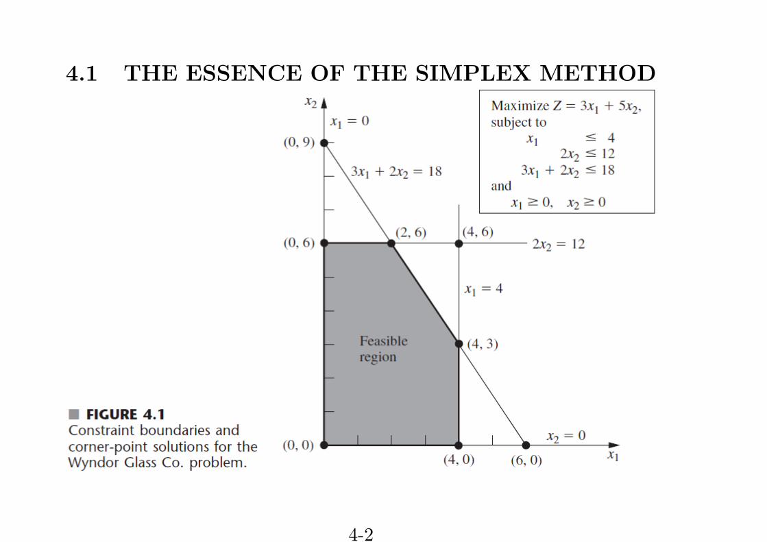
4.1 THE ESSENCE OF THE SIMPLEX METHOD
4-2
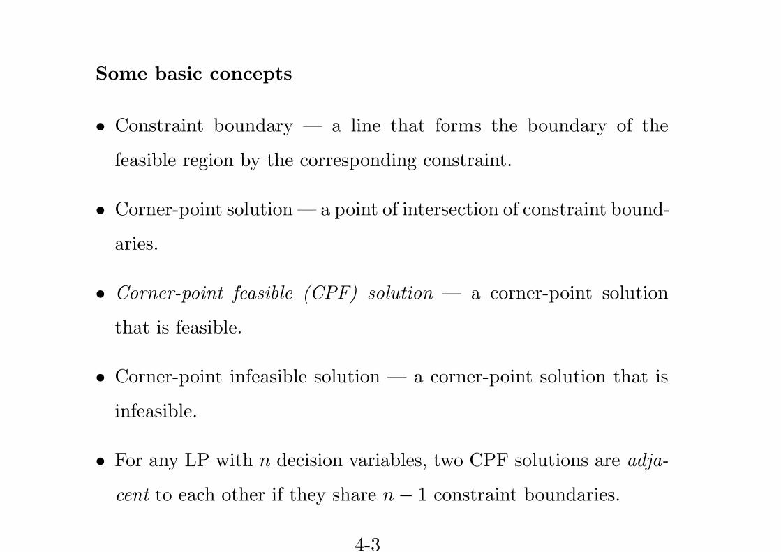
Some basic concepts
• Constraint boundary — a line that forms the boundary of the
feasible region by the corresponding constraint.
• Corner-point solution— a point of intersection of constraint bound-
aries.
• Corner-point feasible (CPF) solution — a corner-point solution
that is feasible.
• Corner-point infeasible solution — a corner-point solution that is
infeasible.
• For any LP with n decision variables, two CPF solutions are adja-
cent to each other if they share n− 1 constraint boundaries.
4-3

• The two adjacent CPF solutions are connected by a line segment
that lies on these same shared constraint boundaries. Such a line
segment is referred to as an edge of the feasible region.
• Optimality test — Suppose an LP has at least one optimal solution.
If a CPF solution has no adjacent CPF solution that are better (as
measured by Z), then it must be an optimal solution.
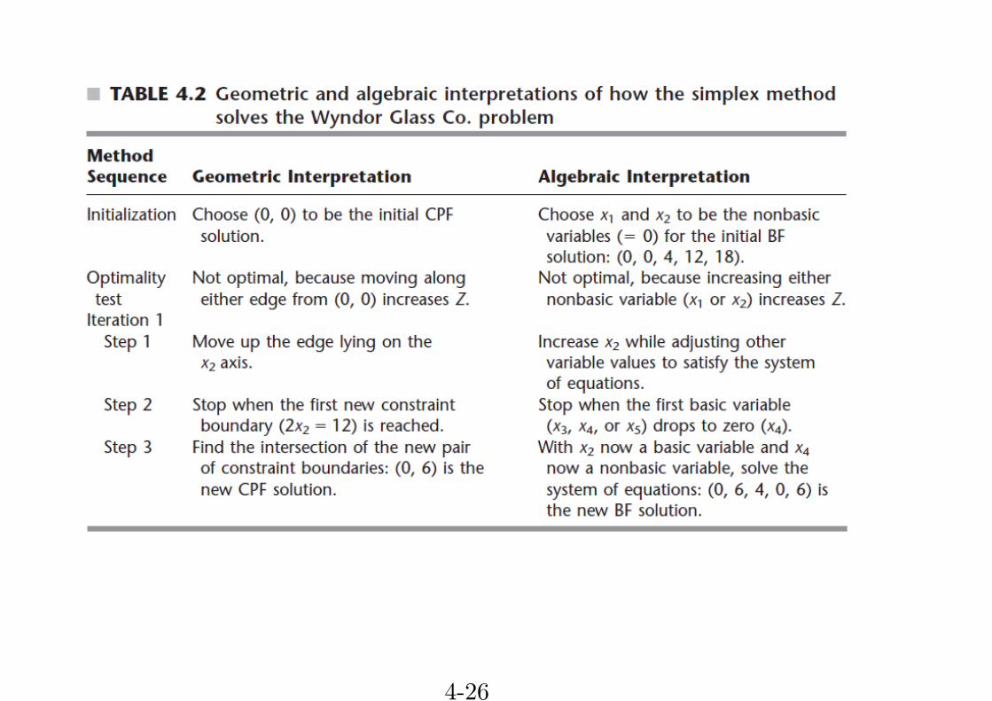
Solving the Wyndor Glass problem
Initialization: Choose (0, 0) as the initial CPF solution to examine.
Optimality Test: Since adjacent CPF solutions are better, (0, 0) is
not an optimal solution.
Iteration 1: Move to a better adjacent CPF solution.
1. There are two edges of the feasible region that emanate from (0,
4-4
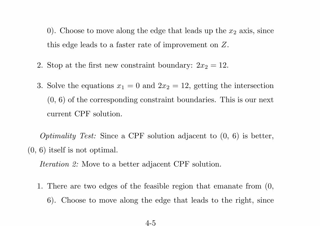
0). Choose to move along the edge that leads up the x2 axis, since
this edge leads to a faster rate of improvement on Z.
2. Stop at the first new constraint boundary: 2x2 = 12.
3. Solve the equations x1 = 0 and 2x2 = 12, getting the intersection
(0, 6) of the corresponding constraint boundaries. This is our next
current CPF solution.
Optimality Test: Since a CPF solution adjacent to (0, 6) is better,
(0, 6) itself is not optimal.
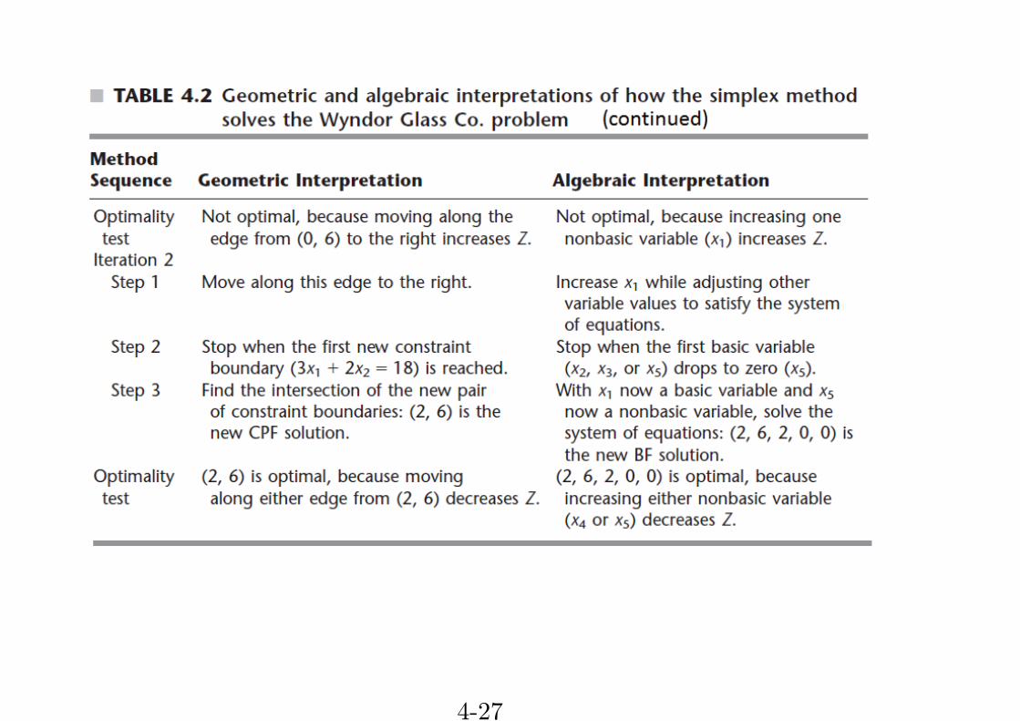
Iteration 2: Move to a better adjacent CPF solution.
1. There are two edges of the feasible region that emanate from (0,
6). Choose to move along the edge that leads to the right, since
4-5

this edge gives positive increasing rate of improvement on Z, while
the other edge gives negative rate.
2. Stop at the first new constraint boundary: 3x1 + 2x2 = 18.
3. Solve the equations 2x2 = 12 and 3x1 + 2x2 = 18, getting the
intersection (2, 6) of the corresponding constraint boundaries. This
is our next current CPF solution.
Optimality Test: The current CPF solution (2, 6) is optimal, since
none of the adjacent CPF solutions are better.
The flow diagram of Simplex
4-6
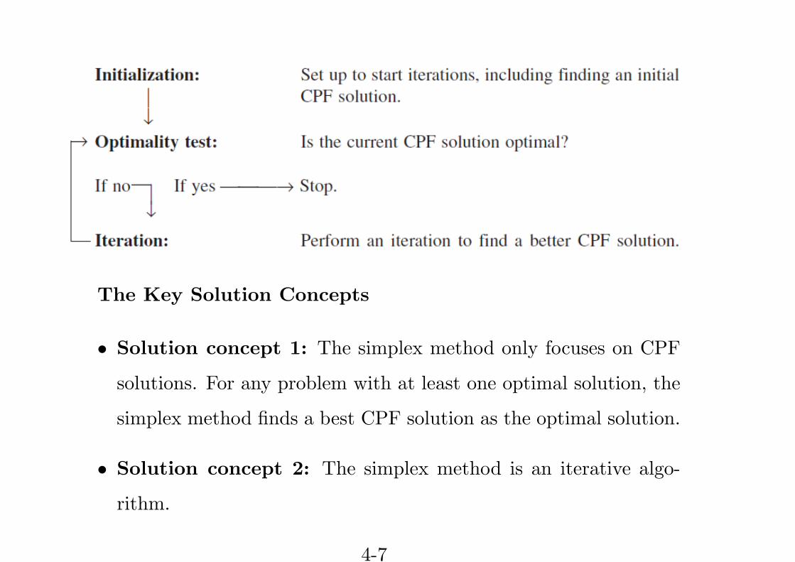
The Key Solution Concepts
• Solution concept 1: The simplex method only focuses on CPF
solutions. For any problem with at least one optimal solution, the
simplex method finds a best CPF solution as the optimal solution.
• Solution concept 2: The simplex method is an iterative algo-
rithm.
4-7
– An iterative algorithm is a systematic solution procedure that
keeps repeating a fixed series of steps, called an iteration, until
a desired result has been obtained.
• Solution concept 3: Whenever possible, the simplex method
selects the origin (that is, all decision variables are equal to zero) as
its initial CPF solution. This avoids solving equations by algebraic
approach to obtain an initial CPF solution.
• Solution concept 4: Given a CPF solution, it is much easier
to compute a CPF solution adjacent to it than to compute other
CPF solutions. Therefore, when the simplex method tries to find
a better CPF solution, it always finds it among the neighbors of
the current CPF solution.
4-8
• Solution concept 5: When there are more than one neighbors of
the current CPF solution, the simplex method chooses the one as
the next current CPF solution that leads to the fastest improving
rate of Z.
• Solution concept 6: The optimality test only needs to check
whether or not there is an edge emanating from the current CPF
solution such that when moving along this edge, the improvement
rate in Z is positive. If there is no such edge, the the current CPF
solution is optimal.
4.2 SETTING UP THE SIMPLEX METHOD
The augmented form of the model
4-9
Although the algebraic viewpoint and the geometric viewpoint of the
simplex method are equivalent, only algebraic method can be used when
the simplex method is implemented in computer.
So, the first step of setting-up is to convert the functional inequal-
ity constraints to equality constraints (that is, equations). Note that
variable constraints themselves are inequality, which need not to be pro-
cessed.
The conversion is done by adding slack variables. For example,
x1 ≤ 4 ⇐⇒ x1 + x3 = 4 and x3 ≥ 0,
where x3 is the slack variable.
In this way, we get the augmented form of the Wyndor Glass problem.
4-10
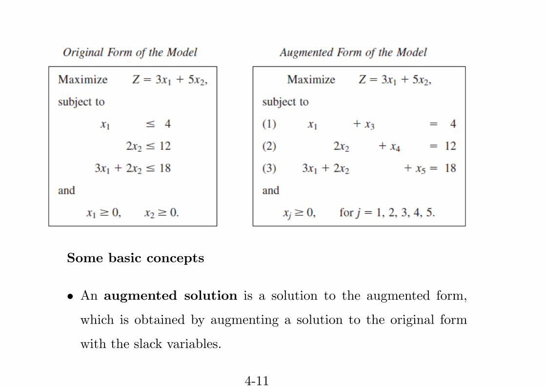
Some basic concepts
• An augmented solution is a solution to the augmented form,
which is obtained by augmenting a solution to the original form
with the slack variables.
4-11
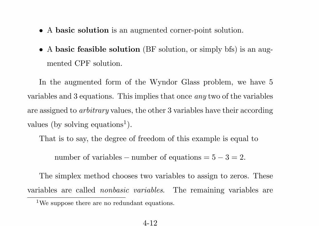
• A basic solution is an augmented corner-point solution.
• A basic feasible solution (BF solution, or simply bfs) is an aug-
mented CPF solution.
In the augmented form of the Wyndor Glass problem, we have 5
variables and 3 equations. This implies that once any two of the variables
are assigned to arbitrary values, the other 3 variables have their according
values (by solving equations1).
That is to say, the degree of freedom of this example is equal to
number of variables− number of equations = 5− 3 = 2.
The simplex method chooses two variables to assign to zeros. These
variables are called nonbasic variables. The remaining variables are
1We suppose there are no redundant equations.
4-12
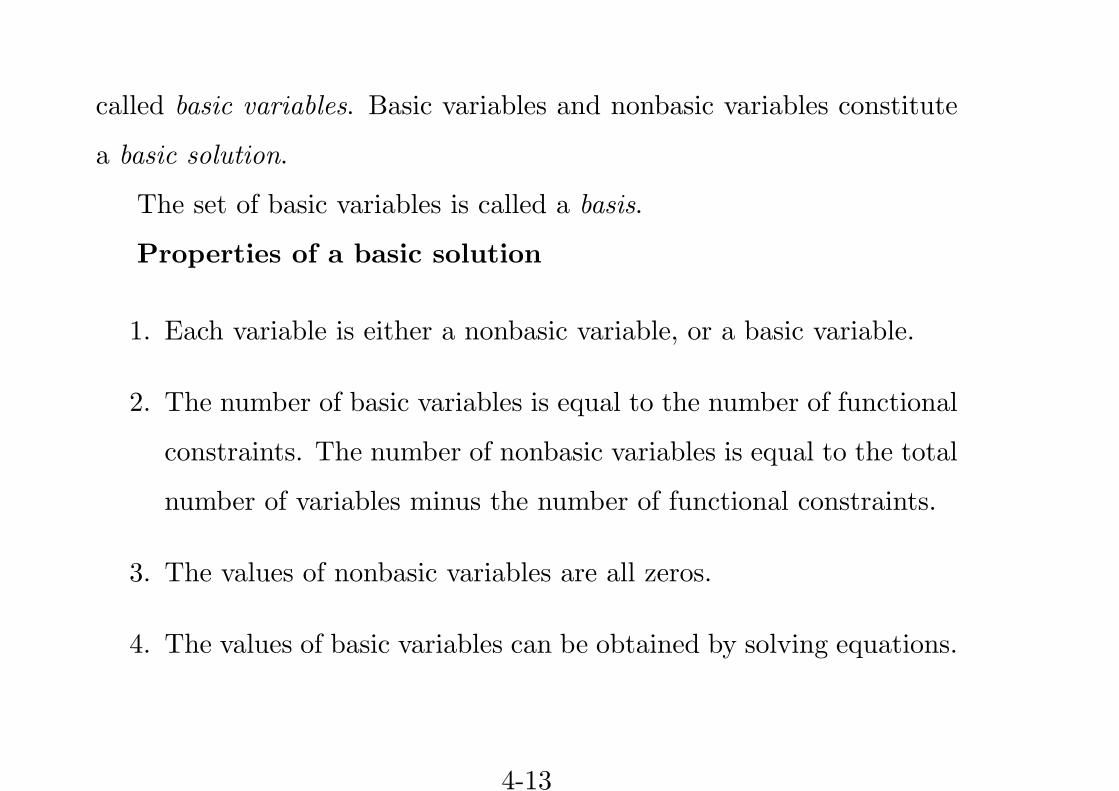
called basic variables. Basic variables and nonbasic variables constitute
a basic solution.
The set of basic variables is called a basis.
Properties of a basic solution
1. Each variable is either a nonbasic variable, or a basic variable.
2. The number of basic variables is equal to the number of functional
constraints. The number of nonbasic variables is equal to the total
number of variables minus the number of functional constraints.
3. The values of nonbasic variables are all zeros.
4. The values of basic variables can be obtained by solving equations.
4-13

5. If the basic variables satisfy the nonnegative constraint, then the
basic solution is also a BF solution (bfs).
Adjacent BF solutions
If two CPF solutions are adjacent, their corresponding BF solutions
are also adjacent, and vice versa.
For BF solutions, we have their own method to determine whether
they are adjacent: Two BF solutions are adjacent if all but one of their
nonbasic variables are the same.
Remarks. The two BF solutions having some same nonbasic variable,
e.g., xi, mean that xi is a nonbasic variable in the both two BF solu-
tions, does not mean that the two BF solutions having the same value of
nonbasic variables.
4-14
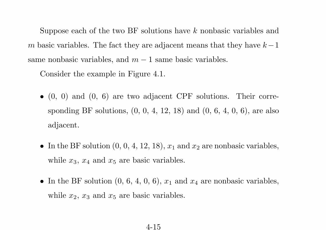
Suppose each of the two BF solutions have k nonbasic variables and
m basic variables. The fact they are adjacent means that they have k−1
same nonbasic variables, and m− 1 same basic variables.
Consider the example in Figure 4.1.
• (0, 0) and (0, 6) are two adjacent CPF solutions. Their corre-
sponding BF solutions, (0, 0, 4, 12, 18) and (0, 6, 4, 0, 6), are also
adjacent.
• In the BF solution (0, 0, 4, 12, 18), x1 and x2 are nonbasic variables,
while x3, x4 and x5 are basic variables.
• In the BF solution (0, 6, 4, 0, 6), x1 and x4 are nonbasic variables,
while x2, x3 and x5 are basic variables.
4-15
• So, they have one same nonbasic variable x1, and two same basic
variables x3 and x5.
Consequently, moving from a BF solution to one of its adjacent BF
solutions, involves that switching one variable from nonbasic to basic
and vice versa for one other variable.
4.3 THE ALGEBRA OF THE SIMPLEX METHOD
When we deal with an LP problem in augmented form, it is convenient
to convert the objective function into a constraint by introducing a new
variable whose value is the objective function.
For example, for the Wyndor Glass problem we may have:
4-16
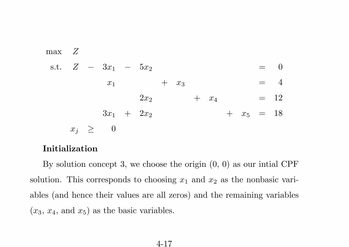
max Z
s.t. Z − 3x1 − 5x2 = 0
x1 + x3 = 4
2x2 + x4 = 12
3x1 + 2x2 + x5 = 18
xj ≥ 0
Initialization
By solution concept 3, we choose the origin (0, 0) as our intial CPF
solution. This corresponds to choosing x1 and x2 as the nonbasic vari-
ables (and hence their values are all zeros) and the remaining variables
(x3, x4, and x5) as the basic variables.
4-17
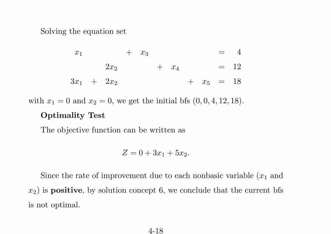
Solving the equation set
x1 + x3 = 4
2x2 + x4 = 12
3x1 + 2x2 + x5 = 18
with x1 = 0 and x2 = 0, we get the initial bfs (0, 0, 4, 12, 18).
Optimality Test
The objective function can be written as
Z = 0 + 3x1 + 5x2.
Since the rate of improvement due to each nonbasic variable (x1 and
x2) is positive, by solution concept 6, we conclude that the current bfs
is not optimal.
4-18

We should increase the value of some nonbasic variable, while the
values of the basic variables are adjusted accordingly.
Iteration 1
Step 1: determining which nonbasic variable should be in-
creased
For x1, the rate of improvement in Z is 3.
For x2, the rate of improvement in Z is 5.
We incline the largest rate. So we choose to increase x2. This variable
is called the entering basic variable.
Step 2: determining how far we can increase the entering
basic variable
4-19
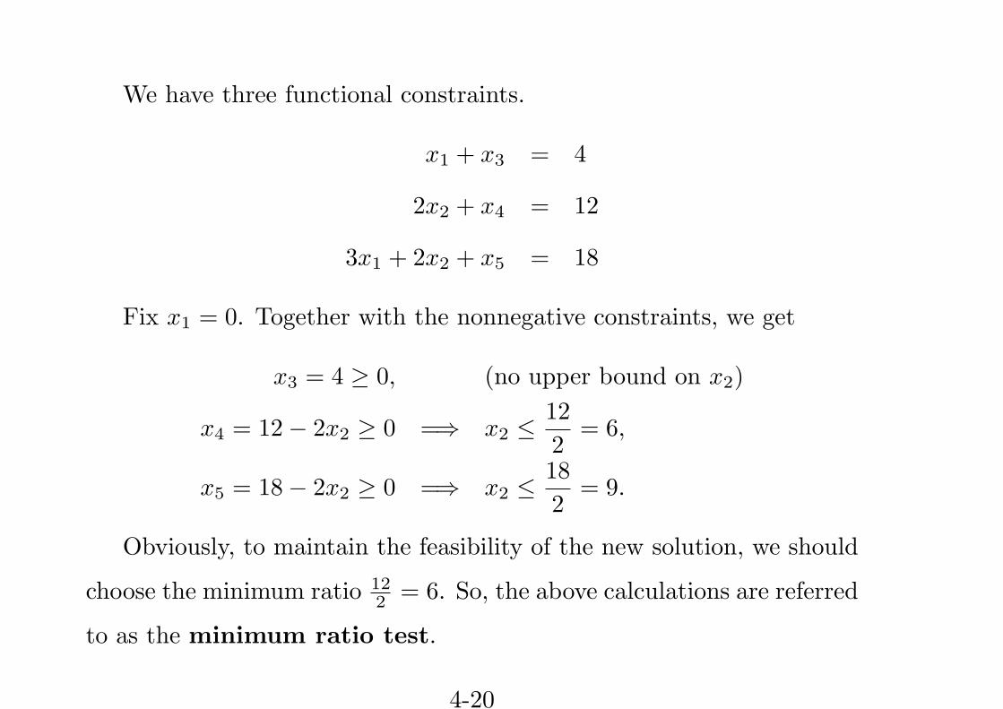
We have three functional constraints.
x1 + x3 = 4
2x2 + x4 = 12
3x1 + 2x2 + x5 = 18
Fix x1 = 0. Together with the nonnegative constraints, we get
x3 = 4 ≥ 0, (no upper bound on x2)
x4 = 12− 2x2 ≥ 0 =⇒ x2 ≤ 12
2= 6,
x5 = 18− 2x2 ≥ 0 =⇒ x2 ≤ 18
2= 9.
Obviously, to maintain the feasibility of the new solution, we should
choose the minimum ratio 122 = 6. So, the above calculations are referred
to as the minimum ratio test.
4-20

Increasing the value of x2 from 0 will make it a basic variable. Mean-
while, the value of x4 will drop to 0. Therefore, this variable is called
the leaving basic variable.
Step 3: solving for the new bfs
So far, for the new bfs we will get we have
nonbasic vars x1 = 0, x4 = 0
basic vars x3 =?, x2 = 6, x5 =?
To determine the vale of the remaining basic variables, we just solve
the equation set by Gaussian elimination, which involves some elemen-
tary algebraic operations.
4-21
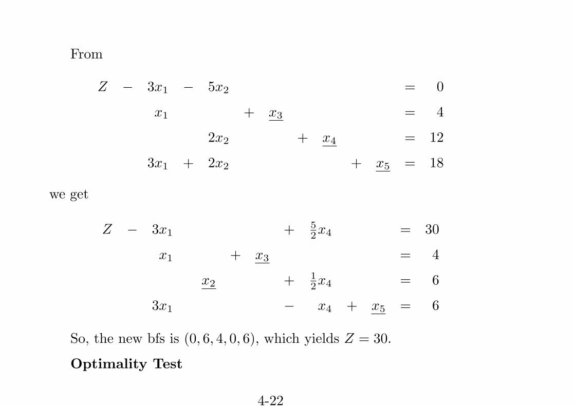
From
Z − 3x1 − 5x2 = 0
x1 + x3 = 4
2x2 + x4 = 12
3x1 + 2x2 + x5 = 18
we get
Z − 3x1 + 52x4 = 30
x1 + x3 = 4
x2 + 12x4 = 6
3x1 − x4 + x5 = 6
So, the new bfs is (0, 6, 4, 0, 6), which yields Z = 30.
Optimality Test
4-22
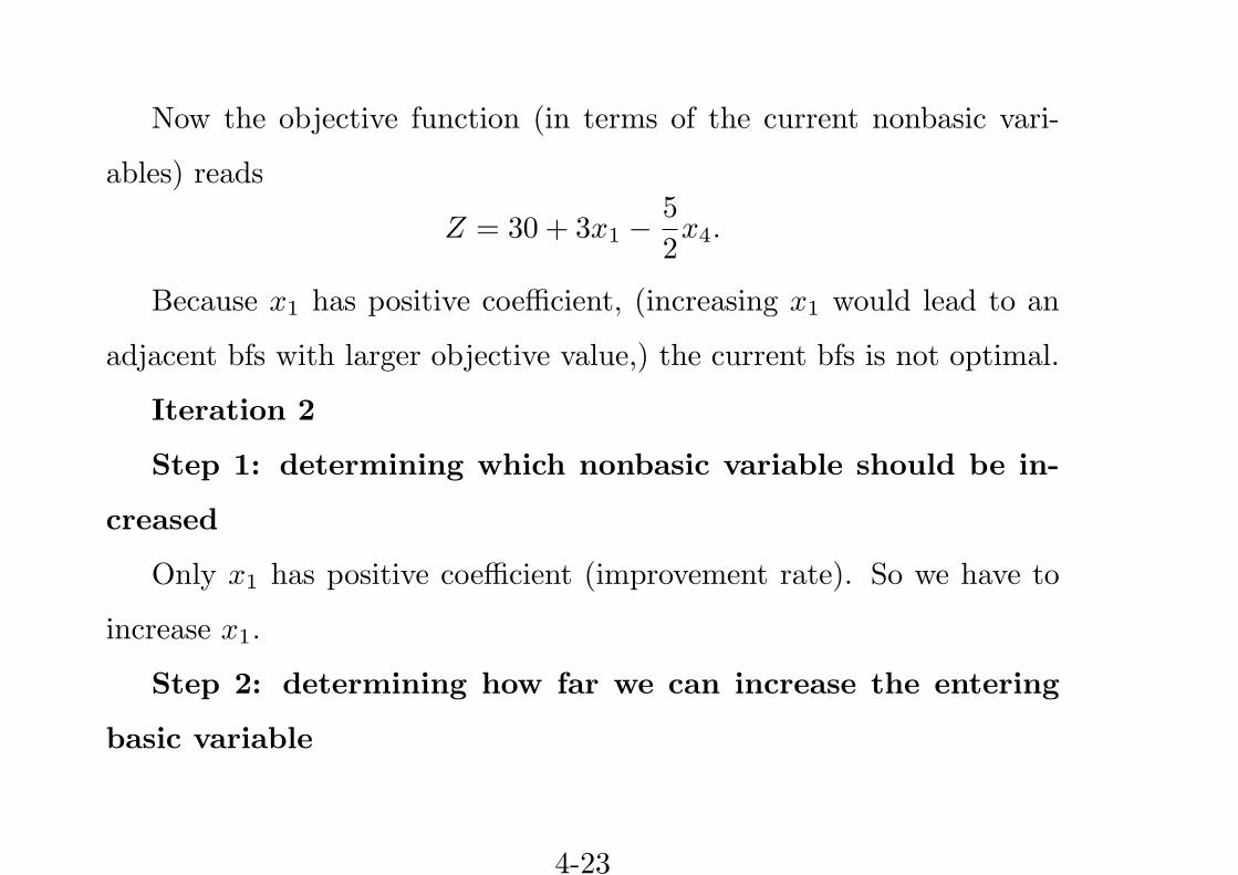
Now the objective function (in terms of the current nonbasic vari-
ables) reads
Z = 30 + 3x1 −5
2x4.
Because x1 has positive coefficient, (increasing x1 would lead to an
adjacent bfs with larger objective value,) the current bfs is not optimal.
Iteration 2
Step 1: determining which nonbasic variable should be in-
creased
Only x1 has positive coefficient (improvement rate). So we have to
increase x1.
Step 2: determining how far we can increase the entering
basic variable
4-23
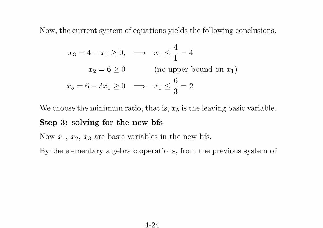
Now, the current system of equations yields the following conclusions.
x3 = 4− x1 ≥ 0, =⇒ x1 ≤ 4
1= 4
x2 = 6 ≥ 0 (no upper bound on x1)
x5 = 6− 3x1 ≥ 0 =⇒ x1 ≤ 6
3= 2
We choose the minimum ratio, that is, x5 is the leaving basic variable.
Step 3: solving for the new bfs
Now x1, x2, x3 are basic variables in the new bfs.
By the elementary algebraic operations, from the previous system of
4-24
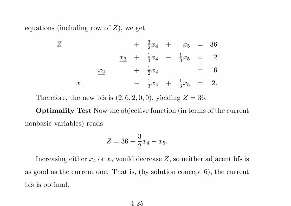
equations (including row of Z), we get
Z + 32x4 + x5 = 36
x3 + 13x4 − 1
3x5 = 2
x2 + 12x4 = 6
x1 − 13x4 + 1
3x5 = 2.
Therefore, the new bfs is (2, 6, 2, 0, 0), yielding Z = 36.
Optimality Test Now the objective function (in terms of the current
nonbasic variables) reads
Z = 36− 3
2x4 − x5.
Increasing either x4 or x5 would decrease Z, so neither adjacent bfs is
as good as the current one. That is, (by solution concept 6), the current
bfs is optimal.
4-25
4-26
4-27
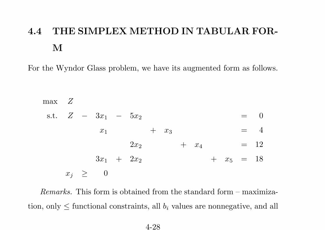
4.4 THE SIMPLEXMETHOD IN TABULAR FOR-
M
For the Wyndor Glass problem, we have its augmented form as follows.
max Z
s.t. Z − 3x1 − 5x2 = 0
x1 + x3 = 4
2x2 + x4 = 12
3x1 + 2x2 + x5 = 18
xj ≥ 0
Remarks. This form is obtained from the standard form – maximiza-
tion, only ≤ functional constraints, all bi values are nonnegative, and all
4-28
nonnegativity constraints. See Sec 4.6 for necessary adjustments if the
problem is not in the standard form.
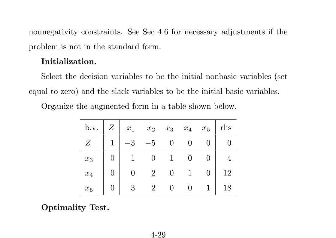
Initialization.
Select the decision variables to be the initial nonbasic variables (set
equal to zero) and the slack variables to be the initial basic variables.
Organize the augmented form in a table shown below.
b.v. Z x1 x2 x3 x4 x5 rhs
Z 1 −3 −5 0 0 0 0
x3 0 1 0 1 0 0 4
x4 0 0 2 0 1 0 12
x5 0 3 2 0 0 1 18
Optimality Test.
4-29
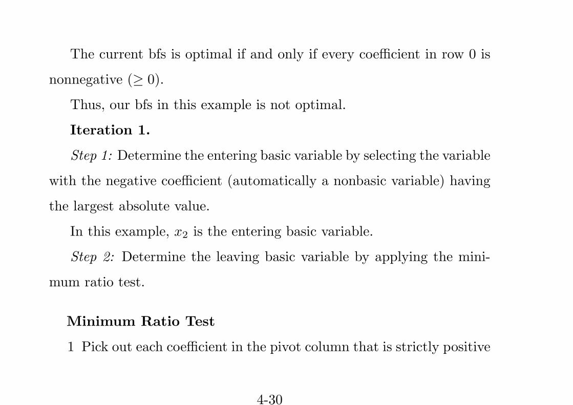
The current bfs is optimal if and only if every coefficient in row 0 is
nonnegative (≥ 0).
Thus, our bfs in this example is not optimal.
Iteration 1.
Step 1: Determine the entering basic variable by selecting the variable
with the negative coefficient (automatically a nonbasic variable) having
the largest absolute value.
In this example, x2 is the entering basic variable.
Step 2: Determine the leaving basic variable by applying the mini-
mum ratio test.
Minimum Ratio Test
1 Pick out each coefficient in the pivot column that is strictly positive
4-30
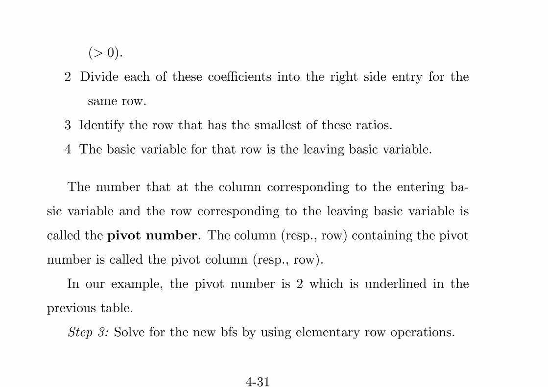
(> 0).
2 Divide each of these coefficients into the right side entry for the
same row.
3 Identify the row that has the smallest of these ratios.
4 The basic variable for that row is the leaving basic variable.
The number that at the column corresponding to the entering ba-
sic variable and the row corresponding to the leaving basic variable is
called the pivot number. The column (resp., row) containing the pivot
number is called the pivot column (resp., row).
In our example, the pivot number is 2 which is underlined in the
previous table.
Step 3: Solve for the new bfs by using elementary row operations.
4-31
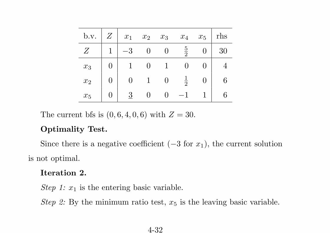
b.v. Z x1 x2 x3 x4 x5 rhs
Z 1 −3 0 0 52 0 30
x3 0 1 0 1 0 0 4
x2 0 0 1 0 12 0 6
x5 0 3 0 0 −1 1 6
The current bfs is (0, 6, 4, 0, 6) with Z = 30.
Optimality Test.
Since there is a negative coefficient (−3 for x1), the current solution
is not optimal.
Iteration 2.
Step 1: x1 is the entering basic variable.
Step 2: By the minimum ratio test, x5 is the leaving basic variable.
4-32
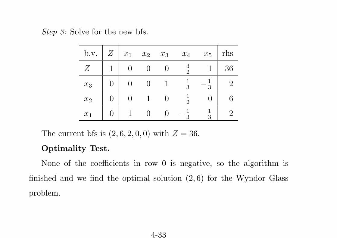
Step 3: Solve for the new bfs.
b.v. Z x1 x2 x3 x4 x5 rhs
Z 1 0 0 0 32 1 36
x3 0 0 0 1 13 −1
3 2
x2 0 0 1 0 12 0 6
x1 0 1 0 0 −13
13 2
The current bfs is (2, 6, 2, 0, 0) with Z = 36.
Optimality Test.
None of the coefficients in row 0 is negative, so the algorithm is
finished and we find the optimal solution (2, 6) for the Wyndor Glass
problem.
4-33
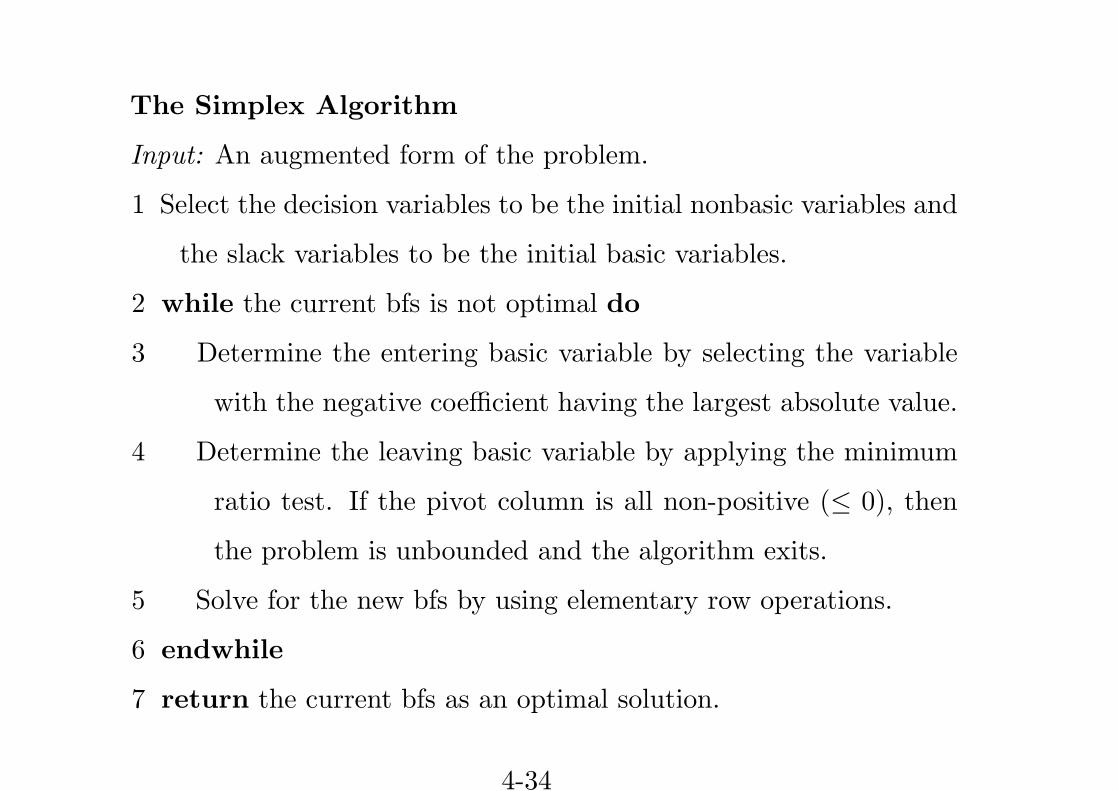
The Simplex Algorithm
Input: An augmented form of the problem.
1 Select the decision variables to be the initial nonbasic variables and
the slack variables to be the initial basic variables.
2 while the current bfs is not optimal do
3 Determine the entering basic variable by selecting the variable
with the negative coefficient having the largest absolute value.
4 Determine the leaving basic variable by applying the minimum
ratio test. If the pivot column is all non-positive (≤ 0), then
the problem is unbounded and the algorithm exits.
5 Solve for the new bfs by using elementary row operations.
6 endwhile
7 return the current bfs as an optimal solution.
4-34
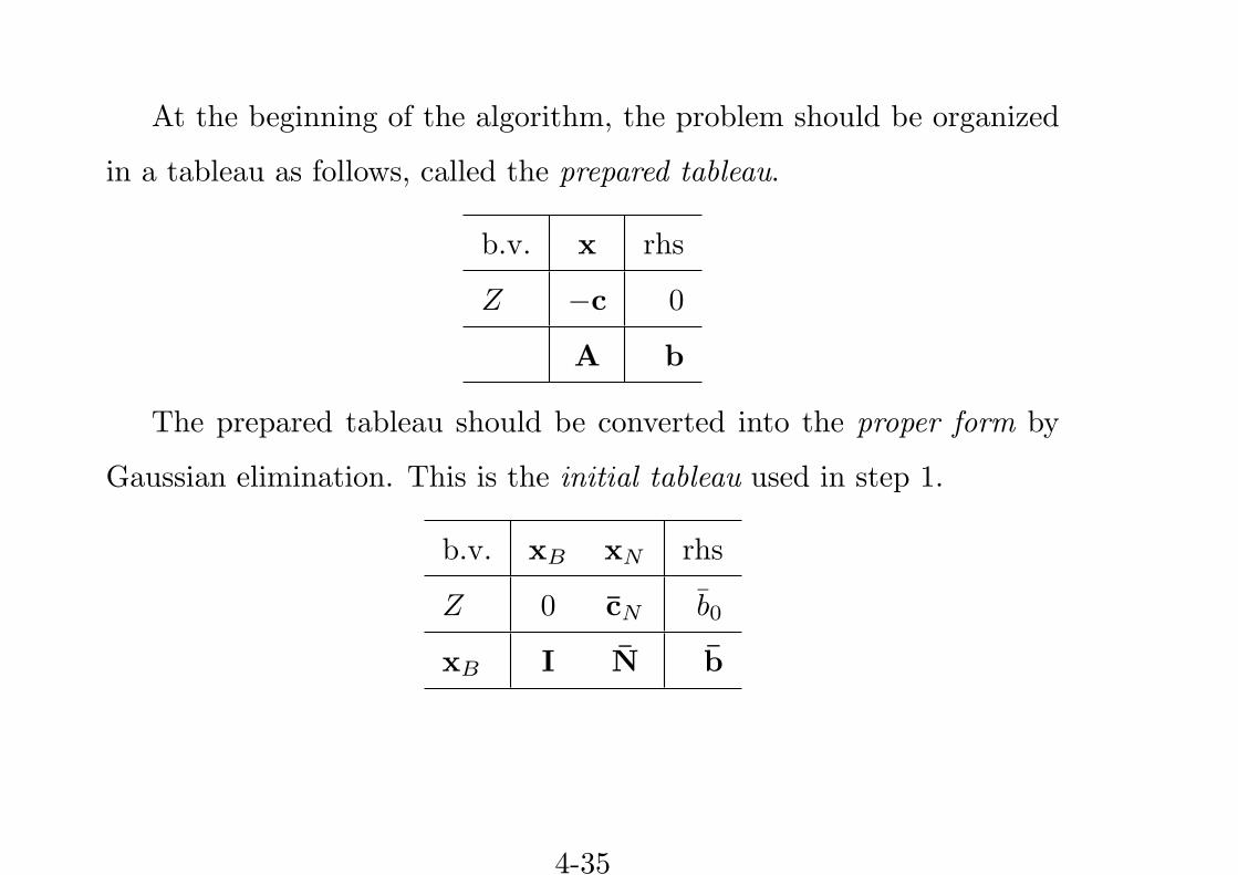
At the beginning of the algorithm, the problem should be organized
in a tableau as follows, called the prepared tableau.
b.v. x rhs
Z −c 0
A b
The prepared tableau should be converted into the proper form by
Gaussian elimination. This is the initial tableau used in step 1.
b.v. xB xN rhs
Z 0 c̄N b̄0
xB I N̄ b̄
4-35

4.5 TIE BREAKING IN THE SIMPLEX METHOD
Tie for the Entering Basic Variable
In step 3 of the simplex algorithm, if there are more than one negative
coefficients with the largest absolute value in row 0 of the current tableau,
then there are more than one candidates for the entering basic variable.
The tie can be broken arbitrarily.
Tie for the Leaving Basic Variable — Degeneracy
Now suppose that two or more basic variables tie for being the leaving
basic variable in step 4 of the simplex algorithm.
In this case tie cannot be broken arbitrarily, because the following
sequence of events that could occur.
1. All the tied basic variables reach zero simultaneously as the enter-
4-36
ing basic variable increases. Therefore, the one or ones not chosen
to be the leaving basic variable also will have a value of zero in the
new bfs.
• A basic variable which has value zero is called degenerate.
• A bfs with degenerate basic variable(s) is called a degenerate
bfs.
• An LP with degenerate bfs(’s) is called a degenerate LP.
2. If one of these degenerate basic variables retains its zero value
until it is chose in a subsequent iteration to be a leaving basic vari-
able, the corresponding entering basic variable also must remain
zero (since it cannot be increased without making the leaving ba-
sic variable negative), so the value of Z must remain unchanged.
4-37

3. If Z may remain the same rather than increase at each iteration,
the simplex algorithm may then go around in a loop, repeating
the same sequence of solutions periodically rather than eventually
increasing Z toward an optimal solution.
There is a simple method breaking this tie, called Bland’s anti-cycling
rule: In case of tie of the above two types, always choose the lowest
numbered variable to enter basis, and choose the lowest numbered variable
to leave basis.
No Leaving Basic Variable — Unbounded Z
In step 4 of the simplex algorithm, if every coefficient in the pivot
column (excluding row 0) is non-positive, then the entering basic variable
can be increased indefinitely (without giving negative values to any of
4-38
the current basic variables), leading to unbounded objective value.
Multiple Optimal Solutions
Suppose that u and v are two optimal bfs. Then their convex com-
bination, that is, (1−λ)u+λv for any λ ∈ [0, 1], is an optimal solution
to the LP.
Proof. Let w = (1− λ)u+ λv. Then w ≥ 0.
For any functional constraint aTi x ≤ bi, we have aTi w = (1−λ)aTi u+
λaTi v ≤ (1− λ)bi + λbi = bi. So, w is a feasible solution.
Let c be the objective vector. Then the objective value of w is cTw =
(1 − λ)cTu + λcTv = (1 − λ)cTu + λcTu = cTu. So, w is an optimal
solution.
Find the next optimal solution by the simplex algorithm when there
4-39
are multiple optimal solutions. (Omitted)
4.6 ADAPTING TO OTHER MODEL FORMS
So far, we have the following conventions on our standard LP model:
• The objective function is in maximization form.
• All bi’s are nonnegative.
• All functional constraints are in ≤ form.
• All variables are nonnegative.
Minimization Objective Function
min∑
cjxj
4-40
is equivalent to
max∑
(−cj)xj
Negative Right-Hand Sides
Multiply by −1 through both sides of the constraint.
Variables Allowed to Be Negative
If the variable constraint is xj ≤ 0 for some j, then replacing xj with
−x′j and adding x′
j ≥ 0 can eliminate this negative variable.
If the variable constraint is xj ≷ 0 for some j, then replacing xj with
x+j − x−
j and adding x+j ≥ 0, x−
j ≥ 0 can eliminate this unrestricted
variable.
Functional Constraints in ≥ Form with bi ≥ 0
In this case we cannot multiply both the two sides of the constraint
by −1, since this would produce a negative right-hand side.
4-41

Instead, the approach is to add a surplus variable as follows. Suppose
the constraint is
ai1x1 + ai2x2 + · · ·+ ainxn ≥ bi.
We replace it by
ai1x1 + ai2x2 + · · ·+ ainxn − xn+1 = bi
and
xn+1 ≥ 0,
converting the “≥” constraint into an equality constraint.
Equality Constraints and the Big M Method
In the last, we deal with the equality constraints. The approach is
the artificial-variable technique given below.
4-42
Suppose the constraint is
ai1x1 + ai2x2 + · · ·+ ainxn = bi.
We replace it by
ai1x1 + ai2x2 + · · ·+ ainxn + x̄n+1 = bi
and
x̄n+1 ≥ 0.
The added variable is called the artificial variable.
Obviously, we should enforce the artificial variable x̄n+1 to be zero to
maintain the equivalence of the original problem and the revised prob-
lem. To this end, we introduce an extra item to the objective function:
4-43
Replace the original objective function
max
n∑j=1
cjxj
by the new function
maxn∑
j=1
cjxj −Mx̄n+1,
where M is a sufficiently large positive constant number.
This processing method is called the Big M method.
————————————–
Before giving the solving procedure of the big M method, we first
give some remarks.
4-44
Another way to deal with the equality constraint ai1x1+ai2x2+ · · ·+
ainxn = bi is to change it with two inequality constraints:
ai1x1 + ai2x2 + · · ·+ ainxn ≤ bi,
ai1x1 + ai2x2 + · · ·+ ainxn ≥ bi.
However, as explained before, the new introduced “≥” constraint
will be processed by changing it to an equality constraint ai1x1+ai2x2+
· · ·+ ainxn −xn+1 = bi, where xn+1 ≥ 0 is a surplus variable. So, a new
equality constraint is introduced, meaning that the method dealing with
the equality constraints is essentially unavoidable.
————————————–
Since in the objective function there is a huge coefficient M , when
applying the simplex method the computation have to be the symbolic
4-45
computation.
Although in theory one can assign a particular huge numerical value
to M and proceed the simplex method as the usual way, this approach
may result in significant rounding errors in practice that invalidate the
optimality test.
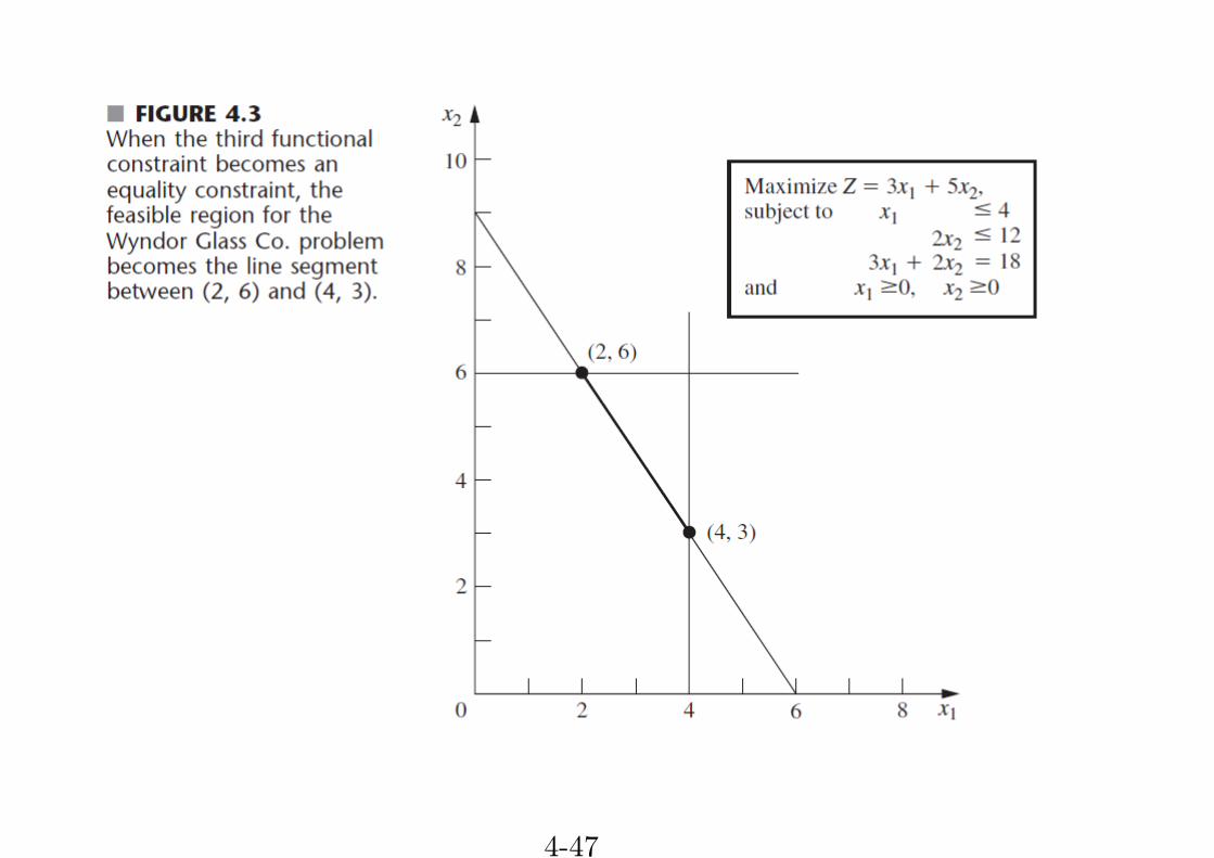
Example. Solving the LP (the revised Wyndor Glass problem)
max 3x1 + 5x2
s.t. x1 ≤ 4
2x2 ≤ 12
3x1 + 2x2 = 18
xj ≥ 0, ∀j
4-46
4-47
By adding slack variables and artificial variable(s), the problem be-
comes
max 3x1 + 5x2 −Mx̄5
s.t. x1 + x3 = 4
2x2 + x4 = 12
3x1 + 2x2 + x̄5 = 18
xj ≥ 0, ∀j
We call this form, the augmented form with artificial variables, the
artificial form in the Big M method (or simply the artificial form when
the context is clear).
Organize the problem in the prepared tableau.
4-48
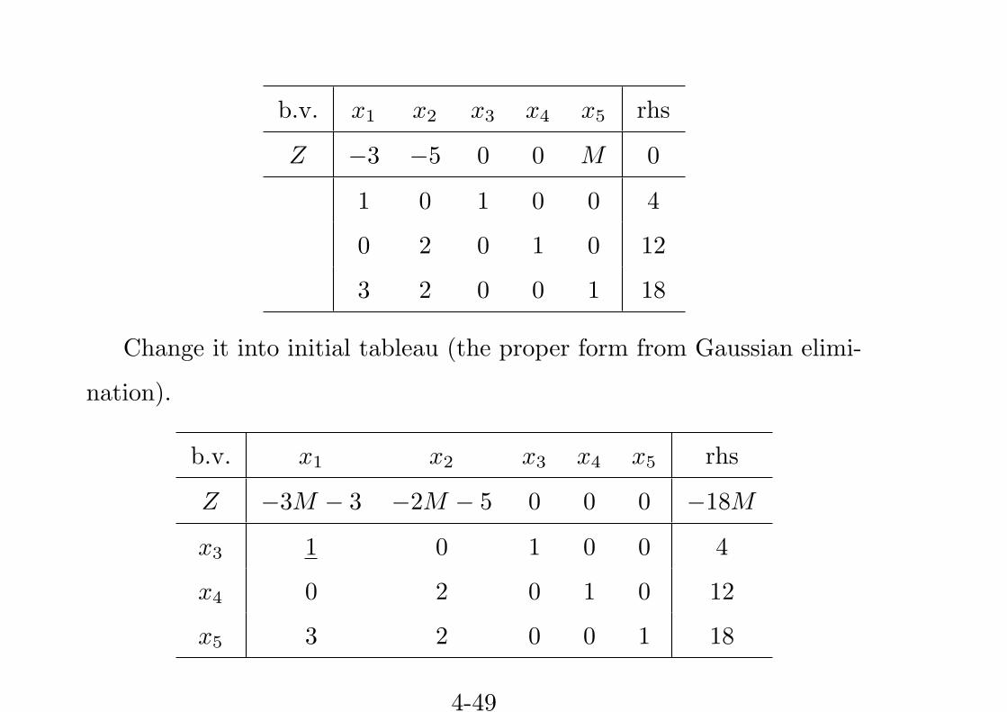
b.v. x1 x2 x3 x4 x5 rhs
Z −3 −5 0 0 M 0
1 0 1 0 0 4
0 2 0 1 0 12
3 2 0 0 1 18
Change it into initial tableau (the proper form from Gaussian elimi-
nation).
b.v. x1 x2 x3 x4 x5 rhs
Z −3M − 3 −2M − 5 0 0 0 −18M
x3 1 0 1 0 0 4
x4 0 2 0 1 0 12
x5 3 2 0 0 1 18
4-49
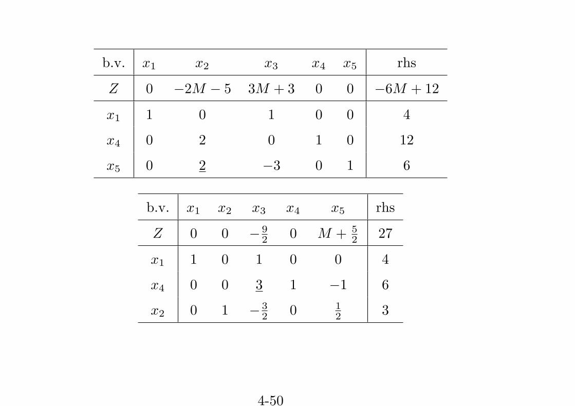
b.v. x1 x2 x3 x4 x5 rhs
Z 0 −2M − 5 3M + 3 0 0 −6M + 12
x1 1 0 1 0 0 4
x4 0 2 0 1 0 12
x5 0 2 −3 0 1 6
b.v. x1 x2 x3 x4 x5 rhs
Z 0 0 −92 0 M + 5
2 27
x1 1 0 1 0 0 4
x4 0 0 3 1 −1 6
x2 0 1 −32 0 1
2 3
4-50
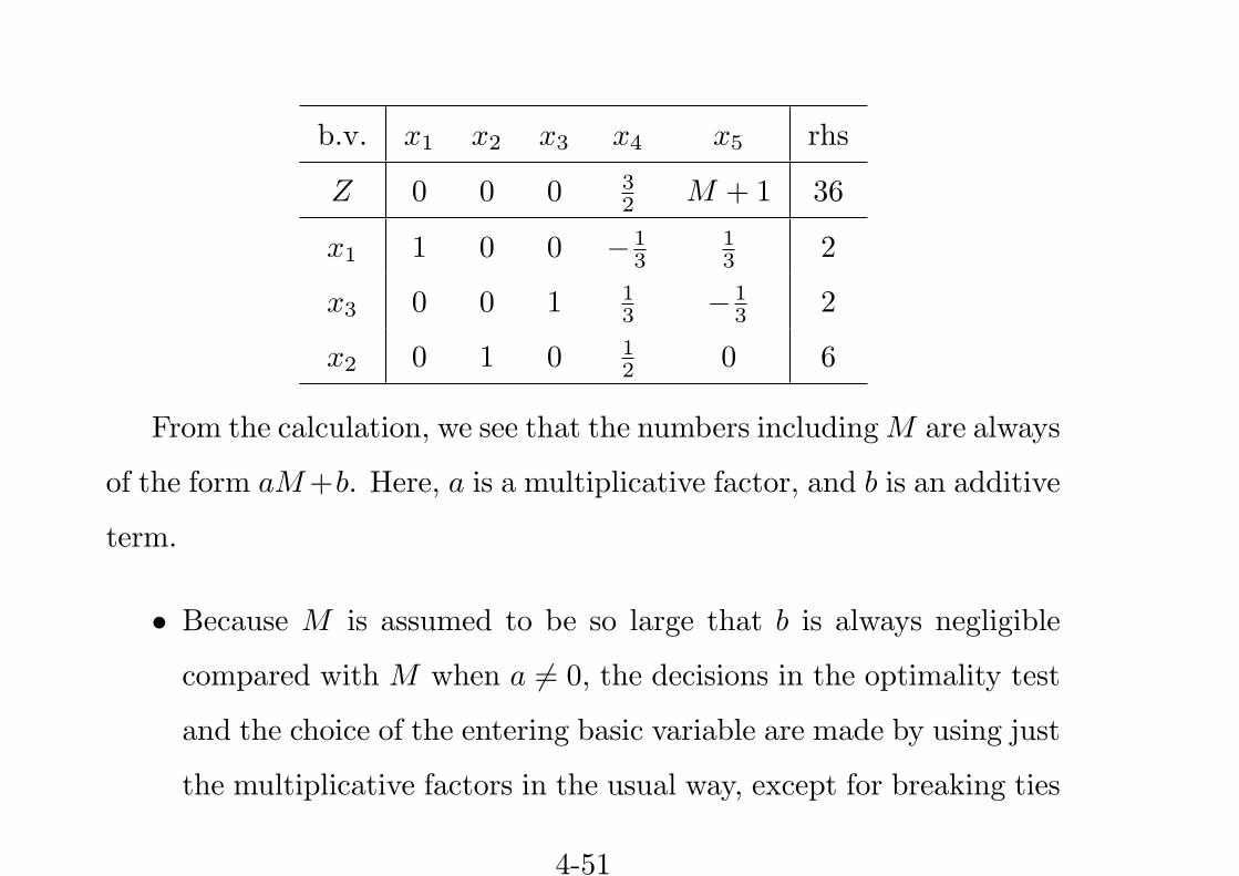
b.v. x1 x2 x3 x4 x5 rhs
Z 0 0 0 32 M + 1 36
x1 1 0 0 −13
13 2
x3 0 0 1 13 − 1
3 2
x2 0 1 0 12 0 6
From the calculation, we see that the numbers includingM are always
of the form aM+b. Here, a is a multiplicative factor, and b is an additive
term.
• Because M is assumed to be so large that b is always negligible
compared with M when a ̸= 0, the decisions in the optimality test
and the choice of the entering basic variable are made by using just
the multiplicative factors in the usual way, except for breaking ties
4-51
with the additive factors.
• If an LP problem contains more than one equality constraints,
each constraint is handled in just the same way — each equality
constraint will have an artificial variable and incur an extra term
of the form −Mx̄j in the objective function.
The execution procedure of the simplex method on the artificial prob-
lem can be explained in Figure 4.4.
4-52
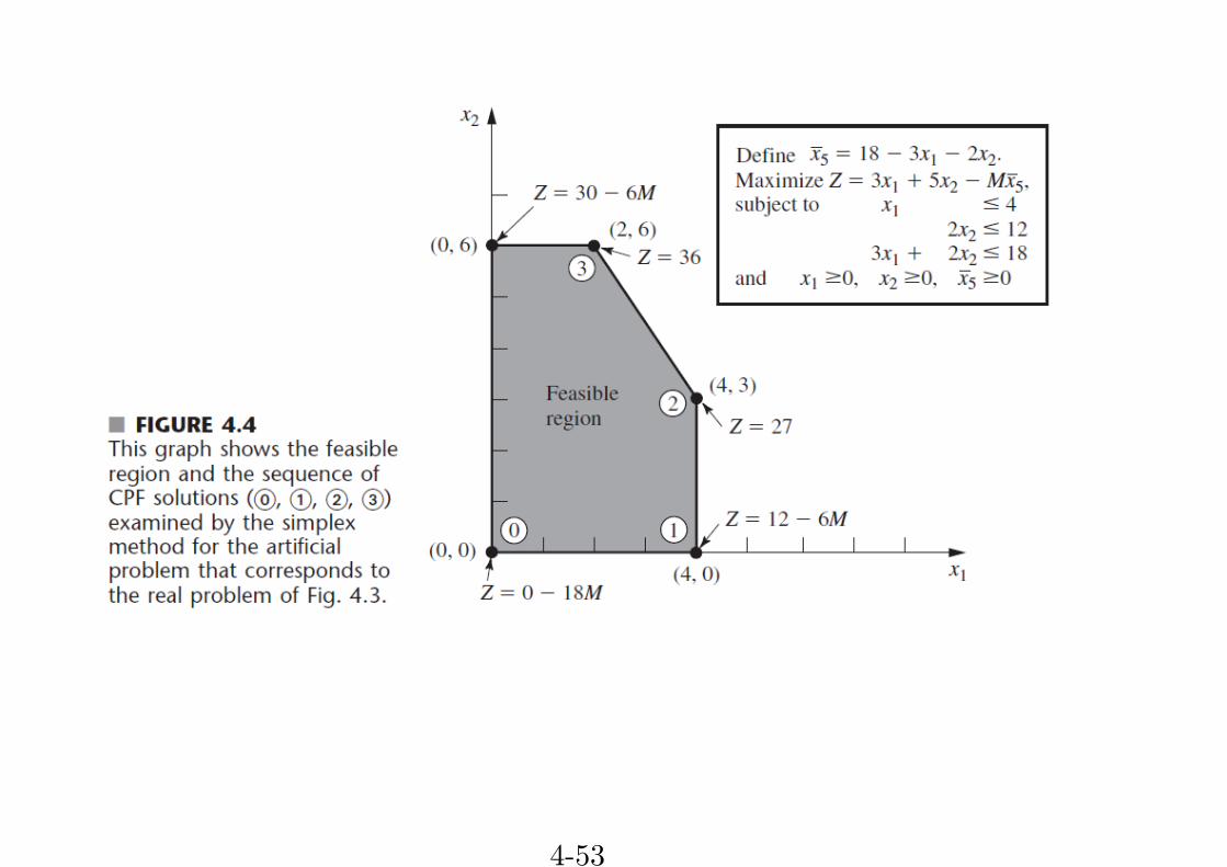
4-53
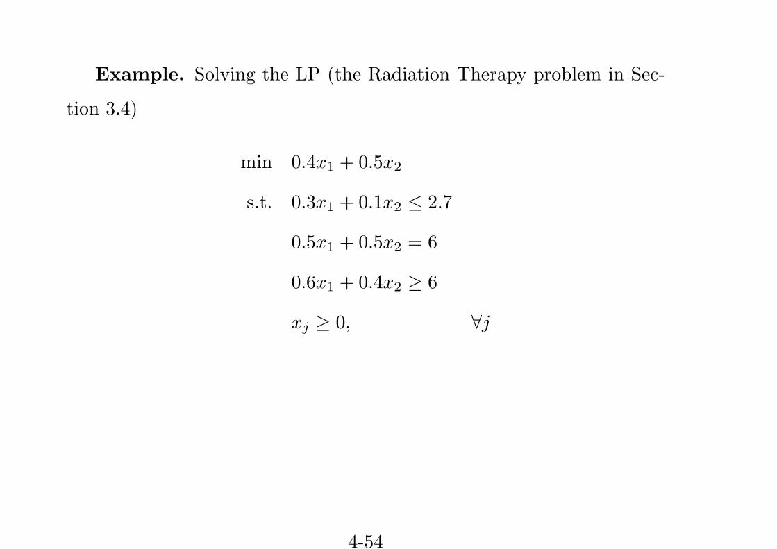
Example. Solving the LP (the Radiation Therapy problem in Sec-
tion 3.4)
min 0.4x1 + 0.5x2
s.t. 0.3x1 + 0.1x2 ≤ 2.7
0.5x1 + 0.5x2 = 6
0.6x1 + 0.4x2 ≥ 6
xj ≥ 0, ∀j
4-54
4-55

Translate the problem into the artificial form.
max − 0.4x1 − 0.5x2 −Mx̄4 −Mx̄6
s.t. 0.3x1 + 0.1x2 + x3 = 2.7
0.5x1 + 0.5x2 + x̄4 = 6
0.6x1 + 0.4x2 − x5 + x̄6 = 6
xj ≥ 0, ∀j
The prepared simplex tableau.
4-56
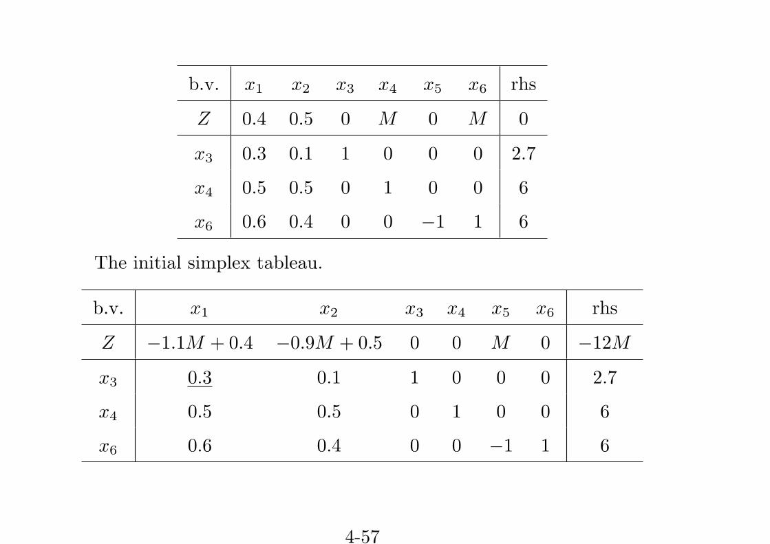
b.v. x1 x2 x3 x4 x5 x6 rhs
Z 0.4 0.5 0 M 0 M 0
x3 0.3 0.1 1 0 0 0 2.7
x4 0.5 0.5 0 1 0 0 6
x6 0.6 0.4 0 0 −1 1 6
The initial simplex tableau.
b.v. x1 x2 x3 x4 x5 x6 rhs
Z −1.1M + 0.4 −0.9M + 0.5 0 0 M 0 −12M
x3 0.3 0.1 1 0 0 0 2.7
x4 0.5 0.5 0 1 0 0 6
x6 0.6 0.4 0 0 −1 1 6
4-57
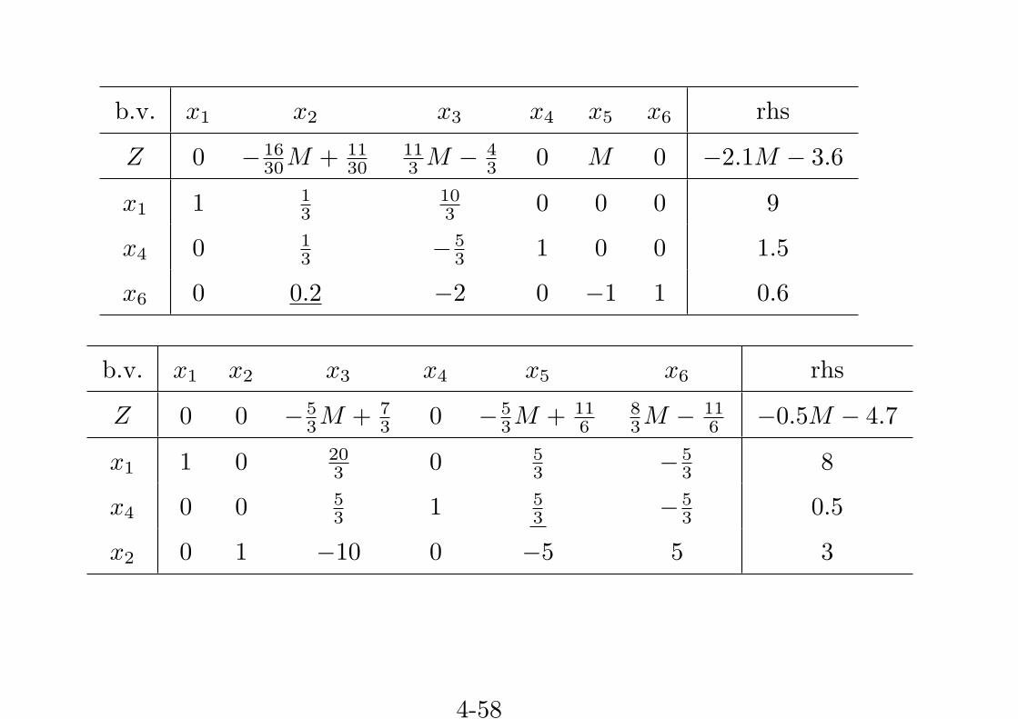
b.v. x1 x2 x3 x4 x5 x6 rhs
Z 0 −1630M + 11
30113 M − 4
3 0 M 0 −2.1M − 3.6
x1 1 13
103 0 0 0 9
x4 0 13 − 5
3 1 0 0 1.5
x6 0 0.2 −2 0 −1 1 0.6
b.v. x1 x2 x3 x4 x5 x6 rhs
Z 0 0 −53M + 7
3 0 − 53M + 11
683M − 11
6 −0.5M − 4.7
x1 1 0 203 0 5
3 −53 8
x4 0 0 53 1 5
3 −53 0.5
x2 0 1 −10 0 −5 5 3
4-58
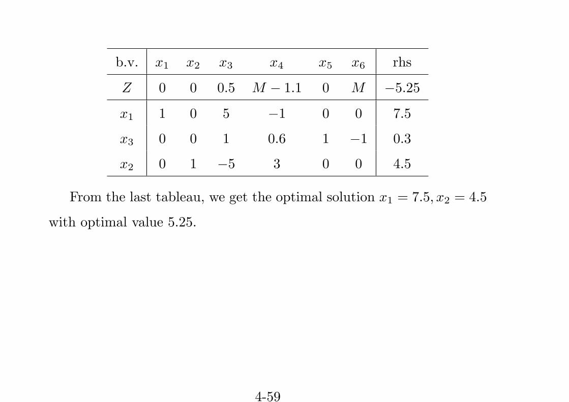
b.v. x1 x2 x3 x4 x5 x6 rhs
Z 0 0 0.5 M − 1.1 0 M −5.25
x1 1 0 5 −1 0 0 7.5
x3 0 0 1 0.6 1 −1 0.3
x2 0 1 −5 3 0 0 4.5
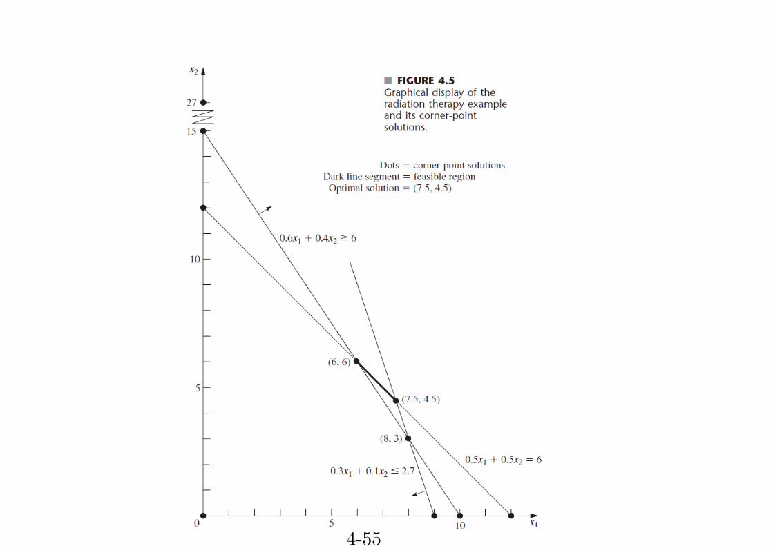
From the last tableau, we get the optimal solution x1 = 7.5, x2 = 4.5
with optimal value 5.25.
4-59

4-60

Observe the two examples of the Big M method. We find that the
Big M method can be thought of as having two phases.
1. In the first phase, all artificial variables are driven to zero (because
of the penalty of M per unit for being greater than zero), resulting
in an initial bfs for the real problem.
2. In the second phase, all the artificial variables are kept at zero
(because of this same penalty) while the simplex method generates
a sequence of bfs for the real problem that leads to an optimal
solution.
These observations inspire the two-phase method, which is a stream-
lined procedure of the Big M method.
The Two-Phase Method
4-61
According to its name, the two-phase method has two phases that in
its first phase, an initial bfs to the real problem is obtained, and in its
second phase, beginning from this initial bfs, an optimal solution to the
real problem is obtained.
Both of the two phases are applying the simplex method.
Before we apply the Two-Phase method, the problem should be in a
proper form. This form is like the artificial form in the Big M method,
with some slight difference.
Recall that the objective function in the artificial form of the Big M
method is
maxn∑
j=1
cjxj −n′∑
j=n+1
Mx̄j ,
4-62
which is equivalent to (modulo a factor of M)
max
n∑j=1
cjM
xj −n′∑
j=n+1
x̄j .
Since no matter what values xj ’s are, we can choose a sufficiently large
M so that∑n
j=1cjM xj ≪
∑n′
j=n+1 x̄j , the above objective function is, in
turn, equivalent to
max −n′∑
j=n+1
x̄j
(in the sense that M can be chosen arbitrarily large).
4-63

So, we get the artificial form in the Two-Phase method as follows.
max −∑
x̄j
s.t. Ax = b
x ≥ 0
By this form, we get rid of the big M from the LP, avoiding the
symbolic computation in the Simplex method.
The Two-Phase Method
1 Intialization: Obtain the artificial form in the Two-Phase method,
so that an initial bfs for the artificial problem is clear.
2 Phase 1: Solve the artificial form by Simplex, obtaining an initial
bfs x for the real problem.
4-64

3 Phase 2: Starting with this bfs x, solve the augmented form of the
real problem by Simplex.
Example. Solving the Radiation Therapy problem by the Two-
Phase method:
min 0.4x1 + 0.5x2
s.t. 0.3x1 + 0.1x2 ≤ 2.7
0.5x1 + 0.5x2 = 6
0.6x1 + 0.4x2 ≥ 6
xj ≥ 0, ∀j
4-65
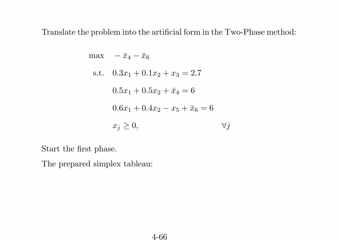
Translate the problem into the artificial form in the Two-Phase method:
max − x̄4 − x̄6
s.t. 0.3x1 + 0.1x2 + x3 = 2.7
0.5x1 + 0.5x2 + x̄4 = 6
0.6x1 + 0.4x2 − x5 + x̄6 = 6
xj ≥ 0, ∀j
Start the first phase.
The prepared simplex tableau:
4-66
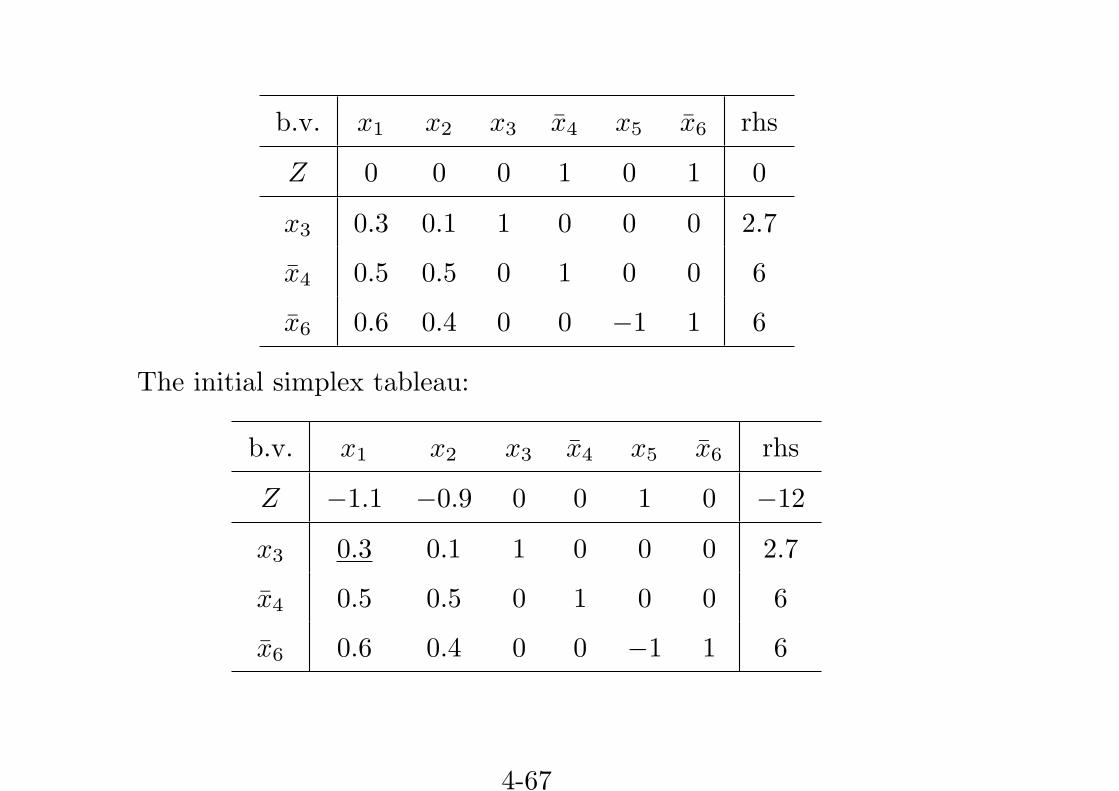
b.v. x1 x2 x3 x̄4 x5 x̄6 rhs
Z 0 0 0 1 0 1 0
x3 0.3 0.1 1 0 0 0 2.7
x̄4 0.5 0.5 0 1 0 0 6
x̄6 0.6 0.4 0 0 −1 1 6
The initial simplex tableau:
b.v. x1 x2 x3 x̄4 x5 x̄6 rhs
Z −1.1 −0.9 0 0 1 0 −12
x3 0.3 0.1 1 0 0 0 2.7
x̄4 0.5 0.5 0 1 0 0 6
x̄6 0.6 0.4 0 0 −1 1 6
4-67
b.v. x1 x2 x3 x̄4 x5 x̄6 rhs
Z 0 − 1630
113 0 1 0 −2.1
x1 1 13
103 0 0 0 9
x̄4 0 13 − 5
3 1 0 0 1.5
x̄6 0 0.2 −2 0 −1 1 0.6
b.v. x1 x2 x3 x̄4 x5 x̄6 rhs
Z 0 0 −53 0 − 5
383 −0.5
x1 1 0 203 0 5
3 −53 8
x̄4 0 0 53 1 5
3 −53 0.5
x2 0 1 −10 0 −5 5 3
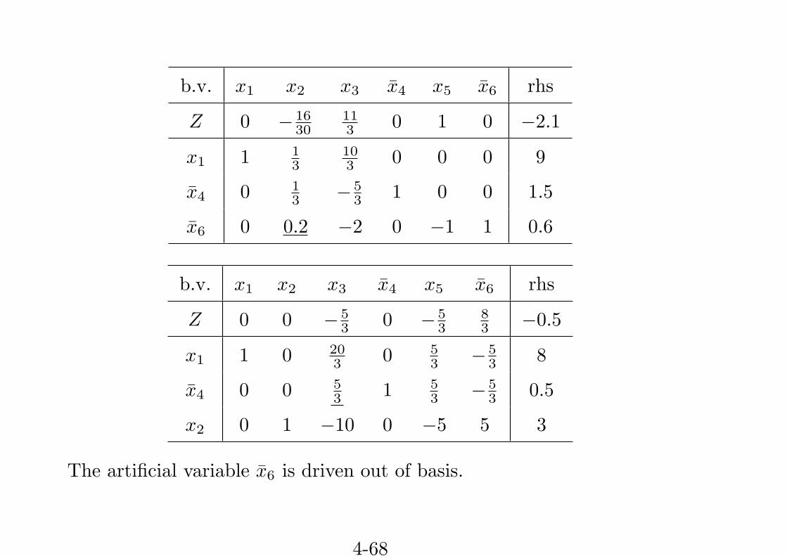
The artificial variable x̄6 is driven out of basis.
4-68
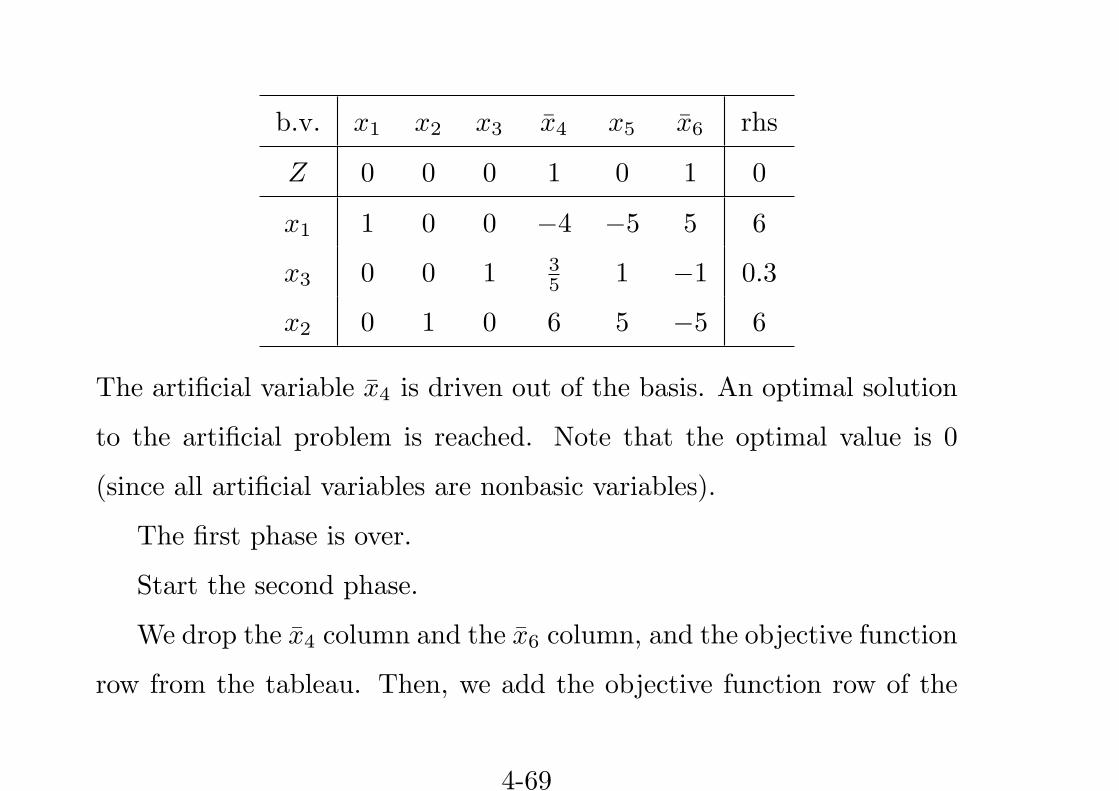
b.v. x1 x2 x3 x̄4 x5 x̄6 rhs
Z 0 0 0 1 0 1 0
x1 1 0 0 −4 −5 5 6
x3 0 0 1 35 1 −1 0.3
x2 0 1 0 6 5 −5 6
The artificial variable x̄4 is driven out of the basis. An optimal solution
to the artificial problem is reached. Note that the optimal value is 0
(since all artificial variables are nonbasic variables).
The first phase is over.
Start the second phase.
We drop the x̄4 column and the x̄6 column, and the objective function
row from the tableau. Then, we add the objective function row of the
4-69
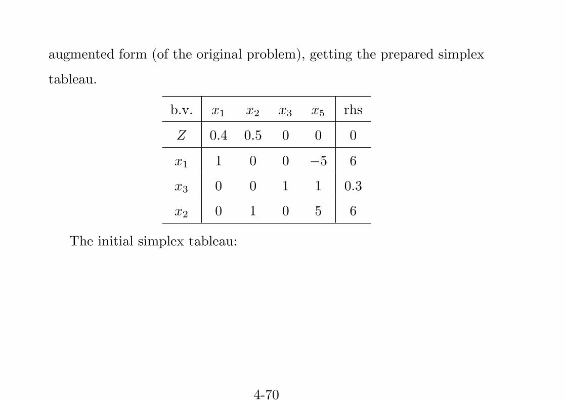
augmented form (of the original problem), getting the prepared simplex
tableau.
b.v. x1 x2 x3 x5 rhs
Z 0.4 0.5 0 0 0
x1 1 0 0 −5 6
x3 0 0 1 1 0.3
x2 0 1 0 5 6
The initial simplex tableau:
4-70
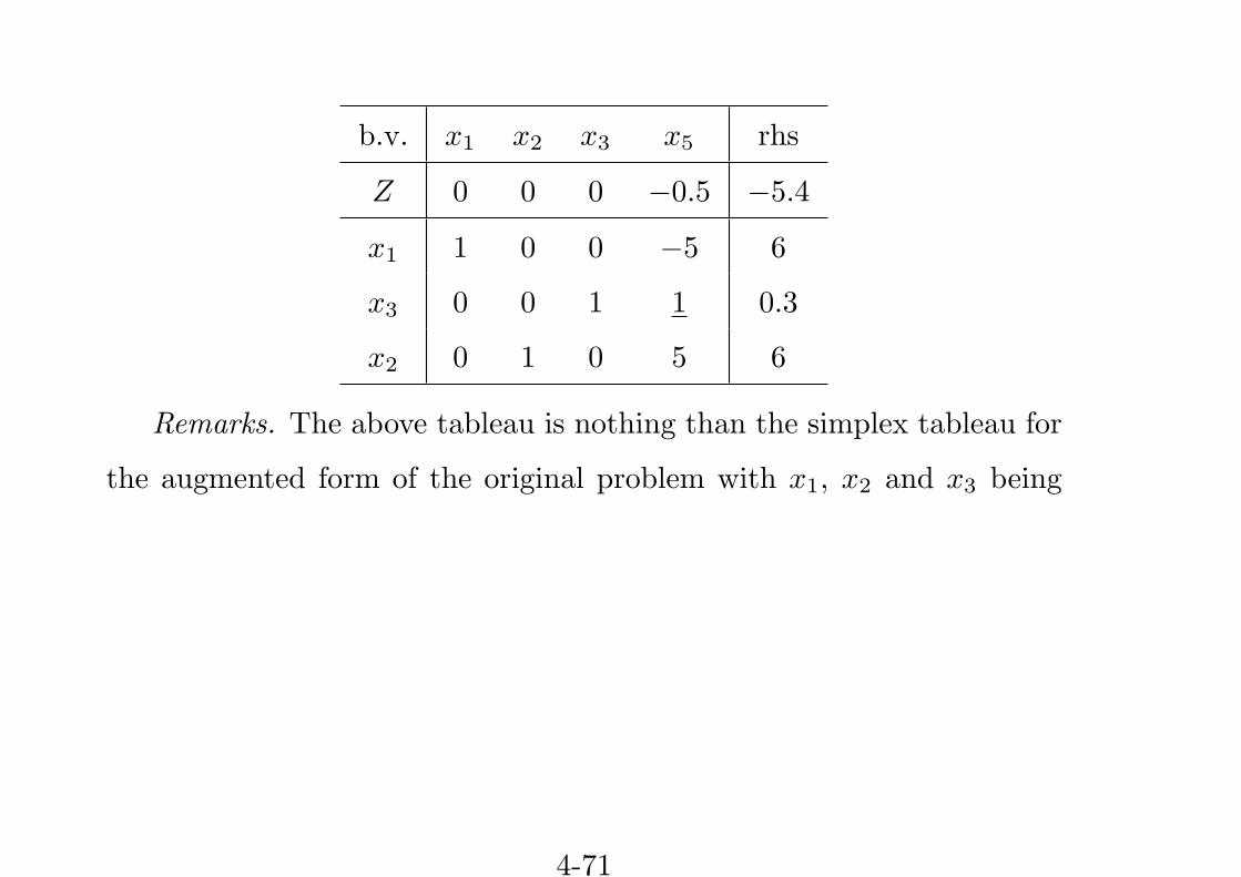
b.v. x1 x2 x3 x5 rhs
Z 0 0 0 −0.5 −5.4
x1 1 0 0 −5 6
x3 0 0 1 1 0.3
x2 0 1 0 5 6
Remarks. The above tableau is nothing than the simplex tableau for
the augmented form of the original problem with x1, x2 and x3 being
4-71
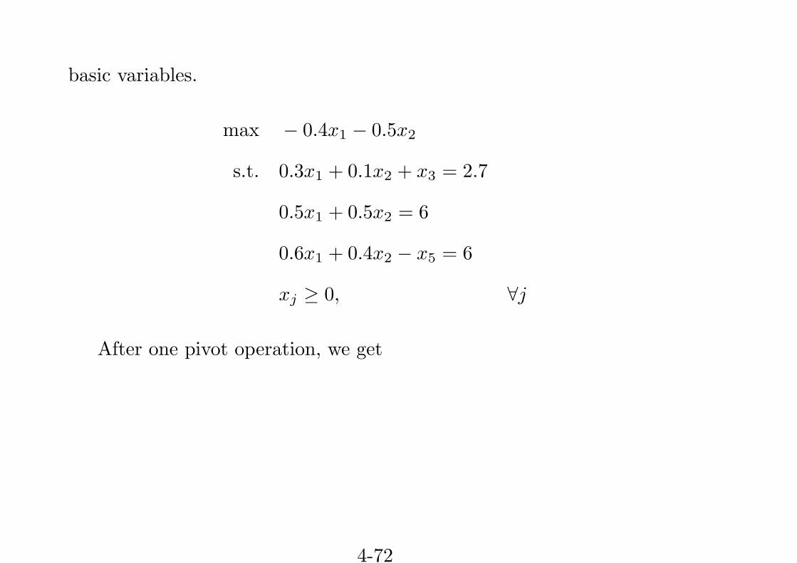
basic variables.
max − 0.4x1 − 0.5x2
s.t. 0.3x1 + 0.1x2 + x3 = 2.7
0.5x1 + 0.5x2 = 6
0.6x1 + 0.4x2 − x5 = 6
xj ≥ 0, ∀j
After one pivot operation, we get
4-72
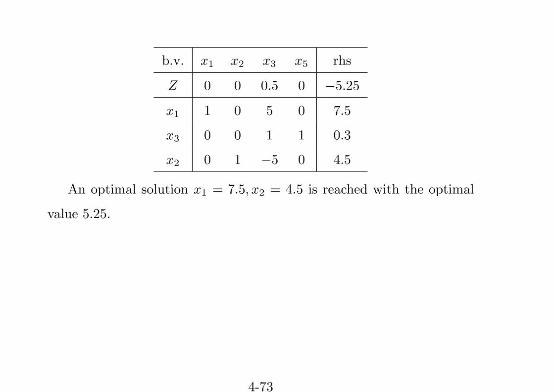
b.v. x1 x2 x3 x5 rhs
Z 0 0 0.5 0 −5.25
x1 1 0 5 0 7.5
x3 0 0 1 1 0.3
x2 0 1 −5 0 4.5
An optimal solution x1 = 7.5, x2 = 4.5 is reached with the optimal
value 5.25.
4-73
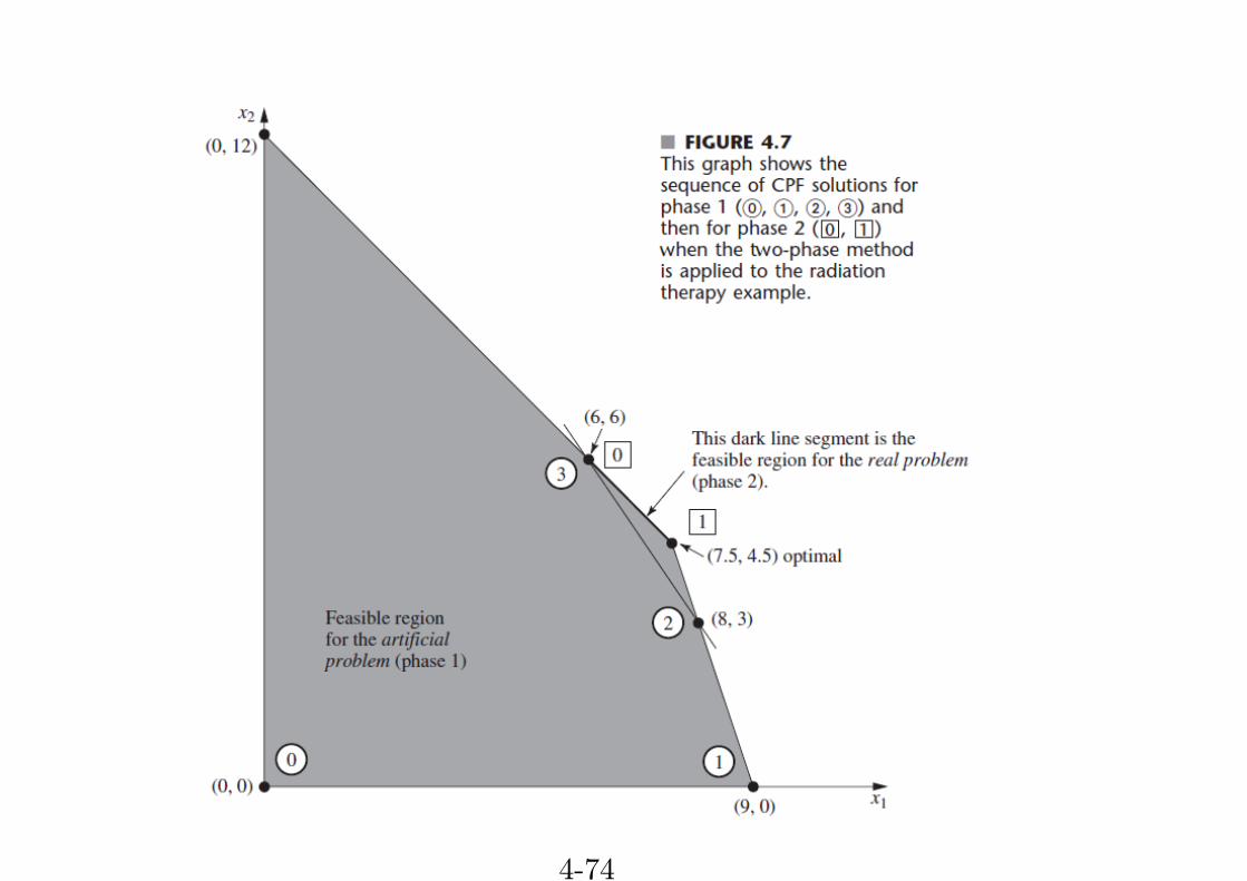
4-74
No Feasible Solutions
If the original problems has no feasible solutions, then either the Big
M method or phase 1 of the Two-Phase method yields a final solution
that has at least one artificial variable greater than zero.
Otherwise, they all equal zero.
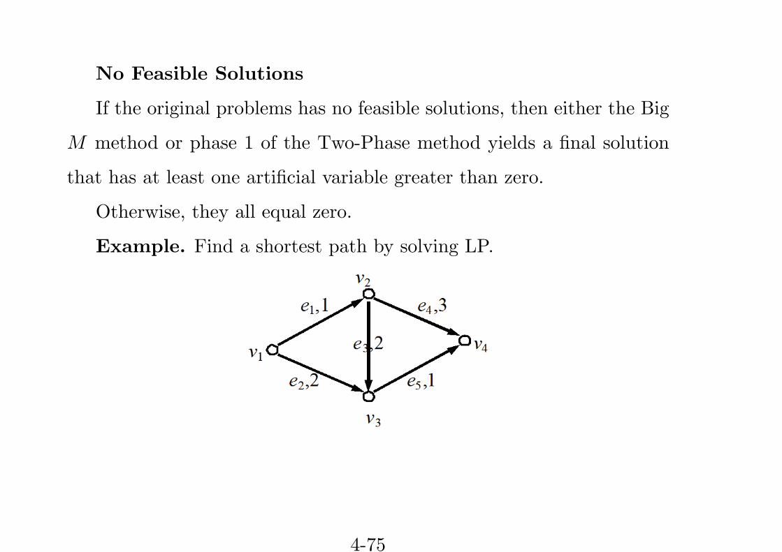
Example. Find a shortest path by solving LP.
4-75
Solution. Write the LP for the instance in the above figure.
min x1 + 2x2 + 2x3 + 3x4 + x5
s.t. x1 + x2 = 1
− x1 + x3 + x4 = 0
− x2 − x3 + x5 = 0
− x4 − x5 = −1
xj ≥ 0, ∀j
4-76
Convert it to the augmented form.
max − x1 − 2x2 − 2x3 − 3x4 − x5
s.t. x1 + x2 = 1
− x1 + x3 + x4 = 0
− x2 − x3 + x5 = 0
x4 + x5 = 1
xj ≥ 0, ∀j
A careful observation shows that the four constraints in the LP are
linearly dependent, but any three constraints of them are not. So, we
4-77
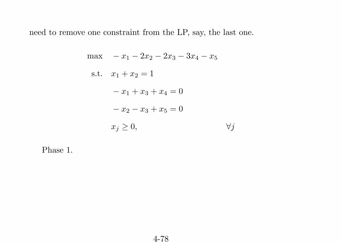
need to remove one constraint from the LP, say, the last one.
max − x1 − 2x2 − 2x3 − 3x4 − x5
s.t. x1 + x2 = 1
− x1 + x3 + x4 = 0
− x2 − x3 + x5 = 0
xj ≥ 0, ∀j
Phase 1.
4-78
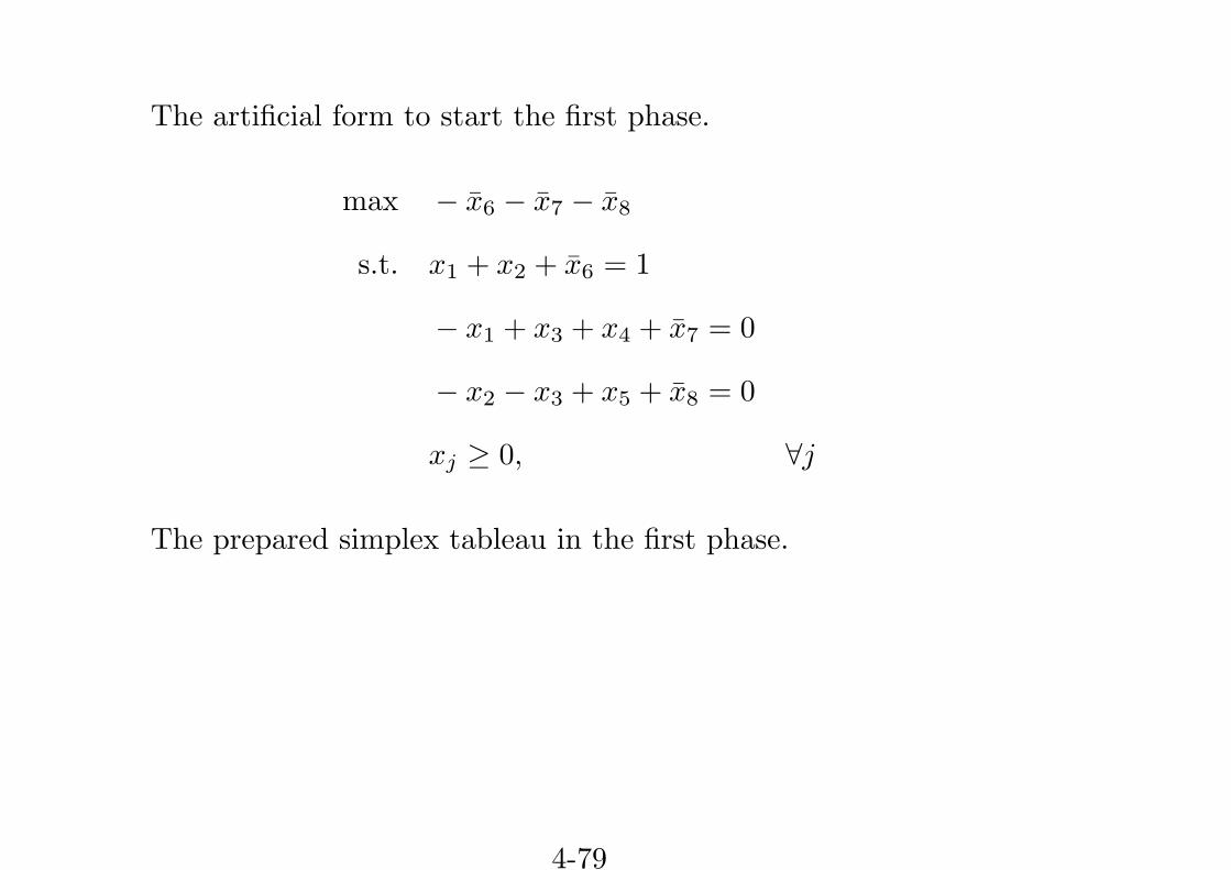
The artificial form to start the first phase.
max − x̄6 − x̄7 − x̄8
s.t. x1 + x2 + x̄6 = 1
− x1 + x3 + x4 + x̄7 = 0
− x2 − x3 + x5 + x̄8 = 0
xj ≥ 0, ∀j
The prepared simplex tableau in the first phase.
4-79

b.v. x1 x2 x3 x4 x5 x̄6 x̄7 x̄8 rhs
Z 0 0 0 0 0 1 1 1 0
x̄6 1 1 0 0 0 1 0 0 1
x̄7 −1 0 1 1 0 0 1 0 0
x̄8 0 −1 −1 0 1 0 0 1 0
The initial simplex tableau in the first phase.
b.v. x1 x2 x3 x4 x5 x̄6 x̄7 x̄8 rhs
Z 0 0 0 −1 −1 0 0 0 −1
x̄6 1 1 0 0 0 1 0 0 1
x̄7 −1 0 1 1 0 0 1 0 0
x̄8 0 −1 −1 0 1 0 0 1 0
4-80
b.v. x1 x2 x3 x4 x5 x̄6 x̄7 x̄8 rhs
Z −1 0 1 0 −1 0 1 0 −1
x̄6 1 1 0 0 0 1 0 0 1
x4 −1 0 1 1 0 0 1 0 0
x̄8 0 −1 −1 0 1 0 0 1 0
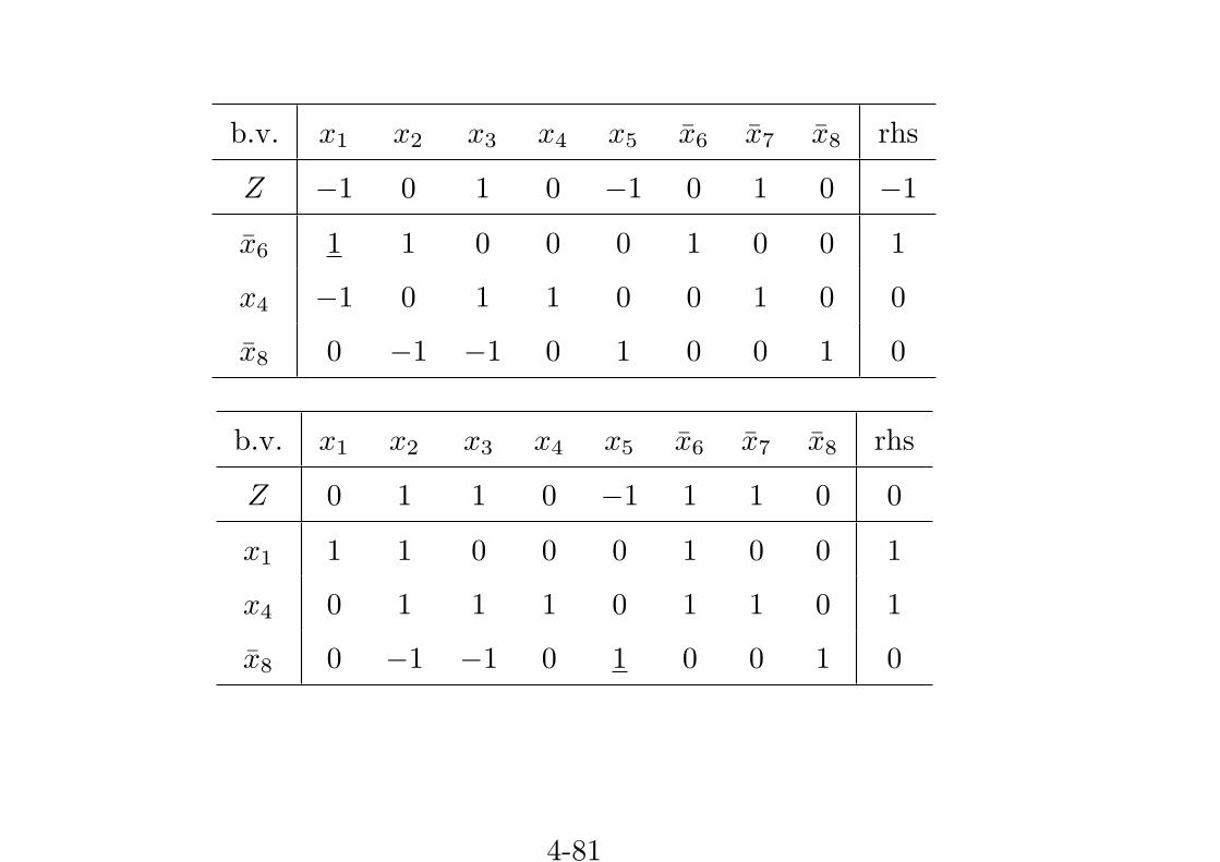
b.v. x1 x2 x3 x4 x5 x̄6 x̄7 x̄8 rhs
Z 0 1 1 0 −1 1 1 0 0
x1 1 1 0 0 0 1 0 0 1
x4 0 1 1 1 0 1 1 0 1
x̄8 0 −1 −1 0 1 0 0 1 0
4-81
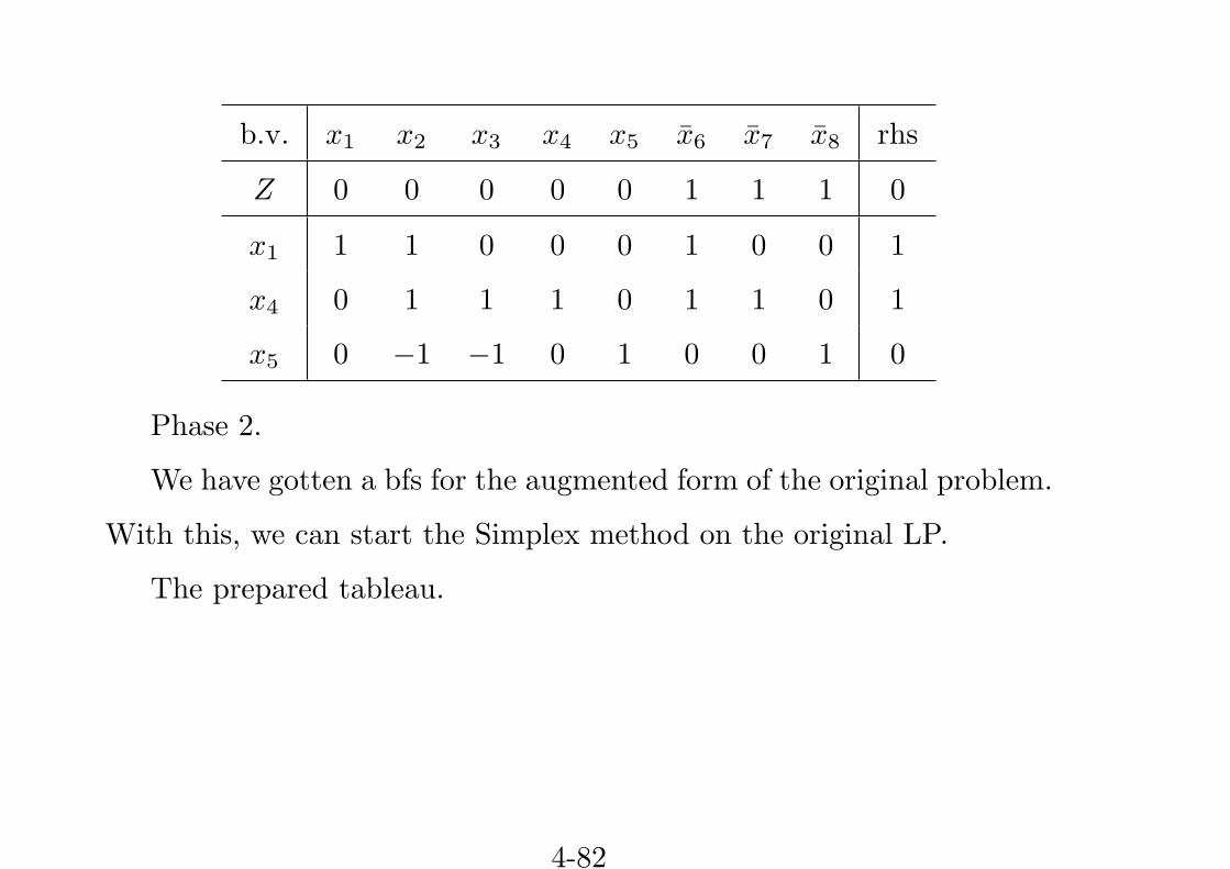
b.v. x1 x2 x3 x4 x5 x̄6 x̄7 x̄8 rhs
Z 0 0 0 0 0 1 1 1 0
x1 1 1 0 0 0 1 0 0 1
x4 0 1 1 1 0 1 1 0 1
x5 0 −1 −1 0 1 0 0 1 0
Phase 2.
We have gotten a bfs for the augmented form of the original problem.
With this, we can start the Simplex method on the original LP.
The prepared tableau.
4-82

b.v. x1 x2 x3 x4 x5 rhs
Z 1 2 2 3 1 0
x1 1 1 0 0 0 1
x4 0 1 1 1 0 1
x5 0 −1 −1 0 1 0
The initial tableau.
b.v. x1 x2 x3 x4 x5 rhs
Z 0 −1 0 0 0 −4
x1 1 1 0 0 0 1
x4 0 1 1 1 0 1
x5 0 −1 −1 0 1 0
4-83
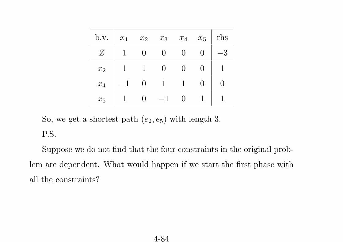
b.v. x1 x2 x3 x4 x5 rhs
Z 1 0 0 0 0 −3
x2 1 1 0 0 0 1
x4 −1 0 1 1 0 0
x5 1 0 −1 0 1 1
So, we get a shortest path (e2, e5) with length 3.
P.S.
Suppose we do not find that the four constraints in the original prob-
lem are dependent. What would happen if we start the first phase with
all the constraints?
4-84
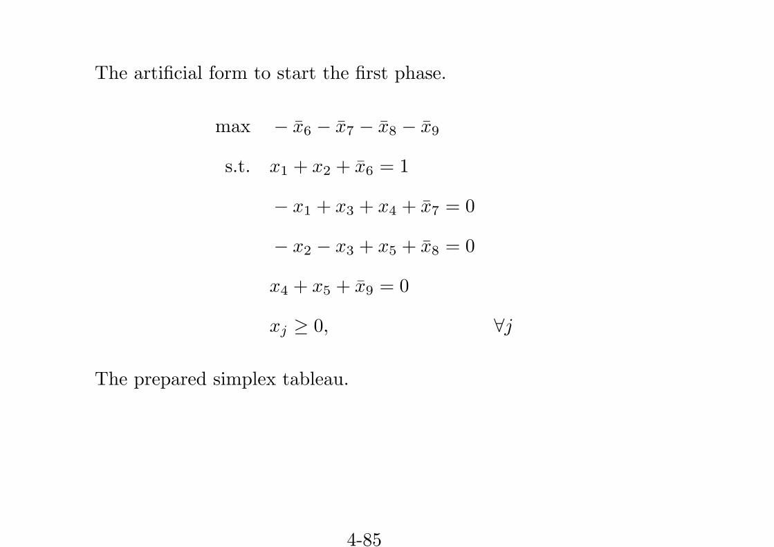
The artificial form to start the first phase.
max − x̄6 − x̄7 − x̄8 − x̄9
s.t. x1 + x2 + x̄6 = 1
− x1 + x3 + x4 + x̄7 = 0
− x2 − x3 + x5 + x̄8 = 0
x4 + x5 + x̄9 = 0
xj ≥ 0, ∀j
The prepared simplex tableau.
4-85
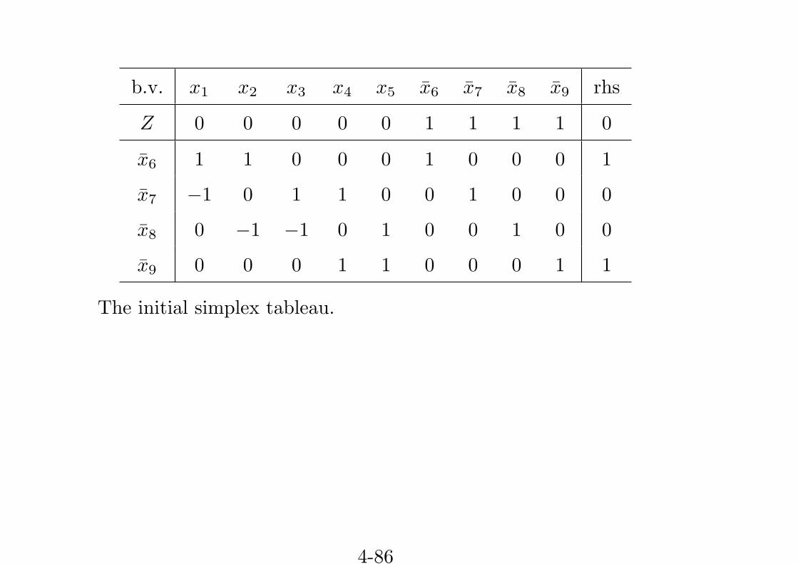
b.v. x1 x2 x3 x4 x5 x̄6 x̄7 x̄8 x̄9 rhs
Z 0 0 0 0 0 1 1 1 1 0
x̄6 1 1 0 0 0 1 0 0 0 1
x̄7 −1 0 1 1 0 0 1 0 0 0
x̄8 0 −1 −1 0 1 0 0 1 0 0
x̄9 0 0 0 1 1 0 0 0 1 1
The initial simplex tableau.
4-86
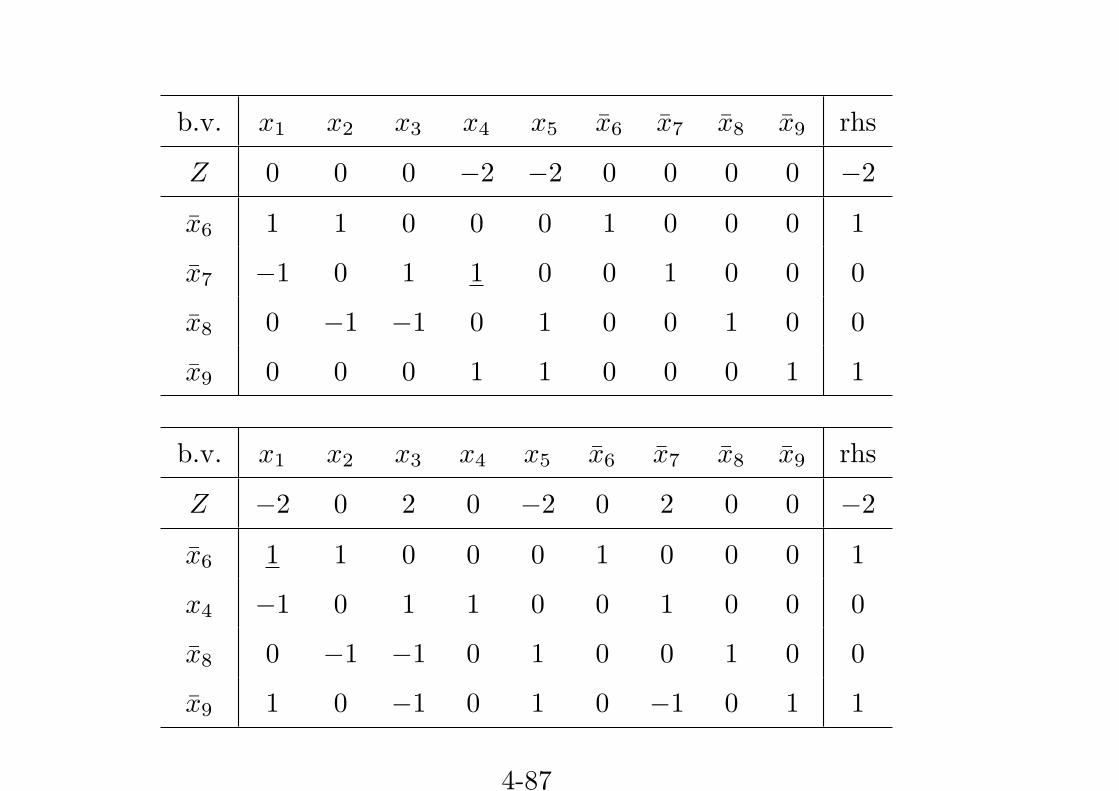
b.v. x1 x2 x3 x4 x5 x̄6 x̄7 x̄8 x̄9 rhs
Z 0 0 0 −2 −2 0 0 0 0 −2
x̄6 1 1 0 0 0 1 0 0 0 1
x̄7 −1 0 1 1 0 0 1 0 0 0
x̄8 0 −1 −1 0 1 0 0 1 0 0
x̄9 0 0 0 1 1 0 0 0 1 1
b.v. x1 x2 x3 x4 x5 x̄6 x̄7 x̄8 x̄9 rhs
Z −2 0 2 0 −2 0 2 0 0 −2
x̄6 1 1 0 0 0 1 0 0 0 1
x4 −1 0 1 1 0 0 1 0 0 0
x̄8 0 −1 −1 0 1 0 0 1 0 0
x̄9 1 0 −1 0 1 0 −1 0 1 1
4-87
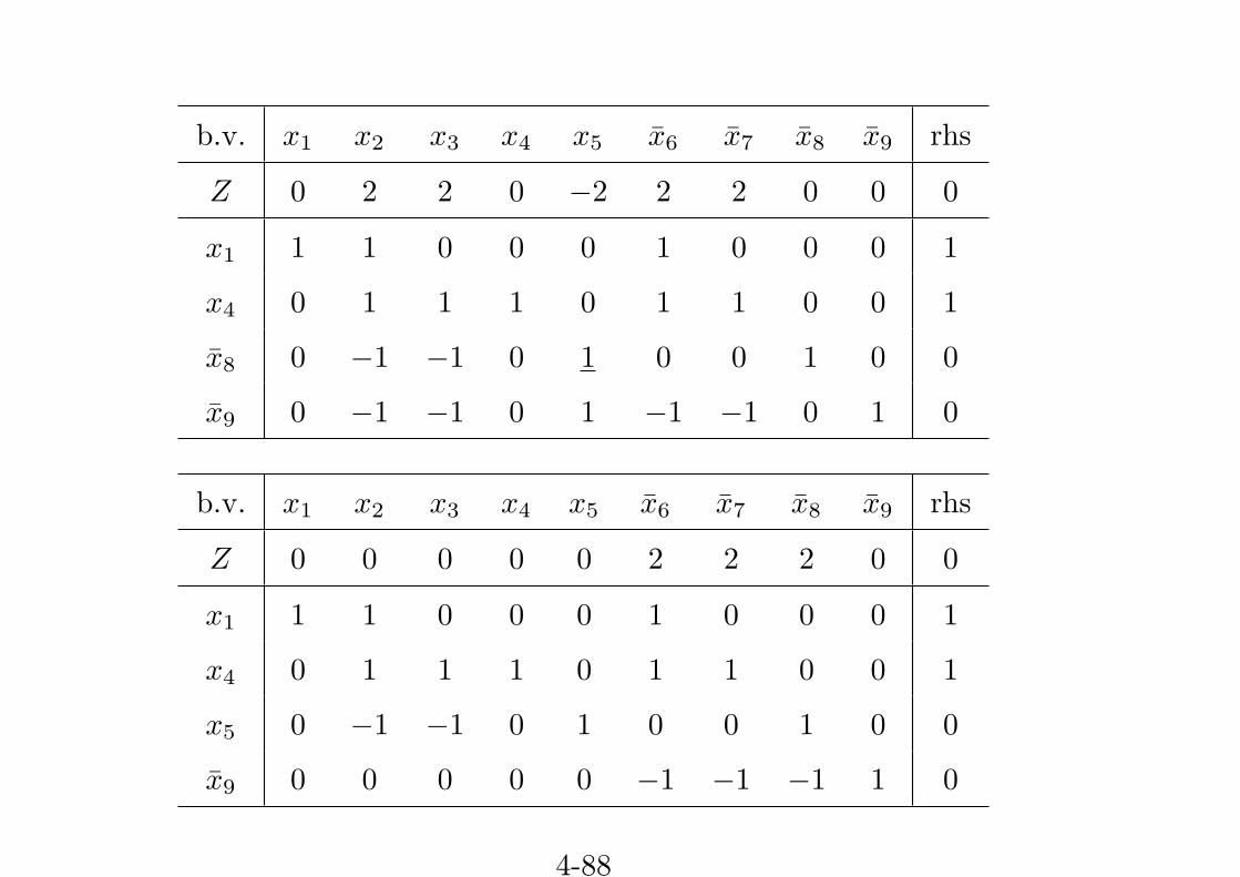
b.v. x1 x2 x3 x4 x5 x̄6 x̄7 x̄8 x̄9 rhs
Z 0 2 2 0 −2 2 2 0 0 0
x1 1 1 0 0 0 1 0 0 0 1
x4 0 1 1 1 0 1 1 0 0 1
x̄8 0 −1 −1 0 1 0 0 1 0 0
x̄9 0 −1 −1 0 1 −1 −1 0 1 0
b.v. x1 x2 x3 x4 x5 x̄6 x̄7 x̄8 x̄9 rhs
Z 0 0 0 0 0 2 2 2 0 0
x1 1 1 0 0 0 1 0 0 0 1
x4 0 1 1 1 0 1 1 0 0 1
x5 0 −1 −1 0 1 0 0 1 0 0
x̄9 0 0 0 0 0 −1 −1 −1 1 0
4-88

We notice that the artificial variable x̄9 still remains in basis. And,
in the line of x̄9 the coefficients corresponding to non-artificial variables
are all zero. This means the constraints of the original problem are
dependent. So, the x̄9 line and the x̄6, x̄7, x̄8, and x̄9 columns can be
removed to obtain the simplex tableau for the second phase.
4-89