1

INTRODUCTION TO OPERATIONS MANAGEMENT WHAT IS OPERATIONS MANAGEMENT?

DEFINITIONS OF OPERATIONS MANAGEMENT (OM)? Management of systems or processes that create goods and/or services. “Operations management is an area of management concerned with overseeing, designing, and controlling the process of production and redesigning business operations in the production of goods or services. It involves the responsibility of ensuring that business operations are efficient in terms of using as few resources as needed, and effective in terms of meeting customer requirements. It is concerned with managing the transformation process that converts inputs (in the forms of raw materials, labour, and energy) into outputs (in the form of goods and/or services).”

efficient AND effective: You need to produce products that are desired by the customers Achieve an economic match of supply and demand

SUPPLY CHAIN A sequence of activities and organizations involved in producing and delivering a good or service.

Everything from raw material to customer OM = MANAGING TRANSFORMATION PROCESSES Managing of processes in which input are transformed into outputs. The essence of the operations function is to add value during transformation process. Feedback= measurements taken at various points in the transformation process Control= The comparison of feedback against previously established standards to determine if corrective action is needed Value added: the difference between the cost of inputs and the value or price of outputs. The greater the value added the greater the effectiveness of these operations. Inputs can be transformed as well as transforme:

o People can be input o People get transformed at the hairdresser

Typical material processors: Mining and extraction, food production, automotive, assembly, machine construction, retail operations, warehousing and distribution, postal services, transport

Typical information processors: Accountants, bank back offices, market research organization, financial analysts, news service, university research unit, archives, telecom company

Typical people processors Hairdressers, hotels, hospitals, mass rapid transports, theatres, theme parks, dentists, schools

PRODUCTION OF GOODS VS. DELIVERY OF SERVICES Goods are physical items that include raw materials, parts, subassemblies, and final products

o Tangible Services are activities that provide some combination of time, location, form, or psychological value. Generally

implies an act. o Not always tangible

Companies sell goods as well as services = product packages o Goods and services often occur jointly o Having the oil changed in your car is a service, but the oil that is delivered is a good o The goods-service combination is a continuum (It’s difficult to say that something is just one of the two,

products can be more a good than a service but they are still both)

2

Manufacturing matters Shift from the manufacturing sector to the service sector towards a knowledge economy: Many services exist to support manufacturing Manufacturing and innovation

o Manufacturing naturally leads to innovation o Return on innovations: after R&D

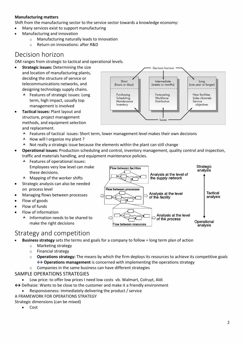
Decision horizon OM ranges from strategic to tactical and operational levels. Strategic issues: Determining the size

and location of manufacturing plants, deciding the structure of service or telecommunications networks, and designing technology supply chains. Features of strategic issues: Long

term, high impact, usually top management is involved

Tactical issues: Plant layout and structure, project management methods, and equipment selection and replacement. Features of tactical issues: Short term, lower management level makes their own decisions How will I organize my plant ? Not really a strategic issue because the elements within the plant can still change

Operational issues: Production scheduling and control, inventory management, quality control and inspection, traffic and materials handling, and equipment maintenance policies. Features of operational issues:

Employees very low level can make these decisions.

Mapping of the worker shifts

Strategic analysis can also be needed on process level

Managing flows between processes

Flow of goods

Flow of funds

Flow of information Information needs to be shared to

make the right decisions

Strategy and competition Business strategy sets the terms and goals for a company to follow = long term plan of action

o Marketing strategy o Financial strategy o Operations strategy: The means by which the firm deploys its resources to achieve its competitive goals

↔ Operations management is concerned with implementing the operations strategy o Companies in the same business can have different strategies

SAMPLE OPERATIONS STRATEGIES Low price: to offer low prices I need low costs vb. Walmart, Colruyt, Aldi

↔ Delhaize: Wants to be close to the customer and make it a friendly environment Responsiveness: immediately delivering the product / service

A FRAMEWORK FOR OPERATIONS STRATEGY Strategic dimensions (can be mixed)

Cost

3

Product differentiation (both differentiation from competitors and differentiation within a firm) Quality Delivery speed Delivery reliability Flexibility

Operations management is concerned with implementing the operations strategy to achieve leadership along one or some of these dimensions Competitiveness: How effectively an organization meets the wants

and needs of customers relative to others that offer similar goods or services

Organizations compete through some combination of their marketing and operations functions

o What do customers want? o How can these customer needs best be

satisfied?

OPERATIONS MANAGEMENT TOOLS

Models And Quantitative Approaches Performance metrics Analysis of trade-offs

use of OM tools to implement A strategy

OM tools can be applied to ensure that resources are used as efficiently as possible The frontier (efficiency-curve) = the most efficient a company can be

OM tools can be used to make desirable trade-offs between competing objectives If a company is on the border:

o It can shorten it’s waiting time ( more operator idle time) to get higher responsiveness o To get higher labour productivity it needs to make their waiting time longer so the operations are

more fully utilized OM tools can be used to redesign or restructure our operations so that we can improve performance along multiple dimensions simultaneously

higher efficiency through redesigning their proces New frontier (efficiency-curve verder weg van de oorsprong)

STRATEGY FORMULATION How to choose a strategy ?

You need to take internal and external variables into account Effective strategy formulation requires taking into account:

Core competencies Environmental scanning

SWOT: Internal Factors

o Strengths and Weaknesses External Factors

o Opportunities and Threats Successful strategy formulation also requires taking into account:

Order qualifiers : Characteristics that customers perceive as minimum standards of acceptability for a product or service to be considered as a potential for purchase

Order winners: Characteristics of an organization’s goods or services that cause it to be perceived as better than the competition

4

WHY SOME ORGANIZATIONS FAIL Neglecting operations strategy

Failing to take advantage of strengths and opportunities and/or failing to recognize competitive threats

Too much emphasis on short-term financial performance at the expense of R&D

Too much emphasis in product and service design and not enough on process design and improvement

Neglecting investments in capital and human resources

Failing to establish good internal communications and cooperation

Failing to consider customer wants and needs

Performance measurement afb?

Balanced scorecard approach and key performance indicators KPIs A top-down management system that organizations can use to clarify their vision and strategy and transform them into action

Develop objectives Develop metrics and targets for each objective Develop initiatives to achieve objectives Identify links among the various perspectives

o Finance o Customer: to achieve our vision, how will we appear to our customers? o Internal business processes o Learning and growth

Monitor results PERFORMANCE MEASUREMENT: KPI’S Every company should have a performance scorecard, sometimes called ‘supply chain dashboard’:

A holistic set of performance metrics (and corresponding performance standards) that address the major concerns of customers,stockholders, employees and suppliers

Implementing such a set of Key Performance Indicators (KPI’s) is a prerequisite to performance improvement:

o People behave based on the way they are measured o What gets measured gets improved o It is hard to win a game without a scoreboard; it is hard to even know which game you are playing

without a scoreboard

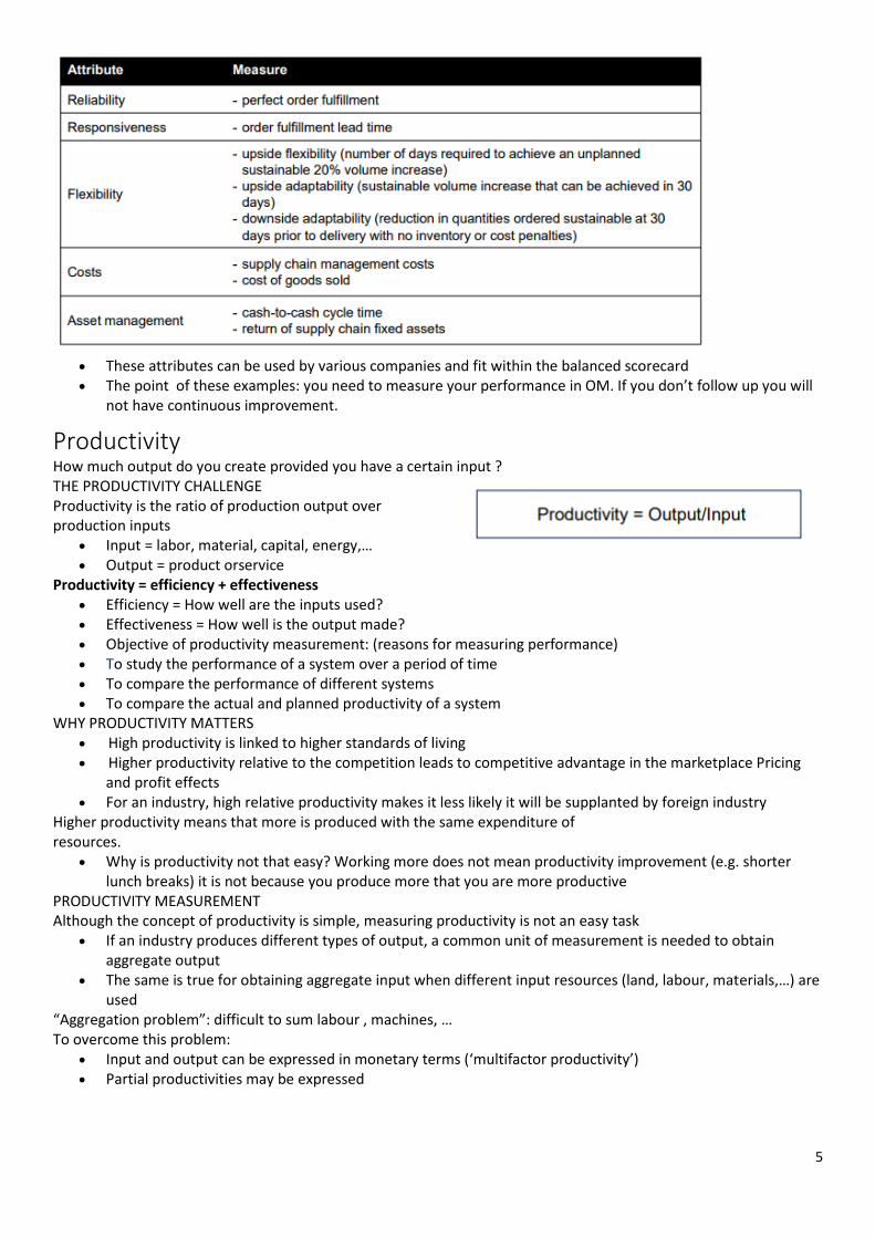
SCORE MEASURES The Supply Chain Council (SCC) has developed the Supply Chain Operations Reference (SCOR) model to

describe, measure and evaluate supply chains. www.supply-chain.org As part of the model, five supply chain performance attributes and nine related measures were defined

5

These attributes can be used by various companies and fit within the balanced scorecard The point of these examples: you need to measure your performance in OM. If you don’t follow up you will

not have continuous improvement.

Productivity How much output do you create provided you have a certain input ? THE PRODUCTIVITY CHALLENGE Productivity is the ratio of production output over production inputs

Input = labor, material, capital, energy,… Output = product orservice

Productivity = efficiency + effectiveness Efficiency = How well are the inputs used? Effectiveness = How well is the output made? Objective of productivity measurement: (reasons for measuring performance) To study the performance of a system over a period of time To compare the performance of different systems To compare the actual and planned productivity of a system

WHY PRODUCTIVITY MATTERS High productivity is linked to higher standards of living Higher productivity relative to the competition leads to competitive advantage in the marketplace Pricing

and profit effects For an industry, high relative productivity makes it less likely it will be supplanted by foreign industry

Higher productivity means that more is produced with the same expenditure of resources.

Why is productivity not that easy? Working more does not mean productivity improvement (e.g. shorter lunch breaks) it is not because you produce more that you are more productive

PRODUCTIVITY MEASUREMENT Although the concept of productivity is simple, measuring productivity is not an easy task

If an industry produces different types of output, a common unit of measurement is needed to obtain aggregate output

The same is true for obtaining aggregate input when different input resources (land, labour, materials,…) are used

“Aggregation problem”: difficult to sum labour , machines, … To overcome this problem:

Input and output can be expressed in monetary terms (‘multifactor productivity’) Partial productivities may be expressed

6

PARTIAL PRODUCTIVITY The ratio of output over the input from a single factor

The type of partial productivity used depends on the nature of the enterprise:

For capital intensive industries: capital productivity For industries with costly material resources: material productivity

7

FORECASTING INTRODUCTION TO FORECASTING

Forecast What is forecasting?

A statement about the future value of a variable of interest.

Primary function is to predict the future.

Why are we interested? Affects the decisions we make today.

o Examples: We make forecasts about such things as weather, demand, and resource availability

Forecast demand for products and services

Forecast availability of manpower

Forecast inventory and material needs daily

Reference to a specific time horizon

Short-term forecasts

Long-term forecasts

New products, new equipment,.

Things that require a long lead time to develop, construct or implement

All users need to agree on the same forecast (accounting, finance,..)

Yield management

Plan a system

Plan the use of a system

Really bad forecasting: Ryanair

Company did not think their employees wanted to take their vacation days

Pilots wanted to take vacation

Promised a bonus if they did not take them

Being on time was a strategy for them

A lot of flights were cancelled

Characteristics of forecasts Forecasting techniques assume that some underlying causal system that existed in the past will continue to

exist in the future .

Forecasts are not perfect. They are usually wrong!

o Because random variation is always present

o There will always be some residual error, even if all other factors have been accounted for

A good forecast is more than a single number

Expected level of demand the level of demand may be a function of some structural variation such as trend

or seasonal variation

Accuracy related to the potential size of forecast error

Aggregate forecasts (forecasts for groups of items) are usually more accurate than those for individual items

o Beter A, B en C samen schatten dan alleen

Forecasting errors among items in a group usually have cancelling effects

Accuracy erodes as we go further into the future.

8

Forecasts should not be used to the exclusion of known information.

Forecast accuracy decreases as the time period covered by the forecast increases.

ELEMENTS OF A GOOD FORECAST The forecast

Should be timely: Time is needed to respond to information contained in a forecast.

Should be accurate and the degree of accuracy should be stated

Should be reliable, it should work consistently.

Should be expressed in meaningful units.

Should be in writing, guarantee that the same information is used.

Technique should be simple to understand and use

The users should understand the limits of the forecasts and in which circumstances it is used.

Should be cost-effective

o Een heel moeilijk maar correcter model

is vaak duurder dan een minder correct

model, rekening houden met de kosten

FORECAST HORIZONS IN OPERATION PLANNING

FORECAST USES Plan the system

Generally involves long-range plans related to:

Types of products and services to offer

Facility and equipment levels

Facility location

Plan the use of the system

Generally involves short- and medium-range plans related to:

Inventory management

Workforce levels

Purchasing

Production

Budgeting

Scheduling

STEPS IN THE FORECASTING PROCESS 1. Determine the purpose of the forecast

o How will it be used and when will it be needed? This steps provides an indication of how detailed your

forecasts needs

2. Establish a time horizon

3. Obtain, clean, and analyse appropriate data

4. Select a forecasting technique

5. Make the forecast

6. Monitor the forecast errors

9

EVALUATION OF FORECASTS

Forecast accuracy and control Minimize forecast errors

Allowances should be made for forecast errors

It is important to provide an indication of the extent to which the forecast might deviate from the value of

the variable that actually occurs

Forecast errors should be monitored

Error = Actual – Forecast

If errors fall beyond acceptable bounds, corrective action

may be necessary

e = A - F

Forecast errors influence decisions in two ways

Making a choice between various forecasting

alternatives.

Evaluating the success or failure of a forecasting

technique.

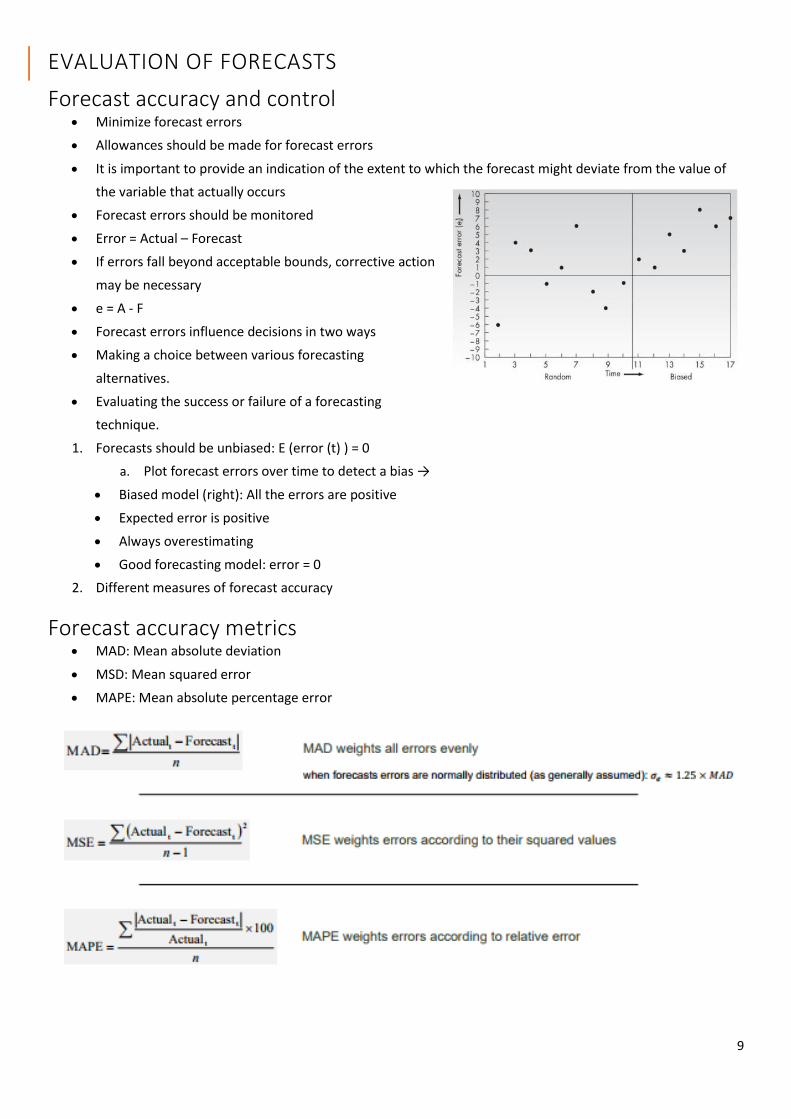
1. Forecasts should be unbiased: E (error (t) ) = 0

a. Plot forecast errors over time to detect a bias →

Biased model (right): All the errors are positive

Expected error is positive

Always overestimating

Good forecasting model: error = 0

2. Different measures of forecast accuracy

Forecast accuracy metrics MAD: Mean absolute deviation

MSD: Mean squared error

MAPE: Mean absolute percentage error

10

Forecast error calculation

FORECASTING APPROACHES Qualitative Forecasting

Qualitative techniques permit the inclusion of soft information such as

o Human factors

o Personal opinions

o Hunches

These factors are difficult, or impossible, to quantify

o Geen historische gegevens nodig

Quantitative Forecasting

o These techniques rely on hard data

o Quantitative techniques involve either the projection of historical data or the development of

associative methods that attempt to use causal variables to make a forecast

QUALITATIVE FORECASTING METHODS

Qualitative forecasts Forecasts that use subjective inputs such as opinions from consumer surveys, sales staff, managers, executives, and

experts

Executive opinions

A small group of upper-level managers may meet and collectively develop a forecast

Long-range planning and new product development

Sales force opinions

Members of the sales or customer service staff can be good sources of information due to their direct

contact with customers and may be aware of plans customers may be considering for the future.

Influenced by recent experience, after a few low sales periods people tend to be more pessimistic.

Forecasts are used to establish a sales quota, there will be a conflict of interest because it is to the

salespersons advantage to estimate low sales

o Low sales estimate so they sell more than that and get a bonus for selling more.

11

Consumer surveys

Since consumers ultimately determine demand, it makes sense to solicit input from the

Consumer surveys typically represent a sample of consumer opinions

Other approaches

Managers may solicit opinions from other managers or staff people or outside experts to help with

developing a forecast.

The Delphi method is an iterative process in which managers and staff complete a series of questionnaires

to achieve a consensus forecast.

Long-term single time forecasts with little hard information available.

Responses are kept anonymous to encourage honest answers and reduce the risk of one person’s

opinion prevailing.

Verschillende groepen zullen verschillende gemiddelden aangeven ?

Iedere expert moet alleen zijn gemiddelde verkoopcijfers doorgeven bv

Alle experts komen samen en bespreken hun cijfers

Ze zijn gelijk of er is geen consensus

Hoge en lage cijfers laten uitleggen waarom ze zo hoog of laag hebben geschat

...

TIME-SERIES FORECASTS Forecasts that project patterns identified in recent time-series observations

Time-series - a time-ordered sequence of observations taken at regular time intervals

Assume that future values of the time-series can be estimated from past values of the time-series.

Analysis of time-series data requires the analyst to identify the underlying behaviour of the series.

o Plotting the data and visually examining the plot and looking for patterns.

Time series behaviours (patterns):

Trend: A long-term upward or downward movement in data

Population shifts

Changing income

Seasonality: Short-term, fairly regular variations

related to the calendar or time of day

Restaurants, service call centres, and

theatres all experience seasonal demand

Loopt samen met tijd

Weekly, daily, monthly,..

Cycles: Wavelike variations lasting more than one

year (not linked to timing such as seasonality)

These are often related to a variety of

economic, political, or even agricultural

conditions

Timing isn't important, goes up and down and isn't linked to the time

Irregular variations: Due to unusual circumstances that do not reflect typical behaviour

Labour strike

12

Weather event

Major changes in products or services

Should be identified and removed from the data

Random variation: Residual variation that remains after all other behaviours have been accounted for

1. Naive Forecast Uses a single previous value of a time series as the basis for a forecast

The forecast for a time period is equal to the previous time period’s value

Can be used with

A stable time series: the forecast for a time period is equal to the previous time period’s value

o Last week demand was 20, so this week demand will also be 20

Seasonal variations: Look back what happened one season ago

o What was the demand last thanksgiving season, this year it will be the same…

Trend

Doesn't do anything complex

o Not able to provide accurate information

o Accuracy is acceptable tho

o Cheap and easy 7

Traces data with a lag of one period

o Doesn’t smooth at all

2. Techniques for Averaging To predict the future you use the past average. Remove white noise (random variations), smooth the data.

These techniques work best when a series tends to vary about an average (stationary series)

Averaging techniques smooth variations in the data

o Averages tend to be less variable than the original data

o This is good because a lot of these variations are because of random variability rather than a true

change in the series

o Responding to change is a great cost

o It is desirable to avoid reacting to minor variations

o Larger variations are seen as real changes

They can handle step changes or gradual changes in the level of a series

Techniques

3. Moving average

4. Weighted moving average

5. Exponential smoothing

MOVING AVERAGE Technique that averages a number of the most recent

actual values in generating a forecast.

Moves as new data becomes available.

Moving average lags behind a trend. The number of data

points included in the average determines the model’s

sensitivity.

13

Fewer data points used -

more responsive

More data points used--

less responsive

Drops and rises are

predicted later

A moving average forecast tends to

smooth and lag changes in the data.

The more periods in a moving average,

greater the average will lag changes in

the data.

Advantages of moving average method Easily understood

Easily computed

Provides stable forecasts

Disadvantages of moving average method Require saving lots of past date points: At least N periods used in the moving average compute

Lags behind trend

Ignores complex relationship data

All data are weight the same (1/N)

WEIGHTED MOVING AVERAGE The most recent values in a time

series are given more weight in

computing a forecast, otherwise

similar to moving average.

The choice of weights, Wt , is

somewhat arbitrary and involves some trial and error

Weighting factors must add to one

o If the sum is over 1, you are overestimating

o Sum lower than 1: Underestimating

More reflective of the most recent occurrences

EXPONENTIAL SMOOTHING A weighted averaging method that is based on the previous forecast plus a percentage of the forecast error.

Next forecast = Precious forecast + 𝛼 (Actual – Previous forecast)

0 < 𝛼 ≤ 1 is the smoothing constant

14

o 𝛼 = Percentage of the error

Actual – Previous forecast = Forecast error

Smoothing:

If Ft is too high, 𝑒𝑡 is positive, and the

adjustment is to decrease the forecast

If Ft is too low, 𝑒𝑡 is negative, and the

adjustment is to increase the forecast

Appropriate for data that varies around an

average or has a gradual change

A set of exponentially declining weights

applied to past data

It is easy to show that the sum of the weights

Houdt alle historische gegevens bij en geeft

deze ook gewichten

Hoe ouder de gegevens, hoe lager de

gewichten

EFFECT OF 𝛼 VALUE ON THE FORECAST

The quickness of forecast adjustment to error is determined by

the smoothing constant (𝛼):

The closer the value to zero, the slower the forecast will

be to adjust to forecast errors (= greater smoothing)

The closer 𝛼 to 1, the greater the responsiveness and the

less the smoothing

The goal is to select an a smoothing constant that balances the

benefits of smoothing random variations

Small values of means that the forecasted value will be

stable (show low variability)

o Low 𝛼 increases the lag of the forecast to the actual data if a trend is present

Large values of 𝛼 mean that the forecast will more closely track the actual time series (quick reaction to changes)

For production applications, stable demand forecasts are desired

Therefore, a small 𝛼 is recommended around 0.1 to 0.2

o You decide which alpha is best for your company

o Most companies chose a low 𝛼

Example:

15

COMPARISON OF MA (MOVING AVERAGES) AND ES (EXPONENTIAL SMOOTHING) Similarities

Both methods are appropriate for stationary series

Both methods lag behind a trend

Both methods depend on a single parameter

For both methods multiple-step-ahead and one-step-ahead forecasts are identical Extended notation: (𝐹𝑡+1

= 𝐹𝑡,𝑡+1) = 𝐹𝑡,𝑡+𝜏

Differences

ES carries all past history (forever!)

MA eliminates “bad” data after N periods

MA requires all N past data points to compute new forecast estimate while ES only requires last forecast

and last observation of ‘demand’ to continue

3. Trend-based methods Analysis of a trend involves developing an equation that will suitably describe trend (assuming that trend is present in the

data). A simple data plot can reveal the existence and nature of a trend. ( exclusively linear trends because they are

fairly common)

LINEAR TREND EQUATION

ESTIMATING SLOPE AND INTERCEPT Slope and intercept can be estimated from historical data

TREND-ADJUSTED EXPONENTIAL SMOOTHING Double exponential smoothing or Holt’s method: Variation of exponential smoothing used when a time series exhibits a

linear trend.

Appropriate for data that shows a trend

predict steepness and level

The trend adjusted forecast consists of two components ̶

Smoothed error

Trend factor

we only look one step ahead

16

One-step-ahead forecast

α and β are smoothing constants

o Chosen through trial and error

Trend-adjusted exponential smoothing has the ability to respond to changes in trend

We begin with an estimate of the intercept and slope at the start (e.g., by using linear regression)

Easier to calculate new forecasts by redefining the smoothing equations than regression analysis

The smoothing constants may be the same, but often more stability is given to the slope estimate : (usually

𝛽 ≤ α)

4. Methods for seasonal series TECHNIQUES FOR SEASONALITY Seasonality: Regularly repeating movements in series values that can be tied to recurring events

Expressed in terms of the amount that actual values deviate from the average value of a series

Models of seasonality

o Additive: Seasonality is expressed as a quantity that

gets added to or subtracted from the time-series

average in order to incorporate seasonality.

Series tends to vary around an average = seasonality

expressed in terms of that average (or moving

average)

o Multiplicative: Seasonality is expressed as a

percentage of the average (or trend) amount which is

then used to multiply the value of a series in order to

incorporate seasonality

Trend is present

More used because it tends to be more representative of actual experience

SEASONAL RELATIVES Seasonal relatives 𝑪𝒕 (𝒔𝒆𝒂𝒔𝒐𝒏𝒂𝒍 𝒊𝒏𝒅𝒆𝒙𝒆𝒔) : The seasonal

percentage used in the multiplicative seasonally adjusted forecasting

model.

Multiplicative seasonal factors or seasonal relatives:

17

Using seasonal relatives

To depersonalize data

o Done in order to get a clearer picture of the non-seasonal (e.g., trend) components of the data series

Remove seasonality from data in order to discern other patterns or lack of patterns in series

o Divide each data point by its seasonal relative

To incorporate seasonality in a forecast

1. Obtain trend estimates for desired periods using a trend equation

2. Add seasonality by multiplying these trend estimates by the corresponding seasonal relative

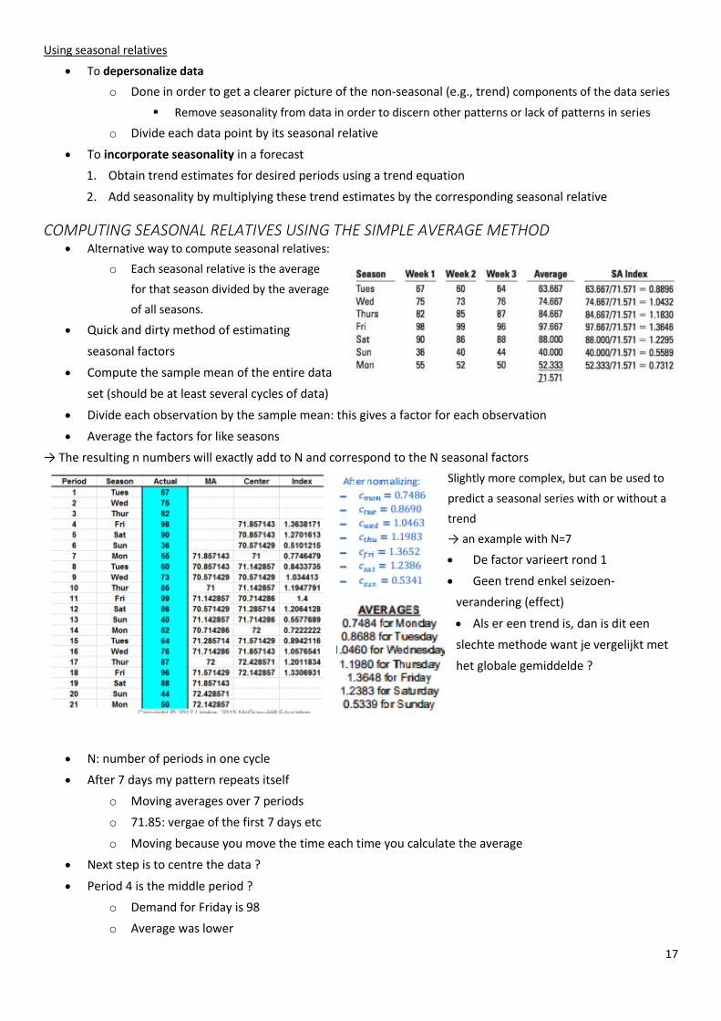
COMPUTING SEASONAL RELATIVES USING THE SIMPLE AVERAGE METHOD Alternative way to compute seasonal relatives:

o Each seasonal relative is the average

for that season divided by the average

of all seasons.

Quick and dirty method of estimating

seasonal factors

Compute the sample mean of the entire data

set (should be at least several cycles of data)

Divide each observation by the sample mean: this gives a factor for each observation

Average the factors for like seasons

→ The resulting n numbers will exactly add to N and correspond to the N seasonal factors

Slightly more complex, but can be used to

predict a seasonal series with or without a

trend

→ an example with N=7

De factor varieert rond 1

Geen trend enkel seizoen-

verandering (effect)

Als er een trend is, dan is dit een

slechte methode want je vergelijkt met

het globale gemiddelde ?

N: number of periods in one cycle

After 7 days my pattern repeats itself

o Moving averages over 7 periods

o 71.85: vergae of the first 7 days etc

o Moving because you move the time each time you calculate the average

Next step is to centre the data ?

Period 4 is the middle period ?

o Demand for Friday is 98

o Average was lower

18

o 36% higher than expected = Ct value for Friday

Average value: 1.37 + 1.4 + 1.33 = 1.3

Sum of the seasonal relatives isn't 7

o ( in tegenstelling tot het voorbeeld hierboven omdat je het hier ‘beweegt’ en bij het bovenste

voorbeeld niet) Fout in slides die in de les gegeven werden (blauw is verbetering …)

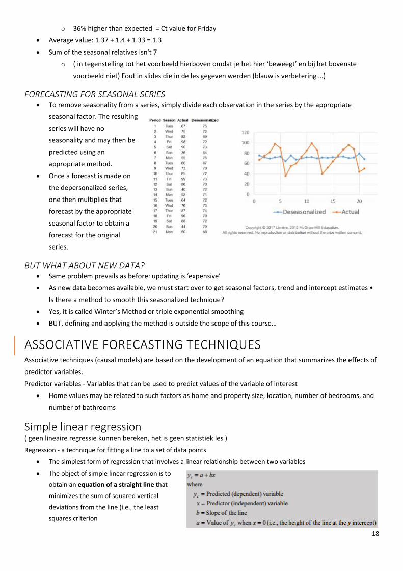
FORECASTING FOR SEASONAL SERIES To remove seasonality from a series, simply divide each observation in the series by the appropriate

seasonal factor. The resulting

series will have no

seasonality and may then be

predicted using an

appropriate method.

Once a forecast is made on

the depersonalized series,

one then multiplies that

forecast by the appropriate

seasonal factor to obtain a

forecast for the original

series.

BUT WHAT ABOUT NEW DATA? Same problem prevails as before: updating is ‘expensive’

As new data becomes available, we must start over to get seasonal factors, trend and intercept estimates •

Is there a method to smooth this seasonalized technique?

Yes, it is called Winter’s Method or triple exponential smoothing

BUT, defining and applying the method is outside the scope of this course…

ASSOCIATIVE FORECASTING TECHNIQUES Associative techniques (causal models) are based on the development of an equation that summarizes the effects of

predictor variables.

Predictor variables - Variables that can be used to predict values of the variable of interest

Home values may be related to such factors as home and property size, location, number of bedrooms, and

number of bathrooms

Simple linear regression ( geen lineaire regressie kunnen bereken, het is geen statistiek les )

Regression - a technique for fitting a line to a set of data points

The simplest form of regression that involves a linear relationship between two variables

The object of simple linear regression is to

obtain an equation of a straight line that

minimizes the sum of squared vertical

deviations from the line (i.e., the least

squares criterion

19

FORECASTING IN PRACTICE MONITORING THE FORECAST Tracking forecast errors and analysing them can provide useful insight into whether forecasts are performing

satisfactorily

Sources of forecast errors:

o The model may be inadequate due to:

1. Omission of an important variable

2. A change or shift in the variable the model cannot handle

3. The appearance of a new variable

o Irregular variations may have occurred

o Random variation

Control charts are useful for identifying the presence of non-random error in forecasts

o Non-random variations need to be investigated

o Control charts: Visual tool for monitoring forecast errors

Tracking signals can be used to detect forecast bias

o To detect any bias in errors over time

o Detect a tendency for a sequence of errors to be positive or negative

o A value of zero is ideal

o If a value outside the acceptable range occur, that would be taken as a single that there is a bias in

the forecast

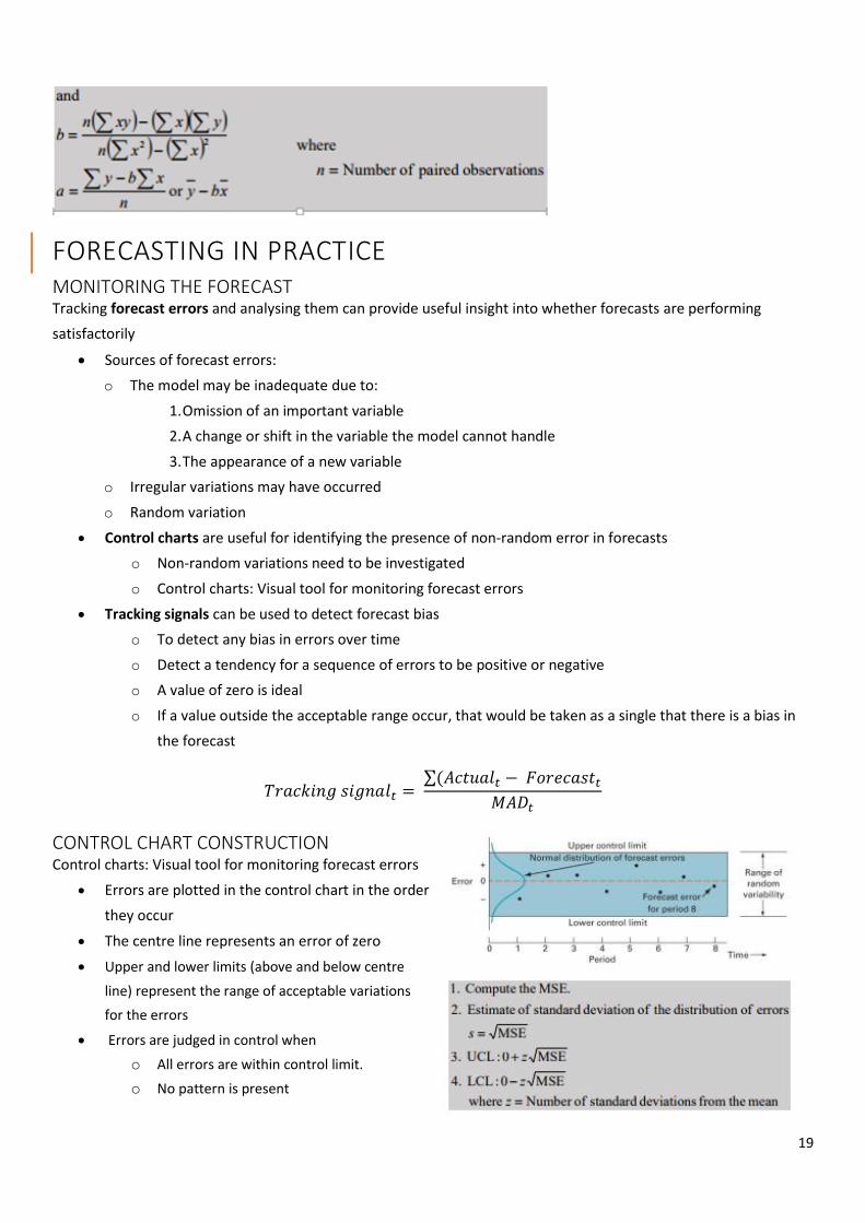
𝑇𝑟𝑎𝑐𝑘𝑖𝑛𝑔 𝑠𝑖𝑔𝑛𝑎𝑙𝑡 = ∑(𝐴𝑐𝑡𝑢𝑎𝑙𝑡 − 𝐹𝑜𝑟𝑒𝑐𝑎𝑠𝑡𝑡

𝑀𝐴𝐷𝑡

CONTROL CHART CONSTRUCTION Control charts: Visual tool for monitoring forecast errors

Errors are plotted in the control chart in the order

they occur

The centre line represents an error of zero

Upper and lower limits (above and below centre

line) represent the range of acceptable variations

for the errors

Errors are judged in control when

o All errors are within control limit.

o No pattern is present

20

How to construct a control chart:

Compute MSE and take its square root

Control charts are based on the assumption that when errors are random, they will be distributed according to

normal distribution around a mean of zero

Z = number of standard deviations from the mean

Choosing a forecasting technique Factors to consider

Cost

Accuracy

Availability of historical data

Availability of forecasting software

Time needed to gather and analyse data and prepare a forecast

Forecast horizon

o Short-range: Moving average and exponential smoothing

o Long-term: Trend and Delphi-method

Operation strategy The better forecasts are, the more able organizations will be to take advantage of future opportunities and reduce

potential risks

A worthwhile strategy is to work to improve short-term forecasts

Accurate up-to-date information can have a significant effect on forecast accuracy:

o Prices

o Demand

o Other important variables

Reduce the time horizon forecasts have to cover

Sharing forecasts or demand data through the supply chain can improve forecast quality

21

STRATEGIC CAPACITY PLANNING INTRODUCTION Capacity: The upper limit or ceiling on the load that an operating unit can handle

Capacity needs include

o Equipment

o Space

o Employee skills

Strategic capacity planning Goal:

To achieve a match between the long-term supply capabilities of an organization and the predicted level of

long-term demand

o Overcapacity⇢ operating costs that are too high

Costs can’t be recovered

Lower demand

o Under-capacity ⇢ strained resources and possible loss of customer

Lost sales: Demand is higher than production, sales you could have made if your supply was

higher.

Key Questions:

What kind of capacity is needed?

o Product design and process design

How much is needed to match demand?

o Different capacity each period ?

When is it needed?

Related Questions?

How much will it cost?

What are the potential benefits and risks?

Should capacity be changed all at once, or through several smaller changes

Can the supply chain handle the necessary changes?

CAPACITY DECISIONS ARE STRATEGIC 1. Impact the ability of the organization to meet future demands

o Limits rate of possible output

2. Affect operating costs

o Fixed costs through decisions of capacity

o These fixed cost continue to exist even if you lower your production

o Possible loss of market share due to loss of customer whom go to the competitors

3. Are a major determinant of initial cost

4. Often involve long-term commitment of resources

o Difficult to modify without increasing costs

5. Can affect competitiveness

o Create an entry barrier for other companies

o Delivery speed can be effected

22

6. Affect the ease of management

7. Have become more important and complex due to globalization

o Worldwide demand and supply makes capacity decisions more difficult

o Customers can get their products everywhere and you can get your supplies everywhere

8. Need to be planned for in advance due to their consumption of financial and other resources

DEFINING AND MEASURING CAPACITY Capacity is often referred to as ‘ upper limit on the rate of output’

Measure capacity in units that do not require updating

o Units per time

o Units per output

Availability of inputs:

Example: Hospital: Capacity isn’t measured in output but in number of beds

o Why is measuring capacity in dollars problematic:

Changes in price require updating of the measure

Two useful definitions of capacity

Design capacity: best case in optimal condition

o The maximum output rate or service capacity an operation, process, or facility is designed for

Effective capacity

o Design capacity minus allowances such as personal time and maintenance

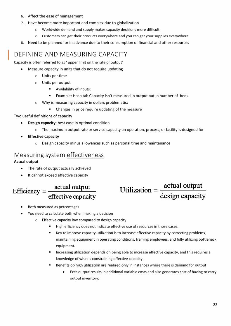
Measuring system effectiveness Actual output

The rate of output actually achieved

It cannot exceed effective capacity

Both measured as percentages

You need to calculate both when making a decision

o Effective capacity low compared to design capacity

High efficiency does not indicate effective use of resources in those cases.

Key to improve capacity utilization is to increase effective capacity by correcting problems,

maintaining equipment in operating conditions, training employees, and fully utilizing bottleneck

equipment.

Increasing utilization depends on being able to increase effective capacity, and this requires a

knowledge of what is constraining effective capacity.

Benefits op high utilization are realized only in instances where there is demand for output

Exes output results in additional variable costs and also generates cost of having to carry

output inventory.

23

DETERMINANTS OF EFFECTIVE CAPACITY Many decisions about system design have an impact on capacity.

Facilities

Size and provision for expansion

Transportation cost, distance to market

Lay out of the work area

Product and service factors

The more uniform the output, the more opportunities for standardisation of methods and materials

Process factors

Quantity capability

Quality

How effective is your production process

Human factors

Motivated and always present

Training, skills and experience

Policy factors

Overtime is regulated

Number of shifts per day

Operational factors

Scheduling

Inventory stocking decisions

Supply chain factors

Major capacity changes ?

What impact will the changes have on suppliers, warehousing, transportation and distribution?

Will the supply chain be able to handle increase in capacity?

Supply chain needs to be able to deal with your supply

External factors

Minimum quality

Pollution standards

STRATEGY FORMULATION Strategies are typically based on assumptions and predictions about:

Long-term demand patterns

Technological change

Competitor behaviour

These typically involve

1) The growth rate and variability demand.

2) The cost of building and operating facilities of various size.

3) The rate and direction of technological innovation.

4) The likely behaviour of competitors.

5) Availability of capital and other inputs.

24

Different capacity strategies:

1. Leading capacity strategy:

o Build capacity in anticipation of future demand increases

o If capacity increases involves a long lead time

2. Following strategy :

1. Build capacity when demand exceeds current capacity.

3. Tracking strategy :

o Similar to the following strategy, but adds capacity in relatively small increments to keep pace with

increasing demand.

Capacity Cushion

Extra capacity used to offset demand uncertainty

Capacity cushion strategy

Organizations that have greater demand uncertainty typically have greater capacity cushion

Organizations that have standard products and services generally have smaller capacity cushion

Steps in capacity planning 1. Estimate future capacity requirements

2. Evaluate existing capacity and facilities; identify gaps

3. Identify alternatives for meeting requirements

4. Conduct financial analyses

5. Assess key qualitative issues

6. Select the best alternative for the long term

7. Implement alternative chosen

8. Monitor results

CALCULATING PROCESSING REQUIREMENTS Capacity planning decisions involve both long-term and short-term considerations.

o Long-term considerations relate to overall level of capacity, such as facility size

o Short-term considerations relate to probable variations in capacity requirements created by such things as

seasonal, random, and irregular fluctuations in demand.

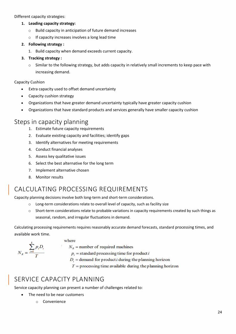
Calculating processing requirements requires reasonably accurate demand forecasts, standard processing times, and

available work time.

SERVICE CAPACITY PLANNING Service capacity planning can present a number of challenges related to:

The need to be near customers

o Convenience

25

The inability to store services

o Cannot store services for later consumption

The degree of demand volatility

o Volume and timing of demand

o Time required to service individual customers

To match supply with demand, three types of buffers may be used:

1) Inventory (e.g., bread) – Remark: not possible for services

2) Time (e.g., patients waiting in the hospital)

3) Capacity (e.g., guests in a luxury hotel)

DEMAND MANAGEMENT STRATEGIES Strategies used to offset capacity limitations and that are intended to achieve a closer match between supply and

demand

Pricing

Promotions

o Als je hoog en laag periodes hebt

o Bij lage verkopen kunnen je promoties voeren zodat de verkoop weer stijgt

o Niet te hoge verkopen op 1 periode waaraan je niet kan voldoen

o Seasonal demand afvlakken

Discounts

Other tactics to shift demand from peak periods into slow periods

IN-HOUSE OR OUTSOURCE? Once capacity requirements are determined, the organization must decide whether to produce a good or service

itself or outsource.

Factors to consider:

Available capacity

o Cost to make it are relatively small compared with those required to buy the product

o Needed Time and equipment

o Outsourcing can increase

Expertise

o If you lack expertise, buying might be a reasonable alternative

Quality considerations

o Firms that specialize can usually offer higher quality

The nature of demand

o High and steady: Produce it yourself

o Fluctuating or small orders are better handled by specialists

Cost

Risks

o Loss of direct control

o Liability

26

DEVELOPING CAPACITY ALTERNATIVES Things that can be done to enhance capacity management:

1. Design flexibility into systems

- The long-term nature of many capacity decisions and the risk inherent in long-term forecasts suggests potential

benefits from designing flexible systems.

- Removing an existing structure is more expensive than provision for future expansion.

- Modification to existing structure can be minimized

Expanding of a restaurant

- Location, lay-out of equipment, equipment selection.. are other

considerations in flexible design

2. Take stage of life cycle into account

- Capacity requirements are often closely linked to the stage of the life

cycle that the products or services are in

- Introduction phase: Overall market may experience rapid growth

Growth means increasing market share

Increase in volume will follow and thus increase in profit

Increase in capacity and investments needs to happen too!

Competitors might increase their volume too which means that the risk overcapacity increases too.

- Maturity phase: Stable market share.

Increase profitability by reducing costs

- Decline phase: underutilization due to declining demand $

Selling excess capacity

Introducing new products or services

3. Take a “big-picture” approach to capacity changes

- When developing capacity alternatives, it’s important to consider how parts of the system interrelate.

- Capacity changes affect an organisation’s supply chain

Suppliers need time to adjust their capacity

- The risk of not taking a big)picture approach is that the system is

unbalanced (bottle-neck operation)

Bottleneck operation: An operation in a sequence of

operations whose capacity is lower than that of the other

operations.

Limiting the system capacity

The capacity of the system is reduced to the

capacity of the bottleneck

4. Prepare to deal with capacity “chunks

- Capacity increases are often acquired in fairly large chunks rather than smooth increments, making it difficult to

achieve a match between desired capacity and feasible capacity.

- Example: One machines produces 40 units, two machines produce 80 but the desired capacity is 55

5. Attempt to smooth capacity requirements

- Unevenness in capacity requirements can create certain problems

- Systems tend to alternate between underutilization and overutilization

27

- Seasonal varieties:

Predictable

Ex. During bad weather, public transportation ridership

tends to increase

Complementary demand patterns:: Patterns that tend to

offset each other (A and B have complementary demand

patterns)

The products use the same resources but at different

times, so the overall capacity requirements remain fairly

stable and inventory levels are minimized

EX demand for snow and water skis

- Random variaties

- Higher demand isn’t always met with higher capacity through expanding of operations size ( they increase fixed

costs and you lose flexibility)

Overtime

Subcontract some of the work

6. Identify the optimal operating level as a function of facility size

- Productions usually have an optimal level of operations in terms of Input or output.

- Cost per unit is at its lowest for that production

- Economies of Scale If output rate is less than the optimal level, increasing the output rate results in

decreasing average per unit costs

- Diseconomies of Scale If the output rate is more than the optimal level, increasing the output rate results in

increasing average per

unit costs.

- Change in capacity gets

you on a different curve

7. Choose a strategy if

expansion is involved

- Incremental expansion or signal step expansion ?

- Leading of following strategy ?

(Dis)economies of scale Reasons for economies of scale:

Fixed costs are spread over a larger number of units

Construction costs increase at a decreasing rate as facility size increases

Processing costs decrease due to standardization

Reasons for diseconomies of scale

Distribution costs increase due to traffic congestion and shipping from a centralized facility rather than

multiple smaller facilities

Complexity increases costs

Inflexibility can be an issue

Additional levels of bureaucracy

28

CONSTRAINT MANAGEMENT Constraint: Something that limits the performance of a process or system in achieving its goals.

Categories

Market: Insufficient demand

Resource: Too little of one or more resources

Material: Too little of one or more materials

Financial: Insufficient funds

Knowledge or competency:

Policy

Supplier

Resolving Constraint Issues

1. Identify the most pressing constraint

2. Change the operation to achieve maximum benefit, given the constraint

3. Make sure other portions of the process are supportive of the constraint

4. Explore and evaluate ways to overcome the constraint

5. Repeat the process until the constraint levels are at acceptable levels

EVALUATING ALTERNATIVES Alternatives should be evaluated from varying perspectives

Economic

Is it economically feasible?

How much will it cost?

How soon can we have it?

What will operating and maintenance costs be?

What will its useful life be?

Will it be compatible with present personnel and present operations?

Non-economic

Possible negative public opinion

o Disrupt lives etc.

Technique for evaluating alternatives

Cost-volume analysis

And other techniques

Financial analysis

Decision theory

Waiting-line analysis

Simulation

Cost-volume analysis Focuses on the relationship between cost, revenue, and volume of output. Estimates income of an organisation

under different operating conditions. Used to compare capacity alternatives.

Fixed Costs (FC): Tend to remain constant regardless of output volume

Variable Costs (VC) vary directly with volume of output

VC = Quantity(Q) x variable cost per unit (v) = Q*v

29

Total Cost

TC = FC + VC

Total Revenue (TR)

TR = revenue per unit (R) x Q = R*Q

Break-Even Point (BEP)

The volume of output at which total cost and total revenue are equal

Profit (P) = TR – TC = R x Q – (FC +v x Q)

= Q(R – v) – FC

Capacity alternatives may involve step

costs, which are costs that increase

stepwise as potential volume increases.

The implication of such a

situation is the possible

occurrence of multiple break-

even quantities.

Buy more machines of you want

to produce more

30

Cost-volume analysis assumptions Cost-volume analysis is a viable tool for comparing capacity alternatives if certain assumptions are satisfied

1. One product is involved

2. Everything produced can be sold

3. The variable cost per unit is the same regardless of volume

4. Fixed costs do not change with volume changes, or they are step changes

5. The revenue per unit is the same regardless of volume

6. Revenue per unit exceeds variable cost per unit

Important to verify that the assumptions on which the technique is based are reasonably satisfied for a particular

situation.

OPERATIONS STRATEGY Capacity planning strategically impacts all areas of the organization

It determines the conditions under which operations will have to function

Flexibility allows an organization to be agile

o Responsive to market changes

o It reduces the organization’s dependence on forecast accuracy and reliability

o Many organizations utilize capacity cushions to achieve flexibility

Blocking market entry for new competitors, producing at lowers costs

Efficiency and utilization improvement

o Streamlining operations and reducing waste

Bottleneck management is one way by which organizations can enhance their effective capacities

Capacity expansion strategies are important organizational considerations

o Expand-early strategy: Before demand capitalizes

Achieve economies of scale, expand market share,..

o Wait-and-see strategy: Expand demand after it materializes

Lower chance of oversupply

Capacity contraction is sometimes necessary

o Capacity disposal strategies become important under these conditions

31

PROCESS SELECTION AND FACILITY LAYOUT

PROCESS SELECTION Refers to deciding on the way production of goods or services will be organized.

It has major implications for:

Capacity planning

Layout of facilities

Equipment

Design of work system

Process selection occurs as a matter of course when new products or services are being planned or periodically due to

technological changes.

How an organisation approaches process selection is determined by the organization’s process strategy.

Key Aspects of Process Strategy:

Capital Intensity: The mix of equipment and labour that will be used by the organization.

Process flexibility: The degree to which the system can be adjusted to changes in processing requirements due to

such factors as:

o Product and service design changes

o Volume changes

o Changes in technology

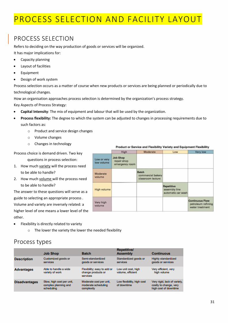
Process choice is demand driven. Two key

questions in process selection:

1. How much variety will the process need

to be able to handle?

2. How much volume will the process need

to be able to handle?

The answer to these questions will serve as a

guide to selecting an appropriate process .

Volume and variety are inversely related: a

higher level of one means a lower level of the

other.

Flexibility is directly related to variety

o The lower the variety the lower the needed flexibility

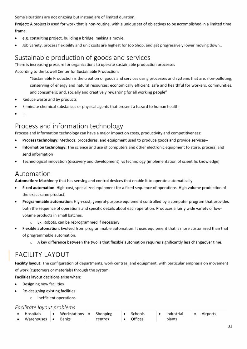
Process types

32

Some situations are not ongoing but instead are of limited duration.

Project: A project is used for work that is non-routine, with a unique set of objectives to be accomplished in a limited time

frame.

e.g. consulting project, building a bridge, making a movie

Job variety, process flexibility and unit costs are highest for Job Shop, and get progressively lower moving down..

Sustainable production of goods and services There is increasing pressure for organizations to operate sustainable production processes

According to the Lowell Center for Sustainable Production:

“Sustainable Production is the creation of goods and services using processes and systems that are: non-polluting;

conserving of energy and natural resources; economically efficient; safe and healthful for workers, communities,

and consumers; and, socially and creatively rewarding for all working people”

Reduce waste and by products

Eliminate chemical substances or physical agents that present a hazard to human health.

…

Process and information technology Process and Information technology can have a major impact on costs, productivity and competitiveness:

Process technology: Methods, procedures, and equipment used to produce goods and provide services ̶

Information technology: The science and use of computers and other electronic equipment to store, process, and

send information

Technological innovation (discovery and development) vs technology (implementation of scientific knowledge)

Automation Automation: Machinery that has sensing and control devices that enable it to operate automatically

Fixed automation: High-cost, specialized equipment for a fixed sequence of operations. High volume production of

the exact same product.

Programmable automation: High-cost, general-purpose equipment controlled by a computer program that provides

both the sequence of operations and specific details about each operation. Produces a fairly wide variety of low-

volume products in small batches.

o Ex. Robots, can be reprogrammed if necessary

Flexible automation: Evolved from programmable automation. It uses equipment that is more customized than that

of programmable automation.

o A key difference between the two is that flexible automation requires significantly less changeover time.

FACILITY LAYOUT Facility layout: The configuration of departments, work centres, and equipment, with particular emphasis on movement

of work (customers or materials) through the system.

Facilities layout decisions arise when:

Designing new facilities

Re-designing existing facilities

o Inefficient operations

Facilitate layout problems Hospitals Warehouses

Workstations Banks

Shopping centres

Schools Offices

Industrial plants

Airports

33

Layout design objectives Basic Objective

Facilitate a smooth flow of work, material, and information through the system.

Supporting objectives

1. Facilitate product or service quality

2. Use workers and space efficiently

3. Avoid bottlenecks

4. Minimize material handling costs

5. Eliminate unnecessary movement of workers or material

6. Minimize production time or customer service time

7. Design for safety

Basic layout types o Product layouts: Most conductive to repetitive processing.

o Process layouts: Intermittent processing.

o Fixed-Position layout: Used when projects require layouts.

o Hybrid layouts

Repetitive processing: Product layouts Layout that uses standardized processing

operations to achieve smooth, rapid, high-

volume flow.

An assembly line: Standardized layout

arranged according to fixed sequence of

assembly tasks.

Highly standardized goods

If one section fails, all fails

Resources are organized in order to create optimal flow from one operation to the next

When there is a limited range of high quantity products

Highly capital intensive

Not work intensive: reduced material handling costs

Little work-in-process inventory and short lead times

Dedicated production lines for very high runners

Production lines per product family for B-products

Low flexibility but high efficiency

34

Non-Repetitive processing: Process layouts Layouts that can handle varied processing

requirements

The variety of jobs that are processed

requires frequent adjustment of equipment.

When there are many low quantity

products

General-purpose machinery

Reduced capital intensity

Work intensive: higher material handling costs

Production in batches: work-in-process inventory and lead times

increase

High flexibility but low efficiency

Common in service environments.

Fixed position layouts Layout in which the product or project remains stationary, and workers, materials, and equipment are moved as needed.

This due to the nature of the product: weight, size,..

Hybrid layouts Some operational environments use a combination of the three basic layout types:

Hospitals

Supermarket

Shipyards

Some organizations are moving away from process layouts in

an effort to capture the benefits of product layouts

Cellular manufacturing

Flexible manufacturing systems

o Automation in a flexible way

CELLULAR LAYOUTS Layout in which workstations are grouped into a cell that can process items that have similar processing requirements

Groupings are determined by the operations needed to perform the work for a set of similar items, part families,

that require similar processing

The cells become, in effect, miniature versions of product layouts

35

Group technology: The grouping into part families of items with similar design or manufacturing characteristics

Design Characteristics

o Size

o Shape

o Function

Manufacturing or processing characteristics

o Type of operations required

o Sequence of operations required

Requires a systematic analysis of parts to identify the part families.

Divided in similar products or families

The cells are miniature versions of products layouts

All parts follow the same route, although minor variations are possible (e.g. skipping an operation)

Service layout Service layouts can be categorized as: product, process, or fixed position:

Fixed position: Equipment is brought to the customers residence or office

Process layouts: High degree of variety

Product layout: Organized sequentially, all following the same or similar sequence.

Service layout requirements are somewhat different due to such factors as:

Degree of customer contact

Degree of customization

Common service layouts:

Warehouse and storage layouts

Retail layouts

Office layouts

DESIGNING PRODUCT LAYOUTS: LINE BALANCING The goal of a product layout is to arrange workers or machines in the sequence that operations need to be performed

The process of assigning tasks to workstations in such a way that the workstations have approximately equal time

requirements

Goal: Obtain task grouping that represent approximately equal time requirements since this minimizes idle time along

the line and results in a high utilization of equipment and labour.

o Same work load on every station

Difficult to form task bundles that have the same duration

Activities are not compatible

Difference in equipment requirements

Difference among elemental takes length, cannot always be overcome by grouping taks

Inability to perfectly balance a line

First and third tasks are combined 6 min, while the second task alone

is also 6 min.. Ideally the first and third tasks would be combined. But

that is not always possible.

E.g. automatic car wash.: Scrubbing and drying can’t be combined, due to the need to rinse the car between the twon

operations.

36

Why is line balancing important?

1. It allows us to use labour and equipment more efficiently.

2. To avoid fairness issues that arise when one workstation must work harder than another

Cycle time: The maximum time allowed at each workstation to complete its set of tasks on a unit

Cycle time also establishes the output rate of a line

Assembly line configuration: grouping tasks and assigning them to stations

Set of elementary operations (tasks) {1, 2, …, K} with task times 𝑡𝑘

Cycle time c: time between the completion of 2 consecutive products

c = takt time = available production time per day/total demand per day

= T/d

Assignment constraints

HOW MANY WORKSTATIONS ARE NEEDED? The required number of workstations is a function of

Desired output rate

Our ability to combine tasks into a workstation

Theoretical minimum number of stations:

Precedence diagram A diagram that shows elemental tasks and their precedence (sequential) requirements.

To start task d, task b as well as task c have to be finished.

How to balance a line depends on how you assign tasks to workstations.

Assigning tasks to workstation Generally there are no techniques available hat guarantee an optimal set of

assignments. Instead managers employ heuristic rules.

Some Heuristic (Intuitive) Rules:

Assign tasks in order of most following tasks

o Count the number of tasks that follow

Assign tasks in order of greatest positional weight.

o Positional weight is the sum of each task’s time and the times of all following tasks.

Method:

1. Assign a numeric score n(x) to every task

2. Update the set of eligible tasks; i.e. tasks for which the immediate predecessors are assigned

37

3. Assign the task with the highest score to the first station for which nor the capacity constraints, nor the

precedence constraints are exceeded. Go to step 2.

Measuring effectiveness Balance delay (percentage of idle time)

Percentage of idle time of a line

When the calculated cycle time and the actual bottleneck station

time differ, the actual bottleneck station time should be used in all

idle time, efficiency, and output calculations.

The actual bottleneck time dictates the actual place of the linen whereas the calculated cycle time just an upper limit on

the amount of time that can be loaded into any situation.

Efficiency: Percentage of busy time of a line.

Measuring effectiveness Smoothness Index:

An index to indicate the relative

smoothness of a given line balance.

A smoothness index of zero indicates a

perfect balance.

Evaluation of heuristics

Jackson 11 problem (Jackson 1956) Feasible line balance = assignment of each task to a station such that the

precedence constraints and further restrictions are fulfilled

38

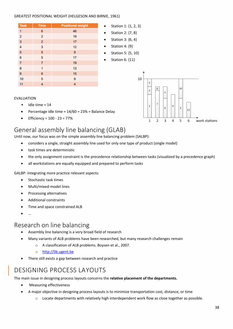
GREATEST POSITIONAL WEIGHT (HELGESON AND BIRNIE, 1961)

Station 1: {1, 2, 3}

Station 2: {7, 8}

Station 3: {6, 4}

Station 4: {9}

Station 5: {5, 10}

Station 6: {11}

EVALUATION

• Idle time = 14

Percentage idle time = 14/60 = 23% = Balance Delay

Efficiency = 100 - 23 = 77%

General assembly line balancing (GLAB) Until now, our focus was on the simple assembly line balancing problem (SALBP):

considers a single, straight assembly line used for only one type of product (single model)

task times are deterministic

the only assignment constraint is the precedence relationship between tasks (visualized by a precedence graph)

all workstations are equally equipped and prepared to perform tasks

GALBP: Integrating more practice relevant aspects:

Stochastic task times

Multi/mixed-model lines

Processing alternatives

Additional constraints

Time and space constrained ALB

…

Research on line balancing Assembly line balancing is a very broad field of research

Many variants of ALB problems have been researched, but many research challenges remain

o A classification of ALB problems. Boysen et al., 2007.

o http://lib.ugent.be

There still exists a gap between research and practice

DESIGNING PROCESS LAYOUTS The main issue in designing process layouts concerns the relative placement of the departments.

Measuring effectiveness

A major objective in designing process layouts is to minimize transportation cost, distance, or time

o Locate departments with relatively high interdependent work flow as close together as possible.

39

Information requirements In designing process layouts, the following information is required:

1. A list of departments to be arranged and their dimensions

2. A projection of future work flows between the pairs of work centres

3. The distance between locations and the cost per unit of distance to move loads between them

4. The amount of money to be invested in the layout

5. A list of any special considerations

6. The location of key utilities, access and exit points, etc.

The ideal situation is to first develop a layout and then design the physical structure around it, thus permitting maximum

flexibility.

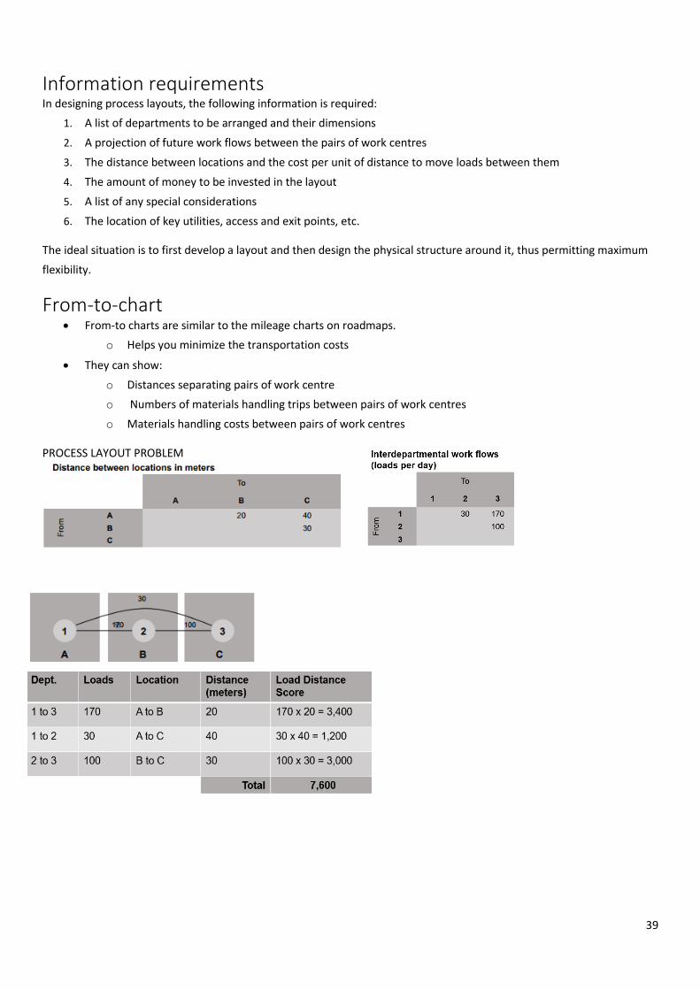
From-to-chart From-to charts are similar to the mileage charts on roadmaps.

o Helps you minimize the transportation costs

They can show:

o Distances separating pairs of work centre

o Numbers of materials handling trips between pairs of work centres

o Materials handling costs between pairs of work centres

PROCESS LAYOUT PROBLEM

40

Activity relationship chart Each pair of operations is given a letter to indicate the desirability of locating the operations near each other.

The letter codes for closeness ratings are:

o A: Absolutely necessary

o E: Especially important

o I: Important

o O: Ordinary importance

o U: Unimportant

o X: Undesirable

41

LOCATION PLANNING AND ANALYSIS

INTRODUCTION TO LOCATION DECISIONS

The need for location decisions Location decisions arise for a variety of reasons:

Addition of new facilities

o As part of a marketing strategy to expand markets

o Growth in demand that cannot be satisfied by expanding existing facilities

Depletion of basic inputs requires relocation (uitputting)

Shift in markets

Cost of doing business at a particular location makes relocation attractive

Strategically important Closely tied to an organization’s strategy

o Low-cost

Locating where labour or material costs are low

o Convenience to attract market share

Increasing profits by increasing market shares might result in locating in high-traffic areas

Effect capacity and flexibility

Space constraints that limit future expansion options.

Local restrictions my restrict my restrict certain products or services thus limiting future options for products

or services.

Represent a long-term commitment of resources

Effect investment requirements, operating costs, revenues, and operations

o A poor choice in location might result in excessive transportation costs

o Shortage of qualified workers

Impact competitive advantage

Importance to supply chains

Objectives Location decisions are based on:

Profit potential or cost and customer service

Finding a number of acceptable locations from which to choose

Position in the supply chain

o End: accessibility, consumer demographics, traffic patterns, and local customs are important

o Middle: locate near suppliers or markets

o Beginning: locate near the source of raw materials

Web-based retail organizations are effectively location independent

Supply chain considerations Supply chain management must address supply chain configuration:

Number and location of suppliers, production facilities, warehouses and distribution centres

42

Centralized vs. decentralized distribution:

o Centralized distribution: Yield scale economies and gives a tighter control

o Decentralized distribution: More responsive to local needs

The importance of such decisions is underscored by their reflection of the basic strategy for accessing customer

markets → significant impact on costs, revenues, and responsiveness.

Location options Existing companies generally have four options available in location planning:

1) Expand an existing facility

o Need of adequate room for expansion

o Expansion cost re other lower than those of other alternatives

2) Add new locations while retaining existing facilities

o Take into account what the impact will be on the total system

o Can be a strategy to maintain market share

o Prevent competitors from entering a market

o Another store needs to draw more consumer and not customers who already patronize an existing

store

3) Shut down one location and move to another

o Exhausted raw materials

4) Do nothing

o If analyses of potential locations fails to uncover benefits to expanding,..

Global: Location: facilitating factors Two key factors have contributed to the attractiveness of globalization:

Trade agreements

o Reduced quotas and tariffs

o North American Free Trade Agreement (NAFTA) ‒ General Agreement on Tariffs and Trade (GATT) ‒ U.S.-

China Trade Relations Act ‒

o EU and WTO efforts to facilitate free trade

Technology

o Advances in communication and information technology

BENEFITS A wide range of benefits have accrued to organizations that have globalized operations

Markets: More opportunities for expanding markets

Cost savings: transportation, labour cost,..

Legal and regulatory

Less restrictive environmental regulations

Financial

Avoid currency changes

State incentives to attract businesses

Other: Globalization may provide new sources of ideas for products and services, new perspectives on

operations, and solutions to problems

43

DISADVANTAGES There are a number of disadvantages that may arise when locating globally:

Transportation costs

Poor infrastructure, shipping over great distances

Security costs

Unskilled labour

Additional employee training may be needed

Import restrictions

Criticism for locating out-of-country

RISKS Organizations locating globally should be aware of potential risk factors related to:

Political instability and unrest can create safety issues

Terrorism

Economic instability might create inflation or deflation, both can negatively impact profit

Legal regulation: may change, you could lose the key benefits

Ethical considerations

Cultural differences

MANAGING GLOBAL OPERATIONS Managerial implications for global operations:

Language and cultural differences

o Risk of miscommunication

o Development of trust

o Different management styles

o Corruption and bribery

Increased travel (and related) costs

Challenges associated with managing far-flung operations

Level of technology and resistance to technological change

Domestic personnel may resist locating, even temporarily

GENERAL PROCEDURE FOR MAKING LOCATION DECISIONS Steps followed to make location decisions:

1. Decide on the criteria to use for evaluating location alternatives

Increased revenue

Decreased costs

2. Identify important factors, such as location of markets or raw materials

3. Develop location alternatives

Identify the country or countries for location

Identify the general region for location

Identify a small number of community alternatives

Identify the site alternatives among the community alternatives

4. Evaluate the alternatives and make a decision

44

Identifying a country, a region, community, and a site IDENTIFYING A COUNTRY

Currency and exchange risks

Low labour productivity

Transfer pricing rules

IDENTIFYING A REGION Primary regional factors:

Location of raw materials

o Necessity: Mining, farming

o Perishability = bederfelijkheid : Freezing of fresh fruits..

o Transportation costs

Location of markets

o As part of a profit-oriented company’s competitive strategy

o So not-for-profits can meet the needs of their service user

o Distribution costs and perishability

Labour factors

o Cost of labour

o Availability of suitably skilled workers

o Wage rates in the area

Labour productivity

o Attitudes toward work

o Whether unions pose a serious potential problem

o difference in worker attitude

Other factors: Climate and taxes may play an important role in location decisions

45

IDENTIFYING A COMMUNITY Many communities actively attempt to attract new businesses they perceive to be a good fit for the

community

Businesses also actively seek attractive communities based on such factors such as:

o Quality of life

o Services

o Attitude

o Taxes

o Environmental regulations

o Utilities

o Development support

IDENTIFYING A SITE Primary site location considerations are:

Land

o Cost, degree of development required

o Soil characteristics,

o Room for expansion

Transportation

o Type: access roads,..

Zoning restrictions

o Environmental/ legal

Other restrictions

Multiple plant manufacturing strategies Organizing operations:

Product plant strategy

o Entire products or product lines are produced in separate plants, and each plant usually supplies the

entire domestic market

Market area plant strategy

o Plants are designated to serve a particular geographic segment of the market

o Plants produce most, if not all, of a company’s products

Process plant strategy

o Different plants focus on different aspects of a process e.g., automobile manufacturers – engine

plant, body stamping plant, etc.

o Coordination across the system becomes a significant issue

General-purpose plant strategy

o Plants are flexible and capable of handling a range of products

Geographic information system (GIS) A computer-based tool for collecting, storing, retrieving, and displaying demographic data on maps

Aids decision makers in

o Targeting market segment

o Identifying locations relative to their market potential

46

o Planning distribution networks

Portraying relevant information on a map makes it easier for decision makers to understand

SERVICE AND RETAIL LOCATIONS Considerations:

Nearness to raw materials is not usually a consideration

Customer access is a

o Prime consideration for some: Banks, restaurants, hotels, etc.

o Not an important consideration for others: service call centers, etc.

o Traffic volume

o Public transportation

o Customer safety and security

o Parking facilities

Tend to be profit or revenue driven, and so are

o Concerned with demographics, competition, traffic volume patterns, and convenience

o Manufacturers are more cost driven

Clustering

o Similar types of

businesses locate near

one another

EVALUATING LOCATION ALTERNATIVES

Common techniques

Locational cost-profit-volume analysis Technique for evaluating location choices in economic terms

Steps:

1. Determine the fixed and variable costs for each alternative

2. Plot the total-cost lines for all alternatives on the same graph

3. Determine the location that will have the lowest total cost (or highest profit) for the expected level of output

Assumptions

1. Fixed costs are constant for the range of probable output

2. Variable costs are linear for the range of probable output

3. The required level of output can be closely estimated

4. Only one product is involved

EXAMPLE: COST-PROFIT-VOLUME ANALYSIS

Fixed and variable costs for four potential plant locations are

shown:

47

Range of output for which each output is superior

B Superior (up to 4,999 units)

Lowest total cost

What if the expected output at a location is 800,000? C is

superior.

The exact range of when alternative is superior based on

output.

(zoeken naar de snijpunten via BEP, B is het best van 00 tot

en 500,000 …)

C Superior (>5,000 to 11,111 units)

A superior (11,112 units and up)

Transportation model Involves finding the lowest-cost plan for distributing a stock of goods or

supplies from multiple points of origin to multiple destinations that

demand the goods

Include transportation cost per unit in cost-volume analysis

It can also be used if a number of new facilities are to be added or if an

entire new system is being developed

TRANSPORTATION PROBLEM: LINEAR PROGRAMMING FORMULATION

TRANSPORTATION: COMPUTER SOLUTION Transportation problems can be solved manually in a straightforward manner

o Except for very small problems, solving the problem manually can be very time consuming

o For medium to large problems, computer solution techniques are more practical

Computer solution techniques can be exact or heuristic

A variety of software packages are available for solving the transportation model

o Some require formulating the problem as a general LP model

48

o Others allow data entry in a more simple, tabular format

Factor rating General approach to evaluating locations that includes quantitative and qualitative input

Gives a rational basis for evaluation and facilitates comparison

Incorporates personal opinions (qualitative) and quantitative information

Procedure:

5. Determine which factors are relevant

6. Assign a weight to each factor that indicates its relative importance compared with all other factors.

Weights typically sum to 1.00

7. Decide on a common scale for all factors, and set a minimum acceptable score if necessary

8. Score each location alternative

9. Multiply the factor weight by the score for each factor, and sum the results for each location alternative

10. Choose the alternative that has the highest composite score, unless it fails to meet the minimum acceptable

score

EXAMPLE: FACTOR RATING

A photo-processing company intends to open a new branch store. The following table contains information on two

potential locations. Which is better?

Center of gravity method Method for locating a distribution center that minimizes distribution costs

Treats distribution costs as a linear function of the distance and the quantity shipped

The quantity to be shipped to each destination is assumed to be fixed

The method includes the use of a map that shows the locations of destination

The map must be accurate and drawn to scale

A coordinate system is overlaid on the map to determine relative locations

49

If quantities to be shipped to every location are equal, you can obtain the

coordinates of the center of gravity by finding the average of the x-coordinates

and the average of the y-coordinates.

EXAMPLE: CENTER OF GRAVITY METHOD

Suppose you are attempting to find the centre of gravity for the problem depicted in Figure c (slide 40)

Here, the centre of gravity is (4.5,4). This is slightly west of D3.

When the quantities to be shipped to every location are unequal, you can

obtain the coordinates of the centre of gravity by finding the weighted

average of the x-coordinates and the average of the y-coordinates

Suppose the shipments for the problem depicted in Figure a are not all

equal. Determine the centre of gravity based on the following information:

50