Web Book of Regional Science Regional Research Institute

2020

An Introduction to Regional Economics An Introduction to Regional Economics

Edgar M. Hoover University of Pittsburgh

Frank Giarratani University of Pittsburgh

Follow this and additional works at: https://researchrepository.wvu.edu/rri-web-book

Recommended Citation Recommended Citation Hoover, Edgar M., & Giarratani, F. (1999). An Introduction to Regional Economics. Reprint. Edited by Scott Loveridge and Randall Jackson. WVU Research Repository, 2020.

This Book is brought to you for free and open access by the Regional Research Institute at The Research Repository @ WVU. It has been accepted for inclusion in Web Book of Regional Science by an authorized administrator of The Research Repository @ WVU. For more information, please contact ian.harmon@mail.wvu.edu.

The Web Book of Regional ScienceSponsored by

An Introduction to Regional EconomicsFourth Edition*

ByEdgar M. Hoover (deceased)

Distinguished Service Professor of Economics, EmeritusUniversity of the Pittsburgh

Frank GiarrataniProfessor of Economics and Director, Center for Industry Studies

Department of EconomicsPittsburgh, PA 15260Tel: (412) 648-1741

Published: 1999Updated: January, 2020

*The web version of the third edition of An Introduction to Regional Economics which first appearedin The Web Book of Regional Science series was edited by:

Scott LoveridgeProfessor, Extension SpecialistMichigan State University This fourth edition of An Introduction to

Regional Economics is the result of extensive revision of the web book version of the third edition by:Randall JacksonDirector, Regional Research InstituteWest Virginia University

This work was originally published by Alfred A. Knopf, Inc., copyright 1971, 1975, and 1984. In1999, copyright was transferred from Knopf to the Hoover Family Trust and Frank Giarratani.West Virginia University’s Regional Research Institute is distributing this electronic versionof the text by permission. Direct copyright permission requests to Professor Giarratani atthe University of Pittsburgh. On 11/24/09, Dr. Larry G. Bray, Research professor of Economics at

the University of Tennessee (UT) writes, “You have been kind enough to allow us to use as class materialyour web book An Introduction to Regional Science by Hoover and Giarratani. This web book formsthe basis for much of the course and complements added material assigned to the class. You have done anexcellent job in creating this document, which we feel which is the best available regional economics textbook.Thanks again for your commitment to the support of higher education in our colleges and universities. Youare going a great job.”

2

<This page blank>

The Web Book of Regional Science is offered as a service to the regional research community in an effortto make a wide range of reference and instructional materials freely available online. Roughly three dozenbooks and monographs have been published as Web Books of Regional Science. These texts covering diversesubjects such as regional networks, land use, migration, and regional specialization, include descriptionsof many of the basic concepts, analytical tools, and policy issues important to regional science. The WebBook was launched in 1999 by Scott Loveridge, who was then the director of the Regional Research Instituteat West Virginia University. The director of the Institute, currently Randall Jackson, serves as the Series editor.

When citing this book, please include the following:

Hoover, Edgar M., & Giarratani, F. (1999). An Introduction to Regional Economics. Reprint. Edited byScott Loveridge and Randall Jackson. WVU Research Repository, 2020.

<This page blank>

ContentsPREFACE 11

1. INTRODUCTION 121.1 What Is Regional Economics? . . . . . . . . . . . . . . . . . . . . . . . . . . . . . . . . . . 121.2 Three Foundation Stones . . . . . . . . . . . . . . . . . . . . . . . . . . . . . . . . . . . . . 121.3 Regional Economic Problems and the Plan of this Book . . . . . . . . . . . . . . . . . 13Selected Readings . . . . . . . . . . . . . . . . . . . . . . . . . . . . . . . . . . . . . . . . . . . . 15

2. INDIVIDUAL LOCATION DECISIONS 162.1 Levles of Analysis and Location Units . . . . . . . . . . . . . . . . . . . . . . . . . . . . . 162.2 Objectives and Procedures for Location Choice . . . . . . . . . . . . . . . . . . . . . . . 172.3 Location Factors . . . . . . . . . . . . . . . . . . . . . . . . . . . . . . . . . . . . . . . . . . 19

2.3.1 Local Inputs and Outputs . . . . . . . . . . . . . . . . . . . . . . . . . . . . . . . . 192.3.2 Transferable Inputs and Outputs . . . . . . . . . . . . . . . . . . . . . . . . . . . . 202.3.3 Classification of Location Factors . . . . . . . . . . . . . . . . . . . . . . . . . . . . 202.3.4 The Relative Importance of Location Factors . . . . . . . . . . . . . . . . . . . . 20

2.4 Spatial Patterns of Differential Advantage in SpecificLocation Factors . . . . . . . . . . . . . . . . . . . . . . . . . . . . . . . . . . . . . . . . . . 22

2.5 Transfer Orientation . . . . . . . . . . . . . . . . . . . . . . . . . . . . . . . . . . . . . . . . 242.6 Location and the Theory of Production . . . . . . . . . . . . . . . . . . . . . . . . . . . . 302.7 Scale Economies and Multiple Markets or Sources . . . . . . . . . . . . . . . . . . . . . 342.8 Some Operational Shortcuts . . . . . . . . . . . . . . . . . . . . . . . . . . . . . . . . . . . 352.9 Summary . . . . . . . . . . . . . . . . . . . . . . . . . . . . . . . . . . . . . . . . . . . . . . . 37Technical Terms Introduced in this Chapter . . . . . . . . . . . . . . . . . . . . . . . . . . . 38Selected Readings . . . . . . . . . . . . . . . . . . . . . . . . . . . . . . . . . . . . . . . . . . . . 38

3. TRANSFER COSTS 403.1 Introduction . . . . . . . . . . . . . . . . . . . . . . . . . . . . . . . . . . . . . . . . . . . . . 403.2 Some Economic Characteristics of Transfer Operations . . . . . . . . . . . . . . . . . . 403.3 Characteristic Features of Transfer Costs and Rates . . . . . . . . . . . . . . . . . . . . 41

3.3.1 Route Systems and Service Points . . . . . . . . . . . . . . . . . . . . . . . . . . . 413.3.2 Long-Haul Economies . . . . . . . . . . . . . . . . . . . . . . . . . . . . . . . . . . . 423.3.3 Transfer Costs and Rates . . . . . . . . . . . . . . . . . . . . . . . . . . . . . . . . . 443.3.4 Time Costs in Transfer . . . . . . . . . . . . . . . . . . . . . . . . . . . . . . . . . . 48

3.4 Locational Significance of Characteristics of Transfer Rates . . . . . . . . . . . . . . . 493.4.1 Effects of Limited Route Systems and Service Points . . . . . . . . . . . . . . . 493.4.2 General Locational Effect of Transfer Rates Rising Less than Proportionally

with Distance . . . . . . . . . . . . . . . . . . . . . . . . . . . . . . . . . . . . . . . . 513.4.3 Modal Interchange Locations . . . . . . . . . . . . . . . . . . . . . . . . . . . . . . 53

3.5 Some Recent Developments Concerning the Structure of Transfer Costs . . . . . . . 553.5.1 Introduction . . . . . . . . . . . . . . . . . . . . . . . . . . . . . . . . . . . . . . . . . 553.5.2 Higher Energy Prices and the Pattern of Industrial Location . . . . . . . . . . 553.5.3 Technological Change in Data Processing and Transmission . . . . . . . . . . . 57

3.6 Summary . . . . . . . . . . . . . . . . . . . . . . . . . . . . . . . . . . . . . . . . . . . . . . . 58Technical Terms Introduced in this Chapter . . . . . . . . . . . . . . . . . . . . . . . . . . . 59Selected Readings . . . . . . . . . . . . . . . . . . . . . . . . . . . . . . . . . . . . . . . . . . . . 59Appendix 3-1 Rate Discrimination by a Transfer Monopolist . . . . . . . . . . . . . . . . 59

4. LOCATION PATTERNS DOMINATED BY DISPERSIVE FORCES 614.1 Introduction . . . . . . . . . . . . . . . . . . . . . . . . . . . . . . . . . . . . . . . . . . . . . 61

4.1.1 Unit Locations and the Pattern of an Activity . . . . . . . . . . . . . . . . . . . 614.1.2 Competition and Interdependence . . . . . . . . . . . . . . . . . . . . . . . . . . . 614.1.3 Some Basic Factors Contributing to Dispersed Patterns . . . . . . . . . . . . . 62

6

4.2 Market Areas . . . . . . . . . . . . . . . . . . . . . . . . . . . . . . . . . . . . . . . . . . . . 634.2.1 Introduction . . . . . . . . . . . . . . . . . . . . . . . . . . . . . . . . . . . . . . . . . 634.2.2 The Market Area of a Spatial Monopolist . . . . . . . . . . . . . . . . . . . . . . 634.2.3 Market-Area Patterns . . . . . . . . . . . . . . . . . . . . . . . . . . . . . . . . . . . 67

4.3 Some Aspects of Spatial Pricing Policy and Market Areas . . . . . . . . . . . . . . . . 704.3.1 Market-Area Overlap . . . . . . . . . . . . . . . . . . . . . . . . . . . . . . . . . . . 704.3.2 Spatial Price Discrimination . . . . . . . . . . . . . . . . . . . . . . . . . . . . . . . 724.3.3 Pricing Policy and Spatial Competition . . . . . . . . . . . . . . . . . . . . . . . . 75

4.4 Competition and Location Decisions . . . . . . . . . . . . . . . . . . . . . . . . . . . . . . 764.5 Market Areas and the Choice of Locations . . . . . . . . . . . . . . . . . . . . . . . . . . 79

4.5.1 The Location Pattern of a Transfer-Oriented Activity . . . . . . . . . . . . . . 794.5.2 Transfer Orientation and the Patterns of Nonbusiness Activities . . . . . . . . 79

4.6 Summary . . . . . . . . . . . . . . . . . . . . . . . . . . . . . . . . . . . . . . . . . . . . . . . 80Technical Terms Introduced in this Chapter . . . . . . . . . . . . . . . . . . . . . . . . . . . 80Selected Readings . . . . . . . . . . . . . . . . . . . . . . . . . . . . . . . . . . . . . . . . . . . . 80Appendix 4-1 Conditions Determining the Existence and Size of Market Areas . . . . 81

5. LOCATION PATTERNS DOMINATED BY COHESION 845.1 Introduction . . . . . . . . . . . . . . . . . . . . . . . . . . . . . . . . . . . . . . . . . . . . . 845.2 External Economies: Output Variety and Market Attraction . . . . . . . . . . . . . . 845.3 External Economies: Characteristics of the Production Process . . . . . . . . . . . . 85

5.3.1 Introduction . . . . . . . . . . . . . . . . . . . . . . . . . . . . . . . . . . . . . . . . . 855.3.2 External Economies and Scale . . . . . . . . . . . . . . . . . . . . . . . . . . . . . . 865.3.3 Lichtenberg’s Study of “External-Economy Industries" . . . . . . . . . . . . . . 87

5.4 Single-Activity Clusters and Urbanization . . . . . . . . . . . . . . . . . . . . . . . . . . 925.4.1 Introduction . . . . . . . . . . . . . . . . . . . . . . . . . . . . . . . . . . . . . . . . . 925.4.2 Urbanization Economies . . . . . . . . . . . . . . . . . . . . . . . . . . . . . . . . . 935.4.3 Measuring Urbanization Economies . . . . . . . . . . . . . . . . . . . . . . . . . . 94

5.5 Mixed Situations . . . . . . . . . . . . . . . . . . . . . . . . . . . . . . . . . . . . . . . . . . 965.5.1 Attraction plus Repulsion . . . . . . . . . . . . . . . . . . . . . . . . . . . . . . . . 965.5.2 Coexistence of Market Areas and Supply Areas, When Both Sellers and

Buyers Are Dispersed . . . . . . . . . . . . . . . . . . . . . . . . . . . . . . . . . . 975.6 Summary . . . . . . . . . . . . . . . . . . . . . . . . . . . . . . . . . . . . . . . . . . . . . . . 98Technical Terms Introduced in this Chapter . . . . . . . . . . . . . . . . . . . . . . . . . . . 98Selected Readings . . . . . . . . . . . . . . . . . . . . . . . . . . . . . . . . . . . . . . . . . . . . 99

6. LAND USE 1006.1 What is “Land"? . . . . . . . . . . . . . . . . . . . . . . . . . . . . . . . . . . . . . . . . . . 1006.2 Competiion for the Use of Land . . . . . . . . . . . . . . . . . . . . . . . . . . . . . . . . 1006.3 An Activity’s Demand for Land: Rent Gradients and Rent Surfaces . . . . . . . . . 102

6.3.1 Rent Gradients and Surfaces with Output Orientation . . . . . . . . . . . . . . 1026.3.2 Rent Gradients and Rent Surfaces with Input Orientation . . . . . . . . . . . 1066.3.3 Rent Gradients and Multiple Access . . . . . . . . . . . . . . . . . . . . . . . . . . 107

6.4 Interactivity Competition for Space . . . . . . . . . . . . . . . . . . . . . . . . . . . . . . 1076.4.1 A Basic Sequence of Rural Land Uses . . . . . . . . . . . . . . . . . . . . . . . . . 1086.4.2 Activity Characteristics Determining Access Priority and Location . . . . . . 109

6.5 Rural and Urban Land Use Allocation . . . . . . . . . . . . . . . . . . . . . . . . . . . . 1126.5.1 Some Characteristics of Urban Economic Activity . . . . . . . . . . . . . . . . . 1126.5.2 Equilibrium of Land Uses and Rents . . . . . . . . . . . . . . . . . . . . . . . . . 114

6.6 Residential Location . . . . . . . . . . . . . . . . . . . . . . . . . . . . . . . . . . . . . . . . 1166.7 Rent and Land Value . . . . . . . . . . . . . . . . . . . . . . . . . . . . . . . . . . . . . . . 119

6.7.1 Speculative Value of Land . . . . . . . . . . . . . . . . . . . . . . . . . . . . . . . . 1196.7.2 Improvements on Land . . . . . . . . . . . . . . . . . . . . . . . . . . . . . . . . . . 120

6.8 Summary . . . . . . . . . . . . . . . . . . . . . . . . . . . . . . . . . . . . . . . . . . . . . . . 120

7

Technical Terms Introduced in this Chapter . . . . . . . . . . . . . . . . . . . . . . . . . . . 120Selected Readings . . . . . . . . . . . . . . . . . . . . . . . . . . . . . . . . . . . . . . . . . . . . 120APPENDIX 6-1 Derivation of Formulas for Rent Gradients and Their Slopes . . . . . 121

7. THE SPATIAL STRUCTURE OF URBAN AREAS 1237.1 Introduction . . . . . . . . . . . . . . . . . . . . . . . . . . . . . . . . . . . . . . . . . . . . . 1237.2 Some Location Factors . . . . . . . . . . . . . . . . . . . . . . . . . . . . . . . . . . . . . . 123

7.2.1 Independent Locations . . . . . . . . . . . . . . . . . . . . . . . . . . . . . . . . . . 1237.2.2 The Center . . . . . . . . . . . . . . . . . . . . . . . . . . . . . . . . . . . . . . . . . . 1247.2.3 Neighborhood Externalities . . . . . . . . . . . . . . . . . . . . . . . . . . . . . . . 1247.2.4 Scale Economies and Urban Land Use . . . . . . . . . . . . . . . . . . . . . . . . 124

7.3 Symmetrical Monocentric Models of Urban Form . . . . . . . . . . . . . . . . . . . . . 1257.3.1 Bases of Simplification . . . . . . . . . . . . . . . . . . . . . . . . . . . . . . . . . . 1257.3.2 The Density Gradient . . . . . . . . . . . . . . . . . . . . . . . . . . . . . . . . . . . 1267.3.3 Land-Use Zones: The Burgess Model . . . . . . . . . . . . . . . . . . . . . . . . . 129

7.4 Differentiation by Sectors . . . . . . . . . . . . . . . . . . . . . . . . . . . . . . . . . . . . . 1307.5 Subcenters . . . . . . . . . . . . . . . . . . . . . . . . . . . . . . . . . . . . . . . . . . . . . . 1317.6 Explaining Urban Form . . . . . . . . . . . . . . . . . . . . . . . . . . . . . . . . . . . . . . 1327.7 Changes in Urban Patterns . . . . . . . . . . . . . . . . . . . . . . . . . . . . . . . . . . . 132

7.7.1 General Effects of Urban Growth . . . . . . . . . . . . . . . . . . . . . . . . . . . 1337.7.2 Changes in Density Gradients for Major Types of Urban Activity . . . . . . . 1347.7.3 Location of Commodity-Exporting Activities . . . . . . . . . . . . . . . . . . . . 1357.7.4 Location of Administrative and Other Information-Processing Activities . . 1397.7.5 Residential Location . . . . . . . . . . . . . . . . . . . . . . . . . . . . . . . . . . . . 1427.7.6 Location of Consumer-Serving Activities . . . . . . . . . . . . . . . . . . . . . . . 146

7.8 Summary . . . . . . . . . . . . . . . . . . . . . . . . . . . . . . . . . . . . . . . . . . . . . . . 147Technical Terms Introduced in this Chapter . . . . . . . . . . . . . . . . . . . . . . . . . . . 148Selected Readings . . . . . . . . . . . . . . . . . . . . . . . . . . . . . . . . . . . . . . . . . . . . 148

8. THE LOCATION OF URBAN PLACES 1498.1 Introduction . . . . . . . . . . . . . . . . . . . . . . . . . . . . . . . . . . . . . . . . . . . . . 1498.2 The Formation of a System of Cities . . . . . . . . . . . . . . . . . . . . . . . . . . . . . . 150

8.2.1 Some Simplifying Assumptions . . . . . . . . . . . . . . . . . . . . . . . . . . . . . 1508.2.2 Shapes of Trading Areas . . . . . . . . . . . . . . . . . . . . . . . . . . . . . . . . . 1508.2.3 A Hierarchy of Trading Areas . . . . . . . . . . . . . . . . . . . . . . . . . . . . . . 1538.2.4 Some Practical limitations . . . . . . . . . . . . . . . . . . . . . . . . . . . . . . . . 1558.2.5 Generalized Areas of Urban Influence . . . . . . . . . . . . . . . . . . . . . . . . . 155

8.3 Trade Centers in an American Region-The Upper Midwest Study . . . . . . . . . . . 1588.4 Activities Extraneous to the Central—Place Hierarchy . . . . . . . . . . . . . . . . . . 1638.5 Trends in Urban Patterns . . . . . . . . . . . . . . . . . . . . . . . . . . . . . . . . . . . . 1658.6 Summary . . . . . . . . . . . . . . . . . . . . . . . . . . . . . . . . . . . . . . . . . . . . . . . 171Technical Terms Introduced in this Chapter . . . . . . . . . . . . . . . . . . . . . . . . . . . 172Selected Readings . . . . . . . . . . . . . . . . . . . . . . . . . . . . . . . . . . . . . . . . . . . . 172Appendix 8-1 Trading-Area Boundaries Under Reilly’s Law . . . . . . . . . . . . . . . . . 173Appendix 8-2 Concentration of U.S. Manufacturing Industries by Size Class of City . 174

9. REGIONS 1769.1 The Nature of a Region . . . . . . . . . . . . . . . . . . . . . . . . . . . . . . . . . . . . . . 1769.2 Delimiting Functional Regions . . . . . . . . . . . . . . . . . . . . . . . . . . . . . . . . . . 1809.3 Relations of Activities Within a Region . . . . . . . . . . . . . . . . . . . . . . . . . . . . 1839.4 Regional Specialization . . . . . . . . . . . . . . . . . . . . . . . . . . . . . . . . . . . . . . 1879.5 Summary . . . . . . . . . . . . . . . . . . . . . . . . . . . . . . . . . . . . . . . . . . . . . . . 190Technical Terms Introduced in this Chapter . . . . . . . . . . . . . . . . . . . . . . . . . . . 191Selected Readings . . . . . . . . . . . . . . . . . . . . . . . . . . . . . . . . . . . . . . . . . . . . 191

8

10. THE LOCATION OF PEOPLE 19210.1 Introduction . . . . . . . . . . . . . . . . . . . . . . . . . . . . . . . . . . . . . . . . . . . . 19210.2 A Look at Some Differentials . . . . . . . . . . . . . . . . . . . . . . . . . . . . . . . . . . 19210.3 The Supply of Labor at a Location . . . . . . . . . . . . . . . . . . . . . . . . . . . . . . 19710.4 Labor Orientation: The Demand for Labor at a Location . . . . . . . . . . . . . . . . 20810.5 The Rationale of Labor Cost Differentials . . . . . . . . . . . . . . . . . . . . . . . . . 20810.6 Labor Cost Differentials and Employer Locations Within an Urban Labor Market

Area . . . . . . . . . . . . . . . . . . . . . . . . . . . . . . . . . . . . . . . . . . . . . . . . . 21210.7 Summary . . . . . . . . . . . . . . . . . . . . . . . . . . . . . . . . . . . . . . . . . . . . . . 214Technical Terms Introduced in this Chapter . . . . . . . . . . . . . . . . . . . . . . . . . . . 216Selected Readings . . . . . . . . . . . . . . . . . . . . . . . . . . . . . . . . . . . . . . . . . . . . 216

11. HOW REGIONS DEVELOP 21711.1 Some Basic Trends and Questions . . . . . . . . . . . . . . . . . . . . . . . . . . . . . . 21711.2 What Causes Regional Growth? . . . . . . . . . . . . . . . . . . . . . . . . . . . . . . . . 22311.3 The Role of Demand . . . . . . . . . . . . . . . . . . . . . . . . . . . . . . . . . . . . . . . 22411.4 The Role of Supply . . . . . . . . . . . . . . . . . . . . . . . . . . . . . . . . . . . . . . . . 23311.5 Interregional Trade and Factor Movements . . . . . . . . . . . . . . . . . . . . . . . . . 23411.6 Interregional Convergence . . . . . . . . . . . . . . . . . . . . . . . . . . . . . . . . . . . 23711.7 The Role of Cities in Regional Development . . . . . . . . . . . . . . . . . . . . . . . . 23911.8 External and Internal Factors in Regional Development . . . . . . . . . . . . . . . . 24211.9 Summary . . . . . . . . . . . . . . . . . . . . . . . . . . . . . . . . . . . . . . . . . . . . . . 243Technical Terms Introduced in this Chapter . . . . . . . . . . . . . . . . . . . . . . . . . . . 244Selected Readings . . . . . . . . . . . . . . . . . . . . . . . . . . . . . . . . . . . . . . . . . . . . 244Appendix 11-1 Further Explanation of Basic Steps in Input-Output Analysis . . . . . . 244Appendix 11-2 Example of an Input-Output Table with Households Included as an

Endogenous Activity . . . . . . . . . . . . . . . . . . . . . . . . . . . . . . . . . . . . . . . 245

12. REGIONAL OBJECTIVES AND POLICIES 24812.1 The Growing Concern with Regional Development . . . . . . . . . . . . . . . . . . . . 24812.2 Objectives . . . . . . . . . . . . . . . . . . . . . . . . . . . . . . . . . . . . . . . . . . . . . . 25012.3 Regional Pathology: The Emergence of “Problem Areas" . . . . . . . . . . . . . . . 25512.4 The Available Tools . . . . . . . . . . . . . . . . . . . . . . . . . . . . . . . . . . . . . . . . 26212.5 Basic Issues of Regional Development Strategy . . . . . . . . . . . . . . . . . . . . . . 26312.6 The Role of Growth Centers . . . . . . . . . . . . . . . . . . . . . . . . . . . . . . . . . . 26712.7 Aspects of United States Regional Development Programs . . . . . . . . . . . . . . . 27212.8 Summary . . . . . . . . . . . . . . . . . . . . . . . . . . . . . . . . . . . . . . . . . . . . . . 277Technical Terms Introduced in this Chapter . . . . . . . . . . . . . . . . . . . . . . . . . . . 278Selected Readings . . . . . . . . . . . . . . . . . . . . . . . . . . . . . . . . . . . . . . . . . . . . 278Appendix 12-1 The Shift-Sare Analysis of Components of Regional Activity Growth . 279

13. SOME SPATIAL ASPECTS OF URBAN PROBLEMS 28213.1 Introduction . . . . . . . . . . . . . . . . . . . . . . . . . . . . . . . . . . . . . . . . . . . . 28213.2 Downtown: Problems and Responses . . . . . . . . . . . . . . . . . . . . . . . . . . . . 28213.3 Urban Poverty . . . . . . . . . . . . . . . . . . . . . . . . . . . . . . . . . . . . . . . . . . . 28713.4 Transforming People . . . . . . . . . . . . . . . . . . . . . . . . . . . . . . . . . . . . . . . 29113.5 Urban Fiscal Distress . . . . . . . . . . . . . . . . . . . . . . . . . . . . . . . . . . . . . . 29613.6 The Value of Choice . . . . . . . . . . . . . . . . . . . . . . . . . . . . . . . . . . . . . . . 30013.7 Summary . . . . . . . . . . . . . . . . . . . . . . . . . . . . . . . . . . . . . . . . . . . . . . 302Technical Terms Introduced in this Chapter . . . . . . . . . . . . . . . . . . . . . . . . . . . 303Selected Readings . . . . . . . . . . . . . . . . . . . . . . . . . . . . . . . . . . . . . . . . . . . . 303

9

<This page blank>

First published in 1970, the third edition of this book appeared in 1985. In 1999 copyright wastransferred from Knopf to the Hoover Family Trust and Frank Giarratani. The book appears onthis Web site with their permission. The book explains many of the classic approaches to regionaleconomics.

PREFACEAn Introduction to Regional Economics

Edgar M. Hoover and Frank Giarratani

This book is designed primarily to serve as a college text for the student’s first course in regional economics,at either the upperclass or the graduate level and running for either one or two terms. It presupposesno previous exposure to regional economics as such, nor anything beyond a minimal background in basiceconomics, nor any advanced mathematical expertise. Most of the book, and all of its essential content, shouldbe comprehensible to the “intelligent layman.” The wide range of topics covered is intended to serve theneeds of the student who will not be going on to more advanced and specialized courses in the regional field;those who do use it as a stepping stone to such later work will find here some useful previews of questions(especially in regional growth analysis and in urban economics) to which they will be addressing themselvesmore intensively later.

Readers already acquainted with regional economics may notice two points on which there is more emphasisin this book than in most similar works.

One of these is the generality of the principles of the location of activities. Some location theories havebeen framed in terms of manufacturing industries alone, and others more broadly in terms of business in afreely competitive economy. We have tried to extend the coverage to such nonbusiness activities as nonprofitand public institutions and their services, as well as residence; and we use the term “activity” rather than“industry” to signal these wide terms of reference. Similarly, we have adopted the broadest possible extensionof the idea of transportation to embrace conveyance not only of goods but also of such intangibles as services,energy, and information. The broad term “transfer” signals this extension.

Second, we have tried to maintain some of the balance and symmetry between supply and demand that isso dear to the economist’s heart. Various formulations of location theory, spatial competition, and regionaleconomic growth have been subject to criticism on the ground that they are too exclusively concerned withdemand or with supply. We have tried consistently to see and show both sides of the picture, as will beevident particularly in some of the early chapters on location theory and in the treatment of regional growthprocesses in Chapter 11.

This book gives some attention to the “microlocational” problem of location choice by the individual businessfirm or other unit but is not designed to compete with the many excellent manuals providing advice on howto go about finding a profitable location. It is, we hope, somewhat more directly relevant to the concerns ofplanners and public policy makers. But it is really most explicitly addressed to that ultimate policy maker,the informed and responsible citizen.

We have tried to rely on principles of economic analysis, so as to expose underlying assumptions and theirimplications. Sections of the book concerning location and the theory of production, spatial pricing andmarket areas, agglomeration economies, and residential location reflect this emphasis most clearly. Othertopics include discussions of the effects of higher energy prices and technological advances in electronics andcommunications on location decisions, the nonmetropolitan turnaround in population growth, techniques forregional delineation, regions in transition, and the problems of urban poverty and fiscal distress in centralcities.

11

1. INTRODUCTION1.1 What Is Regional Economics?Economic systems are dynamic entities, and the nature and consequences of changes that take place in thesesystems are of considerable importance. Such change affects the well-being of individuals and ultimatelythe social and political fabric of community and nation. As social beings, we cannot help but react to thechanges we observe. For some people that reaction is quite passive; the economy changes, and they find thattheir immediate environment is somehow different, forcing adjustment to the new reality. For others, changesin the economic system represent a challenge; they seek to understand the nature of factors that have led tochange and may, in light of that knowledge, adjust their own patterns of behavior or attempt to bring aboutchange in the economic, political, and social systems in which they live and work.

In this context, regional economics represents a framework within which the spatial character of economicsystems may be understood. We seek to identify the factors governing the distribution of economic activityover space and to recognize that as this distribution changes, there will be important consequences forindividuals and for communities.

Thus, regional or “spatial” economics might be summed up in the question “What is where, and why—andso what?” The first what refers to every type of economic activity: not only production establishments in thenarrow sense of factories, farms, and mines, but also other kinds of businesses, households, and private andpublic institutions. Where refers to location in relation to other economic activity; it involves questions ofproximity, concentration, dispersion, and similarity or disparity of spatial patterns, and it can be discussedeither in broad terms, such as among regions, or microgeographically, in terms of zones, neighborhoods, andsites. The why and the so what refer to interpretations within the somewhat elastic limits of the economist’scompetence and daring.

Regional economics is a relatively young branch of economics. Its late start exemplifies the regrettabletendency of formal professional disciplines to lose contact with one another and to neglect some importantproblem areas that require a mixture of approaches. Until fairly recently, traditional economists ignored thewhere question altogether, finding plenty of problems to occupy them without giving any spatial dimensionto their analysis. Traditional geographers, though directly concerned with what is where, lacked any realtechnique of explanation in terms of human behavior and institutions to supply the why, and resorted tomere description and mapping. Traditional city planners, similarly limited, remained preoccupied with thephysical and aesthetic aspects of idealized urban layouts.

This unfortunate situation has been corrected to a remarkable extent within the last few decades. Individualswho call themselves by various professional labels—economists, geographers, ecologists, city and regionalplanners, regional scientists, and urbanists—have joined to develop analytical tools and skills, and to applythem to some of the most pressing problems of the time.

The unflagging pioneer work and the intellectual and organizational leadership of Walter Isard since the1940s played a key role in enlisting support from various disciplines to create this new focus. His domain of“regional science” is extremely broad. This book will follow a less comprehensive approach, using the specialinterests and capabilities of the economist as a point of departure.

1.2 Three Foundation StonesIt will be helpful to realize at the outset that three fundamental considerations underlie the complex patternsof location of economic activity and most of the major problems of regional economics.

The first of these “foundation stones” appears in the simplistic explanations of the location of industriesand cities that can still be found in old-style geography books. Wine and movies are made in Californiabecause there is plenty of sunshine there; New York and New Orleans are great port cities because each hasa natural water-level route to the interior of the country; easily developable waterpower sites located theearly mill towns of New England; and so on. In other words, the unequal distribution of climate, minerals,soil, topography, and most other natural features helps to explain the location of many kinds of economicactivity. A bit more generally and in the more precise terminology of economic theory, we can identify the

12

complete or partial immobility of land and other productive factors as one essential part of any explanation ofwhat is where. Such immobility lies at the heart of the comparative advantage that various regions enjoy forspecialization in production and trade.

This is, however, by no means an adequate explanation. One of the pioneers of regional economics, AugustLösch, set himself the question of what kind of location patterns might logically be expected to appear in animaginary world in which all natural resource differentials were assumed away, that is, in a uniformly endowedflat plain. 1 In such a situation, one might conceivably expect (1) concentration of all activities at one spot,(2) uniform dispersion of all activities over the entire area (that is, perfect homogeneity), or (3) no systematicpattern at all, but a random scatter of activities. What does actually appear as the logical outcome is noneof these, but an elaborate and interesting regular pattern somewhat akin to various crystal structures andshowing some recognizable similarity to real-world patterns of distribution of cities and towns. We shallhave a look at this pattern in Chapter 8. What the Christaller-Lösch theoretical exercises demonstrated wasthat factors other than natural-resource location play an important part in explaining the spatial pattern ofactivities.

In developing his abstract model, Lösch assumed just two economic constraints determining location: (1)economies of spatial concentration and (2) transport costs. These are the second and third essential foundationstones.

Economists have long been aware of the importance of economies of scale, particularly since the days ofAdam Smith, and have analyzed them largely in terms of imperfect divisibility of production factors andother goods and services. The economies of spatial concentration in their turn can, as we shall see in Chapter5 and elsewhere, be traced mainly to economies of scale in specific industries.

Finally, goods and services are not freely or instantaneously mobile: Transport and communication costsomething in effort and time. These costs limit the extent to which advantages of natural endowment oreconomies of spatial concentration can be realized.

To sum up, an understanding of spatial and regional economic problems can be built on three facts of life: (1)natural-resource advantages, (2) economies of concentration, and (3) costs of transport and communication.In more technical language, these foundation stones can be identified as (1) imperfect factor mobility, (2)imperfect divisibility, and (3) imperfect mobility of goods and services.

1.3 Regional Economic Problems and the Plan of this BookWhat, then, are the actual problems in which an understanding of spatial economics can be helpful? Theyarise, as we shall see, on several different levels. Some are primarily microeconomic, involving the spatialpreferences, decisions, and experiences of such units as households or business firms. Others involve thebehavior of large groups of people, whole industries, or such areas as cities or regions. To give some ideaof the range of questions involved and also the approach that this book takes in developing a conceptualframework to handle them, we shall follow here a sequence corresponding to the successive later chapters.

The business firm is, of course, most directly interested in what regional economics may have to say aboutchoosing a profitable location in relation to given markets, sources of materials, labor, services, and otherrelevant location factors. A nonbusiness unit such as a household, institution, or public facility faces ananalogous problem of location choice, though the specific location factors to be considered may be ratherdifferent and less subject to evaluation in terms of price and profit. Our survey of regional economics beginsin Chapter 2 by taking a microeconomic viewpoint. That is, all locations, conditions, and activities otherthan the individual unit in question will be taken as given: The individual unit’s problem is to decide whatlocation it prefers.

The importance of transport and communication services in determining locations (one of the three foundationstones) will become evident in Chapter 2. The relation of distance to the cost of the spatial movement ofgoods and services, however, is not simple. It depends on such factors as route layouts, scale economies in

1A point of departure for Lösch’s work was that of a predecessor, the geographer Walter Christaller, whose studies were moreempirically oriented.

13

terminal and carriage operations, the length of the journey, the characteristics of the goods and servicestransferred, and the technical capabilities of the available transport and communication media. Chapter 3identifies and explains such relations and will explore their effects on the advantages of different locations.

In Chapter 4, an analysis of pricing decisions and demand in a spatial context is developed. This analysisextends some principles of economics concerning the theory of pricing and output decisions to the spatialdimension. As a result, we shall be able to appreciate more fully the relationship between pricing policiesand the market area of a seller. We shall find also that space provides yet another dimension for competitionamong sellers. Further, this analysis will serve as a basis for understanding the location patterns of wholeindustries. If an individual firm or other unit has any but the most myopic outlook, it will want to knowsomething about shifts in such patterns. For example, a firm producing oil-drilling or refinery equipmentshould be interested in the locational shifts in the oil industry and a business firm enjoying favorable accessto a market should want to know whether it is likely that more competition will be coming its way.

While some of the issues developed in Chapter 4 concern factors that contribute to the dispersion of sellerswithin an industry, Chapter 5 recognizes the powerful forces that may draw sellers together in space. Froman analysis of various types of economies of spatial concentration and a description of empirical evidencebearing on their significance, we shall find that the nature of this foundation stone of location decisions canhave important consequences for local areas or regions.

Chapter 6 introduces explicit recognition of the fact that activities require space. Space (or distance, whichis simply space in one dimension) plays an interestingly dual role in the location of activities. On the onehand, distance represents cost and inconvenience when there is a need for access (for instance, in commutingto work or delivering a product to the market), and transport and communication represent more or lesscostly ways of surmounting the handicaps to human interaction imposed by distance. But at the same time,every human activity requires space for itself. In intensively developed areas, sheer elbowroom as well as theamenities of privacy are scarce and valuable. In this context, space and distance appear as assets rather thanas liabilities.

Chapter 6 treats competition for space as a factor helping to determine location patterns and individualchoices. The focus here is still more “macro” than the discussion of location patterns developed in precedingchapters, in that it is concerned with the spatial ordering of different types of land use around some specialpoint—for example, zones of different kinds of agriculture around a market center. In Chapter 6, the locationpatterns of many industries or other activities are considered as constituents of the land-use pattern of anarea, like pieces of a jigsaw puzzle. Many of the real problems with which regional economies deal are infact posed in terms of land use (How is this site or area best used?) rather than in terms of location perse (Where is this firm, household, or industry best situated?). The insights developed in this chapter arerelevant, then, not only for the individual locators but also for those owning land, operating transit or otherutility services, or otherwise having a stake in what happens to a given piece of territory.

The land-use analysis of Chapter 6 serves also as a basis for understanding the spatial organization of economicactivity within urban areas. For this reason, Chapter 7 employs the principles of resource allocation thatgovern land use and exposes the fundamental spatial structure of urban areas. Consideration is given also tothe reasons for and implications of changes in urban spatial structure. This analysis provides a framework forunderstanding a diverse array of problems faced by city planners and community developers and redevelopers.

In Chapter 8, the focus is broadened once more in order to understand patterns of urbanization within aregion: the spacing, sizes, and functions of cities, and particularly the relationship between size and function.Real-world questions involving this so-called central-place analysis include, for example, trends in city-sizedistributions. Is the crossroads hamlet or the small town losing its functions and becoming obsolete, or is itsplace in the spatial order becoming more important? What size city or town is the best location for somespecific kind of business or public facility? What services and facilities are available only in middle-sized andlarger cities, or only in the largest metropolitan centers? In the planned developed or underdeveloped region,what size distribution and location pattern of cities would be most appropriate? Any principles or insightsthat can help answer such questions or expose the nature of their complexity are obviously useful to a widerange of individuals.

14

Chapter 9 deals with regions of various types in terms of their structure and functions. In particular, itconcerns the internal economic ties or “linkages” among activities and interests that give a region organicentity and make it a useful unit for description, analysis, administration, planning, and policy.

After an understanding of the nature of regions is developed in Chapter 9, our attention turns to growthand change and to the usefulness and desirability of locational changes, as distinct from rationalizationsof observed behavior or patterns. Chapter 10 deals specifically with people and their personal locationalpreferences; it is a necessary prelude to the consideration of regional and urban development and policythat follows. Migration is the central topic, since people most clearly express their locational likes anddislikes by moving. Some insight into the factors that determine who moves where, and when, is needed byanyone trying to foresee population changes (such as regional and community planners and developers, utilitycompanies, and the like). This insight is even more important in connection with framing public policiesaimed at relieving regional or local poverty and unemployment.

Chapters 11 and 12, dealing with regional development and related policy issues, are concerned wit the regionas a whole plus a still higher level of concern; namely, the national interest in the welfare and growth ofthe nation’s constituent regions. Chapter 11, building on the concepts of regional structure developed inChapter 9, concentrates on the process and causes of regional growth and change. Viewing the region as a liveorganism, we develop a basic understanding of its anatomy and physiology. Chapter 12 proposes appropriateobjectives for regional development (involving, that is, the definition of regional economic “health”). Itanalyzes the economic ills to which regions are heir (pathology) and ventures to assess the merits of variouskinds of policy to help distressed regions (therapeutics).

Throughout this text, evidence of the special significance of the “urban” region will be found. Discussions ofeconomies associated with the spatial concentration of activity, land use, and regional development and policyhave important urban dimensions. It is fitting, the, that the last chapter of the text, Chapter 13, focuses onsome major present-day urban problems and possible curative or palliative measures. Attention is given tofour areas of concern (downtown blight, poverty, urban transport, and urban fiscal distress) in which spatialeconomic relationships are particularly important and the relevance of our specialized approach is thereforestrong.

It is hoped that this discussion has served to create an awareness of some basic factors governing the spatialdistribution of economic activity and their importance in a larger setting. The course of study on which weare about to embark will introduce a framework for understanding the mechanisms by which these factorshave effect. It holds out the prospect of developing perspective on associated problems and a basis for theanalysis of those problems and their consequences.

Selected ReadingsMartin Beckmann, Location Theory (New York: Random House, 1968).

Edgar M. Hoover, “Spatial Economics: Partial Equilibrium Approach,” in Encyclopedia of the Social Sciences(New York: Macmillan, 1968).

Walter Isard, Location and Space-Economy (Cambridge, Mass.: The MIT Press, 1956).

August Lösch, Die räumliche Ordnung der Wirtschaft (Jena: Gustav Fischer, 1940; 2nd ed., 1944); W. H.Woglom (tr.), The Economics of Location (New Haven, Conn.: Yale University Press, 1954).

Leon Moses, “Spatial Economics: General Equilibrium Approach,” in Encyclopedia of the Social Sciences(New York: Macmillan, 1968).

Hugh O. Nourse, Regional Economics (New York: McGraw-Hill, 1968).

Harry W. Richardson, “The State of Regional Economics,” International Regional Science Review, 3, 1 (Fall1978), 1-48.

Harry W. Richardson, Regional Economics (Urbana, Ill.: University of Illinois Press, 1979).

15

2. INDIVIDUAL LOCATION DECISIONS2.1 Levles of Analysis and Location UnitsLater in this book we shall come to grips with some major questions of locational and regional macroeconomics;our concern will be with such large and complex entities as neighborhoods, occupational labor groups, cities,industries, and regions. We begin here, however, on a microeconomic level by examining the behavior ofthe individual components that make up those larger groups. These individual units will be referred to aslocation units.

Just how microscopic a view one takes is a matter of choice. Within the economic system there are majorproducing sectors, such as manufacturing; within the manufacturing sector are various industries. An industryincludes many firms; a firm may operate many different plants, warehouses, and other establishments. Withina manufacturing establishment there may be several buildings located in some more or less rational relationto one another. Various departments may occupy locations within one building; within one departmentthere is a location pattern of individual operations and pieces of equipment, such as punch presses, desks, orwastebaskets.

At each of the levels indicated, the spatial disposition of the units in question must be considered: industries,plants, buildings, departments, wastebaskets, or whatever. Although determinations of actual or desirablelocations at different levels share some elements,1 there are substantial differences in the principles involvedand the methods used. Thus, it is necessary to specify the level to which one is referring.

We shall start with a microscopic but not ultramicroscopic view, ignoring for the most part (despite theirenticements in the way of immediacy, practicality, and amenability to some highly sophisticated lines ofspatial analysis) such issues as the disposition of departments or equipment within a business establishmentor ski lifts on a mountainside or electric outlets in a house. Our smallest location units will be defined at thelevel of the individual dwelling unit, the farm, the factory, the store, or other business establishment, and soon. These units are of three broad types: residential, business, and public. Some location units can makeindependent choices and are their own “decision units”; others (such as branch offices or chain store outlets)are located by external decision.

Many individual persons represent separate residential units by virtue of their status as self-supportingunmarried adults; but a considerably larger number do not. In the United States in 1980, only about oneperson in twelve lived alone. About 44 percent of the population were living in couples (mostly married);nearly 30 percent were dependent children under eighteen; and a substantial fraction of the remainder wereaged, invalid, or otherwise dependent members of family households, or were locationally constrained asmembers of the armed forces, inmates of institutions, members of monastic orders, and so on. For these typesof people, the residential location unit is a group of persons.

In the business world, the firm is the unit that makes locational decisions (the location decision unit), butthe “establishment” (plant, store, bank branch, motel, theater, warehouse, and the like) is the unit that islocated. Further, the great majority of such establishments are the only ones that their firms operate. Ingeneral, a business location unit defined in this way has a specific site; but in some cases, the unit’s actualoperations can cover a considerable and even a fluctuating area. Thus, construction and service businesseshave fixed headquarters, but their workers range sometimes far afield in the course of their duties; and the“location” of a transportation company is a network of routes rather than a point.

Nonprofit, institutional, social, and public-service units likewise have to be located. Though the decisionmay be made by a person or office in charge of units in many locations, the relevant locational unit for our

1“A recurrent problem in industry is that of determining optimal locations for centers of economic activity. The problems oflocating a machine or department in a factory, a warehouse to serve retailers or consumers, a supervisor’s desk in an office, or anadditional plant in a multiplant firm are conceptually similar. Each facility is a center of activity into which inputs are gatheredand from which outputs are sent to subsequent destinations. For each new facility one seeks, at least as a starting point if notthe final location, the spot where the sum of the costs of transporting goods between existing source and destination points (suchas the sources of raw materials, centers of market demand, other machines and departments, etc.) and the new location is aminimum.” Roger C. Vergin and Jack D. Rogers, “An Algorithm and Computational Procedure for Locating Economic Facilities,”Management Science, 13, 6 (February 1967), B-240. This article and the references appended review some techniques for solvinglocational problems, with special applicability to problems of layout at the intrafirm, intraplant, and even more micro levels.

16

purposes is the smallest one that can be considered by itself: for example, a church, a branch post office, acollege campus, a police station, a municipal garage, or a fraternity house.

2.2 Objectives and Procedures for Location ChoiceLet us now take a locational unit—a single-establishment business firm, as a starting point—and inquire intoits location preferences. First, what constitutes a “good” location? Subject to some important qualificationsto be noted later, we can specify profits, in the sense of rate of return on the owners’ investment of theircapital and effort, as a measure of desirability of alternative sites. We must recognize, however, that thissignifies not just next week’s profits but the expected return over a considerable future period, since a locationchoice represents a commitment to a site with costs and risks involved in every change of location. Thus, theprospective growth and dependability of returns are always relevant aspects of the evaluation.

Because it costs something to move or even to consider moving, business locations display a good deal ofinertia—even if some other location promises a higher return, the apparent advantage may disappear assoon as the relocation costs are considered. Actual decisions to adopt a new location, then, are likely tooccur mainly at certain junctures in the life of a firm. One such juncture is, of course, birth—when theinitial location must be determined. But at some later time, the growth of a business may call for a majorexpansion of capacity, or a new process or line of output may be introduced, or there may be a major shiftin the location of customers or suppliers, or a major change in transport rates. The important point isthat a change in location is rarely just that; it is normally associated with a change in scale of operations,production processes, composition of output, markets, sources of supply, transport requirements, or perhapsa combination of many such changes. 2

It is quite clear that making even a reasonably adequate evaluation of the relative advantages of all possiblealternative locations is a task beyond the resources of most small and medium-sized business firms. Such anevaluation is undertaken, as a rule, only under severe pressure of circumstances (a strong presumption thatsomething is wrong with the present location), and various shortcuts and external aids are used. Perhaps theclosest approach to continuous scientific appraisal of site advantages is to be found in some of the large retailchains. Profit margins are thin and competition intense; the financial and research resources of the firm arevery large relative to the size of the individual store; and the stores themselves are relatively standardized,built on leased land, and easy to move. All these conditions favor a continuous close scrutiny of new siteopportunities and the application of sophisticated techniques to evaluate locations.

Still more elaborate analysis is used as a basis for new location or relocation decisions by large corporationsoperating giant establishments, such as steel mills. These decisions, however, are few and far between, andinvolve in general a whole series of reallocations and adjustments of activities at other facilities of the samefirm.

Within the limitations mentioned above we might characterize business firms as searching for the “best”locations for their establishments. This calls for comparison of the prospective revenues and costs at differentlocations.

What has been said about the choice of location for the business establishment will also apply in essence tomany kinds of public facilities. Thus a municipal bus system will (or, one might argue, should) locate itsbus garages on very much the same basis as would private bus systems. Since the system’s revenues do notdepend on the location of the garages, the problem is essentially that of minimizing the costs of building andmaintaining the garages, storing and servicing the buses, and getting them to and from their routes.

The correspondence between public and private decisions is less close where the product is not marketed withan eye toward profit but is provided as a “public good” and paid for out of taxes or voluntary contributions.Thus an evaluation of the desirability of alternative locations for a new police station or public health clinicwould have to include a reckoning of costs; but on the returns side, difficult estimates of quality and adequacy

2Some factors that may influence the decision to expand on site, establish a branch plant, or relocate are discussed byRoger W. Schmenner, Making Business Location Decisions (Englewood Cliffs, N.J.: Prentice-Hall, 1982), Chapter 1, and idem,“Choosing New Industrial Capacity: Onsite Expansion, Branching, and Relocation,” Quarterly Journal of Economics, 95, 1(August 1980), 103-119.

17

of service rendered to the community may be required. Where public authorities make the decision, the mostreadily available measuring rod might well be political rather than economic: Which location will find favorwith the largest number of voters at the next election? This is in fact an essential feature of a democraticsociety.

Still more unlike the business firm example is that of the location of, say, a church or a nursing home. Inneither case is success likely to be measured primarily in terms of numbers of people served or cost per person.Perhaps the judgment rests primarily on whether the facility is so located as to concentrate its beneficenteffect on the particular neighborhood or group most needing or desiring it.

Finally, suppose we are considering the residence location of a family. Here again, cost is an importantelement in the relative desirability of locations. This cost will include acquiring or renting the house and lot,plus maintenance and utilities expenses, plus taxes, plus costs of access to work, shopping, school, social,and other trip destinations of members of the family. The returns may be measured partly in money terms,if different sites imply different sets of job opportunities; but in any event there will be a large element of“amenity” reflecting the family’s evaluation of houses, lots, and neighborhoods; and this factor will be difficultto measure in any way.

There is a basic similarity in the location decision process of each of these cases: The definition of benefits orcosts may differ in substance, but the goal of seeking to increase net benefit by a choice among alternativelocations is common to all.

Further, it is important to note that a family, a business establishment, or any other locational unit islikely to be ripe for change in location only at certain junctures. There is ample and interesting evidencein Census reports that most changes of residence are associated with entry into the labor force, marriage,arrival of the first child, entry of the first child into school, last child leaving the household, widowhood, andretirement—though for specific families or individuals a move can also be triggered by a raise in salary, anew job opportunity, or an urban redevelopment project or other sudden change in the characteristics of aneighborhood.

For all types of locational units, locational choices normally represent a substantial long-range commitment,since there are costs and inconveniences associated with any shift. This commitment has to be made in theface of uncertainty about the actual advantages involved in a location, and especially about possible futurechanges in relative advantage. Homebuyers cannot foresee with any certainty how the character of theirchosen neighborhood (in terms of access, income level, ethnic mix, prestige, tax rates, or public services) willchange—though they can be sure it will change. The business firm cannot be sure about how a location maybe affected in the future by such things as shifting markets or sources of supply, transportation costs andservices, congestion, changes in taxes and public services, or the location of competitors.

Such uncertainties, along with the monetary and psychic costs of relocation, introduce a strong element ofinertia. They also enhance the preferences for relatively “safe” locations such as “established” residentialneighborhoods, business centers, or industrial areas. For business firms, the conservative tendency is reinforcedby the fact that in a large corporate organization, decisions are made by managers whose earnings andpromotion do not depend directly on the rate of profit made by the corporation so much as on maintenanceof a satisfactory and stable earnings level and growth of output and sales. It is increasingly recognized that“profit maximization” may be an oversimplified conception of the motivating force behind business decisions,including those involving location. 3

The effect of uncertainty from these various sources is to encourage spatial concentration of activities andhomogeneity within areas. We should also expect a more sluggish response to change than would prevailin the absence of costs and uncertainties of locational choice. Further, if the firm is content with any of anumber of “satisfactory” locations rather than insisting on finding the very best, there is substantial room forfactors other than narrowly defined and measurable economic interests of the firm to enter the process oflocational choice in an important way.

3See Harry W. Richardson, Regional Economics (Urbana: University of Illinois Press, 1978), pp. 65-70, for a discussion ofalternatives to profit maximization in location decisions.

18

It is for this reason that the personal preferences of individual decision-makers are present even in thehard-nosed and impersonal corporation. Statistical inquiries into the avowed reasons for business locationconsistently report, however, that “personal considerations” figure most conspicuously in small, new, andsingle-establishment firms. Such considerations are least often cited in explaining locations of branch plantsby large concerns (this being of course the case in which decision makers themselves are least likely to have asubstantial personal stake in the matter, since they themselves will probably not have to live at the chosenlocation).

It would be wrong to label all personal elements of choice as irrational or as necessarily contributing towaste and inefficiency. The preference to locate one’s job and one’s home in a pleasant climate, a congenialcommunity, and with convenient access to urban and cultural amenities may be hard to measure in dollars,but it is at least as real and sensible as one’s preference for a higher money income. In the discussion oflocation factors that follows, the “inputs” and “outputs” should be understood to include even the lessmeasurable and less tangible ones entailed in what are sometimes called nonbusiness motivations.

2.3 Location FactorsDespite the great variety of types of location units, all are sensitive in some degree to certain fundamentallocation factors. That is to say, the advantages of locations can be categorized (for any type of unit) into astandard set of a few elements.

2.3.1 Local Inputs and Outputs

One such element of relative advantage is the supply (availability, price, and quality) of local or nontransferable4

inputs. Local inputs are materials, supplies, or services that are present at a location and could not feasiblybe brought in from elsewhere. The use of land is such an input, regardless of whether land is needed just asstanding room or whether it also contains minerals or other constituents actually used in the process, asin “extractive” activities such as agriculture or mining. Climate and the quality of the local water and airfall into the same category, as do topography and physical soil structure insofar as they affect constructioncosts, amenity, and convenience. Locally provided public services such as police and fire protection also arelocal inputs. Labor (in the short run at least) is another, usually accounting for a major portion of the totalinput costs. Finally, there is a complex of local amenity features, such as the aesthetic or cultural level of theneighborhood or community that plays an especially important role in residential location preferences. Thecommon feature of all these local input factors is that what any given location offers depends on conditionsat that location alone and does not involve transfer of the input from any other location.

In addition to requiring some local inputs, the unit choosing a location may be producing some outputsthat by their nature have to be disposed of locally. These are called nontransferable outputs. Thus, thelabor output of a household is ordinarily used either at home or in the local labor market area, delimited bythe feasible commuting range. Community or neighborhood service establishments (barber shops, churches,movie theaters, parking lots, and the like) depend almost exclusively on the immediately proximate market;and, in varying degree, so do newspapers, retail stores, and schools.

One type of locally disposed output generated by almost every economic activity is waste. At present, onlyradioactive or other highly dangerous or toxic waste products are commonly transported any great distancefor disposal; though the disposal problem is increasing so rapidly in many areas that we may see a good dealmore long-distance transportation of refuse within our lifetimes. Other wastes are just dumped into the airor water or on the ground, with or without incineration or other conversion. In economic terms, a wasteoutput is best regarded as a locally disposed product with negative value. The negative value is particularlylarge in areas where considerations of land scarcity, air and water pollution, and amenity make disposal costshigh; this gives such locations an element of disadvantage for any waste-generating kind of unit.

It is not always possible to distinguish unequivocally between a local input and a local output factor. For4For convenience, we shall be using the very broad term “transfer” to cover both the transportation of goods and the

transmission of such intangibles as energy, information, ideas, sound, light, or color. Modes of transfer service and somecharacteristics of the cost and price of such service are discussed in Chapter 3.

19

example, along the Mahoning River in northeastern Ohio, the use of water by industries long ago so heatedthe river that it could no longer furnish a good year-round supply of water for the cooling required by steamelectric generating stations and iron and steel works. In this instance, excess heat is the waste productinvolved. The thermal pollution handicap to heavy-industry development could be assessed either as arelatively poor supply of a needed local input (cold water) or as a high cost for disposing of a local output(excess heat). This is just one example of numerous cases in which a single situation can be described inalternative ways.

An often-neglected responsibility of government is to see that the costs of environmental pollution are imposedupon the polluting activity. The price of goods should reflect fully the social costs associated with consumingand producing them, if we value a clean environment. It is important to note that this guiding principle canbe defended not only on the basis of equity but even more importantly on the basis of efficiency.

2.3.2 Transferable Inputs and Outputs

A quite different group of location factors can be described in terms of the supply of transferable inputs—suchas fuels, materials, some kinds of services, or information—which can be moved to a given location fromwherever they are produced. Here the advantage of a location depends essentially on its access to sourcesof supply. Some kinds of activities (for example, automobile assembly plants or department stores) use anenormous variety of transferred inputs from different sources.

Analogously, where transferable outputs are produced, there is the location factor of access to places wheresuch outputs are in demand. The seller can sell more easily or at a better net realized price when locatedcloser to markets.

2.3.3 Classification of Location Factors

To sum up, the relative desirability of a location depends on four types of location factors:

1. Local input: the supply of nontransferable inputs at the location in question

2. Local demand.’ the sales of nontransferable outputs at the location in question

3. Transferred input: the supply of transferable inputs brought from outside sources to the location inquestion, reflecting in part the transfer cost from those sources

4. Outside demand: the sales of transferable outputs to outside markets; in particular, the net receiptsfrom such sales, reflecting in part the transfer costs to those markets

It should be kept in mind that, throughout this chapter, “demand for output” means the demand for theoutput of the specific individual plant, factory, household, or other unit under consideration, and not theaggregate demand for all output of that kind. The demand for an individual unit’s product at any givenmarket is affected, of course, by the degree of competition; other things being equal, each unit will generallyprefer to locate away from competitors. The same holds true for supply of an input. This and otherinteractions among competing units and the resulting patterns of location for types of activities are, however,the concerns of Chapters 4 and 5.

2.3.4 The Relative Importance of Location Factors

The classification of location factors just suggested is based on the characteristics of locations. But in orderto rate the relative merits of alternative locations for a specific kind of business establishment, household,or public facility, one needs to know something about the characteristics of that kind of activity. Just howmuch weight should a pool hall or shoe factory or shipyard or city hall assign to the various relevant locationfactors of input supply and output demand?

There have been countless efforts to answer this question with respect to more or less specific classes ofactivities. Those concerned with location choice want to know the answer in order to pick a superior location.Those interested in community promotion seek the answer in order to make their community appear moredesirable to industries, government administrators, and prospective residents.

20

Perhaps the commonest method of measurement is the most direct method: Ask the people who are makingthe locational decision. In many questionnaire surveys addressed to businessmen in connection with “industrystudies,” firms have been given a list of location factors, including such items as labor cost, taxes, watersupply, access to markets, and power cost, and have been asked to rate them in relative importance, eitherby adjectives (“extremely important,” “not very important,” and so forth) or on some kind of simple pointsystem.

This primitive approach is unlikely to provide any insights that were not already available and may sometimesbe positively misleading. In the first place, it provides no real basis for a quantitative evaluation of advantagesand disadvantages. If, for example, “taxes” are given an importance rating of 4 by some respondent, and“labor costs” a rating of 2, we still do not know whether a tax differential of 3 mills per dollar of assessedproperty valuation would offset a wage differential of 10 cents per man-hour. The respondent probably couldhave told us after a few minutes of figuring, but the question was not put to him or her in that way. A furthershortcoming of the subjective rating method is that respondents are implicitly encouraged to overrate theimportance of any location factors that may arouse their emotions or political slant, or if they feel that theirresponse might have some favorable propaganda impact. It has been suggested, for example, that employershave often rated the tax factor more strongly in subjective-response surveys than would be supported bytheir actual locational choices.

A more quantitative approach is often applied to the estimation of the strength of various location factorsinvolving transferred inputs and output. For example, we might seek to determine whether a blast furnace ismore strongly attracted toward coal mines or toward iron ore mines by comparing the total amounts spenton coal and on iron ore by a representative blast furnace in the course of a year, and such a figure is easilyobtained. Unfortunately, this method could not be relied on to give a useful answer where the amounts are ofsimilar orders of magnitude. We might use it to predict that a blast furnace would be more strongly attractedto either coal mines or iron ore mines than it would be to, say, the sources of supply of the lubricating oil forits machinery; but it may be assumed that we know that much without any special investigation. A littlecloser to the mark, perhaps, would be a comparison between the annual freight bills for bringing coal to blastfurnaces 5 and for bringing iron ore to those furnaces. But this comparison is obviously influenced by thedifferent average distances involved for the two materials as well as by the relative quantities transported, soagain it tells us little.

We might instead simply compare tonnages and say that if it takes coke from two tons of coal to smelt oneton of iron ore, the choice of location for a blast furnace should weight nearness to coal mines twice as heavilyas nearness to iron ore mines. Here we are getting closer to a really informative assessment (for these twolocation factors alone), although our answer would be biased if one of the two inputs travels at a highertransport cost per ton-mile than the other (a consideration to be discussed later in this chapter).

It would appear that in order to assess the relative importance of various location factors for a specific kindof activity we need to know the relative quantities of its various inputs and outputs. If, for example, we wantto know whether labor cost is a more potent location factor than the cost of electric power, we first needto know how many kilowatt-hours are required per man-hour. If this ratio is, say, 20, and if wages are 10cents an hour higher in Greenville than in Brownsville, it would be worthwhile to pay up to ½ cent more perkilowatt-hour for power in Brownsville (assuming of course that these two locations are equal with respect toall other factors, including labor productivity).

This kind of answer is what the locator of a plant would need; but it should be noted that it is not necessarilyindicative of the degree to which we should expect to find this kind of activity attracted to cheap poweras against cheap labor locations. Perhaps differentials of ½ cent per kilowatt-hour or more are frequentlyencountered among alternative locations for this industry, whereas wage differentials of as much as 10 centsan hour are rather rare for the kind of labor it uses. In such a case, the power cost differentials would showup more prominently as decisive locational determinants than would wage differentials. Thus we concludethat, for some purposes at least, we need to know something about the degree of spatial variability of the

5Blast furnaces use coke rather than coal, but as a rule the coke is made in ovens adjacent to the furnaces. Thus for purposesof location analysis, a set of coke ovens and the blast furnaces they serve may be considered as a single unit. See also the note toTable 2-1

21

input prices corresponding to the location factors being weighed against one another.

When we consider a location factor such as taxes, we encounter a further complication: There is no appropriateway to measure the quantity of public services that a business establishment or household is buying withits taxes or to establish a “unit price” for these services. The only way in which we can get a measure oflocational sensitivity to tax rates is to refer to the actual range of rates at some set of alternative locationsand translate these into estimates of what the tax bill per year or per unit of output would amount to ateach location. This procedure has been followed in some actual industry studies, such as the one carried outby Alan K. Campbell for the New York Metropolitan Region Study.6 A major relevant problem is how tomeasure and allow for any differences in the quality of public services; this is related to tax burdens, althoughnot in the close positive correspondence that one might be tempted to assume.

Insight into still another problem of assessing relative strength of location factors comes from consideration ofthe implications of a differential in labor productivity. If wages are 10 percent higher in Harkinsville than inParkston, but the workers in Harkinsville work 10 percent faster, the labor cost per unit of output will be thesame in both places, and one might infer that neither place will have a net cost advantage over the other. Infact, however, the speedier Harkinsville workers will need roughly 10 percent less equipment, space, and thelike than their slower counterparts in Parkston to turn out any given volume of output; so there will be quitea sizable saving in overhead costs in Harkinsville. This advantage, though resulting from a quality differencein production workers, will appear in cost accounts under the headings of investment amortization costs, plantheating and services, and perhaps also payroll of administrative personnel and other nonproduction workers.

A somewhat different kind of identification problem arises when there are substantial economies or diseconomiesof scale. Suppose we are trying to compare two locations for the Ajax Foundry, with respect to supply ofthe scrap metal it uses as a principal input. The going price of scrap metal is lower in Burton City than inEvansville; but only relatively small amounts are available at the lower price. If Ajax were to operate on alarge scale in Burton City, it would have to bid higher to attract scrap from a wider supply area, whereasin Evansville scrap is generated in much larger volume and supply would be very elastic: Ajax’s entry as abuyer would not drive the price up appreciably. In this case, Ajax must decide whether the economies oflarger volume would be sufficient to make Evansville the better location or so slight that it would be betterto operate on a reduced scale in Burton City. Similarly, some locations will offer a more elastic demand forthe output than others, and here again the choice of location will depend in part on economies of scale.

The foregoing discussion has brought to light some of the less obvious complexities of the problem ofmeasuring the relative importance of the various factors affecting the choice of location for a specific businessestablishment or other unit. It should now be clear that definite quantitative “weights” can be assigned tothe various factors only in certain cases (to be discussed later in this chapter) involving transfer cost. It hasalso been argued that the relative influence of the various factors upon location depends on the amounts andkinds of inputs and outputs and on the geographical patterns of variation of the respective input suppliesand output demands.

2.4 Spatial Patterns of Differential Advantage in SpecificLocation FactorsIf one views the earth’s surface from space, it looks completely smooth—after all, the highest mountain peaksrise above sea level by only about 1/13 of 1 percent of the planet’s radius. A closer view makes many partsof the earth’s surface look very rough indeed. Again, if one looks at a table-top, it appears smooth, but amicroscope will disclose mountainous irregularities.

The same principle applies to spatial differentials in a location factor: The interregional (macrogeographic)pattern is quite different from the local (microgeographic) pattern. For example, we should not expect landcost to be relevant in choosing whether to locate in Ohio or in Minnesota; but if the choice is narrowed

6E. M. Hoover and Raymond Vernon, Anatomy of a Metropolis (Cambridge, Mass.: Harvard University Press, 1959), pp.55-60 and Appendix F, pp. 277-287. Campbell computed the state and local tax bills for a sample of 25 selected firms placedhypothetically at 64 alternative locations in the New York metropolitan region.

22

down to alternative sites within a particular metropolitan area, land cost will indeed be important. Largedifferences may appear even within one city block.

Labor supply and climate, in contrast, are examples of location factors where there is little microgeographicvariation (say, within a single county or metropolitan area), but wide differences prevail on a macrogeographicscale involving different regions.

Locational alternatives and choices are generally posed in terms of some specific level of spatial disaggregation.The choice is among sites in a neighborhood, among neighborhoods in an urban area, among urban areas,among regions, or among countries. No useful statements about location factors, preferences, or patterns canbe made until we first specify the level of comparison or the “grain” of the pattern we are concerned with.

This principle was in fact implicit in our earlier distinction between local and transferable inputs and outputs.After all, the only really non-transferable inputs are natural resources or land, including topography andclimate. In a very fine-grained comparison of locational advantages (say, the selection of a site for a residenceor retail store within a neighborhood), we must recognize that all other inputs and all outputs are reallytransferred, though perhaps only for short distances. Water, electric energy, trash, and sewage all requiretransfer to or from the specific site. Selling one’s labor or acquiring schooling requires travel to the workplace or school; selling goods at a retail store requires travel by customers.

Accordingly, our distinction between local and transferable inputs is a flexible one: It will vary according tohow microgeographic or macrogeographic a view of location we are taking for the situation at hand. Thus ifwe are concerned with choices of location among cities, “local” means not transferable between cities. Someinputs or outputs properly regarded as local in such a context are properly regarded as transferable betweensites or neighborhoods within a city.

What, then, are the possible kinds of spatial differential patterns for a location factor as among variouslocations at any prescribed level of geographic detail?

The simplest pattern, of course, is uniformity: All the locations being compared rate equally with respect tothe location factor in question. For example, utility services are commonly provided at uniform rates overservice areas far larger than neighborhoods, often encompassing whole cities or counties. Wage rates in anorganized industry or occupation are generally uniform throughout the district of a particular union local,and in industries using national labor bargaining they may even be uniform all over the country. Tax ratesare in general uniform over the whole jurisdiction of the governmental unit levying the tax (for example,city property taxes throughout a city, state taxes throughout a state, and national taxes nationwide). Manycommodities are sold at a uniform delivered price over large areas or even over the whole country. Climatemay be, for all practical purposes, the same over considerable areas.

The special term ubiquity is applied to inputs that are available in whatever quantity necessary at the sameprice at all locations under consideration. Air is a ubiquity, if we are indifferent about its quality. Federal taxstamps for tobacco or alcohol are a ubiquity over the entire country. If an input is ubiquitous, then its supplycannot be a location factor—being equally available everywhere, it has no influence on location preferences.

The demand-side counterpart of a ubiquity is of course an output for which there is the same demand (in thesense of equally good access to markets) at all locations under consideration. There does not seem to be anyspecial technical term for this, and it is in fact a much rarer case than that of an input ubiquity. Perhaps wecould illustrate it. Imagine some type of business that distributes its product by letter mail, but with speedydelivery not being a consideration. In such a case, proximity to customers is inconsequential; demand forthe output is in effect ubiquitous. The reason, in this special case, is that the postal service makes no extracharge for additional miles of transportation of letters.

A different pattern of advantage for a location factor can be illustrated by market access for wheat growers.The demand for their wheat is perfectly elastic, and what they receive per bushel is the price set at a keymarket, such as Chicago, minus the handling and transportation Charges. The net price they receive willvary geographically along a rather smooth gradient reflecting distance from Chicago. The locational effect ofthe output demand factor can be envisaged as a continuous economic pull in the direction of Chicago. Similarpull effects reflecting access advantage operate within individual urbanized areas. For example, workers’

23

residence preferences are affected by the factor of time and cost of commutation to places of employment.

Another kind of systematic pattern involves differential advantage according to the size of the town or city inwhich the unit is located. This might apply to certain location factors involving the supply of or the demandfor inputs or outputs that are not transferable between cities. It would be surprising to find any kind ofdifferential advantage that is precisely determined by size of place; but there are many location factors thatin fact show roughly this kind of pattern. Some activities cater to local markets and cannot operate at aminimum efficient scale except in places of at least a certain minimum size. In selecting a location for suchan activity, the first step in the selection process might well be to winnow down the alternatives to a limitedset of sufficiently large places. Thus one would not ordinarily expect to find patent lawyers, opera houses,investment bankers, or major league baseball teams in towns or small cities.

Finally, there are location factors for which the spatial pattern of advantage is not obviously systematic atall—that is, it cannot be described or predicted in any reasonably simple terms, although it is not necessarilyaccidental or random. Tax rates, local water supply, labor supply, and quality of public services seem to fallinto this category. Some general statements can be made to explain the broad outlines of the pattern (such astatement is attempted for labor costs in Chapter 10); but for making comparisons for actual selection oflocations there is no way of avoiding the necessity of collecting information about every individual locationthat we wish to consider.

Among the kinds of patterns of differential advantage that location factors may assume, three in particularmerit further discussion: those determined by transfer costs, those determined by size of city or local market,and those involving labor cost. We turn here to the transfer cost case, reserving the other two for considerationin later chapters.

2.5 Transfer OrientationUntil fairly recently, location theory laid exaggerated emphasis on the role of transportation costs, for anumber of reasons. Interest was particularly focused on interregional location of manufacturing industries,for which transportation costs are in fact relatively more important and obvious than for most other kinds ofactivities. Moreover, the effect of transfer costs on location is more amenable to quantitative analysis than arethe effects of other factors, so that the development of a systematic body of location theory naturally tendedto use transfer factors as a starting point and core. A basic rationale for emphasis on transfer advantages isgiven by Walter Isard: “Only the transport factor and other transfer factors whose costs are functionallyrelated to distance impart regularity to the spatial setting of activities.”7

We can speak of a particular activity as transfer-oriented8 if its location preferences are dominated bydifferential advantages of sites with respect to supply of transferable inputs, demand for transferable outputs,or both. Similarly, we can call an activity labor-oriented where the locational decisions are usually based ondifferentials in labor cost.

Let us look first at a simple model of transfer orientation. In order to facilitate the development of thismodel, it will be helpful to consider the concept of production. In traditional nonspatial economic theory,production is viewed as a transformation process. One uses factors of production in some combination inorder to produce a good or service; thus, one “transforms” inputs into outputs. Later in this chapter, weshall find that the nature of that transformation process may itself influence the location decision. However,for our immediate purposes, it is important to recall from the discussion of transfer factors earlier in thischapter that the activity of a locational unit involves much more than transformation per se. It also involvesthe acquisition of inputs and the distribution of output, both of which may require transfer over substantial

7Location and Space-Economy (Cambridge, Mass.: MIT Press, 1956), p. 140.8Orientation is a word with an interesting origin. It seems that until a few centuries ago, maps were customarily presented

with east at the top, rather than north as is now the convention. In reading a map, the first thing to do was to get it right sideup; in other words, to place east (oriens, or rising sun) at the top. In location theory, then, orientation means specifying inwhich direction the activity is primarily attracted: to cheap labor supplies, toward markets, toward sources of materials, and soon. Transferred-output (market) orientation and transferred-input (material) orientation are handily lumped together under theheading “transfer orientation.”

24

distances. The same might be said about the activity of a household or other nonprofit establishment. Spaceplays an essential role in economic activity.

Given this, it is easy to recognize that the costs incurred by the firm also have a spatial component. If we areto understand the behavior of business establishments, we must be concerned with the costs associated withbringing inputs together and distributing outputs, just as we are concerned with the costs of transforminginputs into output. The total costs, therefore, include these three components, and a locational unit that isseeking to minimize costs or maximize profits must take them all into consideration.

Let us focus now on the behavior of a single-establishment business firm aiming to maximize profits (revenueless cost) and seeking the best location for that purpose. We shall see that the problem can be quite complex,so it will be helpful to start off with some simplifying assumptions that can later be relaxed.

First, we shall assume that there are markets for this unit’s output at several points, but that the unit is toosmall to have any effect on the selling price in any of those markets. In other words, demand for the unit’soutput is perfectly elastic, and it must take the prevailing prices as given, regardless of its volume of sales.The firm has to pay for the costs of delivering its output, so there is some incentive to locate at or near amarket. Costs associated with distribution of output rise as distance from the market increases.

We simplify the case further by making exactly the same kind of assumption on the input side as we havejust done on the output side. In other words, the kinds of transferable inputs our unit uses are availableat different sources, but at each source the supply is perfectly elastic, so the price can be taken as givenregardless of how much of the input is bought. Consequently, there will be a cost incentive for the unit tolocate at or near a source of transferable inputs, in addition to the already mentioned incentive to locate ator near a market.

Our third assumption is that the unit’s processing costs (using local inputs) will not vary with either locationor scale of operations.

These three simplifying assumptions bypass some highly important factors bearing on the choice of locations,which will be addressed in later chapters. What we have done for the present is to reduce the problem of amaximum-profit location to the much simpler problem of minimizing transfer costs per unit of output, bypostponing consideration of such factors as processing-cost differentials, economies or diseconomies of scale,and control over buying or selling prices by the business unit under consideration.

Finally, we can simplify the problem of minimizing transfer costs by letting transfer costs be uniform perton mile, regardless of distance or direction. This assumption of what is called a uniform transfer surfacepostpones (until the next chapter) a recognition of the various differentials that typically appear in transfercosts in the real world.

If the unit in question uses only one kind of transferable input (say, wood) and produces one kind oftransferable output (say, baseball bats), then the choice of the most profitable location is easy to describe.The first question to be settled is that of input orientation versus output orientation. Will it be preferable tomake the bats at a wood source, or at the market, or at some point on the route between source and market?There are no other rational possibilities, since a detour would obviously be wasteful.

The question can be settled by considering any pair of source and market locations, as in Figure 2-1. Thepossible locations are the points on the line SM. Input costs are reduced as the point is shifted toward S, butreceipts per unit output are increased as the location is shifted the other way, toward M ; that is, transportcosts associated with the delivery of the final product are reduced with movements toward the market. Whichattraction will be stronger? There is a close physical analogy here to a tug of war between two opposing pulls,but how are their relative strengths measured? Let the relative weights of transferred input and transferredoutput be wm and wq respectively (i.e., let it take wm tons of the material to make wq, tons of the product).The material travels at a transfer cost of rm per ton-mile and the product at rq per ton-mile. Moving theprocessing location a mile closer to the market M and thus a mile farther from the material source S willsave wq, rq, in delivery cost but will add wmrm to the cost of bringing in the material. The wq, rq and wmrmare called the ideal weights of product and material respectively, since they measure the strengths of theopposing pulls in the locational tug of war between material source and market, and take account of both the

25

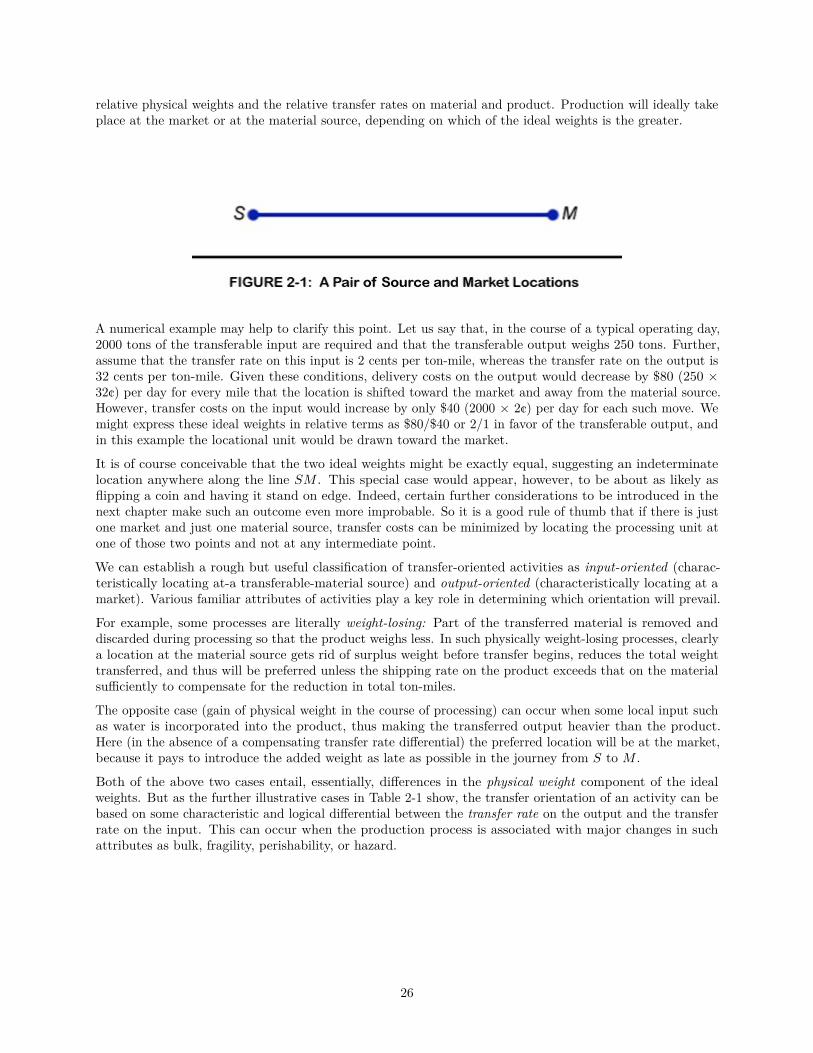
relative physical weights and the relative transfer rates on material and product. Production will ideally takeplace at the market or at the material source, depending on which of the ideal weights is the greater.

A numerical example may help to clarify this point. Let us say that, in the course of a typical operating day,2000 tons of the transferable input are required and that the transferable output weighs 250 tons. Further,assume that the transfer rate on this input is 2 cents per ton-mile, whereas the transfer rate on the output is32 cents per ton-mile. Given these conditions, delivery costs on the output would decrease by $80 (250 ×32¢) per day for every mile that the location is shifted toward the market and away from the material source.However, transfer costs on the input would increase by only $40 (2000 × 2¢) per day for each such move. Wemight express these ideal weights in relative terms as $80/$40 or 2/1 in favor of the transferable output, andin this example the locational unit would be drawn toward the market.

It is of course conceivable that the two ideal weights might be exactly equal, suggesting an indeterminatelocation anywhere along the line SM . This special case would appear, however, to be about as likely asflipping a coin and having it stand on edge. Indeed, certain further considerations to be introduced in thenext chapter make such an outcome even more improbable. So it is a good rule of thumb that if there is justone market and just one material source, transfer costs can be minimized by locating the processing unit atone of those two points and not at any intermediate point.

We can establish a rough but useful classification of transfer-oriented activities as input-oriented (charac-teristically locating at-a transferable-material source) and output-oriented (characteristically locating at amarket). Various familiar attributes of activities play a key role in determining which orientation will prevail.

For example, some processes are literally weight-losing: Part of the transferred material is removed anddiscarded during processing so that the product weighs less. In such physically weight-losing processes, clearlya location at the material source gets rid of surplus weight before transfer begins, reduces the total weighttransferred, and thus will be preferred unless the shipping rate on the product exceeds that on the materialsufficiently to compensate for the reduction in total ton-miles.

The opposite case (gain of physical weight in the course of processing) can occur when some local input suchas water is incorporated into the product, thus making the transferred output heavier than the product.Here (in the absence of a compensating transfer rate differential) the preferred location will be at the market,because it pays to introduce the added weight as late as possible in the journey from S to M .

Both of the above two cases entail, essentially, differences in the physical weight component of the idealweights. But as the further illustrative cases in Table 2-1 show, the transfer orientation of an activity can bebased on some characteristic and logical differential between the transfer rate on the output and the transferrate on the input. This can occur when the production process is associated with major changes in suchattributes as bulk, fragility, perishability, or hazard.

26

Processing activities of course usually result in a product more valuable than the required amount oftransferred inputs; and for a number of good reasons, transfer rates tend to be higher on more valuablecommodities. Risk of damage or pilferage is greater; there is a greater interest cost on the working capital tied

27

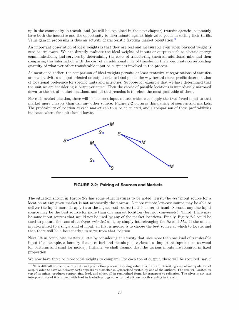
up in the commodity in transit; and (as will be explained in the next chapter) transfer agencies commonlyhave both the incentive and the opportunity to discriminate against high-value goods in setting their tariffs.Value gain in processing is thus an activity characteristic favoring market orientation.9

An important observation of ideal weights is that they are real and measurable even when physical weight iszero or irrelevant. We can directly evaluate the ideal weights of inputs or outputs such as electric energy,communications, and services by determining the costs of transferring them an additional mile and thencomparing this information with the cost of an additional mile of transfer on the appropriate correspondingquantity of whatever other transferable input or output is involved in the process.

As mentioned earlier, the comparison of ideal weights permits at least tentative categorizations of transfer-oriented activities as input-oriented or output-oriented and points the way toward more specific determinationof locational preference for specific units and activities. Suppose for example that we have determined thatthe unit we are considering is output-oriented. Then the choice of possible locations is immediately narroweddown to the set of market locations, and all that remains is to select the most profitable of these.

For each market location, there will be one best input source, which can supply the transferred input to thatmarket more cheaply than can any other source. Figure 2-2 pictures this pairing of sources and markets.The profitability of location at each market can thus be calculated, and a comparison of these profitabilitiesindicates where the unit should locate.

The situation shown in Figure 2-2 has some other features to be noted. First, the best input source for alocation at any given market is not necessarily the nearest. A more remote low-cost source may be able todeliver the input more cheaply than the higher-cost source that is closer at hand. Second, any one inputsource may be the best source for more than one market location (but not conversely). Third, there maybe some input sources that would not be used by any of the market locations. Finally, Figure 2-2 could beused to picture the ease of an input-oriented unit, by simply interchanging the Ss and Ms. If the unit isinput-oriented to a single kind of input, all that is needed is to choose the best source at which to locate, andthen there will be a best market to serve from that location.

Next, let us complicate matters a little by considering an activity that uses more than one kind of transferableinput (for example, a foundry that uses fuel and metals plus various less important inputs such as woodfor patterns and sand for molds). Initially we shall assume that the various inputs are required in fixedproportion.

We now have three or more ideal weights to compare. For each ton of output, there will be required, say, x9It is difficult to conceive of a rational production process involving value loss. But an interesting case of manipulation of

output value to save on delivery costs appears at a smelter in Queensland visited by one of the authors. The smelter, located ontop of its mines, produces copper, zinc, lead, and silver, all in semirefined form, for transport to refineries. The silver is not castinto pigs; instead it is mixed with lead in lead-silver pigs so as to make it less worth stealing in transit.

28

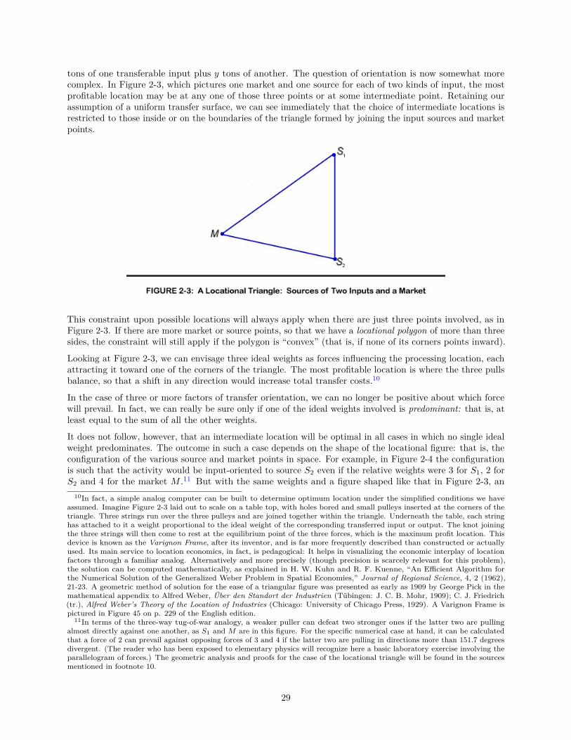
tons of one transferable input plus y tons of another. The question of orientation is now somewhat morecomplex. In Figure 2-3, which pictures one market and one source for each of two kinds of input, the mostprofitable location may be at any one of those three points or at some intermediate point. Retaining ourassumption of a uniform transfer surface, we can see immediately that the choice of intermediate locations isrestricted to those inside or on the boundaries of the triangle formed by joining the input sources and marketpoints.

This constraint upon possible locations will always apply when there are just three points involved, as inFigure 2-3. If there are more market or source points, so that we have a locational polygon of more than threesides, the constraint will still apply if the polygon is “convex” (that is, if none of its corners points inward).

Looking at Figure 2-3, we can envisage three ideal weights as forces influencing the processing location, eachattracting it toward one of the corners of the triangle. The most profitable location is where the three pullsbalance, so that a shift in any direction would increase total transfer costs.10

In the case of three or more factors of transfer orientation, we can no longer be positive about which forcewill prevail. In fact, we can really be sure only if one of the ideal weights involved is predominant: that is, atleast equal to the sum of all the other weights.

It does not follow, however, that an intermediate location will be optimal in all cases in which no single idealweight predominates. The outcome in such a case depends on the shape of the locational figure: that is, theconfiguration of the various source and market points in space. For example, in Figure 2-4 the configurationis such that the activity would be input-oriented to source S2 even if the relative weights were 3 for S1, 2 forS2 and 4 for the market M .11 But with the same weights and a figure shaped like that in Figure 2-3, an

10In fact, a simple analog computer can be built to determine optimum location under the simplified conditions we haveassumed. Imagine Figure 2-3 laid out to scale on a table top, with holes bored and small pulleys inserted at the corners of thetriangle. Three strings run over the three pulleys and are joined together within the triangle. Underneath the table, each stringhas attached to it a weight proportional to the ideal weight of the corresponding transferred input or output. The knot joiningthe three strings will then come to rest at the equilibrium point of the three forces, which is the maximum profit location. Thisdevice is known as the Varignon Frame, after its inventor, and is far more frequently described than constructed or actuallyused. Its main service to location economics, in fact, is pedagogical: It helps in visualizing the economic interplay of locationfactors through a familiar analog. Alternatively and more precisely (though precision is scarcely relevant for this problem),the solution can be computed mathematically, as explained in H. W. Kuhn and R. F. Kuenne, “An Efficient Algorithm forthe Numerical Solution of the Generalized Weber Problem in Spatial Economies,” Journal of Regional Science, 4, 2 (1962),21-23. A geometric method of solution for the ease of a triangular figure was presented as early as 1909 by George Pick in themathematical appendix to Alfred Weber, Über den Standort der Industrien (Tübingen: J. C. B. Mohr, 1909); C. J. Friedrich(tr.), Alfred Weber’s Theory of the Location of Industries (Chicago: University of Chicago Press, 1929). A Varignon Frame ispictured in Figure 45 on p. 229 of the English edition.

11In terms of the three-way tug-of-war analogy, a weaker puller can defeat two stronger ones if the latter two are pullingalmost directly against one another, as S1 and M are in this figure. For the specific numerical case at hand, it can be calculatedthat a force of 2 can prevail against opposing forces of 3 and 4 if the latter two are pulling in directions more than 151.7 degreesdivergent. (The reader who has been exposed to elementary physics will recognize here a basic laboratory exercise involving theparallelogram of forces.) The geometric analysis and proofs for the case of the locational triangle will be found in the sourcesmentioned in footnote 10.

29

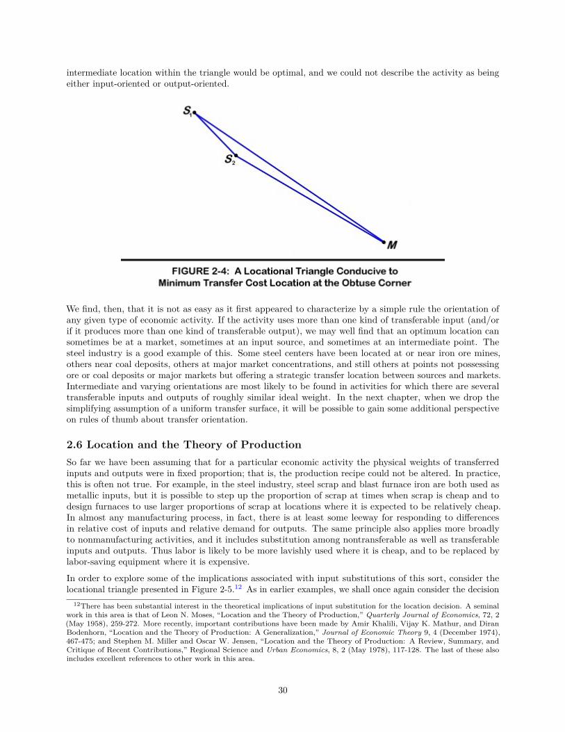
intermediate location within the triangle would be optimal, and we could not describe the activity as beingeither input-oriented or output-oriented.

We find, then, that it is not as easy as it first appeared to characterize by a simple rule the orientation ofany given type of economic activity. If the activity uses more than one kind of transferable input (and/orif it produces more than one kind of transferable output), we may well find that an optimum location cansometimes be at a market, sometimes at an input source, and sometimes at an intermediate point. Thesteel industry is a good example of this. Some steel centers have been located at or near iron ore mines,others near coal deposits, others at major market concentrations, and still others at points not possessingore or coal deposits or major markets but offering a strategic transfer location between sources and markets.Intermediate and varying orientations are most likely to be found in activities for which there are severaltransferable inputs and outputs of roughly similar ideal weight. In the next chapter, when we drop thesimplifying assumption of a uniform transfer surface, it will be possible to gain some additional perspectiveon rules of thumb about transfer orientation.

2.6 Location and the Theory of ProductionSo far we have been assuming that for a particular economic activity the physical weights of transferredinputs and outputs were in fixed proportion; that is, the production recipe could not be altered. In practice,this is often not true. For example, in the steel industry, steel scrap and blast furnace iron are both used asmetallic inputs, but it is possible to step up the proportion of scrap at times when scrap is cheap and todesign furnaces to use larger proportions of scrap at locations where it is expected to be relatively cheap.In almost any manufacturing process, in fact, there is at least some leeway for responding to differencesin relative cost of inputs and relative demand for outputs. The same principle also applies more broadlyto nonmanufacturing activities, and it includes substitution among nontransferable as well as transferableinputs and outputs. Thus labor is likely to be more lavishly used where it is cheap, and to be replaced bylabor-saving equipment where it is expensive.

In order to explore some of the implications associated with input substitutions of this sort, consider thelocational triangle presented in Figure 2-5.12 As in earlier examples, we shall once again consider the decision

12There has been substantial interest in the theoretical implications of input substitution for the location decision. A seminalwork in this area is that of Leon N. Moses, “Location and the Theory of Production,” Quarterly Journal of Economics, 72, 2(May 1958), 259-272. More recently, important contributions have been made by Amir Khalili, Vijay K. Mathur, and DiranBodenhorn, “Location and the Theory of Production: A Generalization,” Journal of Economic Theory 9, 4 (December 1974),467-475; and Stephen M. Miller and Oscar W. Jensen, “Location and the Theory of Production: A Review, Summary, andCritique of Recent Contributions,” Regional Science and Urban Economics, 8, 2 (May 1978), 117-128. The last of these alsoincludes excellent references to other work in this area.

30

of a locational unit with two transferable inputs (x1 located at S1 and x2 located atS2) and one transferableoutput with a market located at M . To focus attention on the effects of input substitution, we shall takedelivery costs as given by limiting our consideration to locations I and J , which are equidistant from themarket, and we shall assume that the same production technology is applicable at either location. The arcIJincludes additional locations at that same distance from the market, which we shall consider later.

The delivered price of a transferable input is its price at the source plus transfer charges. In the presentexample, there are two such inputs, x1 and x2. Their delivered prices are respectively

p′1 = p1 + r1d1

and (1)

p′2 = p2 + r2d2

where p1 and p2 are the prices of each input at is source, and r1 and r2 represent transfer rates per unitdistance for these inputs. The distance from each source to a particular location such as I or J is given by d1and d2.

It is significant that the relative prices of the two inputs will not be the same at I as at J . Location I iscloser than J to the source of x1, but farther away from the source of x2. So in terms of delivered prices, x1is relatively cheaper at I and x2 is relatively cheaper at J . The total outlay (TO) of the locational unit ontransferable inputs is

TO = p′1x1 + p′2x2 (2)

This equation may be reexpressed as

x1 = (TO/p′1)− (p′2/p′1)x2 (3)

31

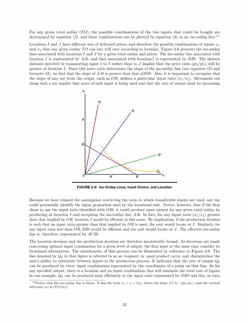
For any given total outlay (TO), the possible combinations of the two inputs that could be bought aredetermined by equation (2), and these combinations can be plotted by equation (3) as an iso-outlay line.13

Locations I and J have different sets of delivered prices, and therefore the possible combinations of inputs x1and x2 that any given outlay TO can buy will vary according to location. Figure 2-6 presents the iso-outlaylines associated with locations I and J for a given total outlay and prices. The iso-outlay line associated withlocation I is represented by AA′, and that associated with locationJ is represented by BB′. The shorterdistance involved in transporting input 1 to I rather than to J implies that the price ratio (p′2/p′1) will begreater at location I. Since this price ratio determines the slope of the iso-outlay line (see equation (3) andfootnote 13), we find that the slope of AA′ is greater than that ofBB′. Also, it is important to recognize thatthe slope of any ray from the origin, such as OR, defines a particular input ratio (x1/x2). Movement outalong such a ray implies that more of each input is being used and that the rate of output must be increasing.

Because we have relaxed the assumption restricting the ratio in which transferable inputs are used, any raycould potentially identify the input proportion used by the locational unit. Notice, however, that if the firmchose to use the input ratio identified with OR′, it could produce more output for any given total outlay byproducing at location I and accepting the iso-outlay line AA′. In fact, for any input ratio (x1/x2) greaterthan that implied by OR, location I would be efficient in this sense. By implication, if the production decisionis such that an input ratio greater than that implied by OR is used, the unit would locate at I. Similarly, forany input ratio less than OR,BB′ would be efficient and the unit would locate at J . The effective iso-outlayline is, therefore, represented by ACB′.

The location decision and the production decision are therefore inextricably bound. As decisions are madeconcerning optimal input combination for a given level of output, the firm must at the same time consider itslocational alternatives. The simultaneity of this process can be illustrated by reference to Figure 2-6. Theline denoted by Q0 in that figure is referred to as an isoquant, or equal product curve, and characterizes theunit’s ability to substitute between inputs in the production process. It indicates that the rate of output Q0can be produced by every input combination represented by the coordinates of a point on that line. So forany specified output, there is a location and an input combination that will minimize the total cost of inputs.In our example, Q0 can be produced most efficiently at the input ratio represented by OR′′ and this, in turn,

13Notice that the iso-outlay line is linear. It has the form x1 = α+ βx2, where the slope (β) is - (p′2/p′1), and the verticalintercept (α) is (TO/p′1).

32

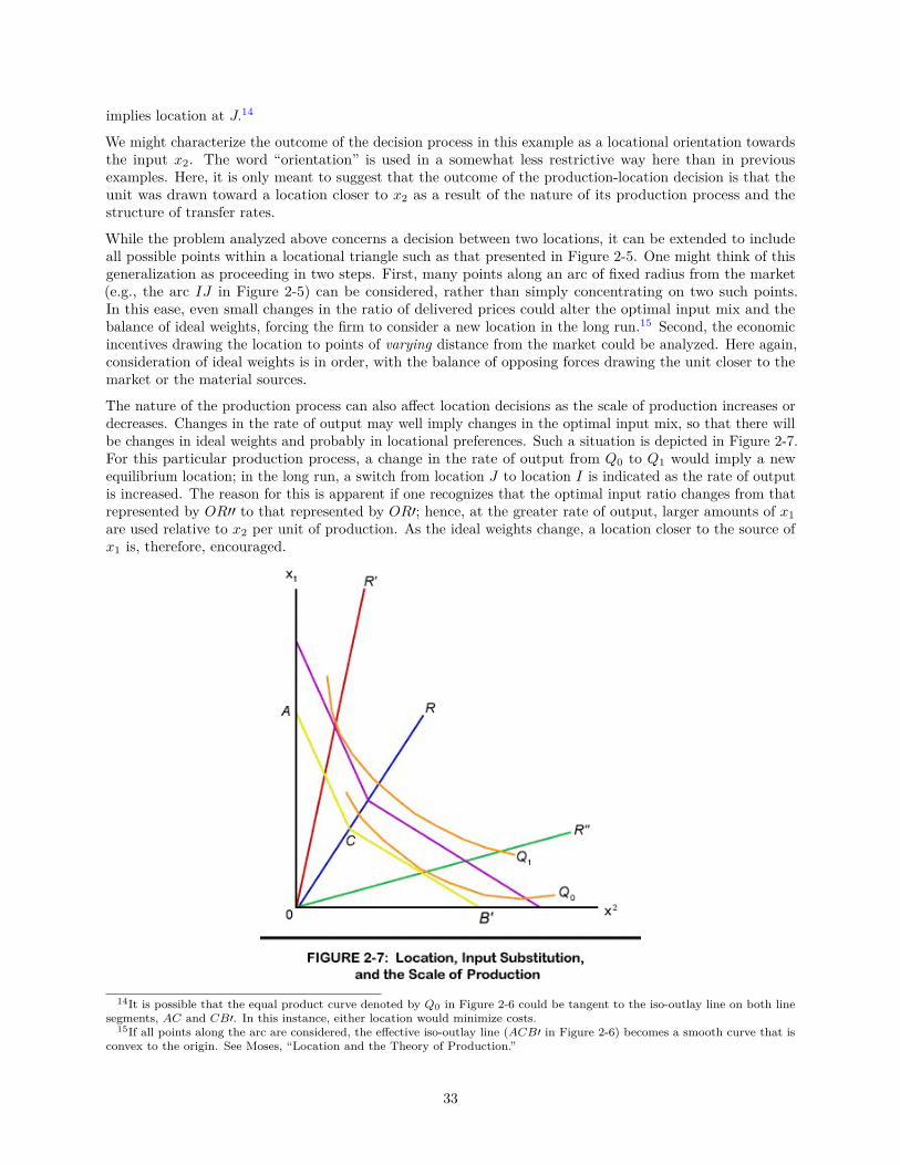
implies location at J.14

We might characterize the outcome of the decision process in this example as a locational orientation towardsthe input x2. The word “orientation” is used in a somewhat less restrictive way here than in previousexamples. Here, it is only meant to suggest that the outcome of the production-location decision is that theunit was drawn toward a location closer to x2 as a result of the nature of its production process and thestructure of transfer rates.

While the problem analyzed above concerns a decision between two locations, it can be extended to includeall possible points within a locational triangle such as that presented in Figure 2-5. One might think of thisgeneralization as proceeding in two steps. First, many points along an arc of fixed radius from the market(e.g., the arc IJ in Figure 2-5) can be considered, rather than simply concentrating on two such points.In this ease, even small changes in the ratio of delivered prices could alter the optimal input mix and thebalance of ideal weights, forcing the firm to consider a new location in the long run.15 Second, the economicincentives drawing the location to points of varying distance from the market could be analyzed. Here again,consideration of ideal weights is in order, with the balance of opposing forces drawing the unit closer to themarket or the material sources.

The nature of the production process can also affect location decisions as the scale of production increases ordecreases. Changes in the rate of output may well imply changes in the optimal input mix, so that there willbe changes in ideal weights and probably in locational preferences. Such a situation is depicted in Figure 2-7.For this particular production process, a change in the rate of output from Q0 to Q1 would imply a newequilibrium location; in the long run, a switch from location J to location I is indicated as the rate of outputis increased. The reason for this is apparent if one recognizes that the optimal input ratio changes from thatrepresented by OR′′ to that represented by OR′; hence, at the greater rate of output, larger amounts of x1are used relative to x2 per unit of production. As the ideal weights change, a location closer to the source ofx1 is, therefore, encouraged.

14It is possible that the equal product curve denoted by Q0 in Figure 2-6 could be tangent to the iso-outlay line on both linesegments, AC and CB′. In this instance, either location would minimize costs.

15If all points along the arc are considered, the effective iso-outlay line (ACB′ in Figure 2-6) becomes a smooth curve that isconvex to the origin. See Moses, “Location and the Theory of Production.”

33

It is possible also that increases in the scale of operations may imply less than proportionate increases in therequirements for one or more of the transferred inputs. Thus large-scale steel making may yield some savingsin fuel requirements per ton of output. Operations that have this characteristic would be drawn toward themarket, because the ideal weight of the inputs decreases relative to that of the final product with increases inthe scale of production.

However, contrary forces may also be evidenced. Increases in scale may require the use of more transferableinputs and fewer local inputs per unit of output—for example, using more material and less labor. Inthis instance, the ideal weight of the final product may actually be reduced relative to the ideal weight oftransferable inputs. Orientation would then be shifted away from the market.

Thus valid generalizations concerning the effect of the scale of production on location decisions are difficultto make.16 Indeed, at a practical level, changes in scale and changes in technology often go hand in hand,lessening the usefulness of analysis based on production processes currently employed. The essential pointis that one must look to changes in ideal weights in order to assess changes in locational orientation. Asrelative prices or the scale of operations change over time, ideal weights may be affected.

2.7 Scale Economies and Multiple Markets or SourcesAnother simplifying assumption that we applied in our discussion of transfer orientation was that a unitdisposes of all its output at one market and obtains all its supply of each input from one source. This accordswith reality in many, but by no means all, cases. If a seller’s economies of scale lead it to produce an outputthat is substantial in relation to the total demand for that output at a single market, it will face a less thanperfectly elastic demand in any one market and it may be profitable for it to sell in such additional marketsas are accessible. In that event, the location factor of “access to market” will entail nearness not just to onepoint, but to a number of points or a market area. Similarly, it may find that it can get its supplies of anyparticular transferable input more cheaply by tapping more than one source if the supply at any one sourceis not perfectly elastic.

Figure 2-8 shows how we might, in principle, analyze the market-access advantages of a specific location interms of possible sales to a number of different market points. In this illustration, there are five markets inall, assumed to be located at progressively greater distances from the seller. If the demand curve at eachof those markets is identical in terms of quantities bought at any given delivered price (price of the goodsdelivered at the market), then the demand curves as seen by the seller (that is, in terms of quantities boughtat any given level of net receipts after transfer costs are deducted) will be progressively lower for the moredistant markets. This is shown by the series of five steeply sloping lines in the left-hand part of the figure. Ifwe now add up the sales that can be made in all markets combined, for each level of net receipts, we obtainthe aggregate demand curve pictured by the broken line ABCDEFG. For example, at a net received priceof OH (after covering transfer costs) it is possible to sell HI,HJ,HK,HL, and HM in the five marketsrespectively. His total sales will be HF , which is the sum of HM plus MN (= HL) plus NP (= HK) plusPQ (= HJ) plus QF (= HI).

16The modern literature on this subject ignores possible interactions between transferable and local inputs as the scale ofproduction increases (see the references in footnote 12). Interactions of this sort are common and have been of some historicalimportance in location decisions. Thus while a number of conclusions can be drawn concerning locational orientation and thenature of the production process when the separability of transferable and local inputs is assumed, the usefulness of these resultsis severely limited.

34

This aggregate demand schedule and the costs of operating at the location in question will determine whatprofits can be made there by choosing the optimum price and output level,17 At possible alternative locations,both market and cost conditions will presumably be different, giving rise to spatial differentials in profitpossibilities.

Although the foregoing may describe fairly well what determines the likelihood of success at a given location,it is hardly a realistic description of the kind of analysis that underlies most location decisions. Followingare descriptions of some cruder procedures for gauging access advantage of locations in the absence ofcomprehensive data.

2.8 Some Operational ShortcutsFor simplicity’s sake, let us consider just the question of evaluating access to multiple markets. If, for example,a market-oriented producer seeks the best location from which to serve markets in fifty major cities in theUnited States, how might it proceed?

What it wants is some sort of “geographical center” of the set of fifty markets. Suppose that this centerwere to be defined as a median point so located that half of the aggregate market lay to the north and halfto the south of it, and likewise half to the east and half to the west18 Then (if it were to be assumed that

17The concepts of demand in space and spatial pricing are discussed in Chapter 4.18For a uniform transfer surface, this can be done by preparing a map showing the sales volume of each market noted at its

proper location. Align a ruler north and south and push it across the map from one edge, keeping track of the total sales volumeof markets passed as the ruler advances. Stopping when that total equals half of the aggregate sales volume for all markets,draw a vertical line. Repeating the process with the ruler held horizontally and moved gradually from top or bottom, get ahorizontal line in similar fashion. The intersection of the two lines is the required minimum transport cost point.

35

transport occurs only on a rectilinear grid of routes) the producer would have the location from which thetotal ton-miles of transport entailed in serving all markets would be a minimum. This is an application ofthe principle of median location.

Naturally, a number of objections might be made to this procedure. One of the most obvious is that itis illogical to assume that our producer’s sales pattern is independent of its location. It would be morereasonable to assume that the producer would have a smaller share of the total sales in markets more remotefrom its location, reflecting higher transport charges and other aspects of competitive disadvantage.

One way to get around this difficulty would be to decide that the producer is really primarily interestedin market possibilities only within, say, a radius of 400 miles, or only within the range of overnight truckdelivery. It could then demarcate such areas around various points and select as its location the center of thearea having the largest market volume.

A somewhat more sophisticated procedure would be to apply a systematic distance discount in the evaluationof markets by calculating what is called an index of market access potential for each of a number of possiblelocations. Thus to compute the potential index Pi for any specific production location (i), the producerwould divide the sales volume of each market (j) by the distanceDij from (i) to (j) and then add up all theresulting quotients. Such potential measures have been widely used, with the distance (or transport costs, ifascertainable) commonly raised to some power such as the square. If the square of the distance is used, thepotential formula becomes

Pi =∑j

(Mj/DZij) (4)

(where M is market size and D is distance); and any given market has the same effect on the index as amarket four times as big but twice as far away. In any ease, when the potential index P has been calculatedfor various possible locations, the location having the largest P can then be rated best with respect to accessto the particular set of markets involved.

This measure of “potential,” in which each source of attraction has its value “discounted for distance,” is alsogenerically known as a gravity formula or model—particularly when the attractive value is deflated by thesquare of distance over which the attraction operates. The reference to gravity reflects analogy to Newton’slaw of gravitation (bodies attract one another in proportion to their masses and inversely in proportion to thesquare of the distance between them). William J. Reilly in 1929 proclaimed the Law of Retail Gravitation onthe basis of an observed rough conformity to this principle in the case of retail trading areas (a subject to beexamined in more detail in Chapter 8), and John Q. Stewart and a host of others subsequently discoveredgravity-type relationships in a wide variety of economic and social distributions. Gravity and potentialmeasures have in fact been applied to almost every important measurable type of human interaction involvingdistance, and numerous variants of the basic formula have been devised, some of which we shall have occasionto examine later.19 All the shortcut methods described here have been widely used. Though they have beenexplained here in terms of the measurement of access to markets, or output access of potential locations, theyare equally applicable to assessment of the input access potential of locations, when a unit is drawing onmore than one source of the same transferable input. The measures can apply also to cases involving thetransfer of services rather than goods—for example, measuring the job-access potential of various residencelocations where a choice of job opportunities is desirable, or measuring the labor-supply access potential ofalternative locations for an employer.

But at best, when a unit can serve many markets and/or draw from many input sources, the appraisal ofalternative locations in terms of access is a complex matter. There is likely to be little opportunity to use thesimple devices discussed earlier in this chapter, such as the balancing off of relative input and output weights,except perhaps as a means of initially narrowing down the range of locational alternatives. In such cases, the

19For a comprehensive survey of the literature on the theory and application of gravity models, see Gunnar Olsson, Distanceand Human Interaction: A Review and Bibliography (Philadelphia: Regional Science Research Institute, 1965), as well asChang-I Hua and Frank Porell, “A Review of the Development of the Gravity Model,” International Regional Science Review 4,2 (Winter 1979), 97-126.

36

maps of cost and revenue prospects will show complex contours rather than simple ones as in the examplesdiscussed earlier; and the evaluation of prospects at different locations will have to approach more nearly anexplicit calculation of the expected costs, revenues, and profits at various possible levels of output at each ofa large set of locations.

For most types of locational decision units, an exhaustive point-by-point approach in which theory andanalysis abdicate in favor of pure empiricism would be so expensive as to outweigh any gain from finallydetermining the ideal spot. So there will always be a vigorous demand for usable shortcuts, ways of narrowingdown the range of location choice, and better analytical techniques. The challenge to regional economists isto provide techniques better than hunch or inertia and cheaper than exhaustive canvassing of locations.

2.9 SummaryThis chapter deals with location at the level of the “location unit” as exemplified by a household, businessestablishment, school, or police station. Location in terms of larger aggregates such as multiestablishmentfirms or public agencies, industries, cities, and regions is taken up in later chapters. A single decision unit(for instance, a firm) can embrace one or more location units.

Prospective income is a major determinant of location preference, but even in the ease of business corporationsin which the profit motive is paramount there are other significant considerations, including security, amenity,and the manifold political and social aims of public and institutional policy. Uncertainties, risks, and thecosts of decision making and moving contribute to locational inertia and often to concentration.

The basis for locational preferences can be expressed generally in terms of a limited set of location factorsinvolving both supply of locally produced and transferable inputs, and demand for transferable outputssatisfied both locally and at a distance; the inputs and outputs include intangibles. Various techniques existfor assessing the relative strength of location factors affecting a specific decision or type of location unit.

Location factors themselves have characteristic spatial patterns of advantage. Some factors, such as rent,may be relevant chiefly in comparing locations on a microspatial (small area) basis; other factors may emergeas important for macrospatial comparisons, involving locations far apart. Some location factors are primarilyrelated to concentration: They may be most favorable in, say, large cities or dusters of activity or, alternatively,in small towns or rural locations. Other location factors involve transfer of input or output, so that locationaladvantage varies systematically according to distance. Other location factors, such as climate, depend whollyor mainly on natural geographic differentials; and still others, such as labor supply or taxes, have patternswhose origins and features may be quite complex and resistant to generalization.

Only the transfer-determined (distance-related) location factors are explored in detail in this chapter. Whena location unit’s locational preference depends primarily on transfer costs of input and/or output, the unit iscalled transfer-oriented; and, more specifically, it may also be input-oriented or output-oriented according towhether access to input sources or to markets for its output is the more important influence. If transfer costsper ton-mile are assumed to be uniform for all goods regardless of direction or distance (the assumption of auniform transfer surface), and if the unit has only one input source and one market for its output, orientationand location choice will depend simply on whether the transferred input used in a given period weighs moreor less than the corresponding transferred output.

If there is a total of three or more input sources plus markets, the orientation is definite only if one of theweights is predominant (exceeding all the others combined). Otherwise, the orientation will depend partly onthe spatial configuration of the input source and markets.

Differences among ton-mile transfer rates for different goods can be allowed for in the determination ofoptimum location by replacing the relative physical weights of inputs and outputs with “ideal weights.”Output orientation is encouraged not only by weight gain in the production process but also by gains in bulk,perishability, fragility, hazard, or value. Input orientation is encouraged by losses in these attributes.

While most of the analysis in this chapter has assumed that the production recipe requires that inputsare used in fixed proportion, we have recognized the implications that follow when flexibility of input useis allowed. In this instance, locators will adapt their input mix to the relative prices of the substitutable

37

inputs at various locations. This increases the number of locations worth considering and means that theproduction-technique decision and the location decision are interdependent. Further, as the scale of operationchanges, the nature of the production process helps to determine whether larger-scale operations encourageorientation toward sources of transferable inputs or toward the market.

In real life, access advantages of location must often be assessed in terms of access to a whole set of marketsand/or a whole set of input sources, and explicit comparative calculations of probable sales, receipts, andcosts at each location may be prohibitively difficult. A number of practical shortcut procedures have beendeveloped for evaluating access factors of location under such conditions; they include a gravity formula, inwhich the attraction of a market or an input source is systematically discounted according to its distancefrom the location whose advantages are being assessed.

The analysis presented in this chapter is based on a model that concentrates attention on transfer factors,neglecting in the process some other potentially important considerations. For example, the effects ofprocessing costs on location decisions are recognized explicitly only to the extent that those costs are affectedby substitution possibilities in the production process. Further, while the importance of multiple marketshas been noted, many other issues concerning demand in space have been set aside for the time being. Inthe following chapter, we consider in additional detail the effects that transfer cost considerations may haveon location choices. In Chapter 4 our attention will turn to issues concerning demand and spatial pricingdecisions and then, in Chapter 5, to economies of concentration as they may affect processing costs.

Technical Terms Introduced in this ChapterLocation unit Weight-losing and weight-gaining activitiesLocation decision unit Locational polygonLocation factor Varignon FrameLocal (or nontransferable) inputs and outputs Predominant weightTransferable inputs and outputs Market or supply areaMacrogeographic Median location principleMicrogeographic Distance discountDelivered price Access potentialUbiquity Gravity formulaOrientation Reilly’s Law of Retail GravitationUniform transfer surface

Selected ReadingsEdgar M. Hoover, The Location of Economic Activity (New York: McGraw-Hill, 1948).

Gerald J. Karaska and David F. Bramhall (eds.), Locational Analysis for Manufacturing (Cambridge, MA:MIT Press, 1969).

Steven M. Miller and Oscar W. Jensen, “Location and the Theory of Production: A Review, Summary, andCritique of Recent Contributions,” Regional Science and Urban Economics 8, 2 (May 1978), 117-128.

Leon N. Moses, “Location and the Theory of Production,” Quarterly Journal of Economics, 72, 2 (May 1958),259-272.

Jean H. Paelinek and Peter Nijkamp, Operational Theory and Method in Regional Economics (Lexington,MA: Lexington Books, D. C. Heath, 1976), Chapters 2-3.

Harry W. Richardson, Regional Economics (Urbana: University of Illinois Press, 1978), Chapter 3.

Roger W. Schmenner, Making Business Location Decisions (Englewood Cliffs, NJ: Prentice-Hall 1982).

Michael J. Webber, Impact of Uncertainty on Location (Cambridge, MA: MIT Press, 1972).

38

Alfred Weber, Über den Standort der Industrien (Tübingen: J. C. B. Mohr, 1909); C. J. Friedrich (tr.), AlfredWeber’s Theory of the Location of Industries (Chicago: University of Chicago Press, 1929).

39

3. TRANSFER COSTS3.1 IntroductionThe discussion of individual locations in the previous chapter placed many restrictions on the nature oftransport costs for the sake of exposing some fundamental characteristics of location decisions. While werecognized that in the real world different kinds of inputs and outputs are transferred at different costs andthat weight is often an inappropriate measure of input and output quantity, we assumed that transfer costsalong a route were proportional to distance. Further, we ignored the fact that transfer generally has to followan established route between established terminal service points rather than going as the crow flies. We alsofailed to distinguish between money costs, time costs, and still other kinds of costs entailed in transfer andignored the great differences in cost and service capabilities of different techniques or modes of transfer, aswell as the distinction between costs to the transfer firm or agency and costs to the user of transfer service.

In this chapter we hasten to remedy these omissions in order to get a more realistic understanding of howtransfer costs affect the location of activities.

3.2 Some Economic Characteristics of Transfer OperationsIt is much easier to develop an understanding of the complex variations of transfer services, costs, and ratesif we first note some basic economic characteristics of transfer activities in general.

In transfer operations (except for a few primitive types) substantial components of the costs are fixed—thatis, they reflect overall and longrun commitments such as the provision and maintenance of right of way andterminals. Partly for this reason, transfer operations are characteristically subject to important economies ofscale. Costs per unit of service tend to be lower (and service more convenient and faster) on routes with largervolumes of traffic. Likewise, costs are generally lower when larger quantities are moved in single-movementunits (for example, ships, trains, or aircraft). There are additional savings in transfer cost when the singleconsignment (that is, what is moved at one time from one specific location unit to another) is larger. Some ofthese scale economies apply principally to costs of actual movement between locations, and others principallyto costs of establishing and operating terminals and such operations as selling, accounting, and billing.

Because of these characteristics, firms or public agencies providing transfer services generally serve many pairsof points and many different classes of customers, and operate with a substantial element of monopolisticcontrol rather than in perfect competition. The rates for the various services rendered can be set so as torecoup disproportionate shares of the transfer operation’s fixed costs from rates on those services for whichdemand is least elastic—to “charge what the traffic will bear.”

Finally, human ingenuity has continually devised new technologies or modes of transfer to serve variousspecial purposes. Although each new mode may partly supplant an older one, it is rare for any mode todisappear completely. Somewhere in the world there is still in use nearly every transfer mode ever devised.Each mode has special advantages for a certain range of services, and is thus partly competitive and partlycomplementary to other modes.

As Table 3-1 shows, transfer operations can be classified according to means or according to purpose. Thepurposes of transfer are to move people, goods, energy, or information from one place to another—informationbeing broadly defined to include queries, aesthetic and emotional effects, and in fact all messages via any ofthe senses.

40

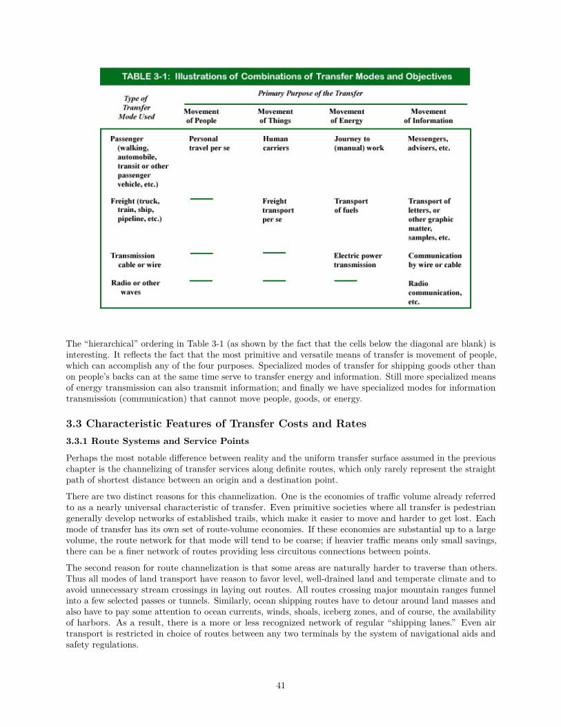
The “hierarchical” ordering in Table 3-1 (as shown by the fact that the cells below the diagonal are blank) isinteresting. It reflects the fact that the most primitive and versatile means of transfer is movement of people,which can accomplish any of the four purposes. Specialized modes of transfer for shipping goods other thanon people’s backs can at the same time serve to transfer energy and information. Still more specialized meansof energy transmission can also transmit information; and finally we have specialized modes for informationtransmission (communication) that cannot move people, goods, or energy.

3.3 Characteristic Features of Transfer Costs and Rates3.3.1 Route Systems and Service Points

Perhaps the most notable difference between reality and the uniform transfer surface assumed in the previouschapter is the channelizing of transfer services along definite routes, which only rarely represent the straightpath of shortest distance between an origin and a destination point.

There are two distinct reasons for this channelization. One is the economies of traffic volume already referredto as a nearly universal characteristic of transfer. Even primitive societies where all transfer is pedestriangenerally develop networks of established trails, which make it easier to move and harder to get lost. Eachmode of transfer has its own set of route-volume economies. If these economies are substantial up to a largevolume, the route network for that mode will tend to be coarse; if heavier traffic means only small savings,there can be a finer network of routes providing less circuitous connections between points.

The second reason for route channelization is that some areas are naturally harder to traverse than others.Thus all modes of land transport have reason to favor level, well-drained land and temperate climate and toavoid unnecessary stream crossings in laying out routes. All routes crossing major mountain ranges funnelinto a few selected passes or tunnels. Similarly, ocean shipping routes have to detour around land masses andalso have to pay some attention to ocean currents, winds, shoals, iceberg zones, and of course, the availabilityof harbors. As a result, there is a more or less recognized network of regular “shipping lanes.” Even airtransport is restricted in choice of routes between any two terminals by the system of navigational aids andsafety regulations.

41

Any kind of communications system requiring either fixed-line facilities (such as cables) or relay stations islikewise constrained to a limited set of routes. Transfer is really “as the crow flies” only within the range ofdirect wave or beam transmission.

Scale economies apply not only to route facilities such as trails, track, roads, pipelines, cable, and navigationalaids, but also to “service points” where transfer by the mode in question can originate and terminate. Thusthere are certain minimum costs of establishing a railroad station or even a siding; the same applies topiggyback terminals, ports for ships and aircraft, transformer stations on long-distance electric transmissionlines, and telephone exchanges and switchboards. There is an economic constraint on the spacing of transitstops along a route, since more stops slow the service. People making shopping trips generally prefer to do alltheir errands with a minimum number of separate stops—except for those who view shopping as a recreation.

Consequently, the pattern of transfer services offered by any particular mode is always spotty, linking up alimited number of pairs of points by routes usually longer than the straight-line distance; and a transfer of aspecific shipment, person, or item of information from initial origin to final destination frequently entails theuse of more than one link or mode.

In addition to restricting the number of routes and service points, transfer scale economies in many instanceshave the effect of making costs and rates lower on more heavily used routes and to and from larger terminals.This works in several ways. In some cases, it is primarily a question of direct cost reduction associated withvolume. Thus a larger-diameter pipeline requires less material and less pumping energy per unit volumecarried, and a four-lane highway can carry more than twice as much traffic as a two-lane highway, with lessthan twice as wide a right of way if the median divider is narrow.

Similarly, terminals and other transfer service points can often operate more efficiently if they handle largevolumes of traffic. Examples are the huge specialized facilities for loading and unloading bulk cargoes such asgrain, coal, and ores, and the more specialized equipment found at large communications terminals.

But apart from and in addition to such volume-of-traffic savings in cost to the operator of individual transferservices, there are likely to be important advantages for the users of the services in terms of quality ofservice. Your letters will probably be delivered sooner if you put them in a heavily used mailbox from whichcollections are made more frequently. If you are shipping goods to a variety of destinations, it may pay tochoose a location near a large transport terminal, not only because the departures are more frequent but alsobecause there are direct connections to more points and a variety of special types of service.

3.3.2 Long-Haul Economies

Virtually every kind of transfer entails some operation at the point of origin prior to actual movement, andalso some further operation at the destination point. The cost of these “terminal” processes ordinarily doesnot depend on the distance to be traveled, whereas the costs of actual movement ordinarily do.

Because of these terminal costs, the relationship between route distance and the total costs of a shipmentwill generally behave as shown in Figure 3-1. Transfer costs are characteristically less than proportional todistance, and the average transfer cost per mile decreases as the length of haul increases. This principle is afundamental one and appears in every kind of transfer mode, even the simplest. When we leave our homes orwork places on various missions, there is almost always some act of preparation that imposes a terminal costin terms of time. Even if we go on foot, we may first have to make sure that we are acceptably clad againstthe strictures of convention or weather, turn off the television, put the dog out, and lock the door. If wedrive, the car has to be activated. If we use public transit, we have to wait for it to appear.

42

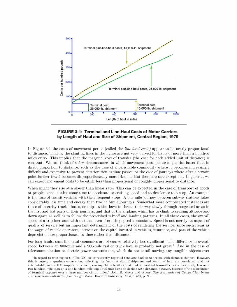
In Figure 3-1 the costs of movement per se (called the line-haul costs) appear to be nearly proportionalto distance. That is, the slanting lines in the figure are not very curved for hauls of more than a hundredmiles or so. This implies that the marginal cost of transfer (the cost for each added unit of distance) isconstant. We can think of a few circumstances in which movement costs per se might rise faster than indirect proportion to distance, such as the case of a perishable commodity where it becomes increasinglydifficult and expensive to prevent deterioration as time passes, or the case of journeys where after a certainpoint further travel becomes disproportionately more irksome. But these are rare exceptions. In general, wecan expect movement costs to be either less than proportional or roughly proportional to distance.

When might they rise at a slower than linear rate? This can be expected in the case of transport of goodsor people, since it takes some time to accelerate to cruising speed and to decelerate to a stop. An exampleis the case of transit vehicles with their frequent stops. A one-mile journey between subway stations takesconsiderably less time and energy than two half-mile journeys. Somewhat more complicated instances arethose of intercity trucks, buses, or ships, which have to thread their way slowly through congested areas inthe first and last parts of their journeys, and that of the airplane, which has to climb to cruising altitude anddown again as well as to follow the prescribed takeoff and landing patterns. In all these cases, the overallspeed of a trip increases with distance even if cruising speed is constant. Speed is not merely an aspect ofquality of service but an important determinant of the costs of rendering the service, since such items asthe wages of vehicle operators, interest on the capital invested in vehicles, insurance, and part of the vehicledepreciation are proportionate to time rather than distance.

For long hauls, such line-haul economies are of course relatively less significant. The difference in overallspeed between an 800-mile and a 900-mile rail or truck haul is probably not great.1 And in the case oftelecommunication or electric power transmission, which do not entail moving any tangible objects over

1In regard to trucking cost, “The ICC has consistently reported that line-haul costs decline with distance shipped. However,this is largely a spurious correlation, reflecting the fact that size of shipment and length of haul are correlated, and notattributable, as the ICC implies, to some operating characteristics that makes line-haul ton-mile costs substantially less on atwo-hundred-mile than on a one-hundred-mile trip Total unit costs do decline with distance, however, because of the distributionof terminal expense over a large number of ton miles.” John R. Meyer and others, The Economies of Competition in theTransportation Industries (Cambridge, Mass.: Harvard University Press, 1959), p. 93.

43

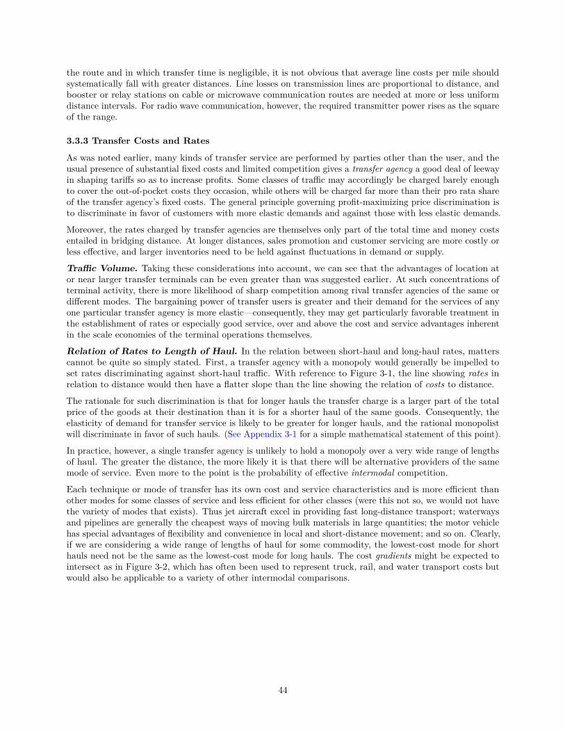
the route and in which transfer time is negligible, it is not obvious that average line costs per mile shouldsystematically fall with greater distances. Line losses on transmission lines are proportional to distance, andbooster or relay stations on cable or microwave communication routes are needed at more or less uniformdistance intervals. For radio wave communication, however, the required transmitter power rises as the squareof the range.

3.3.3 Transfer Costs and Rates

As was noted earlier, many kinds of transfer service are performed by parties other than the user, and theusual presence of substantial fixed costs and limited competition gives a transfer agency a good deal of leewayin shaping tariffs so as to increase profits. Some classes of traffic may accordingly be charged barely enoughto cover the out-of-pocket costs they occasion, while others will be charged far more than their pro rata shareof the transfer agency’s fixed costs. The general principle governing profit-maximizing price discrimination isto discriminate in favor of customers with more elastic demands and against those with less elastic demands.

Moreover, the rates charged by transfer agencies are themselves only part of the total time and money costsentailed in bridging distance. At longer distances, sales promotion and customer servicing are more costly orless effective, and larger inventories need to be held against fluctuations in demand or supply.

Traffic Volume. Taking these considerations into account, we can see that the advantages of location ator near larger transfer terminals can be even greater than was suggested earlier. At such concentrations ofterminal activity, there is more likelihood of sharp competition among rival transfer agencies of the same ordifferent modes. The bargaining power of transfer users is greater and their demand for the services of anyone particular transfer agency is more elastic—consequently, they may get particularly favorable treatment inthe establishment of rates or especially good service, over and above the cost and service advantages inherentin the scale economies of the terminal operations themselves.

Relation of Rates to Length of Haul. In the relation between short-haul and long-haul rates, matterscannot be quite so simply stated. First, a transfer agency with a monopoly would generally be impelled toset rates discriminating against short-haul traffic. With reference to Figure 3-1, the line showing rates inrelation to distance would then have a flatter slope than the line showing the relation of costs to distance.

The rationale for such discrimination is that for longer hauls the transfer charge is a larger part of the totalprice of the goods at their destination than it is for a shorter haul of the same goods. Consequently, theelasticity of demand for transfer service is likely to be greater for longer hauls, and the rational monopolistwill discriminate in favor of such hauls. (See Appendix 3-1 for a simple mathematical statement of this point).

In practice, however, a single transfer agency is unlikely to hold a monopoly over a very wide range of lengthsof haul. The greater the distance, the more likely it is that there will be alternative providers of the samemode of service. Even more to the point is the probability of effective intermodal competition.

Each technique or mode of transfer has its own cost and service characteristics and is more efficient thanother modes for some classes of service and less efficient for other classes (were this not so, we would not havethe variety of modes that exists). Thus jet aircraft excel in providing fast long-distance transport; waterwaysand pipelines are generally the cheapest ways of moving bulk materials in large quantities; the motor vehiclehas special advantages of flexibility and convenience in local and short-distance movement; and so on. Clearly,if we are considering a wide range of lengths of haul for some commodity, the lowest-cost mode for shorthauls need not be the same as the lowest-cost mode for long hauls. The cost gradients might be expected tointersect as in Figure 3-2, which has often been used to represent truck, rail, and water transport costs butwould also be applicable to a variety of other intermodal comparisons.

44

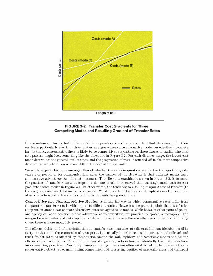
In a situation similar to that in Figure 3-2, the operators of each mode will find that the demand for theirservice is particularly elastic in those distance ranges where some alternative mode can effectively competefor the traffic; consequently, there is likely to be competitive rate cutting on those classes of traffic. The finalrate pattern might look something like the black line in Figure 3-2. For each distance range, the lowest-costmode determines the general level of rates, and the progression of rates is rounded off in the most competitivedistance ranges where two or more different modes share the traffic.

We would expect this outcome regardless of whether the rates in question are for the transport of goods,energy, or people or for communication, since the essence of the situation is that different modes havecomparative advantages for different distances. The effect, as graphically shown in Figure 3-2, is to makethe gradient of transfer rates with respect to distance much more curved than the single-mode transfer costgradients shown earlier in Figure 3-1. In other words, the tendency to a falling marginal cost of transfer (tothe user) with increased distance is accentuated. We shall see later the locational implications of this and theother characteristics of transfer cost and rate gradients being noted here.

Competitive and Noncompetitive Routes. Still another way in which comparative rates differ fromcomparative transfer costs is with respect to different routes. Between some pairs of points there is effectivecompetition among two or more alternative transfer agencies or modes, while between other pairs of pointsone agency or mode has such a cost advantage as to constitute, for practical purposes, a monopoly. Themargin between rates and out-of-pocket costs will be small where there is effective competition and largewhere there is more monopoly power.

The effects of this kind of discrimination on transfer rate structures are discussed in considerable detail inevery textbook on the economics of transportation, usually in reference to the structure of railroad andtruck freight rates as affected by competition among the rail, highway, and waterway modes and amongalternative railroad routes. Recent efforts toward regulatory reform have substantially lessened restrictionson rate-setting practices. Previously, complex pricing rules were often established in the interest of somerather elusive objectives of maintaining competition and preserving equities of particular areas and transport

45

agencies, which placed limits on rate-setting behavior of the sort just described. While the legacy of theseregulations is still in evidence, much more flexibility in rate setting is now permitted.

Discrimination Among Services and Commodities. The locational significance of transfer rate differ-entials among different goods or services was taken into account in our discussion of ideal weights in Chapter2. Let us now see how such differentials arise.

Some transfer services are by their nature costlier to provide than others, and we should expect to see suchdifferences reflected in rates. A ton of pingpong balls or automobile bodies is much bulkier than a ton ofsteel plates. Since extra bulk adds to transport cost in every mode of transport except possibly the use ofpack animals or human carriers, we are not surprised to see systematically higher freight rates per ton onbulky goods. This is one basis for the official commodity classifications governing regulated tariffs. Similarly,we should expect to pay more for shipping a perishable, fragile, or dangerous commodity (such as meat,glassware, or sulfuric acid). Extra-fast service and the carrying of small shipments are more expensive. Inpassenger transport it costs more to provide extra space and comfort. In addition, the marginal costs ofadded service at slack times are far less than at times of peak capacity use of the facilities, so that we are notsurprised to be charged more for a long-distance phone call during business hours, for using a parking lot onthe afternoon of a football game, or for crossing the Atlantic in summer.

None of the foregoing differentials in rates necessarily involves any discrimination on the part of the transferagency, since in every case there is an underlying difference in costs that is passed on to the user.

But there are still further systematic transfer rate differentials that reflect discriminatory rate-making policyrather than costs. In particular, we find that rates are high relative to costs for the transfer of things of highvalue, and low relative to costs for things of low value.

The rationale is essentially the same as that already adduced in the case of long versus short hauls; namely,that a seller’s profits are enhanced by discriminating against buyers with relatively inelastic demands and infavor of buyers with relatively elastic demands.

When a commodity such as cigarettes or scientific instruments, with a high value per pound, is shipped anygiven distance, transport costs will be a smaller part of the delivered price than will be the case when alow-value commodity such as coal or gravel is shipped the same distance. Consequently, the demand fortransport of cigarettes will be much less sensitive to the freight rate than will the demand for transport ofcoal, and any rational profit-seeking transport agency will charge a higher margin over out-of-pocket costs oncigarettes than on coal. Such discrimination, by the way, is not merely in the interest of the carrier but undersome conditions may serve the public interest as well, through promoting a more efficient allocation and useof resources. It may enable a greater amount of transfer service to be provided with any given amount ofinvestment in transfer facilities.

Consequently, we find that freight tariff classifications and special commodity rates rather systematicallyreflect the relative prices per ton of the various commodities, in addition to such other factors as have alreadybeen mentioned. This means that finished goods as a rule pay much higher freight rates than do theircomponent intermediate goods or raw materials, since production processes normally involve getting rid ofwaste components and adding value.

For the transfer of people and for communication, the measure of unit value corresponding to the priceper pound of a transported commodity is not so easy to assign or visualize. The basic rule of transfer ratediscrimination according to value still applies; but it is generally obscured by the fact that in the transport ofpeople and information, a “higher-value” consignment is given a qualitatively different transfer service.

When it is a question of passenger travel, people will set their own valuations simply in terms of how muchthey are willing to pay for a trip rather than forgo it. Transfer agencies do not attempt to charge what thetraffic will bear on a person-by-person and trip-by-trip basis but often provide special services (higher speed,greater comfort, and the like) to those willing to pay more. Similarly in the case of communications, it isgenerally impossible for the seller of the service to judge how valuable a particular transmission is to thecommunicator and charge accordingly; but a choice of different speeds or other qualities of service can be setup, and the rates for these can be adjusted in such a way as to reflect the estimated relative elasticities of

46

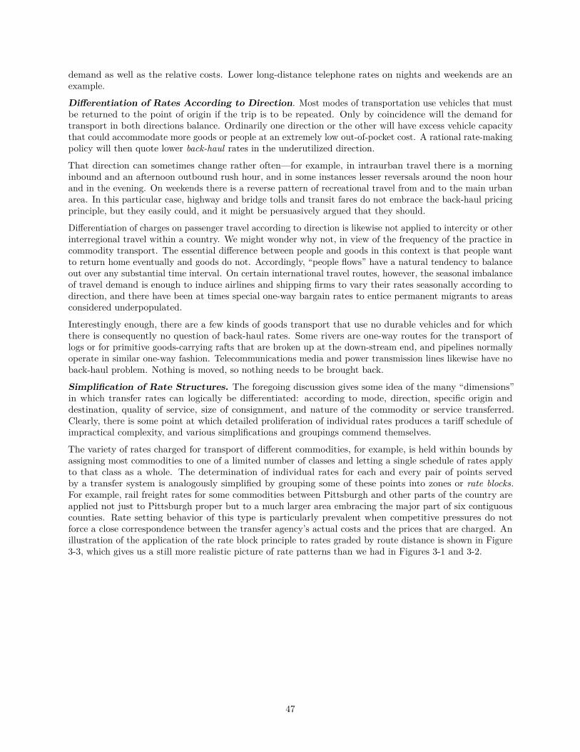
demand as well as the relative costs. Lower long-distance telephone rates on nights and weekends are anexample.

Differentiation of Rates According to Direction. Most modes of transportation use vehicles that mustbe returned to the point of origin if the trip is to be repeated. Only by coincidence will the demand fortransport in both directions balance. Ordinarily one direction or the other will have excess vehicle capacitythat could accommodate more goods or people at an extremely low out-of-pocket cost. A rational rate-makingpolicy will then quote lower back-haul rates in the underutilized direction.

That direction can sometimes change rather often—for example, in intraurban travel there is a morninginbound and an afternoon outbound rush hour, and in some instances lesser reversals around the noon hourand in the evening. On weekends there is a reverse pattern of recreational travel from and to the main urbanarea. In this particular case, highway and bridge tolls and transit fares do not embrace the back-haul pricingprinciple, but they easily could, and it might be persuasively argued that they should.

Differentiation of charges on passenger travel according to direction is likewise not applied to intercity or otherinterregional travel within a country. We might wonder why not, in view of the frequency of the practice incommodity transport. The essential difference between people and goods in this context is that people wantto return home eventually and goods do not. Accordingly, “people flows” have a natural tendency to balanceout over any substantial time interval. On certain international travel routes, however, the seasonal imbalanceof travel demand is enough to induce airlines and shipping firms to vary their rates seasonally according todirection, and there have been at times special one-way bargain rates to entice permanent migrants to areasconsidered underpopulated.

Interestingly enough, there are a few kinds of goods transport that use no durable vehicles and for whichthere is consequently no question of back-haul rates. Some rivers are one-way routes for the transport oflogs or for primitive goods-carrying rafts that are broken up at the down-stream end, and pipelines normallyoperate in similar one-way fashion. Telecommunications media and power transmission lines likewise have noback-haul problem. Nothing is moved, so nothing needs to be brought back.

Simplification of Rate Structures. The foregoing discussion gives some idea of the many “dimensions”in which transfer rates can logically be differentiated: according to mode, direction, specific origin anddestination, quality of service, size of consignment, and nature of the commodity or service transferred.Clearly, there is some point at which detailed proliferation of individual rates produces a tariff schedule ofimpractical complexity, and various simplifications and groupings commend themselves.

The variety of rates charged for transport of different commodities, for example, is held within bounds byassigning most commodities to one of a limited number of classes and letting a single schedule of rates applyto that class as a whole. The determination of individual rates for each and every pair of points servedby a transfer system is analogously simplified by grouping some of these points into zones or rate blocks.For example, rail freight rates for some commodities between Pittsburgh and other parts of the country areapplied not just to Pittsburgh proper but to a much larger area embracing the major part of six contiguouscounties. Rate setting behavior of this type is particularly prevalent when competitive pressures do notforce a close correspondence between the transfer agency’s actual costs and the prices that are charged. Anillustration of the application of the rate block principle to rates graded by route distance is shown in Figure3-3, which gives us a still more realistic picture of rate patterns than we had in Figures 3-1 and 3-2.

47

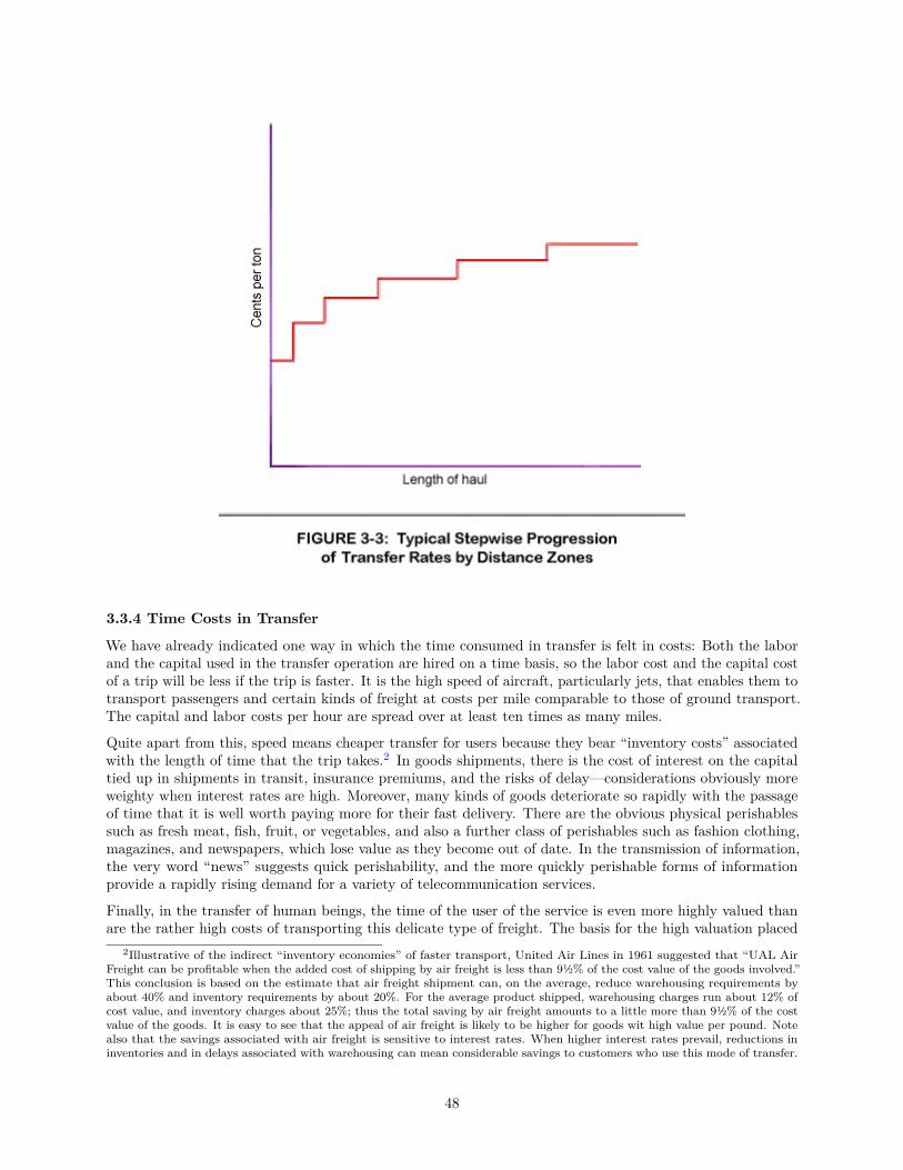
3.3.4 Time Costs in Transfer

We have already indicated one way in which the time consumed in transfer is felt in costs: Both the laborand the capital used in the transfer operation are hired on a time basis, so the labor cost and the capital costof a trip will be less if the trip is faster. It is the high speed of aircraft, particularly jets, that enables them totransport passengers and certain kinds of freight at costs per mile comparable to those of ground transport.The capital and labor costs per hour are spread over at least ten times as many miles.

Quite apart from this, speed means cheaper transfer for users because they bear “inventory costs” associatedwith the length of time that the trip takes.2 In goods shipments, there is the cost of interest on the capitaltied up in shipments in transit, insurance premiums, and the risks of delay—considerations obviously moreweighty when interest rates are high. Moreover, many kinds of goods deteriorate so rapidly with the passageof time that it is well worth paying more for their fast delivery. There are the obvious physical perishablessuch as fresh meat, fish, fruit, or vegetables, and also a further class of perishables such as fashion clothing,magazines, and newspapers, which lose value as they become out of date. In the transmission of information,the very word “news” suggests quick perishability, and the more quickly perishable forms of informationprovide a rapidly rising demand for a variety of telecommunication services.

Finally, in the transfer of human beings, the time of the user of the service is even more highly valued thanare the rather high costs of transporting this delicate type of freight. The basis for the high valuation placed

2Illustrative of the indirect “inventory economies” of faster transport, United Air Lines in 1961 suggested that “UAL AirFreight can be profitable when the added cost of shipping by air freight is less than 9½% of the cost value of the goods involved.”This conclusion is based on the estimate that air freight shipment can, on the average, reduce warehousing requirements byabout 40% and inventory requirements by about 20%. For the average product shipped, warehousing charges run about 12% ofcost value, and inventory charges about 25%; thus the total saving by air freight amounts to a little more than 9½% of the costvalue of the goods. It is easy to see that the appeal of air freight is likely to be higher for goods wit high value per pound. Notealso that the savings associated with air freight is sensitive to interest rates. When higher interest rates prevail, reductions ininventories and in delays associated with warehousing can mean considerable savings to customers who use this mode of transfer.

48

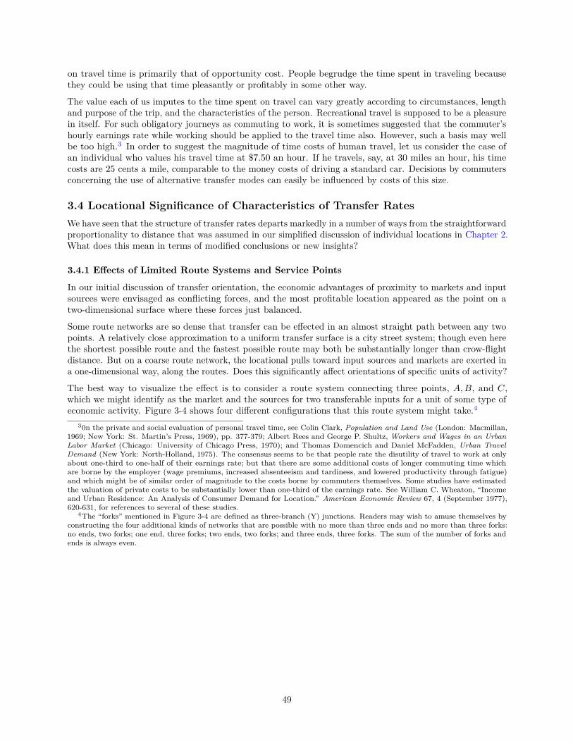
on travel time is primarily that of opportunity cost. People begrudge the time spent in traveling becausethey could be using that time pleasantly or profitably in some other way.

The value each of us imputes to the time spent on travel can vary greatly according to circumstances, lengthand purpose of the trip, and the characteristics of the person. Recreational travel is supposed to be a pleasurein itself. For such obligatory journeys as commuting to work, it is sometimes suggested that the commuter’shourly earnings rate while working should be applied to the travel time also. However, such a basis may wellbe too high.3 In order to suggest the magnitude of time costs of human travel, let us consider the case ofan individual who values his travel time at $7.50 an hour. If he travels, say, at 30 miles an hour, his timecosts are 25 cents a mile, comparable to the money costs of driving a standard car. Decisions by commutersconcerning the use of alternative transfer modes can easily be influenced by costs of this size.

3.4 Locational Significance of Characteristics of Transfer RatesWe have seen that the structure of transfer rates departs markedly in a number of ways from the straightforwardproportionality to distance that was assumed in our simplified discussion of individual locations in Chapter 2.What does this mean in terms of modified conclusions or new insights?

3.4.1 Effects of Limited Route Systems and Service Points

In our initial discussion of transfer orientation, the economic advantages of proximity to markets and inputsources were envisaged as conflicting forces, and the most profitable location appeared as the point on atwo-dimensional surface where these forces just balanced.

Some route networks are so dense that transfer can be effected in an almost straight path between any twopoints. A relatively close approximation to a uniform transfer surface is a city street system; though even herethe shortest possible route and the fastest possible route may both be substantially longer than crow-flightdistance. But on a coarse route network, the locational pulls toward input sources and markets are exerted ina one-dimensional way, along the routes. Does this significantly affect orientations of specific units of activity?

The best way to visualize the effect is to consider a route system connecting three points, A,B, and C,which we might identify as the market and the sources for two transferable inputs for a unit of some type ofeconomic activity. Figure 3-4 shows four different configurations that this route system might take.4

30n the private and social evaluation of personal travel time, see Colin Clark, Population and Land Use (London: Macmillan,1969; New York: St. Martin’s Press, 1969), pp. 377-379; Albert Rees and George P. Shultz, Workers and Wages in an UrbanLabor Market (Chicago: University of Chicago Press, 1970); and Thomas Domencich and Daniel McFadden, Urban TravelDemand (New York: North-Holland, 1975). The consensus seems to be that people rate the disutility of travel to work at onlyabout one-third to one-half of their earnings rate; but that there are some additional costs of longer commuting time whichare borne by the employer (wage premiums, increased absenteeism and tardiness, and lowered productivity through fatigue)and which might be of similar order of magnitude to the costs borne by commuters themselves. Some studies have estimatedthe valuation of private costs to be substantially lower than one-third of the earnings rate. See William C. Wheaton, “Incomeand Urban Residence: An Analysis of Consumer Demand for Location.” American Economic Review 67, 4 (September 1977),620-631, for references to several of these studies.

4The “forks” mentioned in Figure 3-4 are defined as three-branch (Y) junctions. Readers may wish to amuse themselves byconstructing the four additional kinds of networks that are possible with no more than three ends and no more than three forks:no ends, two forks; one end, three forks; two ends, two forks; and three ends, three forks. The sum of the number of forks andends is always even.

49

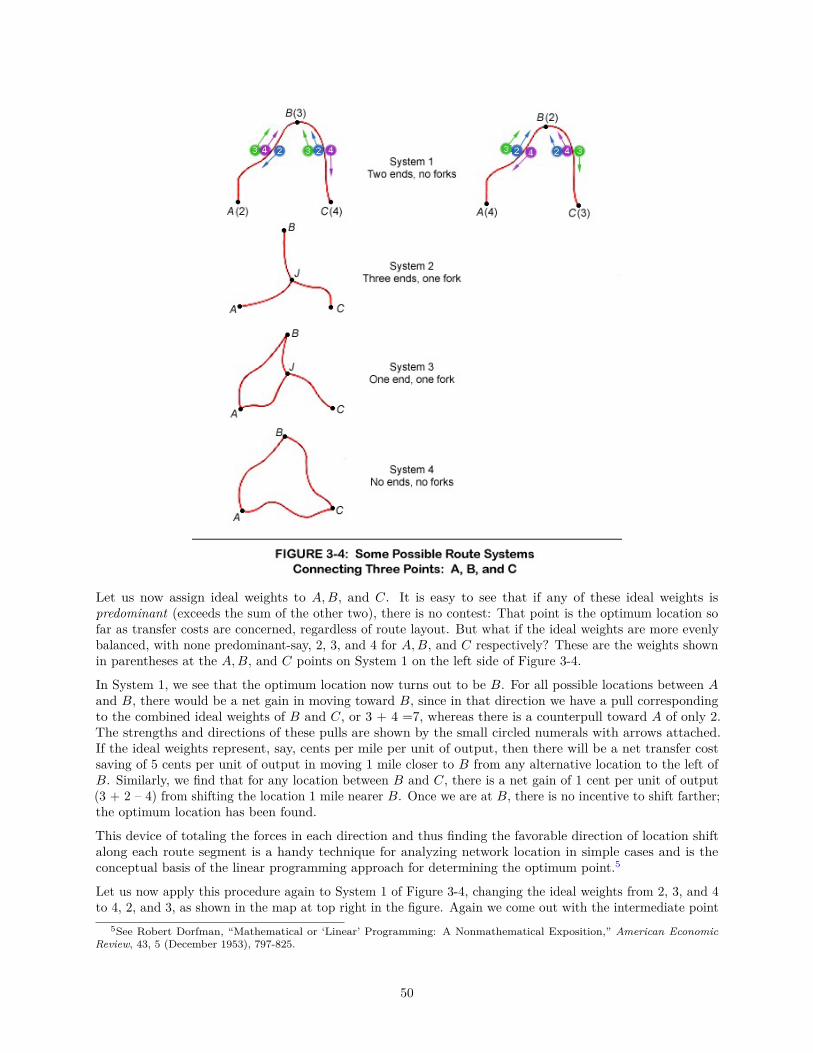
Let us now assign ideal weights to A,B, and C. It is easy to see that if any of these ideal weights ispredominant (exceeds the sum of the other two), there is no contest: That point is the optimum location sofar as transfer costs are concerned, regardless of route layout. But what if the ideal weights are more evenlybalanced, with none predominant-say, 2, 3, and 4 for A,B, and C respectively? These are the weights shownin parentheses at the A,B, and C points on System 1 on the left side of Figure 3-4.

In System 1, we see that the optimum location now turns out to be B. For all possible locations between Aand B, there would be a net gain in moving toward B, since in that direction we have a pull correspondingto the combined ideal weights of B and C, or 3 + 4 =7, whereas there is a counterpull toward A of only 2.The strengths and directions of these pulls are shown by the small circled numerals with arrows attached.If the ideal weights represent, say, cents per mile per unit of output, then there will be a net transfer costsaving of 5 cents per unit of output in moving 1 mile closer to B from any alternative location to the left ofB. Similarly, we find that for any location between B and C, there is a net gain of 1 cent per unit of output(3 + 2 – 4) from shifting the location 1 mile nearer B. Once we are at B, there is no incentive to shift farther;the optimum location has been found.

This device of totaling the forces in each direction and thus finding the favorable direction of location shiftalong each route segment is a handy technique for analyzing network location in simple cases and is theconceptual basis of the linear programming approach for determining the optimum point.5

Let us now apply this procedure again to System 1 of Figure 3-4, changing the ideal weights from 2, 3, and 4to 4, 2, and 3, as shown in the map at top right in the figure. Again we come out with the intermediate point

5See Robert Dorfman, “Mathematical or ‘Linear’ Programming: A Nonmathematical Exposition,” American EconomicReview, 43, 5 (December 1953), 797-825.

50

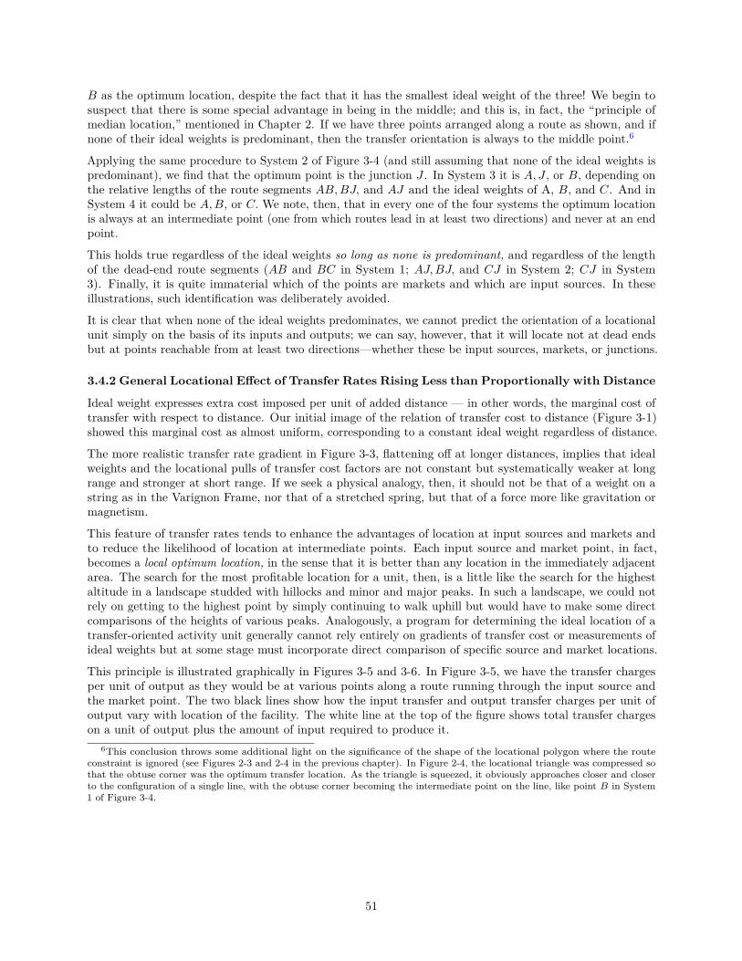
B as the optimum location, despite the fact that it has the smallest ideal weight of the three! We begin tosuspect that there is some special advantage in being in the middle; and this is, in fact, the “principle ofmedian location,” mentioned in Chapter 2. If we have three points arranged along a route as shown, and ifnone of their ideal weights is predominant, then the transfer orientation is always to the middle point.6

Applying the same procedure to System 2 of Figure 3-4 (and still assuming that none of the ideal weights ispredominant), we find that the optimum point is the junction J . In System 3 it is A, J , or B, depending onthe relative lengths of the route segments AB,BJ, and AJ and the ideal weights of A, B, and C. And inSystem 4 it could be A,B, or C. We note, then, that in every one of the four systems the optimum locationis always at an intermediate point (one from which routes lead in at least two directions) and never at an endpoint.

This holds true regardless of the ideal weights so long as none is predominant, and regardless of the lengthof the dead-end route segments (AB and BC in System 1; AJ,BJ, and CJ in System 2; CJ in System3). Finally, it is quite immaterial which of the points are markets and which are input sources. In theseillustrations, such identification was deliberately avoided.

It is clear that when none of the ideal weights predominates, we cannot predict the orientation of a locationalunit simply on the basis of its inputs and outputs; we can say, however, that it will locate not at dead endsbut at points reachable from at least two directions—whether these be input sources, markets, or junctions.

3.4.2 General Locational Effect of Transfer Rates Rising Less than Proportionally with Distance

Ideal weight expresses extra cost imposed per unit of added distance — in other words, the marginal cost oftransfer with respect to distance. Our initial image of the relation of transfer cost to distance (Figure 3-1)showed this marginal cost as almost uniform, corresponding to a constant ideal weight regardless of distance.

The more realistic transfer rate gradient in Figure 3-3, flattening off at longer distances, implies that idealweights and the locational pulls of transfer cost factors are not constant but systematically weaker at longrange and stronger at short range. If we seek a physical analogy, then, it should not be that of a weight on astring as in the Varignon Frame, nor that of a stretched spring, but that of a force more like gravitation ormagnetism.

This feature of transfer rates tends to enhance the advantages of location at input sources and markets andto reduce the likelihood of location at intermediate points. Each input source and market point, in fact,becomes a local optimum location, in the sense that it is better than any location in the immediately adjacentarea. The search for the most profitable location for a unit, then, is a little like the search for the highestaltitude in a landscape studded with hillocks and minor and major peaks. In such a landscape, we could notrely on getting to the highest point by simply continuing to walk uphill but would have to make some directcomparisons of the heights of various peaks. Analogously, a program for determining the ideal location of atransfer-oriented activity unit generally cannot rely entirely on gradients of transfer cost or measurements ofideal weights but at some stage must incorporate direct comparison of specific source and market locations.

This principle is illustrated graphically in Figures 3-5 and 3-6. In Figure 3-5, we have the transfer chargesper unit of output as they would be at various points along a route running through the input source andthe market point. The two black lines show how the input transfer and output transfer charges per unit ofoutput vary with location of the facility. The white line at the top of the figure shows total transfer chargeson a unit of output plus the amount of input required to produce it.

6This conclusion throws some additional light on the significance of the shape of the locational polygon where the routeconstraint is ignored (see Figures 2-3 and 2-4 in the previous chapter). In Figure 2-4, the locational triangle was compressed sothat the obtuse corner was the optimum transfer location. As the triangle is squeezed, it obviously approaches closer and closerto the configuration of a single line, with the obtuse corner becoming the intermediate point on the line, like point B in System1 of Figure 3-4.

51

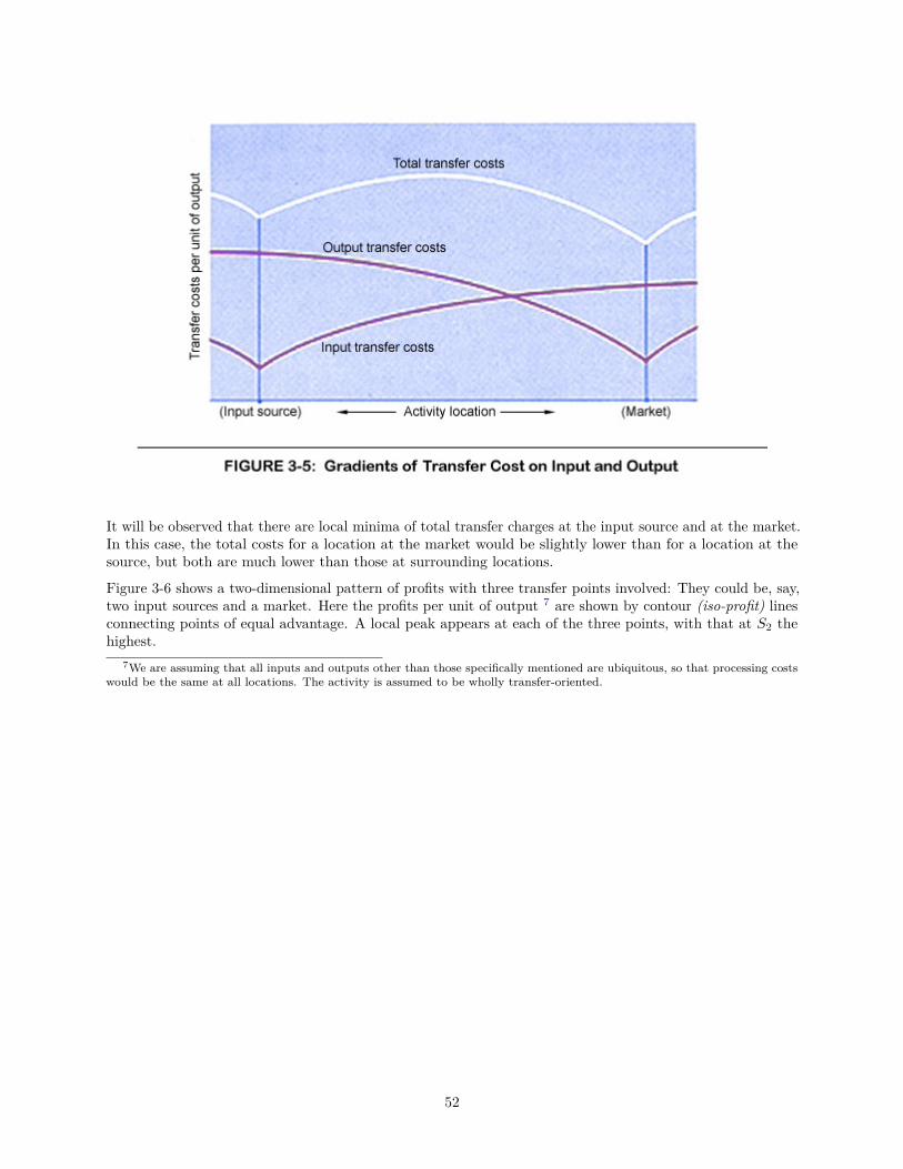
It will be observed that there are local minima of total transfer charges at the input source and at the market.In this case, the total costs for a location at the market would be slightly lower than for a location at thesource, but both are much lower than those at surrounding locations.

Figure 3-6 shows a two-dimensional pattern of profits with three transfer points involved: They could be, say,two input sources and a market. Here the profits per unit of output 7 are shown by contour (iso-profit) linesconnecting points of equal advantage. A local peak appears at each of the three points, with that at S2 thehighest.

7We are assuming that all inputs and outputs other than those specifically mentioned are ubiquitous, so that processing costswould be the same at all locations. The activity is assumed to be wholly transfer-oriented.

52

3.4.3 Modal Interchange Locations

It has been suggested above that the long-haul discount characteristic of transfer costs and rates lessens thetransfer advantages of locations that are neither sources nor markets for transferable inputs and outputs.Some kinds of intermediate points, however, are relatively attractive in terms of transfer costs.

Most transfers involve one or more changes of mode or other terminal type of operation en route rather thanproceeding right through from initial origin to final destination. This situation becomes more frequent as thevariety of available transport modes increases, each with its special advantages for longer or shorter hauls,larger or smaller shipments, high speed, low money cost, and so on.

Textbooks often tell us that points of transshipment or modal interchange, such as ports, are particularlystrategic locations because location of a processing facility at such a point “eliminates transshipment costs.”

Such a statement may be misleading. Let us take a simple hypothetical case involving a flour mill. Grainis collected at an inland point connected by rail to a port (transshipment point), from which ships go to amarket for flour. We want to choose among three possible locations for the mill: (1) at the grain-collectionpoint, (2) at the port, or (3) at the market. To focus directly on the question of the transshipment point’spossible advantage, we assume that the handling and transfer costs (per barrel of flour) are the same for flouras for grain, which makes the grain-collection point and the flour market equal in locational advantage. Thequestion, then, is whether location at the transshipment point (port) is superior or inferior to the grain-sourceand flour-market locations for the mill.

Let us denote the elements of cost as follows, per barrel of flour:

53

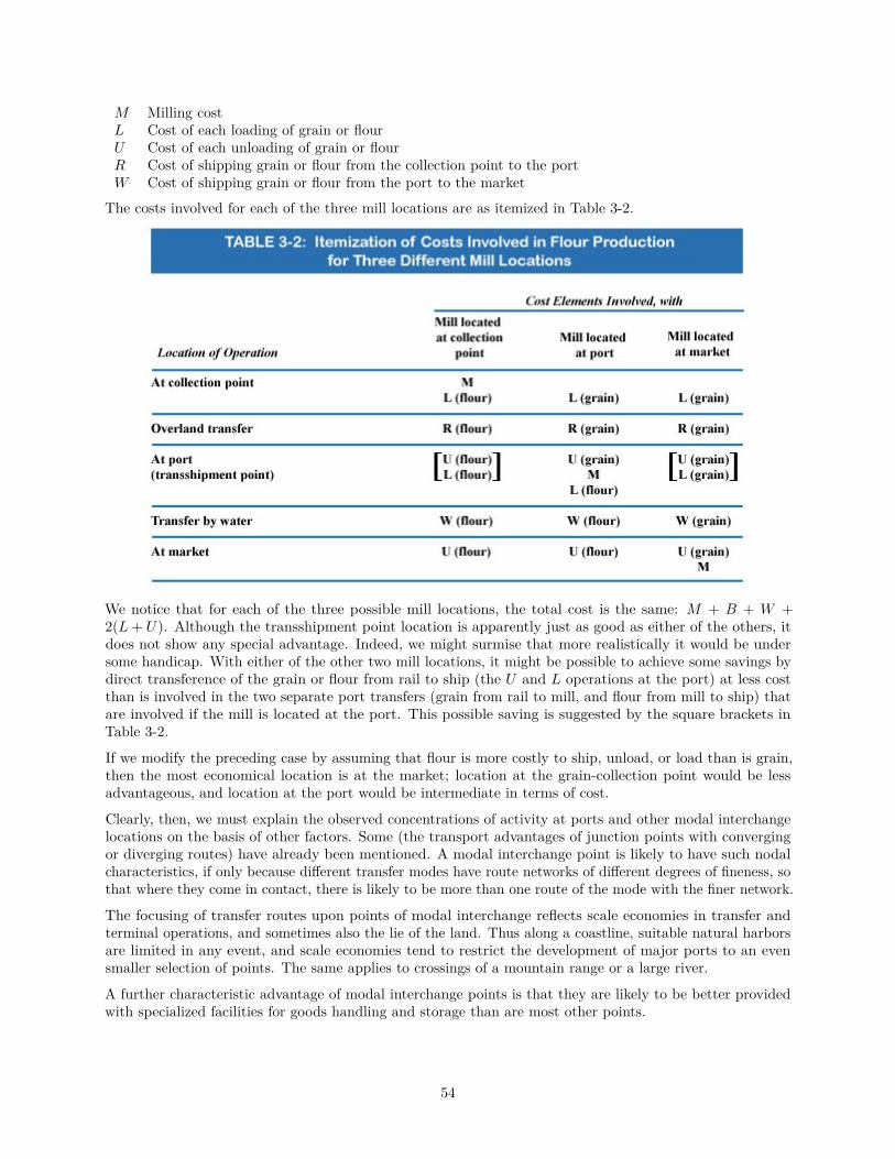
M Milling costL Cost of each loading of grain or flourU Cost of each unloading of grain or flourR Cost of shipping grain or flour from the collection point to the portW Cost of shipping grain or flour from the port to the market

The costs involved for each of the three mill locations are as itemized in Table 3-2.

We notice that for each of the three possible mill locations, the total cost is the same: M + B + W +2(L+ U). Although the transshipment point location is apparently just as good as either of the others, itdoes not show any special advantage. Indeed, we might surmise that more realistically it would be undersome handicap. With either of the other two mill locations, it might be possible to achieve some savings bydirect transference of the grain or flour from rail to ship (the U and L operations at the port) at less costthan is involved in the two separate port transfers (grain from rail to mill, and flour from mill to ship) thatare involved if the mill is located at the port. This possible saving is suggested by the square brackets inTable 3-2.

If we modify the preceding case by assuming that flour is more costly to ship, unload, or load than is grain,then the most economical location is at the market; location at the grain-collection point would be lessadvantageous, and location at the port would be intermediate in terms of cost.

Clearly, then, we must explain the observed concentrations of activity at ports and other modal interchangelocations on the basis of other factors. Some (the transport advantages of junction points with convergingor diverging routes) have already been mentioned. A modal interchange point is likely to have such nodalcharacteristics, if only because different transfer modes have route networks of different degrees of fineness, sothat where they come in contact, there is likely to be more than one route of the mode with the finer network.

The focusing of transfer routes upon points of modal interchange reflects scale economies in transfer andterminal operations, and sometimes also the lie of the land. Thus along a coastline, suitable natural harborsare limited in any event, and scale economies tend to restrict the development of major ports to an evensmaller selection of points. The same applies to crossings of a mountain range or a large river.

A further characteristic advantage of modal interchange points is that they are likely to be better providedwith specialized facilities for goods handling and storage than are most other points.

54

3.5 Some Recent Developments Concerning the Structure of Transfer Costs3.5.1 Introduction

The preceding sections have focused on some important aspects of the structure of transport rates andcharacteristics of route systems. As has been demonstrated, they provide information that can be used inconjunction with the theoretical insights gained from Chapter 2 in order to appreciate more fully the rolethat transfer factors may play in location decisions. In some instances, changes that take place in the marketsof important commodities in a national or international context or changes in basic technological relationscan have direct effects on the spatial distribution of economic activity. These effects often, but certainly notalways, manifest themselves as a result of changes in transfer costs.

In this section, attention is directed to two such changes, both much in evidence at this time. We attempt touse the location principles that have been developed in order to understand some of the spatial consequencesof higher energy prices and technological changes concerning the processing and transmission of information.It should be emphasized that our treatment of issues related to these phenomena is speculative and illustrative.There is a very slim factual basis on which to gauge any of the effects that will be mentioned. However, itis hoped that this analysis will demonstrate how even elementary location theory can help us to speculateconstructively.

3.5.2 Higher Energy Prices and the Pattern of Industrial Location

The rapid increase in energy prices during the decade of the seventies affected our economy in many ways.We are acutely aware of the impact of this phenomenon on the rate of economic growth as well as on thedistribution of income. However, little attention has been paid to the effect of higher energy prices on thespatial distribution of economic activity. It is important to recognize these spatial effects as well as themechanics by which they are transmitted.

The effect of higher energy prices since the 1970s on locational choice might be considered from severalperspectives. It would be possible, for example, to examine the nature of commuting or shopping behaviorwhen people are confronted with higher motor fuel prices. Alternatively, we might recognize that higher energypries have affected production decisions as well as the transport costs on material and finished products. Thisbeing so, our previous analysis of transfer-oriented industries would imply that, for at least some locationalunits, the spatial consequences of higher energy prices will depend on the nature of responses in productionand the kind of changes in the structure of transport costs that take place. Much of the preceding discussionin this text has pointed to the result that the orientation of industry toward particular inputs or toward themarket can be influenced by these locational determinants. We are well equipped to understand many issuesrelated to the effects of higher energy prices if we examine the systematically in this context.

It has been pointed out (see Figure 3-2) that intermodal competition among transfer agencies leads to agradient of transfer rates with respect to distance that is much more curved than that of any single-modecost gradient. For long hauls, customers will find that the decrease in transfer rates with increased distanceis accentuated by competition of this sort. The locational significance of this characteristic of transfer rates isthat it puts intermediate locations (places that are not markets or sources of transferable inputs) at somedisadvantage.

One channel by which higher energy prices might affect location decisions is through their effect on thestructure of intermodal transfer costs.8 As shown in Table 3-3, transfer modes differ in their intensity ofenergy use. Specifically, shorter-haul transport by motor carriers (trucks) is most energy intensive, whereasrail and barge transport, which generally involve longer distances, are much more energy efficient. Themost direct consequence of this is that we might expect the tapering off of transport rates with distance tobecome yet more accentuated as a result of higher energy prices; short-haul (truck) rates will increase relative

8Details on some of the issues raised in the remainder of this section may be fond in Frank Giarratani and Charles F. Socher,“The Pattern of Industrial Location and Rising Energy Prices,” Atlantic Economic Journal 5, 1 (March 1977), 48-55. For atheoretical discussion of some related topics, see Noboru Sakashita, “The Location Theory of Firm Revisited: Impacts of RisingEnergy Prices,” Regional Science and Urban Economics, 10, 3 (August 1980), 423-428.

55

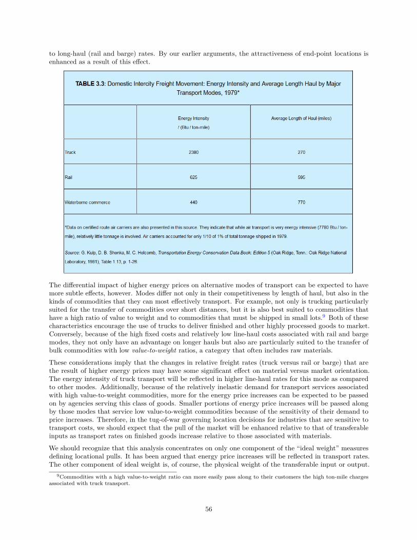
to long-haul (rail and barge) rates. By our earlier arguments, the attractiveness of end-point locations isenhanced as a result of this effect.

The differential impact of higher energy prices on alternative modes of transport can be expected to havemore subtle effects, however. Modes differ not only in their competitiveness by length of haul, but also in thekinds of commodities that they can most effectively transport. For example, not only is trucking particularlysuited for the transfer of commodities over short distances, but it is also best suited to commodities thathave a high ratio of value to weight and to commodities that must be shipped in small lots.9 Both of thesecharacteristics encourage the use of trucks to deliver finished and other highly processed goods to market.Conversely, because of the high fixed costs and relatively low line-haul costs associated with rail and bargemodes, they not only have an advantage on longer hauls but also are particularly suited to the transfer ofbulk commodities with low value-to-weight ratios, a category that often includes raw materials.

These considerations imply that the changes in relative freight rates (truck versus rail or barge) that arethe result of higher energy prices may have some significant effect on material versus market orientation.The energy intensity of truck transport will be reflected in higher line-haul rates for this mode as comparedto other modes. Additionally, because of the relatively inelastic demand for transport services associatedwith high value-to-weight commodities, more for the energy price increases can be expected to be passedon by agencies serving this class of goods. Smaller portions of energy price increases will be passed alongby those modes that service low value-to-weight commodities because of the sensitivity of their demand toprice increases. Therefore, in the tug-of-war governing location decisions for industries that are sensitive totransport costs, we should expect that the pull of the market will be enhanced relative to that of transferableinputs as transport rates on finished goods increase relative to those associated with materials.

We should recognize that this analysis concentrates on only one component of the “ideal weight” measuresdefining locational pulls. It has been argued that energy price increases will be reflected in transport rates.The other component of ideal weight is, of course, the physical weight of the transferable input or output.

9Commodities with a high value-to-weight ratio can more easily pass along to their customers the high ton-mile chargesassociated with truck transport.

56

There are some evidence that the materials and energy are substitute inputs in the production processassociated with U.S. manufacturing as a whole. protect10 This would imply that an increase in energy pricesmay increase the weight of materials transferred for output of a given weight. Such a change would tend toincrease the ideal weight of materials and may serve to counteract any tendency toward market orientationdue to changes in relative transport rates. The highly aggregative nature of empirical evidence concerningthis matter precludes any definitive judgment, however.

Higher domestic energy prices not only affect transport and production costs, they also imply substantialshifts in the spatial distribution of income. Energy- producing regions have gained for at least two reasons.Greater local production at higher prices obviously has meant greater income to workers as well as to theowners of capital in these regions.11 Further, while price controls on domestic petroleum and natural gasproduction are being phased out, the presence of these restrictions has meant at least a short-run advantageto energy consumers in energy-producing regions. They have faced relatively lower energy prices than theywould in regions that must rely exclusively on higher-priced, imported energy. Therefore, recognition of theconcept of “market access potential” developed in Chapter 2 would indicate that for some locational unitshigher energy prices mean that the median location of the market will shift in the direction of those regionswith substantial existing or developing capacity in energy production.12

While we have been able to identify certain gross tendencies that may be manifest as a result of higher energyprices, this analysis is only suggestive of the kind of forces at work. Individuals who are concerned withthe behavior of specific industries could obtain more detailed information on transport modes and on thecharacter of production and markets that are relevant to their interests. They might then be in a position toknow whether transport rate, production, or market considerations will be most influential.

3.5.3 Technological Change in Data Processing and Transmission

In contrast to the behavior of energy prices, the cost of moving and processing information has fallendramatically in recent years, and the end is not in sight. Advances in electronics technology have abruptlyenhanced the efficiency of computers and our ability to interact with them. At the same time, developmentsin communications technology have weakened the constraints of distance on some types of location decisions.Significant locational effects are emerging on both the microspatial and the macrospatial levels, foreshadowingstill further shifts.

As we shall see in Chapter 7, the internal spatial arrangements of urban areas are shaped largely byconsiderations of access—it might even be said that access is what cities are all about. At this microspatiallevel, the journey to work and one’s ability to maintain close, flexible contact with customers, suppliers,co-workers, and friends are major determinants of both business and residence location. So if people or firmsfind that their work and other activities no longer demand close physical contact, locational incentives willchange. For example, it is now becoming increasingly practicable to use computer hookups to communicatewith other workers or with central data banks. As a result, the valuation of locations with respect to theirnearness to long-established foci of urban economic activity is changing considerably. This “communicationsrevolution” has potentially wide implications. Some people have speculated that the “cottage industry”of the near future will comprise people who work at home and maintain business contacts via integratedcomputation and communications systems. Early evidence of such a trend is already appearing.

For some activities, the very nature of outputs or inputs, or both, may change as a result of advances of thesort just mentioned. Banking is an obvious case in point. From one perspective, deposits received by a bankmay be regarded as inputs; banks then take those inputs and use them to earn income by “selling” loans andother investments and services. Alternatively, one might view the receiving of deposits as a form of servicesprovided by the bank and thus as one of the bank’s outputs.

10Ernst R. Berndt and David O. Wood, “Technology, Prices, and the Derived Demand for Energy,” Review of Economics andStatistics 57, 3 (August 1975), 259-268.

11See William H. Miernyk, Frank Giarratani, and Charles Socher, Regional Impacts of Rising Energy Prices (Cambridge,Mass.: Ballinger, 1978), pp. 57-76.

12Not all energy-producing regions can be expected to share equally in these advantages. For example, some coal-producingregions have been severely affected by restrictions placed on the use of coal with high sulfur content because of environmentalconcerns.

57

Until recently, the deposit activity of a bank was essentially non-transferable, and many separate bankingoffices were needed to service adequately a large urban area full of depositors and borrowers. But the depositservices of a bank may soon become very transferable indeed. We see already more and more bankingmachines acting as robot tellers; banking by phone is developing, and banking via home computer is in theoffing.

So depositors who now have to travel to a bank, or use the mails, will soon find that the bank’s services travelinstantly to them. With the proliferation of electronic transactions and home computer terminals, we canforesee that the customer service area of a single banking office will no longer be confined to a neighborhood,and that presumably far fewer bank locations will be needed.

Locational relations among different activities likewise are subject to important alteration when the transfer-ability of information is greatly enhanced, as is now happening. An example of this is firms that providetroubleshooting and repair service to users of complex equipment. The easy and quick availability of suchservices has been an important factor to many firms. While maintenance specialists can be dispatched somedistance to attend to problems, speed is of the essence. Close proximity to the suppliers of the service hasmeant speedy attention, less down time, more regularity of production, and therefore lower operating costs.There is even a saving in capital costs as fewer machines are needed to ensure a given rate of production andas goods spend less time in the production process.

But in recent years some highly sophisticated “smart” machines that incorporate computer systems to monitorperformance have also been endowed with a capacity for self-diagnosis. When a problem occurs, such amachine is capable of immediately signaling the probable nature and extent of the difficulty. This informationcan be relayed by wire to central service facilities that are equipped to interpret it and to recommend orprovide maintenance or repair procedures entailing a minimum of delay. Thus the integrated character ofindustries can take on new forms. The repair facility now has greater flexibility of location as the transfercosts on its output are reduced and the firm operating the complex equipment faces lower transfer costs onan important service input. Both are able to respond more freely to other locational factors.

The communications revolution promises likewise to have significant effects on locational relationships amongestablishments of the same firm. In a study of branch plants in four states over the period 1967—1976,Rodney A. Erickson and Thomas R. Leinbach found that the size of branch plants is positively related totheir distance from corporate headquarters. The farther away from headquarters, the larger the branch tendsto be.13

This relationship reflects the handicap that distance has always imposed on a firm’s ability to centralizedecision-making and at the same time to keep in touch with and direct the operations of scattered field officesor branches. Branches have had to become more autonomous and assume more decision-making functions astheir distance from headquarters increases. It may be surmised that current and foreseeable advances in dataprocessing and transmission will alter this relationship. Effective centralized coordination and control at longdistances should become more feasible. Specialized operations of large firms may be oriented more closely totheir specific markets without sacrificing adequate contact with headquarters.

3.6 SummaryThis chapter explores (1) the ways in which transfer costs in the real world are not simply proportional tocrow-flight distance as was assumed in Chapter 2, and (2) the locational significance of such departures froma uniform transfer surface.

Transfer operations almost always involve a large element of fixed costs. Consequently, there are importantscale economies related to route traffic volume, terminal volume, and size of individual movement unit andconsignment. There is also wide leeway for transfer agencies in apportioning their fixed costs over variousclasses of services so as to improve capacity utilization, meet competition, and increase profits.

Transfer services by any one mode are generally confined to a limited network of routes and service points,13Rodney A. Erickson and Thomas R. Leinbach, “Characteristics of Branch Plants Attracted to Nonmetropolitan Areas,” in

Richard E. Lonsdale and H. L. Seyler (eds.), Nonmetropolitan Industrialization (Washington, D.C.: V. H. Winston, 1979), p. 68.

58

determined by variations in terrain and scale economies. Transfer costs by any one mode also generally riseless than proportionally with longer distance—mainly because of terminal cost, but also often because oflower line-haul cost per mile on longer hauls.

The pattern of rates charged by transfer agencies is even less like a uniform transfer surface than is thepattern of transfer costs. There is normally rate discrimination in favor of larger-volume services, longerhauls, routes and types of services where interagency or intermodal competition exists, and goods of lowvalue relative to their weight or bulk. Further, where the demand for transfer between two points is not thesame in both directions and returnable vehicles are used, cheaper back-haul rates in the direction of lowertransfer demand are likely.

Other important characteristics of transport rates have been noted. Rate structures are generally simplifiedby setting uniform rates for categories of services and ranges of distance, shipment size, and so forth, ratherthan setting a separate rate for each service. Additionally, time costs are an important part of total transfercost for high-valued or perishable shipments and especially for transfer of people and information.

Each of these departures from the uniform transfer surface has an effect on locational preferences. We havealso recognized that both long-haul economies and the restriction of transfer to limited systems of routes andservice points enhance the locational advantages of markets, input sources, and route junctions, includingmodal interchange points.

Together with the theoretical basis developed in Chapter 2, these considerations provide a framework forexamining the locational implications of changes in our economy that alter the structure of transfer costs.

Technical Terms Introduced in this ChapterTransfer mode Back-haul ratesTransfer service points Rate blocks or distance zonesLong-haul economies Local optimum locationTerminal operations and costs Isoprofit linesLine-haul or movement costs modal interchange locationsTransfer agency Transshipment locationsGradient

Selected ReadingsBenjamin Chinitz, Freight and the Metro polls, a report of the ew York Metropolitan Region Study (Cambridge,Mass.: Harvard University Press, for the Regional Plan Association, 1960).

Benjamin Chinitz, “The Effect of Transportation Forms on Regional Economic Growth,” Traffic Quarterly, 14(1960), 129-142. Reprinted in Gerald J. Karaska and David F. Bramhall, Locational Analysis for Manufacturing(Cambridge, Mass.: MIT Press, 1969), pp. 83-96.

John R. Meyer, M. J. Peck, J. Stenason, and C. Zwick, The Economics of Competition in the TransportationIndustries (Cambridge, Mass.: Harvard University Press, 1959).

Hebert Mohring, Transportation Economics (Cambridge, Mass.: Ballinger, 1976).

Appendix 3-1 Rate Discrimination by a Transfer MonopolistAssume that a good is to be shipped to various markets from a single point of origin. At each market thequantity sold (and consequently the quantity shipped to that market) will be

q = a—b(p+ r)

59

Where p is the price at the point of origin (the same for all markets) and r is the transfer charge.

The transfer agency’s cost of carrying the good to a market x miles away from the point of origin is (g + tx)per ton, where g is terminal cost and t is line-haul cost per mile.

On shipments to a market at a distance x, therefore, the transfer agency will make a net return of

Z = (a—bp—br)(r—g—tx)

Differentiating,

dZ/dr = a− bp− 2br + bg + btx

and the most profitable rate to charge (r∗) is calculated as follows:

a—bp—2br∗ + bg + btx = 0

r∗ = (a—bp+ bg)/2b+ tx/2

The ideal tariff will be a flat charge equal to

1/2[(a/b) + g—p]

plus half the line-haul cost for each mile of haul.

60

4. LOCATION PATTERNS DOMINATED BY DISPERSIVEFORCES4.1 Introduction4.1.1 Unit Locations and the Pattern of an Activity

So far, we have considered only the locational preferences and decisions of the individual unit. We nowmove to a different level of inquiry, in which attention is focused on the patterns in which similar units arraythemselves.

We shall refer to an activity as a category of closely similar location units.1 In manufacturing, one speaks ofan “industry”—such as flour milling or job printing; in trade or services, of a “line” of business. We shallextend the term “activities” to cover analogous groupings, such as residential units of a particular class,types of public facilities with a particular function, and so on. Thus in a given city, the fire department is anactivity, with a spatial pattern comprising the locations of fire houses.

Location patterns can take various forms, as can be seen when one sets out to map the locations of differentactivities. The pattern of the copper smelting industry could be shown as a small number of dots, eachrepresenting one smelter. Fashion garment factories are found mainly in tight clusters (such as in midtownManhattan), each of which contains many firms. Automobile dealers in urban areas tend to be concentratedin linear clusters. Particular crops, or types of farming, are often found in continuous zones, which theypreempt to the exclusion of any other major activity.

Sometimes the location pattern of an activity is a planned configuration because there is just a single decisionunit involved. In a nonsocialized economy, however, this situation is confined essentially to certain typesof public facilities (such as schools within a city school system) and to the few lines of private businessesthat are controlled by total monopolies. More characteristically, the location pattern of an activity is theunplanned outgrowth of the behavior of many location decision units.

4.1.2 Competition and Interdependence

As already noted in Chapter 2, individuals and business firms (particularly new and small firms) must makelocation decisions in the face of great uncertainty, and they are strongly influenced by personal preferencesand constraints not closely related to any calculation of money cost, revenue, or profit. But the locationpattern of an activity as a whole cannot be understood simply in terms of the factors governing individualunit locations. Here we have to recognize explicitly the role of competition and other kinds of locationalinterdependence among units.

First, there is the process of competitive weeding out and survival. Establishment of new locations is only oneof the ways in which the locational pattern of an activity is altered. The mortality among new and small firmsis high, and establishments are continually being abandoned or converted to other uses. Business locations,whether based on wisdom, profound study, personal whim, or guesswork, have to meet the test of survival.

A good analogy is the scattering of certain types of seeds by the wind. These seeds may be carried for milesbefore finally coming to rest, and nothing makes them select spots particularly favorable for germination.Some fall in good places and get a quick and vigorous start; others fall in sterile or overcrowded spots anddie. Because of the survival of those which happen to be well located, the resulting distribution of suchplants from generation to generation follows closely the distribution of favorable growing conditions, So inthe location of economic activities, it is not strictly necessary to have both competition and wise businessplanning in order

1Martin Beckmann, Location Theory (New York: Random House, 1968), adopts a different terminology, in which “activity”corresponds to what we have been calling “location unit,” and “industry” to what we call “activity.”

61

to have a somewhat rational location pattern emerge: Either alone will work in that direction.2

To be sure, the role of the “invisible hand” in promoting efficient location patterns should not be exaggerated.The survival test may weed out multitudes of small mistakes in location, though at a substantial cost inwasted resources. Big mistakes associated with large-scale operations— for example, in the location of a steelmill or a major transport terminal— are considerably more durable. Not only is the fixed investment greaterand the competitive pressure less threatening, but in addition such a facility radically alters its environment.It may attract a variety of complementary activities; and, in any event, it will build up a larger local market,thus partly “justifying itself.” The need for informed planning of locations in order to forestall misallocationof resources is obviously greater where large-scale units or complexes are involved. Such major decisions arein fact based on more objective criteria and fuller information than is the typical small-unit location.

Competition among business firms is just one of the manifold ways in which locations depend on oneanother—a dependence that we conveniently ignored in Chapter 2 when considering just one location unitat a time. Whether they be factories, stores, public facilities, offices, or homes, individual location unitsare never indifferent to locations of other units of the same kind but can be either repelled or attracted bythem. Proximity can be an advantage or a disadvantage, or sometimes both at the same time. Our focus inthis chapter is on activity patterns shaped by mutual repulsion among the units, or dispersive forces. Wewill find that the nature of competition in a spatial context may contribute to these forces but that someaspects of spatial competition may have contervailing effects. Subsequently, in Chapter 5, we will considerthe contrasting kinds of patterns in which mutual attraction, or agglomerative forces, dominate.

4.1.3 Some Basic Factors Contributing to Dispersed Patterns

Business firms often go to some pains to select locations where there is no nearby competition; and householderslikewise shy away from too much proximity to other households, whether from a desire to avoid high rents orcongestion, a desire for privacy, or a dislike for some particular category of neighbors. These are instancesof locational repulsion among units of the same specific or general type. But several basic reasons for adispersed pattern can be identified.

One reason is competition for scarce local inputs, such as land, privacy, quiet, or clean air or water. A highconcentration of occupancy makes these local inputs more scarce and more expensive. It also discouragesfurther concentration. The importance of this effect is so great that we shall devote Chapter 6 to exploring itin detail.

Another reason for an activity to have a dispersed pattern is that the activity is output-oriented and itsmarkets are dispersed. Thus an effective demand for convenience goods exists wherever there are people withincome; and a closely market-oriented activity, such as drugstores, will have a pattern resembling that ofpopulation or consumer income. The individual stores prefer locations apart from one another, because theyare selling basically the same items and the customers will tend to patronize the nearest store. The demandfor the goods of any one store will be greater where there is little or no nearby competition. As a result ofthis mutual repulsion, the stores are widely distributed. The degree of dispersion (the closeness of fit to themarket pattern) is limited only by the high costs of operating a small store, and the pattern thus representsan economic compromise between the factors of market access and scale economy.

2E. M. Hoover, The Location of Economic Activity (New York: McGraw-Hill, 1948), p. 10. This point is further developed inArmen A. Alchian, “Uncertainty, Evolution, and Economic Theory,” Journal of Political Economy, 58 (June 1950), 211-221;and in Charles M. Tiebout, “Location Theory, Empirical Evidence, and Economic Evolution,” Papers and Proceedings of theRegional Science Association, 3 (1957), 74-86. Tiebout (p. 85) cites the case of brewing, in which “in the evolutionary struggleto survive, Milwaukee gained the dominant position,” and that of the automobile industry, in which Detroit emerged as chiefvictor in the struggle. In both instances, personal or other “fortuitous” factors played a large part in the initial locations.

Another interesting case is that of the Hershey Chocolate Company, an early giant in its industry. Milton Hershey, havingmade candy successively but not very successfully in Philadelphia, Chicago, Denver, New York, and Lancaster, Pa., finallychose a rural Pennsylvania Dutch location for his famous factory and planned town of Hershey—largely because that was hisbirthplace. A rural location for a large candy factory was then almost unheard-of, and few expected him to survive. But thelocation happened to be an excellent choice in terms of access to milk and imported cocoa beans, nearness to the largest centers,and labor supply. Without those economic advantages, Hershey would probably have failed again. Joseph R. Snavely, Milton S.Hershey, Builder (Hershey, Pa: privately printed, 1935)

62

Where scale economies call for still further restriction on the number of separate units that can survive, wefind individual units selecting not just neighborhoods but cities or regions on a similar basis of avoidance ofproximity: They try to find a relatively undersupplied area where the competition is least intense. In boththe intracity and the intercity situations, the individual unit has a “market area” within which it has theadvantage of better access to the market than its competitors.

Similarly there are activities, oriented to the supply of transferable in puts, that tend to have a dispersedpattern because the pattern of input sources is itself dispersed. Crop-processing activities in agriculturalareas are an example. Individual cheese factories, sugar refineries, and the like repel one another in the sensethat each can get its inputs more cheaply or easily if it has a “supply area” to itself and is to that extentinsulated from competition.

We shall now examine more closely these types of activity patterns involving market areas or supply areas.For brevity’s sake, the discussion will refer basically to market areas, but it should be kept in mind throughoutthat the same principles apply to supply areas as well.

4.2 Market Areas4.2.1 Introduction

First, we may note that the importance of keeping a distance from one’s rivals, and the feasibility of carvingout a market area, depend on the degree of interchangeability of one’s products with those of the competitors.If the products are not closely standardized, the buyers cannot be relied on to prefer the cheapest nor topatronize the nearest seller. But if the products are standardized, there are likely to be considerable scaleeconomies in producing them, since there is relatively great scope for mechanization and even automation ofprocesses, and the organization and management problems are simpler.

Some economies of large scale refer to the size of the individual establishment or location unit, while othersdepend primarily on how large the firm or other decision unit is. The economically justifiable size of theindividual location unit is constrained by the fact that larger size requires a larger market area and increasedtransfer costs; but the size of the firm is not under that constraint and may be associated with such substantialsavings in costs of management, purchasing, research, advertising, and finance that it is profitable for onefirm to operate a number of separate location units. Branch plants are increasingly common in manufacturingand utilities, as are chain stores in retailing. Within the past few decades, multiunit firms have assumeda notably larger role in such activities as hotels and motels, automobile rental, restaurants, theaters, anduniversity education. This trend probably reflects, at least in part, the improvement of communications,data processing, and management techniques, which have widened the scope of economies of large-scalemanagement more than they have affected the scale of individual establishments.

Consequently, one of the important types of market-area patterns is that involving the sales or service areasof different branch units of a single firm—here the relationship among units is obviously different from whatit is when the units belong to rival firms.

4.2.2 The Market Area of a Spatial Monopolist

The development of our discussion concerning market-area patterns will be facilitated if we first understandthe factors contributing to the market boundary of a spatial monopolist. Whether we choose to think of thismonopolist as a branch unit or a single-unit firm with decision-making power is immaterial at present.

The characteristic that distinguishes a firm or a particular location unit as having monopoly power is thatwhen its price is raised, at least some of its customers will remain. No such advantage accrues to the perfectcompetitor. Its demand curve is such that it has no control over price; any increase in price will cause all ofits customers to find alternatives. Most introductory textbooks in economics stress a number of reasons whymonopolies can arise (patents, scale economies, etc.), but they neglect the fact that space itself may impartmonopoly power. For example, customers in the immediate vicinity of a grocery store are, in a sense, attachedto it. Price increases may be tolerated by these customers because switching to an alternative supplier wouldinvolve extra time, trouble, and expense. This principle applies equally to many nonbusiness establishments

63

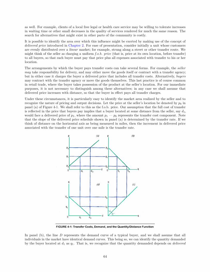
as well. For example, clients of a local free legal or health care service may be willing to tolerate increasesin waiting time or other small decreases in the quality of services rendered for much the same reason. Thesearch for alternatives that might exist in other parts of the community is costly.

It is possible to identify the area over which this influence might be exerted by making use of the concept ofdelivered price introduced in Chapter 2. For ease of presentation, consider initially a unit whose customersare evenly distributed over a linear market; for example, strung along a street or other transfer route. Wemight think of the seller as charging a uniform f.o.b. price (that is, price at its own location, before transfer)to all buyers, so that each buyer must pay that price plus all expenses associated with transfer to his or herlocation.

The arrangements by which the buyer pays transfer costs can take several forms. For example, the sellermay take responsibility for delivery, and may either move the goods itself or contract with a transfer agency;but in either case it charges the buyer a delivered price that includes all transfer costs. Alternatively, buyersmay contract with the transfer agency or move the goods themselves. This last practice is of course commonin retail trade, where the buyer takes possession of the product at the seller’s location. For our immediatepurposes, it is not necessary to distinguish among these alternatives; in any case we shall assume thatdelivered price increases with distance, so that the buyer in effect pays all transfer charges.

Under these circumstances, it is particularly easy to identify the market area realized by the seller and torecognize the nature of pricing and output decisions. Let the price at the seller’s location be denoted by p0 inpanel (a) of Figure 4-1. We shall refer to this as the f.o.b. price. Our assumption that the full cost of transferis reflected in the price that buyers pay implies that a buyer located at some distance from the seller, say d1,would face a delivered price of pI , where the amount p1 — p0 represents the transfer cost component. Notethat the slope of the delivered price schedule shown in panel (a) is determined by the transfer rate. If wethink of distance on the horizontal axis as being measured in miles, then the increment in delivered priceassociated with the transfer of one unit over one mile is the transfer rate.

In panel (b), the line D represents the demand curve of a typical buyer, and we shall assume that allindividuals in the market have identical demand curves. This being so, we can identify the quantity demandedby the buyer located at d1 as q1. That is, we recognize that the quantity demanded depends on delivered

64

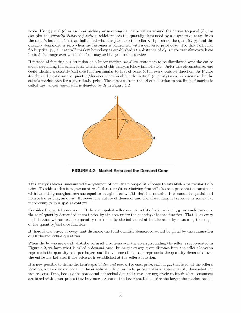
price. Using panel (c) as an intermediary or mapping device to get us around the corner to panel (d), wecan plot the quantity/distance function, which relates the quantity demanded by a buyer to distance fromthe seller’s location. Thus an individual who is adjacent to the seller will purchase the quantity q0, and thequantity demanded is zero when the customer is confronted with a delivered price of p2. For this particularf.o.b. price, p0, a “natural” market boundary is established at a distance of d2, where transfer costs havelimited the range over which the firm may sell its product or service.

If instead of focusing our attention on a linear market, we allow customers to be distributed over the entirearea surrounding this seller, some extensions of this analysis follow immediately. Under this circumstance, onecould identify a quantity/distance function similar to that of panel (d) in every possible direction. As Figure4-2 shows, by rotating the quantity/distance function about the vertical (quantity) axis, we circumscribe theseller’s market area for a given f.o.b. price. The distance from the seller’s location to the limit of market iscalled the market radius and is denoted by R in Figure 4-2.

This analysis leaves unanswered the question of how the monopolist chooses to establish a particular f.o.b.price. To address this issue, we must recall that a profit-maximizing firm will choose a price that is consistentwith its setting marginal revenue equal to marginal cost. This decision criterion is common to spatial andnonspatial pricing analysis. However, the nature of demand, and therefore marginal revenue, is somewhatmore complex in a spatial context.

Consider Figure 4-1 once more. If the monopolist seller were to set its f.o.b. price at p0, we could measurethe total quantity demanded at that price by the area under the quantity/distance function. That is, at everyunit distance we can read the quantity demanded by the individual at that location by measuring the heightof the quantity/distance function.

If there is one buyer at every unit distance, the total quantity demanded would be given by the summationof all the individual quantities.

When the buyers are evenly distributed in all directions over the area surrounding the seller, as represented inFigure 4-2, we have what is called a demand cone. Its height at any given distance from the seller’s locationrepresents the quantity sold per buyer, and the volume of the cone represents the quantity demanded overthe entire market area if the price p0 is established at the seller’s location.

It is now possible to define the firm’s spatial demand curve. For each price, such as p0, that is set at the seller’slocation, a new demand cone will be established. A lower f.o.b. price implies a larger quantity demanded, fortwo reasons. First, because the nonspatial, individual demand curves are negatively inclined; when consumersare faced with lower prices they buy more. Second, the lower the f.o.b. price the larger the market radius,

65

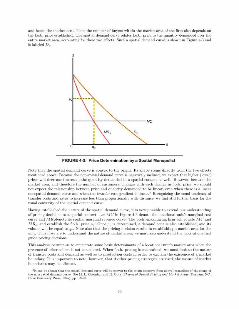
and hence the market area. Thus the number of buyers within the market area of the firm also depends onthe f.o.b. price established. The spatial demand curve relates f.o.b. price to the quantity demanded over theentire market area, accounting for these two effects. Such a spatial demand curve is shown in Figure 4-3 andis labeled Ds.

Note that the spatial demand curve is convex to the origin. Its shape stems directly from the two effectsmentioned above. Because the non-spatial demand curve is negatively inclined, we expect that higher (lower)prices will decrease (increase) the quantity demanded in a spatial context as well. However, because themarket area, and therefore the number of customers, changes with each change in f.o.b. price, we shouldnot expect the relationship between price and quantity demanded to be linear, even when there is a linearnonspatial demand curve and when the transfer cost gradient is linear.3 Recognizing the usual tendency oftransfer costs and rates to increase less than proportionally with distance, we find still further basis for theusual convexity of the spatial demand curve.

Having established the nature of the spatial demand curve, it is now possible to extend our understandingof pricing decisions to a spatial context. Let MC in Figure 4-3 denote the locational unit’s marginal costcurve and MRsdenote its spatial marginal revenue curve. The profit-maximizing firm will equate MC andMRs, and establish the f.o.b. price p∗. Once p∗ is determined, a demand cone is also established, and itsvolume will be equal to q∗. Note also that the pricing decision results in establishing a market area for theunit. Thus if we are to understand the nature of market areas, we must also understand the motivations thatguide pricing decisions.

This analysis permits us to enumerate some basic determinants of a locational unit’s market area when thepresence of other sellers is not considered. When f.o.b. pricing is maintained, we must look to the natureof transfer costs and demand as well as to production costs in order to explain the existence of a marketboundary. It is important to note, however, that if other pricing strategies are used, the nature of marketboundaries may be affected.

3It can be shown that the spatial demand curve will be convex to the origin (concave from above) regardless of the shape ofthe nonspatial demand curve. See M. L. Greenhut and H. Ohta, Theory of Spatial Pricing and Market Areas (Durham, NC.:Duke University Press, 1975), pp. 19-20.

66

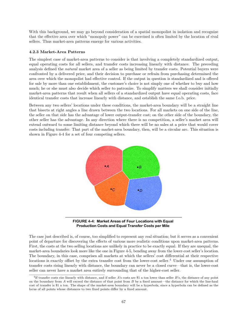
With this background, we may go beyond consideration of a spatial monopolist in isolation and recognizethat the effective area over which “monopoly power” can be exercised is often limited by the location of rivalsellers. Thus market-area patterns emerge for various activities.

4.2.3 Market-Area Patterns

The simplest case of market-area patterns to consider is that involving a completely standardized output,equal operating costs for all sellers, and transfer costs increasing linearly with distance. The precedinganalysis defined the natural market area of a seller as being limited by transfer costs. Potential buyers wereconfronted by a delivered price, and their decision to purchase or refrain from purchasing determined thearea over which the monopolist had effective control. If the output in question is standardized and is offeredfor sale by more than one establishment, the customer’s choice is not simply one of whether to buy and howmuch; he or she must also decide which seller to patronize. To simplify matters we shall consider initiallymarket-area patterns that result when all sellers of a standardized output have equal operating costs, faceidentical transfer costs that increase linearly with distance, and establish the same f.o.b. price.

Between any two sellers’ locations under these conditions, the market-area boundary will be a straight linethat bisects at right angles a line drawn between the two locations. For all markets on one side of the line,the seller on that side has the advantage of lower output-transfer cost; on the other side of the boundary, theother seller has the advantage. In any direction where there is no competition, a seller’s market area willextend outward to some limiting distance beyond which there will be no sales at a price that would covercosts including transfer: That part of the market-area boundary, then, will be a circular arc. This situation isshown in Figure 4-4 for a set of four competing sellers.

The case just described is, of course, too simplified to represent any real situation; but it serves as a convenientpoint of departure for discovering the effects of various more realistic conditions upon market-area patterns.First, the costs at the two selling locations are unlikely in practice to be exactly equal. If they are unequal, themarket-area boundaries look more like the one in Figure 4-5, bending away from the lower-cost seller’s location.The boundary, in this case, comprises all markets at which the sellers’ cost differential at their respectivelocations is exactly offset by the extra transfer cost from the lower-cost seller.4 Under our assumption oftransfer costs rising linearly with distance, the boundary can never be a closed curve—that is, the lower-costseller can never have a market area entirely surrounding that of the higher-cost seller.

4If transfer costs rise linearly with distance, and if seller A’s costs are $1 a ton lower than seller B’s, the distance of any pointon the boundary from A will exceed the distance of that point from B by a fixed amount—the distance for which the line-haulcost of transfer is $1 a ton. The shape of the market-area boundary will be a hyperbola, since a hyperbola can be defined as thelocus of all points whose distances to two fixed points differ by a fixed amount.

67

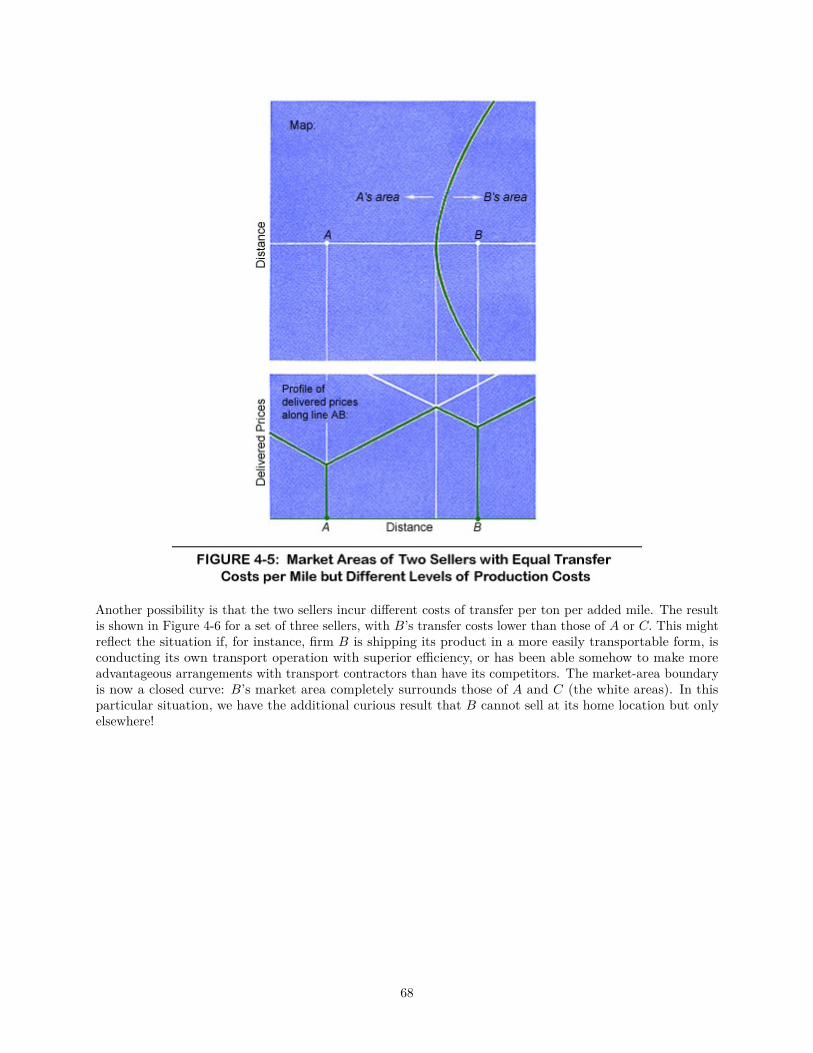
Another possibility is that the two sellers incur different costs of transfer per ton per added mile. The resultis shown in Figure 4-6 for a set of three sellers, with B’s transfer costs lower than those of A or C. This mightreflect the situation if, for instance, firm B is shipping its product in a more easily transportable form, isconducting its own transport operation with superior efficiency, or has been able somehow to make moreadvantageous arrangements with transport contractors than have its competitors. The market-area boundaryis now a closed curve: B’s market area completely surrounds those of A and C (the white areas). In thisparticular situation, we have the additional curious result that B cannot sell at its home location but onlyelsewhere!

68

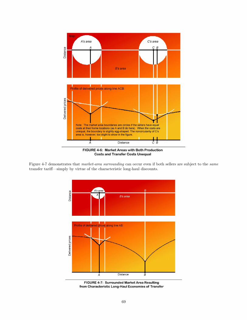
Figure 4-7 demonstrates that market-area surrounding can occur even if both sellers are subject to the sametransfer tariff—simply by virtue of the characteristic long-haul discounts.

69

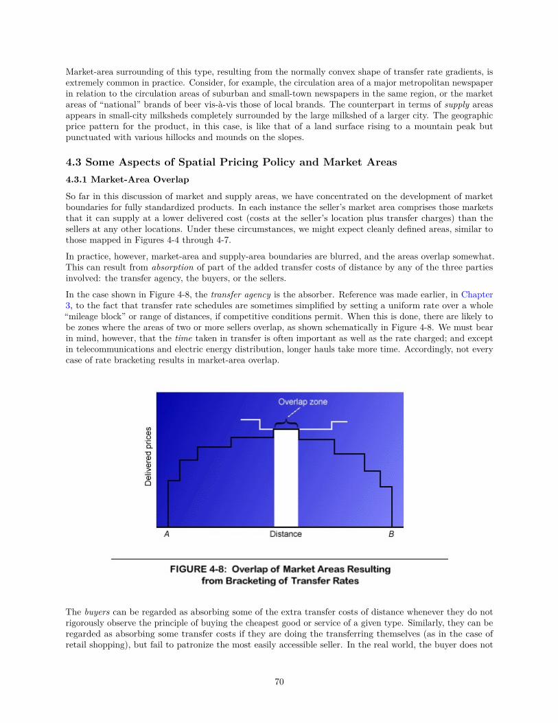
Market-area surrounding of this type, resulting from the normally convex shape of transfer rate gradients, isextremely common in practice. Consider, for example, the circulation area of a major metropolitan newspaperin relation to the circulation areas of suburban and small-town newspapers in the same region, or the marketareas of “national” brands of beer vis-à-vis those of local brands. The counterpart in terms of supply areasappears in small-city milksheds completely surrounded by the large milkshed of a larger city. The geographicprice pattern for the product, in this case, is like that of a land surface rising to a mountain peak butpunctuated with various hillocks and mounds on the slopes.

4.3 Some Aspects of Spatial Pricing Policy and Market Areas4.3.1 Market-Area Overlap

So far in this discussion of market and supply areas, we have concentrated on the development of marketboundaries for fully standardized products. In each instance the seller’s market area comprises those marketsthat it can supply at a lower delivered cost (costs at the seller’s location plus transfer charges) than thesellers at any other locations. Under these circumstances, we might expect cleanly defined areas, similar tothose mapped in Figures 4-4 through 4-7.

In practice, however, market-area and supply-area boundaries are blurred, and the areas overlap somewhat.This can result from absorption of part of the added transfer costs of distance by any of the three partiesinvolved: the transfer agency, the buyers, or the sellers.

In the case shown in Figure 4-8, the transfer agency is the absorber. Reference was made earlier, in Chapter3, to the fact that transfer rate schedules are sometimes simplified by setting a uniform rate over a whole“mileage block” or range of distances, if competitive conditions permit. When this is done, there are likely tobe zones where the areas of two or more sellers overlap, as shown schematically in Figure 4-8. We must bearin mind, however, that the time taken in transfer is often important as well as the rate charged; and exceptin telecommunications and electric energy distribution, longer hauls take more time. Accordingly, not everycase of rate bracketing results in market-area overlap.

The buyers can be regarded as absorbing some of the extra transfer costs of distance whenever they do notrigorously observe the principle of buying the cheapest good or service of a given type. Similarly, they can beregarded as absorbing some transfer costs if they are doing the transferring themselves (as in the case ofretail shopping), but fail to patronize the most easily accessible seller. In the real world, the buyer does not

70

often show this impartiality toward competing sellers, but for one reason or another has a preference even ifthe prices are equal. Such preference is least likely to be an important consideration in business purchases ofsuch standardized goods as wheat or cement, and it is most likely to occur for retail purchases of such highlydifferentiated or even “personalized” items as medical or educational services, high-fashion clothing, andrecreation. It is important to note that the buyer-preference factor will produce market-area overlap, but onlyto the extent that buyers have diverse preferences. Thus in Figure 4-9 (where it is assumed that A producesmore cheaply than B), the line CC might be the market-area boundary for buyers who are indifferent to therelative qualities of A’s and B’s wares and would simply choose whichever is cheaper at their location. Forthose who believe that A’s product is really worth 5 cents a pound more than B’s, the boundary will be DD,which runs through points where the delivered cost from A is 5 cents greater than that from B. For thosewho believe that B’s is worth 5 cents a pound more than A’s, the boundary will be FE. Assuming that atevery location there are buyers representing the whole intermediate gamut of preferences, the “boundary” orzone of overlap will comprise the belt between DD and FE. Both A and B will make sales throughout thisoverlap zone, though each will predominate in the part that is closer to him or her.

Finally, it may be sellers who are absorbing some of the added costs of distance. This is quite common.Indeed, the one case where this is not likely to happen is the special case mentioned earlier, in which thesellers are branch units of a single firm, public agency, or other multilocation decision unit. It is ordinarily inthe interest of a firm or agency to distribute the product from its various facility locations in such a way as tominimize the total cost of supplying any given pattern of demand. This will ordinarily rule out cross-haulingor overlap of the market areas of those facility locations (except to the extent that it might reflect transfercost absorption on the part of buyers or transfer agencies, as already considered). Accordingly, specific salesterritories are allotted to the various branches. These market areas tend to be larger for branches with lowercost or higher capacity, and larger where demand is sparse than where it is dense.

Such definitive demarcation of areas is even more prevalent in public and administrative agencies. TheFederal Reserve System divides the United States into twelve districts, and within some districts there aresubdistricts such as that of the Pittsburgh branch of the Cleveland Federal Reserve Bank. Similarly, everyfederal government agency with field activities has its set of districts exclusively allocated to their respectivebranch office.5

In other activities, however (including most lines of business), the market rivalry between selling locationsmainly involves rival firms, rather than different branches of the same firm. This situation introducesconsiderable possibilities for transfer cost absorption and consequently market-area overlap, depending on the

5See also map Figure 9-3 and accompanying discussion.

71

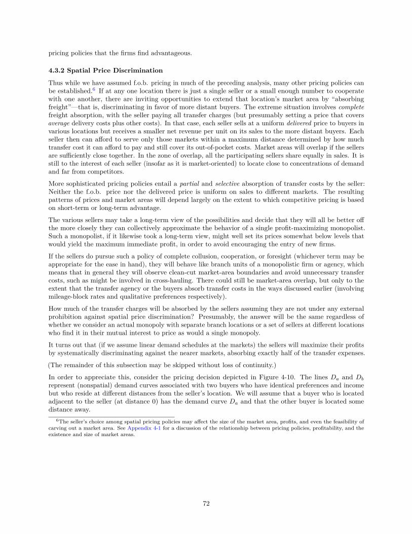
pricing policies that the firms find advantageous.

4.3.2 Spatial Price Discrimination

Thus while we have assumed f.o.b. pricing in much of the preceding analysis, many other pricing policies canbe established.6 If at any one location there is just a single seller or a small enough number to cooperatewith one another, there are inviting opportunities to extend that location’s market area by “absorbingfreight”—that is, discriminating in favor of more distant buyers. The extreme situation involves completefreight absorption, with the seller paying all transfer charges (but presumably setting a price that coversaverage delivery costs plus other costs). In that case, each seller sells at a uniform delivered price to buyers invarious locations but receives a smaller net revenue per unit on its sales to the more distant buyers. Eachseller then can afford to serve only those markets within a maximum distance determined by how muchtransfer cost it can afford to pay and still cover its out-of-pocket costs. Market areas will overlap if the sellersare sufficiently close together. In the zone of overlap, all the participating sellers share equally in sales. It isstill to the interest of each seller (insofar as it is market-oriented) to locate close to concentrations of demandand far from competitors.

More sophisticated pricing policies entail a partial and selective absorption of transfer costs by the seller:Neither the f.o.b. price nor the delivered price is uniform on sales to different markets. The resultingpatterns of prices and market areas will depend largely on the extent to which competitive pricing is basedon short-term or long-term advantage.

The various sellers may take a long-term view of the possibilities and decide that they will all be better offthe more closely they can collectively approximate the behavior of a single profit-maximizing monopolist.Such a monopolist, if it likewise took a long-term view, might well set its prices somewhat below levels thatwould yield the maximum immediate profit, in order to avoid encouraging the entry of new firms.

If the sellers do pursue such a policy of complete collusion, cooperation, or foresight (whichever term may beappropriate for the ease in hand), they will behave like branch units of a monopolistic firm or agency, whichmeans that in general they will observe clean-cut market-area boundaries and avoid unnecessary transfercosts, such as might be involved in cross-hauling. There could still be market-area overlap, but only to theextent that the transfer agency or the buyers absorb transfer costs in the ways discussed earlier (involvingmileage-block rates and qualitative preferences respectively).

How much of the transfer charges will be absorbed by the sellers assuming they are not under any externalprohibition against spatial price discrimination? Presumably, the answer will be the same regardless ofwhether we consider an actual monopoly with separate branch locations or a set of sellers at different locationswho find it in their mutual interest to price as would a single monopoly.

It turns out that (if we assume linear demand schedules at the markets) the sellers will maximize their profitsby systematically discriminating against the nearer markets, absorbing exactly half of the transfer expenses.

(The remainder of this subsection may be skipped without loss of continuity.)

In order to appreciate this, consider the pricing decision depicted in Figure 4-10. The lines Da and Db

represent (nonspatial) demand curves associated with two buyers who have identical preferences and incomebut who reside at different distances from the seller’s location. We will assume that a buyer who is locatedadjacent to the seller (at distance 0) has the demand curve Da and that the other buyer is located somedistance away.

6The seller’s choice among spatial pricing policies may affect the size of the market area, profits, and even the feasibility ofcarving out a market area. See Appendix 4-1 for a discussion of the relationship between pricing policies, profitability, and theexistence and size of market areas.

72

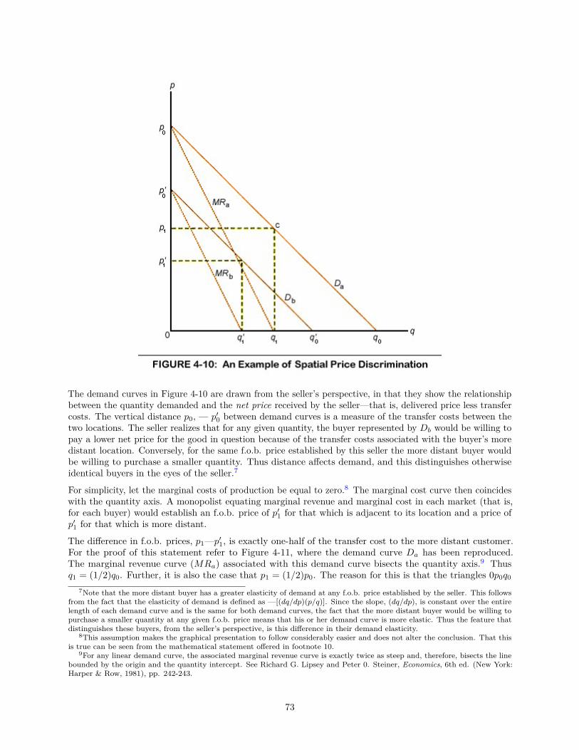
The demand curves in Figure 4-10 are drawn from the seller’s perspective, in that they show the relationshipbetween the quantity demanded and the net price received by the seller—that is, delivered price less transfercosts. The vertical distance p0, — p′0 between demand curves is a measure of the transfer costs between thetwo locations. The seller realizes that for any given quantity, the buyer represented by Db would be willing topay a lower net price for the good in question because of the transfer costs associated with the buyer’s moredistant location. Conversely, for the same f.o.b. price established by this seller the more distant buyer wouldbe willing to purchase a smaller quantity. Thus distance affects demand, and this distinguishes otherwiseidentical buyers in the eyes of the seller.7

For simplicity, let the marginal costs of production be equal to zero.8 The marginal cost curve then coincideswith the quantity axis. A monopolist equating marginal revenue and marginal cost in each market (that is,for each buyer) would establish an f.o.b. price of p′1 for that which is adjacent to its location and a price ofp′1 for that which is more distant.

The difference in f.o.b. prices, p1—p′1, is exactly one-half of the transfer cost to the more distant customer.For the proof of this statement refer to Figure 4-11, where the demand curve Da has been reproduced.The marginal revenue curve (MRa) associated with this demand curve bisects the quantity axis.9 Thusq1 = (1/2)q0. Further, it is also the case that p1 = (1/2)p0. The reason for this is that the triangles 0p0q0

7Note that the more distant buyer has a greater elasticity of demand at any f.o.b. price established by the seller. This followsfrom the fact that the elasticity of demand is defined as —[(dq/dp)(p/q)]. Since the slope, (dq/dp), is constant over the entirelength of each demand curve and is the same for both demand curves, the fact that the more distant buyer would be willing topurchase a smaller quantity at any given f.o.b. price means that his or her demand curve is more elastic. Thus the feature thatdistinguishes these buyers, from the seller’s perspective, is this difference in their demand elasticity.

8This assumption makes the graphical presentation to follow considerably easier and does not alter the conclusion. That thisis true can be seen from the mathematical statement offered in footnote 10.

9For any linear demand curve, the associated marginal revenue curve is exactly twice as steep and, therefore, bisects the linebounded by the origin and the quantity intercept. See Richard G. Lipsey and Peter 0. Steiner, Economics, 6th ed. (New York:Harper & Row, 1981), pp. 242-243.

73

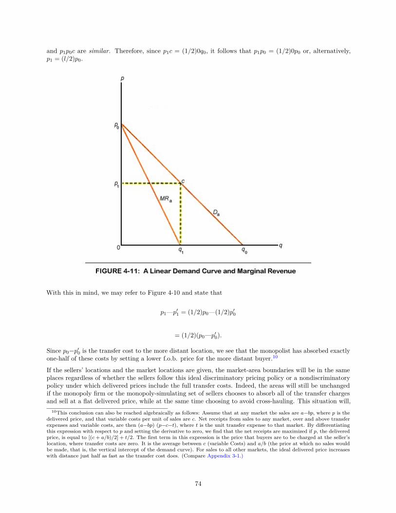
and p1p0c are similar. Therefore, since p1c = (1/2)0q0, it follows that p1p0 = (1/2)0p0 or, alternatively,p1 = (l/2)p0.

With this in mind, we may refer to Figure 4-10 and state that

p1—p′1 = (1/2)p0—(1/2)p′0

= (1/2)(p0—p′0).

Since p0−p′0 is the transfer cost to the more distant location, we see that the monopolist has absorbed exactlyone-half of these costs by setting a lower f.o.b. price for the more distant buyer.10

If the sellers’ locations and the market locations are given, the market-area boundaries will be in the sameplaces regardless of whether the sellers follow this ideal discriminatory pricing policy or a nondiscriminatorypolicy under which delivered prices include the full transfer costs. Indeed, the areas will still be unchangedif the monopoly firm or the monopoly-simulating set of sellers chooses to absorb all of the transfer chargesand sell at a flat delivered price, while at the same time choosing to avoid cross-hauling. This situation will,

10This conclusion can also be reached algebraically as follows: Assume that at any market the sales are a−bp, where p is thedelivered price, and that variable costs per unit of sales are c. Net receipts from sales to any market, over and above transferexpenses and variable costs, are then (a−bp) (p−c−t), where t is the unit transfer expense to that market. By differentiatingthis expression with respect to p and setting the derivative to zero, we find that the net receipts are maximized if p, the deliveredprice, is equal to [(c+ a/b)/2] + t/2. The first term in this expression is the price that buyers are to be charged at the seller’slocation, where transfer costs are zero. It is the average between c (variable Costs) and a/b (the price at which no sales wouldbe made, that is, the vertical intercept of the demand curve). For sales to all other markets, the ideal delivered price increaseswith distance just half as fast as the transfer cost does. (Compare Appendix 3-1.)

74

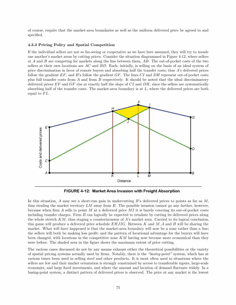
of course, require that the market-area boundaries as well as the uniform delivered price be agreed to andspecified.

4.3.3 Pricing Policy and Spatial Competition

If the individual sellers are not so far-seeing or cooperative as we have here assumed, they will try to invadeone another’s market areas by cutting prices. Consider the situation diagrammed in Figure 4-12, where sellersat A and B are competing for markets along the line between them, AB. The out-of-pocket costs of the twosellers at their own locations are AC and BD. Each, initially, is selling on the basis of an ideal system ofprice discrimination in favor of remote buyers and absorbing half the transfer costs; thus A’s delivered pricesfollow the gradient EF , and B’s follow the gradient GF . The lines CI and DH represent out-of-pocket costsplus full transfer costs from A and from B respectively. It should be noted that the ideal discriminatorydelivered prices EF and GF rise at exactly half the slope of CI and DH, since the sellers are systematicallyabsorbing half of the transfer costs. The market-area boundary is at L, where the delivered prices are bothequal to FL.

In this situation, A may see a short-run gain in undercutting B’s delivered prices to points as far as M ,thus stealing the market territory LM away from B. The possible invasion cannot go any farther, however,because when firm A sells to point M at a delivered price MI it is barely covering its out-of-pocket costsincluding transfer charges. Firm B can logically be expected to retaliate by cutting its delivered prices alongthe whole stretch KM , thus staging a counterinvasion of A’s market area. Carried to its logical conclusion,this game will produce a delivered price schedule EHJIG. Between K and M,A and B will be sharing themarket. What will have happened is that the market-area boundary will now be a zone rather than a line;the sellers will both be making less profit; and the pattern of locational advantage for the buyers will havebeen changed, with locations in the competitive zone KM having now become more economical than theywere before. The shaded area in the figure shows the maximum extent of price cutting.

The various cases discussed do not by any means exhaust either the theoretical possibilities or the varietyof spatial pricing systems actually used by firms. Notably, there is the “basing-point” system, which has atvarious times been used in selling steel and other products. It is most often used in situations where thesellers are few and their market orientation is strongly constrained by access to transferable inputs, large-scaleeconomies, and large fixed investments, and where the amount and location of demand fluctuate widely. In abasing-point system, a distinct pattern of delivered prices is observed: The price at any market is the lowest

75

sum of the fixed f.o.b. price at a basing point plus the actual transfer charges from the basing point to themarket. That is, sellers base their price on that charged at some other place, the basing point. For example,the place used as the basing point may be the largest supplying area for the commodity being sold. Thusunless government price regulation is in force, one might find that the price of crude oil in any U.S. city isbased on the price established by the Organization of Petroleum Exporting Countries (OPEC) for crudeoil from the Persian Gulf. In this case, an American producer who is shipping crude oil from Houston toChicago might charge a price equivalent to the price of OPEC crude oil delivered to Chicago.

The economic incentive for a pricing system of this sort is easy to understand. If the producers in a givenregion (or country) cannot produce enough to satisfy local demand at the equilibrium price, local producerswould be giving up profits if they charged any price lower than that of an identical commodity being importedby the region (country). The price of OPEC oil delivered to Chicago represents the maximum price that canbe charged by the Houston producer. Unless there is competitive undercutting of price by other producers,the OPEC price can prevail.

In such a system, all sales entail either freight absorption or phantom freight charges, except those by a sellerat a basing point to markets within the area governed by its basing point; there is likewise a considerableamount of market-area overlap and cross-hauling. For further discussion of this and still other variants, thecurious reader will have to look elsewhere.11

4.4 Competition and Location DecisionsThe preceding discussion of market areas and spatial pricing policies has described the behavior of sellers atgiven locations. We have recognized one important dimension of competition in a spatial context: the abilityof locational units to absorb transfer costs. Thus spatial pricing policies serve as one mechanism by whichfirms may seek to gain competitive advantage. We now proceed by recognizing that the choice of locationmay itself be part of a competitive strategy.

In order to establish a simple framework for exposing the essential character of this aspect of spatialcompetition, we draw on a model developed by Harold Hotelling.12 Our attention will be focused on twocompetitors who confront a linear-bounded market. It is assumed that production costs are zero for eachlocational unit. Identical buyers are evenly distributed over this market. Their demand for the good inquestion is not sensitive to price differences (the elasticity of demand is zero). One unit of the good isconsumed by each individual per period of time, and each buyer prefers to purchase from the nearest seller.

This situation is depicted in Figure 4-13. In panel (a), the linear market, l, is segmented into two protectedor uncontested parts, a and b, and one contested part, x + y, that is shared equally by the sellers. Thetwo sellers, A and B, can move to any location on the line that will maximize their profit, and they do sobelieving that the rival will not change its location in response to their competitive action. We will assumethat these moves are costless, in the sense that the sellers confront neither moving costs nor costs associatedwith disposing of fixed assets that might be associated with a given location.

11For a discussion of several issues concerning basing-point pricing and additional references to this topic, see David D.Haddock, “Basing-Point Pricing: Competitive vs. Collusive Theories,” American Economic Review, 72, 3 (June 1982), 289-306.Haddock points out that the basing-point system need not imply collusion among sellers, and he discusses the economic incentivefor this pricing behavior when commodities are traded interregionally.

Handy references on the varieties of spatial competition and pricing systems include Beckmann, Location Theory, pp. 30-50;and M. L. Greenhut, Microeconomics and the Space Economy (Chicago: Scott, Foresman, 1963). Mathematical statementsgeneralizing the theory of spatial pricing can be found in Martin J. Beckmann, “Spatial Price Policies Revisited,” Bell Journal ofEconomics, 7, 2 (Autumn 1976), 619-630; and in Daniel F. Spulber, “Spatial Nonlinear Pricing,” American Economic Review,71, 5 (December 1981), 923-933.

12Harold Hotelling, “Stability in Competition,” Economic Journal, 39 (March 1929), 41-57.

76

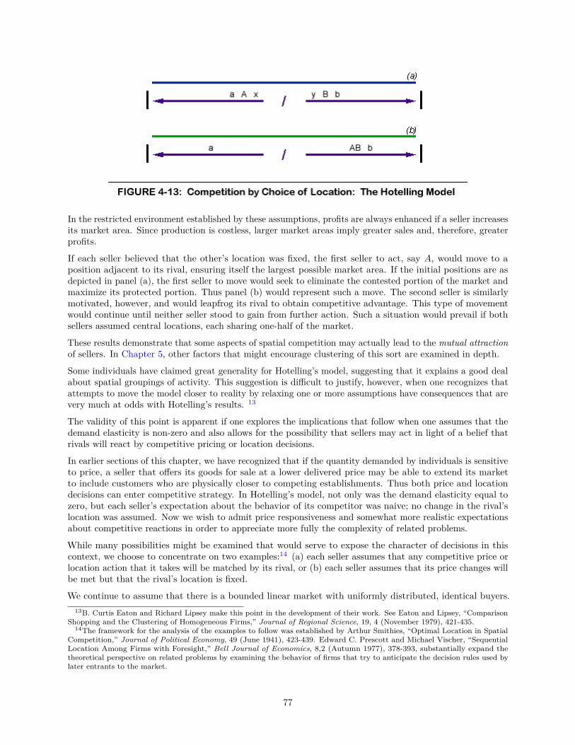
In the restricted environment established by these assumptions, profits are always enhanced if a seller increasesits market area. Since production is costless, larger market areas imply greater sales and, therefore, greaterprofits.

If each seller believed that the other’s location was fixed, the first seller to act, say A, would move to aposition adjacent to its rival, ensuring itself the largest possible market area. If the initial positions are asdepicted in panel (a), the first seller to move would seek to eliminate the contested portion of the market andmaximize its protected portion. Thus panel (b) would represent such a move. The second seller is similarlymotivated, however, and would leapfrog its rival to obtain competitive advantage. This type of movementwould continue until neither seller stood to gain from further action. Such a situation would prevail if bothsellers assumed central locations, each sharing one-half of the market.

These results demonstrate that some aspects of spatial competition may actually lead to the mutual attractionof sellers. In Chapter 5, other factors that might encourage clustering of this sort are examined in depth.

Some individuals have claimed great generality for Hotelling’s model, suggesting that it explains a good dealabout spatial groupings of activity. This suggestion is difficult to justify, however, when one recognizes thatattempts to move the model closer to reality by relaxing one or more assumptions have consequences that arevery much at odds with Hotelling’s results. 13

The validity of this point is apparent if one explores the implications that follow when one assumes that thedemand elasticity is non-zero and also allows for the possibility that sellers may act in light of a belief thatrivals will react by competitive pricing or location decisions.

In earlier sections of this chapter, we have recognized that if the quantity demanded by individuals is sensitiveto price, a seller that offers its goods for sale at a lower delivered price may be able to extend its marketto include customers who are physically closer to competing establishments. Thus both price and locationdecisions can enter competitive strategy. In Hotelling’s model, not only was the demand elasticity equal tozero, but each seller’s expectation about the behavior of its competitor was naive; no change in the rival’slocation was assumed. Now we wish to admit price responsiveness and somewhat more realistic expectationsabout competitive reactions in order to appreciate more fully the complexity of related problems.

While many possibilities might be examined that would serve to expose the character of decisions in thiscontext, we choose to concentrate on two examples:14 (a) each seller assumes that any competitive price orlocation action that it takes will be matched by its rival, or (b) each seller assumes that its price changes willbe met but that the rival’s location is fixed.

We continue to assume that there is a bounded linear market with uniformly distributed, identical buyers.13B. Curtis Eaton and Richard Lipsey make this point in the development of their work. See Eaton and Lipsey, “Comparison

Shopping and the Clustering of Homogeneous Firms,” Journal of Regional Science, 19, 4 (November 1979), 421-435.14The framework for the analysis of the examples to follow was established by Arthur Smithies, “Optimal Location in Spatial

Competition,” Journal of Political Economy, 49 (June 1941), 423-439. Edward C. Prescott and Michael Vischer, “SequentialLocation Among Firms with Foresight,” Bell Journal of Economics, 8,2 (Autumn 1977), 378-393, substantially expand thetheoretical perspective on related problems by examining the behavior of firms that try to anticipate the decision rules used bylater entrants to the market.

77

Now, however, we also assume that they have negatively inclined linear demand functions. As with theHotelling model, the sellers can move without cost and their marginal costs of production are zero; but weextend our assumptions concerning the sellers to include f.o.b. pricing with freight rates that are uniformover the market. The sellers are also profit maximizers.

Under these conditions, in situation (a), where each seller believes that price and location changes will bematched, neither seller can expect to gain from competitive behavior. Each believes that any attempt tolower the f.o.b. price in order to invade the rival’s market will be met and that the original boundary betweenthe two sellers will be reestablished at that lower price. Similarly, each seller expects that any relocationaimed at invading the rival’s market will be matched and that the boundary separating the rivals will bemaintained. Further, movements toward the rival inevitably imply movements away from buyers in theseller’s uncontested market segment. The associated increases in delivered price will affect demand.

There is pressure to avoid competition because of these circumstances. In fact, it has been suggested that apossible outcome in this situation would be for the sellers to cooperate and share the market equally, to theirmutual advantage.15

In situation (b), price competition is eliminated. However, since each seller believes that the other’s location isfixed, both will move toward a central location. These moves are again at the cost of sales in the uncontestedmarket segments as delivered prices rise for more distant consumers. Further, as in situation (a), there isno gain in the contested market segment. As both sellers approach the center, the interior boundary isunchanged.

Here, after their initial move toward the center, both sellers would realize that further movement in thatdirection would result only in additional losses. The tendency toward central locations has been checkedas a result of competitive pressure and decreased sales to more distant customers. Thus we find thatHotelling’s results are very sensitive to assumptions concerning the nature of demand. Specifically, theelasticity of demand (which determines the extent of lost sales to the more distant customers) can be a factorin encouraging dispersed patterns of economic activity.

Once we admit possibilities of the sort just described, it is easy to recognize the complexity of the decisionsfaced by the firm. It must develop expectations about the behavior of competitors before choosing an initiallocation or deciding to relocate. Further, its pricing and location decisions are undertaken with the risk ofretaliation. Any seller is likely to have little or no solid information on which to make the sort of judgmentsthat are required.

Thus in addition to the substantial risks that may exist in any location or production decision because ofuncertainty concerning market conditions, competition also implies uncertainty.16 The costs of guessingincorrectly may be substantial, and location decisions are undoubtedly influenced by this reality. In reactingto increases in uncertainty, firms will make more conservative production and location decisions: Theirlocation choices, it has been suggested, are likely to reflect relatively smaller commitments of physical capital,and they will seek the security of locations with a variety of supply sources and good access to alternativemarkets).17

15The profit of each of the sellers would be maximized if they assumed quartile locations— that is, if the boundary betweenthe sellers were at the midpoint of the market, and each seller located in the center of its market segment. In this way, averagetransfer costs on delivery of the product to customers in each market segment would be minimized, and sales would therefore bemaximized.

16We distinguish here between uncertainty concerning such factors as shifting markets, shifting sources of supply, transportationcosts, taxes, etc. (or uncertainty concerning the “state of nature”) as introduced in Chapter 2 on the one hand, and uncertaintyconcerning rivals on the other.

17See Michael J. Webber, Impact of Uncertainty on Location (Cambridge, Mass.: MIT Press, 1972). These are but twoexamples of the implications that can be drawn from an analysis of location decisions under uncertainty. The interested readerwill find Webber’s text a useful introduction to the related literature.

78

4.5 Market Areas and the Choice of Locations4.5.1 The Location Pattern of a Transfer-Oriented Activity

In light of considerations thus far discussed, we can now formulate some general propositions about thelocational preferences of a transfer-oriented activity.

Regardless of the price strategy involved, an output-oriented seller will still try to find the most rewardinglocation in terms of access to markets. It will not simply be comparing individual markets nor, as a rule,access to all markets wherever situated. Rather, it will have to evaluate the advantage of any location on thebasis of how much demand there will be within the market area that it could expect to command from thatlocation. Each location that it might choose entails a market area and a sales potential determined by wherethe buyers are and where the competition is.18

The best location from this viewpoint is one where demand for the seller’s kind of output is large relativeto the nearby supply. This suggests that the seller will look for a deficit area, one into which the output inquestion is flowing, in preference to a surplus area, one out of which it is flowing. The direction of flow is“uphill,” in the sense of an increasing price of the output; thus the seller will be attracted toward peaks in thepattern of prices, rather than toward low points. In other words, it will try to find the largest gap in thepattern of already established units of its activity as the most promising location for itself. If demand for theoutputs of its activity were distributed evenly, the seller would simply look for the location farthest fromany competition: that is, the center of the largest hole in the pattern. Since any new unit will aim to fillgaps in this way, the tendency will be toward an equal spacing of units of the activity, with market areas ofapproximately equal size and shape.

Analogously, input-oriented location units will look for surplus areas for that input; and if the supply curvefor the input is the same over a large area, the units will tend to distribute themselves equidistantly, withsupply areas identical.

In the real world, of course, no such regularity is found. Neither demand nor supply is spread evenly,competitors and sites are not identical, transfer costs are not the only factor of location, and transfer costsdo not rise regularly with distance in all directions.

4.5.2 Transfer Orientation and the Patterns of Nonbusiness Activities

As was noted earlier, market areas and supply areas are not peculiar to profit-motivated activities. Publicagencies, and a variety of private and semipublic institutions whose outputs and inputs are mainly servicesgiven rather than sold, are likewise subject to the factors of transfer cost and scale economy that give rise tomarket-area or supply-area patterns. In some cases, the boundaries of such service areas are administrativelydefined and perfectly clean-cut; for example, police or electoral precincts, dioceses, tax collection districts,areas of citizens’ associations, or chapter areas of a fraternal lodge or professional association. In others,there is a considerable market-area overlap. Thus church worshipers or communicants need not choosethe nearest church of their denomination; and colleges, welfare agencies, and social clubs likewise competespatially, though generally they have limited areas of market dominance. There are always added transfercosts in operating at a greater distance, but these can be absorbed by the provider, the transfer agency, orthe recipient of the service.

The principle of mutual repulsion among units of the same transfer-oriented activity likewise holds good inmany nonbusiness activities. Thus a philanthropic agency, group, or individual setting up neighborhoodrecreation centers or nursery schools in an urban ghetto will be able to give better service if the units arespaced so that they are more accessible from different parts of the “market,” and each will have its “marketarea.”

Still further extension of the concept of attractive and repulsive forces is involved when we recognize such18In an activity characterized by market-area boundaries that are blurred for any of the reasons discussed earlier, evaluation

of the market potentialities of any location is somewhat more complicated: The locator must estimate what its market share willbe in the penumbra of its market area where this overlaps with that of one or more competitors. See also the discussion inSection 2.8.

79

factors as the individual’s desire for privacy. Human beings and other animals have strong preferences formaintaining certain critical distances from their fellows, when interacting socially or even when simply mindingtheir own business, and social anthropologists have uncovered some interesting ethnic and interculturaldifferences as to what is regarded as the optimum degree of proximity. The study of these preferences andtheir physical and psychological bases has obviously much to contribute to our understanding of the stressesinduced by crowding and to the proper design of facilities for urban living—here as elsewhere, the economistbecomes keenly aware of the limitations of a narrow disciplinary approach in dealing with complex humanproblems.19

4.6 SummaryThe location pattern of an industry or other “activity” changes partly as the result of deliberate moves orchoice of new locations, but also as the result of the competitive survival and growth of well-located unitsand the disappearance or shrinkage of badly located ones.

In some activities, the principal locational interaction among the units is mutual repulsion—each seeks tokeep its distance from others. This is generally the case when the activity is market-oriented and the marketis dispersed, or when the activity is input-oriented and the sources of input are dispersed. In the former case,each unit has its own market area; in the latter, each has its own supply area. In general, statements aboutmarket areas of sellers can be applied, mutatis mutandis, to supply areas of buyers.

The concept of demand in a spatial context is somewhat more complicated than that associated with nonspatialanalysis. The process by which firms make price and output decisions reflects the fact that customers aredistributed over space.

The market-area boundary between two sellers of the same good, with equal production and input costs, is astraight line midway between the sellers. If one seller has a cost advantage, the boundary will be farther fromit and concave toward its higher-cost competitor. If sellers do not pay the same transfer rates per mile, or iftransfer rates are less than proportional to distance (as is quite usual), the higher-cost sellers can have theirmarket areas completely surrounded by those of lower-cost sellers. Market-area overlap is common and canreflect absorption of transfer costs in the overlap zone by sellers, buyers, or the transfer agency.

The complex nature of competitive spatial pricing and location decisions is a source of substantial uncertaintyto firms. They must be concerned with the actions and reactions of rivals. Some competitive pressures mayactually draw sellers toward more central locations, but the potential loss of sales to customers in outlyingareas serves, at least partially, to offset this tendency.

Technical Terms Introduced in this ChapterActivity Surrounded market or supply areasLocational interdependence Absorption of transfer costDispersive and agglomerative forces Cross-haulingF.o.b. pricing Basing pointQuantity/distance function Phantom freightDemand cone Deficit areaSpatial demand curve Surplus areaNatural market (or supply) areas

Selected ReadingsBrian J. L. Berry, Geography of Market Centers and Retail Distribution (Englewood Cliffs, N.J.: Prentice-Hall,1967).

19A fascinating popular treatment of such space relations as the anthropologist sees them is Edward T. Hall, The HiddenDimension (New York: Anchor Books, 1966).

80

Melvin L. Greenhut, Microeconomics and the Space Economy (Chicago: Scott, Foresman, 1963).

M. L. Greenhut and H. Ohta, Theory of Spatial Pricing and Market Areas (Durham, N.C.: Duke UniversityPress, 1975), Chapters 1-6.

David D. Haddock, “Basing-Point Pricing: Competitive vs. Collusive Theories,” American Economic Review,72, 3 (June 1982), 289-306.

Harry W. Richardson, Regional Economics (Urbana: University of Illinois Press, 1978), Chapters 2-3.

Daniel F. Spulber, “Spatial Nonlinear Pricing,” American Economic Review, 71, (December 1981), 923-933.

Charles M. Tiebout, “Location Theory, Empirical Evidence, and Economic Evolution,” Papers and Proceedingsof the Regional Science Association, 3 (1957), 74-86.

Michael J. Webber, Impact of Uncertainty on Location (Cambridge, Mass.: MIT Press, 1972), Chapters 5-8.

Appendix 4-1 Conditions Determining the Existence and Size of Market AreasAmong the spatial pricing policies that may be adopted, several have been given special attention in theliterature concerning this topic. These include the establishment of (1) a uniform f.o.b. price, (2) a uniformdelivered price, and (3) selective price discrimination.20 These policies are directly related to the amount oftransfer costs that a seller chooses to pass along to customers. Thus f.o.b. pricing is defined as a situationwhere each customer pays the full cost of transfer to his or her location, whereas under uniform pricing asingle price is charged to all customers regardless of their location, and in effect some customers pay morethan the actual transfer costs to their location while others pay less. In Section 4.3.2 it was demonstratedthat with linear demand curves, optimum discrimination would require that one-half of the transfer chargesbe passed along and one-half be absorbed by the seller.

The pricing policy will have important effects on the size of the seller’s market area and the seller’s profits.It will even determine the conditions under which sales from a particular location are viable, in the sensethat they are consistent with the seller realizing normal profits. In order to demonstrate these points, weshall make use of some theoretical results obtained by Martin Beckmann concerning the pricing decision of aspatial monopolist.21

The following analysis applies to a highly simplified situation. Demand for the seller’s product is uniform overthe whole area, sales per unit of area being g(h −m) where m is the delivered price and h is the price abovewhich no one will buy; g reflects the “market density.” Transport costs are uniformly t per unit quantityand distance. The total costs of production are given by f + qc, where f is fixed cost, c is unit variable cost(=marginal cost), and q is volume of output. To simplify the analysis still further, market areas are treated asif they were circular in all cases. Distance of a buyer from the selling center is denoted by r, and the marketarea radius by R.

Under these conditions, Beckmann22 has shown that a monopolistic seller can maximize its profits by settingprices as follows:

20As noted earlier in this chapter, other spatial pricing alternatives are available. See, for example, the discussion onbasing-point pricing and Daniel F. Spulber, “Spatial Nonlinear Pricing,” American Economic Review, 71, 5 (December 1981),923-933.

21Beckmann, Location Theory.22lbid., pp. 32, 51, 52. Beckmann’s formulas have been translated here into our notation. He assumed t = l, and he wrote a/b

where we have h, and b where we have g.

81

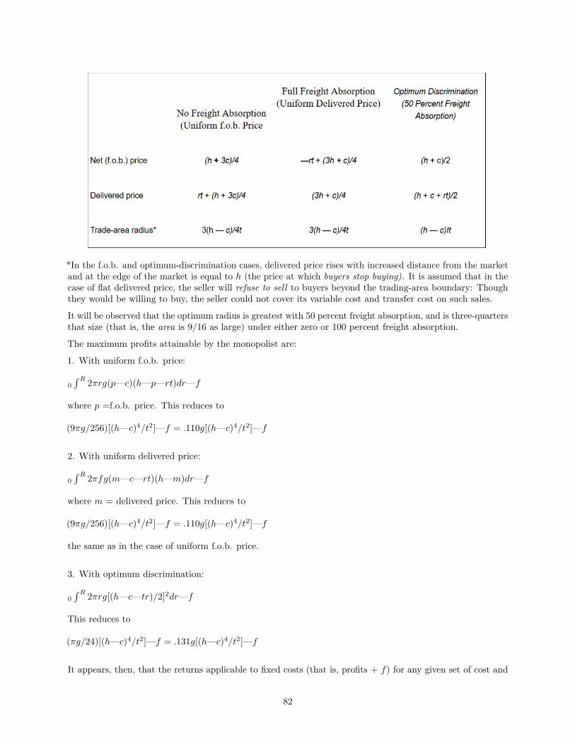
*In the f.o.b. and optimum-discrimination cases, delivered price rises with increased distance from the marketand at the edge of the market is equal to h (the price at which buyers stop buying). It is assumed that in thecase of flat delivered price, the seller will refuse to sell to buyers beyond the trading-area boundary: Thoughthey would be willing to buy, the seller could not cover its variable cost and transfer cost on such sales.

It will be observed that the optimum radius is greatest with 50 percent freight absorption, and is three-quartersthat size (that is, the area is 9/16 as large) under either zero or 100 percent freight absorption.

The maximum profits attainable by the monopolist are:

1. With uniform f.o.b. price:

0∫ R 2πrg(p—c)(h—p—rt)dr—f

where p =f.o.b. price. This reduces to

(9πg/256)[(h—c)4/t2]—f = .110g[(h—c)4/t2]—f

2. With uniform delivered price:

0∫ R 2πfg(m—c—rt)(h—m)dr—f

where m = delivered price. This reduces to

(9πg/256)[(h—c)4/t2]—f = .110g[(h—c)4/t2]—f

the same as in the case of uniform f.o.b. price.

3. With optimum discrimination:

0∫ R 2πrg[(h—c—tr)/2]2dr—f

This reduces to

(πg/24)[(h—c)4/t2]—f = .131g[(h—c)4/t2]—f

It appears, then, that the returns applicable to fixed costs (that is, profits + f) for any given set of cost and

82

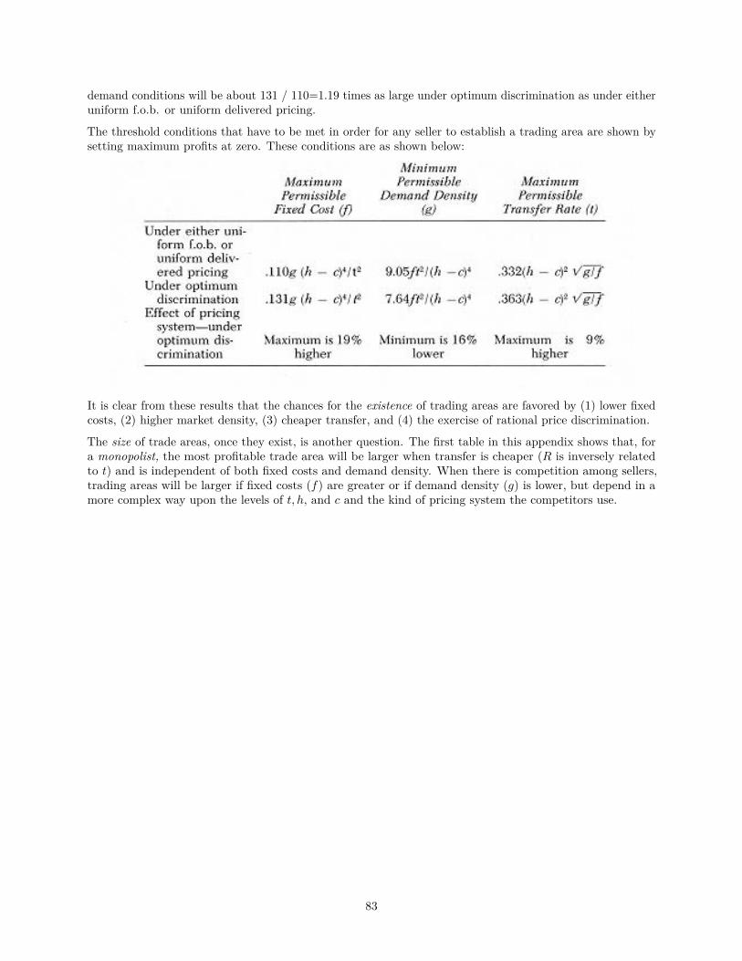
demand conditions will be about 131 / 110=1.19 times as large under optimum discrimination as under eitheruniform f.o.b. or uniform delivered pricing.

The threshold conditions that have to be met in order for any seller to establish a trading area are shown bysetting maximum profits at zero. These conditions are as shown below:

It is clear from these results that the chances for the existence of trading areas are favored by (1) lower fixedcosts, (2) higher market density, (3) cheaper transfer, and (4) the exercise of rational price discrimination.

The size of trade areas, once they exist, is another question. The first table in this appendix shows that, fora monopolist, the most profitable trade area will be larger when transfer is cheaper (R is inversely relatedto t) and is independent of both fixed costs and demand density. When there is competition among sellers,trading areas will be larger if fixed costs (f) are greater or if demand density (g) is lower, but depend in amore complex way upon the levels of t, h, and c and the kind of pricing system the competitors use.

83

5. LOCATION PATTERNS DOMINATED BY COHESION5.1 IntroductionThe discussion in Chapter 4 concerned the market-area or supply-area patterns of activities in which there isstrong spatial repulsion among the individual units. In sharp contrast, however, other activities show highlyclustered patterns.

Cluster is, of course, the logical pattern for units of an output-oriented activity whose markets are concentratedat one or a few locations, and correspondingly for units of an activity oriented to inputs whose source locationsare few. There is a high concentration of producers and suppliers of such theatrical inputs as actors, stagedesigners, and theatrical makeup specialists in Los Angeles and New York because so much movie makingand theater activity is concentrated there. The making of vintage wines is confined to the relatively few areaswhere the right kinds of grapes will flourish.

There are other situations, however, where the basis for clustering is the mutual attraction among thecompeting units of a particular activity, and this attraction outweighs any repulsion that might arise fromtheir rivalry. Thus a frequent practice of chain-store firms is to locate branch stores as close as possibleto a competitor’s branch store. A tendency toward agglomeration is unmistakable in the juxtaposition ofcar sales-rooms along “automobile rows” and in the formation of financial districts, nightlife districts, civiccenters, produce markets, and high-class shopping areas in cities. The larger the city, the more specializedand numerous are such neighborhood agglomerations. In New York, large advertising agencies are so clusteredalong a section of Madison Avenue that the street has given its name to the industry. Similarly, a section ofSeventh Avenue is preempted by the garment trades, part of Forty-seventh Street by diamond merchants,and so on for many other specialties. The common feature of all such clusterings is that each unit findsthe location good because of the presence of the others. There is a positive mutual attraction rather than arepulsion. The explanation of such mutual-attraction clusters lies in special characteristics of the activityitself, its markets, or its suppliers.

5.2 External Economies: Output Variety and Market AttractionIn some activities, the basic reason for the agglomerative tendency is that the outputs of individual units arenot standardized; they are not perfect substitutes for one another, and moreover, they differ in such manifoldand changing ways that they cannot be satisfactorily compared by the buyer without actual inspection. Thelocational significance of this characteristic can best be seen by a pair of contrasting examples.

A manufacturing firm buying sheet steel simply decides on its specifications and then finds out which steelproducer will give the best price and fastest delivery. A visit to warehouses or rolling mills to look over thesheets and make a selection is unnecessary, because the specifications themselves (plus conceivably a samplesent for testing in the buyer’s plant or laboratory) fully identify the characteristics of the steel. Consequently,the transfer costs involved are those of shipping the steel from producer to user, and there is nothing in thesituation that would make it desirable or convenient for the rival sheet steel producers to be concentrated inone place.

Contrast this with a man or woman buying a car or a new hat, a department store selecting its line of fallfashions, or a fashion designer searching for something simply devastating in novelty buttons. In any of thesecases, the buyer does not know exactly what will be purchased. He or she will be selecting one item (in thecase of the car) or maybe more (in the case of the hat) or a very large number (in the case of the departmentstore’s fall line). The items cannot be adequately described in a catalog, and it would be much too expensiveand time consuming for the producers to supply each prospective buyer with a full set of samples. Underthese circumstances, the “demand” is not so much demand for specific items as it is demand for a varieddisplay of products; and the wider the variety presented at a particular location, the more demand thatlocation will attract.

Therefore the buyer makes a shopping trip, preferring the largest display center accessible to him. The morehe is prepared to spend, the farther he will be prepared to go in the interest of variety. Thus most of us

84

would be willing to journey farther out of our way to select a camera than a necktie; still farther to select anew car; and still farther to select a job with career possibilities.

It is clear that the activity that is presenting the displays will tend to adopt a clustered pattern, with itsunits positively attracting one another. A newcomer to the cluster may even be welcomed, because that sellerwill enrich the variety and draw still more demand to the location.

It should be noted also that where comparison shopping is important, the significant transfer costs are borneby the buyer, and the major element in transfer costs is personal travel time. The transfer of the goodsbought may be handled by the buyer himself (he may drive his new car home or carry his other purchases).In any event, however, the transfer cost is not enough to counteract the advantage (to both buyers and sellers)of having the selling units agglomerated.

When the purchases are transferred separately, it is of course feasible to separate production or delivery, orboth, from display. Thus new car dealers sometimes have to order from the nearest assembly plant after thebuyer has made his choice; and in recent years more and more garment producers have moved their factoriesout of the city in order to reduce production costs, and maintain in the city only the functions of display andassociated entertainment for the out-of-town buyers.

These examples illustrate one important kind of external economy of agglomeration of an activity—“external”to the individual unit involved because the advantages depend on how many other units of its type are joiningit to make a cluster that attracts demand.1

5.3 External Economies: Characteristics of the Production Process5.3.1 Introduction

The externalities associated with the size of a cluster are by no means limited to those that enhancedemand as a result of the characteristics of shopping behavior. Some closely analogous external economies ofagglomeration involve cost and supply considerations, and these tend to affect many of the same activities.

If products are complexly differentiated and changeable from one day or week to the next, the chances arethat at least some of the inputs also share those characteristics. Thus a fashion garment shop will have aconstantly changing need for different fabrics, thread, buttons, zippers, and the like. With the nature of theoutput continually changing, manpower needs can vary unpredictably and suddenly; with speedy delivery ata premium and production scheduling intricate, equipment repairs and parts must be quickly available. Sinceperhaps the most important task of the manager is to estimate what the buyers will want and what his orher rivals will offer, a crucial input is fresh information, gathered largely by mixing with the right people andkeeping the eyes and ears open.

Every one of these input requirements, plus others, is best satisfied in a tight cluster. The basic reason can bemade clear by the following example. Suppose we have a small plant that manufactures ladies’ coats. A longsequence of separate operations is involved, including such operations as cutting and binding the buttonholes.Specialized equipment exists for making buttonholes rapidly and cheaply in large quantities, but it representsa sizable investment. Individual coat manufacturers would not find it worthwhile to invest in such a machine,since they could not keep it busy all the time; they have to resort to making their buttonholes in a slower way,involving greater labor cost. However, if they locate in a cluster with enough other clothing manufacturers,their combined need for buttonholes may suffice to keep at least one of the specialized buttonhole machinesreasonably busy. Then a separate firm specializing in buttonhole making joins the cluster. The clothingmanufacturers contract that operation out to that firm, to the advantage of all concerned, including thecustomer who gets the coat cheaper.

This example can be extended to embrace dozens of other individual operations that likewise can be delegatedto specialized firms when there is a cluster, enabling a sufficient number of firms using the specialized serviceto enjoy convenient access to the specialist.

1B. Curtis Eaton and Richard G. Lipsey. “Comparison Shopping and the Clustering of Homogeneous Firms,” Journal ofRegional Science, 19, 4 (November 1979), 421-435, examine some locational implications of comparison shopping in a moretheoretical context.

85

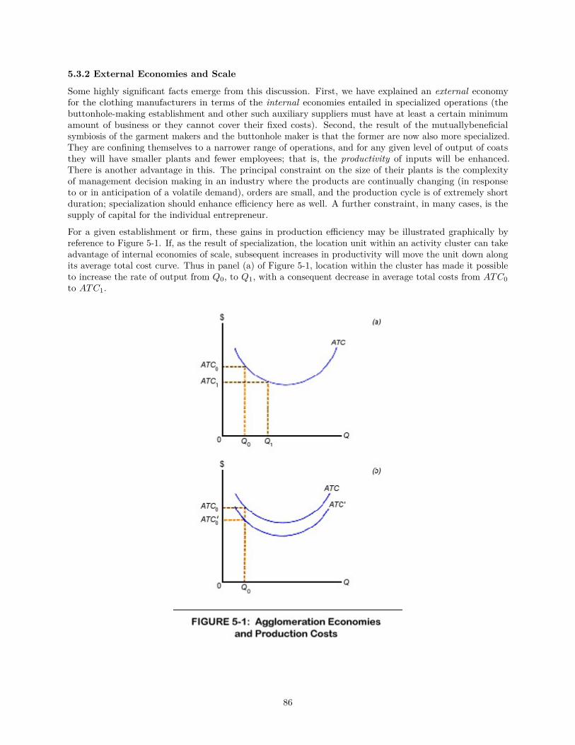
5.3.2 External Economies and Scale

Some highly significant facts emerge from this discussion. First, we have explained an external economyfor the clothing manufacturers in terms of the internal economies entailed in specialized operations (thebuttonhole-making establishment and other such auxiliary suppliers must have at least a certain minimumamount of business or they cannot cover their fixed costs). Second, the result of the mutuallybeneficialsymbiosis of the garment makers and the buttonhole maker is that the former are now also more specialized.They are confining themselves to a narrower range of operations, and for any given level of output of coatsthey will have smaller plants and fewer employees; that is, the productivity of inputs will be enhanced.There is another advantage in this. The principal constraint on the size of their plants is the complexityof management decision making in an industry where the products are continually changing (in responseto or in anticipation of a volatile demand), orders are small, and the production cycle is of extremely shortduration; specialization should enhance efficiency here as well. A further constraint, in many cases, is thesupply of capital for the individual entrepreneur.

For a given establishment or firm, these gains in production efficiency may be illustrated graphically byreference to Figure 5-1. If, as the result of specialization, the location unit within an activity cluster can takeadvantage of internal economies of scale, subsequent increases in productivity will move the unit down alongits average total cost curve. Thus in panel (a) of Figure 5-1, location within the cluster has made it possibleto increase the rate of output from Q0, to Q1, with a consequent decrease in average total costs from ATC0to ATC1.

86

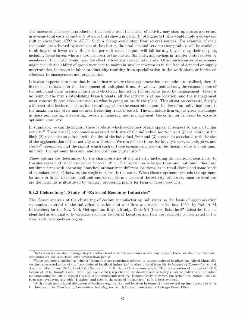
The increased efficiency in production that results from the cluster of activity may show up also as a decreasein average total costs at each rate of output. As shown in panel (b) of Figure 5-1, this would imply a downwardshift in costs from ATC to ATC ′. Such a change could stem from several sources. For example, if scaleeconomies are achieved by members of the cluster, the products and services they produce will be availableto all buyers at lower cost. Hence the per unit cost of inputs will fall for any buyer using their outputs,including those buyers who are also members of the cluster. Similarly, any savings in transfer costs realized bymembers of the cluster would have the effect of lowering average total costs. Other such sources of economiesmight include the ability of group members to maintain smaller inventories in the face of demand or supplyuncertainties, increases in labor productivity resulting from specialization in the work place, or increasedefficiency in management and organization.

It is also important to note that in an industry where these agglomeration economies are realized, there islittle or no rationale for the development of multiplant firms. As we have pointed out, the economic size ofthe individual plant in such industries is effectively limited by the problems faced by management. There isno point in the firm’s establishing branch plants; all the activity is at one location, and the managementmust constantly give close attention to what is going on inside the plant. This situation contrasts sharplywith that of a business such as food retailing, where the constraint upon the size of an individual store isthe maximum size of its market area (reflecting transfer costs). The multistore firm enjoys great advantagesin mass purchasing, advertising, research, financing, and management; the optimum firm size far exceedsoptimum store size.

In summary, we can distinguish three levels at which economies of size appear in respect to any particularactivity.2 These are (1) economies associated with size of the individual location unit (plant, store, or thelike); (2) economies associated with the size of the individual firm; and (3) economies associated with the sizeof the agglomeration of that activity at a location. We can refer to these, for brevity’s sake, as unit, firm, andcluster3 economies, and the size at which each of these economies peaks can be thought of as the optimumunit size, the optimum firm size, and the optimum cluster size.4

These optima are determined by the characteristics of the activity, including its locational sensitivity totransfer costs and other locational factors. When firm optimum is larger than unit optimum, there aremultiunit firms with operating branches, ordinarily in different locations, as in retail chains and some kindsof manufacturing. Otherwise, the single-unit firm is the norm. When cluster optimum exceeds the optimumfor units or firms, there are multiunit and/or multifirm clusters of the activity; otherwise, separate locationsare the norm, as is illustrated by primary processing plants for farm or forest products.

5.3.3 Lichtenberg’s Study of “External-Economy Industries”

The classic analysis of the clustering of certain manufacturing industries on the basis of agglomerationeconomies external to the individual location unit and firm was made in the late 1950s by Robert M.Lichtenberg for the New York Metropolitan Region Study. Table 5-1 (below) lists the 87 industries that heidentified as dominated by external-economy factors of Location and that are relatively concentrated in theNew York metropolitan region.

2In Section 5.4 we shall distinguish yet another level at which economies of size may appear; there, we shall find that sucheconomies are also associated with urbanization per se.

3What are here identified as “cluster” economies are sometimes referred to as economies of localization. Alfred Marshall’ssuccinct characterization of the “economies of localized industries” is often quoted from his Principles of Economics, 8th ed.(London: Macmillan, 1925), Book IV, Chapter 10. F. S. Hall’s Census monograph, “The Localization of Industries” (U.S.Census of 1900, Manufactures, Part 1, pp. cxc—ccxiv), reported on the development of highly clustered patterns of individualmanufacturing industries toward the end of the nineteenth century. Unfortunately, however, the term “localization” has alsobeen used synonymously with “location” and even in the sense of “dispersion,” so it is best avoided.

4A thorough and original discussion of business organization and location in terms of these several optima appears in E. A.G. Robinson, The Structure of Competitive Industry, rev. ed. (Chicago: University of Chicago Press, 1958).

87

TABLE 5-1: Manufacturing Industries Relatively Concentratedin New York City by External Economies, 1954Industry New York Metropolitan Region’s

Share of Total U.S. Employment(percent)

Hatters’ fur 99.9*Lapidary work 99.5*Artists’ materials 91.9*Fur goods 90.4Dolls 87.4*Schiffli-machine embroideries 86.5Hat and cap materials 85.7Suspenders and garters 84.7*Women’s neckwear and scarves 84.7Hairwork 82.7*Embroideries, except Schiffli 80.0Tucking, pleating, and stitching 76.8Handbags and purses 75.6Tobacco pipes 75.3Millinery 64.7Children’s coats 61.6Belts 60.9*Artificial flowers 60.6Women’s suits, coats, and skirts 58.8Dresses, unit price 58.7Furs, dressed and dyed 56.9*Umbrellas, parasols, and canes 54.5*Robes and dressing gowns 54.3Small leather goods 53.1Miscellaneous bookbinding work 53.0*Handkerchiefs 49.8*Buttons 49.5Trimmings and art goods 49.0Men’s and boys’ neckwear 48.3Watchcases 48.1*Phonograph records 48.0*Books, publishing and printing 46.8Periodicals 46.5Lamp shades 46.0Corsets and allied garments 45.9Children’s outerwear, n.e.c+ 43.2Knit outerwear mills 42.3Blouses 41.7Finishing wool textiles 41.5Bookbinding 41.1Jewelry 40.5Suit and coat findings 39.6Costume jewelry 39.5Children’s dresses 39.3Men’s and boys’ cloth hats 38.0Waterproof outer garments 37.6Printing ink 34.7Coated fabrics, except rubberized 34.5*

88

TABLE 5-1: Manufacturing Industries Relatively Concentratedin New York City by External Economies, 1954Industry New York Metropolitan Region’s

Share of Total U.S. Employment(percent)

Women’s and children’s underwear 34.4Luggage 34.3Apparel, n.e.c. 34.0Needles, pins, and fasteners 33.8Jewelry and instrument cases 33.7Engraving and plate printing 33.6Miscellaneous publishing 33.3Curtains and draperies 32.9Typesetting 32.9Straw hats 32.8*Women’s outerwear, n.e.c. 32.7Jewelers’ findings 32.6*Games and toys, n.e.c. 32.1Engraving on metal 30.4Leather and sheep-lined clothing 30.4Textile products, n.e.c. 30.4China decorating for the trade 29.0Housefurnishings 28.9Photoengraving 28.2Book printing 25.5Electrotyping and stereotyping 25.5Fabric dress gloves 25.3Greeting cards 25.2Galvanizing 24.4*Candles 23.5Mirror and picture frames 22.7Men’s and boys’ suits and coats 22.3Knitting mills, n.e.c. 21.2Finishing textiles, except wool 20.6Signs and advertising displays 20.4Plating and polishing 18.7Knit fabric mills 18.3Lithographing 17.9Enameling and lacquering 16.7Statuary and art goods 16.6Commercial printing 16.5Felt goods, n.e.c. 16.0*Narrow fabric mills 15.4Dresses, dozen-price 12.9

*Approximate figure estimated by Lichtenberg: exact figures unavailable because of Census disclosure rules.+n.e.c.: not elsewhere classified.Source Robert M. Lichtenberg, One-Tenth of a Nation (Cambridge, Mass.: Harvard University Press, 1960),pp. 265-268; based on data from U.S. Census of Manufactures, 1954.

89

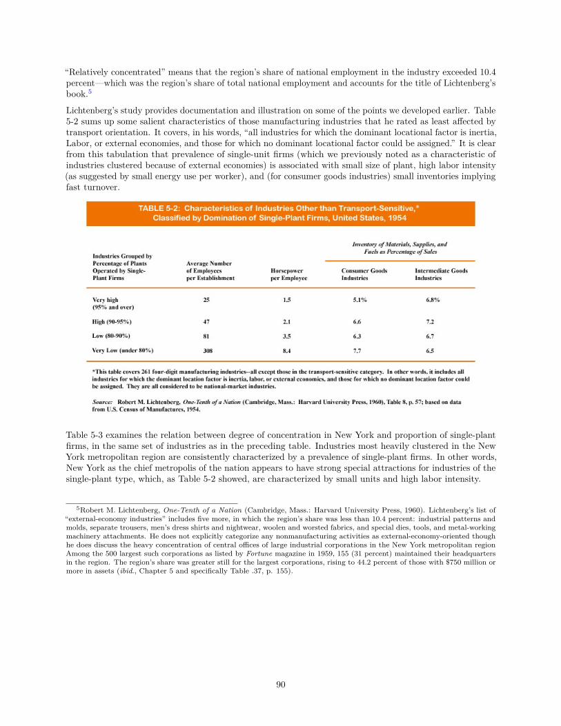
“Relatively concentrated” means that the region’s share of national employment in the industry exceeded 10.4percent—which was the region’s share of total national employment and accounts for the title of Lichtenberg’sbook.5

Lichtenberg’s study provides documentation and illustration on some of the points we developed earlier. Table5-2 sums up some salient characteristics of those manufacturing industries that he rated as least affected bytransport orientation. It covers, in his words, “all industries for which the dominant locational factor is inertia,Labor, or external economies, and those for which no dominant locational factor could be assigned.” It is clearfrom this tabulation that prevalence of single-unit firms (which we previously noted as a characteristic ofindustries clustered because of external economies) is associated with small size of plant, high labor intensity(as suggested by small energy use per worker), and (for consumer goods industries) small inventories implyingfast turnover.

Table 5-3 examines the relation between degree of concentration in New York and proportion of single-plantfirms, in the same set of industries as in the preceding table. Industries most heavily clustered in the NewYork metropolitan region are consistently characterized by a prevalence of single-plant firms. In other words,New York as the chief metropolis of the nation appears to have strong special attractions for industries of thesingle-plant type, which, as Table 5-2 showed, are characterized by small units and high labor intensity.

5Robert M. Lichtenberg, One-Tenth of a Nation (Cambridge, Mass.: Harvard University Press, 1960). Lichtenberg’s list of“external-economy industries” includes five more, in which the region’s share was less than 10.4 percent: industrial patterns andmolds, separate trousers, men’s dress shirts and nightwear, woolen and worsted fabrics, and special dies, tools, and metal-workingmachinery attachments. He does not explicitly categorize any nonmanufacturing activities as external-economy-oriented thoughhe does discuss the heavy concentration of central offices of large industrial corporations in the New York metropolitan regionAmong the 500 largest such corporations as listed by Fortune magazine in 1959, 155 (31 percent) maintained their headquartersin the region. The region’s share was greater still for the largest corporations, rising to 44.2 percent of those with $750 million ormore in assets (ibid., Chapter 5 and specifically Table .37, p. 155).

90

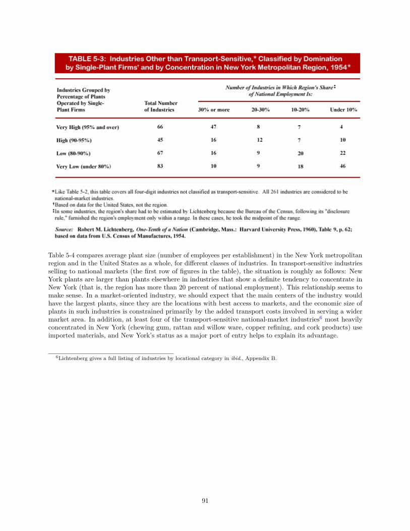
Table 5-4 compares average plant size (number of employees per establishment) in the New York metropolitanregion and in the United States as a whole, for different classes of industries. In transport-sensitive industriesselling to national markets (the first row of figures in the table), the situation is roughly as follows: NewYork plants are larger than plants elsewhere in industries that show a definite tendency to concentrate inNew York (that is, the region has more than 20 percent of national employment). This relationship seems tomake sense. In a market-oriented industry, we should expect that the main centers of the industry wouldhave the largest plants, since they are the locations with best access to markets, and the economic size ofplants in such industries is constrained primarily by the added transport costs involved in serving a widermarket area. In addition, at least four of the transport-sensitive national-market industries6 most heavilyconcentrated in New York (chewing gum, rattan and willow ware, copper refining, and cork products) useimported materials, and New York’s status as a major port of entry helps to explain its advantage.

6Lichtenberg gives a full listing of industries by locational category in ibid., Appendix B.

91

The external-economy industries, which are nearly all rather highly concentrated in the New York region,show a significantly contrasting size relationship. Despite the great prominence of New York as a location forsuch industries, the plants there are smaller than those elsewhere. This should be expected according tothe considerations already discussed. A plant of an external-economy industry located in New York is in aposition to contract out more operations to specialists, such as our buttonhole maker. Within any Censusindustry classification, those firms and plants that to the greatest degree share the special characteristics ofclustered external-economy activities (such as variable demand and product, rapid production cycle, andlow degree of mechanization) will be the ones most likely to find the New York location attractive; andthose characteristics are, as we have seen, strongly associated with small plant size. Plants in the sameCensus industry located elsewhere are more likely to be turning out a less variable kind of product, and theiroptimum plant size is somewhat larger.

Thus industries of the clustered type have, as a class, the peculiar characteristic of operating in smaller units(in terms of both plant and firm) in locations of major concentration than they do elsewhere.

5.4 Single-Activity Clusters and Urbanization5.4.1 Introduction

The advantages of a clustered location pattern for certain types of activities are now apparent. But whatdoes such a cluster contain besides the major beneficiary of those advantages?

There are certainly some types of clusters that need contain nothing else—for example, “automobile rows.”Here the mere juxtaposition of a number of salesrooms makes the area attractive to prospective buyers, andthat is the basis of the agglomeration tendency. The same is true for many other types of single-activityneighborhood cluster in cities, such as art shops, antique stores, secondhand bookstores, wholesale and retailproduce markets, and the like.

But in each of those cases, what really draws the buyers is variety. There would be no advantage inagglomeration (so far as buyers are concerned) if the wares of the different sellers were identical. Accordingly,still other product lines or activities may contribute to the advantage of the cluster, provided they offer

92

something that the same buyers might want to pick up on the same trip. In this way, the attractions of acluster of high-fashion dress shops may well be enhanced by the addition of a shop specializing in high-fashionshoes or jewelry, or even a travel agency catering to high-income travelers. At a more plebeian level, thefamiliar suburban shopping center includes a wide assortment of retail trade and service activities. Thedevelopers of the center usually plan rather closely in advance the kinds of businesses to be included and takepains to pin down at least some of the key tenants (such as a department store branch, a bank, or a movietheater) even before ground is broken. Other relatively broad and diverse clusters based on the attraction ofa common demand are recreation centers and cultural centers.7

Just as externalities associated with shopping behavior imply advantages for clusters of closely related activities,a cluster in which availability of common inputs plays an important role (such as in the external-economyindustries analyzed by Lichtenberg) is also more likely to be a complex of closely related activities thanjust a clump of units of one activity. Thus an essential part of a cluster that is advantageous to garmentmanufacturers is a variety of such related activities as machine rental and repair; designing; provision ofspecial components such as buttonholes, fasteners, and ornaments; trucking services; and so on. Indeed,the Lichtenberg list includes such ancillary activities indiscriminately along with the producers of garmentsand other final products; this is quite fitting, since it is the tightly knit complex of activities that yields theexternal economies that help motivate the cluster.

5.4.2 Urbanization Economies

Our examples suggest that the process of identifying an activity cluster is somewhat more complicated thanmight first appear. Detailed examination of a large activity cluster discloses that while some constituentactivities (such as buttonhole making) are so specialized that they are locationally associated with just oneline of activity, others (such as trucking or forwarding services, entertainment facilities for visiting buyers,and a variety of business services) are not so restricted. They are essentially elements of a large urbanagglomeration. Their presence, and the quality and variety of the services they offer, depend more on the sizeof the city than on the size of the local concentration of any of the activities they serve.

Economies generated by activities and services of this sort are external to any single-activity cluster, butthey are internal to the urban area. There is a parallel to be drawn here to the relationship between asingle-activity cluster and its constituent units. In that instance, economies were realized by the units asthe size of the cluster increased; thus economies are internal to the cluster but external to the unit. In thecase of urbanization economies, we recognize that economies accrue to constituent clusters as the size of theurban area increases. Thus some of the advantages that a particular activity gets by concentrating in NewYork could not be duplicated by simply having an equal amount of that activity clustered in, say, Columbus,Ohio—though, of course, it is possible that Columbus might offer some compensating attractions of a differentnature.

There have been, and still are, some noteworthy multifirm clusters of single activities in relatively smallplaces (historic examples are glove making in Gloversville, New York; hat making in Danbury, Connecticut;and furniture making in Grand Rapids, Michigan). But it is apparent that this type of single-activity cluster(in which the bulk of an activity is found in a few “one-industry towns”) has rather gone out of style since F.S. Hall proclaimed its heyday in 1900.8 Such concentrations depended heavily on the external economiesof a pool of specialized labor skilled in operations peculiar to one industry, and often predominantly ofone nationality group;9 on a reservoir and tradition of entrepreneurship similarly specialized; and on the

7For an empirical analysis of cluster tendencies involving related lines of retail trade, see Arthur Getis and Judith M. Getis,“Retail Store Spatial Affinities,” Urban Studies, 5, 3 (November 1968), 317-322. For a sophisticated and challenging empiricalanalysis of which activities cluster with which, see Joel Bergsman, Peter Greenston, and Robert Healy, “The AgglomerationProcess in Urban Growth,” Urban Studies,9, 3 (October 1972), 263-288; and for a survey of related literature, see Stan Czamanskiand Luiz Augusto de Q. Ablas, “Identification of Industrial Clusters and Complexes: A Comparison of Methods and Findings,”Urban Studies, 16, 1 (February 1979), 61-80.

8Hall’s 1900 Census monograph, previously cited, gives numerous further examples.9Economic historians have often noted the important role of the influx of Germans to the United States in the mid-nineteenth

century in establishing concentrations of certain industries in which they had special skills, such as optical and other scientificinstruments in Rochester, brewing in Milwaukee and St. Louis, and tanning and shoemaking in these and other Midwesterncities.

93

inertial factor of acquired reputation. Technological changes and enhancement of the mobility of labor andentrepreneurship explain why such local specialization has become increasingly rare. By contrast, externaleconomies on the broader basis of urban size and diversity have remained a powerful locational force.

5.4.3 Measuring Urbanization Economies

The symbiotic relationships within single-activity clusters or more complex clusters reflecting urbanizationeconomies have important implications, both for constituent activities and for the regional economy as awhole. As a consequence, much effort has been devoted to understanding and measuring agglomerationeconomies. Many people concerned with the growth and development of specific regions have examined theadvantages inherent in urban concentrations, in an effort to understand the factors most relevant to theirregion’s prosperity and problems.

Our examination of agglomerative forces suggests that they may affect an individual location unit eitherthrough market demand considerations or through modifications of the production process that enhanceefficiency. The evaluation of either or both of these effects entails some challenging difficulties.

Recent efforts to measure the extent of urbanization economies have focused on estimates of the productivitygain accruing to activities that are located in larger urban areas. They proceed by treating production inurban areas as being representative of the aggregate production of component activities. For example, if onewere to estimate the aggregate demand for labor in Boston or Detroit, one would assume that the behavior ofthis aggregate reflects a weighted average of labor demand curves associated with all activities in the city.

Measurements of this sort rest on the belief that the demand for factors of production is determined by thevalue of their marginal product, that is, marginal physical product multiplied by the price of the good orservice being produced. Because of this, the demand for inputs, including labor, would reflect the advantagesof agglomeration economies. Whether the source of these economies is due to the size of the location unit,firm, cluster, or urban area, any associated increase in factor productivity would show up in the urban area’sdemand for labor. With this in mind, researchers interested in measuring agglomeration economies havereasoned that by the comparison of labor markets associated with cities of different size, it might be possibleto isolate the contribution of urbanization economies to labor productivity. Further, if it were possible toisolate a measure of aggregate efficiency in production due to these forces, we would also have a measure oftheir average effect on the activities that make up the urban areas in question.10

Reference to Figure 5-2 will help to explain and reinforce these ideas. The lines Da and Db represent estimatesof the aggregate demand for labor in two different urban areas, (a) and (b). Db is that associated withthe larger of the two. It is drawn to the right of Da in order to reflect the fact that for any given level ofemployment, the value of labor’s marginal product is greater in the larger urban area. This productivitydifference remains even after one accounts for differences in the size of the capital stock and the “quality” oflabor between these areas.

10A second approach to this measurement problem entails the direct estimation of the returns to scale exhibited by activitiesin metropolitan areas. Gerald A. Carlino, “Increasing Returns to Scale in Metropolitan Manufacturing,” Journal of RegionalScience, 19, 3 (August 1979), 363-373, provides estimates of this sort and attempts to decompose them into economies related tothe size of the unit, cluster, or urban area associated with a given activity.

94

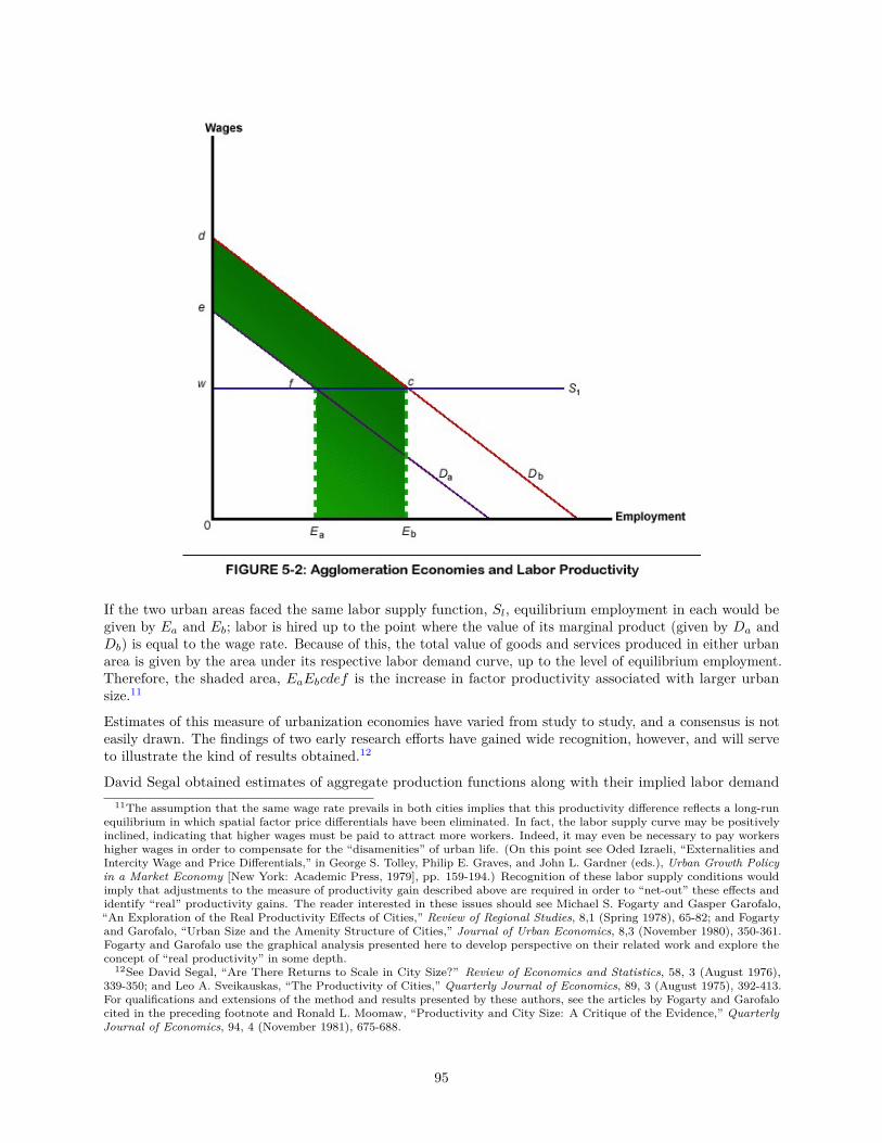
If the two urban areas faced the same labor supply function, Sl, equilibrium employment in each would begiven by Ea and Eb; labor is hired up to the point where the value of its marginal product (given by Da andDb) is equal to the wage rate. Because of this, the total value of goods and services produced in either urbanarea is given by the area under its respective labor demand curve, up to the level of equilibrium employment.Therefore, the shaded area, EaEbcdef is the increase in factor productivity associated with larger urbansize.11

Estimates of this measure of urbanization economies have varied from study to study, and a consensus is noteasily drawn. The findings of two early research efforts have gained wide recognition, however, and will serveto illustrate the kind of results obtained.12

David Segal obtained estimates of aggregate production functions along with their implied labor demand11The assumption that the same wage rate prevails in both cities implies that this productivity difference reflects a long-run

equilibrium in which spatial factor price differentials have been eliminated. In fact, the labor supply curve may be positivelyinclined, indicating that higher wages must be paid to attract more workers. Indeed, it may even be necessary to pay workershigher wages in order to compensate for the “disamenities” of urban life. (On this point see Oded Izraeli, “Externalities andIntercity Wage and Price Differentials,” in George S. Tolley, Philip E. Graves, and John L. Gardner (eds.), Urban Growth Policyin a Market Economy [New York: Academic Press, 1979], pp. 159-194.) Recognition of these labor supply conditions wouldimply that adjustments to the measure of productivity gain described above are required in order to “net-out” these effects andidentify “real” productivity gains. The reader interested in these issues should see Michael S. Fogarty and Gasper Garofalo,“An Exploration of the Real Productivity Effects of Cities,” Review of Regional Studies, 8,1 (Spring 1978), 65-82; and Fogartyand Garofalo, “Urban Size and the Amenity Structure of Cities,” Journal of Urban Economics, 8,3 (November 1980), 350-361.Fogarty and Garofalo use the graphical analysis presented here to develop perspective on their related work and explore theconcept of “real productivity” in some depth.

12See David Segal, “Are There Returns to Scale in City Size?” Review of Economics and Statistics, 58, 3 (August 1976),339-350; and Leo A. Sveikauskas, “The Productivity of Cities,” Quarterly Journal of Economics, 89, 3 (August 1975), 392-413.For qualifications and extensions of the method and results presented by these authors, see the articles by Fogarty and Garofalocited in the preceding footnote and Ronald L. Moomaw, “Productivity and City Size: A Critique of the Evidence,” QuarterlyJournal of Economics, 94, 4 (November 1981), 675-688.

95

functions for 58 metropolitan areas, using 1967 data. A simplified version of the functional form he uses isgiven by

Qi = AScKαi L

βi

where Q is output,K is capital stock, and L is employment (quality adjusted) in city i.13 Technical efficiencyis characterized by the multiplicative constant ASc, where S is a dummy variable denoting size, and A and care parameters. Segal finds constant returns to scale in aggregate production (α+ β = 1), and estimates of care of the order of .08 for cities with populations of 2 to 3 million. This translates to an 8 percent productivitygain (the shaded area in Figure 5-2) for metropolitan areas when this population threshold is reached.

In a study of fourteen industries also based on 1967 data, Leo Sveikauskas finds that an average productivitygain of about 6 percent can be expected with each doubling of city size. He reaches this conclusion byregressing the logarithm of output per worker (productivity) in a given industry on the logarithm of populationand on an index of labor quality across a large sample of cities. Sveikauskas recognizes that these productivitydifferences may be due to differences in capital intensity across cities; if the ratio of capital to labor (K/L) islarge, output per worker will also be large. However, upon investigation he finds that the variation in capitalintensity is not sufficient to account for the observed productivity differences.

Productivity advantages of this magnitude can mean a substantial competitive edge. They can be a powerfullocational incentive and may well have played an important role in encouraging shifts in the spatial distributionof economic activity toward urban areas during much of the postwar period.14

Many problems confront efforts to measure external economies accruing to activities in urban areas, andit is important to keep the limitations of related research in mind. Some types of externalities associatedwith clusters are not necessarily related to urban size and are therefore omitted from measurements of thesort described here. Others are not manifest in productivity differences at all; rather, they are reflectedin demand considerations. Further, because of data constraints, measurement efforts have been limitedto highly aggregate analysis, whereas many of the most interesting aspects of agglomeration economiescan be appreciated only at a much more micro level. The method described in this section is neverthelessrepresentative of the kind of systematic effort that is required to address these and other issues related to themeasurement of this important phenomenon.

5.5 Mixed SituationsIn order to bring out certain controlling factors, we have been considering sharply contrasting types of activitylocation patterns. We have distinguished patterns dominated by mutual repulsion from those dominated bymutual attraction. We have also distinguished patterns involving market areas from patterns involving supplyareas.

It is now time to recognize that in the real world there are various intermediate stages between the extremecases described. In one and the same activity, it is not uncommon to find (1) dispersive forces dominant at onelevel of spatial detail and agglomerative forces dominant at another level, or (2) coexistence of market-areaand supply-area patterns. Let us take a brief look at each of these types of “mixed” situations.

5.5.1 Attraction plus Repulsion

In any given activity, the forces of repulsion and attraction among units are usually both present in somedegree, even though one generally predominates. Thus in an activity characterized by a mosaic of marketareas, some of the locations will have more than one plant, store, or other such unit. Though we think ofretail grocery stores or gasoline stations as primarily mutually repulsive, it is not uncommon to find groupings

13Actually, Segal accounts for differences in labor quality among cities by setting β =∑k

βkqik where qik reflects the city’s

labor force composition by education, sex, race, and age. He also includes a vector of site characteristics (accounting for climate,natural resources, etc.) in the multiplicative constant.

14In Chapter 8, we shall find that the growth rate of nonmetropolitan areas has exceeded that of metropolitan areas in recentyears. Some researchers have speculated that this also may be due to the changing structure of agglomeration economies.

96

of two or more adjacent competitors showing some degree of mutual attraction. Being at essentially the samelocation, these rival units are likely to share the same market area, though one might have a somewhat widerreach than another. If we think of them as simply sharing “the market area of that location,” the statementsmade earlier about market-area determination and pricing policies are still largely valid, except that spatialpricing systems involving systematic transfer cost absorption become less feasible when the seller is not aloneat its location.15

Similarly, an activity that we think of as basically clustered, such as the making of fashion garments, often hasseveral widely separated clusters. Among the external-economy industries of New York enumerated in Table5-1, it will be noted that only a few come close to being exclusively concentrated in the New York region. Therest are found also in substantial, lesser clusters in other large cities. One reason for replication of clusters is,of course, that over long distances transfer costs (in time if not in money) become a significant constraint onconcentration relative to far-flung markets or input sources. Thus, when we look at the country as a whole,we see a pattern of market or supply areas showing some force of mutual repulsion among competing centers.If such an activity is concentrated primarily in, say, New York, Los Angeles, and Chicago, there will be threeroughly demarcated market areas or supply areas, each shared by all the members of the corresponding cluster.In this connection, it is much more likely that market areas rather than supply areas will be involved, sincemost external-economy activities produce transferable outputs that need fast delivery to rather widespreadmarkets, and their transferable inputs come from fewer sources and are of a more staple character.

5.5.2 Coexistence of Market Areas and Supply Areas, When Both Sellers and Buyers AreDispersed

Somewhat different from the case just discussed is a not uncommon situation in which there are many sellinglocations and many markets, and not necessarily any significant clustering tendencies at all. Sales from oneproducing district are distributed over many market points, and at the same time any one market districtbuys from many supplying points. The situation does not lend itself to analysis purely in terms of a set ofsupply areas or a set of market areas. How, then, can we most effectively analyze such a pattern?

Except in the unlikely situation in which the patterns of supply and demand coincide (which would meanthat no transfer is required and that each point is self-sufficient in this particular product), there will besurplus areas where local output exceeds local consumption, and deficit areas where the opposite situationprevails. The product will be transferred from surplus areas to deficit areas; and in order to motivate theflow, there must be a price differential corresponding to the costs of transfer along the paths of flow.

The relationship between price patterns and transfer can be demonstrated as follows. Suppose we were to mapthe spatial variations in the price of the good, depicting a price surface by plotting a set of contour lines, eachconnecting points at which the price is at some particular level. The iso price lines (isotims) correspondingto the highest prices would occur in the principal deficit areas, and those corresponding to the lowest priceswould occur in the principal surplus areas. The price gradient along any path would be determined bythe frequency with which we cross successive isoprice contours as we traverse that path. Shipments of thecommodity would be most likely to occur along the paths with the steepest price gradients, and such pathswould cross the isoprice lines at right angles. Actual shipments would occur wherever there is a price gradientat least as steep as the gradient of transfer costs; and in an equilibrium situation, we should expect thatthese shipments would result in no price gradient being substantially steeper than the transfer cost gradient.

Such a graphic analysis does not, however, explicitly recognize the relation between supply and demandpatterns that creates the price differentials giving rise to shipments. William Warntz has suggested anempirically feasible shortcut method of measuring this supply-demand relation that utilizes the access potentialindex described later.16

15If there are many sellers of a standardized commodity at one location, so that they are in nearly perfect competition, anyseller could dispose of its entire output while confining its sales to that part of the market providing the largest profit margin.Consequently, any attempt to establish a discriminatory pricing system would break down.

16William Warntz, Toward a Geography of Price (Philadelphia: University of Pennsylvania Press, 1959).

97

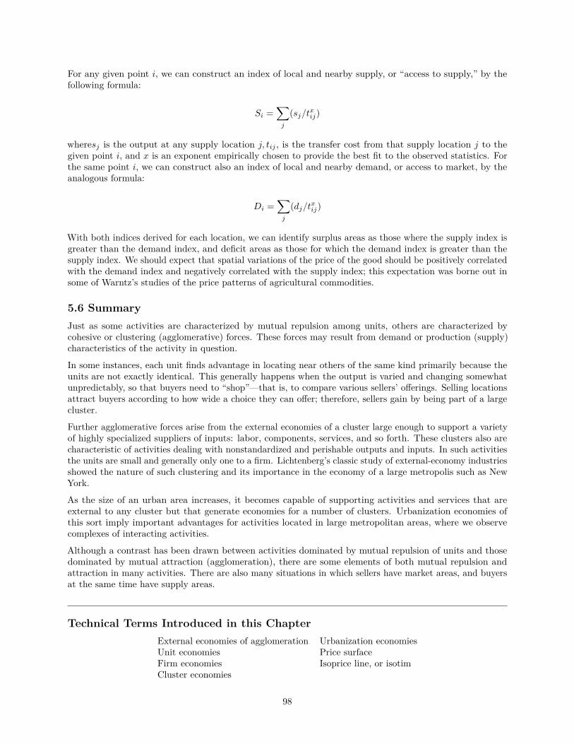
For any given point i, we can construct an index of local and nearby supply, or “access to supply,” by thefollowing formula:

Si =∑j

(sj/txij)

wheresj is the output at any supply location j, tij , is the transfer cost from that supply location j to thegiven point i, and x is an exponent empirically chosen to provide the best fit to the observed statistics. Forthe same point i, we can construct also an index of local and nearby demand, or access to market, by theanalogous formula:

Di =∑j

(dj/txij)

With both indices derived for each location, we can identify surplus areas as those where the supply index isgreater than the demand index, and deficit areas as those for which the demand index is greater than thesupply index. We should expect that spatial variations of the price of the good should be positively correlatedwith the demand index and negatively correlated with the supply index; this expectation was borne out insome of Warntz’s studies of the price patterns of agricultural commodities.

5.6 SummaryJust as some activities are characterized by mutual repulsion among units, others are characterized bycohesive or clustering (agglomerative) forces. These forces may result from demand or production (supply)characteristics of the activity in question.

In some instances, each unit finds advantage in locating near others of the same kind primarily because theunits are not exactly identical. This generally happens when the output is varied and changing somewhatunpredictably, so that buyers need to “shop”—that is, to compare various sellers’ offerings. Selling locationsattract buyers according to how wide a choice they can offer; therefore, sellers gain by being part of a largecluster.

Further agglomerative forces arise from the external economies of a cluster large enough to support a varietyof highly specialized suppliers of inputs: labor, components, services, and so forth. These clusters also arecharacteristic of activities dealing with nonstandardized and perishable outputs and inputs. In such activitiesthe units are small and generally only one to a firm. Lichtenberg’s classic study of external-economy industriesshowed the nature of such clustering and its importance in the economy of a large metropolis such as NewYork.

As the size of an urban area increases, it becomes capable of supporting activities and services that areexternal to any cluster but that generate economies for a number of clusters. Urbanization economies ofthis sort imply important advantages for activities located in large metropolitan areas, where we observecomplexes of interacting activities.

Although a contrast has been drawn between activities dominated by mutual repulsion of units and thosedominated by mutual attraction (agglomeration), there are some elements of both mutual repulsion andattraction in many activities. There are also many situations in which sellers have market areas, and buyersat the same time have supply areas.

Technical Terms Introduced in this ChapterExternal economies of agglomeration Urbanization economiesUnit economies Price surfaceFirm economies Isoprice line, or isotimCluster economies

98

Selected ReadingsBrian J. L. Berry, Geography of Market Centers and Retail Distribution (Englewood Cliffs, N.J.: Prentice-Hall,1967).

Stan Czamanski and Luiz Augusto de Q. Ablas, “Identification of Industrial Clusters and Complexes: AComparison of Methods and Findings,” Urban Studies, 16, 1 (February 1979), 61-80.

Robert M. Lichtenberg, One-Tenth of a Nation (Cambridge, Mass.: Harvard University Press, 1958).

Hugh 0. Nourse, Regional Economics (New York: McGraw-Hill, 1968), pp. 85-92.

Harry W. Richardson, Urban Economics (Hinsdale, Ill.: Dryden Press, 1978), Chapter 3.

David Segal, Urban Economics (Homewood, Ill.: Richard D. Irwin, 1977), Chapter 4.

99

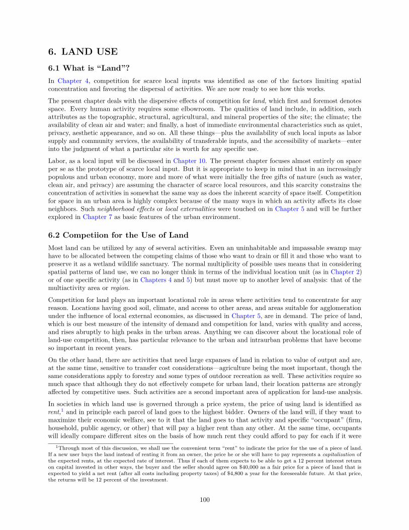
6. LAND USE6.1 What is “Land”?In Chapter 4, competition for scarce local inputs was identified as one of the factors limiting spatialconcentration and favoring the dispersal of activities. We are now ready to see how this works.

The present chapter deals with the dispersive effects of competition for land, which first and foremost denotesspace. Every human activity requires some elbowroom. The qualities of land include, in addition, suchattributes as the topographic, structural, agricultural, and mineral properties of the site; the climate; theavailability of clean air and water; and finally, a host of immediate environmental characteristics such as quiet,privacy, aesthetic appearance, and so on. All these things—plus the availability of such local inputs as laborsupply and community services, the availability of transferable inputs, and the accessibility of markets—enterinto the judgment of what a particular site is worth for any specific use.

Labor, as a local input will be discussed in Chapter 10. The present chapter focuses almost entirely on spaceper se as the prototype of scarce local input. But it is appropriate to keep in mind that in an increasinglypopulous and urban economy, more and more of what were initially the free gifts of nature (such as water,clean air, and privacy) are assuming the character of scarce local resources, and this scarcity constrains theconcentration of activities in somewhat the same way as does the inherent scarcity of space itself. Competitionfor space in an urban area is highly complex because of the many ways in which an activity affects its closeneighbors. Such neighborhood effects or local externalities were touched on in Chapter 5 and will be furtherexplored in Chapter 7 as basic features of the urban environment.

6.2 Competiion for the Use of LandMost land can be utilized by any of several activities. Even an uninhabitable and impassable swamp mayhave to be allocated between the competing claims of those who want to drain or fill it and those who want topreserve it as a wetland wildlife sanctuary. The normal multiplicity of possible uses means that in consideringspatial patterns of land use, we can no longer think in terms of the individual location unit (as in Chapter 2)or of one specific activity (as in Chapters 4 and 5) but must move up to another level of analysis: that of themultiactivity area or region.

Competition for land plays an important locational role in areas where activities tend to concentrate for anyreason. Locations having good soil, climate, and access to other areas, and areas suitable for agglomerationunder the influence of local external economies, as discussed in Chapter 5, are in demand. The price of land,which is our best measure of the intensity of demand and competition for land, varies with quality and access,and rises abruptly to high peaks in the urban areas. Anything we can discover about the locational role ofland-use competition, then, has particular relevance to the urban and intraurban problems that have becomeso important in recent years.

On the other hand, there are activities that need large expanses of land in relation to value of output and are,at the same time, sensitive to transfer cost considerations—agriculture being the most important, though thesame considerations apply to forestry and some types of outdoor recreation as well. These activities require somuch space that although they do not effectively compete for urban land, their location patterns are stronglyaffected by competitive uses. Such activities are a second important area of application for land-use analysis.

In societies in which land use is governed through a price system, the price of using land is identified asrent,1 and in principle each parcel of land goes to the highest bidder. Owners of the land will, if they want tomaximize their economic welfare, see to it that the land goes to that activity and specific “occupant” (firm,household, public agency, or other) that will pay a higher rent than any other. At the same time, occupantswill ideally compare different sites on the basis of how much rent they could afford to pay for each if it were

1Through most of this discussion, we shall use the convenient term “rent” to indicate the price for the use of a piece of land.If a new user buys the land instead of renting it from an owner, the price he or she will have to pay represents a capitalization ofthe expected rents, at the expected rate of interest. Thus if each of them expects to be able to get a 12 percent interest returnon capital invested in other ways, the buyer and the seller should agree on $40,000 as a fair price for a piece of land that isexpected to yield a net rent (after all costs including property taxes) of $4,800 a year for the foreseeable future. At that price,the returns will be 12 percent of the investment.

100

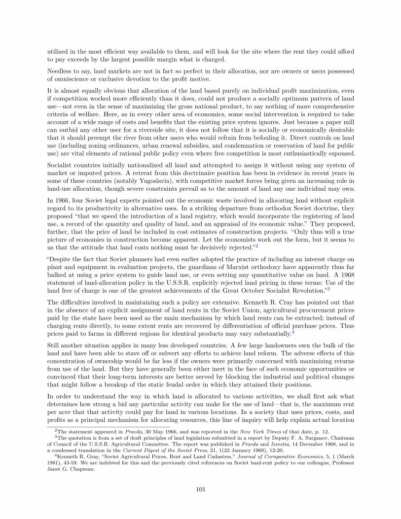
utilized in the most efficient way available to them, and will look for the site where the rent they could affordto pay exceeds by the largest possible margin what is charged.

Needless to say, land markets are not in fact so perfect in their allocation, nor are owners or users possessedof omniscience or exclusive devotion to the profit motive.

It is almost equally obvious that allocation of the land based purely on individual profit maximization, evenif competition worked more efficiently than it does, could not produce a socially optimum pattern of landuse—not even in the sense of maximizing the gross national product, to say nothing of more comprehensivecriteria of welfare. Here, as in every other area of economics, some social intervention is required to takeaccount of a wide range of costs and benefits that the existing price system ignores. Just because a paper millcan outbid any other user for a riverside site, it does not follow that it is socially or economically desirablethat it should preempt the river from other users who would refrain from befouling it. Direct controls on landuse (including zoning ordinances, urban renewal subsidies, and condemnation or reservation of land for publicuse) are vital elements of rational public policy even where free competition is most enthusiastically espoused.

Socialist countries initially nationalized all land and attempted to assign it without using any system ofmarket or imputed prices. A retreat from this doctrinaire position has been in evidence in recent years insome of these countries (notably Yugoslavia), with competitive market forces being given an increasing role inland-use allocation, though severe constraints prevail as to the amount of land any one individual may own.

In 1966, four Soviet legal experts pointed out the economic waste involved in allocating land without explicitregard to its productivity in alternative uses. In a striking departure from orthodox Soviet doctrine, theyproposed “that we speed the introduction of a land registry, which would incorporate the registering of landuse, a record of the quantity and quality of land, and an appraisal of its economic value.” They proposed,further, that the price of land be included in cost estimates of construction projects. “Only thus will a truepicture of economies in construction become apparent. Let the economists work out the form, but it seems tous that the attitude that land costs nothing must be decisively rejected.”2

“Despite the fact that Soviet planners had even earlier adopted the practice of including an interest charge onplant and equipment in evaluation projects, the guardians of Marxist orthodoxy have apparently thus farbalked at using a price system to guide land use, or even setting any quantitative value on land. A 1968statement of land-allocation policy in the U.S.S.R. explicitly rejected land pricing in these terms: Use of theland free of charge is one of the greatest achievements of the Great October Socialist Revolution.”3

The difficulties involved in maintaining such a policy are extensive. Kenneth R. Cray has pointed out thatin the absence of an explicit assignment of land rents in the Soviet Union, agricultural procurement pricespaid by the state have been used as the main mechanism by which land rents can be extracted; instead ofcharging rents directly, to some extent rents are recovered by differentiation of official purchase prices. Thusprices paid to farms in different regions for identical products may vary substantially.4

Still another situation applies in many less developed countries. A few large landowners own the bulk of theland and have been able to stave off or subvert any efforts to achieve land reform. The adverse effects of thisconcentration of ownership would be far less if the owners were primarily concerned with maximizing returnsfrom use of the land. But they have generally been either inert in the face of such economic opportunities orconvinced that their long-term interests are better served by blocking the industrial and political changesthat might follow a breakup of the static feudal order in which they attained their positions.

In order to understand the way in which land is allocated to various activities, we shall first ask whatdetermines how strong a bid any particular activity can make for the use of land—that is, the maximum rentper acre that that activity could pay for land in various locations. In a society that uses prices, costs, andprofits as a principal mechanism for allocating resources, this line of inquiry will help explain actual location

2The statement appeared in Pravda, 30 May 1966, and was reported in the New York Times of that date, p. 12.3The quotation is from a set of draft principles of land legislation submitted in a report by Deputy F. A. Surganov, Chairman

of Council of the U.S.S.R. Agricultural Committee. The report was published in Pravda and Izvestia, 14 December 1968, and ina condensed translation in the Current Digest of the Soviet Press, 21, 1(22 January 1969), 12-20.

4Kenneth R. Gray, “Soviet Agricultural Prices, Rent and Land Cadastres,” Journal of Cornparative Economics, 5, 1 (March1981), 43-59. We are indebted for this and the previously cited references on Soviet land-rent policy to our colleague, ProfessorJanet G. Chapman.

101

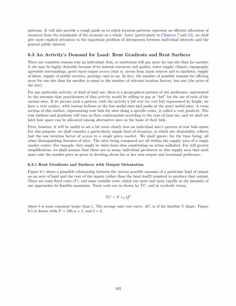
patterns. It will also provide a rough guide as to which location patterns represent an efficient allocation ofresources from the standpoint of the economy as a whole. Later (particularly in Chapters 7 and 13), we shallgive more explicit attention to the important problem of divergences between individual interests and thegeneral public interest.

6.3 An Activity’s Demand for Land: Rent Gradients and Rent SurfacesThere are countless reasons why an individual, firm, or institution will pay more for one site than for another.A site may be highly desirable because of its mineral resources, soil quality, water supply, climate, topography,agreeable surroundings, good input-output access (that is, access from input sources and to markets), supplyof labor, supply of public services, prestige, and so on. In fact, the number of possible reasons for offeringmore for one site than for another is equal to the number of relevant location factors, less one (the price ofthe site).

For any particular activity, or kind of land use, there is a geographical pattern of site preference, representedby the amounts that practitioners of that activity would be willing to pay or “bid” for the use of each of thevarious sites. If we picture such a pattern, with the activity’s bid rent (or rent bid) represented by height, wehave a rent surface, with various hollows at the less useful sites and peaks at the more useful sites. A crosssection of this surface, representing rent bids for sites along a specific route, is called a rent gradient. Therent surfaces and gradients will vary in their conformation according to the type of land use, and we shall seelater how space can be allocated among alternative uses on the basis of their bids.

First, however, it will be useful to see a bit more clearly how an individual user’s pattern of rent bids arises.For this purpose, we shall consider a particularly simple kind of situation, in which site desirability reflectsjust the one location factor of access to a single given market. We shall ignore, for the time being, allother distinguishing features of sites. The sites being compared are all within the supply area of a singlemarket center: For example, they might be dairy-farm sites constituting an urban milkshed. For still greatersimplification, we shall assume that there are so many individual producers in this supply area that eachmust take the market price as given in deciding about his or her own output and locational preference.

6.3.1 Rent Gradients and Surfaces with Output Orientation

Figure 6-1 shows a plausible relationship between the various possible amounts of a particular kind of outputon an acre of land and the cost of the inputs (other than the land itself) required to produce that output.There are some fixed costs (F ), and some variable costs, which rise more and more rapidly as the intensity ofuse approaches its feasible maximum. Total costs are as shown by TC, and in symbolic terms,

TC = F +a Qb

where b is some exponent larger than 1. The average unit cost curve, AC, is of the familiar U shape. Figure6-1 is drawn with F = 100, a = 1, and b = 3.

102

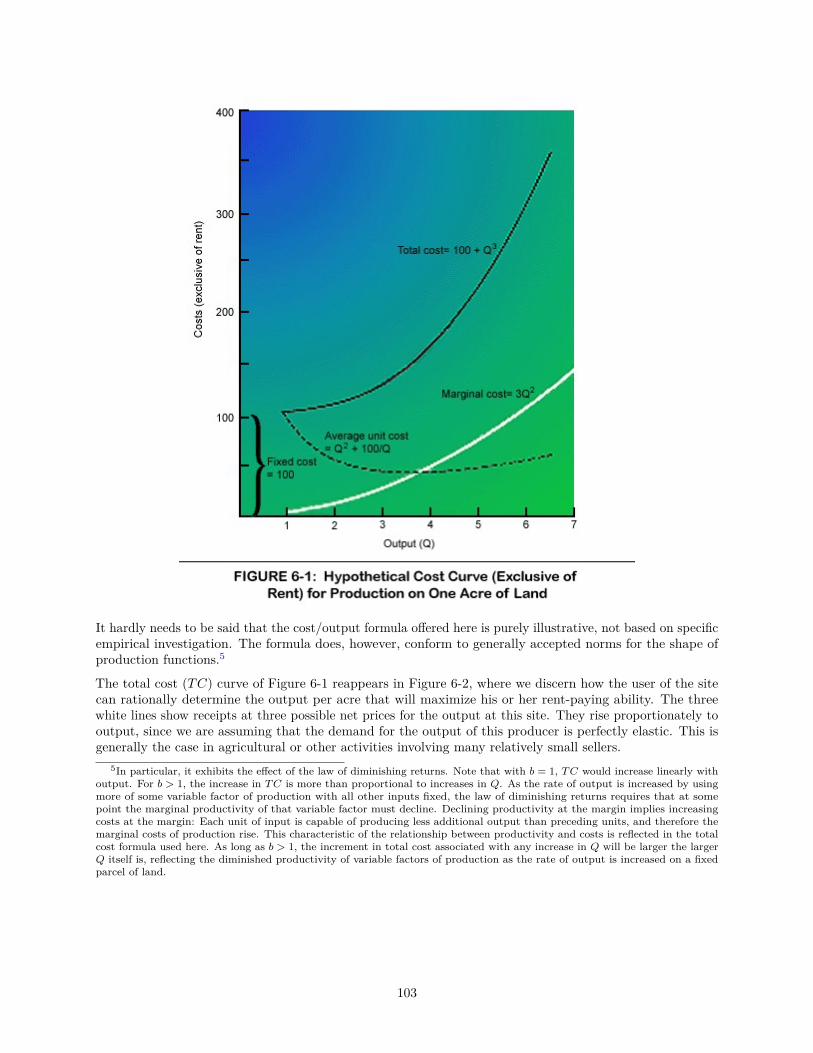
It hardly needs to be said that the cost/output formula offered here is purely illustrative, not based on specificempirical investigation. The formula does, however, conform to generally accepted norms for the shape ofproduction functions.5

The total cost (TC) curve of Figure 6-1 reappears in Figure 6-2, where we discern how the user of the sitecan rationally determine the output per acre that will maximize his or her rent-paying ability. The threewhite lines show receipts at three possible net prices for the output at this site. They rise proportionately tooutput, since we are assuming that the demand for the output of this producer is perfectly elastic. This isgenerally the case in agricultural or other activities involving many relatively small sellers.

5In particular, it exhibits the effect of the law of diminishing returns. Note that with b = 1, TC would increase linearly withoutput. For b > 1, the increase in TC is more than proportional to increases in Q. As the rate of output is increased by usingmore of some variable factor of production with all other inputs fixed, the law of diminishing returns requires that at somepoint the marginal productivity of that variable factor must decline. Declining productivity at the margin implies increasingcosts at the margin: Each unit of input is capable of producing less additional output than preceding units, and therefore themarginal costs of production rise. This characteristic of the relationship between productivity and costs is reflected in the totalcost formula used here. As long as b > 1, the increment in total cost associated with any increase in Q will be larger the largerQ itself is, reflecting the diminished productivity of variable factors of production as the rate of output is increased on a fixedparcel of land.

103

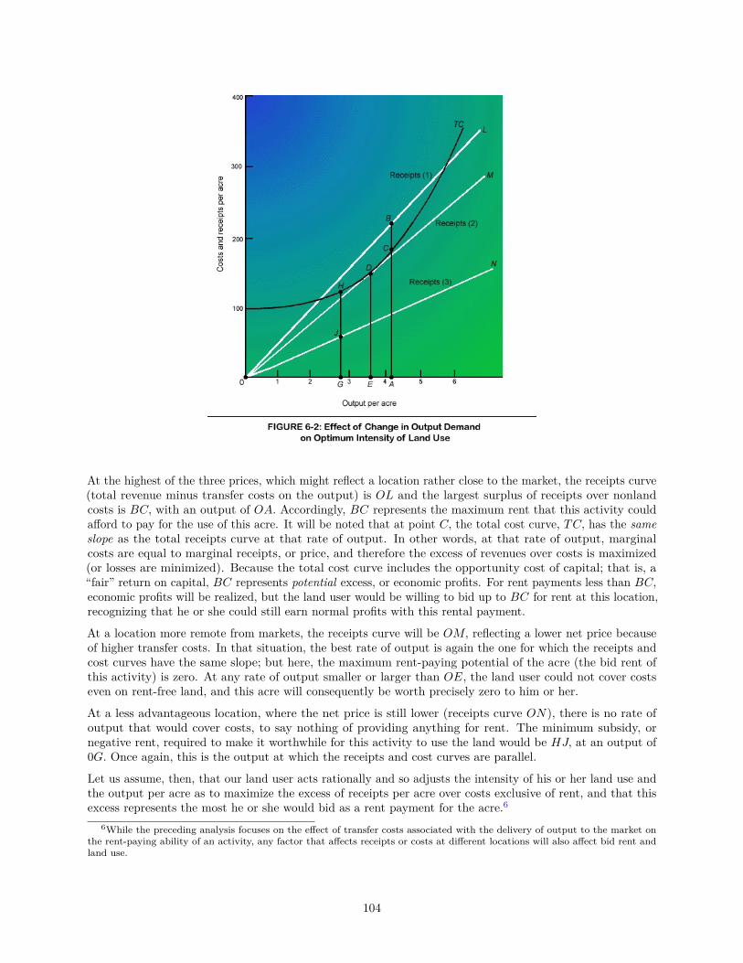
At the highest of the three prices, which might reflect a location rather close to the market, the receipts curve(total revenue minus transfer costs on the output) is OL and the largest surplus of receipts over nonlandcosts is BC, with an output of OA. Accordingly, BC represents the maximum rent that this activity couldafford to pay for the use of this acre. It will be noted that at point C, the total cost curve, TC, has the sameslope as the total receipts curve at that rate of output. In other words, at that rate of output, marginalcosts are equal to marginal receipts, or price, and therefore the excess of revenues over costs is maximized(or losses are minimized). Because the total cost curve includes the opportunity cost of capital; that is, a“fair” return on capital, BC represents potential excess, or economic profits. For rent payments less than BC,economic profits will be realized, but the land user would be willing to bid up to BC for rent at this location,recognizing that he or she could still earn normal profits with this rental payment.

At a location more remote from markets, the receipts curve will be OM, reflecting a lower net price becauseof higher transfer costs. In that situation, the best rate of output is again the one for which the receipts andcost curves have the same slope; but here, the maximum rent-paying potential of the acre (the bid rent ofthis activity) is zero. At any rate of output smaller or larger than OE, the land user could not cover costseven on rent-free land, and this acre will consequently be worth precisely zero to him or her.

At a less advantageous location, where the net price is still lower (receipts curve ON), there is no rate ofoutput that would cover costs, to say nothing of providing anything for rent. The minimum subsidy, ornegative rent, required to make it worthwhile for this activity to use the land would be HJ, at an output of0G. Once again, this is the output at which the receipts and cost curves are parallel.

Let us assume, then, that our land user acts rationally and so adjusts the intensity of his or her land use andthe output per acre as to maximize the excess of receipts per acre over costs exclusive of rent, and that thisexcess represents the most he or she would bid as a rent payment for the acre.6

6While the preceding analysis focuses on the effect of transfer costs associated with the delivery of output to the market onthe rent-paying ability of an activity, any factor that affects receipts or costs at different locations will also affect bid rent andland use.

104

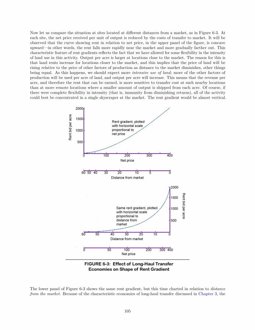
Now let us compare the situation at sites located at different distances from a market, as in Figure 6-3. Ateach site, the net price received per unit of output is reduced by the costs of transfer to market. It will beobserved that the curve showing rent in relation to net price, in the upper panel of the figure, is concaveupward—in other words, the rent falls more rapidly near the market and more gradually farther out. Thischaracteristic feature of rent gradients reflects the fact that we have allowed for some flexibility in the intensityof land use in this activity. Output per acre is larger at locations close to the market. The reason for this isthat land rents increase for locations closer to the market, and this implies that the price of land will berising relative to the price of other factors of production as distance to the market diminishes, other thingsbeing equal. As this happens, we should expect more intensive use of land; more of the other factors ofproduction will be used per acre of land, and output per acre will increase. This means that the revenue peracre, and therefore the rent that can be earned, is more sensitive to transfer cost at such nearby locationsthan at more remote locations where a smaller amount of output is shipped from each acre. Of course, ifthere were complete flexibility in intensity (that is, immunity from diminishing returns), all of the activitycould best be concentrated in a single skyscraper at the market. The rent gradient would be almost vertical.

The lower panel of Figure 6-3 shows the same rent gradient, but this time charted in relation to distancefrom the market. Because of the characteristic economies of long-haul transfer discussed in Chapter 3, the

105

net price of the product will fall more and more slowly with increasing distance: Each extra dollar per tonbuys more and more extra miles of transfer as we go farther from the market. Consequently, we can expectrent as a function of distance to have the accentuated concavity shown in the figure.7

Over a geographic area, we have a rent surface whose basic shape is a concave-sloped “cone” with its peak atthe location of highest possible rent; in the cases discussed so far, that peak is at the market.

But for a number of reasons, real rent gradients and surfaces are never so smooth and regular as our diagramssuggest. In the first place, we have been assuming throughout that all the land is of equal quality for thisparticular kind of use, in all respects save access to market. A location or zone of locations with some superioradvantages (for instance, higher soil fertility or cheaper labor) would be marked by a hump on the rentsurface, and a place with higher costs by a dent (or even a complete gap in the surface if for some reasonthat activity could not be practiced there at all). The rather common stepwise variation of transfer ratesproduces a corresponding terracing of rent surfaces. Rent gradients will be flatter along routes of cheaper orbetter transfer; so if we think of a rent surface around a market as a mountain, it will fall away in slopingridges along such routes and more abruptly elsewhere. Finally, there is usually more than just one market;thus the rent surface of an activity over any sizable area will rise to a number of separate peaks.

6.3.2 Rent Gradients and Rent Surfaces with Input Orientation

One may well ask at this point why the theory of land use places so much stress on access to markets. Whynot access to the sources of transferable inputs? In such a case, of course, we should have rent gradients andrent surfaces peaking at such sources, rather than at markets.

Such patterns do occur. Residents (particularly in resort areas but to some extent elsewhere too) have atendency to cluster around certain foci of consumer attraction, such as beaches. The activity here is residence,which requires space for which it is willing to bid rent. The input is enjoyment of the beach, which is moreeasily available the shorter the distance. The intensity of land use is measured by the degree of crowding ofresidents (persons per acre). In addition, we observe characteristic gradients of intensity and rent. If thereare no considerations of desirability except access to the beach, and if the residents are not too unlike inincomes and tastes, the land values will be lower and the lot sizes larger the greater the distance from thebeach. If the beach is a long one, equally attractive throughout its length, the rent surface will rise not to apeak but to a ridge or cliff along the shore, falling away to landward.

We should expect to find an analogous situation in an urban external-economy activity if the principalattraction of a cluster lies in better access to production inputs, such as supplies and services. A location inthe center of such a cluster is more valuable than one on the periphery.

By and large, however, rent gradients are much more often focused around markets than around inputsources. The great space-using activities are agriculture, forestry, and livestock grazing. They produce bulkytransported outputs but require relatively insignificant amounts of transported inputs; consequently, theirtransfer orientation is overwhelmingly toward markets. The basic reason for this is that their main inputs arenontransferable ones: solar energy, water, and organic properties of the soil. They have a large stake in beingclose to markets but a very small stake in being close to sources of any transferable input, such as fertilizer orpesticide factories.

On the urban scene, the greatest land-using activity is residence, and the transfer orientation of residences ismainly toward markets for labor services; that is, toward employment locations. Only a household consistingwholly of consumers, without any members employed outside, is free to orient itself exclusively to amenity“inputs.” And even in cities known as recreation or retirement centers, the great majority of householdscontain at least one worker. Although within urban areas we do see neighborhood rent gradients rising towardparks or other amenity locations, the overall pattern of rents and land values appears to be shaped to a

7Solow has constructed an interesting urban land-use model in which traffic congestion is taken into account by makingtransport cost per ton-mile depend on traffic density. He finds that the congestion factor makes the rent gradient even moreconcave upward than it would otherwise be. Robert M. Solow, “Congestion, Density, and the Use of Land in Transportation,”Swedish Journal of Economics, 74, 1 (March 1972), 161-173.

106

greater extent by access to jobs. High densities of urban population occur almost exclusively in areas close tomajor job concentrations.8

The various business and government activities of an urban area, insofar as they serve the local market, arestrongly market-oriented because their transferable outputs are so much more perishable and valuable thantheir transferable inputs. Consequently, they have a large stake in access to the distribution of residences,jobs, or both. Once again, we have rent gradients rising in the direction of markets; in this case, generallytoward the center of the urban concentration.

Finally, manufacturing industries oriented toward sources of transferable inputs are mainly those engaged inthe first-stage processing of rural products (crops, including timber, and minerals). They are input-oriented,as noted in Chapter 2, because their processes characteristically reduce weight and bulk, and sometimes(as in the case of canning and preserving operations) perishability as well. But these processing activitiesthemselves are not extensive land users in a rural context. In fact, they are highly concentrated relativeto their suppliers, and they have supply areas rather than being part of market areas. Consequently, theirlocations are not significantly affected by land costs; but each of the units of such a primary processingactivity may represent a peak in the rent surface of the activity supplying it with inputs.

The foregoing discussion has justified the application of the rent gradient and rent surface concepts primarilyto output-oriented activities, with the gradients and surfaces rising as we approach the market for theactivity’s transferable output.

6.3.3 Rent Gradients and Multiple Access

It is best to keep in mind that a land user’s willingness to pay rent for the use of a site need not dependsolely on that site’s access to some single point.

The pure supply-areas case identified in Chapter 4 conforms most nearly to that situation. Each marketis served by many scattered sellers, and each seller disposes of its entire output in just one market. Ruralland uses, and in particular agriculture, are the classic example. The multiplicity of sellers sharing the samemarket, moreover, implies relatively pure competition. Any one seller’s output is small compared to the totalpurchases of any one market; thus it has a perfectly elastic demand for its output and can sell as much as itchooses to produce without affecting the price.

As has already been suggested, however, real-life situations are often more complex. Specifically, the accessadvantages of a location may depend upon nearness to more than one other point. Even small producers,particularly if their outputs are not completely standardized, may sell to more than one market. In addition,with respect to other kinds of access also—for example, supply of transported inputs or labor, or the servingof customers who are themselves mobile, such as retail shoppers—the true access advantage of a location isoften a composite reflecting transfer costs to a number of points. In such a situation, the rent surface maywell have a number of peaks, hollows, and ridges, and may even peak at points of maximum access potentialthat are intermediate between actual centers.

6.4 Interactivity Competition for SpaceAlthough we have explained why any one activity can afford to pay a higher price for land in some locations(primarily, closer to market), and why that activity’s intensity of land use shows a similar spatial pattern ofvariation, nothing has been said yet about land requirements as a factor influencing the relative locations ofdifferent activities.

If we consider a number of different activities, all locationally oriented toward a common market point, acomparison of their respective rent gradients or rent surfaces will indicate which activity will win out in the

8Unfortunately, this does not mean that the inhabitants of the highest density areas in our cities necessarily enjoy adequateaccess to jobs, despite being located near the center. The majority of urban poor persons live in the central cities of metropolitanareas, and yet many of the jobs that they can fill have tended to move to the suburbs. This and some related problems aretaken up later, in Chapter 13.

For an interesting attempt to separate statistically the access and amenity components of land value differentials, see R. N. S.Harris, G.S. Tolley, and C. Harrell, “The Residence Site Choice,” Review of Economics and Statistics, 50, 2 (May 1968), 241-247.

107

competition for each location.

6.4.1 A Basic Sequence of Rural Land Uses

The foundations for a systematic understanding of the principles of land use were laid more than a centuryand a half ago by a scientifically minded North German estate owner named Johann Heinrich von Thünen.9He set himself the problem of how to determine the most efficient spatial layout of the various crops andother land uses on his estate, and in the process developed a more general model or theory of how rural landuses should be arranged around a market town. The basic principle was that each piece of land should bedevoted to the use in which it would yield the highest rent.

In von Thünen’s schematic model, he assumed that the land was a uniform flat plain (not too unrealistic forthe part of the world where he farmed), equally traversable in all directions. Consequently, the various landuses could be expected to occupy a series of concentric ring-shaped zones surrounding the market town, andthe essential question was the most economical ordering of the zones.

A set of rent gradients for three different land uses, extending in both directions from a market, is shown inthe upper part of Figure 6-4; and in the lower part of the figure this arrangement is translated into a map ofthe resulting pattern of concentric land-use zones. Each land use (activity) occupies the zone in which itcan pay a higher rent than any of the other activities. In the case shown, it appears that the land nearestthe market town should be devoted to forestry, the next zone outward to wheat, and the outermost zone tograzing. The land beyond the pasturage zone would not have any value at all in agricultural uses to supplythis market town.10

9See selected readings in this chapter. A thumbnail summary of the main ideas of von Thünen’s pioneer theory of land usesappears in Martin Beckmann, Location Theory (New York: Random House, 1968), Chapter 5.Von Thünen indulged in a convenient simplifying assumption to the effect that any given activity (such as wheat growing)

requires land in a fixed ratio to the other inputs and the output. In other words, the intensity of land use and yield per acre arefixed regardless of the relative prices of the land, the other inputs, and the output. Although this assumption has often beenretained by later theorists, we are here trying for a little more realism by allowing variation in intensity.

10Von Thünen did indeed assign forestry to a nearby zone as this illustration shows, which seems bizarre to us today. Theexplanation is that in his time the woods supplied not only construction timber but also firewood, a quite bulky necessity for thetownspeople.

108

The gradient of actual land rents and land values in Figure 6-4 is the black line following the uppermostindividual-crop gradient in each zone. Such a composite gradient will necessarily be strongly concave upward,since the land uses with the steeper gradients get the inner locations, and the gradients are flatter and flatterfor land uses located successively farther out.

Finally, we may note that this solution of the crop location problem can be applied regardless of whether(1) one individual owns and farms all the land, seeking maximum returns; (2) one individual owns all theland but rents it out to tenant farmers, charging the highest rents he or she can get; or (3) there are manyindependent landowners and farmers, each seeking his or her own advantage. In a perfectly competitiveequilibrium, the rent going to landowners and the value of land would be maximized, and rents would be setat the maximum that any user could afford to pay; as a result, landowners and tenants could all be indifferentas to which zone they occupied, since the rate of return on capital and labor would be the same in all of thezones used.

6.4.2 Activity Characteristics Determining Access Priority and Location

In von Thünen’s basic model (which assumes that each crop has the same delivered price and transfer rate,and a fixed intensity of land use regardless of location or rent), the rule for determining the position of a

109

particular land use in the sequence is a simple one. The activity with the largest amount of output per acrehas the steepest rent gradient and is located closest to the market, and the other activities follow accordingto their rank in per-acre output.

The situation is not quite so simple, however, when we recognize that land-use intensity and output per acrecan vary for any given activity; that the outputs of the different activities are transferred at different rates oftransfer cost per ton-mile; and that the rent gradients themselves are characteristically curved rather thanstraight, so that conceivably any two of them might intersect twice rather than just once. Accordingly, weneed to look more closely into what characteristics of the various activities determine their location sequencein relation to the market.

The question can be posed as follows: If the rent gradients for two different activities intersect (that is,they have the same rent level at some given distance from market), and if we know something about thecharacteristics of these two activities, what can we say about which activity is likely to have the steepergradient at the point of intersection and, consequently, the land-use zone closer to the market?

It was suggested earlier that a reasonable form of cost function for any one of the activities is

TC = F + aQb

where TC is the cost of nonland inputs on an acre, F the fixed cost per acre, and Q the output of the acre;a and b are coefficients characterizing the technology of the activity. More specifically, a large value for ameans that variable-cost outlays are high relative to output and to fixed costs; a large b value means thatvariable costs per unit of output rise rapidly with increased intensity (i.e., as more variable inputs are appliedto a fixed amount of land) because of the law of diminishing returns(see footnote 5).

According to this formulation of the relationship between output per acre and nonland costs per acre, therent gradient for the activity is, as shown in Appendix 6-1,

R = a(b—1)[(P—tx)/ab]b/(b−1)—F

where R is the maximum rent payable per acre, P is the unit price of the activity’s output at the market, t isthe transfer charge per unit of output per unit distance, and x is the distance to the market.

Each of the various identifying characteristics of an activity (a, b, F, and t) affects the shape and slope of therent gradient in some way; and from that effect we can surmise how each of these characteristics affects thelikelihood of the activity’s being a prime candidate for the occupancy of land near the market.

The effects are shown in Figure 6-5 in a series of four diagrams (see Appendix 6-1) for explanation of theunderlying calculations and a proof of the general validity of the relationship shown). In the first panel (upperleft), we have intersecting rent gradients for two activities that differ only with respect to the value of a intheir production functions (i.e., all other factors influencing the slope of the rent gradient are held constant).The steeper gradient (implying location in the inner zone) is that of the activity with the smaller a; that is,the activity in which a given outlay per acre yields a larger amount of product. This makes sense, since suchan activity could be expected to have a larger stake in proximity to markets than an activity producing smallamounts of transported outputs per acre.

110

The upper right panel in Figure 6-5 shows, in like fashion, the locational effect of the b coefficient—which, asmentioned above, measures the strength of diminishing returns to the more intensive use of land. The steepergradient is that of the activity with the smaller b (in other words, the activity with the greater flexibility inintensity, permitting higher intensities nearer the market).11 For example, activities able to use high-risebuildings can generally bid more for central city land than can activities that must have a one-story layout.

The lower left panel indicates that higher fixed costs per acre are associated with steeper gradients andclose-in locations. When a large proportion of costs are fixed, regardless of output per acre, the rise in unitvariable costs with higher intensity has less effect on rent-paying ability.

The locational effect of differences in transfer rates is shown in the last panel of Figure 6-5. As expected, anactivity whose product is bulky, perishable, valuable, or for any other reason expensive to transfer has anespecially strong market orientation and can pay a high premium for locations near its market.

Thus transfer and production characteristics help to determine the ability of an activity to bid for locations atvarious distances from the market center. The savings in transfer costs associated with more central locations

11It may be noted here that the von Thünen assumption of an unchangeable intensity of land use in any given activity is mostclosely approached in our model if we have a very high b coefficient. The total cost curve (see Figure 6-1) then looks almosty-shaped.

111

depends crucially on two factors: (1) the quantity of transported output produced for a given total outlayand (2) the transfer rate per unit of output. Production cost advantages accrue at more central locations tothose activities that (1) can use land more intensively and (2) have higher fixed costs per acre.

6.5 Rural and Urban Land Use AllocationThe general principles of land-use competition and location of space-using activities that we have developedthus far are relevant to the highly extensive rural land uses to which this theory was originally addressed andalso to the relatively microscale land-use patterns within urban areas. These principles can also be used toexplain how land is allocated between rural and urban uses.

In order to appreciate how these principles may be applied in a rural/urban context, it is only necessary torealize that the activities which compose an urban area have assumed relatively central locations becausethey have been successful in bidding that land away from competing uses. As in the preceding discussion ofland-use competition among rural activities, our explanation of this outcome rests on identifying the transferand production characteristics that cause urban land users to place high value on access considerations.

6.5.1 Some Characteristics of Urban Economic Activity

One special feature of activity in urban areas is the important role played by the movement of people andthe necessity of direct and regular face-to-face contact in location decisions. A crucial function of cities is toenable large numbers of people to make contact easily and frequently—for work, consultation, buying andselling, negotiation, instruction, and other purposes. People are more expensive to transport than almostanything else, mainly because their time is so valuable. Accordingly, intracity locations are governed bypowerful linkage attractions operating over short distances and emphasizing speed of travel.

Another feature of urban locations is the intense interdependence caused by proximity and by competitionfor space and other nontransferable inputs. Every activity affects many neighbors, for better or for worse:External economies and diseconomies are always strong.

Both of these features imply that the advantage of physical proximity, as measured by money and time saved,is of the utmost importance to many types of economic activity within urban areas. The primary function ofan urban concentration is to facilitate access, and time costs are a major determinant of access advantage inthe urban setting.

Access linkages among nonresidential activity units involve in part interindustry transactions.12 Thus businessfirms have an incentive to locate with good access to their local suppliers and their local business customers.Some important interbusiness linkages, however, do not directly involve such transactions at all. Local branchoffices or outlets of a firm are presumably located with an eye to maintaining good access to the main localoffice, while at the same time avoiding overlap of the sublocal territories served by the branches (for example,the individual supermarkets of a chain or branch offices of a bank). There are strong access ties between thecentral office of a corporation and its main research laboratory, involving the frequent going and coming ofhighly paid personnel. Additionally, as we saw in Chapter 5, substantial economic advantages can accrue tosome activities as a result of clustering. The nature of these agglomeration economies most often depends onclose proximity.

Linkages among households are also important. A significant proportion of journeys from homes are to thehomes of others. Such trips are by nature almost exclusively social and thus involve people linked by familyties or by similar tastes and interests. This observation suggests that the value of interhousehold access canalso be expressed fairly accurately in terms of a preference for homogeneity. However, the pressures towardneighborhood homogeneity include other factors besides access.

Linkages between residential and nonresidential units are by far the most conspicuous. The entire laborforce, with minor exceptions, is concerned with making the daily journey to work as quick and painless as

12The nature of linkages among economic activities is given detailed consideration in Chapters 9 and 11.

112

possible, and work trips are the largest single class of personal journeys within an urban area.13 Shoppingtrips are another major category. The distribution of goods and services at retail makes mutual proximity anadvantage for both the distributors and the customers. Trips to school and cultural and recreational tripsmake up most of the rest of the personal trip pattern. There is mutual advantage of proximity throughout.The nonresidential activities dealing with households are most advantageously placed when they are close toconcentrations of population, and at the same time residential sites are preferred (other things being equal)when they provide convenient access to jobs, shopping districts, schools, and other destinations.

Thus interdependence, the importance of the movement of people, and the necessity of direct contact issignificant characteristics of urban activity. Individually they suggest the crucial role played by transferconsiderations in shaping urban land use decisions. Jointly, these characteristics have a substantial effect onthe urban rent gradient.

As described in the preceding section of this chapter, transfer factors affect the steepness of rent gradients intwo ways: Higher transfer rates per unit distance and greater quantities of output for a given total outlayboth make movements away from central locations costly. Thus activities with these characteristics arewilling to bid high rents for locations with access, and their bid rents fall rapidly as distance from the centerincreases.

For urban activities, transfer factors of this type are very important in locational decisions. The increasedexpenses associated with maintaining contacts and developing new ones at longer distances, as well as thelost time associated with the movement of people, are important considerations in locational decisions. Theirsignificance is reflected in higher rent bids for locations with good access.

While it is easiest to think of output as measured in physical units (e.g., tons of steel or the number ofcustomers served), many types of output are not so easily described. Financial or consulting services are casesin point; output measures are much less tangible in these activities. However, in some instances the frequencyof personal contact is itself indicative of the rate of output. Therefore, urban land users, particularly serviceindustries, are often not only characterized as having higher transfer rates (primarily time costs associatedwith the movement of people), but they may also have high rates of output (entailing many interpersonalcontacts) for a given total outlay.

In addition to these transfer considerations, our earlier discussion concerning the activity characteristicsdetermining access priority suggests that production factors may also help to explain the high value placed oncentral locations by urban activities. In particular, the ability to substitute easily between nonland and landinputs contributes substantially to the steepness of the urban rent gradient. Thus activities that are able touse high-rise buildings (e.g., insurance companies or corporate headquarters) can bid more for central cityland than can activities that must have a one-story layout. Further, to the extent that substitutions implymore of such fixed costs as buildings and equipment per acre of land, the steepness of urban rent gradients isalso enhanced.

The provision of downtown off-street parking for cars provides an interesting example of the relevance of bothtransfer and production advantages on urban land use. Parking services are oriented toward the destinationof car users after they leave their cars, since they will be making the rest of the journey on foot. In a parkinglot, the nonrent costs are mainly the wages of an attendant, although there may be some capital outlayassociated with the attendant’s hut or an automatic gate mechanism. Also, the capacity of the lot has adefinite limit. Here, then, we have an activity with a high transfer rate, low fixed costs, and a very limitedability to substitute nonland for land inputs. A multilevel parking garage has the same transfer rate butfairly high fixed costs, since there is now a substantial investment in a structure. Additionally, the garage canuse land much more intensively by increasing the height of the building. Consequently, the parking garagewill have an even steeper rent gradient than a parking lot and will be the predominant form of facility inareas where the demand for parking and the demand for space in general are greatest.

13For relevant reference material, see John R. Meyer, J. F. Kain, and M. Wohl, The Urban Transportation Problem (Cambridge,Mass.: Harvard University Press, 1965); and Albert Rees and George P. Shultz, Workers and Wages in an Urban Labor Market(Chicago: University of Chicago Press, 1970). Also, for a primarily bibliographical survey of the whole question of accessevaluation, see Gunnar Olsson, Distance and Human Interaction: A Review and Bibliography, Bibliography Series, No. 2(Philadelphia: Regional Science Research Institute, 1965).

113

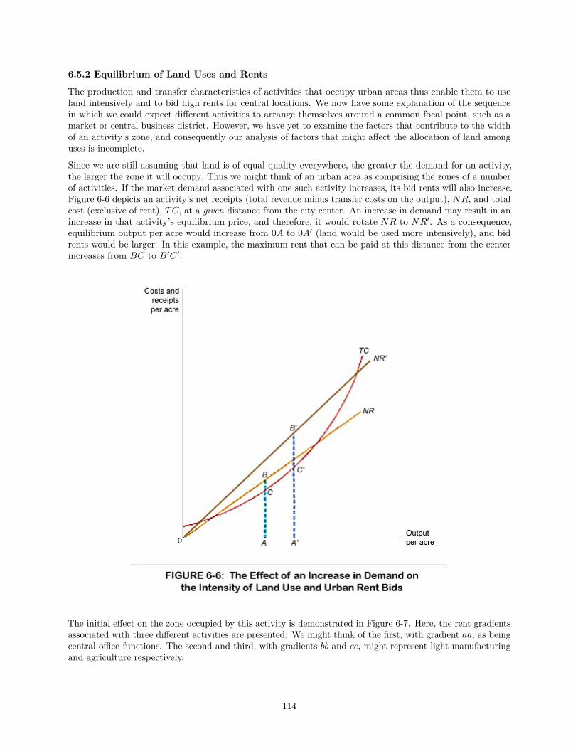
6.5.2 Equilibrium of Land Uses and Rents

The production and transfer characteristics of activities that occupy urban areas thus enable them to useland intensively and to bid high rents for central locations. We now have some explanation of the sequencein which we could expect different activities to arrange themselves around a common focal point, such as amarket or central business district. However, we have yet to examine the factors that contribute to the widthof an activity’s zone, and consequently our analysis of factors that might affect the allocation of land amonguses is incomplete.

Since we are still assuming that land is of equal quality everywhere, the greater the demand for an activity,the larger the zone it will occupy. Thus we might think of an urban area as comprising the zones of a numberof activities. If the market demand associated with one such activity increases, its bid rents will also increase.Figure 6-6 depicts an activity’s net receipts (total revenue minus transfer costs on the output), NR, and totalcost (exclusive of rent), TC, at a given distance from the city center. An increase in demand may result in anincrease in that activity’s equilibrium price, and therefore, it would rotate NR to NR′. As a consequence,equilibrium output per acre would increase from 0A to 0A′ (land would be used more intensively), and bidrents would be larger. In this example, the maximum rent that can be paid at this distance from the centerincreases from BC to B′C ′.

The initial effect on the zone occupied by this activity is demonstrated in Figure 6-7. Here, the rent gradientsassociated with three different activities are presented. We might think of the first, with gradient aa, as beingcentral office functions. The second and third, with gradients bb and cc, might represent light manufacturingand agriculture respectively.

114

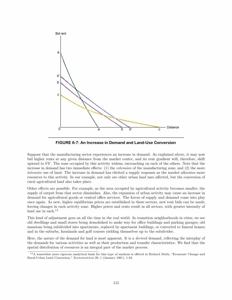
Suppose that the manufacturing sector experiences an increase in demand. As explained above, it may nowbid higher rents at any given distance from the market center, and its rent gradient will, therefore, shiftupward to b′b′. The zone occupied by this activity widens, encroaching on each of the others. Note that theincrease in demand has two immediate effects: (1) the extension of the manufacturing zone, and (2) the moreintensive use of land. The increase in demand has elicited a supply response as the market allocates moreresources to this activity. In our example, not only are other urban land uses affected, but the conversion ofrural agricultural land also takes place.

Other effects are possible. For example, as the area occupied by agricultural activity becomes smaller, thesupply of output from that sector diminishes. Also, the expansion of urban activity may cause an increase indemand for agricultural goods or central office services. The forces of supply and demand come into playonce again. As new, higher equilibrium prices are established in these sectors, new rent bids can be made,forcing changes in each activity zone. Higher prices and rents result in all sectors, with greater intensity ofland use in each.14

This kind of adjustment goes on all the time in the real world. In transition neighborhoods in cities, we seeold dwellings and small stores being demolished to make way for office buildings and parking garages; oldmansions being subdivided into apartments, replaced by apartment buildings, or converted to funeral homes;and in the suburbs, farmlands and golf courses yielding themselves up to the subdivider.

Here, the nature of the demand for land is most apparent. It is a derived demand, reflecting the interplay ofthe demands for various activities as well as their production and transfer characteristics. We find that thespatial distribution of resources is an integral part of the market process.

14A somewhat more rigorous analytical basis for this type of analysis is offered in Richard Muth, “Economic Change andRural-Urban Land Conversion,” Econometricia 29, 1 (January 1961), 1-23.

115

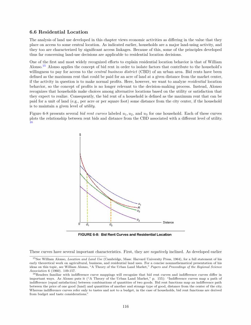
6.6 Residential LocationThe analysis of land use developed in this chapter views economic activities as differing in the value that theyplace on access to some central location. As indicated earlier, households are a major land-using activity, andthey too are characterized by significant access linkages. Because of this, some of the principles developedthus far concerning land-use decisions are applicable to residential location decisions.

One of the first and most widely recognized efforts to explain residential location behavior is that of WilliamAlonso.15 Alonso applies the concept of bid rent in order to isolate factors that contribute to the household’swillingness to pay for access to the central business district (CBD) of an urban area. Bid rents have beendefined as the maximum rent that could be paid for an acre of land at a given distance from the market center,if the activity in question is to make normal profits. Here, however, we want to analyze residential locationbehavior, so the concept of profits is no longer relevant to the decision-making process. Instead, Alonsorecognizes that households make choices among alternative locations based on the utility or satisfaction thatthey expect to realize. Consequently, the bid rent of a household is defined as the maximum rent that can bepaid for a unit of land (e.g., per acre or per square foot) some distance from the city center, if the householdis to maintain a given level of utility.

Figure 6-8 presents several bid rent curves labeled u1, u2, and u3 for one household. Each of these curvesplots the relationship between rent bids and distance from the CBD associated with a different level of utility.16

These curves have several important characteristics. First, they are negatively inclined. As developed earlier15See William Alonso, Location and Land Use (Cambridge, Mass: Harvard University Press, 1964), for a full statement of his

early theoretical work on agricultural, business, and residential land uses. For a concise nonmathematical presentation of hisideas on this topic, see William Alonso, “A Theory of the Urban Land Market,” Papers and Proceedings of the Regional ScienceAssociation 6 (1960). 149-157.

16Readers familiar with indifference curve mappings will recognize that bid rent curves and indifference curves differ inimportant ways. As Alonso puts it (“A Theory of the Urban Land Market,” p. 155): “Indifference curves map a path ofindifference (equal satisfaction) between combinations of quantities of two goods. Bid rent functions map an indifference pathbetween the price of one good (land) and quantities of another and strange type of good, distance from the center of the city.Whereas indifference curves refer only to tastes and not to a budget, in the case of households, bid rent functions are derivedfrom budget and taste considerations.”

116

in this chapter, the rent gradient of a particular activity plots out decreasing rent bids as distance from themarket increases because of transfer costs. Household rent bids are similarly affected by transfer considerations.An individual facing a daily commute to the CBD for work or shopping, or both, must pay lower rents inorder to offset the associated transfer costs of a longer trip, if utility is to be held constant. Second, lowerbid rent curves are associated with greater utility. Assuming that the household’s budget is fixed, at anygiven distance from the CBD, if a lower rent bid is accepted, more other goods can be consumed. Therefore,utility will increase. Finally, bid rent curves are single valued. This means that for a given distance from theCBD only one rent bid is associated with each level of utility. By implication, we may state that bid rentcurves cannot intersect; otherwise they could not be single valued.

The gradient of actual rents in the city is given by R in Figure 6-8. As explained previously, this gradientreflects the outcome of a bidding process by which land is allocated to competing uses. From the household’sperspective, it provides information on the rental cost of land that the household can evaluate, in light of itspreferences and budget, in order to choose a location more or less distant from the city center.

When faced with these rents, the decision makers in the household will prefer to reach the lowest possible bidrent curve in order to maximize utility; thus, a residence at location d2 would be chosen. Note that at anymore central location, the rent gradient (R) is steeper than any intersecting bid rent curve such as u1. Therent gradient offers information on the actual decrease in rents with greater distance from the CBD, while thebid rent curves offer information on the decision makers’ willingness to trade off more distant locations forlower rents. Therefore, for any location to the left of d2, the decrease in actual rents with increased distanceis more than sufficient to compensate the household for the greater commuting costs associated with livingfarther out. A location such as d1 cannot be an equilibrium location for this household: For any move awayfrom the center, actual land rents fall faster than the bid rents necessary to maintain the utility level u1, andutility can therefore be increased by such a move.

The converse is true for locations to the right of d2. A constant level of utility can be maintained if rentpayments decrease at the rate given by the bid rent curves. However, the rent structure of the city requireshigher rents for these locations; therefore, utility is decreased by a move to any location more distant than d2.

Any factors that might cause the slope of the bid rent curve to increase will draw the household closer to thecity center. The bid rent curves describe the household’s willingness to give up access to central locations. Ifthey are steep, access is valued highly, and more remote locations will be accepted only at very low rents.

It is possible to isolate two factors that are important in determining the steepness of a household’s bidrent curve. The first such factor is transfer costs.17 Higher transfer costs tend to increase the slope of thehousehold’s bid rent curve, and this tendency draws the household closer to the CBD. If each move awayfrom the center is more costly in terms of commuting expenses, higher rent bids for close-in locations arewarranted. In considering this factor, one should keep in mind that the opportunity (time) cost of commutingcan be especially important in evaluating the transfer costs of a household. If each hour spent on the roadis valued more, commuting becomes more dear, and rent bids fall more rapidly as distance from the CBDincreases.

The second factor determining the steepness of the bid rent curve is the household’s demand for space. Thelarger the quantity of land occupied by the household, the more it stands to gain in moving to the outlyinglocation. As rents fall per unit of land with increased distance from the CBD, the more units that areoccupied, the more total savings are realized by such a move. It follows that bid rents will fall less rapidlywith distance from the CBD if the amount of land occupied is large: A smaller decrease in rent per unitof land is required to compensate for the commuting costs associated with the more distant location. Thisresults in flatter bid rent curves, and outlying locations are encouraged.

A number of researchers have tried to use models similar to the one developed here in order to analyze theconsequences of higher income on residential location choice. In this context, we find that an increase inincome will have opposing effects on the steepness of the bid rent curve. Transfer costs will certainly increasefor households with higher income as the opportunity cost of commuting increases. By itself, this will tend to

17For an explanation of the effect of transfer costs on the household’s bid rent using indifference curves, see Hugh 0. Nourse,Regional Economics (New York: McGraw-Hill, 1968), pp. 110-114.

117

increase the slope of bid rent curves and should encourage high-income households to live closer to the CBD.At the same time, however, higher-income households are likely to demand more space, and this will drawthe household farther away from the CBD.

In American cities, we often observe higher-income households living in suburban locations, while lower-incomehouseholds occupy more central locations. We shall have more to say about this phenomenon in Chapter7, where the spatial structure of urban areas is examined in some depth; however, the theory of residentiallocation we have presented suggests that the income elasticity of demand for space and the income elasticityof commuting costs may be important factors underlying this spatial pattern.

Alonso does not take into account the opportunity costs associated with commuting; therefore, in his modelthe primary effect of higher incomes on bid rent curves is through changes in the quantity of land demandedby the household. Since he expects this quantity to increase with income, he argues that flatter bid rentcurves, higher incomes, and locations more distant from the CBD go hand in hand.18

Richard Muth, however, explicitly recognizes both of the factors that we have identified as determining theslope of the bid rent curve. His analysis is developed on the basis of the quantity of housing services consumedrather than the quantity of land per so. In fact Muth’s model of residential location decisions also differs inseveral other respects from that presented above, but the factors underlying the income-location relationshipare common to both.

Muth points out that the income elasticity of demand for housing has been empirically estimated as exceeding1 and possibly running as high as 2—in other words, a 1 percent increase in income is associated withwillingness to increase expenditure on housing by more than 1 percent. By contrast, the effect of additionalincome upon hourly commuting costs is almost certainly less than 1 to 1. This is so because the money costsof a given journey do not depend on income at all, whereas the time costs may be assumed to vary roughlyin proportion to income. Consequently, higher income is associated with increased willingness to sacrificeaccess for more spacious and better housing.19

William C. Wheaton has challenged the generality of this conclusion.20 He calculates income elasticities onthe basis of a sample of several thousand households in the San Francisco Bay area and finds no support forMuth’s position. These data suggest that the income elasticity of total travel costs in commuting and theincome elasticity of demand for land are about equal and therefore mutually offsetting in terms of any effecton the bid rent curves. This result leads him to conclude that one must look to other factors in order toexplain the suburbanization of America’s middle- and upper-income groups.

For example, another important basis for these suburban preferences is a liking for modernity as such. Dislikeof old houses and neighborhoods (as well as associated externalities) and a superior mobility may go far toexplain the generally positive association between income and suburbanization.

This association is especially prominent in families with school-age children, who are naturally more sensitive todifferentials in school quality, neighborhood amenity and safety, open space, and neighborhood homogeneity.An analysis of residential patterns in the Greater New York area in the 1950s showed that well-to-dofamilies with children under the age of fifteen showed relatively strong suburban and low-density preferences,while those without such children were more willing to accept the higher densities of close-in communities.Differences according to presence or absence of children were less evident for lower-income families, whoselatitude of choice of residential areas is narrower.21

18See Alonso, Location and Land Use, pp. 106-109.19See Richard F. Muth, Cities and Housing: The Spatial Pattern of Urban Residential Land Use (Chicago: University of

Chicago Press, 1969), pp. 29-34, for further details. He concludes that “on a priori grounds alone the effect of income differencesupon a household’s optimal location cannot be predicted. Empirically, however, it seems likely that increases in income wouldraise housing expenditures by relatively more than marginal transport costs, so that higher-income CBD workers would live atgreater distances from the city center” (p. 8).

20See William C. Wheaton, “Income and Urban Residence: An Analysis of the Consumer Demand for Location,” AmericanEconomic Review, 67, 4 (September 1977), 620-631.

21E. M. Hoover and Raymond Vernon, Anatomy of a Metropolis (Cambridge, Mass.: Harvard University Press, 1959), Table41, p. 180. For an analysis of the locations of various types of families in Cleveland in terms of distance from center, age, density,and industrial characteristics of neighborhoods see Avery M. Guest, “Patterns of Family Location,” Demography, 9 (February1972), 159-171.

118

The foregoing examination of the factors underlying urban residential patterns serves also to remind usthat we are not dealing here with any inexorable or universal law of human behavior. Indeed, an inverserelationship between income and distance from city center has prevailed in some other countries and in otherhistorical periods. In those situations, the wealthy favor inner-city locations with good access, while thepoor huddle in suburban shantytowns. Many Latin American cities, such as Rio de Janeiro, illustrate thispattern;22 and in preindustrial America, the mansions of the rich were generally found quite near the centerof town.

6.7 Rent and Land ValueOur discussion of rents and competition for land has placed almost exclusive emphasis on the location of asite (relative to markets and sources of inputs) as an index of its value. Location has determined how muchrent any particular activity can afford to pay for the use of a site; the purchase price has been explained assimply the capitalized value of the expected stream of future rents. At this point we need to recognize somesignificant complications that have until now been ignored.

6.7.1 Speculative Value of Land

First, the expected future returns on a parcel of land may sometimes be quite different from current returns,particularly in locations where radical changes of use are taking place or expected. This is generally truearound the fringes of urban areas, where the change involves conversion from farm to urban uses. The pricethat anyone will pay for the current use of the land may be quite low in relation to the speculative valuebased on a capitalization of expected returns in a new use.

This point is illustrated in the results of a study of agricultural land near the city of Louisville, Kentucky, wellover half a century ago (see Table 6-1). It will be observed that in the zones farther than 8 or 9 miles fromthe city, the current annual rent was consistently about 5 percent of the average value of the land. In otherwords, the value was approximately 20 years’ rent at the current rate. Closer to the city, the land was worth,on the average, well over 26 times the current annual rent; the capitalization rate was only 3.8 percent. Thisobviously reflected the expectation that returns on the nearby land would rise as the urbanized area spread.

TABLE 6-1: Acreage, Rent per Acre, and Value per Acre of Farms, by Distance from Louisville, Kentucky

Distance from Louisville (Miles)8 or Less 9 to 11 12 to 14 15 or more

(1) Average acres per farm 102 221 256 257(2) Land rent per acre ($ per annum) 11.85 5.59 5.37 4.66(3) Land value per acre ($) 312 110 106 95(4) Capitalization rate (%) (2)/(3) 3.8 5.1 5.1 4.9(5) Rent per farm per annum ($) (1) × (2) 1210 1235 1430 1295

Source: J. H. Arnold and Frank Montgomery, Influence of a City on Farming, Bulletin 678 (Washington,D.C.: U.S. Department of Agriculture, 1918).

Incidentally, the same table (Rows 1, 5) shows that the size of the farm unit increased consistently with greaterdistance from the city in terms of acreage but remained roughly constant in terms of total land rent. This isconsistent with the idea that the scale of the individual farm unit is constrained by size-of-firm considerations

22“In a Latin American city rural migrants and, in general, the proletariat are not customarily crowded into a blighted area atthe urban core, . . . but they are scattered, often in makeshift dwellings, in peripheral or interstitial zones. The Latin Americancity center with its spacious plaza was traditionally the residence area for the wealthy and was the point of concentration forurban services and utilities. The quickening of commercial activity in this center may displace well-to-do residents withoutnecessarily creating ‘contaminated’ and overcrowded belts of social disorganization. The poor are often not attracted intotransitional zones by cheap rents; they tend to move out to unused land as the city expands, erecting their own shacks. Thedowntown area becomes converted for commercial uses or for compact and modern middle- and upper-income residences.”Richard M. Morse, “Latin American Cities: Aspects of Function and Structure,” Comparative Studies in Society and History,4 (1961-1962), 485. For a comprehensive discussion of such characteristic contrasts in urban form and their socioeconomicbackground, see Leo F. Schnore, “On the Spatial Structure of Cities in the Two Americas,” in Philip M. Hauser and Leo F.Schnore (eds.), The Study of Urbanization (New York: Wiley, 1965), pp. 347-398.

119

involving management capability and financial resources. The same study showed systematically greaterinputs of labor and fertilizer per acre and per farm nearer to the city.

6.7.2 Improvements on Land

A further complication is that land is ordinarily priced, sold, and taxed in combination with whateverbuildings and other “improvements” have been erected on it, since such structures are usually durable anddifficult (if not impossible) to move. On urban land, improvements may account for a major part of the valueof the parcel of real estate; and in all cases it is probably difficult to estimate just how much of the pricerepresents the value of space per se, or “site value.” Sometimes the “improvements” have a negative value: Inother words, the land would be more desirable if it were cleared of its obsolete structures.

Such structural obsolescence is an important aspect of some of the most serious problems confronting U.S.cities today. Moreover, the distinction between site value and total real property value is crucial to anevaluation of the role of the real property tax, which is the fiscal mainstay of local governments.

6.8 SummaryCompetition for space and other fixed local resources (collectively termed “land”) plays an important role inlocation, especially in urbanized areas and for activities using much space relative to their outputs. In a freemarket, land goes to the user who can bid the highest rent or price for it. Price represents a capitalization ofexpected rents.

The way in which any activity’s rent bids vary over an area (the rent surface) or along a route (the rentgradient) depends on the local qualities of the sites themselves, on their accessibility, and on other factorsrelevant to the activity’s locational preferences. Rent gradients and surfaces for most activities show peaks atmarket centers.

When several activities are competing for space around some common market point, the activities thatpreempt the land with the best access tend to be those that have a large volume of output per unit of spaceused, those whose output bears high transfer costs, and those least subject to rising operating costs withincreased intensity of land use (crowding).

The production and transfer characteristics associated with activities in urban areas cause them to place highvalue on locations with central access. The location of these activities is especially affected by the need formovement of people and direct personal contact, with time consequently playing the major role in transfercosts and access advantage. Complex linkages among units and activities, and competition for space, are alsoimportant location factors in an urban context.

Access considerations play an important role in residential location decisions. The space occupied by ahousehold and commuting costs (especially the opportunity or time cost of commuting) affect its willingnessto bid for land with good access to central locations.

The demand for land plays an important role in the market process and is affected by changes in the demandfor various activities that compete for its use.

Technical Terms Introduced in this ChapterLand Rent Intensity of land useNeighborhood effects, or local externalities Rent bid, or bid rent Central business district (CBD)Region Rent surface Rent gradient

Selected ReadingsWilliam Alonso, Location and Land Use (Cambridge, Mass.: Harvard University Press, 1964).

120

Edgar S. Dunn, The Location of Agricultural Production (Gainesville: University of Florida Press, 1954).

Johann Heinrich von Thünen, Der isolirte Staat in Beziehung auf Landwirthschaft und Nationalökonomie(1st volume published in 1826, subsequent volumes published later); Carla M. Wartenberg (tr.), The IsolatedState (London: Pergamon Press, 1966).

William C. Wheaton, “Income and Urban Residence: An Analysis of the Consumer Demand for Location,”American Economic Review, 67, 4 (September 1977), 620-631.

APPENDIX 6-1 Derivation of Formulas for Rent Gradients and Their SlopesLet the total cost of production per acre (exclusive of rent) be

TC = F + aQb (1)

where F is fixed cost per acre, Q is output per acre, and b > 1. The bid rent, or maximum rent per acre thatcould be paid, is

R = (P—tx)Q—aQb—F (2)

where P is the unit price of the output at the market, t is the unit transfer cost per mile, and x is the distanceto market.

dR/dQ = P—tx—abQb−1 (3)

d2R/dQ2 = (1—b)abQb−2 < 0 (4)

Since the second derivative is negative because b > 1, setting the first derivative to zero will give the outputthat maximizes R.

P—tx—abQb−1 = 0 (5)

Q = [(P—tx)/ab]1/(b−1) (6)

Substituting in (2), and simplifying,

R = a(b—1)[(P—tx)/ab]b/(b−1)—F (7)

This is the rent gradient with respect to distance from the market.

dR/dx = —t[(P—tx)/ab]1/(b−1) < 0 (8)

Therefore, the rent gradient always slopes downward from the market.

d2R/dx2 = [t2/ab(b—1)][(P—tx)/ab](2−b)(b−1) > 0 (9)

By (9), the rent gradient is always concave upward.

121

The procedure followed in deriving the rent gradients shown in Figure 6-5, which indicate the effect of eachof the parameters on the slope, was as follows:

Since the question as to which one of two activities takes the zone closer to market is determined by therelative slopes of the two gradients at their point of intersection, it is necessary to set the market prices at alevel P ∗ such that the gradients representing activities with different a, b, F, or t values will intersect. Letthe coordinates (rent and distance respectively) of the point of intersection be R∗ and x∗ (which were set at1,000 and 50 respectively in calculating the gradients plotted in Figure 6-5).

Then

R∗ = a(b—1)[(P ∗—tx∗)/ab]b/(b−1)—F

and from this,

(P ∗—tx∗)/ab = [(R∗ + F )/a(b—1)](b−1)/b

Substituting in (8) gives the slope (S∗) at the intersection point:

S∗ = —t[(R∗ + F )/a(b—1)]1/b

From this it is clear that

∂S∗/∂a > 0

∂S∗/∂b > 0

∂S∗/∂F < 0

∂S∗/∂t < 0

In other words, if two activities have intersecting rent gradients and are alike with respect to all but one ofthe four parameters a, b, F, t, the activity with the steeper (more strongly negative) slope at their intersectionwill be the activity with the lower a, or the lower b, or the higher F, or the higher t.

In calculating the illustrative gradients shown in Figure 6-5, the following parameters were used:

a b F t

Standard case for comparison, which appearsin each of the four panels of Figure 6-5 10 2 100 1Larger a 20 2 100 1Larger b 10 4 100 1Larger F 10 2 500 1Larger t 10 2 100 2

122

7. THE SPATIAL STRUCTURE OF URBAN AREAS7.1 IntroductionIn this chapter we are concerned more specifically with spatial relations within the individual urban ormetropolitan area.1 Such an area includes a principal city with an intensively developed core or downtownarea (the central business district, or CBD) and a surrounding fringe of suburbs and satellites linked to theprincipal city by trade, commutation, and other socioeconomic interaction.

It would be hard to think of any significant question or proposition of urban economics not involving space,distance, or location as a fundamental concern, since the essence of a city lies in the close proximity of diverseactivities and persons. So urban economics is just part of the broader field of spatial or regional economics.But it is such a large part that it is often studied as a distinct entity. Our intention in this chapter is notto survey urban economics as a field of study but to expose some essential aspects of the spatial structureof urban economies. In this way, it will be possible to affirm some principles of spatial economics that areparticularly relevant and useful in understanding the development of cities and their problems.

7.2 Some Location FactorsThe land-use analysis that was developed in Chapter 6 allowed us to identify a number of characteristicsassociated with urban activities which implied a willingness to bid high rents for the more central locations.The movement of people and the importance of direct face-to-face contact contribute to the advantages ofcentral locations for these activities. The applicable transfer rates are high, and linkages among nonresidentialactivity units, among households, and among residential units and nonresidential units are substantial.Further, the realization of agglomeration economies most often requires close and frequent contact. Theseeconomies enhance the attractiveness of central locations and tend to bring units together, not merely in thesame city but in the same district of a city.

7.2.1 Independent Locations

While these access and agglomerative factors are quite important in explaining the outcome of the biddingprocess by which land is allocated among competing urban uses, it is necessary to recognize that some kindsof locations within an urban area can be regarded as independently determined. In fact, there are two distinctbases for exogenous determination of locations in an urban area. For some activities, certain topographical orother natural site features are essential; this means that the lie of the land narrows the choice to one or avery small number of locations. Ports for water traffic illustrate this, and there are some urban areas wherethe topography limits airport sites almost as drastically. In the distant past, considerations of defense playeda major part in locating the heart of the city and the city itself. Localized recreational facilities such asbeaches also illustrate this kind of factor, and in a few urban areas extractive industries (mainly mining)occur and are, of course, limited to certain special sites.

There is a further type of exogenously determined location where the independent influence arises not fromsite features as much as from the fact that the activity requires contact with the outside world. Not justwater ports but all kinds of terminal and interarea transport activities come under this head. Since thereare great economies of scale in interregional transport and in terminal handling of goods, the urban area’sgateways to and from the outside world constitute a set of focal points, whose locations within the area helpto determine—rather than just being determined by—the other activities of the area. This does not mean, ofcourse, that such terminal locations are absolutely and permanently unresponsive to the changing patternsof other activities in the area served. Such terminals are from time to time shifted so as to improve localaccessibility or to make way for more insistent claimants for the space. But the terminal locations do play anactive role in shaping the pattern and are to be viewed as part of the basic framework around which otheractivities are fitted.

1Some of the content of this chapter is adapted from Edgar M. Hoover, “The Evolving Form and Organization of theMetropolis,” in Harvey S. Perloff and Lowdon Wingo, Jr. (eds.), Issues in Urban Economics (Baltimore: Johns HopkinsUniversity Press, 1968), pp. 237-284.

123

7.2.2 The Center

There is also a strong element of exogenous determination in the location of the point of “maximum overallaccessibility” within the urban area. If we think of this, for example, as the place where all the people ofthe area could assemble with the least total man-miles of travel, it is the “median center of population” andwould seem to depend simply upon the location of the various types of residence. But travel is cheaper andfaster along developed routes, and the cost and layout of these routes are affected by scale (traffic volume)and topography. Thus, evaluated in terms of travel cost and time, the focal maximum-access point can beregarded as a rather stable datum, even though the extent and importance of its access advantage over otherpoints can change radically. In major American urban areas, despite great overall growth, far-reaching change,and redistribution of activities, this focal point has usually shifted only a relatively short distance over periodsmeasured in decades and generations; and the earlier central foci are well within what we currently recognizeas the central business district.

This concept of a single “most central” focal point in an urban area is significant and useful in developingsimplified bases for understanding the overall pattern. Obviously, it has its limitations, some of which willbe discussed now and others later. First, there are really a variety of distinguishable central points of thissort, depending on what kinds of people or things we are imagining to be assembled with a minimum oftotal expense or effort. The employed workers of the area are not distributed in quite the same patternas the total population, the shopping population, the school-attending population, the office workers, theindustrial blue-collar workers, the theater-going or the library-using population; there might be a differentoptimum location from the standpoint of access to each of these types of people. Where goods rather thanpeople are moving (for example, in the case of wholesale activity or production serving such local needsas daily newspapers or bread), the transport conditions are different, and this may again mean a differentoptimum-access point. Second, we have to recognize that, in varying degrees, the concept of one single pointserving as the origin or destination for all flows of a specified type is unrealistic, and defensible only as aconvenient fiction. Thus if we identify some central point as having best access to the homes of the entireclerical office force of an urban area, this does not imply that all offices should logically be concentratedthere. What it does imply is that, solely from the standpoint of commuting access for the clerical workersand ignoring claims of alternative uses of space, it would make sense for the density of clerical employment topeak at that point.

7.2.3 Neighborhood Externalities

In gaining perspective on the role of access and agglomerative factors in urban location decisions, it is alsonecessary to recognize that proximity can have unfavorable as well as favorable effects. “Neighborhoodcharacter”—in terms of cleanliness, smells, noise, traffic congestion, public safety, variety interest, and generalappearance—is important in attracting some kinds of use and repelling others. Prestige types of residence orbusiness are, of course, particularly sensitive to this kind of advantage, which is often more important thanany access consideration as such. High-income householders may be willing to lengthen their work journeygreatly for the sake of neighborhood amenity or agreeable surroundings.

The usual effect of this type of consideration is to make neighborhoods more homogeneous within themselvesand more unlike other neighborhoods: a tendency toward areal specialization by uses, or “segregation” inthe broad sense.2 With few exceptions, a given type of activity finds advantage in being in a neighborhooddevoted to reasonably similar kinds of uses, and disadvantage in being in violent contrast to the neighborhoodpattern. Zoning controls and planned street layouts play a part in reinforcing this tendency.

7.2.4 Scale Economies and Urban Land Use

Many of the points just raised imply that the broad continuous zones of economic activity suggested byvon Thünen’s simplified model of patterns of land use in Chapter 6 would be substantially modified in anintraurban setting. When that model is applied to such extensive activities as agricultural or residentialland users, it is not really necessary to consider the size of the individual location unit in terms of output or

2See Richard F. Muth, Urban Economic Problems (New York: Harper & Row, 1975), pp. 87-92, for a simple theoreticalstatement of this point.

124

occupied land area, since such zones contain a large number of adjacent units. Accordingly, in that instance,we look for explanations of rent-paying ability and location in terms of inputs, costs, outputs, and rents on aper-acre basis. We could appropriately consider costs as affected by intensity of land use rather than by thesize of the producing unit, the firm, or the cluster.

Consider, however, an activity such as university education, which on the basis of its production characteristicscan best be located, say, 5 miles from the center of the metropolitan area supplying the bulk of the students.A more central location would mean excessive land costs, while a less central one would mean poor access tothe homes of the commuting students and perhaps also to various other urban activities with which contact isdesired. If we brashly apply the basic von Thünen model, we get the answer that a university should occupya ring-shaped zone with a 5-mile radius. If the amount of space needed were, say, 300 acres, the ring-shapedcampus would be about 80 feet wide and more than 31 miles long. Since such a layout would preclude bothhaving a sizable stadium and getting to classes on time, it is clearly unacceptable. In the interest of its owninternal logistics, the university would prefer a blob to a doughnut. Two different institutions in the same citymight find some external-economy advantage in being close to one another in a single “university district,”but if they are intensely competing for commuter students, they might prefer to locate on opposite sides oftown.

The point here is that a university campus is a location unit subject to considerable economies of scale, sothat there will be only a few unit locations, perhaps only one, in any given urban area; at the same time it issufficiently space using to need an off-center or even suburban location. The same principle applies to anyactivity with these characteristics. As a result, the concentric ring pattern appears within urban areas onlywith respect to certain broad classes of activities such as residence. For other noncentral uses, the patterncan range from scattered fragments of a ring to a single off-center concentration. Still further complication isintroduced by the fact that each such concentration can become a focal point for a neighborhood constellationof associated land uses. Any sizable urban area contains a number of such subcenters in addition to theprincipal downtown center.

7.3 Symmetrical Monocentric Models of Urban Form7.3.1 Bases of Simplification

A number of factors relevant to intraurban location decisions have been catalogued above, but basically thereare three kinds of considerations that determine the relative desirability of locations for individual locationunits, such as households or business establishments. These are (1) environmental characteristics, (2) access,and (3) cost. They reflect the fact that the users of a site are concerned with it in three distinct ways. Theyoccupy it, as residents or producers, and are thus concerned with its “site and neighborhood,” or immediateenvironmental qualities. They, as well as goods and services, move between this site and others and aretherefore concerned with its convenience of access to other places. Finally, they have to pay for its use andare therefore concerned with its cost.

It should be evident now that in reducing the complex factor of access within an urban area to the simple formof proximity to a single focal point—as was done in Chapter 6—some important aspects of urban economicactivity are put aside. Within a city, it is as if all intraurban journeys were to or from downtown and allshipments of goods also passed through downtown.3Additionally, such an analysis eliminates all differentiationof sites with respect to topography, amenity, and environmental advantage. These two simplifications alsoimply ignoring the manifold types of external-economy effects and environmental attractions and repulsions

3A considerable (and rising) proportion of journeys from homes are to destinations other than downtown; and for mostnonresidential activities as well, the markets and input sources can be at many points other than the city center. In recognitionof this, the “access-potential” approach to interaction over distance, previously discussed in Chapter 2, has been used for theempirical analysis of travel patterns within urban areas. The method is of some value in describing and predicting transportationdemands, residential development patterns, and locational choice for consumer-oriented activities (retail trade and services). See,for example, T. R. Lakshmanan and Walter G. Hansen, “A Retail Market Potential Model,” Journal of the American Instituteof Planners, 31, Special Issue on Urban Development Models (May 1965), 134-143. In this study of shopping centers in theBaltimore metropolitan area, it was found that the actual sales at the various centers (or, in some cases, the number of shoppingtrips to those centers, estimated from transportation survey data) corresponded well to what would be predicted on the basis ofan index of access to the homes of consumers (weighted by their total retail expenditures).

125

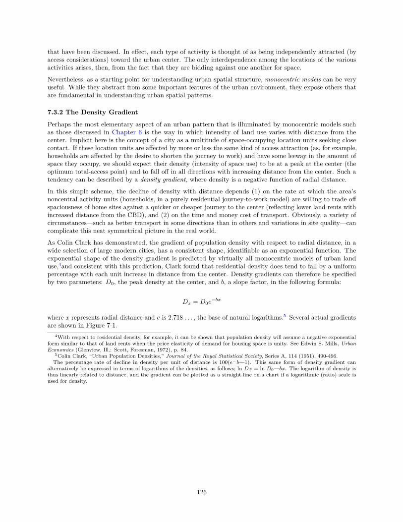
that have been discussed. In effect, each type of activity is thought of as being independently attracted (byaccess considerations) toward the urban center. The only interdependence among the locations of the variousactivities arises, then, from the fact that they are bidding against one another for space.

Nevertheless, as a starting point for understanding urban spatial structure, monocentric models can be veryuseful. While they abstract from some important features of the urban environment, they expose others thatare fundamental in understanding urban spatial patterns.

7.3.2 The Density Gradient

Perhaps the most elementary aspect of an urban pattern that is illuminated by monocentric models suchas those discussed in Chapter 6 is the way in which intensity of land use varies with distance from thecenter. Implicit here is the concept of a city as a multitude of space-occupying location units seeking closecontact. If these location units are affected by more or less the same kind of access attraction (as, for example,households are affected by the desire to shorten the journey to work) and have some leeway in the amount ofspace they occupy, we should expect their density (intensity of space use) to be at a peak at the center (theoptimum total-access point) and to fall off in all directions with increasing distance from the center. Such atendency can be described by a density gradient, where density is a negative function of radial distance.

In this simple scheme, the decline of density with distance depends (1) on the rate at which the area’snoncentral activity units (households, in a purely residential journey-to-work model) are willing to trade offspaciousness of home sites against a quicker or cheaper journey to the center (reflecting lower land rents withincreased distance from the CBD), and (2) on the time and money cost of transport. Obviously, a variety ofcircumstances—such as better transport in some directions than in others and variations in site quality—cancomplicate this neat symmetrical picture in the real world.

As Colin Clark has demonstrated, the gradient of population density with respect to radial distance, in awide selection of large modern cities, has a consistent shape, identifiable as an exponential function. Theexponential shape of the density gradient is predicted by virtually all monocentric models of urban landuse,4and consistent with this prediction, Clark found that residential density does tend to fall by a uniformpercentage with each unit increase in distance from the center. Density gradients can therefore be specifiedby two parameters: D0, the peak density at the center, and b, a slope factor, in the following formula:

Dx = D0e−bx

where x represents radial distance and e is 2.718 . . . , the base of natural logarithms.5 Several actual gradientsare shown in Figure 7-1.

4With respect to residential density, for example, it can be shown that population density will assume a negative exponentialform similar to that of land rents when the price elasticity of demand for housing space is unity. See Edwin S. Mills, UrbanEconomics (Glenview, Ill.: Scott, Foresman, 1972), p. 84.

5Colin Clark, “Urban Population Densities,” Journal of the Royal Statistical Society, Series A, 114 (1951), 490-496.The percentage rate of decline in density per unit of distance is 100(e−b—1). This same form of density gradient can

alternatively be expressed in terms of logarithms of the densities, as follows; ln Dx = ln D0—bx. The logarithm of density isthus linearly related to distance, and the gradient can be plotted as a straight line on a chart if a logarithmic (ratio) scale isused for density.

126

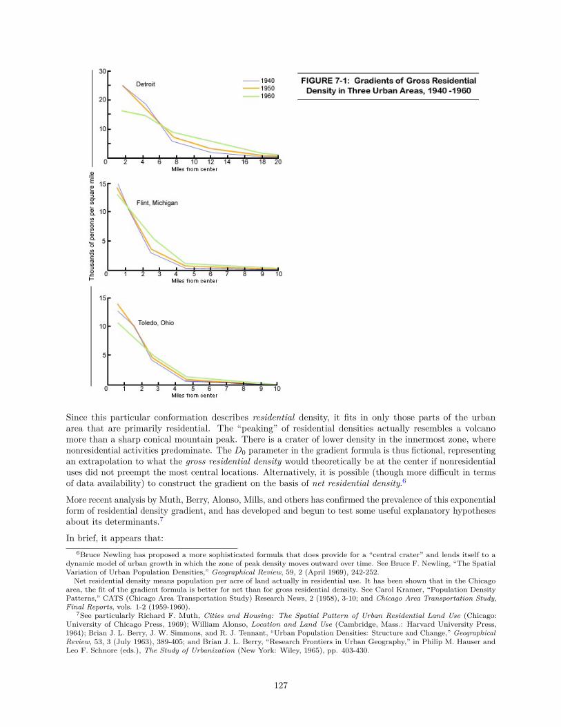
Since this particular conformation describes residential density, it fits in only those parts of the urbanarea that are primarily residential. The “peaking” of residential densities actually resembles a volcanomore than a sharp conical mountain peak. There is a crater of lower density in the innermost zone, wherenonresidential activities predominate. The D0 parameter in the gradient formula is thus fictional, representingan extrapolation to what the gross residential density would theoretically be at the center if nonresidentialuses did not preempt the most central locations. Alternatively, it is possible (though more difficult in termsof data availability) to construct the gradient on the basis of net residential density.6

More recent analysis by Muth, Berry, Alonso, Mills, and others has confirmed the prevalence of this exponentialform of residential density gradient, and has developed and begun to test some useful explanatory hypothesesabout its determinants.7

In brief, it appears that:6Bruce Newling has proposed a more sophisticated formula that does provide for a “central crater” and lends itself to a

dynamic model of urban growth in which the zone of peak density moves outward over time. See Bruce F. Newling, “The SpatialVariation of Urban Population Densities,” Geographical Review, 59, 2 (April 1969), 242-252.

Net residential density means population per acre of land actually in residential use. It has been shown that in the Chicagoarea, the fit of the gradient formula is better for net than for gross residential density. See Carol Kramer, “Population DensityPatterns,” CATS (Chicago Area Transportation Study) Research News, 2 (1958), 3-10; and Chicago Area Transportation Study,Final Reports, vols. 1-2 (1959-1960).

7See particularly Richard F. Muth, Cities and Housing: The Spatial Pattern of Urban Residential Land Use (Chicago:University of Chicago Press, 1969); William Alonso, Location and Land Use (Cambridge, Mass.: Harvard University Press,1964); Brian J. L. Berry, J. W. Simmons, and R. J. Tennant, “Urban Population Densities: Structure and Change,” GeographicalReview, 53, 3 (July 1963), 389-405; and Brian J. L. Berry, “Research Frontiers in Urban Geography,” in Philip M. Hauser andLeo F. Schnore (eds.), The Study of Urbanization (New York: Wiley, 1965), pp. 403-430.

127

1. Larger cities have, in addition to higher central densities, lower slope coefficients (i.e., flatter slope).

2. The observed decline of population per acre with increased distance from the city center is actuallya combination of at least three different gradients. As we go outward from the center, the numberof housing units per acre falls, and so does the proportion of people living outside of households (forexample, in institutions, hotels, and rooming houses); but the declining density effect of those twovariables is partially offset by rising household size.

3. The central density is largely determined by conditions (such as transport, communication, productiontechnology, income levels, and occupation structure) during the period when the city became established.Once set, the basic form of the city (particularly in the central area where investment in structuresis heaviest) is subject to considerable inertia. At any given time, then, the age of a city (definable interms of the date at which it attained some specified minimum size, such as 50,000) is highly correlatedwith its central density. The familiar dichotomy between newer American “auto-oriented” cities such asPhoenix and older “pre-auto” cities recognizes this effect.

Perhaps the most intensive statistical analysis of urban residential density gradients is to be found in RichardMuth’s work. After a series of statistical tests of the relation of distance to gross residential density figures in46 U.S. cities in 1950 (based on samples of 25 Census tracts in each city), he concluded that “the negativeexponential function in distance from the CBD [Central Business District] alone fits population density datafor American cities in 1950 rather well.”8 This held true despite the fact that there were numerous deviationsfrom regularity and that the exponential formula as a regression equation accounted for only about half ofthe observed intracity variation of density (among tracts within any city). The fitted density gradients variedwidely in theirslopes, with b ranging from 0.18 to 1.2. These b values correspond to density declines of 17percent and 70 percent respectively for each mile of distance.

Muth then looked for factors to explain why some cities had steeper density gradients than others. He foundthat flatter gradients (that is, lower values for b) were significantly associated with each of the followingcharacteristics of the urban area:

• High automobile ownership

• High income level

• High proportion of nonwhite to total population

• Large size (population) of urban area

• Low degree of concentration of the metropolitan area’s manufacturing employment in the central city

• Low quality (in terms of condition and plumbing facilities) of housing in the central city

Finally, he found by further analysis that “the distribution of population between the central city and itssuburbs and the land used by the urbanized area are largely governed by the same forces influencing thepopulation distribution within the central city.” Two main qualifications to this general statement appeared.First, an influx of lower-income persons into the central city is apparently associated with a greater degreeof suburbanization of population, whereas within the central city the effect is in the opposite direction (asteeper density gradient). This as Muth suggests makes sense, considering that the central city is a separatefiscal unit and the presence of a larger low income group tends to make the tax burden heavier for the upperincome groups and for business firms, whose incentive to escape to other jurisdictions is thereby increased.9

Various empirical investigations have brought to light similar fairly consistent density gradients for certainnonresidential types of land as well. Otis Dudley Duncan presents a gradient of manufacturing employees perthousand square feet of land occupied (that is, net manufacturing employment density) for Chicago in 1951,showing a reasonably good fit to the exponential formula, with a slope substantially flatter than that of thetypical residential density gradient.10 Daytime population likewise shows the same kind of gradient. In this

8Muth Cities and Housing, p. 184.9Ibid., p. 183.

10Otis Dudley Duncan. “Population Distribution and Community Structure,” Cold Spring Harbor Symposia on QuantitativeBiology, 22 (1957), 357-371.

128

case, the slope is much steeper and the central density much higher than for residential population. Finally,it appears that the gradient of land values in urban areas also follows the same general exponential form.

Analysis of the behavioral factors underlying these gradient patterns poses many complications. If allhouseholds could be assumed alike in preferences and place of work, the form of the gradients of residentialdensities and rents could be read as representing the individual household’s trade-off between more space andquicker access. But it is not so simple. We know that this tradeoff is affected by income level. Higher-incomefamilies tend to live farther out than lower-income families, particularly if allowance is made for presence orabsence of young children. This means that the observed overall residential density and land value gradientsrepresent in part the gradation of trade-offs: The analysis of residential distributions involves an additionaldimension. Similarly for “manufacturing employment density”—in the case of the employment densitygradient referred to earlier, a breakdown of manufacturing into twenty-five industry groups disclosed that theydisplayed very different degrees of centrality, associated with employment density. A still finer breakdownwould, of course, show the same kind of differentiation within an industry group.

7.3.3 Land-Use Zones: The Burgess Model

It is clear that to go beyond such elementary explanations, some explicit attention must be paid to theheterogeneity of both residential and non-residential land uses in a more complicated conceptual scheme.Early attempts in this direction relied on highly descriptive characterizations of urban areas.11

The Burgess zonal hypothesis is a schematic model developed along these lines in the 1920s. 12 Its kinshipwith von Thünen’s much older zonal model of rural land uses around an urban focal point and modernanalyses of urban land use (see Chapter 6) is obvious. Activities are grouped on the basis of concentration insuccessive distance zones from the center outward, in this order:

1. Central business district activities: department stores and smart shops, office buildings, clubs, banks,hotels, theaters, museums, organization headquarters

2. Wholesaling

3. Slum dwellings (in a zone of blight invaded from the center by business and light manufacturing)

4. Middle-income industrial workers’ residences

5. Upper income single-family residences

6. Upper income suburban commuters’ residences

This research is an important example of inductive generalization applied to regional analysis. Burgess movedfrom his descriptive exercise to put forward a simplified dynamic model. The Burgess hypothesis was thatthese land-use zones preserve their sequence, but as the city grows each zone must spread and move outward,encroaching on the next one and creating zones of transition and land-use succession. He emphasized thetransitional problem created in the third (blighted) zone.

In the Burgess model, we have an elementary classification of urban land uses by locational types that isstill useful as a starting point. Downtown uses, light manufacturing, wholesaling, and three or four levels ofresidence characterized by income level are singled out as significantly different and important location types.

11Recent efforts in developing models of urban spatial structure are deductive in nature and rely on systems of equationscharacterizing the behavior of various economic sectors. The models may he normative, in that they solve for the spatialallocation of people, goods, housing, and land about the central business district so as to maximize a social welfare function, orpositive, in that they solve for a competitive equilibrium. See Edwin S. Mills and James Mackinnon, “Notes on the New UrbanEconomics,” Bell Journal of Economics, 4, 2 (Autumn 1973), 593-601; and J. V. Henderson, Economic Theory and the Cities(New York: Academic Press, 1977).

Closely related to these efforts are attempts to simulate urban economies by using computers to seek numerical solutions toequation systems that characterize housing demand and supply in relation to locations of work places. See Gregory K. Ingram,“Simulation and Econometric Approaches to Modeling Urban Areas,” in Peter Mieszkowski and Mahlon Straszheim (eds.),Current Issues in Urban Economics (Baltimore: Johns Hopkins University Press, 1979), pp. 130-164.

12For a brief account of the Burgess model and models involving subcenters and sectors (discussed later in this chapter), andfor references to the original sources, see Chauncy D. Harris and Edward L. Ullman, “The Nature of Cities,” in Harold M. Mayerand Clyde F. Kuhn (eds.), Readings in Urban Geography (Chicago: University of Chicago Press, 1959), pp. 282-286.

129

Finally, heavy industry is not in the Burgess model at all, which makes sense in the light of the locationfactors discussed earlier. Heavy industry requires large level sites with good transport to and from the outsideworld, and access to the urban “center of gravity” is of little relevance since most of the inputs (except labor)and outputs are nonlocal.

One of the most important generalizations introduced by the Burgess model concerns residential locationalpreferences. In his scheme, the richer people are, the farther they live from the city center. As mentioned inChapter 6, this pattern is characteristic of cities in the United States even at the present time. However,the analysis of residential location behavior developed in that chapter (see Section 6.6) made it clear thatsuch a pattern is not universally relevant. Rather, personal preferences and characteristics of individualeconomies, such as the nature of transfer costs in the daily commute to work, can account for the locationpatterns of heterogeneous income groups. Nevertheless, the concept of land-use succession and the transitionof neighborhoods from one income group to another have figured prominently in shaping the spatial patternsof metropolitan areas.

7.4 Differentiation by SectorsSome approaches to the explanation of urban spatial patterns have stressed tendencies toward differentiationaccording to direction, rather than according to distance from the center. The sector theory is associatedhistorically with Homer Hoyt and has been stated as follows: “growth along a particular axis of transportationusually consists of similar types of land use. The entire city is considered as a circle and the various areasas sectors radiating out from the center of that circle; similar types of land use originate near the centerof the circle and migrate outward toward the periphery.”13 Hoyt’s formulation was mainly concerned withresidential land use and assigned a dominant role to the forces determining the direction of expansion of thehighest-class residential district.

In terms of the existing pattern at any given time in an urban area, it is easy to explain sectoral differentiationon the basis of such factors as (1) topographical and other “natural” variation, (2) the presence of a limitednumber of important radial transport routes, and (3) the previously discussed incentives toward a greaterconcentration of any one activity than a symmetrical concentric ring layout would afford. But the Hoythypothesis is couched primarily in dynamic terms, as an explanation of persistent sectoral differences in thecharacter of development. And in that context, it introduces two further useful concepts.

One of these concepts is that of succession of uses of a given site or neighborhood area. Except at the outerfringe of urban settlement, each type of land use as it expands is taking over from an earlier urban use;by and large, the growth process involves (as described earlier in the context of the simple monocentricmodel) an outward encroachment of each type of activity into the next zone out. Some such transitionsare cheaper or easier than others, and the extension tends to be in the direction of easiest transition. Thusobsolete mansions are conveniently converted into funeral homes; row houses and apartments are easilyconverted, subdivided, and downgraded into low-income tenements; and obsolete factory space is easily usedfor wholesaling and storage. The “filtering” theory of succession of uses in the urban housing market impliesgradual and continuous, rather than abrupt, change in residential neighborhood character.

The other useful concept might be called minimum displacement. The growth process uproots all kindsof housing and business activities in the zones of transition, forcing them to seek new locations. Copiousempirical evidence bears out the reasonable presumption that when these moves are made by householders orby small neighborhood-serving businesses, there is a strong preference for remaining as close as possible tothe old location. This cohesion or inertia, which is quite rational in the light of both economic and socialconsiderations, tends to perpetuate a sectoral differentiation and to cause a particular activity to movegradually outward along the line of least resistance, rather than into another sector.

13Homer Hoyt, The Structure and Growth of Residential Neighborhoods in American Cities, U.S. Federal Housing Admin-istration (Washington, D.C.: Government Printing Office, 1939). The quotation is from Harris and Ullman, “The Nature ofCities,” p. 283. See also, in the same volume, Homer Hoyt, “The Pattern of Movement of Residential Rental Neighborhoods,” pp.499-510. A handy collection of most of his writings over the period 1916-1966 is Homer Hoyt, According to Hoyt (Washington,D.C.: Homer Hoyt Associates, 1968).

130

7.5 SubcentersAlthough a city or metropolis generally has one identifiable main center, there are subordinate centers aswell. Spatially, an urban area is multinuclear, and some models of urban spatial structure particularly stressthe development of subcenters. Recent trends have entailed the rapid sprawl and coalescence of originallydiscrete cities and towns into larger metropolitan and megalopolitan complexes, bringing this multinuclearaspect into prominence as a basic characteristic of the urban pattern. Even a small individual city usuallycontains a number of important business centers or other focal points outside the central business district.

Any consumer-serving activity that can attain its economies of scale and agglomeration without having toserve the entire urban area from a single center will increase its proximity to consumers by branching out intoshopping centers, each serving a part of the whole area.14 Each shopping center is in turn a concentration ofemployment activity, a focal access point for work, shopping, and recreational trips. The basic concentricpatterns of access advantage, centripetal movement of people, and centrifugal movement of goods and servicesare replicated in each part of the urban area, albeit for a more limited range of activities than those representeddowntown. Local peaks of the gradients of residential density, land values, intensity of land use, and accesspotential appear around each of these subcentral points, like hillocks on the shoulders of a mountain.

While part of the subcenter phenomenon can be explained, as above, on the basis of its efficiency in providingconsumer-serving activities, other forces are in effect. This is evident as soon as we recognize that among thetypes of activity that usually do agglomerate in one place within an urban area, there are many for which thecentral business district simply is not an economic location. These activities are highly concentrated buttypically off-center.

For some activities, the basic reason is inherent in their production functions—they do not use space intensivelyenough to afford downtown land, but at the same time their internal-access requirements call for a morecompact zone of occupation than a ring would provide. This case was examined in section 7.2.4, with auniversity campus as the example. Off-center cluster is the typical pattern for research centers, culturalcenters, concentrations of automobile salesrooms, and to an increasing extent, wholesale produce marketsand other wholesaling activities with strong external economies of cluster but substantial space requirements.

There is an interesting exception to this principle of “blob rather than doughnut.” The building of fastsuburban beltways around major cities has made it more feasible for some activities (for example, electronicsand other light industries) to assume an extended distribution along at least a sizable arc—that is, part of adoughnut.

Second, the tendency to concentration at the expense of symmetry is found in specific types of residentialland use as well, reflecting among other things the preference for neighborhood homogeneity that acts likean agglomerative force for any particular class of residence (such as high-income single-family houses) evenwhere low densities are involved.

A still further basis for off-center concentration appears in situations where the activity serves a marketthat is itself lopsidedly distributed in relation to the overall area. For example, if residential areas occupiedby higher income and educational groups are predominantly to the northwest of the city center, trade andservice activities catering especially to those groups will find the point of maximum market access potentialsomewhere northwest of the city center. This pattern also applies for those activities that mainly servemarkets outside their own urban area (such as export activities). Access considerations for such activitiesdictate location close to intercity transport terminals or major highways.

Finally, special topographical or other site features may make a particular off-center location optimal eventhough it does not have the best access. The availability of a large level tract amid generally hilly topographymay well be the decisive factor for such uses as airports or major industrial developments.

Thus a typology of urban subcenters might include:14In Chapter 8 we shall find that this is but part of a more general hierarchical structure of urban activity explained by

the central-place model. See also Brian J. L. Berry, “Research Frontiers in Urban Geography,” in Hauser and Schnore, (eds.),Study of Urbanization, pp. 407-408. Berry’s article, in bibliographical notes appended on pp. 424-430, cites literature on bothinterurban and intraurban applications of central-place analysis.

131

1. Retail shopping subcenters each serving a surrounding residential area

2. Subcenters based primarily on nodal advantages of transport—for example, at junctions of major trafficarteries or transit routes

3. Subcenters based essentially on a single large-scale unit, such as a major industrial plant or sportsstadium

4. Subcenters that were formerly separate towns, now engulfed by the spreading metropolitan area

5. Subcenters based on transport terminals connecting to the outside world— for example, near airports

6. Subcenters based on special natural advantages of site

Any particular subcenter may, of course, qualify under more than one heading.

7.6 Explaining Urban FormWe have discussed the location of activities within cities in terms of four simple schematic models: the densitygradient, Burgess’s concentric land-use zones, sectoral differentiation, and systems of subcenters. Each ofthese throws into relief some recognizable features of urban patterns, though none provides by itself a reallygood likeness.

These simple analytical constructs are not to be regarded as rival, mutually exclusive theories of urban form.They are, in fact, mutually consistent and complementary, and each has something to contribute to ourunderstanding of the whole pattern. Subcenters merely represent a replication of the basic concepts involvedin the density gradient and concentric zone models; namely, an ordered sequence of land uses of differentintensities and types around a common focal point. In the view that emphasizes sectoral differentiation,there is still the idea of an outward spread from a center and a recognition of the agglomerative tendencies ofparticular types of land use. Shifts associated with urban growth and change can be, as we shall see in thenext section, analyzed in terms of all four of the basic constructs set forth in this chapter.

It should be noted also that even the simplified economic models of urban spatial form developed by theoristsand econometricians usually superimpose substantial refinements and elaborations on the basic density-gradient, zonal, sectoral, or subcenter framework used. For example, some monocentric models of residentialdensity, based on the density gradient concept, have introduced a commuting cost variable that depends notmerely on distance to the city center but also on the development density of the territory traversed, which ispresumed to affect congestion and therefore speed of travel.

In real cities, spatial patterns are much more complex than in any model (if they were not, models wouldbe unnecessary!) and may appear largely haphazard at first sight. To explain them, we have to analyze indepth the “natural” differentiation of sites and the neighborhood linkages between activities to which thesector and subcenter theories merely allude. We have to take into account the network and nodal structureof urban transport, which makes variation in access advantage less simple and continuous than smoothgradients and nice round concentric zones would suggest. Specifically in the case of retailing areas, we haveto recognize the pattern of ribbon development wherein commercial areas sometimes extend for miles alonga single major street in response to the attractions of access to a moving stream of customers rather thanto a fixed residential or employment concentration. We must also recognize the locational effects of publicdecision making as embodied in zoning, housing finance, property taxation, and placement of public facilities.

Most importantly, an understanding of the spatial layout of a city requires some idea of the processes ofchange. Present locations and neighborhoods embody to a large extent decisions made in the past, whenconditions were different. The pattern is always behind the times and involved in a never-ending process ofadjustment. Accordingly, we now turn to the subject of changes in the spatial structure of urban areas.

7.7 Changes in Urban PatternsMost of the urban problems that concern us today can be traced to underlying changes in land use, location,or locational advantage that make life or business survival more difficult for some group or groups. The

132

regional economist rightly stresses the spatial origins and implications of such problems—where his peculiartalents are most likely to be relevant. The present section is concerned with the principal kinds of changethat have been occurring and seem likely to occur in the spatial patterns of urban areas.

7.7.1 General Effects of Urban Growth

Several simplified models of urban form have been presented, primarily as static descriptions or rationalizationsof spatial structure. Let us now put some of these models to work and see what they may be able to suggestregarding dynamic shifts in patterns. First of all, we shall ask them what may be expected to happen simplyas the result of urban growth. The locational effects of rising levels of affluence and new technologies ofproduction and transport will subsequently be examined in terms of specific types of urban activities.

One appropriate way to see the structural implications of pure size is to make cross-sectional comparisonsamong urban areas of different size classes in the same country at the same time. What differences, then,are associated with larger city size as such? Some of the most obvious ones can be rationalized in terms ofthe basic density-gradient model. Increased total size has both intensive and extensive impacts. The centraldensities or other measures of peak central intensity rise, while at the same time development pushes fartherout. Residential densities in any given zone increase, except that the central nonresidential crater expands.Increases in density are greatest, in percentage terms, at the outer fringe of urban development.

We also envisage (as impacts of growth per se) the successive pushing out and widening of the various moreor less concentric zones of activity already discussed in the context of the original Burgess model. An increasein the length of all types of journeys and hauls of goods is likewise to be expected.

But as such journeys and shipments become lengthier and more expensive with expansion of the area, thereare adjustments to combat or partially offset the increase in travel time and other transfer costs. Subcentersfor various individual activities or groups of activities play a growing role in a larger urban area because thetotal market in the area, for more kinds of goods and services, becomes big enough to support two or moreseparate production or service centers at an efficient scale rather than just one. Further, the larger size of thearea, with its expanded and more variegated manpower, services, materials, and markets also provides thebasis for an increasing number of subcenters of nonresidential activity that are not simply oriented to theneighborhood consumer market but may serve the whole area and outside markets as well.

It would appear, then, that growth as such helps to account for the flattening of density gradients that hascharacteristically shown up as a trend in our American cities—though there are other important reasons aswell.

The picture of changing patterns in an urban area that is simply getting more populous, without majorchanges in technology or income level, is this. Development proceeds both vertically (more intensive use ofspace) and horizontally (use of more space). Each specialized zone of activities widens and moves outward,encroaching on its outer neighbor and giving way to its inner neighbor. New types of activities arise in thecentral area. The variety of types of activity and occupancy increases. Off-center foci of activities increasein number, size, diversity, and importance. The gradients of residential density and land value becomehigher but flatter. The average length of journeys and the total amount of travel and internal goods transferincrease—but not as much as they would if all nonresidential activity remained as highly concentrated at thecenter as it was originally. The pattern of transport flow becomes more complex, with more criss-crossingand more nonradial traffic. Traffic studies show that the larger the urban area, the smaller is the fraction ofits internal travel that enters the central business district.

With the increased variety of activities, occupations, and life styles represented in a larger area, and theproliferation of more and more orders and types of subcenters, it is clear that an urban area’s growth isassociated with a more elaborately differentiated pattern of land uses: more spatial division of labor andmore specialization of functions. This increased macroscale heterogeneity fosters, somewhat paradoxicallyat first sight, increased homogeneity within individual neighborhoods and other subareas, or segregation inthe broad sense of the term. We have considered earlier the various pressures for microscale homogeneitywithin urban areas; and these pressures can operate to a greater degree in the framework of a larger andmore varied community complex. One manifestation of this tendency is the magnitude of the problem of de

133

facto racial segregation of schools (that is, reflecting neighborhood composition) in larger cities. Anotheris the problem (again, most evident in the larger cities) of accommodating intensely cohesive specializedbusiness concentrations such as the Manhattan garment district and urban wholesale produce markets, whichare highly resistant to piecemeal moving or adjustment. A third problem, likewise more evident in the largestmetropolitan areas, is political and economic conflict between the main central city and the surroundingsuburbs, which resist merger or basic coordination with the central city or with one another.

Thus it appears that many of the most pressing problems of larger urban areas today—ranging from trafficcongestion to racial discord, city-suburb conflict, and the fiscal crises of central cities—can be traced in somepart to sheer size and growth. They are implicit in even the simplest models of urban structure. More broadlystill, it is clear that larger agglomerations must raise challenging problems of divergence of private costsand benefits from social ones (and local from overall), in view of the intensified proximity impacts: scarcityof space, pollution of water and air, environmental nuisances, and generally increased interdependence ofinterests. Such problems are part of the price to be paid for the economic and social advantages of greaterdiversity of contact and opportunity that constitute the very reason for the city’s existence. In Chapter 13we shall turn again to these issues and focus more explicitly on some spatial aspects of urban problems.

This hypothetical and mainly deductive picture of trends of change in a single growing area conforms closely,as would be expected, with what we observe empirically in a cross-sectional comparison of urban areas ofdifferent sizes in one country at one time. Moreover, we recognize in this picture many familiar featurescorresponding to observed historical and current trends; and we can infer that simple growth plays a part inaccounting for them, and can be expected to exert a similar influence in the future.

7.7.2 Changes in Density Gradients for Major Types of Urban Activity

Observed trends in density-gradient parameters are not fully explicable in terms of the effects of growthper se but reflect also the influences of other factors. Available data indicate definitely that urban densitygradients have been getting flatter for many decades at least, and that their central-density parameters havecharacteristically declined in the present century, at least in the urban areas of more developed countries.15

Similar trends have been found in the density gradients of employment in manufacturing, wholesale trade,and retail trade in a sample of six U.S. metropolitan areas (see Figure 7-2). The lines in this figure are notdensity gradients; they measure the slopes of the gradients at successive dates. For each activity at each date,Edwin Mills fitted to the historical data a density-gradient formula of the exponential type described earlierin section 7.3.2, in which density of the activity declines by a fixed percentage with each unit increase ofdistance from the city center. Where the line for a given activity slants downward, as occurs consistently inthe figure, this shows a flattening of the density gradient during that time interval.

15See Berry, Simmons, and Tennant, “Urban Population Densities,” p. 399, for relevant evidence concerning the residentialdensity gradient for the Chicago urban area for all decennial years, 1860-1950. Clark, “Urban Population Densities,” traces thesteady flattening of the London density gradient from 1801 to 1941, with central density also showing signs of a decline in morerecent decades.

134

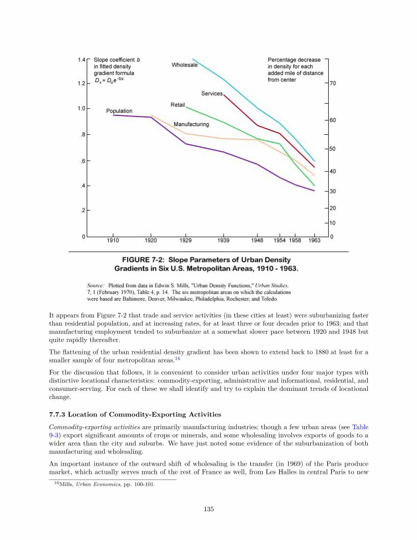
It appears from Figure 7-2 that trade and service activities (in these cities at least) were suburbanizing fasterthan residential population, and at increasing rates, for at least three or four decades prior to 1963; and thatmanufacturing employment tended to suburbanize at a somewhat slower pace between 1920 and 1948 butquite rapidly thereafter.

The flattening of the urban residential density gradient has been shown to extend back to 1880 at least for asmaller sample of four metropolitan areas.16

For the discussion that follows, it is convenient to consider urban activities under four major types withdistinctive locational characteristics: commodity-exporting, administrative and informational, residential, andconsumer-serving. For each of these we shall identify and try to explain the dominant trends of locationalchange.

7.7.3 Location of Commodity-Exporting Activities

Commodity-exporting activities are primarily manufacturing industries; though a few urban areas (see Table9-3) export significant amounts of crops or minerals, and some wholesaling involves exports of goods to awider area than the city and suburbs. We have just noted some evidence of the suburbanization of bothmanufacturing and wholesaling.

An important instance of the outward shift of wholesaling is the transfer (in 1969) of the Paris producemarket, which actually serves much of the rest of France as well, from Les Halles in central Paris to new

16Mills, Urban Economics, pp. 100-101.

135

quarters at suburban Rungis. Produce markets in many American cities (such as Boston and New York) havebeen similarly relocated, and wholesale establishments of other types as well are increasingly represented insuburban industrial zones.

In manufacturing at least, this suburbanization trend goes back even further than Figure 7-2 shows. One ofthe earliest systematic investigations dates it from 1889:

Between 1879 and 1889, manufacturing activity was growing more rapidly in most large metropoli-tan cities than in the surrounding districts... Since 1889, manufacturing activity has grown morerapidly in the suburban sections surrounding great manufacturing cities than in the manufacturingcities themselves. 17

Improvements in Census data made possible Daniel Creamer’s more detailed analyses for the period since1899, which are summed up in Table 7-1. Because the data are not presented in precisely comparable termsby all censuses, and because the picture of location shifts is affected by changes in the classification of specificareas as they grow, three different time series are shown in this summary table. It is clear from each series,however, that location types C and F (suburban areas around important industrial cities) have shown fasterindustrial growth than those cities themselves (location types A and D respectively).18 Suburbanizationbecomes increasingly apparent in the more recent period; by the 1960s, the popularity of outlying locationsfor new and expanded manufacturing plants was so obvious as hardly to require documentation. How canthis tendency be explained?

17Glenn E. McLaughlin, Growth of American Manufacturing Areas, Monograph No. 7 (Pittsburgh: University of Pittsburgh,Bureau of Business Research, 1938), p. 186. His conclusions were based on U.S. Census data for the 13 largest Census IndustrialAreas (composed of whole counties and groups of counties) and their central cities.

18Industrial Areas (location categories A+B +C in Table 7-1) and also selected other important industrial counties (categoryF ) were identified by the Census of Manufactures in 1929 and replaced by the Standard Metropolitan Areas concept in 1947.The Industrial Area was a unit based on concentration of at least 40,000 manufacturing wage earners in an important industrialcity, its county, and adjacent important industrial counties. In 1929 there were 34 Industrial Areas; applying the same criteria inlater years, Creamer had 49 by 1963. This is obviously a more exclusive category than the more recent Standard MetropolitanStatistical Area (SMSA), of which there were 323 by 1980. In the period 1929-1963, the number of B cities (see Table 7-1)ranged from 12 to 23; the number of D cities and E counties, from 41 to 61; and the number of F counties, from 47 to 94.

136

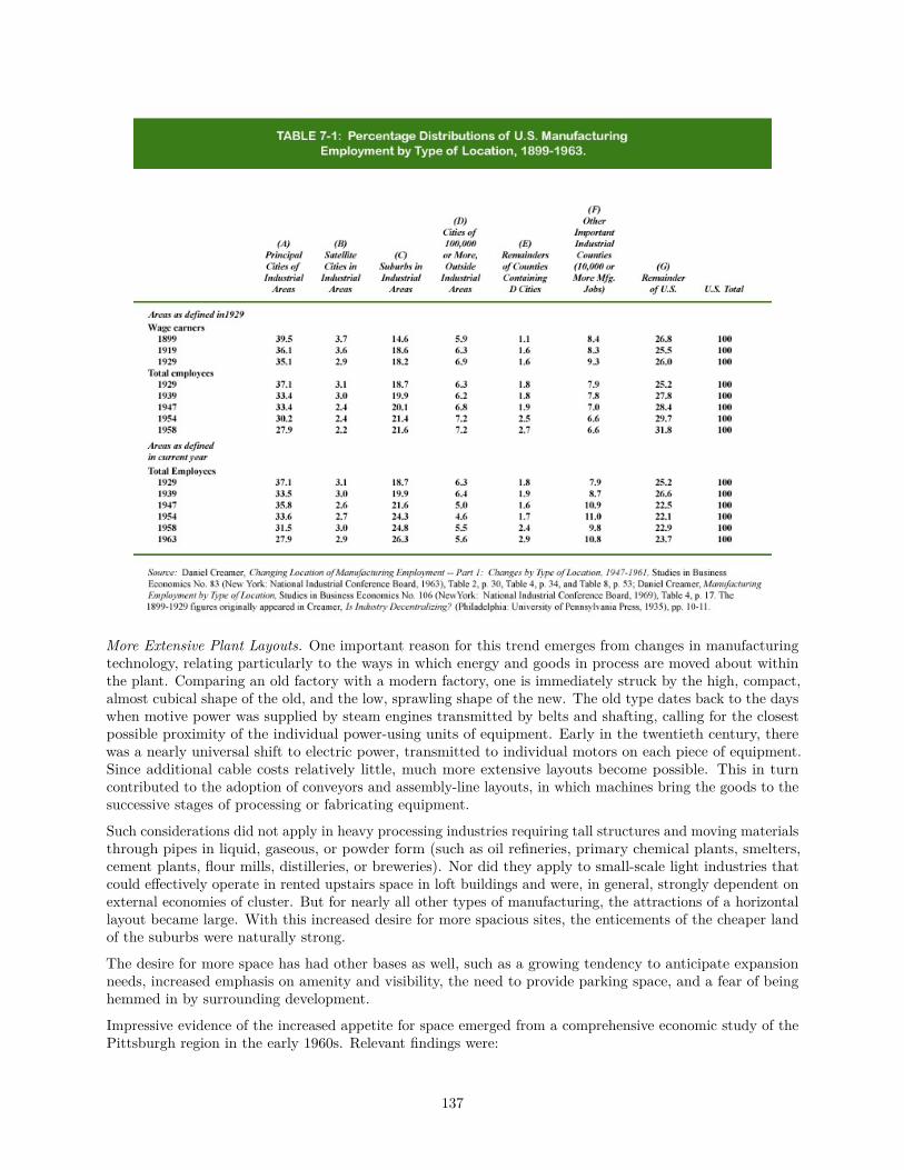
More Extensive Plant Layouts. One important reason for this trend emerges from changes in manufacturingtechnology, relating particularly to the ways in which energy and goods in process are moved about withinthe plant. Comparing an old factory with a modern factory, one is immediately struck by the high, compact,almost cubical shape of the old, and the low, sprawling shape of the new. The old type dates back to the dayswhen motive power was supplied by steam engines transmitted by belts and shafting, calling for the closestpossible proximity of the individual power-using units of equipment. Early in the twentieth century, therewas a nearly universal shift to electric power, transmitted to individual motors on each piece of equipment.Since additional cable costs relatively little, much more extensive layouts become possible. This in turncontributed to the adoption of conveyors and assembly-line layouts, in which machines bring the goods to thesuccessive stages of processing or fabricating equipment.

Such considerations did not apply in heavy processing industries requiring tall structures and moving materialsthrough pipes in liquid, gaseous, or powder form (such as oil refineries, primary chemical plants, smelters,cement plants, flour mills, distilleries, or breweries). Nor did they apply to small-scale light industries thatcould effectively operate in rented upstairs space in loft buildings and were, in general, strongly dependent onexternal economies of cluster. But for nearly all other types of manufacturing, the attractions of a horizontallayout became large. With this increased desire for more spacious sites, the enticements of the cheaper landof the suburbs were naturally strong.

The desire for more space has had other bases as well, such as a growing tendency to anticipate expansionneeds, increased emphasis on amenity and visibility, the need to provide parking space, and a fear of beinghemmed in by surrounding development.

Impressive evidence of the increased appetite for space emerged from a comprehensive economic study of thePittsburgh region in the early 1960s. Relevant findings were:

137

[Plants relocating within Allegheny County, 1957-1959]

In the eleven cases in which the area of site and of buildings at both old and new locations werespecified, the average site area per plant had increased from 4.6 to 19.6 acres, or 300 percent,and the average building area per plant had increased from 90,000 to 122,000 square feet, or 36percent. [This sample consists primarily of rather large manufacturing plants.] The much greaterexpansion of site area than of building area indicates a desire for more open space for storage,loading, and parking, and for subsequent expansion. The site area per employee was at leastdoubled in each of these eleven relocations, and was increased by a factor of more than 20 in twocases.

[Plants that had not relocated but reported need for more space]

The average estimate of additional space [site area] required was 153 percent, but the averageestimate of increased employment associated with those requirements was only 38 percent. Thesefigures imply a desire to increase the amount of space per employee by 83 percent.

[Respondents, primarily occupying rented space in multitenant buildings,who reported need for more floor space]

Although only fourteen of the respondents reporting inadequate floor space gave the requestedinformation on amount of additional space needed and additional employment expected, in allbut one of those cases the percentage increase in floor space was at least as great as the increasein employment. On the average, 138 percent more floor space was called for, with an associatedincrease in employment of only 44 percent. These figures imply a desire to increase the amount offloor space per employee by 65 percent.19

Changes in Transport Technology. Another change contributing to the suburbanization of commodity-exporting activities comes from transport technology, and specifically from the improvement of motor vehiclesand highways that enabled a good part of the inputs of such activities and a still larger part of their outputsto be shipped by truck. This change became important in the 1920s. Earlier, manufacturing establishmentsrelied heavily on the horse and wagon for the intraurban movement of commodities, while the interregionalshipment of a large portion of materials inputs as well as their outputs was effected by rail.

In an insightful analysis of the effect of transport on urban spatial patterns, Leon Moses and HaroldF. Williamson, Jr., point to changes in the relative cost of interregional versus intraregional transfer ofcommodities as an important factor encouraging decentralization.20 The efficiency of rail transport dependsto a large extent on scale economies associated with freight handling and large-lot shipments. During theearly stages of urban development, it was often the case that no more than one central terminal could bemaintained economically in a given city. By clustering about the central terminal, manufacturers could benefitby receiving shipments directly from rail sidings. Also, the clustering minimized the distances involved forshipments among local establishments—an important consideration given the inefficiency of the horse-drawnwagon.

The influence of truck transport came in two stages. Moses and Williamson point out that early in this century(1900—1920) the truck replaced the horse and wagon for intraurban shipments but that manufacturers werestill tied to rail transport for shipments to and from the city. In this early phase, locational ties to theurban “core” were weakened; as the cost of intraurban transfer was reduced, suburbanization was encouraged.However, the full impact of truck transport was not realized until much later. As the interstate highwaysystem became more fully developed (after World War II), suburban export terminals became common, andthe second phase of decentralization came into full swing.21 It has most strongly affected wholesaling and the

19Ira S. Lowry, Portrait of a Region, vol. 2 of the Economic Study of the Pittsburgh Region conducted by the PittsburghRegional Planning Association (Pittsburgh: University of Pittsburgh Press, 1963), p. 73. The three passages quoted here arefrom a section prepared by Edgar M. Hoover. Italics in original.

20Leon Moses and Harold F. Williamson, “‘The Location of Economic Activity in Cities,” American Economics Review, 57, 2(May 1967), 211-222.

21For an interesting theoretical analysis of the effect of a suburban export terminal on urban spatial structure, see Michelle J.White, “Firm Suburbanization and Urban Subcenters,” Journal of Urban Economics, 3, 3 (July 1976), 323-343.

138

lighter types of manufacturing that ship high-value outputs in small consignments; but even steel mills andother heavy industries have come to ship substantial parts of their output over the roads.

However, an interesting reversal occurred in the 1960s in the method of transporting new automobiles fromfactories and assembly plants. Statistics compiled by the Automobile Manufacturers’ Association show that in1959, 90 percent of such traffic was by road and only 8 percent by rail. The railroads then devised equipmentand tariffs that made it more economical to ship by rail for medium and long distances, and by about 1970the rails were carrying the majority of new cars shipped. Barge shipments of new automobiles, which hadbeen nearly 8 percent of the total in 1949, had become insignificant by the mid-1960s.

The use of highway transport greatly widens the choice of locations since the road network is many timesfiner than the rail network and offers an almost unlimited choice of stopping places. For direct shipment inwhole truckloads, there is no need to be near any transport terminal, and many piggyback loading yards havebeen conveniently placed for suburban access. An outlying plant location speeds the receipt and delivery ofgoods by obviating slow and expensive trucking through congested city streets.

Access to Labor Supply. A third factor contributing to industrial sub-urbanization is labor supply. Moses andWilliamson have argued that in the earliest years of this century, the intraurban movement of people was muchmore efficient than the intraurban movement of goods and services. Trolleys and commuter railroads freedworkers from residing in close proximity to the downtown, even while many manufacturing establishmentswere still tied to locations at or near central freight terminals.

During this early period, the urban center was truly a hub of economic activity, where streetcars and railroadsbrought workers and commodities together on a daily basis. However, as automobile ownership became acommon characteristic of urban life, the locational consequences of a decentralized labor force became moreapparent. The urbanization of population and its motorization have made it feasible to attract an adequatework force to locations outside of any major population center, and business location decisions now reflectlabor’s local mobility. As noted in the last section of Chapter 10, some suburban locations are better thandowntown in terms of access to the supply of high-income professional personnel. Locations in beltway zonescan provide quick access to labor from a sizable arc of the metropolitan circumference.

This does not exhaust the list of reasons for the increased attractiveness of suburban locations for exportingactivities. Business firms have become increasingly influenced by amenity, prestige, and public relations. Asuburban location with attractively landscaped grounds, exposed to the view of thousands of daily travelerson a busy expressway, has an advertising value not to be underrated.

Finally, it is important to note that, in the aggregate, all of the forces motivating suburbanization acquirefurther importance from the changing composition of productive and distributive activities. Higher incomelevels and the proliferation of products, brands, and successive stages of processing mean an increasingproportion of the lighter types of activity— those involving relatively little weight loss or orientation totransported inputs and relatively high sensitivity to quick market access, environmental amenity, and localpublic relations.

7.7.4 Location of Administrative and Other Information-Processing Activities

A rapidly increasing proportion of activities produce intangible outputs that are delivered through personalcontact or communications media, with little or no shipment of any actual goods.22 Since new informationobsolesces rapidly (yesterday’s newspaper is trash, and last week’s memo may serve only to clutter the files)and since human time is expensive, market-access advantage for such activities is measured primarily in termsof time.

Technological advance has greatly speeded long-distance communication and personal travel, though in ourtime there has been relatively slight improvement for the short haul. The locational impact is clearly visiblein the rapidly growing operations of administration, data processing, and research. Individual businesscorporations have been increasingly consolidating such operations at headquarters and reducing the relative

22See the discussion at the beginning of Chapter 3 regarding the transfer of commodities and information. For a penetratingstudy of the processes involved in office activity and their locational significance, see J. B. Goddard, “Office Communicationsand Office Location: A Review of Current Research,” Regional Studies, 5, 4 (December 1971), 263-280.

139

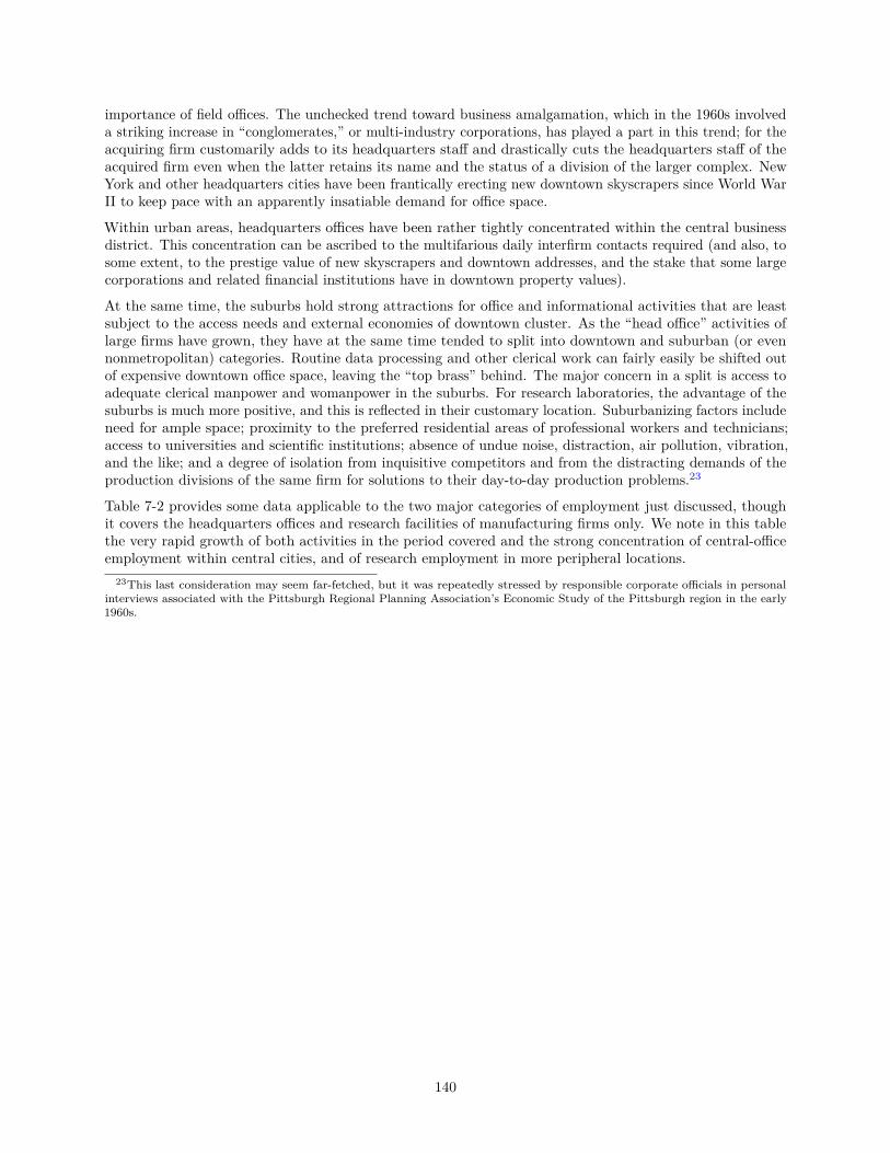
importance of field offices. The unchecked trend toward business amalgamation, which in the 1960s involveda striking increase in “conglomerates,” or multi-industry corporations, has played a part in this trend; for theacquiring firm customarily adds to its headquarters staff and drastically cuts the headquarters staff of theacquired firm even when the latter retains its name and the status of a division of the larger complex. NewYork and other headquarters cities have been frantically erecting new downtown skyscrapers since World WarII to keep pace with an apparently insatiable demand for office space.

Within urban areas, headquarters offices have been rather tightly concentrated within the central businessdistrict. This concentration can be ascribed to the multifarious daily interfirm contacts required (and also, tosome extent, to the prestige value of new skyscrapers and downtown addresses, and the stake that some largecorporations and related financial institutions have in downtown property values).

At the same time, the suburbs hold strong attractions for office and informational activities that are leastsubject to the access needs and external economies of downtown cluster. As the “head office” activities oflarge firms have grown, they have at the same time tended to split into downtown and suburban (or evennonmetropolitan) categories. Routine data processing and other clerical work can fairly easily be shifted outof expensive downtown office space, leaving the “top brass” behind. The major concern in a split is access toadequate clerical manpower and womanpower in the suburbs. For research laboratories, the advantage of thesuburbs is much more positive, and this is reflected in their customary location. Suburbanizing factors includeneed for ample space; proximity to the preferred residential areas of professional workers and technicians;access to universities and scientific institutions; absence of undue noise, distraction, air pollution, vibration,and the like; and a degree of isolation from inquisitive competitors and from the distracting demands of theproduction divisions of the same firm for solutions to their day-to-day production problems.23

Table 7-2 provides some data applicable to the two major categories of employment just discussed, thoughit covers the headquarters offices and research facilities of manufacturing firms only. We note in this tablethe very rapid growth of both activities in the period covered and the strong concentration of central-officeemployment within central cities, and of research employment in more peripheral locations.

23This last consideration may seem far-fetched, but it was repeatedly stressed by responsible corporate officials in personalinterviews associated with the Pittsburgh Regional Planning Association’s Economic Study of the Pittsburgh region in the early1960s.

140

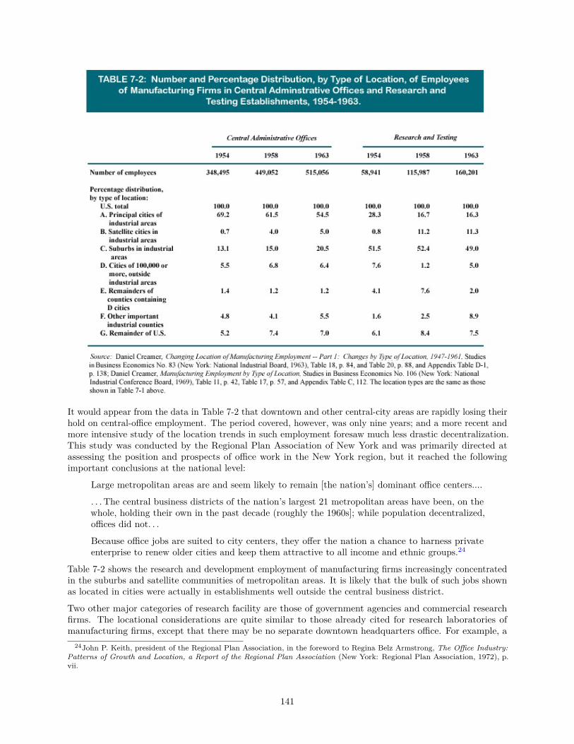
It would appear from the data in Table 7-2 that downtown and other central-city areas are rapidly losing theirhold on central-office employment. The period covered, however, was only nine years; and a more recent andmore intensive study of the location trends in such employment foresaw much less drastic decentralization.This study was conducted by the Regional Plan Association of New York and was primarily directed atassessing the position and prospects of office work in the New York region, but it reached the followingimportant conclusions at the national level:

Large metropolitan areas are and seem likely to remain [the nation’s] dominant office centers....

. . . The central business districts of the nation’s largest 21 metropolitan areas have been, on thewhole, holding their own in the past decade (roughly the 1960s]; while population decentralized,offices did not. . .

Because office jobs are suited to city centers, they offer the nation a chance to harness privateenterprise to renew older cities and keep them attractive to all income and ethnic groups.24

Table 7-2 shows the research and development employment of manufacturing firms increasingly concentratedin the suburbs and satellite communities of metropolitan areas. It is likely that the bulk of such jobs shownas located in cities were actually in establishments well outside the central business district.

Two other major categories of research facility are those of government agencies and commercial researchfirms. The locational considerations are quite similar to those already cited for research laboratories ofmanufacturing firms, except that there may be no separate downtown headquarters office. For example, a

24John P. Keith, president of the Regional Plan Association, in the foreword to Regina Belz Armstrong, The Office Industry:Patterns of Growth and Location, a Report of the Regional Plan Association (New York: Regional Plan Association, 1972), p.vii.

141

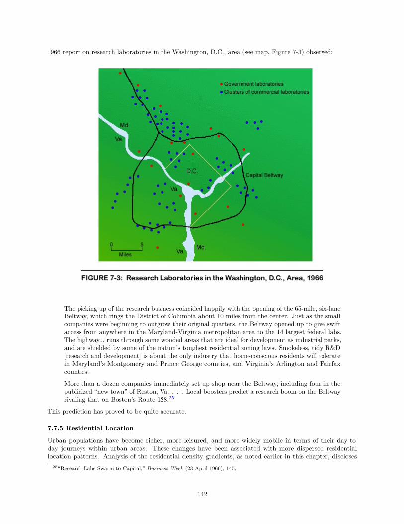
1966 report on research laboratories in the Washington, D.C., area (see map, Figure 7-3) observed:

The picking up of the research business coincided happily with the opening of the 65-mile, six-laneBeltway, which rings the District of Columbia about 10 miles from the center. Just as the smallcompanies were beginning to outgrow their original quarters, the Beltway opened up to give swiftaccess from anywhere in the Maryland-Virginia metropolitan area to the 14 largest federal labs.The highway.., runs through some wooded areas that are ideal for development as industrial parks,and are shielded by some of the nation’s toughest residential zoning laws. Smokeless, tidy R&D[research and development] is about the only industry that home-conscious residents will toleratein Maryland’s Montgomery and Prince George counties, and Virginia’s Arlington and Fairfaxcounties.

More than a dozen companies immediately set up shop near the Beltway, including four in thepublicized “new town” of Reston, Va. . . . Local boosters predict a research boom on the Beltwayrivaling that on Boston’s Route 128.25

This prediction has proved to be quite accurate.

7.7.5 Residential Location

Urban populations have become richer, more leisured, and more widely mobile in terms of their day-to-day journeys within urban areas. These changes have been associated with more dispersed residentiallocation patterns. Analysis of the residential density gradients, as noted earlier in this chapter, discloses

25“Research Labs Swarm to Capital,” Business Week (23 April 1966), 145.

142

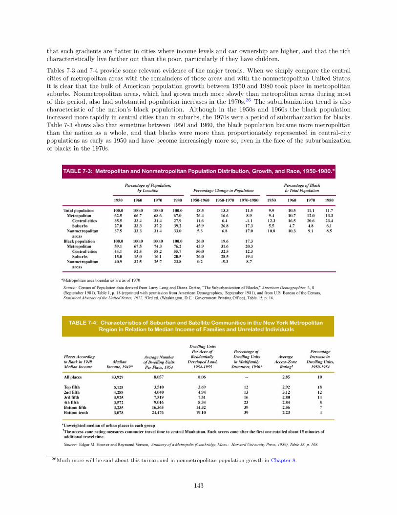
that such gradients are flatter in cities where income levels and car ownership are higher, and that the richcharacteristically live farther out than the poor, particularly if they have children.

Tables 7-3 and 7-4 provide some relevant evidence of the major trends. When we simply compare the centralcities of metropolitan areas with the remainders of those areas and with the nonmetropolitan United States,it is clear that the bulk of American population growth between 1950 and 1980 took place in metropolitansuburbs. Nonmetropolitan areas, which had grown much more slowly than metropolitan areas during mostof this period, also had substantial population increases in the 1970s.26 The suburbanization trend is alsocharacteristic of the nation’s black population. Although in the 1950s and 1960s the black populationincreased more rapidly in central cities than in suburbs, the 1970s were a period of suburbanization for blacks.Table 7-3 shows also that sometime between 1950 and 1960, the black population became more metropolitanthan the nation as a whole, and that blacks were more than proportionately represented in central-citypopulations as early as 1950 and have become increasingly more so, even in the face of the suburbanizationof blacks in the 1970s.

26Much more will be said about this turnaround in nonmetropolitan population growth in Chapter 8.

143

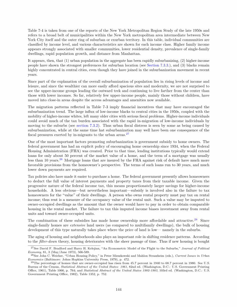
Table 7-4 is taken from one of the reports of the New York Metropolitan Region Study of the late 1950s andrefers to a broad belt of municipalities within the New York metropolitan area intermediate between NewYork City itself and the outer ring of suburban or exurban territory. In this table, individual communities areclassified by income level, and various characteristics are shown for each income class. Higher family incomeappears strongly associated with smaller communities, lower residential density, prevalence of single-familydwellings, rapid population growth, and distance from Manhattan.

It appears, then, that (1) urban population in the aggregate has been rapidly suburbanizing, (2) higher-incomepeople have shown the strongest preferences for suburban location (see Section 7.3.3.), and (3) blacks remainhighly concentrated in central cities, even though they have joined in the suburbanization movement in recentyears.

Since part of the explanation of the overall suburbanization of population lies in rising levels of income andleisure, and since the wealthier can more easily afford spacious sites and modernity, we are not surprised tosee the upper-income groups leading the outward trek and continuing to live farther from the center thanthose with lower incomes. So far, relatively few upper-income people, mainly those without children, havemoved into close-in areas despite the access advantages and amenities now available.

The migration patterns reflected in Table 7-3 imply financial incentives that may have encouraged thesuburbanization trend. The large influx of low-income blacks to central cities in the 1950s, coupled with themobility of higher-income whites, left many older cities with serious fiscal problems. Higher-income individualscould avoid much of the tax burden associated with the rapid in-migration of low-income individuals bymoving to the suburbs (see section 7.3.2). Thus urban fiscal distress is seen by some as being caused bysuburbanization, while at the same time hat suburbanization may well have been one consequence of thefiscal pressures exerted by in-migrants to the urban areas.27

One of the most important factors promoting suburbanization is government subsidy to home owners. Thefederal government has had an explicit policy of encouraging home ownership since 1934, when the FederalHousing Administration (FHA) was created. Prior to that time, lending institutions typically would extendloans for only about 50 percent of the market value of a home, and the term of a mortgage was usuallyless than 10 years.28 Mortgage loans that are insured by the FHA against risk of default have much morefavorable provisions from the homeowner’s perspective. The terms of such loans run to 30 years, and muchlower down payments are required.

Tax policies also have made it easier to purchase a home. The federal government presently allows homeownersto deduct the full value of interest payments and property taxes from their taxable income. Given theprogressive nature of the federal income tax, this means proportionately larger savings for higher-incomehouseholds. A less obvious—but nevertheless important—subsidy is involved also in the failure to taxhomeowners for the “value” of their dwellings. A person who owns rental property must pay tax on rentalincome; thus rent is a measure of the occupancy value of the rental unit. Such a value may be imputed toowner-occupied dwellings as the amount that the owner would have to pay in order to obtain comparablehousing in the rental market. The failure to tax this imputed income biases investment away from rentalunits and toward owner-occupied units.

The combination of these subsidies has made home ownership more affordable and attractive.29 Sincesingle-family homes are extensive land users (as compared to multifamily dwellings), the bulk of housingdevelopment of this type naturally takes place where the price of land is low— namely in the suburbs.

The aging of housing and neighborhoods also plays an important role in shifting residence patterns. Accordingto the filter-down theory, housing deteriorates with the sheer passage of time. Thus if new housing is bought

27See David F. Bradford and Harry H. Kelejian, “An Econometric Model of the Flight to the Suburbs,” Journal of PoliticalEconomy, 81, 3 (May/June 1973), 566-589.

28See John C. Weicher, “Urban Housing Policy,” in Peter Mieszkowski and Mahlon Straszheim (eds.), Current Issues in UrbanEconomics (Baltimore: Johns Hopkins University Press, 1979), p. 472.

29The percentage of homes that are owner-occupied has risen from 45.7 percent in 1940 to 68.7 percent in 1980. See U.S.Bureau of the Census, Statistical Abstract of the United States: 1961, 82nd ed. (Washington, D.C.: U.S. Government PrintingOffice, 1961), Table 1066, p. 764; and Statistical Abstract of the United States 1982-1983, 103rd ed. (Washington, D.C.: U.S.Government Printing Office, 1982), Table 1352, p. 752.

144

mainly by the well-to-do, housing units will in the course of time be handed down to occupants lower and loweron the income scale. Each stratum of urban society except the top will have access to housing relinquishedby the stratum above.30

There is substantial correlation between the age and the condition of structures. Moreover, housing (and thesame applies to nonresidential structures) can become less useful with the passage of time, independent ofany physical deterioration. Preferences change. The design of a house that was well adapted for a typicalwell-to-do family of 1890 or 1920 may not correspond to what a similar family prefers in the 1980s in thecontext of newer alternatives. Neighborhood land-use layouts in terms of lot sizes, front and back yards,block sizes, street widths, and the like are likewise vulnerable to obsolescence and loss of favor in the face ofchanging conditions and tastes. Finally there is the factor of prestige attached to newness per se, whether itrefers to the family car, the family dwelling, or the neighborhood.

Nevertheless, there are a fair number of instances in which old neighborhoods and old housing are visiblyinvolved in a filter-up process. Small-scale remodeling and larger-scale conversion can play a significant rolein housing market adjustment. Indeed, while this has meant that some neighborhoods in older cities havebeen judiciously refurbished (as exemplified by Georgetown in Washington, D.C., and Beacon Hill in Boston),it has also been an important mechanism by which entire suburbs may change to accommodate higher-incomeresidents as a city grows.

The net residential density of new developments on the suburban fringe responds to cyclical ups and downsin land prices, construction costs, and housing demand, as well as to shifts in the relative demands of variousincome groups for such housing. For example, in the New York metropolitan region during the 1950s, averagelot size in new suburban subdivisions was growing by roughly 4 percent per annum.31 But a number ofconsiderations suggest that this rapid growth in size at the margin has not been maintained since, and thatthe density in new fringe settlement may even have risen.

One such consideration is the rise in land prices, construction costs, and interest rates, which have madespacious and spaciously sited dwellings more and more costly. Another important factor is the ability ofdifferent income groups to bid for new suburban housing. The Burgess hypothesis described the twentieth-century American norm in terms of the rich living farther from city centers than the poor. One rationalizationfor this pattern was the fact that only upper-income people could afford to indulge a preference for new housing,and that such people were also more generally provided with automobiles (thus being more independent ofpublic transportation) and with the leisure time to enjoy suburban living.

But these perquisites have become less exclusive. Car ownership has extended gradually to all but therock-bottom income group; lower-income people quite often work shorter hours than people with higherincomes and greater responsibility; and finally, various types of mobile and modular homes have appeared,making new detached private housing at last available to people over a wider range of the income distribution.The point here is that these developments have brought medium-income and lower-income housing at ratherhigh densities to fringe areas. Some single-family areas, of course, are at any given time shifting to multifamilydevelopment by conversion of large old houses and erection of new apartment buildings; and densities at thatstage jump to a much higher level. But we observe also that the peak densities associated with inner-city

30This filter-down process is indeed familiar in the used-car market; but it does not fit as well when applied to housing.Housing deterioration is by no means so closely related to age as is deterioration of automobiles. Instead, condition dependsprimarily on maintenance, the structure itself being almost indefinitely lasting if adequately maintained. See Ira S. Lowry,“Filtering and Housing Standards: A Conceptual Analysis,” Land Economics, 36 (November 1960), 362-370. For a survey ofmore recent efforts to relate the depreciation and deterioration of dwelling units to residential succession see John M. Quigley,“What Have We Learned about Housing Markets?” in Peter Mieszkowski and Mahlon Straszheim (eds.), Current Issues in UrbanEconomics (Baltimore: Johns Hopkins University Press, 1979), pp. 417-420.

31Edgar M. Hoover and Raymond Vernon, Anatomy of a Metropolis (Cambridge, Mass.: Harvard University Press, 1959),Table 49, p. 220. These figures are brought down to 1960 in Regional Plan Association, Spread City (New York: Regional PlanAssociation, 1962).

145

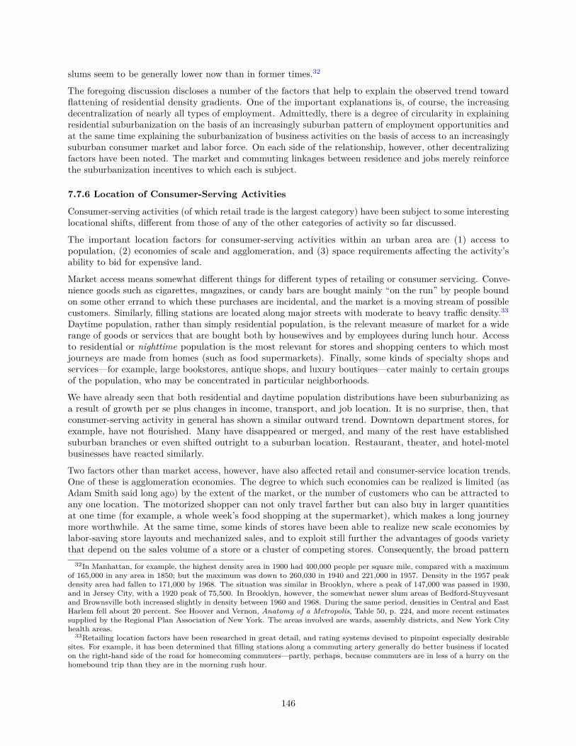
slums seem to be generally lower now than in former times.32

The foregoing discussion discloses a number of the factors that help to explain the observed trend towardflattening of residential density gradients. One of the important explanations is, of course, the increasingdecentralization of nearly all types of employment. Admittedly, there is a degree of circularity in explainingresidential suburbanization on the basis of an increasingly suburban pattern of employment opportunities andat the same time explaining the suburbanization of business activities on the basis of access to an increasinglysuburban consumer market and labor force. On each side of the relationship, however, other decentralizingfactors have been noted. The market and commuting linkages between residence and jobs merely reinforcethe suburbanization incentives to which each is subject.

7.7.6 Location of Consumer-Serving Activities

Consumer-serving activities (of which retail trade is the largest category) have been subject to some interestinglocational shifts, different from those of any of the other categories of activity so far discussed.

The important location factors for consumer-serving activities within an urban area are (1) access topopulation, (2) economies of scale and agglomeration, and (3) space requirements affecting the activity’sability to bid for expensive land.

Market access means somewhat different things for different types of retailing or consumer servicing. Conve-nience goods such as cigarettes, magazines, or candy bars are bought mainly “on the run” by people boundon some other errand to which these purchases are incidental, and the market is a moving stream of possiblecustomers. Similarly, filling stations are located along major streets with moderate to heavy traffic density.33

Daytime population, rather than simply residential population, is the relevant measure of market for a widerange of goods or services that are bought both by housewives and by employees during lunch hour. Accessto residential or nighttime population is the most relevant for stores and shopping centers to which mostjourneys are made from homes (such as food supermarkets). Finally, some kinds of specialty shops andservices—for example, large bookstores, antique shops, and luxury boutiques—cater mainly to certain groupsof the population, who may be concentrated in particular neighborhoods.

We have already seen that both residential and daytime population distributions have been suburbanizing asa result of growth per se plus changes in income, transport, and job location. It is no surprise, then, thatconsumer-serving activity in general has shown a similar outward trend. Downtown department stores, forexample, have not flourished. Many have disappeared or merged, and many of the rest have establishedsuburban branches or even shifted outright to a suburban location. Restaurant, theater, and hotel-motelbusinesses have reacted similarly.

Two factors other than market access, however, have also affected retail and consumer-service location trends.One of these is agglomeration economies. The degree to which such economies can be realized is limited (asAdam Smith said long ago) by the extent of the market, or the number of customers who can be attracted toany one location. The motorized shopper can not only travel farther but can also buy in larger quantitiesat one time (for example, a whole week’s food shopping at the supermarket), which makes a long journeymore worthwhile. At the same time, some kinds of stores have been able to realize new scale economies bylabor-saving store layouts and mechanized sales, and to exploit still further the advantages of goods varietythat depend on the sales volume of a store or a cluster of competing stores. Consequently, the broad pattern

32In Manhattan, for example, the highest density area in 1900 had 400,000 people per square mile, compared with a maximumof 165,000 in any area in 1850; but the maximum was down to 260,030 in 1940 and 221,000 in 1957. Density in the 1957 peakdensity area had fallen to 171,000 by 1968. The situation was similar in Brooklyn, where a peak of 147,000 was passed in 1930,and in Jersey City, with a 1920 peak of 75,500. In Brooklyn, however, the somewhat newer slum areas of Bedford-Stuyvesantand Brownsville both increased slightly in density between 1960 and 1968. During the same period, densities in Central and EastHarlem fell about 20 percent. See Hoover and Vernon, Anatomy of a Metropolis, Table 50, p. 224, and more recent estimatessupplied by the Regional Plan Association of New York. The areas involved are wards, assembly districts, and New York Cityhealth areas.

33Retailing location factors have been researched in great detail, and rating systems devised to pinpoint especially desirablesites. For example, it has been determined that filling stations along a commuting artery generally do better business if locatedon the right-hand side of the road for homecoming commuters—partly, perhaps, because commuters are in less of a hurry on thehomebound trip than they are in the morning rush hour.

146

of decentralization within urban areas has been associated with increasing agglomeration in large stores andlarge shopping centers.

Finally, the location patterns of consumer-serving activities (except the sidewalk-convenience type) havebeen significantly affected by the larger space requirements imposed by the need for parking space. Thisconsideration reinforces the trend to the suburbs, and perhaps also reinforces the tendency to cluster in largeshopping centers, where the pooling of parking space can lead to its more efficient utilization.

7.8 SummaryLocation within urban areas is especially affected by need for movement of people and direct personal contact,with time consequently playing the major role in transfer costs and access advantage. Complex linkagesamong units and activities, and competition for space, are also important location factors in the urbancontext. The monocentric land-use models developed in Chapter 6, which emphasized these factors, abstractfrom other characteristics of urban spatial structure.

Various highly simplified models of urban spatial form are helpful in analyzing the operation of the morebasic location factors. Simplest of all is the concept of land-use intensity rising to a peak at the city center,as predicted by monocentric models of urban land use. Residential density and certain other variables docharacteristically decline with distance from the center at a rate expressed by a density-gradient slope; andinter-city differences in the slope reflect such characteristics as city size, availability and cost of transport,income, and the age of the city.

An early, descriptive analysis of urban patterns pictured the city in terms analogous to the land-use modelsdiscussed in Chapter 6, with a sequence of concentric zones devoted to different broad types of activity.Land-use succession within urban areas can be characterized as changes in the size or spacing of such zones.

Real urban land-use patterns depart drastically from the concentric ring scheme for many reasons. Directionfrom the center can be as important as distance because of topography, major transfer routes, and intracitycluster economies and other forces promoting neighborhood homogeneity and specialization. Further, anyurban area of substantial size has, in addition to its main center, a number of subcenters.

Increased population in an urban area, independently of any changes in income or technology, helps toexplain many of the major observed trends in urban form and travel patterns, such as more extensive andintensive use of space, flattening of density and rent gradients, longer intracity journeys and shipments, and adiminished role of the central business district relative to subcenters and suburbs.

Commodity-exporting activities in cities (primarily manufacturing and wholesaling) have been decentralizedfor many decades as the result of a number of factors, including requirements for more spacious layouts andsites, use of highway transport for both goods and workers, a more decentralized and mobile labor force, andin some cases the attraction of suburban amenities.

Administrative and other information-handling activities have been locationally affected by revolutionaryimprovements in communications and data processing, as well as by a strong attraction toward the suburbsfor the upper-income workers involved. Suburban locations predominate for research facilities and haveattracted much office employment as well, though the central business districts of large cities have kept someof their old preeminence as locations for corporate headquarters.

Residential location patterns in urban areas have been decentralizing (as measured by flatter populationdensity gradients) since the latter part of the nineteenth century at latest. This trend appears associatedwith larger city size, more income and leisure, and more widespread automobile ownership. The increasingconcentration of black metropolitan populations in the central cities seems to have come to a halt by 1970.In the decade to follow, there were substantial increases in the black populations of metropolitan suburbs. Inthe shift to suburban homes, especially by higher-income families, government policies that subsidize homeownership and preference for newer housing have been important factors.

Consumer-serving activities such as retail trade have in general followed population shifts, but at the sametime they have clustered increasingly in subcenters because of scale and other agglomeration economies andthe enhanced mobility and affluence of their customers.

147

Technical Terms Introduced in this ChapterMonocentric urban models Minimum displacementDensity gradient SubcentersGross and net residential density Ribbon developmentCentral density Commodity-exporting activitiesBurgess zonal hypothesis Information-processing activitiesLand-use succession Filter-down and filter-up of housingSector theory

Selected ReadingsHarland Bartholomew, Land Uses in American Cities (Cambridge, Mass.: Harvard University Press, 1955).

J. V. Henderson, Economic Theory and the Cities (New York: Academic Press, 1977).

Edgar M. Hoover and Raymond Vernon, Anatomy of a Metropolis (Cambridge, Mass.: Harvard UniversityPress, 1960).

Edwin S. Mills, Urban Economics, 2nd ed. (Glenview, Ill.: Scott, Foresman, 1980).

Leon Moses and Harold Williamson, “The Location of Economic Activity in Cities,” American EconomicReview, 57 (May 1967), 211-222.

Raymond Vernon, Metropolis 1985 (Cambridge, Mass.: Harvard University Press, 1960).

William C. Wheaton, “Monocentric Models of Urban Land Use: Contributions and Criticisms,” in PeterMieszkowski and Mahlon Straszheim (eds.), Current Issues in Urban Economics (Baltimore, Md.: JohnsHopkins University Press, 1979), pp. 107-129.

148

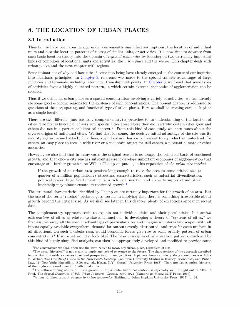
8. THE LOCATION OF URBAN PLACES8.1 IntroductionThus far we have been considering, under conveniently simplified assumptions, the location of individualunits and also the location patterns of classes of similar units, or activities. It is now time to advance fromsuch basic location theory into the domain of regional economics by focusing on two extremely importantkinds of complexes of locational units and activities: the urban place and the region. This chapter deals withurban places and the next chapter with regions.

Some intimations of why and how cities 1 come into being have already emerged in the course of our inquiriesinto locational principles. In Chapter 3, reference was made to the special transfer advantages of largejunctions and terminals, including intermodal transshipment points. In Chapter 5, we found that some typesof activities favor a highly clustered pattern, in which certain external economies of agglomeration can besecured.

Thus if we define an urban place as a spatial concentration involving a variety of activities, we can alreadysee some good economic reasons for the existence of such concentrations. The present chapter is addressed toquestions of the size, spacing, and functional type of urban places. Here we shall be treating each such placeas a single location.

There are two different (and basically complementary) approaches to an understanding of the location ofcities. The first is historical: It asks why specific cities arose where they did, and why certain cities grew andothers did not in a particular historical context.2 From this kind of case study we learn much about thediverse origins of individual cities. We find that for some, the decisive initial advantage of the site was itssecurity against armed attack; for others, a good natural harbor convenient to a productive hinterland; forothers, an easy place to cross a wide river or a mountain range; for still others, a pleasant climate or otheramenities.

However, we also find that in many cases the original reason is no longer the principal basis of continuedgrowth, and that once a city reaches substantial size it develops important economies of agglomeration thatencourage still further growth.3 As Wilbur Thompson puts it, in his exposition of the urban size ratchet,

If the growth of an urban area persists long enough to raise the area to some critical size (aquarter of a million population?) structural characteristics, such as industrial diversification,political power, huge fixed investments, a rich local market, and a steady supply of industrialleadership may almost ensure its continued growth.4

The structural characteristics identified by Thompson are certainly important for the growth of an area. Butthe use of the term “ratchet” perhaps goes too far in implying that there is something irreversible aboutgrowth beyond the critical size. As we shall see later in this chapter, plenty of exceptions appear in recentdata.

The complementary approach seeks to explain not individual cities and their peculiarities, but spatialdistributions of cities as related to size and function. In developing a theory of “systems of cities,” wefirst assume away all the special advantages of particular sites and imagine a uniform landscape—with allinputs equally available everywhere, demand for outputs evenly distributed, and transfer costs uniform inall directions, On such a tabula rasa, would economic forces give rise to some orderly pattern of urbanconcentrations? If so, what would it look like? The basic principles of urbanization patterns, disclosed bythis kind of highly simplified analysis, can then be appropriately developed and modified to provide some

1For convenience we shall often use the term “city” to mean any urban place, regardless of size.2The word “historical” is not meant to imply any lack of relevance to the future. The characteristic of the approach described

here is that it considers changes (past and prospective) in specific cities. A pioneer American study along these lines was AdnaF. Weber, The Growth of Cities in the Nineteenth Century, Columbia University Studies in History, Economics, and PublicLaw, 11 (New York: Macmillan, 1899; rev. ed., Ithaca, N.Y.: Cornell University Press, 1963). There are also countless historiesof the origin and development of individual cities.

3The self-reinforcing nature of urban growth, in a particular historical context, is especially well brought out in Allen R.Pred, The Spatial Dynamics of US. Urban-Industrial Growth, 1800-1914 (Cambridge, Mass.: MIT Press, 1966).

4Wilbur R. Thompson, A Preface to Urban Economics (Baltimore: Johns Hopkins University Press, 1965), p. 24.

149

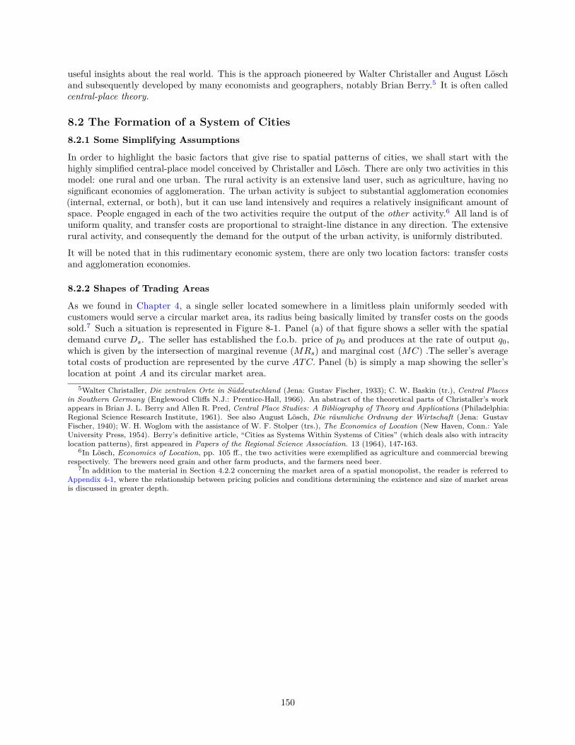
useful insights about the real world. This is the approach pioneered by Walter Christaller and August Löschand subsequently developed by many economists and geographers, notably Brian Berry.5 It is often calledcentral-place theory.

8.2 The Formation of a System of Cities8.2.1 Some Simplifying Assumptions

In order to highlight the basic factors that give rise to spatial patterns of cities, we shall start with thehighly simplified central-place model conceived by Christaller and Lösch. There are only two activities in thismodel: one rural and one urban. The rural activity is an extensive land user, such as agriculture, having nosignificant economies of agglomeration. The urban activity is subject to substantial agglomeration economies(internal, external, or both), but it can use land intensively and requires a relatively insignificant amount ofspace. People engaged in each of the two activities require the output of the other activity.6 All land is ofuniform quality, and transfer costs are proportional to straight-line distance in any direction. The extensiverural activity, and consequently the demand for the output of the urban activity, is uniformly distributed.

It will be noted that in this rudimentary economic system, there are only two location factors: transfer costsand agglomeration economies.

8.2.2 Shapes of Trading Areas

As we found in Chapter 4, a single seller located somewhere in a limitless plain uniformly seeded withcustomers would serve a circular market area, its radius being basically limited by transfer costs on the goodssold.7 Such a situation is represented in Figure 8-1. Panel (a) of that figure shows a seller with the spatialdemand curve Ds. The seller has established the f.o.b. price of p0 and produces at the rate of output q0,which is given by the intersection of marginal revenue (MRs) and marginal cost (MC) .The seller’s averagetotal costs of production are represented by the curve ATC. Panel (b) is simply a map showing the seller’slocation at point A and its circular market area.

5Walter Christaller, Die zentralen Orte in Süddeutschland (Jena: Gustav Fischer, 1933); C. W. Baskin (tr.), Central Placesin Southern Germany (Englewood Cliffs N.J.: Prentice-Hall, 1966). An abstract of the theoretical parts of Christaller’s workappears in Brian J. L. Berry and Allen R. Pred, Central Place Studies: A Bibliography of Theory and Applications (Philadelphia:Regional Science Research Institute, 1961). See also August Lösch, Die räumliche Ordnung der Wirtschaft (Jena: GustavFischer, 1940); W. H. Woglom with the assistance of W. F. Stolper (trs.), The Economics of Location (New Haven, Conn.: YaleUniversity Press, 1954). Berry’s definitive article, “Cities as Systems Within Systems of Cities” (which deals also with intracitylocation patterns), first appeared in Papers of the Regional Science Association. 13 (1964), 147-163.

6In Lösch, Economics of Location, pp. 105 ff., the two activities were exemplified as agriculture and commercial brewingrespectively. The brewers need grain and other farm products, and the farmers need beer.

7In addition to the material in Section 4.2.2 concerning the market area of a spatial monopolist, the reader is referred toAppendix 4-1, where the relationship between pricing policies and conditions determining the existence and size of market areasis discussed in greater depth.

150

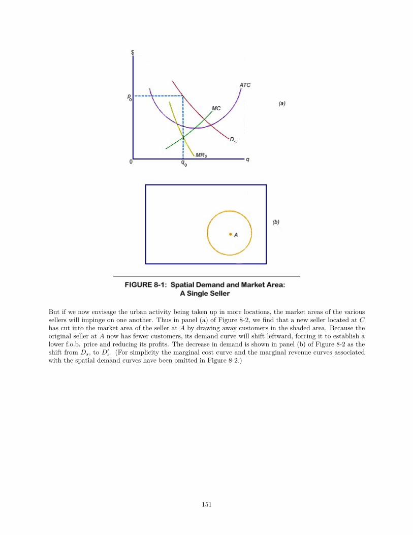
But if we now envisage the urban activity being taken up in more locations, the market areas of the varioussellers will impinge on one another. Thus in panel (a) of Figure 8-2, we find that a new seller located at Chas cut into the market area of the seller at A by drawing away customers in the shaded area. Because theoriginal seller at A now has fewer customers, its demand curve will shift leftward, forcing it to establish alower f.o.b. price and reducing its profits. The decrease in demand is shown in panel (b) of Figure 8-2 as theshift from Ds, to D′s. (For simplicity the marginal cost curve and the marginal revenue curves associatedwith the spatial demand curves have been omitted in Figure 8-2.)

151

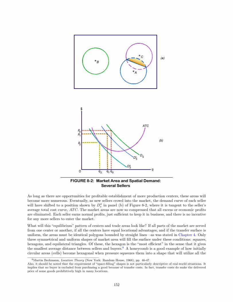
As long as there are opportunities for profitable establishment of more production centers, these areas willbecome more numerous. Eventually, as new sellers crowd into the market, the demand curve of each sellerwill have shifted to a position shown by D′′s in panel (b) of Figure 8-2, where it is tangent to the seller’saverage total cost curve, ATC. The market areas are now so compressed that all excess or economic profitsare eliminated. Each seller earns normal profits, just sufficient to keep it in business, and there is no incentivefor any more sellers to enter the market.

What will this “equilibrium” pattern of centers and trade areas look like? If all parts of the market are servedfrom one center or another, if all the centers have equal locational advantages, and if the transfer surface isuniform, the areas must be identical polygons bounded by straight lines—as was stated in Chapter 4. Onlythree symmetrical and uniform shapes of market area will fill the surface under these conditions: squares,hexagons, and equilateral triangles. Of these, the hexagon is the “most efficient” in the sense that it givesthe smallest average distance between sellers and buyers.8 A honeycomb is a good example of how initiallycircular areas (cells) become hexagonal when pressure squeezes them into a shape that will utilize all the

8Martin Beckmann, Location Theory (New York: Random House, 1968), pp. 46-47.Also, it should be noted that the requirement of “space-filling” shapes is not particularly descriptive of real-world situations. Itimplies that no buyer is excluded from purchasing a good because of transfer costs. In fact, transfer costs do make the deliveredprice of some goods prohibitively high in many locations.

152

available space.

But in many cases the transport grid is basically rectilinear—as in most modern urban street patterns andover a major part of the rural area of the United States, where the land surveys were made in terms of acheckerboard of square townships and sections and where most local roads have followed section and townshipboundaries. Under such conditions, market-area boundaries and the trading areas of towns tend to be nothexagonal or triangular but square.

8.2.3 A Hierarchy of Trading Areas

Next, we shall take a more realistic approach by recognizing more than just a single urban activity. Thesize of the trade area for a specific product depends on (1) the nature of the spatial demand curve and (2)cost or supply considerations. From our discussion of the spatial demand curve and pricing in Chapter 4,we can isolate transfer costs (per ton-mile) and market density (per square mile) as the crucial demandfactors determining the size of trading areas. On the supply side, the extent of scale or other agglomerationeconomies (as shown by the ATC curve) are most important. Obviously, each of these conditions variesfrom one activity to another. Accordingly, we might expect that each new urban activity we introduce willhave a different appropriate size of market area and spacing of supply centers. The appropriate area will besmall, and the centers closely spaced, for products for which there is little economy in agglomeration or forwhich the density of market demand is high. Where the contrary conditions hold (important agglomerationeconomies or sparse demand), we should expect production to be concentrated in a few widely spaced centerseach serving a large area.9

But should we really expect to find as many different and independent systems of market areas and productioncenters as there are different products—an almost infinite variety? We might expect this were it not for theeconomic advantages of channelizing transfer along a limited number of efficient routes, and the advantages ofclustering different activities in the same place so as to get the external economies of agglomeration discussedin Chapter 5. Recalling those considerations, we can see why two or more activities for which the “ideal”pattern of centers may be only slightly different are, in fact, likely to settle for a common “compromise” setof production locations. And if two activities do have very different ideal sizes of areas, the tendency is forthe activity with the larger-sized areas to locate at some of the centers of the other activity—say every otherone, or every third, fourth, or tenth one. In this way, each activity can have a pattern of centers more or lessappropriately spaced to fit its conditions, while at the same time the total number of centers is kept down.This is an advantage because bigger centers provide more economies of agglomeration and because more ofthe total flow of goods and services can travel on efficient high-volume transfer routes.

The pressure for reduction of the number of size classes of areas is so basic that we might even embellish thevocabulary of regional economics by referring here to a Procrustean Law of market areas. Procrustes was amythical innkeeper who provided only one bed for all his guests and achieved a perfect fit by stretching orcropping each guest as required.

What all this implies is a hierarchy of central places. As this sorting takes place and activities with larger-sizedideal areas locate at some of the centers of other activities, this results in some central places having a greatervariety of goods. As the number of activities becomes large, we can envision some centers with a much morecomplete set of activities than other centers. A stylized example of such a system is shown in Figure 8-3. Inthis particular hierarchical pattern, it is assumed that the areas are square. Four “orders” or size classes ofcenters are represented by different sizes of dots, and their respective areas are bounded by black and graylines (shown at the right of the figure).

9It might appear obvious as well that products with lower transfer costs (per unit quantity and distance) would he producedin fewer centers, and distributed over larger market areas, than products with higher transfer costs. For reasons that will beshown later in this chapter, however, no such simple general statement about the relation of transfer costs to area size can bemade.

153

There are many possible variations on this scheme; they have been analyzed in detail for both the squareand the hexagonal systems and need not detain us here. However, one particular feature is important for anunderstanding of urban and regional structure. In the system of cities shown in Figure 8-3, each city of anybut the smallest size class serves as the center not only for its area but also for an area of each of the smallersizes. The implication is, in fact, that each order of centers carries on the activities of all lower orders ofcenters plus some further activities not found in such places. Thus even in the largest city, retail customershave the opportunity to buy goods and services found also in the smallest hamlet, but retail customers insmaller places inevitably must look to larger towns for some of their shopping needs.

As we shall see from some empirical evidence to be introduced later, the mix of activities in urban placesof various sizes does in fact conform rather closely to what we should expect under a fully hierarchicalorganization of this sort. Larger centers do have most if not all of the kinds of urban activities found insmaller centers.

Another feature of the central-place hierarchy characterized in Figure 8-3 is that it exhibits a constant nestingfactor (in this case, 2). That is, market-area size (i.e., the physical extent of the market) increases from onelevel of the hierarchy to the next by a constant factor, so that the number of market areas of one size classthat nest into the next largest size class does not vary as one proceeds through the hierarchy. Central-placemodels need not have this attribute, although the hierarchy developed by Christaller did. John B. Parr hasdeveloped a more general system that allows for variability in the nesting factor.10 As a result, the ratio atwhich market-area size increases from one level of the hierarchy to the next may differ at each step up theladder. This flexibility has the potential of contributing significantly to the descriptive power of central-placemodels.

The basic concept of a central-place hierarchy contributes importantly to our understanding of intraurbanlocation patterns. In the preceding chapter, we identified the phenomenon of subcenters as an elementarycharacteristic of urban spatial structure. Having recognized the interurban hierarchy of central places, it is buta small extension to view the subcenters found within metropolitan areas as central places on a more micro

10John B. Parr, “Models of the Central Place System: A More General Approach,” Urban Studies, 15, 1 (February 1978),35-49.

154

level.11 Corresponding to the central-place hierarchy of hamlet, convenience center, shopping center, andwholesale-retail center in terms of urban places, we have an intraurban subcenter hierarchy of streetcorner,neighborhood, and community center with progressively greater size, variety, and market area.

8.2.4 Some Practical limitations

The highly simplified central-place model presented so far provides a rationale for patterns of cities such asthe one shown in Figure 8-3. There are many size classes of cities; each larger class has a more comprehensivearray of urban activities and comprises a smaller number of cities spaced farther apart. We should expect thevarious extensive rural activities (for example, distinctive types of agriculture) to be arranged in concentriczones around the centers, in the manner shown in Figure 6-4. Any given city above the lowest order willhave more than one rural market area (for its various outputs) and more than one rural supply area (for itsvarious rurally produced inputs); there is no reason to expect any of its market areas to coincide with any ofits supply areas. In addition, all cities except those in the largest class may be getting urban products fromcities of larger size.

This is obviously not an adequate picture of cities, areas, and trade flows in the real world. We begin now toconsider some of the additional factors involved.

First, the simple model assumed a uniform transfer cost per mile on a fine and regular grid of routes, andalso assumed that the rural market was distributed with uniform density. Recognition of a less regulartransfer network, with some routes cheaper or better than others, and recognition of variations in the densityof demand, would lead us to expect substantial deformation of the areas and city patterns. Still furtherdeformation arises because the costs of inputs and the resulting costs of production are not really thesame in different cities, even among those of the same size class. The many activities that are sensitiveto location factors other than agglomeration economies and access to markets were ignored in the simplemodel; superimposing their locations on the basic central-place scheme further complicates the pattern,creating additional cities (and! or larger cities) by adding both more urban activity and more demand.Finally, the whole pattern of locations is constantly shifting in delayed response to changes in such conditionsas population, regional income levels, transfer costs, and technology, so that no picture of an equilibriumsituation can be realistic.

These practical considerations are ample to explain why the distribution of cities by size is not stepwiseby discrete hierarchical classes but continuous;12 and also why there are only loose relations between thepopulation of a city and the size of its trading area, and between city size and the range of activitiesrepresented in a city.

8.2.5 Generalized Areas of Urban Influence

Although the central-place model described implies that any city above the smallest class has a variety ofdifferent-sized market and supply areas, people frequently refer to “the” trading area (or tributary area, orarea of dominance) of a city, as if there were only one. The identification of appropriate and useful nodalregions, which will be taken up later, relies heavily on the notion that for a considerable range of purposes(though perhaps not for all purposes) we can mark out some single area as particularly related to a givencenter.

For example, in one of the early studies of spatial trading patterns by marketing specialist William J. Reilly,an attempt was made to induce an empirical formula to explain retail trading areas of cities in terms of their

11See Brian J. L. Berry, “Research Frontiers in Urban Geography,” in Philip M. Hauser and Leo F. Schnore (eds.), The Studyof Urbanization (New York: Wiley, 1965), pp. 407-408. Berry’s article, in bibliographical notes appended on pp. 424-430, citesliterature on both interurban and intraurban applications of central-place analysis.

12The size distribution of cities within a large and relatively self-contained area has been found empirically to resemble aparticular form described by the Rank-Size Rule. In its simplest formulation, this rule states that the size of a city is inverselyproportional to its rank. Thus the second biggest city would be half the size of the biggest, the third biggest would he one-thirdthe size of the biggest, the 500th biggest 1/500 the size of the biggest, and so on. This rule, originally wholly empirical, has beenextensively tested, modified, and given some theoretical rationalization by Berry, Mills, and others. See Edwin S. Mills, UrbanEconomics (Glenview, Ill.: Scott, Foresman, 1972), Chapter 7; and Harry W. Richardson, “Theory of the Distribution of CitySizes: Review and Prospects,” Regional Studies, 7,3 (September 1973), 239-251.

155

size.13 Reilly’s Law of Retail Gravitation says that “two cities attract retail trade from any intermediatecity or town in the vicinity of the breaking point [the boundary between their spheres of dominance] ,approximately in direct proportion to the populations of the two cities and in inverse proportion to thesquares of the distance from these two cities to the intermediate town.”14

Some overlap of market areas is recognized, but according to this law, the market-area boundary in the senseof the “breaking point” (where trade is equally distributed between the two supplying cities) runs throughpoints where

D2A/D

2B = PA/PB

if PA and PB are the respective populations of the two cities A and B, and DA and DB are their respectivedistances from the boundary. This means that if A and B are of equal size, the market-area boundaryis a straight line midway between them; but if, for example, A is twice as large as B, each point on themarket-area boundary is

√2 as far from A as from B. Figure 8-4 shows a hypothetical set of four centers and

their areas.15 Reilly’s Law worked reasonably well when tested against actual situations (which might beexpected since it was derived empirically rather than theoretically) and has proved more durable than manyother “laws.” Let us see how it might be rationalized in terms of the simple central-place model by makingthe situation a little more realistic.

13William J. Reilly, Methods for the Study of Retail Relationships, University of Texas Bulletin 2944 (Austin: University ofTexas, 1929; reprinted, 1959); and The Law of Retail Gravitation (New York: Knickerbocker Press, 1931; 2nd ed., PillsburyPublishers, 1953). Reilly’s analysis was mentioned above in introducing the “potential” or “gravity model” concept.

14Ibid., p. 9.15If there are two cities w miles apart, one of which has a population m times that of the other, it can be shown that the

market-area boundary according to Reilly’s Law is a circle of radius (w√m)/(m—1) with its center w/(m—1) miles from the

smaller city, in the direction away from the larger city. The larger city’s market area completely surrounds that of the smallercity. See Appendix 8-1 for derivation of these formulas, which were used in constructing Figure 8-4. The centers of the circlesare marked by small crosses in the figure.

156

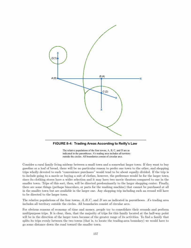
Consider a rural family living midway between a small town and a somewhat larger town. If they want to buygasoline or a loaf of bread, there will be no particular reason to prefer one town to the other, and shoppingtrips wholly devoted to such “convenience purchases” would tend to be about equally divided. If the trip isto include going to a movie or buying a suit of clothes, however, the preference would be for the larger town,since its clothing stores have a wider selection and it may have two movie theaters compared to one in thesmaller town. Trips of this sort, then, will be directed predominantly to the larger shopping center. Finally,there are some things (perhaps binoculars, or parts for the washing machine) that cannot be purchased at allin the smaller town but are available in the larger one. Any shopping trip including such an errand will haveto be directed to the larger town.

The relative populations of the four towns, A,B,C, and D are as indicated in parentheses. A’s trading areaincludes all territory outside the circles. All boundaries consist of circular arcs.

For obvious reasons of economy of time and money, people try to consolidate their errands and performmultipurpose trips. It is clear, then, that the majority of trips for this family located at the half-way pointwill be in the direction of the larger town because of the greater range of its activities. To find a family thatsplits its trips evenly between the two towns (that is, to locate the trading-area boundary) we would have togo some distance down the road toward the smaller town.

157

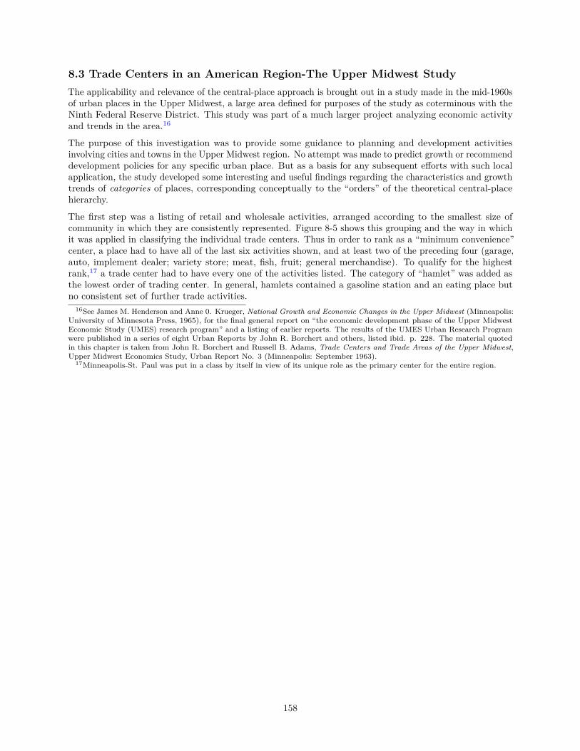
8.3 Trade Centers in an American Region-The Upper Midwest StudyThe applicability and relevance of the central-place approach is brought out in a study made in the mid-1960sof urban places in the Upper Midwest, a large area defined for purposes of the study as coterminous with theNinth Federal Reserve District. This study was part of a much larger project analyzing economic activityand trends in the area.16

The purpose of this investigation was to provide some guidance to planning and development activitiesinvolving cities and towns in the Upper Midwest region. No attempt was made to predict growth or recommenddevelopment policies for any specific urban place. But as a basis for any subsequent efforts with such localapplication, the study developed some interesting and useful findings regarding the characteristics and growthtrends of categories of places, corresponding conceptually to the “orders” of the theoretical central-placehierarchy.

The first step was a listing of retail and wholesale activities, arranged according to the smallest size ofcommunity in which they are consistently represented. Figure 8-5 shows this grouping and the way in whichit was applied in classifying the individual trade centers. Thus in order to rank as a “minimum convenience”center, a place had to have all of the last six activities shown, and at least two of the preceding four (garage,auto, implement dealer; variety store; meat, fish, fruit; general merchandise). To qualify for the highestrank,17 a trade center had to have every one of the activities listed. The category of “hamlet” was added asthe lowest order of trading center. In general, hamlets contained a gasoline station and an eating place butno consistent set of further trade activities.

16See James M. Henderson and Anne 0. Krueger, National Growth and Economic Changes in the Upper Midwest (Minneapolis:University of Minnesota Press, 1965), for the final general report on “the economic development phase of the Upper MidwestEconomic Study (UMES) research program” and a listing of earlier reports. The results of the UMES Urban Research Programwere published in a series of eight Urban Reports by John R. Borchert and others, listed ibid. p. 228. The material quotedin this chapter is taken from John R. Borchert and Russell B. Adams, Trade Centers and Trade Areas of the Upper Midwest,Upper Midwest Economics Study, Urban Report No. 3 (Minneapolis: September 1963).

17Minneapolis-St. Paul was put in a class by itself in view of its unique role as the primary center for the entire region.

158

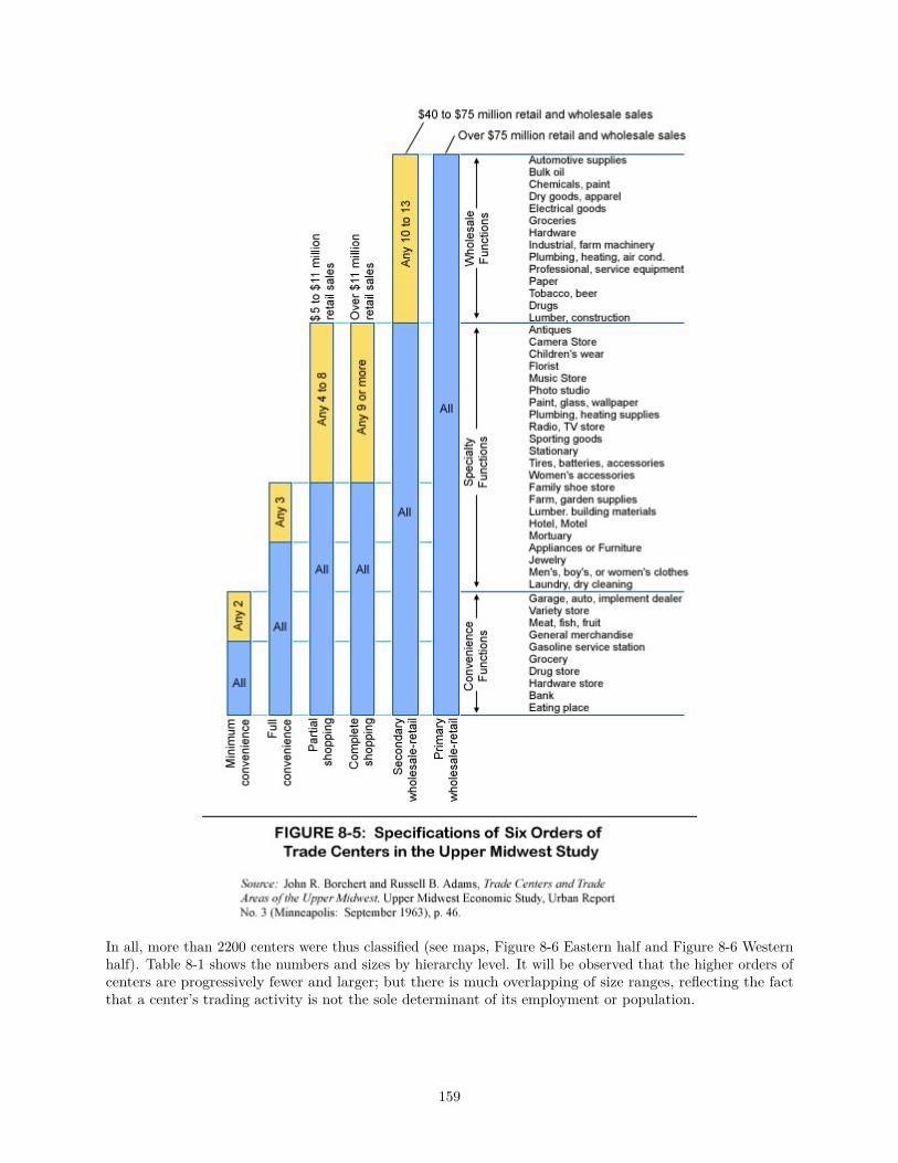
In all, more than 2200 centers were thus classified (see maps, Figure 8-6 Eastern half and Figure 8-6 Westernhalf). Table 8-1 shows the numbers and sizes by hierarchy level. It will be observed that the higher orders ofcenters are progressively fewer and larger; but there is much overlapping of size ranges, reflecting the factthat a center’s trading activity is not the sole determinant of its employment or population.

159

160

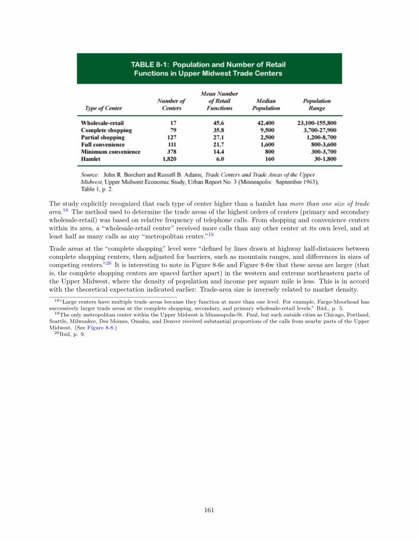
The study explicitly recognized that each type of center higher than a hamlet has more than one size of tradearea.18 The method used to determine the trade areas of the highest orders of centers (primary and secondarywholesale-retail) was based on relative frequency of telephone calls. From shopping and convenience centerswithin its area, a “wholesale-retail center” received more calls than any other center at its own level, and atleast half as many calls as any “metropolitan center.”19

Trade areas at the “complete shopping” level were “defined by lines drawn at highway half-distances betweencomplete shopping centers, then adjusted for barriers, such as mountain ranges, and differences in sizes ofcompeting centers.”20 It is interesting to note in Figure 8-6e and Figure 8-6w that these areas are larger (thatis, the complete shopping centers are spaced farther apart) in the western and extreme northeastern parts ofthe Upper Midwest, where the density of population and income per square mile is less. This is in accordwith the theoretical expectation indicated earlier: Trade-area size is inversely related to market density.

18“Large centers have multiple trade areas because they function at more than one level. For example, Fargo-Moorhead hassuccessively larger trade areas at the complete shopping, secondary, and primary wholesale-retail levels.” Ibid., p. 5.

19The only metropolitan center within the Upper Midwest is Minneapolis-St. Paul, but such outside cities as Chicago, Portland,Seattle, Milwaukee, Des Moines, Omaha, and Denver received substantial proportions of the calls from nearby parts of the UpperMidwest. (See Figure 8-8.)

20Ibid, p. 9.

161

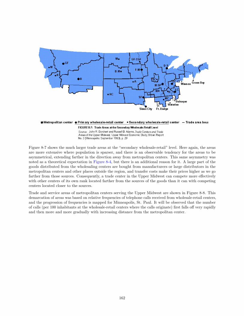
Figure 8-7 shows the much larger trade areas at the “secondary wholesale-retail” level. Here again, the areasare more extensive where population is sparser, and there is an observable tendency for the areas to beasymmetrical, extending farther in the direction away from metropolitan centers. This same asymmetry wasnoted as a theoretical expectation in Figure 8-4, but there is an additional reason for it. A large part of thegoods distributed from the wholesaling centers are bought from manufacturers or large distributors in themetropolitan centers and other places outside the region, and transfer costs make their prices higher as we gofarther from those sources. Consequently, a trade center in the Upper Midwest can compete more effectivelywith other centers of its own rank located farther from the sources of the goods than it can with competingcenters located closer to the sources.

Trade and service areas of metropolitan centers serving the Upper Midwest are shown in Figure 8-8. Thisdemarcation of areas was based on relative frequencies of telephone calls received from wholesale-retail centers,and the progression of frequencies is mapped for Minneapolis, St. Paul. It will be observed that the numberof calls (per 100 inhabitants at the wholesale-retail centers where the calls originate) first falls off very rapidlyand then more and more gradually with increasing distance from the metropolitan center.

162

8.4 Activities Extraneous to the Central—Place HierarchyLet us now consider more explicitly some of the limitations of the simple central-place model. So far in thischapter, our assumption has been that both markets and sources of transferable inputs for urban activities areuniformly distributed in space. The resultant theoretical patterns of market areas and central places simplyreflected the locational effects of the economies of agglomeration available to various kinds of urban activities.We have as yet no rationale for any flows of goods or services (other than primary rural products) either“up” the steps of the urban hierarchy or “horizontally” among cities of equal status. Yet in reality, enormousflows of these types occur. Clevelanders buy cigarettes from Durham, North Carolina, automobile tires fromAkron, frozen orange juice made in small towns in Florida, and government services from Washington, D.C.,and Columbus, Ohio. How does all this relate, if at all, to the hierarchical scheme of urban places, activities,and market areas?

The clue is that neither markets nor transferable inputs are uniformly distributed. Although for most kindsof consumer goods and services there is a market wherever people live, there are some consumer goods andservices that are used mainly or exclusively by people in certain regions, by people in larger cities, or by ruraland small-town people. For inputs, the lack of ubiquity is even more pervasive. Labor supply, of a sort, existswherever people live; but other inputs—such as specific crops, minerals, manufactured goods, or services—arefound only in certain places, and with wide variation in both cost and quality.

Let us consider the locational implications. We can usefully distinguish three classes of activities according towhether their locations are (1) predominantly in larger cities, (2) predominantly in small cities or towns, or(3) not associated with any particular size of city. (Certain manufacturing industries are cited as examples inAppendix 8-2.)

Those activities dependent on the external economies of urban concentration are predominantly located inlarge cities. This class of activities has already been discussed in Chapter 5. Their outputs are disposed of inthe cities where produced, in other cities of all sizes, and in rural areas as well. In other words, the flow ismainly downward in the hierarchy, but it is also horizontal at the highest levels. Activities of this type fitreasonably well into the hierarchical central-place scheme.

There are several reasons why an activity might be found mainly in small centers. First, this is the normallocation pattern for processing operations strongly oriented to rural inputs or to other inputs derived fromextensive land uses; these uses tend to be crowded out from highly urbanized regions by more intensive

163

claimants for land. Forestry and grazing are such activities: Sawmills and meat-packing plants are mostoften not located in large cities, because they must be close to types of land use usually associated withsparse settlement. Meat packing would be even more a small-town industry were it not for the practice ofshipping cattle from range lands to fattening areas prior to slaughter.21 The processing of perishable crops isso strongly input-oriented that individual plants have quite small supply areas; and simply on a probabilitybasis, very few of those areas will contain a large city.22

Small-town locations are characteristic for activities associated with extensive outdoor recreation. Theseactivities need plenty of space, and in some cases (such as ski resorts) topographical or climatic conditionsnot typical of large cities.

Finally, small cities and towns usually provide lower living costs and wage levels. Thus activities stronglyoriented to cheap labor as such, and footloose with regard to other locational considerations, are likely toprefer the smallest size place that will provide enough workers for a plant of efficient scale. Most Americantextile mills, and a wide variety of industries making fairly standardized apparel items (such as shoes), arenow found in rather small cities and towns, the principal explanation being labor-cost economies (Chapter 10gives further attention to the origins and effects of labor-cost differentials).

There are even some basically clerical activities for which a small-town location is appropriate for serving anationwide market, since labor and space are cheap, and the inputs and outputs move by mail. For example,the U.S. Bureau of the Census maintains its central office for the searching of Census files to establish birthrecords for individuals at Pittsburg, Kansas. One of the larger life insurance companies maintains its centraloffice at the very small city of Montpelier, Vermont. Most other firms in this field, however, are in largercities. For activities located in small cities, the flow of outputs is mainly up the urban hierarchy to marketsin larger cities; but it is also partly horizontal, since only some but not all small places have the activity inquestion.

There are a large variety of activities for which size of city seems essentially irrelevant. They occurindiscriminately in small, middle-sized, and large cities. Some of these are primarily oriented to a localizednatural advantage such as water (for processing or for transport) or a mineral resource, and their agglomerationeconomies are internal, involving merely the scale of the individual unit. Thus salt mining and processingworks are found both in isolated locations and within the city of Detroit; steelworks are found both in largecities such as Chicago and in quite small cities such as Butler, Pennsylvania, or Provo, Utah; and automobileparts, electrical equipment, furniture, whiskey, candy, and many other manufactured goods are made inlocations seemingly selected without any systematic concern for city size. There is no discernible relationshiphere to the hierarchical scheme of central places in terms of market areas, industry distribution patterns, orthe flow of inputs or outputs.

In view of such kinds of activity that do not seem to fit the hierarchical central-place scheme at all, we canreadily understand why the relation of range of commercial functions to size of trade area and to city size isless than exact. In fact, it may be surprising that there is as much evidence of hierarchical regularity as doesappear. Let us take another look at the principles involved.

The relationship between trade-area size (that is, spacing of cities) and urban functions principally involvesretail and wholesale trade, which were in fact the basis of the hierarchical ranking in the Upper Midwestinvestigation. Some kinds of manufacturing also play a similar role. Bakeries, soft drink bottling plants, sheetmetal shops, ice cream plants, job printing and newspaper plants, and many other industries can be arranged

21The meat-packing industry in the United States is an interesting example of major locational shift. Initially highly dispersed,in the days when transport was costly and slow and refrigeration in transit impracticable, the industry developed massiveconcentration in the later nineteenth century at the larger Midwestern cities—on the basis of rail transport of both livestock andmeat products and the economical utilization of by-products. But the ideal weights of transported input and output were neververy different, and in the mid-twentieth century a trend toward decentralization set in. The giant stockyards and packing plantsof Chicago, Omaha, Kansas City, St. Paul, and other old-time meat-packing centers were much curtailed during the 1950s and1960s. Two major factors causing this locational shift were apparently (1) the shift of consumer markets toward the West Coastand the Gulf Coast and (2) the greater use of refrigerated transport of meat products by truck and air freight, without anycorresponding improvement in the transportability of live animals. Facilitating the transfer of output tends, of course, to movean activity closer to its sources of inputs, and truck shipment permits more decentralization out of major terminal locations.

22Flour milling and some other processing activities involving little if any loss of perishability or bulk and subject to considerableeconomies of scale are more often found in middlesized or even larger cities (such as Buffalo and Minneapolis).

164

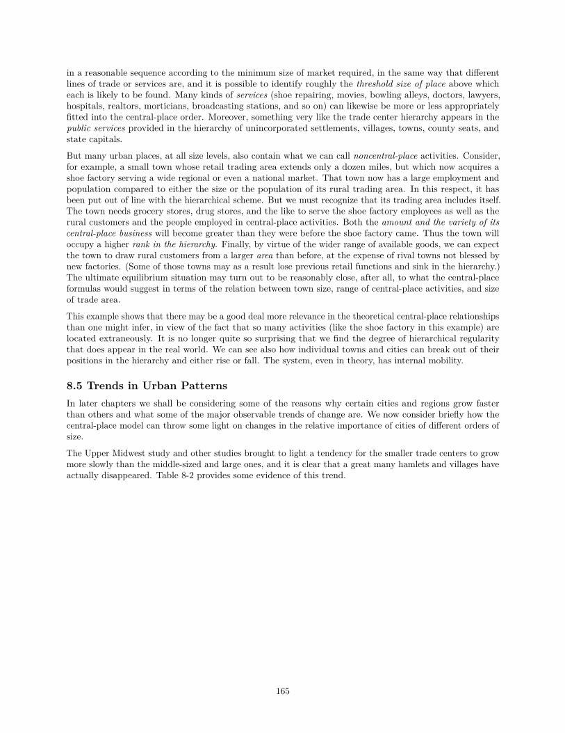
in a reasonable sequence according to the minimum size of market required, in the same way that differentlines of trade or services are, and it is possible to identify roughly the threshold size of place above whicheach is likely to be found. Many kinds of services (shoe repairing, movies, bowling alleys, doctors, lawyers,hospitals, realtors, morticians, broadcasting stations, and so on) can likewise be more or less appropriatelyfitted into the central-place order. Moreover, something very like the trade center hierarchy appears in thepublic services provided in the hierarchy of unincorporated settlements, villages, towns, county seats, andstate capitals.

But many urban places, at all size levels, also contain what we can call noncentral-place activities. Consider,for example, a small town whose retail trading area extends only a dozen miles, but which now acquires ashoe factory serving a wide regional or even a national market. That town now has a large employment andpopulation compared to either the size or the population of its rural trading area. In this respect, it hasbeen put out of line with the hierarchical scheme. But we must recognize that its trading area includes itself.The town needs grocery stores, drug stores, and the like to serve the shoe factory employees as well as therural customers and the people employed in central-place activities. Both the amount and the variety of itscentral-place business will become greater than they were before the shoe factory came. Thus the town willoccupy a higher rank in the hierarchy. Finally, by virtue of the wider range of available goods, we can expectthe town to draw rural customers from a larger area than before, at the expense of rival towns not blessed bynew factories. (Some of those towns may as a result lose previous retail functions and sink in the hierarchy.)The ultimate equilibrium situation may turn out to be reasonably close, after all, to what the central-placeformulas would suggest in terms of the relation between town size, range of central-place activities, and sizeof trade area.

This example shows that there may be a good deal more relevance in the theoretical central-place relationshipsthan one might infer, in view of the fact that so many activities (like the shoe factory in this example) arelocated extraneously. It is no longer quite so surprising that we find the degree of hierarchical regularitythat does appear in the real world. We can see also how individual towns and cities can break out of theirpositions in the hierarchy and either rise or fall. The system, even in theory, has internal mobility.

8.5 Trends in Urban PatternsIn later chapters we shall be considering some of the reasons why certain cities and regions grow fasterthan others and what some of the major observable trends of change are. We now consider briefly how thecentral-place model can throw some light on changes in the relative importance of cities of different orders ofsize.

The Upper Midwest study and other studies brought to light a tendency for the smaller trade centers to growmore slowly than the middle-sized and large ones, and it is clear that a great many hamlets and villages haveactually disappeared. Table 8-2 provides some evidence of this trend.

165

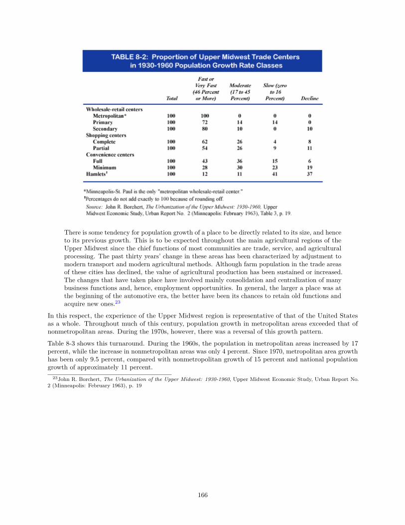
There is some tendency for population growth of a place to be directly related to its size, and henceto its previous growth. This is to be expected throughout the main agricultural regions of theUpper Midwest since the chief functions of most communities are trade, service, and agriculturalprocessing. The past thirty years’ change in these areas has been characterized by adjustment tomodern transport and modern agricultural methods. Although farm population in the trade areasof these cities has declined, the value of agricultural production has been sustained or increased.The changes that have taken place have involved mainly consolidation and centralization of manybusiness functions and, hence, employment opportunities. In general, the larger a place was atthe beginning of the automotive era, the better have been its chances to retain old functions andacquire new ones.23

In this respect, the experience of the Upper Midwest region is representative of that of the United Statesas a whole. Throughout much of this century, population growth in metropolitan areas exceeded that ofnonmetropolitan areas. During the 1970s, however, there was a reversal of this growth pattern.

Table 8-3 shows this turnaround. During the 1960s, the population in metropolitan areas increased by 17percent, while the increase in nonmetropolitan areas was only 4 percent. Since 1970, metropolitan area growthhas been only 9.5 percent, compared with nonmetropolitan growth of 15 percent and national populationgrowth of approximately 11 percent.

23John R. Borchert, The Urbanization of the Upper Midwest: 1930-1960, Upper Midwest Economic Study, Urban Report No.2 (Minneapolis: February 1963), p. 19

166

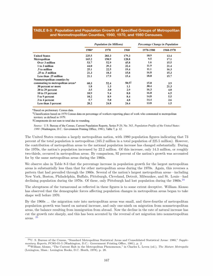
The United States remains a largely metropolitan nation, with 1980 population figures indicating that 73percent of the total population is metropolitan (165.2 million in a total population of 225.5 million). However,the contribution of metropolitan areas to the national population increase has changed substantially. Duringthe 1970s, the nation’s population increased by 22.2 million. Of this increase, only 14.3 million, or roughlytwo-thirds, occurred in metropolitan areas. By comparison, 92 percent of the nation’s growth was accountedfor by the same metropolitan areas during the 1960s.

We observe also in Table 8-3 that the percentage increase in population growth for the largest metropolitanareas is substantially less than that for other metropolitan areas during the 1970s. Again, this reverses apattern that had prevailed through the 1960s. Several of the nation’s largest metropolitan areas—includingNew York, Boston, Philadelphia, Buffalo, Pittsburgh, Cleveland, Detroit, Milwaukee, and St. Louis—haddeclining population during the 1970s. Of these, only Pittsburgh had lost population during the 1960s.24

The abruptness of the turnaround as reflected in these figures is to some extent deceptive. William Alonsohas observed that the demographic forces affecting population changes in metropolitan areas began to takeshape well before 1970.

By the 1960s ... the migration rate into metropolitan areas was small, and three-fourths of metropolitanpopulation growth was based on natural increase, and only one-ninth on migration from nonmetropolitanareas, the balance resulting from immigration from abroad. Now the decline in the rate of natural increase hascut the growth rate sharply, and this has been accented by the reversal of net migration into nonmetropolitanareas. 25

24U. S. Bureau of the Census, “Standard Metropolitan Statistical Areas and Consolidated Statistical Areas: 1980,” Supple-mentary Reports, PC8O-S1-5 (Washington, D.C.: Government Printing Office, 1981), p. 2

25William Alonso, “The Current Halt in the Metropolitan Phenomenon,” in Charles L. Leven (ed.), The Mature Metropolis(Lexington, Mass.: Lexington Books, D.C. Heath, 1978), p. 28.

167

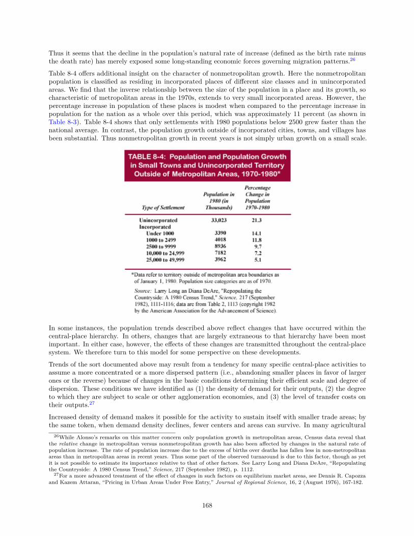
Thus it seems that the decline in the population’s natural rate of increase (defined as the birth rate minusthe death rate) has merely exposed some long-standing economic forces governing migration patterns.26

Table 8-4 offers additional insight on the character of nonmetropolitan growth. Here the nonmetropolitanpopulation is classified as residing in incorporated places of different size classes and in unincorporatedareas. We find that the inverse relationship between the size of the population in a place and its growth, socharacteristic of metropolitan areas in the 1970s, extends to very small incorporated areas. However, thepercentage increase in population of these places is modest when compared to the percentage increase inpopulation for the nation as a whole over this period, which was approximately 11 percent (as shown inTable 8-3). Table 8-4 shows that only settlements with 1980 populations below 2500 grew faster than thenational average. In contrast, the population growth outside of incorporated cities, towns, and villages hasbeen substantial. Thus nonmetropolitan growth in recent years is not simply urban growth on a small scale.

In some instances, the population trends described above reflect changes that have occurred within thecentral-place hierarchy. In others, changes that are largely extraneous to that hierarchy have been mostimportant. In either case, however, the effects of these changes are transmitted throughout the central-placesystem. We therefore turn to this model for some perspective on these developments.

Trends of the sort documented above may result from a tendency for many specific central-place activities toassume a more concentrated or a more dispersed pattern (i.e., abandoning smaller places in favor of largerones or the reverse) because of changes in the basic conditions determining their efficient scale and degree ofdispersion. These conditions we have identified as (1) the density of demand for their outputs, (2) the degreeto which they are subject to scale or other agglomeration economies, and (3) the level of transfer costs ontheir outputs.27

Increased density of demand makes it possible for the activity to sustain itself with smaller trade areas; bythe same token, when demand density declines, fewer centers and areas can survive. In many agricultural

26While Alonso’s remarks on this matter concern only population growth in metropolitan areas, Census data reveal thatthe relative change in metropolitan versus nonmetropolitan growth has also been affected by changes in the natural rate ofpopulation increase. The rate of population increase due to the excess of births over deaths has fallen less in non-metropolitanareas than in metropolitan areas in recent years. Thus some part of the observed turnaround is due to this factor, though as yetit is not possible to estimate its importance relative to that of other factors. See Larry Long and Diana DeAre, “Repopulatingthe Countryside: A 1980 Census Trend,” Science, 217 (September 1982), p. 1112.

27For a more advanced treatment of the effect of changes in such factors on equilibrium market areas, see Dennis R. Capozzaand Kazem Attaran, “Pricing in Urban Areas Under Free Entry,” Journal of Regional Science, 16, 2 (August 1976), 167-182.

168

sections of the Upper Midwest and elsewhere, the farm population has been thinning out for several decadesbecause of the trend toward larger and more mechanized farms employing fewer people on any given area.The American farm population has been shrinking rather steadily for nearly half a century. While the rate ofdecline slowed somewhat during the 1970s, the long-term downward trend has persisted,28 and the increasesin nonmetropolitan population that took place during the 1970s were almost entirely in nonfarm areas.29 Inmany areas, of course, per capita farm income rose more than enough to compensate; but it is reasonable tosurmise that a smaller number of farmers, even without a drop in their aggregate real income, represents areduced demand for the kinds of goods and services available in the smallest settlements. At the same time,there has been a tendency for more farmers to live in town and commute to their farms, or to move to townin the winter. Consequently, farm population trends appear to provide some of the explanation for the slowgrowth or decline of the smallest trade centers prior to 1970.

The recent growth in nonmetropolitan populations also has implied shifts in the density of demand. Table8-3 indicates that suburban development beyond officially recognized metropolitan-area boundaries accountsfor some nonmetropolitan growth, both in the 1960s and in the 1970s. In each decade, nonmetropolitancounties closest to urban centers (those with 30 percent or more commuting) had large percentage changes inpopulation. Estimates by the Bureau of the Census suggest that one-fourth to one-third of nonmetropolitangrowth can be attributed to this outer suburban or “exurban” development.30

This is not the only source of increased density of demand in smaller central places, however. Counties thathad high concentrations of retirees in 1970 also had substantial population growth in the decade to follow.31

The importance of this phenomenon for some nonmetropolitan areas is obvious (as in many parts of Floridaand Arizona, for example), but its significance is much more general. An extensive analysis by Kevin F.McCarthy and Peter A. Morrison of population growth rates by counties in 26 states during the first half of the1970s shows sharp gains in growth rates for areas that they classify as specializing in retirement, particularlyin rural and less urban areas.32 They also find that nonmetropolitan counties specializing in recreation postedsimilarly impressive gains. It appears that these amenity-rich areas may be a major beneficiary of higherlevels of national income and increases in leisure time.

Increased economies of scale for an activity have the effect of enlarging trade areas and concentrating theactivity in fewer and larger urban centers. Scale economies have not been as conspicuously enhanced intrade activities as in industrial activities; but the modern supermarket and shopping center have developedmainly within the past generation and constitute a major change. We must also reckon with the fact thathigher living standards make consumers more sensitive to the appeals of variety in shopping goods and henceadd to the competitive advantages of larger trading centers that can provide such a variety. Recognition ofscale economies has been evidenced also in the trend toward consolidation and concentration of many publicactivities, such as schools and health services. Thus on the whole, this factor has probably contributed tofaster growth of middle-sized and larger trade centers at the expense of smaller ones.

The spread of good roads and automobile ownership has, of course, enabled rural and small-town people tomake longer shopping, crop-delivery, and other trips, and this factor also should be recognized as part of theexplanation for the observed trends of urban growth. But the effect of changes in the level of transfer costson trade-area size and on the spacing of trading centers is less straightforward than it might appear.

If transfer were assumed to be altogether costless, urban activities could be concentrated at the points oflowest operating cost, and economies of agglomeration would tend to concentrate all of an activity in oneplace. At the other extreme, if transfer were infinitely costly (that is, impossible), each location would haveto be self-sufficient. From this contrast of extremes, we might infer that cheaper transfer always enlargestrade areas and leads to fewer, larger, and more widely spaced central places. A similar inference could

28U. S. Bureau of the Census, jointly with U.S. Department of Agriculture, Current Population Reports, Series P-27, No. 54,Farm Population of the United States: 1980 (Washington, D.C.: Government Printing Office, 1981).

29U. S. Bureau of the Census, Current Population Reports, Series P-20, No. 363, Population Profile of the United States:1980 (Washington, D.C.: Government Printing Office, 1981), p. 7.

30Ibid., p. 7.31Larry H. Long and Diana DeAre, Migration to Nonmetropolitan Areas, Special Demographic Analysis, CDS 80-2, U.S.

Bureau of the Census (Washington, D.C.: Government Printing Office, 1980), p. 1.32“The Changing Demographic and Economic Structure of Nonmetropolitan Areas,” International Regional Science Review,

2, 1 (Winter 1977), 123-142.

169

be drawn by regarding transfer services and the services of factors of production as complementary inputs,with possibilities of substituting a cheaper input for a more expensive one. Then if transfer services becamecheaper, we should expect that more transfer would be used in relation to output: that is, distances betweenseller and buyer would increase and trading areas would be larger. This is what we may call the substitutioneffect of a change in transfer cost.

This simple formulation, however, overlooks some side effects of changes in the level of transfer cost. First,there is what might be called the income effect of such changes. If transfer becomes cheaper, buyers at anydistance from the trade center will get the goods cheaper and will normally buy more. With greater salesper buyer, a smaller trade area will suffice to provide the scale economies needed to sustain a center. Morecenters will be able to survive. The income effect of a reduction in transfer costs, then, is a reduction intrade-area size, and it is similar to the effect of an increase in demand density (that is, population density,per capita income, or both).33

There is another way, too, in which cheaper transport may tend to reduce the size of trading areas and leadto a more dispersed pattern of centers. The degree to which activity is concentrated in locations of lowoperating cost depends on (1) transfer costs and (2) the magnitude of the differentials in operating cost. Iftransfer becomes cheaper while the operating cost differentials remain the same, urban activity will becomeless transfer-oriented and will tend to cluster more in efficient operating locations. But in fact, reducedtransfer costs are likely to narrow the operating cost differentials, insofar as they enhance the mobility oflabor and other production factor inputs. Here again, a change in the level of transfer cost cuts both ways inregard to agglomeration versus dispersion, and the net effect could be in either direction.34

Changes in the basic conditions determining the efficient scale and dispersion of activities—such as thoseconditions discussed above—are not the only reason for the changes we observe in the urban place pattern.The structure of the hierarchy is affected also by changes in the mix of activities. It has been mentioned alreadythat, as a result of higher levels of income and leisure, consumer demand tends to shift from staple necessitiesto a wider range of shopping goods and luxuries, with variety becoming a more important dimension ofcompetitive advantage for producers. While this clearly favors the large trade center, we must also recognizethat the national economy is becoming much more dependent on service activities and much less dependenton manufacturing per Se. As population in nonmetropolitan areas increases, the growth of services willfollow, since services are highly oriented toward their respective markets. This fact is surely reflected in thepopulation growth associated with nonmetropolitan areas having high concentrations of retirees or specializingin recreation that were noted above.

The framework of the central-place model is relevant in assessing some of the factors governing trends inurban patterns. However, a number of trends in noncentral-place activities must also be considered. Generally,as the economy develops, a greater proportion of productive activities involves later stages of processingand handling, and a smaller proportion uses rural products directly as inputs. Fewer and fewer activitiesneed to be oriented closely to inputs from rural extractive activity (as do canneries or sawmills); in contrast,there is the widening range of activities (such as the production of electrical equipment, pharmaceuticals,or books) that are technologically remote from any extractive process. Accordingly, there is less and lessreason for many activities to be located in small settlements for the sake of easy access to agricultural,forest, or mineral products. Finally, the increasing variety and complexity of goods, services, and productive

33Where travel by retail buyers is involved, the benefit to the buyers is mainly a saving in time rather than money. To thisextent, the transfer-cost reduction in itself does not increase effective market density and shrink trade areas as the income effectimplies; the substitution effect dominates, and buyers respond to easier transfer by using more transfer (that is, traveling greaterdistances in search of cheaper or better goods and services).The reader with some training in economics will recognize this conflict between substitution effect and income effect as

something that quite generally occurs whenever an activity calls for two or more complementary inputs that are to someextent mutually substitutable. For example, if machinery becomes cheaper, there is an incentive to add machines and reduceemployment; but at the same time, the cheaper machinery leads to a cheaper product and greater sales, which increases thedemand for labor. The net effect on labor demand depends upon the terms of substitution between the two inputs and upon theelasticity of demand for the product.

34For further discussion of transfer cost effects in the framework of simplified central-place models, see Walter Isard, Locationand Space-Economy (Cambridge, Mass.: MIT Press, 1956), pp. 86-87; Hugh 0. Nourse, Regional Economics (New York:McGraw-Hill, 1968), pp. 215-216; Edgar M. Hoover, “Transport Costs and the Spacing of Central Places,” Papers of the RegionalScience Association, 25 (1970), 255-274; and Capozza and Attaran, “Pricing in Urban Areas.”

170

operations in general calls for more close inter-firm and interactivity contact, and tends to increase thelocational importance of urban external economies of agglomeration.

Until very recently, each of these factors contributed to the advantages held by larger metropolitan areasfor manufacturing activity. However, technological advances in production have begun to alter this pattern.Considerable simplification has occurred in some production processes that had involved the acquisition ofmechanical components in order to assemble machines or other goods. Developments in electronics havecontributed to this trend and have changed interindustry relations significantly. Now, one printed circuit ormicrochip may substitute effectively for numerous other parts. As the importance of these “high-technology”goods has increased, the bond of agglomeration economies that had so strongly influenced location patternshas loosened; proximity to a wide array of parts suppliers is no longer essential. These modern componentsare easily transported, thus freeing both the producer of high-technology goods and the industrial user toevaluate a wider range of location alternatives. For some, this has meant taking advantage of relatively lowwages and living costs in nonmetropolitan areas. As discussed in Chapter 3, improvements in informationstorage, retrieval, and transmission facilitate such choices.35

While one might portray this as a technological change in one activity (electronics) that has affected otheractivities in an exogenous way, some researchers see it as part of a larger endogenous process in the lifecycle of many different manufactured goods. They argue that over time, the standardization of productionprocesses takes place. Once this occurs, decentralization of activities can be expected, since they are no longertied by agglomeration economies to large urban complexes. In this analysis, the diffusion of technology tomore peripheral areas also enhances the potential for innovation in these regions at the expense of innovationpotential in older industrial centers, thus promoting further decentralization.36

8.6 SummaryCentral-place theory attempts to explain the spatial patterns of trade and service centers. According to thisline of analysis, centers for the distribution of some single good or service to users scattered uniformly overan area would develop at equidistant sites. Their market areas would all be of a uniform size determined bytransfer costs on the output, density of demand per unit area, and scale economies in the production and/ormarketing of the output.

These market-area determinants would ideally call for a different uniform size of trading areas, and a fineror coarser scatter of distribution centers or central places, for each kind of output. But because of externaleconomies of agglomeration and the economies of channeling transfer along high-volume routes, many differentkinds of trade are conducted in a single central place; and instead of a separate set of centers to handleeach product, there is evolved a rough hierarchy of central places. Central places range from very small andsimple ones carrying on only one or two lines of highly local trade, through higher classes of central placesprogressively larger, more widely separated, and having more different lines of trade and sizes of tradingareas. In the hierarchy, each size class of places carries on all the trading activities practiced in all lower sizeclasses, plus some further types of activity not found in any smaller centers.

The spatial, functional, and size distributions of trading centers in the real world, as identified in suchempirical investigations as the Upper Midwest Economic Study, conform only roughly to the simplified idealcentral-place model, because many additional location factors affect the growth of specific activities in specificcenters, and neither transfer costs nor demand densities are actually uniform. Such studies are, however,useful in assessing the changing roles of urban centers of various size classes and trading functions in a regionaleconomy when population, income, and transfer and other technologies change. In the United States, trendstoward concentration of more trading activities in larger centers, lengthening of the retail buyer’s journey,and relative decay of many of the smallest settlements can be logically explained in terms of a central-placemodel.

35For further reading on the causes and consequences of slow growth and decline in large metropolitan areas, see Charles L.Leven (ed.), The Mature Metropolis (Lexington, Mass.: Lexington Books, D. C. Heath, 1978).

36See R. D. Norton and J. Bees, “The Product Cycle and the Spatial Decentralization of American Manufacturing,” RegionalStudies, 13, 2 (August 1979), 141-151.

171

The trading areas of larger centers are enlarged by the attraction that variety holds for shoppers and the factthat people often combine purchases of different types on a single trip. A larger center has also some lines oftrade in which trading-area radii are characteristically larger than those of the businesses found in smallerplaces. An empirical measurement of this size relation was stated in Reilly’s Law, a gravity formulation thatmakes a center’s trading-area radius proportional to the square root of its population.

The assumptions of central-place theory are clearly inapplicable to many urban activities (including mostkinds of manufacturing). Some of those activities appear to locate without regard to city size. It is possible,however, to identify empirically certain groups of activities that are relatively concentrated in specific sizeclasses of cities and to explain such concentration patterns in terms of considerations complementary to thecentral-place model.

The United States has experienced major changes in the relative importance of cities of different ordersof size. With the 1970s came the reversal of a long-standing trend toward greater growth rates in largermetropolitan areas. Explanations of these developments lie within the central-place framework as well asbeyond it. Regardless of the source of these changes, however, the effects are distributed throughout theurban hierarchy.

Technical Terms Introduced in this ChapterCentral place Rank-Size RuleHierarchy of central places Threshold size of placeMarket density Location quotient (p. 237)Nesting factor

Selected ReadingsMartin Beckmann, Location Theory (New York: Random House, 1968), Chapter 5.

Dennis R. Capozza and Kazem Attaran, “Pricing in Urban Areas Under Free Entry,” Journal of RegionalScience, 16, 2 (August 1976), 167-182.

M. L. Greenhut and H. Ohta, Theory of Spatial Pricing and Market Areas (Durham, N.C.: Duke UniversityPress, 1975).

Edgar M. Hoover, “Transport Costs and the Spacing of Central Places,”Papers of the Regional ScienceAssociation, 25 (1970), 255-274.

Charles L. Leven (ed.), The Mature Metropolis (Lexington, Mass.: Lexington Books, D. C. Heath, 1978), pp.23-41.

August Lösch, Die räumliche Ordnung der Wirtschaft (Jena: Gustav Fischer, 1940; 2nd ed., 1944); W. H.Woglom (tr.), The Economics of Location (New Haven, Conn.: Yale University Press, 1954).

Hugh 0. Nourse, Regional Economics (New York: McGraw-Hill, 1968), Chapter 3.

John B. Parr, “Models of the Central Place System: A More General Approach,” Urban. Studies, 15, 1(February 1978), 35-49.

Harry W. Richardson, Regional Economics (New York: Praeger, 1969), Chapter 7.

172

Appendix 8-1 Trading-Area Boundaries Under Reilly’s Lawsee link

Assume two centers A and B located w miles apart, with center A having m times the population of centerB. According to Reilly’s Law, the square of the distance from A to any point on the trading-area boundarywill be m times the square of the distance from B to that point.

In the diagram below, the locations are plotted with A at the origin and B on the horizontal axis at a distancew. A point X on the boundary is shown with coordinates x and y.

Reilly’s Law may now be stated as

y2 + x2 = m(y2 + x2—2xw + w2) (1)

y2(1—m) = —x2(1—m)—2xmw + w2m (2)

y2 = w2m/(1—m)—2xmw/(1—m)—x2 (3)

Let

z = x+mw/(1—m) (4)

Then

z2 = x2 + 2xmw/(1—m) + [mw/(1—m)]2 (5)

−x2 = −z2 + 2xmw/(1—m) + [mw/(1—m)]2 (6)

Substituting in (3),

y2 = mw2/(1—m)—2xmw/(1—m)—z2 + 2xmw/(1—m) + [mw/(1—m)]2 (7)

y2 = [(mw2—m2w2 +m2w2)/(1—m)2]—z2 (8)

173

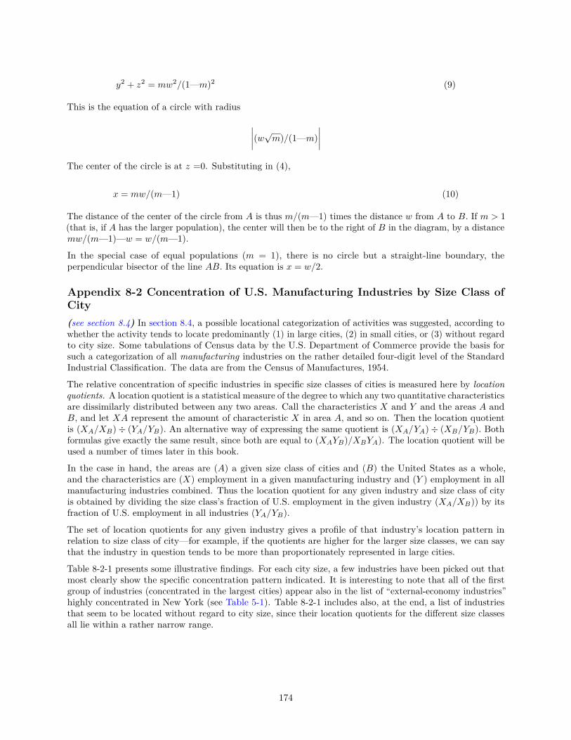
y2 + z2 = mw2/(1—m)2 (9)

This is the equation of a circle with radius

∣∣∣∣(w√m)/(1—m)∣∣∣∣

The center of the circle is at z =0. Substituting in (4),

x = mw/(m—1) (10)

The distance of the center of the circle from A is thus m/(m—1) times the distance w from A to B. If m > 1(that is, if A has the larger population), the center will then be to the right of B in the diagram, by a distancemw/(m—1)—w = w/(m—1).

In the special case of equal populations (m = 1), there is no circle but a straight-line boundary, theperpendicular bisector of the line AB. Its equation is x = w/2.

Appendix 8-2 Concentration of U.S. Manufacturing Industries by Size Class ofCity(see section 8.4) In section 8.4, a possible locational categorization of activities was suggested, according towhether the activity tends to locate predominantly (1) in large cities, (2) in small cities, or (3) without regardto city size. Some tabulations of Census data by the U.S. Department of Commerce provide the basis forsuch a categorization of all manufacturing industries on the rather detailed four-digit level of the StandardIndustrial Classification. The data are from the Census of Manufactures, 1954.

The relative concentration of specific industries in specific size classes of cities is measured here by locationquotients. A location quotient is a statistical measure of the degree to which any two quantitative characteristicsare dissimilarly distributed between any two areas. Call the characteristics X and Y and the areas A andB, and let XA represent the amount of characteristic X in area A, and so on. Then the location quotientis (XA/XB)÷ (YA/YB). An alternative way of expressing the same quotient is (XA/YA)÷ (XB/YB). Bothformulas give exactly the same result, since both are equal to (XAYB)/XBYA). The location quotient will beused a number of times later in this book.

In the case in hand, the areas are (A) a given size class of cities and (B) the United States as a whole,and the characteristics are (X) employment in a given manufacturing industry and (Y ) employment in allmanufacturing industries combined. Thus the location quotient for any given industry and size class of cityis obtained by dividing the size class’s fraction of U.S. employment in the given industry (XA/XB)) by itsfraction of U.S. employment in all industries (YA/YB).

The set of location quotients for any given industry gives a profile of that industry’s location pattern inrelation to size class of city—for example, if the quotients are higher for the larger size classes, we can saythat the industry in question tends to be more than proportionately represented in large cities.

Table 8-2-1 presents some illustrative findings. For each city size, a few industries have been picked out thatmost clearly show the specific concentration pattern indicated. It is interesting to note that all of the firstgroup of industries (concentrated in the largest cities) appear also in the list of “external-economy industries”highly concentrated in New York (see Table 5-1). Table 8-2-1 includes also, at the end, a list of industriesthat seem to be located without regard to city size, since their location quotients for the different size classesall lie within a rather narrow range.

174

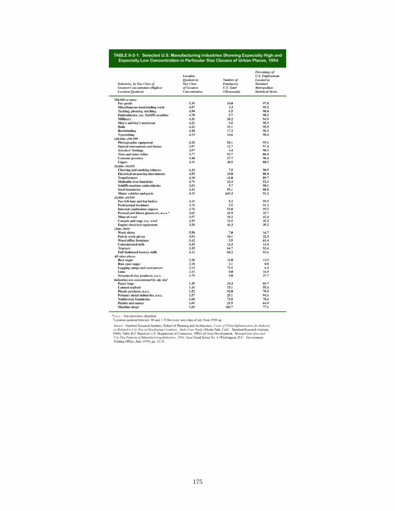
175

9. REGIONS9.1 The Nature of a RegionWhat is a region? A voluminous and somewhat turgid literature has been devoted to this question, with avariety of answers. One irreverent suggestion is that a region means an area which a regional economist getsa grant to study. Be that as it may, it is clear that the most appropriate and useful definition depends on theparticular purpose to be served.

Common to all definitions of a region is the idea of a geographical area constituting an entity, so thatsignificant statements can be made about the area as a whole. Aggregation into regions is useful in connectionwith description, because it means that fewer separate numbers or other facts need to be handled andperceived. Thus for many purposes, totals and averages for a Census tract or a county are just as informativeand much easier to handle and present than stacks of individual Census returns would be, even if one hadaccess to them. Similarly, aggregation is obviously economical in connection with analysis of information; andit is particularly important if there is a good deal of interdependence of units or activities within the area, sothat the whole really is more than merely the sum of its parts. Finally, and for similar reasons, aggregationis necessary for administration and for the formulation and implementation of plans and public policies.From this standpoint at least, the most useful regional groupings are those which follow the boundaries ofadministrative jurisdictions.

A normal attribute of a region is general consciousness of a common regional interest; this is fortunatebecause it makes possible some rational collective efforts to improve regional welfare. The commonality ofinterests may be reflected in numerous ways, but basic to this idea is a high degree of correlation of economicexperiences of the region’s subareas and interest groups. Since this correlation can reflect either of two quitedistinct features of internal structure, we distinguish two different types of regions: the homogeneous and thefunctional.

A homogeneous region is demarcated on the basis of internal uniformity. The winter wheat belt in the centralpart of the United States is a homogeneous agricultural region because all its parts grow the same maincrop in the same way. Some external change, such as a new farm price support or loan program, a series ofdrought years, or a change in the world demand for wheat, will affect all of the region in a similar way; whatis true of one part of the region is true of other parts, and the various parts resemble one another more thanthey resemble areas outside the region. The distinctive land-use zones of the von Thünen model, discussedin Chapter 6, can be regarded as homogeneous regions. America’s Appalachia and Italy’s Mezzogiorno areregions defined on the basis of a common syndrome of poverty, arrested economic development, and limitedhuman opportunity. On a microscale, a homogeneous zone or neighborhood within an urban area (such as aghetto or other ethnic area, a wholesaling district, or a wealthy suburb) might for some purposes be regardedas a homogeneous region.

The set of nonmetropolitan State Economic Areas, established by the U.S. Bureau of the Census for tabulationof various kinds of data such as migration, presents still another example. Those State Economic Areas thatdo not simply coincide with Metropolitan Statistical Areas are made up by grouping contiguous countieswithin a state. The grouping is systematically worked out by computer so that (with respect to a largenumber of characteristics such as income level, racial mix, and principal economic activity) the countieswithin any one State Economic Area are highly similar but the different State Economic Areas are highlydissimilar. The Regional Economics Division of the U.S. Department of Commerce has similarly developed abreakdown of the whole United States into eight relatively homogeneous groups of contiguous states (seeFigure 9-1).

176

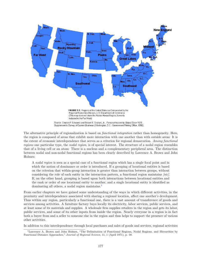
The alternative principle of regionalization is based on functional integration rather than homogeneity. Here,the region is composed of areas that exhibit more interaction with one another than with outside areas: It isthe extent of economic interdependence that serves as a criterion for regional demarcation. Among functionalregions one particular type, the nodal region, is of special interest. The structure of a nodal region resemblesthat of a living cell or an atom: There is a nucleus and a complementary peripheral area. The distinctionbetween nodal and non-nodal functional regions has been clearly described by Lawrence A. Brown and JohnHolmes:

A nodal region is seen as a special case of a functional region which has a single focal point and inwhich the notion of dominance or order is introduced. If a grouping of locational entities is basedon the criterion that within-group interaction is greater than interaction between groups, withoutconsidering the role of each entity in the interaction pattern, a functional region maintains [sic].If, on the other hand, grouping is based upon both interactions between locational entities andthe rank or order of one locational entity to another, and a single locational entity is identified asdominating all others, a nodal region maintains.1

From earlier chapters we have gained some understanding of the ways in which different activities, in theproximity and interdependence associated with sharing a regional location, affect one another’s development.Thus within any region, particularly a functional one, there is a vast amount of transference of goods andservices among activities. A furniture factory buys locally its electricity, labor services, public services, andat least some of its materials and supplies. A wholesale firm supplies retailers in the region and gets its labor,public services, and some of its other inputs from inside the region. Nearly everyone in a region is in factboth a buyer from and a seller to someone else in the region and thus helps to support the presence of variousother activities.

In addition to this interdependence through local purchases and sales of goods and services, regional activities1Lawrence A. Brown and John Holmes, “The Delimitation of Functional Regions, Nodal Regions, and Hierarchies by

Functional Distance Approaches,” Journal of Regional Science, 11, 1 (April 1971), p. 58.

177

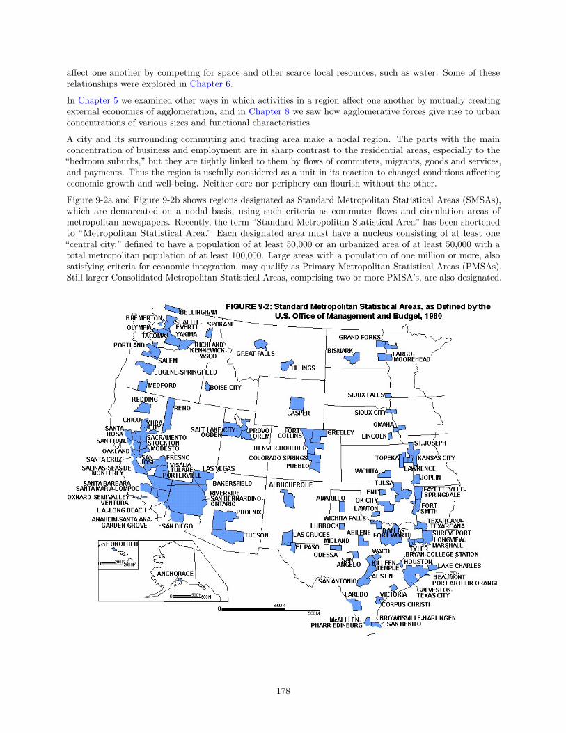
affect one another by competing for space and other scarce local resources, such as water. Some of theserelationships were explored in Chapter 6.

In Chapter 5 we examined other ways in which activities in a region affect one another by mutually creatingexternal economies of agglomeration, and in Chapter 8 we saw how agglomerative forces give rise to urbanconcentrations of various sizes and functional characteristics.

A city and its surrounding commuting and trading area make a nodal region. The parts with the mainconcentration of business and employment are in sharp contrast to the residential areas, especially to the“bedroom suburbs,” but they are tightly linked to them by flows of commuters, migrants, goods and services,and payments. Thus the region is usefully considered as a unit in its reaction to changed conditions affectingeconomic growth and well-being. Neither core nor periphery can flourish without the other.

Figure 9-2a and Figure 9-2b shows regions designated as Standard Metropolitan Statistical Areas (SMSAs),which are demarcated on a nodal basis, using such criteria as commuter flows and circulation areas ofmetropolitan newspapers. Recently, the term “Standard Metropolitan Statistical Area” has been shortenedto “Metropolitan Statistical Area.” Each designated area must have a nucleus consisting of at least one“central city,” defined to have a population of at least 50,000 or an urbanized area of at least 50,000 with atotal metropolitan population of at least 100,000. Large areas with a population of one million or more, alsosatisfying criteria for economic integration, may qualify as Primary Metropolitan Statistical Areas (PMSAs).Still larger Consolidated Metropolitan Statistical Areas, comprising two or more PMSA’s, are also designated.

178

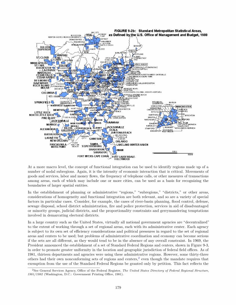
At a more macro level, the concept of functional integration can be used to identify regions made up of anumber of nodal subregions. Again, it is the intensity of economic interaction that is critical. Movements ofgoods and services, labor and money flows, the frequency of telephone calls, or other measures of transactionsamong areas, each of which may include one or more cities, can be used as a basis for recognizing theboundaries of larger spatial entities.

In the establishment of planning or administrative “regions,” “subregions,” “districts,” or other areas,considerations of homogeneity and functional integration are both relevant, and so are a variety of specialfactors in particular cases. Consider, for example, the cases of river-basin planning, flood control, defense,sewage disposal, school district administration, fire and police protection, services in aid of disadvantagedor minority groups, judicial districts, and the proportionality constraints and gerrymandering temptationsinvolved in demarcating electoral districts.

In a large country such as the United States, virtually all national government agencies are “decentralized”to the extent of working through a set of regional areas, each with its administrative center. Each agencyis subject to its own set of efficiency considerations and political pressures in regard to the set of regionalareas and centers to be used; but problems of administrative coordination and economy can become seriousif the sets are all different, as they would tend to be in the absence of any overall constraint. In 1969, thePresident announced the establishment of a set of Standard Federal Regions and centers, shown in Figure 9-3,in order to promote greater uniformity in the location and geographic jurisdiction of federal field offices. As of1981, thirteen departments and agencies were using these administrative regions. However, some thirty-threeothers had their own nonconforming sets of regions and centers,2 even though the mandate requires thatexemption from the use of the Standard Federal Regions be granted only by petition. This fact reflects the

2See General Services Agency, Office of the Federal Register, The United States Directory of Federal Regional Structure,1981/1982 (Washington, D.C.: Government Printing Office, 1981).

179

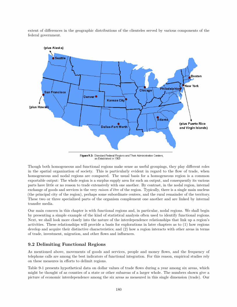
extent of differences in the geographic distributions of the clienteles served by various components of thefederal government.

Though both homogeneous and functional regions make sense as useful groupings, they play different rolesin the spatial organization of society. This is particularly evident in regard to the flow of trade, whenhomogeneous and nodal regions are compared. The usual basis for a homogeneous region is a commonexportable output: The whole region is a surplus supply area for such an output, and consequently its variousparts have little or no reason to trade extensively with one another. By contrast, in the nodal region, internalexchange of goods and services is the very raison d’être of the region. Typically, there is a single main nucleus(the principal city of the region), perhaps some subordinate centers, and the rural remainder of the territory.These two or three specialized parts of the organism complement one another and are linked by internaltransfer media.

Our main concern in this chapter is with functional regions and, in particular, nodal regions. We shall beginby presenting a simple example of the kind of statistical analysis often used to identify functional regions.Next, we shall look more closely into the nature of the interdependence relationships that link up a region’sactivities. These relationships will provide a basis for explorations in later chapters as to (1) how regionsdevelop and acquire their distinctive characteristics; and (2) how a region interacts with other areas in termsof trade, investment, migration, and other flows and influences.

9.2 Delimiting Functional RegionsAs mentioned above, movements of goods and services, people and money flows, and the frequency oftelephone calls are among the best indicators of functional integration. For this reason, empirical studies relyon these measures in efforts to delimit regions.

Table 9-1 presents hypothetical data on dollar values of trade flows during a year among six areas, whichmight be thought of as counties of a state or other subareas of a larger whole. The numbers shown give apicture of economic interdependence among the six areas as measured in this single dimension (trade). Our

180

task is to group these areas into functional regions in such a way that trade flows among areas within eachregion are relatively strong, while flows between regions are relatively weak.

Clearly we should not group areas together simply on the basis of the absolute amount of trade betweenthem. We can get a more meaningful measure of interarea trade linkage by subjecting our data to “doublestandardization”—that is, expressing the actual trade between two areas (in) and (n) in relation to the totalexternal trade (exports and imports) of both areas.3 Perhaps the simplest linkage measure incorporatingdouble standardization would be

Lmn = Lnm = 2(Smn + Snm)/(Em + En + Im + In)

where Smn and Snm are trade flows from (m) to (n) and from (n) to (m)

respectively; Em and En are the total exports from (m) and (n) respectively; and Im and In are the totalimports into (m) and (n) respectively.

The standardized linkages for the present example are shown in Table 9-2. Note that it is necessary to presentonly one such linkage for each pair of areas, since Lmn is equivalent to Lnm.

3Standardization can be accomplished by any of several techniques. For example, Paul B. Slater has developed a techniquethat constrains each row and each column total to unity or some other number. The resultant matrix of flows is thus doublystandardized by one transformation. See P. B. Slater and H. P. M. Winchester, “Clustering and Scaling of Transaction FlowTables: A French Interdepartmental Migration Example,” IEEE Transactions on Systems, Man, and Cybernetics, SMC-8(August 1978), 635-640; and P. B. Slater and Wolfgang Schwarz, “Global Trade Patterns: Scaling and Clustering Analysis,”IEEE Transactions on Systems, Man, and Cybernetics, SMC-9 (July 1979), 381-387. The algorithm used in these studies isavailable in SAS (Statistical Analysis System) Supplemental Library Users Guide (Cary, N.C.: SAS Institute, 1980) under thename IPFPHC.

181

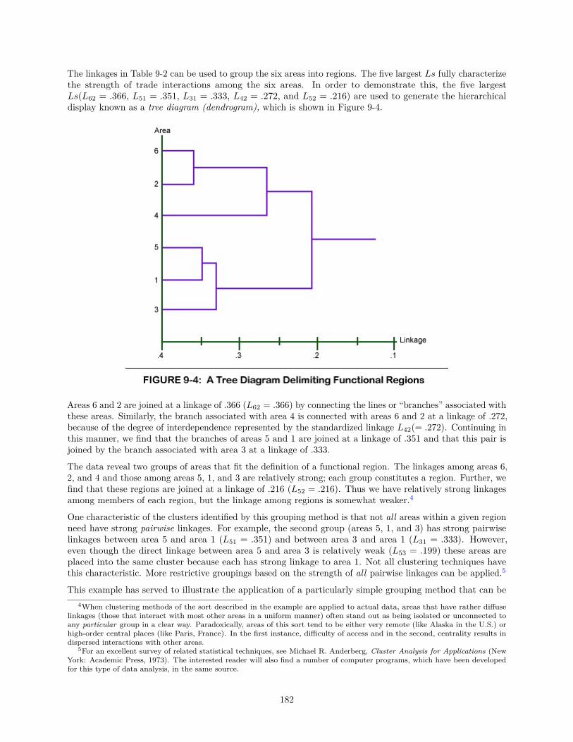
The linkages in Table 9-2 can be used to group the six areas into regions. The five largest Ls fully characterizethe strength of trade interactions among the six areas. In order to demonstrate this, the five largestLs(L62 = .366, L51 = .351, L31 = .333, L42 = .272, and L52 = .216) are used to generate the hierarchicaldisplay known as a tree diagram (dendrogram), which is shown in Figure 9-4.

Areas 6 and 2 are joined at a linkage of .366 (L62 = .366) by connecting the lines or “branches” associated withthese areas. Similarly, the branch associated with area 4 is connected with areas 6 and 2 at a linkage of .272,because of the degree of interdependence represented by the standardized linkage L42(= .272). Continuing inthis manner, we find that the branches of areas 5 and 1 are joined at a linkage of .351 and that this pair isjoined by the branch associated with area 3 at a linkage of .333.

The data reveal two groups of areas that fit the definition of a functional region. The linkages among areas 6,2, and 4 and those among areas 5, 1, and 3 are relatively strong; each group constitutes a region. Further, wefind that these regions are joined at a linkage of .216 (L52 = .216). Thus we have relatively strong linkagesamong members of each region, but the linkage among regions is somewhat weaker.4

One characteristic of the clusters identified by this grouping method is that not all areas within a given regionneed have strong pairwise linkages. For example, the second group (areas 5, 1, and 3) has strong pairwiselinkages between area 5 and area 1 (L51 = .351) and between area 3 and area 1 (L31 = .333). However,even though the direct linkage between area 5 and area 3 is relatively weak (L53 = .199) these areas areplaced into the same cluster because each has strong linkage to area 1. Not all clustering techniques havethis characteristic. More restrictive groupings based on the strength of all pairwise linkages can be applied.5

This example has served to illustrate the application of a particularly simple grouping method that can be4When clustering methods of the sort described in the example are applied to actual data, areas that have rather diffuse

linkages (those that interact with most other areas in a uniform manner) often stand out as being isolated or unconnected toany particular group in a clear way. Paradoxically, areas of this sort tend to be either very remote (like Alaska in the U.S.) orhigh-order central places (like Paris, France). In the first instance, difficulty of access and in the second, centrality results indispersed interactions with other areas.

5For an excellent survey of related statistical techniques, see Michael R. Anderberg, Cluster Analysis for Applications (NewYork: Academic Press, 1973). The interested reader will also find a number of computer programs, which have been developedfor this type of data analysis, in the same source.

182

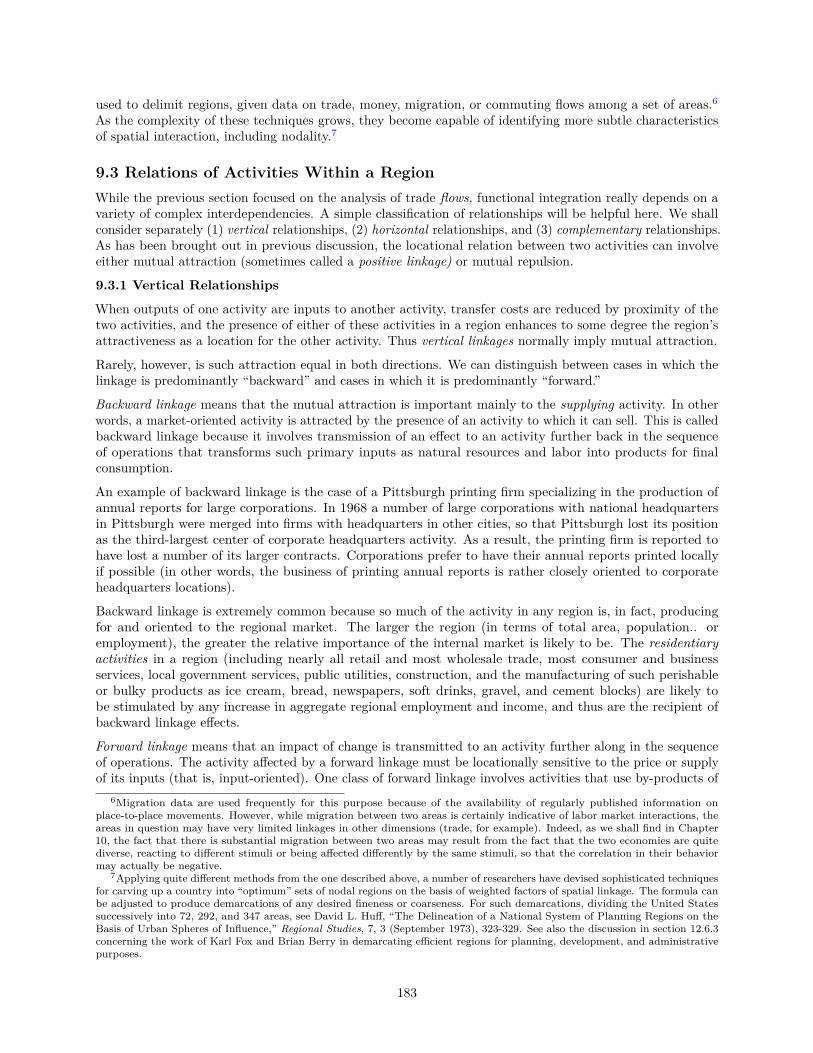
used to delimit regions, given data on trade, money, migration, or commuting flows among a set of areas.6As the complexity of these techniques grows, they become capable of identifying more subtle characteristicsof spatial interaction, including nodality.7

9.3 Relations of Activities Within a RegionWhile the previous section focused on the analysis of trade flows, functional integration really depends on avariety of complex interdependencies. A simple classification of relationships will be helpful here. We shallconsider separately (1) vertical relationships, (2) horizontal relationships, and (3) complementary relationships.As has been brought out in previous discussion, the locational relation between two activities can involveeither mutual attraction (sometimes called a positive linkage) or mutual repulsion.

9.3.1 Vertical Relationships

When outputs of one activity are inputs to another activity, transfer costs are reduced by proximity of thetwo activities, and the presence of either of these activities in a region enhances to some degree the region’sattractiveness as a location for the other activity. Thus vertical linkages normally imply mutual attraction.

Rarely, however, is such attraction equal in both directions. We can distinguish between cases in which thelinkage is predominantly “backward” and cases in which it is predominantly “forward.”

Backward linkage means that the mutual attraction is important mainly to the supplying activity. In otherwords, a market-oriented activity is attracted by the presence of an activity to which it can sell. This is calledbackward linkage because it involves transmission of an effect to an activity further back in the sequenceof operations that transforms such primary inputs as natural resources and labor into products for finalconsumption.

An example of backward linkage is the case of a Pittsburgh printing firm specializing in the production ofannual reports for large corporations. In 1968 a number of large corporations with national headquartersin Pittsburgh were merged into firms with headquarters in other cities, so that Pittsburgh lost its positionas the third-largest center of corporate headquarters activity. As a result, the printing firm is reported tohave lost a number of its larger contracts. Corporations prefer to have their annual reports printed locallyif possible (in other words, the business of printing annual reports is rather closely oriented to corporateheadquarters locations).

Backward linkage is extremely common because so much of the activity in any region is, in fact, producingfor and oriented to the regional market. The larger the region (in terms of total area, population.. oremployment), the greater the relative importance of the internal market is likely to be. The residentiaryactivities in a region (including nearly all retail and most wholesale trade, most consumer and businessservices, local government services, public utilities, construction, and the manufacturing of such perishableor bulky products as ice cream, bread, newspapers, soft drinks, gravel, and cement blocks) are likely tobe stimulated by any increase in aggregate regional employment and income, and thus are the recipient ofbackward linkage effects.

Forward linkage means that an impact of change is transmitted to an activity further along in the sequenceof operations. The activity affected by a forward linkage must be locationally sensitive to the price or supplyof its inputs (that is, input-oriented). One class of forward linkage involves activities that use by-products of

6Migration data are used frequently for this purpose because of the availability of regularly published information onplace-to-place movements. However, while migration between two areas is certainly indicative of labor market interactions, theareas in question may have very limited linkages in other dimensions (trade, for example). Indeed, as we shall find in Chapter10, the fact that there is substantial migration between two areas may result from the fact that the two economies are quitediverse, reacting to different stimuli or being affected differently by the same stimuli, so that the correlation in their behaviormay actually be negative.

7Applying quite different methods from the one described above, a number of researchers have devised sophisticated techniquesfor carving up a country into “optimum” sets of nodal regions on the basis of weighted factors of spatial linkage. The formula canbe adjusted to produce demarcations of any desired fineness or coarseness. For such demarcations, dividing the United Statessuccessively into 72, 292, and 347 areas, see David L. Huff, “The Delineation of a National System of Planning Regions on theBasis of Urban Spheres of Influence,” Regional Studies, 7, 3 (September 1973), 323-329. See also the discussion in section 12.6.3concerning the work of Karl Fox and Brian Berry in demarcating efficient regions for planning, development, and administrativepurposes.

183

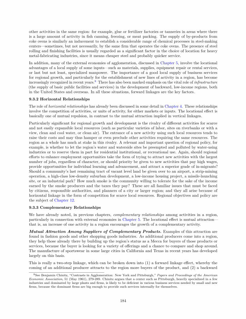
other activities in the same region: for example, glue or fertilizer factories or tanneries in areas where thereis a large amount of activity in fish canning, freezing, or meat packing. The supply of by-products fromcoke ovens is similarly an inducement to establish a considerable range of chemical processes in steel-makingcenters—sometimes, but not necessarily, by the same firm that operates the coke ovens. The presence of steelrolling and finishing facilities is usually regarded as a significant factor in the choice of location for heavymetal-fabricating industries, since it means cheaper steel and probably quicker service.

In addition, many of the external economies of agglomeration, discussed in Chapter 5, involve the locationaladvantages of a local supply of some inputs—such as materials, supplies, equipment repair or rental services,or last but not least, specialized manpower. The importance of a good local supply of business servicesfor regional growth, and particularly for the establishment of new lines of activity in a region, has becomeincreasingly recognized in recent years.8 There has also been marked emphasis on the vital role of infrastructure(the supply of basic public facilities and services) in the development of backward, low-income regions, bothin the United States and overseas. In all these situations, forward linkages are the key factors.

9.3.2 Horizontal Relationships

The role of horizontal relationships has already been discussed in some detail in Chapter 4. These relationshipsinvolve the competition of activities, or units of activity, for either markets or inputs. The locational effect isbasically one of mutual repulsion, in contrast to the mutual attraction implied in vertical linkages.

Particularly significant for regional growth and development is the rivalry of different activities for scarceand not easily expansible local resources (such as particular varieties of labor, sites on riverbanks or with aview, clean and cool water, or clean air). The entrance of a new activity using such local resources tends toraise their costs and may thus hamper or even preclude other activities requiring the same resources. Theregion as a whole has much at stake in this rivalry. A relevant and important question of regional policy, forexample, is whether to let the region’s water and waterside sites be preempted and polluted by water-usingindustries or to reserve them in part for residential institutional, or recreational use. Again, should regionalefforts to enhance employment opportunities take the form of trying to attract new activities with the largestnumber of jobs, regardless of character, or should priority be given to new activities that pay high wages,provide opportunities for individual learning and advancement, and attract a superior grade of in-migrants?Should a community’s last remaining tract of vacant level land be given over to an airport, a strip-miningoperation, a high-class low-density suburban development, a low-income housing project, a missile-launchingsite, or an industrial park? How much smoke is the community willing to tolerate for the sake of the incomeearned by the smoke producers and the taxes they pay? These are all familiar issues that must be facedby citizens, responsible authorities, and planners of a city or larger region; and they all arise because ofhorizontal linkage in the form of competition for scarce local resources. Regional objectives and policy arethe subject of Chapter 12.

9.3.3 Complementary Relationships

We have already noted, in previous chapters, complementary relationships among activities in a region,particularly in connection with external economies in Chapter 5. The locational effect is mutual attraction—that is, an increase of one activity in a region encourages the growth of a complementary activity.

Mutual Attraction Among Suppliers of Complementary Products. Examples of this attraction arefound in fashion goods and other shopping goods industries. As additional producers come into a region,they help those already there by building up the region’s status as a Mecca for buyers of those products orservices, because the buyer is looking for a variety of offerings and a chance to compare and shop around.The manufacture of sportswear in some large cities in California and Texas in recent years has developedlargely on this basis.

This is really a two-step linkage, which can be broken down into (1) a forward linkage effect, whereby thecoming of an additional producer attracts to the region more buyers of the product, and (2) a backward

8See Benjamin Chinitz, “Contrasts in Agglomeration: New York and Pittsburgh,” Papers and Proceedings of the AmericanEconomic Association, 51 (May 1961), 279-289. Chinitz argues that a center such as Pittsburgh, heavily specialized in a fewindustries and dominated by large plants and firms, is likely to be deficient in various business services needed by small and newfirms, because the dominant firms are big enough to provide such services internally for themselves.

184

linkage effect, whereby the greater demand from those buyers enhances the attractiveness of the region forstill more producers.

Such effects are, however, not entirely restricted to shopping goods. Still another example from the Pittsburghregion is pertinent here. In the 1960s, various civic leaders urged Pittsburgh to aim for major league statusas a designer and producer of urban transit systems to meet the projected growing demand from large urbanareas in the United States and other countries. A wide variety of inputs is needed to feed into this line ofactivity: the manufacture of components and supplies, designers knowledgeable in transport technology andurban planning, urban and regional economists, and specialized research facilities and consultants. Had themain effort been successful and had Pittsburgh firms received more orders for transit systems, local suppliersof the various inputs cited above would have flourished and multiplied, and their availability and expertisewould have enhanced further the capabilities and reputation of the prime contractors.

Mutual Attraction Among Users of Jointly Supplied Products. This second kind of complementarylinkage (also with an effect of mutual locational attraction) is basically the converse of the complementarylinkage just discussed. Many activities (perhaps most) turn out not one but several different products, thoseof lesser importance or value being called by-products. A regional activity that furnishes a market for one ormore by-products helps the supplying activity, and this can make the supplier’s other outputs more easily orcheaply available to some third activity which uses them. All three of the activities are then in a situation ofmutual assistance and attraction.

There are many examples of this effect in the chemical industries, which by their nature usually turn outcombinations of products. Producers of coke for blast furnaces also turn out gas and a variety of hydrocarbonchemicals that can serve as building blocks for a still wider range of products, such as synthetic rubber,synthetic gasoline, dyestuffs, and pharmaceuticals. The presence in the same region of industries using any ofthe first-stage outputs of the coal distillation process enhances the returns of the coke producer and mayeven be a significant factor in its decisions to expand or relocate. If it does expand output, this means a stilllarger (and perhaps cheaper and more dependable) regional supply of other coal distillation products, whichin turn makes the region more attractive as a location for industries using these products.

Like the complementary linkage among sellers of jointly demanded products, discussed earlier, this comple-mentary linkage can be broken down into two separate links. There is a backward linkage effect if additionaldemand from a new synthetic rubber producer, for example, leads coke producers to expand their output.Then there is a forward linkage if the resulting increased regional supply of coal distillation products fromthe ovens attracts still other users of these products (for example, producers of pharmaceuticals or dyestuffs)to the region.

In case the reader is by now a bit bemused with the nomenclature of linkages, some surcease is provided inFigure 9-5, where the linkages are all schematically diagrammed and illustrated.

185

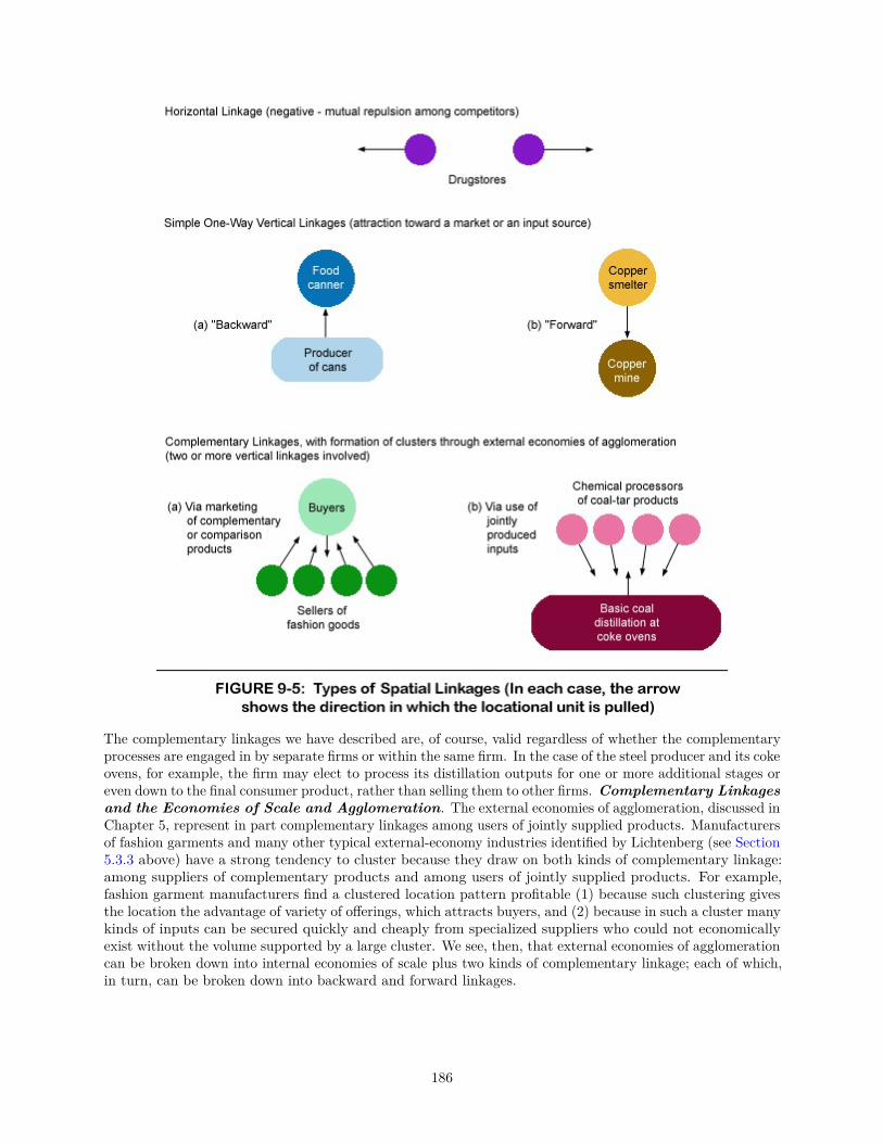
The complementary linkages we have described are, of course, valid regardless of whether the complementaryprocesses are engaged in by separate firms or within the same firm. In the case of the steel producer and its cokeovens, for example, the firm may elect to process its distillation outputs for one or more additional stages oreven down to the final consumer product, rather than selling them to other firms. Complementary Linkagesand the Economies of Scale and Agglomeration. The external economies of agglomeration, discussed inChapter 5, represent in part complementary linkages among users of jointly supplied products. Manufacturersof fashion garments and many other typical external-economy industries identified by Lichtenberg (see Section5.3.3 above) have a strong tendency to cluster because they draw on both kinds of complementary linkage:among suppliers of complementary products and among users of jointly supplied products. For example,fashion garment manufacturers find a clustered location pattern profitable (1) because such clustering givesthe location the advantage of variety of offerings, which attracts buyers, and (2) because in such a cluster manykinds of inputs can be secured quickly and cheaply from specialized suppliers who could not economicallyexist without the volume supported by a large cluster. We see, then, that external economies of agglomerationcan be broken down into internal economies of scale plus two kinds of complementary linkage; each of which,in turn, can be broken down into backward and forward linkages.

186

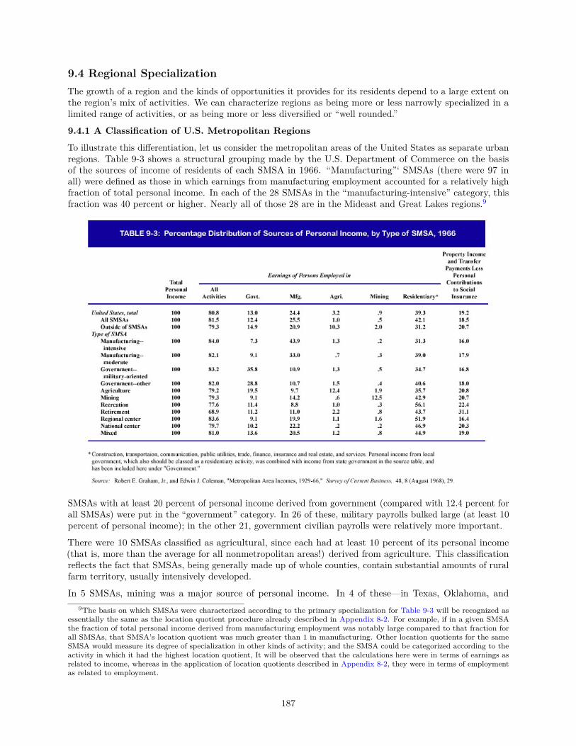
9.4 Regional SpecializationThe growth of a region and the kinds of opportunities it provides for its residents depend to a large extent onthe region’s mix of activities. We can characterize regions as being more or less narrowly specialized in alimited range of activities, or as being more or less diversified or “well rounded.”

9.4.1 A Classification of U.S. Metropolitan Regions

To illustrate this differentiation, let us consider the metropolitan areas of the United States as separate urbanregions. Table 9-3 shows a structural grouping made by the U.S. Department of Commerce on the basisof the sources of income of residents of each SMSA in 1966. “Manufacturing”‘ SMSAs (there were 97 inall) were defined as those in which earnings from manufacturing employment accounted for a relatively highfraction of total personal income. In each of the 28 SMSAs in the “manufacturing-intensive” category, thisfraction was 40 percent or higher. Nearly all of those 28 are in the Mideast and Great Lakes regions.9

SMSAs with at least 20 percent of personal income derived from government (compared with 12.4 percent forall SMSAs) were put in the “government” category. In 26 of these, military payrolls bulked large (at least 10percent of personal income); in the other 21, government civilian payrolls were relatively more important.

There were 10 SMSAs classified as agricultural, since each had at least 10 percent of its personal income(that is, more than the average for all nonmetropolitan areas!) derived from agriculture. This classificationreflects the fact that SMSAs, being generally made up of whole counties, contain substantial amounts of ruralfarm territory, usually intensively developed.

In 5 SMSAs, mining was a major source of personal income. In 4 of these—in Texas, Oklahoma, and9The basis on which SMSAs were characterized according to the primary specialization for Table 9-3 will be recognized as

essentially the same as the location quotient procedure already described in Appendix 8-2. For example, if in a given SMSAthe fraction of total personal income derived from manufacturing employment was notably large compared to that fraction forall SMSAs, that SMSA’s location quotient was much greater than 1 in manufacturing. Other location quotients for the sameSMSA would measure its degree of specialization in other kinds of activity; and the SMSA could be categorized according to theactivity in which it had the highest location quotient, It will be observed that the calculations here were in terms of earnings asrelated to income, whereas in the application of location quotients described in Appendix 8-2, they were in terms of employmentas related to employment.

187

Louisiana—the specialization was in oil and natural gas production, and property incomes also bulked largein their sources of income; the fifth was the Duluth-Superior SMSA, specializing in iron ore mining.

Recreational and retirement SMSAs (there were 4 of each) were characterized by low proportions of incomederived from manufacturing, rather high proportions derived from property, and (in the case of the retirementSMSAs such as Tampa-St. Petersburg and Tucson) high proportions of income derived from transfer payments,principally pensions.

There were 16 SMSAs classed as regional or national centers because an above-average share of their incomeswas derived from typically residentiary types of activity. This reflects the fact that in such areas, some of thetypical residentiary activities such as transportation, communications, finance, trade, and services are reallyexport activities serving an unusually far-flung region. The 4 national centers were New York, Los Angeles,Chicago, and San Francisco, ranking first, second, third, and sixth in population in 1966. It is interesting toobserve that Philadelphia and Boston (ranking fourth and fifth in size) did not appear as national centers;because they are so close to New York, their areas of influence are curtailed.

The residual group of 40 “mixed” SMSAs comprises those lacking any of the marked specializations ofstructure that characterize the other categories.

In similar fashion, larger geographical areas such as states or multistate regions exhibit different specializationsof function and structure. Regional specialization in some specific activity generally implies that the regionis a net exporter of the product of that activity, although in some cases it can reflect instead a distinctivepattern of demand in the region itself. Thus Michigan’s specialization in motor vehicle production and theDistrict of Columbia’s specialization in government are associated with heavy exports of cars and governmentservices from those areas; but the unusually high proportions of health and recreational service activities inretirement areas are primarily accounted for by the local demand.

9.4.2 Some Quantitative Measures of Specialization and Concentration

The location quotient has already been introduced in Appendix 8-2 and further discussed above in section9.4.1. As we have seen, (1) the same quotient measures both the degree of an area’s specialization in anactivity and the degree of concentration of the activity in the area; (2) the quotient can be calculated inthree ways, with identical results; and (3) the quotient can be based on either just one variable, such asemployment, in the areas and activities involved, or on two different variables, such as earnings in a givenactivity and total employment, population, or income.

In still other applications, we might want to compare the location quotient for the same activity and areaat two different dates in order to measure change in specialization or concentration. Finally, we can applythe quotient not to an activity but to some other measurable characteristic of an area (such as the size of aspecified ethnic group, number of motorcycles registered, or number of dog licenses issued) as related to somedifferent characteristic of activity such as population or employment.

The coefficient of specialization, a broader type of measure, can be used to gauge the degree to which the mixof a region’s economy differs from some standard, such as the mix in the national economy or the mix in thesame region at an earlier date. The calculation of this measure is illustrated in Table 9-4.

188

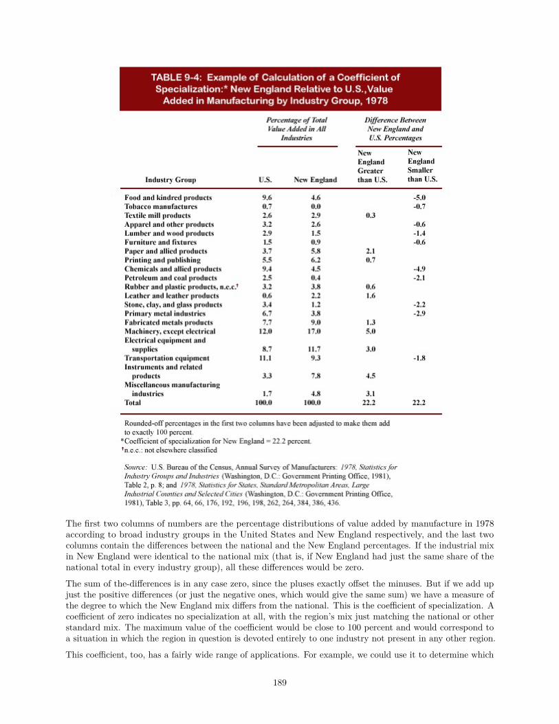
The first two columns of numbers are the percentage distributions of value added by manufacture in 1978according to broad industry groups in the United States and New England respectively, and the last twocolumns contain the differences between the national and the New England percentages. If the industrial mixin New England were identical to the national mix (that is, if New England had just the same share of thenational total in every industry group), all these differences would be zero.

The sum of the-differences is in any case zero, since the pluses exactly offset the minuses. But if we add upjust the positive differences (or just the negative ones, which would give the same sum) we have a measure ofthe degree to which the New England mix differs from the national. This is the coefficient of specialization. Acoefficient of zero indicates no specialization at all, with the region’s mix just matching the national or otherstandard mix. The maximum value of the coefficient would be close to 100 percent and would correspond toa situation in which the region in question is devoted entirely to one industry not present in any other region.

This coefficient, too, has a fairly wide range of applications. For example, we could use it to determine which

189

areas most nearly have a cross section of the national population in terms of age groups or ethnic categories;or whether a given region’s employment pattern diverges more from the national pattern in years of recessionthan in prosperous years; or whether two areas are more like each other than either is like some third area(which might be useful in aggregating areas into regions on the basis of homogeneity).

Finally, one other closely related measure should be mentioned: the coefficient of concentration, whichmeasures how closely one locational distribution (for example, that of population, income, or employment ina specific activity) matches another locational distribution (for example, that of total employment or landarea). Thus if the distribution of population by counties in the United States just matched the distributionof land area among counties, we should say that the population was evenly distributed (at the county level);while if the location pattern of the rubber industry is radically different from that of population or totalemployment, we can say that the rubber industry is spatially concentrated.

The coefficient of concentration is calculated in much the same way as the coefficient of specialization, exceptthat we line up two columns of figures representing location patterns (that is, each is a percentage distributionby areas), take all the positive or all the negative differences, and add.

Although location quotients and coefficients of concentration and specialization are handy summary measures,their limitations must be kept in mind. In particular, their values depend partly on the arbitrary decisions wemake regarding demarcation of both activities and areas. The measures all become larger if we use smallergeographical units (for example, states instead of Census divisions, or counties instead of states, or Censustracts instead of cities), and they become larger also if we employ a more detailed classification of activities.Consequently, any two coefficients of the same type are comparable only if they are based on the sameclassifications.

9.5 SummaryA region is an area that is usefully considered as an entity for purposes of description, analysis, administration,planning, or policy. It can be demarcated on the basis of internal homogeneity or functional integration.Nodal regions are those where the character of functional integration is such that a single specialized urbannucleus can be identified. Homogeneity and nodality are basic even when political, historical, military, orother considerations are importantly involved in regional demarcation.

Functional regions may be delimited by various statistical techniques. Some of these rely on data concerningcommodity, service, financial, migration, or commuting flows among regions in order to identify the strengthof interdependencies between and within regions.

Activities within a region interact in various ways. Horizontal linkages involve basically competition amongsimilar units and are expressed in mutual spatial repulsion, with formation of market areas and/or supplyareas. Vertical linkages (between the two parties in a transaction, such as seller and buyer) involve spatialattraction to save transfer costs. If it is primarily the buyers who are attracted toward the sellers, avertical linkage is called forward; whereas backward linkage means that the sellers are attracted toward thebuyers. Complementary linkages, more complex in nature, entail mutual attraction among (1) suppliers ofcomplementary products or (2) users of jointly supplied products. Such complementary linkages are basic tothe external economies of agglomeration discussed in Chapter 5.

Not only homogeneous regions but also functional ones tend to develop distinctive specializations of activitiesor other characteristics. The nature and degree of specialization can be gauged by such statistical measuresas the location quotient and the coefficients of (area) specialization and (activity) concentration.

190

Technical Terms Introduced in this ChapterHomogeneous region Residentiary activitiesFunctional integration Forward linkageFunctional region InfrastructureNodal region Horizontal linkagePositive linkage Complementary linkageVertical linkage Coefficient of specializationBackward linkage Coefficient of concentration

Selected ReadingsLawrence A. Brown and John Holmes, “The Delimitation of Functional Regions, Nodal Regions, andHierarchies by Functional Distance Approaches,” Journal of Regional Science, 11, 1 (April 1971), 57-72.

Beverly Duncan and Stanley Lieberson, Metropolis and Region in Transition (Beverly Hills, Calif.: SagePublications, 1970).

Otis Dudley Duncan et al., Metropolis and Region (Baltimore: Johns Hopkins University Press, 1960).

David L. Huff, “The Delineation of a National System of Planning Regions on the Basis of Urban Spheres ofInfluence,” Regional Studies, 7, 3 (September 1973), 323-329.

W. F. Lever, “Industrial Movement, Spatial Association, and Functional Linkages,” Regional Studies, 6, 4(December 1972), 371-384.

Harry W. Richardson, Regional Economics (Urbana: University of Illinois Press, 1978), Chapter 1.

191

10. THE LOCATION OF PEOPLE10.1 IntroductionThe importance of manpower supply as a location factor is suggested by the sheer magnitude of labor costs asan element in the total outlays of productive enterprises. In the United States, wage and salary payments, andsupplements thereto, account for about three-fourths of the national income, and this does not include theearnings of self-employed people and business proprietors (for example, farmers, store owners, and free-lanceprofessionals), which mainly represent a return to their labor. Accordingly, we should expect to find manykinds of activities locationally sensitive to the differentials in the availability, price, and quality of labor.

Labor’s role as a purchased input, however, is only one aspect of the locational interdependence of peopleand their economic activities. People in their role as consumers of the final output of goods and servicesaffect the locational choices of market-oriented activities. They play still another role as users of residentialland; and in urban areas, residence is by far the largest land use. Finally, and most important, the purpose ofthe whole economic system is to provide a livelihood for people. Regional economics is vitally concernedwith regional income differences, the opportunities found in different types of communities, and regionalpopulation growth and migration.

The present chapter is devoted to integrating and exploring these various aspects of “the location of people.”We begin by considering the locational differences in the rewards or “price” of labor.

10.2 A Look at Some DifferentialsComparing wages or incomes among different areas is not as straightforward a matter as it might appear,even when appropriate data are at hand. It is a question of what comparison is relevant to the question wehave in mind. For example, if we want to gauge the relative opulence of two communities (perhaps as anindication of how rich a market each would provide for consumer goods and services), then average personalincome in dollars per family or per person would be appropriate to compare. But an individual lookingfor an area where his work will be well rewarded would do better to compare real earnings in his or heroccupational category; that is, monetary earnings deflated by a cost-of-living index. Finally, an employerlooking for a good labor supply location would be most interested in comparisons of labor cost, based onmonetary wage-and-salary rates adjusted for labor productivity and fringe benefits. The relevance of suchdifferent measures should be kept in mind as we look at the data.

10.2.1 Differentials in Pay Levels

Rates of pay in any specific occupation can differ widely from one place to another and even within the samelabor market area. For example, in 1978 the union hourly wage scale for laborers and helpers in the buildingtrades averaged $8.54 for 65 cities surveyed by the U.S. Bureau of Labor Statistics, with the rate in individualcities ranging from a high of $10.54 in Cleveland, Ohio, to a low of $5.21 in Huntsville, Alabama.1

The differentials among regions are not entirely erratic. Some evidence of an underlying pattern appears inTable 10-1, in which the labor markets are classified by broad region and by size. In each of the three broadoccupational categories, the South shows up as the region with the lowest pay levels. The West and NorthCentral regions pay generally higher rates. In addition, with the exception of two occupational categories inthe North Central region, there is a tendency for rates to be higher in the larger metropolitan areas. Finally,it can be noted that the interregional disparities are wider for unskilled workers than for the other groups.This feature of the pattern will be explained later.

1U.S. Department of Labor, Bureau of Labor Statistics, Handbook of Labor Statistics, Bulletin 2070 (Washington, D.C.:Government Printing Office, 1980), Table 120, pp. 292-293.

192

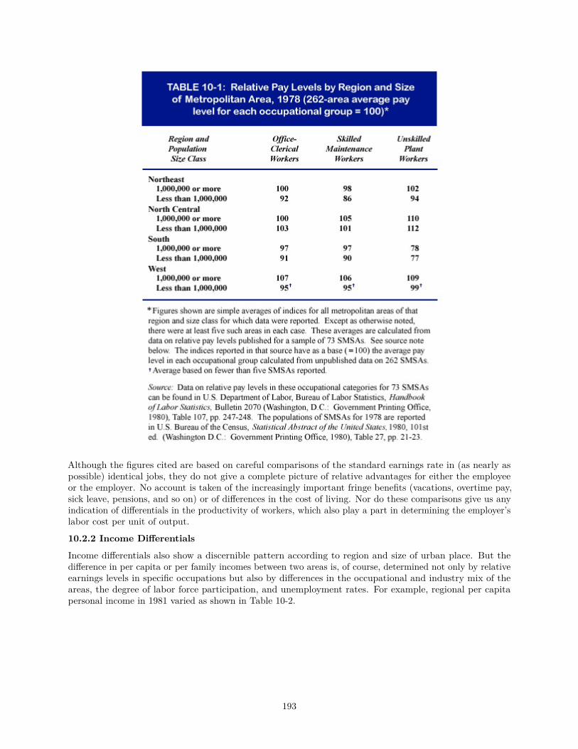
Although the figures cited are based on careful comparisons of the standard earnings rate in (as nearly aspossible) identical jobs, they do not give a complete picture of relative advantages for either the employeeor the employer. No account is taken of the increasingly important fringe benefits (vacations, overtime pay,sick leave, pensions, and so on) or of differences in the cost of living. Nor do these comparisons give us anyindication of differentials in the productivity of workers, which also play a part in determining the employer’slabor cost per unit of output.

10.2.2 Income Differentials

Income differentials also show a discernible pattern according to region and size of urban place. But thedifference in per capita or per family incomes between two areas is, of course, determined not only by relativeearnings levels in specific occupations but also by differences in the occupational and industry mix of theareas, the degree of labor force participation, and unemployment rates. For example, regional per capitapersonal income in 1981 varied as shown in Table 10-2.

193

The relation of income level to type of urban or rural place of residence is shown in Table 10-3. We observethere that in 1980, incomes were higher in metropolitan areas than in nonmetropolitan areas; higher in largermetropolitan areas than in smaller metropolitan areas; higher outside central cities than inside of centralcities; and higher in nonfarm rural areas than on farms.

194

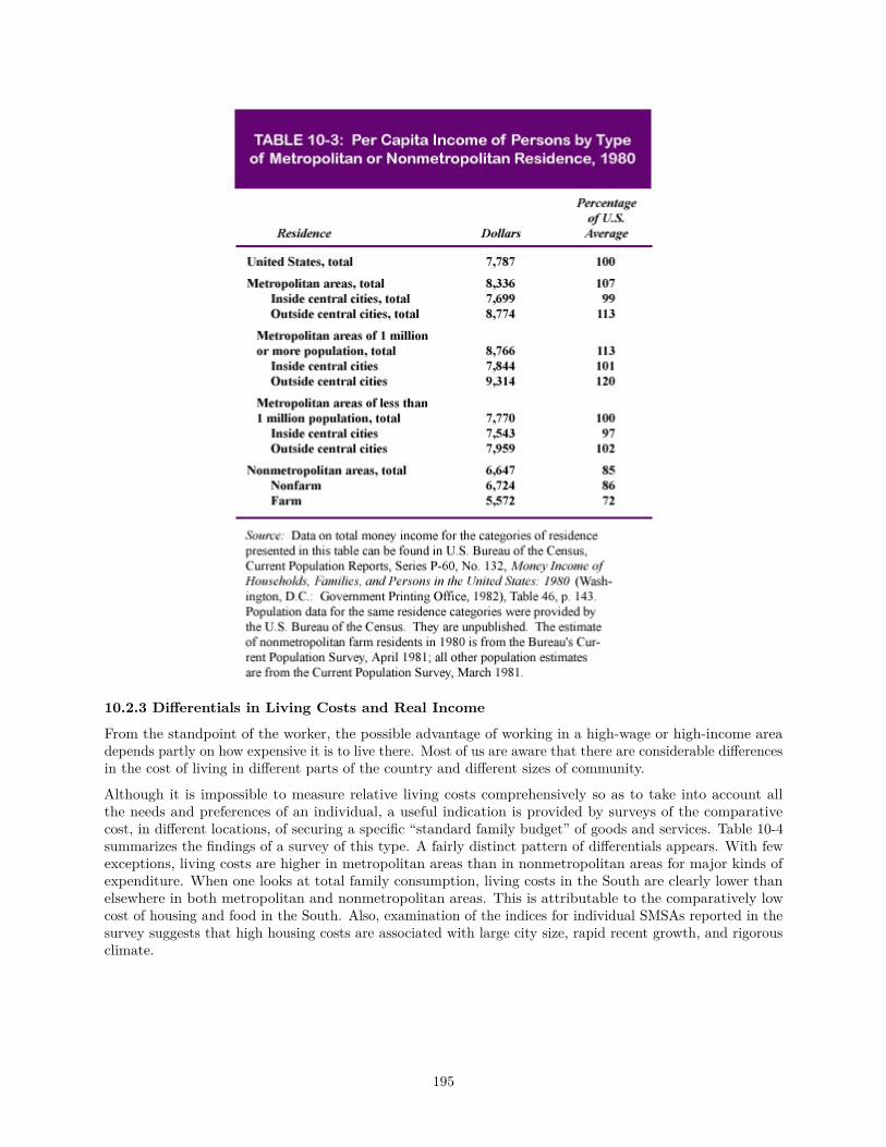
10.2.3 Differentials in Living Costs and Real Income

From the standpoint of the worker, the possible advantage of working in a high-wage or high-income areadepends partly on how expensive it is to live there. Most of us are aware that there are considerable differencesin the cost of living in different parts of the country and different sizes of community.

Although it is impossible to measure relative living costs comprehensively so as to take into account allthe needs and preferences of an individual, a useful indication is provided by surveys of the comparativecost, in different locations, of securing a specific “standard family budget” of goods and services. Table 10-4summarizes the findings of a survey of this type. A fairly distinct pattern of differentials appears. With fewexceptions, living costs are higher in metropolitan areas than in nonmetropolitan areas for major kinds ofexpenditure. When one looks at total family consumption, living costs in the South are clearly lower thanelsewhere in both metropolitan and nonmetropolitan areas. This is attributable to the comparatively lowcost of housing and food in the South. Also, examination of the indices for individual SMSAs reported in thesurvey suggests that high housing costs are associated with large city size, rapid recent growth, and rigorousclimate.

195

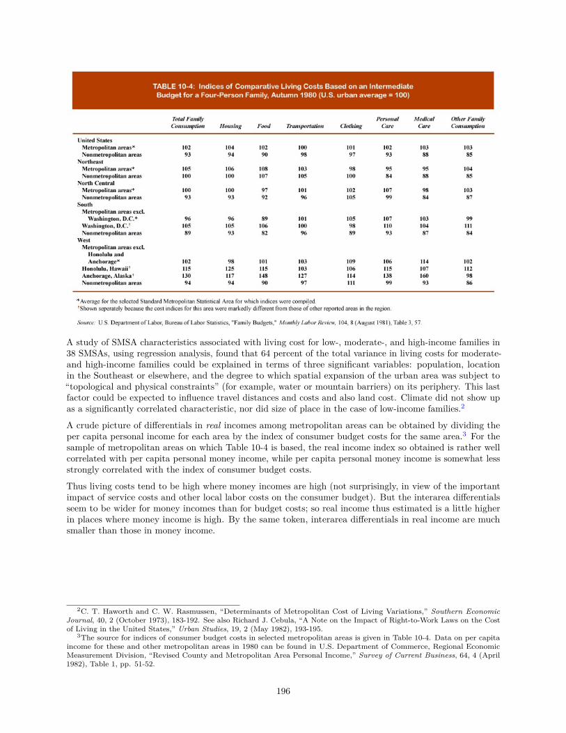
A study of SMSA characteristics associated with living cost for low-, moderate-, and high-income families in38 SMSAs, using regression analysis, found that 64 percent of the total variance in living costs for moderate-and high-income families could be explained in terms of three significant variables: population, locationin the Southeast or elsewhere, and the degree to which spatial expansion of the urban area was subject to“topological and physical constraints” (for example, water or mountain barriers) on its periphery. This lastfactor could be expected to influence travel distances and costs and also land cost. Climate did not show upas a significantly correlated characteristic, nor did size of place in the case of low-income families.2

A crude picture of differentials in real incomes among metropolitan areas can be obtained by dividing theper capita personal income for each area by the index of consumer budget costs for the same area.3 For thesample of metropolitan areas on which Table 10-4 is based, the real income index so obtained is rather wellcorrelated with per capita personal money income, while per capita personal money income is somewhat lessstrongly correlated with the index of consumer budget costs.

Thus living costs tend to be high where money incomes are high (not surprisingly, in view of the importantimpact of service costs and other local labor costs on the consumer budget). But the interarea differentialsseem to be wider for money incomes than for budget costs; so real income thus estimated is a little higherin places where money income is high. By the same token, interarea differentials in real income are muchsmaller than those in money income.

2C. T. Haworth and C. W. Rasmussen, “Determinants of Metropolitan Cost of Living Variations,” Southern EconomicJournal, 40, 2 (October 1973), 183-192. See also Richard J. Cebula, “A Note on the Impact of Right-to-Work Laws on the Costof Living in the United States,” Urban Studies, 19, 2 (May 1982), 193-195.

3The source for indices of consumer budget costs in selected metropolitan areas is given in Table 10-4. Data on per capitaincome for these and other metropolitan areas in 1980 can be found in U.S. Department of Commerce, Regional EconomicMeasurement Division, “Revised County and Metropolitan Area Personal Income,” Survey of Current Business, 64, 4 (April1982), Table 1, pp. 51-52.

196

There is evidence that similar relationships prevail also when we compare different size classes of places,4though it is impossible to compare adequately the psychic satisfactions and costs that come from living inlarge cities as against smaller places.

10.3 The Supply of Labor at a LocationIn trying to understand the causes and effects of wage and income differentials, it is useful to considerseparately the supply and demand sides of the local labor market. The aggregate supply of labor in acommunity may be quite inelastic in the short run, since it can change only through migration or changes inlabor force participation. For a single activity or occupation within the labor market area, the supply is moreelastic because it can be affected by workers changing their activities or occupations as well as by migrationand changes in the labor force. The labor supply as seen by an individual employer is still more elastic, andfor small employers in a large labor market almost perfectly so.

10.3.1 Work Location Preferences and Labor Mobility

There are many reasons for preferring a job in one area to the same kind of job in another area, and thedecision to move can be very complex. A systematic evaluation of costs and benefits is in order, much as adecision-maker in business evaluates the pros and cons of an investment. Thus the potential migrant wouldwant to recognize what he or she would be giving up (the opportunity costs of the move) and make a goodguess about what would lie in store in the new location.

Neither of these tasks is particularly easy, and a number of considerations would have to be recognized. First,it is not adequate to compare only basic wages; all fringe benefits must be considered as well. Also, for anincreasingly large share of the work force, the employment prospects of the spouse may be as important asthat of the “primary” wage earner.5 Second, a community with cheaper living costs might be preferred inthe absence of any pay differential. Third, various aspects of the quality of the job, such as security andprospects of advancement, may be considered. Expected growth in earnings some years down the road maybe an important factor in the decision to act now.6 Finally, other aspects of the desirability of the communityas a place to live can include, for example, climate, cultural and social opportunities, and access to otherplaces that one might like to visit.7 Differences among places on any of these accounts can be compared tomoney income differentials: How much additional compensation is required to give up immediate access tocultural events, or how much less would one be willing to accept in terms of earnings for a climate that suitsone’s tastes?

Spatial mobility refers to people’s propensity to change locations in response to some measurable set ofincentives, identified in practice as “real income” or simply as money wage rates deflated by a cost-of-livingindex. If mobility in this sense were perfect and real wages thus equal everywhere, there would be differentialsin money wages paralleling the differentials in living costs. A labor market where the living costs were 10

4The most widely cited study documenting the positive correlation of real income and population size in urban areas of theUnited States is Irving Hoch, “Income and City Size,” Urban Studies, 9, 3 (October 1972), 299-328. A much earlier study ofworkers’ hourly earnings and living costs in Swedish industrial towns and cities showed a consistently positive relationship, withroughly twice as wide a range of variation in earnings as in living costs. The same study found consistently higher living costs inlarger communities and in regions more distant from food-producing areas or having especially rigorous climates. See BertilOhlin, Interregional and International Trade (Cambridge, Mass.: Harvard University Press, 1933), pp. 215-218.

5See Steven H. Sandell, “Women and the Economics of Family Migration,” Review of Economics and Statistics, 59, 4(November 1977), 406-414; and Jacob Mincer, “Family Migration Decisions,” Journal of Political Economy, 86, 5 (October 1978),749-773.

6Of course, earnings and other benefits expected in the future must be properly discounted if valid comparisons are to bemade. The seminal article recognizing this and other aspects of the individual’s decision to migrate as placing it among a numberof human capital decisions, such as that to “invest” in education or on-the-job training, is Larry A. Sjaastad, “The Costs andReturns of Human Migration,” Journal of Political Economy, 70, 5 (2) (Supplement, October 1962), 80-93. This view has sincecome to dominate empirical and theoretical attempts to explain migration on the basis of economic incentives. For an excellentsurvey of these and related developments—at least until 1975—see Michael J. Greenwood, “Research on Internal Migration inthe United States: A Survey,” Journal of Economic Literature, 13, 2 (June 1975), 397-433.

7A number of recent studies have focused on quality-of-life factors or looked at the relationship between quality-of-life andeconomic factors in migration decisions. See, for example, Philip E. Graves, “Migration and Climate,” Journal of RegionalScience, 20, 2 (May 1980), 227-238; and Frank W. Porell, “Intermetropolitan Migration and the Quality of Life,” Journal ofRegional Science, 22, 2 (May 1982), 137-157.

197

percent above average would pay wages 10 percent above average, but real wages there would be the same asanywhere else.

The term equalizing differentials has been applied to this kind of money wage or income differential.8 Thepattern of actual money differentials is, then, made up of two components: (1) equalizing differentials, whichwould exist even in the absence of any impediment to labor mobility, and (2) real differentials, representingdifferences in real income and thus presumably caused by impediments to mobility.

The significance of this distinction is that workers can logically be expected to choose locations and to movein response to real differentials; whereas employers looking for cheap labor will be more interested in thetotal money wage differential, which combines both real and equalizing differentials.

These concepts of real and money wages, cost of living, equalizing and real differentials, and mobility help usto understand some basic motivations of the locational choices of employees and employers; but unfortunatelythey are not very sharp tools. We have already noted the impossibility of including in indices of income andliving costs all the considerations affecting the desirability of a place to live. For example, such indices takeno account of the attractions of a mild and sunny climate (except as reflected in housing costs), the dirt anddiscomforts of life in a large industrial city, the social pressures and cultural voids of a small town, or theadvantage to a research worker of being stationed where the action is in his or her field. As a result of ourinability to measure real income fully, we are also unable to measure mobility in a completely unambiguousway. If a family, for example, likes the physical and social climate of its surroundings and refrains frommoving to another area where the pay is higher both in money terms and as deflated by a conventional familybudget cost index, should we ascribe its failure to move to a lack of mobility?

A further difficulty with the simple concept of real and equalizing differentials is the implication that migrationis not merely motivated by real-income differentials but tends to eliminate them. Under certain conditions itis possible for migration, even when so motivated, to leave the differential unchanged or even to widen it. Weneed to look further into both the causes and the consequences of migration.

10.3.2 Who Migrates: Why, When, and Where?

Migration is influenced by three conditions: the characteristics of both the origin and destination areas, thedifficulties of the journey itself, and the characteristics of the migrant.

Reasons for Moving. It is a drastic oversimplification to explain migration simply on the basis of responseto differentials in wage rates, income, or employment opportunity. The U.S. Bureau of the Census basesits tabulations of migration on changes in residence. Since some of these are local (moves within the samecounty) and others involve substantial distance (intercounty moves), one would expect reasons for moving todiffer widely.

Those persons who move only within the same county are predominantly influenced by housing considerations.Since all of a county is generally regarded as being included within a single labor market or commuting range,job changes are related only to a minor extent with intracounty moves. Most such movers are not changingjobs.

For those who move to a different county the picture is quite different, with employment changes (includingentry to or exit from military service) emerging as the major reasons for migrating. This reflects the factthat an intercounty migration generally involves shifting to a different labor market beyond the commutingrange for the former job. A change of residence is involved but is not the primary motivation.

Characteristics of Origin and Destination Areas. The characteristics most obviously affecting attrac-tiveness to the individual migrant have already been suggested. In addition, we should expect that a largerplace would have more migrants arriving and departing than a smaller place, more or less in proportion tosize. But size itself can significantly affect the appeal of a place for the individual. Historically, migrants haveresponded to the greater variety of job opportunities in larger urban places and their suburbs by migrating tothem in numbers somewhat more than proportional to their size.

8Ohlin, Interregional Trade, p. 212. The term “equalizing” has sometimes been applied also to wage differences explainableby differences in the attractiveness of different occupations.

198

Rather than thinking of migration as being motivated simply by net advantages of some places over others, itis useful to separate the pull of attractive characteristics from the push of unattractive ones. Clearly, manypeople migrate because they do not like it where they are, or perhaps are even being forced out by economic,political, or social pressures. The basic decision is to get out, and the choice of a particular place to migrateto is a secondary and subsequent decision, involving a somewhat different set of considerations. On the otherhand, some areas can be so generally attractive as to pull migrants from a wide variety of other locations,including many who were reasonably well satisfied where they were.9

Recent studies on migration using detailed data on flows in both directions (rather than just net flows) haveconsiderably revised earlier notions of push and pull. Rather surprisingly, it appears that in most cases theso-called push factor explaining out-migration from an area is not primarily the economic characteristics of thearea (such as low wages or high unemployment) but the demographic characteristics of the population of thearea. Areas with a high proportion of well-educated young adults have high rates of out-migration, regardlessof local economic opportunity. The pull factor (that is, the migrant’s choice of where to go) is, however,primarily a matter of the economic characteristics of areas. Migration is consistently heavier into prosperousareas. Accordingly, the observed net migration losses of depressed areas generally reflect low in-migration butnot high out-migration, and the net migration gains of prosperous areas reflect high in-migration rather thanlow out-migration.10

Difficulties of the Journey. Within a country, distance is perhaps the most obviously significant charac-teristic of the migration journey, and virtually all analyses of migration flows have evaluated the extent towhich migration streams attenuate with longer distance. Thus a simple “gravity model” of migration positsthat the annual net migration from A to B will be proportional to the populations of A and B and to thesize of some differential (say, in wage rates) between A and B, and inversely proportional to the square of thedistance from A to B, as follows:

MAB = gPAPB(WB −WA)/D2AB

(where the P s represent populations, the W s wage rates, D the distance, M the number of migrants per unitof time, and g a constant with a value depending on what units are used for the variables).11 This basicmigration flow model has been statistically tested and modified in many ways in the attempt to make itmore realistic. It has already been suggested that in many circumstances at least, there is a “scale effect”upon migration, which can be incorporated in the model by giving the populations an exponent greater than1. Any relevant factor of differential advantage that can be quantified (for example, unemployment rates,mean summer or winter temperature, percentage of sunny days, average education or income level of thepopulation, percentage of housing in good condition, crime rates, insurance rates, or air pollution) can beintroduced, with whatever relative weighting the user of the model deems appropriate.

The distance factor in the model likewise can be assigned a different exponent to fit the circumstances(there is nothing special about the square of the distance, except for the law of physical gravitation) andelaborated in various ways. Actually, distance per se is at best only loosely related to the difficulties attendingmigration. The factors involved are actual moving costs (which can sometimes be the least important obstacle),uncertainty, risk and investment of time involved (including that associated with acquiring information),restrictions on migration per Se, and what is sometimes called social distance—suggesting the degree ofdifficulty the migrant may have in making adequate social adjustment after he or she arrives.12 As an exampleof this last factor, a model designed by W. H. Somermeijer to explain Dutch internal migration flows included

9Separation of the push from the pull effect is obviously a tricky business, and there has been much controversy about howmuch weight to attach to each with respect to specific historical or current migrations. It has been argued that the migrationsfrom European countries to the United States in the latter part of the nineteenth century were primarily motivated by pull,because they fluctuated from year to year in harmony with fluctuations in American business conditions but did not significantlyvary in response to business cycles in specific European countries. See Richard A. Easterlin, “Long Swings in United StatesDemographic and Economic Growth: Some Findings on the Historical Pattern,” Demography, 2 (1965), 497-500.

10See Ira S. Lowry, Migration and Metropolitan Growth. Two Analytical Models (San Francisco: Chandler, 1966).11See Chang-I Hua and Frank Porell, “A Critical Review of the Development of the Gravity Model,” International Regional

Science Review, 4, 2 (Winter 1979), 97-125.12For a discussion of some issues relevant to the interpretation of the distance factor, see Aba Schwartz, “Interpreting the

Effect of Distance on Migration,” Journal of Political Economy, 81,5 (September/October 1973), 1153-1169.

199

a term that measured the difference in the Catholic-Protestant ratio between the two areas. Introduction ofthis term substantially improved the model’s explanatory power, suggesting that members of each religiouspersuasion tend to move mainly to areas where their coreligionists predominate. 13

Social distance depends partly, of course, on the individual migrant. But wide social distances betweencommunities and regions (that is, great heterogeneity) tend to restrict migration flows to those individualswho can most easily make the required adjustment. With the improvement in communications and travel,social distance in space tends to lessen; but it is still a factor, for example, between French and EnglishCanada, between the North and the Deep South in the United States, or between farm and city.14

Another feature of migration paths is that they seem to be subject to economies of volume of traffic along anyone route. Well-beaten paths become increasingly easy and popular for successive migrants. This is so for avariety of reasons. Sometimes (as in the case of earlier transoceanic and more recent Puerto Rico-to-mainlandmigrant travel) transport agencies have given special rates or in other ways have favored the increase ofmigrant travel on the most frequented routes. Perhaps more generally applicable and more important is thefact that migrants try to minimize uncertainties and risks by choosing places about which they have at leasta little information and where they will find relatives, friends, or others from their home areas who will helpthem to gain a foothold.15 This tendency is particularly important, of course, when the social distance islarge. It goes far to explain the heavy concentration of late-nineteenth-century European migrants to theUnited States in a few large cities, and the even more remarkable concentration of particular ethnic andsub-ethnic groups in certain cities and neighborhoods, which even now retain unto the third generation someof their special character. The most recent ethnically distinctive waves of migration to American cities—thoseof blacks, Puerto Ricans, and Chicanos—have in the same fashion followed a few well-beaten paths. Forexample, it has been established that Southern black migrants to Chicago came mainly from certain sectionsof the South, while those going to Washington, D.C., or Baltimore originated in other Southern areas, andthose going to the West Coast in still other areas. Recent migrants from the Caribbean (other than thosefrom Puerto Rico) remain highly concentrated in the Miami area.

An analysis of labor mobility in the United States between 1957 and 1960, based on Social Security records,gives striking evidence of the beaten-path effect where migration of blacks is concerned. For white workers,both male and female, migration flows were significantly related to earnings differentials (positively) and todistance (negatively) as we might expect. For black men, however (and to a lesser extent for black women),earnings differentials and distance appeared to be less important determinants than either the number ofblacks or the proportion of blacks in the work force of the destination area. In other words, blacks (or at anyrate, black males) were selectively attracted to labor markets in which there already was a high proportion ofblacks.16

The tendency of migration to channelize in well-beaten paths provides part of the explanation for anothercharacteristic of migration streams already mentioned; namely, that places with high rates of inward migrationtend to have high rates of outward migration as well. This so-called counterstream effect was noted as longago as the 1880s in E. G. Ravenstein’s pioneer statement of migration principles, and has been amply verifiedsince.17

The point here is that a well-beaten path eases travel in both directions. Migrants generally come to a placewith incomplete knowledge, and many of the disappointed ones simply retrace their steps. Also, a city that

13H. ter Heide, “Migration Models and Their Significance for Population Forecasts”, Milbank Memorial Fund Quarterly, 41, 1(January 1963), 63-64.

14Functional distance is a still broader concept, wrapping up in one index a measure of all factors impeding migration betweena given pair of points. Functional distance can be evaluated by comparing actual migration flows with the flows that wouldhe expected to occur simply on the basis of, say, the populations of the points in question. Functional distance can then becorrelated with actual distance and other suspected determinants in order to break it down into components.

15See for example, James B. Kau and C. F. Sirmans, “The Influence of Information Costs and Uncertainty on Migration: AComparison of Migrant Types,” Journal of Regional Science, 17, 1 (April 1977), 89-96, where the role of previous migrants as asource of information is examined statistically.

16Lowell E. Galloway, Geographic Labor Mobility in the United States, 1957 to 1960, U.S. Department of Health, Education,and Welfare, Social Security Administration, Office of Research and Statistics, Research Report No. 28 (Washington, D.C.:Government Printing Office, 1969). See also Janet R. Pack, “Determinants of Migration to Central Cities,” Journal of RegionalScience, 13, 2 (August 1973), 249-260.

17E. G. Ravenstein, “The Laws of Migration,” Journal of the Royal Statistical Society, 52 (June 1889), 241-301.

200

offers especially favorable adjustment opportunities for migrants is likely to serve as a “port of entry” formigrants coming into that region or country. New York has historically been the entry place for transatlanticimmigrants, and Chicago has functioned as an important first destination for Mexicans migrating to theAmerican Midwest. In such cases, many of the migrants move out again (either to other places in the regionor perhaps back to their place of origin), so the out-migration rate of such an entry point or staging area islikely to be high. More generally, it is plausible to assume that people who have just migrated are especiallymobile by circumstances or taste and hence more likely than others to swell the outward flow.

Migration flows over long distances within the same country have historically involved a considerable amountof what is sometimes called chain migration. Most of the migrants move relatively short distances, but themoves are predominantly in one direction, forming a stream. As people move from B to A, they are replacedin B by migrants from C, who in turn are replaced by migrants from D. It has been established that most ofthe massive redistribution of population in England during the Industrial Revolution was carried out in suchfashion by short-distance moves cumulating toward the new industrial towns.18

Characteristics of the Migrant. Migration is basically selective. Some people are far more prone tomigrate than are others. This is often expressed as a difference in the mobility of different groups, but wereally cannot explain all of the difference in that way, since the incentives to migrate are not the same. Forexample, a young scientist fresh out of school is confronted with a quite different set of pushes and pulls thanan aging farmer, an established business executive, a manual laborer, or a wealthy widow.

The most conspicuous differences in migration rates are those experienced by the individual in passing throughsuccessive stages of a lifetime. These changes are (as shown in Figure 10-1) rather similar for the two sexes;for simplicity’s sake we describe them here in male terms.

A very young child is relatively portable. After he enters school and has older, more settled parents andprobably more brothers or sisters, his probability of moving declines. The rate rises suddenly when he isready to look for a job or choose a college, and it remains high until after he is married and has children ofhis own. As his stake in his job and community grows, and as his and his family’s other local ties develop, hebecomes less and less likely to move. His mobility recovers somewhat at the stage when all of his children areon their own, and again at the customary mid-sixties retirement age. After about age seventy, migrationrates tend to rise a little, presumably reflecting adjustments to death of the spouse or to growing incapacity.

These characteristic life-cycle variations are manifest in Figure 10-1, showing United States migration ratesby age and sex. The pattern is blurred in the aggregate, of course, by the fact that not all people enter thelabor force, marry, or retire at the same ages. But age remains the characteristic most distinctly associatedwith migration-rate differentials. Most of the migration that occurs (except in massive displacements ofpopulations by military or political force or by natural disaster) is done by people in young adult age groups.

18Arthur Redford, Labour Migration in England, 1800-1850 (Manchester: The University Press, 1926; 2nd ed., New York: A.M. Kelley, 1968). The same process was included as one of the basic principles of migration in Ravenstein’s analysis. It may besurmised that chain migration is less important than it once was in the United States, since the difficulties of moving almostcertainly depend less than they once did on the sheer physical distance involved.

201

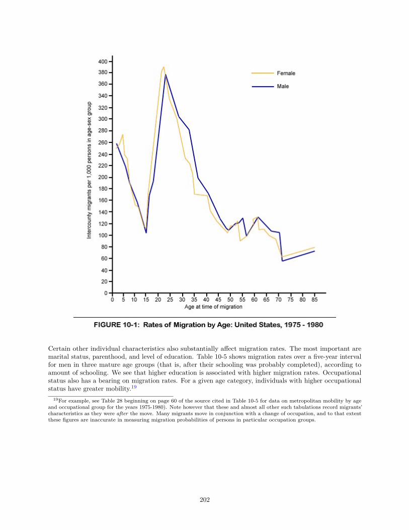
Certain other individual characteristics also substantially affect migration rates. The most important aremarital status, parenthood, and level of education. Table 10-5 shows migration rates over a five-year intervalfor men in three mature age groups (that is, after their schooling was probably completed), according toamount of schooling. We see that higher education is associated with higher migration rates. Occupationalstatus also has a bearing on migration rates. For a given age category, individuals with higher occupationalstatus have greater mobility.19

19For example, see Table 28 beginning on page 60 of the source cited in Table 10-5 for data on metropolitan mobility by ageand occupational group for the years 1975-1980). Note however that these and almost all other such tabulations record migrants’characteristics as they were after the move. Many migrants move in conjunction with a change of occupation, and to that extentthese figures are inaccurate in measuring migration probabilities of persons in particular occupation groups.

202

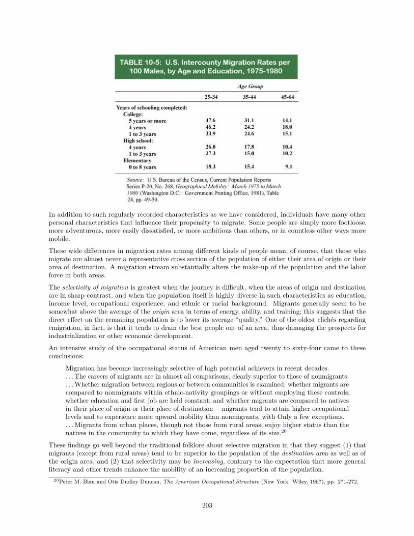
In addition to such regularly recorded characteristics as we have considered, individuals have many otherpersonal characteristics that influence their propensity to migrate. Some people are simply more footloose,more adventurous, more easily dissatisfied, or more ambitious than others, or in countless other ways moremobile.

These wide differences in migration rates among different kinds of people mean, of course, that those whomigrate are almost never a representative cross section of the population of either their area of origin or theirarea of destination. A migration stream substantially alters the make-up of the population and the laborforce in both areas.

The selectivity of migration is greatest when the journey is difficult, when the areas of origin and destinationare in sharp contrast, and when the population itself is highly diverse in such characteristics as education,income level, occupational experience, and ethnic or racial background. Migrants generally seem to besomewhat above the average of the origin area in terms of energy, ability, and training; this suggests that thedirect effect on the remaining population is to lower its average “quality.” One of the oldest clichés regardingemigration, in fact, is that it tends to drain the best people out of an area, thus damaging the prospects forindustrialization or other economic development.

An intensive study of the occupational status of American men aged twenty to sixty-four came to theseconclusions:

Migration has become increasingly selective of high potential achievers in recent decades.. . . The careers of migrants are in almost all comparisons, clearly superior to those of nonmigrants.. . .Whether migration between regions or between communities is examined; whether migrants arecompared to nonmigrants within ethnic-nativity groupings or without employing these controls;whether education and first job are held constant; and whether migrants are compared to nativesin their place of origin or their place of destination— migrants tend to attain higher occupationallevels and to experience more upward mobility than nonmigrants, with Only a few exceptions.. . .Migrants from urban places, though not those from rural areas, enjoy higher status than thenatives in the community to which they have come, regardless of its size.20

These findings go well beyond the traditional folklore about selective migration in that they suggest (1) thatmigrants (except from rural areas) tend to be superior to the population of the destination area as well as ofthe origin area, and (2) that selectivity may be increasing, contrary to the expectation that more generalliteracy and other trends enhance the mobility of an increasing proportion of the population.

20Peter M. Blau and Otis Dudley Duncan, The American Occupational Structure (New York: Wiley, 1967), pp. 271-272.

203

Another study, relating to migrants to the industrial metropolis of Monterrey, Mexico, between 1940 and196021 gives a rather different picture. Migration appears to have become much less selective with respect topopulations of origin in that interval. Early in the period, only a few of the more highly educated venturedthe move to the city; later, mobility increased, so that villagers of all educational and income levels becamemore nearly representative of the populations of its areas of origin, while at the same time it was becomingincreasingly different from (educationally inferior to) the population of the urban destination area.22

Migration selectivity, then, can depend to a large extent on the state of development of the regions involvedand can change in character fairly rapidly. It has already been suggested that a broadening of education andeconomic opportunity in less-developed regions can reduce selectivity. Finally, Everett Lee has proposed aplausible but not easily verifiable hypothesis: that migration motivated by pull tends to be positively selective(i.e., the more productive people are the ones who go), whereas migration motivated by push tends to benegatively selective.

Factors at origin operate most stringently against persons who in some way have failed economicallyor socially. Though there are conditions in many places which push out the unorthodox andthe highly creative, it is more likely to be the uneducated or the disturbed who are forced tomigrate.23

Inward, Outward, and Net Migration: Three Hypotheses. The typical age selectivity of migration issometimes an important factor accounting for the observed tendency that places with high in-migration rateshave high out-migration rates as well. The most mobile age groups (and perhaps also the individuals mostmobile by temperament or other characteristics) are present in abnormally high proportion in a fast-growingarea with high recent and current in-migration; and such local demographic characteristics play a large partin determining how many people leave an area.24

We have learned that the relationships among inward, outward, and net migration are more complex thanone might suspect. Let us review them in terms of three hypotheses or “laws of migration,” using Figure 10-2as a graphic aid.

21Harley L. Browning and Waltraut Feindt, “Selectivity of Migrants to a Metropolis in a Developing Country: A MexicanCase Study,” Demography, 6, 4 (November 1969), 347-357.

22Where the quality (of education, skills, income, or whatever) of a stream of migrants is, as in the Monterrey case, intermediatebetween that of the origin and the destination populations, the curious result is that the immediate effect of the migration is tolower the average quality in both areas, although at the same time it usually improves the quality of the migrants and of thepopulations of the areas combined! A similar apparent paradox is involved in the case of the legendary student who flunked outof Harvard and transferred to a rival New England institution (which shall remain nameless), raising the average scholastic levelof both universities.

23Everett S. Lee, “A Theory of Migration,” Demography, 3, 1 (1966), 56. This article represents a thorough revision andamplification of Ravenstein’s much earlier “Laws of Migration”.

24See Lowry, Migration and Metropolitan Growth.

204

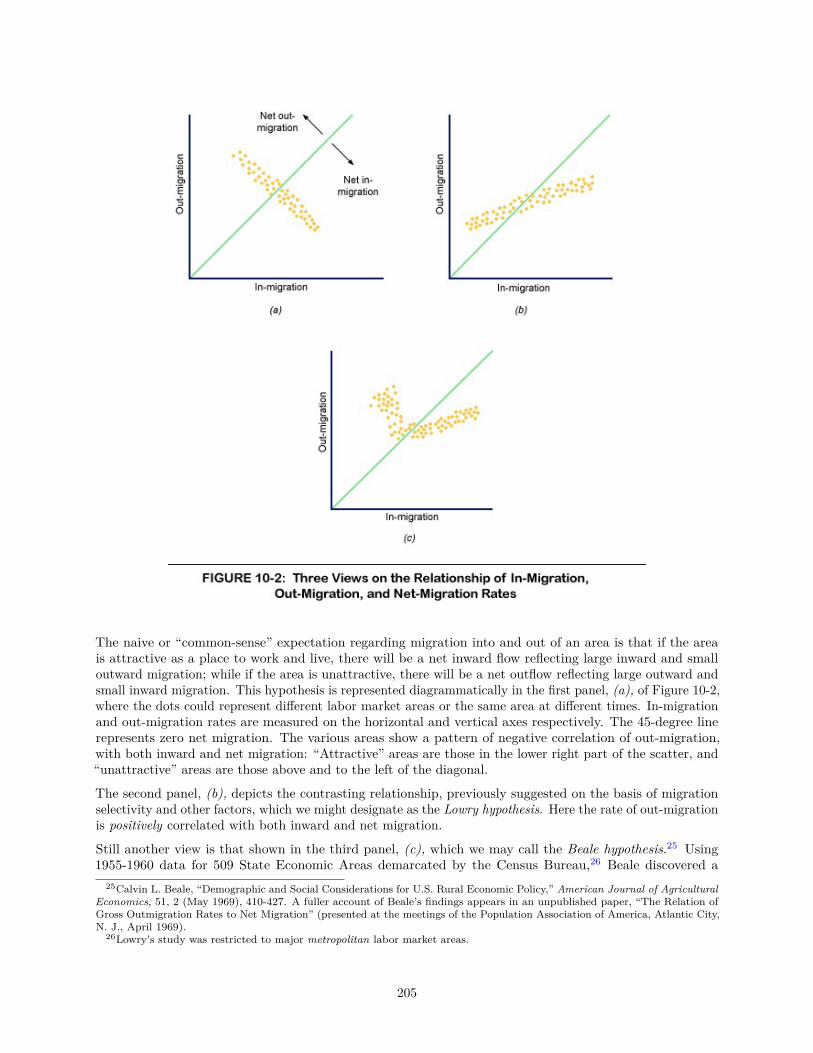
The naive or “common-sense” expectation regarding migration into and out of an area is that if the areais attractive as a place to work and live, there will be a net inward flow reflecting large inward and smalloutward migration; while if the area is unattractive, there will be a net outflow reflecting large outward andsmall inward migration. This hypothesis is represented diagrammatically in the first panel, (a), of Figure 10-2,where the dots could represent different labor market areas or the same area at different times. In-migrationand out-migration rates are measured on the horizontal and vertical axes respectively. The 45-degree linerepresents zero net migration. The various areas show a pattern of negative correlation of out-migration,with both inward and net migration: “Attractive” areas are those in the lower right part of the scatter, and“unattractive” areas are those above and to the left of the diagonal.

The second panel, (b), depicts the contrasting relationship, previously suggested on the basis of migrationselectivity and other factors, which we might designate as the Lowry hypothesis. Here the rate of out-migrationis positively correlated with both inward and net migration.

Still another view is that shown in the third panel, (c), which we may call the Beale hypothesis.25 Using1955-1960 data for 509 State Economic Areas demarcated by the Census Bureau,26 Beale discovered a

25Calvin L. Beale, “Demographic and Social Considerations for U.S. Rural Economic Policy,” American Journal of AgriculturalEconomics, 51, 2 (May 1969), 410-427. A fuller account of Beale’s findings appears in an unpublished paper, “The Relation ofGross Outmigration Rates to Net Migration” (presented at the meetings of the Population Association of America, Atlantic City,N. J., April 1969).

26Lowry’s study was restricted to major metropolitan labor market areas.

205

relationship schematically resembling that of Figure 10-2 (c). He found that high gross out-migration can beassociated with either high net in-migration or high net out-migration. The net rate is mainly determinedby out-migration when the net is negative, and by in-migration when the net is positive. We may interpretthis as meaning that the “Lowry effect” dominates in relatively prosperous and growing areas; whereas inareas that are seriously depressed the predominant effect is the “common-sense” one: Poor prospects bothdiscourage inflow and encourage outflow, and economic factors exert both pull and push.

The significance of this issue is far from trivial, as Beale points out and as we shall more fully appreciate in thecontext of Chapters 11 and Chapter 12. If migration out of seriously depressed or backward areas is assumedto be affected only by demographic characteristics of the population and not by the level of unemployment orincome, then measures to stimulate activity in such areas would not reduce out-migration (in fact, accordingto the Lowry hypothesis they would eventually increase it). The Beale findings suggest, however, that suchstimulus may, in some cases at least, retard out-migration. In choosing among policy decisions regarding aidto depressed or backward areas, it is of some importance to try to gauge this possible impact.

Changes in Migration Rates. There are a number of reasons why one might expect migration rates toincrease over time. Lee has suggested that increasing diversity of the opportunities afforded by differentareas, increasingly diverse specialization of people’s capabilities and preferences, the beaten-path effect,and the increasingly wide knowledge and experience of other locations that is brought about by education,better communication, more income, and increased leisure to travel would each enhance the mobility of thepopulation.

Changes in the socioeconomic and demographic characteristics of households have been working in theopposite direction, however. For short-distance (intracounty) moves, decreases in average size of householdand increases in home ownership are associated with decreases in mobility. With respect to long-distancemoves, the rising incidence of two-wage-earner households also discourages mobility.

Recent tabulations of migration data gathered on an annual basis from sample surveys since 1948 showthat the net effect of these countervailing forces has been a consistent decline in the overall migration rate.For example, the average annual rate for the twelve-month period March to March has fallen from 20.6 in1961-1962 to 18.7 in 1970-1971 and to 17.2 in 1980-1981. Thus in the 1960-1961 period, roughly 21 percent ofthe population changed residences in the United States, whereas that number had fallen to about 17 percentin the 1980-1981 period.27

Much of this trend can be attributed to decreases in the frequency of intracounty moves. However, there arealso indications that regions have become more alike, so that in some respects the incentives for long-distancemoves have probably lessened. Regional incomes in any case have tended to converge toward the nationalaverage. Thus in addition to the socioeconomic and demographic factors mentioned above, reduced migrationincentives could also have offset increases in personal mobility.

Migration rates show marked seasonal and cyclical variations. In general, prosperity favors migration becauseopportunities are more plentiful, risks of unemployment at the new location are less, and migrants themselvesare in a better financial position. In periods of economic recession or depression, people tend to look for theplace with the best economic security. This may mean staying where they are or (in the case of fairly recentmigrants) returning to their last place of residence. Thus the long-term migration stream toward places withbetter long-term prospects is temporarily interrupted or even reversed by severe recessions. For example, inthe worst years of the Great Depression of the 1930s, the longstanding net flows of migrants from farm tononfarm areas and from foreign countries to the United States were both temporarily reversed.

The Effectiveness of Migration. When people migrate, they are seeking to better their prospects. Howwell does migration accomplish that purpose, and how does it affect people other than those who migrate?

The answer obviously depends in part on how accurately people size up the prospects when they decideto move (or not to). The better informed they are, the greater the probability that migration will justifyitself and will contribute to a more efficient allocation of human resources in the economy as a whole. Thuspublic policy with regard to migration should, first, help potential migrants to get the information they need

27U. S. Bureau of the Census, Current Population Reports, Series P-20, No. 377, Geographical Mobility: March 1980 to March1981 (Washington, D.C.: Government Printing Office, 1983), Table A, p. 1.

206

for rational choice. Beyond this rather obvious point, the question of the effectiveness of migration can beexamined on three different levels.

1. The “efficiency of migration” between any two areas is sometimes defined as the ratio of the net flow tothe total gross flow in both directions. In other words, if all migrants go in the same direction, theefficiency is 100 percent, in the sense that there is no cross-hauling of migrants: The net flow equals thegross flow. At the other extreme, if the flows in the two directions just balance, so that there is no netmovement at all, the efficiency is said to be zero.

This measure may be useful in suggesting the degree to which a net migration figure can be misleadingas an indicator of the amount of movement; but it has little to do with efficiency in any meaningfulsense. People are not simply interchangeable units of manpower, as the efficiency ratio implies. Onthe contrary, those moving in one direction may be presumed to differ qualitatively from those movingin the other; with each stream believing, and perhaps correctly, that it is going in the right direction.Accordingly, a situation in which two opposing flows largely cancel out in terms of numbers of people isnot necessarily indicative of any “lost motion” or waste in terms of either the welfare of the individualmigrants or the socially desirable spatial allocation of manpower resources.

2. A different and somewhat more sophisticated question about migration is to ask whether it seems tobe going to the right places so far as the economic benefit to the migrant is concerned. If we findpeople moving predominantly from places of lower incomes to places of higher incomes, or from areas ofheavy unemployment to labor shortage areas, we surmise that they know what they are doing. If theygo the other way, or simply in all directions without any apparent regard to income or employmentdifferentials or any other obvious index of advantage, we have to surmise either that the migrants areignorant about the alternatives or that we are ignorant about their real motivations.

Actually, most migration flows do fit a “rational” pattern in relation to observable differences in earninglevels, unemployment rates, and such other easily identified variables as climate and the level of publicassistance benefits. Even the migration of poor blacks from Southern farms to Northern city ghettoswith high unemployment and dismal living conditions can make sense in terms of improvement in themigrants’ incomes, at any rate if we ignore possible adverse effects on the social adjustment of theindividuals and communities involved.

In relating migration to indices of community economic welfare (for example, wage or income levels) wecannot reasonably assume that the migrant immediately fits into the pattern of the area and receivesthe average pay, employment security, and other perquisites of the residents in his or her age andoccupational category. Migrants are no more representative of the populations of their destinationareas than they are of the populations of their areas of origin. Some of their distinctive characteristicsare subject to modification, so that if they stay they will tend to become more similar to their newneighbors. This tendency toward assimilation applies to skills, consumption patterns, ratings on mostkinds of “intelligence” tests, desired number of children, and social behavior.

3. Finally, we can judge migration on the basis of how much it contributes to aggregate output or, morebroadly, to general social welfare. This is the appropriate level of judgment for public authorities andpublic-spirited citizens to try to use. It calls for assessing the effects of migration not just on themigrants but on the communities they leave and enter.

This is by no means a simple criterion to apply. On the face of it, the transfer of manpower to placeswhere its productivity is higher seems likely to raise national per capita output and increase “aggregatewelfare,” insofar as that term has any meaning. And differentials in real-earnings rates reflect, roughlyat least, differentials in the marginal productivity of labor. But migration (particularly highly selectivemigration) can have important side effects (externalities) on the areas involved, in terms of the costs ofpublic services, the prospects for future economic development, and the quality of life. The discussion ofthese problems will be taken up in later chapters where we come to grips with the processes of regionalgrowth and change.

207

10.4 Labor Orientation: The Demand for Labor at a LocationOur discussion of mobility and migration has shed some light on what determines the supply of labor atdifferent places. To the extent that people move to places offering more jobs or higher earnings, the laborsupply adjusts to the spatial pattern of labor demand. In areas where demand has grown relative to supplyand there are hindrances to inward migration, a tight labor market is manifest by low unemployment ratesand relatively high earnings; in places where labor demand has declined or has failed to keep pace with thegrowth in the labor force (resulting in part from natural increase of the population) and outward migration isnot easy, we find a labor surplus manifest in high unemployment rates and relatively low earnings rates. Thisis, of course, a somewhat simplified picture; many areas, at any given time, do not fit wholly into either ofthese two contrasting categories.

On the demand side, we envisage employers of labor as being concerned about its costs and seeking to makeprofitable adjustments to such labor cost differentials as they are aware of.

What, then, will employers do if labor is expensive (relative to its productivity) in a specific location? Theyhave three possible ways of economizing on this expensive labor: changing their production techniques so as tosubstitute other inputs (for example, labor-saving machinery) for manpower; going out of business; or movingto a different location where labor is cheaper. Where the last two choices are seriously considered, we can saythat the activity in question is locationally sensitive to labor supply, or to some degree is labor-oriented.

The degree of labor orientation varies widely among activities. In one extreme case (activities tightly tied toa locality by market orientation, orientation to inputs other than labor, or some other compulsion), laborcosts may have no significant locational effect at all—the employer’s demand for labor at that location ishighly inelastic. Retail trade and local services illustrate this category of locally bound industries essentiallyunaffected by labor cost differentials. If, for example, drugstore clerks were paid twice as much in Milwaukeeas in Akron, this would not induce Milwaukee drugstore proprietors to relocate to Akron. Their market isentirely local. They are not in competition with Akron in any sense and only need to assure themselves thatthey are not paying their clerks more bounteously than their Milwaukee competitors. There would, however,be a stronger incentive in Milwaukee than in Akron to skimp on labor and substitute other inputs if possible.In the case assumed, we might expect Milwaukee drugstores to be quicker to install such things as vendingmachines, change-making cash registers, and display layouts facilitating self-service.

At the other extreme, we have strongly labor-oriented activities, those whose demand for labor at anyparticular location is highly elastic—unless labor is cheap, they will close down or go elsewhere. Normally,these are activities that are rather footloose with respect to location factors other than labor supply. Achange of location makes relatively little difference in their costs of transfer, level of sales, or outlays for otherlocal inputs per unit of sales, while their labor costs do vary markedly from one location or region to another.Historically, the manufacture of textiles and standard clothing has been strongly oriented to low-wage labor,while labor-intensive activities requiring scarce special skills have been strongly oriented to the few placeswhere such skills are available.

Until rather recently, most activities oriented to cheap labor as such mainly employed unskilled or semiskilledblue-collar workers; but nowadays there are numerous instances of firms moving to places where there ischeap white-collar clerical labor. This is partly the result of the rapidly increasing proportion of white-collarto total employment; but the locational effect also reflects the increased availability of qualified clerical helpin small communities.

10.5 The Rationale of Labor Cost DifferentialsHaving briefly considered the location of manpower from both the supply side and the demand side, we nowhave some insight into the rather complex set of interrelations shown schematically in Figure 10-3. Thisdiagram may be useful in reminding us of the interdependencies and tracing the repercussions of differentkinds of change. For example, the mechanism implied by the concept of equalizing differentials in wages (thatis, the tendency of migration to eliminate real-income differentials) involves the simple feedback sequence ofeffects shown by the solid lines in the diagram below.

208

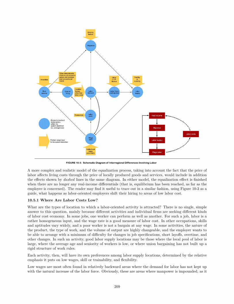
A more complex and realistic model of the equalization process, taking into account the fact that the price oflabor affects living costs through the price of locally produced goods and services, would include in additionthe effects shown by dashed lines in the same diagram. In either model, the equalization effect is finishedwhen there are no longer any real-income differentials (that is, equilibrium has been reached, as far as theemployee is concerned). The reader may find it useful to trace out in a similar fashion, using Figure 10-3 as aguide, what happens as labor-oriented employers shift their hiring to areas of low labor cost.

10.5.1 Where Are Labor Costs Low?

What are the types of location to which a labor-oriented activity is attracted? There is no single, simpleanswer to this question, mainly because different activities and individual firms are seeking different kindsof labor cost economy. In some jobs, one worker can perform as well as another. For such a job, labor is arather homogeneous input, and the wage rate is a good measure of labor cost. In other occupations, skillsand aptitudes vary widely, and a poor worker is not a bargain at any wage. In some activities, the nature ofthe product, the type of work, and the volume of output are highly changeable, and the employer wants tobe able to arrange with a minimum of difficulty for changes in job specifications, short layoffs, overtime, andother changes. In such an activity, good labor supply locations may be those where the local pool of labor islarge, where the average age and seniority of workers is low, or where union bargaining has not built up arigid structure of work rules.

Each activity, then, will have its own preferences among labor supply locations, determined by the relativeemphasis it puts on low wages, skill or trainability, and flexibility.

Low wages are most often found in relatively backward areas where the demand for labor has not kept upwith the natural increase of the labor force. Obviously, these are areas where manpower is impounded, as it

209

were, by its imperfect outward mobility. Less obviously, such areas tend to develop certain characteristicsthat impede out-migration.

Many such areas specialize heavily in kinds of employment for which the demand has grown slowly or declined(for example, general farming or coal mining). This may, in fact, be the chief reason why they are areas oflabor surplus. But this specialization also means that their labor force lacks experience in more dynamicindustries or occupations, which is a disadvantage in seeking work elsewhere. There are attitudinal barriers,too, to giving up an occupation in which one has acquired skill and seniority in order to start near the bottomin a new trade. Derelict coal-mining villages in Appalachia are full of middle-aged and older ex-miners whoare slow to consider any alternative line of work, even though it may be clear that the local mine is closedfor good. Finally, the very existence of a labor surplus and low wages helps to lower the cost of such majorbudget items as shelter and services, and this helps to diminish the economic incentive to move out.

The advantages of experience and skill in a labor supply are most often found in areas where the educationallevel is high and where activities requiring some special skills have been concentrated for a long time. Thesupply of some types of highly paid and scarce manpower (such as scientific and other specialists, or personsof high artistic capability) is coming to be located increasingly in areas and communities of high physical andcultural amenity, since those types of people are in such demand that they can afford to be quite choosyabout where they are willing to live. It is no accident or whim that has located so many advanced-technologyand research-oriented activities in pleasant places near major universities.

Flexibility and diversity of labor supply are most likely to be found in a large labor market in an intensivelyurbanized region, although one might surmise that the rapid population growth of nonmetropolitan areasduring the 1970s has increased the diversity of labor supply in many less developed places as well. In somelarge urban labor markets, however, the potential labor economies of size and diversity are partly offset bythe greater rigidity of union work rules and bargaining practices, and the greater age and seniority of thework force that characterize an area where an activity has developed a mature concentration.

The different kinds of labor cost advantage (low wage rates, skill, and flexibility and diversity of supply) areunlikely to be found in the same places, because to some extent they reflect contrasting area characteristics.Thus low wage rates are associated with less developed areas having low living costs. Experience and diversityof supply are often associated with the opposite type of location: large urban areas in advanced industrializedregions having relatively high living costs. Any given area, then, tends to be classified according to the aspectof labor supply in which it has the greatest comparative advantage.

10.5.2 Indirect Advantages of Labor Quality

The cost savings involved in the use of highly productive (that is, skilled and/or adaptable) manpowerare sometimes underestimated, because not all of them show up in labor cost per se. Recall the case ofHarkinsville and Parkston discussed in Chapter 2. Harkinsville workers work faster, and get correspondinglyhigher hourly wages, than those in Parkston. Thus there is no difference in labor cost per hour. Nevertheless,it will be recalled, Harkinsville is a better location for the employer. For example, if the output of the firm isto be 1000 units a day at whichever location is chosen, the production worker payroll will be the same ateither location; but the plant can be smaller at Harkinsville. This means a smaller investment in land andbuildings; a smaller parking lot and cafeteria; fewer washrooms, drinking fountains, and other facilities; asmaller work load for payroll accounting and personnel management; and so on. Only such cost items as aregeared directly to the volume of output and not the number of people working will be as large in Harkinsvilleas in Parkston: for example, production materials, shipping containers, motive power and fuel for processing,and loading and handling facilities.

10.5.3 Institutional Constraints on Wages and Labor Costs

To an increasing extent in most countries, the supply of labor to an individual employer at one location isaffected by bargaining procedures and constraints involving other employers and other locations as well. Inactivities where the employing firms are few and large and where a strong labor organization includes a majorfraction of the workers, key negotiations can set a quasi-national pattern of fringe benefits and work rulessubject to only minor local differences. Examples include the steel and automobile industries and rail and air

210

transportation. In still other activities, agreements cover major sections of the activity (such as the EastCoast ports with respect to handling ship cargo).

Multiarea bargaining introduces a strong additional equalization element into the wage pattern. Even moregenerally, labor organizations with aspirations for nationwide power try to work toward elimination of regionalwage differentials. Lower wages in areas of weaker organization are viewed as a threat to employment in theareas of stronger organization and higher wages, since employers are naturally tempted to move to save laborcosts. And employers not contemplating such a move are, of course, in favor of higher labor costs for theircompetitors. Both parties, then, may well favor extension of the geographical area of wage bargaining andthe enactment of federal and state minimum-wage laws, which limit differentials still further.

There are often pressures toward similarity of pay rates and fringe benefit levels among different activitiesand occupations within a single-labor market. This means that if there are important high-wage activities inan area, they tend to some extent to set the tone for related types of employment in the same area and tomake it generally a higher-cost area than it might otherwise be.

It is easy to see how this works between occupations calling for similar qualifications, so that the variousactivities in the community are competing in a common pool of available workers with those qualifications.For example, steel workers are relatively highly paid; as a result, a community dominated by steel making islikely to have relatively high wage scales in construction and in other kinds of employment not too different intheir requirements from the jobs of many steel mill employees. There would be no such direct effect, however,on wage rates for sales or clerical workers.

Furthermore, unions of the dominant industry in a community generally organize a number of other industriesas well, the jurisdictional lines being rather loose. Thus in Pittsburgh, metal fabricating plants are mainlyorganized by the steelworkers’ union, while similar plants in Detroit have locals of the automobile workers’union. Though such a union does not necessarily find it feasible or desirable to extend the wage and benefitspattern in the dominant industry to the other industries it has organized in the same community, there iscertainly some pressure in that direction, and a consequent reinforcing of the tendency toward intraarea wagelevel conformity.28

This tendency is not area-wide, as a rule. For example, in the Pittsburgh labor market area the upward wagepressures arising from the importance of some tightly organized and high-paying industries are essentiallyrestricted to blue-collar occupations traditionally dominated by male workers, which heavily predominatein the major industries involved. For many years, however, Pittsburgh wages in retail trade and generallyfor jobs traditionally held by women tended to be a little lower than those in cities of comparable size inthe same part of the country. Presumably, this reflected the relatively slow growth of the area as a wholeand the relative surplus of employable women arising from the predominance of male jobs in the area. It isinteresting to note that in the late 1950s the differentials began to disappear, perhaps reflecting vigorouslocal growth in office employment and no growth in heavy industry employment.29

It has been observed that the wage spread or skill margin among different occupations within a single labormarket is generally wider in less developed and slower growing regions. This has been explained in terms ofthe lower educational standards and the smaller proportion of semiskilled manufacturing jobs in such areas,since education and the availability of an accessible “ladder” of skill development both enhance occupationalmobility and make the labor market more competitive.30

A further explanation lies in the tendency for people of higher occupational, educational, and earnings levelsto be geographically more mobile. As a result, regional differentials in their earnings are narrower than is thecase for lower-status people.31 In an area of labor surplus and out-migration, it is the people in the better-paidoccupations who move out most readily; a relatively larger differential is required to move the unskilled. The

28On this and related questions, see Pittsburgh Regional Planning Association, Region in Transition, Economic Study of thePittsburgh Region, vol. I (Pittsburgh: University of Pittsburgh Press, 1963), Chapter 4, especially pp. 106-109.

29Ibid.30See Melvin W. Reder, “The Theory of Occupational Wage Differentials,” American Economic Review, 45, 5 (December

1955), 846-847.31This relationship was noted earlier in connection with Table 10-1.

211

wage spread in such a labor market is consequently wide compared to that in a more prosperous and activeplace.

10.5.4 Complementary Labor

Different categories of labor are to some extent jointly supplied; that is, the supply of one kind of labor in anarea depends on how much of the other kind is there. A local population or potential labor force is almostalways an assortment of people of different ages, sexes, and physical and mental capabilities. If most of thejobs available in the area call for superior aptitude, the area is likely to have a surplus of people with morepedestrian abilities, and these may represent a bargain in labor supply for an activity with less exactingrequirements. Conversely, if all the jobs in an area involve rugged manual labor, there is likely to be a surplusof not quite so rugged individuals, who might represent a bargain labor supply for an activity not requiringphysical strength.

We have to consider, then, as another kind of advantageous labor location for an activity, places where thereis a heavy demand for some kind of contrasting and complementary labor. This principle assumes, of course,that mobility is quite imperfect, so that not all the different types of workers are able to seek out the locationswhere their own kind of work is best rewarded.

The most important basis for such restriction is inherent in family ties. In a family’s choice of location fromthe standpoint of income, the most important consideration is opportunity and earnings for the principalearner, usually the head of the family. The spouse, and any other full or partial dependents of working age,is then part of the potential labor supply in the area where the principal wage earner locates. Accordingly, alabor market heavily specialized in activities employing men is likely to have a plentiful and relatively cheapfemale labor supply, and a labor market heavily specialized in activities employing mature adults is likely tohave a plentiful and relatively cheap supply of young labor of both sexes.

Historically, many industries have owed their start in certain areas to a complementary labor supply generatedin such a way. A classic case is the making of shoes in colonial days in eastern Massachusetts. The coastalarea north of Boston was heavily specialized in the male occupations of sailing and fishing; this created alarge complementary labor surplus of wives and daughters, who were able to supplement family incomes bymaking shoes—first at home and later in small factories.32 At a later period, the anthracite mining area ofeastern Pennsylvania attracted a substantial amount of the silk-weaving industry on a similar basis. As lateas the 1920s, it was observed that in the anthracite area about 60 percent of the silk weavers were women,while in the previous center of that industry (in and around Paterson, New Jersey) 60 percent were men.The manufacture of cheap standard garments, cigars, and light electrical equipment and components also hashistorically been attracted to places offering plentiful and cheap complementary labor.33

10.6 Labor Cost Differentials and Employer Locations Within an Urban LaborMarket AreaUp to this point, we have been looking at the location of people and differentials in earnings and laborcosts on a macrogeographic scale, comparing labor markets as units. A quite different set of considerationscomes to the fore when we adopt a microgeographic focus. Since the question of people’s residential locationpreferences within urban areas has been dealt with in some detail in Chapters 6 and 7, we shall focus on thelocational preferences of employers as influenced by labor supply.

Although labor market areas are in principle defined in terms of a feasible commuting range, people prefershort work journeys to long ones, and as shown in Chapter 6, residential location decisions reflect this andother access considerations. Thus the supply of labor to an employer is not really ubiquitous throughout anurban area. Differential advantages of labor supply within a local labor market are particularly significantwhen the employer wants a special type of labor or a large supply of job candidates, and in large labor marketareas where residential areas are sharply differentiated in character.

32See E. M. Hoover, Location Theory and the Shoe and Leather Industries (Cambridge, Mass.: Harvard University Press,1937), pp. 109, 215-217, and sources cited therein.

33Robert Murray Haig, “Toward an Understanding of the Metropolis,” Quarterly Journal of Economics, 40, 1 (February 1926),195.

212

Thus if an activity mainly employs a class of people dependent on public transportation to get to work (forexample, very low-income people or married people whose spouses preempt the family car for their owncommuting), it may have difficulty in recruiting an adequate work force in the less accessible suburban areas.Even if there is not an absolute shortage of applicants, there may not be enough of a surplus of applicants toallow much freedom of selection.

In the late 1950s, a study was made of the recruiting experiences of business firms in the Boston metropolitanarea which had relocated to sites along a circumferential suburban freeway.34 Most of the establishmentsin the sample canvassed were sizable manufacturing plants, with electronics equipment the most numerouscategory. Every firm in the sample had made an advance survey of the residential and commuting patterns ofits employees in an effort to anticipate any recruitment problems that the new location might involve. Severalof the firms took explicit account of employee residential locations in choosing the specific section of thehighway on which to relocate. Every firm found it necessary to establish a plant cafeteria at the new location.

The survey’s findings on recruitment problems were summed up as follows:

A summary of the observations of personnel managers interviewed indicated a general, but notuniversal, conclusion that Route 128 locations in comparison with the downtown areas definitelyeased recruitment of engineering, professional and administrative staff, but neither helped norhindered recruitment of skilled labor. Recruiting difficulties arose especially when the firms soughtyoung, female clerical workers, male unskilled workers, and seasonal workers, both male andfemale, particularly in the higher income suburbs of the western subarea of Route 128. The typeof recruitment problem mentioned most frequently was that of the younger, unmarried female,clerical workers.

The most serious of the recruitment problems was that of unskilled production labor, both maleand female, but especially male, for seasonal work. Although this problem did not arise frequently,the need for a seasonal expansion of employment could cause a major headache for the personneldepartment, and [seems?] to indicate very sharply the lack of a casual labor market in the suburbs.At a downtown location, a firm could readily draw unskilled male and female workers with a“Help Wanted” sign in the window for seasonal employment. At a Route 128 location, this type oflabor was scarce, and intown labor found commuting to the plant time-consuming and costly forlow-paying jobs on a seasonal basis.

. . . The existence of a circumferential highway or of a few long-distance commuters does not leadto the conclusion that there is also a circumferential labor market, in which a firm at any onelocation can draw equally well from any other part of the area. On the contrary it would appear asif suburban firms tend to draw from areas nearby, and lose those workers who live at abnormallylong distances away.

. . . Relationship of a firm to the immediate local labor supply seems to be crucial. Where thelocal supply is already committed, or of the wrong composition to meet the demands of the firm,the company will be forced to rely on longer-distance commuters. If this means extension ofcommuting beyond the normal range or direction, for that type of labor, the firm will be likely tohave major labor supply difficulties)35

It has been more than a quarter of a century since this report was published, but these findings are stillrelevant. The area around Route 128 (now an interstate highway) has become one of the nation’s majorcenters for advanced-technology activities; and as the metropolitan area has grown, the labor market in thevicinity of this highway has diversified substantially. However, the recruitment problems described in thereport’s summary are now characteristic of firms considering locations on a yet more remote beltway I-495around the Boston metropolitan area.

More recent and more elaborate studies have brought out some additional details concerning the characteristicsof urban labor markets, For example, Albert Bees and George Shultz found in the Chicago labor market

34Everett J. Burtt, Jr., “Labor Supply Characteristics of Route 128 Firms,” Research Report No. 1-1958 (Boston: FederalReserve Bank of Boston, 1958; mimeographed).

35The excerpts quoted here appear in a somewhat altered sequence.

213

significant wage differentials for the same occupation among different neighborhoods within the metropolitanarea, corresponding generally to the directions of commuter flow.36 Similar differentials have also beenidentified on the basis of distance from the central business district.37 The labor market of a large metropolisis clearly not a single spatially perfect market in the sense that location within it makes no difference.

As one might expect, the least mobile types of manpower (low-skilled workers, members of minority groupswhose housing location choice is restricted by discrimination, and secondary and complementary workers)38

evince the greatest market imperfection in terms of differentials in their net earnings after deducting commutingcosts. This same tendency toward wider geographical wage differentials for lower-income occupational groupshas already been noted at the interregional level.

Workers are attracted in their residential choices toward job locations, whereas employers are attracted towardcheap labor supply. The relative force of these two sides of a mutual linkage varies widely among occupations,of course. At one extreme, the wage rate in an occupation is uniform throughout the labor market area, andthe commuters from more distant residential areas bear all of the extra money and time costs of commutingover those greater distances. In the other extreme case, the employers pay higher wages at job locationsfarther from employee residential areas, absorbing the added costs of commuting longer distances by payingcompensating differentials in wages.39

The amount of variation in wages in any given occupation will depend on the relative mobility of the employeesand the employers and also on the extent to which union agreements or understandings among employersimpose a single wage standard for the whole labor market area. It will depend also on two factors alreadymentioned; namely, the skill and income level of the occupation itself and the extent to which the workers’residential choices are limited by discrimination.

It is clear that the spatial imperfection of large urban labor markets affects particularly the low-incomeworker. One of the most serious aspects of the present-day problem of inadequate job opportunities forresidents of urban slums is that an increasing proportion of the kinds of jobs they might fill has shifted todistant suburban locations with little or no public transportation available, while very few employers havebeen willing to accept some obvious disadvantages of a slum location for the sake of closer access to thatlabor supply.

10.7 SummarySeveral kinds of spatial differentials in earnings and income are of interest to various parties. The relativeopulence of two communities can be compared in a marketing survey in terms of total or per capita moneyincome. An individual looking for a good place to work would be interested in wage rates or annual earningsin his or her specific occupation, adjusted for any differences in the cost of living. An employer looking forlow labor costs would want to compare specific wage scales, adjusted for productivity and fringe benefits.

Relative pay levels in specific occupations in the United States show a pattern of interregional differentials,with lower levels in the South and in smaller labor markets. These two differentials (North-South, andsize of place) appear also in measures of per capita annual income and living costs. Income and pay levels

36Albert Rees and George P. Shultz, Workers and Wages in an Urban Labor Market (Chicago: University of Chicago Press,1970).

37See Randall W. Eberts and Timothy J. Gronberg, “Wage Gradients, Rent Gradients, and the Price Elasticity of Demand forHousing: An Empirical Investigation,” Journal of Urban Economics, 12, 2 (September 1982), 168-176.

38Secondary workers are those who are in the labor force intermittently or part time. Complementary workers (see Section10.5.4) are those who belong to a household in which they are not the principal earner. There is of course a considerable overlapbetween these categories.

39Rees and Shultz found substantial evidence of payment of part of the extra commuting costs of the more distant workers bylarge establishments in the Chicago labor market in the late 1960s. (This does not necessarily imply that specific employerspaid wage premiums to those individual workers who had the longer commuting journeys, but rather that employers locatedlong distances from residential areas of the type of workers they employed tended to pay higher wages than did employerslocated closer to such residential areas.) For a sample of workers in each of a number of occupations, Rees and Shultz found apositive correlation between wage rate and distance traveled to work when such other wage-influencing variables as the age,seniority, education, and race of the worker were also included in the regression equation. As a percentage of mean earnings, theextra compensation for added travel time ranged from 2 percent for janitors to 13 ½ percent for accountants. Rees and Shultz,Workers and Wages, pp. 169-175; see also Hoch, “Income and City Size,” p. 316.

214

deflated by cost-of-living indices seem also to show similar patterns, but to a much smaller degree. The term“equalizing differentials” is applied to a differential in money wages or income that merely compensates for acost-of-living differential.

People move in response to perceived differences in prospective real incomes as well as other factors; migrationflows depend on the characteristics of both the origin and the destination areas, the difficulties of the journey,and the characteristics of the migrant. Within a labor market area, housing and personal considerationsaccount for most moves; for migration between labor market areas, job-related reasons are the most important.

The cost and difficulty of migration is roughly related to distance, and migration streams do show attenuationwith distance, which can be expressed in a gravity-type migration model. Social distance is a broader termdesigned to take account of the degree of sociocultural adjustment required of the migrant in addition tocosts of distance per se. Such considerations account for the beaten-path effect (migration is easier alongpaths used by many previous migrants from the same area).

Age is the personal characteristic most markedly related to migration rates, with generally declining rates tothe late teens, a sharp peak around age eighteen to twenty, and a decelerating decline to old age with a smallpeak at retirement time. Migration rates are positively associated with both education and occupationalstatus or skill, at any given ages.

Places with high rates of in-migration tend to have high rates of outward migration as well, because of thebeaten-path effect and also because heavy in-migration produces a population with characteristics conduciveto high mobility in terms of age, education, family status, disposition, and migration experience. Earningslevels and employment opportunity affect the amount of in-migration to a labor market but seem to havelittle effect on out-migration rates except in seriously distressed areas.

There has been a decline in overall migration rates in the United States since World War II. The factorscontributing to this decline differ for short- and long-distance moves, but they include decreases in the averagesize of households, increased home ownership, and greater incidence of two-wage-earner households. Regionshave also become more alike, thus reducing the incentive to migrate.

Labor mobility and the lack of it play a part in the development of labor cost differentials, which in turn affectthe location of some interregionally footloose activities. Each such activity has its own preferences amonglabor supply locations, determined by the relative emphasis it places upon low wages, skill or trainability,and flexibility.

Low wages are most often found in relatively backward and/or depressed areas where labor demand has notkept up with the natural increase of the labor force. Limitations on outward mobility, particularly for the poorand less skilled, dam up in such places a pool of cheap surplus labor. In addition, low-cost complementaryor secondary labor supplies occur in areas where there is a relatively heavy demand for the kind of laborservices provided by the principal earners of families but relatively little demand for the services of otherfamily members such as spouses or children.

For activities requiring a highly skilled or educated labor force, developed areas with high amenity are morelikely to furnish the desired kind of labor supply. Flexibility and diversity of labor supply are most likely tobe found in large metropolitan areas; however, these advantages are partially offset by more restrictive workand seniority rules.

Institutional constraints and the wage-bargaining procedures associated with large employee and employerorganizations generally work in the direction of greater interregional wage uniformity in a given industry oroccupation and also greater local uniformity among different industries and occupations within a single labormarket area. There is some tendency for the wage spread between occupations to be wider in areas of slowemployment growth or decline, reflecting in large part the higher mobility of the better-paid occupations.

Within large labor market areas, distance and commuting costs produce significant differentials in availablelabor supply, which are reflected in partially compensatory wage premiums at locations relatively far fromworkers’ residential areas.

215

Technical Terms Introduced in this ChapterSpatial mobility Chain migrationEqualizing differentials in wages and incomes Migration rateReal differentials in wages and incomes Selectivity of migrationPull and push factors motivating migration Positively and negatively selective migrationSocial distance Lowry hypothesisFunctional distance Beale hypothesisBeaten-path effect Labor-oriented activitiesCounterstream effect Compensating wage differentials

Selected ReadingsMichael J. Geenwood, “Research on Internal Migration in the United States: A Survey,” Journal of EconomicLiterature, 13, 2 (June 1975), 397-433.

Irving Hoch, “Income and City Size,” Urban Studies, 9, 3 (October 1972), 229-328.

Chang-I Hua and Frank Porell, “A Critical Review of the Development of the Gravity Model,” InternationalRegional Science Review, 4, 2 (Winter 1979), 97-125.

Albert Rees and George P. Shultz, Workers and Wages in an Urban Labor Market (Chicago: University ofChicago Press, 1970).

Harry W. Richardson, Regional Economics (Urbana: University of Illinois Press, 1978), Chapter 5.

Larry A. Sjaastad, “The Costs and Returns of Human Migration,” Journal of Political Economy, 70, 5 (2)(Supplement, October 1962), 80-93.

216

11. HOW REGIONS DEVELOPSome of the most important problems to which regional economists and planners address themselves involveprocesses of growth (or more broadly, change) in the economies of regions. Such changes concern, of course,the people dwelling in the region; they concern also business firms and individuals who are choosing a regionfor their future activities; and they concern administrators and policy makers on the national level.

The objectives and tools of public policy will be examined in Chapter 12; the present chapter inquires whyand how regional growth and other major changes occur.

11.1 Some Basic Trends and QuestionsSheer growth of population is sometimes thought to be a measure of progress. More relevant to the ideaof developmental advance is, of course, rising income levels. Finally, major changes in regional economicstructure seem to accompany development. We shall look briefly at some regional trends in population, percapita income, and activity-mix in the United States in order to identify the most meaningful aspects andissues of regional development.

11.1.1 Relative Regional Growth in Population

Figure 11-1 shows the differences in the population growth rates of the Census divisions’ of the United Statesover the past century or so. We are concerned here not with the absolute sizes of the divisions1 populationsbut only with the question of which areas have shown faster growth than others in each period. Accordingly,the chart is plotted on a logarithmic or ratio scale, so that the slope of a line on it represents the percentagerate of population growth per annum, and the lines for the different Census divisions (see Figure 11-2) aresimply stacked in convenient order on the chart for comparison. We are interested not in the vertical positionof these lines but only in their relative slopes.

1The areas involved are mapped in Figure 11-2. We shall sometimes in this chapter refer to the individual Census divisionsas “regions,” despite the fact that the Census Bureau (as shown in Figure 11-2) groups them into still larger areas, which it calls“Census regions.”

217

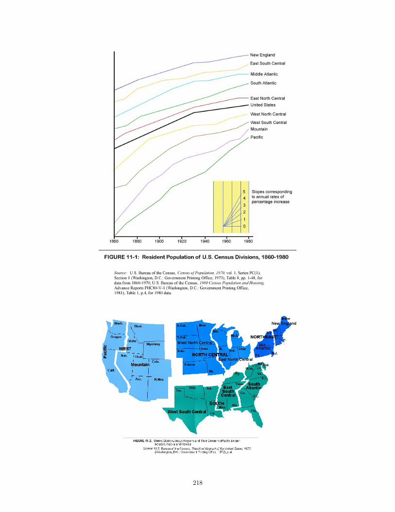
218

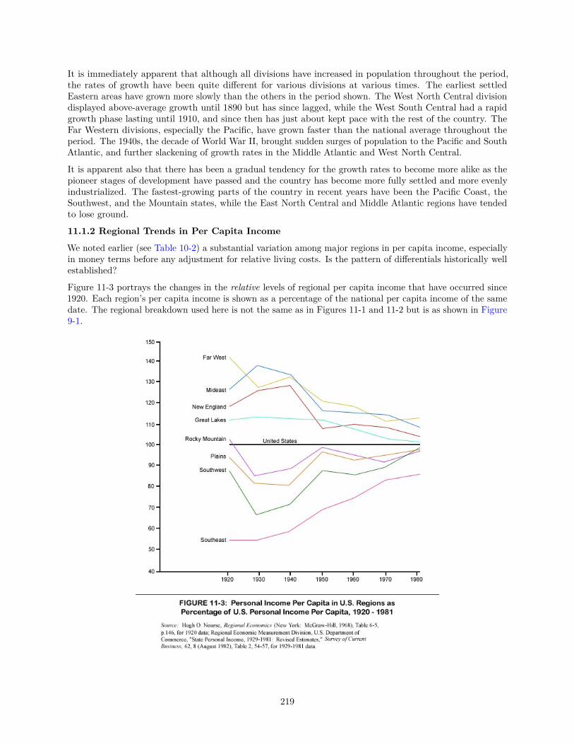
It is immediately apparent that although all divisions have increased in population throughout the period,the rates of growth have been quite different for various divisions at various times. The earliest settledEastern areas have grown more slowly than the others in the period shown. The West North Central divisiondisplayed above-average growth until 1890 but has since lagged, while the West South Central had a rapidgrowth phase lasting until 1910, and since then has just about kept pace with the rest of the country. TheFar Western divisions, especially the Pacific, have grown faster than the national average throughout theperiod. The 1940s, the decade of World War II, brought sudden surges of population to the Pacific and SouthAtlantic, and further slackening of growth rates in the Middle Atlantic and West North Central.

It is apparent also that there has been a gradual tendency for the growth rates to become more alike as thepioneer stages of development have passed and the country has become more fully settled and more evenlyindustrialized. The fastest-growing parts of the country in recent years have been the Pacific Coast, theSouthwest, and the Mountain states, while the East North Central and Middle Atlantic regions have tendedto lose ground.

11.1.2 Regional Trends in Per Capita Income

We noted earlier (see Table 10-2) a substantial variation among major regions in per capita income, especiallyin money terms before any adjustment for relative living costs. Is the pattern of differentials historically wellestablished?

Figure 11-3 portrays the changes in the relative levels of regional per capita income that have occurred since1920. Each region’s per capita income is shown as a percentage of the national per capita income of the samedate. The regional breakdown used here is not the same as in Figures 11-1 and 11-2 but is as shown in Figure9-1.

219

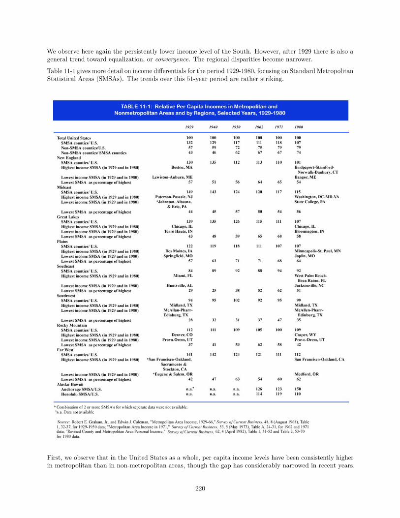
We observe here again the persistently lower income level of the South. However, after 1929 there is also ageneral trend toward equalization, or convergence. The regional disparities become narrower.

Table 11-1 gives more detail on income differentials for the period 1929-1980, focusing on Standard MetropolitanStatistical Areas (SMSAs). The trends over this 51-year period are rather striking.

First, we observe that in the United States as a whole, per capita income levels have been consistently higherin metropolitan than in non-metropolitan areas, though the gap has considerably narrowed in recent years.

220

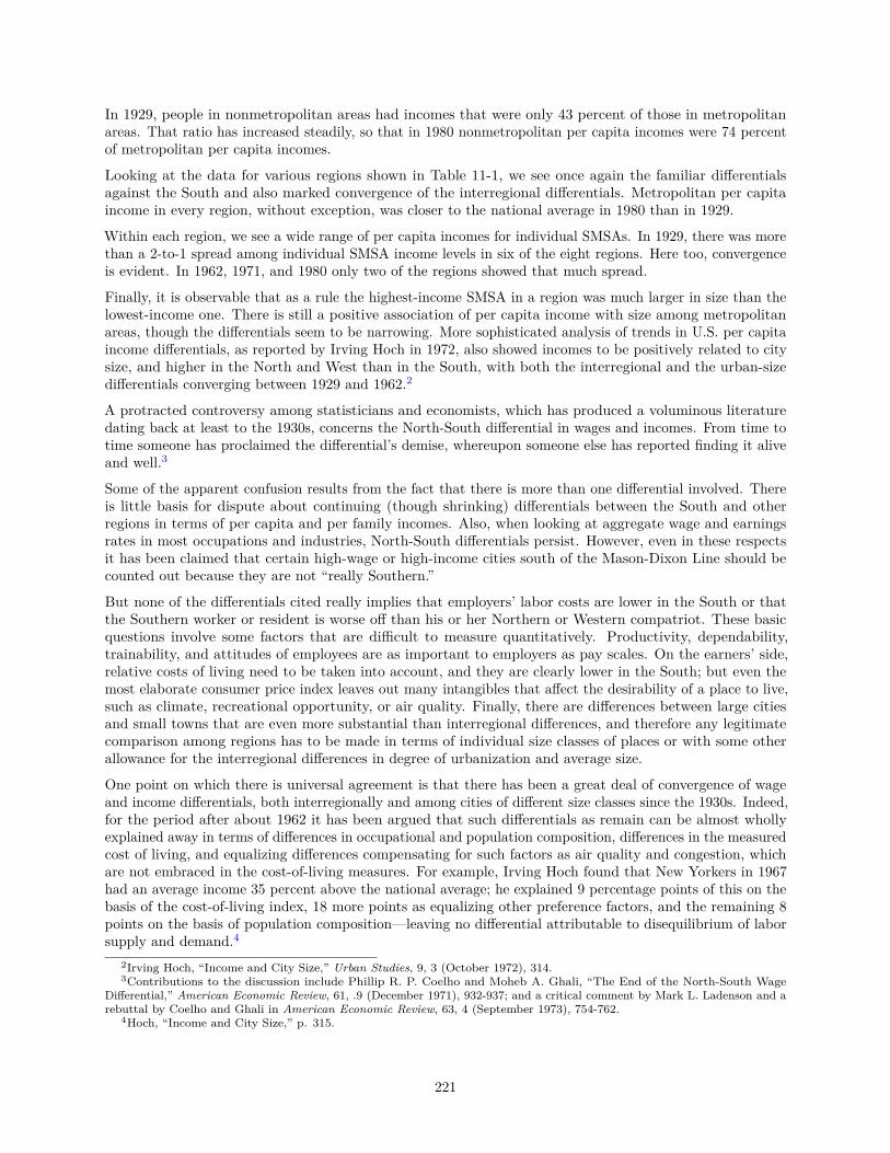
In 1929, people in nonmetropolitan areas had incomes that were only 43 percent of those in metropolitanareas. That ratio has increased steadily, so that in 1980 nonmetropolitan per capita incomes were 74 percentof metropolitan per capita incomes.

Looking at the data for various regions shown in Table 11-1, we see once again the familiar differentialsagainst the South and also marked convergence of the interregional differentials. Metropolitan per capitaincome in every region, without exception, was closer to the national average in 1980 than in 1929.

Within each region, we see a wide range of per capita incomes for individual SMSAs. In 1929, there was morethan a 2-to-1 spread among individual SMSA income levels in six of the eight regions. Here too, convergenceis evident. In 1962, 1971, and 1980 only two of the regions showed that much spread.

Finally, it is observable that as a rule the highest-income SMSA in a region was much larger in size than thelowest-income one. There is still a positive association of per capita income with size among metropolitanareas, though the differentials seem to be narrowing. More sophisticated analysis of trends in U.S. per capitaincome differentials, as reported by Irving Hoch in 1972, also showed incomes to be positively related to citysize, and higher in the North and West than in the South, with both the interregional and the urban-sizedifferentials converging between 1929 and 1962.2

A protracted controversy among statisticians and economists, which has produced a voluminous literaturedating back at least to the 1930s, concerns the North-South differential in wages and incomes. From time totime someone has proclaimed the differential’s demise, whereupon someone else has reported finding it aliveand well.3

Some of the apparent confusion results from the fact that there is more than one differential involved. Thereis little basis for dispute about continuing (though shrinking) differentials between the South and otherregions in terms of per capita and per family incomes. Also, when looking at aggregate wage and earningsrates in most occupations and industries, North-South differentials persist. However, even in these respectsit has been claimed that certain high-wage or high-income cities south of the Mason-Dixon Line should becounted out because they are not “really Southern.”

But none of the differentials cited really implies that employers’ labor costs are lower in the South or thatthe Southern worker or resident is worse off than his or her Northern or Western compatriot. These basicquestions involve some factors that are difficult to measure quantitatively. Productivity, dependability,trainability, and attitudes of employees are as important to employers as pay scales. On the earners’ side,relative costs of living need to be taken into account, and they are clearly lower in the South; but even themost elaborate consumer price index leaves out many intangibles that affect the desirability of a place to live,such as climate, recreational opportunity, or air quality. Finally, there are differences between large citiesand small towns that are even more substantial than interregional differences, and therefore any legitimatecomparison among regions has to be made in terms of individual size classes of places or with some otherallowance for the interregional differences in degree of urbanization and average size.

One point on which there is universal agreement is that there has been a great deal of convergence of wageand income differentials, both interregionally and among cities of different size classes since the 1930s. Indeed,for the period after about 1962 it has been argued that such differentials as remain can be almost whollyexplained away in terms of differences in occupational and population composition, differences in the measuredcost of living, and equalizing differences compensating for such factors as air quality and congestion, whichare not embraced in the cost-of-living measures. For example, Irving Hoch found that New Yorkers in 1967had an average income 35 percent above the national average; he explained 9 percentage points of this on thebasis of the cost-of-living index, 18 more points as equalizing other preference factors, and the remaining 8points on the basis of population composition—leaving no differential attributable to disequilibrium of laborsupply and demand.4

2Irving Hoch, “Income and City Size,” Urban Studies, 9, 3 (October 1972), 314.3Contributions to the discussion include Phillip R. P. Coelho and Moheb A. Ghali, “The End of the North-South Wage

Differential,” American Economic Review, 61, .9 (December 1971), 932-937; and a critical comment by Mark L. Ladenson and arebuttal by Coelho and Ghali in American Economic Review, 63, 4 (September 1973), 754-762.

4Hoch, “Income and City Size,” p. 315.

221

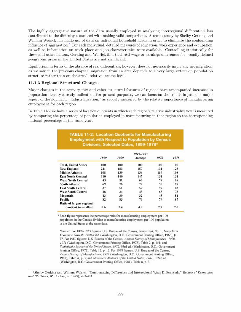
The highly aggregative nature of the data usually employed in analyzing interregional differentials hascontributed to the difficulty associated with making valid comparisons. A recent study by Shelby Gerking andWilliam Weirick has made use of data on individual household heads in order to eliminate the confoundinginfluence of aggregation.5 For each individual, detailed measures of education, work experience and occupation,as well as information on work place and job characteristics were available. Controlling statistically forthese and other factors, Gerking and Weirick find that real-wage or earnings differences for broadly definedgeographic areas in the United States are not significant.

Equilibrium in terms of the absence of real differentials, however, does not necessarily imply any net migration;as we saw in the previous chapter, migration from an area depends to a very large extent on populationstructure rather than on the area’s relative income level.

11.1.3 Regional Structural Changes

Major changes in the activity-mix and other structural features of regions have accompanied increases inpopulation density already indicated. For present purposes, we can focus on the trends in just one majoraspect of development: “industrialization,” as crudely measured by the relative importance of manufacturingemployment for each region.

In Table 11-2 we have a series of location quotients in which each region’s relative industrialization is measuredby comparing the percentage of population employed in manufacturing in that region to the correspondingnational percentage in the same year.

5Shelby Gerking and William Weirick, “Compensating Differences and Interregional Wage Differentials,” Review of Economicsand Statistics, 65, 3 (August 1983), 483-487.

222

For example, in 1899 in the United States as a whole, 6.49 percent of the population was employed inmanufacturing industries, while in New England the percentage was 15.6, or 241 percent of the nationalaverage. This location quotient of 241 percent tells us that New England had 2.41 times as much manufacturingemployment as it would have had on a pro rata basis if manufacturing were distributed in the same geographicalpattern as was population among the regions. Referring again to Table 11-2, we see that in the same year,1899, the West South Central region had a location quotient of only 28 percent, indicating a markedunderrepresentation of manufacturing in that region.

As we read across to the later years, New England’s coefficient drops. The region’s specialization inmanufacturing was diminishing, and New England was becoming more like the rest of the country in itsdegree of industrialization (or rather, the rest of the country was becoming more like New England). TheMiddle Atlantic region, another area of relatively early industrial development, showed a similar trend, whilethe East North Central region became more specialized in manufacturing until around 1950, and then less so.Most of the regions that were far less industrialized than the rest of the country in the earlier period hadrising location quotients for manufacturing, so that the overall trend is strongly convergent. Manufacturinghas come to be distributed among regions in a pattern more and more similar to the pattern of populationdistribution. This convergence is brought out by the bottom row of figures in Table 11-2, which shows therange of variation of the location quotients steadily narrowing.

11.1.4 Some Basic Questions on Regional Development

In this thumbnail survey of population growth, income levels, and industrialization, we gather that morerecently settled regions have tended to show relatively fast growth for a considerable period, followed by aslowdown—suggesting a pattern of successive phases in a development sequence in which migration plays aprominent role. We see also that interregional differences in income level have been quite persistent but seemto have narrowed a great deal, especially in certain periods such as 1930 to 1970. Indeed, convergence in thesense of a growing similarity among regions is observable in respect to all three of the indicators examined:rate of population growth, level of per capita income, and relative importance of manufacturing employment.

Accordingly, some key questions suggest themselves:

1. Causes of growth. Why do some regions grow faster than others? What are the primary initiating factorsresponsible, and through what processes do these causes operate? What is the role of interregional trade,migration, and investment in the spread of development from one region to another?

2. Structure. How does regional economic structure relate to growth? What kinds of structure are conduciveto growth, or the reverse? What structural changes are associated with growth?

3. Convergence. Why is convergence so much in evidence? Is it universal and inevitable, or is it subject toreversals?

4. Control over regional development. Can regional development be substantially guided by policy? If so,what are defensible objectives and appropriate policies?

The questions on policy will come up in Chapter 12; the other questions are examined later in the presentchapter.

11.2 What Causes Regional Growth?Regional growth and change entail complex interactions among activities within the regional economy, soit is not reasonable to expect that any single cause of such change can be identified. Useful explanationsconsist mainly of analyses of the ways in which an impetus of change is passed from one region or oneregional activity to another, and we have in fact sorted out the various intraregional linkages in some detailalready in Chapter 9. Some theories of development, however, emphasize certain kinds of change as especiallyindependent, exogenous, primary, or causal. (All these terms mean much the same.) In particular, we shallsee that the external demand for a region’s exports and its supply of labor and other production factors havebeen stressed as prime movers in some widely accepted theories of regional development.

11.2.1 Self-Reinforcing and Self-Limiting Effects

223

Our examination of the various kinds of linkages among firms and activities in a region brought to light someeffects of a cumulative or chain-reaction character. Both vertical and complementary linkages are generallyof this type. Thus external economies of agglomeration (the expression of complementary linkages) attractfirms and activities of a similar nature, and this further enhances the agglomeration economies, so that stillmore firms and activities are attracted, which leads to still more agglomeration economies.

Vertical linkages per se have cumulative effects. If Detroit can increase its automobile sales to other areas,Detroit’s automobile manufacturers will buy larger quantities of inputs locally. Each of the supplying activitieswill then increase its own local purchases of inputs (for example, automobile workers will spend some of theincreased payroll on housing, consumer goods, and services, and Detroit public utilities will need more laborand other inputs). Some of the additional spending in Detroit will take the form of increased purchases ofautomobiles, which will further contribute to the repercussions of the initial stimulus.

It appears, then, that vertical linkages of activities in a region and also complementary linkages (which arereally combinations of vertical linkages) have self-reinforcing effects. An initial change in the level of activityin the region leads to still further change in the same direction and affects a broader range of activities. Thisapplies to decline as well as to growth.

This being the case, how does it happen that regions do not normally expand in an explosive chain-reactionfashion, or wither away to the vanishing point? What are the forces that provide some constraint and stability,by setting up counterreactions to an initial change and thus limiting its total effects?

Part of the answer lies in the horizontal linkages among activities, which as we have seen are characteristicallynegative, or locationally repulsive, in their effects. In other words, activities in a region are always competingfor some scarce local inputs (land, labor, and others); and, particularly in the short run, increased demandraises the cost of these inputs. Other constraints on explosive growth or decline will appear, as we lookfurther into the mechanics of regional adjustment.

11.2.2 Demand and Supply as Determinants of Regional Development

The various kinds of linkages represent ways in which some impetus to regional change is transmitted fromone activity to another within the regional economy, leading to overall growth or decline. The next question,then, is where can such impetus originate? What really initiates change?

Here as in almost every economic problem, the dichotomy of supply and demand appears. Regional activityrequires both inputs and a market for outputs, and it does not make sense to argue that either supply ordemand is the sole determinant of growth.

If we look to demand for the explanation of regional growth, we first inquire where the demand comes fromand then trace its impact through the regional economic system. This approach will emphasize backwardlinkages among regional activities, since such linkages are the way in which a demand for one regional output(say, automobiles) gives rise to demand for other regional activity (say, the making of automobile parts orpaint, the generation of electricity, or the employment of labor).

If we look to supply for the explanation of regional growth, we inquire where inputs come from and in whatway the supply of, say, mineral resources, capital, or labor in a region leads to regional activity generating aregional supply of, say, coal, electricity, automobile parts, or automobiles. The approach from the supply sidewill emphasize forward linkages.

Clearly, both approaches are relevant and necessary parts of an adequate theory of regional change anddevelopment. Complementary linkages and external economies of agglomeration, as we have seen, involveboth backward and forward vertical linkages; and in evaluating the factor of competition for scarce localinputs, both demand and supply have to be considered.

11.3 The Role of Demand11.3.1 Economic Base Theory and Studies

One approach to an explanation of regional growth is that of the so-called economic base. The essential ideais that some activities in a region are peculiarly basic in the sense that their growth leads and determines the

224

region’s overall development; while other (non basic) activities are simply consequences of the region’s overalldevelopment. If such an identification of basic activities can really be made, then an explanation of regionalgrowth consists of two parts: (1) explaining the location of basic activities and (2) tracing the processes bywhich basic activities in any region give rise to an accompanying development of nonbasic activities. Theusual economic base theory identifies basic activities as those that bring in money from the outside world,generally by producing goods or services for export.6

The argument advanced for this approach is that a region, like a household or a business firm, must earn itslivelihood by producing something that others will pay for. Activities that simply serve the regional marketare there as a result of whatever level of income and demand the region may have achieved: They are passiveparticipants in growth but not prime movers. A household, a neighborhood, a firm, or a region cannot getricher by simply “taking in its own washing”; it must sell something to others in order to get more income.Consequently, exports are viewed as providing the economic base of a region’s growth.

A regional economic base study7 generally seeks (1) to identify the region’s export activities, (2) to forecastin some way the probable growth in those activities, and (3) to evaluate the impact of that additional exportactivity on the other, or nonbasic, activities of the region. The result is not only a projection of the region’sprospective growth and structural change but also a model that can be used in evaluating the effects ofalternative trends of export growth.

A region’s export activities can be determined with various degrees of precision.8 The simplest and crudestprocedure is simply to assign whole industries or activity groups to the export or nonexport category withoutmaking a specific local investigation. Thus retail trade, utilities, local government, and services may beclassed en bloc as nonexport, while manufacturing is considered wholly an export activity.

A more sophisticated approach is to recognize that almost all activities in a region produce partly for exportand partly for the regional market, and to try to estimate how much of each activity is for export. Thesimplest way to make such estimates is by using location quotients. For example, in 1970 North Carolinaaccounted for 2.45 percent of the national output of men’s and boys’ work-clothing factories, while personalincome in North Carolina was estimated at 2.04 percent of the national total. The location quotient is2.45/2.04=1.20. From this we could surmise that 20/120 or about one-sixth of North Carolina’s output ofwork clothing was for export to other areas and the remainder for consumption within the state.

This surmise, however, rests on the rather tenuous assumption that a region’s personal income is a goodmeasure of its purchases of work clothing. If we wanted to use the location quotient approach to estimatehow much of the Toledo SMSA’s output of metalworking machinery is for export, we would do better to basethe location quotient not on personal income or population but on some statistic presumably more indicativeof the demand for such machinery: for example, value added by manufacture in metalworking industries.

Location quotients are likely to lead to an underestimate of a region’s exports, since they are necessarilyapplied to whole industries or even industry groups. Within any industry classification (or for that matter,within any single firm or establishment), there are different specific products, and the region may be importingsome and exporting others. Since the quotient estimates only the net surplus of output over regionalconsumption, it may seriously understate the gross exports of products of that industry.9

6Exporting in this sense does not necessarily imply that the goods or services are sent out of the region by their producers.They may instead be consumed in the region by outsiders who occasionally come for that purpose. Selling of recreational andother services to tourists from outside is a major “export” activity in some regions. What is relevant for the region’s developmentis the income, rather than the movement of the output.

7For a careful and readable description of the purposes and techniques of such studies, see Charles M. Tiebout, The CommunityEconomic Base Study, Supplementary Paper No. 16 (New York: Committee for Economic Development, December 1962).

8For a comprehensive discussion of the methods used to estimate the exports of a region, see Andrew M. lsserman, “EstimatingExport Activity in a Regional Economy: A Theoretical and Empirical Analysis of Alternative Methods,” International RegionalScience Review, 5, 2 (Winter 1980), 155-184.

9See Tiebout, Community Economic Base Study, Table 10, P. 49, for a series of examples of such understatement, involvingeight different industry groups and six different community economic base studies. In each case, a questionnaire survey ofbusiness firms provided the more accurate data against which the location quotient estimate was checked.

More generally, there is an aggregation effect involving the offsetting of “surpluses” and “deficits” that restricts the comparabilityof location quotients. As a rule, the use of a finer activity classification or a smaller region will make quotients larger, whereas acoarser classification or larger region permits more offsetting and reduces the quotients.

225

The location quotient method, however, does have the advantage of taking account of indirect as well asdirect exports:

A community with a large number of packing plants is also likely to have a large number of tincan manufacturers. Even though the cans are locally sold, they are indirectly tied to exports.Location quotients will show them as exports.10

A more painstaking procedure is to get information on actual shipments of goods and services out of the region.In recent years, progress has been made by the Census in collecting and organizing data on manufacturers’shipments between large regions. For some time, however, there will continue to be a dearth of information onexports from smaller regions such as individual metropolitan areas or counties; and exports of some servicespose additional data problems. Many economic base studies have canvassed at least a sample of the firmsthat are believed to be involved in exporting, in order to get a reasonably accurate measure of the region’sexternal trade.

Projection of the future trend of exports from a region involves a series of studies of the prospective nationalgrowth and interregional location trends of each of the activities concerned, and an evaluation of whether theregion’s competitive position is likely to get better or worse. The kinds of location factors to be taken intoaccount in such studies have already been discussed in earlier chapters.

Given some prospective change in the level of export or basic activity in the region, how much overall regionalgrowth in income and employment is implied? This determination requires the tracing of linkage effects.Specifically, it involves the estimation of a regional multiplier, which tells us how much increase in totalregional income (or sales, or employment) to expect as a result of each additional dollar of export sales orincome, or each additional person employed in producing for export.

At this stage too, there are alternative procedures of varying degrees of sophistication. The simplest methodis to derive the multiplier from the “basic ratio.” If, for example, one-third of the region’s employment is inbasic activities, we simply assume that that proportion will be maintained. Accordingly, every worker addedto basic employment will directly lead to the employment of two additional workers in nonbasic activities:the multiplier is 3.

Such a procedure is too easy to be convincing. There is really no reason to assume that the ratio will remainunaffected by export growth, and such ratios vary rather widely. There is a discernible tendency for exportmultipliers (whether derived by this or by more sophisticated analysis) to be larger with increasing regionalsize and diversity.11

The view of export demand as the prime mover in regional growth raises some interesting questions thatindicate the need for a more adequate explanation. Consider, for example, a large area, such as a wholecountry, that comprises several economic regions. Let us assume that these regions trade with one another,but the country as a whole is self-sufficient. We might explain the growth of each of these regions on the basisof its exports to the others and the resulting multiplier effects upon activities serving the internal demandof the region. But if all the regions grow, then the whole country or “superregion” must also be growing,despite the fact that it does not export at all. The world economy has been growing for a long time, thoughour exports to outer space have just begun and we have yet to locate a paying customer for them. It appears,then, that internal trade and demand can generate regional growth: A region really can get richer by takingin its own washing.

Let us next look at the role of imports. In the mechanism of the regional export multiplier, expendituresfor imports represent demand leakage from the regional income stream. The greater the proportion of anyincrease in regional income that is spent outside the region, the smaller is the multiplier.

It follows that if a region can develop local production to meet a demand previously satisfied by imports,this “import substitution” would have precisely the same impact on the regional economy as an equivalentincrease in exports. In either case, there is an increase in sales by producers within the region.

10Ibid, pp. 48-49.11For a series of estimated export multipliers for a dozen cities of assorted sizes, see Charles L. Leven, “Regional Income and

Product Accounts: Construction and Applications,” in Werner Hochwald (ed), Design of Regional Accounts (Baltimore: JohnsHopkins University Press, 1961), Table 1, p. 179.

226

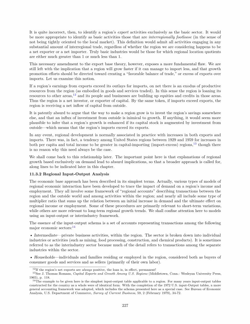
It is quite incorrect, then, to identify a region’s export activities exclusively as the basic sector. It wouldbe more appropriate to identify as basic activities those that are interregionally footloose (in the sense ofnot being tightly oriented to the local market). This definition would admit all activities engaging in anysubstantial amount of interregional trade, regardless of whether the region we are considering happens to bea net exporter or a net importer. Truly basic industries would be those for which regional location quotientsare either much greater than 1 or much less than 1.

This necessary amendment to the export base theory, however, exposes a more fundamental flaw. We arestill left with the implication that a region will grow faster if it can manage to import less, and that growthpromotion efforts should be directed toward creating a “favorable balance of trade,” or excess of exports overimports. Let us examine this notion.

If a region’s earnings from exports exceed its outlays for imports, on net there is an exodus of productiveresources from the region (as embodied in goods and services traded). In this sense the region is loaning itsresources to other areas,12 and its people and businesses are building up equities and credits in those areas.Thus the region is a net investor, or exporter of capital. By the same token, if imports exceed exports, theregion is receiving a net inflow of capital from outside.

It is patently absurd to argue that the way to make a region grow is to invest the region’s savings somewhereelse, and that an influx of investment from outside is inimical to growth. If anything, it would seem moreplausible to infer that a region’s growth is enhanced if its capital stock is augmented by investment fromoutside—which means that the region’s imports exceed its exports.

In any event, regional development is normally associated in practice with increases in both exports andimports. There was, in fact, a tendency among United States regions between 1929 and 1959 for increases inboth per capita and total income to be greater in capital-importing (import-excess) regions,13 though thereis no reason why this need always be the case.

We shall come back to this relationship later. The important point here is that explanations of regionalgrowth based exclusively on demand lead to absurd implications, so that a broader approach is called for,along lines to be indicated later in this chapter.

11.3.2 Regional Input-Output Analysis

The economic base approach has been described in its simplest terms. Actually, various types of models ofregional economic interaction have been developed to trace the impact of demand on a region’s income andemployment. They all involve some framework of “regional accounts” describing transactions between theregion and the outside world and among activities within the region; and nearly all include some type ofmultiplier ratio that sums up the relation between an initial increase in demand and the ultimate effect onregional income or employment. Some of these procedures are primarily relevant to short-term variations,while others are more relevant to long-term regional growth trends. We shall confine attention here to modelsusing an input-output or interindustry framework.

The essence of the input-output schema is a set of accounts representing transactions among the followingmajor economic sectors:14

• Intermediate—private business activities, within the region. The sector is broken down into individualindustries or activities (such as mining, food processing, construction, and chemical products). It is sometimesreferred to as the interindustry sector because much of the detail refers to transactions among the separateindustries within the sector.

• Households—individuals and families residing or employed in the region, considered both as buyers ofconsumer goods and services and as sellers (primarily of their own labor).

12If the region’s net exports are always positive, the loan is, in effect, permanent!13See J. Thomas Romans, Capital Exports and Growth Among U.S. Regions (Middletown, Conn.: Wesleyan University Press,

1965), p. 118.14The example to be given here is the simplest input-output table applicable to a region. For many years input-output tables

constructed for the country as a whole were of identical form. With the completion of the 1972 U.S. input-Output tables, a moregeneral accounting framework was adopted, which includes the schema presented here as a special case. See Bureau of EconomicAnalysis, U.S. Department of Commerce, Survey of Current Business, 59, 2 (February 1979), 34-72.

227

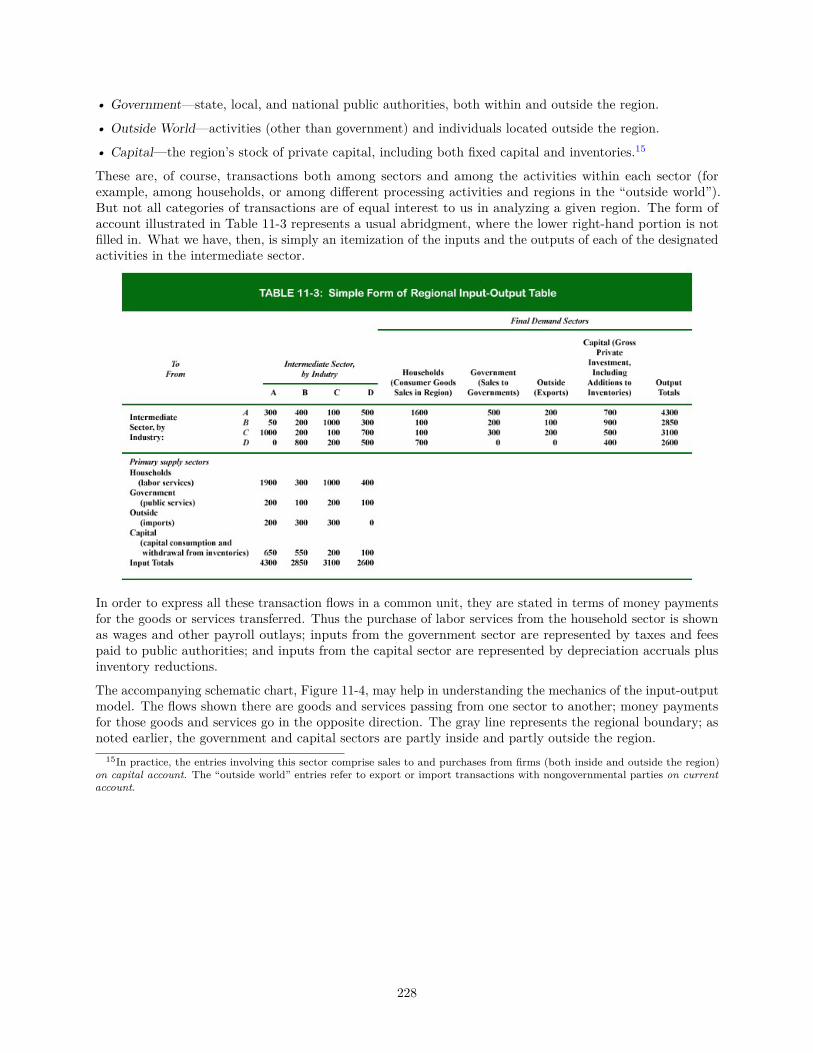
• Government—state, local, and national public authorities, both within and outside the region.

• Outside World—activities (other than government) and individuals located outside the region.

• Capital—the region’s stock of private capital, including both fixed capital and inventories.15

These are, of course, transactions both among sectors and among the activities within each sector (forexample, among households, or among different processing activities and regions in the “outside world”).But not all categories of transactions are of equal interest to us in analyzing a given region. The form ofaccount illustrated in Table 11-3 represents a usual abridgment, where the lower right-hand portion is notfilled in. What we have, then, is simply an itemization of the inputs and the outputs of each of the designatedactivities in the intermediate sector.

In order to express all these transaction flows in a common unit, they are stated in terms of money paymentsfor the goods or services transferred. Thus the purchase of labor services from the household sector is shownas wages and other payroll outlays; inputs from the government sector are represented by taxes and feespaid to public authorities; and inputs from the capital sector are represented by depreciation accruals plusinventory reductions.

The accompanying schematic chart, Figure 11-4, may help in understanding the mechanics of the input-outputmodel. The flows shown there are goods and services passing from one sector to another; money paymentsfor those goods and services go in the opposite direction. The gray line represents the regional boundary; asnoted earlier, the government and capital sectors are partly inside and partly outside the region.

15In practice, the entries involving this sector comprise sales to and purchases from firms (both inside and outside the region)on capital account. The “outside world” entries refer to export or import transactions with nongovernmental parties on currentaccount.

228

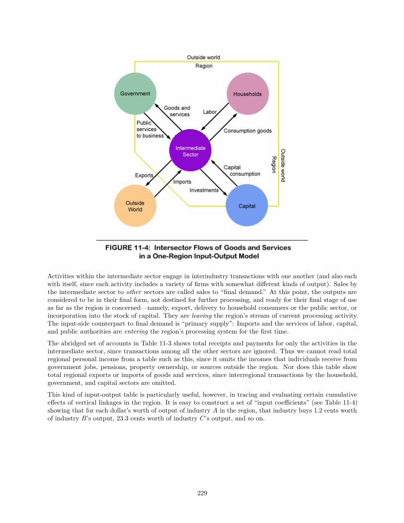
Activities within the intermediate sector engage in interindustry transactions with one another (and also eachwith itself, since each activity includes a variety of firms with somewhat different kinds of output). Sales bythe intermediate sector to other sectors are called sales to “final demand.” At this point, the outputs areconsidered to be in their final form, not destined for further processing, and ready for their final stage of useas far as the region is concerned—namely, export, delivery to household consumers or the public sector, orincorporation into the stock of capital. They are leaving the region’s stream of current processing activity.The input-side counterpart to final demand is “primary supply”: Imports and the services of labor, capital,and public authorities are entering the region’s processing system for the first time.

The abridged set of accounts in Table 11-3 shows total receipts and payments for only the activities in theintermediate sector, since transactions among all the other sectors are ignored. Thus we cannot read totalregional personal income from a table such as this, since it omits the incomes that individuals receive fromgovernment jobs, pensions, property ownership, or sources outside the region. Nor does this table showtotal regional exports or imports of goods and services, since interregional transactions by the household,government, and capital sectors are omitted.

This kind of input-output table is particularly useful, however, in tracing and evaluating certain cumulativeeffects of vertical linkages in the region. It is easy to construct a set of “input coefficients” (see Table 11-4)showing that for each dollar’s worth of output of industry A in the region, that industry buys 1.2 cents worthof industry B’s output, 23.3 cents worth of industry C’s output, and so on.

229

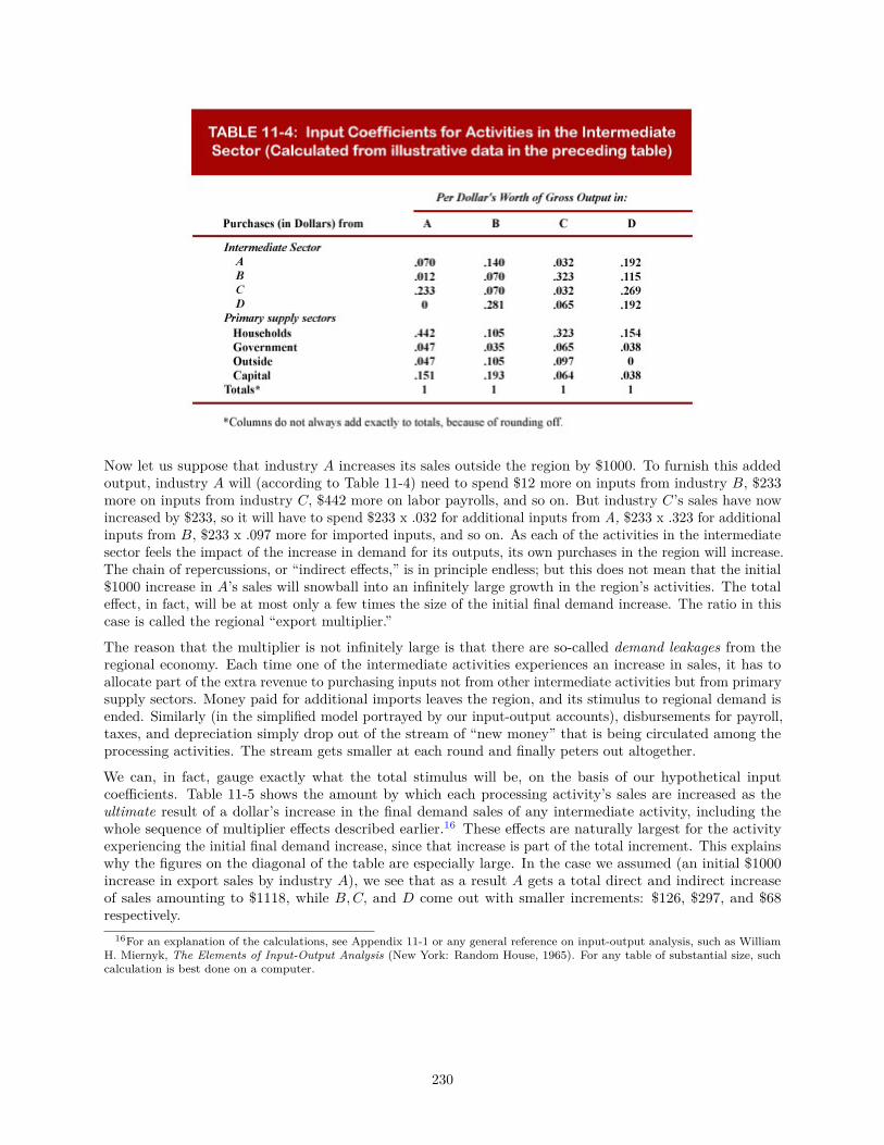
Now let us suppose that industry A increases its sales outside the region by $1000. To furnish this addedoutput, industry A will (according to Table 11-4) need to spend $12 more on inputs from industry B, $233more on inputs from industry C, $442 more on labor payrolls, and so on. But industry C’s sales have nowincreased by $233, so it will have to spend $233 x .032 for additional inputs from A, $233 x .323 for additionalinputs from B, $233 x .097 more for imported inputs, and so on. As each of the activities in the intermediatesector feels the impact of the increase in demand for its outputs, its own purchases in the region will increase.The chain of repercussions, or “indirect effects,” is in principle endless; but this does not mean that the initial$1000 increase in A’s sales will snowball into an infinitely large growth in the region’s activities. The totaleffect, in fact, will be at most only a few times the size of the initial final demand increase. The ratio in thiscase is called the regional “export multiplier.”

The reason that the multiplier is not infinitely large is that there are so-called demand leakages from theregional economy. Each time one of the intermediate activities experiences an increase in sales, it has toallocate part of the extra revenue to purchasing inputs not from other intermediate activities but from primarysupply sectors. Money paid for additional imports leaves the region, and its stimulus to regional demand isended. Similarly (in the simplified model portrayed by our input-output accounts), disbursements for payroll,taxes, and depreciation simply drop out of the stream of “new money” that is being circulated among theprocessing activities. The stream gets smaller at each round and finally peters out altogether.

We can, in fact, gauge exactly what the total stimulus will be, on the basis of our hypothetical inputcoefficients. Table 11-5 shows the amount by which each processing activity’s sales are increased as theultimate result of a dollar’s increase in the final demand sales of any intermediate activity, including thewhole sequence of multiplier effects described earlier.16 These effects are naturally largest for the activityexperiencing the initial final demand increase, since that increase is part of the total increment. This explainswhy the figures on the diagonal of the table are especially large. In the case we assumed (an initial $1000increase in export sales by industry A), we see that as a result A gets a total direct and indirect increaseof sales amounting to $1118, while B,C, and D come out with smaller increments: $126, $297, and $68respectively.

16For an explanation of the calculations, see Appendix 11-1 or any general reference on input-output analysis, such as WilliamH. Miernyk, The Elements of Input-Output Analysis (New York: Random House, 1965). For any table of substantial size, suchcalculation is best done on a computer.

230

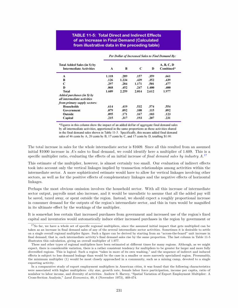
The total increase in sales for the whole intermediate sector is $1609. Since all this resulted from an assumedinitial $1000 increase in A’s sales to final demand, we could identify here a multiplier of 1.609. This is aspecific multiplier ratio, evaluating the effects of an initial increase of final demand sales by industry A.17

This estimate of the multiplier, however, is almost certainly too small. Our evaluation of indirect effectstook into account only the vertical linkages implied by transaction relationships among activities within theintermediate sector. A more sophisticated estimate would have to allow for vertical linkages involving othersectors, as well as for the positive effects of complementary linkages and the negative effects of horizontallinkages.

Perhaps the most obvious omission involves the household sector. With all this increase of intermediatesector output, payrolls must also increase, and it would be unrealistic to assume that all the added pay willbe saved, taxed away, or spent outside the region. Instead, we should expect a roughly proportional increasein consumer demand for the outputs of the region’s intermediate sector, and this in turn would be magnifiedin its ultimate effect by the workings of the multiplier.

It is somewhat less certain that increased purchases from government and increased use of the region’s fixedcapital and inventories would automatically induce either increased purchases in the region by government or

17So far, we have a whole set of specific regional multipliers, since the assumed initial impact that gets multiplied can betaken as an increase in final demand sales of any of the several intermediate sector activities. Sometimes it is desirable to settleon a single overall regional multiplier figure. Such a figure can be derived by starting from an “across-the-board” unit increase infinal demand; that is, each intermediate activity’s final demand sales rise by the same proportion. The last column in Table 11-5illustrates this calculation, giving an overall multiplier of 1.977.

These and other types of regional multipliers have been estimated at different times for many regions. Although, as we mightexpect, there is considerable variation, there is a rather consistent tendency for multipliers to be greater for larger and more fullydiversified regions. This is logical: Such a region “takes in more of its own washing,” and the sequence of indirect and inducedeffects is subject to less demand leakage than would be the case in a smaller or more narrowly specialized region. Presumably,the minimum multiplier (1) would be most closely approached in a community, such as a mining camp, devoted to a singleexporting activity.In a comparative study of export employment multipliers in American cities, it was found that the following characteristics

were associated with higher multipliers: city size, growth rate, female labor force participation, income per capita, ratio ofnonlabor to labor income, and diversity of activities. Andrew S. Harvey, “Spatial Variation of Export Employment Multiplier: ACross-Section Analysis,” Land Economics, 49, 4 (November 1973), 469-474.

231

a step-up in investment activity. And it seems rather unlikely that increased imports would lead (throughraising incomes in other regions) to any significant increase in the demand for the region’s exports.

The upshot of these considerations is that final demand (except perhaps for the export component) is not reallyindependent of primary supply, as our abridged set of input-output accounts assumed. The modificationsor adjustments that might be called for would depend on the particular regional situation. But we mightwell decide that it would be more realistic to assume an automatic feedback from household supply tohousehold demand than to assume no feedback at all. To incorporate this new assumption, we could simplytake households out of final demand and primary supply and put them into the intermediate sector as anadditional, fully interacting activity. Referring to Table 11-3, this would mean supplying numbers to fill outthe presently incomplete “households” row and column.18 The successive steps and results are set forth inAppendix 11-2.

The possibility of shifting households out of the final demand category makes it clear that the decision aboutwhat activities to include to final demand (and primary supply) is not preordained or arbitrary but reflectsour judgment about what relationships are important and relevant to the question at hand. Final demand inthe input-output accounts framework really has the same implications as basic in the simple economic basemodel, and an input-output model with export demand as the only final demand category can be thought ofas a more detailed description of an export-determined regional economy.

The inclusion of government in final demand does not represent any major departure from economic baseprinciples. Government is a basic source of income if public expenditures in the region vary independentlyfrom total regional income. This is true of most federal and state government expenditures; perhaps a casecould be made for putting local government in the intermediate sector.

The role of investment in regional economic change is not really spelled out in the simple form of input-outputmodel that we have been considering; since by convention, sales to the capital sector of final demand includeall sales of capital goods, whether within the region or outside or to governments. There are other, morecomplex, varieties of input-output tables, as well as more general systems of regional income and productaccounts, that do lend themselves to analysis of the mechanisms of saving, investment, and interregionalcapital flow. These will not be discussed here,19 but it is appropriate to ask whether investment in a regionshould more logically be considered (1) an exogenous factor initiating growth of regional income and outputor (2) a response to other changes in the regional economy.

The answer depends on whether we are concerned with the short run or the long run. In the short run, ratesof investment can vary widely and suddenly relative to levels of output, and decisions by major firms in theregion to make extensive additions to their facilities can almost immediately convert a depressed region intoa prosperous one. The question in the short run is the degree to which existing regional labor and productivefacilities are fully employed, and changes in investment outlays can be a major determining factor. Thus ashort-run regional model should certainly treat investment as primarily an exogenous or basic element.

For the long-run development of a region, however, it is reasonable to regard investment at least partly as areflection of regional size and growth, rather than as a sufficient explanation in itself.

Input-output clearly represents a big advance over the simple economic base approach to regional growth;not only because it traces repercussions in a more sophisticated and detailed fashion, but also because itrecognizes possible initiation of growth from various elements of final demand other than export sales.

For simplicity’s sake, we looked at the elementary single-region set of input-output accounts. More compre-hensive and impressive models can be made if the “outside world” is broken down by areas and activities; andprogress has been made in various countries toward complete multiregional accounts systems tracing flows

18There are alternative ways of allowing for the multiplier effect via household income and expenditure. In any case, it iscustomary to refer to this effect as “induced” to distinguish it from the indirect effects resulting from interindustry transactionsin the narrower sense.

19There is a large literature on systems of regional accounts and models for analysis and policy guidance; for a well-roundedtreatment, see Harry W. Richardson, Regional Economics (Urbana: University of Illinois Press, 1978).

232

among economic sectors and activities within each region and among regions as well.20

Such accounts lend themselves to a wide array of useful impact analyses. Starting almost anywhere in thesystem, we can make a change “on paper” and see what happens. We can hypothesize, say, that the salesby some activity in some region increase; or the regional incidence of government expenditures and taxesis shifted; or some major investment project is executed; or consumer expenditures are changed in one ormore regions by virtue of demographic change or shifts in spending habits; or new technology alters some ofthe input coefficients of individual activities. Starting from any such change, we can with an interregionalimpact model trace the initial and subsequent economic repercussions through the various economic sectorsand regions affected.

11.4 The Role of SupplyIn the accounts shown in Table 11-3, the intermediate sector is shown delivering outputs to the variousfinal demand sectors and receiving inputs from those same sectors in their capacity as primary suppliers.Money payments for these goods and services flow in the reverse direction, from final demand sectors to theintermediate sector and then to primary supply.

In tracing changes, we can follow the flow of money payments “backward” from purchaser to seller, or wecan follow the flow of goods and services “forward” from producer to user. The scheme is symmetrical withrespect to supply and demand, or input and output. It does not indicate whether we should look for theinitiating causes of regional growth and change in final demand, in primary supply, or within the intermediatesector; and we might reasonably infer that change can originate in any of these three areas.

In view of this basic symmetry, it is striking that the techniques of input-output and multiplier analysis havenearly always been applied in just the backward direction, tracing the effects of changes from final demand tothe intermediate and primary supply sectors.21 The implication in locational terms is that market orientationand backward linkage are all-important, with no attention being paid to input orientation or to forward andcomplementary linkage effects.

Because an input-output table is a reasonably comprehensive and neutral image of a regional economy, wecan use it as a point of departure for the consideration of supply factors as well as demand factors. Thedemand-driven model discussed above emphasizes final demand, backward linkage, and output orientationof activities. Now let us reverse the emphasis to focus on the roles of primary supply, forward linkage, andinput orientation.

When considering the effects of demand on regional activity, we implicitly assumed that supplies of inputswould automatically be forthcoming, at no increase in per-unit cost, to support any additional activityresponding to increased demand. In other words, supplies of inputs, such as labor, capital, imports, andpublic services, were taken to be perfectly elastic and consequently imposing no constraint on regional growth.If export demand for a region’s steel output increased, the region could freely import as much additional fuelor iron ore as might be needed; if the demand for labor exceeded the region’s labor force, more workers wouldjoin the labor force or move in from other areas.

20See, for example, Karen R. Polenske, The US. Multiregional Input-Output Accounts and Model (Lexington, Mass.: LexingtonBooks, D. C. Heath, 1980); and Jan Oosterhaven, Interregional input-Output Analysis and Dutch Regional Policy Problems(Hampshire, England: Gower, 1981).

21Probably one reason for this overemphasis on the role of demand in regional growth is that modern regional growth theory,input-output analysis, and multiplier analysis were influenced by the contemporary development of Keynesian theories of whatdetermines the degree of utilization of given resources in the short run. A more balanced approach, taking into account long-termgrowth factors on both the supply and the demand sides, has appeared in some theoretical work; notably in Horst Siebert,Regional Economic Growth: Theory and Policy (Scranton, Pa.: International Textbook Co., 1969); Romans, Capital Exports;and G. W. Borts and J. L. Stein, Economic Growth in a Free Market (New York: Columbia University Press, 1964).

One of the first regional economists to question the primacy of exports and call for a balanced theory was Charles M. Tiebout,“Exports and Regional Economic Growth,” Journal of Political Economy, 64, 1 (February 1956), 160-164. His article wasprompted by a forceful statement of the export doctrine by Douglass C. North, “Location Theory and Regional EconomicGrowth,” Journal of Political Economy, 63, 3 (June 1955), 243-258. The whole North-Tiebout controversy, including boththese articles, North’s subsequent reply, and Tiebout’s final rejoinder, is reprinted in John Friedmann and William Alonso(eds.), Regional Policy: Readings in Theory and Application (Cambridge, Mass.: MIT Press, 1975), pp. 332-357. Anothergood statement emphasizing supply factors is Richard T. Pratt, “Regional Production Inputs and Regional Income Generation,”Journal of Regional Science, 7, 2 (Winter 1967), 141-149.

233

Conversely, a supply-driven model of regional growth takes demand for granted (that is, it assumes thatthere is a perfectly elastic demand for the region’s products) and thus makes regional activity depend onthe availability of resources to put into production. Accordingly, the starting point in the process of changenow becomes primary supply rather than final demand. Availability of labor, capital, imported inputs, andgovernment services (infrastructure) makes possible, through forward linkage, certain intermediate activitiesoriented to such primary inputs. Increase in output by an activity that sells in the region can encourage,through further forward linkages, increases by other activities, giving rise to what may be called a “supplymultiplier” effect. This effect is limited by the existence of supply leakages. At each stage, some of theincrease in regional outputs is drained off into exports, investment, deliveries to governments, and householdconsumption—in other words, to the final demand sectors.

This supply-driven process sounds very much like the converse of the demand-driven process discussed earlier,whereby an initial increase in final demand gives rise to indirect growth of income and employment in theregion and increased drafts upon primary supply. Conceptually, the symmetry is complete.

There is, however, an important operational difference. In practice it would not be feasible, save perhapsunder quite special circumstances, to calibrate a supply-driven regional model simply on technical coefficientsderived from the basic input-output table. The reason seems to lie in technology itself. Goods normallybecome more specialized in character as they pass through successive stages of processing and handling.We can legitimately use such input coefficients as, say, the amount of steel needed to make a pound ofnails, because there is not much flexibility in the nature and amount of input required for a given output.By contrast, if we have an extra pound of steel, we cannot say whether it will be used to produce morenails or more steel sheets or automobile parts or whatever. Output coefficients are a weaker reed thaninput coefficients. Consequently, the forward-linkage and multiplier impacts of supply increase, though quitegenuine, cannot normally be spelled out in terms of specific products and activities by input-output analysis,and with presently available techniques they can be estimated only in relatively impressionistic terms.

The demand-driven and supply-driven models should be viewed as complementary rather than as conflictingor rival hypotheses about regional economic change.22 Each of the two model types in itself is one-sided andcan be seriously misleading; for full insight into real processes, both need to be combined. As yet, however,there is no analytical model that adequately incorporates this union of the two complementary approaches.23

11.5 Interregional Trade and Factor MovementsSystems of accounts do not in themselves tell us anything about where growth starts; they merely help usto trace impacts. But we can see already that a region’s growth involves at least three kinds of externalrelationships of the region: (1) trade, or the import and export of goods and services; (2) migration of people,both in their capacity as consumers and in their capacity as workers; and (3) interregional “migration” ofother production factors, notably investment capital. A fourth external influence, to which some attentionwill be paid in the next chapter, is the national government’s revenue collection and expenditure in the region.

Trade among regions has, as David Ricardo noted a long time ago with respect to nations, the beneficenteffect of allowing each region to specialize in those activities for which it is best fitted by its endowments ofresources and other fixed local input factors, with all regions sharing to some extent in the economies of suchspecialization. Recognition of this effect helps to place the value and limitations of the export base theory inbetter perspective. When the local market is so small as to limit seriously the productivity gains that can berealized by specialization, exports may be necessary for growth. Thus the weakness of the export base theorylies not in recognizing exports as being important for growth, but rather in focusing on exports exclusivelyand failing to recognize that it is trade (imports as well as exports) that permits the realization of economiesdue to specialization.

This specialization of regions is limited, of course, by interregional transfer costs as well as by ignorance,22See, for example, Richard F. Muth, “Migration: Chicken or Egg?” Southern Economic Journal, 37, 3 (January 1971),

295-306.23Readers interested in a more detailed presentation and critique of supply-driven input-output analysis are referred to

Frank Giarratani, “The Scientific Basis for Explanation in Regional Analysis,” Papers and Proceedings of the Regional ScienceAssociation, 45 (1980), 185-196; and Oosterhaven, Interregional Input-Output Analysis, Chapter 8.

234

inertia, and the like, and the simplified model implied here fails to take into account the economies of scaleand regional agglomeration. But so far as it goes, the effect of freer interregional trade is likely to be in thedirection of equalizing not only commodity prices among regions but also wages, incomes, and the rates ofreturn to capital. The reason for this is that a region in which capital is scarce relative to labor can, withinterregional trade, specialize in “labor-intensive” lines of production requiring much labor and little capitalwhile importing the products of “capital-intensive” activities from regions better endowed with capital or lesswell endowed with manpower.

This substitution of trade for production-factor mobility is of course only partially effective. Considerabledifferentials persist in the rewards of labor and the returns on capital among the regions, leaving an incentiveto further equalization by migration of those factors of production.24

11.5.1 Mobility of Labor and Capital Among Regions

Determinants of labor mobility have already been explored at considerable length in Chapter 10. The rate ofreturn to labor (real wages) is indeed a major determinant; but migration and regional manpower suppliesdepend also on the handicaps to movement imposed by uncertainty, ignorance, cost of moving, and socialdistance. Moreover, a person’s mobility varies widely according to his age, marital and dependency status,education, skills, and recent migration experience; and migration flows between places depend on suchadditional factors as previous flows (the beaten-path effect), the size and diversity of labor markets, and theeffectiveness of interregional job-information and placement systems.

The mobility of capital is affected by a quite similar array of considerations. The prospective rate of returnis, again, a major determinant; inertia, ignorance of opportunities, and social distance act as limiting factorsin much the same way as they do for manpower mobility. The effectiveness of organization of the nationalfinancial system (including clearing arrangements, facilities for transferring funds from one region to another,securities exchanges, and interregional markets for still other types of investments and obligations) tends toset a limit on how much interest rates and other rates of return on capital can vary geographically withina county. Increased effectiveness of the national financial system in most countries has been evidenced bya trend of interregional convergence in money rates, though such rates still tend to be somewhat higherin places more remote from the chief national financial centers25 and in smaller urban places. Somethinganalogous to the beaten-path effect on labor mobility appears to affect capital mobility as well. Funds flowmore readily and in response to a smaller rate-of-return differential from one point to another if there hasbeen a great deal of previous investment following the same path.

Still another similarity appears in the effect of regional or community characteristics on the outward mobilityof both labor and capital. A young area with a previous experience of inward migration and rapid growthshows more outward mobility of both factors than does a more settled and ingrown community.

Perhaps the most important difference between the processes of capital and labor migration lies in the factthat most capital has to be “sunk” or invested in durable forms such as site improvements, buildings, andproduction equipment before becoming useful. This major portion of the capital stock has virtually nospatial mobility. Movements of capital are thus confined to (1) newly created capital awaiting selection of afixed-investment opportunity, and (2) working capital and other floating funds that remain in the form ofpaper assets or fairly easily movable types of commodities and thus retain interregional mobility.

The phenomenon of sunk capital would be roughly matched in terms of labor mobility if a high proportionof workers signed up for life on their first job. In Japan this is characteristic of employment practices, atleast as they pertain to male workers in major corporations. There, the normal course is for the tenure ofemployment to extend over one’s entire working life as a matter of informal contract between employer and

24Ricardo’s theory and much subsequent theorizing on international trade assumed immobility of production factors—anassumption clearly inappropriate in reference to relations among regions within a single country.

25Such a differential is suggested, though without empirical evidence, in Richardson’s discussion of interregional capitalmobility; see Harry W. Richardson, Regional Economics (New York: Praeger, 1969), p. 305. Lösch found a marked regionaldifferential pattern in money rates in the United States in the 1920s and 1930s, long after the Federal Reserve System had beenput into operation. See August Lösch, The Economics of Location (New Haven, Conn.: Yale University Press), pp. 461-476.Additional material on changes in the geographic structure of the U.S. financial system may be found in Beverly Duncan andStanley Lieberson, Metropolis and Region in Transition (Beverly Hills, Calif.: Sage Publications, 1970), Chapters 11-12.

235

employee. More generally, however, people do lose mobility rather suddenly once they become establishedin an occupation, a community, and a family; and mobility thereafter declines further with increased age.In part this is due to the fact that information and skills relevant to a particular line of work, company,or community may be very specific, in the sense that they are not of comparable value elsewhere. So thecontrast in this regard between the mobility of people and the mobility of capital is not as absolute as itmight appear.

Scale and agglomeration economies affect the migration of both labor and capital, and in not too dissimilarfashion. A location that might be highly advantageous if enough manpower and/or enough capital could beconcentrated there may never get over the threshold imposed by the higher costs of an initial small-scaleoperation or an insufficiently developed production cluster.

Finally, it can be observed that the migration of people from one place to another facilitates the movement ofcapital along the same route, and conversely. Each factor helps beat a path for the other. To some extentthis reflects the fact that migrants normally bring some personal capital with them and often some businesscapital as well. A further explanation is that the increased familiarity with the other area, which comesfrom the movement of either labor or capital, enhances the mobility of the other factor along the same path,eroding the barriers of uncertainty and social distance.

More basically, the relation between labor and capital flows is affected by the way in which these factorscombine to produce goods and services. Labor and capital can substitute for one another in production if it ispossible to choose between a labor-intensive and a capital-intensive technique, depending on which factoris relatively cheap. The substitution relationship in itself would imply that a larger supply of capital ina region would lessen the demand for labor, since there could be a shift to more labor-saving productionmethods and more capital-intensive activities. Similarly a larger labor supply would lessen the region’s capitalrequirements.

But this picture is clearly unrealistic in many cases, because the factors of production are at the sametime complementary. Using more of one may lead to using more of the other as well. The complementaryrelationship in itself would imply that a larger supply of capital in a region would augment the demandfor labor, since production would expand in response to the enhanced competitive position of the region’sactivities. Similarly, a greater supply of labor in a region would create a demand for additional investment inproduction capacity to take advantage of this more ample and perhaps cheaper labor.

In terms of regional growth, the effect of the substitution relationship may be viewed as equilibratory,whereas the effect of the complementary relationship may be viewed as equilibratory. To the extent that thecomplementary relationship between labor and capital predominates, interregional capital and labor flowscan lend themselves to long spells of continued self-sustaining regional growth (or, on the other side of thecoin, cumulative decline).

The effects of trade and of factor movements on regional structural differences can often be opposite. Tradein itself permits more intensive regional specialization and thus a widening of regional structural differences.26

Interregional movements of labor and capital, on the other hand, would seem in general to weaken one ofthe main bases for specialization (that is, relative regional supplies of labor and capital) and thus promoteconvergence of regional structural differences.

This last surmise is subject to qualification, however, since it ignores the effect of regional differencesin endowment of really immobile factors (land or natural resources). To the extent that such resourcesare complementary to labor and capital in production processes, regional specialization and structuraldifferentiation based on fixed-resource endowments will be enhanced by greater interregional mobility of labor,capital, or both. This is likely to be true of mineral resources when they occur in regions with few othernatural advantages—movement of capital and labor into such regions helps them to develop exploitation oftheir mineral resources as a regional specialty.

26For an excellent discussion of the effects of transport changes on industry location and regional concentration in the UnitedStates, see Benjamin Chinitz, “The Effect of Transportation Forms on Regional Economic Growth,” Traffic Quarterly, 14,2(April 1960), 129-142; and Chinitz, Freight and the Metropolis (Cambridge, Mass.: Harvard University Press, 1960).

236

11.6 Interregional ConvergenceIt is not difficult to find plausible explanations for the convergence of regional income differentials. Suchconvergence would seem to be a natural result of the gradual development and maturation of areas onceon the frontiers of settlement, the greatly reduced relative importance of farming as a means of livelihood,the improvement of transport and communications and the enhanced mobility of both capital and labor,and the rise of more activities not closely oriented to natural resources and consequently enjoying a widerchoice of possible locations. Increased interregional trade resulting from improved transport can also promoteconvergence by permitting regions to share to a greater extent the benefits of the production economies ofother regions.

The story is not quite this simple, however, and we cannot infer that convergence will always be the orderof the day. There seem, in fact, to have been two periods in United States history in which interregionalincome differentials either widened or remained about the same: from 1840 to 1880, and from 1920 tillsometime in the 1930s. In the earlier period, the development of railroads brought rapid concentration ofindustrial activity in larger plants and larger industrial centers, and an increase in regional specialization.This raised incomes in the Northeast, where the bulk of the industrial activity was concentrated, compared tothe basically agricultural and undeveloped parts of the country. In the period 1860-1880, the disruption of theSouthern economy by the Civil War dramatically widened the gap between Southern and Northern incomes.Between World Wars I and II, there were at least two special reasons for divergent regional income levels.One was the low level of farm product prices and the consequently depressed condition of agriculture.27 Amajor part of the regional income differentials, especially in that period, simply reflected differences in therelative importance of agriculture in the various regions. In addition, the virtual cutting off of the influx ofcheap immigrant labor after World War I removed a constraint on rising wage levels in the industrial areasthat had previously been employing the bulk of that labor.

The inevitability of convergence can be questioned on more general grounds. To be sure, migration flowspredominantly in the direction of higher income levels, and at least in the United States it seems to be, onbalance, an equalizing factor. It is not always true, however, that in-migration from a region tends to lowerincome levels, and it is even less sure that out-migration tends to raise them.

Interregional capital flows may also be destabilizing. Actually, shifts of employing activities are an equalizingfactor only to the extent that the activities are primarily oriented to labor supply, so that capital is drawnto low-wage regions. Consequently, changes in production and transfer technology, availability and useof resources, economies of agglomeration, and other location factors can either narrow or widen incomedifferentials according to circumstances. For example, if agglomeration economies assert a powerful influenceon capital movements, regions realizing these economies would grow most rapidly, thus creating moreagglomeration economies and promoting continued growth (see the related discussion concerning verticallinkages).

The potential for movements of capital and labor to be stabilizing or destabilizing as circumstances dictate isbrought out clearly in research related to a model developed by Moheb A. Ghali and his colleagues.28 Theydescribe economic growth for U.S. regions as being explained by the growth of capital and labor inputs. In thismodel, interregional movements of factors of production are determined by regional earnings differentials anddifferentials in the rate of growth of output, which they use as a proxy for employment opportunities. Theseresearchers are able to determine empirically that factor movements tend to be equalizing for U.S. regions.Applying the same model for an analysis of regional growth in Indonesia, Soeroso finds that interregionalfactor movements encourage income divergence.29 In both cases the response to larger earnings differentialsis positive. Although this response is much weaker in Indonesia than in the United States (perhaps reflectingdifferent stages in the development of a well-integrated market economy), it has a stabilizing influence in each.

27The farm price parity ratio (index of prices received by farmers to prices paid by farmers, on the base 1910=100) averaged104 in 1911-1920; 88 in 1921-1930; 76 in 1936-1940; and 107 in 1941-1950. U.S. Bureau of the Census, Historical Statistics of theUnited States, Colonial Times to 1957 (Washington, D.C.: Government Printing Office, 1960), p. 283.

28Moheb A. Ghali, Masayuki Akiyama, and Junichi Fujiwara, “Factor Mobility and Regional Growth,” Review of Economicsand Statistics, 90, 1 (February 1978), 78-84.

29Soeroso, The Distribution of Economic Activity over Space and Economic Growth in Indonesia, (Ph.D. dissertation,University of Pittsburgh, 1982).

237

In Indonesia, however, differentials in the rate of growth of output are a much more powerful influence onfactor movements and contribute to widening earnings differentials; the more prosperous areas grow fastestand attract productive resources, in a cumulative and destabilizing process.

Changes in the make-up of demand for goods and services may also affect income differentials in eitherdirection. For example, the practically universal tendency of demand for agricultural products to grow moreslowly than demand for manufactured products and services in a progressive economy seems more likely thannot to widen the differential between incomes in farming areas and those in industrialized and urban areas.

Whether it is the lure of employment opportunities and job-search behavior,30 agglomeration economies,31 orsome other cause at the root of this process, this much is apparent: We cannot take the experience of theUnited States in the last 50 years as being representative of a general tendency toward the convergence ofregional incomes.

We might summarize by quoting Richard Easterlin:

It is by no means certain that convergence of regional income levels is an inevitable outcomeof the process of development. For, while migration and trade do appear to exert significantpressure towards convergence, they operate within such a rapidly changing environment thatdynamic factors may possibly offset their influence. One may argue, of course, that migrationand trade may become progressively more important during growth, as a result, for example,of improvements in transportation, and hence that the pressures towards convergence will tendincreasingly to predominate. But whether this is generally the case cannot be settled on a priorigrounds.32

Consideration of all the factors influencing regional income inequalities leads to an interesting hypothesisrelating convergence and divergence systematically to the stages of the development process. Specifically,the early stages of national economic development are associated with increasing regional income disparities,while regional income levels tend to converge in a more maturely developed national economy.

In the present age, the crux of what we call development and attainment of self-sustaining progress is thetransition from an agrarian economic basis to a basis of secondary and tertiary activities, with accompanyingurbanization. A wide gap exists between the new and the old in terms of income levels, ways of life, andlocation factors.

When industrialization is in its early stages, most of the rise in overall productivity and per capita incomecomes from the change of mix—that is, the increasing importance of the nonagricultural sector relative to theagricultural. The new activities cannot take root everywhere at once but are highly concentrated at first in afew key cities—generally the places with the most active contact with more advanced countries and the largestand most diverse populations. At this stage of development, most regions still lack the necessary local marketpotential and the necessary local inputs to engage in the new and unfamiliar types of activity. Migration islikely to be heavy from the backward areas to the industrializing cities. This migration is highly selective(see the discussion of migration selectivity in Chapter 10), and on the whole this selectivity is prejudicial tothe areas of out-migration. The result is the next stage: progressive agglomeration of modern industry inthe principal urban areas and an accentuation of regional differences in economic structure, productivity,and income. Such conditions appear to have prevailed in the United States during the divergence period1840-1880, which was lengthened by the destructive effects of the Civil War upon the economy of the South;and they prevail today in many Third World countries of Asia, Africa, and South America.

30See Michael P. Todaro, “A Model of Labor Migration and Urban Development in Less Developed Countries,” AmericanEconomic Review, 59, 1 (March 1969), 138-148.

31See Harry W. Richardson, Regional Growth Theory (London: Macmillan, 1973), Chapter 7; and Richardson, RegionalEconomics, (Urbana: University of Illinois Press, 1978), Chapters 4-7.

32Richard A. Easterlin, “Long Term Regional Income Changes: Some Suggested Factors,” Papers and Proceedings of theRegional Science Association, 4 (1958), 325. See also Easterlin, “Interregional Differences in Per Capita Income, Population andTotal Income, United States, 1840-1950,” Trends in the American Economy in the Nineteenth Century, vol. 24, Conference onResearch in Income and Wealth, Studies in Income and Wealth (New York: National Bureau of Economic Research, 1960); andEasterlin, “Regional Income Trends, 1840-1950,” in Seymour Harris (ed.), American Economic History (New York: McGraw-Hill,1961), pp. 525-547.

238

As development proceeds, more and more regions acquire the market potential, attitudes, and access to capitaland know-how required to surmount the threshold of industrialization. A stage of interregional convergencein economic structure, productivity, and income sets in. This convergence may be made cumulative becausemigration is likely to become less selective, and national government policies will be less preoccupied with theobjective of getting industrialization started in the country as a whole and more sensitive to the politicalpressures arising from regional inequality.33

11.7 The Role of Cities in Regional DevelopmentIn Chapter 8 we were able to account for the rise of cities on the basis of the internal and external economiesof agglomeration, discussed in Chapter 5, and the transfer advantages of location at major multimodaltransfer nodes, discussed in Chapter 3. But this does not tell us why cities are so important in a dynamicway. The existence of sizable urban centers seems to be a necessary (though not always sufficient) conditionfor the transition from a basically agrarian economy to an advanced economy with high productivity and awide range of productive activities. The question now is not why cities exist, but why they lead the way inregional and national development.

First of all, there is the relatively cosmopolitan aspect of large cities. They are a region’s eyes and earsperceiving the outside world. “Foreign” ideas, goods, and procedures have much to contribute to thedevelopment of even the most advanced region; and cities, as entrepôts for interregional transfer, are the mainpoints where these vitalizing inputs gain admittance. This aspect of cities is most abundantly evident inthe less developed countries, where the principal cities impressively resemble their counterparts in advancedcountries, even though a few miles away we can step back centuries in time.

Quite apart from their interregional contact function, cities serve an important role in the developmentprocess simply by being places in which people from other parts of the same region or country are broughttogether in densities and living conditions sharply contrasting with those of the rural areas. Conservativetraditions and outlooks that persist in the hinterland tend to dissolve rather quickly in the urban melting pot;the results are always conducive to more rapid social and economic change, though they are often painfuland destructive in terms of personal satisfaction and orderly social and political adjustment. Social effectsof urbanization that can be of major importance in overpopulated countries are the mutually reinforcingtendencies toward smaller families and toward greater labor force participation of women. For the workingpopulation as a whole, urbanization represents exposure to a way of life in which work is more scheduled andorganized, monetized transactions and impersonal relationships play a larger part, literacy and adaptability tochange are more valuable personal assets, and the choice of occupations and lines of individual developmentis widened.

Such considerations as these go far to explain why cities (especially large ones with far-reaching externalcontacts) have been the main seedbeds of innovation; in economic terms, this involves the genesis of newtechniques, new products, and new firms. Such places provide the exposure to a wide range of ideas andproblems from which solutions emerge. They represent large concentrations of customers and suppliers mostreceptive to new products and requirements. They provide the diversified supply of skills and supportingservices that enable a producer to start small and concentrate on a narrowly specialized function (seethe discussion of external economies in Chapter 5). They provide a social and business climate in whichimpediments of tradition and personal inertia are minimized, and initiative and innovation carry prestige;and in which the innovator can learn much from day-to-day contacts with competitors and can most easily

33See Jeffrey G. Williamson, “Regional Inequality and the Process of National Development: A Description of the Patterns,”Economic Development and Cultural Change, 13, 4(2) (July 1965), 3-45; reprinted in L. Needleman (ed.), Regional Analysis(Baltimore: Penguin, 1968). Williamson presented and substantiated the hypothesis described here, using nineteenth-andtwentieth-century data for a number of countries both cross-sectionally and in terms of changes over time. He also investigatedthe degree of income inequality among counties within states in the United States and established that its changes have beenclosely correlated with changes in interstate income inequality.

239

tap the stock of accumulated know-how, exploiting inventions arising not only in his or her own city butelsewhere.34

Major cities are the locations at which the newest types of activities can most easily get a foothold within anyregion or country, and the advent of industrialization in an undeveloped country is generally accompanied byexplosive growth of the largest centers and a heightening of economic and social contrasts between thosecenters and the rural backwaters.35 But as development proceeds, two things happen. Some of the sensitiveinfant industries of yesterday attain maturity: Their techniques become less experimental and their productsmore familiar to a wider market. As a result, these activities are no longer so dependent on the specialadvantages that large cities provide. The fledglings are ready to leave the nest. At the same time, the positiveincentives to decentralize out of the initial large city concentration tend to increase. With a larger andwider market for the product, a location pattern involving a number of regional production centers offerseconomies in distribution costs without undue sacrifice of the economies of scale. The external economies ofcluster become less important with the increase in financial and technical resources of firms and the greaterstandardization of process and product. Costs of labor and other local inputs in the initial large-city locationnow appear unnecessarily high in relation to what these inputs cost in smaller places. And in the originalcenters where the industry developed, maturity may well have meant some development of rigidities and lossof initiative because of the aging of both business leaders and the labor force and the growth of defensivepractices to protect seniority rights, painfully acquired but obsolescent skills, positions of power, and otheraccumulated perquisites. Thus the city that hatched the industry and saw it through its infancy may lose italtogether when it grows up.

The evolutionary process sketched here in terms of locational change accompanying the birth, infancy, andmaturing of an activity is a strikingly familiar one. Wilbur Thompson has referred to it in terms of “afilter-down theory of industrial location” and “the urban-regional growth loop.”36 As he points out, “NewYork has lost nearly every industry it has ever had—flour mills, foundries, meat-packing plants, textile millsand tanneries.” Pittsburgh pioneered and then lost preeminence in a long series of major industries includingoil refining, aluminum, electrical machinery, and steel.

Historically, large cities have been characterized by a disproportionate component of new and small “growthindustries” in their mix of activities, but they generally fail to maintain their share of activities that arepast the early stages. Smaller cities and towns, and less-advanced regions, have been more likely to showcompetitive gains in the sense of increasing their share of the national total of employment in the activitiesrepresented there; but growth in these areas has historically been held down by the fact that their mix of

34For a penetrating and well-documented analysis of the interaction between industrial innovation and urban concentration inthe United States, see Allen R. Pred, The Spatial Dynamics of US. Urban-Industrial Growth, 1800-1914 (Cambridge, Mass.:MIT Press, 1966), Chapter 3.

Pred’s analysis covers the period up to 1914, and as he suggests, the nature and strength of some of the cumulative forces ofurban-industrial agglomeration have subsequently changed. His study is noteworthy in its stress on the interaction betweenconcentration and innovation: That is, technological advance and innovation flourish in the large urban-industrial center, andgive rise to new industries that are established in those same centers, and stimulate their further growth. There are manyexamples of this process in the nineteenth century: the inception of the electrical equipment manufacturing industry in New York,Boston, and Pittsburgh, the making of scientific instruments and optical equipment in Rochester, N.Y., and so on. But (as Predpoints out) under more recent conditions, innovation at one location can as easily give rise to new industry in other locations.This is true because technical knowledge is much more diffused and transferable now, and also because large multiplant andmulti-industry corporations now play a commanding role in the research and development that give rise to new processes andindustries. Such a corporation is perfectly free to choose locations for the new industry quite remote from the headquarters orresearch-center city.This and other changes help to explain why specific manufacturing industries are no longer as strongly or persistently

concentrated in their “parent cities” as they used to be; and perhaps also, why the fastest-growing metropolitan areas today arenot the very largest but those in the intermediate and smaller size classes. (See Section 8.5.)

35As a sobering touch of historical realism, we must note here that leading cities in which wealth, power, and foreign influenceare concentrated have not always been an unmixed blessing to their regions and countries. In some situations of old-stylecolonialism in particular, the dominant externally oriented metropolis has been parasitic on its hinterland. Preexisting nativeindustries, economic and social institutions, and cultures have been damaged to an extent that, for a considerable period atleast, is not compensated by the growth-generative effects. See Bert Hoselitz, “Generative and Parasitic Cities,” EconomicDevelopment and Cultural Change, 3 (1955), 278-294.

36Wilbur R. Thompson, “The Economic Base of Urban Problems,” in Neil W. Chamberlain (ed.), Contemporary EconomicIssues (Homewood, Ill.: Irwin, 1969), pp. 6-9.

240

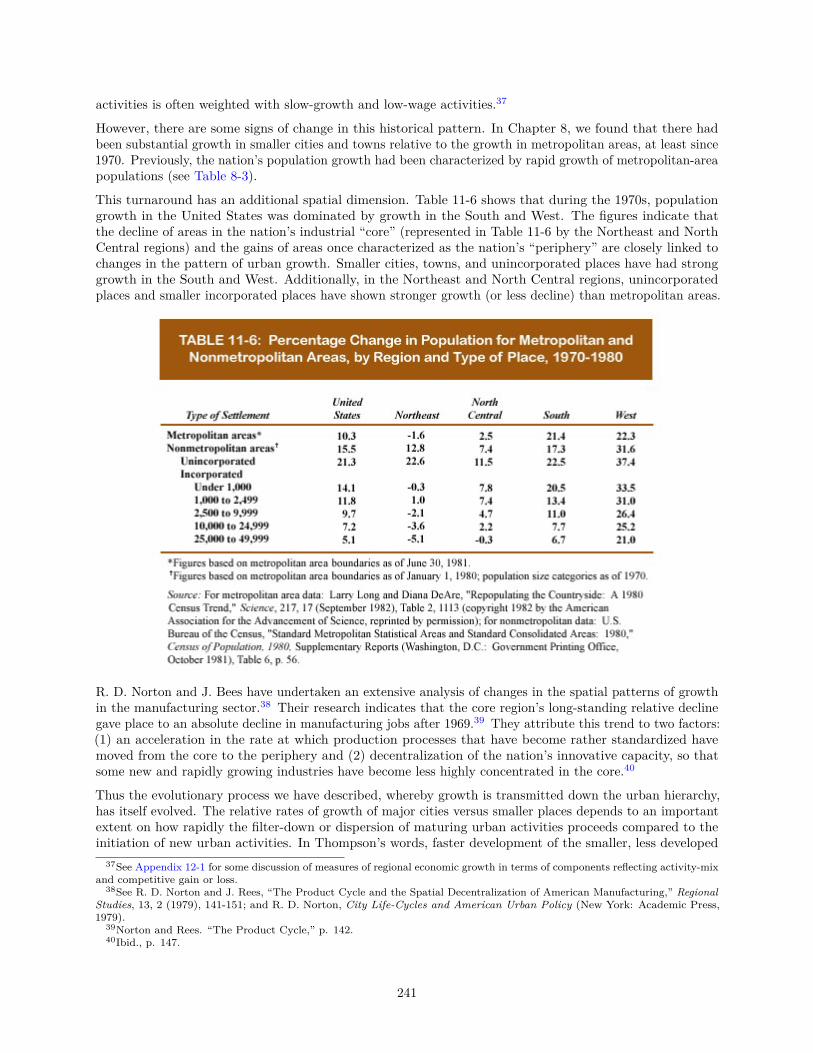
activities is often weighted with slow-growth and low-wage activities.37

However, there are some signs of change in this historical pattern. In Chapter 8, we found that there hadbeen substantial growth in smaller cities and towns relative to the growth in metropolitan areas, at least since1970. Previously, the nation’s population growth had been characterized by rapid growth of metropolitan-areapopulations (see Table 8-3).

This turnaround has an additional spatial dimension. Table 11-6 shows that during the 1970s, populationgrowth in the United States was dominated by growth in the South and West. The figures indicate thatthe decline of areas in the nation’s industrial “core” (represented in Table 11-6 by the Northeast and NorthCentral regions) and the gains of areas once characterized as the nation’s “periphery” are closely linked tochanges in the pattern of urban growth. Smaller cities, towns, and unincorporated places have had stronggrowth in the South and West. Additionally, in the Northeast and North Central regions, unincorporatedplaces and smaller incorporated places have shown stronger growth (or less decline) than metropolitan areas.

R. D. Norton and J. Bees have undertaken an extensive analysis of changes in the spatial patterns of growthin the manufacturing sector.38 Their research indicates that the core region’s long-standing relative declinegave place to an absolute decline in manufacturing jobs after 1969.39 They attribute this trend to two factors:(1) an acceleration in the rate at which production processes that have become rather standardized havemoved from the core to the periphery and (2) decentralization of the nation’s innovative capacity, so thatsome new and rapidly growing industries have become less highly concentrated in the core.40

Thus the evolutionary process we have described, whereby growth is transmitted down the urban hierarchy,has itself evolved. The relative rates of growth of major cities versus smaller places depends to an importantextent on how rapidly the filter-down or dispersion of maturing urban activities proceeds compared to theinitiation of new urban activities. In Thompson’s words, faster development of the smaller, less developed

37See Appendix 12-1 for some discussion of measures of regional economic growth in terms of components reflecting activity-mixand competitive gain or loss.

38See R. D. Norton and J. Rees, “The Product Cycle and the Spatial Decentralization of American Manufacturing,” RegionalStudies, 13, 2 (1979), 141-151; and R. D. Norton, City Life-Cycles and American Urban Policy (New York: Academic Press,1979).

39Norton and Rees. “The Product Cycle,” p. 142.40Ibid., p. 147.

241

urban area “would seem to require that it receive each successive industry a little earlier in its life cycle, toacquire the industry at a point in time when it still has both substantial job-forming potential and high-skillwork.”41 Additionally, it now seems that the filter-down process is less important overall, as innovation andhigh concentrations of fast-growing activities are less exclusively characteristic of growth in the nation’slargest metropolitan areas.

Further implications will be explored in Chapter 12, in connection with growth-promotion policies and thefocusing of development promotion efforts on urban growth centers.

11.8 External and Internal Factors in Regional DevelopmentWe have seen that the development of a region—in terms of its size, income level, and structure—is affectedby external conditions of two types: (1) demand for the region’s outputs, or more broadly, external sources ofincome for the region, and (2) supply of inputs to the region’s productive activity. We have also seen thatthe impact of these external factors is conditioned by the size and maturity of the region and by the internalrelationships of its various activities in the form of vertical, horizontal, and complementary linkages.

Since all regions contain a variety of activities, it is to be expected that some of these activities will bedetermined mainly by external conditions based on demand (such as export markets), while others willbe particularly sensitive to supply conditions. The regional economy as a whole, then, is always subjectto a variety of growth determinants. Although there may be one principal factor affecting its overall levelof activity (as, for example, the nationwide demand for automobiles is the principal factor affecting theprosperity and growth of Flint, Michigan), there is never just a single determinant.

How much influence on a region’s development can be exercised from within the region itself? This question isbasic to the discussion of regional objectives and policies in the next chapter. As far as growth determinantsin the form of final demand are concerned, the latitude for regional initiative is ordinarily limited. Butperhaps export demand in some lines can be stimulated by sales promotion campaigns, or the region canbetter its access to external markets by lobbying or other pressure to get more favorable freight rates ortransport services for its exports, improved waterways, or high-speed highways. Improvement of the region’sown terminal and port facilities may also have some effect on export demand and thus on regional growth.Houston, with its ship channel to the sea, is a dramatic illustration of a successful effort of this type.

A region has some leverage also on primary supply inputs. By persuasion, pressure, and subsidy, it maysecure better and cheaper inbound transport for its imported materials and may be able to attract activitieswith strong forward linkages that will have a supply multiplier effect. Governmental and private researchcenters and universities are increasingly valued as local suppliers of services, people, and ideas providingthe basis for new growth industries. Regions where demand for labor tends to exceed supply can stimulateimmigration by campaigns of advertising and recruitment, publicizing both job opportunities and whateveramenities the region has to offer.

Finally, regional growth can be significantly affected through changes in intraregional input supplies andinteractivity relationships, which are more immediately subject to local choice and action. The quality of thelabor supply can be enhanced by a variety of education and training programs and by removal of barriers tooccupational mobility and technical change (including racial and sex discrimination, restrictive work rules,and job entry requirements). The region’s limited land and other natural resources can be managed soas to increase their contribution to productivity. Local public services, an important input to almost allactivities, can be made more efficient and conducive to productivity and amenity. The region’s economies ofagglomeration can be enhanced by appropriate action involving both public and private sectors (for example,in the planned development of new and improved office centers, regional shopping centers, produce markets,health centers, research parks, and the like).

In the next chapter, we turn to a consideration of how these and other ways of influencing regional developmentare used in the pursuit of objectives involving regional structure and growth.

41Thompson, “Economic Base of Urban Problems,” p. 9.

242

11.9 SummaryThis chapter addresses itself to such basic questions about regional growth and change as the causes of growth,the roles of trade and of the movement of labor and capital, the relation of regional economic structure togrowth, and the convergence of regional differentials in incomes and structure.

Processes of regional economic change work through the various types of linkage examined in Chapter 9. Ingeneral, vertical linkages are involved in self-reinforcing growth or decline tendencies, whereas horizontallinkages have a stabilizing influence. Various theories about the generation of regional growth have emphasizedeither demand for the region’s outputs and backward linkage, or supply of inputs and forward linkage.

The simple economic base approach identifies exports as the generator of growth in a region; nonbasic, orlocal market-serving, activities are assumed to grow only in response to the local demand generated by theexport sector and to maintain a more or less fixed ratio to the latter.

With input-output analysis, it is possible to trace the impact of an increase in business receipts from exportsor other components of “final demand” on payments and incomes in the region through local spending forpayrolls and purchases from other businesses in the region. The total increase in regional income generatedper dollar of initial increase in final demand receipts is the regional income multiplier.

The input-output model treats final demand as the initiator of growth and change. Exports are always part offinal demand, but the household, government, and investment sectors are sometimes taken at least partiallyout of the final demand category and treated as responding to regional demands.

A regional economic model in which all growth and change must come from demand and be transmittedthrough backward linkage is one-sided. A more adequate model would assign major roles to supply factorsand forward linkage as well, but input-output analysis is less well adapted to deal with changes originatingon the supply side.

A still broader multiregional view of the development process focuses on the roles of interregional trade andfactor movements. The migration of capital is subject to determinants closely analogous to those affectinglabor migration, though the patterns of interest and wage differentials are quite dissimilar, as are the patternsof capital and labor flow.

Interregional trade can serve as a partial substitute for labor and capital flows in equalizing returns to thosefactors. Flows of labor and capital can either substitute for or complement one another; the substitutiverelation exerts an influence toward stability in relative regional growth, while the complementary relationshipcan be the basis of self-reinforcing and cumulative tendencies.

The observed convergence in regional income levels and structures in recent decades is not a universal trend.Interregional trade as well as labor and capital movements, though commonly promoting convergence, can insome situations have the opposite effect; and technological dynamics can just as well promote divergence asconvergence. According to one plausible hypothesis of development stages, divergence is likely to characterizethe youthful stages of a country’s industrial development, and convergence the more mature stages.

Large cities have played a crucial role in regional and national economic development, in their capacity astransmitters of ideas and practices from the outside world and also as places where people from diverse partsof the home region or country are brought into close contact and exposed to new institutions and challengesand a wider variety of opportunities. Innovation has flourished in such a germinating ground. New industriesand other activities that started in large cities have historically tended to decentralize at a later stage to playa role in the development of other regions or parts of the region. Evidence suggests that decentralization isoccurring more rapidly in recent years and that the capacity of smaller places to support innovative industrieshas increased.

243

Technical Terms Introduced in this ChapterConvergence of regional incomes Regional multiplierRegional economic base Demand and supply leakagesBasic and nonbasic activities Demand-driven and supply-driven modelsIndirect exports

Selected ReadingsGeorge H. Borts and J. L. Stein, Economic Growth in a Free Market (New York: Columbia University Press,1964).

John Friedmann and William Alonso, Regional Policy. Readings in Theory and Applications (Cambridge,Mass.: MIT Press, 1975).

R. D. Norton, City Lift-Cycles and American Urban Policy (New York: Academic Press, 1979).

Harvey S. Perloff et al., Regions, Resources, and Economic Growth (Baltimore: Johns Hopkins UniversityPress, 1960).

Allen R. Pred, The Spatial Dynamics of U.S. Urban-Industrial Growth, 1800-1914 (Cambridge, Mass.: MITPress, 1966).

Harry W. Richardson, In put-Output and Regional Economics (New York: Wiley, 1972).

Harry W. Richardson, Regional Economics (Urbana: University of Illinois Press, 1978), Chapters 4-7.

Horst Siebert, Regional Economic Growth: Theory and Policy (Scranton, Pa.: International Textbook Co.,1969).

Appendix 11-1 Further Explanation of Basic Steps in Input-Output Analysis(See Section 11.3.2)

The input coefficients (Table 11-4) are derived from the information on interactivity purchases and salesin Table 11-3 as follows: The total output of activity A is 4300 (dollars per month, or other appropriatemoney/time unit). A purchased 50 units of output from B. Therefore, for each unit of A’s output, 50/4300or .012 units of B output is called for. In similar fashion, we find that each unit of A’s output involves thefollowing further purchases of A:

• From A itself (that is, sales from one A firm to another): 300/4300=.070.

• From C: 1000/4300=.233

• From D: none

• From households: 1900/4300=.442

• From government: 200/4300=.047

• From outside: 200/4300=.047

• From capital: 650/4300=.151

Similarly, every unit of output by B involves purchases by B from A amounting to 400/2850=.140 units, andso on. In this fashion, we can derive the rest of the coefficients in Table 11-4.

244

The figures in Table 11-5 (total direct and indirect effects) are derived as follows from the input coefficientsin Table 11-4. Let us denote the outputs of activities A,B,C, and D simply by those letters. Then we canwrite the entire distribution of A’s output as follows:

A = .070A+ .140B + .032C + .192D + FA

where FA represents A’s sales to final demand sectors. The foregoing equation can be restated more simplyas:

.930A —.140B —.032C —.192D —FA = 0 (1)

and, applying the same procedure to the other three intermediate activities, we get

.930B —.012A —.323C —.115D —FB = 0 (2)

.968C —.233A —.070B —.269D —FC = 0 (3)

.808D —.281B —.065C —FD = 0 (4)

We now have four simultaneous equations, (1)—(4), which can be solved for the output levels A,B,C, andD in terms of the final demand sales levels FA, FB , FC , and FD. This solution (“matrix inversion”) of thesimultaneous equations is laborious (for even as few as four equations) if done by hand, but it can be donequickly and cheaply on a computer. The solution is as follows:

A = 1.118FA + .289FB + .157FC + .359FD (5)

B = .126FA + 1.234FB + .439FC + .352FD (6)

C = .297FA + .284FB + 1.171FC ± .501FD (7)

D = .068FA + .452FB + .247FC + 1.400FD (8)

These coefficients are entered in the upper part of Table 11-5.

The figures in the lower part of Table 11-5 are obtained as follows, taking the first figure (.614) as anillustration. From the table of input coefficients (Table 11-4), we see that households sell .442 units to Afor every unit of A’s output. From equation (5) (or from the first figure in Table 11-5), we see that A mustproduce 1.118 units for each unit that A sells to final demand. Consequently, each unit that A sells to finaldemand will require purchases by A from households amounting to .442 X 1.118 units. But as we see from(6), (7), and (8) (or from Table 11-5), each unit of A’s sales to final demand calls for the following furtherpurchases by A:

From B : .126

From C : .297

From D : .068

For each unit that B produces, B buys .105 units (Table 11-4) from households; there is thus an additionalindirect demand via B for .126× .105 units. Similarly for C and D. The total additional sales by householdsresulting from a one-unit increase of final demand sales by A is therefore

1.1118× .442) + (.126× .105) + (.297× .323) + (.068× .154) = .614 units,

which is entered as the first figure in the lower part of Table 11-5.

Appendix 11-2 Example of an Input-Output Table with Households Included asan Endogenous ActivityAs indicated in the text (households may be included as another activity in the intermediate sector if we careto assume that household expenditures are linearly related to household receipts. This first requires filling insome additional cells in Table 11-3, and we shall use the following figures:

245

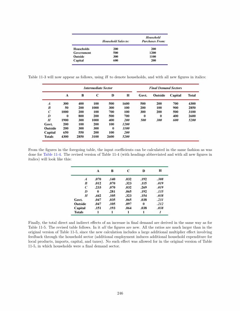
Table 11-3 will now appear as follows, using H to denote households, and with all new figures in italics:

From the figures in the foregoing table, the input coefficients can be calculated in the same fashion as wasdone for Table 11-4. The revised version of Table 11-4 (with headings abbreviated and with all new figures initalics) will look like this:

Finally, the total direct and indirect effects of an increase in final demand are derived in the same way as forTable 11-5. The revised table follows. In it all the figures are new. All the ratios are much larger than in theoriginal version of Table 11-5, since the new calculation includes a large additional multiplier effect involvingfeedback through the household sector (additional employment induces additional household expenditure forlocal products, imports, capital, and taxes). No such effect was allowed for in the original version of Table11-5, in which households were a final demand sector.

246

* Figures in this column show the impact of an added dollar of aggregate final demand sales by all intermediateactivities, apportioned in the same proportions as those activities shared in the final demand sales shown inthe second table above. Specifically, this means added final demand sales of 26¢by A, 22¢by B, 19¢by C, 7¢byD, and 26¢by H, totaling $1.00.

It may be noticed that in each column of this last table, the sum of the figures in the primary-sector rows(government, outside, and capital) comes to 1 (ignoring some trivial rounding-off discrepancies). The sameholds true in Table 11-5. The reader will find it a useful exercise to explain this fact.

247

12. REGIONAL OBJECTIVES AND POLICIES12.1 The Growing Concern with Regional DevelopmentIn the previous chapter, we gained insight into processes of regional economic development involving theinitiation and transmission of changes. We saw, also, that economic change within a region is determinedpartly by external forces beyond the influence of parties within the region itself and partly by decisions andactions that can be taken by such parties.

The present chapter will take up the question of what directions of change are desirable or desired: theobjectives of regional economic policy. We shall look also into the pathology of regional development: whatsituations arise in which there is an urgent need for corrective action. Finally, we shall look into the prophylaxisand therapy aspects of regional development policy: what appropriate means exist for influencing developmentin desired directions and how they can be used most efficiently.1

These questions are definitely in the spotlight today. Vast amounts of talk and action, and a substantialamount of thought, are directed at urgent problems of regional development (including but not limited to thespecial problems of urban life covered in Chapter 13).

Such concern is relatively recent. As late as 1948 it seemed fair to state that:

Although governments have a large stake in the results of locational development, great powerto influence that development, and a correspondingly heavy responsibility for influencing it in asocially desirable direction, few governments have ever followed any coherent policy in regard tolocation.2

The “few governments” referred to certainly did not include the United States.

But a radical change in thinking was already brewing. In Britain even before World War II, it had becomeclear that the depressed economic position of the northern and Welsh industrial areas presented an intractableproblem, and controversy was rife on which national policies might or might not work. Since the 1950s, wehave been observing with some frustration that the so-called developing countries do not seem to catch upautomatically with the more advanced ones, even with continued and massive international assistance ofvarious types.

Moreover (as was noted in the previous chapter) economic statisticians and historians who had beeninvestigating interregional disparities of income within the United States found reason to question theinevitability of convergence. One basis of concern and of desire for better understanding and policies hasbeen a realization that regional stagnation that depression can be quite persistent.

Throughout much of the 1960s, attention was drawn to pockets of poverty in what otherwise was thought ofas the “affluent society.” Today, we are less apt to view regions with low levels of economic growth or eventhose experiencing absolute decline in economic activity as being anomalous. Structural changes in the U.S.economy, which are reflected by the population shifts described in Chapter 11, have given traditional concernsnew weight. These shifts have meant expansion in the “sunbelt” states and relative or absolute decline in many“frostbelt” states. They ‘have also stimulated discussion of programs associated with “reindustrialization,”a term that has come to mean recognizing that the economic base of vast regions of the United States isjeopardized by stiff competition and technological change. Indeed, some pundits now speak of the “rust-belt”as including much, if not all, of the nation’s old industrial heartland.

Important problems must be confronted in the face of such change. Transition can be difficult, whether it isaccompanied by the expansion or the decline of local economic activity. Further, it is rarely easy to identifythe cause or causes of change, and therefore coping with its consequences and planning for corrective actionare also made more difficult.

1Some of the material in this chapter is adapted from E. M. Hoover, “Some Old and New Issues in Regional Development”(paper presented at the International Economic Association Conference on Backward Areas in Advanced Countries, Varenna,Italy, August-September 1967). The conference proceedings were published in E. A. G. Robinson (ed.), Backward Areas inAdvanced Countries (London: Macmillan, 1969; New York: St. Martin’s Press, 1969).

2E. M. Hoover, The Location of Economic Activity (New York: McGraw-Hill, 1948), p. 242.

248

There is a distinctly urban dimension to many of these regional problems. The process of urbanizationaccelerated earlier in this century because of the declining relative importance of agriculture. Unemploymentin urban areas is more visible and more unsettling for both the individual and the community than is ruralunderemployment. Further, the rapid shift of black population from rural areas to urban slums3 intensifiedthis change; and along with a complex of other problems of urban adjustment, it vastly increased the numberof urban areas calling for external economic aid. Problems of traffic congestion and environmental pollution(particularly in and around urban areas) stimulated a search for more rational use of space and resources.

These problems developed during the 1950s and 1960s, when virtually bevery major metropolitan area wasgrowing. Now that a number of larger metropolitan areas are experiencing population decline, additionalproblems have become apparent. At the same time, rapid metropolitan area growth in the South and Westhas meant new pockets of poverty and urban distress in these regions.

Fiscal pressures on local and state governments in the United States are part of the picture too. Forexpanding areas, with increased demands for all kinds of public services, the principal revenue sources ofthose jurisdictions (primarily the real property tax at the local level) often do not keep up with rapidly risingdemands. States and local communities are rightly fearful that higher taxes will drive away or deter businessinvestment.

The same fear persists in regions characterized by decline; the demand for services does not fall proportionatelywith population. Often, the least mobile persons—those left behind—are most in need of public services.This as well as the substantial resources required to maintain the existing infrastructure of roads, bridges,and sewer systems put upward pressure on tax rates that threatens to place areas hard hit by structuralchange at further disadvantage.

As a result of these forces, there has been increasing though sometimes reluctant reliance on the more ampleand flexible taxing powers of the federal government to finance local programs (such as education, health, andhighways), and still more broadly to provide unrestricted grants to the states for use at their discretion. Thischanneling of public money through the national treasury naturally brings to the fore rival regional claims onfederally collected funds, and the competition may be intense as national policy makers are themselves forcedto reconcile diverse pressures for increased expenditures with slow growth in revenues. Thus the problem ofjust and efficient allocation becomes one of the utmost concern.

Still another factor arousing interest in the policy problems of regional development is disillusionment withthe effects and objectives of the more naive forms of local and regional self-promotion. As more localitiesparticipate in this competitive game, more of the total effort is recognized as simply canceling out (that is,each community is driven to promotional efforts in self-defense by the activity of rival areas). And moreand more questions are raised about whether growth itself is a sensible standard of community interest andobjective of public action at the local level.

Next, it appears that there has been a significant shift in the attitude of the general public, and of mosteconomists, toward population growth on a local, regional, national, or world basis. In the 1920s and 1930s,the American credo of the beneficence of population growth was unquestioned, and leading economists andstatesmen were pointing with alarm to the perils of economic stagnation that would beset us if we did notget busy breeding more young consumers. Malthus’s gloomy nineteenth-century warnings were dismissed as adiscredited fantasy.4

This attitude has changed considerably. In part, the change came from the frustration of seeing hard-wonoutput gains in so many of the underdeveloped countries canceled out by mushrooming population growth.Meanwhile at home the postwar baby boom, the all too evident pressures of population growth in urban andoutdoor-recreation areas, the generally inflationary bent of the economy, and the relatively high fertility ofpeople low on the economic and education ladder all helped to undermine the venerable New World traditionof the blessings of increased population. Today, thinking and policy are much more directed toward welfare

3The nonwhite population in the United States has been more urban than the white population since some time in the 1950s.4The best-known statement of this concern over the implications of slow population growth in America is Alvin Hansen’s

presidential address to the American Economic Association in 1938, “Economic Progress and Declining Population Growth,”American Economic Review, 29, 1 (1) (March 1939), 1-15. However, Hansen, unlike some of the other contributors to thatdiscussion, did not advocate incentives to higher fertility as a solution.

249

objectives, such as fuller employment and higher per capita income, rather than to the misleading standardof aggregate growth.

Still another contributing factor in the shift toward more enlightened approaches to regional promotion iswhat might be called the dilution of provincialism. We now find it normal for individuals to make theirhome in several different communities and regions during their lifetime,5 and for them to travel often andwidely. This more varied exposure is conducive to more objective feelings about programs that may benefitone region at the expense of another.

Finally, there have occurred (and are occurring) a number of important changes in the factors determininglocation choices of producers and consumers. These changes, arising mainly from changes in technology andincreased income and leisure, really underlie many of the developments already mentioned and have certainlyplayed a significant part in the rethinking on regional development. These changes in location determinantshave been mentioned in previous chapters and can be briefly recapitulated as follows:

1. In terms of linkages among industries and their sources of materials and markets, the cost of physicaltransport of heavy and bulky goods is less important, and increased importance attaches to thespeedy and flexible transportation of high-value goods and above all to communication—that is, thetransmission of intangible services and information.

2. Access to markets has increased in importance for most industries compared to access to sources ofraw materials and energy sources. This trend reflects the increased variety and complexity of products,which increases, in turn, the importance of shopper comparisons, sales promotion, and servicing, andthus makes proximity to market more desirable. Increased complexity of products has meant also morestages of processing between the primary extraction of natural raw materials and the final consumer,and thus a higher proportion of processes not directly using natural raw materials.

3. More and more importance is attached to amenity factors such as good climate, housing, and communityfacilities, and access to recreational and cultural opportunities. This change reflects rising standards ofincome and leisure, the increased importance of white-collar employment, and the fact that industriesin a dynamic growth stage require a high proportion of well-trained and educated people, who are inshort supply and so can afford to be choosy about where they will live and work.

4. For some industries, there has been an increasing degree of dependence on various services locallysupplied by other industries, institutions, and public bodies. Thus we hear more about the externaleconomies of a location well supplied with such services and facilities. We hear more of the importanceof an adequate regional or community infrastructure—supplying such things as local utility services,police and fire protection, schools, hospitals, reference libraries, and the like—as a necessary basis fordevelopment of profitable enterprises producing goods and services for outside markets.

5. For other industries, the advent of technological advances in electronics and computer equipment hasmeant that production processes which had involved numerous mechanical parts, and therefore theclose proximity of potential suppliers, have been replaced by new processes dependent only on theavailability of one or several microcircuits. The producers using this new technology, as well as thesuppliers of electronic components, are each relatively more free to choose among alternative locations,as compared with their counterparts using or supplying older mechanical parts.

Concern, controversy, and experience have brought into focus some basic issues of regional developmentobjectives and policy, to which we now turn.

12.2 Objectives12.2.1 Individual and Social Welfare Criteria

5Data from the annual Census sample survey indicate that over the twelve-month period March 1980 to March 1981, about 1American in 6 moved to a different house, 1 in 16 to a different county, and 1 in 37 to a different state. See U.S. Bureau of theCensus, Current Population Reports, Series p-20, No. 377, Geographical Mobility: March 1980 to March 1981 (Washington,D.C.: Government Printing Office, 1983), Table 2, p. 8.

250

The ultimate objectives of regional economic policy run in terms of promotion of individual welfare, opportunity,equity, and social harmony. It would seem obvious, then, that economic policy in regard to a region shouldpromote higher per capita real incomes,6 full employment, wide choice of kinds of work and styles of life forthe individual, security of income, and not too much inequality among incomes. The relative importance ofthese goals is, of course, something that economics cannot tell us. Each of us has his or her own values andcan try through the political process to influence the objectives of social policy so as to reflect those values.7

The aspect of equity raises some difficult questions in connection with the application of these criteria toprograms and policies affecting such diverse groups of people as the inhabitants of a region. Any action—such as spending public funds for improved services, subsidizing the establishment of new industries in theregion, or imposing restrictive controls on land uses—is sure to help some people more than others and maywell help some at the expense of others. There is general agreement, however, on the guiding principle ofthe so-called Pareto optimum,8 which says that a change is desirable so long as it helps somebody withouthurting anybody else. In practice, some of the benefits conferred on individuals by a change (for example,building a new highway) can be taxed away from these beneficiaries so as to compensate those who otherwisewould suffer by the change; and the real question is whether the Pareto criterion is satisfied after feasiblecompensatory transfers of this sort have been made.

This guiding principle is much easier to propound than to apply. The very essence of a region is interdependenceof activities and interests, and these interactions become particularly crucial in a high-density urban regionwithin a city or neighborhood. Any change in one activity produces externalities and neighborhood effects ona variety of other activities, and these effects can be either helpful or harmful. Thus the building of a sportsstadium can help the merchants of an area by bringing in more visitors and purchasing power, while at thesame time it can spoil the surrounding residential neighborhood by creating traffic congestion, noise, andlitter.

An important task for regional economists is to devise ways of “internalizing” the externalities involvedin regional change. Take, for example, a chemical plant whose operations pollute a river. The pollutionimposes a variety of injurious externalities on other residents of the area. Thus other industrial plants andwater-supply systems downstream will have to incur extra costs for water treatment preparatory to use;businesses based on recreational use of the river, or fishing, will suffer diminished patronage, higher costs, orboth; and there will be a still broader injury to the community in terms of loss of recreational opportunityand amenity, and possible health hazards. In principle, it might be possible to set a fee or tax on the chemicalplant to reflect all these social costs, whereupon the costs of pollution would become internal costs of thechemical firm. These costs having been properly internalized, or placed where they belong (that is, imposedon the party that causes them), the chemical firm will have to reconsider its profit calculus. It can (1) choosea different location altogether; or (2) invest some money in effluent treatment to reduce or eliminate thepollutant, and thus get relief from the special tax; or (3) continue the pollution and pay the tax, whereuponthe community gets the money to use for downstream water treatment or for compensating in some fashionthe various parties injured by the pollution. Any one of these three outcomes is, of course, preferable to theoriginal situation in which the chemical plant’s activities imposed social costs borne by other parties. Thisholds true regardless of whether the polluting firm absorbs or passes on to its customers the added costsimposed on it.

We can also speak of internalization in the opposite case, in which some individual activity yields externalbenefits to other parties but cannot feasibly collect directly from them in return. In such a case, the sociallyoptimum scale of this activity is greater than the scale on which it will be led to operate on the basis ofits costs and returns. Internalization of the social benefits will then be in the general interest. This is therationale for the granting of various forms of subsidies, inducements, and exemptions to activities that are

6See the discussion in Chapter 10 on real income.7For a more detailed discussion of regional policy objectives, see Charles L. Leven, “Establishing Goals for Regional Economic

Development,” Journal of the American Institute of Planners, 30, 2 (May 1964), 99-105; Thomas Wilson, Policies for RegionalDevelopment, University of Glasgow Social and Economic Studies, Occasional Paper No. 3 (Edinburgh and London: Oliver& Boyd, 1964); Wilbur R. Thompson, A Preface to Urban Economics (Baltimore: Johns Hopkins University Press, 1965),Chapter 5; Benjamin Chinitz, “Appropriate Goals for Regional Policy,” Urban Studies, 3, 1 (February 1966), 1-7; and Harry W.Richardson, Regional Economics (Urbana: University of Illinois Press, 1978), Chapter 9.

8Named after the Italian economist and sociologist Vilfredo Pareto (1848-1923), a pioneer analyst of economic welfare.

251

believed to have beneficial external effects. Thus a chamber of commerce or a neighborhood merchants’association may raise money from its members to help build a convention hall, park, or other facility thatthey believe will eventually help their business; or a municipality or a state may use general tax funds tosubsidize new industries, or give them tax exemptions, on the theory that such subsidy is a sound investmentfor the taxpayers as a group.

12.2.2 Regional Economic Growth as a Goal

What has been said above applies to economic objectives and policies for the welfare of a group of people.But a region is not, except at an instant in time, a definite group of people—it is an area populated bya changing group of people. In any region of consequence, every day sees some new arrivals (by birth ormigration) and some departures.

This continual turnover of a region’s population complicates the question of policy goals. What is to bemaximized over, say, the next ten years? The welfare of the present inhabitants of the region, regardless ofwhere they may be in ten years’ time? The welfare of those who will be living in the region ten years hence,regardless of where they are now? Should it be counted as a regional gain if some people move in whoseincomes are above the regional average, so that the average rises with their advent? If so, should one of theaims of regional policy be the out-migration of its poorer inhabitants? Is a region improved if its populationand total income increase at equal rates, with per capita income unchanged?

Our preferred objective for a region’s development depends, of course, on where we sit. In addition todifferences of interest among groups within a region, there is an important difference between the optimumfor any single region and the optimum pattern of regional growth rates in relation to national welfare.

Is simple regional growth (in aggregate terms, without regard to per capita income or welfare levels) a sensibleobjective? On the face of it, such a criterion sounds quite irrelevant. Yet in practice we find that regionalpromoters and governments spend a great deal of money and effort in the avowed pursuit of a bigger regionaleconomy—that goal is put forward without apology as something worth striving for.

How can this be explained? Partly, perhaps, by emotion and tradition. The idea that “bigger is better” hasbeen a remarkably enduring component of American ideology, although it is no longer such a universal articleof faith.

There is an even more basic explanation, however. A substantial part of the business and political interestsin a region are, in locational terms, oriented to the local demand and thus have a direct stake in the overallpopulation and income of the region. Department stores, newspapers, banks, utility companies, real-estateowners and speculators, and local political leaders have vested interests in aggregate growth. Their fortunesdepend not so much on how well off the region’s people are as on the size and growth rate of the population.Net in-migration is good from their standpoint even when accompanied by a reduction in per capita incomeand other aspects of individual welfare; population losses are viewed with alarm.9

Quite logically in terms of their own interests, therefore, these groups are active promoters of and contributorsto any programs and policies that promise to expand the regional economy in terms of aggregate incomeand employment. It is they who most zealously support chambers of commerce and local or regional boosterassociations. Firms primarily involved in export business have little or nothing to gain from such participationand, indeed, often stand to lose (through higher costs of labor, land, and some other local inputs) in acommunity or region experiencing rapid growth.

Here we have still another important contradiction to the widespread view, discussed in the previous chapter,that the primary sources of regional growth lie in the exporting sector. Local promotional efforts, at any rate,come mainly from the local market-serving or nonbasic sector.

9A challenging and brilliant discussion of the actual and supposed benefits and costs of regional growth is E. J. Mishan,The Costs of Economic Growth (London: Staples Press, 1967). An illustration of the conflicting interests involved in regionalprosperity is the report that in June 1969, an association of residents of Hawaii implored convention visitors from the mainlandto curb their spending, because such spending raises living costs for the residents. The state of Oregon attracted attention (andperhaps ironically a few additional migrants) in the early 1970s when its governor and other high officials enunciated oppositionto in-migration, rapid population growth, and excessive tourism. More and more cities and towns are now seeking constitutionaland effective means of limiting growth.

252

What has just been said refers to regional growth in aggregate terms. In terms of individual economic welfarein the area (as roughly gauged by per capita real income), the interest groups play quite different roles—and it is in such terms that civic responsibility should really be judged. The local market servers, in theirpursuit of the gains to be had from population growth and added business and housing development, toooften assume that what is good for themselves must be good for the community, and then proceed to sacrificequality of life for quantity. Since these interests include such powerful voices as those of utilities, banks,merchants, local public officials and union leaders, and (most important) the local news media, they can easilypush an area into destructive overdevelopment. In one area where residents had been protesting for years thefrantic and planless replacement of orchards and pleasant countryside by solid square miles of subdivisionsand shopping centers, the leading newspaper publisher defended his advocacy of still more growth by thefrank observation, “Trees don’t read newspapers.”

Finally, we note here still another mechanism by which regional or community change can become self-reinforcing and cumulative. Rapid growth confers increased income, prestige, and political influence onreal-estate brokers and promoters, builders, and the other groups whose interests are served by local expansionas distinct from improvement of local well-being. This added power helps “growth-at-any-price” pressuregroups to shape local planning and policies toward still further emphasis on continued growth and still lessconsideration of environmental and other welfare effects. Pure boosterism is truly narcotic, producing firsteuphoria, then addiction, and eventually decay.

12.2.3 Regional Objectives in a National Setting

Regions are not self-contained nor independent of one another. Accordingly, a true concern for human welfarecalls for evaluating development and framing policy goals on a multiregional or national basis.

National High-Employment Policy and Regional Economic Adjustment. Experience has taughtus that we cannot expect any satisfactory solution to the problem of regional unemployment or arresteddevelopment except in the context of a prosperous national economy. In a depression period, businessesare doing relatively little capacity expansion and have little difficulty in finding locally the necessary labor,services, and space for such expansion as they want to undertake. Their investment is more likely to take theform of cost-cutting improvements in existing plants, and this may well involve closing down some branchfacilities at the more marginal locations. Moreover, in slack times, the surplus manpower in any area hasliterally nowhere to go and fewer resources to go anywhere; we cannot look to labor migration for anysignificantly useful adjustment.

We have found also that the national monetary and fiscal authorities have great powers to increase the nation’smoney supply and disposable income, and thus to stimulate spending and investment in the aggregate. Suchaction helps to maintain the necessary buoyant climate in which constructive regional adjustments by peopleand industries can occur.

Efficiency, Equity, and Structural Unemployment. Some people feel that maintaining a high level ofemployment and demand in the economy is as much as the national government should do in regard to regionaleconomies. There are, however, two distinct arguments for other, and more specifically region-oriented,national policies and programs.

The first argument invokes the criterion of efficiency, claiming that there are other ways besides fiscaland monetary policy for facilitating effective allocation of resources among regions and the necessarydynamic adjustments. The second argument is based on equity,claiming that the national government has aresponsibility for helping disadvantaged regions as such.

The efficiency argument rests largely on the idea of “structural unemployment.” This type of unemploymentcomes about because there are wide disparities in the employability of different groups in the labor force.There are poor matching between the kinds of labor that are in demand and those that are available, andthere is insufficient mobility and interchangeability within the labor force. This makes shortages, rising costs,and consequently inflation inevitable, while millions of the less employable are still out of work. Obviously,any policies that will reduce these wide disparities and make manpower more mobile and interchangeable willhave the good effect of shifting the inflationary brink closer to the ideal of full employment.

253

There is, then, a strong case for public programs involving education and worker training and retraining,and for more direct aids to spatial and occupational mobility: for example, improved information about jobopportunities, assistance to migrants, and removal of racial and other discrimination in employment. It isalso clear that such efforts ought to focus on upgrading the least advantaged types of workers and reducingtheir competitive handicaps. Such emphasis is, of course, in accord with equity objectives as well.

Helping Regions and Helping People. When it comes to translating this policy into geographical terms,we pass from consensus into controversy. It is tempting to argue that if public policy should specifically helpthe less-advantaged classes of people to find jobs, then it should by the same token seek to underwrite theprosperity and growth of all communities.

Such a view has been aptly characterized as substituting “place prosperity” for the more fundamental objectiveof “people prosperity.”10 its more naive expressions, the place prosperity doctrine represents merely falseanalogy: an unreasoning assumption that whatever is true of individuals must also apply to areas. On amore rational level, it is possible to suggest place prosperity as a pragmatic proxy for the ultimate ideal ofpeople prosperity—on the hypothesis that the best way to help a person is to promote the overall prosperityof the area in which he or she happens to live.

The place prosperity doctrine will figure importantly in later discussion in this chapter. For now, it is enoughto indicate two of its shortcomings. The first lies in ignoring the fact that a region does not correspond,for any length of time, to a fixed set of people. Since people have some mobility, the best way to helpdisadvantaged people who are living in a particular region may be to encourage them to move. Migrationcan, in fact, serve both the objective of efficient use of resources and the objective of interpersonal equity anddistribution of opportunity.

A second criticism of the place prosperity approach is that in practice it is wastefully nonselective in itsassistance. In any community or region where there are unemployed and needy people, there are also employedand prosperous people. Increased employment and income for the area as a whole may help those whoneed it most; but a large part of its local benefits will come to those who do not need it. Those surest tobenefit, as suggested earlier, are generally property owners and the operators of established locally orientedbusiness, such as utilities, banks, and commercial and consumer service firms.11 Growth of aggregate areaincome and employment does not automatically mean improvement in per capita income or the reduction ofunemployment, and it generally injures some while helping others. Such considerations suggest that attackinghuman hardship and lack of opportunity solely through place prosperity might be like using a shotgun to killflies.

Regional Rivalry and the National Interest. The benefits of growth in a region are directly andstrongly felt by certain influential interest groups, while the costs are likely to be more diffused and lesswell perceived. Most regions, consequently, devote some effort to furthering their own economic growth byattracting additional activities.

Regional rivalry, like other forms of competitive promotion and warfare, can be in large part self-defeating, ora “zero-sum game,” contributing nothing to the national welfare. One region’s gain is another’s loss. Thisis especially likely when the regions are small and when the primary weapons are persuasion and subsidy.Resources such as capital and labor that are drawn to one area cannot be used in production elsewhere, andfrom a national perspective there is no net gain, unless the productivity of those resources is higher in thereceiving region. From this perspective, the nation’s rate of growth is analogous to a pie; a bigger slice forone region means a smaller slice for some other region.

However, regional growth may be generative rat her than competitive. In this more positive light, efficiency10Louis Winnick, “Place Prosperity vs. People Prosperity: Welfare Considerations in the Geographic Distribution of Economic

Activity,” in Essays in Urban Land Economics, in honor of the sixty-fifth birthday of Leo Grebler (Los Angeles: Universityof California, Real Estate Research Program, 1966). For a much deeper exploration of the place prosperity concept and itsrelation to regional and national policy objectives, see Marina von N. Whitman, “Place Prosperity and People Prosperity: TheDelineation of Optimum Policy Areas,” in Mark Perlman, Charles Leven, and Benjamin Chinitz (eds.), Spatial, Regional, andPopulation Economics (New York: Gordon and Breach, 1972), pp. 359-393.

11See Matthew Edel, “’People’ versus ’Place’ in Urban Impact Analysis,” in Norman J. Glickman (ed.), The Urban Impacts ofFederal Policies (Baltimore: Johns Hopkins University Press, 1980), pp. 175-191.

254

gains in each region may promote national prosperity. As Harry Richardson puts it:

It is possible for national growth to be increased by faster regional growth, and it is possible forregional growth performance to be improved without additional resource inputs. Agglomerationeconomies and spatial clustering of activities may induce more output than if production isdispersed. Growth-inducing innovation may be adopted by local entrepreneurs, even though theywere first introduced outside the region. A change in settlement pattern (i.e., a more efficientregional urban hierarchy) or a reorganization of the intra-regional transportation system mayimprove productive efficiency and promote faster growth.12

Thus enlightened local efforts to enhance a region’s growth potential can result in significant net benefits.These efforts may take the form of upgrading the region’s human and natural resources and public services,protecting and improving amenities, stimulating entrepreneurship and innovation, fostering cooperationamong various business, social, and political elements, and discovering the true comparative advantages ofthe region for further development. All these effects favor better utilization of resources and are clearly inboth the national and the regional interest. A logical national policy with regard to regional developmentshould include some effort to channel the growth urge of regions into these constructive paths.

But it is also true that regional rivalry in development can be something worse than a zero-sum game if itdistorts the efficient allocation of resources. This danger is inherent in the use of local subsidies, and most ofall with respect to the use or abuse of natural resources and the neglect of externalities.

Competitive regional and urban development are clearly suboptimal. They may involve regionsin a competitive race to offer up for private exploitation their air and water quality. Theresulting resource deterioration involves transfer of income from local residents to business firms.Competitive tax concessions to attract development may also result in relative weakening ofthe public sector. Competitive regional development may involve serious external diseconomiesresulting from failure to treat environmental units, such as river basins, as planning units. Thelarger the planning region, the more adequately externalities can be assessed.13

We see, then, that national policy in terms of the development of specific regions can help to achieve moreefficient use of natural resources as well as to reduce regional unemployment and broaden human opportunity.

12.3 Regional Pathology: The Emergence of “Problem Areas”Regions, like people, want a doctor only when they are sick. When a region is enjoying growth-euphoria andreasonably full employment, there is no great disposition to examine its situation and prospects in detailand search for ways to gild its robust health. National attention is directed only to those regions that are introuble, and there always are enough of them to worry about. We assume, in other words, that in healthyregions the workings of the market economy under existing constraints are relatively satisfactory.

To focus on regional pathology is both politically and economically rational. Our diagnostic and therapeuticresources are limited enough, and we are more likely to find something helpful to do for regions with obviousailments than to improve comparably an already good situation. The only risk is that we may thus overlookopportunities to nip unwelcome developments in the bud.

Our main concern here is with situations where things have definitely gone awry. Regional economic growthis not a smooth, straightforward process. The persistence of efforts to explain development in terms ofsuccessive “stages” attests to the existence of important discontinuities. We do not by any means know whatall these are, how to foresee them, or how to deal with them. But we do know that the development ofa region, like that of a nation, encounters from time to time crucial situations in which its future coursecan be significantly influenced by major planning decisions and policies. Alternative paths appear; one ofthe alternatives may be a further growth along some new line, and the other may be stagnation, arresteddevelopment, or even regression.

12Richardson, Regional Economics (Urbana: University of Illinois Press, 1978), p. 146.13John H. Cumberland, “A Regional Interindustry Model for Analysis of Development Objectives,” Papers of the Regional

Science Association, 17 (1966), p. 93. For a contrary view see James R. Rinehart and William E. Laird, “Community Inducementsto Industry and the Zero-Sum Game,” Scottish Journal of Political Economy, 19, 1, (February 1972), 73-89.

255

These crucial situations present the biggest challenge to our insight into growth-determining factors. Thestakes are highest and the rewards for correct decisions, in terms of economic progress, are at a maximum.

12.3.1 Backward Regions

A familiar case is that of underdeveloped nations poised on the threshold of industrialization and threatenedby a genuine Malthusian peril of overpopulation. Much effort has gone into defining the conditions necessaryfor a successful surmounting of the threshold, the so-called “takeoff into self-sustaining growth” process.

Most if not all of the advanced countries also include one or more backward regions, which seem to be hungup at a threshold on the road of development and not to have kept pace with the structural changes andthe rising income and opportunity levels of the more fortunate regions of the country. In the United States,Appalachia, a huge zone characterized by rural poverty, straddles the Eastern Highlands from New YorkState to Mississippi. Other large areas demanding special developmental attention have been identified also,and many smaller pockets of relative poverty and apparently arrested development exist in still other parts ofthe country. In Canada, the extreme eastern part of the country (the Maritime Provinces) is regarded as thechief area of concern of this type; in Italy, it is roughly the southern half of the country (Mezzogiorno); inSweden, it is the far north.

12.3.2 Developed Regions in Recession

A second and quite different type of problem area is the mature industrialized urban region afflicted bystagnation. In Britain, the industrial areas of southern Scotland and Wales and northern England enteredthis phase in the 1920s. In the United States, at about the same time, migration of the textile industry tothe South laid heavy blight on the industrialized region of southern New England, and real rejuvenation withnew industries did not set in for more than twenty years. In the Pittsburgh region, slow growth or decline inthe leading industries caused fears of stagnation and regression that gave rise to a major community effort toreverse the trend after World War II.14

Symptoms of this particular syndrome are easily recognizable. The ailing region’s rate of growth has beenincreasingly subnormal for many decades. Unemployment is high and chronic. Out-migration is heavy. Thearea appears to have somehow lost the dynamic growth character that had brought it to its peak importancein days gone by. There is a feeling that unless something really decisive happens, stagnation will prevailindefinitely.

Such a situation can arise in a region whose economy is heavily based on a few activities that have themselvesceased to grow or have begun to decline. They are the activities of yesterday and today, but not those oftomorrow. But arrested growth in a region may also mean simply that the factors of interregional competition,in specific activities, have taken a trend adverse to that particular region. The region’s difficulties arecompounded if both of the above conditions apply, so that it finds itself with shrinking shares of decliningactivities.15 An excellent example of this is the “Steel Valley,” which encompasses much of the upper OhioRiver Basin and includes such cities as Youngstown, Wheeling, and Pittsburgh. The westward movementof the market for steel has left this region with old technology and a declining share of total U.S. steelproduction; all this in an industry that finds itself at an overall disadvantage when competing with foreignmanufacturers.

But in diagnosing the ills of such a region, it is not enough to determine the extent to which it is losing groundto other areas in major activities, or the extent to which its activities are no longer of the growth-industrytype. After all, we could hardly expect that every activity would continue to grow forever, or that any givenregion could forever retain or increase its relative position in its principal activities. A healthy regionaleconomy can absorb losses in its stride and shift its resources into new fields, getting a share of the emergingnew rapid-growth activities to balance the inevitable decline of other activities.

14See Pittsburgh Regional Planning Association, Economic Study of the Pittsburgh Region, 3 vols. (Pittsburgh: University ofPittsburgh Press, 1963). The first volume, Region in Transition, traces the economic history of the region and diagnoses itsposition as of the time of writing. The second volume, Portrait of a Region, by Ira S. Lowry, focuses on population trends andthe geographic patterns of activities within the region. The third volume, Region with a Future, assesses prospects for Furtherchange and suggests some appropriate directions for policy. A concise summary of the study’s approach and findings is E. M.Hoover, “Pittsburgh Takes Stock of Itself,” Pennsylvania Business Survey, 5, 1 (January 1964), 4-9.

15See the illustration of shift-share analysis in Appendix 12-1.

256

It is important to keep this in mind when trying to determine the proper role of federal and local policies inregional development. Change is a necessary aspect of growth, and it is as inevitable that some regions willprosper and others will not as it is that some individuals will fare better than others. Nevertheless, whenchange affects broad areas of the country—as is presently the case in the United States—large numbers ofpeople are involved, and the political pressure for a response to related problems may become intense.

However, all affected regions are not equally in need. For some, the basis for rejuvenation may have beenestablished well before decline becomes evident, and the proper role of policy may be limited to easing thetransition. Other regions fail to make such adjustment successfully, and we must ask why. Perhaps it issimply because the degree of specialization in nongrowing activities was so intense. Perhaps it is becausethe loss of competitive advantage in some important activities has been so drastic. Or perhaps it is becausethe region has developed a sort of economic arthritis that inhibits its ability to adjust to rapidly changingconditions.

Whether regional analysts operate as full-fledged physicians ministering to the economic ills of sick regions,or more narrowly as diagnosticians, they have a special concern for cases in which the patient seems deficientin resistance to infection and in ability to recover. We have to look beyond the immediate symptoms to theless obvious organic difficulties.

12.3.3 Excessive Growth and Concentration

In both types of problem regions thus far mentioned, a basic symptom is that employment opportunities havenot developed (in amount, in variety, or in both) fast enough to keep pace with the size and aptitudes of thelabor force. Resources are underutilized. Somewhat the opposite situation prevails in regions that undergoextremely rapid growth involving massive inward migration. The growing pains of such regions are felt asimpairment of the quality of services, destruction of local resources and amenities through overuse, a highrate of obsolescence of facilities, neighborhoods, and institutions, and a general deterioration of the quality oflife. The forestalling or mitigation of these effects through analytical foresight and advance planning poses amajor challenge to regional specialists.

The most widespread and obvious present-day examples of the perils of too rapid development appear intwo types of areas. One is the suburban fringe of metropolitan areas, where many factors have combined toproduce sudden and often unforeseen growth. The other type of area comprises zones of special recreationalamenity such as beaches. The growth of population plus its increased mobility, leisure, and taste for outdoorpleasures add up to a formidable threat to our basically nonexpansible resources of open space, clean water,and privacy. This problem obviously involves much more than temporary “growing pains.” As was suggestedin section 12.2.2, the pressures of interest groups in a community or region lend themselves to overemphasison growth per se, all too often at the expense of well-being.

Related to, but distinct from, the question of too rapid growth is the problem of excessive spatial concentrationof development, specifically in gigantic metropolitan centers. Concern on this score is felt in nearly everycountry. In the less developed countries, the problem is seen as exclusive concentration of modern industrialdevelopment, business, and population in the chief city. In France and England, the concentration of growthin Paris and London has been officially deplored, and attempts have been made to combat associated problemsfor a generation or more.

The question whether our large metropolitan areas are “too big” defies any easy answer.16 Part of thedifficulty lies in the variety of possible criteria. Large cities have been variously assailed as hotbeds of vice,breeders of psychological and political disorder, and hazards to health and safety; and they have been extolledfor equally diverse virtues. With respect to economic criteria, it is often argued that the rising costs of housing,public services, and similar items make large cities uneconomical as places to produce or to live. Thesediseconomies of size are said to outweigh, in very large cities, the positive advantages of urban agglomerationthat we discussed earlier.

16This question has concerned many researchers. Some of the most notable recent contributions to this literature includeWilliam Alonso, “The Economics of City Size,” Papers and Proceedings of the Regional Science Association, 26 (1971), 67-83;Harry W. Richardson, The Economics of Urban Size (Boston: D. C. Heath, 1973); and A. M. J. Yezer and R. S. Goldfarb, “AnIndirect Test of Efficient City Size”, Journal of Urban Economics, 5, (January 1978), 46-65.

257

A strong substantial body of empirical evidence suggests that there are strong net economies in the provisionof infrastructure and public services of middle-sized cities as compared to small ones. The curve relating percapita expenditures on items in these categories to city size flattens out somewhere in the 100,000-to-500, 000population bracket, with a possibly rising trend thereafter.17 On this limited basis, there is no “economicoptimum size” of city, though we might refer loosely to a “minimum efficient size.”

There are difficulties with this approach, however, in that expenditures reflect differences in the quantity andquality of services provided as well as costs. Thus persons in large cities (where, as mentioned in Chapter10, we expect to find higher real income per capita) may have demands for public services that are differentfrom those of persons in smaller cities, and this will affect per capita expenditures. John L. Gardner hasundertaken an analysis of municipal expenditures that accounts for variation in income and wealth acrosscities.18 For a wide range of expenditure categories, he finds that costs per family increase with city size.However, Gardner also finds that costs typically decline as population densityincreases.19 Thus it may bemisleading to concentrate on size alone; the efficiency of cities appears to depend on population size anddensity jointly.

In any event, costs of public services are only one element in the comparative economic advantages of differentsizes of cities. A more accurate approach to this problem would recognize that the activity of cities includesthe production and consumption of private as well as publicly provided goods and services. In order to makevalid comparisons, one must account for the incremental benefits and costs associated with each as city sizeincreases.

Many regional economists see hidden disadvantages in very large cities, justifying a public policy of divertinggrowth from such cities to medium-sized ones. They argue that there are important external diseconomies(such as added costs of housing, congestion, and environmental spoilage) that do not enter into the calculationsof the firms or individuals who contribute to city size by establishing themselves there—in other words, thesecosts should, but do not, work to limit urban growth. For example, an additional urban freeway commuteradds to congestion and causes losses to all the other commuters whom he slows up, but he does not have topay for the added costs inflicted on the others and is not deterred from rising the freeway.

Such externalities are real enough, and we shall have occasion to consider them further in Chapter 13. Buttheir existence does not necessarily imply a net bias toward excessive city size, as is frequently alleged. First,the usual argument assumes too readily that the external diseconomies of large city size outweigh the externaleconomies; however, as we saw in Chapter 5, the economies associated with urbanization may be substantial.Further, it implicitly assumes that the adverse externalities fall on parties that have no recourse—that is,they are “locked in” and can neither leave the city nor raise the price of their services in order to compensatethemselves for the injuries suffered.

By and large, this assumption is unwarranted. Individuals and firms subjected to such external diseconomiesas air pollution, traffic delays, long commuting journeys, high taxes, expensive housing, or noise can (and do)decide that they will not stay in such an environment unless they are paid extra to do so. Urban populationsare characteristically mobile, and pay rates do run higher in large metropolitan areas than elsewhere, as wesaw in Chapter 10. This suggests that at least some of the disutilities that urban life imposes on the individualare being passed back to employers in the form of higher wage costs. The effect of the cost increases on pricesis undoubtedly greater for local goods and services than for those traded between cities, since prices tend tobe set in the national market for traded goods and services;20 nevertheless location decisions will be affected.

17Werner Z. Hirsch, Urban Economic Analysis (New York; McGraw-Hill, 1973), Chapters 11-12. See also Nibs M. Hansen,Rural Poverty and the Urban Crisis (Bloomington: Indiana University Press, 1970), Chapter 10; and G. M. Neutze, EconomicPolicy and the Size of Cities (Canberra: Australian National University, 1965).

18John L. Gardner, “City Size and Municipal Service Costs,” in George S. Tolley, Philip E. Graves, and John L. Gardner(eds.), Urban Growth Policy in a Market Economy (New York: Academic Press, 1979), pp. 51-61.

19This result lends support to arguments made by Tolley to the effect that economies in the provision of public services arerelated primarily to the density of population in the service area. See George S. Tolley, “Comparing the Gains and Costs of CityGrowth,” in Tolley, Graves, and Gardner, Urban Growth Policy in a Market Economy, pp. 25-34.

20See George S. Tolley, “The Welfare Economics of City Bigness,” Journal of Urban Economics, 1, 3 (July 1974), 324-345,where the relationship between prices and compensation for urban disamenities is discussed in terms of a “wage multiplier.” Seealso, Oded Israeli, “Externalities and Intercity Wage and Price Differentials,” in Tolley, Graves, and Gardner, Urban GrowthPolicy in a Market Economy, pp. 159-194.

258

The market forces set in motion by compensatory payments to labor for urban disamenities may not fullyoffset the tendency for cities to become “too big,” but they certainly work to counteract that tendency.21 Theextent of this offset will depend on the reaction of affected parties to externalities. If workers are immobile(or, more generally, if location-fixed resources are affected by externalities), they may not be compensated forurban disamenities. Similarly, if producers of traded goods lack mobility and also are limited in their abilityto pass compensatory payments along to customers in the form of higher prices, the market adjustment toexternalities will be incomplete. Thus the greater the mobility of workers and producers, the more we canexpect that diseconomies will be internal to the city as a whole in that they fall on firms and households whosedecisions affect city size.22 This does not imply that we may dismiss concern about adverse externalities assuch, or concern about the many serious problems attending urban growth, which do in fact tend to be mostaggravated in very large cities.

The foregoing discussion suggests that the search for an “optimal” city size may be elusive. The task ismade even more difficult by the failure of most researchers to account for the fact that each city is but oneelement in a central-place hierarchy. In Chapter 8, we found that cities specialize by function—rangingfrom the smallest hamlet to large wholesale-retail centers. This specialization was influenced by efficiencyconsiderations: agglomeration economies encouraged some activities to locate in proximity to suppliers orpotential customers. As a result, the mix of goods offered by trade centers varies, and large centers arecharacterized by a more complete set of activities. For persons residing in all but the largest urban area,some shopping in higher-order centers is dictated by the spatial organization of production. It follows thatthe most efficient size for a city depends on the array of goods and services provided elsewhere in the urbanhierarchy and on the efficiency of transport and communications among cities.23

12.3.4 Comparison of Characteristics of Problem Areas

Table 12-1 summarizes the results of a tabulation of American “problem areas” (mainly on a county-by-countybasis) made by Benjamin Chinitz in 1967. The categories are along lines already suggested above, but forone striking difference. It is indicative of the dramatic change in our attitudes toward regional developmentthat Chinitz’s category I (high income, fast growth) was as recently as 1967 considered a problem categoryon the basis of unemployment, with no mention of the environmental impact, destruction of amenities, anddeterioration of the quality of living, which we now consider the major penalties of excessive growth. Asubstantial number of cases of fairly severe unemployment do occur from time to time in basically flourishinglabor markets, such as San Diego in Chinitz’s sample. Often these are transitory situations reflecting cutbacksin federal defense-contract employment in the area, and in some cases the unemployment is mainly seasonal;but it may be more chronic in areas that attract large numbers of migrants by their amenities.

21See Tolley, “Welfare Economics of City Bigness,” pp. 335-338.22The external diseconomies argument would also have more weight if it could be established that personal and business

migration from large cities is somehow more inhibited than the contrary flow, or that state and national governments areconsistently subsidizing locations in large cities at the expense of taxpayers elsewhere.

23See Richardson, Economics of Urban Size, p. 129; and J. Vernon Henderson, “Effect of Taxation of Externalities on CitySize,” in Tolley, Graves, and Gardner, Urban Growth Policy in a Market Economy, pp. 91-97.

259

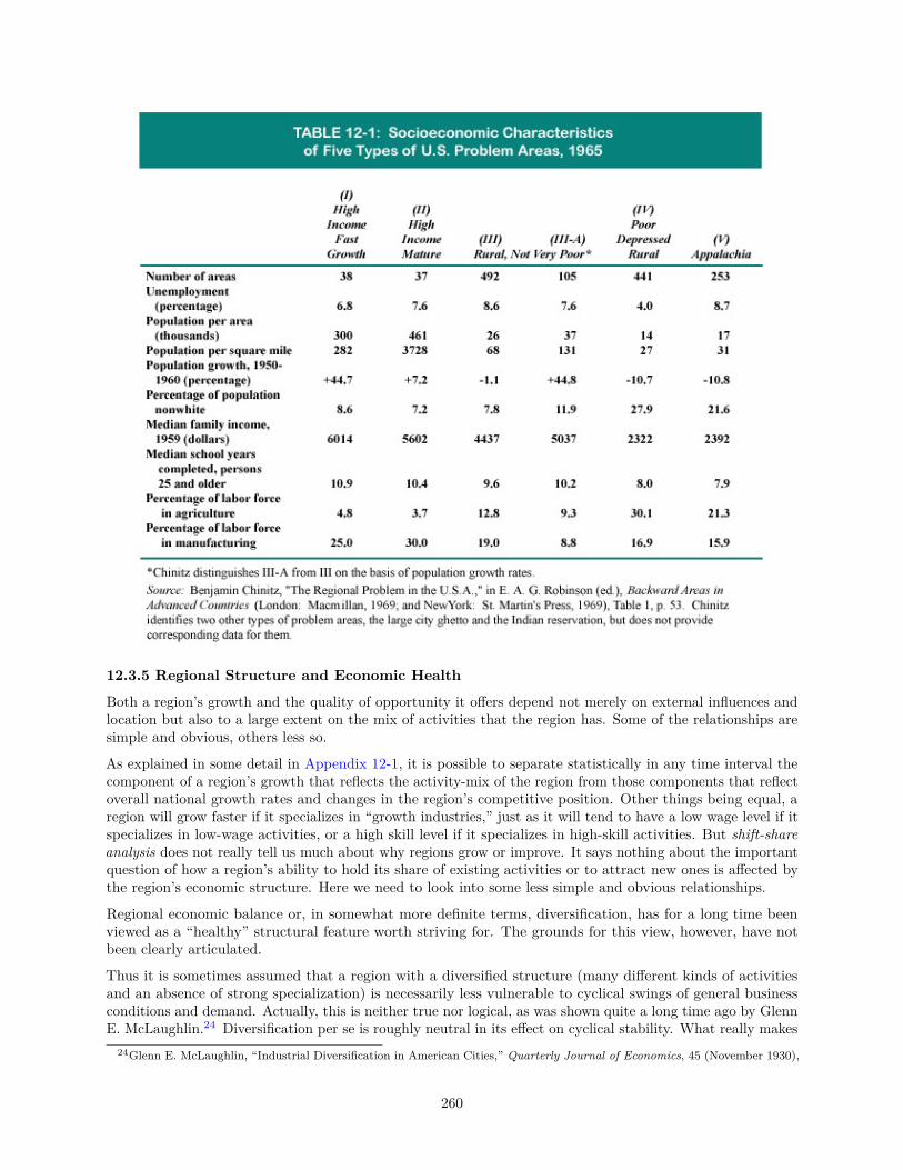
12.3.5 Regional Structure and Economic Health

Both a region’s growth and the quality of opportunity it offers depend not merely on external influences andlocation but also to a large extent on the mix of activities that the region has. Some of the relationships aresimple and obvious, others less so.

As explained in some detail in Appendix 12-1, it is possible to separate statistically in any time interval thecomponent of a region’s growth that reflects the activity-mix of the region from those components that reflectoverall national growth rates and changes in the region’s competitive position. Other things being equal, aregion will grow faster if it specializes in “growth industries,” just as it will tend to have a low wage level if itspecializes in low-wage activities, or a high skill level if it specializes in high-skill activities. But shift-shareanalysis does not really tell us much about why regions grow or improve. It says nothing about the importantquestion of how a region’s ability to hold its share of existing activities or to attract new ones is affected bythe region’s economic structure. Here we need to look into some less simple and obvious relationships.

Regional economic balance or, in somewhat more definite terms, diversification, has for a long time beenviewed as a “healthy” structural feature worth striving for. The grounds for this view, however, have notbeen clearly articulated.

Thus it is sometimes assumed that a region with a diversified structure (many different kinds of activitiesand an absence of strong specialization) is necessarily less vulnerable to cyclical swings of general businessconditions and demand. Actually, this is neither true nor logical, as was shown quite a long time ago by GlennE. McLaughlin.24 Diversification per se is roughly neutral in its effect on cyclical stability. What really makes

24Glenn E. McLaughlin, “Industrial Diversification in American Cities,” Quarterly Journal of Economics, 45 (November 1930),

260

a region especially vulnerable to cyclical swings is specialization in cyclically sensitive activities (mainly,durable goods industries and especially those making producers’ equipment and construction materials andcomponents). Thus a specialized steel-making center such as Youngstown naturally has greater cyclical upsand downs of employment than either tobacco-processing centers such as Winston-Salem or Durham or abroadly diversified manufacturing center such as Philadelphia. Analogously, a community or region highlyspecialized in seasonal recreation (such as Virginia Beach or the coast of Maine) shows much more seasonalvariation in employment than the average area, while a region specialized in some nonseasonal activity maybe more seasonally stable than the average.

It is a different story, however, when we consider stability and other desirable attributes over a longer period.In time, any of a region’s activities will suffer arrested growth and perhaps decline or even extinction, eitherbecause the product itself becomes obsolete (as in the famous case of buggy whips, which sorely affectedWestfield, Massachusetts, the principal whip-making center of the country) or because the region loses outcompetitively (as, for example, New England lost to the South in textile manufacturing, and Pittsburgh inthe nineteenth century successively lost out as a leading producer of salt, wagons, cotton textiles, and refinedpetroleum products).

If a region is narrowly specialized, such a loss can be, at least temporarily, disastrous; in a diversified region,it is unlikely that a major proportion of the total activity will suffer at any one time. Equally significant is thefact that a narrowly specialized region is likely to show less resilience in recovering its stride by developingnew activities to take the place of those lost.

This attribute of resilience is an extremely important aspect of regional economic health. It depends to a largeextent on diversification, since diversity of employment develops a wide variety of skills and interests in thelabor force and also among business entrepreneurs, bankers, and investors, and a wider array of supportinglocal business services and institutions. In such a setting, there is clearly a better chance for new kinds ofbusiness to get a start and to survive the hazardous years of infancy.

Diversity is not the only factor affecting resilience. The inhibiting effects of high specialization are compoundedif the region is specialized in activities characterized by large producing units, large firms, and absenteeownership. Such large units are relatively self-sufficient with respect to most kinds of business services thatsmaller units tend to buy from others; consequently, a region heavily specialized in, say, steel making fails todevelop a broad base of such supporting services. In addition, its business leaders and sources of local financehave a more restricted outlook and interest. The range of local external economies is underdeveloped, andthe whole climate for new and small businesses and new lines of activity is much less favorable than it islikely to be in a region of similar size where the firms and production units are smaller, more numerous, andless self-contained.25

Finally, a region’s resilience partly depends on the amount of overall growth momentum it has at the timethe loss is experienced. If the rest of the region’s activities are growing vigorously, even a sizable loss mayproduce only a short spell of abnormal unemployment. Fluctuations from a sharply rising trend may notinvolve much absolute decline; distress is most meaningfully measured in terms of how long and how far theregion’s employment is below the previous peak, rather than how long and how far it is below a trend line.

Moreover, a region that has been growing rapidly has a number of characteristics favoring resilience. Thelabor force is relatively young because much of it has been recruited through recent migration, and youngadults move the most readily. Thus the labor force is likely to be more occupationally mobile and adaptable,and less afflicted by seniority and tradition. The same applies to employers. Facilities are newer. A greaterproportion of the population has had the broadening experience of living in other places. There is a morebuoyant community climate of expectation of growth and favorable change.

Such considerations as these help to explain why Pittsburgh, for example, took in its stride the losses of suchimportant specialties as textiles, vehicle manufacturing, and oil refining during its dynamic growth period in

131-449.25A cogent discussion of the effects of specialization and business unit size on regional economic resilience is Benjamin Chinitz,

“Contrasts in Agglomeration: New York and Pittsburgh,” American Economic Review, 51, 2 (May 1961), 279-289.

261

the nineteenth century, but was very slow to recover from losses of preeminence in such specialties as steel,glass, electrical equipment, and coal mining after about 1920.26

12.4 The Available ToolsMention has been made of some of the ways in which a region can influence its structure and developmentfrom within. Also, it was suggested earlier in this chapter that a national government can do a great manythings to assist healthy regional adjustment and development, even without having to make any decisions asto which regions should be favored or why. In general, help of this sort involves the provision of informationand the improvement of the quality and mobility of productive resources—including labor, capital, and land.Aid to education and vocational training, improvement of communications and money markets, preparationand distribution of statistical and technical information, improved labor market information and placementservices, and a wide variety of other programs help to reduce the structural underutilization of labor andother resources in all regions. We also noted that maintenance of a high national level of demand makes iteasier for labor and capital to find their most productive uses.

Many national governments nowadays take the important additional step of designating certain regions forspecial attention. In a few special cases (for example, Greater London, Paris, and some recreational areassuch as the National Seashores in the United States), the purpose is to restrict further private developmentin an area judged to be overcrowded. Much more often, the immediate purpose is to increase employmentand income in a backward or otherwise “distressed” area. Let us have a quick look at some of the means thatcan be used for such ends.

One line of action involves easing the supply of capital to encourage growth of employment in an area. Federal,state, and local funds are made available at low interest rates, generally on a matching basis, to establishor expand business facilities. A wide variety of tax exemptions and incentives (such as deferment of taxes,allowance of larger write-offs against income before taxation, and special low assessments on real propertytaxes) further encourage private investors. Public authorities (often working through local developmentassociations) also encourage business expansion in certain areas by direct investment involving the purchaseand assembly of land, clearing of sites, and construction and operation of “industrial parks” provided with allthe necessary utilities and sometimes with buildings that can be adapted or leased by private firms.

In the contrasting case of areas in which development is to be restrained, public policy is implemented byimposing restrictions on further private investment or land use.

Another policy lever involves transport costs and services and the construction or licensing of new routes. Inregulatory decisions on freight rates, the regional effects are given some weight, and the regions that stand togain or lose by the decision often mobilize impressive and costly efforts to protect their interests. Both privateand public leaders in the Pittsburgh region, for example, battled persistently and effectively against Buffaloand Youngstown in favor of adjustments in freight rates on flour-mill products and against the construction ofa canal connecting the Ohio River with Lake Erie. Authorization for United States participation in buildingthe St. Lawrence Seaway was preceded by decades of controversy, with different regional interests aligned proand con. More recently, many cities along inland waterways have been involved in efforts to attract federalassistance for the rebuilding and upgrading of locks and dams. They have also fought hard to promote thecontinuation of pricing policies that shift the maintenance costs of these facilities to the general public byavoiding the imposition of user charges.

Another tool is the regional allocation of procurement contracts (particularly the defense contracts of thefederal government).27 The procurement agencies themselves are not particularly interested in conferringregional stimuli except as a way of pleasing influential congressmen; but they have, from time to time, beenadjured to follow policies of greater decentralization, or of preference to areas of high unemployment. Aregion especially can sometimes effectively increase the demand for some of its products by sales promotion

26For details on this story, see Pittsburgh Regional Planning Association, Region in Transition, vol. 1 of the Economic Studyof the Pittsburgh Region (Pittsburgh: University of Pittsburgh Press, 1963).

27For a thorough analysis of the spatial distribution of federal outlays (including defense expenditures) over the period1970-1976, see Georges Vernez, “Overview of the Spatial Dimensions of the Federal Budget,” in Norman J. Glickman (ed.), TheUrban Impacts of Federal Policies (Baltimore: Johns Hopkins University Press, 1980), pp. 67-102.

262

in outside markets or protective measures designed to restrict imports, and some states have been quiteingenious in setting up interstate trade barriers for certain commodities, such as milk.

A region can sometimes be effectively aided in development by subsidized technological progress or technicalassistance leading to more efficient and profitable ways of using some special regional resource. Thus federallysupported research on new uses for coal may play a significant part in improving the economic status ofAppalachia. In such types of research and development efforts, the state governments, universities, andprivate foundations in the region are generally active as well.

A region’s development can also be guided along more effective lines through support of general analysis ofthe region’s economic situation and potentialities and through the formulation of integrated developmentplans. Modest but significant amounts of federal funds and technical assistance have been made available forplanning activity and demonstration projects.

Allocation of federal funds to improve local public services and utilities has been a substantial element inregional assistance, particularly in Appalachia. This includes, in addition to schools, health services, androads, the construction of water supply and sewerage facilities, libraries, and some kinds of recreation facilities.The Tennessee Valley Authority operation, instituted in 1933, represents one of the earliest large efforts to usefederal funds systematically to develop a particular region; the project emphasized control of water resourcesand electric power but also embraced a wide variety of other forms of development assistance.

Finally, and probably most important, are programs to upgrade and mobilize human resources througheducation, vocational training and retraining, easing of ethnic discrimination and other kinds of restrictions onemployment, and assistance in job finding and relocation in search of employment opportunity. Such programswere mentioned earlier as being in the national interest in all areas; but the need for them is obviously greaterin regions where skills and mobility are particularly restricted and where there is a particularly poor matchbetween labor supply and the demand for labor.

12.5 Basic Issues of Regional Development StrategyAs soon as a national government assumes responsibility for the geographical impact of its actions, it needsto decide which areas merit its favorable attention. The answer is inevitably determined in part by politicalpressures, but it is clearly in the national interest to formulate and apply some more objective social andeconomic rationale.

We note an interesting shift in the use of terms to describe areas to which national public developmentassistance programs are directed. In the 1920s and 1930s, the British used to refer to their “depressed areas.”Later, these same objects of solicitude were rechristened under the curiously neutral term of “special areas.”Still more recently, they have come to be referred to as “development areas.” In the United States in the1930s, we used to refer to “problem areas,” or “stranded areas”; later, to “redevelopment areas”; and now to“development areas,” and to “growth centers” within them. As to our less fortunate brethren across the seas,we used to refer to them as simply “poor” or “backward,” or “low-income” countries. Later they became“undeveloped” and then “underdeveloped.” Nowadays, it is considered more tactful to speak of the “lessdeveloped” or, better still, the “developing” countries.

Does this curious trend reflect anything besides euphemism—that is, a growing squeamishness about offendingthe sensitivities of people in the areas in question? Not necessarily; but perhaps we can read into the newterms a growing emphasis on the positive, and a belief that any and every region can and should be made todevelop faster. We may descry also a disquieting indication that the ideal of place prosperity is enlistinggreater support.

12.5.1 The Four Issues

Actually, three more strategy issues come to light here in addition to place prosperity versus people prosperity.One is whether we consider aid to regions as charity or as investment. Should we select areas on the basis ofthe greatest degree of distress (what has aptly been called the “worst-first” rule of priority) or on the basis ofhow much additional income and employment opportunity can be generated per dollar of aid? A further issueinvolves the spatial focusing of aid to areas: that is, what size area is a proper “development unit,” what is

263

the role of urban focal points within such areas, and should aid be concentrated at a few points or widelyspread? The final issue concerns the appropriate choice of means of assistance from among the large varietyof available devices sketchily catalogued in the previous section of this chapter.

These four issues (place prosperity versus people prosperity, distress versus development potential, concentra-tion versus diffusion, and the choice of means of assistance) will recur often in the discussion that follows.We shall find that they are closely interrelated, and that none of them can be resolved as categorically as theword “versus” might imply.

12.5.2 Should Jobs Move to People, or People to Jobs?

If manpower is scarce in some areas while jobs of similar types are scarce in other areas, the situationcan presumably be improved either by moving some jobs or moving some people or both. Both kinds ofadjustment do take place spontaneously, though not by any means to the extent that would be necessary toeliminate or equalize regional structural unemployment. Both can be assisted or impeded to some extentby public policies. The question of which policy should be emphasized is a perennial one and was debatedwith particular heat several decades ago when the British government was trying to decide what to do aboutcertain depressed industrial areas. It is a crucial question today in every country that is seeking to improveregional adjustment, and it particularly involves the two issues of (1) people versus place prosperity and (2)need versus development potential.

The answer depends on our judgments about the footlooseness of people on the one hand and that ofinvestment and employment opportunity on the other. If we believe that people are reluctant to move, thatwe should not try to induce them to do so, and that practically any populated area can be made attractiveto new employers, then it follows that the proper policy is to induce more employers to move to regionswhere unemployment is high. Consistent with this view is an emphasis on degree of distress as the criterionfor allocation of assistance to regions, since it is assumed that people have to be helped in situ and thatevery region has adequate development potential. By this approach, place prosperity is equivalent to peopleprosperity. Finally, this view would imply that assistance should be given to individual small areas andshould be widely diffused, since people are assumed to be tied to their labor market areas. To sum up, theelements of this position are: place prosperity, allocation on the basis of need to a large number of quitesmall areas, and inducements to employers as the principal means of assistance other than straight charity.

If on the other hand we judge that people can reasonably be induced to move, and that some backwardregions lack the potential for eventually self-sustaining growth in employment or that some developed butdistressed regions must inevitably shrink in size in order to adjust to new economic conditions, the strategyimplications are the opposite of those just described. We conclude that many of the unemployed people willbest be served by moving to some area with better opportunities, and we draw a sharp distinction betweentheir welfare (people prosperity) and place prosperity. Assistance logically takes the form of improving theemployability and mobility of the people affected, facilitating their relocation, and promoting employmentopportunities in the areas of greatest potential. Thus the elements of this position are people prosperity,stimulation of development on the basis of growth potential, and stress on the upgrading of human resources.Job creation does not have to be stimulated on a diffused basis in a large number of individual areas, sincepeople are prepared to move to one of a smaller number of growth centers.

Which of the foregoing two positions is the more correct? Clearly, neither is wholly right or wrong, sinceboth people and employment activities are partially footloose. A few observations are in order, however.

First, certain emotions and prejudices seem, on balance, to impart bias toward the view first mentioned(namely, that jobs must move to people). Because of local pride as well as vested interest in their communityor region, most regional spokesmen are reluctant to admit that their region lacks development potential or tosee its population decline. As we noted earlier, most of the active and articulate spokesmen and leaders inregional development are those who do have a vested economic interest there in the form of large propertyownership, a business depending on local markets, or a political position whose importance and perquisitesdepend to some extent on the region’s size and growth. Quite naturally, they are ready to invoke ethical andcultural arguments in support of their economic interests and loyalties.

It is an article of faith among many that people should not have to move in order to better themselves, any

264

more than they should have to change their religion, political affiliation, or skin color. A presidential advisorycommission in 1967 endorsed “a national policy designed to give residents of rural America equal opportunitywith all other citizens. This must include access to jobs, medical care, housing, education, welfare, and allother public services, without regard to race, religion, or place of residence.” 28

Reinforcing this bias is a general tendency to overrate the footlooseness of activities with which one is notdirectly familiar. In particular, the complex and subtle economies of agglomeration that favor major urbanareas as locations are not well understood. Moreover, the consideration of efficient interregional allocation ofresources and output, from the standpoint of national welfare, has few spokespersons. That faceless individual,the consumer and taxpayer, is here again the forgotten person.

In view of this considerable bias, it is not surprising that official policies and public statements have generallysoft-pedaled migration as an instrument of regional policy, have paid a great deal of deference to the placeprosperity strategy and the criterion of need, and have favored spreading assistance among an increasinglylarge number of claimant areas rather than concentrating it.

How mobile are people in areas of high unemployment, and can their mobility be expected to increase? Anumber of excellent studies have addressed themselves to these questions.29 First, it appears that unemployedpeople (regardless of area) are more likely to want to migrate than are employed people of the sameoccupational or age group. But these desires tend to be frustrated in the case of the less educated, the lessskilled, and the black. John Lansing and Eva Mueller conclude that:

unemployment constitutes a “push” which leads people to move if they are young, well-educatedand trained, or live in a small town. In the absence of such characteristics, unemployment ishighly unlikely to overcome the reluctance to move, unless the unemployment is prolonged, theincome loss substantial, and the family has no alternative local source of support.30

Thus the labor force groups most prone to unemployment are also the least mobile (quite naturally, becausethey’ have the least to offer in relation to labor demands and the least likelihood of finding a job if they domove). Out-migration is highly selective in favor of the better trained and more educated. This has twoserious implications. First, even assuming continuous prosperity, we cannot presently count on migrationalone to solve all the problems of distressed areas by draining away their unemployed. Second, such migrationfrom distressed areas as does occur results in a lowered “quality mix” of the labor supply of those areas,which may further handicap them in any competition for new employers.

But if migration is inadequate, the remedy is not to discourage it, as some would propose. It is quite possibleand certainly more appropriate to upgrade the less productive and less mobile groups so that they will bebetter able to migrate and also will be more attractive to potential employers wherever they are. One ofthe great virtues of a strategy of human resources development, improved job information, and placementservices is this double-action impact. It helps people move to jobs and helps jobs move to people. The dangerin practice is that part of the benefit may be thrown away by misguided efforts to restrict migration— forexample, by training people only for the kinds of jobs existing in their home areas, or by pension plans, unionrestrictions, and relief eligibility rules31 that discriminate against newcomers in areas of in-migration.

The long-term prospects—or at least the possibilities—seem good for some continued increase in the mobilityof the disadvantaged groups in labor surplus areas; this should diminish migration selectivity and allowmigration to contribute more effectively to regional adjustment.

28The People Left Behind, Report of the President’s National Advisory Commission on Rural Poverty (Washington, D.C.:Government Printing Office, 1967), p. xi (italics added). Professor Mary Jean Bowman justly observed that the inclusion of theitalicized words could make this recommendation “a prescription for national disaster.” “Poverty in an Affluent Society,” in NeilW. Chamberlain (ed.), Contemporary Economic Issues (Homewood, Ill.: Irwin, 1969), p. 99.

29Notably John B. Lansing and Eva Mueller, The Geographic Mobility of Labor (Ann Arbor: Survey Research Center,University of Michigan, 1967).

30Ibid., p. 77. See also the reference to the “Beale hypothesis” on p. 284 above.31In April 1969, the U.S. Supreme Court ruled that a state may not impose residency provisions “for the purpose of inhibiting

migration by needy persons into the state.” Up to that time, most states had denied welfare assistance to applicants withless than a year’s residence. There are still large differentials in the level of such benefits, however, which substantially affectinterregional migration.

265

The mobility of employment locations is the other important aspect relating to the issue of bringing jobs topeople or the reverse. It is commonly said that manufacturing industries have become much freer in theirchoice of locations than they were in the age of coal and steam, and this is almost certainly true as amongregions. It is not at all obvious, however, that employers are becoming increasingly indifferent about wherethey locate. There have been substantial population shifts in the last decade or so, and these have beenmirrored to some extent by changing patterns of growth in employment.32 For many companies, smallercities, towns, and unincorporated places are becoming increasingly attractive location alternatives. For others,the nation’s large metropolitan areas continue to offer important advantages. In either case, the decision tolocate is not a matter of whim and fancy but is guided by economic incentives.

In any event, there seems to be ample evidence that an attempt to solve problems of regional employment bybringing new industry to every community or labor market area would be wasteful and futile. Henry Ford I inthe 1920s, and many others before and after, have thought it possible and desirable that industrial employmentbe diffused to every small town and village, and the first Indian Five-Year Plans after independence putsubstantial reliance on developing small-scale village industries. In no country, however, has such an attemptreally succeeded.

On the contrary, shifts of population and employment to major urban areas and out of small towns andthe countryside reflect in part the growing importance of tertiary activities, the declining importance ofagriculture, the improvement of long-distance communication and people transport,33 larger-scale productionand management units, demand for urban-type amenities, and proliferation of the external economies ofagglomeration and urbanization.

Counter movements to smaller communities are similarly selective. Manufacturing activity may respondto the existence of a skilled work force that is particularly well suited to the production of high-technologycomponents, and service industry growth may follow the population movements of retired persons to amenity-rich rural areas, but not all places—metropolitan or nonmetropolitan—share these characteristics equally. Forexample, David L. Brown reports that some 20 percent of all nonmetropolitan counties continue to experienceout-migration and population decline in the face of the population turnaround of the 1970s.34

12.5.3 Some Conclusions

Where does all this leave us in terms of the basic strategy issues for regional development assistance? Thepoints raised thus far suggest these conclusions:

1. Migration can, does, and should play a substantial role in effecting desirable regional adjustments. Itseffectiveness tends to grow and can be greatly enhanced by programs of education, training, retraining,equal opportunity, open entry,35 job information, and placement services especially directed at the leastemployable and least mobile manpower groups in areas of labor surplus. Programs more explicitly directed atthe encouragement of migration can also play a substantial role.36

2. Employment is not fully footloose: There are important differences in the development possibilities ofdifferent areas. It would not be feasible to bring employment (except of the work relief type) to each andevery labor market area.

32See, for example, Niles Hansen, “Policies for Nonmetropolitan Areas,” Growth and Change, 11, 2 (April 1980), 8.33Relevant also is the increasing nonlinearity of costs of transfer with respect to distance— resulting from the relatively greater

speed of long-distance transport and communication and the increasing importance of time as an element in costs of transfer forgoods, people, services, and information. With respect to communication, personal travel, and shipment of an increasing range ofgoods, the added time required for an additional several hundred miles is often less than the time required for the first 10 miles.

34David L. Brown, “Spatial Aspects of Post-1970 Work Force Migration in the United States,” Growth and Change, 12, 1(January 1981), 9.

35Equal opportunity here basically refers to the removal of employment discrimination based on color, sex, or any otherpersonal characteristics not relevant to work performance. Open entry refers to the removal of inappropriate restrictions onoccupational or geographic mobility imposed by union rules and employment agreements regarding hiring, apprenticeship, unionmembership, or transfer of seniority and pension rights.

36For an overview of policies concerning interregional labor mobility in France, Great Britain, and the Netherlands, see NorbertVanhove and Leo H. Klassen, Regional Policy: A European Approach (Montclair, N.J.: Allenheld, Osmun, 1980), pp. 371-379;and P. B. Beaumont, “An Examination of Assisted Labour Mobility Policy,” in Duncan Maclennan and John B. Parr (eds.),Regional Policy (Oxford: Martin Robertson, 1979), pp. 65-80.

266

3. Accordingly, place prosperity is an inadequate and misleading goal; development assistance should beallocated on the basis of the needs of people and the development potential of areas; such assistance shouldbe at least to some extent focused on particularly promising locations; and human resources programs of thetype outlined in (1) above should play a major role.

4. Strong political pressure is to be expected in the direction of the use of local distress as a priority guide,the discouragement of emigration, and the diffusion of assistance to more and more areas.

12.6 The Role of Growth CentersOne of the four basic issues of regional development assistance strategy concerns the focusing of such assistanceupon a relatively small number of selected growth centers,37 at which there exist or can easily be created thenecessary conditions for expanding employment opportunity and, especially, the public infrastructure and theexternal economies that most activities require. Such growth centers are then expected to attract commutersand migrants from surrounding areas of labor surplus, and at the same time to stimulate secondary growth ofemployment in some of those areas.

12.6.1 Applicability of the Growth-Center Strategy to Different Types of Problem Areas

The problem of choosing growth centers arises only in certain of the problem areas characterized in section12.3. There has been a tendency, in assistance programs, to lump together indiscriminately the backwardareas and the developed but distressed areas.

The two types of areas do share, of course, certain symptoms of maladjustment. Both suffer essentially fromobsolescence of the bases for their former economic viability; both need help in making a structural shift toa new base in response to changes that have occurred in demand, resources availability, and competitionfrom other areas. For both, a successful transition calls for modernizing human and capital resources andinfrastructure (including institutions and attitudes) so that they can effectively grasp new opportunitiesprovided by technological and economic change and thus become more resilient, self-reliant, and generative.

But at this point the similarity ends. With respect to needs for education, the two kinds of areas are likelyto differ substantially. The population of a distressed developed area may show no particular deficienciesin all-round literacy and capability for productive industrial or tertiary employment. Internal and externaltransport and communication facilities in such an area are also likely to be adequate or more than adequate.There are substantial local resources of capital and at least some relevant industrial know-how. The basicelements of growth centers are already there, and the problem is essentially one of modernization—reorientingthe local labor force, business community, infrastructure, and public sector toward the opportunities of todayand tomorrow.

By contrast, for truly backward areas with little industrialization or urbanization, the necessity of finding orcreating specific growth centers is of major concern. It is primarily to this kind of region that we refer here.

12.6.2 Justification for Focusing Employment Stimulus in Growth Centers

The next question that concerns us is the role the growth center is supposed to play vis-à-vis the surroundingarea. On both economic and political grounds, it is vital to have an acceptable answer to this question, ifonly to justify the denying of direct aid to places that are not growth centers. Justification is needed becausethese other places cannot be expected to like being left out of the distribution of largess, and because thegrowth centers are likely to be relatively well-off and growing places and thus apparently the least in need of

37The theory and policy of growth centers was developed in Europe and particularly in France, in the 1950s, before attainingmuch currency in the United States. The broader term “growth poles” does not always have a spatial meaning and is quiteloosely used. It refers sometimes to larger developed regions that include centers and sometimes to specific industry complexes,activities, or even single large installations that play a strategic role in sparking new development. Two titles from the largeliterature on this subject are: J. R. Boudeville, Problems of Regional Planning (Edinburgh: University Press, 1966); and NilesM. Hansen, French Regional Planning (Bloomington: Indiana University Press, 1968). For Further references and discussionof growth-center concepts and development strategy, see Gordon C. Cameron, “Growth Areas, Growth Centres and RegionalConversion,” Scottish Journal of Political Economy, 17, 1 (February 1970, 19-38; and Richardson, Regional Economics (Urbana:University of Illinois Press, 1978), Chapter 7.

267

any help. “Unto every one which hath shall be given” is scarcely a policy to evoke the enthusiastic support ofa “hath-not” area.

Two elements appear in the case usually made for the growth-center strategy. The first argument stressesavailability of infrastructure and the external economies of urban size as prerequisites for competitive survivalin a modern economy. Concentration of public investment at growth centers is justified on the ground thatthose are the only locations where adequate public services can be provided at reasonable cost and wherethere is a prospect that prosperity and growth can eventually be self-sustaining without permanent subsidy.

This basis of strategy was clearly involved, for example, in a project proposed by the Québec provincialgovernment in late 1969 for the Gaspé Peninsula, where eleven backwoods villages were slated to be wipedoff the map. The residents would be given cash incentives to relocate in larger coastal towns where schools,hospitals, and vocational training centers could be made available. The project was described as merely theinitial experimental stage in a larger development program for the backward rural areas of the province.38

Were this the only rationale for the growth-center approach, it would imply that the peripheral backwardareas outside of the centers have no prospects of survival except as charity cases, and that they should bevacated as fast as is humanely possible. But there is a second argument in this case; namely, that some of theeffects of economic improvement initiated in growth centers will spread out to their less developed hinterlandsor zones of influence. This implies that the best way to help these hinterland areas may be not by eitheruprooting or direct assistance but indirectly through promoting the progress of accessible growth centers. Letus see how this spread effect may be expected to work.

There was mention in Chapter 11 (see Section 11.7) of the manifold ways in which an urban center canprovide a focal point of leadership in the development of its region. All the considerations mentioned arerelevant to the growth-center strategy, but we still do not know a great deal about how to measure or controlthe effects in question. Most of our quantitative knowledge is in terms of the two familiar frameworks ofcentral-place and input-output analysis. Each of these approaches is helpful only to a limited extent inarticulating the impact of a growth center on its zone of influence.

The central-place model is designed, in fact, to describe essentially the inverse relationship; namely, thedependence of the urban center on demand in its tributary area. Central-place analysis is concerned onlywith a limited set of consumer-serving activities that are stringently market-oriented. The spatial distributionof consumer demand is taken as given, and it determines the extent to which various orders of central placescan develop appropriate ranges of consumer-serving activities.

Despite the fact that the roles of the central place and growth center are so different, the analysis of aregion’s system of central places may be important. First, the central-place analysis will indicate somethingabout minimum size constraints. It can establish that cities or towns below some specified population areunlikely to contain certain trade and service activities that may play an essential role in the operations ofa growth center. Second, the tributary trading area of a central place, being based largely on the feasiblerange of frequent travel, may be a rough indicator of the zone of influence that place would have as a growthcenter. Third, the central-place hierarchy can serve as a mechanism by which innovations are transmittedinterregionally, and growth centers may be important links in that network.39

The structure of the central-place hierarchy in a country can also affect the success of growth-centerstrategies. Typically, less developed nations lack an integrated system of cities; as mentioned previously,they are characterized by a chief (or primal) city and many small villages, but cities of intermediate sizeare underrepresented in the urban hierarchy. The locational influence of agglomeration economies in thedominant city may be difficult to overcome under these circumstances. It would be necessary to concentratethe resources available for development programs in a very small number of designated centers if producers in

38New York Times, 8 November 1969. Some of the same considerations have been involved in programs in Pittsburgh andother cities to eliminate isolated pockets of settlement on steep hillsides where costs of maintaining streets and other publicservices are inordinately high. The properties are acquired by the city and all structures removed, with appropriate landscapingand planting.

39See Brian J. L. Berry, Growth Centers in the American Urban System, vols. 1 and 2 (Cambridge, Mass.: Ballinger, 1973);and John B. Parr, “Growth Poles, Regional Development, and Central Place Theory,” Papers and Proceedings of the RegionalScience Association, 31 (1973), 173-212.

268

these places were to compete effectively in the national market. In this context, growth centers would alsoserve to bring much needed public and private services to backward regions, reducing the attractiveness ofthe primal city for rural residents.40

The relations described by the input-output model are more directly relevant to the role of a growth center,particularly if we think of a model embracing as separate subregions the growth center and the zone ofinfluence. In its usual application, the input-output model traces direct, indirect, and induced impacts of someinitial change via backward linkage, and this is of course one of the mechanisms by which a growth centercan stimulate its tributary zone. For example, manufacturing and other exporting activities in the growthcenter will purchase local materials and services, some of them from the zone of influence. A food-processingplant illustrates the direct effect. By its presence in the growth center, it provides a market for farmers in asurrounding agricultural area. In Chapter 11 we explored the nature and measurement of the subsequentindirect effects (through local purchases by business firms) and induced effects (through local purchases byhouseholds). For as much of the zone of influence as constitutes the commuting field of the growth center,the most obvious impact of growth at the center on the surrounding area is likely to be the direct, indirect,and induced demand for labor.41

In principle, as was suggested in Chapter 11, input-output analysis can provide insights relevant to theevaluation of forward linkages. But input-output analysis is severely constrained in the extent to which itcan express the role of growth centers because, for operational reasons, it ignores the scale economies andthe external economies of agglomeration that are basic to the whole growth-center strategy. Nor does theinput-output approach, as developed so far, take into account growth-initiating factors—such as the supplyof capital, enterprise, and specific public services, or the progressive improvement of productivity througheducation, health, training, and informational services.

It is clear that growth centers exert their influence in many ways that elude the usual quantitative modelsand systems of accounts. In particular, there is a recognized need for more adequate techniques for dealingwith those growth-center effects that operate through supply rather than through demand.

It is difficult in principle to make a meaningful distinction between the forward-linkage effects and theexternal-economies effects of growth-center development; in both cases an activity initially established in thecenter provides cheaper and more accessible inputs that make possible the nearby establishment or expansionof other activities dependent on access to such inputs. Generally, we seem to prefer to speak of externaleconomies when the initially established activity is of a so-called threshold type, normally associated (becauseof scale economies) with a certain minimum size of urban or industrial concentration, and when it providesproducts or service inputs to a wide variety of other activities in the same locality. We are more likely to refersimply to a forward linkage when those conditions do not hold and when the initially established activitysupplies inputs to just one or a few activities locationally oriented to sources of that input. But both casesinvolve a similar principle of input orientation or forward linkage. Finally, terms such as “infrastructure”or “social overhead” generally denote services supplied by the public sector or by public utilities—such asschools, hospitals, water supply, and communications.

The transmission of growth effects outward from a growth center via forward linkages involves only thosekinds of outputs that can be transferred from the center to the people in the tributary region. This would notordinarily include fire protection, elementary schools, or garbage disposal. It does, however, include a widevariety of public services (technical schools, colleges, research libraries, and hospitals) and a similarly widevariety of business services (commercial research and testing laboratories, banks, data-processing centers, andso on).

12.6.3 Size and Number of Growth Centers

Adoption of the strategy of growth centers already implies a substantial degree of geographical focusing ofdevelopment assistance. But should the growth centers be few and large, or numerous and small?

40See Harry W. Richardson, “Growth Centers, Rural Development and National Urban Policy: A Defense,” InternationalRegional Science Review, 3, 2 (Winter 1978), 133-152.

41Such limited empirical evidence as is available concerning the spread effects associated with interindustry linkages suggeststhat they are very weak. See Niles M. Hansen, “An Evaluation of Growth-Center Theory and Practice,” Environment andPlanning A, 7, 7 (November 1975), 827.

269

There are a number of possible approaches to this question. For example, we can examine the past growthrecords of urban areas of various sizes to see whether size seems to affect growth potential in any importantway. Here we would have conflicting evidence. On the basis of the rapid growth of metropolitan areasthroughout the 1950s and 1960s, many researchers surmised that the realization of agglomeration economieswas both necessary and sufficient for sustained regional growth. It was argued that a population of 250,000could be regarded as a threshold in the development process; after that size had been attained these economiescould be expected to ensure continued growth.42 However, the data on population growth presented inChapter 11 (see Table 11-6) show that smaller places participated fully in the rapid growth of the regionsof the South and West, and that metropolitan areas in the Northeast actually lost population, during the1970s. We may find that agglomeration economies are important in nonmetropolitan growth, just as theyare in metropolitan growth; but there is scant evidence on this to date. In any event, the proliferation ofsmall growth centers would be risky and expensive. It is easy to see that sound evidence on the role ofagglomeration economies in the context of metropolitan area decline and nonmetropolitan area growth issorely needed.

Another approach is to try to estimate the costs of providing basic public services or infrastructure in cities ofvarious sizes, to see whether we can identify urban-size economies and an optimum size or a minimum efficientsize of city with regard to such costs. Here we get some limited guidance, to the effect that middle-sized cities(say from 200,000 to 1 million population) tend to have lower unit public service costs than smaller places,and (with some what less certainty) lower costs than the still larger places (see Section 12.3.3). But somedifficult problems are involved in making legitimate comparisons of such costs between one city and another.(Just how, for example, do we measure the cost per unit of output of a police force or a park system?) Moreimportant still, the costs and efficiency of public services (even if we could measure them accurately) wouldbe only one element in the comparative social costs and effectiveness of different sizes of cities viewed asagents for the development of surrounding zones of influence. There is no reason to suppose that the optimumsize of growth center coincides with the minimum cost size of city from the limited standpoint of measuredpublic service costs. Thus all that we really get out of this approach is a warning that when we dip down into,say, the five-figure population range, the potential growth center is increasingly likely to be handicapped.

Still another approach leans on central-place theory and data, and attempts to define a viable growth centerin terms of the range of central-place activities represented there. Leaders in developing this approach wereKarl Fox and Brian Berry. The range of the center’s influence as a purveyor of consumer goods and servicesand the range of its influence as an employer of labor are tied together in the concept of a “fundamentalcommunity” or functional economic area demarcated on the basis of both commuting and shopping distancesand having a sufficiently full line of central-place activities to be relatively self-contained.43

If the area radius is assumed to be large and if we are willing to accept quite small cities as nuclei of functionaleconomic areas, the network of such areas can be spread out to cover the bulk of the population of the UnitedStates. For example, Berry constructed a set of such areas that included in their boundaries 96 percent ofthe 1960 population. The radius in this case was based on one hour’s driving time as the limiting factor,with an assumed average speed of about 50 miles an hour. Many of the central cities were well below 50,000population.44

In the Fox-Berry conception, it is not the size of the central city or growth center that matters but thepopulation of the whole commutation and trading area including it. Such an area is regarded as constitutinga single community, and Fox has suggested that something like 250,000 might constitute a viable size forself-sustaining growth.

42See Thompson, Preface to Urban Economics; and Neutze, Economic Policy.43See Upper Great Lakes Regional Commission, Growth Centers and Their Potentials in the Upper Great Lakes Region

(Washington, D.C.: Upper Great Lakes Regional Commission, May 1969), prepared by Brian J. L. Berry. Fox’s ideas areset forth in “Agricultural Policy in an Urban Society,” American Journal of Agricultural Economics, 50, 5 (December 1968),1135-1148, and in “A New Strategy for Urban and Rural America,” Appalachia, 2, 10 (August 1969), 10-16. Fox’s proposal isto use functional economic areas on the order of a quarter of a million population—not only as units into which to aggregatesmall communities and rural territory for planning, development, and administrative purposes, hut also as units into whichlarge metropolitan areas might be subdivided. In short, he argues that “our metropolitan areas are too large and our ruralcommunities too small for effective government, a creative social life, and an efficient community.”

44Brian J. L. Berry et al., Metropolitan Area Definition: A Re-evaluation of Concept and Statistical Practice, U.S. Bureau ofthe Census, Working Paper No. 28 (Washington, D.C.: Government Printing Office, June 1968).

270

It does not yet appear established, however, that a population of 250,000 spread over 7,900 square miles(the area of a circle of 50 miles radius) and lacking any city of more than 25,000 population would have thesame growth potential as a metropolitan area of 250,000, which might be expected to contain a single countywith an area of just a few hundred square miles and a central city of 60,000 to 150,000 population. Therealization of external economies depends often on the density of population (proximity). This is true forbusiness establishments; but as mentioned earlier, it applies also to the provision of public services. Thus,the spatial distribution of population undoubtedly matters.

All this discussion of growth-center strategy suggests that a major policy problem is how to avoid yielding tothe pressures for too much proliferation of growth centers and spatial diffusion of development investment.

12.6.4 Migration to Growth Centers

The growth-center strategy is sometimes presented as an alternative to migration from backward rural areasand small towns. Nevertheless, it would appear that migration does and should play an important role in asuccessful growth-center strategy.

First, “commuting range” is a somewhat elastic concept. The 50 miles suggested by Fox is certainly feasiblewith automobiles and good highways; but most people prefer not to commute that far if they can avoid it.Growth of employment opportunity in a growth center normally will attract from such distances people whoinitially commute but eventually move closer. Some local inward migration within the zone of influence of agrowth center is, then, a part of the development sequence.

Second, it would be entirely unrealistic to expect a regional development strategy to eliminate incentives andneed for migration among zones of influence of various urban centers. No development plan can or shouldaspire to make the growth of employment opportunity in each regional or labor market area exactly matchthe natural increase rate of the working-age population.

Finally, our consideration of the size requirements for a viable growth center suggests that in many poorer andless developed regions substantial areas will lie outside of even a 50-mile range of any urban center of sufficientsize and promise to merit growth-center status. Though no one would propose the blanket evacuation of allsuch areas, it seems clear that most or all of their natural increase of population, and perhaps also some oftheir existing population, will need to move out in order to find adequate opportunity for self-supportingemployment.

Some researchers have criticized growth-center strategies precisely because of these polarizing effects; theyargue that the selective nature of migration constitutes an important negative or backwash effect of this policyon outside areas.45 While the effects of migration can have serious consequences for areas losing population,it is important to recognize that this is but one phase of a development process that may take many yearsto complete. The most apparent and immediate effects of the growth center may well be migration and asubsequent depletion of human resources from some areas. However, the beneficial consequences of this policymay take longer to be realized.46

An assumption implicit in the growth-center strategy is that people in backward regions will migrate morereadily to a growth center in their own region than they will go to places outside that region. Distance isassumed to be an important determinant of migration flow.

Proximity does indeed seem to encourage migration—thus bearing out one of Ravenstein’s Laws and thedeductions of theorists. The actual costs of moving are probably less important in this connection than the“social distance” involved in moving to an area with very different characteristics and climate and in whichthere is a smaller probability of knowing someone (see the beaten-path principle cited in Chapter 10).

But the big hurdle to be overcome in inducing migration from backward areas to employment centers involvesthe initial decision to move at all. The social distance from any farm or village to a sizable city is enormouslygreater than that separating different rural areas or different urban places of similar size, and many peoplein backward areas suffer special disabilities of lack of education, training, and information. The evidence

45See Hansen, “Evaluation of Growth-Center Theory,” pp. 826-827.46See Harry W. Richardson, “Growth Pole Spillovers: The Dynamics of Backwash and Spread,” Regional Studies, 10, 1 (1976),

1-19.

271

does suggest that such people will probably move more readily to a growth center within, say, a hundredmiles from home than they would to an entirely different part of the country; therefore, the creation of morejobs in such growth centers will help them in getting employed. But clearly the strategy must also involvemeasures to improve mobility and employability as such and to facilitate entry to productive employment atthe growth center.47

The implication of focusing attention on employment in rather few growth centers, all of substantial size, isthat many or perhaps most such centers will lie outside the boundaries of regions demarcated on the basis ofsuch indices as high unemployment, low income, or slow growth. Measures aimed at stimulating employmentby improving infrastructure and inducing private investment may thus be most effective when applied inplaces already relatively well-off, active, and prosperous; while measures applied to less urbanized and poorerareas may be confined largely to human resources development and to income supplements for people who,because of age or disability, cannot be expected to solve their problems by migrating.

12.7 Aspects of United States Regional Development ProgramsThe foregoing discussion has disclosed the main policy issues involved, in national efforts to assist regionaldevelopment as a means of improving people’s welfare; it has suggested solutions with which the readermay or may not wholly agree. It has likewise noted some of the administrative and political difficultiescomplicating strategy decisions and their implementation.

Let us now see how these problems have been handled in the major programs of regional developmentassistance in the United States. We shall not try to deal with the strategies and programs (many of themquite similar) that have been developed in other countries. Nor shall we go into much detail regarding theAmerican experience, since programs focusing on the development problems of specific regions have beenphased out almost completely in recent years. Rather, we shall concentrate on exposing the character of U.S.regional policy generally by discussing the emphasis and goals that can be discerned.

National concern with regional development was sparked during the presidential campaign of 1960. Onceelected, John F. Kennedy fulfilled a campaign promise by introducing legislation for a comprehensivedevelopment program aimed at depressed areas, in particular Appalachia (defined officially as including all ofWest Virginia and parts of 12 other states, stretching from New York, Pennsylvania, and Ohio in the Northto Alabama and Georgia in the South). This initiative culminated in the establishment of the AppalachianRegional Commission (ARC) and the Economic Development Administration (EDA). The latter was set upin the U.S. Department of Commerce by the Public Works and Economic Development Act of 1965 to replacea predecessor agency, the Area Redevelopment Administration (ARA). The discussion to follow will focusfirst on ARA and EDA before turning to regional commissions such as ARC.

In recent years, there has been a change in emphasis from concern with the problems of designated regions toconcern with urban areas facing a common set of problems. In Chapter 13, some aspects of developmentpolicy will be discussed in the context of problems associated with fiscal distress in central cities.

12.7.1 ARA and EDA

Both ARA and EDA were established to enhance employment opportunity in specific areas by making aidavailable that might encourage the expansion of private enterprise. The essential difference between the

47The Appalachian Regional Commission (see section 12.7.1) made a sample survey of the gross migration of workers (usingSocial Security records) between 1960 and 1964, and found that “the migrant workers displayed a distinct tendency to moverelatively short distances. Most migrants from the center of Appalachia migrated to nearby areas, still within Appalachia.Migrants from the fringes of Appalachia were more likely to move to the ring of territory surrounding the Region, or to otherparts of the United States... All outmigrants increased their income substantially, especially those leaving the central part ofAppalachia, where hardcore unemployment has been most severe.” Appalachia, 2, 8 (May 1969), 14-15.

The executive director of the Appalachian Regional Commission observed in 1967 that there are large colonies of recentmigrants from Appalachia in Chicago, Cleveland, Cincinnati, and a number of other cities outside the region, while “there are noAppalachian neighborhoods in Pittsburgh (despite the fact that it is the only major metropolis in the area.” Some explanationfor this surprising fact, as he pointed out, lies in the structure and relatively low growth rate of the Pittsburgh economy. But thisexample is useful in suggesting that centers well outside the boundaries of a depressed or backward area can provide employmentopportunities to people living in such an area. Ralph R. Widner, “Experiment in Appalachia,” Pittsburgh Business Review, 37,3 (March 1967), 1-15.

272

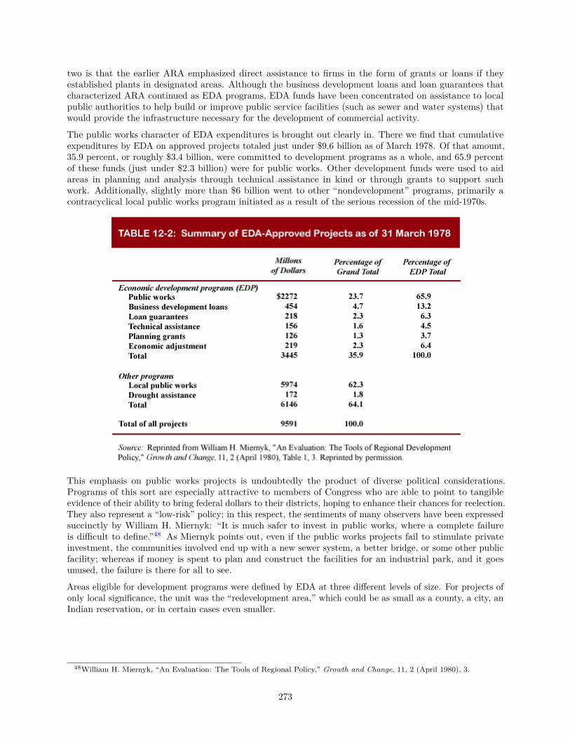
two is that the earlier ARA emphasized direct assistance to firms in the form of grants or loans if theyestablished plants in designated areas. Although the business development loans and loan guarantees thatcharacterized ARA continued as EDA programs, EDA funds have been concentrated on assistance to localpublic authorities to help build or improve public service facilities (such as sewer and water systems) thatwould provide the infrastructure necessary for the development of commercial activity.

The public works character of EDA expenditures is brought out clearly in. There we find that cumulativeexpenditures by EDA on approved projects totaled just under $9.6 billion as of March 1978. Of that amount,35.9 percent, or roughly $3.4 billion, were committed to development programs as a whole, and 65.9 percentof these funds (just under $2.3 billion) were for public works. Other development funds were used to aidareas in planning and analysis through technical assistance in kind or through grants to support suchwork. Additionally, slightly more than $6 billion went to other “nondevelopment” programs, primarily acontracyclical local public works program initiated as a result of the serious recession of the mid-1970s.

This emphasis on public works projects is undoubtedly the product of diverse political considerations.Programs of this sort are especially attractive to members of Congress who are able to point to tangibleevidence of their ability to bring federal dollars to their districts, hoping to enhance their chances for reelection.They also represent a “low-risk” policy; in this respect, the sentiments of many observers have been expressedsuccinctly by William H. Miernyk: “It is much safer to invest in public works, where a complete failureis difficult to define.”48 As Miernyk points out, even if the public works projects fail to stimulate privateinvestment, the communities involved end up with a new sewer system, a better bridge, or some other publicfacility; whereas if money is spent to plan and construct the facilities for an industrial park, and it goesunused, the failure is there for all to see.

Areas eligible for development programs were defined by EDA at three different levels of size. For projects ofonly local significance, the unit was the “redevelopment area,” which could be as small as a county, a city, anIndian reservation, or in certain cases even smaller.

48William H. Miernyk, “An Evaluation: The Tools of Regional Policy,” Growth and Change, 11, 2 (April 1980), 3.

273

Eligibility for assistance could be established on the basis of any of a number of criteria. As of September30, 1981, there were 2654 areas (encompassing over 80 percent of the United States)49 that qualified forassistance under various criteria. The criteria, and the number of areas that qualified under each, are givenin Table 12-3.

For both EDA and ARA, the policies of place prosperity, worst-first, and reliance on stimuli to employment-creating investment appear dominant. One of the reasons for the new 1965 legislation, however, wasdissatisfaction with the exclusive emphasis on the approach under which ARA operated. An importantfeature of the EDA program is the creation of a set of larger units, known as economic development districts.Each such district must contain at least two redevelopment areas plus at least one “economic developmentcenter” (growth center), and those centers are eligible for assistance of the types already described. Localinitiative to form development districts is stimulated by a provision for extra funding for redevelopment areasthat are part of development districts. The economic development center must have “sufficient size andpotential to foster the economic growth activities necessary to alleviate the distress of the redevelopmentareas within the district,” but it must not have a population of more than 250,000.

The stated purpose of this application of the growth-center concept is “that economic development projectsof broader geographical significance may be planned50 and carried out.” Although size and potential arerecognized as criteria for aid to the growth centers, and the latter are recognized as useful in helping thedistressed areas, the act makes no mention of the possibility that people in the redevelopment areas might behelped by migrating to the growth centers. Our earlier discussion suggested that such migration is probablythe principal way in which the growth centers can help, and that quite different strategies are appropriate ingrowth centers and in distressed outlying areas respectively. But EDA’s mandate appears to assume that thesame kinds of assistance are appropriate in both places.

Another point to be noted is that there is no specific minimum population size for growth centers, thoughthere is a maximum of 250,000 (corresponding to what has been suggested by some regional economists as aminimum for self-sustaining growth!). The standards provided in the law do not provide much resistance tothe predictable local pressures for designation of an ever-increasing number of small development districts andcenters, since a combination as small as just two poor counties and a town could be designated as a district.51

Since 1981, EDA has barely survived federal budget cuts. Its operations continued, although at a greatlyreduced level, through 1984 as a result of funds made available by congressional resolutions, even though

49U.S. Department of Commerce, 1981 Annual Report of the Economic Development Administration (Washington, D.C.:Government Printing Office, undated), Foreword.

50As a condition of eligibility, both redevelopment areas and economic development districts are required to prepare approvedplans for their development.

51A redevelopment area can be eligible with as few as 1500 people (or 1000 in the case of an Indian reservation).

274

EDA was omitted from the budgets submitted by President Reagan. Prospects for the continuation of EDAare uncertain at best.

12.7.2 The Regional Commissions

Title V of the same Public Works and Economic Development Act of 1965 provided for designation of stilllarger areas, called economic development regions, extending into two or more states. Each such region had aregional commission made up of a representative of each of the states involved plus a federal representativewith veto power. The prototype was the Appalachian Regional Commission, established under separatelegislation in 1965 but with similar purposes and powers. As of 1983, only the Appalachian RegionalCommission continued to receive federal support; however, it was already committed to a five-year finish-upprogram at that time. For our purposes, we can consider them all together, including Appalachia.

Economic development regions were defined on the basis of

1. High unemployment

2. Low income

3. Low levels of “housing, health, and educational facilities”

4. Dominance of the regional economy by “only one or two industries, which are in a state of long-termdecline”

5. Substantial out-migration of labor, capital, or both

6. Low growth rate of aggregate output

7. Adverse effects from changing industrial technology or changes in national defense facilities or production

ARC and the Title V Regional Commissions were primarily designed to secure interstate cooperation and abroader perspective for development planning and action within areas much larger than development districts.They were expected to produce plans for a coordinated attack on the economic problems of their respectiveregions through all kinds of existing and proposed federal and state programs. They were, of course, incompetition with one another for federal assistance, though some respect for the general national interest wasexpected to be introduced by the federal cochairman of each commission. Each regional commission hadadvisory functions regarding the initiation and coordination of economic development districts.52

By the end of 1972, the economic development regions shown in Figure 12-1 had been established. IncludingAppalachia, they encompassed part or all of 39 states and included such major metropolises as Boston,Pittsburgh, New Orleans, St. Louis, Kansas City, Seattle, and Portland. Most of these regions had beenshowing relatively slow growth for some time and have extensive unindustrialized and even backward areas.

52Except in Appalachia, where the commission itself exercised the functions performed by the EDA for the other economicdevelopment regions.

275

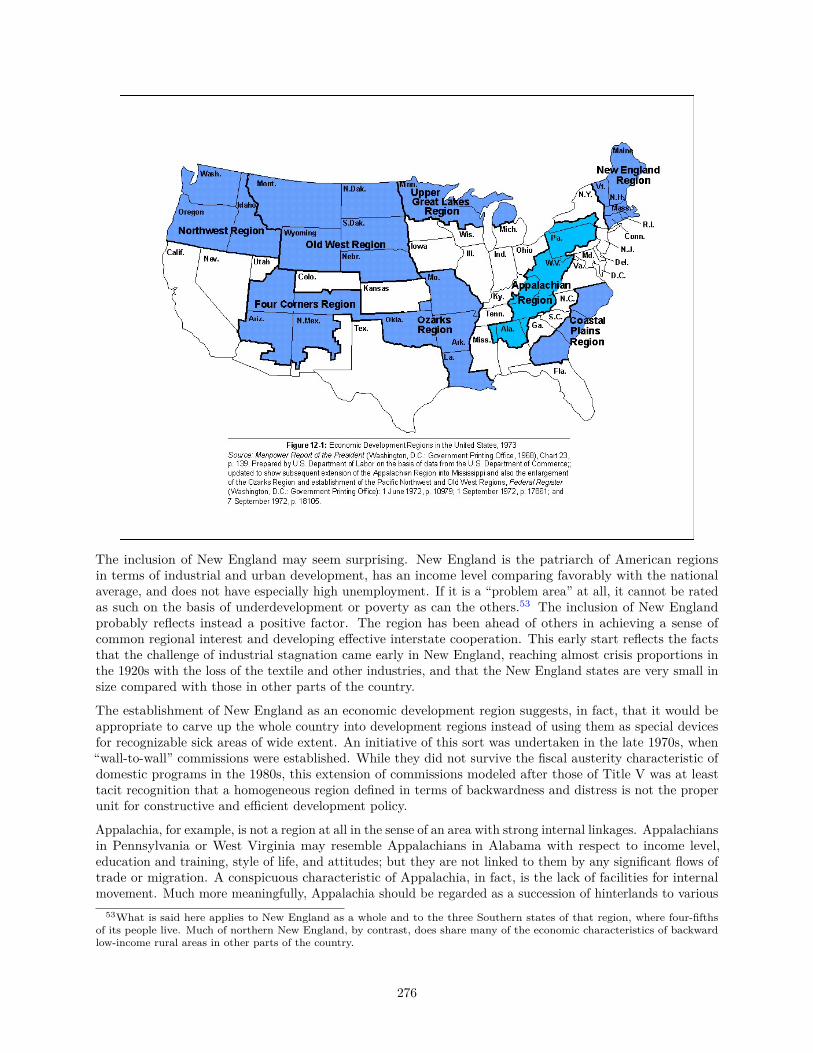
The inclusion of New England may seem surprising. New England is the patriarch of American regionsin terms of industrial and urban development, has an income level comparing favorably with the nationalaverage, and does not have especially high unemployment. If it is a “problem area” at all, it cannot be ratedas such on the basis of underdevelopment or poverty as can the others.53 The inclusion of New Englandprobably reflects instead a positive factor. The region has been ahead of others in achieving a sense ofcommon regional interest and developing effective interstate cooperation. This early start reflects the factsthat the challenge of industrial stagnation came early in New England, reaching almost crisis proportions inthe 1920s with the loss of the textile and other industries, and that the New England states are very small insize compared with those in other parts of the country.

The establishment of New England as an economic development region suggests, in fact, that it would beappropriate to carve up the whole country into development regions instead of using them as special devicesfor recognizable sick areas of wide extent. An initiative of this sort was undertaken in the late 1970s, when“wall-to-wall” commissions were established. While they did not survive the fiscal austerity characteristic ofdomestic programs in the 1980s, this extension of commissions modeled after those of Title V was at leasttacit recognition that a homogeneous region defined in terms of backwardness and distress is not the properunit for constructive and efficient development policy.

Appalachia, for example, is not a region at all in the sense of an area with strong internal linkages. Appalachiansin Pennsylvania or West Virginia may resemble Appalachians in Alabama with respect to income level,education and training, style of life, and attitudes; but they are not linked to them by any significant flows oftrade or migration. A conspicuous characteristic of Appalachia, in fact, is the lack of facilities for internalmovement. Much more meaningfully, Appalachia should be regarded as a succession of hinterlands to various

53What is said here applies to New England as a whole and to the three Southern states of that region, where four-fifthsof its people live. Much of northern New England, by contrast, does share many of the economic characteristics of backwardlow-income rural areas in other parts of the country.

276

major centers located mainly outside the region as officially defined: a row of back yards, as it were. We areled to the view that

a good part of Appalachia’s development effort should be concentrated outside the region, and. . . the region itself should be restructured and, as it were, apportioned among the metropolitanregions on its perimeter.54

Similar statements could be made about some of the other economic development regions as well.

It is true that development assistance in Appalachia has heavily emphasized roads, with the avowed intentionof “opening up” the region to the outside world and to such cities as it contains. But evidence is lacking of anyeffort to encourage out-migration from this or the other economic development regions. On the contrary, lossof population is stipulated as one of the criteria of eligibility for development assistance; and by implicationat least, as one of the conditions to be corrected.

Economic development regions can serve useful and constructive ends. To be effective, however, they mustbe structured around one or more major growth centers with demonstrably high potential. Such a regionwould have the internal cohesion that is missing in an area such as Appalachia. Additionally, it would havethe political, administrative, and technical resources necessary to plan and implement effective developmentstrategies.

The regional problems that were of so much concern in the 1960s and early 1970s have not gone away;their character has simply changed. The nonmetropolitan growth that has been characteristic of recentpopulation trends has reduced the pressure for policy makers to focus their attention on “backward” areas,but many of these remain in distress despite the nonmetropolitan resurgence. Additionally, the slow growthof metropolitan areas, particularly in the Northeast and upper Midwest, is likely to persist for some time;transition of the economic base in such cities as Youngstown, Akron, and Buffalo to new growth industries isnot going to happen overnight.

The coordination of federal and regional efforts can facilitate the type of change that must take place indistressed areas (metropolitan or nonmetropolitan) and keep it from being jeopardized by self-serving localinterests or potentially destructive interregional rivalry. A system of regional commissions characterizedby a combination of intraregional interdependence, greater consciousness of a common regional interest,and financial and technical strength would serve this end; and it could help also to check the trend towardever-increasing dependence on federal initiatives, decisions, and specific subsidies. The federal role could beless paternal and philanthropic, and could consist mainly of maintenance of high overall levels of demand,the provision of information and aggregate national development guidelines, and the design of programs toimprove the quality and mobility of human resources. A system of this sort would be a step toward thedecentralization of federal authority which would ensure that the regions assuming new responsibilities meetat least some of the necessary criteria for success.

12.8 SummaryThe formulation of public policies on location and regional development was stimulated in the secondquarter of this century by continuing interregional disparities in income and economic opportunity, by theincreasing role of the national government in financing and providing regional services, by disenchantmentwith population increases as an objective and with competitive regional subsidization of growth, by thedilution of provincialism, and by changes in factors affecting location.

National government programs to maintain high employment levels and to improve manpower quality andmobility are warranted on grounds of both equity and efficient allocation of resources among and withinregions. An important distinction exists, however, between the objective of “place prosperity,” or economicassistance to regions as such, and the really fundamental goal of “people prosperity.”

54John Friedmann, “Poor Regions and Poor Nations: Perspectives on the Problem of Appalachia,” Southern Economic Journal,32, 4 (April 1966), 472. Similar sentiments are expressed in Niles M. Hansen. Rural Poverty and the Urban Crisis (Bloomington:Indiana University Press, 1970).

277

“Problem regions” are of several different types, including (1) backward areas halted at the threshold ofself-sustaining development; (2) already developed areas with arrested growth due to loss of competitiveadvantage in their basic activities or obsolescence in those activities as such, with accompanying loss of abilityto substitute new kinds of activities; and (3) areas of excessive growth or excessive concentration.

Public policy can influence regional structure and development through many measures, which includeupgrading manpower quality and factor mobility, maintaining a high national employment level, subsidizingor restricting investment, controlling transfer rates and services, allocating public purchases and investmentsamong regions, supporting research and development, and assisting in the provision of local or regionalinfrastructure.

Four main issues arise in connection with public policy toward regions: (1) degree of reliance on the placeprosperity criterion, (2) allocation of regional assistance as charity or as investment, (3) focusing of assistancein growth centers as contrasted with wide dispersion, and (4) choice among available devices for influencingdevelopment.

Throughout the 1960s and 1970s regional development policy in the United States favored “backward” regions.More recently, there has been a shift in emphasis toward distressed urban areas. Certain built-in politicaland economic biases, evident both in this country and abroad, have led to overemphasis on place prosperity,overproliferation of areas receiving public developmental assistance, and underrating of the potential role ofmigration and mobility enhancement.

Technical Terms Introduced in this ChapterPeople prosperity Growth centerPlace prosperity Spread effectGenerative and competitive growth Primal cityShift-share analysis Functional economic areaRegional economic resilience Backwash effect

Selected ReadingsJohn Friedmann and William Alonso, Regional Policy: Readings in Theory and Applications (Cambridge,Mass.: MIT Press, 1975).

Gordon C. Cameron, “Growth Areas, Growth Centres and Regional Conversion,” Scottish Journal of PoliticalEconomy, 17, 1 (February 1970), 19-38.

Ira S. Lowry, “Population Policy, Welfare, and Regional Development,” in Mark Perlman, Charles Leven,and Benjamin Chinitz (eds.), Spatial, Regional, and Population Economics (New York: Gordon and Breach,1972), pp. 233-261.

Niles M. Hansen (ed.), Public Policy and Regional Economic Development (Cambridge, Mass.: Ballinger,1974).

Harry W. Richardson, Regional Economics (Urbana: University of Illinois Press, 1978), Chapters 7, 9, and 10.

E. A. G. Robinson (ed.), Backward Areas in Advanced Countries (London: Macmillan, 1969).

Norbert Vanhove and Leo H. Klassen, Regional Policy, A European Approach (Montclair, N.J.: Allenheld,Osmun, 1980).

278

Appendix 12-1 The Shift-Sare Analysis of Components of Regional ActivityGrowthSee section 12.3.2 and 12.3.5

The overall growth rate of a region’s activity (as measured, say, by total employment or total value added) is,of course, a weighted average of the growth rates of the separate sectors or activities making up the region’seconomy. If the region’s growth rate is compared with that of some other area (for example, the entirenation), it is possible to “explain” the difference in growth rates statistically in terms of two components,which for convenience can be styled “mix” and “competitive.” Quantitative analysis of comparative regionalgrowth rates along these lines is sometimes referred to as the “shift-share” approach.55

An example of a regional growth differential arising exclusively from mix would be the case of a region inwhich each activity grows at exactly the same rate as in the nation as a whole. In other words, the region’sshare of the national total for each industry remains unchanged over the time interval in question, butthe national growth rates for some activities are higher than those for others. If a region contains mainlyfast-growing activities and relatively few of the slow-growing activities, it can be said to have a “favorablegrowth mix” of activities, and its overall percentage growth rate will exceed that of the nation. On the otherhand, if slow-growing industries are more than proportionally represented in the region’s mix, the region’soverall growth rate will be slower than the national growth rate. This is an example of the pure mix effect.

We can evaluate the competitive component by imagining the case of a region that has exactly the same mixof activities, as does the nation:

Its percentage share of the national total is the same for all activities. This region will have an overall growthrate higher than that of the nation if it increases its shares (that is, if most activities grow faster in the regionthan in the nation). Such a case represents the competitive component in isolation.

In any real situation, of course, it is nearly certain that the relative growth rates of region and nation willshow the effects of some combination of mix and competitive components. Either effect, or the net result,can be either positive or negative for the region.

A drastically simplified numerical example will serve to show the way in which shift-share analysis determinesthe effect to be imputed to each component. Let us take the following Census data on manufacturingemployment (in thousands):56

55This approach was apparently first used by Daniel B. Creamer in 1942 in U.S. National Resources Planning Board, IndustrialLocation and National Resources (Washington, D.C.: Government Printing Office, 1943), and was expounded and used on alarge scale by Edgar S. Dunn, Jr., in Harvey S. Perloff, E. S. Dunn, Jr., E. E. Lampard, and R. F. Muth, Regions, Resources,and Economic Growth (Baltimore: Johns Hopkins University Press, 1960). The basic exposition of the method is in that source.What we are calling the “mix component” corresponds to Dunn’s “net proportionality shift,” and our “competitive component”corresponds to his “net differential shift.” The method was later applied still more extensively in the U.S. Department ofCommerce by Dunn and others, and comprehensive tabulations have been prepared and published for U.S. Census regions andsmaller areas. See Lowell D. Ashby, Growth Patterns in Employment by County, 1940-50 and 1950-60 (Washington, D.C.:Government Printing Office, 1965).The logic and usefulness of the shift-share approach were attacked by David B. Houston, “The Shift and Share Analysis of

Regional Growth: A Critique,” Southern Economic Journal, 33, 4 (April 1967), 577-581. A rejoinder in defense was given byLowell D. Ashby in the same journal: “The Shift and Share Analysis: A Reply,” 34, 3 (January 1968), 423-425. A subsequentcritique is H. James Brown, “Shift and Share Projections of Regional Economic Growth: An Empirical Test,” Journal of RegionalScience, 9, 1 (April 1969), 1-18. For a thorough review of this literature see Benjamin H. Stevens and Craig L. Moore, “ACritical Review of the Literature on Shift-Share as a Forecasting Technique,” Journal of Regional Science, 20, 4 (November1980), 419-437.

56Industry Group 19 (ordnance and accessories) has been omitted from our computations, since data for that industry groupfor Pennsylvania were not available. Minor adjustments in the totals have been made to take account of rounding-off errors inadding up the figures for individual industry groups to arrive at the subtotals for durable and nondurable goods industries.Basic data were taken from the 1963 U.S. Census of Manufactures reports.

279

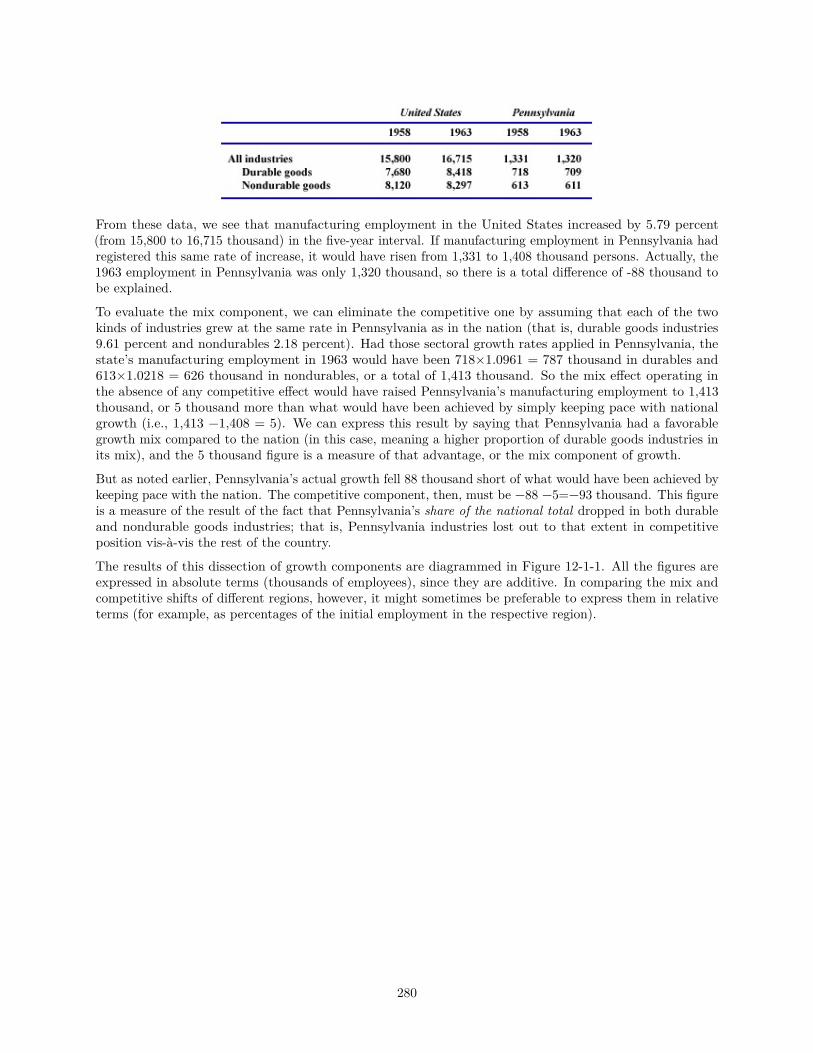
From these data, we see that manufacturing employment in the United States increased by 5.79 percent(from 15,800 to 16,715 thousand) in the five-year interval. If manufacturing employment in Pennsylvania hadregistered this same rate of increase, it would have risen from 1,331 to 1,408 thousand persons. Actually, the1963 employment in Pennsylvania was only 1,320 thousand, so there is a total difference of -88 thousand tobe explained.

To evaluate the mix component, we can eliminate the competitive one by assuming that each of the twokinds of industries grew at the same rate in Pennsylvania as in the nation (that is, durable goods industries9.61 percent and nondurables 2.18 percent). Had those sectoral growth rates applied in Pennsylvania, thestate’s manufacturing employment in 1963 would have been 718×1.0961 = 787 thousand in durables and613×1.0218 = 626 thousand in nondurables, or a total of 1,413 thousand. So the mix effect operating inthe absence of any competitive effect would have raised Pennsylvania’s manufacturing employment to 1,413thousand, or 5 thousand more than what would have been achieved by simply keeping pace with nationalgrowth (i.e., 1,413 −1,408 = 5). We can express this result by saying that Pennsylvania had a favorablegrowth mix compared to the nation (in this case, meaning a higher proportion of durable goods industries inits mix), and the 5 thousand figure is a measure of that advantage, or the mix component of growth.

But as noted earlier, Pennsylvania’s actual growth fell 88 thousand short of what would have been achieved bykeeping pace with the nation. The competitive component, then, must be −88 −5=−93 thousand. This figureis a measure of the result of the fact that Pennsylvania’s share of the national total dropped in both durableand nondurable goods industries; that is, Pennsylvania industries lost out to that extent in competitiveposition vis-à-vis the rest of the country.

The results of this dissection of growth components are diagrammed in Figure 12-1-1. All the figures areexpressed in absolute terms (thousands of employees), since they are additive. In comparing the mix andcompetitive shifts of different regions, however, it might sometimes be preferable to express them in relativeterms (for example, as percentages of the initial employment in the respective region).

280

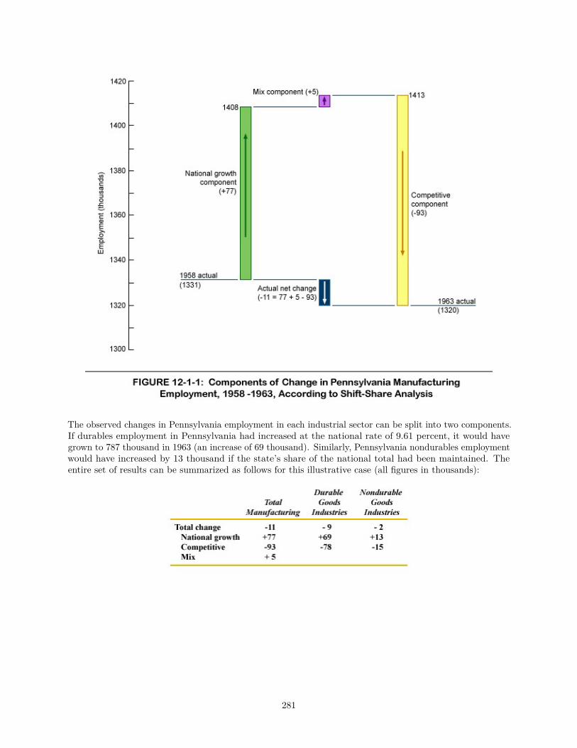
The observed changes in Pennsylvania employment in each industrial sector can be split into two components.If durables employment in Pennsylvania had increased at the national rate of 9.61 percent, it would havegrown to 787 thousand in 1963 (an increase of 69 thousand). Similarly, Pennsylvania nondurables employmentwould have increased by 13 thousand if the state’s share of the national total had been maintained. Theentire set of results can be summarized as follows for this illustrative case (all figures in thousands):

281

13. SOME SPATIAL ASPECTS OF URBAN PROBLEMS13.1 IntroductionThe nation’s concern with urban problems began in earnest during the 1960s. It was easy to perceive thatsomething was wrong. American cities were characterized by high unemployment among nonwhites, highcrime rates, pressing fiscal problems, and serious pollution—conditions that have continued with more or lessintensity to the present day.

The urban crisis was generally viewed as being aggravated by excessive population increase and interregionalmigration to central cities of large metropolitan areas. For some people the solution was as obvious as theproblem: slow down the population growth of urban areas, either by stemming the flow from nonmetropolitanareas or by encouraging out-migration. Establishment of growth centers in less developed or economicallylagging areas was urged as a plausible means of easing urban problems by keeping the rural populationsemployed closer to home and out of the large cities. Viable growth centers, however, were never established.

Even as proposals for diverting migration and population growth away from the larger cities were beingformulated, the long-standing tide of net migration to the large cities was slowing to a trickle.1 In the 1960s,the population growth of American metropolitan areas was almost all accounted for by natural increase. Aswe have seen, the decade of the 1970s brought a resurgence of nonmetropolitan population growth as well asa relative (and in some cases absolute) decline in metropolitan-area populations. With this change came newperspectives on the “urban crisis.” The questions being asked today often concern the problems of urbanareas in transition from one economic base to another, and we have come to recognize more fully that thepowerful forces of decentralization that were discussed at length in Chapter 7 are at the root of many of themost pressing urban problems.

In the present chapter, we focus attention on the role of changes in spatial patterns of urban activities in theemergence of current urban problems, and we discuss associated policy issues. We shall concentrate on fourareas of special concern and importance: declining activity in the central core of cities, urban poverty, thetransportation of people within urban areas, and fiscal disparity between central cities and their surroundingsuburbs. All of the problems that we shall discuss are related and can be traced to underlying changes in landuse, location, or locational advantage that make life or business survival more difficult for some groups. Byrelating these problems to changes in locational incentives, useful perspective can be gained on the challengesthey pose and the responses they may elicit.

13.2 Downtown: Problems and ResponsesGiven the extent of decentralization of economic activity that has characterized urban areas in the UnitedStates,2 we could accept it as normal that the central core of an urban area will tend to show less rapid growth(in terms of such measures as employment, business sales, and daytime population) than peripheral areas. Nospecial problem or basis for concern would arise from such a trend. Actually, however, the downtown areas ofmany American cities are in trouble, and their ills constitute part of the whole complex of urban problems.

There are three principal symptoms: declining levels of activity, congestion, and environmental deterioration.The distress is, of course, felt in different ways by such different groups as downtown merchants, propertyowners, commuters, residents, shoppers, and taxpayers.

13.2.1 Declining Levels of Activity

The acute cause for concern here is, as noted above, absolute losses rather than merely a failure to keep upwith the suburbs. Although the number of office jobs is increasing in many downtown areas, especially thoseof the larger metropolises, a great many other downtown activities shrank substantially in the years followingthe end of World War II, when removal of wartime constraints on automobile production, motor fuels, andnew construction released some pent-up pressures for suburbanization. Estimates of average daily travel into

1See Harry W. Richardson, Regional Economics (Urbana: University of Illinois Press, 1978), pp. 281-289, or a more detaileddiscussion of the transition in regional problems and policies.

2See Section 7.7.

282

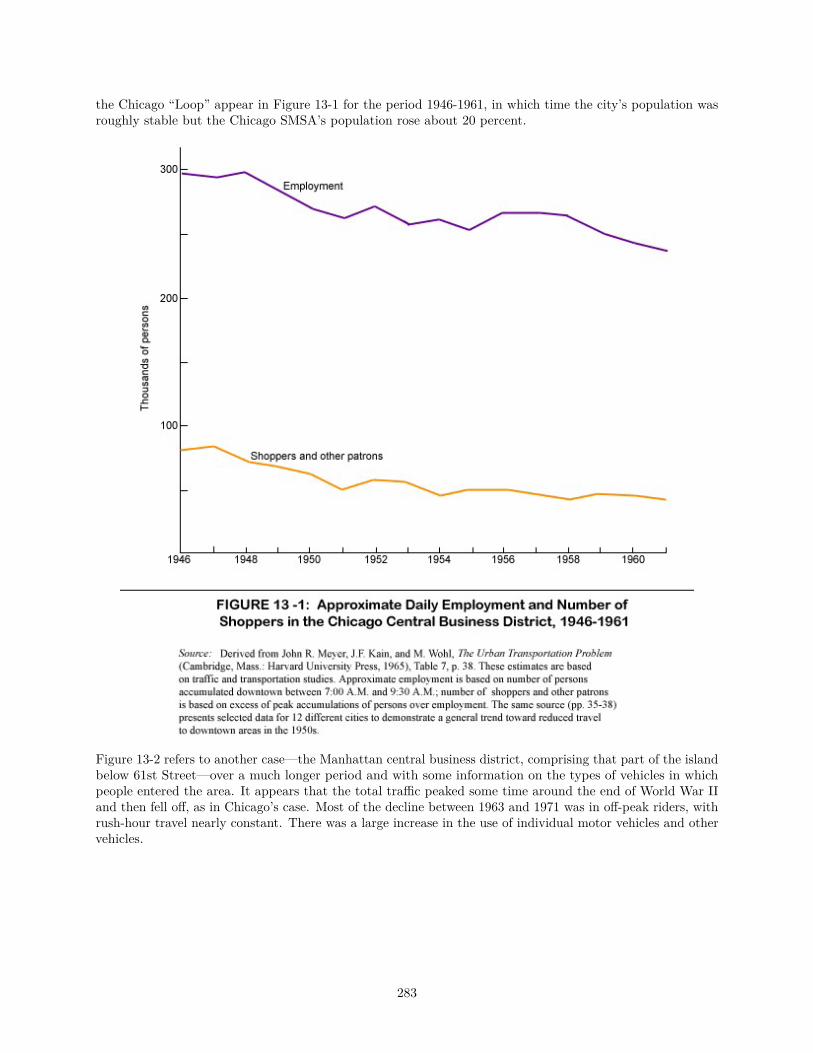
the Chicago “Loop” appear in Figure 13-1 for the period 1946-1961, in which time the city’s population wasroughly stable but the Chicago SMSA’s population rose about 20 percent.

Figure 13-2 refers to another case—the Manhattan central business district, comprising that part of the islandbelow 61st Street—over a much longer period and with some information on the types of vehicles in whichpeople entered the area. It appears that the total traffic peaked some time around the end of World War IIand then fell off, as in Chicago’s case. Most of the decline between 1963 and 1971 was in off-peak riders, withrush-hour travel nearly constant. There was a large increase in the use of individual motor vehicles and othervehicles.

283

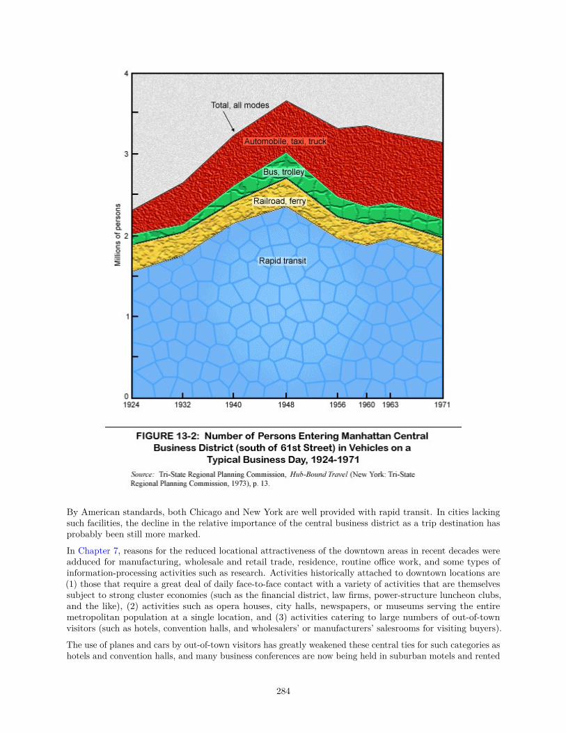
By American standards, both Chicago and New York are well provided with rapid transit. In cities lackingsuch facilities, the decline in the relative importance of the central business district as a trip destination hasprobably been still more marked.

In Chapter 7, reasons for the reduced locational attractiveness of the downtown areas in recent decades wereadduced for manufacturing, wholesale and retail trade, residence, routine office work, and some types ofinformation-processing activities such as research. Activities historically attached to downtown locations are(1) those that require a great deal of daily face-to-face contact with a variety of activities that are themselvessubject to strong cluster economies (such as the financial district, law firms, power-structure luncheon clubs,and the like), (2) activities such as opera houses, city halls, newspapers, or museums serving the entiremetropolitan population at a single location, and (3) activities catering to large numbers of out-of-townvisitors (such as hotels, convention halls, and wholesalers’ or manufacturers’ salesrooms for visiting buyers).

The use of planes and cars by out-of-town visitors has greatly weakened these central ties for such categories ashotels and convention halls, and many business conferences are now being held in suburban motels and rented

284

space at airports. Regional sales and service offices that are the home bases for traveling sales or servicingpersonnel have similarly found access advantage in outlying locations. After these and other defections, thecorporate headquarters office has remained as a bulwark of downtown areas. Even in this activity, however,there has been a continual segmenting of office functions, with many of the more routine jobs being shifted tosuburban locations.

Accordingly, it appears that declining downtown employment is either already prevalent or threatened ineach of the major categories of activity that have historically made up the city core. The mutual interactionbetween fewer employees and fewer customers is obvious.

Though the actuality or the prospect of absolute decline in central business districts obviously injures propertyowners and others who have a stake in the level of downtown activity, we need not fall into the place prosperityfallacy of assuming that every location as such has a “right” to be shielded against obsolescence. If downtowndecay is to be treated as a legitimate public concern justifying preventive action, the case for such concernand action should be made on a broader basis than the interest of the property holders immediately involved.The basic questions for policy judgment are (1) whether an active and viable downtown is a valuable part ofthe urban economic and social complex, affecting its overall efficiency and quality of life, and (2) whetherthere are substantial hidden social benefits and externalities not taken into account in the market pricingsystem. It is hoped that the rest of this chapter will be of some help to the reader in forming an opinion onthese questions.

13.2.2 Congestion

Another cause for concern in downtown areas is traffic congestion—which is not only inordinately wasteful oftime and street space but is certainly one of the important reasons for the declining popularity of downtownlocations. Concern with congestion may seem paradoxical, since total travel to downtown areas is apparentlynot growing much and in many cities is even diminishing. The explanation lies partly in the greater use ofautomobiles and partly in the increased peaking of the traffic in rush hours.

Congestion affects two types of movement: circulation within the downtown area by vehicles and pedestrians,and movement into and out of the area (primarily by vehicles). The former problem has been acute as longas large cities have existed,3 and it would be difficult to demonstrate any great progress or retrogression,in terms of speed or comfort, for mobility within downtown areas. Getting into and out of downtown hashowever become more of a problem with the decay of public transit, greater distances from residential areas,and vastly increased use of the space-consuming private automobile. Thus it is at least a fair surmise thatthe time required for downtown circulation and access has not been reduced. In the face of improved accessby suburbanites to suburban jobs and shopping facilities, this implies deterioration in the relative accessadvantages of downtowns.

13.2.3 Amenity

There is abundant evidence that the troubles of downtown areas involve in part some unfavorable manifestationsof obsolescence. The street utility layouts and the buildings of high-density downtown areas are more expensiveto modernize than those of less intensively developed neighborhoods. In situations of rapid locational andtechnological change, it is especially difficult for districts and buildings to grow old gracefully and to developthe positive attractions associated with maturity and age in downtown areas that have grown up under morestable and regulated conditions (such as those of many old European cities). So far at least, it seems clearthat downtown amenities have not merely failed to keep pace with those of outer areas but have sufferedabsolute deterioration.

Greater use of automobiles is partly responsible. Whether parking at the curb, in open lots, or in multilevelgarages, cars occupy large amounts of scarce downtown space and thus reduce convenience of access byincreasing the distance from one work or shopping destination to another. In a thoroughly motorized citysuch as Los Angeles, more than two-thirds of the downtown area can be preempted by streets and parking

3In Julius Caesar’s Rome, vehicles were excluded from the continuously built-up area during the daylight hours in an effortto cope with traffic jams. Faded photographs of Fifth Avenue in horse-and-buggy days show it crammed from curb to curb inthe rush hour.

285

facilities, and this is all “dead space” as far as any ultimate destinations are concerned. The prime potentialadvantage of a downtown—quick and convenient access among various kinds of activities—is thus dissipated.

Another factor in deterioration of the quality of downtown life reflects rising income levels and the changingdistribution of income groups of the population. In Chapter 7, we found that urban growth was associatedwith the proliferation of subcenters of economic activity. With rising income levels, the density of demandincreases, and a metropolitan area can support more shops catering to the more affluent population. Some ofthese will be located in subcenters that, in effect, compete with the downtown shopping district and drawaway potential customers. Even more important, however, has been the effect of suburbanization. As themiddle- and higher-income people have led the way to the suburbs, the populations with closest access todowntown areas are increasingly the poor. The changing composition of downtown consumer demands hasbeen apparent in the cheapening of stores, restaurants, amusements, and other types of consumer-servingfacilities; and this, of course, further discourages the more affluent from choosing downtown as a place towork, play, shop, or live.

13.2.4 Some Responses

We have identified and explained some aspects of a major urban problem variously described as “strangulation,”“the downtown dilemma,” “dry rot at the core,” and in other equally vivid terms. What can or should bedone about it?

It is important to keep reminding ourselves that the raison d’être of an urban concentration is provision forclose, easy, and multifarious interpersonal contact. From this standpoint, an urban pattern is “efficient” whenthere is a focal point for concentration of as many as possible of those activities that require access to a highproportion of the firms and households of the area and are best concentrated (because of scale economies orexternal economies of close agglomeration) in one single location in the area.4

Among the activities that are logical candidates for central location, on the basis of their access andagglomeration requirements, terminals for interregional passenger transport are certainly included. Yetairports, in the present state of air transport technology, are obviously far too space consuming and noisyto be eligible for anything like a central location, and become increasingly remote as they get larger. If theinterurban public transport of the future can be compactly designed and compatible with intensive developmentin its terminal area, it is reasonable to expect cities to have their main passenger terminals integrated centrallywith their internal transportation as they were until around the middle of this century.5 Possible developmentsin fast interurban ground transport (for example, in the Boston—Washington “Northeast Corridor”) suggestsome hope in this direction. Prospects for relocating air terminals to city centers seem much more conjectural.But it is possible that at some future time urban historians will consider as a curious temporary aberrationthe latter-twentieth-century period in which interurban transport did not go directly from one city center toanother.

Perhaps the most fundamental and abiding urban problem involves the search for ways to exploit thecity’s unique potential for maximum mass and diversity of contact, choice, and opportunity without undulysacrificing other values. However, we need to understand a great deal more (and in more specific andquantitative terms) about what urbanism contributes to economic and social progress through its contactopportunities. There is room for more empirical analysis as well as for amplification of the theories of locationand regional development to cover complex spatial relations involving contact and time as major parameters.A host of suggestive hypotheses still await verification.6

The problem of advantages of concentration and how to exploit them comes to a head in the central businessdistrict, since there the potential contact opportunities are highest and the conflict with space requirements

4For a suggested “hierarchy of CBD land uses and land values,” identifying a series of specific business activities and theranges of land values that they can support, see Larry Smith, “Space for the CBD’s Functions,” Journal of the AmericanInstitute of Planners, 27, 1 (February 1961), Table 4, p. 38.

5This suggestion is introduced simply as provocative speculation. John R. Meyer, J. F. Kain, and M. Wohl, The UrbanTransportation Problem (Cambridge, Mass.: Harvard University Press, 1965), Chapter 2, expect freight terminals to move tobeltway junction locations, and we do not dispute the reasonableness of that projection.

6See, for example, three sources cited in earlier chapters: Robert M. Lichtenberg, One Tenth of a Nation (Cambridge,Mass.: Harvard University Press, 1960); Benjamin Chinitz, “Contrasts in Agglomeration; New York and Pittsburgh,” AmericanEconomic Review, 51, 2 (May 1961), 279-289; and Harry W. Richardson, Regional Growth Theory (London: Macmillan, 1973).

286

the most serious. A basic challenge to the ingenuity of urbanists is to devise ways of improving downtownareas in the three relevant aspects: making them easy to get to, easy to get around in, and attractive andeffective as places to work or visit.

As yet, we do not know very much about the effectiveness of various methods of increasing the realized contactpotential of central business districts. Efforts in this direction in the United States have been fragmentary andoften mutually conflicting, and there has been some reluctance to regard experiences in foreign cities (such asRotterdam or even Toronto) as applicable to American cities. Pedestrian malls have in general been tiny andtentative. New downtown amenities have mostly been in the form of wider streets, parking garages, conventionhalls, and shiny skyscrapers. Radical modernization of mass transit, integrated with adequate parking andtransfer facilities at outlying stations and adequate intradowntown facilities (such as minibuses and movingsidewalks), has not been tried. Policies of various public authorities on transport have generally been bothconflicting and self-defeating, as will be shown later.7 Imaginative and consistent transport planning is basicto any improvement or even maintenance of the functional effectiveness of downtown areas, though clearlynot the only essential element in a solution. The possible benefits of a more efficient system for bringing largenumbers of people into close contact in agreeable surroundings appear large in terms of revitalization of theurban mechanism at its center.

13.3 Urban Poverty13.3.1 Dimensions of Urban Poverty

Our primary concern in this section is with the spatial distribution of poverty and its incidence. We shallfind that important related trends can be explained substantially by the forces that have shaped Americanpatterns of urbanization.

There are two fundamentally different ways of defining poverty. It may be defined in absolute terms, byestablishing a threshold level of income that is consistent with a standard of living which satisfies basic needs,or in relative terms (e.g., 50 percent of the median income). Poverty statistics compiled by the U.S. Bureauof the Census are based on absolute standards. Thus by the 1981 standard, an average nonfarm family offour8 with an annual income below $9287 was considered poor (i.e., classified as living in poverty).9

The poverty thresholds for various groups change from year to year to reflect the effects of inflation on thepurchasing power of income; therefore, in “real” terms they have remained virtually unchanged since the1960s. Median income has risen substantially since that time, so it is not surprising that the poverty rate(the percentage of persons classified as poor) has fallen from 22.2 percent in 1960 to 14 percent in 1981.10

Much less progress would be evidenced if a relative standard had been applied.

Table 13-1 shows that poverty in the United States is primarily urban poverty. In 1981, nearly 61 percent ofthe persons living in poverty resided in metropolitan areas; whereas only 43.9 percent of the nation’s poorwere urban in 1959. Within metropolitan areas, the majority of the poor live in central cities. However, thepercentage of urban poor who live outside central cities has increased from just under 39 percent in 1959to roughly 42 percent in 1981. Thus not surprisingly, these figures indicate that as the nation’s populationbecame more urban, poverty became concentrated in metropolitan areas; and as the metropolitan populationsmoved to the suburbs, urban poverty became somewhat less concentrated in central cities.

7See Section 13.4 and also E. M. Hoover, “Motor Metropolis,” Journal of Industrial Economics, 13, 3 (June 1965), 177.8A family of four may be comprised of two parents and two children, four adults (two or more children over the age of

eighteen), or other such combinations, and poverty standards have been established for each of these. Thus the “average” referredto here is taken across all such standards for a family of four.

9U. S. Bureau of the Census, Current Population Reports, Series P-60, No. 138, Characteristics of the Population Below thePoverty Level: 1981 (Washington, D.C.: Government Printing Office, 1983), p. 1.

10Ibid., Table 1, p. 7.

287

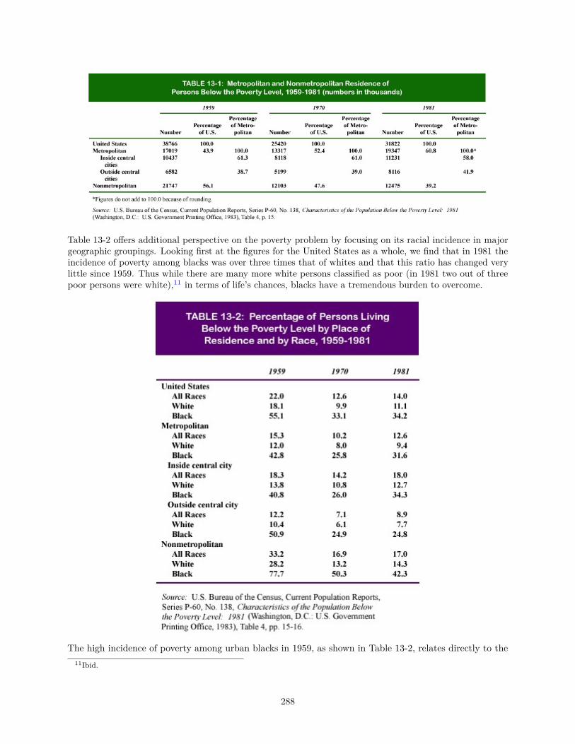
Table 13-2 offers additional perspective on the poverty problem by focusing on its racial incidence in majorgeographic groupings. Looking first at the figures for the United States as a whole, we find that in 1981 theincidence of poverty among blacks was over three times that of whites and that this ratio has changed verylittle since 1959. Thus while there are many more white persons classified as poor (in 1981 two out of threepoor persons were white),11 in terms of life’s chances, blacks have a tremendous burden to overcome.

The high incidence of poverty among urban blacks in 1959, as shown in Table 13-2, relates directly to the11Ibid.

288

in-migration of poor persons “released” from the agricultural sector.12 The rapid increase in metropolitanpopulations of the 1950s was due largely to the decline of the agricultural sector and consequent interregionalmigration, which brought many rural poor people, especially blacks, to the nation’s largest urban areas. Themagnitude of this movement and the subsequent concentrations of poverty in urban areas were at the heart ofthe “urban crisis” as perceived in the 1960s and early 1970s. Despite these regional shifts, nonmetropolitanareas continue to exhibit high rates of poverty. Table 13-2 indicates that in 1981 the percentage of poorpersons in nonmetropolitan areas was nearly as large as that in the central cities of metropolitan areas.

At least some portion of the apparent gains made by blacks in the 1960s was a result of an explicit reaction tothe urban crisis. The “War on Poverty” declared by President Lyndon B. Johnson represented an importantphase of income redistribution in the United States. The rapid economic growth of the overall economyduring this period also could have contributed to whatever progress these figures suggest.

Focusing on metropolitan areas as a whole, we find that the percentage of persons living in poverty decreasedduring the 1960s; however the poverty rate increased for all races during the 1970s. This setback was largestamong blacks—particularly those residing in central cities. But the incidence of poverty among suburbanblacks actually fell slightly from 1970 to 1981, even in the face of an adverse trend in poverty for the nationas a whole.

One factor aggravating the problems of urban poverty areas is their sheer size and cohesiveness. Theyrepresent segregation (often racial) on a grand scale, in contrast to a pattern of small poverty or minoritygroup pockets. And it is all too clear that a given aggregate amount of poverty and deprivation is a far moreserious problem if it is solidly massed in one large area than if it were scattered throughout a city. Thiswill be recognized in theoretical terms as a case of adverse neighborhood effects, or external diseconomies ofagglomeration.

In a large poverty area, a much greater proportion of the residents live far from the edges, where there wouldbe at least some exposure to superior opportunity, amenity, evidences of hope, and avenues of gradual escape;and the “outside world” can come to be something remote and alien, identified as an oppressive and hostile“establishment.” Polarization of ways of life and attitudes between poor persons and outsiders is fostered insuch situations. In more specific terms, access to jobs is harder, and genuine integration of schools becomesimpossible without such controversial devices as the long-distance busing of schoolchildren. Improvement,rehabilitation, and renewal of housing are more difficult in an extensive slum, since the prevailing character ofthe neighborhood determines both the incentive to improve an individual property and the benefits therebyachieved.13 Maintenance of public safety likewise poses greater problems in massive areas of poverty andsocial stress.

Another particularly aggravating factor in poverty areas is poor access to employment opportunities. Althoughurban poverty areas are typically rather central, their people are at an increasing disadvantage in job access.This partly reflects the fact that they are the least mobile group in the whole urban area, in terms of eitherwork or change of residence. Many cannot afford cars and find even transit fares a serious financial burden.Overall home-to-work commuting speeds by most existing modes of transit are lower than by car, whichrestricts the feasible range of commutation. (Halving one’s commuting speed reduces by 75 percent the areathat is within one hour’s travel time.)

The effect of decentralization on the urban poor is complex. Many of the jobs that promoted access to skillladders and encouraged mobility for generations of European and other immigrants were going to the suburbs,or had already gone, while the concentrations of urban poor were growing in the nation’s central cities. Theconsequence of this has been described by some as a “dual” labor market, whereby many persons are trappedin a last-hired, first-fired class of jobs with little opportunity for advancement.

The suburbanization of whites has been a feature of urban areas for many years; however, as we saw inChapter 7, evidence of significant suburbanization of blacks was first apparent in the 1970s. Some of thegrowth of black populations outside central cities during the 1970s may be the result of “spillover,” rather

12See John F. Cogan, “The Decline of Black Teenage Employment: 1950-1970,” American Economic Review, 72, 4 (September1982) 621-638.

13See Otto A. Davis and Andrew B. Whinston, “The Economics of Urban Renewal,” in James Q. Wilson (ed.), Urban Renewal:The Record and the Controversy (Cambridge, Mass.: MIT Press, 1966), pp. 50-67.

289

than of suburbanization per Se. That is, as the number of central-city blacks increases, it is likely thatblack neighborhoods will simply be extended beyond the central-city boundary. As noted earlier, however,Table 13-2 indicates that the incidence of black poverty outside central cities changed little during the 1970s,while poverty among central-city blacks increased substantially. From this, one is tempted to draw theconclusion that suburbanization among blacks has been selective, just as it has been for whites; higher-incomeblacks have moved to the suburbs in sufficient numbers to overcome an adverse national trend in povertythat has been particularly difficult for blacks as a whole. Reduced discrimination and advances made byblacks in gaining better jobs may be enhancing their residential mobility within metropolitan areas. Also,suburbanization itself may be improving the job access of blacks and enabling more of them to move abovethe poverty level.

13.3.2 Some Policy Considerations

The magnitude of the urban poverty problem precludes a detailed discussion of related policies here. However,a subset of policy issues is explicitly spatial in nature and deserves at least some mention. We shall concentrateon policies for central-city poverty areas, which have come to be called ghettos.14

Since the most urgent need of poor populations is more jobs, policies to stimulate new business growthin and near poverty areas have been given a good deal of consideration. The task is not easy, since theprevailing trends of location are in the opposite direction, with increased emphasis on just those thingsthat the inner-city areas lack: ample space for expansion, low taxes, and a community environment offeringamenity, visibility, prestige, and quick access to circumferential and intercity highways. It can be surmisedthat a large permanent subsidy would be needed to entice enough private employers to locate near central-citypoverty areas and employ wholly or mainly local residents; and that such large sums might better be used inother ways to provide improved job access.

A policy akin to “import substitution” had some strong adherents in the 1960s and early 1970s. Recommen-dations entailed assistance to ghetto entrepreneurs to establish small consumer-serving businesses within thearea. The assumption was that such “black capitalism” can take advantage not only of an ample low-cost laborsupply but also of a somewhat protected home market (that is, the ghetto consumers will prefer to patronize afirm operated and staffed by neighbors). It was also urged that the profits of such enterprises would accrue toghetto residents and would, to a greater extent, be spent in the neighborhood. The importance of developingblack entrepreneurial skills and financial backing, so that blacks can win a more adequate foothold on themiddle and higher rungs of the business management ladder, was also recognized.

Unquestionably, the nurturing of a much larger cadre of black business managers and entrepreneurs, andthe accumulation of capital and credit-worthiness by black-controlled firms, must play an essential partin redressing the wide interracial gap in levels of opportunity that exists today. At the same time, thereare obvious limitations on what can be accomplished in the kinds of businesses that can be expected tosurvive within ghetto areas proper. Profitability is color blind; what is profitable for blacks would be equallyprofitable for whites. With respect to the actual creation of additional black employment, it is not realistic toexpect much more to materialize than the equivalent of replacing whites now working in ghetto areas. Such anumber would be small compared to ghetto unemployment. Moreover, empirical investigations have shownthat the neighborhood multiplier effects created by additional employment and income in ghetto areas areextremely small.15

More recently, the merits of “enterprise zones” in poverty areas have been the focus of substantial debate.16

The idea is to create an open “free-market environment” in order to stimulate economic activities of allsorts. Thus the program would not be limited to activities serving the local market but also would hope to

14The term “ghetto” implies ethnic segregation rather than poverty per se, and was originally applied to those parts of Italiancities to which Jews were confined. The first ghetto was established in 1516 on Ghèto (Foundry) Island in Venice.

15For a sobering appraisal of programs aimed at stimulating new business enterprises in ghettos, see Sar Levitan, GarthMangum, and Robert Taggart III, Economic Opportunity in the Ghetto: The Partnership of Government and Business(Baltimore: Johns Hopkins University Press, 1970). See also William H. Oakland, F. T. Sparrow, and H. L. Stettler III, “GhettoMultipliers: A Case Study of Hough,” Journal of Regional Science, 11, 3 (December 1971), 337-345.

16See Peter J. Ferrara, “The Rationale for Enterprise Zones,” Cato Journal, 2, 2 (Fall 1982), 361-371; and Otto A. Davis andDenise DiPasquale, “Enterprise Zones: New Deal, Old Deal, or No Deal” Cato Journal, 2, 2 (Fall 1982), 391-406.

290

attract manufacturing and other activities to inner-city poverty areas. The incentives for relocation and localdevelopment include primarily (1) tax relief and (2) easing of government regulations.

Such programs seem to deny the real disadvantages of central-city locations that are so characteristic ofurban areas, and it is difficult to be optimistic about their success. It is doubtful whether the possiblesavings afforded by tax exemption would be enough to match the economies associated with production anddistribution in suburban locations, especially in light of the considerable body of evidence suggesting thattaxes are not a powerful locational determinant.17

The effects of reduced government regulations are difficult to gauge. Some productivity gains can be expected,but their size relative to the competitive advantages of suburban locations is a matter of speculation. Further,this aspect of the subsidy involved in enterprise zones may well imply further concentration of “nuisance”industries (i.e., industries with relatively large negative side effects such as noise, dirt, or traffic congestion)in poverty areas.18 Thus the social and environmental costs of this policy may be substantial.

All the measures discussed above share a place prosperity approach, in that they focus on improving conditionsand opportunities within the distressed area itself. This is not to say that such measures are misguided orunnecessary. But a complementary line of endeavor, involving opportunities outside central-city ghettos,must be considered also.

One approach has been to recognize the relatively long distances between ghetto areas and the areas ofpositive employment growth: a handicap compounded by inadequacy of public transit, low car ownership,generally low job qualifications, and discrimination. These component factors of the access problem werebeing attacked in various cities by the late 1960s or were the subject of serious proposals for governmentaction. Special bus routes were established on a trial basis to take ghetto workers to job locations previouslyout of reach;19 programs were proposed for financing automobile purchase or rental by ghetto workers seekingto extend their commuting range; continuing public programs of education, training, and inducement tocooperating employers nibbled away at the problems of inadequate training and employer discrimination;and some progress was made in attacking the more serious and extensive racial discrimination practiced byunions.

Here, at least, the “people prosperity” side of the poverty problem is recognized more explicitly. With blacksuburbanization now a reality, many of the old concerns about removing barriers to black decentralizationseem less pressing. However, job training and programs for the provision of high-quality basic educationshould be priority items on any list of policies designed to encourage mobility, even at the local or intraurbanlevel.

13.4 Transforming PeopleAmong the major urban problems covered in this chapter, transportation has a special claim to our attention—not because it is necessarily the most pressing or the most complex, but because it is the most fully identifiedwith the economics of location and space, which is the province of this book.

Urban transportation in America today involves mainly the uses and requirements of the private automobile,and the serious problems confronting us emerge mainly from difficulties in locational accommodation to thevery rapid adoption of this mode of travel. Data from the Census Bureau show that for metropolitan areashaving a population of one million or more, over 80 percent of all workers commute to their jobs by car,truck, or van. Of these, the vast majority drive alone. Public transit is the principal means of transportationfor only 11.9 percent of all workers in these cities.20

17See Davis and DiPasquale, “Enterprise Zones,” p. 397.18Raymond J. Struyk and Franklin J. James, Intrametropolitan Industrial Location (Lexington, Mass.: Lexington Books, D.

C. Heath, 1975), pp. 115-122, examines patterns of intraurban location for manufacturing activities in a sample of four citiesand finds that activities of this type may be especially attracted to poverty areas.

19For an account of an unsuccessful attempt along these lines in St. Louis and some indication of the difficulties involved, seeJohn M. Goering, “Transporting the Unemployed,” Growth and Change, 2, 1 (January 1971), 34-37.

20These percentages are calculated from data published in the U.S. Bureau of the Census, Statistical Abstract of the UnitedStates. 1982-1983, 103rd ed. (Washington, D.C.: Government Printing Office, 1982), Table 1079, p. 622.

291

The twentieth-century locational adjustments required by the use of the automobile were even more drasticand far-reaching than those required in the nineteenth century by the advent of the railroad. In the UnitedStates at any rate, the speed of introduction of the new means of transport was somewhat greater in thecase of the automobile. The changed conditions of transport apply to a wider range of distances, routes,and types of travel. A higher proportion of the population—approaching 100 percent—is directly affected.More potent and articulate political pressures are generated because of the greater number of parties directlyinvolved. Coming at a later stage of economic development, the locational impact of the automobile wasimposed on a larger complex of fixed facilities than was the impact of railroads; for that reason it createdmore functional and locational obsolescence of capital. Particularly relevant within urban areas is the factthat the automobile is not merely a conqueror of distance but, at the same time, is in its own right a majorclaimant for scarce space. A substantial part of the difficulty caused by automobile use in urban areas isprecisely due to its large space requirements. Moreover, the automobile appears to be the chief culprit in theair pollution crisis that has threatened the very habitability of densely populated urban areas.

13.4.1 Some Transport Problems

One aspect of the urban transport problem shows up in the statistics of travel distances and times, not tomention the complaints of individual commuters. It seems that the search for quicker journeys, to work andto other destinations, has been in large part self-defeating. This is particularly true with regard to daily worktrips in urban areas, both large and small. By and large, the advantages of speed, flexibility, and better roadshave been offset by increased traffic and, most important, by a vastly wider separation of residences and workplaces. The average commuter travels greater distances in an American urban area than he or she did ten ortwenty years ago but spends about as much time en route. Relative to the time spent at work, time spent intraveling to and from work has probably even increased. In addition, the trip is more costly. As to whetherthe strain or disutility of the trip is greater for the automobile driver or for the public transit rider, thereappears to be no consensus; this is likely to remain a matter of personal taste. But up to the present, thedirect consumer benefits of automobile ownership seem to involve not reduction of travel times but somewhatmore spacious styles of living and a greater variety and frequency of recreational and other nonwork journeys.

A second aspect of the transport problem, affecting some of the people all the time and all of the peoplesome of the time, is the emasculation of public transport services that has resulted directly from automobilecompetition and indirectly through dispersed residence and employment patterns fostered by highwaytransport. For example, rapid transit systems can achieve substantial economies of scale if large numbers ofpersons are concentrated along “trunk line” routes. A dispersed population means that volumes of trafficsufficient to generate these economies can be realized only if passenger collection systems or “feeder lines” areused. The time and expense involved for commuters in making changes from one bus line to another or frombus to rapid transit reduce the attractiveness of public transportation. As additional dispersion occurs, publictransit is put at further disadvantage, worsening access for substantial groups of the population (especiallythe poor).

13.4.2 Approaches to Solution

In a theoretically perfect “transportation market,” the person wanting transport would choose the mostefficient mode and would be willing to pay for it up to the point where incremental benefits no longer exceededincremental costs. Each kind of transport service provided by others to the user would be made available inresponse to demand, up to the point where incremental revenues no longer exceeded incremental costs ofproviding the service.

In the present urban setting, however, such an ideally efficient allocation of resources is an unattainable andtherefore partially irrelevant goal. The obstacles to any easy attainment of an efficient solution lie partly intravelers’ assessments of their own costs, partly in the externalities involved in transport investment andtraffic congestion, partly in the lack of coordination of public policies, and partly in the feedback effect of thesupply of transport services and facilities on subsequent demand.

The costs of operating a private automobile have been variously estimated, depending on the type of car,roads, and traffic conditions; the allowances for tolls; and the distance driven per year. The Federal HighwayAdministration estimated the costs of owning and operating a car in 1979 at 24.6, 21.7, and 18.5 cents

292

a mile for standard, compact, and subcompact models respectively.21 For a typical new car in that year,they estimated that gasoline, oil, and maintenance accounted for just under half these expenses; fuel per serepresented only 26 percent of total costs. The remainder was attributable to fixed costs, such as depreciation,insurance, registration, and taxes.22

The commuter making a decision on whether to drive to work or use public transportation may be inclinedto look just at the direct out-of-pocket costs associated with the specific trip; that is, fuel plus any parkingfees or tolls involved. It may be reasoned that a car is needed in any case, so that expenses other than fueland parking are fixed costs unaffected by car use and therefore properly ignored in the marginal decision.But maintenance, repairs, and insurance premiums are in fact affected by mileage driven; and in a growingproportion of households, the issue of having a second or even a third car is relevant. If the need for anadditional car depends on whether or not a breadwinner drives to work, then obviously the whole costassociated with owning that added ear ought to be taken into account in the choice of commuting mode.

Even if the traveler were to weigh his own costs fully, a misallocation of resources in urban transport couldresult from a failure to charge him for the use of highways, parking facilities, or public transit in accordancewith how much it costs to provide those facilities.

The building and maintenance of highways (including the necessary traffic control appurtenances) is necessarilya public function. It is financed, in the United States, by the proceeds of state and federal motor fuel taxesand license fees plus further funds from the public treasuries. Because of this, it is often argued that motortravel within cities and elsewhere is heavily subsidized, which would help to explain the growing extent ofprivate automobile commuting and the decay of public transit services.

The existence and magnitude of such subsidy are extremely difficult to establish. A searching study by JohnR. Meyer, J. F. Kain, and M. Wohl in the early 1960s reached the conclusion that the user charges levied onmotorists nearly if not wholly cover the costs of providing urban facilities for motor traffic except for regulartravel on “local streets and roads” and peak-hour travel on high-cost urban expressways.23

There is not, however, general agreement that the subsidy element is inconsequential. Meyer, Kain, and Wohlargue that partial payment for local streets and roads out of general funds is not really subsidy, since suchfacilities would be needed regardless of whether private automobiles or public transit were used for trunk-linetraffic. But since local streets and roads include everything that is not a state or federal highway, it is hardto believe that their widths, construction costs, and maintenance expenditures are in the long run reallyindependent of the number of cars in operation. If such streets (or, say, everything beyond minimal two-laneaccess roadways) were built and maintained solely from charges on motorists, there would doubtless be fewermotorists, fewer highway commuters, and a smaller effective demand for freeways. There would also be betterpublic transit.

The exception noted by the same authors in regard to peak-hour travel is a vital one. The size and design ofa roadway have to be geared to maximum rather than average traffic load, and in this sense the incrementalcost of providing for one more car is many times greater in the rush hour than at off-peak hours. Thisprinciple is, of course, equally true for public transit services.

Congestion costs are a prime example of the multifarious externalities of urban economies that pose a challengeto the pricing system and the economic insight of public authorities.24 “Marginal travelers” in the rush hourare to some extent penalized for their timing by having a slower and less pleasant journey; but they are not

21See G. Kulp, D. B. Shonka, and M. C. Holcomb, Transportation Energy Conservation Data Book. Edition 5 (Oak Ridge,Tenn.: Oak Ridge National Laboratory, November 1981), pp. 2-28.

22Ibid., pp. 2-29. These estimates represent a ten-year average of costs per mile for a new car purchased in 1979. Estimates offixed costs include garaging, parking, and tolls, although a portion of each could be classified as variable costs.

23Meyer, Kain, and Wohl, Urban Transportation, especially Chapter 4. A more recent study, by Mahlon R. Straszheim,“Assessing the Social Costs of Urban Transportation Technologies,” in Peter Mieszkowski and Mahlon R. Straszheim (eds.),Current Issues in Urban Economics (Baltimore: Johns Hopkins University Press, 1979), pp. 196-232, also finds that capital coststhat can be attributed to private auto use are small. Straszheim estimates that roadway land and construction costs, defined ona long-run average cost basis, add only 1.8 cents per mile (in 1975 prices) to automobile costs.

24Congestion costs are the most important negative externality associated with auto use, but others are also significant.Straszheim. “Social Costs,” p. 214, estimates that congestion costs account for nearly 70 percent of the total costs associated withsuch externalities. He attributes the remainder to pollution, right-of-way costs (noise, smell, etc.), and construction dislocation.

293

charged anything for the discomfort and delay they impose on the rest of the traffic stream. For example,rush-hour travelers as a group are surely more responsible than the off-peak driver for costs of the next addedexpressway lane.

One approach to this problem is to internalize the cost of peak travel; that is, make rush-hour travelers payat least some of the extra costs for which they are responsible. Estimates of such costs vary substantiallyfrom city to city and even within cities. As an indication of their magnitude, however, one study of urbantransportation in San Francisco recommended congestion tolls of 16.3 cents per mile (in 1973 prices) forpeak hours of the week in the central city.25 Ingenious suggestions have been formulated that would makeit possible to assess and collect congestion tolls, both for public transit and for private automobiles. Forexample, individualized electronic signals emitted by cars could be recorded at short range by receivers alongcongested routes, appropriate charges automatically figured by electronic computer, and bills periodicallyrendered to the car owner.26

The role of various levels of government in financing highway and transit improvements also has affected thebalance between private automobile and public transit. Federal and state highway authorities enjoy theirown special revenue sources. In 1980, motor fuel tax collections by all levels of government amounted to$14.7 billion, while state and local motor vehicle and operators’ license fees brought in an additional $5.7billion.27 These sources are ready-made and powerful mechanisms for channeling money into urban streetsand expressways; there is no corresponding source of public funds for public transit.

Another factor here is the sharing of expenses among various levels of government. Since World War II, thestate and federal governments have shouldered increasingly large shares of the financial responsibility aslong-distance intercity and interstate routes assumed more importance and the cost of road building outranthe revenue-raising powers of local governments. Presently, up to nine-tenths of the cost of an urban freewaycan be covered by federal money and the rest by state money. Even though all, or nearly all, of the total costis ultimately met from state and federal taxes on vehicles and fuels, the fact that most of the funds comefrom Washington naturally makes such expressways appear to the local and state governments and theircitizens as goodies to be won, rather than as investments to be judiciously pondered.

Bias toward private automobile transport is also encouraged by current practices concerning the provision ofpublic parking facilities in downtown areas. Some space is provided free at the curb, an additional amountat the curb for quite low fees, and a growing amount in garages built by municipal parking authorities andeither operated publicly or leased to private operators. An element of subsidy is implied, of course, by thefact that municipalities are in the parking business at all. The argument advanced for this activity is thatthere is a demand for the service which could not otherwise be met; but this argument can involve a degreeof circularity. The demand for downtown parking depends on how easy it is for people to drive into thedowntown area; thus each new expressway creates fresh evidence in support of the parking authority’s desireto expand. At the same time, provision of easier and cheaper parking downtown makes more people want todrive there, producing fresh evidence in support of the highway planners’ projects. Since two or more separateagencies and budgets are involved, coordination is, at best, difficult to achieve. It is a little reminiscent of theman who took another piece of bread in order to finish his butter, and then another piece of butter in orderto finish his bread. . .

Perhaps a rational policy would be to determine first the maximum number of private automobiles that canefficiently circulate within the downtown area, given the rather inelastic limits of downtown street space. Thiscould then be translated into needed parking capacity, and parking fees could then be set at such a level asto discourage any additional downtown trips. Such a policy, however, would require a degree of coordinationand bureaucratic restraint that apparently does not widely prevail.

25Theodore E. Keeler and Kenneth A. Small, The Full Cost of Urban Transport, Part 3 (Berkeley, Calif.: Institute of Urbanand Regional Development, University of California, July 1975).

26See William S. Vickrey, “Congestion Theory and Transport Investment”, American Economic Review, 59, 2 (May 1969),251-260; and Vickrey, “Current Issues in Transportation,” in Neil W. Chamberlain (ed.), Contemporary Economic Issues(Homewood, Ill.: Irwin, 1969), pp. 185-240. Vickrey led the way in developing the theory of congestion tolls and in working outpractical ways of assessing and collecting them.

27U.S. Bureau of the Census, Statistical Abstract of the United States: 1982-1983, 103rd ed. (Washington, D.C.: GovernmentPrinting Office, 1982), Table 466, p. 276.

294

The rate schedules for parking are likewise open to criticism on economic grounds. A reasonable schedule ofrates would heavily penalize the all-day parker who comes in at the peak hour in the morning and leavesat the peak hour in the evening, and would offer much lower rates to the short-time off-peak parker, whoadds little to traffic congestion but much to the sales of downtown merchants. In practice, however, theopposite principles are generally followed. Hourly rates are lowest for the all-day parker, generally a rush-hourcommuter who is the real culprit in creating the demand for more highway and related facilities; and ratesare generally designed to promote fullest use of the parking facilities, regardless of the effect on traffic.

A minor but interesting misallocation of resources can arise from the provision of parking space that is free orbelow cost by business establishments or institutions for their employees or patrons. Space is not a free good,so the cost of a “free” parking lot is in effect shared among all the employees or patrons, including those whodo not use the lot. Transit riders and pedestrians are thus made to subsidize drivers. Urban universities, forexample, are always under strong pressure from a majority of the students and staff to furnish subsidizedparking space. It may be overlooked that this policy really amounts to a special penalty on the membersof the university community who do not use cars to get to the campus; and these people may well be lessaffluent than those who enjoy the subsidy.

The combination of forces described above contributed to a steady decline in public transit service levelsthroughout the 1960s and early 1970s.28 Transit costs have been rising steadily. Although fares have alsoincreased, they do not come close to covering the total costs of providing transit services.29 In response to thisand formidable political pressure from urban constituencies, Congress passed the Urban Mass TransportationAct of 1964. Capital grants programs under this act were operating at a rate of approximately $2 billiondollars a year in the latter half of the 1970s, and more recently they have been in the neighborhood of $2.5billion to $3 billion per year. The federal subsidy for operating expenses has always been substantially lessthan $1 billion per year,30 although local and state subsidies have been common.

The small size of these commitments relative to state and federal highway funds reveals a striking bias inpublic investment. The apparent historical and political reasons for it are interesting. State, and especiallyfederal, aid to highway building has been defended on two quite separate grounds. One is fiscal: Local sourcesof taxation have simply not been adequate to finance all of the public services and investments demanded.The other reason is geographical: Intercity and interregional highways serve much more than a local need.

In financing intrametropolitan expressways, the fiscal justification is, of course, applicable. The samejustification could be invoked in support of state and federal aid to urban transit, since such transit isrecognized as an essential public service in any sizable urban area, and public transit firms have long beenstrictly regulated as public utilities. But there has been a good deal of delay in recognizing that unaidedprivate enterprise can no longer compete effectively with automobiles operated on the public highways, andgovernment has been slow to accept any responsibility. It has been much easier (though harder on thepatrons) to let the private transit firms sink into bankruptcy before finally taking over their equipment atjunk prices.31

The geographical justification for state and federal aid is not legitimately applicable to the transport withinmetropolitan areas with which we are concerned in this chapter. But in terms of governmental organizationand legislative authority, roads are roads. State and federal aid does not stop at the city or metropolitan

28Revenue passengers carried by public transit dropped steadily from 7521 million in 1960 to 5643 million in 1975. Therehas been a small but significant rebound in public transit service by this measure in subsequent years. See U.S. Bureau of theCensus, Statistical Abstract of the United States: 1982-1983, 103rd ed. (Washington, D.C.: Government Printing Office, 1982),Table 1080, p. 623.

29Straszheim, “Social Costs,” pp. 199-204.30The source of this information was correspondence from the U.S. Department of Transportation, Washington, D.C.Because capital expenditures have been favored by the financing arrangements for transit systems and highways, substantial

building programs have been undertaken without adequate planning for future maintenance. This has placed the currentoperating budgets of some states and localities under serious strain.

31The Port Authority of New York is a good example of the reluctance of local public authorities to assume responsibility forreally supporting local transit. The Port Authority enthusiastically built and operated profitable bridges, tunnels, and a centralbus terminal but refused to help salvage any form of rail transit (on the grounds that its overall earnings position would beimpaired) until it was finally pressured into taking over the trans-Hudson tubes on a “just this once but never again” basis. Fora critique of local-government posture toward private transit firms, see E. M. Hoover, “Motor Metropolis,” Journal of IndustrialEconomics, 13, 3 (June 1965), 177-192.

295

boundary but carries a predominant share of the burden for major arteries and particularly expresswayswithin urban areas serving local needs. It seems obvious that urban transit facilities and services should beequally eligible for outside financial support.

The question of subsidies is complex indeed, and their effects on resource allocation can be significant. If alltransport technologies (private and public) were priced so as to cover the marginal social costs imposed bytransport users, the efficiency of resource allocation would be improved. In such a world, subsidies wouldserve two distinguishable ends. First, for technologies characterized by increasing returns to scale, such aspublic transit, setting price equal to marginal cost would necessarily imply operating deficits (marginal costis always less than average cost when scale economies are realized). Thus subsidies would be necessary toensure continuation of vital services. Second, subsidies would serve as a mechanism for income redistribution,ensuring that those most in need were provided with basic services. Hence efficiency and equity would eachbe given explicit consideration.

Short of implementing such a set of policies, however, we are left to recommend that the nature of publicsubsidies and their effects be fully recognized in a balanced transport program. If highway and transitinvestments were both financed in the same way, it would be feasible and eminently logical to pose theinvestment decisions to voters as alternatives, explicitly spelling out the tradeoffs involved. For example,the benefits of a projected rapid-transit route could be assessed in terms of how much highway investmentwould be saved as a result. Even more broadly, one might try to include the savings in private automobileownership and operating costs; and more broadly still, one could evaluate the long-run implications of thedecision in terms of the transportation costs involved in a dispersed, road-oriented metropolitan complexcompared to those in a partially transit—oriented spatial pattern.32 Our previous discussion explains whythe issue is almost never posed in such terms. And unless voters are asked the right questions, they canhardly be expected to give the right answers.

13.5 Urban Fiscal DistressAnother major problem, closely related to those of transport, poverty, and declining levels of activity incentral business districts, is fiscal distress in central cities of metropolitan areas. Strain on fiscal resources oflocal governments is evidenced by rising local tax rates, growing dissatisfaction with the quality of publicservices, and rapidly rising reliance on state and federal financial support and programs.

The decentralization of economic activity has been a major contributing factor to these trends. Suburbanizationof middle- and upper-income families, decreasing population, and coincident shifts in employment havemeant that the tax base of many central cities has been weakened substantially. However, central-city publicexpenditures have been slow to respond by adjusting downward. In part, this is due to the fact that thesegovernments have always provided some services for the metropolitan area as a whole. Museums, parks, andzoos are there for all to use and enjoy; they are rarely restricted to city residents. Additionally, as we foundearlier in this chapter, the majority of urban poor reside in central cities, and the rate of poverty in centralcities increased substantially during the 1970s (see Tables 13-1 and 13-2). The provision of public services tothis segment of the population also has added to the burden of local governments.

The recent growth of nonmetropolitan areas and the rapid shift of economic activity from the Northeast andNorth Central regions of the country to the South and West have contributed to the difficulties imposedby decentralization on cities in declining regions. Thus the fiscal crisis we observe results from a complexmixture of economic factors. Policies formulated to cope with problems stemming from decentralization maybe quite inappropriate as mechanisms for dealing with problems associated with the transition of economicbase in declining but highly industrialized urban areas.

32Vickrey argues that the usual methods of evaluating costs and benefits of alternative types of urban transport have a built-inbias in favor of modes that require large amounts of space, and against “land-saving” modes (mass rapid transit). Briefly, hisargument runs as follows. The differential access advantages of urban sites are not fully reflected in rent bids and land prices,since part of the benefits of proximity accrue to parties other than the occupier of a given site—it is in fact these mutual orexternal economies of proximity that constitute the main basis of urbanism. Since urban land tends, then, to be valued inthe market at less than the true social value created by its access opportunities, cost assessment for alternative transportationprojects (for example, transit versus highways) understate the costs of the more land-using type of transport compared to thoseof the more land-saving type. Vickrey, “Current Issues in Transportation”, pp. 220-221.

296

We shall turn first to specific consequences of central-city fiscal problems and then go on to discuss policyoptions. We shall look also at some related issues from a regional development perspective.

13.5.1 Some Economic Effects of Fiscal Distress

William H. Oakland has identified several specific consequences of central-city financial problems that concernissues of resource allocation as well as equity.33

Since public expenditure in central cities has been relatively insensitive to population decline, the weakeningof the local tax base in central cities (especially property values) has meant rapidly rising tax rates. Bycontrast, the tax base in suburban areas has been growing, and the tax rates have increased more slowly inthese areas. Location decisions certainly reflect this fiscal disparity. While this has meant tax savings forindividuals and businesses moving to the suburbs, it has added to the tax burden of those remaining in thecity. The net result has been an increase in total transportation costs and wasted resources for the economyas a whole.34

Another resource allocation issue mentioned by Oakland concerns the provision of “public goods.” Bydefinition, the provision of pure public goods by any local authority would mean that all metropolitan-arearesidents could enjoy associated benefits. The benefit-cost calculus by which optimal levels of provision forsuch goods are determined theoretically does not depend on the distribution of population between city andsuburbs. If decentralization results in a diminished willingness and ability of central-city governments to payfor such goods, resource misallocation is implied.

Equity issues also are involved. A substantial share of the cost of providing public services to central-citypoor is borne by middle- and upper-income city residents. Thus our cities are clearly playing an importantredistributive role in the economic system. In Oakland’s view, income redistribution is a matter of concern forthe whole society, and the social benefits of redistribution do not stop at the central-city boundary. Thus“equity would require a household’s redistributive burden to be independent of the community in which itresides.”35

13.5.2 Some Problems and Policy Responses

Each of the consequences of urban fiscal distress mentioned above can be traced to a mismatch between thearea of concern for specific public services and the area responsible for financing these services.36 In thissense, the spatial dimension of related policies lies in recognizing that public service needs can be categorizedas being of local, metropolitan, regional, or national concern.

Metropolitan Needs for Public Services. Since some services that are typically provided by central-citygovernments are important to the metropolitan area as a whole, their planning, operation, and financingshould be carried out with that perspective in mind. Water and sewer systems, intrametropolitan highwaysand transit, airports, large metropolitan outdoor recreation areas, and some types of local environmentalprotection seem to fit this category. Fairly strong arguments could be made for adding to the list such servicesas police and fire protection, libraries, and museums.

For these activities, the economies of scale and the need for coordination are so strong that independent effortsby individual municipalities produce wasteful duplication, inefficiently small facilities, and much bickering.Metropolitan governments, however, are virtually nonexistent in the United States and do not seem likely toproliferate soon. In default of an appropriate existing unit of government, the most practical recourse seemsto be the creation of special-purpose metropolitan authorities or districts, with the constituent cities andtowns sharing the costs, benefits, and ultimate control. Such districts are particularly common in cases of

33This section and portions of the following section concerning policy options draw heavily on William H. Oakland, “CentralCities: Fiscal Plight and Prospects for Reform,” in Peter Mieszkowski and Mahlon R. Straszheim (eds.), Current Issues in UrbanEconomics (Baltimore: Johns Hopkins University Press, 1979), pp. 322-358. which offers excellent perspective on central-cityfiscal problems and should be given high priority by readers interested in this topic. Oakland is concerned with spatial andnonspatial aspects of urban fiscal distress. The latter, which he describes as focusing on the tendency of local governmentstoward over-expenditure, are not included in the discussion to follow.

34Ibid., p. 333.35Ibid., p. 334.36See Mancur Olson, Jr., “The Principle of ’Fiscal Equivalence’: The Division of Responsibilities Among Different Levels of

Government,” American Economic Review. 59, 1 (May 1969), 479-487, for a discussion of some related issues.

297

water supply, sewerage, and rapid transit services, and there are also a number of metropolitan park districts;more fragmentary mergers of two or three adjacent small municipalities or rural school districts also exist forspecial purposes.

Higher Levels of Government as Providers of “Local” Services. When the public services in questionare clearly a metropolitan responsibility, the role of the state or federal government should be limited. If nosuitable metropolitan fiscal unit with adequate taxing power exists, however, a higher level of government(state or federal) may serve as an expedient substitute. Nevertheless, our earlier discussion of the prevailingbias in aid to intraurban highways compared to transit underlies the necessity of a clear understanding of theappropriate role of external financing of those services that benefit a single metropolitan area rather than thewhole country.

In some instances, the area of concern extends well beyond the metropolitan-area boundary. For example, wehave argued previously that it is inappropriate as a matter of equity for local governments to shoulder theresponsibility for income redistribution. On this basis, it is easy to recommend that the cost of welfare servicesshould be the responsibility of state and federal governments, rather than individual cities. In practice, thepublic financing of welfare does follow this structure; however, as Oakland points out, similar justificationexists for extending support to local governments for the public services consumed by the poor.37 Equityconsiderations also argue for reductions in the local role in financing primary and secondary education. Theseservices are now supported primarily from local property tax receipts, and there is an obvious danger ofinequity as the structure of property values changes with decentralization.

User Charges for Public Services. The fact that a service is provided by a public agency does not meanthat it has to be provided free and thus paid for by the taxpayers as a group. On the contrary, there arecogent arguments (to be found in any elementary economics textbook) for applying the pricing mechanismas far as is feasible as a check on demand and a guide to supply. The exceptions are cases in which it istechnically unfeasible or socially undesirable to charge individual users (such as public safety and basiceducation).

The desirability of applying the user charge principle more widely to transport facilities and services hasalready been suggested. If users of street space, public transit, and curb or off-street parking space werecharged according to the incremental costs that they impose on the public authority, depending on the timeand place of use, a more efficient use of scarce space and transport investment could be achieved. Charges forsuch utility-type public services as sewerage and water supply could also be geared more closely than theyare to the incremental cost of providing such service to the individual user or the individual neighborhood.38

User charges placed on those services most commonly used by non-residents could be an effective mechanismfor reducing fiscal disparity between the city and suburbs. By thus reducing the economic incentives thatencourage suburbanization, user charges would promote a land-use pattern more compact in character andconducive to lower average cost of all utility-type services, including transportation.

Intergovernmental Financial Assistance. Direct aid from higher levels of government has had a majorimpact on local government finances. The most important program of this type is known as General RevenueSharing (GRS) and was enacted in 1972. Its purpose is to provide fiscal support from the federal governmentto state and local governments in the form of unrestricted grants. Generally, funds that had been designatedfor specific programs, such as housing, urban renewal, or public transportation, are combined under thisprogram and given to lower levels of government to spend as they see fit.

To the extent that such aid is directed specifically to central cities most in need, it can go far toward relievingthe problems of resource allocation and equity mentioned above.39 Grants of this sort can, for example,ensure that local governments have the financial resources to make public goods available to all persons in

37Oakland, “Central Cities,” p. 334.38Two excellent treatments of this complicated question are Patrick Mann, “The Application of User Charges for Urban Public

Services,” Reviews in Urban Economics, 1, 2 (Winter 1968), 25-46; and William W. Vickrey, “General and Specific Financingof Urban Services,” in Howard G. Schaller (ed.), Public Expenditure Decisions in the Urban Community (Washington, D.C.:Resources for the Future, 1963), pp. 62-90.

39See Oakland, “Central Cities,” pp. 348-351.

298

a metropolitan area. They also have the potential of addressing the equity problems that arise when localgovernments must assume responsibility for the provision of public services to the poor.

As mechanisms for correcting locational distortions, problems associated with the provision of public goods,and redistributional inequities, it is likely that GRS and other such programs will fall short of their task.Part of the reason lies with existing political pressures, which encourage the dispersal of such funds to manylocalities. Part lies also in the fact that we have come to rely on grants programs to meet a wide range ofobjectives. The importance of each of these factors can be brought out if we examine the character of federalgrants programs as a political response to urban development problems—that is, problems faced by urbanareas most seriously affected by regional shifts in economic activity.

13.5.3 Federal Programs for Urban Development

As the General Revenue Sharing legislation was being written, one of the most hotly contested issues wasthat of the mechanism by which grants would be distributed regionally and to various cities and towns. Thiswas basically a matter of choosing between two alternatives. The first would target funds to specific areason the basis of “need,” however defined. The second would spread funds as broadly as possible, so thatvirtually every political jurisdiction would be assured of participation. As Paul R. Dommel puts it, “Thecoalition-building process leading to enactment of general revenue sharing resulted in entitlements to allstates and all units of general purpose local government, nearly 39,000 recipients. ”40 Targeting was thus asecond-level priority.

Because general revenue sharing funds were so widely distributed, the political costs of altering the distribu-tional formula to favor urban areas more explicitly would have been enormous.

The Community Development Block Grant Program. The federal response to this situation was theCommunity Development Block Grant (CDBG) program enacted in 1974, which has been described as “urbanrevenue sharing.”41 It consolidated a number of programs carried out by the U.S. Department of Housing andUrban Development (HUD) such as urban renewal, model cities, and neighborhood improvements. ThoughCDBG funds had to be used in projects included under the programs replaced by the CDBG program, localgovernments had more latitude in choosing how to spend these funds.

Unlike general revenue sharing, the targeting of funds is given a high priority under the CDBG program;thus “need” is defined in terms of the objectives of the program. To quote Harold L. Bunce and Norman J.Glickman:

The 1974 Act listed several national objectives and also stipulated that activities financed with CDBG fundsmust benefit principally families with low or moderate income, or aid in the prevention or elimination of slums,blight, or other urgent community development needs.42

Accordingly, the distributional formula now in use for this program is sensitive to slow population growth,the incidence of poverty, and the age of housing. As one might expect, by these criteria older industrial citiesrank highly and are particularly favored by the CDBG formula.43

The Urban Development Action Grant Program. The Urban Development Action Grant (UDAG)program provides direct capital subsidies to encourage private investment in distressed urban areas. Unlikeindirect subsidies to capital such as the public provision of sewer systems, UDAG funds are meant “to providelocal jurisdiction with ‘up-front’ money to help them capture and ‘leverage’ private investment when it is‘live’ or ready to be committed; hence the term Action Grant.”44 Thus applications to HUD for UDAG fundsinclude commitments from private investors that they will go ahead with a specific project if a subsidy is

40Paul R. Dommel, “Distributional Impacts of General Revenue Sharing,” in Norman J. Glickman (ed.), The Urban Impactsof Federal Policies (Baltimore: Johns Hopkins University Press, 1980), p. 545.

41See Harold L. Bunce and Norman J. Glickman, “The Spatial Dimensions of the Community Development Block GrantProgram: Targeting and Urban Impacts,” in Glickman (ed.), The Urban Impacts of Federal Policies, pp. 515-541.

42Ibid., p. 516.43Ibid., Table 5, p. 525.44Susan S. Jacobs and Elizabeth A. Roistacher, “The Urban Impacts of HUD’s Urban Development Action Grant Program, or

Where’s the Action in Action Grants,” in Norman J. Glickman (ed.), The Urban Impacts of Federal Policies, p. 340.

299

made available. The final package of incentives may include state and local government contributions to theprivate investors as well as the federal UDAG funds.

Here the intent is to create jobs by initiative of the private sector, one consequence of which would be tostrengthen the tax base of the local community. Thus areas with out-migration and stagnating or decliningtax bases are given high priority under this program; but the criteria for designation as a distressed area aresufficiently broad so that “In Fiscal 1978, 66 percent of all central cities in the United States were eligiblefor the UDAG program, as were a smaller percentage of all suburbs and nonmetropolitan areas.”45 Eligibleplaces are concentrated in the Northeast and North Central regions, which together account for 42 percent ofUDAG funds.46

The CBS program is by far the largest of the “grants programs” operated by the federal government; yetbecause its funds are widely distributed, it is an inefficient mechanism for dealing with the resource allocationand equity problems that accompany fiscal distress in central cities. CDBG and UDAG have been targetedat such areas, but these are development programs that happen to relieve some of the problems mentionedearlier.

The characteristics of CDBG and UDAG programs expose a great deal about what Americans learnedand failed to learn from the experiences of the Economic Development Administration and the regionalcommissions, as discussed in Chapter 12. In this respect we might note some similarities and differencesbetween regional programs such as those and the more recent “urban” development programs.

All of these programs can be described as “place prosperity” directed, with “worst first” priorities; distressedareas are defined, and then funds are targeted to those areas.47 Thus in the United States the essential rolesof human resource development and out-migration in economic adjustment have not yet been fully recognized.Though some contracyclical programs, such as the one implemented during the recession of 1981-1983, haveincluded job retraining provisions, our longer-term strategies continue to eschew this option.

One of the major differences between the earlier programs and those directed toward urban areas concernsthe organization of development efforts. Although the planning districts and regional commissions actuallyestablished under the Public Works and Economic Development Act of 1965 had serious faults (Section 12.7),the development programs associated with these efforts recognized a need for planning that went beyondimmediate political boundaries. In contrast, urban programs treat individual political jurisdictions as if theywere always the best development planning regions. Although the wide latitude that local governments havein spending CDBG funds enhances this program’s value as a mechanism for dealing with fiscal problems, thischaracteristic detracts from its value as a development program; here, as with the UDAG program, one neednot justify funding for a particular project on the basis of an overall development strategy.

It is rarely the case that a single policy can achieve diverse ends. Policy makers must recognize that problemsconcerning regional development demand explicit attention, as do the fiscal problems specific to urban areas(which may have little to do with development per se). A coordinated federal-regional response to themetropolitan and nonmetropolitan problems of the 1980s seems unlikely. Instead policies continue to rely onfederal largess, offered through a political system that makes it difficult to avoid partisan interests.

13.6 The Value of ChoiceWe have covered four important problems of present and foreseeable urban life—with emphasis throughout onthe spatial aspects, wherein the special interests and competences of the regional economist are particularlyrelevant. It should now be clear that judgments about goals and policies have to be made in a broad context

45Ibid., p. 347.46Ibid., p. 348.47As discussed in Chapter 12, the criticisms leveled at programs with a place prosperity orientation recognize that the best

way to help people in an area is to direct policies to those persons in need rather than to the areas in which they happen toreside. Oakland, “Central Cities,” argues that grants programs established specifically to address the equity and efficiencyproblems associated with urban fiscal distress cannot be criticized on these grounds, as their immediate concern is not thewell-being of the poor or disadvantaged. The programs described above, however, are not nearly so farsighted in their intent,and the usual criticisms of place versus people prosperity are applicable to a substantial degree.

300

that recognizes at least the major interrelationships among poverty, downtown areas, transport, and publicfinance.

Having these insights, however, does not endow even the most learned urban economists with a set of “rightanswers.” What, then, is their useful role? They can contribute to a realistic and objective presentationof the implications of alternative courses of development, especially in terms of spatial patterns, access,neighborhood character, public services, and fiscal burdens, so that voters will know what they are reallyvoting for and decision makers will know what problems they are creating for themselves. They can use theeconomist’s criterion of efficiency to expose hidden costs, externalities, and demonstrably self-defeating orinconsistent combinations of policies. Finally, on the basis of their insights into the nature of the process ofurban change, they can advocate flexibility and variety as basic aims on a par with the conventional objectivesof high income, low unemployment, equity, and security.48

Recognition of the value of flexibility follows from recognition that an urban economy is a live organism.Thus any formal design for the physical layout of an urban area should be challenged with the question ofwhat happens in response to the forces of change discussed earlier in this book: growth, aging, economicimprovement, and the unforeseeable variety of changes in technology. No design can be judged until pictured ina state of adjustment. Our most acute distresses, and our most intriguing opportunities, are accompanimentsof adjustment.

A fundamental urban value that is partly distinct from flexibility is variety. The prime function of a city is toprovide opportunities for the widest possible variety of contacts. The employer wants to be able to tap alabor market and find, on short notice, the right skills and aptitudes; the job seeker wants to find a job thatfits his or her abilities, interests, and personal preferences; the business firm wants to be able to choose froma wide range of technical, advisory, transport, and marketing services; the shopper wants a large selection ofwares from which to choose; the homeseeker wants to find a neighborhood and a house tailored to his or herneeds; and so on. Wide freedom of choice in these and other respects is unquestionably both desirable andconducive to the best utilization of the community’s resources, quite aside from any other merits or faultsthat cities may have.

Sheer size is associated with increased latitude of choice. A larger city contains not merely more of each kindof activity and opportunity but more kinds, permitting a closer and more efficient fit of supply to demand.But size is not the only determinant of variety—this is a characteristic that can vary rather widely amongcities of a given size, and one that can be enhanced or impaired by technical change or other factors. Let usmerely note here a few of the many ways in which urban variety of choice relates to the spatial pattern.

A conscious policy of fostering variety of opportunity and choice will entail efforts to increase interoccupational,interindustry, and spatial mobility. Programs of education, training and retraining, and improved placementorganization are directed this way. These developments, in addition to providing greater spatial mobility,more effective communication, and progress in softening racial and other discriminatory barriers, shouldwiden effective job choice—making urban labor markets less imperfect as markets, while at the same timeincreasing interregional mobility and choice.

Two spatial factors are principally involved in widening job choices within urban areas: reduced residentialsegregation and improved transportation. Both are especially applicable to low-income, low-skilled, andnonwhite members of the labor force; these are the people for whom and from whom the greatest economicbenefits will accrue in the widening of urban residential and work choice and the fuller utilization of manpowerresources that this makes possible.

The above suggests that intraurban transportation (private, public, or both) has a case for subsidy (thoughnot necessarily an ever-increasing amount of subsidy).49 On the basis of the general virtues of widened choice,one could argue for preserving and developing a wide range of densities of development and a wide rangeof modes of intraurban transport. These could include a core-and-radial configuration with high-density,high-speed transit services on special rights of way in one setting, and a more even dispersion, replicated

48For a good statement of the value of wide choice in this context, see Webb S. Fiser, Mastery of the Metropolis (EnglewoodCliffs, N.J.: Prentice-Hall, 1962), pp. 160 ff.

49On the rationale for subsidy to public transport in urban areas, see Benjamin Chinitz, “City and Suburb,” in BenjaminChinitz (ed.), City and Suburb (Englewood Cliffs, N.J.: Prentice-Hall, 1964), pp. 35-41 (part of a Section written by the editor).

301

subcenters, and a de-emphasized central core with low-density, automobile transport in another.50

Interregionally, the widening of job choices would be greatly enhanced if government-operated employment(job-hunting) services were organized on a national basis rather than by individual states or municipalities.Given the rapid rate of technological change in electronic data transmission, such a change is surely morefeasible now than in the recent past.

Another aspect of variety in the urban pattern is variety in levels and “styles” of public services. The desireof small suburban municipalities to preserve their independence is very strong; this is related to but notidentical with their desire to preserve homogeneity in such characteristics as race, income, or religion. Wecannot consistently condemn their resistance to annexation or metropolitan government while still recognizingthe value of keeping the latitude of choice of environments as wide as possible.

The difficulty, and the challenge to administrative ingenuity, comes in reconciling diversity and local pridewith a suitable degree of coordination in basic services of common importance to the whole metropolitanarea—such as water management, health services, higher education, and transport.

We are still groping for an answer to this problem. Apparently what a large urban area needs, for optimumfunctional efficiency and satisfaction, is great heterogeneity and diversity on a macrospatial scale; but this isassociated in practice with homogeneity on a microspatial scale.51

13.7 SummaryThis chapter deals mainly with the spatial aspects of four urban problems: downtown obsolescence, poverty,transportation of people, and fiscal distress in central cities.

The drift of activity from downtown to outlying areas was observed, and some explanatory factors suggested,in Chapter 7. Additional factors include traffic congestion and the loss of convenience and amenity forpedestrians in central areas—much of which is associated with the relatively large space requirements of theprivate automobile.

High-density downtown areas are believed to have a high, perhaps unique potential in terms of externaleconomies and other benefits derived from variety of direct personal access. More adequate exploitation ofthese potential benefits, however, awaits innovative redesign of downtown spatial structure and means ofcirculation, with focus on the convenience of the pedestrian.

Poverty in the United States is concentrated in metropolitan areas, and its incidence is particularly highamong blacks. The factors contributing to decentralization within the nation’s large cities have affected thepoor significantly. One important aspect of decentralization has been the movement of jobs to suburbancommunities, which has hindered the opportunities open to the central-city poor. Some policies that havebeen suggested for encouraging the growth of employment in urban ghettos do not give sufficient recognitionto the powerful locational forces governing the trends toward decentralization within urban areas.

General adoption of automobile transport has affected in one way or another the whole range of urbanproblems. Densities of settlement have been greatly reduced, resulting in generally longer commuting journeysand other types of trips. Access problems for nondrivers (including many of the poor) have been aggravated.The potential contact advantage of downtown areas has been dissipated to a major extent.

Efforts to avoid or mitigate such undesirable side effects of this revolution in transport should take account ofdistortions in the market for urban personal transport services. It has been argued that distortions biasingdecisions toward still greater reliance on private transport arise from (1) failure of individual travelers toevaluate their driving costs fully; and (2) public policies on financing and pricing of roads, parking facilities,

50One thing that makes comparative evaluation difficult is that in terms of return on the transport investment, each of theschemes tends to be somewhat self-justifying. That is, a well-developed rapid-transit system fosters the kind of settlementpattern that gives such a system good business, while reliance on highways fosters the kind of settlement pattern that can leasteconomically be served by anything but the private automobile.

51For a discussion of some related issues, see Charles M. Tiebout, “A Pure Theory of Local Expenditure,” Journal of PoliticalEconomy, 64, 5 (October 1956), 416-424; and William B. Neenan, Urban Public Economics (Belmont, Calif.: Wadsworth, 1981),pp. 59-67.

302

and other facilities and services that involve net subsidies to highway commuters. The resulting emasculationof public transport in American cities has apparently contributed both to the decay of downtown areas andto the uniformity of residential density and character over large areas.

A fourth major urban problem has been the increasing inability of municipal governments to finance theservices that their residents, workers, and visitors demand. Fiscal difficulties have been especially acute in thecentral cities of metropolitan areas. Suburbanization has weakened the tax base of many cities, and recentpopulation shifts have added to this problem. Fiscal disparities between central cities and suburbs result inresource allocation and equity problems. These can be mitigated to some extent by various policies. One ofthe most important of these policies has been direct aid from the federal government in the form of grants.

One of the greatest challenges facing urban economists and planners is the need to reconcile and coordinatemetropolitan-area interests without sacrificing the legitimate diversity of community life styles and aspirations.Variety of choice for the individual should in fact be one of the chief ultimate objectives for urban planningand public policy.

Technical Terms Introduced in this ChapterGhetto Congestion costsCongestion tolls

Selected ReadingsAnthony Downs, Urban Problems and Prospects, 2nd ed. (Chicago: Rand McNally, 1976).

John F. Kain and John R. Meyer, “Transportation and Poverty,” in John F. Kain (ed.), Essays on UrbanSpatial Structure (Cambridge, Mass.: Ballinger, 1975), pp. 341-352.

John R. Meyer, J. F. Kain, and M. Wohl, The Urban Transportation Problem (Cambridge, Mass.: HarvardUniversity Press, 1965).

Peter Mieszkowski and Mahlon R. Straszheim (eds.), Current Issues in Urban Economics (Baltimore: JohnsHopkins University Press, 1979).

William H. Oakland, “Central Cities: Fiscal Plight and Prospects for Reform,” in Peter Mieszkowski andMahlon R. Straszheim (eds.), Current Issues in Urban Economics (Baltimore: Johns Hopkins UniversityPress, 1979), pp. 322-358.

Arthur F. Schreiber and Richard B. Clemmer, Economics of Urban Problems: An Introduction, 3rd ed.(Boston: Houghton Mifflin, 1982).

Mahlon R. Straszheim, “Assessing the Social Costs of Urban Transportation Technologies,” in PeterMieszkowski and Mahlon R. Straszheim (eds.), Current Issues in Urban Economics (Baltimore: JohnsHopkins University Press, 1979), pp. 196-232.

Raymond Vernon, Metropolis 1985 (Cambridge, Mass.: Harvard University Press, 1960).

303