Pontificia Universidad Javeriana

Science Faculty

Department of Mathematics

Introduction to Geometric Group Theory

Juan Felipe Rodriguez Quinche

Degree work submitted to the Department of Mathematics to qualify for the degree ofMathematics

Directed by:

Mario Andres Velasquez Mendez

Bogota - ColombiaOctober, 2019

Abstract

The purpose of this document is to introduce concepts of an area of mathematics knownas geometric group theory which develops the study of finitely generated groups, exploringthe connection between the algebraic properties of these with geometric and topologicalproperties of spaces they act on.

The document consists of three chapters grouped as two parts, the first part is com-posed of chapters one and two, where the objective is to give groups a representation asmetric spaces and give them geometric properties, such as metrics, geodesics, paths, etc.For this, we use important tools as Cayley’s Graphs and growth functions. Also, we studytwo explicit examples which are the Lamplighter Group L2 and the Thompson’s Group F,where the potential of these tools in the study of infinite groups, can be evidenced.The second part (third chapter), makes an introduction to a very interesting relation be-tween metric spaces known as quasi-isometries and Svarc-Milnor Lemma, that uses the givenconcepts in the first part to relate finitely generated groups with metric spaces, giving alsoimportant properties and ideas to classify this groups up to quasi-isometries.

Acknowledgments

First of all and as always, I thank God for allow me to discover such a beautiful area ofknowledge as the mathematics. To my parents and my siblings, that have been supportingme for this years. To all of my professors, specially Mario, that have teach me the beautyand toughness of mathematics. Finally to my friends, Juanita, Gaitan, Thomas, Sebastian,Diana and all of the other many that I can not mention, each one of you have been importantin my life and this work couldn’t have been completed without your help.Thanks for everything.

1

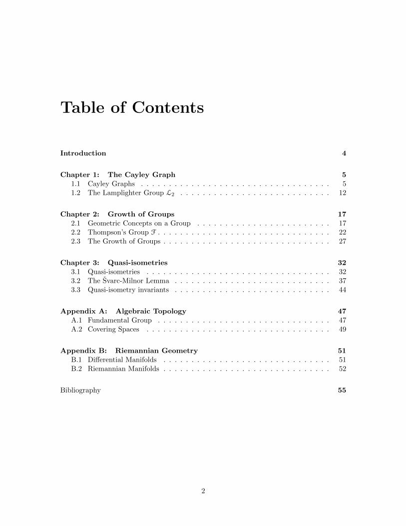
Table of Contents

Introduction 4

Chapter 1: The Cayley Graph 51.1 Cayley Graphs . . . . . . . . . . . . . . . . . . . . . . . . . . . . . . . . . . 51.2 The Lamplighter Group L2 . . . . . . . . . . . . . . . . . . . . . . . . . . . 12

Chapter 2: Growth of Groups 172.1 Geometric Concepts on a Group . . . . . . . . . . . . . . . . . . . . . . . . 172.2 Thompson’s Group F . . . . . . . . . . . . . . . . . . . . . . . . . . . . . . . 222.3 The Growth of Groups . . . . . . . . . . . . . . . . . . . . . . . . . . . . . . 27

Chapter 3: Quasi-isometries 323.1 Quasi-isometries . . . . . . . . . . . . . . . . . . . . . . . . . . . . . . . . . 323.2 The Svarc-Milnor Lemma . . . . . . . . . . . . . . . . . . . . . . . . . . . . 373.3 Quasi-isometry invariants . . . . . . . . . . . . . . . . . . . . . . . . . . . . 44

Appendix A: Algebraic Topology 47A.1 Fundamental Group . . . . . . . . . . . . . . . . . . . . . . . . . . . . . . . 47A.2 Covering Spaces . . . . . . . . . . . . . . . . . . . . . . . . . . . . . . . . . 49

Appendix B: Riemannian Geometry 51B.1 Differential Manifolds . . . . . . . . . . . . . . . . . . . . . . . . . . . . . . 51B.2 Riemannian Manifolds . . . . . . . . . . . . . . . . . . . . . . . . . . . . . . 52

Bibliography 55

2

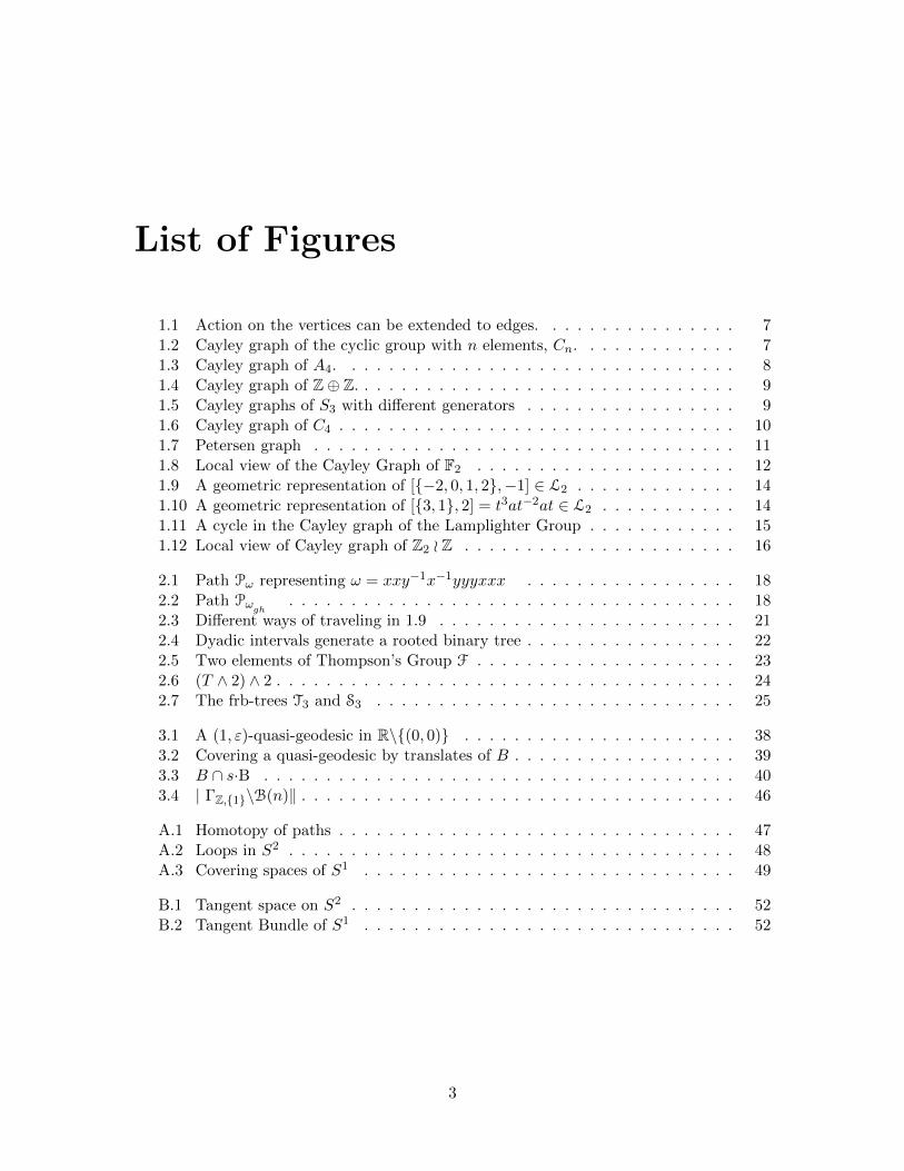
List of Figures

1.1 Action on the vertices can be extended to edges. . . . . . . . . . . . . . . . 71.2 Cayley graph of the cyclic group with n elements, Cn. . . . . . . . . . . . . 71.3 Cayley graph of A4. . . . . . . . . . . . . . . . . . . . . . . . . . . . . . . . 81.4 Cayley graph of Z⊕ Z. . . . . . . . . . . . . . . . . . . . . . . . . . . . . . . 91.5 Cayley graphs of S3 with different generators . . . . . . . . . . . . . . . . . 91.6 Cayley graph of C4 . . . . . . . . . . . . . . . . . . . . . . . . . . . . . . . . 101.7 Petersen graph . . . . . . . . . . . . . . . . . . . . . . . . . . . . . . . . . . 111.8 Local view of the Cayley Graph of F2 . . . . . . . . . . . . . . . . . . . . . 121.9 A geometric representation of [{−2, 0, 1, 2},−1] ∈ L2 . . . . . . . . . . . . . 141.10 A geometric representation of [{3, 1}, 2] = t3at−2at ∈ L2 . . . . . . . . . . . 141.11 A cycle in the Cayley graph of the Lamplighter Group . . . . . . . . . . . . 151.12 Local view of Cayley graph of Z2 o Z . . . . . . . . . . . . . . . . . . . . . . 16

2.1 Path Pω representing ω = xxy−1x−1yyyxxx . . . . . . . . . . . . . . . . . 182.2 Path Pω

gh. . . . . . . . . . . . . . . . . . . . . . . . . . . . . . . . . . . . 18

2.3 Different ways of traveling in 1.9 . . . . . . . . . . . . . . . . . . . . . . . . 212.4 Dyadic intervals generate a rooted binary tree . . . . . . . . . . . . . . . . . 222.5 Two elements of Thompson’s Group F . . . . . . . . . . . . . . . . . . . . . 232.6 (T ∧ 2) ∧ 2 . . . . . . . . . . . . . . . . . . . . . . . . . . . . . . . . . . . . . 242.7 The frb-trees T3 and S3 . . . . . . . . . . . . . . . . . . . . . . . . . . . . . 25

3.1 A (1, ε)-quasi-geodesic in R\{(0, 0)} . . . . . . . . . . . . . . . . . . . . . . 383.2 Covering a quasi-geodesic by translates of B . . . . . . . . . . . . . . . . . . 393.3 B ∩ s·B . . . . . . . . . . . . . . . . . . . . . . . . . . . . . . . . . . . . . . 403.4 | ΓZ,{1}\B(n)‖ . . . . . . . . . . . . . . . . . . . . . . . . . . . . . . . . . . . 46

A.1 Homotopy of paths . . . . . . . . . . . . . . . . . . . . . . . . . . . . . . . . 47A.2 Loops in S2 . . . . . . . . . . . . . . . . . . . . . . . . . . . . . . . . . . . . 48A.3 Covering spaces of S1 . . . . . . . . . . . . . . . . . . . . . . . . . . . . . . 49

B.1 Tangent space on S2 . . . . . . . . . . . . . . . . . . . . . . . . . . . . . . . 52B.2 Tangent Bundle of S1 . . . . . . . . . . . . . . . . . . . . . . . . . . . . . . 52

3

Introduction

The notion of groups is one of the most important ideas in mathematics, it entails a bigvariety of mathematical objects, properties and tools that have been studied for years. Sincethe 1700s Lagrange and Vandermonde were discovering different properties of permutationswhile studying the solution of equations by radicals. Years later Galois understood “group”as the group of permutations of a finite set giving the first concepts of this theory. Galoiswork was published only in 1846, fourteen years after Galois’s dead, his work was takenand systematized by Cauchy that was the first to o consider the possibility of more abstractgroup elements.In 1854 Arthur Cayley gave a first approximation of the theorem that years later was goingto be named in his honor, that declare that every group is a subgroup of a permutationgroup. He also in 1878 the concept of Cayley’s graphs (that were reintroduced in 1909 byMax Dehn under the name of Grouppenbild that means group diagram), this idea led tothe geometric group theory of today.

With finite groups the existence of generators and relations was easy and not interestingto solve, the real problem rises when we ask if it is possible to find sets of generators andrelations for infinite groups, this problem was solved by Felix Klein’s student, which leadthe foundation of the geometric group theory, or how it was introduced in the 1880s,combinatorial group theory.In the first half of the 20th century many different mathematicians introduce topologicaland geometric ideas outside the traditional combinatorial tools into the study of discretegroups, but the emergence of geometric group theory as a new area was given in thelate 1980s when Mikhail Gromov introduced the notion of hyperbolic groups in his essay“Hyperbolic Groups” in 1987, and his subsequent monograph “Asymptotic Invariants ofInfinite Groups”, where captures the ideas of a finitely generated group to have a large-scale negative curvature and the concept of quasi-isometries, a large-scale relation betweenmetric spaces that was used to see geometric properties on groups, an idea completelyrevolutionary.

After this many themes and developments have been done, as the study of Dehn’sfunctions, the interactions with computer science, complexity theory, theory of formal lan-guages, measure-theoretic properties of group actions on metric spaces, new methods ongroup cohomology, etc.

4

Chapter 1

The Cayley Graph

In this chapter we will introduce a notion of a Cayley graph and construct some examples.The Cayley graphs were introduced by Arthur Cayley in the late 1870s, they are a usefultools in algebra, combinatorics and other areas, in particular we are going to introducethem as an algebraic structure and in the following chapters we will see that they can beseen as metric spaces and a way to relate the groups that they represent with some metricspaces. Also in the second part of this chapter we will construct an interesting exampleknown as the Lamplighter group L2

1.1 Cayley Graphs

Definition 1.1.1. A graph Γ consist of a pair (V (Γ), E(Γ)) of vertices and edges respec-tively where each edge is associated to a pair of vertices. If for two vertices {u, v} thereexist an edge that is associated to both, we say that u and v are adjacent.

This definition can be complemented by adding other characteristics as:

1. Locally finite: If each vertex is contained in a finite number of edges.

2. Labeled: It can be vertex labeled or edge labeled if each element of V (Γ), or E(Γ),respectively, is labeled.

3. Connected: If for each pair of vertices {u,w} there exist a sequence of vertices andedges, {u = v0, e1, v1, . . . , vn−1, en, vn = w} where {vi, vi+1} are adjacent for each i(this sequence is a path in Γ).

4. Directed: For each edge it is defined an initial vertex and a terminal vertex. Graphi-cally this direction is often indicated as an arrow.

5. Decorated: Have different elements such as , directed edges, labeled or colored verticesand/or edges, etc.

Definition 1.1.2. If X is a set, we will denote by Sym(X) the collection of all bijectionsfrom X to X that preserve the indicated mathematical structure. For example, if X is agraph, Sym(X) is the bijections of X that preserve the structure of the graph as vertex andedges.

5

Note that under the composition Sym(X) is a group, for example if we consider X to bea graph Γ, then Sym(Γ) consists of all the bijections τ taking vertices to vertices and edgesto edges, such that if e ∈ E(V ) with ending vertices v, w, then the ending vertices of τ(e)are τ(v), τ(w). In particular the symmetry group of a decorated graph is the collection ofall the symmetries that preserve all the decorations. This is going to be explain in 1.1.12.

Definition 1.1.3. An action of a group G on a set X (in our case a graph) is a grouphomomorphism fromG to Sym(X), equivalently, it can be defined as a map fromG×X → Xthat satisfies the following two axioms:

1. e · x = x, for all x ∈ X;

2. (gh) · x = g · (h · x), for all g, h ∈ G, x ∈ X,

And it is denoted as “G acts on X” by Gy X.

If we have a group action Gy X then the associated homomorphism is a representationof G, and it is said to be faithful if this homomorphism is injective.

Theorem 1.1.4. Every finitely generated group can be faithfully represented as a group ofpermutations.

Proof. The proof of this theorem constructs a representation of G as a group of permuta-tions of itself, and it is a standard theorem in a course of abstract algebra. The proof canbe found in Corollary 4.6 of [10].

An important aspect of the use of this theorem is the action of the group, this herethere is a construction of a representation of G as a group of permutations on itself, wekeep this in mind the whole chapter.

Theorem 1.1.5. Every finitely generated group G can be faithfully represented as a sym-metry group of a connected, directed, locally finite graph.

Proof. Let G be a finitely generated group with generating set S = {s1, . . . , sn}. We canprove this theorem by constructing a graph, ΓG,S on which G acts. The vertices of ΓG,S arethe elements of G. For each g ∈ G, s ∈ S, make an edge labeled s from the vertex labeledg to the vertex labeled gs. Since G is finitely generated, this graph is locally finite. SinceS generates G, this graph is connected.

By construction, ΓG,S is directed. Let G act on the graph by left multiplication, thatis, for any g ∈ G, g will send the vertex labeled h to the vertex labeled gh.

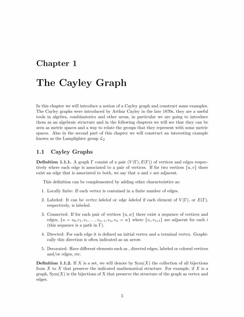
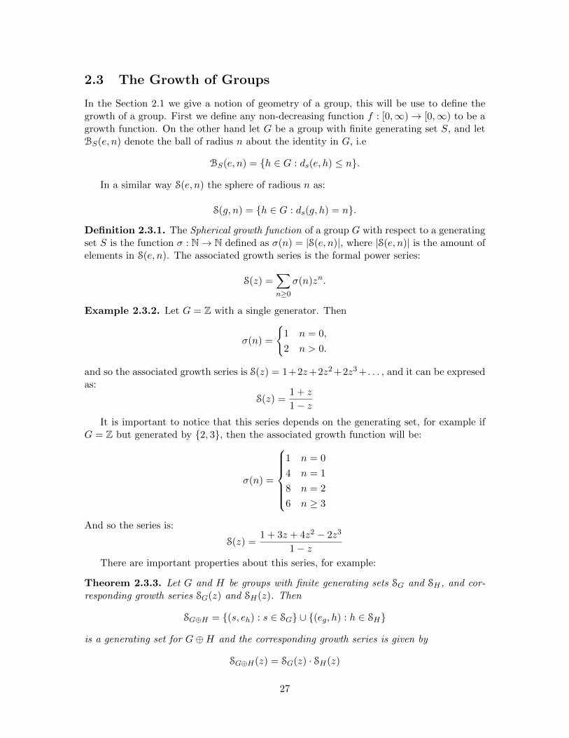
This action can be extended to an action on the edges (see figure 1.1). The vertex vh isjoined to vhs via the edge (generator) s; by the action of g, vh goes to vgh and vhs to vghs,so we can define the action on the edge labeled s that joins vh to vhs sending it to the edgelabeled also s joining vgh to vghs. Note that even if the action is defined on the left, for theedges it is given in terms of right multiplication.

Keeping this in mind, the graph that we constructed in the last theorem that representsG is known as the Cayley graph of G.

6

h

hs

gh

ghs

s s

Figure 1.1: Action on the vertices can be extended to edges.

Definition 1.1.6. Let G be a finitely generated group and S the generating set, we candefine the Cayley graph ΓG,S , which is a directed graph that can be constructed followingthe next steps:

1. Each g ∈ G is a vertex of vg ∈ V (ΓG,S)

2. Each s ∈ S forms a directed edge with initial vertex vg and terminal vertex vg·s;Giving each edge a correspondence with right multiplications of the elements of S.

In general, for different generators s1 and s2 it can be assigned colors c1 and c2 re-spectively to differentiate the action of the different elements of S. After understandingthe definition, an easy way to understand the behavior of Cayley graph is to make someexamples.

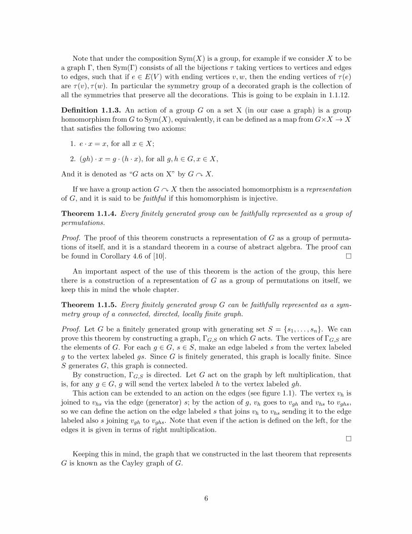
Example 1.1.7. The first and a very intuitive example is to consider the cyclic group ofn elements, Cn, clearly 1 is a generator of Cn, so the only edges are given by the action of1 · g for g ∈ Cn, then the Cayley graph is illustrated at figure 1.2.

n1

2

3

4

5

67

8

9

10

· ··

Figure 1.2: Cayley graph of the cyclic group with n elements, Cn.

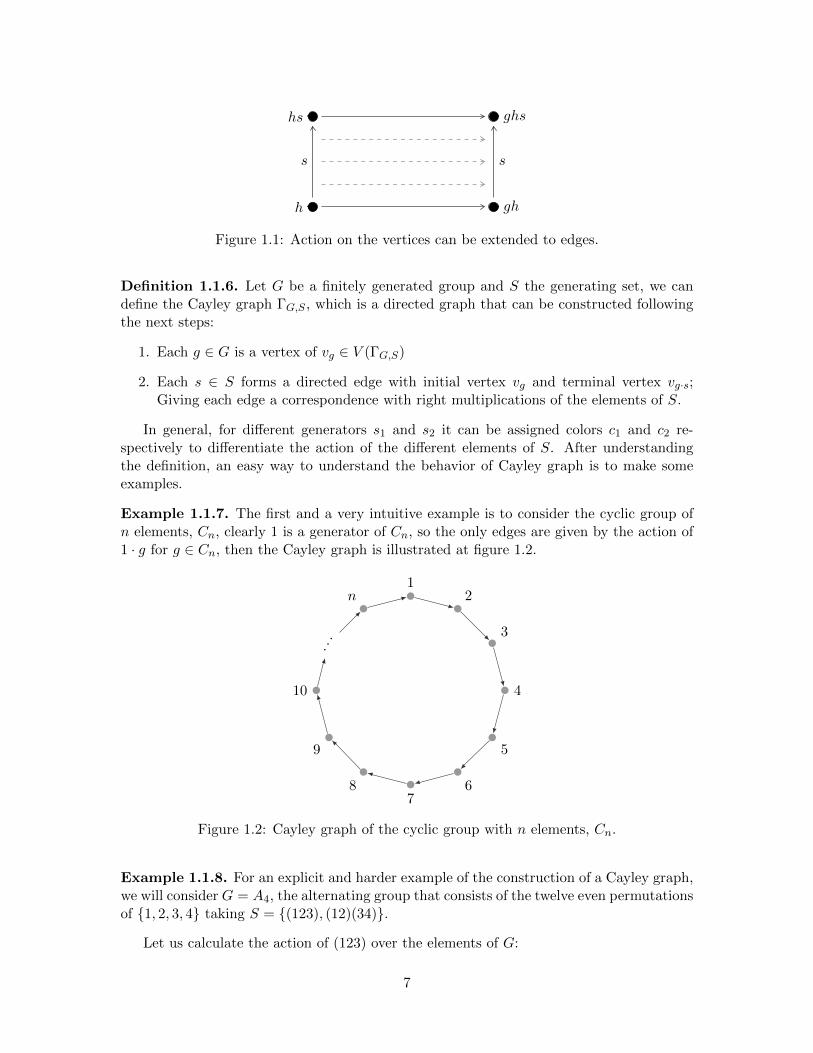
Example 1.1.8. For an explicit and harder example of the construction of a Cayley graph,we will consider G = A4, the alternating group that consists of the twelve even permutationsof {1, 2, 3, 4} taking S = {(123), (12)(34)}.

Let us calculate the action of (123) over the elements of G:

7

• (123) · (123) = (132)

• (123) · (132) = e

• (123) · (12)(34) = (243)...

Then we can calculate the action of (12)(34) over G:

• (12)(34) · (123) = (134)

• (12)(34) · (12)(34) = e...

After knowing the relation of these elements, it is easy to construct the Cayley graph givenin the Figure 1.3, where the dashed lines represent the action of (12)(34) and the othersthe action of (123).

(243)

(143)

(132)

(123)

(142)

(234)

(124)

(134)

(12)(34)

e

(13)(24)

(14)(23)

Figure 1.3: Cayley graph of A4.

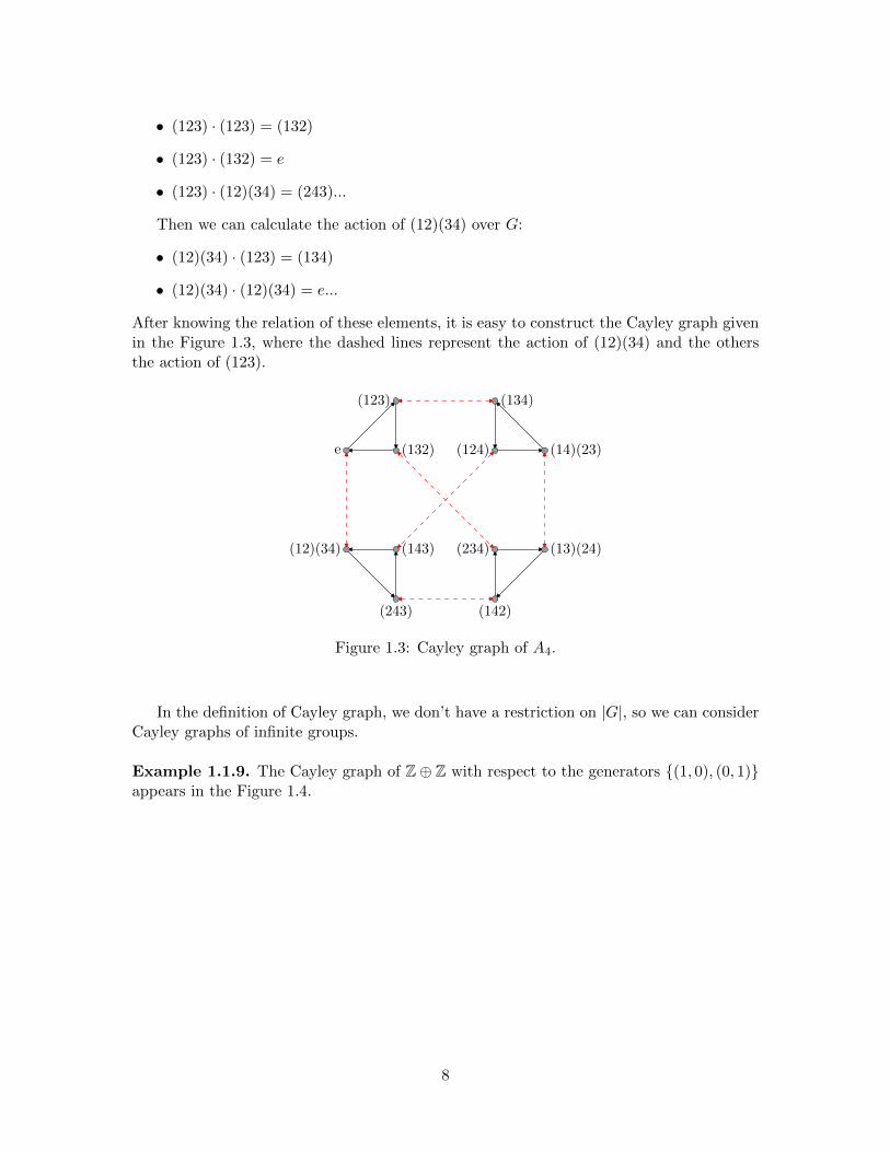
In the definition of Cayley graph, we don’t have a restriction on |G|, so we can considerCayley graphs of infinite groups.

Example 1.1.9. The Cayley graph of Z⊕ Z with respect to the generators {(1, 0), (0, 1)}appears in the Figure 1.4.

8

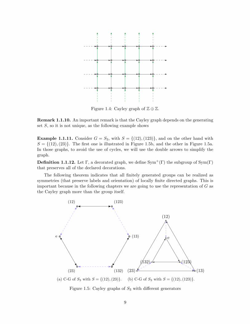
Figure 1.4: Cayley graph of Z⊕ Z.

Remark 1.1.10. An important remark is that the Cayley graph depends on the generatingset S, so it is not unique, as the following example shows

Example 1.1.11. Consider G = S3, with S = {(12), (123)}, and on the other hand withS = {(12), (23)}. The first one is illustrated in Figure 1.5b, and the other in Figure 1.5a.In those graphs, to avoid the use of cycles, we will use the double arrows to simplify thegraph.

Definition 1.1.12. Let Γ, a decorated graph, we define Sym+(Γ) the subgroup of Sym(Γ)that preserves all of the declared decorations.

The following theorem indicates that all finitely generated groups can be realized assymmetries (that preserve labels and orientation) of locally finite directed graphs. This isimportant because in the following chapters we are going to use the representation of G asthe Cayley graph more than the group itself.

(13)

(123)(12)

e

(23) (132)

(a) C-G of S3 with S = {(12), (23)}.

(12)

(23) (13)

e

(132) (123)

(b) C-G of S3 with S = {(12), (123)}.

Figure 1.5: Cayley graphs of S3 with different generators

9

Theorem 1.1.13. Let ΓG,S be the Cayley graph of a group G with respect to a finitelygenerating set S. Consider ΓG,S to be decorated with directions on its edges and labeling ofits edges, corresponding to the generating set S. Then G ∼= Sym+(ΓG,S).

Proof. Let’s consider the action of G on ΓG,S by translation (the same used in 1.1.5, thatalso shows that the representation is faithful). Since this is a left action, we have shownthat this does not affects the direction or the labelling of the edges (the action on the edgesis a right action on 1.1.5), therefore the representation is faithful into Sym+(ΓG,S).Now we need to show the surjectivity. For this, consider an arbitrary element τ ∈ Sym+(ΓG,S)and we will construct a preimage. For any g ∈ G, let vg the vertex in ΓG,S correspondingto g. There exist a g such that τ(ve) = vg. If we consider g as a symmetry of ΓG,S , theproduct τ · g−1 ∈ Sym+(ΓG,S) and also ve 7→ ve with this symmetry, further, it fixes alledges arriving at or leaving from ve. As an element of Sym+(ΓG,S) it fixes all the verticesadjacent to ve and again their edges, so the symmetry τg−1 is the identity, and because ofthat, τ = g. All this says that the preimage of a symmetry is only determined by whatit does to ve. In this case g is the preimage of τ , and as this was for an arbitrary τ ,Sym+(ΓG,S) ∼= G.

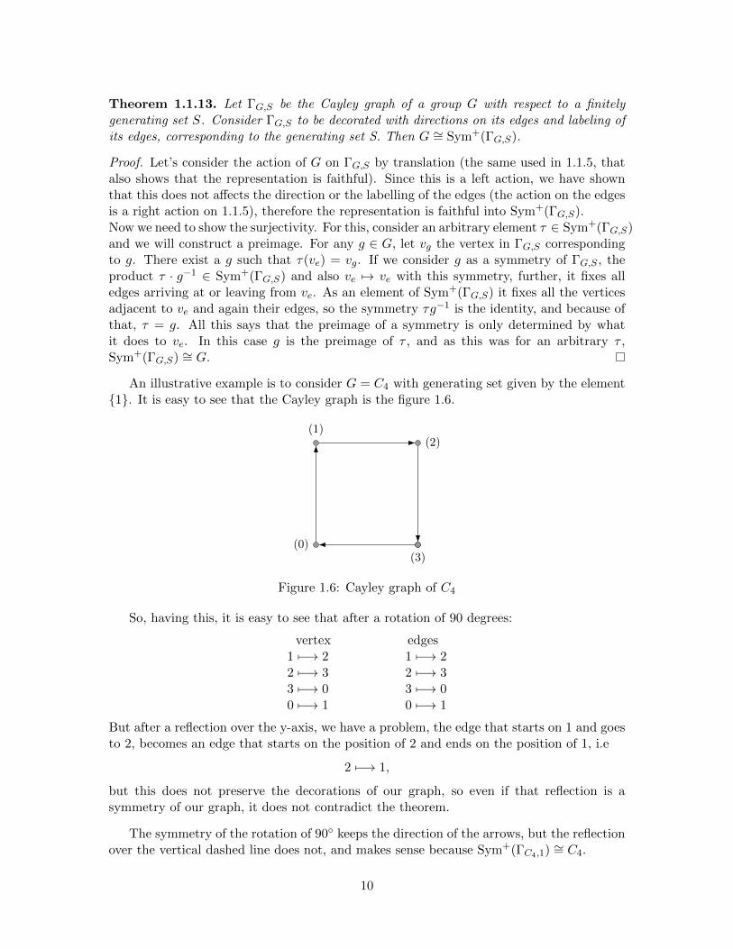
An illustrative example is to consider G = C4 with generating set given by the element{1}. It is easy to see that the Cayley graph is the figure 1.6.

(2)(1)

(0)(3)

Figure 1.6: Cayley graph of C4

So, having this, it is easy to see that after a rotation of 90 degrees:

vertex edges1 7−→ 2 1 7−→ 22 7−→ 3 2 7−→ 33 7−→ 0 3 7−→ 00 7−→ 1 0 7−→ 1

But after a reflection over the y-axis, we have a problem, the edge that starts on 1 and goesto 2, becomes an edge that starts on the position of 2 and ends on the position of 1, i.e

2 7−→ 1,

but this does not preserve the decorations of our graph, so even if that reflection is asymmetry of our graph, it does not contradict the theorem.

The symmetry of the rotation of 90◦ keeps the direction of the arrows, but the reflectionover the vertical dashed line does not, and makes sense because Sym+(ΓC4,1)

∼= C4.

10

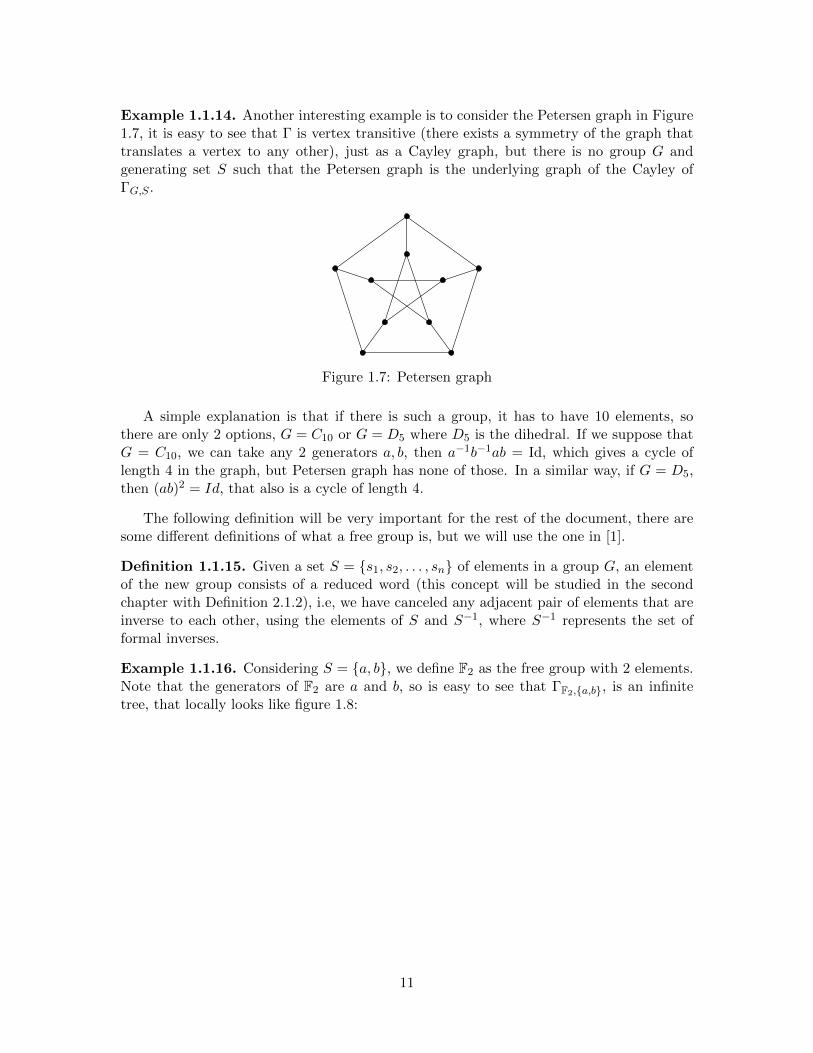
Example 1.1.14. Another interesting example is to consider the Petersen graph in Figure1.7, it is easy to see that Γ is vertex transitive (there exists a symmetry of the graph thattranslates a vertex to any other), just as a Cayley graph, but there is no group G andgenerating set S such that the Petersen graph is the underlying graph of the Cayley ofΓG,S .

Figure 1.7: Petersen graph

A simple explanation is that if there is such a group, it has to have 10 elements, sothere are only 2 options, G = C10 or G = D5 where D5 is the dihedral. If we suppose thatG = C10, we can take any 2 generators a, b, then a−1b−1ab = Id, which gives a cycle oflength 4 in the graph, but Petersen graph has none of those. In a similar way, if G = D5,then (ab)2 = Id, that also is a cycle of length 4.

The following definition will be very important for the rest of the document, there aresome different definitions of what a free group is, but we will use the one in [1].

Definition 1.1.15. Given a set S = {s1, s2, . . . , sn} of elements in a group G, an elementof the new group consists of a reduced word (this concept will be studied in the secondchapter with Definition 2.1.2), i.e, we have canceled any adjacent pair of elements that areinverse to each other, using the elements of S and S−1, where S−1 represents the set offormal inverses.

Example 1.1.16. Considering S = {a, b}, we define F2 as the free group with 2 elements.Note that the generators of F2 are a and b, so is easy to see that ΓF2,{a,b}, is an infinitetree, that locally looks like figure 1.8:

11

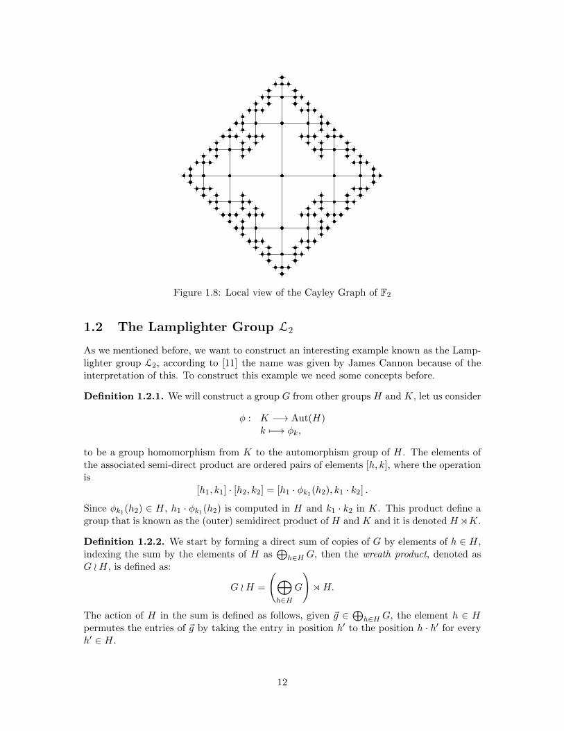
Figure 1.8: Local view of the Cayley Graph of F2

1.2 The Lamplighter Group L2

As we mentioned before, we want to construct an interesting example known as the Lamp-lighter group L2, according to [11] the name was given by James Cannon because of theinterpretation of this. To construct this example we need some concepts before.

Definition 1.2.1. We will construct a group G from other groups H and K, let us consider

φ : K −→ Aut(H)k 7−→ φk,

to be a group homomorphism from K to the automorphism group of H. The elements ofthe associated semi-direct product are ordered pairs of elements [h, k], where the operationis

[h1, k1] · [h2, k2] = [h1 · φk1(h2), k1 · k2] .

Since φk1(h2) ∈ H, h1 · φk1(h2) is computed in H and k1 · k2 in K. This product define agroup that is known as the (outer) semidirect product of H and K and it is denoted HoK.

Definition 1.2.2. We start by forming a direct sum of copies of G by elements of h ∈ H,indexing the sum by the elements of H as

⊕h∈H G, then the wreath product, denoted as

G oH, is defined as:

G oH =

(⊕h∈H

G

)oH.

The action of H in the sum is defined as follows, given ~g ∈⊕

h∈H G, the element h ∈ Hpermutes the entries of ~g by taking the entry in position h′ to the position h · h′ for everyh′ ∈ H.

12

Example 1.2.3. An easy example of this, is to consider Z2 o Z3. This is the semi-directproduct (Z2)

3 o Z3. If we declare φ1 ∈ Aut((Z2)3) as the cyclic permutation φ1(a, b, c) =

(b, c, a), then we can see the behavior, for example computing:

[(0, 1, 1), 1] · [(1, 0, 0), 1] = [(0, 1, 1) · φ1(1, 0, 0), 1 · 1]= [(0, 1, 1) · (0, 0, 1), 1 + 1]= [(0, 1, 1) · (0, 0, 1), 2]= [(0, 1, 1) + (0, 0, 1), 2]= [(0, 1, 0), 2] .

The remainder of this section is devoted to understand the example Z2 o Z. It is thesemidirect product:

Z2 o Z =

(⊕h∈H

Z2

)o Z = (· · · ⊕ Z2 ⊕ Z2 ⊕ Z2 ⊕ . . . )o Z

This particular example is called the lamplighter group, and it is denoted L2. First of all wewill give a geometric description of how this group can be understood (and also the reasonof its name). Imagine a rural town with an infinite main street lined with lampposts, alamplighter walks up and down the street lighting some of the light bulbs, then ends hiswalk just in front one of the lampposts. This situation is what L2 represents. To understandthis analogy let us divide each part of this product:

• First of all, we have the group Z2, that from the description we gave above, we canthink of this as a lamppost where the elements of Z2 represents if it is “on” or “off”More specifically if the element of Z2 is [1], we say that the lamp is “on” and if theelement is [0], we say that it is “off”.

•⊕

h∈H Z2 can be thought as a line of infinite lamps (copies of Z2) that are on or offdepending on the elements of Z2.

• The elements of L2 are determined which (finite number) entries have non zero ele-ments, in the analogy the elements are infinite lines of lamps where some of them areon.

In this group the identity element corresponds to ~0 = (. . . , 0, 0, 0, . . . ) ∈ L2. We need tounderstand the operation of

⊕h∈H Z2, viewing elements of L2 as subsets S ⊂ Z. As there

can only be finite non zero elements, the operation corresponds to the symmetric difference(“4”). For example if S = {−2, 0, 1} and T = {−3, 0, 4}, then {−2, 0, 1}4{−3, 0, 4} ={−3,−2, 1, 4}.

Understanding this, every element in L2 can be represented by an ordered pair [S, n]where S ⊂ Z and n ∈ Z, and defining the operation by:

[S, n] · [T,m] = [S4(T + n), n+m],

where (T + n) = {t+ n|t ∈ T}. We denote the identity element as [∅, 0]

Lemma 1.2.4. The lamplighter group L2 can be generated by two elements, one of order2 and the other of infinite order.

13

Proof. Let t be the element [∅, 1] ∈ L2 and a = [{0}, 0] ∈ L2, notice that a 6= [∅, 0]. Theproduct of them is:

ta = [∅, 1] · [{0}, 0] = [{1}, 1],

more generally:tna = [{n}, n]

andtna = [{n}, n]

Doing some more computations, it is easy to prove that

L2 3 [{n1, n2, . . . , nm}, k] = tn1at−n1 · tn2at−n2 · · · tnmat−nm · tk.

Therefore, the set {a, t} is a generating set for the lamplighter group.

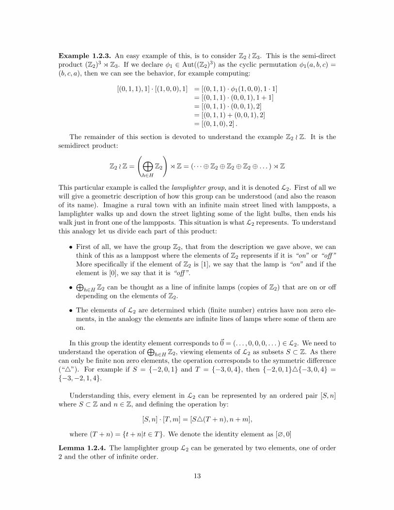
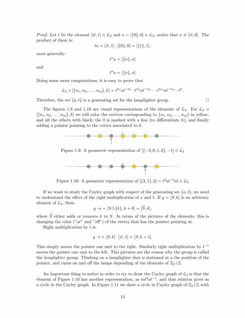
The figures 1.9 and 1.10 are visual representations of the elements of L2. For L2 3[{n1, n2, . . . , nm}, k] we will color the vertices corresponding to {n1, n2, . . . , nm} in yellow,and all the others with black; the 0 is marked with a line (to differentiate it); and finallyadding a pointer pointing to the vertex associated to k.

Figure 1.9: A geometric representation of [{−2, 0, 1, 2},−1] ∈ L2

Figure 1.10: A geometric representation of [{3, 1}, 2] = t3at−2at ∈ L2

If we want to study the Cayley graph with respect of the generating set {a, t}, we needto understand the effect of the right multiplication of a and t. If g = [S, k] is an arbitraryelement of L2, then:

g · a = [S4{k}, k + 0] = [S, k],

where S either adds or removes k to S. In terms of the pictures of the elements, this ischanging the color (”or” and ”off”) of the vertex that has the pointer pointing at.

Right multiplication by t is:

g · t = [S, k] · [∅, 1] = [S, k + 1].

This simply moves the pointer one unit to the right. Similarly right multiplication by t−1

moves the pointer one unit to the left. This pictures are the reason why the group is calledthe lamplighter group. Thinking on a lamplighter that is stationed at a the position of thepointer, and turns on and off the lamps depending of the elements of Z2 o Z.

An important thing to notice in order to try to draw the Cayley graph of L2 is that theelement of Figure 1.10 has another representation, as tat2at−1, and that relation gives usa cycle in the Cayley graph. In Figure 1.11 we show a cycle in Cayley graph of Z2 oZ with

14

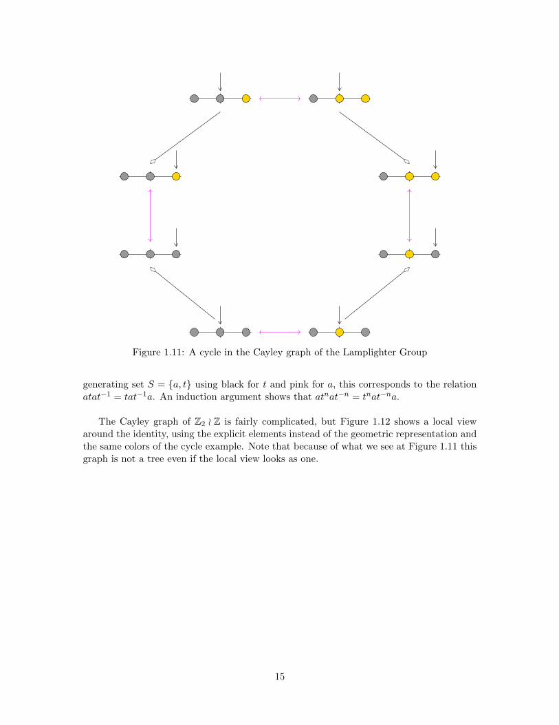
Figure 1.11: A cycle in the Cayley graph of the Lamplighter Group

generating set S = {a, t} using black for t and pink for a, this corresponds to the relationatat−1 = tat−1a. An induction argument shows that atnat−n = tnat−na.

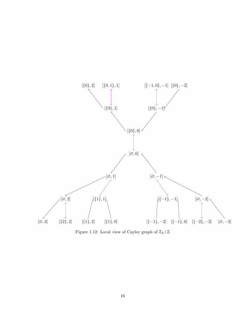
The Cayley graph of Z2 o Z is fairly complicated, but Figure 1.12 shows a local viewaround the identity, using the explicit elements instead of the geometric representation andthe same colors of the cycle example. Note that because of what we see at Figure 1.11 thisgraph is not a tree even if the local view looks as one.

15

[∅, 0]

[{0}, 0]

[{0}, 1] [{0},−1]

[{0, 1}, 1][{0}, 2] [{−1, 0},−1] [{0},−2]

[∅, 1] [∅,−1]

[{1}, 1]

[{1}, 2] [{1}, 0]

[∅, 2]

[{2}, 2][∅, 3]

[{−1},−1]

[{−1}, 0][{−1},−2]

[∅,−2]

[{−2},−2] [∅,−3]

Figure 1.12: Local view of Cayley graph of Z2 o Z

16

Chapter 2

Growth of Groups

An interesting question that appears in the study of infinite groups is how to give a com-parison between the sizes of infinite groups. For example consider the free abelian Z2 andthe free group F2, of course both groups have countably infinite cardinality, so how can wecompare them? The answer can be found on the growth functions that we are going todefine on the third part of this chapter.

We will divide this chapter into 3 parts, in the first one, before giving the definitionof growth functions, we need some notions on the geometric properties of a group. In thesecond part we introduce the Thompson’s Group F, a very interesting group that seems tolook like the answer to a group that has ”intermediate growth”, a concept that is finallyintroduced in the third part together with the definition of growth functions and someexamples of this.

2.1 Geometric Concepts on a Group

Definition 2.1.1. (Metric space). A metric space, consist of a set X and a distancefunction d : X ×X → R, such that, for ant x, y, z ∈ X

1. d(x, y) ≥ 0,

2. d(x, y) = 0 iff x = y ,

3. d(x, y) = d(y, x) ,

4. d(x, y) + d(y, z) ≥ d(x, z).

A function from a metric space to another, ϕ : X1 → X2, with distances d1 and d2respectively, is an isometry if it is onto, and for all x, y ∈ X1, d1(x, y) = d2(ϕ(x), ϕ(y)),also Gy X is an isometric action if for all x, y ∈ X and g ∈ G:

d(x, y) = d(g · x, g · y).

The idea of the metric in the group will be related to the distance between the vertices ofthe Cayley graph, for this we will introduce the concept of words and paths.

Definition 2.1.2. Given a set S, a finite sequence of elements from S, possibly withrepetition, is called a word.

17

We will construct a free monoid that is going to consist in all possible words of a givenset, where the identity is the empty word, and their formal inverses, that is {S ∪S−1}, andthe operation is the concatenation. We remark that this is a monoid, so the element xx−1

is not the identity. One last convention that we use is that (x−1)−1 = x. We will denotethis monoid as {S ∪ S−1}∗.

Note that if S represents the generating set of a group G, then we associate the elementω = x1x2...xk ∈ {S ∪ S−1}∗ with an edge path in the Cayley Graph ΓG,S , where the pathstarts at the vertex corresponding to the identity, and goes through the graph, as it isdictated by ω.

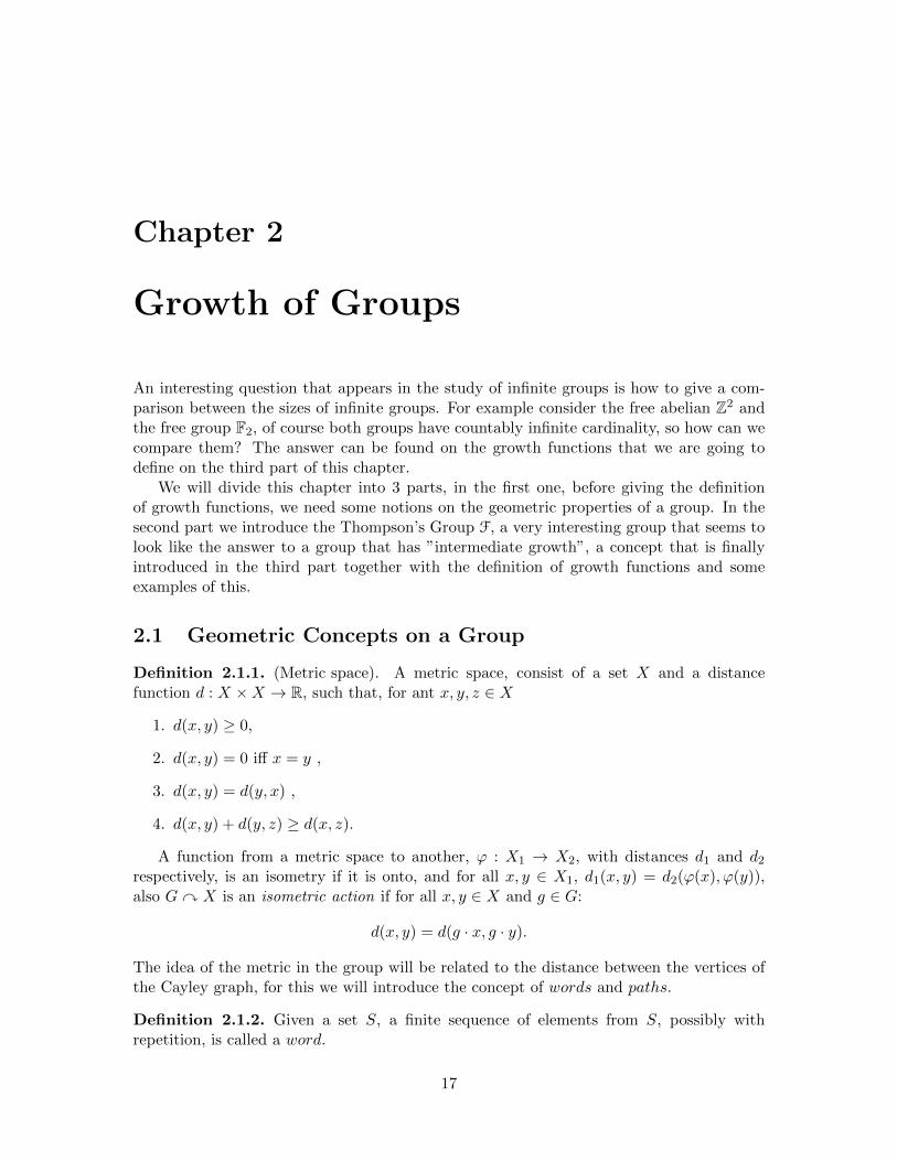
Example 2.1.3. Consider G = Z⊕Z, generated by x = (1, 0) and y = (0, 1), and the wordω = xxy−1x−1yyyxxx, the edge path Pω is illustrated in figure 2.1.

Identity

End of path

Figure 2.1: Path Pω representing ω = xxy−1x−1yyyxxx

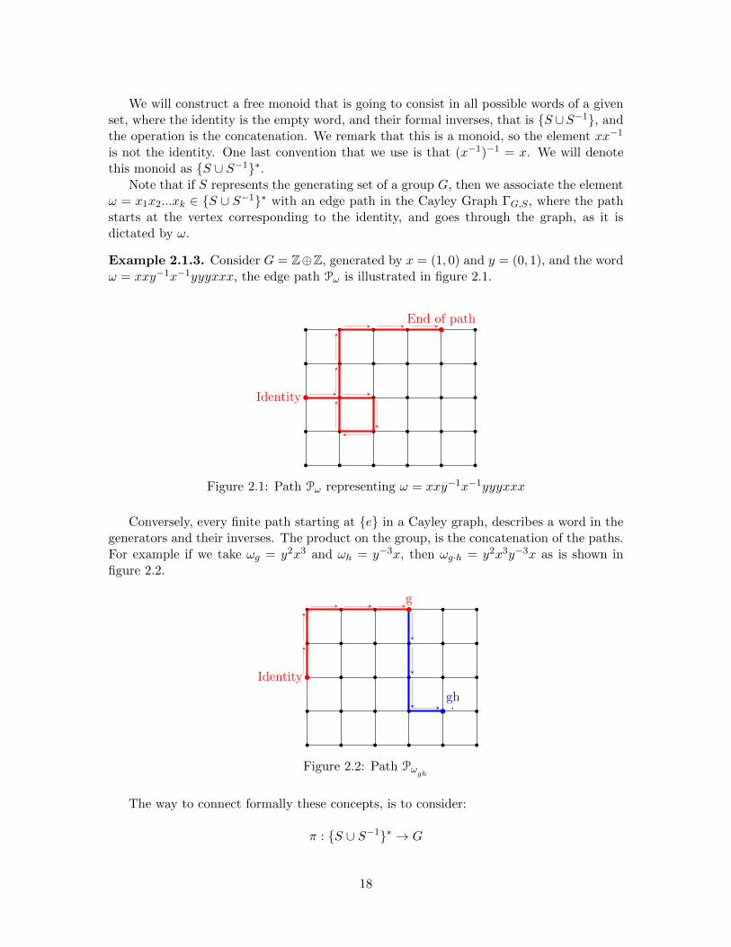
Conversely, every finite path starting at {e} in a Cayley graph, describes a word in thegenerators and their inverses. The product on the group, is the concatenation of the paths.For example if we take ωg = y2x3 and ωh = y−3x, then ωg·h = y2x3y−3x as is shown infigure 2.2.

Identity

g

gh

Figure 2.2: Path Pωgh

The way to connect formally these concepts, is to consider:

π : {S ∪ S−1}∗ → G

18

This maps a word in the monoid to the corresponding element of G. Since S is agenerating set, π is onto. So for example, if we let G = Z⊕ Z, generated by a = (1, 0) andb = (0, 1) ω1 = aba−1bbba and ω2 = bbabb, they are distinct elements on {S ∪ S−1}∗, butπ(ω1) = π(ω2) = (1, 4) ∈ Z⊕ Z. In a similar way, a normal form is a function:

η : G→ {S ∪ S−1}∗.

Such that π ◦ η : G→ G is the identity.

Using this, we can define:

ds(g, h) = the length of the shortest word representing g−1h.

If ω is a word on {S ∪ S−1}∗, representing g−1h, then:

g−1h = π(ω)⇒ h = gπ(ω)

This way, ω labels a path, connecting the vertices associated to g to the vertex associatedto h, also note that a minimal-length word, describes a minimal-length path between vertexin the Cayley graph.

Definition 2.1.4. The length of g ∈ G is the amount of generators of the minimal wordω ∈ {S ∪ S−1}∗ where π(ω) = g. We denote this value as |g|.

Is easy to see that in example 2.1.3, if g = (m,n), then |g| = |m|+ |n|

Theorem 2.1.5 (Gromov’s Corollary). Every finitely generated group can be faithfullyrepresented as a group of isometries of a metric space.

Proof. The first part of this proof shows that the Cayley graph is a metric space.

Similar to the Cayley’s Theorem for groups and Theorem 1.1.5 the metric space is builtfrom the group G, this is because the vertices of the Cayley graph corresponds to elementsof G and using the distance ds(g, h) that was mentioned before. Note that the conditions 1and 2 of the Definition 2.1.1 are already given, so it only remains to show that the distancefunction is symmetric and the triangle inequality holds.

If ds(g, h) = n that means that there exist a word ω such that g−1h = π(ω), also,h−1g = π(ω−1), thus doing one step at a time in the opposite direction, we can see thatds(h, g) ≤ n, but if there exists another word ω′ representing h−1g, then we could takeits formal inverse and form a shorter word that represents g−1h that is a contradiction,therefore our distance is symmetric.

Let ωgk and ωkh be the minimal-length words such that g ·π(ωgk) = k and k ·π(ωkh) = h,then g · π(ωgkωkh) = h, hence

ds(g, h) ≤ |ωgk|+ |ωkh| = ds(g, k) + ds(k, h)

This last property shows that a group G con be viewed as a metric space. Because ofthat, the natural answer to the question of how the can the group be faithfully representedis given by Cayley’s theorem (1.1.4) which shows that left multiplication gives an action of

19

G on itself, the important thing to notice is that the same representation of G as a group ofpermutations gives the representation as a group of isometries because that action preservesdistances, i.e:

ds(h, k) =∣∣h−1k∣∣ =

∣∣h−1g−1gk∣∣ = ds(gh, gk),

for any g, h, k ∈ G.

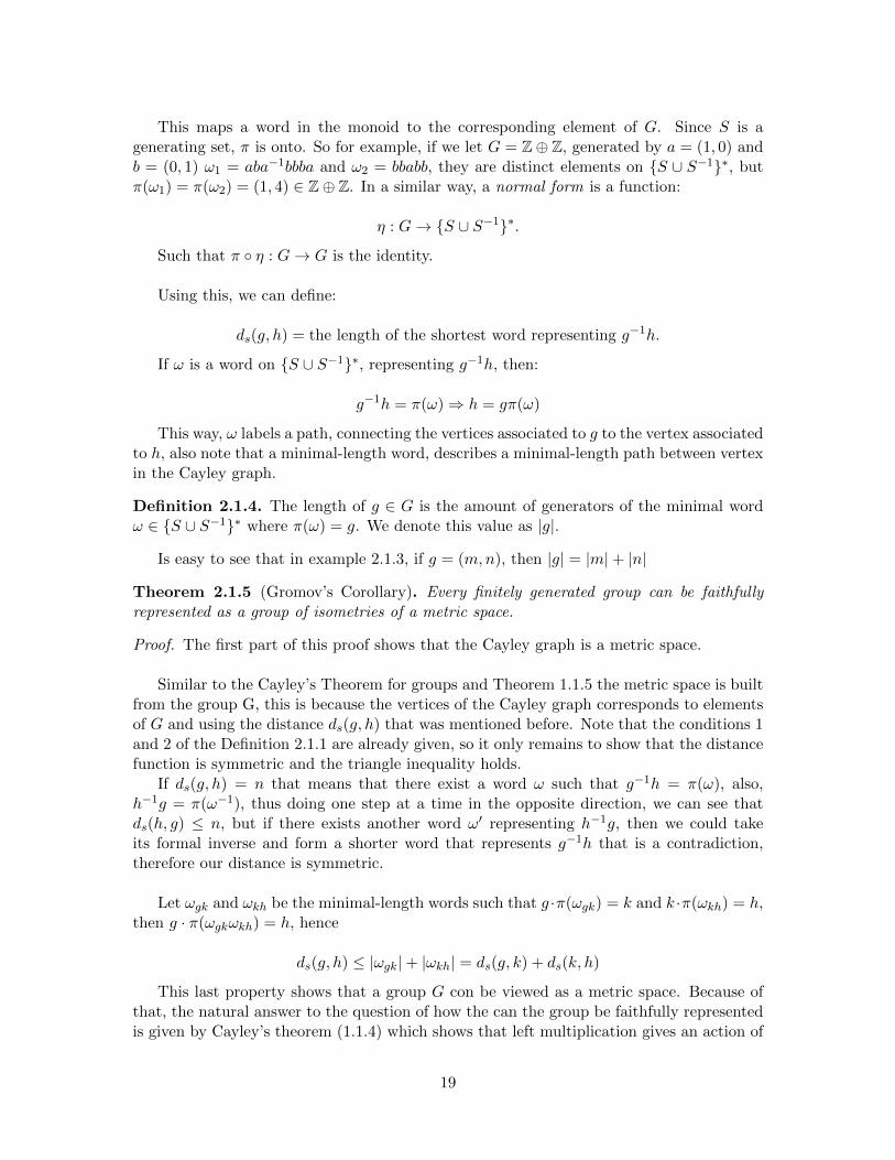
For example, let us consider the next figure that is the same as in 1.4, the distancebetween the lower left-hand vertex and the upper right-hand vertex is 7. This can be donewith

(74

)different words, four x′s and three y′s.

Some natural definitions come after this, the diameter is the minimal integer D suchthat one can get between any 2 vertex by some edge path of length ≤ D, a minimal-lengthpath between two vertices is a geodesic path, and other definitions.

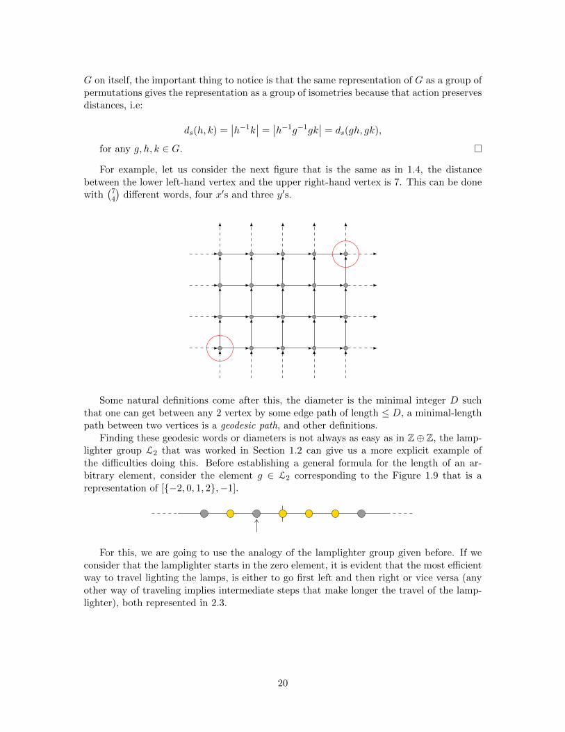
Finding these geodesic words or diameters is not always as easy as in Z⊕ Z, the lamp-lighter group L2 that was worked in Section 1.2 can give us a more explicit example ofthe difficulties doing this. Before establishing a general formula for the length of an ar-bitrary element, consider the element g ∈ L2 corresponding to the Figure 1.9 that is arepresentation of [{−2, 0, 1, 2},−1].

For this, we are going to use the analogy of the lamplighter group given before. If weconsider that the lamplighter starts in the zero element, it is evident that the most efficientway to travel lighting the lamps, is either to go first left and then right or vice versa (anyother way of traveling implies intermediate steps that make longer the travel of the lamp-lighter), both represented in 2.3.

20

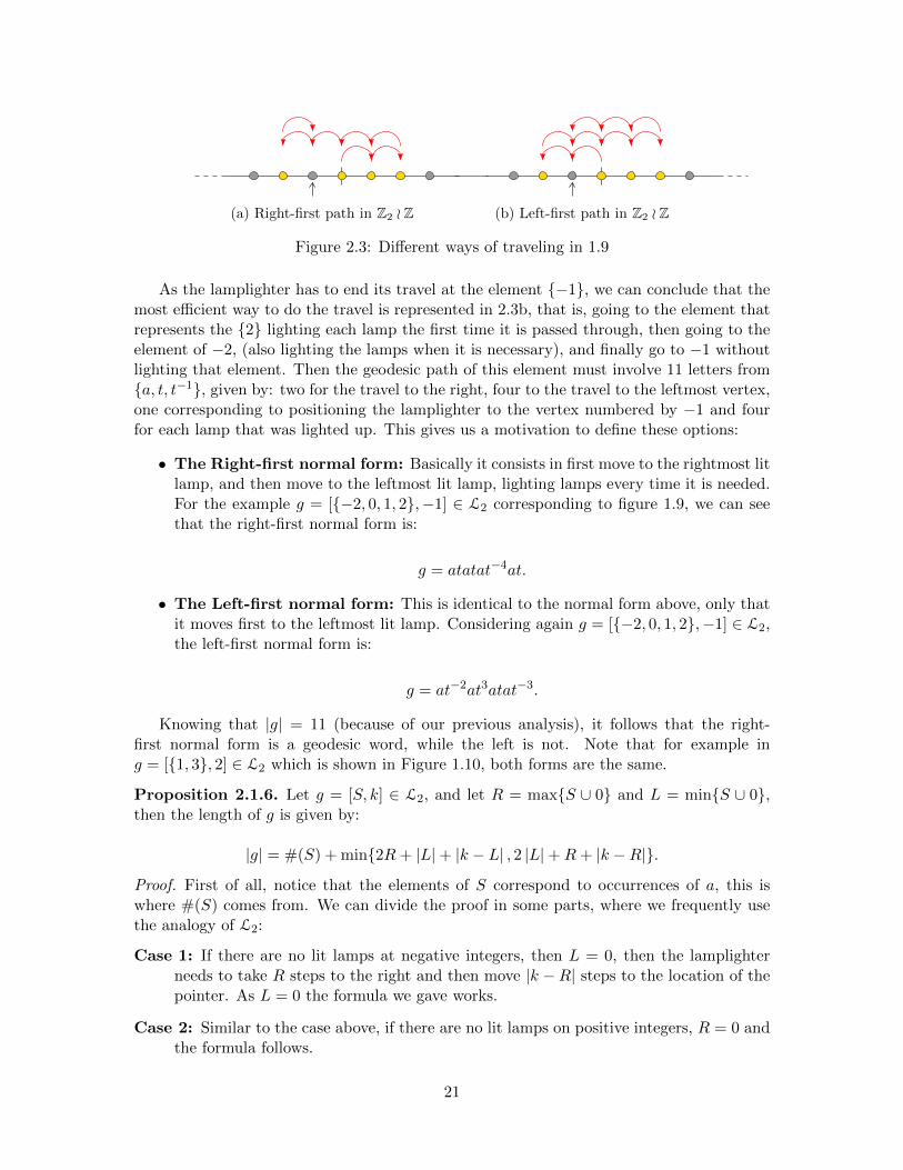
(a) Right-first path in Z2 o Z (b) Left-first path in Z2 o Z

Figure 2.3: Different ways of traveling in 1.9

As the lamplighter has to end its travel at the element {−1}, we can conclude that themost efficient way to do the travel is represented in 2.3b, that is, going to the element thatrepresents the {2} lighting each lamp the first time it is passed through, then going to theelement of −2, (also lighting the lamps when it is necessary), and finally go to −1 withoutlighting that element. Then the geodesic path of this element must involve 11 letters from{a, t, t−1}, given by: two for the travel to the right, four to the travel to the leftmost vertex,one corresponding to positioning the lamplighter to the vertex numbered by −1 and fourfor each lamp that was lighted up. This gives us a motivation to define these options:

• The Right-first normal form: Basically it consists in first move to the rightmost litlamp, and then move to the leftmost lit lamp, lighting lamps every time it is needed.For the example g = [{−2, 0, 1, 2},−1] ∈ L2 corresponding to figure 1.9, we can seethat the right-first normal form is:

g = atatat−4at.

• The Left-first normal form: This is identical to the normal form above, only thatit moves first to the leftmost lit lamp. Considering again g = [{−2, 0, 1, 2},−1] ∈ L2,the left-first normal form is:

g = at−2at3atat−3.

Knowing that |g| = 11 (because of our previous analysis), it follows that the right-first normal form is a geodesic word, while the left is not. Note that for example ing = [{1, 3}, 2] ∈ L2 which is shown in Figure 1.10, both forms are the same.

Proposition 2.1.6. Let g = [S, k] ∈ L2, and let R = max{S ∪ 0} and L = min{S ∪ 0},then the length of g is given by:

|g| = #(S) + min{2R+ |L|+ |k − L| , 2 |L|+R+ |k −R|}.

Proof. First of all, notice that the elements of S correspond to occurrences of a, this iswhere #(S) comes from. We can divide the proof in some parts, where we frequently usethe analogy of L2:

Case 1: If there are no lit lamps at negative integers, then L = 0, then the lamplighterneeds to take R steps to the right and then move |k −R| steps to the location of thepointer. As L = 0 the formula we gave works.

Case 2: Similar to the case above, if there are no lit lamps on positive integers, R = 0 andthe formula follows.

21

Case 3: If there is a lit lamp at m < 0 and at n > 0, using the rightmost normal form,there have to be 2R+|L|+|k − L| occurrences of t or t−1. Similarly using the leftmostnormal form there are 2 |L|+R+ |k −R| movements of the lamplighter.

Considering the minimum between the rightmost normal form and the leftmost normalform, the formula follows.

2.2 Thompson’s Group F

Given the closed interval [0, 1], we define a dyadic division of this, that is constructed fistdividing [0, 1] and [0, 1/2], [1/2, 1], and each sub interval define (or not) another division afinite number of times. For example:

[0, 1] = [0, 1/4] ∪ [1/4, 1/2] ∪ [1/2, 3/4] ∪ [3/4, 1]

We refer to any interval of the form

[m

2n,m+ 1

2n

](0 ≤ m ≤ 2n − 1) as a standard

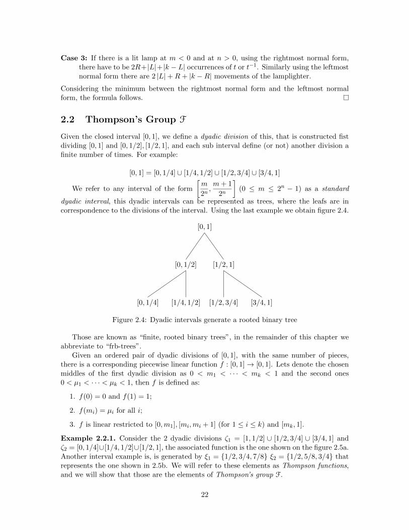
dyadic interval, this dyadic intervals can be represented as trees, where the leafs are incorrespondence to the divisions of the interval. Using the last example we obtain figure 2.4.

[0, 1]

[0, 1/2] [1/2, 1]

[0, 1/4] [1/4, 1/2] [1/2, 3/4] [3/4, 1]

Figure 2.4: Dyadic intervals generate a rooted binary tree

Those are known as “finite, rooted binary trees”, in the remainder of this chapter weabbreviate to “frb-trees”.

Given an ordered pair of dyadic divisions of [0, 1], with the same number of pieces,there is a corresponding piecewise linear function f : [0, 1]→ [0, 1]. Lets denote the chosenmiddles of the first dyadic division as 0 < m1 < · · · < mk < 1 and the second ones0 < µ1 < · · · < µk < 1, then f is defined as:

1. f(0) = 0 and f(1) = 1;

2. f(mi) = µi for all i;

3. f is linear restricted to [0,m1], [mi,mi + 1] (for 1 ≤ i ≤ k) and [mk, 1].

Example 2.2.1. Consider the 2 dyadic divisions ζ1 = [1, 1/2] ∪ [1/2, 3/4] ∪ [3/4, 1] andζ2 = [0, 1/4]∪[1/4, 1/2]∪[1/2, 1], the associated function is the one shown on the figure 2.5a.Another interval example is, is generated by ξ1 = {1/2, 3/4, 7/8} ξ2 = {1/2, 5/8, 3/4} thatrepresents the one shown in 2.5b. We will refer to these elements as Thompson functions,and we will show that those are the elements of Thompson’s group F.

22

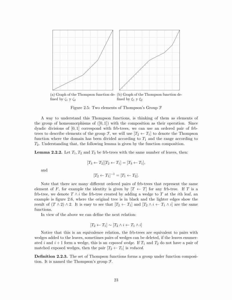
(a) Graph of the Thompson function de-fined by ζ1 y ζ2

(b) Graph of the Thompson function de-fined by ξ1 y ξ2

Figure 2.5: Two elements of Thompson’s Group F

A way to understand this Thompson functions, is thinking of them as elements ofthe group of homeomorphisms of ([0, 1]) with the composition as their operation. Sincedyadic divisions of [0, 1] correspond with frb-trees, we can use an ordered pair of frb-trees to describe elements of the group F, we will use [T2 ← T1] to denote the Thompsonfunction where the domain has been divided according to T1 and the range according toT2. Understanding that, the following lemma is given by the function composition.

Lemma 2.2.2. Let T1, T2 and T3 be frb-trees with the same number of leaves, then:

[T3 ← T2][T2 ← T1] = [T3 ← T1],

and[T2 ← T1]

−1 = [T1 ← T2].

Note that there are many different ordered pairs of frb-trees that represent the sameelement of F , for example the identity is given by [T ← T ] for any frb-tree. If T is afrb-tree, we denote T ∧ i the frb-tree created by adding a wedge to T at the ith leaf, anexample is figure 2.6, where the original tree is in black and the lighter edges show theresult of (T ∧ 2) ∧ 2. It is easy to see that [T2 ← T1] and [T2 ∧ i ← T1 ∧ i] are the samefunctions.

In view of the above we can define the next relation:

[T2 ← T1] ∼ [T2 ∧ i← T1 ∧ i]

Notice that this is an equivalence relation, the frb-trees are equivalent to pairs withwedges added to the leaves, sometimes pairs of wedges can be deleted, if the leaves enumer-ated i and i+ 1 form a wedge, this is an exposed wedge. If T1 and T2 do not have a pair ofmatched exposed wedges, then the pair [T2 ← T1] is reduced.

Definition 2.2.3. The set of Thompson functions forms a group under function composi-tion. It is named the Thompson’s group F.

23

Figure 2.6: (T ∧ 2) ∧ 2

A question that is common studying the Thompson’s group F is that if two functionscome from frb-trees that have different number of leafs, how can they be operated?. Theanswer is that because any two dyadic divisions have a common dyadic subdivision where(seen as functions) the domains coincide and therefore they can be composed.

We will denote Supp(f) = {x ∈ [0, 1] : f(x) 6= x} the support of f . We call an el-ement f ∈ F to be a left element if Supp(f) ⊂ (0, 1/2), similarly f is a right elementif Supp(f) ⊂ (1/2, 1), the set of left and right elements of F form subgroups Fl and Frrespectively.

Let l to be the homomorphism F → F that takes f ∈ F to:

fl(x) =

{f(2x)/2 0 ≤ x ≤ 1/2

x 1/2 ≤ x ≤ 1

Similarly define r that takes f ∈ F to:

fr(x) =

{x 0 ≤ x ≤ 1/2

1/2 + f(2x)/2 1/2 ≤ x ≤ 1

The graph of fl consists of a copy of the graph of f that has been shrunk and tucked into[0, 1/2]× [0, 1/2] and is extended to the remainder of the domain as the identity. Similarlythe graph of fr is embedded into [1/2, 1] × [1/2, 1]. This homomorphism shows that bothFl and Fr are isomorphic to F, since the elements in Fl and Fr are disjoint because of theelements of the support, and the elements of both subgroups commute, then Fl×Fr ∼= F×F,this gives us the proof of the following:

Proposition 2.2.4. Thompson’s group F contains a subgroup isomorphic to F × F.

In order to understand the Thompson’s group F, we want to introduce two families offrb-trees. Lets denote Tn be the frb-tree where T0 is a single wedge and Tn+1 = Tn ∧ (n+1).Let Sn be the frb-tree where S0 = T0 and Sn+1 = Tn ∧ n. Examples of T3 and S3 are in2.7a and 2.7b retrospectively.

24

(a) T3 (b) S3

Figure 2.7: The frb-trees T3 and S3

An element f ∈ F is said to be positive if it corresponds to a pair of the form [T ← Tn];it is negative if it corresponds to a pair [Tn ← T]. Since [T ← Tn]−1 = [Tn ← T], thenegative elements are inverses of positive.

Lemma 2.2.5. Every element f ∈ F can be expressed as a product of a positive and anegative element.

Proof. Let f be a Thompson function given by [S ← T ] where S and T have n+ 1 leaves,then

f = [S ← T ] = [S ← Tn][Tn ← T ].

Because of Lemma 2.2.2, then f is expressed as the product of a positive and a negativeelement.

Let us define xi, the Thompson function described by [Sn+1 ← Tn+1]. Note that thegraphs of x0 and x1 are shown in Figure 2.5; the collection of xi satisfies the followingrelations:

Lemma 2.2.6. If i < n then xi−1xnxi = xn+1.

Proof. First of all, notice that because i < n then Tn ∧ n ∧ i = Tn ∧ i ∧ (n + 1), and ourobjective is to show that:

[Ti+1 ← Si+1][Sn+1 ← Tn+1][Si+1 → Ti+1] = [Sn+2 ← Tn+2],

notice that [Si+1 ← Ti+1] = [Tn+1 ∧ i← Tn+2], then

[Ti+1 ← Si+1][Sn+1 ← Tn+1][Si+1 → Ti+1] = [Ti+1 ← Si+1][Sn+1 ∧ i← Tn+2].

Similarly

[Ti+1 ← Si+1][Sn+1 ∧ i← Tn+2] = [Tn+1 ∧ (n+ 1)← Tn ∧ i ∧ (n+ 1)][Tn ∧ n ∧ i← Tn+2]

= [Sn+2 ← Tn+2]

Lemma 2.2.7. If i < n+ 2 then [T ← Tn] · xi = [T ∧ i← Tn+1].

25

Proof. By definition, xi = [Si+1 ← Ti+1] and since i < n+ 2, Tn ∪ Si+1 = Tn ∧ i, thus:

[T ← Tn] · xi = [T ← Tn] · [Si+1 ← Ti+1]

= [T ← Tn] · [Tn ∧ i← Tn+1]

= [T ∧ i← Tn ∧ i] · [Tn ∧ i← Tn+1]

= [T ∧ i← Tn+1].

Theorem 2.2.8. F is generated by the set of positive elements {x0, x1, x2, . . . }.

Proof. Note that it suffices to show that every positive element of F is a product of thexi’s. For this, let [T ← Tn] and note that there is a maximal sub-tree of the form Tk suchthat T = Tk ∧ i1 ∧ i2 ∧ · · · ∧ im, then Lemma 2.2.7 shows that:

[T ← Tn] = [Tk ← Tk] · xi1 · xi2 · · · · · xim,

so[T ← Tn] = xi1 · xi2 · · · · · xim.

Corollary 2.2.9. Thompson’s group F is generated by x0 and x1.

Proof. The Lemma 2.2.6 shows that x2 = x0−1x1x0, and an induction argument shows that

xn+1 = x0−nx1x0

n. The result follows by the theorem above.

Theorem 2.2.10. The following is a presentation for Thompson’s group F.

〈x0, x1, x2, . . . |x−1k xnxk = xn+1 for k < n〉.

The proof of this fact is long and can be found in [5]. And the following theorem canbe found as Theorem 4.8 of [4].

Theorem 2.2.11. Every non-abelian subgroup of F contains a free abelian subgroup ofinfinite rank

A well known fact of free groups is that every subgroup of a free group is itself free(known as Nielsen-Schreier theorem, it can be found as theorem 1A.4. of [9]). This and theabove theorem implies that F does not contain a subgroup isomorphic to F2, this is going tobe a motivation to consider this group as a candidate for a group with intermediate growthas we see in the following section.

26

2.3 The Growth of Groups

In the Section 2.1 we give a notion of geometry of a group, this will be use to define thegrowth of a group. First we define any non-decreasing function f : [0,∞)→ [0,∞) to be agrowth function. On the other hand let G be a group with finite generating set S, and letBS(e, n) denote the ball of radius n about the identity in G, i.e

BS(e, n) = {h ∈ G : ds(e, h) ≤ n}.

In a similar way S(e, n) the sphere of radious n as:

S(g, n) = {h ∈ G : ds(g, h) = n}.

Definition 2.3.1. The Spherical growth function of a group G with respect to a generatingset S is the function σ : N→ N defined as σ(n) = |S(e, n)|, where |S(e, n)| is the amount ofelements in S(e, n). The associated growth series is the formal power series:

S(z) =∑n≥0

σ(n)zn.

Example 2.3.2. Let G = Z with a single generator. Then

σ(n) =

{1 n = 0,

2 n > 0.

and so the associated growth series is S(z) = 1+2z+2z2+2z3+ . . . , and it can be expresedas:

S(z) =1 + z

1− zIt is important to notice that this series depends on the generating set, for example if

G = Z but generated by {2, 3}, then the associated growth function will be:

σ(n) =

1 n = 0

4 n = 1

8 n = 2

6 n ≥ 3

And so the series is:

S(z) =1 + 3z + 4z2 − 2z3

1− zThere are important properties about this series, for example:

Theorem 2.3.3. Let G and H be groups with finite generating sets SG and SH , and cor-responding growth series SG(z) and SH(z). Then

SG⊕H = {(s, eh) : s ∈ SG} ∪ {(eg, h) : h ∈ SH}

is a generating set for G⊕H and the corresponding growth series is given by

SG⊕H(z) = SG(z) · SH(z)

27

Proof. The claim about the generating set is clear. And the length of (g, h) ∈ G⊕H is thesum of the lengths of g and h, so if we want an element to have length n, it can be done inall the different forms that the sum of elements of G and elements of H is exactly n, thatis:

σG⊕H(n) =

n∑i=0

σG(i) · σH(n− i),

from which the statement follows.

Corollary 2.3.4. The growth series from Zn = Z⊕ · · · ⊕ Z︸ ︷︷ ︸n copies

with respect to a standard

generating set is

SZn(z) =

(1 + z

1− z

)n.

There are many other properties, for example not all growth series of finitely generatedgroups are rational, for example the growth series of Z2 oZ is not rational (see [2] for detailson this).

All we have done depends on the generating set of the group, and some properties ofthe graphs are lost in some sets, so we want to consider some special properties, we aregoing to refer to these as large-scale properties. A property of a Cayley graph of a finitelygenerated group is large-scale only if it is invariant under changes in the generating set. Forexample, using this convention, having a rational growth series is not a large-scale property(see [3]).

Definition 2.3.5. Let Γ and Λ be two graphs, a map from Γ to Λ is a function φ takingvertices of Γ to vertices of Λ, and edges of Γ to edges of Λ, such that if v and w are verticesattached to an edge l ∈ Γ then φ(l) joins φ(v) to φ(w).

Proposition 2.3.6. Let S and T be two finite generating sets for a group G and let ΓSand ΓT the corresponding Cayley graphs. Then there are maps φT←S : ΓS → Γt andφS←T : ΓT → ΓS such that:

1. The compositions φT←S ◦ φS←T and φS←T ◦ φT←S induce the identity on V (ΓS) andV (ΓT ) respectively.

2. There is a constant K > 0 such that the image of any edge l ∈ ΓS under φS←T ◦φT←Sis contained in the ball B(v,K) ⊂ ΓS where v is a vertex that is joined to l. A similarstatement also holds for edges of ΓT .

Proof. If vg denotes the vertex corresponding to g in ΓS and vg′ the vertex in ΓT , then

φT←S(vg) = vg′, in a similar way it is defined φS←T , and the first claim follows.

For each generator s ∈ S we can choose a word ωs = t1t2 · · · tk ∈ {T ∪ T−1}∗ such thats = π(ωs) ∈ G. By the construction of the Cayley graph, if e is an edge of ΓS , then l islabeled by a generator s ∈ S and joins the vertex associated to g to the vertex associatedto g · s. Then the map φT←S sends such edge to the edge path

g −→ g · t1 −→ gt1 · t2 −→ · · · −→ gt1t2 · · · tk

28

in ΓT , and φS←T has a similar behavior with a word ωt ∈ {S∪S−1}∗. Let k be the maximallength of the words ωt and ωs, it follows that φT←S(l) is an edge path of length ≤ k andthe image φS←T of this path is then an edge path of length ≤ k2, then the constant K inthe second claim can be taken to be k2.

Corollary 2.3.7. Let G, S and T as above, then there is a constant λ ≥ 1 such that forany g and h in G,

1

λdS(g, h) ≤ dT (g, h) ≤ λdS(g, h).

Proof. LetΛ1 = max{|ωt| : t ∈ T}

be the maximum length of the words in {S ∪ S−1}∗ which were chosen to represent thegenerators in T . If dT (g, h) = n by definition there is an edge path between vg and vh in ΓTof length n. This map under φS←T has length at most Λ1 · n, thus dS(g, h) ≤ Λ1 · dT (g, h).Repeating this argument with S and T reversed, taking Λ2 = Max{|ωs| : s ∈ S}, thendT (g, h) ≤ Λ2 · dS(g, h), if we set λ = Max(Λ1,Λ2), then the stated inequality holds.

Theorem 2.3.8. Let S, T and G as above lets define the function βS(n) = |BS(e, n)| thatgives the number of elements of G inside the ball of radius n, so there is a constant λ ≥ 1such that

βS

(1

λn

)≤ βT (n) ≤ βS(λn)

for all n ∈ N.

Proof. Let |g|S denote the length of g ∈ G with respect to the generating set S and similarly|g|T , the last corollary (2.3.7) give us a λ ≥ 1 such that |g|T ≤ λ · |g|S thus if g ∈ BT (n)then g ∈ BS(λn) then βT (n) ≤ βS(λn). Exchanging the roles of S and T establish theother inequality.

This last theorem shows an interesting behavior of the growth functions of the groups,and it is a motivation for the next definition.

Definition 2.3.9. Define � to be the relation on growth functions defined by f � g ifthere is a constant λ ≥ 0 such that

f(x) ≤ λg(λx+ λ) + λ

for all x ∈ [0,∞). We say that if f � g then g dominates f . This definition is the result ofpre- and post-composing g(x) with the linear function y = λx+λ. If f � g and g � f theng strictly dominates f denoted by f ≺ g. And if f � g and g � f then f and g are said tobe equivalent, denoted by f ∼ g. Two equivalent growth functions are said to grow at thesame rate. It is easy to prove that “�” is a reflexive and transitive relation, and “∼” is anequivalence relation.

Note that Theorem 2.3.8 implies that if S and T are two finite generating sets for agroup G, then the associated growth functions are equivalent, i.e, βS(n) ∼ βT (n). Thenthe equivalent class of a growth function for a group is a large-scale invariant of the group.

29

Example 2.3.10. Consider the free group of rank k, along with a fixed basis, it is easy toshow that the number of elements in the sphere of radius S(n) is 2k ·(2k−1)n−1, notice thatfor each n there are (2k − 1) possible elements added for each of the initials 2k generatorsfor n ≥ 1, therefore

(2k − 1)n < |S(n)| < |B(n)| .

Hence (2k − 1)n � β(n). On the other hand,

β(n) =n∑i=0

|S(i)| = 1 + 2k + 2k(2k − 1) + · · ·+ 2k(2k − 1)n−1

< 1 + 2k + (2k)2 + · · ·+ (2k)n−1 < (2k)n

So β(n) � (2k)n. The next lemma will help us to finish the example showing that thesebounding functions are equivalent.

Lemma 2.3.11. Let a and b be two integers greater than 1, and α(n) = an, β(n) = bn bethe corresponding functions, then α(n) ∼ β(n).

Proof. With out loss of generality, assume that a < b thus α(n) � β(n). Conversely, ifλ ≥ loga(n), then β(n) ≤ α(λn), so β(n) � α(n) .

With this, we can notice that in the definition of exponential growth, we can changethe base 2 with any other integer ≥ 2, so finally we can say that every finitely generatedfree group whose rank is at least 2, has exponential growth.

And interesting fact that can be derived from this example, is that every finitely gen-erated group G has its growth dominated by 2n, noticing that if G has a generator set Sconsisting of k elements, their growth function is bounded by the growth function of Fk.That observation gives us the next theorem:

Theorem 2.3.12. If G is a finitely generated group, its growth is dominated by 2n.

In 1968 Jhon Milnor asked if there are groups of “intermediate growth”, i.e groupswhose growth function strictly dominates nd for all d but is not equivalent to 2n. As wementioned before, Thompson’s group F contains a copy of F × F (Proposition 2.2.4), butalso F does not contain a non-abelian free group (Theorem 2.2.11), so perhaps the growthof F is not exponential. The next theorem give us an answer to the growth of Thompson’sgroup F.

Theorem 2.3.13. Thompson’s group F has exponential growth.

Proof. Our objective is to show that there is no element in F that can be represented as twodifferent words in {x0, x1}∗. Something really important to notice is that we are ignoringthe inverses. If we can prove that claim, it will tell us that there are at least 2n words oflength n in {x0, x1}∗, then 2n ≤ β(n).

Let us recall that Thompson’s group F is generated by x0 and x1 (Theorem 2.2.9), con-sider ω0 6= ω2 and the evaluation map π that was defined in Section 2.1. Via contradiction,let us suppose that π(ω0) = π(ω2), choosing the combined length (|ω0| + |ω2|) as short as

30

possible. Note that the last letters of both words must be different, if they are not, weremove the last letter from both words forming ω′0 and ω′1, but

π(ω′0)

= π(ω0 · x−1

)= π (ω0)π

(x−1

)= π (ω1)π

(x−1

)= π

(ω′1),

and their combined length has been reduced, which is not possible.

Without loss of generality assume that ω0 ends in x0 and ω1 in x1. Consider an arbi-trary element f ∈ F, when it is restricted to a small interval [0, ε), f is a linear functionwith slope 2k for some k ∈ Z. The function ϕ : F → Z that takes f to the exponent k is ahomomorphism, and in particular ϕ(x0) = −1 and ϕ(x1) = 0. Since both words representthe same element, ϕ(ω0) = ϕ(ω1).

It is important to notice that |ϕ (ω0)| = |ϕ (ω1)| is the number of x0’s in the words(because the slope of x1 and using that we are ignoring the inverses), call that number n.Note that n > 0; otherwise both words would be powers of x1.Think of x0 as the function, x0(3/4) = 1/2, and more generally xk0(3/4) = 1/2k for k ∈ N.Further, since x1 is the identity when it is restricted to [0, 1/2], and ω0 ends in x0, thenπ(ω0) takes 3/4 to 1/2n (the same n above).

On the other hand consider now the action of π(ω1) on [0, 1]. There is some positiveinteger m such that ω1 ends in x0x

m1 , note that x1 takes 3/4 to a number that is smaller

than 3/4, and therefore x0xm1 takes 3/4 to a number that is strictly smaller than 1/2. So it

is impossible that both words represent the same element. It follows that F has exponentialgrowth.

Sadly Thompson’s group F does not answer Milnor’s question. In 1983, Grigorchuckproved the following:

Theorem 2.3.14. There are finitely generated groups G with growth function β where

nd ≺ β ≺ 2n

for all d.

31

Chapter 3

Quasi-isometries

In the second chapter we introduce the idea of large-scale properties in groups, an interestingproperty in the comparison of metric spaces is the existence of quasi-isometries they cansee the coarse structure of a metric space ignoring the local structure.In this chapter we define the quasi-isometries and gave a direct application of this conceptto the relation of groups and metric spaces,by means of the Svarc-Milnor Lemma, that weprove. Finally we end up with some quasi-isometric invariants and properties that are veryinteresting to study.

3.1 Quasi-isometries

We already defined a metric space in Definition 2.1.1, with this in mind, we introduce thefollowing concepts:

Definition 3.1.1. Let f : X −→ Y a function between metric spaces (X, dX) and (Y, dY ),we say that f is an isometric embedding if

∀x, x′ ∈ X dY(f(x), f

(x′))

= dX(x, x′

).

The map is an isometry if there is an inverse isometric embedding such that the compositionof those are the respective identities.

The notion of isometry between spaces is too rigid for our purposes, it preserves all localdetails, and we are looking for a condition that represents the large scales properties. Thatleads us to give the following definition:

Definition 3.1.2. Let f : X −→ Y be a map between metric spaces (X, dX) and (Y, dY ).

• The map f is a (δ, ε)−quasi-isometric embedding (or simply quasi-isometric embed-ding) if there are constants δ ∈ R≥1, ε ∈ R≥0 such that:

∀x, x′ ∈ X 1

δ· dX

(x, x′

)− ε ≤ dY

(f(x), f

(x′))≤ δ · dX

(x, x′

)+ ε

• A map g : X −→ Y has finite distance from f if there is a constant κ ∈ R≥0 with:

∀x ∈ X : dX(f(x), g(x)) ≤ κ.

32

• The map f is a quasi-isometry if it is a quasi-isometric embedding for which there isanother quasi-isometric embedding g : X −→ Y such that g ◦ f has finite distancefrom idX and f ◦ g has finite distance from idY .

If there is a quasi-isometry between X and Y we say that the two metric spaces are quasi-isometric, and we denote it as X ∼QI Y . In the literature equivalent definitions of thisconcept can be found, but the most common is the one that we are using.

Theorem 3.1.3. The property of quasi-isometry is an equivalence relation.

Proof. The reflexive and symmetric properties follow by definition. For the transitive prop-erty, consider functions:

f : X −→ Y, f : Y −→ Z,

g : Y −→ X, g : Z −→ Y.

where all of them are quasi-isometric embeddings, and there exists κ1, κ2, κ1, κ2 ∈ R≥0 suchthat:

dX((g ◦ f)(x), idX(x)) ≤ κ1, dY ((g ◦ f)(y), idY (y)) ≤ κ1,dY ((f ◦ g)(y), idY (y)) ≤ κ2, dZ((f ◦ g)(z), idZ(z)) ≤ κ2.

Since f and f are quasi-isometric embeddings, we have that:

1

δ1dX(x1, x2)− ε1 ≤ dY (f(x1), f(x2)) ≤ δ1dX(x1, x2) + ε1,

1

δ1dY (y1, y2)− ε1 ≤ dZ(f(y1), f(y2)) ≤ δ1dY (y1, y2) + ε1.

Note that we can consider y1 = f(x1), then using both inequalities we get:

1

δ1δ1dX(x1, x2)− (ε1δ1 + ε1) ≤ dZ((f ◦ f)(x1), (f ◦ f)(x2)) ≤ δδ1dX(x1, x2) + (ε1δ1 + ε1)

This shows that (f ◦ f) is a quasi-isometric embedding. In a similar way we can prove that(g ◦ g) is also a quasi-isometric embedding.

Also, note thatdZ((f ◦ f) ◦ (g ◦ g)(z), idZ(z)) ≤ κ2 + κ2,

dX((g ◦ g) ◦ (f ◦ f)(x), idX(x)) ≤ κ1 + κ1.

Then we can conclude that X and Z are quasi-isometric.

Example 3.1.4. Let us define the diameter of an space X as:

D = diamX := supx,y∈X

dX(x, y).

Any metric space with finite diameter is quasi-isometric to a point. Let us consider theconstant function

f : X −→ •,that maps any element of X to the point • , using ε = diam(X), we get

dX(x, y)−D ≤ d•(f(x), f(y)) ≤ dX(x, y) +D,

the quasi-isometric embedding from the point to X is trivial, and as the diameter is finite,the condition of finite distance is clear.

33

We can give an alternative characterization of the quasi isometries. For this, considerthe following definition:

Definition 3.1.5. A map f : X → Y between metric spaces (X, dX) and (Y, dY ) is said tohave quasi dense image if there is a constant c ∈ R such that:

∀y ∈ Y, ∃x ∈ X : dY (f(x), y) ≤ c.

Proposition 3.1.6. A map f : X → Y between metric spaces (X, dX) and (Y, dY ) is aquasi-isometry if and only if it is a quasi-isometric embedding with quasi-dense image.

Proof. First, if f : X → Y is a quasi-isometry, by definition there exists a quasi-inversequasi-isometric embedding g : Y → X and also the composition f ◦ g has finite distancefrom idY , that is:

∀y ∈ Y dY (f ◦ g(y), y) ≤ c,

for some c ∈ R, note that using g(y) = x, we can say that f has quasi-dense image.Conversely, suppose that f : X → Y is a quasi-isometric embedding with quasi-dense

image. We will construct a quasi-inverse quasi isometric embedding.By definition, f is a quasi-isometric embedding and from the fact that it has quasi-dense

image, there exists a c ∈ R such that:

∀x, x′ ∈ X 1

c· dX

(x, x′

)− c ≤ dY

(f(x), f

(x′))≤ c · dX

(x, x′

)+ c,

Also ∀y ∈ Y, ∃x ∈ X : dY (f(x), y) ≤ c and we can define (by the axiom of choice) amap:

g : Y −→ X

y 7−→ xy,

such that dY (f(xy), y) ≤ c for all y ∈ Y . By construction for all y ∈ Y

dY (f ◦ g(y), y) = dY (f (xy) , y) ≤ c,

and conversely because of the fact that f is a quasi-isometric embedding, for all x ∈ X weobtain:

dX(g ◦ f(x), x) = dX(xf(x), x

)≤ c · dY

(f(xf(x)

), f(x)

)+ c2 ≤ c · c+ c2 = 2 · c2.

Therefore g is a quasi-inverse to f . Let y, y′ ∈ Y , then using the triangle inequality we get:

dX(g(y), g

(y′))

= dX(xy, xy′

)≤ c · dY

(f (xy) , f

(xy′))

+ c2

≤ c ·(dY (f (xy) , y) + dY

(y, y′

)+ dY

(f(xy′ , y

′)))+ c2

≤ c ·(dY(y, y′

)+ 2 · c

)+ c2

= c · dY(y, y′

)+ 3 · c2,

and note that:

d(y, y′) ≤ d(y, f(xy)) + d(f(xy), d(xy′)) + d(f(xy′), y′),

34

sod(f(xy), d(xy′) ≥ d(y, y′))− d(y, f(xy))− d(f(xy′), y

′).

Using this we get:

dX(g(y), g

(y′))

= dX(xy, xy′

)≥ 1

c· dY

(f (xy) , f

(xy′))− 1

≥ 1

c·(dY(y, y′

)− dY (f (xy) , y)− dY

(f(xy′), y′))− 1

≥ 1

c· dY

(y, y′

)− 2 · c

c− 1

=1

c· dY

(y, y′

)− 3,

Taking both inequalities and using d = max{

3 · c2, 3}

we get:

1

c· dY

(y, y′

)− d ≤ dX(g(y), g(g′)) ≤ c · dY

(y, y′

)+ d.

Example 3.1.7. For n ∈ N, Zn is quasi-isometric to the euclidean space Rn. Note thatthe natural inclusion ι : Zn −→ Rn is a quasi-isometric embedding with quasi-dense image.

Example 3.1.8. Rn �QI Rm for n 6= m.In general the quasi-isometries are not continuous, so we will construct a continuous

map approximating an hypothetical function that will violate Borsuk-Ulam theorem.The Borsuk-Ulam theorem says that if f : Sn −→ Rn is continuous then there exist an

x ∈ Sn such that f(−x) = f(x).Let f : Rn −→ Rm a (λ,K)-quasi-isometry and n > m. First of all, let us construct a

continuous map approximating f . Consider the cube grid in Rn with vertices at Zn, we cansubdivide each n-cube into n-simplices that give a triangulation of Rn. Let g : Rn −→ Rmbe a map which agrees with f on the integer coordinates, and elsewhere is given by a linearinterpolation with respect to the triangulation.

Notice that if x ∈ Rn, there exists y ∈ Zn with d(x, y) ≤√n/2. Let z ∈ Zn be a point

in the n-simplex that contains x that is furthest from y, we can use the fact that f is aquasi-isometry and the triangular inequality to show that:

d(f(x), g(x)) ≤ d(f(x), f(y)) + d(f(y), g(y)) + d(g(y), g(x))

≤ (λ√n/2 +K) + 0 + (λd(y, z) +K)

≤ 3

2λ√n+ 2K.

Consider the inclusion ι : Sm −→ Rn, which embeds Sm as a sphere of radius R into Rn,notice that g ◦ ι is a continuous map.

If x and −x are a pair of antipodal points on

ι (Sm) ⊂ Rn,

35

then:d(f(x), f(−x)) ≤ d(f(x), g(x)) + d(g(x), g(−x)) + d(g(−x), f(−x))

≤(

3

2λ√n+ 2k

)+ d(g(x), g(−x)) +

(3

2λ√n+ 2k

)= d(g(x), g(−x)) +

(3λ√n− 4k

)And this gave us:

d(g(x), g(−x)) ≥ d(f(x),f(−x))− 3λ√n− 4K

≥ 2R

λ− 3λ

√n− 5K

So, if we take R > λ2 (3λ

√n+ 5K), the right-hand side is positive for any pair of antipodal

points, so g(x) 6= g(−x), that contradicts the Borsulk-Ulam theorem.

Example 3.1.9. Let G be a group and S, T two finite generating sets, then the CayleyGraphs ΓG,S and ΓG,T are quasi-isometric under the induced word metric through theidentity map ι : (G, dT ) −→ (G, dS).

First of all, let us remember that the word metric is given by the minimum amount ofletters of the generating set that represent g ∈ G i.e., dS(1, g).

As S is finite let us consider

M1 := max{dT (e, s) : s ∈ S},

which clearly is finite. Let g, h ∈ G with n :− dS(g, h), we can write g−1h = s1 . . . sn withsi ∈ S. So:

dT (g, h) = dT (g, g · s1 · · · sn)

≤ dT (g, g · s1) + dT (g · s1, g · s1 · s2) + · · ·+ dT (g · s1 · · · sn−1, g · s1 · · · sn)

= dT (1, s1) + dT (1, s2) + · · ·+ dT (1, sn)

≤M1 · n= M1 · dS(g, h).

Interchanging the roles of S and T we obtain that dS(g, h) ≤ M2dT (g, h), for M2 :=max{dS(e, t) : t ∈ T}. Using M = max(M1,M2) we have:

1

MdS(g, h) ≤ dT (g, h) ≤MdS(g, h),

and clearly the identity has quasi-dense image, finishing the proof.

The last example allow us to give the following definition:

Definition 3.1.10. Let G and H be finitely generated groups. We say that G ∼QI H ifthere exist generating sets SG ⊂ G and SH ⊂ H such that ΓG,SG

∼QI ΓH,SH.

Also if a metric space X is quasi-isometric to ΓG,S for a group G and a finite generatingset S, we say that X ∼QI G.

36

3.2 The Svarc-Milnor Lemma

One natural question we can ask is, why should we be interested in understanding finitelygenerated groups up to quasi-isometry? The Svarc-Milnor lemma, in rough words saythat with some special conditions, a group is finitely generated and is quasi-isometric to ametric space. According to Loh [13] “In practice, this result can be applied both ways, ifwe want to know more about the geometry of a group or if we want to know that a givengroup is finitely generated, it suffices to exhibit a nice action of this group on a suitablespace. Conversely if we want to know more about a metric space, it suffices to find a niceaction of a suitable well-known group. Therefore the Svarc-Milnor lemma is also called thefundamental lemma of geometric group theory.”

Before proving the Svarc-Milnor lemma, we have to give some notions.

Definition 3.2.1. Let (X, d) a metric space and 0 ≤ L ∈ R. A geodesic of length L in X isan isometric embedding γ : [0, L] → X where the interval [0, L] carries the metric inducedfrom R, this can be thought as a curve that in some sense is the shortest path between thestart and the end. Also γ(0) is the start point of γ and γ(L) is the end point of γ. Themetric space X is called geodesic, if for all x, x′ ∈ X, there exist a geodesic in X with startpoint x and end point x′.

For a non-example of this, consider X = R2\{0} with the metric induced from theeuclidean metric on R2, note that if we take x = (1, 0) and x′ = (−1, 0), the only possiblegeodesic path is the straight line, but as {0} /∈ X, there is no geodesic between x and x′.

Definition 3.2.2. Let (X, d) be a metric space and let 0 < c and 0 ≤ b, a (c, b)-quasi-geodesic in X is a (c, b)-quasi-isometric embedding γ : I −→ X where I = [t, t′] ⊂ R issome closed interval. The space X is (c, b)-quasi-geodesic if for all x, x′ ∈ X, there exist a(c, b)-quasi-geodesic in X with start point x and end point x′.

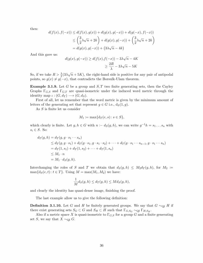
Clearly any geodesic space is also a quasi-geodesic space, but not the other way around.For any ε > 0 ∈ R, the space X = R2\{0} is a (1, ε)-quasi-geodesic space as the figure 3.1shows.

Example 3.2.3. If X = (V,E) is a connected graph, then the associated metric on Vturns V into a (1, 1)-quasi-geodesic space, because the distance between twp vertices is thelength of some path in the graph.

Proposition A.3.4 from [13] shows that any quasi-geodesic space is quasi-isometric to ageodesic space.

We now come to the Svarc-Milnor lemma. First we are going to make a formulationusing the language of quasi-geometries, and then we are going to deduce the “topological”version, that is the version usually used.

Theorem 3.2.4. Let G be a group, and let G act on a metric space (X, d) by isometries.Suppose that there are constants c, b > 0 ∈ R such that X is a (c, b)-quasi-geodesic andsuppose that there is a subset B ⊂ X with the following properties:

• The diameter of B is finite.

• G translates B over all of X, i.e⋃g∈G g ·B = X.

37

}ε/2

γ

Figure 3.1: A (1, ε)-quasi-geodesic in R\{(0, 0)}

• The set S := {g ∈ G|g ·B′ ∩B′ 6= ∅} <∞, where

B′ := B2·b(B) = {x ∈ X : ∃y ∈ B, d(x, y) ≤ 2 · b}.

Then:

1. The group G is generated by S, in particular, G is finitely generated.

2. For all x ∈ X the mapG −→ X,

g 7−→ g · x,

is a quasi-isometry with respect to the word metric on G.

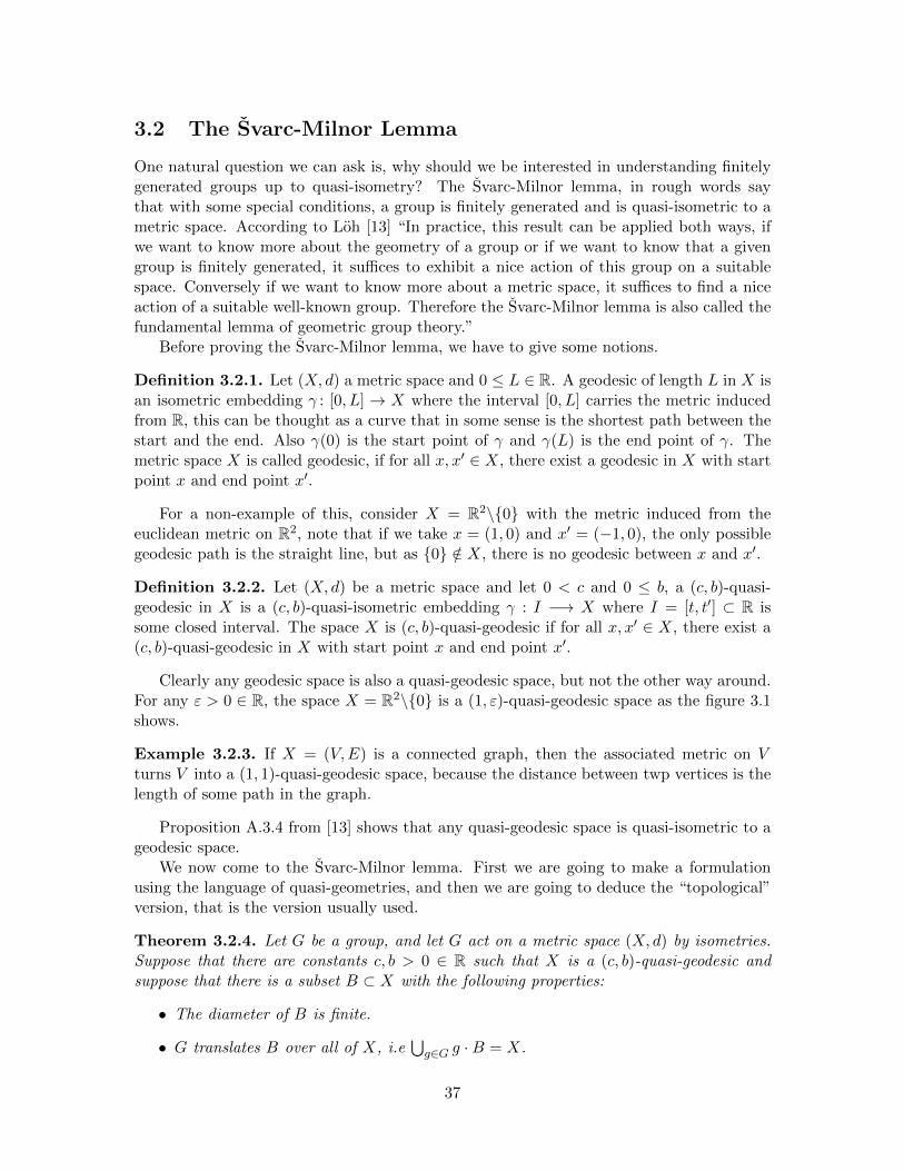
Proof. 1. Let x ∈ B, as X is (c, b)-quasi-geodesic, there is a (c, b)-quasi-geodesic γ oflength L starting in x and ending in g · x, we will define some points in this quasi-geodesic.

Let n = dL · b/ce. For j ∈ {0, . . . n− 1} we define:

tj := j · bc

and tn := L, as well,xj := γ(tj).

Notice that x0 = γ(0) = x and xn = γ(L) = g · x. We know that as G translates Bover all X, there are some elements gj ∈ G with xj ∈ gj · B. In particular we canchoose g0 = e ∈ G and gn = g, the proceedure can be see in Figure 3.2.

38

x0

B

gj ·B

gj ·B′

g ·B

x1

x2xj

. . .

. . .

xn

γ

Figure 3.2: Covering a quasi-geodesic by translates of B

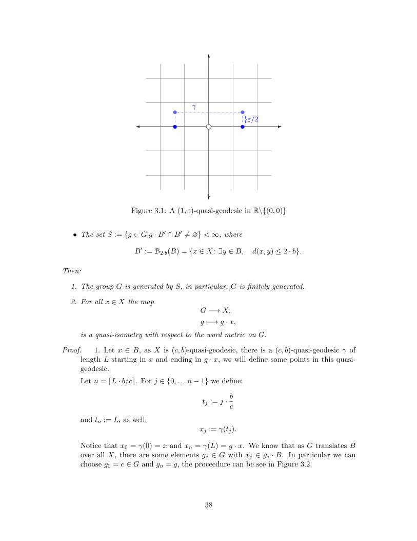
We want to show that sj := g−1j−1 · gj ∈ S for j ∈ {1, . . . n}. For this, notice that,because γ is a (c, d)-quasi-geodesic, then:

d(xj−1, xj) ≤ c · |tj−1 − tj |+ b ≤ c · bc

+ b ≤ 2 · b,

then, xj ∈ B2·b(gj−1 ·B) = gj−1 ·B2·b(B) = gj−1 ·B′, this is because G acts on X byisometries. And on the other hand, xj ∈ gj ·B ⊂ gj ·B′, thus:

gj−1 ·B′ ∩ gj ·B′ 6= ∅.

So, by definition on S it follows that sj ∈ S, in particular:

g = gn = gn−1 · g−1n−1 · gn = · · · = g0 · s1 · · · · sn = s1 · · · · sn

lies in the set generated by S, as desired. We did this for any g ∈ G, so S generatesG.

2. We will show that the mapϕ :G −→ X

g 7−→ g · x

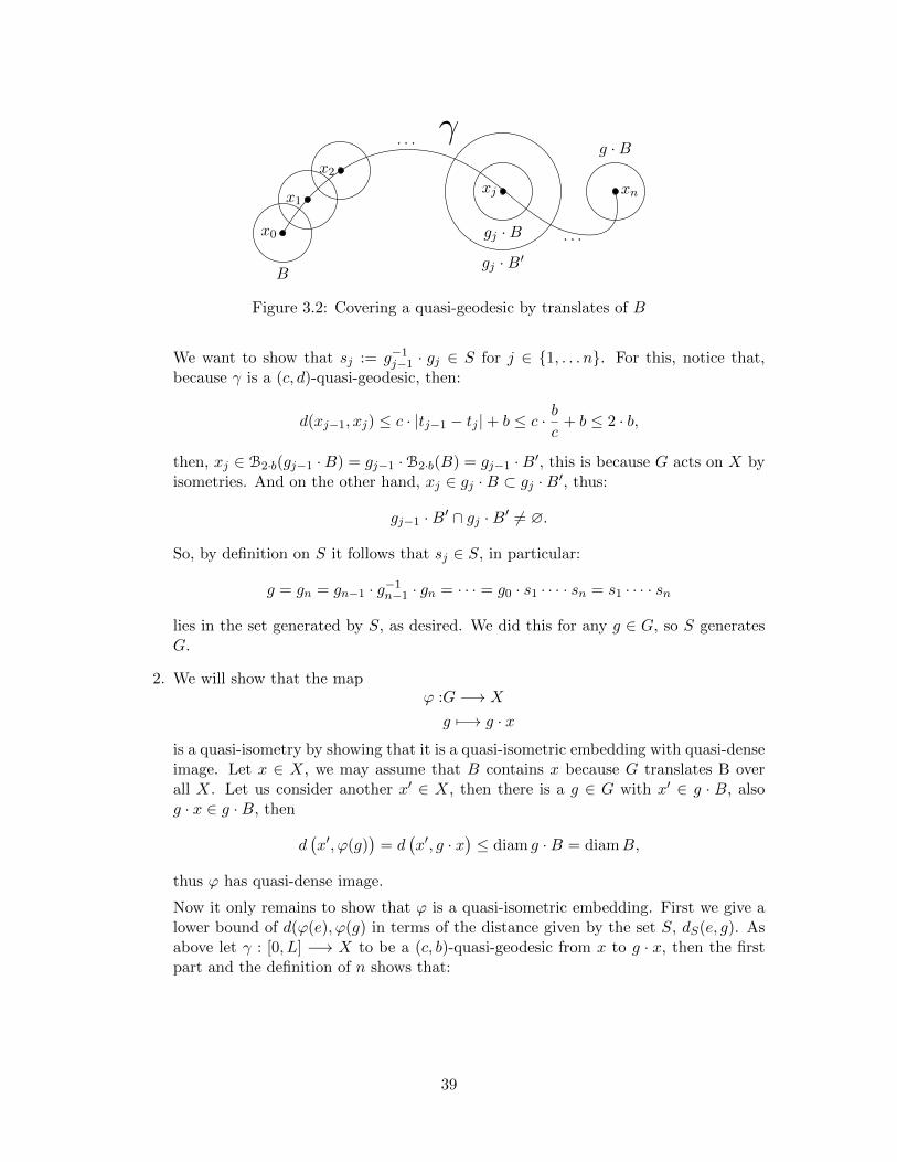
is a quasi-isometry by showing that it is a quasi-isometric embedding with quasi-denseimage. Let x ∈ X, we may assume that B contains x because G translates B overall X. Let us consider another x′ ∈ X, then there is a g ∈ G with x′ ∈ g · B, alsog · x ∈ g ·B, then

d(x′, ϕ(g)

)= d

(x′, g · x

)≤ diam g ·B = diamB,

thus ϕ has quasi-dense image.

Now it only remains to show that ϕ is a quasi-isometric embedding. First we give alower bound of d(ϕ(e), ϕ(g) in terms of the distance given by the set S, dS(e, g). Asabove let γ : [0, L] −→ X to be a (c, b)-quasi-geodesic from x to g · x, then the firstpart and the definition of n shows that:

39

d(ϕ(e), ϕ(g)) = d(x, g · x) = d(γ(0), γ(L))

≥ 1

c· L− b

≥ 1

c· b · (n− 1)

c− b

=b

c2· n− 1

c2− b

≥ b

c2· dS(e, g)− 1

c2− b.

Now we want to give an upper bound of d(ϕ(e), ϕ(g)) in terms of dS(e, g). Even ifthe coefficients are different from the lower bound, using the max of both bounds weget the inequality we are looking for.

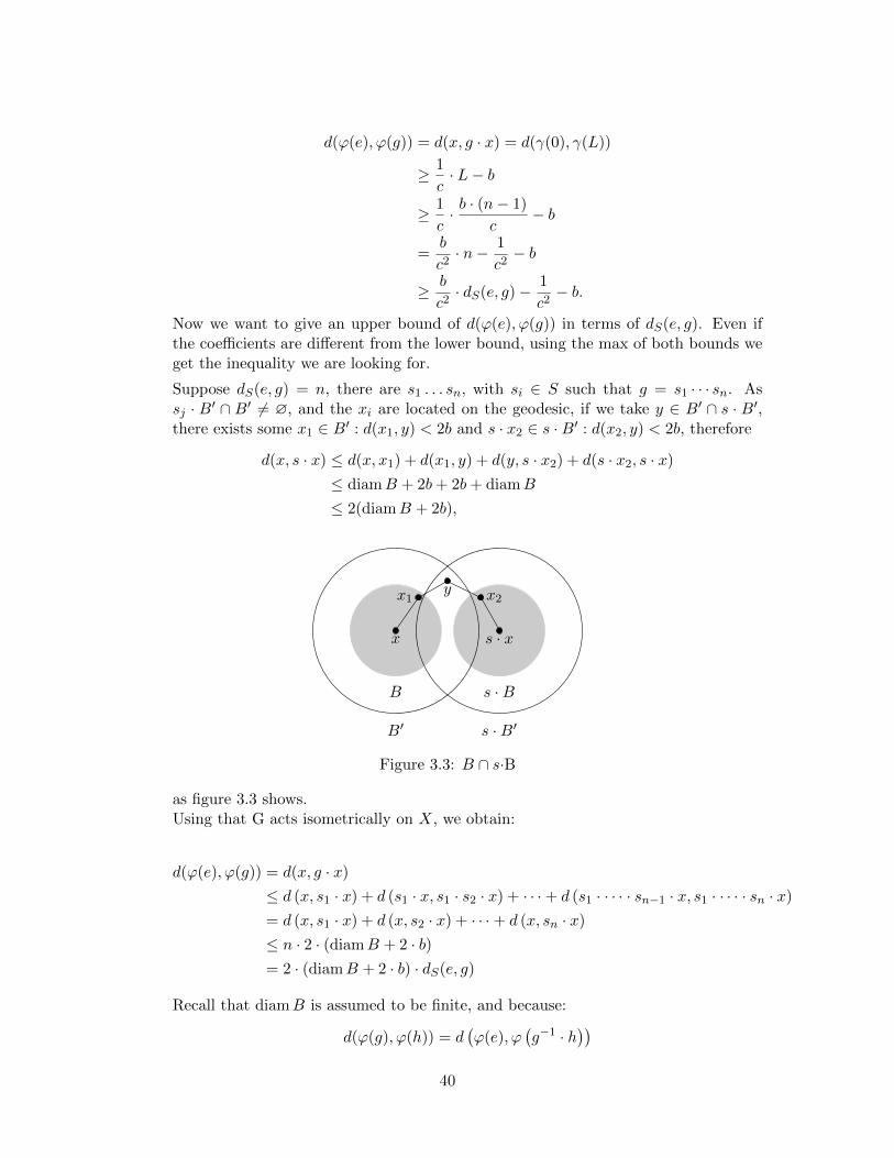
Suppose dS(e, g) = n, there are s1 . . . sn, with si ∈ S such that g = s1 · · · sn. Assj · B′ ∩ B′ 6= ∅, and the xi are located on the geodesic, if we take y ∈ B′ ∩ s · B′,there exists some x1 ∈ B′ : d(x1, y) < 2b and s · x2 ∈ s ·B′ : d(x2, y) < 2b, therefore

d(x, s · x) ≤ d(x, x1) + d(x1, y) + d(y, s · x2) + d(s · x2, s · x)

≤ diamB + 2b+ 2b+ diamB

≤ 2(diamB + 2b),

B s ·B

B′ s ·B′

x s · x

yx1 x2

Figure 3.3: B ∩ s·B

as figure 3.3 shows.Using that G acts isometrically on X, we obtain:

d(ϕ(e), ϕ(g)) = d(x, g · x)

≤ d (x, s1 · x) + d (s1 · x, s1 · s2 · x) + · · ·+ d (s1 · · · · · sn−1 · x, s1 · · · · · sn · x)

= d (x, s1 · x) + d (x, s2 · x) + · · ·+ d (x, sn · x)

≤ n · 2 · (diamB + 2 · b)= 2 · (diamB + 2 · b) · dS(e, g)

Recall that diamB is assumed to be finite, and because:

d(ϕ(g), ϕ(h)) = d(ϕ(e), ϕ

(g−1 · h

))40

and dS(g, h) = dS(e, g−1 · h

), the bounds show that ϕ is an quasi-isometric embed-

ding.

Before deducing the “Topological version” of the Svarc-Milnor lemma, we briefly recallsome topological notions.

Definition 3.2.5. A metric space X is proper if for all x ∈ X and all 0 ≤ r ∈ R, theclosed ball with center x and radius r is compact with respect to the topology induced bythe metric. Notice that proper metric spaces are locally compact.

Definition 3.2.6. An action G×X −→ X of a group G on a topological metric space X,is proper if for all compact sets B ⊂ X the set {g ∈ G : g ·B ∩B 6= ∅} is finite.

Example 3.2.7. The translation action of Z on R is proper.

Lemma 3.2.8. The action by deck transformations on the fundamental group of a locallycompact path-connected topological space on its universal covering is proper.

Proof. Because of the definition of deck transformations, for each y ∈ Y (Y universalcovering space of X), there exists Uy neighborhoods, such that if Uy ∩ g · Uy 6= ∅, theng = e. (See A.2.6.)

Consider the following lemma, for any compact B ∈ Y , (g · Uy) ∩B 6= ∅ for only finiteg, with y ∈ B. To prove it let us define C := {g ∈ G : (g ·Uy)∩B 6= ∅}, for any g ∈ C thereexists xg ∈ Uy such that g · xg ∈ B, (i.e xg ∈ g · Uy ∩B). Consider the following function:

ϕ :C −→⋃g∈C

(g · Uy) ∩B

g 7−→ g · xg.

Notice that ϕ is injective. Now, g · xg ∈ g · Uy, with Uy neighborhood such that if g 6= g′,then g · Uy ∩ g′Uy = ∅, therefore {g · xg : g ∈ C} is a discrete subset in B, and as B iscompact, C is finite.

Clearly

g ·B ∩B ⊆

(n⋃i=1

g · Uyi

)∩B,

but because of the lemma, ⋃g∈G

n⋃i=1

g · Uyi ∩B,

only has finite terms.

Definition 3.2.9. An action G × X −→ X of a group G on a topological space X iscocompact if the quotient space G\X with respect to the quotient topology is compact.

Example 3.2.10. • The translation action of Z y R is cocompact, because the quo-tient is homeomorphic to the circle S1.

41

• The horizontal translation of Z y R2 is not cocompact because the quotient is home-omorphic to the infinite cylinder S1 × R.

• The action by deck transformations of the fundamental group of a compact path-connected topological space X on its universal covering is cocompact because thequotient is homeomorphic to X

Lemma 3.2.11. Let X be a space and let G be a group which acts by homeomorphismson X. Then the map π : X −→ X/G is open.

Proof. Let U ⊂ X an open set, then its image π(U) is open if and only if π−1(π(U)) isopen by definition of the quotient topology. Also, π−1(π(U)) 6= U , but

π−1(π(U)) =⋃g∈G

g · U,

as G acts as a homeomorphism g · U is an open set for any g.

With this in mind we can formulate the Svarc-Milnor lemma in its topological version.

Corollary 3.2.12. Let G be a group acting by isometries on a proper geodesic metricspace (X, d), furthermore, suppose that this action is proper and cocompact. Then G isfinitely generated and for all x ∈ X the map

G −→ Xg 7−→ g · x

is a quasi-isometry.

Proof. First of all, notice that under the given assumptions, X is a (1, ε)-quasi-geodesicspace for all ε ≥ 0. If we want to apply the Theorem 3.2.4, we need to find a nice subsetB ⊂ X.

Because of Lemma 3.2.11, the natural projection π : X −→ G\X is an open map, onthe other hand G\X is compact, so one can find a closed subspace B ⊂ X of finite diameter(for example a suitable union of finitely many closed balls), such that π(B) = G\X, whereπ is the projection π : X −→ G\X associated with the action of G. In particular⋃

g∈Gg ·B = X

and B′ := B2:ε(B) has finite diameter. Because X is proper, the subset B′ is compact, thusthe action of G on X being proper implies that {g ∈ G|g ·B′ ∩B′ 6= ∅} is finite, hence wecan apply Theorem 3.2.4

Corollary 3.2.13. Let M be a compact and without boundary connected Riemannianmanifold, and M be its Riemannian universal covering manifold. Then the fundamentalgroup π1(M) is finitely generated and for every x ∈ M , the map

π1(M) −→ M

g 7−→ g · x

given by the action of the fundamental group on M via deck transformations is a quasi-isometry.

42

Proof. If we want to apply the topological version of the Svarc-Milnor lemma, we have to usesome things. First of all notice that π1(M) acts by isometries in M via deck transformations

(A.2.5). We need to show that M is a proper geodesic metric space. The Proposition B.2.3gives us the metric that is induced by M , and the fact that M is compact (this implies

that is complete, and therefore M is also complete) gives us the conditions we need thanksto Theorem B.2.8. Clearly the action of π1(M) is cocompact (because M is compact) andthe Lemma 3.2.8 shows that the action is also proper, then the result follows.

There are many applications of the Svarc-Milnor lemma, a basic example is the following:

Corollary 3.2.14. Finite index subgroups of finitely generated groups are finitely gener-ated and quasi-isometric to the ambient group.

Proof. Let G be a finitely generated group with generating set S and H ⊂ G be a subgroupof finite index, if we consider the action of H on G by left translation, notice the followingfacts:

• The space (G,dS) is (1, 1)-quasi-geodesic space.

• Let B ⊂ G be a finite set of representatives of H\G, then B has finite diameter.

• H ·B = G

• The set B′ is finite as well, and moreover the set

{h ∈ H : h ·B′ ∩B′ 6= ∅}

is finite.

With all these we can apply the topological version of Svarc-Milnor lemma and thereforeH is finitely genereated and the inclusion H ↪→ G is a quasi-isometry.

This last corollary give us a motivation to the following definition

Definition 3.2.15. • Two groups G and H are commensurable if they contain G′ ⊂ Gand H ′ ⊂ H finite index subgroups with G′ ∼= H ′.

• Two groups G and H are weakly commensurable if they contain finite index subgroupsG′ ⊂ G and H ′ ⊂ H that satisfy that there are finite normal subgroups N E G′ andM E H ′ such that G′/N and H ′/M are isomorphic.

Clearly, because of Corollary 3.2.14, if G and H are commensurable, then they arequasi-isometric.

Corollary 3.2.16. Let G be a group, then:

1. Let G′ be a finite index subgroup of G, then G′ is finitely generated iff G is finitelygenerated. If these groups are finitely generated, then G ∼QI G

′.

2. Let N be a finite normal subgroup, then G/N is finitely generated iff G is finitelygenerated. If these groups are finitely generated, then G ∼QI G/N .

43

In particular, if G is finitely generated, then any group weakly commensurable to G isfinitely generated and quasi-isometric to G.

Proof. 1. With Corollary 3.2.14, it is enough to show that G is finitely generated if G′

is. If we combine the finite generating set of G′ and a finite set of representatives ofthe G′-cosets in G, this yields a finite generating set of G.

2. • If G is finitely generated, then G/N is finitely generated.

• Conversely if G/N is finitely generated, similar to the item 1, combining thefinite set N with the lifts with respect to the canonical projection of G→ G/Nof a generating sets of G/N gives a finite generating set of G.

• Let G and G/N finitely generated with S a generating set of G/N , again similarto Corollary 3.2.14 we take B as G/N , that is finite and the left-translate actionof G over G/N translates B all over G, therefore applying Svarc-Milnor (3.2.4)we have the quasi-isometry.

In particular, if G is finitely generated, then any group weakly commensurable to G isfinitely generated and quasi-isometric to G.

Example 3.2.17. It is known that for n ≥ 2 then the free group of rank 2 contains afree group of rank n as a finite index subgroup, i.e Fn 6 F2. Also Fn 6 Fn, thereforethey are commensurable. This shows that all free groups of finite rank bigger than 1 arequasi-isometric.

3.3 Quasi-isometry invariants

The Svarc-Milnor lemma is in some way an attempt to classify finitely generated groups upto quasi-isometry. One important problem is to construct properties on groups preservedup to quasi-isometries. A common name for this quasi-isometric invariants, are geometricproperties. A similar concept was introduced in Chapter 2 with the large-scale propertiesthat does not depend on the generating set. Example 3.1.9 shows that quasi-isometriesdoes not depend on the generating set, so the geometric properties are more general thanlarge-scale properties.

A simple case of a quasi-isometric invariant is the finiteness, as the Example 3.1.4 shows.From a coarse geometric point of view, if we draw the Cayley graph of a finite group andgo far away enough, we are eventually looking at a dot. Clearly, because of that, beingabelian is not a geometric property of groups.

Example 3.2.17 shows that the rank of free groups is not a quasi-isometric invariant.

Remark 3.3.1. For any property of groups, a group has virtually that property if itcontains a finite index subgroup that has that property.

There are many other properties that are geometric, they can be consulted in Example5.5.11, page 143 of Clara Loh’s book [13], for example:

• Being virtually Zn.

• Being virtually nilpotent.

44

• Being finitely presented.

Theorem 3.3.2. Let G and H finitely generated groups, and let S ⊂ G and T ⊂ H, finitegenerating sets. (Using the notation of the Definition 2.3.9)

1. If there exist a quasi-isometric embedding (G, dS)→ (H, dT ), then

βG,S � βH,dT .

2. In particular, if G and H are quasi isometric, then the growth functions are equivalent.

Proof. Let f : G→ H be a quasi-isometric embedding, there is a c ∈ R>0 such that

∀g, g′ ∈ G 1

c· dS

(g, g′

)− c ≤ dT

(f(g), f

(g′))≤ c · dS

(g, g′

)+ c

We name x = f(eG), and let r ∈ N. Note the following:

• If g ∈ BS(eG, r), then dT (f(g), x) ≤ c · dS(g, eG) + c = c · r + c, therefore

f (BS(eG, r)) ⊂ BT (x, c · r + c).

• If g1, g2 ∈ G such that f(g1) = f(g2),

dS(g1, g2) ≤ c · (dT (f(g1), f(g2) + c) = c2.

These two facts give us the following inequality, the first line holds because we can use thetwo inequalities from above for any g ∈ BS(eG, r), and the second because of the definitionof dS and dT , those metrics are invariant under left translation, so:

βS(r) ≤∣∣BS(eG, c

2)∣∣ · |BT (x, c · r + c)|

=∣∣BS(e, c2)

∣∣ · |BT (eH , c · r + c)|= βS(c2) · βT (c · r + c).

Notice that the term βS(c2) does not depend on the radius, so the last inequality showsthat βG,S � βH,dT . The second item follows from the first one.

This theorem shows that the growth type is a geometric property.

Definition 3.3.3. Let Γ be a connected, locally finite graph (for example a Cayley’s graphof a finitely generated group), and let B(n) be the ball of radius n in Γ, based at some fixedvertex, we define ||Γ\B(n)|| to be the number of connected unbounded components of thecomplement of B(n).

Lemma 3.3.4. Let Γ be a connected, locally finite graph and m ≤ n two positive integers,then

||Γ\B(m)|| ≤ ||Γ\B(n)|| .

Proof. Let C be an unbounded connected component of Γ\B(m), either C remains connectedwhen we remove B(n).

45

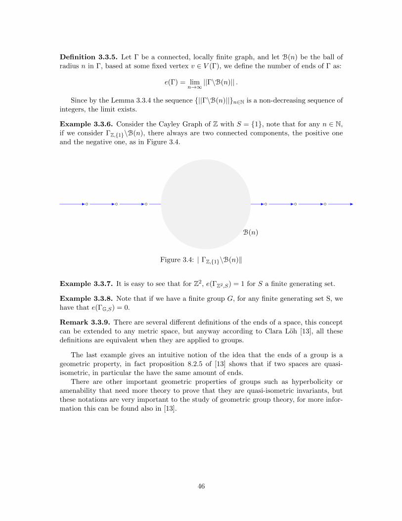
Definition 3.3.5. Let Γ be a connected, locally finite graph, and let B(n) be the ball ofradius n in Γ, based at some fixed vertex v ∈ V (Γ), we define the number of ends of Γ as:

e(Γ) = limn→∞

||Γ\B(n)|| .

Since by the Lemma 3.3.4 the sequence {||Γ\B(n)||}n∈N is a non-decreasing sequence ofintegers, the limit exists.

Example 3.3.6. Consider the Cayley Graph of Z with S = {1}, note that for any n ∈ N,if we consider ΓZ,{1}\B(n), there always are two connected components, the positive oneand the negative one, as in Figure 3.4.

B(n)

Figure 3.4: | ΓZ,{1}\B(n)‖

Example 3.3.7. It is easy to see that for Z2, e(ΓZ2,S) = 1 for S a finite generating set.

Example 3.3.8. Note that if we have a finite group G, for any finite generating set S, wehave that e(ΓG,S) = 0.

Remark 3.3.9. There are several different definitions of the ends of a space, this conceptcan be extended to any metric space, but anyway according to Clara Loh [13], all thesedefinitions are equivalent when they are applied to groups.

The last example gives an intuitive notion of the idea that the ends of a group is ageometric property, in fact proposition 8.2.5 of [13] shows that if two spaces are quasi-isometric, in particular the have the same amount of ends.

There are other important geometric properties of groups such as hyperbolicity oramenability that need more theory to prove that they are quasi-isometric invariants, butthese notations are very important to the study of geometric group theory, for more infor-mation this can be found also in [13].

46

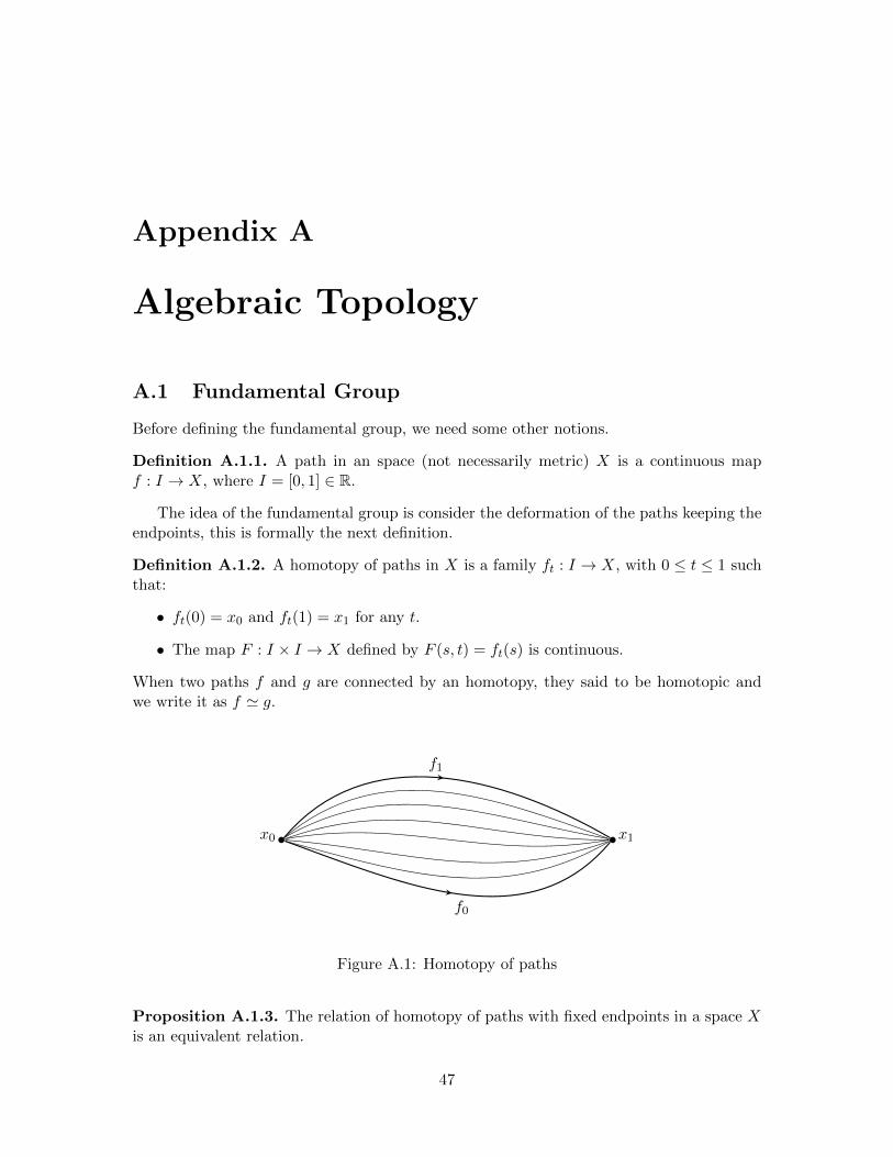
Appendix A

Algebraic Topology

A.1 Fundamental Group

Before defining the fundamental group, we need some other notions.

Definition A.1.1. A path in an space (not necessarily metric) X is a continuous mapf : I → X, where I = [0, 1] ∈ R.

The idea of the fundamental group is consider the deformation of the paths keeping theendpoints, this is formally the next definition.

Definition A.1.2. A homotopy of paths in X is a family ft : I → X, with 0 ≤ t ≤ 1 suchthat:

• ft(0) = x0 and ft(1) = x1 for any t.

• The map F : I × I → X defined by F (s, t) = ft(s) is continuous.

When two paths f and g are connected by an homotopy, they said to be homotopic andwe write it as f ' g.

x0 x1

f1

f0

Figure A.1: Homotopy of paths

Proposition A.1.3. The relation of homotopy of paths with fixed endpoints in a space Xis an equivalent relation.

47

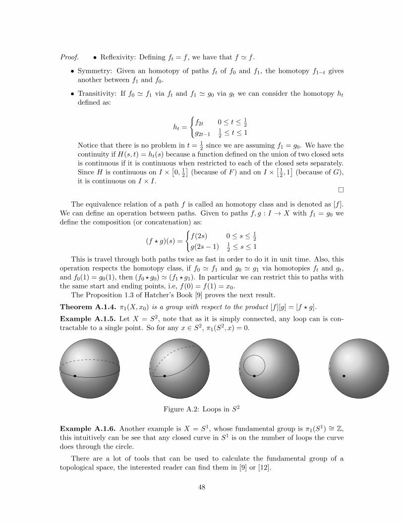
Proof. • Reflexivity: Defining ft = f , we have that f ' f .

• Symmetry: Given an homotopy of paths ft of f0 and f1, the homotopy f1−t givesanother between f1 and f0.

• Transitivity: If f0 ' f1 via ft and f1 ' g0 via gt we can consider the homotopy htdefined as:

ht =

{f2t 0 ≤ t ≤ 1

2

g2t−112 ≤ t ≤ 1

Notice that there is no problem in t = 12 since we are assuming f1 = g0. We have the

continuity if H(s, t) = ht(s) because a function defined on the union of two closed setsis continuous if it is continuous when restricted to each of the closed sets separately.Since H is continuous on I ×

[0, 12]

(because of F ) and on I ×[12 , 1]

(because of G),it is continuous on I × I.

The equivalence relation of a path f is called an homotopy class and is denoted as [f ].We can define an operation between paths. Given to paths f, g : I → X with f1 = g0 wedefine the composition (or concatenation) as:

(f ? g)(s) =

{f(2s) 0 ≤ s ≤ 1

2

g(2s− 1) 12 ≤ s ≤ 1

This is travel through both paths twice as fast in order to do it in unit time. Also, thisoperation respects the homotopy class, if f0 ' f1 and g0 ' g1 via homotopies ft and gt,and f0(1) = g0(1), then (f0 ?g0) ' (f1 ?g1). In particular we can restrict this to paths withthe same start and ending points, i.e, f(0) = f(1) = x0.

The Proposition 1.3 of Hatcher’s Book [9] proves the next result.

Theorem A.1.4. π1(X,x0) is a group with respect to the product [f ][g] = [f ? g].

Example A.1.5. Let X = S2, note that as it is simply connected, any loop can is con-tractable to a single point. So for any x ∈ S2, π1(S

2, x) = 0.

Figure A.2: Loops in S2

Example A.1.6. Another example is X = S1, whose fundamental group is π1(S1) ∼= Z,

this intuitively can be see that any closed curve in S1 is on the number of loops the curvedoes through the circle.

There are a lot of tools that can be used to calculate the fundamental group of atopological space, the interested reader can find them in [9] or [12].

48

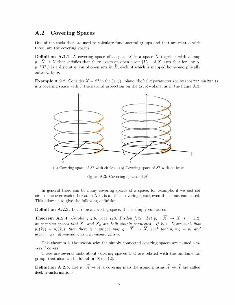
A.2 Covering Spaces

One of the tools that are used to calculate fundamental groups and that are related withthose, are the covering spaces.

Definition A.2.1. A covering space of a space X is a space X together with a mapp : X → X that satisfies that there exists an open cover {Uα} of X such that for any α,p−1(Uα) is a disjoint union of open sets in X, each of which is mapped homeomorphicallyonto Uα by p.

Example A.2.2. ConsiderX = S1 in the (x, y)−plane, the helix parameterized by (cos 2πt, sin 2πt, t)is a covering space with P the natural projection on the (x, y)−plane, as in the figure A.3.

y

x

z

(a) Covering space of S1 with circles

y

x

z

(b) Covering space of S1 with an helix

Figure A.3: Covering spaces of S1

In general there can be many covering spaces of a space, for example, if we just setcircles one over each other as in A.3a is another covering space, even if it is not connected.This allow us to give the following definition.

Definition A.2.3. Let X be a covering space, if it is simply connected.

Theorem A.2.4. Corollary 4.6, page 143, Bredon [12]. Let pi : Xi → X, i = 1, 2,

be covering spaces that X1 and X2 are both simply connected. If xi ∈ Xiare such thatp1(x1) = p2(x2), then there is a unique map g : X1 → X2 such that p2 ◦ g = p1 andg(x1) = x2. Moreover, g is a homeomorphism.

This theorem is the reason why the simply connected covering spaces are named uni-versal covers.

There are several facts about covering spaces that are related with the fundamentalgroup, that also can be found in [9] or [12].

Definition A.2.5. Let p : X → X a covering map the isomorphisms X → X are calleddeck transformations.

49

These form a group under composition (G(X)). For example for example A.2.2 thedeck transformations are the vertical translation of the helix onto itself, so G(X) ∼= Z.

One fact that we used on 3.2.8 is the following lemma:

Proposition A.2.6. The action of deck transformation group satisfies that for each x ∈ Xhas a neighboor U such that for any g1, g2 ∈ G(X), g1 · U ∩ g2 · U 6= ∅ implies g1 = g2.

Proof. Let U ⊂ X projects (via p) to U ⊂ X. If g1 · U ∩ g2 · U 6= ∅ for some g1, g2 ∈ G(X),then g1(x1) = g2(x2) for some x1, x2 ∈ U . Note that x1 and x2 must lie in the same fiberp−1(x), which intersects U in only one point, then x1 = x2, therefore g−11 g2 fixes x, sog−11 g2(U) = id, so g1 = g2.

Note also that this condition is equivalent to the condition that U ∩ g · U 6= only wheng is the identity.

50

Appendix B

Riemannian Geometry

B.1 Differential Manifolds

Definition B.1.1. Let (M,T) be a topological Hausdorff space with countable basis, wesay that M is a topological manifold if there exists an m ∈ Z+ such that for any pointp ∈ M we have an open neighborhood U of p, an open V ⊂ Rm and an homeomorphismφ : U → V .

The pair (U, φ) is called a local chart (parameterization or system of coordinates) onM and the integer m is called the dimension of M .

Also, if M is a m−dimensional topological manifold, then a Cr−atlas on M is a collec-tion:

U = {(Uα, φα) : α ∈ I}

of local charts such that U covers M , i.e M =⋃α Uα and for any α, β ∈ I the transition

maps i.e φβ ◦ φ−1α and φα ◦ φ−1β are r−times continuously differentiable.An atlas M is said to be maximal (or differentiable structure) if it is not contained in alarger atlas, i.e if U is any other atlas containing M then U = M.

Definition B.1.2. An atlas {Uα, φα} is called differentiable if all chart transitions

φβ ◦ φ−1α : φα(Uα ∩ Uβ)→ φβ(Uα ∩ Uβ)

are differentiable of class C∞.

Definition B.1.3. A differentiable manifold of dimension d is a topological manifold ofdimension d with a differentiable structure.

Definition B.1.4. A map g : M → M ′ between differentiable manifolds M and M ′ withcharts {Uα, φα} and {U ′α, φ′α} is called differentiable if all maps φ′β ◦g◦φ−1α are differentiablewhere defined.

The set of tangent vectors to a differential manifold M in a point p have a naturalstructure of real vector space, and we denote it as TpM , an example is shown in figure B.1.

51

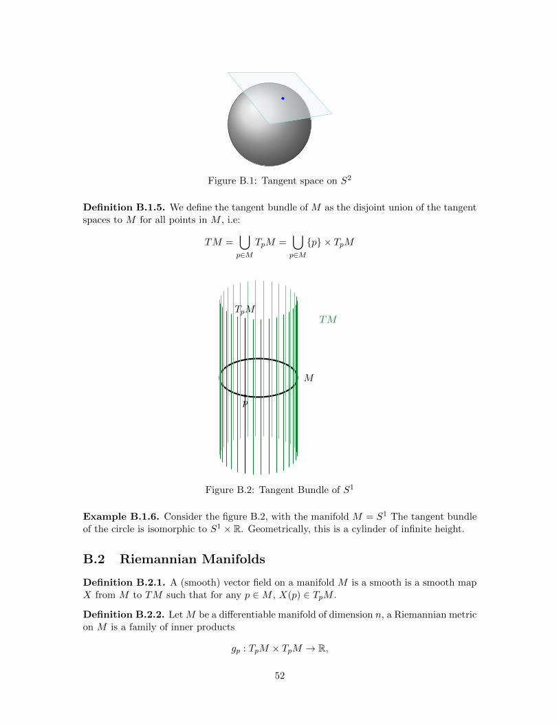
Figure B.1: Tangent space on S2

Definition B.1.5. We define the tangent bundle of M as the disjoint union of the tangentspaces to M for all points in M , i.e:

TM =⋃p∈M

TpM =⋃p∈M{p} × TpM

M

TM

p

TpM

Figure B.2: Tangent Bundle of S1

Example B.1.6. Consider the figure B.2, with the manifold M = S1 The tangent bundleof the circle is isomorphic to S1 × R. Geometrically, this is a cylinder of infinite height.

B.2 Riemannian Manifolds

Definition B.2.1. A (smooth) vector field on a manifold M is a smooth is a smooth mapX from M to TM such that for any p ∈M , X(p) ∈ TpM .

Definition B.2.2. Let M be a differentiable manifold of dimension n, a Riemannian metricon M is a family of inner products

gp : TpM × TpM → R,

52

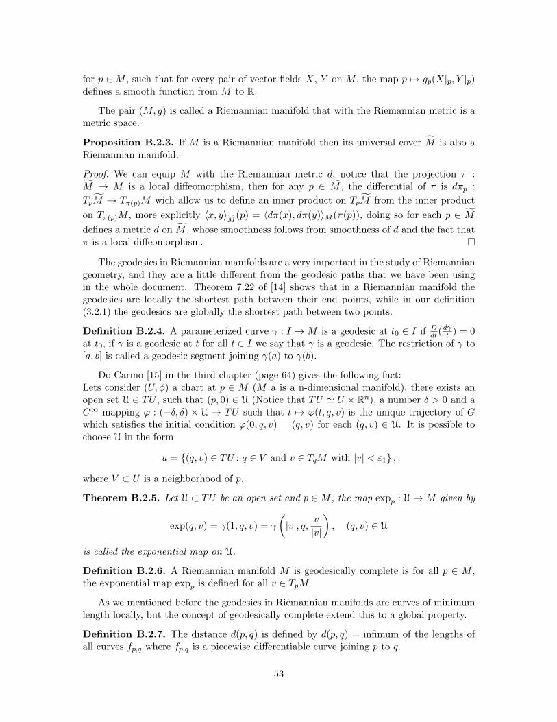
for p ∈M , such that for every pair of vector fields X, Y on M , the map p 7→ gp(X|p, Y |p)defines a smooth function from M to R.

The pair (M, g) is called a Riemannian manifold that with the Riemannian metric is ametric space.

Proposition B.2.3. If M is a Riemannian manifold then its universal cover M is also aRiemannian manifold.

Proof. We can equip M with the Riemannian metric d, notice that the projection π :M → M is a local diffeomorphism, then for any p ∈ M , the differential of π is dπp :

TpM → Tπ(p)M wich allow us to define an inner product on TpM from the inner product

on Tπ(p)M , more explicitly 〈x, y〉M

(p) = 〈dπ(x), dπ(y)〉M (π(p)), doing so for each p ∈ Mdefines a metric d on M , whose smoothness follows from smoothness of d and the fact thatπ is a local diffeomorphism.

The geodesics in Riemannian manifolds are a very important in the study of Riemanniangeometry, and they are a little different from the geodesic paths that we have been usingin the whole document. Theorem 7.22 of [14] shows that in a Riemannian manifold thegeodesics are locally the shortest path between their end points, while in our definition(3.2.1) the geodesics are globally the shortest path between two points.

Definition B.2.4. A parameterized curve γ : I → M is a geodesic at t0 ∈ I if Ddt(

dγt ) = 0

at t0, if γ is a geodesic at t for all t ∈ I we say that γ is a geodesic. The restriction of γ to[a, b] is called a geodesic segment joining γ(a) to γ(b).

Do Carmo [15] in the third chapter (page 64) gives the following fact:Lets consider (U, φ) a chart at p ∈ M (M a is a n-dimensional manifold), there exists anopen set U ∈ TU , such that (p, 0) ∈ U (Notice that TU ' U × Rn), a number δ > 0 and aC∞ mapping ϕ : (−δ, δ) × U → TU such that t 7→ ϕ(t, q, v) is the unique trajectory of Gwhich satisfies the initial condition ϕ(0, q, v) = (q, v) for each (q, v) ∈ U. It is possible tochoose U in the form

u = {(q, v) ∈ TU : q ∈ V and v ∈ TqM with |v| < ε1} ,

where V ⊂ U is a neighborhood of p.

Theorem B.2.5. Let U ⊂ TU be an open set and p ∈M , the map expp : U→M given by

exp(q, v) = γ(1, q, v) = γ

(|v|, q, v

|v|

), (q, v) ∈ U

is called the exponential map on U.

Definition B.2.6. A Riemannian manifold M is geodesically complete is for all p ∈ M ,the exponential map expp is defined for all v ∈ TpM

As we mentioned before the geodesics in Riemannian manifolds are curves of minimumlength locally, but the concept of geodesically complete extend this to a global property.

Definition B.2.7. The distance d(p, q) is defined by d(p, q) = infimum of the lengths ofall curves fp,q where fp,q is a piecewise differentiable curve joining p to q.

53

If there exists a minimizing geodesic γ joining p to q then d(p, q) = length of γ. Theexistence of this minimizing geodesic is not always guaranteed, the following theorem givesthe existence of those under different conditions. The proof of this can be found in theorem2.8 of do Carmo’s book [15]

Theorem B.2.8 (Hopf-Rinow). Let M be a Riemannian manifold and p ∈ M then thefollowing are equivalent:

a) expp is defined on all TpM .

b) The closed and bounded sets of M are compact.

c) M is complete as a metric space.

d) M is geodesically complete.

e) There exits a sequence of compact subsets Kn ⊂ M , Kn ⊂ Kn+1 and⋃nKn = M ,

such that if qn /∈ Kn, then d(p, qn)→∞.

Also, any of the statements above implies that:

f) For any q ∈M there exists a geodesic γ joining p to q with d(p, q) = length(γ).

54

Bibliography

[1] Jhon Meier, Groups, Graphs and Trees. An Introduction to Geometry of Infinite Groups, London Math-ematical Society, Cambridge University Press, New York, 2008.

[2] Walter Parry, Growth Series of Some Wreath Products, Transactions of the American MathematicalSociety 331 (1992).

[3] Michael Stoll, Rational and transcendental growth series for the higher Heisenberg groups, Inventionesmathematicae 126 (1996).

[4] James Cannon, William Floyd, and Walter Parry, Introductory notes on Richard Thompson’s groups,L’Enseignement Mathematique, (1996).

[5] Jose Burillo, Introduction to Thompson’s Group F, Universitat Politecnica de Catalunya, https://

mat-web.upc.edu/people/pep.burillo/F%20book.pdf.

[6] Sameer Kailasa, Topics in Geometric Group Theory, 2014, http://math.uchicago.edu/~may/REU2014/REUPapers/Kailasa.pdf.

[7] Pierre de la Harpe, Topics in Geometric Group Theory, Chicago Letures in Mathematics Series, LondonMathematical Society, The University of Chicago Press, Chicago, 2000.

[8] Jhon M. Lee, Introduction to Smooth Manifolds, Second edition, Springer, University of Washington,Seattle, WA, USA.

[9] Allen Hatcher, Algebraic Topology, Cambridge University Press, 2002.

[10] Thomas W. Hungerford, Algebra, Graduate Texts in Mathematics, Springer, 1980.

[11] Matt Clay and Dan Margalit, Office Hours with a Geometric Group Theorist, Princeton UniversityPress, 2017.

[12] Glen E. Bredon, Topology and Geometry, Graduate Texts in Mathematics, Springer, 1993.

[13] Loh Clara, Geometric Group Theory, an introduction, Lecture notes, Universitat Regensburg, Germany,2015.

[14] Sigmundur Gudmundsson, An Introduction to Riemannian Geometry, Lund University, July 2019.

[15] Manfredo. P do Carmo, Riemannian Geometry, Mathematics: Theory and Applications, Rio de Janeiro,1979.

55