Introduction to FloquetTheory: The Calculation ofSpinning SidebandIntensities in Magic-AngleSpinning NMRALEX D. BAIN, R. S. DUMONT

Department of Chemistry, McMaster University, 1280 Main St. West, Hamilton, Ontario, Canada L8S 4M1

ABSTRACT: In magic-angle spinning, the Hamiltonian of the system changes periodi-cally with time, so the spectrum shows sidebands at multiples of the rotor frequency. This

( )changing Hamiltonian and hence, the changing Liouvillian complicates the simulation of1the line shape considerably. A simple case is that of a spin- with an anisotropic chemical2

shift, spinning at the magic angle. Perhaps the most famous solutions to this problem ofcalculating spinning sideband intensities are those of Herzfeld and Berger and Maricq andWaugh, but there are many alternatives. Floquet theory is a very powerful approach, whichwe describe here. We illustrate the theory by explicit calculation of the sideband patterns.

( )Floquet theory works by expanding the periodic due to sample spinning Hamiltonian intoa Fourier series. The time-independent Fourier components become the blocks in a muchlarger, time-independent, effective Hamiltonian. The same can be done with the Liouvillian

( )superoperator. The effective Hamiltonian or Liouvillian can then be treated using familiarmethods used for time-independent problems. The considerable increase in size of theproblem is normally anathema, and it offers no particular benefit in the specific case treatedhere. The power of the method is its generality. Regardless of the complexity of the timedependence of the Hamiltonian, the Floquet approach is the same. Therefore, learning howto calculate sideband intensities in this way gives us the tools to solve much more difficultproblems. � 2001 John Wiley & Sons, Inc. Concepts Magn Reson 13: 159 � 170, 2001

Received 24 August 2000; revised 10 January2001; accepted 10 January 2001.

Correspondence to: Alex D. Bain; E-mail: bain@mcmaster.ca.

Contract grant sponsor: Natural Sciences and EngineeringŽ .Research Council of Canada NSERC .

Ž . Ž .Concepts in Magnetic Resonance, Vol. 13 3 159�170 2001� 2001 John Wiley & Sons, Inc.

159

BAIN AND DUMONT160

INTRODUCTION

The phenomenon of spinning sidebands inŽ . �magic-angle spinning MAS spectra or rota-

Ž .�tional echoes in the free induction decay FID isŽ .a familiar one 1�3 . The source of the sidebands

is clear, but the detailed calculation of their in-tensities is mathematically quite complex. Thiscalculation is normally done using Bessel func-tions, but there are alternatives. In this article wediscuss Floquet theory, which provides a neat,elegant, and general solution to the calculation ofsideband intensities.Most nuclear spins have an anisotropic chemi-

cal shielding. The shielding is determined by theelectron distribution in the molecule, which af-fects the strength of the external magnetic fieldexperienced by the nucleus. Since the electrondistribution varies with direction in a molecule,

Ž .the nuclear magnetic resonance NMR fre-quency varies with molecular orientation in themagnetic field. If the molecule is tumbling rapidlyin solution, we see only the average frequency. Ifwe use a single crystal sample, we see a single line

1Ž .for a spin- whose frequency depends on the2

orientation of the crystal in the field. However,for a polycrystalline powder sample, there is adistribution of all the frequencies�the powder

Ž .pattern Fig. 1 .It was realized from the earliest days of NMR

that this powder pattern could be narrowed byŽ .spinning the sample at the ‘‘magic angle’’ 4�6 .

The anisotropic interactions are second-ordertensors and so depend on � via the second-order

Ž 2 .Legendre polynomial, 3 cos � � 1 , where � isthe angle between the spinning axis and the mag-netic field. If the sample is spun rapidly at an

�1 'Ž .angle of � � cos 1� 3 , the polynomial van-ishes, and only the isotropic chemical shift isobserved. The anisotropy is said to be ‘‘spun out’’if the spinning frequency is much higher than the

Ž .width of the powder pattern in Hz .If the spinning is not fast, then the powder

pattern breaks up into a series of sidebands,Ž .separated by the spinning frequency Fig. 1 . In

the limit of slow spinning, the envelope of thesidebands corresponds to the powder pattern. Asthe spinning rate increases, the sidebands becomemore widely spaced, and the change in their in-

Ž .tensities is not always intuitive Fig. 2 . In thelimit of very fast spinning, the sidebands diminishin intensity and move away from the center band,until there is only the isotropic frequency visible.

Figure 1 Solid-state NMR spectra of the acetanilidemolecule, which have been 13C enriched at the car-bonyl carbon. These spectra follow the work of Wa-

Ž .sylishen’s group 49 . The bottom spectrum is the staticspectrum, and the spinning speeds for the higher spec-tra are 274, 1990, and 8054 Hz. The spectra wereacquired at 50 MHz on a Bruker DSX-200 by Dr.Hiltrud Grondey of the University of Toronto.

Because a spectrum with one line per nucleus is�so useful, it is often desirable to spin very fast or

use a pulse sequence to eliminate spinning side-Ž .�bands 7 . However, sideband patterns provide a

much richer spectrum for systems to be studied indetail. The full shift tensor is manifest, revealingdetails about the electron distribution. The prob-lem is to relate the sideband pattern back to theshift tensor. This is most conveniently done bysimulating the spectrum and matching it to theexperiment.In this article, we describe a simulation method

Ž .based on Floquet’s theorem 8, 9 in differentialequations. In this approach, the time dependenceŽ .due to the sample rotation is expanded in a

Ž .Fourier series. The result is a larger but simplerproblem, for which solutions are readily available.

INTRODUCTION TO FLOQUET THEORY 161

Figure 2 Simulation of a spinning sideband pattern,using Floquet theory. The spectrometer frequency is

Ž .set at 50 MHz, and the components of the cylindricalshift tensor are �12.1, �12.1, and �22.3 ppm. Therotor frequency is 144 Hz. The center band is set tozero frequency in the plot.

Floquet theory gives us a general method forcalculating sideband patterns applicable to muchmore complicated systems.We describe the general principles of Floquet

theory and then apply them to the calculation of1sideband patterns for a single spin- . This is, of2

course, a classic problem, mostly associated withŽ .Herzfeld and Berger 10 and Maricq and Waugh

Ž .11 . However, it serves as a useful pedagogicalexample to illustrate this powerful and usefultechnique.

FLOQUET THEORY

Floquet theory has been applied to a whole seriesof NMR problems, mostly by Vega and co-workersŽ . Ž .12�19 , McDowell’s group 20�23 , and Levante

Ž . Ž .et al. 24 . It was first used by Shirley 25 , inconnection with the classic problem of what to dowith the counter-rotating part of the rotating

Ž .frame of reference 26 . We present a detailedand specific derivation of the calculation of side-

1band intensities for a single spin- .2

Frames of Reference

The main complication in this problem is thedifferent frames of reference. The static magneticfield, B , defines the laboratory frame. At some0

Ž .angle to this usually the magic angle is the rotorframe, defined by the axis of the sample rotation.

Finally, there is a molecular frame of reference,in which the shielding tensor is diagonal. Therelations between these frames of reference are

Ž .usually defined by the Euler angles 27�29 . Thetensors can be transformed from one frame toanother, using Cartesian rotation operators, which

Ž .is the approach of Herzfeld and Berger 10 . Amore elegant solution is to re-express the Carte-sian tensors as spherical tensors, as was done by

Ž .Maricq and Waugh 11 and in modern workŽ .30 . The advantage of this is that the sphericaltensors are a natural format for applying rota-

Ž .tions 27, 28 , be they mechanical rotations inreal space or the rotations in spin space induced

Ž .by a pulse 31 . To create spherical tensors, thenine elements of a Cartesian tensor are trans-

Žformed into a trace which is rotationally invari-. Žant , three elements of an asymmetry which is

.assumed to be zero for chemical shielding , andfive elements of an anisotropy. The effect of arotation is calculated by the single application ofthe appropriate Wigner matrix. However, in spiteof the advantages of spherical tensors, we willstick with a Cartesian description in this work,since it is probably more familiar from Herzfeldand Berger’s work.

Liouville Space

Most NMR theory is couched in terms of the spinHamiltonian, and its eigenvectors, which are theenergy states. The observed spectrum then corre-sponds to transitions among the energy levels. Itis possible to solve for the transitions directlyŽ . � Ž .�32 , in a space of operators transitions! 33 ,

Ž .called Liouville space 31, 34, 35 . For ordinaryspectra, this offers little advantage. But if relax-

Ž .ation or chemical exchange 36 is involved, Liou-ville space is essential. An ordinary spectrumconsists of transitions, which connect energy lev-els. The transitions are themselves connected byrelaxation and exchange. The transitions are bestdescribed by an operator basis, e.g., product oper-

Ž .ators 37 , in Liouville space. Liouville spacecalculations can become complicated, but for a

1single spin- , they are trivial. The spin operator2

in the Hamiltonian simply becomes a spin super-Ž .operator in Liouville space 31 . For the particu-

1lar case of a single spin- , the equations we use2

closely resemble the Hamiltonian equations inthe literature, except that we solve for the transi-tion frequencies, rather than the energy levels.

BAIN AND DUMONT162

In general, the equation of motion of the den-� �sity matrix is given by Eq. 1 ,

�Ž . � Ž .�� t � �i H , � t

�t

Ž . � �� �iL� t 1

in which � is the density matrix and L is theŽ .Liouvillian Liouville superoperator , which is the

commutator with the Hamiltonian, H. The nota-tion is that operators in spin space, such as theHamiltonian, are in boldface italic type, whereassuperoperators in Liouville space are just bold-face. In Liouville space, the density matrix be-comes a vector, and the Liouvillian is a matrix

� �that acts on it. The formal solution to Eq. 1 has� � Ž .the form of Eq. 2 , where exp means the

exponential of a matrix.

Ž . Ž . Ž . � �� t � exp �iL t � 0 2

This solution is completely general and generallyinvolves complicated matrix calculations. How-

1ever, for a single spin- , there is only one observ-2

able quantity: the precessing magnetization. TheŽ .corresponding density matrix element, � t , is1

1therefore a scalar. For the case of a single spin- ,2the evolution of the observed magnetization is

� �given in Eq. 3 .

Ž . �i 2� � t Ž . � �� t � e � 0 31 1

In this equation, � is the single-quantum coher-1Ž .ence, � is the Larmor frequency in Hz , and

e�i2� � t is a propagator. Propagators may be quitecomplex, but here we see simple precession at theLarmor frequency.

Consequences of Magic-Angle Spinning

Provided that the Liouvillian does not depend on� � � �time, Eq. 2 is the solution to Eq. 1 . However,

when the sample is rotated, the anisotropicHamiltonian depends on the rotor position. Thismeans that the commutator of the Hamiltonian,

� �the Liouvillian, in Eq. 1 is time-dependent. Thetime dependence is simple, since it is periodic atthe rotation frequency, but still it complicates thecalculation. This is the crux of the problem.One solution is to use Bessel functions. One of

Ž . Ž .the properties 38 of Bessel functions, J x , isk

� �given in Eq. 4 .

�

Ž . Ž . Ž . Ž . � �cos n sin � � J n � 2 J n cos 2k� 4Ý0 2 kk�1

� �If Eq. 3 is a solution when � is constant, thenthe Bessel functions suggest themselves when �depends periodically on time. The details of the

Ž .exact solution are more complicated 10, 11 , butthe principle is clear.

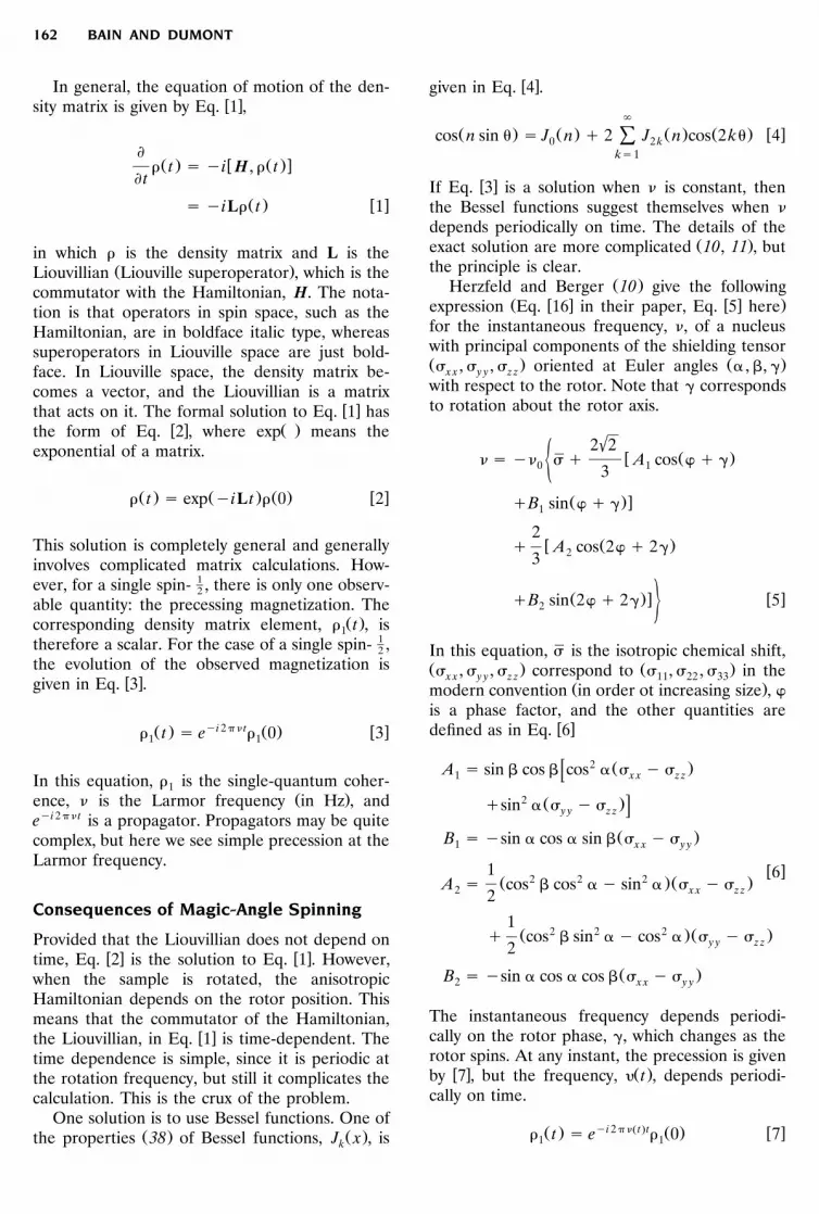
Ž .Herzfeld and Berger 10 give the followingŽ � � � � .expression Eq. 16 in their paper, Eq. 5 here

for the instantaneous frequency, �, of a nucleuswith principal components of the shielding tensorŽ . Ž . , , oriented at Euler angles , �, �x x y y z zwith respect to the rotor. Note that � correspondsto rotation about the rotor axis.

'2 2� Ž .� � �� � A cos � �0 1½ 3

Ž .��B sin � �1

2� Ž .� A cos 2 � 2�23

Ž .� � ��B sin 2 � 2� 52 5In this equation, is the isotropic chemical shift,Ž . Ž . , , correspond to , , in thex x y y z z 11 22 33

Ž .modern convention in order ot increasing size , is a phase factor, and the other quantities are

� �defined as in Eq. 6

2 Ž .A � sin � cos � cos � 1 x x z z

2 Ž .�sin � y y z z

Ž .B � �sin cos sin � � 1 x x y y

12 2 2Ž .Ž .A � cos � cos � sin � 2 x x z z2

� �6

12 2 2Ž .Ž .� cos � sin � cos � y y z z2

Ž .B � �sin cos cos � � 2 x x y y

The instantaneous frequency depends periodi-cally on the rotor phase, �, which changes as therotor spins. At any instant, the precession is given

� � Ž .by 7 , but the frequency, � t , depends periodi-cally on time.

Ž . �i 2� �Ž t . t Ž . � �� t � e � 0 71 1

INTRODUCTION TO FLOQUET THEORY 163

� �Using Eq. 4 , and related identities, we get anFID which can be transformed into a spectrumconsisting of spinning sidebands. The intensitiesof the sidebands are given by sums of Besselfunctions.

Floquet Theory

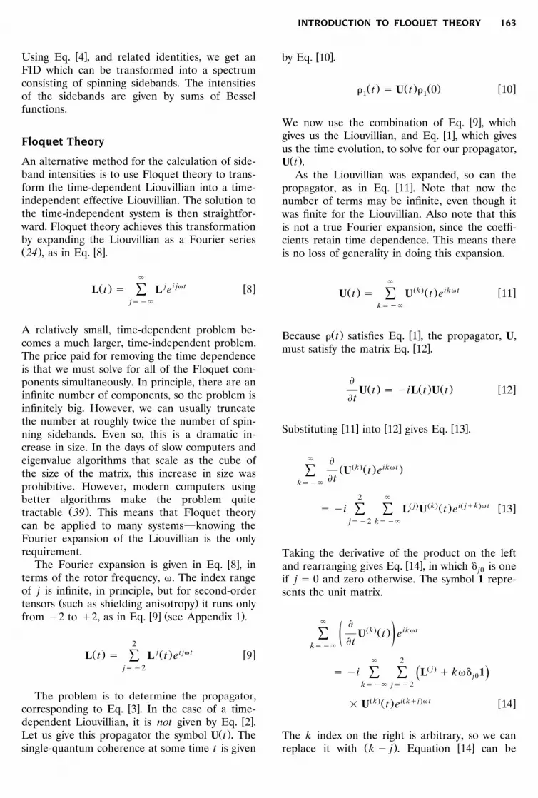
An alternative method for the calculation of side-band intensities is to use Floquet theory to trans-form the time-dependent Liouvillian into a time-independent effective Liouvillian. The solution tothe time-independent system is then straightfor-ward. Floquet theory achieves this transformationby expanding the Liouvillian as a Fourier seriesŽ . � �24 , as in Eq. 8 .

�j i j� tŽ . � �L t � L e 8Ý

j���

A relatively small, time-dependent problem be-comes a much larger, time-independent problem.The price paid for removing the time dependenceis that we must solve for all of the Floquet com-ponents simultaneously. In principle, there are aninfinite number of components, so the problem isinfinitely big. However, we can usually truncatethe number at roughly twice the number of spin-ning sidebands. Even so, this is a dramatic in-crease in size. In the days of slow computers andeigenvalue algorithms that scale as the cube ofthe size of the matrix, this increase in size wasprohibitive. However, modern computers usingbetter algorithms make the problem quite

Ž .tractable 39 . This means that Floquet theorycan be applied to many systems�knowing theFourier expansion of the Liouvillian is the onlyrequirement.

� �The Fourier expansion is given in Eq. 8 , interms of the rotor frequency, �. The index rangeof j is infinite, in principle, but for second-order

Ž .tensors such as shielding anisotropy it runs only� � Ž .from �2 to �2, as in Eq. 9 see Appendix 1 .

2j i j� tŽ . Ž . � �L t � L t e 9Ý

j��2

The problem is to determine the propagator,� �corresponding to Eq. 3 . In the case of a time-

� �dependent Liouvillian, it is not given by Eq. 2 .Ž .Let us give this propagator the symbol U t . The

single-quantum coherence at some time t is given

� �by Eq. 10 .

Ž . Ž . Ž . � �� t � U t � 0 101 1

� �We now use the combination of Eq. 9 , which� �gives us the Liouvillian, and Eq. 1 , which gives

us the time evolution, to solve for our propagator,Ž .U t .As the Liouvillian was expanded, so can the

� �propagator, as in Eq. 11 . Note that now thenumber of terms may be infinite, even though itwas finite for the Liouvillian. Also note that thisis not a true Fourier expansion, since the coeffi-cients retain time dependence. This means thereis no loss of generality in doing this expansion.

�Žk . i k� tŽ . Ž . � �U t � U t e 11Ý

k���

Ž . � �Because � t satisfies Eq. 1 , the propagator, U,� �must satisfy the matrix Eq. 12 .

�Ž . Ž . Ž . � �U t � �iL t U t 12

�t

� � � � � �Substituting 11 into 12 gives Eq. 13 .

� �Žk . i k� tŽ Ž . .U t eÝ

�tk���

2 �Ž j. Žk . iŽ j�k .� tŽ . � �� �i L U t e 13Ý Ý

j��2 k���

Taking the derivative of the product on the left� �and rearranging gives Eq. 14 , in which � is onej0

if j� 0 and zero otherwise. The symbol 1 repre-sents the unit matrix.

� �Žk . i k� tŽ .U t eÝ ž /�tk���

� 2Ž j.� �i L � k�� 1Ž .Ý Ý j0

k��� j��2

Žk . Ž . iŽk�j.� t � �� U t e 14

The k index on the right is arbitrary, so we canŽ . � �replace it with k� j . Equation 14 can be

BAIN AND DUMONT164

� �rewritten as Eq. 15 .

� �Žk . i k� tŽ .U t eÝ ž /�tk���

� 2Ž j. Ž .� �i L � k� j �� 1Ž .Ý Ý j0

k��� j��2

Žk�j. Ž . i k� t � �� U t e 15

The solution to this equation is unique, so it must� �be satisfied by the solutions of Eq. 16 for all

values of k.

�Žk . Ž .U t

�t2

Ž j. Žk�j.Ž . Ž .� �i L � k� j �� 1 U tŽ .Ý j0j��2

� �16

Solving these equations for the Floquet compo-� � � �nents of the propagator gives, via 11 and 10 ,

the density matrix as a function of time.For a sample in which the Hamiltonian is

Ž .constant e.g., in liquids , the propagator is just

�i 2� � t � �e , as in Eq. 3 . For the case of MAS, it will� �be an infinite set of functions that satisfy Eq. 16 .

The simplest way to find these functions is toexpress the problem as a matrix, in what is calledFloquet space. Let the propagators, UŽk ., be the

� �components of an infinite vector, U, as in 17Žmatrices in Floquet space are denoted by a sans

.serif font . For the single-spin case, there are� �scalars, as in Eq. 3 . For more complex cases they

will be matrix blocks.

..� �.Ž�2.UŽ�1.UŽ0.Ž . � �U t � 17U

Ž�1.UŽ�2.U . ..

� � � �Equation 16 can then be written as Eq. 18

�Ž . Ž . � �U t � �iLU t 18

�t

� �where L is given by Eq. 19 .

. . . . . . .. . . . . . .� �. . . . . . .

. .Ž0. Ž�1. Ž�2.. L � 2� L L 0 0 .. .

. .Ž�1. Ž0. Ž�1. Ž�2.. L L � � L L 0 .. .

. .Ž�2. Ž�1. Ž0. Ž�1. Ž�2. � �. L L L L L .L � 19. .

. .Ž�2. Ž�1. Ž0. Ž�1.. 0 L L L � � L .. .

. .Ž�2. Ž�1. Ž0.. 0 0 L L L � 2� .. .. . . . . . . . . . . . . .. . . . . . .

Remember that the superscript denotes theFourier component of the Liouvillian. For MAS

1 Ž0.on a spin- , L is the term that is independent2

of the rotation, LŽ1. is the term that varies at therotor frequency, and LŽ2. is the term that varies attwice the rotor frequency. These are terms such

� �as the A’s and B’s in Eq. 5 .� �Formally, the solution to Eq. 18 is given by

� �Eq. 20

Ž . Ž . Ž . � �U t � exp �iL t U 0 20

� �In practice, we diagonalize the matrix in Eq. 19 ,� �with the matrix of eigenvectors, V. Equation 20

� �becomes Eq. 21 , in which � is a diagonal matrix,with the eigenvalues of L, � , down the diagonal.i

Ž . Ž . �1 Ž . � �U t � V exp �i� t V U 0 21

At time zero, no evolution has occurred, so allŽ . � �the propagators in our vector, U 0 , in Eq. 17

are 0, except UŽ0. which is 1. We can now write

INTRODUCTION TO FLOQUET THEORY 165

out the functions that are the propagators, as in� �Eq. 22

�Žk . �i� t �1jŽ . � �U t � V e V 22Ý k j j0

j���

Since V is unitary, its inverse is equal to its� � � �transpose, so Eq. 22 can be rewritten as 23 .

�Žk . �i� tjŽ . � �U t � V V e 23Ý k j 0 j

j���

The propagator, instead of being a single expo-nential, is now a sum of exponentials, with coef-ficients from the eigenvectors of L.

� � � �This can be substituted into Eqs. 11 and 10to get the evolution of the magnetization. As witha time-independent system, the FID is a sum ofoscillations, whose frequencies and intensities aregoverned by the eigenvalues and eigenvectors of amatrix. But there are further simplifications, whichwill eventually produce a simple and neat expres-sion for an MAS spectrum.

Powder Averaging

Simplification comes from powder averaging. Thesample is a random mixture of crystallites, with a

Ž .uniform distribution of the Euler angles , �, � ,which relate the molecular frames to the rotorframe. In particular, there is a uniform distribu-tion of �, which is the Euler angle around therotor axis. Now, different values of � are equiva-lent to different rotor phases. A change in the

� �rotor phase by � would change Eq. 8 into Eq.� �24

�Ž j. i j� t i j�Ž . Ž . � �L t � L t e e 24Ý

j���

This phase factor will propagate through thewhole calculation. It can be shown that the kth

� � i j�term in Eq. 23 picks up a factor of e . Theimportance of this is that when we average over

� �all values of �, all the propagators in Eq. 23 willaverage to zero, except for the k� 0 term! The

Ž0.Ž .only nonzero propagator is U t . This leaves uswith a very simple expression for the FID. If we

Ž . Ž .assume that � 0 � 1, then � t is given by1 11� �Eq. 25 . Note also that for the single spin- case,2

the density matrix here is the same as the de-tected signal. For a more complex case, we must

take the dot product with the total xy magnetiza-Ž .tion. It is also easy to show Appendix 2 that for

1the single spin- case the eigenvalues, � , arej2

multiples of the rotor frequency. The spectrumconsists of a series of sidebands, each with itsintensity given by V 2 .0 j

�2 �j� tiŽ . � �� t � V e 25Ý1 0 i

j���

This equation is identical to the expression forthe spectrum in a liquid system, in which the

Ž .Liouvillian is time-independent 33 . There is aseries of lines in the spectrum, at frequenciesgiven by the eigenvalues of a matrix, with inten-sities given by elements of the eigenvectors.Because of this analogy with the lines in a liquid-

Ž .state spectrum 33 , we can call each sideband atransition�an independently precessing magneti-zation. Like the spectrum of a liquid, each transi-tion receives coherence from the total, oscillatesat its resonance frequency, and then contributesto the total detected signal. However, this is trueonly because of the averaging over �. Any experi-ment that includes pulses that are not at multi-

Žples of the rotor frequency essentially all solids.experiments will disrupt this and prevent us from

treating the sidebands as independent transitions.

1Example of the Spin- System2

The Herzfeld and Berger expression for the in-� �stantaneous frequency, Eq. 5 , has already iso-

lated the components which are independent ofthe rotor, and those that vary as the rotor fre-quency and twice the rotor frequency. To calcu-late the sideband intensities, it is necessary to set

� �up a matrix of the form of 19 .� �In this matrix, the elements are given by 26 ,

in terms of the parameters A , B , A , and B ,1 1 2 2� �defined in 6 . The dimensionality should be as

large as you can comfortably make it, but at leasttwice the number of spinning sidebands.

LŽ0. � �0

'2Ž���1. 2 2'L � � A � B0 1 13 � �26

1Ž���2. 2 2'L � � A � B0 2 23

BAIN AND DUMONT166

This matrix is diagonalized using one numericalŽ .package Matlab, EISPACK, Maple, etc. , and the

eigenvalues and eigenvectors are determined. Theextreme eigenvalues will deviate substantiallyfrom the fundamental plus a multiple of the rotorfrequency, but they will not contribute to thespectrum. The intensity of each sideband is given

� � 2by Eq. 25 , in which the term V is just the0 jsquare of the jth element of the eigenvector thatcorresponds to the center band line in thespectrum.This expression must be embedded in some

algorithm for powder averaging over the and �Euler angles to give the experimental spectrum.Many authors have designed elegant ways of do-

Ž .ing this average 40�47 . Once this is done, thespectrum will resemble Fig. 2.

More Complex Systems1� �Equation 25 applies only to a single spin- case,2

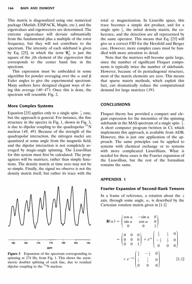
but the approach is general. For instance, the finestructure in the spectra in Fig. 1, shown in Fig. 3,is due to dipolar coupling to the quadrupolar 14N

Ž .nucleus 48, 49 . Because of the strength of thequadrupolar interaction, the nitrogen nuclei arequantized at some angle from the magnetic field,and the dipolar interaction is not completely av-eraged by magic-angle spinning. The Liouvillianfor this system must first be calculated. The prop-agators will be matrices, rather than simple func-tions. The density matrix at time zero may not beso simple. Finally, the signal we observe is not thedensity matrix itself, but rather its trace with the

Figure 3 Expansion of the spectrum corresponding tospinning at 274 Hz, from Fig. 1. This shows the asym-metric doublet splitting of each line, due to residualdipolar coupling to the 14N nucleus.

total xy magnetization. In Liouville space, thistrace becomes a simple dot product, and for a

1single spin- , the initial density matrix, the co-2

herence, and the detection are all represented by� �the same operator. This means that Eq. 25 will

give us a correct FID for the Herzfeld and Bergercase. However, more complex cases must be han-dled with more attention to detail.Note that the matrices will become quite large,

since the number of significant Floquet compo-nents is typically twice the number of sidebands.However, because of its pentadiagonal structure,most of the matrix elements are zero. This meansthat sparse matrix methods, which exploit thisfact, can dramatically reduce the computational

Ž .demand for large matrices 39 .

CONCLUSIONS

Floquet theory has provided a compact and ele-gant expression for the intensities of the spinning

1sidebands in the MAS spectrum of a single spin- .2Ž .A short computer program written in C , which

implements this approach, is available from ADB.However, this is just one application of the ap-proach. The same principles can be applied tosystems with chemical exchange or to systemswith more complicated Liouvillians. What isneeded for these cases is the Fourier expansion ofthe Liouvillian, but the rest of the formalismremains the same.

APPENDIX 1

Fourier Expansion of Second-Rank Tensors

In a frame of reference, a rotation about the zaxis, through some angle, , is described by the

� �Cartesian rotation matrix given in 1.1

cos �sin 0Ž .R � sin cos 0ž /0 0 1

1 i 02 20 0 0i i 1� � e0 0 0 � 02 2ž / 00 0 1 0 0 0

1 i� 02 2�i i 1 � �� e 1.102 2 00 0 0

INTRODUCTION TO FLOQUET THEORY 167

If M is a tensor in this frame, then the effect� �of the rotation is given by Eq. 1.2 .

Ž . Ž . Ž . T Ž . � �M � R M 0 R 1.2

� � � �If we substitute 1.1 into 1.2 , we get a five-termŽ . � �Fourier series for M , given in Eq. 1.3 . In this

equation, the superscript j denotes the Fouriercomponent.

2Ž j. i jŽ . � �M � M e 1.3Ý

j��2

These Fourier components can be written explic-itly in terms of the matrix elements of M in Eqs.� � � � � �1.4 , 1.5 , and 1.6 . Note that the symmetry of Mhas been used in these equations.

Ž .M �M �2 0 011 22Ž0. Ž .0 M �M �2 0M � 11 22 00 0 M33

� �1.4

0 0Ž�1. 0 0M � Ž . Ž .M � iM �2 M � iM �231 32 32 31

Ž .M � iM �231 32

� �1.5Ž .M � iM �232 31 00

Ž .M �M � 2 iM �411 22 12Ž�2.M � Ž .�iM � iM � 2M �411 22 12 0

Ž .�iM � iM � 2M �4 011 22 12

� �1.6Ž .�M �M � 2 iM �4 011 22 12 00 0

� �Equation 1.3 gives us the Fourier expansion ofŽ .the Hamiltonian or the Liouvillian �the fact

that there are five terms arises from the second-rank nature of the tensors. From the Hamilto-nian, we then can calculate the propagators of thedensity matrix. In Floquet theory, the propagatoris also expanded into something resembling aFourier series. The series is infinite, but it can betruncated to leave a much larger, but still finite,

� �propagator. Because of the five terms in 1.3 , thematrix representation of the propagator has apentadiagonal structure�the other off-diagonalterms are zero.

APPENDIX 2

Eigenvalues of the Floquet Matrix

� �The Floquet matrix is given by Eq. 2.1

. . . . . . .. . . . . . .� �. . . . . . .

. .Ž0. Ž�1. Ž�2.. L � 2� L L 0 0 .. .

. .Ž�1. Ž0. Ž�1. Ž�2.. L L � � L L 0 .. .

. .Ž�2. Ž�1. Ž0. Ž�1. Ž�2. � �. L L L L L .L � 2.1. .

. .Ž�2. Ž�1. Ž0. Ž�1.. 0 L L L � � L .. .

. .Ž�2. Ž�1. Ž0.. 0 0 L L L � 2� .. .. . . . . . . . . . . . . .. . . . . . .

This is the important matrix for this problem,since its eigenvalues and eigenvectors determinethe spectrum. It is clear that the diagonal ele-ments are spaced by the rotor frequency, �. Wemust now convince ourselves that the eigenvalues

are also spaced by the rotor frequency, �, so thatwe see a spectrum of equally spaced sidebands.This is an infinite matrix, whose elements off

the diagonal by one or two are all the same andwhose diagonal elements are separated by �.

BAIN AND DUMONT168

Suppose that a vector, u, is an eigenvector of Lwith eigenvalue �. This means that for all values

� �of an index, k, Eq. 2.2 must hold.

�

� �L u � �u 2.2Ý k , j j kj���

Now let us apply L to a vector in which everyelement of u has been shifted down one position;since the vector is infinite, this is possible. The

� �expression for this is given in 2.3 .

�

� �L u 2.3Ý k , j j�1j���

The index in this equation is arbitrary, so we can� �replace j with j� 1, so that expression 2.3

� �becomes expression 2.4 .

�

� �L u 2.4Ý k , j�1 jj���

� �From the properties of L in equation 2.1 , we can� � � �calculate the matrix elements in 2.4 , to give 2.5 .

Ž .L � L j� k� 1k , j�1 k�1, j � �2.5Ž .L � L � � j� k� 1k , j�1 k�1, j

� � � �So expression 2.3 becomes 2.6 .

� �

L u � L u � �uÝ Ýk , j j�1 k�1, j j k�1j��� j���

� �u � �uk�1 k�1

Ž . � �� � � � u 2.6k�1

So by shifting the elements of the eigenvectordown one position, we have created a new eigen-vector whose eigenvalue is shifted by the rotorfrequency, �. This process can be continued toshow that all the eigenvalues must be equallyspaced. Note also the relation between successiveeigenvectors; they are just shifted down oneposition.This is true only for infinite matrices. In a

practical implementation of Floquet theory, thematrices are finite, and so the extreme eigenval-ues do not obey the rules. However, provided thenumber of Floquet components is large enough,the eigenvalues that contribute significantly to thespectrum will be reliable and will be spaced bymultiples of �.

Note that the above derivation is quite general�it applies to any number of spins, with any spinquantum number. For a general system, there is aset of fundamental frequencies, from which allthe frequencies in the spectrum can be obtainedby adding integer multiples of the rotor fre-

1quency. For the single spin- case, there is just2

one fundamental. For the spectrum in Fig. 1,there are three frequencies, due to the couplingto the quadrupolar 14N nucleus.

ACKNOWLEDGMENTS

We thank Dr. Paul Hazendonk and HermannKampermann for many stimulating discussionsand Hiltrud Grondey for running spectra. Wealso thank the Natural Sciences and Engineering

Ž .Research Council of Canada NSERC for finan-cial support.

REFERENCES

1. Mehring M, Principles of high resolution NMR insolids. Berlin: Springer-Verlag; 1983.

2. Gerstein BC, Dybowski CR, Transient techniquesin NMR of solids. New York: Academic Press;1985.

3. Fyfe CA, Solid-state NMR for chemists. Guelph,Ontario: C.F.C. Press; 1983.

4. Andrew ER, Bradbury A, Eades RG. Nuclear mag-netic resonance spectra from a crystal rotated at

Ž .high speed. Nature London 1958; 182:1659�1659.5. Lowe IJ. Free induction decays of rotating solids.Phys Rev Lett 1959; 2:285�287.

6. Hafner S, Spiess HW. Advanced solid-state NMRspectroscopy of strongly dipolar coupled spins un-der fast magic angle spinning. Concepts Magn Re-son 1998; 10:99�128.

7. Dixon WT. Spinning-sideband-free and spinning-sideband-only NMR spectra in spinning samples. JChem Phys 1982; 77:1800�1809.

8. Hartman P, Ordinary differential equations. NewYork: John Wiley & Sons; 1964. p 149.

9. Yakubovich YA, Starzhinskii VM. Linear differen-tial equations with periodic coefficients. New York:John Wiley & Sons; 1975.

10. Herzfeld J, Berger AE. Sideband intensities inNMR spectra of samples spinning at the magicangle. J Chem Phys 1980; 73:6021�6030.

11. Maricq MM, Waugh JS. NMR in rotating solids. JChem Phys 1978; 70:3300�3316.

12. Vega S, Olejniczak ET, Griffin RG. Rotor fre-quency lines in the nuclear magnetic resonancespectra of rotating solids. J Chem Phys 1984;80:4832�4840.

INTRODUCTION TO FLOQUET THEORY 169

13. Schmidt A, Griffin RG, Raleigh DP, Roberts JE,Smith SO, Vega S. Chemical-exchange effects inthe NMR-spectra of rotating solids. J Chem Phys1986; 85:4248�4253.

14. Zax DB, Vega S. Broadband excitation pulsesof arbitrary flip angle. Phys Rev Lett 1988; 62:1840�1843.

15. Goelman G, Vega S, Zax DB. Design of broadbandpropagators in two-level systems. Phys Rev A 1989;39:5725�5743.

16. Schmidt A, Vega S. The Floquet theory of mag-netic resonance spectroscopy of single spins anddipolar coupled spin-pairs in rotating solids. J ChemPhys 1992; 96:2655�2680.

17. Weintraub O, Vega S. Floquet density matricesand effective Hamiltonians in magic-angle-spinningNMR spectroscopy. J Magn Reson A 1993;105:245�267.

18. Zax DB, Goelman G, Abramovich D, Vega S.Floquet formalism and broadband excitation. AdvMagn Res 1990; 14:219�240.

19. Boender GJ, Vega S, De Groot HJM. A physicalinterpretation of the Floquet description of magicangle spinning nuclear magnetic resonance spec-troscopy. Mol Phys 1998; 95:921�934.

20. Nakai T, McDowell CA. Application of Floquettheory to the nuclear magnetic resonance spectraof homonuclear two-spin systems in rotating solids.J Chem Phys 1991; 96:3452�3466.

21. Ding S, McDowell CA. Application of Floquet the-5ory to quadrupolar nuclear spin- nuclei in solids2

undergoing sample rotation. Mol Phys 1998; 95:841�848.

22. Ding S, McDowell CA. The equivalence betweenFloquet formalism and the multistep approach incomputing the evolution operator of a periodicaltime dependent Hamiltonian. Chem Phys Lett 1998;288:230�234.

23. Nakai T, McDowell CA. An analysis of NMR spin-ning sidebands of homonuclear two-spin systemsusing Floquet theory. Mol Phys 1992; 77:569�584.

24. Levante TO, Baldus M, Meier BH, Ernst RR.Formalized quantum mechanical Floquet theoryand its application to sample spinning in nuclearmagnetic resonance. Mol Phys 1995; 86:1195�1212.

25. Shirley JH. Solutions of the Schrodinger equation¨with a Hamiltonian periodic in time. Phys Rev1965; 138:B979�B987.

26. Abragam A. The principles of nuclear magnetism.Oxford, UK: Clarendon Press; 1961.

27. Zare RN. Angular momentum: understanding spa-tial aspects in chemistry and physics. New York:John Wiley & Sons; 1988.

28. Brink DM, Satchler GR. Angular momentum. Ox-ford, UK: Oxford University Press; 1968.

29. Siminovich DJ. Rotations in NMR: Part 1.Euler�Rodrigues parameters and quaternions.Concepts Magn Reson 1997; 9:149�171.

30. Hodgkinson P, Emsley L. Numerical simulation ofsolid-state NMR experiments. Prog Nucl Magn Re-son Spectrosc 2000; 36:201�239.

31. Bain AD. The superspin formalism for pulse NMR.Prog Nucl Magn Reson Spectrosc 1988; 20:295�315.

32. Banwell CN, Primas H. On the analysis of high-resolution nuclear magnetic resonance spectra. I.Methods of calculating NMR spectra. Mol Phys1963; 6:225�256.

33. Bain AD, Fletcher DA, Hazendonk P. What is atransition? Concepts Magn Reson 1998; 10:85�98.

34. Fano U. In Caianiello ER, Editor. Lectures on themany body problem. Vol 2, p 217�239. New York:Academic Press; 1964.

35. Ghose R. Average Liouvillian theory in nuclearmagnetic resonance�principles, properties andapplications. Concepts Magn Reson 2000;12:152�172.

36. Binsch G. A unified theory of exchange effects onnuclear magnetic resonance lineshapes. J Am ChemSoc 1969; 91:1304�1309.

37. Sorensen OW, Eich GW, Levitt MH, BodenhausenG, Ernst RR. Product operator formalism for thedescription of NMR pulse experiments. Prog NuclMagn Reson Spectrosc 1983; 16:163�192.

38. Abramowitz M, Stegun IA. Handbook of mathe-matical functions. New York: Dover; 1964.

39. Hazendonk P, Bain AD, Grondey H, HarrisonPHM, Dumont RS. Simulations of chemical ex-change lineshapes in CP�MAS spectra using Flo-quet theory and sparse matrix methods. J MagnReson 2000; 146:33�42.

40. Alderman DW, Solum MS, Grant DM. Methodsfor analyzing spectroscopic lineshapes. NMR solidstate powder patterns. J Chem Phys 1986;84:3717�3725.

41. Zaremba SC. Good lattice points, discrepancy andnumerical integration. Ann Mat Pura Appl 1966;4-73:293�317.

42. Conroy H. Molecular Schrodinger equation. VIII.¨A new method for the evaluation of multidimen-sional integrals. J Chem Phys 1967; 47:5307�5318.

43. Cheng VB, Suzukawa HH, Wolfsberg M. Investiga-tions of a nonrandom numerical method for multi-dimensional integration. J Chem Phys 1973;59:3992�3998.

44. Mombourquette M, Weil JA. Simulation of mag-netic resonance powder spectra. J Magn Reson1992; 99:37�44.

45. Wang D, Hanson GR. A new method for simulat-ing randomly oriented powder spectra in magnetic

Ž .resonance: the Sydney Opera House SOPHEmethod. J Magn Reson 1995; 117A:1�8.

46. Varner SJ, Vold RL, Hoatson GL. An efficientmethod for calculating powder patterns. J MagnReson 1997; 123A:72�80.

47. Bak M, Neilsen NC. REPULSION, a novel ap-proach to efficient powder averaging in solid stateNMR. J Magn Reson 1997; 125:132�139.

BAIN AND DUMONT170

48. Grondona P, Olivieri AC. Quadrupole effects in1solid-state NMR spectra of spin- nuclei: a pertur-2

bation approach. Concepts Magn Reson 1993;5:319�339.

49. Eichele K, Lumsden M, Wasylishen RE. Nitrogen-14 coupled dipolar-chemical shift C-13 NMR spec-tra of the amide fragment of peptides in the solidstate. J Phys Chem 1993; 97:8909�8916.

Alex D. Bain is from Toronto, Ontario,Canada. He did his undergraduate workin mathematics and chemistry at the Uni-versity of Toronto. He was introduced toNMR during his Ph.D. at Cambridge,under the supervision of Dr. Ruth Lyn-den-Bell. After postdoctoral work, he wasan applications spectroscopist at BrukerCanada for 6 years, before joining the

faculty at McMaster University. His interests are in spindynamics and chemical exchange in liquids, and more recentlyhe has started to learn about solid-state NMR.

Randall S. Dumont completed his Ph.D.in theoretical chemistry at the Universityof Toronto, in 1986. He joined the De-partment of Chemistry of McMaster Uni-versity in 1988 after a postdoctoral fel-lowship at Columbia University. His re-search is primarily concerned with thenumerical simulation of molecular quan-tum dynamics. He began treating spin

systems, for the purpose of NMR spectrum simulation, in1995. This research focused on the superior numerical scalingproperties of sparse matrix methods such as the Lanczosalgorithm.