Intrahousehold Allocation of Education Expenditure and Returns to Education: The Case of Sri Lanka

ISSN 1471-0498

DEPARTMENT OF ECONOMICS

DISCUSSION PAPER SERIES

Intrahousehold Allocation of Education Expenditure and Returns to Education: The Case of Sri Lanka

Rozana Himaz

Number 393 May 2008

Manor Road Building, Oxford OX1 3UQ

Intrahousehold Allocation of Education Expenditure and

Returns to Education: The Case of Sri Lanka

Rozana Himaz

Queen Elizabeth House

University of Oxford

May 6, 2008

Keywords: Intrahousehold Allocation, Returns to Education, Gender

JEL Classification: D13, I21, J16

* I would like to thank Sonia Bhalotra, Pramila Krishnan and Hamish Low for helpful comments on an earlier version of this article. The usual disclaimer applies. E-mail:[email protected]

Abstract

This paper uses demand analysis to explore whether intrahousehold

allocation of education expenditure di¤ers between boys and girls in rural

Sri Lanka. Contrary to most countries in South Asia a signi�cant bias

favouring girls is found in 1990/91 for the 5-9 and 17-19 age groups and

in 1995/96 for the 5-9 and 14-16 age groups. The 5-9 age group captures

the run-up to the Year 5 scholarship exams that are used to gain entry

into better performing secondary schools. The 14-16 and 17-19 age groups

capture those who read for important National level quali�cations vital in

the job market. The paper argues that these household level decisions are

rational because wage returns to junior and senior secondary education

have been higher for females than for males through the 1980s and 1990s.

1

1 Introduction

Developing countries have been a testing ground for the investigation of gender

bias in the allocation of educational resources -mainly schooling expenditure-

in a household (Burgess and Zhuang 2000, Rudd 1993, Kingdon 2003). The

rationale for the exercise is often found in the hypothesis that girls maybe less

favoured than boys (or even discriminated against) in terms of parents spending

towards their education. Often macro data lends support to this contention

with female schooling rates being signi�cantly less than those for men. How-

ever, at the household level, the di¤erential allocation of resources maybe an

e¢ cient decision if returns to schooling di¤er by gender. The empirical liter-

ature on labour market returns to schooling by gender in developing countries

is mixed with studies such as Behrman and Wolfe(1984) for Nicaragua, Bird-

sall and Behrman(1991) for Brazil, Gannicot(1986) for Taiwan and Liu (1998)

for China, amongst others, suggesting that market rates of return to schooling

do not di¤er signi�cantly by gender. Unfortunately most of these papers do

not control for unobservable household and community endowments and focus

mostly on earnings rather than wage rates per hour worked. A more recent

paper by Behrman and Deolalikar (1995) that controls for some of these issues

�nds di¤erential returns to schooling in Indonesia favouring girls. Similarly,

Psacharapoulous and Patrinos(2004) who survey the empirical literature on re-

turns to education (for both developed and developing countries) note that

overall, the studies indicate that females have higher returns to secondary ed-

ucation than men. However, this sort of compilation based on the results of

many studies should be viewed with caution since the original work is not strictly

comparable due to di¤erences in methodology and data sample coverage.

The case of Sri Lanka is interesting to look at both whether there are intra-

household di¤erentials in the allocation of education expenditure and whether

such allocations are e¢ cient in the context of returns to schooling. Sri Lanka is

a developing country well known for her high achievements in male and female

literacy and gender �equality�in terms of school enrolment and exam completion.

2

Such �equality�at the aggregate level does not say much about whether there

is a signi�cant favouring of boys or girls at the margin, when households invest

in education. Such household biases in education expenditure are particularly

important for Sri Lanka because there are several studies done for the 1980s

suggesting that returns to schooling for females are higher than for males. So

how do households respond to this market outcome? Does adding an extra girl

increase the household education budget by more than adding a boy would, con-

trary to what might be expected in most developing countries? Could a gender

bias�if it exists�be more a �cultural�attitude rather than a market response?

This paper answers the above questions. The issue of intrahousehold re-

source allocation has not been investigated in Sri Lanka while estimations of

returns to education have been looked at only for the 1980s. In the �rst part

of this paper, I use demand analysis to try and understand if gender gaps exist

in household education expenditure towards boys and girls in rural Sri Lanka

over the decade beginning in the 1990s. The study uses 3 household income

and expenditure surveys for 90/91, 95/96 and 2000/01 and Engel Curve method

developed in Deaton and Muellbauer (1980), Deaton, Ruiz-Castillo and Thomas

(1989) and Subramaniam (1995). After arguing that the ensuing results are not

due to noisy or poor quality data or because of an inherent �cultural�valuation

of a daughter verses a son, I look at the labour market for any clues that may

shed some light to household behaviour. In the second part of the paper I try

to match the results of the Engel curve analysis with own estimations of returns

to schooling for Sri Lanka from 1990-2000. I use the Mincerian wage function

but adjust the estimations for selectivity as well as heterogeneity arising from

unobserved household and community e¤ects.

3

2 Intrahousehold Allocation of Education Ex-

penditure

2.1 Engel Framework

If individual level data was available, then we could directly compare expen-

diture on education for males and females. However, given the lack of such

individual level data, intrahousehold allocational di¤erences have to be esti-

mated indirectly. Data is available at the level of the household and therefore

I try to detect gender-biases in education expenditure by investigating how the

presence of individuals of similar ages but opposite sexes a¤ect household ex-

penditure on education. The Working-Lesser Engel form for demand analysis

is used with a linear relationship assumed between the share of the budget on

each good and the log of total household expenditure. Deaton and Muellbauer

(1980, p.75) argue that such a relationship has the theoretical advantage of be-

ing consistent with a utility function and conforms to data �in a wide range of

circumstances�. As discussed in Deaton (1997:231), Working�s Engel curve can

be extended to include household demographic composition where age classes

are denoted by nj and are broken down by gender. Separate ij coe¢ cients can

be calculated for males and females:

wi = �i + �i ln(x=n) + �i lnn+

J�1Xj=1

ij(nj=n) + � i:~z + ui (1)

where wi is the share of the household budget devoted to the ith good (edu-

cation expenditure in this paper) calculated as piqi=X with pi and qi denoting

the price and quantity of good i (education) and x is total expenditure per

household, n is household size, nj is the number of people in age-sex class j

(there are J such classes in total)1 . The age categories adopted for children are

important because each of it is the run up to an important national exam that

1The potential endogeneity of household expenditure per capita is checked for with the use

of the instrumental variable approach. I use unearned income and its square as instruments.

4

quali�es a student to enter the next stage and even make the choice of entering

an institution that is reputed for better performance than the one which he or

she leaves. The vector ~z contains other socio-economic variables such as the

education of the household head, ethnic group, location (district) dummies. Fi-

nally, ui is the error-term for good i (education). The coe¢ cient � determines

whether the good is a luxury or a necessity. If � > 0 then the good is a luxury

with the budget share increasing with total outlay making the total expenditure

elasticity greater than 1. The good is a necessity if � < 0 with an expenditure

elasticity less than 1. Gender bias in the allocation of good i can be detected

through a straight forward F test checking whether the coe¢ cients ij = ik

where j and k re�ect boys and girls in the same age group.

This paper �ts the model on the sample of all households, as is conventional,

regardless of whether the households incur a zero or positive budget share of

a particular expenditure. Kingdon (2003) argues that this maybe one of the

reasons as to why the Engel curve analysis may fail to pick up a gender-bias in

schooling expenditure in India as in Subramaniam and Deaton (1991). She

argues that a gender-bias in schooling can work through two possible chan-

nels: one through zero purchases for daughters and positive purchases for sons

and secondly through higher expenditure for sons given positive purchases for

both. If gender-bias works through just one of these mechanisms then averag-

ing across them may lead to the conclusion of no gender bias. She therefore

proposes a hurdle model that separates the households decision whether to in-

cur any expenditure from how much is actually spent given that it is decided

to incur expenditure. She �nds that the basic discriminatory mechanism is via

di¤erential enrolment rates for boys and girls.

Unearned income comprise dividends, interest and rents. Roughly 13 per cent of the rural

households in the HIES have some form of positive unearned income. The instruments are

relevant with an F test on the joint signi�cance of the instruments in an equation predicting the

potentially endogenous variable being signi�cant at the 5 per cent level. An overidenti�cation

test asserts that the instruments are valid. However, the Hausman-Wu test performed fails

to reject the exogeneity of the log of expenditure per capita for all years 1990/91, 1995/6 and

2000/01 and I have therefore retained this variable in the wage equation.

5

In our data-set 54 per cent of the households incur a positive expenditure

on child education. I have opted to use the Engel curve method with the model

�tted on all households (whether the expenditure is positive or zero), instead

of using a hurdle model because descriptive statistics do not suggest signi�cant

gender di¤erences in school enrolment . Contrary to India and other developing

countries, female school enrolment rates are the same or even higher in Sri

Lanka than for males. However, di¤erences are not statistically signi�cant2 .

Moreover, households with a positive share of education expenditure are roughly

the same (at 57 per cent in 1990/1, 53 per cent in 1995/6 and roughly 59 per

cent) in the year 2000/01) whether the unit has all-male or all-female children

aged 0-19. So the bias-if it exists-stems from higher expenditure on sons or

daughters given positive expenditure on both3 .

Another issue to consider is whether the Engel curve is indeed linear, as

assumed, or if it maybe non-linear with households considering education a

luxury at lower levels of income and a necessity at higher levels of income.

In the regression analysis, this would be re�ected by the coe¢ cient on the

log of household expenditure being positive for the lower income groups and

negative for the higher income groups when the analysis accounts for household

socio-economic status. This is not the case, as seen in results discussed later,

education is a luxury across all income groups with an elasticity of 1.02, 0.85,

0.88 and 0.67 in 1990 across the poorest to the richest quintile; 1.09, 1.08,

1.07 and 1.06 in 1995 and an almost equal elasticity of 0.8 across all groups in

2000/01. Even simple descriptive statistics (unreported) of the budget share

of education expenditure by expenditure quartile show a positive correlation.

This is a sign that education is a luxury with the budget share devoted towards

it increasing with income(expenditure). I therefore work with the assumption

2For the 5-9 age group enrolment rates are 100 per cent for both b0ys and girls. For the

10-13 age group it is 94.8 and 95.4 per cent for boys and girls respectively. For the 14-16 age

group the corresponding �gures are 83.2 and 80.5 and for the 17-19 age group 49.8 and 50.8.3Another way to handle zero education expenditure is to use a Tobit model. This, however,

is subject to the potentially severe problem of heteroskedasticity (Deaton 1997).

6

that the Engel curve is linear.

2.2 Data

The data comes from three cross-section Household Income and Expenditure

Surveys (HIES) for 1990/91, 1995/6 and 2000/01 carried out by the Department

of Census and Statistics (DCS), Sri Lanka. The DCS conducts the HIES once

every 5 years. Data collection is done in twelve equal monthly rounds to capture

seasonal variations in income and expenditure. A two stage strati�ed random

sample design is used with urban, rural and estate sectors as the domains for

strati�cation. The primary sampling unit is a census block and the secondary

sampling unit are the housing units within the selected census blocks.

Each housing unit was visited three times in a given week. The �rst visit

was made on a Monday to collect demographic and income related data, and

the members of the household were informed as to how consumption of di¤erent

items should be recorded and reported at subsequent visits. A separate sheet

was provided to report the consumption and expenditure of items on a daily

basis and the previous days consumption was added into the sheet by the enu-

merator directly following an interview. The consumption for the rest of the

week was reported in the sheet by members of the household. A second visit

was made during the middle of the week to supervise the households progress

in reporting. The report was then collected from the households after cross

checking with members regarding unclear entries on a visit made the following

Sunday. Thus the food consumption data is based on the �diary method�rather

than the �recall�method. The former is thought to be more accurate than the

latter and subject to less measurement error (Battistin 2004) although there

are arguments to the contrary (Lydberg and Kasperzyk 1991). Expenditure

on education, housing, fuel, non-durables and consumer durables are recorded

as an average for the previous month. This, therefore is based on the recall

method.

The overall quality of the HIES is quite good with high response rates and

7

a coverage that is consistent with other independent surveys carried out on the

same population. Let us discuss these two survey quality indicators separately.

The 1990/91 and 1995/6 surveys have a 95 per cent response rate while the

2000/01 survey has a 91 per cent response rate. Non-response is due mainly

to respondents being unable to complete the schedule, refusing to do so, being

temporarily away or due to some unspeci�ed �other� reason. The incidence

of non-response showed no signi�cant seasonal variation�i.e., the amount of

non-response was roughly the same during all 12 months of the year. These

response rates compare quite favourably with those of several other countries.

For example, six popular US government household surveys conducted during

the 1990-1999 period indicate an initial response rate between 84 per cent to 95

per cent while UK�s General household survey, which is also based on face-to-

face interviews, records response rates averaging 80 per cent over the decade.

The coverage rate compares the estimated number of people from the HIES

in a speci�c demographic group to the same estimate from an independent pop-

ulation total�usually Census estimates. For example, the under 17 population

by race and gender. The DCS carried out an all-island Census in 1981 and

2001. The HIES 2000/01 results are consistent with the Census 2001 results

in terms of demographic composition with the main limitation that the HIES

excludes several areas in the North and East of the country, due data collection

problems in these war-torn areas. The broad composition of the HIES is also

similar to that of the Consumer Finance Survey carried out by the Central Bank

of Sri Lanka during the 1990s. The two surveys gather similar information and

have roughly the same demographic and ethnic composition. No groups are

noticeably under or over-represented compared to the Consumer Finance Survey

that also excludes areas in the North and East in their work.

Table 1 contains summary statistics for the variables used to estimate the

education Engel curves for rural areas. Education expenditure as a share of

total expenditure is not large at around 2 per cent in the 1990s, with the share

growing, albeit slightly, over the decade. In rupee terms, the average rural

household education expenditure was around Rs. 50 in 1990 and Rs. 324 a

8

month by the year 2000. The rather small share of education expenditure is

unsurprising because education is basically �free�in Sri Lanka. However, there

is still a cost and specially an opportunity cost to education. If a child attends a

state school (as do a majority of children in rural areas), text books and uniform

material as well as a mid-day meal in the case of a few schools was provided

during the decade beginning in the 1990s. However costs of private tuition fees,

exercise books, travelling, equipment and additional costs of uniforms (such as

shoes, socks, etc.), a nominal school fee etc. was still to be borne by households.

As children approach their teens, especially mid teens, there is an opportunity

cost to be borne as well in making the choice between schooling and full-time

employment. The problem is more acute in rural areas where poverty rates are

much higher than in urban areas, and additional income is important. The vari-

ous categories of education expenditure have been aggregated and it is assumed

that separability is not an issue since the composition of various expenditure

categories over time has remained roughly the same.

2.3 Results

Equation 1 is used to run OLS regressions for the budget share of education in

rural areas for 1990/91, 1995/6 and 2000/01 (Table 2). F-tests for the equality

of coe¢ cients are presented at the bottom of the tables.

The goodness of �t of the linear Engel curve is around 0.16 for all 3 years.

The coe¢ cients on log expenditure are positive and close to unity in some cases

showing that education is treated as a luxury. The elasticity is highest in 1995

at 0.95 when the country�s poverty rates were the highest during the decade

at 33 per cent (see DCS 2005). The lower elasticity of 0.73 for 2000 suggests

that education has become to be treated as less of a luxury towards the end of

the decade with the country�s economy picking up and poverty rates dropping

to 25 per cent in rural areas4 .

4Unfortunately no previous study exists for Sri Lanka pertaining to a similar analysis to

compare these education expenditure elasticies. Kingdon(2003)�s estimates for India for 1994

show that for most States the elasticity is close to or above unity. Subramaniam (1995)

9

The coe¢ cient on household size is signi�cant and positive for all three

years and somewhat constant at 0.8. This matches theoretical arguments that

suggest that larger households will be better o¤ due to economies of scale that

accrue from shared public goods, at any given level of per capita resources. The

evidence on economies of scale found in this paper is noteworthy given its usual

elusiveness (Deaton and Paxton 1998). However, note also that household size

may be endogenous because parents with a higher taste for schooling may choose

to have smaller families and a higher education budget share. Unfortunately we

do not have data on households across time in order to capture household level

�xed e¤ects and so address the issue of the potential endogeneity of household

size.

The education of the household head is also positively signi�cant for all

three years. This indicates a higher demand for schooling among households

with more educated heads. Ethnic group is also signi�cant with being a Tamil

household a¤ecting the budget share negatively.

The most important result for this paper is to note the coe¢ cients against

the age-cohort variables and the F tests at the bottom of the table that compare

these coe¢ cients between boys and girls of the same age group Compared to the

omitted category of females aged 30 to 54, children in age categories between

5 and 19 exert a signi�cant positive impact on a household�s budget share on

education. This is not surprising. What is particularly interesting to note,

however, is that the coe¢ cients are higher for girls than for boys for most age

groups especially in 1990 and 1995. In 1990, for instance, if a child had been a

girl rather than a boy in the 5-9 age group within the same household, 1 percent

more would have been spent on her towards education, once controlled for other

factors such as household size, etc. The corresponding �gure for 1995 was 1.35

per cent. Similarly, in 1990, adding an extra girl in the 17-19 age group

increased the household education budget by 1.7 per cent more than adding a

reports elasticities ranging between 1.3 and 2.75 for some of India�s poorest States for the mid

1980s. In comparison to these �gures, Sri Lanka�s rural sector seems to treat education as

less of a luxury than most Indian States.

10

boy of the same age group. The F-tests at the bottom of the table summarise

these results by highlighting the signi�cant biases. In 1990/91, statistically

signi�cant biases favouring girls are indicated for the age cohorts 5 to 9 and 17

to 19 and in 1995/96 for age cohorts 5 to 9 and 14 to 16. In 2000, this girl bias

disappears.

In order to get a better understanding of what component of education

expenditure actually causes the bias, I disaggregate education expenditure into

expenditure on books, fees, travelling and other expenses, and calculate the

budget share of each of these components. I then replace the left-hand-side of

equation 4.1, i.e., wi with each of these budget shares separately and re-estimate

4.1 and carry the F test to check whether the gender bias is more obvious in

any one component of education expenditure. The unambiguous result is that

in 1990/1 and 1995/6, it is expenditure towards books that cause a signi�cant

bias. Expenditure in other categories such as fees are often higher for girls than

boys but is not statistically signi�cant.

As a robustness check, I re-run the estimations for households with only

boys or girls to see if the results are similar to that of pooling all households

together. Around 20 per cent of the households have only boys and 20 per

cent only girls. Descriptive statistics for these two groups show that their

mean values for budget share of education expenditure, household expenditure,

household size and siblings are statistically the same, as the t-value testing the

means to be di¤erent is rejected in all cases. The regression analysis for this

sub-sample of households indicate results that match that of all households. In

other words, age categories 5-9, 14-16 and 17-19 still indicate a signi�cant girl

bias, as the F-tests reveal (results unreported).

These results remain robust even when the age-composition of children is

changed in order to make sure that the regression outcomes are not due to

simply to the way I split the age categories up. For example, the age categories

were changed to (a) 5-9, 10-14 and 15-19 and (b) 5-14, 15-19 and yet again as

(c) 5-9, 10-16 and 17-19. For 1990/91 the signi�cant category(ies) were (a) 5-9

and 15-19 and (c) 5-9 and 17-19. Thus the ages for which there was a girl bias

11

is 8/9 and 17/18. For 1995/96 it was (a) 5-9, 15-19 (c)5-9 and 10-16 with the

most signi�cant ages being 8/9 and 14/15/16. There was no signi�cant bias in

2000/01 regardless of how the age categories were split.

Do the baseline results of a signi�cant bias favouring girls in 1990/1 and

1995/6 result hold across expenditure groups or is it something that it driven

by the poor (non poor)? For all three years, the budget share of education

increases as the household group becomes richer. For example, in 1990, the

poorest quartile spend 1.47 of their budget share on education, the second poor-

est 1.5, the third poorest 1.5 and the richest 1.96. In 1995 the corresponding

shares are 1.34, 1.43, 1.66 and 2.25. In 2000 it is 1.55, 1.81, 1.93 and 2.22.

Household size decreases by expenditure group. None of the other regressors

vary notably between income quartiles. To see if baseline results hold across

expenditure groups, I interact the age cohort variable with a dummy indicating

whether the household belongs to the poorest quartile and re-regress the ed-

ucation Engel curve. I then interact the age cohort variable with a dummy

indicating whether the household belongs to the richest quartile. The results of

the F-test for this exercise (unreported) indicate that as in the baseline case,

there are no signi�cant girl-boy biases for the year 2000 in any expenditure

group. However, there are biases in 1990 and 1995. In 1990, the poorest and

the second richest quartiles indicate a bias in the age group 17-19. The bias

in the 5-9 category is indicated in the two middle-income groups. In 1995 girls

in the 14 to 16 age group among the poorest quartile were favoured at a 1 per

cent level of signi�cance while it was around 12 per cent for the richest quartile.

The age group where the bias arises varies with the income group but what is

common is that the biases always favour the girls.

Let us now discuss the �ndings regarding a girl-bias in 1990/91 and 1995/6,

for the �baseline�results in more detail.

Each of the age cohorts 5 to 9, 14 to 16 and 17-19 run-up to and culminate

at important State examinations. The age cohort 5 to 9 culminates in the

Grade 4 scholarship exams, a competitive national exam, the results of which

can be used to gain entrance to better-performing secondary schools. The

12

age group 14-16 is the senior secondary level ending with the Ordinary Level

(O/L) examinations. It is an important educational milestone that completes

secondary education and is needed to gain entrance to better performing schools

and to qualify for high-school education. High school education is captured by

age group 17-19 that culminates with students reading for the Advanced Level

(A/L) examinations qualifying them to enter university.

The results show that according the Engel curve methodology, rural house-

holds allocate the extra rupee towards daughters at age cohort 5-9 (primary

school) and 17-19 (A/Ls) in 1990/91 and 5-9 and 14-16(O/Ls) 1995/6. The

girl bias does not seem to be indicative of any cultural norm or attitude favour-

ing girls since the Engel curve estimated for food and health shares separately

(unreported) do not indicate any signi�cant boy-girl bias. The bias exists only

in terms of education expenditure. Higher investment at the primary school

level may mean daughters can gain entry to better performing secondary schools.

Higher investment at the senior secondary and high-school level will, most prob-

ably, bring about better performance at the State examinations. This bias does

not exist in the year 2000.

So why does an extra girl increase the household education budget more than

a boy does in 1990 and 1995 and why does this tendency disappear in 2000?

It could be noise in the data that gives us these results. We have, however,

noted in the discussion in section 2.2 that the overall quality of the data is quite

good as judged by the coverage rate and non-response rate and the care with

which it has been gathered and cleaned. It was also argued previously that

the results are not sensitive to the way we break-up the age-cohorts. Thus it

is not noisy data that explains our results. It seems that the addition of a girl

child in certain age-cohorts genuinely increased the household education budget

share more than adding a boy of the same age group.

The girl-bias maybe due to returns to education being higher for girls than

boys (at least in the 1980s) backed by the fact that the opportunity cost of

leaving school was higher for a girl than a boy, given higher youth unemployment

rates among girls with longer waiting periods (Salih 2001).

13

Did higher returns to education for girls persist into the 1990s? If it did,

the household level girl-bias maybe seen to be an e¢ cient allocation of resources

and the decision itself may probably be a response to market outcomes in an

economy, where females are economically active, assuming that a household�s

decision to invest in their children�s education is guided by returns to education

for adults at any given time. We shall turn to this issue next.

3 Returns to Education

Are returns to education higher among secondary or A/L quali�ed girls rather

than it is to boys that make the household bias favouring girls rational? Several

studies done using Sri Lankan data for 1980/81, 1985 and 1990 suggest that it

is. The studies include Gutkind (1984), Glewwe (1985), Sahn and Alderman

(1988), Aturupane (1993), Gunawardane (2002). Most of these works use

the Mincerian earnings or wage function and some (i.e.,Aturupane, Sahn and

Alderman) correct the estimates for selectivity using the Heckman procedure

to �nd that returns for females for secondary and A/L quali�cations are higher

than those for males and the direction of the e¤ects remain unchanged when

corrected for sample selection. What is important to note is that both with

earnings and wages and the dependent variable, returns to completing secondary

education are higher for females than for males in the 1980s and early 1990s.

In rural areas female returns are higher for senior secondary (i.e., completing

the advanced level examinations) as well. This means that if a girl stays on

at school for an extra year at the secondary level or stays on to complete her

education at the high-school level (A/Ls), the extra amount that she earns is

higher than that for a boy.

These tendencies for the 1980s may well have adjusted parental expectations

about what is to happen in the 1990s and thus caused them to favour girls in

terms of education expenditure. However, in order to verify what happens in

the 1990s, I estimate Mincerian wage functions for males and females by level

of education for 1995 and 2000. The choice of the standard Mincerian wage

14

equation �ne-tuned to account for household level unobserved heterogeneity has

been adopted mainly for purposes of comparability with other recent studies

done for Sri Lanka.

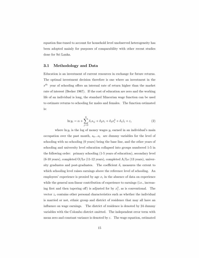
3.1 Methodology and Data

Education is an investment of current resources in exchange for future returns.

The optimal investment decision therefore is one where an investment in the

sth year of schooling o¤ers an internal rate of return higher than the market

rate of interest (Becker 1967). If the cost of education are zero and the working

life of an individual is long, the standard Mincerian wage function can be used

to estimate returns to schooling for males and females. The function estimated

is:

ln yi = �+

6Xj=0

�isij + �2xi + �3x2i + �4~zi + "i (2)

where ln yi is the log of money wages yi earned in an individual�s main

occupation over the past month, s0:::s5 are dummy variables for the level of

schooling with no schooling (0 years) being the base line, and the other years of

schooling and university level education collapsed into groups numbered 1-5 in

the following order: primary schooling (1-5 years of education), secondary level

(6-10 years), completed O/Ls (11-12 years), completed A/Ls (13 years), univer-

sity graduates and post-graduates. The coe¢ cient �i measures the extent to

which schooling level raises earnings above the reference level of schooling. An

employees�experience is proxied by age xi in the absence of data on experience

while the general non-linear contribution of experience to earnings (i.e., increas-

ing �rst and then tapering o¤) is adjusted for by x2i , as is conventional. The

vector zi contains other personal characteristics such as whether the individual

is married or not, ethnic group and district of residence that may all have an

in�uence on wage earnings. The district of residence is denoted by 24 dummy

variables with the Colombo district omitted. The independent error term with

mean zero and constant variance is denoted by ": The wage equation, estimated

15

as above treats the schooling measure as being exogenous, although it might not

be, since unobservables such as ability maybe included in the error term and

be related to the level of schooling attained, making this regressor endogenous.

If schooling level is endogenous then OLS estimates will be biased. This is-

sue has been the preoccupation of the literature since the earliest contributions

and a number of approaches have been used to deal with the issue. In early

studies, measures of ability (e.g., IQ scores) were incorporated, directly into the

wage equation to proxy ability. More recent non-experimental methods have

included matching methods, instrumental variable methods and control func-

tion methods (Blundell. et. al. 2004). The issue of the possible endogeneity

of the level of schooling has not been dealt with directly in this paper. How-

ever, the �xed e¤ects estimation discussed below, that looks at within-sibling

di¤erences in wage returns will account for this if one assumes that unobserved

e¤ects are additive and common within siblings so that they can be di¤erenced

out by regressing the wage di¤erence within the siblings against their education

di¤erence (Ashenfelter and Zimmerman 1997).

The results reported and discussed in the main text are based on a sample

restricted to men and women between ages 15 to 65 who are in paid employ-

ment, in order to capture those who are more likely to be in full-time employ-

ment. These respondents claim that the wage reported is from their �principal�

occupation in the last calender month. In 1995/6, roughly 56 per cent of em-

ployed males and 54 per cent of employed females work as paid employees (i.e.,

wage earners) in the government, semi-government or private sector in rural

Sri Lanka. Employers and own-account workers comprise 39 and 29 per cent

respectively amongst males and females. In 2000/01, 60.79 per cent of males

and 49.19 per cent females were in wage employment. The rest have been in

non-wage employment, without being further classi�ed, unfortunately, as own

account workers or unpaid family workers.

Wages are used instead of earnings (i.e., wage earnings as well as earnings

as an employer or own-account worker) for several key reasons. Firstly, in rural

Sri Lanka, as common in developing countries, a large proportion of females

16

work as unpaid family workers. For example in 1995/6 nearly 16 per cent of

females reported they were unpaid family workers. The corresponding �gure

for males was 4.31 per cent. Moreover, even though 98 per cent of those

claiming to be wage earners actually report the wages they earn, only 42 per

cent of males and 63 per cent of females who claim to be own account workers or

employers actually report earnings in the 1995/6 survey. Thus the information

the survey supplies regarding non-wage earners is incomplete. This problem

is not confronted in the results of the 2000/01 survey. Secondly, in many

cases the male-female contribution is di¢ cult to separate when it comes to

�own-account�work and households are more likely to attribute such earnings

as those arising from the male�s e¤orts than females especially when answering

survey questions. Thirdly, the focus on wage earners in this study is in line with

previous studies for Sri Lanka such as Gunawardane (2002) and references there

in such as Deolalikar(1995) for Taiwan. It ensures that mainly full-time workers

are included in the sample and a¤ords comparability between studies. Fourthly,

and most importantly, own-account earners have been excluded because there

are several studies done for Sri Lanka that indicate a strong preference among

youth in school and those new to the labour market for wage-paid jobs (Salih

2001, National Youth Survey 2001). Most youth seek education in the hope

of doing white collar, preferably government sector jobs. Own-account work is

often an option of last resort. So it can be assumed that parents�and children

base their expectations about returns, on the wage-employment market. We

shall assume in addition that expected wages are based on current wages.

The sample of wage earners I use for the OLS regressions may well be non-

random since they exclude own account workers and employers. In other words,

my estimates will be biased because wage rates are observed only for individ-

uals participating in the labour force as paid employees. The OLS estimates

can be adjusted for selectivity bias using the Heckman correction (Heckman

1979). The correction is akin to adding an extra regressor, the inverse Mills

ratio derived by running a probit estimation in the �rst instance to predict the

probability of being a wage earner. However, to do this, we need to address

17

the issue as to why an individual would choose to work as an employee as op-

posed to being an own account worker or unpaid family worker. Household

level variables that we use to estimate this participation probability are critical

in calculating the inverse Mills ratio that is used for the Heckman correction.

In rural Sri Lanka, many people choose to work in family run agricultural plots.

Some run petty trades or businesses that they start up with private savings

or loans based on private assets left as collateral. Yet some others seek wage

employment in the private sector but fail to �nd it because of a lack of ability in

English language or the right �connections�. Many youth seek self-employment

or fall back into agricultural activity (often following their parents) as an option

of last resort. Unfortunately the data set is not rich enough to o¤er infor-

mation about household wealth, assets (land ownership or the presence of an

established family-run business), English language ability or such factors that

may in�uence a person�s decision to be a wage employee. All that is possible

is to correct for household demographic variables such as the number of young

children (whose presence increases the opportunity cost of joining the labour

force especially for women), the number of older persons in the household, etc.

that are more important for a female�s decision to participate in wage employ-

ment rather than a male�s. In any case, such an estimation may su¤er from

the problem of endogeneity because earned wage may in�uence the number of

children, for instance.

I therefore try to account for the issue of sample selection indirectly through

correcting for unobserved heterogeneity at the household level5 . This is done

by using the �xed e¤ects estimation to a cluster sample, where the well-de�ned

cluster in this case is the household in each cross-section data set. I use devia-

tions from household means for all households where there are two or more males

(females) who are wage earners, to investigate whether �xed e¤ects are impor-

tant, assuming that di¤erences across households (if they exist) can be captured

by parameter �3 estimating unobserved �xed e¤ects f in an extension of the

5This method has also been used in Behrman and Wolfe (1984), Khandker (1990), Behrman

and Deolalikar (1993, 1995) and Gunawardane (2002):

18

model in (2).

ln yik = �+6Xj=0

�isijk + �2xik + �3x2ik + �4~zik + �3fk + " (3)

where k is the household. If there are such unobservable �xed e¤ects, and

they are signi�cant, the constant term of the �xed e¤ects regression would be

signi�cant and the OLS estimations would be biased. Controlling for ��xed

e¤ects�at the household level controls for the sample selection problem as ob-

served by Pitt and Rosenzweig (1990), Heckman and McCurdy (1980). This

is because the household-level observed variables used to control for selectivity

in the paid labour force are those such as wealth, unearned income, assets etc.,

and controlling for household �xed e¤ects should control for the selectivity in

the paid labour force (Behrman and Deolalikar 1995:106). Apart from this, the

�xed e¤ects method addresses the issue of omitted variable bias arising from

unobserved heterogeneity at the household and community level. However,

this procedure only addreses the issue of heterogeneity bias arising from unmea-

sured attributes that are common to individuals in the same household, since

the �xed e¤ects estimation is limited to households that have more than one

male or female earning.

If the unobserved household and community e¤ects are random instead of

being �xed, they would bias the error term and invalidate standard statistical

tests. In order to test for this possibility, I estimate a random e¤ects model

using the same sub-sample. I then use the Hausman test to compare between

the �xed or random e¤ects estimations.

The data sources for the estimation of returns are the same as for the previous

analysis on intrahousehold allocation. Tables 3.1 and 3.2 provide summary

statistics for the variables used for the full sample and reduced sample for 1995/6

and 2000/01, respectively. The reduced sample (i.e., households with two or

more male or female wage earners) is roughly between a quarter and a third

of the full sample. The reduced samples for both 1995 and 2000 can be noted

19

for its younger workers, who seem to earn less on average than wage earners

in the full samples, with fewer of them married and even a bit less educated.

This probably indicates that the households captured in the reduced sample are

mostly those where unmarried siblings still live with their parents or younger

married couples living with parents. This is not uncommon for Sri Lanka where

children leave the parental home mostly after marriage, more often than not into

the homes of their in-laws.

3.2 Results

The OLS regressions on the full sample and the OLS, �xed and random e¤ects

regressions on the reduced sample are reported in Tables 4.1 for males and

4.2 for females in rural areas. The variables �agged as being signi�cant

are almost the same in all the estimations. Moreover, the coe¢ cients for the

OLS estimations (on both the full and reduced samples) and the random e¤ects

estimations are somewhat similar. However, the �xed e¤ects coe¢ cients are

smaller. This implies that unobserved household e¤ects that were not captured

in the OLS estimations were positively correlated with any of the explanatory

variables. Moreover, the standard errors of the �xed e¤ects estimation is smaller

indicating that cluster e¤ects have been taken into account in their calculation

unlike in the case of the OLS.

So are unobserved household e¤ects signi�cant? In all cases the Breusch

-Pagan Lagrange Multiplier test on the random e¤ects model show that un-

observed household e¤ects are indeed signi�cant. The Hausman test, used to

compare the �xed and random e¤ects models, rejects the null hypothesis that

the di¤erence in coe¢ cients is not systematic in all cases at a 1 per cent level of

signi�cance apart from females in 1995, where it is rejected at the 10 per cent

level of signi�cance. Assuming that the speci�cation of the model is correct, I

interpret this result to mean that unobserved household e¤ects and the implicit

correction for selection is indeed important, and that the �xed e¤ects estima-

tions are superior to the OLS or random e¤ects estimations. I therefore focus

20

on the �xed e¤ects-based estimations.

The �xed e¤ects coe¢ cients on the education level variables are often higher

for females with secondary education and those who completed O/Ls than

for males. In the OLS and random e¤ects estimations, this result is more

pronounced. To make this result clearer, I calculate returns to education

using the coe¢ cient values and levels of schooling. They are calculated as

�i � �i�1=si � si�1, following the notation in equation 3 where �i is the coe¢ -

cient on schooling level si. The formula shows the extra return to an extra level

of schooling, with the value of the increase in earnings calculated as exp�1 �1,

given that the dependent variable is the log of wages and the reference level for

schooling is 0. Since individuals may have completed varying years of schooling

in the primary, secondary and graduate level cohorts, I use average years for

these cohorts. Thus s1=3, s2=8, s3=11, s4=13, s5=16 and s6=18.

Table 5 reports �xed e¤ects estimation based returns to education calculated,

using the reported results for rural areas and unreported results for all areas.

The results show that women have an unambiguously higher return to secondary

and O/L education than do men in terms of both rural areas and all-sectors.

This matches trends observed in the 1980s and 1990, reported by Aturupane,

Gunawardane and other studies. Apart from Gunawardane (2000) the other

studies do not account for household level heterogeneity and it is likely that

the returns estimations are in�ated. However, this does not a¤ect the trends

illustrated by these estimations. The trends in all the estimations, regardless

of the econometric re�nement and di¤erences in the dependent variables, is

broadly the same. For the completed O/L and A/L categories, returns to

females is higher. Overall, however, the size of the returns have fallen over the

two decades beginning in 1981. This is partly because the earlier estimates are

�in�ated�in not accounting for household level heterogeneity, and partly, because

true returns have indeed fallen, at least from 1985 onwards when the estimates

discussed become more comparable in terms of methodology adopted.

The calculations in this paper show, in addition, that the clear advantage

females had in terms of returns in the 1980s and even 1995, diminishes slightly

21

especially for rural areas by the year 2000. Secondary school educated women

still have an advantage but the male-female gap has fallen. In the case of

females who have completed O/Ls in rural areas, their returns to education

have fallen dramatically from 8.8 to 1.6 between 1995 and 2000, to be almost

equal to that of men. Moreover, even though the all-sector returns for A/L

educated females remains higher in 2000 than for men, this is not so for women

and men in rural areas. It is beyond the scope of this paper to discuss why

the returns have changed as they have between 1995 and 2000, and indeed

why returns overall have been going down since 1981. Su¢ ce it to note that

there have been many exogenous shocks the Sri Lankan economy experienced

during the post-liberalisation period. Economic liberalisation in 1977 brought

with it a radical policy shift with a welfarist, left-wing government replaced

by right-wing policies, trade liberalisation and privatisation. The early and

mid 1980s saw huge in�uxes of foreign capital and investment especially in

large scale, government backed, infrastructure development programs�mainly

in the area of irrigating the dry-zone. Civil, political and youth unrest was rife

during this period and 1989 brought in a president who sort aggressively to ease

out civil and youth tensions through large scale poverty programs and housing

projects. Insurgencies and political unrest continued until late 1994 brought

with it a new government after 17 years under the rule of the United National

Party. With it came a second wave of liberalisation with large scale privatisation

e¤orts as well as the opening of more large-scale export oriented female-labour

intensive garment factories since the late 1980s. The garment industry o¤ered

a lot of scope and opportunity for young women to work. However, 1995

was a year where poverty rates in Sri Lanka were at an all-time high since the

initial economic liberalisation in 1977. This, together with job opportunities

created after the second wave of liberalisation probably resulted in a higher

labour force participation rate, especially by women. The year 2000 was

signi�cant in that a peace pact was agreed upon between the government and

the Tamil Tigers, ending (temporarily at least) 17 years of civil war, bringing

some amount of stability to the economy. The two decades since initial economic

22

liberalisation in 1977, therefore, has been turbulent for Sri Lanka, politically,

socially and economically. This together with exogenous shocks both national

and international have no doubt a¤ected relative returns, and is a matter that

needs careful further investigation.

Is it possible that our returns to education estimation biased in that it ex-

cludes important �non-market� factors that in�uence a female�s returns, such

as cultural or normative considerations? Some studies for neighbouring coun-

tries such as India and Bangladesh show that a woman often moves in with

her in-laws after marriage and her earnings there onwards accrue to the family

of her in-laws (Malhotra and Tsui 1996). This means that her natal family

bene�ts less from her economic returns, and any �true�estimate of returns to

education should account for this by de�ating a purely market-based calculation

as above. An implication of the girl�s earning not accruing to her own family

is that parents choose to invest more in sons under the implicit assumption

that it will be sons who will look after them �nancially in old age rather than

daughters. This is not so in Sri Lanka. In a majority of Sri Lankan families

the married couple is responsible for their own �nances and daughters are not

constrained in helping out their siblings and parents out of their own income,

if they so wish. So the threat of in-laws� siphoning-o¤ earnings is unlikely.

On the contrary, education gives the girl more autonomy and social mobility

so that she will have more authority to dispense her earnings as she wills�and

perhaps its better to invest in education than in material dowry which can well

be dissipated by the husband/in-laws. In some cases, employment has been a

substitute for the dowry that is still considered important by some Sri Lankan

parents and youth. The Sri Lanka Youth Survey suggests that dowries are

considered important only by 19 per cent of the sample of youth aged 15-29

and that too more predominantly among the Tamils rather than the majority

Sinhalese. Malhotra and Tsui estimate this at to be 30 per cent according to

their survey of Sri Lankan youth. The trend of education and consequent earn-

ing potential being a substitute for the dowry is seen in South India as well,

where higher education is often a dowry substitute and a means of improving a

23

women�s value in the marriage market.

In some cases, dowries are often collected by the girl herself as the age at

marriage is pushed forwards6 . However, in Sri Lanka, the age of marriage being

pushed forwards is not indicative that employment is an alternative to marriage

as in some East Asian countries such as Thailand or Taiwan. The higher age at

�rst marriage in Sri Lanka seems to be driven by poor, rather than improved

economic and political conditions (Caldwell et al 1989). For most females,

employment before marriage is more for the income it provides, than purely for

the dowry they can collect through �saving�or the career they can build as a

substitute for the dowry (Malhotra and Tsui 1996). Female earnings, or rather,

the earnings of both the man and the woman in the family has grown important

over time due to slow economic growth and political unrest and thus, economic

returns to education play an important role when a household decides to invest

in a girl-child, rather than dowry or other �cultural� or normative concerns.

Thus a woman�s non-market in�uences on returns to education placed mainly

by cultural and normative factors do not appear to be very di¤erent to her male

counterparts. A majority of Sri Lankan women participate actively in the

labour market and are not considered a burden. As such, we can assume that

the estimated returns to education, are reasonably representative of the �true�

value and does not need any signi�cant adjustments for unobservable factors

a¤ecting returns.

6The median age at �rst marriage in Sri Lanka, for women in rural areas, has risen from

around 20 in the 1960s to 25-27 in 2000 in rural areas (DHS 2000; Dissanayake 2000). Sri

Lanka has historically had ages at �rst marriage that are higher than those of the rest of the

region. For example, while her counterparts married on reaching puberty at ages as young

as 13 or 14 in Northern India, Pakistan and Bangladesh, the Sri Lankan female has been

marrying at around 18 or 19 even during as far back as the 1940s. During the last couple

of decades, these median ages have increased further, matching other Asian countries such as

Taiwan or Thailand, as have educational levels and social welfare for women (De Silva 1990,

Thornton and Lin 1994).

24

4 Conclusion

The �rst part of the paper showed that contrary to most developing countries,

there is a bias favouring girls in rural Sri Lanka in the allocation of education ex-

penditure within the household. This was seen using demand analysis assuming

a linear Engel curve. Sri Lankan rural households seem to be allocating more

educational resources towards girls in 1990/91 for age groups 5-9 and 17-19 and

in 1995/6 for age groups 5-9 and 14-16. The 5 to 9 age group corresponds

to the run-up to year 5 scholarship exams where children can gain entry into

better performing state schools. The 14-16 age group captures the culmination

of secondary education with the reading for the Ordinary Level examination

and gaining entrance to read particular subjects for the Advanced Levels. The

17-19 age group captures the run-up to and culmination in Advanced Level ex-

amination, by far the most competitive exam in Sri Lanka that allows a student

to gain university entrance. The result of intrahousehold bias in the allocation

of education favouring girls, was tested in various ways for robustness. This in-

cluded analysing the quality of the data, verifying the result by income quartile,

splitting the age-group categorisation in various ways and seeing if the results

held for households with only boys or girls. The results were robust to all these

di¤erent speci�cations: there was indeed a bias favouring girls in the years

1990/91 and 1995/6.

The second part of the paper tried to understand why these biases arise. The

basic hypothesis was that it was due to economic reasons with household level

biases re�ecting labour market returns to education. An analysis of returns

to education showed that the household level allocational biases seem to match

macro-level trends in private returns to education. Corresponding to results

of several previous work done on Sri Lankan returns to education, our results

showed that for 1995, returns to schooling for a girl at the secondary, completed

O/L and completed A/L categories was higher than that for a boy in rural areas

as well as all areas (urban, rural and estate). In other words, schooling a girl

for one extra year at these levels in particular, earned a girl a higher return on

25

that extra year than a boy. At the margin, therefore, it was more �e¢ cient�in

an economic sense to invest in a girl. However, this clear advantage in terms

of economic returns enjoyed in the 1980s and 1990s seems to be lost by the year

2000 and together with it the intrahousehold bias in education favouring girls.

Reasons as to why the relative return structure seems to have changed is beyond

the scope of this paper and is left for further research.

Can the intrahousehold bias be explained purely with reference to private

returns in the labour market? Are girls valued more than boys at a normative or

cultural level? This is not so. This is because the bias is only obvious in terms of

education expenditure but not with respect to health or food expenditure. Thus

there does not seem to be an intrinsic discrimination of boys. Could it be that

our estimate for returns is inadequate in not accounting for non labour market

factors? For example, should returns be revised downwards accommodating

for factors such as the lower status of women in most South Asian countries or

because education maybe a substitute for the dowry at marriage? Both these

are not signi�cant for Sri Lanka. First, Sri Lankan women have historically had

more freedom than her other South Asian counter-parts and later marriage has

been accompanied with a cultural heritage of relative gender equality in terms

of bilateral descent, a daughter�s value in a parental home and continued kin

support following marriage. Thus, there is no necessity to revise estimate for

an elusive �lower status�factor. Secondly, even though the dowry is considered

important by about a quarter to a third of youth interviewed in certain surveys,

the labour market activity of females before marriage is not exclusively for the

purpose of collecting a dowry. The economic and political situation in Sri Lanka

has not been greatly favourable after liberalisation in 1977 and poverty rates are

still high with one in four households below the o¢ cial poverty line. Increased

female participation in the labour market and the bringing in of two incomes

by the male and female in a family has now become an economic necessity.

Liberalisation and the opening of employment opportunities in garment factories

in the free trade zone and in West Asia as domestic aids has mobilised more

women to move away from their homes and seek employment. The returns to

26

educating a daughter are high, and has been so since the early 1980s. It is

perfectly rational, at the household level, therefore to favour daughters at least

at critical stages of the schooling process.

27

References

[1] Ashenfelter, O. and D. Zimmerman (1997), �Estimates of the Returns to

Schooling from Sibling Data: Fathers, Sons and Brothers�, Review of Eco-

nomics and Statistics, 79:1-9.

[2] Aturupane, H (1993) Is Education Bene�cial? A Microeconomic Analysis

of the Impact of Education on Economic Welfare in a Developing Country,�

Ph.D. diss., Cambridge University, UK.

[3] Battistin, E (2004), �Errors in Survey Reports of Consumption Expendi-

tures�, Institute of Fiscal Studies Working Paper 03/07.

[4] Becker, G (1967), Human Capital and personal distribution of income, Uni-

versity of Michigan Press, Ann Arbor MIT.

[5] Behrman, J and A. Deolalikar (1993) �Unobserved Household and Commu-

nity Heterogeneity and the Labour Market Impact of Schooling,�Economic

Development and Cultural Change 41(April):461-488

[6] Behrman, J and A, Deolalikar (1995) �Are there Di¤erential Returns to

Schooling by Gender? The Case of Indonesian Labour Markets�, Oxford

Bulletin of Economics and Statistics 57:97-117

[7] Behrman, J. R and B.L.Wolfe (1984) �The Socioeconomic Impact of School-

ing in a Developing Country,�The Review of Economics and Statistics, vol.

66(2):296-303.

[8] Birdsall, N and J. R. Behrman (1991) �Why do Women Earn Less than

Men in Urban Brazil? Earnings Discrimination? Job discrimination?� in

Birdsall, N and Sabot, R. (eds), Unfair Advantage: Labour Market Dis-

crimination in Developing Countries, Washington: World Bank, 147-70.

[9] Blundell, R., L. Dearden and B. Sianesi (2004), Evaluating the Impact of

Education on Earnings in the UK: Models, Methods and Results from the

NCDS, Centre for the Economics of Education, Paper No: CEEDP0047

28

[10] Burgess, R and J.Zhuang (2000). �Modernisation and Son Preference,�

STICERD - Development Economics Papers 29, Suntory and Toyota In-

ternational Centres for Economics and Related Disciplines, LSE.

[11] Caldwell J. (1989),�Is marriage delay a response to pressures for fertility

decline? The case of Sri Lanka.�Journal of Marriage and Family, 51:327�

335.

[12] Deaton, A (1997), The Analysis of Household Surveys: A Microeconomet-

ric Approach to Development Policy, Johns Hopkins Press for the World

Bank

[13] Deaton, A. and J. Muellbauer (1980) Economics and Consumer Behavior.

Cambridge University Press.

[14] Deaton A. Ruiz-Castillo and D. Thomas (1989), �The In�uence of House-

hold Consumption on Household Expenditure Patterns: Theory and Span-

ish Evidence,�Journal of Political Economy, 97:179-200.

[15] Deaton, A and C. Paxton (1998) �Economies of Scale, Household Size and

the Demand for Food�, Journal of Political Economy, 106, No. 5: 897�910

[16] Department of Census and Statistics (DCS) (2005), Statistical Abstract

2005, Department of Census and Statistics, Colombo, Sri Lanka

[17] De Silva (1990) �Age at marriage in Sri Lanka: Stabilizing or declining?�

Journal of Biosocial Science 22(4):395-404

[18] DHS(2000), Demographic and Health Survey Sri Lanka 2000, Final Report,

Department of Census and Statistics, Sri Lanka.

[19] Dissanayake L (2000) Factors in�uencing stabilization of women�s age at

marriage. In:Demography of Sri Lanka. Colombo, Sri Lanka,Department of

Demography, University of Colombo:45�58

[20] Gannicot, K (1986) �Women, wages and discrimination: Some evidence

from Taiwan,�Economic Development and Cultural Change, vol. 39:721-30

29

[21] Glewwe, P(1985) An Analysis of income distribution and labour markets

in Sri Lanka, Ph.D. diss., Stanford University.

[22] Gunawardane, D (2002), �Reducing the gender wage gap in Sri Lanka: Is

education enough?�, Sri Lanka Economic Journal, Vol. 3(2):57-103

[23] Gutkind, E. (1984) Earnings Functions and Returns to Education in Sri

Lanka. International Labour Organization, Geneva.

[24] Heckman, J.J (1979) �Sample selection bias as a speci�cation error,�Econo-

metrica 47:153-161

[25] Heckman, J. J. and T. E. McCurdy(1980), A Life Cycle Model of Female

Labour Supply, Review of Economic Studies, 1980, vol. 47, issue 1, pages

47-74

[26] Khandker S.R. (1990) �Labour market participation, returns to education

and male-female wage di¤erences in Peru,�Policy Research Working Paper

461., World Bank, Washington D.C.

[27] Kingdon, G.G. (2003), �Where has all the bias gone?: Detecting gender-

bias in the household allocation of educational expenditure�, CASE

WPS/2003 -13

[28] Liu, Z. (1998), �Earning, Education and Economic Reforms in Urban

China.�Economic Development and Cultural Change 46(4): 697-725.

[29] Lydberg, L and D. Kasprzyk (1991), Data Collection Methods and Mea-

surement Errors: An Overview in Beimer, P. P, R. et.al. eds.,(1991), Mea-

surement Errors in Surveys. New York: John Wiley and Sons:237-258.

[30] Lydberg, L and D. Kasprzyk (1997) in P. Biemer, et.al. eds., Survey Mea-

surement and Process Quality, New York: John Wiley and Sons.

[31] Malhotra, A. and A. O. Tsui (1996), �Marriage Timing in Sri Lanka: The

Role of Modern Norms and Ideas�, Journal of Marriage and Family, Vol.

58 (2): 476-490

30

[32] National Youth Survey(2001) Overview Report and Tables on Selected Top-

ics and Illustrated Data Sri Lanka, Centre for Anthropological and Socio-

logical Studies, University of Colombo and South Asia Institute, Colombo,

Sri Lanka

[33] Pitt, M and M.R.Rosenzweig (1990) �Estimating the behavioural conse-

quences of health in a family context: the intrafamily incidence of infant

illness in Indonesia,�International Economic Review 31:969-89

[34] Psacharopoulos, G and H.A. Patrinos (2004) �Returns to investment in

education: a further update,� Education Economics, Taylor and Francis

Journals, vol. 12(2), pages 111-134.

[35] Rudd. J. B (1993) �Boy-girl discrimination in Taiwan:evidence from expen-

diture data�, Research program in development studies, Princeton Univer-

sity, processed.

[36] Sahn, D. E., and H. Alderman (1988) The E¤ects of Human Capital on

Wages, and the Determinants of Labor Supply in a Developing Country,

Journal of Development Economics 29(2):157-183

[37] Salih, R (2001) Youth employment in Sri Lanka: A review of the current

labour market situation, policy and programs, The ILO/Japan Tripartite

Regional Meeting on Youth Employment in Asia and the Paci�c

[38] Subramanian, S(1995) �The demand for food and calories,�Journal of Po-

litical Economy 104(4): 133-62

[39] Thornton, A. and Lin. H (1994). Social Change and the Family in Taiwan.

University of Chicago Press.

31

Table 1: Summary Statistics for Budget Share of Education and Contributory Variables in Rural areas

Variable name

Description of variable 1990/91 1995/96 2000/01

Educ_share Budget share of education: household education expenditure/Total expenditure on food and non-food items X 100

1.60 (0.04)

1.68 (0.04)

1.93 (0.059)

Exp_TOT Total expenditure (in rupees) on food and non-food items per member of the household

791.03 (9.96)

1449.43 (28.37)

3058.65 (47.12)

hsize Log household size 1.51 1.43 1.36 M0_4 Number of males aged 0 to 4 as a proportion of all

household members (excluding boarders and lodges) .04 .04 .035

f0_4 Number of females aged 0 to 4 as a proportion of all household members (excluding boarders and lodges)

.03 .04 .034

M5_9 Number of males aged 5 to 9 as a proportion of all household members (excluding boarders and lodges)

.04 .03 .037


.04 .04 .03


.04 .04 .034


.04 .04 .033


.28 .03 .025


.27 .03 .024


.27 .027 .027


.27 .026 .026


.08 .08 .07


.08 .08 .08


.14 .16 .166


.15 .16 .177

M55** Number of males above age 55 as a proportion of all household members (excluding boarders and lodges)

.07 .07 .07

f55 Number of females above age 55 as a proportion of all household members (excluding boarders and lodges)

.08 .08 .086

Educ_head Education level (in years) of the household head 5.9 9.9 8.6 Tamil Proportion of households with a Tamil household

head .01 .04 .02

Minority Proportion of households with a Muslim, Burgher or other minority as a household head.

.04 .04 .09

Note: Standard errors in parenthesis for continuous variables. ** Reference group for education Engel-curve estimations Source: Own calculations using HIES 1990/91, 1995/6 and 2000/01.

32

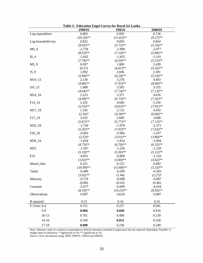
Table 2: Education Engel Curves for Rural Sri Lanka 1990/91 1995/6 2000/01 Log expenditure 0.883 0.950 0.736 (10.26)** (11.63)** (9.27)** Log household size 0.822 0.850 0.854 (9.93)** (5.72)** (5.16)** M0_4 -2.728 -1.908 -2.077 (8.53)** (7.14)** (5.80)** f0_4 -2.642 -1.455 -2.101 (7.78)** (4.29)** (5.15)** M5_9 0.097 1.800 2.439 (0.27) (4.61)** (5.42)** f5_9 1.092 2.696 2.391 (2.84)** (6.24)** (5.16)** M10_13 2.130 3.278 4.403 (4.86)** (7.92)** (8.06)** f10_13 1.988 3.585 3.555 (4.64)** (7.74)** (7.13)** M14_16 2.313 3.371 4.616 (4.49)** (6.73)** (7.41)** F14_16 3.101 4.660 5.350 (5.55)** (9.63)** (7.91)** M17_19 1.345 2.133 4.459 (2.56)* (4.18)** (6.60)** F17_19 3.032 2.849 3.608 (5.67)** (5.77)** (7.13)** M20_29 -1.720 -1.978 -2.371 (5.20)** (7.02)** (7.63)** F20_29 -0.693 -0.906 -1.037 (2.53)* (3.61)** (3.86)** M30_54 -1.824 -1.814 -1.694 (4.73)** (6.70)** (6.32)** M55 -1.507 -1.256 -1.228 (5.19)** (5.50)** (5.11)** F55 -0.851 -0.809 -1.110 (3.02)** (3.80)** (4.62)** hhead_educ 0.101 0.152 0.082 (10.99)** (13.68)** (5.53)** Tamil -0.489 -0.299 -0.393 (3.02)** (1.44) (2.27)* Minority -0.179 -0.098 -0.087 (0.86) (0.43) (0.46) Constant -5.677 -6.699 -4.934 (8.19)** (10.23)** (8.92)** Observations 11007 14234 12487

R-squared 0.15 0.16 0.16 F-Tests: 0-4 0.751 0.257 0.941 5-9 0.006 0.049 0.916 10-13 0.761 0.489 0.139 14-16 0.160 0.031 0.328 17-19 0.008 0.236 0.249 Note: Absolute value of t statistics in parentheses; District dummies included in regressions but not reported. Dependent Variable: is budget share of education. * Significant at 5%; ** significant at 1%. Source: Own calculations using HIES 1990/91, 1995/6 and 2000/01.

33

Table 3.1: Summary Statistics for Selected Returns to Schooling Variables 1995/96 Full sample Reduced sample All Sectors (Urban,

rural and estate) Rural All Sectors (Urban, rural

and estate) Rural

Male Female Male Female Male Female Male Female Wage earned during the past month

2934.03 (51.88)

2435.38 (51.52)

2727.03 (54.3)

2313.32 (57.45)

2633.45 (57.84)

2399.65 (71.21)

2450.42 (89.82)

2273.66 (81.42)

Age 36.78 35.03 36.74 35.08 34.33 32.97 34.36 32.99 Age squared 1476.9 1345.30 1473.05 1350.14 1341.48 1223.18 1345.48 1224.75 Primary (1-5 years of education)

.28 .23 .28 .21 .29 .21 .30 .20

Secondary (6-9 years of education)

.37 .25 .38 .28 .36 .28 .36 .32

Finished O/L .18 .18 .17 .18 .17 .17 .16 .18 Finished A/L .08 .15 .08 .15 .09 .14 .08 .14 University Graduates

.02 .03 .02 .03 .01 .03 .01 .03

Post graduate .01 .01 .00 .00 .00 .00 .00 .00 Married proportion

.73 .69 .73 .68 .53 .53 .52 .53

Sample size 13322 6322 8689 3710 4849 2127 2998 1159 Source: Own calculations using HIES 1990/91, 1995/6 and 2000/01. Table 3.2: Summary Statistics for Selected Returns to Schooling Variables 2000/01 Full sample Reduced sample All Sectors (Urban,

rural and estate) Rural All Sectors (Urban,

rural and estate) Rural

Males Females Males Females Males Females Males Females Wage earned during the past month (Rs.)

5096.02 (76.56)

4228.82 (82.81)

4868.63 (78.69)

4150.54 (97.01)

4560.4 (79.11)

4020.0 (80.37)

4197.6 (81.31)

3746.2 (85.28)

Age 37.98 36.31 38.05 38.05 34.14 33.2 33.8 33.2 Age squared 1573.67 1449.13 1577.69 1474.90 1345.75 1258.9 1333.3 1256.6 Primary (1-5 years of education)

.25 .23 .24 .24 0.25 0.21 0.42 0.17

Secondary (6-9 years of education)

.43 .29 .44 .44 0.46 0.32 0.49 0.36

Finished O/L .15 .14 .16 .16 0.14 0.13 0.35 0.15 Finished A/L .09 .18 .08 .08 0.08 0.16 0.26 0.17 University Graduates

.02 .04 .01 .01 0.17 0.04 0.11 0.04

Post graduate .00 .00 .00 .00 0.006 0.009 0.06 0.004 Married proportion

.78 .71 .78 .78 0.53 0.5 0.5 0.47

Sample size 12646 5432 9110 3502 3367 1530 2177 870 Source: Own calculations using HIES 1990/91, 1995/6 and 2000/01.

34

Table 4.1: Males: Private Returns to Schooling in Rural areas 1995/96 and 2000/01 Dependent variable: log wage

1995/6 2000/01

OLS (full sample)

OLS (restricted sample)

Fixed Effects Random Effects OLS (full sample)


Fixed Effects Random Effects

Age 0.035 0.047 0.037 0.044 0.042 0.060 0.058 0.066 (7.95)** (6.80)** (5.57)** (7.37)** (8.42)** (8.34)** (7.36)** (9.46)** age_2 -0.000 -0.001 -0.000 -0.001 -0.001 -0.001 -0.001 -0.001 (7.53)** (6.77)** (5.60)** (7.17)** (8.59)** (7.98)** (7.71)** (9.33)** ed1 0.103 0.131 0.029 0.135 0.217 0.282 0.222 0.306 (3.37)** (2.43)* (0.50) (2.55)* (5.46)** (3.25)** (2.81)** (4.50)** ed2 0.301 0.354 0.204 0.383 0.444 0.509 0.327 0.558 (9.90)** (6.82)** (3.32)** (7.08)** (10.18)** (5.30)** (4.10)** (8.34)** ed3 0.628 0.669 0.485 0.727 0.752 0.787 0.412 0.825 (17.14)** (11.16)** (7.02)** (12.31)** (15.95)** (7.48)** (4.65)** (11.35)** ed4 0.853 0.862 0.733 0.929 1.051 1.122 0.658 1.154 (20.64)** (14.10)** (9.39)** (13.96)** (21.22)** (10.03)** (6.61)** (14.39)** ed5 1.181 1.318 1.240 1.355 1.430 1.335 0.844 1.392 (24.43)** (13.85)** (9.22)** (12.35)** (22.02)** (10.64)** (5.19)** (10.77)** ed6 1.380 1.273 1.494 1.583 1.336 1.291 0.788 1.286 (13.14)** (5.15)** (6.43)** (7.32)** (13.67)** (5.28)** (3.12)** (6.02)** Married 0.151 0.132 0.115 0.125 0.173 0.085 0.091 0.084 (7.50)** (4.18)** (3.28)** (3.99)** (8.92)** (2.59)* (2.25)* (2.42)* Tamil -0.083 -0.072 -0.133 -0.171 0.091 0.018 0.096 0.068 (1.81) (1.05) (1.93) (3.80)** (1.77) (0.21) (1.00) (1.17) Minority 0.089 -0.023 -0.075 0.025 0.059 0.012 0.051 0.058 (1.75) (0.31) (0.86) (0.43) (1.07) (0.15) (0.52) (0.99) Constant 6.773 6.503 6.529 6.342 7.104 6.644 7.121 6.347 (68.92)** (42.78)** (40.41)** (55.85)** (74.79)** (40.93)** (38.37)** (46.67)** Observations 8794 2519 2519 2519 7994 2177 2177 2177 Number of hhid 889 889 779 779 R-squared 0.33 0.36 0.26 0.31 0.29 0.18 F-ratio/χ2 (p-value)

F=20.89 (0.000)

χ2=808.77 (0.000)

F=11.43 (0.000) χ2=588.59 (0.000)

B-P LM1 χ2=130.3 (0.000) χ2=132.76 (0.000)

Hausman 2 37.5(0.00) 78.3 (0.00) Note: 1. BP- LM: Breusch-Pagan Lagrange Multiplier for significance of household unobserved effects (p-value) 2. Hausman : Hausman test of fixed versus random effects assuming correct model specification (p-value) Absolute value of t statistics in parentheses * significant at 5%; ** significant at 1 %. Source: Own calculations using HIES 1990/91, 1995/6 and 2000/01.

35

Table 4.2: Females: Private Returns to Schooling in Rural areas 1995/96 and 2000/01 Dependent variable: log wage

1995/6 2000/01 OLS (full

sample) OLS

(restricted sample)


OLS (full sample)



Age 0.013 0.021 0.026 0.021 0.014 0.038 0.019 0.033 (1.55) (1.53) (1.97)* (2.04)* (2.00)* (3.07)** (1.37) (2.94)** age_2 -0.000 -0.000 -0.000 -0.000 -0.000 -0.001 -0.000 -0.000 (1.24) (1.40) (1.66) (1.95) (1.77) (2.77)** (1.79) (3.10)** ed1 0.050 -0.117 0.006 -0.064 0.059 0.060 -0.161 0.070 (1.51) (1.89) (0.07) (0.92) (1.35) (0.64) (1.41) (0.79) ed2 0.438 0.334 0.430 0.407 0.426 0.579 0.215 0.621 (9.91)** (3.97)** (4.24)** (5.50)** (7.76)** (5.29)** (1.76) (6.88)** ed3 1.025 0.927 0.891 0.936 0.927 0.890 0.349 0.898 (21.56)** (10.26)** (7.69)** (11.70)** (14.65)** (7.38)** (2.54)* (8.98)** ed4 1.209 1.051 1.011 1.053 1.204 1.052 0.565 1.100 (27.19)** (11.92)** (8.25)** (12.60)** (22.07)** (8.82)** (4.01)** (11.32)** ed5 1.504 1.236 1.240 1.277 1.567 1.477 0.882 1.453 (34.35)** (10.18)** (7.37)** (10.50)** (25.11)** (8.89)** (5.31)** (11.62)** ed6 1.648 1.479 1.136 1.485 1.664 1.642 1.442 1.786 (21.04)** (12.09)** (3.52)** (6.01)** (16.05)** (5.32)** (4.25)** (6.04)** Married 0.006 0.031 0.003 0.036 0.036 0.090 0.139 0.112 (0.17) (0.60) (0.04) (0.73) (1.14) (1.88) (2.02)* (2.17)* Tamil 0.181 0.057 -0.165 0.029 0.127 0.194 0.002 0.119 (3.66)** (0.78) (1.41) (0.43) (2.00)* (2.32)* (0.01) (1.48) Minority 0.170 0.337 0.476 0.210 -0.120 -0.277 -1.585 -0.294 (1.48) (1.46) (1.28) (1.01) (0.94) (1.08) (3.39)** (1.72) Constant 6.748 6.689 6.191 6.581 7.321 6.878 7.650 6.754 (43.47)** (28.76)** (21.64)** (36.04)** (54.95)** (30.23)** (21.14)** (32.03)** Observations 3710 1053 1053 1053 3298 870 870 870 Number of hpouseholds

531 531 459 459

R-squared 0.42 0.41 0.34 0.44 0.39 0.36 F-ratio/χ2 F=9.56 χ2=548.3

(0.000) F=7.94

(0.000) χ2=408.35

(0.000) B-P LM1 χ2=51.5

(0.000) χ2=48.27

(0.000) Hausman2 16.3

(0.10) 42.01 (0.00)

Note 1. BP- LM: Breusch-Pagan Lagrange Multiplier for significance of household unobserved effects (p-value) 2. Hausman : Hausman test of fixed versus random effects assuming correct model specification (p-value) .

Absolute value of t statistics in parentheses * significant at 5%; ** significant at 1%. Source: Own calculations using HIES 1990/91, 1995/6 and 2000/01.

36

Table 5. Private rates of return to education in Sri Lanka 1995 and 20001

Level of Education Secondary

(6-10 years of schooling)

Completed O/L (11 years of schooling)

Completed A/L (13/14 years of schooling)

University Graduate (15-17 years of education)

1995 Male- Rural 2.5 3.6 3.5 8.6 Female-Rural 6.6 8.2 2.4 4.4 Male-All sectors 2.4 4.2 3.1 7.5 Female-All Sectors 5.4 9.6 3.2 6.4 2000 Male- Rural 1.7 1.1 3.2 2.5 Female-Rural 4.8 1.6 2.6 4.1 Male-All sectors 2.4 2.7 3.9 3.9 Female-All Sectors 6.3 5.8 5.0 8.4 Note : Returns for rural sector estimated using results reported in Table 10.1 and 10.2. Returns for all sectors calculated using unreported results. Calculations based on restricted sample fixed effects estimates. Source: Own calculations using HIES 1990/91, 1995/6 and 2000/01.

37

Intrahousehold Allocation of Education Expenditure and Returns to Education: The Case of Sri Lanka

Documents

Transcript of Intrahousehold Allocation of Education Expenditure and Returns to Education: The Case of Sri Lanka