Intraday Value at Risk (IVaR) Using Tick-by-Tick Data

with Application to the Toronto Stock Exchange∗

Georges Dionnea,b, Pierre Duchesneb,c, Maria Pacurara,b,d

aCanada Research Chair in Risk Management, HEC Montréal and CIRPÉEbCentre for Research on E-Finance (CREF)

cDépartement de mathématiques et statistique, Université de MontréaldSchool of Business Administration, Dalhousie University

First Version: December 5, 2005This Version: February 7, 2006

Abstract

The objective of this paper is to investigate the use of tick-by-tick data for market riskmeasurement. We propose an Intraday Value at Risk (IVaR) at different horizons based onirregularly time-spaced high-frequency data by using an intraday Monte Carlo simulation. AnUHF-GARCH model extending the framework of Engle (2000) is used to specify the joint densityof the marked-point process of durations and high-frequency returns. We apply our methodologyto transaction data for the Royal Bank and the Placer Dome stocks traded on the Toronto StockExchange. Results show that our approach constitutes reliable means of measuring intraday riskfor traders who are very active on the market. The UHF-GARCH model performs well out-of-sample for almost all the time horizons and the confidence levels considered even when normalityis assumed for the distribution of the error term, provided that intraday seasonality has beenaccounted for prior to the estimation.

JEL classification: C22, C41, C53, G15

Keywords: Value at Risk, tick-by-tick data, UHF-GARCH models, intraday market risk,

high-frequency models, intraday Monte Carlo simulation, Intraday Value at Risk.

∗Corresponding author: Maria Pacurar. E-mail address: maria.pacurar@dal.ca.We are very grateful to Denitsa Stefanova for extremely valuable remarks and suggestions. We wouldalso like to thank Patrick Burns, Geneviève Gauthier, Alain Guay, Khemais Hammami, Cristian Popescu,Jean-Guy Simonato, and participants at the 2005 International Conference on New Financial MarketStructures, HEC Montreal, in particular, Christian Gourieroux, Ingrid Lo, and Albert Menkveld for helpfulcomments on a previous version of the paper. We have benefited from remarks and comments throughcorrespondence from Pierre Giot, Joachim Grammig, Erick Rengifo, and David Veredas. Mohamed Jabirprovided useful research assistance. Maria Pacurar acknowledges financial support from the Institut deFinance Mathématique de Montréal (IFM2), the Centre for Research on E-Finance (CREF) and theCanada Research Chair in Risk Management.

1 Introduction

Our objective is to propose an Intraday Value at Risk (IVaR) based on tick-by-tick data by

extending the VaR techniques to intraday data. VaR refers to the maximum expected loss

that will not be exceeded under normal market conditions over a predetermined period

at a given confidence level (Jorion, 2001, p.xxii). In other words, VaR corresponds to

the quantile of the conditional distribution of price changes over a target horizon and for

a certain confidence level. Financial institutions generally produce their market VaR at

the end of the business day to measure their total risk exposure over the next day. For

regulated capital adequacy purposes, banks usually compute the market VaR daily and

then re-scale it to a 10-day horizon. Today, VaR has been largely adopted by financial

institutions as a foundation of day-to-day risk measurement.

However, the traditional way of measuring and managing risk has been challenged by

the current trading environment. Over the last several years the speed of trading has been

constantly increasing. Day-trading, once the exclusive territory of floor-traders is now

available to all investors. "High frequency finance hedge funds" have emerged as a new

and successful category of hedge funds. Consequently, risk management is now obliged to

keep pace with the market. For day traders, market makers or other very active agents on

the market, risk should be evaluated on shorter than daily time intervals since the horizon

of their investments is generally less than a day. For example, day-traders liquidate any

open positions at closing, in order to pre-empt any adverse overnight moves resulting in

large gap openings. Brokers must also be able to calculate trading limits as fast as the

clients place their orders. Significant intraday variations in asset prices affect the margins

a client has to deposit with a clearing firm and this should be taken into account in the

design of any margining engine. Moreover, as noted by Gourieroux and Jasiak (1997),

banks also use intraday risk analysis for internal control of their trading desk. For example,

a trader could be asked at 11 a.m. to give his IVaR for the rest of the day.

Over recent years, most exchanges have set up low-cost intraday databases, thus

facilitating access to a new type of financial information where all transactions are recorded

1

according to their time-stamp and market characteristics (price, volume, etc.). Denoted

ultra-high-frequency data in the literature (Engle, 2000), these transaction or tick-by-tick

data represent the limit case for recording events (transactions, quotes, etc.): one by one

and as they occur. Since the time between consecutive events (defined as duration) is

no longer constant, standard time series analysis techniques are inadequate when applied

directly to these transaction data.

Research on high-frequency data has progressed rapidly since Engle and Russell (1998)

introduced the Autoregressive Conditional Duration (ACD) model to take into account

the irregular spacing of such data. Despite a greater interest in searching for appropriate

econometric models, in testing market microstructure theories, and in estimating volatility

more precisely,1 very few contributions link high-frequency data to risk management. Much

effort has been spent on developing more and more sophisticated Value at Risk (VaR)

models for daily data and/or longer horizons but, to the best of our knowledge, the benefit

of using tick-by-tick data for market risk measures has not been sufficiently explored.

With increased access to intraday financial databases and advanced computing power,

an important question arises concerning the utility of high frequency data for market risk

measurement: How is one to define practical IVaRmeasures for investors or market makers

operating on an intraday basis? The irregular feature of high-frequency data also makes

it hard to asses the results obtained from models based on such data. The problem is

further complicated by certain microstructure effects at the intraday level, effects such

as the bid-ask bounce or the discreteness of prices. Giot (2002) estimates a conditional

parametric VaR using ARCH models with equidistantly time-spaced returns re-sampled

from irregularly time-spaced data. He also applies high-frequency duration models (log-

ACD) to price durations,2 but the results from the models for irregularly time-spaced data

are not completely satisfactory.

1Research initiated by Andersen et al. (2000, 2001a,b,c) on realized volatility measures (defined asthe summation of high-frequency intraday squared returns) has shown dramatic improvements in bothmeasuring and forecasting volatility.

2As first noted by Engle and Russell (1998), price durations (the minimum amount of time needed forthe price of an asset to change by a certain amount) are closely linked to the instantaneous volatility ofthe price process.

2

In this paper we investigate the use of high-frequency data in risk management and we

introduce an IVaR at different horizons based on tick-by-tick data. We use the Monte Carlo

simulation approach for estimating and evaluating the IVaR.3 We also propose an extension

of GARCH models for tick-by-tick data (in particular, the ultra-high-frequency (UHF)

GARCH model introduced by Engle, 2000) to specify the joint density of the marked-

point process of durations and high-frequency returns. The advantage of this model is that

it explicitly accounts for the irregular time-spacing of the data by considering durations

when modelling returns. Our specification of the UHF-GARCH model is, however, more

flexible than that of Engle (2000). Instead of considering returns per square root of

time, we model returns divided by a nonlinear function of durations, thus endogenizing the

definition of time units and letting the data speak for themselves.

A by-product of this study is represented by the out-of-sample evaluation of the

predictive abilities of the UHF—GARCH model in a risk management framework. Up to

now the approach taken for computing VaR with intraday data has consisted in aggregating

the irregularly time-spaced data, in order to retrieve a regular sample to which traditional

methods are applied.4 This approach not only requires finding the optimal aggregating

scheme, but also inevitably leads to the loss of important information contained in the

intervals between transactions. We propose an alternative approach which is more closely

related to the literature on market microstructure and which deals directly with irregularly

time-spaced data by using models adapted to the particularities of such data. From a

statistical point of view, the use of more data (all the available observations in this case)

and of their specific dynamics would be expected to improve the estimation of a model.

Our results show that the UHF-GARCH model performs well out-of-sample when

evaluated in a VaR framework for almost all the time horizons and the confidence levels

considered, even in the case when normality is assumed for the distribution of the error

term, at least in our application.

The rest of the paper is organized as follows. In Section 2, we introduce the general

3See Christoffersen (2003) and Burns (2002) for computing VaR using GARCH models and daily data.4See for example Beltratti and Morana (1999).

3

econometric model used to describe the dynamics of durations and returns. In Section 3, we

discuss the concept of IVaR and present the intraday Monte Carlo simulation approach to

estimate it. An extension of Engle’s (2000) UHF-GARCH model is proposed for modelling

the tick-by-tick returns. In Section 4, we apply our methodology to transaction data on

two Canadian stocks traded on the Toronto Stock Exchange (TSE): the Royal Bank of

Canada (RY) stock and the Placer Dome (PDG) stock. Finally, Section 5 concludes and

gives some possible research directions.

2 The General Econometric Model

Asymmetric-information models from the market microstructure literature suggest that

both time between trades and price dynamics are related to the existence of new

information on the market and that time is not exogenous to the price process. In Easley

and O’Hara (1992), informed traders trade only when there are information events that

influence the asset price. Therefore, in this model, long intertrade durations are associated

with no news and, consequently, with low volatility. Opposite relations between duration

and volatility follow from the Admati-and-Pfleiderer model (1988) where frequent trading

is associated with liquidity traders. Hence, low trading means that liquidity traders are

inactive, leaving a high proportion of informed traders on the market, which translates

into higher volatility.

Predictions from theoretical models are relatively ambiguous. As pointed out by

O’Hara, “the importance of time is ultimately an empirical question ...” (1995, p. 177).

In the end, the common viewpoint is that durations and volatility are closely linked.

Consequently, to estimate an IVaR that draws on insights from this microstructure

literature, we use a joint modelling of arrival times and price changes.

To account for the irregularity of durations between consecutive trades, the data is

statistically viewed as a marked-point process. The arrival times form the points, and

random variables such as price, volume, and the bid-ask spread form the marks.

4

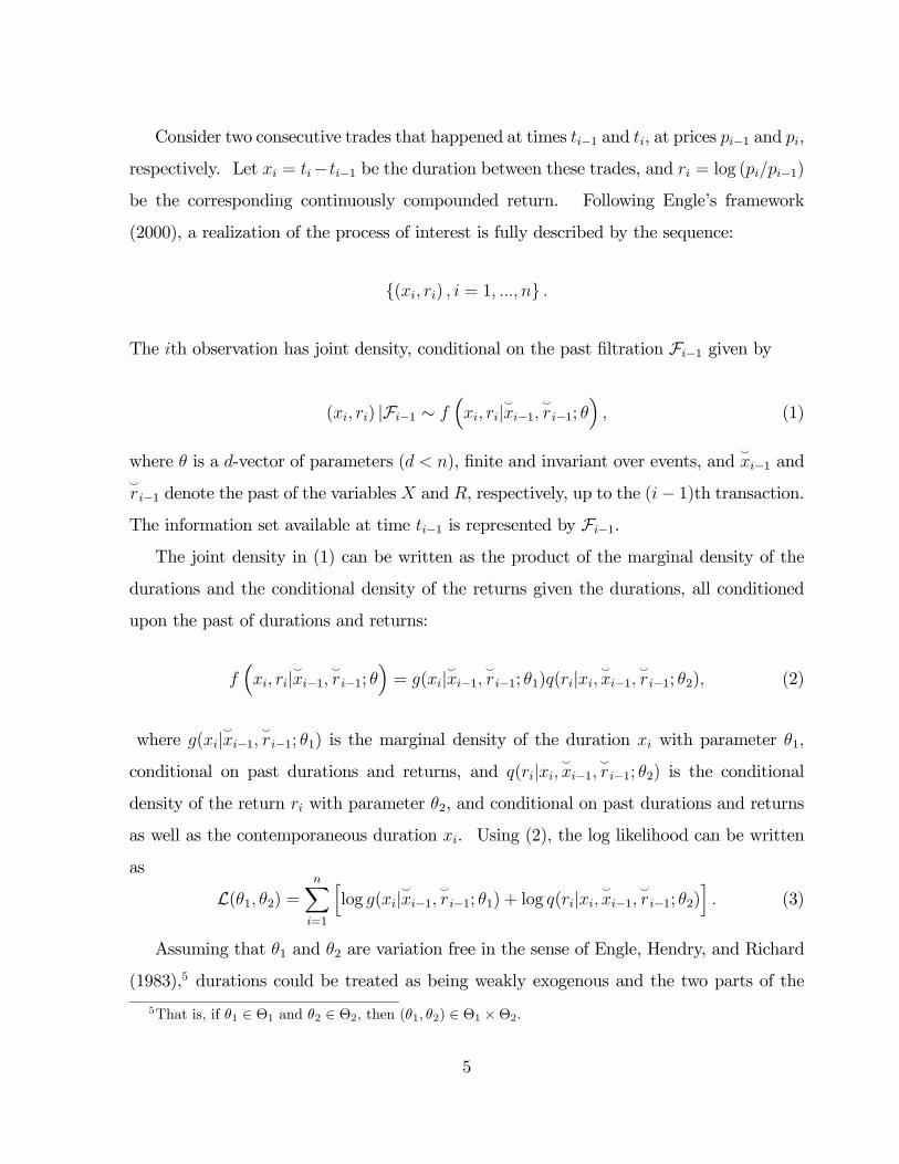
Consider two consecutive trades that happened at times ti−1 and ti, at prices pi−1 and pi,

respectively. Let xi = ti−ti−1 be the duration between these trades, and ri = log (pi/pi−1)be the corresponding continuously compounded return. Following Engle’s framework

(2000), a realization of the process of interest is fully described by the sequence:

{(xi, ri) , i = 1, ..., n} .

The ith observation has joint density, conditional on the past filtration Fi−1 given by

(xi, ri) |Fi−1 ∼ f³xi, ri|`xi−1, `ri−1; θ

´, (1)

where θ is a d-vector of parameters (d < n), finite and invariant over events, and`xi−1 and

`ri−1 denote the past of the variables X and R, respectively, up to the (i− 1)th transaction.The information set available at time ti−1 is represented by Fi−1.

The joint density in (1) can be written as the product of the marginal density of the

durations and the conditional density of the returns given the durations, all conditioned

upon the past of durations and returns:

f³xi, ri|`xi−1, `ri−1; θ

´= g(xi|`xi−1, `ri−1; θ1)q(ri|xi, `xi−1, `ri−1; θ2), (2)

where g(xi|`xi−1, `ri−1; θ1) is the marginal density of the duration xi with parameter θ1,

conditional on past durations and returns, and q(ri|xi, `xi−1, `ri−1; θ2) is the conditionaldensity of the return ri with parameter θ2, and conditional on past durations and returns

as well as the contemporaneous duration xi. Using (2), the log likelihood can be written

as

L(θ1, θ2) =nXi=1

hlog g(xi|`xi−1, `ri−1; θ1) + log q(ri|xi, `xi−1, `ri−1; θ2)

i. (3)

Assuming that θ1 and θ2 are variation free in the sense of Engle, Hendry, and Richard

(1983),5 durations could be treated as being weakly exogenous and the two parts of the

5That is, if θ1 ∈ Θ1 and θ2 ∈ Θ2, then (θ1, θ2) ∈ Θ1 ×Θ2.

5

likelihood function could be maximized separately. However, the evidence suggests that

this assumption is not always valid. In fact, Dolado, Rodriguez-Poo, and Veredas (2004)

reject the null hypothesis of weak exogeneity for seven out of the ten models considered

when analyzing high-frequency data for five stocks traded on the NYSE. Here, we estimate

the two parts of the log-likelihood function simultaneously.

We model the dynamics of trade durations using the log-ACD model proposed by

Bauwens and Giot (2000) (presented in the next subsection) and the price dynamics by

extending Engle’s UHF-GARCH framework (2000) as shown in Section 3.

2.1 The ACD and The Log-ACD Models

Engle and Russell (1998) introduced the ACDmodel as a counterpart of the GARCHmodel

to describe the duration clustering observed in high-frequency financial data. Since then,

a plethora of models has emerged,6 strongly supported theoretically by the recent market

microstructure literature’s emphasis on the information contained in the time between

market events.7

Let ψi be the conditional duration given by

ψi = E(xi|Fi−1) (4)

and supposed to be a nonnegative measurable function of Fi−1.

The ACD model is based on the assumption that all the temporal dependence between

durations is captured by the conditional duration mean function, such that xi/ψi is

independent and identically (i.i.d.) distributed,

xi = ψiεi, (5)

where the process ε = { εi, i ∈ Z} is a strong white noise, that is ε is an i.i.d. process.

6See Bauwens and Giot (2001), and Hautsch (2004) for extensive surveys of the existing models.7See Diamond and Verrecchia (1987), Admati and Pfleiderer (1988), Easley, and O’Hara (1992) among

others.

6

We assume εi to be non-negative with probability one and admit a density p (ε) such that

E(εi) = 1.

By choosing different specifications for the conditional durations in (4) and the density

p (ε) , several forms of the ACD model can be obtained. A popular one is the ACD (m, q)

which is based on a linear parameterization of (4):

ψi = ω +mXj=1

αjxi−j +qX

j=1

βjψi−j , (6)

where ω > 0, αj ≥ 0, j = 1, ...,m and βj ≥ 0, j = 1, ..., q, which are sufficient conditionsto ensure the positivity of the conditional durations.

Several choices can be made for the density p (ε). Engle and Russell (1998) used the

standard exponential distribution (that is the shape parameter is equal to one) and the

standardized Weibull distribution with shape parameter equal to γ and scale parameter

equal to one. The resulting models are called the Exponential ACD (EACD) and the

Weibull ACD (WACD), respectively. The choice of the distribution for the error term

affects the conditional intensity function. The exponential specification implies a flat

conditional hazard function which is quite restrictive and easily rejected in empirical

financial applications (see e.g. Engle and Russell, 1998). The Weibull distribution (that

reduces to the exponential distribution if γ equals 1) allows for a monotonic hazard function

(which is either increasing if γ > 1, or decreasing if γ < 1). For greater flexibility, Grammig

and Maurer (2000) advocate the use of a Burr distribution leading to the Burr ACDmodel,

while Lunde (1999) proposes the generalized gamma distribution. Both distributions allow

for hump-shaped hazard functions to describe situations where, for small durations, the

hazard function is increasing and, for long durations, the hazard function is decreasing.

Once the density function p(ε) is specified, the parameters of the ACDmodel are estimated

using the maximum likelihood estimation technique. In this paper we make use of the

generalized gamma distribution with unit expectation which leads to the so-called GACD

model.

In order to avoid the necessity of imposing non-negativity constraints on the parameters

7

of the conditional mean function, Bauwens and Giot (2000) introduce a logarithmic version

of the ACD model, called the log-ACD model, that specifies the autoregressive equation

on the logarithm of ψi:

ψi = exp

Ãω +

mXj=1

αjεi−j +qX

j=1

βj lnψi−j

!. (7)

Equation (7) is sometimes referred to as a Nelson type ACD model because of its similarity

with Nelson’s EGARCH model (1991). The same hypotheses are made about ε as in the

ACD model and the same probability distribution functions can be chosen. If εi follows

a generalized gamma distribution with parameters γ1, γ2 (γ1 > 0 and γ2 > 0), its density

function is given by

p(ε|γ1, γ2) =

γ1εγ1γ2−1

γγ1γ23 Γ(γ2)

exph−³

εγ3

´γ1i, ε > 0,

0 , elsewhere.

where Γ(·) denotes the gamma function and γ3 = Γ (γ2) /Γ³γ2 +

1γ1

´. The generalized

gamma distribution nests the Weibull distribution when γ2 = 1. Estimation is performed

in the same way as for the ACD model by considering the new specification of ψi.

2.2 The UHF-GARCH model

Once we model the durations between trades conditional on past information, we need to

specify a model for price changes, conditional on the current duration and past information.

Since high-frequency data are irregularly time-spaced, Engle (2000) proposes a GARCH

model that takes into consideration this feature of tick-by-tick data. Let the conditional

variance per transaction be

hi = Vi−1(ri|xi), (8)

8

where the conditioning information set contains the current durations as well as the past

returns and durations. However, as argued by Engle (2000) and Meddahi, Renault and

Werker (2003), the variance of interest is not the "traditional" variance but the variance

per unit of time, naturally defined as:

Vi−1

µri√xi|xi¶= σ2i , (9)

which naturally implies that hi = xiσ2i .

Under the assumption Ei−1 (ri|xi) = 0, the volatility per unit of time is then modeledas a simple GARCH(1,1) process:

σ2i = eω + eαµ ri−1√xi−1

¶2+ eβσ2i−1, (10)

where eω > 0, eα > 0 and eβ > 0.Although it seems natural to model the variance as a function of time when using

irregularly time-spaced data, the above modelling for the unit of time appears as quite

restrictive, since the conditional heteroskedasticity in the returns could depend on time in

a more complicated way. In the next section, we shall propose a useful extension of the

above UHF-GARCH model that is more flexible and seems to provide a better adjustment

of the data, at least in our empirical applications.

3 Monte Carlo IVaR

3.1 IVaR: Definition

To define our IVaR, let Y = {yk, k ∈ Z} be the process of the asset return re-sampled atregular time intervals equal to T units of time. We consider a realization of length n0 of the

process Y {yk; k = 1, ...n0} with yk obtained at times t0k such that t0k − t0k−1 = T. Thus, yk

9

denotes the T -period return which is simply the sum of correspondent tick-by-tick returns

yk =

τ(k)−1Xi=1

ri, (11)

where τ(k) is such that the cumulative duration exceeds T for the first time. This means

thatτ−1Xi=1

xi ≤ T andτXi=1

xi > T.

Thus, by modelling the durations specifically with the ACDmodel, we are able to determine

every τ(k) and keep track of the time step.

The IVaR with confidence level 1− α, is formally defined as

Pr(yk < −IV aRk(α) | Gk) = α. (12)

where Gk denotes the information set that includes all the tick-by-tick data (durationsand returns) up to time t0k . Common confidence levels used in the applications are

1−α = 95%, 97.5%, 99% and 99.5%; we shall consider these values in the empirical study.

It follows from (12) that the IVaR is such that −IV aRk(α) = Qk(α | Gk) where Qk(α | Gk)is the quantile of the conditional distribution of yk.

Various methods exist for computing a VaR: parametric or variance-covariance methods

(e.g. RiskMetrics, GARCH), nonparametric (e.g. Historical Simulation), and semi-

parametric (e.g. CAViar, extreme value theory). We propose a GARCH-type model,

as presented in the next subsection, to specify the time-varying volatility of the tick-by-

tick returns ri and a Monte Carlo simulation approach to simulate the future regularly

spaced returns yk from which the IVaR is computed.

3.2 The Extended UHF-GARCH model

In this subsection, we propose a more flexible specification of the UHF-GARCH model

presented in Section 2.2 in which the time weighting is determined endogenously. We

10

model the volatility of returns as the product of a function of duration and a GARCH

component. More precisely, letVi−1 (ri|xi)

xγi= σ2i , (13)

which implies that

hi = xγi σ2i . (14)

The parameter γ that specifies the duration weighting for the volatility of a particular

stock has to be estimated. This formulation allows us to specify a more general form of

heteroskedasticity in the conditional variance of the returns.

In Section 4, we use transaction prices instead of mid-quotes for forecasting volatility

in an order-driven market. Transaction prices may be affected by various market

microstructure effects, such as nonsynchronous trading and the bid-ask bounce (Tsay,

2002), that may induce serial correlation in high-frequency returns. Therefore, to remove

microstructure effects, we follow Grammig and Wellner (2002) and Ghysels and Jasiak

(1998) and use an ARMA(1,1) model on the tick-by-tick returns:

ri = c+ ϕ1ri−1 + ei + θ1ei−1. (15)

We model the GARCH component as

log σ2i = eω + PXj=1

eβj log σ2i−j + QXj=1

aj

(|ei−j|h1/2i−j−E

Ã|ei−j|h1/2i−j

!)+

QXj=1

eαj

Ãei−jh1/2i−j

!, (16)

where ei = zi√hi and z = {zi, i ∈ Z} denotes a strong white noise, that is the zi’s are i.i.d.

with a zero mean and unit variance. The unknown parameters are c, ϕ1, θ1, eω, eβj, aj, eαj

and γ. When γ = 1 the model is similar, though not equivalent, to Engle’s UHF-GARCH

model (2000) represented by equations (8), (9) and (10). We specify the mean equation

(15) on the returns ri rather than on the returns weighted by a function of durations,

because we want to simulate the future distribution of returns fromwhich the IVaR could be

extracted. As shown in the empirical part of the article, the estimate of parameter γ is far

11

below unity and is statistically significant, at least in our empirical application. When γ =

0, the model becomes a standard GARCH applied to the high-frequency data by ignoring

the irregular spacing of returns when modelling the volatility. The use of an EGARCH(p,q)

model is justified by the advantage of keeping the volatility component positive during

simulations regardless of the variables added to the autoregressive equation. The absence

of non-negativity constraints on the parameters also simplifies numerical optimization.

3.3 Intraday Monte Carlo Simulation

In this subsection, we describe the Monte Carlo simulation approach used for computing the

IVaR based on tick-by-tick data. As the time intervals between consecutive observations

are irregular, the question about how to assess the results needs to be considered. Since the

model we use fully specifies the distribution of returns in event time, one-step forecasts can

be computed analytically. However, we need to run simulations in order to obtain forecasts

of returns in any arbitrary length of calendar time, T . More specifically, the ACDmodel will

define the time step of our simulations and the extended UHF-GARCHmodel introduced in

the previous subsection will generate the corresponding tick-by-tick returns. We compute

the forecasted returns for regular calendar-time intervals as the sum of irregular (tick-by-

tick) intraday returns. Using the simulated distribution of returns over the chosen time

interval T , we calculate the IVaR by extracting the desired percentile. The IVaR obtained

is thus an IVaR for regular time intervals (therefore, comfortably comparable to regular

real returns), but computed using tick-by-tick data and adapted to the non-regularity of

time intervals.

More precisely, we proceed as follows:

(1) The original sample is divided into two parts, one for estimation and one for

forecast/validation. The estimation sub-sample serves to calibrate a log-ACD-GARCH

model for durations and tick-by-tick returns as presented in the previous sections.

(2) We draw random numbers from the standard normal distribution and the standard

generalized gamma distribution, respectively, to compute the innovations which will serve

12

to generate scenarios for future durations, returns, and volatilities.

(3) In order to obtain the simulated durations within the first fixed interval, we forecast

the durations in an iterative way using equations (5) and (7) as long as the sum of forecasted

tick-by-tick durations does not exceed the time interval of interest.

(4) Using equations (14), (15), and (16), we forecast, conditional on the simulated

durations, the tick-by-tick returns corresponding to this first regular interval. By summing

up all these returns we obtain the (regular) return for the first interval.

(5) We continue the procedure until the desired number of fixed intervals or regular

returns is obtained. This corresponds to the first path.

(6) We repeat steps (1) to (5) for the desired number of paths.

(7) For each time-fixed interval, the IVaR corresponds to the quantile of the simulated

distribution of returns for that interval.

(Insert Figure 1 here)

Figure 1 resumes the main steps of the simulation. As one can see, the algorithm

displays similarities with the traditional Monte Carlo simulation used for computing a

multi-period (generally 10-day) VaR. The main difference is at step (3) where we make

use of the ACD model to keep trace of the time step. While, in the standard Monte Carlo

approach the time unit is not very important because all observations are equally spaced,

here we relax this constraint and are able to proceed tick-by-tick by using models adapted

to the irregularity of time intervals, such as the ACD and the UHF-GARCH models. We

illustrate this procedure using real data in the next section.

4 Empirical Study

4.1 Data

In this section we compute the IVaR according to the methodology previously described

using high-frequency data from the "Market Data Equity Trades and Quotes Files" CD-

13

ROM of the Toronto Stock Exchange (TSE). To our knowledge, this is the first econometric

study analyzing (irregular) high-frequency data from the Canadian stock market. Previous

studies used data from the NYSE (e.g., Engle and Russell 1998; Giot 2002), or from

the Paris Bourse (e.g., Jasiak 1998; Gouriéroux, Jasiak and Le Fol, 1999), the German

Stock Exchange (e.g., Grammig and Wellner 2002), and the Moscow Interbank Currency

Exchange (Anatolyev and Shakin 2004). Thus, this study adds another dimension to

previous work. We focus on the Royal Bank of Canada stock (RY) and the Placer Dome

stock (PDG) for the period from April 1st to June 30, 2001 which contains 63 trading

days. The Royal Bank is Canada’s largest bank as measured by market capitalization

(about US$ 33.4 billion) and assets. Placer Dome is Canada’s second largest gold miner

with a market capitalization of US$ 8.2 billion at the end of 2004. Both stocks belong

to the Toronto 35 Index. The Toronto 35 Index was developed by the TSE in 1987 and

consists of the 35 largest and most liquid stocks in Canada. As of April 30, 2001 the

relative weights of the RY stock and PDG stock in the Toronto 35 Index were 4.44% and

1.15%, respectively.

In 1999, the Toronto Stock Exchange (TSE) became Canada’s sole exchange for the

trading of senior equities. The TSE is the seventh largest equities market in the world

as measured by domestic market capitalization, with US$ 1,178 billion at the end of 2004

(source: World Federation of Exchanges Annual Report 2004). The TSE currently trades

equities for approximately 1,485 listed firms, with a daily trading volume averaging CAD$

3,3 billion in 2004. The TSE operates as an automated, continuous auction market. Limit

orders enter the queues of the order book and are matched according to a price-time priority

rule. There is a pre-opening session from 7:00 to 9:30 am during which market participants

can submit orders for possible execution at the beginning of the regular session. The pre-

opening session involves the determination of a Calculated Opening Price (COP) that

equals the price at which the greatest volume of trades can trade or, if it is not unique,

the price at which there is the least imbalance or the price closest to the previous closing

price (see Davies, 2003 for details about the pre-opening session at the TSE and the role

14

of the registered trader at the pre-opening). Regular trading starts at 9:30 and ends at

16:00. Opening trades are at the COP and, as they have a different dynamic we eliminate

them from the empirical analysis . Each stock is assigned to a Registered Trader (RT)

who is required to act as a market maker and to maintain a fair, orderly, and continuous

two-sided market for that stock. The RT contributes to market liquidity and depth and

reduces volatility by buying or selling against the market. He must also guarantee all

oddlot trades and trade all orders of a certain size, known as the Minimum Guaranteed

Fill (MGF) orders, within a set price difference between buy and sell orders. The RT

resembles the specialist at the NYSE but he does not act as an agent for client order flow

and does not have exclusive knowledge of the limit order book. Unlike the NYSE, trading

on the TSE is completely electronic, without any floor trading. An order book open to

subscribers insures a highly transparent market.8

The TSE intraday database contains date-and-time stamped bid-and-ask quotes,

transaction prices, and volume for all firms. Special codes identify special trading

conditions. Prior to the analysis, a couple of operations need to be conducted on the

data. Following the literature, we removed all non-valid trades and interdaily durations

and kept only those transactions made during regular trading hours. As alreadymentioned,

open trades are also deleted in order to avoid effects induced by the opening auction. For

simultaneous transactions, we consider a weighted average price and remove all remaining

observations with this time stamp, thus considering these observations as split transactions.

Previous studies dealing with high-frequency data commonly used mid-quotes instead of

transaction prices (e.g., Engle 2000, Engle and Lange 2001, Manganelli 2002). While this

may be appropriate for the NYSE which is a quote-driven market, working with transaction

prices appears a better choice in our case since we are interested in VaR estimation and

want to forecast returns for real transactions. To liquidate positions in an order-driven

market one has to transact either on the ask or the bid and therefore using the midquote-

8The future of traditional floor trading at the NYSE was questioned after the merger on April 20, 2005of the NYSE with the electronic trading network Archipelago.

15

change quantiles may understate the true VaR.9

Extremely large durations and returns between two successive trades are very unlikely,

therefore we filter out all the observations with absolute returns larger than 10 standard

deviations and durations larger than 25 standard deviations, resulting in 2 outliers for

the RY stock and 9 outliers for the PDG stock. These leaves us with a total of 51,660

observations for the RY stock and 27,956 observations for the PDG stock.

(Insert Figure 2 here)

Figure 2 displays the histograms of the transaction returns for the two stocks considered.

The price increment for the two stocks RY and PDG for the period analyzed was one penny

(C$0.01)10 We observe a disproportionately large number of zero returns (almost 60%)

which seems rather typical for high-frequency data, especially for single stocks. For the

IBM dataset used by Engle and Russell (1998), Tsay (2002, p.182) reported that about

two-thirds of the intraday transactions were without price change. Gorski, Drozdz and

Speht (2002) report the same phenomenon for DAX11 returns and call it the zero return

enhancement. Bertram (2004) also finds a large number of zero price changes for equity

data from the Australian Stock Exchange and argues that zero returns follow from the

absence of significant new information on the market. According to the efficient market

hypothesis, a price changes when new information arrives on the market and, consequently,

traders simply continue to trade at the previous price when the amount of information is

insufficient to move the price.

Information about the raw data is given in Table 1. Of the two stocks, RY with an

average duration of almost 29 seconds is traded almost twice as frequently as PDG, while

PDG is traded on average every minute. We also note overdispersion of durations, i.e.,

the standard deviation is higher than the mean. This is typically found in the literature

9We are grateful to Joachim Grammig for shedding light on this issue.10Starting on January 29, 2001 the TSE introduced the penny tick size for stocks selling at over $0.50.11Deutsche Aktienindex (DAX) represents the index for the 30 largest German companies quoted on the

Frankfurt Stock Exchange.

16

for the trade duration process and it may suggest that the exponential distribution cannot

properly describe the durations. The transaction returns have a sample mean equal to

zero for both stocks and a standard deviation equal to 0.001 and 0.002, respectively. RY

exhibits positive sample skewness while PDG has a negative skewness. Both stocks’ returns

display a kurtosis higher than that of a normal distribution.

(Insert Table 1 here)

4.2 Seasonal Adjustment

As noted by Engle and Russell (1998), high-frequency data exhibits a strong intraday

seasonality explained by the fact that markets tend to be more active at the beginning

and towards the end of the day. While most of the studies on high-frequency data ignore

interday variations in variables, Anatolyev and Shakin (2004) found that durations and

return volatilities of the Russian stocks considered fluctuate throughout different trading

days. To prevent the distortion of results, these interday and intraday seasonalities must

be taken out prior to the estimation of any model . We inspected our data for such

evidence. We noted for example that durations are higher on Mondays and Fridays than

during the rest of the week. A Wald test in a regression of average RY durations on

five day-of-the-week dummies rejects the null hypothesis of equality of all coefficients, thus

providing evidence of interday seasonal effects. No interday effects are identified for PDG

durations and returns. When found, we remove interday seasonality under a multiplicative

form, following the approach taken by Anatolyev and Shakin (2004):

xt,inter =xtxs, (17)

rt,inter =rtpr2s

, (18)

where xs corresponds to the average duration for day s if observation t belongs to day s,

and r2s is the average of squared returns for day s.

17

To take out the time-of-day effect, Engle and Russell (1998) suggest computing

"diurnally adjusted" durations by dividing the raw durations by a seasonal deterministic

factor related to the time at which the duration was recorded. We obtain intraday

seasonally adjusted (isa) durations and returns in the following way:

xt,intra =xt,inter

E(xt,inter|Ft−1),

rt,intra =rt,interq

E(r2t,inter|Ft−1).

where the expectation is computed by averaging the variables over thirty-minute intervals

for each day of the week and then using cubic splines on the thirty-minute intervals to

smooth the seasonal factor. Thus, intraday patterns are different for different days of

the week. Figures 3 and 4 show, respectively, the estimated intraday factor for durations

and squared returns for the RY stock. Similar seasonal-factors patterns are found for the

PDG stock and therefore they are not reported. The patterns are analogous to what has

been found in previous studies. Durations are shorter at the beginning and at the end of

the day and longer in the middle. The return volatility is lower in the middle of the day

than at the beginning and at the end. This reflects the behavior of traders who are very

active at the beginning of the trading session and adjust their positions to incorporate the

overnight change in information. Towards the end of the day, traders are changing their

positions in anticipation of the close and to pre-empt the risk posed by any information

that could arrive during the night. We also notice a difference between the patterns for

different days.

(Insert Figures 3 and 4 here)

Descriptive statistics for deseasonalised data are given in Table 2. We notice the

salient features of high-frequency data, such as overdispersion in trade durations and high

autocorrelations. The Ljung-Box statistics for fifteen lags Q(15) tests the null hypothesis

18

that the first 15 autocorrelations are zero. The large values of these statistics greatly

exceed the 5% critical value of 25, indicating strong autocorrelation of both durations and

returns. The skewness is close to zero for both stocks. There is still excess kurtosis for

both stocks even if at a lesser degree compared to the raw data. We chose the normal

distribution when estimating the GARCH model and we obtained satisfactory simulation

results. It is well known that the conditional normality assumption in ARCH models

generates some degree of unconditional excess kurtosis (see, e.g., Bollerslev et al., 1992).

(Insert Table 2 here)

4.3 Estimation Results

In this section we apply the model presented in Sections 2 and 3 to the deseasonalised data

for the two stocks. Observations of the first month are used for estimation and those of the

last two months serve for forecast and validation. The likelihood function is maximized

using Matlab v. 7 with the Optimization toolbox v. 3.0 and numerical derivatives are used

for computing the standard errors of the estimates.

We first tested our durations for the clustering phenomenon using the test of Ljung-Box

with 15 lags, Q(15). The high coefficients (reported in Table 2) suggest the presence of

ACD effects in our durations data at any reasonable significance level. The high positive

serial dependence of the squared returns greatly exceeding the critical values, as illustrated

by the Ljung-Box test statistics, noted Q2(15), represents evidence of volatility clustering

and justifies the application of a GARCH-type model.

Estimation results are presented in Table 3 together with the p-values for the adequacy

tests applied to the standardized residuals. We tried to find the best fit for our data and

reestimated the model chosen without the variables that were statistically insignificant.

We tested the adequacy of the log-GACD model using the Ljung-Box test applied to the

standardized residuals.12 We judged the quality of the GARCH fit using the Ljung-Box

12We have also applied the test statistics for ACD adequacy introduced by Duchesne and Pacurar (2005)using the Bartlett kernel. The results are similar and therefore not reported.

19

tests for standardized residuals and their squares.

(Insert Table 3 here)

We retain a log-GACD(2,2)-ARMA(1,1)-UHF-EGARCH(1,1) model for our data. We

find that a log-GACD(2,2) specification is successful in removing the autocorrelation in

durations. For both stocks the p-values of the Ljung-Box test with 15 lags are superior

to 0.05. The parameters of the generalized gamma distribution are all significant. For

each stock, the sum of the autoregressive parameters β1+β2 is close to one, revealing high

persistence in durations.

With regard to the high-frequency returns, the ARMA(1,1)-UHF-EGARCH(1,1)

specification accounts satisfactorily for the dependence of both the returns and squared

returns of the PDG stock, as evidenced by the p-values of the order-15 Ljung-Box test

statistics that are all greater than 0.05. For the RY stock, the Ljung-Box test statistics

indicate that some serial dependence is still present in the data, which is inconsistent with

the model’s adequacy. However, the dependence is dramatically reduced compared to the

original data. The Ljung-Box statistic with 15 lags Q(15) for autocorrelation of returns

was reduced from 8195 to 62 (the associated 95% critical value being 24.99). Similarly,

the Ljung-Box statistic Q2(15) for autocorrelation of squared returns was reduced from

15417 to 36. Similar results have been found by Engle (2000) using Ljung-Box test

statistics. The problem of passing tests of model adequacy seems to remain an issue

when using irregular high-frequency data. We have tried higher-order models both for

the mean and the variance equations but we have not been able to gain any considerable

improvement. We keep the ARMA(1,1) - UHF- EGARCH(1,1) specification of the model

for its parsimony and because we are rather interested in assessing its forecasting ability

under a risk management framework. As in Engle (2000), theMA(1) coefficient represented

by θ1 is negative and highly significant for both stocks. The AR(1) term represented by

ϕ1 is positive. This can be explained by the fact that traders split large orders into

smaller orders to obtain a better price overall and therefore make prices move in the same

direction and thus induce a positive autocorrelation of returns (Engle and Russell, 2005).

20

The positive autocorrelation can also be related to negative feedback trading (Sentana and

Wadhwani, 1992). Engle (2000) has also found evidence of positive autocorrelation in

high-frequency returns. The autoregressive parameter fβ1 for the EGARCH(1,1) modelis close to one for the RY stock, indicating a higher persistence in volatility than for the

PDG stock. The parameter fα1 is statistically insignificant (not reported in the table) forboth stocks, so no leverage effect is supported. The parameter γ is approximately equal

to 0.05 for both stocks and it is statistically different from zero.

Now that we have calibrated the model to our data, we may proceed to the simulation

of future durations and returns.

4.4 IVaR Backtesting

In this section we simulate tick-by-tick durations and returns using the estimated

coefficients of our model and the observations of the last day as starting values. We

sum up the irregular simulated returns over a fixed-time interval. Five different interval

lengths are used: 15, 25, 35, 45 and 90. Since all models are applied on deseasonalised data,

the time unit of the interval does not represent a calendar unit (e.g. seconds, minutes).

A correspondence can nevertheless be established for each stock given the number of

resampled intervals generated, depending on the trading intensity of that stock for the

44 days of the validation period. For example, a length = 15 for the RY stock results in

2470 intervals for 44 trading days, which is equivalent to an average interval of 7 minutes.

Assessing the results in a regularly spaced framework allows us to evaluate the performance

of the model in a traditional way, thus circumventing the problem of finding an appropriate

benchmark. We have generated 5000 independent paths and we have extracted the IVaR

as a percentile from the simulated distribution of returns.

We first analyze the performance of the model by using Kupiec’s test (1995) for the

percentage of failures, which is also embedded in the regulatory requirements on the

backtesting of VaR models. Using a standard procedure in the literature, we compute the

empirical failure rate (bα) as the percentage of times actual returns (yk) are greater than21

the estimated IVaR. If the IVaR estimates are accurate, the failure rate should equal α.

Kupiec’s test checks whether the observed failure rate is consistent with the frequency of

exceptions predicted by the IVaR model. Under the null hypothesis that the model is

correct we have bα = α and Kupiec’s likelihood ratio statistic takes the form:

LR = 2£ln(bαm(1− bα)n−m)− ln(αm(1− α)n−m)

¤where m is the number of exceptions and n is the sample size. This likelihood ratio is

asymptotically distributed as a χ2(1) under the null hypothesis. The left panels of Tables

4 and 5 show the p-values for the Kupiec test for the two stocks with a 5%, 2.5%, 1%

and 0.5% IVaR level. Bold entries denote a failure of the model at the 95% confidence

level, since the p-value is inferior to 0.05. The results show that the model performs well

for both stocks. For almost all the intervals and the tails considered the p-values are

superior to 0.05. The only exception is for smallest interval (T = 15) and higher VaR

levels (α = 5%, 2.5%) which could be explained by the fact that the interval length is too

small for obtaining non-zero returns when resampling the tick-by-tick real returns and,

therefore, the theoretical number of IVaR violations cannot be achieved. For an interval

equal to 25 and a 5% IVaR level, the model is rejected at a 95% confidence level but not

at a 97.5% confidence level.

We also apply the dynamic quantile (DQ) test of Engle and Manganelli (2004) to check

for another property a VaR measure should display: the hits (IVaR violations) should not

be serially correlated. According to Engle and Manganelli (2004), this can be tested by

defining a sequence:

Hitk ≡ I (yk < −IV aRk)− α.

The expected value of Hitk is 0 and the DQ test is computed using the regression of

the variable Hitk on its past, on current IVaR, and any other variables:

Hitk = XB + k

22

Then, DQ = bB0X 0X bB/(α(1− α)) ∼ χ2(l), where l is the number of explanatory variables

and bB is the OLS estimate of B. We perform the test using 5 lags of the hits and the

current IVaR as explanatory variables. Results are given in the right panels of Tables

4 and 5 which report the p-values of the DQ test. The results are satisfactory for the

RY stock and coherent with the results from Kupiec’s test. In most cases the p-values

are larger than 0.05. For the PDG stock, some estimates still show some predictability,

especially for the smallest interval. Overall, it seems that the model performs best for the

two stocks when a 1% IVaR level is considered.

(Insert Tables 4 and 5 here)

Figure 5 illustrates the typical IVaR profile obtained from the model. One might

argue that the Monte Carlo simulation is very time-consuming. While this may be true

for backtesting purposes that generally require a sufficiently large number of validation

intervals, computing the next forecasted IVaR (which is normally required for practical

purposes) is reasonably fast. For example, producing the next IVaR with a Pentium

4, one CPU 3.06 GHz and 5000 simulated paths for an interval equal to 90, takes us

approximately 3.5 minutes for each of the two stocks considered. For our samples, an

interval equal to 90 corresponds on average to 41 minutes for RY and 79 minutes for PDG.

The computing time can easily be reduced to less than one minute by using more than one

CPU.

(Insert Figure 5 here)

5 Conclusion

In this paper, we have proposed a way of computing intraday Value at Risk using tick-

by-tick data within the UHF-GARCH framework introduced by Engle (2000). Our

specification of the UHF-GARCH model is more flexible than that of Engle (2000) since

it endogenizes the definition of the time unit and lets the data speak for themselves. We

23

applied our methodology to two actively traded stocks from the TSE (RY and PDG).

While the literature is full of efforts to develop sophisticated VaR models for daily data,

here we investigate the use of irregularly time-spaced intraday data for risk management.

This is particularly useful for defining an IVaR appropriate for agents who are very active

in the market. As a by-product of our study, we provide an out-of-sample evaluation

of the predictive abilities of an UHF-GARCH model in a risk management framework, a

question that has not yet been addressed in the literature.

We developed an intraday Monte Carlo simulation approach which enabled us to

forecast high-frequency returns for any arbitrary interval length, thus avoiding complicated

time manipulations in order to return to a convenient regularly spaced framework. In

our setup the ACD model yields the consecutive steps in time while the UHF-GARCH

model allows us to simulate the corresponding conditional tick-by-tick returns. Regularly

spaced intraday returns are simply the sum of tick-by-tick returns simulated conditional

on the forecasted duration. We considered using a normal distribution to estimate the

UHF-GARCH model but, instead of using the predicted volatility given by that model

and computing the VaR in a parametric way, we preferred to simulate the distribution

of returns and extract the IVaR from it. Therefore, the approach is not totally model

dependent.

Our results for the RY and PDG stocks indicate that the UHF-GARCHmodel performs

well out-of-sample even when normality is assumed for the distribution of the error term,

provided that the intraday seasonality has been accounted for prior to the estimation.

This may be explained by the fact that we use a semiparametric method for computing

the VaR as an empirical quantile from the simulated distribution of returns. In this way, it

becomes possible to define an IVaR for any horizon of interest based on tick-by-tick data.

Thus, our methodology for computing VaR with tick-by-tick data may constitute a reliable

approach for measuring intraday risk.

Potential users of our approach would be traders who need intraday measures of risk;

brokers and clearing firms looking for more accurate computations of margins; or any

24

other entity interested in computing the VaR during a trading day in order to improve

risk control. To compute the next IVaR using the method we propose, one has to monitor

the time using the starting time (i.e. 11 a.m.) and the simulated durations for each path

and, consequently, to apply the appropriate seasonal factors to re-introduce both interday

and intraday seasonality in returns. The IVaR extracted from the simulated raw returns

then has the usual interpretation.

Several extensions follow naturally from this study. First, a comparison of the VaR

based on tick-by-tick data with predictions obtained from volatility models of the ARCH

type (on regularly spaced observations) and realized volatility models in the spirit of Giot

and Laurent (2004) would help clarifying the advantage of each approach. Second, one may

wonder whether banks could benefit from incorporating tick-by-tick information into their

VaR models. Financial institutions and particularly banks currently compute the 1-day

VaR based on end-of-day positions, taking into account only daily closing prices and thus

ignoring possibly wide intraday fluctuations and, consequently, the risks associated with

them. Therefore, one could use our approach to see whether better results can be obtained

by using all the trade information available in intraday databases rather than extracting a

single observation to characterize the activity of a whole day. Third, the impact of using

more sophisticated UHF-GARCH models together with distributions that account for fat

tails and the excessive number of zero returns could also be investigated. Fourth, given

that several methods for dealing with the intraday seasonality have been proposed in recent

literature, one may study the impact of different deseasonalization procedures on the IVaR

estimates. Finally, a challenging but rewarding extension would be the development of a

portfolio IVaR based on irregularly time-spaced high-frequency data.

One may argue that the true VaR is underestimated by using transaction data since

transactions are observed only if the spread is favorable to the trader. In this respect,

since transaction events are certainly timed liquidity risk is not taken into account 13. A

VaR based on knowledge of the order book such as that proposed by Giot and Grammig

13We thank Joachim Grammig for pointing it out.

25

(2005) could provide an upper bound of the estimate.

26

References

[1] Admati, A.R. and P. Pfleiderer (1988), "A Theory of Intraday Patterns: Volume and

Price Variability," Review of Financial Studies, 1, 3-40.

[2] Anatolyev, S. and D. Shakin (2004), "Trade Intensity in an Emerging Stock Market:

New Data and a New Model," working paper, New Economic School.

[3] Andersen, T., T. Bollerslev, F. Diebold and P. Labys (2000), "Exchange Rate Returns

Standardized by Realized Volatility Are (Nearly) Gaussian," Multinational Finance

Journal, 4, 159-179.

[4] Andersen, T., T. Bollerslev, F. Diebold and H. Ebens (2001a), "The Distribution of

Realized Stock Return Volatility," Journal of Financial Economics, 61, 43-76.

[5] Andersen, T., T. Bollerslev, F. Diebold and P. Labys (2001b), "The Distribution of

Realized Exchange Rate Volatility," Journal of the American Statistical Association,

96, 42-55.

[6] Andersen, T., T. Bollerslev, F. Diebold and P. Labys (2001c), "Modeling and

Forecasting Realized Volatility," working paper 01-01, The Wharton School.

[7] Basle Committee on Banking Supervision (1996), "Overview of the Amendment to

the Capital Accord to Incorporate Market Risks," 11 pages, Basle, Switzerland.

[8] Bauwens, L. and P. Giot (2000), "The Logarithmic ACDModel: an Application to the

Bid-Ask Quote Process of Three NYSE Stocks," Annales d’Économie et de Statistique,

60, 117-149.

[9] Bauwens, L. and P. Giot (2001), Econometric Modelling of Stock Market Intraday

Activity, Advanced Studies in Theoretical and Applied Econometrics, Kluwer

Academic Publishers: Dordrecht, 196 pages.

27

[10] Beltratti, A. and C. Morana (1999), "Computing Value-at-Risk with High Frequency

Data," Journal of Empirical Finance, 6, 431-455.

[11] Bertram, W.K. (2004), "A Threshold Model for Australian Stock Exchange Equities,"

working paper, School of Mathematics and Statistics, University of Sydney.

[12] Bollerslev, T., R.Y. Chou and K.F. Kroner (1992), "ARCH Modeling in Finance - A

Review of the Theory and Empirical Evidence," Journal of Econometrics, 52, 5-59.

[13] Burns, P. (2002), "The Quality of Value at Risk via Univariate GARCH," Burns

Statistics working paper, http://www.burns-stat.com.

[14] Campbell, J.H., A.W. Lo and A.C. MacKinlay (1997), The Econometrics of Financial

Markets, Princeton University Press, 632 pages.

[15] Christoffersen, P.F. (2003), Elements of Financial Risk Management, Academic Press:

San Diego, 214 pages.

[16] Davies, R.J. (2003), "The Toronto Stock Exchange Preopening Session," Journal of

Financial Markets, 6, 491-516.

[17] Diamond, D.W. and R.E.Verrechia (1987), "Constraints on Short-Selling and Asset

Price Adjustments to Private Information," Journal of Financial Economics, 18, 277-

311.

[18] Dolado, J.J., J. Rodriguez-Poo and D. Veredas (2004), "Testing Weak Exogeneity in

the Exponential Family: An Application to Financial Point Processes," Discussion

Paper 2004/49, CORE, Université Catholique de Louvain.

[19] Duchesne, P. and M. Pacurar (2005), "Evaluating Financial Time Series Models for

Irregularly Spaced Data: A Spectral Density Approach," Computers & Operations

Research, forthcoming.

28

[20] Easley, D. and M. O’Hara (1992), "Time and the Process of Security Price

Adjustment," Journal of Finance, 47, 577-606.

[21] Engle, R.F., D.F. Hendry and J.-F. Richard (1983), "Exogeneity," Econometrica, 51,

277-304.

[22] Engle, R.F. and J.R. Russell (1998), "Autoregressive Conditional Duration: a New

Model for Irregularly Spaced Transaction Data," Econometrica, 66, 1127-1162.

[23] Engle, R.F. (2000), "The Econometrics of Ultra-High Frequency Data," Econometrica,

68, 1-22.

[24] Engle, R.F. and J. Lange (2001), "Measuring, Forecasting and Explaining Time

Varying Liquidity in the Stock Market," Journal of Financial Markets, 4 (2), 113-

142.

[25] Engle, R.F. and S. Manganelli (2004), "CAViaR: Conditional Autoregressive Value

at Risk by Regression Quantiles," Journal of Business and Economic Statistics, 22,

367-381.

[26] Engle, R.F. and J.R. Russell (2005), "Analysis of High Frequency Data," forthcoming

in Handbook of Financial Econometrics, ed. by Y. Ait-Sahalia and L. P. Hansen,

Elsevier Science: North-Holland.

[27] Ghysels, E. and J. Jasiak (1998), "GARCH for Irregularly Spaced Financial Data:

The ACD-GARCH Model," Studies in Nonlinear Dynamics & Econometrics, 2(4),

133-149.

[28] Giot, P. (2002), "Market Risk Models for Intraday Data," Discussion Paper, CORE,

Université Catholique de Louvain, forthcoming in the European Journal of Finance.

[29] Giot, P. and J. Grammig (2005), "How Large is Liquidity Risk in an Automated

Auction Market ?" Empirical Economics, forthcoming.

29

[30] Giot, P. and S. Laurent (2004), "Modelling Daily Value-at-Risk Using Realized

Volatility and ARCH Type Models," Journal of Empirical Finance, 11, 379-398.

[31] Gorski, A.Z., S. Drozdz and J. Speth (2002), "Financial Multifractality and Its

Subleties: An Example of DAX," Physica A, 316, 496-510.

[32] Gouriéroux, C. and J. Jasiak (1997), "Local Likelihood Density Estimation and Value

at Risk," working paper, York University.

[33] Gouriéroux, C., J. Jasiak and G. Le Fol (1999), "Intra-day Market Activity," Journal

of Financial Markets, 2, 193-226.

[34] Grammig, J. and K.-O. Maurer (2000), "Non-Monotonic Hazard Functions and the

Autoregressive Conditional Duration Model," Econometrics Journal, 3, 16-38.

[35] Grammig, J. and M. Wellner (2002), "Modeling the Interdependence of Volatility and

Inter-Transaction Duration Processes," Journal of Econometrics, 106, 369-400.

[36] Hautsch, N. (2004), Modelling Irregularly Spaced Financial Data — Theory and

Practice of Dynamic Duration Models, Lecture Notes in Economics and Mathematical

Systems, Vol. 539, Springer: Berlin, 291 pages.

[37] Jasiak, J. (1998), "Persistence in Intertrade Durations," Finance, 19, 166-195.

[38] Jorion, P. (2000), Value at Risk: The New Benchmark for Managing Financial Risk,

McGraw-Hill, 544 pages.

[39] Kupiec, P. (1995), "Techniques for Verifying the Accuracy of Risk Measurement

Models," Journal of Derivatives, 2, 73-84.

[40] Lunde, A. (1999), "A Generalized Gamma Autoregressive Conditional Duration

Model," discussion paper, Aalborg University.

[41] Manganelli, S. (2002), "Duration, Volume and Volatility Impact of Trades," working

paper no. 125, European Central Bank.

30

[42] Meddahi, N., E. Renault and B. Werker (2003), "GARCH and Irregularly Spaced

Data," Economics Letters, forthcoming.

[43] Nelson, D.B. (1991), "Conditional Heteroskedasticity in Asset Returns: A New

Approach," Econometrica, 59, 347-370.

[44] O’Hara, M. (1995),Market Microstructure Theory, Blackwell Publishers: Malden, 304

pages.

[45] Pritsker, M. (2001), "The Hidden Dangers of Historical Simulation," working paper

2001-27, Federal Reserve Board, Washington.

[46] Sentana, E. and S. Wadhwani (1992), "Feedback Traders and Stock Return

Autocorrelations: Evidence from a Century of Daily Data," Economic Journal, 102,

415-425.

[47] Tsay, R.S. (2002), Analysis of Financial Time Series, Wiley: New York, 472 pages.

31

Figure 1: Illustration of the Intraday Monte Carlo Simulation Approach :

Path 1: x111+ x112+… = T => r11, r12, …, r1P

Path 2: x211+ x212+… = T => r21, r22, …, r2P

.

.

.

Path B: xB11+ xB12+… = T => rB1, rB2, …, rBP

IVaR1 IVaR2 …IVaRP

EstimationLog-ACDUHF-GARCH

B is the number of independently simulated paths. T is the length of the chosen timeinterval. P is the number of regular intervals used for validation. xijk is the k trade durationcorresponding to the path i for the interval j. r ij is the regular return corresponding to theinterval j for the path i. i = 1,...,B. j = 1,...,P. k = 1, ..., t such that

Ptk=1 xijk 6 T andPt+1

k=1 xijk > T.

Figure 2: Histograms of Intraday Returns for Royal Bank (RY) and Placer Dome(PDG).

-0.01 -0.005 0 0.005 0.010

10

20

30

40

50

60

70

Returns

Freq

uenc

y (%

)RY

-0.02 -0.01 0 0.010

10

20

30

40

50

60

70

Returns

Freq

uenc

y (%

)

PDG

Figure 3: Estimated Intraday Factors for RY Durations

Figure 4: Estimated Intraday Factors for RY Squared Returns

Figure 5: Intraday Returns vs IVaR for RY (interval = 45 or 22 minutes)

Table 1: Descriptive Statistics of Raw Data for Royal Bank (RY) and Placer Dome(PDG) Stocks

Mean Std. dev Skew Kurt Max MinDurationsRY 28.44 35.19 2.98 17.54 526 1PDG 52.59 82.11 5.04 59.87 2248 1ReturnsRY 0.000 0.001 0.024 9.890 0.011 -0.011PDG 0.000 0.002 -0.169 11.195 0.018 -0.020

The sample period runs from April 1st to June 30, 2001. It consists of 51,660 observationsfor the RY stock and 27,956 observations for the PDG stock. Mean is the sample mean, Std. devis the sample standard deviation, Skew is the sample skewness coefficient, Kurt is the samplekurtosis, Max is the sample maximum, Min is the sample minimum.

Table 2: Descriptive Statistics of Deseasonalised Data for Royal Bank (RY) and PlacerDome (PDG) Stocks

Mean Std. dev Skew Kurt Max Min Q(15) Q2(15)DurationsRY 0.99 1.14 2.50 12.36 16.68 0.01 1325 387PDG 0.93 1.50 7.68 170.59 63.33 0.01 5015 185ReturnsRY 0.000 0.815 0.005 7.560 5.960 -6.422 8196 15417PDG 0.001 0.890 -0.009 6.735 6.404 -6.421 2355 3118

The sample period runs from April 1st to June 30, 2001. It consists of 51,660 observationsfor the RY stock and 27,956 observations for the PDG stock. Mean is the sample mean, Std. devis the sample standard deviation, Skew is the sample skewness coefficient, Kurt is the samplekurtosis, Max is the sample maximum, Min is the sample minimum. Q(15) is the Ljung-Boxtest statistics with 15 lags, Q2(15) is the Ljung-Box test statistics applied to squared returnsusing 15 lags. The associated 95% critical value is 24.996.

Table 3: Estimates of ACD-GARCH Models

RY PDGParameter Estimate t-Student Estimate t-Student

β0 -0.017 -30.46 -0.030 -19.26α1 0.075 129.13 0.137 86.58α2 -0.057 -99.32 -0.105 -67.24β1 1.391 265.93 1.421 313.17β2 -0.408 -77.41 -0.434 -95.49γ1 0.425 95.04 0.391 55.36γ2 4.444 50.26 3.772 29.42φ1 0.069 4.11 0.078 2.58θ1 -0.605 -48.50 -0.369 -13.34ω -0.032 -9.27a1 0.242 22.58 0.221 8.25fβ1 0.921 232.00 0.778 19.59γ 0.055 3.15 0.057 2.33

p-value Qd(15) 0.182 0.611p-value Q(15) 0.000 0.208p-value Q2(15) 0.002 0.833

This table contains the parameters estimates of the ACD-GARCH models for RY and PDG.t-Student are the t-statistics associated with the parameters estimates. p-value Qd(15) representsthe p-value associated with the Ljung-Box test statistic computed with 15 lags applied to the ACDstandardized residuals. p-value Q(15) and p-value Q2(15) represent, respectively, the p-valuesof the Ljung-Box test statistic computed with 15 lags for serial correlation in the standardizedEGARCH residuals and in their squares.

Table 4: IVaR Results for RY

Kupiec test DQ testVaR level

T5% 2.5% 1% 0.5% 5% 2.5% 1% 0.5% N

15 0.000 0.000 0.154 0.694 0.000 0.021 0.879 0.672 247025 0.036 0.231 0.928 0.317 0.365 0.344 0.360 0.003 143435 0.153 0.792 0.969 0.624 0.208 0.444 0.999 0.329 101245 0.862 0.914 0.676 0.632 0.974 0.881 0.999 0.982 78190 0.592 0.903 0.651 0.957 0.220 0.847 0.992 0.999 385

This table contains the p-values for Kupiec’s test and the DQ test of Engle and Manganelli(2004) using 5 lags and the current VaR as explicative variable. T is the length of the intervalused for simulation. N represents the number of intervals used for validation. Bold entriesdenote a failure of the model at the 95% confidence level since the p-values are inferior to 0.05.

Table 5: IVaR Results for PDG

Kupiec test DQ testVaR level

T5% 2.5% 1% 0.5% 5% 2.5% 1% 0.5% N

15 0.000 0.018 0.577 0.560 0.009 0.304 0.041 0.000 129425 0.642 0.837 0.837 0.678 0.387 0.251 0.063 0.000 75535 0.762 0.944 0.274 0.675 0.136 0.001 0.991 0.992 53045 0.121 0.692 0.662 0.531 0.038 0.670 0.568 0.711 40990 0.762 0.215 0.994 0.381 0.544 0.590 0.934 0.645 201

This table contains the p-values for Kupiec’s test and the DQ test of Engle and Manganelli(2004) using 5 lags and the current VaR as explicative variable. T is the length of the intervalused for simulation. N represents the number of intervals used for validation. Bold entriesdenote a failure of the model at the 95% confidence level since the p-values are inferior to 0.05.