
The Aga Khan Development Network - A Case Study of Karachi's Health Service Research Proposal
Upload
khangminh22Category
view
3download
0
Interscience Research Network Interscience Research Network
Interscience Research Network Interscience Research Network
Conference Proceedings - Full Volumes IRNet Conference Proceedings
Fall 9-16-2012
Proceeding of International Conference on Future Trend in Proceeding of International Conference on Future Trend in
Electrical, Electronics and Computer Science Engineering Electrical, Electronics and Computer Science Engineering
Prof. (Dr.) Srikanta Patnaik
Follow this and additional works at: https://www.interscience.in/conf_proc_volumes
Part of the Computational Engineering Commons, Computer Engineering Commons, and the Electrical
and Computer Engineering Commons
Editorial
Education has now become the instrument fashioned by men to achieve life’s goals. As, it is being well
observed by The Great Rabindra Nath Tagore “He who sees all being in his own self and his own self in all
beings, he does not remain unrevealed”, that should be the motto of our Indian educational Institutions. Science
had become the twilight in this dark era without science life will become hell . The conference is a thought
provoking outcome of all these interrelated facts.
Electrical, Electronics and Computer Science is the scientific and mathematical approach to computation, and
specifically to the design of computing machines and processes. Its subfields can be divided into practical
techniques for its implementation and application in computer systems and purely theoretical areas. Some, such
as computational complexity theory, which studies fundamental properties of computational problems, are
highly abstract, while others, such as computer graphics, emphasize real-world applications. Still others focus
on the challenges in implementing computations. Modern society has seen a significant shift for Electrical,
Electronics and Computer Science which is being used solely by experts or professionals to a more widespread
user base.
The idea of the conference is for the scientists, scholars, engineers and students from the Universities all around
the world and the industry to present ongoing research activities, and hence to foster research relations between
the Universities and the Industry. This conference provides opportunities for the delegates to exchange new
ideas and application experiences face to face, to establish business or research relations and to find global
partners for future collaboration. Through this conference IRNet provides a forum for Research and
Development.Moreover,it encourages academicians and researchers from all types of institutions and
organizations. It aims to provide the platform for all to interact and share the domain knowledge with each
other. Its motto to bring together developers, users, academicians and researchers for sharing and exploring new
areas of research and development.
Prof. (Dr.) Srikanta Patnaik
Chairman, I.I.M.T., Bhubaneswar
Intersceince Campus,
At/Po.: Kantabada, Via-Janla, Dist-Khurda
Bhubaneswar, Pin:752054. Orissa, INDIA
International Conference on Electronics and Communication Engineering (ICECE) -16th Sept, 2012, Pune- ISBN: 978-93-82208-18-1
1
MICROCONTROLLER BASED E – AGRICULTURE SYSTEM WITH VIDEO MONITORING
1UMESH D DIXIT & 2MALLANAGOUD N PATIL
1&2 Department of Electronics & Communication Engineering, BLDEA’s CET, Bijapur, India-586103
Abstract: E-Agriculture is a modern scientific technique in which electronic instruments can be used to control the various activities performed in the field. The agricultural works such as pumping the water to the farm, checking the moisture content of soil, fencing for the field, voltage regulation, applying the pesticides to the yield etc. can be easily performed by help of E-Agriculture system. The video monitoring helps real time remote monitoring of the field for pest identification by the experts and surveillance of the field by the owner. Key Words: Microcontroller, Soil moisture sensor, Temperature sensor, Water level sensor, Pump lift sensor, Stepper Motor, Web camera, Transmitter, Receiver. 1.0 INTRODUCTION Modern agriculture activities require automation techniques from which farmer can perform his work to have high yield with low cost by taking the help of technology available. E-Agriculture system is a modern scientific technique in which electronic instruments can be used to control the various activities performed in the field. The agricultural works such as pumping the water to the farm, checking the moisture content of soil, fencing of the field, voltage regulation, applying of the pesticides to the yield with video monitoring can be easily performed by help of E-Agriculture system. Here we propose a microcontroller based system that facilitates the farmer to adopt E-agriculture. The moisture sensors inserted in the ground absorbs the level of moisture, the microcontroller collects this information and then triggers the water pump to irrigate the field if the moisture level is less than the threshold value. The threshold value can be chosen based on the crops. The microcontroller also monitors water source. If the water level is below the normal condition, the pump is immediately switched off. The ultrasonic frequency generator is used for protecting the yields from the pests. The arrival of the animals can be avoided by using the electrical fencing system. This system delivers a mild shock to the animals when they try to enter into the field. The shock is not harmful to the animals, thus they move apart from the field. The pump is protected from the thief by using the pump lift sensor (transmitter and receiver). The wireless web camera installed in the field helps real time monitoring of the field to identify pests, growth of the plant by the experts to seek required suggestions. The video monitoring could also help the owner to identify the work going on the field.
2.0 METHODOLOGY The Figure 1 shows the proposed model for E-Agriculture The system consists of soil moisture sensors, temperature sensors, water level sensor, pump lift sensor, piezo sensor, electrical fencing system, transmitter and receiver controlled by an 8-bit microcontroller. The soil moisture sensors are used to absorb the level of the moisture. This information is used by the microcontroller to switch ON or OFF the water pump. If the moisture level is less than the specified Min. value, the pump is switched ON and if the value exceeds the specified maximum value, the pump is switched OFF automatically. The Min and Max values for moisture level can be chosen depending on the crops. The temperature sensor is used to detect overheating of pump due to variation in supply voltage. Water level sensor is used to detect the water level conditions and causes microcontroller to take appropriate action if the water level is below the specified limit. The pump lift sensor helps to prevent the pump from thieves.
Microcontroller Based E – Agriculture System With Video Monitoring
International Conference on Electronics and Communication Engineering (ICECE) -16th Sept, 2012, Pune- ISBN: 978-93-82208-18-1
2
Figure 1. System arrangements in the Field
Figure 2. System arrangements at user side The piezo crystal is used for ultrasonic frequency generation to protect the yields from the pests. The arrival of the animals can be avoided by using the electrical fencing system. This system delivers a mild shock to the animals when they try to enter into the field. The shock is not harmful to the animals, thus they move apart from the field. The transmitter in the system is used to send information, if an attempt is made to steal the pump. 2.1 SOIL MOISTURE SENSOR Figure 3 shows the circuit diagram of Soil Sensing. It consists of Soil Sensor (Copper Conducting Plates), OPAMP, Transistor and Relay. The resistance offered by the sensor depends on moisture level. It is inversely proportional to the moisture condition. The OPAMP is used as a voltage comparator. The increase in moisture content causes change in voltage at comparator input and the output of the comparator goes from its low to high state. The output of the comparator turns the transistor ON, which drives the relay. The relay can be used to switch ON/OFF the water pump depending on requirements. .
Figure 3. Soil moisture sensor
2.2 TEMPERATURE SENSOR
Figure 4. Temperature sensor The temperature sensing circuit is designed with thermistor, OPAMP, Transistor and Relay as shown in Figure 4. Here the OPAMP is used as a voltage comparator. The thermistor ‘T’ and variable resistor VR1 are connected to the non-inverting terminal to provide the potential difference. The inverting terminal gets the potential difference from resistor R1 and variable resistor VR2, to adjust the reference voltage. The thermistor resistance will be high under normal temperature. So the voltage at non-inverting terminal is less than the reference voltage. As soon as temperature increases, the thermistor resistance decreases which causes an increase in the voltage at non-inverting terminal of the OP_AMP. Because of this condition the potential difference between two inputs of comparator changes and the output of the comparator goes from its low to high state and turns the transistor ON. The relay connected to the transistor in turn switch OFF the water pump. Thus it protects the pump from overheating. 2.3 WATER LEVEL SENSOR
Figure 5. Water level sensor
The Figure 5 show the arrangements used for water level sensor. It works similar to the above two sensors discussed in the section 2.1 and 2.2. Depending on the water level, the relay turns the water pump ON/OFF as required.
Rx
Alarm generator
Computer
Microcontroller Based E – Agriculture System With Video Monitoring
International Conference on Electronics and Communication Engineering (ICECE) -16th Sept, 2012, Pune- ISBN: 978-93-82208-18-1
3
2.4 POWER FENCING SYSTEM
Figure 6. Power fencing system
The Figure 6 shows the circuit arrangement for power fencing system. It is designed with CD 4047 astable/monostable multivibrator and ULN 2003, a darlington pair array (current amplification) ICs. Here CD4047 is used astable multivibrator which generates a frequency of 8 KHz. The wave shape of such circuit is a quasi sine wave. The amplitude of this signal is not enough to drive a transformer for step-up application. Therefore ULN 2003 a 7 channel is used to drive the step up transformer. The respective outputs of particular channel are connected to a step-up transformer and the output is taken across secondary of the transformer which is a high voltage AC. The voltage developed across output is connected to fencing arrangements. The output of this circuit is not injurious but leads to a mild shock.
2.5 ULTRASONIC PEST REPELLER Pests like rats, rodents, rabbits, birds, get irritated by ultrasonic frequency in the range of 30 to 50KHz. Fortunately these frequencies are inaudible to humans. These frequencies can be used to get rid of the pests. But all these pests do not react to the same ultrasonic frequency. Some pests may get repelled at 38 to 48 KHz while some others may react at 35 KHz. To increase the effectiveness we used a continuously varying ultrasonic frequency oscillator. The circuit is designed using 555 timer, CD4017 a decade counter with some presets. 2.6 VIDEO MONITORING
Figure 7. Video monitoring system
The video monitoring helps to observe the field operations from a remote place. It can also be used by the experts to seek any required suggestions from a remote place. Such as agriculture officer can view the things from a remote place and provide necessary suggestions. Here we used surveillance camera for video monitoring. Surveillance cameras are closed-circuit television (CCTV) cameras that transmit a video and audio signal to a wireless receiver through a radio band. The Figure 7 shows the camera used with it’s arrangements. The camera used supports a transmission range of about 500 feets with high quality video. It also supports multiple receivers to receive the video signal. 3.0 IMPLEMETATION The system is implemented using ATMEL89C52 microcontroller. The table 1 gives details about sensor and water pump connections with ports of 89C52 and table 2 gives details about different conditions of sensors and water pump.
Table 1. Sensor and Water pump connections Sl.No. Connections Port Pins
01. Soil moisture sensor P1.0 02. Water level sensor P1.1 03. Temperature sensor P1.2 04 Power supply to pump P2.0 Table 2. Sensor, Water pump and Port status
Sl.No.
Sensor and Pump Condition
Pin Status
01 Soil is DRY P1.0(HIGH) 02 Soil is WET P1.0(LOW) 03 Water is PRESENT P1.1(HIGH) 04 Water is ABSENT P1.1(LOW) 05 Temperature NORMAL P1.2(LOW) 06 Temperature ABNORMAL P1.2(HIGH) 07 Water pump ON P2.0(HIGH) 08 Water pump OFF P2.1(LOW)
Figure 8 Flow chart
CD 4047
9 1 16 2
ULN 2004
230
+
Microcontroller Based E – Agriculture System With Video Monitoring
International Conference on Electronics and Communication Engineering (ICECE) -16th Sept, 2012, Pune- ISBN: 978-93-82208-18-1
4
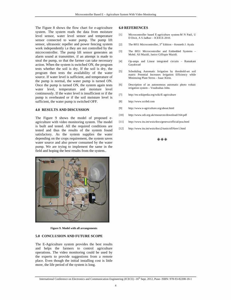
The Figure 8 shows the flow chart for e-agriculture system. The system reads the data from moisture level sensor, water level sensor and temperature sensor connected to water pump. The pump lift sensor, ultrasonic repeller and power fencing system work independently i.e they are not controlled by the microcontroller. The pump lift sensor generates an alarm sound at transmitter, if an attempt is made to steal the pump, so that the farmer can take necessary action. When the system is switched ON, the program tests whether the soil is dry. If the soil is dry, the program then tests the availability of the water source. If water level is sufficient, and temperature of the pump is normal, the water pump is turned ON. Once the pump is turned ON, the system again tests water level, temperature and moisture level continuously. If the water level is insufficient or if the pump is overheated or if the soil moisture level is sufficient, the water pump is switched OFF. 4.0 RESULTS AND DISCUSSION The Figure 9 shows the model of proposed e-agriculture with video monitoring system. The model is built and tested. All the required conditions are tested and thus the results of the system found satisfactory. As the system supplies the water depending on the crops requirement, the system saves water source and also power consumed by the water pump. We are trying to implement the same in the field and hoping the best results from the system..
Figure 9. Model with all arrangements
5.0 CONCLUSION AND FUTURE SCOPE The E-Agriculture system provides the best results and helps the farmers to control agriculture operations. The video monitoring could be used by the experts to provide suggestions from a remote place. Even though the initial installing cost is little more, the life period of the system is long.
6.0 REFERENCES [1] Microcontroller based E-agriculture system-M N Patil, U
D Dixit, A S Jadhav – ICEICE-2010.
[2] The 8051 Microcontroller, 3rd Edition – Kenneth J. Ayala
[3] The 8051 Microcontroller and Embedded Systems – Mohd. Ali Mazidi, Janice Gillispie Mazidi.
[4] Op-amps and Linear integrated circuits – Ramakant
Gayakwad
[5] Scheduling Automatic Irrigation by threshold-set soil matric Potential Increases Irrigation Efficiency while Minimzing Plant Stress – Isaac Klein.
[6] Description of an autonomous automatic photo voltaic
irrigation system – Voudoubas John.
[7] http://en.wikipedia.org/wiki/E-agriculture
[8] http://www.scribd.com
[9] http://www.e-agriculture.org/about.html
[10] http://www.odi.org.uk/resources/download/164.pdf
[11] http://www.itu.int/wsis/docs/geneva/official/poa.html
[12] http://www.itu.int/wsis/docs2/tunis/off/6rev1.html
International Conference on Electronics and Communication Engineering (ICECE) -16th Sept, 2012, Pune- ISBN: 978-93-82208-18-1
5
TREE BASED IMAGE COMPRESSION TECHNIQUE
1RASHMI HANCHINAL & 2SAVITRI RAJU
1BLDEA’s Dr. P. G. Halakatti College of Engineering and Technology Bijapur -586103, Karnataka, India
2SDM, College of Engineering and Technology, Dhavalagiri, Dharwad-580002, Karnataka, India.
Abstract—The objective of this paper is to present one of the tree based image compression technique, i.e. Set Partitioning In Hierarchical Trees (SPIHT), is considered for encoding and decoding image data. The proposed method decomposes an image into several subband images using the discrete wavelet transform, decor related coefficients quantized by SPIHT algorithm. In this paper, biorthogonal wavelet has been used to perform the transform of a test image and their results have been discussed. Simulation results obtained using MATLAB shows that the output image has better Peak Signal to Noise Ratio (PSNR). Keywords— Peak Signal to Noise Ratio (PSNR), Discrete Wavelet Transform (DWT), Mean Squared Error (MSE), Set Partitioning In Hierarchical Trees (SPIHT), MATLAB. I. INTRODUCTION
The fundamental goal of image compression is to
reduce the bit rate for transmission or storage while maintaining an acceptable fidelity or image quality. Image compression can be lossy or lossless. The lossless compression techniques are reversible or non destructive compression. It is guaranteed that the decompression image is identical to the original image, whereas in lossy compression technique the reconstructed image is not identical to the original image.
Various types of coding techniques were proposed for the Image processing Application. The two techniques used are: Predictive coding and Transform coding.
Predictive coding is a technique where information already sent or available is used to predict future values, and the difference is coded. Since this is done in the image or spatial domain, it is relatively simple to implement and is readily adapted to local image characteristics. Differential Pulse Code Modulation (DPCM) is one particular example of predictive coding.
Transform coding, on the other hand, first transforms the image from its spatial domain representation to a different type of representation using some well-known transform and then codes the transformed coefficient values. This method provides greater data compression compared to predictive methods, although at the expense of greater computation. A. General Image Compression System
Fig.1 General block diagram of image compression
The general block diagram of the image compression system is shown in figure 1.It consists of three main components viz; 1) Transform 2) Quantization 3) Entropy Encoding.Compression is achieved by applying a wavelet transforms in order to decorrelate the image data, quantizing the resulting transform coefficients and entropy coding the quantized values. First, the image is transformed into a domain where the image information is represented in a more compact form; here we have used discrete wavelet transform. Quantization refers to the process of approximating the continuous set of values in the image data with a finite, preferably small, set of values. The input to a quantizer is the original data and the output is always one among a finite number of levels. The quantizer is a function whose set of output values are discrete and usually finite. Obviously, this is a process of approximation and a good quantizer is one which represents the original signal with minimum loss or distortion. A quantizer is used to reduce the number of bits needed to store the transformed coefficients.
Entropy coding is used to compress sequence of quantized wavelet coefficients from quantization step further increase compression, without loss. Entropy coder is optional; it is used only when a little more compression is desired.
II. WAVELET TRANSFORM
Wavelet Transform has emerged as a
powerful mathematical tool in many areas of science and engineering specifically for data compression. It has provided a promising vehicle for image processing applications, because of its flexibility in representing images and its ability to take into account Human Visual System characteristic. It is mainly used to decorrelate the image data, so the resulting coefficients can be efficiently coded. It also has good
Tree Based Image Compression Technique
International Conference on Electronics and Communication Engineering (ICECE) -16th Sept, 2012, Pune- ISBN: 978-93-82208-18-1
6
energy compaction capabilities, which results in a high compression ratio.
Wavelets are functions generated from one single
function (basis function) called the prototype or mother wavelet by dilations (scaling) and translations (shifts) in time (frequency) domain. If the mother wavelet is denoted by , the other wavelets , can be represented as
(1)
where a and b are two arbitrary real numbers. The variables a and b represent the parameters for dilations and translations respectively in the time axis.
The translation parameter b relates to the location
of the wavelet function as it is shifted through the signal. Thus, it corresponds to the time information in the Wavelet Transform. The scale parameter a is defined as |1/frequency| and corresponds to frequency information. Scaling either dilates (expands) or compresses a signal. Large scales (low frequencies) dilate the signal and provide detailed information hidden in the signal, while small scales (high frequencies) compress the signal and provide global information about the signal.
Based on this definition of wavelets, the wavelet
transform (WT) of a function (signal) f (t) is mathematically represented by
(2)
The Wavelet Transform, at high frequencies, gives good time resolution and poor frequency resolution, while at low frequencies; the Wavelet Transform gives good frequency resolution and poor time resolution. The Discrete Wavelet Transform decomposes the image into two subbands by passing it through a low pass filter (LP) and a high pass filter (HP) and sub sampling the output of the two filters by two. At each level, the high pass filter produces detail information, while the low pass filter associated with scaling function produces coarse approximations as shown in fig.2 [3]The filtering increases the frequency resolution by 2 and the sub sampling reduces the time resolution by 2. This process is iterated on the low pass branch to obtain finer frequency resolution at lower frequencies. The output subsequences of the low pass branch corresponding to the last iteration and the output subsequence of all the high pass branches in this iterative scheme are collected as the DWT coefficients at various resolutions.
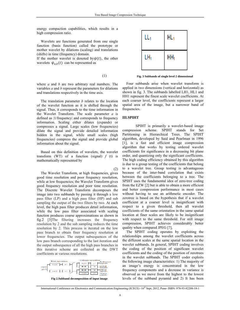
Fig 2.Subband decomposition of input image
Fig. 3 Subbands of single level 2 dimensional
Four subbands arise when wavelet transform is
applied in two dimensions (vertical and horizontal) as shown in fig. 3. The subbands labelled LH1, HL1 and HH1 represent the finest scale wavelet coefficients. At each coarser level, the coefficients represent a larger spatial area of the image, but a narrower band of frequencies.
III. SPIHT
SPIHT is primarily a wavelet-based image
compression scheme. SPIHT stands for Set Partitioning in Hierarchical Trees. The SPIHT algorithm, developed by Said and Pearlman in 1996 [1], is a fast and efficient image compression algorithm that works by testing ordered wavelet coefficients for significance in a decreasing bit plane order, and quantizing only the significant coefficients. The high coding efficiency obtained by this algorithm is due to a group testing of the coefficients that belong to a wavelet tree. Group testing is advantageous because of the inter-band correlation that exists between the coefficients belonging to a tree. The SPIHT uses the fundamental idea of zero-tree coding from the EZW [2] but is able to obtain a more efficient and better compression performance in most cases without having to use an arithmetic encoder. The zerotree is based on the hypothesis that if a wavelet coefficient at a coarser level is insignificant with respect to a given threshold, then all wavelet coefficients of the same orientation in the same spatial location at finer scales are likely to be insignificant with respect to the same threshold. For still image compression, SPIHT achieves considerably better quality when compared JPEG [7],
The SPIHT coding operates by exploiting the relationships among the wavelet coefficients across the different scales at the same spatial location in the wavelet subbands. In general, SPIHT coding involves the coding of the position of significant wavelet coefficients and the coding of the position of zerotrees in the wavelet subbands. The SPIHT coder exploits the following image characteristics: 1) The majority of an image’s energy is concentrated in the low frequency components and a decrease in variance is observed as we move from the highest to the lowest levels of the subband pyramid and 2) It has been
()( ψatψba =,
∫= tψtfw baba ()(),( ,
Tree Based Image Compression Technique
International Conference on Electronics and Communication Engineering (ICECE) -16th Sept, 2012, Pune- ISBN: 978-93-82208-18-1
7
observed that there is a spatial self-similarity among the subbands, and the coefficients are likely to be better magnitude-ordered if we move downward in the pyramid along the same spatial orientation. Each subband is quantized differently depending on its importance, which is often on its energy content or variance [8].
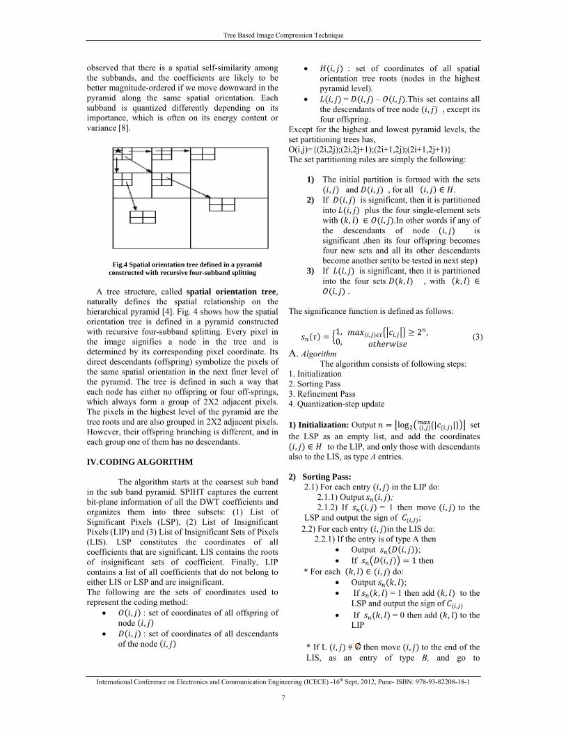
Fig.4 Spatial orientation tree defined in a pyramid constructed with recursive four-subband splitting
A tree structure, called spatial orientation tree,
naturally defines the spatial relationship on the hierarchical pyramid [4]. Fig. 4 shows how the spatial orientation tree is defined in a pyramid constructed with recursive four-subband splitting. Every pixel in the image signifies a node in the tree and is determined by its corresponding pixel coordinate. Its direct descendants (offspring) symbolize the pixels of the same spatial orientation in the next finer level of the pyramid. The tree is defined in such a way that each node has either no offspring or four off-springs, which always form a group of 2X2 adjacent pixels. The pixels in the highest level of the pyramid are the tree roots and are also grouped in 2X2 adjacent pixels. However, their offspring branching is different, and in each group one of them has no descendants.
IV. CODING ALGORITHM
The algorithm starts at the coarsest sub band
in the sub band pyramid. SPIHT captures the current bit-plane information of all the DWT coefficients and organizes them into three subsets: (1) List of Significant Pixels (LSP), (2) List of Insignificant Pixels (LIP) and (3) List of Insignificant Sets of Pixels (LIS). LSP constitutes the coordinates of all coefficients that are significant. LIS contains the roots of insignificant sets of coefficient. Finally, LIP contains a list of all coefficients that do not belong to either LIS or LSP and are insignificant. The following are the sets of coordinates used to represent the coding method:
• , : set of coordinates of all offspring of node ,
• , : set of coordinates of all descendants of the node ,
• , : set of coordinates of all spatial orientation tree roots (nodes in the highest pyramid level).
• , = , – , .This set contains all the descendants of tree node , , except its four offspring.
Except for the highest and lowest pyramid levels, the set partitioning trees has, O(i,j)={(2i,2j);(2i,2j+1);(2i+1,2j);(2i+1,2j+1)} The set partitioning rules are simply the following:
1) The initial partition is formed with the sets , and , , for all , .
2) If , is significant, then it is partitioned into , plus the four single-element sets with , , .In other words if any of the descendants of node , is significant ,then its four offspring becomes four new sets and all its other descendants become another set(to be tested in next step)
3) If , is significant, then it is partitioned into the four sets , , with ,
, . The significance function is defined as follows:
1,0,
, , 2 , (3)
A. Algorithm The algorithm consists of following steps:
1. Initialization 2. Sorting Pass 3. Refinement Pass 4. Quantization-step update 1) Initialization: Output log | , |, set the LSP as an empty list, and add the coordinates , to the LIP, and only those with descendants
also to the LIS, as type A entries. 2) Sorting Pass:
2.1) For each entry , in the LIP do: 2.1.1) Output , ; 2.1.2) If , = 1 then move , to the LSP and output the sign of , ;
2.2) For each entry , in the LIS do: 2.2.1) If the entry is of type A then
• Output , ; • If , 1 then
* For each , , do: • Output , ; • If , = 1 then add , to the
LSP and output the sign of , • If , = 0 then add , to the
LIP
* If L , # then move , to the end of the LIS, as an entry of type B, and go to
Internation
Step the LI
2.2.
* Adas an
* Rem 3) Refinemexcept thowith same│ │;
4) Qb V
Mean S
ratio (PSNmeasuring Mean Squa
Peak Signa
VI. SIMUL SPIHT
in MATLAof size 256and DWTsimulation
Wavelet
Knee Image
Zelda Image
Satellite Image
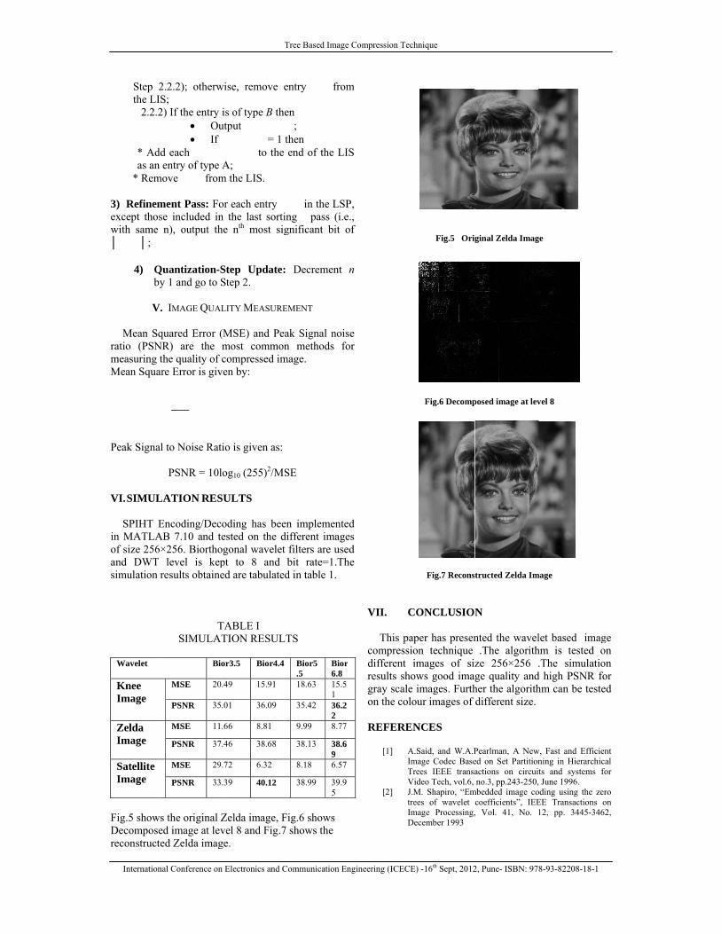
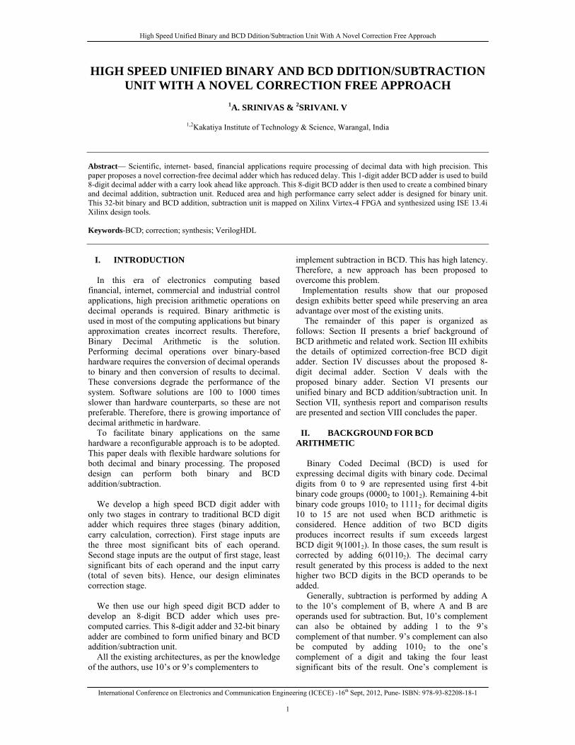
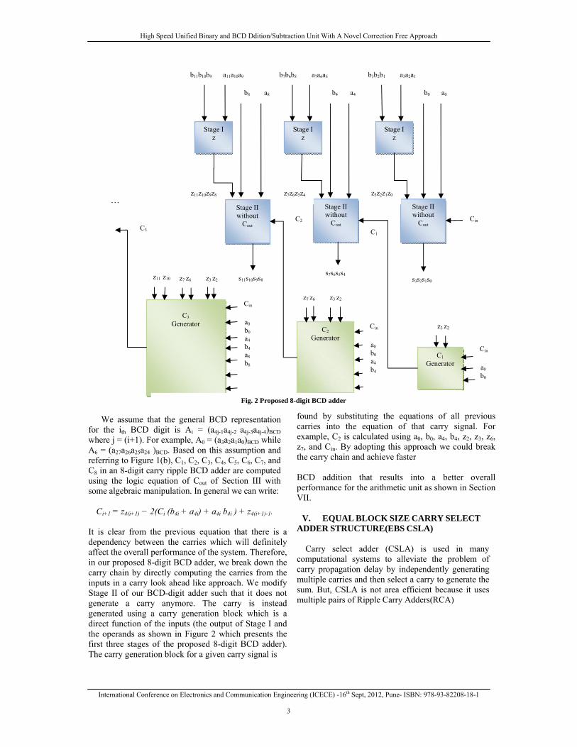
Fig.5 showDecomposreconstruct
nal Conference on
2.2.2); otherwIS; 2) If the entry
• Ou• If
dd each n entry of type move from
ment Pass: Foose included ine n), output th
Quantization-Sby 1 and go to S
V. IMAGE QUA
quared Error (NR) are the the quality of
are Error is giv
al to Noise Rat
PSNR = 10l
LATION RES
Encoding/DecAB 7.10 and t6×256. BiorthoT level is kep
results obtaine
TSIMULA
Bi
MSE 20
PSNR 35
MSE 11
PSNR 37
MSE 29
PSNR 33
ws the original Zsed image at levted Zelda imag
n Electronics and C
wise, remove e
is of type B thutput
= 1 to the
A; m the LIS.
or each entry n the last sortihe nth most sig
Step Update:Step 2.
LITY MEASURE
(MSE) and Pemost commoncompressed im
ven by:
tio is given as:
log10 (255)2/M
SULTS
coding has beeested on the d
ogonal waveletpt to 8 and ed are tabulate
TABLE I TION RESUL
or3.5 Bior4.4
0.49 15.91
.01 36.09
.66 8.81
.46 38.68
.72 6.32
.39 40.12
Zelda image, Fvel 8 and Fig.7ge.
Tree Based Image
Communication En
entry from
en ;
then end of the LI
in the LSPing pass (i.egnificant bit o
: Decrement
EMENT
ak Signal noisn methods fo
mage.
SE
en implementedifferent imaget filters are usebit rate=1.Thd in table 1.
LTS
Bior5.5
Bior6.8
18.63 15.51
35.42 36.22
9.99 8.77
38.13 38.69
8.18 6.57
38.99 39.95
Fig.6 shows 7 shows the
e Compression Tec
ngineering (ICECE
m
IS
P, e., of
n
se or
ed es ed he
r
VII. C This pa
compressidifferent results shogray scaleon the col
REFERE [1] A
ImTV
[2] JtrImD
chnique
E) -16th Sept, 2012
Fig.5 Ori
Fig.6 Decomp
Fig.7 Recons
CONCLUSION
aper has presenion technique images of sizows good imae images. Furthour images of
ENCES
A.Said, and W.A.Pmage Codec Base
Trees IEEE transaVideo Tech, vol.6, .M. Shapiro, “Emrees of wavelet mage Processing,
December 1993
2, Pune- ISBN: 97
ginal Zelda Imag
posed image at lev
tructed Zelda Im
N
nted the wavel.The algorith
ze 256×256 ge quality andher the algorithdifferent size.
Pearlman, A Newed on Set Partitionactions on circuino.3, pp.243-250,
mbedded image cocoefficients”, IEE, Vol. 41, No.
8-93-82208-18-1
ge
vel 8
mage
let based imaghm is tested o.The simulatio
d high PSNR fhm can be teste
w, Fast and Efficiening in Hierarchicits and systems f, June 1996. oding using the zeEE Transactions 12, pp. 3445-346
ge on on for ed
ent cal for
ero on 62,

Tree Based Image Compression Technique
International Conference on Electronics and Communication Engineering (ICECE) -16th Sept, 2012, Pune- ISBN: 978-93-82208-18-1
9
[3] K. Sayood, “Introduction to Data Compression”, 2nd Ed., Academic Press, Morgan Kaufmann Publishers, 2000.
[4] R.Sudhakar and Ms R Karthiga and S.Jayaraman Image Compression using Coding of Wavelet Coefficients – A Survey, GVIP Special Issue on Image Compression, 2007.
[5] K.P.Soman & K.I.Ramachandran “Insight into Wavelets from theory to practice”, Prentice Hall India, New Delhi, 2009.
[6] David Salomon, “Data compression”, the complete reference, 3rd Ed. Springer-Verlag New York,Inc.2005, page no.597-605.
[7] Savitri Raju and Mriyunjaya V Latte, “Comparision of compression algorithms”, Proceeding of two- day national conference on , convergence of signal processing , communication and VLSI Design, page no.85-87.
[8] Raghuveer Rao and Ajit Bopardikar, “Wavelet Transform-Introduction to Theory and Applications”, Addison Wesley Pearson Edu. Edition, 2002.
High Speed Unified Binary and BCD Ddition/Subtraction Unit With A Novel Correction Free Approach
International Conference on Electronics and Communication Engineering (ICECE) -16th Sept, 2012, Pune- ISBN: 978-93-82208-18-1
1
HIGH SPEED UNIFIED BINARY AND BCD DDITION/SUBTRACTION UNIT WITH A NOVEL CORRECTION FREE APPROACH
1A. SRINIVAS & 2SRIVANI. V
1,2Kakatiya Institute of Technology & Science, Warangal, India
Abstract— Scientific, internet- based, financial applications require processing of decimal data with high precision. This paper proposes a novel correction-free decimal adder which has reduced delay. This 1-digit adder BCD adder is used to build 8-digit decimal adder with a carry look ahead like approach. This 8-digit BCD adder is then used to create a combined binary and decimal addition, subtraction unit. Reduced area and high performance carry select adder is designed for binary unit. This 32-bit binary and BCD addition, subtraction unit is mapped on Xilinx Virtex-4 FPGA and synthesized using ISE 13.4i Xilinx design tools. Keywords-BCD; correction; synthesis; VerilogHDL
I. INTRODUCTION
In this era of electronics computing based financial, internet, commercial and industrial control applications, high precision arithmetic operations on decimal operands is required. Binary arithmetic is used in most of the computing applications but binary approximation creates incorrect results. Therefore, Binary Decimal Arithmetic is the solution. Performing decimal operations over binary-based hardware requires the conversion of decimal operands to binary and then conversion of results to decimal. These conversions degrade the performance of the system. Software solutions are 100 to 1000 times slower than hardware counterparts, so these are not preferable. Therefore, there is growing importance of decimal arithmetic in hardware. To facilitate binary applications on the same hardware a reconfigurable approach is to be adopted. This paper deals with flexible hardware solutions for both decimal and binary processing. The proposed design can perform both binary and BCD addition/subtraction. We develop a high speed BCD digit adder with only two stages in contrary to traditional BCD digit adder which requires three stages (binary addition, carry calculation, correction). First stage inputs are the three most significant bits of each operand. Second stage inputs are the output of first stage, least significant bits of each operand and the input carry (total of seven bits). Hence, our design eliminates correction stage. We then use our high speed digit BCD adder to develop an 8-digit BCD adder which uses pre-computed carries. This 8-digit adder and 32-bit binary adder are combined to form unified binary and BCD addition/subtraction unit. All the existing architectures, as per the knowledge of the authors, use 10’s or 9’s complementers to
implement subtraction in BCD. This has high latency. Therefore, a new approach has been proposed to overcome this problem. Implementation results show that our proposed design exhibits better speed while preserving an area advantage over most of the existing units. The remainder of this paper is organized as follows: Section II presents a brief background of BCD arithmetic and related work. Section III exhibits the details of optimized correction-free BCD digit adder. Section IV discusses about the proposed 8-digit decimal adder. Section V deals with the proposed binary adder. Section VI presents our unified binary and BCD addition/subtraction unit. In Section VII, synthesis report and comparison results are presented and section VIII concludes the paper.
II. BACKGROUND FOR BCD ARITHMETIC
Binary Coded Decimal (BCD) is used for expressing decimal digits with binary code. Decimal digits from 0 to 9 are represented using first 4-bit binary code groups (00002 to 10012). Remaining 4-bit binary code groups 10102 to 11112 for decimal digits 10 to 15 are not used when BCD arithmetic is considered. Hence addition of two BCD digits produces incorrect results if sum exceeds largest BCD digit 9(10012). In those cases, the sum result is corrected by adding 6(01102). The decimal carry result generated by this process is added to the next higher two BCD digits in the BCD operands to be added. Generally, subtraction is performed by adding A to the 10’s complement of B, where A and B are operands used for subtraction. But, 10’s complement can also be obtained by adding 1 to the 9’s complement of that number. 9’s complement can also be computed by adding 10102 to the one’s complement of a digit and taking the four least significant bits of the result. One’s complement is

High Speed Unified Binary and BCD Ddition/Subtraction Unit With A Novel Correction Free Approach
International Conference on Electronics and Communication Engineering (ICECE) -16th Sept, 2012, Pune- ISBN: 978-93-82208-18-1
2
computed by inverting bits of that digit. This approach is used in this paper in the design of unified binary and BCD addition/subtraction unit.
III. OPTIMIZED CORRECTION-FREE BCD
DIGIT ADDER
Traditional BCD digit adder requires three stages which includes the correction stage. This correction stage performs the correction by adding (0110)2 to the result when the first stage result is greater than 9 = (1001)BCD. But, this correction stage degrades the performance of the decimal adder. Therefore, we propose a correction-free BCD digit adder in this section. We consider two decimal input digits to the decimal adder shown in fig. 1(a) as A {0, 9} and B{0, 9}, and decimal carry input is Cin. Assume that the decimal sum output is S {0, 9} and the decimal carry output is Cout. 8421 BCD representation of A, B and S can be written as A=a3a2a1a0, B= b3b2b1b0 and S= s3s2s1s0 where ai, bi and si for all i = {0, 1, 2, 3}. A and B can be expressed in terms of two integers m=a3a2a1 and n= b3b2b1 as: A= 2 × m + a0 and B= 2 × n + b0, where 0 ≤ m ≤ 4 and 0 ≤ n ≤ 4. This implies that the output of the BCD adder can be expressed as: {Cout, Sum} = A + B + Cin= (2 × m + a0) + (2 × n + b0) + Cin We can rearrange the equation as {Cout, Sum}=2 × (n + m) + (a0 + b0 + Cin). Based on this formula we have designed the BCD digit adder such that it consists of two stages: Stage I and Stage II. Figure 1(b) shows the block diagram of the proposed BCD adder. The inputs to Stage I are m and n. Stage I generates partial decimal sum: Z = z3z2z1z00 = 2 × (m+ n). It should be noticed that this partial decimal sum consists of an even decimal digit (z2z1z00) and a decimal carry z3 that can be either 1 or 0 based on the values of m and n. For example, if the two input decimal digits A and B are 7 = (0111)BCD and 8 = (1000)BCD, respectively, then we have: m = (011)2 = 3 , n = (100)2 = 4 and Z = z3z2z1z00 = 2 × (m+ n) = 2 × (3 + 4) = (14)10. This means that the decimal carry z3 is 1 and the even decimal digit z2z1z00 = (4)10 = (0100)BCD. Since the produced decimal digit is always even, only z3z2z1z0 are forwarded to Stage II of the BCD digit adder. Three more examples are listed in Table I for clarity. The outputs of Stage I along with a0, b0 and Cin are fed to Stage II. For the purpose of designing Stage II, the values of Cout, s3, s2, s1 and s0 have been calculated for all possible combinations of z3, z2, z1, z0, a0, b0, and Cin. To illustrate this procedure, three possible combinations are presented in Table II.
TABLE I. EXAMPLES THAT DEMONSTRATE HOW THE OUTPUT OF STAGE I IS COMPUTED
(A)BCD (B)BCD (m)10 (n)10 (Z)10 z3z2z1z0
0011 0110 1 3 8 0100
0100 1001 2 4 12 1001
1001 1000 4 4 16 1011
For example, in the first row of the table the values of z3, z2, z1, and z0 are 1, 0, 1, and 1, respectively. This means that the value of 2 × (m + n) that is to be added to the value of (a0 + b0 + Cin) is (16)10. Since a0, b0, and Cin in the example are 1, 0, and 0, respectively, the value of A+B = 2 × (n + m) + (a0 +b0 + Cin) is (17)10. Therefore, the computed values for Cout, s3, s2, s1, and s0 are 1, 0, 1, 1, and 1, respectively. Based on this, Stage II generates the decimal sum output and the decimal carry output. Decimal carry output equation obtained is given by
Cout = z2Cinb0 + z2Cinao + z2a0b0 + z3. It can be emphasized that our design does not require any corrections to the results, and the results are computed with only two stages. As it will be shown in Section VII, this enables our design to achieve better performance over other designs. IV. PROPOSED 8-DIGIT BCD ADDER
N single-BCD digit adders can be cascaded in a
carry ripple fashion, in order to build N-digit BCD adder. Due to the dependency between the carries, long carry chain is introduced. But, carry rippling imposes large latency on the design. This carry chain can be observed in the logic equation of Cout (Section III).
TABLE II. EXAMPLES THAT DEMONSTRATE HOW THE
OUTPUT OF STAGE II IS COMPUTED
z3z2z1z0 (Z)10 a0 b0 Cin Cout s3s2s1s0
1011 16 1 0 0 1 0111
1001 12 0 1 0 1 0011
0100 8 1 0 1 1 0000
Cout
4
4
4 4
B A
3 3
z3z2z1z0
Cout
S S
Cin
Cin
b0 a0 n m
Decimal Digit Adder
Stage I
Stage II
Fig. 1(a) Block Diagram Fig. 1(b) Optimized correction-
free BCD Digit Adder
Fig. 1 BCD Digit Adders
High Speed Unified Binary and BCD Ddition/Subtraction Unit With A Novel Correction Free Approach
International Conference on Electronics and Communication Engineering (ICECE) -16th Sept, 2012, Pune- ISBN: 978-93-82208-18-1
3
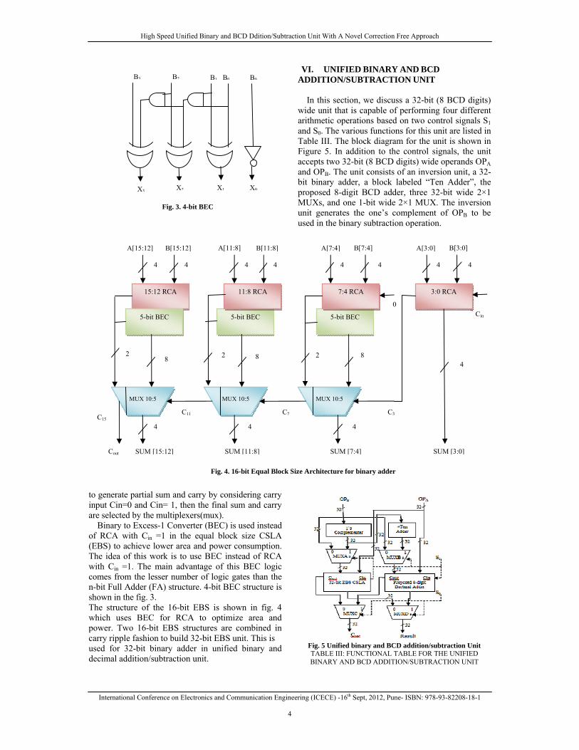
We assume that the general BCD representation
for the ith BCD digit is Ai = (a4j-1a4j-2 a4j-3a4j-4)BCD where j = (i+1). For example, A0 = (a3a2a1a0)BCD while A6 = (a27a26a25a24 )BCD. Based on this assumption and referring to Figure 1(b), C1, C2, C3, C4, C5, C6, C7, and C8 in an 8-digit carry ripple BCD adder are computed using the logic equation of Cout of Section III with some algebraic manipulation. In general we can write:
Ci+1 = z4(i+1) − 2(Ci (b4i + a4i) + a4i b4i ) + z4(i+1)-1.
It is clear from the previous equation that there is a dependency between the carries which will definitely affect the overall performance of the system. Therefore, in our proposed 8-digit BCD adder, we break down the carry chain by directly computing the carries from the inputs in a carry look ahead like approach. We modify Stage II of our BCD-digit adder such that it does not generate a carry anymore. The carry is instead generated using a carry generation block which is a direct function of the inputs (the output of Stage I and the operands as shown in Figure 2 which presents the first three stages of the proposed 8-digit BCD adder). The carry generation block for a given carry signal is
found by substituting the equations of all previous carries into the equation of that carry signal. For example, C2 is calculated using a0, b0, a4, b4, z2, z3, z6, z7, and Cin. By adopting this approach we could break the carry chain and achieve faster BCD addition that results into a better overall performance for the arithmetic unit as shown in Section VII.
V. EQUAL BLOCK SIZE CARRY SELECT ADDER STRUCTURE(EBS CSLA)
Carry select adder (CSLA) is used in many computational systems to alleviate the problem of carry propagation delay by independently generating multiple carries and then select a carry to generate the sum. But, CSLA is not area efficient because it uses multiple pairs of Ripple Carry Adders(RCA)
…
b3b2b1 a3a2a1 b7b6b5 a7a6a5 b11b10b9 a11a10a9
C3
Generator C2
Generator
C1
Generator
Stage I z
Stage I z
Stage I z
Stage II without
Cout
a0 b0 a4b4 a8 b8
Stage II without
Cout
Stage II without
Cout
b0 b4 a4 a0 b8 a8
z11z10z9z8 z7z6z5z4 z3z2z1z0
s11s10s9s8 s7s6s5s4
s3s2s1s0
a0b0 a4 b4
a0 b0
Cin
Cin
Cin
z3 z2 z7 z6 z11 z10
z3 z2 z7 z6
z3 z2
Cin
C1
C2
C3
Fig. 2 Proposed 8-digit BCD adder
High Speed Unified Binary and BCD Ddition/Subtraction Unit With A Novel Correction Free Approach
International Conference on Electronics and Communication Engineering (ICECE) -16th Sept, 2012, Pune- ISBN: 978-93-82208-18-1
4
to generate partial sum and carry by considering carry input Cin=0 and Cin= 1, then the final sum and carry are selected by the multiplexers(mux). Binary to Excess-1 Converter (BEC) is used instead of RCA with Cin =1 in the equal block size CSLA (EBS) to achieve lower area and power consumption. The idea of this work is to use BEC instead of RCA with Cin =1. The main advantage of this BEC logic comes from the lesser number of logic gates than the n-bit Full Adder (FA) structure. 4-bit BEC structure is shown in the fig. 3. The structure of the 16-bit EBS is shown in fig. 4 which uses BEC for RCA to optimize area and power. Two 16-bit EBS structures are combined in carry ripple fashion to build 32-bit EBS unit. This is used for 32-bit binary adder in unified binary and decimal addition/subtraction unit.
VI. UNIFIED BINARY AND BCD ADDITION/SUBTRACTION UNIT
In this section, we discuss a 32-bit (8 BCD digits) wide unit that is capable of performing four different arithmetic operations based on two control signals S1 and S0. The various functions for this unit are listed in Table III. The block diagram for the unit is shown in Figure 5. In addition to the control signals, the unit accepts two 32-bit (8 BCD digits) wide operands OPA and OPB. The unit consists of an inversion unit, a 32-bit binary adder, a block labeled “Ten Adder”, the proposed 8-digit BCD adder, three 32-bit wide 2×1 MUXs, and one 1-bit wide 2×1 MUX. The inversion unit generates the one’s complement of OPB to be used in the binary subtraction operation.
Fig. 5 Unified binary and BCD addition/subtraction Unit TABLE III: FUNCTIONAL TABLE FOR THE UNIFIED BINARY AND BCD ADDITION/SUBTRACTION UNIT
Cin
15:12 RCA
5-bit BEC 5-bit BEC
11:8 RCA
5-bit BEC
7:4 RCA 3:0 RCA
MUX 10:5 MUX 10:5 MUX 10:5
B[3:0]A[3:0] A[7:4] B[7:4]A[11:8] B[11:8]A[15:12] B[15:12]
SUM [3:0] SUM [7:4]SUM [11:8]SUM [15:12]Cout
8 4
2 8 2 8 2
4 4 4
4 4 4 4 4 4 4 4
0
C3C7C11 C15
Fig. 4. 16-bit Equal Block Size Architecture for binary adder
B0B2B3 B1 B0
X3 X2 X1 X0
Fig. 3. 4-bit BEC
High Speed Unified Binary and BCD Ddition/Subtraction Unit With A Novel Correction Free Approach
International Conference on Electronics and Communication Engineering (ICECE) -16th Sept, 2012, Pune- ISBN: 978-93-82208-18-1
5
S1 S0 Operation
0 0 Decimal Addition 0 1 Binary Addition 1 0 Decimal Subtraction
1 1 Binary Subtraction
As we have mentioned before, we compute the nine’s complement by adding (1010)2 to the one’s complement of the BCD digit and ignoring the last carry. Thus, to get the nine’s complement of OPB we feed the one’s complement of OPB to the “Ten Adder” block which, in turn, adds (1010)2 to the inverted bits of each BCD digit in OPB. Based on the control signal S1, MUXA selects between OPB or its one’s complement. Also, MUXB chooses between OPB or its nine’s complement. OPA is connected directly to the first input of the 32-bit EBS that is binary adder and to the first input of the proposed 8-digit BCD adder. The input of the 32-bit EBS is driven by the output of MUXA, while the other input of the proposed 8-digit BCD adder is driven by the output of MUXB. The function of MUXC and MUXD is to choose between a binary (32-bit plus carry) result or a decimal (8-digit plus carry) result based on the control signal S0. VII. SYNTHESIS REPORT AND COMPARISON
VerilogHDL is used to describe this proposed unified binary and decimal addition/subtraction unit. The code is optimized for FPGA synthesis at modular level to ensure best results in-terms of area and delay. This design has been synthesized and implemented using Xilinx ISE 13.4i design tools targeting on Xilinx Virtex 4 FPGA device. For comparison purpose with existing designs, we have targeted the 4VFX60FF672-12 Virtex 4 FPGA device and implemented a 32-bit wide unit. Synthesis reports for the proposed design are listed in Table IV, Table V.
TABLE IV: TIMING SUMMARY OF UNIFIED BINARY AND
BCD ADDITION/SUBTRACTION UNIT
Timing Parameter Proposed Unit
Minimum Period 3.011ns
Maximum Frequency 332.132MHz
Minimum input arrival time before clock
3.999ns
Maximum output required time after clock
3.793ns
Gate Delay(Logic) 1.161ns
Net Delay(Route) 1.850ns
TABLE V: HARDWARE RESOURCE UTILIZATION
SUMMARY OF UNIFIED DESIGN
Device Parameter Number Usage
Number of Slices 243
Number of Slice Flip Flops
286
Number of 4 input LUTs
443
Number of bonded IOBs
100
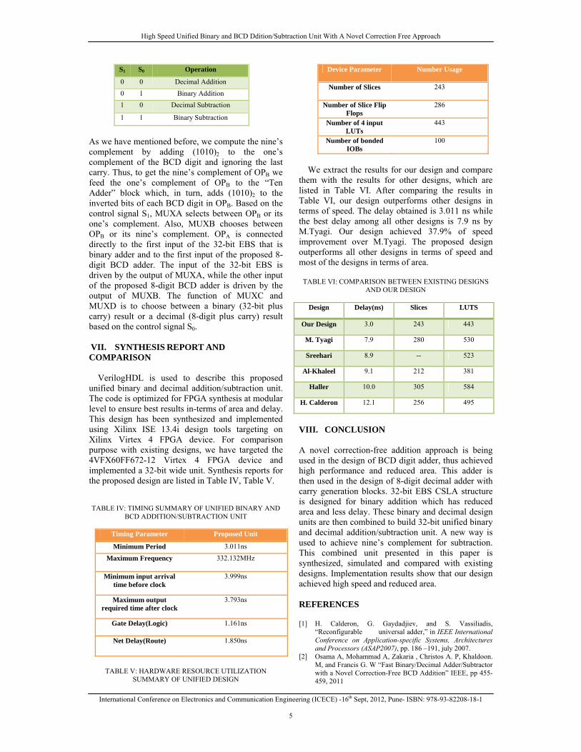
We extract the results for our design and compare them with the results for other designs, which are listed in Table VI. After comparing the results in Table VI, our design outperforms other designs in terms of speed. The delay obtained is 3.011 ns while the best delay among all other designs is 7.9 ns by M.Tyagi. Our design achieved 37.9% of speed improvement over M.Tyagi. The proposed design outperforms all other designs in terms of speed and most of the designs in terms of area.
TABLE VI: COMPARISON BETWEEN EXISTING DESIGNS AND OUR DESIGN
Design Delay(ns) Slices LUTS
Our Design 3.0 243 443
M. Tyagi 7.9 280 530
Sreehari 8.9 -- 523
Al-Khaleel 9.1 212 381
Haller 10.0 305 584
H. Calderon 12.1 256 495
VIII. CONCLUSION A novel correction-free addition approach is being used in the design of BCD digit adder, thus achieved high performance and reduced area. This adder is then used in the design of 8-digit decimal adder with carry generation blocks. 32-bit EBS CSLA structure is designed for binary addition which has reduced area and less delay. These binary and decimal design units are then combined to build 32-bit unified binary and decimal addition/subtraction unit. A new way is used to achieve nine’s complement for subtraction. This combined unit presented in this paper is synthesized, simulated and compared with existing designs. Implementation results show that our design achieved high speed and reduced area. REFERENCES
[1] H. Calderon, G. Gaydadjiev, and S. Vassiliadis,
“Reconfigurable universal adder,” in IEEE International Conference on Application-specific Systems, Architectures and Processors (ASAP2007), pp. 186 –191, july 2007.
[2] Osama A, Mohammad A, Zakaria , Christos A. P, Khaldoon. M, and Francis G. W “Fast Binary/Decimal Adder/Subtractor with a Novel Correction-Free BCD Addition” IEEE, pp 455-459, 2011
High Speed Unified Binary and BCD Ddition/Subtraction Unit With A Novel Correction Free Approach
International Conference on Electronics and Communication Engineering (ICECE) -16th Sept, 2012, Pune- ISBN: 978-93-82208-18-1
6
[3] Sreehari. V, M. Kirthi Krishna, G. Prateek, S. Subroto, S. Bharat, and M. Srinivas, “A novel carry-look ahead approach to a unified bcd and binary adder/subtractor,” in 21st International Conference on VLSI Design (VLSID 2008), pp. 547 –552, jan. 2008.
[4] M. Tyagi, A. Vashist, and K. K., “A novel hardware efficient reconfigurable 32-bit arithmetic unit for binary, bcd and floating point operands,” International Journal of Engineering Science and Technology, vol. 3, pp. 4449–4464, may 2011
[5] W. Haller, W. H. Li, M. R. Kelly, and H. Watter, “Highly Parallel Structure for Fast Cycle Binary and Decimal Adder Unit,” Internetional Business Machines Corporation, US patent 2006/0031289, pp. 1–8, Feb 2006
[6] H. Fischer and W. Rohsaint, “Circuit Arrangement for Adding or Subtracting Operands Coded in BCD-Code or Binary-Code,” Siemens Aktiengesellschaft, US patent 5146423, pp. 1–9, Sep 19
[7] I. S. Hwang, “High-Speed Binary and Decimal Arithmetic Logic Unit,” American Telephone and Telegraph Company, AT & T Bell Laboratories, US patent 4866656, pp. 1–11, Sep 1989.92.
[8] F. Y. Busaba, C. A. Krygowsky, W. H. Li, E. M. Schwarz, and S. R. Carlough, “The IBM z900 Decimal Arithmetic Unit,” Conference Record of the 35th Asilomar Conference on Signals, Systems and Computers, pp. 1353–1339, Sep 2001.
[9] J. Moskal, E. Oruklu, and J. Saniie, “Design and synthesis of a carryfree signed-digit decimal adder,” in IEEE International Symposium on Circuits and Systems (ISCAS 2007), pp. 1089 –1092, may 2007.
[10] H. Thapliyal and M. B. Srinivas, “The New BCD Subtractor and its Reversible Logic Implementation,” Lecture Notes in Computer Science, Springer-Verlag, pp. 466–472, 2006.
[11] W. Haller, U. Krauch, and H. Watter, “Combined Binary/Decimal Adder Unit,” Internetional Business Machines Corporation, US patent 5928319, pp. 1–9, Jul 1999.
International Conference on Electronics and Communication Engineering (ICECE) -16th Sept, 2012, Pune- ISBN: 978-93-82208-18-1
16
DESIGN AND SIMULATION OF UART PROTOCOL BASED ON VERILOG
1B.JEEVAN & 2M.NEERAJA
1,2Dept of E.I.E, KITS,Warangal, Andhra Pradesh, India
Abstract—UART (Universal Asynchronous receiver Transmitter) is a kind of serial communication protocol; mostly used for short-distance, low speed, low-cost data exchange between computer and peripheral. The UART takes bytes of data and transmits the individual bits in a sequential fashion. At the destination, a second UART re-assembles the bits into complete bytes. The UART allows the devices to communicate without the need to be synchronized. UART includes three kernel modules which are generator, receiver and transmitter .The UART implemented with VERILOG language can be integrated into FPGA. The simulation results with Xilinx are completely consistent with the UART protocol. Keywords- UART, asynchronous serial communication, Xilinx I. INTRODUCTION
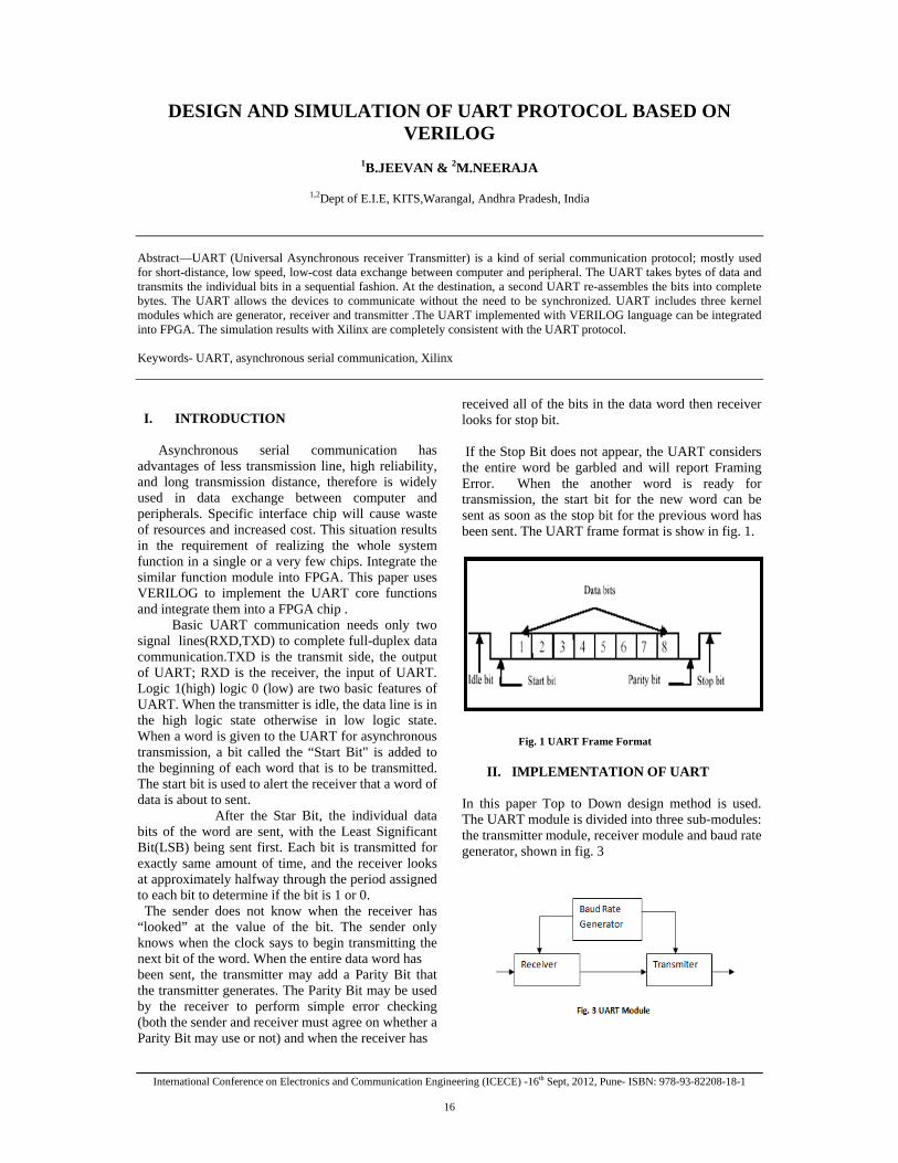
Asynchronous serial communication has advantages of less transmission line, high reliability, and long transmission distance, therefore is widely used in data exchange between computer and peripherals. Specific interface chip will cause waste of resources and increased cost. This situation results in the requirement of realizing the whole system function in a single or a very few chips. Integrate the similar function module into FPGA. This paper uses VERILOG to implement the UART core functions and integrate them into a FPGA chip . Basic UART communication needs only two signal lines(RXD,TXD) to complete full-duplex data communication.TXD is the transmit side, the output of UART; RXD is the receiver, the input of UART. Logic 1(high) logic 0 (low) are two basic features of UART. When the transmitter is idle, the data line is in the high logic state otherwise in low logic state. When a word is given to the UART for asynchronous transmission, a bit called the “Start Bit" is added to the beginning of each word that is to be transmitted. The start bit is used to alert the receiver that a word of data is about to sent.
After the Star Bit, the individual data bits of the word are sent, with the Least Significant Bit(LSB) being sent first. Each bit is transmitted for exactly same amount of time, and the receiver looks at approximately halfway through the period assigned to each bit to determine if the bit is 1 or 0. The sender does not know when the receiver has “looked” at the value of the bit. The sender only knows when the clock says to begin transmitting the next bit of the word. When the entire data word has been sent, the transmitter may add a Parity Bit that the transmitter generates. The Parity Bit may be used by the receiver to perform simple error checking (both the sender and receiver must agree on whether a Parity Bit may use or not) and when the receiver has
received all of the bits in the data word then receiver looks for stop bit. If the Stop Bit does not appear, the UART considers the entire word be garbled and will report Framing Error. When the another word is ready for transmission, the start bit for the new word can be sent as soon as the stop bit for the previous word has been sent. The UART frame format is show in fig. 1.
Fig. 1 UART Frame Format
II. IMPLEMENTATION OF UART
In this paper Top to Down design method is used. The UART module is divided into three sub-modules: the transmitter module, receiver module and baud rate generator, shown in fig. 3

Design and Simulation of uart Protocol Based on verilog
International Conference on Electronics and Communication Engineering (ICECE) -16th Sept, 2012, Pune- ISBN: 978-93-82208-18-1
17
A.BAUD RATE GENERATOR THE Baud Rate Generator is used to produce used to produce a local clock signal which is much higher than the baud rate to control the UART receiver and transmit. The baud rate generator is actually a frequency divider. The frequency factor is calculated according to the given system clock frequency and requested baud rate. Assume that the system clock is 50MHZ, baud rate is 9600bps.Therefore the frequency coefficient (M) of baud rate generator is:
M=50*10^6/9600Hz=5200
B. TRANSMIT MODULE The UART transmit module converts the bytes into serial bits according to the basic frame format and transmits those bits through TXD. The transmit module is to convert the sending 8-bit parallel data into serial data ,adds start bit at the head of the data as well as the parity and stop bits at the end of the data. The schematic of a transmitter module is as shown in the figure below.The 8-bit ASCII data is supplied in to the module via. Din[7:0]. The ‘ready’line is HIGH whenever the module is ready to transmit data, ‘trde’ line is HIGH when the transmission of data is complete i.e. the stop bit is transmitted. ’CLR’ is used to reset all the parameter, the ‘clk’ provides timing information regarding the flow of data bits. Serial output data is transmitted via. Dout line.
Fig.4 Transmitter module
The transmitter only needs to output 1 bit every clock cycles(the transmitting clock frequency generated by baud rate generator). The order follows 1 start bit , 8 data bits ,1 parity bit and 1 stop bit. The parity bits is determined according to the number of logic 1 in 8 data bits. Then the parity bits is output. Finally 1 is output as the stop bit. Fig. 5 shows the transmit module state diagram
Fig. 5 UART Transmiter State Machine This state machine has 5 states : MARK(idle), START(start bit), DELAY, SHIFT(shift), STOP(stop bit).
• MARK Status : When the UART is reset, the state machine will be in this state, the UART transmitter has been waiting a data frame sending command READY. When READY=1 , the state machine transferred to START , get ready to send a start bit.
• START Status : In this state, sends a logic 0 signal to the TXD for one bit time width, the start bit. Then the state machine transferred to DELAY state.
• DELAY Status : when the state machine is in this state, waiting for counting baud rate clock then entering into the SAMPLE to sample the data bits .at the same time determining whether the collected data bit length has reached the data frame length. If reaches, it mens the stop bits arrives.inthis design it is 8, which corresponds to the 8-bit data formate of UART
• SHIFT Status : In this state , the state machine realizes the parallel to serial converision of outgoing data. Then immediately return to DELAY state
• STOP Status : when the data frame transmit is completed, the state machine transferred to this state,and sends 5200 baud clock cycle logic 1 signal,that is 1 stop bit.then the state turns to mark state after sending the stop bitand waits for another data frame transmit
Design and Simulation of uart Protocol Based on verilog
International Conference on Electronics and Communication Engineering (ICECE) -16th Sept, 2012, Pune- ISBN: 978-93-82208-18-1
18
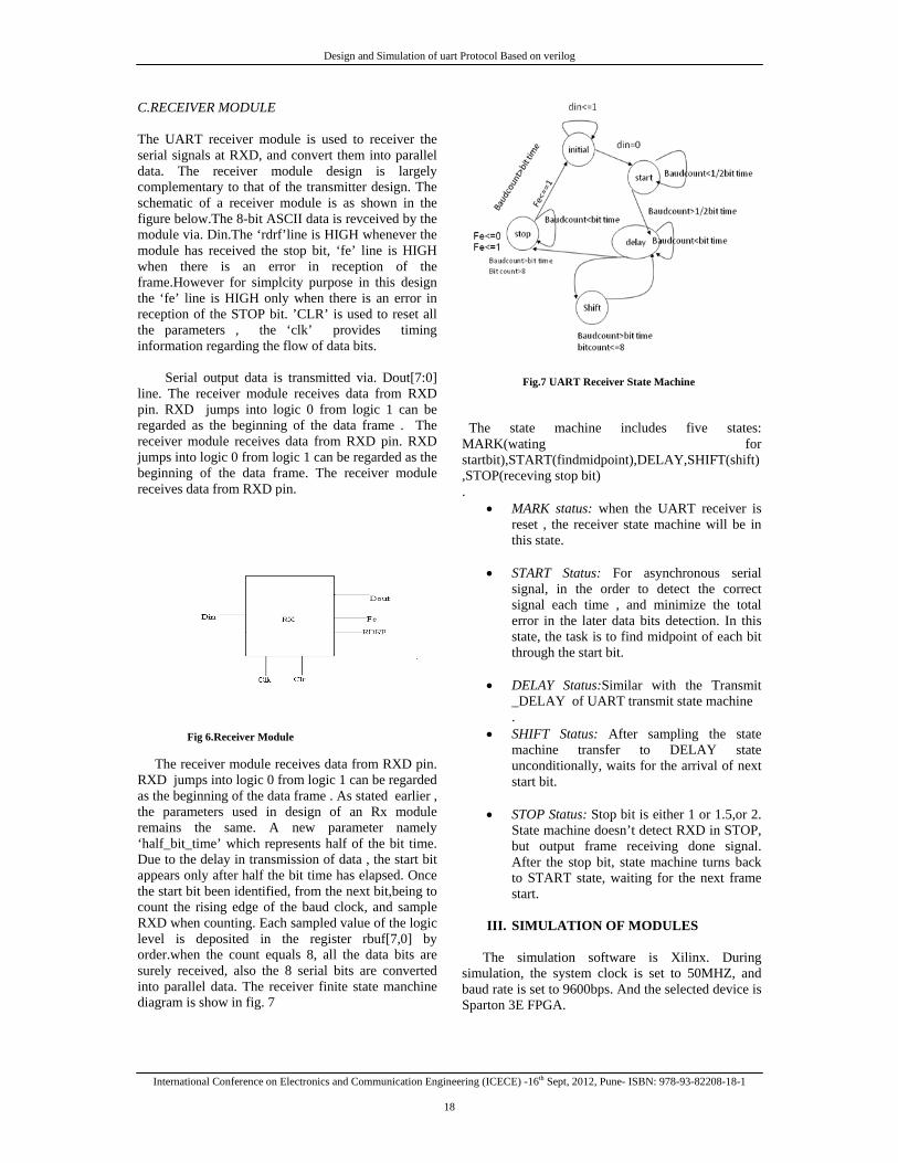
C.RECEIVER MODULE The UART receiver module is used to receiver the serial signals at RXD, and convert them into parallel data. The receiver module design is largely complementary to that of the transmitter design. The schematic of a receiver module is as shown in the figure below.The 8-bit ASCII data is revceived by the module via. Din.The ‘rdrf’line is HIGH whenever the module has received the stop bit, ‘fe’ line is HIGH when there is an error in reception of the frame.However for simplcity purpose in this design the ‘fe’ line is HIGH only when there is an error in reception of the STOP bit. ’CLR’ is used to reset all the parameters , the ‘clk’ provides timing information regarding the flow of data bits. Serial output data is transmitted via. Dout[7:0] line. The receiver module receives data from RXD pin. RXD jumps into logic 0 from logic 1 can be regarded as the beginning of the data frame . The receiver module receives data from RXD pin. RXD jumps into logic 0 from logic 1 can be regarded as the beginning of the data frame. The receiver module receives data from RXD pin.
Fig 6.Receiver Module The receiver module receives data from RXD pin. RXD jumps into logic 0 from logic 1 can be regarded as the beginning of the data frame . As stated earlier , the parameters used in design of an Rx module remains the same. A new parameter namely ‘half_bit_time’ which represents half of the bit time. Due to the delay in transmission of data , the start bit appears only after half the bit time has elapsed. Once the start bit been identified, from the next bit,being to count the rising edge of the baud clock, and sample RXD when counting. Each sampled value of the logic level is deposited in the register rbuf[7,0] by order.when the count equals 8, all the data bits are surely received, also the 8 serial bits are converted into parallel data. The receiver finite state manchine diagram is show in fig. 7
Fig.7 UART Receiver State Machine
The state machine includes five states: MARK(wating for startbit),START(findmidpoint),DELAY,SHIFT(shift),STOP(receving stop bit) .
• MARK status: when the UART receiver is reset , the receiver state machine will be in this state.
• START Status: For asynchronous serial signal, in the order to detect the correct signal each time , and minimize the total error in the later data bits detection. In this state, the task is to find midpoint of each bit through the start bit.
• DELAY Status:Similar with the Transmit _DELAY of UART transmit state machine .
• SHIFT Status: After sampling the state machine transfer to DELAY state unconditionally, waits for the arrival of next start bit.
• STOP Status: Stop bit is either 1 or 1.5,or 2. State machine doesn’t detect RXD in STOP, but output frame receiving done signal. After the stop bit, state machine turns back to START state, waiting for the next frame start.
III. SIMULATION OF MODULES
The simulation software is Xilinx. During simulation, the system clock is set to 50MHZ, and baud rate is set to 9600bps. And the selected device is Sparton 3E FPGA.
Design and Simulation of uart Protocol Based on verilog
International Conference on Electronics and Communication Engineering (ICECE) -16th Sept, 2012, Pune- ISBN: 978-93-82208-18-1
19
A. Transmitter Simulation
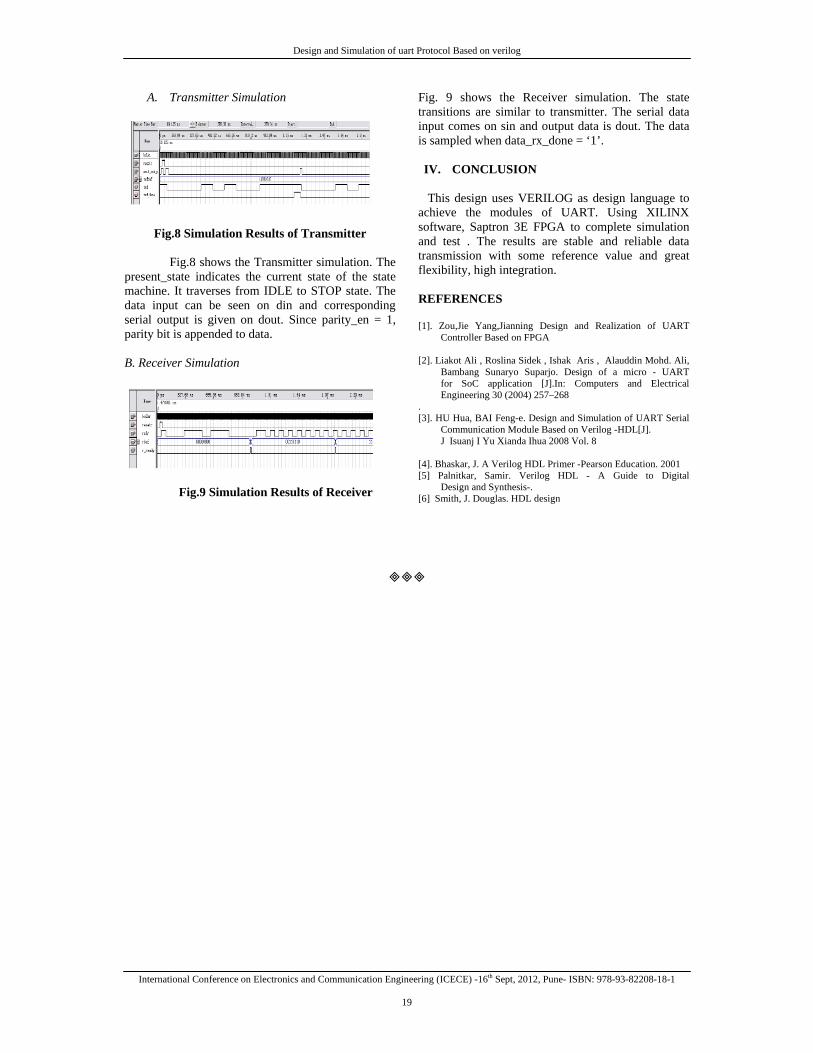
Fig.8 Simulation Results of Transmitter Fig.8 shows the Transmitter simulation. The
present_state indicates the current state of the state machine. It traverses from IDLE to STOP state. The data input can be seen on din and corresponding serial output is given on dout. Since parity_en = 1, parity bit is appended to data.
B. Receiver Simulation
Fig.9 Simulation Results of Receiver
Fig. 9 shows the Receiver simulation. The state transitions are similar to transmitter. The serial data input comes on sin and output data is dout. The data is sampled when data_rx_done = ‘1’. IV. CONCLUSION
This design uses VERILOG as design language to achieve the modules of UART. Using XILINX software, Saptron 3E FPGA to complete simulation and test . The results are stable and reliable data transmission with some reference value and great flexibility, high integration. REFERENCES [1]. Zou,Jie Yang,Jianning Design and Realization of UART
Controller Based on FPGA [2]. Liakot Ali , Roslina Sidek , Ishak Aris , Alauddin Mohd. Ali,
Bambang Sunaryo Suparjo. Design of a micro - UART for SoC application [J].In: Computers and Electrical Engineering 30 (2004) 257–268
. [3]. HU Hua, BAI Feng-e. Design and Simulation of UART Serial
Communication Module Based on Verilog -HDL[J]. J Isuanj I Yu Xianda Ihua 2008 Vol. 8 [4]. Bhaskar, J. A Verilog HDL Primer -Pearson Education. 2001 [5] Palnitkar, Samir. Verilog HDL - A Guide to Digital
Design and Synthesis-. [6] Smith, J. Douglas. HDL design
International Conference on Electronics and Communication Engineering (ICECE) -16th Sept, 2012, Pune- ISBN: 978-93-82208-18-1
20
A FAST WALLACE MULTIPLIER USING PARRLLEL PREFIX ADDER WITH REDUCED COMPLEXITY
1S.V.KRISHNA RAO, 2V.NEEHARIKA & 3V.DEEPIKA
1,2,3KITS,Warangal, Andhra Pradesh, India
Abstract—Wallace high-speed multipliers use full adders and half adders in their reduction phase. Half adders do not reduce the number of partial product bits. Therefore, minimizing the number of half adders used in a multiplier reduction will reduce the complexity. A modification to the Wallace reduction is presented that ensures that the delay is the same as for the conventional Wallace reduction. The modified reduction method greatly reduces the number of half adders; producing implementations with 80 percent fewer half adders than standard Wallace multipliers, with a very slight increase in the number of full adders. Wallace multipliers perform in parallel, resulting in high speed. It uses full adders and half adders in their reduction phase. Reduced Complexity Wallace multiplier will have fewer adders than normal Wallace multiplier. In both multipliers, at the final stage, Carry propagating adder is used, which contributes to delay. This paper proposes, employing parallel prefix adders (fast adders) at the final stage of Wallace multipliers to reduce the delay. Keywords-High speed multiplier Wallace multiplier, Dadda multiplier, Parallel prefix adder, multiplier delay
1. INTRODUCTION The well-known Wallace high-speed multiplier uses carry save adders to reduce an N-row bit product matrix to an equivalent two row matrix that is then summed with a carry propagating adder to give the product [1]. It is a fully parallel version of the multiplier used in the IBM Stretch computer [2]. The carry save adders are conventional full adders whose carries are not connected, so that three words are taken in and two words are output. As described more clearly in [3], the Wallace multiplier also uses half adders in the reduction phase. This paper presents a modified design that greatly reduces the number of half adders in Wallace multipliers. This section describes the notation and terminology used in this paper. Throughout this paper, both input operands are assumed to be N-bit unsigned words. Section 2 reviews the two main previous multiplier reduction approaches (Wallace and Dadda). Section 3 presents the modified Wallace approach to multiplier reduction. Section 4 presents the results for multipliers of sizes ranging from 8 to 64 bits. Finally, Section 5 summarizes the conclusions. The multipliers involve three distinct phases. First, the matrix of partial products is formed. These are simply the AND of each bit of the first operand with each bit of the second operand. This forms an N-row skewed matrix of partial product terms where each row contains N single bit terms. In the second phase, the partial product matrix is reduced with carry save adders to a height of two terms. Finally, in the third phase, the two terms are added with a carry propagating adder to generate the product. It is usually assumed that a carry look ahead adder is used for the addition. This paper is concerned with the second phase where the N rows of partial product bits are reduced to two rows. In this phase, the Wallace approach uses several stages of full and half adders as carry save
adders that are arranged to maximize the reduction at each stage. Full adders take in three bits and output two bits for a net reduction of one bit per full adder. Half adders take in two bits and output two bits. They simply shift the position of one of the bits. For an N-bit by N-bit Wallace multiplier, the number of half adders is roughly proportional to N1:5 which results in the second phase of Wallace multipliers being more complex and larger than that of Dadda multipliers which use N - 1 half adders. The Dadda dot notation for the second stage of multiplier (array reduction) [3] is used here. The multipliers, in this paper, are for unsigned operands, but the same process is used for multipliers for two’s complement operands by inverting the bit products along the bottom and top edge of the initial bit product array from the center column to the next to the leftmost column and adding a one to the first column to the left of the center column [4]. Adding the one can be done using a special half adder that computes the sum of the two data plus one. It is the same complexity as a conventional half adder. Thus, the complexity of the reduction for two’s complement operand is about the same as that for unsigned operands. Arithmetic & Logic Unit (ALU) is the core unit of a processor. It contains units for arithmetic operations. It plays a vital role in computation time of the processor. In applications like Digital Signal Processing (DSP), multiplication operation is more frequent. Reducing delay in the multiplier reduces the overall computation time. Wallace multiplier is one of the fast multipliers available. It works on the basis of “Acceleration of addition of summands.. The final two rows are summed with a carry propagating adder. A direct implementation requires a (2N-2) bit carry propagating adder, where N – number of bits of operands. Carry Propagating Adder (CPA) takes long
A Fast Wallace Multiplier Using Parrllel Prefix Adder With Reduced Complexity
International Conference on Electronics and Communication Engineering (ICECE) -16th Sept, 2012, Pune- ISBN: 978-93-82208-18-1
21
time as the carry need to get propagated until the last adder. In this proposal, a fast adder is implemented at the final stage to get better performance. Employing the parallel prefix adder (fast adder) at the final stage of Wallace multiplier to reduce the delay. 2. PREVIOUS APPROACHES • 2.1 WALLACE REDUCTION APPROACH
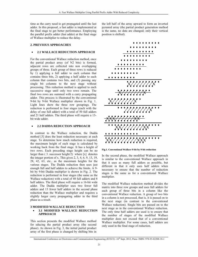
For the conventional Wallace reduction method, once the partial product array (of N2 bits) is formed, adjacent rows are collected into non overlapping groups of three. Each group of three rows is reduced by 1) applying a full adder to each column that contains three bits, 2) applying a half adder to each column that contains two bits, and (3) passing any single bit columns to the next stage without processing. This reduction method is applied to each successive stage until only two rows remain. The final two rows are summed with a carry propagating adder. This process is illustrated by the conventional 9-bit by 9-bit Wallace multiplier shown in Fig. 1. Light lines show the three row groupings. The reduction is performed in four stages (each with the delay of one full adder) with a total of 50 full adders and 21 half adders. The third phase will require a 13-bit wide adder. • 2.2 DADDA REDUCTION APPROACH
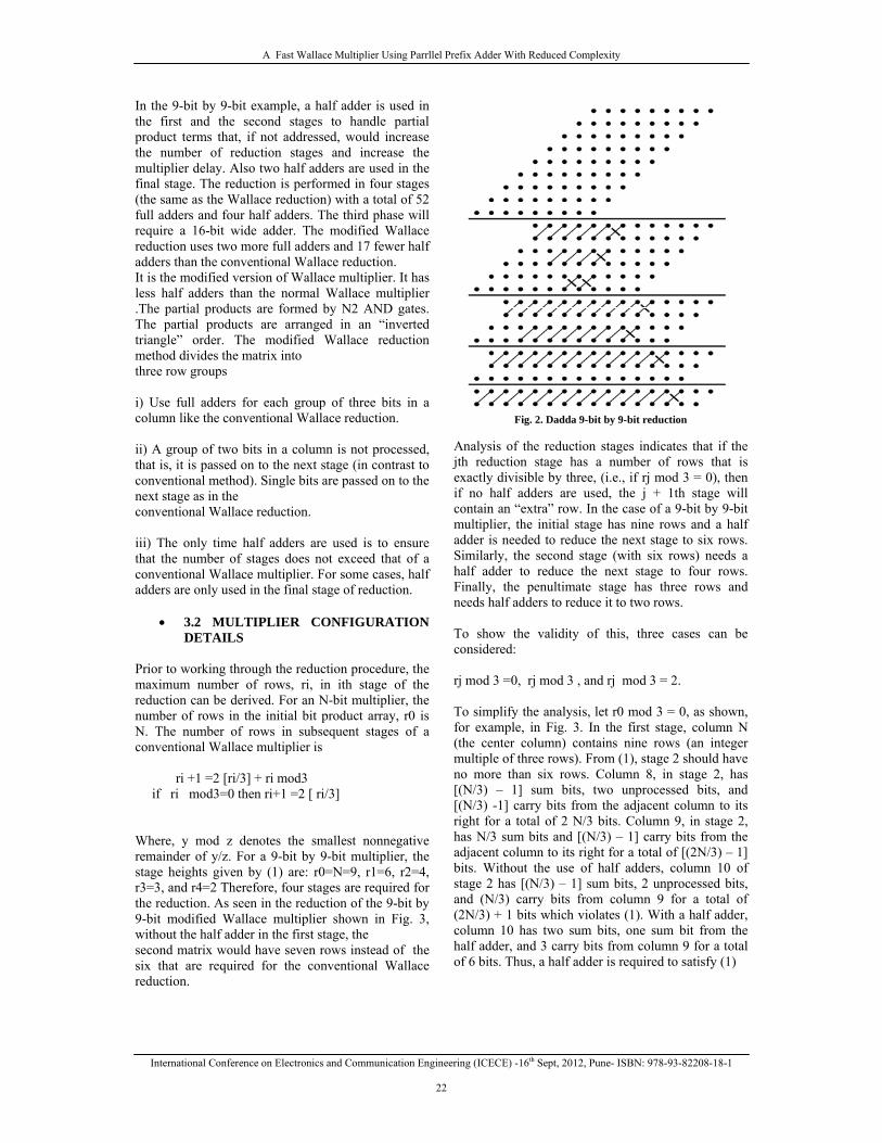
In contrast to the Wallace reduction, the Dadda method [3] does the least reduction necessary at each stage. To determine how much reduction is required, the maximum height of each stage is calculated by working back from the final stage. It has a height of two rows. Each preceding stage height can be no larger than ( 3. successor height/2) where [x] denotes the integer portion of x. This gives 2, 3, 4, 6, 9, 13, 19, 28, 42, 63, etc., as the maximum heights for the various stages. The Dadda reduction then uses just enough full and half adders to achieve the limits. A 9-bit by 9-bit Dadda multiplier is shown in Fig. 2. The reduction is performed in four stages (the same as the Wallace reduction) with a total of 48 full adders and 8 half adders. The third phase will require a 16-bit wide adder. The Dadda multiplier uses two fewer full adders and 13 fewer half adders in the second phase reduction than the Wallace multiplier and requires a slightly larger carry propagating adder in the third phase as a result. 3 MODIFIED WALLACE REDUCTION • 3.1 MODIFIED WALLACE REDUCTION
APPROACH This section presents the modified Wallace method for educing the partial product array (the second phase). As shown in Fig. 3, the initial partial product array of the first phase is changed by shifting bits in
the left half of the array upward to form an inverted pyramid array (the partial product generation method is the same, no data are changed; only their vertical position is shifted).
Fig.1. Conventional Wallace 9-bit by 9-bit reduction In the second phase, the modified Wallace approach is similar to the conventional Wallace approach in that it uses as many full adders as possible, but different in that it only uses half adders when necessary to ensure that the number of reduction stages is the same as for a conventional Wallace multiplier. The modified Wallace reduction method divides the matrix into three row groups and uses full adders for each group of three bits in a column like the conventional Wallace reduction. A group of two bits in a column is not processed, that is, it is passed on to the next stage (in contrast to the conventional Wallace reduction). Single bits are passed on to the next stage as in the conventional Wallace reduction. The only time half adders are used is to ensure that the number of stages of the modified Wallace multiplier does not exceed that of a conventional Wallace multiplier. For some cases, half adders are only used in the final stage of reduction.
A Fast Wallace Multiplier Using Parrllel Prefix Adder With Reduced Complexity
International Conference on Electronics and Communication Engineering (ICECE) -16th Sept, 2012, Pune- ISBN: 978-93-82208-18-1
22
In the 9-bit by 9-bit example, a half adder is used in the first and the second stages to handle partial product terms that, if not addressed, would increase the number of reduction stages and increase the multiplier delay. Also two half adders are used in the final stage. The reduction is performed in four stages (the same as the Wallace reduction) with a total of 52 full adders and four half adders. The third phase will require a 16-bit wide adder. The modified Wallace reduction uses two more full adders and 17 fewer half adders than the conventional Wallace reduction. It is the modified version of Wallace multiplier. It has less half adders than the normal Wallace multiplier .The partial products are formed by N2 AND gates. The partial products are arranged in an “inverted triangle” order. The modified Wallace reduction method divides the matrix into three row groups i) Use full adders for each group of three bits in a column like the conventional Wallace reduction. ii) A group of two bits in a column is not processed, that is, it is passed on to the next stage (in contrast to conventional method). Single bits are passed on to the next stage as in the conventional Wallace reduction. iii) The only time half adders are used is to ensure that the number of stages does not exceed that of a conventional Wallace multiplier. For some cases, half adders are only used in the final stage of reduction.
• 3.2 MULTIPLIER CONFIGURATION DETAILS
Prior to working through the reduction procedure, the maximum number of rows, ri, in ith stage of the reduction can be derived. For an N-bit multiplier, the number of rows in the initial bit product array, r0 is N. The number of rows in subsequent stages of a conventional Wallace multiplier is ri +1 =2 [ri/3] + ri mod3 if ri mod3=0 then ri+1 =2 [ ri/3] Where, y mod z denotes the smallest nonnegative remainder of y/z. For a 9-bit by 9-bit multiplier, the stage heights given by (1) are: r0=N=9, r1=6, r2=4, r3=3, and r4=2 Therefore, four stages are required for the reduction. As seen in the reduction of the 9-bit by 9-bit modified Wallace multiplier shown in Fig. 3, without the half adder in the first stage, the second matrix would have seven rows instead of the six that are required for the conventional Wallace reduction.
Fig. 2. Dadda 9-bit by 9-bit reduction
Analysis of the reduction stages indicates that if the jth reduction stage has a number of rows that is exactly divisible by three, (i.e., if rj mod 3 = 0), then if no half adders are used, the j + 1th stage will contain an “extra” row. In the case of a 9-bit by 9-bit multiplier, the initial stage has nine rows and a half adder is needed to reduce the next stage to six rows. Similarly, the second stage (with six rows) needs a half adder to reduce the next stage to four rows. Finally, the penultimate stage has three rows and needs half adders to reduce it to two rows. To show the validity of this, three cases can be considered: rj mod 3 =0, rj mod 3 , and rj mod 3 = 2. To simplify the analysis, let r0 mod 3 = 0, as shown, for example, in Fig. 3. In the first stage, column N (the center column) contains nine rows (an integer multiple of three rows). From (1), stage 2 should have no more than six rows. Column 8, in stage 2, has [(N/3) – 1] sum bits, two unprocessed bits, and [(N/3) -1] carry bits from the adjacent column to its right for a total of 2 N/3 bits. Column 9, in stage 2, has N/3 sum bits and [(N/3) – 1] carry bits from the adjacent column to its right for a total of [(2N/3) – 1] bits. Without the use of half adders, column 10 of stage 2 has [(N/3) – 1] sum bits, 2 unprocessed bits, and (N/3) carry bits from column 9 for a total of (2N/3) + 1 bits which violates (1). With a half adder, column 10 has two sum bits, one sum bit from the half adder, and 3 carry bits from column 9 for a total of 6 bits. Thus, a half adder is required to satisfy (1)
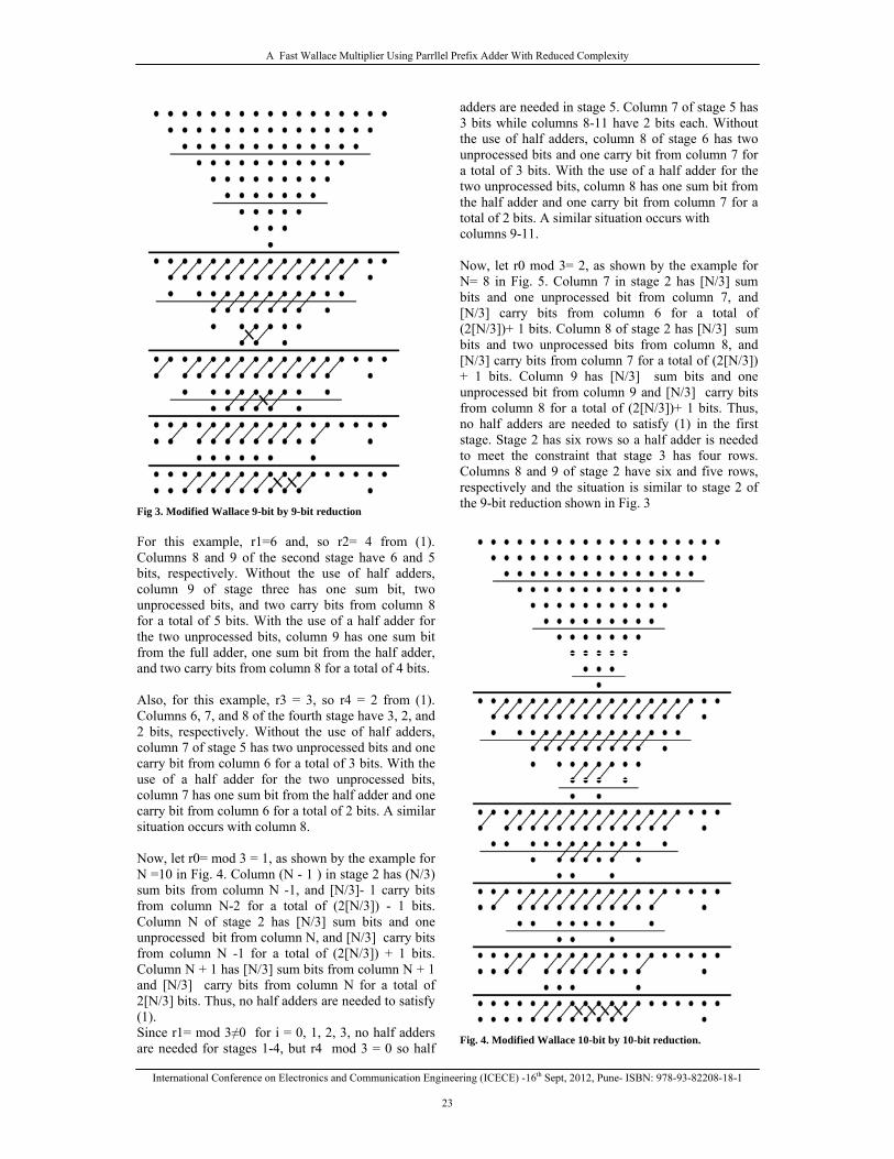
A Fast Wallace Multiplier Using Parrllel Prefix Adder With Reduced Complexity
International Conference on Electronics and Communication Engineering (ICECE) -16th Sept, 2012, Pune- ISBN: 978-93-82208-18-1
23
Fig 3. Modified Wallace 9-bit by 9-bit reduction For this example, r1=6 and, so r2= 4 from (1). Columns 8 and 9 of the second stage have 6 and 5 bits, respectively. Without the use of half adders, column 9 of stage three has one sum bit, two unprocessed bits, and two carry bits from column 8 for a total of 5 bits. With the use of a half adder for the two unprocessed bits, column 9 has one sum bit from the full adder, one sum bit from the half adder, and two carry bits from column 8 for a total of 4 bits. Also, for this example, r3 = 3, so r4 = 2 from (1). Columns 6, 7, and 8 of the fourth stage have 3, 2, and 2 bits, respectively. Without the use of half adders, column 7 of stage 5 has two unprocessed bits and one carry bit from column 6 for a total of 3 bits. With the use of a half adder for the two unprocessed bits, column 7 has one sum bit from the half adder and one carry bit from column 6 for a total of 2 bits. A similar situation occurs with column 8. Now, let r0= mod 3 = 1, as shown by the example for N =10 in Fig. 4. Column (N - 1 ) in stage 2 has (N/3) sum bits from column N -1, and [N/3]- 1 carry bits from column N-2 for a total of (2[N/3]) - 1 bits. Column N of stage 2 has [N/3] sum bits and one unprocessed bit from column N, and [N/3] carry bits from column N -1 for a total of (2[N/3]) + 1 bits. Column N + 1 has [N/3] sum bits from column N + 1 and [N/3] carry bits from column N for a total of 2[N/3] bits. Thus, no half adders are needed to satisfy (1). Since r1= mod 3≠0 for i = 0, 1, 2, 3, no half adders are needed for stages 1-4, but r4 mod 3 = 0 so half
adders are needed in stage 5. Column 7 of stage 5 has 3 bits while columns 8-11 have 2 bits each. Without the use of half adders, column 8 of stage 6 has two unprocessed bits and one carry bit from column 7 for a total of 3 bits. With the use of a half adder for the two unprocessed bits, column 8 has one sum bit from the half adder and one carry bit from column 7 for a total of 2 bits. A similar situation occurs with columns 9-11. Now, let r0 mod 3= 2, as shown by the example for N= 8 in Fig. 5. Column 7 in stage 2 has [N/3] sum bits and one unprocessed bit from column 7, and [N/3] carry bits from column 6 for a total of (2[N/3])+ 1 bits. Column 8 of stage 2 has [N/3] sum bits and two unprocessed bits from column 8, and [N/3] carry bits from column 7 for a total of (2[N/3]) + 1 bits. Column 9 has [N/3] sum bits and one unprocessed bit from column 9 and [N/3] carry bits from column 8 for a total of (2[N/3])+ 1 bits. Thus, no half adders are needed to satisfy (1) in the first stage. Stage 2 has six rows so a half adder is needed to meet the constraint that stage 3 has four rows. Columns 8 and 9 of stage 2 have six and five rows, respectively and the situation is similar to stage 2 of the 9-bit reduction shown in Fig. 3
Fig. 4. Modified Wallace 10-bit by 10-bit reduction.
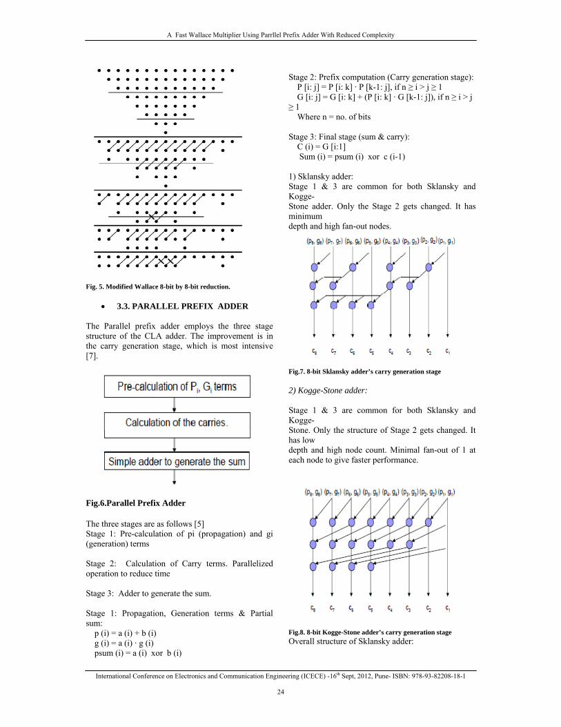
A Fast Wallace Multiplier Using Parrllel Prefix Adder With Reduced Complexity
International Conference on Electronics and Communication Engineering (ICECE) -16th Sept, 2012, Pune- ISBN: 978-93-82208-18-1
24
Fig. 5. Modified Wallace 8-bit by 8-bit reduction.
• 3.3. PARALLEL PREFIX ADDER The Parallel prefix adder employs the three stage structure of the CLA adder. The improvement is in the carry generation stage, which is most intensive [7].
Fig.6.Parallel Prefix Adder The three stages are as follows [5] Stage 1: Pre-calculation of pi (propagation) and gi (generation) terms Stage 2: Calculation of Carry terms. Parallelized operation to reduce time Stage 3: Adder to generate the sum. Stage 1: Propagation, Generation terms & Partial sum: p (i) = a (i) + b (i) g (i) = a (i) · g (i) psum (i) = a (i) xor b (i)
Stage 2: Prefix computation (Carry generation stage): P [i: j] = P [i: k] · P [k-1: j], if n ≥ i > j ≥ 1 G [i: j] = G [i: k] + (P [i: k] · G [k-1: j]), if n ≥ i > j ≥ 1 Where n = no. of bits Stage 3: Final stage (sum & carry): C (i) = G [i:1] Sum (i) = psum (i) xor c (i-1) 1) Sklansky adder: Stage 1 & 3 are common for both Sklansky and Kogge- Stone adder. Only the Stage 2 gets changed. It has minimum depth and high fan-out nodes.
Fig.7. 8-bit Sklansky adder’s carry generation stage 2) Kogge-Stone adder: Stage 1 & 3 are common for both Sklansky and Kogge- Stone. Only the structure of Stage 2 gets changed. It has low depth and high node count. Minimal fan-out of 1 at each node to give faster performance.
Fig.8. 8-bit Kogge-Stone adder’s carry generation stage Overall structure of Sklansky adder:
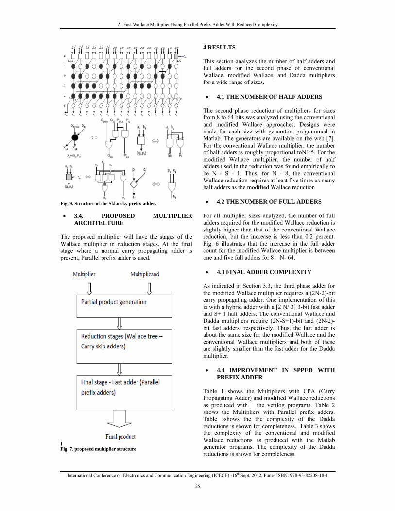
A Fast Wallace Multiplier Using Parrllel Prefix Adder With Reduced Complexity
International Conference on Electronics and Communication Engineering (ICECE) -16th Sept, 2012, Pune- ISBN: 978-93-82208-18-1
25
Fig. 9. Structure of the Sklansky prefix-adder. • 3.4. PROPOSED MULTIPLIER
ARCHITECTURE The proposed multiplier will have the stages of the Wallace multiplier in reduction stages. At the final stage where a normal carry propagating adder is present, Parallel prefix adder is used.
] Fig 7. proposed multiplier structure
4 RESULTS This section analyzes the number of half adders and full adders for the second phase of conventional Wallace, modified Wallace, and Dadda multipliers for a wide range of sizes. • 4.1 THE NUMBER OF HALF ADDERS
The second phase reduction of multipliers for sizes from 8 to 64 bits was analyzed using the conventional and modified Wallace approaches. Designs were made for each size with generators programmed in Matlab. The generators are available on the web [7]. For the conventional Wallace multiplier, the number of half adders is roughly proportional toN1:5. For the modified Wallace multiplier, the number of half adders used in the reduction was found empirically to be N - S - 1. Thus, for N - 8, the conventional Wallace reduction requires at least five times as many half adders as the modified Wallace reduction • 4.2 THE NUMBER OF FULL ADDERS
For all multiplier sizes analyzed, the number of full adders required for the modified Wallace reduction is slightly higher than that of the conventional Wallace reduction, but the increase is less than 0.2 percent. Fig. 6 illustrates that the increase in the full adder count for the modified Wallace multiplier is between one and five full adders for 8 – N- 64. • 4.3 FINAL ADDER COMPLEXITY
As indicated in Section 3.3, the third phase adder for the modified Wallace multiplier requires a (2N-2)-bit carry propagating adder. One implementation of this is with a hybrid adder with a [2 N/ 3] 3-bit fast adder and S+ 1 half adders. The conventional Wallace and Dadda multipliers require (2N-S+1)-bit and (2N-2)-bit fast adders, respectively. Thus, the fast adder is about the same size for the modified Wallace and the conventional Wallace multipliers and both of these are slightly smaller than the fast adder for the Dadda multiplier. • 4.4 IMPROVEMENT IN SPPED WITH
PREFIX ADDER Table 1 shows the Multipliers with CPA (Carry Propagating Adder) and modified Wallace reductions as produced with the verilog programs. Table 2 shows the Multipliers with Parallel prefix adders. Table 3shows the the complexity of the Dadda reductions is shown for completeness. Table 3 shows the complexity of the conventional and modified Wallace reductions as produced with the Matlab generator programs. The complexity of the Dadda reductions is shown for completeness.

A Fast Wallace Multiplier Using Parrllel Prefix Adder With Reduced Complexity
International Conference on Electronics and Communication Engineering (ICECE) -16th Sept, 2012, Pune- ISBN: 978-93-82208-18-1
26
As shown clearly in Table 1, for all word sizes, the modified Wallace reduction uses only a very few full adders more than the conventional Wallace reduction. On the other hand, the number of half adders is reduced by a factor of five (for the 8-bit reduction) to a factor of eight (for the 64-bit reduction). The total gate count is always less for the modified Wallace reduction than for the conventional Wallace reduction by 10 (for the 8-bit reduction) to four percent (for the 64-bit reduction).
TABLE – I MULTIPLIERS WITH CPA - COMPARISON
The delay of multipliers [Wallace & Reduced Complexity Wallace] with Carry Propagating Adder at final stage.
TABLE – II MULTIPLIERS WITH PARALLEL
PREFIX ADDERS The delay of multipliers with Parallel prefix adders [Sklansky and Kogge-Stone adder] at final stage.
TABLE-III COMPLEXITY OF REDUCTION
For all word sizes, the modified Wallace reduction uses a few more full adders than the Dadda reduction. The number of half adders is reduced significantly for the modified Wallace reduction. The Dadda reduction requires a slightly smaller total gate count than the modified Wallace reduction, but a complete Dadda multiplier will require more gates due to its larger carry propagating adder. An interesting point is that the sum of the number of full adders and the number of half adders is the same for the modified Wallace reduction and the Dadda reduction. It is not evident why this occurs. 5 CONCLUSION This paper presents a modification to the second phase reduction (that reduces N rows of bit products to two rows) used in Wallace multipliers. The modified Wallace reduction reduces the number of half adders required by at least 80 percent compared to the conventional Wallace reduction with only a very slight increase in the number of full adders. Both the conventional Wallace and modified Wallace reductions have the same number of stages and consequently the delay is expected to be the same. It is significant that both the conventional and modified Wallace second phase reductions use more gates than the Dadda reduction, although the penalty is less for the modified .This paper proposes improvement of Wallace multipliers [Normal & Reduced Complexity] with reduced delay using Parallel prefix adders at the final stage. From the results, it can be inferred that the proposed multipliers has lesser delay than the conventional multipliers. In processes, where repeated multiplication is done, this multiplier will provide significant performance REFERENCES [1]. Ron S. Waters, Earl E.Swartzlander “A Reduced Complexity
Wallace multiplier reduction” in IEEE transactions on Computers, Aug. 2010.
[2]. Whitney J. Townsend, Earl E.Swartzlander, Jacob A. Abraham “A comparison of Dadda and Wallace multiplier delays” University of Texas at Austin, work under National Science foundation graduate research fellowship.
[3]. Wallace C.S. “A suggestion for a fast multiplier” in IEEE transactions on Electronics & Computers, 1964.
[4]. Kostas Vitoroulis “Parallel prefix adders: notes” Concordia university,2006.
[5]. Taeko Matsunaga and Yuske Matsunaga “Timing constrained Area minimization algorithm for Parallel prefix adders”, IEICE transaction fundamentals, Vol.E90-A, No.12, Dec. 2007.
[6]. Nuno Roma, Tiago Dias & Leonel Sousa “Fast adder architectures: modelling & experimental evaluation” IST/INESC-ID, Lisbon, Portugal ,project under Portuguese foundation for science and technology
International Conference on Electronics and Communication Engineering (ICECE) -16th Sept, 2012, Pune- ISBN: 978-93-82208-18-1
27
FACIAL EXPRESSION RECOGNITION BY USING PCA FOR FEATURE EXTRACTION AND HMM FOR CLASSIFICATION
1TANVI SRIVASTAVA & 2NAVEETA KANT
1,2Vivekanand Education Society Institute of Technology (V.E.S.I.T) Mumbai, India
Abstract— This paper proposes a simple but powerful method for automatic classification of facial expressions from static images. Still images do not bare as much information as in video sequences which have much information activities during the expression actions. The main aim here is to be able to classify every facial image into the six universally researched and accepted prototypic facial expressions like happy, fear, disgust anger, surprise and sadness. We propose a powerful matching algorithm to determine the correct grouping or class of the newly received image into the already learned data in the database. Principal Component Analysis (PCA), a powerful tool in the feature extraction and dimensionality reduction is utilized to generate Eigen-components of the images. The Six representatives (Principal) Eigen-components of the individual facial expressions classes are stored and used at the time of matching. In this method, the condition of facial muscles is assigned to a hidden obtained from image processing. The rationale behind using HMM is that the HMM models human brain as human emotion is quite complex, naturally a human instinct contain hidden layer as well. In addition, markov state chain property is good model human emotion as our emotion is also through our mind state that it is always that it is always dependent on our previous state of our emotion and current event will end up our current emotion state. The individual matching rate is recorded and compared for the evaluation and proper classification. Falsely accepted data (FAR) and the ones rejected falsely (FRR) are studied for algorithms improvement. . With proper initial image processing and noise removal techniques used, a high proper classification is envisioned. The algorithm has worked perfectly with JAFFE data base. More tests are yet to be carried out on other public databases. Keywords- Expressions, PCA, HMM.
I. INTRODUCTION
Emotion is a state of feeling involving thoughts,
physiological changes and an outward expression. A lot of research has been done on recognizing both still image and in videos and yet the faces and its attributes to the emotion have not been fully explored. According to the facial feedback theory [4] emotion is the experience of changes in our facial muscle. The six universal common facial expressions do not fully satisfy the wide range of facial action units and their description. When we smile, we experience pleasure or happiness. It is the changes in our facial muscles that direct our brains and provide the basis for our emotions. As there are many possibilities of muscle configuration in our face, there is seemingly unlimited number of emotions.Ekman and Friesen [1] postulated six primary emotions that posses each a distinctive content together with a unique facial expression.
In this paper, we propose to develop a facial
expression recognition system to identify six universal expression .In this FER system second section shows how we are cropping a still image to remove irrelevant input. In the third section we will see how by using PCA we are extracting features to feed to our classifier. In the fourth section we have HMM as classifier which finally identifies the expression .In fifth section we have briefed about JAFFE database used. In sixth section we have shown our experimental results and followed by this is conclusion.
II. IMAGE PREPROCESSING
Preprocessing of image refers to the removal of the outer parts of an image to improve accentuate subject matter or change aspect ratio. It refers to removing unwanted areas from image and it is performed in order to remove an un wanted subject or irrelevant detail from an image and improve the overall composition. III. FEATURE EXTRACTION [5]
The PCA is a well known and frequently used linear dimensionality reduction method. Several literatures describe this and it works by projecting a number of correlated variables into a smaller number of uncorrelated variables called principal components [6, 3]. The algorithm solves for the eigen values and eigenvectors. The eigenvectors associated with the highest eigen value dictates the direction of the first principal component, literally exposing the highest amount of variance of the original data. This first principal component accounts for the magnitude of variability in the data as much as possible. The subsequent eigenvectors associated with the second largest eigen values determine the direction of the second principal component. The trend continues down to the most insignificant components which do not have any big effect on the data variability. Here, the objective achieved by PCA is the identification of small set of variables which can be more easily interpreted. PCA process is briefly described below as in [2, 3].
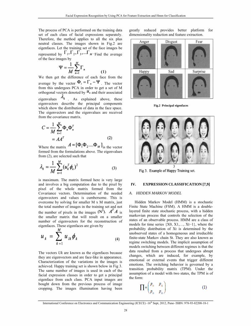
Facial Expression Recognition by Using PCA for Feature Extraction and Hmm for Classification
International Conference on Electronics and Communication Engineering (ICECE) -16th Sept, 2012, Pune- ISBN: 978-93-82208-18-1
28
The process of PCA is performed on the training data set of each class of facial expressions separately. Therefore, the method applies to all the six plus neutral classes. The images shown in Fig.2 are eigenfaces. Let the training set of the face images be represented by Find the average of the face images by
We then get the difference of each face from the average by the vector . The vector from this undergoes PCA in order to get a set of M orthogonal vectors denoted by and their associated
eigenvalues . As explained above, these eigenvectors describe the principal components which show the distribution of data in the face space. The eigenvectors and the eigenvalues are received from the covariance matrix.
Where the matrix is the vector formed from the formulations above. The eigenvalues from (2), are selected such that
is maximum. The matrix formed here is very large and involves a big computation due to the pixel by pixel of the whole matrix formed from the Covariance vectors. Determination of the needed eigenvectors and values is cumbersome. This is overcome by solving for smaller M x M matrix, just the total number of images in the training set and not the number of pixels in the images is the smaller matrix that will result on a smaller number of eigenvectors for the reconstruction of eigenfaces. These eigenfaces are given by
The vectors Uk are known as the eigenfaces because they are eigenvectors and are face-like in appearance. Characterization of the variations in the images is achieved. Happy training set is shown below in Fig 3. The same number of images is used in each of the facial expression classes in order to get a principal eigenface from each class. PCA input images are bought down from the previous process of image cropping. The images illumination having been
greatly reduced provides better platform for dimensionality reduction and feature extraction.
Fig.2 Principal eigenfaces
IV. EXPRESSION CLASSIFICATION [7,9]
A. HIDDEN MARKOV MODEL
Hidden Markov Model (HMM) is a stochastic
Finite State Machine (FSM). A HMM is a double-layered finite state stochastic process, with a hidden markovian process that controls the selection of the states of an observable process. HMM are a class of models for time series {X0, X1,…, Xt−1}, where the probability distribution of Xt is determined by the unobserved states of a homogeneous and irreducible finite-state Markov chain St. They are also known as regime switching models. The implicit assumption of models switching between different regimes is that the data resulted from a process that undergoes abrupt changes, which are induced, for example, by emotional or external events that trigger different emotions. The switching behavior is governed by a transition probability matrix (TPM). Under the assumption of a model with two states, the TPM is of the form:
Facial Expression Recognition by Using PCA for Feature Extraction and Hmm for Classification
International Conference on Electronics and Communication Engineering (ICECE) -16th Sept, 2012, Pune- ISBN: 978-93-82208-18-1
29
where p11 denotes the probability of staying in the first state from period t to period t+1 and p12 is the probability of switching from the first to second state. The second row can be interpreted analogously. The distribution of the observation at time t is specified by the conditional or component distributions
associated with the “state” or “regime” st. Assume that, for instance, a two-state model with normal component distributions yields:
The parameters of a HMM are generally estimated
using the method of maximum-likelihood. The likelihood function is available in the following form:
where P(xt) represents a diagonal matrix with the state -dependent conditional distributions as entries. The initial distribution of the Markov chain is denoted by δ, the model parameters by θ,
and . The log-likelihood can be easily evaluated even for very long sequences of observations and so the parameters can be estimated through direct numerical maximization of the log-likelihood function using, e.g., Newton-type methods (see [6]).
Fig.4 Probabilistic parameters of a HMM (x denotes states,y denotes possible observations)
V. JAFFE DATABASE It contain 213 images of 7 facial expression (6 basic facial expression + 1 neutral) posed by 10 Japanese female models. Each image has been rated on 6 motion objectives by 60 Japanese subjects.
VI. EXPERIMENTAL RESULTS In our experiment we have used statistical toolbox of MATLAB R2010b software. Principal eigenfaces were product of twenty images of the same expression .Each expression has two to three images from one individual and the rest of the images have been used to test images (JAFFE).A total 150 images for training and 60 images for testing were used. The images are of size 256x256.HMM algorithm is used to classify most of the data in its correct class. We could achieve a result of 90%. In out of 10 images 9 image’s FER is correctly recognized. The fig.5 shows the results how our system works and give correct result. In fig.6 graph shows plotting of different expression and their similarity. VII. CONCLUSION Our goal is to be able to classify any new data from still images into one of the universal facial expression classes. Our positive precision rates are high for most of the classes. The static classifier like HMM classifies the single frames into an emotion class.HMM are one of the basic and perhaps the best known probabilistic tool used for time series modeling .In future we can try to make same system more dynamic so that we can classify more complex emotions or expression. REFERENCES [1] Ekman, P. and W.V. Friesen (1971), “Constants across
cultures in the face and emotion”, J. Personality Social Psychol, 17(2): p. 124-129.
[2] Mathew A. Turk and Alex P. Pentland. "Face Recognition Using Eigenfaces".
[3] M. A Turk, A. Pentland. "Eigenfaces for Recognition". Journal of Cognitive Neuroscience. Vo13,No.l.71-86,1991.
[4] Buck, R., (1980), “Nonverbal behavior and the theory of emotion: The facial feedback hypothesis”, Journal of Personality and Social Psychology, 38(5): p. 811-824.
[5] Wilfred Onyango Odoyo”Facial Expression Classification using Eigen components of Principal Expression.”(2009) ISBN 978-89-5519-139-4.
[6] Fukunaga, K. "Introduction to Statistical Pattern Recognition". (1990).
[7] Teik-Toe TEOH and Siu-yeung CHO “Human Emotional States Modelling by Hidden Markov Model.”978-1-4244-9953-3/11/$26.00 ©2011 IEEE
[8] JAFFEdatabase. [9] MacDonald I. and W. Zucchini (1997), Hidden Markov and
Other Models for Discrete Valued Time Series. Chapman Hall.
Facial Expression Recognition by Using PCA for Feature Extraction and Hmm for Classification
International Conference on Electronics and Communication Engineering (ICECE) -16th Sept, 2012, Pune- ISBN: 978-93-82208-18-1
30
a)
Fig.6 Graph plot of different expression
b) Fig.5 Results of experiment
.
International Conference on Electronics and Communication Engineering (ICECE) -16th Sept, 2012, Pune- ISBN: 978-93-82208-18-1
31
BLIND SOURCE SEPARATION USING TEMPORAL REDICTABILITY FOR REDUCTION OF BACKGROUND NOISE IN SPEECH
1DEEPALI A. NEWASKAR & 2PRACHI MUKHERJI
1,2Dept. of Electronics and Telecommunication
Smt. Kashibai Navale College of Engineering, Pune, India
Abstract— Blind Source Separation (BSS) using temporal predictability can be used to get the independent individual noise source signals for noise identification, signal source identification and other fields like acoustic echo cancellation. This method can separate signal mixtures in which each mixture can be a linear combination of source signals (voice or music) with super-Gaussian, sub-Gaussian and Gaussian probability density functions. Thus drawback of Independent Component Analysis of having non-Gaussian distribution for independent components is overcome. One of the applications of BSS can be in share trading office or in call centers where so many operators speaks simultaneously with their customers. Separation of audio sources, which have been mixed and then captured by microphones, is required in this case. If the source of noise is known then this method can be combined with algorithms like Least Mean Square (LMS), or it’s variants like Normalized Least Mean Square (NLMS) algorithm for better noise reduction. Key words: Blind Source Separation (BSS), Independent Component Analysis, Temporal Predictability, LMS, NLMS.
I. INTRODUCTION
Noise has been receiving increasing recognition as one of the critical environmental pollution problems besides air and water pollution. Noise and vibration measurement is the main process not only in the vibration control project but also in the test project of noise detection, environment protection, labor protection and so on. The best way to control noise is at its source which will greatly decrease the complexity of work and help people research new products of low noise and high quality [1]. Almost every signal measured within a physical system is actually a mixture of statistically independent source signals i.e. the sound field, at any point, is a combination of the various contributions from all actual acoustic sources and from the reflections produced by the walls and obstacles present in the hall. It is easier to get the mixed signals rather than individual ones. Consider two people speaking simultaneously, with each person a different distance from two microphones. Each microphone records a linear mixture of the two voices. BSS is a good method to settle such problem of separating the individual signals from the mixed ones [7]. Blind source separation (BSS) algorithms such as independent component analysis (ICA), Principle component Analysis (PCA) and Temporal Predictability deals with recovering a set of underlying sources from observations without knowing mixing processing. Thus BSS can separate the speech signals from different sources. Further noise can be reduced by applying adaptive filter algorithm, as many times there is a situation where clarity and intelligibility of speech is impaired due to ubiquitous noise. There are many types of noise distortion that exist in the field of speech
communication. Adaptive algorithms represent one of the most frequently used computational tools for the processing of digital speech signals. So far, many gradient-based algorithms can be used for speech enhancement [12],[13]. There are many types of adaptive filters which employ different schemes to adjust the filter weights. The LMS algorithm is the most common algorithm used. The performance of LMS-based algorithm can be improved by normalization, i.e. Normalized Least Mean Square (NLMS) algorithm [2], [4], [6], [8]. II. BLIND SOURCE SEPARATION (NOISE
REMOVAL) A. Independent Component Analysis(ICA): BSS aims at recovering the underlying sources by exploiting the assumption of their mutual independence from a given series of observed signals. Applying BSS to an acoustics mixture such as mixed voices from multiple talkers in a room that is known as a cocktail party problem. In 1986, Jutten and Herault proposed the concept of BSS as a novel tool to capture clean individual signals from noisy signals containing unknown, multiple and overlapping signals. The Jutten and Herault model comprised a recursive neural network for finding the clean signals based on the assumption that the noisy source signals were statistically independent. Blind source separation (BSS) is the problem of recovering signals from several observed linear mixtures. These signals could be from different directions or they could have different pitch levels along the same directions. When we deal with the BSS, there is no need for information on the source signals or mixing system (location or room acoustics). The characteristics of the source signals are statistically independent, as well as independent
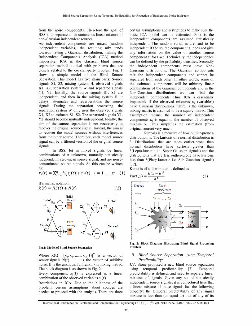
Blind Source Separation Using Temporal Redictability for Reduction of Background Noise in Speech
International Conference on Electronics and Communication Engineering (ICECE) -16th Sept, 2012, Pune- ISBN: 978-93-82208-18-1
32
from the noise components. Therefore the goal of BSS is to separate an instantaneous linear mixture of non-Gaussian independent sources. As independent components are mixed (random independent variables) the resulting mix tends towards having a Gaussian distribution, making the Independent Components Analysis (ICA) method impossible. ICA is the classical blind source separation method to deal with problems that are closely related to the cocktail-party problem. Fig. 1 shows a simple model of the Blind Source Separation. This model has five main parts: Source signals S1, S2, mixing system H, observed signals X1, X2, separation system W and separated signals Y1, Y2. Initially, the source signals S1, S2 are independent, and then in the mixing system H, it delays, attenuates and reverberations the source signals. During the separation processing, the separation system W only uses the observed signals X1, X2 to estimate S1, S2. The separated signals Y1, Y2 should become mutually independent. Ideally, the aim of the source separation is not necessarily to recover the original source signal. Instead, the aim is to recover the model sources without interferences from the other source. Therefore, each model source signal can be a filtered version of the original source signals.
In BSS, let m mixed signals be linear combinations of n unknown, mutually statistically independent, zero-mean source signal, and are noise-contaminated source signals. So this can be written as:
∑ 1 … … 1 It’s matrix notation:
2
Fig.1: Model of Blind Source Separation Where X t x , x , … . . , x t T is a vector of sensor signals, N t is the vector of additive noise. H is the unknown full rank n×m mixing matrix. The block diagram is as shown in Fig. 2. Every component x t is expressed as a linear combination of the observed variables s t Restrictions in ICA: Due to the blindness of the problem, certain assumptions about sources are needed to proceed with the analysis. There are three
certain assumptions and restrictions to make sure the basic ICA model can be estimated. First is the independent components are assumed statistically independent. The random variables are said to be independent if the source component s does not give any information on the value of another source component s for i j .Technically, the independence can be defined by the probability densities. Secondly the independent components must have Non-Gaussian distributions. The Gaussian components mix the independent components and cannot be separated from each other. In other words, some of the estimated components will be arbitrary linear combinations of the Gaussian components and in the Non-Gaussian distributions we can find the independent components. Thus, ICA is essentially impossible if the observed mixtures x (variables) have Gaussian distributions. Third is the unknown, mixing matrix is assumed to be a square matrix. This assumption means, the number of independent components s is equal to the number of observed mixture x . This simplifies the estimation (from original source) very much.
Kurtosis is a measure of how outlier-prone a distribution is. The kurtosis of a normal distribution is 3. Distributions that are more outlier-prone than normal distribution have kurtosis greater than 3(Lepto-kurtotic i.e. Super Gaussian signals) and the distributions that are less outlier-prone have kurtosis less than 3(Platy-kurtotic i.e. Sub-Gaussian signals) [12]. Kurtosis of a distribution is defined as
µ 3
Fig. 2: Block Diagram Illustrating Blind Signal Processing Problem B. Blind Source Separation using Temporal
Predictability: J.V. Stone proposed a new blind source separation using temporal predictability [7]. Temporal predictability is defined, and used to separate linear mixtures of signals. Given any set of statistically independent source signals, it is conjectured here that a linear mixture of those signals has the following property: the temporal predictability of any signal mixture is less than (or equal to) that of any of its
Internatio
componentproperty caset of lineun-mixing temporal pTemporal conventionThis propefrom a sefinding anmeasure ofsignal. Thigeneralizedhave scalinnumber of
Inanalysis, thminimal density funseparate silinear comGaussian, density fumusic. Thehere is:
Where , and isThe term predicted bmoving avterm ismeasured blong-term predicted exponentiameasured have a larg
The half-litimes long
. The rparameter Note that mvariance sstructure. result in a would be maximizedU can be ratio are both sa1) y has a2) the vaNote also norm of
Blind Sourc
nal Conference on
t source signan be used to rar mixtures of
matrix whichpredictability Predictability
nal source sepaerty can be uset of linear mn un-mixing mf temporal predis matrix is od Eigen valung characteristf signal mixturen contrast tohe temporal prassumptions
nctions of sourignal mixturesmbination of
sub-Gaussianunctions, and e definition of
is the vs a vector of K
reflects thby a short-termverage of s a measure ofby the extent tmoving averagvalues
ally weightedup to time (τ
ger weighting th
ife of isger) than the corelation betweλ is defined asmaximizing onignal with noIn contrast, mDC signal. Inobtained for
d by setting theminimized by can be maxi
atisfied: a nonzero ranglues in y changthat the value, so that only
ce Separation Usin
n Electronics and C
nals. It is shrecover source f those signalsh maximizes for each rechas been use
aration methoded to recover
mixtures of thomatrix which dictability for ebtained as the
ue problem. Stics of 0(N3), wes. o independenredictability mregarding th
rce signals. Th in which eacsource signal, and Gaussion mixtures
f signal predic
value of the sigK signal mixtuhe extent to
m values in y. If overall variato which is ge of the vaand of
d sums of -1), such that
han those in th
s much longer orresponding heen a half-lif [1], nly would r constraints ominimizing o
n both cases, trr becausee norm of ty setting . Iimized only if t
ge (i.e., high vage slowly over e of F is indepy changes in th
ng Temporal Redic
Communication En
own that thissignals from a
s by finding ana measure ofovered signaled to augmens, such as ICAsource signals
ose signals bymaximizes a
each recoverede solution to aSuch problemswhere N is the
nt componenmethod requireshe probabilityhis method canch mixture is als with super-an probabilityof voices andtability F used
gnal y at time ures at time
which is
n contrast, theability in y, aspredicted by a
alues in y. The are bothsignal valuest recent valueshe distant past:
(typically 100half-life offe h and the[7].
result in a highon its temporanly wouldrivial solutionse can beo be large, andn contrast, thetwo constraints
ariance) and time.
pendent of thehe direction of
ctability for Reduc
ngineering (ICECE
s a n f l. nt A.
s y a d a s e
nt s y n a -y d d
. s
e s a e h s s
0 f e
h al d s e d e s
e f
affect from mixusing adNLMS al C. Stan
The Leastochasticweight inthe squarto that taof the sinstantanestimate the tap initerates othe directbehind Ldescent minimizeThe LMParamete InitializatComputa
In equati
equation signal anmatrix oformula iteration. input vecgradient n
D. The mainsensitive to choosalgorithmis a varianormaliziThe weig
The onlyin the cnormalizeThe disalarge is re
ction of Backgroun
E) -16th Sept, 2012
the value of Fxture, further
daptive filter lgorithms [10],
ndard LMS (Le
st Mean Squac gradient algn the filter in tred amplitude oap weight [3]. Tteepest desceneous estimate of the gradient
nput vector andver each tap wtion of the app
LMS filters is to find a c
es a cost functioS algorithm c
ers: = filter len µ= step siztion:
ation: For
ion 6, is
7, e(n) and d(nnd desired sigof the coeffici
for updating The tap weigh
ctor. So if noise amplifica
. Normalized
n drawback ofto the scaling e a learning
m. The Normalant of the LMSing with the po
ght adaptation c
y difference wicoefficient upded by the conju
advantage of gemoved by nor
nd Noise in Speech
2, Pune- ISBN: 97
F. After separnoise reductioalgorithms su, [11].
east-Mean-Squ
are, or LMS, gorithm that itthe direction ofof an error sigThe LMS is annt algorithm,
of the gradit is based on s
d an error signaweight in the filproximated grato use the meoefficient vecon [Widrow ancan be summangth e
the input tap are the in
n) denote the ougnal respectiveient vector
the coefficieht adjustment
is large, Lation problem.
d LMS:
f the basic LMof its input rate μ that gu
lized Least MeS algorithm thower of the inpcan be summar
th respect to thdating equatiougate transposgradient noise rmalization [8]
h
8-93-82208-18-1
ration of signaon can be don
uch as LMS
uares) algorith
algorithm is terates each taf the gradient
gnal with respen approximatiowhich uses a
ent vector. Thsample values al. The algorithlter, moving it adient. The id
ethod of steepector n whicnd Hoff] [2], [5arized as
vector while dividual tap utput error esti
ely. is th. Equation 7
ent vector aftis directly pro
LMS filter suSo we go for N
MS algorithm . This makes
uarantees stabean Squares filhat solves this put [5], [6]. rized as:
he LMS algoron (9), whiche of the input vamplification
.
als ne or
m
a ap of
ect on an he of
hm in ea est ch 5].
inputs. In imation he transpose 7 gives the
fter the nth oportional to ffer from a NLMS.
is that it is it very hard
bility of the lter (NLMS) problem by
ithm here is h has been vector
n if input is
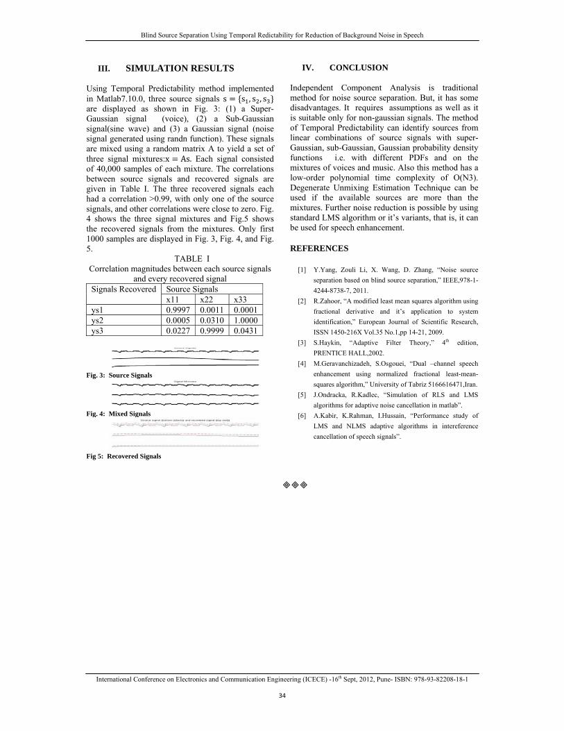
Blind Source Separation Using Temporal Redictability for Reduction of Background Noise in Speech
International Conference on Electronics and Communication Engineering (ICECE) -16th Sept, 2012, Pune- ISBN: 978-93-82208-18-1
34
III. SIMULATION RESULTS Using Temporal Predictability method implemented in Matlab7.10.0, three source signals s s , s , s are displayed as shown in Fig. 3: (1) a Super-Gaussian signal (voice), (2) a Sub-Gaussian signal(sine wave) and (3) a Gaussian signal (noise signal generated using randn function). These signals are mixed using a random matrix A to yield a set of three signal mixtures:x As. Each signal consisted of 40,000 samples of each mixture. The correlations between source signals and recovered signals are given in Table I. The three recovered signals each had a correlation >0.99, with only one of the source signals, and other correlations were close to zero. Fig. 4 shows the three signal mixtures and Fig.5 shows the recovered signals from the mixtures. Only first 1000 samples are displayed in Fig. 3, Fig. 4, and Fig. 5.
TABLE I Correlation magnitudes between each source signals
and every recovered signal Signals Recovered Source Signals
x11 x22 x33ys1 0.9997 0.0011 0.0001ys2 0.0005 0.0310 1.0000 ys3 0.0227 0.9999 0.0431
Fig. 3: Source Signals
Fig. 4: Mixed Signals
Fig 5: Recovered Signals
IV. CONCLUSION
Independent Component Analysis is traditional method for noise source separation. But, it has some disadvantages. It requires assumptions as well as it is suitable only for non-gaussian signals. The method of Temporal Predictability can identify sources from linear combinations of source signals with super-Gaussian, sub-Gaussian, Gaussian probability density functions i.e. with different PDFs and on the mixtures of voices and music. Also this method has a low-order polynomial time complexity of O(N3). Degenerate Unmixing Estimation Technique can be used if the available sources are more than the mixtures. Further noise reduction is possible by using standard LMS algorithm or it’s variants, that is, it can be used for speech enhancement. REFERENCES
[1] Y.Yang, Zouli Li, X. Wang, D. Zhang, “Noise source separation based on blind source separation,” IEEE,978-1-4244-8738-7, 2011.
[2] R.Zahoor, “A modified least mean squares algorithm using fractional derivative and it’s application to system identification,” European Journal of Scientific Research, ISSN 1450-216X Vol.35 No.1,pp 14-21, 2009.
[3] S.Haykin, “Adaptive Filter Theory,” 4th edition, PRENTICE HALL,2002.
[4] M.Geravanchizadeh, S.Osgouei, “Dual –channel speech enhancement using normalized fractional least-mean-squares algorithm,” University of Tabriz 5166616471,Iran.
[5] J.Ondracka, R.Kadlec, “Simulation of RLS and LMS algorithms for adaptive noise cancellation in matlab”.
[6] A.Kabir, K.Rahman, I.Hussain, “Performance study of LMS and NLMS adaptive algorithms in intereference cancellation of speech signals”.
International Conference on Electronics and Communication Engineering (ICECE) -16th Sept, 2012, Pune- ISBN: 978-93-82208-18-1
35
OBJECT TRACKING FOR REAL TIME VIDEO USING MATLAB
1SALONI SHAH & 2MADHVI PANWAR
1&2ECE Deptt., Shri U.S.B. College of Engineering & Mgmt. Abu Road, Sirohi (Rajasthan)
Abstract— In this paper object tracking for real time video is developed which, demonstrates the motion compensated video processing by using sum of absolute differences. First an object has taken as reference object or image then the next successive object is compared with the reference object or image. Each time the successive object is compared with the reference object and produces an absolute difference, then the summation of all these differences shows its sum of absolute difference. This difference shows the change in the two images. Finally by using negative threshold, the change in the motion of sum of absolute differences in the object image is shown. A simulink model is also developed for object tracking for real time video. Keywords- Absolute, Threshold, Tracking, Real time.
I. INTRODUCTION
Image tracking and activity recognition are receiving increasing attention among computer scientists due to the wide spectrum of applications where they can be used, ranging from athletic performance analysis to video surveillance. By image tracking we refer to the ability of a computer to recover the position and orientation of the object from a sequence of images[4]. There have been several different approaches to allow computers to derive automatically the kinematics pose and activity from image sequences.
In digital video communication systems it is important that a video to be compressed, because of storing capacities as well as bit-rate constraints. The video processing is done using Sum of Absolute Differences and with the image processing block set. First motion vectors between successive frames are calculated and use them to reduce redundant information[8]. Then each frame is divided into sub matrices and apply the discrete cosine transform to each sub matrix. Finally, apply a quantization technique to achieve further compression. The Decoder subsystem performs the inverse process to recover the original video.
II. TRACKING: POSSIBLE ISSUES
A. Introduction:
Video tracking is the process of locating a moving object in time using a camera. An algorithm analyses the video frames and outputs the location of moving targets within the video frame. The main difficulty in video tracking is to associate target locations in consecutive video frames, especially when the objects are moving fast relative to the frame rate[10]. Here, video tracking systems usually employ a motion model which describes how the image of the target
might change for different possible motions of the object to track. The role of the tracking algorithm is to analyze the video frames in order to estimate the motion parameters. These parameters characterize the location of the target. B. Component of visual Tracking system:
Target Representation and Localization is mostly a
bottom-up process. Typically the computational complexity for these algorithms is low. The following are some common Target Representation and Localization algorithms:
Blob tracking: Segmentation of object interior (for example blob detection, block-based correlation or optical flow).
Kernel-based tracking (Mean-shift tracking): An iterative localization procedure based on the maximization of a similarity measure.
Contour tracking: Detection of object boundary (e.g. active contours or Condensation algorithm).
Visual feature matching: Registration
One approach to reduce the problem space and to make the problem computationally tractable is to provide constraints on the positions of the object. Constraints can be based on temporal information, camera configuration, or any combination of these. Camera configuration constraints are usually expressed by making assumptions on the relative positioning of the subject with respect to the camera.
III. OPTIMIZATION METHOD OF TRACKING
Most human motion and pose estimation
approaches propose some sort of optimization method, direct or probabilistic, to optimize the pose (and/or body model) subject to the image features observed. A. Direct Optimization
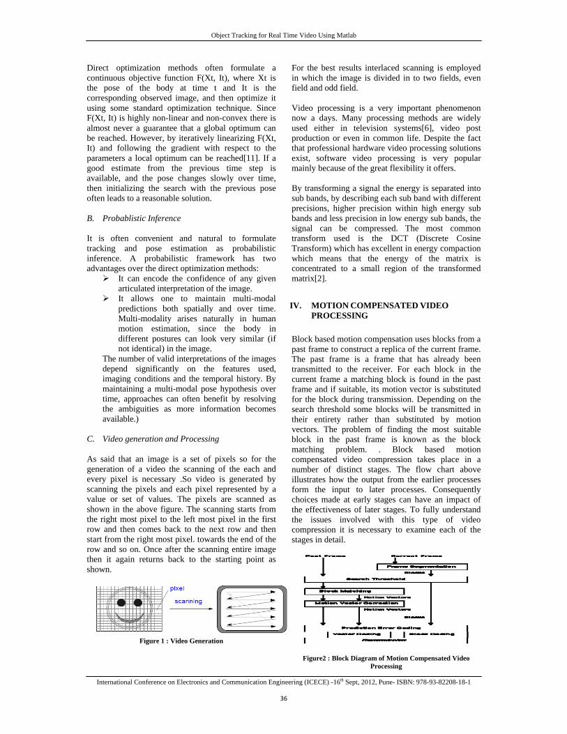
Object Tracking for Real Time Video Using Matlab
International Conference on Electronics and Communication Engineering (ICECE) -16th Sept, 2012, Pune- ISBN: 978-93-82208-18-1
36
Direct optimization methods often formulate a continuous objective function F(Xt, It), where Xt is the pose of the body at time t and It is the corresponding observed image, and then optimize it using some standard optimization technique. Since F(Xt, It) is highly non-linear and non-convex there is almost never a guarantee that a global optimum can be reached. However, by iteratively linearizing F(Xt, It) and following the gradient with respect to the parameters a local optimum can be reached[11]. If a good estimate from the previous time step is available, and the pose changes slowly over time, then initializing the search with the previous pose often leads to a reasonable solution. B. Probablistic Inference
It is often convenient and natural to formulate tracking and pose estimation as probabilistic inference. A probabilistic framework has two advantages over the direct optimization methods:
It can encode the confidence of any given articulated interpretation of the image.
It allows one to maintain multi-modal predictions both spatially and over time. Multi-modality arises naturally in human motion estimation, since the body in different postures can look very similar (if not identical) in the image.
The number of valid interpretations of the images depend significantly on the features used, imaging conditions and the temporal history. By maintaining a multi-modal pose hypothesis over time, approaches can often benefit by resolving the ambiguities as more information becomes available.)
C. Video generation and Processing
As said that an image is a set of pixels so for the generation of a video the scanning of the each and every pixel is necessary .So video is generated by scanning the pixels and each pixel represented by a value or set of values. The pixels are scanned as shown in the above figure. The scanning starts from the right most pixel to the left most pixel in the first row and then comes back to the next row and then start from the right most pixel. towards the end of the row and so on. Once after the scanning entire image then it again returns back to the starting point as shown.
Figure 1 : Video Generation
For the best results interlaced scanning is employed in which the image is divided in to two fields, even field and odd field. Video processing is a very important phenomenon now a days. Many processing methods are widely used either in television systems[6], video post production or even in common life. Despite the fact that professional hardware video processing solutions exist, software video processing is very popular mainly because of the great flexibility it offers. By transforming a signal the energy is separated into sub bands, by describing each sub band with different precisions, higher precision within high energy sub bands and less precision in low energy sub bands, the signal can be compressed. The most common transform used is the DCT (Discrete Cosine Transform) which has excellent in energy compaction which means that the energy of the matrix is concentrated to a small region of the transformed matrix[2].
IV. MOTION COMPENSATED VIDEO PROCESSING
Block based motion compensation uses blocks from a past frame to construct a replica of the current frame. The past frame is a frame that has already been transmitted to the receiver. For each block in the current frame a matching block is found in the past frame and if suitable, its motion vector is substituted for the block during transmission. Depending on the search threshold some blocks will be transmitted in their entirety rather than substituted by motion vectors. The problem of finding the most suitable block in the past frame is known as the block matching problem. . Block based motion compensated video compression takes place in a number of distinct stages. The flow chart above illustrates how the output from the earlier processes form the input to later processes. Consequently choices made at early stages can have an impact of the effectiveness of later stages. To fully understand the issues involved with this type of video compression it is necessary to examine each of the stages in detail.
Figure2 : Block Diagram of Motion Compensated Video Processing
Object Tracking for Real Time Video Using Matlab
International Conference on Electronics and Communication Engineering (ICECE) -16th Sept, 2012, Pune- ISBN: 978-93-82208-18-1
37
These stages can be described as: • Frame Segmentation • Search Threshold • Block Matching • Motion Vector Correction • Vector Coding • Prediction Error Coding
A. Block Matching Block matching is the most time consuming part of the encoding process. During block matching each target block of the current frame is compared with a past frame in order to find a matching block.
Figure3: Corresponding blocks from a current and past frame, and the search area in the past frame.
When the receiver reconstructs the current frame this matching block is used as a substitute for the block from the current frame. Block matching takes place only on the luminance component of frames. The colour components of the blocks are included when coding the frame but they are not usually used when evaluating the appropriateness of potential substitutes or candidate blocks. The search can be carried out on the entire past frame, but is usually restricted to a smaller search area centred on the position of the target block in the current frame (see above figure). This practice e places an upper limit, known as the maximum displacement, on how far objects can move between frames, if they are to be coded effectively[10]. The maximum displacement is specified as the maximum number of pixels in the horizontal and vertical directions that a candidate block can be from the position of the target block in the original frame. The search area need not be square. Because motion is more likely in the horizontal direction than vertical, rectangular search areas are popular. The CLM460x MPEG video encoder, for example, uses displacements of -106 to +99.5 pixels in the horizontal direction, and -58 to +51.5 pixels in the vertical. The half pixel accuracy is the result of the matching including interpolated pixels. The cheaper CLM4500, on the other hand, uses ±48 pixels in the horizontal direction, and ±24 in the vertical, again with half pixel accuracy. If the block size is b and the maximum displacements in the horizontal and vertical directions are dx and dy respectively, then the search area will be of size (2dx + b)(2dy + b). Excluding sub-pixel accuracy it will contain (2dx + 1)(2dy+1) distinct, but overlapping, candidate blocks.
B. Block Based Motion Compensation
Block based motion compensation, like other interframe compression techniques, produces an approximation of a frame by reusing data contained in the frame’s predecessor. This is completed in three stages First, the frame to be approximated, the current frame, is divided into uniform non overlapping blocks, as illustrated below (left)[12]. Then each block in the current frame is compared to areas of similar size from the preceding or past frame in order to find an area that is similar.
Figure 4 : Past Frame - Current frame to be coded
If the target block and matching block are found at the same location in their respective frames then the motion vector that describes their difference is known as a Zero vector.
Figure 5 : Motion Vectors Indicating Changed Blocks
Current frame to be coded divided into blocks. Motion vectors indicating where changed blocks in the current frame have come from. Unchanged blocks are marked by dots.
V. SAD(SUM OF ABSOLUTE IFFERENCE)
Sum Absolute Difference (SAD) is an operation frequently used by a number of algorithms for digital motion estimation. a single vector instruction is proposed that can be performed (in hardware) on an entire block of data in parallel . Assuming a machine cycle comparable to the cycle of a two cycle multiply, it has been shown that for a block of 16x1 or 16x16, the SAD operation can be performed in 3 or 4 machine cycles respectively. The proposed implementation operates as follows: first determination in parallel which of the operands is the smallest in a pair of operands .Second the absolute value of the difference of each pairs are computed by subtracting the smallest value from the largest and finally the accumulation is computed. The operations associated with the second and the third step are
Object Tracking for Real Time Video Using Matlab
International Conference on Electronics and Communication Engineering (ICECE) -16th Sept, 2012, Pune- ISBN: 978-93-82208-18-1
38
performed in parallel resulting in a multiply (accumulate) type of operation. SAD operation is usually considered for 16x16 pixels (pels) blocks and because the search area could involve a high number of blocks, performing the SAD operation could be time-consuming if traditional methods are used for its computation. Here we implement a new instruction that is capable of producing the direct SAD operation. Furthermore we also show that the implemented instruction is scalable, depending on the constraints of the technology considered for the design. This is shown by considering a 16x1 sub-block element and an entire 16x16 element and showing that the implementation will require 3 machine cycles for a 16x1 sub-block and 4 cycles for a 16x16 block. The 16x16 block performance is achieved by using hardware proportional in size to a 16x1 sub-block unit, that is we achieve a 4 cycle 16x16 block SAD using approximately 16 times the area of the 16x1 SAD
INPUT 1 INPUT 2 ACCUMALATOR
Figure 6 : Main Computation in the Sum of Absolute
Differences Kernel
As shown in this figure, the main set of computations in the SAD kernel includes subtraction, followed by computing the absolute, and, finally, accumulating with previous results. A Graphical Representation
Figure 7 : Graphical Representation of a 16 x 1 Unit
Above figure shows a graphical representation of a
16x1 unit, that is a unit operation on 16 couples of elements producing a single output value. The top
half shows 16 times steps 1 and 2 in parallel, and steps 4 and 5 are depicted in the bottom half. Step 3 is represented by the addition term at the left (16). The concept can be expanded to an array capable of computing the SAD of 16x16 pel blocks. In this case, the 2 rows going into the 2-to-1 reduction should go into another 32-to-2 reduction unit, together with the 30 rows of the 15 other units. The result of this 32-to-2 reduction is then reduced by a 2-to-1 final adder. This saves both the execution time and the area of 15 2-to-1 reduction units. VI. SIMULINK MODELS FOR VIDEO
PROCESSING
Motion detection is a key feature for a video surveillance system and can be used to alarm video/audio recording and transmission. However, reliable motion detection techniques should avoid the false alarms. A realistic motion detection technique should tolerate the optical noise reproduced by camera and only respond to the movement in the region of interest (ROI). To measure movement in video scenes, motion detection can use the sum of absolute difference (SAD) and correlation. A. Simulink model formotion detection using SAD
Figure8 : Model for Motion Detection
Sometimes, the color information can also enhance the performance of motion detection. Many smart video surveillance systems currently in market support this feature.
A
+
Object Tracking for Real Time Video Using Matlab
International Conference on Electronics and Communication Engineering (ICECE) -16th Sept, 2012, Pune- ISBN: 978-93-82208-18-1
39
B. Simulink Model for Surveillance Recording Based on Motion Detection
Figure 9 : Model for Surveillance Recording Based on Motion
Detection.
VII. RESULTS AND CONCLUSION
A. Result of Object Tracking for Real Time Video
In Surveillance Systems : The object images from Figure 10 are captured when there is a motion. These images will be shown in the form of Video Queue.
Figure 10. : Images captured when there is a motion
In Motion Tracking : All these figures are captured when there is a change in motion and results were shown to the changes that occurred in object motion. Initially frame 1 explains the captured image , frame 2 explains the black and white characteristics of frame 1, frame 3 explains the greyscale information of frame 1, frame 4 shows the
negative of the frame 1 and frame 5 shows the objects motion which is tracked.
Input Video-Tracked Image Black & White Video Gray Scale Video
Negative Image Video Movement
Input Video-Tracked Image Black & White Video Gray Scale Video
Negative Image Video Movement
Input Video-Tracked Image Black & White Video Gray Scale Video
Negative Image Video Movement
Figure 10. :Result of Object Tracking for Real Time Video
VIII. CONCLUSION
In this paper the main attention is on the object tracking for real time video. Sum of Absolute Differences is used and designed it for object tracking for real time video to detect the motion of object in different views. the basic concepts of object tracking, properties and performance of object tracking , in various fields of its applications i.e. image tracking by keeping camera constant or camera in motion and object constant or object in motion. Some factors are identified which are not performing to its potential. These factors includes faster movements , single object among multiple object etc., and the noise effect

Object Tracking for Real Time Video Using Matlab
International Conference on Electronics and Communication Engineering (ICECE) -16th Sept, 2012, Pune- ISBN: 978-93-82208-18-1
40
and issues of implementing them is crucial for proper functionality. REFRENCES
[1] Digital Image Processing By Gonzalez 4th Edition [2] Digital Signal Processing By John Proakis [3] G. Karlsson and M. Vetterli, “Three-dimensional
subband coding of video,” in Proc. Int. Conf. Acoustics, Speech, Signal Processing, vol. 2, Apr. 1988,
[4] B. J. Kim and W. A. Pearlman, “An embedded wavelet video coder using three-dimensional set partitioning in hierarchical trees (SPIHT) in Proc. IEEE Data Compression Conf., Mar. 1997, pp. 251–260.
[5] Adams, R.; Bischof, L.; “Seeded region growing”, IEEE Transactions on Pattern Analysis and Machine Intelligence, Volume 16, Issue 6, June 1994 Page(s):641 - 647
[6] Chen, B.; Lei, Y.; “Indoor and outdoor people detection and shadow suppression by exploiting HSV color information”, 4th International Conference on Computer and Information Technology, 14-16 Sept 2004, Page(s):137 - 142
[7] Collins, R. T.;Lipton, A. J.; Kanade, T.; Fujiyoshi, H.; Duggins, D.; Tsin, Y.; Tolliver, D.; Enomoto, N. and Hasegawa, O.; “A system for video surveillance and
monitoring”, Technical Report CMU-RI-TR-00-12, CMU, 2000
[8] Collins, R. T.;Lipton, A. J.; Kanade, T.; Fujiyoshi, H.; Duggins, D.; Tsin, Y.; Tolliver, D.; Enomoto, N. and Hasegawa, O.; “A system for video surveillance and monitoring”, Technical Report CMU-RI-TR-00-12, CMU, 2000
[9] Comaniciu, D.; Ramesh, V.; Meer, P.; “Real-time tracking of non-rigid objects using mean shift”, Computer Vision and Pattern Recognition, 2000
[10] Dirks, W.; Yona, G.; “A comprehensive study of the notion of functional link between genes based on microarray data, promoter signals, protein-protein interactions and pathway analysis”, Technical Report, 2003
[11] Elgamal A.; Duraiswami R.; Harwood D. and Davis L.; “Background and foreground modelling using nonparametric kernel density estimation for visual surveillance”, Proc of the IEEE, 90, No 7 (July 2002).
[12] Haritaoglu, I.; Harwood, D.; Davis, L. S.; “Hydra: multiple people detection and tracking using silhouettes”, International Conference on Image Analysis and Processing, 27-29 Sept. Page(s):280 – 285
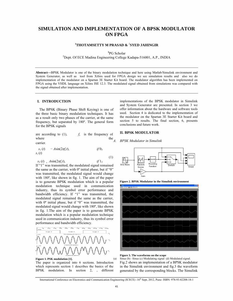
International Conference on Electronics and Communication Engineering (ICECE) -16th Sept, 2012, Pune- ISBN: 978-93-82208-18-1
41
SIMULATION AND IMPLEMENTATION OF A BPSK MODULATOR ON FPGA
1THOTAMSETTY M PRASAD & 2SYED JAHINGIR
1PG Scholar
2Dept. Of ECE Madina Engineering College Kadapa-516001, A.P., INDIA
Abstract—BPSK Modulator is one of the binary modulation technique and here using Matlab/Simulink environment and System Generator, as well as tool from Xilinx used for FPGA design we see simulation results and also we do implementation of the modulator on a Spartan 3E Starter Kit board. The modulator algorithm has been implemented on FPGA using the VHDL language on Xilinx ISE 12.3. The modulated signal obtained from simulations was compared with the signal obtained after implementation.
I. INTRODUCTION
The BPSK (Binary Phase Shift Keying) is one of
the three basic binary modulation techniques. It has as a result only two phases of the carrier, at the same frequency, but separated by 180º. The general form for the BPSK signals
are according to (1), where
fc is the frequency ofthe
carrier.
�s1 (t) � − Asin(2πfct), if 0T si (t) � �
(1)�s2 (t) � Asin(2πfct), if 1T If “1” was transmitted, the modulated signal remained the same as the carrier, with 0º initial phase, but if “0” was transmitted, the modulated signal would change with 180º, like shown in fig. 1. The aim of the paper is to generate BPSK modulation which is a popular modulation technique used in communication industry, thus its symbol error performance and bandwidth efficiency. If “1” was transmitted, the modulated signal remained the same as the carrier, with 0º initial phase, but if “0” was transmitted, the modulated signal would change with 180º, like shown in fig. 1.The aim of the paper is to generate BPSK modulation which is a popular modulation technique used in communication industry, thus its symbol error performance and bandwidth efficiency.
Figure 1. PSK modulation [1]. The paper is organized into 6 sections. Introduction which represents section 1 describes the basics of the BPSK modulation. In section 2, , different
implementations of the BPSK modulator in Simulink and System Generator are presented. In section 3 we offer information about the hardware and software tools used. Section 4 is dedicated to the implementation of the modulator on the Spartan 3E Starter Kit board and section 5 to results. The final section, 6, presents conclusions and future work. II. BPSK MODULATOR
A. BPSK Modulator in Simulink Figure 2. BPSK Modulator in the Simulink environment
Figure 3. The waveforms on the scope (a) Sinus (b) –Sinus (c) Modulating signal (d) Modulated signal.
Fig.2 shows an implementation of a BPSK modulator in the Simulink environment and fig.3 the waveform generated by the corresponding blocks. The Simulink
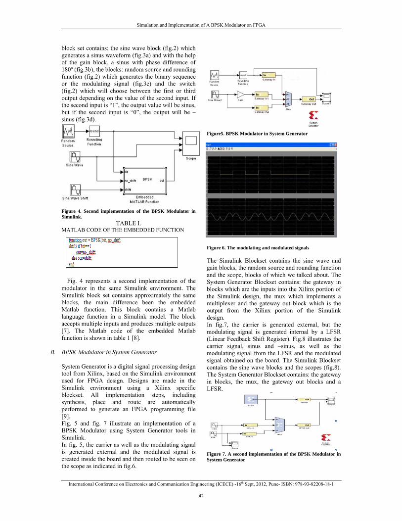
Simulation and Implementation of A BPSK Modulator on FPGA
International Conference on Electronics and Communication Engineering (ICECE) -16th Sept, 2012, Pune- ISBN: 978-93-82208-18-1
42
block set contains: the sine wave block (fig.2) which generates a sinus waveform (fig.3a) and with the help of the gain block, a sinus with phase difference of 180º (fig.3b), the blocks: random source and rounding function (fig.2) which generates the binary sequence or the modulating signal (fig.3c) and the switch (fig.2) which will choose between the first or third output depending on the value of the second input. If the second input is “1”, the output value will be sinus, but if the second input is “0”, the output will be –sinus (fig.3d). Figure 4. Second implementation of the BPSK Modulator in Simulink.
TABLE I. MATLAB CODE OF THE EMBEDDED FUNCTION
Fig. 4 represents a second implementation of the
modulator in the same Simulink environment. The Simulink block set contains approximately the same blocks, the main difference been the embedded Matlab function. This block contains a Matlab language function in a Simulink model. The block accepts multiple inputs and produces multiple outputs [7]. The Matlab code of the embedded Matlab function is shown in table 1 [8].
B. BPSK Modulator in System Generator
System Generator is a digital signal processing design tool from Xilinx, based on the Simulink environment used for FPGA design. Designs are made in the Simulink environment using a Xilinx specific blockset. All implementation steps, including synthesis, place and route are automatically performed to generate an FPGA programming file [9]. Fig. 5 and fig. 7 illustrate an implementation of a BPSK Modulator using System Generator tools in Simulink. In fig. 5, the carrier as well as the modulating signal is generated external and the modulated signal is created inside the board and then routed to be seen on the scope as indicated in fig.6.
Figure5. BPSK Modulator in System Generator
Figure 6. The modulating and modulated signals The Simulink Blockset contains the sine wave and gain blocks, the random source and rounding function and the scope, blocks of which we talked about. The System Generator Blockset contains: the gateway in blocks which are the inputs into the Xilinx portion of the Simulink design, the mux which implements a multiplexer and the gateway out block which is the output from the Xilinx portion of the Simulink design. In fig.7, the carrier is generated external, but the modulating signal is generated internal by a LFSR (Linear Feedback Shift Register). Fig.8 illustrates the carrier signal, sinus and –sinus, as well as the modulating signal from the LFSR and the modulated signal obtained on the board. The Simulink Blockset contains the sine wave blocks and the scopes (fig.8). The System Generator Blockset contains: the gateway in blocks, the mux, the gateway out blocks and a LFSR.
Figure 7. A second implementation of the BPSK Modulator in System Generator
Simulation and Implementation of A BPSK Modulator on FPGA
International Conference on Electronics and Communication Engineering (ICECE) -16th Sept, 2012, Pune- ISBN: 978-93-82208-18-1
43
Figure 8. The waveforms: (a) Sinus (b) --Sinus (c) Modulating signal of the LFSR
Modulated signal.
Figure 9. The third model of the modulator.
The third implementation of a BPSK Modulator, illustrated in fig.9 consists of signals generated internal. The carrier is generated internal by DDS blocks from System Generator and the modulating signal can be generated internal by the LFSR or external by the Agilent 81101A Pulse Generator. Fig.10 illustrates the signals obtained after implementing the modulator. The Simulink Blockset contains the random source and rounding function and the scope, blocks of which we talked about. The System Generator Blockset contains: the gateway in blocks, the mux blocks, the gateway out block, the LFSR block and two DDS compiler blocks.
The DDS Compiler Block is a direct digital synthesizer and it uses a lookup table scheme to generate sinusoids. A digital integrator generates a
phase that is mapped by the lookup table into the output waveform [8]. The sinusoids can be seen in fig.10(c) and (d). The mux block implements a multiplexer. It has one select input and a configurable number of data inputs that can be defined by the user [9].
Figure 10. The waveforms: (a) The modulated signal (b) The modulating signal (c) Sinus
(d) --Sinus (e) The output of the LFSR (g) The signal obtained external, from a function generator. With the System Generator WaveScope, the user can view the waveforms generated in a design.The wavescope allows the user to observe the time-changing values of any wires in the design after the conclusion of the simulation [8]. The d0 and d1 inputs of mux1 represent the modulating signal. The sel input of mux1 selects between the d0 and d1 inputs. Because in the System Generator environment, a switch cannot be represented, we replaced it with a random sequence of bits. The same thing happens in mux2, where depending on the output of mux1, either sinus or –sinus is chosen. III. HARDWARE AND SOFTWARE RESOURCES The Setup Lab measurement used for realizing the BPSK modulator is illustrated in fig. 11. Some of the resources used are the Spartan 3E Starter Kit board [11], the Xilinx WebPack ISE from Xilinx , monitor, a Tektronix oscilloscope and a pulse generator from Agilent . The Agilent 81101A is a single-channel pulse generator, capable of generating all standard pulses and bursts up to 50 MHz The Spartan 3E FPGA Starter Kit board is a development platform based on a Xilinx Spartan 3E FPGA. It provides a development platform for embedded processing applications. The Spartan-3E family of FPGAs is designed to be well suited in a wide range of electronics applications. The ISE WebPack from Xilinx is a fully featured front-to-back FPGA design solution and it offers

Simulation and Implementation of A BPSK Modulator on FPGA
International Conference on Electronics and Communication Engineering (ICECE) -16th Sept, 2012, Pune- ISBN: 978-93-82208-18-1
44
HDL synthesis and simulation, implementation, device fitting and JTAG programming Figure 11. The setup with Spartan 3E Starter Kit board.
IV. BPSK MODULATOR ON SPARTAN 3E STARTER KIT BOARD
The BPSK Modulator that we implemented on the Spartan 3E Starter Kit board has, as a model, the third implementation in System Generator. The carrier is generated internal, but in a ROM and that is the reason of which the sinus signal is represented discontinuous, by instantaneous samples of 16 different values [10], [11], [12]. The only thing that is different is that we used a switch that replaced the mux1 block. The switch behaves as a random sequence of bits which introduces either “1” or “0” depending on its position.
Fig. 12 represents the test bench lab used in implementing the BPSK Modulator on the Spartan 3E Starter Kit Board.
As explained in fig.2, the experimental setup consists of a computer, a monitor, an oscilloscope, a pulse generator and the Spartan 3E board. The ISE Web Pack runs on the computer and it programs the Spartan 3E board. The pulse generator generates the signal from fig.13 and it is measured with a LeCroy Wavesurfer Oscilloscope. The pulses are than fed to an entry of a connector on the board like illustrates in fig.14. Depending on the position of a slide switch (fig.14), the modulating signal is acquired either external, from the pulse generator or internal, from the LFSR. Opposite to System Generator, the switch can be represented or can be configured in VHDL language. The modulated signal obtained is routed to the VGA port of the board, in order to be seen on the monitor.
Figure 12. Test bench lab.
Figure 14. The slide switches and the connector which makes the junction between the pulse generator and the board. V. RESULTS After implementing the BPSK Modulator on the Spartan 3E Starter Kit board, the signals were routed to a monitor. The BPSK modulation can be seen in fig.15 and 16. If the input data is “1”, the transmitted signal to the monitor is unchanged and has a green border on the right of the figure, but if the input data is “0”, the transmitted signal is yielded with 180º phase shift and has a red border on the right of the figure. Fig.17 represents the design summary which represents the utilization of flip-flops, LUTs, slices used from the capabilities of the FPGA from the Spartan 3E board.
Simulation and Implementation of A BPSK Modulator on FPGA
International Conference on Electronics and Communication Engineering (ICECE) -16th Sept, 2012, Pune- ISBN: 978-93-82208-18-1
45
Figure 15. The transmitted signal if the input is 1. Figure 16. The transmitted signal if the input is 0. Figure 17. Design Summary VI. CONCLUSIONS AND FUTURE
WORK
I conclude that we have two implementations of the BPSK Modulator in the Matlab/Simulink environment, the first with simple blocks and the second, with a block in which we wrote Matlab code. Then, we made a proposal of three implementations of a BPSK modulator in System Generator. In the first, the three signals: the carrier, the modulating and the modulated signals where generated external. In the second scheme, the carrier is generated external, and the modulating signal is generated internal by a LFSR. And in the third scheme, all three signals were generated internal with the exception of the modulating signal which can be obtained either internal by the LFSR, or external by the pulse generator.
In the second part of the paper, we implemented
the BPSK modulator on the Spartan 3E Starter Kit based on the third proposal of the modulator made in System Generator. If “1” was transmitted, the modulated signal remained same as the carrier, but if “0” was transmitted, the modulated signal was yielded with a 180º phase (fig.15 and fig.16). The design has been written in the VHDL programming code by Xilinx software.
Our next goal is implementing all the three proposals of the BPSK digital modulator made in System Generator on the Spartan 3E Starter Kit board. We want the modulating signal to be random, not as a train of pulses obtained from the pulse generator. We also want to route the modulated signal to a high performance oscilloscope, not to a VGA monitor in order to have more accuracy in the measurements. After implementing the BPSK modulator, we want to realize a BPSK system. The system will consist of a modulator and demodulator and the signal from the modulator to demodulator will pass through a channel affected by AWGN (Additive White Gaussian Noise). The modulated and demodulated signals will be also routed to VGA monitors, but also to oscilloscopes. REFERENCES [1] F.Xiong, “Digital Modulation Techniques”, Artech House,
UK, 2000. [2] Spartan 3E FPGA Starter Kit board. User guide. Xilinx. 2011. [3] ISE 10.1 Quick Start Tutorial, Xilinx, 2008. [4] Spartan-3E FPGA Family Data Sheet. Xilinx. 2008. [5] S.T.Karris, “Introduction to Simulink with Engineering
Applications”, Orchard Publications, USA, 2006. [6] J.S.Ruque, D.I.Ruiz, C.E. Carrion, “Simulation and
implementation of the BPSK modulation on a FPGA Xilinx 3 xcs200-4ftp256, using Simulink and the System Generator blockset for DSP/FPGA” http://www.ece.unm.edu/xup/docs/collaboration/BPSK_Modulator .pdf
[7] System Generator for DSP. Getting Started Guide. Xilinx. 2008.
[8] S.O.Popescu, G.Budura, A.S.Gontean, “Review of PSK and QAM – Digital Modulation Techniques on FPGA”, International Joint Conference on Computational Cybernatics and Technical Informatics (ICCC-CONTI), Romania, 2010, pp.327-332. F.Ahamed, A.Scorpino, “An educational digital communications project using FPGAs to implement a BPSK Detector”, IEEE Transactions on Education, Vol.48, No.1, 2005, pp.191-197
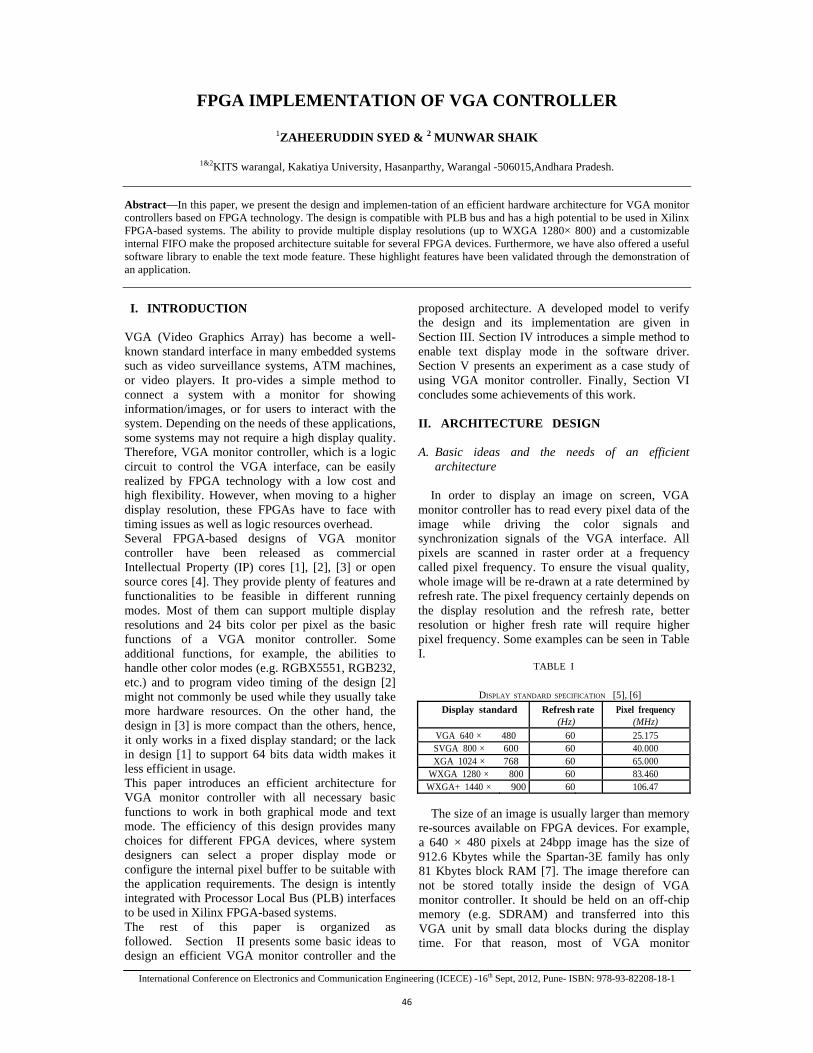
International Conference on Electronics and Communication Engineering (ICECE) -16th Sept, 2012, Pune- ISBN: 978-93-82208-18-1
46
FPGA IMPLEMENTATION OF VGA CONTROLLER
1ZAHEERUDDIN SYED & 2 MUNWAR SHAIK
1&2KITS warangal, Kakatiya University, Hasanparthy, Warangal -506015,Andhara Pradesh.
Abstract—In this paper, we present the design and implemen-tation of an efficient hardware architecture for VGA monitor controllers based on FPGA technology. The design is compatible with PLB bus and has a high potential to be used in Xilinx FPGA-based systems. The ability to provide multiple display resolutions (up to WXGA 1280× 800) and a customizable internal FIFO make the proposed architecture suitable for several FPGA devices. Furthermore, we have also offered a useful software library to enable the text mode feature. These highlight features have been validated through the demonstration of an application. I. INTRODUCTION
VGA (Video Graphics Array) has become a well-known standard interface in many embedded systems such as video surveillance systems, ATM machines, or video players. It pro-vides a simple method to connect a system with a monitor for showing information/images, or for users to interact with the system. Depending on the needs of these applications, some systems may not require a high display quality. Therefore, VGA monitor controller, which is a logic circuit to control the VGA interface, can be easily realized by FPGA technology with a low cost and high flexibility. However, when moving to a higher display resolution, these FPGAs have to face with timing issues as well as logic resources overhead. Several FPGA-based designs of VGA monitor controller have been released as commercial Intellectual Property (IP) cores [1], [2], [3] or open source cores [4]. They provide plenty of features and functionalities to be feasible in different running modes. Most of them can support multiple display resolutions and 24 bits color per pixel as the basic functions of a VGA monitor controller. Some additional functions, for example, the abilities to handle other color modes (e.g. RGBX5551, RGB232, etc.) and to program video timing of the design [2] might not commonly be used while they usually take more hardware resources. On the other hand, the design in [3] is more compact than the others, hence, it only works in a fixed display standard; or the lack in design [1] to support 64 bits data width makes it less efficient in usage. This paper introduces an efficient architecture for VGA monitor controller with all necessary basic functions to work in both graphical mode and text mode. The efficiency of this design provides many choices for different FPGA devices, where system designers can select a proper display mode or configure the internal pixel buffer to be suitable with the application requirements. The design is intently integrated with Processor Local Bus (PLB) interfaces to be used in Xilinx FPGA-based systems. The rest of this paper is organized as followed. Section II presents some basic ideas to design an efficient VGA monitor controller and the
proposed architecture. A developed model to verify the design and its implementation are given in Section III. Section IV introduces a simple method to enable text display mode in the software driver. Section V presents an experiment as a case study of using VGA monitor controller. Finally, Section VI concludes some achievements of this work. II. ARCHITECTURE DESIGN A. Basic ideas and the needs of an efficient
architecture
In order to display an image on screen, VGA monitor controller has to read every pixel data of the image while driving the color signals and synchronization signals of the VGA interface. All pixels are scanned in raster order at a frequency called pixel frequency. To ensure the visual quality, whole image will be re-drawn at a rate determined by refresh rate. The pixel frequency certainly depends on the display resolution and the refresh rate, better resolution or higher fresh rate will require higher pixel frequency. Some examples can be seen in Table I.
TABLE I
DISPLAY STANDARD SPECIFICATION [5], [6] Display standard Refresh rate Pixel frequency
(Hz) (MHz)VGA 640 × 480 60 25.175SVGA 800 × 600 60 40.000XGA 1024 × 768 60 65.000
WXGA 1280 × 800 60 83.460WXGA+ 1440 × 900 60 106.47 The size of an image is usually larger than memory
re-sources available on FPGA devices. For example, a 640 × 480 pixels at 24bpp image has the size of 912.6 Kbytes while the Spartan-3E family has only 81 Kbytes block RAM [7]. The image therefore can not be stored totally inside the design of VGA monitor controller. It should be held on an off-chip memory (e.g. SDRAM) and transferred into this VGA unit by small data blocks during the display time. For that reason, most of VGA monitor
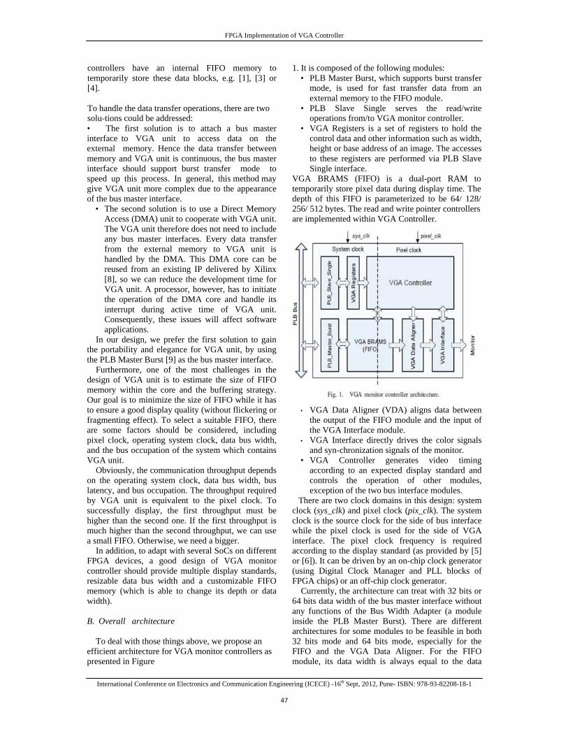
FPGA Implementation of VGA Controller
International Conference on Electronics and Communication Engineering (ICECE) -16th Sept, 2012, Pune- ISBN: 978-93-82208-18-1
47
controllers have an internal FIFO memory to temporarily store these data blocks, e.g. [1], [3] or [4]. To handle the data transfer operations, there are two solu-tions could be addressed: • The first solution is to attach a bus master interface to VGA unit to access data on the external memory. Hence the data transfer between memory and VGA unit is continuous, the bus master interface should support burst transfer mode to speed up this process. In general, this method may give VGA unit more complex due to the appearance of the bus master interface.
• The second solution is to use a Direct Memory Access (DMA) unit to cooperate with VGA unit. The VGA unit therefore does not need to include any bus master interfaces. Every data transfer from the external memory to VGA unit is handled by the DMA. This DMA core can be reused from an existing IP delivered by Xilinx [8], so we can reduce the development time for VGA unit. A processor, however, has to initiate the operation of the DMA core and handle its interrupt during active time of VGA unit. Consequently, these issues will affect software applications.
In our design, we prefer the first solution to gain the portability and elegance for VGA unit, by using the PLB Master Burst [9] as the bus master interface.
Furthermore, one of the most challenges in the design of VGA unit is to estimate the size of FIFO memory within the core and the buffering strategy. Our goal is to minimize the size of FIFO while it has to ensure a good display quality (without flickering or fragmenting effect). To select a suitable FIFO, there are some factors should be considered, including pixel clock, operating system clock, data bus width, and the bus occupation of the system which contains VGA unit.
Obviously, the communication throughput depends on the operating system clock, data bus width, bus latency, and bus occupation. The throughput required by VGA unit is equivalent to the pixel clock. To successfully display, the first throughput must be higher than the second one. If the first throughput is much higher than the second throughput, we can use a small FIFO. Otherwise, we need a bigger.
In addition, to adapt with several SoCs on different FPGA devices, a good design of VGA monitor controller should provide multiple display standards, resizable data bus width and a customizable FIFO memory (which is able to change its depth or data width).
B. Overall architecture
To deal with those things above, we propose an efficient architecture for VGA monitor controllers as presented in Figure
1. It is composed of the following modules: • PLB Master Burst, which supports burst transfer
mode, is used for fast transfer data from an external memory to the FIFO module.
• PLB Slave Single serves the read/write operations from/to VGA monitor controller.
• VGA Registers is a set of registers to hold the control data and other information such as width, height or base address of an image. The accesses to these registers are performed via PLB Slave Single interface.
VGA BRAMS (FIFO) is a dual-port RAM to temporarily store pixel data during display time. The depth of this FIFO is parameterized to be 64/ 128/ 256/ 512 bytes. The read and write pointer controllers are implemented within VGA Controller.
• VGA Data Aligner (VDA) aligns data between the output of the FIFO module and the input of the VGA Interface module.
• VGA Interface directly drives the color signals and syn-chronization signals of the monitor.
• VGA Controller generates video timing according to an expected display standard and controls the operation of other modules, exception of the two bus interface modules.
There are two clock domains in this design: system clock (sys_clk) and pixel clock (pix_clk). The system clock is the source clock for the side of bus interface while the pixel clock is used for the side of VGA interface. The pixel clock frequency is required according to the display standard (as provided by [5] or [6]). It can be driven by an on-chip clock generator (using Digital Clock Manager and PLL blocks of FPGA chips) or an off-chip clock generator.
Currently, the architecture can treat with 32 bits or 64 bits data width of the bus master interface without any functions of the Bus Width Adapter (a module inside the PLB Master Burst). There are different architectures for some modules to be feasible in both 32 bits mode and 64 bits mode, especially for the FIFO and the VGA Data Aligner. For the FIFO module, its data width is always equal to the data
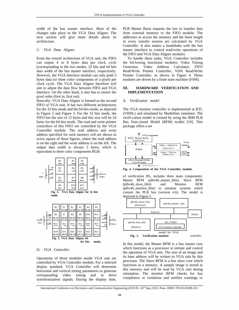
FPGA Implementation of VGA Controller
International Conference on Electronics and Communication Engineering (ICECE) -16th Sept, 2012, Pune- ISBN: 978-93-82208-18-1
48
width of the bus master interface. Most of the changes take place in the VGA Data Aligner. The next section will give more details about its architecture.
C. VGA Data Aligner From the overall architecture of VGA unit, the FIFO can output 4 or 8 bytes data per clock cycle (corresponding to the two modes, 32 bits and 64 bits data width of the bus master interface, respectively. However, the VGA Interface module can only push 3 bytes data (or three color components of a pixel) per clock cycle. The VGA Data Aligner therefore will aim to adjust the data flow between FIFO and VGA Interface. On the other hand, it also has to ensure the pixel order (first in, first out). Basically, VGA Data Aligner is formed as the second FIFO of VGA unit. It has two different architectures for the 32 bits mode and the 64 bits mode, as depicted in Figure 2 and Figure 3. For the 32 bits mode, the FIFO has the size of 12 bytes and this size will be 24 bytes for the 64 bits mode. The read and write pointer controllers of this FIFO are controlled by the VGA Controller module. The read address and write address specified for each memory cell are shown in every square of these figures, where the read address is on the right and the write address is on the left. The output data width is always 3 bytes, which is equivalent to three color components RGB. R0 R1 R2
10/00 10/00 11/00
00
R3 R4 R5 00
01
4 /
10 11/01 11/01 11/01
3 /
WR
10 RD
Input 11
R6
R7
R8 Output
11
00/10
00/10
00/10
R9
R10
R11
00/11 10/11 10/11
Fig. 2. VGA Data Aligner for 32 bits mode.
R0 R1 R2 R3 R4 R5
011 /000 011/000 011 /000 011 /001 011/001 011 /001
000 R6 R7 R8 R9 R10 R11 000
8
WR
010 000 /010 000/010 000 /010 000 /011 000/011 000 /011 001 3
/
…
/Input
111
R12
R13
R14
R15
R16
R17
111 Output
000 /100 000/100 010 /100 010 /101 010/101 010 /101
R18
R19
R20
R21
R22
R23
010 /110 010/110 010 /110 010 /111 011/111 011 /111
Fig. 3. VGA Data Aligner
for 64 bits mode.
D. VGA Controller Operations of those modules inside VGA unit are controlled by VGA Controller module. For a selected display standard, VGA Controller will determine horizontal and vertical timing parameters to generate corresponding video timing and to drive synchronization signals. During the display time,
PLB Master Burst requests the bus to transfer data from external memory to the FIFO module. The addresses to access the memory and the burst length in every transfer session are calculated by VGA Controller. It also makes a handshake with the bus master interface to control read/write operations of the FIFO and VGA Data Aligner modules. To handle these tasks, VGA Controller includes the fol-lowing functional modules: Video Timing Generator, Video Address Calculator, FIFO Read/Write Pointer Controller, VDA Read/Write Pointer Controller, as shown in Figure 4. These modules are driven by a finite state machine (FSM). III. HARDWARE VERIFICATION AND
IMPLEMENTATION A. Verification model The VGA monitor controller is implemented at RTL (VHDL) and simulated by ModelSim simulator. The verifi-cation model is created by using the IBM PLB Bus Func-tional Model (BFM) toolkit [10]. This package offers a set
Fig. 4. Composition of the VGA Controller module. of verification IPs, includes three main components: Master BFM (plbv46_master_bfm), Slave BFM (plbv46_slave_bfm) and Monitor BFM (plbv46_monitor_bfm) to simulate systems which contain the PLB bus (version 4.6). The model is depicted in Figure 5. plbv46_master_bfm
plbv46_monitor _bfm (Processor)
PLBv4.6
Arbiter
plbv46_slave_bfm vga_wrapper
(Memory) VGA monitor controller
Fig. 5. Verificationmodel for VGA monitor controller.
In this model, the Master BFM is a bus master core which functions as a processor to initiate and control the operation of VGA unit. The size of an image and its base address will be written to VGA unit by this processor. The Slave BFM is a bus slave core which functions as a memory. A sample image is stored in this memory and will be read by VGA unit during simulation. The monitor BFM checks for bus compliance or violations and notifies warnings or
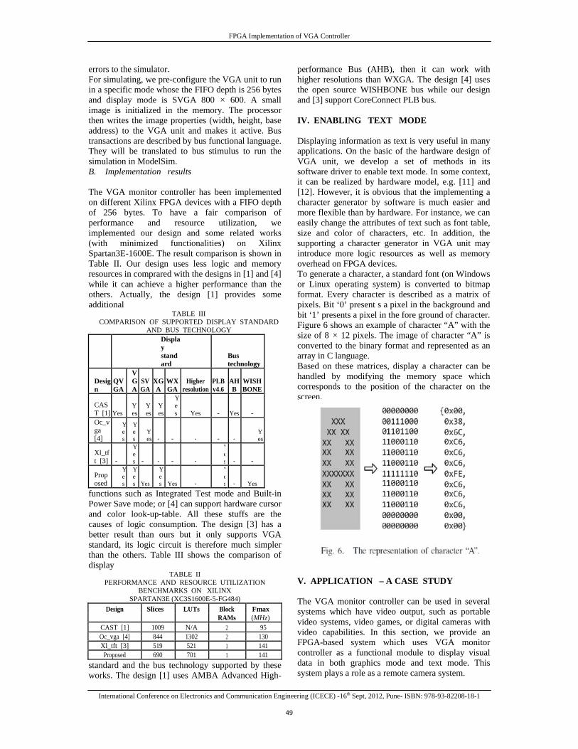
FPGA Implementation of VGA Controller
International Conference on Electronics and Communication Engineering (ICECE) -16th Sept, 2012, Pune- ISBN: 978-93-82208-18-1
49
errors to the simulator. For simulating, we pre-configure the VGA unit to run in a specific mode whose the FIFO depth is 256 bytes and display mode is SVGA 800 × 600. A small image is initialized in the memory. The processor then writes the image properties (width, height, base address) to the VGA unit and makes it active. Bus transactions are described by bus functional language. They will be translated to bus stimulus to run the simulation in ModelSim. B. Implementation results The VGA monitor controller has been implemented on different Xilinx FPGA devices with a FIFO depth of 256 bytes. To have a fair comparison of performance and resource utilization, we implemented our design and some related works (with minimized functionalities) on Xilinx Spartan3E-1600E. The result comparison is shown in Table II. Our design uses less logic and memory resources in comprared with the designs in [1] and [4] while it can achieve a higher performance than the others. Actually, the design [1] provides some additional
TABLE III COMPARISON OF SUPPORTED DISPLAY STANDARD
AND BUS TECHNOLOGY
Display standard
Bus technology
Design
QVGA
VGA
SVGA
XGA
WXGA
Higher resolution
PLBv4.6
AHB
WISHBONE
CAST [1] Yes
Yes
Yes
Yes
Yes Yes - Yes -
Oc_vga [4]
Yes
Yes
Yes - - - - -
Yes
Xl_tft [3] -
Yes - - - -
Yes - -
Proposed
Yes
Yes Yes
Yes Yes -
Yes - Yes
functions such as Integrated Test mode and Built-in Power Save mode; or [4] can support hardware cursor and color look-up-table. All these stuffs are the causes of logic consumption. The design [3] has a better result than ours but it only supports VGA standard, its logic circuit is therefore much simpler than the others. Table III shows the comparison of display
TABLE II PERFORMANCE AND RESOURCE UTILIZATION
BENCHMARKS ON XILINX SPARTAN3E (XC3S1600E-5-FG484)
Design Slices LUTs Block Fmax RAMs (MHz)
CAST [1] 1009 N/A 2 95Oc_vga [4] 844 1302 2 130Xl_tft [3] 519 521 1 141
Proposed 690 701 1 141standard and the bus technology supported by these works. The design [1] uses AMBA Advanced High-
performance Bus (AHB), then it can work with higher resolutions than WXGA. The design [4] uses the open source WISHBONE bus while our design and [3] support CoreConnect PLB bus. IV. ENABLING TEXT MODE Displaying information as text is very useful in many applications. On the basic of the hardware design of VGA unit, we develop a set of methods in its software driver to enable text mode. In some context, it can be realized by hardware model, e.g. [11] and [12]. However, it is obvious that the implementing a character generator by software is much easier and more flexible than by hardware. For instance, we can easily change the attributes of text such as font table, size and color of characters, etc. In addition, the supporting a character generator in VGA unit may introduce more logic resources as well as memory overhead on FPGA devices. To generate a character, a standard font (on Windows or Linux operating system) is converted to bitmap format. Every character is described as a matrix of pixels. Bit ‘0’ present s a pixel in the background and bit ‘1’ presents a pixel in the fore ground of character. Figure 6 shows an example of character “A” with the size of 8 × 12 pixels. The image of character “A” is converted to the binary format and represented as an array in C language. Based on these matrices, display a character can be handled by modifying the memory space which corresponds to the position of the character on the screen. V. APPLICATION – A CASE STUDY The VGA monitor controller can be used in several systems which have video output, such as portable video systems, video games, or digital cameras with video capabilities. In this section, we provide an FPGA-based system which uses VGA monitor controller as a functional module to display visual data in both graphics mode and text mode. This system plays a role as a remote camera system.
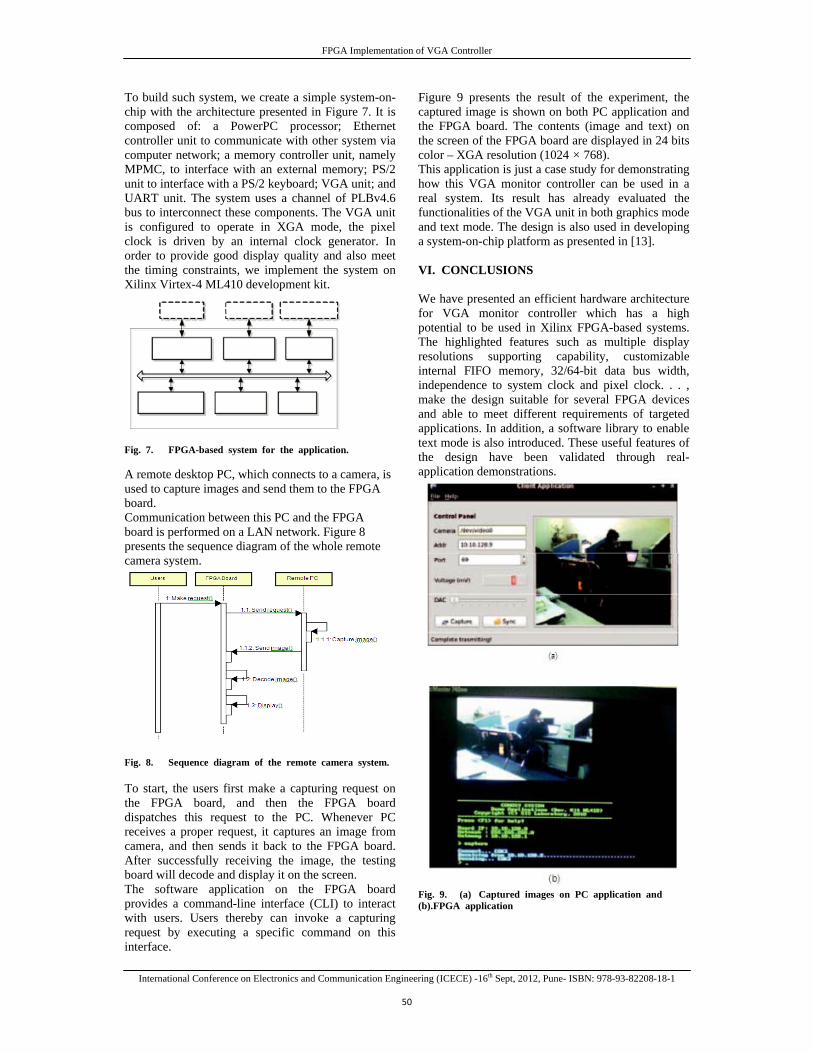
FPGA Implementation of VGA Controller
International Conference on Electronics and Communication Engineering (ICECE) -16th Sept, 2012, Pune- ISBN: 978-93-82208-18-1
50
To build such system, we create a simple system-on-chip with the architecture presented in Figure 7. It is composed of: a PowerPC processor; Ethernet controller unit to communicate with other system via computer network; a memory controller unit, namely MPMC, to interface with an external memory; PS/2 unit to interface with a PS/2 keyboard; VGA unit; and UART unit. The system uses a channel of PLBv4.6 bus to interconnect these components. The VGA unit is configured to operate in XGA mode, the pixel clock is driven by an internal clock generator. In order to provide good display quality and also meet the timing constraints, we implement the system on Xilinx Virtex-4 ML410 development kit. Fig. 7. FPGA-based system for the application. A remote desktop PC, which connects to a camera, is used to capture images and send them to the FPGA board. Communication between this PC and the FPGA board is performed on a LAN network. Figure 8 presents the sequence diagram of the whole remote camera system.
Fig. 8. Sequence diagram of the remote camera system. To start, the users first make a capturing request on the FPGA board, and then the FPGA board dispatches this request to the PC. Whenever PC receives a proper request, it captures an image from camera, and then sends it back to the FPGA board. After successfully receiving the image, the testing board will decode and display it on the screen. The software application on the FPGA board provides a command-line interface (CLI) to interact with users. Users thereby can invoke a capturing request by executing a specific command on this interface.
Figure 9 presents the result of the experiment, the captured image is shown on both PC application and the FPGA board. The contents (image and text) on the screen of the FPGA board are displayed in 24 bits color – XGA resolution (1024 × 768). This application is just a case study for demonstrating how this VGA monitor controller can be used in a real system. Its result has already evaluated the functionalities of the VGA unit in both graphics mode and text mode. The design is also used in developing a system-on-chip platform as presented in [13]. VI. CONCLUSIONS We have presented an efficient hardware architecture for VGA monitor controller which has a high potential to be used in Xilinx FPGA-based systems. The highlighted features such as multiple display resolutions supporting capability, customizable internal FIFO memory, 32/64-bit data bus width, independence to system clock and pixel clock. . . , make the design suitable for several FPGA devices and able to meet different requirements of targeted applications. In addition, a software library to enable text mode is also introduced. These useful features of the design have been validated through real-application demonstrations.
Fig. 9. (a) Captured images on PC application and (b).FPGA application
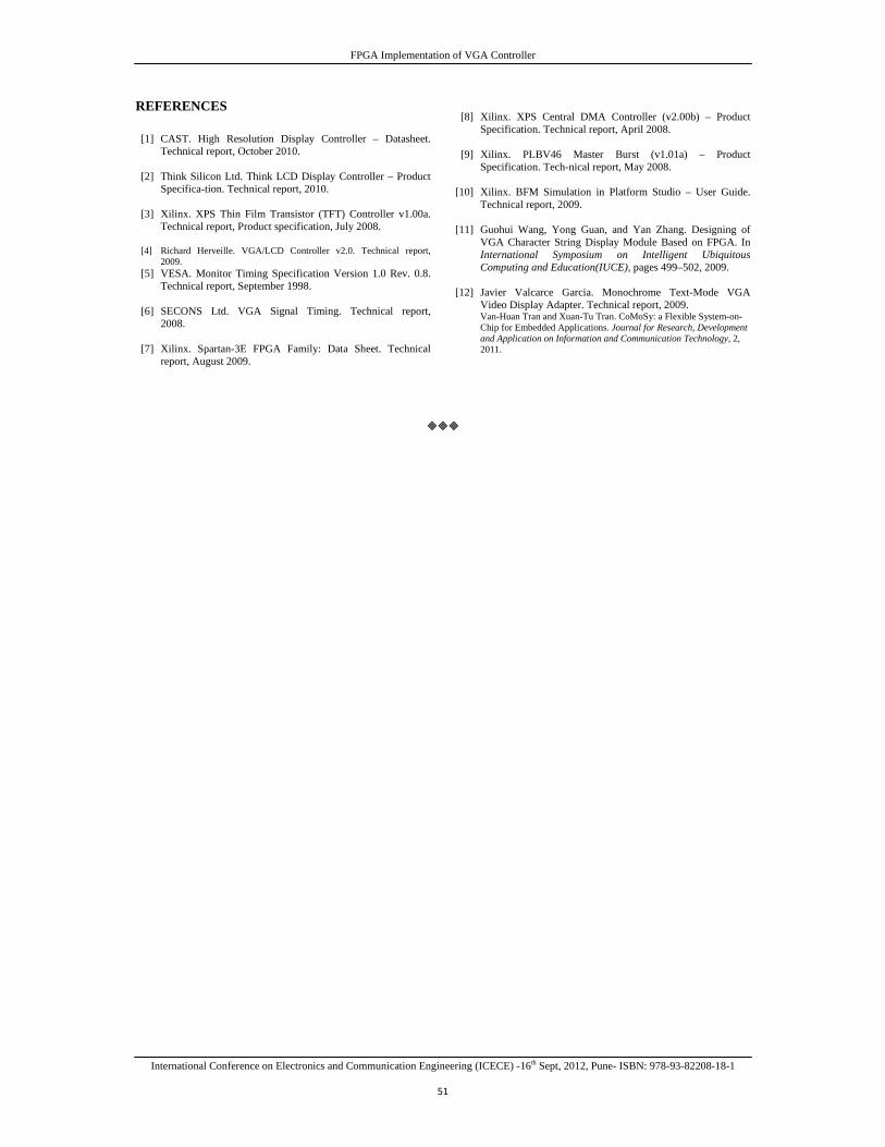
FPGA Implementation of VGA Controller
International Conference on Electronics and Communication Engineering (ICECE) -16th Sept, 2012, Pune- ISBN: 978-93-82208-18-1
51
REFERENCES [1] CAST. High Resolution Display Controller – Datasheet.
Technical report, October 2010. [2] Think Silicon Ltd. Think LCD Display Controller – Product
Specifica-tion. Technical report, 2010. [3] Xilinx. XPS Thin Film Transistor (TFT) Controller v1.00a.
Technical report, Product specification, July 2008.
[4] Richard Herveille. VGA/LCD Controller v2.0. Technical report, 2009.
[5] VESA. Monitor Timing Specification Version 1.0 Rev. 0.8. Technical report, September 1998.
[6] SECONS Ltd. VGA Signal Timing. Technical report,
2008. [7] Xilinx. Spartan-3E FPGA Family: Data Sheet. Technical
report, August 2009.
[8] Xilinx. XPS Central DMA Controller (v2.00b) – Product
Specification. Technical report, April 2008.
[9] Xilinx. PLBV46 Master Burst (v1.01a) – Product Specification. Tech-nical report, May 2008.
[10] Xilinx. BFM Simulation in Platform Studio – User Guide.
Technical report, 2009.
[11] Guohui Wang, Yong Guan, and Yan Zhang. Designing of VGA Character String Display Module Based on FPGA. In International Symposium on Intelligent Ubiquitous Computing and Education(IUCE), pages 499–502, 2009.
[12] Javier Valcarce Garcia. Monochrome Text-Mode VGA
Video Display Adapter. Technical report, 2009. Van-Huan Tran and Xuan-Tu Tran. CoMoSy: a Flexible System-on-Chip for Embedded Applications. Journal for Research, Development and Application on Information and Communication Technology, 2, 2011.
International Conference on Electronics and Communication Engineering (ICECE) -16th Sept, 2012, Pune- ISBN: 978-93-82208-18-1
52
HYBRID DIGITAL VIDEO WATERMARKING TECHNIQUE BASED ON DISCRETE WAVELET TRANSFORM (DWT) AND PRINCIPAL
COMPONENT ANALYSIS (PCA)
1KSHAMA S. KARPE & 2PRACHI MUKHERJI
1,2Department of Electronics and Telecommunication, Smt. Kashibai Navale College of Engineering, Pune, India
Abstract— Digital video watermarking technology is used for copyright protection of digital applications. This paper presents a novel technique for embedding a binary logo watermark into video frames, based on Discrete Wavelet Transform (DWT) and Principal Component Analysis (PCA). PCA is applied to each block of two bands (LL–HH) which results from DWT of every video frame. The video frames are first decomposed using DWT and the binary watermark is embedded in the principal components of the low frequency wavelet coefficients. Results show that there is visible difference between watermarked . Keywords- Digital video; binary watermark; Discrete Wavelet Transform; Principal Component Analysis.
I. INTRODUCTION Recently, the users of networks , especially the world wide web are increasing rapidly. The reproduction, manipulation and the distribution of digital multimedia (images, audio and video) via networks become faster and easier. Hence, the owners and creators of the digital products are concerned about illegal copying of their products. As a result, security and copyright protection are becoming important issues in multimedia applications and services[1]. Copyright protection inserts authentication data such as ownership information and logo in the digital media without affecting its perceptual quality. Watermarking is the process that embeds data called a watermark or digital signature into a multimedia object such that watermark can be detected or extracted later to make an assertion about the object. The object may be an image or audio or video. For the purpose of copyright protection digital watermarking techniques must meet the criteria of imperceptibility as well as robustness against all attacks for removal of the watermark. Many digital watermarking schemes have been proposed for still images and videos. Most of them operate on uncompressed videos, while others embed watermarks directly into compressed videos.Video watermarking introduces a number of issues not present in image watermarking. Due to inherent redundancy between video frames, video signals are highly susceptible to attacks such as frame averaging, frame dropping, frame swapping and statistical analysis. Video watermarking approaches can be classified into two main categories based on the method of hiding watermark bits in the host video. The two categories are:
Spatial domain watermarking where embedding and detection of watermark are performed by directly manipulating the pixel intensity values of the video frame. Transform domain techniques, on the other hand, alter spatial pixel values of the host video according to pre-determined transform and are more robust than spatial domain techniques since they disperse the watermark in the spatial domain of the video frame making it difficult to remove the watermark through malicious attacks like cropping, scaling, rotations and geometrical attacks. The commonly used transform domain techniques are Discrete Fourier Transform (DFT), the Discrete Cosine Transform (DCT), and the Discrete Wavelet Transform (DWT).DWT is more computationally efficient than other transform methods like DFT and DCT. Other transformations have also been explored for watermarking such as principal component analysis (PCA). PCA is a linear transformation that chooses a new coordinate system for the data set. PCA is basically used to hybridize the algorithm as it has the inherent property of removing the correlation amongst the data i.e. the wavelet coefficients and it helps in distributing the watermark bits over the sub-band used for embedding thus resulting in a more robust watermarking scheme that is resistant to almost all possible attacks. The watermark is embedded into the luminance component of the extracted frames as it is less sensitive to the human visual system (HVS). A new video watermarking scheme which combines both the DWT and PCA to develop a new hybrid scheme that is resistant to a variety of attacks. It is well known that even after the orthogonal wavelet decomposition, there still exists some correlation between the wavelet coefficients[2]. PCA removes this correlation and concentrates the energy of the wavelet coefficients and distributes the
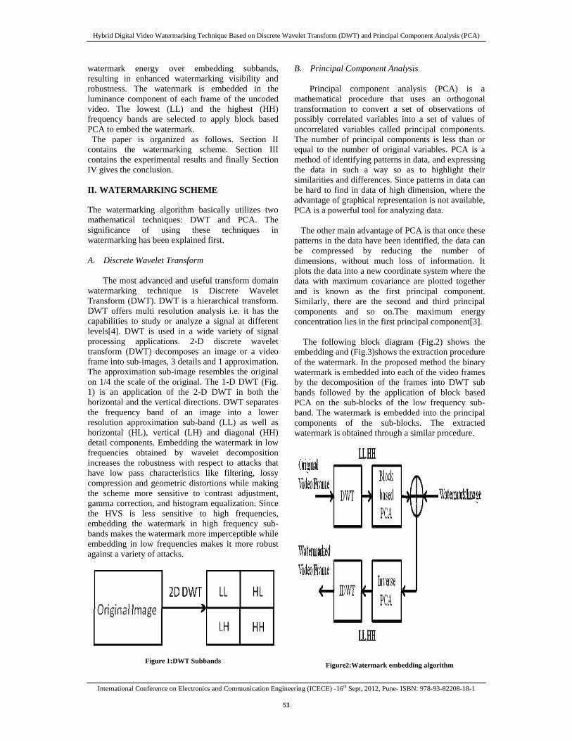
Hybrid Digital Video Watermarking Technique Based on Discrete Wavelet Transform (DWT) and Principal Component Analysis (PCA)
International Conference on Electronics and Communication Engineering (ICECE) -16th Sept, 2012, Pune- ISBN: 978-93-82208-18-1
53
watermark energy over embedding subbands, resulting in enhanced watermarking visibility and robustness. The watermark is embedded in the luminance component of each frame of the uncoded video. The lowest (LL) and the highest (HH) frequency bands are selected to apply block based PCA to embed the watermark. The paper is organized as follows. Section II contains the watermarking scheme. Section III contains the experimental results and finally Section IV gives the conclusion. II. WATERMARKING SCHEME The watermarking algorithm basically utilizes two mathematical techniques: DWT and PCA. The significance of using these techniques in watermarking has been explained first. A. Discrete Wavelet Transform
The most advanced and useful transform domain watermarking technique is Discrete Wavelet Transform (DWT). DWT is a hierarchical transform. DWT offers multi resolution analysis i.e. it has the capabilities to study or analyze a signal at different levels[4]. DWT is used in a wide variety of signal processing applications. 2-D discrete wavelet transform (DWT) decomposes an image or a video frame into sub-images, 3 details and 1 approximation. The approximation sub-image resembles the original on 1/4 the scale of the original. The 1-D DWT (Fig. 1) is an application of the 2-D DWT in both the horizontal and the vertical directions. DWT separates the frequency band of an image into a lower resolution approximation sub-band (LL) as well as horizontal (HL), vertical (LH) and diagonal (HH) detail components. Embedding the watermark in low frequencies obtained by wavelet decomposition increases the robustness with respect to attacks that have low pass characteristics like filtering, lossy compression and geometric distortions while making the scheme more sensitive to contrast adjustment, gamma correction, and histogram equalization. Since the HVS is less sensitive to high frequencies, embedding the watermark in high frequency sub-bands makes the watermark more imperceptible while embedding in low frequencies makes it more robust against a variety of attacks.
Figure 1:DWT Subbands
B. Principal Component Analysis
Principal component analysis (PCA) is a mathematical procedure that uses an orthogonal transformation to convert a set of observations of possibly correlated variables into a set of values of uncorrelated variables called principal components. The number of principal components is less than or equal to the number of original variables. PCA is a method of identifying patterns in data, and expressing the data in such a way so as to highlight their similarities and differences. Since patterns in data can be hard to find in data of high dimension, where the advantage of graphical representation is not available, PCA is a powerful tool for analyzing data. The other main advantage of PCA is that once these patterns in the data have been identified, the data can be compressed by reducing the number of dimensions, without much loss of information. It plots the data into a new coordinate system where the data with maximum covariance are plotted together and is known as the first principal component. Similarly, there are the second and third principal components and so on.The maximum energy concentration lies in the first principal component[3]. The following block diagram (Fig.2) shows the embedding and (Fig.3)shows the extraction procedure of the watermark. In the proposed method the binary watermark is embedded into each of the video frames by the decomposition of the frames into DWT sub bands followed by the application of block based PCA on the sub-blocks of the low frequency sub-band. The watermark is embedded into the principal components of the sub-blocks. The extracted watermark is obtained through a similar procedure.
Figure2:Watermark embedding algorithm
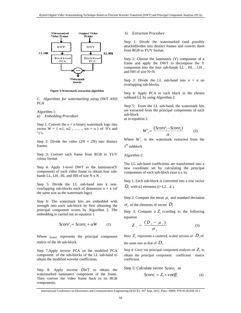
Hybrid Digital Video Watermarking Technique Based on Discrete Wavelet Transform (DWT) and Principal Component Analysis (PCA)
International Conference on Electronics and Communication Engineering (ICECE) -16th Sept, 2012, Pune- ISBN: 978-93-82208-18-1
54
Figure 3:Watermark extraction algorithm
C. Algorithms for watermarking using DWT AND PCA Algorithm 1: a) Embedding Procedure Step 1: Convert the n × n binary watermark logo into vector W = { w1, w2 , ……, wn × n } of ‘0’s and ‘1’s. Step 2: Divide the video (2N × 2N) into distinct frames. Step 3: Convert each frame from RGB to YUV colour format. Step 4: Apply 1-level DWT to the luminance(Y component) of each video frame to obtain four sub-bands LL, LH , HL and HH of size N x N . Step 5: Divide the LL sub-band into k non-overlapping sub-blocks each of dimension n × n (of the same size as the watermark logo). Step 6: The watermark bits are embedded with strength into each sub-block by first obtaining the principal component scores by Algorithm 2. The embedding is carried out as equation 1. WScoreScore ii α+=' (1)
Where
iScore represents the principal component matrix of the ith sub-block. Step 7:Apply inverse PCA on the modified PCA component of the sub-blocks of the LL sub-band to obtain the modified wavelet coefficients.
Step 8: Apply inverse DWT to obtain the watermarked luminance component of the frame. Then convert the video frame back to its RGB components.
b) Extraction Procedure Step 1: Divide the watermarked (and possibly attacked)video into distinct frames and convert them from RGB to YUV format. Step 2: Choose the luminance (Y) component of a frame and apply the DWT to decompose the Y component into the four sub-bands LL , HL , LH , and HH of size N×N. Step 3: Divide the LL sub-band into n × n no overlapping sub-blocks. Step 4: Apply PCA to each block in the chosen subband LL by using Algorithm 2. Step 5: From the LL sub-band, the watermark bits are extracted from the principal components of each sub-block as in equation 2.
α
)'(' iii
ScoreScoreW −= (2)
Where iW ' is the watermark extracted from the thi subblock
Algorithm 2: The LL sub-band coefficients are transformed into a new coordinate set by calculating the principal components of each sub-block (size n x n). Step 1: Each sub-block is converted into a row vector
iD with n2 elements (i=1,2…k ). Step 2: Compute the mean iμ and standard deviation
iσ of the elements of vector iD
Step 3: Compute a iZ ccording to the following equation
i
iii
DZ
σμ )( −
= (3)
Here iZ represents a cantered, scaled version of iD of
the same size as that of iD .
Step 4: Carry out principal component analysis on iZ to obtain the principal component coefficient matrix coefficient. Step 5: Calculate vector iScore as
iii coeffZScore ×= (4)
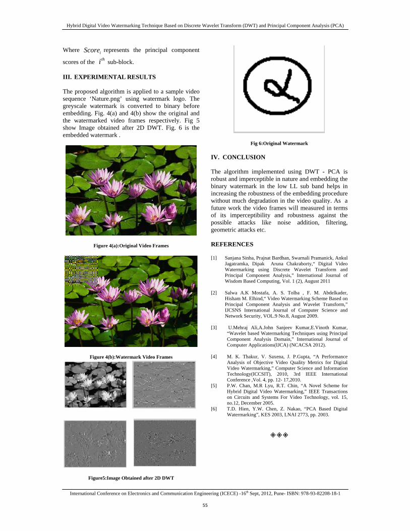
Hybrid Digital Video Watermarking Technique Based on Discrete Wavelet Transform (DWT) and Principal Component Analysis (PCA)
International Conference on Electronics and Communication Engineering (ICECE) -16th Sept, 2012, Pune- ISBN: 978-93-82208-18-1
55
Where iScore represents the principal component
scores of the thi sub-block. III. EXPERIMENTAL RESULTS
The proposed algorithm is applied to a sample video sequence ‘Nature.png’ using watermark logo. The greyscale watermark is converted to binary before embedding. Fig. 4(a) and 4(b) show the original and the watermarked video frames respectively. Fig 5 show Image obtained after 2D DWT. Fig. 6 is the embedded watermark .
Figure 4(a):Original Video Frames
Figure 4(b):Watermark Video Frames
Figure5:Image Obtained after 2D DWT
Fig 6:Original Watermark IV. CONCLUSION The algorithm implemented using DWT - PCA is robust and imperceptible in nature and embedding the binary watermark in the low LL sub band helps in increasing the robustness of the embedding procedure without much degradation in the video quality. As a future work the video frames will measured in terms of its imperceptibility and robustness against the possible attacks like noise addition, filtering, geometric attacks etc.
REFERENCES
[1] Sanjana Sinha, Prajnat Bardhan, Swarnali Pramanick, Ankul
Jagatramka, Dipak Aruna Chakraborty,“ Digital Video Watermarking using Discrete Wavelet Transform and Principal Component Analysis,” International Journal of Wisdom Based Computing, Vol. 1 (2), August 2011
[2] Salwa A.K Mostafa, A. S. Tolba , F. M. Abdelkader, Hisham M. Elhind,“ Video Watermarking Scheme Based on Principal Component Analysis and Wavelet Transform,” IJCSNS International Journal of Computer Science and Network Security, VOL.9 No.8, August 2009.
[3] U.Mehraj Ali,A.John Sanjeev Kumar,E.Vinoth Kumar,
“Wavelet based Watermarking Techniques using Principal Component Analysis Domain,” International Journal of Computer Applications(IJCA) (NCACSA 2012).
[4] M. K. Thakur, V. Saxena, J. P.Gupta, “A Performance Analysis of Objective Video Quality Metrics for Digital Video Watermarking,” Computer Science and Information Technology(ICCSIT), 2010, 3rd IEEE International Conference ,Vol. 4, pp. 12- 17,2010.
[5] P.W. Chan, M.R Lyu, R.T. Chin, “A Novel Scheme for Hybrid Digital Video Watermarking,” IEEE Transactions on Circuits and Systems For Video Technology, vol. 15, no.12, December 2005.
[6] T.D. Hien, Y.W. Chen, Z. Nakao, “PCA Based Digital Watermarking”, KES 2003, LNAI 2773, pp. 2003.
International Conference on Electrical Engineering and Computer Science Engineering (ICEECS) 16th Sept, 2012, Pune- ISBN: 978-93-82208-18-1
56
MODIFICATION TO SPIHT ALGORITHM USING INCREMENTAL THRESHOLD FOR IMAGE COMPRESSION
1A. S. JADHAV & 2RASHMI V. PAWAR
1 ECE department, BLDEA’s Dr. P. G. Halakatti College of Engineering and Technology Bijapur, Karnataka, INDIA.
2 EEE department, BLDEA’s Dr. P. G. Halakatti College of Engineering and Technology Bijapur, Karnataka, INDIA.
Abstract—The Modified SPIHT represents a more efficient implementation of the SPIHT algorithm by using variable thresholds to sort the list of insignificant pixels (LIP) and the list of insignificant sets (LIS). We observe two interesting facts: (I) most of the initial subsets in LIS are not only insignificant with respect to the maximum threshold, but also insignificant with respect to the smaller threshold. And (2) Most of the pixels generating from sorting LIS are smaller than the current threshold. Based on these two observations, it represents a new image codec method, which can make the binary encoded outputs more efficient, and can work well on different image sizes and different decomposition levels. Keywords— Compression, SPIHT, PSNR, Sub-band coding, EZW Algorithm I. INTRODUCTION
Said and Pearlman developed a simple and efficient embedded image coding system based on set partitioning in hierarchical trees (SPIHT) concept. This concept uses three lists to store the significance information: list of insignificant sets (LIS), list of insignificant pixels (LIP), and list of significant pixels (LSP). At every quantization level, it partitions wavelet coefficients into these three lists. Such subset partitioning is so effective and the significance information is so compact that even binary encoded transmission achieves about the same or better performance than almost all previously existing schemes. In the case of 5 level decomposition for 512 x 512 images, the binary encoded bit stream is so efficient that using arithmetic coding can only increase peak signal-to-noise ratio (PSNR) by 0.3 - 0.6 dB for the same bit rate. But, for lower level decomposition with the same image size, it becomes not so compact any more. This is because the number of pixels in low-low band is still large compared to the whole image so that there is lot of time spent in many bits on sorting LIS and LIP at the beginning. For those images with very small size or very large size, this could not make the low-low band very small.
For small sized images, although the low-low band can be decomposed into very small size, it is still quite big as compared to the whole image. On the other hand, for large sized images, if it uses 16 bits integer to save the wavelet coefficients, then it could not do the wavelet decomposition too many levels because overflows would occur otherwise. The outputs will still be very efficient. However, arithmetic coding may not be the best solution as it will largely increase the encoding and decoding time. In fact, it is observed that most of the initial subsets in LIS, that is, the pixel sets with roots in the highest
pyramid level are not only insignificant with respect to the initial threshold, but also insignificant to a smaller threshold.
Therefore, when the low-low band is not very small as compared to the whole image, this redundancy becomes one main reason that makes the binary encoded outputs not efficient. Even for normal sized images with high level decomposition, there still remains some redundancy in the binary encoded outputs. It is found that most of the new pixels generated from sorting LIS are smaller than the current sorting threshold T. The implementation includes modified SPIHT algorithm based on using variable sorting thresholds. The new algorithm can make the binary encoded outputs more efficient on different sized images and different decomposition levels. II. BASIC SPIHT ALGORITHM The SPIHT algorithm [1] uses a partitioning of the spatial orientation trees in a manner that tends to keep insignificant coefficients together in larger subsets. The partitioning decisions are binary decisions that are transmitted to the decoder, providing a significance map encoding. The thresholds used for checking significance are powers of two. So in essence the SPIHT algorithm sends the binary representation of the integer value of the wavelet coefficients. The significance map encoding or set partitioning and ordering step is followed by a refinement step in which the representations of the significant coefficients are refined. The SPIHT algorithm can be applied to both grey-scale and colored images. SPIHT displays exceptional characteristics over several properties like good image quality, fast coding and decoding, a fully progressive bit stream, application in lossless
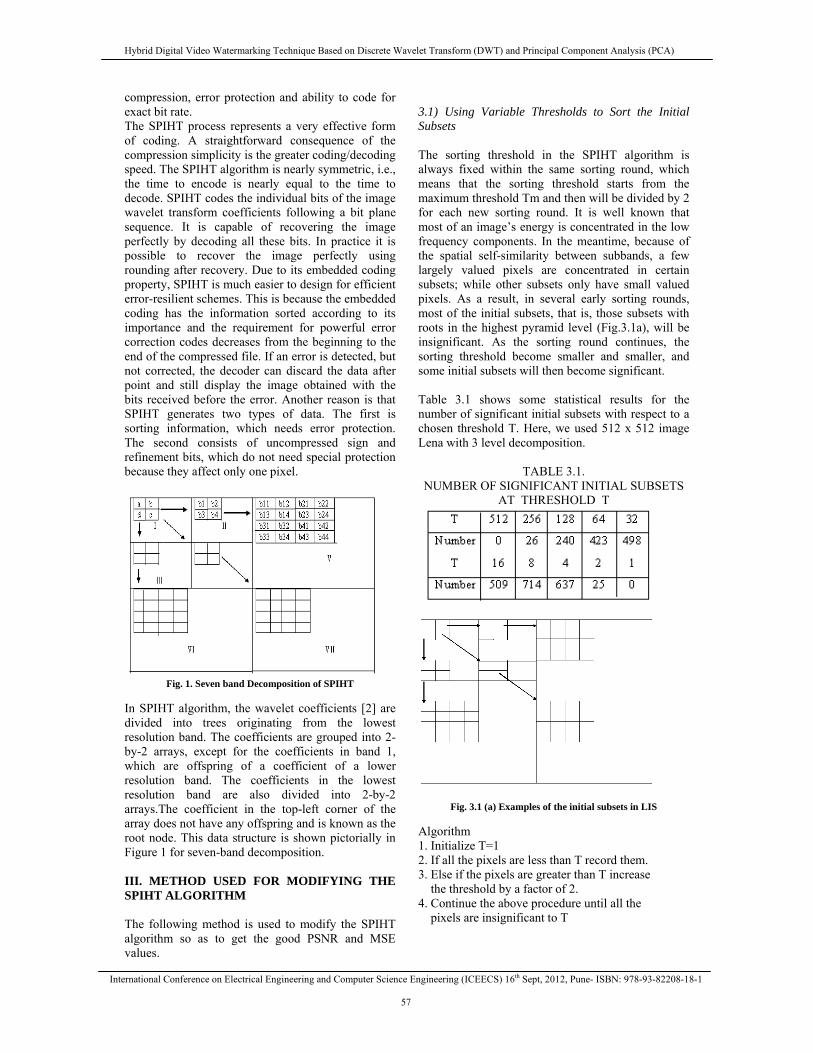
Hybrid Digital Video Watermarking Technique Based on Discrete Wavelet Transform (DWT) and Principal Component Analysis (PCA)
International Conference on Electrical Engineering and Computer Science Engineering (ICEECS) 16th Sept, 2012, Pune- ISBN: 978-93-82208-18-1
57
compression, error protection and ability to code for exact bit rate. The SPIHT process represents a very effective form of coding. A straightforward consequence of the compression simplicity is the greater coding/decoding speed. The SPIHT algorithm is nearly symmetric, i.e., the time to encode is nearly equal to the time to decode. SPIHT codes the individual bits of the image wavelet transform coefficients following a bit plane sequence. It is capable of recovering the image perfectly by decoding all these bits. In practice it is possible to recover the image perfectly using rounding after recovery. Due to its embedded coding property, SPIHT is much easier to design for efficient error-resilient schemes. This is because the embedded coding has the information sorted according to its importance and the requirement for powerful error correction codes decreases from the beginning to the end of the compressed file. If an error is detected, but not corrected, the decoder can discard the data after point and still display the image obtained with the bits received before the error. Another reason is that SPIHT generates two types of data. The first is sorting information, which needs error protection. The second consists of uncompressed sign and refinement bits, which do not need special protection because they affect only one pixel.
Fig. 1. Seven band Decomposition of SPIHT
In SPIHT algorithm, the wavelet coefficients [2] are divided into trees originating from the lowest resolution band. The coefficients are grouped into 2-by-2 arrays, except for the coefficients in band 1, which are offspring of a coefficient of a lower resolution band. The coefficients in the lowest resolution band are also divided into 2-by-2 arrays.The coefficient in the top-left corner of the array does not have any offspring and is known as the root node. This data structure is shown pictorially in Figure 1 for seven-band decomposition. III. METHOD USED FOR MODIFYING THE SPIHT ALGORITHM The following method is used to modify the SPIHT algorithm so as to get the good PSNR and MSE values.
3.1) Using Variable Thresholds to Sort the Initial Subsets The sorting threshold in the SPIHT algorithm is always fixed within the same sorting round, which means that the sorting threshold starts from the maximum threshold Tm and then will be divided by 2 for each new sorting round. It is well known that most of an image’s energy is concentrated in the low frequency components. In the meantime, because of the spatial self-similarity between subbands, a few largely valued pixels are concentrated in certain subsets; while other subsets only have small valued pixels. As a result, in several early sorting rounds, most of the initial subsets, that is, those subsets with roots in the highest pyramid level (Fig.3.1a), will be insignificant. As the sorting round continues, the sorting threshold become smaller and smaller, and some initial subsets will then become significant. Table 3.1 shows some statistical results for the number of significant initial subsets with respect to a chosen threshold T. Here, we used 512 x 512 image Lena with 3 level decomposition.
TABLE 3.1. NUMBER OF SIGNIFICANT INITIAL SUBSETS
AT THRESHOLD T
Fig. 3.1 (a) Examples of the initial subsets in LIS Algorithm 1. Initialize T=1 2. If all the pixels are less than T record them. 3. Else if the pixels are greater than T increase the threshold by a factor of 2. 4. Continue the above procedure until all the pixels are insignificant to T
Hybrid Digital Video Watermarking Technique Based on Discrete Wavelet Transform (DWT) and Principal Component Analysis (PCA)
International Conference on Electrical Engineering and Computer Science Engineering (ICEECS) 16th Sept, 2012, Pune- ISBN: 978-93-82208-18-1
58
In Table 3.1. ‘Number’ represents the number of significant initial subsets when the sorting threshold is set at value T. Here, the maximum threshold Tm is chosen to be 512. It is seen that all of the initial subsets are insignificant with respect to this Maximum threshold. Actually, the significant initial subsets can spread at the entire sorting thresholds, from Tm to 1.
From these statistic results, we can see that sorting these initial subsets from Tm is not a good choice. So, it starts sorting these initial subsets from a smaller threshold T0 directly. Using this method saves many bits and can largely increase PSNR, particularly at low bit rates.
To deal with those significant subsets, if it detects one initial subset significant to T0, it has to increase the threshold value and check it again until it become insignificant to the latest threshold Ti. After that, it is then not necessary to test this subset because it is already known that it is significant with respect to threshold value Ti-1.
After finding these thresholds for every initial subset in LIS, it will not process them until the threshold of the current sorting round equals to their own threshold. Fig. 3.1 b shows the flow chart about how it sorts the initial subsets. Let’s make a comparison between the new sorting method and the old one. Suppose that we start sorting LIP from the maximum threshold Tm, and start sorting the initial subsets from T0. After that, we can find directly those subsets smaller than T0 (using 1 bit), and, at the same time, get all subsets Є [To, 2To) using 2 bits, all subsets Є [2To, 4To) using 3 bits, etc. Let T1 = 2To, T2 = 4T0, ..., Tn=Tm. Let Po, P1, ..., Pn be the probabilities of the initial subsets being only smaller than T0, T1, T2, . . ., Tn, respectively. The average bits spent for sorting these initial subsets are:
3.5 Where
3.6 However, if we use the original method, the average bits are:
3.7 Then equation (3.7) - (3.5) gives the average bits saved:
3.8 For images with size 512 x 512 and L level decomposition, there are 3 x (512 / 2L)2/ 4 initial subsets. Thus, the total bits saved are:
3.9 There exists an optimal threshold for a
particular image and it is not difficult to get it. The encoder should first compute P1, P2,. . ., Pn beforehand. Then, for every TO, we can use equation (3.6) to find the optimal threshold that maximum (3.9). This procedure does not need much time. Since the saved bits for TO being around the optimal threshold are still very large, the results will still be close to the optimal results even if we just select To smaller than Tm (not too small).
3.2) Using Variable Threshold to Sort the New Pixels
Except for the pixels in the highest pyramid
level, all new pixels added to LIP and LSP are first generated from sorting LIS. These new pixels are generated in the following way: when subsets in LIS is found to be significant, it is removed from the list and partitioned, and its four offspring (the new pixels) are tested with the current threshold and added to the end of LIP or LSP, depending on whether they are insignificant or significant, respectively.
Since the encoder will spend many bits to
sort these pixels, this step becomes very important to the coding efficiency. Our work shows that there is some redundancy in these pixels. Most of these pixels are insignificant with respect to the threshold that they are tested at the first time. Below is some test results for these pixels.
From Tables 2 it is clear that nearly one half of the new pixels are not only smaller than T, but also smaller than T/2. In fact, we have tested many images and they show similar statistics. So, it starts sorting from T/2 directly. If a pixel is smaller than T/2, then it saves one bit. If not, test it again use T. If it is in the region [T/2, T), we do not use any extra bit. If it is significant to T, we have spent one more bit to sort this pixel. But, since most of the new pixels are smaller than T, we can therefore save many bits. In Tables 3.2, the ‘gain’ represents
TABLE 3.2 THE STATISTICS OF THE NEW PIXELS IN LENA IMAGE
In the current sorting round, we have to spend one more bit for each pixel not smaller than T/2. At that time, the performance will decrease. But, in the next sorting round, it can save bits from those pixels
Hybrid Digita
International Con
smaller thafirst decreaproposed npixels in thlarge, e.g. generated more waysthat if we pixel belonby testing performancis that it csmall part can also rfinally incr IV. RESU 4.1) ResultModified S ThSPIHT alg
(a) Fig. 4.1(a) Le(SPIHT) (c) 4.2) CompSPIHT
Fig. 4.2 Com
Fig.
al Video Waterma
nference on Electri
an T/2. Overalase slightly, bnew algorithmhe beginning. H
32, we just ufrom current ss to improve t
can first estings to, that is, [
it using T orce will then in
can design a fiof the new pixreduce many rease the perfo
ULTS AND DI
ts of Lena ImagSPIHT Algorith
he results prodorithm are sho
(b)
ena Original Ima Decoded Lena im
arison Results
mparison of MSE V
4.3 Comparison
arking Technique B
ical Engineering a
ll, the coding but increase su
m, it uses T/2 tHowever, whenuse T to sort tsorting round. the coding effiimate which re[T, 2T) or [T/2r Ti, adaptivecrease remarka
filter bank thatxels being smal
bits from sormance.
SCUSSIONS
ge using SPIHThm
duced by impleown below
age (b) Decoded Lmage (Modified S
of SPIHT WIT
Vs Passes (Lena)
of PSNR Vs Pass
Based on Discrete
and Computer Scie
efficiency wilubsequently. Ino sort the newn T is not verythe new pixelsThere are two
iciency. One isegion the new
2,T) or [O,T/2)ely, the codingably. The othert makes only aller than T/2, irting LIP and
HT and
ementation of
(c)
Lena image SPIHT TH Modified
ses (Lena)
Wavelet Transform
ence Engineering (
l n w y s o s
w , g r a t d
V. CONC
Wcoding aPartitionibeen demperformaalgorithmsort pixeprocedureimplemenfurther eeven high
REFERE
[1] DbIE
[2] M
c
M [3] W
e
Aa
[4] Aah
[5] JtP
[6] A
“
A
[7] C
S [8] M
ItA
m (DWT) and Prin
(ICEECS) 16th Sep
CLUSION
We have beealgorithm basing in Hierarch
monstrated to beances. The uniqm is to use difels and initiale is fast and ntations. The ntropy encodeher coding perf
ENCES
R.ViswanathReddDr.Govind Sharmbands using BInternational JoEngineering, Vol 2
M. Santhi and DSPIHT Algorithmcolor CorrelationComputer ScienceMarch 2010.
W. R. Franklin aelevation data”, PrInternational Sym
Aug. 1996. Nationand Communicatio
Amir Said, Williamand efficient Imaghierarchical trees”Technol., vol. 6, pp
J. M. Shapiro, “Etrees of waveletsProcessing, vol. 4
Anilkumar V. “Hardware modelimodified SPIHT aimages”. Second IIndustrial and Inf
August 2007, Sri L
Christopher M. BSymmetry in MuSignal Processing
Marc Antonini, MIngrid Daubechietransform”, IEEEApril, 1992.
ncipal Component
pt, 2012, Pune- ISB
en presenting sed on the whical Trees (SPe able to produque feature of fferent (variabll subsets. Sucdoes not requoutputs of thi
ed, and therefoformances.
dy, T. Sreeniv
ma, “Efficient CoBlock based
Journal of Re2, No. 5, Novembe
Dr. R.S.D.Wahidm for Coding Colorn” IJCSNS Interne and Network Sec
and A. Said, “Loroceedings of Sevemposium on Spanal Conference onons-2006 (NCSPC
m A. Pearlman, “Age codec based o”. IEEE Trans. Cp. 243-250, June 1
Embedded images coefficients”, I1, pp. 3445-3462,
Nandi and ing and implemenalgorithm for comInternational Confformation SystemsLanka.
Brislawn, “Preservultirate Signal Cog, vol. 43, pp. 3046
Michel Barlaud, es, “Image cod
E Trans. Image
t Analysis (PCA)
BN: 978-93-82208
a new imagwell-known S
PIHT), which huce better codinthis new codin
le) thresholds ch new sortin
uire complicateis codec can bfore can achiev
asulu Reddy ading of Image SModified SPIH
ecent Trends er 2009
a Banu, “Modifir Images using Intnational Journal curity, VOL.10 No
ossy compression enth tial Data Handlin Signal Processi
C- 2006).
A new, fast, n set partitioning Circuits Syst. Vid1996.
e coding using zeIEEE Trans. SignDec. 1993.
Dr.R.M.Banaktation of
mpression of ference on s, ICIIS 2007, 8 –
vation of Sub bading”, IEEE Tran
6-3050 Dec. 1995.
Pierre Mathieu aing using waveProcessing, vol.
8-18-1
ge-Set has ng ng to ng ed be ve
and Sub HT”
in
ied er-of
o.3,
of
ing ing
in deo
ero nal
kar,
11
and ns. .
and elet
1,

International Conference on Electrical Engineering and Computer Science Engineering (ICEECS) 16th Sept, 2012, Pune- ISBN: 978-93-82208-18-1
60
WIRELESS SENSOR NETWORK BASED MONITORING SYSTEM IN REAL TIME ENVIRONMENT
1M N PATIL & 2UMESH D DIXIT
1&2 Department of Electronics & Communication Engineering, BLDEA’s CET, Bijapur, India-586103
Abstract: Monitoring of temperature, opening of extinguisher plays an important role in preventing fire accidents. Here we present a monitoring system based on wireless sensor network in real time environment. The system is modeled to function in real time. It consists of three motes interconnected by RF channel. First mote consists of temperature sensor and PIR sensor that monitors temperature and detects intruders. The data produced at the first mote is transmitted to the second mote which consists of an LCD and speech recorder to display the information and to generate the required instructions. Third mote is incorporated between these two motes that act as a transceiver. Key Words: Microcontroller, Motes, PIR Sensor, Temperature Sensor, Fire extinguisher, WSN 1.0 INTRODUCTION A wireless sensor network (WSN) consists of a large number of resource limited sensor nodes, working in a self-organizing and distributed manner called as motes. A mote is capable of performing some processing, gathering sensory information and communicating with other connected nodes in network. Typically, mote consists of one or more sensors that can monitor the surroundings for specific parameters like temperature, light, sound, position, acceleration, vibration, stress, weight, pressure, humidity, etc. each wireless sensor mote (WSN) is self-contained unit comprised of a power supply(generally batteries), a communication device(radio transceiver), a set of sensors, analog to digital converters(ADSs),a microprocessor, and data storage. Motes self-organize themselves into wireless network and data is relayed from one mote to other neighboring mote until it reaches the desired destination for processing. Each node has limited resource in terms of processing speed, storage capacity and communication bandwidth. In addition, their lifetime is determined by their ability to conserve the power. These limitations are significant factor and must be addressed while designing and implementing a WSN for specific application.
Fig. 1 Wireless Sensor Networks
As shown in the figure1.3, a WSN is system comprised of RF transceivers, sensors, microcontrollers and power sources. The microcontroller performs all data processing tasks and controls the functionality of other components in the sensor mote. Sensors sense and measure physical data to be monitored. The continual analog signal sensed by the sensors is digitized by an analog to digital converter and sent to controllers for the further processing. The mote also contains the wireless module which provides communication over wireless medium using transceivers. Sensor motes make use of ISM band which gives the free radio, huge spectrum allocation and global availability. Motes can be powered either by using batteries or capacitors. All of these parts together in the smallest container possible. Data transfer between WSMs The transmission of data can be achieved using infrared (IR) and radio frequency (RF). IR requires line of sight (LOS) path between transmitter and receiver and hence not used frequently. Instead, RF use in WSN as it implements the wireless link in which wave can penetrate a limited number of walls. A wireless transmission has set of protocol has set rules or agreed upon guidelines of communication. Various communication protocols are use in respect to achieve reliability, integrity, availability, and security of the data. Some of the standard wireless technologies available for WSN are infrared (IrDA), ultra wideband 802.15.3a (UWB), Bluetooth 802.15.1 and Zigbee 802.15.4. 2.0 METHODOLOGY Here we demonstrate and implement a WSN based monitoring system using sensor motes. Sensors have to be placed at specific location to monitor the most sensitive areas. The data is read from these sensors and suitable care is taken for the changes took place. An LCD is used to display the current room temperature. A speech unit is used to play the recorded message when the temperature crosses the
Wireless Sensor Network Based Monitoring System in Real Time Environment
International Conference on Electrical Engineering and Computer Science Engineering (ICEECS) 16th Sept, 2012, Pune- ISBN: 978-93-82208-18-1
61
threshold or when an intruder is detected. The figure 2 shows arrangement of the motes. The arrangement includes the transmit mote, intermediate mote and receive motes. As shown in the figure 2 these three motes are connected using the RF network.
Fig. 2 Arrangement of motes
Transmit mote This mote has temperature sensor, a PIR sensor, a microcontroller, and RF unit. These sensors continuously sense changes around them and the sensed data is provided to the microcontroller. Microcontroller process the received data and provides it to the RF unit, which transmits the data to the receive mote as shown in the figure 3. Appropriate signal conditioning has to be done before transmission of data.
Fig 3 Transmit mote
Intermediate mote This mote has a microcontroller and RF unit. The RF unit acts as transceiver. As shown in figure 4, the data is received from the transmit mote and the same is transmitted to the receive mote after signal conditioning. The intermediate mote is used only when the distance between transmit mote and receive is very large.
Fig. 4 Intermediate mote
Receive mote This mote has RF unit, a microcontroller, speech recording unit, an LCD and a valve. As shown in the figure 5, RF unit receives the data transmitted by the transmitter and provides it to the microcontroller after signal conditioning. Microcontroller initiates the speech recording unit to play the massages as per the
data received. The continuous changes in the temperature are displayed on LCD. Any intruder detected is also displayed on to the LCD. Whenever there is enormous increase in the temperature, microcontroller opens solenoid valve to reduce the impact of fire accidents.
Fig. 5 Receive mote
3.0 IMPLEMENTATION The motes are designed and implemented using ATMEL 8052 microcontroller. The figure 6 shows models of transmitting, receiving and intermediate motes.
Transmitting mote
Receiving mote
Intermediate mote
Fig. 6 Transmitting, Receiving & Intermediate motes
Wireless Sensor Network Based Monitoring System in Real Time Environment
International Conference on Electrical Engineering and Computer Science Engineering (ICEECS) 16th Sept, 2012, Pune- ISBN: 978-93-82208-18-1
62
The major responsibilities of the microcontroller are initializing the system and taking appropriate actions depending on the data conditions. The flow charts shown in the figure 7,8 and 9 describe the actions taking place at transmitter, intermediate and receiver motes respectively. The microcontroller in transmitter mote initialize the ADC for converting the temperature read in to digital by sending SOC signal. The ADC in turn sends the EOC signal to microcontroller to indicate the conversion is over. The microcontroller compares the temperature value with the threshold temperature and opens the solenoid valve, if the read temperature exceeds the threshold value. It also transmits this information to receiver mote. The intermediate motes can be used for retransmitting the information to sink node when the distance is too large. The receiver mote receives the information and an arrangement is made to display the received information and also plays recorded instructions to the people working around it, to reduce the impact of fire accident.
Fig. 7, Flow chart for Transmit Mote
Fig. 8, Flow chart for Intermediate Mote
Fig. 9, Flow chart for Receiver Mote
4.0 APPLICATIONS There exist numerous applications that are ideal for the redundant, self-configuring and self-healing capabilities of WSNs. Key ones include • Home Automation - To provide flexible
management of lighting, heating and cooling, security and home entertainment systems from anywhere in the home.
• Building Automation- To integrate and centralize management of lighting, heating, cooling and security.
• Industrial Automation - To extend the reliability and efficiency of the existing manufacturing and process control systems.
• Energy Management and Efficiency- To provide information and control of energy usage, better management of resources and reduce impact on environment.
• Petrol Pumps and Oil Factories - To continuously monitor the surroundings and be alert to act for accidental situations that take place such as short circuits or fire.
• Bio-medical Applications - To measure ambulatory blood pressure, continuous glucose monitoring, core body temperature, blood levels and signals related to respiratory inductive plethysmography, electrocardiography (ECG), electroencephalography (EEG), and electromyography (EMG).
Wireless Sensor Network Based Monitoring System in Real Time Environment
International Conference on Electrical Engineering and Computer Science Engineering (ICEECS) 16th Sept, 2012, Pune- ISBN: 978-93-82208-18-1
63
• Fire Monitoring and Extinguishing System - Firefighting is one of the most dangerous profession in which people are employed. The dangers associated are the result of a number of factors such as lack of information regarding the location, size and spread of the fire. The use of WSNs may be one way of reducing the risks faced by the firefighters and assist in the process of rapid extinguishment of the fire.
5.0 CONCLUSION Here we designed and implemented a low cost, low power embedded device called the Mote that offers all the capabilities provided by commercially available sensor nodes. The Mote has been tested and provides communication ranging of about 150 m. The device is powered by two AA size batteries and consumes about 20 mA during transmission. The motes designed are tested for fire accident prevention and found that they work properly.
6.0 REFERENCES [1]. P.N.Narendrareddy, P.I.Basarkod, S.S.Manvi – Wireless
sensor networks based fire monitoring and extinguishing system in real time environment – Internationa Journal of Advanced Networking Applications.
[2]. M. Naveen, ‗Mote - Design and Implementationof Wireless Sensor Networks‘ IIT Kanpur, May 2007.
[3]. Mainwaring, A. , Culler, D., Polastre, J., Szewczyk, R., and Anderson, J. Wireless sensor networks for habitat onitoring. In WSNA ’02: Proceedings of the 1st ACM international workshop on Wireless sensor networks and applications
[4]. Raman, B., Chebrolu, K., Madabhushi, N., Gokhale, D. Y., Valiveti, P. K., and Jain, D. Implications of link range and (in)stability on sensor network architecture.
[5]. Sheth, A., Tejaswi, K., Mehta, P., Parekh, C., Bansal, R., Merchant, S., Singh, T., Desai, U. B., Thekkath, C. A., and Toyama, K. Senslide: a sensor network based landslide prediction aystem.
[6]. Werner-Allen, G., Lorincz, K., Welsh, M., Marcillo, O., Johnson, J., Ruiz, M., and Lees, J. Deploying a wireless sensor network on an active volcano. IEEE Internet Computing 10, 2 (2006), 18–25.
Color Histogram Based Medical Image Retrieval System
International Conference on Electrical Engineering and Computer Science Engineering (ICEECS) 16th Sept, 2012, Pune- ISBN: 978-93-82208-18-1
1
COLOR HISTOGRAM BASED MEDICAL IMAGE RETRIEVAL SYSTEM
1A. S. JADHAV & 2RASHMI V. PAWAR
1 ECE department, BLDEA’s, Dr. P. G. Halakatti College of Engineering and Technology Bijapur, Karnataka, INDIA.
2 EEE department, BLDEA’s Dr. P. G. Halakatti College of Engineering and Technology Bijapur, Karnataka, INDIA.
Abstract—This paper aims to focus on the feature extraction, selection and database creation of brain images for image retrieval which will aid for computer assisted diagnosis. The impact of content-based access to medical images is frequently reported but existing systems are designed for only a particular context of diagnosis. But, our concept of image retrieval in medical applications aims at a general structure for semantic content analysis that is suitable for numerous applications in case-based reasoning. By using the features, the database created for comparison. The color histogram is used to measure the similarity between the stored database image and the query image. The image which is more similar to the query image is retrieved as the resultant image. If the query image does not match with the stored database image, it will be considered as the new image to the database system. Keywords— Medical image, diagnosis, image retrieval, database, feature extraction, t-test. I. INTRODUCTION
In medical applications, processing of chest x-rays, cineangiograms, projection images of transaxonal tomography, and other medical images that occur in radiology, nuclear magnetic resonance, and ultrasonic scanning etc are being carried out. These images may be used for patient screening and monitoring or for detection of tumors or other diseases.
Radar and sonar images are used for detection and recognition of various types of targets or in guiding and maneuvering of aircrafts or missile systems. There are many more applications ranging from robot vision for industrial automation to image synthesis for cartoon making or fashion design. The term DIP generally refers to processing of a two dimensional picture by a digital computer. A digital image is an array of real or complex numbers presented by a finite number of bits. DIP is a technique of image manipulation using appropriate algorithms and mathematical tools. The steps involved in DIP are Image acquisition, Image manipulation, Pre-processing, Recognition and interpretation. II. FEATURE EXTRACTION 2.1 Feature Extraction Transforming the input data into the set of features is called feature extraction. Thus for a given medical image, the following types of features are extracted from each image:
1. First order statistics from the image histogram.
2. Second order statistics from the the co-occurance matrices.
First order features are the statistics calculated from the original image value. They do not consider pixel relationships. HSI features based on histogram from the first order feature. Second order statistics or the features consider the relationships between the groups of two pixels in the original image. Texture features are extracted using Gray Level Co-occurrence Matrices (GLCM) from second order features. 2.2 Color Feature Extraction Models
The extraction of the color features for each of the four methods is performed in the HSV (hue, saturation and value) perceptual color space, where Euclidean distance corresponds to the human visual system’s notion of distance or similarity between colors.
2.2.1 The Conventional Color Histogram
The conventional color histogram(CCH) of an image indicates the frequency of occurrence of every color in the image. From a probabilistic perspective, it refers to the probability mass function of the image intensities. It captures the joint probabilities of the intensities of the color channels. The CCH can be represented as hA,B,C(a,b,c) = N.Prob(A=a, B=b, C=c), Where A, B and C are the three color channels and N is the number of pixels in the image. Computationally, it is constructed by counting the number of pixels of each color (in the quantized color space). 2.2.2 The Fuzzy Color Histogram
In the fuzzy color histogram (FCH) approach, a pixel belongs to all histogram bins with different degrees of membership to each bin. More
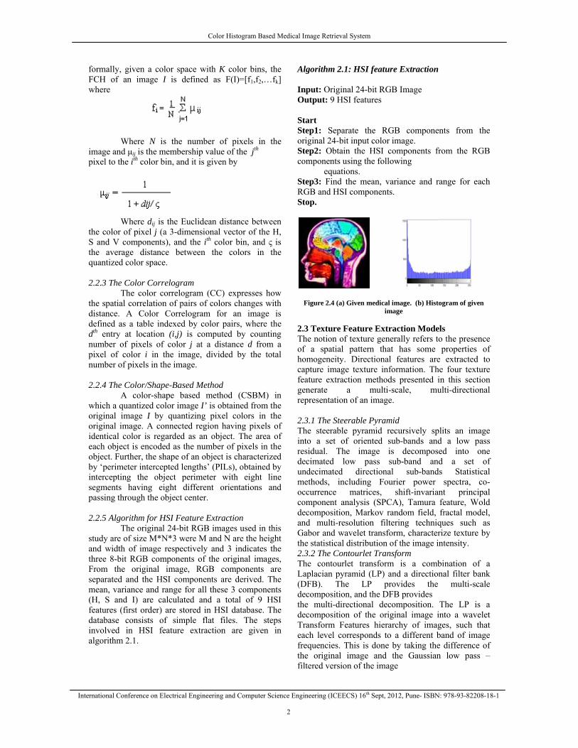
Color Histogram Based Medical Image Retrieval System
International Conference on Electrical Engineering and Computer Science Engineering (ICEECS) 16th Sept, 2012, Pune- ISBN: 978-93-82208-18-1
2
formally, given a color space with K color bins, the FCH of an image I is defined as F(I)=[f1,f2,…fk] where
Where N is the number of pixels in the image and μij is the membership value of the jth pixel to the ith color bin, and it is given by
Where dij is the Euclidean distance between
the color of pixel j (a 3-dimensional vector of the H, S and V components), and the ith color bin, and ς is the average distance between the colors in the quantized color space. 2.2.3 The Color Correlogram
The color correlogram (CC) expresses how the spatial correlation of pairs of colors changes with distance. A Color Correlogram for an image is defined as a table indexed by color pairs, where the dth entry at location (i,j) is computed by counting number of pixels of color j at a distance d from a pixel of color i in the image, divided by the total number of pixels in the image. 2.2.4 The Color/Shape-Based Method
A color-shape based method (CSBM) in which a quantized color image I’ is obtained from the original image I by quantizing pixel colors in the original image. A connected region having pixels of identical color is regarded as an object. The area of each object is encoded as the number of pixels in the object. Further, the shape of an object is characterized by ‘perimeter intercepted lengths’ (PILs), obtained by intercepting the object perimeter with eight line segments having eight different orientations and passing through the object center. 2.2.5 Algorithm for HSI Feature Extraction
The original 24-bit RGB images used in this study are of size M*N*3 were M and N are the height and width of image respectively and 3 indicates the three 8-bit RGB components of the original images, From the original image, RGB components are separated and the HSI components are derived. The mean, variance and range for all these 3 components (H, S and I) are calculated and a total of 9 HSI features (first order) are stored in HSI database. The database consists of simple flat files. The steps involved in HSI feature extraction are given in algorithm 2.1.
Algorithm 2.1: HSI feature Extraction Input: Original 24-bit RGB Image Output: 9 HSI features Start Step1: Separate the RGB components from the original 24-bit input color image. Step2: Obtain the HSI components from the RGB components using the following equations. Step3: Find the mean, variance and range for each RGB and HSI components. Stop.
Figure 2.4 (a) Given medical image. (b) Histogram of given image
2.3 Texture Feature Extraction Models The notion of texture generally refers to the presence of a spatial pattern that has some properties of homogeneity. Directional features are extracted to capture image texture information. The four texture feature extraction methods presented in this section generate a multi-scale, multi-directional representation of an image.
2.3.1 The Steerable Pyramid The steerable pyramid recursively splits an image into a set of oriented sub-bands and a low pass residual. The image is decomposed into one decimated low pass sub-band and a set of undecimated directional sub-bands Statistical methods, including Fourier power spectra, co-occurrence matrices, shift-invariant principal component analysis (SPCA), Tamura feature, Wold decomposition, Markov random field, fractal model, and multi-resolution filtering techniques such as Gabor and wavelet transform, characterize texture by the statistical distribution of the image intensity. 2.3.2 The Contourlet Transform The contourlet transform is a combination of a Laplacian pyramid (LP) and a directional filter bank (DFB). The LP provides the multi-scale decomposition, and the DFB provides the multi-directional decomposition. The LP is a decomposition of the original image into a wavelet Transform Features hierarchy of images, such that each level corresponds to a different band of image frequencies. This is done by taking the difference of the original image and the Gaussian low pass –filtered version of the image
Color Histogram Based Medical Image Retrieval System
International Conference on Electrical Engineering and Computer Science Engineering (ICEECS) 16th Sept, 2012, Pune- ISBN: 978-93-82208-18-1
3
2.3.3 The Complex Directional Filter Bank The complex directional filter bank (CDFB) consists of a Laplacian pyramid and a pair of DFBs, designated as primal and dual filter banks. The filters of these filter banks are designed to have special phase functions, so that the overall filter is the Hilbert transform of the primal filter bank. A multi-resolution representation is obtained by reiterating the decomposition in the low pass branch
Figure 2.5. Pyramid Wavelet Transform (Level 3)
The standard Pyramid Wavelet Transform is shown in the Figure 2.5. The first step is to resize the image size into 256X256 in a matrix format. Then the pyramid wavelet transform is applied to get the sub bands of the image. To find the energy measures of the image Daubechies filter is applied. The decomposition is applied to 6 levels so that we can able to get the low frequency contents in the LL sub band and other frequencies in LH, HL and HH bands separately. Finally we will get the 4X4-sized image. Once the wavelet coefficients of an image are available, features are computed from each sub-band, resulting in 19 features for each image. The mean µ is the energy measure used to compute the features, and then the feature vector f, for a particular image is calculated as;
f = [µmn], n≠1 except for the coarsest level, m=6
f = [µ1,2, µ1,3, µ1,4, µ2,2, µ2,3 … µ6,1, µ6,2, µ6,3, µ6,4 ] Where µmn is the energy measure for the
decomposition level and the sub bands. In this we get the energy coefficients and stored in the database. Algorithm 2.2: Calculation of co-occurrence matrix Pf,d(x,y) from the image f(x,y) Input: Input gray level image f(x,y). Output: Co-occurrence matrix Pf,d(x,y) for d=1 in the direction f. Start Step1: Assign Pf,d(x,y) = 0 for all x,y e[0,L] where L is maximum gray level. Step2: For all pixels (x1,y1) in the image, determine (x2,y2) which is at distance d in direction f and perform
Pf,d [f(x1,y1), f(x2,y2)] = Pf,d [f(x1,y1), f(x2,y2)] +1 Stop.
Algorithm 2.3: Textural feature extraction Input: RGB components of original image. Output: 24 Textural Features. Start Step1: Derive the Gray Level Co-occurrence
Matrices (GLCM) Pf,d(x,y) for four different values of direction f ( 00, 450, 900, and 1350) and d=1 which are dependent on direction f. (for simplicity d is taken to be 1)
Step2: Compute Co-occurrence Matrix which is dependent on direction using the Equation
C = 1 (P00 + P450 + P900 + P1350) 4 Step3: For large height (M) and width (N) of the
image, the relative frequency of co-Occurrences P(x,y) = C(x,y)/(M*N) represents approximately the joint probability mass of the discrete variables x,y. Henceforth the co-occurrences matrix be assumed to have the elements P(x,y) in place of C(x,y). Eight GLCM features namely mean variance, range, energy, entropy, contrast, inverse difference moment, correlation and homogeneity are calculated. Important measures based on texture are defined below.
Mean µ = Σ xP(x,y) x,y
Variance σ = Σ (x-µ)2P(x,y) x,y
Range = max2-min2 Where max2 = max (max1), max1 = max(image), min2 = min(min1) min1 = min(image) Maximum probability = max(P(x,y)) Energy = Σ P2(x,y) x,y
Contrast = Σ |x-y|kP(x,y)
x,y
Inverse difference moment = Σ P(x,y) x,y:x≠y |x-y|k
Where µx, µy, Sx, Sy are standard deviations defined by µx = Σ x Σ P(x,y) x y
µy = Σ y Σ P(x,y) y x
Sx = Σ (x-µx)2 Σ P(x,y) x y
Sy = Σ (y-µy)2 Σ P(x,y) y x
Stop.
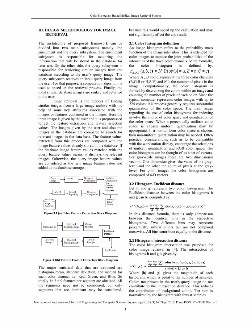
Color Histogram Based Medical Image Retrieval System
International Conference on Electrical Engineering and Computer Science Engineering (ICEECS) 16th Sept, 2012, Pune- ISBN: 978-93-82208-18-1
4
III. DESIGN METHODOLOGY FOR IMAGE RETRIEVAL
The architecture of proposed framework can be divided into two main subsystems namely, the enrollment and the query subsystem. The enrollment subsystem is responsible for acquiring the information that will be stored in the database for later use. On the other side, the query subsystem is responsible for retrieving similar images from the database according to the user’s query image. The query subsystem receives an input query image from the user. For that purpose, a computation algorithm is used to speed up the retrieval process. Finally, the most similar database images are ranked and returned to the user.
Image retrieval is the process of finding similar images from a large image archive with the help of some key attributes associated with the images or features contained in the images. Here the input image is given by the user and it is preprocessed to get the feature extraction and feature selection values. The images given by the user and also the images in the database are compared to search for relevant images in the data base. The feature values extracted from this process are compared with the image feature values already stored in the database. If the database image feature values matched with the query feature values means, it displays the relevant images. Otherwise, the query image feature values are considered as the new image feature value and added to the database storage.
Figure 3.1 (a) Color Feature Extraction Block Diagram
Figure 3.1(b) Texture Feature Extraction Block Diagram
The major statistical data that are extracted are histogram mean, standard deviation, and median for each color channel i.e. Red, Green, and Blue. So totally 3× 3 = 9 features per segment are obtained. All the segments need not be considered, but only segments that are dominant may be considered,
because this would speed up the calculation and may not significantly affect the end result. 3.1 Color histogram definition An image histogram refers to the probability mass function of the image intensities. This is extended for color images to capture the joint probabilities of the intensities of the three color channels. More formally, the color histogram is defined by,
Where A , B and C represent the three color channels (R,G,B or H,S,V) and N is the number of pixels in the image. Computationally, the color histogram is formed by discretizing the colors within an image and counting the number of pixels of each color. Since the typical computer represents color images with up to 224 colors, this process generally requires substantial quantization of the color space. The main issues regarding the use of color histograms for indexing involve the choice of color space and quantization of the color space. When a perceptually uniform color space is chosen uniform quantization may be appropriate. If a non-uniform color space is chosen, then non-uniform quantization may be needed. Often practical considerations, such as to be compatible with the workstation display, encourage the selections of uniform quantization and RGB color space. The color histogram can be thought of as a set of vectors. For gray-scale images these are two dimensional vectors. One dimension gives the value of the gray-level and the other the count of pixels at the gray-level. For color images the color histograms are composed of 4-D vectors. 3.2 Histogram Euclidean distance Let h and g represent two color histograms. The Euclidean distance between the color histograms h and g can be computed as:
In this distance formula, there is only comparison between the identical bins in the respective histograms. Two different bins may represent perceptually similar colors but are not compared crosswise. All bins contribute equally to the distance. 3.3 Histogram intersection distance The color histogram intersection was proposed for color image retrieval in [4]. The intersection of histograms h and g is given by:
Where |h| and |g| gives the magnitude of each histogram, which is equal to the number of samples. Colors not present in the user's query image do not contribute to the intersection distance. This reduces the contribution of background colors. The sum is normalized by the histogram with fewest samples.
Color Histogram Based Medical Image Retrieval System
International Conference on Electrical Engineering and Computer Science Engineering (ICEECS) 16th Sept, 2012, Pune- ISBN: 978-93-82208-18-1
5
3.4 Histogram quadratic (cross) distance The color histogram quadratic distance was used by the QBIC system. The cross distance formula is given by:
The cross distance formula considers the cross-correlation between histogram bins based on the perceptual similarity of the colors represented by the bins. And the set of all cross-correlation values are represented by a matrix A, which is called a similarity matrix. And a (i,j)th element in the similarity matrix A is given by : for RGB space,
Where dij is the distance between the color i and j in the RGB space. In the case that quantization of the color space is not perceptually uniform the cross term contributes to the perceptual distance between color bins. For HSV space it is given by:
which corresponds to the proximity in the HSV color space.
IV. RESULTS AND DISCUSSIONS
The general flow of the experiments starts
with the decomposition of data base image using Haar, D4 wavelets and Haar, D4 Lifting procedure in offline. The maximal decomposition level J = 4. The repeated decomposition is used for query image. The features are extracted from the image to form feature vector and performed highly efficient image matching. The progressive retrieval strategy is used to balance between computational complexity and retrieval accuracy. The main focus is on the comparison of two important retrieval indices, namely retrieval accuracy and the speed. The test
image database contains over 100 medical images of 24 bits true color. In this all images are pre processed to 256x256 sizes before decomposition. Sample data base images for each category are shown below. The retrieval accuracy is defined as the ratio between the number of relevant images (belongs to the same category) retrieved and the total number of retrieved images (known as a single precision) Retrieval = Number of relevant images Accuracy Total number of images retrieved In the literature survey for various CBIR methods, the semantic gap between low level features and high level concept is more and the retrieved output consisted lot of errors. Hence the proposed method retrieves the images based on color, texture and metadata features. The integrated results will be outputted to the user hence the retrieval accuracy will be high and less interaction is needed. The proximity between two images is calculated using two different techniques: Euclidian distance between color histograms and ED between wavelet energies.
Figure 4.1(a) Query image
Figure 4.1 (b).Retrieved mages from Database The below images show RGB plane separation and its corresponding Histograms.
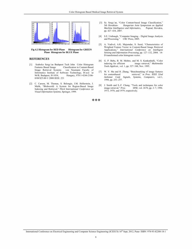
Color Histogram Based Medical Image Retrieval System
International Conference on Electrical Engineering and Computer Science Engineering (ICEECS) 16th Sept, 2012, Pune- ISBN: 978-93-82208-18-1
6
Fig 4.2 Histogram for RED Plane Histogram for GREEN Plane Histogram for BLUE Plane
REFERENCES [1] Szabolcs Sergy´an Budapest Tech John Color Histogram
Features Based Image Classification in Content-Based Image Retrieval Systems von Neumann Faculty of Informatics Institute of Software Technology, B´ecsi ´ut 96/B, Budapest, H-1034, Hungary, 978-1-4244-2106-0/08/$25.00 © 2008 IEEE. 221
[2] C. Carson, M. Thomas, S. Belongie, J.M. Hellerstein, J.
Malik, “Blobworld: A System for Region-Based Image Indexing and Retrieval,” Third International Conference on Visual Information Systems, Springer, 1999.
[3] Sz. Sergy´an, “Color Content-based Image Classification,” 5th Slovakian- Hungarian Joint Symposium on Applied Machine Intelligence and Informatics, Poprad, Slovakia, pp. 427–434, 2007.
[4] S.E. Umbaugh, “Computer Imaging – Digital Image Analysis
and Processing,” CRC Press, 2005. [5] A. Vadivel, A.K. Majumdar, S. Sural, “Characteristics of
Weighted Feature Vector in Content-Based Image Retrieval Applications,” International Conference on Intelligent Sensing and Information Processing, pp. 127–132, 2004. 14-D transformed color histogram vector.
[6] G. P. Babu, B. M. Mehtre, and M. S. Kankanhalli, “Color
indexing for efficient image retrieval,” Multimedia Tools Applicat., vol. 1, pp. 327–348, Nov. 1995.
[7] W. Y. Ma and H. Zhang, “Benchmarking of image features
for contentbased retrieval,” in Proc. IEEE 32nd Asilomar Conf. Signals, Systems, Computers, vol.1, 1998, pp. 253–257.
[8] J. Smith and S.-F. Chang, “Tools and techniques for color
image retrieval,” Proc. SPIE, vol. 2670, pp. 2–7, 1996. 1973, 1976, and 1979, respectively.
International Conference on Electrical Engineering and Computer Science Engineering (ICEECS) 16th Sept, 2012, Pune- ISBN: 978-93-82208-18-1
70
A META CLUSTERING APPROACH FOR ENSEMBLE PROBLEM
1DIVYA D J & 2GAYATHRI DEVI B
1Dept of Computer Science Engineering, B.T.L. Institute of Technology, Bangalore, India 2Dept of Electrical Engineering, P E S Institute of Technology, Bangalore, India
Abstract— A critical problem in cluster ensemble research is how to combine multiple clustering to yield a superior clustering result. Leveraging advanced graph partitioning techniques, we solve this problem by reducing it to a graph partitioning problem. We introduce a new reduction method that constructs a bipartite graph from a given cluster ensemble. The resulting graph models both instances and clusters of the ensemble simultaneously as vertices in the graph. Our approach retains all of the information provided by a given ensemble, allowing the similarity among instances and the similarity among clusters to be considered collectively in forming the clustering. Further, the resulting graph partitioning problem can be solved efficiently. We empirically evaluate the proposed approach against two commonly used graph formulations and show that it is more robust and achieves comparable or better performance in comparison to its competitors. Keywords-meta clustering approach; graph partitioning problem; ensemble problem; meta clustering
I. INTRODUCTION Clustering is to group analogous elements in a data set in accordance with its similarity such that elements in each cluster are similar while elements from different clusters are dissimilar. It doesn’t require the class label information about the data set because it is inherently a data,driven approach. So, the most interesting and well developed method of manipulating and cleaning spatial data in order to prepare it for spatial data mining analysis is by clustering that has been recognized as a primary data mining method for knowledge discovery in spatial database Clustering fusion is the integration of results from various clustering algorithms using a consensus function to yield stable results. Clustering fusion approaches are receiving increasing attention for their capability of improving clustering performance. At present, the usual operation mechanism for clustering fusion is the “combining” of clusterer outputs. One tool for such combining or consolidation of results Clustering for unsupervised data exploration and analysis has been investigated for decades in the statistics, data mining, and machine learning communities. A recent advance of clustering techniques is the development of cluster ensemble or consensus clustering techniques which seek to improve clustering performance by generating multiple partitions of a given data set and then combining them to form a (presumably superior) clustering solution. Such techniques have been shown to provide a generic tool for improving the performance of basic clustering algorithms. Cluster ensembles can be generated in different ways. The resulting ensembles may differ and the same approach for solving the ensemble problems may perform differently accordingly. It is thus important for our experiments to consider different
ways to generate cluster ensembles. Our experiments use two approaches, random subsampling and random projection [Fern & Brodley, 2003], to generate the ensembles. Note that for both approaches, K,means is used as the base clustering algorithm and the number K is pre,specified for each data set and remains the same for all clustering runs. Note that we also examined a third approach, randomly restarting K means, and it produced similar results to those of random subsampling. So we omit these results in the discussion of our experiments. Random projection should be diverse because it provides the base learner with different views of the data. On the other hand, we expect the quality of the clusterings produced by random subsampling to be higher because it provides the base learner with more complete information of the data. A. Graph Partitioning Algorithms Our goal is to evaluate different graph formulation approaches. To reduce the infuence of any chosen graph partitioning algorithm on our evaluation, we use two well, known graph partitioning algorithms that differ with respect to their search for the best partition.
B. Spectral Graph Partitioning Spectral graph partitioning is a well studied area with many successful applications. We choose a popular multi, way spectral graph partitioning algorithm proposed by Ng et al. [Alexander Strehl and J. Ghosh,2002], which seeks to optimize the normalized cut criterion [Shi & Malik, 2000]. We refer to this algorithm as SPEC. SPEC can be simply described as follows. Given a graph G = (V;W), it computes the degree matrix D, which is a diagonal matrix such that D(i; i) =Pj W(i; j). Based on D, it then computes a normalized weight matrix K largest eigenvectors u1; u2; _ _
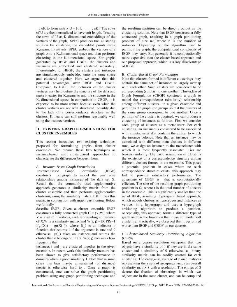
A Meta Clustering Approach for Ensemble Problem
International Conference on Electrical Engineering and Computer Science Engineering (ICEECS) 16th Sept, 2012, Pune- ISBN: 978-93-82208-18-1
71
_ ; uK to form matrix U = [u1; _ _ _ ; uK]. The rows of U are then normalized to have unit length. Treating the rows of U as K dimensional embeddings of the vertices of the graph, SPEC produces the clustering solution by clustering the embedded points using K,means. Intuitively, SPEC embeds the vertices of a graph onto a K,dimensional space and then performs clustering in the K,dimensional space. For graphs generated by IBGF and CBGF, the clusters and instances are embedded and clustered separately. Interestingly, for HBGF, the clusters and instances are simultaneously embedded onto the same space and clustered together. Here we argue that this potential advantages over IBGF and CBGF. Compared to IBGF, the inclusion of the cluster vertices may help define the structure of the data and make it easier for K,means to and the structure in the K, dimensional space. In comparison to CBGF, it is expected to be more robust because even when the cluster vertices are not well structured, possibly due to the lack of a correspondence structure in the clusters, K,means can still perform reasonably well using the instance vertices. II. EXISTING GRAPH FORMULATIONS FOR CLUSTER ENSEMBLES This section introduces two existing techniques proposed for formulating graphs from cluster ensembles. We rename these two techniques as instance,based and cluster,based approaches to characterize the differences between them. A. Instance-Based Graph Formulation Instance,Based Graph Formulation (IBGF) constructs a graph to model the pair wise relationships among instances of the data set X. Recall that the commonly used agglomerative approach generates a similarity matrix from the cluster ensemble and then performs agglomerative clustering using the similarity matrix. IBGF uses this matrix in conjunction with graph partitioning. Below we formally describe IBGF. Given a cluster ensemble IBGF constructs a fully connected graph G = (V;W), where V is a set of n vertices, each representing an instance of X.W is a similarity matrix and W(i; j) =1R PRr=1 I(gr(Xi) = gr(Xj )), where I(_) is an indicator n function that returns 1 if the argument is true and 0 otherwise; gr(_) takes an instance and returns the cluster that it belongs to in Cr. W(i; j) measures how frequently the instances i and j are clustered together in the given ensemble. In recent work this similarity measure has been shown to give satisfactory performance in domains where a good similarity 1. Note that in some cases this bias maybe unwarranted (or distance) metric is otherwise hard to . Once a graph is constructed, one can solve the graph partitioning problem using any graph partitioning technique and
the resulting partition can be directly output as the clustering solution. Note that IBGF constructs a fully connected graph, resulting in a graph partitioning problem of size n2, where n is the number of instances. Depending on the algorithm used to partition the graph, the computational complexity of IBGF may vary. But generally it is computationally more expensive than the cluster based approach and our proposed approach, which is a key disadvantage of IBGF. B. Cluster-Based Graph Formulation Note that clusters formed in different clusterings may contain the same set of instances or largely overlap with each other. Such clusters are considered to be corresponding (similar) to one another. Cluster,Based Graph Formulation (CBGF) constructs a graph to model the correspondence (similarity) relationship among different clusters in a given ensemble and partitions the graph into groups so that the clusters of the same group correspond to one another. Once a partition of the clusters is obtained, we can produce a clustering of instances as follows. First we consider each group of clusters as a metacluster. For each clustering, an instance is considered to be associated with a metacluster if it contains the cluster to which the instance belongs. Note that an instance may be associated with different meta clusters in different runs, we assign an instance to the metacluster with which it is most frequently associated. Ties are broken randomly. The basic assumption of CBGF is the existence of a correspondence structure among different clusters formed in the ensemble. This poses a potential problem in cases where no such correspondence structure exists, this approach may fail to provide satisfactory performance. The advantage of CBGF is that is computationally efficient. The size of the resulting graph partitioning problem is t2, where t is the total number of clusters in the ensemble. This is significantly smaller than the n2 of IBGF, assuming .hypergraph based approach, which models clusters as hyperedges and instances as vertices in a hypergraph and uses a hypergraph artitioning algorithm to produce a partition. onceptually, this approach forms a different type of graph and has the limitation that it can not model soft clustering. Practically, we observed that it performed worse than IBGF and CBGF on our datasets. C. Cluster-based Similarity Partitioning Algorithm (CSPA) Based on a coarse resolution viewpoint that two objects have a similarity of 1 if they are in the same cluster and a similarity of 0 otherwise, a binary similarity matrix can be readily created for each clustering. The entry,wise average of r such matrices representing the r sets of groupings yields an overall similarity matrix S with a resolution. The entries of S denote the fraction of clusterings in which two objects are in the same cluster, and can be computed
A Meta Clustering Approach for Ensemble Problem
International Conference on Electrical Engineering and Computer Science Engineering (ICEECS) 16th Sept, 2012, Pune- ISBN: 978-93-82208-18-1
72
in one sparse matrix multiplication S =rHHy. the generation of the cluster,based similarity matrix Now, we can use the similarity matrix to recluster the objects using any reasonable similarity,based clustering algorithm. We hose to partition the induced similarity graph (vertex = object, edge weight = similarity) using METIS [Karypis and Kumar, 1998] because of its robust and scalable properties. CSPA is the simplest and most obvious heuristic, but its computational and storage complexity are both quadratic in n, as opposed to the next two approaches that are near linear in n. D. HyperGraph-Partitioning Algorithm (HGPA)
The second algorithm is a direct approach to cluster ensembles that re,partitions the data using the given clusters as indications of strong bonds. The cluster ensemble problem is formulated [Kunal Punera, Joydeep Ghosh] as partitioning the hypergraph by cutting a minimal number of hyperedges. We call this approach the hypergraph, partitioning algorithm (HGPA). All hyperedges are considered to have the same weight. Also, all vertices re equally weighted. Note that this includes n`,way relationship information, while CSPA only considers pairwise relationships.
E. Representing Sets of Clusterings as a
Hypergraph The first step for both of our proposed consensus functions is to transform the given cluster label vectors into a suitable hypergraph representation. In this subsection, we describe how any set of clusterings can be mapped to a hypergraph. A hypergraph consists of vertices and hyperedges. An edge in a regular graph connects xactly two vertices. A hyperedge is a generalization of an edge in that it can connect any set of vertices. For each label vector _(q) 2 Nn, we construct the binary membership indicator matrix H(q), with a column for each cluster (now represented as a hyperedge) All entries of a row in the binary membership indicator matrix H(q) add to 1, if the row corresponds to an object with known label. Rows for objects with unknown label are all zero.The concatenated block matrix H = H(1;:::;r) = (H(1) : : : H(r)) defines the adjacency matrix of a hypergraph with n vertices and Pr q=1 k(q) hyperedges. Each column vector ha specifies a hyperedge ha, where 1 indicates that the vertex corresponding to the row is part of that hyperedge and 0 indicates that it is not. Thus, we have mapped each cluster to a hyperedge and the set of clusterings to a hypergraph III. META CLUSTERING ALGORITHM We introduce the algorithm to solve the cluster ensemble problem. The Meta,Clustering Algorithm (MCLA) is based on clustering clusters. It also yields
object,wi se confidence estimates of cluster membership. We represented each cluster by a hyperedge. The idea in MCLA is to group and collapse related hyperedges and assign each object to the collapsed hyperedge in which it participates most strongly. The hyperedges that are considered related for the purpose of collapsing are determined by a graph,based clustering of hyperedges. We refer to each cluster of hyperedges as a meta,cluster C(M). Collapsing reduces the number of hyperedges from:
to k. The detailed steps are : A. Construct Meta Graph Let us view all the indicator vectors h (the hyperedges of H ) as vertices of another regular undirected graph, the meta,graph. The edge weights are proportional to the similarity between vertices. A suitable similarity measure here is the binary Jaccard measure, since it is the ratio of the intersection to the union of the sets of objects corresponding to the two hyperedges. Formally, the edge weight wa,b between two vertices ha and hb as defined by the binary Jaccard measure of the corresponding indicator vectors ha and hb is: Since the clusters are non,overlapping there are no edges amongst vertices of the same clustering H(q) and, thus, the meta,graph is r,partite B. Cluster Hyperedges
Find matching labels by partitioning the meta,graph into k balanced meta,clusters. Each vertex is weighted proportional to the size of the corresponding cluster. Balancing ensures that the sum of vertex,weights is approximately the same in each meta,cluster. We use the graph partitioning package METIS in this step. This results in a clustering of h vectors. Since each vertex in the meta, graph represents a distinct cluster label, a meta,cluster represents a group of corresponding labels. C. Collapse Meta Clusters
For each of the k meta,clusters, we collapse the hyperedges into a single meta,hyperedge. Each meta, hyperedge has an association vector which contains an entry for each object describing its level of association with the corresponding meta,cluster. The level is computed by averaging all indicator vectors h of a particular meta,cluster. An entry of 0 or 1 indicates the weakest or strongest association, respectively. D. Compete for Objects
In this step, each object is assigned to its most associated meta,cluster: Specifically, an object is assigned to the meta,cluster with the highest entry in the association vector. Ties are broken randomly. The
A Meta Clustering Approach for Ensemble Problem
International Conference on Electrical Engineering and Computer Science Engineering (ICEECS) 16th Sept, 2012, Pune- ISBN: 978-93-82208-18-1
73
confidence of an assignment is reflected by the winner's share of association (ratio of the winner's association to the sum of all other associations). Note that not every meta,cluster can be guaranteed to win at least one object. Thus, there are at most k labels in the final combined clustering λ. E. Multilevel Graph Partition: METIS
Metis a multilevel graph partitioning system, approaches the graph partitioning problem from a different angle. It partitions a graph using three basic steps: (1) coarsen the graph by collapsing b vertices and edges; (2) partition the coarsened graph and (3) refine the partitions. In comparison to other graph partitioning algorithms, Metis is highly efficient and achieves competitive performance.
Figure 1. Meta clustering
IV. ADVANTAGES OF META CLUSTERING After the text edit has been completed, the paper is ready for the template. Duplicate the template file by using the Save As command, and use the naming convention prescribed by your conference for the name of your paper. In this newly created file, highlight all of the contents and import your prepared text file. You are now ready to style your paper. 1) Provides for a method to represent the consensus across multiple runs of a clustering algorithm, to determine the number of clusters in the data, and to assess the stability of the discovered clusters. 2) The method can also be used to represent the consensus over multiple runs of a clustering algorithm with random restart so as to account for its sensitivity to the initial conditions. 3) It also provides for a visualization tool to inspect cluster number, membership, and boundaries.
4) We will be able to extract lot of features / attributes from multiples runs of different clustering algorithms on the data. These features can give us valuable information in doing a final consensus clustering. V. CONCLUSION sMCLA extends MCLA by accepting soft clusterings as input. sMCLA’s working can be divided into the following steps: 1) Construct Soft Meta,Graph of Clusters 2) Group the Clusters into Meta,Clusters 3) Collapse Meta,Clusters using Weighting 4) Compete for Object Other worthwhile future work includes a thorough theoretical analysis of the average normalized mutual information (ANMI) objective, including how it can be applied to soft clusterings. We also plan to explore possible sMCLA schemes in more detail. The CSPA scheme introduced is not very practical by itself. However, it can be used as a post,processing step to refine good solutions when n is not too large. For example, one can use the supra,consensus labeling as the initialization instead of the best single input clustering. Preliminary experiments indicate that this post,processing a. Another direction of future work is to better understand the biases of the three proposed consensus functions. We would also like to extend our application scenarios. Cluster ensembles could enable federated data mining systems to work on top of distributed and heterogeneous databases. REFERENCES [1] Alexander Strehl and J. Ghosh, “Cluster ensembles – a
knowledge reuse framework for combining multiple partitions”, Journal of Machine Learning Research, vol. 3, 2002, pp. 583,617
[2] Kunal Punera, Joydeep Ghosh, “Consensus Based Ensembles of Soft Clusterings”, Applied Artificial Intelligence: An International Journal, Aristides vol. 22, Issue 7,8, 2008, pp. 780,810 [3] Fern, X. Z., & Brodley, C. E.. Random projection for high dimensional data clustering: A cluster ensemble approach Hongjun Wang, Hanhuai Shan, Arindam Banerjee. Bayesian Cluster Ensembles, SIAM International Conference on Data Mining, SDM 09, 2003
[4] Topchy, A., Jain, A. K., & Punch, W, “Combining multiple weak clusterings”, ICDM. 2003
[5] Strehl, A., & Ghosh, J., “Cluster ensembles – a knowledge reuse framework for combining multiple partitions. Machine Learning Research”,2002
[6] Karypis, G., & Kumar, V., “A fast and high quality multilevel scheme for partitioning irregular graphs”, 1998.

Energy Audit: for Effective Use of Electrical Energy To Conserve Energy
International Conference on Electrical Engineering and Computer Science Engineering (ICEECS) 16th Sept, 2012, Pune- ISBN: 978-93-82208-18-1 1
ENERGY AUDIT: FOR EFFECTIVE USE OF ELECTRICAL ENERGY TO CONSERVE ENERGY
1JAYPREET KAUR KEER, 2N.M.DESHKAR & 3V.HUCHCHE
Dept. of Electrical Engg, SRCOEM, Nagpur, India
Abstract— The requirement of energy is increasing in leap and bounds, whereas the power generation is still comparatively lower. Electrical energy, a vital energy input in any industrial activity, is demanding increasing attention on account of power shortages. There is general awareness of the opportunities for reducing the cost of electricity consumption, but the progress in implementation has been slow and stagnant. Part of the reason for the slow progress is lack of information on the methodologies for the electrical energy management. Thus, a systematic approach is required for reducing the power consumption and increasing the energy efficiency. This paper discusses common aspects of electrical energy management. It contains the finding and the analysis of the results obtained from the electrical energy audit program which is done in an educational institution. The analyses are focused on the load management, power factor management, and loss management, general energy conservation measures (ECMs) that can be commonly recommended. Keywords-component;Energymanagement,Energy audit,Energy consevation measures(ECMs)
I. INTRODUCTION
“The judicious and effective use of energy to maximize profits (minimize costs) and enhance competitive positions.” is the basic definition of energy audit. Increasing energy efficiency without adversely affecting its productivity is provided by “Energy Audit”.
Energy Conservation and Energy Efficiency are separate, but related concepts. Energy conservation is achieved when growth of energy consumption is reduced, measured in physical terms. Energy Conservation, therefore, is the result of several processes or developments, such as productivity increase or technological progress. Electricity energy management refers to the optimal utilization of every KWh consumed by the consumers and the minimization of the total electricity consumption. The aims of electrical energy management are to optimize the present operations to promote the wise and efficient utilization of electrical energy and to reduce the cost of electricity in industry [4].
Energy Audit helps in highlighting energy waste in a facility, determining how this waste can be eliminated at a reasonable cost with a suitable time frame. Energy audit is widely used and many have different meaning depending on energy service companies. It not only serves to identify energy use in various areas and to identify opportunities for energy conservation but it is also a crucial first step in establishing an energy management program. The audit will produce the data on which such a program is based. The study should reveal to the owner, manager, or management team of institution the options available for reducing energy waste, the costs involved, and the benefits achievable from
implementing those energy-conserving
opportunities (ECOs).
II. TYPES OF AUDIT
III. PRELIMINARY AUDIT
The total energy survey is conducted by means of onsite inspections, measurements, questions and discussions with the maintenance staff. Preliminary audit is a relatively quick exercise to:
• Establish energy consumption survey in the organization
• Estimate the scope of saving. • Identify the most likely and the easiest areas
for attention. • Identify immediate (especially no- / low–cost)
improvements /savings • Set a ‘reference point’ • Identify areas for more detailed
study/measurement
Types
Preliminary Audit
Detailed Audit
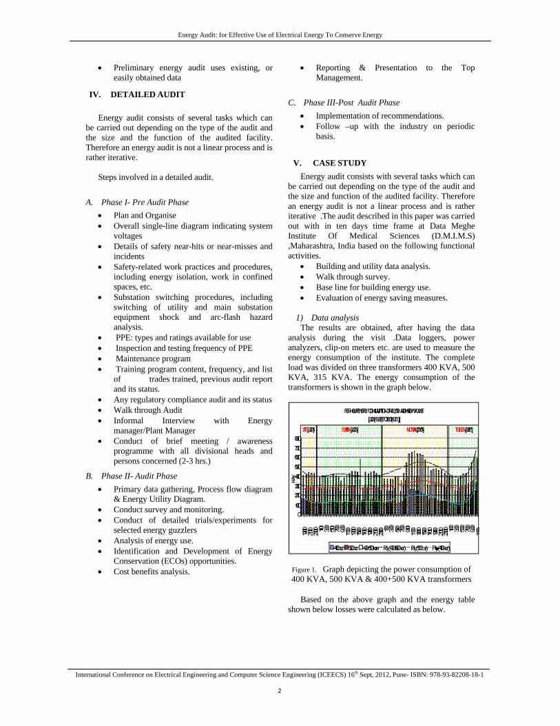
Energy Audit: for Effective Use of Electrical Energy To Conserve Energy
International Conference on Electrical Engineering and Computer Science Engineering (ICEECS) 16th Sept, 2012, Pune- ISBN: 978-93-82208-18-1 2
• Preliminary energy audit uses existing, or easily obtained data
IV. DETAILED AUDIT
Energy audit consists of several tasks which can be carried out depending on the type of the audit and the size and the function of the audited facility. Therefore an energy audit is not a linear process and is rather iterative.
Steps involved in a detailed audit.
A. Phase I- Pre Audit Phase • Plan and Organise • Overall single-line diagram indicating system
voltages • Details of safety near-hits or near-misses and
incidents • Safety-related work practices and procedures,
including energy isolation, work in confined spaces, etc.
• Substation switching procedures, including switching of utility and main substation equipment shock and arc-flash hazard analysis.
• PPE: types and ratings available for use • Inspection and testing frequency of PPE • Maintenance program • Training program content, frequency, and list
of trades trained, previous audit report and its status.
• Any regulatory compliance audit and its status • Walk through Audit • Informal Interview with Energy
manager/Plant Manager • Conduct of brief meeting / awareness
programme with all divisional heads and persons concerned (2-3 hrs.)
B. Phase II- Audit Phase • Primary data gathering, Process flow diagram
& Energy Utility Diagram. • Conduct survey and monitoring. • Conduct of detailed trials/experiments for
selected energy guzzlers • Analysis of energy use. • Identification and Development of Energy
Conservation (ECOs) opportunities. • Cost benefits analysis.
• Reporting & Presentation to the Top Management.
C. Phase III-Post Audit Phase • Implementation of recommendations. • Follow –up with the industry on periodic
basis.
V. CASE STUDY Energy audit consists with several tasks which can
be carried out depending on the type of the audit and the size and function of the audited facility. Therefore an energy audit is not a linear process and is rather iterative .The audit described in this paper was carried out with in ten days time frame at Data Meghe Institute Of Medical Sciences (D.M.I.M.S) ,Maharashtra, India based on the following functional activities.
• Building and utility data analysis. • Walk through survey. • Base line for building energy use. • Evaluation of energy saving measures.
1) Data analysis
The results are obtained, after having the data analysis during the visit .Data loggers, power analyzers, clip-on meters etc. are used to measure the energy consumption of the institute. The complete load was divided on three transformers 400 KVA, 500 KVA, 315 KVA. The energy consumption of the transformers is shown in the graph below.
Figure 1. Graph depicting the power consumption of 400 KVA, 500 KVA & 400+500 KVA transformers
Based on the above graph and the energy table
shown below losses were calculated as below.

Energy Audit: for Effective Use of Electrical Energy To Conserve Energy
International Conference on Electrical Engineering and Computer Science Engineering (ICEECS) 16th Sept, 2012, Pune- ISBN: 978-93-82208-18-1 3
Losses of 500 KVA – 1368 KWH Losses of 400 KVA – 784.8 KWH Total Losses (400+500) (Calculated) –2152.8 KWH Total Losses (MSEDCL) – 2450 KWH Difference Between calculated and MSEDCL readings are 297.2 KWh. These Losses are very high and are due to transmission losses.
2) Analysis of the individual transformers in the system. a) 400 KVA Transformer
Figure 2. (a) Total area under 400 KVA transformer (b) Power Factor variation for 400 KVA transformer
DATE
TIME
500 KVA READIN
G IN KWh
400 KVA READIN
G IN KWh
MSEB READIN
G IN KWh
400 KVA DIFF. IN
KWh
500 KVA DIFF. IN
KWh
(400+500) KVA DIFF IN
KWh
ENERGY CONSUME
D BY MSEB
MULT.
FACT.
ENERGY CONSUME
D BY MSEB
LOSSES
(UNITS)
23/05 19:00 12153 2355.8 729772 23/05 23:00 13248 2967.8 729945 612 1095 1707 173 10 1730 23 24/05 03:00 14376 3472.6 730111 504.8 1128 1632.8 166 10 1660 27.2 24/05 07:00 15471 3970.6 730278 498 1095 1593 167 10 1670 77 24/05 11:00 16533 4447.2 730458 476.6 1062 1538.6 180 10 1800 261.4 24/05 15:00 17694 5024 730635 576.8 1161 1737.8 177 10 1770 32.2 24/05 19:00 18861 5613.6 730820 589.6 1167 1756.6 185 10 1850 93.4 24/05 23:00 20019 6213.6 731000 600 1158 1758 180 10 1800 42 25/05 03:00 21051 6689.2 731158 475.6 1032 1507.6 158 10 1580 72.4 25/05 07:00 22104 7168.4 731326 479.2 1053 1532.2 168 10 1680 147.8 25/05 11:00 23397 7851.8 731526 683.4 1293 1976.4 200 10 2000 23.6 25/05 15:00 24969 8878.8 731798 1027 1572 2599 272 10 2720 121 25/05 19:00 26337 9663.6 732043 784.8 1368 2152.8 245 10 2450 297.2 25/05 23:00 27606 10279 732238 615.4 1269 1884.4 195 10 1950 65.6
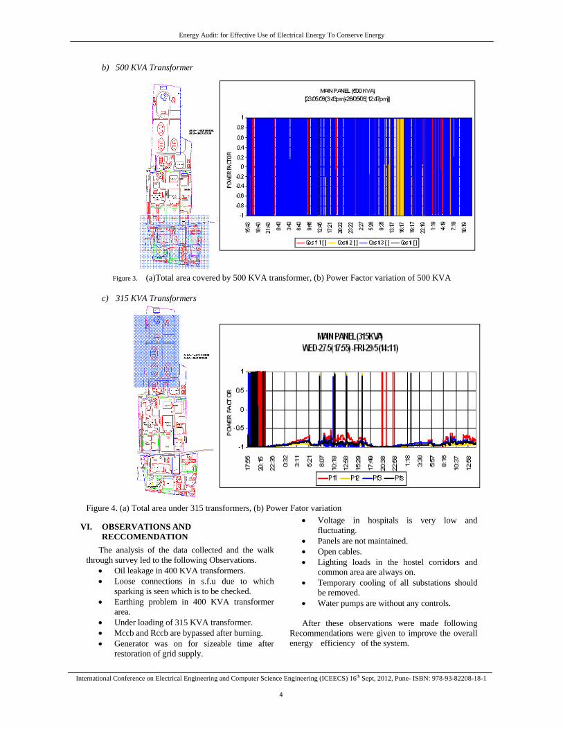
Energy Audit: for Effective Use of Electrical Energy To Conserve Energy
International Conference on Electrical Engineering and Computer Science Engineering (ICEECS) 16th Sept, 2012, Pune- ISBN: 978-93-82208-18-1 4
b) 500 KVA Transformer
Figure 3. (a)Total area covered by 500 KVA transformer, (b) Power Factor variation of 500 KVA
c) 315 KVA Transformers
Figure 4. (a) Total area under 315 transformers, (b) Power Fator variation
VI. OBSERVATIONS AND RECCOMENDATION
The analysis of the data collected and the walk through survey led to the following Observations.
• Oil leakage in 400 KVA transformers. • Loose connections in s.f.u due to which
sparking is seen which is to be checked. • Earthing problem in 400 KVA transformer
area. • Under loading of 315 KVA transformer. • Mccb and Rccb are bypassed after burning. • Generator was on for sizeable time after
restoration of grid supply.
• Voltage in hospitals is very low and fluctuating.
• Panels are not maintained. • Open cables. • Lighting loads in the hostel corridors and
common area are always on. • Temporary cooling of all substations should
be removed. • Water pumps are without any controls.
After these observations were made following
Recommendations were given to improve the overall energy efficiency of the system.
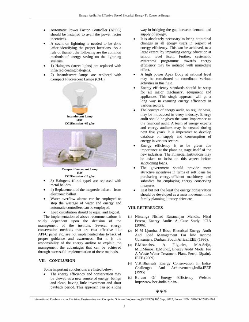
Energy Audit: for Effective Use of Electrical Energy To Conserve Energy
International Conference on Electrical Engineering and Computer Science Engineering (ICEECS) 16th Sept, 2012, Pune- ISBN: 978-93-82208-18-1 5
• Automatic Power Factor Controller (APFC) should be installed to avail the power factor incentives.
• A count on lightning is needed to be done ,after identifying the proper locations .As a rule of thumb , the following are the common methods of energy saving on the lightning systems.
• 1) Halogens (street lights) are replaced with infra red coating halogens.
• 2) Incandescent lamps are replaced with Compact Fluorescent Lamps (CFL).
Incandescent Lamp
60W CO2Emission –65 g/hr
Compact fluorescent Lamp
15W CO2Emission –16 g/hr
• 3) Halogens (flood type) are replaced with metal halides.
• 4) Replacement of the magnetic ballast from electronic ballast.
• Water overflow alarms can be employed to stop the wastage of water and energy and automatic controllers can be employed.
• Load distribution should be equal and logical. The implementation of above recommendations is
solely dependent upon the decision of the management of the institute. Several energy conservation methods that are cost effective like APFC panel etc. are not implemented due to lack of proper guidance and awareness. But it is the responsibility of the energy auditor to explain the management the advantages that can be achieved through successful implementation of these methods.
VII. CONCLUSION
Some important conclusions are listed below: • The energy efficiency and conservation may
be viewed as a new source of energy, benign and clean, having little investment and short payback period. This approach can go a long
way in bridging the gap between demand and supply of energy.
• It is absolutely necessary to bring attitudinal changes in all energy users in respect of energy efficiency. This can be achieved, to a large extent, by imparting energy education at school level itself. Further, systematic awareness programme towards energy efficiency may be initiated with immediate effect.
• A high power Apex Body at national level may be constituted to coordinate various activities in this field.
• Energy efficiency standards should be setup for all major machinery, equipment and appliances. This single approach will go a long way in ensuring energy efficiency in various sectors.
• The concept of energy audit, on regular basis, may be introduced in every industry. Energy audit should be given the same importance as the financial audit. A team of energy experts and energy auditors may be created during next five years. It is imperative to develop database on supply and consumption of energy in various sectors.
• Energy efficiency is to be given due importance at the planning stage itself of the new industries. The Financial Institutions may be asked to insist on this aspect before sanctioning loans.
• The government should provide more attractive incentives in terms of soft loans for purchasing energy-efficient machinery and subsidies for employing energy conserving measures.
• Last but not the least the energy conservation should be developed as a mass movement like family planning, literacy drive etc.
VIII. REFERENCES
[1] Nissanga Nishad Rasananjan Mendis, Nisal Perera, Energy Audit: A Case Study, ICIA (2006).
[2] N M Ljumba, J Ross, Electrical Energy Audit And Load Management For low Income Consumers, Durban ,South Africa,IEEE (1996).
[3] F.M.sanchez, A Filgueira, M.A.Seijo, M.E.Munoz, E.Munoz, Energy Audit Model For A Waste Water Treatment Plant, Ferrol (Spain), IEEE (2009).
[4] V.K.Bhansali ,Energy Conservation In India-Challenges And Achievements,India.IEEE (1995)
[5] Bureau Of Energy Efficiency Website http:/www.bee-india.nic.in/.
International Conference on Electrical Engineering and Computer Science Engineering (ICEECS) 16th Sept, 2012, Pune- ISBN: 978-93-82208-18-1
79
GREEDY CLUSTER HEAD SELECTION BASED ROUTING PROTOCOL FOR MOBILE AD HOC NETWORKS
1NEHA GUPTA, 2MANISH SHRIVASTAVA & 3ANGAD SINGH3
1,2&3 I.T. Department, L.N.C.T.,Bhopal, India
Abstract— Ad-hoc networking is a model in wireless device interactions, which represent that users wanting to communicate with each other form a temporary network, without any form of centralized administration. Each node participating in the network acts both as host and a router and must therefore is willing to forward packets for other nodes. For this purpose, a routing protocol is needed. This means that the routing protocol should try to minimize control traffic, such as periodic update messages. Cluster formation in Ad-hoc network is an important issue; Clustering in Mobile Ad Hoc Networks (MANETs) has many advantages compared to the traditional networks. But the highly dynamic and unstable nature of MANETs makes it difficult for the cluster based routing protocols to divide a mobile network into clusters and determination of cluster heads for each cluster. In recent years, several routing protocols and Cluster based protocols have been proposed for mobile ad hoc networks and prominent among them are DSR, AODV. This survey paper provides an overview of these protocols by presenting their characteristics, functionality, benefits and limitations and then makes their comparative analysis so to analyze their performance and compare some of existing works on clustering in MANETs. We categorize the works as Location based, Neighbor based, Power Based, Artificial Intelligence Based, Mobility based and Weight Based. We also present the advantages and disadvantages of these techniques and suggest a best clustering approach based on the observation. The objective is to make observations about how the performance of these protocols can be improved. We also proposed new technique for cluster head selection for improving efficiency of overall algorithm. Keywords- MANET, Routing Protocol, Clustering, AODV, CMDSR.
I. INTRODUCTION
Wireless communication between mobile users is becoming more popular than ever before. This due to recent technological advances in laptop computers and wireless data communication devices, such as wireless modems and wireless LANs. This has leaded to lower prices and higher data rates, which are the two main reasons why mobile computing continues to enjoy rapid growth. Starting from the development of the packet radio networks (PRNET) in the 1970s and survivable adaptive networks (SURAN) in the 1980s to the global mobile (GloMo) networks in the 1990s and the current mobile ad hoc networks (MANET) [1], the multi-hop ad hoc network has received great amount of research attention.
Mobile Ad hoc Network (MANET), set of wireless mobile node forming a temporary network without the aid of any infrastructure or centralized control. Flexibility and simplicity of adhoc network attracted everyone and solved many problems of communication where infrastructure establishment/reestablishment is not easy task, such as rescue area, Military operations, creates these components, incorporating the applicable criteria that follow.
Modern research area in ad hoc networks has paying attention on MAC and routing strategy. For the reason that of shared wireless broadcast medium, contention, near and for and hidden terminals are common in ad hoc networks and hence MAC
demands significant improvement and routing is another issue especially in multi-hop environment.
Routing is also an interesting issue as routes are typically multi-hop. An ad-hoc network has certain characteristics, which imposes new demands on the routing protocol. The most important characteristic is the dynamic topology, which is a consequence of node mobility. Nodes can change position quite frequently, which means that we need a routing protocol that quickly adapts to topology changes. The nodes in an ad-hoc network can consist of laptops and personal digital assistants and are often very limited in resources such as CPU capacity, storage capacity, battery power and bandwidth. Instead the routing protocol should be reactive, thus only calculate routes upon receiving a specific request.
Generally, traditional routing protocols that are used in wired networks can’t support routing in fixed wireless networks and mobile networks with fixed access points. Only one-hop routing is required over a link in a wireless network with fixed access points and many fixed wireless network. Routing in mobile ad hoc networks and some fixed wireless networks use multiple-hop routing. Routing protocols for this kind of wireless network should be able to maintain paths to other nodes and in most cases, must handle changes in paths due to mobility. Traditional routing cannot properly support routing in a MANET.
Much wireless technology is based upon the principle of direct point-to-point communication. Popular solutions like Group Standard for Mobile
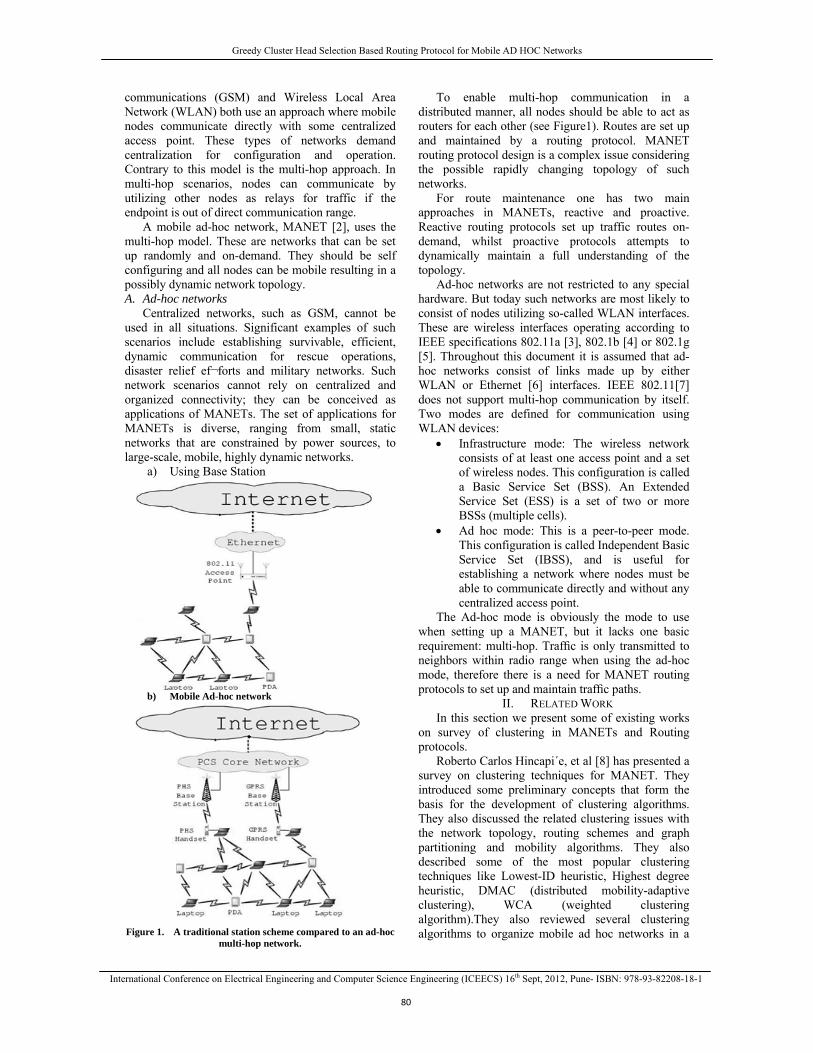
Greedy Cluster Head Selection Based Routing Protocol for Mobile AD HOC Networks
International Conference on Electrical Engineering and Computer Science Engineering (ICEECS) 16th Sept, 2012, Pune- ISBN: 978-93-82208-18-1
80
communications (GSM) and Wireless Local Area Network (WLAN) both use an approach where mobile nodes communicate directly with some centralized access point. These types of networks demand centralization for configuration and operation. Contrary to this model is the multi-hop approach. In multi-hop scenarios, nodes can communicate by utilizing other nodes as relays for traffic if the endpoint is out of direct communication range.
A mobile ad-hoc network, MANET [2], uses the multi-hop model. These are networks that can be set up randomly and on-demand. They should be self configuring and all nodes can be mobile resulting in a possibly dynamic network topology. A. Ad-hoc networks
Centralized networks, such as GSM, cannot be used in all situations. Significant examples of such scenarios include establishing survivable, efficient, dynamic communication for rescue operations, disaster relief ef¬forts and military networks. Such network scenarios cannot rely on centralized and organized connectivity; they can be conceived as applications of MANETs. The set of applications for MANETs is diverse, ranging from small, static networks that are constrained by power sources, to large-scale, mobile, highly dynamic networks.
a) Using Base Station
b) Mobile Ad-hoc network
Figure 1. A traditional station scheme compared to an ad-hoc
multi-hop network.
To enable multi-hop communication in a distributed manner, all nodes should be able to act as routers for each other (see Figure1). Routes are set up and maintained by a routing protocol. MANET routing protocol design is a complex issue considering the possible rapidly changing topology of such networks.
For route maintenance one has two main approaches in MANETs, reactive and proactive. Reactive routing protocols set up traffic routes on-demand, whilst proactive protocols attempts to dynamically maintain a full understanding of the topology.
Ad-hoc networks are not restricted to any special hardware. But today such networks are most likely to consist of nodes utilizing so-called WLAN interfaces. These are wireless interfaces operating according to IEEE specifications 802.11a [3], 802.1b [4] or 802.1g [5]. Throughout this document it is assumed that ad-hoc networks consist of links made up by either WLAN or Ethernet [6] interfaces. IEEE 802.11[7] does not support multi-hop communication by itself. Two modes are defined for communication using WLAN devices:
• Infrastructure mode: The wireless network consists of at least one access point and a set of wireless nodes. This configuration is called a Basic Service Set (BSS). An Extended Service Set (ESS) is a set of two or more BSSs (multiple cells).
• Ad hoc mode: This is a peer-to-peer mode. This configuration is called Independent Basic Service Set (IBSS), and is useful for establishing a network where nodes must be able to communicate directly and without any centralized access point.
The Ad-hoc mode is obviously the mode to use when setting up a MANET, but it lacks one basic requirement: multi-hop. Traffic is only transmitted to neighbors within radio range when using the ad-hoc mode, therefore there is a need for MANET routing protocols to set up and maintain traffic paths.
II. RELATED WORK In this section we present some of existing works
on survey of clustering in MANETs and Routing protocols.
Roberto Carlos Hincapi´e, et al [8] has presented a survey on clustering techniques for MANET. They introduced some preliminary concepts that form the basis for the development of clustering algorithms. They also discussed the related clustering issues with the network topology, routing schemes and graph partitioning and mobility algorithms. They also described some of the most popular clustering techniques like Lowest-ID heuristic, Highest degree heuristic, DMAC (distributed mobility-adaptive clustering), WCA (weighted clustering algorithm).They also reviewed several clustering algorithms to organize mobile ad hoc networks in a
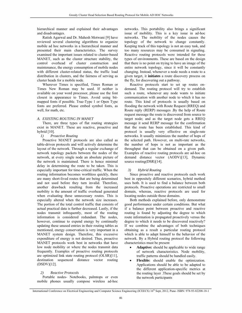
Greedy Cluster Head Selection Based Routing Protocol for Mobile AD HOC Networks
International Conference on Electrical Engineering and Computer Science Engineering (ICEECS) 16th Sept, 2012, Pune- ISBN: 978-93-82208-18-1
81
hierarchical manner and explained their advantages and disadvantages.
Ratish Agarwal and Dr. Mahesh Motwani [9] have reviewed several clustering algorithms to organize mobile ad hoc networks in a hierarchical manner and presented their main characteristics. The survey examined the important issues related to cluster-based MANET, such as the cluster structure stability, the control overhead of cluster construction and maintenance, the energy consumption of mobile nodes with different cluster-related status, the traffic load distribution in clusters, and the fairness of serving as cluster heads for a mobile node.
Wherever Times is specified, Times Roman or Times New Roman may be used. If neither is available on your word processor, please use the font closest in appearance to Times. Avoid using bit-mapped fonts if possible. True-Type 1 or Open Type fonts are preferred. Please embed symbol fonts, as well, for math, etc.
A. EXISTING ROUTING IN MANET
There, are three types of flat routing strategies exist in MANET. These are reactive, proactive and hybrid [10].
1) Proactive Routing Proactive MANET protocols are also called as
table-driven protocols and will actively determine the layout of the network. Through a regular exchange of network topology packets between the nodes of the network, at every single node an absolute picture of the network is maintained. There is hence minimal delay in determining the route to be taken. This is especially important for time-critical traffic. When the routing information becomes worthless quickly, there are many short-lived routes that are being determined and not used before they turn invalid. Therefore, another drawback resulting from the increased mobility is the amount of traffic overhead generated when evaluating these unnecessary routes. This is especially altered when the network size increases. The portion of the total control traffic that consists of actual practical data is further decreased. Lastly, if the nodes transmit infrequently, most of the routing information is considered redundant. The nodes, however, continue to expend energy by continually updating these unused entries in their routing tables as mentioned, energy conservation is very important in a MANET system design. Therefore, this excessive expenditure of energy is not desired. Thus, proactive MANET protocols work best in networks that have low node mobility or where the nodes transmit data frequently. Examples of proactive routing protocols are optimized link state routing protocol (OLSR)[11], destination sequenced distance vector routing (DSDV)[12].
2) Reactive Protocols
Portable nodes- Notebooks, palmtops or even mobile phones usually compose wireless ad-hoc
networks. This portability also brings a significant issue of mobility. This is a key issue in ad-hoc networks. The mobility of the nodes causes the topology of the network to change constantly. Keeping track of this topology is not an easy task, and too many resources may be consumed in signaling. Reactive routing protocols were intended for these types of environments. These are based on the design that there is no point on trying to have an image of the entire network topology, since it will be constantly changing. Instead, whenever a node needs a route to a given target, it initiates a route discovery process on the fly, for discovering out a pathway.
Reactive protocols start to set up routes on-demand. The routing protocol will try to establish such a route, whenever any node wants to initiate communication with another node to which it has no route. This kind of protocols is usually based on flooding the network with Route Request (RREQ) and Route reply (RERP) messages .By the help of Route request message the route is discovered from source to target node; and as the target node gets a RREQ message it send RERP message for the confirmation that the route has been established. This kind of protocol is usually very effective on single-rate networks. It usually minimizes the number of hops of the selected path. However, on multi-rate networks, the number of hops is not as important as the throughput that can be obtained on a given path. Examples of reactive routing protocols are ad-hoc on demand distance vector (AODV)[13], Dynamic source routing(DSR)[14].
3) Hybrid Routing
Since proactive and reactive protocols each work best in oppositely different scenarios, hybrid method uses both. It is used to find a balance between both protocols. Proactive operations are restricted to small domain, whereas, reactive protocols are used for locating nodes outside those domains.
Both methods explained before, only demonstrate good performance under certain conditions. But what if a balance point between proactive and reactive routing is found by adjusting the degree to which route information is propagated proactively versus the degree to which it needs to be discovered reactively? If we combine the advantages of both techniques obtaining as a result a particular routing protocol which is able to adapt himself to the behavior of the network. By a Hybrid routing protocol the following characteristics must be present
• Adaptive: should be applicable to wide range of network characteristics. Node mobility, traffic patterns should be handled easily.
• Flexible: should enable the optimization. Applications should be able to be adapted to the different application-specific metrics at the routing layer .These goals should be set by the network participants
Greedy Cluster Head Selection Based Routing Protocol for Mobile AD HOC Networks
International Conference on Electrical Engineering and Computer Science Engineering (ICEECS) 16th Sept, 2012, Pune- ISBN: 978-93-82208-18-1
82
• Efficient and Practical: The protocol should achieve better performance than pure, non-hybrid, strategies without invoking costly low-level primitives. Such as reliable broadcasts and distributed agreements Hybrid protocols try to explode the benefits of both Proactive and Reactive protocols.
• The proactive part of the protocol is reduced to a small neighborhood of a node. The network is divided in small networks in order to decrease the problem of delay.
• The reactive part is used for routing across the network. Routing in large scale networks is implemented to reduce the overhead control problem.
The main difference between the Hybrid Adaptive protocols is the way they implement the PRP and RRP, and the way they define the routing zones. Next, we will briefly describe the most known Hybrid protocol, to finally compare them with each other
Example of hybrid protocols are zone routing protocol (ZRP)[15], cluster based routing protocol(CBRP)[16]. The evaluation predicts that in spite of slightly more overhead in some cases DSR and AODV in all cases. AODV is still better in Route updating and maintenance process.
B. Cluster Based Routing in MANETs
1) Location Based Clustering In the location-based routing protocol, the location
information of mobile nodes are used to confine routing space into a smaller range .It reduces routing overhead and broadcast storm. [17].
In [17] Tzay-Farn Shih and Hsu Chun Yen have proposed a cluster-based routing protocol, named Core Location-Aided Cluster-based Routing protocol (CLACR). The characteristics of CLACR are stated as the entire network is partitioned into square clusters. In each cluster, the selection of cluster head is done by a cluster head election algorithm. The number of nodes responsible for routing and data transfer is decreased considerably by the usage of the cluster mechanism. It also diminished the routing overhead and increased the route lifetime massively. The path is computed using Dijkstra algorithm in a cluster-by-cluster basis by the CLACR.
2) Mobility Based Clustering
In [18] S. Muthuramalingam et al proposed a modified algorithm that uses Weighted Clustering Algorithm (WCA) for cluster formation and Mobility Prediction for cluster maintenance. In a MANET node management is done by Clustering. Cluster formation: At first, a beacon message is send by each node to notify its presence to its neighbors. A beacon message contains the state of the node. A neighbor list is built by each node based on the received beacon messages. The cluster head is elected based on the weight values of the nodes. The node with the lowest weight is chosen as the CH.
Maintenance: It has two distinct types of operations like the battery power threshold property and the node movement to the outside of its cluster boundary. Mobility prediction: The improvement in the weighted clustering algorithm is due to the use of mobility prediction in the cluster maintenance phase.
3) Neighbor Based Clustering
In [19] Hui -Yao An et al proposed a Cluster-Based Multipath Dynamic Source Routing in MANET (CMDSR). In this scheme, the hierarchy is used to perform Route Discovery and distributes traffic among diverse multiple paths.
Cluster Architecture: The CMDSR is based on the 3-level hierarchical scheme. The 0-node is the first level of the cluster. 1-cell cluster is the second level of cluster. Here each node of the cell is 1-hop away from the Cluster Head. The 2-server cluster gathers a set of cells of which the Server is the leader. The cluster changes due to the nodal mobility dynamically. Hence the cluster will be disassembled or reassembled and also the cluster members update at every turn.
4) Power Based Clustering
In [20] Pi-Rong Sheu and Chia-Wei Wang proposed an efficient clustering algorithm that can establish a stable clustering architecture by keeping a host with weak battery power from being elected as a cluster head. In their proposed new clustering algorithm, a stable clustering architecture is formed by defining a bottleneck node to be a node with battery power lower than a predefined value Threshold. Bottleneck cluster head refers to the bottleneck node elected as a cluster head. The proposed clustering algorithm is based on the assumption that if the clustering architecture has fewer bottlenecks then the cluster heads have a longer lifetime.
5) Artificial Intelligence Based Clustering
In [21] Chongdeuk Lee and Taegwon Jeong proposed a Fuzzy Relevance-based Cluster head selection Algorithm (FRCA). The proposed mechanism selects the cluster head using fuzzy relevance for clustering in wireless mobile ad hoc sensor networks. In the network, the Fuzzy Relevance-based Cluster head selection Algorithm (FRCA) efficiently clusters and manages sensors using the fuzzy information of node status. The Fuzzy Relevance Degree (FRD) with fuzzy value μ is used to perform and manage clustering in the proposed FRCA. In the proposed algorithm, some nodes acting as coordinators of the clustering are chosen by FRD to perform clustering.
6) Weighed Based Clustering
In [22] R. Pandi Selvam and V.Palanisamy presented a flexible weight based clustering algorithm in mobile ad hoc networks. The proposed algorithm is a 2-hop clustering algorithm. The performance of the proposed clustering algorithm showed that it
International Con
outperformmake the number ofdisplaceme
The wweight fundone by coneighbors iweight decshows thtechniques
III. LPRO
A. ClusterWe use
Clustering interconneccluster hasthe substrustation witwith otherpossible stCLUSTERare in the the NEIGHthe other ntable (CHNthe other nclustering iB. Greedy
In this a MANETnetwork is positive h. hops the wminimum overhead b
To starof the decino larger distributed an approxiis the maxi
There approxima25]). Howminimum within a rahas nO(logpolynomiaproblem, w
, are degree ofapproximagiven posialgorithm afor the selebe a node, as Nh(h),
Gree
nference on Electri
med the existinnumber of cl
f nodes, transment.
weight of eachnction w(p). Tomparing the win the two hop clares itself a
he comparisonat a glance.
OPOSED WOR
ring e clustering's sis a process t
cted substructs a cluster headucture. Each Cthin its zone or CHs. In ouates for the no
RHEAD and GAstate of ISOLA
HBOR table wneighbor nodesNEIGHBOR) wneighbor CHs iis the CH electy distributed alsection we con
T of n nodes swithin distanc Such a set of whole networkset of CHs to
between CHs. rt, we state a reision problem than k CHs. algorithm allo
imation factor imum degree o
are many te the minimum
wever, it is kndominating s
atio of (1- ε) glog n) time aal time approxwhich produceessentially besf the networtion factor of itive h, we dapproximation ection of a distthe distance- h contains all n
edy Cluster Head S
ical Engineering a
ng LID, HD lusters. It alsomission range
h node is calcThe cluster heweight of eachrange. The nods the cluster n of differe
RK
structure for rothat divides thtures, called d (CH) as coor
CH acts as a tor cluster and ur protocol, tode: NORMALATEWAY. IniATED. Each n
wherein the infos is stored CHwherein the infois stored. The ption. lgorithm for CHnsider the selecsuch that everce h hops of a CCHs is said to k. It is naturao reduce the c
esult on the NPof finding sucThen, we pre
owing to selectof min(lnΔh ,lf the topology centralized a
m dominating sown by Feige
set cannot be , for any ε>
algorithms. Theximation algore an approximst possible. If rk graph is
can be acdesign a greed
the minimum tance h dominah neighborhoodnodes within h
Selection Based R
and Computer Scie
and WCA too increases theand maximum
culated by theead election ish node with itsde with higheshead. Table 2ent clustering
outing protocole network intoclusters. Eachrdinator withintemporary base
communicatesthere are fourL, ISOLATEDitially all nodesnode maintainsormation abou
Hs have anotherformation abouprimary step in
H selection ction of CHs inry node in thisCH, for a givencover within h
al to seek thecommunication
P-completenessch a set of sizeesent a greedyt the CHs withln n), where Δgraph. algorithms toset (cf. [23, 24e [27] that the
approximated>0 , unless NPerefore, knownrithms for thisation factor ofthe maximumΔ, then an
chieved. For ady, distributeddominating seating set. Let vd of v, denotedh hops from v
Routing Protocol fo
ence Engineering (
o e
m
e s s t 2 g
l. o h n e s r , s s
ut r
ut n
n s n h e n
s e y h Δ
o 4, e d P n s f
m n a d t v d v.
The distaWh(v) bewh(v)=| Wneighborhnode v tuεNh(v). MANETsto satisfy
Each algorithmh constrai
In thiselected athis is truwhich thehop neigwh(u) in then formthe topolmarked athis newcomplexisize of thfactor achresult on(see also may refer
Nodespredetermnode befosets IDchNORMAmessage NEIGHBthan its Wneighbor parameteCLUSTEOtherwis2Tetime. LIVE meand sets IDch witreceive L
or Mobile AD HOC
(ICEECS) 16th Sep
ance-h degree oe the set of unWh(v) |. We ashood discoverto know Nh(vTypically, for s by Clausen ethis requiremenode v exe
m to select the Cint:
is greedy algafter each rounue: it is true foere is at least o
ghbors (at leasthe whole netw
ms its cluster anlogy graph beas covered. Thew topology gity of the CH she network. Wehievable by thi
n the greedy sChvátal [24]),
r for full details can start mined period oore Te receivesh with CH a
AL. If SOLATfrom any CH
BOR table for nW parameter.
table with higr, it elects itse
ERHEAD and e it continuesIf a node aft
essage from anit's STATE
th its own IDLIVE message
C Networks
pt, 2012, Pune- ISB
of node v is dh(ncovered nodessume there exry protocol thv), Wh(v) anh=2 h , the NH
et al [26] can eent. ecutes the foCHs according
gorithm, at lend of its execuor the first exeone node u selet the node u work will be send this cluster iecause the clue algorithm is rgraph. Thereelection is at me also know this algorithm baet-covering al, to which the ils.
to elect of time (Te). Ifs LIVE messagaddress and sTED node do
after Te timenodes with highIf node does ngher W paramelf as CH and
set IDch wi to send LIVEter 2Te time dny CH, it declato CLUSTER
D. When the Nfrom another
BN: 978-93-82208
(v)=| Nh(v) |. Les in Nh(v) anxists a distancehat allows eacnd wh(u) for aHDP protocol feasily be adapte
ollowing greedg to the distanc
east one CH ution. To see thecution round ected by all its with the largeelected.) Nodeis removed fro
uster's nodes are-executed wifore, the tim
most linear in thhe approximatioased on a simillgorithm in [2interested read
CH after thf an ISOLATEge from any CHsets its state ose not receive, it searches thher W parametnot find node
meter than its Wsets its state
ith its own IDE message undoes not receivares itself as C
RHEAD and sNORMAL nod
CH and do n
8-18-1
Let nd
e-h ch all for ed
dy ce-
is
hat in h-
est e u om are ith me he on lar 3]
der
he ED H, to ve he ter in W to D.
ntil ve
CH set de
not
Greedy Cluster Head Selection Based Routing Protocol for Mobile AD HOC Networks
International Conference on Electrical Engineering and Computer Science Engineering (ICEECS) 16th Sept, 2012, Pune- ISBN: 978-93-82208-18-1
84
find it in its NEIGHBOR table, it sends CTGATEWAY message to its CH and insert CH information in its NEIGHBOR table. The CTGATEWAY message includes information of new CH (X). CH by receiving CTGATEWAY message from normal node checks the CHNEIGHBOR table and if does not find X, it inserts X information in the CHNEIGHBOR table and sends ARGATEWAY message to normal node. Otherwise sends NRGATEWAY message to normal node. When NORMAL node receive ARGATEWAY message from CH, it goes to GATEWAY state and sets its IDch with highest W CH. NORMAL node for changing to GATEWAY state requires to receive accept from its CH, to prevent from creating unused GATEWAY node and reduce incremental overhead. If NORMAL node receives LIVE message from another NORMAL or GATEWAY node in a different cluster, it repeats up the task (Figure 2).
Figure 2. cluster formation
C. Cluster maintenance
Because of the nodes mobility, the network topology will change over time. A node may join or leave an existing cluster at a time. Two CHs may come within one hop, which may trigger a cluster head change event. Unfortunately, the moment that two CHs hear LIVE message from each other, it may be frequently due to rapid node mobility in mobile ad hoc networks. In our algorithm, for the two meeting CHs A and B, if A is the first one to receive LIVE massage, it checks NEIGHBOR table. If all member nodes were GATEWAYs it changes the state to a NORMAL and sets IDch with address of B. Otherwise it checks its W parameters. If A finds out that the W parameter is lower, it simply changes the state to GATEWAY and set IDch with address of B. The reason to convert to GATEWAY node is because when an existing CH gives up the cluster head role, where the member does not range B can use A for service (e.g. routing). If A finds that it has higher W parameters, it sends a unicast COVERLAP message
to B. Then B terminates its clusterhead role and changes the state to GATEWAY and sets IDch with the address of A.
D. Routing
When a source node S wants to deliver data to an unknown (no match in routing table) node D, S first check its neighbor table, if there is a match, it simple adds this route into routing table and directly send data to D. otherwise s initiate a path discovery process to locate the destination. Each node maintains the routing table where in the information about the routes is stored. The format of this table is defines as: RTABLE (IDdest, IDsource, IDnext,DSN, HC, and LT). Here, IDdestis destination address, IDsourceis source address, ID nextis next hop node address, HC is hop count and LT is route life time. The destination sequence number (DSN) field is the last known destination sequence number for each destination and is copied from the destination sequence number field in the routing messages. The DSN is used to distinguish stable routes from new ones to avoid the formation of loops. The DSN is incremented every time that the source node initiates a route request message.
1) Route discovery When the source node wants to send a message to
the destination node and does not already have a valid route to that destination, it initiates a path discovery process to locate the destination. When a source node S seeks to set up a connection to a destination D, S send route request message (RDemand) to its cluster head. RDemand message includes the following fields: IDdest, IDsource, DSN, HC, and LT. It may be the case node D may be available within the cluster or across the cluster. If node D falls within the cluster or cluster head has a valid route to the destination node, then the cluster head sends RResponse message to the node S. Otherwise, S forwards the RDemand message to the cluster heads available in its CHNEIGHBOR table and updates the its routing table. When an intermediate CH node receives the RDemand from its neighbors, it first increases the hop count value in the RDemand, to account for new hop through the intermediate node if the packet should not be discarded. The originator sequence number contained in the RDemand must be compared to the corresponding destination sequence number in the route table. If the originator sequence number of the RDemand is not greater than existing value, it the intermediate node discards it. If the originator sequence contained in the RDemand is greater than the existing value in its route table, the relay CH creates new entry with the sequence number of the RDemand.
Once the RDemand has arrived the destination CH or an intermediate CH with an active route to destination, node forwards the message of finding the route in the reverse route (RRespone message). To
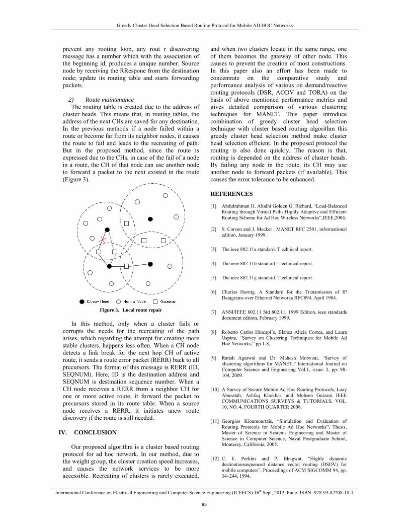
Greedy Cluster Head Selection Based Routing Protocol for Mobile AD HOC Networks
International Conference on Electrical Engineering and Computer Science Engineering (ICEECS) 16th Sept, 2012, Pune- ISBN: 978-93-82208-18-1
85
prevent any rooting loop, any rout r discovering message has a number which with the association of the beginning id, produces a unique number. Source node by receiving the RRespone from the destination node; update its routing table and starts forwarding packets.
2) Route maintenance The routing table is created due to the address of
cluster heads. This means that, in routing tables, the address of the next CHs are saved for any destination. In the previous methods if a node failed within a route or become far from its neighbor nodes, it causes the route to fail and leads to the recreating of path. But in the proposed method, since the route is expressed due to the CHs, in case of the fail of a node in a route, the CH of that node can use another node to forward a packet to the next existed in the route (Figure 3).
Figure 3. Local route repair
In this method, only when a cluster fails or
corrupts the needs for the recreating of the path arises, which regarding the attempt for creating more stable clusters, happens less often. When a CH node detects a link break for the next hop CH of active route, it sends a route error packet (RERR) back to all precursors. The format of this message is RERR (ID, SEQNUM). Here, ID is the destination address and SEQNUM is destination sequence number. When a CH node receives a RERR from a neighbor CH for one or more active route, it forward the packet to precursors stored in its route table. When a source node receives a RERR, it initiates anew route discovery if the route is still needed.
IV. CONCLUSION
Our proposed algorithm is a cluster based routing
protocol for ad hoc network. In our method, due to the weight group, the cluster creation speed increases, and causes the network services to be more accessible. Recreating of clusters is rarely executed,
and when two clusters locate in the same range, one of them becomes the gateway of other node. This causes to prevent the creation of most constructions. In this paper also an effort has been made to concentrate on the comparative study and performance analysis of various on demand/reactive routing protocols (DSR, AODV and TORA) on the basis of above mentioned performance metrics and gives detailed comparison of various clustering techniques for MANET. This paper introduce combination of greedy cluster head selection technique with cluster based routing algorithm this greedy cluster head selection method make cluster head selection efficient. In the proposed protocol the routing is also done quickly. The reason is that, routing is depended on the address of cluster heads. By failing any node in the route, its CH may use another node to forward packets (if available). This causes the error tolerance to be enhanced. REFERENCES
[1] Abdulrahman H. Altalhi Golden G. Richard, “Load-Balanced
Routing through Virtual Paths:Highly Adaptive and Efficient Routing Scheme for Ad Hoc Wireless Networks”,IEEE,2004.
[2] S. Corson and J. Macker . MANET RFC 2501, informational edition, January 1999.
[3] The ieee 802.11a standard. T echnical report.
[4] The ieee 802.11b standard. T echnical report.
[5] The ieee 802.11g standard. T echnical report.
[6] Charles Hornig. A Standard for the Transmission of IP
Datagrams over Ethernet Networks RFC894, April 1984.
[7] ANSI/IEEE 802.11 Std 802.11, 1999 Edition, ieee standards document edition, February 1999.
[8] Roberto Carlos Hincapi´e, Blanca Alicia Correa, and Laura
Ospina, “Survey on Clustering Techniques for Mobile Ad Hoc Networks,” pp.1-8,
[9] Ratish Agarwal and Dr. Mahesh Motwani, “Survey of
clustering algorithms for MANET,” International Journal on Computer Science and Engineering Vol.1, issue: 2, pp. 98-104, 2009.
[10] A Survey of Secure Mobile Ad Hoc Routing Protocols, Loay
Abusalah, Ashfaq Khokhar, and Mohsen Guizani IEEE COMMUNICATIONS SURVEYS & TUTORIALS, VOL. 10, NO. 4, FOURTH QUARTER 2008.
[11] Georgios Kioumourtzis, “Simulation and Evaluation of
Routing Protocols for Mobile Ad Hoc Networks”, Thesis, Master of Science in Systems Engineering and Master of Science in Computer Science, Naval Postgraduate School, Monterey, California, 2005.
[12] C. E. Perkins and P. Bhagwat, “Highly dynamic
destinationsequenced distance vector routing (DSDV) for mobile computers”, Proceedings of ACM SIGCOMM 94, pp. 34–244, 1994.
Greedy Cluster Head Selection Based Routing Protocol for Mobile AD HOC Networks
International Conference on Electrical Engineering and Computer Science Engineering (ICEECS) 16th Sept, 2012, Pune- ISBN: 978-93-82208-18-1
86
[13] A. Kush and S. Taneja, “A Survey of Routing Protocols in Mobile Adhoc Networks”, International Journal of Innovation, Management and Technology, Vol. 1, No. 3, pp 279-285, 2010.
[14] D. B. Johnson, D. A. Maltz, Y.C. Hu, “The Dynamic Source
Routing Protocol for Mobile Ad Hoc Networks (DSR)”, IETF Internet Draft, 2003.
[15] Performance Evaluation of ZRP over AODV and DSR in
Mobile Adhoc Networks Using Qualnet, European Journal of Scientific Research, SreeRangaRaju , Jitendranath Mungara,2010
[16] Comparative Analysis of CBRP, DSR, AODV Routing
Protocol in MANET,Mukesh Kumar, Rahul Rishi ,International Journal on Computer Science and Engineering 2010.
[17] T-F. Shih and H-C. Yen, “Core Location-Aided Cluster-
Based Routing Protocol for Mobile Ad Hoc Networks,” pp223-228, 2006.
[18] S. Muthuramalingam, R. Raja Ram, Kothai Pethaperumal, and V.Karthiga Devi, “A Dynamic Clustering Algorithm for MANETs by modifying Weighted Clustering Algorithm with Mobility Prediction,” International Journal of Computer and Electrical Engineering, Vol. 2, No. 4,pp.709-714, August, 2010.
[19] H-Y. An, Z. Ling, X-C. Lu, and P. Wei, “A Cluster-Based
Multipath Dynamic SourceRouting in MANET”.
[20] P-R. Sheu and C-W. Wang, “A Stable Clustering Algorithm Based on Battery Power for Mobile Ad Hoc Networks,” Tamkang Journal of Science and Engineering, Vol. 9, No 3, pp. 233-242, 2006.
[21] Chongdeuk Lee and Taegwon Jeong, “FRCA: A Fuzzy
Relevance-Based Cluster Head Selection Algorithm for Wireless Mobile Ad-Hoc Sensor Networks”.
[22] R. Pandi Selvam and V. Palanisamy, “Stable and Flexible
Weight based Clustering Algorithm in Mobile Ad hoc Networks,” International Journal of Computer Science and Information Technologies, Vol. 2 (2), pp.824-828, 2011.
[23] T. H. Cormen, C. E. Leiserson, R. L. Rivest, and C. Stein,
“Introduction to Algorithms,” 2nd ed. The MIT Press, September 2001.
[24] V. Chvátal, “A greedy heuristic for the set-covering
problem,” Mathematics of Operations Research, vol. 4, no. 3, pp. 233–235, 1979.
[25] L. Jia, R. Rajaraman, and T.Suel, “An efficient distributed
algorithm for constructing small dominating sets,” Journal of Distributed Computing, vol. 15, no. 4, pp. 193–205, 2002.
[26] T. H. Clausen, C. Dearlove, and J. W. Dean, “Mobile ad hoc
network (manet) neighborhood discovery protocol (nhdp),” IETF Internet-Draft (work inprogress), draft-ietf-manet-nhdp-12, March 2010.
[27] U. Feige, “A threshold of ln n for approximating set cover,”
Journal of the ACM, vol. 45, pp. 314–318, 1998.
International Conference on Electrical Engineering and Computer Science Engineering (ICEECS) 16th Sept, 2012, Pune- ISBN: 978-93-82208-18-1
87
MULTI LAYER SECURITY SYSTEM FOR CONFIDENTIAL DATA FOR E-COMMERCE
1MORE L. D., 2DHAWALE C.A. & 3JADHAV M. B.
1&3Dept. of Computer Sci. & IT, MGM’s College of CS & IT, Nanded Nanded(Maharashtra), India
2Principal, S. P. College, P. R. Patil gr. of educational Institutes, Kathora, Amravati.
Abstract— development in security system has taken place over the last twenty years. Areas to which these disciplines have been applied include business and e-governance, military intelligence, communications, and many others [1]. A comprehensive literature review on confidential information in a business-to-consumer e-commerce internet transaction from three key perspectives of customers, businesses as well government and industry is presented in this paper. The literature review examines how customers perceive their confidential information, how businesses comprehend and provide solutions to protect the confidential information and how the government’s legislation and industry’s self regulation define the confidential information. Significant gaps in identifying confidential information among the three key perspectives are discussed. A framework is proposed for identifying confidential information in a B2C ecommerce Internet transaction by integrating the three key perspectives. The framework could be used by customers and businesses to identify confidential information in a consistent way. This paper is concluded by introducing possible future research technique Keywords- Soft computing, feed forward neural networks, Classification, Segmentation, Handwritten character recognition, on-line handwritten signature verification, iris recognition, biometric identification, pattern recognition, time sequence. INTRODUCTION
Security is one of the most important issues in E-commerce. Usually for business or in banking networks we can communicate to each other through networks, as most of them are connected for transferring information, but businesses are competitors and they don't disclose their sensitive information. Today the users or programmers (Hackers or abusers!) are very smart and intelligent, and they can attack in several forms and so the defense level has to be sufficiently strong and comprehensive. In this paper we discuss the security of confidential data used in e-commerce. This paper’s primary focus is on the techniques commonly referred in security system for confidential data through internet,’’ which are attachments to documents used to verify or authenticate a ‘‘signer’’ and the document signed. Combined with certificates issued by trusted third parties and enhanced by biometric authentication tools like thumb impression, face recognition, and iris scan. Each security technique have five fundamental performance factors are used to compare these: failure to authenticate, false acceptance rate, false rejection rate, ease of use, and highly secure as shown in following fig. Public Key Infrastructure (PKI) : PKI is an enabler of trust in e-Governance transaction by way of : • Authentication (Knowing who has send the message / document )
Fig. for An Authentication system Each security technique have five fundamental performance factors are used to compare these: failure to authenticate, false acceptance rate, false rejection rate, ease of use, and highly secure. Usually we know the security techniques as follows:
I. Traditional Password : Usually we use this authentication. This is the simplest and oldest way of authenticating a computer system user and is the most widely used authentication technology today. It is easy to use on any system. However, it is generally viewed as a relatively low-security option, due to the frequency of forgotten or co-opted passwords. In addition, there are well-structured and effective hacking techniques for password log-ons.
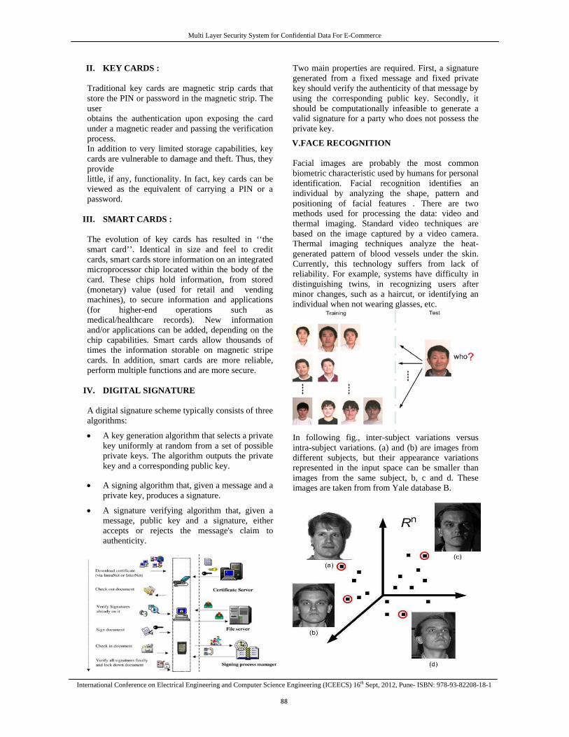
Multi Layer Security System for Confidential Data For E-Commerce
International Conference on Electrical Engineering and Computer Science Engineering (ICEECS) 16th Sept, 2012, Pune- ISBN: 978-93-82208-18-1
88
II. KEY CARDS : Traditional key cards are magnetic strip cards that store the PIN or password in the magnetic strip. The user obtains the authentication upon exposing the card under a magnetic reader and passing the verification process. In addition to very limited storage capabilities, key cards are vulnerable to damage and theft. Thus, they provide little, if any, functionality. In fact, key cards can be viewed as the equivalent of carrying a PIN or a password.
III. SMART CARDS : The evolution of key cards has resulted in ‘‘the smart card’’. Identical in size and feel to credit cards, smart cards store information on an integrated microprocessor chip located within the body of the card. These chips hold information, from stored (monetary) value (used for retail and vending machines), to secure information and applications (for higher-end operations such as medical/healthcare records). New information and/or applications can be added, depending on the chip capabilities. Smart cards allow thousands of times the information storable on magnetic stripe cards. In addition, smart cards are more reliable, perform multiple functions and are more secure.
IV. DIGITAL SIGNATURE
A digital signature scheme typically consists of three algorithms:
• A key generation algorithm that selects a private key uniformly at random from a set of possible private keys. The algorithm outputs the private key and a corresponding public key.
• A signing algorithm that, given a message and a private key, produces a signature.
• A signature verifying algorithm that, given a message, public key and a signature, either accepts or rejects the message's claim to authenticity.
Two main properties are required. First, a signature generated from a fixed message and fixed private key should verify the authenticity of that message by using the corresponding public key. Secondly, it should be computationally infeasible to generate a valid signature for a party who does not possess the private key.
V.FACE RECOGNITION Facial images are probably the most common biometric characteristic used by humans for personal identification. Facial recognition identifies an individual by analyzing the shape, pattern and positioning of facial features . There are two methods used for processing the data: video and thermal imaging. Standard video techniques are based on the image captured by a video camera. Thermal imaging techniques analyze the heat-generated pattern of blood vessels under the skin. Currently, this technology suffers from lack of reliability. For example, systems have difficulty in distinguishing twins, in recognizing users after minor changes, such as a haircut, or identifying an individual when not wearing glasses, etc.
In following fig., inter-subject variations versus intra-subject variations. (a) and (b) are images from different subjects, but their appearance variations represented in the input space can be smaller than images from the same subject, b, c and d. These images are taken from from Yale database B.
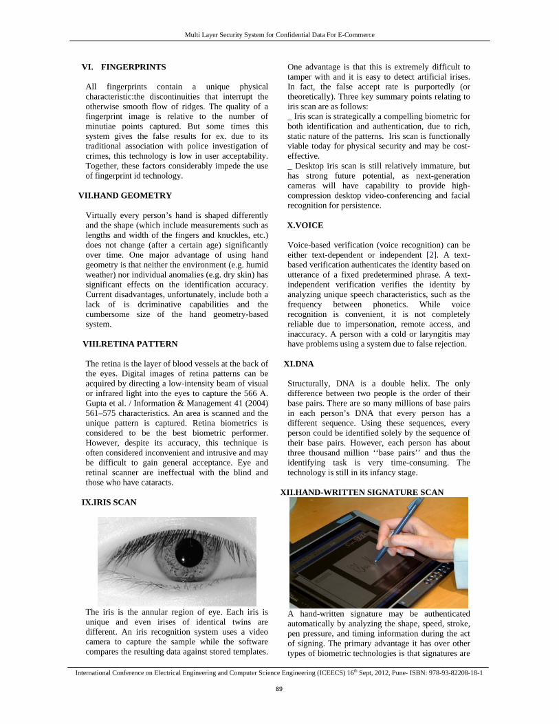
Multi Layer Security System for Confidential Data For E-Commerce
International Conference on Electrical Engineering and Computer Science Engineering (ICEECS) 16th Sept, 2012, Pune- ISBN: 978-93-82208-18-1
89
VI. FINGERPRINTS All fingerprints contain a unique physical characteristic:the discontinuities that interrupt the otherwise smooth flow of ridges. The quality of a fingerprint image is relative to the number of minutiae points captured. But some times this system gives the false results for ex. due to its traditional association with police investigation of crimes, this technology is low in user acceptability. Together, these factors considerably impede the use of fingerprint id technology.
VII.HAND GEOMETRY
Virtually every person’s hand is shaped differently and the shape (which include measurements such as lengths and width of the fingers and knuckles, etc.) does not change (after a certain age) significantly over time. One major advantage of using hand geometry is that neither the environment (e.g. humid weather) nor individual anomalies (e.g. dry skin) has significant effects on the identification accuracy. Current disadvantages, unfortunately, include both a lack of is dcriminative capabilities and the cumbersome size of the hand geometry-based system.
VIII.RETINA PATTERN
The retina is the layer of blood vessels at the back of the eyes. Digital images of retina patterns can be acquired by directing a low-intensity beam of visual or infrared light into the eyes to capture the 566 A. Gupta et al. / Information & Management 41 (2004) 561–575 characteristics. An area is scanned and the unique pattern is captured. Retina biometrics is considered to be the best biometric performer. However, despite its accuracy, this technique is often considered inconvenient and intrusive and may be difficult to gain general acceptance. Eye and retinal scanner are ineffectual with the blind and those who have cataracts.
IX.IRIS SCAN
The iris is the annular region of eye. Each iris is unique and even irises of identical twins are different. An iris recognition system uses a video camera to capture the sample while the software compares the resulting data against stored templates.
One advantage is that this is extremely difficult to tamper with and it is easy to detect artificial irises. In fact, the false accept rate is purportedly (or theoretically). Three key summary points relating to iris scan are as follows: _ Iris scan is strategically a compelling biometric for both identification and authentication, due to rich, static nature of the patterns. Iris scan is functionally viable today for physical security and may be cost-effective. _ Desktop iris scan is still relatively immature, but has strong future potential, as next-generation cameras will have capability to provide high-compression desktop video-conferencing and facial recognition for persistence. X.VOICE
Voice-based verification (voice recognition) can be either text-dependent or independent [2]. A text-based verification authenticates the identity based on utterance of a fixed predetermined phrase. A text-independent verification verifies the identity by analyzing unique speech characteristics, such as the frequency between phonetics. While voice recognition is convenient, it is not completely reliable due to impersonation, remote access, and inaccuracy. A person with a cold or laryngitis may have problems using a system due to false rejection.
XI.DNA
Structurally, DNA is a double helix. The only difference between two people is the order of their base pairs. There are so many millions of base pairs in each person’s DNA that every person has a different sequence. Using these sequences, every person could be identified solely by the sequence of their base pairs. However, each person has about three thousand million ‘‘base pairs’’ and thus the identifying task is very time-consuming. The technology is still in its infancy stage.
XII.HAND-WRITTEN SIGNATURE SCAN
A hand-written signature may be authenticated automatically by analyzing the shape, speed, stroke, pen pressure, and timing information during the act of signing. The primary advantage it has over other types of biometric technologies is that signatures are
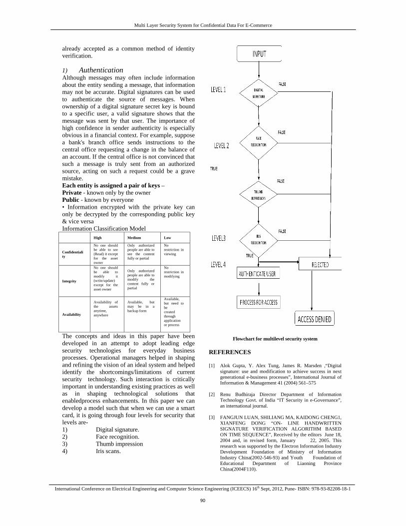
Multi Layer Security System for Confidential Data For E-Commerce
International Conference on Electrical Engineering and Computer Science Engineering (ICEECS) 16th Sept, 2012, Pune- ISBN: 978-93-82208-18-1
90
already accepted as a common method of identity verification. 1) Authentication Although messages may often include information about the entity sending a message, that information may not be accurate. Digital signatures can be used to authenticate the source of messages. When ownership of a digital signature secret key is bound to a specific user, a valid signature shows that the message was sent by that user. The importance of high confidence in sender authenticity is especially obvious in a financial context. For example, suppose a bank's branch office sends instructions to the central office requesting a change in the balance of an account. If the central office is not convinced that such a message is truly sent from an authorized source, acting on such a request could be a grave mistake. Each entity is assigned a pair of keys – Private - known only by the owner Public - known by everyone • Information encrypted with the private key can only be decrypted by the corresponding public key & vice versa Information Classification Model High Medium Low
Confidentiality
No one should be able to see (Read) it except for the asset owner
Only authorized people are able to see the content fully or partial
No restriction in viewing
Integrity
No one should be able to modify it (write/update) except for the asset owner
Only authorized people are able to modify the content fully or partial
No restriction in modifying
Availability
Availability of the assets anytime, anywhere
Available, but may be in a backup form
Available, but need to be created through application or process
The concepts and ideas in this paper have been developed in an attempt to adopt leading edge security technologies for everyday business processes. Operational managers helped in shaping and refining the vision of an ideal system and helped identify the shortcomings/limitations of current security technology. Such interaction is critically important in understanding existing practices as well as in shaping technological solutions that enabledprocess enhancements. In this paper we can develop a model such that when we can use a smart card, it is going through four levels for security that levels are- 1) Digital signature. 2) Face recognition. 3) Thumb impression 4) Iris scans.
Flowchart for multilevel security system
REFERENCES
[1] Alok Gupta, Y. Alex Tung, James R. Marsden ,“Digital
signature: use and modification to achieve success in next generational e-business processes”, International Journal of Information & Management 41 (2004) 561–575
[2] Renu Budhiraja Director Department of Information
Technology Govt. of India “IT Security in e-Governance”, an international journal.
[3] FANGJUN LUAN, SHILIANG MA, KAIDONG CHENG1,
XIANFENG DONG “ON- LINE HANDWRITTEN SIGNATURE VERIFICATION ALGORITHM BASED ON TIME SEQUENCE”, Received by the editors June 18, 2004 and, in revised form, January 22, 2005. This research was supported by the Electron Information Industry Development Foundation of Ministry of Information Industry China(2002-546-93) and Youth Foundation of Educational Department of Liaoning Province China(2004F110).
Multi Layer Security System for Confidential Data For E-Commerce
International Conference on Electrical Engineering and Computer Science Engineering (ICEECS) 16th Sept, 2012, Pune- ISBN: 978-93-82208-18-1
91
[4] Seyyed Mohammad Reza Farshchi, Fariba Gharib, Reza Ziyaee, “Study of Security Issues on Traditional and New Generation of E-commerce Model”2011 International conference on Software and Computer Applications IPCSIT vol.9 (2011) © (2011) IACSIT Press, Singapore
[5] K.Elumalai, M.Kannan “Multimodal Authentication For
High End Security” ISSN : 0975-3397 Vol. 3 No. 2 Feb 2011
[6] Wikipedia, the free encyclopedia “Automated teller
machine” [7] Prof G.Ramaswamy, Vuda Sreenivasarao, Dr.P.Ramesh,
D.Ravi Kiran, “A Novel Approach for Human Identification through Fingerprints” International Journal of Computer Applications (0975 – 8887) Volume 4 – No.3, July 2010
[8] T. A. Albert, S. Ganesan “Applications of Principal
Component Analysis in Multimodal Biometric Fusion System” European Journal of Scientific Research ISSN 1450-216X Vol.67 No.2 (2012), pp. 248-259© EuroJournals Publishing, Inc. 2012
[9] John Daugman OBE,” Iris recognition border-crossing
system in the UAE” , Reproduced from International Airport Review, Issue 2, 2004.
o Review, Issue 2, 2004 [10]https://www.google.co.in/search?q=images+of+thumb+impre
ssion+biometric+machine&hl=en&prmd=imvns&tbm=isch&tbo=u&source=univ&sa=X&ei=7DfMT- bbI4WqrAe16smyDg&ved=0CG8QsAQ&biw=1366&bih=587#hl=en&tbm=isch&sa=1&q=images+of+online+handwritten+signature+biometric+machine&oq=images+of+online+handwritten+signature+biometric+machine&aq=f&aqi=&aql=&gs_l=img.3...23759.43041.0.45115.37.35.2.0.0.1.453.5537.2-15j4j1.20.0...0.0.90vWytbozIM&bav=on.2, or.r_gc.r_pw.r_qf.,cf.osb&fp=cd57c5b5349a8501&biw=1366&bih=587
[11] D. Gayathri, R. Uma Rani, “A Prototype for Secure Web
Access Model using multimodal Biometric System based on Fingerprint and Face Recognition”, D. Gayathri et al, / (IJCSIT) International Journal of Computer Science and Information Technologies, Vol. 3 (3) , 2012,3985-3988
[12] ARPITA PATRA, “DEVELOPMENT OF EFFICIENT
METHODS FOR FACE COGNITION AND MULTIMODAL BIOMETRY”, June 2006
[13] Eugen Lupu, Petre G. Pop, Marius N. Roman, “A survey of
multimodal biometric systems”, 1st International Conference on Advancements of Medicine and Health Care through Technology, MediTech2007, 27-29th September, 2007, Cluj-Napoca, ROMANIA
[14] K.Sasidhar, Vijaya L Kakulapati, Kolikipogu Ramakrishna
& K.KailasaRao,”MULTIMODAL BIOMETRIC SYSTEMS – STUDY TO IMPROVE ACCURACY AND PERFORMANCE”, International Journal of Computer Science & Engineering Survey (IJCSES) Vol.1, No.2, November 2010.
[15] Imuetinyan Bernadette Iyawe,” Towards Implementing An
Efficient Biometric Authentication Framework For Nigeria Customer Banking Systems”, The Information Manager Vol.10 (1 & 2) 2010.
[16] Libor Masek, “ Recognition of Human Iris Patterns for
Biometric Identification”, This report is submitted as partial fulfilment of the requirements for the Bachelor of Engineering degree of the School of Computer Science and Software Engineering, The University of Western Australia, 2003.
[17] Prof G.Ramaswamy, Vuda Sreenivasarao, Dr.P.Ramesh D.Ravi Kiran,” A Novel approach for Human Identification through Fingerprints” International Journal of computer Applications (0975 – 8887), Volume 4 – No.3, July 2010.
[18] Libor Masek,” Recognition of Human Iris Patterns for
Biometric Identification”, This report is submitted as partial fulfilment of the requirements for the Bachelor of Engineering degree of the School of Computer Science and Software Engineering, The University of Western Australia, 2003.
[19] Yale University face database, <http://cvc.yale.edu/projects/yalefaces/yalefaces.html>.
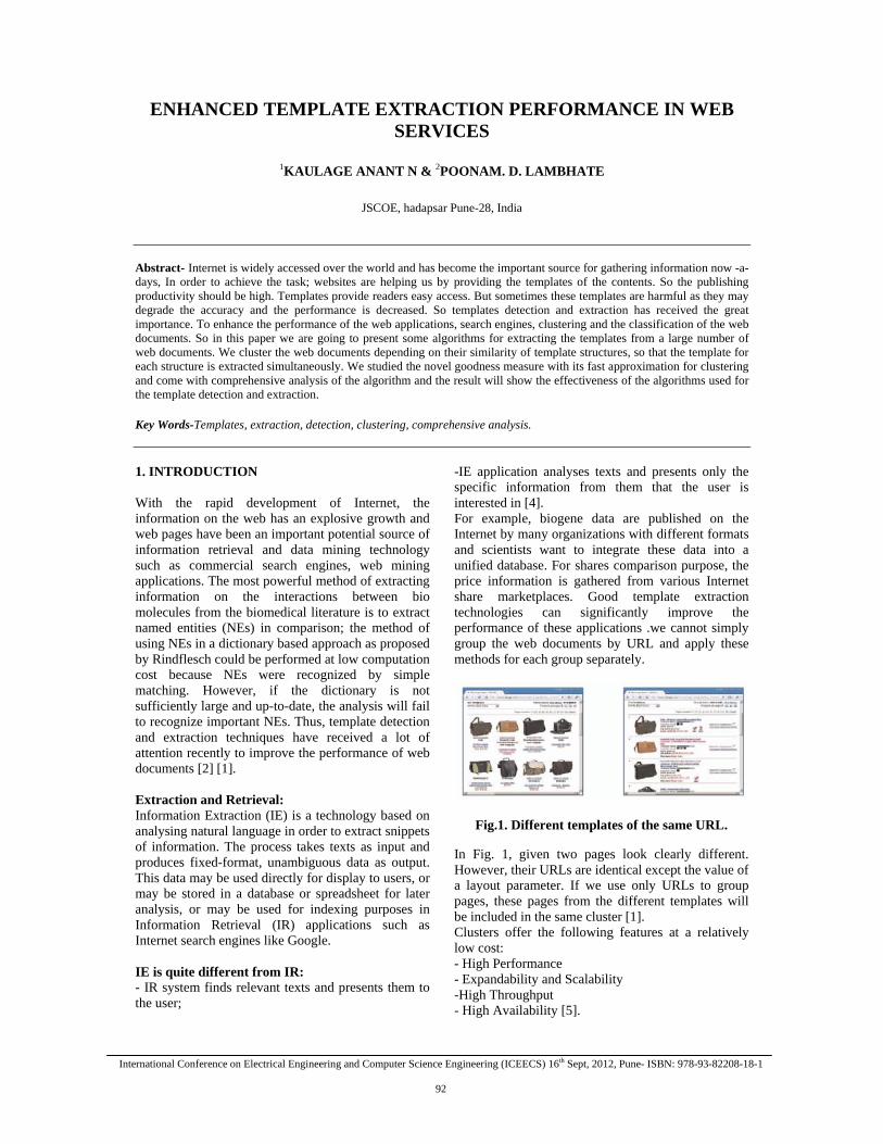
International Conference on Electrical Engineering and Computer Science Engineering (ICEECS) 16th Sept, 2012, Pune- ISBN: 978-93-82208-18-1
92
ENHANCED TEMPLATE EXTRACTION PERFORMANCE IN WEB SERVICES
1KAULAGE ANANT N & 2POONAM. D. LAMBHATE
JSCOE, hadapsar Pune-28, India
Abstract- Internet is widely accessed over the world and has become the important source for gathering information now -a-days, In order to achieve the task; websites are helping us by providing the templates of the contents. So the publishing productivity should be high. Templates provide readers easy access. But sometimes these templates are harmful as they may degrade the accuracy and the performance is decreased. So templates detection and extraction has received the great importance. To enhance the performance of the web applications, search engines, clustering and the classification of the web documents. So in this paper we are going to present some algorithms for extracting the templates from a large number of web documents. We cluster the web documents depending on their similarity of template structures, so that the template for each structure is extracted simultaneously. We studied the novel goodness measure with its fast approximation for clustering and come with comprehensive analysis of the algorithm and the result will show the effectiveness of the algorithms used for the template detection and extraction. Key Words-Templates, extraction, detection, clustering, comprehensive analysis. 1. INTRODUCTION With the rapid development of Internet, the information on the web has an explosive growth and web pages have been an important potential source of information retrieval and data mining technology such as commercial search engines, web mining applications. The most powerful method of extracting information on the interactions between bio molecules from the biomedical literature is to extract named entities (NEs) in comparison; the method of using NEs in a dictionary based approach as proposed by Rindflesch could be performed at low computation cost because NEs were recognized by simple matching. However, if the dictionary is not sufficiently large and up-to-date, the analysis will fail to recognize important NEs. Thus, template detection and extraction techniques have received a lot of attention recently to improve the performance of web documents [2] [1]. Extraction and Retrieval: Information Extraction (IE) is a technology based on analysing natural language in order to extract snippets of information. The process takes texts as input and produces fixed-format, unambiguous data as output. This data may be used directly for display to users, or may be stored in a database or spreadsheet for later analysis, or may be used for indexing purposes in Information Retrieval (IR) applications such as Internet search engines like Google. IE is quite different from IR: - IR system finds relevant texts and presents them to the user;
-IE application analyses texts and presents only the specific information from them that the user is interested in [4]. For example, biogene data are published on the Internet by many organizations with different formats and scientists want to integrate these data into a unified database. For shares comparison purpose, the price information is gathered from various Internet share marketplaces. Good template extraction technologies can significantly improve the performance of these applications .we cannot simply group the web documents by URL and apply these methods for each group separately.
Fig.1. Different templates of the same URL.
In Fig. 1, given two pages look clearly different. However, their URLs are identical except the value of a layout parameter. If we use only URLs to group pages, these pages from the different templates will be included in the same cluster [1]. Clusters offer the following features at a relatively low cost: - High Performance - Expandability and Scalability -High Throughput - High Availability [5].
Enhanced Template Extraction Performance in Web Services
International Conference on Electrical Engineering and Computer Science Engineering (ICEECS) 16th Sept, 2012, Pune- ISBN: 978-93-82208-18-1
93
To over the limitations of the classification of web documents based on URLs, we have to bring the similar types of documents in a same cluster, hence how much good quality of cluster is, that much extraction of web document is easily and efficient. Web document extraction means, in fact we are, extracting the HTML documents and is a little typical process. Since an HTML document can be naturally represented with a Document Object Model (DOM) tree, web documents are considered as trees. However, clustering is very expensive with Tree-related distance measures. In advance we don’t know coming wed document and how many clusters we need to issue to the user. Empirically they have suggested that 80% threshold should match, but it doesn’t work all the time. So, in this paper we have studied the proposed algorithms that will help to represent a web document and a template as a set of paths in a DOM tree. Paths are sufficient to express tree structures and useful to be queried. Our aim is to handle all the queries given by the user and survive with the scalability and efficiency of template detection and extraction. We employ Rissanen’s Minimum Description Length (MDL). The MDL cost is the number of bits required to describe data with a model. Since a large number of web documents are massively crawled from the web, the scalability of template extraction algorithms is very important to be used practically. Thus, we extend MinHash technique to estimate the MDL cost quickly, so that a large number of documents can be processed [1] [2]. 2. RELATED WORK
The template extraction problem can be categorized into two broad areas. The first area is the site-level template detection where the template is decided based on several pages from the same site. We consider the MDL principle as well as the frequencies to decide templates from heterogeneous documents. In the problem of the template extraction from heterogeneous document, how to partition given documents into homogeneous subsets is important. Reis et al. used a restricted tree-edit distance to cluster documents and, it is assumed that labeled training data are given for clustering. Additionally we need to control the length of the sentences in the cluster. However, the tree edit distance is expensive and it is not easy to select good training pages. The motivation of our work is to extract text from web pages and remove the irrelevant template. We take advantage of page tag tree structure to find the template, therefore identifying template in HTML pages is more straightforward than frequent term set clustering problem. Corresponding to different category of products, slightly different template is applied. Thus there can be more than one template from a web site. Assuming pages that look similar belong to the same template; we cluster html pages
and then identify elements of web pages that were generated by a common template. The other area is the page-level template detection where the template is computed within a single document. [1] [2]. 3. OUR APPROACH
3.1. HTML Documents and Document Object Model: The DOM defines a standard for accessing documents, like HTML and XML. The DOM presents an HTML document as a tree structure. <html> <html> <html>
<body> <body> <body>
<h1>yahoo</h1> <h1>web</h1> <h1>google</h1>
<br> <br> <br>
</body> </body> </body>
</html> </html> </html>
(i) (ii) (iii)
Fig. 2. Simple web documents. (i) Document d1. (ii) Document
d2. (iii) Document d3.
The DOM tree of a simple HTML document d2 in Fig. 2(b) is given in Fig. 3.For a node in a DOM tree, we denote the path of the node by listing nodes from the root to the node in which we use “\” as a delimiter between nodes. For example, in the DOM tree of d2 in Fig. 3, the path of a node “World” is “Document\<html>\<body>\<h1>\<Web>.”
Fig.3. DOM Tree of d2 in Fig. 2. 3.2. Minimum Description Length Principle: In order to manage the unknown number of clusters and to select good partitioning from all possible partitions of HTML documents, we employ Rissanen’s MDL principle. The MDL principle states that the best model inferred from a given set of data is the one which minimizes the sum of 1) the length of the model, in bits, and 2) the length of encoding of
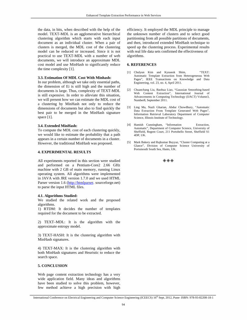
Enhanced Template Extraction Performance in Web Services
International Conference on Electrical Engineering and Computer Science Engineering (ICEECS) 16th Sept, 2012, Pune- ISBN: 978-93-82208-18-1
94
the data, in bits, when described with the help of the model. TEXT-MDL is an agglomerative hierarchical clustering algorithm which starts with each input document as an individual cluster. When a pair of clusters is merged, the MDL cost of the clustering model can be reduced or increased. Since it is not practical to use TEXT-MDL with a number of web documents, we will introduce an approximate MDL cost model and use MinHash to significantly reduce the time complexity [1]. 3.3. Estimation Of MDL Cost With Minhash: In our problem, although we take only essential paths, the dimension of Ei is still high and the number of documents is large. Thus, complexity of TEXT-MDL is still expensive. In order to alleviate this situation, we will present how we can estimate the MDL cost of a clustering by MinHash not only to reduce the dimensions of documents but also to find quickly the best pair to be merged in the MinHash signature space [1]. 3.4. Extended MinHash: To compute the MDL cost of each clustering quickly, we would like to estimate the probability that a path appears in a certain number of documents in a cluster. However, the traditional MinHash was proposed. 4. EXPERIMENTAL RESULTS All experiments reported in this section were studied and performed on a Pentium-Core2 2.66 GHz machine with 2 GB of main memory, running Linux operating system. All algorithms were implemented in JAVA with JRE version 1.7.0 and we used HTML Parser version 1.6 (http://htmlparser. sourceforge.net) to parse the input HTML files. 4.1. Algorithms Studied: We studied the related work and the proposed algorithms. 1) RTDM: It decides the number of templates required for the document to be extracted.
2) TEXT–MDL: It is the algorithm with the approximate entropy model. 3) TEXT-HASH: It is the clustering algorithm with MinHash signatures. 4) TEXT-MAX: It is the clustering algorithm with both MinHash signatures and Heuristic to reduce the search space. 5. CONCLUSION Web page content extraction technology has a very wide application field. Many ideas and algorithms have been studied to solve this problem, however, few method achieve a high precision with high
efficiency. It employed the MDL principle to manage the unknown number of clusters and to select good partitioning from all possible partitions of documents, and then, introduced extended MinHash technique to speed up the clustering process. Experimental results with real life data sets confirmed the effectiveness of algorithms. 6. REFERENCES
[1] Chulyun Kim and Kyuseok Shim, “TEXT: Automatic Template Extraction from Heterogeneous Web Pages”, IEEE Transactions on Knowledge and Data Engineering, vol. 23, no. 4, April 2011.
[2] Chuanchang Liu, Baohua Liao, “Gaussian Smoothing-based
Web Content Extraction”, International Journal of Advancements in Computing Technology (IJACT) Volume3, Number8, September 2011.
[3] Ling Ma, Nazli Gharian, Abdur Chowdhury, “Automatic
Data Extraction From Template Generated Web Pages”, Information Retrieval Laboratory Department of Computer Science, Illinois Institute of Technology.
[4] Hamish Cunningham, “Information Extraction,
Automatic”, Department of Computer Science, University of Sheffield, Regent Court, 211 Portobello Street, Sheffield S1 4DP, UK.
[5] Mark Bakery and Rajkumar Buyyaz, “Cluster Computing at a
Glance”, Division of Computer Science University of Portsmouth South Sea, Hants, UK.
International Conference on Electrical Engineering and Computer Science Engineering (ICEECS) 16th Sept, 2012, Pune- ISBN: 978-93-82208-18-1
95
APPLICATION OF SWARM INTELLIGENCE ALGORITHMS FOR SOLVING OPTIMIZATION PROBLEMS
1CHAITRALI P. CHAUDHARI & 2D. N. CHAUDHARI
1Department of Computer, Lokmanya Tilak college of Engg., Koperkhairane, Navi Mumbai, India.
2Department of Computer, Jawaharlal Darda, Institute of Engineering and Technology, Yavatmal, India Abstract- Swarm Intelligence (SI) indicates a recent computational and behavioral metaphor for solving distributed problems that originally took its inspiration from the biological examples that are provided by social insects and by swarming, flocking, herding behavior in vertebrates. The characteristic of real ant colonies is exploited in Ant System (AS) algorithm to solve, discrete optimization problems. The Particle Swarm Optimization (PSO) technique modeled on the social behaviors observed in animals or insects. Both the AS and PSO algorithm are the data clustering algorithms by implementing swarm behavior. In this paper we present the overview that AS is more applicable for problems where source and destination are predefined and specific. We also summarize that PSO is a clustering algorithm in the areas of mutliobjective, dynamic optimization and constraint handling. Keywords: Swarm Intelligence, Ant System Algorithm, Particle Swarm Optimization.
I. INTRODUCTION
Ant System algorithm models a problem as the search problem for the minimum cost path in a graph. Each ant has a rather simple behavior capable of finding relatively costlier paths. Cheaper paths are found as the emergent result of global cooperation among ants in the colony. Whereas PSO simulates the behaviors of bird flocking. AS is more applicable for problems that require crisp results and PSO is applicable for problems that are fuzzy is nature. According to Bonabeau, Dorigo and Theraulaz, 1999, SI is any attempt to design algorithms or distributed problem solving devices inspired by the collective behavior of social insects or other animal societies.
Swarm Intelligence is interesting for IT because there are analogies in IT and social insects. These are distributed system of interacting autonomous agents to achieve goals like performance optimization and robustness, self-organized control and cooperation (decentralized), division of labor, distributed task allocation and indirect interactions. Biologically inspired computing requires identification of analogies, computer modeling of biological mechanisms, and adaptation of biological mechanisms for IT applications.
II. PRINCIPLES IN SWARM INTELLIGENCE
In a Swarm Intelligence design we allocate computing resources to a number of relatively simple units i.e. swarm which has no centralized control and the units interact in a relatively simple and a localized way to get some useful global behavior.
A. Principal of Self-Organization
This principal of Swarm Intelligence is based on activity amplification by positive feedback, activity balancing by negative feedback, amplification of random fluctuations and multiple interactions. . ‘Self-organization is a set of dynamic mechanisms whereby structures appear at the global level of a system from interactions of its lower-level components.’ (Bonabeau et al, in Swarm Intelligence, 1999). Characteristics of self Organized Systems are structure emerging from a homogeneous startup state, multistability - coexistence of many stable states, state transitions with a dramatic change of the system behavior.
i) Process of Self Organization
Self organization consists of set of rules
specifying the interactions among the system’s constituent units which execute on the basis of the purely local information, without reference to the global pattern which is an emergent property of the system rather than the property imposed upon the system by an external ordering influence . Various types of Self organization include Point to point, Broadcast and Indirect. In Indirect Self Organization two individuals interact indirectly when one of them modifies environment and the other responds to the new environment at a later time. This is called Stigmergy (pheromone laying/following).
B. Principal of Stigmergy
Stigma (sting) + ergon (work) = ‘stimulation
by work’. It is indirect communication via interaction with environment. It is based on work as behavioral
Application of Swarm Intelligence Algorithms for Solving Optimization Problems
International Conference on Electrical Engineering and Computer Science Engineering (ICEECS) 16th Sept, 2012, Pune- ISBN: 978-93-82208-18-1
96
response to the environmental state, an environment that serves as a work state memory, work that does not depend on specific agents.
Stigmergy has led to Ant algorithms and specially Ant Colony Algorithms (ACO). Broadcast like communication is related to schooling and flocking behaviors that have inspired Particle Swarm Optimization.
i) Characteristics of Stigmergy
Indirect agent interaction, modification of
the environment which serves as external memory, work which can be continued by any individual, the same and simple behavioral rules which can create different designs according to the environmental state
III. THE ANT COLONY OPTIMIZATION
Ants are ‘grand masters’ in search and exploitation. Control is fully distributed among a number of individuals, communications among the individuals happen in the localized way, system level behaviors appears to transcend the behavioral repertoire of the single individual, the overall response of the system is quite robust and adaptive with respect to the changes in the environment.
Some interesting collective behaviors include Nest building and maintenance, division of labor and adaptive task allocation, discovery of shortest path between nest and food, clustering and sorting(e.g. dead bodies and eggs), structure formation(e.g. deal with obstacles), recruitment for foraging (e.g. tandem, group, mass), cooperative transport(e.g. food), regulation of 1degree Celsius range, cooperation in carrying large items, forming bridges, emigration of a colony, preferentially exploiting the richest food source available. It makes the use of Visual landmarks (use of memory and learning, encounters with colony mates), chemical landmark (pheromone), compass-based (cataglyphis desert ant makes the use of light polarization), dead-reckoning, path integration (calculation of the home vector), correlated random walk.
Ants lay pheromone trails in mathematical form on the graph edges and choose their path with respect to probabilities that depends on pheromone trails. These pheromone trails progressively decrease by evaporation. Artificial ants live in a discrete world of a graph and their move consists of transitions from nodes to nodes. Pheromone placed on the edges like a distributed long term memory. The memory instead of being stored locally within individual ants, remains distributed on the edges of the graph. This provides a means of communication among the ants i.e. Stigmergy.
Pheromone trails are updated only after having constructed a complete path and not during the walk, and the amount of pheromone deposited is usually a function of a quality of the path. Finally the probability for an artificial ant to choose an edge, not only depends on pheromone deposited on that edge in the past but also on some problem dependent local heuristic functions.
A. The Ant System Ants are agents that choose next town to go
with probability that is a function of distance of town and amount of pheromone on edge. Legal tours are ‘’forced’’ by use of tabu list. An ant can only visit a town once. Each ant has its own “tour memory”. When the tour is complete, a pheromone is laid down on the trail. Iteration is defined to be m moves –one by each ant. Tour completes in one move i.e. n iterations.
Tij = pheromone intensity on edge Bi (t) = #ants at ith town at t
(1- e) = evaporation rate When tour complete: Tij (t + n) = eTij(t) + δ Tij δ Tij = Σ δ Tijk
δ Tijk =on route else 0 Transition probability:
Pijk (t) = [Tij (t)] α [1 / d ij] β / Nk Nk = Σk in ( S – Tabu ( k ) ) [Tij( t )] α [ 1/ d ij]
β
α and β are control parameters that determine the sensitivity of the algorithm to distance and pheromone.
B. Algorithm 1: Ant System Algorithm for TSP Problem
1. Initialize Set t: = 0 Set NC: = 0 {number of cycles} For every edge ( i, j) set an initial value Tij( t ) for trail intensity and δ Tij = 0. Place m ants on the n nodes.
2. Set s := 1 { tabu list index} For k: = 1 to m do Place starting town of the k th ant in tabu k (S).
3. Repeat until tabu list full Set S: = S + 1 For K: = 1 to m do Choose the town j to move to with probability Pij
k (t) Move the kth ant to the town j. Insert town j in tabu k (S).
4. For K : = 1 to m do Compute the length Lk of the tour described by tabu k (S). Update the shortest tour found.
For every edge (i, j)
Application of Swarm Intelligence Algorithms for Solving Optimization Problems
International Conference on Electrical Engineering and Computer Science Engineering (ICEECS) 16th Sept, 2012, Pune- ISBN: 978-93-82208-18-1
97
For K: = 1 to m do δ Tijk = δ Tij + δ Tijk
5. For every edge ( i, j ) , compute Tij ( t + n ) = e Tij ( t ) + Tij Set t: = t + n Set NC: = NC +1
For all edges ( i, j ), Set Tij = 0 6. If NC < NCmax, empty tabu lists, go to 2
Else Print shortest tour; stop. IV. THE PARTICLE SWARM OPTIMIZATION
(PSO)
It is one of the latest algorithms inspired from the nature, introduced in the mid 1990s and since then, it has been utilized as an optimization tool in various applications, ranging from biological and medical applications to computer graphics and music composition.
Consider the scenario in which a group of birds are randomly searching food in an area. There is only one piece of food in the area being searched. All birds do not know where the food is. But they know how far the food is in each iteration. So what's the best strategy to find the food? The effective one is to follow the bird which is nearest to the food. PSO learned from the scenario and used it to solve the optimization problems. In PSO, each single solution is a "bird" in the search space. We call it "particle". All of particles have fitness values which are evaluated by the fitness function to be optimized, and have velocities which direct the flying of the particles. The particles fly through the problem space by following the current optimum particles. PSO is initialized with a group of random particles (solutions) and then searches for optima by updating generations. In every iteration, each particle is updated by following two "best" values. The first one is the best solution (fitness) it has achieved so far. (The fitness value is also stored.) This value is called pbest. Another "best" value that is tracked by the particle swarm optimizer is the best value obtained so far by any particle in the population. This best value is a global best and called gbest. When a particle takes part of the population as its topological neighbors, the best value is a local best and is called lbest.
A. Algorithm 2 Particle swarm optimization
algorithm
PSO Algorithm input: Randomly initialized position and velocity of the particles: Xi (0) and Vi (0) Output: Position of the approximate global optima
Begin While terminating condition is not reached do Begin
for i = 1 to number of particles Evaluate the fitness: = f (Xi (t)); Update P(t) and g(t);
Adapt velocity of the particle Update the position of the
particle; increase;
end while; end;
PSO does not require any gradient information of the function to be optimized. It uses only primitive mathematical operators and is primitively very simple. PSO is in principal a multiagent parallel search technique. Particles are conceptual entities which fly through the multi-dimensional search space. At particular instance each particle has a position and a velocity. The position vector of the particle with respect to the origin of the search space represents the trial solution of the search problem. At the beginning the population of the particles is initialized with random positions marked by vectors Xi and velocities Vi. The population of such particles is called Swarm S. A neighborhood relation N is defined in the Swarm. N determines for any two parties Zi and Zj whether they are neighbors or not. Thus for any particle Z, a neighborhood can be assigned as N (Z), containing all the neighbor of that particle. Different neighborhood topologies and their effect on the swarm performance is discussed in .In the basic PSO, each particle P has two state variables.
1. It’s current position Xi(t) 2. It’s current velocity Vi(t)
And also a small memory comprising, 1. It’s previous best position Pi (t), i.e. personal
best experience. 2. The best P (t), i.e. the best position found so
far in the neighborhood of the particle. The personal best experience P (t) of the particle
is referred as the cognitive part and g (t) is interpreted as the social term which represents how an individual particle is influenced by the other members of the society. After finding the two best values, the particle updates its velocity and positions with following equation (a) and (b). v[] = v[] + c1 * rand() * (pbest[] - present[]) + c2 * rand() * (gbest[] - present[])……..(a) present[] = present[] + v[]………. (b) v[] is the particle velocity, present[] is the current particle (solution). pbest [] and gbest[] are defined as stated before. rand () is a random number between (0, 1). c1, c2 are learning factors. Usually c1 = c2 = 2.
Application of Swarm Intelligence Algorithms for Solving Optimization Problems
International Conference on Electrical Engineering and Computer Science Engineering (ICEECS) 16th Sept, 2012, Pune- ISBN: 978-93-82208-18-1
98
V. COMPARISON BETWEEN GENETIC ALGORITHM AND PSO
PSO share many common points with GA. Both algorithms start with a group of a randomly generated population, both have fitness values to evaluate the population. Both update the population and search for the optimum with random techniques. However, PSO does not have genetic operators like crossover and mutation. Particles update themselves with the internal velocity. They also have memory, which is important to the algorithm. Compared with genetic algorithms (GAs), the information sharing mechanism in PSO is significantly different. In GAs, chromosomes share information with each other. So the whole population moves like a one group towards an optimal area. In PSO, only gBest (or lBest) gives out the information to others. It is a one -way information sharing mechanism. The evolution only looks for the best solution. Compared with GA, all the particles tend to converge to the best solution quickly even in the local version in most cases. Artificial neural network and PSO PSO is a romising method to train ANN. It is faster and gets better results in most cases.PSO can be used to train the ANN to get lower number of misclassified patterns as possible. There are not many parameters in PSO need to be adjusted. We only need to adjust the number of hidden layers and the range of the weights to get better results in different trials. VI. ADVANTAGES AND DISADVANTAGES
A. Advantages of the Ant Colony Optimization
It was found that within the range of
parameter optimality, good solutions are given by Ant System algorithm for tested problems. When compared to GAs the Ant System Algorithm finds good solutions quickly and stagnation behavior is not exhibited since the ants always look for new and better solutions. When Ant system sensitivity was investigated with respect to problem dimensionality, little sensitivity was observed with increasing size of problem. To solve routing Problem, ants use only local knowledge for routing and avoid costly communication of state to the network nodes. More flexible adaptation is made to network congestion and failures because ants drop different pheromones used to compute shortest path from source to destinations. Ant System algorithm successfully solves routing problems due to centralized control, fixed ‘’Shortest path” algorithm, global state available on all nodes and ability to deal with congestion or failure. ACO supports inherent parallelism. It can be used in
dynamic applications since adapts to changes such as new distances,. Hence efficient for Traveling Salesman and similar problems. Positive Feedback accounts for rapid discovery of good solutions.
B. Disadvantages of the Ant Colony
Optimization
Theoretical analysis of ACO is difficult. Probability distribution changes by iteration. Time to convergence is uncertain. Research is experimental rather than theoretical.
C. Advantages of the Particle Swarm
Optimization Algorithm PSO is based on the intelligence. It can be
applied into both scientific research and engineering use. PSO have no overlapping and mutation calculation. The search can be carried out by the speed of the particle. During the development of several generations, only the most optimist particle can transmit information onto the other particles, and the speed of the researching is very fast. The calculation in PSO is very simple. Compared with the other developing calculations, it occupies the bigger optimization ability and it can be completed easily. PSO adopts the real number code, and it is decided directly by the solution. The number of the dimension is equal to the constant of the solution. PCO has gained increasing popularity as a robust and efficient technique for solving difficult robust and population based stochastic optimization problems
D. Disadvantages of the Particle Swarm Optimization Algorithm
The method easily suffers from the partial
optimism, which causes the less exact at the regulation of its speed and the direction. The method cannot work out the problems of scattering and optimization. And also problems of non-coordinate system, such as the solution to the energy field and the moving rules of the particles in the energy field.. VII. APPLICATIONS OF ACO AND PSO
Swarm Intelligence is the emergent collective intelligence of groups of simple agents related to spatial intelligence since the swarm lives distributed in some space and local communication is the key aspect to get nonlinear behavior. Application areas include fields of application like Robotics / Artificial Intelligence, Process optimization / Staff scheduling, Telecommunication companies and Entertainment.
Ant colony optimization algorithms have been applied to many combinatorial optimization problems, ranging from quadratic assignment to fold
Application of Swarm Intelligence Algorithms for Solving Optimization Problems
International Conference on Electrical Engineering and Computer Science Engineering (ICEECS) 16th Sept, 2012, Pune- ISBN: 978-93-82208-18-1
99
protein or routing vehicles and a lot of derived methods have been adapted to dynamic problems in real variables, stochastic problems, multi-targets and parallel implementations. They have an advantage over simulated annealing and genetic algorithm approaches of similar problems when the graph may change dynamically. The ant colony algorithm can run continuously and adapt to changes in real time. This is of interest in network routing and urban transportation systems.
The practical application of PSO is in the field of neural network training and was reported together with the algorithm itself (Kennedy and Eberhart 1995). Many more areas of application have been explored ever since, including telecommunications, control, data mining, design, combinatorial optimization, power systems, signal processing, and many others. To date, there are hundreds of publications reporting applications of particle swarm optimization algorithms. Although PSO has been used mainly to solve unconstrained, single-objective optimization problems, PSO algorithms have been developed to solve constrained problems, multi-objective optimization problems, problems with dynamically changing landscapes, and to find multiple solutions VIII. CONCLUSIONS AND FUTURE WORK Biology makes compromises between different goals, biology sometimes fails, some natural mechanisms are not well understood, and well-defined problems can be solved by better means. The ACO and PSO can be analyzed for future enhancement such that new research could be focused to produce better solution by improving the effectiveness and reducing the limitations. More possibilities for dynamically determining the best destination through ACO can be evolved and a plan to endow PSO with fitness sharing aiming to investigate whether this helps in improving performance. In future the velocity of each individual must be updated by taking the best element found in all iterations rather than that of the current iteration only.
REFERENCES
[1] M. Dorigo, V. Maniezzo, and A. Colorni, “Ant System:
Optimization by a colony of cooperating agents,” IEEE Transactions on Systems, Man, and Cybernetics – Part B, vol. 26, no. 1, pp. 29–41, 1996.
[2] Kennedy, J. and Eberhart, R. C. Particle swarm optimization.
Proc. IEEE int'l conf. on neural networks Vol. IV, pp. 1942-1948. IEEE service center, Piscataway, NJ, 1995.
[3]. Eberhart, R. C. and Shi, Y. Particle swarm optimization:
developments, applications and resources. Proc. congress on evolutionary computation 2001 IEEE service center, Piscataway, NJ., Seoul, Korea., 2001.
[4]. Eberhart, R. C. and Shi, Y. Evolving artificial neural networks. Proc. 1998 Int'l Conf. on neural networks and brain pp. PL5-PL13. Beijing, P. R. China, 1998.
[5]. Eberhart, R. C. and Shi, Y. Comparison between genetic
algorithms and particle swarm optimization. Evolutionary programming vii: proc. 7th ann. conf. on evolutionary conf., Springer-Verlag, Berlin, San Diego, CA.,1998.
[6]. M. Dorigo et L.M. Gambardella, Ant Colony System : A
Cooperative Learning Approach to the Traveling Salesman Problem, IEEE Transactions on Evolutionary Computation, volume 1, numéro 1, pages 53-66, 1997.
[7]. Swarm Intelligence: From Natural to Artificial Systems by
Eric Bonabeau, Marco Dorigo and Guy Theraulaz New York, NY: Oxford University Press, Santa Fe Institute Studies in the Sciences of Complexity 1999 Paper: ISBN 0-19-513159-2
[8]. Computational Intelligence in Bioinformatics edited by
Arpad Kelemen, Ajith Abraham, Yuehui Chen [9]. An Introduction to Swarm Intelligence Issues by Gianni Di
Caro, IDSIA,USI/SUPSI, LUGANO(CH) [10]. Handbook Of Computational Intelligence In Manufacturing
And Production By Dipak Laha, Purnendu Mandal [11]. Self-Organization in Autonomous Sensor/Actuator Networks
[SelfOrg] byDr.-Ing. Falko Dressler, Computer Networks and Communication Systems,University of Erlangen-Nürnberg
[12]. Swarm Intelligence –Introduction, by Thiemo Krink,
EVALife Group, Dept. of Computer Science, University of Aarhus
[13]. A survey on bio-inspired networking Falko Dressler a,, Ozgur
B. Akan b, Science Directa Computer Networks and ommunication Systems, Dept. of Computer Science, University of Erlangen, Erlangen 91058, Germany b Dept. of Electrical and Electronics Engineering, Middle East Technical University, Ankara, Turkey
[14]. Eberhart, R. C. and Kennedy, J. A new optimizer using
particle swarm theory. Proceedings of the sixth international symposium on micro machine and human science pp. 39-43. IEEE service center, Piscataway, NJ, Nagoya, Japan, 1995
Copyright © 2022 FDOKUMEN