Numerical method for the stochastic projected Gross-Pitaevskii equation
Upload
independentCategory
view
0download
0
w.elsevier.com/locate/rse
Remote Sensing of Environmen
Integration of radar and Landsat-derived foliage projected cover for
woody regrowth mapping, Queensland, Australia
Richard M. Lucas a,*, Natasha Cronin b, Mahta Moghaddam c, Alex Lee d,
John Armston b, Peter Bunting a, Christian Witte e
a Institute of Geography and Earth Sciences, The University of Wales, Aberystwyth, Penglais Campus, Aberystwyth, Ceredigion, SY23 3DB, United Kingdomb Climate Impacts and Natural Resource Systems, Queensland Department of Natural Resources and Mines, Natural, Resource Sciences,
80 Meiers Road, Indooroopilly, Queensland, 4068, Australiac Department of Electrical Engineering and Computer Science University of Michigan Ann Arbor, MI 48109, USA
d School of Resources, Environment and Society, the Australian National University, Canberra, ACT 0200, Australiae Forest Ecosystem Research and Assessment, Queensland Department of Natural Resources and Mines, Natural, Resource Sciences Centre,
80 Meiers Road, Indooroopilly, Queensland, 4068, Australia
Received 23 June 2005; received in revised form 15 September 2005; accepted 17 September 2005
Abstract
In Queensland, Australia, forest areas are discriminated from non-forest by applying a threshold (¨12%) to Landsat-derived Foliage
Projected Cover (FPC) layers (equating to ¨20% canopy cover), which are produced routinely for the State. However, separation of woody
regrowth following agricultural clearing cannot be undertaken with confidence, and is therefore not mapped routinely by State Agencies.
Using fully polarimetric C-, L- and P-band NASA AIRSAR and Landsat FPC data for forests and agricultural land near Injune, central
Queensland, we corroborate that woody regrowth dominated by Brigalow (Acacia harpophylla) cannot be discriminated using either FPC or
indeed C-band data alone, because the rapid attainment of a canopy cover leads to similarities in both reflectance and backscatter with
remnant forest. We also show that regrowth cannot be discriminated from non-forest areas using either L-band or P-band data alone. However,
mapping can be achieved by thresholding and intersecting these layers, as regrowth is unique in supporting both a high FPC (>¨12%) and C-
band SAR backscatter (>~�18 dB at HV polarisation) and low L-band and P-band SAR backscatter (e.g. <=¨14 dB at L-band HH
polarisation). To provide a theoretical explanation, a wave scattering model based on that of Durden et al. [Durden, S.L., Van Zyl, J.J. &
Zebker, H.A. (1989). Modelling and observation of radar polarization signature of forested areas. IEEE Trans. Geoscience and Remote
Sensing, 27, 290–301.] was used to demonstrate that volume scattering from leaves and small branches in the upper canopy leads to increases
in C-band backscattering (particularly HV polarisations) from regrowth, which increases proportionally with FPC. By contrast, low L-band
and P-band backscatter occurs because of the lack of double bounce interactions at co-polarisations (particularly HH) and volume scattering at
HV polarisation from the stems and branches, respectively, when their dimensions are smaller than the wavelength. Regrowth maps generated
by applying simple thresholds to both FPC and AIRSAR L-band data showed a very close correspondence with those mapped using same-
date 2.5 m Hymap data and an average 73.7% overlap with those mapped through time-series comparison of Landsat-derived land cover
classifications. Regrowth mapped using Landsat-derived FPC from 1995 and JER-1 SAR data from 1994–1995 also corresponded with areas
identified within the time-series classification and true colour stereo photographs for the same period. The integration of Landsat FPC and L-
band SAR data is therefore expected to facilitate regrowth mapping across Queensland and other regions of Australia, particularly as Japan’s
Advanced Land Observing System (ALOS) Phase Arrayed L-band SAR (PALSAR), to be launched in 2006, will observe at both L-band HH
and HV polarisations.
D 2005 Published by Elsevier Inc.
Keywords: Remote sensing; Synthetic aperture radar; Landsat; Regrowth mapping; Land cover change; Biomass; Queensland; Australia
0034-4257/$ - s
doi:10.1016/j.rse
* Correspondi
E-mail addr
t 100 (2006) 388 – 406
ww
ee front matter D 2005 Published by Elsevier Inc.
.2005.09.020
ng author. Tel.: +44 1970 622612; fax: +44 1970 622659.
esses: [email protected] (R.M. Lucas), [email protected] (N. Cronin), [email protected] (M. Moghaddam),
du.au (A. Lee), [email protected] (J. Armston), [email protected] (C. Witte).

R.M. Lucas et al. / Remote Sensing of Environment 100 (2006) 388–406 389
1. Introduction
Since European settlement, over half of Queensland’s
forests and woodlands (herein referred to as just forest) have
been progressively cleared for agricultural development (Smith
et al., 1994) and, despite recognition of the problems associated
with their clearance, deforestation rates accelerated in the
1990s, with over 1 million ha cleared during the period 1999–
2001. Much of the clearance in Queensland occurred in the
more productive native forest ecosystems and particularly
within the Brigalow Belt, a biogeographic region of south
central Queensland, where over 52%, 57% and 59% of the
statewide total occurred in 1991–1995, 1995–1997 and 1997–
1999, respectively (Statewide Land Cover and Trees Study;
SLATS, 1999). Such clearance has been documented from
1988 through land cover change detection based on Landsat-5
Thematic Mapper (TM) and Landsat-7 Enhanced TM (ETM+ )
data and has resulted in extensive losses of carbon, as indicated
by Australia’s National Greenhouse Gas Inventories (NGGI)
for the State (AGO, 2002; AGO, 2005), increased levels of
salinity (ACF, 2002), depletion of biodiversity (Fairfax &
Fensham, 2000; NLWRA, 2002) and extinction of species
(Environment Australia, 2001).
Across large areas of the State, extensive regrowth of woody
vegetation is also evident, with the extent and rate of growth
dependent largely upon prior land management practices and
climatic variability (Fairfax & Fensham, 2000). One reason for
the occurrence of woody regrowth in recent years is that
extensive areas of forest were cleared in the year prior to
proclamation of the Queensland Vegetation Management Act
1999 (15th September 2000) (SLATS, 2003). However, in
many of the areas, pastoral land use has not been maintained
and extensive areas of woody regrowth have inevitably started
to appear. The species composition of the regrowth is often
linked to that of the original forest prior to clearance and in the
Brigalow Belt, large tracts are dominated by Brigalow (Acacia
harpophylla; Henry et al., 2002; SLATS, 2003).
The mapping of this regrowth, both in cleared areas but also
in forested areas subject to thickening (Burrows et al., 2000;
Burrows et al., 2002; Henry et al., 2002), is critical for
assessing greenhouse gas emissions and biodiversity values.
Regrowth represents the primary mechanism by which forests
can restore carbon, biological diversity and also function lost
during clearance of the remnant vegetation. Forests in the early
stages of growth represent a sink for carbon that is potentially
enhanced by increased CO2 levels in the atmosphere (Bond &
Midgeley, 2000). Clearance of regrowth areas also leads to
losses of carbon, which are lower than if remnant forests are
cleared. For example, Henry et al. (2002) noted that of the
425,000 ha year�1 cleared in Queensland between 1997 and
1999, 138,000 ha�1 was estimated to be due to clearing of non-
remnant or regrowth of a lower biomass than that associated
typically with forests. Hence, improved knowledge of regrowth
extent and both biomass and biomass increment can lead to
better estimates of carbon emissions (e.g., for accounting of
national greenhouse gas emissions). In terms of vegetation and
land management, knowledge of regrowth extent and state is
indicative of pasture degradation and can assist assessments of
long-term agricultural productivity. Knowledge of the capacity
of regrowth forests to recover biological diversity also assists
conservation of habitats and their flora and fauna (Fairfax &
Fensham, 2000). The provision of maps showing the age class
distribution of forest areas is also now required following the
introduction of legislation that requires permits for clearing
stands older than 15 years (Environment Australia, 2001).
Despite the importance of regrowth, its mapping represents
a significant challenge (Fensham et al., 1998; NGGI, 1997) and
no reliable technique currently exists. There are several reasons
for this.
& Regrowth dominated by species such as Brigalow often
attains a cover equivalent to or exceeding that of the more
intact and mature (herein referred to as remnant) forests,
where forests are defined as vegetation greater than 2 m in
height with a minimum crown cover of 20% (National
Forest Inventory, 2003). A crown cover of 20% is suggested
as being equivalent to a Foliage Projected Cover (FPC) of
12% (SLATS, 2003). FPC is defined as the horizontal
percentage cover of photosynthetic foliage of all strata and
provides a more appropriate estimate of the photosynthetic
potential of the landscape due to the low density foliage of
Australian vegetation (Specht & Specht, 1999). Herein, FPC
refers to the overstorey component only, which includes
trees and shrubs above 2 m (Kuhnell et al., 1998). The
relationship between crown cover and FPC will vary
according to the Leaf Area Index (LAI), leaf angle and
foliage clumping of a forest stand, and is the subject of a
forthcoming paper by SLATS.
& Queensland legislation defines non-remnant vegetation,
which consists largely of regrowth, as having less than
70% of the height or 50% of the cover of the dominant
stratum relative to ‘‘normal’’ height and cover. However, the
height differences cannot currently be retrieved at a regional
level using remote sensing data and hence statewide
mapping is reliant on cover, as estimated from Landsat
sensor data. For this reason, areas of mature and regrowth
woody vegetation are not separated in maps of woody
vegetation produced by the Queensland Department of
Natural Resources and Mines (QDNRM) (SLATS, 2003).
& The spectral reflectance of regenerating vegetation is
sensitive primarily to cover and is therefore often similar
to that of remnant forest, especially during the later stages of
growth. Reflectance is also influenced by the presence or
otherwise of photosynthetic herbaceous cover, particularly
following wet periods.
& Mapping regrowth through comparison of classifications
generated from historical land cover data is limited because
Landsat sensor data are available only from 1986 onwards,
and from 1988 in most cases. Areas cleared or regrowth
establishing prior to this date cannot be easily mapped
because of the lack of appropriate datasets. Although
historical aerial photography is available, regional Fwall-to-wall_ mapping is impractical with these data, although
sampling represents an alternative (Fensham et al., 1998).
R.M. Lucas et al. / Remote Sensing of Environment 100 (2006) 388–406390
& The mapping of regrowth by relating structural development
to the progression of Landsat sensor reflectance data or
derived products (e.g., FPC, NDVI, endmember fractions)
over time is also problematic as intra- and inter-annual
variations between dates may be associated with phenolog-
ical variation and uncertainties resulting from spatial and
temporal differences in atmospheric composition and
bidirectional reflectance.
Although maps of the extent of regrowth are important,
knowledge of regrowth structure and biomass is also needed,
particularly for assessments of habitat, vegetation management
practices, and carbon accumulation and turnover, but is
similarly difficult to obtain from optical remote sensing data.
Using Landsat data, for example, only a two-dimensional
overview of vegetation is provided and hence differences or
changes in the vertical structure of woody vegetation, which
might be indicative of age and hence biomass, are difficult to
assess from measures such as FPC alone. Relationships have
been established between FPC and basal area, which are often
used for approximating biomass (Back et al., 1999; Burrows et
al., 2000; Burrows et al., 2002), but these tend to be less robust
for Brigalow-type regrowth because of the disproportionately
high FPC typical of these forests.
Recognising the difficulty in characterising and mapping
woody regrowth using both single date and multi-temporal
Landsat sensor data, we present a new method for mapping that
integrates Landsat-derived FPC with low frequency L-band or
P-band Synthetic Aperture Radar (SAR) data acquired by
airborne and/or spaceborne sensors. We provide a theoretical
basis for the detection of woody regrowth by parameterising a
wave scattering model, based on that of Durden et al. (1989),
with structural and biomass data obtained for regrowth forests
through ground survey and published allometric data. Using
this model, we simulate the backscattering coefficient (j-) fordifferent height and density configurations and at selected
frequencies and polarisations to establish why mapping of
Brigalow-type regrowth can be achieved using a combination
of FPC and low frequency SAR. A particular advantage of the
mapping method is that it can be applied across large areas
a)
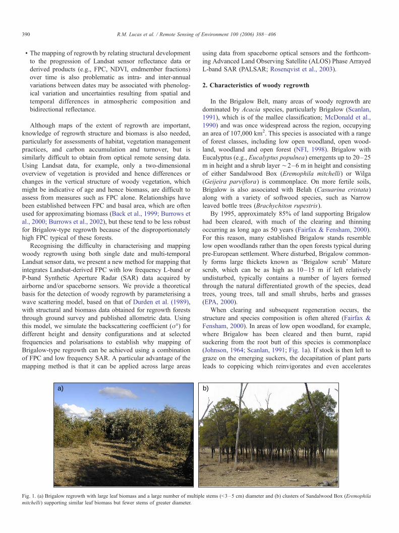
Fig. 1. (a) Brigalow regrowth with large leaf biomass and a large number of multip
mitchelli) supporting similar leaf biomass but fewer stems of greater diameter.
using data from spaceborne optical sensors and the forthcom-
ing Advanced Land Observing Satellite (ALOS) Phase Arrayed
L-band SAR (PALSAR; Rosenqvist et al., 2003).
2. Characteristics of woody regrowth
In the Brigalow Belt, many areas of woody regrowth are
dominated by Acacia species, particularly Brigalow (Scanlan,
1991), which is of the mallee classification; McDonald et al.,
1990) and was once widespread across the region, occupying
an area of 107,000 km2. This species is associated with a range
of forest classes, including low open woodland, open wood-
land, woodland and open forest (NFI, 1998). Brigalow with
Eucalyptus (e.g., Eucalyptus populnea) emergents up to 20–25
m in height and a shrub layer ¨2–6 m in height and consisting
of either Sandalwood Box (Eremophila mitchelli) or Wilga
(Geijeira parviflora) is commonplace. On more fertile soils,
Brigalow is also associated with Belah (Casuarina cristata)
along with a variety of softwood species, such as Narrow
leaved bottle trees (Brachychiton rupestris).
By 1995, approximately 85% of land supporting Brigalow
had been cleared, with much of the clearing and thinning
occurring as long ago as 50 years (Fairfax & Fensham, 2000).
For this reason, many established Brigalow stands resemble
low open woodlands rather than the open forests typical during
pre-European settlement. Where disturbed, Brigalow common-
ly forms large thickets known as FBrigalow scrub_ Mature
scrub, which can be as high as 10–15 m if left relatively
undisturbed, typically contains a number of layers formed
through the natural differentiated growth of the species, dead
trees, young trees, tall and small shrubs, herbs and grasses
(EPA, 2000).
When clearing and subsequent regeneration occurs, the
structure and species composition is often altered (Fairfax &
Fensham, 2000). In areas of low open woodland, for example,
where Brigalow has been cleared and then burnt, rapid
suckering from the root butt of this species is commonplace
(Johnson, 1964; Scanlan, 1991; Fig. 1a). If stock is then left to
graze on the emerging suckers, the decapitation of plant parts
leads to coppicing which reinvigorates and even accelerates
b)
le stems (<3–5 cm) diameter and (b) clusters of Sandalwood Box (Eremophila
R.M. Lucas et al. / Remote Sensing of Environment 100 (2006) 388–406 391
growth in some species (Burrows et al., 1990). This process
also tends to encourage numerous slender trunks to regenerate
from the root stock, thereby drastically altering the root to
shoot relationship of the plants and increasing density (Ceule-
mans et al., 1996). This ability to coppice confers a degree of
resilience to natural and anthropogenic disturbance and hence
coppiced stands become extensive following the formation and
subsequent neglect or abandonment of agricultural land. The
greater number of stems per hectare and the faster growth rate
(compared to individual seedlings; Burrows et al., 1990) of
sprouts from the already established root system also leads to
the rapid development of a canopy and the formation of
relatively homogeneous stands, particularly as most other plant
growth is excluded. The densities of stems (suckers) can
approach 25,000 per hectare (QLD DPI, 1984; Scanlan, 1991)
but despite the formation of a dense canopy, the basal area of
these stands remains low (Kuhnell et al., 1998). When these
trees become taller (e.g. >¨5 m), the number of stems reduces
to one or two bases at ground level, and the dimensions (e.g.
diameter) of each are greater. This later stage of regeneration,
commonly referred to as whipstick brigalow, is typically of
lower density (2000–5000 stems ha�1; Johnson, 1964). These
regrowth stands differ from those dominated by other (e.g.,
Eucalyptus, Eremophila) species where trees are often more
widely spaced and support single or a few multiple stems of
comparatively greater size (Fig. 1b).
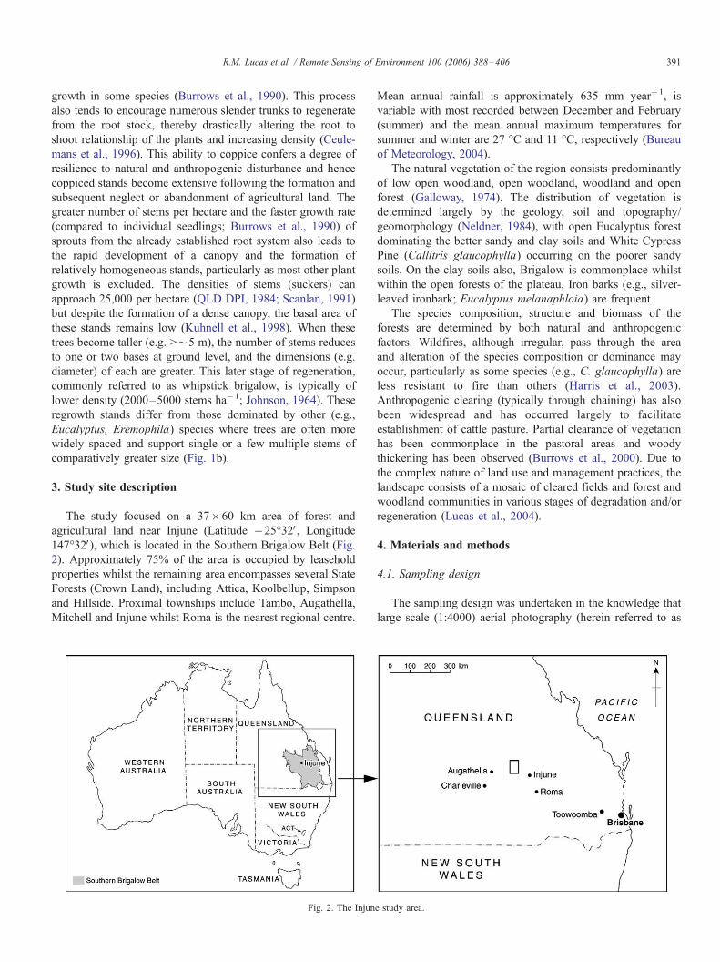
3. Study site description
The study focused on a 37�60 km area of forest and
agricultural land near Injune (Latitude �25-32V, Longitude
147-32V), which is located in the Southern Brigalow Belt (Fig.
2). Approximately 75% of the area is occupied by leasehold
properties whilst the remaining area encompasses several State
Forests (Crown Land), including Attica, Koolbellup, Simpson
and Hillside. Proximal townships include Tambo, Augathella,
Mitchell and Injune whilst Roma is the nearest regional centre.
Fig. 2. The Injun
Mean annual rainfall is approximately 635 mm year�1, is
variable with most recorded between December and February
(summer) and the mean annual maximum temperatures for
summer and winter are 27 -C and 11 -C, respectively (Bureau
of Meteorology, 2004).
The natural vegetation of the region consists predominantly
of low open woodland, open woodland, woodland and open
forest (Galloway, 1974). The distribution of vegetation is
determined largely by the geology, soil and topography/
geomorphology (Neldner, 1984), with open Eucalyptus forest
dominating the better sandy and clay soils and White Cypress
Pine (Callitris glaucophylla) occurring on the poorer sandy
soils. On the clay soils also, Brigalow is commonplace whilst
within the open forests of the plateau, Iron barks (e.g., silver-
leaved ironbark; Eucalyptus melanaphloia) are frequent.
The species composition, structure and biomass of the
forests are determined by both natural and anthropogenic
factors. Wildfires, although irregular, pass through the area
and alteration of the species composition or dominance may
occur, particularly as some species (e.g., C. glaucophylla) are
less resistant to fire than others (Harris et al., 2003).
Anthropogenic clearing (typically through chaining) has also
been widespread and has occurred largely to facilitate
establishment of cattle pasture. Partial clearance of vegetation
has been commonplace in the pastoral areas and woody
thickening has been observed (Burrows et al., 2000). Due to
the complex nature of land use and management practices, the
landscape consists of a mosaic of cleared fields and forest and
woodland communities in various stages of degradation and/or
regeneration (Lucas et al., 2004).
4. Materials and methods
4.1. Sampling design
The sampling design was undertaken in the knowledge that
large scale (1:4000) aerial photography (herein referred to as
e study area.
R.M. Lucas et al. / Remote Sensing of Environment 100 (2006) 388–406392
LSP) was to be acquired over the 37�60 km study area. A
systematic grid of 150 (10 columns numbered from east to
west and 15 rows numbered from north to south starting from
the north west corner) 800�800 m (64 ha) Primary Photo
Plots (PPPs) was therefore established, with each PPP centre
located 4 km apart in the north–south and east–west
directions (Fig. 3). Within each PPP, a 150�500 m Primary
Sampling Unit (PSU) was positioned to encompass the area of
potential LSP overlap (Fig. 3). The scheme also divided each
of the 150 PSUs into 30 Secondary Sampling Units (SSU),
50�50 m (0.25) in dimension and numbered progressively by
row from top left (1) to bottom right (30). Based on this
scheme, the equivalent of 4500�0.25 ha (i.e., 1125 ha) was
sampled by the PSUs/SSUs, which collectively represented
0.46% of the 240,000 ha study area. A detailed overview of
the scheme is provided by Lucas et al. (2004).
4.2. Remote sensing data acquisition: Aerial photography and
SAR
For each of the 150 PPPs, and using pre-defined coordi-
nates, 1:4000 LSP (in negative format) were acquired on the
11th July 2000 by QASCO Surveys Pty. Ltd. on behalf of the
Queensland Department of Natural Resources and Mines
(QDNRM) Landcare Centre. Photographs were taken using
an RC20 large format photographic camera from late morning
to mid afternoon. The effective swath width was 920 m with a
60% (50 ha) overlap corresponding to the approximate size of
a PSU. For each photo principle point, GPS coordinates were
recorded with a nominal precision of T20 m. As 150 PPPs
were sampled, 300 frames of photographs were obtained.
Following delivery of the 150 hard copy stereo pairs, the main
vegetation communities were differentiated and delineated
manually within the PPP and specifically within the area of
stereo overlap (equivalent to the PSU) by a trained photo-
grammetrist and described in terms of their species composi-
tion, height, cover and disturbance (Jones, 2000).
On 3rd September 2000, fully polarimetric C-band (5.6 cm
or 5.3 GHz), L-band (23.9 cm, 1.25 GHz) and P-band (68 cm
wavelength, 0.44 GHz frequency) band data were acquired by
the NASA JPL AIRSAR (on board a DC-8) across the entire
PSU grid, and also across an area extending ¨20 km to the
south. The POLSAR data were acquired in four parallel strips
(S1–S4; length and width approximately 80 km and 12.5 km,
respectively) in a ‘‘race track’’ path trajectory and from an
altitude of ¨8294 m. Interpretation of the LSP and ground
survey established that extensive areas of woody regrowth
were evident only in the west and to the south of the study
area, and so only two of the four POLSAR strips were used for
the analysis presented in this paper. The POLSAR images
were synthesized from the 16-look compressed Stokes Matrix
into HH, VV and HV polarisations (as well as total power, TP)
to a pixel resolution in range and azimuth of 4.62 m. These
data, in units of r-, were slant-to-ground range corrected to a
nominal resolution of 5 m (Van Zyl et al., 1987; Zebker et al.,
1987). Geometric rectification to Universal Transverse Mer-
cator (UTM) coordinates was achieved using ground control
points (GCPs) established between each of the AIRSAR strips
and Landsat ETM+ data of the study area acquired 2nd
September 2000. These data had been georeferenced previ-
ously (to a spatial resolution of 25 m) using an independent set
of GCPs and procedures standardised within the SLATS
project (SLATS, 2003). Between 100 and 150 GCPs were
established for each POLSAR strip, generating r.m.s. errors of
<10 m after a third order polynomial nearest neighbour
transformation was applied during the registration process.
Comparison with LSP confirmed high registration accuracy.
Following georeferencing, each ground range image was
resampled to 10 m spatial resolution through pixel aggregation.
Topographic correction was not applied as the terrain within
the 37�60 study area was considered to be largely ‘‘flat’’,
consisting of valley bottoms, plains or plateaux, or slightly
undulating hills. As the influence of incidence angle on the
retrieval of above ground biomass was a topic of interest
(Lucas et al., 2005), no corrections were undertaken. Hyper-
spectral HyMap strips (¨1.2 km swath width), consisting of
128 bands of visible to shortwave infrared data at 2.6 m spatial
resolution, were also acquired in September 2000 for sections
of PSU columns 1–4 and 8–9. These data were georeferenced
using Inertial Navigation Systems (INS) and Global Position-
ing Systems (GPS).
4.3. Determination of FPC from Landsat sensor data
A stand scale allometric estimate of FPC is estimated
routinely from Landsat TM and ETM+ data by SLATS based
on empirical relationships established between FPC, basal area
and reflectance data. For completeness, an overview of the
method is summarised in this paper, although refer to Danaher
et al. (2004) for further information.
SLATS obtained path-orientated Landsat-5 Thematic Map-
per (TM) data through the Australian Centre for Remote
Sensing (ACRES) for 1988, 1991, 1993, 1995 and 1997 and
Landsat-7 Enhanced TM (ETM+ ) data for 2000. These data
were acquired in the dry season (May–October) to maximise
spectral contrast between perennial and herbaceous vegetation
due to the senescence of annual grasses. The Landsat TM data
were calibrated by replacing the on-board radiometric calibra-
tion with vicarious calibration based on a model of the lifetime
response of the sensor (De Vries et al., 2004). Pre-flight
coefficients were used to calibrate the Landsat-7 ETM+ data to
radiance (NASA, 2004). All imagery was then corrected for
bidirectional reflectance variations of the atmosphere and land
surface (Danaher, 2002). The method combines a simple top-of
atmosphere (TOA) reflectance adjustment with a modified
version of the Walthall empirical BRDF model (Walthall et al.,
1985). The model parameters were derived from an over-
lapping sequence of Landsat 7 ETM+ images and were applied
to produce spatially matched mosaics of Landsat ETM+ and
TM imagery (Danaher, 2002).
The training dataset for estimating FPC from these data was
compiled from basal area data collected between 1996 and
1999 from 1630 sites uniformly distributed throughout
Queensland in stands of contiguous mature remnant forest,
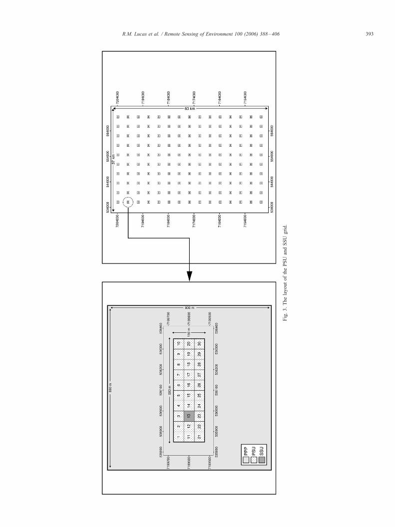
Fig.3.ThelayoutofthePSU
andSSU
grid.
R.M. Lucas et al. / Remote Sensing of Environment 100 (2006) 388–406 393
R.M. Lucas et al. / Remote Sensing of Environment 100 (2006) 388–406394
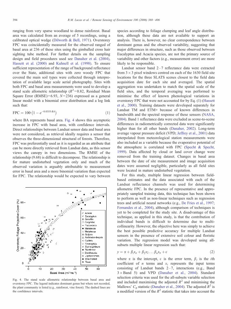
ranging from very sparse woodland to dense rainforest. Basal
area was calculated from an average of 5 recordings, using a
calibrated optical wedge (Dilworth & Bell, 1971). Overstorey
FPC was coincidentally measured for the observed ranged of
basal area at 236 of these sites using the gimballed cross hair
sighting tube method. For further details on the sampling
design and field procedures used see Danaher et al. (2004),
Hassett et al. (2000) and Kuhnell et al. (1998). To ensure
sufficient representation of the range of background reflectance
over the State, additional sites with zero woody FPC that
covered the main soil types were collected through interpre-
tation of available large scale aerial photography. Sites with
both FPC and basal area measurements were used to develop a
stand scale allometric relationship (R2=0.82, Residual Mean
Square Error (RMSE)=6.93, N =236) expressed as a general
linear model with a binomial error distribution and a log link
such that:
FPC ¼ 100I 1� e�0:0355IBA� �
ð1Þ
where BA represents basal area. Fig. 4 shows this asymptotic
increase in FPC with basal area, with confidence intervals.
Direct relationships between Landsat sensor data and basal area
were not considered, as retrieval ideally requires a sensor that
observes the three-dimensional structural of forests. Therefore,
FPC was preferentially used as it is regarded as an attribute that
can be more directly retrieved from Landsat data, as this sensor
views the canopy in two dimensions. The RMSE of the
relationship (9.68) is difficult to decompose. The relationship is
for mature undisturbed vegetation only and much of the
observed variation is arguably attributable to measurement
error in basal area and a more binomial variation than expected
for FPC. The relationship would be expected to vary between
Fig. 4. The stand scale allometric relationship between basal area and
overstorey FPC. The legend indicates dominant genus but where not recorded,
the plant community is listed (e.g., rainforest, vine forest). The dashed lines are
the confidence intervals.
species according to foliage clumping and leaf angle distribu-
tion, although these data are not available to support an
analysis. There is, however, no clear correspondence between
dominant genus and the observed variability, suggesting that
major differences in structure, such as those observed between
Eucalyptus and Acacia species, are not the primary source of
variability and other factors (e.g., measurement error) are more
likely to be responsible.
Landsat sensor band 2–7 reflectance data were extracted
from 3�3 pixel windows centred on each of the 1630 field site
locations for the three SLATS scenes closest to the field data
acquisition date for each site and averaged. The spatial
aggregation was undertaken to match the spatial scale of the
field sites, and the temporal averaging was performed to
minimise the effect of known phenological variations in
overstorey FPC that were not accounted for by Eq. (1) (Hassett
et al., 2000). Training datasets were developed separately for
Landsat TM and ETM+ because of known differences in
bandwidth and the spectral response of these sensors (NASA,
2004). Band 1 reflectance data were excluded as scene-to-scene
differences in radiometrically corrected data were significantly
higher than for all other bands (Danaher, 2002). Long-term
average vapour pressure deficit (VPD; Jeffrey et al., 2001) data
interpolated from meteorological station measurements were
also included as a variable because the evaporative potential of
the atmosphere is correlated with FPC (Specht & Specht,
1999). Data affected by cloud or land cover change were
removed from the training dataset. Changes in basal area
between the date of site measurement and image acquisition
dates were assumed negligible, particularly as all field sites
were located in mature undisturbed vegetation.
For this study, multiple linear regression between field-
based estimates and the data associated with each of the
Landsat reflectance channels was used for determining
allometric FPC. In the presence of representative and appro-
priately sampled training data, this technique has been shown
to perform as well as non-linear techniques such as regression
trees and artificial neural networks (e.g., De Fries et al., 1997;
Fernandes et al., 2004), although comparison of techniques is
yet to be completed for the study site. A disadvantage of this
technique, as applied in this study, is that the contribution of
individual bands is difficult to determine due to multi-
collinearity. However, the objective here was simply to achieve
the best possible predictive accuracy for multiple Landsat
sensors in the presence of extensive soil colour and floristic
variation. The regression model was developed using all-
subsets multiple linear regression such that:
y ¼ a þ bixa þ b2x2 . . . bnxn þ q ð2Þ
where a is the intercept, q is the error term, bi is the ith
coefficient of n terms and xi represents the input terms
consisting of Landsat bands 2–7, interactions (e.g., Band
3�Band 5) and VPD (Danaher et al., 2004). Standard
selection criteria was used for the all-subsets variable selection
and included maximising the adjusted R2 and minimising the
Mallows’ Cp statistic (Danaher et al., 2004). The adjusted R2 is
a modified version of the R2 statistic that takes into account the

Fig. 5. Comparison of field measured (observed) FPC and modelled allometric
FPC. Landsat-7 ETM+ data acquired on 2nd September 2000 over Injune were
used as input to the FPC estimation algorithm.
R.M. Lucas et al. / Remote Sensing of Environment 100 (2006) 388–406 395
reduced degrees of freedom resulting from the inclusion of
more terms in the regression model
R2Adjusted ¼ 1� n� 1ð Þ 1� r2ð Þ
n� t: ð3Þ
The Mallows’ Cp statistic, which provides a measure of the
trade-off between bias resulting from the exclusion of
important terms and extra variance associated with the
inclusion of too many, is given as:
Cp ¼SSE
r2exp
� n� 2tð Þ ð4Þ
where SSE is the sum of the squared error between the
observed and predicted values of y and rexp2 is the expected
value of the residual variance. As there was no a priori
knowledge of rexp2 , the value was set as the residual variance of
the regression model with all possible terms. The use of these
statistics in multiple regression analysis of remotely sensed
data is discussed by Salvador and Pons (1998).
The resulting candidate models were assessed by 5-fold
cross-validation to ensure the model predictions were not
spurious (Table 1). Here, the accuracy of the regression models
are reasonable, with an adjusted R2 greater than or equal to
0.80 and a RMSE of less than 10.0 for both the models and the
cross-validation results. The high number of terms was
accepted due to the complexity of the soil and overstorey
spectral response within Queensland, the high number of
observations (N), and cross-validation results. The differences
between the terms selected for the Landsat-5 TM and Landsat-
7 ETM+ models were attributed to the minor differences of
spectral response and bandwidth between the two sensors. An
evaluation of regression modelling strategies applicable to the
derivation of basal area and FPC from Landsat sensor data over
large areas together with state-wide validation of resulting
predictions using a combination of field and Light Detection
and Ranging (LiDAR) data is currently is progress by SLATS.
For use with the 2000 AIRSAR data, estimates of FPC
were generated for the Injune study area by applying the
techniques above to Landsat-7 ETM+ data acquired on 2nd
September 2000. A good correspondence between FPC
Table 1
Results of the models selected using all-subsets multiple linear regression
Results Landsat-5 TM Landsat-7 ETM+
Model N 2342 2402
Adjusted R2 0.82 0.80
S.E. 7.98 8.25
Cross-validation Mean Adjusted R2 0.81 0.80
Mean S.E. 8.14 8.31
Model terms Single Band ffiffiffiffiffiffiB3
p;
ffiffiffiffiffiffiB4
p;
ffiffiffiffiffiffiB5
p;
ffiffiffiffiffiffiB7
pffiffiffiffiffiffiB3
p;
ffiffiffiffiffiffiB4
p;
ffiffiffiffiffiffiB5
p;
ffiffiffiffiffiffiB7
p
VPD�1 VPD�1
Interaction ffiffiffiffiffiffiffiffiffiffiffiB2B5
p;
ffiffiffiffiffiffiffiffiffiffiffiB3B5
p;
ffiffiffiffiffiffiffiffiffiffiffiB3B7
p;
ffiffiffiffiffiffiffiffiffiffiffiB4B5
p;
ffiffiffiffiffiffiffiffiffiffiffiB2B4
p;
ffiffiffiffiffiffiffiffiffiffiffiB3B5
p;
ffiffiffiffiffiffiffiffiffiffiffiB3B7
p;
ffiffiffiffiffiffiffiffiffiffiffiB4B5
p;
ffiffiffiffiffiffiffiffiffiffiffiB4B7
p ffiffiffiffiffiffiffiffiffiffiffiB4B7
p;
ffiffiffiffiffiffiffiffiffiffiffiB5B7
p
modelled from the stand scale allometric equation with that
measured in selected SSUs during a field campaign to Injune
(Lucas et al., 2004) was observed (R2=0.73, RMSE=4.28),
although the former was consistently greater (Fig. 5). The
reasons for this are (a) the field observations do not include
perennial foliage less than 2 m above the ground, to which the
Landsat-7 ETM+ derived estimates are still sensitive and (b)
FPC was recorded along three 50-m transects in structurally
heterogeneous forests; by shifting the transect location, some
differences in FPC would have been observed. Despite these
limitations, it was considered that the SLATS allometric FPC
predictions were sufficiently accurate for application within
the study site. AIRSAR C-, L- and P-band r- data (all
polarisations) as well as Landsat-derived FPC were then
extracted independently from each SSU within PSU column 3
where areas of woody regrowth dominated by Brigalow as
well as a range of other forest types were evident. Scatterplots
relating FPC and SAR r- for the different forest types were
then generated with a view to fitting a regression line for all
types combined. Extensive regrowth was also evident to the
south of the PSU, although LSP were not available for
this area.
5. Results
5.1. Relationships between SAR r- and FPC
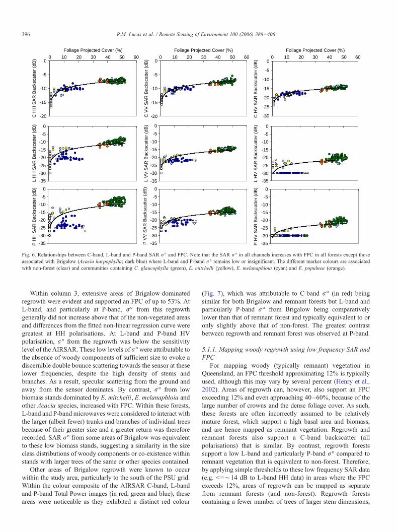
For the majority of forests, most of which were remnant, an
increase in FPC with SAR r- was observed at all frequencies
and polarisations which could be described using a non-linear
regression curve, as illustrated for Column 3 (Fig. 6). At C-
band, the increase in r- with FPC was particularly evident at
HV polarisations as were differences between communities,
with those dominated by C. glaucophylla and E. melanphloia
typically supporting higher values. This increase was evident
for all 10 PSU columns suggesting opportunities for species/
community discrimination and mapping. This is the focus of a
forthcoming paper.
-20
-15
-10
-5
00 10 20 30 40 50 60
Foliage Projected Cover (%)
0 10 20 30 40 50 60
Foliage Projected Cover (%)
0 10 20 30 40 50 60
Foliage Projected Cover (%)
C H
H S
AR
Bac
ksca
tter
(dB
)
-20
-15
-10
-5
0
C V
V S
AR
Bac
ksca
tter
(dB
)
-30
-25
-20
-15
-10
-5
0
C H
V S
AR
Bac
ksca
tter
(dB
)
-35
-30
-25
-20
-15
-10
-5
0
L H
H S
AR
Bac
ksca
tter
(dB
)
L H
V S
AR
Bac
ksca
tter
(dB
)
-35
-30
-25
-20
-15
-10
-5
0
L V
V S
AR
Bac
ksca
tter
(dB
)
-35
-30
-25
-20
-15
-10
-5
0
-35
-30
-25
-20
-15
-10
-5
0
-35
-30
-25
-20
-15
-10
-5
0
P H
H S
AR
Bac
ksca
tter
(dB
)
-35
-30
-25
-20
-15
-10
-5
0
P V
V S
AR
Bac
ksca
tter
(dB
)
P H
V S
AR
Bac
ksca
tter
(dB
)Fig. 6. Relationships between C-band, L-band and P-band SAR r- and FPC. Note that the SAR r- in all channels increases with FPC in all forests except those
associated with Brigalow (Acacia harpophylla; dark blue) where L-band and P-band r- remains low or insignificant. The different marker colours are associated
with non-forest (clear) and communities containing C. glaucophylla (green), E. mitchelli (yellow), E. melanaphloia (cyan) and E. populnea (orange).
R.M. Lucas et al. / Remote Sensing of Environment 100 (2006) 388–406396
Within column 3, extensive areas of Brigalow-dominated
regrowth were evident and supported an FPC of up to 53%. At
L-band, and particularly at P-band, r- from this regrowth
generally did not increase above that of the non-vegetated areas
and differences from the fitted non-linear regression curve were
greatest at HH polarisations. At L-band and P-band HV
polarisation, r- from the regrowth was below the sensitivity
level of the AIRSAR. These low levels of r-were attributable tothe absence of woody components of sufficient size to evoke a
discernible double bounce scattering towards the sensor at these
lower frequencies, despite the high density of stems and
branches. As a result, specular scattering from the ground and
away from the sensor dominates. By contrast, r- from low
biomass stands dominated by E. mitchelli, E. melanaphloia and
other Acacia species, increased with FPC. Within these forests,
L-band and P-band microwaves were considered to interact with
the larger (albeit fewer) trunks and branches of individual trees
because of their greater size and a greater return was therefore
recorded. SAR r- from some areas of Brigalow was equivalent
to these low biomass stands, suggesting a similarity in the size
class distributions of woody components or co-existence within
stands with larger trees of the same or other species contained.
Other areas of Brigalow regrowth were known to occur
within the study area, particularly to the south of the PSU grid.
Within the colour composite of the AIRSAR C-band, L-band
and P-band Total Power images (in red, green and blue), these
areas were noticeable as they exhibited a distinct red colour
(Fig. 7), which was attributable to C-band r- (in red) being
similar for both Brigalow and remnant forests but L-band and
particularly P-band r- from Brigalow being comparatively
lower than that of remnant forest and typically equivalent to or
only slightly above that of non-forest. The greatest contrast
between regrowth and remnant forest was observed at P-band.
5.1.1. Mapping woody regrowth using low frequency SAR and
FPC
For mapping woody (typically remnant) vegetation in
Queensland, an FPC threshold approximating 12% is typically
used, although this may vary by several percent (Henry et al.,
2002). Areas of regrowth can, however, also support an FPC
exceeding 12% and even approaching 40–60%, because of the
large number of crowns and the dense foliage cover. As such,
these forests are often incorrectly assumed to be relatively
mature forest, which support a high basal area and biomass,
and are hence mapped as remnant vegetation. Regrowth and
remnant forests also support a C-band backscatter (all
polarisations) that is similar. By contrast, regrowth forests
support a low L-band and particularly P-band r- compared to
remnant vegetation that is equivalent to non-forest. Therefore,
by applying simple thresholds to these low frequency SAR data
(e.g. <=¨14 dB to L-band HH data) in areas where the FPC
exceeds 12%, areas of regrowth can be mapped as separate
from remnant forests (and non-forest). Regrowth forests
containing a fewer number of trees of larger stem dimensions,
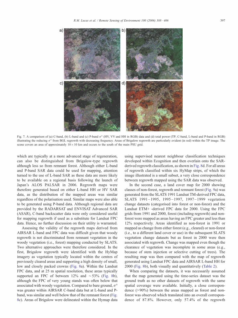
Fig. 7. A comparison of (a) C-band, (b) L-band and (c) P-band r- (HV, VV and HH in RGB) data and (d) total power (TP; C-band, L-band and P-band in RGB)
illustrating the reducing r- from BGL regrowth with decreasing frequency. Areas of Brigalow regrowth are particularly evident (in red) within the TP image. The
scene covers an area of approximately 10�10 km and occurs to the south of the main PSU grid.
R.M. Lucas et al. / Remote Sensing of Environment 100 (2006) 388–406 397
which are typically at a more advanced stage of regeneration,
can also be distinguished from Brigalow-type regrowth
although less so from remnant forest. Although either L-band
and P-band SAR data could be used for mapping, attention
turned to the use of L-band SAR as these data are more likely
to be available on a regional basis following the launch of
Japan’s ALOS PALSAR in 2006. Regrowth maps were
therefore generated based on either L-band HH or HV SAR
data, as the distribution of the mapped areas was similar
regardless of the polarisation used. Similar maps were also able
to be generated using P-band data. Although regional data are
provided by the RADARSAT and ENVISAT Advanced SAR
(ASAR), C-band backscatter data were only considered useful
for mapping regrowth if used as a substitute for Landsat FPC
data. Hence, no further discussion on their utility is warranted.
Assessing the validity of the regrowth maps derived from
AIRSAR L-band and FPC data was difficult given that woody
regrowth is not discriminated from remnant vegetation in the
woody vegetation (i.e., forest) mapping conducted by SLATS.
Two alternative approaches were therefore considered. In the
first, Brigalow regrowth were identified with the HyMap
imagery as vegetation typically located within the centres of
previously cleared areas and supporting a high density of small,
low and closely packed crowns (Fig. 8a). Within the Landsat
FPC data, and at 25 m spatial resolution, these areas typically
supported an FPC of between 12% and ¨53% (Fig. 8b),
although the FPC of very young stands was often below that
associated with woody vegetation. Compared to bare ground, r-was greater within AIRSAR C-band data but at L-band and P-
band, was similar and well below that of the remnant forest (Fig.
8c). Areas of Brigalow were delineated within the Hymap data
using supervised nearest neighbour classification techniques
developed within Ecognition and then overlain onto the SAR-
derived regrowth classification, as shown in Fig. 8d. For all areas
of regrowth classified within six HyMap strips, of which the
image illustrated is a small subset, a very close correspondence
between regrowth mapped using the SAR data was observed.
In the second case, a land cover map for 2000 showing
classes of non-forest, regrowth and remnant forest (Fig. 9a) was
generated from the SLATS 1991 Landsat TM-derived FPC data,
SLATS 1991–1995, 1995–1997, 1997–1999 vegetation
change datasets (categorised into forest or non-forest) and the
Landsat ETM+ -derived FPC data for 2000. Using the FPC
grids from 1991 and 2000, forest (including regrowth) and non-
forest were mapped as areas having an FPC greater and less than
12% respectively. Areas identified as non-forest in 1991 or
mapped as change from either forest (e.g., cleared) or non-forest
(i.e., to a different land cover or use) in the subsequent SLATS
vegetation change datasets but as forest in 2000 were then
associated with regrowth. Change was mapped even though the
clearance of vegetation was incomplete in some areas (e.g.,
because of stem injection or selective cutting of trees). The
resulting map was then compared with the map of regrowth
generated using Landsat FPC data and AIRSAR L-band HH for
2000 (Fig. 8b), both visually and quantitatively (Table 2).
When comparing the datasets, it was necessarily assumed
that the map generated using the time-series dataset was the
ground truth as no other datasets of regrowth with the same
spatial coverage were available. Initially, a close correspon-
dence (>90%) between the areas mapped as forest and non-
forest was observed which translated into an overall correspon-
dence of 87.8%. However, only 57.4% of the regrowth
a) c) d)b)
5512
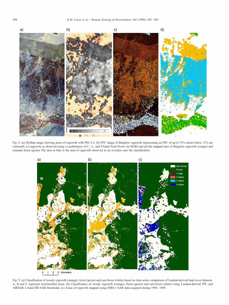
Fig. 8. (a) HyMap image showing areas of regrowth with PSU C3, (b) FPC image of Brigalow regrowth representing an FPC of up to 53% (areas below 12% are
coloured), (c) regrowth as observed using a combination of C-, L- and P-band Total Power (in RGB) and (d) the mapped area of Brigalow regrowth (orange) and
remnant forest (green) The area in blue is the area of regrowth observed in (a) overlain onto the classification.
Fig. 9. (a) Classification of woody regrowth (orange), forest (green) and non-forest (white) based on time-series comparison of Landsat-derived land cover datasets.
A, B and C represent misclassified areas. (b) Classification of woody regrowth (orange), forest (green) and non-forest (white) using Landsat-derived FPC and
AIRSAR L-band HH SAR thresholds. (c) Areas of regrowth mapped using JERS-1 SAR data acquired during 1994–1995.
R.M. Lucas et al. / Remote Sensing of Environment 100 (2006) 388–406398
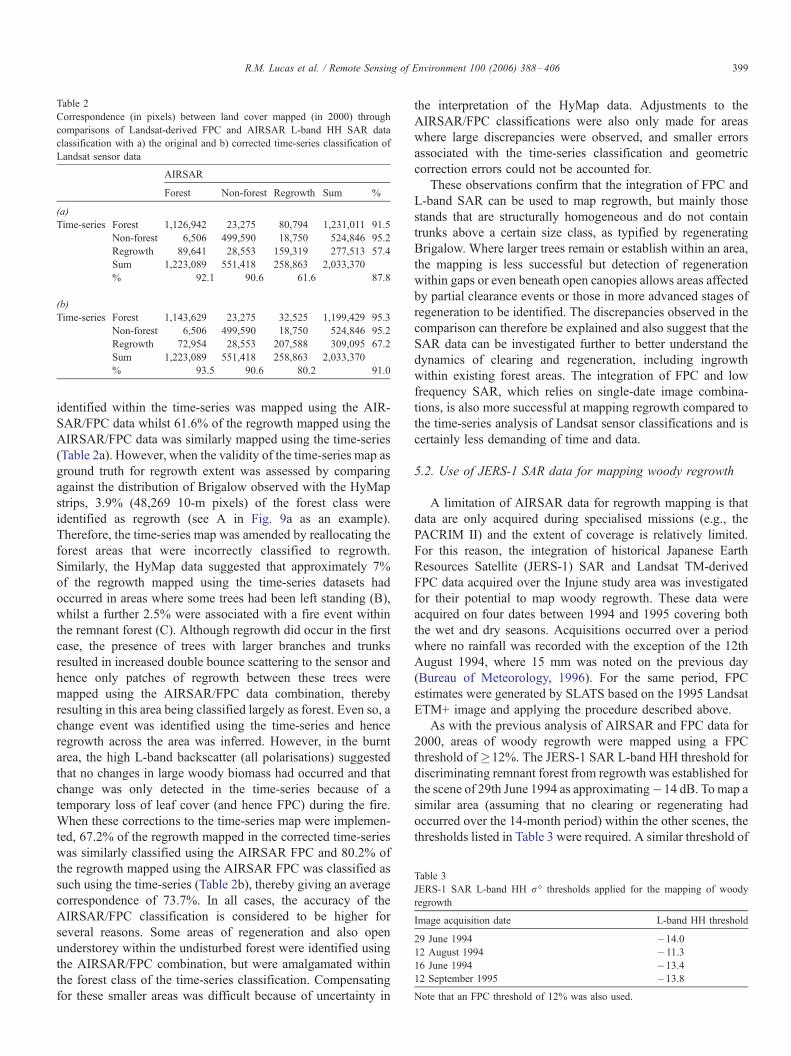
Table 2
Correspondence (in pixels) between land cover mapped (in 2000) through
comparisons of Landsat-derived FPC and AIRSAR L-band HH SAR data
classification with a) the original and b) corrected time-series classification of
Landsat sensor data
AIRSAR
Forest Non-forest Regrowth Sum %
(a)
Time-series Forest 1,126,942 23,275 80,794 1,231,011 91.5
Non-forest 6,506 499,590 18,750 524,846 95.2
Regrowth 89,641 28,553 159,319 277,513 57.4
Sum 1,223,089 551,418 258,863 2,033,370
% 92.1 90.6 61.6 87.8
(b)
Time-series Forest 1,143,629 23,275 32,525 1,199,429 95.3
Non-forest 6,506 499,590 18,750 524,846 95.2
Regrowth 72,954 28,553 207,588 309,095 67.2
Sum 1,223,089 551,418 258,863 2,033,370
% 93.5 90.6 80.2 91.0
Table 3
JERS-1 SAR L-band HH r- thresholds applied for the mapping of woody
regrowth
Image acquisition date L-band HH threshold
29 June 1994 �14.0
12 August 1994 �11.3
16 June 1994 �13.4
12 September 1995 �13.8
Note that an FPC threshold of 12% was also used.
R.M. Lucas et al. / Remote Sensing of Environment 100 (2006) 388–406 399
identified within the time-series was mapped using the AIR-
SAR/FPC data whilst 61.6% of the regrowth mapped using the
AIRSAR/FPC data was similarly mapped using the time-series
(Table 2a). However, when the validity of the time-series map as
ground truth for regrowth extent was assessed by comparing
against the distribution of Brigalow observed with the HyMap
strips, 3.9% (48,269 10-m pixels) of the forest class were
identified as regrowth (see A in Fig. 9a as an example).
Therefore, the time-series map was amended by reallocating the
forest areas that were incorrectly classified to regrowth.
Similarly, the HyMap data suggested that approximately 7%
of the regrowth mapped using the time-series datasets had
occurred in areas where some trees had been left standing (B),
whilst a further 2.5% were associated with a fire event within
the remnant forest (C). Although regrowth did occur in the first
case, the presence of trees with larger branches and trunks
resulted in increased double bounce scattering to the sensor and
hence only patches of regrowth between these trees were
mapped using the AIRSAR/FPC data combination, thereby
resulting in this area being classified largely as forest. Even so, a
change event was identified using the time-series and hence
regrowth across the area was inferred. However, in the burnt
area, the high L-band backscatter (all polarisations) suggested
that no changes in large woody biomass had occurred and that
change was only detected in the time-series because of a
temporary loss of leaf cover (and hence FPC) during the fire.
When these corrections to the time-series map were implemen-
ted, 67.2% of the regrowth mapped in the corrected time-series
was similarly classified using the AIRSAR FPC and 80.2% of
the regrowth mapped using the AIRSAR FPC was classified as
such using the time-series (Table 2b), thereby giving an average
correspondence of 73.7%. In all cases, the accuracy of the
AIRSAR/FPC classification is considered to be higher for
several reasons. Some areas of regeneration and also open
understorey within the undisturbed forest were identified using
the AIRSAR/FPC combination, but were amalgamated within
the forest class of the time-series classification. Compensating
for these smaller areas was difficult because of uncertainty in
the interpretation of the HyMap data. Adjustments to the
AIRSAR/FPC classifications were also only made for areas
where large discrepancies were observed, and smaller errors
associated with the time-series classification and geometric
correction errors could not be accounted for.
These observations confirm that the integration of FPC and
L-band SAR can be used to map regrowth, but mainly those
stands that are structurally homogeneous and do not contain
trunks above a certain size class, as typified by regenerating
Brigalow. Where larger trees remain or establish within an area,
the mapping is less successful but detection of regeneration
within gaps or even beneath open canopies allows areas affected
by partial clearance events or those in more advanced stages of
regeneration to be identified. The discrepancies observed in the
comparison can therefore be explained and also suggest that the
SAR data can be investigated further to better understand the
dynamics of clearing and regeneration, including ingrowth
within existing forest areas. The integration of FPC and low
frequency SAR, which relies on single-date image combina-
tions, is also more successful at mapping regrowth compared to
the time-series analysis of Landsat sensor classifications and is
certainly less demanding of time and data.
5.2. Use of JERS-1 SAR data for mapping woody regrowth
A limitation of AIRSAR data for regrowth mapping is that
data are only acquired during specialised missions (e.g., the
PACRIM II) and the extent of coverage is relatively limited.
For this reason, the integration of historical Japanese Earth
Resources Satellite (JERS-1) SAR and Landsat TM-derived
FPC data acquired over the Injune study area was investigated
for their potential to map woody regrowth. These data were
acquired on four dates between 1994 and 1995 covering both
the wet and dry seasons. Acquisitions occurred over a period
where no rainfall was recorded with the exception of the 12th
August 1994, where 15 mm was noted on the previous day
(Bureau of Meteorology, 1996). For the same period, FPC
estimates were generated by SLATS based on the 1995 Landsat
ETM+ image and applying the procedure described above.
As with the previous analysis of AIRSAR and FPC data for
2000, areas of woody regrowth were mapped using a FPC
threshold of�12%. The JERS-1 SAR L-band HH threshold for
discriminating remnant forest from regrowth was established for
the scene of 29th June 1994 as approximating�14 dB. Tomap a
similar area (assuming that no clearing or regenerating had
occurred over the 14-month period) within the other scenes, the
thresholds listed in Table 3 were required. A similar threshold of
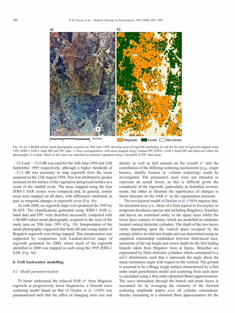
Fig. 10. (a) 1:40,000 colour aerial photography acquired on 29th June 1995, showing areas of regrowth (including A) and (b) the area of regrowth mapped using
1995 JERS-1 SAR L-band HH and FPC data. A close correspondence with areas mapped using Landsat FPC/JERS-1 SAR L-band HH and observed within the
photography is evident. Much of this area was classified as remnant vegetation using a threshold of FPC data alone.
R.M. Lucas et al. / Remote Sensing of Environment 100 (2006) 388–406400
�13.4 and �13.8 dB was used for the 16th June 1994 and 12th
September 1995 respectively, although a higher threshold of
�11.3 dB was necessary to map regrowth from the scene
acquired on the 12th August 1994. This was attributed to greater
moisture on the surface of the vegetation and ground surface as a
result of the rainfall event. The areas mapped using the four
JERS-1 SAR scenes were compared and, in general, similar
areas were mapped on all dates, with differences attributed, in
part, to temporal changes in regrowth cover (Fig. 9c).
As with 2000, no regrowth maps were produced for 1995 by
SLATS. The classifications generated using JERS-1 SAR L-
band data and FPC were therefore necessarily compared with
1:40,000 colour aerial photography acquired to the west of the
study area on 29th June 1995 (Fig. 10). Interpretation of the
aerial photography suggested that both old and young stands of
Brigalow regrowth were being mapped. This interpretation was
supported by comparison with Landsat-derived maps of
regrowth generated for 2000, where much of the regrowth
identified in 2000 was mapped as such using the 1995 JERS-1
SAR (Fig. 9a).
6. SAR backscatter modelling
6.1. Model parameterisation
To better understand the reduced SAR r- from Brigalow
regrowth at progressively lower frequencies, a forward wave
scattering model based on that of Durden et al. (1989) was
parameterised such that the effect of changing stem size and
density as well as leaf amount on the overall r- and the
contribution of the differing scattering mechanisms (e.g., single
bounce, double bounce or volume scattering) could be
investigated. The parameters used were not intended to
represent an actual forest, as this is difficult given the
complexity of the regrowth, particularly in disturbed environ-
ments, but rather to illustrate the significance of changes in
forest structure on the SAR r- as the regeneration proceeds.
The two-layered model of Durden et al. (1989) requires that,
for decurrent trees (i.e., those of a form typical to Eucalyptus or
temperate deciduous species and including Brigalow), branches
and leaves are contained solely in the upper layer whilst the
lower layer consists of stems, which are modelled as randomly
located vertical dielectric cylinders. The depth of the two layers
varies depending upon the vertical space occupied by the
canopy relative to total tree height and was determined using an
empirical relationship established between field-based mea-
surements of the top height and crown depth (to the first leafing
branch) taken from Brigalow trees at Injune. Branches are
represented by finite dielectric cylinders which correspond to a
sin4a distribution, such that a represents the angle about the
mean orientation angle with respect to the vertical. The ground
is assumed to be a Bragg rough surface characterised by a first
order small perturbation model and scattering from each layer
is calculated using a first order (distorted Born) approximation.
The wave attenuation through the branch and trunk layers is
accounted for by averaging the elements of the forward
scattering amplitude matrix over all cylinder orientations,
thereby amounting to a distorted Born approximation for the
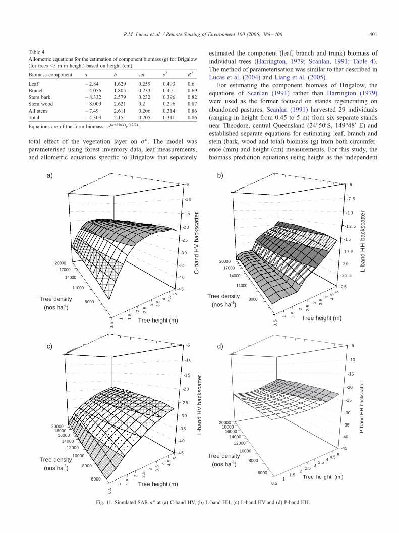
Table 4
Allometric equations for the estimation of component biomass (g) for Brigalow
(for trees <5 m in height) based on height (cm)
Biomass component a b seb s2 R2
Leaf �2.84 1.629 0.259 0.493 0.6
Branch �4.056 1.805 0.233 0.401 0.69
Stem bark �8.332 2.579 0.232 0.396 0.82
Stem wood �8.009 2.621 0.2 0.296 0.87
All stem �7.49 2.611 0.206 0.314 0.86
Total �4.303 2.15 0.205 0.311 0.86
Equations are of the form biomass=e(a+blnX)e(s2/2).
R.M. Lucas et al. / Remote Sensing of Environment 100 (2006) 388–406 401
total effect of the vegetation layer on r-. The model was
parameterised using forest inventory data, leaf measurements,
and allometric equations specific to Brigalow that separately
20000
17000
14000
11000
8000
0.5
1 1.5
2 2.5
3 3.5
4 4.5
5
-4 5
-4 0
-3 5
-3 0
-2 5
-2 0
-1 5
-1 0
-5
C-b
and
HV
bac
ksca
tter
Tree density
(nos ha-1)
Tree density
(nos ha-1)
Tree height (m)
Tree height (m)
2000018000
1600014000
12000
10000
8000
6000
0.5
1 1.5
2 2.5
3 3.5
4 4.5
5
-4 5
-4 0
-3 5
-3 0
-2 5
-2 0
-1 5
-1 0
-5
L-b
an
d H
V b
ack
sca
tter
a)
c)
Fig. 11. Simulated SAR r- at (a) C-band HV, (b) L
estimated the component (leaf, branch and trunk) biomass of
individual trees (Harrington, 1979; Scanlan, 1991; Table 4).
The method of parameterisation was similar to that described in
Lucas et al. (2004) and Liang et al. (2005).
For estimating the component biomass of Brigalow, the
equations of Scanlan (1991) rather than Harrington (1979)
were used as the former focused on stands regenerating on
abandoned pastures. Scanlan (1991) harvested 29 individuals
(ranging in height from 0.45 to 5 m) from six separate stands
near Theodore, central Queensland (24-50VS, 149-48V E) andestablished separate equations for estimating leaf, branch and
stem (bark, wood and total) biomass (g) from both circumfer-
ence (mm) and height (cm) measurements. For this study, the
biomass prediction equations using height as the independent
Tree density
(nos ha-1)
Tree density
(nos ha-1)
Tree height (m)
20000
17000
14000
11000
8000
0.5
1 1.5
2 2.5
3 3.5
4 4.5 5
-2 5
-2 2. 5
-2 0
-1 7. 5
-1 5
-1 2. 5
-1 0
-7 .5
-5
L-ba
nd H
H b
acks
catte
r
2000018000
1600014000
12000
10000
8000
6000
0.51
1.52
2.53
3.54
4.5 5
-45
-40
-35
-30
-25
-20
-15
-10
-5
P-b
and
HH
bac
ksca
tter
Tree he ight (m )
b)
d)
-band HH, (c) L-band HV and (d) P-band HH.
2000017000
14000
11000
8000
0.5
1 1.5
2 2.5
3 3.5
4 4.5
5
-40
-35
-30
-25
-20
-15
-10
-5
Volume Scattering (Branches)
2000017000
14000
11000
8000
0.5
1 1.5
2 2.5
3 3.5
4 4.5
5
-50
-45
-40
-35
-30
-25
-20
-15
-10
-5
Branch Ground
2000017000
14000
11000
8000
0.5
1 1.5
2 2.5
3 3.5
4 4.5
5
-65
-60
-55
-50
-45
-40
-35
-30
-25
-20
-15
-10
-5
Trunk-Ground Scattering
2000017000
14000
11000
8000
0.5
1 1.5
2 2.5
3 3.5
4 4.5
5-30
-25
-20
-15
-10
-5
L-ba
nd H
H b
acks
catte
r
L-ba
nd H
H b
acks
catte
r
L-ba
nd H
H b
acks
catte
r
L-ba
nd H
H b
acks
catte
r
Tree density (nos ha-1)
Tree height (m)
Tree density (nos ha-1)
Tree height (m)
Tree density (nos ha-1)
Tree height (m)
Tree density (nos ha-1)
Tree height (m)
Grounda) b)
c) d)
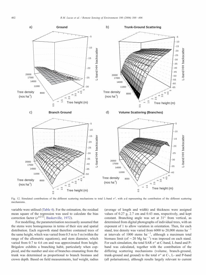
Fig. 12. Simulated contributions of the different scattering mechanisms to total L-band r-, with a-d representing the contribution of the different scattering
mechanisms.
R.M. Lucas et al. / Remote Sensing of Environment 100 (2006) 388–406402
variable were utilised (Table 4). For the estimation, the residual
mean square of the regression was used to calculate the bias
correction factor (e(s2/2); Baskerville, 1972).
For modelling, the parameterisation necessarily assumed that
the stems were homogeneous in terms of their size and spatial
distribution. Each regrowth stand therefore contained trees of
the same height, which was varied from 0.5 m to 5 m (within the
range of the allometric equations), and stem diameter, which
varied from 0.7 to 4.6 cm and was approximated from height.
Brigalow exhibits a branching habit, particularly when cop-
piced, and the number and size of branches emanating from the
trunk was determined as proportional to branch biomass and
crown depth. Based on field measurements, leaf weight, radius
(average of length and width) and thickness were assigned
values of 0.27 g, 2.7 cm and 0.43 mm, respectively, and kept
constant. Branching angle was set at 31- from vertical, as
determined from digital photographs of individual trees, with an
exponent of 1 to allow variation in orientation. Then, for each
stand, tree density was varied from 6000 to 20,000 stems ha�1
at intervals of 1000 stems ha�1, although a maximum total
biomass limit (of ¨20 Mg ha�1) was imposed on each stand.
For each simulation, the total SAR r- at C-band, L-band and P-band was calculated, together with the contribution of the
differing scattering mechanisms (volume, branch-ground,
trunk-ground and ground) to the total r- at C-, L- and P-band
(all polarisations), although results largely relevant to current
R.M. Lucas et al. / Remote Sensing of Environment 100 (2006) 388–406 403
and near future spaceborne SAR are reported here. The
incidence angle was set at 45-.
6.1.1. Scattering behaviour
Previous studies at Injune (Lucas et al., 2004) have indicated
a close relationship between C-band HV r- and the biomass of
the leaves and small (<1 cm diameter) branches combined.
Simulations at C-band HV for Brigalow stands also confirmed
an increase in r- from the early stages of regeneration to an
asymptote approximating �20 dB (Fig. 11a). By contrast,
simulations at L-band HH suggested that r- remained relatively
similar (at less than ¨22 dB) until stem height exceeded 2.0 m,
at which point a rapid increase in r- was observed (Fig. 11b).
Only slight increases in L-band HH r- were observed for standsof height less than 2 m. Simulations at L-band HV suggested r-increased with both height and density but was generally
below�25 dB indicating low sensitivity (Fig. 11c). However, it
can be expected that L-band HV r- will increase as the size anddensity of the branches increases, due to greater sensitivity to
these components (Lucas et al., 2004). Simulations at P-band
HH generally resulted in small values of r- until stands
approached 4–5 m (Fig. 11d), at which point a slight increase
was evident. Simulated P-band HV r- was insignificant for thestands considered.
To better understand the influence of the changing structure
of Brigalow regrowth on microwave interaction, the contribu-
tion of the different scattering mechanisms to the total r- wasinvestigated, focusing specifically on L-band HH because of
greater sensitivity to changes in Brigalow structure. Lower
stature stands were associated with a greater contribution
through direct ground scattering (Fig. 12a). As indicated in Fig.
12b, L-band HH r- only increased above �22 dB at a height
above 2 m, and trunk-ground double bounce scattering
dominates this co-polarised channel increasing steadily above
2 m (Fig. 12b). Branch-ground scattering also increased, but
less so within stands of higher density (Fig. 12c). Volume
scattering (primarily from branches) showed a marked increase
from stands exceeding 3.5 m in height (Fig. 12d). At L-band
HV and for the taller stands, scattering was primarily from
branch volume interactions and HV increases were relatively
small and would only occur when stands support a more
substantial crown layer.
Although the model may indicate a threshold for separating
woody vegetation, this is different from that determined using
the actual SAR data, with these differences attributable to
instrument calibration errors and also errors in the modelling
(e.g., in parameterisation and simulation). It should therefore
be emphasized that the model corroborates the concept of
using SAR for regrowth mapping whereas the actual thresh-
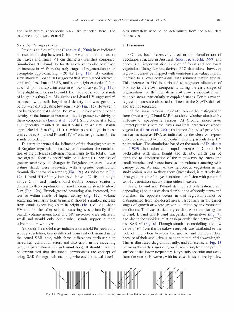
Fig. 13. Diagrammatric representation of the scattering proc
olds ultimately need to be determined from the SAR data
themselves.
7. Discussion
FPC has been extensively used in the classification of
vegetation structure in Australia (Specht & Specht, 1999) and
hence is an important discriminator of forest and non-forest
vegetation. Using Landsat-derived FPC data alone, however,
regrowth cannot be mapped with confidence as values rapidly
increase to a level comparable with remnant mature forests.
This increase in FPC is attributed to a greater allocation of
biomass to the crown components during the early stages of
regeneration and the high density of crowns associated with
multiple stems, particularly in coppiced stands. For this reason,
regrowth stands are classified as forest in the SLATS datasets
and are not separated.
For the same reasons, regrowth cannot be distinguished
from forest using C-band SAR data alone, whether obtained by
airborne or spaceborne sensors. At C-band, microwaves
interact primarily with the leaves and small branches of woody
vegetation (Lucas et al., 2004) and hence C-band r- provides asimilar measure as FPC, as indicated by the close correspon-
dence observed between these data at Injune, particularly at HV
polarisations. The simulations based on the model of Durden et
al. (1989) also indicated a rapid increase in C-band HV
backscatter with stem height and density, which can be
attributed to depolarisation of the microwaves by leaves and
small branches and hence increases in volume scattering with
canopy cover. As much of the herbaceous vegetation in the
study region, and also throughout Queensland, is relatively dry
throughout much of the year, minimal confusion with perennial
woody vegetation occurs using either measure.
Using L-band and P-band data of all polarisations, and
depending upon the size class distributions of woody stems and
branches, the opposite occurs in that regrowth cannot be
distinguished from non-forest areas, particularly in the earlier
stages of growth or where growth is limited by environmental
conditions. This was particularly evident when comparing the
C-band, L-band and P-band image data themselves (Fig. 7),
and also in the empirical relationships established between FPC
and SAR r- (Fig. 6). Through simulation modelling, the low
value of r- from the Brigalow regrowth was attributed to the
lack of interaction between the ground and stem/branches,
because of their small size in relation to that of the wavelength.
This is illustrated diagrammatically, and for stems, in Fig. 13
where in the early stages of growth, scattering from the ground
surface at the lower frequencies is typically specular and away
from the sensor. However, with increases in stem size by a few
ess from Brigalow regrowth with increases in tree size.
R.M. Lucas et al. / Remote Sensing of Environment 100 (2006) 388–406404
individuals or the cohort as whole, stem-ground double bounce
interactions become more dominant, which raises the level of
r- recorded, particularly at HH polarisations. Similarly,
branch-ground interactions and also volume scattering increase
(particularly at HV polarisations) with branch size. At L-band
and P-band, and for the simulated stand, the transfer from
specular to double bounce interactions (primarily with stems)
occurs when stems are about 2 m and ¨4–5 m in height,
respectively. Simulations of L-band HV suggest also that
interactions with branches only take place within stands
exceeding 3.5–5 m.
Although regrowth cannot be discriminated using either of
these data alone, mapping can be achieved using a combination
of either FPC or C-band r- and lower frequency L-band or P-
band r-. Specifically, all areas with an FPC above a threshold
of 12% are mapped as forest and, within this category, all areas
with an L-band or P-band r- below a specified threshold
(approximating to non-forest) are mapped as regrowth. Those
remaining are classified as remnant forest.
Not all regrowth communities can be mapped using this
approach. For example, older regrowth dominated by E.
mitchelli and other Acacia and Eucalyptus species (including
some stands of A. harpophylla) allocate a greater proportion of
biomass to the trunks and are also generally single-stemmed,
although multiple stems (rarely more than 4–5) may occur
(Fig. 1b). These stands may support a basal area that is
equivalent to that of similarly aged Brigalow regrowth, but the
greater size of stems leads to a L-band or P-band r- that is
typically above that of non-forest areas. Areas of heath
vegetation or understorey that typically support a large number
of small stems with low basal area and high FPC may also be
confused. Nevertheless, Brigalow-type regrowth is common
throughout the region, particularly on cleared agricultural land,
and hence the ability to map these areas represents a significant
advance in Statewide forest assessment.
For regional mapping of Brigalow-type regrowth, the
integration of Landsat-derived FPC and L-band HH and HV
data provided by the ALOS PALSAR is advocated for several
reasons. First, data from this sensor will be used to provide
regional image mosaics of Australia (including Queensland) on
at least an annual basis (Rosenqvist et al., 2004), which can be
used in conjunction with the FPC datasets produced routinely
by the SLATS programme. Second, by integrating these single-
period PALSAR mosaics with the FPC data, classifications can
be obtained by applying simple thresholds, thereby negating
the need for extensive analysis of time-series datasets.
Although close timing of the SAR and optical data acquisitions
is preferable, the dates for which the FPC surfaces are
generated are unlikely to influence the reliability of the
regrowth maps, as the foliage cover is relatively constant,
although it is affected by differences in photosynthetic activity
of the herbaceous layer. The quantity and structure of woody
material also remains relatively constant over an annual cycle
(Grigg & Mulligan, 1999) and even between years, unless
clearing events or adverse environmental conditions (e.g.,
drought, fire) occur. Although the use of FPC renders C-band
SAR from spaceborne sensors effectively redundant for
regrowth mapping, these data could nevertheless provide a
viable alternative should the provision of Landsat sensor data
discontinue.
The method for mapping regrowth has been developed
using data acquired over forests associated with savanna–
woodland formations and is only successful because of the
relatively low rate of forest recovery and the openness of the
canopy. The regression model used to derive a measure of
horizontal vegetation structure (FPC) is preferred to spectral
indices such as the Normalised Difference Vegetation Index
(NDVI), because of its greater sensitivity to the complex spatial
variation in soil colour existing in Queensland (Danaher et al.,
2004). However, within the Injune study area, substituting
NDVI might produce similar results as the predominantly
sandy soils are bright and thus exhibit a strong spectral contrast
with the photosynthetic canopy components. Of equal impor-
tance is that FPC is a measure of horizontal cover and as a
result it does not change with the vertical growth of foliage
shoots. Consequently, this measure shows less variation in
response to changes in soil moisture and nutrients than one
related to productivity (e.g., LAI or NDVI).
The FPC relationship was established for a wide range of
forest types in Queensland, which are also typical to large areas
of Australia. The approach of integrating FPC and L-band
backscatter is therefore potentially applicable also to the
Australian continent and also overseas (e.g., the Cerrado of
Brazil and Acacia woodlands in southern Africa). However,
results will be less reliable in the higher biomass forests of
temperate or tropical regions where a closed canopy is typically
formed within 5 years of growth (Lucas et al., 2000, 2002),
often resulting in saturation of both vegetation indices and L-
band backscatter due to the rapid accumulation of foliage cover
and biomass.
8. Summary and conclusions
The research presented in this paper has proposed a simple
method for mapping woody regrowth through integration of
low frequency SAR data, acquired by both airborne or
spaceborne platforms, and Landsat sensor-derived FPC. Evi-
dence has been presented to support the method. In particular:
& Empirical relationships established between FPC and SAR
r- indicated increases in C-band r- with FPC for all forest
types but highlighted a lag in L-band and P-band r-.& Areas corresponding to Brigalow regrowth were observed
within AIRSAR C-band data but these progressively
disappeared within L- and P-band images.
& Simulation of SAR r- from Brigalow stands of increasing
height and density indicated a rapid increase in C-band HV
but delayed response at the lower frequencies. At L-band
and at HH polarisations, increases in r- were associated
primarily with trunk-ground scattering for stands greater
than ¨2 m in height and an associated reduction in ground
scattering. Branch (volume) scattering became significant at
heights exceeding 3.5–5 m and only where branches were
of sufficient size to evoke a response. Lower returns were
R.M. Lucas et al. / Remote Sensing of Environment 100 (2006) 388–406 405
observed at both L-band HV and P-band HH and HV
polarisations.
Using simple thresholds of L-band HH r- for areas mapped
as forest based on a 12% FPC threshold, maps of woody
regrowth were generated using both AIRSAR (for 2000) and
also JERS-1 SAR data (acquired on four separate dates in 1994
and 1995). The mapped areas corresponded closely with those
observed within hyperspectral data, time-series classifications
of land cover change, and stereo aerial photography acquired in
the different years. The areas of regrowth mapped using
Landsat-derived FPC from 1995 and JER-1 SAR data from
1994–1995 were similar to those identified within true colour
aerial photography and classified using the 2000 AIRSAR and
FPC data. The analysis therefore supports the use of L-band
data for mapping woody regrowth across the study area but
also regionally.
A particular advantage of the method for mapping is that
historical data layers are generally not required and relatively
consistent estimates can be obtained from images acquired on
different dates. The study therefore has implications for the
assessment/characterisation, mapping and monitoring of re-
growth within Queensland but potentially in other parts of
Australia or overseas. Application of the method is likely to
assist regional land cover change monitoring, carbon account-
ing, sustainable utilisation of forests and the restoration of
cover and biodiversity.
Following the launch of the ALOS PALSAR, dual
polarimetric L-band HH and HV data from this sensor will
be acquired twice annually over Queensland and processed into
wall-to-wall image mosaics. By combining these data with
FPC estimates generated over the same time-period, opportu-
nities for mapping woody regrowth across the State will be
provided. Integration of historical JERS-1 SAR data with
proximal-date FPC rasters for the State might also allow
regional mapping of regrowth for the early to mid 1990s, and
the production of the Australia-wide JERS-1 SAR mosaic by
JAXA is timely for this purpose. By comparing the two
datasets, significant changes in land cover could be better
quantified and existing classifications improved or validated.
This study forms the basis for undertaking such mapping and
monitoring.
Acknowledgements
The authors thank the Australian Research Council (ARC)
under their SPIRT Program (for a grant to the University of New
South Wales), the Queensland Department of Natural Resources
and Mines (QDNR and M), Bureau of Rural Sciences (BRS),
the Australian Greenhouse Office and the Cooperative Research
Centre (CRC) for Greenhouse Accounting for collectively
funding this research, the Queensland Department of Primary
Industries (QDPI) Tropical Beef Centre and QDPI for assisting
with destructive harvesting and the NASA Jet Propulsion
Laboratory for acquiring the AIRSAR data. Definiens Imaging,
particularly Ursula Benz, and the AMPER network are thanked
for their support. Ake Rosenqvist and the Japan Space
Exploration Agency (JAXA) are thanked for providing the
JERS-1 SAR data. The anonymous reviewers are also thanked
for their valuable comments on the manuscript.
References
ACF. (2002, June). Australian Conservation Foundation ‘‘Licking the salt’’.
Natural advantage: A blueprint for sustainable Australia. URL: http://
www.acfonline.org.au
AGO. (2002). National greenhouse gas inventory 2000-Land use change
and forestry: 2000 Inventory and trends. http://www.greenhouse.gov.au/
inventory/2000/facts/pubs/05.pdf
AGO. (2005). National greenhouse gas inventory 2000—Land use change and
forestry: 2003. http://www.greenhouse.gov.au/inventory/2003/index.html
Back, P. V., Burrows, W. H., & Hoffman, M. B. (1999). TRAPS: A method for
monitoring the dynamics of trees and shrubs in rangelands. In D. Eldridge,
& D. Freudenberger (Eds.), People and rangelands: Building the future.
Proceedings of the Sixth International Rangeland Congress, Townsville,
Queensland, Australia (pp. 742–744).
Baskerville, G. L. (1972). Use of logarithmic regression in the estimation of
plant biomass. Canadian Journal of Forestry Research, 2, 49–53.
Bond, W. J., & Midgeley, G. F. (2000). A proposed CO2 controlled mechanism
of woody plant invasion in grasslands and savannas. Global Change
Biology, 6, 865–869.
Bureau of Meteorology. (1996). URL: http://www.bom.gov.au (Accessed April
1996).
Bureau of Meteorology. (2004). URL: http://www.bom.gov.au (Accessed April
2004).
Burrows, W. H., Carter, J. O., Scanlan, J. C., & Anderson, E. R. (1990).
Management of savannas for livestock production in north-east Australia:
Contrasts across the tree-grass continuum. Journal of Biogeography, 17,
503–512.
Burrows, W. H., Henry, B. K., Back, P. V., Hoffman, M. B., Tait, L. J.,
Anderson, E. R., et al. (2002). Growth and carbon stock change in eucalypt
woodland stands in north-east Australia: Ecological and greenhouse sink
implications. Global Change Biology, 8, 769–784.
Burrows, W. H., Hoffman, M. B., Compton, J. F., Back, P. V., & Tait, L. J.
(2000). Allometric relationships and community biomass estimates for
some dominant eucalypts in central Queensland woodlands. Australian
Journal of Botany, 48, 707–714.
Ceulemans, R., McDonald, A. J. S., & Pereira, J. S. (1996). A comparison
among Eucalypt, Poplar and Willow characteristics with particular
reference to a coppice growth-modelling approach. Biomass and Bioenergy,
11, 215–231.
Danaher, T. J. (2002). An empirical BRDF correction for Landsat TM and
ETM+ imagery. Proceedings of the 11th Australasian Remote Sensing and
Photogrammetry Conference, Brisbane, Australia, September 2002.
Danaher, T. J., Armston, J. D., & Collett, L. J. (2004). A regression approach to
mapping woody foliage projective cover in Queensland with Landsat data.
International Geoscience and Remote Sensing Symposium (IGARSS),
Anchorage, Alaska, September 2004.
De Fries, R., Hansen, M., Steininger, M., Dubayah, R., Sohlberg, R., &
Townshend, J. (1997). Subpixel forest cover in Central Africa from
multisensor, multitemporal data. Remote Sensing of Environment, 60,
228–246.
De Vries, C., Danaher, T. J., & Scarth, P. (2004). Calibration of multiple
Landsat sensors based on pseudo-invariant target sites in western Queens-
land, Australia. Proceedings International Geoscience and Remote Sensing
Symposium (IGARSS).
Dilworth, J. R., & Bell, J. F. (1971). Variable probability sampling—variable
plot and P. Corvalis’ OSU Book Stores.
Durden, S. L., Van Zyl, J. J., & Zebker, H. A. (1989). Modelling and
observation of radar polarization signature of forested areas. IEEE
Transactions on Geoscience and Remote Sensing, 27, 290–301.
Environment Australia. (2001). Brigalow Regrowth and the Environment
Protection and Biodiversity Conservation Act 1999. http://www.deh.gov.
au/biodiversity/threatened/information/factsheets/brigalownote.html
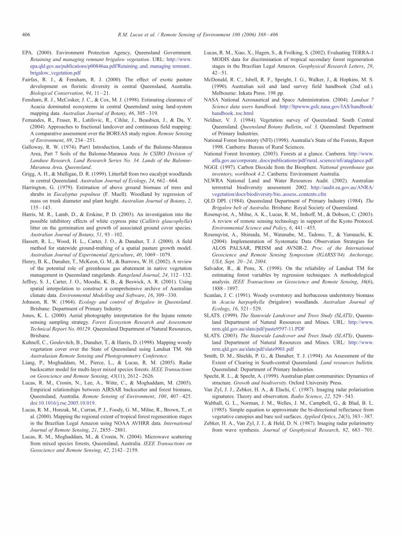
R.M. Lucas et al. / Remote Sensing of Environment 100 (2006) 388–406406
EPA. (2000). Environment Protection Agency, Queensland Government.
Retaining and managing remnant brigalow vegetation. URL: http://www.
epa.qld.gov.au/publications/p00846aa.pdf/Retaining_and_managing remnant_
brigalow_vegetation.pdf
Fairfax, R. J., & Fensham, R. J. (2000). The effect of exotic pasture
development on floristic diversity in central Queensland, Australia.
Biological Conservation, 94, 11–21.
Fensham, R. J., McCosker, J. C., & Cox, M. J. (1998). Estimating clearance of
Acacia dominated ecosystems in central Queensland using land-system
mapping data. Australian Journal of Botany, 46, 305–319.
Fernandes, R., Fraser, R., Latifovic, R., Cihlar, J., Beaubien, J., & Du, Y.
(2004). Approaches to fractional landcover and continuous field mapping:
A comparative assessment over the BOREAS study region. Remote Sensing
of Environment, 89, 234–251.
Galloway, R. W. (1974). Part1 Introduction, Lands of the Balonne-Maranoa
Area, Part 7 Soils of the Balonne-Maranoa Area. In CSIRO Division of
Landuse Research, Land Research Series No. 34. Lands of the Balonne-
Maranoa Area, Queensland.
Grigg, A. H., & Mulligan, D. R. (1999). Litterfall from two eucalypt woodlands
in central Queensland. Australian Journal of Ecology, 24, 662–664.
Harrington, G. (1979). Estimation of above ground biomass of trees and
shrubs in Eucalyptus populnea (F. Muell). Woodland by regression of
mass on trunk diameter and plant height. Australian Journal of Botany, 2,
135–143.
Harris, M. R., Lamb, D., & Erskine, P. D. (2003). An investigation into the
possible inhibitory effects of white cypress pine (Callitris glaucophylla)
litter on the germination and growth of associated ground cover species.
Australian Journal of Botany, 51, 93–102.
Hassett, R. L., Wood, H. L., Carter, J. O., & Danaher, T. J. (2000). A field
method for statewide ground-truthing of a spatial pasture growth model.
Australian Journal of Experimental Agriculture, 40, 1069–1079.
Henry, B. K., Danaher, T., McKeon, G. M., & Burrows, W. H. (2002). A review
of the potential role of greenhouse gas abatement in native vegetation
management in Queensland rangelands. Rangeland Journal, 24, 112–132.
Jeffrey, S. J., Carter, J. O., Moodie, K. B., & Beswick, A. R. (2001). Using
spatial interpolation to construct a comprehensive archive of Australian
climate data. Environmental Modelling and Software, 16, 309–330.
Johnson, R. W. (1964). Ecology and control of Brigalow in Queensland.
Brisbane’ Department of Primary Industry.
Jones, K. L. (2000). Aerial photography interpretation for the Injune remote
sensing sampling strategy. Forest Ecosystem Research and Assessment
Technical Report No. 00129. Queensland Department of Natural Resources,
Brisbane.
Kuhnell, C., Goulevitch, B., Danaher, T., & Harris, D. (1998). Mapping woody
vegetation cover over the State of Queensland using Landsat TM. 9th
Australasian Remote Sensing and Photogrammetry Conference.
Liang, P., Moghaddam, M., Pierce, L., & Lucas, R. M. (2005). Radar
backscatter model for multi-layer mixed species forests. IEEE Transactions
on Geoscience and Remote Sensing, 43(11), 2612–2626.
Lucas, R. M., Cronin, N., Lee, A., Witte, C., & Moghaddam, M. (2005).
Empirical relationships between AIRSAR backscatter and forest biomass,
Queensland, Australia. Remote Sensing of Environment, 100, 407–425.
doi:10.1016/j.rse.2005.10.019.
Lucas, R. M., Honzak, M., Curran, P. J., Foody, G. M., Milne, R., Brown, T., et
al. (2000). Mapping the regional extent of tropical forest regeneration stages
in the Brazilian Legal Amazon using NOAA AVHRR data. International
Journal of Remote Sensing, 21, 2855–2881.
Lucas, R. M., Moghaddam, M., & Cronin, N. (2004). Microwave scattering
from mixed species forests, Queensland, Australia. IEEE Transactions on
Geoscience and Remote Sensing, 42, 2142–2159.
Lucas, R. M., Xiao, X., Hagen, S., & Frolking, S. (2002). Evaluating TERRA-1
MODIS data for discrimination of tropical secondary forest regeneration
stages in the Brazilian Legal Amazon. Geophysical Research Letters, 29,
42–51.
McDonald, R. C., Isbell, R. F., Speight, J. G., Walker, J., & Hopkins, M. S.
(1990). Australian soil and land survey field handbook (2nd edR).
Melbourne’ Inkata Press. 198 pp.
NASA National Aeronautical and Space Administration. (2004). Landsat 7
Science data users handbook. http://ltpwww.gsfc.nasa.gov/IAS/handbook/
handbook_toc.html
Neldner, V. J. (1984). Vegetation survey of Queensland. South Central
Queensland. Queensland Botany Bulletin, vol. 3. Queensland’ Department
of Primary Industries.
National Forest Inventory (NFI) (1998). Australia’s State of the Forests, Report
1998. Canberra’ Bureau of Rural Sciences.
National Forest Inventory. (2003). Forests at a glance. Canberra. http://www.
affa.gov.au/corporate_docs/publications/pdf/rural_science/nfi/ataglance.pdf
NGGI. (1997). Carbon Dioxide from the Biosphere. National greenhouse gas
inventory, workbook 4.2. Canberra’ Environment Australia.
NLWRA National Land and Water Resources Audit. (2002). Australian
terrestrial biodiversity assessment 2002. http://audit.ea.gov.au/ANRA/
vegetation/docs/biodiversity/bio_assess_contents.cfm
QLD DPI. (1984). Queensland Department of Primary Industry (1984). The
Brigalow belt of Australia. Brisbane’ Royal Society of Queensland.
Rosenqvist, A., Milne, A. K., Lucas, R. M., Imhoff, M., & Dobson, C. (2003).
A review of remote sensing technology in support of the Kyoto Protocol.
Environmental Science and Policy, 6, 441–455.
Rosenqvist, A., Shimada, M., Watanabe, M., Tadono, T., & Yamauchi, K.
(2004). Implementation of Systematic Data Observation Strategies for
ALOS PALSAR, PRISM and AVNIR-2. Proc. of the International
Geoscience and Remote Sensing Symposium (IGARSS’04). Anchorage,
USA, Sept. 20–24, 2004.
Salvador, R., & Pons, X. (1998). On the reliability of Landsat TM for
estimating forest variables by regression techniques: A methodological
analysis. IEEE Transactions on Geoscience and Remote Sensing, 36(6),
1888–1897.
Scanlan, J. C. (1991). Woody overstorey and herbaceous understorey biomass
in Acacia harpophylla (brigalow) woodlands. Australian Journal of
Ecology, 16, 521–529.
SLATS. (1999). The Statewide Landcover and Trees Study (SLATS), Queens-
land Department of Natural Resources and Mines. URL: http://www.
nrm.qld.gov.au/slats/pdf/paste9597-11.PDF
SLATS. (2003). The Statewide Landcover and Trees Study (SLATS), Queens-
land Department of Natural Resources and Mines. URL: http://www.
nrm.qld.gov.au/slats/pdf/slats9901.pdf
Smith, D. M., Shields, P. G., & Danaher, T. J. (1994). An Assessment of the
Extent of Clearing in South-central Queensland. Land resources bulletin.
Queensland’ Department of Primary Industries.
Specht, R. L., & Specht, A. (1999). Australian plant communities: Dynamics of
structure. Growth and biodiversity. Oxford University Press.
Van Zyl, J. J., Zebker, H. A., & Elachi, C. (1987). Imaging radar polarisation
signatures. Theory and observation. Radio Science, 22, 529–543.
Walthall, G. L., Norman, J. M., Welles, J. M., Campbell, G., & Blad, B. L.
(1985). Simple equation to approximate the bi-directional reflectance from
vegetative canopies and bare soil surfaces. Applied Optics, 24(3), 383–387.
Zebker, H. A., Van Zyl, J. J., & Held, D. N. (1987). Imaging radar polarimetry
from wave synthesis. Journal of Geophysical Research, 92, 683–701.
Copyright © 2022 FDOKUMEN