Projected Changes to the Southern Hemisphere Ocean and Sea Ice in theIPCC AR4 Climate Models

ALEXANDER SEN GUPTA, AGUS SANTOSO, ANDREA S. TASCHETTO, CAROLINE C. UMMENHOFER,JESSICA TREVENA, AND MATTHEW H. ENGLAND

Climate Change Research Centre, University of New South Wales, Sydney, New South Wales, Australia

(Manuscript received 4 September 2008, in final form 13 November 2008)

ABSTRACT

Fidelity and projected changes in the climate models, used for the Intergovernmental Panel on Climate

Change (IPCC) Fourth Assessment Report (AR4), are assessed with regard to the Southern Hemisphere

extratropical ocean and sea ice systems. While individual models span different physical parameterizations

and resolutions, a major component of intermodel variability results from surface wind differences. Projected

changes to the surface wind field are also central in modifying future extratropical circulation and internal

properties. A robust southward shift of the circumpolar current and subtropical gyres is projected, with a

strong spinup of the Atlantic gyre. An associated increase in the core strength of the circumpolar circulation

is evident; however, this does not translate into robust increases in Drake Passage transport. While an

overarching oceanic warming is projected, the circulation-driven poleward shift of the temperature field

explains much of the midlatitude warming pattern. The effect of this shift is less clear for salinity, where,

instead, surface freshwater forcing dominates. Surface warming and high-latitude freshwater increases drive

intensified stratification, and a shoaling and southward shift of the deep mixed layers. Despite large inter-

model differences, there is also a robust weakening in bottom water formation and its northward outflow. At

the same time the wind intensification invigorates the upwelling of deep water, transporting warm, salty

water southward and upward, with major implications for sequestration and outgassing of CO2. A robust

decrease is projected for both the sea ice concentration and the seasonal cycling of ice volume, potentially

altering the salt and heat budget at high latitudes.

1. Introduction

The Southern Ocean acts as the engine room to the

world’s overturning circulation, drawing its energy from

the powerful midlatitude westerlies acting over a zon-

ally continuous ocean. A high-latitude wind-driven di-

vergence draws deep waters to the surface. Subse-

quently, these upwelled waters are driven both north

and south via Ekman fluxes and buoyancy-driven sink-

ing around the Antarctic margin. The northward flow

subducts to form the basis of the thermocline, mode,

and intermediate water masses that comprise the upper

limb of the global overturning circulation. The south-

ward flow, modified by a salt injection from sea ice de-

velopment and large winter heat losses, forms the densest

bottom water masses that ventilate the abyssal ocean.

These vertical movements of water help to set the den-

sity structure of the Southern Ocean.

Intimately linked to this overturning circulation is the

zonally continuous Antarctic Circumpolar Current (ACC),

which connects the three ocean basins with a transport

of ;135 Sv (1 Sv [ 106 m3 s21) through the Drake

Passage (e.g., Cunningham et al. 2003). Surface wind

and buoyancy forcing, internal circulation, the under-

lying bathymetry and the action of mesoscale eddies all

play a role in determining its characteristics (Gent et al.

2001; Rintoul et al. 2001; Olbers et al. 2004). At lower

latitudes, gradients in the surface wind stress largely

determine the dynamics of the subtropical gyres that

control the flow pathways that extend from the surface

down to intermediate depths. The Southern Ocean also

hosts the most expansive volume of homogeneous mode

waters, formed through vigorous winter convection.

Annual communication between the surface and ocean

interior mean that this water mass sequesters large

Corresponding author address: Dr. Alex Sen Gupta, Faculty of

Science, Climate Change Research Centre, University of New

South Wales, Sydney, NSW 2052, Australia.

E-mail: a.sengupta@unsw.edu.au

1 JUNE 2009 S E N G U P T A E T A L . 3047

DOI: 10.1175/2008JCLI2827.1

� 2009 American Meteorological Society

quantities of heat and gases from the atmosphere. This

is complemented by the formation and northward ex-

port of Antarctic Intermediate Water (AAIW) into

the ocean middepths and Antarctic Bottom Water

(AABW) into the abyssal ocean. Observational studies

have shown that these water masses play a major role in

the removal of additional anthropogenic CO2 (Sabine

et al. 2004) and heat (Gille 2002; Alley et al. 2007), and

that, furthermore, the properties of these water masses

have been subject to significant trends over recent de-

cades (e.g., Bindoff and McDougall 2000; Bryden et al.

2003; Aoki et al. 2005a,b; Johnson et al. 2007; Rintoul

2007).

The Southern Hemisphere (SH) boasts one of the

most profound and robust climate trends observed over

the past few decades, characterized by a poleward shift

and strengthening of the midlatitude jet (Kushner et al.

2001), and more generally of the midlatitude westerly

winds. This is often described in terms of a shift to an

increasingly positive phase of the dominant mode of ex-

tratropical variability, the Southern Annular Mode (SAM;

e.g., Thompson et al. 2000; Thompson and Solomon 2002;

Marshall et al. 2004). This trend has been linked to

changes in both stratospheric ozone and greenhouse

forcing (Gillett and Thompson 2003; Thompson and

Solomon 2002). Moreover, the surface signature of this

atmospheric rearrangement has the potential to signif-

icantly modify characteristics of the ocean and sea ice

systems (Hall and Visbeck 2002; Sen Gupta and England

2006). This modification of the general circulation is on

the backdrop of, and intimately tied to, unprecedented,

large-scale increases in global temperatures and modifi-

cations to the hydrological cycle (Alley et al. 2007).

In light of both the observed and projected changes to

the surface forcing, there has been a growing focus on the

Southern Ocean, driven in part by a recognition of the

potential changes to its enormous sequestration capac-

ity. This has profound consequences when considering

requirements for the mitigation of future climate change

(e.g., Russell et al. 2006a; Toggweiler and Russell 2008;

Friedlingstein 2008). Scientific progress has been greatly

aided by the availability of model output from the Cou-

pled Model Intercomparison Project (CMIP3), used as

part of the Intergovernmental Panel on Climate Change

(IPCC) Fourth Assessment Report (AR4), which covers

a wide range of control and forced scenarios. Most of

the AR4 models show robust changes in the SH mid-

latitude westerlies over the twentieth century, however,

the poleward intensification tends to be underestimated

compared to recent observations (Yin 2005). Further-

more, Fyfe and Saenko (2006) show that for a subset

of the AR4 models, this projected trend continues un-

der increasing greenhouse forcing.

In model experiments using both an ocean-only

model (Oke and England 2004) and an intermediate-

complexity climate model (Fyfe et al. 2007), changes in

the position and strength of the midlatitude westerlies

are shown to induce major changes in Southern Ocean

temperature, extending from the surface to intermedi-

ate depths, independent of any surface warming. As

such, one might expect an associated modification of the

circulation into the future. Such shifts were found by

Fyfe and Saenko (2006) in the Southern Ocean across a

subset of CMIP3 models, with a poleward contraction

and strengthening of the zonal (ACC) and meridional

(Ekman) flow. While part of the circulation change can

be directly attributed to the altered wind field, other

factors, including surface warming, an intensified hy-

drological cycle, and modifications to the Antarctic sea

ice, can also cause a reorganization of the internal

density field, and thus the internal flow. For instance,

Russell et al. (2006b) investigate the factors affecting

the fidelity of the Southern Ocean simulations in the

CMIP3 models. They find that the most important

gauges of realistic circulation are the strength of the

westerlies over the Drake Passage latitudes, the heat

flux gradient over this region, and the salinity gradient

across the ACC through the water column. The authors

suggest that it is this latter property—modulated by the

upwelling of North Atlantic Deep Water (NADW) to

the south of the ACC—that is the most important in

affecting intermodel variability in the ACC. There is

modeling evidence that the future potential for the

Southern Ocean to sequester atmospheric heat and

gases in climate simulations is also strongly modulated

by the present-day position and strength of the midlat-

itude westerlies (Russell et al. 2006a). Despite rising

temperatures causing increased surface stratification,

stronger westerlies and greater high-latitude divergence

help to maintain a strong connection between the sur-

face ocean and the interior, mitigating against seques-

tration decreases in anthropogenic CO2 resulting from

the increased stratification. This result does not, how-

ever, make allowance for changes in the natural carbon

cycle. Recent modeling (Lovenduski et al. 2007) and

observational (Le Quere et al. 2007) studies suggest that

a positive SAM is actually associated with increased

CO2 outgassing as a result of enhanced wind-driven

upwelling of old carbon-rich subsurface waters, result-

ing in a potential positive feedback. This is an issue of

ongoing debate (Zickfeld et al. 2008; Le Quere et al.

2008; Law et al. 2008).

The subtropical gyre circulation is more directly

controlled by the curl of the wind stress via Sverdrup

dynamics. This circulation extends to considerable

depth and controls the flow pathways of surface, waters,

3048 J O U R N A L O F C L I M A T E VOLUME 22

but also the thermocline, mode, and intermediate water

masses. Roemmich et al. (2007) find an increase in the

observed wind-driven transport of the South Pacific

subtropical gyre since 1993, which they link to an in-

tensification of the wind stress curl to the east of New

Zealand, possibly associated with the positively trend-

ing SAM. Cai et al. (2005) investigate projected changes

to the wind stress curl in one of the AR4 models

Commonwealth Scientific and Industrial Research

Organisation Mark version 3.0 (CSIRO Mk3.0) and find

an intensification of wind stress curl over the subtropical

gyres. This manifests itself as a spinup of the gyre, with a

significant increase in the East Australian Current

(EAC) transport and an associated enhanced warming

in the Tasman Sea. A similar shift in the wind stress curl

and subtropical gyres was found by Saenko et al. (2005)

for the Canadian Centre for Climate Modelling and

Analysis (CCCma) Coupled General Circulation

Model, version 3.1 (T47 resolution) [CGCM3.1(T47)].

In contrast to the clear long-term decrease in ob-

served Arctic sea ice cover in the Northern Hemisphere

(NH; e.g., Serreze et al. 2007; Alley et al. 2007), SH sea

ice exhibits large interannual variations but no consis-

tent large-scale trends (Alley et al. 2007). Only at re-

gional scales is there evidence that annual sea ice du-

ration and monthly sea ice concentration have de-

creased (increased) in the western Antarctic Peninsula

and southern Bellingshausen Sea (western Ross Sea)

region since 1979 (Stammerjohn et al. 2008). These

changes are postulated to be related to decadal varia-

tions in the SAM and the extratropical response to

El Nino–Southern Oscillation (ENSO). For the AR4

models, Parkinson et al. (2006) find that their ability to

reproduce the observed annual cycle in sea ice cover is

better in the NH than the SH. They attribute this to a

more realistic representation of the ocean circulation in

the NH. Arzel et al. (2006) and Lefebvre and Goosse

(2008) investigate sea ice fidelity in the AR4 model

simulations and find that there is a reasonable repro-

duction of the observed Antarctic sea ice trends over

the twentieth century by the multimodel mean, espe-

cially for the decrease along the Antarctic Peninsula.

Again, an associated link with a positively trending

SAM is suggested (Lefebvre and Goosse 2008).

In this study we compare large-scale simulated ocean

and sea ice characteristics from the last two decades of

the CMIP3 twentieth-century control runs with obser-

vations. Future projections of these characteristics are

also assessed for the Special Report on Emissions Sce-

narios (SRES) A1B scenario. The SRES A1B scenario

contains the largest selection of data available for the

present study. By assessing the largest possible set of

models, various relationships may be drawn between

characteristics of the oceanic forcing (particularly per-

taining to differences in wind stress) and oceanic

intermodel differences. A primary aim is to provide a

self-consistent explanation for the projected changes

throughout the extratropical ocean, given the projected

changes to surface forcing. In section 2, we briefly describe

the CMIP3 models used in our analysis. In section 2a we

discuss the need to correct for model drift in order to

investigate future projections, particularly in the deeper

ocean. In section 3, we present comparisons of simu-

lated SH properties with observations, and we show the

projected changes to the atmospheric forcing (section

3a), various oceanic fields (sections 3b–3g), and sea ice

(section 3h). Finally, in section 4, we present our con-

clusions and summary.

2. CMIP3 models

The CMIP3 is an initiative by the World Climate Re-

search Programme to bring together output from an

unprecedented array of climate models used as part of

the IPCC AR4 [for details on the initiative see Meehl

et al. (2005, 2007)]. Output is stored and disseminated by

the Program for Climate Model Diagnoses Intercom-

parison (PCMDI). Outputs from three standard experi-

ments are used in this study for the available models.

First, the twentieth-century control run (20C3M) is an

integration from 1850 to ;2000 using realistic natural

and anthropogenic forcing. This integration is generally

initialized from a long preindustrial control run. For the

analysis of a given variable, we use all possible realiza-

tions available for the last 20 yr of the twentieth century

(20C). Sensitivity studies related to the time period

employed suggests that 20 yr is sufficient to account for

interannual variability, providing a robust mean state.

Second, to investigate future changes, we use output

from the SRES A1B scenario (Nakicenovic and Swart

2000), which is initialized from the end of the 20C3M

integrations. This scenario has increasing greenhouse

forcing out to 2100, reaching doubled present-day

values; thereafter, concentrations are kept constant. We

analyze the last 20 yr of the twenty-first century (21C).

Finally, to assess model drift we use 100 yr of the pre-

industrial control run, corresponding to the twenty-first-

century time period, but with constant preindustrial

forcing. The variables, time spans, and number of real-

izations are not necessarily the same across the various

models or experiments used. For any given variable we

generally present analyses from all available models and

realizations.

The CMIP3 repository contains a large set of disparate

models (although a few of the component models are

implemented in more than one model) encompassing a

1 JUNE 2009 S E N G U P T A E T A L . 3049

broad range of resolutions and incorporating a variety

of different physical parameterizations. Table 1 shows

model information with a focus on ocean/sea ice com-

ponents that supplement information presented in Alley

et al. (2007). For the ocean components, resolutions

vary from the eddy-permitting Model for Interdiscipli-

nary Research on Climate 3.2, high-resolution version

[MIROC3.2(hires); 0.288 3 0.198 3 47 levels] to the

coarse-resolution Goddard Institute for Space Studies

Model E-R (GISS-ER; 58 3 48 3 13 levels). Most

models employ a z-level vertical coordinate, although

isopycnal, sigma, and various hybrid schemes are also

represented. The subgrid-scale mixing parameterization

is implemented at different levels of sophistication.

Most models implement some form of the Gent and

McWilliams (1990; GM) scheme, to account for the

mixing of tracers by subgrid-scale eddies. A major im-

provement over the models used for the third IPCC

assessment is that all of the models [except for Meteo-

rological Research Institute Coupled General Circula-

tion Model, version 2.3.2 (MRI CGCM2.3.2), Institute

of Numerical Mathematics Coupled Model, version 3.0

(INM-CM3.0), and both CGCM3.1 models] can main-

tain a realistic present-day climate without the need for

flux correction.

Model drift

A model integrated forward in time from some set of

initial conditions will tend to ‘‘drift’’ until a quasi-equi-

librium state is reached. The equilibration time scale is

highly dependent on the model component, with the

slowly ventilated deep ocean taking thousands of years to

reach steady conditions. Unfortunately, it is not feasible

to integrate these computationally expensive climate

models for such periods, and the various forced simula-

tions are generally started from control runs that have

been integrated out for a few hundred years at best. As a

result, some model drift is to be expected, particularly

within the ocean. For many of the models, the control

simulations, from which the forced scenarios are initial-

ized, are integrated out to provide an overlap with the

forced runs. By subtracting out linear trends from the

control integration, for the concurrent twenty-first-cen-

tury period, a first-order correction for the drift is made.

This assumes that any low-frequency variability in the

ocean is small compared to the drift. Where possible, we

apply such corrections to ocean temperature, salinity,

barotropic and overturning streamfunctions, and to any

subsequent derived variables. Preindustrial datasets are

not, however, available for all model–variable combina-

tions. In general, only a single realization of the control

integration is available to make drift corrections. How-

ever, for the Flexible Global Ocean–Atmosphere–Land

System Model gridpoint version 1.0 (FGOALS-g1.0)

model, three control realizations are available. The

spatial pattern of trends in these realizations are very

similar, indicating that, for this model at least, the linear

trend is insensitive to initial conditions and the long-

term variability is adequately sampled, providing a

representative drift.

Figure 1 shows the trend in the zonally averaged

temperature across the 100 yr of the preindustrial con-

trol run for individual models. A sizeable drift is evident

in many of the models, with regional drift sometimes

exceeding 0.58C century21. To put this into perspective,

these regional drifts may exceed both the range of nat-

ural variability (not shown) and the magnitude of pro-

jected change over the 100 yr of the forced run (Fig. 1,

superimposed). This is most evident in the deeper ocean,

where ventilation by new water is weak and subsequently

any forced change is small. In regions of strong ventila-

tion, on the other hand, forced trends generally exceed

the drift. It is clearly of great importance to take account

of any model drift when investigating changes in the

ocean interior, particularly when analyzing changes at

smaller spatial scales or in the deep ocean. Averaging

across the models (Fig. 1, bottom panel) shows that the

multimodel mean drift is small, indicating that there is no

systematic bias in the sign of the drift. Drift in the interior

circulation is discussed in section 3f.

3. Results

a. Atmospheric forcing

We begin by assessing the present-day state and

twenty-first-century projections for the surface atmo-

spheric fields that force the ocean and sea ice. Figure 2

shows the multimodel and time-averaged 20C means for

these variables, the associated standard deviations

across the models, the biases between the observations

and multimodel mean (20C), and the differences be-

tween the 21C and 20C. Multimodel averages are cal-

culated as unweighted means of all available models

(unless otherwise stated), where means over multiple

realizations for a given model are computed first. As-

sociated zonal means are presented in Fig. 3.

1) WIND STRESS

Large-scale features of the surface wind fields are well

represented in all the models (Figs. 2, 3), with easterlies

in the subtropics and strong westerlies at midlatitudes,

with maximum strengths in the Indian Ocean basin

(although the maximum generally tends to extend too

far east) and the most poleward position in the Pacific

basin. In the multimodel mean, it is clear that the band

3050 J O U R N A L O F C L I M A T E VOLUME 22

TA

BL

E1

.A

R4

mo

de

ld

eta

ils.

Ve

rtic

al

coo

rdin

ate

colu

mn

—Z

:d

ep

th,

P:

pre

ssu

re,

M:

ma

ssp

er

un

ita

rea

,E

:to

po

gra

ph

yw

eig

hte

d,

RH

O:

iso

py

cna

l,S

:si

gma

,a

nd

H:

hy

bri

d.

Pa

ram

ete

riza

tio

nco

lum

n—

GM

:Ge

nt

an

dM

cWil

liam

s(1

990

),G

M*

:Gri

ffie

s’s

(19

98

)im

ple

me

nta

tio

no

fG

M,B

L:B

rya

na

nd

Le

wis

’s(1

97

9)

de

pth

-va

ryin

gv

ert

ica

lm

ixin

g,P

P:v

ert

ica

l

ed

dy

vis

cosi

tya

nd

dif

fusi

on

(Pa

can

ow

ski

an

dP

hil

an

de

r1

98

1),N

K:N

oh

an

dK

im’s

(19

99)

ve

rtic

al

dif

fusi

on

an

dv

isco

sity

,E

VD

:co

nv

ect

ive

mix

ing

pa

ram

ete

riza

tio

n,T

KE

:B

lan

ke

an

d

De

lecl

use

(19

93),

V:

Vis

be

cke

ta

l.’s

(19

97)

con

tro

le

dd

y-i

nd

uce

dtr

an

spo

rtco

effi

cie

nt,

KT

:K

rau

s–T

urn

er

win

d-g

ene

rate

dtu

rbu

len

tk

ine

tic

en

erg

y(K

rau

sa

nd

Tu

rne

r1

96

7),

KP

P:

mix

ed

-la

ye

rsc

hem

e(L

arg

ee

ta

l.1

99

4),B

BL

-NS

:Nak

an

oa

nd

Su

gin

oh

ara

(20

02

)b

ott

om

bo

un

da

ryla

yer

(BB

L),

BB

L-B

D:B

eck

ma

nn

an

dD

osc

he

r(1

99

7)

BB

L,a

nd

NO

-BB

L:n

oB

BL

.

Ice

dy

na

mic

sco

lum

n—

FH

:F

lato

an

dH

ible

r(1

99

0);

S:

Se

mtn

er

(19

76

);S

*:

Se

mtn

er

(19

87

);O

F:

O’F

arr

ell

(19

98);

HD

:H

un

ke

an

dD

uk

ow

icz

(19

97);

H:

Hib

ler

(1979

).F

lux

corr

ect

ion

colu

mn

—N

:no

ne,

H:h

ea

t,F

:fre

shw

ate

r,a

nd

M:m

om

en

tum

.Fo

rcin

g(a

nth

rop

og

en

ic)

colu

mn

—A

LL

:gre

en

ho

use

ga

sses

,ozo

ne

,an

dsu

lfa

tea

ero

sols

,an

d2

O:n

oa

nth

rop

og

en

ico

zon

e.

Fu

rth

er

de

tail

sa

nd

ad

dit

ion

al

refe

ren

ces

are

av

ail

ab

lea

tP

CM

DI

We

bsi

te(h

ttp

://w

ww

-pcm

di.

lln

l.g

ov/

).

Mo

de

l

Oce

an

ic

mo

de

l

Oce

an

ic

reso

luti

on

Ve

rtic

al

coo

rdin

ate

Mix

ing

pa

ram

ete

riza

tio

n

Ice

dy

na

mic

,

rhe

olo

gy

Atm

osp

he

ric

reso

luti

on

Flu

x

corr

ecti

on

Fo

rcin

gR

efe

ren

ce

BC

CR

BC

M2

.0M

ICO

M2.8

1.5

83

1.5

8(0

.58)

,L

35

RH

OK

T,

KP

PH

T63

L3

1N

AL

L,2

OF

ure

vik

et

al.

(20

03

)

CG

CM

3T

47

M0

M1.

11

.858

31

.858

,L

29

ZG

M,

EV

DF

H,

H,

ST

47L

31

H,

F-

Kim

et

al.

(20

02

)C

GC

M3

T6

3M

OM

1.1

1.4

183

0.9

48,

L2

9Z

GM

,E

VD

FH

,H

,S

T63

L3

1H

,F

-

CN

RM

CM

3O

PA

8.1

28

(0.5

8)3

28,

L31

ZG

M,

TK

EH

DT

63L

45

NA

LL

,2

OS

ala

sM

eli

a

(20

02

)

CS

1R

OM

k3

.0M

OM

2.2

0.8

483

1.8

758,

L3

1Z

GM

*,

BL

,P

PS

,F

H,

OF

T63

L1

8N

-G

ord

on

et

al.

(20

02

)C

SIR

OM

k3

.5M

OM

2.2

0.8

483

1.8

758,

L3

1Z

GM

*,

BL

,P

P,

V,

KT

S,

FH

,O

FT

63L

18

N-

GF

DL

CM

2.0

OM

3P

418

(1/3

8)3

18,

L5

0Z

GM

*,

BL

,

BB

L-B

D,

KP

P

S*

,H

D2

.58

328,

L24

NA

LL

De

lwo

rth

et

al.

(20

06

)

GF

DL

CM

2.1

OM

3.1

P4

1(1

/38)

318,

L5

0Z

GM

*,

BL

,

BB

L-B

D,

KP

P

S*

,H

D2

.58

328,

L24

NA

LL

GIS

S-E

RR

uss

ell

et

al.

(19

95,

20

00

)

48

358,

L13

Z,

MG

M*

,K

PP

Ru

ssel

le

ta

l.

(19

95)

48

358,

L9

NA

LL

Sch

mid

te

ta

l.

(20

06

)

IAP

FG

OA

LS

LIC

OM

1.0

18

318,

L33

EG

M,

PP

ST

42L

26

NA

LL

Yu

et

al.

(20

04

)

ING

VE

CH

AM

4O

PA

8.2

28

328

(18)

,L

31Z

BB

L-B

D,

TK

EH

T10

6L

19

NA

LL

,2

OV

alck

ee

ta

l.

(20

00

)

INM

CM

3.0

INM

CM

328

32

.58,

L33

SP

PY

ak

ov

lev

(20

03)

N48

358,

L2

1F

AL

LD

ian

sky

an

d

Vo

lod

in

(20

02

)

IPS

LC

M4

OP

A28

328

(18)

,L

31Z

GM

,B

BL

-BD

,

EV

D,

TK

E

H2

.58

33

.758

,L

19N

AL

L,2

OM

art

ie

ta

l.

(20

06

)

MIR

OC

Hir

es

CO

CO

3.3

0.1

983

0.2

88,

L4

7H

GM

,N

K,

BB

L-N

S,

EV

D

S,

H,

HD

T10

6(1

.128

31

.128

)L

56N

AL

LK

-1m

od

el

de

ve

lop

ers

(20

04

)M

IRO

CM

ed

res

CO

CO

3.3

1.4

8(0

.58)

31

.48,

L4

3H

GM

,N

K,

BB

L-N

S,

EV

D

S,

H,

HD

T42

(2.8

18

32

.818

)L

20N

AL

L

MIU

BE

CH

O-G

HO

PE

-G2

.88

32

.88

(0.5

8 ),

L2

0Z

PP

,E

VD

S,

HT

30(3

.758

33

.758

)L

19H

,F

AL

LM

ine

ta

l.

(20

05

)

MP

IE

CH

AM

5M

PI-

OM

1.5

83

1.5

8,L

40

ZG

M*

,P

P,

BB

L-B

DS

,H

T63

(1.8

758

31

.875

8)L

31

NA

LL

Jun

gcl

au

se

ta

l.

(20

06

)

MR

IG

CM

2.3

Bry

an

–C

ox

2.0

8(0

.58)

32

.58,

L2

3Z

GM

Me

llo

ra

nd

Kan

tha

(19

89)

T42

L3

0H

,F

,M

AL

L,2

OY

uk

imo

toe

ta

l.

(20

01

)

1 JUNE 2009 S E N G U P T A E T A L . 3051

of westerlies is situated too far equatorward, particu-

larly south of Australasia (cf. 0.18 6 0.03 N m22 and

49.2 6 3.18S for the simulations, and 0.18 N m22 and

53.28S for the observations). Only the CSIRO Mark

version 3.5 (CSIRO Mk3.5) and ECHAM4 models

have poleward biases. Projected wind stress over the

twenty-first century shows a robust southward displace-

ment (1.08 6 0.3 8 in the multimodel mean; see Table 2)

and intensification (8.0% 60.1%) of the maximum

zonal wind stress band across the models. Using a subset

of 12 CMIP3 models, Fyfe and Saenko (2006) found a

considerably stronger response in the position and

strength of the maximum westerlies (;1.98 southward

shift, ;15% strength increase) for the more extreme A2

emissions scenario. Of the 20 models analyzed here,

only 2—FGOALS-g1.0 and the Parallel Climate Mod-

el (PCM)—exhibit a northward displacement; and

only 1—the PCM—simulates a weakening of the west-

erlies (Fig. 4b). For most models, this poleward inten-

sification is most pronounced over the Pacific (Table 2).

The wind shift projects strongly onto the positive phase

of the SAM (Thompson and Wallace 2000; Alley et al.

2007). Despite large differences in model resolutions and

physics, there are strong correlations between the posi-

tion and strength of the maximum (20C) wind stress

(Fig. 4a) and between the associated changes in these var-

iables over the twenty-first century (Fig. 4b). We also note

that models with more poleward 20C wind stress maxima

tend to have smaller southward shifts into the future

(Fig. 4c). This suggests an increasing resistance to succes-

sively greater poleward wind stress maximum migration.

2) WIND STRESS CURL

In the open ocean, the depth-integrated meridional

transport can be estimated from the curl of the wind

stress. The large-scale wind stress curl distribution is

captured by individual models, in particular, the cir-

cumpolar maximum situated near 408S (Figs. 2, 3). The

largest positive values are seen around 358S, 118E, in the

southeastern Indian Ocean, consistent with Harrison

(1989), and in the southeastern South Atlantic, sug-

gesting strong transport associated with the Agulhas

Current. Figure 2f shows small standard deviation in

the tropics and subtropics, revealing good agreement

among the models where the curl magnitudes are large.

The largest intermodel disagreement occurs near 508S,

where the meridional gradient of the wind stress curl is

large. In the multimodel mean the maximum curl is

stronger than observed and situated too far to the north

(Fig. 3b). Like the wind stress, the largest biases occur

south of Australia and New Zealand (Fig. 2g). The

projected southward intensification of the wind stress is

mirrored by the wind stress curl, although the maximum

TA

BL

E1

.(C

on

tin

ued

)

Mo

de

l

Oce

an

ic

mo

de

l

Oce

an

ic

reso

luti

on

Ve

rtic

al

coo

rdin

ate

Mix

ing

pa

ram

ete

riza

tio

n

Ice

dy

na

mic

,

rheo

log

y

Atm

osp

he

ric

reso

luti

on

Flu

x

corr

ect

ion

Fo

rcin

gR

efere

nce

NC

AR

CC

SM

3P

OP

1.1

8(0

.278

)3

1.1

8,L

40Z

GM

,K

PP

,N

O-B

BL

S,

FH

,H

DT

85

L2

6N

AL

LC

oll

ins

et

al.

(20

06)

NC

AR

PC

M1

PO

P2

/38

(0.5

8)3

2/3

8,L

32Z

GM

,K

PP

,N

O-B

BL

S,

FH

,H

DT

42

L1

8N

AL

LW

ash

ing

ton

et

al.

(20

00)

Ha

dC

M3

Bry

an

–C

ox

1.2

58

31

.258

,L

20Z

GM

*,

V,

KT

,P

PH

,S

2.7

58

33

.758,

L19

NA

LL

Go

rdo

ne

ta

l.

(20

00);

Joh

ns

et

al.

(20

03)

Ha

dle

yC

en

tre

Glo

ba

l

En

vir

on

me

nta

l

Mo

del

vers

ion

1

(Had

GE

M1)

Bry

an

–C

ox

18

(1/3

8)3

1,

L4

0Z

GM

*,

V,

KT

,P

PH

,H

D,

S1

.258

31

.87

58,

L38

NA

LL

Joh

ns

et

al.

(20

06)

3052 J O U R N A L O F C L I M A T E VOLUME 22

change occurs ;108 further north, over the southern

parts of the subtropical gyres. In the zonal and multi-

model mean there is an increase of ;8.5% and a pole-

ward shift of 18 in the curl maximum.

3) PRECIPITATION

Large biases in precipitation exist across all the

models. While the 20C multimodel mean captures the

low precipitation over the eastern side of the subtropical

oceans (Fig. 2i), where subsidence occurs, the AR4

models are generally unable to correctly simulate the

observed rainfall band associated with the subtropical

convergence zones. As a consequence, the zonally

averaged precipitation is generally underestimated

over the midlatitudes, compared to the Climate Pre-

diction Center (CPC) Merged Analysis of Precipitation

FIG. 1. Model drift calculated as the linear trend in zonally averaged temperature at each grid point over the 100-yr period coincident

with the twenty-first century (color contours). (top) Individual models and (bottom) the multimodel mean are shown. Superimposed

contours are the ratio of the model drift to the projected change (from 20C to 21C), such that a value of one implies that the magnitude of

the drift is of equal magnitude to the projected change.

1 JUNE 2009 S E N G U P T A E T A L . 3053

FIG

.2.(

left

tori

gh

t)M

ult

imo

de

l(2

0C

)m

ea

n,s

tan

da

rdd

ev

iati

on

,dif

fere

nce

fro

mth

eo

bse

rva

tio

n,a

nd

pro

ject

ed

cha

ng

e(2

1C

–20

C)

of

(a)–

(d)

win

dst

ress

(Nm

22),

(e)–

(h)

win

dst

ress

curl

(Nm

21),

(i)–

(l)

pre

cip

ita

tio

n(m

md

ay

21),

(m)–

(p)

late

nt

he

atfl

ux

(Wm

22),

(q)–

(t)

sen

sib

leh

eat

flu

x(W

m2

2),

an

d(u

)–(x

)n

et

he

atfl

ux

(Wm

22).

Po

siti

ve

he

at

flu

xe

sin

dic

ate

ga

in

toth

eo

cea

n.

Ob

serv

ati

on

so

fw

ind

stre

ssa

nd

win

dst

ress

curl

are

ba

sed

on

the

40

-yr

Eu

rop

ea

nC

en

tre

for

Me

diu

m-R

ang

eW

eat

he

rF

ore

cast

s(E

CM

WF

)R

e-A

nal

ysi

s(E

RA

-40

;19

79

–

20

01,

see

Up

pa

lae

ta

l.2

00

5).

Pre

cip

ita

tio

no

bse

rva

tio

ns

are

ba

sed

on

the

CM

AP

gri

dd

ed

da

tase

t(1

979

–2

00

6,

see

Xie

an

dA

rkin

19

97

).H

ea

tfl

ux

es

are

ba

sed

on

the

SO

Cg

rid

de

d

ob

serv

ati

on

s(J

ose

ye

ta

l.1

99

9).

3054 J O U R N A L O F C L I M A T E VOLUME 22

(CMAP) climatology (Fig. 3c). Biases in the represen-

tation of the midlatitude convergence zones are known

to be present in both general circulation models and

reanalysis products (e.g., Quartly et al. 2007; Taschetto

and Wainer 2008). Along the midlatitude storm track,

the simulated precipitation is generally overestimated

(Figs. 2i,k). It should be noted, however, that large

disagreement also exists between observed rainfall

products (Quartly et al. 2007; Gruber et al. 2000).

Precipitation is projected to increase at tropical lati-

tudes associated with increased evaporation and en-

hanced convection in a warmer world (see changes in

latent heat flux). At midlatitudes, between 158 and 408S,

rainfall tends to decrease, particularly over the central

to eastern Pacific (Fig. 2l). Farther south, the band of

maximum precipitation across the Southern Ocean in-

tensifies and shifts southward, mirroring the poleward

intensification of the maximum wind stress. Previous

studies have reported a poleward shift in storm-track

location and increased storm intensity over the last few

decades (e.g., Simmonds and Keay 2000; Simmonds

et al. 2003; Yin 2005). These changes in extratropical

cyclones have again been associated with the SAM

trend (Simmonds and Keay 2000).

4) HEAT FLUX

Turbulent fluxes generally result in heat loss from the

ocean. In agreement with the observations, the largest

contribution is from latent heat losses in the subtropics

(see Fig. 3d), in particular, over the Indian Ocean and at

higher latitudes over the warm boundary currents. The

latent heat loss steadily decreases south of 158S with the

reduction in SST. Sensible heat losses are generally of

considerably smaller magnitude, with largest magni-

tudes between 208 and 408S. Minimum heat loss is

centered along 508S (Fig. 3e) because of the enhanced

poleward heat transport by the transient eddies in the

atmosphere. Intermodel variability for sensible heat is

particularly large. For both turbulent latent and sensible

fluxes, the largest intermodel differences are associated

with discrepancies in the positions of the boundary

currents and the ACC (discussed below) and in regions

of coastal upwelling. Both terms show consistent low

biases across most models compared to the observations

(although this is much improved when comparing

against the reanalysis, which also uses bulk formulas

to estimate fluxes). Observed fluxes are known to be

poorly constrained, particularly at higher latitudes, with

sizeable differences between products (Taylor 2000).

The projections show an enhancement of the latent heat

loss from the ocean, particularly at lower latitudes, indi-

cating higher evaporation in a warmer world (Fig. 2p).

There is a weaker intensification in the Southern Ocean

consistent with the smaller increases in SST at higher

latitudes (see section 3b). The largest regional intensi-

fication occurs in the Agulhas Current retroflection, the

FIG. 3. (a) Zonally averaged wind stress (N m22), (b) wind stress curl (N m21), (c) precipitation (N m21), (d) latent heat flux (W m22),

(e) sensible heat flux (W m22), (f) net radiative flux (W m22), and (g) net heat flux (W m22) from the multimodel ensemble for 20C and

21C. Strengthening (red) and weakening (blue) of the variable from 20C to 21C. ERA-40 results (yellow line). (c) CMAP and (d)–(f)

SOC (green lines). 20C zonal averages for the individual models (gray lines).

1 JUNE 2009 S E N G U P T A E T A L . 3055

Brazil–Malvinas confluence regions, and in the Tasman

Sea, again consistent with projected SST changes. While

SST is generally projected to rise, air temperatures in-

crease more rapidly. As such, there is a general reduc-

tion in the air–sea temperature gradient and an associated

reduction in ocean sensible heat losses (Fig. 3e). This ef-

fect is accentuated south of 508S, where increased pole-

ward eddy heat transport resulting from the poleward-

intensified wind field contributes to increased air tem-

peratures, and relatively weak SST increases, further

reducing the air–sea temperature gradient. As a con-

sequence, only at higher latitudes is there a substantial

net heat flux into the ocean (Fig. 3g).

b. Sea surface temperature and salinity

Figure 5a shows the difference between observed

and modeled (20C) long-term mean SST for the multi-

model ensemble. All observations of temperature and

salinity (throughout the water column) are taken from

the CSIRO Atlas of Regional Seas 2006 (CARS2006)

gridded dataset (Ridgway et al. 2002), derived from all

available historical subsurface ocean property mea-

surements for the SH extratropics through to 2006.

While the use of profiling floats in particular is rapidly

increasing the SH data coverage, high-latitude observa-

tions are still sparse, particularly for subsurface proper-

ties. For individual models, the zonally averaged SST

distribution (Fig. 5g) is well represented with biases,

compared to observations, generally less than 18C dif-

ference. However, regional differences for individual

models (not shown) can exceed 58C. While regional

biases are, in general, considerably reduced in the mul-

timodel mean, compared to any individual model, certain

regions still retain sizeable biases, indicating locations

of systematic bias over a number of the models. Strong

midlatitude meridional gradients mean that small biases

in the position of the ACC translate into large SST bia-

ses. In particular, the Malvinas Confluence region is

generally simulated too far to the north and removed

from the continental margin, resulting in too much cold

freshwater in this region, with warm, salty subtropical

water adjacent to the continent. A warm bias along the

eastern boundaries is associated with the common

problem of overly sluggish eastern boundary currents

(e.g., Large and Danabasoglu 2006). Close to steep to-

pography (e.g., along the Chilean margin) there are also

problems with the representation of upwelling-favorable

winds, which lead to biases in low cloud formation and

radiative heat transfer Randall et al. (2007). These

biases are common to a number of the models, sug-

gesting similar model deficiencies. The pattern of the

biases are reflected in the standard deviation across the

TABLE 2. Position of the maximum zonal wind stress for 20C, zonally averaged over the Southern Ocean (Total) and over each ocean

basin and the associated projected differences between 21C and 20C. Bold numbers, for individual models, indicate an equatorward

displacement of the maximum wind stress position.

Zonal wind

stress position

Total

Atlantic sector,

508W–208E

Indian sector,

308–1008E

Pacific sector,

1808E–908W

20C

(8S)

21C220C

(8S)

20C

(8S)

21C220C

(8S)

20C

(8S)

21C220C

(8S)

20C

(8S)

21C220C

(8S)

Observation (ERA-40) 253.2 - 250.0 - 249.9 - 257.5 -

Multimodel mean 249.3 21.2 248.6 21.2 248.2 20.8 250.5 21.7

CGCM3.1(T47) 248.0 22.4 247.7 21.7 248.3 21.3 248.3 23.8

CGCM3.1(T63) 250.5 22.1 249.2 21.7 249.5 21.4 252.2 23.1

CNRM-CM3 246.7 20.7 246.1 20.9 245.8 21.1 247.7 20.7

CSIRO Mk3.0 251.0 20.7 249.7 21.2 250.4 20.6 253.5 20.8

CSIRO Mk3.5 253.7 20.5 252.0 21.5 251.5 20.6 257.7 0.0GFDL CM2.0 247.3 21.5 247 21.2 247.2 20.6 247.7 22.6

GFDL CM2.1 252.1 20.9 250.1 21.1 250.0 20.7 254.9 21.1

GISS-AOM 243.5 20.8 244.2 20.6 243.8 20.4 242.1 21.5

FGOALS-g1.0 249.6 0.1 248.3 0 248.5 0.3 251.1 0.1

ECHAM4 254.4 20.8 252.2 21.0 251.0 20.6 257.5 20.8

INM-CM3.0 249.0 20.5 249.4 20.2 247.3 20.4 249.8 20.7

IPSL-CM4 242.4 23.1 244.3 22.3 242.6 22.4 240.1 25.2

MIROC3.2(hires) 249 21.1 248.1 20.9 248.3 20.5 249.8 21.7

MIROC3.2(medres) 246.9 21.8 246.9 21.5 246.6 21.0 246.8 22.8

ECHO-G 247.2 24.2 247.3 23.1 246.9 22.7 248.2 25.7

ECHAM5 250.3 20.8 249.4 21.1 249.0 20.9 252.6 20.6

MRI CGCM2.3.2 250.5 20.7 249.5 21.0 249.7 20.6 252.2 0.2

CCSM3 252.1 21.0 250.7 21.2 249.8 20.9 254.7 21.3

PCM 251.4 0.2 250.8 0.1 250.0 0.08 253.9 0.5

3056 J O U R N A L O F C L I M A T E VOLUME 22

models (Fig. 5c), indicating that model SST biases are

controlled, to a large extent, by biases in the circulation

of the ACC and boundary currents.

Projected changes in SST are robust at a large scale,

with all of the models showing significant warming ev-

erywhere, except in the vicinity of Antarctica, where

some models show areas of weak regional cooling,

particularly in the Weddell gyre region (figure not

shown). In the zonal mean, the degree of warming

generally increases equatorward to about 458S, north of

which the magnitude of warming remains stable. These

meridional differences are consistent with changes to

the northward midlatitude Ekman transport. Most

models show an increase in the northward transport of

cold high-latitude water to the south of 458S, with an

anomalous decrease north of this latitude (Fig. 5e).

Between 208 and 458S, individual models generally

show a warming of between 1.38 and 2.58C, except for

MIROC3.2(hires), in which temperature increases ex-

ceed 38C (in the zonal mean). Many of the models [e.g.,

the Bjerknes Centre for Climate Research (BCCR)

Bergen Climate Model version 2.0 (BCM2.0), CGCM3.1

FIG. 4. Scatterplots for (a) zonally averaged wind stress maximum position (tP) vs zonally averaged wind stress maximum strength

(|tP|, N m22), (b) D|tP| vs D|tS|, (c) tP vs position of ACC core (ACCP; calculated from zonally averaged depth-integrated zonal velocity),

(d) |tS| vs ACC core strength (ACCS, Sv), (e) D|tP| vs DACCP, (f) D|tS| vs DACCS, (g) = 3 tP vs position of minimum zonally averaged

barotropic streamfunction (STF), (h) D(= 3 tP) vs DSTF. Where either ordinate or abscissa values is missing for a given model, the value

for the available variable is plotted along the side of the panel. The numbers next to the plotted circles refer to 1: Obs, 2: CGCM3.1(T47),

3: CGCM3.1(T63),4: CNRM-CM3, 5: CSIRO Mk3.0, 6: CSIRO Mk3.5, 7: GFDL CM2.0, 8: GFDL CM2.1, 9: Goddard Institute for Space

Studies Atmosphere–Ocean Model (GISS-AOM), 10: GISS-ER, 11: FGOALS-g1.0, 12: ECHAM4, 13:INM-CM3.0, 14: IPSL-CM4, 15:

MIROC3.2(hires), 16: MIROC3.2(medres), 17: ECHO-G, 18: ECHAM5, 19: MRI CGCM2.3.2, 20: CCSM3.0, 21: PCM, and 22:

HadCM3. Models where ozone hole recovery over the twenty-first century is simulated are highlighted with an ‘‘3’’ (based on infor-

mation from Son et al. 2008); those where information regarding ozone recovery is unavailable are highlighted with a ‘‘-’’; all other

models do not simulate a recovery. Correlation coefficients (r), p values (p), and best-fit linear regression lines are also shown.

1 JUNE 2009 S E N G U P T A E T A L . 3057

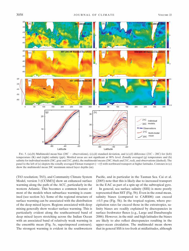
(T63 resolution; T63), and Community Climate System

Model, version 3 (CCSM3)] show an enhanced surface

warming along the path of the ACC, particularly in the

western Atlantic. This becomes a common feature of

most of the models when subsurface warming is exam-

ined (see section 3e). Some of the regional structure of

surface warming can be associated with the distribution

of the deep mixed layers. Regions associated with deep

mixing generally show weaker surface warming. This is

particularly evident along the southeastward band of

deep mixed layers stretching across the Indian Ocean

with an associated band of relatively weak warming in

the ensemble mean (Fig. 5e, superimposed contours).

The strongest warming is evident in the southwestern

Pacific, and in particular in the Tasman Sea. Cai et al.

(2005) note that this is likely due to increased transport

in the EAC as part of a spin up of the subtropical gyre.

In general, sea surface salinity (SSS) is more poorly

represented than SST (Fig. 5b). Even in the zonal mean,

salinity biases (compared to CARS06) can exceed

60.5 psu (Fig. 5h). In the tropical regions, where pre-

cipitation rates far exceed those in the extratropics, sa-

linity biases are readily explained by discrepancies in

surface freshwater fluxes (e.g., Large and Danabasoglu

2006). However, in the mid- and high latitudes the biases

are likely to also reflect discrepancies resulting in the

upper-ocean circulation. The multimodel mean shows

that in general SSS is too fresh at midlatitudes, although

FIG. 5. (a),(b) Multimodel mean bias (20C 2 observations), (c),(d) standard deviation, and (e),(f) difference (21C – 20C) for (left)

temperature (K) and (right) salinity (ppt). Mottled areas are not significant at 90% level. Zonally averaged (g) temperature and (h)

salinity for individual models (20C, gray and 21C, pink), the multimodel means (20C, black and 21C, red), and observations (dashed). The

panel to the left of (e) depicts the zonally averaged Ekman transport (2t/f) with northward transport at higher latitudes. Contours in (e)

show the multimodel mean 20C maximum mixed layer depths (m).

3058 J O U R N A L O F C L I M A T E VOLUME 22

some models do have a strong salty bias [particularly

ECHAM4, L’Institut Pierre-Simon Laplace Coupled

Model, version 4 (IPSL-CM4), and GISS-ER, not shown].

Also evident in many of the models are extended re-

gions of high salinity along parts of the South American

margin, again associated with a poor representation of

local atmospheric processes and upwelling. At higher

latitudes, surface waters tend to be too saline, particu-

larly at some regions around the Antarctic margin.

Unlike SST, the largest intermodel variability occurs at

lower latitudes (Fig. 5d) and likely results from inter-

model differences in surface freshwater fluxes. The very

large intermodel variability is clearly evident in the

zonally averaged profiles (Fig. 5h).

Compared to the intermodel differences and model

biases, the projected changes in SSS are relatively mod-

est. The most robust feature is a freshening of surface

waters around Antarctica. This is consistent with the

large-scale increase in precipitation over the Southern

Ocean and enhanced runoff from Antarctic. These

models do not simulate changes to land ice cover, and as

such a large potential source of additional freshwater

runoff is likely absent. Salinity changes resulting from

altered sea ice conditions are discussed in section 3h.

c. Mixed layer depth

The SH midlatitude oceans are home to some of the

deepest, most expansive mixed layers in the world,

formed through vigorous winter convection. These deep

mixed layers are fundamental to the formation of Sub-

antarctic Mode Water (SAMW) in the Pacific and In-

dian Oceans and of AAIW in the southeastern Pacific,

and in setting thermocline properties. These water

masses are also associated with the sequestration and

storage of large quantities of anthropogenic CO2 (e.g.,

Sabine et al. 2004). As noted above, the mixed layer

depth (MLD) distribution also affects the simulated

pattern of projected surface warming. A realistic rep-

resentation of MLD is therefore a vital component of

any coupled climate model.

To compare model and observed depths we estimate

the maximum annual mixed layer depth, calculated as the

depth where the buoyancy difference between the near

surface and the mixed layer base exceeds 0.003 m s22.

While many of the models actually diagnose MLD via a

variety of schemes (see, e.g., Griffies et al. 2009), this

diagnostic is unavailable as part of the PCMDI reposi-

tory and the use of a common definition throughout

means that we are comparing like with like. Deep ob-

served MLD stretches in a band from the central Indian

Ocean southeastward toward the Drake Passage, with

weaker enhanced convection in the southwest Atlantic

(Fig. 6, last panel). The deepest midlatitude mixed layers

are evident south of Australia and New Zealand and in

the eastern Pacific. Very deep mixing also occurs in the

Weddell Sea and at other locations around the Atlantic

margin, although little in situ data are available to

constrain the observational products used in the esti-

mation of ‘‘observed’’ MLD.

Most models simulate the enhanced midlatitude

mixed layers forming a southeastward band across the

Indian and Pacific regions. The GISS-ER shows the

greatest midlatitude MLD bias across all basins with a

basin-wide zonally averaged depth that is too great by

a factor of 3. On the other hand, FGOALS-g1.0 has

only a weakly enhanced midlatitude maximum MLD,

reaching to only ;250 m, where in the observations

depths exceed 700 m in places. Figure 7 shows the sur-

face area within the midlatitude domain that has MLD

within (20 m) binned ranges for the 20C and 21C, with

the observed distribution superimposed for reference.

The right-hand tails of the distributions represent the

important deepest mixed layers associated with water

mass formation. Many of the models [particularly

BCCR BCM2.0, CSIRO Mk3.5, Geophysical Fluid

Dynamics Laboratory Climate Model version 2.0 (GFDL

CM2.0), FGOALS-g1.0, MIROC3.2(hires), MRI

CGCM2.3.2, and the Met Office’s third climate configu-

ration of the Met Office Unified Model (HadCM3)] lack

the deepest mixed layers (.400 m) that are evident in

the observations; although this is often compensated by

more substantial areas of medium-depth (200–400 m)

MLD. On the shallow end of the distribution, nearly all

models lack a substantial area of very shallow (,40 m)

mixed layers. It should be stressed that the lack of ob-

servational constraints could affect both ends of the

observed distribution. Despite large regional inter-

model differences, integrated over the full midlatitude

domain, the volume of water contained within the

winter MLD envelope varies by less than 30% from that

observed (;1.4 3 l016 m3) across all of the models,

except for CSIRO Mk3.0 and GISS-ER, whose volumes

are too large by ;50% and 150%, respectively.

A comparison of the surface area of deep mixed layers

(.200 m) in the Pacific versus the Indian basin (where

MLD reach considerable depths) across the models re-

veal a significant correlation (r 5 0.8 using all models),

that is, a model with a deep bias in the Pacific will also

tend to have a deep bias in the Indian basin. This sug-

gests that a large proportion of the model MLD bias is

unrelated to local forcing, and instead results from dif-

ferent mixing parameterizations or large-scale forcing

biases. In an intercomparison of ocean–ice GCMs

forced using a common Coordinated Ocean-Ice Refer-

ence Experiments (CORE) climatology, Griffies et al.

(2009) suggest that a large component of the intermodel

1 JUNE 2009 S E N G U P T A E T A L . 3059

variability might be explained by differences in the

treatment of the neutral physics scheme (Gent and

McWilliams 1990) rather than different vertical coor-

dinate systems. The standard deviation across the

models indicate that the largest intermodel variability is

associated with the depth of the deepest mixed layers in

the eastern Pacific, but is more related to the position of

these layers in the east Indian basin. Large variability

also exists around the Antarctic margin, as some models

exhibit very deep MLD, while others have essentially no

enhanced deep mixing.

Figures 6 and 7 also show the projected changes for

the twenty-first century. In general, there is a consistent

shoaling of the deepest midlatitude mixed layers.

Similarly, around the Antarctic there is an extensive

shoaling of deep mixed layers. Considering the midlat-

itude domain only (see Fig. 7), the total volume con-

tained within the MLD is projected to decrease for all

the models, ranging from a drop of ;5% for GFDL

CM2.0 and MRI CGCM2.3.2 to over 20% for the

Centre National de Recherches Meteorologiques Cou-

pled Global Climate Model, version 3 (CNRM-CM3),

ECHAM and the global Hamburg Ocean Primitive

Equation (ECHO-G). The anomalous projected mid-

latitude shoaling is situated slightly south of the maxi-

mum MLD, in the multimodel mean, indicating a small

poleward shift in position in addition to the shoaling.

d. Horizontal circulation

A major component of the oceanic circulation is

driven by the wind. As a result, the robust shifts in

Southern Hemisphere winds, both observed and simu-

lated, are likely to drive major changes to the ocean

circulation. Modified heat and moisture fluxes associ-

ated with enhanced greenhouse forcing will also modify

the circulation via buoyancy changes.

The barotropic streamfunction represents the depth-

integrated ocean circulation. Figure 8 shows the multi-

model mean barotropic streamfunction and observed

streamfunction derived from the University of Mary-

land’s Simple Ocean Data Assimilation Reanalysis

(SODA) version 2.0.2-3. The main features are well

captured in the multimodel mean and across individual

models (not shown). The simulated ACC has the

FIG. 6. Maximum mixed layer depth (m) for 20C for (top to bottom) individual models, multiple models, and observations. Superimposed is

twenty-first-century change in MLD (contour interval: 50 m, dashed lines indicate shoaling). (bottom middle) Also shown is the intermodel

standard deviation (color contours) with the 20C MLD superimposed for reference. Buoyancy B, used for MLD criteria, is calculated as B 5

g(1 2 ssurface/smld), where s is the potential density (see Griffies et al. 2009). All color ranges are the same except for the standard deviation.

3060 J O U R N A L O F C L I M A T E VOLUME 22

characteristic southeastward pathway from the western

Atlantic through to the eastern Pacific, with regional

meandering as a result of topographic steering (par-

ticularly over the Macquarie Ridge system and the

Kerguelen Plateau), and a contraction in the flow

through the Drake Passage followed by a sharp north-

ward excursion. In general, the Weddell gyre is realis-

tically situated, albeit slightly weaker than observed;

however, the Ross gyre is very weak and confined too

far to the south in the ensemble mean. The simulated

subtropical gyre in the Indian Ocean basin is generally

situated too far to the north, consistent with the equa-

torward bias in the wind stress curl, and the western

boundary currents are overly sluggish, a common fea-

ture of coarse-resolution models. For the most part, the

individual models capture the general lateral circulation

features described for the multimodel mean, that is,

western intensification in the subtropical gyre and a

strong circumpolar circulation, although, there are sig-

nificant regional intermodel differences.

In a selection of the AR4 models, Fyfe and Saenko

(2006) found that associated with the poleward shift in the

FIG. 7. Midlatitude mixed layer depth frequency distributions for domain 308–608S (except between 1608 and 3008E, where 308–658S is

used), showing the area within the domain with MLD of a given depth (in bins of 20 m, units: m2). Observations (gray lines) and models

(black bars). Twenty-first-century decrease (blue) and increase (red) in the area associated with a given MLD range.

1 JUNE 2009 S E N G U P T A E T A L . 3061

midlatitude westerlies, over the twentieth and twenty-first

centuries, there is a consistent poleward intensification of

both the ACC and high-latitude meridional Ekman flow.

They fit the depth-integrated zonal velocity and the zonal

wind stress to a Gaussian distribution at each longitude

to obtain an estimate of the latitude and magnitude

of the maximum flow. While this method works well

for the wind stress (see Fyfe and Saenko 2006, Fig. 1),

we find that the structure of the ACC is less amenable

to this approach because the distribution is often heavily

skewed or has multiple cores (commonly associated

with sub-Antarctic and polar fronts in observations).

We implement an alternative approach whereby at each

longitude, an average of latitude weighted by the depth-

integrated zonal flow strength is calculated to obtain

an estimate of the average core position (using only

those latitudes where the zonal flow exceeds 50% of the

maximum eastward flow magnitude). Core strength is

then simply the mean depth-integrated velocity over

these values. While this strength estimate does not cor-

respond to the maximum core strength (as it includes

everything to 50% of the maximum), it provides a rep-

resentative magnitude for the ACC core.

Figure 9 shows the position of the ACC core for the

different models, with the SODA reanalysis ACC core

superimposed. Two of the models, CSIRO Mk3.0 and

GISS-ER, have the largest overall biases, with the ACC

core over 58 too far south (in the zonal mean), but with

regional differences exceeding 108. Conversely, the

IPSL-CM4 and MIROC3.2(hires) have ACC cores in

excess of 38 too far to the north. The multimodel mean

of the ACC position (Fig. 10), however, closely tracks

the observed pathway across most of its domain. The

largest bias is evident in the western Atlantic, where the

ACC for the majority of models tracks too far to the

north. This bias was also manifest in the SST (Fig. 5,

section 3b), where a large, cold bias occurs as high-lat-

itude water is advected too far northward.

Figure 9 also shows the projected change in the po-

sition of the ACC core over the twenty-first century.

Our findings, which comprise an expanded set of 15

models, are essentially in agreement with the 8 models

analyzed by Fyfe and Saenko (2006). The majority of

models show an overall poleward contraction of the

ACC core, although a number of models have regions

where the core moves equatorward. Four models show a

net equatorward movement (GISS-ER, CSIRO Mk3.0,

FGOALS-g1.0, and CNRM-CM3, although the change

is small in the first two). The FGOALS-g1.0 change is

associated with the only net northward wind shift across

the models (Fig. 4f) and the CNRM-CM3 change is re-

lated to a large northward movement in the mid-Pacific,

where the core is weak and poorly defined.

The model with the largest southward shift in the

maximum westerlies (ECHO-G) also shows the greatest

overall (zonally averaged) ACC shift (almost 38 in the

zonal mean). Across the models there is a strong link

between the magnitude of the wind stress shift and the

ACC shift, with a correlation of r 5 0.7 (p 5 0.01; see

Fig. 4). A regression analysis indicates that the shift in

the position of the ACC is approximately half that of the

wind stress shift. This may relate to the fact that the

ACC flow is somewhat constrained by contours of f/H

(H 5 bottom depth), although the strength of flow along

lines of constant f/H may change, leading to a meridi-

onal shift in the ACC core. The multimodel average

shows a poleward shift at all longitudes, with a zonally

averaged shift of ;20.68 6 0.48.

FIG. 8. Barotropic streamfunction for the multimodel mean (color contours, white labels) and obser-

vations (line contours, black labels), derived from SODA zonal velocities. Positive streamline spacing is

25 Sv, and negative spacing is 10 Sv. Streamfunctions have been adjusted so the zero contour passes

through the northern limit of the Drake Passage.

3062 J O U R N A L O F C L I M A T E VOLUME 22

In addition to the poleward shift in the ACC, Fyfe and

Saenko (2006) found a consistent strengthening of the

maximum depth-integrated flow at all longitudes. While

we also find an increase in the strength of the ACC over

the majority of the models, there is a high degree of

regional and intermodel variability. CSIRO Mk3.0 is

again an outlier and shows a zonally averaged weak-

ening of the ACC core strength with a reduction of over

5%. All of the other models show an increased core

magnitude with many models having projected in-

creases exceeding 10% (Fig. 4g). The change in core

strength does not necessarily correspond to a change in

ACC transport, however, as the total flow width may also

contract or expand. An important and well-measured

metric for ACC flow is the volume transport passing

through the Drake Passage. Table 3 shows the 20C and

21C mean volume transports. Common estimates of

Drake Passage transport are ;135 Sv (e.g., Cunningham

FIG. 9. Lateral, depth-averaged circulation and heat content changes. Color contours show the projected change in the depth-

integrated heat content (21C – 20C; J m22). Superimposed are (i) the mean barotropic streamfunction for 20C (black) and 21C (green,

only streamlines indicative of subtropical gyre positions are shown), and (ii) the position of ACC maximum for 20C and 21C [poleward

(red) and equatorward (blue) movement of ACC axis over the period]. Mean position of the observed ACC (dotted line).

1 JUNE 2009 S E N G U P T A E T A L . 3063

et al. 2003). A model’s ability to capture this transport

varies considerably, with present-day estimates ranging

from less than 50 Sv for IPSL-CM4 to in excess of 300 Sv

for CSIRO Mk3.0. Projected changes in the transport

are also highly variable with a range of almost a 30%

increase for INM-CM3.0 to almost a 30% decrease for

CNRM-CM3. There is essentially no projected change

in the ACC core position passing through the Drake

Passage for any of the models.

Cai et al. (2005) find that for the CSIRO Mk3.0 there

is a projected spinup of the midlatitude gyre circulation

into the future, particularly along the path of the EAC,

as the SAM trends toward an increasingly positive state.

Figure 9 shows selected streamfunction contours rep-

resentative of the position of the midlatitude gyres for

the 20C and 21C periods. Zonally averaged stream-

function and wind stress curl are also shown for the

individual models. As expected, a significant link exists

between the position of the wind stress curl minimum

and the cores of the subtropical gyres across the models

(Fig. 4). A southward shift occurs across all the models

over the twenty-first century. A strong correlation exists

across the models between the magnitude of the shift

in the zonally averaged position of the wind stress curl

core and the associated change in the position of the

zonally averaged streamfunction core (Fig. 4; r 5 0.8,

p 5 0.01). As with the shift in the position of the ACC,

a regression analysis indicates that the shift in the wind

stress curl position is approximately twice the magni-

tude of shift in the position of the gyre cores.

To provide a measure of the gyre strength, Fig. 11 tracks

the strength (calculated as the component of the depth-

integrated core strength traveling along the coast) of

the western boundary current core for the three subtrop-

ical gyres. The projected changes have quite different

characteristics within the different basins. Along the

EAC there is often a strong increase in flow at higher

latitudes with a compensating decrease at lower lati-

tudes, indicative of a southward shift in the circulation.

There is no robust increase in the maximum flow how-

ever, although, as noted by Cai et al. (2005), CSIRO

Mk3.0 does show an enhanced flow into the Tasman Sea

region. Along the Brazil Current, on the other hand, as

FIG. 10. Same as Fig. 9, but for the multimodel mean.

TABLE 3. ACC transport calculated as the difference in the

streamfunction across the Drake Passage. The * indicates that

where streamfunction data are unavailable it has sometimes been

possible to estimate transport using the zonal velocity integrated

across the passage through the water column (different model

groups have made available different variable sets).

20C (Sv) 21C (Sv) Difference

BCCR BCM2.0* 95.9 92.4 23.7

CGCM3.1(T47) 97.4 100.3 3.0

CGCM3.1(T63) 110.2 121.9 10.6

CNRM-CM3 83.8 58.7 229.9

CSIRO Mk3.0 312.8 296.9 25.1

CSIRO Mk3.5 148.9 156.8 5.3

GISS-ER 226.1 223.4 21.2

FGOALS-g1.0 71.0 65.6 27.5

ECHAM4* 139.0 131.0 25.8

INM-CM3.0 72.1 91.8 27.4

IPSL-CM4 44.2 50.5 14.2

MIROC3.2(hires) 121.6 134.0 10.2

MIROC3.2(medres) 185.1 183.7 20.8

ECHO-G 71.4 73.3 2.8

ECHAM5 154.8 161.4 4.3

MRI CGCM2.3.2 93.5 95.5 2.1

CCSM3* 205.4 190.2 27.4

PCM* 250.3 241.3 23.6

HadCM3 216.0 218.8 1.3

Multimodel mean 144.6 144.2

Observation 135

3064 J O U R N A L O F C L I M A T E VOLUME 22

well as a southward shift, there is a robust increase in the

strongest flow, indicative of a spinup of the gyre. In the

Agulhas region changes are less robust, with some

models showing weak projected reductions in the

higher-latitude flow.

e. Heat content

Figures 9 and 10 also show the change in the depth-

integrated heat content for individual models and

the ensemble mean, respectively. The pattern of heating

appears to be strongly modulated by changes in the

lateral circulation. For most models, the largest heating

occurs at midlatitudes, broadly constrained by the ACC

to the south and the eastward-flowing limbs of the

subtropical gyres to the north. This is clearly seen in the

multimodel mean, where both the ACC core and the

subtropical gyres show obvious shifts to the south.

Were the change in heat content mainly attributable

to altered surface heat fluxes, the midlatitude region

might be expected to be an area of enhanced warming

because the deep overturning would mix additional

surface heat into the interior. However, the largest heat

content changes occur in the western Atlantic and In-

dian Ocean regions, where the MLDs are generally

shallower than in the eastern Indian and Pacific regions.

Furthermore, the primary input of additional surface

heating occurs to the south of 508 (Fig. 3f). However, the

western Atlantic and Indian Ocean regions are gener-

ally associated with the strongest meridional tempera-

ture gradients (figure not shown). Thus, any poleward

FIG. 11. Model and observed strengths of the (top) EAC, (middle) Brazil, and (bottom) Agulhas western boundary currents by latitude.

Western boundary current strength shown as depth-integrated velocity, calculated as the gradient of the barotropic streamfunction. Red

(black) areas indicate locations when future strengths are increased (decreased) with respect to present day. Core strengths are defined as

the average flow, where flow exceeds 80% of the maximum value at a given latitude and near to the continental margin. For the EAC, the

flow is simply the southward depth-integrated velocity, while for the Brazil and Agulhas Currents, the flow is the depth-integrated

component of velocity in the southwestward direction.

1 JUNE 2009 S E N G U P T A E T A L . 3065

shift in the circulation would preferentially enhance

heat content change at these locations.

f. Vertical circulation

The extratropical large-scale Eulerian meridional

overturning circulation (MOC) is characterized by the

following three main cells: the Antarctic overturning

cell, which is related to the sinking of AABW; the

abyssal cell, which extends north of approximately 408S,

representing the northward flow of AABW and the

compensating southward flow of lower Circumpolar

Deep Water (CDW) and lower NADW; and the Dea-

con cell, which represents the upwelling of upper

CDW and northward Ekman transport. The Deacon

cell overturning should be interpreted with care because

by construction a part of the cell strength is an artifact

of zonal averaging in a region where isopycnal depths

change with longitude (Doos and Webb 1994). The

MOC diagnostic is not readily calculable in the obser-

vations because it requires a full three-dimensional

knowledge of the ocean meridional velocity fields.

Figure 12 shows the 20C mean state MOC overlaid on

the projected twenty-first-century changes. The three-

cell configuration is clear in the multimodel mean, but is

also present in all the models except for the INM-CM3.0

where, for example, a negative subsurface cell exists

at the characteristic position of the Deacon cell. In

IPSL-CM4 both the Deacon and Antarctic cells are

situated in a much more northward position than the

other models. This bias is associated with the largest

northward zonal wind stress (and ACC) position (Fig. 4)

and manifests itself as the most extreme midlatitude

cold bias (figure not shown). Dynamical reasons would

suggest a relationship between wind stress position–

strength and overturning position–strength, via changes

in the strength and position of Ekman pumping, and

indeed significant correlations exist across the models.

The standard deviation in MOC across the models

(Fig. 12) indicates that large intermodel variability is

associated not only with the strength of the Deacon

circulation, but also with the magnitude and position of

the deep water exchange. By comparing the mean and

standard deviation of individual cell strengths (Fig. 13),

we also find significant intermodel differences in the

weaker cells. In particular, the magnitude of the stan-

dard deviation and the mean of the Antarctic cells are

of comparable magnitude. These differences are partly

associated with the strength of high-latitude density

stratification. A significant correlation (r ; 20.7) exists

between the mean vertical density gradient over the top

100 m, south of 608S, and the AABW overturning across

the models (excluding INM-CM3.0). This implies that

models with weak stratification, which also tend to have

low vertical resolution, tend to exhibit strong AABW

overturning.

The sign of the projected changes for the three

overturning cells are, however, robust across almost all

of the models. In all but CSIRO Mk3.5, there is a spinup

of the Deacon cell (Fig. 13). The behavior of this outlier

is related to the equatorward shift of the zonal wind

stress in the Pacific sector (Table 2). The projected

multimodel mean increase of the Deacon cell is ;4 Sv

(Fig. 12), indicating an intensified upwelling of rela-

tively warm and saline upper CDW. Significant corre-

lations exist between the change in both the position

and the strength of the maximum zonally averaged wind

stress and the corresponding changes in the position and

strength of the Deacon cell across the models (r . 0.75,

p , 0.007 for position, and r . 0.8, p , 0.001 for

strength, excluding INM-CM3.0). Despite substantial

differences in resolution, bathymetry, and physical pa-

rameterizations, intermodel differences in the midlati-

tude MOC is primarily determined by biases in wind

field. Previous studies have shown a strong short-term

response in the Deacon cell driven by changes in the

SAM (Hall and Visbeck 2002; Sen Gupta and England

2006). For a positive SAM this cell spins up and shifts

poleward. The long-term trend toward a more positive

SAM phase seen in the models would therefore be

consistent with these projected changes.

In the multimodel mean, the AABW cell weakens by

;2 Sv (Fig. 13). This spindown is consistent with the

projected surface-intensified buoyancy gain around

the Antarctic margin. A comparable reduction in the

abyssal cell strength reflects the weaker AABW for-

mation and its subsequent outflow. A weak correlation

exists between changes to the abyssal and AABW cell

strengths. As an aside, Fig. 13 also shows the over-

turning calculated without any correction for drift. It is

evident that for some models drift explains an important

proportion of the raw MOC change, particularly in the

abyssal cell. Figure 12 also shows the standard deviation

in the projected overturning changes. Large differences

in the projected response are associated with the Deacon

cell and the inflow of deep water. There are also large

surface-intensified intermodel differences along 408S,

presumably associated with wind-driven differences in

the convergence zone.

g. Internal properties

Figure 14 shows the projected changes to the zonally

averaged potential temperature. A general warming

pervades the extratropics with enhanced surface

warming particularly between 408 and 608S that extends

to middepth; and for almost all models there is an en-

hanced abyssal warming near the Antarctic margin. The

3066 J O U R N A L O F C L I M A T E VOLUME 22

FIG. 12. Modeled projected change in MOC (21C – 21C, color maps). Only differences that are significant above the 95%

level are displayed. The significance level is determined by a two-tailed t test. The 20C mean state of MOC is superimposed.

(bottom left) Multimodel mean of 20C MOC [solid contours for positive MOC (4-Sv interval), dashed contours for negative

(1-Sv interval)] and projected changes (color map). (bottom right) Multimodel standard deviation for both the 20C mean

states (contours with 1-Sv interval) and projected changes (color map).

1 JUNE 2009 S E N G U P T A E T A L . 3067

weakest warming, and in some models a weak cooling,

occurs at middepth north of 408S.

It was suggested in section 3d that a large component

of the change in heat content can be attributed to the

poleward shift of the midlatitude circulation. Super-

imposed on Fig. 14 are contours indicating the change

in temperature that would arise from a 18 southward

translation of the 20C temperature distribution. At the

midlatitudes, as far north as 208S, and primarily for the

upper 1000 m, there is a very close correspondence be-

tween the projected warming and the warming that

would result from a pure southward shift. This technique

was used by Alory et al. (2007) to show that projected

warming in the Indian Ocean could be explained, in part,

by a simple southward translation of the temperature

field. A recent analysis of upper Southern Ocean warm-

ing by Gille (2008) over the latter part of the twenty-first

century also supports the idea that the warming trend is

intimately tied to a southward shift in the ACC.

The corresponding changes in salinity across the

models (Fig. 15) are more varied. However, certain

general features are evident. There is a freshening

signal that tracks the upper part of the AAIW salinity

minimum and at lower latitudes in the thermocline.

Furthermore, most of the models show a saline anomaly

in the surface layer at lower latitudes. At locations as-

sociated with upwelled CDW, there is generally a

poleward-intensified salination (except in the CNRM-CM3

and CSIRO Mk3.0), which in some models [e.g., CGCM

models and MIROC3.2(hires)] feeds into the lower

layers of AAIW. In most models abutting this region of

salination, both at middepths and north of 408S there is

a freshening signal that coincides with the region of

cooling (or relatively weak warming) in Fig. 14. This

FIG. 13. Projected differences in the transport (Sv) of the Southern Ocean overturning cells for individual models (circles). Data are

either drift corrected (red circles) or uncorrected (black circles). Horizontal error bars indicate the corresponding 95% confidence

interval, with significant differences from zero (filled circles) indicated. The multimodel mean differences (corrected and uncorrected)

are indicated by the corresponding dashed vertical lines, with the gray region indicating the 95% confidence interval for the drift-

corrected (red) vertical line. The 20C mean values of each model overturning cell are shown on the left-hand side, with the multimodel

mean values shown in bold at the bottom. Mean values that fall within the 95% confidence interval of the multimodel mean (bold) and the

values that fall in the upper (gray) and lower (black) tail of the 95% interval are shown. Note that the preindustrial run of ECHAM5 is not

available for estimating the drift. Its uncorrected values are shown nonetheless.

3068 J O U R N A L O F C L I M A T E VOLUME 22

signal is most prominent in the Atlantic basin (Fig. 16),

indicating that these changes are associated with a modi-

fication in the southward export of NADW. In other ba-

sins, changes in this region are weak, consistent with areas

of old, poorly ventilated waters (e.g., Pacific Deep Water)

where recent surface changes would not have penetrated.

Unlike temperature, which possesses a strong mono-

tonic meridional gradient at all longitudes, zonally av-

eraged salinity changes are less clearly attributable to a

southward shift in the wind-driven circulation. Other

factors are evidently more important in part because

salinity is much more spatially heterogeneous than

temperature. Only in the upper ocean near 408S, where

there are strong meridional salinity gradients, is there

an obvious contribution by this shift. This pattern

originates in the Atlantic region (Fig. 16) where, as

noted, there is a large poleward shift and a spinup of the

subtropical gyre. The projected salination and warming

signal seen in most models south of 408S reflect changes

in CDW. While changes in CDW could occur through

property changes in NADW or via changes in the rate of

diapycnal mixing with neighboring AAIW/AABW

(Santoso et al. 2006), such mechanisms would not result

in changes consistent with those projected. Instead,

the dominant mechanism appears to be an increased

southward and upward transport of freshwater and

heat, within the CDW, associated with the spinup of the

Deacon circulation.

North of 408S the freshening of the deep water is con-

sistent with the slowdown of the North Atlantic over-

turning cell that transports warm and salty water south-

ward. This signal appears to be decoupled from changes in

the Southern Ocean, south of the region of NADW sep-

aration. At shallower depths enhanced advection of warm

and salty water into the Southern Ocean occurs primarily

in the Atlantic basin via the poleward-intensified Brazil

Current (Fig. 16) across the Brazil–Malvinas confluence

where strong T–S gradients mean that the poleward

FIG. 14. Projected change in the zonally averaged potential temperature (color contours). Superimposed contours indicate the changes

that would result from a southward shift of the 20C temperature distribution by 18 latitude. Contour interval: 0.28C, with zero contour in

gray. Positive (black solid) and negative (black dashed) changes with an absolute maximum value of 18C.

1 JUNE 2009 S E N G U P T A E T A L . 3069

intensification of the circulation generates substantial

T–S changes. This warm, salty signal connects into the

upper CDW. This is consistent with a modeling study by

Santoso et al. (2006), which showed that a significant

portion of upper CDW T–S variability originates within

the Brazil–Malvinas confluence via meridional advec-

tion. The anomalous signal then propagates into the

Southern Ocean CDW via the ACC.

As noted in section 3f, in polar regions AABW over-

turning is generally projected to weaken. This is consis-

tent with an increase in buoyancy in the surface regions

(see below) as a result of surface warming, increased

surface freshwater flux, and changes to the seasonal

cycle of sea ice (see section 3h). Combined with a gen-

erally negative vertical gradient in the mean state T and

S at polar latitudes (i.e., colder and fresher conditions

near the surface), this slow down of the overturning

translates into a warm, saline signal close to the

Antarctic margin. These modifications reinforce the

changes in T–S noted for the CDW. Changes in upper-

ocean temperature and salinity result in robust large-scale

reductions in potential density (Fig. 17). These changes

are most pronounced toward the surface, resulting in a

large-scale increase in the stratification of the Southern

Ocean. This is consistent with the findings of Lefebvre

and Goosse (2009, manuscript submitted to Climate

Dyn.), which show a robust increase in the density

gradient in the upper ocean for the CMIP3 models. At

midlatitudes, as well as the poleward shift in the steep

isopycnals, there is also an increase in the meridional

density gradient, consistent with the simulated acceler-

ation of the zonal flow, through the thermal wind bal-

ance and a strengthening of the frontal gradients

(Wainer et al. 2004). Figure 17 also indicates the regions

where the density changes are primarily controlled by

salinity. This occurs primarily around Antarctica, where

there is an increased surface freshwater input. Salinity

also plays an important role at middepth in the sub-

tropics, driven by changes in the subduction of fresh-

water into upper intermediate water.

FIG. 15. Same as Fig. 14, but for salinity. Salinity contour representative of the salinity minimum (yellow contour), associated with the

pathway of intermediate water. Line contour interval is 0.01 psu with an absolute maximum contour value of 0.1 psu.

3070 J O U R N A L O F C L I M A T E VOLUME 22

h. Sea ice

For completeness we briefly discuss the fidelity and

projections associated with sea ice. All models except

for FGOALS-g1.0 have a reasonable representation of

the seasonal cycle in the sea ice concentration (SIC)

surrounding the Antarctica sea ice. This outlier has a

highly unrealistic seasonal cycle (with double the inte-

grated SIC in wintertime) resulting from high levels of

numerical filtering applied at high latitudes (see http://

www-pcmdi.llnl.gov/ipcc/model_documentation/more_

info_iap_fgoals.pdf) and is excluded from the multi-

model analysis. Simulated maximum SIC generally oc-

curs between August and October and the minimum

SIC extent is between January and March, in line with

observations. During wintertime, all models except

CGCM3.1(T63) (which strongly overestimates SIC) are

within 30% of the observed total concentration. During

summer, a number of models have very low ice concen-

trations, in particular, CNRM-CM3, MIROC3.2(hires),

MIROC3.2(medres), and IPSL-CM4 have between

6% and 30% of the observed amount. Holland and

Raphael (2006) look at the representation of sea ice in

six of the AR4 models and find little systematic bias in

regional SIC across the models. This is borne out to

some extent by the larger ensemble set evaluated

here. The spatial patterns of the multimodel SIC are in

reasonable agreement with observations in both seasons

(Fig. 18).

The sea ice trends into the future are robust across all

simulations. All of the models show a loss of sea ice cover

over the twenty-first century in both summer and winter

(Table 4). The reduction in the integrated SIC ranges

from 10% [ECHO-G and CGCM3.1(T47)] to almost

50% (CNRM-CM3 and BCCR BCM2.0) during winter.

For the majority of the models, larger fractional losses

in summer ranges from 33% in CSIRO Mk3.0 to almost

complete loss of sea ice cover in the MIROC3.2(hires).

Using their smaller subset of AR4 models, Holland

and Raphael (2006) found a possible link between the

FIG. 16. Same as Figs. 14 and 15, but for multimodel mean global and individual basin zonal averages. (top) Anomalous (21C – 20C)

Ekman-related transport of (left) heat and (right) salt. (right) The anomalous salt flux resulting from precipitation (dashed curve), using a

50-m surface layer, is also shown.

1 JUNE 2009 S E N G U P T A E T A L . 3071

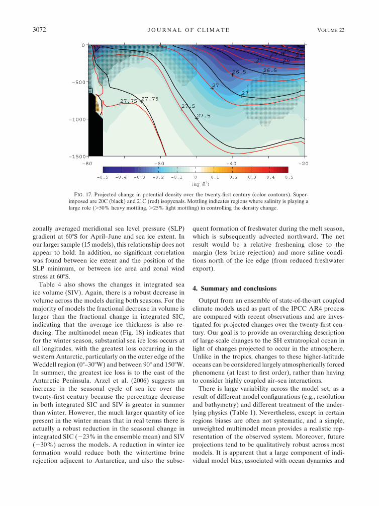
zonally averaged meridional sea level pressure (SLP)

gradient at 608S for April–June and sea ice extent. In

our larger sample (15 models), this relationship does not

appear to hold. In addition, no significant correlation

was found between ice extent and the position of the

SLP minimum, or between ice area and zonal wind

stress at 608S.

Table 4 also shows the changes in integrated sea

ice volume (SIV). Again, there is a robust decrease in

volume across the models during both seasons. For the

majority of models the fractional decrease in volume is

larger than the fractional change in integrated SIC,

indicating that the average ice thickness is also re-

ducing. The multimodel mean (Fig. 18) indicates that

for the winter season, substantial sea ice loss occurs at

all longitudes, with the greatest loss occurring in the

western Antarctic, particularly on the outer edge of the

Weddell region (08–308W) and between 908 and 1508W.

In summer, the greatest ice loss is to the east of the

Antarctic Peninsula. Arzel et al. (2006) suggests an

increase in the seasonal cycle of sea ice over the

twenty-first century because the percentage decrease

in both integrated SIC and SIV is greater in summer

than winter. However, the much larger quantity of ice

present in the winter means that in real terms there is

actually a robust reduction in the seasonal change in

integrated SIC (223% in the ensemble mean) and SIV

(230%) across the models. A reduction in winter ice

formation would reduce both the wintertime brine

rejection adjacent to Antarctica, and also the subse-

quent formation of freshwater during the melt season,

which is subsequently advected northward. The net

result would be a relative freshening close to the

margin (less brine rejection) and more saline condi-

tions north of the ice edge (from reduced freshwater

export).

4. Summary and conclusions

Output from an ensemble of state-of-the-art coupled

climate models used as part of the IPCC AR4 process

are compared with recent observations and are inves-

tigated for projected changes over the twenty-first cen-

tury. Our goal is to provide an overarching description

of large-scale changes to the SH extratropical ocean in

light of changes projected to occur in the atmosphere.

Unlike in the tropics, changes to these higher-latitude

oceans can be considered largely atmospherically forced

phenomena (at least to first order), rather than having

to consider highly coupled air–sea interactions.

There is large variability across the model set, as a

result of different model configurations (e.g., resolution

and bathymetry) and different treatment of the under-

lying physics (Table 1). Nevertheless, except in certain

regions biases are often not systematic, and a simple,

unweighted multimodel mean provides a realistic rep-

resentation of the observed system. Moreover, future

projections tend to be qualitatively robust across most

models. It is apparent that a large component of indi-

vidual model bias, associated with ocean dynamics and

FIG. 17. Projected change in potential density over the twenty-first century (color contours). Super-

imposed are 20C (black) and 21C (red) isopycnals. Mottling indicates regions where salinity is playing a

large role (.50% heavy mottling, .25% light mottling) in controlling the density change.

3072 J O U R N A L O F C L I M A T E VOLUME 22

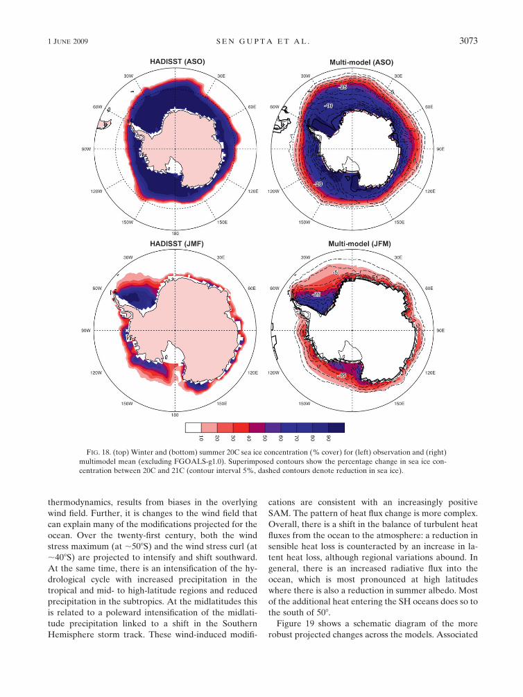
thermodynamics, results from biases in the overlying

wind field. Further, it is changes to the wind field that

can explain many of the modifications projected for the

ocean. Over the twenty-first century, both the wind

stress maximum (at ;508S) and the wind stress curl (at

;408S) are projected to intensify and shift southward.

At the same time, there is an intensification of the hy-

drological cycle with increased precipitation in the

tropical and mid- to high-latitude regions and reduced

precipitation in the subtropics. At the midlatitudes this

is related to a poleward intensification of the midlati-

tude precipitation linked to a shift in the Southern

Hemisphere storm track. These wind-induced modifi-

cations are consistent with an increasingly positive

SAM. The pattern of heat flux change is more complex.

Overall, there is a shift in the balance of turbulent heat

fluxes from the ocean to the atmosphere: a reduction in

sensible heat loss is counteracted by an increase in la-

tent heat loss, although regional variations abound. In

general, there is an increased radiative flux into the

ocean, which is most pronounced at high latitudes

where there is also a reduction in summer albedo. Most

of the additional heat entering the SH oceans does so to

the south of 508.

Figure 19 shows a schematic diagram of the more

robust projected changes across the models. Associated

FIG. 18. (top) Winter and (bottom) summer 20C sea ice concentration (% cover) for (left) observation and (right)

multimodel mean (excluding FGOALS-g1.0). Superimposed contours show the percentage change in sea ice con-

centration between 20C and 21C (contour interval 5%, dashed contours denote reduction in sea ice).

1 JUNE 2009 S E N G U P T A E T A L . 3073

with the southward intensification of the westerlies

there is a southward shift in the position of the ACC

core. As the ACC position is strongly affected by ba-

thymetry, its poleward shift is, in general, only about

half as large as the shift in the position of the wind stress.

Sen Gupta and England (2006) showed modest changes

in the barotropic flow of the ACC resulting from

changes in surface slope associated with high-frequency

SAM variability. At these short time scales they found

little change in flow associated with modifications to the

ocean density structure. For the long-term changes

discussed here, an increase in the meridional density

gradient is evident, which is consistent with an intensi-

fied ACC, driven in part by changes in surface Ekman

pumping and an associated spinup of the Deacon cir-

culation. At lower latitudes the maximum wind stress

curl also moves southward and intensifies, driving a

southward shift in the position of the subtropical gyres.

Only in the Atlantic basin, where the gyre core has a

more southerly mean position, is there evidence of a

robust increase in the depth-integrated flow of the

western boundary current. The overall southward shift of

the lateral circulation manifests itself as an increase in the

heat content of the water column, primarily between the

southern limb of the gyres and the core of the ACC. This

can be understood as a simple poleward displacement in

the temperature distribution in a region where the me-

ridional temperature gradients are large. The largest in-

crease in heat content occurs in the western Atlantic,

where, in addition to the circulation shift, there is in-

creased transport of warm water in the boundary flow.

Around the Antarctic margin enhanced heating from

above and below results in a melt back of the summer

and winter sea ice. As noted, this feeds back to the ra-

diative balance through a decrease in the surface al-

bedo. The seasonal cycling of sea ice acts as a factory for

the production of freshwater during the summer melt,

which is advected northward in the Ekman flow, and

saline water during wintertime ice formation and brine

rejection, which is exported to depth. A reduction in the

output of the factory by the reduced projected seasonal

cycle in ice volume, will therefore result in relatively

fresher conditions at high latitudes and saltier condi-

tions north of the ice edge. The latter process appears to

be completely offset by increased high-latitude precipi-

tation over the ocean and increased runoff from water

precipitated onto Antarctica. The surface freshening and

surface-intensified warming is consistent with a weaken-

ing of AABW formation, which in turn is manifest as a

warming signal close to the Antarctic margin that reaches

abyssal depths. Possible changes to the Antarctic ice sheet

are not accounted for in the IPCC AR4 models.

TABLE 4. Total Antarctic sea ice area (3 1014 m2) and volume (3 1014 m3) for summer [January–March (JFM)] and winter [August–

October (ASO)] seasons for 20C and 21C periods. Last column shows the percentage change over the twenty-first century in the

ASO – JFM difference in ice volume (i.e., a measure of the change in the seasonal cycle).

SIC Ice volume

Winter Summer Winter Summer

% change20C 21C 20C 21C 20C 21C 20C 21C

BCCR BCM2.0 13.3 7.7 2.1 0.6 13.3 5.3 2.1 0.4 257

CGCM3.1(T47) 20.0 18.0 4.9 3.0 12.5 12.0 3.2 2.1 6

CGCM3.1(T63) 24.4 18.4 7.0 2.5 13.8 10.7 4.2 1.2 21

CNRM-CM3 16.4 9.1 0.2 0.1 5.9 2.7 0.1 0.0 255

CSIRO Mk3.0 15.5 13.5 3.5 2.3 13.8 10.4 2.5 1.3 219

CSIRO Mk3.5 15.6 10.7 5.5 3.2 14.1 8.9 2.8 1.4 233

GISS-ER 11.8 9.2 1.2 0.7 10.7 7.7 1.5 0.8 224

FGOALS-g1.0 37.9 33.7 34.4 30.9 39.3 33.2 21.8 15.2 3

ECHAM4 12.4 9.3 1.8 1.0 8.0 5.7 1.6 1.1 228

INM-CM3.0 18.0 13.3 4.0 1.8 20.0 9.3 9.6 1.9 229

IPSL-CM4 14.7 10.0 0.9 0.2 10.0 5.3 1.6 0.4 242

MIROC3.2(hires) 14.8 8.1 0.9 0.0 12.7 5.5 0.6 0.0 254

MIROC3.2(medres) 11.2 8.8 0.8 0.4 5.8 4.1 0.5 0.1 225

ECHO-G 14.2 12.9 1.0 0.6 5.0 4.2 0.4 0.2 213

ECHAM5 13.2 8.3 2.6 1.0 9.1 4.9 2.2 0.6 237

MRI-CGCM2.3.2 18.5 17.3 4.3 1.9 11.8 9.0 2.0 0.5 212

CCSM3 19.6 16.5 5.1 1.6 23.7 18.2 7.8 2.1 1

PCM 14.3 10.7 3.7 2.7 11.2 7.3 3.9 2.3 231

HadCM3 11.2 13.8 2.5 1.5 15.6 4.0 1.5

HadGEM1 18.5 14.3 4.1 2.3 24.3 18.5 11.1 8.6 225

Multimodel mean 15.7 12.1 3.0 1.4 12.5 8.7 3.2 1.4 227

HadlSST (obs) 16.0 3.1

3074 J O U R N A L O F C L I M A T E VOLUME 22

While the poleward displacement of the circulation

can account for much of the temperature distribution

change, it explains less of the salinity changes. Instead,

surface changes are closely tied to the projected inten-

sification of the hydrological cycle and of Ekman

transport. This is consistent with the idea that inter-

model variability in SST is primarily driven by circula-

tion differences, while SSS variability is more related to

differences in freshwater fluxes (section 3b). Only in the

Atlantic is there a clear ‘‘circulation shift’’ signal in the

salinity as the Brazil–Malvinas confluence, which acts as

a barrier between salty subtropical and fresh Southern

Ocean water, moves southward. In the interior, south of

;408S, there is a subsurface increase in salinity that is

consistent with an intensified southward and upward

movement of relatively warm and saline CDW, associ-

ated with the more rapid Deacon cell overturning. This

is further enhanced by an injection of warm and saline

upper CDW entering from the Atlantic sector as a result

of the southward-intensified Brazil Current coupled

with the large meridional T–S gradients in the Brazil–

Malvinas confluence zone. At lower latitudes, primarily

in the Atlantic basin, there is a freshening signal at

depth, consistent with the projected slowdown of the

relatively salty NADW circulation. Throughout the

extratropics there is an increase in stratification driven

by a surface-intensified density reduction. At high lati-

tudes, in the upper ocean, this is primarily a result of

salinity changes, while at lower latitudes it is primarily

driven by temperature changes. This results in a large-

scale shoaling of the deep mixed layers at midlatitudes.

While this paper provides a consistent picture of fu-

ture changes, our analysis is essentially qualitative. A

more quantitative accounting of the various changes

must follow. For instance, by looking at changes along

density surfaces (e.g., Bindoff and McDougall 1994), the

contributions of heat and freshwater fluxes and pure

displacements of isopycnals via ‘‘heave’’ effects can be

FIG. 19. Schematic showing the robust changes in the SH extratropics.

1 JUNE 2009 S E N G U P T A E T A L . 3075

disentangled. This will be the subject of future work. We

also note two caveats in interpreting projections from

the AR4 models. First, the dynamics of the ocean cir-

culation still lacks certain physical processes. For ex-

ample, subgrid-scale eddies could be critical to realisti-

cally capturing future oceanic changes. Recent model-

ing and observational studies (e.g., Meredith and Hogg

2006) suggest that a proportion of the additional energy

entering the ocean via a momentum flux would energize

the eddy field rather than enhance the circumpolar

circulation. Second, recent evidence based on models

with more realistic depictions of the stratosphere (Son

et al. 2008) suggests that the poleward intensification of

the wind field may halt, or even reverse, at least during

austral summer as a result of the recovery of strato-

spheric ozone over Antarctica. Only a few of the AR4

models incorporate any form of ozone recovery (see

Fig. 4), and these tend to underestimate the resulting

modification in the atmospheric circulation compared

to models with more realistic stratospheres (Son et al.

2008). Thus, a definitive assessment of the changes in

certain oceanic properties may be beyond the scope of

the AR4 models. Nevertheless, it is encouraging to find

that despite sometimes large intermodel differences,

systematic biases are generally small and projected

changes are for the most part qualitatively robust.

Acknowledgments. We would like to acknowledge the

effort of all the groups involved in putting together the

CMIP3 repository. We would also like to thank Olivier

Arzel and our two anonymous reviewers for their useful

comments. This research was supported by the Aus-

tralian Research Council ARC.

REFERENCES

Alley, R. B., and Coauthors, 2007: Summary for Policymakers.

Cambridge University Press, 18 pp. [Available online at http://

www.ipcc.ch/pdf/assessment-report/ar4/wg1/ar4-wg1-spm.pdf.]

Alory, G., S. Wijffels, and G. Meyers, 2007: Observed temperature

trends in the Indian Ocean over 1960–1999 and associated

mechanisms. Geophys. Res. Lett., 34, L02606, doi:10.1029/

2006GL028044.

Aoki, S., N. L. Bindoff, and J. A. Church, 2005a: Interdecadal

water mass changes in the Southern Ocean between 308E

and 1608E. Geophys. Res. Lett., 32, L07607, doi:10.1029/

2004GL022220.

——, S. R. Rintoul, S. Ushio, S. Watanabe, and N. L. Bindoff,

2005b: Freshening of the Adelie Land Bottom Water

near 1408E. Geophys. Res. Lett., 32, L23601, doi:10.1029/

2005GL024246.

Arzel, O., T. Fichefet, and H. Goosse, 2006: Sea ice evolution over

the 20th and 21st centuries as simulated by current AOGCMs.

Ocean Modell., 12, 401–415.

Beckmann, A., and R. Doscher, 1997: A method for improved rep-

resentation of dense water spreading over topography in

geopotential-coordinate models. J. Phys. Oceanogr., 27, 581–591.

Bindoff, N. L., and T. J. McDougall, 1994: Diagnosing climate

change and ocean ventilation using hydrographic data.

J. Phys. Oceanogr., 24, 1137–1152.

——, and ——, 2000: Decadal changes along an Indian Ocean

section at 328S and their interpretation. J. Phys. Oceanogr., 30,

1207–1222.

Blanke, B., and P. Delecluse, 1993: Variability of the tropical At-

lantic Ocean simulated by a general circulation model with two

different mixed-layer physics. J. Phys. Oceanogr., 23, 1363–1388.

Bryan, K., and L. J. Lewis, 1979: A water mass model of the world

ocean. J. Geophys. Res., 84, 2503–2517.

Bryden, H. L., E. L. McDonagh, and B. A. King, 2003: Changes in

ocean water mass properties: Oscillations or trends. Science,

300, 2086–2088.

Cai, W., G. Shi, T. Cowan, D. Bi, and J. Ribbe, 2005: The response

of the Southern Annular Mode, the East Australian Current, and

the southern mid-latitude ocean circulation to global warming.

Geophys. Res. Lett., 32, L23706, doi:10.1029/2005GL024701.

Collins, W. D., and Coauthors, 2006: The Community Climate

System Model Version 3 (CCSM3). J. Climate, 19, 2122–2143.

Cunningham, S. A., S. G. Alderson, B. A. King, and M. A.

Brandon, 2003: Transport and variability of the Antarctic

Circumpolar Current in Drake Passage. J. Geophys. Res.,

108, 8084, doi:10.1029/2001JC001147.

Delworth, T. L., and Coauthors, 2006: GFDL’s CM2 global cou-

pled climate models. Part I: Formulation and simulation

characteristics. J. Climate, 19, 643–674.

Diansky, N. A., and E. M. Volodin, 2002: Simulation of present-

day climate with a coupled atmosphere–ocean general circu-

lation model. Izv. Atmos. Ocean. Phys., 38, 732–747.

Doos, K., and D. J. Webb, 1994: The Deacon Cell and the other

meridional cells of the Southern Ocean. J. Phys. Oceanogr.,

24, 429–442.

Flato, G. M., and W. D. Hibler III, 1990: On a simple sea-ice dy-

namics model for climate studies. Ann. Glaciol., 14, 72–77.

Friedlingstein, P., 2008: A steep road to climate stabilization.

Nature, 451, 297–298.

Furevik, T., M. Bentsen, H. Drange, I. K. T. Kindem, N. G.

Kvamst, and A. Sorteberg, 2003: Description and evaluation

of the Bergen climate model: ARPEGE coupled with

MICOM. Climate Dyn., 21, 27–51.

Fyfe, J. C., and O. A. Saenko, 2006: Simulated changes in the

extratropical Southern Hemisphere winds and currents.

Geophys. Res. Lett., 33, L06701, doi:10.1029/2005GL025332.

——, ——, K. Zickfeld, M. Eby, and A. J. Weaver, 2007: The role

of poleward-intensifying winds on Southern Ocean warming.

J. Climate, 20, 5391–5400.

Gent, P. R., and J. C. McWilliams, 1990: Isopycnal mixing in ocean

circulation models. J. Phys. Oceanogr., 20, 150–155.

——, W. G. Large, and F. O. Bryan, 2001: What sets the mean

transport through Drake Passage? J. Geophys. Res., 106,

2693–2712.

Gille, S. T., 2002: Warming of the Southern Ocean since the 1950s.

Science, 295, 1275–1277.

——, 2008: Decadal-scale temperature trends in the Southern

Hemisphere ocean. J. Climate, 21, 4749–4765.

Gillett, N. P., and D. W. J. Thompson, 2003: Simulation of recent

Southern Hemisphere climate change. Science, 302, 273–275.

Gordon, C., C. Cooper, C. A. Senior, H. Banks, J. M. Gregory,

T. C. Johns, J. F. B. Mitchell, and R. A. Wood, 2000: The

simulation of SST, sea ice extents and ocean heat transports in a

version of the Hadley Centre coupled model without flux

adjustments. Climate Dyn., 16, 147–168.

3076 J O U R N A L O F C L I M A T E VOLUME 22

Gordon, H. L., and Coauthors, 2002: The CSIRO Mk3 Climate

System Model. CSIRO Atmospheric Research Tech. Paper

60, 134 pp.

Griffies, S. M., 1998: The Gent–McWilliams skew flux. J. Phys.

Oceanogr., 28, 831–841.

——, and Coauthors, 2009: Coordinated Ocean-Ice Reference

Experiments (COREs). Ocean Modell., 26, 1–46.

Gruber, A., X. Su, M. Kanamitsu, and J. Schemm, 2000: The

comparison of two merged rain gauge–satellite precipitation

datasets. Bull. Amer. Meteor. Soc., 81, 2631–2644.

Hall, A., and M. Visbeck, 2002: Synchronous variability in the

Southern Hemisphere atmosphere, sea ice, and ocean result-

ing from the annular mode. J. Climate, 15, 3043–3057.

Harrison, D. E., 1989: On climatological monthly mean wind stress

and wind stress curl fields over the world ocean. J. Climate, 2,

57–70.

Hibler, W. D. III, 1979: A dynamic thermodynamic sea ice model.

J. Phys. Oceanogr., 9, 815–846.

Holland, M. M., and M. N. Raphael, 2006: Twentieth century

simulation of the Southern Hemisphere climate in coupled

models. Part II: Sea ice conditions and variability. Climate

Dyn., 26, 229–245.

Hunke, E. C., and J. K. Dukowicz, 1997: An elastic-viscous-plastic

model for sea ice dynamics. J. Phys. Oceanogr., 27, 1849–1867.

Johns, T. C., and Coauthors, 2003: Anthropogenic climate change

for 1860 to 2100 simulated with the HadCM3 model under

updated emissions scenarios. Climate Dyn., 20, 583–612.

——, and Coauthors, 2006: The New Hadley Centre Climate

Model (HadGEM1): Evaluation of coupled simulations.

J. Climate, 19, 1327–1353.

Johnson, G. C., S. Mecking, B. M. Sloyan, and S. E. Wijffels,

2007: Recent bottom water warming in the Pacific Ocean.

J. Climate, 20, 5365–5375.

Josey, S., C. Kent, and P. Taylor, 1999: New insights into the ocean

heat budget closure problem from analysis of the SOC air–sea

flux climatology. J. Climate, 12, 2856–2880.

Jungclaus, J. H., and Coauthors, 2006: Ocean circulation and

tropical variability in the coupled model ECHAM5/MPI-

OM. J. Climate, 19, 3952–3972.

K-1 model developers, 2004: K-1 coupled model (MIROC) de-

scription. K-1 Tech. Rep. 1, H. Hasumi and S. Emori, Eds.,

Center for Climate System Research, University of Tokyo,

34 pp.

Kim, S.-J., G. Flato, G. Boer, and N. McFarlane, 2002: A coupled

climate model simulation of the Last Glacial Maximum, Part 1:

Transient multi-decadal response. Climate Dyn., 19, 515–537.

Kraus, E. B., and J. S. Turner, 1967: A one-dimensional model of

the seasonal thermocline. II. The general theory and its con-

sequences. Tellus, 19, 98–106.

Kushner, P. J., I. M. Held, and T. L. Delworth, 2001: Southern

Hemisphere atmospheric circulation response to global

warming. J. Climate, 14, 2238–2249.

Large, W. G., and G. Danabasoglu, 2006: Attribution and impacts

of upper ocean biases in CCSM3. J. Climate, 19, 2325–2346.

——, J. C. McWilliams, and S. C. Doney, 1994: Oceanic vertical

mixing: A review and a model with a nonlocal boundary layer

parameterization. Rev. Geophys., 32, 363–403.

Law, R. M., R. J. Matear, and R. J. Francey, 2008: Comment on

‘‘saturation of the Southern Ocean CO2 sink due to recent

climate change.’’ Science, 319, 570.

Lefebvre, W., and H. Goosse, 2008: Analysis of the projected re-

gional sea-ice changes in the Southern Ocean during the

twenty-first century. Climate Dyn., 30, 59–76.

Le Quere, C., and Coauthors, 2007: Saturation of the Southern

Ocean CO2 sink due to recent climate change. Science, 316,

1735–1738.

——, and Coauthors, 2008: Response to comments on ‘‘saturation

of the Southern Ocean CO2 sink due to recent climate

change.’’ Science, 319, 570.

Lovenduski, N. S., N. Gruber, S. C. Doney, and I. D. Lima, 2007:

Enhanced CO2 outgassing in the Southern Ocean from

a positive phase of the Southern Annular Mode. Global

Biogeochem. Cycles, 21, GB2026, doi:10.1029/2006GB002900.

Marshall, G. J., P. A. Stott, J. Turner, W. M. Connolley, J. C. King,

and T. A. Lachlan-Cope, 2004: Causes of exceptional atmo-

spheric circulation changes in the Southern Hemisphere.

Geophys. Res. Lett., 31, L14205, doi:10.1029/2004GL019952.

Marti, O., and Coauthors, 2006: The new IPSL climate system

model: IPSL-CM4. Institut Pierre-Simon Laplace Note du

Pole de Modelisation 26, 84 pp.

Meehl, G. A., C. Covey, B. McAvaney, M. Latif, and R. J. Stouffer,

2005: Overview of the coupled model intercomparison pro-

ject. Bull. Amer. Meteor. Soc., 86, 89–93.

——, ——, T. Delworth, M. Latif, B. McAvaney, J. F. B. Mitchell,

R. J. Stouffer, and K. E. Taylor, 2007: The WCRP CMIP3

multimodel dataset: A new era in climate change research.

Bull. Amer. Meteor. Soc., 88, 1383–1394.

Mellor, G., and L. Kantha, 1989: An ice–ocean coupled model.

J. Geophys. Res., 94, 10 937–10 954.

Meredith, M. P., and A. M. Hogg, 2006: Circumpolar response of

Southern Ocean eddy activity to a change in the Southern

Annular Mode. Geophys. Res. Lett., 33, L16608, doi:10.1029/

2006GL026499.

Min, S.-K., S. Legutke, A. Hense, and W.-T. Kwon, 2005: Internal

variability in a 1000-yr control simulation with the coupled

climate model ECHO-G-II. El Nino Southern Oscillation and

North Atlantic Oscillation. Tellus, 57A, 622–640.

Nakano, H., and N. Suginohara, 2002: Effects of bottom boundary

layer parameterization on reproducing deep and bottom waters

in a world ocean model. J. Phys. Oceanogr., 32, 1209–1227.

Nakicenovic, N., and R. Swart, 2000: Emissions Scenarios.

Cambridge University Press, 570 pp.

Noh, Y., and H. J. Kim, 1999: Simulations of temperature and

turbulence structure of the oceanic boundary layer with

the improved near-surface process. J. Geophys. Res., 104,

15 621–15 634.

O’Farrell, S. P., 1998: Investigation of the dynamic sea-ice com-

ponent of a coupled atmosphere sea-ice general circulation

model. J. Geophys. Res., 103 (C8), 15 751–15 782.

Oke, P. R., and M. H. England, 2004: Oceanic response to changes

in the latitude of the Southern Hemisphere subpolar westerly

winds. J. Climate, 17, 1040–1054.

Olbers, D., D. Borowski, C. Volker, and J.-O. Wolff, 2004: The

dynamical balance, transport and circulation of the Antarctic

Circumpolar Current. Antarct. Sci., 16, 439–470.

Pacanowski, R. C., and S. G. H. Philander, 1981: Parameterization

of vertical mixing in numerical models of tropical oceans.

J. Phys. Oceanogr., 11, 1443–1451.

Parkinson, C. L., K. Y. Vinnikov, and D. J. Cavalieri, 2006:

Evaluation of the simulation of the annual cycle of Arctic and

Antarctic sea ice coverages by 11 major global climate models.

J. Geophys. Res., 111, C07012, doi:10.1029/2005JC003408.

Quartly, G. D., E. A. Kyte, M. A. Srokosz, and M. N. Tsimplis, 2007:

An intercomparison of global oceanic precipitation climatol-

ogies. J. Geophys. Res., 112, D10121, doi:10.1029/2006JD007810.

1 JUNE 2009 S E N G U P T A E T A L . 3077

Randall, D. A., and Coauthors, 2007: Climate models and their

evaluation. Climate Change 2007: The Physical Science Basis,

S. Solomon et al., Eds., Cambridge University Press, 589–662.

Ridgway, K. R., J. R. Dunn, and J. L. Wilkin, 2002: Ocean inter-

polation by four-dimensional weighted least squares—

Application to the waters around Australasia. J. Atmos.

Oceanic Technol., 19, 1357–1375.

Rintoul, S. R., 2007: Rapid freshening of Antarctic Bottom Water

formed in the Indian and Pacific Oceans. Geophys. Res. Lett.,

34, L06606, doi:10.1029/2006GL028550.

——, C. W. Hughes, and D. Olbers, 2001: Antarctic Circumpolar

Current system. Ocean Circulation and Climate, G. Siedler

et al., Eds., Academic Press, 271–302.

Roemmich, D., J. Gilson, R. Davis, P. Sutton, S. Wijffels, and

S. Riser, 2007: Decadal spinup of the South Pacific sub-

tropical gyre. J. Phys. Oceanogr., 37, 162–173.

Russell, G. L., J. R. Miller, and D. Rind, 1995: A coupled atmosphere-

ocean model for transient climate change studies. Atmos.–Ocean,

33, 683–730.

——, ——, ——, R. A. Ruedy, G. A. Schmidt, and S. Sheth, 2000:

Comparison of model and observed regional temperature

changes during the past 40 years. J. Geophys. Res., 105,

14 891–14 898.

Russell, J. L., K. W. Dixon, A. Gnanadesikan, R. J. Stouffer, and

J. R. Toggweiler, 2006a: The Southern Hemisphere west-

erlies in a warming world: Propping open the door to the

deep ocean. J. Climate, 19, 6382–6390.

——, R. J. Stouffer, and K. W. Dixon, 2006b: Intercomparison of

the Southern Ocean circulations in IPCC coupled model

control simulations. J. Climate, 19, 4560–4575.

Sabine, C., and Coauthors, 2004: The oceanic sink for anthropo-

genic CO2. Science, 305, 367–371.

Saenko, O., J. Fyfe, and M. England, 2005: On the response of the

oceanic wind-driven circulation to atmospheric CO2 increase.

Climate Dyn., 25, 415–426.

Salas Melia, D., 2002: A global coupled sea ice-ocean model.

Ocean Modell., 4, 137–172.

Santoso, A., M. H. England, and A. C. Hirst, 2006: Circumpolar

deep water circulation and variability in a coupled climate

model. J. Phys. Oceanogr., 36, 1523–1552.

Schmidt, G. A., and Coauthors, 2006: Present-day atmospheric

simulations using GISS ModelE: Comparison to in situ, sat-

ellite, and reanalysis data. J. Climate, 19, 153–192.

Semtner, A. J., Jr, 1976: A model for the thermodynamic growth

of sea-ice in numerical investigations of climate. J. Phys.

Oceanogr., 6, 379–389.

——, 1987: A numerical study of sea ice and ocean circulation in

the Arctic. J. Phys. Oceanogr., 17, 1077–1099.

Sen Gupta, A., and M. England, 2006: Coupled ocean–atmos-

phere–ice response to variations in the Southern Annular

Mode. J. Climate, 19, 4457–4486.

Serreze, M. C., M. M. Holland, and J. Stroeve, 2007: Perspectives on

the Arctic’s shrinking sea-ice cover. Science, 315, 1533–1536.

Simmonds, I., and K. Keay, 2000: Variability of Southern Hemi-

sphere extratropical cyclone behavior 1958–97. J. Climate, 13,

550–561.

——, ——, and E.-P. Lim, 2003: Synoptic activity in the seas

around Antarctica. Mon. Wea. Rev., 131, 272–288.

Son, S.-W., and Coauthors, 2008: The impact of stratospheric

ozone recovery on the Southern Hemisphere westerly jet.

Science, 320, 1486–1489.

Stammerjohn, S. E., D. G. Martinson, R. C. Smith, X. Yuan, and

D. Rind, 2008: Trends in Antarctic annual sea ice retreat and

advance and their relation to El Nino–Southern Oscillation

and Southern Annular Mode variability. J. Geophys. Res.,

113, C03S90, doi:10.1029/2007JC004269.

Taschetto, A. S., and I. Wainer, 2008: Reproducibility of South

American precipitation due to subtropical South Atlantic

SSTs. J. Climate, 21, 2835–2851.

Taylor, P. K., 2000: Intercomparison and Validation of Ocean–

Atmosphere Energy Flux Fields. WMO, 303 pp.

Thompson, D. W. J., and J. M. Wallace, 2000: Annular modes in

the extratropical circulation. Part I: Month-to-month varia-

bility. J. Climate, 13, 1000–1016.

——, and S. Solomon, 2002: Interpretation of recent Southern

Hemisphere climate change. Science, 296, 895–899.

——, J. M. Wallace, and G. C. Hegerl, 2000: Annular modes in the

extratropical circulation. Part II: Trends. J. Climate, 13,

1018–1036.

Toggweiler, J. R., and J. Russell, 2008: Ocean circulation in a

warming climate. Nature, 451, 286–288.

Uppala, S. M., and Coauthors, 2005: The ERA-40 Re-Analysis.

Quart. J. Roy. Meteor. Soc., 131, 2961–3012.

Valcke, S., L. Terray, and A. Piacentini, 2000: The OASIS Coupler

user guide version 2.4. CERFACE Tech. Rep. TR/CGMC/

00-10, 85 pp.

Visbeck, M., J. Marshall, T. Haine, and M. Spall, 1997: Specifica-

tion of eddy transfer coefficients in coarse resolution ocean

circulation models. J. Phys. Oceanogr., 27, 381–402.

Wainer, I., A. S. Taschetto, B. Otto-Bliesner, and E. Brady, 2004:

A numerical study of the impact of greenhouse gases on the South

Atlantic Ocean climatology. Climatic Change, 66, 163–189.

Washington, W. M., and Coauthors, 2000: Parallel climate model

(PCM) control and transient simulations. Climate Dyn., 16,

755–774.

Xie, P., and P. A. Arkin, 1997: Global precipitation: A 17-year

monthly analysis based on gauge observations, satellite esti-

mates, and numerical model outputs. Bull. Amer. Meteor.

Soc., 78, 2539–2558.

Yakovlev, N., 2003: Coupled model of ocean general circulation

and sea ice evolution in the Arctic Ocean. Izv. Atmos. Ocean.

Phys., 39, 355–368.

Yin, J. H., 2005: A consistent poleward shift of the storm tracks in

simulations of 21st century climate. Geophys. Res. Lett., 32,

L18701, doi:10.1029/2005GL023684.

Yu, Y., X. Zhang, and Y. Guo, 2004: Global coupled ocean-

atmosphere general circulation models in LASG/IAP. Adv.

Atmos. Sci., 21, 444–455.

Yukimoto, S., and Coauthors, 2001: The new Meteorological Re-

search Institute coupled GCM(MRICGCM 2). Model climate

and variability. Pap. Meteor. Geophys., 51, 47–88.

Zickfeld, K., J. C. Fyfe, M. Eby, and A. J. Weaver, 2008: Comment

on ‘‘saturation of the southern ocean CO2 sink due to recent

climate change.’’ Science, 319, 570b.

3078 J O U R N A L O F C L I M A T E VOLUME 22