Integration in a dynamical stochastic geometric framework

arX

iv:0

805.

3912

v1 [

mat

h.PR

] 2

6 M

ay 2

008

1

A set–valued framework for birth–and–growth

process

Giacomo Aletti, Enea G. Bongiorno, Vincenzo Capasso

Department of Mathematics, University of Milan,via Saldini 50, 10133 Milan [email protected]

[email protected]

[email protected]

Summary. We propose a set–valued framework for the well–posedness of birth–and–growth process. Our birth–and–growth model is rigorously defined as a suitablecombination, involving Minkowski sum and Aumann integral, of two very generalset–valued processes representing nucleation and growth respectively. The simplicityof the used geometrical approach leads us to avoid problems arising by an analyticaldefinition of the front growth such as boundary regularities. In this framework,growth is generally anisotropic and, according to a mesoscale point of view, it is notlocal, i.e. for a fixed time instant, growth is the same at each space point.

Introduction

Nucleation and growth processes arise in several natural and technological applica-tions (cf. [7, 8] and the references therein) such as, for example, solidification andphase–transition of materials, semiconductor crystal growth, biomineralization, andDNA replication (cf., e.g., [15]).

A birth–and–growth process is a RaCS family given by Θt =S

n:Tn≤tΘt

Tn(Xn),

for t ∈ R+, where ΘtTn

(Xn) is the RaCS obtained as the evolution up to time t > Tn

of the germ born at (random) time Tn in (random) location Xn, according to somegrowth model.An analytical approach is often used to model birth–and–growth process, in par-ticular it is assumed that the growth is driven according to a non–negative normalvelocity, i.e. for every instant t, a border point x ∈ ∂Θt “grows” along the outwardnormal unit (e.g. [3–6, 11, 13, 22]). Thus, growth is pointwise isotropic; i.e. given apoint belonging ∂Θt, the growth rate is independently from outward normal direc-tion. Note that, the existence of the outward normal vector imposes a regularitycondition on ∂Θt and also on the nucleation process (it cannot be a point process).

This paper is an attempt to offer an original alternative approach based on apurely geometric stochastic point of view, in order to avoid regularity assumptionsdescribing birth–and–growth process. In particular, Minkowski sum (already em-ployed in [19] to describe self–similar growth for a single convex germ) and Aumann

http://arXiv.org/abs/0805.3912v1

2 A set–valued framework for birth–and–growth process

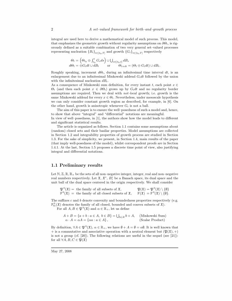
integral are used here to derive a mathematical model of such process. This model,that emphasizes the geometric growth without regularity assumptions on ∂Θt, is rig-orously defined as a suitable combination of two very general set–valued processesrepresenting nucleation Btt∈[t0,T ] and growth Gtt∈[t0,T ] respectively

Θt =“Θt0 ⊕

R t

t0Gsds

”∪S

s∈[t0,t] dBs

dΘt = ⊕Gtdt ∪ dBt or Θt+dt = (Θt ⊕ Gtdt) ∪ dBt.

Roughly speaking, increment dΘt, during an infinitesimal time interval dt, is anenlargement due to an infinitesimal Minkowski addend Gtdt followed by the unionwith the infinitesimal nucleation dBt.As a consequence of Minkowski sum definition, for every instant t, each point x ∈Θt (and then each point x ∈ ∂Θt) grows up by Gtdt and no regularity borderassumptions are required. Then we deal with not–local growth; i.e. growth is thesame Minkowski addend for every x ∈ Θt. Nevertheless, under mesoscale hypothesiswe can only consider constant growth region as described, for example, in [6]. Onthe other hand, growth is anisotropic whenever Gt is not a ball.

The aim of this paper is to ensure the well–posedness of such a model and, hence,to show that above “integral” and “differential” notations are meaningful.In view of well–posedness, in [1], the authors show how the model leads to differentand significant statistical results.

The article is organized as follows. Section 1.1 contains some assumptions about(random) closed sets and their basilar properties. Model assumptions are collectedin Section 1.2 and integrability properties of growth process are studied in Section1.3. For the sake of simplicity, we present, in Section 1.4, main results of the paper(that imply well-posedness of the model), whilst correspondent proofs are in Section1.4.1. At the last, Section 1.5 proposes a discrete time point of view, also justifyingintegral and differential notations.

1.1 Preliminary results

Let N, Z, R, R+ be the sets of all non–negative integer, integer, real and non–negativereal numbers respectively. Let X, X∗, B∗

1 be a Banach space, its dual space and theunit ball of the dual space centered in the origin respectively. We shall consider

P 0(X) = the family of all subsets of X, P(X) = P 0(X) \ ∅F

0(X) = the family of all closed subsets of X, F(X) = F0(X) \ ∅.

The suffixes c and b denote convexity and boundedness properties respectively (e.g.F

0bc(X) denotes the family of all closed, bounded and convex subsets of X).

For all A, B ∈ P 0(X) and α ∈ R+, let us define

A + B = a + b : a ∈ A, b ∈ B =S

b∈Bb + A, (Minkowski Sum)

α · A = αA = αa : a ∈ A , (Scalar Product)

By definition, ∀A ∈ P 0(X), α ∈ R+, we have ∅+ A = ∅ = α∅. It is well known that+ is a commutative and associative operation with a neutral element but (P(X), +)is not a group (cf. [20]). The following relations are useful in the sequel (see [21]):for all ∀A, B, C ∈ P(X)

May 27, 2008


3

(A ∪ B) + C = (A + C) ∪ (B + C)if B ⊆ C, A + B ⊆ A + C

In the following, we shall work with closed sets. In general, if A, B ∈ F0(X) then

A + B does not belong to F0(X) (e.g., in X = R let A = n + 1/n : n > 1 and

B = Z, then 1/n = (n + 1/n) + (−n) ⊂ A + B and 1/n ↓ 0, but 0 6∈ A + B). Inview of this fact, we define A ⊕ B = A + B where (·) denotes the closure in X.

For any A, B ∈ F(X) the Hausdorff distance (or metric) is defined by

δH(A, B) = max

supa∈A

infb∈B

‖a − b‖X

, supb∈B

infa∈A

‖a − b‖X

ff.

For all (x∗, A) ∈ B∗1 × F(X), the support function is defined by s(x∗, A) =

supa∈A x∗(a). It can be proved (cf. [2,14]) that for each A,B ∈ Fbc(X),

δH(A, B) = sup |s(x∗, A) − s(x∗, B)| : x∗ ∈ B∗1 . (1.1)

Let (Ω, F) be a measurable space with F complete with respect to some σ-finitemeasure, let X : Ω → P 0(X) be a set–valued map, and

D(X) = ω ∈ Ω : X(ω) 6= ∅ be the domain of X

X−1(A) = ω ∈ Ω : X(ω) ∩ A 6= ∅ , A ⊂ X, be the inverse image of X

Roughly speaking, X−1(A) is the set of all ω such that X(ω) hits set A.Different definitions of measurability for set–valued functions are developed over

the years by several authors (cf. [2, 10, 16, 17] and reference therein). Here, X ismeasurable if, for each O, open subset of X, X−1(O) ∈ F.

Proposition 1.1.1 (See [17]) X : Ω → P 0(X) is a measurable set–valued map ifand only if D(X) ∈ F, and ω 7→ d(x,X(ω)) is a measurable function of ω ∈ D(X)for each x ∈ X.

From now on, U [Ω, F, µ; F(X)] (= U [Ω; F(X)] if the measure µ is clear) denotes thefamily of F(X)–valued measurable maps (analogous notation holds whenever F(X)is replaced by another family of subsets of X).

Let (Ω, F, P) be a complete probability space and let X ∈ U [Ω, F, P;F(X)], thenX is a RaCS.It can be proved (see [18]) that, if X, X1, X2 are RaCS and if ξ is a measurable real–valued function, then X1 ⊕ X2, X1 ⊖ X2, ξX and (Int X)C are RaCS. Moreover, ifXnn∈N

is a sequence of RaCS then X =S

n∈NXn is so.

Let (Ω, F, µ) be a finite measure space (although most of the results are valid forσ-finite measures space). The Aumann integral of X ∈ U [Ω, F, µ; F(X)] is defined by

Z

Ω

Xdµ =

Z

Ω

xdµ : x ∈ SX

ff,

where SX =˘x ∈ L1[Ω; X] : x ∈ X µ − a.e.

¯and

RΩ

xdµ is the usual Bochner in-tegral in L1[Ω; X]. Moreover,

RA

Xdµ =˘R

Axdµ : x ∈ SX

¯for A ∈ F. If µ is a

probability measure, we denote the Aumann integral by EX =R

ΩXdµ.

Let X ∈ U [Ω, F, µ; F(X)], it is integrably bounded, and we shall write X ∈L1[Ω, F, µ; F(X)] = L1[Ω; F(X)], if ‖X‖

h∈ L1[Ω, F, µ; R].

May 27, 2008


1.2 Model assumptions

Let us consider

Θt =“Θt0 ⊕

R t

t0Gsds

”∪S

s∈[t0,t] dBs

dΘt = ⊕Gtdt ∪ dBt or Θt+dt = (Θt ⊕ Gtdt) ∪ dBt.(1.2)

In fact, above equation is not a definition since, for example, problems arise handlingnon–countable union of (random) closed sets. The well–posedness of (1.2) and hencethe existence of such a process are the main purpose of this paper.From now on, let us consider the following assumptions.

(A-0) - (X, ‖·‖X) is a reflexive Banach space with separable dual space (X∗, ‖·‖

X∗),(then, X is separable too, see [12, Lemma II.3.16 p. 65]).

- [t0, T ] ⊂ R is the time observation interval (or time interval),

-“Ω, F, Ftt∈[t0,T ] , P

”is a filtered probability space, where the filtration

Ftt∈[t0,T ] is assumed to have the usual properties.

(Nucleation Process). B = B(ω, t) = Bt : ω ∈ Ω, t ∈ [t0, T ] is a process with non–empty closed values, i.e. B : Ω × [t0, T ] → F(X) such that

(A-1) B(·, t) ∈ U [Ω, Ft, P; F(X)], for every t ∈ [t0, T ], i.e. Bt is an adapted (toFtt∈[t0,T ]) process.

(A-2) Bt is increasing: for every t, s ∈ [t0, T ] with s < t, Bs ⊆ Bt.

(Growth Process). G = Gt = G(ω, t) : ω ∈ Ω, t ∈ [t0, T ] is a process with non–empty closed values, i.e. G : Ω × [t0, T ] → F(X) such that

(A-3) for every ω ∈ Ω and t ∈ [t0, T ], 0 ∈ G(ω, t).

(A-4) for every ω ∈ Ω and t ∈ [t0, T ], G(ω, t) is convex, i.e. G : Ω × [t0, T ] → Fc(X).

(A-5) there exists K ∈ Fb(X) such that G(ω, t) ⊆ K for every t ∈ [t0, T ] and ω ∈ Ω.

As a consequence, G(ω, t) ∈ Fb(X) and ‖G(ω, t)‖h≤ ‖K‖

h, ∀(ω, t) ∈ Ω × [t0, T ].

In order to establish the well–posedness of integralR t

t0Gsds in (1.2), let us con-

sider a suitable hypothesis of measurability for G (analogously to what is).A F(X)–valued process G = Gtt∈[t0,T ] has left continuous trajectories on [t0, T ] if,

for every t ∈ [t0, T ] with t < t,

limt→t

δH

`G(ω, t), G(ω, t)

´= 0, a.s.

The σ-algebra on Ω × [t0, T ] generated by the processes Gtt∈[t0,T ] with left con-tinuous trajectories on [t0, T ], is called the previsible (or predictable) σ-algebra andit is denoted by P .

Proposition 1.2.1 The previsible σ-algebra is also generated by the collection ofrandom sets A × t0 where A ∈ Ft0 and A × (s, t] where A ∈ Fs and (s, t] ⊂ [t0, T ].

May 27, 2008


5

Proof. Let the σ-algebra generated by the above collection of sets be denoted byP ′. We shall show P = P ′. Let G be a left continuous process and let α = (T − t0),consider for n ∈ N

Gn(ω, t) =

8>>><>>>:

G(ω, t0), t = t0

G`ω, t0 + kα

2n

´,

`t0 + kα

2n

´< t ≤

“t0 + (k+1)α

2n

”

k ∈ 0, . . . , (2n − 1)

It is clear that Gn is P ′-measurable, since G is adapted. As G is left continuous,the above sequence of left-continuous processes converges pointwise (with respect toδH) to G when n tends to infinity, so G is P ′-measurable, thus P ⊆ P ′.Conversely consider A × (s, t] ∈ P ′ with (s, t] ⊂ [t0, T ] and A ∈ Fs. Let b ∈ X \ 0and G be the process

G(ω, v) =

b, v ∈ (s, t], ω ∈ A0, otherwise

this function is adapted and left continuous, hence P ′ ⊆ P .

Then let us consider the following assumption.

(A-6) G is P-measurable.

1.3 Growth process properties

Theorem 1.3.2 is the main result in this section. It shows that ω 7→R b

aG(ω, τ )dτ is

a RaCS with non–empty bounded convex values. This is the first step in order toobtain well–posedness of (1.2).

Proposition 1.3.1 Suppose (A-3), . . . , (A-6), and let µλ be the Lebesgue measureon [t0, T ], then

• G(ω, ·) ∈ Uˆ[t0, T ],B[t0,T ], µλ; Fbc(X)

˜for every ω ∈ Ω.

• G(·, t) ∈ U [Ω, eFt− , P; Fbc(X)] for each t ∈ [t0, T ], where eFt− is the so called

history σ-algebra i.e. eFt− = σ (Fs : 0 ≤ s < t) ⊆ F.• G ∈ L1[[t0, T ],B[t0,T ], µλ; Fbc(X)] ∩ L1[Ω, F, P; Fbc(X)]

Proof. Assumptions (A-3) and (A-4) imply that G is non–empty and convex. Mea-surability and integrability properties are consequence of (A-6) and (A-5) respec-tively.

Theorem 1.3.2 Suppose (A-3), . . . , (A-6). For every a, b ∈ [t0, T ], the integralR b

aG(ω, τ )dτ is non–empty and the set–valued map

Ga,b : Ω → P(X)

ω 7→R b

aG(ω, τ )dτ

is measurable. Moreover, Ga,b is a non–empty, bounded convex RaCS.

May 27, 2008


In order to prove Theorem 1.3.2, consider following properties for real processes.A real–valued process X = Xtt∈[t0,T ] is predictable with respect to filtrationFtt∈R+

, if it is measurable with respect to the predictable σ-algebra PR, i.e. the

σ-algebra generated by the collection of random sets A × 0 where A ∈ F0 andA × (s, t] where A ∈ Fs.

Proposition 1.3.3 (See [9, Propositions 2.30, 2.32 and 2.41]) Let X = Xtt∈[t0,T ]

be a predictable real–valued process, then X is (F ⊗ B[t0,T ],BR)-measurable. Further,for every ω ∈ Ω, the trajectory X(ω, ·) : [t0, T ] → R is (B[t0,T ],BR)-measurable .

Lemma 1.3.4 Let x∗ be an element of the unit ball in the dual space B∗1 , then

G 7→ s(x∗, G) is a measurable map.

Proof. By definition s(x∗, G) = sup x∗(g) : g ∈ G. Since X is separable (A-0),there exists gnn∈N

⊂ G such that G = gn. Then, for every x∗ ∈ B∗1 we have

s(x∗, G) = supg∈G

x∗(g) = supn∈N

x∗(gn).

Since x∗ is a continuous map then, s(x∗, ·) is measurable.

Proof of Theorem 1.3.2. At first, we prove that Ga,b is a measurable map.

From Proposition 1.3.1, integral Ga,b =R b

aG(ω, τ )dτ is well defined for all ω ∈ Ω.

Assumption (A-3) implies 0 ∈ Ga,b(ω) 6= ∅ for every ω ∈ Ω. Hence, the domain ofGa,b is the whole Ω for all a, b ∈ [t0, T ]

D (Ga,b) = ω ∈ Ω : Ga,b 6= ∅ = Ω ∈ F.

Thus, by Proposition 1.1.1 and for a fixed couple a, b ∈ [t0, T ], Ga,b is (weakly)measurable if and only if, for every x ∈ X, the map

ω 7→ d

„x,

Z b

a

G(ω, τ )dτ

«= δH

„x,

Z b

a

G(ω, τ )dτ

«(1.3)

is measurable. Equation (1.1) guarantees that (1.3) is measurable if and only if, forevery x ∈ X, the map

ω 7→ supx∗∈B∗

1

˛˛s(x∗, x) − s

„x∗,

Z b

a

G(ω, τ )dτ

«˛˛

is measurable. The above expression can be computed on a countable family densein B∗

1 (note that such family exists since X∗ is assumed separable (A-0)):

ω 7→ supn∈N

˛˛s(x∗

i , x) − s

„x∗

i ,

Z b

a

G(ω, τ )dτ

«˛˛ .

It can be proved ( [18, Theorem 2.1.12 p. 46]) that

s

„x∗,

Z b

a

G(ω, τ )dτ

«=

Z b

a

s (x∗, G(ω, τ )) dτ, ∀x∗ ∈ B∗1

May 27, 2008


7

and therefore, since s(x∗i , x) is a constant, Ga,b is measurable if, for every x∗ ∈

x∗i i∈N

, the following map

(Ω, F) → (R,BR)

ω 7→R b

as (x∗, G(ω, τ )) dτ

(1.4)

is measurable. Note that s(x∗, G(·, ·)), as a map from Ω × [t0, T ] to R, is predictablesince it is the composition of a predictable map (A-6) with a measurable one (seeLemma 1.3.4):

s (x∗, G(·, ·)) : (Ω × [t0, T ],P) → (F(X), σf ) → (R,BR)(ω, t) 7→ G(ω, t) 7→ s (x∗, G(ω, t))

thus, by Proposition 1.3.3, it is a P-measurable map and hence (1.4) is a measurablemap.

In view of the first part, it remains to prove that Ga,b is a bounded convex setfor a.e. ω ∈ Ω. Since X is reflexive (A-0), by Proposition 1.3.1 we have that Ga,b isclosed ( [18, Theorem 2.2.3]). Further, Ga,b is also convex (see [18, Theorem 2.1.5and Corollary 2.1.6]).To conclude the proof, it is sufficient to show that Ga,b is included in a bounded set:

Z b

a

G(ω, τ )dτ =

Z b

a

g(ω, τ )dτ : g(ω, ·) ∈ G(ω, ·) ⊆ K

ff

⊆

Z b

a

kdτ : k ∈ K

ff= (b − a)k : k ∈ K = (b − a)K.

1.4 Geometric Random Process

For the sake of simplicity, let us present the main results which proofs will be givenin Section 1.4.1.Let us assume conditions from (A-0) to (A-6). For every t ∈ [t0, T ] ⊂ R, n ∈ N andΠ = (ti)

n

i=0 partition of [t0, t], let us define

sΠ(t) =

„Bt0 ⊕

Z t

t0

G(τ )dτ

«∪

n[

i=1

„∆Bti

⊕

Z t

ti

G(τ )dτ

«(1.5)

SΠ(t) =

„Bt0 ⊕

Z t

t0

G(τ )dτ

«∪

n[

i=1

∆Bti

⊕

Z t

ti−1

G(τ )dτ

!(1.6)

where ∆Bti= Bti

\ Boti−1

(Boti−1

denotes the interior set of Bti−1) and where the

integral is in the Aumann sense with respect to the Lebesgue measure dτ = dµλ.We write sΠ and SΠ instead of sΠ(t) and SΠ(t) when the dependence on t is clear.

Proposition 1.4.1 guarantees that both sΠ and SΠ are well defined RaCS, fur-ther, Proposition 1.4.3 shows sΠ ⊆ SΠ as a consequence of different time intervalsintegration: if the time interval integration of G increases then the integral of G doesnot decrease with respect to set-inclusion (Lemma 1.4.2). Proposition 1.4.4 meansthat sΠ (SΠ) increases (decreases) whenever a refinement of Π is considered.

May 27, 2008


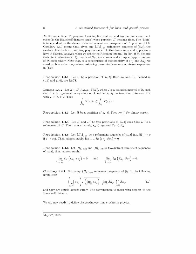
At the same time, Proposition 1.4.5 implies that sΠ and SΠ become closer eachother (in the Hausdorff distance sense) when partition Π becomes finer. The “limit”is independent on the choice of the refinement as consequence of Proposition 1.4.6.Corollary 1.4.7 means that, given any Πjj∈N

refinement sequence of [t0, t], therandom closed sets sΠj

and SΠjplay the same role that lower sums and upper sums

have in classical analysis when we define the Riemann integral. In fact, if Θt denotestheir limit value (see (1.7)), sΠj

and SΠjare a lower and an upper approximation

of Θt respectively. Note that, as a consequence of monotonicity of sΠjand SΠj

, weavoid problems that may arise considering uncountable unions in integral expressionin (1.2).

Proposition 1.4.1 Let Π be a partition of [t0, t]. Both sΠ and SΠ , defined in(1.5) and (1.6), are RaCS.

Lemma 1.4.2 Let X ∈ L1[I,F, µλ; F(X)], where I is a bounded interval of R, suchthat 0 ∈ X µλ-almost everywhere on I and let I1, I2 be two other intervals of R

with I1 ⊂ I2 ⊂ I . Then Z

I1

X(τ )dτ ⊆

Z

I2

X(τ )dτ.

Proposition 1.4.3 Let Π be a partition of [t0, t]. Then sΠ ⊆ SΠ almost surely.

Proposition 1.4.4 Let Π and Π ′ be two partitions of [t0, t] such that Π ′ is arefinement of Π . Then, almost surely, sΠ ⊆ sΠ′ and SΠ′ ⊆ SΠ .

Proposition 1.4.5 Let Πjj∈Nbe a refinement sequence of [t0, t] (i.e. |Πj | → 0

if j → ∞). Then, almost surely, limj→∞ δH

`sΠj

, SΠj

´= 0.

Proposition 1.4.6 Let Πjj∈Nand Π ′

ll∈Nbe two distinct refinement sequences

of [t0, t], then, almost surely,

limj → ∞

l → ∞

δH

“sΠj

, sΠ′l

”= 0 and lim

j → ∞

l → ∞

δH

“SΠj

, SΠ′l

”= 0.

Corollary 1.4.7 For every Πjj∈Nrefinement sequence of [t0, t], the following

limits exist 0@[

j∈N

sΠj

1A,

„lim

j→∞sΠj

«, lim

j→∞SΠj

,\

j∈N

SΠj, (1.7)

and they are equals almost surely. The convergences is taken with respect to theHausdorff distance.

We are now ready to define the continuous time stochastic process.

May 27, 2008


9

Definition 1.4.8 Assume (A-0), . . . , (A-6). For every t ∈ [t0, T ], let Πjj∈Nbe

a refinement sequence of the time interval [t0, t] and let Θt be the RaCS defined by

0@[

j∈N

sΠj(t)

1A =

„lim

j→∞sΠj

(t)

«= Θt = lim

j→∞SΠj

(t) =\

j∈N

SΠj(t),

then, the family Θ = Θt : t ∈ [t0, T ] is called geometric random process G-RaP(on [t0, T ]).

Theorem 1.4.9 Let Θ be a G-RaP on [t0, T ], then Θ is a non-decreasing processwith respect to the set inclusion, i.e.

P (Θs ⊆ Θt, ∀t0 ≤ s < t ≤ T ) = 1.

Moreover, Θ is adapted with respect to filtration Ftt∈[t0,T ].

Remark 1.4.10 We want to point out that, assumptions we considered on Btand Gt are so general, that a wide family of classical random sets and evolu-tion processes can be described (for example, Boolean model is a birth–and–growthprocess with “null growth”).

1.4.1 Proofs of Propositions in Section 1.4

Proof of Proposition 1.4.1. For every i ∈ 0, . . . , n,R t

ti−1G(τ )dτ is a RaCS

(Theorem 1.3.2). Thus, measurability Assumption (A-1) on B guarantees that, for

every ti ∈ Π , Bti, ∆Bti

,“∆Bti

⊕R t

tiG(τ )dτ

”, and hence sΠ and SΠ are RaCS.

Proof of Lemma 1.4.2. Let y ∈“R

I1X(τ )dτ

”, then there exists x ∈ SX , for

which y =“R

I1x(τ )dτ

”. Let us define on I2(⊃ I1)

x′(τ ) =

x(τ ), τ ∈ I1

0, τ ∈ I2 \ I1

then x′ ∈ SX and y =“R

I2x′(τ )dτ

”∈“R

I2X(τ )dτ

”.

Proof of Proposition 1.4.3. Thesis is a consequence of Lemma 1.4.2 and

Minkowski addition properties, in fact“R t

ti−1G(τ )dτ

”⊆“R t

tiG(τ )dτ

”implies

sΠ ⊆ SΠ .

Proof of Proposition 1.4.4. Let Π ′ be a refinement of partition Π of [t0, t], i.e.Π ⊂ Π ′. We prove that sΠ ⊆ sΠ′ (SΠ′ ⊆ SΠ is analogous). It is sufficient to showthe thesis only for Π ′ = Π ∪

˘t¯

where Π = t0, . . . , tn with t0 < . . . < tn = t andt ∈ (t0, t). Let i ∈ 0, . . . , (n − 1) be such that ti ≤ t ≤ ti+1 then

sΠ =

„Bt0 ⊕

Z t

t0

G(τ )dτ

«∪

n[

j = 1

j 6= i + 1

∆Btj

⊕

Z t

tj

G(τ )dτ

!∪

"`Bti+1

\ Boti

´⊕

Z t

ti+1

G(τ )dτ

#

May 27, 2008


and

sΠ′ =

„Bt0 ⊕

Z t

t0

G(τ )dτ

«∪

n[

j = 1

j 6= i + 1

∆Btj

⊕

Z t

tj

G(τ )dτ

!∪

»`Bt \ Bo

ti

´⊕

Z t

t

G(τ )dτ

–∪

"`Bti+1

\ Bot

´⊕

Z t

ti+1

G(τ )dτ

#

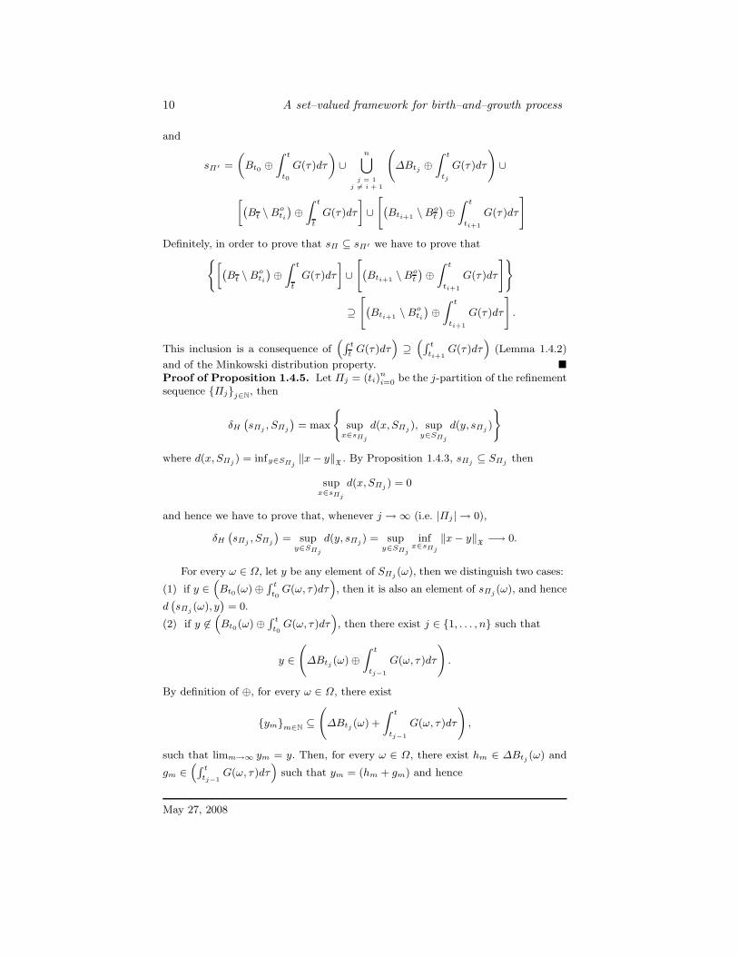
Definitely, in order to prove that sΠ ⊆ sΠ′ we have to prove that(»`

Bt \ Boti

´⊕

Z t

t

G(τ )dτ

–∪

"`Bti+1

\ Bot

´⊕

Z t

ti+1

G(τ )dτ

#)

⊇

"`Bti+1

\ Boti

´⊕

Z t

ti+1

G(τ )dτ

#.

This inclusion is a consequence of“R t

tG(τ )dτ

”⊇“R t

ti+1G(τ )dτ

”(Lemma 1.4.2)

and of the Minkowski distribution property.

Proof of Proposition 1.4.5. Let Πj = (ti)n

i=0 be the j-partition of the refinementsequence Πjj∈N

, then

δH

`sΠj

, SΠj

´= max

(sup

x∈sΠj

d(x,SΠj), sup

y∈SΠj

d(y, sΠj)

)

where d(x,SΠj) = infy∈SΠj

‖x − y‖X. By Proposition 1.4.3, sΠj

⊆ SΠjthen

supx∈sΠj

d(x,SΠj) = 0

and hence we have to prove that, whenever j → ∞ (i.e. |Πj | → 0),

δH

`sΠj

, SΠj

´= sup

y∈SΠj

d(y, sΠj) = sup

y∈SΠj

infx∈sΠj

‖x − y‖X−→ 0.

For every ω ∈ Ω, let y be any element of SΠj(ω), then we distinguish two cases:

(1) if y ∈“Bt0(ω) ⊕

R t

t0G(ω, τ )dτ

”, then it is also an element of sΠj

(ω), and hence

d`sΠj

(ω), y´

= 0.

(2) if y 6∈“Bt0(ω) ⊕

R t

t0G(ω, τ )dτ

”, then there exist j ∈ 1, . . . , n such that

y ∈

∆Btj

(ω) ⊕

Z t

tj−1

G(ω, τ )dτ

!.

By definition of ⊕, for every ω ∈ Ω, there exist

ymm∈N

⊆

∆Btj

(ω) +

Z t

tj−1

G(ω, τ )dτ

!,

such that limm→∞ ym = y. Then, for every ω ∈ Ω, there exist hm ∈ ∆Btj(ω) and

gm ∈“R t

tj−1G(ω, τ )dτ

”such that ym = (hm + gm) and hence

May 27, 2008


11

y = limm→∞

(hm + gm) = limm→∞

ym

where the convergence is in the Banach norm, then let m ∈ N be such that‖y − ym‖

X< |Πj |, for every m > m.

Note that, for every ω ∈ Ω and m ∈ N, by Aumann integral definition, thereexists a selection cgm(·) of G(ω, ·) (i.e. cgm(t) ∈ G(ω, t) µλ-a.e.) such that

gm =

Z t

tj−1

cgm(τ )dτ and ym = hm +

Z t

tj−1

cgm(τ )dτ.

For every ω ∈ Ω, let us consider

xm = hm +

Z t

tj

cgm(τ )dτ

then xm ∈ sΠj(ω) for all m ∈ N. Moreover, the following chain of inequalities hold,

for all m > m and ω ∈ Ω,

infx′∈sΠj

‚‚x′ − y‚‚

X≤ ‖xm − y‖

X≤ ‖xm − ym‖

X+ ‖ym − y‖

X

≤

‚‚‚‚‚

Z tj

tj−1

cgm(τ )dτ

‚‚‚‚‚X

+ |Πj | ≤

Z tj

tj−1

‖cgm(τ )‖X

dτ + |Πj |

≤

Z tj

tj−1

‖G(τ )‖h

dτ + |Πj | ≤ |tj − tj−1| ‖K‖h

+ |Πj |

≤ |Πj |`‖K‖h + 1

´ j→∞−→ 0

since ‖K‖h is a positive constant. By the arbitrariness of y ∈ SΠj(ω) we obtain the

thesis.

Proof of Proposition 1.4.6. Let Πj and Π ′l be two partitions of the two distinct

refinement sequences Πjj∈Nand Π ′

ll∈Nof [t0, t]. Let Π ′′ = Πj ∪ Π ′

l be the

refinement of both Πj and Π ′l . Then Proposition 1.4.4 and Proposition 1.4.3 imply

that sΠj⊆ sΠ′′ ⊆ SΠ′′ ⊆ SΠ′

l. Therefore sΠj

⊆ SΠ′l

for every j, l ∈ N. Then

0@[

j∈N

sΠj

1A ⊆

\

l∈N

SΠ′l.

Analogously [

l∈N

sΠ′l

!⊆\

j∈N

SΠj.

Proposition 1.4.5 concludes the proof.

In order to prove Theorem 1.4.9, let us consider the following Lemma.

Lemma 1.4.11 Let s, t ∈ [t0, T ] with t0 < s < t and let Πs and Πt be twopartition of [t0, s] and [t0, t] respectively, such that Πs ⊂ Πt. Then

sΠs(s) ⊆ sΠt(t) and SΠs(s) ⊆ SΠt(t).

May 27, 2008


Proof. The proofs of the two inclusions are similar. Let us prove that sΠs(s) ⊆sΠt(t).Since Πs ⊂ Πt, then Πs = (ti)

n

i=0 and Πt = Πs∪(ti)n+m

i=n+1 with m ∈ N. By Lemma1.4.2, we have that

sΠs(s) =

„Bt0 ⊕

Z s

t0

G(τ )dτ

«∪

n[

i=1

„∆Bti

⊕

Z s

ti

G(τ )dτ

«

⊆

„Bt0 ⊕

Z t

t0

G(τ )dτ

«∪

n[

i=1

„∆Bti

⊕

Z t

ti

G(τ )dτ

«

⊆

„Bt0 ⊕

Z t

t0

G(τ )dτ

«∪

n[

i=1

„∆Bti

⊕

Z t

ti

G(τ )dτ

«

∪n+m[

i=n+1

„∆Bti

⊕

Z t

ti

G(τ )dτ

«

i.e. sΠs(s) ⊆ sΠt(t).

Proof of Theorem 1.4.9. For every s, t ∈ [t0, T ] with s < t, let Πsi i∈N

and˘Πt

i

¯i∈N

be two refinement sequences of [t0, s] and [t0, t] respectively, such that

Πsi ⊂ Πt

i for every i ∈ N. Then, by Lemma 1.4.11, SΠsi⊆ SΠt

i. Now, as i tends to

infinity, we obtain

Θs =\

i→∞

SΠsi⊆\

i→∞

SΠti

= Θt.

For the second part, note that Theorem 1.3.2 still holds replacing Ft instead of F,

so that for every s ∈ [t0, T ], the familynR t

sG(ω, τ )dτ

ot∈[s,T ]

is an adapted process

to the filtration Ftt∈[t0,T ]. This fact together with Assumption (A-1) guaranteesthat SΠt∈[s,T ] is adapted for every partition Π of [s, T ] and hence Θ is adaptedtoo.

1.5 Discrete time case and infinitesimal notations

Let us consider Θs and Θt with s < t. Let˘Πs

j

¯j∈N

and˘Πt

j

¯j∈N

be two refinement

sequences of [t0, s] and [t0, t] respectively, such that Πsj ⊂ Πt

j for every j ∈ N (i.e.Πs

j = (ti)n

i=0 and Πtj = Πs

j ∪ (ti)n+m

i=n+1 with n, m ∈ N). It is easy to compute

sΠtj

=

„sΠs

j⊕

Z t

s

G(τ )dτ

«∪

n+m[

i=n+1

„∆Bti

⊕

Z t

ti

G(τ )dτ

«.

Then, by Definition 1.4.8, whenever˛Πt

j

˛→ 0, we obtain

Θt =

„Θs ⊕

Z t

s

G(τ )dτ

«∪ lim|Πt

j |→0

n+m[

i=n+1

„∆Bti

⊕

Z t

ti

G(τ )dτ

«. (1.8)

The following notations

Gk =

Z t

s

G(τ )dτ and Bk = lim|Πt

j |→0

n+m[

i=n+1

„∆Bti

⊕

Z t

ti

G(τ )dτ

«

May 27, 2008


13

lead us to the set-valued discrete time stochastic process

Θk =

(Θk−1 ⊕ Gk) ∪ Bk, k ≥ 1,B0, k = 0.

In view of this, we are able to justify infinitesimal notations introduced in (1.2). Inparticular, from Equation (1.8), whenever

˛Πt

j

˛→ 0, we obtain

Θt =

„Bt0 ⊕

Z t

t0

G(τ )dτ

«∪

t[

s=t0

„dBs ⊕

Z t

s

G(τ )dτ

«, t ∈ [t0, T ].

Moreover, with a little abuse of this infinitesimal notation, we get two differentialformulations

dΘt = ⊕Gtdt ∪ dBt and Θt+dt = (Θt ⊕ Gtdt) ∪ dBt.

References

1. G. Aletti, E. G. Bongiorno, and V. Capasso. Statistical aspects of set–valuedcontinuous time stochastic processes. (submitted).

2. J. Aubin and H. Frankowska. Set–valued Analysis, volume 2 of Systems &Control: Foundations & Applications. Birkhauser Boston Inc., 1990.

3. G. Barles, H. M. Soner, and P. E. Souganidis. Front propagation and phase fieldtheory. SIAM J. Control Optim., 31(2):439–469, 1993.

4. M. Burger. Growth of multiple crystals in polymer melts. European J. Appl.Math., 15(3):347–363, 2004.

5. M. Burger, V. Capasso, and A. Micheletti. An extension of the Kolmogorov–Avrami formula to inhomogeneous birth–and–growth processes. In Math Ev-erywhere (G. Aletti et al., Eds). Springer, Berlin, 63–76, 2007.

6. M. Burger, V. Capasso, and L. Pizzocchero. Mesoscale averaging of nucleationand growth models. Multiscale Model. Simul., 5(2):564–592 (electronic), 2006.

7. V. Capasso, editor. Mathematical Modelling for Polymer Processing. Poly-merization, Crystallization, Manufacturing. Mathematics in Industry, Vol. 2,Springer–Verlag, Berlin, 2003.

8. V. Capasso. On the stochastic geometry of growth. In Morphogenesis andPattern Formation in Biological Systems (Sekimura, T. et al. Eds). Springer,Tokyo, 45–58, 2003.

9. V. Capasso and D. Bakstein. An Introduction to Continuous–Time StochasticProcesses. Modeling and Simulation in Science, Engineering and Technology.Birkhauser Boston Inc., 2005.

10. C. Castaing and M. Valadier. Convex Analysis and Measurable Multifunctions.Lecture Notes in Mathematics, Vol. 580, Springer–Verlag, Berlin, 1977.

11. S. N. Chiu. Johnson–Mehl tessellations: asymptotics and inferences. In Proba-bility, finance and insurance, pages 136–149. World Sci. Publ., River Edge, NJ,2004.

12. N. Dunford and J. T. Schwartz. Linear Operators. Part I. Wiley ClassicsLibrary. John Wiley & Sons Inc., New York, 1988.

May 27, 2008


13. H. J. Frost and C. V. Thompson. The effect of nucleation conditions on thetopology and geometry of two–dimensional grain structures. Acta Metallurgica,35:529–540, 1987.

14. E. Gine, M. G. Hahn, and J. Zinn. Limit theorems for random sets: an applica-tion of probability in Banach space results. In Probability in Banach Spaces, IV(Oberwolfach, 1982). Lecture Notes in Mathematics, Vol. 990, 112–135, Springer,Berlin, 1983.

15. J. Herrick, S. Jun, J. Bechhoefer, and A. Bensimon. Kinetic model of DNAreplication in eukaryotic organisms. J.Mol.Biol., 320:741–750, 2002.

16. F. Hiai and H. Umegaki. Integrals, conditional expectations, and martingalesof multivalued functions. J. Multivariate Anal., 7(1):149–182, 1977.

17. C. J. Himmelberg. Measurable relations. Fund. Math., 87:53–72, 1975.18. S. Li, Y. Ogura, and V. Kreinovich. Limit Theorems and Applications of Set–

Valued and Fuzzy Set–Valued Random Variables. Vol. 43 of Theory and Deci-sion Library. Series B: Mathematical and Statistical Methods. Kluwer AcademicPublishers Group, Dordrecht, 2002.

19. A. Micheletti, S. Patti, and E. Villa. Crystal growth simulations: a new mathe-matical model based on the Minkowski sum of sets. In Industry Days 2003-2004(D.Aquilano et al. Eds), volume 2 of The MIRIAM Project, pages 130–140. Es-culapio, Bologna, 2005.

20. H. Radstrom. An embedding theorem for spaces of convex sets. Proc. Amer.Math. Soc., 3:165–169, 1952.

21. J. Serra. Image Analysis and Mathematical Morphology. Academic Press Inc.[Harcourt Brace Jovanovich Publishers], London, 1984.

22. Bo Su and Martin Burger. Global weak solutions of non-isothermal front prop-agation problem. Electron. Res. Announc. Amer. Math. Soc., 13:46–52 (elec-tronic), 2007.

May 27, 2008

Integration in a dynamical stochastic geometric framework

Documents

Transcript of Integration in a dynamical stochastic geometric framework