Integrating Arc Hydro Features with a Schematic Network

Transactions in GIS

, 2006, 10(2): 219–237

© 2006 The Authors. Journal compilation © 2006 Blackwell Publishing Ltd

Research Article

Integrating Arc Hydro Features with a Schematic Network

Timothy L Whiteaker

Institute for Physics University of Texas at Austin

Jonathan L Goodall

Center for Research in Water Resources University of Texas at Austin

David R Maidment

Center for Research in Water ResourcesUniversity of Texas at Austin

Masatsugu Takamatsu

Center for Research in Water ResourcesUniversity of Texas at Austin

Abstract

A framework for integrating GIS features with processing engines to simulate hydrologicbehavior is presented. The framework is designed for compatibility with the ArcGISModelBuilder environment, and utilizes the data structure provided by the SchemaLinkand SchemaNode feature classes from the ArcGIS Hydro data model. SchemaLink andSchemaNode form the links and nodes, respectively, in a schematic network representingthe connectivity between hydrologic features pertinent to the movement of surfacewater in the landscape. A specific processing engine is associated with a given schematicfeature, depending on the type of feature the schematic feature represents. Processingengines allow features to behave as individual hydrologic processors in the landscape.The framework allows two types of processes for each feature, a Receive process and aPass process. Schematic network features operate with four types of values: received values,incremental values, total values, and passed values. The framework assumes that theschematic network is dendritic, and that no backwater effects occur between schematicfeatures. A case study is presented for simulating bacterial loading in Galveston Bayin Texas from point and nonpoint sources. A second case study is presented forsimulating rainfall-runoff response and channel routing for the Llano River in Texas.

1 Introduction

The ArcGIS Hydro data model, or Arc Hydro, provides a framework for organizing andpreprocessing geospatial and temporal data in a geographic information system (GIS)

Address for correspondence:

Timothy L Whiteaker, Institute for Geophysics, P.O. Box 7456, MCR2200, University of Texas at Austin, Austin, TX 78712, USA. Email: [email protected]

220

T L Whiteaker, D R Maidment, J L Goodall and M Takamatsu


Transactions in GIS

, 2006, 10(2)

for use in hydrologic and hydraulic simulation models (Maidment 2002). One of theproducts created by Arc Hydro is a schematic network, which is a graphical represen-tation of connectivity between hydrologic features in the landscape through a dendriticnetwork of nodes and links. Each node represents a given feature, while each link connectstwo nodes, showing connectivity between the features represented by those nodes. Whilethis connectivity is essential in modeling the movement of water and its constituentsthrough the landscape, Arc Hydro does not provide a mechanism for describing

how

each feature in the schematic network handles the water it receives or determines thewater it passes to other features in the network.

This paper describes a methodology for processing schematic networks usingArcGIS 9 geoprocessing technology. The methodology builds on the connectivity providedby the Arc Hydro schematic network, by allowing certain behaviors that define howfeatures in the network process information received from and passed to other schematicfeatures. A GIS tool called the Schematic Processor implements this methodology, andextends Arc Hydro from a preprocessing framework to a system for actually performinghydrologic simulations. Example applications of how the Schematic Processor is used tointegrate features with processing engines to simulate hydrologic behavior are presented.

2 Previous Work

A GIS is a useful tool in supplying simulation models with their spatial data inputs (Yoon1996, Hellweger and Maidment 1997, Prisloe Jr. et al. 2000). Arc Hydro provides astructure for organizing hydrologic data, analyzing that data, and establishing relation-ships between hydrologic features. Whiteaker (2001) developed a tool for creating aschematic network from Arc Hydro features based on feature connectivity establishedthrough Arc Hydro attributes. ESRI subsequently improved the tool and now distributesit with the Arc Hydro data model.

Features in a schematic network may undergo different hydrologic processes, dependingon the type of spatial entity those features represent. These processes can be describedby hydrologic simulation models. Charnock et al. (1996) recommend simulating a givenhydrologic process with an appropriate model designed for that process, and then chaininga sequence of models together to model the entire situation. Feng (2000) recommendsthat such components be assembled together in a common environment with rules governingthe communication between components. Pullar (2003) develops such a framework formodeling fluxes and flows as continuous fields with Map Algebra in a GIS. Pullar andSpringer (2000) cite flexibility as an additional advantage attained by creating individualhydro components that can be assembled to perform work.

Correia et al. (1998) observe that a GIS may be suitable for modeling processes thatare not time-dependent, but recommends calling external simulation models when timeseries of data are used. Charnock et al. (1996) state that information transfer betweenmodels and GIS can be inefficient, especially when the GIS is the storehouse for modelinformation, due to the large size of GIS files.

This paper describes a framework for associating individual modeling componentswith features and simulating hydrologic processes relevant to those features. Ratherthan operate from software outside of the GIS (e.g. Paniconi et al. 1999), the frameworkoperates with Arc Hydro schematic features in the ArcGIS 9 ModelBuilder environment,resulting in a tighter linkage between the modeling components and GIS features. Following

Integrating Arc Hydro Features

221


Transactions in GIS

, 2006, 10(2)

Feng’s (2000) recommendations, the framework defines the rules governing communica-tion between each feature. Rather than follow the process-oriented approach of Charnocket al. (1996) or the field-oriented approach of Pullar (2003), the framework takes afeature-oriented approach, with each feature executing its own hydrologic process as theflow of water passes from one feature to the next in the landscape. The suitability ofthe framework for modeling time-varying and time-invariant situations is exploredthrough case studies simulating each type of scenario, with results confirming the findingsof Correia et al. (1998) and Charnock et al. (1996) regarding time variant modeling anddata storage in a GIS.

3 Arc Hydro and the Schematic Network

The Arc Hydro data model defines a structure for storing water resources features in aGIS, such that the attributes and relationships between those features facilitate the useof the GIS data in hydrologic and hydraulic simulation models. A key concept of ArcHydro is the HydroID, a unique identifier for all hydrologic features in the landscape.Arc Hydro uses the HydroID to establish relationships defining the direction of flow ofwater between GIS features. For example, a watershed feature is related to the pointfeature representing its outlet by storing the HydroID of the point feature as an attributeof the watershed feature (Maidment 2002).

Through the attributes and relationships of Arc Hydro, a schematic network maybe created that describes the connectivity between geographic features (Figure 1). Schematicfeatures differ from geographic features in that schematic features describe connectivity,while geographic features describe the true location of a physical entity.

Typically, Watersheds and HydroJunctions are used to create the schematic network.The JunctionID attribute on a Watershed stores the HydroID of the HydroJunction thatserves as the outlet for that Watershed. The NextDownID attribute of a HydroJunctionstores the HydroID of the next downstream HydroJunction. Thus, the HydroID is a key

Figure 1 The schematic network describes connectivity between features in the landscape.Type 1 features connect watersheds to the stream network. Type 2 features connect junctionsin the stream network

222



Transactions in GIS

, 2006, 10(2)

attribute allowing the linking of schematic features. With these attributes, connectivityis established between Watersheds and HydroJunctions. From this connectivity, a schematicnetwork representing those features may be created.

The schematic network is composed of two feature classes: SchemaNode andSchemaLink, representing schematic nodes and schematic links, respectively. A schematicnode represents a hydrologic feature, such as a watershed or a junction in the streamnetwork. Schematic nodes are typically created from polygon or point features, with anode being located at the centroid of its related polygon feature or at the same locationas its related point feature. The schematic nodes contain a field called FeatureID, whichstores the HydroID of the source feature that is represented by the schematic feature.

Schematic links are straight lines that connect Schematic nodes. A schematic linkcannot be connected to more than two schematic nodes, although a schematic node couldbe connected to several schematic links. In other words, a schematic link exists for everyconnection that a schematic node has with other schematic nodes. Schematic linkscontain FromNodeID and ToNodeID, which identify the HydroID of the schematicnodes connected to a given schematic link. FromNodeID identifies the from node, andToNodeID identifies the to node.

Arc Hydro schematic features are further subdivided into two types. Type 1 featuresare associated with a JunctionID-HydroID relationship from the source features, suchas JunctionID on Watershed pointing to the HydroID of that Watershed’s outlet Hydro-Junction. Type 1 SchemaNodes are shown as squares in Figure 1. Type 2 features areassociated with a NextDownID-HydroID relationship from the source features, such asNextDownID on HydroJunction pointing to the HydroID of that HydroJunction’s nextdownstream HydroJunction. Type 2 SchemaNodes are shown as circles in Figure 1.

The types are specified in the SrcType attribute of SchemaNode, and the LinkTypeattribute of SchemaLink. Additional node or link types may be added to denote additionalfeature categories. For this research, a “Type 3” was created to connect the stream networknodes to underlying water bodies.

Once the schematic network has been created, attributes from the source featuresmay be copied to the schematic features using the FeatureID-HydroID association betweena schematic node and its related Arc Hydro feature. These attributes are stored in fields,which are supplemental to the base schematic network attributes defined by Arc Hydro.Additional attributes to further describe schematic features may also be added.

4 Methodology

The Schematic Processor is a tool which extends the functionality of the Arc Hydroschematic network to include behaviors that process attributes throughout the network.Each feature in a schematic network has a set of attributes that describe the state of thatfeature and what information it will pass to the next downstream feature in the net-work. A set of behaviors is also associated with each feature that defines how the featureresponds to information from upstream features, and how the feature determines whatinformation will be passed to the next downstream feature.

This methodology makes the following assumptions:

• The schematic network is dendritic. If branching occurs, information from the nodeat a branch will be passed to all downstream links at the branch.


223


Transactions in GIS

, 2006, 10(2)

• No backwater effects occur. The processing takes place from upstream to downstreamfeatures. Once an upstream feature has been processed, its values cannot be changeddue to influences from downstream features.

These assumptions can be relaxed by implementing custom processing engines, whichare described later in this paper.

4.1 Schematic Values

The movement of water (or contaminants in the water) across the landscape can besimulated by passing values down through the schematic network. Schematic networkfeatures incorporate four types of values:

received

values

,

incremental

values

,

total

values

,and

passed

values

.

Received values

are those values received by a schematic feature from adjacentupstream schematic features. A node can only receive values from adjacent upstreamlinks, and a link can only receive a value from its adjacent upstream node. As an example,consider the simple schematic network shown in Figure 2. Node 4 represents the mostdownstream feature in the network. Suppose that bacterial loads are being transmittedthrough the stream network. Link 1 and Link 2 both flow into Node 3. Therefore, thereceived values for Node 3 consist of the bacterial loads discharging from Link 1 andLink 2. Once the loads are combined, Node 3 passes those flows to Link 3. Thus, thereceived value for Link 3 consists of the load from Node 3.

An

incremental value

is the value incorporated into the schematic network at agiven schematic feature’s location. Continuing the example above, suppose that Node 3is a representative location for a plot of agricultural land. This land contributes a certainbacterial load into the stream network. Thus in addition to the loads from Link 1 andLink 2, there is an incremental loading at Node 3 from this local area.

The

total value

for a schematic feature is obtained by combining the incrementalvalue and the received values. For example, the total load for Node 3 in the aboveexample is the sum of the loads from Links 1 and 2, plus the incremental load fromNode 3. A simple method to combine incremental and received values is by addition,although the total value could be any function of incremental and received values:

Figure 2 Example schematic network with bacterial load

224



Transactions in GIS

, 2006, 10(2)

t

=

f

(

r

,

i

) (1)

where

t

= the total value,

r

= the received value, and

i

= the incremental value.A

passed value

is the value that a schematic feature passes to the next downstreamfeature in the network. Mathematically, a passed value could be any function of thetotal value (Equation 2). In the case of Node 3 in the example above, the passed valueis the same as the total value. However, as the bacteria travel along the length of thestream connecting the junctions represented by Nodes 3 and 4, suppose that the bacteriadecay according to a first order decay rate. The bacterial load at the most downstreampoint of Link 3, after the decay rate has been applied, is the load that Link 3 passes toNode 4. Thus, Link 3 receives a certain value from Node 3, but passes a smaller valueto Node 4 due to decay:

p

=

g

(

t

) (2)

where

p

= the passed value and

t

= the total value.

4.2 Schematic Behaviors

When communicating with other schematic features, a given schematic feature possessescertain behaviors that control how that feature will accept values from upstream features,and how it will pass values to downstream features. These behaviors are called

receivingbehavior

and

passing behavior

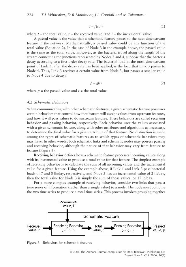
, respectively. Each behavior uses the values associatedwith a given schematic feature, along with other attributes and algorithms as necessary,to determine the final value for a given attribute of that feature. No distinction is madeamong the types of schematic features as to which types of schematic behaviors theymay have. In other words, both schematic links and schematic nodes may possess passingand receiving behavior, although the nature of that behavior may vary from feature tofeature (Figure 3).

Receiving behavior

defines how a schematic feature processes incoming values alongwith its incremental value to produce a total value for that feature. The simplest exampleof receiving behavior is to calculate the sum of all incoming values and the incrementalvalue for a given feature. Using the example above, if Link 1 and Link 2 pass bacterialloads of 7 and 8 lb/day, respectively, and Node 3 has an incremental value of 2 lb/day,then the total value for Node 3 is simply the sum of those values, or 17 lb/day.

For a more complex example of receiving behavior, consider two links that pass atime series of information (rather than a single value) to a node. The node must combinethe two time series to produce a total time series. This process involves grouping together

Figure 3 Behaviors for schematic features


225


Transactions in GIS

, 2006, 10(2)

and processing values based on each time step, which may require temporal interpolationof one or both time periods.

By default, the Schematic Processor invokes a simple accumulation for a receiveprocess, so that all values received by a feature are added to its incremental value toproduce the total value for that feature. If more complex processing is required, such asdecaying bacterial loads in a lake, a processing engine may be provided to simulate thereceiving behavior.

Passing behavior

defines how a schematic feature processes its total value to pro-duce a value that will be passed to the next downstream schematic feature. The simplestexample of passing behavior is to pass the total value for a given feature. More complexpassing behaviors may also be modeled. Using the example above, the passing behaviorfor Link 3 involves a first order decay process. Thus, without any new bacterial loadinputs, the load passed to Node 4 from Link 3 will be less than the load received byLink 3, due to decay while the flow passes through the link. Note that the SchematicProcessor does not define where the passing behavior takes place on the link (e.g. at thebeginning, middle, or end, or along the entire length of the link). It merely defines howthe total value for the link is changed to produce a value that is passed to its down-stream node.

By default, the Schematic Processor simply passes the total value for a given featureto the next downstream feature. If more complex processing is required, a processingengine may be provided to simulate the passing behavior.

4.3 Processing Order

This methodology applies to schematic networks in which no backwater effects occur.In other words, each schematic feature receives no information from or about down-stream schematic features. However, since each feature does receive information fromupstream features, all upstream features should be processed (so that they know whatvalue they should pass) before processing a given schematic feature. The SchematicProcessor uses the Hydro, FromNodeID and ToNodeID attributes on schematic featuresto arrange those features in a processing order from upstream to downstream.

5 Implementation Procedure

The procedure used to implement the methodology described above within the ArcGIS9 geoprocessing environment includes a data model to support schematic navigation andattribute storage, an algorithm for sorting the schematic features from upstream todownstream, and the actual implementation of the procedure with an ArcGIS geoprocessingtool called the Schematic Processor.

5.1 Data Model

The Schematic Processor is designed to work with ArcGIS software. ArcGIS storesgeospatial data in a geodatabase, which is a relational database containing both spatialand attribute data. Feature classes are tables in the database for which each recordcontains a shape which may be displayed in the GIS. Object classes are tables for whicheach record is not associated with a specific shape to be displayed in the GIS.

226



Transactions in GIS

, 2006, 10(2)

The Schematic Processor operates on two geodatabase object classes: a schematicnode class and a schematic link class. These classes may be feature classes or object classes,as the geometry of the nodes and links is not explicitly taken into consideration by theSchematic Processor. Rather, the tool uses attributes within the node and link classes toestablish connectivity between them. Thus, any two feature classes or tables may be usedwith the Schematic Processor, as long as they are located in the same geodatabase.

Because the Schematic Processor was designed to operate on an Arc Hydro schematicnetwork, the tool assumes that the Arc Hydro schematic attributes exist in the schematicnode and schematic link classes. These attributes are used for identifying schematicfeatures and navigating the schematic network. For Schematic Nodes, the relevantattributes include:

•

HydroID

– Long integer automatically defined providing a unique identifier for thefeature in the geodatabase.

•

SrcType

– Short integer, user-defined, which indicates the type of the schematicfeature, populated by Node/Link Schema Generation tool in the Arc Hydro tools.

For Schematic Links, these attributes include:

•

HydroID

– Unique identifier for the feature in the geodatabase.•

LinkType

– Short integer, user-defined, which indicates the type of the schematicfeature, populated by Node/Link Schema Generation tool in the Arc Hydro tools.

•

FromNodeID

– The HydroID of the schematic node located at the upstream end ofthe schematic link.

•

ToNodeID

– The HydroID of the schematic node located at the downstream end ofthe schematic link.

In addition to the Arc Hydro attributes, schematic features may also possess attributesthat describe the values that those features operate with. For both the schematic nodeand link classes, these attributes include:

•

Incremental Value

– Stores the incremental value for the given feature.•

Total Value

– Stores the total value for the given feature.•

Passed Value

– Stores the value that the feature will pass to the next downstreamfeature in the network.

Depending on what type of process is specified for each feature, other attributesmay be required. For example, when decaying loads along a schematic link, travel timeand decay constants may be required. In these cases, the attributes may be located on thefeatures to which they pertain. These attributes are not read directly by the SchematicProcessor, but by the specific processing engine designed to work with those attributes.

5.2 Processing Procedure

The procedure used by the Schematic Processor for working with schematic networks maybe summarized into two major components:

Data Preparation

and the

Process Loop

.In

Data Preparation

, the features in the schematic network are sorted fromupstream to downstream, and Collections are initialized that will store values during theprocessing of the network. A Collection is a standard Visual Basic object which storesa set of values or pointers to other objects. For each schematic feature, a TopologyCollection stores a list of HydroIDs of upstream features, indexed by the HydroID of


227


Transactions in GIS

, 2006, 10(2)

the current feature. A Value Collection stores the schematic values that each feature willpass to the next downstream feature, indexed by the HydroID of the current feature.Using Collections improves the performance of the Schematic Processor.

Once the features have been sorted, each feature is processed in the correct orderuntil all features have been processed. This is called the

Process Loop

. There are fivesteps in each interation of the process loop (Figure 4):

1. Get upstream features2. Get upstream values3. Process upstream and incremental values4. Process current value to pass downstream5. Update Value Collection with value to pass

Thus, for a given feature, adjacent upstream features are located. The values fromthese upstream features are combined with the incremental value for the current featureusing Receiving behavior to produce a total value for the current feature. This value isthen modified by Passing behavior to produce a value to pass to the next downstreamfeature. This value is then updated in the Value Collection. The Process Loop thenmoves to the next downstream feature in the schematic network and repeats the fivesteps for that feature.

5.3 Implementation in ArcGIS 9

ArcGIS 9, the latest GIS software from ESRI, features a geoprocessing framework calledModelBuilder that allows users to chain together a series of geoprocessing tasks anddata sources in a workflow model. In addition to standard ArcGIS tools, the framework

Figure 4 Summary of single iteration in the process loop

228



Transactions in GIS

, 2006, 10(2)

allows users to create custom Script Tools, which may also be inserted into a workflowmodel. Each Script Tool is attached to an underlying script, written in a scripting languagesuch as VBscript or Python, which performs the actual work. The Schematic Processoris implemented in this framework as a script tool called ProcessSchematic. The associ-ated script is called ProcessSchematic.vbs. This script calls a Visual Basic DLL calledMBSchematic.dll, which sorts the schematic features and handles the calling of processDLLs. Thus, ProcessSchematic.vbs is simply used as an intermediary between ArcGISand MBSchematic.dll. A DLL (Dynamic Linked Library) contains a library of classesand subroutines which may be used by another application. A DLL was used rather thana standalone script because a DLL typically allows for more robust programming.

In addition to MBSchematic.dll, zero, one, or more DLLs may be called as processingengines to simulate custom behavior associated with schematic features. The Process-Schematic Script Tool instructs MBSchematic.dll which processing engines are associatedwith each type of schematic feature. If no processing engine is specified for a given typeof schematic feature, the Process Schematic tool uses the defaults for receiving andpassing behavior as described above. This gives the user the ability to create as manyprocessing engines as desired, or to use the default behaviors if no specialized behaviorsare required (Figure 5).

6 Case Studies

Two case studies are presented, which use the Schematic Processor to model hydrologicbehavior with features in a GIS. The first simulates rainfall-runoff response and channelrouting using routines from the Hydrologic Engineering Center’s library of hydrologicfunctions, LibHydro. The second simulates bacterial loading in Galveston Bay frompoint and nonpoint sources.

Figure 5 Implementation of methodology using scripts and DLLs

Integrating Arc Hydro Features 229

© 2006 The Authors. Journal compilation © 2006 Blackwell Publishing LtdTransactions in GIS, 2006, 10(2)

6.1 Case Study I: LibHydro Application

The Hydrologic Engineering Center (HEC) is an organization within the US Army Corpsof Engineers that provides technical expertise, models, methods, research, and trainingin the areas of hydrology, hydraulics, and water resources. HEC-HMS (HydrologicModeling System) is a publicly available standalone rainfall-runoff simulation modelprovided by HEC and designed for dendritic watershed systems. HEC-HMS has beenutilized in many applications throughout the years, and is now considered one of thestandard hydrologic simulation models to use in the USA. HEC recognized that certainfunctions in its models could be extracted to provide useful routines applicable in manysituations outside of the HEC modeling environment. This led to the development of alibrary of functions called LibHydro. These functions were derived from the HEC-1software, which is the predecessor to HEC-HMS. The routines are coded in FORTRAN,and can be accessed by calling the LibHydro DLL using a variety of programming languages,including Visual Basic and C++. Examples of routines include unit conversions andMuskingum routing (Hydrologic Engineering Center 1995). By referencing LibHydro, ahydrologic application can make use of effective modeling routines that have alreadybeen proven through years of use.

In this example, functions from LibHydro are used to simulate rainfall-runoff androuting calculations for a portion of the Llano River basin in Texas (Figure 6). The rawdata for this application includes a Watershed feature class representing the target sub-basins for the analysis, precipitation data stored in the Arc Hydro TimeSeries table, anda HydroNetwork composed of HydroEdges and HydroJunctions. The precipitation datacovered a period from 2–8 November, 2000, at 15-minute intervals. A schematic net-work was built using the Arc Hydro tools (Figure 7). The schematic network includesnodes representing Watersheds (Type 1 nodes) and HydroJunctions (Type 2 nodes), andlinks connecting those nodes. Type 1 links connect Type 1 nodes to Type 2 nodes, whileType 2 links connect Type 2 nodes to Type 2 nodes.

Four LibHydro functions were used in this analysis: Initial Constant Loss, SnyderUnit Hydrograph, Baseflow, and Modified Puls Routing. The first three functions wereused to prepare time series of watershed outflows to the stream network, while the lastfunction was used by the schematic network to route the flows to the outlet of thesubbasin network. These functions were incorporated into an ArcGIS 9 workflow modelcalled Rainfall to Routed Flow, and executed in the ModelBuilder environment. More

Figure 6 Target subbasins in Llano River Basin

230 T L Whiteaker, D R Maidment, J L Goodall and M Takamatsu


information about the specifics of each LibHydro function can be found in Takamatsu(2003).

The Rainfall to Routed Flow workflow model consists of four script tools, oneassociated with each of the LibHydro functions listed above. The first three tools pre-pare time series information to be used by the Schematic Processor for routing the flows.The last tool is the Schematic Processor. Each tool accesses a DLL called MBlibHydroin order to use the functions in LibHydro.

The first tool, Loss Initial Constant, calls the Loss Initial Constant function fromLibHydro to calculate precipitation excess for each Watershed using rainfall data fromthe TimeSeries table. Fields in the Watershed feature class provide the values of initialloss, constant loss rate, and impervious area ratio for each Watershed. The second tool,UnitgraphSnyder, calls the Snyder Unit Hydrograph function from LibHydro to calcu-late a runoff hydrograph for each watershed, given the precipitation excess time seriesdetermined by the Loss Initial Constant Tool. Fields in the Watershed feature classprovide the values of Snyder Cp, Snyder Tp, and Basin Area for each Watershed. Thethird tool, Baseflow, calls the Baseflow function from LibHydro to calculate Baseflowfor each watershed, given the precipitation excess time series determined by the LossInitial Constant Tool. The tool then adds the baseflow to the runoff hydrograph toproduce an outflow time series for each watershed. Fields in the Watershed feature classprovide the values of recession ratio and recession threshold for each Watershed.

The final tool in the workflow model is the Schematic Processor. Once outflow timeseries have been calculated for each watershed, this tool uses the schematic network toroute the flows through the stream network to the outlet of the target subbasins. Thisparticular application of the Schematic Processor uses the tool in a unique way. The toolis designed to pass single values from feature to feature. However, the Rainfall to RoutedFlow model requires time series of flows to be passed between features, rather than asingle value. Therefore, instead of passing single values between features, the SchematicProcessor is set up to pass time series type IDs, or TSTypeIDs, which categorize valuesin the Arc Hydro TimeSeries table (such as rainfall, runoff, etc.). SchemaLinkPuls.DLLand SchematicNode.DLL are set as processing engines, whose purpose is to extract timeseries data for each feature based on the TSTypeID, route the time series, and write theresulting time series of routed flows back to the TimeSeries table. SchemaLinkPuls.DLLuses the Modified Puls Routing function from LibHydro to route flows along a riverreach, represented by a schematic link of Type 2. When two reaches converge, their time

Figure 7 Schematic network for Llano target subbasins



series of routed flows are added together to produce a combined flow. SchematicNode.DLLperforms that task, with the assumption that there are no backwater effects (Table 1).

Once the Rainfall to Routed Flow model has completed execution, a time series ofoutflow values for the basin comprised of the target Llano subbasins is recorded in theArc Hydro TimeSeries table.

The Rainfall to Routed Flow model was run for the Llano subbasins covering preci-pitation events from 2–8 November, 2000. An identical model was setup and run withinHEC-HMS for comparison. The results from both models matched almost exactly(Figure 8), with differences of less than 0.5% in most cases (Table 2). Rounding withineach model may account for the differences in results between the two models. Still,with nearly identical results, this experiment verifies that the Rainfall to Routed Flowmodel is successful in calling the same functions used by HMS.

Another important observation from the execution of these two models is thatHMS performed the simulation much quicker than the Rainfall to Routed Flow model.A complete run of Rainfall to Routed Flow within ArcGIS took approximately 20minutes to finish. The HMS model took only 20 seconds to run. From these results, itis clear that improvements in efficiency of handling time series in GIS are needed inorder for time varying modeling within a GIS to be practical. For example, time seriesrecords from HEC-HMS are processed in memory or stored in a special binary formatdesigned for handling time series data, and so manipulation of time series is very fast.However, in the Rainfall to Routed Flow model, time series data are stored as recordsin a database, which results in very costly transactions in terms of processing time.

6.2 Case Study II: Water Quality Modeling in Galveston Bay

Whiteaker and Goodall (2003) applied the Schematic Processor to water quality modelingin Galveston Bay, Texas, by examining fecal coliform loading from point and nonpoint

Table 1 Explanation of processing engines for schema links and nodes in Rainfall to RoutedFlow model

Links

Type Purpose Process DLL

1 land to river transport TSTypeID of outflow time series passed from watershed to outlet

none

2 along river routing Flow is routed along a stream segment using the Modified Puls method from libHydro

SchemaLinkPuls

Nodes

Type Purpose Process DLL

1 represent watershed Store TSTypeID of outflow time series none2 combine flows Sum time series of flows at a junction

along the stream networkSchematicNode



sources into the bay (Figure 9). The procedure and equations used to model bacterialloadings were adapted from Zoun (2003), who used the Arc Hydro tools and conventionalGIS techniques to determine loadings. Three processing engines were developed for theSchematic Processor to simulate bacterial load transport, while an ArcGIS workflow model,WQModel, was assembled to perform the analysis. WQModel includes components todetermine watershed loads, as well as the Schematic Processor to accumulate loads intothe bay. WQModel assumes that general data development, such as watershed delineationand the calculation of travel times on reaches, has already been accomplished and verified.The schematic network must also have already been created with three types of nodesand links to represent the hydrologic features used in the water quality analysis (Table 3).

WQModel uses rainfall data and watershed characteristics such as land use todetermine annual watershed loads. The Schematic Processor is then called to move theloads from the watersheds into the bay, decaying the loads as they travel through thestream network. The model contains fifteen tools, including standard ArcGIS tools aswell as custom script tools that access DLLs. The reader is referred to Whiteaker andGoodall (2003) for a detailed explanation of each tool in the model.

Figure 8 Outflow hydrographs computed by HMS and Rainfall to Routed Flow Model

Table 2 Values Computed by HMS and Rainfall to Routed Flow Model Varied by Fractionsof a Percent

TimestampFlow (cms) from HMS

Flow (cms) from Rainfall to Routed Flow Model

Percent Difference (%)

11/3/00 6:45 PM 577.980 577.785 0.03411/3/00 7:00 PM 560.730 560.627 0.01811/3/00 7:15 PM 542.840 542.861 0.00411/3/00 7:30 PM 523.750 523.928 0.034



The three types of links and three types of nodes signify the behavior that featuresin the schematic network will implement. When behavior more complex than simpleaccumulation is required, the Schematic Processor calls functions from a WaterQuality-Processors DLL that was written to support water quality modeling. The processesassociated with each type of link and node are shown in Tables 2 and 3. The objects in the‘dll’ column in the tables are classes that exist in the WaterQualityProcessors DLL.,which were constructed to function as processing engines. The classes are associatedwith the appropriate link or node types when the user specifies inputs to the SchematicProcessor.

Three processing engines were constructed for this case study. The first engine,Decay, used a first order decay rate and received loads to simulate the decay of bacteriaalong stream segments. The decay rate represents the loss of mass due to biologicaldecay, sorption, uptake, etc. as material moves downstream. Decay rates for each stream

Figure 9 Gavleston Bay watershed with schematic network



segment were determined by Zoun (2003) and stored as attributes on the SchemaLinkfeature representing that segment. The Decay processing engine is called when a SchemaLinkis passing a load to its next downstream node. The load passed is reduced according toa first-order reaction shown below:

loadpassed = loadreceieved × e−kt (3)

where loadpassed = downstream bacteria load (cfu/yr), loadreceived = upstream bacteria load(cfu/yr), k = first-order decay coefficient (day−1), and t = travel time (day).

Table 3 Explanation of processing engines for schema links and nodes in WQModel(Whiteaker and Goodall 2003)

Links

Type Purpose Process Class in DLL

1 land to river mass transport

Mass is passed to downstream node without decay because incremental value represents mass of bacteria which reaches watershed outlet.

none

2 along river transport Mass passed to downstream node is decayed according to time of travel and decay coefficient.

clsDecay

3 river to bay Mass is passed from river outlet to bay without decay.

none

Nodes

Type Purpose Process Class in DLL

1 losses or additions of mass for watersheds

Mass is passed to downstream link without decay.

none

2 losses or additions of mass along river network

Mass is passed to downstream link without decay except for one feature for which the LossCoef field is nonzero. The 0.5 factor is to account for bacteria that enters Sabine Lake from the upstream Watersheds for East Bay.

clsLossCoef

3 losses or additions of mass for bays

Mass is received by the bay and used to estimate concentration (cfu/m3) within the bay. Estimated concentration in bay is based on continuous flow stired tank reactor (CFSTR) assumptions.

clsCFSTR



The second processing engine, CFSTR, calculates a bay’s increase in concentrationdue to an import of bacteria mass. Each bay’s volume, estimated yearly flow, and first-order decay term are stored in the SchemaNode feature class. The load received by theSchemaNode representing the bay is used to estimate the bay concentration, assumingthe bay has constant inflow equal to its outflow, and that mass entering the bay isinstantaneous and perfectly mixed within the bay (Equation 4). These are commonlyknown as continuous flow, stirred tank reactor (CFSTR or CSTR) assumptions:

(4)

where c = concentration within bay (coliform units/m3), L = bacteria load entering bay(coliform units/yr), Q = total flow (m3/yr), k = first-order decay term (day−1), and V = volumeof bay (m3).

The third processing engine, LossCoef, accounts for bacteria from the watershedsupstream of East Bay that flow into Sabine Lake and not East Bay. From Zoun (2003),half of the load from these watersheds is assumed to flow into East Bay, while the otherhalf is delivered to Sabine Lake. The LossCoef processing engine uses the LossCoefattribute of a SchemaNode feature to determine the fraction of the load from that nodethat is passed to its downstream link. This allows one to easily adjust the proportioningof load between East Bay and Sabine Lake. The LossCoef value for the appropriatenodes in the Galveston Bay database were assigned a value of 0.5.

Once the data were prepared and the processing engines defined, the WQModelwas run. The results of WQModel execution match up quite well with Zoun’s results,although some discrepancies as high as 2.6% were present. These discrepancies were dueto differences in the runoff grid used by Zoun and the one used during ModelBuilderexecution. The cells in the runoff from Zoun’s work did not exactly overlap the cellsin the precipitation grid. However, because the runoff grid used by WQModel inModelBuilder was generated directly from the input precipitation grid, the cells overlapexactly. Because the cell size for the runoff grid was so coarse, a slight shift in the celllocations resulted in enough variation in load calculations to produce different con-centrations in the bay. However, even with this discrepancy, the loads matched upvery well, especially given the inexact nature of nonpoint load calculations for thiswatershed.

WQModel was constructed in three weeks, and executed in 20 minutes for GalvestonBay on an average desktop computer. The ease of execution greatly improves the efficiencyof the water quality modeling algorithms developed by Zoun (2003), as those algorithmsneed no longer be carried out manually. The algorithms may also be repeated for differentapplications by supplying different input datasets or parameters to the model.

7 Conclusions

One limitation of ModelBuilder is that the standard ArcGIS tools are designed to oper-ate at the dataset level, rather than the feature level. However, feature level operationsmay be implemented through custom tools, such as the Schematic Network Processor,which may operate in the ModelBuilder environment but utilize DLLs (or other pro-gramming constructs) to analyze data one feature at a time.

c

L

Q kV

=

+



The Schematic Processor allows links and nodes (which represent hydrologic fea-tures) in a schematic network to control how information is received from upstreamfeatures, and what information is passed to downstream features, by associating eachtype of feature with a specific processing engine which simulates hydrologic behavior.The modular design of the Schematic Processor gives the user the ability to developprocessing engines geared towards solving a wide variety of water resources problems.However, the Schematic Processor assumes that the schematic network is dendritic, andthat no backwater effects occur between schematic features. Violating these assumptionscould hamper the performance of the Schematic Processor, or produce incorrectresults. The Rainfall to Routed Flow model proves that hydrologic and hydraulic calcu-lations comparable to those possible with simulation models such as HMS can becarried out within a GIS application by accessing functions from LibHydro. The workcould be extended to include functions from other object libraries. The modular nature ofModelBuilder tools makes the components in Rainfall to Routed Flow extensible andreusable.

One important finding from the LibHydro application was that the creation andmanipulation of large amounts of time series data is very costly in time when writingto an ArcGIS geodatabase. For time-invariant analysis, such as with the water qualitymodeling in Galveston Bay example, the computation time was very fast. However, theLibHydro application executed much slower than an identical model setup in the HMSprogram. For these types of applications, the best approach may be to write only thefinal results of model simulations back to the Arc Hydro TimeSeries table. The interme-diate time series can be calculated through LibHydro and managed in a more efficientmedium, or an independent simulation model (e.g. HMS) can be called from ModelBuilderto perform the simulation, returning control to the GIS when the simulation iscompleted.

Using the Schematic Processor and the ModelBuilder environment provides a gooddeal of flexibility to the user. In addition to bacterial loads, WQModel may be appliedto other contaminants simply by applying the model to different attributes on the sche-matic network. The workflow model could also be applied to different regions, bysupplying the model with different input datasets. The modular nature of the SchematicProcessor also permits the addition of other processing engines, to appropriately modelthe behavior of hydrologic features in the region of interest.

The integration of GIS features with processing engines simulating hydrologic behaviorprovide water resources engineers with valuable analysis tools that take full advantage ofArc Hydro and the ArcGIS 9 geoprocessing framework. Arc Hydro changes the role ofGIS features from blue lines on a map to data constructs that correlate to specific featuresin a hydrologic simulation model. The Schematic Processor goes one step further, byproviding a mechanism to attach simulation models or components of those modelsdirectly with the Arc Hydro features themselves.

Acknowledgements

This research was financially supported by the GIS in Water Resources Consortium andthe Texas Commission on Environmental Quality. We appreciate the efforts of ReemJihan Zoun in preparing data used for the water quality modeling of Galveston Bay, andthe Hydrologic Engineering Center for helping with implementing LibHydro.



References

Charnock T W, Hedges P D, and Elgy J 1996 Linking multiple process level models with GIS.In Kovar K and Natchnebel H P (eds) Application of Geographic Information Systemsin Hydrology and Water Resources Management. Wallingford, International Association ofHydrological Sciences Publication No 235: 29–36

Correia F N, Rego F C, Saraiva M G, and Ramos I 1998 Coupling GIS with hydrologic andhydraulic flood modelling. Water Resources Management 12: 229–49

Feng C 2000 Open hydrologic model for facilitating GIS and hydrologic model interoperability.In Proceedings of the Fourth International Conference on Integrating GIS and EnvironmentalModeling, Banff, Alberta (available at http://www.colorado.edu/Research/cires/banff/pubpapers/6)

Hydrologic Engineering Center 1995 LibHydro Users Manual. Davis, CA, Hydraulic EngineeringCenter

Hellweger F and Maidment D R 1997 HEC-PREPRO: A GIS Preprocessor for Lumped ParameterHydrologic Modeling Programs. WWW document, http://www.crwr.utexas.edu/reports/1997/rpt97–8.shtml

Maidment D R 2002 Arc Hydro: GIS for Water Resources. Redlands, CA, ESRI PressPaniconi C, Kleinfeldt S, Deckmyn J, and Giacomelli A 1999 Integrating GIS and data visualization

tools for distributed hydrologic modeling. Transactions in GIS 3: 97–118Prisloe Jr M P, Arnold Jr C L, Civco D L, and Lei Y 2000 A simple GIS-based model to characterize

water quality in Connecticut watersheds. In Proceedings of the Fourth International Conferenceon Integrating GIS and Environmental Modeling, Banff, Alberta (available at http://www.colorado.edu/Research/cires/banff/pubpapers/11)

Pullar D 2003 Simulation modelling applied to runoff modelling using MapScript. Transactionsin GIS 7: 267–83

Pullar D and Springer D 2000 Towards integrating GIS and catchment models. EnvironmentalModelling and Software 15: 451–9

Takamatsu M 2003 LibHydro. WWW document, https://webspace.utexas.edu/mtaka/www/lh_home.htm

Whiteaker T 2001 A Prototype Toolset for the ArcGIS Hydro Data Model. Unpublished Ph.D.Dissertation, University of Texas at Austin (available at http://www.crwr.utexas.edu/reports/2001/rpt01–6.shtml)

Whiteaker T and Goodall J 2003 Water quality modeling in Galveston Bay with Model Builder.In Proceedings of the Twenty-third ESRI International User Conference, San Diego, California

Yoon J 1996 Watershed-scale nonpoint source pollution modeling and decision support systembased on a model-GIS-RDBMS linkage. In Proceedings of the AWRA Symposium on GIS andWater Resources, Fort Lauderdale, Florida (available at http://www.awra.org/proceedings/gis32/jyoon)

Zoun R J 2003 Estimation of Fecal Coliform Loadings to Galveston Bay. Unpublished M.S.Thesis, University of Texas at Austin (available at http://www.crwr.utexas.edu/reports/2003/rpt03–5.shtml)

Integrating Arc Hydro Features with a Schematic Network

Documents

Transcript of Integrating Arc Hydro Features with a Schematic Network