Integrated Vehicle-Based Safety Systems (IVBSS) - ROSA P
439
National Highway Traffic Safety Administration DOT HS 810 905 February 2008 Integrated Vehicle-Based Safety Systems (IVBSS): Human Factors And Driver-Vehicle Interface (DVI) Summary Report This document is available to the public from the National Technical Information Service, Springfield, Virginia 22161
-
Upload
khangminh22 -
Category
Documents
-
view
1 -
download
0
Transcript of Integrated Vehicle-Based Safety Systems (IVBSS) - ROSA P
National Highway Traffic Safety Administration
DOT HS 810 905 February 2008
Integrated Vehicle-Based SafetySystems (IVBSS): Human FactorsAnd Driver-Vehicle Interface (DVI)Summary Report
This document is available to the public from the National Technical Information Service, Springfield, Virginia 22161

This publication is distributed by the U.S. Department ofTransportation, National Highway Traffic Safety Administration, inthe interest of information exchange. The opinions, findings andconclusions expressed in this publication are those of the author(s) andnot necessarily those of the Department of Transportation or theNational Highway Traffic Safety Administration. The United States Government assumes no liability for its content or use thereof. If trade or manufacturer’s names or products are mentioned, it is because theyare considered essential to the object of the publication and should notbe construed as an endorsement. The United States Government does not endorse products or manufacturers.

Technical Report Documentation Page 1. Report No. 2. Government Accession No. 3. Recipient’s Catalog No.
DOT HS 810 905 4. Title and Subtitle 5. Report Date
Integrated Vehicle-Based Safety Systems (IVBSS): February 2008 Human Factors and Driver-Vehicle Interface (DVI) 6. Performing Organization Code
Summary Report 052004 7. Author(s) 8. Performing Organization Report No.
Green, P., Sullivan, J., Tsimhoni, O., Oberholtzer, J., Buonarosa, UMTRI-2007-43 M.L., Devonshire, J., Schweitzer, J., Baragar, E., & Sayer, J. 9. Performing Organization Name and Address 10. Work Unit no. (TRAIS)
The University of Michigan Transportation Research Institute 11. Contract or Grant No.
2901 Baxter Road Cooperative Agreement Ann Arbor, Michigan 48109-2150 DTNH22-05-H-01232 12. Sponsoring Agency Name and Address 13. Type of Report and Period Covered
The University of Michigan November 2005 – November 2007 Industry Affiliation Program for 14. Sponsoring Agency Code
Human Factors in Transportation Safety Office of Human Vehicle Performance Research – Intelligent Technologies Research Division, NVS-332
15. Supplementary Notes
16. Abstract
The IVBSS program is a four-year, two-phase project to design and evaluate an integrated crash warning system for forward collision, lateral drift, lane-change merge, and curve speed warnings for both light vehicles and heavy trucks. This report, covering human factors research and DVI development in the first two years of the program, describes five laboratory studies, four driving simulator studies, and two on-road pilot tests conducted to assess a variety of driver-interface concepts related to the development of integrated warning systems.
Selected major findings are as follows: 1) For the vehicles selected, warning sounds should be at least 80 dB(A) in the 1 to 5 KHz range. 2) Auditory warning durations should be less than the expected mean response time. 3) No approaches to warning combination (single, dual-simple, dual-hybrid, or multiple warnings) led to noticeably better driver responses, though drivers favored the multiple warning approach least, and for a variety of reasons a dual-warning approach is recommended for IVBSS. 4) Delays between 150 and 300 ms are acceptable for the LDW algorithm. 5) No single prioritization scheme for warnings (simultaneous, priority interrupt, or delayed presentation) is recommended based on the findings from a simulator study. Extended pilot testing is likely to suggest minor refinements to the DVIs developed here. In the pilot tests that have been conducted, all of the warning systems operated as planned, with some changes required to reduce false alarm rates. Overall, drivers reported IVBSS to be intuitive and easy to use. Most drivers stated warnings were received with about the right frequency, and in general the warnings were not distracting. Results from the laboratory and simulator experiments, in particular, are likely to assist future developers of driver-vehicle interfaces for integrated crash warning systems. 17. Key Words 18. Distribution Statement
Integrated Vehicle-Based Safety System, IVBSS, DVI, driver vehicle interface, Document is available to the human factors, ergonomics, warnings public through the National
Technical Information Service, Springfield, VA 22161
19. Security Classification (of this report) 20. Security Classification (of this page) 21. No. of Pages 22. Price
Unclassified Unclassified 396
i

Table of Contents 1 Executive Summary ................................................................................................................ 11.1 Goal of the Human Factors and Driver-Vehicle Interface Effort ....................................... 11.2 Overview............................................................................................................................. 1 1.3 Initial Human Factors and DVI Development Efforts........................................................ 21.4 Available DVI Options ....................................................................................................... 31.5 Experiment 1: Auditory Warnings...................................................................................... 3
1.5.1 Summary Findings .......................................................................................................... 31.6 Experiment 2: Driver Response to Warnings ..................................................................... 4
1.6.1 Summary Findings .......................................................................................................... 41.7 Experiment 3: Combined Warnings for IVBSS.................................................................. 4
1.7.1 Summary Findings .......................................................................................................... 51.8 Experiment 4: Warning Time-Accuracy Trade .................................................................. 5
1.8.1 Summary Findings .......................................................................................................... 51.9 Experiment 5: Driver Response to Simultaneous Warnings............................................... 5
1.9.1 Summary Findings .......................................................................................................... 51.10 Light-Vehicle Stage 2 Pilot Test......................................................................................... 6
1.10.1 Summary Findings .......................................................................................................... 6 1.11 Heavy-Truck Stage 2 Pilot Test.......................................................................................... 6
1.11.1 Summary Findings .......................................................................................................... 7 1.12 Conclusions......................................................................................................................... 7 2 Overview................................................................................................................................. 82.1 The Need to Conduct Studies on Integrated DVIs.............................................................. 9 2.2 Prior Warning Studies - What Do They Say About How Drivers Should Be Warned?... 10
2.2.1 Warning Timing............................................................................................................ 10 2.2.2 Warning Reliability....................................................................................................... 11 2.2.3 Warnings Systems with Multiple Warnings ................................................................. 112.2.4 Modality of Warning and Multi-Modal Warnings........................................................ 122.2.5 Auditory Warnings........................................................................................................ 12
2.3 Research Questions Identified and Addressed.................................................................. 162.4 Work Plan ......................................................................................................................... 17
2.4.1 Impact of Human Factors Testing on IVBSS Design................................................... 172.4.2 Timeline ........................................................................................................................ 19
2.5 Report Structure ................................................................................................................ 21 3 Research Summary ............................................................................................................... 22 3.1 Platform-Based Hardware Constraints ............................................................................. 22 3.2 Available Option Space .................................................................................................... 22
3.2.1 Light-Vehicle Option Space ......................................................................................... 22 3.2.2 Heavy-Truck Option Space........................................................................................... 29
3.3 Research Questions........................................................................................................... 31 3.3.1 Q1. Shared Warnings .................................................................................................... 333.3.2 Q2. Sequencing Co-Occurring Warnings ..................................................................... 343.3.3 Q3. Warning Set Confusion.......................................................................................... 343.3.4 Q4. Time Course of Driver Actions.............................................................................. 34 3.3.5 Q5. Warning Processing Time-Accuracy Tradeoff ...................................................... 35 3.3.6 Q6. Auditory Characteristics of Warnings.................................................................... 35
ii

3.3.7 Q7. Influence of Pauses and Repetition........................................................................ 35 3.4 Driving Simulator Overview............................................................................................. 353.5 Test Scenarios ................................................................................................................... 37
3.5.1 Introduction................................................................................................................... 37 3.5.2 Scenario Development .................................................................................................. 403.5.3 Multiple Warning Scenarios ......................................................................................... 40
4 Experiment 1 – Auditory Warnings...................................................................................... 414.1 Subtask 1 – Sound Environment of the Light Vehicle and Heavy Truck......................... 41
4.1.1 Overview....................................................................................................................... 41 4.1.2 Method .......................................................................................................................... 41 4.1.3 Light-Vehicle Results ................................................................................................... 424.1.4 Heavy-Truck Results .................................................................................................... 424.1.5 Conclusions................................................................................................................... 43
4.2 Subtask 2 – Acoustic Features of Warnings ..................................................................... 434.2.1 Overview....................................................................................................................... 43 4.2.2 Method .......................................................................................................................... 43 4.2.3 Results........................................................................................................................... 44 4.2.4 Conclusions................................................................................................................... 46
4.3 Subtask 3 – Warning Sound Suites: Acquisition and Response Speed ............................ 474.3.1 Overview....................................................................................................................... 47 4.3.2 Method .......................................................................................................................... 48 4.3.3 Results........................................................................................................................... 48 4.3.4 Conclusions................................................................................................................... 49
4.4 Subtask 4 – Localization of Auditory Warnings............................................................... 494.4.1 Overview....................................................................................................................... 49 4.4.2 Method .......................................................................................................................... 49 4.4.3 Results........................................................................................................................... 50 4.4.4 Conclusions................................................................................................................... 50
4.5 Subtask 5 – LDW Timing ................................................................................................. 50 4.5.1 Overview....................................................................................................................... 50 4.5.2 Method .......................................................................................................................... 51 4.5.3 Results........................................................................................................................... 52 4.5.4 Conclusions................................................................................................................... 53
5 Experiment 2 – Driver Response to Warnings ..................................................................... 555.1 Overview........................................................................................................................... 55 5.2 Method .............................................................................................................................. 55 5.3 Results............................................................................................................................... 56 5.4 Conclusions....................................................................................................................... 64 6 Experiment 3 – Combined Warnings for IVBSS.................................................................. 676.1 Overview........................................................................................................................... 67 6.2 Method .............................................................................................................................. 67 6.3 Results............................................................................................................................... 68 6.4 Conclusions....................................................................................................................... 72
iii

7 Experiment 4 ņ Warning Delay-Accuracy Tradeoff............................................................ 737.1 Overview........................................................................................................................... 73 7.2 Method .............................................................................................................................. 73 7.3 Results............................................................................................................................... 74 7.4 Conclusions....................................................................................................................... 78 8 Experiment 5 ņ Driver Response to Simultaneous Warnings.............................................. 808.1 Overview........................................................................................................................... 80 8.2 Method .............................................................................................................................. 80 8.3 Results............................................................................................................................... 81 8.4 Conclusions....................................................................................................................... 84 9 Light-Vehicle Stage 2 Pilot Test........................................................................................... 859.1 Overview........................................................................................................................... 85 9.2 Method .............................................................................................................................. 85 9.3 Results............................................................................................................................... 86
9.3.1 Objective Results .......................................................................................................... 86 9.3.2 Subjective Results......................................................................................................... 88
9.4 Conclusions....................................................................................................................... 89 10 Heavy-Truck Stage 2 Pilot Test............................................................................................ 9110.1 Overview........................................................................................................................... 91 10.2 Method .............................................................................................................................. 91 10.3 Results............................................................................................................................... 92
10.3.1 Objective Results .......................................................................................................... 92 10.3.2 Subjective Results......................................................................................................... 92
10.4 Conclusions........................................................................................................................... 93 11 Conclusions........................................................................................................................... 9411.1 Next Steps ......................................................................................................................... 94 11.2 Conclusions and Implementation of Research Results..................................................... 94 12 References............................................................................................................................. 96Appendix A: Driving Simulator and Upgrades .......................................................................... 101A.1 Overview......................................................................................................................... 101 A.2 Road Scenes .................................................................................................................... 103 A.3 Vehicle Cab..................................................................................................................... 104 A.4 Upgrades ......................................................................................................................... 106 Appendix B: Scenario Details..................................................................................................... 110B.1 Introduction..................................................................................................................... 110 B.2 FCW Scenarios ............................................................................................................... 113 B.3 LCM Scenarios ............................................................................................................... 117 B.4 LDW Scenarios............................................................................................................... 119 B.5 CSW Scenarios ............................................................................................................... 119 B.6 Multiple Warning Scenarios ........................................................................................... 120
B.6.1 FCW and LCM............................................................................................................ 120 B.6.2 LCM and LDW ........................................................................................................... 121 B.6.3 FCW and LDW ........................................................................................................... 121
Appendix C: Prototyping Tools .................................................................................................. 122C.1 Scenario Development Tool ........................................................................................... 122
iv

C.2 Warning Interface Prototyping Tool............................................................................... 124 Appendix D: Literature Review.................................................................................................. 126Appendix E: Experiment 1 ņ Auditory Warnings...................................................................... 133E.1 Subtask 1: Light-Vehicle and Heavy-Truck Sound Environment .................................. 133
E.1.1 Overview ...................................................................................................................... 133 E.1.2 Method.......................................................................................................................... 133 E.1.3 Results .......................................................................................................................... 133 E.1.4 Conclusions .................................................................................................................. 138 E.1.5 Forms............................................................................................................................ 139
E.2 Subtask 2: Acoustic Features of Warnings ..................................................................... 140 E.2.1 Overview ..................................................................................................................... 140 E.2.2 Method......................................................................................................................... 140 E.2.3 Results .......................................................................................................................... 142 E.2.4 Conclusions .................................................................................................................. 148 E.2.5 Forms............................................................................................................................ 149
E.3 Subtask 3: Warning Sound Suites: Acquisition and Response Speed ............................ 150 E.3.1 Overview ...................................................................................................................... 150 E.3.2 Method.......................................................................................................................... 152 E.3.3 Results .......................................................................................................................... 153 E.3.4 Conclusions .................................................................................................................. 159 E.3.5 Forms............................................................................................................................ 160
E.4 Subtask 4: Localization of Auditory Warnings .............................................................. 162E.4.1 Overview ...................................................................................................................... 162 E.4.2 Method.......................................................................................................................... 164 E.4.3 Results .......................................................................................................................... 165 E.4.4 Conclusions .................................................................................................................. 167 E.4.5 Forms............................................................................................................................ 168
E.5 Subtask 5: LDW Timing................................................................................................. 169 E.5.1 Overview ...................................................................................................................... 169 E.5.2 Method.......................................................................................................................... 170 E.5.3 Results .......................................................................................................................... 172 E.5.4 Conclusions .................................................................................................................. 182 E.5.5 Forms............................................................................................................................ 188
Appendix F: Experiment 2 – Driver Response to Warnings ...................................................... 194F.1 Overview......................................................................................................................... 194 F.2 Method ............................................................................................................................ 194
F.2.1 World Design............................................................................................................... 195 F.2.2 Warnings and Warning Triggers ................................................................................. 197F.2.3 Warning Scenario Frequency and Sequences.............................................................. 200F.2.4 Test Participants ........................................................................................................... 208
F.3 Results............................................................................................................................. 209 F.3.1 How Many Warnings Occurred?.................................................................................. 209F.3.2 How Often Did Multiple Warnings Occur? ................................................................. 213F.3.3 What Was the Time between Warnings? ..................................................................... 217F.3.4 Eye-Tracking System, Target Identification, and Data Filtering and Reduction ......... 221F.3.5 Fixation Duration.......................................................................................................... 227
v

F.3.6 How Were the Fixation Durations Distributed? ............................................................ 233F.3.7 Driving Data .................................................................................................................. 241 F.3.8 Post-Test Analysis ........................................................................................................ 257 F.3.9 Collisions ...................................................................................................................... 260
F.4 Conclusions..................................................................................................................... 261 F.5 Forms .............................................................................................................................. 263
F.5.1 Biographical Form....................................................................................................... 263 F.5.2 Instructions to Subjects................................................................................................ 264 F.5.3 Post-Test Evaluation Form .......................................................................................... 275
Appendix G: Experiment 3 – Integrating Warnings for IVBSS................................................. 277G.1 Overview......................................................................................................................... 277 G.2 Method ............................................................................................................................ 279
G.2.1 Participants................................................................................................................... 279 G.2.2 Apparatus ..................................................................................................................... 280 G.2.3 Warning Approaches ................................................................................................... 280G.2.4 Driving Scenarios and the Simulator World................................................................ 281G.2.5 Procedure ..................................................................................................................... 284
G.3 Results............................................................................................................................. 284 G.3.1 Data Overview ............................................................................................................. 284 G.3.2 Responses to FCWs and CSWs ................................................................................... 288G.3.3 Speed Reduction and Lane Position ............................................................................ 291G.3.4 Subjective Data ............................................................................................................ 293
G.4 Conclusions..................................................................................................................... 296 G.5 Forms .............................................................................................................................. 297
G.5.1 Post-Block Questionnaire ............................................................................................. 297 G.5.2 Post-Drive Questionnaire.............................................................................................. 298G.5.3 Training Instructions..................................................................................................... 300
Appendix H: Experiment 4 ņ Warning Delay-Accuracy Tradeoff ............................................ 303H.1 Overview......................................................................................................................... 303 H.2 Method ............................................................................................................................ 303 H.3 Results............................................................................................................................. 313
H.3.1 Warning Frequency...................................................................................................... 313H.3.2 Driving Data................................................................................................................. 316 H.3.3 Collisions ..................................................................................................................... 324 H.3.4 Post-Test Analysis ....................................................................................................... 324
H.4 Conclusions..................................................................................................................... 330 H.5 Forms .............................................................................................................................. 332
H.5.1 Biographical Form ....................................................................................................... 332 H.5.2 Instructions................................................................................................................... 333 H.5.3 Post-Test Evaluation Form ........................................................................................... 337
Appendix I: Experiment 5 ņ Driver Response to Simultaneous Warnings................................ 340I.1 Overview......................................................................................................................... 340 I.2 Method ............................................................................................................................ 341
I.2.1 Scenario Frequency ....................................................................................................... 344 I.2.2 Test Participants ............................................................................................................ 349
I.3 Results............................................................................................................................. 351
vi

I.3.1 How Often Did Warnings Occur? ................................................................................. 351I.3.2 Collisions....................................................................................................................... 369 I.3.3 Post-Test Analysis ......................................................................................................... 369
I.4 Conclusions..................................................................................................................... 372 I.5 Forms .............................................................................................................................. 373
I.5.1 Biographical Form.......................................................................................................... 373 I.5.2 Instructions .................................................................................................................... 374 I.5.3 Post-Test Evaluation Form............................................................................................. 378
Appendix J: Light-Vehicle Stage 2 Pilot Test ............................................................................ 381J.1 Overview......................................................................................................................... 381 J.2 Method ............................................................................................................................ 381 J.3 Results............................................................................................................................. 382
J.3.1 Objective Results........................................................................................................... 382 J.3.2 Subjective Results ......................................................................................................... 385
J.4 Conclusions..................................................................................................................... 395 J.5 Forms .............................................................................................................................. 396
J.5.1 Light-Vehicle Pilot Testing Questionnaire and Evaluation .......................................... 396Appendix K: Heavy-Truck Stage 2 Pilot Test ............................................................................ 404K.1 Overview......................................................................................................................... 404 K.2 Method ............................................................................................................................ 404 K.3 Results............................................................................................................................. 405
K.3.1 Objective Results ......................................................................................................... 405 K.3.2 Subjective Results........................................................................................................ 406
K.4 Conclusions..................................................................................................................... 412 K.5 Forms .............................................................................................................................. 413
K.5.1 Heavy-Truck Pilot Testing Questionnaire and Evaluation .......................................... 413Impressions of the Display and Controls……………………………………………………….418
List of Figures Figure 1. IVBSS DVI timeline...................................................................................................... 19 Figure 2. Timeline for experiments .............................................................................................. 20 Figure 3. LCM indicator (LED in right mirror). ........................................................................... 25
Figure 4. Center stack visual display for advisory information.................................................... 25 Figure 5. Frequency of LDW sensitivity adjustment from the RDCW FOT…………………….26 Figure 6. Frequency of CSW sensitivity adjustment from the RDCW FOT ...………………….27 Figure 7. VORAD driver interface unit ........................................................................................ 30
Figure 8. Side sensor display unit ................................................................................................. 30 Figure 9. Close-up of simulator cab interior (without eye fixation system installed) .................. 37 Figure 10. One-third octave distribution of roadway noise collected on a smooth
roadway at 65 mph with closed windows (overall level: 68 dB(A)) ................................... 42 Figure 11. Average ranking of ratings for each crash scenario .................................................... 46 Figure 12. Trials to criterion by sound suite ................................................................................. 48
vii
Figure 13. Mean reaction times for responding within each sound suite ..................................... 49 Figure 14. Rumble strip sound bursts (ms)................................................................................... 51 Figure 15. Frequency distribution of response times to LDW...................................................... 52
Figure 16. Relationship of LDW variations to response time ...................................................... 53
Figure 17. Mean reduction in speed in response to FCW and CSW warnings............................. 60 Figure 18. Mean reduction in speed after FCWs for each scenario.............................................. 60 Figure 19. Distance from lane-center in response to LDW and LCM warnings .......................... 61 Figure 20. Driver response to initial LDW ................................................................................... 62
Figure 21. Driver response to initial LCM.................................................................................... 62
Figure 22. Driver response to initial FCW.................................................................................... 63
Figure 23. Driver response to initial CSW.................................................................................... 63
Figure 24. Pairwise accelerator pedal release and brake onset times by warning type ................ 68
Figure 25. Mean achieved reduction in speed in response to FCW warnings.............................. 69
Figure 26. Mean achieved reduction in speed in response to CSW warnings.............................. 70 Figure 27. Mean distance from the center of the lane (meters) in response to LDW warnings ... 71 Figure 28. Drivers’ most preferred warning approach by age group............................................ 71 Figure 29. Response time to FCW by scenario, warning delay, and acceleration delay .............. 75
Figure 30. Reduction in speed after FCW warnings as function of acceleration delay and warning delay across all scenarios ................................................................................. 76
Figure 31. Distance from center after LDW as function of warning delay .................................. 76
Figure 32. Speed change related to LDW..................................................................................... 81 Figure 33. Lateral position for single and paired LCM scenarios ................................................ 82
Figure 34. Mean speed reduction following an FCW for each of the priority schemes ............... 82
Figure 35. Mean lane position following an LCM for each of the priority schemes.................... 83
Figure 36. Division of warnings from Table 22 by warning type ................................................ 87 Figure 37. Comparison of IVBSS’ mean satisfaction and usefulness scores to those
of other warning systems ...................................................................................................... 89
Figure 38. Simulator cab, front screen, front-right screen, and front-side screen ...................... 101 Figure 39. Dimensions of the simulator room without the side screens..................................... 102 Figure 40. Equipment layout in the driving simulator buck ....................................................... 103
Figure 41. Example of roadway scenery..................................................................................... 104 Figure 42. View of the inside of the simulator cab..................................................................... 105 Figure 43. Simulated destination entry screen............................................................................ 106
Figure 44. Side screen and projector installation........................................................................ 107
Figure 45. Side view displayed on side screens.......................................................................... 107 Figure 46. Before (left) and after (right) pictures of simulator racks. ........................................ 108
Figure 47. Scenario development tool interface ......................................................................... 123
Figure 48. Interface for the warning prototype tool.................................................................... 125
viii

Figure 49. One-third octave distribution of roadway noise for light vehicles on a smooth roadway at 65 mph with windows closed (sound level: 80 dB(A)) ....................... 134
Figure 50. One-third octave distribution of roadway noise for light vehicles on asmooth roadway at 65 mph with windows open (sound level: 80 dB(A)) ......................... 134
Figure 51. One-third octave distribution of roadway noise for light vehicles on asmooth roadway at 35 mph with windows closed (sound level: 60 dB(A)) ....................... 135
Figure 52. One-third octave distribution of roadway noise for light vehicles on asmooth roadway at 35 mph with windows closed (sound level: 66 db(A))........................ 135
Figure 53. One-third octave distribution of roadway noise for light vehicles on a rough-surfaced roadway at 35 mph with windows open (sound level: 68 dB(A))........................ 136
Figure 54. Sound pressure level of the cab interior of a tractor accelerating at full throttle ...... 137 Figure 55. One-twelfth frequency content of a stationary tractor idling at 2,300 and 700 rpm . 137 Figure 56. Magnitude estimation screen used in rating presented sounds.................................. 141 Figure 57. Overview of the correlation between sound ratings .................................................. 142 Figure 58. Average ranking of ratings for each crash scenario .................................................. 145 Figure 59. Distribution of warning sounds by the rated urgency and annoyance....................... 146 Figure 60. Warning samples used by Tan and Lerner (1995)..................................................... 147 Figure 61. LDW-imminent warning used in the RDCW project................................................ 148 Figure 62. Scenario diagrams from subtask 3............................................................................. 152 Figure 63. Trials to criterion by sound suite ............................................................................... 153
Figure 64. Interaction effect between subject age and sound suite............................................. 154 Figure 65. Sound confusions for sounds used in suite A............................................................ 156 Figure 66. Sound confusions for sounds used in suite B ............................................................ 157 Figure 67. Sound confusions for sounds used in suite C ............................................................ 157 Figure 68. Mean reaction time by age group. ............................................................................. 158 Figure 69. Mean reaction times for responding within each sound suite. .................................. 158 Figure 70. Frequency analysis of filtered broadband noise. ....................................................... 164 Figure 71. Frequency analysis of broadband noise and the LCM-A warning sound ................. 164 Figure 72. Reaction time to respond to warning sounds............................................................. 166 Figure 73. Percent errors in direction judgment pooled across all trials .................................... 167 Figure 74. Characteristics of simulated rumble strip sound ....................................................... 169 Figure 75. Rumble strip sound bursts: 16-ms lead-in before sequence, 37-ms beep, 113 ms
between beeps, burst gaps of 162 ms or 362 ms................................................................. 169 Figure 76. Keypad buttons and corresponding warning sounds ................................................. 170 Figure 77. Frequency distribution of response times to all warnings (lognormal fit) ................ 173 Figure 78. Cumulative distribution of response times to all warnings ....................................... 173 Figure 79. Frequency distribution of response times to LDW.................................................... 174 Figure 80. Cumulative distribution of response times to LDW.................................................. 175 Figure 81. Response time versus trial for LDW ......................................................................... 175
ix

Figure 82. Age, sex, and subject differences .............................................................................. 176 Figure 83. Errors versus response time for all warnings by subject ........................................... 177 Figure 84. Response time by block............................................................................................. 177
Figure 85. Effect of warning duration on mean response time per warning............................... 178 Figure 86. Relationship of LDW variations to response time .................................................... 179 Figure 87. Warning duration versus response time, number of beeps highlighted..................... 179 Figure 88. Warning duration versus response time, number of bursts highlighted .................... 180 Figure 89. Warning duration versus response time, burst gap highlighted ................................ 180 Figure 90. Frequency distribution of response times for three beeps per burst,
short gap, and two bursts .................................................................................................... 184 Figure 91. Cumulative distribution of response times for three beeps per burst,
short gap, and two bursts .................................................................................................... 184 Figure 92. Frequency distribution of response times for three beeps per burst,
short gap, and three bursts .................................................................................................. 185
Figure 93. Cumulative distribution of response times for three beeps per burst,short gap, and three bursts .................................................................................................. 185
Figure 94. Frequency distribution of log response times for three beeps per burst, short gap, and two bursts .................................................................................................... 186
Figure 95. Cumulative distribution of log response times for three beeps per burst, short gap, and two bursts .................................................................................................... 186
Figure 96. Frequency distribution of log response times for three beeps per burst, short gap, and three bursts .................................................................................................. 187
Figure 97. Cumulative distribution of log response times for three beeps per burst, short gap, and two bursts .................................................................................................... 187
Figure 98. Configuration of the world for IVBSS experiment 2 ................................................ 196 Figure 99. Warning trigger vehicle geometry............................................................................. 200 Figure 100. Block A scenario sequence...................................................................................... 204 Figure 101. Block B (distracted) scenario sequence................................................................... 205 Figure 102. Block C scenario sequence...................................................................................... 206 Figure 103. Block D (distracted) scenario sequence .................................................................. 207 Figure 104. Warning frequency by block used for counterbalancing......................................... 211 Figure 105. Warning frequency by block in order of occurrence............................................... 212 Figure 106. Multiple warning event frequencies by block name and block sequence ............... 216 Figure 107. Distribution of time intervals between warnings of all types.................................. 217 Figure 108. Time since last warning for warning 3.0 seconds apart or less ............................... 218 Figure 109. Distribution and descriptive statistics of time since warning of same
type (seconds) according to warning type........................................................................... 219 Figure 110. Distribution of time since warning of same type (seconds) for multiple
warning situations according to warning type .................................................................... 220 Figure 111. Example head and eye tracking models .................................................................. 221
x

Figure 112. World model: full view ........................................................................................... 222
Figure 113. Close-up view of in-vehicle objects, head position, gaze, and attention vectors .... 222 Figure 114. Example of unedited world model (subject 14) ...................................................... 224 Figure 115. Example of world model object placement (regions 2 and 3, subject 11) .............. 224 Figure 116. Example of final edited world model (subject 14) .................................................. 225 Figure 117. Fixation duration distributions for front area by time interval, FCW, and LDW ... 234 Figure 118. Fixation duration distributions for front area by time interval, CSW, and LCM.... 235 Figure 119. Fixation duration distributions for right area by time interval, FCW, and LDW.... 236 Figure 120. Fixation duration distributions for navigation system by time interval,
FCW, and LDW .................................................................................................................. 237
Figure 121. Fixation duration distributions for speedometer by time interval, FCWand LDW............................................................................................................................. 238
Figure 122. Fixation duration distribution for speedometer by CSW and time interval ............ 239 Figure 123. Distributions of accelerator pedal release times and brake onset times for FCW... 242 Figure 124. Distribution of accelerator pedal release times for CSWs....................................... 242 Figure 125. FCW mean accelerator pedal release and brake onset times................................... 244 Figure 126. CSW mean accelerator pedal release times............................................................. 245 Figure 127. Mean reduction in speed in response to FCW and CSW alerts............................... 247 Figure 128. Distributions of speeds post-warning ...................................................................... 248 Figure 129. Mean reduction in speed after FCWs for each type of scenario.............................. 249 Figure 130. Distance from lane-center in response to LDWs and LCMs................................... 251 Figure 131. Box plots for LDW (left and right collapsed) for each time interval ...................... 252 Figure 132. Effect of age on distance from lane center after LDWs .......................................... 253 Figure 133. Box plots for LCM (left and right collapsed) for each time interval....................... 254 Figure 134. Driver response to initial LDW ............................................................................... 255 Figure 135. Driver response to initial LCM................................................................................ 255 Figure 136. Driver response to initial FCW................................................................................ 256 Figure 137. Driver response to initial CSW................................................................................ 256 Figure 138. Configuration of the simulated road........................................................................ 284 Figure 139. Distribution of time between each warning and its preceding warning .................. 286 Figure 140. Sample time history plot for LDW.......................................................................... 287 Figure 141. Sample time history plots for FCW......................................................................... 287 Figure 142. Sample time history plot for CSW .......................................................................... 288 Figure 143. Average accelerator pedal release times for CSW and FCW.................................. 289 Figure 144. Pairwise accelerator pedal release and brake onset times by warning type ............ 289 Figure 145. CSW accelerator pedal release and brake onset times by warning approach.......... 290 Figure 146. FCW accelerator pedal release and brake onset times by warning approach.......... 290 Figure 147. Mean achieved reduction in speed in response to FCWs ........................................ 292 Figure 148. Mean achieved reduction in speed in response to CSWs ........................................ 292
xi
Figure 149. Mean distance from the center of the lane (m) in response to LDWs..................... 293 Figure 150. Average TLX ratings across all drivers for each TLX category ............................. 294 Figure 151. Drivers’ most preferred warning approach.............................................................. 295 Figure 152. Drivers’ most preferred warning approach by age group........................................ 295 Figure 153. Configuration of the world for IVBSS experiment 4 .............................................. 306 Figure 154. Scenario sequence - block A (no delay) .................................................................. 310 Figure 155. Scenario sequence - block B (150ms delay)............................................................ 311 Figure 156. Scenario sequence - block C (300ms delay)............................................................ 312 Figure 157. Warning frequency by block name.......................................................................... 315 Figure 158. Warning frequency by block sequence.................................................................... 315 Figure 159. Distribution of accelerator pedal release times for FCW ........................................ 316 Figure 160. Distribution of brake onset times for FCW ............................................................. 317 Figure 161. FCW mean accelerator pedal release times for each of the warning delays ........... 318 Figure 162. Response time to FCW by scenario, warning delay, and acceleration delay .......... 318 Figure 163. FCW mean accelerator pedal release and brake onset times................................... 320 Figure 164. Effect of delay of warning on speed decrease (FCW - scenario 1) ......................... 321 Figure 165. Reduction in speed after FCW alerts as function of time and timing of
lead vehicle acceleration ..................................................................................................... 321
Figure 166. Distance from lane center after LDW alerts as function of warning delay ............. 322 Figure 167. Effect of wind gust on LDW for 0, 150, 300 ms warning delays............................ 323 Figure 168. Mean ratings for frequency of warnings by block order ......................................... 324 Figure 169. Mean ratings for timing of warnings by block order............................................... 325 Figure 170. Configuration of the world for IVBSS experiment 5 (1 tile = 200 m) .................... 344 Figure 171. Scenario sequence - Block A (present at trigger).................................................... 347 Figure 172. Scenario sequence - Block B (priority preempt) ..................................................... 348 Figure 173. Scenario sequence - Block C (delayed sequential).................................................. 349 Figure 174. Warning frequency by priority block type .............................................................. 353 Figure 175. Warning frequency by block number ...................................................................... 353 Figure 176. Distribution and descriptive statistics for the time since warning of same
type (s) according to warning type...................................................................................... 355 Figure 177. Frequency of multiple warnings by block name and block sequence ..................... 359 Figure 178. Distribution and descriptive statistics of time since same warning (seconds) in
multiple warning situations................................................................................................. 360
Figure 179. Speed change related to FCW and other warnings in the lead decelerates scenario362 Figure 180. Speed change related to FCW and other warnings in the reveal scenario............... 363 Figure 181. Lateral position as a function of time for LDW and FCW...................................... 364 Figure 182. Lateral position as a function of time for LDW and LCM...................................... 364 Figure 183. Lateral position for single and paired LCM scenarios ............................................ 365 Figure 184. Lateral position involving LCM or LCM followed by a warning (FCW) .............. 366
xii

Figure 185. Speed reduction following an FCW ........................................................................ 367 Figure 186. Mean speed reduction following an FCW for each of the priority schemes ........... 368 Figure 187. Distance from the center of the lane following an LCM......................................... 368 Figure 188. Mean lane position following an LCM for each of the priority schemes................ 369 Figure 189. Stage 2 pilot testing route ........................................................................................ 383
Figure 190. IVBSS warnings received by drivers in stage 2 pilot testing (from Table 130)...... 385 Figure 191. Breakdown of warnings from Table 130 by warning type...................................... 386 Figure 192. Subjective ratings for ease of driving with IVBSS ................................................. 387 Figure 193. Subjective ratings for intuitiveness of IVBSS warnings ......................................... 388 Figure 194. Subjective ratings for frequency of IVBSS warnings ............................................. 388 Figure 195. Subjective ratings for distraction by warnings ........................................................ 389 Figure 196. Subjective ratings for ability of warnings to alert driver to conflict ....................... 389 Figure 197. Subjective ratings for the understandability of IVBSS warnings............................ 390 Figure 198. Subjective ratings for warnings getting attention.................................................... 391 Figure 199. Subjective ratings for timing of IVBSS warnings................................................... 391 Figure 200. Subjective ratings for frequency of IVBSS warnings ............................................. 392 Figure 201. Subjective ratings for distinguishing direction of auditory warnings ..................... 393 Figure 202. Subjective ratings for distinguishing direction of haptic warnings ......................... 393 Figure 203. Subjective ratings for ease reading warning text..................................................... 394 Figure 204. Subjective ratings for ease of understanding warning text...................................... 394 Figure 205. Comparison of mean satisfaction scores for of IVBSS and other
warning systems.................................................................................................................. 395 Figure 206. Comparison of mean usefulness scores for IVBSS and other warning systems ..... 396 Figure 207. Heavy-truck Stage 2 pilot testing route ................................................................... 406 Figure 208. Subjective ratings for helpfulness of IVBSS........................................................... 409 Figure 209. Subjective ratings for understandability of warnings.............................................. 409 Figure 210. Subjective ratings for IVBSS warning appropriateness .......................................... 410 Figure 211. Subjective ratings for IVBSS warning frequency ................................................... 410 Figure 212. Subjective ratings for meaning of and response to IVBSS warnings...................... 411 Figure 213. Subjective ratings for IVBSS warning distraction .................................................. 411 Figure 214. Subjective ratings for distinguishing characteristics of IVBSS warnings............... 412 Figure 215. Subjective ratings for lateral warning annoying or startling qualities..................... 412 Figure 216. Subjective ratings for IVBSS auditory lateral warnings ......................................... 413 Figure 217. Subjective ratings for FCW startling or annoying characteristics........................... 413 Figure 218. Subjective ratings for IVBSS text and graphics …………………………………..414
xiii

List of Tables Table 1. IVBSS warning subsystems.............................................................................................. 1
Table 2. Seven research questions examined................................................................................ 16 Table 3. Sequence of experiments and mapping to research questions........................................ 17 Table 4. Light-vehicle DVI........................................................................................................... 28 Table 5. Heavy-truck DVI ............................................................................................................ 31 Table 6. Research questions mapped to experiments ................................................................... 33 Table 7. Significance levels of the effect of sound....................................................................... 38 Table 8. Experiment 1 research questions .................................................................................... 41 Table 9. Significance levels of the effect of sound characteristics, age, and gender
on ratings when rated loudness is included as a covariate.................................................... 44 Table 10. Relative influence of sound attributes, loudness rating, age, and gender
on judgments of urgency, annoyance, and noticeability....................................................... 45 Table 11. Modification of auditory icons used in subtask 3 ......................................................... 47 Table 12. ANOVA of LDW response times................................................................................. 52 Table 13. Number of errors for LDW........................................................................................... 53
Table 14. Warning frequency ....................................................................................................... 57 Table 15. Frequency of each warning type in multiple warning situations .................................. 58 Table 16. Eye fixation frequencies after LDW warning............................................................... 58 Table 17. Overall mean post-test ratings of the warnings ............................................................ 64 Table 18. Effect of delay on FCW................................................................................................ 74 Table 19. Summary of post-test and post-block ratings ............................................................... 77 Table 20. Experiment 5 warning ratings....................................................................................... 84
Table 21. Stage 2 pilot testing warning suite................................................................................ 85
Table 22. Distance traveled, warnings received, and warning rates for stage 2 pilot test ............ 87 Table 23. Number and type of wanring received for heavy-truck stage 2 pilot testing………….92 Table 24. Single and multiple warning scenarios ....................................................................... 112 Table 25. Literature review summary......................................................................................... 126
Table 26. Significance levels of main effects of sound characteristics and age andgender on judgments of urgency, annoyance, noticeability, and loudness. ........................ 143
Table 27. Significance levels of the effect of sound characteristics, age, and genderon ratings when rated loudness is included as a covariate.................................................. 143
Table 28. Relative influence of sound attributes, loudness rating, age, and genderon judgments of urgency, annoyance, and noticeability..................................................... 144
Table 29. Types of warning sounds used in experiment 1, subtask 3......................................... 150 Table 30. Modifications of auditory icons used in experiment 1, subtask 3 .............................. 151 Table 31. Characteristics of the abstract warning sounds that comprise the Suite C
set of warnings. ................................................................................................................... 151 Table 32. Experimental design for subtask 3…………………………………………………...152
xiv

Table 33. Confusion matrix for distribution of responses for warnings in each stimulus suite ...................................................................................................................... 155
Table 34. Confusion matrix partitioned by age .......................................................................... 155 Table 35. Stimulus sets used in to examine noise treatment....................................................... 163 Table 36. Stimulus sets used to examine effects of QSound treatment ...................................... 163 Table 37. Estimated duration of experimental tasks................................................................... 171 Table 38. LDW characteristics, blocks, and super-block grouping............................................ 172 Table 39. Mean response time and number of responses (two missing responses).................... 174 Table 40. ANOVA of LDW response times............................................................................... 176 Table 41. Mean response times to LDW variations.................................................................... 178 Table 42. Number of errors for LDW......................................................................................... 181 Table 43. Number of errors by subject ....................................................................................... 181
Table 44. Comparison of 2s4 and 3m3 warnings ....................................................................... 182 Table 45. Estimated duration of experimental tasks, experiment 2............................................ 195 Table 46. Warnings from experiment 1, subtask 3, suite A........................................................ 197 Table 47. Warnings used in the order in which experiments occurred....................................... 197 Table 48. Warnings used in experiment 3 .................................................................................. 198 Table 49. Characteristics of warning sounds in experiment 3 .................................................... 198 Table 50. Warning trigger and retrigger criteria......................................................................... 199 Table 51. Distribution of true warning and false-alarm scenarios among warnings .................. 201 Table 52. Planned distribution of true warning and false-alarm scenarios among blocks ......... 202 Table 53. Sequence of true warning and false-alarm scenarios according to block name ......... 203 Table 54. Biographical summary data ........................................................................................ 208 Table 55. Warning frequency ..................................................................................................... 210 Table 56. Frequency of expected warnings by block ................................................................. 211 Table 57. Warning frequency by age group................................................................................ 212 Table 58. Warning frequency by gender..................................................................................... 212 Table 59. Warning frequency by informed and not informed .................................................... 213 Table 60. Warning frequency by distracted and not distracted .................................................. 213 Table 61. Frequency of each warning type in multiple warning situations ................................ 214 Table 62. Frequency of multiple warning events by combined warnings types......................... 215 Table 63. Multiple warnings frequency by subject and block characteristics ............................ 216 Table 64. Eye-tracking targets .................................................................................................... 223 Table 65. Filtering method for erratic eye-tracking data ............................................................ 226 Table 66. Grouping method for eye-tracking objects ................................................................. 227 Table 67. Fixation durations by subject and block characteristics ............................................. 229 Table 68. Fixation durations by object ....................................................................................... 230 Table 69. Baseline mean fixation durations (seconds) ............................................................... 231
xv
Table 70. Fraction of fixations on eye-tracking object by warning type and time interval ........ 232 Table 71. Correlations between fixation duration measures by warning type
and time interval ................................................................................................................. 233 Table 72. Eye fixation frequencies after FCW warning ............................................................. 240 Table 73. Eye fixation frequencies after CSW warning ............................................................. 240 Table 74. Eye fixation frequencies after LDW warning............................................................. 241 Table 75. Eye fixation frequencies after LCM warning ............................................................. 241 Table 76. Frequency distribution of FCW alerts for each scenario ............................................ 246 Table 77. Overall mean ratings for format of warnings and blind spot light.............................. 258 Table 78. Overall mean post-test ratings of the warnings .......................................................... 263 Table 79. Summary of considerations for the design of integrated CWS .................................. 279 Table 80. Auditory and haptic combinations for each of the four warning approaches............. 280 Table 81. Characteristics of the auditory sounds used in the warning approaches..................... 281 Table 82. Frequency of warnings across warning type............................................................... 285 Table 83. Frequency of warning types presented across subjects .............................................. 285 Table 84. Estimated duration of experimental tasks for experiment 4 ....................................... 304 Table 85. Effect of delay on FCW.............................................................................................. 305 Table 86. Expected frequency of warnings presented according to block delay........................ 307 Table 87. Summary of expected warnings according to block delay ......................................... 308 Table 88. Frequency of expected warnings by block ................................................................. 308 Table 89. Summary of expected warnings according to block delay ......................................... 309 Table 90. Biographical summary data ........................................................................................ 313 Table 91. Experiment 4 warning frequency................................................................................ 314 Table 92. Warning frequency by age group................................................................................ 316 Table 93. Warning frequency by gender..................................................................................... 316 Table 94. Sample sizes for delay analyses.................................................................................. 319 Table 95. FCW post-block ratings .............................................................................................. 326
Table 96. FCW post-test ratings ................................................................................................. 326 Table 97. CSW post-block ratings .............................................................................................. 327
Table 98. CSW post-test ratings ................................................................................................. 327 Table 99. LDW post-block ratings.............................................................................................. 327
Table 100. LDW post-test ratings............................................................................................... 328
Table 101. LCM post-block ratings ............................................................................................ 328
Table 102. LCM post-test ratings ............................................................................................... 328
Table 103. BSD post-block ratings............................................................................................. 329
Table 104. BSD post-test ratings ................................................................................................ 329 Table 105. Summary of warning ratings..................................................................................... 332 Table 106. Estimated duration of experimental tasks, experiment 5.......................................... 341
xvi

Table 107. Warnings presented for each scenario and priority scheme ..................................... 343 Table 108. Warnings presented for each scenario and priority scheme ..................................... 343 Table 109. Frequency of scenarios in each block ....................................................................... 345 Table 110. Summary of expected warnings according to block delay ....................................... 346 Table 111. Biographical summary data ...................................................................................... 350 Table 112. Planned warning frequency by block........................................................................ 351 Table 113. Warning frequency by warning type ........................................................................ 352 Table 114. Warning frequency by warning type and subject gender ......................................... 352 Table 115. Warning frequency by warning type and subject age group .................................... 352 Table 116. Warning frequency by triggering category for single warning scenarios................. 354 Table 117. Frequency of multiple warnings and warnings in multiple warning scenarios ........ 356 Table 118. Frequency of multiple warnings combinations......................................................... 357 Table 119. Frequency of multiple warnings by subject age and gender..................................... 358 Table 120. Frequency and probability (in parentheses) of time since last occurrence
of same warning in multiple warning situations by warning.............................................. 361 Table 121. Frequency and probability (in parentheses) of time since last occurrence of
same warning in multiple warning situations by priority scheme ...................................... 361 Table 122. Frequency of FCW combinations ............................................................................. 362 Table 123. Frequency of LDW combinations............................................................................. 363 Table 124. Combinations with LCM .......................................................................................... 365 Table 125. Number of warnings for which preemption was possible ........................................ 366 Table 126. FCW post-test ratings ............................................................................................... 371
Table 127. LDW post-test ratings............................................................................................... 372
Table 128. LCM post-test ratings ............................................................................................... 372
Table 129. CSW post-test ratings ............................................................................................... 372
Table 130. Blind spot detection post-test ratings........................................................................ 373 Table 131. Experiment 5 warning ratings................................................................................... 374 Table 132. Stage 2 pilot testing warning approach..................................................................... 381 Table 133. Distance traveled, warnings received, and warning rates for stage 2 pilot testing ... 384 Table 134. Number and type of warnings received for heavy-truck stage 2 pilot testing……...407
xvii
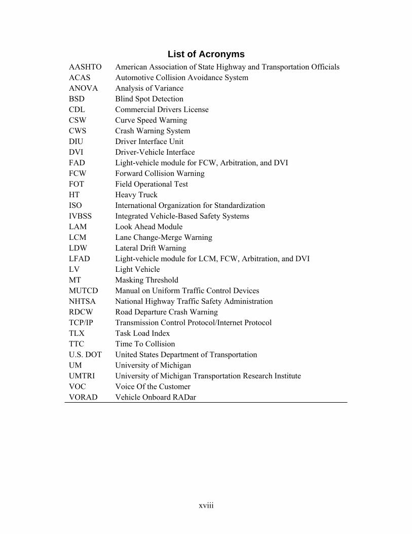
List of Acronyms AASHTO American Association of State Highway and Transportation Officials ACAS Automotive Collision Avoidance System ANOVA Analysis of Variance BSD Blind Spot Detection CDL Commercial Drivers License CSW Curve Speed Warning CWS Crash Warning System DIU Driver Interface Unit DVI Driver-Vehicle Interface FAD Light-vehicle module for FCW, Arbitration, and DVI FCW Forward Collision Warning FOT Field Operational Test HT Heavy Truck ISO International Organization for Standardization IVBSS Integrated Vehicle-Based Safety Systems LAM Look Ahead Module LCM Lane Change-Merge Warning LDW Lateral Drift Warning LFAD Light-vehicle module for LCM, FCW, Arbitration, and DVI LV Light Vehicle MT Masking Threshold MUTCD Manual on Uniform Traffic Control Devices NHTSA National Highway Traffic Safety Administration RDCW Road Departure Crash Warning TCP/IP Transmission Control Protocol/Internet Protocol TLX Task Load Index TTC Time To Collision U.S. DOT United States Department of Transportation UM University of Michigan UMTRI University of Michigan Transportation Research Institute VOC Voice Of the Customer VORAD Vehicle Onboard RADar
xviii

1 Executive Summary
1.1 Goal of the Human Factors and Driver-Vehicle Interface Effort The goal of this project is to contribute to the design and implementation of safe and effective driver-vehicle interfaces for integrated vehicle-based crash warning systems installed in light vehicles and commercial trucks by studying warning characteristics and their effect on driver responses to crash warnings.
1.2 Overview In November 2005, the U.S. Department of Transportation entered into a cooperative research agreement with a team led by the University of Michigan Transportation Research Institute (UMTRI) to develop and test an integrated, vehicle-based, crash warning system to help reduce rear-end, lane change-merge, and road departure crashes for light vehicles and heavy commercial trucks. The first two years of the Integrated Vehicle-Based Safety Systems (IVBSS) Program included a series of human factors tests and various driver-vehicle interface (DVI) engineering tasks to support the development and testing of the integrated warning systems. Specifically, and as outlined in this report, the human factors and DVI development is intended to help ensure that the DVI is safe and effective at accurately communicating crash threats to drivers. Table 1 shows the crash warning subsystems integrated into the IVBSS program.
Table 1. IVBSS warning subsystems
Warning Abbrev. Platform Description Forward collision warning
FCW Light vehicle
Heavy truck
Warns drivers of the potential for a rear-end collision
Lateral drift warning
LDW Light vehicle
Heavy truck
Warns drivers that they may be leaving their lane of travel, or possibly the roadway
Lane change-merge LCM Light vehicle
Heavy truck
Warns drivers that it might not be safe to perform a lane change or merge maneuver due to the presence of other vehicles
Curve speed warning
CSW Light vehicle Warns drivers that they may be traveling too fast to successfully navigate an upcoming curve
The IVBSS program is different from previous field tests of crash warning systems in the number of subsystems that are being integrated and the number of vehicle platforms on which the integration is taking place. While the human factors and DVI efforts have focused on safe and effective communication with the driver, even greater effort has gone into engineering, integrating the subsystems into vehicles, fusing sensor data, and prioritizing warnings. The human factors studies took place in parallel with the development of the vehicles themselves. In anticipation of this, DVI hardware was designed from the beginning of the program to remain flexible in order to accommodate the findings of the human factors studies.
1

Early in the IVBSS program, the IVBSS team considered a wide variety of approaches to DVIs for both light vehicles and heavy commercial trucks, including the use of several warning modalities (visual, audio, and haptic). In doing so, it was recognized that light vehicles and commercial trucks are distinctly different both in the characteristics of their drivers and the environment in which the DVI has to function. Therefore, a singular DVI design and approach for both platforms was ruled out. Nonetheless, the human factors studies that were performed in the laboratory and a driving simulator sought to answer basic questions specific to developing DVIs for integrated crash warning systems. Many of the experiments dealt with general human performance issues (e.g., responses to tone sequences in experiment 1, subtask 5 combined warnings in experiment 3, delays in experiment 4, and interference in experiment 5) and the results should therefore apply to both platforms. What follows in this executive summary, and the remainder of the report in much greater detail, is information on how the experiments, evaluations, and pilot tests were carried out and reports of the associated findings. Wherever applicable, the report highlights how findings from the human factors testing contributed to DVI development for vehicles to be used in the IVBSS field operational test.
1.3 Initial Human Factors and DVI Development Efforts After a review of existing literature on warning design (in general and specific to crash warnings for drivers), expert human factors judgment, and discussions with those overseeing the engineering efforts of subsystem development and integration, seven research questions that warranted study were identified by the human factors team. Given the available time and resources allocated for human factors testing, a team of human factors experts designed a series of five experiments that would attempt to answer these seven research questions with particular interest towards recommending how DVIs should be implemented in the IVBSS program. A work plan was developed, and several upgrades to the UMTRI driving simulator were made to support the conduct of the experiments. A series of experiments was carried out to help the team members select among DVI options. In experiment 1, subjects rated warnings on various dimensions and responded to them by pressing buttons (to indicate which was presented), and researchers collected physical measurements of cab environments. The human performance experiments were conducted in the laboratory and in vehicle cabs. In experiments 2 through 5, subjects drove in the UMTRI simulator while various events occurred (vehicles cut in, lead vehicle braked, lead vehicle changed lanes to reveal parked vehicles, etc.). When these events occurred, one or more of the four warnings (FCW, CSW, LDW, and LCM) would trigger, and sometimes the subject would respond by slowing down, braking, or returning to the lane. Within and across experiments, the warning modalities and, in particular, sound characteristics varied in a systematic manner to examine issues pertaining to simultaneous warnings, warning processing delays, etc. In addition to collecting driving performance data (speed, lane position, throttle position, brake on or off, etc.), warnings were rated on various characteristics (loudness, frequency of occurrence, ease of understanding, usefulness, etc.) at various points in time.
2
1.4 Available DVI Options In the IVBSS program the integration of the IVBSS system, including the DVI, had to occur in post-production vehicles. Therefore, certain constraints associated with existing vehicle designs existed a priori. The current DVI designs are based upon the options available to the team, while retaining the goal of safe and effective communication of warnings to drivers. The design approaches may not, however, be completely representative of those that might be selected by a vehicle manufacturer if an IVBSS-like system was planned for early in the vehicle development stage. On both vehicle platforms, the primary modality used to warn drivers is auditory, with the addition of some haptic warnings on the light-vehicle platform. The auditory warnings are directional, as they are presented from the location where the threat resides (forward, left, or right of the vehicle). Visual displays are not a source of presenting warnings per se, but they indicate the presence of vehicles in blind spots so that drivers might see those indicators, located in or near the left and right rearview mirrors, prior to initiating a maneuver that would otherwise result in an auditory warning. Visual displays are largely used to convey system status information on both platforms. Haptic warnings that are implemented on the light-vehicle platform consist of a directional-vibrating seat pan to convey cautionary lateral drift warnings (LDWs), and a brake pulse that is used in conjunction with an auditory warning to convey imminent forward collision warnings (FCWs) and curve speed warnings (CSWs). With the emphasis on the use of auditory warnings for both platforms, the human factors experiments conducted to support DVI design focused largely on how auditory warning characteristics, and methods of implementing auditory warnings, affect both objective and subjective driver response.
1.5 Experiment 1: Auditory Warnings The first experiment consisted of five subtasks: x Characterize the light-vehicle and truck cabin sound environments; x Systematically study the acoustic properties of sounds having listeners rate the sounds for
perceived urgency, annoyance, noticeability, and loudness, and use the gained understanding in developing crash warnings;
x Construct two suites of sounds comprised of auditory icons and abstract sounds that could serve as crash warnings, and test them for the relative speed at which naïve subjects could learned and respond to them;
x Study how the addition of noise and spatial enhancement modifications made to sounds affect their ability to be localized to determine if such modification might enhance response speed and accuracy; and
x Examine how the characteristics of pulsed tones (the number of bursts, number of beeps in a burst, and time between bursts) affect reaction time to directional warnings.
1.5.1 Summary Findings x Based upon measurements and analyses of sound environments in the Honda Accord and
International 8600 tractor using some standard assumptions, IVBSS warning sounds should be a minimum of 80 dB(A) included frequency content in the 1 to 5 KHz range.
3

x The empirical results from subtask 3 suggest that both urgency and annoyance increase as frequency increases, with annoyance increasing more rapidly. Use of high frequencies risks increasing annoyance levels. 1,000 Hz is two octaves above middle C and may be considered high with respect to fundamental pitch (only the best soprano singers can reach this note). The recommendation, however, is based on considerations beyond just perceived urgency and annoyance, and must also consider the need for the warning to not be masked by background noise levels.
x In comparison to abstract sounds, one set of auditory icons required substantially fewer trials to learn and resulted in substantially shorter reaction times. However, another set of sounds that were modest variants of the auditory icons (and assigned to the same scenarios) were more difficult to learn and produced longer reaction times. Thus, even minor alterations to the sound characteristics of auditory icons can result in markedly different performance.
x Neither the addition of noise nor spatial enhancement improved the accuracy or the speed of responding to a warning sound.
x Response times increased slightly when warnings have increasing numbers of bursts, numbers of beeps in a burst, or delays between bursts. To minimize response time, pulsed warnings should consider two bursts of three beeps each, and short gaps between bursts.
1.6 Experiment 2: Driver Response to Warnings This experiment addressed three questions: x How do drivers respond to warnings; especially, where do they look? x Do drivers respond differently to warnings when they are distracted? x How well do drivers understand a candidate set of IVBSS warnings, and are any
confused or misunderstood?
1.6.1 Summary Findings x For all threat types, in most cases, a driver’s vision was likely to fixate on the area
forward of the vehicle (about 65% of the time during the baseline periods and 75% of the time immediately after a warning), even for lane change-merge (LCM) warnings where the hazard was on the side of the vehicle.
x There were no statistically significant effects associated with distraction; however, the complexity of the basic task meant that many participants were not diligent in completing the distraction task—so that they were not in fact truly distracted.
x All of the warnings were rated as somewhat easy to understand with only small differences among them; however, none of the warnings was initially well understood when drivers were uninformed.
1.7 Experiment 3: Combined Warnings for IVBSS x How does the combining of warnings, using a single cue to represent more than one
threat scenario, affect (a) driver performance when responding to them, and (b) driver ratings of them? Of interest were single warnings, dual warnings (simple and hybrid), and multiple warnings.
4

1.7.1 Summary Findings x No combination of threat scenarios into one or more combined cues (single [master
warning], dual-simple [lateral warning and longitudinal warning], dual-hybrid, or multiple [each treat type had a distinctly different warning]) led to substantially better driver responses than any other combination.
x Subjects least preferred multiple warnings for the four subsystems. x IVBSS should use one of the dual-warning approaches, or a variation of them.
1.8 Experiment 4: Warning Time-Accuracy Trade x How does the tradeoff between warning system processing time (to start to inform the
driver) and warning accuracy affect driver responses to warnings? x How well do drivers respond to a candidate set of IVBSS warnings? Are any confused or
misunderstood?
1.8.1 Summary Findings x Subjects did not perceive the difference in warning delays.
x Delays (the time between the onset of a threat and the presentation of a warning to a driver) between 150 and 300 ms are acceptable for the LDW algorithm implemented in this experiment.
1.9 Experiment 5: Driver Response to Simultaneous Warnings x How does responding to one warning differ from responding to two warnings that are co
occurring (simultaneous or nearly simultaneous)? x Should co-occurring warnings be presented:
o Whenever they occur, even if simultaneously? o One at a time with higher priority warnings interrupting those of lower priority? o In sequence of occurrence, with the first warning playing to completion before the
second (delayed warning) starts? x In the simulator, how well do drivers respond to the set of candidate IVBSS warnings?
Are any confused or misunderstood?
1.9.1 Summary Findings x No single prioritization rule can be recommended based on the data collected.
x BSD (blind spot detection) should be used as is. All other warnings could use enhancements.
5
1.10 Light-Vehicle Stage 2 Pilot Test x How well did the warning hardware or software work on the road and what could be
improved ? x How often did warnings occur?
The light-vehicle stage 2 pilot testing sought to gain feedback and first impressions from 18 laypeople while driving a vehicle equipped with a developmental version of IVBSS. This evaluation was performed along a 90-mile, prescribed route with a researcher present. Objective measures of warning type and frequency were collected, as was subjective data on preliminary acceptance.
1.10.1 Summary Findings x The number of warnings triggered was sufficient for the purpose of the pilot test. x The IVBSS warnings were rated as easy to use. x The IVBSS hardware and software worked fairly well, but some changes are needed to
reduce the false alarm rate (13 warnings per 100 miles), particularly for LDW. Those changes are readily achieved.
In over 1,528 miles of driving, a total of 379 warnings were received in the pilot test. The average number of warnings per driver was 21, with one driver receiving only five warnings and another receiving 38. There were a total of 263 LDW warnings, which were dominated by false warnings when drivers drifted toward a lane boundary and IVBSS mistakenly identified an adjacent threat. Based upon a sampling of the LDW imminent alerts, the false alarm rate for LDW is approximately 12.8 warnings per 100 miles, as compared to an overall false alarm rate of 13 warnings per 100 miles. This was a known problem with the LDW subsystem. Scheduled changes to the LCM subsystem that provides AMR data to the LDW subsystem will significantly reduce false warnings. The second most common warning was cautionary LDW, which was largely associated with lane changes in which the turn signal was not used (98). The frequency of FCW and CSW warnings was quite low. Drivers subjectively reported IVBSS to be intuitive and easy to use. Most drivers stated they received warnings with about the right frequency, and on average were not distracted by IVBSS warnings. The warnings were also deemed to be helpful in identifying potential conflicts. However, the high false warning rate associated with the known LDW problems did lead to driver uncertainty about what each warning was intended to represent. Overall, when compared to the subjective results from previous field evaluations of crash warning systems (RDCW and ACAS), the results are on par despite the recognized need to correct the LDW subsystem.
1.11 Heavy-Truck Stage 2 Pilot Test The heavy-truck stage 2 pilot testing sought to gain feedback and first impressions from commercial truck drivers operating a vehicle equipped with a developmental version of IVBSS. This evaluation was performed along a prescribed route with a researcher present. Objective measures of warning type and frequency were collected, as was subjective data on preliminary acceptance.
6

1.11.1 Summary Findings The heavy-truck stage 2 pilot test will be run in mid-November 2007. Findings will be reported when the test is complete.
1.12 Conclusions The human factors testing described in this report provided guidance in developing the driver interfaces for the prototype vehicles used in the IVBSS program. If the program is approved to move forward with the planned field operational test in Phase II, then additional testing of the interface designs will provide data for further improvement.
Both vehicle platform teams worked with the human factors staff to determine the constraints imposed by vehicle hardware and software, as well as driver characteristics. The team identified the research questions most critical to integrated crash warning system implementation. The integrated system was developed for existing production vehicles. The specifics of the driver interface implementation for this project, however, are likely to be different from how a vehicle manufacturer might elect to implement a suite of integrated warnings, having the benefit of designing the system from the onset of vehicle planning. This is particularly true with regard to the possible use of advanced visual and haptic displays that could not readily be retrofitted into a production vehicle. The results of the experiments presented in this report will provide information for such future systems, as well as the driver-vehicle interfaces implemented in this research program.
The integrated system driver interface design is centered on auditory warnings, which is consistent with both current and accepted automotive human factors practice; auditory signals are appropriate for time-critical events, are less likely to interfere with the visual aspects of driving, and capture driver attention even when the driver is distracted. The experimental results given in this report support the particular implementation of auditory warnings for the IVBSS program. Supplemental warnings are provided by visual and haptic alerts to reinforce the effectiveness of the auditory warnings. These supplemental warnings were developed by each platform’s design team apart from the human factors experiments discussed in this report or incorporated into the DVI design, in consultation with the all IVBSS partners.
At the conclusion of this stage of the IVBSS program, the DVI design for the light vehicle platform will have one warning for longitudinal hazards (FCW and CSW), and a second for lateral hazards (LDW and LCM), supplemented by directional cues. Based on the findings of driver preference surveys, this approach will provide a safe, effective and usable driver-vehicle interface for the IVBSS field operational test. For the heavy truck platform, a similar approach for all subsystems was used. The heavy-truck implementation differs from the light-vehicle approach due to the constraints imposed by the Eaton crash warning system, which was used as the basis for the production of the heavy-truck warning system.
The results of the human factors experiments described in this report will not only provide the basis for the current driver interface implementations, they will also substantially extend the knowledge of how the design of auditory warnings for a suite of integrated warnings impact driver response to those warnings.
7
2 Overview In November 2005, the U.S. Department of Transportation entered into a cooperative research agreement with an industry team led by the University of Michigan Transportation Research Institute (UMTRI) to develop and test an integrated, vehicle-based, crash warning system to reduce rear-end, lane change-merge, and roadway departure crashes for light vehicles and heavy commercial trucks. The work being carried out under this agreement is known as the Integrated Vehicle-Based Safety System (IVBSS) program. The IVBSS program is a four-year effort divided into two consecutive, non-overlapping phases of 24 months each. The UMTRI-led team is responsible for designing, building, and field-testing the prototype integrated crash warning systems. This report summarizes the initial human factors testing and driver-vehicle interface development performed during the first phase of the program in support of an overall integration effort, all prior to the field test. This first phase includes (1) the development and specification of the driver-vehicle interfaces (visual, audio, and haptic information provided to the driver), (2) the development of prototype hardware, and (3) the design and conduct of a series of laboratory and driving simulator studies to assess and enhance the ease of use and usefulness of the evolving driver interface. Subsequent research in Phase II will assess the safety benefits and driver acceptance associated with the prototype integrated crash warning systems. Preliminary analyses conducted by the U.S. DOT indicate that the number of crashes can be reduced significantly by the widespread deployment of integrated crash warning systems that address rear-end, lateral drift, and lane change-merge crashes (NHTSA, 1996; Pomerleau & Everson, 1999; Talmadge, Chu, Eberhard, Jordan, & Moffa, 2001). Such integrated warning systems have the potential to provide comprehensive, coordinated information, from which the individual crash warning subsystems can determine the existence of a threat and, thus, provide the appropriate warning to drivers. Three crash warning subsystems are being integrated into each platform of the IVBSS program: forward collision warning (FCW), lateral drift warning (LDW), and lane change-merge (LCM) warning. A fourth, curve speed warning (CSW), is being integrated into the light-vehicle platform. x Forward collision warning provides warnings to drivers to assist them in avoiding or
mitigating rear-end crashes with other vehicles. x Lateral drift warning consists of a system that warns drivers that they may be drifting
inadvertently from their lane or departing the roadway. x Lane change-merge warning warns drivers of possible unsafe maneuvers based on adjacent
or approaching vehicles in adjacent lanes, and includes full-time side-object-presence indicators.
x Curve-speed warning warns drivers that they may be driving too quickly into an upcoming curve and as a result might lose control and depart the roadway.
What differentiates the IVBSS program from previous programs supported by the U.S. DOT is that these subsystem are being evaluated as part of an integrated crash warning system, rather than independently. To realize the maximum potential benefits, the integration in the IVBSS
8

program is greater than that undertaken in any prior program of its kind. The integration should dramatically improve the IVBSS performance relative to the standalone subsystems by increasing system reliability and reducing false warnings. As a result, consumer acceptance of crash warning systems, in general, might be expected to improve. However, the scope of integration effort on the IVBSS program is not limited to sensor data, but includes the arbitration of warnings based upon threat severity and the development of an integrated driver-vehicle interface. Arbitration and a well-designed driver-vehicle interface are critical to ensuring driver comprehension of warnings, reduction of driver workload, and reduction of driver reaction times. The IVBSS team at the Department of Transportation includes representatives from the National Highway Traffic Safety Administration, the Research and Innovative Technology Administration (specifically, its Intelligent Transportation Systems Joint Program Office and the Volpe National Transportation Systems Center), the Federal Motor Carrier Safety Administration, and the National Institute of Standards and Technology. The team led by UMTRI working on the light-vehicle platform includes Visteon Corporation (a major supplier), Honda R&D Americas (a manufacturer), and Cognex Corporation (a supplier of crash warning systems). On the heavy-truck platform the partners are Eaton Corporation (a supplier of sensors), International Truck (a truck manufacturer), and Cognex Corporation. In addition, Con-Way Freight (a commercial trucking company) is working on the program. The involvement of industrial partners on the IVBSS program is seen to be critical, given the partners’ technical knowledge of and ultimate ability to deploy actual systems into the Nation’s vehicle fleet. Additional members of the team include Battelle Memorial Institute, which is assisting in the development of the heavy-truck driver-vehicle interface, and the Michigan Department of Transportation, which is providing technical support as it relates to the acquisition of crash and roadway geometry data. Additional information detailing the development of the integrated crash warning systems during the first year can be found in the first annual report of the IVBSS program (UMTRI, 2007).
2.1 The Need to Conduct Studies on Integrated DVIs The design of an integrated crash warning system differs significantly from that of a single, stand-alone system. A stand-alone system does not need a warning that is readily distinguishable from any other warnings presented to the driver. A single system simply has to present a warning that is readily detected and acted upon. In the implementation of a stand-alone system, effective warnings can be designed that do not convey much in the way of meaning or intent. In other words, if a vehicle is only equipped with a forward crash warning system, the driver can readily learn that the presentation of a warning, almost independent of its characteristics, is associated with a forward crash scenario. There is less cognitive processing required by the driver to determine what the warning means, or how to respond, in a stand-alone system relative to an integrated crash warning system. For an integrated crash warning system, the driver must determine (1) what warning was presented, (2) what the warning means (i.e., what crash type is detected (forward, curve speed, lateral drift, or lane change-merge) and (3) how best to respond. Furthermore, a warning stimulus that works well in a stand-alone system (e.g., FCW) may not work as well in a multiple warning system, even when warnings do not occur concurrently. If the stimulus does not work well in a multiple warning system, it could be a result of the extra time
9
required for the driver to compare this stimulus to the possible stimuli from other warnings to verify its identification. The implication for design is that the identification of several stimuli, all of which appear to be optimal for stand-alone systems, may require further empirical comparison to select the most effective of those stimuli for a multiple warning system. This is a significant issue because it appears likely that the majority of warnings issued from a multiple warning system will be issued for single conflicts. Ideally, the best possible warnings for an integrated crash warning system would result in reaction times, and the types of responses, that one would observe in a well-designed stand-alone crash warnings system. However, most of the human factors testing and DVI development work to date that is published in the open literature has concentrated on stand-alone systems (e.g., what constitutes a good auditory warning regardless of the application); in addition, it has not taken into consideration the potential for confusion or uncertainty by a driver when multiple warnings are present and what is needed to mitigate uncertainty. Therein lies the challenge facing the design of an integrated warning system, and hence the need for DVI testing and development on the IVBSS program, which is the central theme to the simulator testing in particular.
2.2 Prior Warning Studies and What Do They Say About How Drivers Should Be Warned? A vast body of literature exists for the design and evaluation of warning systems, in particular integrated warning systems. Most notably, this body of literature has recently been surveyed and discussed in the context of IVBSS in Campbell, Richard, Brown & McCallum (2007). This section identifies the literature that is of specific importance to this project in several categories: warning timing, warning reliability, multi-collision warnings, modality of warning, multi-modal warnings, auditory warnings, warning design, warning urgency, auditory icons, and sound localization. Notice that the emphasis of this review and the literature in general is on the characteristics of individual warnings, not on the integration of warnings, which is the focus of IVBSS. For a complete listing of the literature reviewed, see Appendix D.
2.2.1 Warning Timing The timing of warnings has a critical effect on the safety benefit of any warning system. Early warnings have been shown to reduce the number and severity of crashes (McGehee, Brown, Lee, & Wilson, 2002) and to help drivers to react more quickly to avoid collisions, even when drivers are not distracted (Lee, Ries, McGehee, Brown, & Perel, 2000). The extent to which appropriate timing predictions can be made is straightforward, as predictions must be based on assumptions about the driver’s expectations and typical responses (Kiefer, LeBlanc, & Flannagan, 2005). The timing of warnings not only affects the driver’s immediate responses, but also the trust they develop in the warning system. A series of simulator studies has shown that in imminent crash situations, response and trust for early warnings (e.g., .05 seconds after a lead vehicle braking) is better than for late warnings (e.g., 0.99 seconds) (Abe & Richardson, 2004, 2005, 2006). Although there is clear evidence to support use of early warnings, there also appears to be a price—overall warning reliability may be reduced if warnings are produced too early. The timing issue is particularly relevant to experiment 5.
10
2.2.2 Warning Reliability Response frequency to alarms has been shown to decline with decreasing reliability (Bliss & Acton, 2003). Reliability, in this context, can be defined as the extent to which a system yields the same results on repeated trials. According to signal detection theory, in assessing the reliability of a warning, there are four cases to consider: (1) a signal and a response (hit); (2) a signal and no response (miss); (3) no signal and a response (false warning); and (4) no signal and no response (correct rejection). What confuses the matter is that responding to an event is a two-stage process. In the first stage, the warning system responds to the event; in the second stage, the driver responds either to the warning system alone or to the warning system and the event, depending on the situation. So, from the perspective of the warning system, if an event leads to a warning based on the system rules, it is a hit. However, if from the driver’s perspective the warning is considered unnecessary, it would be considered a nuisance warning relative to the original event (even though is was correctly triggered based on the warning system rules). Thus, what the driver considers a nuisance warning depends on what their assessment is with regard to the warning system and the triggering event. Nuisance warnings are important because of their effect on driver acceptance and sometimes the extent to which they can be reduced through the application of technology. Yamada and Kuchar (2006) found that the mean driving speed decreased as the missed detection rate of a collision warning system increased, demonstrating a decrease in a driver’s reliance on warnings when the system has low reliability. Furthermore, they found that both the acceleration pedal and brake pedal reaction time increased when the system became more prone to false alarms. The inherent problem of a collision warning system, however, is that the base rate of crash events is extremely small. As a result, even excellent warning systems, which provide correct detection 99 percent of the time and generate false alarms only 1 percent of the time, will be prone to generate many more false alarms than hits because the opportunity to provide a true positive alarm is scarce when the baseline is low, while the opportunity to provide false positives is immense (Parasuraman, Hancock, & Olofinboba, 1997). Drivers need to accept this probability imbalance and expect to hear many false alarms if they want a system with the potential to save lives. Another effect of reliability on system effectiveness is annoyance, which is likely to increase as the number of inappropriate warnings increases. For example, a rate of four inappropriate warnings per hour has been rated in a naturalistic driving study as most annoying (Lerner, Dekker, Steinberg, & Huey, 1996). Recognizing the importance of reliability, a significant number of false alarms were included in experiments 2 through 5.
2.2.3 Warnings Systems with Multiple Warnings These systems are now becoming available but have not been studied extensively in the literature. Chiang, Brooks, & Llaneras (2004) were particularly interested in the rare event of warnings that occur at the same time. They found that drivers were not confused when they received different warnings for different collision systems, as opposed to receiving a single combined warning for all different systems. They found that drivers receiving a multiple warnings looked in the direction of the threat more often than drivers receiving a combined warning, and they were sometimes able to avoid a collision as they were quicker to realize that the second warning was distinct from the first. In another simulator study, no difference in reaction time and response accuracy was found between a single collision warning and individual alerts (Ho, Cummings, Wang, Tijerina, & Kochhar, 2006). Subjects did show a preference, however, for the multiple warning condition. The topic of multiple warnings is
11
central to all of the major experiments. The mapping of threats onto warnings was specifically examined in experiment 3.
2.2.4 Modality of Warning and Multi-Modal Warnings The literature on multi-modal warnings offers mixed recommendations. The redundancy effect and the overall increased magnitude of combined signals contribute to a general preference for multi-modal warnings. Manual reaction time responses have been found to be faster with trimodal stimuli (visual, auditory, and tactile) than with bi-modal stimuli, which were faster than uni-modal stimuli (Diederich & Colonius, 2004). Similarly, bi-modal interfaces (vision and tone or vision and voice) for forward collision warning were judged more helpful than uni-modal interfaces (Maltz & Shinar, 2004). In contrast to these and other findings, Lee, McGehee, Brown, and Marshall (2006) found that combining all four redundant warning modes resulted in a driver reaction that was 400 ms slower than just an auditory and visual alert. They suggest that redundant multi-modal warnings are not universally beneficial, and that in some circumstances might introduce complex sensory interplay that counteracts the benefits of redundancy. An additional point of view has to do with the magnitude of the signals and their spatial separation. In general, for strong multi-sensory facilitation, stimuli must occur simultaneously and in the same spatial location. Further, a strong facilitation effect is found only if the individual signals are relatively weak (Schnupp, Dawe, & Pollack, 2005). These findings imply that some intervening factors (such as the magnitude of the signals and their spatial location) may overwhelm the redundancy effect. To support that conclusion, a study that compared driver attentional prompting to a spatial location found that there was a facilitatory effect of cross-modal auditory prompting of the spatial direction, but not for vibrotactile prompting (Ho, Tan, & Spence, 2006).
2.2.5 Auditory Warnings The use of sound to signal an imminent warning condition is ubiquitous in many warning contexts, and virtually indispensable for collision avoidance. There are few other ways to inform a driver quickly (without involving a redirection of gaze) that something is, or may be going very wrong. In comparing the suitability of an auditory to a visual warning, Deatheridge (1972) suggested that an auditory signal is best suited to convey a simple and short message requiring immediate action, while the visual system is overburdened, and the person’s position may not be fixed. It is difficult to imagine a better fit to an in-vehicle collision avoidance system. Indeed, the use of sound to warn of danger is ubiquitous. This has generated a variety of secondary problems, not the least of which is the need to ensure that a driver interprets the sound as appropriately urgent, distinctive, and recognizable in order to make a timely response. In the context of collision avoidance, a fast and appropriate response is indispensable. In the context of an automotive product it is also desirable that the sound should not annoy those in the vehicle. The literature on auditory warnings covers several broad themes: general discussions of methods for constructing warning sounds (e.g., Casali, 2003; Deatheridge, 1972; Edworthy, Stanton, & Hellier, 1995; Patterson & Mayfield, 1990) to ensure they are heard; investigations of the relationship between the acoustic attributes of a sound and a listener’s perception of urgency (e.g., Arrabito, Mondor, & Kent, 2004; Edworthy & Stanton, 1995; Guillaume, Drake, Rivenez, Pellieux, & Chastres, 2002; Haas & Edworthy, 1996; Hellier, Edworthy, & Dennis, 1993; Hellier, Edworthy, Weedon, Walters, & Adams, 2002; Marshall, Lee, & Austria, 2007); the
12
association of meaning with a sound through the use of natural sounds or auditory icons (Belz, Robinson, & Casali, 1999; Graham, 1999; Hellier et al., 2002; Stephan, Smith, Martin, Parker, & McAnally, 2006); and the use of spatial information in sounds to enhance localization (Catchpole, McKeown, & Withington, 2004; Tan & Lerner, 1996). Each of these topics is discussed below. As noted elsewhere, this literature is sufficiently supportive of the use of sound for imminent warnings that the auditory modality was chosen as the primary modality for IVBSS warnings that were assessed in this project.
2.2.5.1 Design of Warnings Existing guidelines for sound construction include prescriptions about the contexts in which auditory warnings are best used (Deatheridge, 1972) and algorithms to effectively design a sound that is not excessively invasive. For example, Patterson and Mayfield (1990) discuss the use of spectral analysis of background noise to design warnings that reduce spectral overlap with the noise. Rather than designing a sound that exceeds the overall decibel level of the background noise, the warning only needs to exceed the noise levels in a few spectral bands. This allows the design of a sound that can be heard without being excessively loud. These authors also put forward a common method and vocabulary of warning construction in which pulses are combined to form sound bursts. Concern for background sound levels led to experiment 1, subtask 1.
2.2.5.2 Urgency There has been a good deal of focus on the perceived urgency of warning sounds especially for circumstances requiring immediate response. In part, this is due to results that find response time to warnings perceived as urgent is shorter than to those perceived as less urgent. Much of the research on urgency has been directed toward establishing which acoustic properties of a sound are associated with urgency (e.g., Edworthy, Loxley, & Dennis, 1991). Several acoustic attributes have been associated with urgency—high frequency, rapid pulse rate, high or rising volume (to name a few), short onset time. Other attributes appear to be more equivocal (e.g., timbre, rhythmic variation). Although urgency has been recognized as a particularly important component for crash warnings, it is also recognized that sounds produce other subjective impressions in listeners as well. Tan and Lerner (1995) made a comprehensive study of 28 warning sounds (including speech-based warnings) using a multiple attribute evaluation (MAE) method that quantified the utility of each sound in the context of crash warnings. This report includes a correlation matrix that suggests many attributes are related to each other—in particular, annoyance seems to be highly correlated with urgency. This makes the design of an urgent warning particularly challenging for a safety system embedded in a consumer product. If the warning is insufficiently urgent, the warning may not be effective. If the warning is sufficiently urgent, it may annoy the prospective customer so that it is avoided or somehow subverted. Recent research has been directed toward finding the combination of acoustic attributes that increase urgency without also raising annoyance levels, or at least finding attributes that raise urgency more than annoyance (e.g., Marshall et al., 2007). There are two important issues that this focus on acoustic properties associated with urgency does not address. Warning sounds do not occur in a vacuum; they are often presented in the
13

context of other warning sounds and thus must be easily distinguishable. If all sounds were designed to be the most urgent, they would likely all sound the same. A second problem is that occasionally, the acoustic properties of a sound suggest it should be perceived as urgent, but instead it is perceived as silly or comical. For example, Guillaume et al. (2002) found that a learned semantic association may override the effects predicted by an acoustic analysis alone. The need to relate sound physical characteristics to the perception of urgency led to experiment 1, subtask 2.
2.2.5.3 Auditory Icons An auditory icon is a natural sound that has a semantic association with a warning condition. In the context of collision warnings, horn honks, squealing tires, and rumble-strip sounds have been employed to represent side-collision, forward collision, and lane departure warnings. Several studies have shown that auditory icons can be learned easily and responded to quickly (Belz, 1997; Graham, 1999; Stephan et al., 2006). To obtain the best results, a preexisting association between the sound and the warning condition is important. In some situations the warning condition may not lend itself to an obvious sound, or the semantic relationship may be odd. For example, the sound of squealing brakes may not immediately be interpreted by a driver as the need to brake, only that someone nearby is braking. Contrast this with a rumble strip sound for a lane departure warning—the sound mimics what is heard if a vehicle wanders onto the shoulder. The naturalness of the sound of an auditory icon is relevant only in as much as such sounds usually have built-in semantic associations. Unnatural sounds with semantic associations can work equally as well. For example, if a warning sound happened to mimic the sound of a familiar radio clock, a frequently heard artificial sound, that warning would carry semantic associations that would likely influence the perception of urgency. Thus, warning sounds that resemble cartoon pratfalls or video games are often reported by listeners as silly, inappropriate, or unsuitable as warning sounds. These associations have been learned through repeated exposure. Thus warning urgency may also be learned through repeated exposure, much as one becomes highly sensitized to the sound of one’s cell phone. Issues pertaining to auditory icons and their naturalness were examined in experiment 1, subtask 3.
2.2.5.4 Sound Localization Directional warnings should coincide with the location of lateral warning (such as for lane departure and lane change-merge warnings). This should lead to faster recognition of a warning and reduce the effort to locate the radial direction the conflict. Research on this issue is scant and has generally shown that, inside a vehicle, localization is dependent on the kind of sounds presented (speech and complex sounds are more easily localized than simple sounds) and speaker placement (localization performance is best with speakers directed toward the listener’s ears) (Tan & Lerner, 1996). It remains to be demonstrated that a lateralized sound indeed enhances a driver’s response to a lateralized warning. In most cases, lateralized warnings lack sufficient radial resolution to pinpoint the direction of concern. At best, lateralized warnings distinguish only left and right. Moreover, sound direction cues are easily overshadowed by visual cues—even if the voice of a speaker is displaced from the speaker’s radial direction, the voice is still likely to be heard as
14

originating from the speaker’s direction. If drivers have even a modest level of situational awareness, they are likely to be aware of the direction of their merge or lane drift without being told. Issues pertaining to sound localization were examined in experiment 1, subtask 4.
15

2.3 Research Questions Identified and Addressed As extensive as the literature on warnings is, there were still many questions that needed to be addressed in order to implement an easy-to-use, understandable, and useful driver interface for IVBSS. Based on an expert review of the literature and review of the design issues for the option space being considered for IVBSS, the seven most prominent questions regarding human factors considerations in the design of an integrated crash warning system were identified. Although there were many other possible questions that could have been addressed, those listed in Table 2 were considered most pertinent to the IVBSS program, and could be addressed within the constraints of the program.
Table 2. Seven research questions examined
Issue Comment Q1. Shared warnings (When and how should warnings be shared or differentiated, e.g., FCW and CSW, LDW and LCM?)
In response to warnings, drivers can return to their lane, steer out of it, or slow down. Warnings can indicate what is wrong (so each warning is unique), what to do (which suggest common warnings based on desired actions), or both.
Q2. Sequencing co-occurring warnings (Should warnings occurring at the same time be presented together or with a delay between them?)
Presenting two warnings at the same time (e.g., forward collision warning and lateral drift) could confuse drivers as they will not be able to determine what each warning is.
Q3. Warning set/confusion (Are warnings in the IVBSS sets confused with each other?)
Warnings that sound, look, or feel alike, could be confused. But, what constitutes “alike”?
Q4. Time course of driver actions (When responding to warnings, what is the process by which drivers respond?)
To design warnings, the sequence of how drivers respond to warnings needs to be known—in particular where and when they look, when they release the throttle, and when they brake or steer.
Q5. Warning processing time/accuracy tradeoff (How does the tradeoff between warning system processing time [to start to inform the driver] and warning accuracy affect driver responses to warnings?)
For some systems, waiting to respond improves warning accuracy, for example allowing a radar unit to make more sweeps and increase threat identification accuracy. However, that delay gives the driver less time to respond.
Q6. Auditory characteristics of warnings (How does auditory warning effectiveness vary with warning sound characteristics [loudness, pitch, speed] in sound environments of each vehicle platform?)
Although there are basic data on auditory discrimination, their application to multidimensional variations found in real warnings is difficult. In real systems, due to signal generator limitations and the desire for warning sounds to resemble particular real-world sounds, there are constraints on which sounds can be used.
Q7. Influence of pauses and repetitions (For sounds that involve periods of silence (or pauses), are responses deferred to coincide with silence? What is the optimal number of repetitions?)
For lateral drift, sounds resembling a rumble strip are sometimes used. That sequence takes time to play, potentially delaying a driver response. Can the sequence be sped up?
16

2.4 Work Plan Table 3 shows the mapping of the seven issues onto five planned experiments, with experiment 1 actually being comprised of five smaller experiments (subtasks). Experiments 2 to 4 involve use of the driving simulator.
Table 3. Sequence of experiments and mapping to research questions
Experiment Question/ Topic Central Theme Procedure Subsystem
Exp 1 jury selection
Auditory warning characteristics (Q6)
Characterize sound environment of light vehicle and heavy truck; select sounds best suited to environment, five sub-tasks
Jury evaluations: (sub-task 1) of masking of warnings, (2) of sound appropriateness, (4) localization of candidates sounds RT evaluations: (sub-task 3) confusability of ensemble, (5) repeating sounds
All
Exp 2 Time course, method (Q3, Q4)
How people respond (where and when they look) suggests warning presentation modality and content
Collect eye fixations, steering and brake data, etc. to initial warnings (includes uninformed warnings)
FCW, LDW, CSW, maybe LCM
Exp 3 Shared warnings (Q1, Q3)
If two warnings (FCW, CSW) lead to the same response, should the warning be the same?
Collect steering and brake data, etc. for shared warnings and unique warnings
All
Exp 4 System time/accuracy tradeoff (Q3, Q5)
Warnings that are delayed may be more accurate? What tradeoff is “best?”
Use full set of candidate warnings, vary accuracy and delay of each warning, collect steering and brake data, etc.
All
Exp 5 Co-occurring warnings (Q2)
When two warnings occur at the same time, should one be delayed and by how much?
Create situations to trigger two warnings at the same time. Sometimes present both, sometimes present in priority order with delays. Collect steering and brake data, etc.
All
2.4.1 Impact of Human Factors Testing on IVBSS Design
2.4.1.1 Laboratory and Driving Simulator Testing The goals of human factors testing in the laboratory and driving simulator were to provide information useful in making IVBSS driver interface design decisions and to provide more general knowledge that will assist in the development of driver interfaces for collision warning systems. Additionally, the driving simulator experiments served to test elements of the DVI before they were implemented on prototype vehicles. For example, some of the messages that would appear on the center console display of the light-vehicle platform were tested and
17

modified in experiment 3. Based on feedback from experimenters and subjects, the messages were modified to make them easier to understand and less distracting. Experiment 1 guided the selection of warning tones primarily for the light-vehicle platform. It provided the experimenters with tools for the selection of suites of auditory warnings based on predicted levels of parameters such as perceived urgency, discriminability from other tones, and annoyance. Using the CSound software tool (www.csounds.com), the experimenters were able to change sounds in a systematic manner. After one of the original warning tones was not well received, an alternative tone was quickly developed for the jury drives using CSound, with predicted levels of urgency and discriminability developed from testing of other tones. In addition, subtask 5 led to a heightened awareness of the effect of auditory warning on response time and an effort to keep auditory warnings short. Experiments 2 through 4 were conducted in the UMTRI driving simulator. Experiment 2 examined where drivers looked when responding to warnings and their reactions to the initial warnings set. In fact, the primary class of measures of interest, those relating to eye fixations, seemed to be relatively unaffected by warnings, but that may be because the analysis was at too gross a level. However, this experiment did point out that several of the warnings needed improvement and provided useful data on how often planned and unplanned triggering of each warning actually occurred. Experiment 3 was designed to determine how much, if at all, warnings should be combined. Results from the study ruled out the use of four individual warnings (one each for LDW, CSW, FCW, and LCM). Furthermore, an analysis that led up to the experiment discouraged the use of a single warning to represent all subsystem warnings collectively. As a result, a solution using two warnings, one for longitudinal and one for lateral threats, was selected. Objective results from the simulator experiment did not strongly favor any one of the warning approaches examined, so a subsequent design decision was made based on other considerations (such as the preferences of experts in the jury drives and laypeople in the initial pilot test). Experiment 4 examined the effect of warning delays (time to allow drivers to gather additional information). For LDW, there was no difference between 0 and 150 ms delays in terms of the time to return to the lane, but there was a difference between 150 and 300 ms. For FCW, there were differences between the three delays, but that difference may be due to other confounded factors, not delay. Experiment 5 addressed the issue of simultaneous warnings. The results of this experiment were important in restricting the length of auditory warnings and in confirming their adequacy. The experiment also provided useful perspective concerning the relatively rare occurrence of near-simultaneous warnings, even when there was a deliberate effort to force them to occur.
2.4.1.2 Light-Vehicle Jury Drives The light-vehicle jury drives involved human factors experts and IVBSS team engineers driving a fixed route on public roads using a prototype system. One significant issue identified in the light-vehicle jury drives was an inter-vehicle variation in the haptic brake pulse used for FCW and CSW warnings. There were several cases in which the brake pulse was not noticed. This finding led to additional consideration of the technical aspects of the brake pulse cue.
18
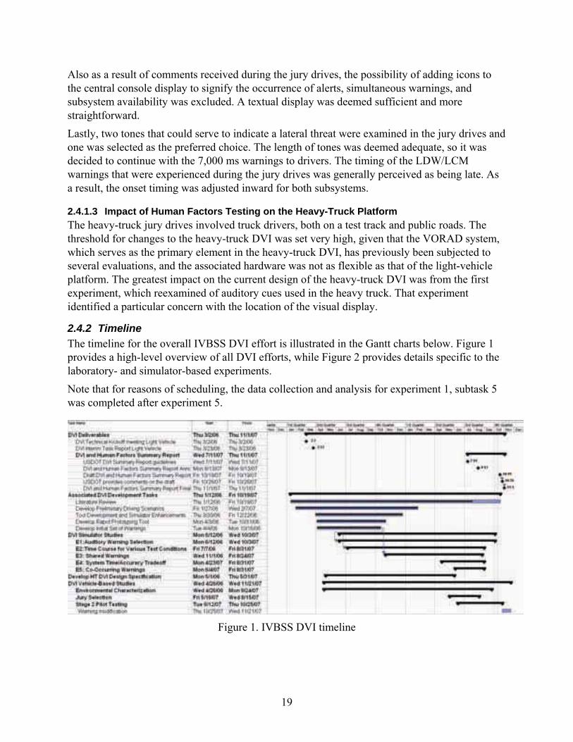
Also as a result of comments received during the jury drives, the possibility of adding icons to the central console display to signify the occurrence of alerts, simultaneous warnings, and subsystem availability was excluded. A textual display was deemed sufficient and more straightforward. Lastly, two tones that could serve to indicate a lateral threat were examined in the jury drives and one was selected as the preferred choice. The length of tones was deemed adequate, so it was decided to continue with the 7,000 ms warnings to drivers. The timing of the LDW/LCM warnings that were experienced during the jury drives was generally perceived as being late. As a result, the onset timing was adjusted inward for both subsystems.
2.4.1.3 Impact of Human Factors Testing on the Heavy-Truck Platform The heavy-truck jury drives involved truck drivers, both on a test track and public roads. The threshold for changes to the heavy-truck DVI was set very high, given that the VORAD system, which serves as the primary element in the heavy-truck DVI, has previously been subjected to several evaluations, and the associated hardware was not as flexible as that of the light-vehicle platform. The greatest impact on the current design of the heavy-truck DVI was from the first experiment, which reexamined of auditory cues used in the heavy truck. That experiment identified a particular concern with the location of the visual display.
2.4.2 Timeline The timeline for the overall IVBSS DVI effort is illustrated in the Gantt charts below. Figure 1 provides a high-level overview of all DVI efforts, while Figure 2 provides details specific to the laboratory- and simulator-based experiments. Note that for reasons of scheduling, the data collection and analysis for experiment 1, subtask 5 was completed after experiment 5.
Figure 1. IVBSS DVI timeline
19
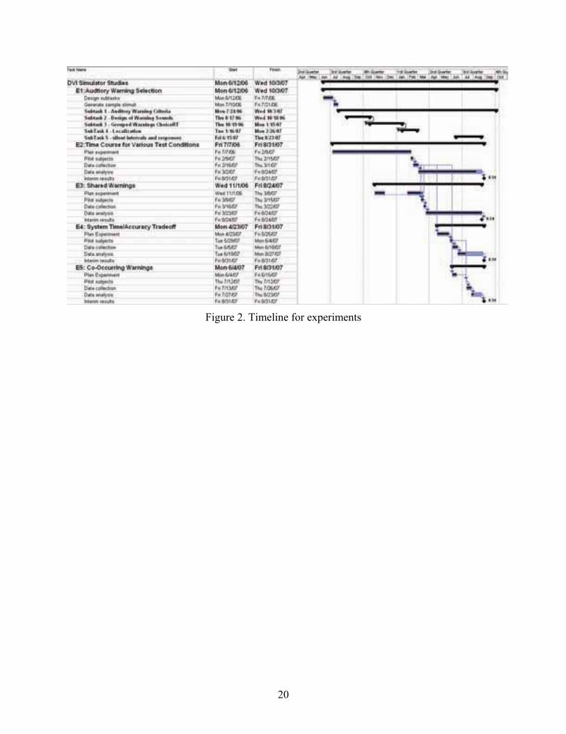
Figure 2. Timeline for experiments
20

2.5 Report Structure The remainder of this report is organized as follows: x Section 3 provides a summary of the research conducted in this study, including
performance-based hardware results, the available option spaces on each platform, research questions addressed, and overviews of the driving simulator and test scenarios.
x Section 4 provides an overview of experiment 1 (subtasks 1 through 5) on auditory warnings (the complete details of which are provided in Appendix E).
x Section 5 provides an overview of experiment 2 on driver response to warnings (the complete details of which are provided in Appendix F).
x Section 6 provides an overview of experiment 3 on integrating IVBSS warnings (the complete details of which are provided in Appendix G).
x Section 7 provides an overview of experiment 4 on warning-delay/accuracy tradeoffs (the complete details of which are provided in Appendix H).
x Section 8 provides an overview of experiment 5 on driver response to simultaneous warnings (the complete details of which are provided in Appendix I).
x Section 9 provides an overview of the light-vehicle stage 2 pilot test (the complete details of which are provided in Appendix J).
x Section 10 provides an overview of the heavy-truck stage 2 pilot test (the complete details of which are provided in Appendix K).
x Section 11 provides next steps regarding the development of the DVIs and conclusions. x Section 12 contains the list of references. x Appendix A provides details of the driving simulator used in the experiments. x Appendix B discusses the various driving scenarios used in this study. x Appendix C details the prototyping tools for scenario development and warning interface
creation. x Appendix D provides an additional literature review, in greater detail than could be
provided in Section 3. x Appendix E details the five subtasks of experiment 1, auditory warnings. x Appendix F details experiment 2, driver response to warnings. x Appendix G details experiment 3, integrating warnings for IVBSS. x Appendix H details experiment 4, warning delay-accuracy tradeoff. x Appendix I details experiment 5, driver response to simultaneous warnings. x Appendix J details the light-vehicle stage 2 pilot test. x Appendix K details the heavy-truck stage 2 pilot test.
21

3 Research Summary
3.1 Platform-Based Hardware Constraints This section identifies any existing DVI design constraints, by platform, which had to be taken into consideration when planning the DVI option spaces and experiments. This includes, but is not limited to, issues related to working with vehicles that are post-production.
3.2 Available Option Space The IVBSS program recognized that the integration of the warning system, including the DVI, would have to occur in post-production vehicles and be consistent with the constraints imposed by real products. Thus, working within the range of available modifications that could be made to the production vehicles, option spaces (outlines of the DVI alternatives available for implementation) were determined for both light-vehicle and heavy-truck platforms. For production vehicles, the development of the DVI for an integrated crash warning system would most likely occur early in vehicle design. However, the goal of developing DVIs for the IVBSS program was to design an interface that was effective in communicating warnings to drivers, but not necessarily to develop the optimal DVI for an integrated crash warning system. Despite the initial constraints, early feedback and evaluation suggest that the approaches taken in the IVBSS DVI development are useful, effective, and acceptable to drivers.
3.2.1 Light-Vehicle Option Space The DVI option space for the light-vehicle platform was explored during weekly meetings that included representatives from UMTRI, Visteon, and Honda. Many of the decisions to include or exclude certain options were the result of fruitful discussions among those who attended these meetings. Much of the justification for decisions was based on the literature review and on other human factors considerations. The design process started with an option space that included as many options as possible and then narrowed the design down by eliminating options that were not technologically feasible for installation in a production vehicle, did not meet human factors guidelines, or were inconsistent with the overall goals of IVBSS. Among the constraints for the light-vehicle option space, the primary concern was that large-scale structural changes could not be made to the production vehicles. For example, the installation of a head-up display (HUD) would require excessive modifications to the structure of the production vehicle. Similarly, in considering a display for advisories, there was an attempt to use hardware that already exists in other Honda Accord implementations. An additional constraint of major impact was that of safety. Some ideas that may have been explored further in a design phase were dropped upfront for the production vehicle. For example, there was discussion of vibrating the steering wheel as a means of warning the driver. This was not pursued because of concerns that the vibration from a post-production subsystem would input vibration into the steering system and might adversely affect the safety of the system. Nevertheless, structural changes were made to the car seat to allow for seat vibration, and an implementation of a brake pulse was added after thorough discussions between Visteon and Honda representatives on implementation and on the safety aspects of such a modification. Auditory warnings were selected as the primary modality for alerting drivers on the light-vehicle platform. A strategic decision had been made early in the IVBSS design process to center the
22

DVI for light vehicles on imminent collision warnings. This decision was primarily driven by the need to keep the number of warnings to a minimum and the recognition that several multistage warnings would be confusing to lay drivers. The focus on imminent collision warnings led to the choice of warning drivers with the auditory modality. Justification for the use of auditory warnings can be found in a summary of design guidelines for auditory warnings (Campbell, Richard, Brown, & McCallum, 2007, and COMSIS, 1996). Campbell et al. concluded that auditory warnings were appropriate when: (1) a high-priority warning is needed (i.e., imminent collision warnings), (2) drivers may be distracted, and (3) attention needs to be drawn directly to the location of a potential crash threat. In the light vehicle, auditory warnings are played through an MP3-capable sound card and then amplified and played through headrest speakers. Headrest speakers were chosen because they are close to the driver’s ears (making them more likely to be heard and less likely to be masked by other sounds), separate from other speakers in the vehicle (making the discrimination task easier because of spatial separation), not so intrusive to other passengers, and likely to be perceived as louder than they actually are. The volume of the headrest speakers can be set to one of three preset levels (80, 85, and 90 dB). The auditory tones that were selected were based on a review of the literature and on findings from experiment 1. The headrest speakers were used in the simulator experiments and were well accepted by subjects. Haptic warnings were considered as additional or redundant cues for auditory warnings. There was a preference for warnings that would intuitively draw the driver’s attention to the appropriate location of the threat. For longitudinal warnings, the driver’s attention should be drawn to the forward scene, and for lateral warnings the driver’s attention should be drawn to the appropriate side. Although a few haptic solutions involving the steering wheel were initially considered for longitudinal warnings, they were not explored further because of the potential for confusion between the physical location of the steering wheel (front) and the implied connotation of steering (lateral control). Consequently, a haptic warning in the form of a brake pulse was explored and later implemented for longitudinal warnings. Currently, the brake pulse consists of two phases. The purpose of the first phase is to get the brake pump ready for the second phase so that brake pulses appear consistent to drivers. The magnitude of the first phase is 75 psi and its duration is 160 ms. The magnitude of the second phase is 325 psi and it lasts for 240 ms. The resulting vehicle deceleration is 0.20 plus or minus 0.02 g. Although a rough simulation of a haptic brake pulse was built into the driving simulator, most of the testing and design of the brake pulse was done by Visteon on the road in development vehicles, with limited input from UMTRI during several test drives, and then with additional input throughout the jury drives. Given the success of the haptic transducers located in the pan of the driver’s seat for lateral drift warning (LDW) in the road departure crash warning (RDCW) field test (LeBlanc et al., 2006), they were again chosen as the haptic cue conveying certain lateral threats in the current project. As an exception to the decision to focus on the use of auditory cues for imminent warnings, for the relatively benign case of crossing a lane boundary into an unoccupied adjacent lane, providing a haptic warning, without an accompanying auditory warning, was selected. The magnitude of the signals was tested at Visteon, with UMTRI team members present to approve and comment on the design. Early on, an analysis of the preferred position of the seat shakers was provided by the biosciences division at UMTRI. Later in the process, possible confusion
23

between right and left shakers was identified by UMTRI in the prototype seat, and addressed by Visteon for all development vehicles. The visual modality was considered for warnings, advisories, and supplemental information. Because of the inherent directionality of visual warnings, visual warnings were decided to accompany, but not replace, an auditory or haptic warning. Visual warnings were selected as a means to inform the driver of threats in the surrounding area (a top-view display) and as a way to draw the attention to the front of the vehicle (a light bar reflected off of the windshield). The former was excluded from the final design so that drivers would not have to shift attention away from the road. This decision followed a thorough examination of the concept and a unanimous decision by UMTRI and Visteon human factors researchers not to include it in the final design of IVBSS. The light bar was excluded because its added value, especially when the driver is not already looking ahead, was deemed insufficient to justify its intrusive nature. Initial testing of the visual display was done in experiment 3 and the display continued to be used in later experiments. Testing of the wording of messages and their timing were a byproduct of these experiments. A visual advisory for lane change-merge (LCM) warnings was included in the final design. Specifically, LCM indicators appear in the side-view mirrors to convey the presence of a potential threat in an adjacent lane should the driver decide to attempt a lane change (Figure 3). If the driver chooses to look at the mirror before making a lane change, an indicator would serve as a means to advise against initiating an unsafe maneuver because of a vehicle in the blind zone (red indicator) or a vehicle that is approaching the blind zone (yellow indicator). There is consideration to combine both warnings to a single red LED indicator. Lane changes that are initiated without checking the side-view mirror, when a threat was present in the adjacent lane, would result in an auditory warning once the maneuver begins. Some testing with prototypes of icons was done at UMTRI before the decision to keep the information in the side mirrors to a minimum. UMTRI researchers used the literature review and their knowledge of human factors literature to support the implementation of the LCM indicator as a part of the LCM system rather than an extension of a blind spot detection icon.
24

Figure 3. LCM indicator (LED in right mirror).
The visual modality is also used for supplemental information by providing text messages to the driver via a reconfigurable display located in the top of the center stack or cluster, above the radio and just below the hood line (Figure 4). Because of the potential conflict between looking at the road and looking at a visual display, the visual demand of the display was reduced in the following ways: (1) any information provided would remain on the display for an extended amount of time (ten seconds), and (2) information would not appear immediately so that drivers would not be trained to always glance immediately at the display after an warning has sounded. (For technical reasons, this delay is not currently implemented in the prototype vehicle.) Although these measures are not necessarily in strict agreement with a driver’s intuitive desires, they are deemed as safety measures to reduce glancing away from the road at undesired times.
Figure 4. Center stack visual display for advisory information
25
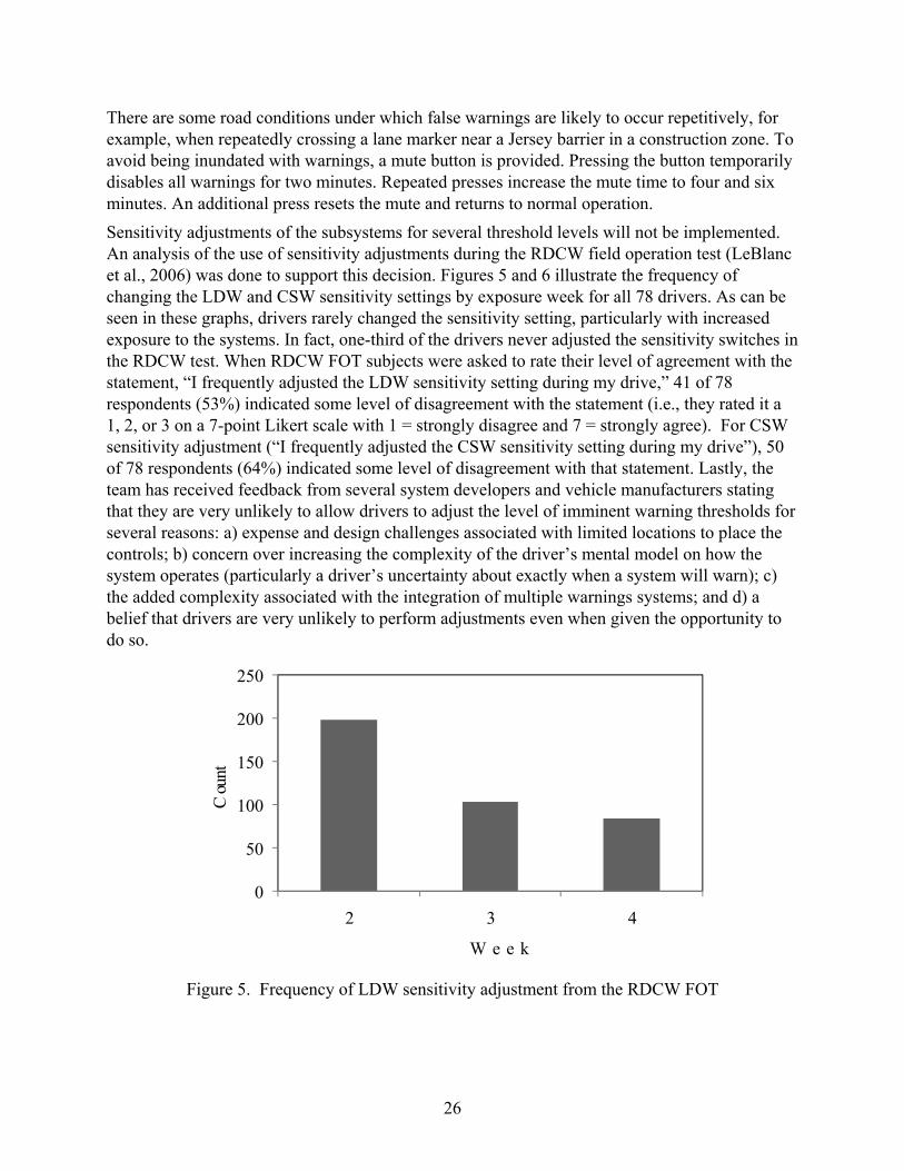
There are some road conditions under which false warnings are likely to occur repetitively, for example, when repeatedly crossing a lane marker near a Jersey barrier in a construction zone. To avoid being inundated with warnings, a mute button is provided. Pressing the button temporarily disables all warnings for two minutes. Repeated presses increase the mute time to four and six minutes. An additional press resets the mute and returns to normal operation. Sensitivity adjustments of the subsystems for several threshold levels will not be implemented. An analysis of the use of sensitivity adjustments during the RDCW field operation test (LeBlanc et al., 2006) was done to support this decision. Figures 5 and 6 illustrate the frequency of changing the LDW and CSW sensitivity settings by exposure week for all 78 drivers. As can be seen in these graphs, drivers rarely changed the sensitivity setting, particularly with increased exposure to the systems. In fact, one-third of the drivers never adjusted the sensitivity switches in the RDCW test. When RDCW FOT subjects were asked to rate their level of agreement with the statement, “I frequently adjusted the LDW sensitivity setting during my drive,” 41 of 78 respondents (53%) indicated some level of disagreement with the statement (i.e., they rated it a 1, 2, or 3 on a 7-point Likert scale with 1 = strongly disagree and 7 = strongly agree). For CSW sensitivity adjustment (“I frequently adjusted the CSW sensitivity setting during my drive”), 50 of 78 respondents (64%) indicated some level of disagreement with that statement. Lastly, the team has received feedback from several system developers and vehicle manufacturers stating that they are very unlikely to allow drivers to adjust the level of imminent warning thresholds for several reasons: a) expense and design challenges associated with limited locations to place the controls; b) concern over increasing the complexity of the driver’s mental model on how the system operates (particularly a driver’s uncertainty about exactly when a system will warn); c) the added complexity associated with the integration of multiple warnings systems; and d) a belief that drivers are very unlikely to perform adjustments even when given the opportunity to do so.
Cou
nt
250
200
150
100
50
0
W e e k
2 3 4
Figure 5. Frequency of LDW sensitivity adjustment from the RDCW FOT
26
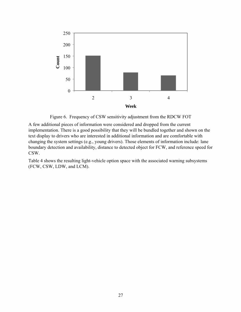
0
50
100
150
200
250
Cou
nt
2 3 4
Week
Figure 6. Frequency of CSW sensitivity adjustment from the RDCW FOT A few additional pieces of information were considered and dropped from the current implementation. There is a good possibility that they will be bundled together and shown on the text display to drivers who are interested in additional information and are comfortable with changing the system settings (e.g., young drivers). Those elements of information include: lane boundary detection and availability, distance to detected object for FCW, and reference speed for CSW. Table 4 shows the resulting light-vehicle option space with the associated warning subsystems (FCW, CSW, LDW, and LCM).
27

Table 4. Light-vehicle DVI
Warning Auditory Haptic Visual Driver Adjustments FCW You are approaching a hazard ahead
Tone from headrest speakers.
Brake pulse
Inform driver which alert occurred, about two seconds after it is over
Drivers can select from three predefined headrest volume levels (low, medium, and high).
Temporary warning mute button: a keypress can disable all warnings for two, four, or six minutes.
CSW You are entering a curve too fast
LDW You are unintentionally drifting across a lane boundary (out of lane or off road). Possible object identified as crash threat.
When object identified as crash threat, directional LDW tone from headrest speakers from side where threat exists
Directional haptic vibration in seat pan
LCM The lane you are intentionally entering is hazardous
LCM tone, from side of threat, through headrest speakers
Inform driver which alert occurred, about two seconds after it is over. LCM icon in left and right side view mirror appears in advance of the LCM warning. Blind zone: red. Closing zone: yellow.
28

3.2.2 Heavy-Truck Option Space Drivers of light vehicles are generally both the vehicle owner and the vehicle operator; the situation is different in heavy trucks where the driver is often not the owner—instead, a commercial operation is often the purchaser. One consequence of this difference is that in heavy trucks, styling and comfort may play a secondary role to concerns about safety and efficiency. Thus, a warning system is conceived as both a means of implementing a carrier’s safety policy and as a driver support system. When a conflict arises between the two roles, the carrier policy usually prevails. Consequently, heavy-truck warning systems limit the degree to which a driver can control warning characteristics. Notably, limits are typically placed on control over warning sensitivity and sound volume, and strict policies regulating minimum following distances are incorporated into carrier safety policies. Indeed, one reason a fleet would obtain Eaton VORAD systems is to enforce such a following-distance policy. Another difference between light-vehicle and heavy-truck production involves the degree to which component customization is feasible. Heavy-truck components are typically produced by several different independent suppliers—the engine, transmission, seating, and suspension may come from different suppliers. Moreover, the purchaser is given a great deal of control over the final vehicle configuration. This degree of configuration flexibility imposes some constraints on customization. For example, one cannot integrate a collision warning system employing haptic actuators into a generic seating system without significant customization of the seating. Customization may make little business sense for a seating manufacturer or a collision warning system manufacturer if only a small volume of the combination of components is projected. As a group, truck drivers are professional drivers—they have significantly more training and spend significantly more time behind the wheel than an average light-vehicle operator. Presumably, heavy-truck drivers may be more capable of managing somewhat more complicated vehicle-based systems than average light-vehicle drivers. Finally, because of the greater mass of heavy trucks, they are generally less maneuverable than light vehicles—they take significantly more time to stop, their turn radius is large, and their roll threshold is small. Consequently, truck drivers need generally longer lead times for warnings, especially in forward collisions. Unfortunately, extension of warning lead times also increases the likelihood that nuisance warnings will be generated. The dilemma is that if a warning is withheld until a problem is certainly imminent, it may be too late for a driver to effectively respond. If the warning is delivered too early, before a collision is certainly imminent, but in a time window that permits an effective response, the number of nuisance warnings may become problematic. Given these constraints for forward collision warnings, the heavy-truck driver interface has graded forward warnings. Progressively urgent auditory warnings are produced at progressively shorter headways.
29

3.2.2.1 Warning Presentation Modalities The heavy-truck platform warning presentation is restricted to auditory presentation via one of three audio channels, and visual presentation via a central display unit (Figure 7) and two lateral warning displays located near the driver- and passenger-side rearview mirrors (Figure 8). Haptic warnings (e.g., seat rumble, steering wheel shake, and brake-pulse) were determined to fall outside of the feasible scope of the heavy-truck implementation and have not be implemented as part of IVBSS on the heavy-truck platform.
Figure 7. VORAD driver interface unit
EATON VORAD
Red LED
Light Sensor
Yellow LED
Figure 8. Side sensor display unit
Sound reproduction in the previous generation of the Eaton VORAD system limited the maximum output sound frequency to 2.2 KHz, with an eight-bit dynamic range. This is arguably below the fidelity required to easily distinguish natural sound sources and thus precludes use of auditory icons, or extensive use of sound timbre for auditory warnings. The system speaker size of the VORAD unit (as well as environmental noise in the truck cabin) places a practical lower limit of 500 Hz on the usable auditory frequency. The resulting heavy-truck option space is shown in Table 5 along with the associated warning condition.
30

Table 5. Heavy-truck DVI
Warning Auditory Visual Driver Adjustments
FCW
You are approaching a hazard ahead
Forward sound source from driver interface unit (DIU)
Red and yellow warning LEDs on DIU, collision warning LCD display on DIU DIU contains indicator LEDs and a monochromatic LCD display
Drivers control sound volume (70 to 90 dB), display brightness Temporary warning mute function: A key-press can disable all warnings for up to six minutes in 120-second increments No sensitivity adjustment is provided to drivers for warnings
LDW
You are unintentionally drifting across a lane boundary
Directional, from side of threat, using lateral speaker channels controlled by DIU
Informational only – e.g., status, availability; drift diagram
Adjustment same as above
LCM
The lane you are intentionally entering is hazardous
Directional, from side of threat, using new speakers controlled by DIU
Lateral indicators mounted to A-pillar area. Always visible, directional indicator near each side view mirror
EATON VORAD
Red LED
Light Sensor
Yellow LED
Adjustment same as above
3.3 Research Questions The goals of the simulator studies on the IVBSS program were to (1) provide information to guide the design of individual IVBSS warnings; (2) determine how warnings should be combined to maximize effectiveness, safety, and acceptability of the system; and (3) provide a better understanding of how warnings should be presented in general. To satisfy these goals, test methods were developed. The application of the test methods and results are largely independent of whether one is working on the heavy-truck or light-vehicle platforms, except as noted. Admittedly, a significant body of literature on warning design provides a good basis for the development of DVIs for integrated crash warning systems. (See Appendix D.) However, the literature is far from complete, especially from an engineering perspective. Many of the conclusions in the literature are qualitative, for example, indicating that drivers respond more rapidly to louder sounds. Often, however, absolute or percentage differences do not appear in the literature (e.g., specifying by how much brake response time varies between the least meaningful and most meaningful speech message).
31
In addition, there is very little framework presented in the literature about how drivers respond to warnings other than open-loop or closed-loop concepts (e.g., Abe & Richardson, 2004). A greater understanding of the process of responding to warnings, especially where drivers look and when, should help considerably with selecting warning modalities and content. Do drivers just hear something and respond, or do they look towards a target area, confirm, and respond? Decisions about where and when to provide visual, haptic, and auditory warnings, alone and in combination, will be much better informed as a result of addressing this issue. When and which multiple warnings might be confused is a core issue of the project and is addressed in several experiments. However, the definitive study cannot be carried out until the end of the sequence of simulator studies when individual warnings have been finalized. Otherwise, one would not know if confusability problems are generic or due to the specific (and potentially suboptimal) set of warnings examined. Nuisance warnings are one of the problems that plague warning systems. For example, in the ACAS FOT “36 percent of all alerts were of the nuisance type that became triggered by nonthreatening, stationary targets” (Ervin, Sayer, LeBlanc, Bogard, Mefford, Hagan, Bareket, & Winkler, 2005). With multiple warnings systems, drivers are likely to experience more nuisance warnings per unit of time, potentially leading to greater annoyance and other consequences. Hence, for most, if not all, of the simulator experiments, subjects experienced a mixture of real, nuisance, and false alarms. Finally, during the discussions of how IVBSS should be designed, many design and engineering issues could not be resolved based on the existing literature or logic, and as a consequence, led to some of experiments proposed in this project. Balancing the need to support the design of a real system with pursuing basic research questions is always difficult. The resources proposed here are sufficient to answer the major questions and develop a warning set that will satisfy the objective of fielding an effective, safe, and practical integrated crash warning system. In many ways, the questions to be addressed are a mixture of specific implementation questions for IVBSS and more overarching questions about how drivers respond to multiple warnings, individually, collectively, and in close temporal proximity. The seven questions listed in Table 6 were identified as requiring further attention. Each question is discussed in the following subsections.
32
Table 6. Research questions mapped to experiments
# Question Topic Exp. Subsystem
Q1 When and how should warnings be shared or differentiated?
Shared warnings 3 All
Q2 Should warnings occurring at the same time be presented together or with a delay between them?
Sequencing cooccurring warnings
5 All
Q3 Are warnings in the IVBSS sets confused with each other?
Warning set confusion 2, 3, 4, 5
All
Q4 When responding to warnings, what is the process by which drivers respond?
Time course of driver actions
2 FCW, LDW, CSW, maybe LCM
Q5 How does the tradeoff between warning system processing time and warning accuracy affect driver responses to warnings?
Warning processing time-accuracy tradeoff
4 All
Q6 How does auditory warning effectiveness vary with warning sound characteristics (loudness, pitch, speed) in sound environments of each vehicle platform?
Auditory warning characteristics
1 All
Q7 For sounds that involve periods of silence or pauses, are responses deferred to coincide with silence? What is the optimal number of repetitions?
Influence of pauses and repetition
1subtask
5
LDW
3.3.1 Q1. Shared Warnings When should warnings be shared or differentiated (e.g., FCW and CSW, LDW, and LCM) and if so, how? How does that depend on factors such as having a common action in response to the warning (brake or slow down, stay in your lane), the collision potential or severity of the outcome (crash target present or absent), and, possibly, the warning reliability and nuisance warning frequency? Rationale. Should multiple situations, such as approaching a curve too fast or a potential forward collision, have the same warning if the same driver response is required, or should there be multiple (unique) warnings? Using common warnings could shorten response time by removing steps in the process of sensing a warning, deciding how to respond, and executing that response. If drivers simply do what the warning suggests, then a warning should only indicate the response desired. However, if the driver assesses the situation, then indicating what is wrong as part of the warning could shorten the duration of the assessment and response time. The shared warnings question arose both in discussions of the DVI and in the U.S. DOT’s review of the initial proposed experimental plan, and is central to IVBSS. The answer could be specific to a particular warning set or context. This question is distinct from the master caution warning concept explored by Chiang, Llaneras, and Foley (2006) because warnings are linked to specific driver actions, either brake or slow down, or stay in or return to one’s lane.
33

3.3.2 Q2. Sequencing Co-Occurring Warnings When sequencing co-occurring warnings:
a. Should only one warning be presented because the second will delay the driver’s response? or
b. Should the second warning be presented with a delay (and what should that delay/lockout be)? or
c. If the second warning is of higher priority, should it preempt the first and, if so, how (fade out the first, immediately start the second, provide delay or lockout and then start, etc.)?
Rationale. A central integration issue is how to sequence multiple warnings and whether one or multiple warnings should be presented. The relevant fundamental concept, the psychological refractory period, asserts that presenting two signals in close temporal proximity (for simple lights and tones, within about 500 ms) can interfere with responding to either of them (Karlin & Kestenbaum, 1968; Wu & Liu, 2004). The impression from Ho, Cummings, Wang, Tijerina, and Kochhar (2006) is that a single master warning leads to performance equivalent to multiple tailored warnings (for FCW, LDW), but drivers prefer tailored warnings. (See also Chiang, Brooks, & Llaneras, 2004.) What clearly emerges from that research is the need for a more detailed look at the specific warnings and the process of how drivers respond to them (e.g., where they look and when). Additional thought is needed concerning the hypothetical situations in which this could occur. Much of that thinking will be guided by an ongoing review of crash statistics.
3.3.3 Q3. Warning Set Confusion How well do drivers respond to candidate sets of IVBSS warnings? Are any confused or misunderstood? Rationale. One of the consequences of integrating warnings from independently developed systems is that the warnings can be confused or misunderstood. That concern needs to be addressed before warnings are implemented in a test vehicle.
3.3.4 Q4. Time Course of Driver Actions What is the time course of driver actions in responding to single and multiple warnings, both when the warnings are unique to the situation and when multiple situations lead to the same warning (such as a common warning for LDW and LCM)? Of particular interest is where drivers look. Rationale. From previous research, in particular the road departure crash warning (RDCW) simulator experiments (LeBlanc, Sayer, Winkler, Ervin, Bogard, Devonshire, Mefford, Hagan, Bareket, Goodsell, & Gordon, 2006), the project team has some sense of the time course response for steering wheel movements and brake actuations of drivers responding to warnings. Responding to warnings always involves some visual element, either searching for hazards when alerted by warnings or confirming their existence while responding. Thus, an important element of the task is getting drivers to look in the appropriate place and then to execute the desired response. However, where and when drivers look, both pre- and post-warning, for each of the four subsystems being implemented in the IVBSS program, has yet to be fully explored.
34

Understanding this process should provide insights into the use of shared warning signals (where the driver action is the same), desired warning durations, the need for repetition, and the use of orientation cues.
3.3.5 Q5. Warning Processing Time-Accuracy Tradeoff How does the tradeoff between warning system processing time (to start to inform the driver) and warning accuracy affect driver responses to warnings? Rationale. This question has not been addressed in the published literature. In brief, the system integrators wanted to know how long a system could take to process information and warn the driver. Ideally this would be zero, but in reality systems need to sample over time, computers need to process the data, and information needs to be sent over a network to other devices for presentation to the driver. For example, delaying a warning will allow for additional sweeps of the radar system, resulting in higher confidence levels for target detection and fewer false and nuisance warnings. The current time limit, from the beginning of signal processing to the initiation of a warning, is probably on the order of 300 ms (estimations range from 100 to 500 ms). Driver response times are on the order of one to two seconds, and accordingly, this is a 30 percent difference—a nontrivial effect.
3.3.6 Q6. Auditory Characteristics of Warnings How does auditory warning effectiveness vary with warning sound characteristics (loudness, pitch, and timbre) in sound environments representative of each vehicle platform? Rationale. To be effective, an auditory warning must be heard and recognized above the din of other sounds that naturally occur during driving. This includes background cabin noise, sounds from the vehicle audio system, and other in-vehicle warning sounds like low-fuel indicators and safety belt reminders. Moreover, warning sounds designed for IVBSS must also be easily learned and unlikely to be confused for each other, and for some warning conditions, they must also be localized. The ultimate goal is to produce warnings that are easily detected and quickly learned, and which produce quick and accurate avoidance responses.
3.3.7 Q7. Influence of Pauses and Repetition For sounds that involve periods of silence (or pauses), are responses deferred to coincide with silence? What is the optimal number of repetitions? Rationale. In the RDCW study (LeBlanc et al., 2006) response times were often on the order of a second for some warnings. However, the durations of the auditory warnings were much longer— some lasted as long three seconds. One question, for example, is that for a simulated rumble strip, can the number of simulated strips or the silent period between them be reduced? The silent period is important because the continuing sound of a warning may serve to inhibit a person from responding. In a previous study (Nowakowski, Friedman, & Green, 2001) there was a strong bias toward answering the phone in the silent period of the ringing sequence.
3.4 Driving Simulator Overview The simulator-based experiments took place after the first major upgrade of the third-generation UMTRI driving simulator (www.umich.edu/~driving/sim.html). The simulator consists of a full-size cab, ten computers, six video projectors, seven cameras, audio equipment, and other
35

electronic devices. The main functions (generation of scene graphics; processing of steering wheel, throttle, and brake inputs; provision of torque feedback; and data collection) were controlled by hardware and software provided by DriveSafety (Vection and HyperDrive Authoring Suite, version 1.6.2). The UMTRI driving simulator has a forward field-of-view of 200 degrees and a rear field-ofview of 40 degrees created by five forward channels and a single rear channel. Appendix A provides additional dimensions and equipment layout of the simulator configuration. The simulator is controlled from an enclosure behind and to the left of the cab. The enclosure contains four quad-split video monitors that show the output of every camera and computer , a display of the quad-split combination being recorded, and a variety of equipment controls. Also in the enclosure is a 19-inch rack containing audio and video equipment (audio mixers, video patch panel and switchers, distribution amplifiers, VCR, quad splitter, etc.) and two separate racks for computers. The vehicle cab consisted of the A-to-B pillar section of a 1985 Chrysler Laser, complete with foot controls, a steering wheel, and several speaker systems (to provide simulated background road noise, auditory warnings, and vertical vibration). The computer-generated, back-projected speedometer-tachometer cluster display was controlled by a computer running REALbasic. A custom-made, vibrating (haptic) seat was installed on the driver’s side in place of the stock seat. The seat, from a 2002 Nissan Altima, was modified with the installation of eight InSeat Solutions Relaxor CJ transducers: four in the seat pan and four in the seat back. Mounted in and around the cab are seven video cameras. Images captured by these cameras include the driver’s face (viewed from outside and inside the cab), two over-the-shoulder images (showing the instrument panel), an image from the package shelf showing the instrument panel and forward scene, and an image of the foot well. These images, combined with output from any of the projected images (simulated driving scene), could be recorded using a quad splitter. Figure 9 shows a close-up of the cab interior. Not shown in the image is a Seeing Machines faceLAB version 3 system, which consisted of two cameras mounted on top of the instrument panel, about one foot apart, and cables to a computer just outside of the control enclosure. To provide illumination for those cameras, one-inch square IR illuminators were mounted on stalks attached to the A pillar and center console.
36

Figure 9. Close-up of simulator cab interior (without eye fixation system installed)
To perform the studies for the IVBSS program, major essential upgrades were made to the driving simulator that had a significant impact on the project schedule. Prior to the IVBSS program, the driving simulator had three forward channels (120-degree field of view) and one rear channel (60-degree field of view). Because this project involved testing lane change-merge (LCM) warning systems, a wider field of view was required. Thus, two side channels were added by installing two, 12-foot wide pull-down screens on either side of the vehicle, increasing the field of view to 200 degrees. However, the field-of-view upgrade necessitated a significant number of other, associated changes. Two new projectors were required, and each new projector needed a new image generation computer. In brief, the video and graphics systems were completely rebuilt and an eye fixation system was installed and tested. Also, to comply with common safety practice, a sprinkler system was installed in the entire UMTRI facility (the associated noise from which prevented testing from being performed). Finally, many of the driving scenarios were quite complex, involving careful positioning of several vehicles. Developing the software to control them also took several months.
3.5 Test Scenarios
3.5.1 Introduction Eight scenarios were created for the IVBSS experiments, four FCW (lead vehicle brakes, lead vehicle brakes while the subject changes lanes, lead vehicle reveals a stopped vehicle ahead, cutin), two LCM (vehicle in or accelerates to blind spot), one LDW (due to a wind gust), and one CSW. All scenarios involved driving on an expressway, with two lanes in each direction in light traffic (LOS A). Table 7 illustrates those scenarios. For a complete description, see Appendix B.
37

Table 7. Significance levels of the effect of sound
Scenario Depiction 1-FCW
Lead vehicle (L) suddenly decelerates.
3-FCW
Subject vehicle (S) changes lanes due to construction zone and lead vehicle suddenly decelerates to trigger FCW.
4-FCW
The lead vehicle changes lanes to reveal a stopped vehicle.
5-FCW
Cut-in.
6-LCM
Subject changes lanes- vehicle in blind spot.
38

Scenario Depiction 7-LCM
Subject changes lanes due to construction zone. Adjacent vehicle accelerates into blind spot. 8-LDW
Subject drifts out of lane due to wind gust.
10-CSW
Subject approaches curve traveling too fast.
F = S
A =
CSW L
In creating scenarios, the goal was to put subjects in a particular location (e.g., by adjusting the lead vehicle speed or adjacent vehicle location) that would cause a warning to trigger. To provide a sufficient amount of data for statistical analysis, how often warning-triggering events occurred was much higher than would be experienced in normal driving. The scenario selection process described in the automotive collision avoidance system (ACAS) report (Ervin, Sayer, LeBlanc, Bogard, Mefford, Hagan, Bareket, & Winkler, 2005) was considered, which identified scenarios on the basis of video data of real driving situations. Although appropriate for ACAS, that approach was thought to lead to too few triggering events in a simulator study. The crash frequency data of Najm, Smith, and Toma (2005) were also considered, but mimicking the absolute frequency of warnings was not the goal of this experiment. Selecting scenarios that drivers could not predict, or for which they could form an expectation of the timing, frequency, and type of warning was important, so the scenarios were developed to closely resemble real-world driving situations. Triggering events could occur in any lane and could be caused by a variety of simulated vehicles. For some warnings, multiple different scenarios were used to trigger the same warning type. The flaw of some prior research has been the focus on a single scenario, often involving a single vehicle (“I know the lead vehicle will brake, so I will keep watching it.”). The simulated lead and adjacent vehicles present in each
39
scenario were programmed to perform a considerable amount of positioning before each scenario to closely mimic real driving situations and elicit the triggering event and to make the triggering vehicle less predictable. The lead vehicle generally maintained a lead headway of 35 to 40 meters from the subject vehicle unless programmed to do otherwise. The adjacent vehicle generally maintained a side separation (midpoint of subject vehicle to midpoint of adjacent vehicle) of 10 to 20 meters, unless programmed to do otherwise. Each warning scenario included both true warning and a false alarm cases. The true warning case was designed to cause an actual triggering event where a threat was present and the warning sounded. In the false alarm case, the lead and adjacent vehicles moved out of their normal positions as though to set up a true warning scenario, but in such a way that no actual threat existed, and a false alarm warning was presented anyway. In addition, most of the time, there was following traffic as well.
3.5.2 Scenario Development As long as subjects followed the instructions they were given (drive at 70 mph, do not change lanes unless forced, etc.), the forward collision warning (FCW) triggering events were the easiest to develop as they were caused almost entirely by lead vehicle actions and did not require the subject to perform specific maneuvers. Lange change-merge (LCM) triggering events were more difficult to induce because in order to trigger a warning, subjects had to be induced to perform dangerous lane changes. Construction zone lane closures, marked by cones, were sometimes used to serve that purpose. Although lateral drift warning (LDW) triggering events were not difficult to induce, they were difficult to control because they depend entirely upon driver action. Lane departures naturally occur quite frequently in the simulator, despite driver attention to speed and lane position, due to sensitive steering controls and sharp corners. However, to ensure that subjects would trigger enough LDWs, simulated wind gusts were used to encourage unintentional lane departures. Curve speed warning (CSW) triggering events were very difficult to induce, but naturally occur quite frequently due to difficulty sensing speed in a simulated driving environment.
3.5.3 Multiple Warning Scenarios Multiple warning scenarios were created so that two different warnings would be triggered nearly simultaneously. Multiple warning scenarios involving CSW were not considered because of programming constraints, but all other combinations were evaluated. The multiple warning scenarios were created such that each set would occur twice. This allowed each warning the opportunity to occur first in the set. For example, in scenario 7-LCM plus scenario 1-FCW, LCM is followed by FCW, where in scenario 4-FCW plus scenario 6-LCM, the order is reversed. (See Appendix B for full explanations, including graphics, of the scenarios investigated.) The LCM-FCW combination was the only case where two different scenario pairings were needed to switch the warning order; for other warning combinations, scenarios could be easily reversed with only slight changes.
40

4 Experiment 1 – Auditory Warnings This section provides a high-level summary of experiment 1 that succinctly conveys the major elements of the experiment. Please refer to Appendix E for a detailed description of the 5 subtasks that constitute experiment 1. The main purpose of experiment 1 was to collect data that would help guide the design and selection of auditory warnings used in both the light-vehicle and heavy-truck platforms. The key research questions addressed in each of the subtasks of experiment 1 are shown below.
Table 8. Experiment 1 research questions
Question Subtask How loud should the warning be to be heard? 1 Will the sound not be mistaken for another sound in the vehicle? 3 Are there acoustical characteristics of sounds that can increase urgency without also increasing annoyance?
2
Are abstract sounds more confusable than auditory icons? 3 How do sounds work together as collections? 3 Can sound lateralization be enhanced with additional acoustic content? 4 How do the sound characteristics influence the time to indicate the direction of the sound?
5
4.1 Subtask 1 – Sound Environment of the Light Vehicle and Heavy Truck
4.1.1 Overview The purpose of this task was to measure the background sound distributions (in one-third octave bands) of the target vehicle platforms (2006 Honda Accord, International Truck for the 8600series class-8 tractor) as well as those of existing standard vehicle warnings (e.g., safety belt, key-in reminder, lights-on chimes). This was done to ensure that candidate warnings would be sufficiently loud to be heard over background noise, and sufficiently different that they would not be confused with existing (non-urgent) vehicle sounds. Human factors guidelines (e.g., Campbell, Richard, Brown, & McCallum, 2007b) often recommend that warnings not exceed 90 dB(A), and also exceed background noise levels by 15 dB(A). Obviously, if the background noise level is 80 dB(A), complying with both guidelines cannot occur. Patterson & Mayfield (1990) suggest that decibel levels exceed background levels in at least four frequency components (i.e., frequency bands). Thus, the spectral characteristics of background noise levels of each platform are also relevant.
4.1.2 Method For the light-vehicle platform, road noise data was collected for a 2007 Honda Accord in the range of 100 to 2,000 Hz at two speeds (65 mph (105 kph) and 35 mph (56 kph)), two window conditions (opened and closed), two noise levels (68 dB(A) and 80 dB(A)), and two road conditions (smooth and rough).
41
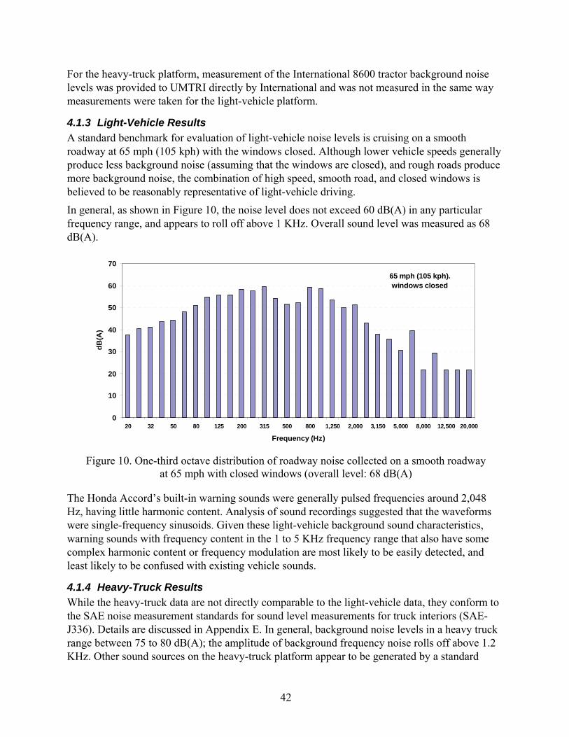
65 mph (105 kph). windows closed
40
30
20
10
20 32 50 80 125 200 315 500 800 1,250 2,000 3,150 5,000 8,000 12,500 20,000
Frequency (Hz)
50
60
70
dB(A
)
0
For the heavy-truck platform, measurement of the International 8600 tractor background noise levels was provided to UMTRI directly by International and was not measured in the same way measurements were taken for the light-vehicle platform.
4.1.3 Light-Vehicle Results A standard benchmark for evaluation of light-vehicle noise levels is cruising on a smooth roadway at 65 mph (105 kph) with the windows closed. Although lower vehicle speeds generally produce less background noise (assuming that the windows are closed), and rough roads produce more background noise, the combination of high speed, smooth road, and closed windows is believed to be reasonably representative of light-vehicle driving. In general, as shown in Figure 10, the noise level does not exceed 60 dB(A) in any particular frequency range, and appears to roll off above 1 KHz. Overall sound level was measured as 68 dB(A).
Figure 10. One-third octave distribution of roadway noise collected on a smooth roadway at 65 mph with closed windows (overall level: 68 dB(A)
The Honda Accord’s built-in warning sounds were generally pulsed frequencies around 2,048 Hz, having little harmonic content. Analysis of sound recordings suggested that the waveforms were single-frequency sinusoids. Given these light-vehicle background sound characteristics, warning sounds with frequency content in the 1 to 5 KHz frequency range that also have some complex harmonic content or frequency modulation are most likely to be easily detected, and least likely to be confused with existing vehicle sounds.
4.1.4 Heavy-Truck Results While the heavy-truck data are not directly comparable to the light-vehicle data, they conform to the SAE noise measurement standards for sound level measurements for truck interiors (SAEJ336). Details are discussed in Appendix E. In general, background noise levels in a heavy truck range between 75 to 80 dB(A); the amplitude of background frequency noise rolls off above 1.2 KHz. Other sound sources on the heavy-truck platform appear to be generated by a standard
42

magnetic sounder component that produces unmodulated square waves in the range of 1 to 1.5 KHz. Therefore, the recommendation is that a warning sound achieve an amplitude of 85 to 90 dB(A) above 1.2 KHz. To be distinguishable from other sounds, consider the use of frequency modulation and/or higher fundamental frequency.
4.1.5 Conclusions x For the light-vehicle platform, the recommended level of IVBSS warning sounds should be a
minimum of 80 dB(A). This recommendation is based on the signal noise level being sufficient above the background noise level be based on a vehicle cruising at 65 mph (105 kph) with windows closed on a smooth roadway. Also, to maximize detection, sounds should include frequency content in the 1 to 5 KHz range, where the spectral power of the background noise is attenuated (at least with the windows closed). Further, to ensure the distinctiveness of the IVBSS warning sounds from the base vehicle’s warnings, frequencies that overlap the existing warning range should be avoided. Warning sounds with more elaborate harmonic content, onset envelopes, rhythmic patterns, and spatial locations are unlikely to be mistaken for the sounds on the base Honda Accord. Similar to the suggestions made for the light-vehicle platform, the recommended IVBSS warning sounds for the heavy-truck platform should not include sounds similar to the base sound set of the heavy-truck platform.
4.2 Subtask 2 – Acoustic Features of Warnings
4.2.1 Overview The purpose of this study is to expand the number of acoustic attributes investigated and to examine how they influence other perceptual attributes (besides urgency) that may be relevant to the effectiveness of a crash warning system. Subjective ratings were collected concerning the perceived relative urgency of the four prototype IVBSS crash scenarios: forward collision warning (FCW), curve speed warning (CSW), lane change-merge warnings (LCM), and lateral drift warning (LDW). The study is an amalgam of the prior work of Tan and Lerner (1995) in which a set of sample sounds were assessed on a variety of subjective attributes, and of Edworthy (e.g., Edworthy et al., 1991) in which a relationship between the acoustic properties of sounds and perceived urgency was investigated. In this study, several acoustic properties of sounds were systematically varied while listeners rated the sounds on each of four perceived attributes: urgency, annoyance, noticeability, and loudness. Sound stimuli were generated to produce an orthogonal set of sounds based on the eight acoustic properties: fundamental frequency, timbre, harmonic dissonance, pulse rate, pulse onset, pitch variation, and rhythmic variation.
4.2.2 Method Twenty-four subjects participated in the study. Subjects were partitioned into six groups based on gender and three levels of age (old, middle, and young). Before rating the sounds, subjects were presented with the entire set in order to acquaint them with the range of sounds that would be played. Ratings were made in blocks for each of the four attribute judgments. A second set of four blocks were repeated after the first set.
43
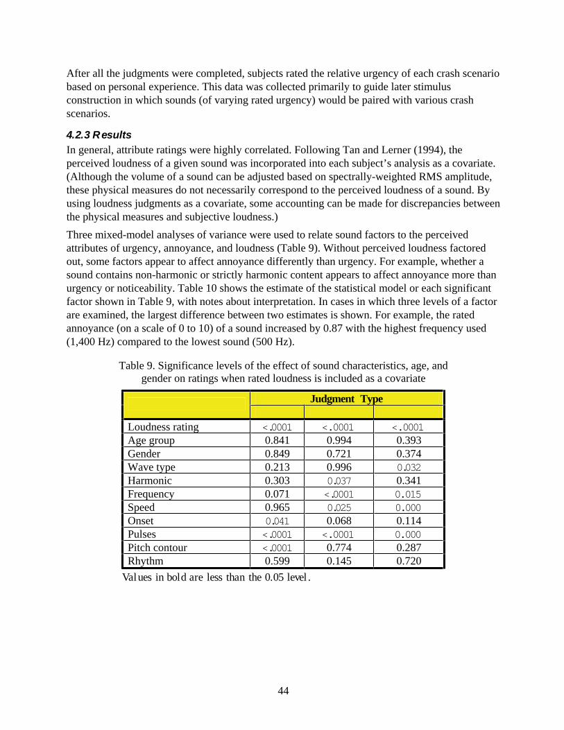
44
Table 9. Significance levels of the effect of sound characteristics, age, and gender on ratings when rated loudness is included as a covariate
Judgment TypeEffectUrgency Annoyance Noticeabi lity
Values in bold are less than the 0.05 level .
Loudness rating <.0001 <.0001 <.0001Age group 0.841 0.994 0.393 Gender 0.849 0.721 0.374 Wave type 0.213 0.996 0.032Harmonic 0.303 0.037 0.341Frequency 0.071 <.0001 0.015Speed 0.965 0.025 0.000Onset 0.041 0.068 0.114Pulses <.0001 <.0001 0.000Pitch contour <.0001 0.774 0.287Rhythm 0.599 0.145 0.720
After all the judgments were completed, subjects rated the relative urgency of each crash scenario based on personal experience. This data was collected primarily to guide later stimulus construction in which sounds (of varying rated urgency) would be paired with various crash scenarios.
4.2.3 ResultsIn general, attribute ratings were highly correlated. Following Tan and Lerner (1994), the perceived loudness of a given sound was incorporated into each subject’s analysis as a covariate. (Although the volume of a sound can be adjusted based on spectrally-weighted RMS amplitude, these physical measures do not necessarily correspond to the perceived loudness of a sound. By using loudness judgments as a covariate, some accounting can be made for discrepancies between the physical measures and subjective loudness.) Three mixed-model analyses of variance were used to relate sound factors to the perceived attributes of urgency, annoyance, and loudness (Table 9). Without perceived loudness factored out, some factors appear to affect annoyance differently than urgency. For example, whether a sound contains non-harmonic or strictly harmonic content appears to affect annoyance more than urgency or noticeability. Table 10 shows the estimate of the statistical model or each significant factor shown in Table 9, with notes about interpretation. In cases in which three levels of a factor are examined, the largest difference between two estimates is shown. For example, the rated annoyance (on a scale of 0 to 10) of a sound increased by 0.87 with the highest frequency used (1,400 Hz) compared to the lowest sound (500 Hz).
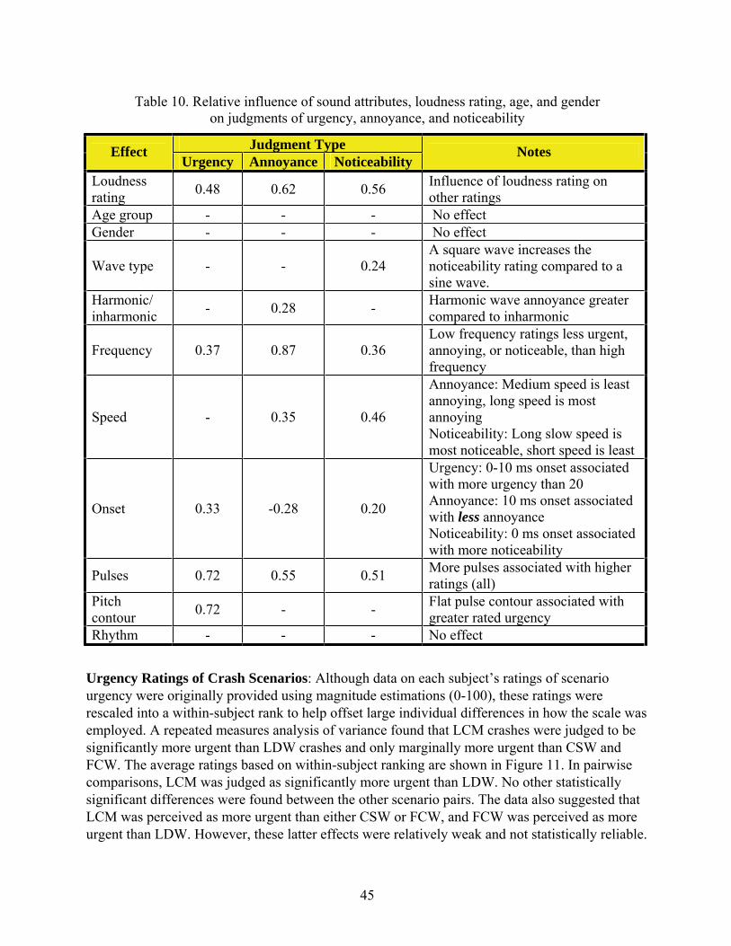
Table 10. Relative influence of sound attributes, loudness rating, age, and gender on judgments of urgency, annoyance, and noticeability
Effect Judgment Type NotesUrgency Annoyance Noticeability
Loudness rating 0.48 0.62 0.56 Influence of loudness rating on
other ratings Age group - - - No effect Gender - - - No effect
Wave type - - 0.24 A square wave increases the noticeability rating compared to a sine wave.
Harmonic/ inharmonic - 0.28 - Harmonic wave annoyance greater
compared to inharmonic
Frequency 0.37 0.87 0.36 Low frequency ratings less urgent, annoying, or noticeable, than high frequency
Speed - 0.35 0.46
Annoyance: Medium speed is least annoying, long speed is most annoying Noticeability: Long slow speed is most noticeable, short speed is least
Onset 0.33 -0.28 0.20
Urgency: 0-10 ms onset associated with more urgency than 20 Annoyance: 10 ms onset associated with less annoyance Noticeability: 0 ms onset associated with more noticeability
Pulses 0.72 0.55 0.51 More pulses associated with higher ratings (all)
Pitch contour 0.72 - - Flat pulse contour associated with
greater rated urgency Rhythm - - - No effect
Urgency Ratings of Crash Scenarios: Although data on each subject’s ratings of scenario urgency were originally provided using magnitude estimations (0-100), these ratings were rescaled into a within-subject rank to help offset large individual differences in how the scale was employed. A repeated measures analysis of variance found that LCM crashes were judged to be significantly more urgent than LDW crashes and only marginally more urgent than CSW and FCW. The average ratings based on within-subject ranking are shown in Figure 11. In pairwise comparisons, LCM was judged as significantly more urgent than LDW. No other statistically significant differences were found between the other scenario pairs. The data also suggested that LCM was perceived as more urgent than either CSW or FCW, and FCW was perceived as more urgent than LDW. However, these latter effects were relatively weak and not statistically reliable.
45
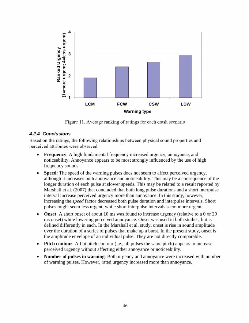
Ran
ked
Urg
ency
(1
=mor
e ur
gent
; 4=l
ess
urge
nt) 4
3
2
1 LCM FCW CSW LDW
Warning type
Figure 11. Average ranking of ratings for each crash scenario
4.2.4 Conclusions Based on the ratings, the following relationships between physical sound properties and perceived attributes were observed:
x Frequency: A high fundamental frequency increased urgency, annoyance, and noticeability. Annoyance appears to be most strongly influenced by the use of high frequency sounds.
x Speed: The speed of the warning pulses does not seem to affect perceived urgency, although it increases both annoyance and noticeability. This may be a consequence of the longer duration of each pulse at slower speeds. This may be related to a result reported by Marshall et al. (2007) that concluded that both long pulse durations and a short interpulse interval increase perceived urgency more than annoyance. In this study, however, increasing the speed factor decreased both pulse duration and interpulse intervals. Short pulses might seem less urgent, while short interpulse intervals seem more urgent.
x Onset: A short onset of about 10 ms was found to increase urgency (relative to a 0 or 20 ms onset) while lowering perceived annoyance. Onset was used in both studies, but is defined differently in each. In the Marshall et al. study, onset is rise in sound amplitude over the duration of a series of pulses that make up a burst. In the present study, onset is the amplitude envelope of an individual pulse. They are not directly comparable.
x Pitch contour: A flat pitch contour (i.e., all pulses the same pitch) appears to increase perceived urgency without affecting either annoyance or noticeability.
x Number of pulses in warning: Both urgency and annoyance were increased with number of warning pulses. However, rated urgency increased more than annoyance.
46
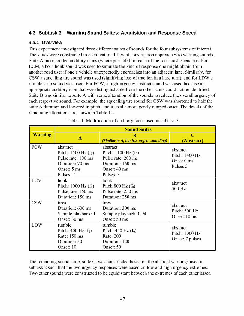
4.3 Subtask 3 – Warning Sound Suites: Acquisition and Response Speed
4.3.1 Overview This experiment investigated three different suites of sounds for the four subsystems of interest. The suites were constructed to each feature different construction approaches to warning sounds. Suite A incorporated auditory icons (where possible) for each of the four crash scenarios. For LCM, a horn honk sound was used to simulate the kind of response one might obtain from another road user if one’s vehicle unexpectedly encroaches into an adjacent lane. Similarly, for CSW a squealing tire sound was used (signifying loss of traction in a hard turn), and for LDW a rumble strip sound was used. For FCW, a high-urgency abstract sound was used because an appropriate auditory icon that was distinguishable from the other icons could not be identified. Suite B was similar to suite A with some alteration of the sounds to reduce the overall urgency of each respective sound. For example, the squealing tire sound for CSW was shortened to half the suite A duration and lowered in pitch, and it used a more gently ramped onset. The details of the remaining alterations are shown in Table 11.
Table 11. Modification of auditory icons used in subtask 3
Warning Sound Suites
A B (Similar to A, but less urgent sounding)
C (Abstract)
FCW abstract Pitch: 1500 Hz (f0) Pulse rate: 100 ms Duration: 70 ms Onset: 5 ms Pulses: 7
abstract Pitch: 1100 Hz (f0) Pulse rate: 200 ms Duration: 160 ms Onset: 40 ms Pulses: 3
abstract Pitch: 1400 Hz Onset 0 ms Pulses 5
LCM honk Pitch: 1000 Hz (f0) Pulse rate: 160 ms Duration: 150 ms
honk Pitch:800 Hz (f0) Pulse rate: 250 ms Duration: 250 ms
abstract 500 Hz
CSW tires Duration: 600 ms Sample playback: 1 Onset: 30 ms
tires Duration: 300 ms Sample playback: 0.94 Onset: 50 ms
abstract Pitch: 500 Hz Onset: 10 ms
LDW rumble Pitch: 400 Hz (f0) Rate: 150 ms Duration: 50 Onset: 10
rumble Pitch: 450 Hz (f0) Rate: 200 Duration: 120 Onset: 50
abstract Pitch: 1000 Hz Onset: 7 pulses
The remaining sound suite, suite C, was constructed based on the abstract warnings used in subtask 2 such that the two urgency responses were based on low and high urgency extremes. Two other sounds were constructed to be equidistant between the extremes of each other based
47

Average Trials to Criterion
140120100
768060 47 40 22 20
0 A B C
Sound Suite Figure 12. Trials to criterion by sound suite
Tria
ls
on a model of the urgency ratings from subtask 2, and then were associated with the crash scenarios in order of rated urgency as reported in subtask 2.
4.3.2 Method Twenty-four naïve subjects participated in the experiment. Subjects were partitioned into four groups by age (older and younger) and gender. A four-choice reaction time task was used in which four buttons were each associated with the four crash scenarios. A sound was randomly selected and played. Subjects were asked to respond by pressing the button paired with the crash scenario associated with the sound. After an initial learning trial, subjects were given acquisition trials until eight errorless responses were achieved. Afterwards, subjects responded to 40 more trials. The key dependent measures included trials to criterion, reaction time, and error rate.
4.3.3 Results Analysis of the trials to criterion found main effects of sound suite and age group. Paired comparisons found that suite A took significantly fewer trials to learn than suite B (shown in Figure 12). The error analyses suggested greater confusion among the sounds in suites B and C than in suite A. Confusion in suite C seemed to be among sounds of neighboring levels of rated urgency. In suite B, there appeared to be significant confusion between the LCM and CSW sounds, although it is difficult to understand why this happened—the sounds were derived from two disparate sounds: a honking horn and squealing tires.
Reaction time was significantly faster for the sounds in suite A than in either suites B or C (Figure 13). In general, responses were about 150 ms faster for sound in suite A than in suite B.
48

29
122
82
15 30
13
0 20 40 60 80
100 120 140
Tria
ls
Old Young
Average Trials to Criterion
A B C Sound Suite
Figure 13. Mean reaction times for responding within each sound suite (Error bars depict 95-percent confidence intervals on the mean reaction time)
4.3.4 Conclusions x The sounds in suite A are preferred. The sounds included in suite A resulted in substantially fewer acquisition trials and in substantially smaller reaction times. However the results for suite B suggest that it might be premature to credit suite A’s superiority entirely to its use of auditory icons. x Even minor alterations in sound characteristics may significantly affect a listener’s
performance. Suite B used similar icons, assigned to the same scenarios, and displayed significantly inferior performance.
4.4 Subtask 4 – Localization of Auditory Warnings
4.4.1 Overview This study was a pilot evaluation in which two modifications were made to a lateralized warning sound to determine if such modification might enhance response speed and accuracy. The two modifications were investigated in separate pilot evaluations using UMTRI staff as subjects.
4.4.2 Method The first modification introduced broadband noise into the warning sound, following a procedure described in a study by Catchpole, McKeon, and Withington (2004). They found that localization accuracy could be increased if broadband noise is added to the sound. The second modification introduced an enhancement to the stereo sound image (Qsound) that increased the apparent lateral direction of the sound. For example, a sound, normally originating in the leftmost stereo channel, could be made to sound even farther left of the radial direction of the speaker. It was expected that each modification would facilitate directional judgments that might be reflected in faster
49

responding. Less clear was whether such enhancements would interfere with sound identification; this could possibly result in increasing errors or response time. The four-choice reaction time task from subtask 3 was also used in this study. Subjects heard a warning sound and selected the lateral direction (right or left) and the crash scenario (LCM or LDW) associated with the sound. The four basic warning sounds were either enhanced with the addition of broadband noise (in the pilot 1 study) or QSound (in the pilot 2 study), or not enhanced (i.e., the control condition). The warning sounds used in the study were selected from the LDW and LCM sounds from suites A and C of the stimuli used in subtask 3.
4.4.3 Results In the first pilot evaluation (using broadband noise), reaction time to warnings taken from suite A was faster than for warnings taken from suite C, but no effects of broadband noise were observed. In the second pilot evaluation (spatial enhancement of the sound), no effect of sound suite or spatial enhancement was observed. Analysis of the error data found no effects or interactions between sound suite, spatial enhancement, or presentation order on error rates. Partitioning of the error data into identification errors and direction errors also revealed no influence of the factors on specific errors.
4.4.4 Conclusions x Neither the addition of noise nor spatial enhancement improved the accuracy or the speed of
responding to a warning sound.
4.5 Subtask 5 – LDW Timing
4.5.1 Overview This subtask examined three sound characteristics: (1) number of bursts, (2) time between bursts, and (3) number of beeps per burst. When developing warning sounds, one has the choice of abstract sounds (often tones or groups of tones), earcons (brief, structured sound patterns that sound like what they are representing such as the bell one hears when driving into a gas station representing low fuel), and speech. Speech, although likely to be well understood (“left lane departure”), takes time to play, potentially delaying the driver response. For lateral drift warning (LDW), there is considerable interest in using an earcon resembling the sound of driving over a rumble strip, which is already associated with leaving a lane and is distinct from other warnings being considered. Exposure to real rumble strips depends on where and when one drives (one would encounter them more frequently if driving on expressways when fatigued or in road construction sites). Figure 14 shows the distinctive temporal pattern of driving over a sample rumble strip, which consists of a series of tones of specific durations (37 ms) separated by short periods (113 ms) grouped into three bursts. Also variable were the number of bursts (in this case, one plus the start of a second) and the time between bursts (162 or 362 ms).
50

16 37 113 162
362
Figure 14. Rumble strip sound bursts (ms)
It is not unusual to find earcons and speech warnings that take two to three seconds to play. If users wait until the warning is completed before responding, then desired response times of less than one second are not possible. Therefore, there is considerable interest is making warnings (here LDW) as brief as possible without diminishing their understandability.
4.5.2 Method There was considerable discussion on how this experiment could be conducted. One option was to induce numerous lane departures, using crosswinds or a distracting task, while subjects drove in the simulator. However, at one or two lane departures per minute, it would have taken several hours per subject to obtain enough data, and the programming effort for such an experiment was beyond the project scope. In addition, the large number of lateral maneuvers would have increased the likelihood of simulator sickness. Replacing the driving task with another tracking task was also considered, but the effort to develop and integrate such a task was not feasible. Although the experiment took place in the UMTRI driving simulator (described in Appendix A), the experimental method did not involve driving at all. Instead, subjects listened to the warning sounds (presented approximately every 5.3 seconds) and pressed specific buttons in response. Specifically, subjects sitting in the driver’s seat pressed a left button on a keypad if LDW left was presented, the right button if LDW right was presented, and the center button if FCW or LCM (a directional sound) was presented. LDW left and right were identical except the sounds came from speakers on the left or right. Subjects were told “When you’re responding to these sounds, it’s important to be both accurate and fast. Please don’t sacrifice one for the other.” The driving simulator saved the system status (if sounds were presented, if buttons were pressed) at 60 Hz, so response times were accurate to the nearest 16.6 ms. To maximize the number of LDWs responded to, but at the same time to require subjects to discriminate LDWs from other sounds, most of the warnings were LDWs. Each combination of LDW characteristics (number of bursts, time between bursts, and number of beeps per burst) was fixed in each block of 12 trials (warning responses). Each block included two FCWs, two LCMs (one on each side), and eight LDWs (four on each side) in a different random order for each block. The 12 blocks (144 total trials) were grouped into super-blocks of 48 trials each, counterbalanced across subjects. To minimize practice effects, the experiment began with eight practice trials per subject. Some 2,302 responses were collected. The data for two trials were missing.
51
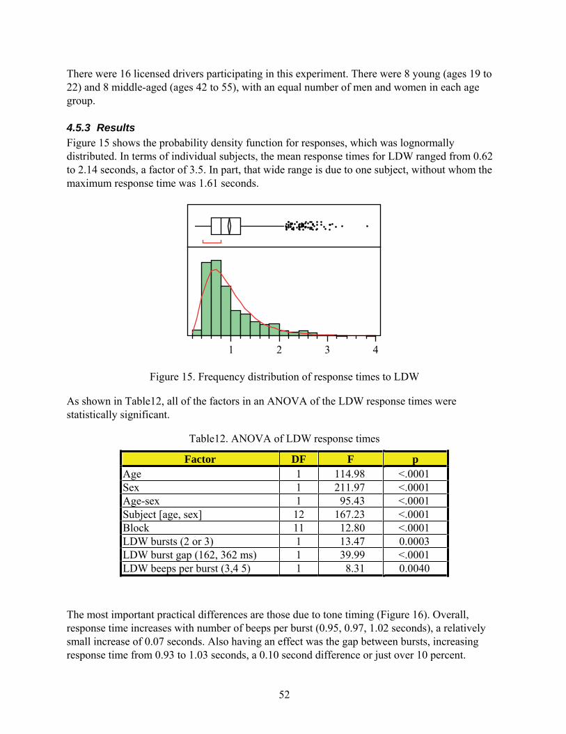
There were 16 licensed drivers participating in this experiment. There were 8 young (ages 19 to 22) and 8 middle-aged (ages 42 to 55), with an equal number of men and women in each age group.
4.5.3 Results Figure 15 shows the probability density function for responses, which was lognormally distributed. In terms of individual subjects, the mean response times for LDW ranged from 0.62 to 2.14 seconds, a factor of 3.5. In part, that wide range is due to one subject, without whom the maximum response time was 1.61 seconds.
1 2 3 4
Figure 15. Frequency distribution of response times to LDW
As shown in Table12, all of the factors in an ANOVA of the LDW response times were statistically significant.
Table12. ANOVA of LDW response times
Factor DF F p Age 1 114.98 <.0001 Sex 1 211.97 <.0001 Age-sex 1 95.43 <.0001 Subject [age, sex] 12 167.23 <.0001 Block 11 12.80 <.0001 LDW bursts (2 or 3) 1 13.47 0.0003 LDW burst gap (162, 362 ms) 1 39.99 <.0001 LDW beeps per burst (3,4 5) 1 8.31 0.0040
The most important practical differences are those due to tone timing (Figure 16). Overall, response time increases with number of beeps per burst (0.95, 0.97, 1.02 seconds), a relatively small increase of 0.07 seconds. Also having an effect was the gap between bursts, increasing response time from 0.93 to 1.03 seconds, a 0.10 second difference or just over 10 percent.
52

Finally, going from two to three bursts increases response time from 0.95 to 1.01 seconds, a rather small difference of 0.06 seconds. Figure 16 shows that as warning duration increases from about 1000 ms to 1700 ms, response time increases from about 900 to about 1050 ms. Increasing warning duration beyond 1700 ms has no effect on response time.
0.8
0.85
0.9
0.95
1
1.05
1.1
1.15
2, short 2, medium 3, short 3, medium
2 3 4 5 6
Number of Beeps per Burst
Figure 16. Relationship of LDW variations to response time
Table 13 shows the number of errors, which when examined by subject was weakly correlated with response time (r = 0.29) for all trials, but not correlated for LDW (r = 0.04). Of all 11 LDW errors, five (almost half) were made by one subject, so only slight emphasis should be placed on the number of errors. Notice there were more errors with medium gaps than short gaps (eight versus three), more errors with two bursts versus three (ten versus one), and, surprisingly, more errors with more beeps per burst (one, three, and seven) for three, four, and five beeps per burst. Thus, shortening the warning increases errors (giving subjects less information), except for changes in the number of beeps per burst, which has the opposite effect.
Table 13. Number of errors for LDW
Short Gap Medium Gap Total LDW Bursts 3 4 5 3 4 5
2 2 1 1 1 5 10 3 1 1
Total 2 1 1 1 6 Gap means 3 8 11
4.5.4 Conclusions The LDW pattern should be either a sequence of three bursts of two or three beeps separated by a short gap (162 ms).
53
x

x The warning duration should be no more than about 90 percent of the expected mean response time. Response time to warnings increases as the warning duration increases up to 1.7 time the mean response time. Beyond that time, increasing warning duration has a minimal effect on response time.
This finding has implications for all warnings, not just LDW, for which warning duration was examined. For LDW, the shortest response times occurred with warnings whose duration was slightly less the mean response time, about one second. Increases in the warning duration up to 1.7 times the mean response time increased the response time by about 150 ms (over 10%, an important practical difference).
54
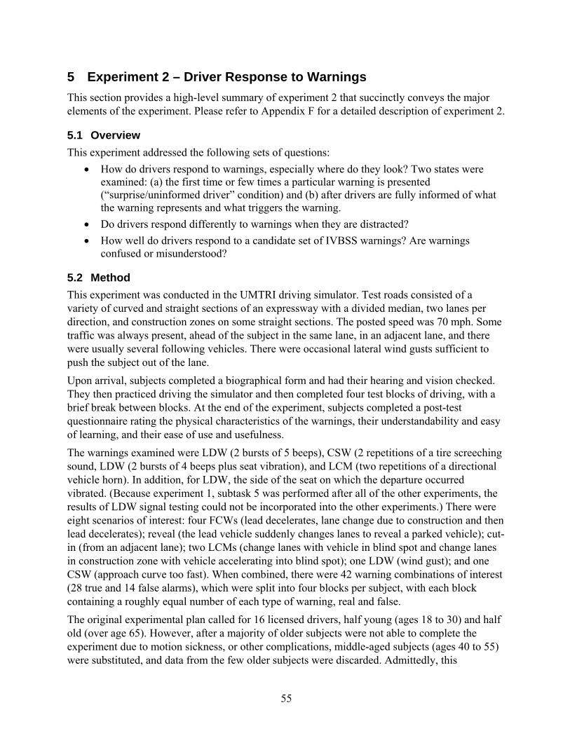
5 Experiment 2 – Driver Response to Warnings This section provides a high-level summary of experiment 2 that succinctly conveys the major elements of the experiment. Please refer to Appendix F for a detailed description of experiment 2.
5.1 Overview This experiment addressed the following sets of questions: x How do drivers respond to warnings, especially where do they look? Two states were
examined: (a) the first time or few times a particular warning is presented (“surprise/uninformed driver” condition) and (b) after drivers are fully informed of what the warning represents and what triggers the warning.
x Do drivers respond differently to warnings when they are distracted?
x How well do drivers respond to a candidate set of IVBSS warnings? Are warnings confused or misunderstood?
5.2 Method This experiment was conducted in the UMTRI driving simulator. Test roads consisted of a variety of curved and straight sections of an expressway with a divided median, two lanes per direction, and construction zones on some straight sections. The posted speed was 70 mph. Some traffic was always present, ahead of the subject in the same lane, in an adjacent lane, and there were usually several following vehicles. There were occasional lateral wind gusts sufficient to push the subject out of the lane. Upon arrival, subjects completed a biographical form and had their hearing and vision checked. They then practiced driving the simulator and then completed four test blocks of driving, with a brief break between blocks. At the end of the experiment, subjects completed a post-test questionnaire rating the physical characteristics of the warnings, their understandability and easy of learning, and their ease of use and usefulness. The warnings examined were LDW (2 bursts of 5 beeps), CSW (2 repetitions of a tire screeching sound, LDW (2 bursts of 4 beeps plus seat vibration), and LCM (two repetitions of a directional vehicle horn). In addition, for LDW, the side of the seat on which the departure occurred vibrated. (Because experiment 1, subtask 5 was performed after all of the other experiments, the results of LDW signal testing could not be incorporated into the other experiments.) There were eight scenarios of interest: four FCWs (lead decelerates, lane change due to construction and then lead decelerates); reveal (the lead vehicle suddenly changes lanes to reveal a parked vehicle); cutin (from an adjacent lane); two LCMs (change lanes with vehicle in blind spot and change lanes in construction zone with vehicle accelerating into blind spot); one LDW (wind gust); and one CSW (approach curve too fast). When combined, there were 42 warning combinations of interest (28 true and 14 false alarms), which were split into four blocks per subject, with each block containing a roughly equal number of each type of warning, real and false. The original experimental plan called for 16 licensed drivers, half young (ages 18 to 30) and half old (over age 65). However, after a majority of older subjects were not able to complete the experiment due to motion sickness, or other complications, middle-aged subjects (ages 40 to 55) were substituted, and data from the few older subjects were discarded. Admittedly, this
55
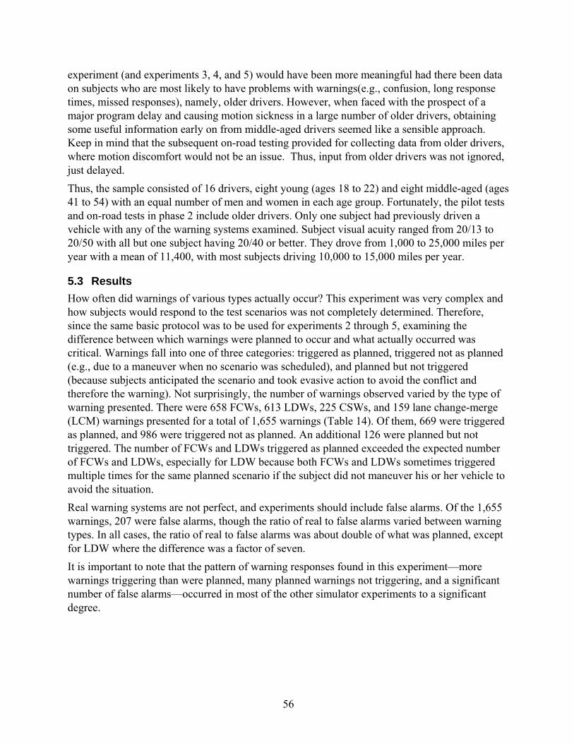
experiment (and experiments 3, 4, and 5) would have been more meaningful had there been data on subjects who are most likely to have problems with warnings(e.g., confusion, long response times, missed responses), namely, older drivers. However, when faced with the prospect of a major program delay and causing motion sickness in a large number of older drivers, obtaining some useful information early on from middle-aged drivers seemed like a sensible approach. Keep in mind that the subsequent on-road testing provided for collecting data from older drivers, where motion discomfort would not be an issue. Thus, input from older drivers was not ignored, just delayed. Thus, the sample consisted of 16 drivers, eight young (ages 18 to 22) and eight middle-aged (ages 41 to 54) with an equal number of men and women in each age group. Fortunately, the pilot tests and on-road tests in phase 2 include older drivers. Only one subject had previously driven a vehicle with any of the warning systems examined. Subject visual acuity ranged from 20/13 to 20/50 with all but one subject having 20/40 or better. They drove from 1,000 to 25,000 miles per year with a mean of 11,400, with most subjects driving 10,000 to 15,000 miles per year.
5.3 Results How often did warnings of various types actually occur? This experiment was very complex and how subjects would respond to the test scenarios was not completely determined. Therefore, since the same basic protocol was to be used for experiments 2 through 5, examining the difference between which warnings were planned to occur and what actually occurred was critical. Warnings fall into one of three categories: triggered as planned, triggered not as planned (e.g., due to a maneuver when no scenario was scheduled), and planned but not triggered (because subjects anticipated the scenario and took evasive action to avoid the conflict and therefore the warning). Not surprisingly, the number of warnings observed varied by the type of warning presented. There were 658 FCWs, 613 LDWs, 225 CSWs, and 159 lane change-merge (LCM) warnings presented for a total of 1,655 warnings (Table 14). Of them, 669 were triggered as planned, and 986 were triggered not as planned. An additional 126 were planned but not triggered. The number of FCWs and LDWs triggered as planned exceeded the expected number of FCWs and LDWs, especially for LDW because both FCWs and LDWs sometimes triggered multiple times for the same planned scenario if the subject did not maneuver his or her vehicle to avoid the situation. Real warning systems are not perfect, and experiments should include false alarms. Of the 1,655 warnings, 207 were false alarms, though the ratio of real to false alarms varied between warning types. In all cases, the ratio of real to false alarms was about double of what was planned, except for LDW where the difference was a factor of seven. It is important to note that the pattern of warning responses found in this experiment—more warnings triggering than were planned, many planned warnings not triggering, and a significant number of false alarms—occurred in most of the other simulator experiments to a significant degree.
56

Table 14. Warning frequency
Warning Triggering Category Warning Category Total (1655)Real FA
Triggered as planned 280 81 361 Triggered not as planned 282 15 297
FCW Planned but not triggered 9 1 10 Total triggered 562 96 658 Triggered as planned: Observed / expected 280/96 81/96 Triggered as planned 62 34 96 Triggered not as planned 129 0 129
CSW Planned but not triggered 1 0 1 Total triggered 191 34 225 Triggered as planned: Observed / expected 62/64 34/32 Triggered as planned 88 14 102 Triggered not as planned 510 1 511
LDW Planned but not triggered 16 16 32 Total triggered 598 15 613 Triggered as planned: Observed / expected 88/64 14/32 Triggered as planned 49 61 110 Triggered not as planned 48 1 49
LCM Planned but not triggered 79 4 83 Total triggered 97 62 159 Triggered as planned: Observed / expected 49/128 61/64
Multiple warning sequences can be identified from two perspectives, stimulus interference and response interference. With stimulus interference, the presentation of multiple warnings overlap for a duration that depends on the warnings used. For brief warnings, a value of about 0.85 seconds seems reasonable. For response interference, experience from the RDCW program indicated that most responses to a single warning (either a significant drop in speed or the distance from the center of the lane) are complete in about three seconds, so warnings whose onsets were three seconds or less apart were considered part of a multiple warning sequence. Since any potential interference was of concern, the response criterion was most commonly used to identify multiple warning sequences. Using the response interference criteria, there were 384 warnings in multiple warning sequences (Table 15).
57

Table 15. Frequency of each warning type in multiple warning situations
Warning Frequency of Multiple Warnings (N)
Lateral drift warning 220 Forward collision warning 66 Lane change-merge warning 40 False forward collision warning 26 False lane change-merge 23 Curve speed warning 9 Total 384
These 384 warnings were grouped into 166 multiple warning events, where an event is at least two warnings in succession within a three-second time period. LDW warnings predominated. Some two-thirds of the sequences started with LDW, with one-third of the total being two LDWs in succession. The longest string was six warnings, five LDWs followed by a CSW. Interestingly, when the definition of a multiple event was based on stimulus interference, less than 4 percent of all warnings were part of multiple warning events. As to where drivers looked, the eye tracking data showed very few differences in terms of fixation frequency to various locations (the road, mirrors, etc.), or the mean duration of fixations, comparing baseline periods (5 to 10 seconds before a warning and 5 to 10 seconds after a warning) with those shortly after the warning (0 to 3 seconds). This is probably because warnings were often not truly surprise events and subjects were assessing and responding to the situation, often well before the warning was presented. However, looking at the data more closely (for example, for LDW as shown in Table 16), at the start of the warning, the number of fixations to the front screen is larger than even a short time after the warning, suggesting an immediate reaction. What is needed is an even finer-grained analysis that considers each scenario separately and the prewarning driver situation. Such an analysis would require more data than is in the existing data set.
Table 16. Eye fixation frequencies after LDW warning
Area Start of Warning
.5 s after Warning
1 s after Warning Total
Unknown 14 7 7 28 Front screen 38 27 27 92 Rearview mirror 2 4 1 7 Speedometer 7 2 8 17 Bottom right of front screen 10 6 7 23 Subject lane 86 79 79 241 Bottom left of front screen 9 12 11 32 Left front screen 1 1 Right front screen 2 2 1 5 Total 168 139 139 446
58

How did drivers respond to warnings? Do drivers respond differently to warnings when they are distracted? Responding to a warning was defined as the subject releasing the throttle completely or applying the brakes in the three seconds after the warning, but not in the six seconds prior to the warning. Using these criteria, drivers responded to approximately 27 percent of the FCWs (562 warnings) and 18 percent of the CSWs (225 warnings). Interestingly, no subjects responded to a CSW with braking. Thus, there were 149 responses to FCWs and 42 responses to CSWs. For FCW, the mean times were 0.79 seconds and 1.07 seconds for accelerator pedal release time and brake onset time, respectively with standard deviations of 0.85 and 0.53 seconds. The mean accelerator pedal release time for CSW was 1.47 seconds with a standard deviation of 0.91 seconds. The accelerator related distributions are exponential and the CSW distributions are log normal. Three mixed-effect models were developed with FCW accelerator release time, FCW brake onset time, and CSW accelerator release time being the dependent measures. In all three analyses, age and gender were the between-subjects factors. Whether the subject was performing a distraction task (distracted, undistracted) and whether the subject was informed about the crash warning system (uninformed, informed) were the within-subjects factors. (Note that being in a “distraction” block does not necessarily mean the driver was distracted, only that he or she was instructed to engage in a secondary task when feeling it appropriate to do so.) Scenarios were included in the model as well as age-by-gender and distraction-by-informed-state interactions. There were no statistically significant effects in any of the analyses, with the lack of a distraction difference being of particular note. To maintain schedule, performance on the distraction task (address entry) was not tracked. However, it was the impression of the experimenters that many subjects were not diligent in completing the distraction task, so that they were not really distracted. In part, this is due to the nature of the experiment conducted—there were so many external events that subjects just focused on driving. In real driving, or other situations where crash inducing situations are much rarer, drivers are more likely to give greater attention to distracting secondary tasks, and distraction differences are more likely to be apparent. Figure 17 shows the mean speed reduction to the forward warnings, FCW and CSW. Mean speed changes to CSW were extremely small, on the order of 1 mph. As a reminder, driving through a curve had no consequences (e.g., skidding) and because the simulator was fixed-base, there was no feeling of lateral acceleration.
59

Figure 17. Mean reduction in speed in response to FCW and CSW warnings
Figure 18 shows how substantially the reduction in speed was in response to FCWs dependent upon the scenario.
Figure 18. Mean reduction in speed after FCWs for each scenario
Lane position changed substantially in response to LCM and LDW warnings (Figure 19). For LDW, younger drivers returned to the lane more quickly, with a difference of 1.5 seconds at about 0.1 meters from the center of the lane.
60

Figure 19. Distance from lane-center in response to LDW and LCM warnings
How do initial responses to warnings differ from subsequent responses to the same warning? Warnings in real driving occur quite rarely. Thus, collecting sufficient data on responses to warnings at real-world frequencies could require hundreds, if not thousands, of hours of driving per subject, which will not provide the desired data within a timeframe or cost needed to make engineering decisions. Therefore, the common engineering practice is to engage in accelerated testing to have warnings occur more often than normal so there are enough data to analyze in a typical experiment. But are those initial responses somehow fundamentally different? Figure 20 compares the first response to LDW (16 responses, one per subject) with all subsequent responses. The only significant difference in absolute lane position was at 2.5 seconds with drivers making a larger correction for the first response (by about 0.1 meters). Thus, for LDW, pooling all responses seems reasonable. Of course, considering the mean response time for many warnings is on the order of a second or so, one would not expect much of a difference until after that time.
61

Dist
ance
from
cent
er o
f lan
e (m
)
1.2
1
0.8
0.6
0.4
0.2
0
First occurence Subsequent warnings
0.5 1 1.5 2 2.5 3
Time post-warning (s)
Figure 20. Driver response to initial LDW
First occurence Subsequent warnings
0.5 1 1.5 2 2.5 3
Time post-warning (s)
Figure 21. Driver response to initial LCM
Dist
ance
from
cent
er o
f lan
e (m
)
1.2
1
0.8
0.6
0.4
0.2
0
For LCM (Figure 21), the result is somewhat similar in that the driver reaction to the first warning is greater (i.e., drivers approach the middle of the lane more rapidly), though most of the difference occurs at 1.5 and 2.0 seconds after the warning and is quite small.
For FCW (Figure 22), the pattern is different from that of the lateral warnings (LDW and LCM). Again there are no initial differences (in this case, the first 1.5 seconds), but after that, the decrease in speed for warnings is less than that for subsequent occurrences by about 10 mph. Curiously, the pattern for CSW (Figure 23) is the opposite after the first second or so, with drivers reducing their speed more for the first warning than for subsequent warnings, probably because they realized that in a simulator-based experiment, there are no consequences of driving curves too quickly.
62

Ach
ieve
d re
duct
ion
in sp
eed
(mph
)
25
20
15
10
5
0
-5
First occurence Subsequent warnings
0.5 1 1.5 2 2.5 3
Time post-warning (s)
Figure 22. Driver response to initial FCW
Ach
ieve
d re
duct
ion
in sp
eed
(mph
)
1
0.8
0.6
0.4
0.2
0
First occurence Subsequent warnings
0.5 1 1.5 2 2.5 3
Time post-warning (s)
Figure 23. Driver response to initial CSW
How did drivers rate the warnings? Were warnings confused or misunderstood? As indicated by the post-test survey (Table 17) most of the physical characteristics (light brightness, sound) of the warnings examined seemed to be about at the desired level, though subjects did rate the vibration level of the haptic seat to be a bit high. However, keep in mind that subjects were wearing light clothing, and when wearing winter clothing or driving on a rough road surface more intensive vibration is needed to ensure the warning is conveyed to the driver. Subjects also rated determining the side of the LDW somewhat difficult. Thus, some improvements are needed.
63

With regard to whether the drivers were informed about different crash warnings, none of the warnings was initially well understood when the drivers were uninformed, with CSW being most noteworthy. This suggests that the warning should be revised, though improvement of all of the warnings should be considered. It should be noted that these data were collected in a fixed-base simulator, and in this experiment there were no consequences of driving a curve too quickly.
Table 17. Overall mean post-test ratings of the warnings
Category Characteristic Scale FCW CSW LDW LCM Format Sound level 1=too soft, 5=too loud 3.1 3.1 3.4 3.3
Distinguishing sound side 1=easy, 5=difficult - - 2.3 2.6 Vibration level 1=too little, 5=too much 3.3 2.9 3.6 -Distinguishing vibration side 1=easy, 5=difficult - - 2 -Light brightness 1=too dim, 5=too bright - - 2.8 -Distinguishing light side 1=easy, 5=difficult - - 2.4 -
Meaning- Initial understanding 1= not, 5=well understood 3.0 2.2 2.9 2.7 fulness Midpoint understanding 1= not, 5=well understood 4.5 4.3 4.5 4.3
End understanding 1= not, 5=well understood 4.7 4.5 4.8 4.7 Learning 1=easy, 5=difficult 4.4 4.0 4.4 4.2
Overall Frequency 1=too little, 5=too often 3.4 3.5 3.5 3.3 Usefulness 1=useless, 5=useful 3.8 3.2 3.6 3.5 Ease of use 1=difficult, 5=easy 3.8 4.2 4.1 3.9
Nonetheless, all of the warnings were rated as somewhat easy to use (about 4) with only slight differences among them. However, none of the warnings was well rated in terms of usefulness, a troubling finding, with the highest rating being for FCW (3.8).
5.4 Conclusions How often did warning of various types occur? x In this experiment, 1,655 warnings were presented to 16 subjects, or about 100 per subject.
This was more than enough for most analyses. Of these, 658 were for FCW, 225 for CSW, 613 for LDW, and 159 for LCM. Thus, roughly speaking, the probability of a forward event and side event were almost equal. In addition, there were 126 warnings that were planned but not triggered, mostly for LCM. Further, of the 1,655 warnings, 986 were not triggered as planned, with more than half (511) being for LDW. So, there were more than enough warnings to examine differences between conditions of interest. Being distracted, or at least being in a condition where distraction occurred, had a small effect on how often drivers received warnings (8% increase). x Of the warnings presented, some 384 (166 events) occurred within three seconds of each
other, with the time between events being exponentially distributed. A major concern of the IVBSS project is what happens when multiple warnings are presented, which in this experiment, occurred by chance. Three seconds is roughly the time required to completely respond to a warning (return to a lane, decelerate to a desired speed). Some two-thirds of multiple warnings started with an LDW, with one-third being two LDWs in a row. In this
64

experiment, about 23 percent of all warnings were part of a multiple warning sequence, a somewhat uncommon but not rare occurrence. Thus, even with a very inclusive definition of what constituted a multiple warning sequence, single warnings predominated. Where do drivers look in response to warnings? x Glances immediately after warnings differ little from glance patterns at other times, with just
slightly more glances ahead. Data from baseline conditions were compared with the zero-to-three-second period after a warning. An important distinction was whether CSW was included, as in the period immediately after a CSW, drivers were scanning the curve, not looking straight ahead. Curiously, there were few differences among warnings in terms of the number of glances to various locations between the baseline conditions (5 to 10 seconds before a warning and 5 to 10 seconds after a warning) and when a warning was being responded to (0 to 3 seconds after the warning). In all cases, drivers were more likely to fixate forward of the vehicle (about 65% of the time during the baseline periods and 75% of the time immediately after a warning), even for LCM where the hazard was on the side. Other analyses concerning fixations at 0, 0.5, and 1.0 seconds after a warning showed some additional attention to the forward scene. How do drivers respond to warnings? Using the criteria of no release of the throttle (to zero) within six seconds of a warning and release within three seconds of a warning, drivers responded to only about 27 percent of the FCWs and 18 percent of the CSWs. For the reveal scenario (which triggered an FCW), the desired response was a lane change; for the cut-in scenario (which also triggered an FCW), the intruding vehicle returned to its own lane so braking could be avoided. Furthermore, in some situations, the throttle was released, but not to zero. For FCW, the mean accelerator pedal release and brake onset times were 0.79 seconds and 1.07 seconds, respectively. The mean accelerator pedal release time for CSW was 1.47 seconds. Note that these driver responses relate to a variety of scenarios. In terms of speed reduction in response to FCWs, drivers decelerated about 4 mph for every 0.5 seconds, ignoring the first 0.5 seconds in which little speed change occurred due to the time needed by the driver to respond. For CSW, the speed drop was low (about 1 mph over a three-second interval). However, there were major differences in speed reduction across scenarios—8 mph per second for lead vehicle deceleration, about 4 mph for lead vehicle deceleration after a lane change, about 3 mph for cut-ins, and just over 1 mph for reveals. For LDW and LCM, the key response was the change in lane position. Departure in terms of distance from lane center continued until about 0.3 seconds after a warning was presented, returning to the initial position at the warning by 0.6 seconds, and continuing to decrease, with very minor changes, after 1.8 seconds. On average, distances were about 0.2 seconds greater for LCM than for LDW. Is the first response to a warning different? x Differences between first reactions to warnings and subsequent reactions were small and only
manifested themselves, if at all after 1 to 1.5 seconds post warning. x For LDW, drivers return to center more quickly for the first warning.
65

x For LCM, there is no real difference. For FCW, drivers decelerate less quickly the first time, whereas for CSW, they decelerate more quickly.
There were multiple FCW scenarios, but there was only one scenario for most other warnings, so there may be some sort of underlying between scenario difference. However, examining scenario differences at this point was beyond the scope of the work. How well did drivers rate the various warnings and where should they be improved? None of the warnings were initially well understood, and all were rated as only moderately useful. In summary, based upon the implementation of warnings tested in the simulator, some improvements are needed to make it easier for drivers to tell on which side the LDW occurs. Steps should be taken to make warnings more intuitive (easier to understand initially); this is particularly true for CSW. In fact, as is shown in Appendix G and in the next section, a completely different warning philosophy was explored in experiment 3 to overcome some of these problems.
66

6 Experiment 3 – Combined Warnings for IVBSS This section provides a high-level summary of experiment 3 that succinctly conveys the major elements of the experiment. Please refer to Appendix G for a detailed description of experiment 3.
6.1 Overview Experiment 3 address a single question—how does the combining of warnings, using a singular warning to represent more than one possible threat, affect (a) driver performance when responding to them and (b) driver ratings of them? Of interest were single warnings, dual warnings (simple and hybrid), and multiple warnings. Single Warning. A fully combined and minimalist approach favors a single warning for any subsystem warning. In this experiment it is implemented simultaneously auditorily and haptically with vibrations on both sides of the seat. Its main purpose is to warn the driver that something is wrong, similar to the concept of a single caution warning. If the driver was not focused on the road, the warning would draw attention quickly. Dual Warning - Simple. A possible expansion of the single-warning approach is to have a warning for longitudinal warnings and a directional (left or right) warning for lateral warnings. In this experiment longitudinal warnings are implemented as an auditory warning with a brake pulse. The lateral warnings are implemented as a different auditory warning with lateral shaking of the seat in the direction of the event. Thus, a driver would receive coarse directional information about the location of the hazard that needs to be addressed and would be able to initiate a response quickly (either by returning to the lane or slowing down). Dual Warning – Hybrid. Similar to the simple dual warning, only two auditory warnings are given but the haptic signals are different for the four subsystems. For longitudinal warnings, an auditory warning is either accompanied by a brake pulse (FCW) or used alone (CSW). LCM warnings have a different auditory warning without haptic cues and LDW has a lateralized seat vibration without an auditory warning. Thus, each of the four subsystems has a unique representation. Multiple Warnings. Further elaboration of the warning scheme may result in multiple warnings that allow the driver to distinguish among each of the subsystems. In this experiment, there are four distinct unique warnings that correspond to each of the four IVBSS subsystems and associated lateral information.
6.2 Method Sixteen licensed drivers participated in this study. Eight were middle-aged (41 to 55 years old, with a mean age of 49 years) and eight were younger drivers (18 to 30 years old, with a mean age of 25 years). The age groups were balanced for gender. Each driver was paid $50 for two and a half hours of participation. The UMTRI DriveSafety driving simulator was used in this experiment. A simulated haptic brake pulse was added for the purposes of this experiment. A linear motor, attached to the bottom of the simulator buck, provided a quick burst of longitudinal motion that was both felt and heard, and was distinct from the seat shaker signal.
67

Driving scenarios were developed to induce the driver into a situation in which a warning is given. For FCW, a lead vehicle suddenly decelerated at about 0.2 g. In some cases, the lead vehicle decelerated more slowly, which did not cause an FCW. For LCM, the subjects were encouraged to change lanes by a stopped vehicle in the subject’s lane and another vehicle in the left-mirror blind zone. For CSW, the lead vehicle accelerated to 75 mph on an approach to a curve. In contrast to the previous experiment, if the subject drove too fast, the vehicle skidded, a cue that driving a curve too fast was not acceptable. For LDW, cross winds caused drifting out of the lane. After participants viewed a short video introducing the IVBSS concept and the four types of warnings being investigated, they test drove in the driving simulator to become comfortable with the controls. Each simulator session was divided into four blocks of 18 trials counterbalanced across age-by-gender groups. In each block, a different set of warning approaches was presented. At the end of the fourth block, participants completed a post-drive questionnaire (shown in section G.5.2).
6.3 Results Overall, drivers encountered 1,075 warnings during the experiment. The majority of warnings were FCWs, comprising just under 50 percent of all warnings. CSWs were the next most common warning type at 23 percent. Were the differences between warning combinations in terms of driver performance? Accelerator pedal release times and brake onset times to FCWs and CSWs were examined as the dependent variables in separate, linear mixed models. Overall, accelerator release times were 0.60 and 0.88 seconds for FCW and CSW, respectively, and there was no statistically significant difference between them. Brake onsets were 1.12 and 1.86 seconds for FCW and CSW, respectively, a difference that was statistically significant (F(1, 73) = 10.89, p < .001). The pairwise difference between accelerator pedal release and brake onset for FCW and CSW was 0.52 and 0.98 seconds, respectively, F(1, 72.50) = 13.46, p < .001 (Figure 24). These results suggest that for both FCW and CSW, there was a quick accelerator release, but for CSW there was a longer duration before the brake onset occurred.
CSW FCW
Figure 24. Pairwise accelerator pedal release and brake onset times by warning type
0 0.2 0.4 0.6 0.8
1 1.2 1.4 1.6 1.8
2
Res
pons
e Tim
e (s
)
Brake Onset Accel Pedal Release
68
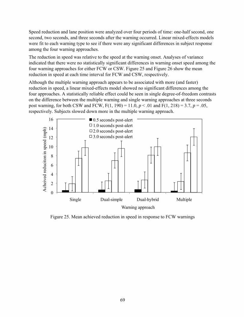
Speed reduction and lane position were analyzed over four periods of time: one-half second, one second, two seconds, and three seconds after the warning occurred. Linear mixed-effects models were fit to each warning type to see if there were any significant differences in subject response among the four warning approaches. The reduction in speed was relative to the speed at the warning onset. Analyses of variance indicated that there were no statistically significant differences in warning onset speed among the four warning approaches for either FCW or CSW. Figure 25 and Figure 26 show the mean reduction in speed at each time interval for FCW and CSW, respectively. Although the multiple warning approach appears to be associated with more (and faster) reduction in speed, a linear mixed-effects model showed no significant differences among the four approaches. A statistically reliable effect could be seen in single degree-of-freedom contrasts on the difference between the multiple warning and single warning approaches at three seconds post warning, for both CSW and FCW, F(1, 190) = 11.0, p < .01 and F(1, 218) = 3.7, p = .05, respectively. Subjects slowed down more in the multiple warning approach.
16
14
12
10
8
6
4
2
0 Single Dual-simple Dual-hybrid Multiple
0.5 seconds post-alert 1.0 seconds post-alert 2.0 seconds post-alert 3.0 seconds post-alert
Ach
eive
d re
duci
ton
in sp
eed
(mph
)
Warning approach
Figure 25. Mean achieved reduction in speed in response to FCW warnings
69

0.0
1.0
2.0
3.0
4.0
5.0
6.0
Ach
eive
d re
duci
ton
in sp
eed
(mph
)
0.5 seconds post-alert 1.0 seconds post-alert 2.0 seconds post-alert 3.0 seconds post-alert
Single Dual-simple Dual-hybrid Multiple
Warning approach
Figure 26. Mean achieved reduction in speed in response to CSW warnings
Figure 27 shows the mean distance from the center of the lane (in inches) in response to LDW warnings. On average, subjects were still drifting out of their lane at the half-second mark, but then began to correct their lane position between half a second and one second after the warning. There was a sharp correction between one and two seconds after the warning. A linear mixed-effects model showed no statistically significant differences among the warning approaches.
70
0.0
0.2
0.4
0.6
0.8
1.0
1.2
Mea
n di
stan
ce fr
om la
ne c
ente
r (m
) At alert 0.5 seconds post-alert 1.0 seconds post-alert 2.0 seconds post-alert 3.0 seconds post-alert
Single Dual-simple Dual-hybrid Multiple
Warning approach
Figure 27. Mean distance from the center of the lane (meters) in response to LDW warnings
Which warning approach did drivers prefer? Only one selected the multiple warning approach as her most preferred, and more drivers selected the single warning approach than any other. As illustrated below, overall, middle-aged drivers preferred the single warning approach, while younger drivers favored dual warnings (simple or hybrid).
7
Num
ber o
f sub
ject
s
6
5
4
3
2
1
0 Single Dual-Simple Dual-Hybrid Multiple
Young Middle-aged
Warning Approach
Figure 28. Drivers’ most preferred warning approach by age group
71

6.4 Conclusions x No warning combination (single, dual-simple, dual-hybrid, multiple) led to substantially
better driver responses than any other combination. Sometimes, the outcome of any experiment is that there is no substantial difference between conditions, as was the case here, and that is useful information. x The lowest rated warning combination was the multiple warning where each warning
subsystem had a distinct and unique warning. Subjects did not show an overwhelming preference for any of the warning approaches, but they clearly did not favor the fully distributed warning approach (four warnings for four subsystems). Which warning approach was preferred depended on the driver’s age. Middle-aged drivers preferred full integration (single warning), while younger drivers favored dual warnings. Older subjects (over 65 years) were not tested in this experiment because of experimental limitations. Generally, the objective results did not reveal significant differences among the warning approaches tested. Subjects responded more slowly to CSW than to FCW, possibly because they were already aware of the driving context. If there was no vehicle in front of them, drivers were less likely to respond immediately and waited half a second longer before applying the brake. Analysis of responses by warning approach suggests, however, that in the single warning approach, the delay between accelerator release and brake onset for CSW was the same as for FCW. Drivers may have chosen to respond immediately to single caution warnings as a matter of strategy in the absence of other information from the integrated warning system. Analysis of the reduction in speed after warnings revealed some benefit to the multiple warning approach over the single warning approach. Three seconds after an FCW or a CSW, there was greater speed reduction with the multiple warning approach than with the single warning approach. x IVBSS should use one of the dual-warning approaches, or a variation of them. Based on (1) the subjective preference for some or full integration, (2) the weak objective benefit for a multiple warning approach versus a single warning approach, and (3) the analysis of the various considerations for integration, the recommendation is that IVBSS use one of the dual-warning approaches (simple or hybrid), or a variation of them. If, however, a different approach is sought, the current experiment does not provide compelling evidence against any of the approaches that were tested. In considering this recommendation it should be noted that: (1) there were no motion cues (which lead to later responses to CSW0, (2) subjects were not distracted and (3) subjects were aware many warnings would be presented (so they were responding more quickly than would naturally occur). Although these considerations affect how quickly drivers respond, they do not differentially affect the warning approaches examined.
72

7 Experiment 4 ņ Warning Delay-Accuracy Tradeoff This section provides a high-level summary of experiment 4 that succinctly conveys the major elements of the experiment. Please refer to Appendix H for a detailed description of experiment 4.
7.1 Overview Experiment 4 addressed two major questions: x How does the tradeoff between warning system processing time (to start to inform the
driver) and warning accuracy affect driver responses to warnings? x How well do drivers respond to a candidate set of IVBSS warnings? Are any confused or
misunderstood?
Many vehicle-sensing and information-integration tasks take time. Radars need to sweep, detection decisions may need to be made across multiple sweeps, and data from various sensors may need to be combined. The more time is allotted to process the data, the more reliable the warning with fewer false alarms and fewer misses. However, the later the warning is presented to drivers, the less time they have to assess the situation and respond. What is an acceptable tradeoff between added certainty and potentially delaying the driver’s response?
7.2 Method This experiment took place in the UMTRI driving simulator. The test method in this experiment was based on that of experiments 2 and 3, and used the same set of scenarios, world (simulated route), procedure, and experimental sequence. In brief, subjects had their vision and hearing checked, practiced driving in the simulator, drove three, 20-minute test blocks, and then completed a post-test questionnaire. There were also questions asked at the end of each test block. The post-block questionnaire consisted of six to seven questions (e.g., rate the volume of the warning on a scale of 1 to 5) for each of the four primary warnings (FCW, LDW, LCM, and CSW), plus a blind-spot detection system (BSD). The post-test questionnaire also included three open-ended questions (e.g., did you notice changes among the drives? Which drive was best? How should each warning be changed?). The warnings examined included FCW (7 beeps and a brake pulse), CSW (same as FCW), LDW (directional haptic seat), and LCM (5 beeps, lower pitch than FCW and CSW). The FCW had the following characteristics (pitch f0 of1500 Hz, pulse rate of100 ms, duration of 70 ms, onset of 5 ms). The LDW characteristics were (pitch f0 of 400 Hz, pulse rate of 150 m, duration of 50 ms, onset of 10 ms). The two sounds were identical to those evaluated in experiment 1, subtask 3, suite A. The BSD included an LED indicator in the left and right outside mirrors, illuminated if there was a vehicle in, or quickly approaching, the blind spot. For FCW and LDW, three warning delays were examined (none, 150 ms, and 300 ms), each presented in a different block (and unknown to subjects). The order of blocks per delay conditions was counterbalanced across subjects. To simulate situations where waiting to gather additional information might be helpful for FCWs (how long time-to-collision [TTC] was below the threshold), the lead vehicle was programmed to accelerate 100 or 250 ms after the warning was triggered, or at the end of the trial, resulting in the conditions shown in Table 18. So, for example, if the warning delay was 300 ms and the
73

acceleration delay was 250 ms, for the first 250 ms of the interval, the warning should be presented. However, after that point, because the lead vehicle sped away, the warning was no longer needed.
Table 18 Effect of delay on FCW
Acceleration Delay W arningDelay
None 150m s 300m s
Until end of trial (normal) Warning Warning Warning 250 ms Warning Warning No warning 100 ms Warning No warning No warning
Delays were not manipulated for the other FCW scenarios, primarily because there were not enough trials available to explore how those scenarios were affected by delay. However, those other scenarios were relatively uncommon. For LDW, wind gusts were used to induce lane departures and wind gusts (2000 N) were presented for either one, two, or three seconds. Wind gust is not a manipulation of “accuracy” in exactly the same sense as the delays manipulated for FCW, but in both cases something about the situation will lead it to be resolved without the warning. In the case of LDW, the brief gust duration indicates a less severe situation, one less needing driver attention, and therefore less certain (and in some sense accurate) that a warning is needed. Thus for both FCW and LDW, the warning was presented only if the threat was still present after the warning delay had elapsed. Sixteen subjects, all licensed drivers, participated in experiment 4. There were eight young drivers (ages 18 to 30) and eight middle-aged drivers (ages 40 to 55), with both age groups balanced for gender. Visual acuity ranged from 20/13 to 20/40, with all but one subject having 20/30 or better. No subjects had previously driven a vehicle with any of the warnings being tested.
7.3 Results As in other experiments, warnings were not always presented as planned. Of the 960 planned events, only 590 warnings were triggered as planned. An additional 390 unplanned warnings were triggered. Overall warning frequencies across all subjects varied by warning type. The warnings presented were: 653 FCW, 185 LDW, 90 CSW, and 52 LCM. Note that in this experiment, although there were no planned CSWs in this experiment, they did occur. Overall, approximately 40 percent (390 out of 980 warnings) of presented warnings were triggered not as planned, reflecting the difficulty of completely predicting driver behavior. As before, there were more than enough warnings to develop reliable statistics. How does the tradeoff between warning system processing time and warning accuracy affect driver responses to warnings? Figure 29 shows differences in FCW responses for warning scenarios from Table 19. Keep in mind that warning delay was only varied for the lead vehicle deceleration scenario, not for other scenarios (lead vehicle reveals a parked vehicle, vehicle cuts in from an adjacent lane). Notice the lack of any consistent pattern, in part because of the small sample sizes in this case, with the key difference being between the lead vehicle acceleration delays. As a reminder, because of the way the scenarios were designed, some combinations
74
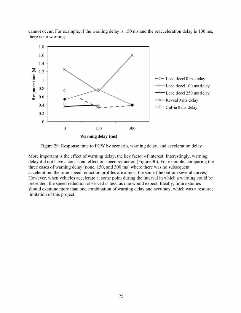
cannot occur. For example, if the warning delay is 150 ms and the reacceleration delay is 100 ms, there is no warning.
0
0.2
0.4
0.6
0.8
1
1.2
1.4
1.6
1.8
Res
pons
e tim
e (s
)
Lead decel 0 ms delay Lead decel 100 ms delay Lead decel 250 ms delay Reveal 0 ms delay Cut-in 0 ms delay
0 150 300
Warning delay (ms)
Figure 29. Response time to FCW by scenario, warning delay, and acceleration delay
More important is the effect of warning delay, the key factor of interest. Interestingly, warning delay did not have a consistent effect on speed reduction (Figure 30). For example, comparing the three cases of warning delay (none, 150, and 300 ms) where there was no subsequent acceleration, the time-speed reduction profiles are almost the same (the bottom several curves). However, when vehicles accelerate at some point during the interval in which a warning could be presented, the speed reduction observed is less, as one would expect. Ideally, future studies should examine more than one combination of warning delay and accuracy, which was a resource limitation of this project.
75

Figure 30. Reduction in speed after FCW warnings as function of acceleration delay and warning delay across all scenarios
As shown in Figure 31, increasing the delay in LDWs led to a more immediate reduction in lateral position error after the warning, but also led to a final position that was much further from the center of the lane (by about 0.1 m). It could be that the delay leads to less strict control over lane position because the LDW is a less consistent indicator of lane error. This suggests that for an LDW system warning delays on the order of 300 ms are not desired, and the lack of a difference between no warning delay and a 150-ms delay suggests the maximum acceptable warning delay is somewhere between 150 and 300 ms.
Figure 31. Distance from center after LDW as function of warning delay
76
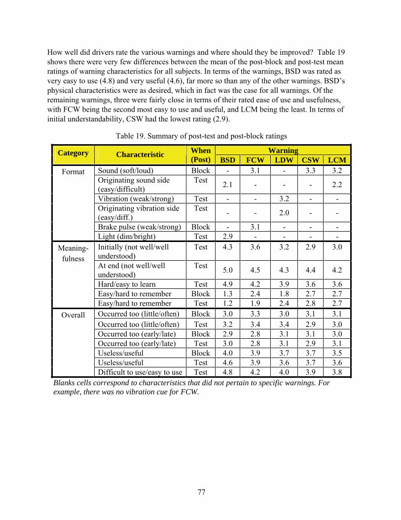
How well did drivers rate the various warnings and where should they be improved? Table 19 shows there were very few differences between the mean of the post-block and post-test mean ratings of warning characteristics for all subjects. In terms of the warnings, BSD was rated as very easy to use (4.8) and very useful (4.6), far more so than any of the other warnings. BSD’s physical characteristics were as desired, which in fact was the case for all warnings. Of the remaining warnings, three were fairly close in terms of their rated ease of use and usefulness, with FCW being the second most easy to use and useful, and LCM being the least. In terms of initial understandability, CSW had the lowest rating (2.9).
Table 19. Summary of post-test and post-block ratings
Category Characteristic When (Post)
Warning BSD FCW LDW CSW LCM
Format Sound (soft/loud) Block - 3.1 - 3.3 3.2 Originating sound side (easy/difficult)
Test 2.1 - - - 2.2
Vibration (weak/strong) Test - - 3.2 - -Originating vibration side (easy/diff.)
Test - - 2.0 - -
Brake pulse (weak/strong) Block - 3.1 - - -Light (dim/bright) Test 2.9 - - - -
Meaningfulness
Initially (not well/well understood)
Test 4.3 3.6 3.2 2.9 3.0
At end (not well/well understood)
Test 5.0 4.5 4.3 4.4 4.2
Hard/easy to learn Test 4.9 4.2 3.9 3.6 3.6 Easy/hard to remember Block 1.3 2.4 1.8 2.7 2.7 Easy/hard to remember Test 1.2 1.9 2.4 2.8 2.7
Overall Occurred too (little/often) Block 3.0 3.3 3.0 3.1 3.1 Occurred too (little/often) Test 3.2 3.4 3.4 2.9 3.0 Occurred too (early/late) Block 2.9 2.8 3.1 3.1 3.0 Occurred too (early/late) Test 3.0 2.8 3.1 2.9 3.1 Useless/useful Block 4.0 3.9 3.7 3.7 3.5 Useless/useful Test 4.6 3.9 3.6 3.7 3.6 Difficult to use/easy to use Test 4.8 4.2 4.0 3.9 3.8
Blanks cells correspond to characteristics that did not pertain to specific warnings. For example, there was no vibration cue for FCW.
77

7.4 Conclusions x Subjects did not perceive the difference in warning delays. The relationship between warning delays and driver responses was surprisingly unclear. Based upon the post-test ratings, subjects did not perceive a difference in the warning timing even though they experienced a significant number of similar warning events over a fairly brief time period. This result should be similar regardless of whether implemented in a light-vehicle or heavy-truck platform, as much of the lack of a perceived difference in warning onset time is likely due to limitations in human perception. x Delays between 150 and 300 ms are acceptable for the LDW algorithm implemented in this
experiment. For LDWs, increasing the delay to 300 ms led to a more immediate response of the subject to the lateral position error at 0.5 seconds after the warning delay, where lateral error increased for the first 0.5 seconds if the delay was 0 or 150 ms. That probably occurred because subjects noticed the lateral position error before the warning was presented. With the shorter delays, subjects stabilized closer to lane center (0.3 meters for 0 and 150 ms, 0.45 meters for 300 ms). It also could be that the LDW delay leads subjects to believe that less accurate control of lane position is acceptable (“If the warning system accepts sloppy lateral position control, then I should.”) Given this, delays between 150 and 300 ms are acceptable given the LDW algorithm implemented in this experiment. Interestingly, in contrast to predictions, gust duration did not increase the maximum excursion and the mean in a consistent manner. For FCW, the situation is quite complex. For the “no acceleration delay” cases, the differences in speed reduction were quite small. Where the vehicle reaccelerated, especially after a 250 ms delay, speed reductions were much greater; it is uncertain why. A key constraint of this experiment is that a particular warning delay-warning accuracy tradeoff was examined and the results could be different for a different tradeoff. Furthermore, subjects were continually adjusting their headway, and sometimes aware of the need for a response well before a warning was presented. However, exploring this tradeoff function more extensively was beyond the scope of this study. Driver responses to warnings were mixed. Most received reasonably favorable ratings from subjects in terms of the warnings’ physical format (sound, vibration, intensity, etc.). However, responses to the various warnings differed in their initial meaningfulness, usefulness, and ease of use. From best to worst, initial understanding ratings were: BSD, FCW, LDW, LCM, and CSW. This suggests most of the warnings except BSD would benefit from modification to improve their initial understandability. The ease of use ratings were, from best to worst: BSD, FCW, LDW, CSW, and LCM, indicating that subjects found BSD to be extremely easy to use. The usefulness ratings showed that BSD was also the most useful, and certainly more useful than the other warnings. Thus, overall the impression from the subjective ratings is that BSD and FCW were acceptable warnings, LDW could use some improvements in initial understanding, and CSW and LCM needed overall improvement.
78

Previous research on the RDCW program found that the LDW function and warnings were readily understood once drivers had a brief, on-road exposure to the system. Given that the approach to presenting LDW warnings examined in this series of studies was very similar to that fielded in the RDCW FOT, it is thought that brief on-road exposure to the system will quickly improve driver understanding of the LDW warning. For the CSW and LCM warnings, it remains a challenge as to how best to convey the nature of the threat to the driver and have it readily understood. However, it is believed that the grouping of warnings by nature of the threat, either lateral or longitudinal, will minimize the need for drivers to specifically differentiate each warning. Additional testing, in an equipped vehicle, will need to be performed to either prove or disprove this assumption.
79

8 Experiment 5 ņ Driver Response to Simultaneous Warnings This section provides a high-level summary of experiment 5 that succinctly conveys the major elements of the experiment. Please refer to Appendix I for a detailed description of experiment 5.
8.1 Overview Experiment 5 examined how to deal with warnings that occur concurrently or almost concurrently (either a second warning triggers while the driver is still responding to the first [about 3.0 seconds after the onset of the first warning], or while the auditory portion of the first warning is still playing [0.85 seconds after the first warning onset]). One of the assumptions behind this question is that such situations will occur often enough to be of concern. However, some of the findings from this experiment may challenge that assumption. The experiment considered several issues related to multiple warnings, and narrowed down the questions addressed to: x How does responding to one warning differ from responding to two warnings that are co
occurring (simultaneous or nearly simultaneous)? x Should co-occurring warnings be presented:
o Whenever they occur, even if simultaneously? o One at a time with higher priority warnings interrupting those of lower priority? o In sequence of occurrence, with the first warning playing to completion before the
second (delayed warning) starts? x In the simulator, how well do drivers respond to the set of candidate IVBSS warnings?
Are any confused or misunderstood?
8.2 Method This experiment took place in the UMTRI driving simulator. The test method developed for experiment 2 was used as a basis for this experiment as the scenarios, simulated route (world), procedure, and design basis are quite similar. In brief, subjects completed a biographical form, had their vision and hearing checked, practiced driving in the simulator, and then drove three 20minute test blocks followed by completing a post-test questionnaire. The post-test was similar to that used in previous studies, where subjects rated the intensity and frequency of warning stimuli, as well their understandability, ease of use, and usefulness. To create the multiple warning scenarios, experimenters combined single warning scenarios so that triggering events would occur in close succession. In prior experiments, there were many instances in which even a single warning triggering event did not occur as planned. Key planned events included single warning scenarios, multiple warning scenarios, single false alarms, lead vehicle lane changes (to provide variety), and trials where no scenarios occurred.
As in all IVBSS DVI experiments, the most current version of the warning set was used. Warnings examined included FCW (7 beeps and simulated brake pulse), CSW (same as FCW), LDW (seat shakes), and LCM (3 low beeps followed by 3 high beeps). The FCW had the following characteristics (pitch f0 of 1500 Hz, pulse rate of 100 ms, duration of 70 ms, onset of 5 ms). The LDW characteristics were (pitch f0 of 400 Hz, pulse rate of 150 m, duration of 50 ms, onset of 10 ms). The two sounds were identical to those evaluated in experiment 1, subtask 3,
80

30 18 FCW (lead decelerates),
25
0.5 1.0 1.5 2.0 2.5 3.0
Time after warning (s)
followed by LDW
20 71 LCM (construction zone), followed by FCW (lead15 decelerates)
10 61 LDW, followed by FCW (Lead decelerates)
5
1 FCW (Lead decelerates)0
Spee
d R
educ
tion
(mph
)
The numbers in the figure refer to the scenarios, e.g., 1=FCW, 7=LCM, 8=LDW
Figure 32. Speed change related to LDW
suite A. Given the need to get enough multiple warning trials to analyze, and the large number of possible combinations, only a limited number of warnings (LCM, FCW, and LDW) were considered. Curve speed warnings (CSWs) were available, but not paired with others. Three different priority rules for presenting multiple warnings were examined: (1) present when triggered, even if simultaneous (warnings could overlap), (2) delayed sequential (the second warning starts after the first is done), and (3) priority preempt (higher priority warnings can interrupt lower priority). Under the circumstances tested, FCW always had the highest priority assigned to it, followed by LCM and LDW.
Eight young participants (ages 20 to 27) and eight middle-aged participants (ages 42 to 55) took part in the experiment. Gender was balanced within age group, and all were licensed drivers. Visual acuity ranged from 20/15 to 20/35 (one subject).
8.3 Results Figure 32 shows that changes in speed linked to FCW are relatively unaffected by other warnings. There is only a slight difference between an FCW by itself, an FCW preceded either by an LCM or LDW, or an FCW followed by an LDW. The points representing each warning sequence shown in the figure are based on six to 47 responses, with only the “LCM then FCW” warning sequence having less than 20 responses.
However, in contrast, responses to LDW were negatively affected by other warnings. A leading or trailing FCW delayed the response by at least 0.5 seconds (Figure 33), and LCM where a leading or trailing FCW delayed the response by at least 0.5 seconds (Figure 34), where each line on the figure is based on 31 to 44 instances.
81

Spee
d R
educ
tion
(mph
) 1.6
1.4
1.2
1
0.8
0.6
0.4
0.2
0
46 FCW (reveal), followed by LCM
86 LDW, followed by LCM
6 LCM
At alert 0.5 1.0 1.5 2.0 2.5 3.0 Time after warning (s)
Figure 33. Lateral position for single and paired LCM scenarios
How do the warning priority rules affect driver responses to warnings? Interestingly, there were some practical differences due to preempt rules, but they were not consistent. As shown in Figure 34, the greatest reduction in speed for FCW occurred when it was presented simultaneously with another warning. Presenting warnings sequentially reduced the speed by about 3 mph at 3.0 seconds and the preempt rule decreased speed by 10 mph, a substantial amount.
30
Spee
d R
educ
tion
(mph
) 25
20
15
10
5
0 0.5 1.0 1.5 2.0 2.5 3.0
Preempt Sequential Simultaneous
Time (s)
Figure 34. Mean speed reduction following an FCW for each of the priority schemes
82
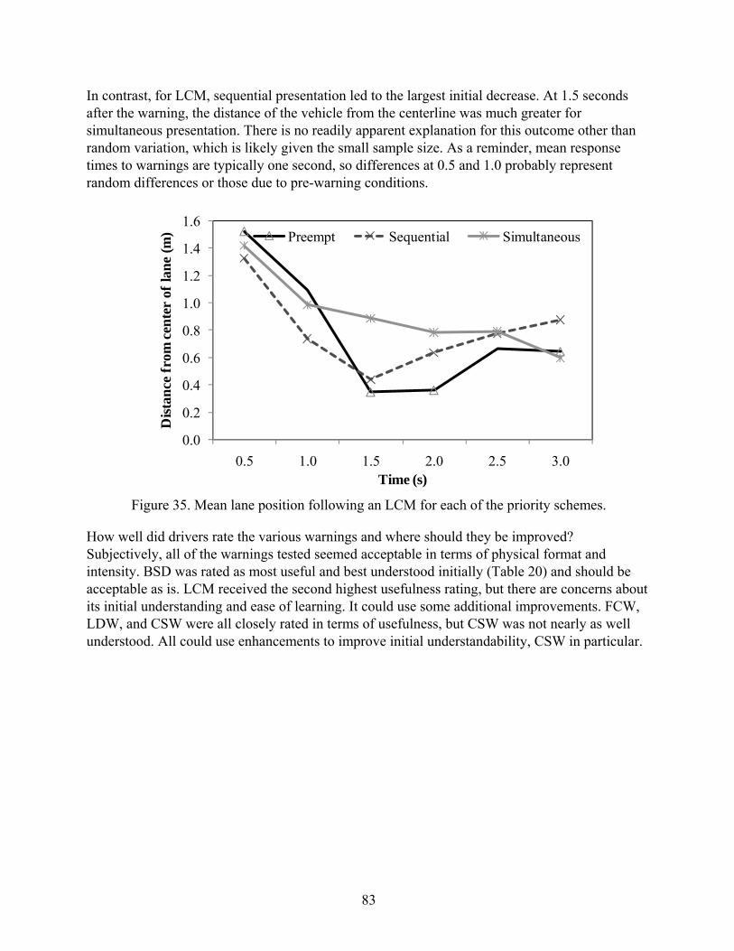
In contrast, for LCM, sequential presentation led to the largest initial decrease. At 1.5 seconds after the warning, the distance of the vehicle from the centerline was much greater for simultaneous presentation. There is no readily apparent explanation for this outcome other than random variation, which is likely given the small sample size. As a reminder, mean response times to warnings are typically one second, so differences at 0.5 and 1.0 probably represent random differences or those due to pre-warning conditions.
0.5 1.0 1.5 2.0 2.5 3.0 Time (s)
Figure 35. Mean lane position following an LCM for each of the priority schemes.
0.0
0.2
0.4
0.6
0.8
1.0
1.2
1.4
1.6
Dist
ance
from
cent
er o
f lan
e (m
) Preempt Sequential Simultaneous
How well did drivers rate the various warnings and where should they be improved? Subjectively, all of the warnings tested seemed acceptable in terms of physical format and intensity. BSD was rated as most useful and best understood initially (Table 20) and should be acceptable as is. LCM received the second highest usefulness rating, but there are concerns about its initial understanding and ease of learning. It could use some additional improvements. FCW, LDW, and CSW were all closely rated in terms of usefulness, but CSW was not nearly as well understood. All could use enhancements to improve initial understandability, CSW in particular.
83

Table 20. Experiment 5 warning ratings
Category Characteristic Warning BSD FCW LDW CSW LCM
Format Sound (soft/loud) - 3.1 3.0 2.9 3.1 Originating sound side (easy/difficult) - - - - 2.3 Vibration (weak/strong) - - 3.0 - -Originating vibration side (easy/diff.) - - 2.1 - -Brake pulse (weak/strong) - 3.2 - - -
Meaning- Initially (not well/well understood) 4.7 3.8 4.1 3.1 3.9 fulness At end (not well/well understood) - 4.5 4.5 3.9 4.4
Hard/easy to learn 4.6 4.2 4.3 3.6 3.7 Easy/hard to remember 4.8 4.2 4.2 3.5 3.6
Overall Occurred to (little/often) - 3.5 3.4 3.1 3.1 Occurred to (early/late) - 2.7 2.9 3.9 3.0 Useless/useful 4.3 3.8 3.7 3.6 3.9 Difficult/easy to use - 3.6 3.9 3.5 3.9
Blanks cells indicate characteristics not pertaining to specific warnings, e.g., there was no vibration cue for BSD.
8.4 Conclusions x No single prioritization rule can be recommended based on the data collected. The results concerning the effects of presenting warnings in close time proximity are mixed, and no single rule can be recommended. For FCW, simultaneous presentation led the greatest reductions in speed, followed by sequential presentation, followed by preemption. The maximum difference between rules, 10 mph at 3 seconds after the first warning, is practically significant. For LCM, both preceding and following warnings delayed correction of the lateral position by about 0.5 seconds. The largest differences were at 1.5 and 2.0 seconds after the first warning. In terms of best to worst performance for LCM, the priority rules were preempt, sequential, simultaneous, the opposite of that for FCW. However, for all of these situations, the data are limited and some care must be exercised in interpreting differences as being practically important. Even though there were a large number of warnings, only a limited subset involved pairs that occurred within 0.85 seconds of each other where preemption of an auditory warning was needed. x BSD should be used as is. All other warnings could use enhancements. In terms of driver ratings of warnings, BSD was rated very useful and well understood initially, and should be acceptable as is. In terms of usefulness, LCM received the second highest rating, but there are concerns about its initial understanding and ease of learning. It could use some additional improvements, but it is believed that on-road exposure to the system readily helps improve the driver’s understanding of this system. FCW, LDW, and CSW were all closely rated in terms of usefulness, but CSW was not nearly as well understood. Except for BSD, all could use enhancements, especially CSW, to improve initial understandability. It remains a challenge on how best to convey the nature of the threat to the driver and have it readily understood. The grouping of warnings by nature of the threat, either lateral or longitudinal, will minimize the need for drivers to specifically differentiate each warning. Further, it may be that other approaches (e.g., spoken audio messages) or modalities (e.g., brake pulses) should be explored, but they were outside of the scope of testing that could be performed on the current program.
84

Table 21. Stage 2 pilot testing warning suite
Forward Warning Lateral Warning
FCW CSW LCMLDW Imminent LDW Cautionary
Auditory Tone 1 (L) (R) Tone 2 -----
Haptic Brake pulse Brake pulse ----- Haptic seat L/R
Visual ----- ----- Blind zone: RedClosing zone: Yellow -----
Warning text Hazard ahead Sharp curve Left/right hazard Left/right drift
85
9 Light-Vehicle Stage 2 Pilot Test This section provides a high-level summary of the major elements of the light-vehicle stage 2 pilot testing. Please refer to Appendix J for a detailed description of this test.
9.1 Overview The overarching goal of the pilot tests was to make sure the IVBSS warnings and vehicles were ready for the subsequent field operational test. In the light-vehicle pilot test, data was collected from lay drivers accompanied by an experimenter who drove the test vehicle for two hours on a fixed route. The pilot testing was conducted to address three questions: x How well did the warning hardware and software work on the road and what should be altered? x How often did warnings actually occur? x Did drivers find the warnings easy to use and useful? How could they be improved?
9.2 Method Eighteen licensed drivers between the ages of 20 to 30, 40 to 50, and 60 to 70 were recruited through an advertisement in the local newspaper. They were each paid for one daytime, three-hour session. Participants watched a video overview of IVBSS and received detailed explanations of the IVBSS warnings. Next, before any driving commenced, subjects experienced each type of warning (both auditory and haptic components where appropriate) through a static demonstration, along with an explanation of which warnings represent what types of warning scenarios. The fixed route was 90 miles in length, took about two hours to complete, and consisted of a mix of surface streets and expressways. Several subjects drove a slightly altered route as a result of congestion along the route due to highway construction. After completing the route, each subject filled out a 15-page questionnaire, consisting mostly of seven-point, Likert-scale questions with higher numbers indicating positive attributes. Questions concerned topics such as frequency of warnings, attention-getting properties of warnings, and understandability. Table 21 lists the warnings examined. The suite includes FCW, CSW, LCM, and LDW.
9.3 Results
9.3.1 Objective Results How often did warnings actually occur? How well did the warning hardware and software work on the road and what should be changed? The 18 drivers in the pilot test accumulated 1,528 miles of driving. As shown in Table 22, a total of 379 warnings were received during the pilot test. The mean number was 21 warnings per driver, with one driver receiving only five warnings and another receiving 38 warnings. Figure 36 illustrates the breakdown of warnings by type from those tabulated in Table 22. Almost three out of four warnings received were LDW-imminent warnings (i.e., warnings associated with drifts toward or over a lane edge with the system sensing an object near or just beyond the lane edge). The intention was that during a lane drift, objects such as guardrails, concrete barriers, or adjacent-lane traffic represent significant crash threats and should be treated with salient warning displays to the driver. However, at the time of testing, IVBSS was overly-sensitive to adjacent objects such that at times tall grass growing in the freeway median would trigger an indication of a “near” threat. LDW-cautionary warnings were the next most common warning, with 98 warnings occurring (6.4 warnings per 100 miles). The stage 2 pilot route was not designed to be a perfectly representative route in terms of potential driver lane drifts. Nevertheless, it should be noted that during the road departure crash warning RDCW FOT, the rate of these types of warnings was approximately seven warnings per 100 miles. Hence, the number of this type of warning is not unreasonable, either as being overly silent (missing warnings) or overly intrusive (too sensitive). Table 22 also shows ten LCM warnings in which the system perceived the driver moving laterally toward another occupied lane with a turn signal activated. Three FCWs were received as well as five CSWs. The number of FCW and CSW events is considered potentially encouraging, based on previous field operational tests in which the number of these warnings was significantly greater. Again, the stage 2 pilot test was rather limited in its scope and exposure of IVBSS to different roadway and traffic situations.
86

Table 22. Distance traveled, warnings received, and warning rates for stage 2 pilot test
Subject Gender Age (yrs)
Travel Distance
(mi) LDW-
Warning LDW-
Cautionary
Lane-change/ merge FCW CSW All Alerts
1 Female 60 to 70 88.5 16 6 0 22 2 Female 60 to 70 108.2 29 5 4 38 3 Female 20 to 30 95.4 36 1 1 38 4 Male 60 to 70 88.5 21 12 0 33 5 Female 60 to 70 88.6 2 4 0 6 6 Female 40 to 50 69.8 4 3 0 1 8 7 Female 20 to 30 72.7 9 2 0 11 8 Male 40 to 50 83.2 19 4 0 1 24 9 Male 60 to 70 94.3 17 12 0 29 10 Female 40 to 50 72.7 13 4 0 1 18 11 Female 40 to 50 72.7 14 1 3 18 12 Male 40 to 50 88.5 15 10 1 26 13 Male 60 to 70 88.6 20 5 0 1 26 14 Male 20 to 30 76.2 7 10 1 18 15 Male 40 to 50 88.7 21 13 0 1 35 16 Male 20 to 30 88.5 6 1 0 1 2 10 17 Male 20 to 30 73.9 4 1 0 5 18 Female 20 to 30 88.6 10 4 0 14
Alerts : 263 98 10 3 5 379 Alerts/100 mi: 17.2 6.4 0.7 0.2 0.3 24.8
Curve speed threat, 5
Forw ard crash threat, 3
Lane change tow ard perceived threat, 10
Lane drift into clear lane, 98
Lane drift w ith perceived adjacent
threat, 263
Figure 36. Division of warnings from Table by warning type
Video analysis was conducted to determine the number of false warnings per 100 miles. Since there were only a few CSWs, FCWs, and LCMs, all of those alert types were analyzed. Twenty percent of the LDWs were analyzed. For CSW, FCW, and LCM, the false warning rate was 0.2
87

warnings per 100 miles. The false warning rate for LDW was 12.4 warnings per 100 miles, for a system total of 13 warnings per 100 miles. Several changes have been made to IVBSS since stage 2 pilot testing that will dramatically reduce the number of false warnings. The LCM false warning rate is estimated to be reduced by up to 50 percent by first improving the characterization of objects around the vehicle (available maneuvering room) and second by changing to a new warning algorithm that is TTC-based. It is estimated that LDW false warnings will be reduced by 50 to 75 percent from (a) taking into account road curvature for the threat assessment and (b) improved AMR characterization from the LCM subsystem. FCW has incorporated improved radar processing techniques, whereby the rejection of false targets is vastly improved. FCW false warnings for over-drive (e.g., manhole covers) and under-drive (e.g., overpasses) objects are expected to decrease by 75 percent. Lastly, the CSW subsystem incorporates a false warning management tool. A typical driver would not receive a warning for subsequent traversals of the same stretch of road. This would reduce the number of overall false warnings and improve customer satisfaction compared to other systems.
9.3.2 Subjective Results Did drivers find the warnings to be easy to use and useful? How could they be improved? Ratings were based on a seven point scale unless otherwise noted. Overall, drivers found IVBSS easy to use (mean of 6.6, SD of 0.8) and intuitive (mean of 5.2, SD of 2.7). Despite a mean of 21 warnings per driver, drivers felt that they received warnings with about the right frequency (mean of 3.6, SD of 1.4; anchors on the seven-point scale were 1 was “ too frequently” and 7 was “ too infrequently”). While three drivers strongly disagreed with the statement, “I was not distracted by the warnings,” on average drivers were not distracted by IVBSS warnings (mean of 5.1, SD of 1.6). The IVBSS warnings were deemed to be helpful in notifying drivers about potential conflicts (mean of 3.8, SD of 1.0; anchors on the five-point scale were 1 was “not helpful” and 5 was “very helpful”). The rather high false alarm rate for LDW could explain why the mean response for the statement, “I always understood why the IVBSS system was providing a warning” was 4.6 (SD of 1.8; anchors on the seven-point scale were 1 = strongly disagree and 7 = strongly agree). Although there is no standardized way to measure driver acceptance of new technologies, the van der Laan scale has been employed in several studies to assess and compare driver acceptance across technologies. The van der Laan scale is a five-point scale composed of nine opposite adjective pairs (e.g., useful-useless, irritating-likeable). Scores for each pair of adjectives range from minus 2 to plus 2 with positive numbers corresponding to positive attributes. The scores are collapsed for each driver resulting in a satisfaction score and a usefulness score. In order to determine if the total number of warnings could be used to predict driver acceptance, regression analyses were performed. The results of these analyses showed that the total number of warnings received by a driver did not reliably predict the driver’s satisfaction or usefulness score. The usefulness and satisfaction scores were then averaged across all drivers to arrive at mean ratings of driver satisfaction and usefulness of IVBSS as experienced in stage 2 pilot testing. The mean usefulness score is 1.33 and the mean satisfaction score is 0.75, both of which indicate positive feelings towards IVBSS. Figure 37 shows comparisons of the satisfaction and usefulness scores of IVBSS to those of RDCW (combined system), LDW, CSW (both from the RDCW
88
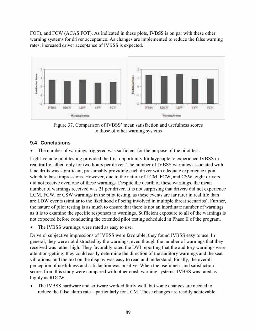
FOT), and FCW (ACAS FOT). As indicated in these plots, IVBSS is on par with these other warning systems for driver acceptance. As changes are implemented to reduce the false warning rates, increased driver acceptance of IVBSS is expected.
Figure 37. Comparison of IVBSS’ mean satisfaction and usefulness scores to those of other warning systems
9.4 Conclusions x The number of warnings triggered was sufficient for the purpose of the pilot test. Light-vehicle pilot testing provided the first opportunity for laypeople to experience IVBSS in real traffic, albeit only for two hours per driver. The number of IVBSS warnings associated with lane drifts was significant, presumably providing each driver with adequate experience upon which to base impressions. However, due to the nature of LCM, FCW, and CSW, eight drivers did not receive even one of these warnings. Despite the dearth of these warnings, the mean number of warnings received was 21 per driver. It is not surprising that drivers did not experience LCM, FCW, or CSW warnings in the pilot testing, as these events are far rarer in real life than are LDW events (similar to the likelihood of being involved in multiple threat scenarios). Further, the nature of pilot testing is as much to ensure that there is not an inordinate number of warnings as it is to examine the specific responses to warnings. Sufficient exposure to all of the warnings is not expected before conducting the extended pilot testing scheduled in Phase II of the program. x The IVBSS warnings were rated as easy to use. Drivers’ subjective impressions of IVBSS were favorable; they found IVBSS easy to use. In general, they were not distracted by the warnings, even though the number of warnings that they received was rather high. They favorably rated the DVI reporting that the auditory warnings were attention-getting; they could easily determine the direction of the auditory warnings and the seat vibrations; and the text on the display was easy to read and understand. Finally, the overall perception of usefulness and satisfaction was positive. When the usefulness and satisfaction scores from this study were compared with other crash warning systems, IVBSS was rated as highly as RDCW. x The IVBSS hardware and software worked fairly well, but some changes are needed to
reduce the false alarm rate—particularly for LCM. Those changes are readily achievable.
89

Further development of the warning algorithms should lower the false alarm rate that was experienced in the stage 2 pilot testing. While currently good, driver acceptance of IVBSS should continue to improve as these changes are implemented.
90

10 Heavy-Truck Stage 2 Pilot Test This section provides a high-level summary of the major elements of the heavy-truck stage 2 pilot testing. Please refer to Appendix K for a detailed description of this test. The overarching goal of the pilot tests was to make sure the warnings and vehicles were ready for the subsequent field operational test. The pilot testing was conducted to address three questions: x Did the warning hardware and software work on the road? x How often did warnings actually occur? x Did drivers find the warnings to be easy to use and useful? How could they be improved?
10.1 Overview The heavy-truck stage 2 pilot testing sought to gain feedback and first impressions from five commercial truck drivers operating a vehicle equipped with a developmental version of IVBSS. This evaluation was performed along a 52-mile, prescribed route with a researcher present. Objective measures of warning type and frequency were collected, as was subjective data on preliminary acceptance.
10.2 Method Five professional truck drivers (some of whom have positions within safety management) were recruited from an Ann Arbor, Michigan, terminal owned by Con-way Freight. The drivers were all male, between the ages of 48 and 57 (with a mean age of 52.4 years). Given the national demographics of truck drivers, this was determined to be a sufficiently representative sample for this level of pilot testing. The mixture of managers and drivers ensured that, as a whole, the sample was also representative in terms of driving experience, types of routes driven, and experience with in-vehicle electronic and advanced safety system operation. One vehicle was used throughout the testing: the “Bronze” truck, an International 8600 model class 8 tractor with a day cab. The tractor was also pulling a 53-foot trailer that had 9,000 pounds of ballast weight. The drivers received brief instructions on how the session would be conducted, and were shown the exterior of the truck while the researcher pointed out the IVBSS sensors. The researcher also explained the overall purpose of IVBSS and highlighted the three crash warning scenarios. The driver was given an opportunity to become oriented to the inside of the cab, and was shown both the forward and side IVBSS displays. The researcher then proceeded through a laptop demonstration of each IVBSS warning, and answered any initial questions that the driver had. The 52-mile route consisted of roughly 50 percent surface roads and 50 percent limited access freeways. The route spanned both urban and rural scenarios, and generally took 1 hour and 15 minutes to complete. Each run consisted of one driver per day. Three of these drivers participated over Thanksgiving weekend somewhat early in the morning (8 to 9:30 a.m.), while the other two participated during busier rush-hour traffic (4 to 5:30 p.m.), both before and after the holiday. As such, there was a wide range of traffic conditions. The two drivers who participated later in the day had at least part of their drive take place after dark. Finally, all traversals of the route took place during dry conditions.
91

At the completion of driving, each driver completed an extensive questionnaire and was also invited to give more open-ended feedback in an informal question and answer session that lasted 5 to 10 minutes.
10.3 Results
10.3.1 Objective Results Table 23 shows the number and type of warnings received by each driver. Where it was evident to the experimenter, the status of the warning (e.g., false, intentional) is noted. A total of 49 warnings were received by the five drivers. (This includes the lower priority FCWs; if one includes only imminent warnings, the total becomes 46). The average number was 10 warnings per driver, with one driver receiving only three warnings and another receiving 15 warnings. As far as the experimenter could tell, there was only one intentional warning. LCMs were by far the most common type of warning, comprising 61 percent of the total number of warnings. The next most common type of warning was FCW, almost all of which were caused by the same physical locations along the route: an overpass on the freeway and an exit that was blocked by construction barrels.
Table 23. Number and type of warnings received for heavy-truck stage 2 pilot testing
Warning Driver 1 Driver 2 Driver 3 Driver 4 Driver 5 Total
LDW - Left (toward unoccupied) 0 0 1 1 (Intentional) 0 2
LDW - Right (toward unoccupied) 0 0 0 0 0 0 LDW - Left (toward occupied) 0 0 0 0 1 1 LDW - Right (toward occupied) 1 1 1 1 1 5 LCM - Left 4 1 4 2 3 14 LCM - Right 3 0 4 2 7 16 FCW - 2-Second headway 0 0 1 0 1 2 FCW - 1-Second headway 0 0 0 0 1 1 FCW - Imminent 1 (False) 1 (False) 2 (False) 3 (False) 1 (False) 8
Total: 9 3 13 9 15 49
10.3.2 Subjective Results The evaluation of driver acceptance of IVBSS is based on a combination of two sources: the subjective assessments provided by drivers in a questionnaire completed at the end of the 75minute drive and more informal comments made by the drivers or observations made by the experimenter. In general, three of the five drivers had very positive overall feedback, while two had specific concerns that made them generally dislike the system. The negative comments were generally limited to the issue of false or unnecessary alerts, with one driver having a very low tolerance for false alerts (he mentioned that the system would need a zero-percent false alert rate). As far as the route was concerned, every driver thought that the route was representative of routes that they would typically drive. Most of the questions on the post-drive questionnaire employed seven-point Likert-type scales with higher numbers indicating positive attributes. Overall, drivers found IVBSS easy to use
92

(mean = 6.0, SD = 1.0), but only thought it was somewhat helpful regarding potential conflicts (mean = 3.4, SD = 0.9; anchors on the five-point scale were 1 = not helpful and 5 = very helpful). On average, drivers felt that they received warnings with about the right frequency (mean = 3.8, SD = 1.6; anchors on the seven-point scale were 1 = too frequently and 7 = too infrequently). There was general agreement with the statement “I always understood why IVBSS was providing a warning,” (mean = 4.8, SD = 1.3). While two drivers somewhat disagreed with the statement “I was not distracted by the alerts,” on average drivers were not distracted by IVBSS warnings (mean = 4.8, SD = 1.8). In terms of the look and feel of the system, the drivers generally were not distracted by the displays, although one driver commented that the side-display LEDs were too bright at night, and one driver said that he did not like the simulated horn sound as a warning, as it sounded too similar to a real horn.
10.4 Conclusions Heavy-truck pilot testing provided the first opportunity for “naive” truck drivers to experience IVBSS in real traffic. While the results of stage 2 pilot testing have yet to be thoroughly analyzed, the first impression is that, overall, the alert rates were reasonable and the driver feedback was generally positive. LCMs constituted the majority of warnings, and some false warning scenarios may have influenced some of the negative feedback that was received. More insights are bound to develop as the subjective results are compared to the objective driving data, and as the subjective results themselves are analyzed in more detail.
93

11 Conclusions
11.1 Next Steps Pending approval of Phase II of the IVBSS program, additional pilot testing for prolonged periods will be undertaken. The outcome of this testing is likely to provide driver feedback that will help to make further subtle refinements to the DVIs on both the light-vehicle and heavy-truck platforms. This is most likely to occur with the auditory warnings or visual system state messages. Repeated exposure to the auditory warnings, in particular, might alter the team’s understanding of warning characteristics considered annoying when experienced for prolonged periods in situ—particularly on the heavy-truck platform where drivers will spend several hours every day driving. However, the flexibility built into the prototype systems to allow the human factors testing to proceed in parallel with subsystem development will also readily allow for minor DVI revisions once a fleet of vehicles is built.
11.2 Conclusions and Implementation of Research Results This report covers human factors research and DVI development that was conducted in the first two years of the IVBSS program for both the light-vehicle and heavy-truck platforms. Five laboratory studies, four driving simulator studies, and two on-road pilot tests were conducted to assess a variety of driver-vehicle interface concepts related to the development of integrated warning systems, and the results described herein. The simulator studies, in particular, were conducted in such a way that the results would be applicable to either the light-vehicle or heavy-truck platforms. However, the use of some warning strategies, such as a haptic seat, is not currently being implemented in the heavy-truck platform. In fact, considerable differences are planned in the driver-vehicle interfaces of the two platforms, as discussed in Section 3 of this report. The rationale for different DVI strategies is based on the significant differences that exist between the two populations of drivers (with truck drivers having considerably more driving training, more exposure to the warning system, and longer durations in their vehicles) and the environments in which the warnings are presented (with the heavy truck being noisier and experiencing more vibration). The human factors testing and DVI efforts on the IVBSS program have contributed toward the successful development of a safe and effective means of conveying warnings to drivers via an integrated crash warning system. Several important research questions were identified early in the IVBSS program, and a combination of human factors testing and expertise went into addressing these questions. The outcome of the experimental studies, especially those pertaining to auditory warnings, will certainly assist others who undertake the task of developing DVIs for integrated crash warning systems. A few of the research findings that have contributed to the current DVIs, and are most likely to serve future system developers, include:
Perceived warning urgency was associated with high frequencies, abrupt onsets, high pitches, loudness, and increased number of pulses. Perceived warning annoyance increased with high frequencies, rapid pulses, loudness, and increasing number of pulses. Perceived warning noticeability increased with high frequencies and loudness.
94
x

x Auditory icons required substantially fewer trials to learn and resulted in substantially shorter reaction times in comparison to abstract sounds. Even very minor alterations in sound characteristics affected reaction time and the rate at which warnings were learned.
x Auditory warning durations should be less than the expected mean response time to a warning.
x Attempts to add noise and spatial enhancement improved neither the accuracy nor the speed of localizing a warning sound.
x When considering the use of pulsed warnings, response time is minimized when one uses short gaps between bursts, the fewest number of bursts, and the fewest number of beeps in a burst.
x Glances drivers made immediately after warnings differed little from glance patterns at other times, with just slightly more glances directly ahead immediately after a warning was presented.
x Differences between initial reactions to crash warnings in the simulator and subsequent reactions to the same warnings were small, and only manifested themselves, if at all, after 1 to 1.5 seconds post warning.
x No warning combination (single, dual-simple, dual-hybrid, or multiple) led to substantially better driver responses than any other combination. However, participants liked the multiple warning strategy the least for the combination of subsystems examined.
x The use of indicators in the vicinity of the exterior rearview mirrors to convey the presence of a lateral threat was effective.
x IVBSS should utilize a dual-warning approach based on subjective preferences, the weak objective benefit for a multiple warnings approach, and the analysis of the various considerations for integration into the post-production vehicles.
x The results concerning the effects of presenting warnings in close time proximity are mixed, and no single arbitration rule could be recommended.
x Subjects did not perceive the difference in warning delays ranging from 0 to 300 ms.
95
12 References AASHTO (American Association of State Highway and Transportation Officials). (2001). A
policy on geometric design of highways and streets. Washington, DC. Abe, G., & Richardson, J. (2004). The effect of alarm timing on driver behaviour: Lean
investigation of differences in driver trust and response to alarms according to alarm timing. Transportation Research Part F-Traffic Psychology and Behaviour, 7(4-5), 307-322.
Abe, G., & Richardson, J. (2005). The influence of alarm timing on braking response and driver trust in low speed driving. Safety Science, 43(9), 639-654.
Abe, G., & Richardson, J. (2006). Alarm timing, trust and driver expectation for forward collision warning systems. Applied Ergonomics, 37(5), 577-586.
Arrabito, G.R., Mondor, T.A., & Kent, K.J. (2004). Judging the urgency of non-verbal auditory alarms: a case study. Ergonomics, 47(8), 821-840.
Banbury, S., Fricker, L., Tremblay, S., & Emery, L. (2003). Using auditory streaming to reduce disruption to serial memory by extraneous auditory warnings. Journal of Experimental Psychology-Applied, 9(1), 12-22.
Belz, S.M. (1997). A simulator-based investigation of visual, auditory, and mixed-modality display of vehicle dynamic state information to commercial vehicle operators. Unpublished Master's Thesis. Blacksburg, VA: Virginia Polytechnic Institute and State University.
Belz, S.M., Robinson, G.S., & Casali, J.G. (1999). A new class of auditory warning signals for complex systems: Auditory icons. Human Factors, 41(4), 608-618.
Bliss, J.P., & Acton, S.A. (2003). Alarm mistrust in automobiles: how collision alarm reliability affects driving. Applied Ergonomics, 34(6), 499-509.
Bliss, J.P., Fallon, C.K., & Nica, N. (2007). The role of alarm signal duration as a cue for alarm validity. Applied Ergonomics, 38(2), 191-199.
Campbell, J.L., Richard, C.M., Brown, J.L., & McCallum, M. (2007). Crash warning system interfaces: human factors insights and lessons learned (Technical Report No. HS 810 697). Washington, DC: National Highway Traffic Safety Administration.
Campbell, J.L., Richman, J.B., Carney, C., & Lee, J.D. (2004). In-Vehicle Display Icons and Other Information Elements. Volume I: Guidelines (Integrative Report No. FHWA-RD-03065). McLean, VA: Office of Safety Research and Development, Federal Highway Administration
Casali, J.G. (2003). Human factors issues in auditory warning signal design including the influence of hearing protection. Paper presented at the 18th International Meeting of the Brazilian Academy of Audiology, Curitiba, Parana, Brazil. Retrieved October 22, 2007, from http://www.utp.br/eia/Casali_Brazil_ACA_Aud_HO.ppt.
Catchpole, K., McKeown, J.D., & Withington, D.J. (2004). Localizable auditory warning pulses. Ergonomics, 47(7), 748-771.
Chiang, D., Brooks, A., & Llaneras, E. (2004). Final Task Report: Investigation of Multiple Collision Alarm Interference Driving Simulator Study (Final Report No. DRI-TR-04-10). Washington, DC: National Highway Traffic Safety Administration.
Chiang, D., Llaneras, E., Foley. (2006). Driving Simulator Investigation of Multiple Collision Alarm Interference Issues presented at DSCAsia/Pacific 2006, Tsukuba, Japan, May-June 2006.
96
COMSIS Corporation. (1996). Preliminary human factors guidelines for crash avoidance warning devices (NHTSA Project No. DTNH22-91-07004). Silver Spring, MD: COMSIS.
Deatheridge, B.H. (1972). Auditory and other sensory forms of information presentation. In H.P. Van Cott and R.G. Kinkade (Eds.), Human Engineering Guide to Equipment Design. Washington, DC: Government Printing Office.
Diederich, A., & Colonius, H. (2004). Bimodal and trimodal multisensory enhancement: Effects of stimulus onset and intensity on reaction time. Perception and Psychophysics, 66(8), 13881404.
Edworthy, J., & Hards, R. (1999). Learning auditory warnings: The effects of sound type verbal labelling and imagery on the identification of alarm sounds. International Journal of Industrial Ergonomics, 24(6), 603-618.
Edworthy, J., Loxley, S., & Dennis, I. (1991). Improving Auditory Warning Design - Relationship between Warning Sound Parameters and Perceived Urgency. Human Factors, 33(2), 205-231.
Edworthy, J.,& Stanton, N. (1995). A User-Centered Approach to the Design and Evaluation of Auditory Warning Signals .1. Methodology. Ergonomics, 38(11), 2262-2280.
Edworthy, J., Stanton, N., & Hellier, E. (1995). Warnings in Research and Practice. Ergonomics, 38(11), 2145-2154.
Ervin, R.; Sayer, J.; LeBlanc, D.; Bogard, S.; Mefford, M.L.; Hagan, M.; Bareket, Z.; & Winkler, C. (2005). Automotive Collision Avoidance System (ACAS) Field Operational Test – Methodology and Results (U.S. DOT technical report HS 809 901). Washington, DC.
Federal Highway Administration. (2003). Manual on Uniform Traffic Control Devices for Streets and Highways: 2003 Edition. Washington, DC.
Graham, R. (1999). Use of auditory icons as emergency warnings: evaluation within a vehicle collision avoidance application. Ergonomics, 42(9), 1233-1248.
Guillaume, A., Drake, C., Rivenez, M., Pellieux, L., & Chastres, V. (2002). Perception of urgency and alarm design. Paper presented at the Eighth International Conference on Auditory Display, Kyoto, Japan.
Guillaume, A., Pellieux, L., Chastres, V., & Drake, C. (2003). Judging the urgency of nonvocal auditory warning signals: Perceptual and cognitive processes. Journal of Experimental Psychology-Applied, 9(3), 196-212.
Gupta, N., Bisantz, A.M., & Singh, T. (2002). The effects of adverse condition warning system characteristics on driver performance: an investigation of alarm signal type and threshold level. Behaviour and Information Technology, 21(4), 235-248.
Haas, E.C., & Casali, J.G. (1995). Perceived Urgency of and Response-Time to Multitone and Frequency-Modulated Warning Signals in Broad-Band Noise. Ergonomics, 38(11), 23132326.
Haas, E.C., & Edworthy, J. (1996). Designing urgency into auditory warnings using pitch, speed and loudness. Computing and Control Engineering Journal, 7(4), 193-198.
Hellier, E., Edworthy, J., & Dennis, I. (1993). Improving Auditory Warning Design - Quantifying and Predicting the Effects of Different Warning Parameters on Perceived Urgency. Human Factors, 35(4), 693-706.
Hellier, E., Edworthy, J., Weedon, B., Walters, K., & Adams, A. (2002). The perceived urgency of speech warnings: Semantics versus acoustics. Human Factors, 44(1), 1-17.
97

Hellier, E., & Edworthy, J. (1999). On using psychophysical techniques to achieve urgency mapping in auditory warnings. Applied Ergonomics, 30(2), 167-171.
Hick, W.E. (1952). On the rate of gain of information. Quarterly Journal of Experimental Psychology, 4, 11-26.
Ho, A.W.L., Cummings, M.L., Wang, E., Tijerina, L., & Kochhar, D.S. (2006). Integrating Intelligent Driver Warning Systems: Effects of Multiple Alarms and Distraction on Driver Performance. Paper presented at the Transportation Research Board 2006 Annual Meeting, Washington, DC.
Ho, C., Tan, H., & Spence, C. (2006). The differential effect of vibrotactile and auditory cues on visual spatial attention. Ergonomics, 49(7), 724-738.
Karlin, L. & Kestenbaum, R. (1968). Effect of number of alternatives on the psychological refractory period. Quarterly Journal of Experimental Psychology, 20, 167-178.
Kiefer, R.J., LeBlanc, D.J., & Flannagan, C.A. (2005). Developing an inverse time-to-collision crash alert timing approach based on drivers' last-second braking and steering judgments. Accident Analysis and Prevention, 37(2), 295-303.
König, W. & Mutschler, H. (2002). MMI of warning systems in vehicles. (Technical Report, Draft, Reference No. ISO/TC22/SC13/WG8). International Organization for Standardization (ISO).
LeBlanc, D., Sayer, J., Winkler, C., Bogard, S., Devonshire, J. Mefford, M., Hagan, M.L., Bareket, Z., Goodsell, R., & Gordon, T. 2006. Road Departure Crash Warning System (RDCW) Field Operational Test – Final Report (U.S. DOT report). Washington, DC.
Lee, J.D., McGehee, D.V., Brown, T.L., & Marshall, D. (2006). Effects of Adaptive Cruise Control and Alert Modality on Driver Performance. Paper presented at the Transportation Research Board 2006 Annual Meeting, Washington, DC.
Lee, J.D., Ries, M.L., McGehee, D.V., Brown, T.L., & Perel, M. (2000). Can collision warning systems mitigate distraction due to in-vehicle devices? Retrieved in 2006 from http://wwwnrd.nhtsa.dot.gov/departments/nrd-13/driver-distraction/PDF/31.PDF
Lerner, N.D., Dekker, D.K., Steinberg, G.V., & Huey, R.W. (1996). Inappropriate Alarm Rates and Driver Annoyance (Technical Report No. DOT HS 808 533). Washington, DC.: Office of Crash Avoidance Research, National Highway Traffic Safety Administration.
Lerner, N.D., Kotwal, B.M., Lyons, R.D., & Gardner-Bonneau, D.J. (1996). Preliminary Human Factors Guidelines for Crash Avoidance Warning Devices (Interim Report No. DOT HS 808 342). Washington, DC.: Office of Crash Avoidance, National Highway Traffic Safety Administration.
Maltz, M., & Shinar, D. (2004). Imperfect in-vehicle collision avoidance warning systems can aid drivers. Human Factors, 46(2), 357-366.
Marshall, D.C., Lee, J.D., & Austria, P.A. (2007). Alerts for In-Vehicle Information Systems: Annoyance, Urgency, and Appropriateness. Human Factors, 49(1), 145-157.
McGehee, D.V., Brown, T.L., Lee, J.D., & Wilson, T.B. (2002). Effect of warning timing on collision avoidance behavior in a stationary lead vehicle scenario. Human Performance: Models, Intelligent Vehicle Initiative, Traveler Advisory and Information Systems, 1803, 1-7.
Najm, W.G., Smith, J.D., & Toma, S. (2005). Crash-imminent test scenarios for integrated vehicle-based safety systems (HS22-05-01). Washington, DC.
98

Neuhoff, J. G. (2001). An adaptive bias in the perception of looming auditory motion. Ecological Psychology, 13(2), 87-110.
NHTSA. (1996). “Preliminary Assessment of Crash Avoidance Systems Benefits.” Version II, Chapter 3, NHTSA Benefits Working Group. December 1996. Washington, DC: National Highway Traffic Safety Administration.
Norman, D.A., & Bobrow, D.G. (1975). On data-limited and resource-limited processes. Cognitive Psychology, 7, 44-64.
Nowakowski, C., Friedman, D., & Green, P. (2001). Cell Phone Ring Suppression and HUD Caller ID: Effectiveness in Reducing Momentary Driver Distraction Under Varying Workload Levels (UMTRI-2001-29). Ann Arbor, MI: University of Michigan Transportation Research Institute.
Parasuraman, R., Hancock, P.A., & Olofinboba, O. (1997). Alarm effectiveness in driver-centred collision-warning systems. Ergonomics, 40(3), 390-399.
Patterson, R.D., & Mayfield, T.F. (1990). Auditory warning sounds in the work environment. Philosophical Transactions of the Royal Society of London. Series B, Biological Sciences., 327(1241), 485-492.
Pomerleau, D., & Everson, J. (1999). Run-Off-Road Collision Avoidance Using IVHS Countermeasures – Final Report (NHTSA Report DOT HS 809 170). Washington, DC: National Highway Traffic Safety Administration.
Schnupp, J.W.H., Dawe, K.L., & Pollack, G.L. (2005). The detection of multisensory stimuli in an orthogonal sensory space. Experimental Brain Research, 162(2), 181-190.
Seagull, F.J., Wickens, C.D., & Loeb, R.G. (2001). When is less more? Attention and workload in auditory, visual, and redundant patient-monitoring conditions. Paper presented at the Human Factors and Ergonomics Society 45th Annual Meeting, Minneapolis, MN.
Stanton, N.A., & Edworthy, J. (1999). Auditory warnings and displays: an overview. In N.A. Stanton and J. Edworthy (Eds.), Human factors in auditory systems. Brookfield, VT: Ashgate.
Stephan, K.L., Smith, S.E., Martin, R.L., Parker, S.P.A., & McAnally, K.I. (2006). Learning and retention of associations between auditory icons and denotative referents: Implications for the design of auditory warnings. Human Factors, 48(2), 288-299.
Talmadge, S., Chu, R., Eberhard, C., Jordan, K., & Moffa, P. (2001). Development of Performance Specifications for Collision Avoidance Systems for Lane Change Crashes (DOT HS 809 414). Washington, DC: National Highway Traffic Safety Administration.
Tan, A.K., & Lerner, N.D. (1995). Multiple Attribute Evaluation of Auditory Warning Signals for In-Vehicle Crash Avoidance Warning Systems (DOT HS 808 535). Washington, DC: National Highway Traffic Safety Administration, Office of Crash Avoidance Research.
Tan, A.K., & Lerner, N.D. (1996). Acoustic Localization of In-Vehicle Crash Avoidance Warnings as a Cue to Hazard Direction (DOT HS 808 534). Washington, DC: National Highway Traffic Safety Administration, Office of Crash Avoidance Research.
UMTRI. (2007). Integrated Vehicle-Based Safety Systems First Annual Report (DOT HS 810 842). Washington, DC: National Highway Traffic Safety Administration.
U.S. Department of Transportation, Federal Highway Administration. (2003). Manual on Uniform Traffic Control Devices for Streets and Highways: 2003 Edition. Washington, DC.
Wang, E., Ho, A. W.L., & Cummings, M.L. (2006). Integrating multiple alarms and driver situation awareness (Report No. HAL2006-03). Cambridge, MA: Massachusetts Institute of Technology.
99

Wickens, C.D., & Dixon, S.R. (2005). Is there a magic number 7 (to the minus1)?: The benefits of imperfect diagnostic automation: A synthesis of the literature (AHFD-05-01/MAAD-0501). Savoy, IL: University of Illinois, Aviation Human Factors Division.
Wiese, E., & Lee, J.D. (2004). Auditory alerts for in-vehicle information systems: The effects of temporal conflict and sound parameters on driver attitudes and performance. Ergonomics, 47(9), 965-986.
Wu, C. & Liu, Y. (2004). Modeling Psychological Refractory Period (PRP) and Practice Effect on PRP with Queuing Networks and Reinforcement Learning Algorithms, Proceedings of the 2004 International Conference on Cognitive Modeling (ICCM-2004).
Yamada, K., & Kuchar, J.K. (2006). Preliminary study of behavioral and safety effects of driver dependence on a warning system in a driving simulator. IEEE Transactions on Systems Man and Cybernetics Part a-Systems and Humans, 36(3), 602-610.
100
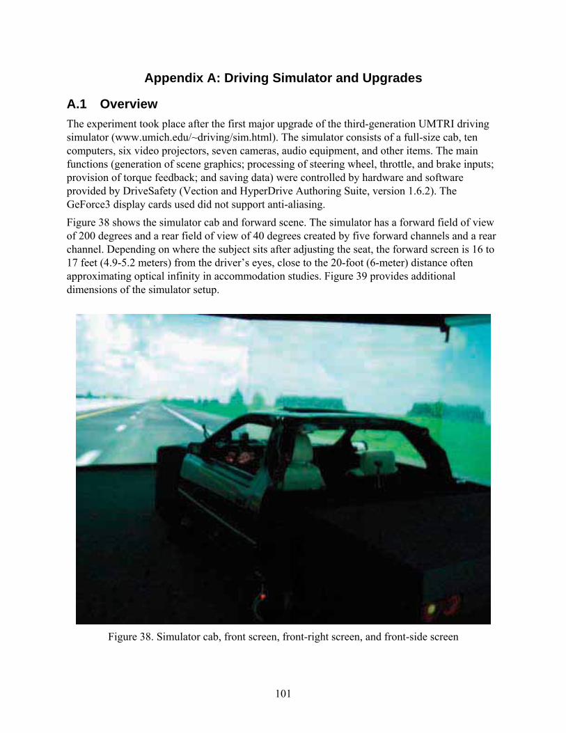
Appendix A: Driving Simulator and Upgrades
A.1 Overview The experiment took place after the first major upgrade of the third-generation UMTRI driving simulator (www.umich.edu/~driving/sim.html). The simulator consists of a full-size cab, ten computers, six video projectors, seven cameras, audio equipment, and other items. The main functions (generation of scene graphics; processing of steering wheel, throttle, and brake inputs; provision of torque feedback; and saving data) were controlled by hardware and software provided by DriveSafety (Vection and HyperDrive Authoring Suite, version 1.6.2). The GeForce3 display cards used did not support anti-aliasing. Figure 38 shows the simulator cab and forward scene. The simulator has a forward field of view of 200 degrees and a rear field of view of 40 degrees created by five forward channels and a rear channel. Depending on where the subject sits after adjusting the seat, the forward screen is 16 to 17 feet (4.9-5.2 meters) from the driver’s eyes, close to the 20-foot (6-meter) distance often approximating optical infinity in accommodation studies. Figure 39 provides additional dimensions of the simulator setup.
Figure 38. Simulator cab, front screen, front-right screen, and front-side screen
101
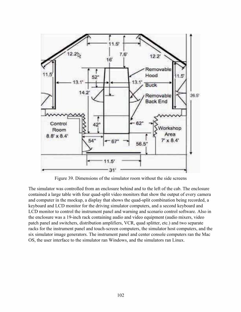
Figure 39. Dimensions of the simulator room without the side screens
The simulator was controlled from an enclosure behind and to the left of the cab. The enclosure contained a large table with four quad-split video monitors that show the output of every camera and computer in the mockup, a display that shows the quad-split combination being recorded, a keyboard and LCD monitor for the driving simulator computers, and a second keyboard and LCD monitor to control the instrument panel and warning and scenario control software. Also in the enclosure was a 19-inch rack containing audio and video equipment (audio mixers, video patch panel and switchers, distribution amplifiers, VCR, quad splitter, etc.) and two separate racks for the instrument panel and touch-screen computers, the simulator host computers, and the six simulator image generators. The instrument panel and center console computers ran the Mac OS, the user interface to the simulator ran Windows, and the simulators ran Linux.
102

Figure 40. Equipment layout in the driving simulator buck
A.2 Road Scenes Each projector (Canon Realis SX-50 for the front channel, Epson Powerlite 82c for the rear, and Epson 703c for the side and front side channels) presented XGA resolution (1024x768) images updated at 30 Hz. Simulated worlds were created using tiles (as in SimCity) that represent 200meter x 200-meter sections of a world. There are about 250 tiles in the library, including scenes from rural, urban, residential, industrial, and expressway settings. Tiles represented straight and curved sections of roads, intersections with programmable traffic signals, and expressway ramps.
103

Scenes included hills, vegetation, and signs. All roads complied with AASHTO (AASHTO, 2001) and MUTCD standards (U.S. Department of Transportation, 2001). Figure 41 shows an example of a scene used in these experiments.
Figure 41. Example of roadway scenery
A.3 Vehicle Cab The vehicle cab consisted of the A-to-B pillar section of a 1985 Chrysler Laser with a custom-made hood and back end mounted on wheels for easy access. Mounted in the mockup were: operating foot controls, a torque motor connected to the steering wheel (to provide steering force feedback), a LCD projector under the hood (to show the speedometer-tachometer cluster), a ten-speaker sound system (for auditory warnings), a haptic seat (for haptic warnings), a sub-bass sound system (to provide vertical vibration), and a five-speaker surround system (to provide simulated background road noise). The ten-speaker sound system was from a 2002 Nissan Altima and was installed in the A-pillars, lower door panels, and behind each of the two front seats. The stock amplifier (from the 2002 Nissan Altima) drove the speakers. The speedometer-tachometer display was controlled by a Macintosh computer running REALbasic and looked similar to those in an early 1990s Honda Accord. A custom-made, vibrating (haptic) seat was installed on the driver’s side in place of the stock seat. A leather seat, from a 2002 Nissan Altima, was modified with the installation of eight InSeat Solutions Relaxor CJ transducers: four in the seat pan and four in the seat back. Two
104

transducers were under the driver’s thighs (one left, one right) and one was under each of the buttocks. The seat back transducers were placed even with the lower back (one left, one right) and just below the shoulders (about three quarters of the way up the seat). Mounted in and around the cab were seven video cameras. Images included the driver’s face (viewed from outside and inside the cab), two over-the-shoulder images (showing the instrument panel), an image from the package shelf showing the instrument panel and forward scene, an image of the feet and pedals, and an image from a “floater,” a camera on a tripod that could be positioned anywhere. These images, combined with output from any of the projected images, could be recorded on videotape using a quad splitter. Figure 42 shows a close up of the cab interior. A unique feature of the simulator is the computer-generated, back-projected speedometer-tachometer cluster. Not shown in the image is a Seeing Machines faceLAB version 3 system, which consisted of two cameras mounted on top of the instrument panel, about one foot apart, and cables to a computer just outside of the control enclosure. To provide illumination for those cameras, one-inch square IR illuminators were mounted on stalks attached to the A pillar and center console.
Figure 42. View of the inside of the simulator cab
Also visible in that figure on the center console is a touch screen display used in experiment 2 for the simulated destination entry tasks. Figure 43 shows the screen as seen by the subject in that experiment. In other experiments, the screen was blank.
105

Figure 43. Simulated destination entry screen
A.4 Upgrades The upgrades necessary to complete this research had a huge impact on the project schedule, but were essential to the research. Prior to this project, the simulator had three forward channels (120-degree field of view) and one rear channel (60-degree field of view). This project involved testing lane change-merge (LCM) warning systems, which required a wider field of view because the locations from which merging vehicles would appear where not shown in the previous version of the simulator. Thus, two side channels were added by installing two 12-feet wide pull-down screens in front of the simulator bay doors on either side of the vehicle, increasing the field of view to 200 degrees. To fit in the side screens, the size of the workshop was reduced and some items in the workshop were relocated. Ideally, an additional rear channel would have been installed to reduce the size of the right rear blind spot. However, that would have required removing the workshop, which was not feasible. In fact, having a larger than normal blind spot increased subject dependence on the blind spot warning system. However, the field of view upgrade necessitated a large number of other changes. New projectors were needed and, given that the current projectors were no longer in production, the decision was to move the center and rear channel projectors to the sides (so they would match the forward side channels) and install a new higher resolution and brighter center channel projector (the most important image for the driver) and a brighter rear projector (second most important). Once reinstalled, all of the projectors were realigned and projector settings were changed to better match all images. Figure 44 shows one of the new pull-down side screens and projector installations required for the larger field of view. Figure 45 shows a sample side view (a vehicle passing the subject on the left) projected onto these side screens.
106

Figure 44. Side screen and projector installation
Figure 45. Side view displayed on side screens
Each projector needs its own image generator, but there was no space remaining in the equipment racks, so new, taller racks were purchased. Of course, all computers needed to be removed from the old racks, and remounted and reconnected in the new racks. Also, all of the equipment that was associated with the simulator (TViews, ExpandViews, power supplies, etc.) had to be removed, remounted, and reconnected. To ensure that all connections were correct, each wire had to be labeled on both ends before moving the equipment. In brief, the entire video system was rebuilt, a major upgrade. Figure 46 shows the before and after photos of the racks that contained the simulator equipment.
107

Figure 46. Before (left) and after (right) pictures of simulator racks.
As the main simulator upgrade neared completion, the University decided to install sprinklers in the UMTRI building, which required the ceiling to be removed, pipes to be run to and through the simulator bay, and the acoustic ceiling to be reinstalled. Special non-reflective sprinkler heads were installed to eliminate stray light. There were also issues with the simulator room’s new power requirements, so electrical work was also done. For experiment 2, a Seeing Machines eye fixation system was installed in the simulator as noted earlier. For experiment 3, a ButtKicker model BK-LFE shaker was mounted to the driver’s seat from behind to simulate the effects of a brake pulse on the vehicle. LEDs were also mounted just above the outside mirrors. The LEDs illuminated when a vehicle was in the simulator vehicle’s blind spot. Stepping back from the specifics, there were a number of major lessons worth communicating to others involved in simulator development.
Upgrades need to be ongoing and funds for some of them need to be accumulated from the hourly rate for simulator use.
The prior hourly rate for the simulator was set too low, so minor improvements were never made, making major changes even larger. That rate needs to include funding for continual upgrades of the simulator. Projectors will need to be replaced as resolution improves and computers will become obsolete. (Think about running a three-year-old version of Windows.) Funding is also needed for personnel to do the work and for management oversight. At UMTRI, this is assumed to be three to four months every few years of each key staff person. These
108
x

upgrades are distinct from the significant upgrade made during this project. However, that upgrade would have proceeded more swiftly had other minor improvements occurred previously. All of this may lead to high hourly rates, potentially discouraging simulator use. However, the cost of the simulator needs to include all costs.
x Major structural, electrical, plumbing, or other problems invariably occur during major upgrades. The actual completion duration is about double the planned duration.
One would have never thought that the major delay in upgrading a simulator was due to plumbing, but in this case, the University mandated installation of a sprinkler system at UMTRI led to removal and replacement of the ceiling and lack of access to the space for electrical work. x Assume cabling (power and data) will grow by 200-300 percent during the life of a
simulator. During initial development 50 percent was assumed, so addition conduit and wireways were needed, which would have been much easier to install when the simulator was first built. x To aid in maintenance and upgrades of computer, video, and audio systems, aisles are needed
both in front of and behind equipment racks. When the UMTRI driving simulator was first designed, additional space was requested. However, the UMTRI administration was not willing to provide the funds for moving a wall, so the control room was jammed into a small space. Every organization has “space wars,” but simulators need large screen to driver distances, and space for a workshop, control room, storage, and staff office space. Getting adequate space can be as difficult as getting capital funding for the initial effort. To do it right, at least a 40-foot by 40-foot space is needed. x One cannot predict how big of a problem motion discomfort will be in advance. The upgrades to the UMTRI simulator were needed to research on VII (Vehicle Infrastructure Integration), merging, and driving though intersections could be conducted, all current topics. UMTRI’s previous version of the simulator had a 120-degree forward field of view and the upgrade was not expected to have increased motion discomfort very much. In fact, the upgrade made it very difficult to test older subjects, and middle-aged drivers were used instead. x Research and the development of simple methods to reduce motion discomfort are needed. The quality of the visual aspects of driving simulators is improving, but if those improvements lead to simulators that are not useable by some of the most vulnerable drivers, older drivers, then they may be excluded from future studies, an undesired consequence.
109

Appendix B: Scenario Details
B.1 Introduction To develop the IVBSS scenarios, analysts developed possible triggering events that could induce drivers to perform the required maneuvers. In order to elicit enough warnings to provide data for statistical analysis, the rate of triggering events needed to be much higher than in normal driving. Analysts considered the scenario selection process described in the automotive collision avoidance system (ACAS) report (Ervin, Sayer, LeBlanc, Bogard, Mefford, Hagan, Bareket, and Winkler, 2005), which identified scenarios on the basis of video data of real driving situations. Although appropriate for ACAS, that approach would lead to too few triggering events in the simulator studies. The crash frequency data of Najm, Smith, and Toma (2005) were also considered, but mimicking the true frequency of warnings was not the goal of these experiments. As a reminder, four warning subsystems were examined, LDW (lane departure warning; when a vehicle leaves its lane), FCW (forward collision warning; when the distance to the forward vehicle is small enough to potentially collide with it), LCM (lane change-merge; when a vehicle may collide with a vehicle in an adjacent lane), and CSW (curve speed warning; approaching a curve too fast). Scenarios were designed to make it difficult for drivers to predict which maneuver by which vehicle would trigger a warning. In the archetypal crash warning studies, subjects follow a leading vehicle and the only significant event is the lead vehicle unexpectedly braking. After the first event, subjects focus their attention on the lead vehicle, waiting for it to brake again. In the IVBSS studies, the lead vehicle could unexpectedly brake, vehicles could cut in from an adjacent lane, a wind gust could blow the subject vehicle out of the lane, etc. Furthermore, some events were not tied to a particular lane. If the subject was in the left lane, a cut in could come from the right, or vice versa. The plan was for cut-ins to occur equally often from each direction. In addition, for some warnings, multiple scenarios were used to trigger the same warning so that subjects would not associate (and focus on) a single vehicle or vehicle maneuver with a particular warning. For example, FCW could be triggered by a lead vehicle braking, cut-ins, and by other means. All of this occurred with vehicle speeds, braking rates, etc. that are appropriate for real vehicles. To achieve this, the lead and adjacent vehicles had to do a considerable amount of positioning before each scenario to closely mimic real driving situations and make the triggering event, triggering vehicle, etc. less predictable. A lead vehicle and an adjacent vehicle were present for the duration of each experiment. The lead vehicle maintained a lead heading (back bumper of lead vehicle to front bumper of subject vehicle) of 35 to 40 meters from the subject vehicle at all times unless programmed to do otherwise. The adjacent vehicle maintained a side heading (midpoint of subject vehicle to midpoint of adjacent vehicle) of 10 to 20 meters at all times unless programmed to do otherwise. Each warning scenario had a true warning and a false alarm case. The true warning case was designed to cause an actual triggering event where a threat was present and the warning sounded. In the false alarm case, the lead and adjacent vehicles moved out of their normal positions as
110

though to set up a true warning scenario, but in such a way that there was no threat, and a false alarm warning was presented anyway. Eight scenarios were examined. Four triggered FCWs (lead vehicle suddenly brakes, lead vehicle suddenly brakes after lane change, lead vehicle changes lanes to reveal a parked vehicle, or vehicle in an adjacent lane cuts in). Two triggered LCMs (subject changes lanes with vehicle in blind spot or subject changes lanes and vehicle accelerates into blind spot). LDW was designed to be triggered by a wind gust, but could be triggered by a normal drift or the subject changing lanes without signaling. CSW was triggered when a curve was approached too quickly.
Table 24 shows the combinations of warnings that could be triggered nearly simultaneously to create multiple warning sequences. For example, when a lead vehicle braked (as in FCW scenario 1), a simultaneous wind gust would trigger an LDW. To avoid making this table too complex, detail about which scenarios and scenario combinations had false alarms are presented in later appendices for each specific experiment (Appendices F, G, H, and I).
111

Table 24. Single and multiple warning scenarios
112

B.2 FCW Scenarios As long as subjects followed driving guidelines (drive at 70 mph, do not change lanes unless forced, etc.), forward collision warning (FCW) triggering events were easiest to develop as they were caused almost entirely by lead vehicle action and did not require the subject to perform specific maneuvers. Scenario 1-FCW: Lead vehicle (L) suddenly decelerates. Step 1. Subject vehicle (S) follows lead vehicle (L) traveling at about 70 mph. Adjacent vehicle
(A) blocks subject from changing lanes.
Step 2. Lead vehicle suddenly decelerates. Adjacent vehicle still blocks subject from changing lanes.
Step 3. Triggering Event: Lead triggers FCW.
F S L
A
=
=
FCW
Step 4. Subject decelerates to avoid a collision while adjacent vehicle blocks subject from changing lanes. The lead vehicle accelerates to 70 mph after a short distance.
113

Scenario 3-FCW: Subject changes lanes due to construction zone and lead suddenly decelerates to trigger FCW. Step 1: Lead vehicle changes lanes and falls back to block subject from lane change. As all
vehicles approach cones, adjacent vehicle is behind subject’s blind spot.
Step 2. Lead vehicle accelerates just before cones, increasing A-L heading to allow subject to change lanes.
Step 3. Subject begins to change lanes.
Step 4. Triggering Event: Lead suddenly decelerates at .5 g to trigger FCW.
False Alarm: Subject safely merges into traffic, no FCW triggering event, but alarm is set off anyway to create false alarm.
114

Scenario 4-FCW: Reveal. Step 1. Subject follows lead vehicle as normal. Reveal vehicle (R) is stopped ahead of lead.
Step 2. As lead and subject approach reveal vehicle, lead vehicle changes lanes very close to reveal vehicle.
Step 3. Lead accelerates and completes lane change to show stopped reveal vehicle.
Step 4. Triggering Event: Reveal vehicle triggers FCW.
Step 5. Subject must change lanes to avoid collision with reveal vehicle.
False Alarm: Lead vehicle changes lanes earlier, leaving subject enough time to change lanes before triggering an FCW; true FCW is possible, but less likely in this situation.
115

Scenario 5-FCW: Cut in. Step 1. Lead vehicle accelerates to increase L-S headway. Adjacent vehicle pulls slightly ahead of
subject as though subject is in the adjacent vehicle’s blind spot.
Step 2. Triggering Event: Adjacent vehicle swerves into subject lane to trigger FCW.
False Alarm: Adjacent swerves farther ahead, out of FCW range.
116

B.3 LCM Scenarios Lange change-merge (LCM) triggering events were difficult to induce because to trigger the alarm, subjects had to be induced to perform dangerous lane changes. Scenario 6-LCM: Subject changes lanes with adjacent vehicle in blind spot. Step 1. Subject follows lead vehicle as normal, lead changes lanes well before stopped reveal
vehicle, and adjacent vehicle blocks subject vehicle from changing lanes.
Step 2. Triggering Event: Subject attempts lane change with adjacent vehicle in blind spot, triggering LCM.
Step 3. Adjacent vehicle decelerates to allow subject vehicle to change lanes in front of it.
False Alarm: Adjacent vehicle falls well behind subject’s blind spot, and subject changes lanes earlier to avoid reveal vehicle.
117

Scenario 7-LCM: Subject changes lanes due to construction zone, and adjacent vehicle suddenly accelerates into blind spot to trigger LCM. (Steps 1-3 are the same as in Scenario 3FCW.)
Step 1. Lead vehicle changes lanes and falls back to block subject from lane change. As all vehicles approach cones, adjacent vehicle is behind subject’s blind spot.
Step 2. Lead accelerates just before cones, increasing A-L heading to allow subject to change lanes.
Step 3. Subject begins to change lanes.
Step 4. Triggering Event: Adjacent vehicle accelerates into subject’s blind spot to trigger LCM warning.
False Alarm: Adjacent vehicle provides enough room for earlier lane change, and subject merges safely into traffic.
118

B.4 LDW Scenarios Although lateral drift warning (LDW) triggering events were not difficult to induce, they were difficult to control because they depend entirely upon driver action. Lane departures naturally occur quite frequently in the simulator, despite driver attention to speed and lane position, due to sensitive steering controls and sharp corners. However, to ensure that subjects would trigger enough LDWs, wind gusts were used to encourage unintentional lane departures. When the wind gust was presented, the subject’s vehicle veered from the lane being driven and the subject felt the torque imposed on the steering wheel. There was no associated sound (as in real vehicle, one cannot usually hear a wind gust). The first time a gust occurred, about half of the subjects asked what it was, a quarter specifically asked if it was wind, and the remaining quarter made no remarks.
Scenario 8-LDW: Subject drifts out of lane due to wind gust. Step 1. Triggering Event: Sudden crosswinds cause subject to drift from lane
False Alarm: Alarm is presented even though no lane drift occurred.
B.5 CSW Scenarios Curve speed warning (CSW) triggering events were nearly impossible to induce due to difficulty sensing speed in simulator.
10-CSW: Subject approaches curve with excessive speed. Step 1: Triggering Event: Subject crossed threshold with speed greater than 73 mph, triggering
CSW.
SF
A
=
=
CSW L
False Alarm: Speed threshold is reduced to 45 mph, so a subject driving with speed greater than 45 mph would trigger false CSW.
119

B.6 Multiple Warning Scenarios The following scenarios were created so that two different alarms would be triggered nearly simultaneously. Multiple warning scenarios involving CSW were not considered because of programming constraints, but all other combinations were evaluated. The multiple warning scenarios were created such that each set of alarm triggers would occur twice, so that each alarm could occur first. For example, in 7-LCM + 1-FCW, LCM is followed by FCW, where in 4-FCW + 6-LCM, the order is reversed. The LCM-FCW combination was the only case where two different FCW and two different LCM scenarios were needed to switch the alarm order; for other warning combinations, scenarios could be easily reversed with only slight manipulations.
B.6.1 FCW and LCM Scenario 7-LCM + 1-FCW: Subject changes lanes due to construction zone and triggers LCM, then lead vehicle suddenly decelerates to trigger FCW. Triggering Event 1: As subject is changing lanes, adjacent vehicle accelerates into blind
spot to trigger LCM.
Triggering Event 2: Nearly simultaneously, lead suddenly decelerates at 0.5 g to trigger FCW.
Scenario 4-FCW + 6-LCM: Reveal and adjacent vehicle accelerates into blind spot. Triggering Event 1: Lead vehicle completes lane change to show stopped reveal vehicle
to trigger FCW.
Triggering Event 2: As subject changes lanes to avoid reveal vehicle, adjacent vehicle accelerates into subject’s blind spot to trigger LCM.
120

B.6.2 LCM and LDW Scenario 6-LCM + 8-LDW: Adjacent vehicle accelerates into blind spot and cross winds cause lane drift. (Scenario order switched to achieve 8-LDW + 6-LCM.)
Triggering Event 1: As subject changes lanes to avoid reveal vehicle, adjacent vehicle accelerates into blind spot to trigger LCM.
Triggering Event 2: As subject changes lanes, cross winds blow to trigger LDW.
B.6.3 FCW and LDW Scenario 1-FCW + 8-LDW: Lead suddenly decelerates and cross winds cause lane drift. (Scenario order switched to achieve 8-LDW + 1-FCW.) Triggering Event 1: Lead suddenly decelerates to trigger FCW.
Triggering Event 2: Nearly simultaneously, cross winds blow to trigger LDW.
121

Appendix C: Prototyping Tools
C.1 Scenario Development Tool In order to run multiple experiments quickly, a single world with very flexible programming needed to be developed so that it was possible to quickly test and change scenarios and their parameters. Researchers needed control over the vehicles around the subjects and some warning parameters. They wrote a tool in REALbasic that would communicate with the driving simulator over TCP/IP and allow controlling the simulator scenarios and warnings in real time. During the initial planning stages, this ability was essential to finding the right distances, speeds, and timing of each of the scenarios used in the experiments. Code for the simulator was written so that shortly before the beginning of a trial, a message would be sent to the scenario tool to trigger the tool to send the settings for the next trial. The settings for the simulated vehicles included minimum and maximum headway, driving actions (change speed, switch lanes, cut into the subject’s lane, or some combination of those actions), speed control (both starting speed and the speed to change to if given that action), and control over when in the trial the vehicles were to begin their maneuvers. There were also controls for a reveal vehicle that would control where it was placed in the roadway during the reveal scenarios. The settings for wind strength, wind length, and false alarms were also sent from the scenario tool. The scenario control tool controlled almost all changeable aspects of each scenario. The ability to import a tab-delimited text file was added to control the experiments. The settings could then be standardized for all scenarios across all subjects. This also eliminated the need for the experimenter to change settings manually while running subjects, to ensure that no mistakes were made. At program startup, the TCP/IP socket displayed a message indicating connection status, which provided an easy check to ensure that the system was working properly. Any information that was sent over TCP/IP was also logged in a text box, which allowed for much easier troubleshooting and debugging. Figure 47 shows the interface for the tool.
122

Figure 47. Scenario development tool interface
123

C.2 Warning Interface Prototyping Tool In order to properly control the different systems necessary to create the different types of warnings (haptic seat, directional sound, or warning lights on the side mirrors), a tool was created to centrally control all warnings. This tool was connected to the driving simulator over a TCP/IP connection. Whenever the simulator conditions called for a warning, a signal was sent to the warning prototype tool. Each experiment needed its own suite of warnings. Some experiments used multiple different sounds or haptic patterns, and some did not use the blind spot detection system. The tool allowed the experimenter to select which suite was used, and the suites were automatically programmed with the correct settings. The experimenter was allowed to set the volume (each sound was set to 70 dB), the delay, the number of repetitions of a sound, and the pattern that was used for the haptic seat. All of these options were set for each suite so that the experimenter could easily switch among them and to maintain consistency throughout each experiment. This tool was also very helpful in the early stages of planning. It allowed experimenters to hear exactly what the warnings sounded like, with the speakers that were used in the light vehicles, to narrow down the sounds to use in the experiments. The warning prototype tool also communicated over TCP/IP with two other programs that controlled the haptic seat and the blind spot detection system’s lights. At startup of this program, each of the three TCP/IP sockets showed a message indicating connection status, which provided an easy check to ensure that the system was working properly. Any information (such as commands to activate warnings) that was sent over TCP/IP was also logged in a text box. This allowed for much easier troubleshooting and debugging. Figure 48 shows the interface for the tool.
124
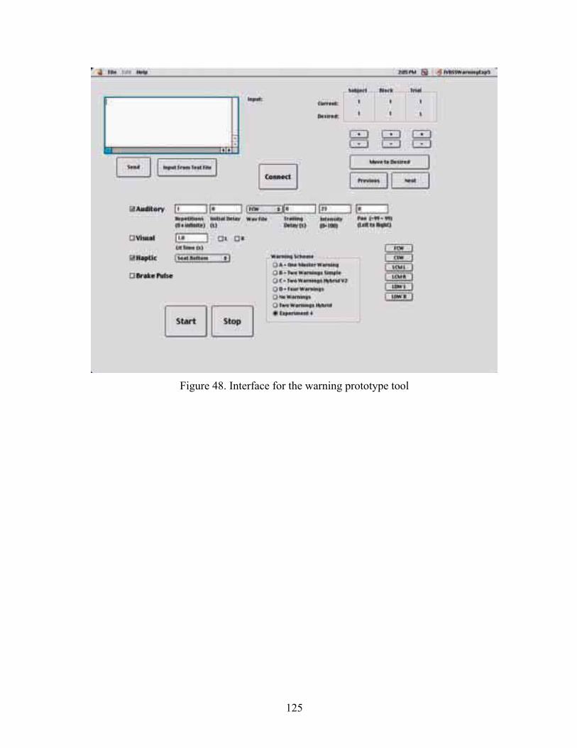
Figure 48. Interface for the warning prototype tool
125

126
Collision Warning Design GuidelinesStudy Topic NotesCampbell,Richard,B rown,and McCallum,2007; Campbell,Richman, Carney,and Lee, 2004
Human factorsguidelines for collisionavoidance system
Comprehensive review of human factors guidelines in the design of collision warnings. This work updates theCOMSYS Corporation report.
Lerner,K otwal,Lyons, andGardner-Bonneau,1996
Human factorsguidelines for crashavoidance devices
General reference on all aspects of crash avoidance systems. Authors often referred to as COMSYS Corporation.Although the guideline is more than ten years old, several concepts first described in this report have establishedthe general framework of crash-avoidance systems. General guidelines are presented in which the differencebetween an imminent warning and cautionary warning is first articulated, along with general issues coveringwarning presentation and system operation. Specific warning applications are then discussed (e.g., blind spotdetection, backup warning, driver alertness monitoring, and headway warning).
Warning TimingStudy Topic NotesAbe andRichardson,2004
Alarm timing Simulator study of forward-collision warning.Relates alarm timing to driver trust. Reports that for imminent collisions, response and trust for early timing isbetter than for late timing. The timing of the warnings occurred at 0.05 seconds (early),0 .64 seconds (middle),and 0.99 seconds (late) after the lead vehicle braking.
Abe andRichardson,2005
Alarm timing(early,l ate, none)
Simulator study of forward collision warning.Relates alarm timing to low-speed (30 mph) imminent collisions. Trust is diminished in the late timing ofwarnings when forward vehicle speed is rapidly reduced.
Abe andRichardson,2006
Alarm timing Simulator study of forward collision warning.Examined FCW timing under three driving speeds (40, 60, and 70 mph) and two headway conditions (1.7 and2.2 sec seconds). Alarm promptness affected trust more than braking performance.
Kiefer, LeBlanc,and Flannagan,2005
Developed an inversetime-to-collision modelof warning timing
Test track study of forward-collision warnings.A model of the timing of a forward-collision warning was developed based on inverse time to collision (TTC).The model assumes that driver deceleration response to a crash alert is based on an inverse TTC threshold thatdecreases linearly with driver’s speed.
Appendix D : Liter at ure Revi ew
Table 25 shows all the studies used for the literature review portion of this study. The literature review is summarized in the section Prior Warning Studies and What Do They Say About How Drivers Should Be Warned? on page 10.
Table 25. Literature review summary

127
Warning TimingStudy Topic NotesLee, Ries,McGehee, Brown,and Perel,2 000
Timing of warningdelivery
Simulator study of forward-collision warning (rear-end collision avoidance).Results suggest that early warnings help drivers react more quickly and avoid more collisions, compared to latewarnings or no warnings.Other results demonstrate benefits of warning system even when drivers are not distracted.
McGehee, Brown,Lee, and Wilson,2002
Effects of timing offorward-collisionwarnings on driverperformance
Simulator study of forward-collision warning.Examined forward-collision warning times using two versions of a driver response model that assumed short(1.0-second) versus long (1.5-second) driver reaction time. Drivers reaction times to release the accelerator weresubstantially shorter, and they crashed less often and less severely when warned earlier rather than later.
Wiese and Lee,2004
Effect of temporalconflicts in warnings
Simulator study of forward-collision warning.Found that the temporal conflict of an e-mail alert occurring 300 ms before a collision warning interfered withthe response to the collision warning, but an e-mail alert occurring 1,000 ms before the collision warning had theopposite effect and enhanced the response to the collision warning.
Warning ReliabilityStudy Topic NotesBliss and Acton,2003; Bliss,Fallon, and Nica,2007
Warning systemreliability;spatial cues
Simulator study of rear-end collisions from approaching vehicles.Examined reliability of alarms that were 50, 75, or 100 percent accurate (with respect to false-alarm rate).Response frequency to alarms declined with decreasing reliability. No rigorous test of the effect of spatial cueson alarm response was done, although the authors report better performance with spatial cues.
Bliss et al.,2007 Effect of signalduration on perceivedreliability of a warningin which reliability isvaried
Gauge-monitoring performance with presented warnings.Found that the duration of a warning can modulate its perceived reliability. A “short” alarm can be perceived asless reliable.
Lerner, Dekker,Steinberg, andHuey,1996
Acceptance ofinappropriate warnings
Naturalistic driving in subject’s vehicle.Subjective annoyance towards inappropriate alarms was measured as a function of rate of occurrence and type ofsignal generated (voice or tone). Four rates of inappropriate alarm were investigated: four per hour, one per hour,one per four hours, and one per eight hours. Subjects made daily and weekly ratings. The two most annoyingconditions reported were the four-per-hour tone, and the one-per-hour voice conditions. (There was only onevoice condition—one per hour voice.)
Parasuraman,Hancock, andOlofinboba, 1997
Theoreticalimplications ofwarnings for low-probabilitye vents
Statement of the practical constraints involved in designing warnings for low-probability events.The report illustrates that even for sensors capable of correctly detecting an imminent collision situation 99percent of the time (issuing false alarms only 1 percent of the time), if the apriori probability of the crash eventis very small, the posterior probability that a warning is a true alarm becomes vanishingly small.

128
Warning ReliabilityStudy Topic NotesYamada andKuchar, 2006
Warning reliability Mean driving speed decreased as the missed detection rate increased, demonstrating a decrease in drivers’reliance on warnings when the system was less effective in detecting threats. Both acceleration-pedal and brake-pedal reaction times increased as the PPV of the warning system decreased, demonstrating a decrease in drivercompliance with warnings when the system became more prone to false alarms. A key implication is thatperformance is not necessarily directly correlated to warning system quality or trends in subjective ratings,highlighting the importance of objective evaluation. Practical applications of the work include design andanalysis of in-vehicle warning systems.
Multi-Collision WarningsStudy Topic NotesChiang, Brooks, andLlaneras, 2004
Performance withsingle forward CWS,master warning withmultiple CWSs, andmulti-warnings formulti-CWSs
Driving simulator study.Highlights the advantage of multiple warnings for a case of two warning systems occurring simultaneously.Found that drivers were not confused by multiple warning systems that produce separate warnings. They lookedin the direction of the threat more often than drivers with a master warning, were sometimes able to avoidcollision, and realized that the second warning was distinct from the first.
Gupta, Bisantz, andSingh, 2002
Warningcharacteristics in thecontext of the warnedcondition
Simulator study of detection of adverse road conditions (loss of road traction).Found that driver response to an adverse road condition was affected by the alarm sensitivity and the type ofalarm—on or off versus graded. Participants had fewer skids with the low sensitivity and graded warnings. Trustwas lower for the high (versus low) sensitivity condition. (In the high-sensitivity condition, alarm activationoccurred moref requently.)
Ho, Cummings,Wang, Tijerina, andKochhar, 2006
Driver performancewith a mastercollision warning tomultiple individualalerts
Simulator study of multiple collision warnings.No difference was found between the master collision warning and individual alerts for either reaction time orresponse accuracy. Drivers preferred multiple warnings.Low system reliability produced diminished accuracy performance.Reliability was also manipulated in the study.
Wang, Ho, andCummings, 2006
Integration ofmultiple warnings(forward collision,rear collision, lateraldrift warning)
Driving simulator studyFound no significant difference in driver performance regardless of alarm altering schemes (single versusmultiple alarms). Young participants( 26±5 years) had overwhelming preference for distinct alarms even thoughperformance indicates no difference. When many false alarms were present in the systems, accuracy of initialresponses dropped significantly (about 40%).
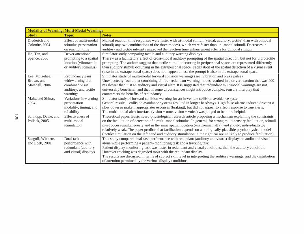
Modality of Warning; Multi-Modal WarningsStudy Topic NotesDiederich andColonius,2004
Effect of multi-modalstimulus presentationon reaction time
Manual reaction time responses were faster with tri-modal stimuli (visual, auditory, tactile) than with bimodalstimuli( any two combinations of the three modes), which were faster than uni-modal stimuli. Decreases inauditory and tactile intensity improved the reaction time enhancement effects for bimodal stimuli.
Ho, Tan, andSpence, 2006
Driver attentionalprompting to a spatiallocation (vibrotactileor auditory stimulus)
Simulator study comparing tactile and auditory warning displays.Therew as a facilitatory effect of cross-modal auditory prompting of the spatial direction, but not for vibrotactileprompting. The authors suggest that tactile stimuli, occurring in peripersonal space, are represented differentlythan auditory stimuli occurring in the extrapersonal space. Facilitation of the spatial detection of a visual event(also in the extrapersonal space) does not happen unless the prompt is also in the extrapersonal space.
Lee, McGehee,Brown, andMarshall, 2006
Redundancy gainwithw arning thatcombined visual,auditory, and tactilewarnings
Simulator study of multi-modal forward collision warnings (seat vibration and brake pulse).Unexpectedly found that combining all four redundant warning modes resulted in a driver reaction that was 400ms slower than just an auditory and visual alert. It is suggested that redundant multimodal warnings are notuniversally beneficial, and that in some circumstances might introduce complex sensory interplay thatcounteracts the benefits of redundancy.
Maltz and Shinar,2004
Variations inw arningpresentationmodality, timing, andreliability
Simulator study of forward collision warning for an in-vehicle collision avoidance system.General results—collision avoidance systems resulted in longer headways. High false-alarms induced driverst oslow down or make inappropriater esponses (braking), but did not appear to affect response to true alerts.The multi-modal alert interface (vision + tone, vision + voice) was judged to be more helpful.
Schnupp, Dawe, andPollack, 2005
Effectiveness ofmulti-modalstimulation
Theoretical paper. Basic neuro-physiological research article proposing a mechanism explaining the constraintson the facilitation of detection of a multi-modal stimulus. In general, for strong multi-sensory facilitation, stimulimust occur simultaneously and in the same spatial location (environmentally), and should, individually,berelatively weak. The paper predicts that facilitation depends on a biologically plausible psychophysical model(tactiles timulation on the left hand and auditory stimulation in the right ear are unlikely to produce facilitation).
Seagull, Wickens,and Loeb, 2001
Dual-taskperformance withredundant (auditoryand visual) displays
This study compared dual-task performance with redundant (auditory and visual) displays to audio and visualalone while performing a patient- monitoring task and a tracking task.Patient display-monitoring task was faster in redundant and visual conditions, than the auditory condition.However tracking was degraded most with the redundant display.The results are discussed in terms of subject skill level in interpreting the auditory warnings, and the distributionof attention permitted by the various display conditions.
129

130
Auditory Warnings: UrgencyStudy Topic NotesArrabito,M ondor,and Kent,20 04
Urgency of auditoryalarms
Investigated sounds used in helicopter cockpit.Found evidence that rated urgency of condition may be based on perceived urgency of alarm’s acoustic properties.
Edworthy, Loxley,and Dennis, 1991
Acoustic propertiesaffecting perceivedurgency
Perceived urgency was increased by several acoustic factors: high pitch (530 Hz >1 50 Hz; 350 Hz > 200 Hz),pulse envelop (20 ms onset and offset > slow—150 ms—onset and offset),i rregular harmonics > regularharmonics, fast pulse speed > moderate >low, regular rhythm > syncopated, 4 pulses >2 > 1, tempo change:speed > regular > slowing, pitch range: large > small, pitch contour: random > down/up; musical structure:atonal > unresolved > tonal.
Banbury, Fricker,Tremblay, andEmery, 2003
Reduction of auditoryinterference by usingstreaming
Used spatial streaming to reduce the disruptive effects of auditory interference on a serial memory task.Auditory warnings were found to disrupt performance of a simple short-term memory task. When the warningsare streamed by manipulation of spatial location and timing, interference can be attenuated.
Guillaume,Pellieux, Chastres,and Drake, 2003
Acoustic propertiesaffecting perceivedurgency
Incorporated a multidimensional approach in which subjects were asked to make dissimilarity and urgencyjudgmentsf or stimuli designed by Edworthy, Loxley, and Dennis (1991). Results support earlier work relatingacousticp roperties to urgency with the additional observation that when the acoustic characteristics resemble asound associated with a high or low urgency condition (e.g., French police siren or a bicycle bell), the urgency ofthe situation evoked by the sound may overshadow the predicted effects of the sound’s acoustic attributes.
Haas and Casali,1995
Perceived urgencyrelated to responsetime; acousticproperties related toperceived urgency
Abstract rating task.Investigated the following sound attributes: pulse format:( sequential,s imultaneous,a nd frequency modulated),pulse level, and inter-pulse interval (0, 150, and 300 ms). Sequential signals were rated as less urgent; as pulselevel increased, rated urgency increased. Short inter-pulse intervals were associated with greater perceivedurgency.
Haas andEdworthy, 1996
Acoustic propertiesrelated to perceivedurgency
Abstract ratings of sounds.Investigated the relationship of the following sound attributes on perceived urgency: pitch: high frequencyincreased urgency; loudness: increased loudness increased urgency; high speed increased urgency. Increases inallt hree parameters produced increases in perceived urgency ratings individually, and increases in pitch andloudness decreased response time.
Hellier andEdworthy, 1999;Hellier, Edworthy,and Dennis, 1993
Related acousticproperties to perceivedurgency using Stevenspower law
Abstract ratings of sounds.Applied a psychophysical model to map sound properties to urgency in order to determine the relative strengthof the contribution of each property to the perception of urgency.The influence of five sound parameters on perceived urgency was investigated, and a power function wasderived for each. Changes in speed, pitch, repetitions, and harmonicity were found to affect perceived urgency.With pulse speed appearing to have the strongest effect on urgency.
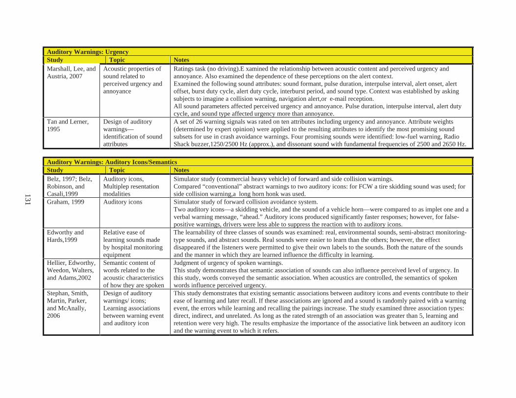
Auditory Warnings: UrgencyStudy Topic NotesMarshall, Lee, andAustria, 2007
Acoustic properties ofsound related toperceived urgency andannoyance
Ratings task (no driving).E xamined the relationship between acoustic content and perceived urgency andannoyance. Also examined the dependence of these perceptions on the alert context.Examined the following sound attributes: sound formant, pulse duration, interpulse interval, alert onset, alertoffset, burst duty cycle, alert duty cycle, interburst period, and sound type. Context was established by askingsubjects to imagine a collision warning, navigation alert,or e-mail reception.All sound parameters affected perceived urgency and annoyance. Pulse duration, interpulse interval, alert dutycycle, and sound type affected urgency more than annoyance.
Tan and Lerner,1995
Design of auditorywarnings—identification of soundattributes
A set of 26 warning signals was rated on ten attributes including urgency and annoyance. Attribute weights(determined by expert opinion) were applied to the resulting attributes to identify the most promising soundsubsets for use in crash avoidance warnings. Four promising sounds were identified: low-fuel warning, RadioShack buzzer,1250/2500 Hz (approx.), and dissonant sound with fundamental frequencies of 2500 and 2650 Hz.
131
Auditory Warnings: Auditory Icons/SemanticsStudy Topic NotesBelz, 1997; Belz,Robinson, andCasali,1999
Auditory icons,Multiplep resentationmodalities
Simulator study (commercial heavy vehicle) of forward and side collision warnings.Compared “conventional” abstract warnings to two auditory icons: for FCW a tire skidding sound was used; forside collision warning,a long horn honk was used.
Graham, 1999 Auditory icons Simulator study of forward collision avoidance system.Two auditory icons—a skidding vehicle, and the sound of a vehicle horn—were compared to as implet one and averbal warning message, “ahead.” Auditory icons produced significantly faster responses; however, for false-positive warnings, drivers were less able to suppress the reaction with to auditory icons.
Edworthy andHards,1999
Relative ease oflearning sounds madeby hospital monitoringequipment
The learnability of three classes of sounds was examined: real, environmental sounds, semi-abstract monitoring-type sounds, and abstract sounds. Real sounds were easier to learn than the others; however, the effectdisappeared if the listeners were permitted to give their own labels to the sounds. Both the nature of the soundsand the manner in which they are learned influence the difficulty in learning.
Hellier, Edworthy,Weedon, Walters,and Adams,2002
Semantic content ofwords related to theacoustic characteristicsof how they are spoken
Judgment of urgency of spoken warnings.This study demonstrates that semantic association of sounds can also influence perceived level of urgency. Inthis study, words conveyed the semantic association. When acoustics are controlled, the semantics of spokenwords influence perceived urgency.
Stephan, Smith,Martin, Parker,and McAnally,2006
Design of auditorywarnings/ icons;Learning associationsbetween warning eventand auditory icon
This study demonstrates that existing semantic associations between auditory icons and events contribute to theirease of learning and later recall. If these associations are ignored and a sound is randomly paired with a warningevent, the errors while learning and recalling the pairings increase. The study examined three association types:direct, indirect, and unrelated. As long as the rated strength of an association was greater than 5, learning andretention were very high. The results emphasize the importance of the associative link between an auditory iconand the warning event to which it refers.
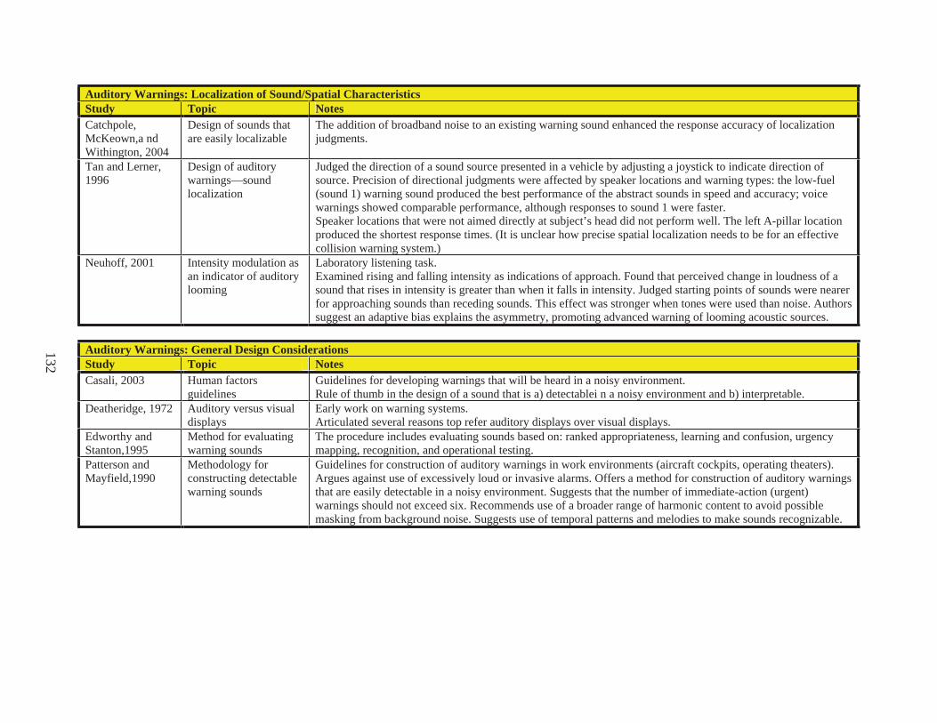
Auditory Warnings: Localization of Sound/Spatial CharacteristicsStudy Topic NotesCatchpole, Design of sounds that The addition of broadband noise to an existing warning sound enhanced the response accuracy of localizationMcKeown,a nd are easily localizable judgments.Withington, 2004Tan and Lerner, Design of auditory Judged the direction of a sound source presented in a vehicle by adjusting a joystick to indicate direction of1996 warnings—sound source. Precision of directional judgments were affected by speaker locations and warning types: the low-fuel
localization (sound 1) warning sound produced the best performance of the abstract sounds in speed and accuracy; voicewarnings showed comparable performance, although responses to sound 1 were faster.Speaker locations that were not aimed directly at subject’s head did not perform well. The left A-pillar locationproduced the shortest response times. (It is unclear how precise spatial localization needs to be for an effectivecollision warning system.)
Neuhoff, 2001 Intensity modulation as Laboratory listening task.an indicator of auditory Examined rising and falling intensity as indications of approach. Found that perceived change in loudness of alooming sound that rises in intensity is greater than when it falls in intensity. Judged starting points of sounds were nearer
for approaching sounds than receding sounds. This effect was stronger when tones were used than noise. Authorssuggest an adaptive bias explains the asymmetry, promoting advanced warning of looming acoustic sources.
132
Auditory Warnings: General Design ConsiderationsStudy Topic NotesCasali, 2003 Human factors Guidelines for developing warnings that will be heard in a noisy environment.
guidelines Rule of thumb in the design of a sound that is a) detectablei n a noisy environment and b) interpretable.Deatheridge, 1972 Auditory versus visual Early work on warning systems.
displays Articulated several reasons top refer auditory displays over visual displays.Edworthy and Method for evaluating The procedure includes evaluating sounds based on: ranked appropriateness, learning and confusion, urgencyStanton,1995 warning sounds mapping, recognition, and operational testing.Patterson and Methodology for Guidelines for construction of auditory warnings in work environments (aircraft cockpits, operating theaters).Mayfield,1990 constructing detectable Argues against use of excessively loud or invasive alarms. Offers a method for construction of auditory warnings
warning sounds that are easily detectable in a noisy environment. Suggests that the number of immediate-action (urgent)warnings should not exceed six. Recommends use of a broader range of harmonic content to avoid possiblemasking from background noise. Suggests use of temporal patterns and melodies to make sounds recognizable.
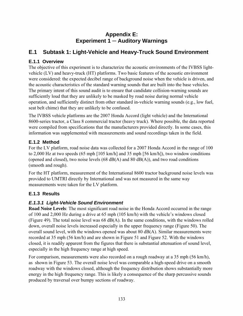
Appendix E: Experiment 1 ņ Auditory Warnings
E.1 Subtask 1: Light-Vehicle and Heavy-Truck Sound Environment E.1.1 Overview The objective of this experiment is to characterize the acoustic environments of the IVBSS light-vehicle (LV) and heavy-truck (HT) platforms. Two basic features of the acoustic environment were considered: the expected decibel range of background noise when the vehicle is driven, and the acoustic characteristics of the standard warning sounds that are built into the base vehicles. The primary intent of this sound audit is to ensure that candidate collision-warning sounds are sufficiently loud that they are unlikely to be masked by road noise during normal vehicle operation, and sufficiently distinct from other standard in-vehicle warning sounds (e.g., low fuel, seat belt chime) that they are unlikely to be confused. The IVBSS vehicle platforms are the 2007 Honda Accord (light vehicle) and the International 8600-series tractor, a Class 8 commercial tractor (heavy truck). Where possible, the data reported were compiled from specifications that the manufacturers provided directly. In some cases, this information was supplemented with measurements and sound recordings taken in the field.
E.1.2 Method For the LV platform, road noise data was collected for a 2007 Honda Accord in the range of 100 to 2,000 Hz at two speeds (65 mph [105 km/h] and 35 mph [56 km/h]), two window conditions (opened and closed), two noise levels (68 dB(A) and 80 dB(A)), and two road conditions (smooth and rough). For the HT platform, measurement of the International 8600 tractor background noise levels was provided to UMTRI directly by International and was not measured in the same way measurements were taken for the LV platform.
E.1.3 Results
E.1.3.1 Light-Vehicle Sound Environment Road Noise Levels: The most significant road noise in the Honda Accord occurred in the range of 100 and 2,000 Hz during a drive at 65 mph (105 km/h) with the vehicle’s windows closed (Figure 49). The total noise level was 68 dB(A). In the same conditions, with the windows rolled down, overall noise levels increased especially in the upper frequency range (Figure 50). The overall sound level, with the windows opened was about 80 dB(A). Similar measurements were recorded at 35 mph (56 km/h) and are shown in Figure 51 and Figure 52. With the windows closed, it is readily apparent from the figures that there is substantial attenuation of sound level, especially in the high frequency range at high speed. For comparison, measurements were also recorded on a rough roadway at a 35 mph (56 km/h), as shown in Figure 53. The overall noise level was comparable a high-speed drive on a smooth roadway with the windows closed, although the frequency distribution shows substantially more energy in the high frequency range. This is likely a consequence of the sharp percussive sounds produced by traversal over bumpy sections of roadway.
133

dB(A
)
70
60 65 mph (105 kph). windows closed
50
40
30
20
10
0 20 32 50 80 125 200 315 500 800 1,250 2,000 3,150 5,000 8,000 12,500 20,000
Frequency (Hz)
Figure 49. One-third octave distribution of roadway noise for light vehicles on a smooth roadway at 65 mph with windows closed (sound level: 80 dB(A))
dB(A
)
65 mph (105 kph). 70 windows open
60
50
40
30
20
10
0 20 32 50 80 125 200 315 500 800 1,250 2,000 3,150 5,000 8,000 12,500 20,000
Frequency (Hz)
Figure 50. One-third octave distribution of roadway noise for light vehicles on a smooth roadway at 65 mph with windows open (sound level: 80 dB(A))
134

dB(A
)
70
60
50
40
30
20
10
35 mph (56 kph). windows closed
0 20 32 50 80 125 200 315 500 800 1,250 2,000 3,150 5,000 8,000 12,500 20,000
Frequency (Hz)
Figure 51. One-third octave distribution of roadway noise for light vehicles on a smooth roadway at 35 mph with windows closed (sound level: 60 dB(A))
dB(A
)
70
35 mph (56 kph).60 windows opened
50
40
30
20
10
0 20 32 50 80 125 200 315 500 800 1,250 2,000 3,150 5,000 8,000 12,500 20,000
Frequency (Hz)
Figure 52. One-third octave distribution of roadway noise for light vehicles on a smooth roadway at 35 mph with windows open (sound level: 66 db(A))
135

dB(A
)
35 mph (56 kph). 70 windows closed
rough roadway 60
50
40
30
20
10
0 20 32 50 80 125 200 315 500 800 1,250 2,000 3,150 5,000 8,000 12,500 20,000
Frequency (Hz)
Figure 53. One-third octave distribution of roadway noise for light vehicles on a rough-surfaced roadway at 35 mph with windows closed (sound level: 68 dB(A))
Other Warning Sounds: A survey of the standard warning sounds found on the Honda Accord suggests that current warnings are generated in a relatively simple manner. For example, the warning sounds that indicated a key in the ignition, lights on (door open), parking brake on, and the safety belt reminder shared the same base frequency of 2,048 Hz and appeared to have little other harmonic content. Differentiation among the various warning conditions was accomplished by variations in the duration and rhythm of the pulses.
E.1.3.2 Heavy-Truck Sound Environment Road Noise Levels: Measurement of the International 8600 tractor background noise levels was provided to UMTRI directly by International and was not measured in the same way measurements were taken for the LV platform. The data presented for the HT platform differs from LV with respect to the manner in which background noise measurements were made. Specifically, the measures provided by International followed the SAE-J336 measurement standard, Sound Level for Truck Cab Interior. The test relates the engine rpm of an accelerating tractor to sound pressure level measured as dB(A). The resulting measure is shown in Figure 54. The measure is typically made on a smooth test track and it includes road and wind noise that accompanies the acceleration.
136

19 24 31 39 49 61 7 7 97 122
154
194
244
307
387
487
613
772
97212
2315
4019
3924
4130
7338
6848
7061
3177
1897
1612
23215
39919
387
Figure 54. Sound pressure level of the cab interior of a tractor accelerating at full throttle
Frequency Content at High-Idle (2300 rpm) and Low-Idle (700 rpm) Stationary Conditions
10
20
30
40
50
60
70
80
SPL,
dB
(A) r
e 20
mPa
High-Idle Spectrum Idle Spectrum
OA SPL = 76.8 dB(A)
OA SPL = 61.8 dB(A)
1/12 Octave Band Frequency, Hz
Figure 55. One-twelfth frequency content of a stationary tractor idling at 2,300 and 700 rpm. Overall SPL levels for each idle condition are identified in the accompanying text boxes.
Overall SPL During Full-Throttle Acceleration from Half-Governed to Governed Speed (SAE J336)
71
72
73
74
75
76
77
78
79
80
1,050 1,150 1,250 1,350 1,450 1,550 1,650 1,750 1,850 1,950 2,050 2,150 2,250 Engine Speed (rpm)
SPL,
dB
(A) r
e 20
mPa
137

Figure 55 illustrates the spectral power distribution of the internal noise levels of a stationary tractor at high and low idle. It shows a roll-off in the noise level at frequencies above 1,500 Hz, similar to that observed in light vehicles (see Figure 49). It seems likely, however, that because the measurements were taken from a stationary vehicle, they underestimate the amount of additional noise introduced by the road and wind. More direct measurements of the HT platform have been thwarted by measuring equipment failure and logistics, although measurement is still planned. Based on the currently available information, it appears that background cabin noise levels may be in the range of 75 to 80 db(A). Other alerting sounds: Standard alerting sounds used in the International 8600 tractor are based on the Star Micronics TMX-12H, a high sound pressure magnetic sounder. The component’s sound output is a square wave with frequencies of 1,000 and 1,500 Hz.
E.1.4 Conclusions
E.1.4.1 Light-Vehicle Platform Patterson and Mayfield (1990) recommended that the decibel level of a warning sound exceed the masking threshold (MT) of the sound in background noise by about 15 dB in at least four frequency components. Elsewhere, the limit was broadly defined as 15 dB above the background noise level (Stanton and Edworthy, 1999). A more recently reported guideline (Campbell et al., 2007b), suggests using auditory warnings above 10 to 30 db above MT, not exceeding 90 dB(A). (Note that db above MT is not the same as dB above background noise levels, although many reports appear to treat them as equivalent.) Rather than adopt a worst-case driving condition (e.g., high speed, windows open, rough road, radio on), it is reasonable to use a more common noisy driving situation as an assumed background noise level. One difficulty in using a worst-case sound level is that the resulting estimated level of a reliably audible warning sound will exceed the 90 dB(A) limit. Instead, the authors suggest that the background noise level be based on Figure 49, a vehicle cruising at 65 mph (105 km/h) with windows closed on a smooth roadway. Based on this standard, the recommended level of IVBSS warning sounds should be a minimum of 80 dB(A). It would also be best if the sounds included frequency content in the 1,000 to 5,000 Hz range, where the spectral power of the background noise is attenuated (at least with the windows closed). Further, to ensure the distinctiveness of the IVBSS warning sounds from the base vehicle’s warnings, avoidance of frequencies that overlap the existing warning range is recommended. Warning sounds with more elaborate harmonic content, onset envelopes, rhythmic patterns, and spatial locations are unlikely to be mistaken for the sounds on the base Honda Accord.
E.1.4.2 Heavy-Truck Platform Following the most recently published guidelines (Campbell et al., 2007b), the HT warning sounds should contain frequency content outside the 100 to 1,200 Hz range, where competition from background noise is strongest. It also suggests that overall sound decibel levels in the 85 to 90 dB(A) range may be required, although this range borders on being excessively loud. Note that many loudness standards for warnings were developed in the context of flight deck, manufacturing, and medical operations. In many of these contexts, the warning is presented with the expectation that an individual is performing other tasks unrelated to the warning and the
138

warning itself is about an exceedingly rare and urgent event. It is unclear whether application of the same standard to vehicle warnings is appropriate. In vehicles, warnings may occur more frequently and include substantially more false alarms than in these other contexts. Similar to the suggestions made for the LV platform, to minimize confusability it is recommended that IVBSS warning sounds avoid using sounds similar to the base sound set of the HT platform.
E.1.5 Forms No forms were needed for this subtask of the experiment.
139

E.2 Subtask 2: Acoustic Features of Warnings E.2.1 Overview The objective of this experiment was to relate acoustic features of warning sounds to a listener’s subjective judgments of urgency, annoyance, and noticeability. In addition, participants in this study were also asked to provide judgments of the relative urgency of each of four prototypic crash scenarios addressed by the IVBSS system: forward collision warning (FCW), curve speed warning (CSW), lane change-merge warning (LCM), and lateral drift warnings (LDW). By later matching sound urgency to perceived scenario urgency, the team expected to reduce potential annoyance to drivers. It is noted that matching scenario urgency to sound urgency has recently been shown to reduce perceived annoyance in drivers (Marshall, Lee, and Austria, 2007).
E.2.2 Method Stimulus Construction: A variety of sound stimuli were constructed along the guidelines articulated by several authors (Edworthy, Loxley, and Dennis, 1991; Haas and Edworthy, 1996). A typical auditory warning consists of a series of sound pulses combined to form a sound burst. Sound bursts can then be repeated to form the auditory warning. In constructing the stimuli for subtask 1, several acoustic attributes were varied to determine how they influenced perceived urgency. The selected attributes included:
x Fundamental frequency of the pulse (three factors: 1,400 Hz, 1,000 Hz, and 500 Hz) x Timbre (two factors: square wave or sine wave with three harmonics) x Harmonic content (two factors: natural or dissonant harmonics) x Pulse speed (three factors: 80, 110, or 140 ms). Speed was manipulated so that duration
of the sound varied as well. Pulse durations were scaled to 0.8 of the speed interval so that pulse duration was shorter at high speeds and longer at low speeds. Thus, for an 80ms interval, pulse duration was 64 ms; for a 140-ms interval, pulse duration was 112 ms. This is noted to make it clear that pulse duration was shorter at high speeds and longer at low speeds.
x Onset ramp (three factors: 0, 10, or 20 ms) x Pulse count in each burst (three factors: three, five, or seven pulses) x Pitch variation (two factors: modulation of pitch frequency by 1.12 times the fundamental
in alternating pulses) x Rhythmic variation (two factors: modulation of pulse speed by lengthening a pulse by
1.25 times the initial speed)
Because generation of a complete set of warnings from this base would produce 1,296 stimulus combinations (a prohibitively large set to expose to a subject) a smaller set of 24 orthogonal attribute combinations was generated with the assistance of SAS statistical software. From this, sounds were digitally generated using CSound scripts. Eight additional sounds were used to provide a general context for the 24 generated sounds: two sounds rated as highly urgent (Tan and Lerner, 1995), an FCW sound used in the ACAS project, a sound used in Eaton’s VORAD FCW system, an LDW used in the road departure crash warning (RDCW) project, a rumble-strip sound used in an RDCW simulator experiment, and two additional
140

custom-generated rumble-strip sounds. All sounds were digitally balanced for loudness with the assistance of a sound pressure meter positioned at the location of the listener’s head. Subjects: Twenty-four subjects participated in this study, partitioned into six groups based on age – young (ages 20 to 35), middle-aged (ages 36 to 55), and older (ages 56 to 70) – and gender. There were four participants in each of the six groups. After obtaining informed consent, participants were given a hearing screening to ensure they were able to adequately hear the presented sounds. After this, they were instructed to rate the sounds for urgency, annoyance, noticeability, and loudness. Each rating criterion was explicitly defined in the instructions. Stimulus Presentation: Sounds were presented in a small room outfitted with acoustic insulation to dampen sound reflections. Throughout the session, background driving noise was played continuously at 70 dB to emulate the sound environment of a moving passenger vehicle. Warning sounds were presented at 80 dB. The driving sounds and warning sounds were played through the respective soundcards of independent desktop computers. Each computer controlled separate pairs of powered speakers. Trials were blocked by rating type (urgency, annoyance, noticeability, and loudness) and sounds were randomized within each rating block. After completing the first four rating blocks, a repetition of each rating block was presented. Subjects thus made judgments of the 32 sounds with respect to each of the four rating types in two repetitions for a total of 256 ratings. Blocks were counterbalanced across subjects. At the start of each block, all warning sounds were played in a random sequence to provide participants with a sense of the range of sounds they would hear. Next, a ratings block was run in which the listener produced a magnitude estimation for each sound’s urgency, annoyance, noticeability, or loudness by adjusting a slider control on a computer display (see Figure 56) that adjusted a number from zero to ten in one-tenth increments.
Figure 56. Magnitude estimation screen used in rating presented sounds
Rated Severity of Crash Scenarios: After completing the sound ratings, participants were asked to listen to descriptions of each of four crash scenarios, and rate the relative severity of the scenario based on their personal experience. These ratings were solicited to obtain a basis for differentiating scenarios using acoustic characteristics of sounds found to be associated with urgency. Although diagrams were available to illustrate each crash scenario, it was desirable to encourage participants to judge severity based on their personal driving experience.
141

E.2.3 Results The principal analysis addressed the question of which acoustic properties of the set of sounds are most strongly related to rated urgency, annoyance, noticeability, and loudness. Consequently four general linear models relating the acoustic factors to each of the four ratings were constructed. Interaction effects among acoustic factors could not be modeled since participants were not shown all combinations of acoustic factors. The ratings were highly correlated with one another, as illustrated in Figure 57, which shows a strong association between each of the rating types. For example, sounds that are rated as urgent are also rated as annoying, noticeable, and loud.
Figure 57. Overview of the correlation between sound ratings
A mixed model analysis was conducted to relate each of the four judgment types to the acoustic characteristics of the 24 generated sounds. In addition, the loudness judgments were factored as a covariate into a later analysis of both the urgency and annoyance to remove this perceptual factor, which is likely to play a common role in each judgment. (A similar approach was taken in the Tan and Lerner studies.) By removing this factor, the team hoped to heighten any differences in how perceived urgency and annoyance are affected by different sound attributes. The results of the first analyses are shown in Table 26. Not surprisingly, strong associations were found among sound frequency, onset ramp, number of pulses, and whether the pulses alternated in pitch or were fixed. When loudness is factored out, an interesting pattern emerges that distinguishes the urgency ratings from the annoyance ratings. For example, whether a pulse is harmonic seems more closely associated with judged annoyance than with perceived urgency or noticeability. The waveform type appears to affect judged noticeability more reliably than either urgency or annoyance.
142
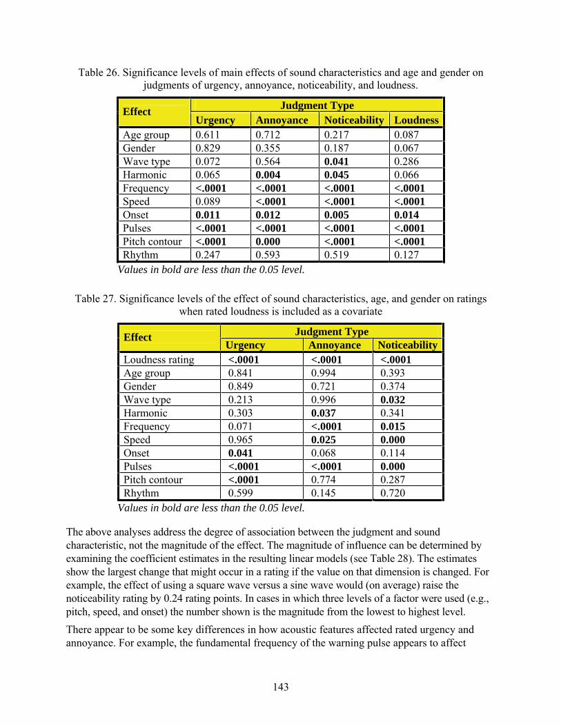
Table 26. Significance levels of main effects of sound characteristics and age and gender on judgments of urgency, annoyance, noticeability, and loudness.
Effect Judgment Type Urgency Annoyance Noticeability Loudness
Age group 0.611 0.712 0.217 0.087 Gender 0.829 0.355 0.187 0.067 Wave type 0.072 0.564 0.041 0.286 Harmonic 0.065 0.004 0.045 0.066 Frequency <.0001 <.0001 <.0001 <.0001 Speed 0.089 <.0001 <.0001 <.0001 Onset 0.011 0.012 0.005 0.014 Pulses <.0001 <.0001 <.0001 <.0001 Pitch contour <.0001 0.000 <.0001 <.0001 Rhythm 0.247 0.593 0.519 0.127
Values in bold are less than the 0.05 level.
Table 27. Significance levels of the effect of sound characteristics, age, and gender on ratings when rated loudness is included as a covariate
Effect Judgment Type Urgency Annoyance Noticeability
Loudness rating <.0001 <.0001 <.0001 Age group 0.841 0.994 0.393 Gender 0.849 0.721 0.374 Wave type 0.213 0.996 0.032 Harmonic 0.303 0.037 0.341 Frequency 0.071 <.0001 0.015 Speed 0.965 0.025 0.000 Onset 0.041 0.068 0.114 Pulses <.0001 <.0001 0.000 Pitch contour <.0001 0.774 0.287 Rhythm 0.599 0.145 0.720
Values in bold are less than the 0.05 level.
The above analyses address the degree of association between the judgment and sound characteristic, not the magnitude of the effect. The magnitude of influence can be determined by examining the coefficient estimates in the resulting linear models (see Table 28). The estimates show the largest change that might occur in a rating if the value on that dimension is changed. For example, the effect of using a square wave versus a sine wave would (on average) raise the noticeability rating by 0.24 rating points. In cases in which three levels of a factor were used (e.g., pitch, speed, and onset) the number shown is the magnitude from the lowest to highest level. There appear to be some key differences in how acoustic features affected rated urgency and annoyance. For example, the fundamental frequency of the warning pulse appears to affect
143

annoyance judgments more strongly than urgency (beyond its correlated effect on perceived loudness). That is, raising the pitch from 500 Hz to 1,400 Hz raised rated annoyance by 0.87, while raising rated urgency by 0.37. On the other hand, use of a level pitch contour (as opposed to an alternating series of pitches) strongly affected perceived urgency (increasing it by 0.72) while leaving perceived annoyance unaffected (again, beyond its effect on loudness.)
Table 28. Relative influence of sound attributes, loudness rating, age, and gender on judgments of urgency, annoyance, and noticeability
Effect Judgment Type Notes
Urgency Annoyance Noticeability Loudness rating 0.48 0.62 0.56 Influence of loudness rating on other
ratings Age group - - -Gender - - -
Wave type - - 0.24 A square wave increases the noticeability rating compared to a sine wave.
Harmonic- inharmonic - 0.28 - Harmonic wave annoyance greater
compared to inharmonic
Frequency 0.37 0.87 0.36 Low frequency ratings less urgent, annoying, or noticeable than high frequency
Speed - 0.35 0.46
Annoyance-Medium speed is least annoying; long speed is most annoying. Noticeability-Long slow speed is most noticeable; short speed is least.
Onset 0.33 -0.28 0.20
Urgency-0 to 10 ms onset associated with more urgency than 20. Annoyance-10 ms onset associated with less annoyance; Noticeability-0 ms onset associated with more noticeability.
Pulses 0.72 0.55 0.51 More pulses associated with higher ratings Pitch contour 0.72 - - Flat pulse contour associated with greater
rated urgency Rhythm - - -
Urgency Ratings of Crash Scenarios. Although data on each subject’s ratings of scenario urgency were originally provided using magnitude estimations (0 to 100), these ratings were rescaled into a within-subject rank to help offset large differences in how the scale was employed. A repeated measures analysis of variance found that LCMs were judged to be the significantly more urgent than LDWs and only marginally more urgent than CSWs and FCWs. The average ratings based on within-subject ranking are shown in Figure 58. In pairwise comparisons, LCMs were judged as significantly more urgent than LDWs; no other statistically significant differences were found. The data also suggested that LCMs were perceived as more
144

4
3
2
1 LCM FCW CSW LDW
Warning type
Figure 58. Average ranking of ratings for each crash scenario
Ran
ked
Urg
ency
(1
=mor
e ur
gent
; 4=l
ess
urge
nt)
urgent than either CSWs or FCWs, and FCWs were perceived as more urgent than LDWs. However, these latter effects were relatively weak and unreliable.
Abstract Warning Sounds in Context: Figure 59 illustrates how the generated warning sounds (lettered A through X) were distributed along the urgency and annoyance ratings scales, compared to sounds taken from prior work. Notably, two sounds that were rated as highly urgent from Tan and Learner’s 1995 study (stimulus 1 and stimulus 5) were similarly rated in the present study. In some ways, these sounds were in a class by themselves—stimulus 1 was comprised of modulated rising pitch bursts and stimulus 2 was an alternating high frequency (1,300 to 2,000 Hz) sound, unbroken by silence (see Figure 60). None of the other sounds used in the current study had these features. Instead, most had discrete intervals of silence as shown in Figure 61. Arguably, use of silence in warning tones may reduce the potential that the sound could mask other important sounds.
145
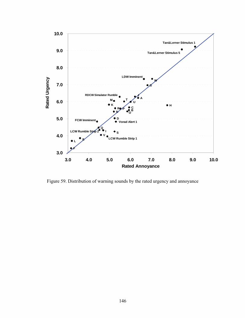
Rat
ed U
rgen
cy
10.0
9.0
8.0
7.0
6.0
5.0
4.0
3.0
A
B C
D
F
K
L
N P
Q
R
E
FCW Imminent
LCW Rumble Strip 1
LCW Rumble Strip 2
LDW Imminent
RDCW Simulator Rumble
Vorad Alert 1
I
J M
O
S
T U
V
G
H
Tan&Lerner Stimulus 1
Tan&Lerner Stimulus 5
W
3.0 4.0 5.0 6.0 7.0 8.0 9.0 10.0 Rated Annoyance
Figure 59. Distribution of warning sounds by the rated urgency and annoyance
146

Figure 60. Warning samples used by Tan and Lerner (1995). Note the unbroken sound output over the (approximately) two-second duration for both samples.
147

Figure 61. LDW-imminent warning used in the RDCW project The sound sample is broken into periods of silence.
E.2.4 Conclusions This study distinguished the relative contributions of several acoustic characteristics to a listener’s perception of urgency, annoyance, and noticeability. This provides some guidance in creating sounds that are perceived as appropriately urgent without being excessively annoying. The results suggest that the judged loudness of a sound influences all three attributes in nearly equal measure. When perceived loudness is included in the models as a covariate, differences among the remaining acoustic properties are observed. The strongest results can be summarized as follows: x Frequency: A high fundamental frequency increases urgency, annoyance, and
noticeability. However, annoyance appears to be most strongly influenced by the use of high frequency sounds.
x Speed: The speed of the warning pulses does not seem to affect perceived urgency, although it increases both annoyance and noticeability. Perhaps this is a consequence of the longer duration of each pulse at slower speeds. This may be related to a result reported by Marshall et al. (2007) that concluded that both long pulse durations and short interpulse interval increases perceived urgency more than annoyance. In the present study, however, increasing the speed factor had the effect of both decreasing pulse duration while and decreasing interpulse intervals. Short pulses might seem less urgent, while short interpulse intervals seem more urgent.
x Onset: A short onset of about 10 ms was found to increase urgency (relative to a 0- or 20-ms onset) while lowering perceived annoyance. Onset was used in both studies as well, but is defined differently in each. In the Marshall et al. study, onset is rise in sound amplitude over the duration of a series of pulses that make up a burst. In the present study, onset was defined as the amplitude envelope of an individual pulse. They are not directly comparable.
x Pitch contour: A flat pitch contour (i.e., all pulses the same pitch) appears to improve perceived urgency without affecting either annoyance or noticeability.
x Number of pulses in warning: Both urgency and annoyance were increased with the number of warning pulses. However, rated urgency increased more than annoyance.
148

Using the above results as a guideline, this study suggests that the design of a sound that maximizes urgency and minimizes annoyance would avoid high frequencies (above 1,000 Hz), use a medium pulse speed (110 ms per cycle), a 10-ms onset ramp, a flat pitch contour, and as many as seven pulses.
E.2.5 Forms E.2.5.1 Instructions In this study you will be presented with a series of warning sounds intended to warn drivers that they are in imminent danger of colliding with another vehicle or running off the roadway. We want you to listen to the sounds and rate each one using criteria that we will describe later. Please try to imagine yourself in your vehicle, driving along a roadway, perhaps tuning your radio, when you hear the warning sound. Also imagine that sometimes the warning may sound but there may be no collision danger. First we will present you the entire set of 32 sounds to generally familiarize you with what they sound like. Each sound will repeat once. You will be asked to rate the URGENCY, ANNOYANCE, NOTICEABILITY and LOUDNESS of each sound as they are played. By URGENCY, we mean: How strongly does the sound seem to suggest that you take immediate action to avoid a collision? Does the sound convey a sense of importance motivating you to take immediate action? By ANNOYANCE, we mean: How strongly would you dislike this sound especially if it occurred when there was no danger of collision? By NOTICEABILITY, we mean: Is the sound readily noticeable among other sounds and noises in a vehicle? Can you easily hear this sound within the vehicle noise? How easily you think you would recognize the sound as a collision warning, especially if other sounds are present in the vehicle? By LOUDNESS, we mean: Do you think the sound has a high volume and intensity? Secondary Rating – Crash ScenariosIn this task, we would like you to listen to descriptions of four types of collision scenarios. Please give us your impression (based on your experience as a driver) of what the relative severity of each collision scenario might be along a line that ranges from not severe to very severe. FCW (Forward Collision Warning): The first scenario we will describe is a situation in which your vehicle or truck is closing on another car or truck that is either stopped or moving very slowly. This could happen if you failed to see the car in the first place; or if it was temporarily hidden by another car or truck between your car and the stopped vehicle. In other FCW scenarios, a slow-moving vehicle might cut in front of you, leaving very little time to stop; or you might be forced to cut in behind a slow-moving vehicle. In other scenarios, you might be turning a corner or coming over a hill and are not able to see far enough ahead to recognize that there is a stopped vehicle in the road. From your experience, and relative to the other scenarios, please rate the seriousness or urgency of this crash situation. CSW (Curve Speed Warning): In this scenario, you are in a situation where you find that you enter a curved section of roadway that is sharper than you anticipate. Your speed may be too high to stay in your lane, or on the roadway. From your experience, and relative to the other scenarios, please rate the seriousness or urgency of this crash situation. LDW (Lane Departure Warning): In this scenario, your vehicle is drifting to one side of your lane. You might be drifting into another lane of traffic, into an oncoming lane of traffic, or onto the shoulder area of the roadway where there may be a guardrail, bridge abutment, or a drainage ditch. From your experience, and relative to the other scenarios, please rate the seriousness or urgency of this crash situation. LCM (Lane Change-Merge Warning): In this scenario, your vehicle is making a lane change, a turn, or a merge into traffic and there is another vehicle in the area into which you are about to turn, but which you might not easily see. From your experience, and relative to the other scenarios, please rate the seriousness or urgency of this crash situation.
149

E.3 Subtask 3: Warning Sound Suites: Acquisition and Response Speed
E.3.1 Overview The objective of this experiment is to investigate the relative speed with which different sound suites could be learned and could elicit a fast response from a subject. The experiment focuses on the difference between warning suites that contain auditory icons—sounds that resemble real-world sounds—and those comprised of abstract sounds with no real-world referents. Three suites were constructed containing four sounds associated with each of the four IVBSS scenarios: forward-collision warning (FCW), curve speed warning (CSW), lane change-merge (LCM) warning, and lateral drift warning (LDW). Each suite varied in the extent to which auditory icons were incorporated, with suites A and B incorporating auditory icons, and suite C using abstract sounds of differing urgency derived from experiment 1, subtask 2. Suite B was derived from A by modifying pitch, duration, onset envelope, and pulse speed to produce a generally less urgent-sounding suite in order to assess how such modifications could affect driver performance.
Table 29. Types of warning sounds used in experiment 1, subtask 3
Suite FCW LCM CSW LDW A Abstract Horn-honk Squealing tires Rumble strip B (less urgent A) Abstract Horn-honk Squealing tires Rumble strip
C Abstract (High urgency)
Abstract (Med-High)
Abstract (Med-Low)
Abstract (Low)
This study also indirectly acknowledges that warning sounds often occur in the context of other warning sounds. Within such contexts, the effectiveness of a sound could be diminished especially if is difficult to learn and discriminate. For example, construction of a sound suite containing only urgent warnings based on the results of experiment 1, subtask 2 is not recommended. Auditory Icon Construction: Ideally, an auditory icon should be easily associated with a crash scenario and easily discriminated from other warning sounds. Ease of association can make the sound perhaps self-explanatory, and easy to learn and remember. An auditory icon designed to warn of an imminent crash should reference some aspect of the dangerousness of the pre-crash condition that is developing (while there is time to respond), but that has not necessarily occurred. Thus, squealing tires are used for a CSW to resemble the sound a vehicle might make if a turn is attempted at an excessively high speed. A tire squeal would presumably precede a road departure. Similarly, a (potentially lateralized) horn honk is used for LCM to imitate a cautionary response one might receive if one’s vehicle encroached another’s lane. A rumble-strip like sound is used to resemble the sound produced as a vehicle leaves the lane (but before it collides with a fixed object or leaves the roadway). The FCW icon proved to somewhat problematic to design. Suggested candidate sounds included the sound of aggressive braking (screeching tires) and horn honking. Apart from the similarity to the sounds used for CSW and LCM, in terms of the way the real scenarios would play out both sounds imitate a sound that a vehicle might make after the driver has responded. While it might be
150
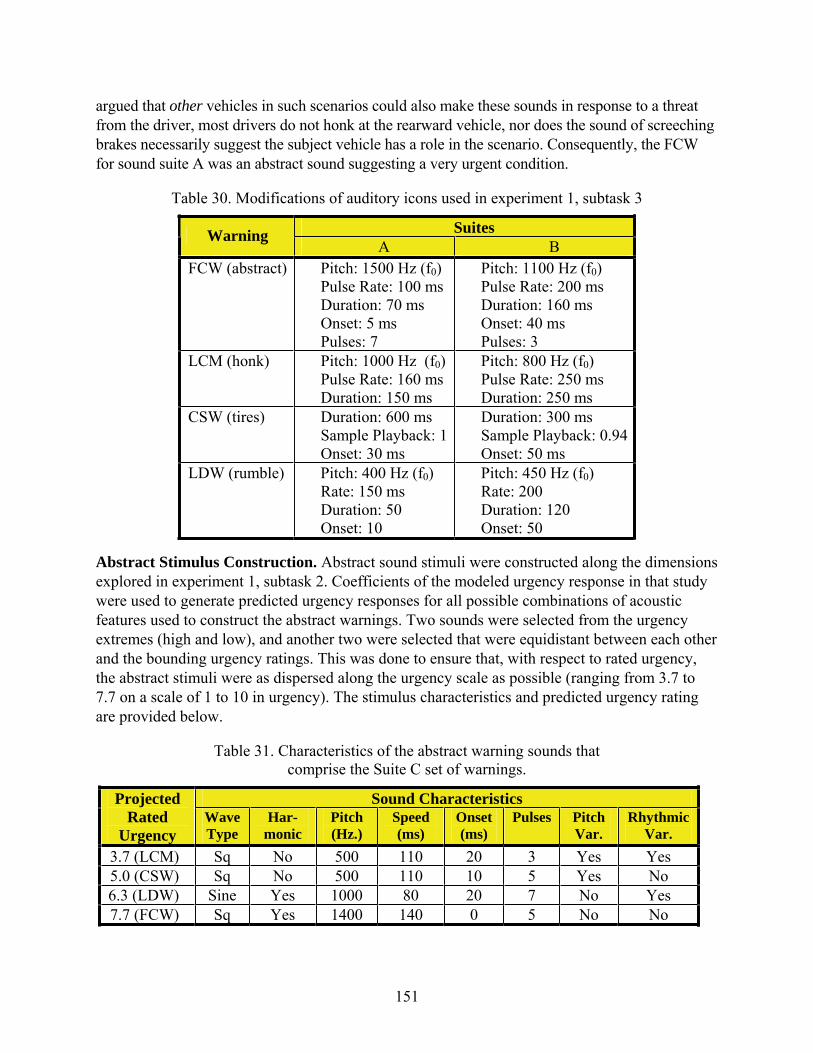
argued that other vehicles in such scenarios could also make these sounds in response to a threat from the driver, most drivers do not honk at the rearward vehicle, nor does the sound of screeching brakes necessarily suggest the subject vehicle has a role in the scenario. Consequently, the FCW for sound suite A was an abstract sound suggesting a very urgent condition.
Table 30. Modifications of auditory icons used in experiment 1, subtask 3
Warning Suites A B
FCW (abstract) Pitch: 1500 Hz (f0) Pulse Rate: 100 ms Duration: 70 ms Onset: 5 ms Pulses: 7
Pitch: 1100 Hz (f0) Pulse Rate: 200 ms Duration: 160 ms Onset: 40 ms Pulses: 3
LCM (honk) Pitch: 1000 Hz (f0) Pulse Rate: 160 ms Duration: 150 ms
Pitch: 800 Hz (f0) Pulse Rate: 250 ms Duration: 250 ms
CSW (tires) Duration: 600 ms Sample Playback: 1 Onset: 30 ms
Duration: 300 ms Sample Playback: 0.94 Onset: 50 ms
LDW (rumble) Pitch: 400 Hz (f0) Rate: 150 ms Duration: 50 Onset: 10
Pitch: 450 Hz (f0) Rate: 200 Duration: 120 Onset: 50
Abstract Stimulus Construction. Abstract sound stimuli were constructed along the dimensions explored in experiment 1, subtask 2. Coefficients of the modeled urgency response in that study were used to generate predicted urgency responses for all possible combinations of acoustic features used to construct the abstract warnings. Two sounds were selected from the urgency extremes (high and low), and another two were selected that were equidistant between each other and the bounding urgency ratings. This was done to ensure that, with respect to rated urgency, the abstract stimuli were as dispersed along the urgency scale as possible (ranging from 3.7 to 7.7 on a scale of 1 to 10 in urgency). The stimulus characteristics and predicted urgency rating are provided below.
Table 31. Characteristics of the abstract warning sounds that comprise the Suite C set of warnings.
Projected Sound Characteristics Rated
Urgency Wave Type
Har-monic
Pitch (Hz.)
Speed (ms)
Onset (ms)
Pulses Pitch Var.
Rhythmic Var.
3.7 (LCM) Sq No 500 110 20 3 Yes Yes 5.0 (CSW) Sq No 500 110 10 5 Yes No 6.3 (LDW) Sine Yes 1000 80 20 7 No Yes 7.7 (FCW) Sq Yes 1400 140 0 5 No No
151
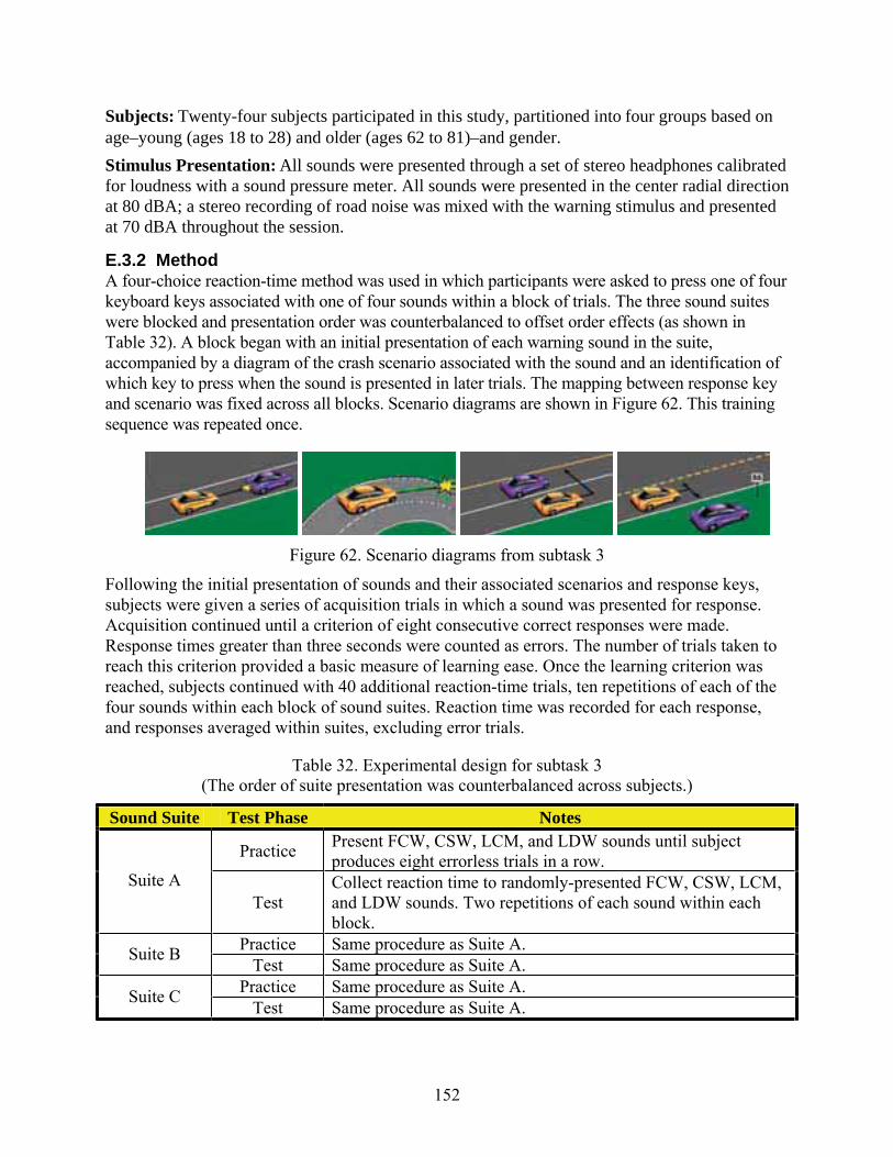
Table 32. Experimental design for subtask 3 (The order of suite presentation was counterbalanced across subjects.)
Sound Suite Test Phase Notes
Suite A
Practice Present FCW, CSW, LCM, and LDW sounds until subject produces eight errorless trials in a row.
Test Collect reaction time to randomly-presented FCW, CSW, LCM, and LDW sounds. Two repetitions of each sound within each block.
Suite B Practice Same procedure as Suite A. Test Same procedure as Suite A.
Suite C Practice Same procedure as Suite A. Test Same procedure as Suite A.
152
Subjects: Twenty-four subjects participated in this study, partitioned into four groups based on age–young (ages 18 to 28) and older (ages 62 to 81)–and gender. Stimulus Presentation: All sounds were presented through a set of stereo headphones calibrated for loudness with a sound pressure meter. All sounds were presented in the center radial direction at 80 dBA; a stereo recording of road noise was mixed with the warning stimulus and presented at 70 dBA throughout the session.
E.3.2 Method A four-choice reaction-time method was used in which participants were asked to press one of four keyboard keys associated with one of four sounds within a block of trials. The three sound suites were blocked and presentation order was counterbalanced to offset order effects (as shown in Table 32). A block began with an initial presentation of each warning sound in the suite, accompanied by a diagram of the crash scenario associated with the sound and an identification of which key to press when the sound is presented in later trials. The mapping between response key and scenario was fixed across all blocks. Scenario diagrams are shown in Figure 62. This training sequence was repeated once.
Figure 62. Scenario diagrams from subtask 3
Following the initial presentation of sounds and their associated scenarios and response keys, subjects were given a series of acquisition trials in which a sound was presented for response. Acquisition continued until a criterion of eight consecutive correct responses were made. Response times greater than three seconds were counted as errors. The number of trials taken to reach this criterion provided a basic measure of learning ease. Once the learning criterion was reached, subjects continued with 40 additional reaction-time trials, ten repetitions of each of the four sounds within each block of sound suites. Reaction time was recorded for each response, and responses averaged within suites, excluding error trials.

Average Trials to Criterion
140120100
768060 47
40 2220
0
A B C
Sound Suite
Figure 63. Trials to criterion by sound suite
Tria
ls
E.3.3 Results Trials to Criterion: An analysis of variance of trials to criterion found a main effect of age group and sound suite on trials to criterion. Younger subjects learned to associate the responses to the sounds more quickly than older subjects. On average, younger subjects reached the criterion of eight consecutive errorless trials after 19 trials while older subjects required 77 trials (F(1,20) = 17.6, p < 0.01). On average, subjects reached criterion earlier with suite A than the others (F (2,36) = 6.15, p < 0.01). Older subjects learned suite A with fewer trials than either suites B and C and younger subjects learned both suite A and C more quickly than suite B. The effect of sound suite is illustrated in Figure 63. Post-hoc comparisons (with Bonferroni adjustment) found a significant difference between A and B pairs, but no others (t = 3.51, p = 0.004). A marginal effect of order was also observed. Subjects reached criterion in fewer trials in each consecutive block (64, 54, and 27 trials in the first, second, and third blocks, respectively). An interaction between age group and suite was observed (F(2,36) = 3.5, p = 0.041), suggesting that age influenced the relative ease of learning the suites (Figure 64). It is especially interesting that younger subjects had substantially less difficulty learning suite C than older subjects. Perhaps their greater exposure to sound-emitting electronic devices and video games has induced younger subjects to employ more effective strategies in associating a sound with a response.
153

Average Trials to Criterion
140 122 120 Old Young 100 82
Tria
ls
80 60 40 29 30 20 15 13
0 A B C
Sound Suite
Figure 64. Interaction effect between subject age and sound suite
Error Rates: Overall, subjects made errors on 15 percent of the trials. An analysis of variance on the error data found a main effect of age and order; older subjects had more errors than younger subjects (23 versus 6 percent; F(1, 18.2) = 36.18, p < 0.0001) and the error rate declined across blocks (F(2, 33.4) = 4.77, p = 0.02). Average subject error rates were 19 percent on the initial trial block, 13 percent on the second block, and 11 percent on the third. No effect of sound suite on error rate was observed. The error data were sorted by stimulus suite into a summary confusion matrix showing how response errors were distributed among the other possible response choices (Table 33). The confusion matrix shown in Table 33 was then partitioned into older and younger subject error performance to create Table 34.
154

Table 33. Confusion matrix for distribution of responses for warnings in each stimulus suite
Suite
A
B
C
Stimulus
FCW
Warning
LCM CSW LDW FCW LCM CSW LDW FCW LCM CSW LDW
FCW
86.7% 3.3% 2.9% 4.6%
90.8% 1.7% 1.7% 7.1%
94.2% 11.7%
6.3%
LCM
2.9% 89.2%
2.1% 3.8% 1.7%
81.3% 8.8% 5.8% 3.3%
77.5% 5.4% 5.4%
CSW
1.7%
Response
2.1% 89.6%
4.2% 1.7%
10.8% 84.6%
2.9% 1.3% 6.7%
76.7% 8.8%
LDW
8.3% 5.0% 3.3%
85.8% 5.4% 2.9% 4.6%
83.3% 0.4% 3.3%
10.8% 85.0%
No Response
0.4% 0.4% 2.1% 1.7% 0.4% 3.3% 0.4% 0.8% 0.8% 0.8% 0.8% 0.8%
Table 34. Confusion matrix partitioned by age
Age Suite Warning Stimulus
Response FCW LCM CSW LDW No Response
Old A FCW 80.8% 5.0% 3.3% 10.0% 0.8% LCM 5.8% 83.3% 2.5% 7.5% 0.8% CSW 5.0% 3.3% 83.3% 4.2% 4.2% LDW 5.0% 6.7% 8.3% 76.7% 3.3%
B FCW 85.0% 3.3% 3.3% 7.5% 0.8% LCM 1.7% 72.5% 15.8% 4.2% 5.8% CSW 3.3% 14.2% 72.5% 9.2% 0.8% LDW 10.0% 8.3% 4.2% 75.8% 1.7%
C FCW 91.7% 3.3% 2.5% 0.8% 1.7% LCM 15.8% 63.3% 12.5% 6.7% 1.7% CSW 11.7% 8.3% 62.5% 15.8% 1.7% LDW 9.2% 15.0% 74.2% 1.7%
Young A FCW 92.5% 0.8% 6.7% LCM 0.8% 95.0% 1.7% 2.5% CSW 0.8% 0.8% 95.8% 2.5% LDW 4.2% 0.8% 95.0%
B FCW 96.7% 3.3% LCM 1.7% 90.0% 5.8% 1.7% 0.8% CSW 3.3% 96.7% LDW 4.2% 3.3% 1.7% 90.8%
C FCW 96.7% 3.3% LCM 7.5% 91.7% 0.8% CSW 0.8% 2.5% 90.8% 5.8% LDW 1.7% 2.5% 95.8%
155

1.00
0.90
0.80
0.70
FCW LCM
0.60
Percent Responses 0.50 CSW 0.40 LDW0.30
No Response No Response 0.20 LDW
0.10 CSW0.00
LCMFCW Subject Response A LCM FCW
CSW
Stimulus LDW
Figure 65. Sound confusions for sounds used in suite A
Confusions among sounds in suite A are shown in Figure 65. The height of each bar shows, for a given sound stimulus, the percent of responses made to each sound in suite A. Responses falling off the main diagonal are errors. The plot suggests that there is a slight tendency for the FCW sound to be confused with the LDW sound. In the context of this suite, the two sounds may have appeared similar because they are both somewhat abstract sounding, compared to the LCM (horn honk) and CSW (squealing tires) sounds. Confusions among sounds in suite B, a variant of A, are shown in Figure 66. In this set, there appears to be a similar confusion between LDW and FCW to that in suite A. There also appears to be some confusion between the LCM and CSW sounds; LCMs were identified as CSWs 11 percent of the time, and CSWs were identified as LCMs 9 percent of the time. Confusions among the abstract sounds in suite C are shown in Figure 67. In this set, the confusion pattern seems to suggest that neighboring sounds on the urgency scale are more likely to be confused with each other. Thus, when an LCM was played, it was confused with an FCW 12 percent of the time (although FCW was confused as an LDW only 3 percent of the time). When a CSW was played, it was confused with an LDW 11 percent of the time. When an LDW was played, it was confused for a CSW 9 percent of the time.
156

1.00
0.90
0.80
0.70
FCW LCM
0.60
Percent Responses 0.50 CSW LDW
0.40
0.30 No Response No Response 0.20
LDW 0.10
CSW0.00
LCMFCW Subject Response B LCM FCW
CSW
Stimulus LDW
Figure 66. Sound confusions for sounds used in suite B
1.00
0.90
0.80
0.70
FCW LCM
0.60
Percent Responses 0.50 CSW LDW
0.40
0.30 No Response No Response 0.20
LDW 0.10
CSW0.00
LCM FCW Subject Response
C LCM FCW CSW
Stimulus LDW
Figure 67. Sound confusions for sounds used in suite C
Choice Reaction Time: Trials in which a response error occurred were excluded from the reaction time analysis. An analysis of variance revealed a main effect of age group (F(1,19) = 11.57, p = 0.0032) and sound suite (F(2,32) = 4.03, p = 0.0273). In general, the mean reaction time in older subjects was about 300 ms longer than in younger subjects (see Figure 68). Reaction times for suite A sounds were about 150 ms faster than for suite B, and 130 ms faster than for suite C (see Figure 69).
157

1161 1433
0
250
500
750
1000
1250
1500
1750
2000
Rea
ctio
n Ti
me
(mse
c)
O Y Age Group
Figure 68. Mean reaction time by age group. Error bars depict 95-percent confidence intervals on the mean.
1220 1363 1346
0
250
500
750
1000
1250
1500
1750
2000
Rea
ctio
n Ti
me
(mse
c)
A B C Sound Suite
Figure 69. Mean reaction times for responding within each sound suite. Error bars depict 95-percent confidence intervals on the mean reaction time.
158
E.3.4 Conclusions The results suggest that the sounds included in suite A resulted in substantially fewer acquisition trials and substantially smaller reaction times. It is less clear why subjects’ performance with suite B warnings (a modification of suite A) was comparatively difficult to learn and resulted in substantially longer response times. Examination of the error pattern obtained for suite B suggests that, unlike suite A, the warning sounds for LCM and CSW were more easily confused with one another for both younger and older drivers. In addition, suite B also appears to have retained a confusion pattern between FCW and LDW similar to one observed in suite A. The confusion data from suite C follow a different pattern seemingly related to rated urgency: Sounds of similar rated urgency are more often confused with one another. It is worth noting that response errors might arguably have been related to response confusion, since warning functions were paired with the same responses across all three sound suites. However, if response confusion were a factor, similar response patterns should have appeared across all sound suites. One lesson learned in this study is that even a few minor alterations in sound characteristics may significantly affect a listener’s reaction time performance. Thus, a sound’s status as an auditory icon does not necessarily guarantee that it will outperform an abstract sound. While subjects found suite A easy to learn, a minor variant of the same suite resulted in a lengthier acquisition period, longer reaction times, and more confusion. Finally, compared to suite A, the abstract sounds that were selected across a range of perceived urgency were also difficult to learn, less quickly responded to, and resulted in more errors.
159

E.3.5 Forms
E.3.5.1 Instructions for Grouped Warnings and Choice Reaction Time
In this study, we want to test sets of warning alarms for possible use in a collision warning system. In our study, we will be testing 3 sets of sounds. In each set, there are four warning sounds, with each sound associated with a different crash scenario.
The sounds presented to you will vary in how urgent they sound. They also vary in how abstract or concrete they sound. For example, some of the sounds you will hear will resemble a rumble strip, squealing tires, or a vehicle horn. These sounds may be identified with one of four crash scenarios:
1) Forward Collision Warning (FCW) – used to warn a driver that a forward collision may be imminent.
2) Curve Speed Warning (CSW)—used to warn the driver that the vehicle may be approaching a curved section of roadway too quickly (squealing tires).
3) Lane Departure Warning (LDW)—used to warn the driver that the vehicle is wandering out of the lane boundary (rumble strip).
4) Lane Change Merge (LCM)—used to warn the driver that the vehicle is enter an occupied traffic lane. (e.g., honking horn).
Each crash scenario will be associated with a single key press as follows:
FCW—A; CSW—Z; LDW—‘; LCM—/
We are interested in finding how easy theses sounds are to associate with each scenario, and how quickly you can learn them. And, once they have been learned, how quickly you select the response associated with the sound.
FCW LDW ‘ A CSW LCM
Z /
Procedure: In the experiment, you will be seated at a computer wearing a pair of headphones. We will test the sounds of each set in a block of experimental trials. Each block will begin with an initial exposure phase in which we will play each sound and display a picture of the crash scenario associated with the sound. This will be done two times.
Following this initial exposure, we will present a sound and you must select the appropriate key (on the keyboard) to indicate the selected scenario associated with the sound. If your choice is correct, you will be presented with a “correct” message. If you make a mistake, the proper key (and scenario picture) will be displayed to help you remember it. If you delay responding for more than 3 seconds, you will also be advised to respond more quickly. These learning trials will continue until you make eight correct judgments in a row (and respond within the 3-second criteria).
160

After this learning phase, there will be 40 more reaction time judgments using the sounds in this set. Please respond as quickly as you can without making errors.
Two more sets of sounds will be tested following the first set using the same procedure.
161
Subtask 4: Localization of Auditory Warnings
This subtask of the experiment addressed the question of whether broadband noise and QSound can enhance localization.
E.4.1 Overview The objective of this pilot evaluation was to investigate the relative speed with which different sample warning sounds can be directionally located by listeners. Prior work suggests that the addition of a broadband noise component to simple warning sounds may enhance a listener’s ability to judge the radial direction of the sound (Catchpole, McKeown, and Withington, 2004). For directional warnings presented in a vehicle, where a driver must identify both the meaning and location of a sound to respond appropriately, any enhancement of a sound that improves accuracy of directional judgments might also enhance the speed with which such judgments are made. It is also possible that the introduction of a noise component might interfere with identification of the sound. The first part of subtask 4 examines these possibilities by introducing a broadband noise component into the lateral warning sounds examined in subtask 3 (lateral drift warning (LDW) and lane change-merge (LCM) warning). For additional contrast, two different stimulus sets were investigated: auditory icons (suite A) and abstract warning sounds (suite B). A second pilot study was conducted to examine whether directional enhancements in the stereo sound image might enhance localization. This was done by modifying monaural versions of the LDW and LCM sounds to image the sound at more extreme radial directions than can be portrayed by simple panning between stereo channels. The spatial manipulation of the warning sounds was accomplished with the help of QSound© enhancement of the original warning sounds. Such sound processing techniques use interaural time differences (ITD), interaural amplitude differences (IAD), and crosstalk cancellation (attenuation of the acoustic crosstalk between pairs of stereo speakers that reduces the apparent separation of sound sources between stereo channels) to enhance the apparent spatial separation of sound sources. Some of these techniques require listeners to be equidistant from each speaker in a stereo pair for maximum effectiveness. For IVBSS, headrest speakers are used for optimal effectiveness— speaker pairs mounted in a headrest provide the best opportunity to place the listener at an equal distance between the speakers. With conventional speaker placement in vehicles (e.g., in doors or on the rear window deck) it is less feasible to situate a driver equidistant between two speakers. It is also noteworthy that deviations of head position from the ideal position are likely to reduce or eliminate lateralization effects. The second pilot study was conducted to examine the relative effectiveness of QSound processing to stereo panning in enhancing reaction time performance. As in the previous subtask, the LDW and LCM warnings used as stimulus suite A (LDW-A, LCM-A) and C (LDW-C, LCM-C) were investigated. The conditions in each pilot study are illustrated in Table 35 and Table 36.
162

Table 35. Stimulus sets used in to examine noise treatment
Stimulus Suite Warning Direction Noise Treatment
Left No
LCM Yes No
A Right Yes
Left No
LDW Yes NoRight Yes
Left No
LCM Yes No
C Right Yes
LDW Left No
Yes
Right No Yes
Table 36. Stimulus sets used to examine effects of QSound treatment
Stimulus Suite Warning Direction QSound Treatment
Left No
LCM Yes No
A Right Yes
Left No
LDW Yes NoRight Yes
Left No
LCM Yes No
C Right Yes
LDW Left No
Yes
Right No Yes
163

E.4.2 Method Sound Construction—Noise: The sounds used in both pilot experiments were based on the LDW and LCM sounds used in subtask 3 of experiment 1 (suites A and C). For the sounds used in the noise condition, filtered broadband noise was combined with the original sound. The noise was filtered to attenuate frequencies below 100 Hz and above 10 KHz. Depending on the target sound, a 1,000 Hz-wide band-reject filter was applied. The filter was centered on the strongest frequency components of the original warning sound. Thus the spectral power distribution of the broadband noise was modified to reduce any overlap with the warning sound to reduce potential masking effects of the noise. An example of the resulting noise spectra is shown in Figure 70. Frequencies below 100 Hz and above 1 KHz were filtered and a stop band filter 1,000 Hz wide, centered on 700 Hz, was applied. Figure 71 shows the LCM-A warning combined with the broadband noise.
Figure 70. Frequency analysis of filtered broadband noise.
Figure 71. Frequency analysis of broadband noise and the LCM-A warning sound
164

The amplitude envelope of the added noise followed the same attack and decay profile used for each warning sound. Noise and non-noise stimuli were also balanced in volume with the help of a sound pressure meter positioned near the listening position of a subject’s head. Left and right versions of the stimuli were produced by digitally panning the monaural versions of the sound to the left and right speaker channels. Sound Construction—QSound: The pilot study employing QSound enhancements used the same base sounds as the pilot study employing broadband noise. Instead of noise, QSound enhancements were made to increase the apparent spatial offset of the sounds. Sounds panned to the left or right stereo channel produced an apparent directional offset that was limited to the maximal offset of the headrest speaker—about 45 degrees left or right of center. QSound enhancements produced sounds with an apparent location about 90 degrees off the center axis. Subjects: Nine subjects participated in this study drawn from the research staff at UMTRI. All subjects were men. Method: A four-choice reaction-time method was used in which participants were asked to press a key to indicate both the identity and direction of the warning sounds. The two sound suites (A and C) were presented in blocks that were counterbalanced among subjects to offset order effects. Each block began with a set of learning trials in which each auditory warning was presented along with an illustration of the associated response key. The learning trials were repeated once. Next, response trials were presented in which subjects quickly pressed a key associated with each sound-direction combination. Sounds were randomized within blocks. Each sound was repeated ten times for a total of 80 trials per block (e.g., two sounds x two noise levels x two directions x ten repetitions). The same procedure used to study noise treatment was also used to examine QSound processed warnings, substituting QSound treatment for the noise treatment. Stimulus Presentation: Subjects were seated in the driver’s seat of a stationary vehicle with a response keyboard placed on their lap. A small LCD screen over the steering wheel provided instructions and response feedback. In the noise study, warning sounds were presented using a set of powered speakers mounted near the vehicle A-pillars; in the QSound study, warning sounds were presented through pair of speakers mounted in the headrest of the driver’s seat. All warning sounds were adjusted to levels of 80 dBA at the approximate listening position. As in subtask 3, a stereo recording of road noise was played continuously throughout the session at 70 dBA using a dedicated set of speakers located on the rear-window deck and controlled by an independent computer system.
E.4.3 Results A mixed-model analysis of variance on the reaction time data in found a main effect of warning suite (F(1, 119) = 24.25, p < 0.01). The warning sounds in suite A were about 110 ms shorter than those from suite C (shown in Figure 72). No other main effects or interactions were observed on reaction time. Analysis of the overall error rate found no significant effects of any factor on error rate. The error data were also partitioned into localization errors (where a subject’s response was incorrect with respect to sound direction) and identification errors (where a subject’s response misidentified the sound (e.g., an LDW response to an LCM warning) to determine if the noise treatment affects the type of error committed. For example, the addition of
165
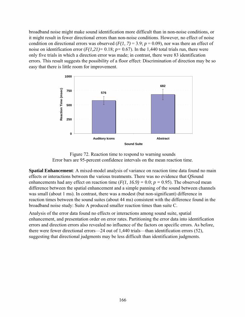
576
682
0
250
500
750
1000
Rea
ctio
n Ti
me
(mse
c)
Auditory Icons Abstract
Sound Suite
Figure 72. Reaction time to respond to warning sounds Error bars are 95-percent confidence intervals on the mean reaction time.
broadband noise might make sound identification more difficult than in non-noise conditions, or it might result in fewer directional errors than non-noise conditions. However, no effect of noise condition on directional errors was observed (F(1, 7) = 3.9; p = 0.09), nor was there an effect of noise on identification error (F(1,21)= 0.18; p= 0.67). In the 1,440 total trials run, there were only five trials in which a direction error was made; in contrast, there were 83 identification errors. This result suggests the possibility of a floor effect: Discrimination of direction may be so easy that there is little room for improvement.
Spatial Enhancement: A mixed-model analysis of variance on reaction time data found no main effects or interactions between the various treatments. There was no evidence that QSound enhancements had any effect on reaction time (F(1, 16.9) = 0.0; p = 0.95). The observed mean difference between the spatial enhancement and a simple panning of the sound between channels was small (about 1 ms). In contrast, there was a modest (but non-significant) difference in reaction times between the sound suites (about 44 ms) consistent with the difference found in the broadband noise study: Suite A produced smaller reaction times than suite C. Analysis of the error data found no effects or interactions among sound suite, spatial enhancement, and presentation order on error rates. Partitioning the error data into identification errors and direction errors also revealed no influence of the factors on specific errors. As before, there were fewer directional errors—24 out of 1,440 trials—than identification errors (52), suggesting that directional judgments may be less difficult than identification judgments.
166

0.8% 1.7%
3.9%
0.3% 0%
2%
4%
6%
8%
10%
Dire
ctio
n Er
ror R
ate
Icon Abstract
Qsound None
Treatment Condition
Figure 73. Percent errors in direction judgment pooled across all trials Each bar represents 720 observations; 80 per each of nine subjects.
E.4.4 Conclusions The general results suggest that neither the addition of noise nor QSound enhancement improve the accuracy or the speed of a subject’s response to a warning. In the context of the present study, judgments of direction appear to be more accurate than sound identification. The localization enhancements reported by Catchpole et al. (2004) were examined under considerably more challenging conditions than those in the present study. In this study, the sound was always presented at an extreme radial direction, to the left or to the right. In the Catchpole et al. study, radial direction was less strongly lateralized; in some cases, subjects were asked to judge the direction of sounds offset as little as 5 radial degrees from center. In addition, the present study was conducted in an acoustically dead environment—the passenger compartment of a closed vehicle. There are very few sound reflections in this environment. In the Catchpole et al. study, listeners made their judgments after listening to binaural recordings made in an acoustically active environment (without any incidental masking noise). Finally, the sounds Catchpole et al. enhanced with broadband noise were simpler sounds than those used in as warning sounds. It is possible that sound complexity reduces the effectiveness of broadband noise in supporting localization.
167

E.4.5 Forms E.4.5.1 Instructions In this study, we want to test sets of warning alarms for ease of directional discrimination and for learnability. We define learnability as the number of trials to a criterion of learning.
You will be presented with one of two sounds, from either the left or right side of the vehicle cabin. The sound will be mapped to one of four keyboard buttons which you should press to indicate which warning is being played.
The association of the key to the warning will be provided using a spatial cue presented on the screen for the driver (shown below). One kind of sound is associated with the Tab and Backslash key (sound A), another kind of sound is associated with the Right Shift or Left Shift key (sound B) on the keyboard.
For example, a diagram of the key mapping is shown in the figure below:
TAB
Left Shift
\
Right Shift
Sound A and sound B can be presented from either the left or right direction on a given trial. You indicate the direction of the sound by pressing one of the keys in the compatible direction: TAB or Left Shift for the left direction, and Backslash or Right Shift for the right direction. Thus your response identifies both the kind of sound presented (A or B) and the direction of the sound (left or right).
You will first receive some instruction about the response mapping and examples of each sound associated with the four keys. Following this, we will run acquisition trials: a sound will be presented, and you will be asked to respond within 3 seconds after the presentation. If you take longer than 3 seconds, the trial will be counted as incorrect and the display will change to show you will be asked to respond faster. If you select and incorrect button, the correct button will be displayed. If you select a correct response, a “correct” message will be displayed. Acquisition trials will be run until you respond correctly eight consecutive times. (This is the acquisition criteria).
After acquisition criterion is reached, reaction time trials will be conducted. Reaction time trials will involve speeded reaction time to a warning presentation. These trials will look like the criterion trials, but will proceed for a fixed number of trials. You are asked to respond as quickly as you can without making errors. If you make too many errors, you may need to slow down.
[Run sample pre-acquisition trials.]
Do you have any questions?
[If subjects recognize noise-modified, or Q-Sound-modified sounds, advise them to respond as they would to the non-modified sounds.]
168

Beep
Burst Time between Bursts
Figure 74. Characteristics of simulated rumble strip sound
E.4 Subtask 5: LDW Timing E.5.1 Overview This subtask examined how the sound characteristics (number of bursts, time between bursts, number of beeps per burst) of a simulated rumble strip influence the time to indicate the direction of the sound (Figure 74). Due to scheduling constraints, this subtask occurred after experiment 5 was conducted.
When developing driver warning sounds, one has the choice of abstract sounds (often tones or groups of tones); earcons (brief, structured sound patterns that sound like what they are representing); and speech. As an example, the warning for low fuel might resemble the bell one hears when driving into a gas station. Speech, although likely to be well understood (“left lane departure”), takes time to play. In some situations, drivers may not be able to understand and respond to the message until it is played in its entirety. Thus, responses to spoken warnings are accurate and potentially less subject to misinterpretation, but slow. For lateral drift warning (LDW), there is considerable interest in using an earcon resembling the sound of driving over a rumble strip, which is already associated with leaving a lane. Figure 74 shows the distinctive temporal pattern of a hypothetical simulated rumble strip. This earcon could be immediately understood and it has the advantage of being distinct from the other warning sounds being considered (as shown in the previous subtasks of this experiment). Exposure to real rumble strip depends on where and when one drives (one would encounter them more frequently if driving on expressways (which often have rumble strips) when fatigued or in road construction sites.
Figure 75. Rumble strip sound bursts: 16-ms lead-in before sequence, 37-ms beep, 113 ms between beeps, burst gaps of 162 ms or 362 ms
169

For warnings such as the rumble strip sound, which lasts almost three and a half seconds, some drivers wait for the warning to play to completion before responding. Others respond as soon as they know what the warning represents. Interesting insights into this problem come from Nowakowski, Friedman, and Green (2001) where drivers answered a ringing phone while driving. Drivers were far more likely to answer the phone during the silent period between rings then during rings. Does the continued playing of a rumble strip sound delay drivers from responding because they need to process the continuing sound? The solution may not simply be to shorten the sound because, as shown in previous subtasks, earcons that are too abstract are not understood. Thus, an experiment was needed to resolve the conflicting perspectives about how to optimize the response to a simulated rumble strip sound for LDW.
E.5.2 Method Although the experiment took place in the UMTRI driving simulator (described in Appendix A), the experimental method did not involve driving at all; instead, subjects listened to the warning sounds and pressed specific buttons in response. Specifically, subjects sitting in the driver’s seat pressed a left button on a keypad if an LDW left was presented, the right button if an LDW right was presented, and the center button if a forward collision warning (FCW) or a lane change-merge (LCM) warning (a directional sound) was presented. LDW left and right were identical except the sounds came from speakers on the left or right. The keypad subjects used in shown in Figure 76.
X Y Z
LDW -L
LDW -R
FCW, LCM
Figure 76. Keypad buttons and corresponding warning sounds
The subject’s primary goal was to discern if LDW was presented (and not something else), and if it was presented, from which direction. Thus, the selected method captured the essence of the driver’s decision in an expedient manner, about 30 minutes per subject. The sequence and timing of experimental tasks is shown in Table 37. The interstimulus interval was approximately 5.3 seconds. Specifically, subjects were given eight practice trials followed by four blocks of 48 test trials, with a brief break in between blocks. Subjects were told, “When you’re responding to these sounds, it’s important to be both accurate and fast. Please don’t sacrifice one for the other.” Additional details concerning what subjects did appear in the forms section at the end of this appendix.
170

Table 37. Estimated duration of experimental tasks
Task Category Description ApproximateDuration (min)
Preparation(10 min)
Reading and signing consent form 5Filling out biographical data form 3Hearing test 2
Set-up, training, and practice (8 min)
Simulator introduction 2Explanation of warning sounds 3Practice responding to warning sounds 3
Data collection (13 min)
First block 3Second block 3Break 1Third block 3Fourth block 3
Total 13
To maximize the number of LDWs responded to, but at the same time to require subjects to discriminate LDW from other sounds, about two-thirds of the warnings were LDWs. This equalized the frequency of use of each of the keys. In a fielded system, responses to LDWs would probably occur far more than other warnings. Each combination of LDW characteristics (number of bursts, time between bursts, and number of beeps per burst) was fixed in each block of 12 trials (warning responses). Each block included two FCWs, two LCMs (one on each side), and eight LDWs (four on each side). The order of warnings within blocks was randomized to prevent subjects from memorizing presentation patterns. The random order of warnings throughout the 12 blocks was fixed, so that each subject had the same order of warnings with only the specific LDW characteristics changed between blocks and between subjects. As shown in Table 38, the 12 blocks (144 total trials) were grouped into super-blocks (e.g., “A”) of 48 trials each. The order of blocks within super-blocks was counterbalanced (see “Order of Blocks” column in Table 38). Finally, the order of super-blocks was varied between subjects for further counterbalancing, as below (four subjects per series, each being an age-sex group): 1, 2, 3, 4 2, 3, 4, 1 3, 4, 1, 2 4, 1, 2, 3
171
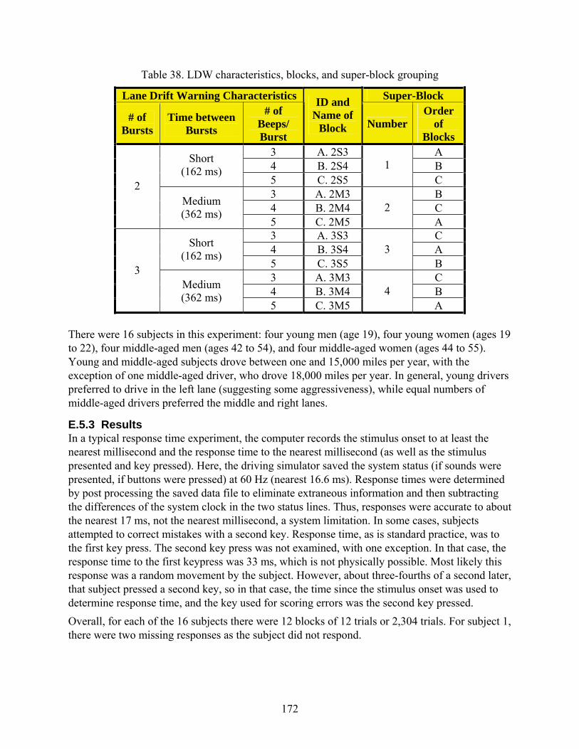
Table 38. LDW characteristics, blocks, and super-block grouping
Lane Drift Warning Characteristics
# of Bursts
Time between Bursts
# of Beeps/ Burst
3 4
Short (162 ms)
5 3 4
2 Medium (362 ms)
5 3 4Short
(162 ms) 5 3 4
3 Medium (362 ms)
5
Super-BlockID and Name of
Block Number Order
of Blocks
A. 2S3 A B. 2S4 B C. 2S5
1 C
A. 2M3 B B. 2M4 C C. 2M5
2 A
A. 3S3 C B. 3S4 A C. 3S5
3 B
A. 3M3 C B. 3M4 B C. 3M5
4 A
There were 16 subjects in this experiment: four young men (age 19), four young women (ages 19 to 22), four middle-aged men (ages 42 to 54), and four middle-aged women (ages 44 to 55). Young and middle-aged subjects drove between one and 15,000 miles per year, with the exception of one middle-aged driver, who drove 18,000 miles per year. In general, young drivers preferred to drive in the left lane (suggesting some aggressiveness), while equal numbers of middle-aged drivers preferred the middle and right lanes.
E.5.3 Results In a typical response time experiment, the computer records the stimulus onset to at least the nearest millisecond and the response time to the nearest millisecond (as well as the stimulus presented and key pressed). Here, the driving simulator saved the system status (if sounds were presented, if buttons were pressed) at 60 Hz (nearest 16.6 ms). Response times were determined by post processing the saved data file to eliminate extraneous information and then subtracting the differences of the system clock in the two status lines. Thus, responses were accurate to about the nearest 17 ms, not the nearest millisecond, a system limitation. In some cases, subjects attempted to correct mistakes with a second key. Response time, as is standard practice, was to the first key press. The second key press was not examined, with one exception. In that case, the response time to the first keypress was 33 ms, which is not physically possible. Most likely this response was a random movement by the subject. However, about three-fourths of a second later, that subject pressed a second key, so in that case, the time since the stimulus onset was used to determine response time, and the key used for scoring errors was the second key pressed. Overall, for each of the 16 subjects there were 12 blocks of 12 trials or 2,304 trials. For subject 1, there were two missing responses as the subject did not respond.
172

1 2 3 4 Response Time (s)
Figure 77. Frequency distribution of response times to all warnings (lognormal fit)
0.8 0.9 1.0
Percentiles
% Statistic RT 0.7 (s)
0.5 0.6
Cum
Pro
b 100.0 Maximum 4.23 99.5 2.99 97.5 2.47
0.4 90.0 1.67 0.3 75.0 Quartile 1.10
0.1 0.2
0 .5 1 1.5 2 2.5 3 3.5 4 4.5 Response Time (s)
50.0 Median 0.77 25.0 Quartile 0.57 10.0 0.47 2.5 0.40 0.5 0.33 0.0 Minimum 0.27
Figure 78. Cumulative distribution of response times to all warnings
Figure 77 and Figure 78 show the distribution of response times for all responses. Response times ranged from 0.27 to 4.23 seconds with a mean of 0.93 seconds and a standard deviation of 0.52 seconds. (Again, times were only accurate to the nearest 0.017 second.)
Note: In the figure above and in some subsequent figures, a box plot appears above the probability density function. The vertical sides of the box are the 25th and 75th percentiles, the middle bar is the median (50th percentile), and the diamond shape is the mean. The red underline emphasizes the mean. Potential outliers, shown as individual points, are values 1.5 times the interquartile range beyond the 25th or 75th percentiles.
173

1 2 3 4 Response Time (s)
Figure 79. Frequency distribution of response times to LDW
Table 39 summarizes the responses by stimulus type. The mean response time was 0.92 seconds for correct responses and 1.49 seconds for errors. The error rate was 2 percent, reasonably low. Note that for all warnings, errors took longer the correct responses.
Table 39. Mean response time and number of responses (two missing responses)
Warning
Correct Incorrect
Response Mean
Time (s)
# of Responses Response
Mean
Time (s)
# of Responses
LDW left 0.99 760 1.80 6 LDW right 0.95 763 1.45 5 FCW 0.72 382 1.15 2 LCM left 0.85 180 1.39 12 LCM right 0.93 171 1.51 21
Mean 0.92 2,256 1.49 46
Given that the FCW and LCM warnings were just foils, the remaining analysis focuses on LDW except for an analysis of the error data. Figure 79 and Figure 80 show the density and cumulative distributions for LDW. Responses in excess of three seconds were rare. The mean time for LDW was 0.972 seconds and the error rate 0.72 percent, even lower than for all stimuli, in part because subjects had more practice with the LDW stimuli. Note there were a significant number of responses in excess of 2 seconds, and this was for a simple experiment in which there were no older drivers (consistent with other studies in this project).
174
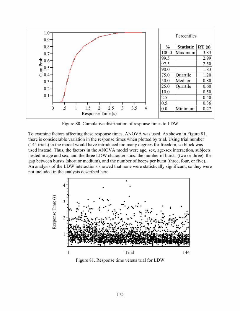
0.9 1.0 Percentiles
0.8 % Statistic RT (s) 0.7 100.0 Maximum 3.83
0.5 0.6
Cum
Pro
b 99.5 2.99 97.5 2.50 90.0 1.83
0.4 75.0 Quartile 1.20 0.3 50.0 Median 0.80
0.1 0.2 25.0 Quartile 0.60
10.0 0.50 2.5 0.40 0.5 0.36
0 .5 1 1.5 2 2.5 3 3.5 4 Response Time (s)
0.0 Minimum 0.27
Figure 80. Cumulative distribution of response times to LDW
Res
pons
e Ti
me
(s)
4
3
2
1
1 Trial 144
Figure 81. Response time versus trial for LDW
To examine factors affecting these response times, ANOVA was used. As shown in Figure 81, there is considerable variation in the response times when plotted by trial. Using trial number (144 trials) in the model would have introduced too many degrees for freedom, so block was used instead. Thus, the factors in the ANOVA model were age, sex, age-sex interaction, subjects nested in age and sex, and the three LDW characteristics: the number of bursts (two or three), the gap between bursts (short or medium), and the number of beeps per burst (three, four, or five). An analysis of the LDW interactions showed that none were statistically significant, so they were not included in the analysis described here.
175

In brief, all factors in the model were very highly statistically significant (see Table 40).
Table 40. ANOVA of LDW response times
Factor DF F p Age 1 114.98 <.0001 Sex 1 211.97 <.0001 Age-sex 1 95.43 <.0001 Subject [age, sex] 12 167.23 <.0001 Block 11 12.80 <.0001 LDW bursts 1 13.47 0.0003 LDW burst gap 1 39.99 <.0001 LDW beeps per burst 1 8.31 0.0040
Figure 82 shows the differences by age, sex, and subject. Of the four groups, the young men responded more rapidly and the middle-aged women were slowest, with the difference within age groups by sex being much larger for middle-aged subjects than younger subjects.
Mea
n R
espo
nse
Tim
e (s
)
0.5
1.0
1.5
2.0
Men
Women
Middle Young
Age
Figure 82. Age, sex, and subject differences Open circles = men, dots = women
In terms of individual subjects, the mean response times for LDW ranged from 0.62 to 2.14 seconds, a factor of 3.5. In part, that wide range is due to one subject, without whom the maximum response time was 1.614 seconds. In general, subjects that had long responses times also tended to make more errors (r = 0.29). Figure 83 shows the data for all warnings except LDW.
176

Mea
n R
espo
nse
Tim
e (s
)
2.00
1.75
1.50
1.25
1.00
0.75
0.50 0 5 10 15
Number of Errors per Subject
Figure 83. Errors versus response time for all warnings by subject
Particularly noteworthy are subjects 14 (a middle-aged man) and 9 (a middle-aged woman) who had the longest response times (2.14 seconds) and largest error rates (12%), respectively. Figure 84 shows the effects of practice (blocks). The decline is fairly steady, about 0.03 seconds per 12 trial blocks. Thus, counterbalancing blocks (with which the warning combination was fixed) to avoid confounding warning characteristics with practice was very appropriate.
Mea
n R
espo
nse
Tim
e (s
)
0
200
400
600
800
1000
1200
1 2 3 4 5 6 7 8 9 10 11 12
Block
Figure 84. Response time by block
177

Table 41. Mean response times to LDW variations
Short Gap Medium Gap TotalLDW Bursts 3 4 5 3 4 5
2 0.89 0.89 0.94 0.98 0.99 1.01 0.953 0.87 0.95 1.02 1.07 1.05 1.09 1.01
Total 0.88 0.92 0.98 1.02 1.02 1.05 0.99Gap means 0.93 1.03
178
The most important practical differences are those due to tone timing. As shown in Figure 85, as the warning duration increases from about 1,000 ms to about 1,700, response time increases from about 850 to just over 1,000 ms. For warning durations greater than 1,700 ms, there are no changes in response time.
0 500 1000 1500 2000 2500 3000
Warning Duration (ms)
Figure 85. Effect of warning duration on mean response time per warning
0
200
400
600
800
1000
1200R
espo
nse
Tim
e(m
s)
To support further analysis, Table 41 shows all of the data and Figure 86 shows the relationships of interest. Overall, response time increases with number of beeps per burst (0.95, 0.97, 1.02 seconds), a relatively small increase of 0.07 seconds. Also having an effect was the gap between bursts, increasing response time from 0.93 to 1.03 seconds, a 0.10 second difference or just over 10 percent. Finally, going from two to three bursts increases response time from 0.95 to 1.01 seconds, a rather small difference of 0.06 seconds. Thus, to minimize response time, these data indicate LDW should involve two or bursts of three beeps, and the gap between them should be short (162 ms). The result that response time for three three-beep bursts was less than 2.0 seconds probably reflects random variation in the data.

Res
pons
e T
ime
(s)
1.15
1.1
1.05
1
0.95
0.9
0.85
0.8
2, short
2, medium
3, short
3, medium
2 3 4 5 6
Number of Beeps per Burst
Figure 86. Relationship of LDW variations to response time
Figure 87, Figure 88, and Figure 89 show the relationship between the warning duration and response time, which were well correlated (r = 0.78). As shown in Figure 87 and Figure 88, neither the number of beeps nor the number of bursts (both repetitions of sound) had any systematic effect on the relationship between these two measures. However, increasing the burst gap (Figure 89) elevated the relationship between warning duration and response time (i.e., it added a pure delay). One interpretation of this result is that increasing the delay only has the effect of increasing response time.
1100
Mea
n R
espo
nse
Tim
e (m
s) 1050
1000
950
900
850
800 -500 0 500 1000 1500 2000 2500 3000
Warning Duration (ms)
Figure 87. Warning duration versus response time, number of beeps highlighted Open circle = five beeps, dark dot = four beeps, small dot = three beeps.
179

800
850
900
950
1000
1050
1100
Mea
n R
espo
nse
Tim
e (m
s)
-500 0 500 1000 1500 2000 2500 3000 Warning Duration (ms)
Figure 88. Warning duration versus response time, number of bursts highlighted Asterisk = Three bursts, dot = Two bursts
800
850
900
950
1000
1050
1100
Mea
n R
espo
nse
Tim
e (m
s)
-500 0 500 1000 1500 2000 2500 3000 Warning Duration (ms)
Figure 89. Warning duration versus response time, burst gap highlighted Y = 362 ms burst gap, small dot = 162 ms gap
Table 42 shows the number of errors. Notice there were more errors with medium gaps than short gaps (eight versus three), more errors with two bursts versus three (ten versus one), and,
180

surprisingly, more errors with more beeps per burst (one, three, seven) for three, four, and five beeps per burst. Thus, shortening the warning increases errors (giving subjects less information), except for changes in the number of beeps per burst, which has the opposite effect. Bear in mind all of this is based on a very small sample of only 11 errors. To provide further context, for LDW alone, there was no correlation between the number of errors and response time (r = 0.04) or the number of errors and warning duration (r = -0.09).
Table 42. Number of errors for LDW
Short Gap Medium Gap TotalLDW Bursts 3 4 5 3 4 5
2 2 1 1 1 5 10 3 1 1
Total 2 1 1 1 6 Gap means 3 8 11
Examining these data by subject provides some context. Notice, in Figure 81, that all but two of the errors were from middle-aged subjects. (Note: Two responses were missing for subject 1.) Furthermore, of all 11 errors, five (almost half) were made by one subject (# 9). The small number and distribution suggests not placing too much emphasis on the number of errors.
Table 43. Number of errors by subject
Age Sex Subject # of Errors Young Men 1 1
2 0 3 0 4 0
Women 5 0 6 0 7 1 8 0
Middle Men 9 5 10 1 11 0 12 3
Women 13 0 14 0 15 0 16 0
Total 11
As noted earlier, Nowakowski, Friedman, and Green (2001) found that when presented with an intermittent sound (a ringing phone), people tended to pick up the phone in the silent period of the ring, as if listening to the ring interfered with responding to it. In fact, the same may be true here for LDW.
181

Since the LDW variants presented consisted of a variety of burst and warning durations, there are a number of ways to determine the likelihood of a response. One way involves comparing responses to two different warnings of similar durations, in this case, 2s4 (two bursts of four beeps) with a medium (362 ms) gap and 3s3 (three bursts of three beeps) with a short (162 ms) gap. The duration of the 2s4 warning is 1,352 ms and 1,751 ms for 3m3, a difference too small to matter. Table 44 shows the number responses in each period of the warnings along with the rate at which they occur. Keep in mind there was a delay 16 ms before the first beep, included here in the time for the first burst. The interesting data that pertain to the respond in silence hypothesis is the response rate column, the number of responses per ms. For the 2m4 warning, the burst 1 data can largely be ignored, since the subjects can respond before 503 ms. However, in comparing gap 1 and burst 2, per unit time, subjects were 1.8 times more likely (0.127/0.070) to respond during the silent period (the gap). For the 3s3 warning, the number of responses per ms was about the same for the two gaps (0.111 and 0.099), but there was a substantial difference in the rates for the two bursts (0.181 and 0.042). These data do not support the response in silence hypothesis. Further analysis is needed.
Table 44. Comparison of 2s4 and 3m3 warnings
Pattern-> 2m4 (1352 ms warning) 3s3 (1351 ms warning)
Period #
Responses in Interval
Interval Duration Response
/ms(ms)
# Responses in Interval
Interval Duration Response
/ms(ms) Burst 1 19 503 0.038 1 353 0.003 Burst 2 34 487 0.070 61 337 0.181 Burst 3 --. -- 14 337 0.042 Gap 1 46 362 0.127 18 162 0.111 Gap 2 -- -- 16 162 0.099 After warning 28 1748 0.016 18 766 0.023
Total 127 128
E.5.4 Conclusions The central question was how the number of beeps per burst, the time between bursts, and the number of bursts affected driver response time and errors for LDW. For all warnings, response times that involved errors were greater than those not involving errors, which often suggests extra steps in the decision-making process for error trials. However, when only the data for LDW were considered, there was no overall relationship between response time and errors, probably because the number of errors was small (11, five of which were made by one subject). Increasing the burst gap increased the number of errors, as did increasing the number of beeps per burst. If anything, increasing the amount of information should reduce errors, not increase them. That was the case for the number of bursts, with far fewer errors for three bursts than one. Thus, the error data suggest the recommended pattern should be three bursts of three beeps, with a short gap (162 ms) between them.
182

The response time data present a similar picture. Each beep within a burst increased response time by 0.033 seconds. Interestingly, that beep lasted 0.037 seconds followed by a 0.113 second delay (0.150 seconds total time). Adding a beep did not just add a pure delay to response time, especially since adding a beep to a burst meant adding several beeps to the sequence (since there were two or three bursts). Based on the data, to minimize response time, there should be three beeps per burst. In terms of gaps between bursts, going from short (0.162 seconds) to medium (0.362 seconds) duration increased response time by 0.104 seconds, a statistically significant amount close to 10 percent. Thus, the shorter duration (0.162 seconds) is recommended. (The recommendation is not for exactly 0.162 seconds, but this experiment only examined two durations, 0.162 and 0.262 seconds, and the shorter duration was much better.) The exact function relating burst gap to response time is unknown, so it could be that times larger or smaller than 0.162 seconds are optimal. Accordingly, the recommendation is the gap should be approximately 0.162 seconds. Finally, there is the issue of the number of bursts. The time difference between two and three bursts was only 0.059 seconds, a relatively small difference given that even the shortest possible burst (three beeps plus two gaps between beeps) was 0.337 seconds. Thus, the recommendation is for two bursts, but the cost of going to three is small. The overall recommendation is three beeps per burst, a burst gap of 0.162 seconds, and two or three bursts (two preferred). In the data collected, the response times for those two situations were 0.887 and 0.975 seconds. However, to designers, the question sometimes is not how long drivers took on average to respond, but how often they were over some maximum time limit. Since that limit is unknown, the cumulative response times for those two situations are shown in Figure 90 and Figure 91 for the two-burst case (mean and standard deviations of 0.866 and 0.400 seconds, respectively), and Figure 92 and Figure 93 for the three-burst case (mean and standard deviations of 0.870 and 0.404 seconds, respectively). As apparent in Figure 90 and Figure 92, the shapes of both distributions of response times appear to be log-normal. Note that the maximum for the two-burst case was 2.7 seconds and for three bursts it was 2.1167 seconds. Again, the value of the cumulative distribution function is that it makes it easy to determine if a particular response time is over some limit. The argument has been made that the mean time to a warning is a secondary indicator of a warning’s performance and the primary consideration is if the response time exceeds some maximum (e.g., the driver responds too late).
183
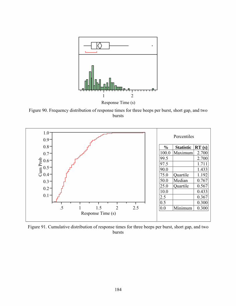
1 2
Response Time (s)
Figure 90. Frequency distribution of response times for three beeps per burst, short gap, and two bursts
0.1 0.2 0.3 0.4 0.5 0.6 0.7 0.8 0.9 1.0
Cum
Pro
b
.5 1 1.5 2 Response Time (s)
2.5
Percentiles
% Statistic RT (s) 100.0 Maximum 2.700 99.5 2.700 97.5 1.711 90.0 1.433 75.0 Quartile 1.192 50.0 Median 0.767 25.0 Quartile 0.567 10.0 0.433 2.5 0.367 0.5 0.300 0.0 Minimum 0.300
Figure 91. Cumulative distribution of response times for three beeps per burst, short gap, and two bursts
184

1 2 Response Time (s)
Figure 92. Frequency distribution of response times for three beeps per burst, short gap, and three bursts
Cum
Pro
b
1.0 0.9 0.8 0.7 0.6 0.5 0.4 0.3 0.2 0.1
.5 1 1.5 2 2.5 Response Time (s)
Percentiles
% Statistic RT (s) 100.0 maximum 2.167 99.5 2.167 97.5 1.885 90.0 1.567 75.0 quartile 1.025 50.0 median 0.733 25.0 quartile 0.575 10.0 0.467 2.5 0.408 0.5 0.333 0.0 minimum 0.333
Figure 93. Cumulative distribution of response times for three beeps per burst, short gap, and three bursts
Finally, to further assist with application, the log transforms of those values are presented. Figure 94 and Figure 95 show the density and cumulative distributions for the log transformed case for two bursts (and short gaps, three beeps). Notice that the density function is very close to normal and the cumulative function is linear from -1 to 0.6 log units. Using that result and the log mean and standard deviations (-0.242, 0.445), precise estimates for the probabilities of various response times can be determined.
185

0.1 0.2 0.3 0.4 0.5 0.6 0.7 0.8 0.9 1.0
Cum
Pro
b
-1 -0.5 0 .5 Log Response Time (s)
1
Percentiles
% Statistic RT (s) 100.0 maximum 0.993 99.5 0.993 97.5 0.537 90.0 0.360 75.0 quartile 0.175 50.0 median -0.266 25.0 quartile -0.568 10.0 -0.836 2.5 -1.003 0.5 -1.204 0.0 minimum -1.204
Figure 95. Cumulative distribution of log response times for three beeps per burst, short gap, and two bursts
-1 0 1 Log Response Time (s)
Figure 94. Frequency distribution of log response times for three beeps per burst, short gap, and two bursts
Figure 96 and Figure 97 show the density and cumulative distributions for the log transformed case for three bursts (and short gaps, three beeps). Notice that the density function departs a bit from normality, with a few long response times. That is also reflected in the slight departure from linearity of the cumulative function (from -1 to 0.8 log units). Using that result and the log mean and standard deviations (-0.231, 0.419), precise estimates for the probabilities of various response times can be determined. Beyond these specific warning characteristics, there is the more general issue of how elongating a warning influences its associated response time. For LDW, the shortest response times
186

-1 0 Log Response Time (s)
Figure 96. Frequency distribution of log response times for three beeps per burst, short gap, and three bursts
0.1 0.2 0.3 0.4 0.5 0.6 0.7 0.8 0.9 1.0
Cum
Pro
b
-1 -0.5 0 .5 Log Response Time (s)
1
Percentiles
% Statistic RT (s) 100.0 maximum 0.773 99.5 0.773 97.5 0.634 90.0 0.449 75.0 quartile 0.025 50.0 median -0.310 25.0 quartile -0.554 10.0 -0.762 2.5 -0.898 0.5 -1.099 0.0 minimum -1.099
Figure 97. Cumulative distribution of log response times for three beeps per burst, short gap, and two bursts
occurred to warnings whose duration was approximately the mean response time, here about one second. Increases in the warning duration up to 1.7 times the mean response time increased the response time by about 100 ms (10%, an important practical difference). Further increases in warning duration had negligible effects on response time.
187

E.5.5 Forms
E.5.5.1 Biographical Form
Date: ___________ Participant #: ____
You
Name: _______________________________________ Sex (circle one): { M } { F }
Age ____
Phone: ( ____ ) ______________ E-mail address: _____________________________
Occupation: _____________________________________________
(engineer, teacher, etc.; if retired, write “retired” and list previous occupation)
Is English your first language? { Yes } { No }
Education (circle highest level completed):
{ High School } { Some College } { College Degree } { Graduate School }
If you attended college, what was your major? ________________________________
Your Driving
Which motor vehicle do you drive most often?
Year ___________ Make _______________ Model _____________________
Approximately how many miles do you drive per year? ________________
For an expressway with 3 lanes in each direction, in which lane do you drive most often?
(circle one) { Left } { Middle } { Right }
May we contact you for future UMTRI studies? { Yes } { No }
Scoring for hearing test (experimenter use only):
188

E.5.5.2 Instruction Script Experiment Introduction and Preparation
Greet Subject <Introduce self> Thank you for coming in today. Before we get started, you will need a visitor parking pass for UMTRI. Please place this pass face-up on your dashboard and when you return, we can start the experiment.
<When they return> Let's go to the conference room and get started.
Lead subject to conference room
Overview (in conference room) First, a brief overview of the study and what you will be doing. The purpose of this study is to test the safety and usability of in-vehicle warning systems that could make the next new vehicle you buy much safer to drive. The experiment will take place on the second floor where another experimenter will collect data on you while you as you push buttons in response to different sounds. More details about the experiment will be provided in the laboratory downstairs.
The entire experiment will take about a half hour to complete. At the end you will receive $20 as thanks for your participation. You may choose not to continue with the experiment at any time. If you do choose not to complete the experiment, you will still be paid.
To examine how effective these in-vehicle systems are, we will be recording your actions and what you say for the entire time you are driving in the simulator. In addition to using these recordings for data analysis, it is possible that we (UMTRI), or the Department of Transportation (who is funding this project), may use portions of your videotape in presentations or in the study reports. Furthermore, our work sometimes appears in the media so there is a chance that some portion of your tape will be shown on TV. If your tape is used for these purposes, your name, driver’s license number, and any other personal information that could be used for identification would never be used. Personal information would not leave UMTRI as it is used only for verification and, if you choose, to contact you about future UMTRI studies. Do you have any questions about how the video data we collect today may be used?
Answer any questions they have to the best of your ability
Is it alright with you if we videotape you during the experiment?
If “no,” dismiss subject
Before moving on to the laboratory, read and sign the consent form and answer some questions about yourself. If they did not participate in a previous experiment, I will also test your hearing. Then we will go to the driving simulator laboratory, though you will not be driving.
Consent and Bio Forms Here is the consent form, please read it carefully and sign at the bottom when you are finished.
If the subject does not read the consent form, say: Even though I have covered the basics of the information on the form, please make sure you read it thoroughly. It may seem annoying, but we are required to make sure that you understand this information.
Thank you. Would you like a copy for yourself?
If yes, have them sign another form to keep
Here is the biographical data sheet. Please fill it out and feel free to ask me questions at any time.
Provide bio form (Check that both forms are legible and complete)
Payment Form All right, just one more form for you to fill out.
This is the payment form you need to fill out in order to get your money at the end of the experiment. Are you a University employee?
189

If “yes”, have them fill out University Employee form
Ok, just go ahead and fill this out. Although it says you’ve already received the money, I’d like you to go ahead and sign it anyway. It speeds up the process for us so you can fill out all the paperwork at once. Let me know if you have any questions while you’re filling this out.
We are done with the preliminary paperwork.
If they did not participate in a previous experiment: Now I need to check your hearing.
Otherwise, walk them down to the sim.
Hearing Test Make sure the office door is closed so it’s quiet.
In this test we will be testing the full range of hearing. Very few people are capable of hearing all of the tones presented.
I am going to play you a series of tones. Please raise your hand for whichever side you hear the tone. So if you hear a tone in your left ear, raise your left hand and vice versa.
To check the procedure, a practice tone will be presented, and then the hearing evaluation will start. Go ahead and put on these headphones, the red goes on your right ear.
Play a sample tone at 35 dB and 1500 Hz (either ear).
Ok, now we’re going to start the hearing evaluation.
Do all tones for one ear in sequence. Make sure the subject cannot see which ear is being tested. Move dial to 25 dB and play 2 tones a 1000 Hz, 2 tones at 2000 Hz, and 2 tones at 3000 Hz. Wait after playing each tone for a response. If they miss a tone, increase the dB by 5 dB each time until they hear the tone 2 times successfully. Record the dB level on the screening sheet. Continue by testing the other ear. Maximum passing values are: 45 dB for 1000 Hz, 55-60 dB for 2000 Hz, and 65 dB for 3000 Hz. If they do not pass, pay and dismiss the subject.
The hearing evaluation is complete. Let’s go to the driving simulator laboratory for the rest of the experiment.
Take subject to simulator
In the Simulator
Seat Subject Please have a seat in the cab and adjust the seat to a comfortable position using the automatic controls on the left side of the seat. The cameras and microphones around the vehicle will be used to record your reactions.
Set up the sim
x Flip sign on door x Secondary Task computer must be on (Mac on wall) x Switches by front and back wheels must be on x Rotate steering wheel (see Sim instructions) to make buttons work x On 16 x 16 Switcher/ “Knox” (to the right of monitors), press [R] [0] [1] [EN] to display the desired
images x Rack Power 1 (to the right of monitors) must be on x Audio (to the right of monitors) must be on x On IP Monitor computer
- Open E5 Subtask 1Folder - Open E5 Subtask 1 File (executable, paper with pencil) - In program, click “Input from text file” - Program may be left on
x On HyperDrive computer
190

- If program was closed, click on the Simulator menu and select an item under Set Active Sim - Open E5 Subtask 1 File - Uncheck box on HyperDrive program
For the experiment you will be pressing either the X or Y button in response to certain sounds. There are a total of three sounds, but you’ll only be using two buttons. So, if you hear one sound, which we’ll play you in a minute, press the X button. If you hear either of the other two sounds, press the Y button. The experiment will take about 15 minutes, including a short break halfway through.
Do you have any questions?
Ok then, now I’ll play you the sounds so you can become familiar with them.
Practice Period There are three different sounds. Two of the sounds can come from either your left or right side. When you hear each of the sounds, you will press a specific button. Make sure that when you press a button, hold it down for half a second or so.
To play a sound x On IP Monitor computer, pick each sound to play and press Start, and then Stop after the sound is
played.
The first sound (LDW) can be identified as a series of low beeps. Some features of the sound will vary, but the pitch of the sound will remain the same. When you hear this sound coming from your left side, press button X (Play LDWL). The same sound can also come from the right side. When you hear this sound (Play LDWLR), press button Z.
For the next two sounds, press the Y button. The first sound can be identified by a series of high-pitched beeps (Play FCW). The next sound can be identified by low-pitched beeps followed by high-pitched beeps. It can come from either your left or right, but in either case press the Y button (Play LCML and LCMR).
When you’re responding to these sounds, it’s important to be both accurate and fast. Please don’t sacrifice one for the other.
Do you have any questions?
Now I’m going to have you practice responding to the sounds. Please press the button and say the letter on the button you press each time. Make sure that when you press a button, you hold it for a half a second or so. We’ll keep going until you get eight in a row correct. Do you have any questions?
To play a practice block x On HyperDrive computer, press Start (so it connects to IP Monitor computer) x On IP Monitor computer, pick a random subject, press Start, and press Stop after the subject has
gone through eight trials correctly (don’t save or change name of data file)
Alright, it looks like you’re ready to begin the actual experiment. You’ll be done in about 15 minutes, and halfway through we’ll give you a break to get up and stretch if you need to. So, from now on, you only need to press the button, you don’t have to tell me the letter of the button anymore. If you press an incorrect button for a sound, I’ll temporarily stop the experiment and tell you what was the correct response. As I said before, be prepared that some features of the warnings will change during the experiment, but the warnings will always remain identifiable by their pitch, which will not change.
Data Collection Do you have any questions? Ok, remember it’s important to be both accurate and fast, and to press and hold each button for about half a second.
To set up the sim x Make sure there is a new tape in the VCR x On VCR, Press Record and Play simultaneously to start recording video x On HyperDrive computer, press Start x On IP Monitor computer, pick the corresponding subject number and press Start
191

x Give subject short break after Block 6 is finished; press stop on IP Monitor computer, don’t press stop on HyperDrive
x On IP Monitor computer, press Start x Play through the remaining 6 blocks until Block 12 is finished
That’s it for this part of the experiment. x Press stop on the VCR x Label tape
Saving data 1. Click Stop on the HyperDrive 2. Click IVBSS Subtask 1.5 folder on the HyperDrive computer. 3. Change the name of the file labeled last. subject to S(subject number)(subject initials)(date).txt, for
example, S01DM073107.txt. Make sure the file datacol.txt is not in the folder. If it is, it means last subject is not complete; wait until datacol.txt disappears.
4. After four or five subjects are saved, save again on a thumb drive in case the computer crashes.
If a data file doesn’t save (on HyperDrive) 1. Click the Help menu 2. Go to Manually Retrieving a Data Collection File, which will tell you where to go 3. Click on the right-most button in the group of buttons next to Start on Windows. 4. Highlight Sim Host Data File 5. Click Connect 6. Click on E1 Subtask 5 folder 7. Highlight datacol.txt 8. Select File, Download To… 9. Select C:/ ÆProgram Files ÆHyperDrive Æ Data Simulator ProjectsÆ E1 Subtask 5 Æ Collected
Data then click Save 10. Click on E1 Subtask 5 Folder on Desktop 11. Rename file (see Saving Data)
Wrap-Up Walk subject downstairs and thank them for coming. At the end of the day x Flip over sign x Turn off four stacked monitors to the left of IP Monitor and HyperDrive x Turn off electronics on rack to the right of monitors x Turn off buck switches
192

E.5.5.3 Hearing Screening Test
193
Appendix F: Experiment 2 – Driver Response to Warnings
F.1 Overview This experiment addressed three sets of questions: x How do drivers respond to real and false warnings, and, especially, where do they look?
Two states were examined: (a) the first time or few times a particular warning is presented (“surprise-uninformed driver” condition) and (b) after drivers are fully informed of its functioning.
x Do drivers respond differently to warnings when they are distracted? x How well do drivers respond to the set of IVBSS warnings? Are any warnings confused
or misunderstood?
As noted in the literature review (Appendix D), there is considerable information on driver responses to warnings, especially characteristics such as the intensity of sounds. However, very little is known about the process of interpreting sounds. If drivers hear a warning, do they start a search of the entire scene, look to a particular area, or just respond to the warning without checking the scene? How does the response process depend on the information conveyed in a warning? For example, most lateral drift warnings (LDWs) contain directionality information. Does providing directionality affect the process by which drivers respond? Furthermore, for some types of warnings, the set of potential actions is limited. For forward collision warning (FCW), the response is to brake and to steer, whereas for LDW, it is to steer. In a very general way, knowing how people respond to a specific warning will suggest how (visually, auditorily, and haptically) and when each warning should be presented and what it should contain. Given the need to understand the process, eye fixation data were collected in addition to driving performance data. How drivers respond may depend on whether they are distracted. It is precisely when drivers are not looking at the road that a warning system would be most valuable. Hence, conditions to assess distraction were included in this experiment. Finally, every major simulator experiment in this project addressed whether warnings were understood and distinguishable. Given that the warning set evolved throughout this project, warning understandability and confusion need to be examined in every experiment in this project.
F.2 Method This experiment was conducted in the UMTRI driving simulator (details in Appendix A) and was the first experiment involving the wide field of view (200 degrees forward and 40 degrees to the rear) implementation. As a reminder, the simulator consists of a vehicle cab (with a computer-generated instrument panel and torque feedback on the steering wheel), screens 16 feet from the driver, directional audio, and multiple video cameras to record driver performance. The scripts controlling vehicle behavior were moderately engaging.
194

Test roads consisted of variety of curved and straight sections, with construction zones on some straight sections. Some traffic was always presented, usually ahead of the subject in the same lane, but also in an adjacent lane, and there were usually several following vehicles. There were occasional lateral gusts sufficient to push the subject out of the lane. The basic procedure was used for the major simulator experiments, experiments 2 through 5. The experiment consisted of a single two-hour test session. Given the need to cover administrative matters, biographical forms, post-tests, and other paperwork, the estimated time available for driving was about one hour and 15 minutes (75 minutes), including practice time. Given that guidance, the task sequence and timing shown in Table 45 was developed.
Table 45. Estimated duration of experimental tasks, experiment 2 (see section F.5 for experiment 2 instructions and post-test forms)
Task Category Description Approximate Duration (min)
Preparation (15 min)
Filling out biographical data form 5 Reading and signing consent form 5 Vision and hearing tests 5
Set-up, training and practice (36 min)
Simulator introduction 3 Eye-tracking set-up 15 Practice driving in the simulator (practice world) 3 Distracting task instructions 3 Practice distracting task 3 Practice driving in the simulator while performing the distracting task (practice world)
4
Final eye-tracking adjustments 5 Data collection (70 min)
Break 2 First block 15 Break 2 Second block (with secondary task) 15 Break 4 Third block 15 Break 2 Fourth block (with secondary task) 15
Wrap-up (10 min) Fill out post-test and payment 10 Total 131
F.2.1 World Design Subjects drove on expressways with a divided median, two lanes per direction, at a posted speed of 70 mph, the posted speed on expressways in the Ann Arbor, Michigan, area. The basic design of the world was a loop, chosen because the project timeframe did not allow for development and testing of a world where every section would be unique. The road loop for experiment 2 was designed so that subjects would drive two loops per block and each block would take about 15 minutes (Figure 98). Subjects drove four blocks total (eight loops). Each loop had eight straight
195

sections (in civil engineering terms, tangents), each of which could contain one or more trial, but each trial could contain only one scenario. Furthermore, to avoid the expectation of exactly one event per straight section, the 2,400-meter straight section has multiple trials (two 1,200-meter trials), so there were eight straight sections and 18 opportunities for events per loop. Starting and ending each block in the middle of the 2,400-meter segment, using both left and right turns, and varying the length of each straightaway (no two were the same) made the route difficult for subjects to memorize. Of particular concern was avoiding subject being able to guess when a straight section would end (or which events occurred), when a curve would appear, and in which direction they would turn.
Figure 98. Configuration of the world for IVBSS experiment 2 = The two construction zones, one in each lane.
196

Table 46. Warnings from experiment 1, subtask 3, suite A
Warning Pitch (Hz) Pulse (ms) Onset (ms) Offset (ms) Pulses FCW(abstract)
1500 Hz fundamental freq. 4 odd harmonics
(4500,7500,10500, 13500 (square wave))
100(70 pulse followedby 30 ms silence)
5exponentialrise
20exponentialdecay
7
LCM (honk) 1,000 (fo) 160 (150 ms sound)
CSW (tires) 600 30
LDW(rumble)
400 (fo) 150 (50 ms sound)
10
Table 47. Warnings used in the order in which experiments occurred
Experiment FCW CSW LDW LCM 2
3 See Table 48 and Table 49
See Table 48 and Table 49
See Table 48 and Table 49
See Table 48 and Table 49
4
(+ brake pulse) Seat shakes
5
(+ brake pulse) Seat shakes
1, subtask 5 �
None� See note�
F.2.2 Warnings and Warning Triggers In the main simulator experiments (experiments 2 through 5), the warnings evolved from experiment to experiment. Warnings used in experiment 2 were selected based on the findings from experiment 1, subtasks 1 through 4. The physical characteristics of the warnings in experiment 2 were identical to those used in experiment 1, subtask 3, suite A (see Table 46).
Warnings used in the other experiments are shown in Table 47 (experiment 1, subtask 5 occurred after experiment 5, so it is shown last). Warnings used in experiment 3, which varied with the test condition, are shown in Table 48 and Table 49.
Note: For experiment 1, subtask 5, the LDW combinations were two or three bursts for three, four, or five beeps with gaps of 162 ms (short) or 362 ms (medium) between them.
197

Table 48. Warnings used in experiment 3
FCW CSW LCM LDW
Single warning Single sound 1
Bottom seat vibration both sides together Dual warning-simple Two sounds
1 (L) (R) 5 Brake pulse Seat shaker (L) (R)
Dual warning-hybrid Two sounds 1 (L) (R)
3 -----
combined Brake pulse ----- ----- Seat shaker (L) (R) Multiple warnings Four separate sounds
1 2 (L) (R) 3
(L) (R) 4
Brake pulse ----- ----- Seat shaker (L) (R)
Table 49. Characteristics of warning sounds in experiment 3
Warning Pitch (Hz)
Pulse Rate (ms)
Duration (ms)
Onset (ms) Pulses
Tone 1 (abstract) 1,500 100 70 5 7 Tone 2 (tires) 600 30 Tone 3 (honk) 1,000 160 150 Tone 4 (rumple strip) 400 150 50 10 Tone 5 (abstract) 500 110 10 4
Experiment 4 used a Visteon revision of the FCW sound. As before, there were seven 100-ms bursts (70 ms on, 30 ms off), with a fundamental frequency of 1,500 Hz. However, there were only two odd harmonics (4,500 and 7,500 Hz), making it a low-fidelity square wave. The pulse onset and offset were exponential (6 ms and 20 ms, respectively) as before. Experiment 4 also used a Visteon revision of the LCM sound with a base frequency of 415.3 Hz (an Ab4 pitch). The waveform is square with three odd-numbered harmonics. (Square waves have only odd harmonics.) The five pulses had start times 150 ms apart. The duration of each pulse was 50 ms. (The silence between pulses was 100 ms.) The onset was linear over 1 ms, effectively immediate. The offset was 20 ms and the decay was linear. Experiment 5 used another Visteon revision of the LCM sound, though this sound was not used by Visteon because it sounded cartoonish. The LCM sound had some modulated frequency components. The basic waveform was a square wave containing three odd harmonics. The frequency of the lower note was 415.3 Hz (Ab4) and the higher note was 440 Hz (A4). The sound consisted of three 80-ms pulses with a 40 ms delay at the start, but no silent gaps within each triple set of pulses. Pulse onsets were exponential over 10 ms and pulse offsets were
198

exponential over 30 ms. A complicating factor was that each pulse frequency was ramped up from a frequency half of the final frequency in the first 20 ms (of the 80-ms pulse duration). Table 50 and Figure 99 show the criteria for triggering warnings. The criteria were the same for all experiments except experiment 5, where the delay varied among test conditions. All checks of triggers occurred at 60 Hz.
Table 50. Warning trigger and retrigger criteria
Warning Initial Trigger Criteria Retrigger Criteria
Experiments 2, 3,4 Experiment 5 All Experiments FCW Time to collision (computed
using distance to other vehicle and closing velocity) < 6seconds
Time to collision < 6 seconds (wait 0, 0.15 or 0.30 seconds to check the subject is back in the lane or makes a large correction (steering wheel angle < 2 degrees for left lane, >-2 degrees for right lane))
Wait 5 seconds after last trigger before checking
CSW* At 50 meters before the curve (point of curvature), check if subject velocity > 75 mph
Same Not applicable
LDWƒ If turn signal is off, the subject velocity > 25 mph, and the outer edge of the “middle” tire goes past the centerline of the lane marking (“edge of the lane’)
Same Wait 2 seconds after last trigger before checking
LCMƓ If the subject velocity > 25 mph, the outer edge of the “middle” tire goes past the centerline of the lane marking, and there is a vehicle in the blind spot (less than even with front bumper or less than 8 meters behind)
Same Wait 2 seconds after last trigger before checking
* The criteria were the same as for RDCW. ƒ Departures were determined as if the vehicle had six tires on three axles, one axle at the middle of the vehicle. A
departure occurred when the outer edge of the middle tire touched the centerline of the edge marking. Ɠ Overlap was computed using the center-to-center distance (4 meters forward, 12 meters to the rear).
199

3.6 m wide lane (centerline to centerline)
Other vehicle
subject
Other vehicle
8 m
All vehicles are 4 m long x 1.8 m wide
Figure 99. Warning trigger vehicle geometry
F.2.3 Warning Scenario Frequency and Sequences In the real world, warnings are rare. However, if warnings were to occur with that frequency in experiments, there might only be two warnings per subject (for an entire session), which are far too few to gain the needed insights. Furthermore, real-world warning systems are not completely reliable, which means that drivers need to verify if warnings are correct. Having a false warning occur about one-third of the time balanced the need to generate real-world behavior with collecting data on driver responses to warnings and having false alarms occur as often as they do in the real world (as exemplified by experience from ACAS described earlier). Admittedly, a plan for 33-percent false alarms (or 67-percent reliability) is near the cost-benefit threshold for a related characteristic, automation reliability estimated in a single evaluation (Wickens and Dixon, 2005), but it was important that IVBSS experiments consider likely real-world exposure. As is shown later, how often warnings were planned to occur and how often they actually occurred were quite different. To the extent feasible, it was important for the false alarm percentage to be the same for every warning and every warning scenario so there would be no reliability confounding. However, because of constraints from the simulated world (the sequence of scenarios, the lane position of the subject, and the relative position of traffic, as well as limitations in vehicle movement due to the laws of physics) and scenario construction time, false-alarm percentages were sometimes not equal for each scenario, but were equal by warning. Given all of these constraints, there were 42 warnings total for each subject spread over four blocks (28 true warnings and 14 false alarms; Table 51). Notice that simply deleting a single false alarm for a particular scenario changes the false alarm rate for that scenario from 33 percent (2/6) to 20 percent (1/5). Appendix B contains a detailed description of the warning scenarios.
200
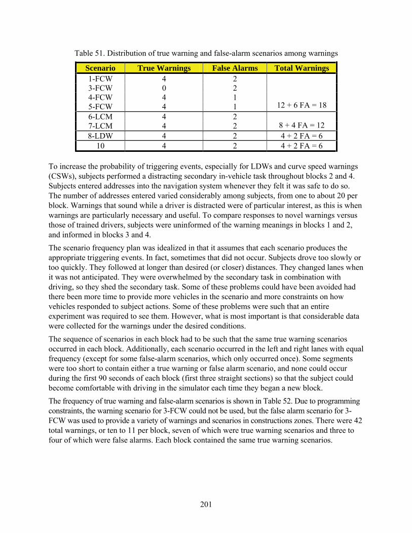
Table 51. Distribution of true warning and false-alarm scenarios among warnings
Scenario True Warnings False Alarms Total Warnings 1-FCW 3-FCW 4-FCW 5-FCW
4 0 4 4
2 2 1 1 12 + 6 FA = 18
6-LCM 7-LCM
4 4
2 2 8 + 4 FA = 12
8-LDW 4 2 4 + 2 FA = 6 10 4 2 4 + 2 FA = 6
To increase the probability of triggering events, especially for LDWs and curve speed warnings (CSWs), subjects performed a distracting secondary in-vehicle task throughout blocks 2 and 4. Subjects entered addresses into the navigation system whenever they felt it was safe to do so. The number of addresses entered varied considerably among subjects, from one to about 20 per block. Warnings that sound while a driver is distracted were of particular interest, as this is when warnings are particularly necessary and useful. To compare responses to novel warnings versus those of trained drivers, subjects were uninformed of the warning meanings in blocks 1 and 2, and informed in blocks 3 and 4. The scenario frequency plan was idealized in that it assumes that each scenario produces the appropriate triggering events. In fact, sometimes that did not occur. Subjects drove too slowly or too quickly. They followed at longer than desired (or closer) distances. They changed lanes when it was not anticipated. They were overwhelmed by the secondary task in combination with driving, so they shed the secondary task. Some of these problems could have been avoided had there been more time to provide more vehicles in the scenario and more constraints on how vehicles responded to subject actions. Some of these problems were such that an entire experiment was required to see them. However, what is most important is that considerable data were collected for the warnings under the desired conditions. The sequence of scenarios in each block had to be such that the same true warning scenarios occurred in each block. Additionally, each scenario occurred in the left and right lanes with equal frequency (except for some false-alarm scenarios, which only occurred once). Some segments were too short to contain either a true warning or false alarm scenario, and none could occur during the first 90 seconds of each block (first three straight sections) so that the subject could become comfortable with driving in the simulator each time they began a new block. The frequency of true warning and false-alarm scenarios is shown in Table 52. Due to programming constraints, the warning scenario for 3-FCW could not be used, but the false alarm scenario for 3FCW was used to provide a variety of warnings and scenarios in constructions zones. There were 42 total warnings, or ten to 11 per block, seven of which were true warning scenarios and three to four of which were false alarms. Each block contained the same true warning scenarios.
201

Table 52. Planned distribution of true warning and false-alarm scenarios among blocks
Block A Block B Block C Block D True warning scenarios
1-FCW4-FCW5-FCW6-LCM 7-LCM 8-LDW10-CSW
1-FCW 4-FCW 5-FCW
6-LCM 7-LCM 8-LDW
10-CSW
1-FCW 4-FCW 5-FCW
6-LCM 7-LCM 8-LDW
10-CSW
1-FCW 4-FCW 5-FCW 6-LCM 7-LCM 8-LDW 10-CSW
False-alarm scenarios
1-FCW 3-FCW6-LCM 8-LDW
1-FCW 3-FCW6-LCM 8-LDW
4-FCW7-LCM
10-CSW
5-FCW 7-LCM
10-CSW
The sequence of scenarios for each block was created using the guidelines in Appendix B. Remember that even though the scenarios used were the same for all subjects, the frequency of warnings varied because driver actions were not completely predictable or controllable, especially for LDW and CSW. The order of test blocks was counterbalanced among subjects. A normal block was presented first for all subjects so that they were not distracted the first time they heard each warning and could begin to establish an idea of what each warning means early in the experiment. Therefore, all subjects started with a normal block and alternated between normal and distracted blocks, as follows (four subjects per age-sex group):
- A, B, C, D - A, D, C, B - C, B, A, D - C, D, A, B
202

Table 53. Sequence of true warning and false-alarm scenarios according to block name (Segments with construction zones are underlined.)
Event # or Direction of Curvature
Length of Segment
(m)
Block A Block B Block C Block D
Loop 1 1200 1 Left
2 600 Right
3 800 Left
4 1000 1-FCW 4-FCW 8-LDW 2-FCW Left
5 1600 FA 3-FCW 8-LDW 7-LCM FA 7-LCM Left
6 400 Right 10-CSW 10-CSW
7 1400 8-LDW FA 6-LCM 4-FCW 5-FCW Left
8 1200 FA 1-FCW 6-LCM Left 10-CSW
9 1200 7-LCM 7-LCM Loop 10 1200 FA 6-LCM 5-FCW FA 4-LCM 8-LDW
2 Left 11 600
Right FA 10-CSW 12 800 FA 8-LDW FA 1-FCW 5-FCW
Left 13 1000 4-FCW FA 8-LDW 56-LCM 4-FCW
Left 14 1600 7-LCM
Left 10-CSW FA 10-CSW 15 800 6-LCM 1-FCW 2-FCW FA 5-FCW
Right 16 1600 6-LCM 1-FCW 2-FCW FA 5-FCW
Left 17 800 5-FCW 6-LCM
Left 18 1200 FA 3-FCW FA 7-LCM
Figure 100 through Figure 103 provide a graphical representation of the sequence of scenarios in each block. Each warning and false alarm scenario is indicated along with the length of each segment (1 tile = 200 meters). Each curve has a 300-meter radius. The circular icons ( ) indicate construction barrels.
203

Figure 100. Block A scenario sequence
204

Figure 101. Block B (distracted) scenario sequence
205

Figure 102. Block C scenario sequence
206

Figure 103. Block D (distracted) scenario sequence
207
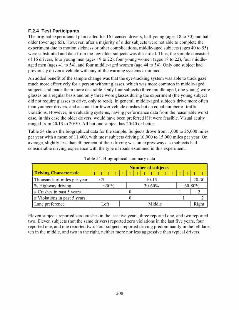
F.2.4 Test Participants The original experimental plan called for 16 licensed drivers, half young (ages 18 to 30) and half older (over age 65). However, after a majority of older subjects were not able to complete the experiment due to motion sickness or other complications, middle-aged subjects (ages 40 to 55) were substituted and data from the few older subjects was discarded. Thus, the sample consisted of 16 drivers, four young men (ages 19 to 22), four young women (ages 18 to 22), four middle-aged men (ages 41 to 54), and four middle-aged women (age 44 to 54). Only one subject had previously driven a vehicle with any of the warning systems examined. An added benefit of the sample change was that the eye-tracking system was able to track gaze much more effectively for a person without glasses, which was more common in middle-aged subjects and made them more desirable. Only four subjects (three middle-aged, one young) wore glasses on a regular basis and only three wore glasses during the experiment (the young subject did not require glasses to drive, only to read). In general, middle-aged subjects drive more often than younger drivers, and account for fewer vehicle crashes but an equal number of traffic violations. However, in evaluating systems, having performance data from the reasonable worst case, in this case the older drivers, would have been preferred if it were feasible. Visual acuity ranged from 20/13 to 20/50. All but one subject has 20/40 or better. Table 54 shows the biographical data for the sample. Subjects drove from 1,000 to 25,000 miles per year with a mean of 11,400, with most subjects driving 10,000 to 15,000 miles per year. On average, slightly less than 40 percent of their driving was on expressways, so subjects had considerable driving experience with the type of roads examined in this experiment.
Table 54. Biographical summary data
Driving Characteristic Number of subjects
1 1 1 1 1 1 1 1 1 1 1 1 1 1 1 1 Thousands of miles per year d5 10-15 20-30 % Highway driving <30% 30-60% 60-80% # Crashes in past 5 years 0 1 2 # Violations in past 5 years 0 1 2 Lane preference Left Middle Right
Eleven subjects reported zero crashes in the last five years, three reported one, and two reported two. Eleven subjects (not the same drivers) reported zero violations in the last five years, four reported one, and one reported two. Four subjects reported driving predominantly in the left lane, ten in the middle, and two in the right, neither more nor less aggressive than typical drivers.
208

F.3 Results F.3.1 How Many Warnings Occurred? During the analysis, some minor errors in implementing the experiment design were noted, and where feasible, corrected manually. Blocks A and B for subject 4 had characteristics of block C (warning for scenario, warning triggered, etc.) and were changed in the coding to block C. Similarly, block C for subject 2 was changed to block D. Some errors were not corrected; for example, the last three trials with planned warnings for block D of subject 2 had the characteristics of block C but were left as block D since changing a block name within the block could not be rationalized. Additionally, the warning presented in block B, trial 13 for all subjects should have been a false alarm LDW but was coded as a false alarm FCW. The third trial in block A of subject 9 included a false alarm FCW trigger, but no warning was planned. Each observed warning falls into one of three categories: triggered as planned, triggered not as planned (e.g., due to a maneuver when no scenario was scheduled, such as an unexpected lane change too close to an adjacent vehicle), and planned but not triggered (because subjects anticipated the scenario and took evasive action to avoid the conflict and therefore the warning). Not surprisingly, the number of warnings observed varied by the type of warning presented, as there were 658 FCWs, 613 LDWs, 225 CSWs, and 159 lane change-merge (LCM) warnings presented for a total of 1,655 warnings (Table 55). Of them, 669 were triggered as planned, and 986 were triggered not as planned. An additional 126 were planned but not triggered. The number of FCWs and LDWs triggered as planned exceeded the expected number of FCWs and LDWs, especially for LDW because both FCWs and LDWs sometimes triggered multiple times for the same planned scenario if the subject did not maneuver his or her vehicle to avoid the situation. Having subjects behave in exactly the desired manner in the multiple sequential scenarios examined was extremely difficult to script, and only after the experiment was complete was there sufficient data to fully know how subjects would respond. As has been noted previously, real warning systems are not perfect and experiments should include false alarms. Of the 1,655 warnings, 207 were false alarms, though the ratio of real to false alarms varied from warning to warning. In all cases, the ratio of real to false alarms was about double of what was planned, except for LDW where the difference was a factor of seven.
209
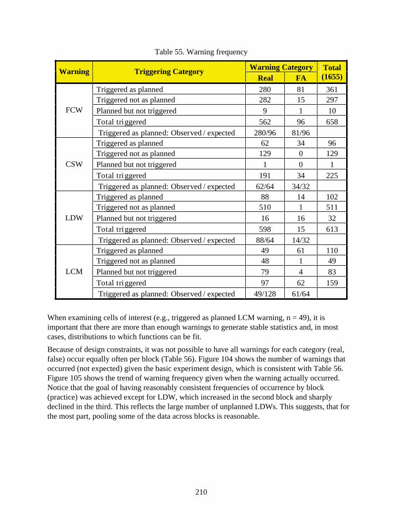
Table 55. Warning frequency
Warning Triggering Category Warning Category Total(1655)Real FA
Triggered as planned 280 81 361Triggered not as planned 282 15 297
FCW Planned but not triggered 9 1 10Total triggered 562 96 658Triggered as planned: Observed / expected 280/96 81/96Triggered as planned 62 34 96Triggered not as planned 129 0 129
CSW Planned but not triggered 1 0 1Total triggered 191 34 225Triggered as planned: Observed / expected 62/64 34/32Triggered as planned 88 14 102Triggered not as planned 510 1 511
LDW Planned but not triggered 16 16 32Total triggered 598 15 613Triggered as planned: Observed / expected 88/64 14/32Triggered as planned 49 61 110Triggered not as planned 48 1 49
LCM Planned but not triggered 79 4 83Total triggered 9 7 62 159Triggered as planned: Observed / expected 49/128 61/64
When examining cells of interest (e.g., triggered as planned LCM warning, n = 49), it is important that there are more than enough warnings to generate stable statistics and, in mostcases, distributions to which functions can be fit. Because of design constraints, it was not possible to have all warnings for each category (real, false) occur equally often per block (Table 56). Figure 104 shows the number of warnings that occurred (not expected) given the basic experiment design, which is consistent with Table 56. Figure 105 shows the trend of warning frequency given when the warning actually occurred. Notice that the goal of having reasonably consistent frequencies of occurrence by block (practice) was achieved except for LDW, which increased in the second block and sharply declined in the third. This reflects the large number of unplanned LDWs. This suggests, that for the most part, pooling some of the data across blocks is reasonable.
210

Table 56. Frequency of expected warnings by block
Warning Warning Category Block A B C D
FCW Real 3 3 3 3 False alarm 3 2 1 1
CSW Real 1 1 1 1 False alarm 1 1 1 1
LCM Real 2 2 2 2 False alarm 1 1 1 1
LDW Real 1 1 1 1 False alarm 1 1 0 0
0
50
100
150
200
250
CSW LCM
FCW LDW
Freq
uenc
y
Block A Block B Block C Block D
Figure 104. Warning frequency by block used for counterbalancing
211

Block 1 Block 2 Block 3 Blocko 4
Freq
uenc
y
250 FCW
CSW LCM
Block 1 Block 2 Block 3 Block 4
LDW
200
150
100
50
0
Figure 105. Warning frequency by block in order of occurrence
The frequency with which warnings occurred differed due to many of the factors of interest. As shown in Table 57, younger drivers received more warnings that middle-aged drivers (Chi-Square (3) = 16.5, p <.0001), with the primary difference being about 20 percent more LDWs. Women received more warnings than men (Chi-Square (3) = 26.0, p<.0001 ) especially for LCM and LDW (Table 58). As expected, uninformed (Table 59) and distracted drivers (Table 60) received more warnings (Chi-Square (3) = 105.1, p<.0001), and Chi-Square (3) = 21.9, p<.0001, respectively). Again, the primary source of these differences was in LDW.
Table 57. Warning frequency by age group
Warning Age Group Grand Total
Statistics Young Middle-Aged Mean SD
CSW 116 109 225 112.5 4.9 FCW 345 313 658 329 22.6 LCM 73 86 159 79.5 9.2 LDW 334 279 613 306.5 38.9 Grand Total 868 787 1655
Table 58. Warning frequency by gender
Warning Gender Grand Total
Statistics Women Men Mean SD
CSW 114 111 225 112.5 2.1 FCW 335 323 658 329 8.5 LCM 93 66 159 79.5 19.1 LDW 338 275 613 306.5 44.5 Grand Total 880 775 1655
212
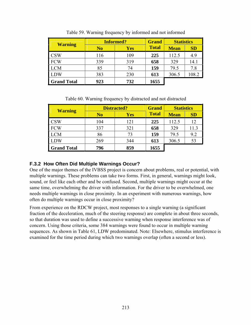
Table 59. Warning frequency by informed and not informed
Warning Informed? Grand Total
Statistics No Yes Mean SD
CSW 116 109 225 112.5 4.9 FCW 339 319 658 329 14.1 LCM 85 74 159 79.5 7.8 LDW 383 230 613 306.5 108.2 Grand Total 923 732 1655
Table 60. Warning frequency by distracted and not distracted
Warning Distracted? Grand Total
Statistics No Yes Mean SD
CSW 104 121 225 112.5 12 FCW 337 321 658 329 11.3 LCM 86 73 159 79.5 9.2 LDW 269 344 613 306.5 53 Grand Total 796 859 1655
F.3.2 How Often Did Multiple Warnings Occur? One of the major themes of the IVBSS project is concern about problems, real or potential, with multiple warnings. These problems can take two forms. First, in general, warnings might look, sound, or feel like each other and be confused. Second, multiple warnings might occur at the same time, overwhelming the driver with information. For the driver to be overwhelmed, one needs multiple warnings in close proximity. In an experiment with numerous warnings, how often do multiple warnings occur in close proximity? From experience on the RDCW project, most responses to a single warning (a significant fraction of the deceleration, much of the steering response) are complete in about three seconds, so that duration was used to define a successive warning when response interference was of concern. Using those criteria, some 384 warnings were found to occur in multiple warning sequences. As shown in Table 61, LDW predominated. Note: Elsewhere, stimulus interference is examined for the time period during which two warnings overlap (often a second or less).
213
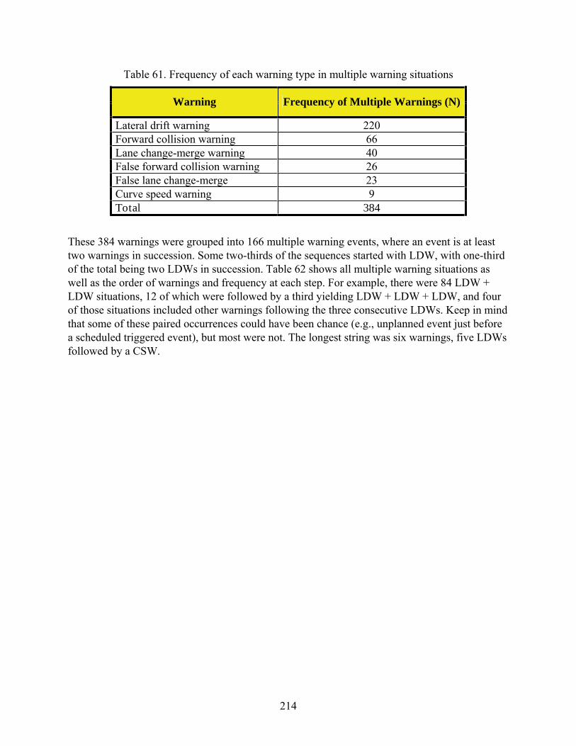
Table 61. Frequency of each warning type in multiple warning situations
Warning Frequency of Multiple Warnings (N)
Lateral drift warning 220 Forward collision warning 66 Lane change-merge warning 40 False forward collision warning 26 False lane change-merge 23 Curve speed warning 9 Total 384
These 384 warnings were grouped into 166 multiple warning events, where an event is at least two warnings in succession. Some two-thirds of the sequences started with LDW, with one-third of the total being two LDWs in succession. Table 62 shows all multiple warning situations as well as the order of warnings and frequency at each step. For example, there were 84 LDW + LDW situations, 12 of which were followed by a third yielding LDW + LDW + LDW, and four of those situations included other warnings following the three consecutive LDWs. Keep in mind that some of these paired occurrences could have been chance (e.g., unplanned event just before a scheduled triggered event), but most were not. The longest string was six warnings, five LDWs followed by a CSW.
214

Table 62. Frequency of multiple warning events by combined warnings types
Warning Sequence First Second
(Freq.) (Freq.) CSW (3) LDW (3)
FCW (16)
FCW LCM (9) (33)
LDW (8)
FCW (17)
LCM LCM(36) (14)
LDW (5)
CSW (1)
FCW (7)
LCM (2)
LDW (94)
LDW (84)
Third (Freq.)
FCW (3)
FCW (1) LDW (5)
FCW (1) LCM (1)
FCW (1)
CSW (3)
FCW (1) LDW (1)
CSW (1)
FCW (9)
LCM (1)
LDW (12)
Fourth (Freq.)
LDW (1)
FCW (1)
FCW (1)
LDW (4)
CombinationFifth Sixth Total
(Freq.) (Freq.) 3 13 3 9 2 1 5 15 1 1 12 1 1 23 1 5 1 1 2 61 1 81 1 81 2LDW (3) CSW (1) 1
166Grand Total
Multiple warning event frequencies often varied by the characteristics of the subjects and the blocks (Table 63). Middle-aged drivers received fewer total warnings, but slightly more multiple warnings. In contrast, women, who received more warnings overall, received a substantially greater fraction of multiple warnings than men. Consistent with the total number of warnings, informed drivers received fewer multiple warnings. However, the pattern for multiple warnings connected with distraction was the opposite of the total. The authors have no explanations for these findings.
215

Table 63. Multiple warnings frequency by subject and block characteristics
Characteristic Number of Multiple Warning Events
(166)
Total Warnings (1655)
Young/middle-aged 81/85 868/787 Women/men 101/65 880/775 Not informed/informed 108/58 923/732 Not distracted/distracted 87/79 796/859
Multiple warnings were more likely to occur in the beginning of the experiment (blocks 1 and 2), before subjects were informed about the warnings (Figure 106). There was also something strange noted, with more multiple warnings occurring in block C of the randomization sequence. The authors have no explanations for these findings.
Figure 106. Multiple warning event frequencies by block name and block sequence
Because it is difficult to assess the effect of these close temporal events on the driving performance measures in question, the 384 warnings in multiple warning sequences (23% of all warnings) were excluded from the following analyses. (This is not to suggest that these events are unimportant, but rather to highlight the fact that they belong to a different class of events.)
216

F.3.3 What Was the Time between Warnings?
F.3.3.1 Repetitions of the Same Warning While subjects received a warning on average every 36.5 seconds, the variability was quite high (SD = 42.8 seconds). Figure 107 shows a histogram of how many seconds elapsed between a given warning and the warning that preceded it (within a given subject and block of driving), binned in five-second increments. Notice that the range is from zero seconds to about five minutes, and that the majority of the warnings happened within ten seconds of a preceding warning. Within this sample, 217 warnings (or 13.1%) were part of multiple warning events.
Figure 107. Distribution of time intervals between warnings of all types
Figure 108 shows an expansion of the histogram, showing warnings that occurred 3.0 seconds apart or less, the duration over which one warning could affect the execution of another. The peak at 2.0 seconds represents an LDW that retriggers after a time out because the vehicle is past a lane boundary. Note that there were only 32 that were the second warning in a warning sequence separated by 0.85 seconds, the duration of several auditory warnings. This is 1.9 percent of the 1,655 total warnings presented.
217

Figure 108. Time since last warning for warning 3.0 seconds apart or less
Another measure of interest was the time since warnings of the same type. The distribution of these times for each warning type in each 15-minute (900-second) trial block is shown in Figure 109. There is a large peak at the interval around 0 for all warning types because time since warning of same type was equal to 0 when the warning was the first of its type in the block or for that subject. The probability of another CSW and LDW decreases as the time interval increases. For LCM and FCW there are minor peaks (FCW at 150 seconds and LCM at 300 seconds) due to scheduled warnings.
218

CSW FCW
0 100 200 300 400 500 600 700 Time since previous warning (s)
0 100 200 300 400 500 600 700 Time since previous warning (s)
LCM LDW
0 100 200 300 400 500 600 700 Time since previous warning (s)
0 100 200 300 400 500 600 700 Time since previous warning (s)
Warning N Mean SD P(25) P(50) P(75) Max CSW 194 117.66 139.41 0.00 73.35 181.24 644.17 FCW 546 75.63 96.42 5.17 19.22 139.75 592.40 LCM 97 95.59 150.56 0.00 2.17 190.07 495.23 LDW 599 60.58 88.92 2.20 24.97 78.00 690.43
Figure 109. Distribution and descriptive statistics oftime since warning of same type (seconds) according to warning type
Note: As described earlier, the upper portion of each quadrant displays a box plot, showing the 25th, 50th, and 75th quartiles, the mean, and values likely to be outliers. Figure 110 shows the distributions of time since warning of same type for multiple warnings only. CSW had a very low frequency in multiple warning situations, but the eight CSWs that did occur produced a fairly regular tapered-off distribution. The FCW distribution for multiple warnings is similar to that of all warnings (shown in Figure 109) in that it has a minor peak at 150 seconds, and a normal distribution excluding the 0 data. LCM also had a tapered-off distribution for multiple warning situations, with almost all time falling between 25 and 75
219

CSW FCW
0 50 100150 200 250 300 350400 450 500
Time since previous warning (s)
0 100 200 300 400 500 Time since previous warning (s)
LCM LDW
0 50 100150 200 250 300 350400 450 500 0 50 100150 200 250 300 350400 450 500 Time since previous warning (s) Time since previous warning (s)
seconds (excluding 0 data). Time since warning of same type for LDW in multiple warning situations had a very sporadic distribution, with no trend apparent.
Warning N Mean SD P(25) P(50) P(75) Max CSW 8 42.89 44.57 0.00 33.30 86.58 112.80 FCW 65 117.11 99.29 8.25 140.60 171.02 403.17 LCM 40 91.77 136.64 0.00 2.50 208.4 412.93 LDW 221 30.86 58.45 2.20 2.20 30.78 366.60
Figure 110. Distribution of time since warning of same type (seconds) for multiple warning situations according to warning type
Note: As described earlier, the upper portion of each quadrant displays a box plot, showing the 25th, 50th, and 75th quartiles, the mean, and values likely to be outliers.
220
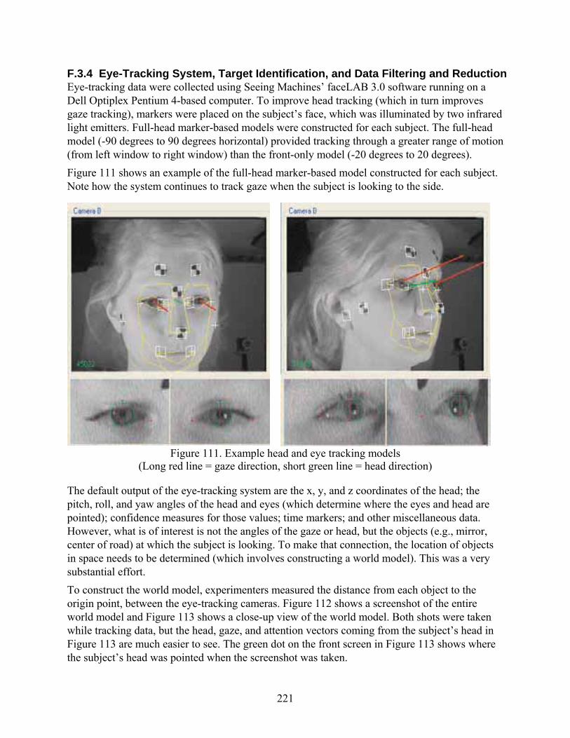
F.3.4 Eye-Tracking System, Target Identification, and Data Filtering and Reduction Eye-tracking data were collected using Seeing Machines’ faceLAB 3.0 software running on a Dell Optiplex Pentium 4-based computer. To improve head tracking (which in turn improves gaze tracking), markers were placed on the subject’s face, which was illuminated by two infrared light emitters. Full-head marker-based models were constructed for each subject. The full-head model (-90 degrees to 90 degrees horizontal) provided tracking through a greater range of motion (from left window to right window) than the front-only model (-20 degrees to 20 degrees). Figure 111 shows an example of the full-head marker-based model constructed for each subject. Note how the system continues to track gaze when the subject is looking to the side.
Figure 111. Example head and eye tracking models (Long red line = gaze direction, short green line = head direction)
The default output of the eye-tracking system are the x, y, and z coordinates of the head; the pitch, roll, and yaw angles of the head and eyes (which determine where the eyes and head are pointed); confidence measures for those values; time markers; and other miscellaneous data. However, what is of interest is not the angles of the gaze or head, but the objects (e.g., mirror, center of road) at which the subject is looking. To make that connection, the location of objects in space needs to be determined (which involves constructing a world model). This was a very substantial effort. To construct the world model, experimenters measured the distance from each object to the origin point, between the eye-tracking cameras. Figure 112 shows a screenshot of the entire world model and Figure 113 shows a close-up view of the world model. Both shots were taken while tracking data, but the head, gaze, and attention vectors coming from the subject’s head in Figure 113 are much easier to see. The green dot on the front screen in Figure 113 shows where the subject’s head was pointed when the screenshot was taken.
221

Figure 112. World model: full view
Figure 113. Close-up view of in-vehicle objects, head position, gaze, and attention vectors
222
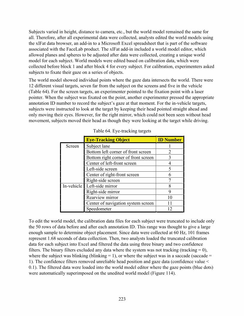
Subjects varied in height, distance to camera, etc., but the world model remained the same for all. Therefore, after all experimental data were collected, analysts edited the world models using the xlFat data browser, an add-in to a Microsoft Excel spreadsheet that is part of the software associated with the FaceLab product. The xlFat add-in included a world model editor, which allowed planes and spheres to be adjusted after data were collected, creating a unique world model for each subject. World models were edited based on calibration data, which were collected before block 1 and after block 4 for every subject. For calibration, experimenters asked subjects to fixate their gaze on a series of objects. The world model showed individual points where the gaze data intersects the world. There were 12 different visual targets, seven far from the subject on the screens and five in the vehicle (Table 64). For the screen targets, an experimenter pointed to the fixation point with a laser pointer. When the subject was fixated on the point, another experimenter pressed the appropriate annotation ID number to record the subject’s gaze at that moment. For the in-vehicle targets, subjects were instructed to look at the target by keeping their head pointed straight ahead and only moving their eyes. However, for the right mirror, which could not been seen without head movement, subjects moved their head as though they were looking at the target while driving.
Table 64. Eye-tracking targets
Eye-Tracking Object ID Number Screen Subject lane 1
Bottom left corner of front screen 2 Bottom right corner of front screen 3 Center of left-front screen 4 Left-side screen 5 Center of right-front screen 6 Right-side screen 7
In-vehicle Left-side mirror 8 Right-side mirror 9 Rearview mirror 10 Center of navigation system screen 11 Speedometer 12
To edit the world model, the calibration data files for each subject were truncated to include only the 50 rows of data before and after each annotation ID. This range was thought to give a large enough sample to determine object placement. Since data were collected at 60 Hz, 101 frames represent 1.68 seconds of data collection. Then, two analysts loaded the truncated calibration data for each subject into Excel and filtered the data using three binary and two confidence filters. The binary filters excluded any data where the system was not tracking (tracking = 0), where the subject was blinking (blinking = 1), or where the subject was in a saccade (saccade = 1). The confidence filters removed unreliable head position and gaze data (confidence value < 0.1). The filtered data were loaded into the world model editor where the gaze points (blue dots) were automatically superimposed on the unedited world model (Figure 114).
223

Figure 114. Example of unedited world model (subject 14)
To distinguish fixations, data were generally divided between far and near regions, then grouped by targets so that individual targets could still be identified. Analysts viewed and edited the world model for each region division by moving the target location over the cluster of points for each region. The analysts placed each target such that it covered the majority of the points in each region cluster (Figure 115). Other factors accounted for in target placement editing included: the target’s position relative to nearby targets (to avoid overlapping targets as much as possible), the confidence values for clusters of data, and the confidence values for extraneous points. Analysts first used data from the beginning calibration file to edit the world model, then compared the edited model with the end data and made adjustments accordingly. Figure 116 shows the final world model for subject 14.
Figure 115. Example of world model object placement (regions 2 and 3, subject 11)
224

Figure 116. Example of final edited world model (subject 14)
Analysts encountered several common problems when trying to edit the world model. In some cases, there appeared to be two or more separate data clusters within the same data file (beginning or end calibration), major differences between region placement in beginning versus end calibration data, spread-out data, and data clusters in extraneous locations. To solve these problems, analysts sometimes had to further separate the data into individual regions, compromise object placement between beginning and end calibration data, or filter gaze with higher confidence values. Another common problem occurred with overlapping objects. If a point was inside more than one object region (for example bottom right and front screen [blue rectangle] in Figure 115), the point registers to the object whose center is closest to the point. This sometimes required a lot of manipulation and excluding large portions of a region so that points within the region would register for the correct object. The overall goal of the world model editing process was to encompass as much of each region as possible while preventing the misidentification of adjacent targets. Clusters and individual points could appear in extraneous locations, especially for objects on the extreme sides (left and right screen, right mirror). For these areas, much of the data had low tracking confidence, but some high-confidence clusters occurred in extraneous locations (opposite side of the world, far away from screens, on the front screen, etc.). Targets were moved to encompass clustered extraneous data because, despite their incorrect placement, the eye-tracking system reliably places points for the region in the extraneous locations. Scattered extraneous data or extraneous data that interfered with other regions (i.e., the front screen) were ignored. In such situations, it was impossible to account for all the regions’ data without interfering with other, more reliably placed, targets in the front-screen area.
225
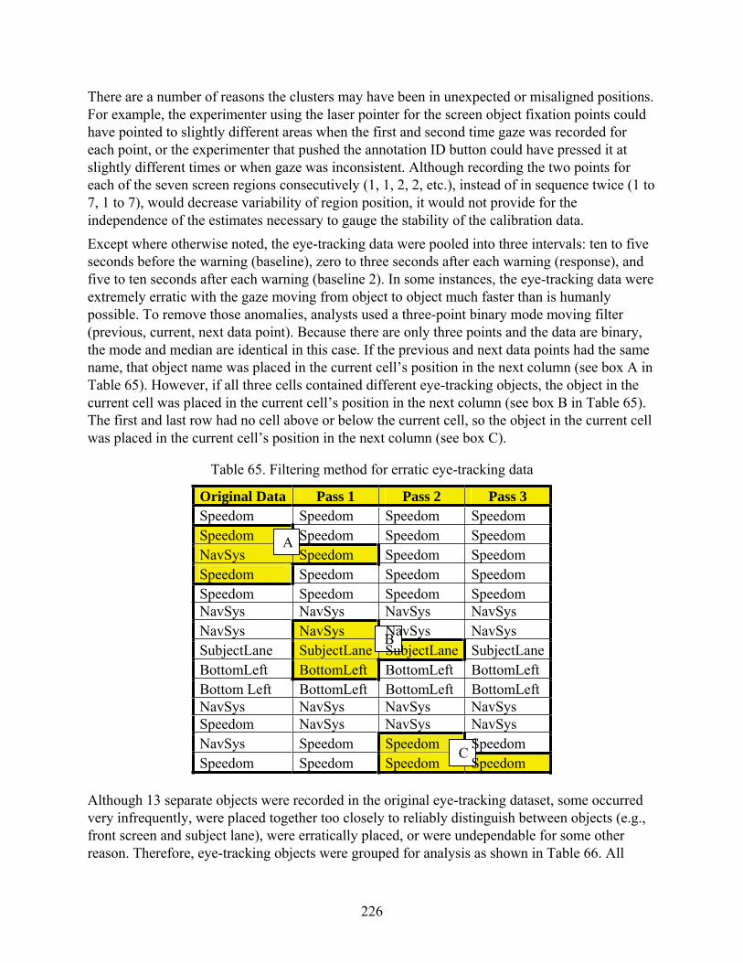
Table 65. Filtering method for erratic eye-tracking data
Original Data
Pass 1 Pass 2 Pass 3 Speedom Speedom Speedom Speedom SpeedomNavSys
A Speedom Speedom Speedom
Speedom SpeedomSpeedom
Speedom Speedom
Speedom Speedom
Speedom Speedom Speedom Speedom NavSys NavSys NavSys NavSys NavSys NavSys NaB vSys NavSys SubjectLane BottomLeft
SubjectLane BottomLeft
SubjectLane BottomLeft
SubjectLane BottomLeft
Bottom Left BottomLeft BottomLeft BottomLeft NavSys NavSys NavSys NavSys Speedom NavSys NavSys NavSys NavSys Speedom Speedom C Speedom Speedom Speedom Speedom Speedom
There are a number of reasons the clusters may have been in unexpected or misaligned positions. For example, the experimenter using the laser pointer for the screen object fixation points could have pointed to slightly different areas when the first and second time gaze was recorded for each point, or the experimenter that pushed the annotation ID button could have pressed it at slightly different times or when gaze was inconsistent. Although recording the two points for each of the seven screen regions consecutively (1, 1, 2, 2, etc.), instead of in sequence twice (1 to 7, 1 to 7), would decrease variability of region position, it would not provide for the independence of the estimates necessary to gauge the stability of the calibration data. Except where otherwise noted, the eye-tracking data were pooled into three intervals: ten to five seconds before the warning (baseline), zero to three seconds after each warning (response), and five to ten seconds after each warning (baseline 2). In some instances, the eye-tracking data were extremely erratic with the gaze moving from object to object much faster than is humanly possible. To remove those anomalies, analysts used a three-point binary mode moving filter (previous, current, next data point). Because there are only three points and the data are binary, the mode and median are identical in this case. If the previous and next data points had the same name, that object name was placed in the current cell’s position in the next column (see box A in Table 65). However, if all three cells contained different eye-tracking objects, the object in the current cell was placed in the current cell’s position in the next column (see box B in Table 65). The first and last row had no cell above or below the current cell, so the object in the current cell was placed in the current cell’s position in the next column (see box C).
Although 13 separate objects were recorded in the original eye-tracking dataset, some occurred very infrequently, were placed together too closely to reliably distinguish between objects (e.g., front screen and subject lane), were erratically placed, or were undependable for some other reason. Therefore, eye-tracking objects were grouped for analysis as shown in Table 66. All
226
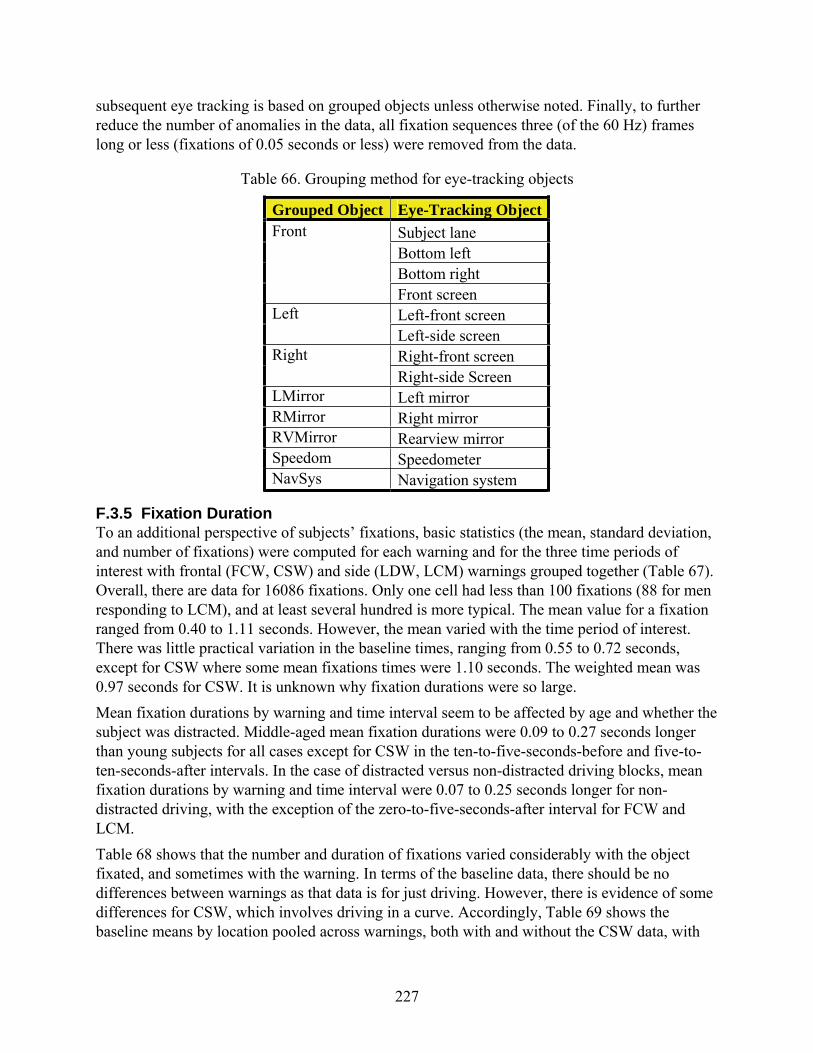
Table 66. Grouping method for eye-tracking objects
Grouped Object Eye-Tracking ObjectFront Subject lane
Bottom left Bottom right Front screen
Left Left-front screen Left-side screen
Right Right-front screen Right-side Screen
LMirror Left mirror RMirror Right mirror RVMirror Rearview mirror Speedom Speedometer NavSys Navigation system
subsequent eye tracking is based on grouped objects unless otherwise noted. Finally, to further reduce the number of anomalies in the data, all fixation sequences three (of the 60 Hz) frames long or less (fixations of 0.05 seconds or less) were removed from the data.
F.3.5 Fixation Duration To an additional perspective of subjects’ fixations, basic statistics (the mean, standard deviation, and number of fixations) were computed for each warning and for the three time periods of interest with frontal (FCW, CSW) and side (LDW, LCM) warnings grouped together (Table 67). Overall, there are data for 16086 fixations. Only one cell had less than 100 fixations (88 for men responding to LCM), and at least several hundred is more typical. The mean value for a fixation ranged from 0.40 to 1.11 seconds. However, the mean varied with the time period of interest. There was little practical variation in the baseline times, ranging from 0.55 to 0.72 seconds, except for CSW where some mean fixations times were 1.10 seconds. The weighted mean was 0.97 seconds for CSW. It is unknown why fixation durations were so large. Mean fixation durations by warning and time interval seem to be affected by age and whether the subject was distracted. Middle-aged mean fixation durations were 0.09 to 0.27 seconds longer than young subjects for all cases except for CSW in the ten-to-five-seconds-before and five-toten-seconds-after intervals. In the case of distracted versus non-distracted driving blocks, mean fixation durations by warning and time interval were 0.07 to 0.25 seconds longer for non-distracted driving, with the exception of the zero-to-five-seconds-after interval for FCW and LCM. Table 68 shows that the number and duration of fixations varied considerably with the object fixated, and sometimes with the warning. In terms of the baseline data, there should be no differences between warnings as that data is for just driving. However, there is evidence of some differences for CSW, which involves driving in a curve. Accordingly, Table 69 shows the baseline means by location pooled across warnings, both with and without the CSW data, with
227

times without CSW being indicative of driving on a straight road. Mean fixation durations to the forward scene were about 0.82 seconds. Glances to the left forward scenes were about 0.12 seconds versus 0.22 to the right. Mirror glances were typically about 0.18 seconds. Glances to the speedometer were about 0.40 seconds and to the navigation system 0.29 seconds. In contrast to the baseline data, there are differences evident in the glance behavior immediately after warnings. For FCW, the relative number of glances to the mirrors drops (as one would expect for a forward event), but as shown in Table 67, the mean durations to various objects show little change from the baseline. For CSW, mirror glances are rare as expected, but the mean glance duration increases considerably to 1.15 seconds. For LDW, the mean fixation to the patterns closely resemble those of the baseline and, to some extent, so do those for LCM, though the number of LCM fixations is relatively small.
228

Table 67. Fixation durations by subject and block characteristics
229
Interval
Baseline 1:5t o1 0
secondsbefore
warning
TimeBlock Char.Subject or
#Fixations Mean
FCWStdDev
#Fixations Mean
CSWStdDev
#Fixations Mean
LDWStdDev
#Fixations Mean
LCMStdDev
WomenMen
Middle-agedYoung
Not informedInformed
Not distractedDistracted
Total
150611821185150312911397138413042688
0.580.690.700.570.650.610.670.580.63
0.820.880.910.790.870.830.90.79
634626619641636624512748
1260
0.600.590.620.580.630.570.710.520.60
0.770.70.860.580.780.680.830.65
1037978845
1170122678980412112015
0.630.720.790.590.680.680.720.650.68
0.840.940.980.810.90.870.920.87
198117161154144171153162315
0.610.590.660.540.570.630.680.530.60
0.810.660.820.690.620.860.780.74
secondsafter
warning
0t o3Men
Middle-agedYoung
Not informed
Women
InformedNot distracted
DistractedTotal
686695987886
996
796847835
1682
0.780.790.570.68
0.58
0.630.630.680.66
0.820.820.70.76
0.71
0.760.740.78
270259280278
269
261219320539
0.951.010.920.98
0.98
0.951.110.860.96
0.970.960.930.95
0.92
0.941.040.86
597470705724
578
451439736
1175
0.720.880.610.71
0.71
0.730.80.670.72
0.750.890.680.79
0.81
0.780.820.75
88114118109
144
123119113232
0.450.550.400.46
0.49
0.490.480.470.47
0.560.610.490.54
0.56
0.570.590.53
Baseline 2:5t o1 0
secondsafter
warning
WomenMen
Middle-agedYoung
Not informedInformed
Not distractedDistracted
Total
164812031241161015001351133615152851
0.550.710.710.550.650.590.650.590.62
0.740.860.870.730.840.740.830.76
458417448427439436367508875
0.951.000.941.011.020.931.100.890.98
1.151.181.091.231.211.111.241.09
10781051913
1216127385678813412129
0.610.640.710.560.640.610.710.570.62
0.830.80.910.730.840.780.890.76
207118168157139186168157325
0.630.550.660.530.600.600.650.550.60
0.720.660.800.570.630.750.780.59

Table 68. Fixation durations by object
230
Interval
Baseline 1:5t o1 0
secondsbefore
warning
TimeBlock Char.Subject or
#Fixations Mean
FCWStdDev
#Fixations Mean
CSWStdDev
#Fixations Mean
LDWStdDev
#Fixations Mean
LCMStdDev
FrontLeft
RightL. mirrorR. mirror
R.V. mirrorSpeedometerNav. system
Total
173545
3114329110215200
2688
0.830.150.200.170.140.220.430.270.63
0.970.210.180.140.110.210.550.31
7324
10544
102122187
1260
0.830.220.230.170.230.210.390.250.60
0.860.250.250.070.150.190.370.29
13782218778
571671892015
0.860.110.220.080.180.190.380.290.67
1.000.060.210.030.110.170.500.35
1899
49132
231416315
0.840.110.200.170.150.150.330.570.60
0.880.060.150.140.140.080.150.59
secondsafter
warning
0t o3Left
RightL. mirror
Front
R. mirror
2013315
1292
3
0.120.220.13
0.78
0.14
0.050.340.09
0.80
0.05
2331
4160.080.240.07
1.150.020.23
0.977
108
840
2
0.100.18
0.87
0.36
0.060.15
0.83
0.37
9181
1740.080.150.08
0.570.030.12
0.61
Nav. systemTotal
R.V. mirrorSpeedometer
431682
50126
0.280.66
0.140.40
0.49
0.100.50
21539
1749
0.290.96
0.150.46
0.57
0.090.50
771168
34100
0.310.70
0.180.36
0.37
0.120.26
6232
915
0.250.47
0.130.29
0.14
0.070.14
Baseline 2:5t o1 0
secondsafter
warning
FrontLeft
RightL. mirrorR. mirror
R.V. mirrorSpeedometerNav. system
Total
197537
2742512105282141
2851
0.770.120.210.150.180.180.380.290.62
0.890.070.220.150.160.140.400.47
6693
4044
338436873
1.170.180.190.150.130.160.330.540.97
1.210.150.140.060.040.130.191.04
1303112096
161241992612129
0.850.110.220.260.230.210.380.280.63
0.940.070.250.110.170.190.430.38
2262
31
193917325
0.780.020.32
0.720.180.310.360.64
0.050.070.05
0.170.150.33

Table 69. Baseline mean fixation durations (seconds)
Object with CSW withoutCSW Baseline1 Baseline2 Baseline1 Baseline2
Front 0.84 0.86 0.84 0.80 Left 0.14 0.12 0.13 0.11
Right 0.21 0.22 0.21 0.22 L. mirror 0.16 0.17 0.16 0.17 R. mirror 0.16 0.21 0.15 0.23
R.V. mirror 0.21 0.19 0.20 0.20 Speedometer 0.40 0.37 0.41 0.37 Nav. system 0.28 0.31 0.29 0.29
Total 0.64 0.67 0.64 0.63
Curiously, there were few differences between warnings in terms of the fraction of glances to various locations (Table 70). In all cases, drivers were more likely to fixate on the front area (about 65% of the time during the baseline periods, and 75% of the time immediately after a warning), even for LCM, where the hazard was on the side of the vehicle. There were hardly any differences among warnings in terms of the fraction of time where drivers looked, though there were more glances for LCM to the right as subjects were often looking for merging vehicles before the warning was presented. Table 70 provides an example for fixations to the front, which were the most numerous. There were, however, two points of note, with subjects looking 15 percent of the time to the navigation system before a CSW (with the front area fraction being low) and 12 percent for LDW to the navigation system (and again the forward fraction being low) in the baseline after an LDW. This may reflect drivers in the distraction condition attending to the navigation task. What is interesting is drivers returned so quickly to a navigation task after an LDW (within five to ten seconds).
231

Table 70. Fraction of fixations on eye-tracking object by warning type and time interval
Time Eye-Tracking Fraction of Fixations within Time Interval Interval (s) Object FCW LDW LCM CSW
Front 0.65 0.68 0.60 0.58 Left 0.02 0.01 0.03 0.00
10 to 5 Right 0.12 0.09 0.16 0.08 seconds Left mirror 0.02 0.00 0.04 0.00 before warning
Right mirror 0.01 0.00 0.01 0.00 R.V. mirror 0.04 0.03 0.07 0.08 Speedometer 0.08 0.08 0.04 0.10 Nav. system 0.07 0.09 0.05 0.15 Front 0.77 0.72 0.75 0.77 Left 0.01 0.01 0.04 0.00
0 to 3 seconds after warning
Right 0.08 0.09 0.08 0.06 Left mirror 0.01 0.00 0.00 0.00 Right mirror 0.00 0.00 0.00 0.00 R.V. mirror 0.03 0.03 0.04 0.03 Speedometer 0.07 0.09 0.06 0.09 Nav. system 0.03 0.07 0.03 0.04 Front 0.69 0.61 0.70 0.77 Left 0.01 0.01 0.01 0.00
5 to 10 seconds after warning
Right 0.10 0.10 0.10 0.05 Left mirror 0.01 0.00 0.00 0.00 Right mirror 0.00 0.01 0.00 0.00 R.V. mirror 0.04 0.06 0.03 0.04 Speedometer 0.10 0.09 0.12 0.10 Nav. system 0.05 0.12 0.05 0.04
As a final footnote to the warning fixation statistics, relationships between statistics were examined. As is often the case, the means and standard deviations were almost perfectly correlated (greater mean – greater variability) as were the mean fixation and the number of fixations (longer glance – more glances) in all cases except for LCM (Table 71). This may be due to the smaller number of data points examined.
232

Table 71. Correlations between fixation duration measures by warning type and time interval
TimeInterval (s)
Correlated FixationDuration Measures
FCW CSW LDW LCM
Baseline 1: 10-5 before
Mean and std dev 0.99 0.98 0.99 0.98 Mean and # fixations 0.84 0.96 0.96 0.80
0-3 after Mean and std dev 0.93 0.92 0.98 0.96 Mean and # fixations 0.94 0.97 0.92 0.90
Baseline 2: 5-10 after
Mean and std dev 0.97 0.92 0.97 -0.12 Mean and # fixations 0.96 0.94 0.96 0.62
F.3.6 How Were the Fixation Durations Distributed? Duration distributions for the locations in which each time period (ten to five seconds before, zero to three after, or five to ten after) that had 40 or more fixations are shown in Table 72 through Table 73. The spikes at three-plus seconds for the zero-to-three second distributions, and at five-plus seconds for the five-second baseline intervals, represent fixations that began in the time window of interest but ended outside of it or a series of fixations to the same region that exceeded the window duration (e.g., a four-second fixation in a three-second interval). The presence of these long “fixations” suggests opportunities for additional filtering of the data. Ignoring the spikes, many of the distributions appear to be exponential, especially the baseline data. In fact, the pre- and post-warning distributions to the front area are remarkably exponential-like, especially to the front for FCW and LDW (Figure 117). That is also the case for FCW just after a warning (to the front), but less so for LDW, which could even be log-normal. Exponential search times are generated by processes where the probability per unit time of completing the search is a fixed value p, so the probability for two units is p2, and so forth. Since the search in LDW is for a particular object, a log-normal distraction makes sense: normal because it is for a single item, and log because the duration is short and impinges upon the floor. In Figure 118, the baseline for search times for CSW and LCM are clearly exponential as before. However, immediately after the warning, LCM appears a bit exponential. For CSW, there is no immediately obvious function. In Figure 119, for glances to the right, pre- and post-baseline glances were exponentially distributed. For FCW, this makes sense as they were check glances (not searching for anything specific) and were generally short. For LDW, notice the times are much greater on average, as subjects were searching for specific lane-related information pertaining to the warning. Figure 120 shows that fixations to the navigation system not related to the warning, were short, few, and exponentially distributed. These were check glances. Speedometer glance durations (Figure 121 and Figure 122) seemed relatively unaffected by the warning, with the times before, immediately after, and well after a warning having the same duration and distribution (possibly log-normal). They were similar to those for CSW, where checking the speedometer may have been necessary.
233

0 1 2 3 4 5 0 1 2 3 4 5 0 1 2 3 4 5
Front, 5 to 10 Seconds before FCW Front, 0 to 3 Seconds after FCW Front, 5 to 10 Seconds after FCW
0 1 2 3 4 5 0 1 2 3 4 5 0 1 2 3 4 5
Front, 5 to 10 Seconds before LDW Front, 0 to 3 Seconds after LDW Front, 5 to 10 Seconds after LDW
Figure 117. Fixation duration distributions for front area by time interval, FCW, and LDW
234

0 1 2 3 4 5
Front, 5 to 10 Seconds before CSW
0 1 2 3 4 5
Front, 5 to 10 Seconds before LCM
0 1 2 3 4 5
Front, 0 to 3 Seconds after CSW
0 1 2 3 4 5
Front, 0 to 3 Seconds after LCM
0 1 2 3 4 5
Front, 5 to 10 Seconds after CSW
0 1 2 3 4 5
Front, 5 to 10 Seconds after LCM
Figure 118. Fixation duration distributions for front area by time interval, CSW , and LCM
235

0 1 2 3 4 5
Right, 5 to 10 Seconds before FCW
0 1 2 3 4 5
Right, 5 to 10 Seconds before LDW
0 1 2 3 4 5
Right, 0 to 3 Seconds after FCW
0 1 2 3 4 5
Right, 0 to 3 Seconds after LDW
0 1 2 3 4 5
Right, 5 to 10 Seconds after FCW
0 1 2 3 4 5
Right, 5 to 10 Seconds after LDW
Figure 119. Fixation duration distributions for right area by time interval, FCW ,and LDW
236

0 1 2 3 4 5 0 1 2 3 4 5 0 1 2 3 4 5
Navigation System, 5 to10 Secondsbefor e Navigation System, 0 to3 Seconds after Navigation System, 5 to10 Seconds after FCW FCW FCW
0 1 2 3 4 5 0 1 2 3 4 5 0 1 2 3 4 5
Navigation System, 5 to10 Seconds before Navigation System, 0 to3 Seconds after Navigation System, 5 to10 Seconds after LDW LDW LDW
Figure 120. Fixation duration distributions for navigation system by time interval, FCW ,and LDW
237

0 1 2 3 4 5 0 1 2 3 4 5 0 1 2 3 4 5
Speedometer, 5 to 10 Seconds before FCW Speedometer, 0 to3 Seconds af ter FCW Speedometer , 5 to10 Seconds after FCW
Speedometer, 5to 10 Seconds before LDW Speedometer, 0 to3 Seconds af ter LDW Speedometer, 5 to10 Seconds after LDW
Figure 121. Fixation duration distributions for speedometer by time interval, FCW and LDW
238
0 1 2 3 4 5 0 1 2 3 4 5 0 1 2 3 4 5
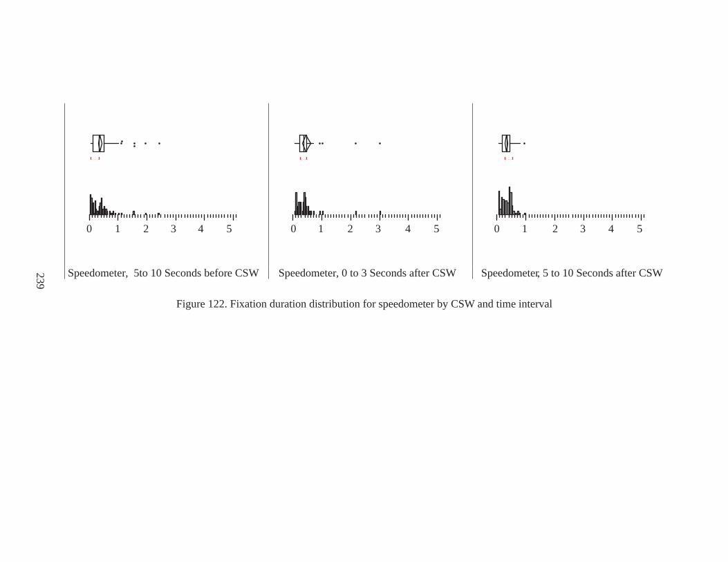
0 1 2 3 4 5 0 1 2 3 4 5 0 1 2 3 4 5
Speedometer, 5to 10 Seconds before CSW Speedometer, 0 to 3 Seconds after CSW Speedometer, 5 to 10 Seconds after CSW
Figure 122. Fixation dur ation distribution for speedometer by CSW and time interval
239

The preceding data suggest that warning occurrences have only a minimal effect on where drivers look. In part, that conclusion is reached based on the manner the data were examined— pooling over large timeframes. It could be the effect of the warning on glance patterns is very short lived. Table 72 through Table 75 show fixation counts over a much shorter time window of one second. Notice there is no major change in gaze location due to the warnings. Another explanation is that drivers were processing the situation related to a warning well before the warning was triggered, so the actual warning was unlikely to lead to a change in scanning.
Table 72. Eye fixation frequencies after FCW warning
Area Start of Warning
.5 s after Warning
1 s after Warning Total
Unknown 52 58 63 173 Front screen 61 61 58 180 Left mirror 2 2 4 Speedometer 8 6 6 20 Nav system 1 1 2 Bottom right of front screen 18 18 18 54
Subject lane 147 146 145 438 Bottom left of front screen 16 14 14 44 Right front screen 6 4 5 15 Total 310 310 310 930
Table 73. Eye fixation frequencies after CSW warning
Area Start of Warning
.5 s after Warning
1 s after Warning Total
Unknown 3 4 5 12 Front screen 26 24 23 73 Rearview mirror 1 4 5 Speedometer 2 1 2 5 Bottom right of front screen 2 2 6 10
Subject lane 55 48 46 149 Bottom left of front screen 4 7 11 Right front screen 1 3 1 5 Total 90 90 90 270
240

Table 74. Eye fixation frequencies after LDW warning
Area Start of Warning
.5 s after Warning
1 s after Warning Total
Unknown 14 7 7 28 Front screen 38 27 27 92 Rearview mirror 2 4 1 7 Speedometer 7 2 8 17 Bottom right of front screen 10 6 7 23 Subject lane 86 79 79 241 Bottom left of front screen 9 12 11 32 Left front screen 1 1 Right front screen 2 2 1 5 Total 168 139 139 446
Table 75. Eye fixation frequencies after LCM warning
Area Start of Warning
.5 s after Warning
1 s after Warning Total
Unknown 197 15 10 222 Front screen 16 12 5 33 Left mirror 1 1 Rearview mirror 1 1 Speedometer 10 1 11 Nav system 2 1 1 4 Bottom right of front screen 10 4 1 15 Subject lane 38 34 32 104 Bottom left of front screen 8 5 2 15 Left front screen 1 1 Left side screen 1 1 Right front screen 2 2 Total 286 73 51 410
F.3.7 Driving Data How Long Did It Take Drivers to Respond to Forward Warnings (FCW, CSW)? For FCW and CSW, the primary response was to slow down, either by backing off or removing one’s foot from the accelerator, and sometimes by braking as well. A response to the warning was considered to occur if the subject released the throttle completely or applied the brakes in the three seconds after the warning but did not do so in the six seconds before the warning. This combined criteria helped assure that the responses examined were truly in response to the warning and not follow-up to a subject-initiated pre-warning response. Using these criteria, drivers responded to approximately 27 percent of the FCWs (562 warnings) and 18 percent of
241

0 1 2 3 4 5 6 7 8 9
10
Freq
uenc
y
0.25 0.75 1.25 1.75 2.25 2.75 3.25 3.75
Response Time (s)
Figure 124. Distribution of accelerator pedal release times for CSWs
the CSWs (225 warnings). For some FCWs, drivers had responded in some way well before the criterion period (by slowing down) or the situation evolved in some way such that the situation was not critical. Interestingly, no subjects responded to a CSW with braking, in part because there were no lateral acceleration cues to suggest excess speed and there were no consequences of driving too fast in a curve. Accelerator pedal release time and brake onset time were computed for each FCW to which a driver responded, while only accelerator pedal release time was computed for each CSW. Accelerator pedal release time was defined as the time from the onset of the warning until the accelerator signal was zero. Brake onset time was the time from the onset of the warning until a nonzero brake signal was observed. As with the eye fixation data, response times were not recorded to the nearest millisecond but rather determined by the status of various variables (accelerator percentage, etc.) at 60 Hz. Therefore, all times are accurate to the nearest 0.016 second. There were 149 responses to FCWs and 42 responses to CSWs. For FCW, the mean times were 0.788 seconds and 1.072 seconds for accelerator pedal release time and brake onset time, respectively, with standard deviations of 0.853 and 0.534 seconds. The mean accelerator pedal release time for CSW was 1.474 seconds with a standard deviation of 0.907 seconds. Figure 123 and Figure 124 show the accelerator release and brake onset times for FCW and the accelerator release times for CSW. (Again, there were no braking events for CSW.) Notice the accelerator-related distributions are exponential and the CSW distributions are log normal.
0 5
10 15 20 25 30 35 40
0.25 0.75 1.25 1.75 2.25 2.75 3.25 3.75
Freq
uenc
y
Response Time (s)
0
5
10
15
20
25
0.25 0.75 1.25 1.75 2.25 2.75 3.25 3.75
Freq
uenc
y
Response Time (s)
Figure 123. Distributions of accelerator pedal release times and brake onset times for FCW
242

Traditionally, the FCW and CSW response times would be analyzed using ANOVA. In this case, a mixed-effect model, a broader form of the general linear model, was chosen. Because the structure of the data represents a within-subjects design (i.e., there were potentially multiple observations of the same conditions on the same driver), a repeated-measures analysis was required. However, because of the observational nature of the data, there were largely unequal n’s among the levels of the independent and predictor variables. That is, the data were unbalanced. More traditional forms of the general linear model (such as ANOVA) exclude entire cases from the dataset if an observation on one variable is missing. Further, using linear mixed-effects models allows modeling the variance and covariance structure of the data, which can lead to more accurate parameter estimates and test statistics. The method of model selection used for all analyses was essentially a “backwards” selection in which all main effects (and two-way interactions of a priori interest) were initially included. Each model was then refit multiple times, each time excluding the main effect or interaction that was least significant. When only significant effects remained, the model was refit several more times to achieve a parsimonious final model. Unless otherwise noted, all pairwise comparisons used a Bonferroni correction. The model also included random effects to model variation among subjects. Consequently, a fixed effect would only show statistical significance if it accounted for more variance than “random” subject-to-subject variance. Thus, three mixed-effect models were developed with FCW accelerator release time, FCW brake onset time, and CSW accelerator release time being the dependent measures. In all three analyses, age and gender were the between-subjects factors. Whether the subject was performing a distraction task (distracted, undistracted) and whether the subject was informed about the crash warning system (uninformed, informed) were the within-subjects factors. (Note that being in a “distraction” block does not necessarily mean the driver was distracted, only that he or she was instructed to engage in a secondary task when feeling comfortable doing so.) Scenarios were included in the model as well as age-by-gender and distraction-by-informed state interactions. There were no statistically significant effects in any of the analyses. Figure 125 shows some of the main effects for FCW. Some of the results are consistent with past research. For example, young men had the shortest response times. However, most of the differences for FCW were quite small, for example, the difference between the distracted and nondistracted response times was 0.052 seconds. However, on average, for FCW, uninformed drivers took less time to respond (by 0.187 seconds).
243

1
1.5
2
2.5
0
1
2
Young Middle-aged
Female Male
2.5
2
0.5 0.5
0 0 Undistracted Distracted
Uninformed Informed
Mean accelerator pedal release times for age and gender Mean accelerator pedal release times for distracted and informed states
2.5 2.5
Res
pons
e Tim
e (s
)
Res
pons
e Tim
e (s
) R
espo
nse T
ime
(s)
1.5
1
Young Middle-aged
Female Male
0 Undistracted Distracted
Uninformed Informed
Mean brake onset times for age and gender Mean brake onset times for distracted and informed states
Figure 125. FCW mean accelerator pedal release and brake onset times
2
1.5 1.5
1
0.5 0.5
Res
pons
e Tim
e (s
)
244

0
1
Young Middle-aged
Female Male
Res
pons
e Tim
e (s
)
2.52.5
22
Undistracted Distracted
Uninformed Informed R
espo
nse T
ime
(s)
1.5 1.5
1
0.50.5
0
Mean accelerator pedal release times for distracted Mean accelerator pedal release times for age and gender and informed states
Figure 126. CSW mean accelerator pedal release times
Figure 126 shows the results for CSW. For CSW, uninformed drivers took longer to initiate a response to the warning than when they were informed about the warnings (2.13 versus 1.32 seconds). Additionally, distracted drivers had longer response times to warnings by 0.22 seconds. However, none of these differences were statistically significant, and that was probably because of how the experiment was conducted. In terms of being informed, drivers were only truly uninformed the first time the warning was presented. After that, they had some awareness of it, whether or not it was explained. In terms of distraction, distraction was a condition, not simply an indicator of whether the subject was engaged in completing the distraction task. In many cases, subjects did not pay much attention to carrying out that task even though they were asked to try.
How Much Did Drivers Slow Down after FCW and CSW? To simplify the analysis, speed changes from only the onset of single warnings (no other warnings within three seconds) were examined. (Multiple warnings are discussed later.) To further simplify the analysis, six snapshots of time (0.5, 1.0, 1.5, 2.0, 2.5, and 3.0 seconds post-warning onset) were examined rather than entire time histories. Means were computed based on exposure, not subjects, so if a warning occurred four times for one subject and once for another, the denominator was four (four instances) not two (two subjects). Finally, for FCW, warnings were only included in the sample if they occurred in a planned FCW scenario, which included the reveal, cut-in, and both lead vehicle deceleration scenarios. For example, if an FCW alert happened to occur during an LCM scenario, the FCW alert would be excluded from these analyses. This was done both to further simplify the analyses as well as to focus more specifically on the scenarios of interest. (Because CSW alerts were not associated with different scenarios, this strategy did not apply to CSW.) To get a sense of how this data reduction technique affected the sample size, a frequency distribution of FCW alerts that occurred in each scenario is presented in Table 76. Scenarios with planned FCW alerts are listed first, and they consist of 328 alerts (or 66 percent of the entire sample of single FCWs). The majority of unplanned FCWs occurred in the two LCM scenarios, with reveals being most
245

common. As these scenarios both involved forced lane changes, the FCW warning was most likely associated with a delayed lane change while the driver was attempting to negotiate the conflict with the adjacent vehicle.
Table 76. Frequency distribution of FCW alerts for each scenario
Scenario n FCW: Reveal 120 FCW: Lead vehicle deceleration 99 LCM: Reveal-induced lane change 83 LCM: Construction-induced lane change 83 FCW: Cut-in 74 FCW: Lead decelerates after lane change 35 LDW: Wind gust 1 CSW 1 Total 496
In the following summary of results, many of the figures depict predicted parameter estimates (i.e., least square means) from linear mixed-effects models. These estimates were calculated such that they represent unweighted means, but have estimated standard errors that account for the covariance structure in the model. This resulted in predicted means that were very close to the observed means, but more accurately reflect the random variance among drivers and correlations among repeated measurements on the same driver. This also allowed appropriate 95-percent confidence intervals to be constructed for each set of means. Consequently, error bars in all of the following graphs represent 95-percent confidence intervals. Figure 127 shows the mean reduction in speed at each of the six time intervals for both FCW and CSW. For FCW, by three seconds after the alert occurred, subjects had slowed, on average, by about 10 mph. This deceleration was relatively smooth throughout the entire three-second duration. CSW alerts, however, did not result in a substantial reduction in speed; the average reduction in speed at three seconds is less than one mile per hour. This could have been due to a design issue with the simulated world, since there was no particular consequence of not slowing (e.g., the driver would not run off the road if traveling at 70 mph).
246

Ach
eive
d re
duct
ion
in sp
eed
(mph
) 12
10
8
6
4
2
0 0.5 1.0 1.5 2.0 2.5 3.0
FCW CSW
Time post-warning (s)
Figure 127. Mean reduction in speed in response to FCW and CSW alerts
To better characterize driver response to FCW alerts, it is helpful to examine the distribution of speeds at each time interval. This is illustrated in the following series of histograms (Figure 128), where speed is presented in 5 mph bins. The average speed at warning onset for FCWs was 53.4 mph (SD = 18.9 mph). Notice that at the time of the alert, the distribution is somewhat bimodal; while the majority of subjects are driving at about 70 mph, there is also a small spike at around 40 mph. There are also a handful of cases in which the subjects are traveling at modest speeds (below 15 mph). As time progresses, the distribution peaks between 30 and 40 mph, but there are still of cases in which the driver does not appreciably slow down. By three seconds post-alert, the average speed was 42.2 mph (SD = 18.1). It is interesting to note that the overall variability in speed hardly changes throughout the course of subjects’ response to FCWs.
247

Speed(mph)
f
248
Speed(mph)
Speed(mph)
Speed(mph)
Spee
d(m
ph)
Spee
d(m
ph)
Spee
d(m
ph)
Spee
d(m
ph)
Figu
re12
8. D
istrib
utio
ns o
f spe
eds p
ost-w
arni
ng
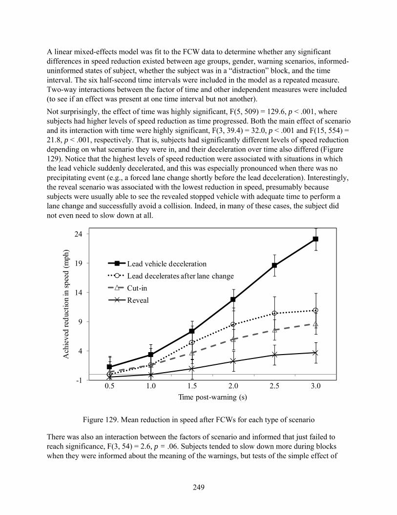
A linear mixed-effects model was fit to the FCW data to determine whether any significant differences in speed reduction existed between age groups, gender, warning scenarios, informed-uninformed states of subject, whether the subject was in a “distraction” block, and the time interval. The six half-second time intervals were included in the model as a repeated measure. Two-way interactions between the factor of time and other independent measures were included (to see if an effect was present at one time interval but not another). Not surprisingly, the effect of time was highly significant, F(5, 509) = 129.6, p < .001, where subjects had higher levels of speed reduction as time progressed. Both the main effect of scenario and its interaction with time were highly significant, F(3, 39.4) = 32.0, p < .001 and F(15, 554) = 21.8, p < .001, respectively. That is, subjects had significantly different levels of speed reduction depending on what scenario they were in, and their deceleration over time also differed (Figure 129). Notice that the highest levels of speed reduction were associated with situations in which the lead vehicle suddenly decelerated, and this was especially pronounced when there was no precipitating event (e.g., a forced lane change shortly before the lead deceleration). Interestingly, the reveal scenario was associated with the lowest reduction in speed, presumably because subjects were usually able to see the revealed stopped vehicle with adequate time to perform a lane change and successfully avoid a collision. Indeed, in many of these cases, the subject did not even need to slow down at all.
24
19
14
9
4
-1 0.5 1.0 1.5 2.0 2.5 3.0
Lead vehicle deceleration Lead decelerates after lane change Cut-in Reveal
Time post-warning (s)
Figure 129. Mean reduction in speed after FCWs for each type of scenario
Ach
ieve
d re
duct
ion
in sp
eed
(mph
)
There was also an interaction between the factors of scenario and informed that just failed to reach significance, F(3, 54) = 2.6, p = .06. Subjects tended to slow down more during blocks when they were informed about the meaning of the warnings, but tests of the simple effect of
249
scenario showed that this effect was only significant for the lead vehicle deceleration scenario, F(1, 42.8) = 6.4, p < .05. In this scenario, by three seconds post-alert, subjects reduced their speed by 24.5 mph when informed compared to 19.8 mph when uninformed. In other words, not only were subjects slowing down the most in this scenario, but they also seemed especially primed to slow down in this scenario when they were informed about what FCW alerts mean. There were no significant effects of age or gender in terms of speed reduction in response to FCW alerts. Given the absence of older drivers (i.e., above 60 years old), the absence of an age difference is not surprising. For CSW, the mean speed at warning onset was 72.8 mph (SD = 3.8 mph). Because there were no scenarios associated with CSW alerts, the total sample of 216 single FCW alerts were included in these analyses. An examination of each of the six time intervals in this sample revealed that the standard deviations of speed ranged from a minimum of 3.68 to a maximum of 3.77. Given the relatively low variation or overall change in speed across time, the individual distributions for each time interval are not displayed here. There were, however, two cases of speed reduction in response to a CSW that were clearly outliers. In both of these cases, the subject achieved a speed reduction of nearly 10 mph. Influence diagnostics were calculated for these cases, which revealed that neither of these cases had a significant effect on parameter estimates in the model. These cases were therefore retained. A linear mixed-effects model was fit to the CSW accelerator release times (including the same factors as with FCW, except no factor of scenario), which revealed some of the same relationships as seen with FCW. For example, the effect of time was highly significant, F(5, 422) = 47.6, p < .001. Even though the overall level of speed reduction was low (on average, one mile per hour by three seconds), subjects were still slowing down after the CSW alert was issued. Considering that CSWs were triggered 50 meters before the beginning of a curve, and subjects were driving at about 70 mph (or 31.3 meters per second), they would have reached the beginning of the curve in a little less than two seconds. The speed reduction observed here may therefore be due to the normal process of slowing down for the curve. Subjects also tended to slow down more for CSW alerts when they were informed of their meaning, F(1, 14.7) = 6.7, p < .05. Note that while the strength of this effect was similar to the FCW lead vehicle deceleration scenario, it is less noteworthy from a practical standpoint, considering that by three seconds post-alert, subjects tended to slow down only 0.6 mph more when informed (and, overall, subjects showed little speed reduction to CSW alerts). As with FCW, there were no significant effects of age or gender on speed reduction in response to CSW alerts. How Did Lane Position Change in Response to LDW and LCM? Because LDW alerts were not associated with any particular scenario, and could easily happen anywhere, all single LDW alerts were included in these analyses (n = 379). LCM alerts, on the other hand, had specific scenarios associated with them (reveal-induced lane changes, and construction-induced lane changes), but the n’s were rather low for these categories. In total, these two scenarios accounted for 37 single LCM alerts. There were 20 LCMs, however, that occurred in scenarios other than these two. To preserve a larger sample size, all LCM alerts were retained in the following analyses, such that the total sample was 57.
250
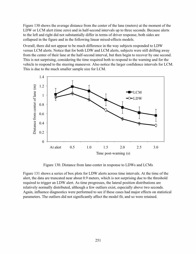
Dist
ance
from
cen
ter o
f lan
e (m
)
1.4
1.2
1
0.8
0.6
0.4
0.2
0
At alert 0.5 1.0 1.5 2.0 2.5 3.0
LCM LDW
Time post-warning (s)
Figure 130. Distance from lane-center in response to LDWs and LCMs
Figure 130 shows the average distance from the center of the lane (meters) at the moment of the LDW or LCM alert (time zero) and in half-second intervals up to three seconds. Because alerts to the left and right did not substantially differ in terms of driver response, both sides are collapsed in the figure and in the following linear mixed-effects models. Overall, there did not appear to be much difference in the way subjects responded to LDW versus LCM alerts. Notice that for both LDW and LCM alerts, subjects were still drifting away from the center of their lane at the half-second interval, but then begin to recover by one second. This is not surprising, considering the time required both to respond to the warning and for the vehicle to respond to the steering maneuver. Also notice the larger confidence intervals for LCM. This is due to the much smaller sample size for LCM.
Figure 131 shows a series of box plots for LDW alerts across time intervals. At the time of the alert, the data are truncated near about 0.9 meters, which is not surprising due to the threshold required to trigger an LDW alert. As time progresses, the lateral position distributions are relatively normally distributed, although a few outliers exist, especially above two seconds. Again, influence diagnostics were performed to see if these cases had major effects on statistical parameters. The outliers did not significantly affect the model fit, and so were retained.
251

Figure 131. Box plots for LDW (left and right collapsed) for each time interval
A linear mixed-effects model that collapsed left and right LDW alerts together and included the same factors as previous models showed only two significant results. The first was a predictable main effect of time, F(5, 1,642) = 538.62, p < .0001. Also, younger subjects returned to their lane more quickly after an LDW alert than middle-aged subjects, F(1, 14.6) = 6.5, p < .05, as illustrated in Figure 132.
252

0.0
0.2
0.4
0.6
0.8
1.0
1.2
Dist
ance
from
cen
ter o
f lan
e (m
)
Middle-age
Younger
At alert 0.5 1.0 1.5 2.0 2.5 3.0
Time post-warning (s)
Figure 132. Effect of age on distance from lane center after LDWs
A similar series of box plots is presented for LCM in Figure 133. Again, notice the larger variability in driver response across time. While no clear outliers exist (except for a few cases in the initial lane position), the data are generally skewed in the positive direction.
253

Figure 133. Box plots for LCM (left and right collapsed) for each time interval
A linear mixed-effects model showed only one significant effect for LCMs, and that was time, as might be expected, F(5, 51.1) = 25.6, p < .0001. However, no other effects, including age and gender, were significant. How Do Initial Responses to Warnings Differ from Subsequent Responses to the Same Type of Warning? The data in response to each warning were split into two groups: the first response to each warning and all subsequent warnings. Admittedly, the first response to a particular warning may be different if the driver had first responded to other warnings, but given the small subject sample size, they were assumed to be the same. Figure 134 compares the first response to LDW for all subjects (16 responses). Using paired t tests, the only significant difference in absolute lane position was at 2.5 s (t(15) = 2.27, p = .0390), with drivers making a larger correction for the first response (by about 0.1 meters). Thus, for LDW, pooling all responses seems reasonable.
254

Dist
ance
from
cent
er o
f lan
e (m
)
1.2
1
0.8
0.6
0.4
0.2
0
First occurence Subsequent warnings
0.5 1 1.5 2 2.5 3
Time post-warning (s)
Figure 134. Driver response to initial LDW
First occurence Subsequent warnings
0.5 1 1.5 2 2.5 3
Time post-warning (s)
Figure 135. Driver response to initial LCM
Dist
ance
from
cent
er o
f lan
e (m
)
1.2
1
0.8
0.6
0.4
0.2
0
For LCM (Figure 135), the result is somewhat similar in that the driver reaction to the first warning is greater, that is approaching the middle of the lane more rapidly, though most of the difference occurs at 1.5 and 2.0 seconds after the warning.
For FCW (Figure 136), the pattern is the different from that of the lateral warnings (LDW and LCM). Again there are no initial differences (in this case, the first 1.5 seconds), but after that the decrease in speed for warnings is less than that for subsequent occurrences by about 10 mph. Curiously, the pattern for CSW (Figure 137) is the opposite after the first second or so, with drivers reducing their speed more for the first warnings than subsequent warnings, probably because they realized that in this experiment there were no consequences of driving curves too quickly. (The vehicle would not leave the road.)
255

Ach
ieve
d re
duct
ion
in sp
eed
(mph
)
25
20
15
10
5
0
-5
First occurence Subsequent warnings
0.5 1 1.5 2 2.5 3
Time post-warning (s)
Figure 136. Driver response to initial FCW
Ach
ieve
d re
duct
ion
in sp
eed
(mph
)
1
0.8
0.6
0.4
0.2
0
First occurence Subsequent warnings
0.5 1 1.5 2 2.5 3
Time post-warning (s)
Figure 137. Driver response to initial CSW
Thus, one would not expect any differences between responses to a particular warning the first versus subsequent times up to about 1.0 second, the mean response time. For LDW, drivers return to the center more quickly for the first warning. For LCM, there is no real difference. For FCW, drivers decelerate less quickly the first time, whereas for CSW, they decelerate more quickly. Keep in mind that there were multiple FCW scenarios, but there was only one scenario for most other warnings, so there may be some sort of underlying difference among scenarios.
256

F.3.8 Post-Test Analysis Table 77 shows the mean ratings for each characteristic split by age and sex, and overall. For FCW, subjects thought the sound and vibration were about right (3.1 and 3.4 respectively). Initial understanding was midrange (3.0) but improved as the experiment progressed (to 4.7). The warning was rated moderately easy to learn (4.4), though much more so by young men than by middle-aged men (4.8 versus 3.8). The warning was rated as occurring with about the desired frequency (3.4), as moderately useful (3.8), and as moderately easy to use (3.8). For LDW, the sound level (3.4) and light brightness (2.8) were about right. The side from which the sound, light, and vibration were presented was somewhat difficult to determine (2.3, 2.4, and 2.0, respectively), but the rating of the vibration intensity was as being too great (3.7). LDW was rated as moderately understandable initially (2.9), well understood at the end (4.8), and easy to learn (4.4). The warning occurred with the desired frequency (3.5), was moderately easy to use, but only somewhat useful (3.6). For LCM, the sound level was about right (3.3) and the sound side was somewhat easy to determine (2.6). Initial understanding was midrange (2.7) but improved toward the end (4.7). The warning was moderately easy to learn (4.2). The warning occurred with the desired frequency (3.3), was moderately easy to used (3.9), but only midrange in usefulness (3.5). For CSW, the sound level and vibration level were about right (3.3 and 2.6, respectively). Initial understand was not good (2.2), but reasonably good at the end (4.5). The warning was moderately easy to learn (4.0). The warning was somewhat easy to use (4.2), but only midrange in usefulness (3.2). Differences among warning ratings were as large as 2.0, with about 1.0 being typical. There were a number of instances in which the rating from young women differed from other groups. Their ratings for initial understanding were consistently lower and their ratings indicated greater difficulty in determining the direction of a warning. Most subjects found the sound level of each warning and seat vibration amount to be appropriate or slightly too strong (just over 3), and the light brightness to be appropriate or too dim (just below 3). The characteristic with the greatest departure from the desired value was directional vibration for LDW (3.6, a bit too strong). Keep in mind that subjects wore light clothing in this experiment (long-sleeved shirt and pants or skirt and blouse, not a winter coat). One subject, a young man, wrote, “I found the sounds and vibrations to be annoying and possibly dangerous. They made driving in a difficult situation more demanding and stressful.” However, another subject (whose data was not used for analysis) commented, “The seat vibration is great because it can’t blend in with competing sounds.”
257

Table 77.Overall mean ratings for format of warnings and blind spot light
Young Young Middle- Middle-AgedWarning Characteristic MeanMen Women Aged Men WomenFCW Sound level (1=too soft,5= too loud) 3.0 3.3 3.0 3.0 3.1
Vibration level (1=too weak, 5=too strong) 3.5 3.3 3.7 3.0 3.4Initial understanding (1= not,5= well understood) 3.5 2.8 3.0 2.8 3.0Midpoint understanding (1= not, 5=well understood) 4.5 4.5 4.3 4.5 4.5End understanding (1= not,5= well understood) 4.5 4.8 4.8 4.8 4.7
ng (1=easy, 5=diffiLearni t)cul 4.8 4.5 3.8 4.3 4.4Frequency (1=too little, 5=too often) 3.8 3.3 2.5 3.8 3.4Useful ess, 5=useful)ness (1=usel 3.5 4.0 3.8 3.8 3.8Ease of use (1=diffi , 5=easy)cult 4.0 4.0 3.8 3.5 3.8
LDW Sound level (1=too soft,5= too loud) 3.3 3.8 3.3 3.3 3.4Sound side (1=easy to tell which side,5= difficult) 3.3 1.5 2.3 2.0 2.3Light brightness (1=too dim, 5=too bright) 3.0 3.5 2.3 2.5 2.8Light side (1=easy to tell which side, 5=difficult) 3.3 1.0 3.3 2.0 2.4Vibration level (1=too little, 5=too much) 3.5 3.8 3.8 3.5 3.7Vibration side (1=easy tot ellw hich side,5= difficult) 2.5 1.0 2.3 2.3 2.0Initial understanding (1= not,5= well understood) 3.5 2.8 2.5 2.8 2.9Midpoint understanding (1= not, 5=well understood) 4.3 4.5 4.5 4.5 4.5End understanding (1= not,5= well understood) 4.5 5.0 4.8 5.0 4.8
ng (1=easy, 5=diffiLearni t)cul 4.8 4.5 4.5 3.8 4.4Frequency (1=too little, 5=too often) 3.8 3.5 3.3 3.5 3.5Useful ess, 5=useful)ness (1=usel 3.0 3.5 4.7 3.0 3.6Ease of use (1=diffi , 5=easy)cult 3.8 4.8 4.3 3.3 4.1
258
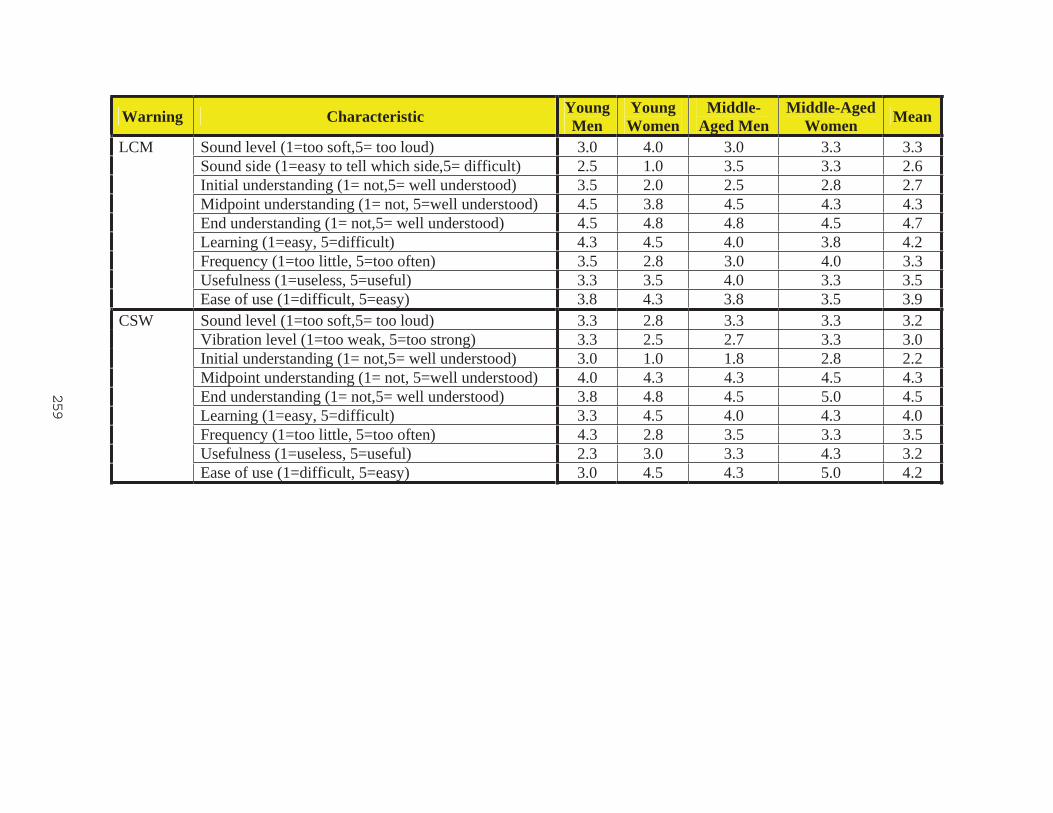
259
Warning Characteristic YoungMen
YoungWomen
Middle-Aged Men
Middle-AgedWomen Mean
LCM Sound level (1=too soft,5= too loud) 3.0 4.0 3.0 3.3 3.3Sound side (1=easy to tell which side,5= difficult) 2.5 1.0 3.5 3.3 2.6Initial understanding (1= not,5= well understood) 3.5 2.0 2.5 2.8 2.7Midpoint understanding (1= not, 5=well understood) 4.5 3.8 4.5 4.3 4.3End understanding (1= not,5= well understood) 4.5 4.8 4.8 4.5 4.7
ng (1=easy, 5=diffiLearni )cult 4.3 4.5 4.0 3.8 4.2Frequency (1=too little, 5=too often) 3.5 2.8 3.0 4.0 3.3Useful ess, 5=useful)ness (1=usel 3.3 3.5 4.0 3.3 3.5Ease of use (1=diffi , 5=easy)cult 3.8 4.3 3.8 3.5 3.9
CSW Sound level (1=too soft,5= too loud) 3.3 2.8 3.3 3.3 3.2Vibration level (1=too weak, 5=too strong) 3.3 2.5 2.7 3.3 3.0Initial understanding (1= not,5= well understood) 3.0 1.0 1.8 2.8 2.2Midpoint understanding (1= not, 5=well understood) 4.0 4.3 4.3 4.5 4.3End understanding (1= not,5= well understood) 3.8 4.8 4.5 5.0 4.5
ng (1=easy, 5=diffiLearni t)cul 3.3 4.5 4.0 4.3 4.0Frequency (1=too little, 5=too often) 4.3 2.8 3.5 3.3 3.5Useful ess, 5=useful)ness (1=usel 2.3 3.0 3.3 4.3 3.2Ease of use (1=diffi , 5=easy)cult 3.0 4.5 4.3 5.0 4.2

F.3.9 Collisions Although the focus of this experiment was not on collisions, two types of collisions occurred: inadvertent (or real, at-fault) collisions and deliberate (or not-at-fault) collisions. In the at-fault collisions, crash provocative events occurred, and even with the warning systems, the subject was not able to avoid the collision. In the not at-fault collisions, something had happened (e.g., the subject failed to merge in the desired location) to place the subject was out of position for subsequent events. Most of the time, the subject would come to a stop (and, in response, so too would the traffic) and the experimenter would tell the subject what to do. Since the subject was invincible (a collision did not stop the simulation, though crashes were logged), sometimes the quickest way to return the simulation to the desired configuration was to have the subject drive through other vehicles, which was feasible because all objects in the simulation were virtual. Code was written for the lead, side, and following vehicles to go at roughly the same speed as the subject in order to maintain the parameters (distances and timings) of the designed scenarios, regardless of subject speed. When the subject behaved unexpectedly, such as accelerating excessively or occasionally failing to follow directions (changing lanes unexpectedly), the subject would get off the pre-programmed sequence of the experiment, requiring that steps be taken to return the subject to the desired sequence. In retrospect, it might have been useful to have an experimenter-initiated freeze/unfreeze function, such that if a subject (and traffic) came to a stop, the traffic would remain stopped (frozen) until the subject had driven to the desired position, at which point the experimenter would unfreeze (restart) the simulation. Had this feature been provided, subjects would not have had to drive through other vehicles, and the simulation would have been preserved. In addition, code was needed to prevent the lead vehicle from driving through the subject when the subject got ahead of that vehicle. Both of these enhancements required time, which was not in the project schedule, to implement. There were 46 collisions in experiment 2 – of which 34 were not-at-fault and 12 were at-fault. The 12 at-fault collisions were distributed among 9 of the 16 subjects, with each having one or two collisions. Seven of those nine subjects were young, accounting for 10 of the 12 collisions. All at-fault collisions occurred in the first three blocks. (Not-at-fault collisions were more common in block 1, at 14 of 34 collisions.) One at-fault collision was associated with no particular scenario, one was associated with scenario 3 (FCW-lead vehicle changes lanes due to construction and then decelerates), two with scenario 4 (FCW-reveal), two with scenario 6 (LCM-subject changes lanes with vehicle in blind spot), and seven with scenario 7 (LCM-subject changes lanes and vehicle accelerates into blind spot). Four collisions involved a lead vehicle, two a reveal vehicle, and seven a side vehicle. Keep in mind that even though the field of view was 200 degrees, there were still some areas a subject might see in a real vehicle that were not visible in the simulation, and because of the rear projection screen location, the outer edge of the right mirror was cut off, enlarging the right side blind spot. A blind spot detection system could have reduced the likelihood of more than half of these crashes. Another reason for the seemingly high number of crashes is that, by design, subjects experienced many very dangerous situations in a short period of time, a situation necessary to trigger alarms (and see how subjects respond). Scenarios were created to make it difficult for subjects to avoid collision situations when following the experiment plan.
260

F.4 Conclusions Conclusions are discussed in terms of the questions that the research addressed.
Were There Enough Warnings to Examine Differences? In this experiment, 1,655 warnings were presented to 16 subjects, or about 100 per subject. Of these, 658 were for FCW, 225 for CSW, 613 for LDW, and 159 for LCM. Thus, roughly speaking, the probability of a forward event and side event were close to being equal. In addition, there were 126 warnings that were planned but not triggered, mostly for LCM. Further, of the 1,655 warnings, 986 were not triggered as planned, with more than half (511) being for LDW. Thus, there were more than enough warnings to examine differences among conditions of interest, even at the level of planned versus unplanned warnings. Both planned and unplanned situations contained events that legitimately required warnings. However, for the planned warnings, the pre-warning configurations were very similar. In the unplanned warnings, there was greater variation in the pre-warning configurations, making comparisons more difficult. As expected, young drivers received more warnings than middle-aged drivers, especially for LDW. However, interestingly, women received more warnings than men, especially for LCM and LDW, which was not expected. When drivers were informed, warnings were less likely to occur (31%) and distraction increased the number of warnings (by 8%). The effect of distraction noted here probably underestimates what would occur in the real world as subjects were not always conscientious about performing the secondary task. A major concern of the IVBSS project is what happens when multiple warnings are presented. In this experiment, there was no deliberate effort to have warnings occur concurrently, only frequently, which does make concurrent events much more likely than in real driving. Of the warnings presented, some 384 (166 events) occurred within three seconds of each other, with the time between events being exponentially distributed. The three-second window was chosen because over that time period most of the response to a warning has occurred, so there is some independence of a response to a second warning. Some two-thirds of multiple warnings started with an LDW, with one-third being two LDWs in a row.
Where Did Drivers Look? Data from baseline conditions (five to ten seconds before a warning and five to ten seconds after a warning) were compared with the zero-to-three-second period after a warning. An important distinction was whether CSW was included, as in the period immediately after a CSW, drivers were scanning the curve, not straight ahead. Curiously, there were few differences between warnings in terms of the number of glances to various locations. In all cases, drivers were more likely to fixate on the front area (about 65% of the time during the baseline periods and 75% of the time immediately after a warning), even for LCM where the hazard was on the side of the vehicle. There were hardly any differences between warnings in terms of the fraction of time where drivers looked, though there were more glances for LCM to the right as subjects were often looking for a merging vehicle before the warning was presented. There were, however, two odd points of note, with subject looking 15 percent of the time to the navigation system before a CSW (with the front area fraction being low) and 12 percent for LDW to the navigation system (and again the forward fraction being low) in the baseline after an LDW. This may reflect drivers in the distraction condition attending to the navigation task. What is interesting is drivers
261

returned so quickly to a navigation task after an LDW (within five to ten seconds). It could be the primary influence of a warning is on the first glance after a warning, so a finer grained analysis is required. Furthermore, there were many instances where drivers had begun to respond before the warning was presented, thus making partitioning the glance data more difficult. Interestingly, most of the distributions of eye fixations were exponentially distributed, with means of about 0.85 seconds for the front, 0.40 seconds for the speedometer, 0.30 seconds for the navigation system, and about 0.14 to 0.20 seconds elsewhere (mirrors, other parts of the scene). Glance data for multiple warnings were not examined, as there was too little data to examine for each combination of warnings.
How Long Did Drivers Take to Respond to Warnings and What Did They Do? For forward warnings, the primary response was slowing down, of which the first step is backing off the throttle. Using the criteria of no release of the throttle (to zero) within six seconds of a warning and release within three seconds of a warning, drivers responded to only about 27 percent of the FCWs and 18 percent of the CSWs. For FCW, the mean times were 0.788 seconds and 1.072 seconds for accelerator pedal release time and brake onset time, respectively, with standard deviations of 0.853 and 0.534 seconds. The mean accelerator pedal release time for CSW was 1.474 seconds with a standard deviation of 0.907 seconds. Keep in mind that these driver responses relate to a several different scenarios. In terms of speed reduction, drivers decelerated about 4 mph for every 0.5 seconds, ignoring the first 0.5 seconds in which little speed change occurred. For CSW, the speed drop was small at about 1.0 mph over the three-second interval. There were major differences in speed reduction among scenarios—8 mph per second for lead vehicle deceleration, about 4 mph for lead vehicle deceleration after a lane change, about 3.0 mph for cut ins, and just over 1.0 mph for reveals. For LDW and LCM, the key response was the change in lane position. Distance from lane center continued until about 0.3 seconds after the warning, returning to the level at the warning by 0.6 seconds, and continuing to decrease, with very minor changes, after 1.8 seconds. On average, distances were about 0.2 seconds greater for LCM than for LDW.
Did Distraction Affect Driver Responses?
Drivers appeared to respond the same way (in terms of response time to warnings, deceleration after warnings, and lateral positioning in both distracted and nondistracted conditions). It is important to note, however, that drivers were not always diligent in performing the distraction task, so in fact, they may not have been distracted.
How Well Did Drivers Understand the Warnings? The major insight into this question comes from the post-test survey of the experimental experience, a series of questions on a 1-to-5 scale. Table 78 shows the mean post-test ratings grouped into categories. Most of the physical characteristics (light brightness, sound) seemed to be about at the desired level, though subjects did rate the vibration level as a bit too high. However, keep in mind that subjects were wearing light clothing, and when wearing winter clothing, more intensive vibration is needed. Subjects also rated determining the side of the LDW (due to the light) somewhat difficult. Some improvements are needed.
262

None of the warnings was initially well understood, with the lack understanding of CSW being most noteworthy. This suggests this warning should be revised, though improvement of all of the warnings should be considered. Keep in mind that these data were collected in a fixed-base simulator, and in this experiment there were no consequence of driving a curve too quickly.
Table 78. Overall mean post-test ratings of the warnings
Category Characteristic Scale FCW CSW LDW LCM Format Sound level 1=too soft, 5=too loud 3.1 3.1 3.4 3.3
Distinguishing sound side 1=easy, 5=difficult - - 2.3 2.6 Vibration level 1=too little, 5=too much 3.3 2.9 3.6 -Distinguishing vibration side 1=easy, 5=difficult - - 2 -Light brightness 1=too dim, 5=too bright - - 2.8 -Distinguishing light side 1=easy, 5=difficult - - 2.4 -
Meaning- Initial understanding 1= not, 5=well understood 3.0 2.2 2.9 2.7 fulness Midpoint understanding 1= not, 5=well understood 4.5 4.3 4.5 4.3
End understanding 1= not, 5=well understood 4.7 4.5 4.8 4.7 Learning 1=easy, 5=difficult 4.4 4.0 4.4 4.2
Overall Frequency 1=too little, 5=too often 3.4 3.5 3.5 3.3 Usefulness 1=useless, 5=useful 3.8 3.2 3.6 3.5 Ease of use 1=difficult, 5=easy 3.8 4.2 4.1 3.9
Nonetheless, all of the warnings were rated as somewhat useful (about 4) with only small differences among them. However, none of the warnings was well rated in terms of usefulness, with the highest rating being for FCW (3.8).
F.5 Forms F.5.1 Biographical Form
Date: ___________ Participant #: ____
Personal Data Name: _______________________________________ Sex (circle one): { M } { F } Phone: ( ____ ) ______________ E-mail address: _____________________________ May we contact you for future UMTRI studies? { Yes } { No } Date of Birth (month / day / year): ____ / ____ / ____ Is English your first language? { Yes } { No } Occupation: _____________________________________________
(engineer, teacher, etc.; if retired, write “retired” and list previous occupation) Education (circle highest level completed):
{ High School } { Some College } { College Degree } { Graduate School } If you attended college, what was your major? ________________________________
Driving Data Licensed driver's in the State of ____ . Is it current? { Yes } { No } What motor vehicle do you drive most often?
Year: ________ Make: ___________________ Model: ___________________ Approximately how many miles do you drive per year? ____________ mi / yr
263

Approximately what percentage of your time driving is spent on expressways? _____ % Do you have any special driving licenses (commercial, chauffer, etc.)? { Yes } { No }
If yes, please list: _________________________________________ How many accidents have you been involved in during the past 5 years? ______
Brief description: ___________________________________________________ _________________________________________________________________ How many traffic violations have you been involved in the past 5 years? _______
Brief description: ___________________________________________________ _________________________________________________________________ On a 3-lane expressway, which lane do you normally drive in?
{ Left } { Middle } { Right }
Cellular Telephone Use Do you use a cellular phone for your primary telephone? { Yes } { No } On a typical trip, how many cell phone calls do you place and/or answer?
{ 0 (go to next section) } { 1 } { 2 } { 3 } { 4 } { 5 } { more than 5 } Which type of cell phone do you usually use while driving?
{ Hand-held } { Hands-free } { Use hand-held/hands-free equally } To place a call while driving, how do you usually retrieve a phone number?
{ Enter manually } { Speed dial } { Choose from contact list } { Voice } Where is your cell phone usually located when you are driving?
{ Pocket/Belt holder } { Seat/Lap } {Vehicle-mounted cradle/Cup holder} { Purse } { Other } If other, please explain: ________________________
Navigation System Use Does your vehicle have a navigation system? { Yes } { No } If yes, do you enter addresses while you are driving? { Yes } { No }
Vision What type of corrective lenses do you wear corrective lenses while driving?
{ None } { Glasses } { Contacts } If yes, what type?
{ Near-Vision/Reading } { Far-Vision } { Bifocal } { Multifocal } { Other } If other, please describe: _________________________________
What type of corrective lenses do you wear corrective lenses while reading? { None } { Glasses } {Contacts }
If yes, what type? { Near-Vision/Reading } { Far-Vision } { Bifocal } { Multifocal } { Other } If other, please describe: _________________________________
Scoring for vision and hearing test (experimenter use only):
F.5.2 Instructions to Subjects Well in Advance
In the simulator lab, prepare a folder with enough copies of all the forms (consent, biographical, post-test evaluation) and blank videotapes for all subjects plus 25 percent extra for spares. Also, make sure there are several spare pens in the drawer of the operator’s station plus a pad for notes.
Coordinate with Denise to have enough cash to pay subjects. At the end of every day get her the signed payment forms so she can go to the cashier to have her supply of cash replenished.
Make sure the conference room is reserved for subject testing.
Preparation for Subject Arrival Make sure supplies are in order, including: x Sim lab key x Forms:
o Consent
264

o Biographical o Post-test evaluation
x Subject list (know name of next subject) x New videotape with label x Notepad x Extra pen (for subject) x $50 for subject payment x Visitor parking pass for that day x Write "sim" on the log-in board and the times you will be there
Sim-Lab Setup x Flip experiment signs on door (testing in progress, do not enter) x Follow the provided simulator start-up sheet x Check that channels on quad screens are correct (front, rear , face, IP) x Chain the doors and pull side screens down x Check image quality on screens and adjust cameras or video switcher if needed x Check that eye-tracking camera is aligned x Drive test loop to make sure everything is running as planned (warning signals, scenarios,
distracting task, fog, construction, etc.) x Get forms, vision test, and hearing test ready
Go to lobby to wait for subject.
Experiment Introduction and Preparation
Greet Subject Hi <subject’s name> my name is <experimenter's name> and I’ll be conducting the driving simulator study. Thank you for coming in today, you will need a visitor parking pass to park at UMTRI, did you receive one in the mail?
If subject needs another parking pass say: To avoid getting a ticket, you’ll need to place this pass face-up on your dashboard and we’ll be ready to go when you return.
Let's go to the conference room and get started.
Lead subject to conference room.
Overview (in conference room) Before we get started, I will give you a brief overview of the study and what you will be doing.
The purpose of this study is to test the safety and usability of in-vehicle systems that could make the next new vehicle you buy much safer to drive. The experiment will take place in the driving simulator where I will collect data on you during both normal and distracted driving. I’ll explain more about what that means later on.
To examine how effective these in-vehicle systems are, we will be recording your actions and what you say for the entire time you are driving in the simulator. In addition to using these recordings for data analysis, it is possible that we (UMTRI), or the Department of Transportation (who is funding this project), may use portions of your videotape in presentations or in the study reports. Furthermore, our work sometimes appears in the media so there is a chance that some portion of your tape will be shown on TV. If your tape is used for these purposes, your name, driver’s license number, and any other personal information that could be used for identification would never be used. Personal information would not leave UMTRI as it is used only for verification and, if you choose, to contact you about future UMTRI studies. Do you have any questions about how the video data we collect today may be used?
Answer any questions they have to the best of your ability. Is it alright with you if we videotape you during the experiment?
265

If “no,” dismiss subject.
Alright, let’s continue. Before you start driving I’ll need you to answer some questions about your driving background and I’ll need to test your vision and your hearing. After that we will go to the simulator laboratory so you can practice driving and using the navigation system.
After about ten minutes of practice, you will drive in the simulator for four 15-minute periods, with a short break between each period. So you will be driving in the simulator for about 1 hour and 10 minutes. Video cameras and audio recording devices will be recording you during the entire time you are driving in the simulator. These recordings will be used to study things like how you react to different driving situations, where you look when you drive and how your driving is affected by distraction. After you finish the last 15-minute driving period, there will be a short survey for you to complete.
The entire experiment will take about two and a half hours to complete, at the end of which, you will receive $50 in thanks for your participation. Would you like to continue?
If no, dismiss subject.
You may choose not to continue with the experiment at any time. If you do choose not to complete the experiment, you will still be paid.
Consent and Bio Forms Before we go any further I’ll need you to read and then sign this consent form. Even though I have covered the basics of the information on the form, please read it carefully and sign at the bottom when you are finished. Feel free to ask me questions at any time.
If the subject does not read the consent form, say: Please make sure you read this form thoroughly. I know it seems like extra paperwork, but we’re required to ensure that you understand this information.
Thank you. Here is the biographical data sheet. Please fill it out and feel free to ask me questions at any time.
Provide bio form. Check that both the consent form and bio form are legible and complete.
We’re done with the preliminary paperwork, now I need to check your eyesight and hearing.
Vision Test Do you use any corrective eyewear while you drive?
If subject answers “yes,” say: Is that what you are wearing now? If subject is not wearing the same eyewear they wear while driving ask subject to put that on.
We’re not professional optometrists or audiologists, these tests are just for screening. Please look into the vision device and keep looking straight ahead for the entire eye test.
Test Visual Acuity (FAR #2): - Can you see that in the first diamond in the top circle is complete but the other 3 are broken? In
each diamond, tell me the location of the solid circle - top, left, bottom, or right. -
Continue until 2 in a row are wrong. The last correct answer is the visual acuity.
Test Near Vision (80 cm) (FAR#2) with lenses: - Can you see in the first diamond that one of the circles is complete but the other 3 are broken? In
each diamond, tell me its number and the location of the complete circle—top, bottom, left or right.
Continue until 2 in a row are wrong. The last correct answer is the visual acuity.
266

Color-Abnormality (FAR #6): - In each circle, there is a number. Please tell me the number in circle.
Go through each circle (Circle F does not really have a number).
Hearing Test In this test we will be testing the full range of hearing. Very few people are capable of hearing all of the tones I will play.
Perform hearing test.
That’s all I need for now, let’s go to the driving simulator for the rest of the experiment.
Take subject to simulator.
Simulator Introduction and Setup
Sim Lab Introduction In this driving simulator, we have a very wide image, which covers the 3 areas in front of the cab, the 2 side screens and the area behind the cab. The screens will cover the doors when pulled down, and I will to use this chain lock to prevent someone from opening one of the doors and tearing a screen. However, you are not “chained in” as anyone on the inside or outside of the door can easily unhook the chains.
Pull down screen.
Seat Subject Please have a seat in the cab and adjust the seat to a comfortable position using the automatic controls on the left side of the seat.
As I mentioned before, there are cameras in the vehicle to provide a variety of camera angles. Point out cameras.
There is also a live microphone here. Show subject the microphone.
The 2 cameras directly in front of you that say A and B are used to track your eye-movement and these are infrared light emitters that help the eye-tracking system see in the dark.
Show subject eye-tracking cameras and infrared pods.
Create New Face Model The last thing we have to do before you can start driving is set up the eye tracking system, which will record where you look while you’re driving.
Click on FaceLAB 3 on the desktop (if not already open).
Step 1: Adjust camera tilt so that subject’s entire face in on the screen, ideally all features should be inside red box.
- Use tilt-o-meter to measure tilt angle of cameras and note angle. - Go to the Controls window and click on the Stereo-Head tab and enter that value for “tilt.”
Step 2: If necessary, adjust camera focus to focus directly on subject’s eyes.
Step 3: Click on Face Model Menu > New Face Model > Manual model.
Step 4: Use radio buttons to choose “Full Head Mode,l” “Features and Markers,” and “Head, Eye, and Gaze.”
- If necessary, ask subject to remove eye makeup (especially eyeliner).
267

Step 5: Click next to get to marker placement screen. Have subject place markers on face as shown. Subject will have one marker at the tip of the nose, one between the eyebrows, and two symmetrically placed on flat front of forehead. Two additional markers will be symmetrically placed on the temples.
- Explain that it’s very important that markers are secure and are not moved AT ALL throughout the study (or you will need to construct a new face model).
- If necessary ask subject to clean face using wipes (if subject has oily patches where markers will be placed).
- Make sure hair does not obstruct markers, if necessary ask subject to use an elastic band to keep hair out of face and markers.
Step 6: Click next to get to Snapshot window. - Adjust camera brightness for maximum contrast. - Make sure sim is showing road scene so that brightness matches actual testing conditions.
Step 7: Follow instructions on top of screen to take the five snapshots. - Ask subject to hold steering wheel and assume a driving posture so that snapshots are close to
the driving head pose. - If necessary, ask subject to assume neutral expression, all shots should use the same
expression, no smiling, etc. - For the 20 degree shots ask subject to look at seam between the front and side screens
(approximately 20 degrees from center). - Snapshots must be retaken every time the focus or camera brightness is adjusted.
(The following steps should be performed while the subject practices driving in the simulator.)
Step 8: Click next to get to Reference points window. - Check placement of each reference point in Camera B window, if necessary (usually is) move
points to areas of maximum contrast. - Check that reference points match well for both cameras, if necessary, use fine adjustment option
to adjust position of camera A points, - Choose points that are visible from every shot, and match selected points in each snapshot.
o Especially important for placement of mouth and side points. - Use temple markers for side point if no other good choice is available (such as sideburns, strong
hairline point around ears, etc). - Placement of reference points must be as follows:
o Reference points for “straight ahead” snapshot: � Outside corner of left eye � Inside corner of left eye � Outside corner of right eye � Inside corner of left eye � Left corner of mouth � Right corner of mouth
o Reference points for “20 degrees to the left” snapshot: � Outside corner of right eye � Inside corner of left eye � Outside corner of left eye � Left corner of mouth � Right corner of mouth � Right side point
o Reference points for “20 degrees to the right” snapshot: � Outside corner of left eye � Inside corner of left eye � Outside corner of right eye � Left corner of mouth � Right corner of mouth � Left side point
o Reference points for “90 degrees to the left” snapshot:
268

� Outside corner of right eye � Right corner of mouth � Right side point
o Reference points for “90 degrees to the right” snapshot: � Outside corner of left eye � Left corner of mouth � Left side point
Step 9: Click Next to go to Features window. - Confirm marker target placement in Camera B screen, adjust if necessary. - If necessary use Fine Adjustment option to match feature placement in Camera A screen. - Remove extra features, features should be only where reference points were and high-contrast
stationary features such as moles. - Use temple markers for side point features.
Step 10: Click Next to go to Face Tracking window. Check tracking quality. - If reference points “jump around,” return to that step and adjust placement. - If features “jump around,” return to that step and stop tracking those features.
Step 11: Click Next to go to Gaze tracking window. - Use radio button to select “Dark Iris, Dark Pupil.” - Adjust parameters to achieve best pupil tracking quality.
Step 12: Click Next to go to Gaze calibration window. Say: I may have to do this a couple of times. - Click the “Calibrate” button and follow on screen instructions. - For best calibration, ask subject to keep gaze as consistent as possible and not to blink.
Step 13: Confirm gaze tracking calibration by asking subject to look into Camera A and then Camera B. - If calibrated properly the gaze vector in the Camera A and Camera B viewing windows should
appear as points when subject looks into the respective camera. - If gaze tracking is poor, click Back and recalibrate gaze. - If recalibration does not improve gaze tracking quality, click Back again and adjust pupil, iris, and
eye closure parameters. Recalibrate gaze.
Step 14: Click Next and confirm tracking quality. - Adjust settings as necessary to achieve optimal head and gaze tracking quality.
Step 15: When gaze tracking is good, click Finish and save face model.
Practice Drives
First Practice Drive Now it is time to try out the simulator. For the duration of this experiment please drive normally, being
sure to be safe. You should use your turn signal as normal and use the speedometer on the instrument panel to check your speed, just as in a real vehicle.
The speed limit is 70 mph and you will see speed limit signs throughout the course as a reminder. The speed limit signs may look like they’re flashing, that’s just the way that they look in the simulator it does not mean you should change anything or that you are doing anything wrong. Try to maintain a speed of 70 mph at all times. If 70 mph is an uncomfortably fast driving speed for you, go as fast as you are comfortable. However, keep in mind that if you go slower than 70 mph the experiment will take longer to complete.
The steering wheel in the simulator doesn’t feel exactly like one in a real vehicle and it is easy to overcorrect. So the key is to make small corrections with the steering wheel.
Some people experience motion sickness in the simulator, so if you start feeling nauseous, dizzy, or anything else that could occur prior to being motion sick, let me know immediately and I’ll tell you how to stop. As I said before, you may end the experiment at any time and you will still be paid $50.
Do you have any questions?
269

Before we begin, please adjust the left side mirror and the center rear-view mirror. The control for the right side mirror does not work properly, so I will help you adjust the position.
Ok then, put the vehicle in “D” using the shift lever between the seats. This practice drive will last for about 3 minutes. I will tell you when the time is up.
Now, please press on the accelerator and begin driving.
While subject is practicing, one experimenter will be working with the eye-tracking system, the other experimenter watching the face monitor in the control room (one experimenter can do both tasks if necessary).
Have the subject drive for approximately three minutes.
Ok, that’s the end of the first practice drive. Please coast to a slow stop and shift the vehicle into park.
Stop the simulator ten seconds after the vehicle is in park.
Secondary Task Training Now I will show you how to perform the secondary task of entering addresses into the navigation system.
Sit in passenger seat to explain task to subject.
Here’s how to enter a destination: - Touch the “Start” button. - Then touch the “Navigation” button on the first screen menu. - Then touch “Destination Entry” and the navigation system will appear on the touch screen. - Enter the addressed shown on these index cards in order, when you finish each packet I will give
you a new one. - Enter the full three-line address exactly as it is shown on the card, don’t forget the road
abbreviation, such as “r-d” for road or “a-v-e” for avenue. You can use the backspace arrow key to make corrections.
o Enter the text on the first line, then press Enter. o Enter the text on the second line, then press Enter. o Enter the text on the third line and then press Enter to finish.
- You will hear a beep if you entered the address correctly and a game show buzzer if the address is incorrect.
- Whether the address was entered correctly or incorrectly go to the next card each time you press finish.
Try the next address. Have the subject practice entering two to five more addresses. Stop when they get it.
Seconds Practice Drive (With Secondary Task) Ok, now you’re ready to practice the secondary task while driving. This second and final practice drive will last for about 5 minutes. Enter as many addresses as you can in this time, but do your best to not make mistakes. As soon as you finish one address, flip the card over to read the next address.
Do you have any questions?
Ok, you may begin driving. Begin entering addresses once you have reached 70 mph. I will let you know when the practice drive is over. You may begin driving whenever you are ready.
Subject drives for about five minutes while using the navigation system.
Ok, that’s the end of the second practice drive. Please coast to a slow stop and shift the vehicle into park.
Stop the simulator ten seconds after the vehicle is in park.
270

Calibrate Eye Tracking System for Placement of Objects in World Step 1: In the faceLAB 3 Controls window, click on the “logging” tab and then the “file” button. Change file name to correct name and format (subject’s initials_subject number_Calib_Start).
- If necessary click on “Directory” button and assign correct directory.
Step 2: Click on the “Start Logging” button.
Step 3: Make sure road scene is visible and ask subject to fixate on the following sequence of screen objects. Perform sequence twice. Click on appropriate annotation button when subject is fixated (may use laser pointer to direct subject’s gaze):
1: Upper right corner of screen 2: Upper left corner of screen 3: Subject lane 4: Bottom left of screen 5: Bottom right of screen 6: Center of Left Front screen 7: Center of Left Side screen 8: Center of Right Front screen 9: Center of Right Side screen
Step 4: Have subject fixate on the following sequence of cab objects. Perform sequence twice: 1: Left side mirror 2: Right side mirror 3: Center rear-view mirror 4: Gear Shift 5: Center of nav system screen 6: Speedometer
End Practice and Set-Up Portion That is the end of the driving practice and set-up portion of the experiment. We will now take a short break before beginning the first 15-minute drive. You will also get a break between each drive. Feel free to get out of the simulator and walk around for a minute. And if you would like to get a drink of water or use the restroom during any of these breaks, I will be happy to show you where it is.
Data Collection
Block 1 We will now begin the first 15-minute drive. There will be a total of four 15-minute drives and a short break between each drive. Just as in the practice drives, please drive normally, being sure to be safe. Please buckle up, use your turn signal and use the speedometer on the instrument panel to check your speed. Above all, your task is to avoid crashes. Don’t change lanes unless there is a stopped vehicle or an object in your lane. When you are forced to change lanes, stay in that lane unless forced to change again. The speed limit is 70 mph, and you will see speed limit signs throughout the course as a reminder, try to maintain a speed of 70 mph at all times.
For the remaining four drives there will be other vehicles in the road. Keep in mind that the screens do not go all the way around the cab and that sometimes a vehicle may be on the road where it can’t be seen.
The system we are testing has a number of new features that have not appeared in vehicles you can now buy.
You will not be using the navigation system in this drive, which will occur later. Do you have any questions?
Make sure driver is buckled.
271

Ok, now I will turn on the simulator, don’t begin driving until I tell you to begin.
Start logging eye-tracking data. When simulator starts, click annotation buttons for time synch. - A metronome-type sound will start with a rhythmic series of three low tones and one high tone.
Click on the annotation button the moment the high tone sounds until no more tones are presented.
Alright, you may begin driving whenever you’re ready.
Subject drives for 15 minutes. If necessary, remind subject to keep speed close to 70 mph for the entire drive. If subject is ever in the wrong lane, tell him how to get back.
(At the end of Block 1) Ok, turn on your right turn signal and gradually slow down as you pull off onto the shoulder. Once you have stopped, please put the vehicle in park. (10 seconds after you are parked, please stop the simulator.) You may take a break for a minute if you wish. Do you have any comments or questions about what happened in the last 15 minutes?
Block 2 Same as Block 1, but with secondary task. Now we’re ready to begin the second 15-minute drive, during which you will be entering destinations into the navigation system as you practiced before. Enter as many destinations as you can and throughout the drive, but remember, your primary task is to avoid crashes. Any questions? Ok, now I will turn on the simulator, don’t begin driving until I tell you to begin.
Start logging eye-tracking data. When simulator starts, click annotation buttons for time synch. - A metronome-type sound will start with a rhythmic series of three low tones and one high tone.
Click on the annotation button the moment the high tone sounds until no more tones are presented.
Alright, you may begin driving whenever you’re ready.
Subject drives for 15 minutes. Give them a break. Break may be slightly longer than others if needed for bathroom breaks, etc. If subject leaves the sim be sure to stress that they DO NOT MOVE OR TOUCH the eye-tracking markers at all. If they do you will have to create a new face model, which will extend the length of the experiment.
Explain the Warning Systems Now that you’ve had a chance to experience all of the warning systems, I will explain how each of them works. (Play each of the sounds before explaining them.)
FCW – Forward Collision Warning If you are gaining quickly on the vehicle in front of you, and will crash into them unless you begin braking immediately, this warning will sound. For the warning to sound, only part of the vehicle needs to be in your lane.
LDW – Lateral Drift Warning This warning is presented when you begin to leave your lane. If you contact the right edge boundary, then the beep comes from the right side and the right side of the seat vibrates. If you contact the left edge boundary, then the same happens on the left side. If you have your turn signal on to signal a lane change, the warning will not be presented. So, when you change lanes, use your turn signal to keep the system from beeping unnecessarily.
LCM – Lane Change-Merge This warning tells you there is a vehicle in your blind spot when you are changing lanes towards it, even if your turn signal is on. As with the lateral drift, it indicates which side of your vehicle has a vehicle in the blind spot by displaying a red light on the mirror and playing a sound on that side.
272

CSW – Curve Speed Warning This warning will sound when you are approaching a curve too fast. You should slow down to avoid skidding in the curve. When giving the warning the front of the seat will vibrate, and the sound will play.
Block 3 Ok, in this 15-minute drive please drive normally without entering destinations into the navigation system. Ok, now I will turn on the simulator, don’t begin driving until I tell you to begin.
Start logging eye-tracking data. When simulator starts, click annotation buttons for time synch. - A metronome-type sound will start with a rhythmic series of three low tones and one high tone.
Click on the annotation button the moment the high tone sounds until no more tones are presented.
Alright, you may begin driving whenever you’re ready.
Subject drives for 15 minutes. Give subject a break.
Block 4 In this 15-minute drive, you will be entering destinations into the navigation system as you drive. Enter as many destinations as you can and throughout the drive, but remember, your primary task is to avoid crashes. Any questions? Ok, now I will turn on the simulator, don’t begin driving until I tell you to begin.
Start logging eye-tracking data. When simulator starts, click annotation buttons for time synch. - A metronome-type sound will start with a rhythmic series of three low tones and one high tone.
Click on the annotation button the moment the high tone sounds until no more tones are presented.
Alright, you may begin driving whenever you’re ready.
Subject drives for 15 minutes.
Ok, turn on your right turn signal and gradually slow down as you pull off onto the shoulder. Once you have stopped, please put the vehicle in park. (10 seconds after you are parked, please stop the simulator.)
Recalibrate World Objects Perform world calibration again as explained in above, Rename logging file to “…_calib_End”
Forms and Payment Your last task before being paid is to complete this short survey about warning systems and the simulator. (Give subject post-test form to read.) Feel free to ask me questions at any time. (Verify completion of post-test form.)
If subject is a University employee, choose payment form according to affiliation and give subject payment.
Here is your $50, I will walk you out. Walk with the subject to the front door. Thank you very much for your time.
Cleanup (sim lab, data) x Copy simulator and eye fixation data files to thumb drive x Close everything x Shut down x Turn off lights and perform “glow test.” (With the room lights off, is anything glowing?) x Lock the sim lab
273

x Make copy of forms and file them x Copy data from the thumb drive to a hard disk x Update the subject data
274

F.5.3 Post-Test Evaluation Form
Date: ____________ Participant number: ________
Warning Explanation Forward Collision Warning
This warning is presented when you are gaining on the vehicle in front of you, and if you do not begin to brake immediately, you will crash into them. For the warning to sound, only part of the vehicle needs to be in your lane.
Lateral Drift Warning
This warning is presented when you begin to leave your lane. If you contact the right edge boundary, then the beep comes from the right side and the right side of the seat vibrates. If you contact the left edge boundary, then the same happens on the left side. If you have you turn signal on to signal a lane change, the warning will not be presented for that side.
Lane Change- Merge Warning (Blind Spot Warning)
This warning tells you there is a vehicle in your blind spot when you are changing lanes towards it, even if your turn signal is on. As with lateral drift, it indicates (by which side of the seat vibrates and where the sound comes from), on which side there is a vehicle in your blind spot
Curve Speed Warning
This warning will sound when you are going approaching a curve too fast. You should slow down to avoid skidding in the curve. When warning the warning sounds, the front of the seat also vibrates
1. Have you ever driven a vehicle with the following warning systems? (circle one) Forward Collision Warning: { No } { Yes } Lane Change-Merge (Blind Spot) Warning: { No } { Yes } Lateral Drift Warning: { No } { Yes } Curve Speed Warning: { No } { Yes }
2. Forward Collision Warning Format sound was too soft 1 2 3 4 5 too loud
seat vibration was too weak 1 2 3 4 5 too strong Meaningfulness initially, was not understood 1 2 3 4 5 initially, well understood
after midpoint explanation was not understood 1 2 3 4 5 well understood after explanation at the end, was not understood 1 2 3 4 5 at the end, well understood
meaning was difficult to learn 1 2 3 4 5 easy to learn Overall occurred too little 1 2 3 4 5 occurred to often
useless 1 2 3 4 5 useful difficult to use 1 2 3 4 5 easy to use
3. Lateral Drift Warning Format sound was too soft 1 2 3 4 5 too loud
easy to tell which side sound came from 1 2 3 4 5 difficult to tell which side light on side mirror was too dim 1 2 3 4 5 too bright
easy to tell which side light is on 1 2 3 4 5 difficult seat vibration was too little 1 2 3 4 5 too much
easy to tell which side was vibrating 1 2 3 4 5 hard to tell Meaningfulness initially, was not understood 1 2 3 4 5 initially, well understood after midpoint explanation was not understood 1 2 3 4 5 well understood after explanation
at the end, was not understood 1 2 3 4 5 at the end, well understood meaning was difficult to learn 1 2 3 4 5 easy to learn
Overall occurred too little 1 2 3 4 5 occurred to often useless 1 2 3 4 5 useful
difficult to use 1 2 3 4 5 easy to use
275

4. Lane Change-Merge Warning (Blind Spot Warning) Format sound was too soft 1 2 3 4 5 too loud
easy to tell which side sound came from 1 2 3 4 5 difficult to tell which side Meaningfulness initially, was not understood 1 2 3 4 5 initially, well understood after midpoint explanation was not understood 1 2 3 4 5 well understood after explanation
at the end, was not understood 1 2 3 4 5 at the end, well understood meaning was difficult to learn 1 2 3 4 5 easy to learn
Overall occurred too little 1 2 3 4 5 occurred to often useless 1 2 3 4 5 useful
difficult to use 1 2 3 4 5 easy to use
5. Curve Speed Warning Format sound was too soft 1 2 3 4 5 too loud seat vibration was too weak 1 2 3 4 5 too strong Meaningfulness initially, was not understood 1 2 3 4 5 initially, well understood after midpoint explanation was not understood 1 2 3 4 5 well understood after explanation
at the end, was not understood 1 2 3 4 5 at the end, well understood meaning was difficult to learn 1 2 3 4 5 easy to learn
Overall occurred too little 1 2 3 4 5 occurred to often useless 1 2 3 4 5 useful
difficult to use 1 2 3 4 5 easy to use
How should each warning be changed, if at all? Consider what it is presented, its intensity, the sounds chosen, etc.
6. Forward Collision Warning
7. Lane Change-Merge (blind spot warning)
8. Lateral Drift Warning
9. Curve Speed Warning
10. Additional Comments:
276
Appendix G: Experiment 3 – Integrating Warnings for IVBSS
G.1 Overview Experiment 3 addressed the following question: How does combining warnings, using a singular warning to represent more than one possible threat, affect (a) driver performance when responding to them and (b) driver ratings of them? Of interest were single warnings, dual warnings (simple and hybrid), and multiple warnings. The stated goal of the IVBSS field operational test (FOT) is to integrate a suite of crash warning systems (CWS) into a package that provides drivers with an integrated driver-vehicle interface (DVI). Although the need for an integrated DVI is supported by various different design considerations, the optimal level of DVI integration is not always clear. An example of a fully integrated system is that of a single-warning system, in which drivers are alerted for all CWS by one type of warning. In a fully distributed system, on the other hand, drivers are alerted independently by several warnings, one for each CWS or hazard. Intermediate levels of integration vary by the number of CWS and hazards represented by each warning. A preferred integrated system might be designed to optimize safety benefits, driver acceptance, and marketability of the integrated system. The purpose of experiment 3 was to compare several representative levels of integration in terms of objective and subjective driver responses to warnings. General design guidelines for CWS integration have been discussed in a recent analysis of crash warning system interfaces (Campbell, Richard, Brown, and McCallum, 2007). As Campbell et al. point out, CWS integration occurs at the system and subsystem levels, not only at the DVI level. The level of integration of the DVI should therefore match and reflect the integration of CWS hardware and software. In experiment 3, only integration of the DVI was considered so that results could inform the design of the entire IVBSS system. Another design topic highlighted by Campbell et al. is that of prioritization and arbitration of simultaneous hazards. An analysis of crash statistics suggests that simultaneous hazards are not a common cause for crashes (Najm, Smith, and Toma, 2005). Najm et al. recommend a set of crash-imminent scenarios that represent likely crash situations based on the General Estimates System (GES) crash database. None of the common pre-crash scenarios consist of simultaneous hazards, which suggests that the design of an integrated CWS should not heavily consider the case of simultaneous hazards. In addition to the consideration of crash statistics, the team took a user-centered approach to characterize how drivers can benefit from warnings given their processing limitations. There is a distinction between warnings that correspond to data-limited and resource-limited processes (Norman and Bobrow, 1975). As an example, a lane departure warning usually corresponds to a resource-limited process. In most cases, the drivers depart the lane because they are not attending to the driving task, not because they cannot see the position of the lane borders. If drivers are alerted and redirect their full attention back to the regular driving task, they are likely to notice the problem immediately and be able to initiate a correction. In contrast, a lane change warning usually corresponds to a data-limited process. In most cases, drivers initiate a lane change into an
277
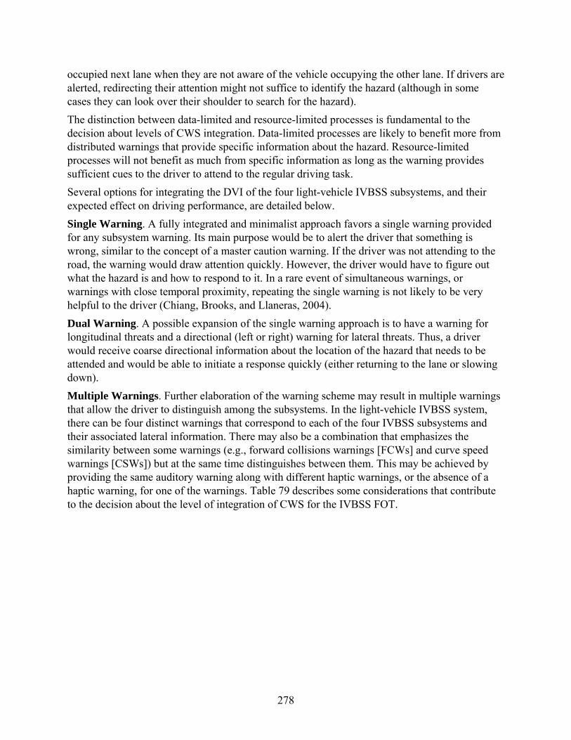
occupied next lane when they are not aware of the vehicle occupying the other lane. If drivers are alerted, redirecting their attention might not suffice to identify the hazard (although in some cases they can look over their shoulder to search for the hazard). The distinction between data-limited and resource-limited processes is fundamental to the decision about levels of CWS integration. Data-limited processes are likely to benefit more from distributed warnings that provide specific information about the hazard. Resource-limited processes will not benefit as much from specific information as long as the warning provides sufficient cues to the driver to attend to the regular driving task. Several options for integrating the DVI of the four light-vehicle IVBSS subsystems, and their expected effect on driving performance, are detailed below. Single Warning. A fully integrated and minimalist approach favors a single warning provided for any subsystem warning. Its main purpose would be to alert the driver that something is wrong, similar to the concept of a master caution warning. If the driver was not attending to the road, the warning would draw attention quickly. However, the driver would have to figure out what the hazard is and how to respond to it. In a rare event of simultaneous warnings, or warnings with close temporal proximity, repeating the single warning is not likely to be very helpful to the driver (Chiang, Brooks, and Llaneras, 2004). Dual Warning. A possible expansion of the single warning approach is to have a warning for longitudinal threats and a directional (left or right) warning for lateral threats. Thus, a driver would receive coarse directional information about the location of the hazard that needs to be attended and would be able to initiate a response quickly (either returning to the lane or slowing down). Multiple Warnings. Further elaboration of the warning scheme may result in multiple warnings that allow the driver to distinguish among the subsystems. In the light-vehicle IVBSS system, there can be four distinct warnings that correspond to each of the four IVBSS subsystems and their associated lateral information. There may also be a combination that emphasizes the similarity between some warnings (e.g., forward collisions warnings [FCWs] and curve speed warnings [CSWs]) but at the same time distinguishes between them. This may be achieved by providing the same auditory warning along with different haptic warnings, or the absence of a haptic warning, for one of the warnings. Table 79 describes some considerations that contribute to the decision about the level of integration of CWS for the IVBSS FOT.
278

Table 79. Summary of considerations for the design of integrated CWS
Consideration Description Considerations favoring integration – fewer warnings than subsystems Information theory. Hick-Hyman law
The time it takes a user to make a decision increases (logarithmically) with the number of possible choices.
Number of subsystems As the number of subsystems in the vehicle increases, there is more need for integration of warnings to reduce memory load.
Warnings that suggest course of action
Warnings that are intended to offer the driver a course of action (e.g., “slow”, “stay in your lane”) can be integrated more easily than those that direct the driver’s awareness to a hazard.
Other systems offered in isolation or as aftermarket
The possibility of other subsystems to enter the vehicle (e.g., phones, after market navigation systems) favors integration among built-in systems.
Considerations favoring distribution – a unique warning for each subsystem Multiple stages If there are multiple stages for some or all of the warnings, it is best to
distinguish them from warnings from other subsystems to communicate the link among the stages and decrease confusion with other subsystems.
Simultaneous warnings (“multiple threats”)
If two or more warnings occur simultaneously, and the system does not suppress the lower priority warning, there needs to be a distinction between the first and second warning.
System reliability The perception of system reliability is likely to be affected by the level of integration of warnings. If there is no distinction among subsystems, drivers will find it difficult to distinguish between true warnings and nuisance warnings. Differentiation between systems may help the driver attribute different reliability values for different subsystems.
Considerations that do not lead to a clear preference between integration and distribution Available modalities to alert the driver
If available, more than one modality (e.g., auditory, Haptic, visual) may be used to either reinforce the alert in two modalities or to help distinguish among the alerts by using different modalities.
Understanding the system in an FOT
For the special case of an FOT, too much integration may make it difficult for subjects to make specific observations about each subsystem. On the other hand, too many alerts may also be confusing.
Data-limited vs. resource-limited processes
Data-limited processes (e.g., when the driver cannot see the hazard) are more likely to benefit from specific and directional information. Resource-limited processes do not require more than a simple alert.
Levels of automation At high levels of automation, the alert need not be specific for each subsystem. If an immediate action is required and there may be some confusion among automated systems, integration might be unsafe.
G.2 Method G.2.1 Participants Sixteen licensed drivers participated in this study. Eight were middle-aged (41 to 55 years old, mean = 48.5 years) and eight were younger drivers (18 to 30 years old, mean = 25.3 years). The age groups were balanced for gender. Each driver was paid $50 for two-and-a-half hours of participation. Each participant had visual acuity of 20/40 or better as determined by an Optec 2000 vision tester. A pure-tone audiometer was used to determine whether a person could hear
279

the following frequencies at 25 dB: 1,000 Hz, 2,000 Hz, and 3,000 Hz. All but two participants were able to hear all of the frequencies at 25 dB. Two participants were unable to hear the 3,000 Hz tone at 25 dB, but could hear it at 45 dB, which was deemed to be acceptable for this study.
G.2.2 Apparatus The DriveSafety driving simulator has a full-size vehicle cab with operating foot controls and a torque motor to provide realistic force feedback. Road scenes are projected on three forward screens almost 16 feet from the driver, two side screens approximately 13 feet from the driver (200-degree field of view), and a rear channel 12 feet away (40-degree field of view). A pair of 3.5-inch Boston Acoustic speakers was inserted into the headrest, through which the warning sounds were presented. QCreator, an audio software package, was used to provide directionality for the lateral drift and lane change-merge warnings (LDW and LCM, respectively). A simulated haptic brake pulse was added to the simulator for the purposes of this experiment. A linear motor, attached to the bottom of the simulator buck provided a quick burst of longitudinal motion that was both felt and heard, and was distinct from the seat shaker signal.
G.2.3 Warning Approaches Four warning approaches were investigated in this study. Table 80 describes the approaches as well as the auditory and haptic combinations for each of the subsystems. Table 81 provides details about each auditory warning. All auditory warnings were presented at about 80 dB(A) and ambient driving levels of about 70 dB(A).
Table 80. Auditory and haptic combinations for each of the four warning approaches
FCW CSW LCM LDW
Single warning Single sound
1
bottom seat vibration both sides together
Dual warning-simple Two sounds
1 (L) (R) 5
Brake pulse Seat shaker (L) (R)
Dual warning-hybrid Two sounds combined
1 (L) (R) 3
-----
Brake pulse ----- ----- Seat shaker (L) (R)
Multiple warnings Four separate sounds
1 2 (L) (R) 3
(L) (R) 4
Brake pulse ----- ----- Seat shaker (L) (R)
280

Table 81. Characteristics of the auditory sounds used in the warning approaches
Warning Pitch (Hz)
Pulse Rate (ms)
Duration (ms)
Onset (ms) Pulses
Tone 1 (abstract) 1,500 100 70 5 7 Tone 2 (tires) 600 30 Tone 3 (honk) 1,000 160 150 Tone 4 (rumple strip) 400 150 50 10 Tone 5 (abstract) 500 110 10 4
G.2.4 Driving Scenarios and the Simulator World This section includes graphics and detailed descriptions of selected scenarios (see Appendix B for the complete set of scenarios). In benign case situations, the suggested modifications change the warning scenario to benign when there is no triggering event. Displaying a warning when there is no triggering event (such as in the benign case) creates a false alarm scenario.
FCW Scenario: Lead vehicle (L) suddenly decelerates
Subject vehicle (S) follows lead vehicle (L) (S-L heading | 1 sec) traveling at about 70 mph. Adjacent vehicle (A) blocks subject from changing lanes (blocking vehicle is needed later).
At action point, lead vehicle suddenly decelerates at 0.5g (4.9 m/s2). Adjacent vehicle still blocks subject from changing lanes.
Benign Case: Lead vehicle decelerates at slower rate (normal rate is about -.2g (1.96 m/s2)). Since deceleration is gradual, subject vehicle will likely decelerate at same rate and FCW will not be triggered. (The subject will have sufficient time to react.)
Triggering Event: FCW is triggered when time to collision (TTC) = 1 second.
281
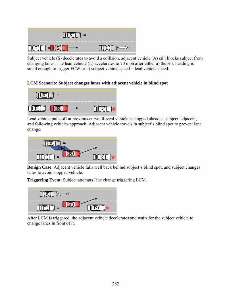
Subject vehicle (S) decelerates to avoid a collision, adjacent vehicle (A) still blocks subject from changing lanes. The lead vehicle (L) accelerates to 70 mph after either a) the S-L heading is small enough to trigger FCW or b) subject vehicle speed = lead vehicle speed.
LCM Scenario: Subject changes lanes with adjacent vehicle in blind spot
Lead vehicle pulls off at previous curve. Reveal vehicle is stopped ahead as subject, adjacent, and following vehicles approach. Adjacent vehicle travels in subject’s blind spot to prevent lane change.
Benign Case: Adjacent vehicle falls well back behind subject’s blind spot, and subject changes lanes to avoid stopped vehicle.
Triggering Event: Subject attempts lane change triggering LCM.
After LCM is triggered, the adjacent vehicle decelerates and waits for the subject vehicle to change lanes in front of it.
282

CSW Scenario: Subject approaches curve with excessive speed
The subject (S) follows the lead vehicle (L) at comfortable dist. (S-L heading § 1 sec). The adjacent vehicle (A) blocks subject from changing lanes, and the lead vehicle accelerates to 75 mph near the curve entrance.
Triggering Event: The subject enters the curve with excessive speed, which triggers CSW.
LDW scenario: Subject drifts out of lane without turn signal on
Triggering Event: Cross winds cause the subject to drift from the lane. (Distracting tasks should also cause LDWs.)
283
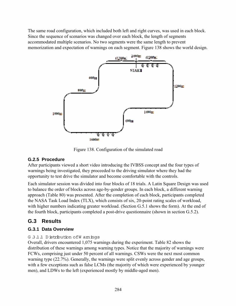
The same road configuration, which included both left and right curves, was used in each block. Since the sequence of scenarios was changed over each block, the length of segments accommodated multiple scenarios. No two segments were the same length to prevent memorization and expectation of warnings on each segment. Figure 138 shows the world design.
Figure 138. Configuration of the simulated road
G.2.5 Procedure After participants viewed a short video introducing the IVBSS concept and the four types of warnings being investigated, they proceeded to the driving simulator where they had the opportunity to test drive the simulator and become comfortable with the controls. Each simulator session was divided into four blocks of 18 trials. A Latin Square Design was used to balance the order of blocks across age-by-gender groups. In each block, a different warning approach (Table 80) was presented. After the completion of each block, participants completed the NASA Task Load Index (TLX), which consists of six, 20-point rating scales of workload, with higher numbers indicating greater workload. (Section G.5.1 shows the form). At the end of the fourth block, participants completed a post-drive questionnaire (shown in section G.5.2).
G.3 Results G.3.1 Data Overview G.3.1.1 Distribution ofW arningsOverall, drivers encountered 1,075 warnings during the experiment. Table 82 shows the distribution of these warnings among warning types. Notice that the majority of warnings were FCWs, comprising just under 50 percent of all warnings. CSWs were the next most common warning type (22.7%). Generally, the warnings were split evenly across gender and age groups, with a few exceptions such as false LCMs (the majority of which were experienced by younger men), and LDWs to the left (experienced mostly by middle-aged men).
284

Within this sample, 107 warnings (10.6%) occurred within three seconds of a preceding warning. These warnings were considered to be part of multiple warning events, where an event consists of the precipitating warning and all following warnings that occur within three seconds of each other. Using these criteria, 82 multiple warning events were found in the data, and these events included 190 individual warnings (17.7%). These 190 warnings were excluded from all further analyses.
Table 82. Frequency of warnings across warning type
Warning Total ( f ) Total, Excluding Multiple Warnings ( f ) FCW 534 468 CSW 244 240 False FCW 104 41 LDW - right 93 60 LDW - left 60 38 False LCM 40 38
Total 1,075 885
The distribution of warnings among the 16 subjects was also generally balanced. Table 83 shows the frequency of each presented warning type across subjects. Some noticeable exceptions to the even distribution include LDWs to the left, in which two subjects account for nearly 40 percent of the total, and false LCMs to the right, where subjects either appeared to receive about the same number of warnings or none at all.
Table 83. Frequency of warning types presented across subjects
Group Subject FCW CSW False FCW
False LCM (Right)
LDW (Right)
LDW (Left) CSW Total
You
ngw
omen
1 30 12 4 4 5 0 12 55 2 30 13 4 3 0 7 13 57 3 27 16 4 4 5 3 16 59 4 28 11 4 4 2 1 11 50
You
ngm
en 5 28 17 0 0 7 0 17 52
6 26 9 0 0 5 3 9 43 7 31 18 4 4 9 3 18 69 8 38 20 4 4 2 0 20 68
Mid
dle-
age
wom
en
9 29 9 0 0 3 3 9 44 10 30 11 4 4 4 0 11 53 11 33 23 4 3 3 2 23 68 12 24 25 4 4 5 8 25 70
Mid
dle-
age
men
13 34 25 0 0 4 2 25 65 14 24 8 0 0 1 6 8 39 15 31 8 0 0 1 0 8 40 16 25 15 5 4 4 0 15 53
285

G.3.1.2 Timing of Warnings Excluding multiple warning events, subjects received a warning, on average, every 52 seconds, although the variability was quite (ranging from 3.17 to 248 seconds). For the purpose of this analysis, multiple warning events (whenever any warning happened within three seconds of another warning, either preceding or following it) were discarded. Figure 139 shows a histogram, in five-second increments, of how many seconds elapsed between a given warning and the warning that preceded it (within a given subject and block of driving) excluding multiple warning events. The range of time between events is from 3.17 seconds to over four minutes, and 181 warnings (20.5% of the 885 single warnings) occurred within ten seconds of a preceding warning.
Figure 139. Distribution of time between each warning and its preceding warning
G.3.1.3 Time History Plots As an initial exploration into the data, a macro was written to generate time history plots for all of the warnings. The plots included data from ten seconds prior to the warning to ten seconds after the warning, and included the measures of steering wheel angle, lane position, brake input, accelerator input, and headway. The plots were used to learn about individual responses to warnings and helped in the determination of data reduction algorithms. Sample time history plots are shown in Figure 140 for LDW, Figure 141 for FCW, and Figure 142 for CSW.
286
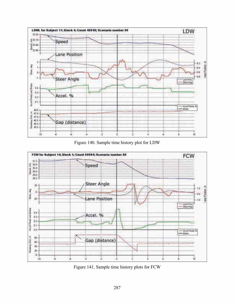
Figure 140. Sample time history plot for LDW
Figure 141. Sample time history plots for FCW
287

Figure 142. Sample time history plot for CSW
G.3.2 Responses to FCWs and CSWs In post-test data analysis, a driver’s response to an FCW or CSW warning was recorded if the driver completely removed his or her foot from the accelerator pedal (accelerator pedal release), or if the driver’s foot was not on the accelerator pedal at the time of the warning, when the driver began braking (brake onset). If there was an accelerator pedal release or a brake onset during the six seconds before the warning, the driver was assumed to have predicted the need for a response before hearing or feeling the warning, and the warning was therefore not recorded. For the FCW and CSW warnings for which there was a response, accelerator pedal release times and brake onset times, when present, were calculated. To investigate responses to FCWs and CSWs, accelerator pedal release times were examined as the dependent variable in a linear mixed model, with warning type and approach as fixed factors. There were 228 cases (117 FCWs and 111 CSWs) in the analysis. Warning type was statistically significant, F(1, 224.75 ), p < 0.01. As shown in Figure 143, on average, drivers completely removed their foot from the accelerator pedal faster when responding to an FCW than to a CSW (0.84 versus 1.17 seconds, respectively).
288
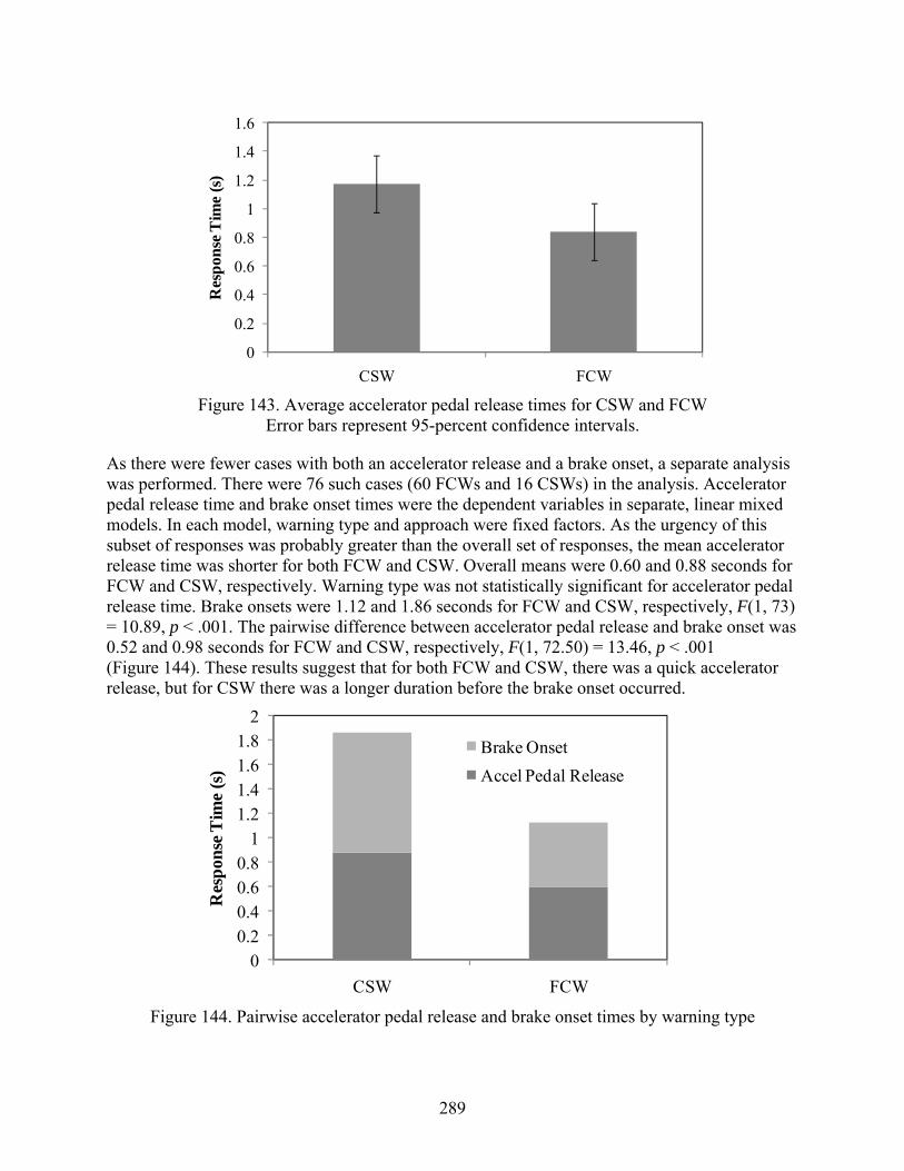
CSW FCW 0
0.2
0.4
0.6
0.8
1
1.2
1.4
1.6
Res
pons
e Tim
e (s
)
Figure 143. Average accelerator pedal release times for CSW and FCW Error bars represent 95-percent confidence intervals.
As there were fewer cases with both an accelerator release and a brake onset, a separate analysis was performed. There were 76 such cases (60 FCWs and 16 CSWs) in the analysis. Accelerator pedal release time and brake onset times were the dependent variables in separate, linear mixed models. In each model, warning type and approach were fixed factors. As the urgency of this subset of responses was probably greater than the overall set of responses, the mean accelerator release time was shorter for both FCW and CSW. Overall means were 0.60 and 0.88 seconds for FCW and CSW, respectively. Warning type was not statistically significant for accelerator pedal release time. Brake onsets were 1.12 and 1.86 seconds for FCW and CSW, respectively, F(1, 73) = 10.89, p < .001. The pairwise difference between accelerator pedal release and brake onset was 0.52 and 0.98 seconds for FCW and CSW, respectively, F(1, 72.50) = 13.46, p < .001 (Figure 144). These results suggest that for both FCW and CSW, there was a quick accelerator release, but for CSW there was a longer duration before the brake onset occurred.
0 0.2 0.4 0.6 0.8
1 1.2 1.4 1.6 1.8
2
Res
pons
e Tim
e (s
)
Brake Onset Accel Pedal Release
CSW FCW
Figure 144. Pairwise accelerator pedal release and brake onset times by warning type
289
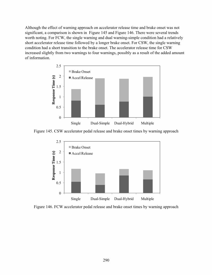
Although the effect of warning approach on accelerator release time and brake onset was not significant, a comparison is shown in Figure 145 and Figure 146. There were several trends worth noting. For FCW, the single warning and dual warning-simple condition had a relatively short accelerator release time followed by a longer brake onset. For CSW, the single warning condition had a short transition to the brake onset. The accelerator release time for CSW increased slightly from two warnings to four warnings, possibly as a result of the added amount of information.
0
0.5
1
1.5
2
2.5
Res
pons
e Tim
e (s
)
Brake Onset Accel Release
Single Dual-Simple Dual-Hybrid Multiple
Figure 145. CSW accelerator pedal release and brake onset times by warning approach
0
0.5
1
1.5
2
2.5
Res
pons
e Tim
e (s
)
Brake Onset Accel Release
Single Dual-Simple Dual-Hybrid Multiple
Figure 146. FCW accelerator pedal release and brake onset times by warning approach
290
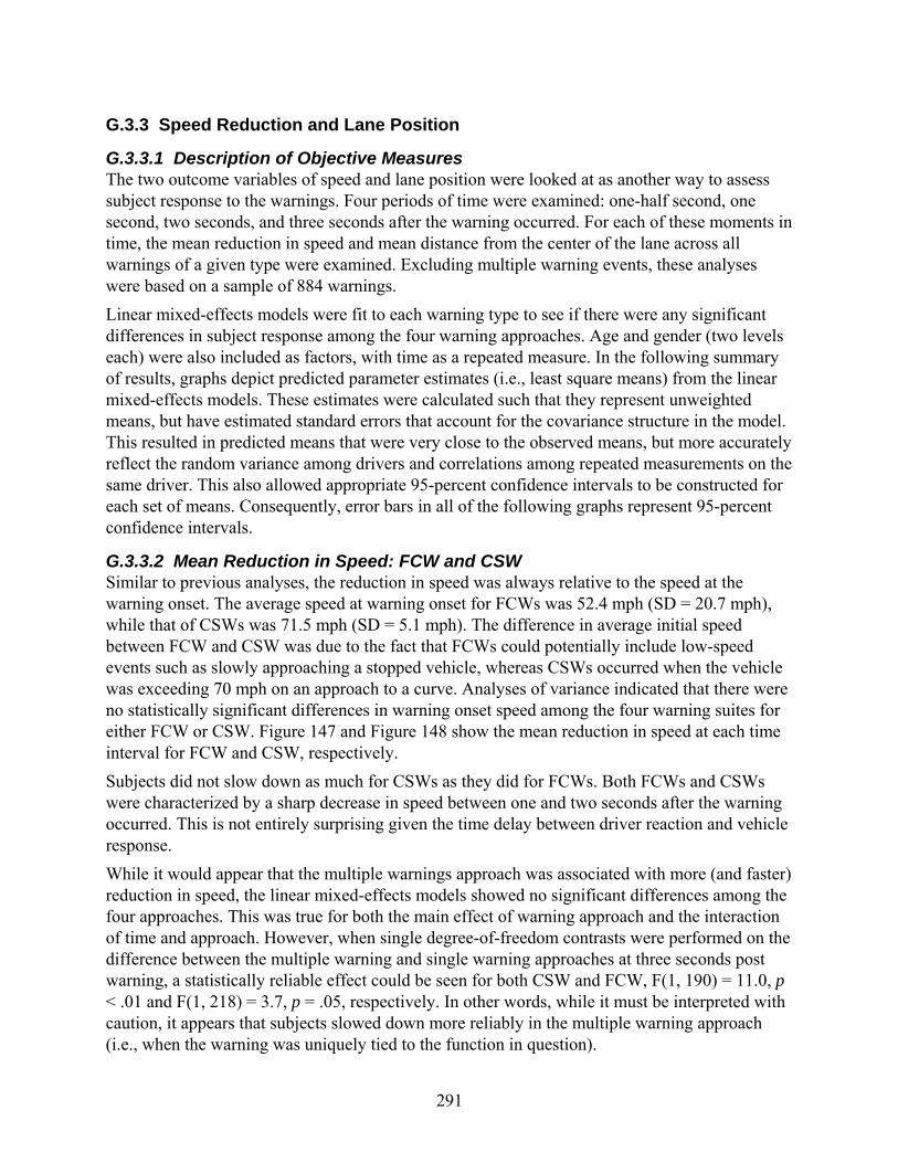
G.3.3 Speed Reduction and Lane Position
G.3.3.1 Description of Objective Measures The two outcome variables of speed and lane position were looked at as another way to assess subject response to the warnings. Four periods of time were examined: one-half second, one second, two seconds, and three seconds after the warning occurred. For each of these moments in time, the mean reduction in speed and mean distance from the center of the lane across all warnings of a given type were examined. Excluding multiple warning events, these analyses were based on a sample of 884 warnings. Linear mixed-effects models were fit to each warning type to see if there were any significant differences in subject response among the four warning approaches. Age and gender (two levels each) were also included as factors, with time as a repeated measure. In the following summary of results, graphs depict predicted parameter estimates (i.e., least square means) from the linear mixed-effects models. These estimates were calculated such that they represent unweighted means, but have estimated standard errors that account for the covariance structure in the model. This resulted in predicted means that were very close to the observed means, but more accurately reflect the random variance among drivers and correlations among repeated measurements on the same driver. This also allowed appropriate 95-percent confidence intervals to be constructed for each set of means. Consequently, error bars in all of the following graphs represent 95-percent confidence intervals.
G.3.3.2 Mean Reduction in Speed: FCW and CSW Similar to previous analyses, the reduction in speed was always relative to the speed at the warning onset. The average speed at warning onset for FCWs was 52.4 mph (SD = 20.7 mph), while that of CSWs was 71.5 mph (SD = 5.1 mph). The difference in average initial speed between FCW and CSW was due to the fact that FCWs could potentially include low-speed events such as slowly approaching a stopped vehicle, whereas CSWs occurred when the vehicle was exceeding 70 mph on an approach to a curve. Analyses of variance indicated that there were no statistically significant differences in warning onset speed among the four warning suites for either FCW or CSW. Figure 147 and Figure 148 show the mean reduction in speed at each time interval for FCW and CSW, respectively. Subjects did not slow down as much for CSWs as they did for FCWs. Both FCWs and CSWs were characterized by a sharp decrease in speed between one and two seconds after the warning occurred. This is not entirely surprising given the time delay between driver reaction and vehicle response. While it would appear that the multiple warnings approach was associated with more (and faster) reduction in speed, the linear mixed-effects models showed no significant differences among the four approaches. This was true for both the main effect of warning approach and the interaction of time and approach. However, when single degree-of-freedom contrasts were performed on the difference between the multiple warning and single warning approaches at three seconds post warning, a statistically reliable effect could be seen for both CSW and FCW, F(1, 190) = 11.0, p < .01 and F(1, 218) = 3.7, p = .05, respectively. In other words, while it must be interpreted with caution, it appears that subjects slowed down more reliably in the multiple warning approach (i.e., when the warning was uniquely tied to the function in question).
291
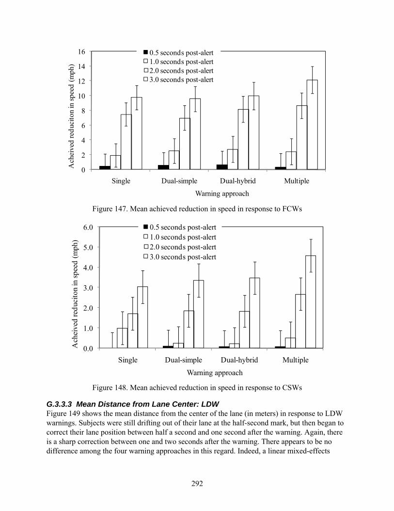
0
2
4
6
8
10
12
14
16
Ach
eive
d re
duci
ton
in sp
eed
(mph
)
0.5 seconds post-alert 1.0 seconds post-alert 2.0 seconds post-alert 3.0 seconds post-alert
Single Dual-simple Dual-hybrid Multiple
Warning approach
Figure 147. Mean achieved reduction in speed in response to FCWs
0.0
1.0
2.0
3.0
4.0
5.0
6.0
Ach
eive
d re
duci
ton
in sp
eed
(mph
)
0.5 seconds post-alert 1.0 seconds post-alert 2.0 seconds post-alert 3.0 seconds post-alert
Single Dual-simple Dual-hybrid Multiple
Warning approach
Figure 148. Mean achieved reduction in speed in response to CSWs
G.3.3.3 Mean Distance from Lane Center: LDW Figure 149 shows the mean distance from the center of the lane (in meters) in response to LDW warnings. Subjects were still drifting out of their lane at the half-second mark, but then began to correct their lane position between half a second and one second after the warning. Again, there is a sharp correction between one and two seconds after the warning. There appears to be no difference among the four warning approaches in this regard. Indeed, a linear mixed-effects
292
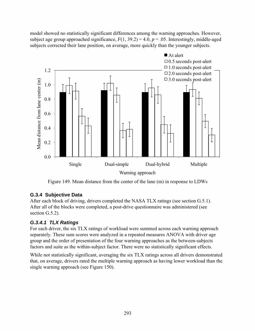
0.0
0.2
0.4
0.6
0.8
1.0
1.2
Mea
n di
stan
ce fr
om la
ne c
ente
r (m
)
At alert 0.5 seconds post-alert 1.0 seconds post-alert 2.0 seconds post-alert 3.0 seconds post-alert
Single Dual-simple Dual-hybrid Multiple
Warning approach
Figure 149. Mean distance from the center of the lane (m) in response to LDWs
model showed no statistically significant differences among the warning approaches. However, subject age group approached significance, F(1, 39.2) = 4.0, p = .05. Interestingly, middle-aged subjects corrected their lane position, on average, more quickly than the younger subjects.
G.3.4 Subjective Data After each block of driving, drivers completed the NASA TLX ratings (see section G.5.1). After all of the blocks were completed, a post-drive questionnaire was administered (see section G.5.2).
G.3.4.1 TLX Ratings For each driver, the six TLX ratings of workload were summed across each warning approach separately. These sum scores were analyzed in a repeated measures ANOVA with driver age group and the order of presentation of the four warning approaches as the between-subjects factors and suite as the within-subject factor. There were no statistically significant effects. While not statistically significant, averaging the six TLX ratings across all drivers demonstrated that, on average, drivers rated the multiple warning approach as having lower workload than the single warning approach (see Figure 150).
293

0
2
4
6
8
10
12
14
16
18
20 R
atin
g
Single Dual-Simple Dual-Hybrid Multiple
Mental Physical Temporal Effort Performance Frustration
TLX Category
Figure 150. Average TLX ratings across all drivers for each TLX category
G.3.4.2 Post-Drive Questionnaire When asked to state which warning approach they preferred, only one driver selected the multiple warning approach as her most preferred approach (see Figure 151) and more drivers selected the single warning approach than any other approach. Overall, middle-aged drivers preferred the single warning approach, while younger drivers favored dual warnings (see Figure 152).
294

Num
ber o
f sub
ject
s
7
6
5
4
3
2
1
0 Single Dual-Simple Dual-Hybrid Multiple
Warning Approach
Figure 151. Drivers’ most preferred warning approach
Single Dual-Simple Dual-Hybrid Multiple
Warning Approach
Figure 152. Drivers’ most preferred warning approach by age group
0
1
2
3
4
5
6
7
Num
ber o
f sub
ject
s
Young Middle-aged
Six questions from the post-drive questionnaire asked drivers to rate their level of agreement on a Likert-type scale of 1 to 7 (1 = strongly disagree and 7 = strongly agree) with statements describing various warning attributes. Subjects provided a level of agreement for each suite. For example, for each warning approach, drivers were asked to rate their level of agreement with the following statement, “This method of presenting crash alert information would get my attention without being overly annoying.” (See section G.5.2 for the post-drive questionnaire.) Similar to the method employed with the TLX ratings, sum scores, indicating an overall rating of each warning approach, were computed for each driver. These scores were analyzed in a repeated measures ANOVA with driver age group as the between-subjects factor and warning approach as the within-subject factor. The results showed that there were no statistically significant differences among the overall ratings of the warning approaches.
295
G.4 Conclusions Although the results of this experiment did not put forward a single suggested approach, they provided insight as to the potential benefits and costs of CWS integration. Subjects did not show an overwhelming preference to any of the warning approaches, but they clearly did not favor the fully distributed approach (four warnings for four subsystems). A clear age effect was observed in the subjective preference data. Middle-aged drivers preferred full integration (single warning approach), while younger drivers favored dual warnings. Warning approach preference did not reflect subjective workload ratings, which showed slightly reduced workload for the multiple warnings approach, consistent across the various TLX categories. In an experiment addressing the same question as this experiment, Ho et al. (2006) reported preference for a distributed, rather than integrated, warning approach. It is noted, however, that in that study there were only younger subjects. The inclusion of middle-aged subjects in this study was a primary cause for the preference of integration of warnings and the overwhelming indifference to the multiple warnings solution. Experimental limitations prevented the testing of older drivers, which prevented drawing conclusions about that age sector. By and large, the objective results did not reveal significant differences among the warning approaches tested. Subjects responded more slowly to CSW than to FCW, possibly because they were already aware of the driving context. If there was no vehicle in front of them, they were less likely to respond immediately and waited half a second longer before applying the brake. Analysis of responses by warning approach suggests, however, that in the single warning approach, the delay between accelerator release and brake onset for CSW was the same as for FCW. Drivers may have chosen to respond immediately to single warnings as a matter of strategy in the absence of other information from the integrated warning system. Analysis of the reduction in speed after warnings revealed some benefit to the multiple warnings approach over the single warning approach. Three seconds after an FCW or a CSW, there was greater speed reduction with the multiple warnings approach than with the single warning approach. Based on the subjective preference for some or full integration, the weak objective benefit for a multiple warnings approach versus a single warning approach, and the analysis of the various considerations for integration, it is recommended that the IVBSS system uses one of the dual-sound approaches, or a variation of them. If, however, a different approach is sought, the current experiment does not provide compelling evidence against any of the warning approaches that were tested. The recommendation must be qualified by the experimental assumptions and limitations that were made in this simulator study. First, the study was conducted in a fixed-based driving simulator with only a representative set of driving scenarios. Second, subjects were alert and well aware of the need for immediate responses to events in the driving scene. Third, as a lesson learned from experiment 2, drivers did not have to perform a distracting task while they drove and were therefore less in need of the warning system, even though the events were still somewhat surprising. Finally, although subjects had been trained and tested with each of the warning approach, their performance and subjective preference is likely to have been characteristic of a novice user rather than an experienced one.
296

1 2 3 4 5 6 7 Not at Very All well Suite _____
MENTAL DEMAND
Low High
PHYSICAL DEMAND
Low High
TEMPORAL DEMAND
Low High
EFFORT
Low High
PERFORMANCE
Good Poor
FRUSTRATION
Low High
G.5 Forms G.5.1 Post-Block Questionnaire Date____________ Subject #_______ Block_______
Thinking about the suite of warnings (both auditory and vibrations) that you just experienced, please evaluate it on the scales below. The rating scales are defined on a separate sheet.
1. How well were you able to tell which sound or vibration corresponded to each warning?
297

G.5.2 Post-Drive Questionnaire Date____________ Subject #_______
The four suites of warnings that you experienced are as follows (perhaps in a different order than you experienced):
A. One master warning – The same warning (auditory and vibration) for each system.
B. Two sets of warnings – One set of warnings (auditory and vibration) for Forward Collision Warning (FCW) and Curve Speed Warning (CSW), and another set of warnings (auditory and vibration) for Lane Departure Warning (LDW) and Blind Spot Warning (BSW).
C. Two auditory warnings – One auditory warning accompanied by a vibration for FCW, the same auditory warning for CSW with no vibration, a different auditory warning for BSW, and only a vibration for LDW.
D. Four warnings – Each system has a different auditory warning. Additionally, FCW and LDW are accompanied by different vibrations.
1. Which suite did you prefer? ___________________
Using the seven-point scale shown below (1 = Strongly Disagree, 7 = Strongly Agree), please indicate your agreement with statements 2 – 7, providing a rating for each of the four warning suites described above:
1 2 3 4 5 6 7 Strongly Strongly Disagree Agree
Example:
A. Ice cream is tasty.
a. Chocolate ice cream ___7___ b. Strawberry ice cream ___2___ c. Vanilla ice cream ___4___
2. This method would get my attention immediately if I was distracted and not concentrating on the driving task.
a. Suite A ______ b. Suite B ______ c. Suite C ______ d. Suite D ______
3. This method would NOT startle me, that is, cause me to blink, jump, or make rapid reflex-like movement.
a. Suite A ______ b. Suite B ______ c. Suite C ______ d. Suite D ______
298
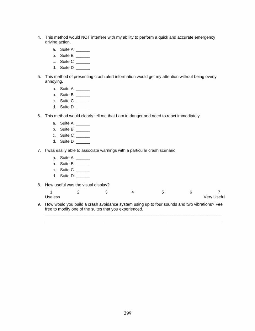
____________________________________________________________________________ ____________________________________________________________________________
4. This method would NOT interfere with my ability to perform a quick and accurate emergency driving action.
a. Suite A ______ b. Suite B ______ c. Suite C ______ d. Suite D ______
5. This method of presenting crash alert information would get my attention without being overly annoying.
a. Suite A ______ b. Suite B ______ c. Suite C ______ d. Suite D ______
6. This method would clearly tell me that I am in danger and need to react immediately.
a. Suite A ______ b. Suite B ______ c. Suite C ______ d. Suite D ______
7. I was easily able to associate warnings with a particular crash scenario.
a. Suite A ______ b. Suite B ______ c. Suite C ______ d. Suite D ______
8. How useful was the visual display?
1 2 3 4 5 6 7 Useless Very Useful
9. How would you build a crash avoidance system using up to four sounds and two vibrations? Feel free to modify one of the suites that you experienced.
299

G.5.3 Training Instructions Overview
1. Eye tracking 2. Practice drive 3. Calibrate Eye Tracking System for Placement of Objects in World 4. Four blocks
a. Learning the warnings associated with each subsystem b. Testing subject’s knowledge of the learned warnings c. ~15 minutes of driving d. Post-block questionnaire e. Break
5. Post-drive questionnaire (not completed in the simulator)
Practice Drive Now it is time to try out the simulator. For the duration of this experiment please drive normally, being sure to be safe. You should use your turn signal as normal and use the speedometer on the instrument panel to check your speed, just as in a real vehicle.
The speed limit is 70 mph and you will see speed limit signs throughout the course as a reminder. The speed limit signs may look like they’re flashing, that’s just the way that they look in the simulator it does not mean you should change anything or that you are doing anything wrong. Try to maintain a speed of 70 mph at all times. If 70 mph is an uncomfortably fast driving speed for you, go as fast as you are comfortable. However, keep in mind that if you go slower than 70 mph the experiment will take longer to complete.
The steering wheel in the simulator doesn’t feel exactly like one in a real vehicle and it is easy to overcorrect. So the key is to make small corrections with the steering wheel.
Some people experience motion sickness in the simulator, so if you start feeling nauseous, dizzy, or anything else that could occur prior to being motions sick, let me know immediately and I’ll tell you how to stop. As I said before, you may end the experiment at any time and you will still be paid $50.
Do you have any questions?
Ok then, put the vehicle in “D” using the shift lever between the seats. This practice drive will last for about 3 minutes. I will tell you when the time is up.
Now, please press on the accelerator and begin driving.
While subject is practicing, one experimenter will be working with the eye-tracking system, the other experimenter watching the face monitor in the control room (one experimenter can do both tasks if necessary).
Have the subject drive for approximately three minutes.
Ok, that’s the end of the first practice drive. Please coast to a slow stop and shift the vehicle into park.
Stop the simulator ten seconds after the vehicle is in park.
Calibrate Eye Tracking System for Placement of Objects in World Step 1: In the faceLAB 3 Controls window, click on the “logging” tab and then the “file” button. Change file name to correct name and format (subject’s initials_subject number_Calib_Start).
- If necessary click on “Directory” button and assign correct directory.
Step 2: Click on the “Start Logging” button.
Step 3: Make sure road scene is visible and ask subject to fixate on the following sequence of screen objects. Perform sequence twice. Click on appropriate annotation button when subject is fixated (may use laser pointer to direct subject’s gaze):
1: Upper right corner of screen 2: Upper left corner of screen
300
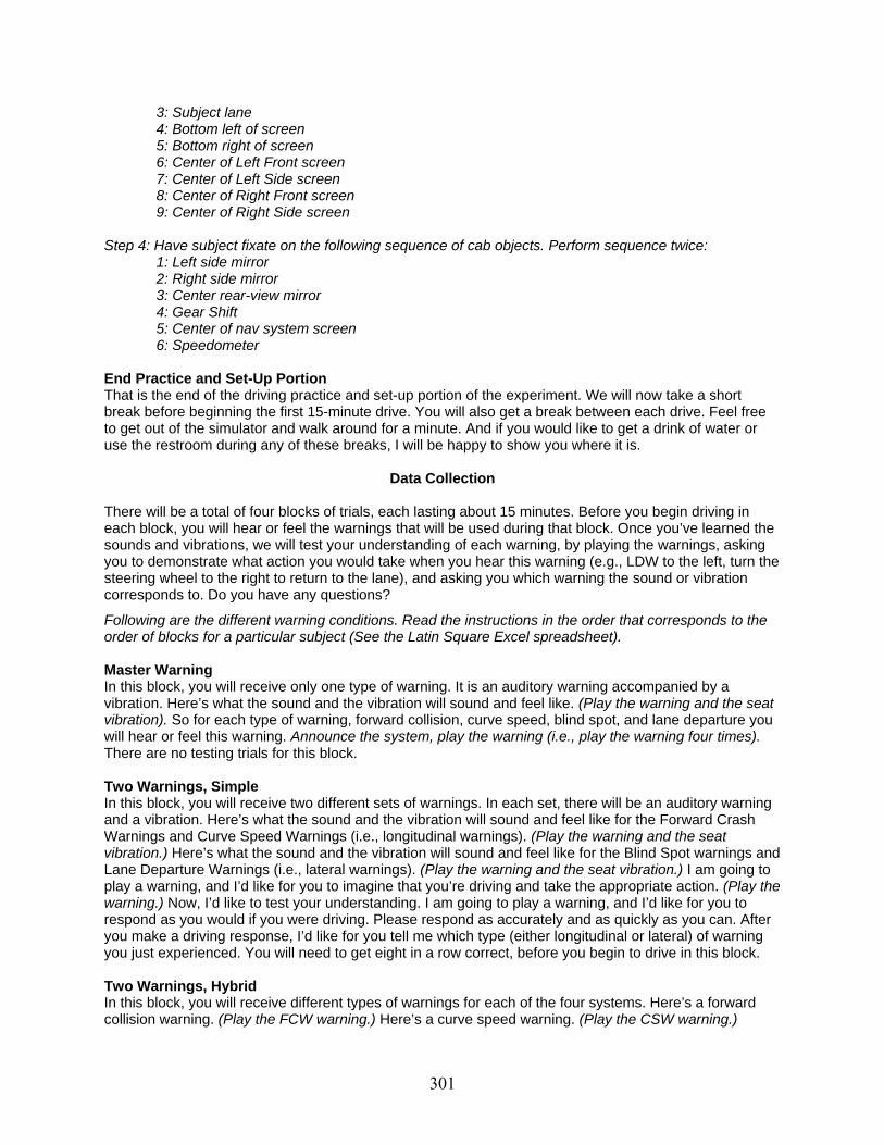
3: Subject lane 4: Bottom left of screen 5: Bottom right of screen 6: Center of Left Front screen 7: Center of Left Side screen 8: Center of Right Front screen 9: Center of Right Side screen
Step 4: Have subject fixate on the following sequence of cab objects. Perform sequence twice: 1: Left side mirror 2: Right side mirror 3: Center rear-view mirror 4: Gear Shift 5: Center of nav system screen 6: Speedometer
End Practice and Set-Up Portion That is the end of the driving practice and set-up portion of the experiment. We will now take a short break before beginning the first 15-minute drive. You will also get a break between each drive. Feel free to get out of the simulator and walk around for a minute. And if you would like to get a drink of water or use the restroom during any of these breaks, I will be happy to show you where it is.
Data Collection
There will be a total of four blocks of trials, each lasting about 15 minutes. Before you begin driving in each block, you will hear or feel the warnings that will be used during that block. Once you’ve learned the sounds and vibrations, we will test your understanding of each warning, by playing the warnings, asking you to demonstrate what action you would take when you hear this warning (e.g., LDW to the left, turn the steering wheel to the right to return to the lane), and asking you which warning the sound or vibration corresponds to. Do you have any questions?
Following are the different warning conditions. Read the instructions in the order that corresponds to the order of blocks for a particular subject (See the Latin Square Excel spreadsheet).
Master Warning In this block, you will receive only one type of warning. It is an auditory warning accompanied by a vibration. Here’s what the sound and the vibration will sound and feel like. (Play the warning and the seat vibration). So for each type of warning, forward collision, curve speed, blind spot, and lane departure you will hear or feel this warning. Announce the system, play the warning (i.e., play the warning four times). There are no testing trials for this block.
Two Warnings, Simple In this block, you will receive two different sets of warnings. In each set, there will be an auditory warning and a vibration. Here’s what the sound and the vibration will sound and feel like for the Forward Crash Warnings and Curve Speed Warnings (i.e., longitudinal warnings). (Play the warning and the seat vibration.) Here’s what the sound and the vibration will sound and feel like for the Blind Spot warnings and Lane Departure Warnings (i.e., lateral warnings). (Play the warning and the seat vibration.) I am going to play a warning, and I’d like for you to imagine that you’re driving and take the appropriate action. (Play the warning.) Now, I’d like to test your understanding. I am going to play a warning, and I’d like for you to respond as you would if you were driving. Please respond as accurately and as quickly as you can. After you make a driving response, I’d like for you tell me which type (either longitudinal or lateral) of warning you just experienced. You will need to get eight in a row correct, before you begin to drive in this block.
Two Warnings, Hybrid In this block, you will receive different types of warnings for each of the four systems. Here’s a forward collision warning. (Play the FCW warning.) Here’s a curve speed warning. (Play the CSW warning.)
301
Here’s a blind spot warning. (Play the LCM warning.) Here’s a lane departure warning. (Play the LDW warning.) I am going to play a warning, and I’d like for you to imagine that you’re driving and take the appropriate action. (Play the warning.) Now, I’d like to test your understanding. I am going to play a warning, and I’d like for you to respond as you would if you were driving. Please respond as accurately and as quickly as you can. After you make a driving response, I’d like for you tell me which type of warning you just experienced. You will need to get eight in a row correct, before you begin to drive in this block.
Four warnings In this block, you will receive different types of warnings for each of the four systems. Here’s a forward collision warning. (Play the FCW warning.) Here’s a curve speed warning. (Play the CSW warning.) Here’s a blind spot warning. (Play the LCM warning.) Here’s a lane departure warning. (Play the LDW warning.) I am going to play a warning, and I’d like for you to imagine that you’re driving and take the appropriate action. (Play the warning.) Now, I’d like to test your understanding. I am going to play a warning, and I’d like for you to respond as you would if you were driving. Please respond as accurately and as quickly as you can. After you make a driving response, I’d like for you tell me which type of warning you just experienced. You will need to get eight in a row correct, before you begin to drive in this block.
Block 1 We will now begin the first 15-minute drive. There will be a total of four 15-minute drives and a short break between each drive. Just as in the practice drives, please drive normally, being sure to be safe. Please buckle up, use your turn signal and use the speedometer on the instrument panel to check your speed. Above all, your task is to avoid crashes. Don’t change lanes unless there is a stopped vehicle or an object in your lane. When you are forced to change lanes, stay in that lane unless forced to change again. The speed limit is 70 mph and you will see speed limit signs throughout the course as a reminder, try to maintain a speed of 70 mph at all times.
For the remaining four drives there will be other vehicles in the road. Keep in mind that the screens do not go all the way around the cab and that sometimes a vehicle may be on the road where it can’t be seen.
The system we are testing has a number of new features that have not appeared in vehicles you can now buy.
Do you have any questions?
Make sure driver is buckled.
Ok, now I will turn on the simulator, don’t begin driving until I tell you to begin.
Start logging eye-tracking data. When simulator starts, click annotation buttons for time synch.
- A metronome type sounds will start with a rhythmic series of 3 low and 1 high tone. Click on the annotation button the moment the high tone sounds until no more tones are presented.
Alright, you may begin driving whenever you’re ready.
Subject drives for 15 minutes. If necessary, remind subject to keep speed close to 70mph for the entire drive. If subject is ever in the wrong lane, tell them how to get back.
(At the end of Block 1) Ok, turn on your right turn signal and gradually slow down as you pull off onto the shoulder. Once you have stopped, please put the vehicle in park. (10 seconds after you are parked, please stop the simulator.) Please complete the following questionnaire. You may take a break for a minute if you wish. Do you have any comments or questions about what happened in the last 15 minutes?
Blocks 2-4 These blocks proceed in the same manner as Block 1 did. At the end of Block 4 (Call Mary Lynn, 223.2445) and have her get the subject so that he or she can complete the post-drive questionnaire outside of the simulator so that the next subject can begin.
302

Appendix H: Experiment 4 ņ Warning Delay-Accuracy Tradeoff
H.1 Overview This experiment addressed two questions:
x How does the tradeoff between warning system processing time (to start to inform the driver) and warning accuracy affect driver responses to warnings?
x How well do drivers respond to the set of IVBSS warnings? Are any warnings confusing or misunderstood by drivers?
As noted earlier, many vehicle sensing and information integration tasks take time. Radars need to sweep, detection decisions may need to be made across multiple sweeps, and data from various sensors need to be combined. The more time taken to process the data, the more reliable the warning with fewer false alarms and fewer misses. However, the later the warning is presented to drivers, the less time they have to assess the situation and respond. What is an acceptable tradeoff? Across experiments, as knowledge from experiments and design constraints were applied, the set of IVBSS warnings evolved, and therefore needed continual reevaluation, especially for understandability.
H.2 Method This experiment took place in the UMTRI driving simulator. (See Appendix A for a complete description of the simulator and the simulator upgrade.) The warning system examined was the most current version at the time of the experiment. There were four primary warnings (FCW, LDW, LCM, and CSW, plus the blind spot detection system). FCW and CSW were the same, seven beeps and a brake pulse. For LDW, the seat shook. For LCM, there were three low beeps followed by three high beeps. The blind spot detection system contains an LED on the left and right outside mirrors that illuminated if there was a vehicle in, or quickly approaching, the blind spot. This system is a component of the LCM subsystem. Refer to Table 85 for a complete description. The test method in this experiment was based on that of experiments 2 and 3, and used the same basic scenarios, world, procedure, and experimental sequence. In addition, at the end of each test block, subjects completed a short survey of six to seven questions (e.g., Rate the warning on a scale of 1 (sound was too soft) to 5 (sound was too loud)) for each of the five warnings. At the end of the experiment, subjects responded to eight or nine questions per warning plus three open-ended questions (e.g., Did you notice changes between the drives? Which drive was best? How should each warning be changed?). The forms are shown in section H.5. A summary of the approximate timing of experimental tasks is shown in Table 84.
303
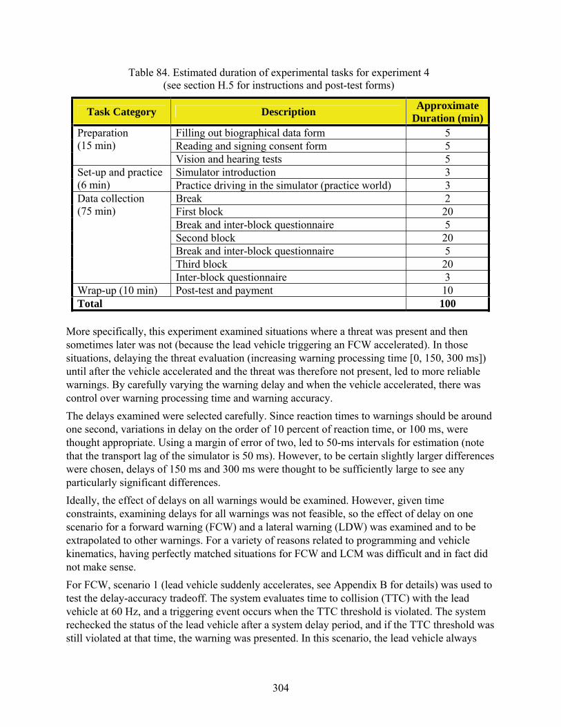
Table 84. Estimated duration of experimental tasks for experiment 4 (see section H.5 for instructions and post-test forms)
Task Category Description Approximate Duration (min)
Preparation (15 min)
Filling out biographical data form 5 Reading and signing consent form 5 Vision and hearing tests 5
Set-up and practice (6 min)
Simulator introduction 3 Practice driving in the simulator (practice world) 3
Data collection (75 min)
Break 2 First block 20 Break and inter-block questionnaire 5 Second block 20 Break and inter-block questionnaire 5 Third block 20 Inter-block questionnaire 3
Wrap-up (10 min) Post-test and payment 10 Total 100
More specifically, this experiment examined situations where a threat was present and then sometimes later was not (because the lead vehicle triggering an FCW accelerated). In those situations, delaying the threat evaluation (increasing warning processing time [0, 150, 300 ms]) until after the vehicle accelerated and the threat was therefore not present, led to more reliable warnings. By carefully varying the warning delay and when the vehicle accelerated, there was control over warning processing time and warning accuracy. The delays examined were selected carefully. Since reaction times to warnings should be around one second, variations in delay on the order of 10 percent of reaction time, or 100 ms, were thought appropriate. Using a margin of error of two, led to 50-ms intervals for estimation (note that the transport lag of the simulator is 50 ms). However, to be certain slightly larger differences were chosen, delays of 150 ms and 300 ms were thought to be sufficiently large to see any particularly significant differences. Ideally, the effect of delays on all warnings would be examined. However, given time constraints, examining delays for all warnings was not feasible, so the effect of delay on one scenario for a forward warning (FCW) and a lateral warning (LDW) was examined and to be extrapolated to other warnings. For a variety of reasons related to programming and vehicle kinematics, having perfectly matched situations for FCW and LCM was difficult and in fact did not make sense. For FCW, scenario 1 (lead vehicle suddenly accelerates, see Appendix B for details) was used to test the delay-accuracy tradeoff. The system evaluates time to collision (TTC) with the lead vehicle at 60 Hz, and a triggering event occurs when the TTC threshold is violated. The system rechecked the status of the lead vehicle after a system delay period, and if the TTC threshold was still violated at that time, the warning was presented. In this scenario, the lead vehicle always
304

decelerates quickly, but after the FCW triggering event (TTC threshold violated) one of three cases could occur (case A1 refers to acceleration level 1):
case A1: Lead vehicle accelerates after 100 ms case A2: Lead vehicle accelerates after 250 ms case A3: Lead vehicle does not accelerate until end of trial
(same as scenario 1 for previous experiments)
For LDW, scenario 8 was modified to test the delay-accuracy tradeoff. The system evaluates if the vehicle has crossed a lane boundary at 5 Hz and then triggers a LDW after a prescribed system delay period unless the subject made a steering reversal (t 2 degrees) to correct lateral drift. Subjects could trigger a LDW at any time, but a periodic 2000 N wind gust served to induce a lane departure. However, there was no easy way to directly manipulate LDW accuracy, so the extent to which a departure should occur was varied based on the wind gust duration. The wind durations are on the order of seconds, because it takes that long for a realistic level cross wind to move a vehicle a significant distance. As with the FCW gradated scenarios, LDW has three cases (case W1 refers to wind level 1):
case W1: 2000 N wind gust lasting 1 seconds case W2: 2000 N wind gust lasting 2 seconds case W3: 2000 N wind gust lasting 3 seconds
Thus, there were three threat levels for the two scenarios evaluated (FCW and LDW). Depending on the system delay, one, two, or all three of those threat levels should trigger true FCW or LDW warnings. So, if the warning delay is 300 ms, the warning system reevaluates the situation 300 ms after the triggering event and, if the threat is still valid, displays the warning. However, if the threat is no longer present, the warning is suppressed. Therefore a 300 ms system delay would suppress case W1 and W2 warnings, but display a warning for case W3. Table 85 shows the effect of scenario and system delays on the presentation or suppression of warnings. Keep in mind that depending on the system delay, either one-third, two-thirds, or all of the scenarios will trigger a warning.
Table 85. Effect of delay on FCW
Acceleration Delay Warning Delay None 150 ms 300 ms
Until end of trial (normal) Warning Warning Warning 250 ms Warning Warning No warning 100 ms Warning No warning No warning
After each block, subjects were provided a rating of warning responsiveness according to various parameters. It was implied that some of the warning parameters were altered between blocks. However, subjects did not know which terms were altered. After subjects had completed all three blocks, they were asked what term(s) was altered to see if they noticed the delay and, if so, at what point.
305

The loop for experiment 4 was designed so that subjects would drive one revolution per block and each block would take about 20 minutes at 70 mph (Figure 153), slightly larger than the world used in experiments 2 and 3. Subjects drove three blocks total. In each block there were ten long straightaways, each of which could contain multiple trials. There were 26 trials in all. Starting and ending each block in the middle of a segment, using both left and right-hand turns, and varying the length of each straightaway made the shape of the world difficult for subjects to memorize.
16 tiles
16
18
9
4
7
8
14
15
5
Figure 153. Configuration of the world for IVBSS experiment 4 are construction zones, two in the left lane and one in the right. Each tile is 200 meters long.) (
To trigger enough warnings for analysis, warnings were presented at a much higher frequency than they would appear under normal driving conditions, with subjects receiving about one warning per minute. However, some subjects received warnings at a higher or lower frequency
306

depending on their individual reactions to scenarios. Additional true warning scenarios used in previous experiments were included in experiment 4 to prevent subjects from anticipating warnings or vehicle maneuvers. No false alarms were included, due to design constraints and the concern that subjects would interpret false alarms as an intentional system delay. The scenarios and delays used in this experiment are shown in Table 86 and Table 87. Note that only scenarios 1 and 8 have any associated scenario delay. The number of suppressed warnings (rejected triggering events) depended upon the system delay, which varied by block. (Had the delay varied trial by trial, the system would have appeared to be inconsistent and unreliable to subjects.) As the length of the system delay increased, the number of warnings presented decreased.
Table 86. Expected frequency of warnings presented according to block delay
Block A (No Delay)
Block B (150 ms Warning Delay)
Block C (300 ms Warning Delay)
True warning scenarios 1 and 8
Warnings presented
1. A1-FCW 1. A1-FCW 1. A2-FCW 1. A2-FCW 1. A3-FCW 1. A3-FCW 8. W1-LDW 8. W1-LDW 8. W2-LDW 8. W2-LDW 8. W3-LDW 8. W3-LDW
1. A2-FCW 1. A2-FCW 1. A3-FCW 1. A3-FCW
8. W2-LDW 8. W2-LDW 8. W3-LDW 8. W3-LDW
1. A3-FCW 1. A3-FCW
8. W3-LDW 8. W3-LDW
Warnings suppressed
1. A1-FCW 1. A1-FCW
8. W1-LDW 8. W1-LDW
1. A1-FCW 1. A1-FCW 1. A2-FCW 1. A2-FCW 8. W1-LDW 8. W1-LDW 8. W2-LDW 8. W2-LDW
Other true warning scenarios
4-FCW4-FCW4-FCW5-FCW5-FCW5-FCW6-LCM 7-LCM
4-FCW 4-FCW 4-FCW 5-FCW 5-FCW 5-FCW 6-LCM 7-LCM
4-FCW 4-FCW 4-FCW 5-FCW 5-FCW 5-FCW 6-LCM 7-LCM
307

Table 87. Summary of expected warnings according to block delay
System Delay True Warning Scenarios 1 and 8 # Other True
Warning Scenarios
Total# Warnings Presented
# Warnings Suppressed
Block A (no delay) 12 0 8 20 Block B (150ms delay) 8 4 8 20 Block C (300ms delay) 4 8 8 20
There were 960 total warnings planned for all subjects (see below), mostly FCW with some LCM and LDW warnings as well.
Table 88. Frequency of expected warnings by block
Warning Warning Frequency
(Each Subject) Total Warning
Frequency (All 16 Subjects)Block A Block B Block C
FCW 12 12 12 576 CSW 0 0 0 0 LCM 6 6 6 288 LDW 2 2 2 96 Total 20 20 20 960
The sequence of warning scenarios in each block was fixed because of the design of the world, with no warnings in the first two straightaways so that subjects could become comfortable with driving in the simulator each time they began a new block. Between subjects, the order of test blocks was counterbalanced as shown in Table 89. Perfect counterbalancing would have required an even multiple of three subjects per age x sex group. Twelve subjects was too small a sample (and below the contract requirements) and 24 subjects was too large a sample to be tested within the contract constraints.
308

Table 89. Summary of expected warnings according to block delay
Age Group Gender Subject # Block Sequence
1 A, B, C
Men 2 B, C, A 3 C, A, B
Young 4 A, B, C 5 A, B, C
Women 6 B, C, A 7 C, A, B 8 B, C, A 9 A, B, C
Men 10 B, C, A 11 C, A, B
Middle 12 C, A, B aged
Women
13 A, B, C 14 B, C, A 15 C, A, B 16 A, B, C
The sequence of scenarios for each block is shown in Figure 154, Figure 155, and Figure 156.
309

Figure 154. Scenario sequence - block A (no delay)
310

Figure 155. Scenario sequence - block B (150ms delay)
311

Figure 156. Scenario sequence - block C (300ms delay)
Sixteen subjects participated in experiment 4: four young men (ages 18 to 30), four young women, four middle-aged men (ages 40 to 55), and four middle-aged women. Visual acuity ranged from 20/13 to 20/40, with all but one subject having 20/30 or better. No subjects had previously driven a vehicle with any of the warnings tested. Table 90 shows a summary of the biographical data.
312

Table 90. Biographical summary data
Driving Characteristic Number of subjects
1 1 1 1 1 1 1 1 1 1 1 1 1 1 1 1 Thousands of miles per year <5 >5-15 >15-20 �30 % Highway driving <30% 30-60% 60-80% # Crashes in past 5 years 0 1 # Violations in past 5 years 0 1 2 3 Lane preference Left Middle Right
Young subjects drove between 1,000 and 11,000 miles per year, except for one young woman who reported driving 48,000 miles per year, which seems unreasonably high (130 miles per day including weekends). Middle-aged subjects drove more than young subjects and had a range of 3,000 to 30,000 miles per year. There was no apparent age or sex trend regarding percent expressway driving or expressway lane preference (left, middle, or right), an indicator of driving risk. Two young women and two young men had one automobile crash in the past five years, and one additional young man and young woman had one traffic violation in the past five years. Middle-aged subjects accounted for 9 out of 15 automobile crashes and traffic violations that subjects had in the past five years. One middle-aged man had three violations and one crash, one middle-aged woman had two violations, and two middle-aged men accounted for one crash and one violation each. Three middle-aged subjects and two young subjects had no driving violations or crashes in the past five years.
H.3 Results H.3.1 Warning Frequency As in other experiments, warnings were not always presented as planned. Of the 960 planned, only 590 were triggered as planned. An additional 390 unplanned warnings were triggered. Overall warning frequencies across all subjects varied by alarm type. The alarms presented were: 653 FCWs, 185 LDWs, 90 CSWs, and 52 LCMs. Note that in this experiment, although there were no planned CSWs, they did occur. Overall, approximately 40 percent (390 out of 980 warnings) of presented warnings were triggered not as planned, reflecting the difficulty of completely predicting driver behavior. As before, there were more than enough warnings to develop reliable statistics.
313
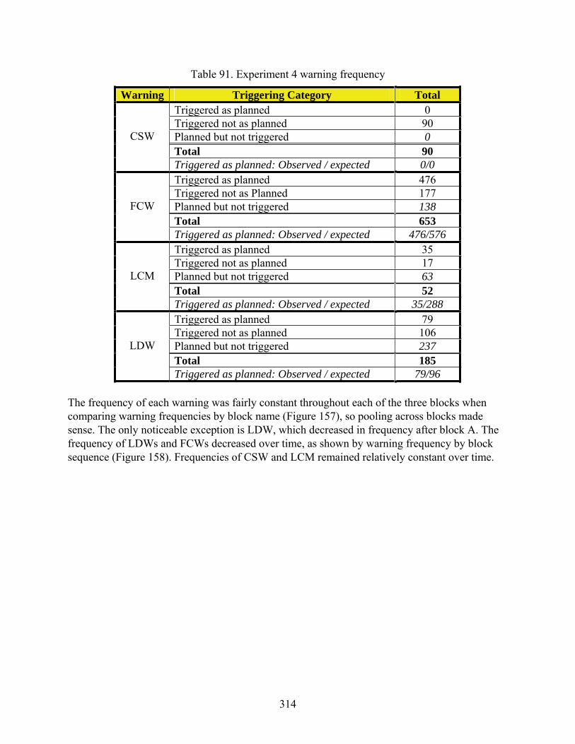
Table 91. Experiment 4 warning frequency
Warning Triggering Category Total Triggered as planned 0 Triggered not as planned 90
CSW Planned but not triggered 0 Total 90 Triggered as planned: Observed / expected 0/0 Triggered as planned 476 Triggered not as Planned 177
FCW Planned but not triggered 138 Total 653 Triggered as planned: Observed / expected 476/576 Triggered as planned 35 Triggered not as planned 17
LCM Planned but not triggered 63 Total 52 Triggered as planned: Observed / expected 35/288 Triggered as planned 79 Triggered not as planned 106
LDW Planned but not triggered 237 Total 185 Triggered as planned: Observed / expected 79/96
The frequency of each warning was fairly constant throughout each of the three blocks when comparing warning frequencies by block name (Figure 157), so pooling across blocks made sense. The only noticeable exception is LDW, which decreased in frequency after block A. The frequency of LDWs and FCWs decreased over time, as shown by warning frequency by block sequence (Figure 158). Frequencies of CSW and LCM remained relatively constant over time.
314

1 2 3
# Warnings 250
200
150
100
50
0
CSW LCM LDW
FCW
Block A Block B Block C
Figure 157. Warning frequency by block name
# Warnings
0
50
100
150
200
250
300
LCMCSW LDW
FCW
Block 1 Block 2 Block 3
Figure 158. Warning frequency by block sequence
Warning frequencies were also analyzed across subject gender and age groups. Middle-aged and young subjects received approximately the same number of warnings (Table 92), and men received more warnings than women, especially LDWs (Table 93).
315
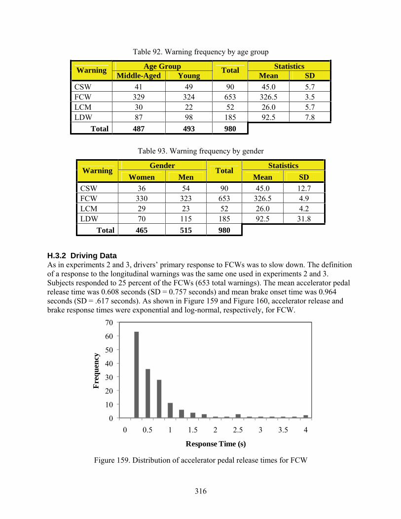
Table 92. Warning frequency by age group
Warning Age Group Total Statistics Middle-Aged Young Mean SD
CSW 41 49 90 45.0 5.7 FCW 329 324 653 326.5 3.5 LCM 30 22 52 26.0 5.7 LDW 87 98 185 92.5 7.8
Total 487 493 980
Table 93. Warning frequency by gender
Warning Gender Total Statistics Women Men Mean SD
CSW 36 54 90 45.0 12.7 FCW 330 323 653 326.5 4.9 LCM 29 23 52 26.0 4.2 LDW 70 115 185 92.5 31.8
Total 465 515 980
H.3.2 Driving Data As in experiments 2 and 3, drivers’ primary response to FCWs was to slow down. The definition of a response to the longitudinal warnings was the same one used in experiments 2 and 3. Subjects responded to 25 percent of the FCWs (653 total warnings). The mean accelerator pedal release time was 0.608 seconds (SD = 0.757 seconds) and mean brake onset time was 0.964 seconds (SD = .617 seconds). As shown in Figure 159 and Figure 160, accelerator release and brake response times were exponential and log-normal, respectively, for FCW.
Freq
uenc
y
70
60
50
40
30
20
10
0 0 0.5 1 1.5 2 2.5 3 3.5 4
Response Time (s)
Figure 159. Distribution of accelerator pedal release times for FCW
316
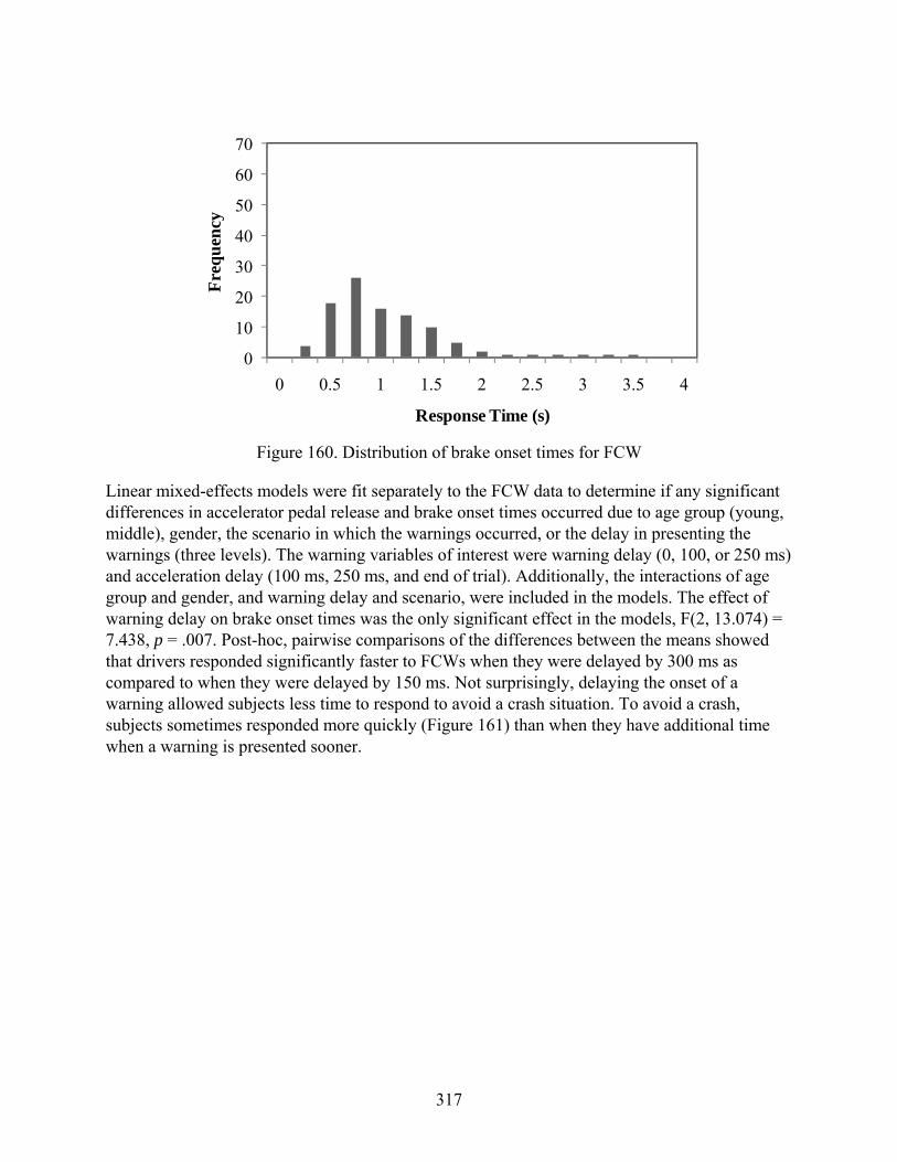
0
10
20
30
40
50
60
70
Freq
uenc
y
0 0.5 1 1.5 2 2.5 3 3.5 4
Response Time (s)
Figure 160. Distribution of brake onset times for FCW
Linear mixed-effects models were fit separately to the FCW data to determine if any significant differences in accelerator pedal release and brake onset times occurred due to age group (young, middle), gender, the scenario in which the warnings occurred, or the delay in presenting the warnings (three levels). The warning variables of interest were warning delay (0, 100, or 250 ms) and acceleration delay (100 ms, 250 ms, and end of trial). Additionally, the interactions of age group and gender, and warning delay and scenario, were included in the models. The effect of warning delay on brake onset times was the only significant effect in the models, F(2, 13.074) = 7.438, p = .007. Post-hoc, pairwise comparisons of the differences between the means showed that drivers responded significantly faster to FCWs when they were delayed by 300 ms as compared to when they were delayed by 150 ms. Not surprisingly, delaying the onset of a warning allowed subjects less time to respond to avoid a crash situation. To avoid a crash, subjects sometimes responded more quickly (Figure 161) than when they have additional time when a warning is presented sooner.
317

Res
pons
e Tim
e (s
)
3.5
3
2.5
2
1.5
1
0.5
0 0 150 300
Warning Delay (ms)
Figure 161. FCW mean accelerator pedal release times for each of the warning delaysThe error bars represent 95% confidence intervals
Figure 162 shows differences in FCW responses by scenario. Notice the lack of any consistent pattern, in part because of the small samples sizes. Because of the way the scenarios were designed, some combinations cannot occur. For example, if the warning delay is 150 ms and the reacceleration delay is 100 ms, there is no warning. As a reminder, the reveal (a lead car changes lanes to reveal a parked car) and cut-in (of a car from an adjacent lane) scenarios were included to provide a variety of potential forward crash scenarios and induce the subject to distribute attention to all traffic, not just the lead vehicle.
Res
pons
e tim
e (s
)
1.8
1.6
1.4
1.2
1
0.8
0.6
0.4
0.2
0
Lead decel 0 ms delay Lead decel 100 ms delay Lead decel 250 ms delay Reveal 0 ms delay Cut-in 0 ms delay
0 150 300
Warning delay (ms)
Figure 162. Response time to FCW by scenario, warning delay, and acceleration delay
318
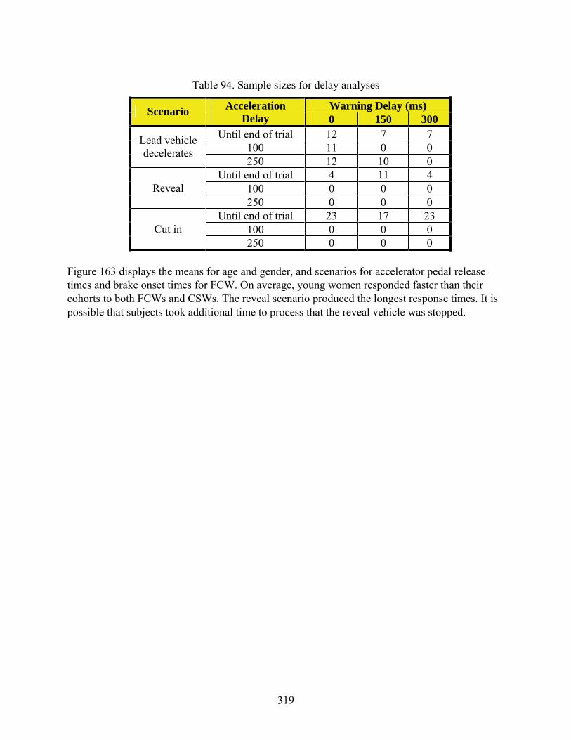
Table 94. Sample sizes for delay analyses
Scenario Acceleration Delay
Warning Delay (ms) 0 150 300
Lead vehicle decelerates
Until end of trial 12 7 7 100 11 0 0 250 12 10 0
Until end of trial 4 11 4 Reveal 100 0 0 0
250 0 0 0 Until end of trial 23 17 23
Cut in 100 0 0 0 250 0 0 0
Figure 163 displays the means for age and gender, and scenarios for accelerator pedal release times and brake onset times for FCW. On average, young women responded faster than their cohorts to both FCWs and CSWs. The reveal scenario produced the longest response times. It is possible that subjects took additional time to process that the reveal vehicle was stopped.
319

0
0.5
1
1.5
2
2.5
Young Middle-aged
Res
pons
e Tim
e (s) Female
Male
Mean accelerator pedal release times for age and gender
0
0.5
1
1.5
2
2.5
Lead Decel Reveal Cut-in
Res
pons
e Tim
e (s)
Scenario Mean accelerator pedal release times for scenarios in which an FCW was received
0
0.5
1
1.5
2
2.5
Young Middle-aged
Res
pons
e Tim
e (s) Female
Male
Mean brake onset times for age and gender
0
0.5
1
1.5
2
2.5
Lead Decel Reveal Cut-in
Res
pons
e Tim
e (s)
Scenario Mean brake onset times for scenarios in which a FCW was received
Figure 163. FCW mean accelerator pedal release and brake onset times
Figure 164 shows that the reduction in speed was proportional to the delay in the warning, with the size of the effect growing until about 1.5 seconds, and then decreasing. At 1.5 seconds, each millisecond of delay deceased the reduction in speed by 0.16 mph. Notice these data are quite stable, with the only reversal occurring at 3.0 seconds after the warning for the 0 and 100 ms delays. This figure is based on the data pooled from the left and right sides, which typically differed by 10 percent or less.
320

16
Ach
eive
d re
duct
ion
in sp
eed
(mph
) 14
12
10
8
6
4
2
0
No warning delay - 100 ms accel No warning delay - 250 ms accel No warning delay - No accel 150 ms warning delay - 250 ms accel 150 ms warning delay - No accel 300 ms warning delay - No accel
0.5 1.0 1.5 2.0 2.5 3.0 Time post-warning (s)
Figure 165. Reduction in speed after FCW alerts as function of time and timing of lead vehicle acceleration
Ach
ieve
d re
duct
ion
in sp
eed
(mph
)
14
12
10
8
6
4
2
0
Lead car acceleration - 100 ms
Lead car acceleration - 250 ms
Lead car acceleration - None
0.5 1.0 1.5 2.0 2.5 3.0
Time post-warning (s)
Figure 164. Effect of delay of warning on speed decrease (FCW - scenario 1)
Figure 165 illustrates the effects of warning delay (warning processing time) and reacceleration delay of the lead vehicle on these data. Surprisingly, there was no effect of warning delay. For example, the dotted lines, showing no warning delay, resulted in both the smallest and largest reduction in speed. This could be because warning delays were fixed within blocks but acceleration delays and their likelihood may not have been as well controlled, with the possibility that the two effects may not have been fully separated.
321

For LDW, small delays had noteworthy effects on lane position (Figure 166). However, what is surprising is the very small difference between 0 and 150 ms relative to the difference between 150 and 300 ms. Curiously, immediately after the warning (which is not the same as when the departure occurred), lane position error was immediately reduced when the delay was 300 ms, but not when it was 0 or 150 ms. Also, in the 300 ms case, the position at the end of the period examined (3.0 seconds) was about 0.2 meters farther from center. It could be that the delay in the warning led to subjects increasing the acceptable error tolerance for lane position.
Figure 166. Distance from lane center after LDW alerts as function of warning delay
Figure 167 shows these data partitioned by the duration of the gust for all of the cases of interest, except for a one-second gust for a 150-ms delay. Why this situation did not occur is unknown. Interestingly, there was no consistent effect of gust duration. It was expected that both the maximum distance from center and the mean distance from center would increase as gust duration increased. In some cases, the means and maxima were lower for larger gust durations. What may have happened is that subjects sensed gusts were continuing and overcorrected for them. Also keep in mind that the 300-ms warning delay case represents situations where the vehicle has already been displaced some distance beyond the warning threshold before the warning onset.
322

0.0
0.2
0.4
0.6
0.8
1.0
1.2
0 ms Warning Delay
At alert 0.5 1.0 1.5 Time (s)
2.0 2.5 3.0
1-second gust 2-second gust 3-second gust No wind gust
0.0 0.2 0.4 0.6 0.8 1.0 1.2 1.4
150 ms Warning Delay
At alert 0.5 1.0 1.5 Time (s)
2.0 2.5 3.0
2-second gust
3-second gust
No wind gust
0.0 0.2 0.4 0.6 0.8 1.0 1.2 1.4 1.6
300 ms Warning Delay At alert 0.5 1.0 1.5
Time (s) 2.0 2.5 3.0
1-second gust 2-second gust 3-second gust No wind gust
Figure 167. Effect of wind gust on LDW for 0, 150, 300 ms warning delays
323
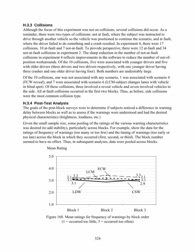
H.3.3 Collisions Although the focus of this experiment was not on collisions, several collisions did occur. As a reminder, there were two types of collisions: not at fault, where the subject was instructed to drive through another vehicle so the vehicle was positioned to continue the scenario, and at fault, where the driver failed to do something and a crash resulted. In experiment 4, there were 17 collisions, 10 at-fault and 7 not-at-fault. To provide perspective, there were 12 at-fault and 34 not-at-fault collisions in experiment 2. The sharp reduction in the number of not-at-fault collisions in experiment 4 reflects improvements in the software to reduce the number of out-ofposition workarounds. Of the 10 collisions, five were associated with younger drivers and five with older drivers (three drivers and two drivers respectively, with one younger driver having three crashes and one older driver having four). Both numbers are undesirably large. Of the 10 collisions, one was not associated with any scenario, 1 was associated with scenario 4 (FCW-reveal), and 7 were associated with scenario 6 (LCM-subject changes lanes with vehicle in blind spot). Of these collisions, three involved a reveal vehicle and seven involved vehicles to the side. All at-fault collisions occurred in the first two blocks. Thus, as before, side collisions were the most common collision type.
H.3.4 Post-Test Analysis The goals of the post-block surveys were to determine if subjects noticed a difference in warning delay between blocks as well as to assess if the warnings were understood and had the desired physical characteristics (brightness, loudness, etc.) Given the small sample size, some pooling of the ratings of the various warning characteristics was desired (to add stability), particularly across blocks. For example, show the data for the ratings of frequency of warnings (too many or too few) and the timing of warnings (too early or too late) across the block in which they occurred (first, second, or third). The block number seemed to have no effect. Thus, in subsequent analyses, data were pooled across blocks.
Mean Rating
5.0
4.0
3.0
2.0
1.0
3.1 3.33.2
2.93.1 3.13.1 3.1
Block 1 Block 2 Block 3
LDW CSW
LCM FCW
Figure 168. Mean ratings for frequency of warnings by block order (1 = occurred too little, 5 = occurred too often)
324
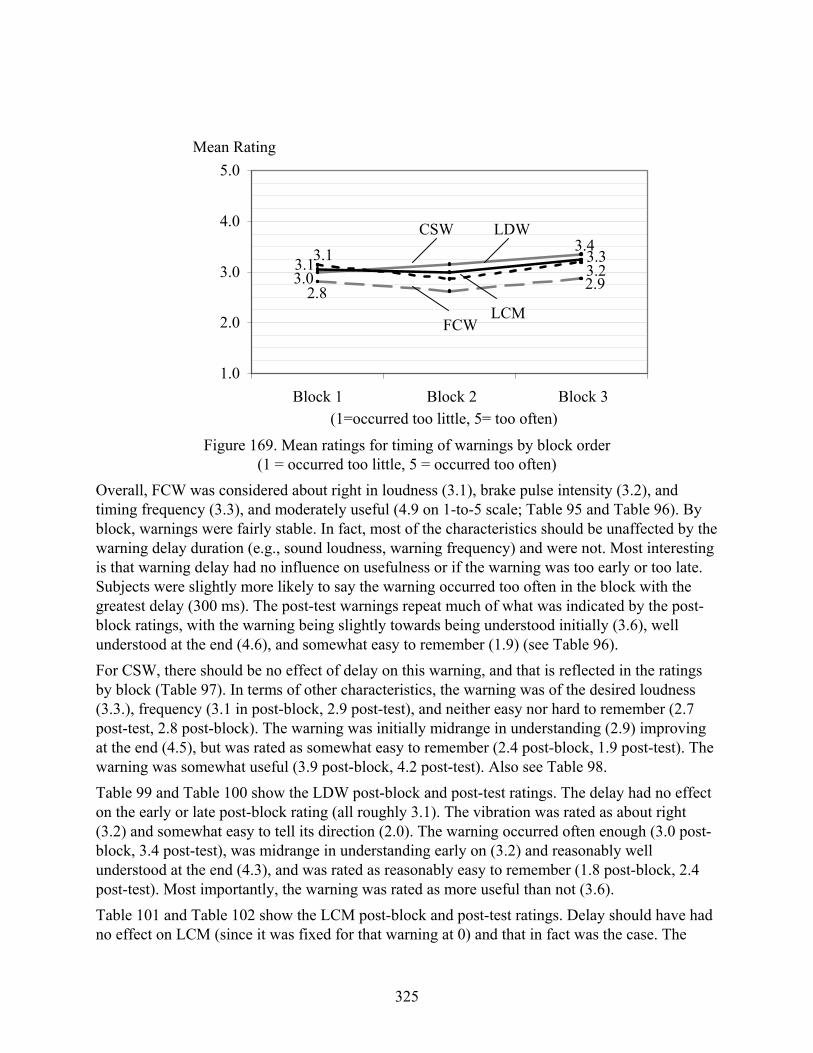
Mean Rating 5.0
4.0
3.0
2.0
1.0
2.8 2.93.0
3.43.1 3.23.1 3.3
Block 1 Block 2 Block 3
CSW LDW
FCW LCM
(1=occurred too little, 5= too often)
Figure 169. Mean ratings for timing of warnings by block order (1 = occurred too little, 5 = occurred too often)
Overall, FCW was considered about right in loudness (3.1), brake pulse intensity (3.2), and timing frequency (3.3), and moderately useful (4.9 on 1-to-5 scale; Table 95 and Table 96). By block, warnings were fairly stable. In fact, most of the characteristics should be unaffected by the warning delay duration (e.g., sound loudness, warning frequency) and were not. Most interesting is that warning delay had no influence on usefulness or if the warning was too early or too late. Subjects were slightly more likely to say the warning occurred too often in the block with the greatest delay (300 ms). The post-test warnings repeat much of what was indicated by the post-block ratings, with the warning being slightly towards being understood initially (3.6), well understood at the end (4.6), and somewhat easy to remember (1.9) (see Table 96). For CSW, there should be no effect of delay on this warning, and that is reflected in the ratings by block (Table 97). In terms of other characteristics, the warning was of the desired loudness (3.3.), frequency (3.1 in post-block, 2.9 post-test), and neither easy nor hard to remember (2.7 post-test, 2.8 post-block). The warning was initially midrange in understanding (2.9) improving at the end (4.5), but was rated as somewhat easy to remember (2.4 post-block, 1.9 post-test). The warning was somewhat useful (3.9 post-block, 4.2 post-test). Also see Table 98. Table 99 and Table 100 show the LDW post-block and post-test ratings. The delay had no effect on the early or late post-block rating (all roughly 3.1). The vibration was rated as about right (3.2) and somewhat easy to tell its direction (2.0). The warning occurred often enough (3.0 post-block, 3.4 post-test), was midrange in understanding early on (3.2) and reasonably well understood at the end (4.3), and was rated as reasonably easy to remember (1.8 post-block, 2.4 post-test). Most importantly, the warning was rated as more useful than not (3.6). Table 101 and Table 102 show the LCM post-block and post-test ratings. Delay should have had no effect on LCM (since it was fixed for that warning at 0) and that in fact was the case. The
325

Table 95. FCW post-block ratings
Block andWarning Delay
Category Question (ms) MeanA B C0 150 300
Format Sound level 1=too soft, 5=too loud 3.2 3.0 3.1 3.1 Brake pulse 1=too soft, 5=too hard 3.3 3.2 3.1 3.2
Meaningfulness Meaning 1=easy to remember, 5=hard 2.6 2.2 2.4 2.4 Overall Frequency 1=too little, 5=too often 3.1 3.3 3.4 3.3
Warning was 1=useless, 5=useful 3.8 4.0 4.0 3.9 Timing 1=too early, 5=too late 2.8 2.8 2.9 2.8
Table 96. FCW post-test ratings
Category Question MeanMeaning-fulness
Initial understanding 1=not well understood, 5=well understood 3.6 Final understanding 1= not well understood, 5=well understood 4.5 Meaning 1=difficult to learn, 5=easy to learn 4.2 Learning 1=easy to remember, 5=hard to remember 1.9
Overall Frequency 1=too little, 5=too often 3.4 Usefulness 1=useless, 5=useful 3.9 Usability 1=difficult to use, 5=easy to use 4.2 Timing 1=too early, 5=too late 2.8
sound was rated as being of the appropriate loudness (3.2) and its direction was rated as somewhat easy to determine (2.2). LCMs were rated as occurring at the desired frequency (3.1 post-block, 3.0 post-test). The warning was midrange in terms of its initial understanding (3.0), moderately well understood at the end (4.2), and neither easy nor hard to remember (2.7 post-block, 2.7 post-test). The warning tended towards being useful (3.6), but only slightly. Table 103 and Table 104 show the blind spot detection (BSD) data. As before, the ratings were consistent across blocks since the delay for all blocks was the same. The brightness of the light was about right (2.9) as was the timing (2.9, neither too early nor too late). The direction from which the light came was reasonably easy to determine (2.1). The light was illuminated at the desired frequency (3.0 post-block, 3.2 post-test). The BSD was fairly well understood initially (4.3), extremely well understood at the end (5.0), and very easy to remember (1.3 post-block, 1.2 post-test). In fact, 12 subjects said the BSD light was very useful or needed no change. However, one subject (a young man) said, “It seems good to have, but I don’t feel comfortable relying on it.”
326

Table 97. CSW post-block ratings
Category Question
Block and Warning Delay
(ms) Mean A 0
B 0
C 0
Format Sound level 1=too soft, 5=too loud 3.3 3.3 3.2 3.3 Meaningfulness Memorability 1=easy to remember meaning, 5=hard 2.7 2.8 2.6
2.7 Overall Frequency 1=too little, 5=too often 2.9 3.1 3.2 3.1
Usefulness 1=useless, 5=useful 3.7 3.5 3.9 3.7 Timing 1=too early, 5=too late 3.3 2.9 3.1 3.1
Table 98. CSW post-test ratings
Category Question Mean Meaningfulness
Initial understanding 1=not well understood, 5=well understood 2.9 Final understanding 1=not well understood, 5=well understood 4.4 Learning meaning 1=difficult to learn, 5=easy to learn 3.6 Memorability 1=easy to remember meaning, 5=hard 2.8
Overall Frequency 1=too little, 5=too often 2.9 Usefulness 1=useless, 5=useful 3.7 Ease of use 1=difficult to use, 5=easy to use 3.9 Timing 1=too early, 5=too late 2.9
Table 99. LDW post-block ratings
Category Question
Block and Warning Delay
(ms) Mean A 0
B 150
C 300
Format Seat vibration 1=too weak 5=too strong 3.3 3.1 3.1 3.2 Vibrating side 1=easy to tell, 5=hard to tell 1.9 2.3 1.9 2.0
Meaningfulness Memorability 1=easy to remember meaning, 5=hard 1.9 1.9 1.7 1.8
Overall Frequency 1=too little, 5=too often 3.1 3.1 2.9 3.0 Usefulness 1=useless, 5=useful 3.6 3.5 3.9 3.7 Timing 1=too early, 5=too late 3.2 3.1 3.1 3.1
327
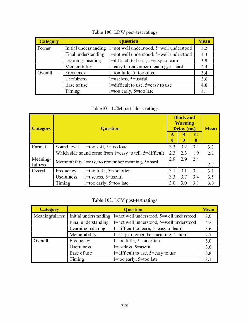
Table 100. LDW post-test ratings
Category Question Mean Format Initial understanding 1=not well understood, 5=well understood 3.2
Final understanding 1=not well understood, 5=well understood 4.3 Learning meaning 1=difficult to learn, 5=easy to learn 3.9 Memorability 1=easy to remember meaning, 5=hard 2.4
Overall Frequency 1=too little, 5=too often 3.4 Usefulness 1=useless, 5=useful 3.6 Ease of use 1=difficult to use, 5=easy to use 4.0 Timing 1=too early, 5=too late 3.1
Table101. LCM post-block ratings
Category Question
Block and Warning
Delay (ms) Mean A 0
B 0
C 0
Format Sound level 1=too soft, 5=too loud 3.3 3.2 3.1 3.2 Which side sound came from 1=easy to tell, 5=difficult 2.3 2.3 1.9 2.2
Meaningfulness Memorability 1=easy to remember meaning, 5=hard 2.9 2.9 2.4
2.7 Overall Frequency 1=too little, 5=too often 3.1 3.1 3.1 3.1
Usefulness 1=useless, 5=useful 3.3 3.7 3.4 3.5 Timing 1=too early, 5=too late 3.0 3.0 3.1 3.0
Table 102. LCM post-test ratings
Category Question Mean Meaningfulness Initial understanding 1=not well understood, 5=well understood 3.0
Final understanding 1=not well understood, 5=well understood 4.2 Learning meaning 1=difficult to learn, 5=easy to learn 3.6 Memorability 1=easy to remember meaning, 5=hard 2.7
Overall Frequency 1=too little, 5=too often 3.0 Usefulness 1=useless, 5=useful 3.6 Ease of use 1=difficult to use, 5=easy to use 3.8 Timing 1=too early, 5=too late 3.1
328

Table 103. BSD post-block ratings
Category Question
Block and Warning
Delay (ms) Mean A 0
B 0
C 0
Format Side mirror light brightness 1=too dim, 5=too bright 2.8 2.9 2.9 2.9 Which side sound came from 1=easy to tell, 5=difficult 2.3 2.2 1.9 2.1
Meaningfulness Memorability 1=easy to remember meaning, 5=hard 1.5 1.4 1.0 1.3
Overall Frequency 1=too little, 5=too often 3.0 3.1 3.0 3.0 Usefulness 1=useless, 5=useful 3.9 4.2 3.9 4.0 Timing 1=too early, 5=too late 2.9 3.0 2.9 2.9
Table 104. BSD post-test ratings
Category Question Mean Meaningfulness Initial understanding 1=not well understood, 5=well understood 4.3
Final understanding 1=not well understood, 5=well understood 5.0 Learning meaning 1=difficult to learn, 5=easy to learn 4.9 Memorability 1=easy to remember meaning, 5=hard 1.2
Overall Frequency 1=too little, 5=too often 3.2 Usefulness 1=useless, 5=useful 4.6 Ease of use 1=difficult to use 5=easy to use 4.8 Timing 1=too early, 5=too late 3.0
Only one subject correctly noticed that all of the warnings started occurring less frequently for FCW and two subjects correctly noticed the difference in LDW frequency or timing. A few reported not noticing any changes (for example, differences in warning volume). Six of the 16 subjects said that their third drive was the best because they were more comfortable with the warnings and driving simulator, while one subject indicated that their second drive was the best because they became familiar with the warnings. One subject said their second block, block B, was the best because “the first was hard to get used to the warnings, but the third had harder conditions.” Similarly, another subject said block C was the best, their second block, because “the other cars were interfering just the right amount of time.” It is difficult to tell whether those two subjects simply thought that the driving behavior of the surrounding vehicles was more erratic in other blocks or if they may have noticed a difference in warning frequency throughout the blocks. The remaining six subjects did not give a reason for their block choice, gave no response, indicated no preference, or described what they thought was the best warning instead of the best block. When asked for additional comments, one subject said it would take several weeks for her to be able to remember the warnings and integrate the system into her driving, and another subject said, “If I had a car that did all this I’d probably crash because it’s too distracting.” However, most responses were positive.
329
H.4 Conclusions How Does the Tradeoff Between Warning System Processing Time (to Start to Inform the Driver) and Warning Accuracy Affect Driver Responses to Warnings? Even though subjects experienced a significant number of warning events with different delays in different blocks, the ratings of the timing of the warnings in each block (too early, too late) were the same, suggesting that subjects did not notice delays, that delays did not matter, or both. For LDW, increasing the delay to 300 ms led to a more immediate response of the subject to the lateral position error at 0.5 seconds after the warning delay, where lateral error increased for the first 0.5 seconds if the delay was 0 or 150 ms. This could be a misleading comparison, however, since one needs to consider not just the time period after the warning, but the time period after the point where the warning would have occurred without a warning delay. Furthermore, with the shorter delays, subjects stabilized closer to lane center (0.3 meters for 0 and 150 ms, 0.45 meters for 300 ms). It could be that the added delay leads subjects to believe that less accurate control of lane position is acceptable. Thus, these data suggest that delays of 300 ms are too long for LDW, and that the threshold for acceptable delay is probably between 150 and 300 ms. Interestingly, it was thought that increasing the gust duration to trigger LDW would increase the maximum excursion and the mean as well. However, that did not occur and it could be that some sort of compensation occurs when gusts are long. For FCW, the situation is quite complex. For cases of no acceleration delay (in which the warnings are completely accurate and only differ in terms of warning delay (warning processing time)), the differences in speed reduction were quite small. Thus, a pure warning delay seemed to have no substantial effect on how much drivers slowed down over time. However, in situations where the vehicle could sometimes reaccelerate, especially after a 250-ms delay, speed reductions were much greater. Particularly curious is the warning delay in the 250 ms case, when slowing down was least needed, but led to the greatest reduction in speed over time. It could be that these results reflect subjects noticing the lead vehicle deceleration before the TTC threshold is reached and braking before the warning is presented, as well as situations where the following distance is quite large so the TTC threshold is not reached. Thus, from these data, it is difficult to say how warning response time and accuracy jointly affect driver responses. It could be that a more sophisticated analysis, which considers when drivers are responding to the warning system and when they are responding independent of it, is needed. The results certainly are curious and need further thought. How Well Do Drivers Respond to the Set of IVBSS Warnings for IVBSS? Are Any Confused or Misunderstood? As a reminder, most of the warning characteristics were rated on five-point scales where 1 indicated something was insufficient (e.g., a sound was too soft or occurred too infrequently) and 5 indicated excess (e.g., a warning was too loud or occurred too often). For those characteristics, mid-scale values (3) were desired. Exceptions were meaningfulness and learning (1 = easy to remember and learn, 5 = hard), understandability (1= not well understood, 5 = well understood), and usability (1 = difficult, 5 = easy), where end of scale values, usually 5, were desired.
330
Driver reactions to warnings varied by warning type. Subjects responded to 25 percent of the FCWs (653 total warnings) and 56 percent of the CSWs (90 total warnings) by slowing down. Mean accelerator pedal release times were 0.61 seconds and 1.20 seconds for FCW and CSW warnings, respectively. Mean brake onset times followed a similar pattern, with drivers responding nearly twice as fast to FCWs as to CSWs (0.96 seconds and 1.86 seconds, respectively). Of the four primary warnings, FCW received the most favorable ratings. Responses were close to ideal for loudness, brake pulse intensity, early versus late occurrence, and desired frequency of occurrence (3.3, 3.1, 3.1, 2.9). Four subjects (a young man, a young woman, and two middle-aged men) said that the warning should be less intense, and one middle-aged woman said that the FCW and CSW sounded too similar. The warning was neither easy nor difficult to remember, but initial understanding was not that good (3.6). It was rated as somewhat useful. LDW was rated favorably. Its timing (3.1) and vibration (3.2) were as desired, as was its frequency (3.4), though less so than other warnings. Accordingly, four subjects (three young) said that it should be less sensitive or less intense. In contrast, one young woman said the warning should have occurred more frequently. Middle-aged subjects found it easier to use than young subjects, though initially, the warning was not well understood (3.2, where 1 = not well understood and 5 = well understood). Although CSW was rated well for some characteristics (ideal timing and frequency (overall mean = 2.9), it had the lowest ratings of the warnings examined. Note that some subjects did not receive a CSW in every block (block A: two subjects, B: two subjects, C: four subjects). CSW was more difficult to learn (3.6) and remember (2.8), although middle-aged men found CSW to be easy (1.0). CSW was the most difficult to understand initially (overall mean = 2.9). When asked what changes should be made to CSW, two subjects said CSW was too similar to LCM, and one subject thought CSW was too similar to FCW. Eight subjects gave no response or said the warning should stay the same. The unimpressive initial understanding suggests the warning should be reexamined. In terms of its physical characteristics, LCM rings were good (loudness = 3.1, frequency = 3.1 and 3.0, side = 2.2). However, its initial understanding was only 3.0, which is not stellar. It was not that easy to remember (2.7). In addition to one subject who thought LCM was too similar to the CSW, one subject said LCM was too similar to LDW. Ten subjects said LCM was very helpful or no change is needed. This suggests some changes in the LCM warning are desired so that it can be immediately understood Though not part of the initial set, the ratings for BSD were quite good. It was very close to ideal in terms of physical characteristics (light brightness, 2.9; frequency, 2.9 post-block and 3.0 post-test; early or late, 2.9 post-block and 3.2 post-test). BSD was rated as easy to remember by almost every subject (1.3 post-block, 1.2 post-test), useful (4.0 post-block, 4.6 post-test), and easy to use (4.8). Quite frankly, after those involved in the development of these experiments had driven with BSD in the pilot tests, the common reaction was, “I want that!” To provide additional perspective, Table 105 summarizes some warning ratings.
331

Table 105. Summary of post-test warnings
Category Characteristic Warning BSD FCW LDW CSW LCM
Meaning (Initially) not/well understood 4.3 3.6 3.2 2.9 3.0 fulness Hard/easy to learn 4.9 4.2 3.9 3.6 3.6
Easy/hard to remember (post-block) 1.3 2.4 1.8 2.7 2.7 Easy/hard to remember (post-test) 1.2 1.9 2.4 2.8 2.7
Overall Useless/useful (post-block) 4.0 3.9 3.7 3.7 3.5 Useless/useful (post-test) 4.6 3.9 3.6 3.7 3.6
Thus, the overall impression is that BSD and FCW are acceptable in terms of their intensity, frequency of occurrence, timing, and understandability. LDW could use some improvements in initial understanding, though its timing and frequency of occurrence are acceptable. CSW and LCM need overall improvement as they were not well understood.
H.5 Forms H.5.1 Biographical Form
Date: ___________ Participant #: ____
Personal Data Name: _______________________________________ Sex (circle one): { M } { F } Phone: ( ____ ) ______________ E-mail address: _____________________________ May we contact you for future UMTRI studies? { Yes } { No } Date of Birth (month / day / year): ____ / ____ / ____ Is English your first language? { Yes } { No } Occupation: _____________________________________________
(engineer, teacher, etc.; if retired, write “retired” and list previous occupation) Education (circle highest level completed):
{ High School } { Some College } { College Degree } { Graduate School } If you attended college, what was your major? ________________________________
Driving Data
Licensed driver's in the State of ____ . Is it current? { Yes } { No } What motor vehicle do you drive most often?
Year: ________ Make: ___________________ Model: ___________________ Approximately how many miles do you drive per year? ____________ mi / yr Approximately what percentage of your time driving is spent on expressways? _____ % Do you have any special driving licenses (commercial, chauffer, etc.)? { Yes } { No }
If yes, please list: _________________________________________ How many accidents have you been involved in during the past 5 years? ______
Brief description: ___________________________________________________ _________________________________________________________________ How many traffic violations have you been involved in the past 5 years? _______
332

Brief description: ___________________________________________________ _________________________________________________________________ On a 3-lane expressway, which lane do you normally drive in?
{ Left } { Middle } { Right }
Vision
What type of corrective lenses do you wear corrective lenses while driving? { None } { Glasses } { Contacts }
If yes, what type? { Near-Vision/Reading } { Far-Vision } { Bifocal } { Multifocal } { Other } If other, please describe: _________________________________
What type of corrective lenses do you wear corrective lenses while reading? { None } { Glasses } {Contacts }
If yes, what type? { Near-Vision/Reading } { Far-Vision } { Bifocal } { Multifocal } { Other } If other, please describe: _________________________________
Scoring for vision and hearing test (experimenter use only):
H.5.2 Instructions Experiment Introduction and Preparation
Greet Subject
<Introduce self> Thank you for coming in today, I’ll be conducting introductory part of the driving simulator study. Before we get started, you will need a visitor parking pass to park at UMTRI. Please place this pass face-up on your dashboard and we’ll be ready to go when you return.
Let's go to the conference room and get started.
Lead subject to conference room.
Overview (in conference room)
Before we get started, I will give you a brief overview of the study and what you will be doing.
The purpose of this study is to test the safety and usability of in-vehicle warning systems that could make the next new vehicle you buy much safer to drive. The experiment will take place in the driving simulator where another experimenter will collect data on you while you are driving. I’ll explain more about what that means later on.
To examine how effective these in-vehicle systems are, video cameras and sound recording devices will be recording you during the entire time you are driving in the simulator. These recordings will be used to study things like how you react to different driving situations and in-vehicle systems. In addition to using these recordings for data analysis, it is possible that UMTRI or NHTSA (the National Highway Traffic Safety Administration), who is funding this project, may use portions of your videotape in presentations or in the study reports. Furthermore, our work sometimes appears in the media so there is a chance that some portion of your tape will be shown on TV. Participant’s personal information never leaves UMTRI and is only used here for verification and to contact you about future UMTRI studies if you choose. So if your tape is used for any of the purposes that I mentioned, your name, driver’s license number, and any other personal information that could be used for identification would never be disclosed. Do you have any questions about how the video data we collect today may be used?
Answer any questions they have to the best of your ability.
Is it alright with you if we videotape you during the experiment?
If “no,” dismiss subject.
333

The entire experiment will take about two hours to complete, at the end of which, you will receive $50 in thanks for your participation. You may choose not to continue with the experiment at any time. If you do choose not to complete the experiment, you will still be paid.
Before you start driving I’ll need you to read and sign a consent form, answer some questions about your driving background, and test your vision and hearing. Then I’ll take you to the simulator for the driving portion of the experiment. After three minutes of practice, you will drive in the simulator for three 20-minute drives, with a short break between each. You will be asked to fill out a short questionnaire at the end of each drive and at the end of the study.
Would you like to continue?
If no, dismiss subject.
Consent and Bio Forms
Here is the consent form, please read it carefully and sign at the bottom when you are finished.
If the subject does not read the consent form, say: Even though I have covered the basics of the information on the form, please make sure you read it thoroughly. I know it seems like extra paperwork, but we’re required that you understand this information.
Thank you. Would you like a copy for yourself?
if yes, have them sign another form to keep.
Here is the biographical data sheet. Please fill it out and feel free to ask me questions at any time.
Provide bio form.
Check that both the consent form and bio form is legible and complete.
Payment Form
All right, just one more form for you to fill out.
This is the payment form you need to fill out in order to get your money at the end of the experiment. Are you a University employee?
If “yes”, have them fill out University Employee form.
Ok, just go ahead and fill this out. Although it says you’ve already received the money, I’d like you to go ahead and sign it anyway. It speeds up the process for us so you can fill out all the paperwork at once. Let me know if you have any questions while you’re filling this out.
We’re done with the preliminary paperwork, now I need to check your eyesight and hearing.
Vision Test
Do you use any corrective eyewear while you drive?
If subject answers “yes,” say: Is that what you are wearing now?
If subject is not wearing the same eyewear they wear while driving ask subject to put that on.
We’re not professional optometrists or audiologists, these tests are just for screening. Please look into the vision device and keep looking straight ahead for the entire eye test.
Test Visual Acuity (FAR #2):
Can you see that in the first diamond in the top circle is complete but the other 3 are broken? In each diamond, tell me the location of the solid circle - top, left, bottom, or right.
Continue until 2 in a row are wrong. The last correct answer is the visual acuity. Subjects must have 20/40 or better vision. If they do not pass, pay and dismiss the subject.
Hearing Test
Make sure the office door is closed so it’s quiet.
334

In this test we will be testing the full range of hearing. Very few people are capable of hearing all of the tones I will play.
I’m going to play you a series of tones, and you just need to simply raise your hand for whichever side you hear the tone coming from. So if you hear a tone in your left ear, raise your left hand.
I’m going to start off by playing one practice tone just to make sure it’s working, and then we’ll start the test. Go ahead and put on these headphones. The red side should cover your right ear.
Play a sample tone at 35 dB and 1500 Hz (either ear).
Ok, now we’re going to start the test.
Do all tones for one ear in sequence. Make sure the subject cannot see which ear is being tested. Move dial to 25 dB and play 2 tones a 1000 Hz, 2 tones at 2000 Hz, and 2 tones at 3000 Hz. Wait after playing each tone for a response. If they miss a tone, increase the dB by 5 dB each time until they hear the tone 2 times successfully. Record the dB level on the screening sheet. Continue by testing the other ear. Maximum passing values are: 45 dB for 1000 Hz, 55-60 dB for 2000 Hz, and 65 dB for 3000 Hz. If they do not pass, pay and dismiss the subject.
That’s all I need for now, let’s go to the driving simulator for the rest of the experiment.
Take subject to simulator.
In the Simulator
Seat Subject
Please have a seat in the cab and adjust the seat to a comfortable position using the automatic controls on the left side of the seat. Once I put a road scene up on the screen I’ll have you adjust the mirrors as well.
The cameras in the vehicle to provide a variety of camera angles. There is also a live microphone here.
Point out cameras and microphone.
For this part of the experiment you will have a three-minute practice drive, then three 20-minute drives with breaks in between. There will also be a questionnaire to fill out after each drive and at the end of the experiment.
Practice Drive
Now it is time to try out the simulator. For the duration of this experiment please drive normally, being sure to be safe. Use the speedometer on the instrument panel to check your speed, just as in a real car.
The speed limit is 70 mph for the entire experiment and you will see speed limit signs throughout the course as a reminder. Try to maintain the speed limit at all times, however, if you are not comfortable driving that fast, just go as fast as you are comfortable. Keep in mind that if you go slower than 70 mph the experiment will takes slightly longer to complete.
The steering wheel in the simulator doesn’t feel exactly like one in a real vehicle and it is easy to overcorrect. The key is to make small, slow corrections with the steering wheel.
Some people experience motion sickness in the simulator, so if you start feeling warm, dizzy, nauseous, or anything else that could occur prior to being motion sick, let me know immediately and I’ll tell you how to stop. As I said before, you may end the experiment at any time and you will still be paid $50.
Do you have any questions?
Ok then, now we’ll begin the practice drive so you can get a feel for driving in the simulator. Please adjust the left and rear-view mirrors, the right mirror control does not work properly, so I will help you adjust it. This practice drive will last for about three minutes and I’ll tell you when the time is up.
Put the car in “D” using the shift lever between the seats. Now, please press on the accelerator and begin driving.
335

Have the subject drive for approximately three minutes.
Ok, that’s the end of the practice drive. Please coast to a stop and shift the car into park.
Stop the simulator about 10 seconds after the car is in park.
Warning System Training
In each drive you will receive four different warnings, and one informational light. The forward crash warning will go off when you are at high risk of crashing into the car in front of you. When the warning goes off you will hear a series of beeps and feel a pulse in the brake pedal. Here’s what the forward crash warning sounds and feels like. (Play the FCW warning.) The curve speed warning goes off when your speed is too high in a curve and you are at risk of skidding. It has the same beeping sound as the Forward Crash Warning, but no brake pulse. (Play the CSW warning.) The Lane Change / Merge warning warns you if there is a car in your blind spot as you are attempting to change lanes. The warning is directional so it goes off only on the side of the threat. You will hear a honking sound and feel a vibration in your seat. (Play the LCM warning.) The Lane Departure Warning is intended to alert you when you unintentionally leave your lane, so it goes off when you drift from your lane without using your turn signal. This warning is also directional and consists of a seat vibration on the side of the lane departure to simulate rumble strips. (Play LDW warning.) There is also a blind spot warning. Whenever there is a vehicle or another object in your blind spot, a red light will appear on either the left or right side mirror, depending on the object’s location. The light will appear even if you’re not making a maneuver. The light only works while driving, so right now I can’t show you what that looks like, you will also not be tested on your knowledge of the blind spot light before beginning the drives.
Now I’d like to test your understanding of these warnings. I am going to play a warning, and I’d like for you to respond to the warning as if you were driving. So for the forward crash warning and the curve speed warning you would brake, for the lane change/merge warning you would check your blind spot and correct your lane position, and for lane departure warning you would correct your lane position (e.g., lane departure warning on the left, turn the steering wheel to the right to return to the lane). Please respond as accurately and as quickly as you can. After you make a driving response, I’d like for you tell me which type of warning you just experienced (FCW, CSW, LCM, or LDW). In addition to the four warnings, please tell me when you identify the blind spot light. You will need to get eight in a row correct before we can go on. Do you have any questions?
Training and Practice Wrap-Up
That is the end of the training and practice portion of the experiment. We will now take a short break before beginning the first 20-minute drive. You will also get a break between each drive. Feel free to get out of the simulator and walk around for a minute. And if you would like to get a drink of water or use the restroom during any of these breaks, I will be happy to show you where they are.
Data Collection
Block 1
We will now begin the first of the three 20-minute drives. Just as in the practice drive, please drive normally, being sure to be safe. Use your turn signal and use the speedometer on the instrument panel to check your speed. For the remaining three drives there will be other vehicles in the road. Keep in mind that the screens do not go all the way around the cab and that sometimes a car may be on the road where it can’t be seen.
Above all, your task is to avoid crashes. Don’t change lanes unless there is a stopped car or an object in your lane. In other words, don’t change lanes unless you are forced to. When you are forced to change lanes, stay in that lane until forced to change again. The speed limit is 70 mph and you will see speed limit signs throughout the course as a reminder, try to maintain the speed limit at all times.
Do you have any questions?
Ok, now I will turn on the simulator, don’t begin driving until I tell you to begin.
All right, you may begin driving whenever you’re ready.
336

Subject drives first block. If necessary, remind subject to keep speed close to 70mph for the entire drive. If subject is ever in the wrong lane, tell them how to get back.
(At the end of Block 1) Ok, turn on your right turn signal and gradually slow down as you pull off onto the shoulder. Once you have stopped, please put the car in park.
Stop the simulator about 10 seconds after the car is in park
You may take a break for a minute if you wish. Do you have any comments or questions about what happened in the last drive?
Blocks 2 and 3
These blocks proceed in the same manner as Block 1. At the end of Block 3 call Jessica or Erin and have her get the current subject so that the subject can complete the post-drive questionnaire outside of the simulator and the next subject can begin.
H.5.3 Post-Test Evaluation Form Participant #: _____
Warning Display Explanation Forward Collision
Beeping sound and Brake Pulse High risk of crashing into the car ahead
Curve Speed High-pitched beeping sound (one note)
Traveling too fast in curve, danger of skidding
Lane Change-Merge
Lower-pitched beeping sound (two notes, directional)
Attempting to change lanes with vehicle in blind spot; Not disabled by turn signal
Lateral Drift Seat vibration (directional) Unintentional lane drift; Disabled by turn signal
Blind Spot Light Red light on side mirror Vehicle in blind spot
Drive 1 Drive 2 Drive 3
1. Forward Collision Warning sound was too soft 1 2 3 4 5 too loud _____ _____ _____
brake pulse was too soft 1 2 3 4 5 too hard _____ _____ _____ occurred too little 1 2 3 4 5 occurred too often _____ _____ _____
warning was useless 1 2 3 4 5 useful _____ _____ _____ occurred too early 1 2 3 4 5 too late _____ _____ _____
easy to remember meaning 1 2 3 4 5 hard to remember _____ _____ _____
2. Curve Speed Warning (if applicable, if you heard no curve speed warning go on to Question 3) sound was too soft 1 2 3 4 5 too loud _____ _____ _____
occurred too little 1 2 3 4 5 occurred to often _____ _____ _____ warning was useless 1 2 3 4 5 useful _____ _____ _____
occurred too early 1 2 3 4 5 too late _____ _____ _____ easy to remember meaning 1 2 3 4 5 hard to remember _____ _____ _____
3. Lane Change/Merge Warning sound was too soft 1 2 3 4 5 too loud _____ _____ _____
easy to tell side sound came from 1 2 3 4 5 difficult to tell _____ _____ _____ full warning occurred too little 1 2 3 4 5 occurred too often _____ _____ _____
full warning was useless 1 2 3 4 5 useful _____ _____ _____ full warning occurred too early 1 2 3 4 5 too late _____ _____ _____
easy to remember meaning 1 2 3 4 5 hard to remember _____ _____ _____
337

Drive 1 Drive 2 Drive 3 4. Blind Spot Light
light on side mirror was too dim 1 2 3 4 5 too bright _____ _____ _____ easy to tell which side light is on 1 2 3 4 5 difficult to tell _____ _____ _____
occurred too little 1 2 3 4 5 occurred too often _____ _____ _____ warning was useless 1 2 3 4 5 useful _____ _____ _____
occurred too early 1 2 3 4 5 too late _____ _____ _____ easy to remember meaning 1 2 3 4 5 hard to remember _____ _____ _____
5. Lane Departure Warning seat vibration was too weak 1 2 3 4 5 too strong _____ _____ _____
easy to tell which side was vibrating 1 2 3 4 5 hard to tell _____ _____ _____ occurred too little 1 2 3 4 5 occurred too often _____ _____ _____
warning was useless 1 2 3 4 5 useful _____ _____ _____ occurred too early 1 2 3 4 5 too late _____ _____ _____
easy to remember meaning 1 2 3 4 5 hard to remember _____ _____ _____
To be completed at the end of the experiment.
6. Have you ever driven a vehicle with the following warning systems? (circle one)
Forward Collision Warning: { No } { Yes } Curve Speed Warning { No } { Yes } Lane Change-Merge Warning { No } { Yes } Lane Departure Warning: { No } { Yes }
7. Forward Collision Warning Initially, the warning was not well understood 1 2 3 4 5 initially was well understood At end, the warning was not well understood 1 2 3 4 5 at end was well understood
Meaning was difficult to learn 1 2 3 4 5 easy to learn Overall the warning occurred too little 1 2 3 4 5 occurred too often
Overall the warning was useless 1 2 3 4 5 useful Overall the warning was difficult to use 1 2 3 4 5 easy to use Overall the warning occurred too early 1 2 3 4 5 too late
Overall the meaning was easy to remember 1 2 3 4 5 hard to remember
8. Curve Speed Warning (if applicable) Initially, the warning was not well understood 1 2 3 4 5 initially was well understood
At end, the warning was not well understood 1 2 3 4 5 at end was well understood Meaning was difficult to learn 1 2 3 4 5 easy to learn
Overall the warning occurred too little 1 2 3 4 5 occurred too often Overall the warning was useless 1 2 3 4 5 useful
Overall the warning was difficult to use 1 2 3 4 5 easy to use Overall the warning occurred too early 1 2 3 4 5 too late
Overall the meaning was easy to remember 1 2 3 4 5 hard to remember
9. Lane Change/Merge Warning Initially, the warning was not well understood 1 2 3 4 5 initially was well understood At end, the warning was not well understood 1 2 3 4 5 at end was well understood
Meaning was difficult to learn 1 2 3 4 5 easy to learn Overall the warning occurred too little 1 2 3 4 5 occurred too often
Overall the warning was useless 1 2 3 4 5 useful Overall the warning was difficult to use 1 2 3 4 5 easy to use Overall the warning occurred too early 1 2 3 4 5 too late
Overall the meaning was easy to remember 1 2 3 4 5 hard to remember
338

10. Blind Spot Light Initially, the light was not well understood 1 2 3 4 5 initially was well understood At end, the light was not well understood 1 2 3 4 5 at end was well understood
Meaning was difficult to learn 1 2 3 4 5 easy to learn Overall the warning occurred too little 1 2 3 4 5 occurred too often
Overall the warning was useless 1 2 3 4 5 useful Overall the warning was difficult to use 1 2 3 4 5 easy to use Overall the warning occurred too early 1 2 3 4 5 too late
Overall the meaning was easy to remember 1 2 3 4 5 hard to remember
11. Lane Departure Warning Initially, the warning was not well understood 1 2 3 4 5 initially was well understood At end, the warning was not well understood 1 2 3 4 5 at end was well understood
Meaning was difficult to learn 1 2 3 4 5 easy to learn Overall the warning occurred too little 1 2 3 4 5 occurred too often
Overall the warning was useless 1 2 3 4 5 useful Overall the warning was difficult to use 1 2 3 4 5 easy to use Overall the warning occurred too early 1 2 3 4 5 too late
Overall the meaning was easy to remember 1 2 3 4 5 hard to remember
12. Did you notice any changes in the warnings between the three drives? Please list below
a. Forward Collision Warning
b. Curve Speed Warning
c. Lane Change/Merge Warning
d. Lane Departure Warning
e. Blind Spot Light
f. Overall
13. In your opinion, which drive was best and why?
14. How should each warning be changed, if at all? Consider what it is presented, its intensity, the sounds chosen, etc.
a. Forward collision warning
b. Curve Speed Warning
c. Lane Change/Merge Warning
d. Lane Departure Warning
e. Blind Spot Light
f. Additional Comments
339

Appendix I: Experiment 5 ņ Driver Response to Simultaneous Warnings
I.1 Overview A central program issue was how to deal with warnings that occur concurrently or almost concurrently. One of the assumptions behind this question is that such situations will occur often enough to be a concern. Some of the findings from this experiment may challenge that assumption. Nonetheless, there are a number of issues related to multiple warnings that could be considered, only some of which could be addressed.
x Should interruption of warnings occur? If warnings are not interrupted, the first warning is played and when it is completed, the second is played (delayed presentation). An alternative is to play the warning whenever it occurs, even if it occurs at the same time as another warning (concurrent presentation).
x If warnings are interrupted, should the rule be to use priority interruption (if the first is more important than the second, continue the first and play the second, otherwise cut off the first and play the second)?
x Should transitions between warnings be immediate or delayed (to demark a break and avoid confusion), and, if delayed, by how much? Furthermore, should the transition be sudden or should there be a fade in (or fade out), and over what time period?
Exploring all of these issues was beyond the scope of the project. Given the time criticality of these warnings, it made sense to set the transition time between warnings to 0, eliminating the third issue. In addition, one could also consider the warning reliability independently, or fold that factor into the prioritization scheme. However, consideration of that factor was beyond the project resources and not considered. Therefore, this experiment examines two sets of issues:
x Should co-occurring warnings be presented: o Whenever they occur, even if concurrent? o One a time with higher priority warning interrupting those of lower priority
(without gaps or fade in)? o In sequence of occurrence, with the first warning playing to completion before the
second starts? x In the simulator, how well do drivers respond to the set of IVBSS warnings? Are any
confused or misunderstood?
As is noted in previous studies, even in scenarios where a large number of warnings were presented over a short period of time, there were few co-occurring warnings where the presentation of one overlapped with the presentation of another. As a rough engineering approximation, one might consider three seconds after a warning as the maximum period to consider for overlap as by that time, the driver has basically completed the response to a warning in most cases (braked, steered and returned to a lane, etc.). An even stricter rule is to only consider the time period over which a warning would need to be preempted, which is 0.85 seconds for the auditory warnings considered here. In this experiment, the planning has gone one step further in that there was a deliberate effort to force warnings to co-occur.
340

Table 106. Estimated duration of experimental tasks, experiment 5 (see experiment 5 forms section of appendix for instructions and post-test)
Task Category Description ApproximateDuration (min)
Preparation (15 min)
Filling out biographical data form 5 Reading and signing consent form 5 Vision and hearing tests 5
Set-up and practice (6 min)
Simulator introduction 3 Practice driving in the simulator (practice world) 3
Data collection (68 min)
Break 2First block 20 Break 3Second block 20 Break 3Third block 20
Wrap-up (10 min.) Fill out post-test and payment 10 Total 93
I.2 Method This experiment took place in the UMTRI driving simulator. (See Appendix A for a complete description of the simulator and simulator upgrade.) The test method developed for experiment 2 was used as a basis for this experiment in that the scenarios are the same (some with minor modifications), and the world, procedure, and design basis are quite similar. Table 106 shows the sequence and duration of tasks. (Complete subject instructions appear in section I.5.2 and the post-test evaluation form is shown in section I.5.3. The post-test was similar to that used in previous studies, where subjects rated the intensity and frequency of warning stimuli, as well their understandability, ease of use, and usefulness.) As in all DVI IVBSS experiments, the most current version of the warning approach was used. Refer to Table 46 for a complete description.
To create the multiple warning scenarios, experimenters combined single warning scenarios so that triggering events would occur in close succession. In prior experiments, there were many instances in which even a single warning triggering event did not occur as planned. Accordingly, getting multiple events to occur at specific times (to trigger multiple alarms) was expected to be difficult. As in experiment 4, single warning scenarios were used to create variety so that subjects did not begin to anticipate certain warnings or vehicle maneuvers. Five scenarios were used in experiment 5, summarized as follows (for scenario details, see Appendix B):
x Single W arningScenarios. Only one warning is planned. These are most common during normal driving.
x M ultiple W arningScenarios. Two warnings are planned to occur at approximately the same time.
x FalseAlarm Scenarios. A single warning is presented without a triggering event. In normal driving, false alarms are common.
341

x Lead Lane Change. The lead vehicle changes lanes. These changes provided more variety in the traffic situation and made anticipating maneuvers more difficult (especially in construction zones). Although subjects were instructed not to change lanes until forced, many would simply follow the lead vehicle.
x No Scenario Trials: All vehicles drive safely at approximately 70 mph.
The most interesting multiple warning scenarios are those where two different warnings are triggered nearly simultaneously and lead to different patterns of driver response. Warnings included lateral drift warning (LDW) where drivers adjust lane position, forward collision warnings (FCW) where drivers decelerate, and lane change-merge (LCM) warnings where drivers adjust lane position. Curve speeds warnings (CSW) were not included in multiple warning scenarios because of programming constraints. Each combination of warnings was presented twice so that each warning in the pair could be presented first. For many multiple warning combinations, only minor scenario changes were required to change the order of triggering events. For the LCM-FCW combination, completely different scenarios needed to be created to trigger each alarm first. Three different priority rules for presenting multiple warnings were used in this experiment:
x Present at Trigger. Warnings are presented at the time of the triggering event, so if two warnings are triggered simultaneously, they are presented simultaneously. The time period that the warnings overlap depended upon each warning’s duration and time of trigger. Warning priority is not considered.
x Delayed Sequential. The second warning in a multiple warning situation is delayed until the first has finished. The first alarm triggered is presented in its entirety followed by the second alarm presented in its entirety. Warning priority is not considered.
x Priority Preempt. Each warning has an associated priority (FCW had first priority, LCM second, and LDW third). The first warning was presented when the triggering event occurred. If another triggering event occurred while the first warning was still playing, it interrupted the first warning if it had a higher priority and was suppressed if it had a lower priority. Higher priority warnings were always presented in their entirety.
Warning priority was based on the likelihood that a crash would lead to a fatality. Forward crash situations (leading to an FCW) posed the greatest risk, followed by sideswipes (leading to LCM), followed by lane departures (leading to LDW) as many drifts might lead to moving into another empty lane or shoulder. Table 107 shows how warnings for each multiple warning scenario are presented according to the three warning presentation methods. The higher priority warning is shaded for each combination, although priority is only taken into consideration under the priority preempt presentation method.
342

Table 107. Warnings presented for each scenario and priority scheme
Multiple Warning Presentation Method Multiple Warning Scenario Present at Trigger Sequential Priority Preempt
FCW FCW FCW4-FCW + 6-LCM LCM LCM
LCM LCM LCM7-LCM + 1-FCW FCW FCW FCW
LDW LDW LDW 8-LDW + 1-FCW FCW FCW FCW
FCW FCW FCW1-FCW + 8-LDW LDW LDW
LCM LCM LCM6-LCM + 8-LDW LDW LDW
LDW LDW LDW 8-LDW + 6-LCM LCM LCM LCM
Table 108 shows the multiple warning scenario codes as described in section 3.5.1 and in Appendix B.
Table 108. Warnings presented for each scenario and priority scheme
Code Scenario Description Code Scenario Description 1 FCW - lead vehicle braking 6 LCM - Lane change with a vehicle in the
blind spot 4 FCW – reveal 7 LCM – lane change with a vehicle
accelerating to the blind spot 8 LDW – due to wind gust
The driving loop for experiment 5 was the same as used for experiment 4 (Figure 170). Subjects drove one loop per block. Each block took about 20 minutes to drive at 70 mph so this world is slightly larger than the world used in experiments 2 and 3. Each subject drove three loops (three blocks). In each loop there were ten long straightaways, each of which could contain multiple trials (26 trials in all). Starting and ending each block in the middle of a segment, using both left and right turns, and varying the length of each straightaway made it difficult for subjects to memorize the shape of the world.
343

16 tiles
16
18
9
4
7
8
14
15
5
Figure 170. Configuration of the world for IVBSS experiment 5 (1 tile = 200 m) = Construction zones, two in the left lane and one in the right lane
I.2.1 Scenario Frequency To trigger enough warnings for analysis, warnings were presented at a much higher frequency than they would occur under normal driving conditions. Subjects were expected to receive about one warning per minute, though the actual frequency depended upon individual reactions to scenarios. Each block contained one of each type of multiple warning scenario, or six in all. Additional true warning scenarios used in previous experiments were included in experiment 5 so that subjects did not build expectations of warnings and vehicle actions. False alarms were also included to simulate real-world driving. The scenarios used in this experiment are shown in Table 109.
344

Table 109. Frequency of scenarios in each block
Scenario Type Scenario Number Multiple warning (6) 4-FCW + 6-LCM
7-LCM + 1-FCW 8-LDW + 1-FCW 1-FCW + 8-LDW 6-LCM + 8-LDW 8-LDW + 6-LCM
Single warning (6) 1-FCW 4-FCW 5-FCW 6-LCM 7-LCM 8-LDW
Lead lane change (1) False alarm (5) FA 1-FCW
FA 4-FCW FA 5-FCW FA 6-LCM FA 8-LDW
Across subjects, the order of blocks (priority schemes) was partially counterbalanced (Table 110). Within subjects, the order of scenarios in each block was different for each block (Figure 171 through Figure 173), with the further constraint that no scenario occurred during the first two straightaways on each block so that subjects could become comfortable with driving in the simulator.
345
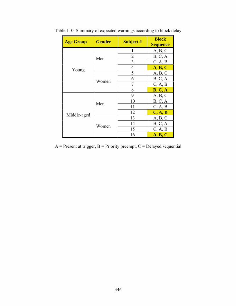
Table 110. Summary of expected warnings according to block delay
Age Group Gender Subject # Block Sequence
1 A, B, C
Men 2 B, C, A 3 C, A, B
Young 4 A, B, C 5 A, B, C
Women 6 B, C, A 7 C, A, B 8 B, C, A 9 A, B, C
Men 10 B, C, A 11 C, A, B
Middle-aged 12 C, A, B
Women
13 A, B, C 14 B, C, A 15 C, A, B 16 A, B, C
A = Present at trigger, B = Priority preempt, C = Delayed sequential
346
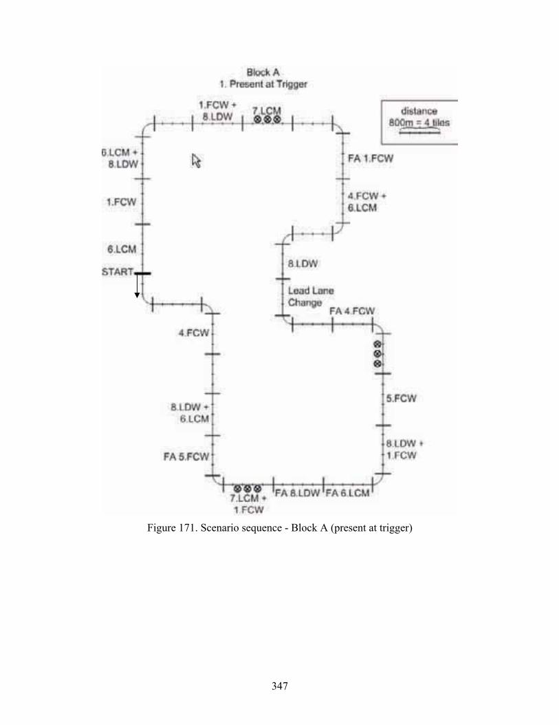
Figure 171. Scenario sequence - Block A (present at trigger)
347

Figure 172. Scenario sequence - Block B (priority preempt)
348
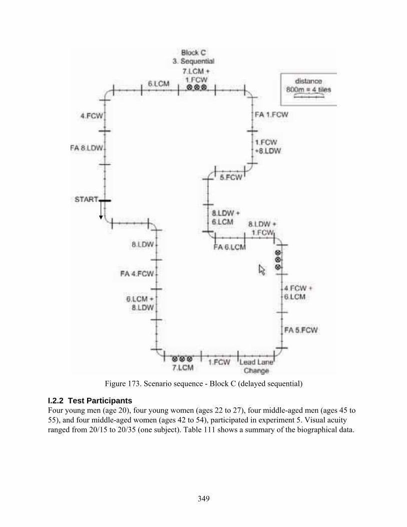
Figure 173. Scenario sequence - Block C (delayed sequential)
I.2.2 Test Participants Four young men (age 20), four young women (ages 22 to 27), four middle-aged men (ages 45 to 55), and four middle-aged women (ages 42 to 54), participated in experiment 5. Visual acuity ranged from 20/15 to 20/35 (one subject). Table 111 shows a summary of the biographical data.
349

Table 111. Biographical summary data
Driving Characteristic Number of subjects
1 1 1 1 1 1 1 1 1 1 1 1 1 1 1 1 Thousands of miles per year £5� >5-15 �20 % Highway driving <30% 30-60% >60-80% # Crashes in past 5 years 0 1 2 3 # Violations in past 5 years 0 1 2 4 Lane preference Left Middle Right
Most young subjects drive between 600 and 10,000 miles per year, with one subject driving 20,000 miles per year. Young subjects drive a varied amount of time on the expressway, with percentages ranging from 20 to 80 percent. Three young subjects prefer to drive in the left lane on a three-lane expressway, three prefer to drive in the middle, and two prefer to drive in the right. Young subjects account for 16 out of 18 automobile crashes and traffic violations subjects have had in the past five years. One young man had three crashes and four violations, one young woman had two crashes and two violations, two young subjects had one crash and one violation, one young man had one violation, and three had none. The majority of middle-aged subjects drive more often than young subjects. Middle-aged subjects drive 9,000 and 25,000 miles per year, with one middle-aged man driving 40,000 miles per year. Similarly to young subjects, middle-aged subjects spend a varied percentage of their driving on the expressway, ranging from 3 to 80 percent. Most middle-aged subjects prefer to drive in the middle lane of a three-lane expressway, with two middle-aged men preferring the right lane. Middle-aged subjects had far fewer traffic violations and crashes than young subjects. No middle-aged subject had an automobile in the past five years, and one middle-aged man and one middle-aged woman each had one traffic violation.
350

I.3 Results I.3.1 How Often Did Warnings Occur? In experiment 5, 1,104 total warnings were planned across all subjects (Table 112). Note that multiple warnings are counted as two separate warnings in the totals and that CSWs were not planned in the experiment but were still triggered. Also note that all false alarms involved one alarm by itself. In real systems, there is some probability that when two warnings are triggered, one of them will be a false alarm, and an even smaller probability that both will be false alarms. In this experiment, as will become apparent, it was difficult to get enough occurrences of pairs of warnings of interest for each preemption strategy to get enough cases to analyze. Including false alarms in pairs of alarms would have reduced the sample size further.
Table 112. Planned warning frequency by block
Warning Warning Frequency (Each Subject)
Total Warning
Frequency (All Subjects) Type
Block A-Present at
Trigger
Block B-Priority Preempt
Block C-Delayed
Sequential Total
FCW 3 3 3 144 Single-real
(288) LDW 1 1 1 48 LCM 2 2 2 96 False Alarm FCW 3 3 3 144 Single-
false (240)
False Alarm LDW 1 1 1 48 False Alarm LCM 1 1 1 48 FCW+LDW 1 1 1 96
Pair (576)
LDW+FCW 1 1 1 96 FCW+LCM 1 1 1 96 LCM+FCW 1 1 1 96 LDW+LCM 1 1 1 96 LCM+LDW 1 1 1 96 Total (all subjects) 368 368 368 1,104
The number of warnings actually presented was nearly 1.8 times the number planned, with 1,952 warnings presented (Table 113).
351

Table 113. Warning frequency by warning type (actual)
Warning Frequency CSW 64 FCW 678 LCM 234 LDW 976 Total 1,952
The effects of subject and block characteristics on the frequency of all warnings were examined. Men received nearly 20 percent more warnings than women, with the most notable difference being in LDW (32-percent difference, Table 114). Additionally, middle-aged subjects received nearly 10 percent more warnings than young subjects, with the largest difference being in FCW (18-percent difference, Table 115).
Table 114. Warning frequency by warning type and subject gender (actual)
Warning Gender Total Statistics Women Men Mean SD
CSW 23 41 64 32 13 FCW 332 346 678 339 10 LCM 119 115 234 117 3 LDW 420 556 976 488 96
Total 894 1,058 1,952
Table 115. Warning frequency by warning type and subject age group (actual)
Warning Age Group
Total Statistics
Young Middle-Aged Mean SD
CSW 42 22 64 32 14 FCW 311 367 678 339 40 LCM 111 123 234 117 9 LDW 473 503 976 488 21
Total 937 1,015 1,952
Warning frequency was also analyzed by priority scheme (block type and block number) (Figure 175). Warning frequency appears to remain fairly consistent throughout each block and sequence of blocks over time, with the only exception being the sharp decrease in LDW frequency after block A (present at trigger). One might expect that the number of warnings would decrease over time as subjects became accustomed to using the warning system, but the high overall frequency of warnings may have hindered subjects’ ability to anticipate warnings.
352
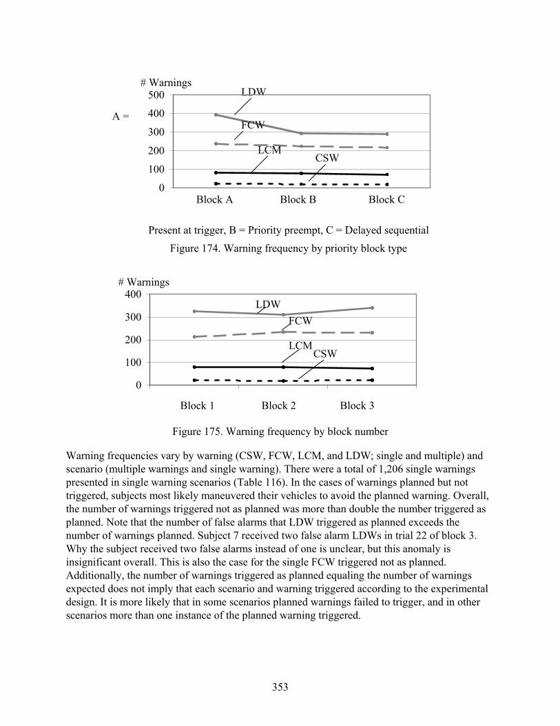
1 2 3
# Warnings
0
100
200
300
400
LCM
LDW FCW
CSW
Block 1 Block 2 Block 3
Figure 175. Warning frequency by block number
1 2 3
# Warnings LDW500
A = 400
300
200
100
0
FCW
LCM CSW
Block A Block B Block C
Present at trigger, B = Priority preempt, C = Delayed sequential
Figure 174. Warning frequency by priority block type
Warning frequencies vary by warning (CSW, FCW, LCM, and LDW; single and multiple) and scenario (multiple warnings and single warning). There were a total of 1,206 single warnings presented in single warning scenarios (Table 116). In the cases of warnings planned but not triggered, subjects most likely maneuvered their vehicles to avoid the planned warning. Overall, the number of warnings triggered not as planned was more than double the number triggered as planned. Note that the number of false alarms that LDW triggered as planned exceeds the number of warnings planned. Subject 7 received two false alarm LDWs in trial 22 of block 3. Why the subject received two false alarms instead of one is unclear, but this anomaly is insignificant overall. This is also the case for the single FCW triggered not as planned. Additionally, the number of warnings triggered as planned equaling the number of warnings expected does not imply that each scenario and warning triggered according to the experimental design. It is more likely that in some scenarios planned warnings failed to trigger, and in other scenarios more than one instance of the planned warning triggered.
353

Table 116. Warning frequency by triggering category for single warning scenarios
Warning Triggering Category Real False Alarm Total
Triggered as planned 0 0 0 Triggered not as planned 64 0 64
CSW Planned but not triggered 0 0 0 Total 64 0 64 Triggered as planned: Observed / expected 0/0 0/0 0 Triggered as planned 144 48 192 Triggered not as planned 308 1 309
FCW Planned but not triggered 11 96 107 Total 452 49 501 Triggered as planned: Observed / expected 144/144 48/144 0 Triggered as planned 14 47 61 Triggered not as planned 25 0 25
LCM Planned but not triggered 82 1 83 Total 39 47 86 Triggered as planned: Observed / expected 14/96 47/48 0 Triggered as planned 68 49 117 Triggered not as planned 438 0 438
LDW Planned but not triggered 26 0 26 Total 506 49 555 Triggered as planned: Observed / expected 48/68 49/48 0 Triggered as planned 226 144 370
All warnings
Triggered not as planned 835 1 836 Planned but not triggered 119 97 216 Grand total 1,061 145 1,206 Triggered as planned: Observed / expected 226/308 144/240 370/548
As shown in Figure 176, repetitions of the same warning occurred either within a very short time of the presentation of the first warning (less than 15 seconds) or a minute or several minutes later, with LDW being a notable exception (where there could be several warnings in a row).
354

WCF WSC
0 100 200 300 400 500 600 700 Time since previous warning (s)
0 100 200 300 400 500 600 700 Time since previous warning (s)
WDL MCL
0 100 200 300 400 500 600 700 Time since previous warning (s)
0 100 200 300 400 500 600 700 Time since previous warning (s)
Warning N Mean P(25) P( 50) P( 75) M axSD CSW 64 79.94 104.86 0.00 40.82 120.76 420.07 FCW 629 63.72 59.56 12.07 45.20 99.53 352.03 LCM 187 156.33 195.74 0.00 241.93 247.10 724.03 LDW 927 37.15 80.42 0.73 0.77 36.20 559.97
Figure 176. Distribution and descriptive statistics for thetime since warning of same type (s) according to warning type
Note: As described earlier, the upper portion of each quadrant displays a box plot, showing the 25th, 50th, and 75th quartiles, the mean, and values likely to be outliers. However, the major interest is in overall time gap between warnings and how often multiple warning sequences occurred. Consistent with prior experiments, a three-second gap was considered. Warnings of interest included: single warnings triggered as planned in multiple warning scenarios (where the second warning did not trigger in three seconds), multiple warnings triggered as planned, and multiple warnings triggered not as planned (Table 117). The total number of multiple warnings (the sum of multiple warnings triggered as planned and triggered not as planned) was 1,237, with 75 percent (or 927) LDWs. The high proportion of
355

Table 117. Frequency of multiple warnings and warnings in multiple warning scenarios
Warning Triggering Category FrequencySingle warnings triggered as planned in multiple warning
CSW
scenarios 0 Multiple warnings triggered as planned 0 Multiple warnings triggered not as planned 0 All multiple warnings 0 Multiple warnings triggered as planned: Observed / expected 0/0Single warnings triggered as planned in multiple warning
FCW
scenarios 92 Multiple warnings triggered as planned 85 Multiple warnings triggered not as planned 86 All multiple warnings 171 Multiple warnings triggered as planned: Observed / expected 85/96Single warnings triggered as planned in multiple warning
LCM
scenarios 115 Multiple warnings triggered as planned 33 Multiple warnings triggered not as planned 106 All multiple warnings 139 Multiple warnings triggered as planned: Observed / expected 33/96Single warnings triggered as planned in multiple warning
LDW
scenarios 331 Multiple warnings triggered as planned 90 Multiple warnings triggered not as planned 837 All multiple warnings 927 Multiple warnings triggered as planned: Observed / expected 90/96
356
LDWs is reasonable, since the majority of warnings presented were LDWs, and subjects may have drifted out of their lane independent of the position of other vehicles (in contrast with LCMs and FCWs). Note that the total frequency of multiple warnings is higher than anticipated because scenarios did not trigger properly on some occasions. For example, on two occasions, subjects crashed into vehicles causing a string of multiple warnings to trigger. In addition, subjects received strings of multiple LDWs (261 out of the 436 multiple warning events, or almost 60 percent, consisted of repeated LDWs). Note that crashes did not stop the simulation as the subject was invincible and able to drive though objects (other vehicles, barriers, trees), which felt uncomfortable to do. As subjects drove though objects, the closest part of the object vanished, which was very obvious to subjects. The number of multiple warnings expected for each warning type was calculated knowing each warning appears twice in multiple warning scenarios, each multiple warning scenario appears once in all three blocks, and each block appears once for all 16 subjects (2 x 3 x 16 = 96).

Warning Triggering Category Frequency Single warnings triggered as planned in multiple warning
All warnings
scenarios 538 Multiple warnings triggered as planned 208 Multiple warnings triggered not as planned 1029 All multiple warnings 1237 Multiple warnings triggered as planned: Observed / expected 208/288
Table 118 shows the 436 multiple warning events that occurred in this experiment. Again, to qualify as such, a warning had to follow another warning within three seconds. Multiple warnings were further analyzed by multiple warnings events, or sets of multiple warnings (warnings occurring within three seconds of the preceding warning). For example, there were 50 events beginning with an FCW, 36 of which were FCW + LDW situations. Thirty-four of those were followed by an additional LDW, yielding FCW + LDW + LDW, and 27 of those were complete multiple warning event combinations (the remaining seven were followed by an LCM or an LDW). The most common multiple warning event was LDW + LDW, with 176 combination instances.
Table 118. Frequency of multiple warnings combinations
Warning Sequence Combo First Second Third Fourth Fifth Sixth Seventh Eighth Ninth Tenth Total
(Freq.) (Freq.) (Freq.) (Freq.) (Freq.) (Freq.) (Freq.) (Freq.) (Freq.) (Freq.) CSW (0) 0 FCW FCW (3) 3 (50) LCM(13) 9
LCM (1) 1 LDW (3) 3
LDW (36) 2 LDW (34) 27
LCM (1) LCM LDW (1) (1) 1
LDW (6) LDW (6) 2 FCW (2) 2 LDW (2)
1LDW LDW LDW LDW FCW (1) (1) (1) (1) (1) 1
LCM FCW (46) 45 (85) LDW LDW (1) LCM LCM LDW (1)
(1) (1) (1) 1 LCM (18) 7
LCM (2) 2 LDW (9) 9
LDW (21) 18 FCW (1) 1 LDW LDW (2) LDW (2) (2) 2
357

Warning Sequence First
(Freq.) Second (Freq.)
Third (Freq.)
Fourth (Freq.)
Fifth (Freq.)
Sixth (Freq.)
Seventh (Freq.)
Eighth (Freq.)
Ninth (Freq.)
Tenth (Freq.)
Combo Total
FCW (2)
FCW (1) 1
LDW (1) 1 LCM (3)
LDW (3) 3
LDW (294) 176 FCW (37) 27
LDW (10)
LDW (10) 7
LCM (1)
LCM (1)
LDW (1) 1
LDW (2)
LDW(2) 1
LDW (1) 1 LCM (4) 1
LCM (3) FCW (1) 1 LDW (2) 2
LDW (77) 54 LDW (23)
FCW (14) 13
LCM (1) 1
LCM (1)
FCW (1)
LCM (1)
LCM (1) 1
LDW (8)
LDW (8) 6
FCW (1) 1
LDW (299)
LDW (1)
LDW (1) 1
Grand Total 436
Subject and block differences were examined in the case of multiple events ( Table 119). Men received over 20 percent more multiple warning events than women. The multiple warning event frequency by age group was much smaller, with a difference of approximately 4 percent.
Table 119. Frequency of multiple warnings by subject age and gender
Subject Characteristic # Multiple Warning Events
Women 195 Men 241 Young 214 Middle-aged 222
The trends in multiple warning event frequencies by block name and block sequence (Figure 177) differ from the trends for all warnings. Although the frequency of warnings by block name still decreases after block A (present at trigger), in the case of multiple warnings, the frequency
358

1 2 3
# Warnings
0
50
100
150
200
Block Name Block Sequence
Block 1 Block 2 Block 3 Block A Block B Block C
A = Present at trigger, B = Priority preempt, C = Delayed sequential
Figure 177. Frequency of multiple warnings by block name and block sequence
of warnings by block sequence also decreases by nearly 40 percent (174 warnings in block 1, 126 warnings in block 2). This may indicate that although the overall warning frequency remained high over time, subjects learned how to react to warnings and drive without inducing multiple warnings as they spent more time driving in the simulator.
359

Warning N Mean SD P(25) P(50) P(75) Max FCW 168 85.60 70.87 31.59 76.78 135.06 269.20 LCM 133 129.26 178.99 0.01 45.47 221.70 705.47 LDW 927 37.15 80.42 0.73 0.77 36.20 559.97
Figure 178. Distribution and descriptive statistics of time since same warning (seconds) in multiple warning situations
CSW FCW
No multiple warnings situations involving CSW
0 100 200 300 400 500 600 700
Time since previous warning (s) LCM LDW
0 100 200 300 400 500 600 700
Time since previous warning (s)
0 100 200 300 400 500 600 700
Time since previous warning (s)
360

Table 120. Frequency and probability (in parentheses) of time since last occurrence of same warning in multiple warning situations by warning
Time Since Last Warning Occurrence of Same
Warning (s) FCW LCM LDW
0 19 (11.31)
33 (24.81)
48 (5.18)
>0 - 100 83 (49.40)
51 (38.35)
766 (82.63)
>100 - 200 53 (31.55)
6 (4.51)
59 (6.36)
>200 - 300 13 (7.74)
23 (17.29)
29 (3.13)
>300 - 400 0 (0.00)
3 (2.26)
15 (1.62)
>400 0 (0.00)
17 (12.78)
10 (1.08)
Total 168 133 927
Table 121. Frequency and probability (in parentheses) of time since last occurrence of same warning in multiple warning situations by priority scheme
Same Type (s)
0
Time Since Warning of A- Present at
trigger 31
(7.36)
B- Priority Preempt
41 (10.22)
Block Name
C- Sequential
37 (8.92)
>0 - 100 297 (70.55)
282 (70.32) 321 (77.35)
>100 - 200 41 (9.74)
45 (11.22)
32 (7.71)
>200 - 300 32 (7.60)
18 (4.49)
15 (3.61)
>300 - 400 3 (0.71)
8 (2.00)
7 (1.69)
>400
Total
17 (4.04) 421
7 (1.75)
428
3 (0.72) 415
361

30
25
20
15
10
5
0
FCW lead decel then LDW LCM then FCW lead decel LDW then FCW lead decel FCW lead decel
0.5 1.0 1.5 2.0 2.5 3.0
Time post-warning (s)
Ach
ieve
d re
duct
ion
in sp
eed
(mph
) Table 122. Frequency of FCW combinations
First Warning Second Warning n 4. FCW reveal None 58 4. FCW reveal 6. LCM 34 1. FCW lead decelerates none 47 1. FCW lead decelerates 8. LDW 20 7. LCM construction zone 1. FCW lead decelerates 6 8. LDW 1. FCW lead decelerates 24
Figure 179 shows changes in speed for the lead vehicle deceleration scenario are relatively unaffected by other warnings. That is, there is hardly any difference between an FCW by itself, an FCW preceded either by an LCM or LDW, or an FCW followed by an LDW.
Figure 179. Speed change related to FCW and other warnings in the lead decelerates scenario
Figure 180 shows the change in speed in response to the FCW reveal scenario, by itself or followed by an LCM. Having the LCM follow the FCW led to a much more rapid decrease in speed for the first 2.5 seconds.
362

4.5 4.0 3.5 3.0 2.5 2.0 1.5 1.0 0.5 0.0
FCW - reveal then LCM
FCW - reveal
0.5 1.0 1.5 2.0 2.5 3.0
Time post-warning (s)
Figure 180. Speed change related to FCW and other warnings in the reveal scenario
Ach
eive
d re
duci
ton
in sp
eed
(mph
)
Table 123 shows how often various combination related to LDWs occurred.
Table 123. Frequency of LDW combinations
First Warning Second Warning n 8-LDW None 26 8-LDW 1-FCW lead decel 24 1-FCW lead decel 8-LDW 20 8-LDW 6-LCM 24 6-LCM 8-LDW 1
Figure 181 shows how lateral position in response to a LDW was affected by a leading and following FCW. The leading FCW increased the lateral position error considerably over just an LDW, by about 0.2 meters. For following an FCW, the initial lateral position error was much greater, as sometimes the response to an FCW was a lane change, but by 2.0 seconds, reached a stable level. The case of an LDW preceded by an LCM is not shown because that combination occurred only once.
363

0.0
0.2
0.4
0.6
0.8
1.0
1.2
1.4
1.6
Dist
ance
from
cen
ter o
f lan
e (m
) FCW lead decel then LDW
LDW then FCW lead decel
LDW
At alert 0.5 1.0 1.5 2.0 2.5 3.0 Time post-warning (s)
Figure 181. Lateral position as a function of time for LDW and FCW
As shown in Figure 182, when an LDW was follow by an LCM, the lateral position was much larger than when an LCM was not present. This may just be a restatement of the situation that large lane departures can cause LCMs to trigger. It is noteworthy that in this complex situation, even after three seconds, the lateral position error is still close to the value as when the warning was presented.
1.6
Dist
ance
from
cen
ter o
f lan
e (m
) 1.4
1.2
1.0
0.8
0.6
0.4
0.2
0.0 At alert 0.5 1.0 1.5 2.0 2.5 3.0
LDW then LCM
LDW
Time post-warning (s)
Figure 182. Lateral position as a function of time for LDW and LCM
364

Dist
ance
from
cen
ter o
f lan
e (m
)
1.6
1.4
1.2
1.0
0.8
0.6
0.4
0.2
0.0
FCW reveal then LCM LDW then LCM LCM
At alert 0.5 1.0 1.5 2.0 2.5 3.0 Time post-warning (s)
Figure 183. Lateral position for single and paired LCM scenarios
Table 124 shows combinations involving LCM. There were few observations involving LCM where a construction based lane change was needed.
Table 124. Combinations with LCM
FirstW arning Second W arning n
6.LCM None 44 4-FCW lane change 6-LCM 31 8-LDW 6-LCM 44 7-LCM construction None 5 7-LCM construction 1-FCW lead decelerates 6
Having another warning precede an LCM (FCW or LDW) delayed the initial response to LCM by about 0.5 seconds (Figure 183). Given the number of instances shown in Table 124, there is adequate evidence to support this finding. Figure 184, where LCM is followed by a warning (FCW), also shows an effect, but the figure is based only on a small sample of 11 trials.
365
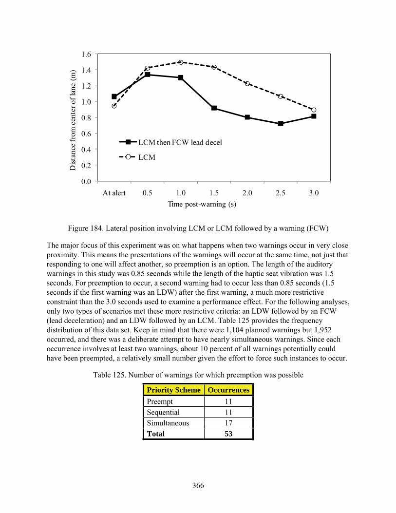
Dist
ance
from
cen
ter o
f lan
e (m
)
1.6
1.4
1.2
1.0
0.8
0.6
0.4
0.2
0.0 At alert 0.5 1.0 1.5 2.0 2.5 3.0
LCM then FCW lead decel
LCM
Time post-warning (s)
Figure 184. Lateral position involving LCM or LCM followed by a warning (FCW)
The major focus of this experiment was on what happens when two warnings occur in very close proximity. This means the presentations of the warnings will occur at the same time, not just that responding to one will affect another, so preemption is an option. The length of the auditory warnings in this study was 0.85 seconds while the length of the haptic seat vibration was 1.5 seconds. For preemption to occur, a second warning had to occur less than 0.85 seconds (1.5 seconds if the first warning was an LDW) after the first warning, a much more restrictive constraint than the 3.0 seconds used to examine a performance effect. For the following analyses, only two types of scenarios met these more restrictive criteria: an LDW followed by an FCW (lead deceleration) and an LDW followed by an LCM. Table 125 provides the frequency distribution of this data set. Keep in mind that there were 1,104 planned warnings but 1,952 occurred, and there was a deliberate attempt to have nearly simultaneous warnings. Since each occurrence involves at least two warnings, about 10 percent of all warnings potentially could have been preempted, a relatively small number given the effort to force such instances to occur.
Table 125. Number of warnings for which preemption was possible
Priority Scheme Occurrences Preempt 11 Sequential 11 Simultaneous 17 Total 53
366

-5
0
5
10
15
20
25
30
Spee
d R
educ
tion
(mph
)
0.5 1.0 1.5 2.0 2.5 3.0 Time (s)
Figure 185. Speed reduction following an FCWError bars represent 95-percent confidence intervals.
A linear mixed-effects model was fit to the speed changes after FCWs to determine whether any significant differences in speed reduction existed between age groups (young, middle-ages), gender (men, women), and the priority scheme (preemption, sequential, simultaneous). The six half-second time intervals were included in the model as a repeated measure. Two-way interactions between the factor of time and other independent measures were included. The model also included subjects as a random effect. Consequently, a fixed effect would only show statistical significance if it accounted for more variance than “random” subject-to-subject variance. The only significant effect in the model was time, which was highly significant, F(5, 72.6) = 65.5, p < .001, where subjects had higher levels of deceleration as time progressed (Figure 185). The effects of priority scheme, age, and gender were not statistically significant. Mean speed reduction over time for each of the priority schemes is shown in Figure 186.
When partitioned by priority scheme (Figure 186), the differences between the simultaneous and sequential schemes were quite small, but not trivial, about 3 mph at three seconds after the warning (with the best performance from simultaneous presentation). However, the difference between preemption, and simultaneous presentation is about 10 mph at three seconds, a substantial difference. Again, although not statistically significant, this suggests that the best design strategy is to present warnings simultaneously. Getting information to the driver quickly is more important than potential interference, an unexpected outcome.
367
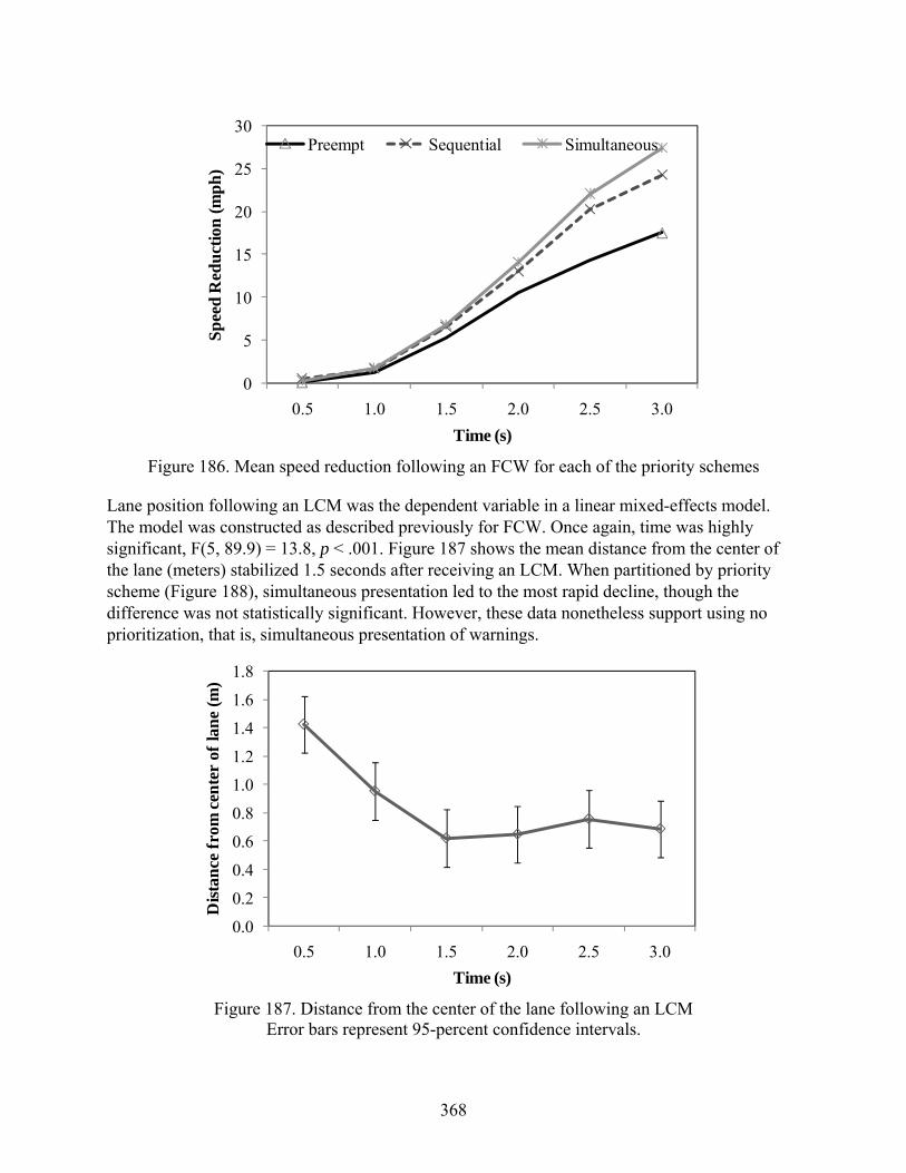
0
5
10
15
20
25
30
Spee
d R
educ
tion
(mph
)
Preempt Sequential Simultaneous
0.5 1.0 1.5 2.0 2.5 3.0 Time (s)
Figure 186. Mean speed reduction following an FCW for each of the priority schemes
Lane position following an LCM was the dependent variable in a linear mixed-effects model. The model was constructed as described previously for FCW. Once again, time was highly significant, F(5, 89.9) = 13.8, p < .001. Figure 187 shows the mean distance from the center of the lane (meters) stabilized 1.5 seconds after receiving an LCM. When partitioned by priority scheme (Figure 188), simultaneous presentation led to the most rapid decline, though the difference was not statistically significant. However, these data nonetheless support using no prioritization, that is, simultaneous presentation of warnings.
0.0
0.2
0.4
0.6
0.8
1.0
1.2
1.4
1.6
1.8
Dist
ance
from
cent
er o
f lan
e (m
)
0.5 1.0 1.5 2.0 2.5 3.0 Time (s)
Figure 187. Distance from the center of the lane following an LCM Error bars represent 95-percent confidence intervals.
368

0.0
0.2
0.4
0.6
0.8
1.0
1.2
1.4
1.6
Dist
ance
from
cent
er o
f lan
e (m
) Preempt Sequential Simultaneous
0.5 1.0 1.5 2.0 2.5 3.0 Time (s)
Figure 188. Mean lane position following an LCM for each of the priority schemes
I.3.2 Collisions Although collisions were not the focus of this experiment, 21 collisions occurred, 15 where the driver was at fault and six where the driver was not at fault (workarounds to reposition the driver). Given the effort to create simultaneous triggering of multiple warnings, 15 at-fault collisions is a reasonable total. Nine drivers had at least one at-fault collision, with one driver having five, one having two, and the remaining drivers having one collisions each. Five of the nine drivers were young, but nine of the 15 at-fault collisions were experienced by older drivers. Four collisions occurred in scenario 6 (LCM-subject changes lanes with vehicle in blind spot), two collisions occurred in the combination of 4 (FCW-reveal) and 6 (LCM-subject changes lanes with vehicle in blind spot), and eight collisions occurred in the combination of 6 and 8 (LDWwind gust). One collision was not associated with any scenario. Given the scenarios, four collisions were with reveal vehicles and seven with side vehicles. All at-fault collisions occurred in the first two blocks. Thus, as before, side collisions were the most common collision type.
As mentioned above, some collisions were associated with multiple warning events. There were two collisions, for example, that triggered several subsequent multiple warnings. There were four additional collisions that were preceded by a multiple warning event within the past three seconds. Because only a few multiple warning events were associated with collisions, there was no attempt to remove these cases from analyses conducted for this experiment.
I.3.3 Post-Test Analysis Table 126 shows the post-test ratings for FCW. The physical characteristics were as desired (too soft/too loud = 3.1, brake too weak/too strong = 3.2) though there was a slight tendency for the warning to occur too often (3.5) and a tad early (2.7). Separate ratings for the different priority schemes were not obtained. The warning was somewhat meaningful initially (3.8), quite meaningful at the end (4.5), and moderately easy to learn and remember (4.2). It was somewhat useful (3.8), but somewhat less easy to use (3.6).
369
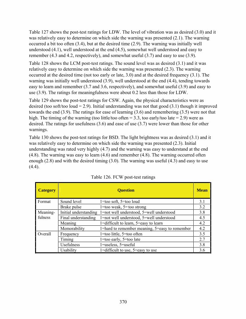
Table 126. FCW post-test ratings
Category Question Mean
Format Sound level 1=too soft, 5=too loud 3.1 Brake pulse 1=too weak, 5= too strong 3.2
Meaning-fulness
Initial understanding 1=not well understood, 5=well understood 3.8 Final understanding 1=not well understood, 5=well understood 4.5 Meaning 1=difficult to learn, 5=easy to learn 4.2 Memorability 1=hard to remember meaning, 5=easy to remember 4.2
Overall Frequency 1=too little, 5=too often 3.5 Timing 1=too early, 5=too late 2.7 Usefulness 1=useless, 5=useful 3.8 Usability 1=difficult to use, 5=easy to use 3.6
370
Table 127 shows the post-test ratings for LDW. The level of vibration was as desired (3.0) and it was relatively easy to determine on which side the warning was presented (2.1). The warning occurred a bit too often (3.4), but at the desired time (2.9). The warning was initially well understood (4.1), well understood at the end (4.5), somewhat well understood and easy to remember (4.3 and 4.2, respectively), and somewhat useful (3.7) and easy to use (3.9). Table 128 shows the LCM post-test ratings. The sound level was as desired (3.1) and it was relatively easy to determine on which side the warning was presented (2.3). The warning occurred at the desired time (not too early or late, 3.0) and at the desired frequency (3.1). The warning was initially well understood (3.9), well understood at the end (4.4), tending towards easy to learn and remember (3.7 and 3.6, respectively), and somewhat useful (3.9) and easy to use (3.9). The ratings for meaningfulness were about 0.2 less than those for LDW. Table 129 shows the post-test ratings for CSW. Again, the physical characteristics were as desired (too soft/too loud = 2.9). Initial understanding was not that good (3.1) though it improved towards the end (3.9). The ratings for ease of learning (3.6) and remembering (3.5) were not that high. The timing of the warning (too little/too often = 3.3, too early/too late = 2.9) were as desired. The ratings for usefulness (3.6) and ease of use (3.7) were lower than those for other warnings. Table 130 shows the post-test ratings for BSD. The light brightness was as desired (3.1) and it was relatively easy to determine on which side the warning was presented (2.3). Initial understanding was rated very highly (4.7) and the warning was easy to understand at the end (4.8). The warning was easy to learn (4.6) and remember (4.8). The warning occurred often enough (2.8) and with the desired timing (3.0). The warning was useful (4.3) and easy to use (4.4).

Table 127. LDW post-test ratings
Category Question Mean
Format Seat vibration 1=too weak, 5=too strong 3.0 Which side seat vibration came from 1=easy to tell, 5=hard to tell 2.1
Meaning-fulness
Initial understanding 1=not well understood, 5=well understood 4.1 Final understanding 1=not well understood, 5=well understood 4.5 Meaning 1=difficult to learn, 5=easy to learn 4.3 Memorability 1=hard to remember meaning, 5=easy to remember 4.2
Overall Frequency 1=too little, 5=too often 3.4 Timing 1=too early, 5=too late 2.9 Usefulness 1=useless, 5=useful 3.7 Usability 1=difficult to use, 5=easy to use 3.9
Table 128. LCM post-test ratings
Category Question Mean
Format Sound level 1=too soft, 5=too loud 3.1 Which side seat vibration came from 1=easy to tell, 5=hard to tell 2.3
Meaning-fulness
Initial understanding 1=not well understood, 5=well understood 3.9 Final understanding 1=not well understood, 5=well understood 4.4 Meaning 1=difficult to learn, 5=easy to learn 3.7 Memorability 1=hard to remember meaning, 5=easy to remember 3.6
Overall
Frequency 1=too little, 5=too often 3.1 Timing 1=too early, 5=too late 3.0 Usefulness 1=useless, 5=useful 3.9 Usability 1=difficult to use, 5=easy to use 3.9
Table 129. CSW post-test ratings
Category Question Mean
Format Sound level 1=too soft, 5=too loud 2.9
Meaning-fulness
Initial understanding 1=not well understood, 5=well understood 3.1 Final understanding 1=not well understood, 5=well understood 3.9 Meaning 1=difficult to learn, 5=easy to learn 3.6 Memorability 1=hard to remember meaning, 5=easy to remember 3.5
Overall
Frequency 1=too little, 5=too often 3.3 Timing 1=too early, 5=too late 2.9 Usefulness 1=useless, 5=useful 3.6 Usability 1=difficult to use, 5=easy to use 3.7
371

Table 130. Blind spot detection post-test ratings
Category Question Mean
Format Side mirror light brightness 1=too dim, 5=too bright 3.1 Which side seat vibration came from 1=easy to tell, 5=hard to tell 2.3 Initial understanding 1=not well understood, 5=well understood 4.7
Meaning- Final understanding 1=not well understood, 5=well understood 4.8 fulness Meaning 1=difficult to learn, 5=easy to learn 4.6
Memorability 1=hard to remember meaning, 5=easy to remember 4.8 Frequency 1=too little, 5=too often 2.8
Overall Timing 1=too early, 5=too late 3.0 Usefulness 1=useless, 5=useful 4.3 Usability 1=difficult to use, 5=easy to use 4.4
I.4 Conclusions How Often Did Warnings Occur? The plan for this experiment called for 288 single warnings (real), 240 false alarms, and 576 warnings occurring pairs, all real, for a total of 1,104 warnings. The relative high fraction of paired warning was needed to explore warning priority in an efficient manner. In fact, there were 1,952 warnings, including 64 CSWs all of which were unplanned. For the 208 multiple warnings, the situation of interest, none involved CSW, 85 involved FCW, 90 involved LDW, and 33 involved LCM. Did the Occurrence of a Second Warning Affect Driver Response to a Prior Warning? The evidence concerning pairs of warning is mixed. For LCM, both preceding and following warning delayed correction of the lateral position by about 0.5 seconds. For LDW, a following warning delayed response to the LDW and increased the extent of the lane departure. However, for all of these situations, the data are limited and some care must be exercised in interpreting direction differences as being practically important. What Should be the Priority Scheme for Warnings? Even though there were a large number of warnings, only a limited subset involved pairs that occurred within 0.85 seconds of each other where preemption was feasible. For FCW, the most noteworthy difference was at 3.0 seconds after the warning when simultaneous presentation led to the greatest speed reduction (about 3 mph greater than sequential delayed presentation and 10 mph greater than preemption). For LCM, sequential delay led to the most immediate return to the lane center, with simultaneous presentation having the worst performance at 1.5 seconds with the slowest return to the lane center. This suggests simultaneous presentation is not desired. Thus, these data do no yet provide a well-supported recommendation for a single prioritization scheme because the priority scheme that led to the best performance depended on the situation.
372
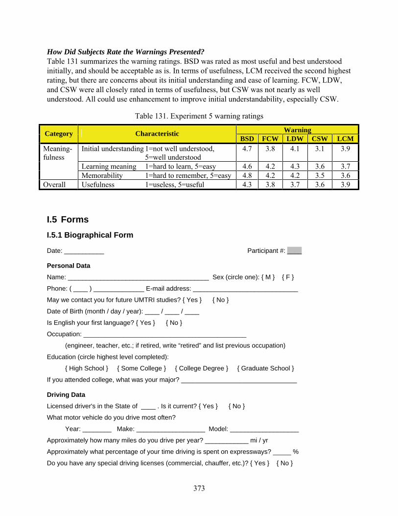
How Did Subjects Rate the Warnings Presented? Table 131 summarizes the warning ratings. BSD was rated as most useful and best understood initially, and should be acceptable as is. In terms of usefulness, LCM received the second highest rating, but there are concerns about its initial understanding and ease of learning. FCW, LDW, and CSW were all closely rated in terms of usefulness, but CSW was not nearly as well understood. All could use enhancement to improve initial understandability, especially CSW.
Table 131. Experiment 5 warning ratings
Category Characteristic Warning BSD FCW LDW CSW LCM
Meaningfulness
Initial understanding 1=not well understood, 5=well understood
4.7 3.8 4.1 3.1 3.9
Learning meaning 1=hard to learn, 5=easy 4.6 4.2 4.3 3.6 3.7 Memorability 1=hard to remember, 5=easy 4.8 4.2 4.2 3.5 3.6
Overall Usefulness 1=useless, 5=useful 4.3 3.8 3.7 3.6 3.9
I.5 Forms I.5.1 Biographical Form
Date: ___________ Participant #: ____
Personal Data
Name: _______________________________________ Sex (circle one): { M } { F }
Phone: ( ____ ) ______________ E-mail address: _____________________________
May we contact you for future UMTRI studies? { Yes } { No }
Date of Birth (month / day / year): ____ / ____ / ____
Is English your first language? { Yes } { No }
Occupation: _____________________________________________
(engineer, teacher, etc.; if retired, write “retired” and list previous occupation)
Education (circle highest level completed):
{ High School } { Some College } { College Degree } { Graduate School }
If you attended college, what was your major? ________________________________
Driving Data
Licensed driver's in the State of ____ . Is it current? { Yes } { No }
What motor vehicle do you drive most often?
Year: ________ Make: ___________________ Model: ___________________
Approximately how many miles do you drive per year? ____________ mi / yr
Approximately what percentage of your time driving is spent on expressways? _____ %
Do you have any special driving licenses (commercial, chauffer, etc.)? { Yes } { No }
373

If yes, please list: _________________________________________
How many accidents have you been involved in during the past 5 years? ______
Brief description: ___________________________________________________
_________________________________________________________________
How many traffic violations have you been involved in the past 5 years? _______
Brief description: ___________________________________________________
_________________________________________________________________
On a 3-lane expressway, which lane do you normally drive in?
{ Left } { Middle } { Right }
Vision
What type of corrective lenses do you wear corrective lenses while driving?
{ None } { Glasses } { Contacts }
If yes, what type?
{ Near-Vision/Reading } { Far-Vision } { Bifocal } { Multifocal }
{ Other } If other, please describe: _________________________________
What type of corrective lenses do you wear corrective lenses while reading?
{ None } { Glasses } {Contacts }
If yes, what type?
{ Near-Vision/Reading } { Far-Vision } { Bifocal } { Multifocal }
{ Other } If other, please describe: _________________________________
Scoring for vision and hearing test (experimenter use only):
I.5.2 Instructions Experiment Introduction and Preparation
Greet Subject
<Introduce self> Thank you for coming in today, I’ll be conducting introductory part of the driving simulator study. Before we get started, you will need a visitor parking pass to park at UMTRI. Please place this pass face-up on your dashboard and we’ll be ready to go when you return.
Let's go to the conference room and get started.
Lead subject to conference room.
Overview (in conference room)
Before we get started, I will give you a brief overview of the study and what you will be doing.
The purpose of this study is to test the safety and usability of in-vehicle warning systems that could make the next new vehicle you buy much safer to drive. The experiment will take place in the driving simulator where another experimenter will collect data on you while you are driving. I’ll explain more about what that means later on.
To examine how effective these in-vehicle systems are, video cameras and sound recording devices will be recording you during the entire time you are driving in the simulator. These recordings will be used to study things like how you react to different driving situations and in-vehicle systems. In addition to using these recordings for data analysis, it is possible that UMTRI or NHTSA (the National Highway Traffic Safety Administration), who is funding this project, may use portions of your videotape in presentations or
374
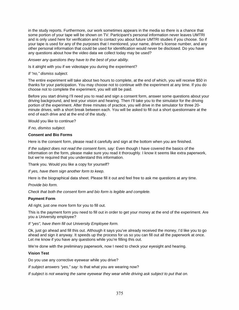
in the study reports. Furthermore, our work sometimes appears in the media so there is a chance that some portion of your tape will be shown on TV. Participant’s personal information never leaves UMTRI and is only used here for verification and to contact you about future UMTRI studies if you choose. So if your tape is used for any of the purposes that I mentioned, your name, driver’s license number, and any other personal information that could be used for identification would never be disclosed. Do you have any questions about how the video data we collect today may be used?
Answer any questions they have to the best of your ability.
Is it alright with you if we videotape you during the experiment?
If “no,” dismiss subject.
The entire experiment will take about two hours to complete, at the end of which, you will receive $50 in thanks for your participation. You may choose not to continue with the experiment at any time. If you do choose not to complete the experiment, you will still be paid.
Before you start driving I’ll need you to read and sign a consent form, answer some questions about your driving background, and test your vision and hearing. Then I’ll take you to the simulator for the driving portion of the experiment. After three minutes of practice, you will drive in the simulator for three 20-minute drives, with a short break between each. You will be asked to fill out a short questionnaire at the end of each drive and at the end of the study.
Would you like to continue?
If no, dismiss subject.
Consent and Bio Forms
Here is the consent form, please read it carefully and sign at the bottom when you are finished.
If the subject does not read the consent form, say: Even though I have covered the basics of the information on the form, please make sure you read it thoroughly. I know it seems like extra paperwork, but we’re required that you understand this information.
Thank you. Would you like a copy for yourself?
If yes, have them sign another form to keep.
Here is the biographical data sheet. Please fill it out and feel free to ask me questions at any time.
Provide bio form.
Check that both the consent form and bio form is legible and complete.
Payment Form
All right, just one more form for you to fill out.
This is the payment form you need to fill out in order to get your money at the end of the experiment. Are you a University employee?
If “yes”, have them fill out University Employee form.
Ok, just go ahead and fill this out. Although it says you’ve already received the money, I’d like you to go ahead and sign it anyway. It speeds up the process for us so you can fill out all the paperwork at once. Let me know if you have any questions while you’re filling this out.
We’re done with the preliminary paperwork, now I need to check your eyesight and hearing.
Vision Test
Do you use any corrective eyewear while you drive?
If subject answers “yes,” say: Is that what you are wearing now?
If subject is not wearing the same eyewear they wear while driving ask subject to put that on.
375

We’re not professional optometrists or audiologists, these tests are just for screening. Please look into the vision device and keep looking straight ahead for the entire eye test.
Test Visual Acuity (FAR #2):
Can you see that in the first diamond in the top circle is complete but the other 3 are broken? In each diamond, tell me the location of the solid circle - top, left, bottom, or right.
Continue until 2 in a row are wrong. The last correct answer is the visual acuity. Subjects must have 20/40 or better vision. If they do not pass, pay and dismiss the subject.
Hearing Test
Make sure the office door is closed so it’s quiet.
In this test we will be testing the full range of hearing. Very few people are capable of hearing all of the tones I will play.
I’m going to play you a series of tones, and you just need to simply raise your hand for whichever side you hear the tone coming from. So if you hear a tone in your left ear, raise your left hand.
I’m going to start off by playing one practice tone just to make sure it’s working, and then we’ll start the test. Go ahead and put on these headphones. The red side should cover your right ear.
Play a sample tone at 35 dB and 1500 Hz (either ear).
Ok, now we’re going to start the test.
Do all tones for one ear in sequence. Make sure the subject cannot see which ear is being tested. Move dial to 25 dB and play 2 tones a 1000 Hz, 2 tones at 2000 Hz, and 2 tones at 3000 Hz. Wait after playing each tone for a response. If they miss a tone, increase the dB by 5 dB each time until they hear the tone 2 times successfully. Record the dB level on the screening sheet. Continue by testing the other ear. Maximum passing values are: 45 dB for 1000 Hz, 55-60 dB for 2000 Hz, and 65 dB for 3000 Hz. If they do not pass, pay and dismiss the subject.
That’s all I need for now, let’s go to the driving simulator for the rest of the experiment.
Take subject to simulator.
In the Simulator
Seat Subject
Please have a seat in the cab and adjust the seat to a comfortable position using the automatic controls on the left side of the seat. Once I put a road scene up on the screen I’ll have you adjust the mirrors as well.
The cameras in the vehicle to provide a variety of camera angles. There is also a live microphone here.
Point out cameras and microphone.
For this part of the experiment you will have a three-minute practice drive, then three 20-minute drives with breaks in between. There will also be a questionnaire to fill out after each drive and at the end of the experiment.
Practice Drive
Now it is time to try out the simulator. For the duration of this experiment please drive normally, being sure to be safe. Use the speedometer on the instrument panel to check your speed, just as in a real car.
The speed limit is 70 mph for the entire experiment and you will see speed limit signs throughout the course as a reminder. Try to maintain the speed limit at all times, however, if you are not comfortable driving that fast, just go as fast as you are comfortable. Keep in mind that if you go slower than 70 mph the experiment will takes slightly longer to complete.
The steering wheel in the simulator doesn’t feel exactly like one in a real vehicle and it is easy to overcorrect. The key is to make small, slow corrections with the steering wheel.
376

Some people experience motion sickness in the simulator, so if you start feeling warm, dizzy, nauseous, or anything else that could occur prior to being motion sick, let me know immediately and I’ll tell you how to stop. As I said before, you may end the experiment at any time and you will still be paid $50.
Do you have any questions?
Ok then, now we’ll begin the practice drive so you can get a feel for driving in the simulator. Please adjust the left and rear-view mirrors, the right mirror control does not work properly, so I will help you adjust it. This practice drive will last for about three minutes and I’ll tell you when the time is up.
Put the car in “D” using the shift lever between the seats. Now, please press on the accelerator and begin driving.
Have the subject drive for approximately three minutes.
Ok, that’s the end of the practice drive. Please coast to a stop and shift the car into park.
Stop the simulator about 10 seconds after the car is in park.
Warning System Training
In each drive you will receive four different warnings, and one informational light. The forward crash warning will go off when you are at high risk of crashing into the car in front of you. When the warning goes off you will hear a series of beeps and feel a pulse in the brake pedal. Here’s what the forward crash warning sounds and feels like. (Play the FCW warning.) The curve speed warning goes off when your speed is too high in a curve and you are at risk of skidding. It has the same beeping sound as the Forward Crash Warning, but no brake pulse. (Play the CSW warning.) The Lane Change / Merge warning warns you if there is a car in your blind spot as you are attempting to change lanes. The warning is directional so it goes off only on the side of the threat. You will hear a honking sound and feel a vibration in your seat. (Play the LCM warning.) The Lane Departure Warning is intended to alert you when you unintentionally leave your lane, so it goes off when you drift from your lane without using your turn signal. This warning is also directional and consists of a seat vibration on the side of the lane departure to simulate rumble strips. (Play LDW warning.) There is also a blind spot warning. Whenever there is a vehicle or another object in your blind spot, a red light will appear on either the left or right side mirror, depending on the object’s location. The light will appear even if you’re not making a maneuver. The light only works while driving, so right now I can’t show you what that looks like, you will also not be tested on your knowledge of the blind spot light before beginning the drives.
Now I’d like to test your understanding of these warnings. I am going to play a warning, and I’d like for you to respond to the warning as if you were driving. So for the forward crash warning and the curve speed warning you would brake, for the lane change/merge warning you would check your blind spot and correct your lane position and for lane departure warning you would correct your lane position. (e.g., lane departure warning on the left, turn the steering wheel to the right to return to the lane). Please respond as accurately and as quickly as you can. After you make a driving response, I’d like for you tell me which type of warning you just experienced (FCW, CSW, LCM, or LDW). In addition to the four warnings, please tell me when you identify the blind spot light. You will need to get eight in a row correct before we can go on. Do you have any questions?
Training and Practice Wrap-Up
That is the end of the training and practice portion of the experiment. We will now take a short break before beginning the first 20-minute drive. You will also get a break between each drive. Feel free to get out of the simulator and walk around for a minute. And if you would like to get a drink of water or use the restroom during any of these breaks, I will be happy to show you where they are.
Data Collection
Block 1
We will now begin the first of the three 20-minute drives. Just as in the practice drive, please drive normally, being sure to be safe. Use your turn signal and use the speedometer on the instrument panel to check your speed. For the remaining three drives there will be other vehicles in the road. Keep in mind
377

that the screens do not go all the way around the cab and that sometimes a car may be on the road where it can’t be seen.
Above all, your task is to avoid crashes. Don’t change lanes unless there is a stopped car or an object in your lane. In other words, don’t change lanes unless you are forced to. When you are forced to change lanes, stay in that lane until forced to change again. The speed limit is 70 mph and you will see speed limit signs throughout the course as a reminder, try to maintain the speed limit at all times.
Do you have any questions?
Ok, now I will turn on the simulator, don’t begin driving until I tell you to begin.
All right, you may begin driving whenever you’re ready.
Subject drives first block. If necessary, remind subject to keep speed close to 70 mph for the entire drive. If subject is ever in the wrong lane, tell them how to get back.
(At the end of Block 1) Ok, turn on your right turn signal and gradually slow down as you pull off onto the shoulder. Once you have stopped, please put the car in park.
Stop the simulator about 10 seconds after the car is in park.
You may take a break for a minute if you wish. Do you have any comments or questions about what happened in the last drive?
Blocks 2 and 3
These blocks proceed in the same manner as Block 1.
If short on time, at the end of Block 3 call Jessica or Erin and have her get the current subject so that the subject can complete the post-drive questionnaire outside of the simulator and the next subject can begin.
I.5.3 Post-Test Evaluation Form Participant #: _____
Warning Display Explanation Forward Collision
Beeping sound and Brake Pulse. High risk of crashing into the car ahead.
Curve Speed High-pitched beeping sound (one note)
Traveling too fast in curve, danger of skidding.
Lane Change-Merge
Lower-pitched beeping sound (two notes, directional)
Attempting to change lanes with vehicle in blind spot. Not disabled by turn signal.
Lateral Drift Seat vibration. (directional) Unintentional lane drift. Disabled by turn signal.
Blind Spot Light Red light on side mirror Vehicle in blind spot
1. Have you ever driven a vehicle with the following warning systems? (circle one)
Forward Collision Warning: { No } { Yes } Lane Change / Merge Warning: { No } { Yes } Lane Departure Warning: { No } { Yes } Curve Speed Warning: { No } { Yes } Blind Spot Warning Light: { No } { Yes }
378

2. Forward Collision Warning
Format sound was too soft 1 2 3 4 5 too loud brake pulse was too weak 1 2 3 4 5 too strong
Meaningfulness initially, was not understood 1 2 3 4 5 initially, well understood at end, was not understood 1 2 3 4 5 at end, well understood
meaning was difficult to learn 1 2 3 4 5 easy to learn meaning was difficult to remember 1 2 3 4 5 easy to remember
Overall occurred too little 1 2 3 4 5 occurred too often occurred too early 1 2 3 4 5 occurred too late
useless 1 2 3 4 5 useful difficult to use 1 2 3 4 5 easy to use
3. Lateral Drift Warning
Format seat vibration was too weak 1 2 3 4 5 too strong easy to tell which side seat vibration came from 1 2 3 4 5 difficult to tell which side Meaningfulness initially, was not understood 1 2 3 4 5 initially, well understood at end, was not understood 1 2 3 4 5 at end, well understood
meaning was difficult to learn 1 2 3 4 5 easy to learn meaning was difficult to remember 1 2 3 4 5 easy to remember
Overall occurred too little 1 2 3 4 5 occurred too often occurred too early 1 2 3 4 5 occurred too late
useless 1 2 3 4 5 useful difficult to use 1 2 3 4 5 easy to use
4. Lane Change-Merge Warning (Blind Spot Warning)
Format sound was too soft 1 2 3 4 5 too loud easy to tell which side sound came from 1 2 3 4 5 difficult to tell which side
Meaningfulness initially, was not understood 1 2 3 4 5 initially, well understood at end, was not understood 1 2 3 4 5 at end, well understood
meaning was difficult to learn 1 2 3 4 5 easy to learn meaning was difficult to remember 1 2 3 4 5 easy to remember
Overall occurred too little 1 2 3 4 5 occurred too often occurred too early 1 2 3 4 5 occurred too late
useless 1 2 3 4 5 useful difficult to use 1 2 3 4 5 easy to use
5. Curve Speed Warning
Format sound was too soft 1 2 3 4 5 too loud Meaningfulness initially, was not understood 1 2 3 4 5 initially, well understood at end, was not understood 1 2 3 4 5 at end, well understood
meaning was difficult to learn 1 2 3 4 5 easy to learn meaning was difficult to remember 1 2 3 4 5 easy to remember
Overall occurred too little 1 2 3 4 5 occurred too often occurred too early 1 2 3 4 5 occurred too late
useless 1 2 3 4 5 useful difficult to use 1 2 3 4 5 easy to use
379

6. Blind Spot Light
Format light was too dim 1 2 3 4 5 too bright easy to tell which side light came from 1 2 3 4 5 difficult to tell which side
Meaningfulness initially, was not understood 1 2 3 4 5 initially, well understood at end, was not understood 1 2 3 4 5 at end, well understood
meaning was difficult to learn 1 2 3 4 5 easy to learn meaning was difficult to remember 1 2 3 4 5 easy to remember
Overall occurred too little 1 2 3 4 5 occurred too often occurred too early 1 2 3 4 5 occurred too late
useless 1 2 3 4 5 useful difficult to use 1 2 3 4 5 easy to use
7. Multiple Warnings (2 warnings within a few seconds of each other)
Did you notice any situations with multiple warnings (2 warnings within a few seconds or each other)?
{ No } { Yes }
How distressed did you feel when multiple warnings occurred?
No more than with single warnings 1 2 3 4 5 completely overwhelmed
meaning of each warning was difficult to understand 1 2 3 4 5 easy to understand each difficult to distinguish warnings 1 2 3 4 5 easy to distinguish
warnings made it more difficult to understand the situation 1 difficult to understand the 1st warning before 2nd arrived 1
2 2
3 3
4 4
5 5
made it easier to understand easy to understand before 2nd warning
How should each warning be changed, if at all? Consider what it is presented, its intensity, the sounds chosen, etc.
8. Forward Crash Warning
9. Lane Change / Merge Warning
10. Lane Departure Warning
11. Curve Speed Warning
12. Blind Spot Light
Additional Comments:
380

Appendix J: Light-Vehicle Stage 2 Pilot Test
J.1 Overview IVBSS has been developed, integrated, and tested preliminarily by engineers and human factors professionals. The results of extensive simulator testing and the jury drives informed the decision to investigate the warning approach shown in Table 132 in on-road pilot testing. Light-vehicle pilot testing seeks to gain feedback and first impressions from laypeople while driving a vehicle equipped with IVBSS along a prescribed route, with a researcher present.
J.2 Method Eighteen licensed drivers in the age groups of 20 to 30, 40 to 50, and 60 to 70 were recruited through an ad in the local newspaper. They were each paid for one, daytime, three-hour session. Subjects watched a video overview of IVBSS and heard researchers give a full explanation of the IVBSS warnings. Next, before any driving commenced while seated in the vehicle, every subject experienced each type of warning (both the auditory and haptic components where appropriate) through a laptop demonstration. The 90-mile route consisted of about two hours of driving with a mix of surface streets and expressways (Figure 189). Several subjects drove a slightly altered route as a result of highway construction congestion. At the completion of the two hours of driving, each subject completed an extensive questionnaire. Table 132 shows the stage 2 pilot testing warning approaches for forward collision warning (FCW), curve speed warning, lane change-merge (LCM) warning, and lateral drift warning (LDW). Yellow LEDs were illuminated in the driver-side and passenger-side mirrors whenever vehicles were approaching the research vehicle’s blind zone. Likewise, if a vehicle was in the research vehicle’s blind zone, a red LED was illuminated in the mirror.
Table 132. Stage 2 pilot testing warning approach
Forward Warning Lateral Warning
FCW CSW LCMLDW Imminent
LDWCautionary
Auditory Tone 1 (L) (R) Tone 2 -----
Haptic Brake pulse Brake pulse ----- Haptic seat L/R
Visual ----- ----- Blind zone: Red Closing zone: Yellow -----
Warning text Hazard ahead Sharp curve Left/right hazard Left/right drift
381

Figure 189. Stage 2 pilot testing route
J.3 Results J.3.1 Objective Results The 18 drivers in the pilot test accumulated 1,528 miles of driving while the IVBSS system provided the type of crash alerts and driver information indicated in Table 133. Figure 189 shows the nominal route, which was just over 88 miles long with over half of the distance in the route consisting of freeway driving around the Ann Arbor, Michigan, region. The other segments included driving within the city of Ann Arbor (population 130,000), as well as driving on surface roads in rural areas outside the city. During this period, four of the five freeway approaches to Ann Arbor were undergoing substantial construction, so that traffic-related congestion was an issue in some of the drives. The experimenters then determined alternative routes. Five of the drivers ended up with shorter drives than the nominal route (as shown in Table 133), while three drivers had longer drives. Because the objectives and the analyses of the study did not require that all drivers to have an identical experience, this variation is not thought to be a significant factor in the interpretation of results.
382

Table 133 also shows the number and type of warnings received by each driver. A total of 379 warnings were received by the 18 drivers. The number of alerts per driver is shown in Figure 190. The average number was 21 warnings per driver, with one driver receiving only five warnings and another receiving 38 warnings. Figure 190 illustrates the breakdown of warnings by subject number Table 133. Figure 191 shows that almost three in four warnings received were lateral drift warning (LDW)-imminent warnings, that is, warnings associated with drifts toward or over a lane edge when the system detects an object near or just beyond the lane edge). This was a system weakness that has in the interim been corrected with major system modifications. The intention of having the system detect an object during a lane drift, was to avoid significant crash threats and give salient warning displays to the driver. However, at the time of testing, IVBSS had an overly-sensitive perception of adjacent objects such that at times tall grass growing along an adjacent freeway median would trigger an internal indication of a near threat. A new side-looking lane change-merge system has been implemented after this testing such that the perception of near threats is much less sensitive. The developers estimate that a 50 to 75 percent reduction in such false warnings is likely. LDW cautionary warnings were the next most common warning, with 98 warnings occurring (6.4 warnings per 100 miles). Although the stage 2 pilot route is not designed to be a perfectly representative route in terms of potential driver lane drifts, it is nevertheless noted that during the road departure crash warning system field operational test, the rate of these types of warnings was approximately ten warnings per 100 miles. Hence the number of this type of warning is not at first look out of bounds, either as being overly silent (missing warnings) or overly intrusive (too sensitive). Table 133 also shows ten lane change-merge warnings, in which the system perceived the driver moving laterally toward another occupied lane with a turn signal activated. Three forward collision warning warnings were received as well as five curve speed warnings. The number of forward collision warning events and curve speed warning events are considered potentially encouraging, based on previous field operational tests in which the number of these warnings was significantly greater. This cannot be considered a conclusion, however, given that the stage 2 testing was rather limited in its scope and exposure of IVBSS to different roadways and traffic situations.
383

0
5
10
15
20
25
30
35
40
2 3 15 4 9 12 13 8 1 10 14 11 18 7 16 6 5 17
Subject Number
Tota
l num
ber o
f ale
rts
18 drivers, 379 alerts. Average alerts per driver: 21
Figure 190. IVBSS warnings received by drivers in stage 2 pilot testing (from Table 133)
Table 133. Distance traveled, warnings received, and warning rates for stage 2 pilot testing
Subject Gender Age (yrs)
Travel Distance
(mi) LDW-
Warning LDW-
Cautionary
Lane-change/ merge FCW CSW All Alerts
1 Female 60 to 70 88.5 16 6 0 22 2 Female 60 to 70 108.2 29 5 4 38 3 Female 20 to 30 95.4 36 1 1 38 4 Male 60 to 70 88.5 21 12 0 33 5 Female 60 to 70 88.6 2 4 0 6 6 Female 40 to 50 69.8 4 3 0 1 8 7 Female 20 to 30 72.7 9 2 0 11 8 Male 40 to 50 83.2 19 4 0 1 24 9 Male 60 to 70 94.3 17 12 0 29 10 Female 40 to 50 72.7 13 4 0 1 18 11 Female 40 to 50 72.7 14 1 3 18 12 Male 40 to 50 88.5 15 10 1 26 13 Male 60 to 70 88.6 20 5 0 1 26 14 Male 20 to 30 76.2 7 10 1 18 15 Male 40 to 50 88.7 21 13 0 1 35 16 Male 20 to 30 88.5 6 1 0 1 2 10 17 Male 20 to 30 73.9 4 1 0 5 18 Female 20 to 30 88.6 10 4 0 14
Alerts : Alerts/100 mi:
263 98 10 3 5 379 17.2 6.4 0.7 0.2 0.3 24.8
384

Lane drift into clear lane, 98
Lane change tow ard perceived threat, 10
Forw ard crash threat, 3
Curve speed threat, 5 Lane drift w ith
perceived adjacentthreat, 263
Figure 191. Breakdown of warnings from Table 133 by warning type
Video analysis was conducted to determine the number of false warnings per 100 miles. Since there were only a few CSWs, FCWs, and LCMs, all of those alert types were analyzed. Twenty percent of the LDWs were analyzed. For CSW, FCW, and LCM, the false warning rate was 0.2 warnings per 100 miles. The false warning rate for LDW was 12.4 warnings per 100 miles. Several changes have been made to IVBSS since stage 2 pilot testing that will dramatically reduce the number of false warnings. The LCM false warning rate is estimated to be reduced by up to 50 percent by first improving the characterization of objects around the vehicle (available maneuvering room) and second, by changing to a new warning algorithm that is TTC-based. It is estimated that LDW false warnings will be reduced by 50 to 75 percent from (a) taking into account road curvature for the threat assessment and (b) improved AMR characterization from the LCM subsystem. FCW has incorporated improved radar processing techniques, whereby the rejection of false targets is vastly improved. FCW false warnings for over-drive (i.e., manhole covers) and under-drive (i.e., overpasses) objects are expected to decrease by 75 percent. Lastly, the CSW subsystem incorporates a false warning management tool. A typical driver would not receive a warning for subsequent traversals of the same stretch of road. This would reduce the number of overall false warnings and improve customer satisfaction compared to other systems.
J.3.2 Subjective Results The evaluation of driver acceptance of IVBSS is based on subjective assessments provided by drivers in a questionnaire completed at the end of the two-hour drive. Most of the questions employed seven-point Likert-type response alternatives with most often higher numbers indicating positive attributes. For some items, the positive response was in the middles of the numeric range. Overall, drivers found IVBSS easy to use (mean = 6.6, SD = 0.8) and intuitive (mean = 5.2, SD = 2.7). Despite an average of 21 warnings per driver, drivers felt that they received warnings with
385

about the right frequency (mean = 3.6, SD = 1.4. Anchors on the seven-point scale were 1 = too frequently and 7 = too infrequently). While three drivers strongly disagreed with the statement “I was not distracted by the alerts,” on average drivers were not distracted by IVBSS warnings (mean = 5.1, SD = 1.6). The IVBSS warnings were deemed to be helpful in notifying drivers about potential conflicts (mean = 3.8, SD = 1.6. Anchors on the five-point scale were 1 = not helpful and 5 = very helpful). The mean response for the statement “I always understood why the IVBSS system was providing a warning” was 4.6 (SD = 1.8). The above results are presented in Figure 192 through Figure 197.
Figure 192. Subjective ratings for ease of driving with IVBSS
386
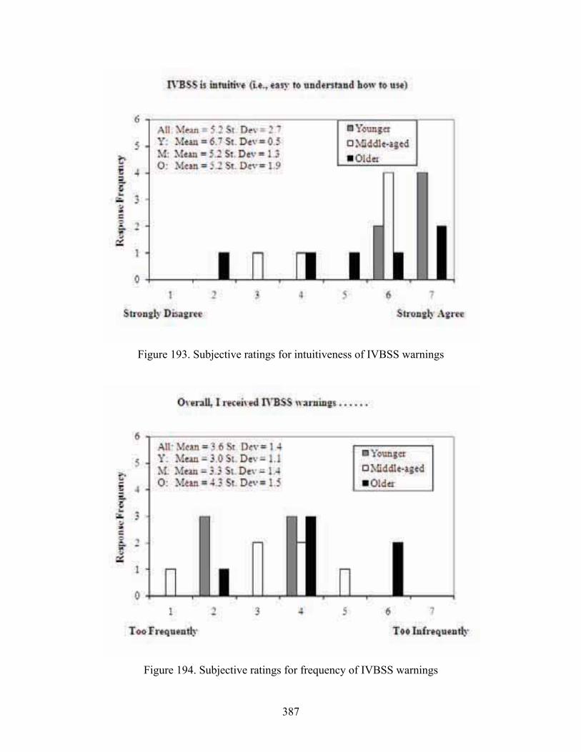
Figure 193. Subjective ratings for intuitiveness of IVBSS warnings
Figure 194. Subjective ratings for frequency of IVBSS warnings
387

Figure 195. Subjective ratings for distraction by warnings
Figure 196. Subjective ratings for ability of warnings to alert driver to conflict
388

Figure 197. Subjective ratings for the understandability of IVBSS warnings
Drivers were asked to evaluate various aspects of the longitudinal and lateral systems separately. Only one-third of the drivers received an FCW or a CSW. Of those drivers, only one driver received more than one longitudinal warning. Therefore, a discussion of only the lateral system follows. The auditory warnings were attention-getting (mean = 6.5, SD = 3.3) and provided at the right time (mean = 5.6, SD = 2.6). Additionally, participants also felt that the seat vibrations were provided at the right time (mean = 6.0, SD = 2.0). Once again, in spite of a rather high false alarm rate for LDW, drivers did not find the frequency with which they received lateral auditory warnings to be annoying (mean = 5.4, SD = 2.1). These results are displayed in Figure 198 through Figure 200.
389

Figure 198. Subjective ratings for warnings getting attention
Figure 199. Subjective ratings for timing of IVBSS warnings
390

Figure 200. Subjective ratings for frequency of IVBSS warnings
The implementation of IVBSS components in the vehicle was rated well. Most drivers were able to recognize from which side of the headrest the lateral auditory warnings came (mean = 5.1, SD = 1.8) as well as from which side of the seat pan the vibration warnings originated (mean = 6.2, SD = 2.2). Most drivers were able to read text on the display (mean = 5.6, SD = 2.0) and understand (mean = 5.7, SD = 1.8). Figure 201 through Figure 204 show these results.
391

Figure 201. Subjective ratings for distinguishing direction of auditory warnings
Figure 202. Subjective ratings for distinguishing direction of haptic warnings
392

Figure 203. Subjective ratings for ease reading warning text
Figure 204. Subjective ratings for ease of understanding warning text
393

While there is no standardized way to measure driver acceptance of new technologies, the van der Laan scale has been employed in several studies to assess and compare driver acceptance across technologies. The van der Laan scale is a five-point scale composed of nine opposite adjective pairs (e.g., useful/useless, irritating/likeable). One end of the scale is anchored by the positive adjective, while the other end is anchored by the negative adjective. Drivers checked one of five boxes for each of the nine pairs of adjectives to indicate their overall acceptance rating of IVBSS. Scores for each pair of adjectives range from -2 to +2 with positive numbers corresponding to positive attributes. The scores are collapsed for each driver resulting in a satisfaction score and a usefulness score. In order to determine if the total number of warnings could be used to predict driver acceptance, regression analyses were performed. The results of the regressions showed that the total number of warnings a driver received did not reliably predict the driver’s satisfaction or usefulness score. The usefulness and satisfaction scores were then averaged across all drivers to arrive at mean ratings of drivers’ satisfaction and usefulness of IVBSS. The mean usefulness score is 1.33 and the mean satisfaction score is 0.75. Both of these scores indicate positive feelings towards IVBSS. Figure 205 and Figure 206 show comparisons of the satisfaction and usefulness scores of IVBSS to those of RDCW (combined system), LDW, CSW (both from the RDCW FOT), and FCW (ACAS FOT). As can be seen in these plots, IVBSS is on par with these other warning systems for driver acceptance. As changes are implemented to reduce the false warning rates, it is expected that driver acceptance of IVBSS will increase.
Figure 205. Comparison of mean satisfaction scores for of IVBSS and other warning systems
394

Figure 206. Comparison of mean usefulness scores for IVBSS and other warning systems
J.4 Conclusions Light-vehicle pilot testing provided the first opportunity for laypeople to experience IVBSS in real traffic. The number of IVBSS warnings associated with lateral drifts was significant, presumably providing each driver with adequate experience on which to base impressions of the system DVI. However, due to the nature of LCMs, FCWs, and CSWs, eight drivers did not receive even one of these warnings. Despite the dearth of these types of warnings, the average number of warnings received for two hours of driving was 21. Drivers’ subjective impressions of IVBSS were favorable. They found IVBSS easy to use. In general, they were not distracted by the warnings even though the number of warnings that they received was rather high. They favorably rated the DVI reporting that the auditory warnings were attention-getting; they could determine the direction of the auditory warnings and the seat vibrations; and the text on the display was easy to read and understand. Finally, the overall perception of usefulness and satisfaction was positive. When the usefulness and satisfaction scores from this study were compared with other crash warnings systems (e.g., RDCW), IVBSS was rated as well as RDCW, CSW, LDW, and FCW. Changes to IVBSS that occurred after stage 2 pilot testing will dramatically reduce the false warnings rate that was experienced in this pilot testing. While currently good, driver acceptance of IVBSS should continue to improve as these changes are implemented.
395

J.5 Forms J.5.1 Light-Vehicle Pilot Testing Questionnaire and Evaluation
Subject #_______________ Date _____________
Please answer the following questions about the Integrated Vehicle Based Safety System (IVBSS). If you like, you may include comments alongside the questions to clarify your responses.
Example:A.) Strawberry ice cream is better than chocolate.
1 2 3 4 5 6 7 Strongly Strongly Disagree Agree
If you prefer chocolate ice cream over strawberry, you would circle the 1, 2, or 3 according to how strongly you like chocolate ice cream, and therefore disagree with the statement.
However, if you prefer strawberry ice cream, you would circle 5, 6, or 7 according to how strongly you like strawberry ice cream, and therefore agree with the statement.
If a question does not apply:Write NA, for not applicable, next to any question that does not apply to your driving experience with the system. For example, you might not experience every type of warning the questionnaire addresses.
General Impression of IVBSS
1. How difficult or easy did you find it to drive using IVBSS? 1 2 3 4 5 6 7
Very Very Difficult Easy
2. How helpful were the IVBSS warnings in notifying you of potential conflicts? 1 2 3 4 5
Not Slightly Somewhat Helpful Very Helpful Helpful Helpful Helpful
3. I always understood why the IVBSS system was providing a warning. 1 2 3 4 5 6 7
Strongly Strongly Disagree Agree
4. The IVBSS always provided a warning when I thought it should. 1 2 3 4 5 6 7
Strongly Strongly Disagree Agree
5. Overall, I received IVBSS warnings . . . . . . 1 2 3 4 5 6 7
Too Too Frequently Infrequently
396

Combinatorial Effects of the Warnings
6. I understood the meaning of and required response to each warning when it occurred. 1 2 3 4 5 6 7
Strongly Strongly Disagree Agree
7. I always understood why the system was providing an alert. 1 2 3 4 5 6 7
Strongly Strongly Disagree Agree
8. I was not distracted by the alerts. 1 2 3 4 5 6 7
Strongly Strongly Disagree Agree
9. Overall, I could easily identify the urgency of the side alerts. 1 2 3 4 5 6 7
Strongly Strongly Disagree Agree
19. IVBSS is intuitive (i.e., easy to understand how to use). 1 2 3 4 5 6 7
Strongly Strongly Disagree Agree
Auditory Alerts Overall
20. I could easily distinguish between the two auditory alerts. 1 2 3 4 5 6 7
Strongly Strongly Disagree Agree
21. I understood the meaning of and required response to each auditory alert when it occurred. 1 2 3 4 5 6 7
Strongly Strongly Disagree Agree
Side System (LCM and LDW) - Auditory and Haptic Alerts
22. I could easily recognize which direction the side auditory alerts were coming from (the left or the right speakers).
1 2 3 4 5 6 7 Strongly Strongly Disagree Agree
23. The auditory side alerts were not startling. 1 2 3 4 5 6 7
Strongly Strongly Disagree Agree
24. The auditory side alerts got my attention. 1 2 3 4 5 6 7
Strongly Strongly Disagree Agree
397

_______________________________________________________________
_______________________________________________________________
_______________________________________________________________ _______________________________________________________________
25. Overall, I thought the side auditory alerts were provided at the right time (i.e., they were not presented too early or too late).
1 2 3 4 5 6 7 Strongly Strongly Disagree Agree
If you feel the timing should be adjusted, would you make it come earlier or later?
26. The frequency with which I received side auditory alerts was not annoying. 1 2 3 4 5 6 7
Strongly Strongly Disagree Agree
27. The seat vibration alerts got my attention. 1 2 3 4 5 6 7
Strongly Strongly Disagree Agree
28. I could easily distinguish between the seat vibration alerts on the right and left sides of the seat bottom.
1 2 3 4 5 6 7 Strongly Strongly Disagree Agree
29. Overall, I thought the seat vibration alerts were provided at the right time (i.e., they were not presented too early or too late).
1 2 3 4 5 6 7 Strongly Strongly Disagree Agree
If you feel the timing should be adjusted, would you make it come earlier or later?
30. The frequency with which I received seat vibration alerts was not annoying. 1 2 3 4 5 6 7
Strongly Strongly Disagree Agree
22. The side system always provided an alert when I thought it should. 1 2 3 4 5 6 7
Strongly Strongly Disagree Agree
If the side system did not warn you when you expected an alert, please describe the situation(s).
398

_______________________________________________________________ _______________________________________________________________
_______________________________________________________________ _______________________________________________________________
____________________________________________________________
For the next 2 questions, please consider the following definitions.
An alert is defined as UNNECESSARY when an alert is generated while: you happen to drive on, near or toward a lane or road boundary and you do not perceive any threatening circumstances that warrant the alert
An alert is defined to be FALSE when an alert is generated while: you are not driving on, near or toward a lane or road boundary and you do not perceive any threatening circumstances that warrant the alert
23. I did not receive any unnecessary side system alerts. 1 2 3 4 5 6 7
Strongly Strongly Disagree Agree
If you received unnecessary alerts, describe the situation(s).
24. I did not receive any false side system alerts. 1 2 3 4 5 6 7
Strongly Strongly Disagree Agree
If you received false alerts, describe the situation(s).
25. Overall, I received side system alerts . . . . . . 1 2 3 4 5 6 7
Too Too Frequently Infrequently
26. Can you suggest any changes or modifications to the side warning system? ____________________________________________________________
____________________________________________________________
Forward Systems (FCW and CSW) - Auditory and Haptic Alerts
27. The auditory and brake pulse alerts for the forward system got my attention. 1 2 3 4 5 6 7
Strongly Strongly Disagree Agree
28. The auditory alert for the forward system was not startling. 1 2 3 4 5 6 7
Strongly Strongly Disagree Agree
29. The auditory alert for the forward system was synchronized well with the brake pulse alert.
1 2 3 4 5 6 7 Strongly Strongly Disagree Agree
399
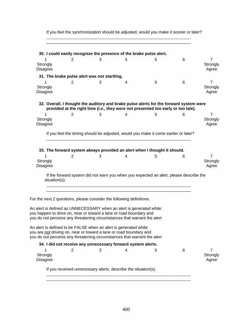
_______________________________________________________________ _______________________________________________________________
_______________________________________________________________
_______________________________________________________________ _______________________________________________________________
_______________________________________________________________ _______________________________________________________________
If you feel the synchronization should be adjusted, would you make it sooner or later?
30. I could easily recognize the presence of the brake pulse alert. 1 2 3 4 5 6 7
Strongly Strongly Disagree Agree
31. The brake pulse alert was not startling. 1 2 3 4 5 6 7
Strongly Strongly Disagree Agree
32. Overall, I thought the auditory and brake pulse alerts for the forward system were provided at the right time (i.e., they were not presented too early or too late).
1 2 3 4 5 6 7 Strongly Strongly Disagree Agree
If you feel the timing should be adjusted, would you make it come earlier or later?
33. The forward system always provided an alert when I thought it should. 1 2 3 4 5 6 7
Strongly Strongly Disagree Agree
If the forward system did not warn you when you expected an alert, please describe the situation(s).
For the next 2 questions, please consider the following definitions.
An alert is defined as UNNECESSARY when an alert is generated while: you happen to drive on, near or toward a lane or road boundary and you do not perceive any threatening circumstances that warrant the alert
An alert is defined to be FALSE when an alert is generated while: you are not driving on, near or toward a lane or road boundary and you do not perceive any threatening circumstances that warrant the alert
34. I did not receive any unnecessary forward system alerts. 1 2 3 4 5 6 7
Strongly Strongly Disagree Agree
If you received unnecessary alerts, describe the situation(s).
400

_______________________________________________________________ _______________________________________________________________
___________________________________________________________ ___________________________________________________________ ___________________________________________________________
35. I did not receive any false forward system alerts. 1 2 3 4 5 6 7
Strongly Strongly Disagree Agree
If you received false alerts, describe the situation(s).
36. Overall, I received forward system alerts . . . . . . 1 2 3 4 5 6 7
Too Too Frequently Infrequently
37. Can you suggest any changes or modifications to the forward system?
38. Please indicate your overall acceptance rating of the warning system alerts (not the controls and display).
For each choice you will find five possible answers. When a term is completely appropriate, please put a check (¥) in the square next to that term. When a term is appropriate to a certain extent, please put a check to the left or right of the middle at the side of the term. When you have no specific opinion, please put a check in the middle. The alerts were:
useful useless
pleasant unpleasant
bad good
nice annoying
effective superfluous
irritating likeable
assisting worthless
undesirable desirable
raising alertness sleep-inducing
401

Impressions of the Display and Controls
Display
39. I could easily read the text on the display. 1 2 3 4 5 6 7
Strongly Strongly Disagree Agree
79. I understood the information on the display. 1 2 3 4 5 6 7
Strongly Strongly Disagree Agree
80. The text on the display was not distracting. 1 2 3 4 5 6 7
Strongly Strongly Disagree
Agree Volume Control Access and Operation
81. It was easy for me to locate and use the volume control when I needed it. 1 2 3 4 5 6 7
Strongly Strongly Disagree Agree
82. It was easy to determine the existing volume setting. 1 2 3 4 5 6 7
Strongly Strongly Disagree Agree
83. It was easy to determine how changes to the volume setting affected the auditory warnings.
1 2 3 4 5 6 7 Strongly Strongly Disagree Agree
Blind Spot Lights in Side Mirrors
84. I could easily see the yellow and red lights in the mirror on the driver side. 1 2 3 4 5 6 7
Strongly Strongly Disagree Agree
85. I could easily see the yellow and red lights in the mirror on the passenger side. 1 2 3 4 5 6 7
Strongly Strongly Disagree Agree
86. The lights in the mirror on the driver side were about the right size. 1 2 3 4 5 6 7
Strongly Strongly Disagree Agree
402
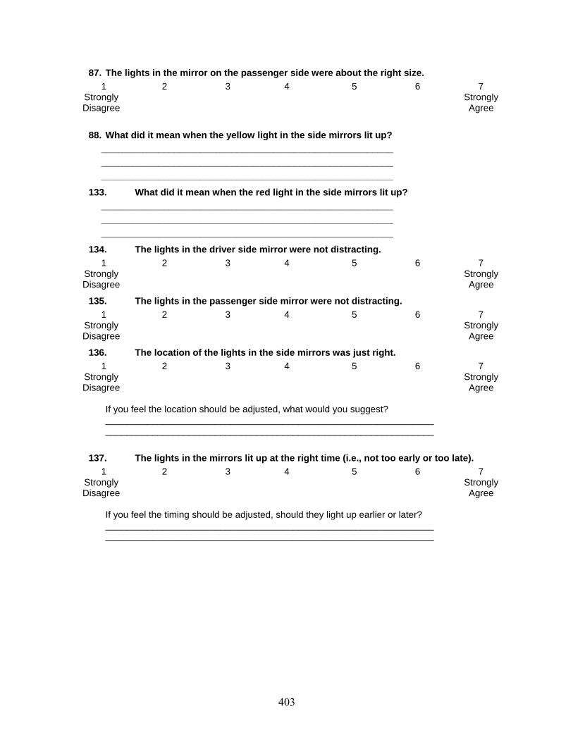
________________________________________________________ ________________________________________________________ ________________________________________________________
________________________________________________________ ________________________________________________________ ________________________________________________________
_______________________________________________________________ _______________________________________________________________
_______________________________________________________________ _______________________________________________________________
87. The lights in the mirror on the passenger side were about the right size. 1 2 3 4 5 6 7
Strongly Strongly Disagree Agree
88. What did it mean when the yellow light in the side mirrors lit up?
133. What did it mean when the red light in the side mirrors lit up?
134. The lights in the driver side mirror were not distracting. 1 2 3 4 5 6 7
Strongly Strongly Disagree Agree
135. The lights in the passenger side mirror were not distracting. 1 2 3 4 5 6 7
Strongly Strongly Disagree Agree
136. The location of the lights in the side mirrors was just right. 1 2 3 4 5 6 7
Strongly Strongly Disagree Agree
If you feel the location should be adjusted, what would you suggest?
137. The lights in the mirrors lit up at the right time (i.e., not too early or too late). 1 2 3 4 5 6 7
Strongly Strongly Disagree Agree
If you feel the timing should be adjusted, should they light up earlier or later?
403

Appendix K: Heavy-Truck Stage 2 Pilot Test
K.1 Overview As on the light-vehicle platform, the heavy-truck pilot testing sought to gain feedback and first impressions from professional truck drivers and fleet managers who drove an IVBSS-equipped truck along a prescribed route with a researcher present. The heavy-truck stage 2 pilot testing was conducted during the last two weeks of November 2007. A brief explanation of the method and results of the pilot testing follows.
K.2 Method Five professional truck drivers (some of whom have positions within safety management) were recruited from an Ann Arbor, Michigan, terminal owned by Con-way Freight. The drivers were all male, between the ages of 48 and 57 (with a mean of 52.4 years). Given the national demographics of truck drivers, this was determined to be a sufficiently representative sample for this level of pilot testing. The mixture of managers and drivers ensured that, as a whole, the sample was also representative in terms of driving experience, types of routes driven, and experience with in-vehicle electronic and advanced safety system operation. Because the drivers were considered IVBSS team members (i.e., employees of Con-way), they participated in the pilot testing as part of their paid employment with Con-way. One vehicle was used throughout the testing: the “Bronze” truck, which is an International 8600 model class 8 tractor with a day cab. The tractor was also pulling a 53-foot trailer that had 9,000 pounds of ballast weight. The drivers arrived at UMTRI, reviewed an informed consent document, and received brief instructions on how the session would be conducted. Each driver was then shown the exterior of the truck while the researcher pointed out all of the sensors that comprise IVBSS. The researcher also explained the overall purpose of IVBSS and highlighted the three crash warning scenarios. The driver was then given an opportunity to become oriented to the inside of the cab, and was shown both the forward and side IVBSS displays. The researcher then proceeded through a laptop demonstration of each IVBSS warning, and answered any initial questions that the driver had. The 52-mile route consisted of roughly 50 percent surface roads and 50 percent limited access freeways. The route (Figure 207) spanned both urban (e.g., downtown Ann Arbor) and rural (e.g., Ford Rd. east of Ann Arbor) scenarios, and generally took one hour and 15 minutes to complete. Each run consisted of one driver per day. Three of these drivers participated over Thanksgiving weekend somewhat early in the morning (8 to 9:30 a.m.), while the other two participated during busier rush-hour traffic (4 to 5:30 p.m.), both before and after the holiday. As such, there was a wide range of traffic conditions. The two drivers who participated later in the day had at least part of their drive take place after dark. Finally, all traversals of the route took place during dry conditions.
404

At the completion of driving, each driver completed an extensive questionnaire and was also invited to give more open-ended feedback in an informal question and answer session that lasted five to ten minutes.
Figure 207. Heavy-truck Stage 2 pilot testing route
K.3 Results K.3.1 Objective Results Table 134 shows the number and type of warnings received by each driver. Where it was evident to the experimenter, the status of the warning (e.g., false, intentional) is noted. A total of 49 warnings were received by the five drivers. (This includes the lower priority FCWs; if one includes only imminent warnings, the total becomes 46). The average number was 10 warnings per driver, with one driver receiving only three warnings and another receiving 15 warnings. As far as the experimenter could tell, there was only one intentional warning. LCMs were by far the most common type of warning, comprising 61 percent of the total number of warnings. The next most common type of warning was FCW, almost all of which were caused by the same physical locations along the route: an overpass on the freeway and an exit that was blocked by construction barrels.
405

Table 134. Number and type of warnings received for heavy-truck stage 2 pilot testing
Warning Driver 1 Dr iver 2 Dr iver 3 Dr iver 4 Dr iver 5 Total1 (Inten
LDW - Left (toward unoccupied) 0 0 1 tional) 0 2 LDW - Right (toward unoccupied) 0 0 0 0 0 0 LDW - Left (toward occupied) 0 0 0 0 1 1 LDW - Right (toward occupied) 1 1 1 1 1 5 LCM - Left 4 1 4 2 3 14 LCM - Right 3 0 4 2 7 16 FCW - 2-Second headway 0 0 1 0 1 2 FCW - 1-Second headway 0 0 0 0 1 1
FCW - Imminent 1 (False) 1 (False) 2 (False) 3 (False) 1 (False) 8
Total: 9 3 13 9 15 49
K.3.2 Subjective Results The evaluation of driver acceptance of IVBSS is based on a combination of two sources: the subjective assessments provided by drivers in a questionnaire completed at the end of the 75minute drive and more informal comments made by the drivers or observations made by the experimenter. In general, three of the five drivers had very positive overall feedback, while two had specific concerns that made them generally dislike the system. The negative comments were generally limited to the issue of false or unnecessary alerts, with one driver having a very low tolerance for false alerts (he mentioned that the system would need a zero-percent false alert rate). As far as the route was concerned, every driver thought that the route was representative of routes that they would typically drive. Most of the questions on the post-drive questionnaire employed seven-point Likert-type scales with higher numbers indicating positive attributes. Overall, drivers found IVBSS easy to use (mean = 6.0, SD = 1.0), but only thought it was somewhat helpful regarding potential conflicts (mean = 3.4, SD = 0.9; anchors on the five-point scale were 1 = not helpful and 5 = very helpful). On average, drivers felt that they received warnings with about the right frequency (mean = 3.8, SD = 1.6; anchors on the seven-point scale were 1 = too frequently and 7 = too infrequently). There was general agreement with the statement “I always understood why IVBSS was providing a warning,” (mean = 4.8, SD = 1.3). While two drivers somewhat disagreed with the statement “I was not distracted by the alerts,” on average drivers were not distracted by IVBSS warnings (mean = 4.8, SD = 1.8). The above results are presented in Figure 208 through Figure 218, along with histograms of some other selected questions. In terms of the look and feel of the system, the drivers generally were not distracted by the displays, although one driver commented that the side-display LEDs were too bright at night, and one driver said that he did not like the simulated horn sound as a warning, as it sounded too similar to a real horn.
406
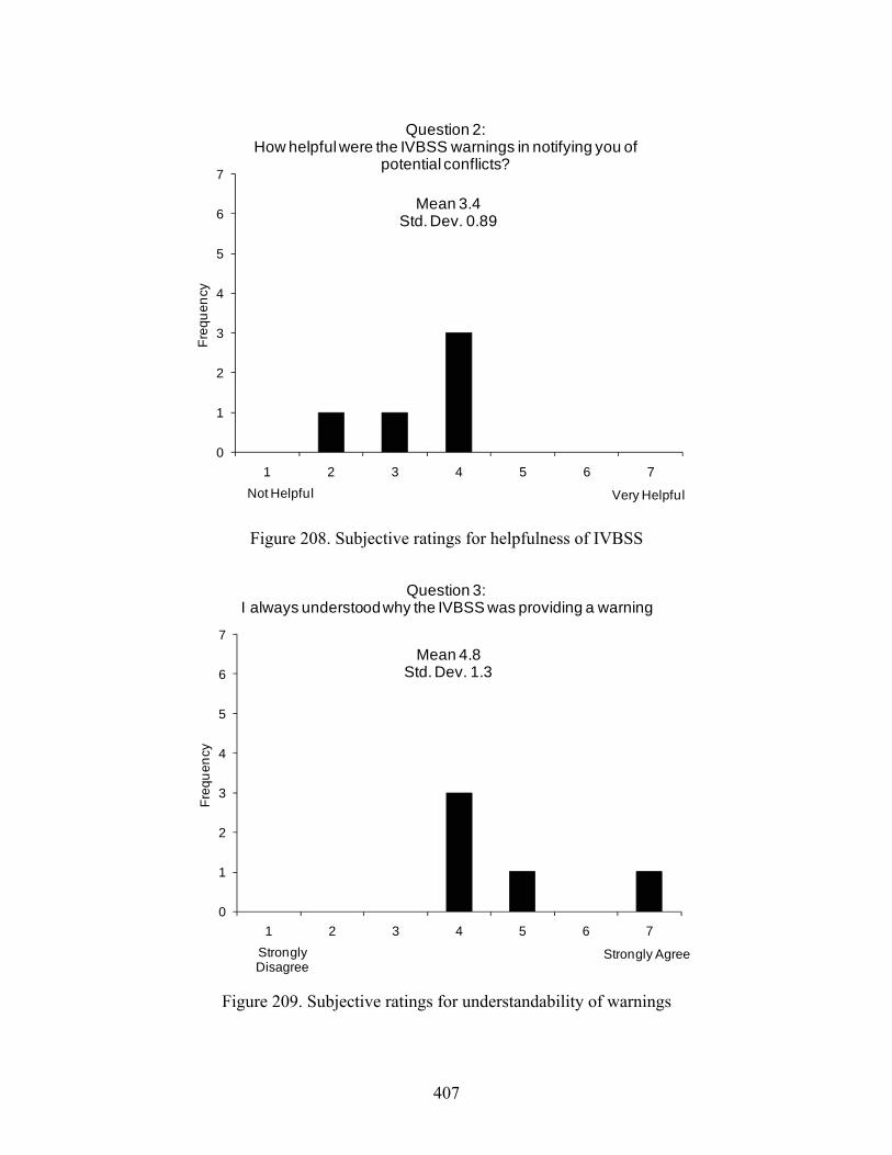
Freq
uenc
y
7
6
5
4
3
2
1
0
Question 2:How helpful were the IVBSS warnings in notifying you of
potential conflicts?
Mean 3.4Std. Dev. 0.89
1 2 3 4 5 6 7 Not Helpful Very Helpful
Figure 208. Subjective ratings for helpfulness of IVBSS
Freq
uenc
y
7
6
5
4
3
2
1
0
Question 3: I always understood why the IVBSS was providing a warning
Mean 4.8 Std. Dev. 1.3
1 2 3 4 5 6 7 Strongly Strongly Agree Disagree
Figure 209. Subjective ratings for understandability of warnings
407
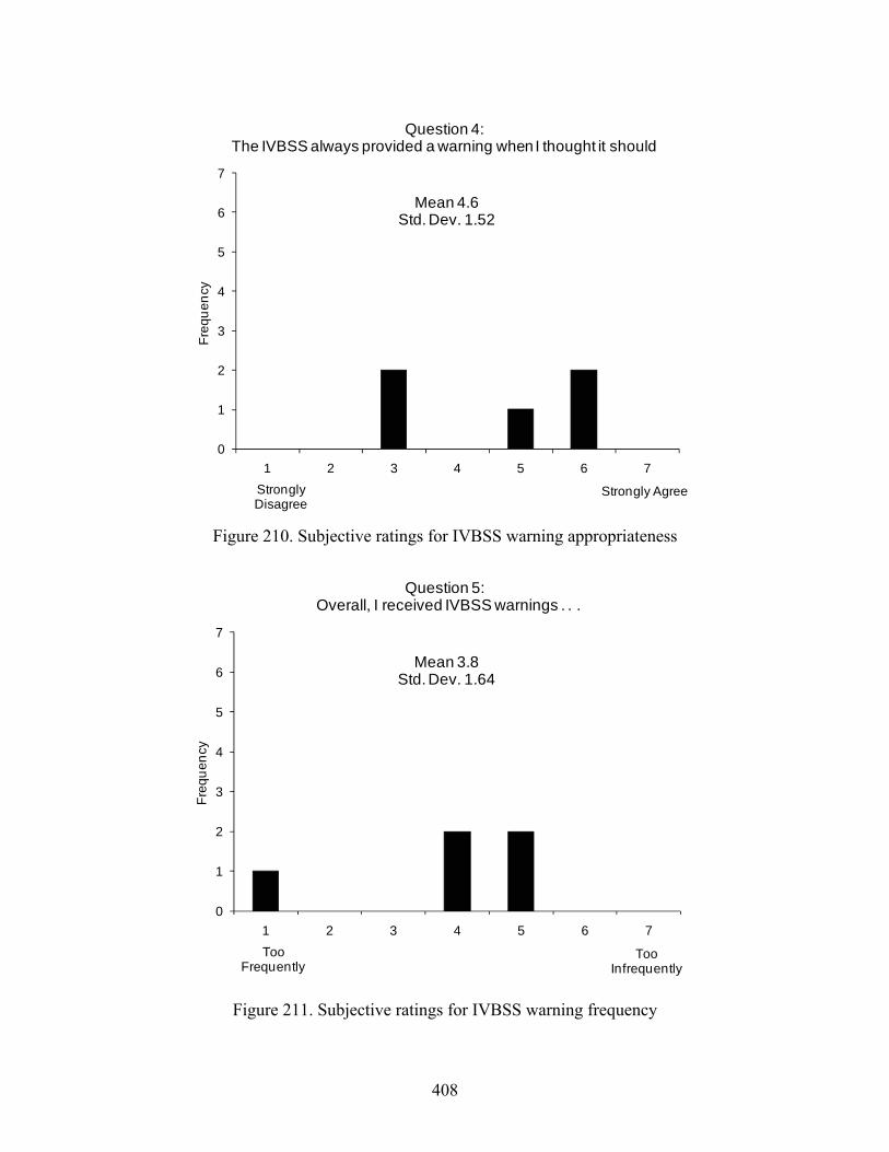
Freq
uenc
y
Question 4: The IVBSS always provided a warning when I thought it should
7
Mean 4.6 6 Std. Dev. 1.52
5
4
3
2
1
0 1 2 3 4 5 6 7
Strongly Strongly Agree Disagree
Figure 210. Subjective ratings for IVBSS warning appropriateness
Freq
uenc
y
Question 5: Overall, I received IVBSS warnings . . .
7
Mean 3.8 6 Std. Dev. 1.64
5
4
3
2
1
0 1 2 3 4 5 6 7 Too Too
Frequently Infrequently
Figure 211. Subjective ratings for IVBSS warning frequency
408
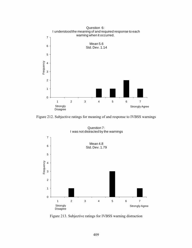
Freq
uenc
y
7
6
5
4
3
2
1
0
Question 6:I understood the meaning of and required response to each
warning when it occurred.
Mean 5.6Std. Dev. 1.14
1 2 3 4 5 6 7 Strongly Strongly Agree Disagree
Figure 212. Subjective ratings for meaning of and response to IVBSS warnings
Question 7:I was not distracted by the warnings
Freq
uenc
y
7
Mean 4.8 6 Std. Dev. 1.79
5
4
3
2
1
0 1 2 3 4 5 6 7
Strongly Strongly Agree Disagree
Figure 213. Subjective ratings for IVBSS warning distraction
409
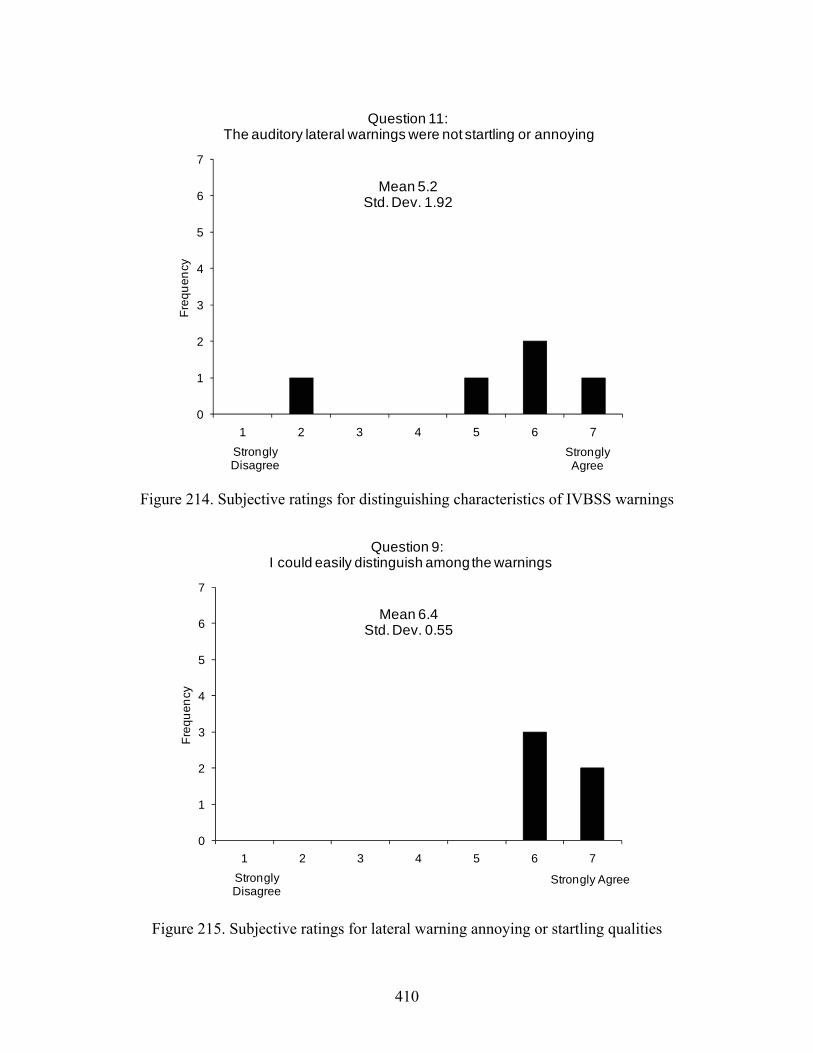
Freq
uenc
y
7
6
5
4
3
2
1
0
Question 11: The auditory lateral warnings were not startling or annoying
Mean 5.2Std. Dev. 1.92
1 2 3 4 5 6 7 Strongly Disagree
Strongly Agree
Figure 214. Subjective ratings for distinguishing characteristics of IVBSS warnings
Question 9:I could easily distinguish among the warnings
7
Mean 6.46 Std. Dev. 0.55
5
Freq
uenc
y
4
3
2
1
0 1 2 3 4 5 6 7
Strongly Strongly Agree Disagree
Figure 215. Subjective ratings for lateral warning annoying or startling qualities
410

7
6
5
4
3
2
1
0
Question 12:The auditory lateral warnings got my attention
Mean 6.4Std. Dev. 0.89
1 2 3 4 5 6 7 Strongly Strongly Agree Disagree
Figure 216. Subjective ratings for IVBSS auditory lateral warnings
Freq
uenc
y Fr
eque
ncy
7
6
5
4
3
2
1
0
Question 20:The FCWs were not startling or annoying
Mean 6.0Std. Dev. 1.0
3 4 5 6 71 2 Strongly Strongly Agree Disagree
Figure 217. Subjective ratings for FCW startling or annoying characteristics
411

Question 29:The text and graphics on the front display were not distracting
Freq
uenc
y
7
Mean 5.4 6 Std. Dev. 1.52
5
4
3
2
1
0 1 2 3 4 5 6 7
Strongly Strongly Agree Disagree
Figure 218. Subjective ratings for IVBSS text and graphics
K.4 Conclusions Heavy-truck pilot testing provided the first opportunity for “naive” truck drivers to experience IVBSS in real traffic. While the results of stage 2 pilot testing have yet to be thoroughly analyzed, the first impression is that, overall, the alert rates were reasonable and the driver feedback was generally positive. LCMs constituted the majority of warnings, and some false warning scenarios may have influenced some of the negative feedback that was received. More insights are bound to develop as the subjective results are compared to the objective driving data, and as the subjective results themselves are analyzed in more detail.
412

K.5 Forms K.5.1 Heavy-Truck Pilot Testing Questionnaire and Evaluation
Subject #_______________ Date _____________
Please answer the following questions about the Integrated Vehicle Based Safety System (IVBSS). If you like, you may include comments alongside the questions to clarify your responses.
Example:A.) Strawberry ice cream is better than chocolate.
1 2 3 4 5 6 7 Strongly Strongly Disagree Agree
If you prefer chocolate ice cream over strawberry, you would circle the 1, 2, or 3 according to how strongly you like chocolate ice cream, and therefore disagree with the statement.
However, if you prefer strawberry ice cream, you would circle 5, 6, or 7 according to how strongly you like strawberry ice cream, and therefore agree with the statement.
Ifa question does notapply:Write NA, for not applicable, next to any question which does not apply to your driving experience with the system. For example, you might not experience every type of warning the questionnaire addresses.
General Impression of IVBSS
138. How difficult or easy did you find it to drive using IVBSS? 1 2 3 4 5 6 7
Very Very Difficult Easy
139. How helpful were the IVBSS warnings in notifying you of potential conflicts? 1 2 3 4 5
Not Slightly Somewhat Helpful Very Helpful Helpful Helpful Helpful
140. I always understood why the IVBSS was providing a warning. 1 2 3 4 5 6 7
Strongly Strongly Disagree Agree
141. The IVBSS always provided a warning when I thought it should. 1 2 3 4 5 6 7
Strongly Strongly Disagree Agree
413

_______________________________________________________________
_______________________________________________________________
______________________________________________________________ _______________________________________________________________
142. Overall, I received IVBSS warnings . . . . . . 1 2 3 4 5 6 7
Too Too Frequently Infrequently
If you did receive warnings too frequently, which type (s) of warnings did you receive too frequently?
Combinatorial Effects of the Warnings
143. I understood the meaning of and required response to each warning when it occurred.
1 2 3 4 5 6 7 Strongly Strongly Disagree Agree
144. I was not distracted by the warnings. 1 2 3 4 5 6 7
Strongly Strongly Disagree Agree
145. IVBSS is intuitive (i.e., easy to understand how to use). 1 2 3 4 5 6 7
Strongly Strongly Disagree Agree
146. I could easily distinguish among the warnings. 1 2 3 4 5 6 7
Strongly Strongly Disagree Agree
Lateral System – Lane Change Merge and Lane Departure Warning
147. I could easily recognize which direction the lateral warnings were coming from (the left or the right speakers).
1 2 3 4 5 6 7 Strongly Strongly Disagree Agree
148. The auditory lateral warnings were not startling or annoying. 1 2 3 4 5 6 7
Strongly Strongly Disagree Agree
If the auditory lateral warnings were annoying, what about them were annoying?
414

_______________________________________________________________
_______________________________________________________________ _______________________________________________________________
_______________________________________________________________ _______________________________________________________________
149. The auditory lateral warnings got my attention (e.g., they were clearly audible and identifiable).
1 2 3 4 5 6 7 Strongly Strongly Disagree Agree
150. Overall, I thought the lateral warnings were provided at the right time (i.e., they were not presented too early or too late).
1 2 3 4 5 6 7 Strongly Strongly Disagree Agree
If you feel the timing should be adjusted, would you make it come earlier or later?
151. The frequency with which I received lateral warnings was not annoying. 1 2 3 4 5 6 7
Strongly Strongly Disagree Agree
152. The lateral system always provided a warning when I thought it should. 1 2 3 4 5 6 7
Strongly Strongly Disagree Agree
If the lateral system did not warn you when you expected a warning, please describe the situation(s).
For the next 2 questions, please consider the following definitions.
A warning is defined as UNNECESSARY when a warning is generated while: you happen to drive on, near or toward a lane or road boundary and you do not perceive any threatening circumstances which warrant the warning
A warning is defined to be FALSE when a warning is generated while: you are not driving on, near or toward a lane or road boundary and you do not perceive any threatening circumstances which warrant the warning
153. I did not receive any unnecessary lateral system warnings. 1 2 3 4 5 6 7
Strongly Strongly Disagree Agree
If you received unnecessary warnings, describe the situation(s).
415

_______________________________________________________________ _______________________________________________________________
____________________________________________________________ ___________________________________________________________
_______________________________________________________________ _______________________________________________________________
_______________________________________________________________
154. I did not receive any false lateral system warnings. 1 2 3 4 5 6 7
Strongly Strongly Disagree Agree
If you received false warnings, describe the situation(s).
155. Can you suggest any changes or modifications to the lateral warning system? ___________________________________________________________
Forward Crash Warning (FCW)
156. The FCWs got my attention (e.g., the auditory warnings were clearly audible and identifiable).
1 2 3 4 5 6 7 Strongly Strongly Disagree Agree
157. The FCWs were not startling or annoying. 1 2 3 4 5 6 7
Strongly Strongly Disagree Agree
If the auditory FCW warnings were annoying, what about them were annoying?
158. I understood the urgency associated with each different FCW (e.g., 2-second headway, 1-second headway, etc.)
1 2 3 4 5 6 7 Strongly Strongly Disagree Agree
159. Overall, I thought the FCW warnings were provided at the right time (i.e., they were not presented too early or too late).
1 2 3 4 5 6 7 Strongly Strongly Disagree Agree
If you feel the timing should be adjusted, would you make it come earlier or later?
416

_______________________________________________________________ _______________________________________________________________
_______________________________________________________________ _______________________________________________________________
_______________________________________________________________ _______________________________________________________________
___________________________________________________________ ___________________________________________________________
160. I always received an FCW when I thought that I should have. 1 2 3 4 5 6 7
Strongly Strongly Disagree Agree
If you did not receive an FCW when you expected one, please describe the situation(s).
For the next 2 questions, please consider the following definitions.
A warning is defined as UNNECESSARY when a warning is generated while:you are approaching a vehicle ahead of you, you are slowing down, and you do not perceive any threatening circumstances which warrant the warning.
A warning is defined to be FALSE when a warning is generated while: there is no lead vehicle and you do not perceive any threatening circumstances which warrant the warning.
161. I did not receive any unnecessary FCWs. 1 2 3 4 5 6 7
Strongly Strongly Disagree Agree
If you received unnecessary warnings, describe the situation(s).
162. I did not receive any false FCWs. 1 2 3 4 5 6 7
Strongly Strongly Disagree Agree
If you received false warnings, describe the situation(s).
163. Can you suggest any changes or modifications to the FCW system?
Overall IVBSS Warning Acceptance
164. Please indicate your overall acceptance rating of the IVBSS warnings (not the controls and display).
For each choice you will find five possible answers. When a term is completely appropriate, please put a check (¥) in the square next to that term. When a term is appropriate to a certain extent, please put a check to the left or right of the middle at the side of the term. When you have no specific opinion, please put a check in the middle.
417

_______________________________________________________________
The warnings were:
useful useless
pleasant unpleasant
bad good
nice annoying
effective superfluous
irritating likeable
assisting worthless
undesirable desirable
raising alertness sleep-inducing
Impressions of the Display and Controls
165. I could easily read the text on the front display. 1 2 3 4 5 6 7
Strongly Strongly Disagree Agree
166. The text and graphics on the front display were not distracting. 1 2 3 4 5 6 7
Strongly Strongly Disagree Agree
167. I understood the information that was presented on the front display. 1 2 3 4 5 6 7
Strongly Strongly Disagree Agree
168. I understood the meaning of the yellow and red lights on the two side displays. 1 2 3 4 5 6 7
Strongly Strongly Disagree Agree
169. I could easily see the front and side displays while driving. 1 2 3 4 5 6 7
Strongly Strongly Disagree Agree
If not, indicate which displays you could not see, and in what specific situations:
170. The brightness and loudness controls were easy to use. 1 2 3 4 5 6 7
Strongly Strongly Disagree Agree
418

DOT HS810 905February 2008