Integrated Geological, Geomorphological and Geostatistical Analysis to Study Macroseismic Effects of...

O. Gervasi et al. (Eds.): ICCSA 2009, Part I, LNCS 5592, pp. 50–65, 2009. © Springer-Verlag Berlin Heidelberg 2009

Integrated Geological, Geomorphological and Geostatistical Analysis to Study Macroseismic Effects of

1980 Irpinian Earthquake in Urban Areas (Southern Italy)

Maria Danese1,2, Maurizio Lazzari1, and Beniamino Murgante2

1 Archaeological and monumental heritage institute, National Research Council, C/da S. Loia Zona industriale, 85050, Tito Scalo (PZ), Italy

2 Laboratory of Urban and Territorial Systems, University of Basilicata, Via dell’Ateneo Lucano 10, 85100, Potenza, Italy

[email protected], [email protected], [email protected]

Abstract. This paper focuses on using the integrated methodological, approach and analysis to study macroseismic damage effects in urban areas. A case study inherent seismic risk analysis of the old town centre of Potenza hilltop town has been discussed, with particular attention to the evaluation of possible local am-plifying factors (stratigraphy and geomorphology) deduced from comparison with data studied with a geostatistical approach (kernel density, Moran Index, Getis & Ord index). Geostatistics have been applied to seismic damage scenario of 1980 Irpinian earthquake macroseismic data, offering a new point of view in seismic risk assessment.

Keywords: Geostatistics, kernel density, Moran index, autocorrelation, spatial analysis, geomorphology, earthquake, southern Italy.

1 Introduction

The use of geostatistics to process historical macroseismic data is a new field of application of these techniques [1] and it represents a new approach to territorial analysis. Particularly, our application allows to define urban areas, historically most exposed to seismic risk. In fact, the application of geostatistics to other environmental and landscape parameters helps to define the relationships between them according to their spatial distribution, autocorrelation and density. The approach proposed in this paper suggests a new point of view in seismic risk assessment. It allows knowledge base integration for emergency planning in case of earthquakes, such as the Civil Defence Plan, and above all it concerns waiting and refuge areas and strategic points of entrance to the old town centre.

2 Spatial Analysis and Autocorrelation

Spatial analysis studies phenomena distribution in the space, their aggregation status and their relationships, according to the first principle of geography: “Nearest things

Integrated Geological, Geomorphological and Geostatistical Analysis 51

are more related then distant things” [2]. This law generates the four main different families of spatial techniques, all based on the concepts of distance and proximity between spatial events: interpolation techniques, density based measures, distance based measures and autocorrelation measures. In all this techniques data are consid-ered as a spatial process and points, representing the phenomenon, as its events, characterized by a couple of x, y coordinates. In this study density, distance based measures and autocorrelation indexes have been adopted.

2.1 Kernel Density Estimation

Density based measures study the spatial concentration of a phenomenon. The sim-plest technique counts the number of events falling inside the elements of an over imposed grid to generate density classes. Besides, Kernel Density Estimation (KDE) considers a mobile three-dimensional function that weights events according to their intensity and their relative distances. It is a technique very used in many application field as social and economic studies [3], physics and astronomy [4] [5], agriculture [6], public health [7], crime analysis [8], spatial epidemiology [9], visualization of population distribution [10], social segregation [11 and references therein], interpola-tion between different zoning schemes [12], natural sciences – animal and plant ecol-ogy [13], [14], [15 and references therein], urban modelling [16] and more recently macroseismic data analysis [17].

It makes possible to estimate the distribution probability function of a point pattern composed by N points s1,…sN, characterized by their x and y coordinates. It is defined by the expression [18]:

.)(1

)(

1)(ˆ

12∑

=

⎟⎠⎞

⎜⎝⎛ −=

n

i

issk

ss

ττδλ

ττ

(1)

where, λ is the intensity of the distribution for each point, k is the kernel function, τ is the bandwidth and δ is a factor for the correction of the edge effects.

KDE strongly depends from a good choice of these parameters, according to condi-tions and constraints depending on the case study [1].

2.2 The Nearest Neighbour Index

Distance analysis represents an alternative to measures based on density in many cases study, where just some examples are epidemiology [19] and agricultural studies [20]. Sometimes they are also used together; in particular the Nearest-Neighbour distance is used as input datum for KDE [21].

Nearest-Neighbour Index (NNI) is defined by the following equation:

rand

dNNI min=

(2)

The numerator of equation (2) represents the average of N events considering the minimum distance of each event from the nearest one, and it can be represented by:

52 M. Danese, M. Lazzari, and B. Murgante

n

ssd

d

n

iji∑

== 1min

min

),(

(3)

where dmin (Si,Sj) is the distance between each point and its nearest neighbour, and n is the number of points in the distribution.

The denominator can be expressed by the following equation:

. 5.0n

Adran = (4)

where n is the distribution of number of events and A is the area of the spatial do-main. This equation represents the expected nearest neighbour distance, based on a completely random distribution. This means that when NNI is less than 1, mean ob-served distance is smaller than expected distance, then one event is closer to each other one than expected. If NNI is greater than 1, mean observed distance is higher than the expected distance and therefore events are more scattered than expected.

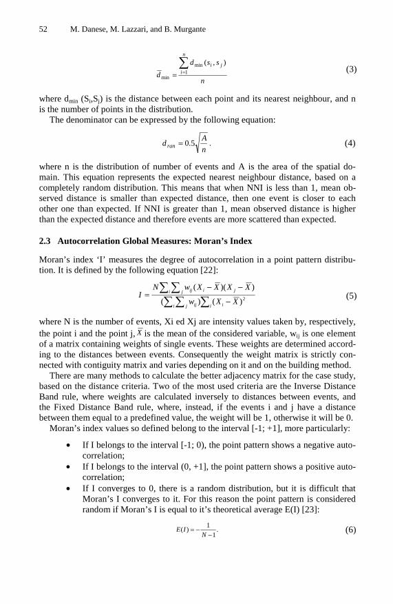
2.3 Autocorrelation Global Measures: Moran’s Index

Moran’s index ‘I’ measures the degree of autocorrelation in a point pattern distribu-tion. It is defined by the following equation [22]:

∑ ∑ ∑∑ ∑

−

−−=

i j i iij

i j jiij

XXw

XXXXwNI

2)()(

))((

(5)

where N is the number of events, Xi ed Xj are intensity values taken by, respectively, the point i and the point j, X is the mean of the considered variable, wij is one element of a matrix containing weights of single events. These weights are determined accord-ing to the distances between events. Consequently the weight matrix is strictly con-nected with contiguity matrix and varies depending on it and on the building method.

There are many methods to calculate the better adjacency matrix for the case study, based on the distance criteria. Two of the most used criteria are the Inverse Distance Band rule, where weights are calculated inversely to distances between events, and the Fixed Distance Band rule, where, instead, if the events i and j have a distance between them equal to a predefined value, the weight will be 1, otherwise it will be 0.

Moran’s index values so defined belong to the interval [-1; +1], more particularly:

• If I belongs to the interval [-1; 0), the point pattern shows a negative auto-correlation;

• If I belongs to the interval (0, +1], the point pattern shows a positive auto-correlation;

• If I converges to 0, there is a random distribution, but it is difficult that Moran’s I converges to it. For this reason the point pattern is considered random if Moran’s I is equal to it’s theoretical average E(I) [23]:

.1

1)(

−−=

NIE

(6)


The significance of results obtained by Moran’s index can be tested with the stan-dardized variable z (I), defined as:

)(

)()(

IES

IEIIz

−= (7)

where SE(I) is the theoretical standard deviation from the value E(I).

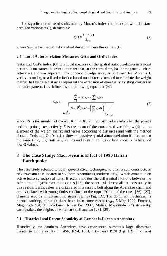
2.4 Local Autocorrelation Measures: Getis and Ord’s Index

Getis and Ord’s index (G) is a local measure of the spatial autocorrelation in a point pattern. It measures the events number that, at the same time, has homogeneous char-acteristics and are adjacent. The concept of adjacency, as just seen for Moran’s I, varies according to a fixed criterion based on distances, needed to calculate the weight matrix. In this case distances represent the extension of eventually existing clusters in the point pattern. It is defined by the following equation [24]:

( )

2

)()(1

)(

)( )(

)(2

1 1

11

−

⎥⎥

⎦

⎤

⎢⎢

⎣

⎡

⎟⎟⎠

⎞⎜⎜⎝

⎛−−

−

=

∑ ∑

∑∑

= =

−

==

N

dwdwN

iS

dwxxdw

dGn

i

n

iii

n

iiii

n

ii

i

(8)

where N is the number of events, Xi and Xj are intensity values taken by, the point i

and the point j, respectively, X is the mean of the considered variable, wi(d) is one element of the weight matrix and varies according to distances and with the method chosen. Getis and Ord’s index shows a positive spatial autocorrelation if there are, at the same time, high intensity values and high G values or low intensity values and low G values.

3 The Case Study: Macroseismic Effect of 1980 Italian Earthquake

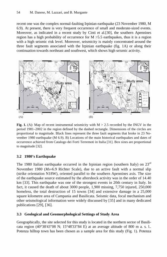
The case study selected to apply geostatistical techniques, to offer a new contribute in risk assessment is located in southern Apennines (southern Italy), which constitute an active tectonic region of Italy. It accommodates the differential motions between the Adriatic and Tyrrhenian microplates [25], the source of almost all the seismicity in this region. Earthquakes are originated in a narrow belt along the Apennine chain and are associated with young faults confined to the upper 20 km of the crust [26], [27], characterized by an extensional stress regime (Fig. 1A). The dominant mechanism is normal faulting, although there have been some recent (e.g., 5 May 1990, Potenza, Magnitude 5.4; 31 October–1 November 2002, Molise, Magnitude 5.4) strike-slip earthquakes, the origins of which are still unclear [28], [29].

3.1 Historical and Recent Seismicity of Campania-Lucania Apennines

Historically, the southern Apennines have experienced numerous large disastrous events, including events in 1456, 1694, 1851, 1857, and 1930 (Fig. 1B). The most


recent one was the complex normal-faulting Irpinian earthquake (23 November 1980, M 6.9). At present, there is very frequent occurrence of small and moderate-sized events. Moreover, as indicated in a recent study by Cinti et al.[30], the southern Apennines region has a high probability of occurrence for M >5.5 earthquakes, thus it is a region with a high seismic risk level. Moreover, seismicity is mainly concentrated around the three fault segments associated with the Irpinian earthquake (fig. 1A) or along their continuation towards northeast and southwest, which shows high seismic activity.

Fig. 1. (A): Map of recent instrumental seismicity with M > 2.5 recorded by the INGV in the period 1981–2002 in the region defined by the dashed rectangle. Dimensions of the circles are proportional to magnitude. Black lines represent the three fault segments that broke in 23 No-vember 1980 earthquake (M 6.9). B) Locations of the main historical earthquakes and dates of occurrence achieved from Catalogo dei Forti Terremoti in Italia [31]. Box sizes are proportional to magnitude [32].

3.2 1980’s Earthquake

The 1980 Italian earthquake occurred in the Irpinian region (southern Italy) on 23rd November 1980 (MS=6.9 Richter Scale), due to an active fault with a normal slip (strike orientation N18W), oriented parallel to the southern Apennines axis. The size of the earthquake source estimated by the aftershock activity was in the order of 14.40 km [33]. This earthquake was one of the strongest events in 20th century in Italy. In fact, it caused the death of about 3000 people, 1,900 missing, 7,750 injured, 250,000 homeless, the total destruction of 15 towns [34] and extensive damage in a 25,000 square kilometre area of Campania and Basilicata. Seismic data, focal mechanism and other seismological information were widely discussed by [35] and in many dedicated publications [29], [36].

3.3 Geological and Geomorphological Settings of Study Area

Geographically, the site selected for this study is located in the northern sector of Basili-cata region (40°38'43"08 N; 15°48'33"84 E) at an average altitude of 800 m a. s. l.. Potenza hilltop town has been chosen as a sample area for this study (Fig. 1). Potenza


municipality is the main town of Basilicata region (southern Italy), located in the axial-active seismic belt (30 to 50 km wide) of southern Apennines, characterized by high seismic hazard and where strong earthquakes have occurred (Fig. 1). In fact, Potenza was affected at least by five earthquakes with intensity higher than or equal to VIII MCS, such as those of 1 January 1826 (VIII MCS), 16 December 1857 (VIII-IX MCS), 23 July 1930 (VI-VII MCS) and 23 November 1980 (VII MCS), of which we have wide historical documentation. In this work we focus on the analysis of macroseismic effects occurred during the latter earthquake.

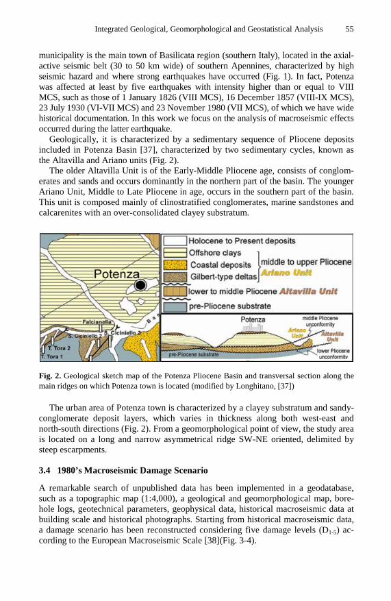
Geologically, it is characterized by a sedimentary sequence of Pliocene deposits included in Potenza Basin [37], characterized by two sedimentary cycles, known as the Altavilla and Ariano units (Fig. 2).

The older Altavilla Unit is of the Early-Middle Pliocene age, consists of conglom-erates and sands and occurs dominantly in the northern part of the basin. The younger Ariano Unit, Middle to Late Pliocene in age, occurs in the southern part of the basin. This unit is composed mainly of clinostratified conglomerates, marine sandstones and calcarenites with an over-consolidated clayey substratum.

Fig. 2. Geological sketch map of the Potenza Pliocene Basin and transversal section along the main ridges on which Potenza town is located (modified by Longhitano, [37])

The urban area of Potenza town is characterized by a clayey substratum and sandy-conglomerate deposit layers, which varies in thickness along both west-east and north-south directions (Fig. 2). From a geomorphological point of view, the study area is located on a long and narrow asymmetrical ridge SW-NE oriented, delimited by steep escarpments.

3.4 1980’s Macroseismic Damage Scenario

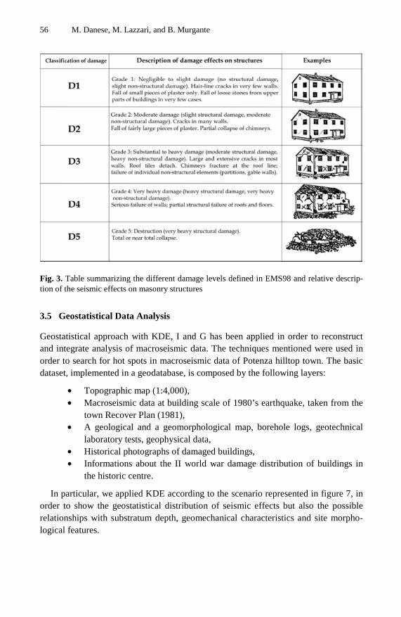
A remarkable search of unpublished data has been implemented in a geodatabase, such as a topographic map (1:4,000), a geological and geomorphological map, bore-hole logs, geotechnical parameters, geophysical data, historical macroseismic data at building scale and historical photographs. Starting from historical macroseismic data, a damage scenario has been reconstructed considering five damage levels (D1-5) ac-cording to the European Macroseismic Scale [38](Fig. 3-4).


Fig. 3. Table summarizing the different damage levels defined in EMS98 and relative descrip-tion of the seismic effects on masonry structures

3.5 Geostatistical Data Analysis

Geostatistical approach with KDE, I and G has been applied in order to reconstruct and integrate analysis of macroseismic data. The techniques mentioned were used in order to search for hot spots in macroseismic data of Potenza hilltop town. The basic dataset, implemented in a geodatabase, is composed by the following layers:

• Topographic map (1:4,000), • Macroseismic data at building scale of 1980’s earthquake, taken from the

town Recover Plan (1981), • A geological and a geomorphological map, borehole logs, geotechnical

laboratory tests, geophysical data, • Historical photographs of damaged buildings, • Informations about the II world war damage distribution of buildings in

the historic centre.

In particular, we applied KDE according to the scenario represented in figure 7, in order to show the geostatistical distribution of seismic effects but also the possible relationships with substratum depth, geomechanical characteristics and site morpho-logical features.


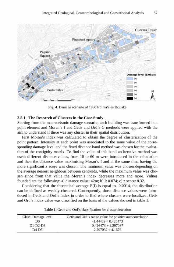
Fig. 4. Damage scenario of 1980 Irpinia’s earthquake

3.5.1 The Research of Clusters in the Case Study Starting from the macroseismic damage scenario, each building was transformed in a point element and Moran’s I and Getis and Ord’s G methods were applied with the aim to understand if there was any cluster in their spatial distribution.

First Moran’s index was calculated to obtain the degree of clusterization of the point pattern. Intensity at each point was associated to the same value of the corre-sponding damage level and the fixed distance band method was chosen for the evalua-tion of the contiguity matrix. To find the value of this band an iterative method was used: different distance values, from 10 to 60 m were introduced in the calculation and then the distance value maximising Moran’s I and at the same time having the more significant z score was chosen. The minimum value was chosen depending on the average nearest neighbour between centroids, while the maximum value was cho-sen since from that value the Moran’s index decreases more and more. Values founded are the following: a) distance value: 42m; b) I: 0.074; c) z score: 8.32.

Considering that the theoretical average E(I) is equal to -0.0014, the distribution can be defined as weakly clustered. Consequently, those distance values were intro-duced in Getis and Ord’s index in order to find where clusters were localized. Getis and Ord’s index value was classified on the basis of the values showed in table 1:

Table 1. Getis and Ord’s classification for cluster detection

Class: Damage level Getis and Ord’s range value for positive autocorrelation D0 -1.44409 ÷ 0.426473

D1-D2-D3 0.426473 ÷ 2.297037 D4-D5 2.297037 ÷ 4.1676


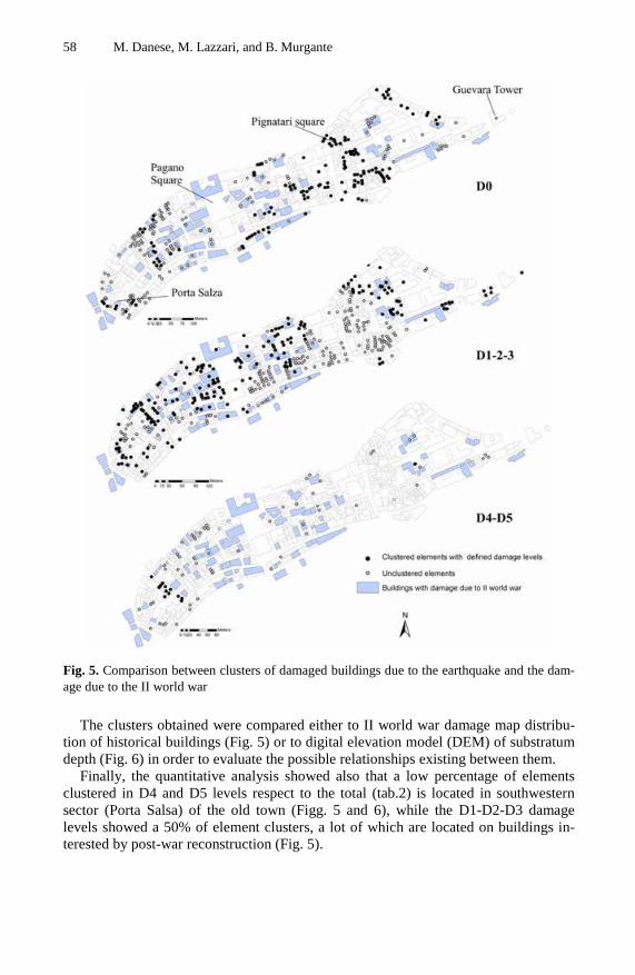
Fig. 5. Comparison between clusters of damaged buildings due to the earthquake and the dam-age due to the II world war

The clusters obtained were compared either to II world war damage map distribu-tion of historical buildings (Fig. 5) or to digital elevation model (DEM) of substratum depth (Fig. 6) in order to evaluate the possible relationships existing between them.

Finally, the quantitative analysis showed also that a low percentage of elements clustered in D4 and D5 levels respect to the total (tab.2) is located in southwestern sector (Porta Salsa) of the old town (Figg. 5 and 6), while the D1-D2-D3 damage levels showed a 50% of element clusters, a lot of which are located on buildings in-terested by post-war reconstruction (Fig. 5).


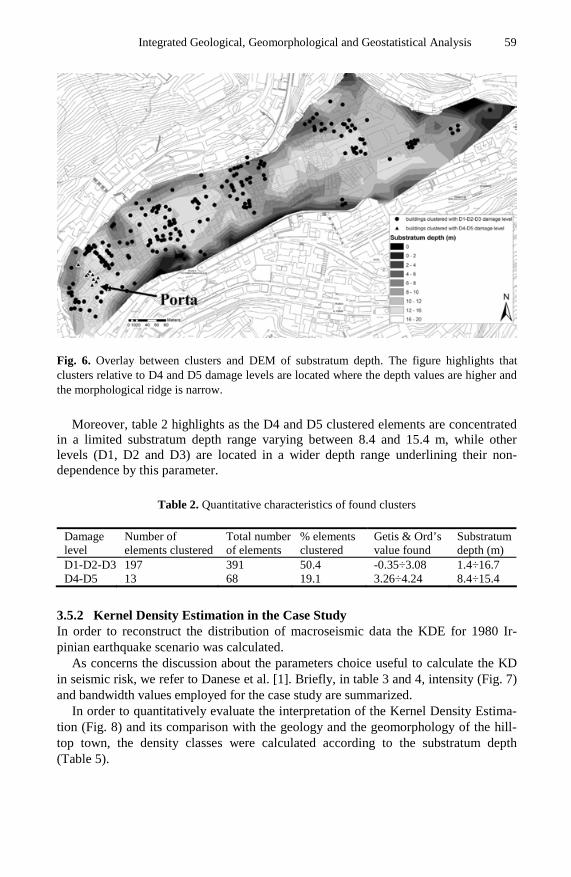
Fig. 6. Overlay between clusters and DEM of substratum depth. The figure highlights that clusters relative to D4 and D5 damage levels are located where the depth values are higher and the morphological ridge is narrow.

Moreover, table 2 highlights as the D4 and D5 clustered elements are concentrated in a limited substratum depth range varying between 8.4 and 15.4 m, while other levels (D1, D2 and D3) are located in a wider depth range underlining their non-dependence by this parameter.

Table 2. Quantitative characteristics of found clusters

Damage level

Number of elements clustered

Total number of elements

% elements clustered

Getis & Ord’s value found

Substratum depth (m)

D1-D2-D3 197 391 50.4 -0.35÷3.08 1.4÷16.7 D4-D5 13 68 19.1 3.26÷4.24 8.4÷15.4

3.5.2 Kernel Density Estimation in the Case Study In order to reconstruct the distribution of macroseismic data the KDE for 1980 Ir-pinian earthquake scenario was calculated.

As concerns the discussion about the parameters choice useful to calculate the KD in seismic risk, we refer to Danese et al. [1]. Briefly, in table 3 and 4, intensity (Fig. 7) and bandwidth values employed for the case study are summarized.

In order to quantitatively evaluate the interpretation of the Kernel Density Estima-tion (Fig. 8) and its comparison with the geology and the geomorphology of the hill-top town, the density classes were calculated according to the substratum depth (Table 5).


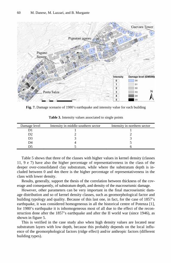
Fig. 7. Damage scenario of 1980’s earthquake and intensity value for each building

Table 3. Intensity values associated to single points

Damage level Intensity in middle-southern sector Intensity in northern sector D1 1 1 D2 2 2 D3 3 3 D4 4 5 D5 5 6

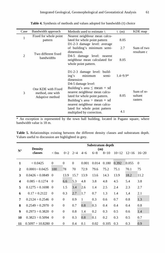
Table 5 shows that three of the classes with higher values in kernel density (classes

11, 9 e 7) have also the higher percentage of representativeness in the class of the deeper over-consolidated clay substratum, while where the substratum depth is in-cluded between 0 and 4m there is the higher percentage of representativeness in the class with lower density.

Results, generally, support the thesis of the correlation between thickness of the cov-erage and consequently, of substratum depth, and density of the macroseismic damage.

However, other parameters can be very important in the final macroseismic dam-age distribution and so of kernel density classes, such as geomorphological factor and building typology and quality. Because of this last one, in fact, for the case of 1857’s earthquake, it was considered homogeneous in all the historical centre of Potenza [1], for 1980’s earthquake it is inhomogeneous most of all due to the effect of the recon-struction done after the 1857’s earthquake and after the II world war (since 1946), as shown in figure 5.

This is verified in the case study also when high density values are located near substratum layers with low depth, because this probably depends on the local influ-ence of the geomorphological factors (ridge effect) and/or anthropic factors (different building types).


Table 4. Synthesis of methods and values adopted for bandwidth (τ) choice

Case Bandwidth approach Methods used to estimate t t (m) KDE map

1 Fixed for whole point

pattern Nearest neighbour mean calcu-lated for whole point pattern

8.05

2 Two different fixed

bandwidths

D1-2-3 damage level: average of building’s minimum semi-dimension. D4-5 damage level: nearest neighbour mean calculated for whole point pattern.

2.7

8.05

Sum of two resultant c

3 One KDE with Fixed

method, one with Adaptive method

D1-2-3 damage level: build-ing’s minimum semi-dimension D4-5 damage level: Building’s area ≤ mean + sd nearest neighbour mean calcu-lated for whole point pattern. Building’s area > mean + sd nearest neighbour mean calcu-lated for whole point pattern multiplied by correction.

1.4÷9.9*

8.05

4.1

Sum of re-sultant rasters

* An exception is represented by the town hall building, located in Pagano square, where bandwidth value is 18 m.

Table 5. Relationships existing between the different density classes and substratum depth. Values useful to discussion are highlighted in grey.

Substratum depth (m) N° Density

classes < 0m 0÷2 2÷4 4÷6 6÷8 8÷10 10÷12 12÷16 16÷20

1 < 0.0425 0 0 0 0.001 0.014 0.180 0.392 0.055 0

2 0.0001÷ 0.0425 100 78 70 72.9 79.6 75.2 75.1 70.1 75

3 0.0426 ÷ 0.0849 0 13.9 15.7 13.9 13.6 14.3 13.9 18.2 11.2

4 0.085 ÷ 0.1274 0 6.6 5.3 4.8 3.8 4.8 4.5 5.4 3.8

5 0.1275 ÷ 0.1698 0 1.5 3.4 2.6 1.4 2.5 2.4 2.3 2.7

6 0.17 ÷ 0.2122 0 0.3 2.7 1.7 0.7 1.3 1.4 1,4 2.1

7 0.2124 ÷ 0.2546 0 0 0.9 1 0.3 0.6 0.7 0.8 1.3

8 0.2549 ÷ 0.2970 0 0 0.7 0.8 0.3 0.4 0.4 0.4 0.8

9 0.2973 ÷ 0.3820 0 0 0.8 1.4 0.2 0.3 0.5 0.6 1.4

10 0.3823 ÷ 0.5094 0 0 0.3 0.8 0.1 0.2 0.3 0.5 0.7

11 0.5097 ÷ 10.8280 0 0 0.4 0.1 0.02 0.105 0.3 0.3 0.9


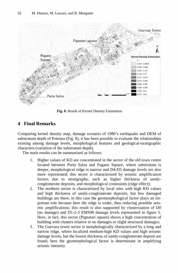
Fig. 8. Result of Kernel Density Estimation

4 Final Remarks

Comparing kernel density map, damage scenario of 1980’s earthquake and DEM of substratum depth of Potenza (Fig. 8), it has been possible to evaluate the relationships existing among damage levels, morphological features and geological-stratigraphic characters (variation of the substratum depth).

The main results can be summarized as follows:

1. Higher values of KD are concentrated in the sector of the old town centre located between Porta Salza and Pagano Square, where substratum is deeper, morphological ridge is narrow and D4-D5 damage levels are also more represented; this sector is characterized by seismic amplification factors due to stratigraphy, such as higher thickness of sandy-conglomerate deposits, and morphological constraints (ridge effect);

2. The northern sector is characterized by local sites with high KD values and high thickness of sandy-conglomerate deposits, but few damaged buildings are there; in this case the geomorphological factor plays an im-portant role because here the ridge is wider, thus reducing possible seis-mic amplifications; this result is also supported by clusterization of D0 (no damage) and D1-2-3 EMS98 damage levels represented in figure 5. Here, in fact, this sector (Pignatari square) shows a high concentration of building with clusters relative to no damages or slight structural damages;

3. The Guevara tower sector is morphologically characterized by a long and narrow ridge, where localized medium-high KD values and high seismic damage levels, but the lowest thickness of sandy-conglomerate deposit are found; here the geomorphological factor is determinant in amplifying seismic intensity.


Comparison of the autocorrelation map to the II world war damaged buildings dis-tribution (Fig. 5) was useful to highlight that a lot of buildings showing D4 and D5 damage levels are concentrated in a town sector not interested by post-war reconstruc-tion. This last factor, in fact, determined an improving of building typology compared to those of the 1857’s earthquake [1] with a consequent decrease in seismic risk level.

References

1. Danese, M., Lazzari, M., Murgante, B.: Kernel density estimation methods for a geostatis-tical approach in seismic risk analysis: The case study of potenza hilltop town (Southern italy). In: Gervasi, O., Murgante, B., Laganà, A., Taniar, D., Mun, Y., Gavrilova, M.L. (eds.) ICCSA 2008, Part I. LNCS, vol. 5072, pp. 415–429. Springer, Heidelberg (2008)

2. Tobler, W.R.: A Computer Model Simulating Urban Growth in the Detroit Region. Eco-nomic Geography 46, 234–240 (1970)

3. Worswick, C.: Adaptation and Inequality: Children of Immigrants in Canadian Schools. Canadian Journal of Economics 1(37), 53–77 (2004)

4. Price, D.J., Monaghan, J.J.: An Energy-Conserving Formalism or Adaptive Gravitational Force Softening in Smoothed Particle Hydrodynamics and N-body Codes. Mon. Not. R. Astron. Soc. 374, 1347–1358 (2006)

5. Schregle, R.: Bias Compensation for Photon Maps. Computer graphics 4(22), 729–742 (2003)

6. Wolf, C.A., Sumner, D.A.: Are Farm Size Distributions Bimodal? Evidence from Kernel Density Estimates of Dairy Farm Size Distribution. Amer. J. Agr. Econ. 1(83), 77–88 (2001)

7. Portier, K., Tolson, J.K., Roberts, S.M.: Body Weight Distributions for Risk Assessment. Risk analysis 1(27), 11–26 (2007)

8. Chainey, S., Reid, S., Stuart, N.: When is a Hotspot a Hotspot? A Procedure for Creating Statistically Robust Hotspot Maps of Crime. In: Kidner, D., Higgs, G., White, S. (eds.) In-novations in GIS 9: Socio-Economic Applications of Geographic Information Science, pp. 21–36. Taylor and Francis, Abington (2002)

9. Gatrell, A.C., Bailey, T.C., Diggle, P.J., Rowlingson, B.S.: Spatial Point Pattern Analysis and Its Application in Geographical Epidemiology. Transaction of Institute of British Ge-ographer 21, 256–271 (1996)

10. Wood, J.D., Fisher, P.F., Dykes, J.A., Unwin, D.J.: The Use of the Landscape Metaphor in Understanding Population Data. Environment and Planning B: Planning & Design 2(26), 281–295 (1999)

11. O’Sullivan, D., Wong, D.W.S.: A Surface-Based Approach to Measuring Spatial Segrega-tion. Geographical Analysis 39, 147–168 (2007)

12. Bracken, I., Martin, D.: Linkage of the 1981 and 1991 Censuses Using Surface Modelling Concepts. Environment and Planning A 27, 379–390 (1995)

13. Dixon, K.R., Chapman, J.A.: Harmonic Mean Measure of Animal Activity Areas. Ecol-ogy 61, 1040–1044 (1980)

14. Worton, B.J.: Kernel Methods for Estimating the Utilization Distribution in Home-Range Studies. Ecology 70(1), 164–168 (1989)

15. Hemson, G., Johson, P., South, A., Kenward, R., Ripley, R., MacDonald, D.: Are Kernel the Mustard? Data From Global Positioning System (GPS) Collars Suggests Problems for Kernel Home-Range Analyses with Least-Squares Cross-Validation. Journal of Animal Ecology 74, 455–463 (2005)


16. Borruso, G.: Network Density and the Delimitation of Urban Areas. Transaction in GIS 2(7), 177–191 (2003)

17. Danese, M., Lazzari, M., Murgante, B.: Kernel Density Estimation Methods for a Geosta-tistical Approach in Seismic Risk Analysis: The Case Study of Potenza Hilltop Town (Southern Italy). In: Gervasi, O., Murgante, B., Laganà, A., Taniar, D., Mun, Y., Gavrilova, M.L. (eds.) ICCSA 2008, Part I. LNCS, vol. 5072, pp. 415–429. Springer, Hei-delberg (2008)

18. Bailey, T.C., Gatrell, A.C.: Interactive Spatial Data Analysis. Longman Higher Education, Harlow (1995); International Journal of epidemiology 37(5), 1169–1179

19. McNally, R.J.Q., Rankin, J., Shirley, Mark, S.D.F., Stephen, R.P., Pless-Mulloli, T.: Space-time analysis of Down syndrome: results consistent with transient pre-disposing contagious agent. Experimental Agriculture 44(2008), 547–557 (2008)

20. Peiris, T.U., Samita, S., Veronica, W.H.: Accounting for Spatial Variability in Field Ex-periments on Tea

21. Murgante, B., Las Casas, G., Danese, M.: Where are the slums? New approaches to urban regeneration. In: Liu, H., Salerno, J., Young, M. (eds.) Social Computing, Behavioral Modeling and Prediction, pp. 176–187. Springer, US (2008)

22. Moran, P.: The interpretation of statistical maps. Journal of the Royal Statistical Soci-ety 10, 243–251 (1948)

23. O’Sullivan, D., Unwin, D.: Geographic Information Analysis. John Wiley & Sons, Chich-ester (2002)

24. Ord, J.K., Getis, A.: Testing for Local Spatial Autocorrelation in the Presence of Global Autocorrelation. Journal of Regional Science 41, 411–432 (2001)

25. Jenny, S., Goes, S., Giardini, D., Kahle, H.G.: Seismic potential of Southern Italy. Tec-tonophysics 415, 81–101 (2006)

26. Meletti, C., Patacca, E., Scandone, P.: Construction of a seismotectonic model: The case of Italy. Pure and Applied Geophysics 157, 11–35 (2000)

27. Valensise, G., Amato, A., Montone, P., Pantosti, D.: Earthquakes in Italy: Past, present and future. Episodes 26(3), 245–249 (2003)

28. Fracassi, U., Valensise, G.: The “layered” seismicity of Irpinia (Southern Italy): Important but incomplete lessons learned from the 23 November 1980 earthquake. In: Pecce, M., Manfredi, G., Zollo, A. (eds.) The Many Facets of the Seismic Risk, Proceedings of the Workshop on Multidisciplinary Approach to Seismic Risk Problem, pp. 46–52. CRdC AMRA, S. Angelo dei Lombardi (2003)

29. Valensise, G.: Summary of contributions on the 23 November 1980, Irpinia earthquake. Ann. Geofis. XXXVI(1), 345–351 (1993)

30. Cinti, F.R., Faenza, L., Marzocchi, W., Montone, P.: Probability map of the next M ≥ 5.5 earthquakes in Italy. Geochemistry, Geophysics, Geosystems 5, Q11003 (2004)

31. Boschi, E., Guidoboni, E., Ferrari, G., Valensise, G., Gasperini, P.: Catalogo dei Forti Ter-remoti in Italia dal 461 a.C. al 1900. ING-SGA, Bologna (1997)

32. Weber, E., Convertito, V., Iannaccone, G., Zollo, A., Bobbio, A., Cantore, L., Corciulo, M., Di Crosta, M., Elia, L., Martino, C., Romeo, A., Satriano, C.: An Advanced Seismic Network in the Southern Apennines (Italy) for Seismicity Investigations and Experimenta-tion with Earthquake Early Warning. Seismological Research Letters 78(6), 622–634

33. Deschamps, A., King, G.C.P.: The Campania Lucania (Southern Italy) Earthquake of No-vember 23, 1980. Earth Planet. Sci. Lett. 62, 296–304 (1980)

34. Westaway, R., Jackson, J.: The earthquake of 1980 in Campania-Basilicata (southern It-aly). Geophysical Journal of the Royal Astronomical Society 90, 375–443 (1987)


35. Boschi, E., Pantosti, D., Slejko, D., Stucchi, M., Valensise, G. (eds.): Special Issue on the Meeting Irpinia Dieci Anni Dopo Sorrento, November 19-24 1990. Ann. Geofis. XXXVI(1), 376 (1993)

36. Bernard, P., Zollo, A.: The Irpinia 1980 Earthquake: Detailed Analysis of a Complex Normal Faulting. J. Geophys. Res. 94, 1631–1647 (1989)

37. Longhitano, S.G.: Sedimentary Facies and Sequence Stratigraphy of Coarse-Grained Gil-bert-type Deltas Within the Pliocene Thrust-top Potenza Basin (Southern Apennines, It-aly). Sedimentary Geology 210, 87–110 (2008)

38. Grünthal, G.G.: European Macroseismic Scale 1998. Conseil de l’Europe Cahiers du Cen-tre Européen de Géodynamique et de Séisomologie, vol. 15, Luxembourg (1998)

Integrated Geological, Geomorphological and Geostatistical Analysis to Study Macroseismic Effects of...

Documents

Transcript of Integrated Geological, Geomorphological and Geostatistical Analysis to Study Macroseismic Effects of...