Digital Signal Processing 35 (2014) 1–13

Contents lists available at ScienceDirect

Digital Signal Processing

www.elsevier.com/locate/dsp

Instantaneous frequency in time–frequency analysis:

Enhanced concepts and performance of estimation algorithms

Ljubiša Stankovic, Igor Djurovic, Srdjan Stankovic, Marko Simeunovic, Slobodan Djukanovic ∗, Miloš Dakovic

University of Montenegro/Electrical Engineering Department, 20 000, Podgorica, Montenegro

a r t i c l e i n f o a b s t r a c t

Article history:Available online 26 September 2014

Keywords:Instantaneous frequencyTime–frequency signal analysisParametric estimationNon-parametric estimationRobust estimation

The instantaneous frequency (IF) is a very important feature of nonstationary signals in numerous applications. The first overview of the concept and application of the IF estimators is presented in seminal papers by Boashash. Since then, a significant knowledge has been gained about the performance of the IF estimators. This knowledge has been used not only for development of various IF estimators but also for introduction of novel time–frequency (TF) representations. The IF estimation in environments characterized by low signal-to-noise (SNR) has achieved significant benefits from these theoretical developments. In this paper, we review some of the most important developments in the last two decades related to the concept of the IF, performance analysis of IF estimators, and development of IF estimators for low SNR environments.

© 2014 Elsevier Inc. All rights reserved.

1. Introduction

Signals generated and sampled in time are often analyzed and processed in the frequency domain. Basic tool for mapping a signal from time into the frequency domain is the Fourier transform (FT). The FT-based analysis is efficient when the frequency content of the analyzed signal does not change over time. However, in many applications, we deal with signals where important information about the physical process is conveyed within the time varia-tions of the signal’s spectral components. The time–frequency (TF) analysis provides efficient tools for analyzing such signals. The instantaneous frequency (IF) represents one of the most impor-tant parameters in the TF analysis. Its representation, estimation, and relation to the physical quantities represent key topics in the TF analysis [1–5]. One of the oldest applications of signals with time–varying frequency is in communications based on fre-quency modulation, where the information is conveyed through the frequency variations. In radar and sonar systems, information about the position and/or velocity of the target is contained in the phase (and hence in the IF) of the returned signal [4,6–8]. At each instant, the speech signal can be represented with sev-eral FM components whose IFs bear information important for speech analysis and recognition [9]. The motion parameters of ob-jects in video-sequences can be embedded in the IF of correspond-

* Corresponding author. Fax: +382 20 245 873.E-mail address: slobdj@ac.me (S. Djukanovic).

http://dx.doi.org/10.1016/j.dsp.2014.09.0081051-2004/© 2014 Elsevier Inc. All rights reserved.

ing signals [10,11]. In seismology, TF tools can be very helpful in representing seismic signals and extracting the IF [12]. The IF es-timation tools can be used in hydrocarbon detection since oil and gas reservoirs can cause anomalies in the energy and frequency of seismic signals [13]. In biology, the tracking of some animal popu-lations can be performed using the IF extracted from sounds pro-duced by these animals [14]. Numerous applications of the IF are present in medicine. For example, in newborn’s electroencephalo-gram (EEG), the IF estimation can be used for seizure detection, modeling and classification [15]. Image processing techniques, such as image segmentation, can be combined with the TF signal anal-ysis and multichannel signal analysis to improve the performance of EEG abnormalities detection based on the IF estimation [16].

The IF concept is reviewed in Section 2, along with the model of an ideal TF mapping using the stationary phase method. The IF in TF representations is addressed in Section 3, including the IF es-timation model, use of time–scale representations, IF estimation in low SNR environments, as well as the IF estimation of multicompo-nent signals. Parametric and combined parametric–nonparametric IF estimators are considered in Section 4. In Section 5, several alternative TF methods related to the IF estimation are briefly re-viewed. Conclusions are drawn in Section 6.

2. Definitions

Consider a complex sinusoid

x(t) = Ae j(Ω0t+φ0) = Ae jφ(t), (1)

2 Lj. Stankovic et al. / Digital Signal Processing 35 (2014) 1–13

where A, Ω0 and φ0 represent a constant amplitude, (angular) fre-quency, and phase offset of x(t), respectively. Its phase derivative,

Ω(t) = φ′(t) = Ω0, (2)

is constant and equal to angular frequency. The frequency Ω0 can be considered as the rate of change of the phase function φ(t). Sig-nal (1) can be interpreted as a vector in the complex plane with a constant amplitude A and an angle φ(t), rotating with a con-stant angular velocity Ω0, making Ω0/(2π) cycles per second. The signal form x(t) = Ae jφ(t) can be generalized for an arbitrary differ-entiable phase function φ(t). Then, in analogy with (2), we can still interpret the phase derivative as the instantaneous rate of change of the phase function (instantaneous angular velocity).

Consider the signal

x(t) = A(t)e jφ(t), (3)

where A(t) represents an amplitude that varies significantly slower than the phase φ(t), |A′(t)| � |φ′(t)|. Within the frequency frame-work, we can interpret the phase derivative at t = t0 as the fre-quency of signal that would behave as a complex sinusoid with constant frequency Ω = φ′(t0) and amplitude A(t0). Thus we may consider a sinusoid e jΩt that locally fits x(t) around t0, i.e., a sinu-soid that produces constant phase of the product x(t)e− jΩt at the considered instant t0 and its vicinity. Then φ′(t0) = Ω holds. This consideration leads to the method of stationary phase which states that if the phase function φ(t) is monotonous and amplitude A(t)is sufficiently smooth function [17,18,8], then the FT of a signal A(t)e jφ(t) can be approximated as

∞∫−∞

A(t)e jφ(t)e− jΩtdt � A(t0)e jφ(t0)e− jΩt0

√2π j

φ′′(t0), (4)

where t0 is the solution of φ′(t0) = Ω .The most significant contribution to the integral on the left side

of (4) comes from the region where the phase of exp( j(φ(t) −Ωt))is constant, since the contribution of intervals with fast varying φ(t) − Ωt averages to zero. In a narrow time region around t , the phase φ(t) behaves as Ωt . Thus, we may say that, for a particular instant t , the IF (rate of the phase change, φ′(t)) of signal A(t)e jφ(t)

corresponds to frequency Ω . In this way, for each time instant t , we obtain the corresponding frequency Ω = φ′(t), and map the signal from the time into the frequency domain. This mapping can be written as a two dimensional TF function by using δ(Ω − φ′(t))and amplitudes according to (4), which is illustrated in Fig. 1.

The method of stationary phase has been used as a starting point in developing reassignment techniques as well. Namely, for each TF point (t, Ω), the TF representation values can be reas-signed towards the local gravity center (a point where they con-tribute the most) in order to approach an ideal TF representation in terms of concentrating energy along the IF and the group delay, as its dual notion [19,20].

3. IF in TF representations

The IF concept has played a significant role in definition and analysis of TF representations. The key idea behind the representa-tions defined using the IF is to achieve high (full) concentration of the signal generalized energy along its IF [21]

ITF(t,Ω) = 2π Aq(t)δ(Ω − φ′(t)

)= Aq(t)

∞∫e jφ′(t)τ e− jΩτ dτ , (5)

−∞

Fig. 1. Illustration of the stationary phase method which relates a signal in time, at an instant t , with the FT value at frequency Ω = φ′(t) via the TF domain.

where q is the power of amplitude (depending on the representa-tion order) and ITF(t, Ω) denotes the ideal TF representation. The whole signal generalized power Aq(t) would be concentrated at a single point Ω = φ′(t) for a given instant t . Thus, the TF represen-tations could be defined as

TF(t,Ω) =∞∫

−∞

p∏i=1

xbi (t + ciτ )e− jΩτ dτ , (6)

where p, bi and ci are constants. For signal x(t) = A(t) exp( jφ(t)), phase function of the product in (6) is

p∑i=1

biφ(t + ciτ ) = φ′(t)τ + �φ(t, τ ). (7)

The ideal representation (5) is achieved for the spread factor �φ(t, τ ) = 0. When �φ(t, τ ) �= 0, the representation will be spread around the IF.

For example, we can easily derive the Wigner distribution (WD) following this analysis. For a linear FM signal, with φ(t) = at2 +bt + c, it is known that

φ(t + τ/2) − φ(t − τ/2) = φ′(t)τ .

Thus, the WD is obtained for the coefficients b1 = 1, c1 = 1/2, c2 =−1/2, and b2 = −1 (negative b2 means complex conjugate of the signal). The WD represents an ideal TF representation of linear FM signals [8].

In general, the phase functions φ(t + ciτ ), i = 1, . . . , P , are ex-panded in Taylor series around τ = 0. The coefficients bi and ci in (7) should satisfy the following conditions:

• Sum of coefficients with φ(t) equals 0. This condition may be omitted if the absolute value of distribution is used.

• Sum of coefficients with φ′(t)τ equals 1.• Coefficients with φ(p)(t)τ p , up to the desired order, equal 0.

If we add the requirement that the TF representation is real-valued, then c2i+1 = −c2i and b2i+1 = −b2i hold. The fourth-order (p = 4) polynomial Wigner–Ville distribution (PWVD) ideally con-centrates the signals with polynomial phase up to the fourth or-der [1]. Assuming integer signal powers in (6), we may show that the lowest possible powers are b1 = −b2 = 2 and b3 = −b4 = −1. If we take b1 = −b2 = L (L is an even number) and c1 = −c2 =1/(2L), the L-Wigner distribution is obtained [21,22]. Complex-time distributions may be derived using a similar analysis, allowing

Lj. Stankovic et al. / Digital Signal Processing 35 (2014) 1–13 3

Table 1Coefficients of some TF representations with their spread factors.

Representation Coefficients Spread factor

Wigner distribution

b1 = −b2 = 1 φ′′′(t)τ 3/24 + . . .

c1 = −c2 = 1/2

Rihaczek distribution

b1 = 1 b2 = −1 φ′′(t)τ 2/2 + . . .

c1 = 0 c2 = −1

Polynomial Wigner–Ville distribution

b1 = −b2 = 2 φ(5)(t)τ 5/3 + ...

b3 = −b4 = −1c1 = −c2 � 0.675c3 = −c4 � 0.85

L-Wigner distribution

bL = −b2 = L φ′′′(t)τ 3/(24L2) + . . .

c1 = −c2 = 1/(2L)

Complex-time distribution

b1 = −b2 = 1 φ(5)(t)τ 5/(425!) + ...

b3 = −b4 = jc1 = −c2 = 1/4c3 = −c4 = − j/4

complex arguments [23]. The coefficients of some TF representa-tions with their spread factors are presented in Table 1.

Similarly to (5), TF representations that are concentrated along the second phase derivative φ′′(t), i.e., along the IF rate, can be introduced [24,25].

3.1. IF estimation model

The IF estimation is crucial in numerous signal processing ap-plications [1,2]. Techniques based on the TF analysis represent the state-of-the-art in this area due to high accuracy and robustness to the noise influence. One of the basic properties of TF representa-tions is that the IF can be obtained as [26,8]∫ ∞

−∞ Ω TF(t,Ω)dΩ∫ ∞−∞ TF(t,Ω)dΩ

= Ω(t) = d

dtarg

[x(t)

] = φ′(t). (8)

This theoretically important relation is rarely used in the IF es-timation since it is very sensitive to noise (multiplication by Ωincreases noise at high frequencies). In the case of multicompo-nent signals, relation (8) will result in a single value that generally does not correspond to the IFs of the signal components. Instead, the nonparametric IF estimation based on the maxima position of the TF representation will be used as follows [1,27,28]:

Ω(t) = arg maxΩ

TF(t,Ω). (9)

The position of maximum Ω = φ′(t) can be found as a solution of

∂TF(t,Ω)

∂Ω= 0.

Deviation of detected maxima positions from the signal’s IF is caused by the noise and the spread factor �φ(t, τ ). According to (5) and (7), the TF representation with the spread factor �φ(t, τ )

can be written as,

TF(t,Ω) = Aq(t)

∞∫−∞

e j(φ′(t)τ+�φ(t,τ ))e− jΩτ dτ .

Including both disturbances, the spread factor and the noise, the derivative ∂TF(t, Ω)/∂Ω can be written as

∂TF(t,Ω)

∂Ω

= ∂

∂Ω

(Aq(t)

∞∫w(τ )e j(φ′(t)τ+�φ(t,τ ))e− jΩτ dτ + Ξ(t,Ω)

),

−∞

where Ξ(t, Ω) represents all terms in the TF representation in-fluenced by an additive noise. An equivalent window function w(τ ) is added to emphasize the fact that all calculations are done over a finite lag interval. It is usually an even function, de-creasing away from the origin, i.e. it satisfies w(τ ) = w(−τ ) and w(|τ1|) ≥ w(|τ2|) for |τ1| < |τ2|.

Due to the higher order phase derivatives �φ(t, τ ) and the noise influenced terms Ξ(t, Ω), the TF maxima position is shifted from the true IF position φ′(t) by �Ω . First we will present an analysis assuming small disturbances in the sense that maximum position deviation remains within the auto-term. The auto-term width depends on the lag interval width and the spread factor �φ(t, τ ). The zero-value of ∂TF(t, Ω)/∂Ω will be shifted from Ω = φ′(t) to Ω = φ′(t) + �Ω . The error �Ω can be analyzed by using a linear model of the TF derivative with respect to the small disturbances �φ(t, τ ) and Ξ(t, Ω), [29,8],

∂TF(t,Ω)

∂Ω

∣∣∣∣Ω=φ′(t)+�Ω

= ∂TF(t,Ω)

∂Ω

∣∣∣∣ Ω=φ′(t),�φ(t,τ )=0,Ξ(t,Ω)=0

+ ∂Ξ(t,Ω)

∂Ω

∣∣∣∣ Ω=φ′(t),�φ(t,τ )=0

+ �Ω∂2TF(t,Ω)

∂Ω2

∣∣∣∣ Ω=φ′(t),�φ(t,τ )=0,Ξ(t,Ω)=0

.

For the new maximum position of the disturbed TF, the IF estimate satisfies

∂TF(t,Ω)

∂Ω

∣∣∣∣Ω=φ′(t)+�Ω

= 0.

Note that ∫ ∞−∞ w(τ )τdτ = 0. For small �φ(t, τ ), it holds

exp( j�φ(t, τ )) ∼= 1 + j�φ(t, τ ). The approximative error in the IF estimation is

�Ω =Aq(t)

∫ ∞−∞w(τ )τ�φ(t, τ )dτ + ∂Ξ(t,Ω)

∂Ω

∣∣Ω=φ′(t),

�φ(t,τ )=0

∂2TF(t,Ω)

∂Ω2

∣∣Ω=φ′(t),

�φ(t,τ )=0,Ξ(t,Ω)=0

.

For example, the bias and variance of the pseudo-WD-basedIF estimator with the Hann window of the width h are approxi-mately [8]

E{�Ω} = Bias (t,h) ∼= 1

76Ω(2)(t)h2, (10)

Var{�Ω} = σ 2(t,h) ∼= 14σ 2

ε

A2(t)

1

h3, (11)

where Ω(2)(t) is the second derivative of the IF and σ 2ε is the vari-

ance of additive Gaussian noise. Obviously, the bias is an increasing function of h, while the variance is a decreasing one, pointing out that there is a trade-off in selection of the window width in the pseudo-WD-based IF estimator. Similar bias and variance relations may be derived for other TF representations (spectrogram, PWVD, quadratic class of distributions) as functions depending on the ker-nel size, the window width, and the distribution order [30].

Fig. 2 depicts the pseudo-WD-based IF estimation of an FM sig-nal corrupted by a Gaussian noise

x(t) = e j∫ t

0 Ω(u)du + ε(t) (12)

where

Ω(t) = 1.8π

3

(cos(4πt/256) − 1

3cos(12πt/256)

+ 1cos(20πt/256)

).

5

4 Lj. Stankovic et al. / Digital Signal Processing 35 (2014) 1–13

Fig. 2. The IF estimation of a noisy nonlinear FM signal by using the WD with a narrow window (left) and a wide window (right). Cases with negligible noise (top row), moderate noise (middle row), and higher noise (bottom row) are presented. The true IF is presented by the green line, while the estimated IF is presented by the red line. (For interpretation of the references to color in this figure legend, the reader is referred to the web version of this article.)

The signal is considered for −128 < t < 128 and sampled with �t = 0.5. The top row in Fig. 2 compares the IF estimations ob-tained using a narrow window with 5 samples (left), and a wide window with 81 samples (right), when the noise is almost neg-ligible (SNR = 100 dB). Windowed signals are zero-padded up to 256 samples. Narrow window based estimation follows the true IF, while the bias in the wide window based estimation is no-table. Here the auto-term contains significant inner interferences caused by the spread factor. The IF estimates for the moderate noise case (SNR = 12 dB) are presented in the middle row. Fluctu-ations within the auto-term caused by noise are significant in the narrow window case. The bottom row depicts the IF estimation in a higher noise (SNR = 9 dB), showing that some IF estimates com-pletely miss the auto-term. The IF estimation at low SNR will be considered later.

The MSE of the TF-based IF estimators can, in general, be writ-ten as the sum of the squared bias and variance as [31,29,8]

MSE(t,h) = σ 2(t,h) + Bias 2(t,h) = V (t)/hm + B(t)hn.

According to (10) and (11), for the pseudo-WD we get m = 3, n = 4, V (t) = 14σ 2

ε /A2(t) and B(t) = (Ω(2)(t)/76)2. Obviously, there is an optimal window h(t) = hopt(t) that follows from ∂MSE(t, h)/∂h = 0. However, such a window depends on signal it-self since parameter B(t) depends on the IF derivatives. For the estimation of the optimal window width hopt(t) without prior knowledge of parameter B(t), an algorithm based on the intersec-tion of the confidence intervals (ICI) is introduced [31], and briefly described here. Let us introduce a set H of window-width values h1 < h2 < . . . < h J . Define the confidence intervals Ds = [Ls, Us]for s = 1, 2, . . . , J of the estimates, with the following upper and lower bounds

Ls = Ωs(t) − Kσ(hs),

Us = Ωs(t) + Kσ(hs),

Fig. 3. Illustration of the IF estimation using the WD with constant and variable windows. FM signal is corrupted by Gaussian white noise with SNR = 20 dB. (a) The WD with wide window; (b) The WD with a narrow window; (c) The WD with adaptive window whose width is presented in (d).

where Ωs(t) is an estimate of Ω(t), obtained from (9) using the window width hs , and σ(hs) represents its standard devia-tion. For small window widths hs , the bias of Ωs(t) is negligible, thus Ω(t) ∈ Ds . Then, obviously, Ds−1 ∩ Ds �= ∅, since at least the true value Ω(t), belongs to both confidence intervals. For wide windows the variance is small, but the bias is large. Clearly, a large enough s exists such that Ds ∩ Ds+1 = ∅ for a finite K and Bias (t, hs) �= 0. The idea behind the algorithm is that the optimal window width can be determined as highest hs for which the suc-cessive confidence intervals Ds−1 and Ds have at least one point in common. Intersection of the confidence intervals Ds−1 and Ds∣∣Ωhs−1(t) − Ωhs (t)

∣∣ ≤ K[σ(hs−1) + σ(hs)

], (13)

works as an indicator of the event hs ∼ hopt . The algorithm is not sensitive to the value of K , so K ∼ 3 could be used [31]. There are many methods in literature for an efficient SNR estimation needed for the calculation of σ(hs) [31–34].

The ICI algorithm performance is illustrated in Fig. 3. An FM signal corrupted by Gaussian white noise with SNR = 20 dB is considered. The signal has the form represented by (12) with the following IF

Ω(t) =

⎧⎪⎪⎨⎪⎪⎩

−2π/3 for t < −299−2π/3 cos(6π(t + 128)/256) for − 299 ≤ t < −1282π/3 cos(2πt/256) for − 128 ≤ t < 2992π/3(400 − t)/100 for t ≥ 299.

The signal is sampled with �t = 0.5. Set H = {32, 38, 46, 54, 64, 76,

90, 108, 128, 152, 182, 216, 256} of window widths is used. Nar-row windows produce noisy estimates, whereas wider windows produce biased estimates. The ICI algorithm takes window width adaptively, producing an accurate IF estimation. The algorithm uses the widest windows in the constant and linear IF segments (no

Lj. Stankovic et al. / Digital Signal Processing 35 (2014) 1–13 5

higher order phase derivatives), while narrower windows are used when the IF is not linear (higher order phase derivatives exist).

3.2. IF estimation with time–scale representations

Alternative to the TF representations are the time–scale rep-resentations, of which the most notably is the wavelet transform (WT) [34–39]. The WT is not an often used tool for analysis of FM signals due to several reasons. In [34] it has been shown that for any basic wavelet function, different relationship between scale and frequency has to be established. For example, for the wavelet transform given as

CWT(t, s) =+∞∫

−∞x(u)

1√sψ∗

(u − t

s

)du (14)

where ψ∗(u) represents the mother wavelet function, the rela-tionship between the scale and frequency depends on parameters of ψ∗(u). For three commonly used mother wavelets, this relation-ship is summarized in [34, Table I]. Also, in [34], a general analysis of the scalogram (energetic version of the WT) as the IF estimator is presented, together with the expressions for the bias and vari-ance of a scalogram-based estimator.

The second issue is the fact that it is meaningful to apply the WT only in the case when we are interested in varying resolution of the representation for different frequencies. This is again of in-terest only for signals with quite specific variations in frequency. Consider, for example, practically important and simple case of a linear frequency modulated (LFM) signal. This signal has the IF of the form Ω = at +b, where a and b are constants. In Fourier analy-sis, the optimal window width (effective time interval used in the transform calculation) for the analysis of LFM signal is a signal-dependent constant proportional to the square root of the IF rate h ∼ √

a, [40,8]. The effective width in time of the wavelet function ψ∗(t/s) changes with frequency. It means that, in the case of an LFM signal, the WT is optimally concentrated at a single time (or frequency) point. When the IF of an LFM signal is lower than this frequency, the WT will use too wide windows and its concentra-tion will be poor due to significant nonstationarity included within such windows. On the other hand, when the IF of an LFM signal is higher than this frequency, the WT will use too narrow windows, and again the WT concentration will be poor. This example shows that the WT cannot be used in the analysis of some standard sig-nals such as LFM signal.

The S-transform S(t, ω) is introduced as the phase correction of the continuous WT [41], i.e.

S(t,ω) = e jωtCWT(t, s)

=+∞∫

−∞x(τ )

|ω|√2π

e− (t−τ )2ω22 e− jωτ

dτ . (15)

Conceptually, it is a hybrid of short-time Fourier analysis and wavelet analysis. It uses variable window length, but preserves the phase information by using the Fourier kernel in the signal decom-position [41]. As a result, the phase spectrum is absolute in the sense that it is always referred to a fixed time reference. Quan-titative analysis of the S-transform as the IF estimator is given in [42], where it is shown that the IF estimation, obtained as the peak position of the considered adaptive S-transform, can outper-form (in terms of the MSE) estimation obtained using the STFT or the pseudo-WD for specific signals whose IF changes correspondto the S-transform window width changes. The linear Gabor trans-form based tool for TF analysis and IF estimation of nonstationary signals produced by atmospheric clutter having hyperbolic modu-lation has been proposed in [43,44].

3.3. IF estimation at low SNR

In low SNR environments, there is a significant probability that the TF values caused by noise exceed the TF values along the IF of the analyzed signal. The detected maximum then can be at an ar-bitrary position, thus producing high estimation error (see Fig. 2, bottom row). This effect is more emphasized for narrower win-dows used in calculation of the TF representations. Three strategies are in use for handling the IF estimation at low SNR. They are re-viewed below.

1. The cross WD (XWD) is proposed to extend the operating SNR range of the WD [45]. It is calculated as

XWD(t,Ω) =∞∫

−∞x(t + τ/2)x∗(t − τ/2)exp(− jΩτ)dτ , (16)

where x(t) represents a unit amplitude signal obtained as x(t) = exp( j

∫ t−∞ Ω(τ )dτ ). The initial IF estimate Ω(τ ) can be

obtained by using any estimator, for example, the maxima po-sition of the TF representation (STFT or WD). The IF Ω(τ ) is estimated in an iterative procedure where each step includes the maximization of new XWD(t, Ω) that is calculated using the improved unit amplitude signal, obtained with the IF es-timate calculated in the previous step. In each iteration we improve the signal energy concentration, increasing the prob-ability of correct IF estimation. The cross PWVD is proposed to improve the IF estimation of polynomial phase signals at lower SNRs [46].Asymptotic performance of the XWD as an IF estimator has been assessed in [47]. The obtained results are used, in turn, to develop an algorithm for selection of adaptive window width in the IF estimation.Performance of the XWD in the estimation of sinusoidal FM signal is presented by the green line in Fig. 4.

2. Modifications of the ICI algorithm. Based on the estimated SNR and percentage of outliers, set of the window widths in the ICI algorithm is divided into three subsets: (1) subset of the narrowest windows, Hn , that produce poor results at low SNR, (2) subset of middle-width windows, Hm , with low per-centage of outliers caused by low SNR, and (3) subset of wide windows, H w , that are robust to low SNR influence, but usu-ally yield biased estimates. In the modified ICI algorithm [48], windows from set Hn are not used, since they are character-ized by high probability of outliers, whereas those from the Hm ∪ H w subset are used. The IF estimates obtained using win-dows from Hm have to be filtered (e.g., using median filter) in order to eliminate possible outliers, although the probability of outliers is low. The estimates obtained with H w windows are used unchanged. The rest of the algorithm is the same as the standard adaptive ICI algorithm described in Section 3. In this way, short windows are eliminated from considera-tion since they produce significant number of outliers. The algorithm starts with the narrowest window (with the small-est bias) from Hm where the influence of errors due to low SNR is eliminated. Then the algorithm proceeds towards wider windows until the optimal window width is reached. Fig. 4presents the performance of the modified ICI in the estima-tion of a sinusoidal FM signal.An application of the ICI algorithm that includes lower order distributions is presented in [49]. The performance of the orig-inal ICI algorithm can be significantly improved by introducing an additional criterion for a proper window width selection, which takes into account the amount of overlap between the current and previous confidence intervals relative to the cur-rent interval length [33].

6 Lj. Stankovic et al. / Digital Signal Processing 35 (2014) 1–13

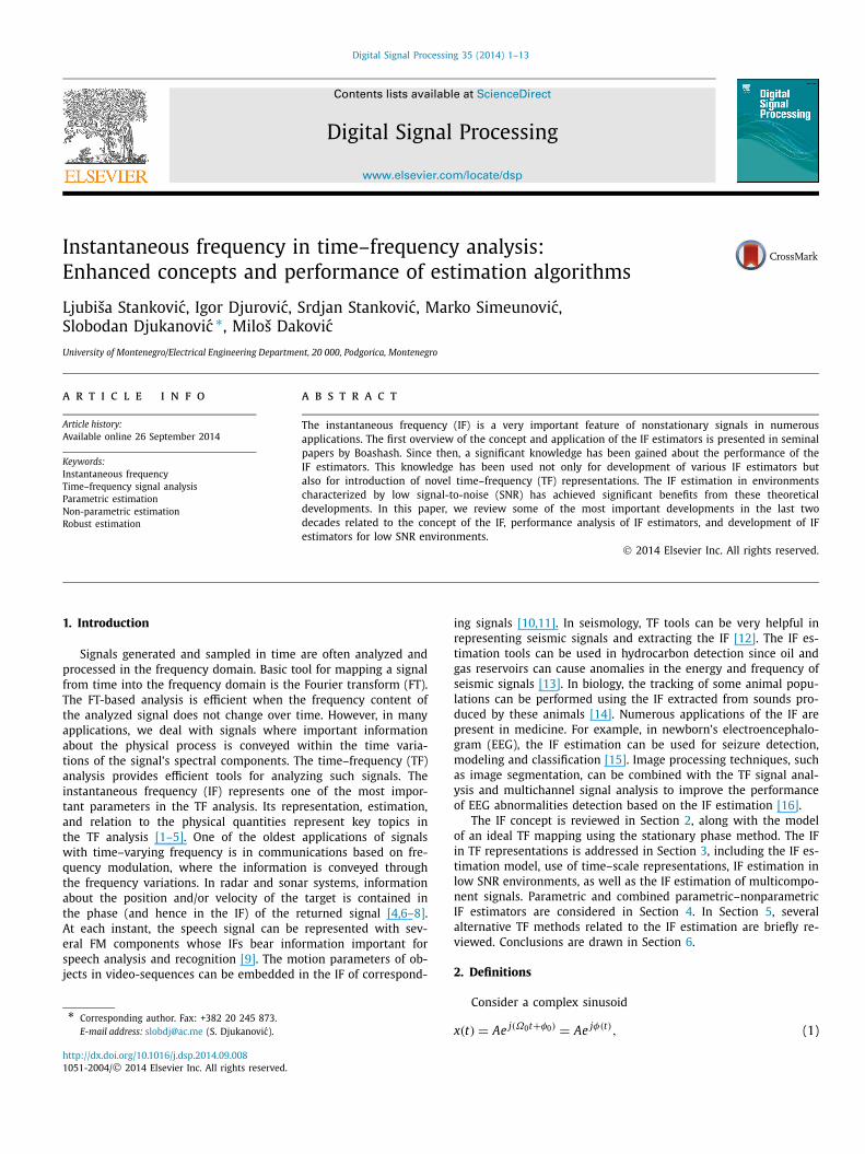
Fig. 4. Top: IF estimation of a sinusoidal FM signal in Gaussian noise with low SNR using the WD. The position of maximum works inaccurately for all three consid-ered SNRs. The modified ICI, XWD and Viterbi algorithm are close to exact IF for SNR = −1 dB. For lower SNR, the modified ICI has considerable errors, while the XWD can still be used for SNR = −3 dB. For the lowest SNR = −5 dB, only the Viterbi algorithm produces satisfactory results. Bottom: The MSE for several IF esti-mators for the above signal. The estimator based on the position of maximum has breakdown point about SNR = 8 dB and below this value it becomes extremely in-accurate, the XWD estimator has higher bias, but it can work for SNR = 0 dB, the modified ICI algorithm compensates the bias for high SNR and it has better accu-racy than the estimator based on the position of maximum, whereas for low SNR its accuracy is close to that of the XWD algorithm. The Viterbi algorithm is the most accurate for low SNR, which is paid by increased calculation complexity. (For inter-pretation of the references to color in this figure, the reader is referred to the web version of this article.)

3. Tracking filters in the TF plane. The IF estimation errors due to low SNR are of impulsive nature (see Fig. 4). In this case, the median filter could be used to remove IF estimates charac-terized by significant deviation from the neighboring IFs. The accuracy of median filter, applied to the obtained IF estimate, is limited due to the correlation between errors at consecu-tive samples. More sophisticated techniques are then required. One such technique considers the Viterbi algorithm [50] for the IF tracking [51]. The algorithm is based on two criteria: (A) IF estimate should pass through the highest values of the TF representation, and (B) the IF variation between consecu-tive instants should be as small as possible. Considering the TF representation as a grayscale image with the lightest tones associated to the highest representation values, the task of the Viterbi algorithm is to form as smooth line as possible by con-necting as light points of image as possible. The IF estimate can be represented as a path (n, k(n)), n = n1, n1 + 1, . . . , n2, in the TF plane that minimizes the following function:

n2∑n=n1

f(TF

(n,k(n)

)) +n2−1∑n=n1

g(∣∣k(n) − k(n + 1)

∣∣). (17)

In (17), the first sum considers criterion (A) ( f (·) is a non-increasing function), while the second sum considers criterion (B) (g(·) is a non-decreasing function). For the considered in-stant n, function f can be formed as follows. First, TF(n, k)

is sorted into nonincreasing order, i.e., frequency indices k j , j = 1, 2, ..., Q , are determined so that the following relation holds:

TF(n,k1) ≥ TF(n,k2) ≥ · · · ≥ TF(n,kQ ). (18)

The function f is then formed as f (TF(n, k j)) = j − 1, which corresponds to the idea that larger transform values yield smaller values of f (TF(n, k j)) and therefore are more impor-tant candidates for the IF estimates. For example, zero value of f (TF(n, k j)) corresponds to the maximum value of TF(n, k). For function g(|x − y|), we can take linear form with respect to |x − y|, for example, g(|x − y|) = c(|x − y| −�) for |x − y| > �

and zero elsewhere. The threshold is denoted by �.Performance of the Viterbi in the estimation of sinusoidal FM signal is presented by the blue line in Fig. 4. For lower SNR, i.e. below 2–3 dB, it provides more accurate estimates than those obtained by the XWD or modified ICI.In [52], the Viterbi algorithm is used for resolving over-the-horizon radar (OTHR) Doppler returns, characterized by close IF trajectories. More precisely, it is used to detect TF-domain positions of the signal of interest in heavily cluttered data. Based on the obtained positions, cross-terms free high-resolution TF representation can be calculated.

There are several alternative approaches handling the IF estima-tion in low SNR environments. A family of TF distributions, based on the directionally smoothed PWVD, has been proposed in [53]in order to reduce outliers, inherent to quadratic TF distributions at low SNR, and therefore to improve the IF estimation.

For the IF estimation in presence of both multiplicative and ad-ditive noise, an estimator based on the position of the polynomial Wigner–Ville distribution (PWVD) is proposed [54]. The optimal window length, that resolves the bias-variance trade-off in the IF estimation, is obtained from derived analytical expressions for the bias and asymptotic variance of the estimator.

Note that papers listed in this section consider Gaussian noise. The IF estimation in non-Gaussian environments, i.e. impulse noise environments, is addressed in [55,56].

3.4. IF estimation of multicomponent signals

In practical applications, it is quite common that the analyzed signal contains several components of form (3). For example, a radar signal can contain signals reflected from various targets or signals received through multiple paths. Speech and sound signals are also very rich in components. Signals produced by vehicle en-gines contain components on several time-varying resonance fre-quencies [57]. Such signals can be represented as

x(t) =M∑

m=1

Am(t)e jφm(t) = A(t)e jφ(t), (19)

where Am(t) are slow varying amplitudes. Note that a real val-ued signal x(t) = 2

∑Mm=1 Am(t) cos(φm(t)) could be considered as

x(t) = ∑Mm=1 Am(t)e− jφm(t) + ∑M

m=1 Am(t)e jφm(t) [17].The resulting amplitude A(t) variations can be of the same

order as variations of the phase function. Here we may use esti-mators that produce a single resulting IF as Ω = φ′(t). However, in the case of multicomponent signals (19), real physical quanti-ties are usually not related to the single resulting IF; instead, they are related to the individual IFs Ωm = φ′

m(t), m = 1, 2, . . . , M , of the signal components. Therefore, in the case of multicomponent signals, an ideal TF is of the form

ITF(t,Ω) =M∑

m=1

2π Aqm(t)δ

(Ω − φ′

m(t)), (20)

where Am(t) and φ′m(t) represent the amplitude and the phase

derivative of the m-th component. Within the TF analysis frame-work, it implies cross-terms free (or reduced) realization of TF representations. After more than three decades of development,

Lj. Stankovic et al. / Digital Signal Processing 35 (2014) 1–13 7

the problem of estimating multicomponent signals is still open for research. In many cases, signal components can be separated in time, frequency, or the TF domain, so that the IF can be de-termined for each component. Various separation algorithms exist, while the TF-based ones are the most effective [57,58].

One direction in the analysis of multicomponent signals is to di-vide the TF domain into regions corresponding to individual com-ponents and applying the standard IF analysis within these regions. Since the ideal representation of an M-component signal contains only M non-zero values at the considered instant, it is sparse in frequency, and it can also be used as a starting point for defini-tion and efficient implementation of algorithms for processing of signals that are sparse in the TF domain [59,60].

Another research direction in the analysis of multicomponent signals is aimed towards obtaining a TF representation concen-trated along the IF of components as sharply as possible. The ob-tained TF representation image can be separated into components and the IF estimated from each component separately. The sim-plest approach is the so-called peeling, where the IF is estimated based on the maxima position of the strongest component [57]. Other components are estimated after the strongest one has been removed from the image. If no component is significantly stronger than the others, the TF plane can be segmented using some pat-tern recognition techniques [57]. Mathematical morphology and other sophisticated tools are sometimes used in the segmentation process [57,61]. Namely, the IF estimation based on the maxima position is related to common edge estimation algorithms used in digital image processing. The IF trajectories of signal compo-nents can be discontinuous, for example due to noise influence. For connecting components, we can use the morphological tech-niques such are dilatation, erosion and component linking [62,57]. A more robust modification of this transform has been proposed recently [63]. In [58], it is shown that, at low SNR, multicomponent signals can be separated using a blind source separation strategy and estimated using the ICI algorithm proposed for monocompo-nent signal IF estimation [29,31]. The blind source separation is the separation of a set of source signals from a mixture of signals, without information (or with very little information) about the source signals or the mixing process. Commonly, the information is based on statistics or, in our case, on the fact that components are FM signals. A comprehensive analysis of the blind source sepa-ration can be found in [64].

The IF estimation of multicomponent signals based on image processing has been dealt with in [62]. The signal is first trans-formed to the TF domain using a reduced interference quadratic TF distribution. The IF estimation of signal components is then achieved by implementing two steps, namely local peak detection followed by an image processing technique called component link-ing. Application of this method to real signals is illustrated with newborn EEG signals.

The vector representation of multicomponent FM signals can lead to one more direction in this analysis. If the rotation speeds of vectors are of different orders, we may imagine that our detection system is so inert that it cannot observe the fastest rotation. Then, we can detect the trajectory of the fastest rotating vector central point (e.g. by detecting local maxima and local minima caused by the fastest rotation). We remove this rotation, and continue in the same way with the next fastest rotation. This is the basic idea of the empirical mode decomposition (EMD) approach in the IF anal-ysis [65]. The decomposition is illustrated on a three component signal x(t) = A1e jφ1(t) + A2e jφ2(t) + A3e jφ3(t) , where A1 > A2 > A3and |φ′

1(t)| � |φ′2(t)| � |φ′

3(t)|. Imaginary part of x(t) is used in decomposition presented in Fig. 5. The EMD, however, has limited application range due to problems with mode mixing and sensitiv-ity to noise influence [66,67]. These problems attracted significant

Fig. 5. Vector illustration of a multicomponent signal and its decomposition.

research in description of phenomena related to the EMD and its modifications in order to reduce the observed problems [68,66].

Alternative decomposition scheme has been proposed in [69]where nonstationary signals are decomposed using discrete evolu-tionary transform into series of the chirp functions. This technique is applied to the IF estimation for excision of jammers from signals in communication systems [70]. In the decomposition strategies presented in [71–74] various basis functions, such as chirplets [75], are used for nonstationary signal decomposition. These techniques, however, are limited to situations when the signal can be decom-posed into a relatively small number of atoms or basis functions and when the signal is embedded in a moderate level of noise. Additional problem can be in a reduced efficiency due to the in-creased computational complexity in parameter estimation, such as four-dimensional search in the case of chirplets [75].

A decomposition strategy based on the eigenvalues or singular values of the TF representations is presented [76,77]. For example, in [77] the TF representation is decomposed into a series of TF representations of separate signal components. This method allows detection of a weak radar return in a heavy clutter.

The EMD approach and the TF representation-based eigen-value decomposition (EVD) are illustrated on an example. A signal x(t) = 2 cos(5π/4 − 5π(t − 128)2/12 000) exp(−((t − 128)/72)2) +3 cos(πt/6 + 4π(128 − t)2/3000 + 3π(128 − t)310−5/5) exp(−((t −150)/42)2), within −50 ≤ t ≤ 350 discretized with step 1, is con-sidered. Its EMD decomposition is presented in Fig. 6 (first column) and the TF-based EVD decomposition is presented in Fig. 6 (second column). Since the EMD detects the highest IF first, for each time instant, it would be mixing the components if the shorter duration component were with higher IF values, as in the case presented in Fig. 6 (third column). The TF-based EVD decomposition is not influenced by the IF values of the components, Fig. 6 (fourth col-umn). The TF-based decomposition is obtained up to the initial phase ambiguity in each component.

The main difference between decomposition based on eigen-values and singular values, on one side, and decomposition into atomic functions, on the other side, is similar to difference be-

8 Lj. Stankovic et al. / Digital Signal Processing 35 (2014) 1–13

Fig. 6. The EMD approach and the TF representation based eigenvalue decomposition (EVD) applied on a two-component signal: The original signal and its TF representation (S-method [78]) are presented on top. The components (intrinsic mode functions IMF) obtained by the EMD (first column) and the components based on the EVD of the S-method (second column). The EMD and the TF-based EVD decomposition, for a shorter duration component on a higher IF, are shown in the third and fourth columns, respectively.

tween nonparametric and parametric estimation techniques. When signal model is known in advance and fits well the atomic func-tion, these techniques would produce better results; otherwise, it is better to apply decomposition that does not assume specific sig-nal model such as eigenvalues decomposition. In addition, both decomposition techniques are able to deal with moderate noise level.

Similar idea like in atomic decomposition is considered in [79–81,63] where it has been established time-varying auto-regressive (TVAR) model of nonstationary signals. The main simi-larity comes from the dependence of these techniques on proper selection of basis function. In original form, this technique is very sensitive to noise influence.

4. Parametric and combined IF estimators

The most common parametric signal model is the polynomial-phase or polynomial-FM model, that is grounded by the Weier-strass theorem. A polynomial phase signal (PPS) can be defined as x(t) = A exp( j

∑Pk=0 aktk) where P is the polynomial order and

{ak|k ∈ [0, P ]} are the phase coefficients. The IF of the PPS equals Ω(t) = ∑P

k=1 kaktk−1 and it comprises all phase coefficients ex-cept a0. For P = 1 (complex sinusoid), the FT represents an ap-propriate estimation tool since the signal energy is ideally con-centrated at a single point in the frequency domain. For P > 1, the signal energy is spread over a frequency range. In that case, it would be convenient to use an operator that can transform the PPS into a complex sinusoid. The maximum likelihood (ML) estimation

of the phase parameters requires multidimensional search, which can be computationally exhaustive procedure [82]. The PPS param-eters can be efficiently estimated by reducing the polynomial order in the signal phase and estimating the phase parameters, starting from the highest one. The most popular estimators from this class are the high order ambiguity function (HAF) [83], and its variations [84–86].

To transform the signal x(t) to a complex sinusoid, the HAF uses the phase difference (PD) operator

PDp[t;τ (l)

1 , ..., τ(l)p

] = PDp−1[t + τ(l)p ;τ (l)

1 , ..., τ(l)p−1

]× (

PDp−1[t − τ(l)p ;τ (l)

1 , ..., τ(l)p−1

])∗, (21)

where p = 1, 2, . . . , P − 1, represents the PD order, and τ (l)i , i =

1, . . . , p, are the lag parameters. Superscript l identifies lag set used in the PD calculation.1 In addition, PD0[t] = x(t). Since the frequency of sinusoid equals Ω = 2P−1 P !aP

∏P−1i=1 τ

(l)i , the highest-

order phase parameter is estimated as follows:

aP = 1

2P−1 P !∏P−1i=1 τ

(l)i

arg maxΩ

∣∣HAF(l)(Ω)∣∣2

,

1 Lag set identifier l is introduced to denote that the PD can be calculated with various lag sets, which is later used in the PHAF calculation.

Lj. Stankovic et al. / Digital Signal Processing 35 (2014) 1–13 9

HAF(l)(Ω) =∞∫

−∞PDP−1[t, τ (l)

1 , ..., τ(l)P−1

]exp(− jΩt)dt.

Once aP is estimated, aP−1 can be obtained from the dechirped signal x(t) exp(− jaP t P ). The procedure is repeated until all the phase parameters are estimated. However, numerous problems ap-pear in the estimation process, namely (a) noise influence in-creases with each PD leading to increased estimation MSE and high SNR threshold, (b) appearance of cross-terms when multi-component signals are considered, and (c) error propagation from higher to lower order phase parameters. To reduce the influence of cross-terms, the product HAF (PHAF) is proposed as the product of several HAFs calculated using different sets of lag parameters [84]

PHAF(Ω) =∏

l

HAF(l)(FlΩ),

where Fl = ∏P−1i=1 τ

(l)i /τ

(1)i is the frequency scaling factor. The scal-

ing in frequency ensures that, in all the HAFs, the auto-terms appear at the same frequency Ω proportional to

∏P−1i=1 τ

(1)i . The

frequencies of cross-terms, however, are not proportional to this product after scaling in frequency [84]. Multiplying HAFs, there-fore, enhances the auto-terms more significantly than cross-terms.

If the presented higher-order transforms, including possible post-processing of the IF estimates, cannot produce satisfactory results at low SNR, it is recommended to resort to linear signal representations. The optimal processing can be performed if the signal form is known (matched filters). In many cases, we can assume that the signal phase can be locally approximated by a polynomial (using a finite Taylor series), reducing the analysis to the PPS case. In the TF analysis, this is referred to as the local polynomial FT (LPFT) [87,88]

LPFT(t,�) =∞∫

−∞x(t + τ )w(τ )e− jθ(�,τ )dτ , (22)

where w(τ ) is a sliding localization window, θ(�, τ ) = Ωτ +Ω2τ

2/2! + · · · + ΩMτ M/M! and M is the LPFT order. The LPFT is an M-dimensional transform which concentrates at � = (φ(1)(t),φ(2)(t), ..., φ(M)(t)), and the IF and its derivatives can be estimated as

�(t) = arg max�

∣∣LPFT(t,�)∣∣,

where the IF is the first element of �(t). Note that the STFT repre-sents a special case of the LPFT obtained with M = 1. Due to time localization by the sliding window, the LPFT of relatively low or-ders could be used, e.g., M = 2 or 3, even if the phase order P is much higher. Also the time localization enables the LPFT to deal with signals that have nonpolynomial modulation. The LPFT is a linear transform, and it requires a search over M parameters for each instant. The search for optimal parameters is a compromise between accuracy and complexity. Direct search over parameter space could be performed when accuracy is crucial. The LPFT with M = 2 can be connected to the fractional Fourier transform (FrFT) [8,89–91].

Alternatives to the LPFT are the Radon–Wigner transform [92], Wigner–Hough transform [93], Hough–Radon transform [94], di-rectional smoothed PWVD bank [53], where quadratic distributions are projected along lines with small number of parameters. These techniques are, however, characterized by significant calculation complexity. They entail the calculation of a TF representation and performing a transform in order to estimate the signal parameters, whereas the LPFT calculation and local parameter estimation are performed jointly.

Fig. 7. The IF of a sinusoidal FM signal estimated by the QML approach and STFT for SNR = 0 dB. The QML estimator produces estimates that are very close to the true IF frequency. The IF estimates obtained by the STFT (N = 42) are significantly worse than those obtained by the STFT (N = 22).

Another approach related to the LPFT is the phase unwrap-ping, where the PPS parameters are estimated directly from the signal phase. It produces accurate estimates only at higher SNRs. However, the phase unwrapping approach can be used to im-prove the accuracy of methods that can work at lower SNRs [95]. Assuming that the initial estimates of the phase parameters, ak , are obtained by some standard technique, the dechirping of the signal x(t) exp(− j

∑Pk=1 akt P ) yields a PPS with parameters {a0,

δak = ak −ak|k ∈ [1, P ]}. Then, the phase unwrapping (coupled with signal decimation and filtering) can be used to estimate errors δak , thus refining initial estimates. This algorithm is extended to deal with multicomponent PPSs in [96]. This extension has significantly lower complexity than computationally intensive nonlinear least squares (NLS) methods [82].

The IF estimators, robust to noise influence, should be used in the initial stage (prior to refinement). The TF representations, in particular the linear ones, are the main candidates for this purpose. For example, the STFT with various window widths h, STFTh(t, Ω), can be used for obtaining the initial IF estimate Ωh(t). Approx-

imation of Ωh(t) by a polynomial, i.e., Ωh(t) ≈ ∑Pk=1 kak,htk−1,

yields rough estimation of the signal parameters {ak,h|k ∈ [1, P ]}, which in turn can be refined using the approach proposed by O’Shea in [95], giving estimates {a( f )

k,h |k ∈ [0, P ]}. The procedure is repeated for all the considered window widths h, and for the optimal window width, h, we declare the one that satisfies h = arg maxh | ∫t x(t) exp(− j

∑Pk=0 a( f )

k,h tkdt)|. This technique could be extended to deal with unknown phase order P , as well as with non-polynomial modulations. The performance of this combined approach, referred to as the quasi-ML (QML) [97], is evaluated on a sinusoidal FM signal. In Fig. 7, the IF estimates obtained by using the STFTs with fixed window widths are compared with the QML approach.

Another refinement technique is considered in [82], where the rough estimate of multicomponent signals has been refined using a nonlinear least squares approach. The obtained results clearly demonstrated that the component-by-component estima-tion is suboptimal and can be improved using the NLS approach.

In general, low order parametric methods achieve excellent ro-bustness to noise, whereas higher order techniques, such as those based on quadratic TF representations or higher order PD, have limited robustness to noise. Also it is important to emphasize that when exact parametric signal model is not known or when signif-icant errors occur in the model, parametric techniques introduce significant estimation bias.

10 Lj. Stankovic et al. / Digital Signal Processing 35 (2014) 1–13

5. Other TF methods related to the IF estimation

The Viterbi algorithm, presented in Section 3.3, could be consid-ered as an image based technique for tracking IF lines (similar to diverse edge tracking algorithms). The reassignment method is also a form of the approaches defined in order to improve the readabil-ity of TF representations [98,20]. In this method, the values of the TF representation of a signal are reassigned so as to achieve bet-ter energy concentrated in the TF plane, close to or on the IF. The basic idea for reassigning comes from the method of stationary phase. The synchrosqueezed TF representation based methods re-assign the complex signal representation toward the IF in order to improve readability [99]. They preserve the unbiased energy con-dition. Ridge detection methods are also members of this class of TF post-processing methods. They are based on reassigning the TF representation values toward the TF ridges, improving the overall TF representation readability [100]. A similar strategy for improv-ing the readability of the TF representation of a signal containing multiple resonances in combustion engine is proposed in [101]. These methods are meant for the TF readability improvement and they are not directly used for the IF estimation. Thus, they are not given in detail in this review. It is common for all these techniques that they are post-processing procedures including pattern analy-sis of the TF representation (image). Also, some parametric meth-ods like those based on the Radon–Wigner distribution and the Hough transform [93,102,94] are only briefly mentioned herein. These techniques can be reduced to various local polynomial pro-cessing algorithms already described in the paper.

6. Conclusions

Developments in the IF estimation in the past 20 years have been reviewed. The focus was on three important directions:

• performance analysis of the IF estimators,• development of adaptive algorithms that can produce highly

accurate results under moderate level of noise, and• development of IF estimators that can work at low SNR.

Some other developments in the field have also been addressed.The following set of conclusions could be drawn for monocom-

ponent signals:

• In the case of signals under reasonable SNR (SNR > 10 dB) the adaptive algorithms based on the ICI rule could serve as excellent IF estimators, especially in the case of signals with abrupt changes in the frequency when parametric estimators commonly have poor accuracy;

• For moderate level of noise and a known model of the IF law we can employ various parametric estimators (based on the LPFT, FrFT, projection algorithms etc.). We prefer techniques based on the linear time–frequency representations (such as the LPFT or FrFT) as more robust to the noise influence. We also prefer cases when smaller number of parameters is ad-justed in the transform. They are more robust to the model deviations and less computationally demanding;

• In low SNR environment (SNR ≤ 2 dB), the Viterbi based IF tracking algorithm is, in our opinion, currently the most ac-curate estimation tool. Alternatives to the Viterbi based algo-rithm could be the directionally smoothed Wigner distribution, adaptive fractional spectrogram, or when the calculation com-plexity is critical, the X-Wigner distribution and the forms of the modified ICI algorithm.

In case of multicomponent signals, there are several possible strategies applied in various circumstances:

• Obtaining a sharp TF image of signal (including application of post-processing techniques), segmentation of image and sepa-ration of components, and the IF estimation of separate com-ponents. These approaches are usually robust to the noise in-fluence, but tracking and connecting components is not trivial when components intersect each other, when components are close to each other in frequency, or when some components have much smaller magnitudes than the others;

• Decomposition of the TF plane into mode functions produces good results for well separated components and high SNR en-vironments. The most prominent method from this group is based on the EMD;

• Eigen-decomposition of the TF representations with reduced interference shows excellent results for all signals that are highly concentrated in the TF plane with breakdown point somewhere about SNR = 5 dB;

• Decomposition into (parametric) atomic functions shows ex-cellent accuracy even at low SNR, but it is very sensitive to sig-nals quite different from base functions (technique could be-come inaccurate or infeasible requiring large number of atoms in decomposition);

• Parametric estimation methods based on the phase differenti-ation have limited application due to high SNR threshold for signals with higher order polynomial modulations. There are encouraging results in the techniques with reduced number of phase differentiation and with techniques employing linear biased estimators (for example the STFT), polynomial interpo-lation and phase unwrapping;

• The use of linear TF representations (LPFT or FrFT) with one time-varying design parameter, along with the adjustment of this parameter at each instant (QML estimator). The obtained results are quite accurate and robust to noise.

However, the analysis and IF estimation of multicomponent sig-nals still remain open research issues due to their significance and ubiquitous presence. More general solutions are required, that have the potential to be used under various circumstances. From our point of view, a vast potential lies in estimators based on linear TF representations, that are robust to noise and do not induce spurious cross-terms, like the QML estimators. However, there is no simple strategy for their application to multicomponent sig-nals and for signals with abrupt IF changes. A recent development has shown that the estimation of signal parameters component by component has limited accuracy. However, the accuracy of IF estimation of multicomponent signals can be improved by using refinement strategies.

There is still more room for better theoretical understanding of various approaches and of the IF concept itself. In addition to algo-rithms and methods that will appear in the future, we should point out that some old approaches have reappeared recently and will continue to reappear in the future. For example, the TVAR tech-niques have been considered as very sensitive to noise influence, but some recent modifications have significantly improved their applicability. Also, the IF estimator based on the XWD, proposed more than two decades ago, had been regarded as outdated, but recent advances brought a new life to it. Therefore, we believe that the future will bring novel estimation strategies and algorithms, new insights into the IF concept, along with the improvements of the existing IF estimation strategies that will increase their appli-cation range.

Acknowledgment

This work has been supported in part by the Ministry of Sci-ence of Montenegro, the FP7 Fore-Mont project (Grant Agreement

Lj. Stankovic et al. / Digital Signal Processing 35 (2014) 1–13 11

No. 315970 FP7-REGPOT-CT-2013) and the BIO-ICT Centre of Excel-lence (Contract No. 01-1001).

References

[1] B. Boashash, Estimating and interpreting the instantaneous frequency of a sig-nal. I. Fundamentals, Proc. IEEE 80 (4) (1992) 520–538.

[2] B. Boashash, Time Frequency Signal Analysis and Processing: A Comprehen-sive Reference, Elsevier, Boston, 2003.

[3] P. Loughlin, B. Tacer, Comments on the interpretation of instantaneous fre-quency, IEEE Signal Process. Lett. 4 (5) (1997) 123–125.

[4] V.C. Chen, H. Ling, Time–Frequency Transforms for Radar Imaging and Signal Analysis, Artech House, Boston, USA, 2002.

[5] C. Wang, M. Amin, Performance analysis of instantaneous frequency-based interference excision techniques in spread spectrum communications, IEEE Trans. Signal Process. 46 (1) (1998) 70–82.

[6] R. Raney, Synthetic aperture imaging radar and moving targets, IEEE Trans. Aerosp. Electron. Syst. AES-7 (3) (1971) 499–505.

[7] I. Orovic, S. Stankovic, T. Thayaparan, Lj. Stankovic, Multiwindow S-method for instantaneous frequency estimation and its application in radar signal analy-sis, Signal Process. 4 (4) (2010) 363–370.

[8] Lj. Stankovic, M. Dakovic, T. Thayaparan, Time–Frequency Signal Analysis with Applications, Artech House, Boston, 2013.

[9] H. Kawahara, I. Masuda-Katsuse, A. de Cheveigné, Restructuring speech representations using a pitch-adaptive time–frequency smoothing and an instantaneous-frequency-based F0 extraction: possible role of a repetitive structure in sounds, Speech Commun. 27 (3) (1999) 187–207.

[10] S. Stankovic, I. Djurovic, Motion parameter estimation by using time frequency representations, Electron. Lett. 37 (24) (2001) 1446–1448.

[11] D. Alexiadis, G. Sergiadis, Estimation of multiple accelerated motions us-ing chirp-Fourier transform and clustering, IEEE Trans. Image Process. 16 (1) (2007) 142–152.

[12] H. Hashemi, Fuzzy clustering of seismic sequences: segmentation of time–frequency representations, IEEE Signal Process. Mag. 29 (3) (2012) 82–87.

[13] Y.-J. Xue, J.-X. Cao, R.-F. Tian, EMD and Teager–Kaiser energy applied to hy-drocarbon detection in a carbonate reservoir, Geophys. J. Int. (2014) ggt530.

[14] B. Dugnol, C. Fernández, G. Galiano, J. Velasco, On a chirplet transform-based method applied to separating and counting wolf howls, Signal Process. 88 (7) (2008) 1817–1826.

[15] M. Mesbah, J. O’Toole, P. Colditz, B. Boashash, Instantaneous frequency based newborn EEG seizures characterization, EURASIP J. Adv. Signal Process. 2012 (1) (2012) 143, http://dx.doi.org/10.1186/1687-6180-2012-143, http://asp.eurasipjournals.com/content/2012/1/143.

[16] B. Boashash, L. Boubchir, G. Azemi, A methodology for time–frequency image processing applied to the classification of non-stationary multichannel signals using instantaneous frequency descriptors with application to newborn EEG signals, EURASIP J. Adv. Signal Process. 2012 (1) (2012) 1–21.

[17] A. Papoulis, Signal Analysis, McGraw–Hill, 1977.[18] E. Copson, Asymptotic Expansions, vol. 55, Cambridge University Press, 2004.[19] K. Kodera, R. Gendrin, C. Villedary, Analysis of time-varying signals with small

bt values, IEEE Trans. Acoust. Speech Signal Process. 26 (1) (1978) 64–76.[20] F. Auger, P. Flandrin, Improving the readability of time–frequency and time–

scale representations by the reassignment method, IEEE Trans. Signal Process. 43 (5) (1995) 1068–1089.

[21] Lj. Stankovic, S. Stankovic, An analysis of instantaneous frequency presen-tation using time–frequency distributions – generalized Wigner distribution, IEEE Trans. Signal Process. 43 (2) (1995) 549–552.

[22] S. Stankovic, I. Orovic, C. Ioana, Effects of Cauchy integral formula discretiza-tion on the precision of IF estimation: unified approach to complex-lag distri-bution and its L-form, IEEE Signal Process. Lett. 16 (4) (2009) 307–310.

[23] S. Stankovic, Lj. Stankovic, Introducing time–frequency distribution with a ‘complex-time’ argument, Electron. Lett. 32 (14) (1996) 1265–1267.

[24] P. O’Shea, A new technique for instantaneous frequency rate estimation, IEEE Signal Process. Lett. 9 (8) (2002) 251–252.

[25] S. Stankovic, I. Orovic, Time–frequency rate distributions with complex-lag ar-gument, Electron. Lett. 46 (13) (2010) 950–952.

[26] L. Cohen, Time–Frequency Analysis, vol. 778, Prentice Hall PTR, Englewood Cliffs, New Jersey, 1995.

[27] B. Boashash, Estimating and interpreting the instantaneous frequency of a sig-nal. II. Algorithms and applications, Proc. IEEE 80 (4) (1992) 540–568.

[28] P. Rao, F. Taylor, Estimation of instantaneous frequency using the discrete Wigner distribution, Electron. Lett. 26 (4) (1990) 246–248.

[29] V. Katkovnik, Lj. Stankovic, Instantaneous frequency estimation using the Wigner distribution with varying and data-driven window length, IEEE Trans. Signal Process. 46 (9) (1998) 2315–2325.

[30] V. Ivanovic, M. Dakovic, Lj. Stankovic, Performance of quadratic time–frequency distributions as instantaneous frequency estimators, IEEE Trans. Signal Process. 51 (1) (2003) 77–89.

[31] Lj. Stankovic, V. Katkovnik, Algorithm for the instantaneous frequency esti-mation using time–frequency distributions with adaptive window width, IEEE Signal Process. Lett. 5 (9) (1998) 224–227.

[32] S. Sekhar, T. Sreenivas, Signal-to-noise ratio estimation using higher-order mo-ments, Signal Process. 86 (4) (2006) 716–732.

[33] J. Lerga, V. Sucic, Nonlinear IF estimation based on the pseudo-WVD adapted using the improved sliding pairwise ICI rule, IEEE Signal Process. Lett. 16 (11) (2009) 953–956.

[34] E. Sejdic, I. Djurovic, Lj. Stankovic, Quantitative performance analysis of scalo-gram as instantaneous frequency estimator, IEEE Trans. Signal Process. 56 (8) (2008) 3837–3845.

[35] I. Daubechies, The wavelet transform, time–frequency localization and signal analysis, IEEE Trans. Inf. Theory 36 (5) (1990) 961–1005.

[36] F. Hlawatsch, G. Boudreaux-Bartels, Linear and quadratic time–frequency sig-nal representations, IEEE Signal Process. Mag. 9 (2) (1992) 21–67.

[37] N. Delprat, B. Escudie, P. Guillemain, R. Kronland-Martinet, P. Tchamitchian, B. Torresani, Asymptotic wavelet and Gabor analysis: extraction of instantaneous frequencies, IEEE Trans. Inf. Theory 38 (2) (1992) 644–664.

[38] M. Vetterli, J. Kovacevic, Wavelets and Subband Coding, vol. 87, Prentice Hall PTR, Englewood Cliffs, New Jersey, 1995.

[39] R. Carmona, W. Hwang, B. Torresani, Multiridge detection and time–frequency reconstruction, IEEE Trans. Signal Process. 47 (2) (1999) 480–492.

[40] L. Cohen, Time–Frequency Analysis, Prentice Hall, Englewood Cliffs, NJ, 1995.[41] R. Stockwell, L. Mansinha, R. Lowe, Localization of the complex spectrum: the

S transform, IEEE Trans. Signal Process. 44 (4) (1996) 998–1001.[42] E. Sejdic, Lj. Stankovic, M. Dakovic, J. Jiang, Instantaneous frequency estima-

tion using the S-transform, IEEE Signal Process. Lett. 15 (2008) 309–312.[43] S. Qian, D. Chen, Joint Time–Frequency Analysis: Methods and Applications,

Prentice Hall, Inc., 1996.[44] S. Qian, D. Chen, Joint time–frequency analysis, IEEE Signal Process. Mag.

16 (2) (1999) 52–67.[45] B. Boashash, P. O’Shea, Use of the cross Wigner–Ville distribution for esti-

mation of instantaneous frequency, IEEE Trans. Signal Process. 41 (3) (1993) 1439–1445.

[46] B. Ristic, B. Boashash, Instantaneous frequency estimation of quadratic and cubic FM signals using the cross polynomial Wigner–Ville distribution, IEEE Trans. Signal Process. 44 (6) (1996) 1549–1553.

[47] I. Djurovic, Lj. Stankovic, XWD-algorithm for the instantaneous frequency es-timation revisited: statistical analysis, Signal Process. 94 (2014) 642–649.

[48] I. Djurovic, Lj. Stankovic, Modification of the ICI rule-based IF estimator for high noise environments, IEEE Trans. Signal Process. 52 (9) (2004) 2655–2661.

[49] Lj. Stankovic, V. Katkovnik, Instantaneous frequency estimation using higher order distributions with adaptive order and window length, IEEE Trans. Inf. Theory 46 (2) (2000) 302–311.

[50] G. Forney Jr., The Viterbi algorithm, Proc. IEEE 61 (3) (1973) 268–278.[51] Lj. Stankovic, I. Djurovic, A. Ohsumi, H. Ijima, Instantaneous frequency estima-

tion by using Wigner distribution and Viterbi algorithm, in: IEEE International Conference on Acoustics, Speech, and Signal Processing, ICASSP ’03, vol. 6, 2003, pp. 121–124.

[52] I. Djurovic, S. Djukanovic, M.G. Amin, Y.D. Zhang, B. Himed, High-resolution time–frequency representations based on the local polynomial Fourier trans-form for over-the-horizon radars, Proc. SPIE 8361 (2012).

[53] P. Shui, H. Shang, Y. Zhao, Instantaneous frequency estimation based on di-rectionally smoothed pseudo-Wigner–Ville distribution bank, IET Radar Sonar Navig. 1 (4) (2007) 317–325.

[54] B. Barkat, Instantaneous frequency estimation of nonlinear frequency-modulated signals in the presence of multiplicative and additive noise, IEEE Trans. Signal Process. 49 (10) (2001) 2214–2222.

[55] V. Katkovnik, I. Djurovic, Lj. Stankovic, Instantaneous frequency estimation using robust spectrogram with varying window length, AEÜ, Int. J. Electron. Commun. 54 (4) (2000) 193–202.

[56] I. Djurovic, Lj. Stankovic, Robust Wigner distribution with application to the instantaneous frequency estimation, IEEE Trans. Signal Process. 49 (12) (2001) 2985–2993.

[57] I. Djurovic, M. Urlaub, Lj. Stankovic, J. Böhme, Estimation of multicompo-nent signals by using time–frequency representations with application to knock signal analysis, in: 12th European Signal Processing Conference, EU-SIPCO 2004, 2005, pp. 1785–1788.

[58] J. Lerga, V. Sucic, B. Boashash, An efficient algorithm for instantaneous fre-quency estimation of nonstationary multicomponent signals in low SNR, EURASIP J. Adv. Signal Process. (2011).

[59] Z. Hussain, B. Boashash, Adaptive instantaneous frequency estimation of mul-ticomponent FM signals using quadratic time–frequency distributions, IEEE Trans. Signal Process. 50 (8) (2002) 1866–1876.

[60] P. Flandrin, P. Borgnat, Time–frequency energy distributions meet compressed sensing, IEEE Trans. Signal Process. 58 (6) (2010) 2974–2982.

[61] N. Khan, B. Boashash, Instantaneous frequency estimation of multicomponent nonstationary signals using multiview time–frequency distributions based on the adaptive fractional spectrogram, IEEE Signal Process. Lett. 20 (2) (2013) 157–160.

12 Lj. Stankovic et al. / Digital Signal Processing 35 (2014) 1–13

[62] L. Rankine, M. Mesbah, B. Boashash, IF estimation for multicomponent sig-nals using image processing techniques in the time–frequency domain, Signal Process. 87 (6) (2007) 1234–1250.

[63] R. Pally, Implementation of instantaneous frequency estimation based on time-varying AR modeling, Ph.D. thesis, Virginia Polytechnic Institute and State University, 2009.

[64] P. Comon, C. Jutten, Handbook of Blind Source Separation: Independent Com-ponent Analysis and Applications, Academic Press, 2010.

[65] N. Huang, Z. Shen, S. Long, M. Wu, H. Shih, Q. Zheng, N. Yen, C. Tung, H. Liu, The empirical mode decomposition and the Hilbert spectrum for nonlinear and non-stationary time series analysis, Proc. R. Soc. Lond., Ser. A, Math. Phys. Eng. Sci. 454 (1971) (1998) 903–995.

[66] X. Hu, S. Peng, W. Hwang, EMD revisited: a new understanding of the enve-lope and resolving the mode-mixing problem in AM–FM signals, IEEE Trans. Signal Process. 60 (3) (2012) 1075–1086.

[67] G. Rilling, P. Flandrin, One or two frequencies? The empirical mode decompo-sition answers, IEEE Trans. Signal Process. 56 (1) (2008) 85–95.

[68] T. Oberlin, S. Meignen, V. Perrier, An alternative formulation for the empirical mode decomposition, IEEE Trans. Signal Process. 60 (5) (2012) 2236–2246.

[69] R. Suleesathira, L. Chaparro, A. Akan, Discrete evolutionary transform for time–frequency analysis, in: Conference Record of the Thirty-Second Asilomar Conference on Signals, Systems & Computers, vol. 1, 1998, pp. 812–816.

[70] L. Chaparro, R. Suleesathira, A. Akan, B. Unsal, Instantaneous frequency es-timation using discrete evolutionary transform for jammer excision, in: IEEE International Conference on Acoustics, Speech, and Signal Processing, ICASSP’ 01, vol. 6, 2001, pp. 3525–3528.

[71] S. Ghofrani, D. McLernon, A. Ayatollahi, Comparing Gaussian and chirplet dic-tionaries for time–frequency analysis using matching pursuit decomposition, in: Proceedings of the 3rd IEEE International Symposium on Signal Processing and Information Technology, ISSPIT 2003, 2003, pp. 713–716.

[72] S. Ghofrani, D. McLernon, A. Ayatollahi, Weighted average instantaneous fre-quency based on adaptive signal decomposition, in: 13th European Signal Processing Conference, EUSIPCO 2005, 2005.

[73] S. Ghofrani, D.C. McLernnon, A. Ayatollahi, Estimation of instantaneous fre-quency and instantaneous bandwidth via adaptive signal decomposition, in: IEEE International Conference on Acoustics, Speech, and Signal Processing, ICASSP ’06, vol. 3, 2006, pp. 484–487.

[74] P. Cancela, E. López, M. Rocamora, Fan chirp transform for music represen-tation, in: Proceedings of the 13th International Conference on Digital Audio Effects, DAFx10, Graz, Austria, 2010, pp. 1–8.

[75] A. Bultan, A four-parameter atomic decomposition of chirplets, IEEE Trans. Signal Process. 47 (3) (1999) 731–745.

[76] B. Santhanam, J. McClellan, The discrete rotational Fourier transform, IEEE Trans. Signal Process. 44 (4) (1996) 994–998.

[77] Lj. Stankovic, T. Thayaparan, M. Dakovic, Signal decomposition by using the S-method with application to the analysis of HF radar signals in sea-clutter, IEEE Trans. Signal Process. 54 (11) (2006) 4332–4342.

[78] Lj. Stankovic, A method for time–frequency analysis, IEEE Trans. Signal Pro-cess. 42 (1) (1994) 225–229.

[79] Y. Grenier, Time-dependent ARMA modeling of nonstationary signals, IEEE Trans. Acoust. Speech Signal Process. 31 (4) (1983) 899–911.

[80] K. Sharman, B. Friedlander, Time-varying autoregressive modeling of a class of nonstationary signals, in: IEEE International Conference on Acoustics, Speech, and Signal Processing, ICASSP ’84, vol. 9, 1984, pp. 227–230.

[81] P. Shan, A. Beex, High-resolution instantaneous frequency estimation based on time-varying AR modeling, in: Proceedings of the IEEE-SP International Sym-posium on Time–Frequency and Time–Scale Analysis, IEEE, 1998, pp. 109–112.

[82] D. Pham, A. Zoubir, Analysis of multicomponent polynomial phase signals, IEEE Trans. Signal Process. 55 (1) (2007) 56–65.

[83] S. Peleg, B. Friedlander, The discrete polynomial-phase transform, IEEE Trans. Signal Process. 43 (8) (1995) 1901–1914.

[84] S. Barbarossa, A. Scaglione, G. Giannakis, Product high-order ambiguity func-tion for multicomponent polynomial-phase signal modeling, IEEE Trans. Signal Process. 46 (3) (1998) 691–708.

[85] S. Barbarossa, V. Petrone, Analysis of polynomial-phase signals by the in-tegrated generalized ambiguity function, IEEE Trans. Signal Process. 45 (2) (1997) 316–327.

[86] I. Djurovic, M. Simeunovic, S. Djukanovic, P. Wang, A hybrid CPF-HAF esti-mation of polynomial-phase signals: detailed statistical analysis, IEEE Trans. Signal Process. 60 (10) (2012) 5010–5023.

[87] X. Li, G. Bi, S. Stankovic, A. Zoubir, Local polynomial Fourier transform: a re-view on recent developments and applications, Signal Process. 91 (6) (2011) 1370–1393.

[88] V. Katkovnik, Nonparametric estimation of instantaneous frequency, IEEE Trans. Inf. Theory 43 (1) (1997) 183–189.

[89] L. Almeida, The fractional Fourier transform and time–frequency representa-tions, IEEE Trans. Signal Process. 42 (11) (1994) 3084–3091.

[90] Lj. Stankovic, S. Djukanovic, Order adaptive local polynomial FT based in-terference rejection in spread spectrum communication systems, IEEE Trans. Instrum. Meas. 54 (6) (2005) 2156–2162.

[91] E. Sejdic, I. Djurovic, Lj. Stankovic, Fractional Fourier transform as a signal processing tool: an overview of recent developments, Signal Process. 91 (6) (2011) 1351–1369.

[92] J. Wood, D. Barry, Linear signal synthesis using the Radon–Wigner transform, IEEE Trans. Signal Process. 42 (8) (1994) 2105–2111.

[93] S. Barbarossa, Analysis of multicomponent LFM signals by a com-bined Wigner–Hough transform, IEEE Trans. Signal Process. 43 (6) (1995) 1511–1515.

[94] R. Rangayyan, S. Krishnan, Feature identification in the time–frequency plane by using the Hough–Radon transform, Pattern Recognit. 34 (6) (2001) 1147–1158.

[95] P. O’Shea, On refining polynomial phase signal parameter estimates, IEEE Trans. Aerosp. Electron. Syst. 46 (3) (2010) 978–987.

[96] S. Djukanovic, M. Simeunovic, I. Djurovic, Refinement in the estimation of multicomponent polynomial-phase signals, in: ICASSP, 2012, pp. 3957–3960.

[97] I. Djurovic, Lj. Stankovic, Quasi-maximum-likelihood estimator of polynomial phase signals, IET Signal Process. 8 (4) (2014) 347–359.

[98] F. Auger, P. Flandrin, The why and how of time–frequency reassignment, in: Proceedings of the IEEE-SP International Symposium on Time–Frequency and Time–Scale Analysis, IEEE, 1994, pp. 197–200.

[99] F. Auger, P. Flandrin, Y.-T. Lin, S. McLaughlin, S. Meignen, T. Oberlin, H.-T. Wu, Time–frequency reassignment and synchrosqueezing: an overview, IEEE Signal Process. Mag. 30 (6) (2013).

[100] R. Carmona, W. Hwang, B. Torresani, Multiridge detection and time–frequency reconstruction, IEEE Trans. Signal Process. 47 (2) (1999) 480–492.

[101] Lj. Stankovic, J. Böhme, Time–frequency analysis of multiple resonances in combustion engine signals, Signal Process. 79 (1) (1999) 15–28.

[102] S. Barbarossa, O. Lemoine, Analysis of nonlinear FM signals by pattern recog-nition of their time–frequency representation, IEEE Signal Process. Lett. 3 (4) (1996) 112–115.

Ljubiša Stankovic was born in Montenegro in 1960. He received the B.S. degree in EE from the University of Montenegro (UoM), the M.S. de-gree in Communications from the University of Belgrade and the Ph.D. in Theory of Electromagnetic Waves from the UoM. As a Fulbright grantee, he spent 1984–1985 academic year at the Worcester Polytechnic Institute, USA. Since 1982, he has been on the faculty at the UoM, where he has been a full professor since 1995. In 1997–1999, he was on leave at the Ruhr University Bochum, Germany, supported by the AvH Foundation. At the beginning of 2001, he was at the Technische Universiteit Eindhoven, The Netherlands, as a visiting professor. He was vice-president of Mon-tenegro 1989–1990. During the period of 2003–2008, he was Rector of the UoM. He is Ambassador of Montenegro to the United Kingdom, Ireland, and Iceland. His current interests are in Signal Processing. He published about 400 technical papers, more than 130 of them in the leading jour-nals. Professor Stankovic received the highest state award of Montenegro in 1997, for scientific achievements. He was a member of the IEEE SPS Technical Committee on Theory and Methods, an Associate Editor of the IEEE Transactions on Image Processing, the IEEE Signal Processing Letters, the IEEE Transactions on Signal Processing and numerous special issues of jour-nals. Prof. Stankovic has recently published a book Time–Frequency Signal Analysis with Applications, with Artech House. He is a member of the Na-tional Academy of Science and Arts of Montenegro (CANU) since 1996, a member of the European Academy of Sciences and Arts, and a Fellow IEEE for the contributions in theory of time–frequency analysis.

Igor Djurovic received the B.S., M.S., and Ph.D. degrees, all in electrical engineering, from the University of Montenegro, in 1994, 1996, and 2000, respectively. He is currently a professor at the University of Montenegro. His current research interests include application of virtual instruments, time–frequency analysis based methods for signal estimation and filter-ing, parametric and nonparametric methods for estimation of parameters of highly nonstationary signals, fractional Fourier transform applications, image processing, robust estimation, motion-estimation, and digital wa-termarking.

Srdjan Stankovic received the B.S. (Hons.) degree in Electrical Engi-neering from the University of Montenegro, in 1988, the M.S. degree in Electrical Engineering from the University of Zagreb, Croatia, in 1991, and the Ph.D. degree in Electrical Engineering from the University of Mon-tenegro in 1993. Currently, he is a Full Professor and Vice Rector at the University of Montenegro. From 2007 to 2013, he was the Dean of the Fac-ulty of Electrical Engineering, University of Montenegro. His interests are

Lj. Stankovic et al. / Digital Signal Processing 35 (2014) 1–13 13

in signal processing, multimedia systems, and digital electronics. He pub-lished a book “Multimedia Signals and Systems” by Springer and several textbooks on electronics devices (in Montenegrin). He coauthored three monographs on time–frequency signal analysis (in English). He published about 250 papers in the leading scientific journals and conferences in the areas of signal and image processing. In 2010, he was the Lead Guest Ed-itor of the EURASIP Journal on Advances in Signal Processing for special issue: Time–frequency analysis and its applications to multimedia signals, as well as the Guest Editor of the Signal Processing for special issue: Fourier related transforms. He was the Lead Guest Editor of the IET Sig-nal Processing for the 2014 Special issue: Compressive Sensing and Robust Transforms in IET Signal Processing. From 2005 to 2009 Dr. Stankovic was serving as an Associate Editor of the IEEE Transactions on Image Process-ing. In 2011 he was awarded by the Ministry of Science in Montenegro as the Leader of the Best Scientific Project in Montenegro.

Marko Simeunovic was born in Tuzla, Bosnia & Herzegovina, in 1985. He received the B.S., M.S. and Ph.D. degrees in electrical engineering from the Faculty of Electrical Engineering of the University of Montenegro, in 2008, 2009 and 2013, respectively. His research interests include time–frequency signal analysis, parameter estimation, statistical and array signal

processing, genetic algorithm applications and radar signal processing. He is currently working as postdoc researcher at the Faculty of Electrical En-gineering of the University of Montenegro.

Slobodan Djukanovic was born in Valjevo, the Republic of Serbia, in 1976. He received the B.Sc., M.Sc. and Ph.D. degrees in electrical engineer-ing from the University of Montenegro, Podgorica, in 2001, 2004 and 2008, respectively. He is currently an Associate Professor at the Faculty of Elec-trical Engineering, University of Montenegro. During 2008/2009, he was in Grenoble, France, where he finished his post-doctoral studies at GIPSA-lab, CNRS. His research concerns parameter estimation, array signal processing, time–frequency based methods for signal estimation and filtering.

Miloš Dakovic was born in 1970 in Nikšic, Montenegro. He received a B.S. in 1996, an M.S. in 2001, and a Ph.D. in 2005, all in electrical engi-neering from the University of Montenegro. He is an Associate Professor at the University of Montenegro. His research interests are in signal pro-cessing, time–frequency signal analysis, and radar signal processing. He is a member of the Time–Frequency Signal Analysis Group (www.tfsa.ac.me) at the University of Montenegro, where he is involved in several research projects.