UNIVERSITY OF SOUTHAMPTON

INSTITUTE OF SOUND AND VIBRATION RESEARCH

FLUID DYNAMICS AND ACOUSTICS GROUP

The estimation of geoacoustic properties from broadband acoustic data, focusing on Instantaneous frequency techniques

by

G.B.N. Robb, P.R. White, J.M. Bull, A.I. Best, T.G. Leighton and J.K. Dix.

ISVR(technical report) No. 298

August, 2002

Authorised for issue by Professor C L Morfey

Group Chairman

© Institute of Sound & Vibration Research

1

ACKNOWLEDGEMENTS

This work was funded by NERC studentship NER/S/A/2000/03621. In addition the authors would like to thank Associated British ports for access to Dibden Bay.

2

3

Contents Page

Acknowledments ii

Contents iii

List of figures and tables iv

Abstract vi

List of abbreviations vii

List of symbols viii

I Introduction 1

II Acoustic propagation in marine sediments 2

III Present analysis techniques available for broadband data 6

IIIa Spectral ratio methods 7

IIIb Use of Instantaneous Frequency and spectral shift. 9

IIIc Filter correlation techniques 13

IIId Wavelet modeling 15

IIIe Conclusions 16

IV Application of selected techniques to reflection data 17

IVa The chirp sub-bottom profiler 17

IVb Fundamentals of IF and group delay estimates 20

IVc Theory behind selected techniques 21

IVd Data used and details of implementation 24

IVe Results and discussion 25

IVf Conclusions 36

References 38

4

LIST OF FIGURES AND TABLES. PAGES. Figure 1. Attenuations of compressional waves in water saturated

sediments and sedimentary strata. (From (Hamilton 1987)) 5

Figure 2. Application of spectral ratio method to reflection data. (From Matheney and Nowack 1995)) 8

Figure 3. Attenuation measurements (from literature) converted

into equivalent relaxation time and plotted as a function of mean grain size. (From LeBlanc et al. 1991.) 10

Table 1. Average relaxation times for different sediment types. (From Leblanc et al.1991.) 10

Figure 4. Modeled shift in 2 – 8 kHz chirp pulse for three general

sediment types. (From LeBlanc et al. 1991.) 11

Figure 5. Relationship between shift in central frequency of pulse per

meter and relaxation time of sediment.

(From LeBlanc et al. 1992.) 11

Figure 6. Figure 5: Estimation of frequency shift per meter and

assignment of sediment type. (From LeBlanc et al. 1992). 12

Table 2. Summary of techniques discussed in section 3. 16 Figure 7. Properties of the normalised 32 ms, 2-8 kHz linearly swept

chirp pulse. 18 Figure 8. Properties of autocorrelation of normalised 32 ms, 2-8 kHz

Linearly swept chirp pulse. 18

Figure 9. The main components of the Geoacoustics GeoChirp acquisition System. (From Quinn et al. 1998) 18

Figure 10. Typical chirp section (CDPs 475-775 of dataset collected from Bouldner Cliff, Isle of Wight) 19

Figure 11. Plot of relaxation time against modeled frequency shift, in Hz/ms, for a 2-8 kHz linearly swept chirp pulse. 26

Figure 12. Typical results of IF techniques applied to a single uncorrelated trace, i.e. CDP 470 from the Dibden Bay dataset. 29

Figure 13. Typical results of IF techniques applied to a single correlated trace, i.e. CDP 470 from the Dibden Bay dataset. 30

5

Figure14. Application of stacking to IF estimations, based on first

moments of WVD, to section of 9 traces centred on CDP 479 form Dibden dataset. 31

Figure 15. Comparison of seven IF estimation techniques applied to

sections of correlated data. Composite IF is obtained using stacked IF approach. 33

Figure 16. Results of optimum IF estimation techniques applied to

data from Dibden dataset. 33

Figure 17. Application of optimum IF estimation technique to data from Bouldner Cliff dataset. 36

Figure 18. Estimation of: (i) Frequency shift; (ii) Relaxation time; (iii) Attenuation at 4.5 kHz. For first 700 CDPs from Bouldner Cliff Dataset. 36

Abstract

The compressional wave velocity and attenuation of marine sediments are fundamental to marine science. In order to obtain reliable estimates of these parameters it is necessary to examine in situ acoustic data, which is generally broadband. A variety of techniques for estimating the compressional wave velocity and attenuation from broadband acoustic data are reviewed. The application of Instantaneous Frequency (IF) techniques to data collected from a normal-incidence chirp profiler is examined. For the datasets examined the best estimates of IF are obtained by dividing the chirp profile into a series of sections, estimating the IF of each trace in the section using the first moments of the Wigner Ville distribution, and stacking the resulting IF to obtain a composite IF for the section. As the datasets examined cover both gassy and saturated sediments, this is likely to be the optimum technique for chirp datsets collected from all sediment environments.

6

LIST OF ABBREVIATIONS.

BT product: Bandwidth-Duration product.

DCTF: Discrete classical time formulae.

IF: Instantaneous Frequency.

LSR: Log-spectral-ratio.

PWVD: Polynominal Wigner-Ville distribution.

SNR: Signal to noise ratio.

STFT: Short time Fourier transform.

TFD: Time-frequency distribution.

WVD: Wigner-Ville distribution.

XWVD: Cross Wigner-Ville distribution.

7

List of symbols

x Distance traveled by an acoustic wave (m)

t Time over which acoustic pulse has traveled (ms)

Ao Amplitude of acoustic pulse at t = 0 and x = 0 (mV)

A(x,t) Amplitude of acoustic pulse a time t after emission and corresponding

distance x from the source (mV)

G(x) Spreading loss a distance x from the acoustic source (dB/m)

k Wavenumber of acoustic wave (m-1)

A(x) Amplitude of acoustic pulse a distance x from the source (mV)

Q Quality factor (dimensionless)

π pi (dimensionless)

E Mean energy per cycle of oscillation (joules)

ΔE Energy lost per cycle (joules)

vp Phase velocity (m/s)

f Frequency (Hz)

A(f) Amplitude spectra (dimensionless)

R Reflectivity of an impedance boundary (dimensionless)

T difference in two-way time between two sediment interfaces (ms)

m Gradient (V/Hz)

X difference in distance travel by two signals (m)

Qt Quality factor of test medium (dimensionless)

Qr Quality factor of reference medium (dimensionless)

vt Phase velocity of test medium (m/s)

vr Phase velocity of reference medium (m/s)

fj Central frequency of jth passband (Hz)

)( fA ja Root-mean-square energy of jth passband of windowed attenuated signal

(Joules)

)( fA jr Root-mean-square energy of jth passband of windowed reference signal

(Joules)

tref Two-way time of reflectorsms (ms)

ζ Set of variable Q and tref parameters (dimensionless)

8

S(ζ) Difference function (dimensionless)

F(t,ζ) Theoretical value predicted for parameter set ζ and at time t (mV)

M(t) Observed value at time t (mV)

Tr Start of window of reference signal (ms)

Ta Start of window of attenuated signal (ms)

x(t) Received signal, as a function of time t (mV)

)(ˆ tx Quadrature of received signal as a function of time t (mV)

n Integer, representing time instant (dimensionless)

)21( +nIF IF at time t=(n+1/2)τs (Hz)

x(n) real signal at time nτs (mV)

)(ˆ nx quadrature of signal at time nτs (mV)

dx(n) x(n+1)-x(n) (mV)

)(ˆ nxd )(ˆ)1(ˆ nxnx −+ (mV)

S(t,f) Coefficients of STFT at time t and frequency f (dimensionless)

w(τ-t) Windowing function (dimensionless)

WVD(t,f) WVD coefficients at time t and frequency f (dimensionless)

r(t,τ) Correlation function

Kq(n,m) qth order PWVD kernal (dimensionless)

bk, ck Coefficients of PWVD kernal (dimensionless)

fshift Gradient of linear least-squares fit applied to IF data (Hz/ms)

k Parameter which controls effect of sediment type on attenuation (dB/ms/Hz)

Greek letters

ω Angular frequency of acoustic wave (rad/s)

τs Sampling interval (ms)

αn Intrinsic attenuation coefficient (Nepers/m)

αdB Intrinsic attenuation coefficient (dB/m)

λ Wavelength of acoustic wave (m)

τ Relaxation time (s)

δ Logarithmic decrement (dimensionless) j

nα Attenuation of jth passband (Nepers/m)

9

φ(t) Phase of complex signal at time t (degrees)

τj Time shift of cross-correlation maximum of jth passband (ms)

ζ Set of variable Q and tref parameters (dimensionless)

σ(t) Analytic signal as a function of time t (mV)

σ(τ) Analytic signal at lag τ (mV)

σob(t-τ/2) Analytic observed signal at time t and tag τ/2 (mV)

σref(t-τ/2) Analytic reference signal at time t and tag τ/2 (mV)

σ(n+ckm) Analytic signal at time nτs and lag mτs (mV)

10

1. Introduction.

The geotechnical and geoacoustic properties of marine sediments are of fundamental

importance to a wide suite of marine fields. The properties which this report will focus on are

compressional wave velocity and attenuation. These properties, if combined with additional

physical information, e.g. porosity and density, can be used to estimate many additional physical

and acoustic parameters, such as frame and bulk moduli. These estimations are primarily done

using empirical equations or regressions (Richardson and Briggs 1993). Compressional wave

velocity and attenuation also control the manner in which sound interacts with the seafloor, and

hence are applicable to military sonar performance studies. They can be used to assess the stability

of seafloor sediments (Sills, Wheller et al. 1991), which is important in predicting submarine

landslides and locating sites for oil rigs. They can also be used to identify hydrocarbon reservoirs

(Sheriff and Geldart 1995) and hence have commercial applications in the prospecting of energy

resources.

A variety of techniques can be used to measure geoacoustic properties of marine sediments.

Laboratory techniques involve the collection of sediment samples, through grab sampling or coring

and subsequent analysis in the laboratory. This has several limitations. Firstly the relatively small

sample volumes that are collected limit the analysis to high frequencies, typically over 100 kHz.

Secondly the collection, transport and storage of the samples will disturb the sample in a manner

which cannot be predicted. Hence even if in situ pressure of the sample is maintained during

collection, transport and storage (Tuffin 2001) or such pressures and temperatures are simulated

(McCann, Sothcott et al. 1998) the resulting measured geoacoustical properties cannot be directly

related to the sediments in situ.

Alternatively geoacoustcal parameters can be estimated from in situ acoustic data. This possesses

the advantage that any sediment disturbance is minimised. In addition the volume of sediment

examined can be controlled and hence the acoustics of lower frequencies can be investigated. In

situ acoustic data can be collected using two possible techniques.

• Reflection techniques.

Reflection techniques traditionally involve using an acoustic profiler located at the water

surface to propagate an acoustic pulse into seabed sediments. The reflected waves are then

detected by acoustic sensors situated near the water surface. Depending on the profiler employed

the emitted signal can be monotone or broadband, and can impact the seabed at close to normal

incidence, or a range of incidence angles. Frequencies used depend on the source but are typically

below 15 kHz. The profilers and sensors are normally towed behind a surface vessel, thus allowing

the profiling of a wide region of undisturbed seafloor sediment in a single survey. Resolutions

11

obtained depend on the profiler, e.g. the normal incidence chirp profiler can obtain vertical

resolutions on the decimeter scale in the top c. 30 m of unconsolidated sediment and horizontal

resolutions of approximately 1 - 2 m (Quinn 1997). Simultaneous acquisition from several parallel

rows of streamers, i.e. long lines of acoustic sensors, enables the production of 3-D images of the

sediment subsurface (Kearey and Brooks 1991). Reflection techniques can be applied to

shallow/deep-water sediments.

• In-situ transmission techniques.

In situ transmission techniques involve the positioning of acoustic sources and receivers in

marine sediments. A suite of devices allows the full range of sediment environments to be

examined, from land/inter-tidal sediments to deep-water sediments. The acoustic signal transmitted

from the source to the receivers is collected and analysed. Sediments under examination will

experience some disturbance through the insertion of the acoustic devices. However if sufficiently

large transmission paths are used, these disturbances should have negligible effect. Transmission

techniques are essentially 1-D spot tests, with many such surveys required to achieve any form of

“3-D” image.

Both monotone and broadband sources can be used, with frequencies generally limited to

less than 50 kHz. Individual surveys typically using only a finite number of frequencies over a

limited frequency range, which is primarily due to technological reasons.

The purpose of this report is to review and improve present techniques available for the

estimation of compressional wave velocity and attenuation, or Q values, from broadband acoustic

data.

Section 2 discusses the propagation of acoustic waves through marine sediments, as this

must be fully understood in order to review and modify present techniques. Section 3 reviews

techniques that have been used to estimate the compressional wave velocity and attenuation from

broadband acoustic data. Section 4 examines the application of Instantaneous Frequency

techniques to chirp reflection data, thus allowing the optimum estimation technique to be selected.

II. Acoustic wave propagation in marine sediments.

This section will summarise the general theories behind compressional wave velocity and

attenuation of marine sediment.

Theories governing velocity

12

The velocity estimation techniques discussed here are based on relatively simple concepts.

They assume that the distance x travelled by certain components of the received signal is known

and focus on accurately estimating the time taken t to do so:

txv = . (1)

If broadband signals are being examined the velocity obtained depends on which component

of the signal is under investigation. The use of individual frequency components results in the

estimation of phase velocities, while the examination of the whole signal results in a group

velocity.

Velocity estimators based on equation 1 cannot be applied to reflection data, a result of the

depth of sub-surface reflection horizons reflections being generally unknown. The use of spatially

frequent coring may help to alleviate, but not solve, this problem.

In the case of in situ transmission data the distance travelled by the directly transmitted wave

is accurately known and so these techniques can be used. One approach of estimating the arrival

time is to detect the first arrival of the directly transmitted signal above a threshold level.

Alternatively if the source pulse, or another reference pulse, is available, the received signal can be

correlated with this. The time at which the correlated signal peaks represents the first arrival time.

Theories governing attenuation

For a real source wavelet propagating into an attenuating, or inelastic, medium the amplitude

A of the wave a distance x from the source and time t after emission is:

)()(),( tkxixn eexGoAtxA ωα −−

= (2)

where Ao is the amplitude of the wave at t = 0 and x = 0, G(x) represents geometric spreading, ω is

the angular frequency of the wave, k the wavenumber and αn the intrinsic attenuation coefficient in

units of inverse length/m, or nepers/m. The spreading term is usually assumed to take the form of

spherical spreading or cylindrical spreading, neither of which may be completely accurate. The

intrinsic attenuation coefficient denotes the loss of power per unit distance and will be used

extensively in the rest of this report. This includes the effects of scattering, absorption, and

diffraction losses.

The intrinsic attenuation αn of the medium, in Nepers/m, can be calculated (Johnstone and

Toksoz 1981) from:

.)()(

.)()(

ln1

1

2

2

1

12

⎥⎦

⎤⎢⎣

⎡−

=xGxG

xAxA

xxnα

(3)

13

where A(x1) and A(x2) are the amplitude of waves that have propagated through distances x1

and x2 repectivelly, with x1<x2, and G(x1) and G(x2) account for geometric spreading effects

at these distances. Alternatively the intrinsic attenuation coefficient can be measured in dB/m

using equation 4, while equation 5 allows αn to be converted to αdB using a basic conversion

constant.

B

.

)()(.

)()(log201

1

2

2

1

12

⎥⎦

⎤⎢⎣

⎡−

=xGxG

xAxA

xxdBα (4)

.686.8)log(20ndB

e αα == (5)

The Quality factor, or Q value, is an additional measure of energy loss that has widespread

use in both mechanics and acoustics. It represents the inverse fractional energy loss per cycle, i.e.

is defined by 2π.E/ΔE, where E is the mean energy per cycle of oscillation and ΔE is the energy

lost per cycle. In the case of acoustics this is equivalent to equation 6, where λ represents the

wavelength:

λα

πne

Q 212

−−= . (6)

It is important to note that the intrinsic attenuation coefficient and the Q value are equally

valid measures of attenuation and the actual parameter estimated from acoustic data depends on the

analysis technique used. The majority of the techniques discussed in this report focus on the

estimation of Q.

Relevant research

For saturated sediments the majority research implies that velocity is independent of

frequency, over the range of kHz to MHz, (Hamilton 1972). However, this is contradicted by

recent work which has observed a significant amount of velocity dispersion in seafloor sands from

50 Hz to 50 kHz (Stoll 2002).

Over the frequency range of kHz to MHz, the intrinsic attenuation in dB/m is found to have a

frequency dependence that is approximately linear, (Figure 1), (Hamilton 1972; Hamilton 1979;

Buckingham 2000). However, with the present data available one cannot statistically differentiate

between this linear relationship and frequency dependences which possess slightly different

exponents, e.g. between f1 and f1.12 for fine grained sediments (Bowles 1997). The implied linear

relationship between intrinsic attenuation, in dB/m, and frequency confirms that the dominant

attenuation mechanism in marine sediments is absorption, a consequence of the wavelengths over

14

the frequency range of a few Hz to several hundred kHz being much greater than the grain size,

and hence negligible Rayleigh scattering occurring (Hamilton 1972). If Rayleigh scattering were

a dominant attenuation mechanism αdB would be related to the fourth power of frequency.

Figure 1: Attenuations of compressional waves in water saturated sediments and sedimentary strata: symbols denote measurements in different sediment types; shorter lines denotes fits applied to certain data sets and the longer line indicates a linear relationship. (From (Hamilton 1987)).

Though a Hookean, or elastic, model accurately accounts for the compressional and shear

wave velocities of saturated sediments, it cannot account for the frequency dependence of the

attenuation. This is because it neglects the relative motion of the pore water and mineral structure,

which is a dominant attenuation mechanism. A viscoelastic model must be implemented if the

attenuation is to be modeled accurately (Hamilton 1972). Most water saturated sediments qualify

as media with “small damping” and so the exponential in equation 6 can be expanded as a series

with only the first order term retained, (Hamilton 1972):

.1πδ

πα

==fv

Qpn

(7)

15

where vp is the phase velocity, f is the frequency and δ is the logarithmic decrement, an

additional measure of attenuation. In the case of an attenuation which varies linearly with

frequency Q will be independent of frequency.

For partially saturated, or gassy, sediments the above trends and models do not hold. The

frequency dependence of compressional wave velocity and attenuation are much more complex,

both of which depend on the resonant frequency of the gas bubbles present. A model of gassy

sediments has been developed (Anderson and Hampton 1980; Anderson and Hampton 1980).

Application of this to in situ gassy sediments resulted in the model allowing a broad classification

of attenuation, with discrepancies between the modeled and measured attenuation explained by the

omission of diffusivity effects and assumption of spherical bubbles in the model (Tuffin 2001).

One can see that in order to examine the full range of marine sediments an estimation

technique used should be able to handle attenuations which vary both linearly and non-linearly

with frequency.

III. Present analysis techniques available for broadband data.

This section will review present published techniques that can be used to estimate the

compressional wave velocity and attenuation from broadband acoustic data. Not all of the

techniques present in literature will be thoroughly examined, with the following techniques being

disregarded in favour of other more promising techniques.

• Rise time method: this technique is highly unstable in the presence of noise and requires

essentially noise free data. Any form of field data does not fulfil this requirement (Jannsen,

Voss et al. 1985; Tarif and Bourbie 1987);

• Inverse Q filtering: the primary aim of Inverse Q filtering is the removal of attenuation

effects from seismic data sets. Examination of this method found that it is essentially that of

wavelet modelling, whose primary aim is the estimation of velocity and attenuation, or Q value.

Hence inverse Q filtering will be discarded in favour of more applicable wavelet modelling

techniques.

• Spectrum modelling: this is a technique that is very similar to wavelet modelling, but does

not convert the modelled attenuated spectrum into the time domain before comparison, i.e. it

directly compares the spectra of the observed and modelled data. Though this has the advantage

that the Inverse Fourier Transform is not required, it disregards half the information present in

the seismic data. Spectrum modelling is a by-product of wavelet modelling. If these two

methods produce consistent results it can be assumed that the amplitude spectrum contains

sufficiently accurate phase information and all absorption information. As this may not be the

case, this method is discarded in favour of wavelet modelling;

16

IIIa Spectral ratio methods.

This technique has been used for many years by seismologists to analyse reflection, in situ

transmission and laboratory data. It can be applied to monotone pulses or pulses with a finite

bandwidth. The basic theory involves calculating the log-spectral-ratio (LSR) of two signals, i.e.

the ratio of the Fourier Amplitude spectra of the signals, and relating this to the different degree of

attenuation experienced by each signal. However, slightly different approaches are assumed

depending on the data being analysed.

• Reflection data.

Here the two signals being analysed will be the reflections from two different interfaces at

two different depths. This is specifically discussed in Jannsen et al. (1985) and results in the

following relationship between signals reflected from interfaces at depths x1 and x2:

).(2)1(ln)()(ln)(

)(ln12

1

2

12

1

2

2

1 xxR

RRxG

xGfA

fAn

−−−

+=⎟⎠⎞⎜

⎝⎛ α

(7)

where A(f)1 and A(f)2 are the amplitude spectra of the wavelets reflected at depths x1 and x2

respectively, G(x1) and G(x2) are the corresponding geometric spreading coefficients, R1 and R2

are the corresponding reflection coefficients and αn is the intrinsic attenuation coefficient of the

intermediate layer, in nepers/m. Under the assumption that the geometric spreading and

reflection coefficients are independent of frequency, and substituting for αn from equation 6,

this converts to:

( ).21ln2

)2)(

1)(ln( Q

fTconstfAfA π−+= (8)

where T is the difference in the two-way travel times to each reflector. This allows the spectral

ratio for discrete points in the spectrum to be plotted against f. For Q independent of frequency

this plot is a straight line and the Q value can be calculated from the gradient m1 through the

equation:

( )[ ].12

/2 1 TmeQ

−=

π (9)

17

Figure 2: Application of spectral ratio method to reflection data: Upper diagram displays spectra of reference pulse, i.e. that reflected at depth x1, and the observed spectrum, i.e. that reflected at x2. Lower diagram displays spectral ratio and linear fit applied. (From (Matheney and Nowack 1995)).

• In situ Transmission data.

In order to use the spectral ratio method on in situ transmission data, it is necessary to have data

from two receivers at known distances x1 and x2 from the source. The LSR of these signals can

be related to the Q value of the sediment using equation 9:

.21ln.2

))()(ln(

2

1 ⎟⎠⎞⎜

⎝⎛ −+= Qf

vXconstfA

fAp

π (10)

where X=x2-x1 and A(f)1 and A(f)2 represent the amplitude spectra of signals received at

distances x1 and x2 from the source. As before this allows the spectral ratio for discrete points in

the spectrum to be plotted against f, which will form a straight line if both vp and Q are

independent of frequency. The Q value can be calculated from the gradient m2 as described

below:

([ )].12

/2 2 xmv peQ Δ−

=π

(11)

An inherent problem of any spectral ratio technique is the assumption that velocity is

independent of frequency and attenuation varies linearly with frequency, i.e. the Q value is

independent of frequency. This limits the validity of the technique to saturated sediments.

18

In addition the original spectral ratio method is not applicable to interfering signals. A

modified version, which uses the Smoothed Pseudo Wigner Ville distribution and excludes the

frequencies at which interfering signals overlap, has been developed (Maroni and Quinquis 1997).

However this was only tested on synthetic data and concludes that though the new technique

reduces the error when overlapping signals are present, it is not yet valid.

For noise free data collected in the laboratory, the best accuracy for the spectral ratio method

is for intermediate Q values (5<Q<50). The method is less accurate for Q<5, which corresponds to

highly attenuated signals, and highly inaccurate for Q>50, where the slope of the spectral ratio

curve is nearly flat (Tarif and Bourbie 1987). As a comparison typical Q values of saturated

sediments and sedimentary rocks range from 10 – 100, while Q values of gassy sediments are

typically less than 10.

Tests on synthetic data demonstrate that “the spectral ratio method is reliable in the presence

of strong noise” (Tarif and Bourbie 1987), while Jannsen et al. (Jannsen, Voss et al. 1985) note

that the lateral reflections and coupling problems “could well lead to erroneous measurements of

Quality factors”.

It may be possible to modify this technique to include Q values that vary slowly with

frequency. This can be attempted by dividing the frequency axis into intervals of width Δf,

assuming that Q is independent of frequency over Δf and imposing a linear fit to the data in each

interval. The Q value of frequencies in this interval can be calculated from the gradient of the

linear fit, as described previously. This is limited by the increment between recorded frequencies.

IIIb Use of Instantaneous Frequency and spectral shift.

This method uses the preferential attenuation of high frequency components, and the

subsequent shift in the central frequency of a broadband source, to estimate the attenuation

(LeBlanc, Panda et al. 1992; Panda, LeBlanc et al. 1994). Though the following discussion applies

the Instantaneous Frequency technique to chirp reflection data, the method can also be applied to

in situ transmission data.

The first stage is to use a single relaxation time theory to model shifts in central frequency.

The relaxation time of the media is the finite time necessary for a sudden change in pressure, such

as a sound field, to translate into a density change. Different attenuation processes will exhibit

different relaxation times. The single relaxation theory assumes that marine sediment is

macroscopically homogeneous and its many different relaxation times can be represented by a

mean relaxation time. In first order approximation this results in the frequency dependent intrinsic

attenuation coefficient αn, measured in nepers/metre :

19

.2 22

pn v

f τπα = (12)

where vp is the compressional wave phase velocity, f is the frequency and τ is the relaxation time.

LeBlanc et al. (1992) use equation 12 to convert measured attenuations from the literature

into relaxation times (Figure 3). These attenuations were measured in a range of saturated sediment

types and environments. Measurements at frequencies less than 50 kHz were made using in situ

probes, while measurements at higher frequencies involved the laboratory analysis of sediment

samples. LeBlanc et al. argue that the reduction in scatter resulting from plotting relaxation time,

as opposed to attenuation, against mean grain diameter, justifies the application of a single-

relaxation time model to marine sediments.

A trendline is then applied to figure 3, from which typical relaxation times for the six

general sediment types are obtained (Table 1).

Figure 3: Attenuation measurements (from literature) converted into equivalent relaxation time and plotted as a function of mean grain size. (From LeBlanc et al., 1991.)

Sediment type Relaxation time(μs) Medium Sand 0.15 Fine Sand 0.17 Coarse Silt 0.13 Medium Silt 0.06 Fine Silt 0.03 Clay 0.02

Table 1: Average relaxation times for different sediment types. (From Leblanc et al.,1991.)

20

The attenuation described in equation 12 is applied to a 2 - 10 kHz synthetic chirp pulse

propagating through three of the sediment types listed in table 1, i.e. sand, silt and clay. A velocity

of 1500 ms-1 is assumed. Analysis of the spectra allows the down-shift of the pulse’s central

frequency to be calculated (Figure 4). If a linear fit is assumed, a frequency shift per meter can be

assigned to each sediment type. In order to obtain an empirical relationship between frequency

shift per meter and relaxation time, this shift is plotted against the relaxation time (Figure 5). Note

that the fit in Figure 5 is very poorly defined, as only three data points and the origin are used in its

construction.

Figure 4: Relationship between shift in central Figure 5: Modelled shift in 2-10 kHz chirp pulse frequency of pulse per metre and relaxation of for three general sediment types. sediment. (From LeBlanc et al.., 1991.) (From LeBlanc et al., 1991.)

The second stage calculates the frequency shift per meter observed from actual chirp

reflection data. It uses the Instantaneous Frequency (IF) as an estimate of the central frequency of

the received signal (Boashash 1992).

For a single trace this is calculated using the following method, the validity of which will be

discussed in Section 4.b:

• Compression of the data, i.e. correlation of the received signal with the emitted chirp pulse,

in order to improve resolution and SNR;

• Conversion of the compressed trace into a complex trace, using the Hilbert transform;

• Estimation of the IF from the phase of the complex signal φ(t) using equation 13, which is

calculated numerically:

21

.)(21)(

tttIF

∂∂

=φ

π (13)

Estimations of IF can contain many anomalous points, a probable consequence of the

unstable nature of IF. In the literature two approaches are used to remove such points. The first

method involves calculating the IF for 20 adjacent traces individually and then stacking these IF

series to form a composite IF which represents the section (LeBlanc, Panda et al. 1992). The

second method selects only those points that possess a high SNR, i.e. points that correspond to the

envelope peaks of reflections events with high SNR. For twenty adjacent traces, all such points

above the 1st multiple are plotted against depth in sediment to obtain a composite IF (Panda,

LeBlanc et al. 1994).

A best-fit line is then applied to the resulting IF plot, neglecting data in the vicinity of, and

below, the first multiple. The gradient of this line is an estimate of the mean frequency shift per

metre (see Figure 6). This is related to a relaxation time using the empirical relationship derived

from Figure 5 and allows a sediment type to be assigned. Attenuation can then be calculated using

equation 12.

Figure 6: Estimation of frequency shift per meter and assignment of sediment type. (From LeBlanc et al.., 1992).

The IF spectral shift technique possesses an inherent problem. It assumes that all attenuation

mechanisms present in marine sediment can be classified by a single relaxation time. This

assumption is used in the estimation of relaxation time from seismic data and, if not applicable to

the sediment under examination, will result in incorrect assignments of relaxation time. Hence the

estimation of attenuation will also be incorrect. In addition the attenuation is assumed to increase

with the square of frequency, with the justification of this assumption being unconvincing. This

contradicts previous research into compressional wave attenuation, which implies a linear

relationship (Section 2).

22

The assignment of sediment type by this method is also ambiguous. This is due to the non-

monotonic nature of the trendline in Figure 3, which relates relaxation time to mean grain size, e.g.

a relaxation time of 0.15 μs may correspond to coarse silt or medium sand. Even if this is only

used to classify silts and clays the wide scatter from the trendline makes such classifications

unreliable.

LeBlanc et al. (1992) compares the sediment type predicted using the IF technique to core

samples for seven sites in Narragansett Bay, Rhodes Island. Predictions of sediment type are

generally within 1 sediment group of that observed in the core sample, e.g. IF predicts a fine sand

while the core sample displays a coarse silt. Panda et al. (1994) use synthetic data, and so offer no

evidence that the techniques work well with real data. However, both papers provide no

quantitative assessment of the IF techniques used.

A comparison of spectral ratio and IF techniques, using IF values at envelope peaks only, on

5 - 30 kHz in situ data concludes that the IF method applied by Dasios et al. “ is more robust and

suitable to the application of sonic waveform data” (Dasios, Astin et al. 2001). It is noted that this

is possible because IF measurements are based on one stable point only, and so are less affected by

secondary arrivals. Spectral ratio techniques are based on the whole spectrum and will be affected

by secondary arrivals.

Finally, both methods of removing the scatter in IF involve an effective stacking of twenty

adjacent traces. Assuming a survey speed of 4 knots (2 m/s), and using a typical pulse rate of 4 per

second, this corresponds to approximately 10 m. This will limit the effective horizontal resolution

of this technique.

IIIc Filter correlation techniques.

The filter correlation technique involves two stages. First the received signal is bandpass

filtered and then it is correlated with the source wavelet. If the source to receiver separation is

known this allows the simultaneous estimation of a frequency dependent attenuation and velocity.

The method discussed below is an adaptation of the filter correlation method developed by

Courtney and Mayer (Courtney and Mayer 1993), which was used by Best et al. (2001).

The filter correlation method requires a reference signal and an attenuated signal. Typical

reference signals include the signal emitted by a repeatable source and, for in situ transmission, the

signal received at the smallest source to receiver separation. Both the reference and attenuated

signal are over-sampled in time, with respect to the Nyquist frequency, in order to allow accurate

temporal resolution in the correlation step. In addition both signals are windowed in time. This

helps to remove noise and unwanted reflections. The symbols Tr and Ta denote the start times of

the reference and attenuated windows, relative to the time instant at which the source signal was

23

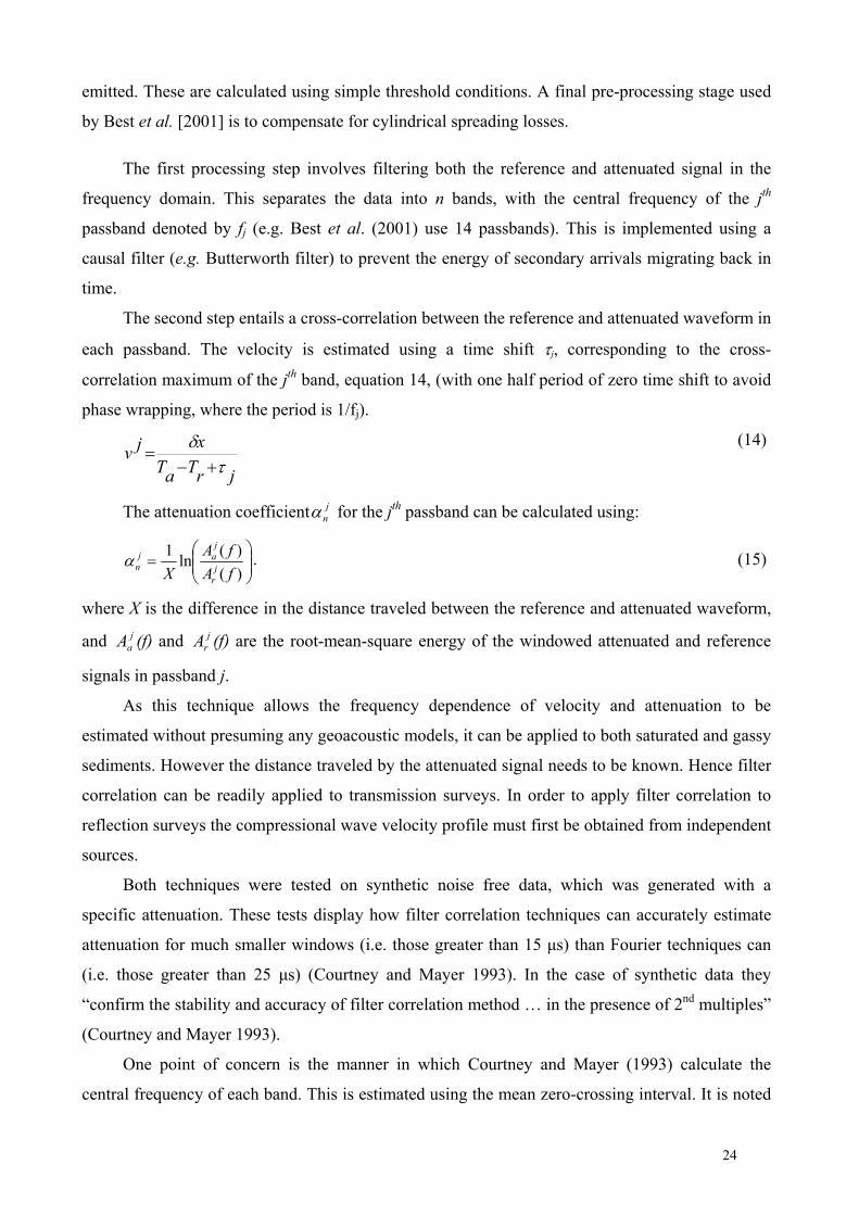
emitted. These are calculated using simple threshold conditions. A final pre-processing stage used

by Best et al. [2001] is to compensate for cylindrical spreading losses.

The first processing step involves filtering both the reference and attenuated signal in the

frequency domain. This separates the data into n bands, with the central frequency of the jth

passband denoted by fj (e.g. Best et al. (2001) use 14 passbands). This is implemented using a

causal filter (e.g. Butterworth filter) to prevent the energy of secondary arrivals migrating back in

time.

The second step entails a cross-correlation between the reference and attenuated waveform in

each passband. The velocity is estimated using a time shift τj, corresponding to the cross-

correlation maximum of the jth band, equation 14, (with one half period of zero time shift to avoid

phase wrapping, where the period is 1/fj).

jrTaTxjv

τδ

+−=

(14)

The attenuation coefficient for the jjnα th passband can be calculated using:

⎟⎟⎠

⎞⎜⎜⎝

⎛=

)()(ln1

fAfA

X jr

jaj

nα . (15)

where X is the difference in the distance traveled between the reference and attenuated waveform,

and (f) and (f) are the root-mean-square energy of the windowed attenuated and reference

signals in passband j.

jaA j

rA

As this technique allows the frequency dependence of velocity and attenuation to be

estimated without presuming any geoacoustic models, it can be applied to both saturated and gassy

sediments. However the distance traveled by the attenuated signal needs to be known. Hence filter

correlation can be readily applied to transmission surveys. In order to apply filter correlation to

reflection surveys the compressional wave velocity profile must first be obtained from independent

sources.

Both techniques were tested on synthetic noise free data, which was generated with a

specific attenuation. These tests display how filter correlation techniques can accurately estimate

attenuation for much smaller windows (i.e. those greater than 15 μs) than Fourier techniques can

(i.e. those greater than 25 μs) (Courtney and Mayer 1993). In the case of synthetic data they

“confirm the stability and accuracy of filter correlation method … in the presence of 2nd multiples”

(Courtney and Mayer 1993).

One point of concern is the manner in which Courtney and Mayer (1993) calculate the

central frequency of each band. This is estimated using the mean zero-crossing interval. It is noted

24

that this produces a very rough estimate of the mean frequency. Better estimates may be obtained

by using the mean frequency of each band (Best, Higgett et al. 2001).

IIId Wavelet modeling.

In wavelet modeling, synthetic seismograms are calculated for a range of varying parameters

and a best fit is found with observed seismic data. The simple application to a single arrival on a

seismogram is described in Jannsen et al. (1985). The wave incident on the water-sediment

interface, which is denoted by x = 0, is used as a reference wave. This automatically removes any

errors that may be introduced through either the transmission of the signal from the profiler or the

transmission of the signal through the water column and overlying sediment layers.

The spectrum of the reference wave can be used to produce synthetic seismograms for

reflectors located at a range of two-way times tref and frequency dependent Quality factors Q.

These frequency dependent Quality factors will be the result of an assumed attenuation model.

Wavelet modeling then back-transforms the spectral information into the time domain, typically

using an Inverse Fourier Transform. The synthetic seismograms are compared to the observed

data, with the best fit values of Q and tref resulting in the minimum of the function S(ζ):

∑ −=k

tMtFS ).(),()( ζζ . (16)

where F(k,ζ) is the theoretical value at time t and parameter set ζ=(Q,T) and M(t) is the observed

value at time t.

The calculation of the cross correlation of the modeled and observed signals may provide an

alternative manner of estimating the best fit parameters, i.e. the best fit parameters correspond to

the maximum cross correlation. In order to conserve computational time it is necessary to limit the

variation of tref to a “reasonable time-interval.” Hence a rough estimate of tref should be known.

This is calculated from the covariance of seismograms (calculated for Q values chosen roughly

equidistant on a logarithmic scale) and the reference signal, with a relative minimum indicating a

relatively good temporal fit between the major reflections (Jannsen, Voss et al. 1985). However it

may be possible to estimate tref using IF events, which supplies an unambiguous and robust manner

of identifying the first arrival from a reflection (Taner, Koehler et al. 1979).

The above method assumes that the velocity is known. However it could easily be modified

to allow velocity and Q value to become the two unknown variables, by simply calculating tref

using the IF events and assuming this to be a constant in the attenuation models used.

A comparison of four techniques by Jannsen et al (1985) (rise time, spectral ratio, wavelet

and spectrum modeling) concludes that for real data the modeling techniques result in significantly

25

less scatter than other methods. However care must be taken during the application of the initial

constraints on tref as these will affect results dramatically.

IIIe Conclusions.

The desirable features of a technique that can be used to estimate the attenuation and velocity

of seafloor sediments from acoustic data are:

• It is robust in the presence of noise and overlapping reflections;

• It is able to incorporate frequency dependent velocities and Q values;

• It is independent of any specific geoacoustic models or theories, the use of which will limit

the range of sediment types the technique is valid for;

Table 2 summarizes these properties for each of the techniques discussed in section 3. Technique Geoacoustic

Properties assessed Robust in presence of noise/overlapping reflections/

geoacoustic model assumed?

incorporates non-linear frequency dependence

Spectral ratio

Q Possibly / No Q independent of frequency

No

IF

α Yes / Unsure single relaxation-time theory

Possibly

filter correlation

Q, v Yes / Yes None Yes

Wavelet modelling

Q, v Yes / Yes general attenuation

Yes

Table 2: Summary of techniques discussed in section 3.

In the case of reflection data the filter correlation method is not applicable, as the distances

travelled by received pulses are unknown and can only be estimated through the use of modelling

or ground-truthing cores. Spectral ratio posses the disadvantage that only media with frequency

independent Q values can be examined. Both wavelet modelling and IF techniques appear more

promising. However, it is possible that wavelet modelling may produce a variety of ambiguous

results, all of which fit the data under examination. The use of Instantaneous Frequency requires

some modifications, including:

• The use of a technique that accurately estimates the Instantaneous Frequency of reflection

data;

• The use of attenuation equations, in the modelling stage and in the final calculation of

attenuation, which are applicable to the sediments under examination;

26

For in situ transmission data the most promising technique appears to be filter correlation.

This technique is permitted due to accurate knowledge of the distance through which the directly

transmitted wave has propagated. Wavelet modelling and IF techniques also appear promising for

in situ transmission data, with the concerns/modifications mentioned above.

IV Application of selected techniques to reflection data.

It was decided to examine the application of the IF to reflection data collected from a chirp

profiler, with efforts focusing on deducing the IF estimation technique which is most applicable to

such data. Section 4.i. will discuss the main features of the chirp sub-bottom profiler and the

specific datasets examined. Section 4.ii. investigates the fundamentals of IF and Group Delay

estimates while section 4.iii. examines a variety of IF estimation techniques. The details of the

application of the techniques are discussed in section 4.vi. and conclusions are presented in section

4.v.

IVa The chirp sub-bottom profiler.

The chirp sub-bottom profiler is a high-resolution, frequency-modulated, normal-incidence

acoustic profiler. It emits a swept frequency pulse, which can incorporate a variety of FM laws

(e.g. linear, quadratic and logarithmic) and span a frequency range of 1.5 – 15 kHz. An example of

a 32 ms, linearly swept 2-8 kHz pulse is displayed in Figure 7. The chirp pulse permits better

penetration than monotone surveying systems, without a significant reduction in resolution. The

vertical resolution is “of the decimetre scale in the top c. 30m of unconsolidated sediments”

(Quinn, Bull et al. 1998), and is dependent on the bandwidth of the source. The horizontal

resolution depends on source characteristics (beam angle and dominant frequency), the

compressional wave velocity of the sediments, the towfish altitude and the pulse rate of the

system. Characteristic horizontal resolutions of 1 - 2m are obtained (Quinn 1997)

In order to achieve these resolutions the chirp pulse is compressed using a matched signal that

correlates the chirp return signal with a replica of the “outgoing pulse” (LeBlanc, Mayer et al.

1992). The “outgoing pulse” used is the electronic pulse sent to the emitting transducers. This

correlation produces a new effective wavelet, which is the auto-correlation of the outgoing pulse.

The auto-correlation of the 32 ms, linearly swept 2 - 7 kHz pulse is displayed in Figure 8. As the

correlation process squares the spectral amplitudes, the auto-correlated pulse possesses a sharper

spectrum than the “outgoing pulse”, An additional advantage of this correlation is that it achieves a

signal processing gain over the background noise. Research by LeBlanc et al (1992) found that, in

order to equal the performance of chirp sonar pulses, conventional pulse sonar would have to use a

pulse with a peak power 100 times larger.

27

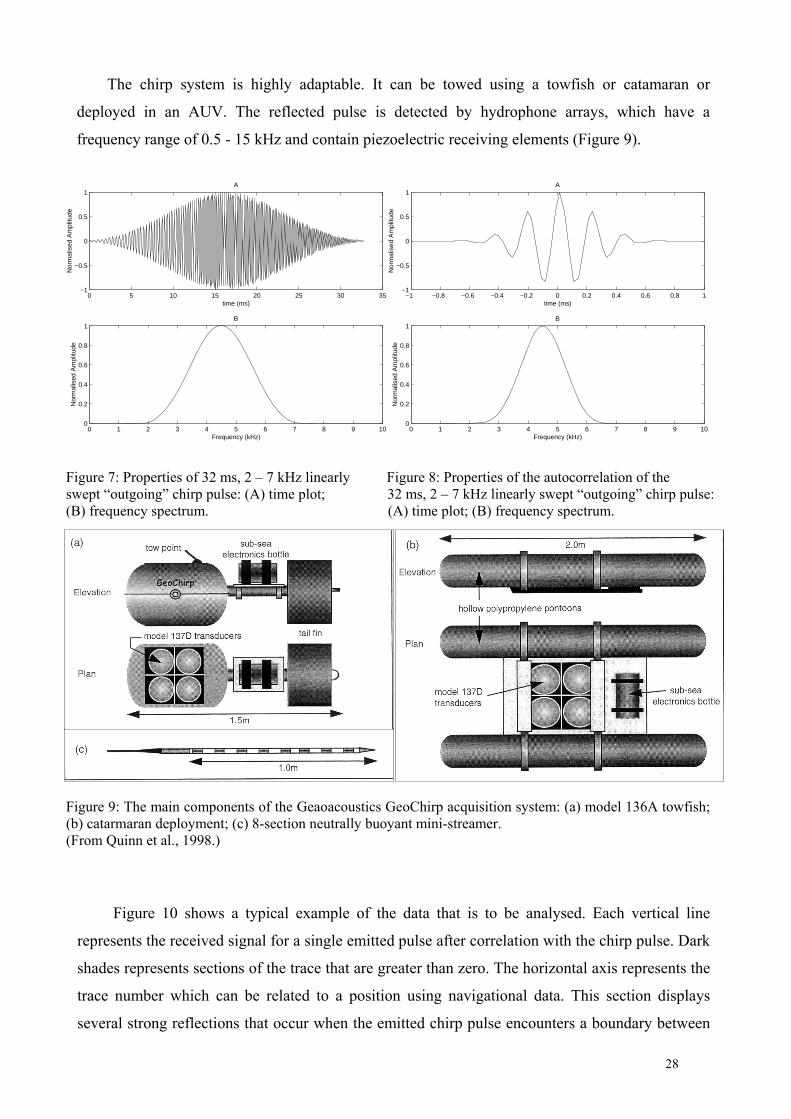
The chirp system is highly adaptable. It can be towed using a towfish or catamaran or

deployed in an AUV. The reflected pulse is detected by hydrophone arrays, which have a

frequency range of 0.5 - 15 kHz and contain piezoelectric receiving elements (Figure 9).

Figure 7: Properties of 32 ms, 2 – 7 kHz linearly Figure 8: Properties of the autocorrelation of the swept “outgoing” chirp pulse: (A) time plot; 32 ms, 2 – 7 kHz linearly swept “outgoing” chirp pulse: (B) frequency spectrum. (A) time plot; (B) frequency spectrum.

Figure 9: The main components of the Geaoacoustics GeoChirp acquisition system: (a) model 136A towfish; (b) catarmaran deployment; (c) 8-section neutrally buoyant mini-streamer. (From Quinn et al., 1998.)

Figure 10 shows a typical example of the data that is to be analysed. Each vertical line

represents the received signal for a single emitted pulse after correlation with the chirp pulse. Dark

shades represents sections of the trace that are greater than zero. The horizontal axis represents the

trace number which can be related to a position using navigational data. This section displays

several strong reflections that occur when the emitted chirp pulse encounters a boundary between

0 5 10 15 20 25 30 35−1

−0.5

0

0.5

1

time (ms)

Nor

mal

ised

Am

plitu

de

A

0 1 2 3 4 5 6 7 8 9 100

0.2

0.4

0.6

0.8

1

Frequency (kHz)

Nor

mal

ised

Am

plitu

de

B

1

−1 −0.8 −0.6 −0.4 −0.2 0 0.2 0.4 0.6 0.8 1−1

−0.5

0

0.5

Nor

mal

ised

Am

plitu

de

time (ms)

A

0 1 2 3 4 5 6 7 8 9 100

0.2

0.4

0.6

0.8

1

Frequency (kHz)

Nor

mal

ised

Am

plitu

de

B

28

two media of different acoustic impedances. Both the seafloor reflection and additional subsurface

reflections, occurring at the boundaries between sediment layers, are apparent. The first multiple

reflection from the seabed is also marked.

Though chirp profiles can clearly identify geological interfaces, the estimation of the

velocity and attenuation of sediment layers has proven more difficult. This is the aim of present

research.

Figure 10: Typical chirp section (CDPs 475-775 of dataset collected from Bouldnor Cliff, Isle of Wight). Seabed, additional sub-surface layers and first multiple of seabed are marked.

Two chirp datasets from the South coast of England will be used in the following

investigation. The first dataset was collected from Bouldnor Cliff, which lies on the NW coast of

the Isle of Wight. The sediments in this area consist of Late Eocene material, e.g. marls and

clays, underlain by Bembridge limestone at a depth of c. 22m (Dix, Jarvis et al. 2000). The

second dataset was collected from Dibden Bay, Southampton Water. The sediment in this region

consists of Holocene clays/silty clays, Pleistocene sands and gravels and Eocene bedrock (Robb

2000). Both physical and acoustic evidence of a widespread blanket of shallow gas has been

observed (Tuffin 1997; Robb 2000)

Both datasets were collected using a 2-8 kHz linear chirp pulse, with duration of 32 ms and a

pulse rate of 4/s.

29

IVb Fundamentals of IF and group delay estimates.

The calculation of IF requires that the real seismic trace is first transformed into a complex

trace. The complex trace used is the analytical signal σ(t), which is constructed by treating the

seismic trace x(t) as the real part and its quadrature x) (t) as the imaginary part. The quadrature is

estimated using the Hilbert Transform (Boashash 1992):

. (17) )(

^

)()()()( tjetAtxjtxt φσ =+=

The equation above displays how, at any time within the signal, it can be uniquely defined by

a single amplitude A and phase φ, i.e. the instantaneous envelope and instantaneous phase.

The estimation of the complex signal obtained using the Hilbert transform will be

sufficiently accurate if the spectra of the envelope function and phase of a signal do not overlap

(Boashash 1992). If these spectra overlap the Hilbert transform will be the result of overlapping,

phase distorted functions and will not correspond to the signal plus its quadrature component. The

phase and envelope functions of the traces under examination are difficult to obtain and have little

practical meaning. Hence we will consider these traces to be the convolution of the autocorrelation

of the emitted pulse (Figure 8), with a simple reflectivity series, with additional noise components

present. Hence if the spectrum of the envelope and phase of the autocorrelation do not overlap in

frequency the Hilbert transform can be used to accurately construct the analytic signal. This

condition is satisfied, with a phase spectrum containing frequencies from 2-7 kHz (Figure 8), and

the envelope spectrum containing frequencies less 2 kHz. Hence the Hilbert transform is used to

calculate the analytic signal. This is implemented discretely, as outlined in (Marple 1999), in order

to correctly scale the DC and Nyquist Frequency terms.

As mentioned earlier the IF is simply the differential of the phase with respect to time

(equation 14). For discrete data this differentiation can be calculated directly, using the

convolution of the phase and the impulse function of a finite impulse response differentiating

filter. However this results in the amplification of high frequency noise. Hence a variety of

estimation techniques, each of which have different properties and subsequently result in slightly

different estimation of IF have been developed (Boashash 1992). LeBlanc et al. (1992) and Panda

et al. (1994) simply state that the IF was calculated numerically, which omits the critical matter of

which technique was used. The optimum technique to use for chirp reflection data is examined in

section 4.c.

In addition the Bandwidth-Duration product, or BT product, of a signal will affect our

concept of IF. An alternative manner to estimate the frequency present in a signal is to use the

Group Delay, i.e. find the time at which frequency f makes its maximum contribution to the signal.

If the BT product is high, i.e. >10 (Boashash 1992), and the signal is monocomponent the

30

frequency estimate produced by IF and group delay methods will converge. If not, these two

methods will produce different frequency estimates and raise the issue of which estimate is more

realistic. As the correlated traces under examination are multicomponent and the BT product of the

autocorrelation of the emitted wave, calculated using standard definations for B and T (Cohen

1995), is approximately 0.5, IF and group delay will produce different frequency estimates. This

inconsistancy will simply be noted and the rest of the report will focus on the best manner of

estimating the IF.

IVc Theory behind selected techniques.

Based on comprehensive research into IF (Boashash 1992; Boashash 1992; Boashash and

O'Shea 1993; Boashash and O'Shea 1994; Ristic and Boashash 1996; Barkat and Boashash 1999)

five basic estimation techniques were selected. Boashash states that, for linear chirps, techniques

that use the moments of time frequency distributions are “computationally demanding … and not

generally statistically optimal” (Boashash 1992). However the following work will examine both

uncorrelated and correlated data and, as the correlation of the data reduces the linear chirp to a

broadband signal, both peak and moment estimations of IF will be tested.

As the selected techniques include the use of both linear and quadratic time-frequency

distributions (TFDs) it is necessary to examine the square of the TFD coefficients. This allows

resulting IF estimates to be directly compared. The IF at a time t is calculated by analyzing the

coefficients at that time, i.e. taking a time-slice through the distribution. The IF can be considered

to be either the frequency at which the coefficients peak or the mean frequency (first moment) of

the time slice. Both of these adaptations were tested for techniques that incorporate a TFDs.

The use of an alternative TFD, the Cross Polynomial Wigner-Ville Distribution, has been

omitted owing to its highly intensive computational demands, i.e. it involves resampling to 105

times the original sampling rate (Ristic and Boashash 1996).

The following basic techniques were selected for testing.

• The discrete classical time formula (DCTF). The DCTF estimates IF using the discrete

differentiation of arctangent form of the phase, equation 18. It is extremely efficient to

implement.

.)()(

)().()(ˆ).(21)2/1( 22 nxnx

ndxnxnxdnxnIF )

)

+−

⎟⎠⎞

⎜⎝⎛=+

π (18)

where IF(n+1/2) is the IF at the time instant tn=(n+1/2)τs, with τs as the sampling interval and n

an integer, x(n) and are the values of the real and imaginary parts of the analytic signal at t)(ˆ nx n

and dx(n) and are the differences between the (n+1))(ˆ nxd th and nth values of the real and

31

imaginary components of the analytical signal, i.e. dx(n)=x(n+1)-x(n) and

)(ˆ)1(ˆ)(ˆ nxnxnxd −+=

• The peak and first moment of the short time Fourier transform (STFT). The STFT is a linear

TFD and is defined as the Fourier transform of windowed sections of a signal:

∫∞

−∞=

−−=τ

τπ τττσ .)()(),( 12 detwftS f (19)

where S(t,f) are the STFT coefficients at time t and frequency f, w(τ-t) is the windowing

function and σ(τ) is analytical signal at time lag τ. Both peak and first moment estimations of IF

were investigated.

STFT estimations should perform well if the signal is quasi-stationary. However resolution

limitations, which arise from the uncertainty principle, will produce poor results for rapidly

varying signals (Boashash 1992).

• The peak and first moment of the Wigner-Ville Distribution (WVD). The WVD is the Fourier

Transform of the instantaneous correlation function ),( τtr :

ττ τπ detrftWVD if∫ −= 2),(),( . (20a)

( ) ( 22),(* τστστ +−= tttr ). (20b)

where WVD(t,f) are the WVD coefficients at time t and frequency f and σ(t) is the analytic

signal. This is implemented discretely by replacing t by nτs, τ by mτs and the integral over τ to a

sum over m, where n and m are integers and τs is the sampling interval.

The correlation function, which represents the kernel of this TFD, simply weights all lags

equally. The WVD allows good localisation of energy and satisfies theoretical conditions.

However it can be negative at some points, denoting a negative energy, and, owing to its

quadratic nature, possess cross-terms. Hence it is of critical importance that the analytical signal

is used, as this will reduce needless cross terms (Boashash 1988). IF is estimated using both

peak and first moment methods, as described previously.

Using the peaks of the WVD is noted to be the optimum method for “high to moderate SNR

signals which can be approximated well (at least locally) to linear FM signals” (Boashash

1992).

• The peak and moment of the cross Wigner-Ville Distribution (XWVD). The XWVD is formed

in similar manner to the WVD, expect that the kernel used is the correlation function of the

analytic observed signal σob and an analytic reference signal σref,, i.e. equation 20b is replaced

by:

32

( ) ( )22),(* τστστ +−= tttr refob . (21)

An iterative approach is suggested (Boashash 1992), in which it is assumed that the reference

signal is unknown and is calculated from the estimated IF of the observed signal. This is used to

generate the XWVD and a new IF calculated from the peaks. A new reference signal is created

and this process repeated until the difference in IF estimates from successive iterations is less

than a specified amount. As the reference signal for a chirp profiler is both repeatable and

accurately known this iterative procedure was omitted and the emitted pulse used as the

reference signal. IF is estimated using both peak and first moment techniques.

“For low SNR non-stationary signals, which are comparatively long,” the peaks of the iterative

XWVD, generated using a sliding window, may supply a reliable estimate of the IF (Boashash

1992; Boashash and O'Shea 1993). However, the performance of the non-iterative approach

used in this report is unknown.

• The peak and first moment of the Polynomial Wigner-Ville Distribution (PWVD). The

WVD is similar to a central finite difference estimator and hence yields good energy

concentration for noise-free linear FM signals. The PWVD incorporates a kernel that includes

non-linear terms, with the general equation for a qth order PWVD kernel displayed below:

∏=

−−

−−+=2/

0

* )}({)}({),(q

k

bk

bk

q kk mcnmcnmnK σσ . (22)

where σ represents the analytic signal, bk controls the weighting of different phase values, ck

controls the separation of different phase values used and n and m are the discrete versions of t

and τ used earlier. The PWVD is simply the Fourier Transform of the above kernel.

The optimum settings for these constants have been deduced in (Boashash and O'Shea 1994) for

a 4th order PWVD, i.e. one that can examine linear, quadratic, cubic and quadratic FM laws.

These are listed below, along with the resulting kernel and are used in the subsequent analysis:

1;2;0 22110 =−==−== −− bbbbb

85.0;675.0 2211 =−==−= −− cccc

(23) ).85.0().85.0(.)}675.0().675.0({),( *2*4 mnmnmnmnmnK −+−+= σσσσ

Note that in order to form a discrete kernel the data must be resampled, to forty times its

original rate. A frequency-scaled version of the kernel (Boashash and O'Shea 1994), which can

be used to reduce errors that may arise during resampling has not been used due to its large

computational demand, i.e. it would involve resampling to 1000 times the original rate. Again

both peak and first moment estimates of IF are tested.

33

The PWVD peak based IF estimation performs well for polynomial phase laws, (Boashash and

O'Shea 1994), with the IF estimation from the peaks of the PWVD out-performing other

estimation techniques for signals with a SNR larger than 3 dB (Barkat and Boashash 1999).

IVd Data used and details of implementation.

The above techniques were applied to the two chirp datasets discussed in section 4.i. It is

usual to compress the chirp pulse by correlating the signal received by the chirp profiler with the

emitted pulse. However, as the performance of TFDs which incorporate correlations is not fully

understood for reflection data, techniques were applied to both correlated and uncorrelated data.

Note the XWVD techniques were not applied to correlated data, as these techniques inherently

involve a correlation process. No geometric spreading corrections were applied to the traces, as

application of such corrections usually assume basic spreading laws, which may not be completely

accurate.

For each dataset 4 sections, of 9 traces each, were selected from both the correlated and

uncorrelated data. The choice of 9 traces per section is an attempt to halve the section size used in

previous IF research, while retaining a unique central trace to which composite results for the

section can be compared. As the order in which the information from these traces is combined to

produce a composite IF for the section is important, a variety of approaches were tested. These

included the use of:

• The central trace, i.e. estimate the IF of the central trace of the section;

• Stacked traces, i.e. stack the traces to obtain a composite trace, from which IF is estimated;

• Stacked IFs, i.e. calculate the IF for each trace in the section individually, stack the IFs and

normalize over the number of traces in the section. This is essentially the technique used by

(LeBlanc, Panda et al. 1992), except a section of 9, rather than 20, traces is used;

• Stacked distributions, i.e. generate the relevant TFD for each trace in the section, square the

coefficients and stack the resulting distributions. The IF is then calculated from the composite

distribution;

Note that the absence of a TFD in the case of the DCTF prevents the use of the final

approach for this technique.

As the manner in which the techniques were implemented is of paramount importance,

particularly for those techniques based on the peaks of TFDs, such details will now be discussed.

Care was taken to ensure that almost all techniques produced IF profiles with the same

theoretical frequency and temporal resolutions. These were set at 12.2 Hz and 0.04 ms, which

were the most convenient values for the sampling frequency of the received data (25 kHz) and the

34

data length examined (2048 points). An exception is the DCTF, which theoretically has an

infitesimally small frequency resolution. Note that this does not translate into an infinitely accurate

value of IF, as the techniques which we are examine estimate IF.

In order to obtain these resolutions the following parameters were used:

• The number of frequency bins in each TFD was set to the number of data points under

analysis.

• The TFDs used windows with maximum overlap.

In addition the STFT window size was set to 2.56 ms, to optimize it performance, and digital

version of the 32 ms,

2-8 kHz linear chirp pulse used to collect both datasets, which was supplied by Geo-

acoustics Ltd., was used as the reference pulse in the formation of the XWVD. Note that the only

difference between the techniques is the degree of smoothing each one incorporates, with the

XWVD, PWVD and WVD using maximum smoothing, the STFT using intermediate smoothing

and the DCTF using no smoothing.

A final point is that the acquisition of data by the chirp system introduces a delay of

approximately 3.5 ms. This has not been removed as the absolute depth of reflectors below the sea

surface bears no relationship on the relaxation times and attenuations which will be estimated. If

geometric spreading losses had been corrected for, or we wished to accurately locate the depth of

the seabed or other sub-surface reflectors, it would be necessary to account for this time delay.

IVe Results and discussion.

The IF estimations obtained from the techniques and stacking methods discussed in section

4.iv. were examined. This was done with the aim of identifying the method which produces IF

estimates that are most effective in the calculation of relaxation time, grain size and attenuation.

Such a technique will ideally result in:

• An IF which varies smoothly with two-way time and clearly displays regions over which IF

decreases linearly with two-way time;

• The two-way times at which these regions start and end corresponding to observed reflection

events and hence to individual sediment layers;

• Relaxation times that are less than 0.2 μs. This value was obtained from Figure 3 as a upper

limit for relaxation time;

Figure 11 displays the relationship between the modeled frequency shift of a 2 – 7 kHz

linearly-swept chirp pulse, in Hz/ms, and the mean relaxation time of each sediment types listed in

Table 1. The use of units of Hz/ms removes the effects of phase velocity on the equation used in

35

the modeling stage. This eliminates any errors that may be induced by inaccuracies in velocity,

which will be particularly important for gassy sediments (Anderson and Hampton 1980). In

addition the propagation of the pulse is modeled for all six sediment types listed in table 1 and

allows the empirical relationship derived to be more tightly constrained than that obtained by

LeBlanc et al. (1992).The relaxation time was calculated by applying a least squares linear fit to

the region over which IF decreases with two-way time. The gradient of this line is then converted

into a relaxation time using the empirical relationship derived from Figure 11, i.e.

.00672.0 shiftf=τ (24)

where τ is relaxation time in μs and fshift represents the gradient of the linear trendline applied in

Hz/ms. This relaxation time can be used to calculate the attenuation using equation 12.

0 5 10 15 20 25 300

0.05

0.1

0.15

0.2

0.25

Modeled frequency shift per unit time (Hz/ms)

Rel

axat

ion

time

(μs)

Figure 11: Plot of relaxation time against modeled frequency shift, in Hz/ms, for a 2-8 kHz linearly swept chirp pulse. Both modeled shift (X) and linear fit from which equation 25 is obtained (solid line) are displayed

As Figure 3 applies to saturated sediment, the third condition will be relaxed for IF results

from Dibden Bay. Sediments here are gassy and will possess larger attenuations than saturated

sediments. If the single relaxation time theory assumed is applicable to gassy sediments, this will

result in larger relaxation times than expected.

The results of the techniques will be discussed in four stages. Firstly we will compare the use

of uncorrelated and correlated data; secondly the best order of stacking will be examined; thirdly

the optimum technique for estimating the IF of chirp data will be discussed; the fourth section will

apply this optimum technique to the entirety of the two datasets used and discuss the resulting

estimates of relaxation time and attenuation.

36

• Comparison of correlated and uncorrelated data.

Both datasets displayed similar results and typical results for an uncorrelated trace are

included in Figure 12. The trace displayed is taken from a gassy region of the Dibden Bay dataset.

The envelope of the uncorrelated trace is displayed in Figure 12(v), with the main signal event

occurring between approximately 20 – 42 ms. The relatively broad and overlapping nature of

reflection events, compared to those present in correlated data (Figure 13(v)) display the inability

of uncorrelated data to locate reflection events accurately. Examination of the corresponding

correlated trace, Figure 13(v), locates the peak of the seabed event at 14.6 ms, the peak of the gas

horizon at 15.8 ms and the peak of the first multiple at 26 ms.

The IF estimated using the DCTF (Figure 12(i)) contains extremely large anomalies, with

magnitudes greater than the Nyquist frequency of 12.5 kHz. However from 20 – 40 ms, i.e. over

the duration of the main signal event, the majority of anomalies are less than 1 kHz and IFs which

increase with two-way time, from 2.5 kHz at 20 ms to 4 kHz at 42 ms, can be observed.

Estimations of IF arising from the STFT (Figure 12(i)) contain negligible anomalies. These are

however replaced by discontinuities, with maximum magnitudes of 0.5 kHz for first moment

estimates and 1.5 kHz for peak estimates. Decreasing trends in IF, which commence at two-way

times corresponding to the seabed reflections, result in relaxation times greater than 1 μs. These

are greater than expected, even for gassy sediments. Again IFs which increase with two-way time

are observed over the duration of the main signal event. Estimates of IF derived from the WVD,

(Figure 12(ii)) and PWVD (Figure 12(iii)), display similar general trends, with IF increasing with

two-way time, over two-way times corresponding to the duration of the main signal and varying

frequency ranges. Outside this region anomalies are relatively large and act to conceal any trends

in IF. In general IF estimates arising from the first moment of TFDs display a region, which

extends over the upper 5 ms of sediment, where IF decreases with two-way time. However the

resulting relaxation times for this region are greater than 0.33 μs. Estimates of IF derived from the

peaks of the XWVD (Figure 12(iv)) display IFs which generally increase with two-way time,

while the location of IF trends arising from the first moment (Figure 12(iv)) display little

correlation to the seabed location.

It is clear that techniques based on the first moment of TFDs produce the better IF

estimations for uncorrelated data, than those based on the peak of TFDs. However little effective

information about frequency shift and relaxation time can be obtained from uncorrelated data for

the following reasons:

• The lack of temporal resolution of uncorrelated data;

• The poor signal to noise ratio of uncorrelated data;

37

• All IF estimations obtained from uncorrelated data are dominated by IFs that increase

linearly with two-way time, i.e. we observe the increasing frequency of the emitted chirp pulse;

• Any regions where IF decreases with two-way time result in relaxation times greater than the

expected upper limit;

• The use of sections of traces, as discussed in section 4.iv. simply reduced the amplitude of

the anomalies present, with an IF which linearly increase with two-way time still dominating

the results;

Figure 13 displays IF estimates for the correlated version of the trace discussed above and

represent typical results for correlated data. The techniques used display similar characteristics to

those previously observed, i.e. the DCTF estimates contain large anomalies, STFT estimates are

disrupted by discontinuities and the smoothest IF estimates arise from the first moments of the

WVD. However the important difference to IF estimates from uncorrelated data is the presence of

IF trends, which decrease with two-way time and produce acceptable relaxation times.

Anomalies are generally smaller than those for uncorrelated data. This is a consequence of

the increased signal to noise ratio achieved by correlation. The improved IF estimates are a

consequence of two main factors. Firstly the duration of effective sampling pulse has been reduced

from 4.5 ms to 0.15 ms. This allows reflection events to be more accurately resolved in time.

Secondly the effective sampling pulse is now purely a broadband signal, i.e. it does not contain

any linear chirp components. Hence IF now truly represents the central frequency of the signal.

This assumption is of paramount importance if we wish to convert frequency shift per ms into

useful geoacoustic parameters. Note that anomalous points still inhibit accurate estimation of both

the gradient of the observed decreasing trends in IF and the two-way times at which such

decreasing trends in IF commence. For some techniques anomalies completely conceal any trends

in IF which may be present.

It is concluded that the use of correlated data produces IF estimates which are more

applicable to the spectral shift technique of obtaining the geoacoustic properties of the sediment.

38

0 10 20 30 40 50 60 70 800

1

2

3

4

5

6

7

8

two−way time (ms)

IF (

kHz)

(i)

0 10 20 30 40 50 60 70 800

1

2

3

4

5

6

7

8

two−way time (ms)

IF (

kHz)

(ii)

0 10 20 30 40 50 60 70 800

1

2

3

4

5

6

7

8

two−way time (ms)

IF (

kHz)

(iii)

0 10 20 30 40 50 60 70 800

1

2

3

4

5

6

7

8

two−way time (ms)

IF (

kHz)

(iv)

0 10 20 30 40 50 60 70 800

0.1

0.2

0.3

0.4

0.5

0.6

0.7

0.8

0.9

1

two−way time (ms)

Norm. A

mplitud

e

(v)

Figure 12: Typical results of IF techniques applied to a single uncorrelated trace, i.e. CDP 470 from Dibden Bay dataset. (i) IF estimate using DCTF (yellow), peak of STFT (black) and first moment of STFT (red). (ii) IF estimate using peak (green) and first moment (blue) of WVD. (iii) IF estimate using peak (cyan) and first moment (magenta) of PWVD. (iv) IF estimate using peak (red dashed line) and first moment (black dashed line) of XWVD. (v) Envelope of uncorrelated trace used.

39

0 10 20 30 40 50 60 70 800

1

2

3

4

5

6

7

8

two−way time (ms)

IF (

kHz)

(i)

0 10 20 30 40 50 60 70 800

1

2

3

4

5

6

7

8

two−way time (ms)

IF (

kHz)

(ii)

0 10 20 30 40 50 60 70 800

1

2

3

4

5

6

7

8

two−way time (ms)

IF (

kHz)

(iii)

0 10 20 30 40 50 60 70 800

0.1

0.2

0.3

0.4

0.5

0.6

0.7

0.8

0.9

1

two−way time (ms)

Nor

mal

ised

Am

plitu

de

(iv)

Figure 13: Typical results of IF techniques applied to a single correlated trace, i.e. CDP 470 from the Dibden Bay dataset. (i) IF estimate using DCTF (yellow), peaks of STFT (black) and first moment of STFT (red). (ii) IF estimate using peaks (green) and first moment (blue) of WVD. (iii) IF estimate using peaks (cyan) and first moment (magenta) of PWVD. (iv) Normalised envelope of correlated trace used.

• Comparison of stacking orders.

Figure 14 shows the application of the four stacking processes discussed in section 4.iv. to IF

estimates obtained using the first moment of the WVD. The data displayed is for the section of

correlated traces centred on CDP 470 from the Dibden Bay dataset.

The general features of the IF plot are displayed in Figure 14(i) and the envelope of the

central trace displayed in Figure 14(ii). The IF decreases sharply with two-way time from 12.5 to

15 ms. This is followed by a sharper rise to a local peak at approximately 16 ms and then a linear

decrease, which extends over approximately 5ms, at which point it rises sharply. This linear

40

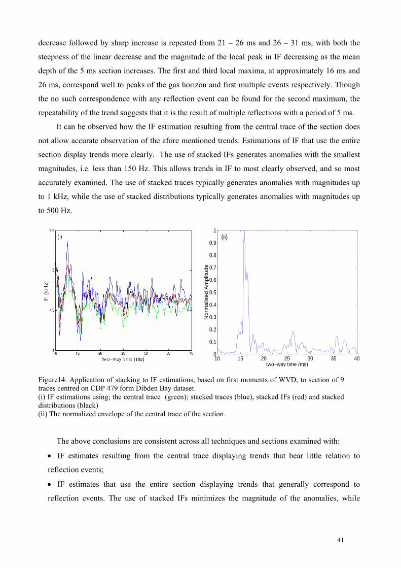
decrease followed by sharp increase is repeated from 21 – 26 ms and 26 – 31 ms, with both the

steepness of the linear decrease and the magnitude of the local peak in IF decreasing as the mean

depth of the 5 ms section increases. The first and third local maxima, at approximately 16 ms and

26 ms, correspond well to peaks of the gas horizon and first multiple events respectively. Though

the no such correspondence with any reflection event can be found for the second maximum, the

repeatability of the trend suggests that it is the result of multiple reflections with a period of 5 ms.

It can be observed how the IF estimation resulting from the central trace of the section does

not allow accurate observation of the afore mentioned trends. Estimations of IF that use the entire

section display trends more clearly. The use of stacked IFs generates anomalies with the smallest

magnitudes, i.e. less than 150 Hz. This allows trends in IF to most clearly observed, and so most

accurately examined. The use of stacked traces typically generates anomalies with magnitudes up

to 1 kHz, while the use of stacked distributions typically generates anomalies with magnitudes up

to 500 Hz.

10 15 20 25 30 35 400

0.1

0.2

0.3

0.4

0.5

0.6

0.7

0.8

0.9

1

two−way time (ms)

No

rma

lise

d A

mp

litu

de

(ii)

Figure14: Application of stacking to IF estimations, based on first moments of WVD, to section of 9 traces centred on CDP 479 form Dibden Bay dataset. (i) IF estimations using; the central trace (green); stacked traces (blue), stacked IFs (red) and stacked distributions (black) (ii) The normalized envelope of the central trace of the section.

The above conclusions are consistent across all techniques and sections examined with:

• IF estimates resulting from the central trace displaying trends that bear little relation to

reflection events;

• IF estimates that use the entire section displaying trends that generally correspond to

reflection events. The use of stacked IFs minimizes the magnitude of the anomalies, while

41

moderate anomalies are observed for stacked distributions and anomalies possess maximum

magnitudes for the stacked traces approach;

These imply that the optimum manner of stacking is to estimate the IF of each trace in the

section individually and stack the IF estimations to obtain a composite IF for the section.

• Comparison of selected techniques.

The techniques discussed in section 4.c.iv. were applied to the sections of correlated data,

with the composite IF of the section calculated using the stacked IF approach. To maintain

consistency Figure 15 displays results for the same section of traces from Dibden bay that has been

used previously in this report. These results are typical for all other sections examined.

The IF estimates arising from the DCTF (Figure 15(i)) display lower IFs than expected, i.e. a

mean IF of approximately 2.3 kHz. Anomalies possess typical magnitudes of 1 kHz. The fact that

the composite IF of the section is less than the IF of the single central trace, i.e. the yellow line in

Figure 13(i), implies that stacking does not enhance DCTF estimations of IF. This is probably a

result of the large anomalies that dominate DCTF estimates.

Figures 15(ii) to 15(iv) display how first moment estimates of IF possess anomalies with

magnitudes typically less than 50% of those present in the corresponding peak estimations. Hence

first moment estimates produce smoother IFs. These provide a more accurate basis for the

estimation of frequency shift, relaxation time and other geoacoustic parameters.

The IF estimates obtained from the moments of the STFT (Figure 15(ii)) possess negligible

anomalies. However IF trends observed generally exhibit poor correlation to the observed reflection

events.

Estimates of IF derived from first moments of the WVD (Figure 15(iii)) display IF ranging

from 4.1 - 4.7 kHz in the sediment. Owing to the preferential attenuation of higher frequencies, the

central frequency of the received pulse is expected to be lower than 4.5 kHz, i.e. the central

frequency of the emitted pulse. Hence the range of IF values obtained by this technique appear

reasonable, with high-frequency noise possibly being the source of IF values greater than 4.5 kHz.

Anomalies are typically less than 100 Hz and IF displays a smooth variation with two-way time. The

events and trends observed in IF, such as the sharp rise in IF followed by a region over which IF

decreases linearly with two-way time mentioned earlier, correlate well to observed reflection events.

In addition relaxation times, resulting from the application of first-order least squares fits to regions

where IF decreases with two-way time, typically lie within the acceptable limits of 0 – 0.2 μs.

However, for all sections analysed, IF estimations which use the WVD display a region of two-way

times, which commences between 41 ms and 43 ms and possess a duration of 5 – 7.5 ms, where IF

42

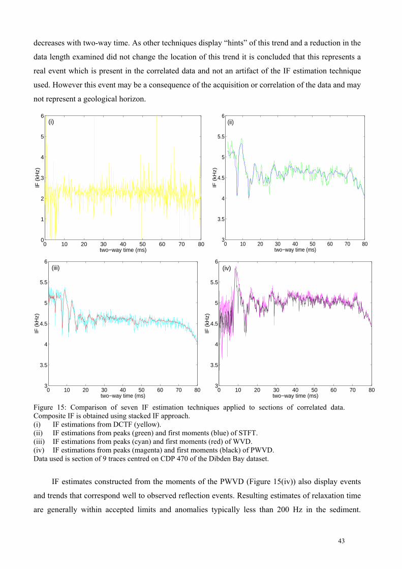
decreases with two-way time. As other techniques display “hints” of this trend and a reduction in the

data length examined did not change the location of this trend it is concluded that this represents a

real event which is present in the correlated data and not an artifact of the IF estimation technique

used. However this event may be a consequence of the acquisition or correlation of the data and may

not represent a geological horizon.

0 10 20 30 40 50 60 70 800

1

2

3

4

5

6

two−way time (ms)

IF (

kHz)

(i)

0 10 20 30 40 50 60 70 803

3.5

4

4.5

5

5.5

6

IF (

kHz)

two−way time (ms)

(ii)

0 10 20 30 40 50 60 70 803

3.5

4

4.5

5

5.5

6

IF (

kHz)

two−way time (ms)

(iii)

0 10 20 30 40 50 60 70 803

3.5

4

4.5

5

5.5

6

IF (

kHz)

two−way time (ms)

(iv)

Figure 15: Comparison of seven IF estimation techniques applied to sections of correlated data. Composite IF is obtained using stacked IF approach. (i) IF estimations from DCTF (yellow). (ii) IF estimations from peaks (green) and first moments (blue) of STFT. (iii) IF estimations from peaks (cyan) and first moments (red) of WVD. (iv) IF estimations from peaks (magenta) and first moments (black) of PWVD. Data used is section of 9 traces centred on CDP 470 of the Dibden Bay dataset.

IF estimates constructed from the moments of the PWVD (Figure 15(iv)) also display events

and trends that correspond well to observed reflection events. Resulting estimates of relaxation time

are generally within accepted limits and anomalies typically less than 200 Hz in the sediment.

43

However, the majority of IF values are greater than 5 kHz, which is greater than the expected values

of 4.5 kHz or lower. This raises doubt in IF estimates produced by this technique.

For all IF estimation techniques, particularly those that use TFDs, the IF appears to drop off

over the last 20 ms of the trace. It is hypothesized that, beyond 60 ms, the SNR of the signal drops

below the level at which IF can be accurately estimated. The high level of noise in IF estimates

below this point result in ineffective stacking.

As we are primarily interested in the uppermost sediments, where SNR is highest, using the

first moment of the WVD appears to be the optimum IF estimation technique. This produces:

• IF which vary smoothly with two-way time and possess anomalies with magnitudes typically

less than 100 Hz;

• IF values approximately that expected;

• Events and trends in IF that correspond well to observed reflection events;

• Estimates of relaxation time which generally lie within accepted limits;

However the presence of a possible artifact centred on approximately 45 ms and an IF that

decreases over the last 20 ms of analysed data limits the use of this techniques to the upper 40ms of

correlated data.

• Application of optimum technique.

The IF estimation technique that performed best in these trials, i.e. the estimation of IF using

the first moment of the WVD and the stacking of IF across a nine trace section of correlated data,

was used to estimate the relaxation time and attenuation of chirp data, as described earlier in section

4.v. In the case of the dataset from Dibden Bay it was difficult to locate a peak in the seabed

reflection, as this event merged with the stronger reflection from the gas horizon. IF appears to

decrease in a linear fashion with two-way time from two-way times that correspond to peaks in gas

horizon reflection events to those that correspond to peaks in the first multiple of the gas horizon.

Hence the least-squares linear fit is applied between these two limits. Typical results are displayed

in Figure 15, for the same section from Dibden Bay used previously. The linear plot results in a

relaxation time of 0.01 μs and an attenuation of 0.02 dB/m for the central frequency of the emitted

pulse, i.e. 4.5 kHz, and predicted velocity of 1500 m/s. These are clearly incorrect for gassy

sediments, which possess large attenuations of the order of 100 dB/m, and may arise for a range of

reasons. Firstly the linear line incorporates two distinct events and does not truly represent the

variation of IF with two-way time. However as no reflection event corresponds to the two-way time

at which the second event commences, one cannot justify the use of a linear fit which incorporates

the first event only, the use of which would result in much higher relaxation times and attenuations.

44

Secondly the fundamental equation, equation 12, which is used to obtain relaxation time from

frequency and convert relaxation time into attenuation assumes a quadratic relationship between

attenuation an frequency. This is not applicable to gassy sediments were the attenuation depends on

the resonant frequency of the gas bubbles present (Anderson and Hampton 1980). In addition the

velocity assumed above may also be significantly in error.

10 15 20 25 30 35 400

0.1

0.2

0.3

0.4

0.5

0.6

0.7

0.8

0.9

1

two−way time (ms)

Norm

alis

ed A

mplit

ude

(ii)

10 15 20 25 30 35 404

4.5

5

5.5

two−way time (ms)

IF (

kHz)

(i)

Figure 16: Results of optimum IF estimation techniques applied to data from Dibden dataset. (i) IF estimation, with two-way time of gas horizon peak (red line) and trendline from two-way time of gas horizon peak to two-way time of peak in first multiple of gas horizon (blue line). (ii) Normalised amplidue of central trace Data is section of 9 traces centred on CDP 470.

However, when applied to the Bouldnor Cliff dataset, results proved more promising. The

clearly resolved nature of the seabed reflections allow the least-squares fit to be selected with greater

confidence. The application of a least-squares fit is displayed in Figure 17. This fits the data much

better than in Figure 16 and results in a relaxation time of 0.1 μs and an attenuation of 0.2 dB/m.

Figure 18 results from the application of such least-squares fits to the first 700 CDPs of the

Bouldnor Cliff dataset. The rest of this dataset was neglected as the peaks of the first multiple event

could not be accurately located. The resulting frequency shifts (Figure 18(i)) all display negative

values. Corresponding relaxation times (Figure 18(ii)) all lie below 0.14 μs, which are within

accepted limits. Resulting attenuations at 4.5 kHz are all less than 0.32 dB/m. These result in Q

values greater than 30, which appear reasonable for the saturated sediments and sedimentary rocks

under examination. There is however a large degree of variation from one section to the next.

Assuming that sediments display small lateral variations, resulting estimates of relaxation time and

attenuation should vary smoothly with central CDP. This scatter is particularly noticeable for

sections with central CDPs greater than 525, the reason for this unknown.

45

Figure 17: Application of optimum IF estimation technique to data from Bouldnor Cliff dataset. (i) IF estimation, with location of seabed peak (red line) and trendline from seabed to first multiple (blue line) marked. (ii) Normalised amplitude of central trace, displaying seabed and sub-surface reflections. Data used is section of 9 traces centred on CDP 25.

Figure 18: Estimation of: (i) Frequency shift; (ii) Relaxation time; (iii) Attenuation at 4.5 kHz For first 700 CDPs from Bouldnor Cliff Dataset.

IVf Conclusions.

Work to date has dealt with the development of a technique that can accurately estimate the

IF of chirp reflection data. This has been achieved with the technique outlined below:

• Divide the correlated chirp profile into a series of sections, each containing a fixed number

of adjacent traces;

5

Nor

mal

ised

Ampl

itude

10 15 20 25 30 35 404

4.1

4.2

4.3

4.4

4.5

4.6

4.7

4.8

(i) 4.9

IF (

kHz)

two−way time (ms)

0 100 200 300 400 500 600 700−30

−20

−10

0

CDP

Freque

ncy shi

ft (Hz/m

s)

0 100 200 300 400 500 600 7000

0.05

0.1

0.15

0.2

CDP

τ (μs)

0 100 200 300 400 500 600 7000

0.1

0.2

0.3

0.4

CDP

α (dB/m

)

(i)

(ii)

(iii)

46

• In each section estimate the IF of each trace using the first moment of the WVD;

• Stack the resulting IF to obtain a composite IF for the section;

IF estimates obtained from this technique are only valid for the upper 40 ms of received data,

with estimates below this becoming less realistic. A section size of 9 traces was selected in this

report. Estimates of geoacoustic parameters obtained using least-square linear fits to IF above the

first multiple, and the approach outlined by LeBlanc et al. (LeBlanc, Panda et al. 1992) appear

realistic in the case of saturated sediments, i.e. the Bouldnor Cliff dataset. However in the case of

gassy sediments, i.e. the Dibden Bay dataset, estimated attenuations are dramatically lower than

expected. Concern is raised about whether the intrinsic equation used, equation 12, in both the

conversion of shift in central frequency to relaxation time and the calculation of attenuation is

applicable to marine sediments. Previous research suggests that the quadratic relationship between

attenuation and frequency is valid for neither saturated nor gassy sediments.

Hence the aims of future work are:

• To develope a reliable method of converting shift in central frequency into geoacoustic

parameters, e.g. for saturated sediments use an attenuation αdB that varies linearly with

frequency f (Hamilton 1972; Hamilton 1979; Toksoz, Johnstone et al. 1979):

kfdB =α (25)

where k is a parameter that depends on sediment properties, such as grain size and porosity. The

shift per unit time in the central frequency of the emitted chirp pulse could then be modelled for

a range of k and so sediment types. If the velocity of the sediment layers present could be

obtained, the theoretical relationship between frequency shift and k could be used to invert

measured shifts in central frequency into values of k and αdB. Note that the use of an attenuation

linearly related to frequency requires knowledge of the velocity, while the quadratic relationship

used previously, (LeBlanc, Panda et al. 1992), does not require this information.

In theory a model which incorporates the frequency dependent attenuation displayed by gassy

sediments could be used for such environments, though the more complex nature of this

relationship may make this process problematic;

• To assess the smallest window in two-way time over which the optimum technique selected

can be used to reliable estimate shift in central frequency. This will dictate the minimum

thickness of sediment layers that can be resolved. Previous work on IF has neglected the issue

of windowing by simply applying linear fits to IF values between the seabed and first multiple

reflections. However this may contain a variety of sediment layers and will hence produce a

47

composite attenuation for all sediment layers present. The introduction of smaller windows of

two-way time will may allow these layers be both resolved and examined individually.

References. Anderson, A. L. and L. D. Hampton (1980). “Acoustics of gas bearing sediments 2.

Measurements and models.” Journal of the Acoustical Society of America 67(6): 1890-1905.

Anderson, A. L. and L. D. Hampton (1980). “Acoustics of gas bearing sediments 1. Background.” Journal of the Acoustical Society of America 67(6): 1865-1889.

Barkat, B. and B. Boashash (1999). “Instantaneous Frequency Estimation of Polynominal FM Signals Using the Peak of the PWVD: Statisical Performance in the Presence of Additive Noise.” IEEE Transactions on Signal Processing 47(9): 2480-2491.

Best, A. I., Q. J. Higgett, et al. (2001). “Comparison of in-situ and acoustic measurements on Lough Hyne marine sediments.” Journal of the Acoustical Society of America 100(2): 695-709.

Boashash, B. (1988). “Note on the Use of the Wigner Distribution for Time-Frequency Signal Analysis.” IEEE Transactions on Acoustics, Speech and Signal Processing 36(9): 1518-1521.

Boashash, B. (1992). “Estimating and Interpreting The Instantaneous Frequency of a signal-Part 1: Fundamentals.” Proceedings to the IEEE 80(4): 520-538.

Boashash, B. (1992). “Estimating and Interpreting The Instantaneous Frequency of a Signal-Part 2: Algoritms and Applications.” Proceedings to the IEEE 80(4): 539-568.

Boashash, B. and P. O'Shea (1993). “Use of the Cross Wigner-Ville Distribution for Estimation of Instantaneous Frequency.” IEEE Transactions on Signal Processing 41(3): 1439-1445.

Boashash, B. and P. O'Shea (1994). “Polynominal Wigner-Ville Distributions and Their Relationship to Time-Varying Higher Order Spectra.” IEEE Transactions on Signal Processing 42(1): 216-220.

Bowles, F. A. (1997). “Observations on attenuations and shear wave velocity in fine-grained, marine sediments.” Journal of the Acoustic Society of America 101(6): 3385-3397.

Buckingham, M. J. (2000). “Wave propagation, stress relaxation, and grain-to-grain shearing in saturated, unconsolidated marine sediments.” Journal of the Acoustic Society of America 108(6): 2798-2815.

Cohen, L. (1995). Time-Frequency analysis., Prentice-Hall Inc.: 299.pp Courtney, R. C. and L. A. Mayer (1993). “Calculation of acoustic parameters by a filter-

correlation method.” Journal of the Acoustical Society of America 93(2): 1145-1154. Dasios, D., T. R. Astin, et al. (2001). “Compressional-wave Q estimation from full-

waveform sonic data.” Geophysical Prospecting 49: 353-373. Dix, J. K., N. Jarvis, et al. (2000). A reconstruction of the paleolandscape of Bouldnor

Cliff, Isle of Wight. 33rd Conference on Historical Archeology: Waterways and Landscapes., Quebec city, Canada, Society of Historical Archeology.

Hamilton, E. L. (1972). “Compressional-wave attenuation in marine sediments.” Geophysics 37(4): 620-646.

Hamilton, E. L. (1979). “Sound velocity gradients in marine sediments.” Journal of the Acoustical Society of America 65(4): 909-922.

Hamilton, E. L. (1979). “Vp/Vs and Poisson's ratio in marine sediments and rocks.” Journal of the Acoustical Society of America 66(4): 1093-1101.

Hamilton, E. L. (1987). Acoustic properties of sediments. Acoustics and ocean bottom. A. lara-Saenz, C. Ranz-Guerra and C. Carbo-Fite: 279.

48

Jannsen, D., J. Voss, et al. (1985). “Comparison of methods to determine Q in shallow marine sediments from vertical reflection seismograms.” Geophysical Prospecting 33: 479-497.

Johnstone, D. H. and M. N. Toksoz (1981). Definitions and terminology. Seismic wave attenuation. M. N. Toksoz and D. H. Johnstone, Society of Exploration Geophysics: 1-5.

Kearey, P. and M. Brooks (1991). An introduction to geophysical exploration, Blackwell Science: 254.pp

LeBlanc, L. R., L. Mayer, et al. (1992). “Marine sediment classification using the chirp sonar.” Journal of the Acoustical Society of America 91(1): 107-115.

LeBlanc, L. R., S. Panda, et al. (1992). “Sonar attenuation modeling for classification of marine sediments.” Journal of the Acoustical Society of America 91(1): 116-126.

Maroni, C. S. and A. Quinquis (1997). Estimation of chirp sonar signal attenuation for classification of marine sediments: Improved Spectral ratio method. High frequency acoustics in shallow water, Lerici, Italy:347-354.

Marple, S. R. (1999). “Computing the Discrete-Time "Analytic" Signal via FFT.” IEEE Transactions on Signal Processing 47(9): 2600-2603.

Matheney, M. P. and R. L. Nowack (1995). “Seismic attenuation values obtained from instantaneous-frequency matching and spectral ratios.” Geophysics Journal International 123: 1-15.

McCann, C., J. Sothcott, et al. (1998). Low frequency measurements of the acoustic properties of seafloor sediments under confining pressures to 3.5 MPa. Oceanology International 98-The Global Ocean, Brighton, UK:10-13.

Panda, S., L. R. LeBlanc, et al. (1994). “Sediment classification based on impedance and attenuation estimation.” Journal of the Acoustical Society of America 96(5): 3022-3035.

Quinn, R., Ed. (1997). Marine high-resolution seismology: Acquisition processing and applications. School of Ocean and Earth Science. Southampton, Southampton.

Quinn, R., J. M. Bull, et al. (1998). “Optimal processing of Marine High Resolution Seismic Reflection (Chirp) Data.” Marine Geophysical Researches 20: 13-20.

Richardson, M. D. and K. B. Briggs (1993). “On the use of acoustic impedance values to determine sediment properties.” Proceedings to the Institute of Acoustics 15(2): 15-23.

Ristic, B. and B. Boashash (1996). “Instantaneous Frequency Estimation of Quadratic and Cubic FM Signals Using the Cross Polynominal Wigner-Ville Distribution.” IEEE Transactions on Signal Processing 44(6): 1548-1553.

Robb, G. B. O. (2000). A multitechnical analysis of the shallow gas blanket in Southampton Water. School of Ocean and Earth Science. Southampton, Southampton: 52.pp

Sheriff, R. E. and L. P. Geldart (1995). Exploration Seismology, Cambridge Unieversity Press: 592.pp

Sills, G. C., S. J. Wheller, et al. (1991). “Behaviour of offshore soils containing gas bubbles.” Geotechnique 41: 227-241.

Stoll, R. D. (2002). “Velocity-dispersion in water saturated granular sediment.” Journal of the Acoustical Society of America 111(2): 785-793.

Taner, M. T., F. Koehler, et al. (1979). “Complex seismic trace analysis.” Geophysics 44(6): 1041-1063.

Tarif, P. and T. Bourbie (1987). “Experimental comparison between spectral ratio and rise time techniques for attenuation measurements.” Geophysical Prospecting 35: 668-680.

Toksoz, M. N., D. H. Johnstone, et al. (1979). “Attenuation of seismic waves in dry and saturated rocks: 1. Laboratory measurements.” Geophysics 44(4): 681-690.

Tuffin, M. (1997). The reflection characteristics of shallow gas formations. School of Ocean and Earth Science. Southampton, Southampton: 55.pp

49

Tuffin, M. (2001). The geoacoustic properties of shallow gas bearing sediments. School of Ocean and Earth Science. Southampton, Southampton: 149.pp

50