INITIAL LAYERS AND UNIQUENESS OF WEAK ENTROPYSOLUTIONS TO HYPERBOLIC CONSERVATION LAWSGUI-QIANG CHEN AND MICHEL RASCLEAbstract. We consider initial layers and uniqueness of weak entropy solutionsto hyperbolic conservation laws through the scalar case. The entropy solutionswe address assume their initial data only in the sense of weak-star in L1 ast! 0+ and satisfy the entropy inequality in the sense of distributions for t > 0.We prove that, if the ux function has weakly genuine nonlinearity, then theentropy solutions are always unique and the initial layers do not appear. Wealso discuss its applications to the zero relaxation limit for hyperbolic systemsof conservation laws with relaxation.Gui-Qiang Chen: Department of Mathematics, Northwestern University, 2033 Sheri-dan Road, Evanston, IL 60208, USAEmail: gqchen@math.nwu.eduMichel Rascle: Laboratoire J.A. Dieudonn�e, Universit�e de Nice, Parc Valrose, F-06108, Nice Cedex 02, FranceEmail: rascle@math.unice.fr.Proposed Running Title: Initial Layers and Uniqueness

1991 Mathematics Subject Classi�cation. Primary:35L65,35B30,35L45;Secondary:35B35,76E30.Key words and phrases. Weak entropy solutions, Kruzkov solutions, uniqueness, initial layers,traces, conservation laws.. 1

2 GUI-QIANG CHEN AND MICHEL RASCLE1. IntroductionWe are concerned with initial layers and uniqueness of weak entropy solutionsfor the Cauchy problem of scalar hyperbolic conservation laws:@tu+ @xf(u) = 0;(1.1) u(x; 0) = u0(x):(1.2)The weak entropy solutions we address are de�ned in the following sense.De�nition 1.1. (1). We say that a function u(x; t) 2 L1 is a weak entropy solutionof (1.1)-(1.2) if u : (x; t)! u(x; t) satis�es the following.(a). u is a weak solution: For any function � 2 C10 (IR2+); IR2+ � IR� [0;1);Z 10 Z 1�1(u @t�+ f(u) @x�)dxdt + Z 1�1 u0(x)�(x; 0)dx = 0:(1.3)(b). For any nonnegative function � 2 C10 (IR2+ � ft = 0g) and any convexentropy pair (�(u); q(u)); �00(u) � 0; q0(u) = �0(u)f 0(u),Z 10 Z 1�1(�(u)@t�+ q(u) @x�)dx dt � 0:(1.4)(2). In contrast, we say that a function u(x; t) 2 L1 is a Kruzkov solution ifu(x; t) satis�es, besides (1.3)-(1.4), the following property of (weak) L1 continuityin time: For any R > 0,1T Z T0 Zjxj�R ju(x; t)� u0(x)j dxdt ! 0; when T ! 0:(1.5)(3). We say that a function u(x; t) satis�es the strong entropy inequality if, forany convex entropy pair (�(u); q(u)) and any � 2 C10 (IR2+); � � 0;Z 10 Z 1�1(�(u)@t�+ q(u) @x�)dx dt+ Z 1�1 �(u0)(x)�(x; 0)dx � 0:(1.6)It is easy to check that any function u(x; t) satisfying the strong entropy inequal-ity (1.6) is a Kruzkov solution. This fact can be easily achieved with the aid ofbasic properties of divergence-measure �elds, especially the normal traces, whichwill be discussed in Section 3. First, we pick a trivial entropy �(u) = �u in (1.6)to conclude that u satis�es (1.3) and has a trace u(�; 0+) = u0 on the set t = 0,de�ned at least in the weak-star sense in L1. Then, using the Gauss-Green formulaof divergence-measure �elds, we conclude from (1.6) that, for any strictly convexentropy �, the trace �(u)(�; 0+) of �(u) at t = 0+ satis�es�(u)(�; 0+) � �(u0) = �(u(�; 0+)):Then the strict convexity of � implies that the trace of u on the set t = 0 is in factde�ned in the strong sense in L1, which immediately implies (1.5).The main objective of this paper is to establish the uniqueness and L1 strongcontinuity in time of solutions satisfying only (1.3)-(1.4), provided that equation(1.1) has weakly genuine nonlinearity, that is,There exists no nontrivial interval on which f is a�ne:(1.7)

INITIAL LAYERS AND UNIQUENESS OF SOLUTIONS TO CONSERVATION LAWS 3Remark that the solutions de�ned in (1.3)-(1.4) are in general weaker than theKruzkov solutions. It has been proved ([20, 10], see also [35] for the extension tothe Lp case) that the Kruzkov solutions are uniquely de�ned.For approximate solutions generated by either the vanishing viscosity method ora total variation diminishing (TVD) numerical scheme, e.g. a monotone conserva-tive scheme, one can easily show that the limit function u(x; t) satis�es (1.6), evenif the initial data u0(x) are only in L1. Then, by the above arguments, there is noinitial layer, which implies that the solution u(x; t) is unique and stable in L1.However, when we consider the limit behavior of other physical regularizinge�ects, especially the zero relaxation limit, there is de�nitely an initial layer, unlessthe initial data are already at the equilibrium. Therefore, the uniqueness of limitfunctions becomes a crucial problem, as observed in [25] (also see [19]). To be morespeci�c, we will recall in Section 2 a particular case (cf. [16]), in which the relaxingsystem is a semilinear 2� 2 system. In this case one can show that, for any strictlyconvex entropy pair (�; q)(u) of (1.1), there exists a strictly convex entropy pair(��; q�)(u; v) of (2.1) such that(�; q)(u) � (��; q�)(u; f(u));by using the theory developed in [6, 7]. Then it is easy to show by compensatedcompactness (see [9, 6, 7]) that the limit function u(x; t) satis�es the followinginequality: For any nonnegative function � 2 C10 (IR2+) and any convex entropypair (�; q)(u) of (1.1),Z 10 Z 1�1(�(u)@t�+ q(u) @x�)dxdt + Z 1�1 ��(u0; v0)(x)�(x; 0)dx � 0:(1.8)Inequality (1.8) implies that u satis�es (1.3)-(1.4).Now, if the initial data of the relaxing system (2.1) are at the equilibrium,i.e. v0(�) = f(u0(�)), then u(x; t) satis�es (1.6), and hence (1.3)-(1.5), by theabove convexity arguments (also see [10]). Therefore, u(x; t) is the unique Kruzkovsolution. In contrast, if the initial data of (2.1) are away from the equilibrium,i.e. v0(�) 6= f(u0(�)), then there is obviously an initial layer. Then the problem iswhether the limit function u(x; t) satis�es not only (1.8), but also (1.6). In otherwords, we have to show that the limit function u(x; t) is strongly continuous in timein L1 and is indeed the unique Kruzkov solution of (1.1)-(1.2), that is, the initiallayer has entirely collapsed to the line t = 0. In general, this is not the case.With this type of motivations, in this paper we establish a more general result:any weak entropy solution u(x; t) of (1.1)-(1.2), satisfying only (1.3)-(1.4), is in factthe unique Kruzkov solution, provided that the ux function has weakly genuinenonlinearity.The outline of the paper is as follows. The main result is stated and proved inSection 4. In particular, it covers the case of the above-mentioned zero relaxationlimit, which is recalled more precisely in Section 2. Our proof uses the theory ofnormal traces and the Gauss-Green formula for divergence-measure �elds, whichare discussed in Section 3.Naturally, quite similar questions arise in studying the initial-boundary valueproblems. See e.g. [2, 4, 11, 17, 18, 34], also [26, 38, 40] for the zero relaxationapproximation and related results in [28, 36, 37] for kinetic approximations. It

4 GUI-QIANG CHEN AND MICHEL RASCLEwould be also interesting to apply the techniques and ideas developed here to theboundary layer problems. 2. zero relaxation limitAs a prototype, consider the semilinear relaxing system of (1.1)-(1.2):( @tu+ @xv = 0;@tv + a2 @xu = 1" (f(u)� v);(2.1) (u; v)(x; 0) = (u0; v0)(x);(2.2)where " > 0 is the relaxation time and a > 0 a constant (see [16]). We assume thata satis�es the classical subcharacteristic condition (see [39, 23]):supuff 0(u)g < a:(2.3)Now we list the following facts obtained by using either the compensated com-pactness method (see [6, 7, 9]), or BV estimates uniform in ", see [25, 19], whichare used in Section 4.(i). For all " > 0, there exists a unique globally de�ned solution (u"; v") to(2.1)-(2.2), uniformly bounded in L1.(ii). This sequence (u"; v") is uniformly bounded in the space L1((0; 1);BV (IR))if the initial data (2.2) are in the space of functions of x with bounded variation.(iii). For any strictly convex entropy pair (�(u); q(u)) of equation (1.1), thereexists a strictly convex entropy pair (��; q�)(u; v) such that(��; q�)(u; f(u)) � (�; q)(u);(2.4)and ��(u; f(u)) � minv f��(u; v)g:(2.5)Note that there is no di�culty in extending the convexity properties far from theequilibrium, since the relaxing system is semilinear (see [6, 7, 25]). Therefore, con-structing these extended entropy pairs amounts to solving the linear wave equationwith data on a curve which is noncharacteristic, in view of (2.3) (see [9, 15]).(iv). For any " > 0 and any function � 2 C10 (IR2+), we haveZ 10 Z 1�1 (u@t�+ v @x�)dxdt + Z 1�1 u0(x) �(x; 0)dx = 0;(2.6)and a similar relation holds, with the obvious right-hand side, for the second equa-tion.(v). For all �xed " > 0 and any convex entropy �, the entropy equality holds:R10 R1�1 (�(u; v)@t�+ q(u; v) @x�)dxdt + R1�1 �(u0; v0)(x) �(x; 0)dx= 1" R10 R1�1 @v�(u; v) (f(u)� v)� dxdt:(2.7)In particular, the right-hand side is nonpositive if � is nonnegative, in view of (iii).(vi). Now we assume that f(u) has weakly genuine nonlinearity (1.7). Then,using only two entropy pairs (see [8], also [6, 7, 9]), we conclude the following result,with the aid of the classical Cauchy-Schwarz inequality (see [8, 9, 29, 30, 31]).

INITIAL LAYERS AND UNIQUENESS OF SOLUTIONS TO CONSERVATION LAWS 5Proposition 2.1. Assume that (1.7) holds. Then there exists a subsequence (stilldenoted by) (u"; v") of solutions of (2.1)-(2.2) such that(a). (u"; v")! (u; v) boundedly a.e..(b). v(x; t) = f(u(x; t)); t > 0. More precisely,kv" � f(u")kL2(Q) = O("1=2); for any Q b IR2+:(2.8)(c). u(x; t) is a weak solution of (1.1)-(1.2).(d). For any convex entropy pair (�; q)(u) and any function � 2 C10 (IR2+); � � 0,Z 10 Z 1�1 (�(u)@t�+ q(u) @x�)dx dt+ Z 1�1 ��(u0(x); v0(x))�(x; 0)dx � 0;(2.9)where ��(u; v) is the above-mentioned convex extension of �(u) satisfying�(u0(x)) � ��(u0(x); v0(x)); a.e.(2.10)(e). If the initial data are at the equilibriumv0(x) = f(u0(x)) a.e.then u(x; t) satis�es (1.6) and hence is the unique Kruzkov solution of (1.1)-(1.2).In Section 3, we give more details on the last point in Proposition 2.1 with theconvexity argument of Section 1 in mind. In Section 4, we deal with the case wherev0(�) 6= f(u0(�)).3. Divergence-Measure Fields in L1 and Normal TracesIn this section, we discuss some properties of divergence-measure �elds, especiallytheir normal traces de�ned in [4] (also see [1] for a related notion from a di�erentpoint of view). These properties are important in the proof of our main theoremin Section 4.De�nition 3.1. Let D � IRN be an open set. We say F 2 L1(D; IRN ) is adivergence-measure �eld ifjdivF j(D) = sup�ZD F � r� dy j � 2 C10 (D; IR); j�(y)j � 1; y 2 D <1:(3.1)Then divF is a Radon measure over D. We de�ne DM(D) as the space ofdivergence-measure �elds over D and, under the normkFkDM = kFkL1 + jdivF j(D);DM(D) is a Banach space.One of the main points for divergence-measure �elds is to understand the normaltraces on a deformable Lipschitz boundary. We recall the notion of normal tracesintroduced in [4]. The notion has the advantage of providing essential informationabout the normal trace on certain hypersurfaces from the knowledge of the normaltraces in its neighboring hypersurfaces, as we will see in Theorem 3.1. This advan-tage is made possible by introducing Lipschitz deformations, which are importantnot only for the de�nition of the normal traces, but also for its applications. Notethat a related notion of normal traces was also introduced with a di�erent pointof view in [1], in which a normal trace was de�ned as a representation function ofa linear functional, in a more abstract fashion. However, the Gauss-Green formula(3.6) coincides, which means - fortunately ! - that both notions are consistent.

6 GUI-QIANG CHEN AND MICHEL RASCLEIt is important to observe that, in general, one cannot de�ne the trace for eachcomponent of aDM �eld over any Lipschitz boundary, as opposed to the case of BV�elds. This fact can be easily seen through the example of the DM �eld F (y1; y2) =(cos( 1y1�y2 ); cos( 1y1�y2 )). It is indeed impossible to de�ne any reasonable notion oftrace over the line y1 = y2 for its components. Nevertheless, the unit normal ��to the line y1 � y2 = � is the vector (�1=p2; 1=p2) so that the scalar productF (y1; y1 � �) � �� is identically zero over this line. Hence, we note that F � � � 0over the line y1 = y2 and the Gauss-Green formula in this case implies0 = h divF jy1>y2 ; �i = � Zy1>y2 F � r� dy1dy2;for any � 2 C10 (IR2).Let be an open subset in IRN . Following [4], we say that @ is a deformableLipschitz boundary provided that the following hold.(i): For each x 2 @, there exist r > 0 and a Lipschitz mapping : IRN�1 ! IRsuch that, upon rotating and relabeling the coordinate axes if necessary, \Q(x; r) = f y 2 IRN j (y1; � � � ; yN�1) < yN g \Q(x; r);where Q(x; r) = f y 2 IRN j jyi� xij � r; i = 1; � � � ; N g. We denote by ~ themap (y1; � � � ; yN�1) 7! (y1; � � � ; yN�1; (y1; � � � ; yN�1)).(ii): There exists a map : @� [0; 1] ! � such that is a homeomorphismbi-Lipschitz over its image and (�; 0) � I , where I is the identity map over@.Denote @� � (@ � f�g), � 2 [0; 1], and denote � the open subset of whose boundary is @� . We call a Lipschitz deformation of @.We say that the Lipschitz deformation is regular iflim�!0+r� � ~ = r~ in L1loc(B);(3.2)where ~ is a map as in condition (i), and � denotes the map of @ into , givenby � (x) = (x; �). Here B denotes the largest open set such that ~ (B) � @.Remark 3.1. Conditions (i)-(ii) above can be veri�ed even for the star-shaped do-mains and the domains whose boundaries satisfy the cone property. If is the imagethrough a bi-Lipschitz map of a domain � with a (regular) Lipschitz deformableboundary, then itself possesses a (regular) Lipschitz deformable boundary.Let F 2 DM(D). Let � D be an open set with deformable Lipschitz bound-ary. Let be a Lipschitz deformation of @. Then, following [4], there exists aT � (0; 1) withmeas([0; 1]�T ) = 0 such that, for every � 2 T and all � 2 C10 (IRN ),hdivF j� ; �i = Z@� �(!)F (!) � �� (!) dHN�1(!)� Z� F (y) � r�(y) dy;(3.3)where �� is a unit outward normal �eld de�ned HN�1-almost everywhere in @� .Since F ��� is de�ned HN�1-almost everywhere on @� for � 2 T , we may regardF � �� as either a Radon measure over @� or a Radon measure over @. We thende�ne F � �j@ = w- lim�!0 �2T F � �� ; in M(@):(3.4)We justify (3.4) in the following theorem.

INITIAL LAYERS AND UNIQUENESS OF SOLUTIONS TO CONSERVATION LAWS 7Theorem 3.1 ([4]). (1). Let F 2 DM(D) and � D be an open set with regulardeformable Lipschitz boundary. The limit in (3.4) exists when F � �� are regardedas Radon measures on @ through the formula:hF � �� ; �i � Z@� �(�1� (!))F (!) � �� (!) dHN�1(!);(3.5)where � : @! @� is given by � (!) = (!; �).(2). This de�nition for F � � over @ yields the following Gauss-Green formula:hdivF j; �i = Z@ �(!)F (!) � �(!) dHN�1(!)� Z F (y) � r�(y) dy(3.6)for any � 2 C10 (RN ), where, in the �rst integral in the right-hand side, the formalnotation F (!)��(!) dHN�1(!) � F �� is used for the normal trace measure justi�edin (i) below.(3). The normal trace measure F � � has the following properties:(i): F � � does not depend on the particular Lipschitz deformation for @ andis absolutely continuous with respect to HN�1��@;(ii): If @ � D and jdivF j(@) = 0, the density of F � � coincides with thefunction F � �, HN�1- a.e. in @, whenever HN�1(@ \ N ) = 0, where N isthe null set in the de�nition of the precise representative of F ;(iii): Denote also F � � the corresponding density. Then F � � 2 L1(@) and,kF � �kL1(@) � kFkL1();(3.7) F � � = w� � ess lim�!0+(F � �� ) �� ; in L1(@):(3.8)The relations between divergence-measure �elds and hyperbolic conservationlaws can be seen via the Lax entropy inequality (1.4) and the Schwartz lemma[33]. Let u be an L1 entropy solution of (1.1)-(1.2). First, we deduce from (1.4)that, for any convex entropy pair (�; q),��;u � @xq(u) + @t�(u) 2M(IR� (0;1));(3.9)using the Schwartz lemma, where M(IR � (0;1)) denotes the space of Radonmeasure de�ned on IR� (0;1). Therefore, we haveLemma 3.1. Let u 2 L1(IR2+) be an entropy solution to (1.1), which is endowedwith a strictly convex entropy ~�. Then, for any C2 entropy pair (�; q) and for anyT 2 (0;1) and �1 < a < b <1,j��;uj((a; b)� (0; T )) <1;and (q(u); �(u)) 2 DM((a; b)� (0; T )):Proof. We divide the proof into two steps.Step 1. We �rst consider the case where �(u) is convex. Then the measure ���;uin IR� (0;1) is positive, that is,���;u � �(@xq(u) + @t�(u)) � 0in the sense of measures.Set Q� = (a; b)� (�; T ); 0 < � < T <1; �1 < a < b <1:

8 GUI-QIANG CHEN AND MICHEL RASCLEThen Q0 := Q � (a; b)� (0; T ). We notice that(q(u); �(u)) 2 (L1(Q))2;(3.10)which implies that (q(u); �(u)) is a divergence-measure �eld over any Q�, � > 0, forany C2 convex entropy pair (�; q).For any � > 0, we use the Gauss-Green formula (3.6) with �� 2 C10 (IR2+); �� �0; ��jQ� � 1, and (3.7) to obtain< ���;u; �� >= j < ��;u; �� > j= j R ba �(u)(x; T�)dx� R ba �(u)(x; �+)dx+ R T� q(u)(a+; t)dt� R T� q(u)(b�; t)dtj� Ck(q(u); �(u))kL1 �M <1;where M =M(a; b; T ) is independent of � > 0.In particular, for any compact set K b Q, there exists � > 0 such that K � Q�.Then, since ���;u is a positive Radon measure, we havej��;uj(K) = ���;u(K) � ���;u(Q�) =< ���;ujQ� ; 1 >�< ���;u; �� >�M <1;where M > 0 is independent of K. This implies j��;uj(Q) <1.Step 2. The extension to an arbitrary C2 entropy � follows then from the same ar-gument as in [3], by adding and subtracting if necessary the strictly convex entropyC ~�, with a suitable positive constant C so that both C ~� and C ~� � � are convexentropies. Then j��;uj(Q) � j�C~�;uj(Q) + j�C~���;uj(Q) <1:This fact, together with (3.10), implies(q(u); �(u)) 2 DM(Q);for any C2 entropy-entropy ux pair (�; q). This completes the proof.We will also need the following Lemma.Lemma 3.2. (1). Let � be a bounded measure of one variable on (0; 1]. Then�((0; t]) tends to zero as t goes to 0+:(2). Similarly, let � be a bounded measure of two variables on (a; b) � (0; 1].Then �((a; b)� (0; t]) tends to zero as t goes to 0+, for any �xed �1 < a < b <1.Proof: Step 1. Fact (1) can be proved as follows:limn!1�((0; 1n ]) = �(\1n=1(0; 1n ]) = 0;since the set \1n=1(0; 1n ] is empty (see e.g. page 2 of [13]). More intuitively, we candecompose � into three parts: the part �ac which is absolutely continuous withrespect to the Lebesgue measure (i.e. the L1 part), the Cantor part �c, and theatomic part �at: � = �ac + �c + �at:The �rst two parts do not charge t = 0. The last part is a convergent series ofDelta functions, located on a countable set of points ftng; tn > 0, and their massis a convergent series. Therefore, one concludes that �(ftng) ! 0 as tn convergesto 0+.

INITIAL LAYERS AND UNIQUENESS OF SOLUTIONS TO CONSERVATION LAWS 9Step 2. The extension to the two-dimensional case, or even to the multidimensionalcase is trivial by Fubini's Theorem.Lemma 3.3. Let u 2 L1(IR2+) be an entropy solution of hyperbolic conservationlaws with a strictly convex entropy. Then, for any C2 entropy pair (�; q), thedi�erence between the normal traces of the divergence-measure �eld (q; �) at t� > 0,denoted by �(u)(�; t�), and at 0+, by �(u)(�; 0+), tends to zero in the L1 weak-startopology as t! 0+. That is,�(u)(�; t�)� �(u)(�; 0+) �* 0; t! 0+:Proof. For any � 2 C10 (IR2+); with � � 1 on t := (a; b)� (0; t), �1 < a < b <1,we apply the Gauss-Green formula to the divergence-measure �eld F = (q(u); �(u))with � 2 C2, by Lemma 3.1. We obtain< divF jt ; 1 >= Z@t(q; �) � � dH1(!):Notice that j Z t0 q(u)(a+; �) d� j+ j Z t0 q(u)(b�; �) d� j � Ct;for some constant C. Using Lemma 3.2, we conclude that, for some new constantC, j Z ba �(u)(x; t�)dx� Z ba �(u)(x; 0+)dxj�j < �divF jt ; 1 > j+ Ct=jdivF j ((a; b)� (0; t)) + Ct! 0; when t! 0:Remark. We emphasize that Lemmas 3.1 and 3.3 are also true for nonlinear hy-perbolic systems of conservation laws in one space variable. They can be directlyreformulated for the systems in several space variables.4. Main Theorem and Its ApplicationsMain Theorem. Assume that (1.7) is satis�ed. Let u(x; t) be an L1 weak en-tropy solution of the Cauchy problem (1.1)-(1.2). Then u(x; t) satis�es (1.6), whichimplies that u(x; t) is the unique Kruzkov solution.Proof. We divide the proof into eight steps.Step 1. Let (~�; ~q) be a strictly convex entropy pair of (1.1). Since u(x; t) satis�es(1.3)-(1.4), Lemma 3.1 indicates that, for any C2 entropy pair (�; q),@t�(u) + @xq(u) := ��;u(4.1)is a bounded measure on any bounded subset of IR� (0; 1): Then, for any positivetime t, �(u) has two normal traces �(u)(t�) := �(u)(�; t�). These two traces areL1 functions, de�ned (at least) as weak-star limits in L1(IR), and coincide foralmost all time t (those which are not charged by the bounded measure ��;u in(4.1)).Moreover, the Gauss-Green formula (3.6) holds as stated in Section 3. In par-ticular, the right-hand side of (1.1) is 0, so that u is continuous in time with values

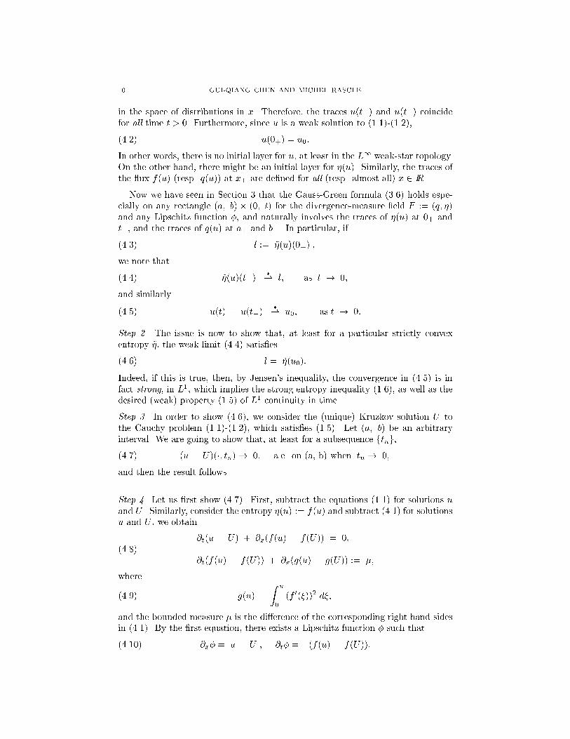
10 GUI-QIANG CHEN AND MICHEL RASCLEin the space of distributions in x. Therefore, the traces u(t�) and u(t+) coincidefor all time t > 0. Furthermore, since u is a weak solution to (1.1)-(1.2),u(0+) = u0:(4.2)In other words, there is no initial layer for u, at least in the L1 weak-star topology.On the other hand, there might be an initial layer for �(u). Similarly, the traces ofthe ux f(u) (resp. q(u)) at x� are de�ned for all (resp. almost all) x 2 IR .Now we have seen in Section 3 that the Gauss-Green formula (3.6) holds espe-cially on any rectangle (a; b) � (0; t) for the divergence-measure �eld F := (q; �)and any Lipschitz function �, and naturally involves the traces of �(u) at 0+ andt�, and the traces of q(u) at a+ and b�. In particular, ifl := ~�(u)(0+) ;(4.3)we note that ~�(u)(t�) �* l; as t ! 0;(4.4)and similarly u(t) = u(t�) �* u0; as t ! 0:(4.5)Step 2. The issue is now to show that, at least for a particular strictly convexentropy ~�, the weak limit (4.4) satis�esl = ~�(u0):(4.6)Indeed, if this is true, then, by Jensen's inequality, the convergence in (4.5) is infact strong, in L1, which implies the strong entropy inequality (1.6), as well as thedesired (weak) property (1.5) of L1 continuity in time.Step 3. In order to show (4.6), we consider the (unique) Kruzkov solution U tothe Cauchy problem (1.1)-(1.2), which satis�es (1.5). Let (a; b) be an arbitraryinterval. We are going to show that, at least for a subsequence ftng,(u� U)(�; tn)! 0; a.e. on (a, b) when tn ! 0;(4.7)and then the result follows.Step 4. Let us �rst show (4.7). First, subtract the equations (1.1) for solutions uand U . Similarly, consider the entropy �(u) := f(u) and subtract (4.1) for solutionsu and U , we obtain@t(u� U) + @x(f(u)� f(U)) = 0;@t(f(u)� f(U)) + @x(g(u)� g(U)) := �;(4.8)where g(u) = Z u0 (f 0(�))2 d�;(4.9)and the bounded measure � is the di�erence of the corresponding right hand sidesin (4.1). By the �rst equation, there exists a Lipschitz function � such that@x� = u� U ; @t� = �(f(u)� f(U)):(4.10)

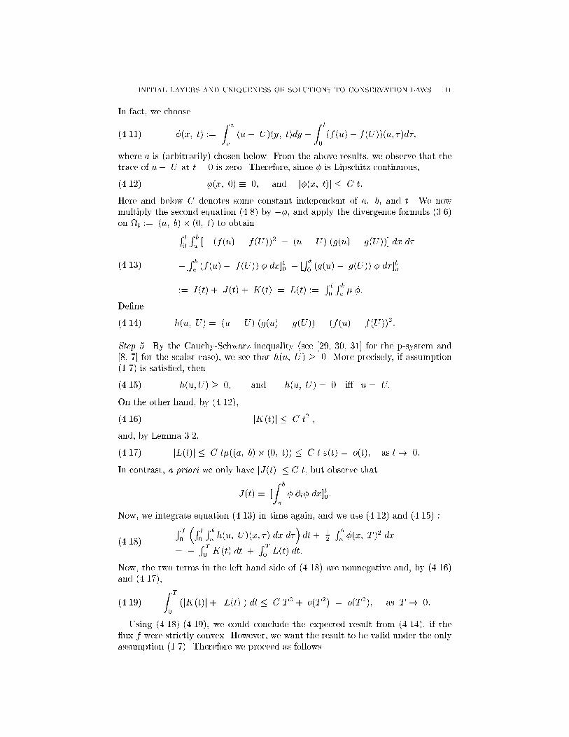
INITIAL LAYERS AND UNIQUENESS OF SOLUTIONS TO CONSERVATION LAWS 11In fact, we choose�(x; t) := Z xa (u� U)(y; t)dy � Z t0 (f(u)� f(U))(a; �)d�;(4.11)where a is (arbitrarily) chosen below. From the above results, we observe that thetrace of u� U at t = 0 is zero. Therefore, since � is Lipschitz continuous,�(x; 0) � 0; and j�(x; t)j � C t:(4.12)Here and below C denotes some constant independent of a; b, and t. We nowmultiply the second equation (4.8) by ��, and apply the divergence formula (3.6)on t := (a; b)� (0; t) to obtainR t0 R ba [� (f(u)� f(U))2 + (u� U) (g(u)� g(U))] dx d��[R ba (f(u)� f(U)) � dx]t0 � [R t0 (g(u)� g(U)) � d� ]ba:= I(t) + J(t) + K(t) = L(t) := R t0 R ba � �:(4.13)De�ne h(u; U) = (u� U) (g(u)� g(U))� (f(u)� f(U))2:(4.14)Step 5. By the Cauchy-Schwarz inequality (see [29, 30, 31] for the p-system and[8, 7] for the scalar case), we see that h(u; U) � 0. More precisely, if assumption(1.7) is satis�ed, thenh(u; U) � 0; and h(u; U) = 0 i� u = U:(4.15)On the other hand, by (4.12), jK(t)j � C t2 ;(4.16)and, by Lemma 3.2,jL(t)j � C t�((a; b)� (0; t)) � C t "(t) = o(t); as t! 0:(4.17)In contrast, a priori we only have jJ(t)j � C t, but observe thatJ(t) = [Z ba � @t� dx]t0:Now, we integrate equation (4.13) in time again, and we use (4.12) and (4.15) :R T0 �R t0 R ba h(u; U)(x; �) dx d�� dt+ 12 R ba �(x; T )2 dx= � R T0 K(t) dt + R T0 L(t) dt:(4.18)Now, the two terms in the left-hand side of (4.18) are nonnegative and, by (4.16)and (4.17),Z T0 (jK(t)j+ jL(t)j) dt � C T 3 + o(T 2) = o(T 2); as T ! 0:(4.19)Using (4.18)-(4.19), we could conclude the expected result from (4.14), if the ux f were strictly convex. However, we want the result to be valid under the onlyassumption (1.7). Therefore we proceed as follows.

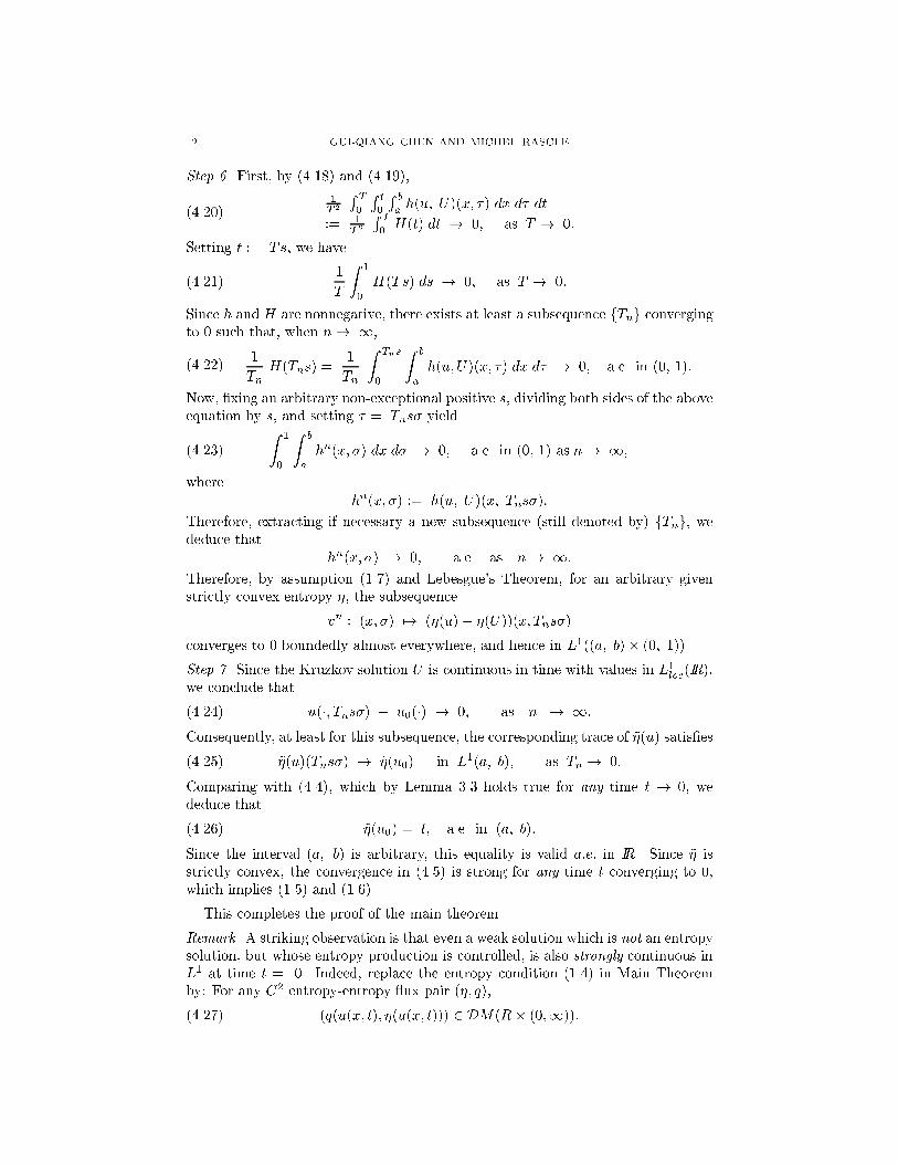
12 GUI-QIANG CHEN AND MICHEL RASCLEStep 6. First, by (4.18) and (4.19),1T 2 R T0 R t0 R ba h(u; U)(x; �) dx d� dt:= 1T 2 R T0 H(t) dt ! 0; as T ! 0:(4.20)Setting t := Ts, we have1T Z 10 H(Ts) ds ! 0; as T ! 0:(4.21)Since h and H are nonnegative, there exists at least a subsequence fTng convergingto 0 such that, when n! 1,1Tn H(Tns) = 1Tn Z Tns0 Z ba h(u; U)(x; �) dx d� ! 0; a.e. in (0, 1):(4.22)Now, �xing an arbitrary non-exceptional positive s, dividing both sides of the aboveequation by s, and setting � = Tns� yieldZ 10 Z ba hn(x; �) dx d� ! 0; a.e. in (0, 1) as n! 1;(4.23)where hn(x; �) := h(u; U)(x; Tns�):Therefore, extracting if necessary a new subsequence (still denoted by) fTng, wededuce that hn(x; �) ! 0; a.e. as n! 1:Therefore, by assumption (1.7) and Lebesgue's Theorem, for an arbitrary givenstrictly convex entropy �, the subsequencevn : (x; �) 7! (�(u)� �(U))(x; Tns�)converges to 0 boundedly almost everywhere, and hence in L1((a; b)� (0; 1)).Step 7. Since the Kruzkov solution U is continuous in time with values in L1loc(IR),we conclude that u(�; Tns�) � u0(�) ! 0; as n ! 1:(4.24)Consequently, at least for this subsequence, the corresponding trace of ~�(u) satis�es~�(u)(Tns�) ! ~�(u0) in L1(a; b); as Tn ! 0:(4.25)Comparing with (4.4), which by Lemma 3.3 holds true for any time t ! 0, wededuce that ~�(u0) = l; a.e. in (a; b):(4.26)Since the interval (a; b) is arbitrary, this equality is valid a:e: in IR. Since ~� isstrictly convex, the convergence in (4.5) is strong for any time t converging to 0,which implies (1.5) and (1.6).This completes the proof of the main theorem.Remark. A striking observation is that even a weak solution which is not an entropysolution, but whose entropy production is controlled, is also strongly continuous inL1 at time t = 0. Indeed, replace the entropy condition (1.4) in Main Theoremby: For any C2 entropy-entropy ux pair (�; q),(q(u(x; t); �(u(x; t))) 2 DM(R� (0;1)):(4.27)

INITIAL LAYERS AND UNIQUENESS OF SOLUTIONS TO CONSERVATION LAWS 13Then (1.5) still holds, but of course that does not imply that u is the Krushkovsolution, if u does not satisfy (1.4)!An application of the main theorem is the study of the zero relaxation limitdescribed in Section 2, where u(x; t) a priori only satis�ed the weaker inequality(2.9), and where the initial data were not at the equilibrium. Then at the limit,the initial layer has entirely collapsed to the line t = 0. More precisely, we haveCorollary 4.1. Consider the relaxing system (2.1). Assume that (1.7) is satis�ed.Let u(x; t) 2 L1 be the zero relaxation limit of an arbitrary subsequence fu"g, asin Proposition 2.1, even if the initial data (2.2) for (2.1) are not at the equilibrium.Then the whole sequence (u"; v") converges strongly to (u; f(u)), where u is theunique Kruzkov solution of the local equation (1.1), with the initial data (1.2): atthe limit, the initial layer has collapsed to the line t = 0. :v(�; 0+) = f(u)(�; 0+) = f(u0) 6= v(�; 0�) = v0:Similarly, the main theorem can be applied to clarify the initial layers and unique-ness of the relaxation limits for various physical relaxation systems whose initialdata are not at the equilibrium.Acknowledgments. Gui-Qiang Chen's research was supported in part by theNational Science Foundation grants INT-9726215 and DMS-9971793, and by anAlfred P. Sloan Foundation Fellowship. Michel Rascle's research was supported inpart by the National Science Foundation grant DMS 9708261, by the EC TMRnetwork HCL: n� ERB FMRX CT 96 0033, and by the (NSF)-CNRS contract n�5909. References[1] Anzellotti, G., Pairings between measures and bounded functions and compensated compact-ness, Ann. Mat. Pura Appl. (4) 135 (1983), 293{318.[2] Bardos, C., Le Roux, A. Y., and Nedelec, J. C., First order quasilinear equations withboundary conditions, Comm. Partial Di�. Eqs. 4 (1979), 1017-1034.[3] Chen, G.-Q., Hyperbolic systems of conservation laws with a symmetry, Comm. Partial Di�.Eqs. 16 (1991), 1461{1487.[4] Chen, G.-Q. and Frid, H., Divergence-measure �elds and hyperbolic conservation laws, Arch.Rational Mech. Anal. 147 (1999), 89-118.[5] Chen, G.-Q. and Frid, H., Large-time behavior of entropy solutions in L1 for multidimen-sional conservation laws, In: Advances in Nonlinear Partial Di�erential Equations and Re-lated Areas, edited by G.-Q. Chen et al, pp. 28-44, World Scienti�c: Singapore, 1998.[6] Chen, G.-Q. and Liu, T.-P., Zero relaxation and dissipation limits for hyperbolic conservationlaws, Comm. Pure Appl. Math. 46 (1993), 755-781.[7] Chen, G.-Q., Levermore, D., and Liu, T.-P., Hyperbolic conservation laws with sti� relaxationterms and entropy, Comm. Pure Appl. Math. 47 (1994), 787-830.[8] Chen, G.-Q. and Lu, Y.-G., A study of approaches of the theory of compensated compactness,Chinese Science Bulletin, 9 (1988), 641{644 (in Chinese); 34 (1989), 15{19 (in English).[9] Collet, J. F. and Rascle, M., Convergence of the relaxation approximation to a scalar nonlinearhyperbolic equation arising in chromatography, Z. Angew. Math. Phys. 47 (1996), 400{409.[10] DiPerna, R.-J., Measure-valued solutions to conservation laws, Arch. Rational Mech. Anal.88 (1985), 223-270.[11] Dubois, F. and LeFloch, Ph. G., Boundary conditions for nonlinear hyperbolic systems ofconservation laws, J. Di�. Eqs. 71 (1988), 93{122.[12] Engquist, E., Large time behavior and homogenization of solutions of two-dimensional con-servation laws, Comm. Pure Appl. Math. 46 (1993), 1-26.

14 GUI-QIANG CHEN AND MICHEL RASCLE[13] Evans, L. C. and Gariepy, R. F. Measure Theory and Fine Properties of Functions, Studiesin Advanced Mathematics, CRC Press, Boca Raton, FL, 1992.[14] Glimm, J. and Lax, P., Decay of solutions of systems of nonlinear hyperbolic conservationlaws, Amer. Math. Soc. Memoir 101, A.M.S.: Providence, 1970.[15] Jin, S., A convex entropy for a hyperbolic system with relaxation, J. Di�. Eqs. 127 (1996),97{109.[16] Jin, S. and Xin, Z., The relaxation schemes for systems of conservation laws in arbitraryspace dimensions, Comm. Pure Appl. Math. 48 (1995), 235{276.[17] Joseph, K. T. and LeFloch, P., Boundary layers in weak solutions to hyperbolic conservationlaws, Arch. Rational Mech. Anal. 147 (1999), 47-88.[18] Kan, P.-T., Santos, M., and Xin, Z., Initial-boundary value problem for conservation laws,Comm. Math. Phys. 186 (1997), 701-730.[19] Katsoulakis, M. and Tzavaras, A., Contractive relaxation systems and the scalar multidimen-sional conservation law, Comm. Partial Di�. Eqs. 22 (1997), 195-233.[20] Kruzkov, S. N., First-order quasilinear equations in several independent variables, Math.USSR Sb. 10 (1970), 217{243.[21] Kurganov, A. and Tadmor, E., Sti� systems of hyperbolic conservation laws: convergenceand error estimates, SIAM J. Math. Anal. 28 (1997), 1446{1456.[22] Lax, P., Hyperbolic Systems of Conservation Laws and the Mathematical Theory of ShockWaves, CBMS. 11, SIAM, 1973.[23] Liu, T.-P., Hyperbolic conservation laws with relaxation, Comm. Math. Phys. 108 (1987),153{175.[24] Lions, P. L., Perthame, B., and Tadmor, E., A kinetic formulation of multidimensional scalarconservation laws and related equations, J. Amer. Math. Soc. 7 (1994), 169{192.[25] Natalini, R., Convergence to equilibrium for the relaxation approximations of conservationlaws, Comm. Pure Appl. Math. 49 (1996), 795-823.[26] Nouri, A., Omrane, A., and Vila, J.P., Boundary conditions for scalar conservation laws:from a kinetic point of view, J. Statist. Phys. 94 (1999), 779-804.[27] Otto, F., First order equations with boundary conditions, Preprint no. 234, SFB 256, Univ.Bonn. 1992.[28] Perthame, B., Uniqueness and error estimates in �rst order quaislinear conservation laws viathe kinetic entropy defect measure, J. Math. Pures Appl. 77 (1998), 1055-1064.[29] Rascle, M., Perturbations par viscosit�e de certains syst�emes hyperboliques non lin�eaires,Th�ese d'Etat,Univ. Lyon 1, 1983.[30] Rascle, M., Convergence of approximate solutions to some systems of conservation laws: aconjecture on the product of the Riemann invariants, In: Oscillations Theory, Computationand Method of Compensated Compactness, C. M. Dafermos and M. Slemrod (eds.), IMASeries, Vol. 2, pp. 275-288, Springer-Verlag: New York, 1986.[31] Rascle, M. and Serre, D., Compacit�e par compensation et syst�emes hyperboliques de lois deconservation, Compt. Rend. Acad. Sciences, S�erie 1, 299 (1984), 673-676.[32] Schroll, H. J., Tveito, A. and Winther, R., A system of conservation laws with a relaxationterm, In: Hyperbolic Problems: Theory, Numerics and Applications, J. Glimm et al (eds.),pp. 431-440, World Scienti�c: Singapore, 1996.[33] Schwartz, L., Th�eorie des Distributions (2 volumes), Actualites Scienti�ques et Industrielles1091, 1122, Herman, Paris, 1950-51.[34] Serre, D., Systems of Conservation Laws, Fondations, Diderot Editeur, Paris, 1996.[35] Szepessy, A., An existence result for scalar conservation laws using measure-valued solutions,Comm. Partial Di�. Eqs. 14 (1989), 1329-1350.[36] Vasseur, A., Time continuity for the system of isentropic gas dynamics with = 3., Preprint,1998.[37] Vasseur, A., Kinetic semi-discretization of scalar conservation laws and convergence by usingaveraging lemmas. SIAM J. Numer. Anal. 36 (1999), 265-474.[38] Wang, W.-C. and Xin, Z., Asymptotic limit of initial-boundary value problems for conserva-tion laws with relaxational extensions, Comm. Pure Appl. Math. 51 (1998), 505{535.[39] Whitham, J., Linear and Nonlinear Waves, Wiley: New York, 1974.[40] Yong, W.-A., Boundary conditions for hyperbolic systems with source terms, Preprint, 1998.

INITIAL LAYERS AND UNIQUENESS OF SOLUTIONS TO CONSERVATION LAWS 15(Gui-Qiang Chen) Department of Mathematics, Northwestern University, 2033 Sheri-dan Road, Evanston, IL 60208, USAE-mail address: gqchen@math.nwu.edu(Michel Rascle) Laboratoire J. A. Dieudonn�e, Universit�e de Nice, Parc Valrose, F-06108, Nice Cedex 02, FranceE-mail address: rascle@math.unice.fr