
Ingrida_thesis_Final.pdf - LU|ZONE|UL @ Laurentian University
102
DESIGN OF A NEUTRON CALIBRATION SOURCE FOR THE SNO+ EXPERIMENT by Ingrida Semenec A thesis submitted in partial fulfillment of the requirements for the degree of Master of Science in Physics The Faculty of Graduate Studies Laurentian University Sudbury, Ontario, Canada © Ingrida Semenec, 2018
-
Upload
khangminh22 -
Category
Documents
-
view
0 -
download
0
Transcript of Ingrida_thesis_Final.pdf - LU|ZONE|UL @ Laurentian University
DESIGN OF A NEUTRON CALIBRATION SOURCE
FOR THE SNO+ EXPERIMENT
by
Ingrida Semenec
A thesis submitted in partial fulfillment
of the requirements for the degree of
Master of Science in Physics
The Faculty of Graduate Studies
Laurentian University
Sudbury, Ontario, Canada
© Ingrida Semenec, 2018
ii
THESIS DEFENCE COMMITTEE/COMITÉ DE SOUTENANCE DE THÈSE
Laurentian Université/Université Laurentienne
Faculty of Graduate Studies/Faculté des études supérieures
Title of Thesis
Titre de la thèse DESIGN OF A NEUTRON CALIBRATION SOURCE
FOR THE SNO+ EXPERIMENT
Name of Candidate
Nom du candidat Semenec, Ingrida
Degree
Diplôme Master of Science
Department/Program Date of Defence
Département/Programme Physics Date de la soutenance November 13, 2017
APPROVED/APPROUVÉ
Thesis Examiners/Examinateurs de thèse:
Dr. Christine Kraus
(Supervisor/Directeur(trice) de thèse)
Dr. Clarence Virtue
(Committee member/Membre du comité)
Dr. Erica Caden
(Committee member/Membre du comité)
Approved for the Faculty of Graduate Studies
Approuvé pour la Faculté des études supérieures
Dr. David Lesbarrères
Monsieur David Lesbarrères
Dr. Mark Boulay Dean, Faculty of Graduate Studies
(External Examiner/Examinateur externe) Doyen, Faculté des études supérieures
ACCESSIBILITY CLAUSE AND PERMISSION TO USE
I, Ingrida Semenec, hereby grant to Laurentian University and/or its agents the non-exclusive license to archive and
make accessible my thesis, dissertation, or project report in whole or in part in all forms of media, now or for the
duration of my copyright ownership. I retain all other ownership rights to the copyright of the thesis, dissertation or
project report. I also reserve the right to use in future works (such as articles or books) all or part of this thesis,
dissertation, or project report. I further agree that permission for copying of this thesis in any manner, in whole or in
part, for scholarly purposes may be granted by the professor or professors who supervised my thesis work or, in their
absence, by the Head of the Department in which my thesis work was done. It is understood that any copying or
publication or use of this thesis or parts thereof for financial gain shall not be allowed without my written
permission. It is also understood that this copy is being made available in this form by the authority of the copyright
owner solely for the purpose of private study and research and may not be copied or reproduced except as permitted
by the copyright laws without written authority from the copyright owner.
Abstract
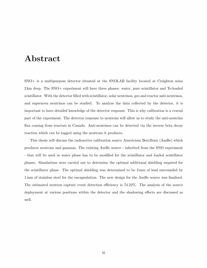
SNO+ is a multipurpose detector situated at the SNOLAB facility located at Creighton mine
2 km deep. The SNO+ experiment will have three phases: water, pure scintillator and Te-loaded
scintillator. With the detector filled with scintillator, solar neutrinos, geo and reactor anti-neutrinos,
and supernova neutrinos can be studied. To analyze the data collected by the detector, it is
important to have detailed knowledge of the detector response. This is why calibration is a crucial
part of the experiment. The detector response to neutrons will allow us to study the anti-neutrino
flux coming from reactors in Canada. Anti-neutrinos can be detected via the inverse beta decay
reaction which can be tagged using the neutrons it produces.
This thesis will discuss the radioactive calibration source Americium Beryllium (AmBe) which
produces neutrons and gammas. The existing AmBe source - inherited from the SNO experiment
- that will be used in water phase has to be modified for the scintillator and loaded scintillator
phases. Simulations were carried out to determine the optimal additional shielding required for
the scintillator phase. The optimal shielding was determined to be 2 mm of lead surrounded by
1 mm of stainless steel for the encapsulation. The new design for the AmBe source was finalised.
The estimated neutron capture event detection efficiency is 74.22%. The analysis of the source
deployment at various positions within the detector and the shadowing effects are discussed as
well.
iii
Acknowledgments
First and foremost, I would like to thank my supervisor, Dr. Christine Kraus for accepting me
into her group and giving me this opportunity to work on one of the most amazing experiments in
the world, SNO+. Additionally, I would like to thank my committee members Dr. Erica Caden
and Dr. Clarence Virtue for all of the constructive advice and for setting a work standard of high
quality, which shaped me into a better physicist.
I would also like to extend my gratitude to all the amazing people at SNOLAB and in the
SNO+ collaboration. I truly felt like part of a community, which was uplifting and encouraging.
I am particularly grateful for Dr. Christopher Grant’s assistance. Your prompt answers to my
questions and enthusiastic conversations about various physics topics kept me motivated.
In my daily Canadian life, I have been blessed by an amazing group of friends, who always stood
by my side. A huge thank you goes to my BNF Steve, to Caitlyn, Janet, Colin, Chris, Rachel,
Pooja, Matt and Jaz for being part of some amazing adventures and board game nights. I’d also
like to thank Stephane Venne, my soulmate. Thank you for always being there for me, even if it is
5am in a hospital emergency room.
I cannot forget to thank my best friend, Christopher Woodhead. Your kind heart always restores
my faith in humanity.
Finally, I’d like to thank the most important person in my life, my mother, Lolita Semenec.
Aciu mama uz tai, kad per pastaruosius metus tu man parodei, kokia stipri gali buti moters
dvasia. Noriu tau padekoti uz tai kad myli mane ir tiki manimi. Myliu tave.
iv
Contents
Abstract iii
Acknowledgments iv
List of Figures vii
List of Tables xii
1 Physics 2
1.1 The brief history of the neutrino . . . . . . . . . . . . . . . . . . . . . . . . . . . . . 2
1.2 Neutrinos in the Standard Model of Particle Physics . . . . . . . . . . . . . . . . . . 3
1.2.1 Neutrinoless double beta decay . . . . . . . . . . . . . . . . . . . . . . . . . . 6
1.3 Neutrino oscillations . . . . . . . . . . . . . . . . . . . . . . . . . . . . . . . . . . . . 7
1.3.1 The MSW effect . . . . . . . . . . . . . . . . . . . . . . . . . . . . . . . . . . 15
1.4 Neutrino mass . . . . . . . . . . . . . . . . . . . . . . . . . . . . . . . . . . . . . . . 16
1.5 Anti-neutrino physics . . . . . . . . . . . . . . . . . . . . . . . . . . . . . . . . . . . . 16
1.5.1 Reactor neutrinos . . . . . . . . . . . . . . . . . . . . . . . . . . . . . . . . . 18
1.5.2 Geo-neutrinos . . . . . . . . . . . . . . . . . . . . . . . . . . . . . . . . . . . 20
1.5.3 Supernova neutrinos . . . . . . . . . . . . . . . . . . . . . . . . . . . . . . . . 22
2 The SNO+ experiment 23
2.1 The SNO+ Detector . . . . . . . . . . . . . . . . . . . . . . . . . . . . . . . . . . . . 23
2.1.1 SNO . . . . . . . . . . . . . . . . . . . . . . . . . . . . . . . . . . . . . . . . . 24
2.1.2 Upgrades . . . . . . . . . . . . . . . . . . . . . . . . . . . . . . . . . . . . . . 27
v
2.2 Phases of experiment . . . . . . . . . . . . . . . . . . . . . . . . . . . . . . . . . . . . 29
2.2.1 Water Phase . . . . . . . . . . . . . . . . . . . . . . . . . . . . . . . . . . . . 29
2.2.2 Pure Scintillator Phase . . . . . . . . . . . . . . . . . . . . . . . . . . . . . . 30
2.2.3 Te-loaded Scintillator Phase . . . . . . . . . . . . . . . . . . . . . . . . . . . . 31
2.3 Anti-neutrino Detection . . . . . . . . . . . . . . . . . . . . . . . . . . . . . . . . . . 32
3 Detector calibration 35
3.1 Calibration hardware . . . . . . . . . . . . . . . . . . . . . . . . . . . . . . . . . . . . 36
3.2 Optical calibration sources . . . . . . . . . . . . . . . . . . . . . . . . . . . . . . . . . 36
3.3 Radioactive calibration sources . . . . . . . . . . . . . . . . . . . . . . . . . . . . . . 38
4 Neutron source design 40
4.1 Source simulation software . . . . . . . . . . . . . . . . . . . . . . . . . . . . . . . . . 42
4.1.1 AmBe source geometry . . . . . . . . . . . . . . . . . . . . . . . . . . . . . . 43
4.1.2 AmBe source event generator . . . . . . . . . . . . . . . . . . . . . . . . . . . 45
4.2 Shielding simulations . . . . . . . . . . . . . . . . . . . . . . . . . . . . . . . . . . . . 47
4.2.1 Shielding materials . . . . . . . . . . . . . . . . . . . . . . . . . . . . . . . . . 48
4.2.2 Simulating gammas . . . . . . . . . . . . . . . . . . . . . . . . . . . . . . . . 48
4.2.3 Simulating neutrons . . . . . . . . . . . . . . . . . . . . . . . . . . . . . . . . 49
4.2.4 Results . . . . . . . . . . . . . . . . . . . . . . . . . . . . . . . . . . . . . . . 52
5 Neutron Source Analysis 57
5.1 Scintillator Fitter . . . . . . . . . . . . . . . . . . . . . . . . . . . . . . . . . . . . . . 57
5.2 Energy peak dependence on source position . . . . . . . . . . . . . . . . . . . . . . . 59
5.3 Shadowing . . . . . . . . . . . . . . . . . . . . . . . . . . . . . . . . . . . . . . . . . . 62
5.4 Tagged event efficiency . . . . . . . . . . . . . . . . . . . . . . . . . . . . . . . . . . . 64
6 Conclusions 70
A Matter Oscillations 72
A.1 Schematics . . . . . . . . . . . . . . . . . . . . . . . . . . . . . . . . . . . . . . . . . 75
B Source Shielding plots 78
vi

Bibliography 78
vii
List of Figures
1.1 The schematic diagram of the neutrino detector by Frederic Reines and Clyde Cowan 3
1.2 The illustration of the basic components of the standard model . . . . . . . . . . . . 4
1.3 Feynman diagrams for ββ2ν (left) and ββ0ν (right) . . . . . . . . . . . . . . . . . . 6
1.4 The comparison between the predictions of the standard solar model with the mea-
sured rates in the solar neutrino experiments . . . . . . . . . . . . . . . . . . . . . . 8
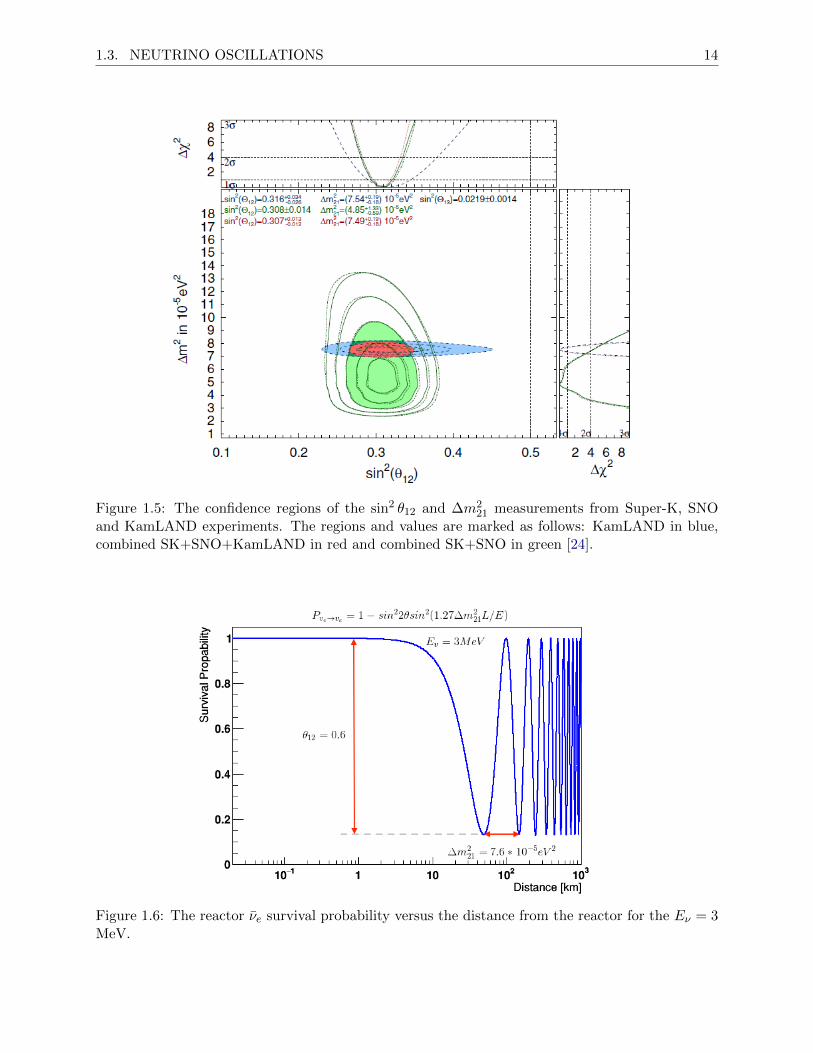
1.5 The confidence regions of the sin2 θ12 and ∆m221 measurements from Super-K, SNO
and KamLAND experiments. . . . . . . . . . . . . . . . . . . . . . . . . . . . . . . . 14
1.6 The reactor νe survival probability versus the distance from the reactor for the Eν = 3
MeV. . . . . . . . . . . . . . . . . . . . . . . . . . . . . . . . . . . . . . . . . . . . . . 14
1.7 The two possible neutrino mass hierarchies . . . . . . . . . . . . . . . . . . . . . . . 16
1.8 The expected anti-neutrino energy spectrum in SNO+ . . . . . . . . . . . . . . . . . 17
1.9 The map of nearby nuclear reactors and their distances to SNO+. . . . . . . . . . . 18
1.10 The illustration of neutrino oscillation probability smearing due to the finite energy
resolution of the detector. . . . . . . . . . . . . . . . . . . . . . . . . . . . . . . . . . 19
1.11 The expected spectrum of reactor anti-neutrino signal for different values of ∆m212
for the SNO+ experiment . . . . . . . . . . . . . . . . . . . . . . . . . . . . . . . . . 20
1.12 A worldwide νe flux map combining geoneutrinos from natural 238U and 232Th de-
cays, with the ones emitted from the nuclear reactors around the world. . . . . . . . 21
1.13 The energy spectra of the geo neutrinos produced from the Equation 1.49 (238U
chain, solid black line), Equation 1.50 (232Th chain, red dashed-dotted red line) and
Equation 1.51 (40K chain, blue dashed blue line). . . . . . . . . . . . . . . . . . . . . 21
2.1 Artist illustration of SNO+ detector. . . . . . . . . . . . . . . . . . . . . . . . . . . . 24
viii
2.2 The muon flux dependency on the depth of the various underground laboratories. . . 25
2.3 The charged current (CC), neutral current (NC) and elastic scattering interactions
seen in SNO . . . . . . . . . . . . . . . . . . . . . . . . . . . . . . . . . . . . . . . . . 26
2.4 Left: Suspension ropes of the SNO AV. Right: SNO+ hold-down rope net . . . . . . 28
2.5 The stages of “Float The Boat” test, to test the rope strength, while simulating
buoyancy of the acrylic vessel. . . . . . . . . . . . . . . . . . . . . . . . . . . . . . . . 28
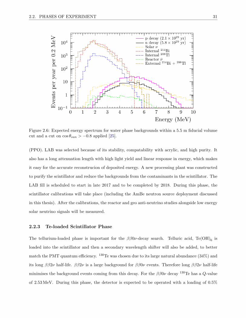
2.6 Expected energy spectrum for water phase backgrounds within a 5.5 m fiducial
volume cut and a cut on cos θsun > −0.8 applied . . . . . . . . . . . . . . . . . . . . 31
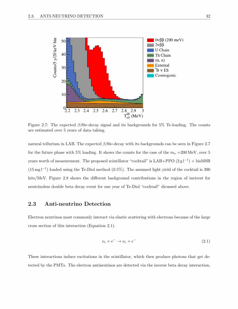
2.7 The expected ββ0ν-decay signal and its backgrounds for 5% Te-loading. The counts
are estimated over 5 years of data taking. . . . . . . . . . . . . . . . . . . . . . . . . 32
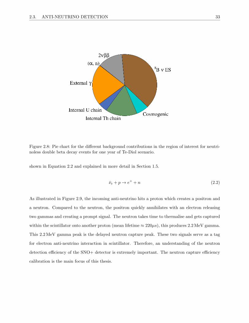
2.8 Pie chart for the different background contributions in the region of interest for
neutrinoless double beta decay events for one year of Te-Diol scenario. . . . . . . . . 33
2.9 Illustration of the inverse beta decay reaction inside the scintillator for electron anti-
neutrinos. . . . . . . . . . . . . . . . . . . . . . . . . . . . . . . . . . . . . . . . . . . 34
3.1 Illustration of the calibration source deployment mechanisms. . . . . . . . . . . . . . 37
3.2 Sketch showing an example of the light injection points . . . . . . . . . . . . . . . . 38
4.1 The deexcitation modes of 12C in the 9Be(α, n)12C reaction . . . . . . . . . . . . . . 41
4.2 The schematics of SNO NCD phase neutron calibration sources. The AmBe source
discussed in this thesis is denoted as “Am-Be High” . . . . . . . . . . . . . . . . . . 42
4.3 The schematic of the main AmBe source geometry parts for illustration . . . . . . . 44
4.4 The energy fit of the DEAP-1 AmBe generator. Neutrons and gammas in coincidence 46
4.5 The NHit spectrum produced using the SNO+ AmBe generator, which includes the
correlation between neutrons and gammas with the appropriate deexcitation modes
of 12C in the 9Be(α, n)12C reaction . . . . . . . . . . . . . . . . . . . . . . . . . . . . 46
4.6 241Am decay scheme . . . . . . . . . . . . . . . . . . . . . . . . . . . . . . . . . . . . 47
4.7 The Nhit plot of 106 events of 59.5 keV γ generated. With different thicknesses of
lead shielding around the source. The legend shows the number of triggers within
the range of 10→ 50 NHits. . . . . . . . . . . . . . . . . . . . . . . . . . . . . . . . 50
ix
4.8 104 events of 4.4 MeV γ for 1, 1.3, 1.6, 2, 3 mm of lead shielding. The legend shows
number of triggers within the range of 1900→ 2500 NHits. . . . . . . . . . . . . . . 50
4.9 The energy fit using scintillator fitter for 1, 1.3, 1.6, 2 and 3 mm of lead shielding. . 51
4.10 The NHit for 1,2,3 mm of lead shielding. . . . . . . . . . . . . . . . . . . . . . . . . . 51
4.11 The breakdown of the separate NHit ”triggers” of 10000 neutron events going through
1mm of lead. The 0th trigger represents the first reconstructed event associated with
a simulated particle. Here, the 0th trigger corresponds to the thermalisation of a
neutron before it gets captured. The 1st trigger is the neutron capture event peak. . 52
4.12 The third revision of the AmBe source shielding cross-section. Layers account for the
spacing of screws and connections for the stem attachment and the original source
screw placement. The purple depicts the original AmBe source container, with the
2 mm of lead shielding in blue and the additional stainless steel encapsulation (green).
The additional millimeter of stainless steel added to the bottom of container for the
structual integrity. The source connector to the stem is also made out of stainless
steel. . . . . . . . . . . . . . . . . . . . . . . . . . . . . . . . . . . . . . . . . . . . . . 54
4.13 The finalised schematic of the AmBe source geometry including the stem. The
measurements and layers are shown as in the latest geometry file for the AmBe
source simulations. . . . . . . . . . . . . . . . . . . . . . . . . . . . . . . . . . . . . 55
4.14 The finalised schematic of the AmBe source connector geometry. . . . . . . . . . . . 56
5.1 The MC true versus EV reconstructed energy from the scintillator fitter for total
deposited energy within a simulated event. The narrow linear trend shows strong
correlation between the true and reconstructed energy. . . . . . . . . . . . . . . . . . 58
5.2 The fractional error of MC true versus the EV reconstructed energy. Slight bias to
the negative values shows that reconstructed energy tends to be lower than true. . . 58
5.3 NHit plot of the AmBe source spectrum, source simulated at different Z positions
inside the detector with 0 offline PMTs. The plot shows the neutron capture peaks
between 1000 to 1500 NHit and the 4.4 MeV gamma peak around 2200 to 1400 NHit.
The plot illustrates the way sharp neutron capture peak was fitted to get the mean
number of hits. (5000 events simulated) . . . . . . . . . . . . . . . . . . . . . . . . . 60
x
5.4 Neutron capture peak values in Nhit relative to the Z axis source positions inside of
the detector. . . . . . . . . . . . . . . . . . . . . . . . . . . . . . . . . . . . . . . . . 60
5.5 Neutron capture peak values in Nhit relative to the X axis source positions inside of
the detector. . . . . . . . . . . . . . . . . . . . . . . . . . . . . . . . . . . . . . . . . 61
5.6 Neutron capture peak values in Nhit relative to the Y axis source positions inside of
the detector. . . . . . . . . . . . . . . . . . . . . . . . . . . . . . . . . . . . . . . . . 61
5.7 The Nhit distributions of AmBe spectrum with different shielding scenarios. 5000
events were simulated for each case. The neutron capture and 4.4 MeV γ peaks are
fitted with gaussian functions to get the peak positions in Nhit shown in the legend. 63
5.8 The neutron capture time comparison between the MC truth versus reconstructed
time. The reconstructed time was fitted with an inverse exponential to find the mean
neutron capture time (dotted green line). . . . . . . . . . . . . . . . . . . . . . . . . 66
5.9 The neutron capture event selection using MC truth information. . . . . . . . . . . . 67
5.10 The neutron capture event selection using reconstructed event information. . . . . . 68
5.11 The neutron capture event distance from the source using MC truth information. . . 69
A.1 The SNO AmBe schematics . . . . . . . . . . . . . . . . . . . . . . . . . . . . . . . . 76
A.2 The SNO+ source manipulator schematic. . . . . . . . . . . . . . . . . . . . . . . . . 77
B.1 The NHit distribution for 10000 4.4MeV γ events going through 1mm of lead, stain-
less steel and hevimet. . . . . . . . . . . . . . . . . . . . . . . . . . . . . . . . . . . . 78
B.2 The NHit distribution for 10000 4.4MeV γ events going through 2mm of lead, stain-
less steel and hevimet. . . . . . . . . . . . . . . . . . . . . . . . . . . . . . . . . . . . 79
B.3 The NHit distribution for 10000 4.4MeV γ events going through 3mm of lead, stain-
less steel and hevimet. . . . . . . . . . . . . . . . . . . . . . . . . . . . . . . . . . . . 79
B.4 The NHit distribution for 10000 4.4MeV γ events going through 5mm of lead, stain-
less steel and hevimet. . . . . . . . . . . . . . . . . . . . . . . . . . . . . . . . . . . . 80
B.5 The NHit distribution for 10000 4.4MeV γ events going through 7mm of lead, stain-
less steel and hevimet. . . . . . . . . . . . . . . . . . . . . . . . . . . . . . . . . . . . 80
B.6 The NHit distribution for 10000 4.4MeV γ events going through 8mm of lead, stain-
less steel and hevimet. . . . . . . . . . . . . . . . . . . . . . . . . . . . . . . . . . . . 81
xi
B.7 The NHit distribution for 10000 59.5keV γ events going through 1mm of lead, stain-
less steel and hevimet. . . . . . . . . . . . . . . . . . . . . . . . . . . . . . . . . . . . 81
B.8 The NHit distribution for 10000 59.5keV γ events going through 2mm of lead, stain-
less steel and hevimet. . . . . . . . . . . . . . . . . . . . . . . . . . . . . . . . . . . . 82
B.9 The NHit distribution for 10000 59.5keV γ events going through 3mm of lead, stain-
less steel and hevimet. . . . . . . . . . . . . . . . . . . . . . . . . . . . . . . . . . . . 82
B.10 The NHit distribution for 10000 59.5keV γ events going through 5mm of lead, stain-
less steel and hevimet. . . . . . . . . . . . . . . . . . . . . . . . . . . . . . . . . . . . 83
B.11 The NHit distribution for 10000 59.5keV γ events going through 7mm of lead, stain-
less steel and hevimet. . . . . . . . . . . . . . . . . . . . . . . . . . . . . . . . . . . . 83
B.12 The NHit distribution for 10000 59.5keV γ events going through 8mm of lead, stain-
less steel and hevimet. . . . . . . . . . . . . . . . . . . . . . . . . . . . . . . . . . . . 84
xii
List of Tables
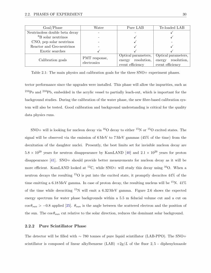
2.1 The main physics and calibration goals for the three SNO+ experiment phases. . . . 30
3.1 The radioactive calibration sources for SNO+ . . . . . . . . . . . . . . . . . . . . . . 39
4.1 The % of gammas let through the different thicknesses of lead, stainless steel and
hevimet. The NHit distribution plots for samples of 10000 events with each thickness
can be seen in Appendix B. . . . . . . . . . . . . . . . . . . . . . . . . . . . . . . . . 49
4.2 The % of gammas and neutrons penetrating the different thicknesses of lead. . . . . 53
5.1 The shadowing effects of the AmBe source container components on the neutron
capture peak in AmBe source spectrum. . . . . . . . . . . . . . . . . . . . . . . . . . 62
5.2 The shadowing effects of the AmBe source container components on the 4.4 MeV γ
peak in the AmBe source spectrum. . . . . . . . . . . . . . . . . . . . . . . . . . . . 63
1
Chapter 1
Physics
1.1 The brief history of the neutrino
While investigating radioactive beta decay of 14N and 6Li, Wolfgang Pauli noticed that energy
was missing from the outgoing electron. What he observed was a continuous spectrum of electron
energies, which violated the conservation of energy. Two body decay implies a fixed energy line for
electrons. The fact that the measured spectrum was continuous suggested that part of the energy
was carried out by a third particle. As a desperate remedy, Pauli penned a letter to physicists
in Germany on December 4, 1930. In this letter he proposed the existence of a neutral, spin 1/2
particle also emitted in beta decay [1].
This sparked the interest of Enrico Fermi, who later named the particle “neutrino”, meaning
“neutral little one” [2]. Around this time, Fermi had developed the theory of beta decay. In his
theory the principles of relativity were applied to the creation of particles and anti-particles in the
following fashion:
(Z,A)→ (Z + 1, A) + e− + νe (1.1)
(Z,A)→ (Z − 1, A) + e+ + νe (1.2)
Equation 1.1 and Equation 1.2 represent what are called “beta minus decay” and “beta plus
decay”, respectively.
2
1.2. NEUTRINOS IN THE STANDARD MODEL OF PARTICLE PHYSICS 3
In 1953, two determined physicists Frederic Reines and Clyde Cowan started making plans to
detect the neutrino. Their first proposal was to use a nuclear bomb as a neutrino source, but after
careful consideration they decided on a nuclear reactor instead. In 1959, they built a detector 12 m
underground near a nuclear reactor in Savannah River, South Carolina. The detector consisted of
two tanks filled with ≈ 400 liters of water loaded with 40 kg cadmium chloride, used as a target
material. The antineutrino created inside the nuclear reactor interacted with a proton in the target
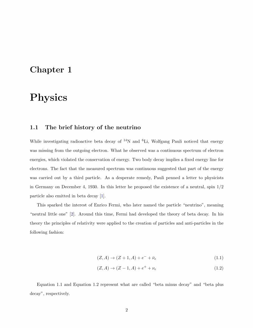
material, giving a positron and neutron, shown in Figure 1.1. The prompt light signal created from
positron annihilation and the delayed signal from neutron capture on cadmium was observed by
55 photomultiplier tubes (PMTs). This was a first measurement of a free neutrino event [3]. This
result was awarded Nobel Prize 40 years later in 1995 [4].
Figure 1.1: The schematic diagram of neutrino detector by Frederivc Reines and Clyde Cowan [5].
1.2 Neutrinos in the Standard Model of Particle Physics
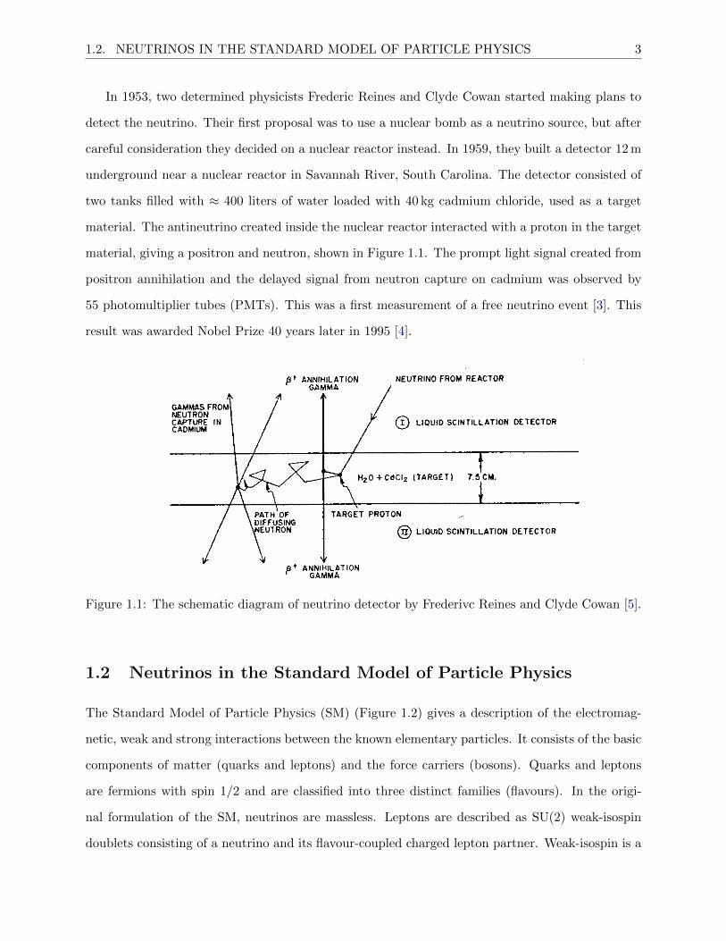
The Standard Model of Particle Physics (SM) (Figure 1.2) gives a description of the electromag-
netic, weak and strong interactions between the known elementary particles. It consists of the basic
components of matter (quarks and leptons) and the force carriers (bosons). Quarks and leptons
are fermions with spin 1/2 and are classified into three distinct families (flavours). In the origi-
nal formulation of the SM, neutrinos are massless. Leptons are described as SU(2) weak-isospin
doublets consisting of a neutrino and its flavour-coupled charged lepton partner. Weak-isospin is a
1.2. NEUTRINOS IN THE STANDARD MODEL OF PARTICLE PHYSICS 4
quantum number, that relates to weak interaction and SU(2) represents the weak isospin symmetry
group. It is assumed that the neutrino fields contained in these doublets are left-handed chirality.
The right-handed components of the other leptons are represented as singlets in the hypercharge
symmetry group U(1). Each left-handed doublet is accompanied by a right-handed charged sin-
glet. The left-handed doublets and right-handed singlets form the basis of the symmetry group
SU(2)×U(1), which describes the electroweak interactions of neutrinos. That shows that weak
interactions couple only to νL and νR.
Figure 1.2: The illustration of the basic components of the standard model [6].
Of the three flavours of neutrinos, the electron flavour was detected by Reines and Cowan. The
muon flavour was discovered by Melvin Schwartz, Leon Lederman and Jack Steinberger using the
Alternating Gradient Synchrotron (AGS) at Brookhaven National Laboratory in 1962 [7]. They
collided protons onto a Beryllium target to produce pions. Then they looked for decay into muons
and muon neutrinos:
1.2. NEUTRINOS IN THE STANDARD MODEL OF PARTICLE PHYSICS 5
π± → µ± + (ν/ν) (1.3)
Then the resulting neutrino beam hit a thick iron shield wall at a distance of 21 m from the
Beryllium target. Behind the iron shield there was a 10 t aluminium spark chamber, which observed
neutrino interactions. Detailed cross sections were calculated for the following interactions:
νµ + n→ e− + p (1.4)
νµ + p→ e+ + n (1.5)
νµ + n→ µ− + p (1.6)
νµ + p→ µ+ + n (1.7)
(1.8)
If neutrinos associated with muons are the same as with electrons, then neutrino interactions
should produce muons and electrons in equal abundance. However, they have observed 34 single
muon events and only 6 electron showers. Furthermore, these electron events are more consistent
with the expected background. This determined that the muon neutrino is a separate particle from
the electron neutrino.
A while after in 2000 the tau neutrino (ντ ) was discovered by the DONUT experiment at Fermilab
[8]. It was predicted for the conservation of the lepton number during tau decays. Because lepton
number is additive quantum number, the sum of leptons and antileptons must be preserved in
interactions. The DONUT experiment observed charged current interactions of the ντ by looking
for τ lepton to be created at the neutrino interaction vertex. They used an accelerated proton beam
to produce ντ via decay of charmed mesons. In the set of 203 neutrino interactions, they observed
four τ lepton inetractions. The probability that those four events came from the background was
estimated to be 4× 10⁻⁴, which concluded that ντ events were observed [8].
1.2. NEUTRINOS IN THE STANDARD MODEL OF PARTICLE PHYSICS 6
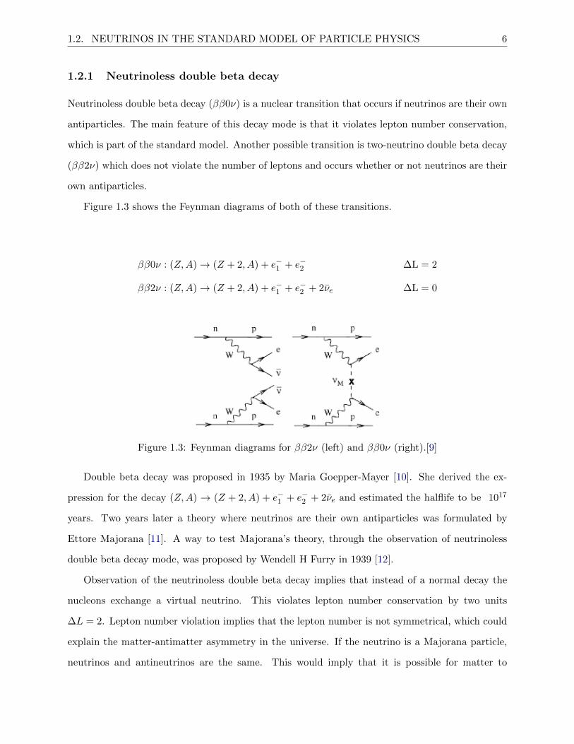
1.2.1 Neutrinoless double beta decay
Neutrinoless double beta decay (ββ0ν) is a nuclear transition that occurs if neutrinos are their own
antiparticles. The main feature of this decay mode is that it violates lepton number conservation,
which is part of the standard model. Another possible transition is two-neutrino double beta decay
(ββ2ν) which does not violate the number of leptons and occurs whether or not neutrinos are their
own antiparticles.
Figure 1.3 shows the Feynman diagrams of both of these transitions.
ββ0ν : (Z,A)→ (Z + 2, A) + e−1 + e−2 ∆L = 2
ββ2ν : (Z,A)→ (Z + 2, A) + e−1 + e−2 + 2νe ∆L = 0
Figure 1.3: Feynman diagrams for ββ2ν (left) and ββ0ν (right).[9]
Double beta decay was proposed in 1935 by Maria Goepper-Mayer [10]. She derived the ex-
pression for the decay (Z,A) → (Z + 2, A) + e−1 + e−2 + 2νe and estimated the halflife to be 1017
years. Two years later a theory where neutrinos are their own antiparticles was formulated by
Ettore Majorana [11]. A way to test Majorana’s theory, through the observation of neutrinoless
double beta decay mode, was proposed by Wendell H Furry in 1939 [12].
Observation of the neutrinoless double beta decay implies that instead of a normal decay the
nucleons exchange a virtual neutrino. This violates lepton number conservation by two units
∆L = 2. Lepton number violation implies that the lepton number is not symmetrical, which could
explain the matter-antimatter asymmetry in the universe. If the neutrino is a Majorana particle,
neutrinos and antineutrinos are the same. This would imply that it is possible for matter to
1.3. NEUTRINO OSCILLATIONS 7
transform to antimatter and vice-versa, thus creating an imbalance between matter and antimatter
in the early universe. This effect is also known as “leptogenesis”.
The neutrino being a Majorana particle could lead to determining the absolute mass of the neu-
trino. If neutrinos are Majorana particles, that implies two additional Majorana phases responsible
for lepton number violating processes such as neutrinoless double beta decay. The effective Majo-
rana neutrino mass from neutrinoless double beta decay depends on these phases, which then can
cause cancellations among the contributions of the neutrino masses [13]. The effective majorana
mass in ββ0ν decay can be written as Equation 1.9 [14], using the Pontecorvo-Maki-Nakagawa-
Sakata matrix Equation 1.17, which will be discussed in detail in Section 1.3.
|mββ | = |c213c
212e
2iα1m1 + c213s
212e
2iα2m2 + s213m3| (1.9)
Therefore, if neutrinoless double beta decay is detected it is possible to compute the absolute
mass for neutrinos by taking into account the already known experimental values of neutrino mass
splittings provided by neutrino oscillation measurements and combining it with the results of the
lowest neutrino mass.
1.3 Neutrino oscillations
The solar neutrino experiments revealed the phenomenon of the adiabatic flavour conversion of neu-
trinos in the sun. This led to the discovery of neutrino oscillations. The Homestake experiment was
the experiment led by astrophysicist Raymond Davis, who used the theoretical calculations made
by John N. Bahcall in the late 1960s [15]. The purpose of this experiment was to detect neutrinos
emitted by nuclear fusion reactions in the Sun. The detector was located 1.5 km underground. As
a target the 6 m diameter and 15 m long tank held about 400 tons of perchloroethylene. The exper-
iment involved neutrino capture on chlorine to form argon (Equation 1.10) which has good cross
section for observation of neutrinos coming from 7Be, 13N and 15O decays and the proton-proton
(p-p) reaction [16].
ν + 37Clcapture−−−−⇀↽−−−−decay
37Ar + e− (1.10)
Even though the Homestake experiment was first to detect solar neutrinos, the measured rate
1.3. NEUTRINO OSCILLATIONS 8
of the neutrinos was only one third of what was expected from the solar models at the time. This
raised many speculations and questions about the quality of the experiment and the theoretical
predictions. This deficit in neutrino signal was also called the solar neutrino problem.
The Homestake experiment was then followed by others: Kamiokande, GALLEX and SAGE.
Kamiokande used a large water Cherenkov detector and looked for neutrino scattering with an
electron [17]. While SAGE and GALLEX looked at 71Ga(νe, e)71Ge reaction in gallium. SAGE
used 50-57 tonnes of liquid gallium as a target for the reaction at the Baksan Neutrino Observatory
in Caucasus mountains. GALLEX was another large gallium-germanium experiment. It used 101 t
of gallium trichloride-hydrochloric acid solution, which also contained 30.3 t of gallium and was
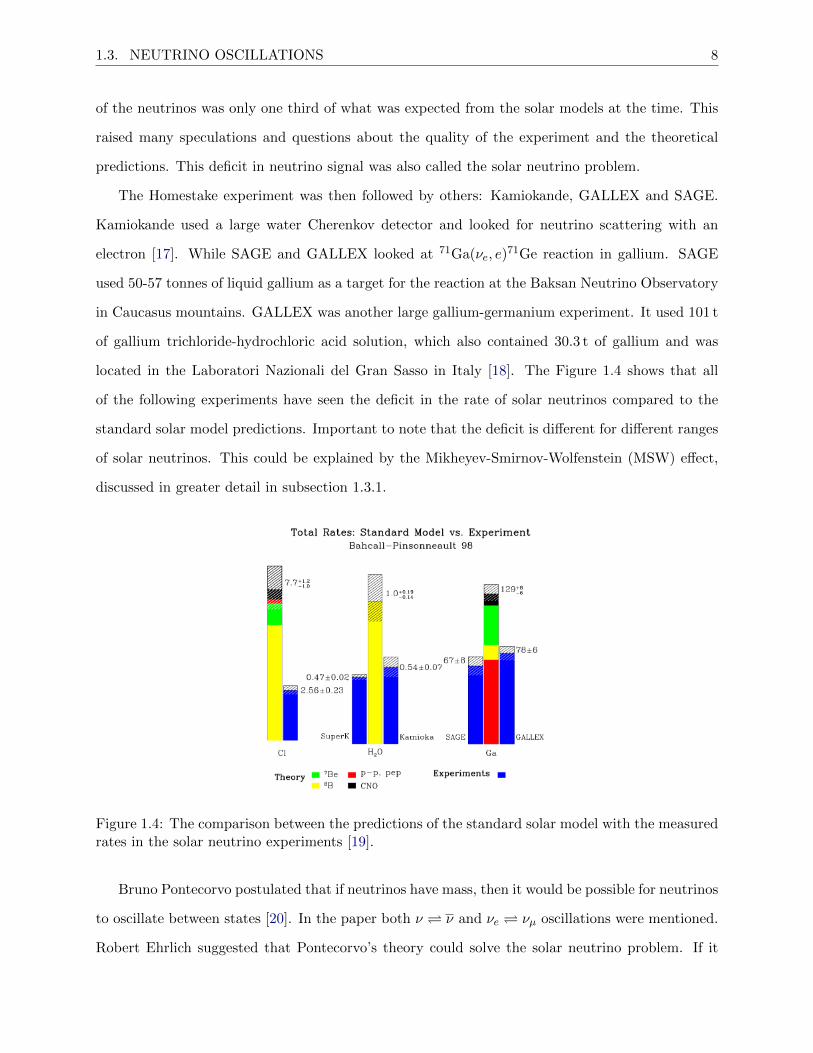
located in the Laboratori Nazionali del Gran Sasso in Italy [18]. The Figure 1.4 shows that all
of the following experiments have seen the deficit in the rate of solar neutrinos compared to the
standard solar model predictions. Important to note that the deficit is different for different ranges
of solar neutrinos. This could be explained by the Mikheyev-Smirnov-Wolfenstein (MSW) effect,
discussed in greater detail in subsection 1.3.1.
Figure 1.4: The comparison between the predictions of the standard solar model with the measuredrates in the solar neutrino experiments [19].
Bruno Pontecorvo postulated that if neutrinos have mass, then it would be possible for neutrinos
to oscillate between states [20]. In the paper both ν ν and νe νµ oscillations were mentioned.
Robert Ehrlich suggested that Pontecorvo’s theory could solve the solar neutrino problem. If it
1.3. NEUTRINO OSCILLATIONS 9
was possible for νe and νµ to oscillate between themselves, a fraction of electron neutrinos coming
from the sun would transform into muon or even tau neutrinos, before they get detected on Earth.
This could explain why while detecting electron neutrinos, fewer of them are seen than expected
[21].
On June 18, 2001 Sudbury Neutrino Observatory (SNO, subsection 2.1.1) announced their first
solar neutrino results that solved the solar neutrino mystery [22]. SNO used 1000 tonnes of heavy
water (D2O) to study higher energy solar neutrinos than the SAGE or GALLEX experiments. The
electron neutrino measurements from SNO were compared to the ones from Super-Kamiokande
[17]. According to the theory at the time, the measured fractions should have been the same for
the same type of neutrino. However, the fractions were different. This implied that the theoretical
models were incorrect. SNO was sensitive to not only charged current (CC, Equation 1.12), but
also neutral current (NC, Equation 1.13) interactions and elastic scattering (ES, Equation 1.11),
which can provide information about other flavours of neutrinos.
ES: νe,µ,τ + e− → νe,µ,τ + e− (1.11)
CC: νe + d→ e− + p+ p (1.12)
NC: νe,µ,τ + d→ νe,µ,τ + n+ p (1.13)
The combined measurements from SNO and the Super-Kamiokande determined the total flux
of solar neutrinos of all types. The number for the total flux agreed with the standard solar model.
This proved that the missing neutrino signal was not actually missing. It showed that the rest of
the flux was muon and tau neutrinos, which were not detected by the previous experiments. The
SNO experiment determined the ratio between CC and NC rates [23]:
φSNOCC
φSNONC
= 0.301± 0.033 (1.14)
About two thirds of the electron neutrinos oscillate or change into other flavours by the time they
are detected, Equation 1.14. Even though the adiabatic change in flavour observed by SNO is due
to the MSW effect (subsection 1.3.1), these combined results from SNO and Super-Kamiokande
1.3. NEUTRINO OSCILLATIONS 10
provided proof for the Pontecorvo theory about neutrino oscillations.
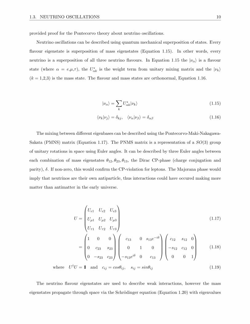
Neutrino oscillations can be described using quantum mechanical superposition of states. Every
flavour eigenstate is superposition of mass eigenstates (Equation 1.15). In other words, every
neutrino is a superposition of all three neutrino flavours. In Equation 1.15 the |να〉 is a flavour
state (where α = e,µ,τ), the U∗αk is the weight term from unitary mixing matrix and the |νk〉
(k = 1,2,3) is the mass state. The flavour and mass states are orthonormal, Equation 1.16.
|να〉 =∑k
U∗αk|νk〉 (1.15)
〈νk|νj〉 = δkj , 〈να|νβ〉 = δαβ (1.16)
The mixing between different eigenbases can be described using the Pontecorvo-Maki-Nakagawa-
Sakata (PMNS) matrix (Equation 1.17). The PNMS matrix is a representation of a SO(3) group
of unitary rotations in space using Euler angles. It can be described by three Euler angles between
each combination of mass eigenstates θ12, θ23, θ13, the Dirac CP-phase (charge conjugation and
parity), δ. If non-zero, this would confirm the CP-violation for leptons. The Majorana phase would
imply that neutrinos are their own antiparticle, thus interactions could have occured making more
matter than antimatter in the early universe.
U =
Ue1 Ue2 Ue3
Uµ1 Uµ2 Uµ3
Uτ1 Uτ2 Uτ3
(1.17)
=
1 0 0
0 c23 s23
0 −s23 c23
c13 0 s13e−iδ
0 1 0
−s13eiδ 0 c13
c12 s12 0
−s12 c12 0
0 0 1
(1.18)
where U †U = 1l and cij = cosθij , sij = sinθij (1.19)
The neutrino flavour eigenstates are used to describe weak interactions, however the mass
eigenstates propagate through space via the Schrodinger equation (Equation 1.20) with eigenvalues
1.3. NEUTRINO OSCILLATIONS 11
Ek =√~p2 +m2
k.
H|να〉 = Ek|νk〉 (1.20)
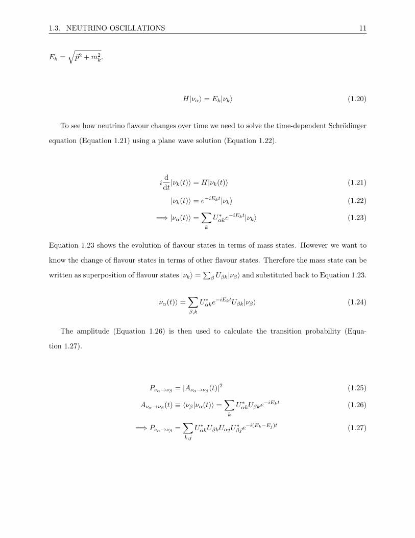
To see how neutrino flavour changes over time we need to solve the time-dependent Schrodinger
equation (Equation 1.21) using a plane wave solution (Equation 1.22).
id
dt|νk(t)〉 = H|νk(t)〉 (1.21)
|νk(t)〉 = e−iEkt|νk〉 (1.22)
=⇒ |να(t)〉 =∑k
U∗αke−iEkt|νk〉 (1.23)
Equation 1.23 shows the evolution of flavour states in terms of mass states. However we want to
know the change of flavour states in terms of other flavour states. Therefore the mass state can be
written as superposition of flavour states |νk〉 =∑
β Uβk|νβ〉 and substituted back to Equation 1.23.
|να(t)〉 =∑β,k
U∗αke−iEktUβk|νβ〉 (1.24)
The amplitude (Equation 1.26) is then used to calculate the transition probability (Equa-
tion 1.27).
Pνα→νβ = |Aνα→νβ (t)|2 (1.25)
Aνα→νβ (t) ≡ 〈νβ|να(t)〉 =∑k
U∗αkUβke−iEkt (1.26)
=⇒ Pνα→νβ =∑k,j
U∗αkUβkUαjU∗βje−i(Ek−Ej)t (1.27)
1.3. NEUTRINO OSCILLATIONS 12
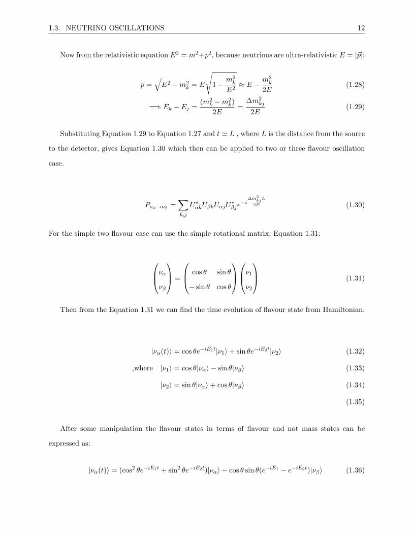
Now from the relativistic equation E2 = m2+p2, because neutrinos are ultra-relativistic E = |~p|:
p =√E2 −m2
k = E
√1−
m2k
E2≈ E −
m2k
2E(1.28)
=⇒ Ek − Ej =(m2
k −m2k)
2E=
∆m2kj
2E(1.29)
Substituting Equation 1.29 to Equation 1.27 and t ' L , where L is the distance from the source
to the detector, gives Equation 1.30 which then can be applied to two or three flavour oscillation
case.
Pνα→νβ =∑k,j
U∗αkUβkUαjU∗βje−i
∆m2kjL
2E (1.30)
For the simple two flavour case can use the simple rotational matrix, Equation 1.31:
νανβ
=
cos θ sin θ
− sin θ cos θ
ν1
ν2
(1.31)
Then from the Equation 1.31 we can find the time evolution of flavour state from Hamiltonian:
|να(t)〉 = cos θe−iE1t|ν1〉+ sin θe−iE2t|ν2〉 (1.32)
,where |ν1〉 = cos θ|να〉 − sin θ|νβ〉 (1.33)
|ν2〉 = sin θ|να〉+ cos θ|νβ〉 (1.34)
(1.35)
After some manipulation the flavour states in terms of flavour and not mass states can be
expressed as:
|να(t)〉 = (cos2 θe−iE1t + sin2 θe−iE2t)|να〉 − cos θ sin θ(e−iE1 − e−iE2t)|νβ〉 (1.36)
1.3. NEUTRINO OSCILLATIONS 13
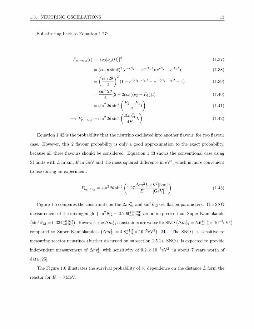
Substituting back to Equation 1.27:
Pνα→νβ (t) = |〈νβ|να(t)〉|2 (1.37)
= (cos θ sin θ)2(e−iE2t − e−iE1t)(eiE2 − eiE1t) (1.38)
=
(sin 2θ
2
)2
(1− ei(E2−E1)t − e−i(E2−E1)t + 1) (1.39)
=sin2 2θ
4(2− 2cos((e2 − E1))t) (1.40)
= sin2 2θ sin2
(E2 − E1
2t
)(1.41)
=⇒ Pνα→νβ = sin2 2θ sin2
(∆m2
21
4EL
)(1.42)
Equation 1.42 is the probability that the neutrino oscillated into another flavour, for two flavour
case. However, this 2 flavour probability is only a good approximation to the exact probability,
because all three flavours should be considered. Equation 1.43 shows the conventional case using
SI units with L in km, E in GeV and the mass squared difference in eV2, which is more convenient
to use during an experiment.
Pνα→νβ = sin2 2θ sin2
(1.27
∆m2L
E
[eV2][km]
[GeV]
)(1.43)
Figure 1.5 compares the constraints on the ∆m221 and sin2 θ12 oscillation parameters. The SNO
measurement of the mixing angle(sin2 θ12 = 0.299+0.023
−0.020
)are more precise than Super Kamiokande(
sin2 θ12 = 0.334+0.027−0.023
). However, the ∆m2
21 constraints are worse for SNO(∆m2
21 = 5.6+1.9−1.4× 10⁻⁵eV2
)compared to Super Kamiokande’s
(∆m2
21 = 4.8+1.5−0.8× 10⁻⁵eV2
)[24]. The SNO+ is sensitive to
measuring reactor neutrinos (further discussed on subsection 1.5.1). SNO+ is expected to provide
independent measurement of ∆m221 with sensitivity of 0.2 × 10⁻⁵eV2, in about 7 years worth of
data [25].
The Figure 1.6 illustrates the survival probability of νe dependence on the distance L form the
reactor for Eν =3 MeV.
1.3. NEUTRINO OSCILLATIONS 14
Figure 1.5: The confidence regions of the sin2 θ12 and ∆m221 measurements from Super-K, SNO
and KamLAND experiments. The regions and values are marked as follows: KamLAND in blue,combined SK+SNO+KamLAND in red and combined SK+SNO in green [24].
Figure 1.6: The reactor νe survival probability versus the distance from the reactor for the Eν = 3MeV.
1.3. NEUTRINO OSCILLATIONS 15
1.3.1 The MSW effect
The flavour specific neutrino interactions must be taken into account when considering neutrino
propagation through matter. In general all neutrinos may interact with matter via charged current
(CC) or neutral current (NC) interactions. In addition to NC interactions via Z bosons, the electron
neutrinos at solar neutrino energies interact through CC channel via W bosons, whereas muon
and tau neutrinos are bellow energy threshold for CC interactions. Therefore electron neutrinos
experience an additional potential energy VCC =√
2GFNe, where Ne is the electron density in
matter and GF = 1.166× 10⁻⁵GeV−2 is the Fermi constant. Because the effect of NC interactions
with matter is equal for all types of neutrino it only adds a certain constant to the oscillations.
The neutrino oscillation in matter derivation is shown in Appendix A. The new matter
neutrino oscillation parameters get defined as ∆m2M and sin2 2θM in terms of ∆m2 and sin2 2θ
from Equation 1.42, as shown in Equation 1.44 and Equation 1.45 respectively, where ACC =
2√
2GFNeE/∆m221.
∆m2M ≡ ∆m2
21
√sin2 2θ + (cos 2θ −ACC)2 (1.44)
sin2 2θM ≡sin2 2θ
sin2 2θ + (cos 2θ −ACC)2(1.45)
Then the oscillation probability in matter becomes:
PMνα→νβ = sin2 2θM sin2
(∆m2
M
4EL
)(1.46)
After the measurement the materials that neutrinos passed through must be taken into account
to correct the measured mass difference and mixing angles. Looking at Equation 1.45 it is visible
that, if ACC = cos 2θ, then sin2 2θM = 1 and θM = 45 deg, the mixing matter can be maximal.
This specific case, when the electron density and neutrino energy are at the right values for the
maximum mixing is called Mikheyev-Smirnov-Wolfenstein (MSW) effect.
1.4. NEUTRINO MASS 16
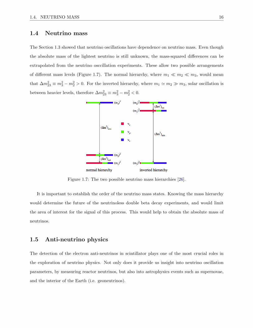
1.4 Neutrino mass
The Section 1.3 showed that neutrino oscillations have dependence on neutrino mass. Even though
the absolute mass of the lightest neutrino is still unknown, the mass-squared differences can be
extrapolated from the neutrino osccillation experiments. These allow two possible arrangements
of different mass levels (Figure 1.7). The normal hierarchy, where m1 � m2 � m3, would mean
that ∆m223 ≡ m2
3 −m22 > 0. For the inverted hierarchy, where m1 ' m2 � m3, solar oscillation is
between heavier levels, therefore ∆m223 ≡ m2
3 −m22 < 0.
Figure 1.7: The two possible neutrino mass hierarchies [26].
It is important to establish the order of the neutrino mass states. Knowing the mass hierarchy
would determine the future of the neutrinoless double beta decay experiments, and would limit
the area of interest for the signal of this process. This would help to obtain the absolute mass of
neutrinos.
1.5 Anti-neutrino physics
The detection of the electron anti-neutrinos in scintillator plays one of the most crucial roles in
the exploration of neutrino physics. Not only does it provide us insight into neutrino oscillation
parameters, by measuring reactor neutrinos, but also into astrophysics events such as supernovae,
and the interior of the Earth (i.e. geoneutrinos).
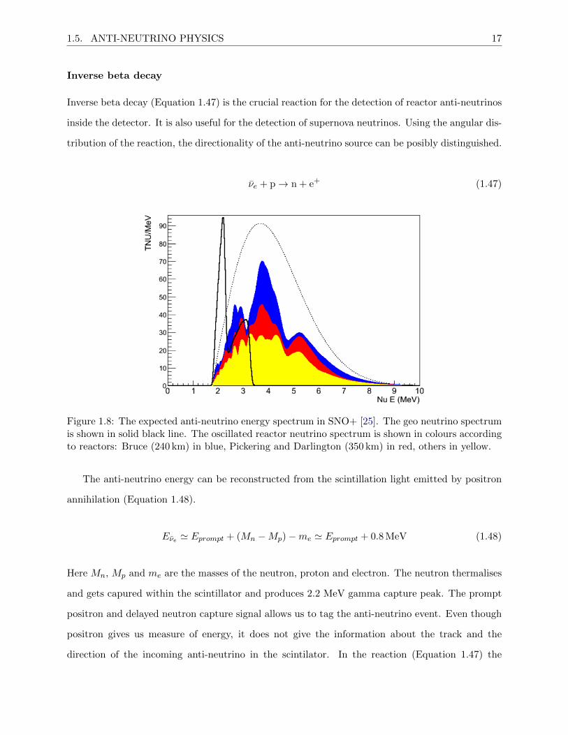
1.5. ANTI-NEUTRINO PHYSICS 17
Inverse beta decay
Inverse beta decay (Equation 1.47) is the crucial reaction for the detection of reactor anti-neutrinos
inside the detector. It is also useful for the detection of supernova neutrinos. Using the angular dis-
tribution of the reaction, the directionality of the anti-neutrino source can be posibly distinguished.
νe + p→ n + e+ (1.47)
Figure 1.8: The expected anti-neutrino energy spectrum in SNO+ [25]. The geo neutrino spectrumis shown in solid black line. The oscillated reactor neutrino spectrum is shown in colours accordingto reactors: Bruce (240 km) in blue, Pickering and Darlington (350 km) in red, others in yellow.
The anti-neutrino energy can be reconstructed from the scintillation light emitted by positron
annihilation (Equation 1.48).
Eνe ' Eprompt + (Mn −Mp)−me ' Eprompt + 0.8 MeV (1.48)
Here Mn, Mp and me are the masses of the neutron, proton and electron. The neutron thermalises
and gets capured within the scintillator and produces 2.2 MeV gamma capture peak. The prompt
positron and delayed neutron capture signal allows us to tag the anti-neutrino event. Even though
positron gives us measure of energy, it does not give the information about the track and the
direction of the incoming anti-neutrino in the scintilator. In the reaction (Equation 1.47) the
1.5. ANTI-NEUTRINO PHYSICS 18
outgoing neutrons tend to be forward-peaked [27]. In other words, the positron, because of being
very light, gets scattered more than the much heavier neutron. Therefore the separation between
positron and neutron directions can be measured. Understanding the neutron event detection
efficiency and reconstruction would lead to better reconstruction of anti-neutrino direction and
track. This can be either used for rejecting backgrounds or locating the source of the anti-neutrinos.
1.5.1 Reactor neutrinos
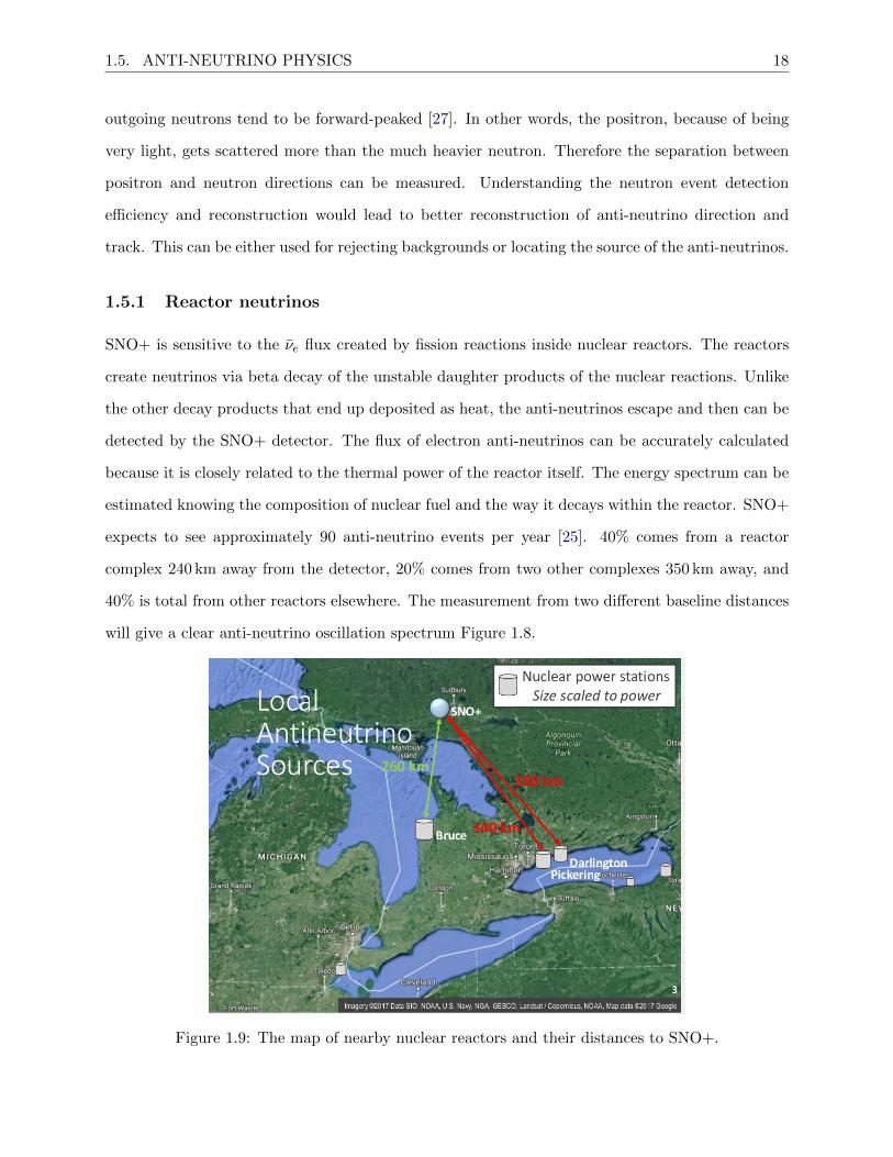
SNO+ is sensitive to the νe flux created by fission reactions inside nuclear reactors. The reactors
create neutrinos via beta decay of the unstable daughter products of the nuclear reactions. Unlike
the other decay products that end up deposited as heat, the anti-neutrinos escape and then can be
detected by the SNO+ detector. The flux of electron anti-neutrinos can be accurately calculated
because it is closely related to the thermal power of the reactor itself. The energy spectrum can be
estimated knowing the composition of nuclear fuel and the way it decays within the reactor. SNO+
expects to see approximately 90 anti-neutrino events per year [25]. 40% comes from a reactor
complex 240 km away from the detector, 20% comes from two other complexes 350 km away, and
40% is total from other reactors elsewhere. The measurement from two different baseline distances
will give a clear anti-neutrino oscillation spectrum Figure 1.8.
Figure 1.9: The map of nearby nuclear reactors and their distances to SNO+.
1.5. ANTI-NEUTRINO PHYSICS 19
Typically 99% of reactor anti-neutrinos are produced by beta decay of unstable daughter frag-
ments: 235U, 238U, 239Pu, 241Pu [28].
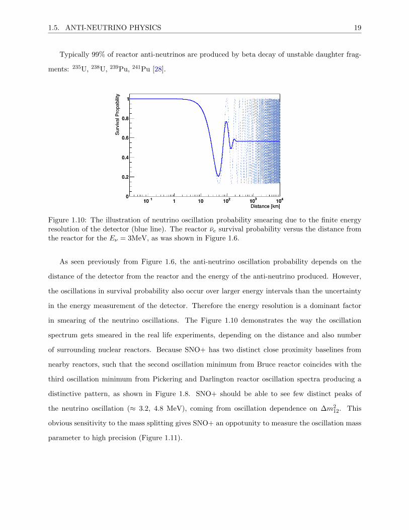
Figure 1.10: The illustration of neutrino oscillation probability smearing due to the finite energyresolution of the detector (blue line). The reactor νe survival probability versus the distance fromthe reactor for the Eν = 3MeV, as was shown in Figure 1.6.
As seen previously from Figure 1.6, the anti-neutrino oscillation probability depends on the
distance of the detector from the reactor and the energy of the anti-neutrino produced. However,
the oscillations in survival probability also occur over larger energy intervals than the uncertainty
in the energy measurement of the detector. Therefore the energy resolution is a dominant factor
in smearing of the neutrino oscillations. The Figure 1.10 demonstrates the way the oscillation
spectrum gets smeared in the real life experiments, depending on the distance and also number
of surrounding nuclear reactors. Because SNO+ has two distinct close proximity baselines from
nearby reactors, such that the second oscillation minimum from Bruce reactor coincides with the
third oscillation minimum from Pickering and Darlington reactor oscillation spectra producing a
distinctive pattern, as shown in Figure 1.8. SNO+ should be able to see few distinct peaks of
the neutrino oscillation (≈ 3.2, 4.8 MeV), coming from oscillation dependence on ∆m212. This
obvious sensitivity to the mass splitting gives SNO+ an oppotunity to measure the oscillation mass
parameter to high precision (Figure 1.11).
1.5. ANTI-NEUTRINO PHYSICS 20
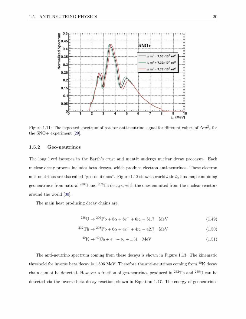
Figure 1.11: The expected spectrum of reactor anti-neutrino signal for different values of ∆m212 for
the SNO+ experiment [29].
1.5.2 Geo-neutrinos
The long lived isotopes in the Earth’s crust and mantle undergo nuclear decay processes. Each
nuclear decay process includes beta decays, which produce electron anti-neutrinos. These electron
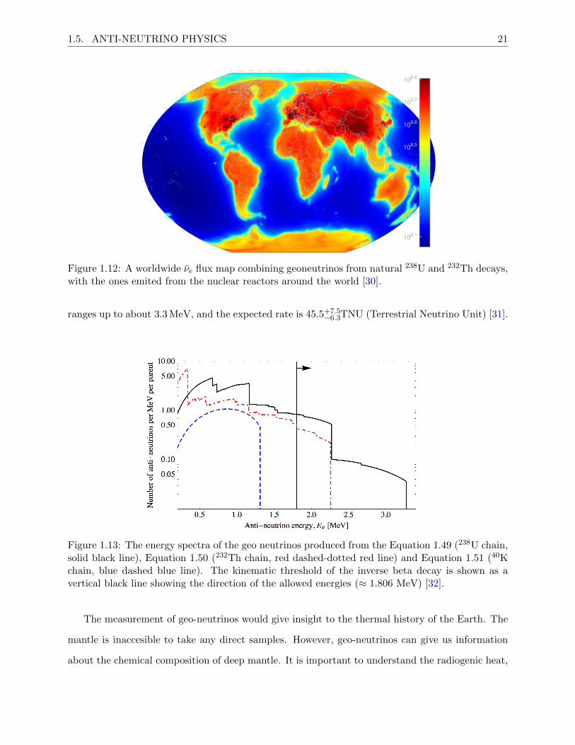
anti-neutrinos are also called “geo-neutrinos”. Figure 1.12 shows a worldwide νe flux map combining
geoneutrinos from natural 238U and 232Th decays, with the ones emmited from the nuclear reactors
around the world [30].
The main heat producing decay chains are:
238U→ 206Pb + 8α+ 8e− + 6νe + 51.7 MeV (1.49)
232Th→ 208Pb + 6α+ 4e− + 4νe + 42.7 MeV (1.50)
40K→ 40Ca + e− + νe + 1.31 MeV (1.51)
The anti-neutrino spectrum coming from these decays is shown in Figure 1.13. The kinematic
threshold for inverse beta decay is 1.806 MeV. Therefore the anti-neutrinos coming from 40K decay
chain cannot be detected. However a fraction of geo-neutrinos produced in 232Th and 238U can be
detected via the inverse beta decay reaction, shown in Equation 1.47. The energy of geoneutrinos
1.5. ANTI-NEUTRINO PHYSICS 21
Figure 1.12: A worldwide νe flux map combining geoneutrinos from natural 238U and 232Th decays,with the ones emited from the nuclear reactors around the world [30].
ranges up to about 3.3 MeV, and the expected rate is 45.5+7.5−6.3TNU (Terrestrial Neutrino Unit) [31].
Figure 1.13: The energy spectra of the geo neutrinos produced from the Equation 1.49 (238U chain,solid black line), Equation 1.50 (232Th chain, red dashed-dotted red line) and Equation 1.51 (40Kchain, blue dashed blue line). The kinematic threshold of the inverse beta decay is shown as avertical black line showing the direction of the allowed energies (≈ 1.806 MeV) [32].
The measurement of geo-neutrinos would give insight to the thermal history of the Earth. The
mantle is inaccesible to take any direct samples. However, geo-neutrinos can give us information
about the chemical composition of deep mantle. It is important to understand the radiogenic heat,
1.5. ANTI-NEUTRINO PHYSICS 22
as it contributes to the movement of plate tectonics and relates to the Earth’s magnetic field.
1.5.3 Supernova neutrinos
Ever since the observation of the 24 νe events from the collapse of supernova SN 1987A, a new
interest in neutrino astrophysics was born [33]. For core-collapse supernovae neutrino emission
represents ≈ 99% of the gravitational binding energy. Based on SN 1987A events the neutrinos
coming from supernova are high energy (12 MeV to 18 MeV). For the νe specifically, the mean
predicted energy is 15 MeV. However, the predictions are completely model dependent and the
energy of neutrinos produced can vary depending on the type of supernova.
The measured relationship between νe and other flavours of neutrinos could reveal the pattern of
flavour changes. This could shed light to the neutrino mixing parameters and the mass hierarchy.
Neutrinos from supernova arrive earlier than light, because neutrinos escape the dense core before
photons. Therefore SNO+ will also participate in the Supernova Neutrinos Early Warning System
(SNEWS) [34]. SNEWS is an international project of various experiments worldwide that can see
the early neutrino signal and and prompt the alert for a supernova event.
This thesis is focused on the SNO+ experiment and the detection of anti-neutrinos using the
SNO+ detector. The purpose of this thesis is the design of the AmBe neutron source used for
the neutron capture efficiency calibration for the detector in the scintillator phase. The following
chapters will discuss the SNO+ detector, calibration systems and the AmBe source design and
importance for the success of the experiment. Chapter 2 gives an overview of the SNO+ experiment
and the different phases of the experiment for various physics goals. Chapter 3 discusses the detector
calibration systems, hardware and optical and radioactive calibration sources. Chapter 4 gives an
intoduction to the AmBe neutron source, includes the improvements made to the source design
and discusses the new proposed design for the AmBe source for the SNO+ scintillator phase.
The new introduced design requires some analysis on shadowing and the deployment simulations
with the new and improved source, these are all studied in the Chapter 5. Finally, Chapter 6
summarises the work, establishes the work needed to be done for the successful neutron capture
effciency calibration and draws conclusions about the importance of this calibration for the possible
anti-neutrino physics data, which would lead to insight on wide range of different neutrino physics
topics such as neutrino oscillation parameters, supernova events, and the interior of the Earth.
Chapter 2
The SNO+ experiment
2.1 The SNO+ Detector
SNO+ is a multipurpose scintillator detector located in SNOLAB, a 2070 m underground, 10000
sq ft, Class-2000 clean room in Vale’s Creighton mine near Sudbury, Ontario, Canada. The main
objective of SNO+ is the search of the neutrinoless double beta decay (ββ0ν) in order to determine
if neutrinos are Majorana or Dirac particles and to gain knowledge about the absolute mass of
the neutrino. Other topics of interest are reactor neutrino oscillations, supernova neutrinos, geo-
neutrinos, and some exotic searches, such as nucleon decay. Given its multipurpose nature, the
experiment has three phases. In the first phase, the detector is filled with water. In the second
phase, the acrylic vessel is filled with 780 tons of liquid scintillator. Finally, in the third phase, the
scintillator is loaded with tellurium.
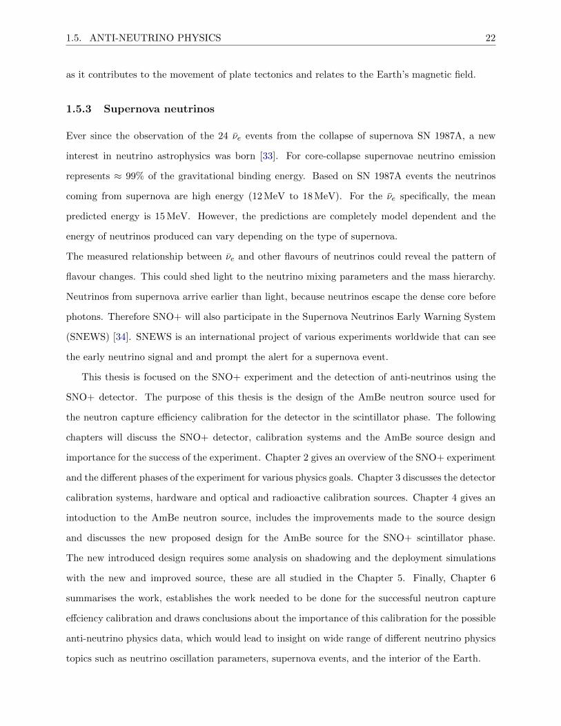
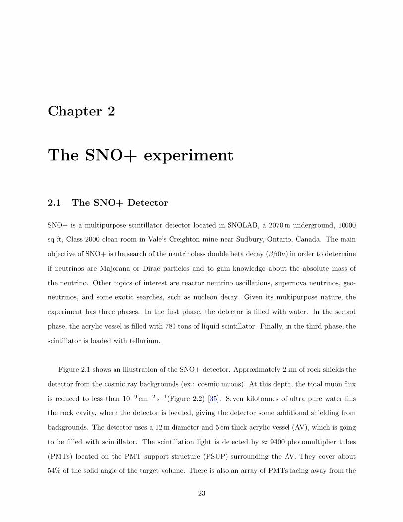
Figure 2.1 shows an illustration of the SNO+ detector. Approximately 2 km of rock shields the
detector from the cosmic ray backgrounds (ex.: cosmic muons). At this depth, the total muon flux
is reduced to less than 10−9 cm−2 s−1(Figure 2.2) [35]. Seven kilotonnes of ultra pure water fills
the rock cavity, where the detector is located, giving the detector some additional shielding from
backgrounds. The detector uses a 12 m diameter and 5 cm thick acrylic vessel (AV), which is going
to be filled with scintillator. The scintillation light is detected by ≈ 9400 photomultiplier tubes
(PMTs) located on the PMT support structure (PSUP) surrounding the AV. They cover about
54% of the solid angle of the target volume. There is also an array of PMTs facing away from the
23
2.1. THE SNO+ DETECTOR 24
target volume. These detect events that happen outside the AV and provides a veto to identify
backgrounds and incoming muons.
The AV can be accessed through its neck, which has been surrounded by the deck clean room
(DCR). The DCR is cleaner than the SNOLAB environment. This minimizes contamination of the
AV during calibrations or maintenance.
Figure 2.1: Artist illustration of SNO+ detector.
2.1.1 SNO
SNO+ is the successor to the Sudbury Neutrino Observatory (SNO) experiment. SNO was a
heavy water Cherenkov detector able to measure the flux of solar neutrinos using neutral current
interactions and the electron neutrino flux using charge current interactions. The experiment
reached its goal to demonstrate that neutrinos indeed change flavour and confirmed the predicted
2.1. THE SNO+ DETECTOR 25
Figure 2.2: The muon flux dependency on the depth of the various underground laboratories.
2.1. THE SNO+ DETECTOR 26
solar models. This confirmation lead to the Nobel Prize in Physics awarded to Dr. Arthur B.
McDonald jointly with Dr. Takaaki Kajita in 2015, for the discovery of neutrino oscillations, which
shows that neutrinos have mass [36].
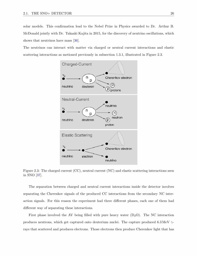
The neutrinos can interact with matter via charged or neutral current interactions and elastic
scattering interactions as metioned previously in subsection 1.3.1, illustrated in Figure 2.3.
Figure 2.3: The charged current (CC), neutral current (NC) and elastic scattering interactions seenin SNO [37].
The separation between charged and neutral current interactions inside the detector involves
separating the Cherenkov signals of the produced CC interactions from the secondary NC inter-
action signals. For this reason the experiment had three different phases, each one of them had
different way of separating these interactions.
First phase involved the AV being filled with pure heavy water (D2O). The NC interaction
produces neutrons, which get captured onto deuterium nuclei. The capture produced 6.3 MeV γ-
rays that scattered and produces electrons. Those electrons then produce Cherenkov light that has
2.1. THE SNO+ DETECTOR 27
a different energy range than the signal from charged current interaction. The difference in energy
spectrum and multiple applied fits and analysis helped to distinguish the NC from CC interactions.
However, in order to fit the energy spectra the solar neutrino spectral shape had to be assumed,
which is not ideal. Therefore, the second phase on SNO experiment had 2 t of NaCl disolved into
the heavy water. Chlorine has large neutron capture cross section which produced several γ-rays.
The light produced by several compton electrons following neutron capture was more isotropic than
single electron CC interaction. From this the difference between these interactions could be defined
by an isotropical parameter, which did not depend on energy. This gave additional information to
distinguish between charged and neutral current neutrino interactions.
The third phase deployed an array of neutral current detectors (NCDs). These detectors were
3He counters and provided separate neutral current measurement that was uncorrelated to charged
current signals. NCDs detected the number of neutrons coming from neutral current interactions
of coming solar neutrinos.This provided the total flux of 8B solar neutrinos.
After the SNO experiment the existing SNO detector infrastructure was repurposed for SNO+.
The existing detector cavity and AV volume with the surrounding PMT array matched the features
required for large liquid scintillator detector. The upgrades from SNO to SNO+ are described in
the following subsection.
2.1.2 Upgrades
SNO+ is using most of the already existing infrastructure from the SNO detector. Changing from
heavy water Cherenkov to a liquid scintillator detector required a lot of changes to the infrastruc-
ture, electronics and software of the experiment.
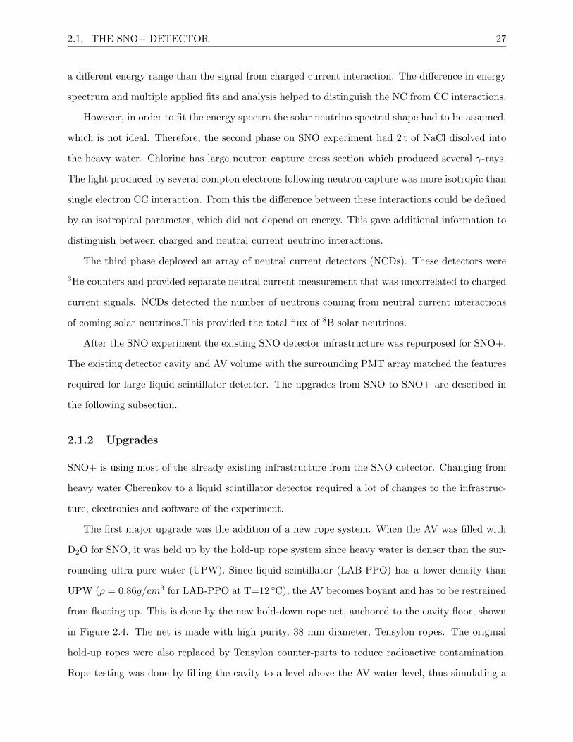
The first major upgrade was the addition of a new rope system. When the AV was filled with
D2O for SNO, it was held up by the hold-up rope system since heavy water is denser than the sur-
rounding ultra pure water (UPW). Since liquid scintillator (LAB-PPO) has a lower density than
UPW (ρ = 0.86g/cm3 for LAB-PPO at T=12 ◦C), the AV becomes boyant and has to be restrained
from floating up. This is done by the new hold-down rope net, anchored to the cavity floor, shown
in Figure 2.4. The net is made with high purity, 38 mm diameter, Tensylon ropes. The original
hold-up ropes were also replaced by Tensylon counter-parts to reduce radioactive contamination.
Rope testing was done by filling the cavity to a level above the AV water level, thus simulating a
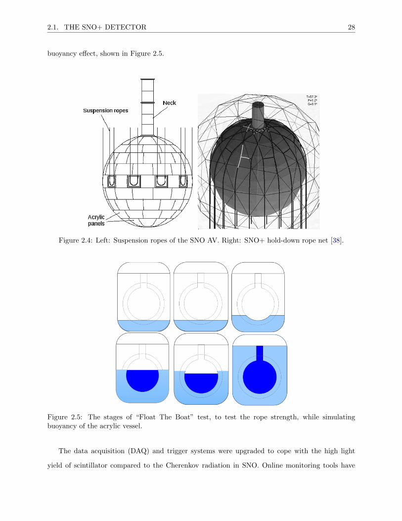
2.1. THE SNO+ DETECTOR 28
buoyancy effect, shown in Figure 2.5.
Figure 2.4: Left: Suspension ropes of the SNO AV. Right: SNO+ hold-down rope net [38].
Figure 2.5: The stages of “Float The Boat” test, to test the rope strength, while simulatingbuoyancy of the acrylic vessel.
The data acquisition (DAQ) and trigger systems were upgraded to cope with the high light
yield of scintillator compared to the Cherenkov radiation in SNO. Online monitoring tools have
2.2. PHASES OF EXPERIMENT 29
been developed to be able to display data at 20 kHz. Also, a remote detector monitoring feature
was added, a new alarm GUI was implemented to monitor any changes in operation, and the over-
all user interface was highly improved. Features such as extra crate voltage and current readouts
allows operators to check changes from channel to channel. Because of the increased trigger rate
from scintillation light, the grid based processing and the storage channels have been updated as
well. The anticipated increased trigger rate also led to upgrades of the electronic hardware such as
the addition of new XL3 readout cards and MTC/A+ trigger cards.
A new cover gas system was introduced to limit radon ingress into the detector. As radon decay
chain daughters are a large part of the background for the experiment. The closed system with
high purity nitrogen gas acts as a barrier between the detector and the radon in the outside air.
There are also upgrades to the calibration system, discussed in more detail in Chapter 3).
Amidst these changes, the photomultiplier tubes will remain unchanged. SNO+ is using the 8
inch Hamamatrsu R1408 photomultiplier tubes from SNO [39]. Large numbers of malfunctioning
PMTs, that failed over SNO lifetime, have been repaired and installed back into the detector.
2.2 Phases of experiment
The SNO+ experiment will have three main phases: the water phase, the pure scintillator phase,
and the tellurium-loaded scintillator phase. Currently the detector is in the water phase, taking
data. From water data we will gain knowledge of the internal and external backgrounds for the
experiment. The detector is to be filled with scintillator in start of 2018.
2.2.1 Water Phase
In this phase, the acrylic vessel is filled with ultra-pure water. The main physics goals are the exotic
searches. These include the search for invisible nucleon decay, axion-like particles, and supernova
neutrinos. Also, reactor anti-neutrinos with an energy higher than 1.8 MeV can be detected. This
phase will provide information about the DAQ characteristics, the PMT response, and overall de-
2.2. PHASES OF EXPERIMENT 30
Goal/Phase Water Pure LAB Te-loaded LAB
Neutrinoless double beta decay - - X8B solar neutrinos - X X
CNO, pep solar neutrinos - X -Reactor and Geo-neutrinos - X X
Exotic searches X X X
Calibration goalsPMT response,electronics
Optical parameters,energy resolution,event efficiency
Optical parameters,energy resolution,event efficiency
Table 2.1: The main physics and calibration goals for the three SNO+ experiment phases.
tector performance since the upgrades were installed. This phase will allow the impurities, such as
210Po and 210Pb, embedded in the acrylic vessel to partially leach-out, which is important for the
background studies. During the calibration of the water phase, the new fibre-based calibration sys-
tem will also be tested. Good calibration and background understanding is critical for the quality
data physics runs.
SNO+ will is looking for nucleon decay via 16O decay to either 15N or 15O excited states. The
signal will be observed via the emission of 6 MeV to 7 MeV gammas (45% of the time) from the
deexitation of the daughter nuclei. Presently, the best limits set for invisible nucleon decay are
5.8 × 1029 years for neutron disappearance by KamLAND [40] and 2.1 × 1029 years for proton
disappearance [41]. SNO+ should provide better measurements for nucleon decay as it will be
more efficient. KamLAND looked at 12C, while SNO+ will study this decay using 16O. When a
neutron decays the resulting 15O is put into the excited state, it promptly deexcites 44% of the
time emitting a 6.18 MeV gamma. In case of proton decay, the resulting nucleus will be 15N. 41%
of the time while deexciting 15N will emit a 6.32 MeV gamma. Figure 2.6 shows the expected
energy spectrum for water phase backgrounds within a 5.5 m fiducial volume cut and a cut on
cos θsun > −0.8 applied [25]. θsun is the angle between the scattered electron and the position of
the sun. The cos θsun cut relative to the solar direction, reduces the dominant solar background.
2.2.2 Pure Scintillator Phase
The detector will be filled with ∼ 780 tonnes of pure liquid scintillator (LAB-PPO). The SNO+
scintillator is composed of linear alkylbenzene (LAB) +2g/L of the fluor 2, 5 - diphenyloxazole
2.2. PHASES OF EXPERIMENT 31
Figure 2.6: Expected energy spectrum for water phase backgrounds within a 5.5 m fiducial volumecut and a cut on cos θsun > −0.8 applied [25].
(PPO). LAB was selected because of its stability, compatability with acrylic, and high purity. It
also has a long attenuation length with high light yield and linear response in energy, which makes
it easy for the accurate reconstrucion of deposited energy. A new processing plant was constructed
to purify the scintillator and reduce the backgrounds from the contaminants in the scintillator. The
LAB fill is scheduled to start in late 2017 and to be completed by 2018. During this phase, the
scintillator calibrations will take place (including the AmBe neutron source deployment discussed
in this thesis). After the calibrations, the reactor and geo anti-neutrino studies alongside low energy
solar neutrino signals will be measured.
2.2.3 Te-loaded Scintillator Phase
The tellurium-loaded phase is important for the ββ0ν-decay search. Telluric acid, Te(OH)6 is
loaded into the scintillator and then a secondary wavelength shifter will also be added, to better
match the PMT quantum efficiency. 130Te was chosen due to its large natural abundance (34%) and
its long ββ2ν half-life. ββ2ν is a large background for ββ0ν events. Therefore long ββ2ν half-life
minimises the background events coming from this decay. For the ββ0ν decay 130Te has a Q-value
of 2.53 MeV. During this phase, the detector is expected to be operated with a loading of 0.5%
2.3. ANTI-NEUTRINO DETECTION 32
Figure 2.7: The expected ββ0ν-decay signal and its backgrounds for 5% Te-loading. The countsare estimated over 5 years of data taking.
natural tellurium in LAB. The expected ββ0ν-decay with its backgrounds can be seen in Figure 2.7
for the future phase with 5% loading. It shows the counts for the case of the mν =200 MeV, over 5
years worth of measurement. The proposed scintillator “cocktail” is LAB+PPO (2 g l−1) + bisMSB
(15 mg l−1) loaded using the Te-Diol method (0.5%). The assumed light yield of the cocktail is 390
hits/MeV. Figure 2.8 shows the different background contributions in the region of inetrest for
neutrinoless double beta decay event for one year of Te-Diol “cocktail” dicussed above.
2.3 Anti-neutrino Detection
Electron neutrinos most commonly interact via elastic scattering with electrons because of the large
cross section of this interaction (Equation 2.1).
νe + e− → νe + e− (2.1)
These interactions induce excitations in the scintillator, which then produce photons that get de-
tected by the PMTs. The electron antineutinos are detected via the inverse beta decay interaction,
2.3. ANTI-NEUTRINO DETECTION 33
Figure 2.8: Pie chart for the different background contributions in the region of interest for neutri-noless double beta decay events for one year of Te-Diol scenario.
shown in Equation 2.2 and explained in more detail in Section 1.5.
νe + p→ e+ + n (2.2)
As illustrated in Figure 2.9, the incoming anti-neutrino hits a proton which creates a positron and
a neutron. Compared to the neutron, the positron quickly annihilates with an electron releasing
two gammas and creating a prompt signal. The neutron takes time to thermalise and gets captured
within the scintillator onto another proton (mean lifetime ≈ 220µs), this produces 2.2 MeV gamma.
This 2.2 MeV gamma peak is the delayed neutron capture peak. These two signals serve as a tag
for electron anti-neutrino interaction in scintillator. Therefore, an understanding of the neutron
detection efficiency of the SNO+ detector is extremely important. The neutron capture efficiency
calibration is the main focus of this thesis.
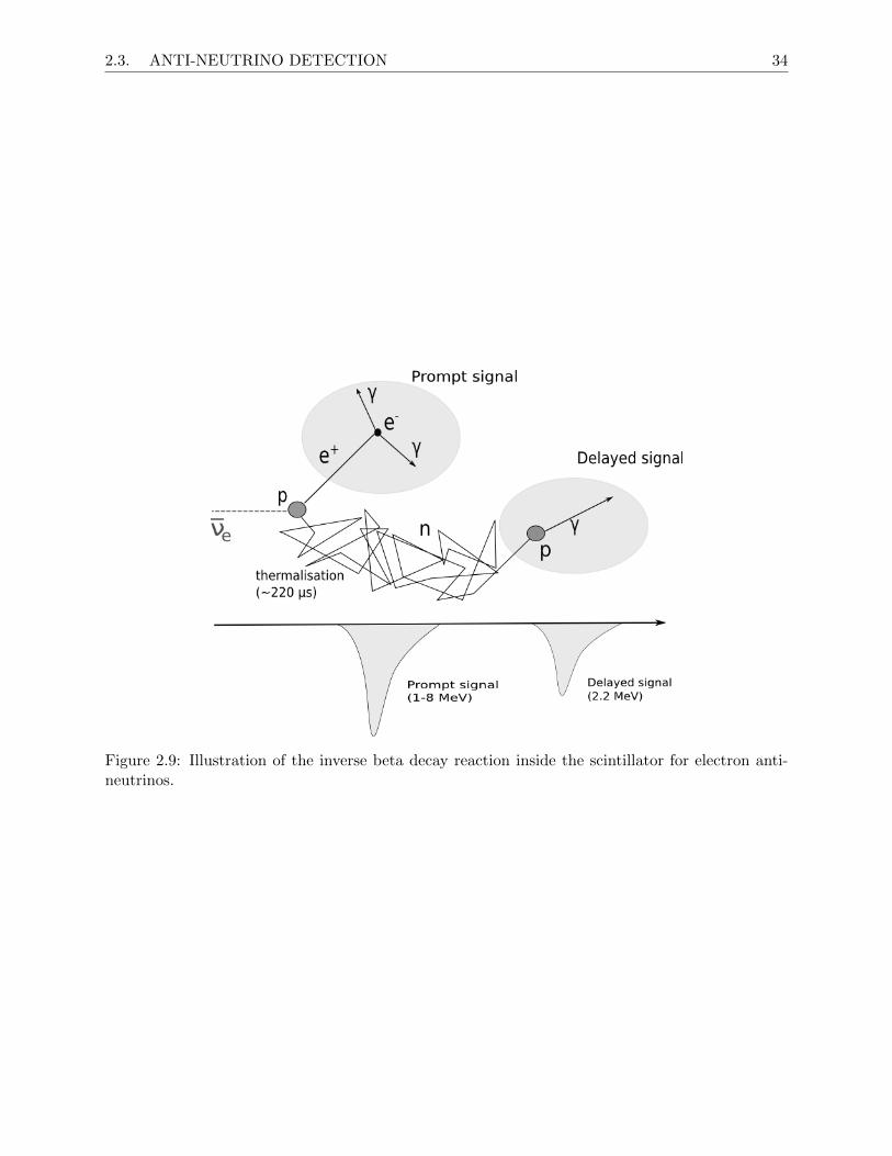
2.3. ANTI-NEUTRINO DETECTION 34
Figure 2.9: Illustration of the inverse beta decay reaction inside the scintillator for electron anti-neutrinos.
Chapter 3
Detector calibration
Calibration is necessary for understanding the detector response over the full energy range (0.1-10MeV).
In particular, it is necessary to understand the performance of the detector in reconstruction of
particle type, energy, and position. Calibration is required to determine the uncertainties on these
reconstructed values.
The three different phases of SNO+ have different calibration goals that will end up comple-
menting each other. In the water phase, the main goal is to characterise the electronics, the response
of the PMTs and light reflectors and to take data for water physics discussed in subsection 2.2.1.
Furthermore, in the pure scintillator phase, the most important parameters to understand are the
scintillator optical absorption, reemission, and scattering as well as the energy resolution and neu-
tron event efficiency. Moving into the Te-loaded phase, the parameters determined in previous
phases will have to be modified because tellurium will change the properties of the scintillator.
Various optical sources (LEDs and lasers coupled to optical fibres) and radioactive sources (γ,n)
are used to calibrate the detector. The optical sources are used to calibrate the PMTs and the
optical properties of the target (water, scintillator). The radioactive sources are used to measure
energy scale, resolution and detection efficiency of various particles. Comprehensive Monte Carlo
simulations are done for each source in order to compare the expected detector response to the
actual calibration data. A calibration analysis plan was developed to ensure that all properties in
the detector model can be measured to the necessary accuracy for physics data runs. An estimation
of the background rates and of the detection efficiency can be determined during the calibration.
From the calibration analysis work, the required uncertainties can be added to the reconstruction
35
3.1. CALIBRATION HARDWARE 36
of physics events.
3.1 Calibration hardware
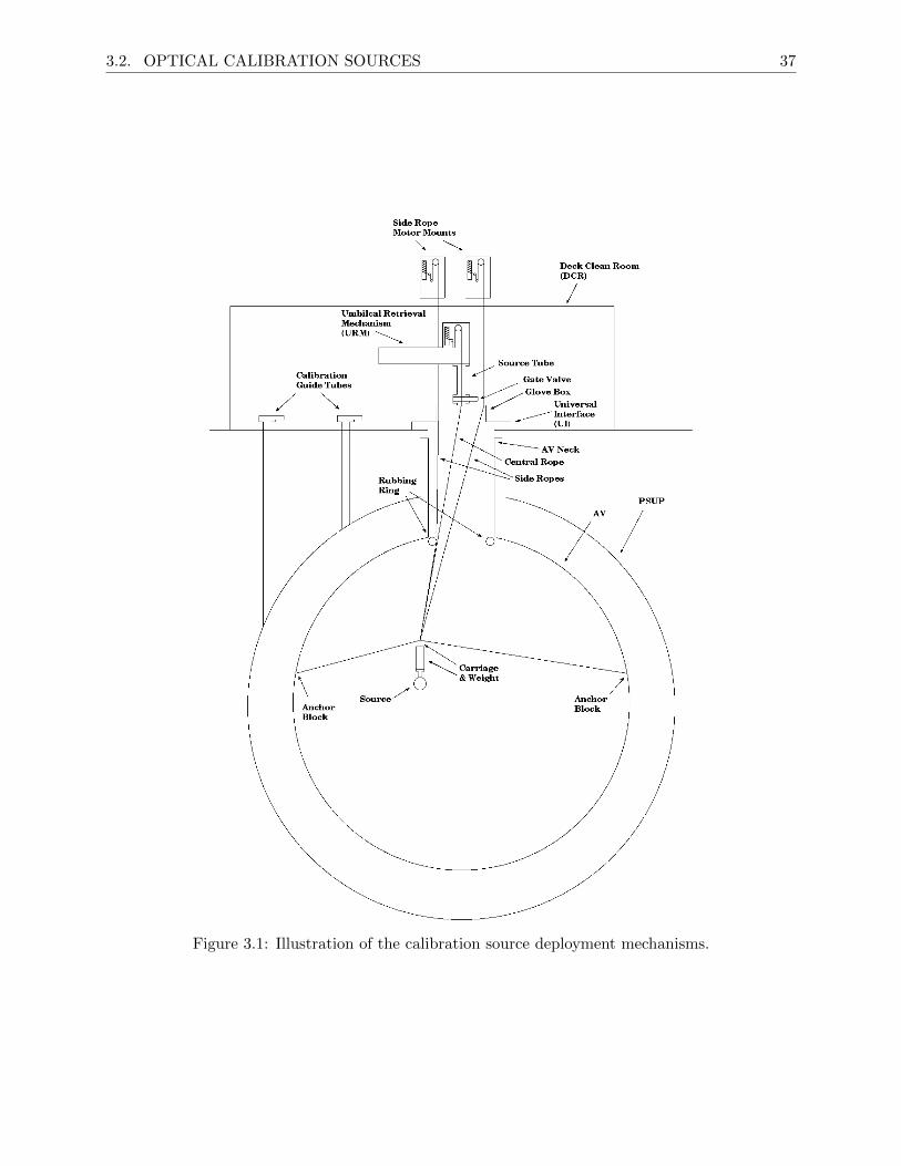
Sources are connected to an umbilical and lowered down into the detector through the neck, as
shown in Figure 3.1. The umbilical provides all the necessary feeding lines to the source such as
high voltage or output cables. The Umbilical Retreval Mechanism (URM) stores the umbilical and
contains motors that control it. A glove box, located on the top of the detector provides temporary
storage for the sources that are not in use. A central rope supports the weight of the source, while
side ropes are used to move the source inside the detector, for positional analysis. The ropes are
controlled by the rope motors.
With the help of the side ropes, the detector can be scanned off the central axis in two orthogonal
planes. A system of cameras inside the detector is used to monitor the position of the AV and the
ropes. Also, it will provide information about the deployed source position by detecting an LED
light attached to the source container.
Deployment of the sources is done through a new universal interface (UI) that was designed for
SNO+. The UI also provides sensor information from the water level sensor and the veto PMTs.
All of the materials used in the calibration hardware are designed to match the purity require-
ments of SNO+ and need to be compatible with LAB.
3.2 Optical calibration sources
The optical calibration sources inject light pulses into the detector through optical fibres mounted
on the PSUP Figure 3.2. The injected light is in the 375 nm to 510 nm range.
These optical sources were first used to calibrate the PMT timing and gains. The calibration
used 92 sets of fibres which covered the entire set of PMTs [42]. The position reconstruction is
highly dependent on the timing calibration of the entire detector. The time response depends on the
decay time of the scintillator signal and overall synchronisation of the PMT array. The PMT gain
calibration is important for the energy reconstruction. Time and charge information are measured
for each PMT pulse. The required dynamic range of PMT gain is between 1 to 4 photoelectrons.
3.2. OPTICAL CALIBRATION SOURCES 37
Figure 3.1: Illustration of the calibration source deployment mechanisms.
3.3. RADIOACTIVE CALIBRATION SOURCES 38
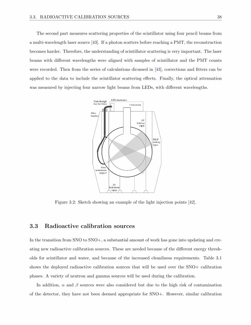
The second part measures scattering properties of the scintillator using four pencil beams from
a multi-wavelength laser source [43]. If a photon scatters before reaching a PMT, the reconstruction
becomes harder. Therefore, the understanding of scintillator scattering is very important. The laser
beams with different wavelengths were aligned with samples of scintillator and the PMT counts
were recorded. Then from the series of calculations dicussed in [43], corrections and fitters can be
applied to the data to include the scintillator scattering effects. Finally, the optical attenuation
was measured by injecting four narrow light beams from LEDs, with different wavelengths.
Figure 3.2: Sketch showing an example of the light injection points [42].
3.3 Radioactive calibration sources
In the transition from SNO to SNO+, a substantial amount of work has gone into updating and cre-
ating new radioactive calibration sources. These are needed because of the different energy thresh-
olds for scintillator and water, and because of the increased cleanliness requirements. Table 3.1
shows the deployed radioactive calibration sources that will be used over the SNO+ calibration
phases. A variety of neutron and gamma sources will be used during the calibration.
In addition, α and β sources were also considered but due to the high risk of contamination
of the detector, they have not been deemed appropriate for SNO+. However, similar calibration
3.3. RADIOACTIVE CALIBRATION SOURCES 39
information can be obtained from internal radioactive sources. Some naturally occuring radiation
comes from 238U and 232U chains inside the liquid scintillator. The 210Po-α, 14C-β, delayed 214Bi-Po
and 212Bi-Po coincidences are typical calibration references for alpha and beta signals [25].
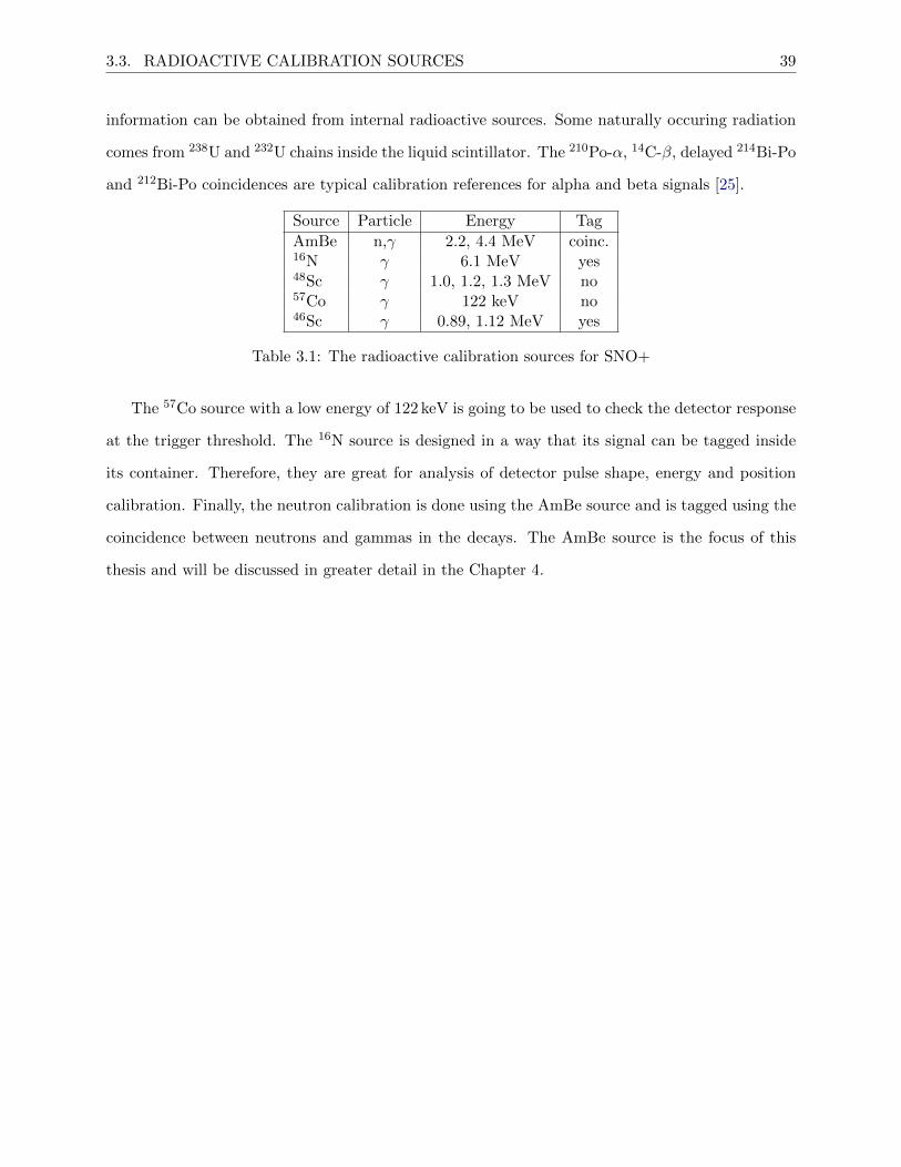
Source Particle Energy Tag
AmBe n,γ 2.2, 4.4 MeV coinc.16N γ 6.1 MeV yes48Sc γ 1.0, 1.2, 1.3 MeV no57Co γ 122 keV no46Sc γ 0.89, 1.12 MeV yes
Table 3.1: The radioactive calibration sources for SNO+
The 57Co source with a low energy of 122 keV is going to be used to check the detector response
at the trigger threshold. The 16N source is designed in a way that its signal can be tagged inside
its container. Therefore, they are great for analysis of detector pulse shape, energy and position
calibration. Finally, the neutron calibration is done using the AmBe source and is tagged using the
coincidence between neutrons and gammas in the decays. The AmBe source is the focus of this
thesis and will be discussed in greater detail in the Chapter 4.
Chapter 4
Neutron source design
AmBe is a neutron source, which consists of a mixture of 241Am and 9Be. The 241Am produces α
particles. The alpha particles then react with beryllium. The two dominant processes are shown
in Equation 4.1 and Equation 4.2.
α+ 9Be→ 1n + 12C Q = 5.701MeV (4.1)
α+ 9Be→ 1n + 12C∗deexcites−−−−−→ 12C + γ + 4.44MeV Q = 1.261MeV (4.2)
The cross sections for Equation 4.1 and Equation 4.2 reactions depend on the alpha energy.
The source activity is dependent on the arrangement of the 241Am and 9Be within the source itself.
The minimum spacing between the isotopes creates larger contact are for the actinide to induce the
(α, n) reaction. The AmBe sources can be “foil sources” or “powder sources”. The SNO experiment
had one of each type: “AmBe med” and “AmBe high” (foil and powder respectively). However,
SNO+ is using the powder type AmBe source (“AmBe high”). The powder source has a higher
activity than its foil type counterpart, as the powder has a larger interfacial area.
Depending on the energy of the produced alpha, the neutron and the coresponding 12C excitation
level changes. Therefore, the produced gamma energy and neutron energy are co-dependent. The
deexcitation levels of carbon with corresponding gamma energies are shown in Figure 4.1 and listed
below. Important to note that π next to excitation energy of 7.654 MeV does not stand for pion, it
40
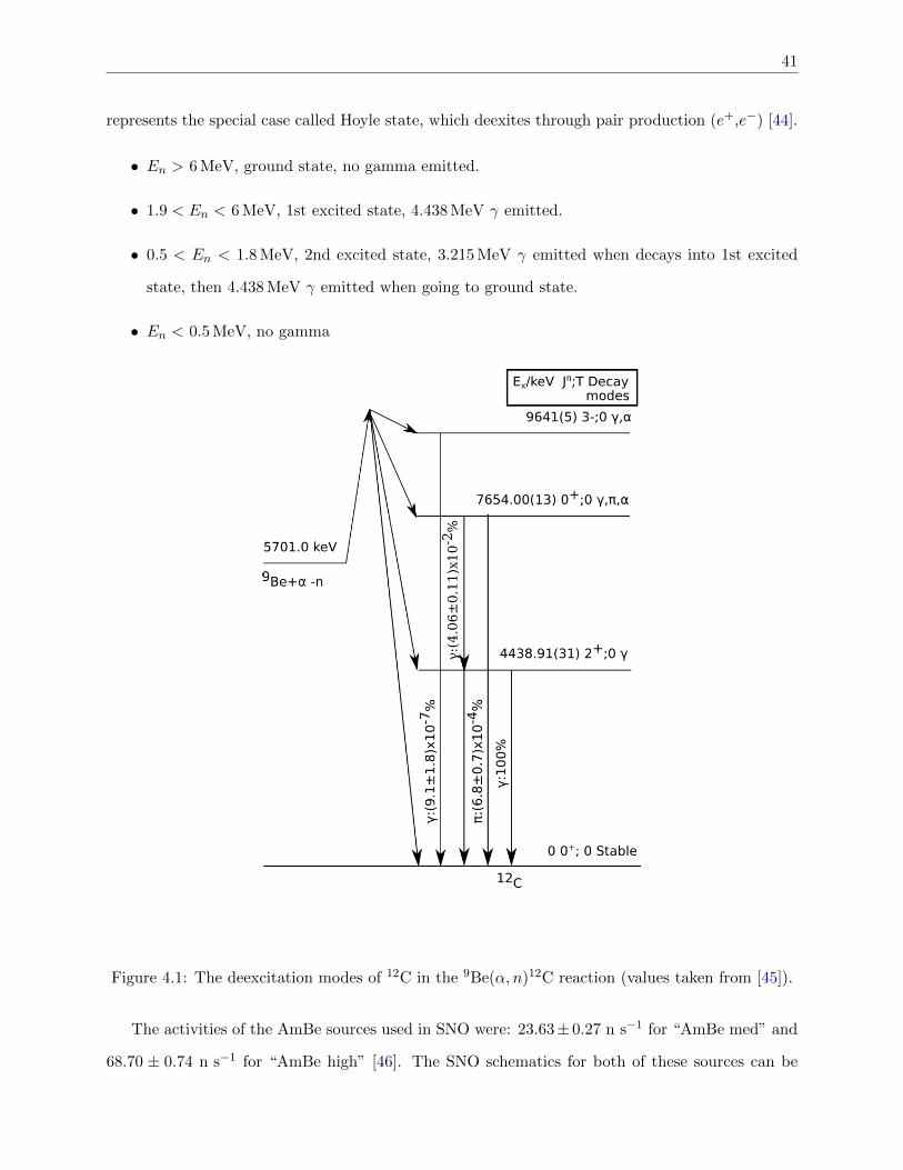
41
represents the special case called Hoyle state, which deexites through pair production (e+,e−) [44].
• En > 6 MeV, ground state, no gamma emitted.
• 1.9 < En < 6 MeV, 1st excited state, 4.438 MeV γ emitted.
• 0.5 < En < 1.8 MeV, 2nd excited state, 3.215 MeV γ emitted when decays into 1st excited
state, then 4.438 MeV γ emitted when going to ground state.
• En < 0.5 MeV, no gamma
Figure 4.1: The deexcitation modes of 12C in the 9Be(α, n)12C reaction (values taken from [45]).
The activities of the AmBe sources used in SNO were: 23.63± 0.27 n s−1 for “AmBe med” and
68.70 ± 0.74 n s−1 for “AmBe high” [46]. The SNO schematics for both of these sources can be
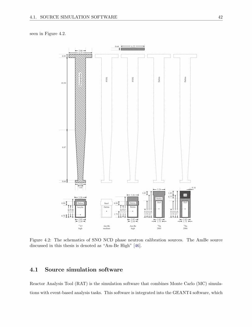
4.1. SOURCE SIMULATION SOFTWARE 42
seen in Figure 4.2.
Figure 4.2: The schematics of SNO NCD phase neutron calibration sources. The AmBe sourcediscussed in this thesis is denoted as “Am-Be High” [46].
4.1 Source simulation software
Reactor Analysis Tool (RAT) is the simulation software that combines Monte Carlo (MC) simula-
tions with event-based analysis tasks. This software is integrated into the GEANT4 software, which
4.1. SOURCE SIMULATION SOFTWARE 43
is used by numerous physics collaborations for particles going through matter MC simulations [47]
[48] [49]. All of the macros for RAT are written in C++. The analysis for this thesis was done with
GEANT4.10.0.p02, RAT version 5.3.2 and all the output files were analysed using ROOT 5.34.34.
The C++ macro files were used to extract information from created ROOT output files. By doing
so, the processing power is used more efficiently on tools such as function generators and data cuts.
The SNO+ collaboration is constantly updating and developing RAT for better use of the
physics needed for the experiment. The geometry of the detector and its components are stored in
a dedicated database. The geometry of different calibration sources and materials can be added.
Part of the discussion later in this thesis will be the different geometry files of AmBe source and
additional materials that were added to the materials files in the database (subsection 4.1.1).
After the simulation of the detector response is completed, the data is stored in the EV and MC
branches of the output ROOT file’s TTree. The EV branch stores the information that would be
accessible after an actual measurement within the detector. The MC branch has detailed informa-
tion of the simulated particles and their tracks. Using the information from both branches makes
it easy to do a detailed analysis of advantages and disadvantages of different source geometries.
4.1.1 AmBe source geometry
The geometry of the AmBe source inherited from SNO is composed of the source container and a
source holder. In the geometry file, these source parts are defined as polycones. This allows the
use cylindrical coordinates to define the dimension of the layer volumes. The particles produced
by the source are simulated as a point source inside the most inner volume of the source container.
Generators at the end of the macro files can generate: individual particles, particles in coincidence,
or the full spectrum of source particles. The old generator for the AmBe source generates neutrons
and gammas in coincidence. Improvements made to this generator will be further discussed in
subsection 4.1.2.
The Figure 4.3 shows the illustration of the main AmBe source geometry parts that were
manipulated. The geometry has the original source encapsulation made out of derlin denoted
as “G4 POLYOXYMETHYLENE” within the source geometry file. The original encapsulation of the
source is going to stay untouched, as the source is already double encapsulated and the activity is
known. Leaving the original encapsulation intact makes the source extra safe from the potential
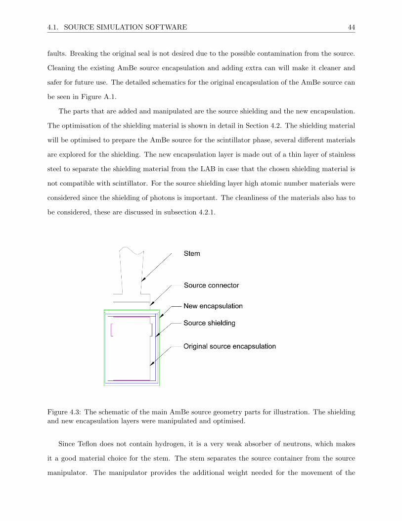
4.1. SOURCE SIMULATION SOFTWARE 44
faults. Breaking the original seal is not desired due to the possible contamination from the source.
Cleaning the existing AmBe source encapsulation and adding extra can will make it cleaner and
safer for future use. The detailed schematics for the original encapsulation of the AmBe source can
be seen in Figure A.1.
The parts that are added and manipulated are the source shielding and the new encapsulation.
The optimisation of the shielding material is shown in detail in Section 4.2. The shielding material
will be optimised to prepare the AmBe source for the scintillator phase, several different materials
are explored for the shielding. The new encapsulation layer is made out of a thin layer of stainless
steel to separate the shielding material from the LAB in case that the chosen shielding material is
not compatible with scintillator. For the source shielding layer high atomic number materials were
considered since the shielding of photons is important. The cleanliness of the materials also has to
be considered, these are discussed in subsection 4.2.1.
Figure 4.3: The schematic of the main AmBe source geometry parts for illustration. The shieldingand new encapsulation layers were manipulated and optimised.
Since Teflon does not contain hydrogen, it is a very weak absorber of neutrons, which makes
it a good material choice for the stem. The stem separates the source container from the source
manipulator. The manipulator provides the additional weight needed for the movement of the
4.1. SOURCE SIMULATION SOFTWARE 45
source inside the LAB. It is made out of stainless steel which is a material that is good at absorbing
neutrons. Therefore, having a stem to separate the source form the manipulator decreases the
amount of neutrons reabsorbed by the source deployment system.
The source connector connects the source capsule to the stem. The original source connector was
made out of Derlin as well. However, delrin is not compatible with LAB, and for the refurbishment
the material for the connector was changed to stainless steel to match the new source encapsulation.
Even though stainless steel is good at absorbing neutrons, having thin layer closer to the source
does not affect the neutron count significantly, as demonstrated in Section 4.2.
4.1.2 AmBe source event generator
As explained in Chapter 4, the AmBe source produces neutrons via (α, n) reactions. The AmBe
event generator code for the MC simulations was inherited from the DEAP-1 experiment [46]. The
spectrum creates the separate neutron spectrum in coincidence with 4.4 MeV gammas 60% of the
time and 10 keV gammas 40%. These low energy 10 keV gammas were below the energy threshold
for detection for the water phase. However, the SNO+ scintillator phase is sensitive to lower event
energies, therefore having the actual energies and ratios for the produced low energy gammas is
desired. Also as shown in the Figure 4.1, there is a correlation between the neutron spectrum and
the produced gamma energies, which was not implemented in the DEAP-1 AmBe generator. The
AmBe spectrum from this generator can be seen in Figure 4.4.
DEAP-1 AmBe generator was modified to include the correlations between the neutron and
gamma energies. Work performed in this thesis tests the new and improved generator for the
scintillator phase. Multiple simulations were done to test the features of the SNO+ AmBe generator
to include the correct deexitation modes, applications of the generator are shown in Chapter 5. The
Figure 4.5 shows the NHit spectrum produced using the new AmBe generator, which includes the
correlation between neutrons and gammas with the appropriate deexcitation modes of 12C. The
sharp neutron capture peak lies around 1200 NHits, which equates to approximately 2.2 MeV. The
4.4 MeV γ peak is more spreadout and lies in between 2200 → 3000 Nhits. The effect of the 12C
going into a second excited state and producing 3.213 MeV γ shortly followed by 4.4 MeV γ is seen
at approximately 3600 NHit which would corresponds to the energy of the sum of both gammas.
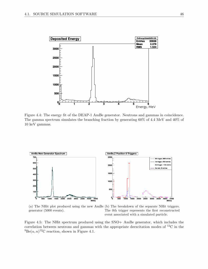
4.1. SOURCE SIMULATION SOFTWARE 46
Figure 4.4: The energy fit of the DEAP-1 AmBe generator. Neutrons and gammas in coincidence.The gamma spectrum simulates the branching fraction by generating 60% of 4.4 MeV and 40% of10 keV gammas.
(a) The NHit plot produced using the new AmBegenerator (5000 events).
(b) The breakdown of the separate NHit triggers.The 0th trigger represents the first reconstructedevent associated with a simulated particle.
Figure 4.5: The NHit spectrum produced using the SNO+ AmBe generator, which includes thecorrelation between neutrons and gammas with the appropriate deexcitation modes of 12C in the9Be(α, n)12C reaction, shown in Figure 4.1.
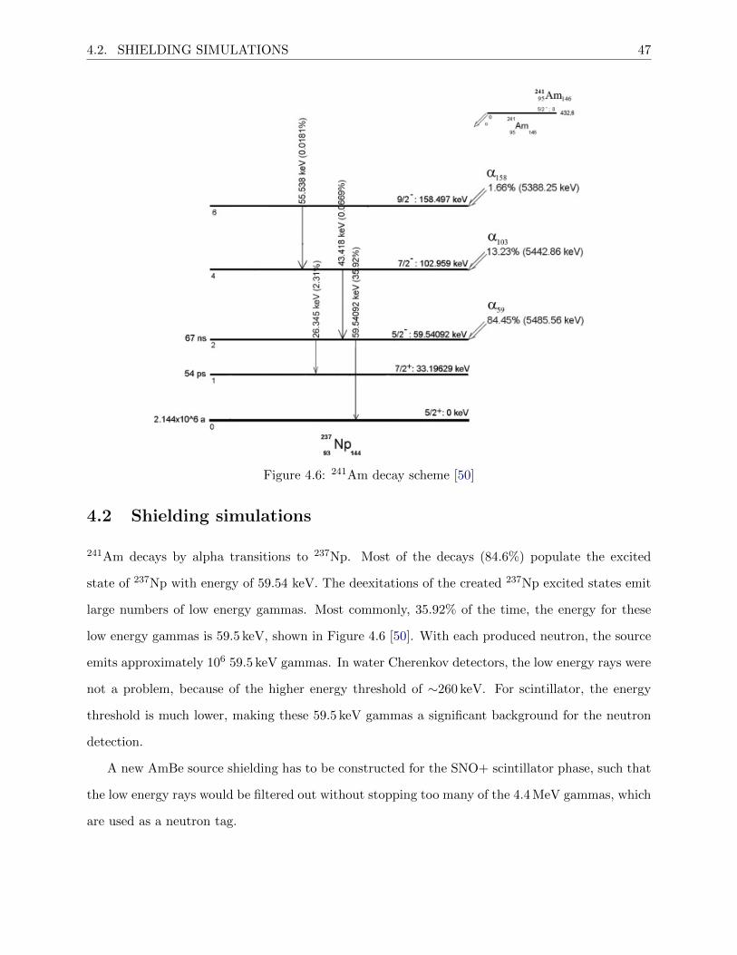
4.2. SHIELDING SIMULATIONS 47
Figure 4.6: 241Am decay scheme [50]
4.2 Shielding simulations
241Am decays by alpha transitions to 237Np. Most of the decays (84.6%) populate the excited
state of 237Np with energy of 59.54 keV. The deexitations of the created 237Np excited states emit
large numbers of low energy gammas. Most commonly, 35.92% of the time, the energy for these
low energy gammas is 59.5 keV, shown in Figure 4.6 [50]. With each produced neutron, the source
emits approximately 106 59.5 keV gammas. In water Cherenkov detectors, the low energy rays were
not a problem, because of the higher energy threshold of ∼260 keV. For scintillator, the energy
threshold is much lower, making these 59.5 keV gammas a significant background for the neutron
detection.
A new AmBe source shielding has to be constructed for the SNO+ scintillator phase, such that
the low energy rays would be filtered out without stopping too many of the 4.4 MeV gammas, which
are used as a neutron tag.
4.2. SHIELDING SIMULATIONS 48
4.2.1 Shielding materials
High atomic number materials are considered since the shielding of photons is important. Lead
is commonly used for radiation shielding because of its density (ρ =11.3 g cm−3), but it is not
considered a “clean” material. If exposed to the LAB, it would contaminate the detector. There-
fore, to consider lead, it has to be encased within an outside container, that is compatible with
LAB. Tungsten, being an excellent but expensive shielding material, was also considered for the
AmBe source. It has a high density (ρ =19.3 g cm−3) and a high melting temperature (3410 ◦C),
which makes it a commonly used material for photon shields and beam collimators within science
experiments. Hevimet (a tungsten alloy) was considered for the AmBe source shielding as well.
It consists of 90% tungsten, ∼ 7% nickel and ∼ 3% copper (depending on the manufacturer, the
ratios might vary). The typical density of Hevimet is ρ =16.9 g cm−3 to 17.2 g cm−3 [51].
Stainless steel is another material widely used in radiation shielding. It has relatively high
density (ρ =7.87 g cm−3) and is composed of 71% iron, 19% chromium, and 1% nickel. It has good
resistance to corrosion and is a non-magnetic material, which makes it commonly used in many
accelerator components.
The original source container from SNO is made out of polyoxymethylene ((CH2O)n, ρ =1.41 g cm−3).
Due to it’s hydrogen content, it can easily absorb neutrons. It is thus a poor choice of material
for the encapsulation of a neutron source. Thermal neutrons get captured through a 1H(n, γ)2H
reaction and emits 2.2 MeV gamma.
These materials were carefully considered and multiple simulations were performed to optimise
a suitable shielding for the AmBe source.
4.2.2 Simulating gammas
The selection of the appropriate shielding material was done in two steps. First the most promising
shielding material was identified. Then additional simulations were performed to fine-tune the
selection. First, separate simulations of 59.5 keV and 4.4 MeV gamma particles (10000 events each)
emitted from a point source were performed using a range of thicknesses for different shielding
materials Table 4.1. All shieldings have an extra 1 mm of stainless steel around them, because lead
and hevimet are not compatible with LAB. Compared to lead and hevimet, stainless steel appeared
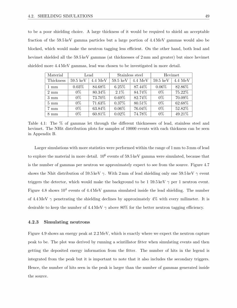
4.2. SHIELDING SIMULATIONS 49
to be a poor shielding choice. A large thickness of it would be required to shield an acceptable
fraction of the 59.5 keV gamma particles but a large portion of 4.4 MeV gammas would also be
blocked, which would make the neutron tagging less efficient. On the other hand, both lead and
hevimet shielded all the 59.5 keV gammas (at thicknesses of 2 mm and greater) but since hevimet
shielded more 4.4 MeV gammas, lead was chosen to be investigated in more detail.
Material Lead Stainless steel Hevimet
Thickness 59.5 keV 4.4 MeV 59.5 keV 4.4 MeV 59.5 keV 4.4 MeV
1 mm 0.03% 84.68% 6.25% 87.44% 0.06% 82.86%
2 mm 0% 80.34% 2.1% 84.74% 0% 75.22%
3 mm 0% 73.70% 0.69% 82.74% 0% 70.09%
5 mm 0% 71.63% 0.37% 80.51% 0% 62.68%
7 mm 0% 63.84% 0.06% 76.04% 0% 52.82%
8 mm 0% 60.81% 0.02% 74.78% 0% 49.21%
Table 4.1: The % of gammas let through the different thicknesses of lead, stainless steel andhevimet. The NHit distribution plots for samples of 10000 events with each thickness can be seenin Appendix B.
Larger simulations with more statistics were performed within the range of 1 mm to 3 mm of lead
to explore the material in more detail. 106 events of 59.5 keV gamma were simulated, because that
is the number of gammas per neutron we approximately expect to see from the source. Figure 4.7
shows the Nhit distribution of 59.5 keV γ. With 2 mm of lead shielding only one 59.5 keV γ event
triggers the detector, which would make the background to be 1 59.5 keV γ per 1 neutron event.
Figure 4.8 shows 104 events of 4.4 MeV gamma simulated inside the lead shielding. The number
of 4.4 MeV γ penetrating the shielding declines by approximately 4% with every milimeter. It is
desirable to keep the number of 4.4 MeV γ above 80% for the better neutron tagging efficiency.
4.2.3 Simulating neutrons
Figure 4.9 shows an energy peak at 2.2 MeV, which is exactly where we expect the neutron capture
peak to be. The plot was derived by running a scintillator fitter when simulating events and then
getting the deposited energy information from the fitter. The number of hits in the legend is
integrated from the peak but it is important to note that it also includes the secondary triggers.
Hence, the number of hits seen in the peak is larger than the number of gammas generated inside
the source.
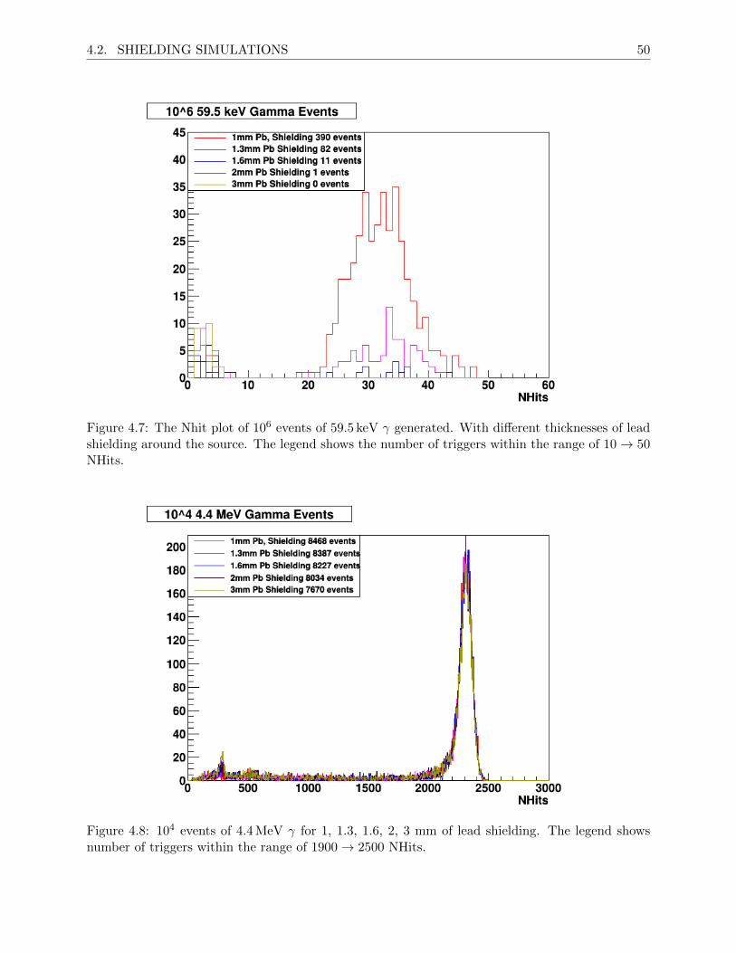
4.2. SHIELDING SIMULATIONS 50
Figure 4.7: The Nhit plot of 106 events of 59.5 keV γ generated. With different thicknesses of leadshielding around the source. The legend shows the number of triggers within the range of 10→ 50NHits.
Figure 4.8: 104 events of 4.4 MeV γ for 1, 1.3, 1.6, 2, 3 mm of lead shielding. The legend showsnumber of triggers within the range of 1900→ 2500 NHits.
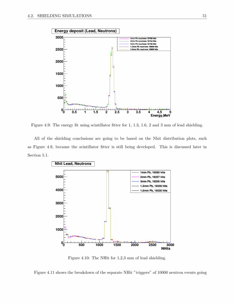
4.2. SHIELDING SIMULATIONS 51
Figure 4.9: The energy fit using scintillator fitter for 1, 1.3, 1.6, 2 and 3 mm of lead shielding.
All of the shielding conclusions are going to be based on the Nhit distribution plots, such
as Figure 4.9, because the scintillator fitter is still being developed. This is discussed later in
Section 5.1.
Figure 4.10: The NHit for 1,2,3 mm of lead shielding.
Figure 4.11 shows the breakdown of the separate NHit ”triggers” of 10000 neutron events going
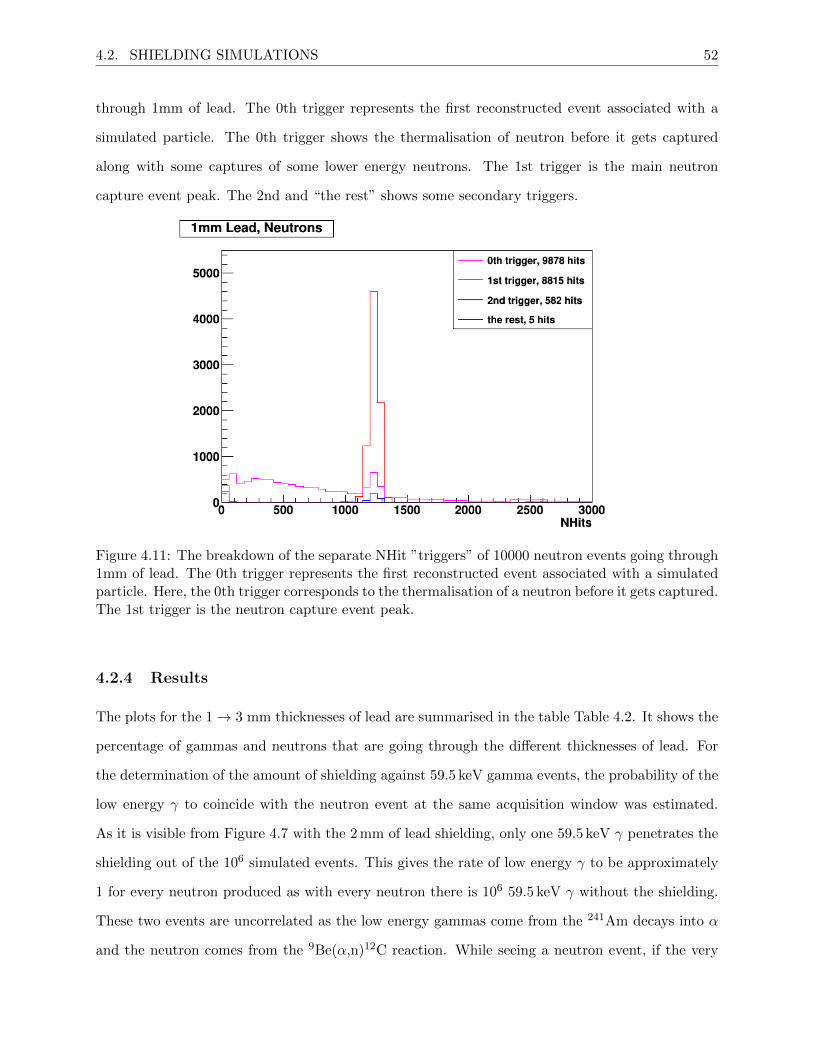
4.2. SHIELDING SIMULATIONS 52
through 1mm of lead. The 0th trigger represents the first reconstructed event associated with a
simulated particle. The 0th trigger shows the thermalisation of neutron before it gets captured
along with some captures of some lower energy neutrons. The 1st trigger is the main neutron
capture event peak. The 2nd and “the rest” shows some secondary triggers.
Figure 4.11: The breakdown of the separate NHit ”triggers” of 10000 neutron events going through1mm of lead. The 0th trigger represents the first reconstructed event associated with a simulatedparticle. Here, the 0th trigger corresponds to the thermalisation of a neutron before it gets captured.The 1st trigger is the neutron capture event peak.
4.2.4 Results
The plots for the 1→ 3 mm thicknesses of lead are summarised in the table Table 4.2. It shows the
percentage of gammas and neutrons that are going through the different thicknesses of lead. For
the determination of the amount of shielding against 59.5 keV gamma events, the probability of the
low energy γ to coincide with the neutron event at the same acquisition window was estimated.
As it is visible from Figure 4.7 with the 2 mm of lead shielding, only one 59.5 keV γ penetrates the
shielding out of the 106 simulated events. This gives the rate of low energy γ to be approximately
1 for every neutron produced as with every neutron there is 106 59.5 keV γ without the shielding.
These two events are uncorrelated as the low energy gammas come from the 241Am decays into α
and the neutron comes from the 9Be(α,n)12C reaction. While seeing a neutron event, if the very
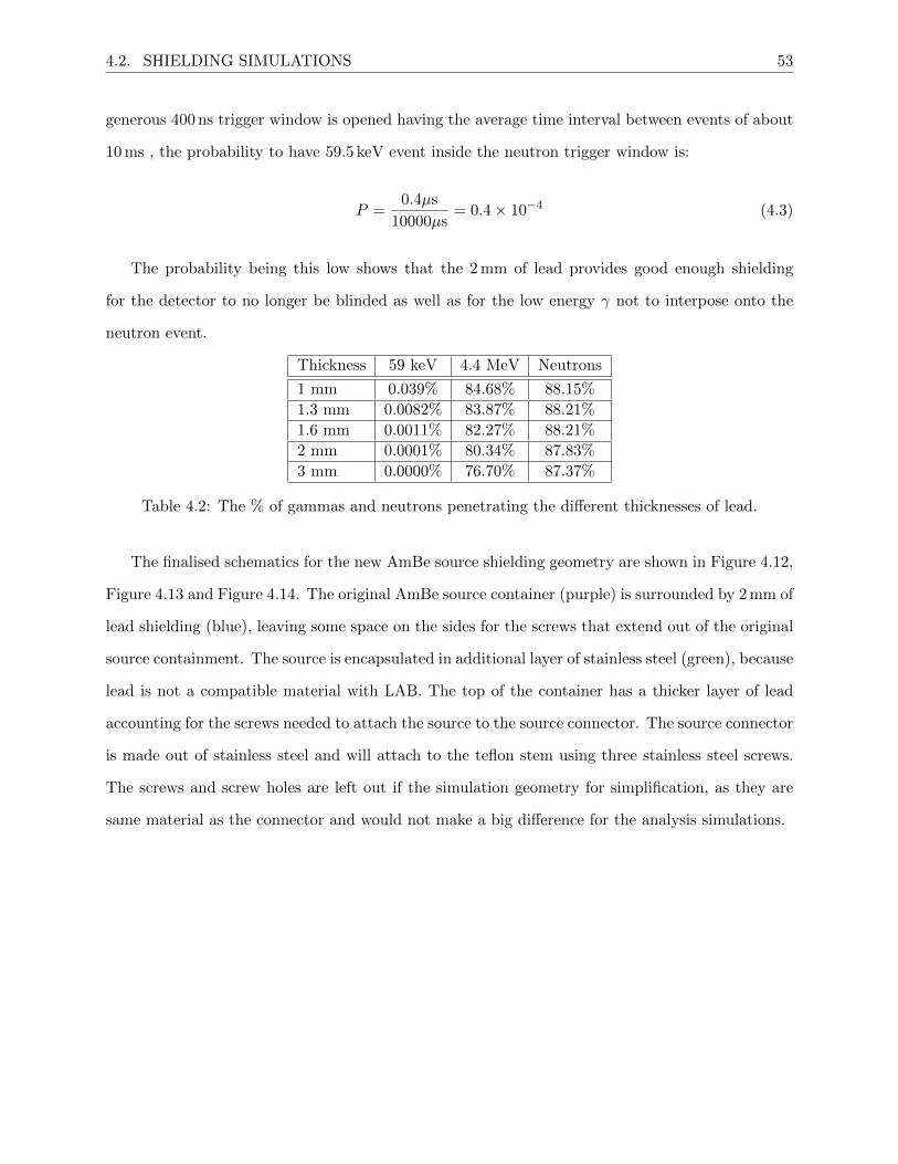
4.2. SHIELDING SIMULATIONS 53
generous 400 ns trigger window is opened having the average time interval between events of about
10 ms , the probability to have 59.5 keV event inside the neutron trigger window is:
P =0.4µs
10000µs= 0.4× 10⁻⁴ (4.3)
The probability being this low shows that the 2 mm of lead provides good enough shielding
for the detector to no longer be blinded as well as for the low energy γ not to interpose onto the
neutron event.
Thickness 59 keV 4.4 MeV Neutrons
1 mm 0.039% 84.68% 88.15%
1.3 mm 0.0082% 83.87% 88.21%
1.6 mm 0.0011% 82.27% 88.21%
2 mm 0.0001% 80.34% 87.83%
3 mm 0.0000% 76.70% 87.37%
Table 4.2: The % of gammas and neutrons penetrating the different thicknesses of lead.
The finalised schematics for the new AmBe source shielding geometry are shown in Figure 4.12,
Figure 4.13 and Figure 4.14. The original AmBe source container (purple) is surrounded by 2 mm of
lead shielding (blue), leaving some space on the sides for the screws that extend out of the original
source containment. The source is encapsulated in additional layer of stainless steel (green), because
lead is not a compatible material with LAB. The top of the container has a thicker layer of lead
accounting for the screws needed to attach the source to the source connector. The source connector
is made out of stainless steel and will attach to the teflon stem using three stainless steel screws.
The screws and screw holes are left out if the simulation geometry for simplification, as they are
same material as the connector and would not make a big difference for the analysis simulations.
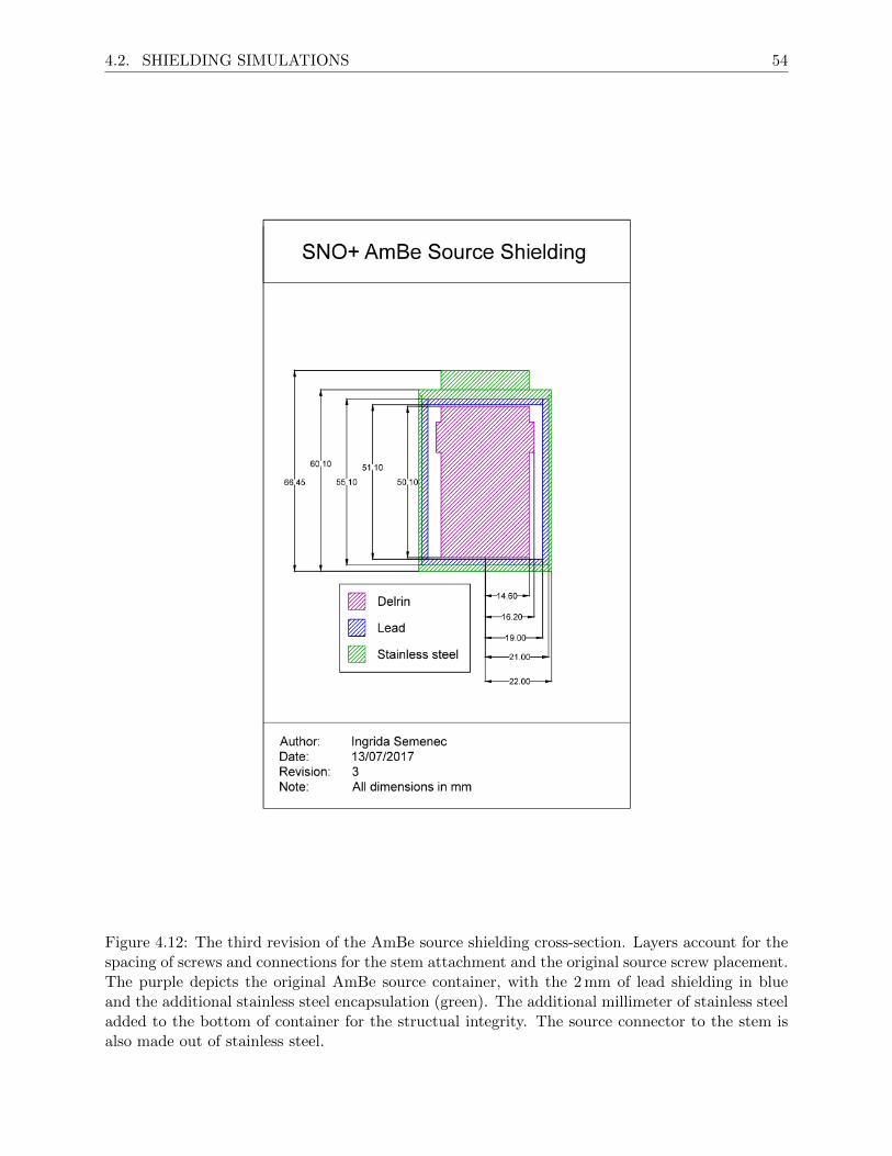
4.2. SHIELDING SIMULATIONS 54
Figure 4.12: The third revision of the AmBe source shielding cross-section. Layers account for thespacing of screws and connections for the stem attachment and the original source screw placement.The purple depicts the original AmBe source container, with the 2 mm of lead shielding in blueand the additional stainless steel encapsulation (green). The additional millimeter of stainless steeladded to the bottom of container for the structual integrity. The source connector to the stem isalso made out of stainless steel.
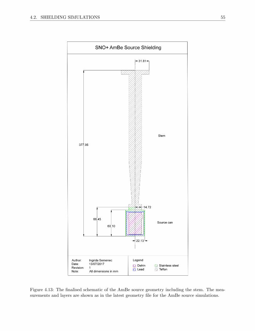
4.2. SHIELDING SIMULATIONS 55
Figure 4.13: The finalised schematic of the AmBe source geometry including the stem. The mea-surements and layers are shown as in the latest geometry file for the AmBe source simulations.
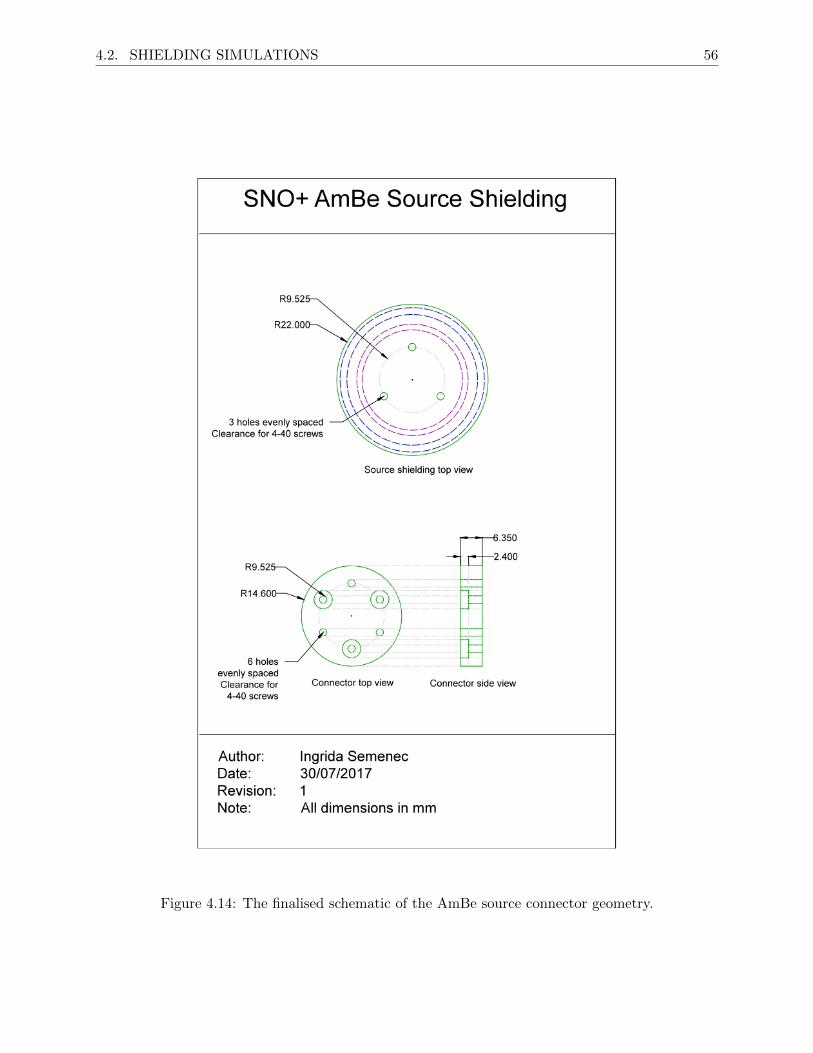
4.2. SHIELDING SIMULATIONS 56
Figure 4.14: The finalised schematic of the AmBe source connector geometry.
Chapter 5
Neutron Source Analysis
5.1 Scintillator Fitter
The scintillator fitter “energy fit” was used in some parts of the analysis to see if the AmBe
spectrum peaks lay at the expected energies. To compare the true energy to the reconstructed
energy provided by the scintillator fitter, the plot of the MC true energy versus the reconstructed
energy is shown in Figure 5.1. Here,“true spectra” indicates the true neutron energy distributions of
the MC events. As it has been shown in Figure 4.1 there is correlation between the neutron energies
and the produced gamma energies. Therefore it is important to have a accurate reconstruction of
the neutron energy.
The reconstructed energy provided by the EV branch is the summed deposited energy for all
particles in a single event (it does not provide the deposited energy of each individual particle).
Therefore, to make a valid comparison, it was necessary to obtain the total true deposited energy
in MC, summing over all particles that were reconstructed.
The variation between the true and reconstructed data is very small. The reason for the two
outlier events is unknown. However, it was reported to the people responsible for the development of
the fitter and it will be resolved. The fractional error of the energy fit is calculated by Equation 5.1
shown in Figure 5.2.
Eerr =Ereconstructed − Etrue
Etrue(5.1)
57
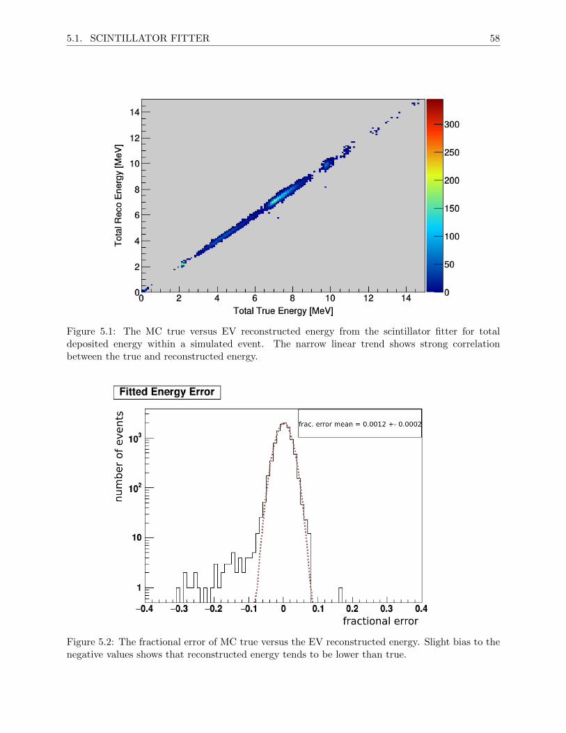
5.1. SCINTILLATOR FITTER 58
Figure 5.1: The MC true versus EV reconstructed energy from the scintillator fitter for totaldeposited energy within a simulated event. The narrow linear trend shows strong correlationbetween the true and reconstructed energy.
Figure 5.2: The fractional error of MC true versus the EV reconstructed energy. Slight bias to thenegative values shows that reconstructed energy tends to be lower than true.
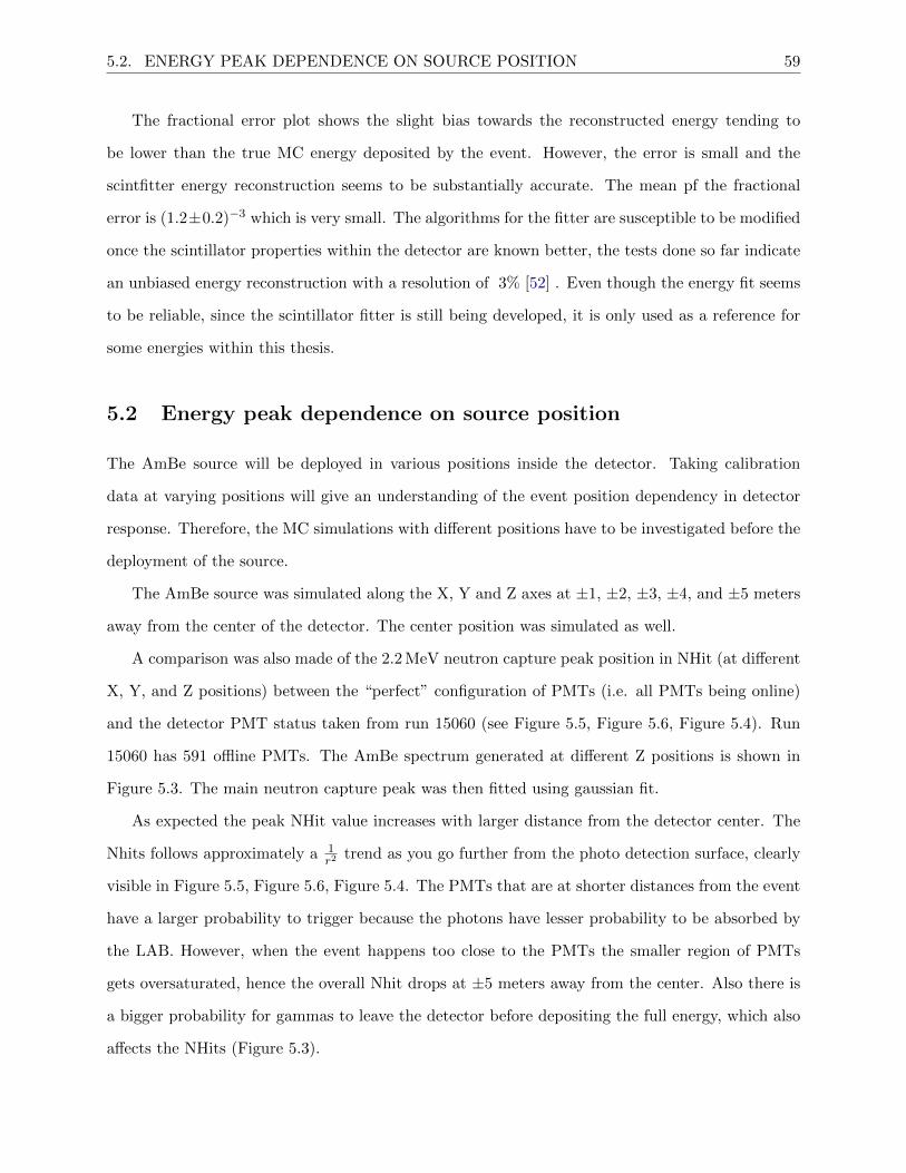
5.2. ENERGY PEAK DEPENDENCE ON SOURCE POSITION 59
The fractional error plot shows the slight bias towards the reconstructed energy tending to
be lower than the true MC energy deposited by the event. However, the error is small and the
scintfitter energy reconstruction seems to be substantially accurate. The mean pf the fractional
error is (1.2±0.2)−3 which is very small. The algorithms for the fitter are susceptible to be modified
once the scintillator properties within the detector are known better, the tests done so far indicate
an unbiased energy reconstruction with a resolution of 3% [52] . Even though the energy fit seems
to be reliable, since the scintillator fitter is still being developed, it is only used as a reference for
some energies within this thesis.
5.2 Energy peak dependence on source position
The AmBe source will be deployed in various positions inside the detector. Taking calibration
data at varying positions will give an understanding of the event position dependency in detector
response. Therefore, the MC simulations with different positions have to be investigated before the
deployment of the source.
The AmBe source was simulated along the X, Y and Z axes at ±1, ±2, ±3, ±4, and ±5 meters
away from the center of the detector. The center position was simulated as well.
A comparison was also made of the 2.2 MeV neutron capture peak position in NHit (at different
X, Y, and Z positions) between the “perfect” configuration of PMTs (i.e. all PMTs being online)
and the detector PMT status taken from run 15060 (see Figure 5.5, Figure 5.6, Figure 5.4). Run
15060 has 591 offline PMTs. The AmBe spectrum generated at different Z positions is shown in
Figure 5.3. The main neutron capture peak was then fitted using gaussian fit.
As expected the peak NHit value increases with larger distance from the detector center. The
Nhits follows approximately a 1r2 trend as you go further from the photo detection surface, clearly
visible in Figure 5.5, Figure 5.6, Figure 5.4. The PMTs that are at shorter distances from the event
have a larger probability to trigger because the photons have lesser probability to be absorbed by
the LAB. However, when the event happens too close to the PMTs the smaller region of PMTs
gets oversaturated, hence the overall Nhit drops at ±5 meters away from the center. Also there is
a bigger probability for gammas to leave the detector before depositing the full energy, which also
affects the NHits (Figure 5.3).
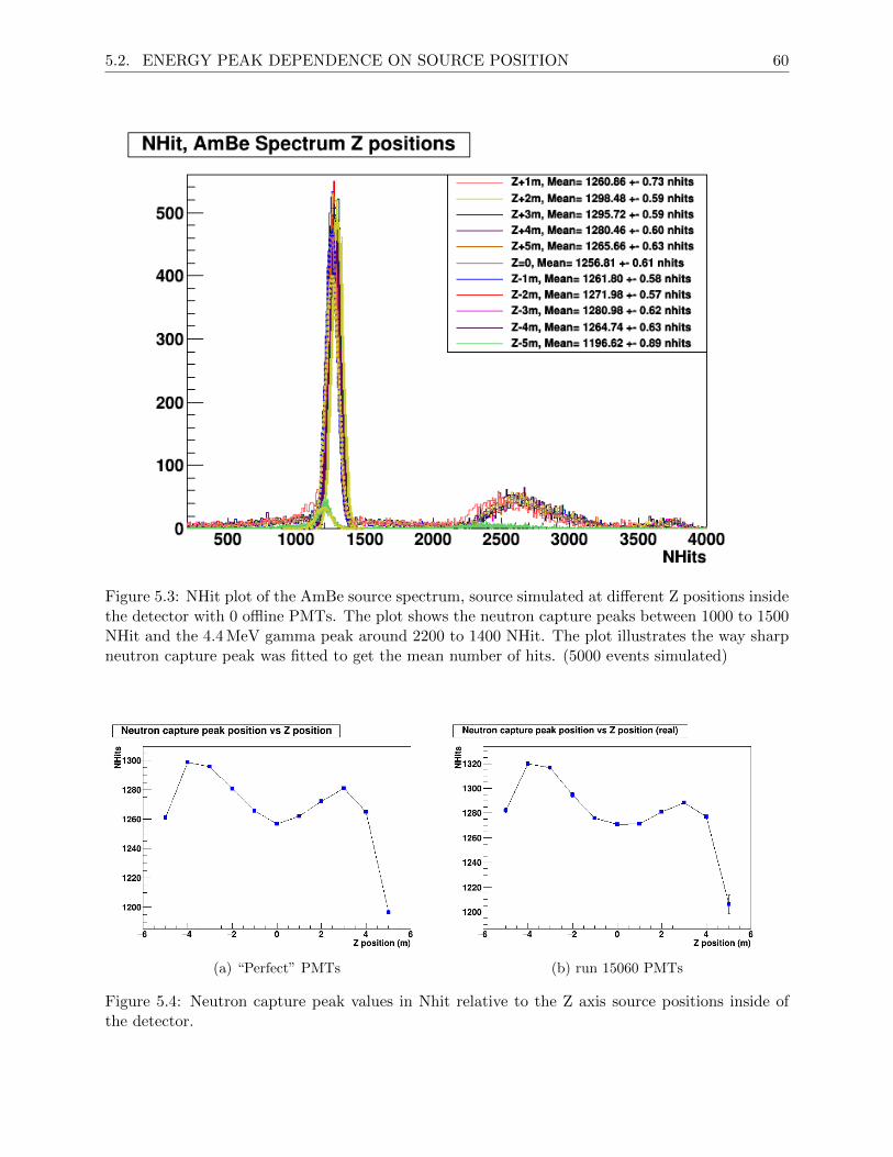
5.2. ENERGY PEAK DEPENDENCE ON SOURCE POSITION 60
Figure 5.3: NHit plot of the AmBe source spectrum, source simulated at different Z positions insidethe detector with 0 offline PMTs. The plot shows the neutron capture peaks between 1000 to 1500NHit and the 4.4 MeV gamma peak around 2200 to 1400 NHit. The plot illustrates the way sharpneutron capture peak was fitted to get the mean number of hits. (5000 events simulated)
(a) “Perfect” PMTs (b) run 15060 PMTs
Figure 5.4: Neutron capture peak values in Nhit relative to the Z axis source positions inside ofthe detector.
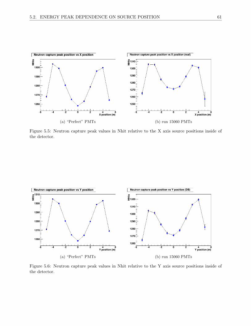
5.2. ENERGY PEAK DEPENDENCE ON SOURCE POSITION 61
(a) “Perfect” PMTs (b) run 15060 PMTs
Figure 5.5: Neutron capture peak values in Nhit relative to the X axis source positions inside ofthe detector.
(a) “Perfect” PMTs (b) run 15060 PMTs
Figure 5.6: Neutron capture peak values in Nhit relative to the Y axis source positions inside ofthe detector.
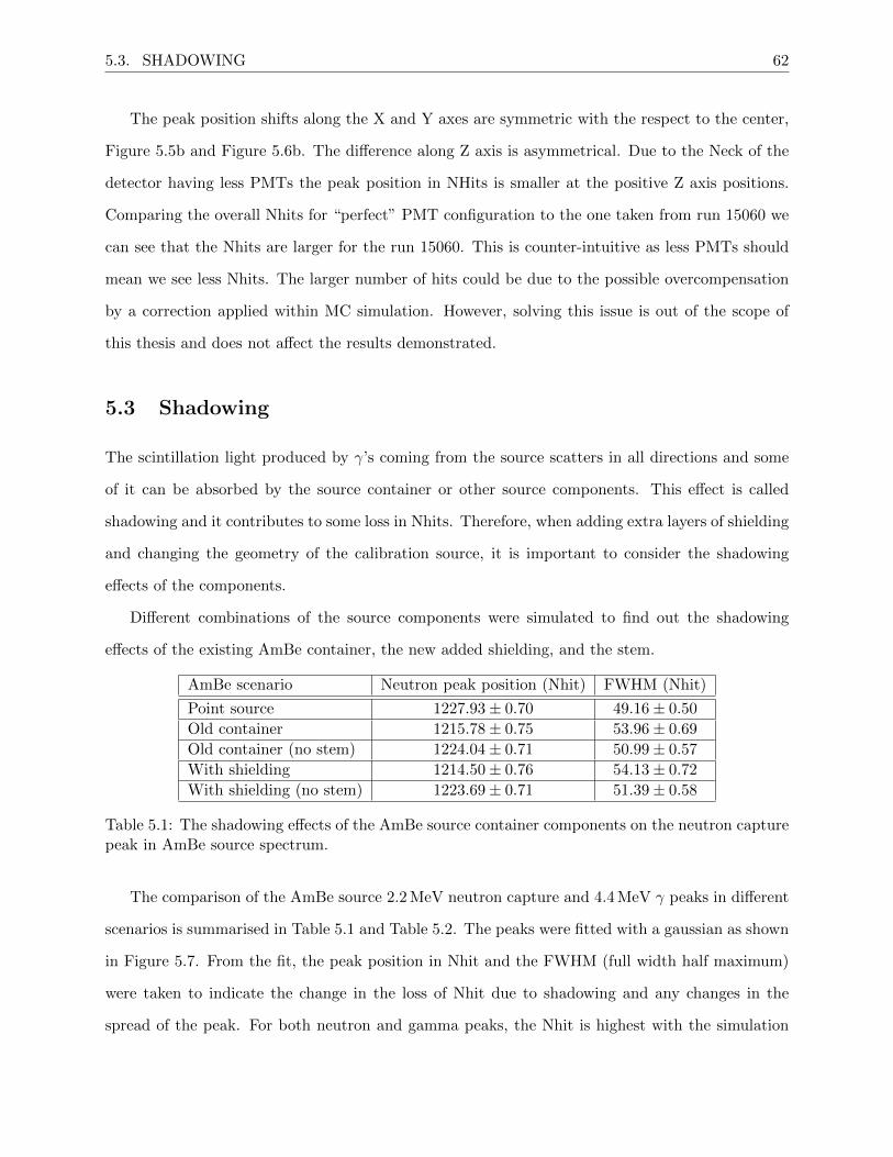
5.3. SHADOWING 62
The peak position shifts along the X and Y axes are symmetric with the respect to the center,
Figure 5.5b and Figure 5.6b. The difference along Z axis is asymmetrical. Due to the Neck of the
detector having less PMTs the peak position in NHits is smaller at the positive Z axis positions.
Comparing the overall Nhits for “perfect” PMT configuration to the one taken from run 15060 we
can see that the Nhits are larger for the run 15060. This is counter-intuitive as less PMTs should
mean we see less Nhits. The larger number of hits could be due to the possible overcompensation
by a correction applied within MC simulation. However, solving this issue is out of the scope of
this thesis and does not affect the results demonstrated.
5.3 Shadowing
The scintillation light produced by γ’s coming from the source scatters in all directions and some
of it can be absorbed by the source container or other source components. This effect is called
shadowing and it contributes to some loss in Nhits. Therefore, when adding extra layers of shielding
and changing the geometry of the calibration source, it is important to consider the shadowing
effects of the components.
Different combinations of the source components were simulated to find out the shadowing
effects of the existing AmBe container, the new added shielding, and the stem.
AmBe scenario Neutron peak position (Nhit) FWHM (Nhit)
Point source 1227.93± 0.70 49.16± 0.50
Old container 1215.78± 0.75 53.96± 0.69
Old container (no stem) 1224.04± 0.71 50.99± 0.57
With shielding 1214.50± 0.76 54.13± 0.72
With shielding (no stem) 1223.69± 0.71 51.39± 0.58
Table 5.1: The shadowing effects of the AmBe source container components on the neutron capturepeak in AmBe source spectrum.
The comparison of the AmBe source 2.2 MeV neutron capture and 4.4 MeV γ peaks in different
scenarios is summarised in Table 5.1 and Table 5.2. The peaks were fitted with a gaussian as shown
in Figure 5.7. From the fit, the peak position in Nhit and the FWHM (full width half maximum)
were taken to indicate the change in the loss of Nhit due to shadowing and any changes in the
spread of the peak. For both neutron and gamma peaks, the Nhit is highest with the simulation
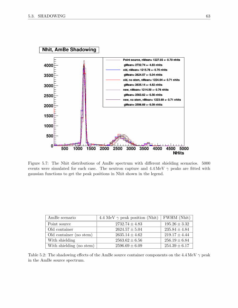
5.3. SHADOWING 63
Figure 5.7: The Nhit distributions of AmBe spectrum with different shielding scenarios. 5000events were simulated for each case. The neutron capture and 4.4 MeV γ peaks are fitted withgaussian functions to get the peak positions in Nhit shown in the legend.
AmBe scenario 4.4 MeV γ peak position (Nhit) FWHM (Nhit)
Point source 2732.74± 4.83 195.26± 3.32
Old container 2624.57± 5.04 235.84± 4.84
Old container (no stem) 2635.14± 4.62 219.17± 4.44
With shielding 2563.62± 6.56 256.19± 6.84
With shielding (no stem) 2596.69± 6.09 254.39± 6.17
Table 5.2: The shadowing effects of the AmBe source container components on the 4.4 MeV γ peakin the AmBe source spectrum.
5.4. TAGGED EVENT EFFICIENCY 64
of AmBe as a point source with no container. In this case, there are no components to absorb
neutrons or scintillation light.
For the neutron peak position in Nhit, the difference between the point source scenario and two
scenarios with container (no stem) is that the Nhit drops by approximately 0.32%. With the stem,
the difference is approximately 0.98%. The difference between the old containment of AmBe and
the addition of 2 mm of lead surrounded by 1 mm of stainless steel is very small. The additional
shielding drops the Nhit by approximately 0.03%, which is within statistical uncertainty in the
peak positions given in Table 5.1. Thus, the added shielding effects are not significantly large.
For the 4.4 MeV gamma peak positions in Nhit, the uncertainties are larger due to the peak
having a larger spread, as shown in Table 5.2. The difference in Nhit between the point source
scenario and the old container scenario (no stem) is 3.57% lower, whereas the difference to the
container with shielding is 4.97% lower. The larger shift in Nhit can also be explained by the effect
of γ losing more energy while going through additional shielding unlike the neutron capture peak,
which requires neutrons to thermalise after leaving the shielding to be captured to produce a much
sharper peak. Therefore, the spread of the γ peak also increases, with gammas losing more energy
and extra light being absorbed by the source components.
5.4 Tagged event efficiency
The understanding of the neutron capture efficiency within the detector will lead to an estimated
efficiency of the detection of anti-neutrino events. As discussed before in Section 1.5, the anti-
neutrino events are detected via inverse beta decay, which produces a positron and a neutron.
Detecting the neutron coming from this event allows the anti-neutrino event tagging and energy
reconstruction. The AmBe neutron source deployment will give insight into the detector response
to neutron capture events.
The measured activity of the AmBe source is 68.7 n/s [46]. The 30 minutes of an AmBe
calibration run would give approximately 105 neutron events. However, using γ as a tag for the
neutron reduces the efficiency of tagged neutron events because a 4.4 MeV gamma is only created
60% of the time with the neutron. Therefore, the rate of tagged neutron events becomes 41.44 n/s.
With the added shielding, the number of neutrons that can be tagged is less due to the loss of
5.4. TAGGED EVENT EFFICIENCY 65
4.4 MeV γ tags. With 2 mm of lead plus 1 mm of stainless steel shielding, approximately 19.66%
of 4.4 MeV γ are lost, shown in Table 4.2. This leaves the tagged neutron event efficiency to be
around 33.30 n/s. The estimated number of events to get the precision of 1% is 10000 this equates
to approximately 5 minute of a source deployment run.
The neutron capture efficiency is the ratio of observed neutron capture events after selection
cuts to the total number of true neutron capture events in which a 4.4 MeV gamma was also tagged
(Equation 5.2).
ε =# of n-captures observed in detector
# of true n-captures with the 4.4 MeV tag(5.2)
The logic flow for the selection of the true number of the neutron capture events within the
detector is shown in Figure 5.9. The script checks if the neutron was generated with 4.4 MeV
gamma and if the neutron was captured inside the inner AV volume. For the observed number of
neutron capture events from the reconstructed MC data, the script checks the number of NHits
that would equate to 4.4 MeV gamma in the generated AmBe spectrum and then checks for the
number of NHits for the neutron capture peak which is 2.2 MeV gamma peak in the AmBe spectrum
(Figure 5.7, as shown in Figure 5.10. Then for the selection of the event, the time and order of both
events has to be compared. When producing neutron and gamma in coincidence, the generator
technically produces the gamma particle first. The time of the neutron capture event minus the
time of the gamma tag event must then be positive. Also, the events must be within a reasonable
time for neutron capture event to happen and they must come from the same generated entry.
Out of 9349 events simulated, 5528 neutrons came with 4.4 MeV gamma tag and was captured
inside the inner AV volume. To do the time selection cut, the MC truth neutron capture time was
compared to the true capture time, shown in Figure 5.8. The reconstructed neutron capture time
was fitted to function N(t) = N0e−t/τ , where τ is the neutron capture mean time. The capture
mean time from the fit is 204.95± 3.30µs. With the time selection cut being approximately three
times the neutron capture mean time (≈ 620µs), the neutron capture efficiency is 74.22%. The time
cut can be later optimised, while considering all of the backgrounds. The possible backgrounds
for AmBe neutron capture events are the neutrons coming from external sources, such as cosmic
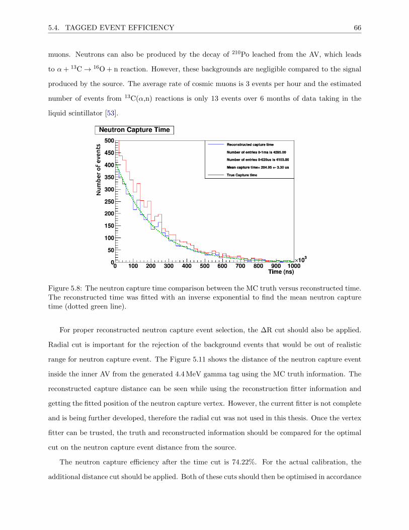
5.4. TAGGED EVENT EFFICIENCY 66
muons. Neutrons can also be produced by the decay of 210Po leached from the AV, which leads
to α+ 13C→ 16O + n reaction. However, these backgrounds are negligible compared to the signal
produced by the source. The average rate of cosmic muons is 3 events per hour and the estimated
number of events from 13C(α,n) reactions is only 13 events over 6 months of data taking in the
liquid scintillator [53].
Figure 5.8: The neutron capture time comparison between the MC truth versus reconstructed time.The reconstructed time was fitted with an inverse exponential to find the mean neutron capturetime (dotted green line).
For proper reconstructed neutron capture event selection, the ∆R cut should also be applied.
Radial cut is important for the rejection of the background events that would be out of realistic
range for neutron capture event. The Figure 5.11 shows the distance of the neutron capture event
inside the inner AV from the generated 4.4 MeV gamma tag using the MC truth information. The
reconstructed capture distance can be seen while using the reconstruction fitter information and
getting the fitted position of the neutron capture vertex. However, the current fitter is not complete
and is being further developed, therefore the radial cut was not used in this thesis. Once the vertex
fitter can be trusted, the truth and reconstructed information should be compared for the optimal
cut on the neutron capture event distance from the source.
The neutron capture efficiency after the time cut is 74.22%. For the actual calibration, the
additional distance cut should be applied. Both of these cuts should then be optimised in accordance
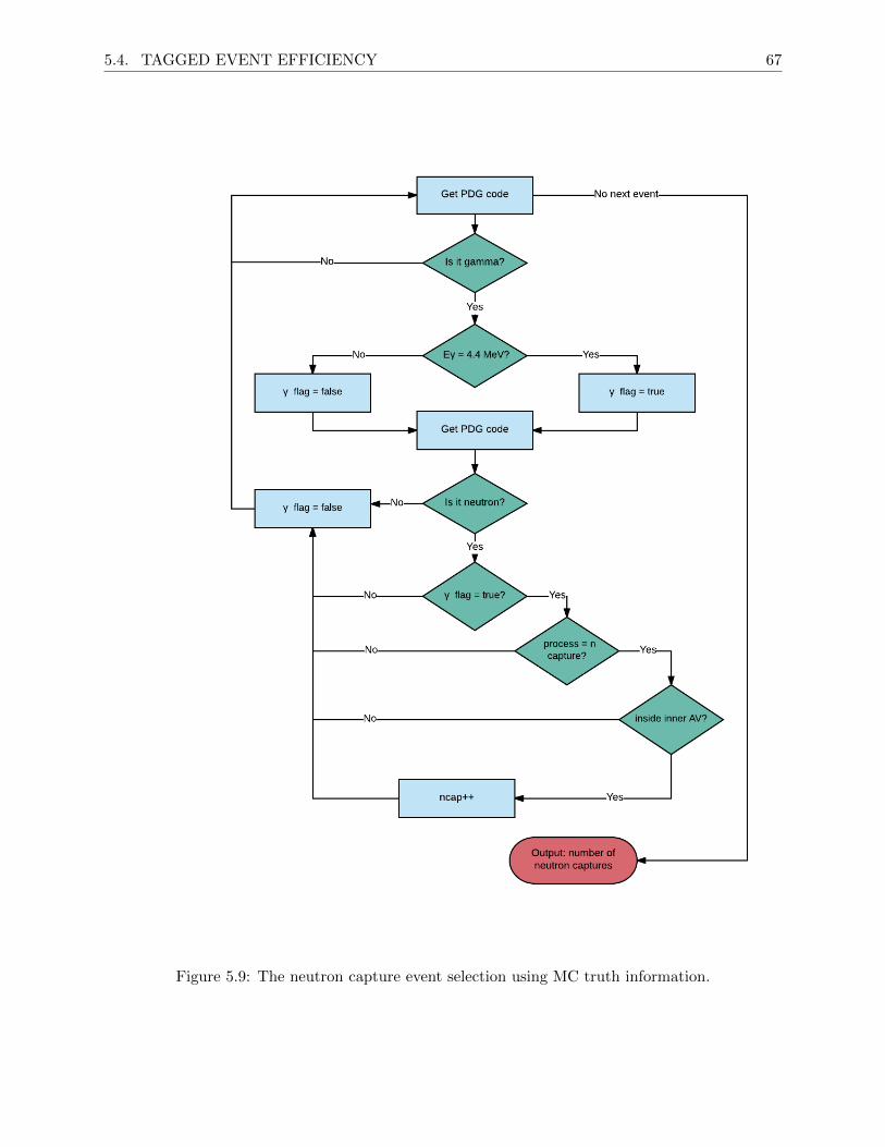
5.4. TAGGED EVENT EFFICIENCY 67
Figure 5.9: The neutron capture event selection using MC truth information.
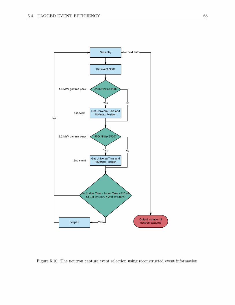
5.4. TAGGED EVENT EFFICIENCY 68
Figure 5.10: The neutron capture event selection using reconstructed event information.
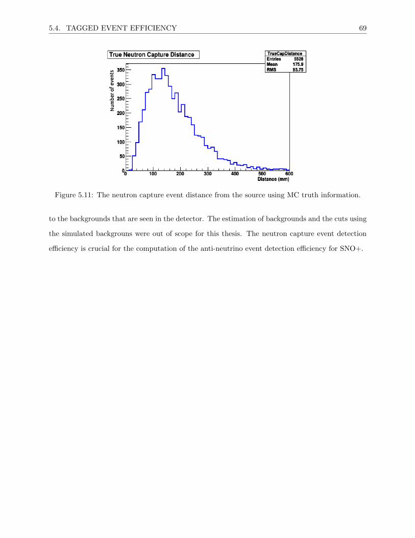
5.4. TAGGED EVENT EFFICIENCY 69
Figure 5.11: The neutron capture event distance from the source using MC truth information.
to the backgrounds that are seen in the detector. The estimation of backgrounds and the cuts using
the simulated backgrouns were out of scope for this thesis. The neutron capture event detection
efficiency is crucial for the computation of the anti-neutrino event detection efficiency for SNO+.
Chapter 6
Conclusions
The SNO+ experiment provides a great opportunity to study low energy solar neutrinos, reactor
anti-neutrinos, geo anti-neutrinos, and supernova neutrinos. These studies will provide a valuable
insight into several different topics of neutrino, astro and geo physics. The tellurium-loaded scintil-
lator phase will be able to search for neutrinoless double beta decay. This would provide an insight
to the Dirac or Majorana nature of the neutrino, which is one of the most sought after answers in
neutrino physics at the current time.
The AmBe calibration source is an esential part of the scintillator phase calibration of neutron
capture efficiency. The original AmBe source had to be refurbished with additional shielding, given
the wider energy resolution range of the scintillator. The new source design (Figure 4.12) includes
2 mm of lead as a shielding material against 59.5 keV x-rays produced by the α decays from 241Am
(Section 4.2). Additionally, the source and lead are encapsulated in a layer of stainless steel, to
make the source compatible and safe to use inside the detector. Alongside neutrons, the AmBe
source produces 4.4 MeV gammas used as a neutron event tag. With the new encapsulation, only
one of the 106 simulated 59.5 keV γ events escapes the source. This makes the probabilty of the
low energy gamma event to coincide with the neutron event only approximately 0.4× 10⁻⁴, which
is very low. With this new encapsulation, 19.66% of 4.4 MeV γ are lost. This can be compensated
by leaving the source inside the detector for longer periods of time. Even though the activity of
the AmBe source is 68.7 n/s, with all the additional shielding, the tagged neutron event efficiency
is estimated to be 33.30 n/s. To get the precision of 1% the estimated number of events is 10000
neutrons, which equates to approximately 5 minute source deployment run for every position inside
70
71
the detector. The short amount of time per position inside the detector allows the source to be
deployed in multiple positions during an assigned calibration shift.
The AmBe source will be deployed in various positions inside the detector. The dependence of
neutron capture and 4.4 MeV gamma peak positions (in Nhit) to the source deployement positions
were studied in Section 5.2. The peak NHit values increases with larger distance from the detector
center. The peak position shifts along the X and Y axes are symmetric, relatively to detector’s
center, Figure 5.5b and Figure 5.6b. The difference along Z axis is asymmetrical. Due to the
Neck of the detector having less PMTs, the peak position in Nhits is smaller at the positive Z axis
positions as expected.
Since parts made out of dense materials were added to the calibration source, the shadowing
effects were also inspected. It was found that the added shielding effects are not significantly large
as shown in Section 5.3. The new shielding and encapsulation drops the fitted Nhit value of the
neutron capture peak in the AmBe spectrum by approximatelly 0.03%.
From the MC simulations of the AmBe source the estimated neutron capture event detection
efficiency is 74.22%. Only the time cut was applied to estimate this number, the additional radial
selection cut and the optimisation of cuts in accordance to the observed background rates is needed
for more accurate computation of the neutron capture detection efficiency. The 210Po coming from
210Pb decays via alpha emmision and can create a 2.2 MeV gamma background for the neutron
capture events coming from the AmBe source. However, the estimated rate of possible background
events is negligible compared to the event rate coming from the AmBe source.
The design of the new AmBe neutron source is finalised and ready to be used for the source
refurbishment. A basic run plan was developed and demonstrated in this thesis. The deploye-
ment of the AmBe source will provide information about neutron event reconstruction and energy
reconstruction important to SNO+ physics objectives.
Appendix A
Matter Oscillations
To derive the neutrino oscillations in matter for electrons, first we need to define the Hamiltionian
we have previously used in a vacuum, to then incorporate the the VCC term. Expressing the
Schrodinger equation in matrix form:
id
dt
ν1
ν2
= H
ν1
ν2
=1
2E
m21 0
0 m22
ν1
ν2
(A.1)
Then for expressing Equation A.1 in terms of flavour states we use Equation A.2.
ν1
ν2
= U †
νeνµ
(A.2)
Then the Equation A.1 becomes:
72
73
id
dt
ν1
ν2
= H
ν1
ν2
(A.3)
=⇒ U †id
dt
νeνµ
= HU †
νeνµ
(A.4)
=⇒ id
dt
νeνµ
= UHU †
νeνµ
(A.5)
Then we can write the Hamiltonian for the flavour oscillations in vaccum as Equation A.6.
Hvac = UHU † =m2
1 +m22
4E
1 0
0 1
+∆m2
4E
− cos 2θ sin 2θ
sin 2θ cos 2θ
(A.6)
The first term of the Hamiltonian is constant (no mixing), therefore it can be neglected, giving the
vacuum Hamiltonian to be:
=⇒ Hvac =∆m2
4E
− cos 2θ sin 2θ
sin 2θ cos 2θ
(A.7)
Now to derive the oscillation probability in matter, we inlcude the VCC term to the Schrodinger
74
equation.
id
dt
νeνµ
= (Hvac + VCC)
νeνµ
(A.8)
=
∆m2
4E
− cos 2θ sin 2θ
sin 2θ cos 2θ
+ VCC
1 0
0 0
νeνµ
(A.9)
=
∆m2
4E
− cos 2θ sin 2θ
sin 2θ cos 2θ
+ VCC
1 0
0 −1
+ VCC
1 0
0 1
νeνµ
(A.10)
=⇒ HM =∆m2
4E
−(cos 2θ −ACC) sin 1θ
sin 1θ (cos 2θ −ACC)
(A.11)
Equation A.11 shows the Hamiltonian for the 2 flavour matter oscilations, whereACC = 2√
2GFNeE/∆m221.
To write HM in the same form of Hvac we define the parameters ∆m2M and sin2 2θM as shown in
Equation A.12 and Equation A.13 respectively.
∆m2M ≡ ∆m2
21
√sin2 2θ + (cos 2θ −ACC)2 (A.12)
sin2 2θM ≡sin2 2θ
sin2 2θ + (cos 2θ −ACC)2(A.13)
Now the Equation A.11 becomes:
HM =∆m2
M
4E
− cos 2θM sin 2θM
sin 2θM cos 2θM
(A.14)
Hence the oscillation probability in matter is:
PMνα→νβ = sin2 2θM sin2
(∆m2
M
4EL
)(A.15)
A.1. SCHEMATICS 75
A.1 Schematics
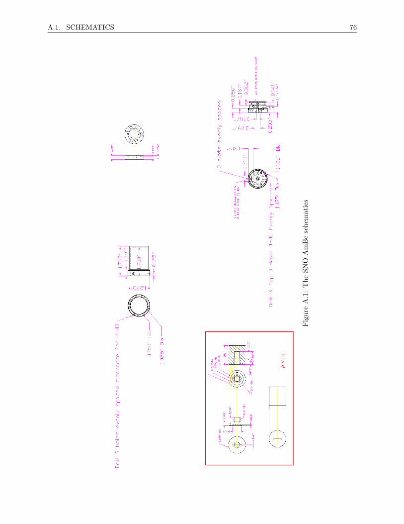
A.1. SCHEMATICS 76
Fig
ure
A.1
:T
he
SN
OA
mB
esc
hem
atic
s
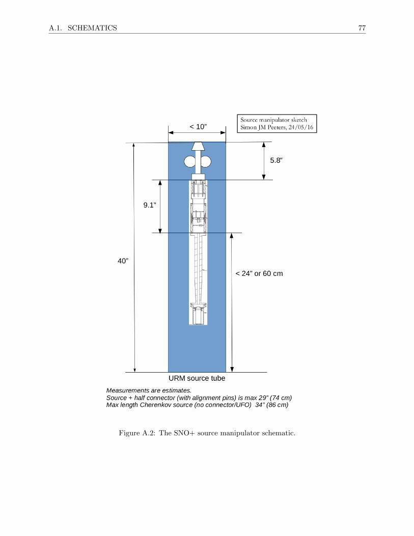
A.1. SCHEMATICS 77
Figure A.2: The SNO+ source manipulator schematic.
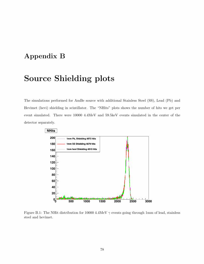
Appendix B
Source Shielding plots
The simulations performed for AmBe source with additional Stainless Steel (SS), Lead (Pb) and
Hevimet (hevi) shielding in scintillator. The “NHits” plots shows the number of hits we get per
event simulated. There were 10000 4.4MeV and 59.5keV events simulated in the center of the
detector separately.
Figure B.1: The NHit distribution for 10000 4.4MeV γ events going through 1mm of lead, stainlesssteel and hevimet.
78
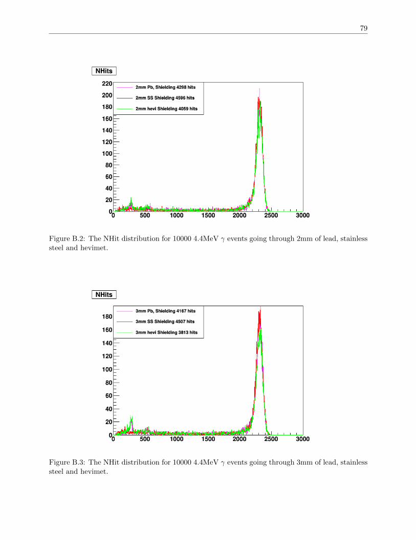
79
Figure B.2: The NHit distribution for 10000 4.4MeV γ events going through 2mm of lead, stainlesssteel and hevimet.
Figure B.3: The NHit distribution for 10000 4.4MeV γ events going through 3mm of lead, stainlesssteel and hevimet.
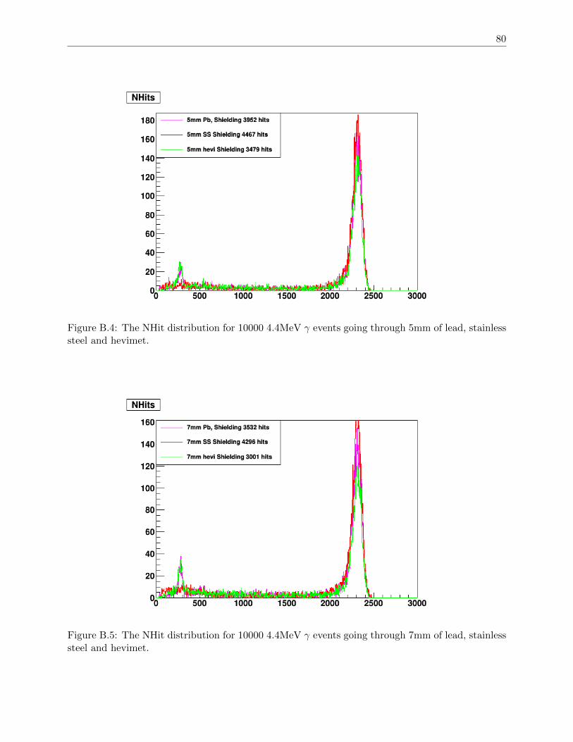
80
Figure B.4: The NHit distribution for 10000 4.4MeV γ events going through 5mm of lead, stainlesssteel and hevimet.
Figure B.5: The NHit distribution for 10000 4.4MeV γ events going through 7mm of lead, stainlesssteel and hevimet.
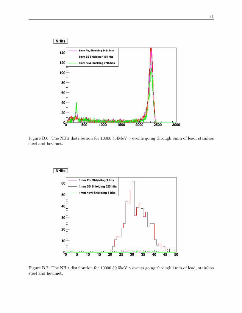
81
Figure B.6: The NHit distribution for 10000 4.4MeV γ events going through 8mm of lead, stainlesssteel and hevimet.
Figure B.7: The NHit distribution for 10000 59.5keV γ events going through 1mm of lead, stainlesssteel and hevimet.
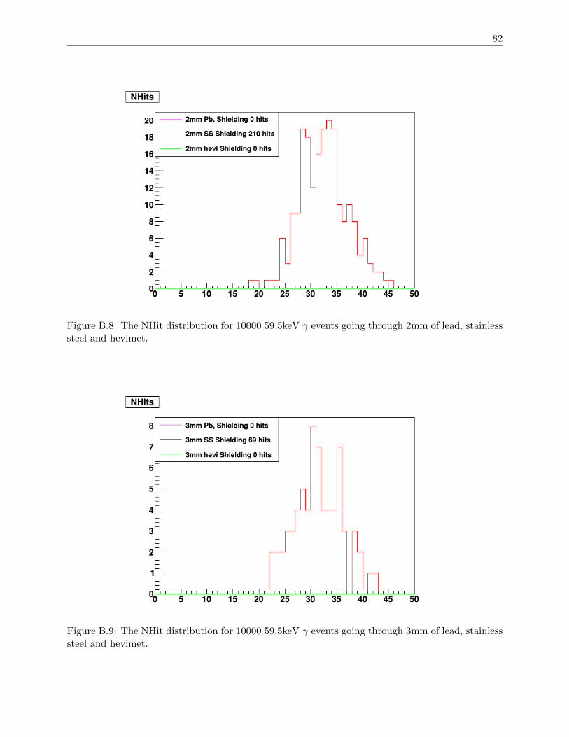
82
Figure B.8: The NHit distribution for 10000 59.5keV γ events going through 2mm of lead, stainlesssteel and hevimet.
Figure B.9: The NHit distribution for 10000 59.5keV γ events going through 3mm of lead, stainlesssteel and hevimet.
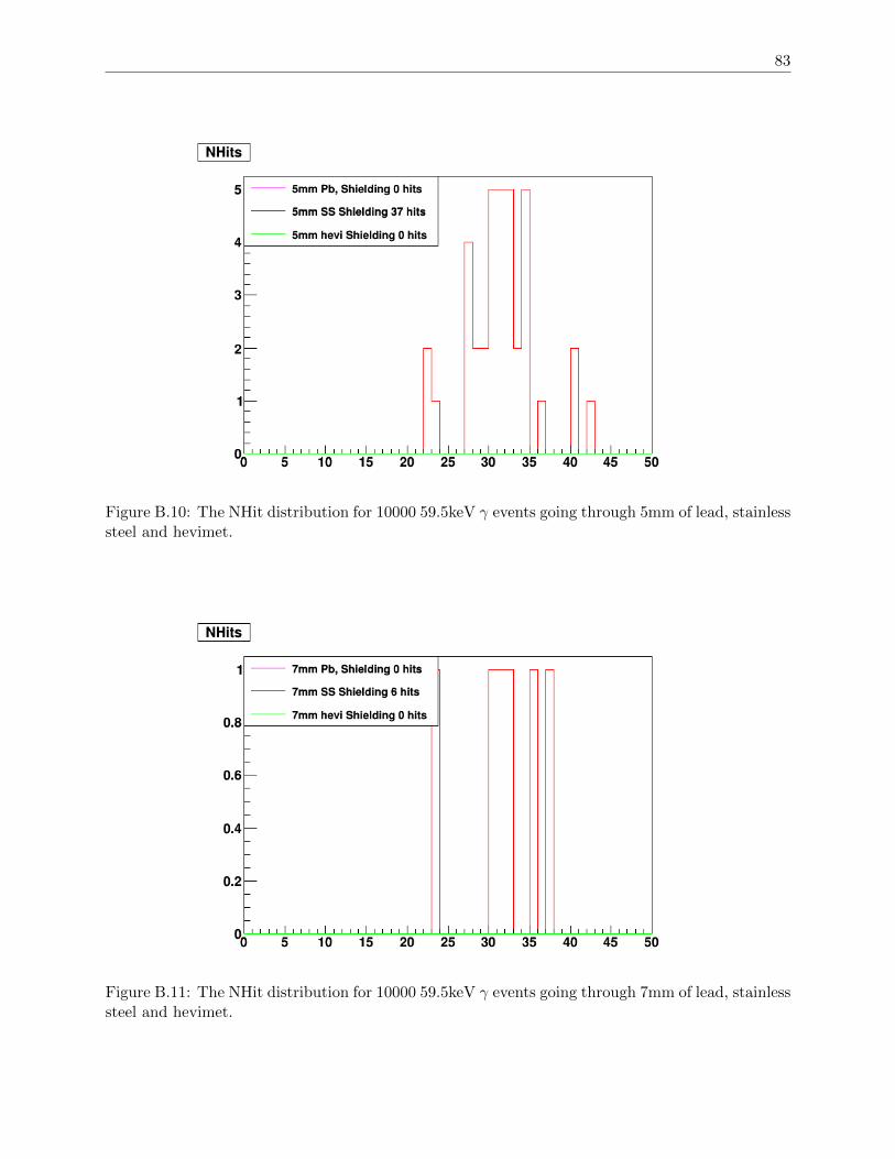
83
Figure B.10: The NHit distribution for 10000 59.5keV γ events going through 5mm of lead, stainlesssteel and hevimet.
Figure B.11: The NHit distribution for 10000 59.5keV γ events going through 7mm of lead, stainlesssteel and hevimet.
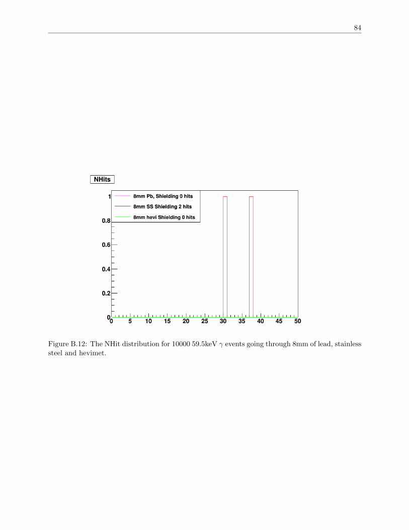
84
Figure B.12: The NHit distribution for 10000 59.5keV γ events going through 8mm of lead, stainlesssteel and hevimet.
Bibliography
[1] W. Pauli. Dear radioactive ladies and gentlemen. Phys. Today, 31N9:27, 1978.
[2] Fred L. Wilson. Fermi’s theory of beta decay. American Journal of Physics, 36(12):1150–1160,
1968.
[3] C. L. Cowan, Jr., F. Reines, F. B. Harrison, H. W. Kruse, and A. D. McGuire. Detection of
the Free Neutrino: A Confirmation. Science, 124:103–104, July 1956.
[4] The nobel prize in physics 1995. Nobelprize.org. Nobel Media AB 2014. Web. 21 Nov 2017.
[5] Frederick Reines and Clyde L Cowan. The neutrino. Nature, 178(4531):446–449, 1956.
[6] MissMJ. Standard model of elementary particles, 2006. By MissMJ [CC BY 3.0
(http://creativecommons.org/licenses/by/3.0) or Public domain], via Wikimedia Commons.
[7] G. Danby, J-M. Gaillard, K. Goulianos, L. M. Lederman, N. Mistry, M. Schwartz, and J. Stein-
berger. Observation of high-energy neutrino reactions and the existence of two kinds of neu-
trinos. Phys. Rev. Lett., 9:36–44, Jul 1962.
[8] K. Kodama et al. Observation of tau neutrino interactions. Phys. Lett., B504:218–224, 2001.
[9] Frank T. Avignone, III, Steven R. Elliott, and Jonathan Engel. Double Beta Decay, Majorana
Neutrinos, and Neutrino Mass. Rev. Mod. Phys., 80:481–516, 2008.
[10] M. Goeppert-Mayer. Double beta-disintegration. Phys. Rev., 48:512–516, 1935.
[11] Ettore Majorana. Teoria simmetrica dell’elettrone e del positrone. Il Nuovo Cimento (1924-
1942), 14(4):171, 2008.
85
BIBLIOGRAPHY 86
[12] W. H. Furry. On transition probabilities in double beta-disintegration. Phys. Rev., 56:1184–
1193, 1939.
[13] Manfred Lindner, Tommy Ohlsson, and Gerhart Seidl. Seesaw mechanisms for Dirac and
Majorana neutrino masses. Phys. Rev., D65:053014, 2002.
[14] S. M. Bilenky and C. Giunti. Neutrinoless Double-Beta Decay: a Probe of Physics Beyond
the Standard Model. Int. J. Mod. Phys., A30(04n05):1530001, 2015.
[15] B. T. Cleveland, Timothy Daily, Raymond Davis, Jr., James R. Distel, Kenneth Lande, C. K.
Lee, Paul S. Wildenhain, and Jack Ullman. Measurement of the solar electron neutrino flux
with the Homestake chlorine detector. Astrophys. J., 496:505–526, 1998.
[16] John N Bahcall and Raymond Davis Jr. Solar neutrinos: a scientific puzzle. Science, 191:264–
267, 1976.
[17] Kohji S Hirata, Takaaki Kajita, T Kifune, K Kihara, Masayuki Nakahata, K Nakamura,
S Ohara, Y Oyama, N Sato, M Takita, et al. Observation of b 8 solar neutrinos in the
kamiokande-ii detector. Physical Review Letters, 63(1):16, 1989.
[18] W. Hampel et al. GALLEX solar neutrino observations: Results for GALLEX III. Phys. Lett.,
B388:384–396, 1996.
[19] John N. Bahcall. Solar models and solar neutrinos: Current status. Phys. Scripta, T121:46–50,
2005.
[20] B. Pontecorvo. Neutrino Experiments and the Problem of Conservation of Leptonic Charge.
Sov. Phys. JETP, 26:984–988, 1968. [Zh. Eksp. Teor. Fiz.53,1717(1967)].
[21] Robert Ehrlich. Possible Evidence for Neutrino Oscillations in the Brookhaven Solar Neutrino
Experiment. Phys. Rev., D18:2323, 1978.
[22] Q. R. Ahmad and et al Allen. Measurement of the rate of νe+d → p +p +e− interactions pro-
duced by 8b solar neutrinos at the sudbury neutrino observatory. Phys. Rev. Lett., 87:071301,
Jul 2001.
BIBLIOGRAPHY 87
[23] B Aharmim, SN Ahmed, JF Amsbaugh, AE Anthony, J Banar, N Barros, EW Beier, A Bel-
lerive, B Beltran, M Bergevin, et al. Independent measurement of the total active b 8 solar
neutrino flux using an array of he 3 proportional counters at the sudbury neutrino observatory.
Physical Review Letters, 101(11):111301, 2008.
[24] K Abe, Y Haga, Y Hayato, M Ikeda, K Iyogi, J Kameda, Y Kishimoto, Ll Marti, M Miura,
S Moriyama, et al. Solar neutrino measurements in super-kamiokande-iv. Physical Review D,
94(5):052010, 2016.
[25] S. Andringa et al. Current Status and Future Prospects of the SNO+ Experiment. Adv. High
Energy Phys., 2016:6194250, 2016.
[26] R. N. Cahn, D. A. Dwyer, S. J. Freedman, W. C. Haxton, R. W. Kadel, Yu. G. Kolomensky,
K. B. Luk, P. McDonald, G. D. Orebi Gann, and A. W. P. Poon. White Paper: Measuring
the Neutrino Mass Hierarchy. In Proceedings, 2013 Community Summer Study on the Future
of U.S. Particle Physics: Snowmass on the Mississippi (CSS2013): Minneapolis, MN, USA,
July 29-August 6, 2013, 2013.
[27] P. Vogel and John F. Beacom. Angular distribution of neutron inverse beta decay, νe + p →1n + e+. Phys. Rev., D60:053003, 1999.
[28] Z Djurcic, J A Detwiler, A Piepke, V R Foster, L Miller, and G Gratta. Uncertainties in
the anti-neutrino production at nuclear reactors. Journal of Physics G: Nuclear and Particle
Physics, 36(4):045002, 2009.
[29] Eugene Guillian. The Sensitivity of SNO+ to ∆m212 Using Reactor Anti-neutrino Data. 2008.
[30] Shawn M Usman, Glenn R Jocher, Stephen T Dye, William F McDonough, and John G
Learned. Agm2015: Antineutrino global map 2015. Scientific reports, 5, 2015.
[31] Yu Huang, Viacheslav Chubakov, Fabio Mantovani, Roberta L. Rudnick, and William F. Mc-
Donough. A reference earth model for the heat-producing elements and associated geoneutrino
flux. Geochemistry, Geophysics, Geosystems, 14(6):2003–2029, 2013.
[32] G Bellini, A Ianni, L Ludhova, F Mantovani, and WF McDonough. Geo-neutrinos. Progress
in Particle and Nuclear Physics, 73:1–34, 2013.
BIBLIOGRAPHY 88
[33] I. V. KRIVOSHEINA. Sn 1987a — historical view about registration of the neutrino signal
with baksan, kamiokande ii and imb detectors. International Journal of Modern Physics D,
13(10):2085–2105, 2004.
[34] Snews. http://snews.bnl.gov/ , Accessed: 2017-10-11.
[35] Billy Liggins. SNO+ Commissioning Status. In Prospects in Neutrino Physics (NuPhys2016)
London, London, United Kingdom, December 12-14, 2016.
[36] Nobelprize.org. The 2015 nobel prize in physics - press release. 2015.
[37] Koushik Ghosh K. Mofazzal Hossain, Dipendra N. Ghosh and Tapas Saha. Application of
Signal Processing to Investigate the Total Active 8B Solar Neutrino Flux Signal from Sudbury
Neutrino Observatory (SNO). International Journal of Electronic Engineering Research, 2:303–
324, 2010.
[38] A. Bialek, M. Chen, B. Cleveland, P. Gorel, A. Hallin, P.J. Harvey, J. Heise, C. Kraus, C.B.
Krauss, I. Lawson, C.J. Ng, B. Pinkney, D.M. Rogowsky, L. Sibley, R. Soluk, J. Soukup, and
E. Vazquez-Jauregui. A rope-net support system for the liquid scintillator detector for the sno+
experiment. Nuclear Instruments and Methods in Physics Research Section A: Accelerators,
Spectrometers, Detectors and Associated Equipment, 827:152 – 160, 2016.
[39] J Brack, B Delgado, J Dhooghe, J Felde, B Gookin, S Grullon, JR Klein, R Knapik, A La-
Torre, S Seibert, et al. Characterization of the hamamatsu r11780 12 in. photomultiplier tube.
Nuclear Instruments and Methods in Physics Research Section A: Accelerators, Spectrometers,
Detectors and Associated Equipment, 712:162–173, 2013.
[40] T Araki, S Enomoto, K Furuno, Y Gando, K Ichimura, H Ikeda, K Inoue, Y Kishimoto,
M Koga, Y Koseki, et al. Search for the invisible decay of neutrons with kamland. Physical
review letters, 96(10):101802, 2006.
[41] SN Ahmed, AE Anthony, EW Beier, A Bellerive, SD Biller, J Boger, MG Boulay, MG Bowler,
TJ Bowles, SJ Brice, et al. Constraints on nucleon decay via invisible modes from the sudbury
neutrino observatory. Physical review letters, 92(10):102004, 2004.
BIBLIOGRAPHY 89
[42] R. Alves et al. The calibration system for the photomultiplier array of the SNO+ experiment.
JINST, 10(03):P03002, 2015.
[43] Alexandra Huss. Measurements of photon scattering lengths in scintillator and a test of the
linearity of light yield as a function of electron energy. Bulletin of the American Physical
Society, 58, 2013.
[44] M. Chernykh, H. Feldmeier, T. Neff, P. von Neumann-Cosel, and A. Richter. Pair decay width
of the Hoyle state and carbon production in stars. Phys. Rev. Lett., 105:022501, 2010.
[45] Ali Asghar Mowlavi and Rahim Koohi-Fayegh. Determination of 4.438mev γ-ray to neutron
emission ratio from a 241am–9be neutron source. Applied Radiation and Isotopes, 60(6):959 –
962, 2004.
[46] James Chilton Loach. Measurement of the Flux of 8B Solar Neutrinos at the Sudbury Neutrino
Observatory. PhD thesis, Lincoln College, University of Oxford, 2008.
[47] S. Agostinelli, J. Allison, et al. Geant4—a simulation toolkit. Nuclear Instruments and Methods
in Physics Research Section A: Accelerators, Spectrometers, Detectors and Associated Equip-
ment, 506(3):250 – 303, 2003.
[48] J. Allison, K. Amako, et al. Geant4 developments and applications. IEEE Transactions on
Nuclear Science, 53(1):270–278, Feb 2006.
[49] J. Allison, K. Amako, J. Apostolakis, et al. Recent developments in geant4. Nuclear Instru-
ments and Methods in Physics Research Section A: Accelerators, Spectrometers, Detectors and
Associated Equipment, 835:186 – 225, 2016.
[50] M.-M. Be, V. Chiste, C. Dulieu, X. Mougeot, E. Browne, V. Chechev, N. Kuzmenko, F. Kon-
dev, A. Luca, M. Galan, A.L. Nichols, A. Arinc, and X. Huang. Table of Radionuclides,
volume 5 of Monographie BIPM-5. Bureau International des Poids et Mesures, Pavillon de
Breteuil, F-92310 Sevres, France, 2010.
[51] Mi-Tech Metals Inc. Shielding Materials and Neutron Energy Spectra. Mi-Tech Metals
Inc.Indianapolis, Indiana, 2001.

BIBLIOGRAPHY 90
[52] Nuno Barros, 2017-10-04. Personal communication.
[53] Valentina Lozza. Background summary document. Technical report, Technische Universitat
Dresden 01069 Dresden, Germany, 02 2017. Internal SNO+ report.