The present work was submitted to the Institute of Solar Research,

German Aerospace Center (DLR)

Commissioning and validation of the underly-ing model of a test rig analyzing rotation andexpansion performing assemblies in parabolictrough collector power plants

MASTER-THESIS

presented byMüller, Thore

Sustainable Energy Supply (M.Sc.)

Supervision and Assessment1st Examiner: Univ.-Prof. Dr.-Ing. Bernhard Ho�schmidt

2nd Examiner: Univ.-Prof. Dr.-Ing. Robert Pitz-PaalTutor: Dipl.-Ing. Christoph Hilgert

Almería, January 27, 2017

Declaration of Academic Honesty /Eidesstattliche Erklärung

I hereby declare to have written the present master's thesis on my own, having used noother resources and tools than the listed. All contents cited from published or nonpub-lished documents are indicated as such.

Hiermit erkläre ich, dass ich die vorliegende Masterarbeit selbständig verfasst und keineanderen als die angegebenen Hilfsmittel verwendet habe. Alle Inhalte, die wörtlich odersinngemäÿ aus verö�entlichten oder nicht verö�entlichten Schriften entnommen sind,sind als solche kenntlich gemacht.

Place, Date Signature

iii

Abstract

In parabolic through power plants, Rotation and Expansion Performing Assemblies(REPAs) compensate for the rotational movement of the absorber tube while trackingthe sun to optimize optical e�ciency. This movement as well as hostile working condi-tions, e.g. high pressure and temperature, cause stress that makes REPAs one of themain reasons for leakage of potentially toxic Heat Transfer Fluids (HTFs). A new test rig,that will reproduce accelerated aging under typical operational conditions, is being con-structed at the Plataforma Solar de Almería (PSA) under the surveillance of the GermanAerospace Center (DLR) and Centro de Investigaciones Energéticas, Medioambientalesy Tecnológicas (CIEMAT). It's purpose is to understand and qualify the mechanismsthat lead to REPA-failure.

The �rst part of this work deals with the commissioning of the main measurementassembly, the kinematic unit that will replicate all motion responsible for REPA-agingand the �rst of later four dynamo-meters that will measure all forces and momentsthat a�ect the REPA. This work discusses taken actions and possibilities to reduce theuncertainties of these measurements. This includes a photogrammetric survey of thepiping system and test rig machinery in order to verify compliance with the allowedtolerances as well as optimal testing conditions.

The second part describes the validation process of the (ROHR2-) model, thatestimates the piping system behavior. The operating behavior of the piping system isexamined experimentally, in order to validate the model and to account for manufac-turing inaccuracies. Results from simulation and experiment are then compared andstatements about the measurement uncertainty will be deduced. In order to reducesaid uncertainty, the dynamo-meter has been re-calibrated and it's temperature relatedbehavior has been tested. Further more the sensor- and piping insulation has been im-proved. Important aspects of continued e�orts to improve measurement accuracy aregiven.

v

Contents

1 Introduction 1

1.1 REPA working conditions and operational loads . . . . . . . . . . . . . . . 2

2 REPA test-rig 5

2.1 Reproducing representative REPA working conditions . . . . . . . . . . . 5

2.2 REPA force measurement . . . . . . . . . . . . . . . . . . . . . . . . . . . 8

2.3 Content of this work . . . . . . . . . . . . . . . . . . . . . . . . . . . . . . 11

3 Dynamo-meter measurements and uncertainty 12

3.1 Measurement Uncertainties . . . . . . . . . . . . . . . . . . . . . . . . . . 13

3.2 Measurement Uncertainty Estimation . . . . . . . . . . . . . . . . . . . . . 17

3.3 Implications of re-calibration and temperature test . . . . . . . . . . . . . 18

4 Photogrammetry 20

4.1 Traverse: ideal pretension and model geometry . . . . . . . . . . . . . . . 21

4.2 Test Rig: Alignment of rotation axes . . . . . . . . . . . . . . . . . . . . . 25

5 The ROHR2 model 28

5.1 Model con�gurations . . . . . . . . . . . . . . . . . . . . . . . . . . . . . . 28

5.2 Model parameters . . . . . . . . . . . . . . . . . . . . . . . . . . . . . . . . 29

5.3 Results and discussion . . . . . . . . . . . . . . . . . . . . . . . . . . . . . 31

6 Validation 35

6.1 Temperature response . . . . . . . . . . . . . . . . . . . . . . . . . . . . . 36

6.2 Rotation angle response . . . . . . . . . . . . . . . . . . . . . . . . . . . . 44

7 Conclusion 47

8 Outlook 51

Abbreviations 55

Glossary: Test-Rig Operation 56

Glossary: Dynamo-Meter Theory 58

Glossary: Dynamo-Meter Uncertainty 59

Appendices 62

vi

A Additional Information 62

A.1 Test-rig speci�cations and problems . . . . . . . . . . . . . . . . . . . . . . 62

A.2 De�nition of terms . . . . . . . . . . . . . . . . . . . . . . . . . . . . . . . 65

A.3 Dynamo-meter algebra . . . . . . . . . . . . . . . . . . . . . . . . . . . . . 74

A.3.1 Theory . . . . . . . . . . . . . . . . . . . . . . . . . . . . . . . . . . 74

A.3.2 Some actual values . . . . . . . . . . . . . . . . . . . . . . . . . . . 75

A.4 Calibration and data sheet values . . . . . . . . . . . . . . . . . . . . . . . 79

A.5 Important information for future sensor purchases . . . . . . . . . . . . . . 81

A.6 ROHR2 - MATLAB post-processing . . . . . . . . . . . . . . . . . . . . . 82

A.7 All temperature response validation experiment results . . . . . . . . . . . 83

A.8 Operation loads estimation from experiment results . . . . . . . . . . . . . 85

A.9 Improvements . . . . . . . . . . . . . . . . . . . . . . . . . . . . . . . . . . 88

A.10 REPA translation due to thermal dilatation . . . . . . . . . . . . . . . . . 95

B Data sheets and certi�cates 96

List of Figures

1.1 Types of REPAs . . . . . . . . . . . . . . . . . . . . . . . . . . . . . . 2

1.2 PTC power plant loop . . . . . . . . . . . . . . . . . . . . . . . . . . . 3

1.3 REPA rotation and translation . . . . . . . . . . . . . . . . . . . . . . 4

2.1 A sketch of the REPA test-rig with its sub-units . . . . . . . . . . . . 6

2.2 The main assembly . . . . . . . . . . . . . . . . . . . . . . . . . . . . . 7

2.3 Main assembly and motion . . . . . . . . . . . . . . . . . . . . . . . . 9

2.4 REPA with dynamo-meters . . . . . . . . . . . . . . . . . . . . . . . . 9

2.5 Dynamo-meter positions during operation . . . . . . . . . . . . . . . . 10

3.1 Photo of K6D175 dynamo-meter . . . . . . . . . . . . . . . . . . . . . 12

3.2 Measurement Chain . . . . . . . . . . . . . . . . . . . . . . . . . . . . 12

3.3 Sensor Characteristic Curve . . . . . . . . . . . . . . . . . . . . . . . . 14

3.4 Force measurement uncertainties . . . . . . . . . . . . . . . . . . . . . 15

3.5 Results temperature test . . . . . . . . . . . . . . . . . . . . . . . . . . 19

4.1 Indirect target placement . . . . . . . . . . . . . . . . . . . . . . . . . 21

4.2 Traverse photogrammetry setup . . . . . . . . . . . . . . . . . . . . . . 22

4.3 Traverse photogrammetry step by step . . . . . . . . . . . . . . . . . . 23

4.4 REPA rotation and translation axes . . . . . . . . . . . . . . . . . . . 25

4.5 Main assembly photogrammetry setup . . . . . . . . . . . . . . . . . . 26

4.6 Photogrammetry results . . . . . . . . . . . . . . . . . . . . . . . . . . 27

vii

4.7 Relative axis positions . . . . . . . . . . . . . . . . . . . . . . . . . . . 27

5.1 The traverse model . . . . . . . . . . . . . . . . . . . . . . . . . . . . . 30

5.2 ROHR2: displacement of compensator 2 . . . . . . . . . . . . . . . . . 31

5.3 ROHR2 angle response . . . . . . . . . . . . . . . . . . . . . . . . . . 32

5.4 ROHR2 temperature response . . . . . . . . . . . . . . . . . . . . . . . 33

5.5 ROHR2 pressure response . . . . . . . . . . . . . . . . . . . . . . . . . 34

6.1 Dynamo-meter with broken pin and cable connection . . . . . . . . . . 35

6.2 The experiment setup . . . . . . . . . . . . . . . . . . . . . . . . . . . 36

6.3 Temperature sensor wiring . . . . . . . . . . . . . . . . . . . . . . . . 37

6.4 Standard temperature validation experiment results . . . . . . . . . . 40

6.5 Temperature response experiment results . . . . . . . . . . . . . . . . 42

6.6 Experiment setup: Traverse angle response . . . . . . . . . . . . . . . 44

6.7 Rotation angle response . . . . . . . . . . . . . . . . . . . . . . . . . . 45

7.1 REPA test-rig: Before and after . . . . . . . . . . . . . . . . . . . . . 47

7.2 Commissioning: Steps taken . . . . . . . . . . . . . . . . . . . . . . . . 48

8.1 Commissioning: Future necessary steps. . . . . . . . . . . . . . . . . . 51

A.1.1 Rotation cylinder stroke east and west . . . . . . . . . . . . . . . . . . 62

A.7.1 All temperature response experiment results - 1/2 . . . . . . . . . . . 83

A.7.2 All temperature response experiment results - 2/2 . . . . . . . . . . . 84

A.8.1 All validation results: Forces . . . . . . . . . . . . . . . . . . . . . . . 87

A.9.1 Geometric model - 1/3 . . . . . . . . . . . . . . . . . . . . . . . . . . . 88

A.9.2 Geometric model - 2/3 . . . . . . . . . . . . . . . . . . . . . . . . . . . 89

A.9.3 Geometric model - 3/3 . . . . . . . . . . . . . . . . . . . . . . . . . . . 89

A.9.4 Static heat �ow model . . . . . . . . . . . . . . . . . . . . . . . . . . . 91

A.9.5 Dynamo-meter improved insulation . . . . . . . . . . . . . . . . . . . . 92

A.9.6 Dynamo-meter temperature before and after insulation . . . . . . . . . 92

A.9.7 Photo of ventilator and guide plate . . . . . . . . . . . . . . . . . . . . 93

A.9.8 Dynamo-meter temperature before and after ventilation . . . . . . . . 93

A.9.9 Pipe insulation design speci�cations . . . . . . . . . . . . . . . . . . . 94

A.10.1 REPA translation due to thermal dilatation . . . . . . . . . . . . . . . 95

List of Tables

4.1 Traverse piping system geometry . . . . . . . . . . . . . . . . . . . . . 24

5.1 ROHR2 base models . . . . . . . . . . . . . . . . . . . . . . . . . . . . 29

5.2 ROHR2 Compensator resistance coe�cients . . . . . . . . . . . . . . . 31

6.1 Validation experiments overview . . . . . . . . . . . . . . . . . . . . . 38

viii

6.2 Temperature response validation . . . . . . . . . . . . . . . . . . . . . 43

6.3 Angle response validation . . . . . . . . . . . . . . . . . . . . . . . . . 46

A.1.1 REPA working conditions . . . . . . . . . . . . . . . . . . . . . . . . . 64

A.2.1 Sensor descriptions - 1/2 . . . . . . . . . . . . . . . . . . . . . . . . . . 7

A.2.2 Sensor descriptions - 2/2 . . . . . . . . . . . . . . . . . . . . . . . . . . 8

A.3.1 Change in dynamo-meter reading due to re-calibration . . . . . . . . . 77

A.4.1 Overview dynamo-meter Loads . . . . . . . . . . . . . . . . . . . . . . 79

A.4.2 Overview Dynamo-meter Uncertainties . . . . . . . . . . . . . . . . . . 80

A.8.1 Re-calibration scenario . . . . . . . . . . . . . . . . . . . . . . . . . . . 85

ix

1 Introduction

At the Paris climate conference (COP21) in December 2015, 195 countries agreed to limitglobal mean temperature increase to well below 2 ◦C. This implies signi�cant reductionsof global carbon dioxide emissions. The European Union for example targets to reduceemissions by at least 40% by 2030 [1]. Concentrated Solar Power (CSP) strives to bepart of the key to reach that goal. At the same time CSP promises to provide cheapenergy that ensures economic growth and wealth.

For theses purposes it is indispensable that CSP proves to be a fail-safe and com-petitive source of energy. Parabolic Trough Collector (PTC) power plants, next to SolarTower Collector (STC) power plants, appear to be the most promising CSP technologyso far. Their success however will depend on improvements regarding cost and safety.One of the most critical parts are the Rotation and Expansion Performing Assemblies(REPAs), �exible tube connections, that link the absorber tubes in the focal lines ofthe parabolic mirrors and the �xed pipes on the ground, leading to the power block.In a typical solar �eld there are eight REPAs per collector loop with a cost of approx.1000 Euro each. [2]. A report of the International Renewable Energy Agency (IRENA)states that for a 50 MW PTC power plant 2.6 Million USD or 0.7% of the investmentis needed for swivel joints (i.e. REPAs) [3]. But this is the investment only. Beyondthe investments REPA wear requires maintenance during operation and often expensivereplacements and repair. The latter require an operation stop and oil discharge of thewhole loop which means costly production losses. REPA leakage due to spillage of po-tentially very toxic HTFs is a severe threat to the environment. REPA failures, whichhave to be avoided by all means, may lead to �res and explosions, as shown in �gure1.1c, that may also damage other parts of the power plant. It can therefore be concludedthat REPAs are an important, expensive and safety relevant part that needs to be wellunderstood.

Currently there are two main types of REPAs: Rotary Flex Hose Assemblies(RFHAs) which consist of a �exible tube and a swivel joint, and Ball Joint Assemblies(BJAs) which are made from three swivel joints connected by two rigid pipes. Examplesare shown in �gures 1.1a and 1.1b. Regardless of the type used, REPAs have to endurehigh temperatures and pressures while compensating for rotational and translationalmotion between the two pipes they connect.

Improvements to the current designs are limited by the fact that the causes of wearand failure, i.e. the pressures, forces and temperatures are not really understood. In factno test-rig exists yet that reproduces the interaction of all important parameters thatoccur in daily REPA life. To increase e�ciency and thus lower costs in PTC power plants,higher �uid temperatures and pressures are aimed for. This further increases operationalloads and the necessity of a better understanding of wear mechanisms. Against thisbackground REPA manufacturers have approached the German Aerospace Center (DLR)to build a test-rig and further investigate REPA wear and failure mechanisms.

1

(a) Rotary Flex Hose Ass. (RFHA) (b) Ball Joint Assembly (BJA) (c) REPA Failure

Figure 1.1: Left: RFHA (insulated) with swivel joint connection (here not insulated). Middle: BJA(insulated) [2], Right: Consequences of REPA-failure: �re in an Andasol PTC power plant, 2009 [4].

The DLR and the Centro de Investigaciones Energéticas, Medioambientales y Tec-nológicas (CIEMAT) are therefore currently building a new test rig at the PlataformaSolar de Almería (PSA) in Tabernas, Almería, Spain for investigating all di�erent typesof REPAs under representative and complete operational conditions. This thesis docu-ments e�orts undertaken to accompany the mounting and commissioning process of thetest-rig. The main focus is on the validation of the principle behind the REPA-forcemeasurements. A correct measurement of the static and dynamic forces acting on and inthe REPA is the key to understanding REPA wear under authentic working conditions.

1.1 REPA working conditions and operational loads

PTC power plants consist of long parabolic troughs that collect and focus sunlight toheat the HTF inside the absorber tubes in their focal lines. The hot HTF is then usedas heat source in a steam cycle. Usually troughs, also called Solar Collector Assemblies(SCAs), such as the EuroTrough, are of modular built, consisting of twelve Solar CollectorElements (SCEs) each. One SCE contains 28 mirrors and three absorber tubes. SCEsitself are usually organized in loops of four (or six), connected by eight (or twelve)REPAs. Figure 1.2 shows a standard loop assembly and the positions of the REPAs:two are placed on each 'shared pylon' that interconnects two SCAs and one on each 'endpylon' that supports the free end of each SCA. As HTF temperature rises on its paththrough the absorber tubes and as pressure drops due to friction losses, every REPAexperiences di�erent working conditions.

In all commercial PTC power plants SCAs are oriented in north-south direction,allowing the collector to track the sun on its path from east to west. At every sunrisecollectors rotate from their stow position ϕstow to the sunrise position ϕr, then whiletracking the sun, slowly rotate to ϕs at sunset and back to ϕstow at which the collectorrests at night. A typical day cycle of a REPA therefore consists of a slow rotation fromeast to west, followed by a quick rotation back and a longer standstill at rest positionduring night. During the day HTF temperatures typically rise from 293 ◦C to 393 ◦C in

2

Figure 1.2: Schematic description of a typical loop in a PTC power plant and the typical positions ofREPAs (black circles) and drive pylons (small black squares). The HTF is heated between inlet andoutlet, inside four SCAs (e.g.: EuroTrough) before being brought back to the power block in order tofuel the steam cycle. Sources: Photos 1) and 2), as well as the basis for the drawing and informationfrom [5] and photos 3) and 4) taken at Andasol Power Plant by DLR.

the absorber tubes between inlet and outlet of a loop. At the same time HTF pressureusually drops from 30 bar at the inlet to 20 bar at the outlet. Consequently averageoperational conditions are 350 ◦C and 25 bar. During night HTF temperatures usuallydo not fall below 110 ◦C [6]. During its 25 year lifetime a REPA is set to executeapproximately 10.000 of such hot-cold rotation cycles [7].

Every day the collector tracks the sun on it path between sunrise and sunset. Thismotion appears to be identical every day and continous at macro level, omitting theseasonal in�uences. This however is not true for the micro-level: The tracking algorithmusually recalculates the exact position of the sun every 20-40 seconds. The two hydrauliccylinders of the drive pylon then rotate the whole trough according. In order to controland stabilize the overall power generation process it is common practice to eventuallydelay optimal tracking to lower the heat intake [8]. This practice is called dumping andleads to additional rotational motion. Time-discrete tracking and superimposed dump-ing lead to small intermittent movements of the cylinder pistons that adjust the rotation

3

Figure 1.3: REPA translation and rotation at the example of a RFHA: due to absorber tube heatdilatation, the upper end experiences up to 600mm of translational motion which is compensated forby the �exible hose. During one day a REPA experiences up to 215° of rotational motion which iscompensated for by the swivel joint. The necessary torque that is needed to move the swivel drive istransduced by the torque sword, which forms a rigid connection to the collector structure.

angle ϕ of receiver and REPA. Consequently operational motion itself is discontinuous,even at drive pylon level. Additional breakaway torques apply. They delay the rotationexperienced by the outer ends of each SCA and thus by each REPA. Once the torque ap-plied by the drive pylon exceeds the combined static friction of all bearings, the rotationbreaks free and the REPAs perform a swift rotation step.

In addition to the rotational motion REPAs also experience translational motiondepending on the average absorber tube temperature which causes heat dilatation. Themaximum change in length of all combined absorber tubes on one side of the drive pylonis ≈ 600 mm. REPAs have to compensate for this translational motion at the outermostend of the collector. In real-life applications absorber tube temperature �uctuations dueto clouds and dumping superimpose additional mini-cycles, that make "approx. 13% ofthe total dilatation"[8, p.37] and that have to be considered as well.

The REPA test-rig at Tabernas will be the �rst of its kind to a) reproduce allloads previously mentioned and b) do this in an accelerated manner. The only loadsthat can not be tested are those from weather and spillage. Weather e�ects, such aswind and rain are believed to be negligible concerning REPA lifetime and would hurtthe measurement equipment. Spillage is direct irradiation of concentrated sunlight whichmisses the absorber tubes and occurs at lower elevation angles, usually at the northernend of a SCA (northern hemisphere). It leads to increased temperatures of the insulationmaterial covering the REPA. The e�ect on REPA lifetime is still unknown. For moredetails on REPA loads and typical day cycles, please have a look at the master's thesisof Andreas Plumpe [8]. Knowing all the parameters to be measured the appropriatetest-rig design was developed.

4

2 REPA test-rig

The concept of the REPA test-rig is to simultaneously rotate two REPAs in varioustranslational positions, while hot and pressurized HTF is �owing through them. Thistask requires the work of three mayor sub-units: The Kinematic Unit (KU) is responsiblefor all mechanical stress simulation, the HTF-Cycle assures correct and representativeHTF-temperatures, -pressures and -mass �ow rates and �nally the Supervisory Controland Data Acquisition (SCADA)-System and monitors correct functioning of the twopreviously named sub-units and at the same time gathers all of the required data. Figure2.1 shows a sketch of the test-rig: Kinematic Unit (KU), HTF-Cycle and both electricalcabinets that contain the SCADA-System.

Themain assembly is a term to describe the KU, the traverse and the two tables theREPAs are placed upon. Figure 2.2 shows the state of the test-rig end of January 2017.The KU consists of the hydraulic system, which actuates the four hydraulic cylindersinside and on top of the drive pylon. The traverse that connects the upper ends of bothREPAs is carried and rotated by the inner two drive pylon arms. The outer swivel drivearms solely serve to transfer the rotational motion to the swivel drives of the REPA(compare �gure 1.3).

The HTF-Cycle consists of a pump, that generates makes the HTF �ow circularand six electric band heaters. Further more there is an expansion vessel that compen-sates for the thermal expansion of the HTF by introducing nitrogen into or evacuatingnitrogen from the expansion vessel. The nitrogen system is also responsible for the sys-tem pressure. A bypass that shortcuts the main assembly guarantees quick separationof pump and main assembly in case of any failure.

The SCADA-System is divided into �ve main areas (Observe System / CheckStatus, Operate HTF cycle, Operate Kinematics Unit, Data Acquisition and Human-Machine Interface). It's subsystems are the Programmable Logic Controller (PLC) thatcarries out most basic operations such as cylinder movements that require safe and fault-free running, the Graphical User Interface (GUI) done in LabVIEW (LV) that showsresults and o�ers more sophisticated tools for evaluation and �nally the Open PlatformsCommunications Server (OPC-Server) that is the interface between LV and PLC. Pleaserefer to the work of Tobias Hilbel for more information [9].

2.1 Reproducing representative REPA working conditions

All three sub-units work together to reproduce all important REPA working conditions:rotational and translational motion as well as HTF-temperature, pressure and mass-�owrate.

The life of a REPA can be seen as a sequence of many day-cycles. These day-cycles are mainly de�ned by the rotational motion. The test-rig is designed to perform a

5

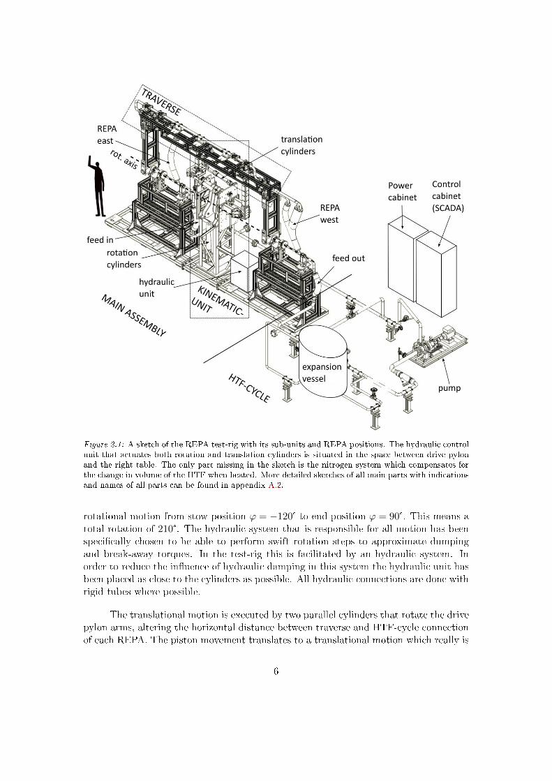
Figure 2.1: A sketch of the REPA test-rig with its sub-units and REPA positions. The hydraulic controlunit that actuates both rotation and translation cylinders is situated in the space between drive pylonand the right table. The only part missing in the sketch is the nitrogen system which compensates forthe change in volume of the HTF when heated. More detailed sketches of all main parts with indicationsand names of all parts can be found in appendix A.2.

rotational motion from stow position ϕ = −120° to end position ϕ = 90°. This means atotal rotation of 210°. The hydraulic system that is responsible for all motion has beenspeci�cally chosen to be able to perform swift rotation steps to approximate dumpingand break-away torques. In the test-rig this is facilitated by an hydraulic system. Inorder to reduce the in�uence of hydraulic damping in this system the hydraulic unit hasbeen placed as close to the cylinders as possible. All hydraulic connections are done withrigid tubes where possible.

The translational motion is executed by two parallel cylinders that rotate the drivepylon arms, altering the horizontal distance between traverse and HTF-cycle connectionof each REPA. The piston movement translates to a translational motion which really is

6

Figure 2.2: The main assembly as built including insulation and REPAs with the traverse still restingon additional supports at stow position.

a rotational motion and therefore measured by a translation angle θ. Even though thedesign of the test-rig allows up to 45° of such rotation, only a fraction of this range will ac-tually be used to reproduce the 500-600 mm of heat dilatation at maximum temperature.Therefore the small angle approximation applies, meaning that a linear relation betweenθ and absorber pipe temperature can be assumed. According to the manufacturer thesmall change in focal length is negligible for REPA lifetime.

The HTF temperature ϑHTF is maintained by six high performance band heaterswith 3.500 W of power each, put around pipes leading to the traverse. All tubes arecovered in 120 mm of insulation material allowing HTF temperatures up to 450 ◦C toalso test new silicone oils with higher maximum temperatures. The maximum designtemperature was set to 500 ◦C. The pump as the heart of the HTF-cycle is responsible forthe hydraulic loads: HTF mass �ow rate mHTF with a range of 6 to 60 m/h3 and HTFpressure pHTF up to 40 bar. HTF density %HTF usually depends on HTF temperatureϑHTF and the �uid used (HELISOL©for commissioning).

Next to this operating parameters is is also possible to investigate the e�ect ofexceeded mounting tolerances. A photogrammetric setup has been provided, makingit possible to accurately determine and set REPA installation position and orientationin order to test the e�ect of tolerances and ill-positioning. A detailed list of all REPAparameters and speci�cations as well as some remarks on limitations and problems canbe found in appendix A.1.

Once put in operation the test-rig will will perform up to 400 cycles a day, tryingto represent a whole REPA life-span of 25 years (approx. 10000 day-cycles) in only afew weeks or months [7]. In an actual power-plant REPAs slowly rotate from ϕr ≈ 90°at sunrise to ϕs ≈ −90° at sunset. After that they are quickly rotated to their stowposition ϕstow where they are left during the night. Usually ϕstow ≈ ϕr meaning thatthe quick rotation is done while the system is still hot. If ϕstow ≈ ϕs the rotation back

7

happens just a few moments before sunrise, i.e. in cold state. Due to the thermal inertiaof the system, it will be impossible to perform an alternating sequence of 'hot' and'cold' rotations. Instead there will probably be some 'hot' followed by the same numberof 'cold' rotations. The question whether this approach leads to results comparable toreal-life wear is not part of this thesis, but will be subject to future research. The sameapplies to the maximum acceleration ratio1 which will depend on how accurate the typicaloperational conditions have to be reproduced in order to recreate failure scenarios.

Although similar in appearance, the traverse does not represent the absorber tubes,meaning that one side experiences 'inlet'-conditions, while the other experiences 'outlet'-conditions. Both REPAs always represent the same of the eight possible positions insidethe a loop (compare �gure 1.2). That way both experience similar stresses and theirresults can be directly compared to each other.

2.2 REPA force measurement

In order to understand the reasons and mechanisms that lead to REPA-wear and �-nally to its failure, there are four dynamo-meters that measure the forces and momentseach REPA exerts onto its bearings. Both REPAs, called 'west' and 'east', rest ontwo dynamo-meters each, one on top and one at the bottom. The dynamo-meters aretherefore referred to as 'top-west', 'bottom-west', 'top-east' and 'bottom-east'. Figure2.3 indicates test-rig motion and dynamo-meter positions. Dynamo-meters are measure-ment devices based on strain gauges that transduce forces and moment into signals. Forall force and torque measurements a K6D175 - dynamo-meter from 'ME-Messsysteme'is used. This sensor measures x-, y- and z- components of the forces and moments thebearing supports that is placed on top of the K6D175. A measurement ampli�er thentransforms these voltages into three forces and three moments, here called the dynamo-meter reading Fdyn.

1The actual acceleration ratio is the life span divided by time needed to represent life span

8

Figure 2.3: A sketch of theREPA test-rig main assembly:the Kinematic Unit (KU) andthe traverse chapter of theHTF-Cycle, without REPAs.The dotted orange line rep-resents the axis of rotation,the dotted blue line representsthe axis of translation. Thered arrows indicate the po-sitions of the four dynamo-meters. Graphic taken from [8,p.66]

Figure 2.4: The graphic shows a technical draw-ing of one of both REPAs 'as build' for translationangle θ = 0°.

REPAs and the adjacent traversepiping system are directly mounted ontothe dynamo-meters and held in place by alocation bearing/ �oating bearing combi-nation. This is shown in �gure 2.4. Dur-ing test-rig operation the dynamo-meterstherefore measure the sum of forces andmoments stemming from the respective ad-jacent piping system and the REPAs. Tobe able to subtract the e�ect of the ad-jacent piping system from the dynamo-meter reading, it has to be approximatedwith a simulation. The simulation is donewith ROHR2 pipe system simulation soft-ware, the model will be referred to as theROHR2-model.

Naturally every model is a simpli�-cation of the actual technical system andthus has to be erroneous to some extend.To keep the relative error made by the sim-ulation as small as possible, the heat dilata-tion of the traverse piping system is com-pensated by two angular and one gimbalcompensators, also reducing the resultingforces onto the the dynamo-meter bearing.

The dynamo-meter reading Fdyn can be represented as the sum of forces and

9

moments exerted by �x and �oating part of the dynamo-meter bearing.

Fdyn = Ffix + Ffloat (2.1)

As the e�ect of the piping system is known from the ROHR2 model, the REPA forcesand moments can be calculated using a simple substraction, as shown in equation 2.2.

Fdyn = Fpiping sys + FREPA

Fpiping sys = FROHR2

FREPA = Fdyn − FROHR2

(2.2)

The ideal positions of bearings, dynamo-meters and REPAs are not identical, levershave to be taken into account when calculating the resulting moment. Ideal positionsand levers h are shown in �gure 2.4.

MROHR2 = Mfix +Mfloat + Ffix × hfix + Ffloat × hfloatMREPA = Mdyn −MROHR2 − FREPA × hREPA + FROHR2 × hROHR2 (2.3)

So far only the top-west position is equipped with a K6D1175 - 10kN/1kNm dynamo-meter from ME-Messsysteme. The other three positions are �lled with 'dummies' (simpleblocks of steel with matching dimensions). Dynamo-meter positions and their motionand rotation during test-rig operation is indicated in �gure 2.5.

Figure 2.5: Dynamo-meter positions during operation: both rotation ϕ and translation ϑ lead todynamo-meter displacement. In blue: a few positions of dynamo-meter top-west. Dynamo-meterstop-east, bottom-east and bottom-west indicated in black.

10

As the implementation and mounting of the test-rig continues, the three vacantpositions will be equipped with dynamo-meters. Due to more detailed knowledge aboutfuture measurement circumstances, another dynamo-meter model might yield betterresults. The same applies for the ROHR2-model: For the lower position no such modelexists yet and thus will have to be created. The experiences made during this thesis willhelp to do this in an e�cient manner.

2.3 Content of this work

This thesis aimed to support the mounting and commissioning process of the REPAtest-rig. First chapter 3 explains the dynamo-meter measurements and investigates theexpected measurement error. Chapter 4 then deals with the two photogrammetrics thatwere done to align all rotation axes to the main rotation axis as an important stepduring mounting and to derive the exact dimensions of the traverse piping system forthe ROHR2 model. This thesis further deals with the validation of the ROHR2 model.Chapter 5 presents chosen parameters and discusses results. Chapter 6 compares modeland experiment in order to evaluate the predictions made and make improvements tothe model. Validation experiments also led to improvements at the test-rig, mainlyconcerning insulation and sensor cooling. These are presented in chapter A.9. Finallythe whole work is then summed up and evaluated in chapter 7.

11

3 Dynamo-meter measurements and uncertainty

Every force measurement chain consists of a sensor that transduces the physical forcesand moments into a measurement signal, a signal ampli�er and some indication device.At the REPA test-rig the �rst dynamo-meter is a K6D175 from ME-Messsysteme, shownin �gure 3.1.

Figure 3.1: Right: Dynamo-meter K6D175 10kN/1kNm; Center: Measurement ampli�er GSV-1A16USBK6D/M16; Left: Computer with measurement software GSV-multi running.

Figure 3.2 depicts a graphical representation. Normally we assume a linear behav-ior for both sensor and measurement ampli�er, which means that the whole chain hasa linear dependency of ampli�er output voltage U on the forces (and moments) appliedF . We will call the result displayed the dynamo-meter reading Fdyn.

Figure 3.2: A scematic representation of the measuerment chain, transducing a physical quantitiy intoan output voltage. Source: [10]. As the bridge voltage UD is proportional to the supply voltage Us, thatis provided by the measuring ampli�er, the output signal uS is usually given in relation to the supplyvoltage.

This linear behavior can be expressed by a simple expression using the calibration matrixK:

Fdyn = K · U (3.1)

K is fully equipped, 6x6 matrix. Therefore all six channels of U have an in�uence oneach of the three forces and three moments of Fdyn. If only one of the channels is defect,none of the results displayed is accurate. For detailed information on the linearity of

12

both dynamo-meter and measurement ampli�er as well as other useful information pleaseread the appendix A.3 and have a look at the glossary.

3.1 Measurement Uncertainties

Generally speaking, equation 3.1 is never fully valid. Even at calibration loads andcalibration temperature, uncertainties have to be taken into account when interpretingthe results. These can be split in three groups:

� Measurement uncertainties that a�ect the zero-signal:

� zero signal when mounted SF0

� rel. reversibility error (hysteresis error) µ

� rel. creep dcr

� Measurement uncertainties that a�ect the characteristic:

� rel. linearity error dlin

� rel. repeatability error brg

� uncertainties from calibration on basis of an inappropriate load scenario

� Temperature related uncertainties:

� temperature e�ect on zero signal TK0

� temperature e�ect on characteristic value TKC

� di�erence in zero signal due to increased sensor temperature U0,ϑ

� di�erence in zero signal after complete heating cycle ∆U0,20C

In order to keep the measurement uncertainties as low as possible all dynamo-metersshould be comissioned according to the document 'Inbetriebnahme von Sensoren' pub-lished by ME-Messsysteme [11]. Information about uncertainties are taken from the FAQand documentation chapter of www.me-systeme.de (20.11.2016), as well as VDI2638 [12].

E�ects on Zero Signal

The Zero signal is the output signal of the unloaded sensor. A distinction is madebetween the zero signal when removed S0 (no mounting parts) and the zero signal whenmounted SF0 (not mechanically loaded, with mounting parts, at the beginning of aloading cycle) [12]. Values are given in appendix A.3.

13

S0 itself, or its expression U0 in Volt are far from being zero. The multiplicationwith K yields forces as high as −400 N (Compare equations A.10 and A.12 in the ap-pendix.) Therefore no measurement is valid if neither a) the zero signal stated in thecalibration certi�cate is subtracted from the output signal before being multiplied withK, or b) the dynamo-meter reading is de�ned to be zero at the beginning of a measure-ment (o�set compensation). On the one hand b) has advantages over a) as regular o�setcompensation ensures that possible changes to the zero signal are accounted for as well.On the other hand a) is an absolute measurement, while b) is only relative.

Looking at �gure 3.3 we can see that SF0 possibly di�ers from S0. This is dueto the e�ect of mounting the sensor on an uneven surface or onto soft material suchthat tightening the sensor screws leads to its deformation. During sensor mounting thechange of zero signal should therefore be measured and evaluated. This e�ect constitutesanother reason to choose b) over a).

Figure 3.3: This �gure, based on a graphic in VDI 2638[12, p.9], shows a schematic sensor characteristic,that would be obtained when plotting the sensor signal during applying an increasing force starting fromzero up to nominal force Fnom and then back down to zero. The so-called reference straight line thatwill be used as characteristic curve represents a best �t of the curve obtained (It's exact derivation isdescribed in DIN EN ISO 7500-1 [13]). The black curve represents the standard case when the sensor iscalibrated for rated force Fnom, the second curve represents the special case when the sensor is calibratedfor a di�erent load scenario Fcal. C is the true signal measured at calibration force, CR is the linearapproximation evaluated at calibration force and Cnom is the value stated in the data-sheet or calibrationcerti�cate. Representation of uncertainties exaggerated and axes not drawn to scale for better visibility.

Another measurement uncertainty related to the zero signal is the rel. reversibilityerror or hysteresis µ, which describes the biggest di�erence between sensor output signalfor an increasing and decreasing force from zero to rated force (Alternatively the hys-teresis can also be given for speci�ed forces such as 50% of the nominal force µ50 [12]).Figure 3.4-A shows that due to this the zero signal might change after one cycle (ger-man: Nullpunktrückkehrfehler). The explanation are smallest in-elastic deformations ofthe casting compound that the sensor hull is �lled with. To eliminate this change of zero

14

signal the sensor should be completely unloaded and set to zero after each cycle. This ofcourse is not possible at the REPA test-rig which is why the error has to be taken intoaccount at all times. Likewise, there is a temperature-related reversibility error that isequal to the di�erence in zero signal after one complete heating/cooling cycle. Duringtest-rig operation the total hysteresis error might be bigger due to friction inside �oatingbearings.

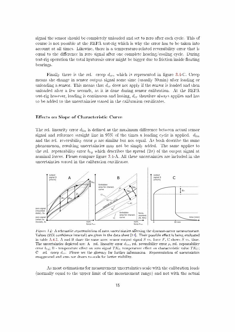
Finally there is the rel. creep dcr, which is represented in �gure 3.4-C. Creepmeans the change in sensor output signal some time (usually 30min) after loading orunloading a sensor. This means that dcr does not apply if the sensor is loaded and thenunloaded after a few seconds, as it is done during sensor calibration. At the REPAtest-rig however, loading is continuous and lasting, dcr therefore always applies and hasto be added to the uncertainties stated in the calibration certi�cates.

E�ects on Slope of Characteristic Curve

The rel. linearity error dlin is de�ned as the maximum di�erence between actual sensorsignal and reference straight line in 95% of the times a loading cycle is applied. dlinand the rel. reversibility error µ are similar but not equal. As both describe the samephenomenon, resulting uncertainties may not be simply added. The same applies tothe rel. repeatability error brg which describes the spread (2σ) of the output signal atnominal forces. Please compare �gure 3.4-A. All these uncertainties are included in theuncertainties stated in the calibration certi�cates.

Figure 3.4: A schematic representation of most uncertainties a�ecting the dynamo-meter measurements.Values (95% con�dence interval) are given in the data sheet [14]. Their possible e�ect is being evaluatedin table A.4.2. A and B share the same axes: sensor output signal S vs. force F , C shows S vs. time.The uncertainties depicted are: A - rel. linearity error dlin, rel. reversibility error µ, rel. repeatabilityerror brg; B - temperature e�ect on zero signal TK0, temperature e�ect on characteristic value TKC ;C - rel. creep dcr. Please see the glossary for further information. Representation of uncertaintiesexaggerated and axes not drawn to scale for better visibility.

As most estimations for measurement uncertainties scale with the calibration loads(normally equal to the upper limit of the measurement range) and not with the actual

15

measurement value (compare the data sheet of the K6D175 dynamo-meter [14]) therelative uncertainty increases for smaller loads. This represents a �rst reason to have thesensor calibrated for the most representative load scenario possible. The second goodreason is that the slope of the characteristic curve is dependent on the the calibrationforce Fcal as the comparison between the two curves in �gure 3.3 indicates. This meansthat in order to keep calibration errors as small as possible, calibration loads shouldalways be chosen in the range of the expected loads during operation. For all futuresensor purchases for the three dynamo-meter positions that are still vacant, it is stronglyrecommended to buy the smallest sensor possible. This has advantages both accuracyand money-wise. Concerning safety, please keep in mind that for force transducers fromME-Messsysteme the failure load is 300% of the nominal load. Please also read theadvice and information given in appendix A.5.

Temperature related Uncertainties

The nominal calibration curve is given for a speci�c calibration temperature, which isstated in the calibration certi�cate of the K6D175 [15] to be (21±1.5)◦C. A sensor tem-perature that deviates from the calibration temperature leads to increasing measurementuncertainties. Figure 3.4-B shows that this is equivalent to a wider area the calibrationcurve possibly lies in and can be split up in two separate e�ects. First: The temperaturee�ect on zero signal TK0, which is equivalent to a possible parallel shift of the nominalcalibration curve (lines a)). And second: The temperature e�ect on characteristic valueTKC , which is equivalent to a possible changing slope of the nominal calibration curve(lines b)). The total e�ect is the sum of both parts (lines c)).

The di�erence between TK0 and TKC is that there are two relatively easy waysto get rid of TK0. The �rst possibility is to make sure that the sensor heats up beforeapplying the �rst loads. That way, the change in zero signal can be neglected by sim-ply o�set compensation of the output (i.e. setting its value to zero which is equal tosubtracting the initial value from every output) before starting the measurement. Thishowever is not possible at the REPA test-rig, as the dynamo-meter and the piping systemhave a closed connection. However, it is possible to measure the TK0 in un-mountedstate (either completely free or with some parts connected) by putting the sensor in anoven and track both temperature and di�erence in zero signal due to increased sensortemperature U0,ϑ

2. This will be referred to as temperature test. Under the assumptionthat conditions during temperature test and later operation are identical, this data canbe used to mathematically exclude its e�ect from the dynamo-meter reading Fdyn:

Fdyn′ = Fdyn −K · U0,ϑ = K · U −K · U0,ϑ = K · (U − U0,ϑ) (3.2)

The underlying assumptions are that there are no temperature and time gradients, mean-ing that the temperature distribution is always perfectly homogeneous and changes in-�nitesimally slow (steady state). Further more, we assume that U0,ϑ is independent of

2Please note that the output signal has either the unit V or mV (symbol U) or the unit mV/V (symbolS). Compare appendix A.3 for explanations.

16

the loads applied and the mounting situation. In chapter 3.2 we will see that there isgood reason to believe that both assumptions do not always hold. The change in zerosignal after one complete heating/cooling cycle is ∆U0,20C .

3.2 Measurement Uncertainty Estimation

Normally all sensors are calibrated for nominal forces which more or less represent areasonable upper limit for the expected loads: Fnom = Fcalib >≈ F . At the REPA test-rig however, the dynamo-meter had been chosen in order to withstand the forces thatwould break a standard absorber tube support in a PTC power plant, multiplied by somesecurity factor. The results were nominal forces in the range of 10-20 kN and 1-2 kN m,compared to best estimation of operating forces these make only approximately 10-20%of the forces and 50-70% of the moments. Please compare the appendix, table A.4.1for calculations and exact values. The estimated load scenario will be the basis for allevaluations of uncertainty improvements.

When the �rst dynamo-meter was bought, a calibration was done for nominalforces and as it is good practice, the calibration was done for the whole measurementchain3. For the calibration, the dynamo-meter is clamped into a hydraulic press whichthen applies a set of known forces and moments. The output signal U is logged duringapprox. 80 distinct load stages, with three repetitions each. Between two loading cycles,the sensor is unloaded completely each time and o�set compensated. Maximum loadis applied for 30-40 seconds to account for transient oscillations. The results are thenused to derive the 36 degrees of freedom of the 6x6 calibration matrix using a linearregression.

Calibration measurement data is also used to estimate the measurement uncertain-ties. These are calculated on the basis of twice the maximum di�erence within the threerepetitions per load stage. Due to the fact that calibration measurements only last afew seconds and are done at ambient temperature, the found measurement uncertaintiesdo neither include the relative creep dcr nor any of the temperature related uncertain-ties. To be able to do that a re-calibration was done based on a load scenario estimatedwith data from �rst validation experiments (compare appendix A.8). The re-calibrationincluded a temperature test which gives data for the temperature e�ect on zero signalTK0, di�erence in zero signal due to increased sensor temperature U0,ϑ and di�erence inzero signal after complete heating cycle ∆U0,20C .

When having to interpret measurement results, a single value for the measurementuncertainty comes in handy. In order to derive the measurement uncertainty of theREPA test-rig, individual values have been summed up in table A.4.2 of the appendix.There are three cases being compared: 1) the original state where calibration data wasavailable for nominal loads only, 2) the current state after �rst re-calibration and the

3dynamo-meter (K6D175 10kN/1kNm, SN: 15401935) + ampli�er (GSV-1A8USB K6D/M16, SN:15156211.)

17

�rst temperature test and 3) an idealized future where temperature e�ect on zero signalTK0 is perfectly known due to an advanced and repeated temperature test.

The total measurement uncertainty always depends on the calibration loads Fcal,the actual loads applied F and the dynamo-meter temperature ϑdyn, compare appendixA.3.2. In our comparison, all three parts of the table assume the worst case scenario ofϑdyn = 70 ◦C and F being equal to the best estimation possible, derived in table A.4.1in the appendix. What changes from case to case is the information about the behaviorof the sensor.

This means that we can use the table to assess the improvements made and pos-sible future improvements: Due to the re-calibration, the total non-temperature relateduncertainties dropped by 56.6% in average. Together with the data from the �rst tem-perature test, total uncertainty estimates are now in average 67.8% lower than they wereoriginally. Yet, there is still room for further improvement: If we assume that a repeatedadvanced temperature test yields perfect knowledge about the sensors behavior whenheated, it is theoretically possible to simply subtract this behavior from the results andassume an uncertainty of zero. However, repeated test will most likely show that resultsspread a little, which is why the uncertainty in the end will be slightly greater than zero.

3.3 Implications of re-calibration and temperature test

In a perfect world there would be no di�erence between original and re-calibration ma-trices. Due to sensor aging however, and the circumstances shown in �gure 3.3 we don'tget the same values. This is supported by equation A.13 and table A.3.1 in the appendix.

As long as none of the forces and moments exceeds the re-calibration scenario, wecan use the re-calibration matrix. In case any of the forces measured (absolute values!)exceeds the re-calibration scenario, both result and expected uncertainties (without tem-perature and aging e�ects) can be linearly interpolated according to equations A.17 andA.18 in the appendix.

For the temperature test by ME-Messsysteme, the free sensor has been put in anoven and heated up to 5 K below its maximum operation temperature of 85 ◦C. Thezero-signal has been continuously tracked. Exact temperature however has only beenlogged at the beginning, its peak and after reaching ambient temperature again. Figure3.5 shows the results. the x-axis however does not represent temperature, as this hasnot been tracked. The only information we have that temperature steadily increases,then decreases, probably asymptotically and given enough time to even out temperaturegradients. This lack of information signi�cantly reduces our means to interpret thegraphs.

Still we can make an interesting observation: In the cases of Fx, Fy and My themaximum error is reached shortly after the begin of either heating or cooling phase, in

18

0 200 400 600 800 1000 1200 1400 1600

meas. points

-200

-100

0

100

200

300

400

500fo

rces

in N

0 200 400 600 800 1000 1200 1400 1600

meas. points

-15

-10

-5

0

5

10

15

mom

ents

in N

m

FORCES:FxFyFz

MOMENTS:MxMyMz

Figure 3.5: The results of the temperature test: the physically meaningless zero signals have beentransformed to resolving forces and moments. Duration of test approximately 2 hours. Cross-markersfor extreme values, circle markers for measurements for which temperatures are known. Dotted lines foreye guidance.

opposed directions. After that the value asymptotically converges to its �nal value at80 ◦C, just like Fz, Mx and Mz do not show this behavior. We could suspect that the�rst group is more sensitive to temperature gradients (time or spacial) than the second.

The measurement data I obtained from ME-Messsysteme and which is plotted in�gure 3.5 does not cover the end of the measurements. If they did, we would see that theforces and moments do not go back to zero, as it is stated in the calibration certi�cate.This behavior is called di�erence in zero signal after complete heating cycle ∆U0,20C andpart of the uncertainty estimation of table A.4.2 in the appendix. It can be interpretedas evidence for increased sensor aging after a few temperature and load cycles only (14temperature validation experiments of a few hours each, compare chapter 6.1). Laterduring test-rig operation the sensor will eventually be loaded for thousands of cycles andmonths of time without being completely unloaded once. Severe aging and thus increasesuncertainty could be an issue.

Sadly no standardized test procedure exists to evaluate and describe the long-termbehavior of force transducers, which is why no respective parameters are given in neitherdata-sheet nor calibration protocol. I will therefore name two possibilities to deal withthis issue: First, instead of one temperature test, many consecutive tests could helpunderstand how ∆U0,20C behaves over time. Second, Before mounting the sensor, somereproducible measurements with examination weights and levers should be performed,which could be repeated after a greater number of cycles to subsequently estimate theuncertainty from sensor aging.

Third, all measurements could be changed to relative measurements by regularlyperforming an o�set compensation (setting all values to zero). In this sense, regularlycould for example mean every time that the traverse begins a new cycle at ϕ = 90° orevery time the sensor reaches a certain temperature. The results would still be compara-ble, uncertainties would drop, but there would be no information about absolute forcesonto the sensor.

19

4 Photogrammetry

The new REPA test-rig is meant to produce precise and accurate measurements of thestresses that lead to the deterioration of REPAs. Further more, the possibility to pre-cisely measure the positions of both REPA connections allows intended misalignment ofcomponents in order to investigate its e�ect on REPA lifetime. In order to guaranteegood functioning and reliable measurements, the test rig must conform with speci�edtolerances. During this thesis the exact geometry of the traverse piping system, treatedin chapter 4.1, as well as correct orientation and alignment of all rotation axes, treatedin chapter 4.2, were of special interest.

To verify these, a quick, e�cient and accurate measurement of relative posi-tions and distances between machine parts was required. After a �rst attempt witha tachymeter failed, a photogrammetric approach was chosen. Although more time andmaterial expensive in the preparations, a photogrammetry has the advantage to be easilyand very cost-e�ectively repeated, once the setup is put in place. The approach thereforeo�ers the possibility to verify deformations due to mechanical stress and/or heating laterduring operation.

Close range photogrammetry (hereafter referred to as photogrammetry) is a computer-based measurement method that calculates 3D-positions of retro-re�ecting targets froma set of photos taken from various perspectives. The photos can be taken by a normalSLR camera and a �ash, the post-processing is done by specialized software, such asAICON 3D Studio in this case. A photogrammetry setup consists of coded and uncodedtargets made from retro-re�ective foil, scale bars and a coordinate cross. If a targetappears on enough photos there is only one possible solution for their relative position inspace, that can be iteratively found using a numerical approach. References sticks, thathave a very precisely known length help to scale relative distances of points and increasethe results accuracy. The coordinate cross serves to specify a �rst coordinate system forbetter orientation. For general information about close range photogrammetry pleaserefer to [16], for information about the use of photogrammetry in CSP, please refer to[17].

The �rst step in a photogrammetry measurement is to put the targets onto thestructure. The uncoded targets are put on every point of interest, as well as the back-ground and other parts to give the setup more depth and create a more homogeneouspoint-cloud, which also improves measurement accuracy. If a measurement point itselfis hidden, such as the center line of a pipe, an indirect measurement is needed: uncodedtargets are put around the pipe circumference forming a circle, a so-called sleeves. Thecenter is then later calculated by �tting a circle in the points on the pipe surface. Inother cases adapters can help, e.g. bolts that exactly �t pockets which center needs tobe measured, but stand out and can be equipped with targets.

The second step is then to make photos (about 200-300 per measurement) fromvarious angles and from all around the structure, if needed with the help of a lifting

20

Figure 4.1: Indirect target placement: Left - axis sleeve: targets put around cylindrical object to getcenter; middle - compensator sleeve: rotation axis de�ned by two angle points; right - adapter (withsleeve) to �nd center of pocket

platform. The data is then fed into AICON 3D studio which gives back a list of 3D-coordinates as result. For best results, camera-positions have to form a homogeneous'cloud' around the setup, compare �gure 4.3c.

Finally the found points have to be named within AICON 3D studio as a prepa-ration for automated post-processing, for example with MATLAB. The �rst time thishas to be done manually, all following times this can be done automatically if relativepoint positions haven't changed more than a few millimeter. The desired coordinatesystem can be speci�ed using coordinate transformation. For a detailed description ofall necessary steps, please have a look Luhmann, 2006 [16] or other documentation4.

4.1 Traverse: ideal pretension and model geometry

Objectives and Requirements

For most accurate model description (please compare chapter 5), as well as veri�cationof correct pre-tensioning, the exact geometry of the piping system inside the traverse isneeded. This comprises pipe segment length, coordinates of pipe segment connectionsand the bracing planes of the compensators. Ideally, the traverse piping system centerline is only only two-dimensional. Deviations in the third dimension (here: x) are ofspecial interest as they could be a possible explanation for the forces measured normalto the main axis.

Photogrammetry process

The seven pictures in �gure 4.3 explain the seven steps necessary in order to obtainthe exact traverse piping system geometry and change the ROHR2 model accordingly.The �rst step was to prepare the setup (a). To indirectly measure the center-line of the

4There is a REPA-speci�c Photogrammetry How To available on the DLR servers

21

piping system, as well as the angle points of the compensators, fourteen pipe sleeves andthree compensator sleeves were used5. Their positions are depicted in �gure 4.2. Thenapproximately 200 to 300 photos were taken (b) and fed into AICON 3D-software, whichcalculated camera and target positions (c).

Figure 4.2: Traverse photogrammetry setup: pipe and compensator sleeve positions and segment names.

The post-processing was done by MATLAB which calculates sleeve centers byusing a circle �t (d). The coordinate system was re-set, de�ning the �xed part of thedynamo-meter bearing as the origin and pipe axis A as parallel to the y-axis. Based onthe center points found, pipe segment axes and connection points were derived as best�t through two or more pipe and compensator sleeve center points.

Finally the pipe section connection points were put into a 2D-geometric model inInventor (f) in order to calculate and verify compensator angles in cold and hot state andin order to verify if pre-tentioning was done perfectly (compare chapter A.9). At last,the geometric representation and actual pretension of the traverse in the ROHR2-modelwas updated (g).

5Compensator sleeves refer to two targets placed on both sides of a compensator at which center thecompensator angle point is assumed.

22

(a) Step 1: Preparations (b) Step 2: Taking photos

(c) Step 3: Running AICON 3D (d) Step 4: Make circle �t in MATLAB

(e) Step 5: Plot pipe center points (f) Step 6: Geometric model as Inventor sketch

(g) Step 7: Update ROHR2-model

Figure 4.3: Work�ow necessary in order to represent exact piping system geometry in ROHR2 model.

23

Results

Table 4.1 shows lengths of the piping systems segments and the coordinates of seg-ment connection points as de�ned in �gure 4.2. These constitute the result of the post-processing of the true dimensions of the piping system found by the photogrammetry.Ideally, the center line of the piping system does not have any extension in x-direction.Results show that this is not the case, as connection point 4 deviates from its ideal posi-tion by as much as 10.7 mm in x. During post-processing, this value has been calculatedtwice, column 'x' gives the mean of the two values found, column 'δx,calc.' gives the dis-tance of this mean to each of the two solutions. This does not include the measurementuncertainty of the photogrammetric approach itself, which was su�ciently small to beignored: the average measurement uncertainty, estimated by AICON 3D for each pointindividually, is only 0.04 mm. The maximum uncertainty is given to be 0.13 mm.

Based on the coordinates of the connections points, the pipe segment lengths canbe calculated. When comparing these to lengths speci�ed in the technical drawings ofthe traverse piping system, we can see that deviations are in the range of 5.7 mm. Thetrue pipe lengths are then used in chapter 5.2 to derive ideal pretension.

Table 4.1: Photogrammetry results: traverse piping system geometry. All values in millimeters. The leftpart of the table shows coordinates of start and end points of pipe segments, as well as the uncertaintyin the x-coordinate6. By de�nition the origin of the coordinate system is equal to point 1 (�x part ofdynamo-meter bearing) and segment A is parallel to the y-axis. The right side of the table shows pipesegment lengths as planned and as built, as well as their di�erence.

Pipe segment connections Pipe segments

No. x y z δx,calc. Name as planned as built ∆l

1 0 0 0 0 A 470.5 475.5 5.02 0 477.1 -0.7 1.29 B 295.5 295.4 -0.13 -1 771.8 -9.7 4.55 C 450.0 451.5 1.54 -10.7 783.2 440.6 3.09 D 295.5 290.7 -4.85 -9.8 1073.2 430.7 0.88 E 915.0 915.8 0.86 1.2 1987.2 449.9 1.71 F 1075.5 1069.8 -5.77 9.5 3055.5 447.4 0

.

6Only uncertainty stemming from axis �t only. Photogrammetry measurement uncertainty not in-cluded.

24

4.2 Test Rig: Alignment of rotation axes

Objectives and Requirements

The REPA test-rig is designed to perform rotational and translational motion. Figure4.4 shows all axes that play a role in this motion. For the rotational motion �ve axesapply: the main axis de�ned by the drive pylon (a), the two axes of the two swivel drives(b) and the two axes of the swivel joints (c). For the translational motion eight axesapply: the two main axes de�ned by the drive pylon arm bearing (left and right) (A),the two axes of the drive pylon arm connections (B), and the four axes of the upper andlower bearing of the swivel drive arms (C) and (D).

These two groups of axes have to be aligned to prevent the test rig from su�eringdamage due to high stresses and deformation caused by the rotational or translationalmotion. Further more, it is desired to avoid possible e�ects on the force and torquemeasurements itself that could stem from any deformation of the traverse and or pipingsystem. Badly aligned rotation axes may lead to high torsion of tables and bearingswhich may cause their destruction. Furthermore the greater the angle between one ofthe tables rotation axis and the drive pylon rotation axis, the greater the forces and theinduced stresses which ultimately leads to greater deterioration of the REPA test-rig.

Figure 4.4: REPA rotation and translation axes. Rotation: a) drive pylon , b) swivel drives, c) swiveljoints. Translation: A) drive pylon arm bearings, B) drive pylon arm connections, C) and D) - swiveldrive arm bearing and traverse connections

During mounting, before adding end plates and arms to the main assembly, rotationaxes a and b needed to be aligned. IW-Maschinenbau, the designer of the test-rig, statesin their manual that translation axes A and B, as well as rotation axes a and b may notdi�er more than ±0.1 mm from each other [18]. As it is not feasible to even measure axesthat are �ve meters apart with such high accuracy, tolerances were increased to ±1 mm,

25

meaning that each of the three rotation axes at the height of the ideal bearing positionsmay not have an o�set greater than 1 mm from the main rotation axis, compare �gure4.5.

Senior Flexonics, the manufacturer of the �rst REPAs tested states that swiveljoints axes and the main roation axes should not di�er more than ±2 mm [19] from eachother. This, as well as the alignment of the translation axes will have to be veri�ed, oncethe assembly of the test-rig is complete. In order to facilitate this, the method found andthe code written for the post-processing should be easily adaptable. A photogrammetrywas again chosen because it allows indirect measurements of the axes by using sleevesand adapters as well as quick repetition once the setup is put in place, while at the sametime having a very low measurement uncertainty. The latter is important as all axeshave to be measured multiple times while iteratively adjusting axis orientation7.

Photogrammetry process

Figure 4.5: Main assembly photogrammetry setup: main rotation axis indicated in red. The threerotation axes of the two table bearings and the drive pylon have to be aligned. The allowed tolerance isde�ned as the maximum distance between the projections of the ideal bearing positions onto the mainrotation axis 'X' and the respective rotation axis 'O'. This is represented for the left swivel joint bearingeast only (exaggerated for better visibility).

The photogrammetry is carried out as previously described, using sleeves to �ndcenter lines of swivel drive bearing shafts and the drive pylon head rotation axis. Figure4.5 shows two photos of the setup. The post-processing is done in MATLAB, which �rstcalculates the centers of the sleeves via circle �ts. The tree rotation axes are then foundby linear regression. The result is shown in �gure 4.6. Finally, the coordinate system isre-de�ned, setting the rotation axis of drive pylon as main rotation axis. The origin isset to be in the center of the drive pylon head.

7It turned out that using dial gauges and an adapted vice works best to move the heavy bearingstructures. the e�ect of tightening screws has to be anticipated.

26

Results

The alignment process was successful and can easily be repeated. Several iterations wereneeded, adjusting table height and bearing orientation each time, in order to decreasehorizontal o�set and vertical o�set below < 1 mm. Remaining o�sets are shown in �gure4.7.

−4,000 −3,000 −2,000 −1,000 0 1,000 2,000 3,000 4,000

−200

−100

0

100

200

−200

−100

0

100

200

x in mm

y in mm

zin

mm

Figure 4.6: The plot shows all measured circle points (blue), their calculated center points (cyan,magenta and green) and the corresponding axes (colors as center points). Please note that y and zcoordinates are not drawn to scale for better visibility. The coordinate system (solid blue lines) isrotated compared to the three axes, as could not be precisely de�ned before taking the photos.

−4,000 −3,000 −2,000 −1,000 0 1,000 2,000 3,000 4,000−1

−0.5

0

0.5

1

EAST � WEST, in mm

Horizontalo�set

NORTH�

SOUTH,in

mm

−4,000 −3,000 −2,000 −1,000 0 1,000 2,000 3,000 4,000−1

−0.5

0

0.5

1

EAST � WEST, in mm

Verticalo�set

DOWN�

UP,in

mm

Figure 4.7: Rotation axes measured after last adjustment iteration: Blue lines indicate three rotationaxes. Drive pylon head rotation axes de�ned to be main rotation axis. Black dots indicate measuredcenters of sleeves, red points indicate projections of the ideal bearing positions onto their respectiverotation axis. O�sets are equal to the value of the y-axis of the plot.

27

5 The ROHR2 model

In complex piping systems it is not only necessary to assure that the static require-ments are met. The combined in�uences of changing pressures and alternating �uidtemperatures have to be considered also. ROHR2 is a simulation software of SigmaIngenieurgesellschaft that predicts static behavior of complex piping systems. UsuallyROHR2 models are used to perform strength calculations for industrial size piping sys-tems. Bearing reactions are calculated to ensure safe operation. In chapter 3 we have seenthat in the case of the REPA test-rig, we need to very accurately estimate comparablysmall residual bearing reactions that can not completely be eliminated by compensationof thermal expansion or other measures. This constitutes a very particular case. For thisreason it is extremely important to describe the realized piping system as accurately aspossible.

Here the ROHR2 model is needed to simulate forces and moments that the traversepiping system exerts onto the dynamo-meter at speci�c operational conditions, calledLoad Cases (LCs). LCs refer to the sum of HTF temperature, -pressure and the mediumused. In ROHR2 the latter is de�ned by its density, which can be taken from therespective data-sheets given its temperature. The mass �ow rate is not part of a LCas it can't be represented in ROHR2. The same is true for all time- and most spacialgradients of pressure and temperature. During a day a REPA moves through a numberof very di�erent LCs. These depend on the time of the year, the time of the day, theweather and the question which of the normally eight REPAs in a PCT power plant oneis looking at. Please refer to chapter 2.1 for detailed information.

5.1 Model con�gurations

In his work, Andreas Plumpe created a model in ROHR2 that represents the pipingsystem in between the two REPAs, called the traverse [8]. This chapter will describehow the model has been improved and modi�ed to best represent the actual traversepiping system, before discussing its predictions.

In order to improve and adapt the model there are now four versions that havedi�erent speci�cations. The di�erent versions serve as reference either during validationexperiments or test-rig operation. The initial base model is called Traverse_40. In thismodel, pipe geometry, dimensions and pretensioning are represented as planned, laterinsulation thickness is realistically assumed. For better comparability during validationexperiments, the insulation has been removed to create Traverse_999. To account forconstruction tolerances and changes to the initial design (missing compensators), thismodel has been improved and changed according to the �nal traverse as built, using aphotogrammetric approach described in chapter 4.1. Two new base models have been cre-ated: Traverse_100 without insulation to be compared with the validation experimentsdescribed in chapter 6 and Traverse_200 with insulation for later test rig operation. Asummary is shown in table 5.1.

28

Table 5.1: ROHR2 base models: main changes in the evolution of the base model.

Base model Geometry Insulation Compensators Purpose

Traverse_40 as planned as planned initial values initial modelTraverse_999 as planned none initial values ref. 'unchanged'Traverse_100 photogr. none updated values ref. 'validation exp.'Traverse_200 photogr. as built updated values ref. 'test-rig op.'

To introduce and investigate the e�ect of rotation, base model has been givena set of sub-models that represent the piping system at di�erent rotation angles ϕ =−120°,−110°, ..., 0°, 10°, ...90°. Since it is not possible to de�ne a rotation angle inROHR2 or arbitrarily set the direction of gravity, which would have the same e�ect,each rotation angle means a new model (hereafter called sub-models).

Finally, LCs are de�ned in ROHR2. For good resolution up to 60 LCs have beencreated, each representing a static operation scenario covering the possible ranges ofϑHTF and pHTF : �ve di�erent pressures for each of the twelve di�erent temperatures.More resolution or new �uids can easily be achieved by introducing more LCs to themodels. Due to internal requirements of ROHR2, a so-called reference load case has tobe de�ned. This represents a maximum stress scenario, i.e. contains the highest valuesfor temperature, pressure and density of all LCs that are based upon this reference loadcase. The reference load case only serves for ROHR2-internal simulation purposes andhas no value for interpretation.

The post-processing consists of calculating resulting forces onto the dynamo-meterusing equation 2.3 and plotting the results. This is done in MATLAB. For automatedplots and comparison, both the sub-model- and the LC-names have been coded. Thesub-models' are named Traverse_aaabccc: three digits 'aaa' for the base model, one digit'b' for the sign ('4' for '+' and '7' for '-') and three digits 'ccc' for the rotation angle ϕin °, e.g.: Traverse_1007080 is the base model Traverse_100 rotated to ϕ = −80°. TheLCs are named TxxxPyy-Z : three digits 'xxx' for the temperature in ◦C, two digits 'yy'for the pressure in bar and one digit 'Z' for the HTF used. Possible HTFs are Syltherm800 (Z = S), HELISOL©(Z = H) and maybe more. During validation experiments themedium was air (Z = A). For Commissioning HELISOL©is used. To get results for anycombination of operation variables, linear interpolation is used. Please refer to appendixA.6 for more information.

5.2 Model parameters

The traverse can be separated in two parts, east and west. The ROHR2 model followsthis distinction. Figure 5.1 shows a graphic representation. As bearing 4 is assumed tobe rigid enough to hinder any deformation or displacement, the two parts of the traversepiping system can be dealt with independently. In order to absorb pipe heat dilatation

29

and minimize the forces and moments that the traverse piping system exerts onto thedynamo-meter bearing, two single and one gimbal hinged angular expansion joints, calledcompensators, were installed in the western part.

Figure 5.1: Top and side view of Traverse_100 base model. A, B and C: compensators west-outer(gimbal hinged), west-center and west-inner (both single hinged). 1 and 4 are �x bearings. 2,3,5,6 and7 are �oating bearings.

As compensators work as springs that try to remain in un-deviated position, small-est deviation cycles also mean smallest moments that have to be applied to keep thecompensators in deviated position and thus smallest bearing reactions. In order to havethe resulting forces as small as possible, the three compensators are pre-tensioned, mean-ing that they are mounted slightly de�ected at ambient temperature so that, reaching350 ◦C the de�ection is zero and the resulting forces are minimal. For a more detaileddescription and explanation of both compensation and pre-tensioning, please have a lookat appendix A.9.

Table 5.2 shows resistance coe�cients or spring constants as a function of HTFpressure pHTF and compensator angle α as well as the torsion angle.

All values given in table 5.2 have to be applied with caution as the manufacturerstates a tolerance of 30% for all values. In ROHR2 these constants can be set in theentry-mask belonging to each compensator. Strictly speaking these values only apply atambient temperature. For higher temperatures a reducing factor Kc needs to added[20,p.42-43]. ROHR2 only considers reducing factors for pre-set compensators taken fromthe database. Custom-de�ned compensators as in this model do not allow reducingfactors yet. This means that the ROHR2 model might not be the best choice of softwarefor this task. This has to be kept in mind when assessing the model validation in chapter6.

In order to address these limitations inherent to the used software the traversepiping system should be represented as accurate as possible. In order to account for allinevitable deviations of the �nal traverse piping system as built from the ideal geometryas planned, a photogrammetry measurement has been performed to �nd the true pipinggeometry. Please refer to chapter 4.1 for details. Photogrammetry results were also usedto verify and improve pretensioning, please refer to appendix A.9 for detailed information.

30

Table 5.2: Compensator resistance coe�cients and temperature dependent reducing factors. As de-�ned by the help chapter of ROHR2: cα is elastic angular bellow resistance, pressure-independent;cr is pressure-dependent angular friction resistance; cp is elastic angular bellow resistance, pressure-dependent; cT is elastic bellow (german: 'Balg') resistance for torsion, values are big compared to othersas compensators do not allow rotation around this axis; α is the compensator angle; ciϑ = Kc · ci arethe operation temperature adjusted resistance coe�cients[20, p.42]. Tolerance not included in values.In the model, regulating powers are increased by the tolerance, compare ROHR2-help chapter.

Comp. Axes Regulating powers at 20 ◦C Max. allowed

cα cr cp cT αmax momentN m/° N m/bar N m/(bar °) N m/° ° N m

Singlex-axis 8.3 0.7 0.2 - ± 5.5 -z-axis - - - - - -y-axis (torsion) - - - 6.6k ± 0,1 764

Gimbalx-axis 8.3 0.7 0.2 - ± 5.5 -z-axis 8.3 0.7 0.2 - ± 5.5 -y-axis (torsion) - - - 6.6k ± 0,1 764

Operation temperature ϑ in ◦C 200 300 400 500 600 700 800 900Reducing factor Kc 0.93 0.90 0.86 0.83 0.80 0.75 0.71 0.67

5.3 Results and discussion

ROHR2 calculates displacements, rotations, forces, moments and relative stresses forevery pipe segment and at every node. Expected dynamo-meter forces and moments arecalculated as shown in �gure 2.4 using the information of nodes one and two.

Looking at LC T020P00-A and T350P00-A at ϕ = 0, which are depicted in �gure5.2, we �rst �nd that in hot state ROHR2 estimates all compensators to be nearlyundeviating, which means that pretension representation is done correctly.

Figure 5.2: The displacement of the piping system (Traverse_100 ) open (p = 0bar) and air-�lled. Left:LC T020P00-A at ϑpipe = 350 ◦C. Right: LC T020P00-A at ambient temperature.

The di�erence in height of the angle point of compensator B for this temperaturechange is 20 mm. The geometric model in Autodesk-Inventor8 yields the same result.This value can easily be checked during experiments as vertical motion of the angle pointof compensator B was continuously measured during validation experiments. The mostcomparable value obtained is 14.5±1 mm resulting in a 6 mm di�erence. An explanation

83D-CAD-Software

31

could be a) that the average pipe temperature never reached 350 ◦C during experiments(max. average pipe temperature ≈ 320−340 ◦C), b) huge temperature gradients in bothaxial and radial direction due to insu�cient insulation and c) measurement error, bothduring the photogrammetry as well as when measuring the height of compensator Bitself. Increasing the the compensator sti�ness signi�cantly was tried, but did not havean in�uence. Later during test-rig operation, compensator height measurements shouldbe repeated.

In the following we will have a look at the traverse piping systems behavior if eitherrotation angle, HTF pressure or HTF temperature change, while the other parametersremain constant. We will call the respective change in dynamo-meter reading Fdyn: angleresponse Fϕdyn, pressure response ∆F pdyn and temperature response ∆F ϑdyn. Please note

that Fϕdyn is an absolute measure, while ∆F pdyn and ∆F ϑdyn are relative meaning they aredecreased by the value for pHTF = 0 bar or ϑHTF = 20 ◦C.

Figure 5.3 shows representative model results predicted by all models, at the ex-ample of base model Traverse_200. The �rst observation is that all forces and momentsare either symmetrical to the origin or to the y-axis. This is plausible, as the systemitself is symmetrical if we neglect minor manufacturing tolerances. When rotating thesystem at constant temperature and pressure forces and moments will redistribute asthe dynamo-meter rotates relative to gravity. Forces and moments itself do also changesince the sum forces is not equal over all angles.

-120 -90 -60 -30 0 30 60 90

angle in °

-1500

-1000

-500

0

500

1000

forc

es in

N

-120 -90 -60 -30 0 30 60 90

angle in °

-300

-200

-100

0

100

200

300

mom

ents

in N

m

FORCES:FxFyFz

MOMENTS:MxMyMz

Marker style:0 bar40 bar

Line style:20 °C450 °C

Figure 5.3: ROHR2 forces (left) and moments (right) over rotation angle ϕ for maximum and minimumHTF pressures pHTF and HTF temperature ϑHTF each. The base model is Traverse_200. Please note,that for air, data only exists for pHTF = 0bar.

Second, it seems that the choice of �uid has very little e�ect on the results, whichis why we will discuss results for the example of HELISOL only. This is plausible becausethe change of line mass with or without �uid is only 9.6%. Further, we can divide resultsin two groups: Fx, My and Mz, don't show temperature or pressure dependency, whileFy, Fz andMx do. Theses temperature and pressure responses seem mostly independentof ϕ. In the following we will have a closer look at the second group.

32

Looking at forces and moments over HTF temperature ϑHTF at maximum pressureand for two di�erent rotation angles, as shown in �gure 5.4 we �nd that for HTF tempera-tures ϑHTF < 325 ◦C ROHR2 predicts a linear temperature response. For pHTF = 0 bar,the temperature response remains linear for higher temperatures, while for higher pres-sures, there is a swift step between 325 ◦C and 375 ◦C in some angle dependent cases:For ϕ = 0° Fy, Fz, Mx and Mz show nonlinear behaviour, For ϕ = 90° Fy, Fx, Mx andMy show nonlinear behavior. An interesting observation is that Fx and Fz seem to haveswitched places after the 90° change depicted in �gure 5.4. This might be plausible asin the �rst case gravity points in negative z, in the second case in negative x-direction.The described behavior is predicted by all four base-models, being signi�cantly strongerfor the models Traverse_100 and Traverse_200, which have the updated, more complexgeometry. The choice of �uid has a negligible e�ect on the results.

Figure 5.4: ROHR2 forces (left) and moments (right) over temperature. The model used is Traverse_200

at maximum pressure and for two di�erent rotation angles. Due to the nonlinear behavior between 320 ◦Cand 370 ◦C the number of measurements has been increased around the non-linearity.

Finally, let's have a look at the predicted pressure response of the piping system:As �gure 5.5 indicates, the change in dynamo-meter forces and moments is expectedto linearly depend on HTF pressure pHTF in all cases, except Mz. For all others thepressure response does not depend on the rotation angle, but strongly on the HTFtemperature: Temperatures below ≈ 350 ± 20 ◦C lead to a negative pressure response,while temperatures above ≈ 350 ± 20 ◦C lead to a positive pressure response. Risingfrom ambient temperature to design temperature, the slope of the curve does not changesteadily, but experiences the same swift step at about 350 ◦C that we have alreadyseen for the temperature response. In the case of Mz, the temperature response doesnot depend on HTF temperature, but does depend on rotation angle, being symetricalaroung ϕ = 0. The described behavior is similar in all models: Traverse_100 andTraverse_200 show the same behavior, being slightly stronger than in Traverse_999and Traverse_40, meaning that the insulation has no e�ect on the pressure response.

33

Figure 5.5: ROHR2 forces (left) and moments (right) over pressure. The model used is Traverse_200

at maximum and minimum temperature and for three di�erent rotation angles. The markers indicateat which points model results have been calculated.

34

6 Validation

The dynamo-meter that is mounted in the REPA test-rig always measures the sum of thee�ects from adjacent piping system and the REPA. Hence a ROHR2 model exists whichis meant to estimate the e�ect of the traverse piping system onto the dynamo-meterreading Fdyn so that it can be subtracted. Please compare chapter 2.2 and equation2.2. This chapter will present e�orts undertaken to validate the model by comparing itsresults to those of an experiment.

The individual e�ects of rotation angle ϕ, HTF pressure pHTF and HTF tempera-ture ϑHTF onto the dynamo-meter reading Fdyn will be called (rotation) angle response,pressure response and temperature response (of the traverse). In order to be able tocompare experiment and model results, both have to describe at least very similar cir-cumstances. For this reason only temperature and angle response at ambient pressureand with air as medium can be used for validation. All other experiments require thetraverse being mounted and the REPAs being connected to have oil circulating. Thiscan not be represented in ROHR2. The e�ect of translation angle θ and HTF mass �owrate mHTF , called translation response and �ow response (of the traverse) could not beinvestigated so far due to delayed test-rig commissioning.

Before entering the description of experiment setup, method and results, it hasto be mentioned, that all experiments were conducted with a broken pin in the sensor-ampli�er connection. This broken pin, that is visible in the photo in �gure 6.1, hasa�ected all experiments, but was discovered after the last experiment only. Consequentlychannel six of the dynamo-meter returned the constant value of 0 V in all measurements.However, the multiplication with the calibration matrix K still yields three forces andthree moments. This is why it wasn't obvious that an error had occurred, falsifyingall measurements to an extend that can not be estimated. Hence, all results obtainedhave to be dealt with caution. The pin is now repaired and the dynamo-meter producedresults again.

Figure 6.1: Left: The dynamo-meter with a broken pin. Right: The dynamo-meter-cable connection inthe traverse. Fixing the union nut of the plug can be done with two �ngertips only. Holding the plugstraight at the same time is extremely di�cult.

35

6.1 Temperature response

The temperature response is de�ned as the change in dynamo-meter reading ∆Fdyn =Fdyn,ϑ−Fdyn,amb. that occurs when the mean traverse piping temperature ϑpipe (≈ ϑHTF )changes, while all other parameters stay constant.

Experiment setup, method and uncertainties

The experiment setup is shown in �gure 6.2. A compressor led air through an electricheating system and then further through the piping system inside the traverse, heating itup to ≈ 350 ◦C. The yellow compressor on the left is connected to the electric heater bya �exible green tube. The electric heater is '�anged' to the traverse piping system, thatis partially insulated. In order to experimentally measure the temperature response, theopen traverse piping system was heated with hot air. The resulting forces and momentsonto the dynamo-meter bearing were logged during both heating and cooling phase.

Figure 6.2: The experiment setup: Only the western part of the traverse piping system is of interest.The eastern part of the piping system, after the second �x bearing in the middle of the traverse, is leftout as it should not have an in�uence. The second dynamo-meter bearing (east) has been left openas the heat dilatation of this part of the piping system is not compensated and would otherwise getdestroyed.

In addition to the dynamo-meter, a total of twelve temperature sensors surveyedthe temperature of pipe system, bearing and dynamo-meter. This is indicated in thephotos in �gure 6.3. Four PT100-temperature sensors were placed along the pipe: Onejust behind the �oating bearing part of the dynamo-meter bearing, two just in front ofcompensator west-center and compensator west-inner, the last one just in front of thered steel bearing center (second �x bearing). Two type-K-thermocouples measured thetemperatures of the air �owing in and out: one inside the open �ange connection andthe other at the outlet of the traverse. The dynamo-meter temperature was monitoredby two PT1000-temperature sensors placed in the steel plate that connects bearing anddynamo-meter. As the steel plate heats up �rst, its temperature can be interpreted asan upper estimate of the dynamo-meter temperature ϑdyn.

36

(a) temp. sensors: dynamo-meter bearing (b) temp. sensors: traverse piping system

Figure 6.3: Temperature sensor wiring on dynamo-meter bearing (left) and traverse piping system(right). Left: 1 and 2: two PT1000 for sensor temperatures; 3, 4, 5 and 6: type K thermocouplesfor bearing temperatures; 7: PT100 for pipe temperature; 8: sensor insulation; 9: insulation plate(cut); 10: �x bearing; 11: �oating bearing; 12: K6D175 output. Right: 1: Compensator west-outer;2: Compensator west-center; 3: Compensator west-inner; 4, 5 and 6: PT100 for pipe temperaturemonitoring; 7: Red steel bearing west (sliding bearing); 8: red steel bearing center (�x bearing)

In order to investigate the individual e�ects of di�erent parameters a total offourteen experiments were executed. The �rst six experiments served to improve thesetup. All following experiments create the basis for the model validation. An overviewover all valid temperature experiments is given in table 6.1 which will be used as referencein the results and discussion section.

A typical experiment procedure consisted of a heating and a cooling phase. Duringheating, compressor and electrical heater were controlled manually in order to maintainthe desired air temperature at the inlet as monitored by one of the thermocouples. Thecooling phase begun after reaching the desired pipe temperatures or once the desiredheating time had passed. During cooling the compressor was either left running forquick cooling or switched o� to reduce temperature gradients.

During the experiments, changes to the original setup have been made. The resultsand discussion section of this chapter is therefore split in two parts. First, those resultsare discussed that motivated necessary improvements. Second, the temperature responseof the traverse piping system will be investigated and compared to the respective resultsof the ROHR2-model.

37

Table 6.1: Overview over the eight validation experiments. The columns show from left to right: theexperiment number; the rotation angle; four columns with information about sensor, pipe and bearinginsulation as well as whether or not an exhaust pipe had been connected. Although insulation makesresults more di�cult to compare to model results, it was not possible to achieve higher pipe temperatureswithout. 1) wind shield; 2) sensor insulation as shown in �gure 6.3a; the duration of the heating phaseand some information about the '�ange' connection; the duration of the cooling phase and whetheror not the compressor was left running; a column saying whether or not the dynamo-meter had beencooled actively; other commentaries. 3) stands for �oating bearing opened, meaning that one side ofthe dynamo-meter bearing was opened when changing from heating to cooling. The graphic results ofall other valid temperature response validation experiments (no. 7-14) are given in the appendix A.7.

Insulation Heating phase Cooling phase OtherNo. ϕ Sens. PipeBear. Exh. Time Flange Time Compr. Vent.Other

° hh:mm hh:mm

7 0 No Yes no No 2:33 Open 1:26 Yes No8 0 No No no No 0:54 Open 0:29 Yes No9 0 Yes No no No 0:57 Open 0:35 Yes No10 0 Yes Yes 1) No 2:45 Open 0:45 Yes No11 -90 Yes Yes 1) No / Yes 1:28 Open 0:34 Yes No12 -90 Yes Yes 1) Yes 4:00 Open 8:59 No No13 0 Yes Yes 2) Yes 2:52 Open 6:02 No No14 0 Yes Yes 2) Yes 3:07 Touching 6:01 No Yes 3)

Results and discussion: Improvements and uncertainty

Within the �rst six experiments and still later, improvements to the experiment setuphave been made. In order to rule out mayor sources of uncertainty and obtain trustworthymeasurement results, seven changes to the original setup were needed:

1. open the �ange connection between heater and piping system

2. remove insulation material from the compensators in order to free their movement

3. improve dynamo-meter insulation to reduce heat �ow and install a ventilator inorder to decrease measurement uncertainties

4. verify and improve pretensioning based on exact piping system dimensions obtainedwith a photogrammetric approach

5. re-calibrate the dynamo-meter based on a scenario that represents actual loads

6. install an exhaust pipe that prevents the ITEM-pro�le from heating and thusexperiencing heat dilatation

7. apply grease to moving parts of �oating bearings to decrease friction

38

For more information about the improvements and changes made to both sensor- andpipe insulation, the active cooling system as well as the pre-tensioning please compareto appendix A.9. For more information about dynamo-meter calibration, temperaturedependence and uncertainties, please refer to chapter 3.

Figure 6.4 shows the results of Experiment no. 7 as an standard example. Mainresponses to actions taken can easily be detected: shortly after the beginning of the mea-surements, compressor and heater had been started, letting the air in temperature in (b)rise and settle at around 400 ◦C. Pipe temperatures follow increasing asymptotically totheir steady state, at which further heating is made impossible by insu�cient insulation.After 02 : 40 h heating is turned o� while the compressor remains working. The 'air in'temperature quickly drops to ambient temperature, e�ectively cooling the piping systemfrom the inside.

During the �rst experiments the �ange connection between heater and piping sys-tem had been closed to minimize air and thus heat losses. However, it quickly becameapparent that to be able to observe the piping systems behavior in most isolated state,the �ange connection had to be left open, leaving a small air gap in between both sidesto prevent them from touching. All attempts to install a di�erent kind of closed con-nection, that would prevent loosing hot air while at the same time ensure negligibleparasitic forces, failed. As the pipes on both sides of the �ange expanded with increasingtemperature, the air gap had to be restored a few times during heating. This lead to avarying air gap and thus varying heat losses as well as short times in which both sides ofthe �ange touched. Clearly observable peaks in the measurements were the consequence.In the discussion of the results, these peaks have not been taken into account, as long asthey coincide with a �ange adjustment in the experiment protocol. Flange adjustmentsare indicated as vertical black lines. A touching �ange connection lowers the forces andmoments measured by the dynamo-meter.

A �rst experiment without any insulation quickly showed that the naked pipingsystem could not be heated up to 350 ◦C. Covering the whole system however signi�-cantly increased forces and moments onto the bearing. The insulation material aroundthe compensators was therefore removed in order to free compensator movement. Mea-sured forces decreased to 10−30% of their original value. However, temperature gradientsincreased, which e�ect is di�cult to quantify.

Another early result was that the dynamo-meter heated far more than expected.In the initial con�guration sensor temperatures up to 60 to 70◦C were reached after onlyone hour of operation and even though an insulation board had been installed. Highersensor temperatures lead to greater measurement uncertainty, as chapter 3.1 explains.The sensor insulation has therefore been improved in between experiments 8 and 9.

Another interesting result is that with advanced cooling, dynamo-meter measure-ments do not go back to zero, please compare the right end of the graphs in �gure 6.4a.Further more we can see in �gure 6.4c, that when plotting forces and moments over themean pipe temperature one �nds that there seems to be a linear correlation between

39

(a) Forces and moments as f(t) (b) Pipe temperatures as f(t)

(c) Forces as f(ϑpipe) (d) Moments as f(ϑpipe)

Figure 6.4: Results of Experiment No. 7: a) dynamo-meter reading during heating and cooling phase.b) Pipe and air temperatures: The rise and fall of 'hot air in' clearly shows when the heating hadbeen turned on and o�. The mean traverse piping temperature ϑpipe represented by the dotted lineis calculated on the bases of the four pipe temperatures measured and serves as reference. c) and d)Forces and moments plotted over ϑpipe. Curves show hysteresis behavior. a), c) and d) The colored linesshow the measured value, the colored areas show the respective uncertainty (95%-con�dence interval,original calibration) of the measurement value as estimated on the basis of data sheet values and sensortemperature measured. Black vertical lines indicate when the �ange-connection had been adjusted(correlation not perfect as adjustment itself took some time as well as short period of time betweenadjustment and notation).

temperature and dynamo-meter measurements with a superimposed hysteresis e�ect.Possible explanations for both overshoot and hysteresis are ITEM-pro�le temperature,dynamo-meter temperature, a change of zero signal after each temperature cycle andfriction.

As the natural outlet of the piping system points inwards and none of the pipingbearings is insulated (except the dynamo-meter bearings), parts of the aluminium-pro�leheat up to ≈ 60 − 70◦C. In order to decrease ITEM-pro�le heating a �exible exhaustpipe was added to the setup during the cooling phase of experiment 12 and in all tree

40

following experiments, leading the air away from the ITEM-pro�le. This also increasedthe �ow resistance through the piping system, and therefore heat losses at the open�ange connection increased. Comparing results, especially the overshoot during coolingphases does not reveal any systematic di�erences between the experiments before andafter the exhaust pipe. The in�uence of the traverse ITEM-pro�le temperature ϑtrav istherefore said to be not visible.

The most likely explanations for the overshoot remaining are therefore linked tothe dynamo-meter temperature. Chapter 3.1 explained that both the temperature e�ecton zero signal as well as the di�erence in zero signal after complete heating cycle couldbe responsible.

Finally, we should have a look at friction. When changing the sensor insulationit was found that the �oating bearing can not be moved by hand, once the screwsof the lid are tightened, even at cold state. Further more, the plain bearing bushing(german: Gleithülse) had su�ered plastic deformation in one of the experiments or duringmounting. In hot state, the friction is even higher: The plain bearing bushing is madeout of brass (german: Messing) which has a higher linear heat dilatation coe�cient thanthe steel of the surrounding bearing (brass: 18.4 µm/(m K) and steel: 13.5 µm/(m K)).Before opening the �oating bearing in hot state, loosening tension by softly hammeringagainst bearings and piping system. The e�ect was very small. The conclusion is thatbrass as material is not appropriate for both its heat dilatation and softness.

To see if high friction between plain bearing bushing (brass) and the �oating bear-ing was responsible for at least some of the forces and moments measured, the �oatingpart of the �x-�oating sensor-bearing was opened, when changing from heating to coolingin experiment 14. The result was a drop in Fx ans Fz by about 30% and a drop (rise to-wards zero) of Fy by about 10% of the measurement value, even though high temperaturegrease was applied to ensure low friction. This e�ect however seems implausible becauseboth, �x bearing and �oating bearing are connected to the dynamo-meter, compare�gure 2.4. Therefore tension between these two should not a�ect the measurements.

The ROHR2 model assumes homogeneous temperature distribution along the pipeand through the pipe wall. However temperature measurements show that this is notthe case during the experiments. As temperature gradients generally lead to stress anddeformation, this may be a plausible explanation for the di�erences between model andexperiment. An observation which could be presented as evidence for this hypothesisis that the piping system immediately responds to switching o� the electric heating.It seems implausible that this fast reaction stems from homogeneous cooling of thepiping system, but more plausible that in this short of time only the inner pipe wallhas experienced a change in temperature. Later during test-rig operation, temperaturegradients will be smaller because of better insulation, the heat capacity of the HTF andmore steady operational conditions.

41

Results and discussion: Model validation

For validation purposes experiments were grouped by the rotation angle. For each group,forces and moments of all experiments were plotted over the mean pipe temperature,omitting extreme values9. Then, the linear regression of the experiment results is madeand compared to the results obtained from base model Traverse_100 and for air as�uid. A graphical comparison is shown in �gure A.7.2, a statistical comparison is shownin table 6.2.

0 50 100 150 200 250 300 350 400

mean pipe temperature

-100

-50

0

50

100

150

200

For

ce X

in N

meas. dataROHR2lin. regres.

(a)

0 50 100 150 200 250 300 350 400

mean pipe temperature

-350

-300

-250

-200

-150

-100

-50

0

50

100

For

ce Y

in N

meas. dataROHR2lin. regres.

(b)

0 50 100 150 200 250 300 350 400

mean pipe temperature

-100

-50

0

50

100

150

For

ce Z

in N

meas. dataROHR2lin. regres.

(c)

0 50 100 150 200 250 300 350 400

mean pipe temperature

-5

0

5

10

15

20

25

30

35

Mom

ent X

in N

m

meas. dataROHR2lin. regres.

(d)

Figure 6.5: Temperature response experiment results: measurement data, linear regression and ROHR2results (Traverse_100 ) of all experiments that have been conducted at rotation angle ϕ = 0°. Allmeasurement results for both for ϕ = 0° and ϕ = 0° can be found in appendix A.7.

To evaluate the model prediction, we use the standardized Roots-Mean-Squared-Error (std. RMSE), which is a measure for the goodness of �t between a predictive model

9A value is said to be extreme if its di�erence to the (�rst) regression is more than twice the standarddeviation σ of all di�erences.

42

Table 6.2: Temperature response experiment results and assessment of model predictions: The �rst twocolumns show slope and intercept of the linear regression of all temperature response experiments atrotation angle ϕ = 0°. Results show that rotation angle ϕ did not have a signi�cant e�ect on dynamo-meter reading. The right half of the table presents values that help assessing the goodness of predictionboth absolute and relative: the total uncertainty of the measurements that has been estimated in chapter3.2 and which is presented in the appendix in table A.4.2; The Root-Mean-Square-Error (RMSE) iscalculated as the square root of the variance of the prediction error[21]. Lower values mean a better �t[22]; The standardized RMSE �nally is a relative measure that helps inter-comparing di�erent models:0 means a perfect prediction, while 1 means the opposite.

Regression Assessment of model predictions

F regresdyn,i = a · ϑpipe + b experiment model: Traverse_100

Fi a b U RMSE std. RMSE

in N/K in N/K in N in N -Fx 0.46 -28.15 116 70 0.97Fy -1.03 69.55 117 68 0.28Fz 0.38 -13.33 508 91 0.99

in Nm/K in Nm/K in Nm in Nm -Mx 0.05 -0.30 19 4 0.19My -0.01 5.52 16 13 0.80Mz -0.01 0.40 28 5 0.85

and an experiment: the value 0 zero means that the prediction is perfect, the value 1means that the model has no predictive value. Here, the presented results can only beexplained in the cases of Fy and Mx. The model does not seem to have any explanatorypower in any of the other cases.

High values for relative measurement uncertainty make the interpretation of the re-sults di�cult. Throughout all experiments, minimum relative measurement uncertaintywas as high as 358% in the case of Fz (other values: 66% for Fx, 38% for Fx, 93% forMx,80% for My and 139% for Mz, compare table A.4.2 in the appendix). Absolute valuesfor the uncertainty U are given in table 6.2.

The measurement uncertainty U is greater than the RMSE in all six cases, whichmeans that it is theoretically possible to explain the di�erences between experiment andmodel with the measurement uncertainty. This, of course, does not mean that the modelis therefore validated. On the contrary, the only valid statement that can be made is thatit is reasonably possible that repeated validation results might produce this outcome.Before doing that however, it is utterly important to address the uncertainty issues.Against this background this work passes a detailed discussion of the di�erences in thepredictions of the di�erent base models (compare chapter 5) which should be done, oncethe uncertainty and measurement issues have been addressed.

So far we have been looking at the temperature responses of the traverse for ϕ = 0°only. The two experiments at ϕ = −90° yield similar results. The temperature response is

43

not dependent of the rotation angle, a result, that we have already found when discussingthe model results in chapter 5.3. Even though all experiment results might be false tosome extend because of the broken pin, this statement can be made, ass both groups ofexperiments would be a�ected equally.

6.2 Rotation angle response

The rotation angle response is de�ned as the dynamo-meter reading Fdyn that occurswhen the traverse is rotated around its main axis at constant temperature and pressure.As the dynamo-meter rotates with the traverse the re-partition of forces onto the sixdynamo-meter channels changes even though the total force might be the same.

Experiment setup, method and uncertainties

Figure 6.6: The photo shows the experiment setupto investigate the pressure response of the traversepiping system under ambient temperature and pres-sure.

To estimate the e�ect of rotation ontothe dynamo-meter reading the traverse hasbeen rotated 180° ([−90°,90°]) at ambienttemperature with the use of a crane andlong wooden levers. While doing so thedynamo-meter reading has been logged forevery 10° of rotation. Figure 6.6 shows aphoto of the setup. At that time the tra-verse still hadn't been mounted on the KU,the traverse was empty and there were noREPAs and no insulation to be taken intoaccount. Therefore results obtained by theROHR2-model and the experiment can di-rectly compared. However, a few di�er-ences and possible sources of uncertaintyhave to be considered:

1. There has been a �ange connection welded to the end of the pipe of the traversewhich couldn't be represented in the model, but which weight of ca. 5 Kg con-tributes to the experiment result.

2. During rotation the traverse has been hanging from to ropes attached to the ITEM-pro�le while still be partly resting on some pieces of wood with its lower edge.As crane movements led to observable dynamo-meter reading instability, traversebending and torsion may be an issue. In the model, the ITEM-pro�le is notrepresented and therefore it's bending isn't either.

3. The unsertainty of the rotation angle measurement is in the range of 3°.

44

Results and discussion

Figure 6.7 shows the results of the �rst experiment. The two plots compare the mea-surement data with the results of the adequate ROHR2 model: In most cases (all forcesand moments except Fz and My) the model results predict the range of measurementdata quite well. However it seems that the the curves for Fy and Mx are shifted alongthe x-Axis. At this point it should be noted that the measurement results show someunexpected behavior as some curves have their minimum at approximately −60° (Fy andMx) and 30° (Fz), instead of at 0° as the model predicts and as it would be plausible forsymmetry reasons. The biggest deviations between model and experiment results canbe observed for Fz and My.

Figure 6.7: Absolute (not o�set compensated) forces (left) and moments (right) measured with dynamo-meter top-west while rotating the system at ambient temperature with no REPAs connected and noinsulation. Cross-markers: measurement data (from rotation angle ϕ = −90° to ϕ = +90°), solid lines:cubic �t of measurement data, diamond-markers: ROHR2 results of base model Traverse_999 (withinsulation, geometry as planned), triangle-markers: ROHR2 results of base model Traverse_100 (noinsulation, geometry as measured by photogrammetry)

The assessment of the predictive power of the ROHR2 model is again done in anobjective manner. Table 6.3 shows absolute and standardized RMSE for both modelsand each of three forces and three moments measured. The total uncertainty of thedynamo-meter measurements is also given. Comparing these values to each other we�nd that the predictions of the more sophisticated base model 'Traverse_100', which in-cludes photogrammetrically measured piping system dimensions, over the original model'Traverse_999'. Referring to the standardized RMSE, predictions are better in 4 out of6 cases and in average.

Again, we compare the means squared unexplained measurements, the RMSE, withthe total measurement uncertainty U, in order to see whether the �rst can be explained bythe second. This time, other than when assessing the temperature response experiments,the RMSE can not be explained by the measurement uncertainty. This means that the

45

three named sources of systematic uncertainty, as well as the problem of the broken pinremain to explain the di�erences.

Table 6.3: Angle response experiment results and assessment of model predictions: values that helpassessing the goodness of prediction both absolute and relative are presented for two base models: thetotal uncertainty of the measurements that has been estimated in chapter 3.2 and which is presentedin the appendix in table A.4.2; The Root-Mean-Square-Error (RMSE) is calculated as the square rootof the variance of the prediction error. Lower values mean a better �t [22]; The standardized RMSE�nally is a relative measure that helps inter-comparing di�erent models: 0 means a perfect prediction,while 1 means the opposite.

Assessment of model predictions

experiment model: Traverse_999 model: Traverse_100Fi U RMSE std. RMSE RMSE std. RMSE

in N in N - in N -Fx 16 214 0.43 361 0.50Fy 35 261 0.75 212 0.69Fz 56 710 0.61 608 0.45

in Nm in Nm - in Nm -Mx 5 45 0.29 45 0.25My 4 122 0.51 94 0.34Mz 8 17 0.11 20 0.13

Given these results, it appears necessary to repeat validation experiments un-der di�erent circumstances and with improved dynamo-meter measurement uncertainty.Chapters 7 and 8 provide more information.

46

7 Conclusion

Rotation and Expansion Performing Assemblies (REPAs) are an important part inparabolic through collector power plants. Their correct and safe operation is crucialfrom a economical, ecological and safety perspective. The REPA test-rig at the PSAin Tabernas is now nearly ready to contribute investigating and improving this simpleyet complex part. Between June and December 2016, essential elements of the REPAtest-rig have been mounted and prepared for commissioning. As one can see comparingthe two photos in �gure 7.1, the progress was signi�cant.

Figure 7.1: Top: REPA test-rig in June 2016, bottom: January 2017

This thesis described the e�orts undertaken to guarantee correct functioning of theREPA test-rig and to validate the force-measurement principle and simulation model.Additionally, measurement uncertainties have been estimated and decreased by applyinga number of improvements to test-rig, sensor and simulation model. The main improve-ment tasks carried out and described in this thesis and the correlations between thesetasks are shown in �gure 7.2.

In order to verify that both traverse and main assembly comply with the allowedtolerances, a photogrammetric setup has been installed and adapted to the speci�c re-quirements: Pipe sleeves and adapters have been placed, allowing indirect measurements

47

Figure 7.2: Main tasks that were carried out during this thesis in order to improve the performance ofthe REPA test-rig. These can be subdivided in four groups: test-rig mounting, veri�cation, validationand simulation model. Lines indicate which tasks are required to complete before another task.

of the center lines of pipes and the exact positions of axes hidden inside a structure. Re-sults could be obtained with measurement uncertainties below 0.1 mm. Three importanttasks could be successfully accomplished: rotation axes alignment, model adaptation andimprovement of pre-tensioning.

Well aligned rotation axes help to prevent the test rig from su�ering damage dueto high stresses and deformations. Further more, possible e�ects on the force and torquemeasurements can be ruled out. After several iterations of photogrammetric measure-ments and small adaptations of the bearing positions and orientations, all rotation axeshave been aligned with the main rotation axis with a tolerance of less than 1 mm. Thesetup and the code can also be used for the alignment of the translation axes and toverify the alignment of the rotation axes after some extended test-rig operation. It canalso be used in order to investigate temperature driven deformation of some parts of thetest-rig and spot problems before damage occurs.

The second result of the photogrammetry were the exact dimensions of the tra-verse piping system. These were used improve and adapt the ROHR2-model, which is animportant element behind the measurement principle of the REPA test-rig. After adapt-ing the model to the traverse piping system as built, temperature- and rotation angleresponses of the model were compared to the results of several validation experiments.

This comparison between model and experiment results showed that the model isnot yet able to explain all the forces and moments measured. With the help of the RootsMean Squared Error (RMSE) as quantitative statistic measure, it could be shown thatthe reliable prediction with the ROHR2 model so far is limited to two out of six target

48

variables during temperature response experiments and three out of six target variablesduring the angle response experiments. However, measurement uncertainties were huge,especially during the temperature response experiments, where their lower boundary was146% of the measurement values in average.

These results have two main implications. First, the model validation experimentswill have to be repeated, as a broken pin in the sensor-ampli�er connection was discov-ered after the last experiment. it is believed to be the main reason for the unexplaineddi�erences between model and experiment and for the implausibilities within the ex-periment results. Its e�ect on the results however can not be quanti�ed. A part of theinformation is lost and all six measured forces and moments are a�ected. Please comparethe introduction of chapter 3 and equation A.6 in the appendix.

Second, the REPA test-rig requires further improvements to the measurementaccuracy in order to yield valid force-measurements. This is especially true for all un-certainties caused by an increased dynamo-meter temperature. Improvements can beaccomplished in three manners: a) Sensor heating can be reduced by improving sen-sor insulation and/or by installing an active cooling system. b) The e�ect of increaseddynamo-meter temperature can be measured in isolated state in a number of extendedtemperature tests and then be subtracted from later measurements. If the e�ect is pre-cisely known, it doesn't have to be considered in the total uncertainty anymore. c) Allmeasurements can be changed to relative measurements, performing an o�set compen-sation after each temperature- (and/ or load-) cycle. Doing this, experiment resultswould loose their information about absolute forces and moments onto the REPAs, butstatements about the relative di�erence between two cycles would be more accurate.

In the course of this thesis, uncertainties have already been decreases signi�cantlyby the above mentioned measures a) and b). Next to the dynamo-meter measurements,the fourteen temperature response experiments have also been used to investigate theheating behavior of the dynamo-meter. It was found that the insulation board alone,that was placed between pipe bearing and dynamo-meter is not enough to maintainthe dynamo-meter at a temperature below the maximum allowed temperature. Next tothe potential danger to the dynamo-meter itself, increased temperatures also in�uencethe measurement uncertainty. Two measures have therefore been installed: First, theinsulation has been improved by adding insulation washers that reduces the thermalconnection between bearing and sensor through the four bolts. Second, a ventilator hasbeen installed. The e�ect was a drastic decrease in dynamo-meter heating. Please referto appendix A.9 for detailed information.

Further more, model results were used to get a better estimation of the forces andmoments the dynamo-meter will most likely measure during operation. Using this infor-mation, the sensor has been re-calibrated, clearly improving measurement accuracy. Atthe same time a �rst temperature test of the sensor has been made. The combined e�ectwas a reduction of the total uncertainty by as much as 68% in average. As the relativemeasurement uncertainty depends on the actual value measured. A smaller absolutemeasurement leads to greater relative uncertainty. This is why especially measurements

49

of isolated e�ects such as the temperature response during validation experiments requirefurther reductions of the measurement uncertainty.

Other than agreed, ME-Messsysteme did not provide the exact dynamo-metertemperatures during the temperature-test they performed, but only provided three mea-surement signal - temperature combinations. This means that the uncertainty stemmingfrom temperature e�ect on zero signal can only be estimated. Further more, the test in-dicates a change in zero signal after the temperature test was complete. It could be thatthis change increases with every temperature cycle. To get a better understanding, anadvanced temperature test should therefore be repeated, including multiple temperaturecycles.

The commissioning of the REPA test-rig is a work in progress. Being a complexprototype, it is di�cult to accurately schedule dates of important milestones. At thetime this master's thesis started, the mounting and commissioning process was expectedto be even more advanced than it is today. The original idea of this thesis has thereforebeen adapted to the given circumstances. In doing so, this work has provided importantsupport and introduced interesting new aspects to the continued REPA test-rig project.

50

8 Outlook

Using the information and experience obtained during this thesis we can map out thesteps that need to be taken in order to continue and �nish the commissioning of theREPA test-rig. The principal steps are presented in the �owchart in �gure 8.1.

Figure 8.1: Future steps required to complete the commissioning of the REPA test-rig. Dotted linesindicate the path of the next three dynamo-meters that will be bought.

First we need further decrease dynamo-meter temperature. Insulation has alreadybeen improved and an active cooling system has been added. When commissioningthe HTF-Cycle, attention has to be paid to the question whether these measures aresu�cient to keep the sensor temperature below 50-60 ◦C. Under all circumstances thesensor-temperature has to be held below 80 ◦C to prevent the sensor from taking damage.

Once we know the temperature range in which the dynamo-meter will be workingduring test-rig operation, better temperature-tests should be designed. These tests caneither be performed at the PSA or by ME-Messsysteme. Temperature tests must be asclose to actual working conditions as possible. To guarantee that, it might be useful toperform the oven test with the bearing and connection plate being mounted onto thesensor and maybe with some constant load on the sensor.

Before performing any experiments, it is important to add a routine check to thepost-processing that automatically gives out an alert, in case one of the channels stopsproducing reasonable output. It would thereby be ensured that no other problem in thehardware, like the broken pin, a�ects the measurements for such a long time withoutbeing discovered.

51

Before the validation experiments test-rig commissioning has to be completed.Next, the hydraulic unit and all the cylinders and perform �rst rotational and transla-tional motion. During that, special interest should be paid to the question if the hydraulicunit is able to produce the swift rotational steps that occur in real PTC power plantsdue to breakaway torques. Afterwards nitrogen cycle (pressure), pump (mass-�ow) andband heaters (temperature) have to be tested, before all sub-units are ready and �rstreal experiments can be made.

Once the measurement uncertainty is in a reasonable range, validation experimentswill have to be repeated to some extend. Rotation angle, and pressure experiments couldbe performed without disconnecting the traverse from the kinematic unit. But one ofthe REPAs will have to be disconnected. To do that, the oil has to be discharged, theREPA has to be cut o� and the two open ends have to be blanked o� with a metalplate that is able to withstand pressures up to 40 bar. Then oil has to be �lled in again,allowing the combined test of both rotation angle and HTF pressure without the e�ectof the REPAs. If these experiments yield good results, it might not be necessary to alsoperform temperature response experiments.

During the commissioning of the HTF-Cycle great attention has to be paid to thedynamo-meter temperature. This involves both the position that is already equippedwith an dynamo-meter as well as all three positions that are currently not �lled with adynamo-meter and only contain a dummy. Every upper connection plate has slots fortwo PT1000 temperature sensors and every information about realistic dynamo-metertemperatures during operation is of great value when designing temperature tests forsensor calibration. Further more a photogrammetry should be performed after somehours of HTF-Cycle operation to check for unwanted deformation of traverse and tablesin order to spot problems before they cause damage.

As soon as validation was successful for the upper-west dynamo-meter position andthe measurement principle is successfully tested, the last three dynamo-meter positionscan be equipped. Any other position can be equipped a ROHR2-model needs to becreated for the respective adjacent piping systems. For further advice, please have a lookat appendix A.5. The �rst use of this will be to estimate whether the heat dilatation ofthe short piping sections adjacent to the lower dynamo-meters, between swivel-joints andfeed-in / feed-out will damage the dynamo-meters if not compensated. Before equippingthe upper-east dynamo-meter position, the eastern part of the traverse-piping system hasto be equipped with three angular compensators, just like the western part is. Until thisis done the �x bearing at the eastern end of the traverse may not be closed to preventthe bearing from taking damage.

Reaching this point, the test-rig is �nally ready for complete REPA lifetime tests asdesigned. As last preparation, test have to be designed which wear REPAs in acceleratedmanner and at the same time reproduce authentic REPA operation conditions.

52

References

[1] European comission. Key elements of the paris agreement. website, Jan-uary 2017. available at http://ec.europa.eu/clima/policies/international/negotiations/paris_en, downloaded: 13/01/2017.

[2] Christoph Hilgert, Christoph Happich, Timo E�ertz, and Nicole Janotte. Repateststand, 2015. available at http://www.dlr.de/sf/Portaldata/73/Resources/dokumente/soko/soko2015/poster/Hilgert_-_REPA_Test_Rig_-_DLR_2015.

pdf, 2016-11-03.

[3] International Renewable Engery Agency (IRENA). Renewable engery technologies:cost analysis series, 2012. Volume 1: Power Sector, Issue 2/5.

[4] iNTERURBE.com. Incendio en la planta andasol. Video - Youtube, December 2009.available at https://www.youtube.com/watch?v=aGyvicfgZm0,2016-11-15.

[5] Lourdes A. Barcia, Rogelio Peón Menéndez, Juan Á. Martínez Esteban, Miguel A.José Prieto, Juan A. Martín Ramos, F. Javier de Cos Juez, and Antonio Nevado Re-viriego. Dynamic modeling of the solar �eld in parabolic trough solar power plants.Energies, 8(12):12373, 2015.

[6] Senior Flexonics. Kurzpräsentation einbausituation, dlr-teststand, rotation�ex®-system, kon�guration eurothrough, October 2015.

[7] Christoph Happich, Christoph Hilgert, Andreas Plumpe, Niels Algner, WolfgangReinalter, and Nicole Janotte. Teststand für �exible rohrverbindungen (repa), 2016.available at http://www.dlr.de/sf/Portaldata/73/Resources/dokumente/

soko/soko2016/poster/DLR-Sonnenkolloquium2016_Poster_Happich_DLR_

Teststand_f_flex_Rohrverbindungen.pdf, 2016-11-03.

[8] Andreas Plumpe. Design of a test rig and its testing methods for rotation and ex-pansion performing assemblies in parabolic trough collector power plants. Master'sThesis - RWTH - University, Aachen, Germany, 2016.

[9] Tobias Hilbel. Design of the motion control for a test rig analyzing rotation andexpansion performing assemblies in parabolic through collector power plant appli-cations. Bachelor's Thesis - Hochschule Mannheim, Mannheim, Germany, 2016.

[10] ME-Messsysteme GmbH. Faq: Skalierung des ausgangssignals. Technical report,ME-Messsysteme GmbH, 23.05.2015. available at https://www.me-systeme.de/

docs/de/basics/pdf/kb-display.pdf, 2016-11-07.

[11] M. E.-Messsysteme GmbH. Inbetriebnahme von sensoren. available at https:

//www.me-systeme.de/docs/de/basics/kb-measure.pdf,2016-11-23.

[12] Fachbereich Fertigungsmesstechnik. Vdi/vde/dkd 2638 - german: Kenngröÿen fürkraftaufnehmer - begri�e, english: Characteristics of force transducers - terms andde�nitions. Technical report, VDI/VDE-Gesellschaft Mess- und Automatisierung-stechnik, 2008-10.

53

[13] DIN Deutsches Institut für Normung e. V. Din en iso 7500-1: Metallische werk-sto�e � prüfung von statischen einachsigen prüfmaschinen � teil 1: Zug- und druck-prüfmaschinen � prüfung und kalibrierung der kraftmesseinrichtung (iso/dis 7500-1:2014); deutsche fassung pren iso 7500-1:2014. Technical report, DIN DeutschesInstitut für Normung e. V., 2014.

[14] ME-Messsysteme GmbH. Data sheet for k6d175 10kn/1knm. Technical report,ME-Messsysteme GmbH, Stand: 29.06.2015.

[15] Tommy Künstner. Werkszerti�kat 20543306, prüfbericht kalibrierungmehrkomponenten-sensor:, typ k6d175 10kn/1knm s/n: 15401935. Technicalreport, ME-Messsysteme GmbH, 15.10.15.

[16] Thomas Luhmann, Stuart Robson, Stephen Kyle, and Ian Harley. Close rangephotogrammetry: Principles, Techniques and Applications. Whittles Publishing,2006.

[17] Klaus Pottler, Eckhard Lüpfert, Glen HG Johnston, and Mark R Shortis. Pho-togrammetry: A powerful tool for geometric analysis of solar concentrators andtheir components. In ASME 2004 International Solar Energy Conference, pages719�726. American Society of Mechanical Engineers, 2004.

[18] iw Maschinenbau GmbH. Betriebsanleitung repa-testrig 2014149. Manual, 2015.

[19] Mirko Saur. Senior �exonics. email, October 2016.

[20] Witzenmann GmbH. Handbuch der kompensatoren. Technical report, WitzenmannGmbH, Nov 2012.

[21] JCGM. Evaluation of measurement data � Guide to the expression of uncertaintyin measurement, GUM 1995 with minor corrections. JCGM, �rst edition edition,2008.

[22] Karen. Assessing the �t of regression models. http://www.theanalysisfactor.com/,January 2017. available at http://www.theanalysisfactor.com/

assessing-the-fit-of-regression-models/,2017-01-15.

[23] Tommy Künstner. Werkszerti�kat 20547788, prüfbericht kalibrierungmehrkomponenten-sensor:, typ k6d175 10kn/1knm s/n: 15401935. Technicalreport, ME-Messsysteme GmbH, 2016.

54

Abbreviations

Term Description

BJA Ball Joint Assembly

CIEMAT Centro de Investigaciones Energéticas, Medioambientales y

Tecnológicas

CSP Concentrated Solar Power

DLR German Aerospace Center

GUI Graphical User Interface

HTF Heat Transfer Fluid

KU Kinematic Unit

LC Load Case

LV LabVIEW

OPC-Server Open Platforms Communications Server

PLC Programmable Logic Controller

PSA Plataforma Solar de Almería

PTC Parabolic Trough Collector

REPA Rotation and Expansion Performing Assembly

RFHA Rotary Flex Hose Assembly

SCA Solar Collector Assembly

SCADA Supervisory Control and Data Acquisition

SCE Solar Collector Element

STC Solar Tower Collector

55

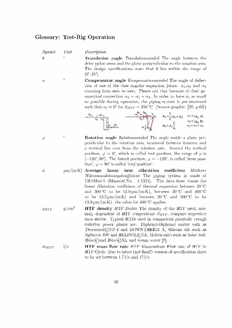
Glossary: Test-Rig Operation

Symbol Unit Description

θ ° Translation angle Translationswinkel The angle between thedrive pylon arms and the plane perpendicular to the rotation axis.The design speci�cations state that θ lies within the range of[0°, 45°].

α ° Compensator angle Kompensatorenwinkel The angle of de�ec-tion of one of the thee angular expansion joints: α1,α2 and α3

counting from east to west. Please not that because of their ge-ometrical connection α2 = α1 + α3. In order to have αi as smallas possible during operation, the piping system is pre-tensionedsuch that αi ≈ 0° for ϑHTF = 350 ◦C. (Source graphic: [20, p.63])

ϕ ° Rotation angle Rotationswinkel The angle inside a plane per-pendicular to the rotation axis, measured between traverse anda vertical line seen from the rotation axis. Around the verticalposition, ϕ = 0°, which is called rest position, the range of ϕ is[−120°, 90°]. The lowest position, ϕ = −120°, is called 'stow posi-tion', ϕ = 90° is called 'end position'.

α µm/(m K) Average linear heat dilatation coe�cient MittlererWärmeausdehnungskoe�zient The piping system is made of13CrMo4-5 (Material-No. 1.7335). The data-sheet states thelinear dilatation coe�cient of thermal expansion between 20 ◦Cand 300 ◦C to be 12.9 µm/(m K), between 20 ◦C and 400 ◦Cto be 13.5 µm/(m K) and between 20 ◦C and 500 ◦C to be13.9 µm/(m K). the value for 400 ◦C applies.

%HTF g/cm3 HTF density HTF Dichte The density of the HTF used, nor-maly dependent of HTF temperature ϑHTF , compare respectivedata sheets. Typical HTFs used in commercial parabolic troughcollector power plants are: Diphenyl-Diphenyl oxides such asTherminol©VP-1 and DOWNTHERM A, Silicone oils such asSyltherm 800 and HELISOL©5A, Molten salts such as Solar Salt,Hitec©and Hitec©XL and steam/water [8].

mHTF l/s HTF mass �ow rate HTF Massenstrom Flow rate of HTF inHTF-Cycle. Due to latest (not �nal!) version of speci�cation sheetto be set between 1.7 l/s and 17 l/s

56

Symbol Unit Description

pHTF bar HTF pressure HTF Druck The pressure of the HTF inside thepiping system. The maximum pressure allowed is de�ned by datasheet of the HTF used and the HTF temperature set. The maxi-mum design pressure is 40 bar

ϑHTF◦C HTF temperature HTF Temperatur The temperature of the

HTF inside the piping system. Load Cases are de�ned accordingtypical situations in parabolic trough power plants. Temperatureat Inlet of trough THTF = 300 ◦C, temperature at Inlet of troughTHTF = 400 ◦C. The highest temperature the REPA test rig hasbeen designed for is THTF = 450 ◦C[8]. Due to latest (not �nal!)version of speci�cation sheet to be set between 40 ◦C and 450 ◦C,taking into consideration the speci�cations for the HTF used andadjust the HTF pressure accordingly.

ϑamb◦C Ambient temperature Umgebungstemperatur If not individually

measured, the ambient temperature is given the value 20 ◦C.

ϑabs.tube,avg.◦C Average absorber tube temperature Durchschnittliche Tem-

peratur der Absorberröhre We assume that absorber-tube tempera-tures in a real-life PTC power-plant are equal to the HTF temper-ature in the tube in every section, and that these rise linearly fromstart to end. That way ϑabs.tube,avg. = (ϑHTF,start + ϑHTF,end)/2.For a REPA situated at an inlet, the important pipe section isfrom inlet to the drive pylon in the middle, for a REPA situatedat an outlet, the important pipe section is from the drive pylonto the outlet (please compare �gure 1.2). The average absorbertube temperatures important for the translation angles for the LCsare therefore: 'LC Inlet': ϑabs.tube,avg. = 325 ◦C and 'LC Outlet':ϑabs.tube,avg. = 375 ◦C.

ϑpipe◦C Mean traverse piping temperature durchschn. Rohrtemper-

atur Average temperature of traverse piping. In temperature-response validation experiments calculated as the mean of the fourpipe temperature measurement values taken during the validationexperiments. ϑpipe is used for all plots in which 'pipe temperature'is one of the axes. Be aware that maximum and minimum pipetemperature might deviate from the mean value by up to 50 K.During later test-rig operation estimated to equal the HTF tem-perature.

57

Glossary: Dynamo-Meter Theory

Symbol Unit Description

UD mV bridge voltage of the Wheatstone bridge Brückenspannungder Wheatstone'schen Brücke The output voltage of the dynamo-meter is equal to the bridge voltage of the Wheatstone bridge andscales with the supply voltage Us. The output signal uS is thereforegiven per V supply voltage Us.

K N/V Calibration matrix Kalibriermatrix The calibration matrix Kcontains the combined e�ects of both slope of sensor calibrationcurve cS and slope of ampli�er calibration curve cA. It's unit caneither be N/V, then Fdyn = K ·U ; or N/(mV V), then Fdyn = K ′·S.K ′ = K · 5V

2mV/V = K · 2.5 VmV/V

Fdyn N,Nm Dynamo-meter reading Dynamometer Messwert The vector ofthree forces and three moments that are obtained after multiplyingthe ampli�er output voltage with the calibration matrix. This isequal to the output of GSV-multi.

S mV Sensor output signal Sensor-Ausgangsspannung The absoluteoutput voltage of the dynamo-meter. S = UD · US .

Us V Supply voltage Speisespannung The output signal of thedynamo-meter scales with the supply voltage from the measure-ment ampli�er. Sensor signals are therefore given in mV/V. Forthe K6D175 the supply voltage is 5 V.

cA V/(mV V) Slope of ampli�er calibration curve Steigung der Messwertver-staerkerkennlinie The slope of the ampli�er calibration curve is theoutput voltage of the ampli�er per input given in relation to thesupply voltage and therefore in the unit mV/V. It is equal to theamplifying factor.

cS mV/(V N) Slope of sensor calibration curve Steigung der SensorkennlinieThe slope of the sensor calibration curve is the output voltage ofthe sensor per input per N of the force (or Nm of the moment)applied.

UA mV/V Input sensitivity Eingangsemp�ndlichkeit des Verstaerkers Theinput sensitivity is equal to the highest signal at the input of theampli�er which is produced if the dynamo-meter is loaded withnominal forces and moments.

UA V Upper limit of measuring range Messbereichsendwert des Ver-staerkers The upper limit of the measurement range is equal to theampli�er output voltage at nominal forces.

U V Ampli�er output voltage Verstaerker-Ausgangsspannung Theampli�er output voltage that is multiplied with calibration matrixK to obtain the dynamo-meter reading Fdyn.

58

Symbol Unit Description

uS mV sensor output signal per V supply voltage Sensor-Ausgangsspannung pro V Speisespannung, see bridge voltage of theWheatstone bridge UD.

Glossary: Dynamo-Meter Uncertainty

Symbol Unit Description

C mV/V Characteristic Value Kennwert Output signal at rated forceFnom, decreased by the zero signal when mounted SF0[12].

Fcal N,Nm Calibration force Kalibrierkraft The forces and moments thedynamo-meter is calibrated for.

dcr %FS Relative creep Relatives Kriechen By creep the time-dependentvariation (in 30 min)of the out-put signal of the force transducerafter force variation is understood. A distinction is to be madebe-tween: creep under load and creep when load is relieved[12].

Fnom N Rated force Nennkraft Greatest force for which the transducer isnominally designed, i. e. up to which the manufacturer's metro-logical speci�cations are complied with[12].

F N Force (Wirk-)Kraft Vectorial physical quantity with point of ap-plication, direction of action and amount (1 N = 1 kg m−1 s−2[12].

brg %FS Relative repeatability error (in un-changed mounting po-

sition) Relative Spannweite (in unveraenderter Einbaustellung)Maximum di�erence of the output signals at equal force, deter-mined from several series of measurements without the mountingposition being changed, in relation to the mean output signal de-creased by the zero signal in the mounted state. The rel. repeata-bility error is a measure of the repeatability[12].

dlin %FS Relative linearity error Relative Linearitaetsabweichung Maxi-mum deviation of a characteristic curve of a force transducer, de-termined at increasing force, from the reference straight line, inrelation to the upper limit of the measurement range used[12].

µ %FS Relative reversibility error Relative Umkehrspanne Di�erenceof the output signals of an increasing and decreasing series at equalforce F , in relation to the output signal at increasing force, de-creased by the zero signal when mounted SF0[12].

Fϕdyn N,Nm Angle angle response Rotationswinkelantwort Absolutedynamo-meter reading Fdyn for changing rotation angle ϕ atconstant HTF temperature ϑHTF , HTF pressure pHTF andtranslation angle θ. The angle response is a absolute value.

59

Symbol Unit Description

∆F pdyn N,Nm Pressure response Druckantwort Change in the dynamo-meterreading Fdyn for changing HTF pressure pHTF at constant HTFtemperature ϑHTF , rotation angle ϕ and translation angle θ. Thepressure response is a relative value as ∆F pdyn is set to zero forpHTF = 0 bar.

∆F ϑdyn N,Nm Temperature response Temperaturantwort Change in thedynamo-meter reading Fdyn for changing HTF temperature ϑHTFat constant HTF pressure pHTF , rotation angle ϕ and translationangle θ. The temperature response is a relative value as ∆F ϑdyn isset to zero for ϑHTF = 20 ◦C.

TK0 %FS/K Temperature e�ect on zero signal Temperaturein�uss auf dasNullsignal Variation of the zero signal of the force transducer,in relation to the rated characteristic value, due to variation ofthe dynamo-meter temperature ϑdyn by 10 K, within a de�nedtemperature range after steady states free of gradients have beenadjusted[12]. (Value adjusted to change for 1K)

TKC %RD/K Temperature e�ect on characteristic value Temperaturein-�uss auf den Kennwert Relative variation of the characteristicvalue of the force transducer due to variation of the dynamo-metertemperature ϑdyn by 10 K, within a de�ned temperature range af-ter steady states free of gradients have been adjusted[12]. (Valueadjusted to change for 1K)

ϑdyn Dynamo-meter temperature Dynamometertemperatur The ef-fective internal temperature of one of the four dynamo-meters. In-�uences measurement uncertainty via temperature e�ect on zerosignal and temperature e�ect on characteristic value. The sen-sor temperature is measured by two PT1000-temperature sensorsplaced in the steel plate that connects bearing and dynamo-meter.As the steel plate heats up �rst, their measurement value is usedas an (upper) estimate of the sensor temperature. Having twoPT1000 placed in the dynamo-meter by the manufacturer wouldhave been possible on request but was unfortunately forgottenwhen purchasing the dynamo-meter. The maximum operationtemperature for the K6D175 is 70 ◦C, the maximum allowed tem-perature is 85 ◦C. A greater temperature will do harm to the sensor(change the zero-signal).

60

Symbol Unit Description

U0,ϑ V Di�erence in zero signal due to increased sensor temper-

ature Drift des Sensor-Nullsignals bei Temperaturerhöhung Whena dynamo-meter is heated, it's zero signal changes in relation toit's internal temperature. This e�ect is measured in a so-calledtemperature test. The data obtained is then used to subtract thee�ect from the actual measurements. During the temperature test,the sensor is either completely unloaded and unmounted, or loadedwith a constant force. It is assumed, but not necessarily true, thatthe then measured behavior will be the same during test-rig op-eration. Another problem are temperature gradients. Their e�ectas well as the gradients itself are di�cult to measure. The �rsttemperature test however indicates that the e�ect of the gradientsmight even be greater than the e�ect of a higher but constant tem-perature. This might be, because the six strain gauges inside thesensor are temperature compensated, which only works if all sixstrain gauges experience the same temperature.

∆U0,20C V Di�erence in zero signal after complete heating cycle

Nullpunktrückkehrfehler nach Temperaturzyklus The �rst temper-ature test showed that the zero signal at ambient temperature hadchanged after heating up to 80 ◦C once. A change in zero signalis equal to an undesired o�set in the measurement results. Pleasecompare appendix A.3.2 for values. This behavior could be a ma-jor problem, if this e�ect is found to increase (accumulate) withrepeated cycles. An advanced temperature test should do a seriesof temperature cycles to investigate this.

S0 mV/V Zero signal when removed Nullsignal im ausgebauten ZustandOutput signal of the unloaded force transducer, without mountingparts in the unit milli volt per volt supply voltage. S0 = U0 ·(5 V/2 mV/V) = U0 · 2.5V/(mV/V )[12]

SF0 mV/V Zero signal when mounted Nullsignal im eingebauten Zus-tand Output signal of the force transducer when not mechani-cally loaded, with mounting parts, at the beginning of a loadingcycle[12].

U0 V Zero signal when removed Nullsignal im ausgebauten Zus-tand Output signal of the unloaded force transducer, withoutmounting parts in the unit volt. U0 = S0 · (2 mV/V)/5 V =S0 · 0.4(mV/V )/V .

61

Appendices

A Additional Information

A.1 Test-rig speci�cations and problems

Rotational motion

Geometric calculations, shown in �gure A.1.1 give reason to believe that the cylinderstroke of 700 mm is not su�cient to perform the whole rotation margin speci�ed. Thestroke needed to geometrically perform the whole range of ϕ is 648.4 mm (east) and686.8 mm (west), however as in the lowest position, the cylinders are already pushed outa little: 84.3 mm (east and west), the e�ective stroke is only 667 mm (east) and 629 mm(west). The possible angle ϕ with the e�ective cylinder stroke is then ca. [−90°, 80°].Elongating the rotation cylinders may be considered.

(a) (b)

Figure A.1.1: Rotation cylinder stroke east (left) and west (right). The blue lines indicate the di�erencein stroke compared to the vertical position: ϕ = 0°. The red line indicates the actual cylinder stroke.Geometric calculations show that the cylinder is not long enough to perform the full rotation, as itsshortest position is already too far out.

Translational motion

In real-life trough collectors the translational motion of the REPAs due to heat dilata-tion can be described as a function of the HTF-temperature ϑHTF . If we assume thatabsorber-tube temperatures in a real-life PTC power-plants are equal to the HTF tem-perature in the tube in every section, and that these rise linearly from inlet to outlet and

62

�nally that the dilatation is small compared to the focal length so that the small angleapproximation applies, we can express the translation angle θ as a linear function of theaverage absorber tube temperature. Using this relation, translational motion cycles fordi�erent REPA-positions in the loop can be designed.

Necessary translation angles needed to reproduce typical values were �rst calcu-lated by Senior Flexonics (SF), on the basis of which (compare App. A.10) the test-riggeometry has been designed. They de�ne the corresponding ϑHTF at θ = 0° to beϑHTF,θ=0,ap = 342.0 ◦C. Here the index 'ap' stands for 'as planned'. Due to deviationsfrom the original plan during construction (compare section 4) this temperature has tobe rede�ned 'as built': ϑHTF,θ=0,ab = 331.8 ◦C.

Knowing this, three di�erent relations for θ = f(ϑHTF ) can be found using a linear�t: 1) approximation on basis of angles and corresponding temperatures given by SF:θ = −0.0524 °/K·(ϑHTF−ϑHTF,θ=0); 2) approximation on basis of translational positionsand corresponding temperatures given by SF: θ = −0.0418 °/K · (ϑHTF − ϑHTF,θ=0); orusing small angle approximation: 3) calculation on basis of linear heat dilatation model:θ = − α·labs

f · 3602π [°/K] · (ϑHTF − ϑHTF,θ=0) = −0.0424 °/K · (ϑHTF − ϑHTF,θ=0), with

average linear heat dilatation coe�cient α = 1.8 µm/(m K), absorber length l = 75 m(typical for EuroTrough) and focal length f = 1.825 m.

In this thesis approach 1) is used, as is was introduced �rst and the questionwhether to use another one is still pending. That way the translation angle equivalent tostandard operation temperatures ϑHTF = [400 ◦C, 18 ◦C] is θ = [−3°, 17°] and the transla-tion angle equivalent to design temperatures ϑHTF = [450 ◦C, 18 ◦C] is θ = [−5.65°, 17°].

With the stroke of the translation cylinder of 450 mm a range of θ = [−19°, 28°]is theoretically possible. What range will also be mechanically possible (i.e. withoutany parts of the test-rig touching) will have to be tested. Special positions: θ = 17°is called 'maximum cold position' and is equivalent to ambient temperature, θ = 12° iscalled 'maximum cold position in operation' and is equivalent to their position at 110 ◦Cin a commercial power plant and �nally θ = −3° is called 'maximum hot position inoperation' and is equivalent to their position at 400 ◦C in a commercial power plant.

HTF pressure

The highest pressure allowed at higher temperatures is de�ned by the data sheets of theHTF used, but may never exceed the design pressure of 40 bar. At cold ambient temper-ature a pressure test up to 75 bar was successfully passed. Appendix A.10 states that themaximum operational conditions of the REPAs currently used are: 40 bar at 400 ◦C fora short period of time and static conditions and 35 bar at 400 ◦C as maximum operationconditions. The maximum operation conditions of the Witzenmann compensators usedis 40 bar at 450 ◦C for all three.

63

Table A.1.1: The table shows parameters as planned and as built and compares them to other typical values found. Italso states the measurement accuracy for the respective parameter in the test-rig. Subscripts: 1) range possibly smallerdue to mechanical obstacles, see glossary; 2) ambient temperature ϑamb de�ned as 20 ◦C, see glossary; 3)possibility whentesting new silicone based oils; 4) calculated for HELISOL©at LCs 'Inlet' and 'Outlet' as typical REPA test-rig workingconditions; 5) complete stroke can't be used, as cylinder is already pushed out a little in lowest position, see glossary.Sources: AP - Andreas Plumpe, master's thesis, [8]; CH - Christoph Hilgert, Hydraulic_Torque_and_Forces_CHa.xlsx;GG - Gines Garcia, Instrumentations department PSA, verbal information, no written documentation; SF - Senior Flexonics,Manufacturer for �ex hose REPAs; SI - Sigma Ingenieurgesellschaft, technical drawings of REPA test-rig as planned; TH -Tobias Hilbel, bachelor's thesis, [9].

Variable Unit As planned Source As built Source Compare to Source

rotation angle ϕ

full range ° -120...90 AP -90. . . 805) A.1 -124. . . 91 SF

day cycle range ° -120...90 AP 5) A.1 -124...91 SF

stow position ° -120 AP 5) A.1 -124 SF

end position ° 90 AP 5) A.1 91 SF

measurement accuracy ° ±(0.014 + 0.004%) of meas. val. TH 0.1 TH, GG

rotational motion

max speed rot. °/s 1.4 TH 0.6 TH, GG

max. speed cylinder m/s 0.1 data sheet

max. cylinder stroke mm 700 CH total: 7005) data sheet

step interval s 20. . . 40; > 3 AP; TH, GG

pos. precision ° 0.1 TH (excl. uncert. of meas.) 0.1 GG

step size ° ≤0.25 TH

tolerance axis orientation mm 1; 2 SI; SF (email) Photogr., sec 4

translation angle θ

design range (poss. w. cyl. stroke)) ° 0. . . 45 AP -19...281) SF, A.1

operation range ° -5.65...17 see below -4.94. . . 13.03; -5.01. . . 13.22 SF, A.1 -3...17 calc. based on SF

max. hor. dist. REPA at θ = 0 mm 600 SF Photogr., sec 4

temp. at θ = 0 ◦C 342 SF, A.1 331.8 SF, A.1

slope lin. rel. θ = f(ϑHTF ) °/K -0.0524 A.1 -0.0418; -0.0424 see glossary

max. cold (20◦C) ° 17 SF 13.03; 13.22 calc.

max. cold in op. (110◦C) ° 12 SF 9.27; 9.40 calc.

max. hot in op. (400◦C) ° -3 SF -2..85; -2.89 calc.

design max. hot (450◦C) ° -5.65 A.1 -4.94; -5.01 calc.

measurement accuracy °

translational motion

max speed transl. °/s

max speed cylinder m/s 0.03 CH

max cylinder stroke mm 450 CH 450 data sheet

tolerance axis orientation mm 1; 2 SI; SF (email) Photogr., sec 4

HTF temperature ϑHTF

operation range ◦C 202)...4503) 202)...400 SF

day cycle range ◦C

inlet ◦C 300 AP 293 SF

outlet ◦C 400 AP 393 SF

design (max.) ◦C 500 AP

HTF pressure pHTF

operation range bar 0...40 AP 0...35 SF (max. val.)

typical range bar 20. . . 30 AP

inlet bar 30 AP

outlet bar 20 AP

design bar 45 AP

HTF mass �ow rate mHTF

design range m3/h 6...60 AP

. . . with HELISOL HTF kg/s 0.9...114) calc. based on AP

operation range kg/s 6...7.3 SF

General operation

cycles per day 1/d ca. 400 AP 336 calc.

focal length m 1.825 SI Photogr., sec 4

64

A.2 De�nition of terms

1. Overview: Main Assembly + HTF Cycle

2. Main Assembly

3. HTF Cycle

4. Sensors part 1/3

5. Sensors part 2/3

6. Sensors part 3/3

7. List of sensor details

65

1

2

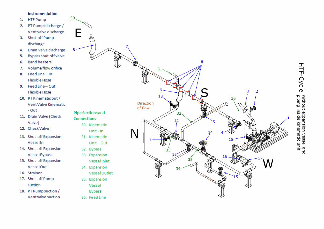
3

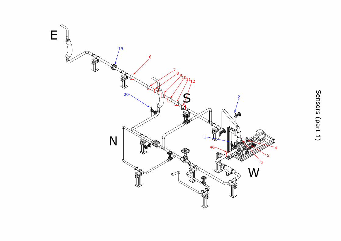
4

5

6

Table A.2.1: Sensor descriptions: taken from signal list (02. Dec 2016)

No. Ch.-Type Description Sensor-Type PSA-nom.

1 absolute pressure suction side absolute S-20 PE-HTF-01-W

2 absolute pressure pressure side absolute S-20 PE-HTF-02-W

3 temperature motor, HTF pump Pt100_T1, 4 wire TT-HTF-01-W

4 temperature Bearing, HTF pump Pt100_T2, 4 wire TT-HTF-02-W

5 temperature lubricating oil, HTF pump Pt100_T3, 4 wire TT-HTF-03-W

6 temperature �uid temp. heater outlet Thermocouple Type K TC-15 TT-HTF-04-W

7 temperature tube surface temp. heater 1 Thermocouple Type K TT-HTF-05-W

8 temperature tube surface temp. heater 2 Thermocouple Type K TT-HTF-06-W

9 temperature tube surface temp. heater 3 Thermocouple Type K TT-HTF-07-W

10 temperature tube surface temp. heater 4 Thermocouple Type K TT-HTF-08-W

11 temperature tube surface temp. heater 5 Thermocouple Type K TT-HTF-09-W

12 temperature tube surface temp. heater 6 Thermocouple Type K TT-HTF-10-W

19 di�erential pressure ori�ce plate di�erential pressure DTP-10 PE-HTF-03-W

20 absolute pressure absolute pressure test facility outlet S-20 PE-HTF-04-W

21 multi axis load cell force/torque REPA No. 1 east top K6D175

22 multi axis load cell force/torque REPA No. 2 est bottom K6D175

23 multi axis load cell force/torque REPA No. 3 west top K6D175

24 multi axis load cell force/torque REPA No. 4 west bottom K6D175

25 temperature temperature multi force east top 1.1 Pt1000

26 temperature temperature multi force east top 1.2 Pt1000

27 temperature temperature multi force east top 1.3 Pt1000

28 temperature temperature multi force east top 1.4 Pt1000

29 absolute pressure absolute pressure, N2 tubing S-20 PE-HTF-05-W

30 level switch level switch expansion vessel (top) 2 x SPDT FA-HTF-01-W

31 level switch level switch expansion vessel (bottom) 2 x SPDT FA-HTF-03-W

32 temperature temperature expansion vessel 1 (liquid) Thermocouple Type K TC-10 TT-HTF-15-W

33 temperature temperature expansion vessel 2 (gas) Thermocouple Type K TC-10 TT-HTF-16-W

7

Table A.2.2: Sensor descriptions: continued

No. Ch.-Type Description Sensor-Type PSA-nom.

40 limit switch inductive sensor rotation negative Balluf BES M12MI-POC40B-S04G ZS-CI-01-W

41 limit switch inductive sensor rotation positive Balluf BES M12MI-POC40B-S04G ZS-CI-02-W

42 inclination magnetic tape sensor rotation ASM PMIS3-50-50-20Khz-HTL-21-7M-S ZT-CI-11-W

43 limit switch inductive sensor translation negative Balluf BES M12MI-POC40B-S04G ZS-CI-04-W

44 limit switch inductive sensor translation positive Balluf BES M12MI-POC40B-S04G ZS-CI-05-W

45 rotary encoder rotary encoder -translation MH64-1023MU multiturn FSG ZS-CI-06-W

46 temperature HTF temperature pump inlet Thermocouple Type K TC-15 TT-HTF-17-W

47 temperature hydraulic oil temperature SSM.1.B4.150.54.S1 level switch with PT100 TT-CI-13-W

48 level switch hydraulic oil level SSM.1.B4.150.54.S1 level switch with PT100 LA-CI-03-W

61 leakage sensor leakage / swim sensor FA-HTF-02-W

62 leakage sensor conrad leakage sensor FA-HTF-02-W

63 leakage sensor conrad leakage sensor FA-HTF-02-W

117 relative preasure pressure transmitter hydraulic unit rotation (150) MODS-250-G1/4-A-M12 PE-CI-01-W

118 relative preasure pressure transmitter hydraulic unit translation (151) MODS-250-G1/4-A-M12 PE-CI-02-W

119 temperature temperature multi force east bottom 2.1 Pt1000

120 temperature temperature multi force east bottom 2.2 Pt1000

121 temperature temperature multi force east bottom 2.3 Pt1000

122 temperature temperature multi force east bottom 2.4 Pt1000

123 temperature temperature multi force west top 3.1 Pt1000 TT-HTF-11-W

124 temperature temperature multi force west top 3.2 Pt1000 TT-HTF-12-W

125 temperature temperature multi force west top 3.3 Pt1000 TT-HTF-13-W

126 temperature temperature multi force west top 3.4 Pt1000 TT-HTF-14-W

127 temperature temperature multi force west bottom 4.1 Pt1000

128 temperature temperature multi force west bottom 4.2 Pt1000

129 temperature temperature multi force west bottom 4.3 Pt1000

130 temperature temperature multi force west bottom 4.4 Pt1000

64-69 EVs

M1 servo control controller

8

A.3 Dynamo-meter algebra

A.3.1 Theory

The dynamo-meter that is used transforms forces and moments into six output voltageswith the magnitude of a few mV. These output voltages are equal to the bridge voltagesof the Wheatstone bridges UD which form the core of every dynamo-meter that is basedon resistance strain gauges. For further information, please have a look at the FAQ anddocumentation section of www.me-systeme.de. This chapter is based on the contentprovided there, if not indicated else.

The bridge voltage UD is proportional to the supply voltage Us, that is provided bythe measuring ampli�er, the output signal uS is usually given in relation to the supplyvoltage. In this sense, the actual signal S equals uS if the supply voltage was set to1V. As linear behavior is assumed, the output signal uS can be described as a functiondependent on only one parameter, that is the slope of the calibration curve of the sensorcS in [mV/VN]. cS is derived as the fraction of the characteristic value C, i.e. the signalobtained when the dynamo-meter is exposed to nominal force Fnom and the nominalforce itself. Please note that C is given in [mV/V], i.e. per V of supply voltage. Indoing so, characteristic values of di�erent dynamo-meters and other force measurementdevices can be compared to one another. For the value of C the data sheet states a valueof ca. 0.5mV/V [14], however it's exact value is never derived but contributes to thecalibration matrix K, provided by the manufacturer on demand.

uS =UDUS

= cS · F =C

Fnom· F (A.1)

The sensor output uS becomes the ampli�er input. It's behavior is also assumedto be linear which is equivalent to a constant ampli�cation factor cA independent of theinput voltage. The ampli�er output voltage U then is the product of ampli�cation factorcA and measurement voltage signal uS . The ampli�cation factor is the quotient of theupper limit of the measurement range UA in [V] and the input sensitivity UA in [mV/V]and therefore has the unit [V/mV/V]. The input sensitivity can be interpreted as themaximum measurement signal the ampli�er can process per V of supply voltage.

U = cA · uS =UAuE· uS (A.2)

To describe the behavior of the whole measurement chain, both characteristiccurves, equations A.1 and A.2 can be combined to a single function describing the am-pli�ed output voltage U as a function of the forces (and moments) induced: equationA.3. The inverse function, eqaution A.4, can be written using K, the calibration matrix.

74

U = cA · cS · F =UAuE· C

Fnom· F (A.3)

Fdyn = F = K · U (A.4)

The Calibration matrix K is a 6x6 matrix given in the calibration certi�cates(original calibration [15] and re-calibration [23]. It's unit is N or Nm per V output signalof the ampli�er.

Please note that the matrix loaded into GSV multi, the con�guration and loggingsoftware provided by the manufacturer in a .mat-�le, K ′, has the unit N and Nm permV/V sensor output:

K ′ = K · USuE

=FnomC· USUA

K ′ = K · 5V

2mV/V= K · 2.5 V

mV/V(A.5)

A.3.2 Some actual values

Calibration Matrices

Equation A.6 and A.8 show the calibration matrices before and after re-calibration. AsK is fully occupied, a force along one axis or a moment around another will always a�ectall six output voltages U .

Korig =

−4.94 1987.29 −1942.62 1.02 1952.86 −2044.15

−2186.25 1160.60 1140.62 −2339.92 1139.83 1171.18

−3164.33 −3057.03 −3225.61 −3162.95 −3207.57 −3154.80

−114.53 −103.25 −112.21 −122.35 238.17 235.81

−194.06 −200.09 206.67 196.83 −0.58 11.69

125.94 −137.18 140.15 −130.11 128.32 −143.87

in N/V

or Nm/V

(A.6)

UorigCC = ±(30N, 70N, 80N, 8Nm, 6Nm, 16Nm) (A.7)

75

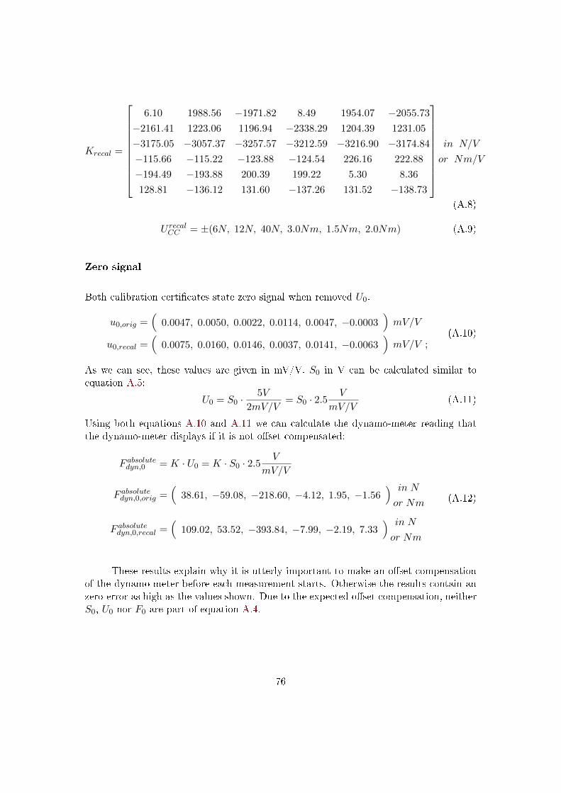
Krecal =

6.10 1988.56 −1971.82 8.49 1954.07 −2055.73

−2161.41 1223.06 1196.94 −2338.29 1204.39 1231.05

−3175.05 −3057.37 −3257.57 −3212.59 −3216.90 −3174.84

−115.66 −115.22 −123.88 −124.54 226.16 222.88

−194.49 −193.88 200.39 199.22 5.30 8.36

128.81 −136.12 131.60 −137.26 131.52 −138.73

in N/V

or Nm/V

(A.8)

U recalCC = ±(6N, 12N, 40N, 3.0Nm, 1.5Nm, 2.0Nm) (A.9)

Zero signal

Both calibration certi�cates state zero signal when removed U0.

u0,orig =(

0.0047, 0.0050, 0.0022, 0.0114, 0.0047, −0.0003)mV/V

u0,recal =(

0.0075, 0.0160, 0.0146, 0.0037, 0.0141, −0.0063)mV/V ;

(A.10)

As we can see, these values are given in mV/V. S0 in V can be calculated similar toequation A.5:

U0 = S0 ·5V

2mV/V= S0 · 2.5

V

mV/V(A.11)

Using both equations A.10 and A.11 we can calculate the dynamo-meter reading thatthe dynamo-meter displays if it is not o�set compensated:

F absolutedyn,0 = K · U0 = K · S0 · 2.5V

mV/V

F absolutedyn,0,orig =(

38.61, −59.08, −218.60, −4.12, 1.95, −1.56) in N

or Nm

F absolutedyn,0,recal =(

109.02, 53.52, −393.84, −7.99, −2.19, 7.33) in N

or Nm

(A.12)

These results explain why it is utterly important to make an o�set compensationof the dynamo-meter before each measurement starts. Otherwise the results contain anzero-error as high as the values shown. Due to the expected o�set compensation, neitherS0, U0 nor F0 are part of equation A.4.

76

Evaluating the change from one calibration to another

Due to the re-calibration, we now have two calibration matrices we could possibly applyto any measured output voltage U. The result will not be the same, as �gure 3.3 indicates.The di�erence can be calculated with equation A.13. Please keep in mind, that thiscalculation is very sensitive to the signs of the six values of F.

∆Fdyn = Fdyn,re−calib − Fdyn,orig = Kre−calib · U −Korig · Uwith U = K−1

orig · F∆Fdyn = Kre−calib ·K−1

orig · F −Korig ·K−1orig · F

= (Kre−calib ·K−1orig − I) · F

(A.13)

Table A.3.1: Change in dynamo-meter reading due to re-calibration: Rows 1 and 2 show the min. andmax. value of the best estimate of future dynamo-meter forces according to table A.4.1. Rows 3 and4 show the min. and max. result of equation A.13 that have occured testing a subset of the countlesscombinations there are for the three forces and three moments within their margin.

Name Fx Fy Fz Mx My Mz Unit

FestimMin -1,457 -224 -2,310 464 -521 -1,062 N, Nm

Max 1,555 849 126 675 575 895 N, Nm

∆FdynMin -56 -89 -73 -5 -18 -33 N, Nm

Max 30 48 86 15 11 8 N, Nm

Change in zero signal due to temperature test

estimation of the relative temperature reversibility error due to the change in zero signalafter the temperature test ∆S0,ϑ, stated in the calibration certi�cate of the re-calibration[23].

U∆U0,20 ◦C = K ·∆U0,20 ◦C = K ·∆S0,20 ◦C · 2.5V

mV/V(A.14)

∆S0,20 ◦C =(−0.0001, −0.0012, 0.0003, −0.0036, −0.0021, 0.0013

)mV/V

Uorig∆U0,20 ◦C =(−24.32, 16.80, 42.59, 0.87, −0.93, 0.51

) in N

or Nm

U recal∆U0,20 ◦C =(−24.46, 16.49, 43.01, 0.94, −1.01, 0.57

) in N

or Nm

(A.15)

77

Uncertainties

The total uncertainty of the dynamo-meter measurements of the REPA test-rig U canbe calculated as the square root of the sum of the squared parts[21] stemming from cal-ibration certi�cate (CC), temperature e�ect on zero signal TK0, temperature e�ect oncharacteristic value TKC , rel. creep dcr and di�erence in zero signal after complete heat-ing cycle ∆U0,20C . This technique has been derived with and approved by Mr. Kabelitzfrom ME-Messsysteme, the manufacturer of the K6D175 dynamo-meter. Conditions arethat none of the forces and moments exceeds the nominal value too much and that sensortemperatures stay below 70 ◦C.

U =√U2i =

√U2CC + U2

TK0 + U2TKC + U2

dcr + U2∆U0,20 ◦C

(A.16)

If any of the six forces and moments of the dynamo-meter reading Fdyn,i exceeds there-calibration scenario, uncertainties and resulting forces and moments can be linearlyinterpolated between the results of the two calibration scenarios using equations A.17and A.18

UCC =

{U recalCC if Fdyn,i ≤ F recalcal,i ∀ i = 1 . . . 6

U recalCC + k · (UorigCC − U recalCC ) else(A.17)

Fdyn =

{Krecal · U if Fdyn,i ≤ F recalcal,i ∀ i = 1 . . . 6

Krecal · U + k · (Korig −Krecal) · U else(A.18)

k = maxi

(Fdyn,i − F recalcal,i

F origcal,i − F recalcal,i

)(A.19)

The e�ect of TK0 has been derived in chapter 3.1. The e�ect of TKC and dcr is derivedaccording to the data-sheet value, the best load estimation Festim from table A.4.1,the re-calibration scenario F recalcal and the di�erence between dynamo-meter temperatureϑdyn and ambient temperature ϑamb.

UTKC = 0.05 %FS/K · Festim · (ϑdyn − ϑamb)Ucr = 0.1 %FS · F recalcal

(A.20)

The e�ect of ∆U0,20C has been derived above.

78

A.4 Calibration and data sheet values

Table A.4.1: Content: This table compares 'Nominal loads', 'Estimated Loads', 'Measured Loads' and 'CalibrationLoads'. Nominal loads are loads the sensor has been designed for. Estimated loads are loads that the dynamo-meterwill probably measure during operation and should therefore be calibrated for. 'Measured Loads' are loads that haveactually been measured during temperature response experimetns. Calibration Loads are the loads the sensor hasactually been calibrated for. Sources: DS - data sheet of the K6D175 [14], compare appendix B; R2 - ROHR2simulation based on Traverse_200 base model for 40 bar, 350 ◦C and the complete range of rotation angle ϕ; AP -Andreas Plumpe, master's thesis, [8]; MF - Data from REPA manufacturer for operation at 20 and 30 bars, ambienttemperature, without mass �ow, for ± 120° rotation and the upper side of the REPA; CC - calibration certi�catesfor original calibration [15] and re-calibration [23]. Explanations: Loads are estimated as the sum of forces fromthe traverse (ROHR2 simulations), the calculated e�ect from mass �ow and estimated loads for the REPA. Sensorcalibration is done for speci�ed loads, both positive and negative (exception: Fz only negative). Best calibrationloads are therefore calculated as ±mean(abs(min), abs(max)) (min value for Fz). The re-calibration loads, compareappendix A.8, had been calculated on the base of faulty measurement results (dead channel) and have to be used withcaution.

Dynamometer K6D175 - Loads estimation

Name Fx in N Fy in N Fz in N Mx in Nm My in Nm Mz in Nm Source

Nominal Loads

nominal load / calibration load, Fnom 10,000 10,000 20,000 1,000 1,000 2,000 DS

working load (allowed load), Fwork 15,000 15,000 30,000 1,500 1,500 3,000 DS

failure load, Ffail 30,000 30,000 60,000 3,000 3,000 6,000 DS

Estimated Loads during test-rig operation

ROHR2 (40 bar,350 ◦C)Min -882 -714 -1,045 -109 -201 -207

R2Max 880 -141 386 149 195 215

max. mass �ow 0 -110 110 -66 0 0 AP

estim. REPA (40 bar)Min -575 600 -1,375 639 -320 -855

MFMax 675 1,100 -370 592 380 680

sumMin -1,457 -224 -2,310 464 -521 -1,062

Max 1,555 849 126 675 575 895

max. % of nominal load 16 8 12 67 58 53

Measured loads during temperature response experiments

measured forces Ftemp. responseMin -67 -311 -45 -5 -19 -17

Max 176 83 142 20 23 11

max. % of nominal load 2 3 1 2 2 1

Measured loads during angle response experiments

measured forces Fangle. responseMin -371 -171 -1,296 -119 -278 -107

Max 121 427 620 9 207 87

max. % of nominal load 4 4 6 12 28 5

Calibration Loads

original calibration loads, F origcal ±10000 ±10000 -20,000 ±1000 ±1000 ±1000 CC

re-calibration loads, F recalcal ±2350 ±800 -2,050 ±400 ±400 ±300 CC

best calibration loads, Festim ±1506 ±537 -2,310 ±569 ±548 ±978

79

Table A.4.2: Content: This table shows estimations for total measurement uncertainties for the original, the currentand a possible future state. All calculations use the best load estimation from A.4.1 as load scenario and assumethe worst case for the sensor temperature. Some results are also compared to max. results of validation experiments.Sources: DS - data sheet of the K6D175 [14], compare appendix B; CC - calibration certi�cates for original calibration[15] and re-calibration [23] IMPORTANT: values only true for whole system composed of dynamo-meter K6D175 (serialnumber: 15401935) and measurement ampli�er GSV-1A16USB K6D/M16 (serial number: 15156211/15356132), com-pare appendix B; TT - Calculated on basis of temperature test; TT2 - Calculated on basis of ideal future temperaturetest. Explanations: Some uncertainties scale with the nominal loads the sensor is designed for (FS = full scale) andsome scale with the actual load of the sensor (RD = reading). For the original calibration temperature e�ects on zerosignal and sensitivity were not part of the calibration and have been estimated using values given in the data sheet.Together with the re-calibration, a temperature test has been performed, compare chapter 3.3.

Dynamometer K6D175 - Uncertainties estimation

Name Param Fx Fy Fz Mx My Mz Unit Source

1) Original state: (original calibration, ϑdyn = 70 ◦C)

measurement uncertainty, UCC 30 70 80 8 6 16 N, Nm CC, eqn. A.7

rel. creep, Ucr 0.1 % FS 10 10 20 1 1 2 N, Nm DS, eqn. A.20

sum. uncertainty, U (without temperature e�ects) 32 71 82 8 6 16 N, Nm eqn. A.16

min % of Festim 2 13 4 1 1 2 %

temp. e�ect on zero signal, UTK0 0.1 % FS / K 490 490 980 49 49 98 N, Nm DS

temp. e�ect on sensitivity, UTKC 0.05 % RD / K 37 13 57 14 13 24 N, Nm DS, eqn. A.20

rel. temperature reserv. error, U∆U0 25 17 43 1 1 1 N, Nm TT, eqn. A.14

sum. uncertainty, U 493 496 986 52 51 102 N, Nm eqn. A.16

min % of Festim 33 92 43 9 9 10 %

2) Current state: (First re-calibration, ϑdyn = 70 ◦C)

measurement uncertainty, UCC 16 35 56 5 4 8 N, Nm CC, eqn. A.9

rel. creep, Ucr 0.1 % FS 3 1 3 1 1 1 N, Nm DS, eqn. A.20

sum. uncertainty, U (without temperature e�ects) 16 35 56 5 4 8 N, Nm eqn. A.16

min % of Festim 1 7 2 1 1 1 %

min % of Fangle. response 4 8 4 4 1 7 %

temp. e�ect on zero signal, UTK0 106 110 500 11 8 12 N, Nm TT, eqn. A.18

temp. e�ect on sensitivity, UTKC 0.05 % RD / K 37 13 57 14 13 24 N, Nm DS, eqn. A.20

rel. temperature reserv. error, U∆U0 25 17 44 1 1 1 N, Nm TT, eqn. A.14

sum. uncertainty, U 116 117 508 19 16 28 N, Nm eqn. A.16

min % of Festim 8 22 22 3 3 3 %

min % of Ftemp. response 66 38 358 93 70 254 %

3) Ideal future state: (Improved temperature test, ϑdyn = 70 ◦C)

measurement uncertainty, UCC 16 35 56 5 4 8 N, Nm CC, eqn. A.9

rel. creep, Ucr 0.1 % FS 3 1 3 1 1 1 N, Nm DS, eqn. A.20

temp. e�ect on zero signal, UTK0 0* 0* 0* 0* 0* 0* N, Nm TT2

temp. e�ect on sensitivity, UTKC 0.05 % RD / K 37 13 57 14 13 24 N, Nm DS, eqn. A.20

rel. temperature reserv. error, U∆U0 25 17 44 1 1 1 N, Nm TT, eqn. A.14

sum. uncertainty, U 47 41 91 15 14 25 N, Nm eqn. A.16

min % of Festim 3 8 4 3 3 3 %

80

A.5 Important information for future sensor purchases

Before it makes sense to think about what sensors to buy to equip the last three dynamo-meter positions, the test-rig has to be functional enough to perform authentic operationsfor at least a short period of time. These have to be used to further understand thesensors behavior and well estimate authentic load and temperature scenarios. Buyingnew dynamo-meters only makes sense if their later usage is exactly known. Calibrationand temperature-tests have to be performed for scenarios as close to the real ones aspossible. To do that, it makes sense to also send in the connection plate and the bearingto perform these tests in mounted state. In any case the measurement ampli�er, whichhas already been bought for all four positions, has to be send back for calibration, asthis is always done for the whole system.

At the current state of knowledge, the K6D175 is to 'big' for its application. Pleasekeep in mind that allowed forces are 300% of the nominal forces, best accuracy is normallyreached at 70% - 100% of nominal forces (= calibration forces). Yet the best availableload scenario estimates forces of only 15% of the nominal forces and moments of at least60% of the nominal moments. A 'smaller' sensor would therefore be more suitable. Incase this 'smaller' sensor is also physically smaller, adapters have to be made to �t thenew sensor in the spaces provided. Maybe ME-Messsysteme can help here and buildcustomized sensors with lower nominal forces but the same dimensions.

At the same time it is very important to ask for two PT1000 placed inside thedynamo-meter by the manufacturer at the exact place where increased temperatures actupon the sensor signal. Further more, it might be considered to ask for a more durablecable connection. To decrease the di�erence in zero signal after complete heating cycle∆U0,20C , it might make sense to do without potting the inside of the sensor. The polymerused might su�er smallest plastic deformations when heated. Its normal purpose is toprotect the sensor from high humidity. In the desert of Tabernas, this might not bean issue. In principle, ME-Messsysteme is able to build their sensors according to theirclients needs. It is therefore advised to make the decision in close collaboration withthem. Even non-linear calibration is an option.

Once the new sensors are bought, they need to be mounted and commissioned. Itis utterly important that no new sensor is mounted before it has been con�rmed thatits adjacent piping system will not exert to high forces stemming from heat dilatation,which might damage the sensor. The top-east position may not be equipped under anycircumstances until the last three compensators have been added to the eastern part ofthe traverse.

81

A.6 ROHR2 - MATLAB post-processing

When adding new LCs make sure to proceed as follows: �rst add LCs to the basemodel, best saving it under a new name and following the nomenclature. Then proceediteratively: rotate the model (select all, edit-rotate around y-axis and node 1), save itunder new name, run the simulation, export results as .csv to the default folder R2DOC(documentation - exports results in csv format, only relevant load cases), save again,repeat. The same procedure has to be chosen, if model parameters, e.g.: insulationthickness, are altered. It's quite boring work, I know;)

Evaluating the model results is done using a MATLAB script. Running ROHR2_ReadIn.mcreates and saves a four-dimensional array FMall_Z. There is two variations of FMall, fortwo di�erent �uids, HELISOL©(H) and air (A), with the di�erence that the pressuredimension of FMall_A only contains one pressure: 0 bar. containing all six dynamo-meter forces and moments predicted by the model for the di�erent HTF temperatures,HTF pressures and rotation angles using linear interpolation10. Evaluation for all pos-sible combinations of ϑHTF , pHTF and ϕ can now easily be done using N-dimensionalinterpolation:

load('27-12-16_17-53_Traverse_100.mat')

tq = 345; % in degC, range [20,450]pq = 10:5:35; % in bar, range [0,40]phiq = -63.5; % in deg, range [-120,90]axq = 2; % 1 = Fx; 2 = Fy ... 6 = Mzf = interpn(tH,pH,axH,alphaH,FMall_H,tq,pq,axq,phiq,'linear')

Automated plots can be made using ROHR2_PlotResults.m, here comparing modelsTraverse_100 and Traverse_200, for two �uids and plotting forces and moments overHTF temperature as x-axis:

models = [2,3] % index of modelno. in [40,100,200,999]fluids_str = {'H','A'} % 'H' for Helisol, 'A' for Airxaxis_str = 'temperature' % also possible: 'pressure','angle'ROHR2_PlotResults(tq,pq,axq,phiq,models,fluids_str,xaxis_str)

10'linear' is the default option of interpn, other options, such as 'spline' may be chosen.

82

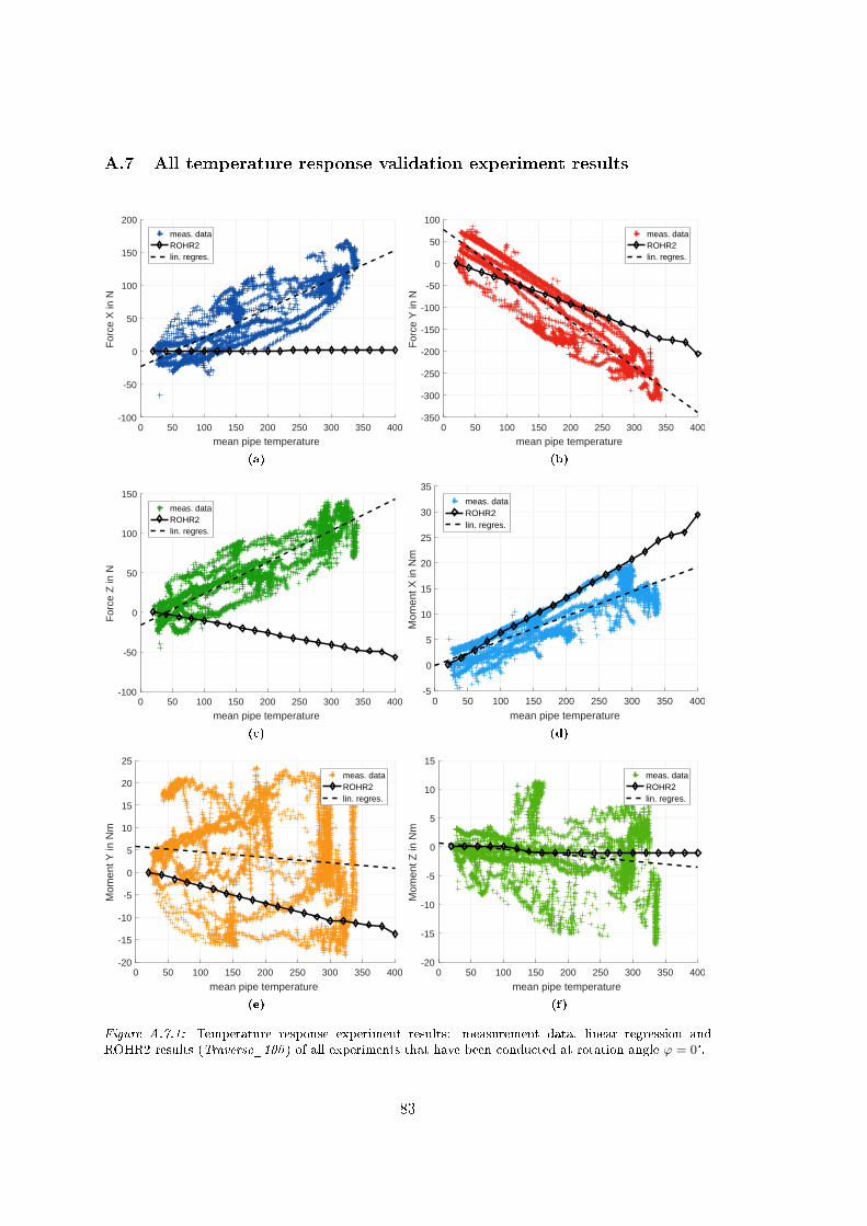
A.7 All temperature response validation experiment results

0 50 100 150 200 250 300 350 400

mean pipe temperature

-100

-50

0

50

100

150

200

For

ce X

in N

meas. dataROHR2lin. regres.

(a)

0 50 100 150 200 250 300 350 400

mean pipe temperature

-350

-300

-250

-200

-150

-100

-50

0

50

100

For

ce Y

in N

meas. dataROHR2lin. regres.

(b)

0 50 100 150 200 250 300 350 400

mean pipe temperature

-100

-50

0

50

100

150

For

ce Z

in N

meas. dataROHR2lin. regres.

(c)

0 50 100 150 200 250 300 350 400

mean pipe temperature

-5

0

5

10

15

20

25

30

35

Mom

ent X

in N

m

meas. dataROHR2lin. regres.

(d)

0 50 100 150 200 250 300 350 400

mean pipe temperature

-20

-15

-10

-5

0

5

10

15

20

25

Mom

ent Y

in N

m

meas. dataROHR2lin. regres.

(e)

0 50 100 150 200 250 300 350 400

mean pipe temperature

-20

-15

-10

-5

0

5

10

15

Mom

ent Z

in N

m

meas. dataROHR2lin. regres.

(f)

Figure A.7.1: Temperature response experiment results: measurement data, linear regression andROHR2 results (Traverse_100 ) of all experiments that have been conducted at rotation angle ϕ = 0°.

83

0 50 100 150 200 250 300 350 400

mean pipe temperature

-40

-20

0

20

40

60

80

100F

orce

X in

N

meas. dataROHR2lin. regres.

(a)

0 50 100 150 200 250 300 350 400

mean pipe temperature

-350

-300

-250

-200

-150

-100

-50

0

50

For

ce Y

in N

meas. dataROHR2lin. regres.

(b)

0 50 100 150 200 250 300 350 400

mean pipe temperature

-100

-50

0

50

100

150

200

For

ce Z

in N

meas. dataROHR2lin. regres.

(c)

0 50 100 150 200 250 300 350 400

mean pipe temperature

-5

0

5

10

15

20

25

30

35

Mom

ent X

in N

mmeas. dataROHR2lin. regres.

(d)

0 50 100 150 200 250 300 350 400

mean pipe temperature

-20

-15

-10

-5

0

5

Mom

ent Y

in N

m

meas. dataROHR2lin. regres.

(e)

0 50 100 150 200 250 300 350 400

mean pipe temperature

-2

0

2

4

6

8

10

Mom

ent Z

in N

m

meas. dataROHR2lin. regres.

(f)

Figure A.7.2: Temperature response experiment results: measurement data, linear regression andROHR2 results (Traverse_100 ) of all experiments that have been conducted at rotation angle ϕ = −90°.

84

A.8 Operation loads estimation from experiment results

In order to re-calibrate the dynamo-meter for a more appropriate load scenario, operationloads had to be estimated. At the time the re-calibration could best be performed, nocomplete traverse rotation at average operational conditions (25 bar and 350 ◦C) had yetbeen possible. The best data available was that taken during the rotation of the traverseat design pressure 40 bar and ambient temperature (a small range of ϕ only). To accountfor the di�erence in pressure and temperature the calibration scenario was calculated asfollows:

avg40 bar20 ◦C = mean(abs(′Rotation at 40 bar′))

estim25 bar20 ◦C = avg40 bar

20 ◦C + load25 barϕ=114.7°, 20 ◦C − load40 bar

ϕ=114.7°, 20 ◦C

calibration = estim25 bar350 ◦C = estim25 bar

20 ◦C + load0 bar350 ◦C

(A.21)

The data (experiment results) used in equation A.21 and the results are shown in tableA.8.1 and �gure A.8.1.

Table A.8.1: Re-calibration scenario

Channel: Fx Fy Fz Mx My Mz

value: 2350 N 800 N 2050 N 400 Nm 400 Nm 300 Nm

85

-120 -90 -60 -30 0 30 60 90-4000

-3000

-2000

-1000

0

1000

2000

3000

rotation angle ϕ in degrees

Fxin

N

Pressure test: 0 barPressure test: 25 barPressure test: 40 barTemperature Exp.: 350°C 0 barRotation at 0 bar no REPAsRotation at 40 bar 20°CAvg: Rot. 40 bar 20°CEstim: Rot. 25 bar 20°CEstim: Rot. 25 bar 350°C(Calibration)

-120 -90 -60 -30 0 30 60 90−1,000

−500

0

500

1,000

1,500

2,000

2,500

rotation angle ϕ in degrees

Fyin

N

Pressure test: 0 barPressure test: 25 barPressure test: 40 barTemperature Exp.: 350°C 0 barRotation at 0 bar no REPAsRotation at 40 bar 20°CAvg: Rot. 40 bar 20°CEstim: Rot. 25 bar 20°CEstim: Rot. 25 bar 350°C(Calibration)

-120 -90 -60 -30 0 30 60 90-5000

-4000

-3000

-2000

-1000

0

1000

2000

rotation angle ϕ in degrees

Fzin

N

Pressure test: 0 barPressure test: 25 barPressure test: 40 barTemperature Exp.: 350°C 0 barRotation at 0 bar no REPAsRotation at 40 bar 20°CAvg: Rot. 40 bar 20°CEstim: Rot. 25 bar 20°CEstim: Rot. 25 bar 350°C(Calibration)

-120 -90 -60 -30 0 30 60 90−1,000

−500

0

500

rotation angle ϕ in degrees

Mxin

Nm

Pressure test: 0 barPressure test: 25 barPressure test: 40 barTemperature Exp.: 350°C 0 barRotation at 0 bar no REPAsRotation at 40 bar 20°CAvg: Rot. 40 bar 20°CEstim: Rot. 25 bar 20°CEstim: Rot. 25 bar 350°C(Calibration)

86

-120 -90 -60 -30 0 30 60 90−1,000

−500

0

500

1,000

rotation angle ϕ in degrees

Myin

Nm

Pressure test: 0 barPressure test: 25 barPressure test: 40 barTemperature Exp.: 350°C 0 barRotation at 0 bar no REPAsRotation at 40 bar 20°CAvg: Rot. 40 bar 20°CEstim: Rot. 25 bar 20°CEstim: Rot. 25 bar 350°C(Calibration)

-120 -90 -60 -30 0 30 60 90−500

0

500

rotation angle ϕ in degrees

Mzin

Nm

Pressure test: 0 barPressure test: 25 barPressure test: 40 barTemperature Exp.: 350°C 0 barRotation at 0 bar no REPAsRotation at 40 bar 20°CAvg: Rot. 40 bar 20°CEstim: Rot. 25 bar 20°CEstim: Rot. 25 bar 350°C(Calibration)

Figure A.8.1: The six plots above show all experiment results, i.e. pressure, temperature and rotationangle response, in one plot per force or moment. Data showing the e�ect of pressurizing the system wastaken during the o�cial pressure tests and is available for two rotation angle ϕ. For better readability,the plots only contain values for the pressurized state 0 bar, the average operation pressure 25 bar andthe design pressure 40 bar. Data showing the e�ect of additional support forces due to heating upto 350 ◦C was taken in several experiments without REPAs and for two angles only. Please comparechapter 6.1. Data showing the e�ect of rotating the traverse was taken once for the empty traversewithout any REPA's connected and once built in at 40 bar. Please compare chapter 6.2. The horizontalline Avg: Rot. 40 bar 20 ◦C shows the average value of the curve Rotation at 40 bar 20 ◦C. On the basisof this value the horizontal lines 'Estim: Rot. 25 bar 20 ◦C' and 'Estim: Rot. 25 bar 350 ◦C' have beencalculated. The latter is used as re-calibration scenario (positive and negative value, as calibration isdone for both, except Fz: calibration only for negative value. Please compare chapter A.3).

87

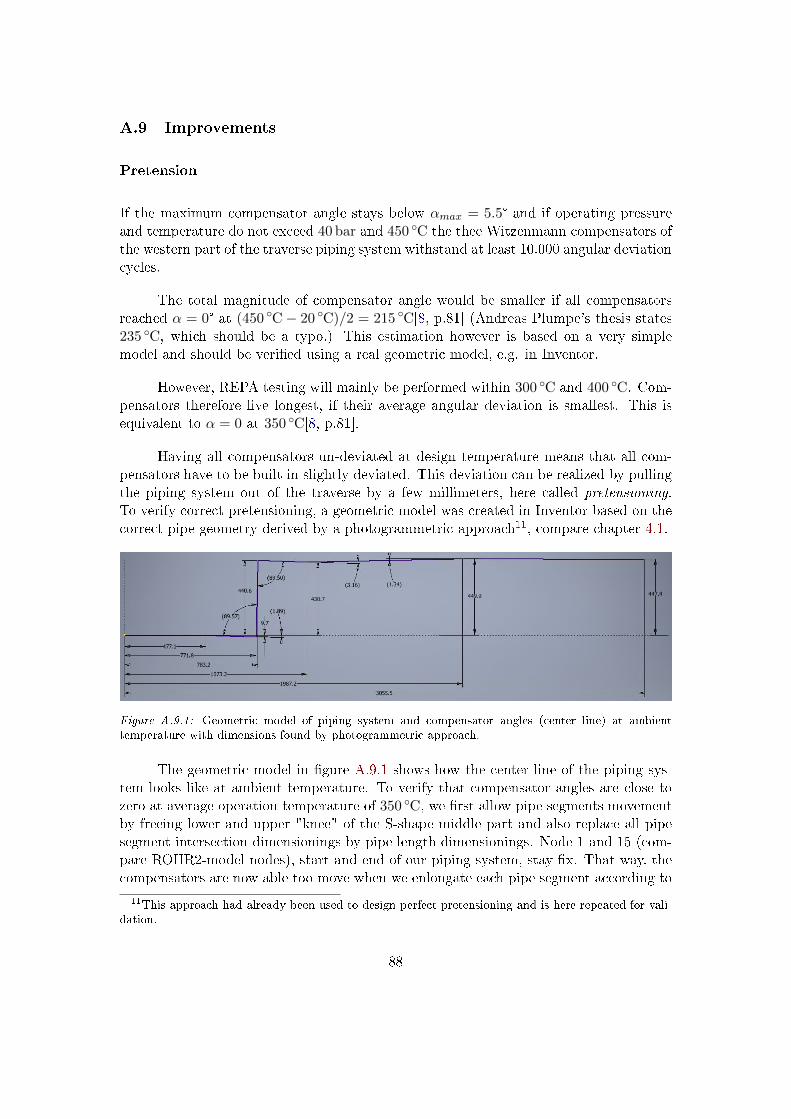
A.9 Improvements

Pretension

If the maximum compensator angle stays below αmax = 5.5° and if operating pressureand temperature do not exceed 40 bar and 450 ◦C the thee Witzenmann compensators ofthe western part of the traverse piping system withstand at least 10.000 angular deviationcycles.

The total magnitude of compensator angle would be smaller if all compensatorsreached α = 0° at (450 ◦C− 20 ◦C)/2 = 215 ◦C[8, p.81] (Andreas Plumpe's thesis states235 ◦C, which should be a typo.) This estimation however is based on a very simplemodel and should be veri�ed using a real geometric model, e.g. in Inventor.

However, REPA testing will mainly be performed within 300 ◦C and 400 ◦C. Com-pensators therefore live longest, if their average angular deviation is smallest. This isequivalent to α = 0 at 350 ◦C[8, p.81].

Having all compensators un-deviated at design temperature means that all com-pensators have to be built in slightly deviated. This deviation can be realized by pullingthe piping system out of the traverse by a few millimeters, here called pretensioning.To verify correct pretensioning, a geometric model was created in Inventor based on thecorrect pipe geometry derived by a photogrammetric approach11, compare chapter 4.1.

Figure A.9.1: Geometric model of piping system and compensator angles (center line) at ambienttemperature with dimensions found by photogrammetric approach.

The geometric model in �gure A.9.1 shows how the center line of the piping sys-tem looks like at ambient temperature. To verify that compensator angles are close tozero at average operation temperature of 350 ◦C, we �rst allow pipe segments movementby freeing lower and upper "knee" of the S-shape middle part and also replace all pipesegment intersection dimensionings by pipe length dimensionings. Node 1 and 15 (com-pare ROHR2-model nodes), start and end of our piping system, stay �x. That way, thecompensators are now able too move when we enlongate each pipe segment according to

11This approach had already been used to design perfect pretensioning and is here repeated for vali-dation.

88

formula A.22, just like the real system would. Here ∆Lϑ is the change in pipe length, Lis the length of the pipe section, α is the average linear heat dilatation coe�cient and∆ϑ is the change in pipe temperature.

∆Lϑ = L · α ·∆ϑ ; α = 13.5 µm/(m K) (A.22)

Figure A.9.2 now shows the piping system and compensator angles at validation tem-perature. We see that angles are already small compared to the cold system: α1 = 0.2°,α2 = 0.16° and α3 = 0.09°, as the angle point of compensator 2 (West-Center) raised by450.7 mm− 430.7 mm = 20 mm.

Figure A.9.2: Geometric model of piping system and compensator angles (center line) at 350 ◦C.

We can thus conclude that pretensioning was done correctly. To determine whatchange is needed to establish perfect pretension, we can free the length of the �rst pipesection and �x the deviation angle of compensator 2 to be 0°. The result is most perfectpretension with the given geometry: α1 = 0.04°, α2 = 0° and α3 = 0.02°, shown in�gure A.9.3. If we wanted to change the traverse piping system accordingly, we hadto change the length of the �rst pipe segment by pushing it into the ITEM-pro�le by479.9 mm− 479.2 mm = 0.7 mm.

Figure A.9.3: Geometric model of piping system and compensator angles (center line) at 350 ◦C, idealpretension.

89

Improved insulation

The interpretation of the measurement results of the temperature response validationexperiments suggests that sensor temperature is crucial to guaranteeing a su�cientlysmall measurement uncertainty. The experience made shows that the sensor tempera-ture has to be monitored and limited in order to protect the sensor against too hightemperatures.

It has to be expected that the sensor in the original con�guration will reach temper-atures beyond 70 ◦C, which is the upper limit for valid results. Eventually temperatureswould even rise above 85 ◦C, which is the maximum allowed temperature. The goal istherefore to minimize the heat �ow from the upper stainless steel plate to the lower steelplate and to the dynamo-meter.

Before addressing more complex, maintenance intensive, expensive and failure en-dangered active cooling solutions, passive possibilities, i.e. better insulation were ad-dressed. To evaluate possible improvements to the sensor insulation, a simpli�ed staticheat transfer model has been created, assuming a representative worst-case scenario: Weassume that the bearing and the upper stainless steel plate have constant 200 ◦C, whilethe bottom steel plate and dynamo-meter have a constant 40 ◦C. This constitutes avery conservative estimation, as the stainless steel plate will actually be colder than thebearing and the lower steel plate will be warmer than the dynamo-meter. Assuming agreater temperature di�erence however ensures that the heat �ow derived can be seenas an upper limit. As another conservative step, we neglect natural any heat exchangewith the environment, such as natural convection and heat radiation. Finally, we assumethat the temperature distribution in hot and cold reservoir is homogeneous and does notchange over time.

Figure A.9.4 depicts the static heat �ow model before and after the insulation.The screws are assumed to be placed in the perfect center of their boreholes, which inreality will be di�cult to obtain. However, changes to heat �ow should be small if boltand steel plate touch as the contact area of two round shapes with di�erent diameters isin�nitely small in theory.

Before the insulation, the heat �ow (red) is assumed to pass from the bearing tothe bolt (via steel washer and air gap) and to the lower steel plate, as well as throughthe insulation board. The heat �ow between insulation board and bolt as well as heatradiation inside the air gap is not considered. After the insulation, the heat �ow isassumed to pass from the bearing to the bolt (via steel plate and bearing) and to thelower steel plate (via steel plate and air gap), as well as through the remaining insulationboard. Radiation (blue) between upper and lower steel plate is assumed, but again notinside the air gaps between bolts and lower steel plate or bearing. Heat transfer dueto forced convection (green) from both steel plates to air passing between the plates isindicated.

These were the four steps taken. Please compare �gures A.9.5 and A.9.4.

90

Figure A.9.4: Static heat �ow model: Thickness of lines represents amount of heat �ow, all numbersrepresent totals for the whole bearing (e.g. all four bolts). 1) bolt, 2) bearing, 3) stainless steel plate,4) insulation board (Promat MONOLUX-800), 5) lower steel plate/ dynamo-meter connection plate, 6)insulation washer (K-Therm®-AS 600M), 7) steel washer (square shape).

1. Increase diameter of all boreholes from 16 mm vs holes: 17.5 mm in order toremove thread and prevent bolt from touching lower steel plate.

2. Cut insulation board as small as possible while still guaranteeing that it can with-stand maximum compressive loads (nominal loads of dynamo-meter plus bolt forcesat nominal torque) with a security factor of 2. This means that 56 % of the mate-rial had to remain to support double the maximum loads. The insulation materialused is Promat MONOLUX-800 with a cold compressive strength of 27 N/mm2.The thermal conductivity is 0.22 W/(m K) at 200 ◦C and, 0.24 W/(m K) at 400 ◦C.

3. Introduce insulation washers made from K-Therm®-AS 600M, 30 mm x 40 mmwith center holes of 16.5 mm diameter. Insulation washers are designed to with-stand double the bolt forces at nominal torque. The heat conductivity is 0.28 W/(m K)and the cold compressive strength is 250 N/mm2 both at 200 ◦C.

4. Add square shaped steel washers to uniformly distribute compression loads oninsulation washers.

As we can see in �gure A.9.4, the reduction of the heat �ow because of the changesapplied is signi�cant. Total heat �ow reduces from 303 W to 140 W, which is a decreaseof 54 %. As indicated, the combined e�ects of heat �ow and radiation after insulationare actually greater than the heat �ow through the insulation board before. However,the di�erences are in the range of a few W only, but the possibility of very e�ective activecooling through ventilation is introduced.

91

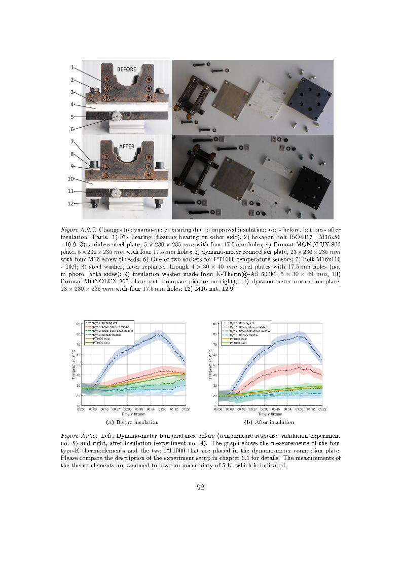
Figure A.9.5: Changes to dynamo-meter bearing due to improved insulation: top - before, bottom - afterinsulation. Parts: 1) Fix bearing (�oating bearing on other side); 2) hexagon bolt ISO4017 - M16x80- 10.9; 3) stainless steel plate, 5 × 230 × 235 mm with four 17.5mm holes; 4) Promat MONOLUX-800plate, 5×230×235 mm with four 17.5mm holes; 5) dynamo-meter connection plate, 23×230×235 mmwith four M16 screw threads; 6) One of two sockets for PT1000 temperature sensors; 7) bolt M16x110- 10.9; 8) steel washer, later replaced through 4 × 30 × 40 mm steel plates with 17.5mm holes (notin photo, both sides); 9) insulation washer made from K-Therm®-AS 600M, 5 × 30 × 49 mm; 10)Promat MONOLUX-800 plate, cut (compare picture on right); 11) dynamo-meter connection plate,23× 230× 235 mm with four 17.5mm holes; 12) M16 nut, 12.9

(a) Before insulation (b) After insulation

Figure A.9.6: Left, Dynamo-meter temperatures before (temperature response validation experimentno. 8) and right, after insulation (experiment no. 9). The graph shows the measurements of the fourtype-K thermoelements and the two PT1000 that are placed in the dynamo-meter connection plate.Please compare the description of the experiment setup in chapter 6.1 for details. The measurements ofthe thermoelements are assumed to have an uncertainty of 5 K, which is indicated.

92

Active cooling

Although improvements from the better insulation of the dynamo-meter bearing weresigni�cant, longer experiments still led to a dangerous increase of the dynamo-metertemperature. As we can see in �gure A.9.8, even though ambient temperatures were low,the temperatures monitored by the two PT1000 in the connection plate rose to 50 ◦Cafter less than 3 hours of operation. Please keep in mind, that later test-rig operationwill be for a continued time of several months at even higher pipe temperatures.

Sensor cooling is therefore mandatory. The �rst attempt with a simple ventilator,as shown in �gure A.9.7 already yielded good results. An additional guide plate wasused to redirect the air stream to the sensor, actively keeping its temperature below ata steady 40 ◦C, as we can see in �gure A.9.8.

Figure A.9.7: Photo of ventilator and guide plate. The air stream produced by the ventilator is redirectedby the "guide plate" (german: Leitblech) in order to cool the sensor but not the pipe and pass throughthe open space between stainless steel plate and dynamo-meter connection plate.

(a) Before ventilation (b) After ventilation

Figure A.9.8: Left, Dynamo-meter temperatures before (temperature response validation experimentno. 13) and right, after ventilation (experiment no. 14). The graph shows the measurements of thefour type-K thermoelements and the two PT1000 that are placed in the dynamo-meter connection plate.Please compare the description of the experiment setup in chapter 6.1 for details. The measurements ofthe thermoelements are assumed to have an uncertainty of 5 K, which is indicated.

93

Pipe insulation design speci�cations

As described in chapter 6.1, one result of the temperature response validation experi-ments was that the insulation material may not entirely cover the the compensators notto hinder their movement and introduce parasitic forces. The insulation was thereforeexecuted as depicted in �gure A.9.9. To decrease heat losses, additional heat shields(german: Wärmeschutzbleche) should be considered, to decrease heat losses throughconvection and irradiation. Again, these should not be connected on both sides of thecompensator at the same time. The same applies for the insulation of the part of thepiping system inside the bearing. During temperature response validation experiments,the dynamo-meter reading Fdyn proved to be very sensitive to anything touching thedynamo-meter bearing. Here, increased insulation may be tried if proven necessary.

Figure A.9.9: Long Caption.

94

A.10 REPA translation due to thermal dilatation

Figure A.10.1: REPA translation due to thermal dilatation of the absorber tubes. A document providedby Senior Flexonics. The REPA test-rig was designed on the basis of this document.

95

B Data sheets and certi�cates

1. Data-sheet dynamo-meter K6D175 10kN/1kNm

2. Calibration certi�cate: original calibration

3. Calibration certi�cate: re-calibration and �rst temperature test!!! Important: Temperature test; value for 'Kanal 3' and 80 degC has to be 0.00077 instead of

0.0077. This is due to a reading error of ME-Messsysteme !!!

96

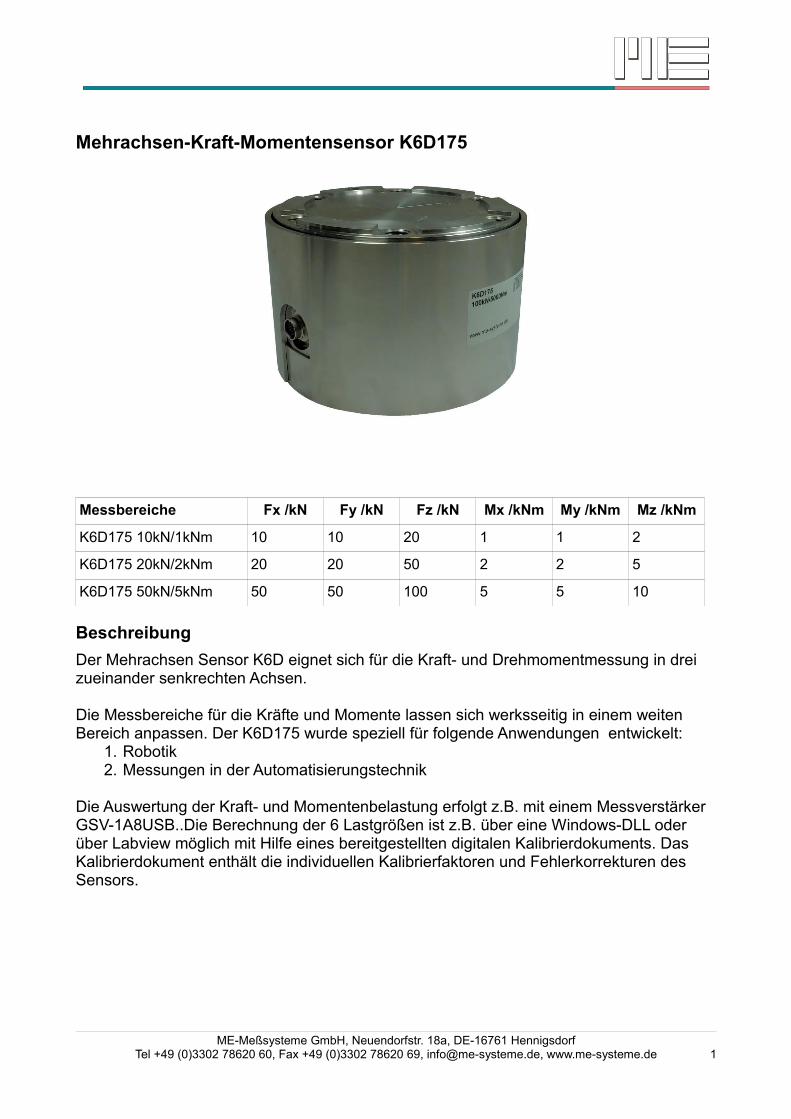
Mehrachsen-Kraft-Momentensensor K6D175

Messbereiche Fx /kN Fy /kN Fz /kN Mx /kNm My /kNm Mz /kNm

K6D175 10kN/1kNm 10 10 20 1 1 2

K6D175 20kN/2kNm 20 20 50 2 2 5

K6D175 50kN/5kNm 50 50 100 5 5 10

BeschreibungDer Mehrachsen Sensor K6D eignet sich für die Kraft- und Drehmomentmessung in drei zueinander senkrechten Achsen.

Die Messbereiche für die Kräfte und Momente lassen sich werksseitig in einem weiten Bereich anpassen. Der K6D175 wurde speziell für folgende Anwendungen entwickelt:

1. Robotik2. Messungen in der Automatisierungstechnik

Die Auswertung der Kraft- und Momentenbelastung erfolgt z.B. mit einem Messverstärker GSV-1A8USB..Die Berechnung der 6 Lastgrößen ist z.B. über eine Windows-DLL oder über Labview möglich mit Hilfe eines bereitgestellten digitalen Kalibrierdokuments. Das Kalibrierdokument enthält die individuellen Kalibrierfaktoren und Fehlerkorrekturen des Sensors.

ME-Meßsysteme GmbH, Neuendorfstr. 18a, DE-16761 HennigsdorfTel +49 (0)3302 78620 60, Fax +49 (0)3302 78620 69, info@me-systeme.de, www.me-systeme.de 1

Abmessungen

ME-Meßsysteme GmbH, Neuendorfstr. 18a, DE-16761 Hennigsdorf2 Tel +49 (0)3302 78620 60, Fax +49 (0)3302 78620 69, info@me-systeme.de, www.me-systeme.de

Technische Daten Maße / MaterialBauform MessplattformMaterial Edelstahl 1.4542Abmessungen mm x mm Ø175 x 110Krafteinleitung 6x M16mechanische DatenNennkräfte (FS) Fx, Fy, Fz kN 10, 20, 50Nennmomente (FS) Mx, My, Mz kNm 1, 2, 5Gebrauchslast %FS 150Bruchlast %FS 300Messweg bei FS 1) mm ca. 0,1Verdrillung bei FS 1) rad ca. 0,01elektrische DatenNennkennwert 2) mV/V @ FS ca. 0,5Nullsignal mV/V <2max. Speisespannung V 5Eingangswiderstand Ohm 350 ±10Ausgangswiderstand Ohm 350 ±10Isolationswiderstand Ohm >2 109

Steckverbinder, 24-polig, M16, Serie 723 09-0497-00-24 Genauigkeitrel. Spannweite 3) %FS 0,5rel. Linearitätsabweichung %FS <0,1rel. Umkehrspanne %FS <0,1Temperatureinfluss auf das Nullsignal %FS/K <0,1Temperatureinfluss auf den Kennwert %RD/K <0,05rel. Kriechen (30 min) %FS <0,1Temperatur / UmweltNenntemperaturbereich °C -10… +70Gebrauchstemperaturbereich °C -10 … +85Lagertemperaturbereich °C -10 … +85Schutzart IP67

Abkürzungen: RD: Istwert („Reading“); FS: Endwert („Full Scale“);1) Messweg bei einachsiger Belastung Fx oder Fy oder Fz;2) Vergleichswert bei einachsiger Belastung Fz;3) Wiederholbarkeit bei gleicher Einbaulage und mehrachsiger Belastung;

ME-Meßsysteme GmbH, Neuendorfstr. 18a, DE-16761 HennigsdorfTel +49 (0)3302 78620 60, Fax +49 (0)3302 78620 69, info@me-systeme.de, www.me-systeme.de 3

Werkszertifikat 20543306Kalibriergegenstand: Mehrkomponenten-Sensor:, Typ K6D175

10kN/1kNm S/N: 15401935Messverstärker: GSV-1A16USB K6D/M16SN:15156211/15356132

Kalibrierlabor: ME-Meßsysteme GmbHNeuendorfstr. 18a16761 Hennigsdorf

Auftraggeber: Deutsches Zentrum f. Luft- u. RaumfahrtAuftragsnummer: 20543306Ort der Kalibrierung HennigsdorfAnzahl Seiten 5Umgebungsbedingungen 21,0 °C ±1,5°C

Kalibrierverfahren

Der Mehrkomponenten-Sensor Typ K6D175 wurde in Reihe mit einem Referenzkraftsensor 1) in einer Referenzvorrichtung 4) belastet. Die Richtung der Referenzkräfte und Referenzmomente auf den Mehrkomponenten-Sensor wurde durch unterschiedliche Montagepositionen des Mehrkomponenten-Sensors in der Referenzvorrichtung sichergestellt.

Als Anzeige wurde der Messverstärker GSV-1A16USB K6D/M16 (15156211/15356132) verwendet.

Zur Ermittlung der Kalibriermatrix wurden aus 48 Messreihen 6 linear unabhängige Lastvektoren mit Hilfe des Referenzvorrichtung, des Referenzhebels und einer Belastungseinrichtung aufgebracht.

Zur Ermittlung der Kalibriermatrix dienen drei Kräfte in drei zueinander rechtwinkligen Richtungen, sowie drei Momente um drei zueinander rechtwinklige Achsen. Es werden die Lastvektoren (Fx,0,0,0,0,0), (0, Fy,0,0,0,0, (0,0, Fz,0,0,0), (0,0,Fz, Mx,0,0), (0,0,Fz,0,My,0) und (Fx,0,00,0,Mz) verwendet.

Zur Bestimmung der Matrix der relativen Spannweiten wird die Kalibriermatrix in gleicher Einbaulage des Mehrkomponenten-Sensors angewendet.

Vor jeder Belastung mit einem Lastvektor wird ein Nullabgleich durchgeführt.

ME-Meßsysteme GmbH, Neuendorfstr. 18a, DE-16761 HennigsdorfTel +49 (0)3302 78620 60, Fax +49 (0)3302 78620 69, info@me-systeme.de, www.me-systeme.de 1

Prüfnormale1 Referenz-

Maschine/KraftsensorWerkstoffprüfmaschine, ZD20EDC, SN:04/M06. 13-09.1726

2 Referenz Kraftsensor KD9363s 1t/C3, Kalibrierzeichen 62305911 ME 2015-7

KD9363s 1t/C3, Kalibrierzeichen 62255133 ME 2015-73 Referenz Platte nN296 mm x 70mm

4 Referenz Hebel n 58 mm x 852mm

Zustand der KalibriergegenständeMessmittel Typ S/N Zustand

Mehrkomponenten-Sensor

K6D175 10kN/1kNm 15301453 Neu /Erstkalibrierung

Messverstärker GSV-1A16USB K6D/M16

1515621115356132

Neu /Erstkalibrierung

Nullpunkterfassung

ME-Meßsysteme GmbH, Neuendorfstr. 18a, DE-16761 Hennigsdorf2 Tel +49 (0)3302 78620 60, Fax +49 (0)3302 78620 69, info@me-systeme.de, www.me-systeme.de

Kanal 1 2 3 4 5 60,0047 0,0050 0,0022 0,0114 0,0047 -0,0003mV/V

KalibriermatrixDie Kalibriermatrix beschreibt den Zusammenhang zwischen den angezeigten Spannungen des Messverstärkers an den Kanälen 1 bis 6 (Bezeichner „ai0“ bis „ai5“) und den Komponenten 1 bis 6 (Fx, Fy, Fz, Mx, My, Mz) des Lastvektors.

ME-Meßsysteme GmbH, Neuendorfstr. 18a, DE-16761 HennigsdorfTel +49 (0)3302 78620 60, Fax +49 (0)3302 78620 69, info@me-systeme.de, www.me-systeme.de 3

Abbildung 1: Kalibriermatrix in N/ V und Nm/V

Kanal1 2 3 4 5 6

Referenz -4,94 1987,29 -1942,62 1,02 1952,86 -2044,15 -2186,25 1160,60 1140,62 -2339,92 1139,83 1171,18 -3164,33 -3057,03 -3225,61 -3162,95 -3207,57 -3154,80 -114,53 -103,25 -112,21 -122,35 238,17 235,81 -194,06 -200,09 206,67 196,83 -0,58 11,69 125,94 -137,18 140,15 -130,11 128,32 -143,87

Fx in N / VFy in N / VFz in N / VMx in Nm / VMy in Nm / VMz in Nm / V

UrsprungDer Ursprung des Koordinatensystems befindet sich im Zentrum des Sensors auf der Oberfläche der oberen Seite. An der Stelle des Ursprungs ist eine Gravierung vorhanden.

Matrix der relativen SpannweitenDie Matrix der relativen Spannweiten („Reproduzierbarkeit“) beschreibt die Abweichung der angezeigten Kräfte und Momente in Prozent vom jeweiligen Endwert bei einachsiger Belastung mit den Lastvektoren (Fx,0,0,0,0,0), (0, Fy,0,0,0,0, (0,0, Fz,0,0,0), (0,0,0,Mx,0,0), (0,0,0,0,My,0),(0,0,0,0,0,Mz);

MessunsicherheitMit einer Wahrscheinlichkeit von 95% besitzen die Messergebnisse folgende Unsicherheit.

ME-Meßsysteme GmbH, Neuendorfstr. 18a, DE-16761 Hennigsdorf4 Tel +49 (0)3302 78620 60, Fax +49 (0)3302 78620 69, info@me-systeme.de, www.me-systeme.de

Abbildung 2: Ursprung des Koordinatensystems

Fx Fy Fz Mx My Mz

Nennlast 10kN 10kN 20kN 1kNm 1kNm 2kNm

Messunsicherheit ±30N ±70N ±80N ±8Nm ±6Nm ±16Nm

Einzelergebnisse der PrüfungMerkmal Istwert Sollwert Ergebnis

Isolationswiderstand@5V

> 2GOhm >2 GOhm in Ordnung

Messunsicherheit <2% <2% in Ordnung

Wir erklären hiermit, dass alle für das Produkt relevanten Prüfungen auf Einhaltung der Spezifikationen mit Messmitteln durchgeführt wurden, die auf nationale und internationale Normale rückführbar sind. Die regelmäßige Überprüfung durch die zertifizierten und akkreditierten Institutionen sichert, dass die Rückführbarkeit aufrecht erhalten wird.

PrüferTesting Engineer

Datumdate

Künstner 15.10.15

ME-Meßsysteme GmbH, Neuendorfstr. 18a, DE-16761 HennigsdorfTel +49 (0)3302 78620 60, Fax +49 (0)3302 78620 69, info@me-systeme.de, www.me-systeme.de 5

20547788-1

ME

2017-1

K6D-CalibrationMatrix HL

Kalibriergegenstand: System bestehend aus:

6-Achsen Kraft-Momentensensor und Messverstärker

Hersteller: ME-Meßsysteme GmbHNeuendorfstr. 18a16761 Hennigsdorf

Typ: Sensor: K6D175 10kN/1kNm SN:15401935

Messverstärker: GSV-1A8USB K6D/M16 SN:15156211

Auftraggeber: Deutsches Zentrum für Luft und Raumfahrt

Geb. Plataforma Solar de Almeria (DLR-PSA), Raum 1

Ctra. de Senés s/n

ES-04200 Tabernas/Almeria

Auftragsnummer: 20547788

Anzahl der Seiten des Kalibrierscheins 4

Die Kalibrierung erfolgte unter Berücksichtigung der Anforderungen der DIN EN ISO/IEC 17025 mit Messmitteln die im Sinne der DIN EN ISO 9001 und DIN EN ISO 10012 auf Nationale Normale rückführbar sind. Die regelmäßige Überprüfung durch die zertifizierten und akkreditierten Institutionen sichert, dass die Rückführbarkeit aufrecht erhalten wird.

Prüfer: T.Künstner

Datum: 03.01.2017

ME-Meßsysteme GmbH, Neuendorfstr. 18a, DE-16761 HennigsdorfTel +49 (0)3302 78620 60, Fax +49 (0)3302 78620 69, info@me-systeme.de, www.me-systeme.de 1

20547788-1

ME

2017-1

Kalibriereinrichtung / Prüfnormale

1 Referenzgewicht Gewichtssatz von 2,5 g – 10 kg, Klasse M1, SN:4840416, 73118-D-K-15192-01-00-2016-4

Gewichtssatz von 2,5 g – 10 kg, Klasse M1, SN:4840416, 73119-D-K-15192-01-00-2016-4

Gewichtssatz 100g – 10 kg, Klasse M1, SN: 4900416, 73120-D-K-15192-01-00-2016-04

Gewichtssatz 100g – 10 kg, Klasse M1, SN: 4910416, 73121-D-K-15192-01-00-2016-04

2 Werkstoffprüfmaschine ZD20EDC, SN:04/M06, 5759-D-K-17452-01-01, 2016-10

Angaben zur Kalibrierung

Umgebungstemperatur 21 °C± 1,5 °C

Kalibrierverfahren /Messbedingungen

Der 6-Achsen Kraft-Momentensensor Typ K6D175 wurde in Reihe mit einem Referenzgewicht sowie mit einer Werkstoffprüfmaschine belastet. Die Richtung der Referenzkräfte und Referenzmomente auf den Sensor wurde durch unterschiedliche Montagepositionen des Mehrkomponenten-Sensors in der Kalibriervorrichtung sichergestellt.

Als Anzeige wurde der Messverstärker GSV-1A8USB K6D/M16 (15156211) verwendet.

Zur Ermittlung der Kalibriermatrix wurden aus 48 Messreihen 6 linear unabhängige Lastvektoren mit Hilfe des Kalibriervorrichtung aufgebracht.

Vor jeder Belastung mit einem Lastvektor wird ein Nullabgleich durchgeführt.

Zustand der Kalibriergegenstände

Gegenstand Typ S/N Zustand

6-Achsen Kraft-Momentensensor

K6D17510kN/1kNm

15401935 Gebraucht/Rekalibrierung

Messverstärker GSV-1A8USBK6D/M16

15156211 Gebraucht/Rekalibrierung

ME-Meßsysteme GmbH, Neuendorfstr. 18a, DE-16761 HennigsdorfTel +49 (0)3302 78620 60, Fax +49 (0)3302 78620 69, info@me-systeme.de, www.me-systeme.de 2

20547788-1

ME

2017-1

Nullpunkterfassung

Kalibriermatrix

Die Kalibriermatrix beschreibt den Zusammenhang zwischen den angezeigten Spannungen des Messverstärkers an den Kanälen 1 bis 6 (Bezeichner „ai0“ bis „ai5“) und den Komponenten 1 bis 6 (Fx, Fy, Fz, Mx, My, Mz) des Lastvektors.

ME-Meßsysteme GmbH, Neuendorfstr. 18a, DE-16761 HennigsdorfTel +49 (0)3302 78620 60, Fax +49 (0)3302 78620 69, info@me-systeme.de, www.me-systeme.de 3

Kanal 1 2 3 4 5 6

0,0075 0,0160 0,0146 0,0037 0,0141 0,0063mV/V

Abbildung 1: Kalibriermatrix in N/V und Nm/V

Kanal

1 2 3 4 5 6

Referenz

6,10 1988,56 -1971,82 8,49 1954,07 -2055,73 -2161,41 1223,06 1196,94 -2338,29 1204,39 1231,05 -3175,05 -3057,37 -3257,57 -3212,60 -3216,90 -3174,84 -115,66 -115,22 -123,88 -124,54 226,16 222,88 -194,49 -193,88 200,39 199,22 5,30 8,36 128,81 -136,12 131,60 -137,26 131,52 -138,73

Fx in N/VFy in N/VFz in N/VMx in Nm/VMy in Nm/VMz in Nm/V

Abbildung 2: Kalibriermatrix in N/mV/V und Nm/mV/V

Kanal

1 2 3 4 5 6

Referenz

15,24 4971,41 -4929,54 21,22 4885,18 -5139,34 -5403,52 3057,65 2992,35 -5845,72 3010,98 3077,63 -7937,62 -7643,42 -8143,92 -8031,49 -8042,25 -7937,10 -289,14 -288,05 -309,71 -311,34 565,39 557,21 -486,21 -484,71 500,96 498,05 13,25 20,90 322,03 -340,30 329,00 -343,15 328,81 -346,83

Fx in N / mV/VFy in N / mV/VFz in N / mV/VMx in Nm / mV/VMy in Nm / mV/VMz in Nm / mV/V

20547788-1

ME

2017-1

Koordinatenursprung

Der Ursprung des Koordinatensystems befindet sich imZentrum des Sensors auf der Oberfläche der oberen Seite.An der Stelle des Ursprungs ist eine Gravierung vorhanden.

Messunsicherheit

Mit einer Wahrscheinlichkeit von 95% besitzen die Messergebnisse folgende Unsicherheit.

Temperaturtest

Nullpunktsignal in mV/V

Temperatur Kanal 1 Kanal 2 Kanal 3 Kanal 4 Kanal 5 Kanal 6

20 °C 0,0000 0,0000 0,0000 0,0000 0,0000 0,0000

80 °C -0,0072 -0,0108 0,0077 -0,0109 -0,0085 -0,0256

20 °C -0,0001 -0,0012 0,0003 -0,0036 -0,0021 0,0013

ME-Meßsysteme GmbH, Neuendorfstr. 18a, DE-16761 HennigsdorfTel +49 (0)3302 78620 60, Fax +49 (0)3302 78620 69, info@me-systeme.de, www.me-systeme.de 4

Fx Fy Fz Mx My Mz

Nennlast 2350 N 800 N 2050 N 400 Nm 400 Nm 300 Nm

Messunsicherheit ±6N ±12N ±40N ±3,0Nm ±1,5Nm ±2,0Nm