Infrastructural Needs & Economic Development in Southeastern Europe: The Case of Rail and Road...

Working Papers|060| December 2004

Mario Holzner, Edward Christie and Vladimir Gligorov

Infrastructural Needs & Economic Development in Southeastern Europe: The Case of Rail and Road Transport Infrastructure

The wiiw Balkan Observatory

www.balkan-observatory.net

About Shortly after the end of the Kosovo war, the last of the Yugoslav dissolution wars, theBalkan Reconstruction Observatory was set up jointly by the Hellenic Observatory, theCentre for the Study of Global Governance, both institutes at the London School ofEconomics (LSE), and the Vienna Institute for International Economic Studies (wiiw).A brainstorming meeting on Reconstruction and Regional Co-operation in the Balkanswas held in Vouliagmeni on 8-10 July 1999, covering the issues of security,democratisation, economic reconstruction and the role of civil society. It was attendedby academics and policy makers from all the countries in the region, from a number ofEU countries, from the European Commission, the USA and Russia. Based on ideas anddiscussions generated at this meeting, a policy paper on Balkan Reconstruction andEuropean Integration was the product of a collaborative effort by the two LSE institutesand the wiiw. The paper was presented at a follow-up meeting on Reconstruction andIntegration in Southeast Europe in Vienna on 12-13 November 1999, which focused onthe economic aspects of the process of reconstruction in the Balkans. It is this policypaper that became the very first Working Paper of the wiiw Balkan ObservatoryWorking Papers series. The Working Papers are published online at www.balkan-observatory.net, the internet portal of the wiiw Balkan Observatory. It is a portal forresearch and communication in relation to economic developments in Southeast Europemaintained by the wiiw since 1999. Since 2000 it also serves as a forum for the GlobalDevelopment Network Southeast Europe (GDN-SEE) project, which is based on aninitiative by The World Bank with financial support from the Austrian Ministry ofFinance and the Oesterreichische Nationalbank. The purpose of the GDN-SEE projectis the creation of research networks throughout Southeast Europe in order to enhancethe economic research capacity in Southeast Europe, to build new research capacities bymobilising young researchers, to promote knowledge transfer into the region, tofacilitate networking between researchers within the region, and to assist in securingknowledge transfer from researchers to policy makers. The wiiw Balkan ObservatoryWorking Papers series is one way to achieve these objectives.


IBEU

This study has been developed in the framework of the IBEU project - Integrating the Balkans in theEuropean Union: Functional Borders and Sustainable Security. The IBEU project was funded by the 3rd Call of the Key-Action: “Improving the Socio-Economic Knowledge Base” of the European Commission, DG Research under Theme3: Citizenship, governance, and the dynamics of European integration and enlargement. IBEU was coordinated by ELIAMEP (Athens) and involved the LSE (London), IECOB(Forli), WIIW (Vienna), CLS (Sofia), IME (Sofia) and SAR (Bucharest). For additional information see www.balkan-observatory.net, www.wiiw.ac.at andwww.eliamep.gr


2

The Vienna Institute for International Economic Studies

Infrastructural Needs & Economic Development

in Southeastern Europe

The Case of Rail and Road Transport Infrastructure

Mario Holzner, Edward Christie and Vladimir Gligorov (wiiw)

Abstract

This paper seeks to analyse the state of rail and road transport infrastructure in the Southeast European Countries (SEECs). The paper is structured in four parts. Part one summarises theoretical findings and international empirical evidence on the theory of the ‘Big Push’, on the issues of infrastructure quality and efficiency and on the subject of liberalisation. Part two explores the current state of rail and road transport infrastructure of the SEECs in comparison with the Central and East European Countries (CEECs) and the European Union (EU) and provides information about ongoing, committed and possible new projects in the core networks of the region. Part three gives some econometric analysis concerning road infrastructure and economic development in the SEE region. Finally, part four generalises some of the findings and discusses some of the obstacles to regional infrastructure cooperation and development. The paper concludes with some policy considerations. Keywords: Transport Infrastructure, Economic Development, South East Europe JEL classification: H54, R40, L92

3

Contents

1. Introduction ...................................................................................................................5 2. Theoretical Findings and International Empirical Evidence................................................5

2.1. The ‘Big Push’.........................................................................................................6 2.2. Quality, Efficiency and Liberalisation.........................................................................9

3. The Current State of Transport Infrastructure in SEE......................................................11 3.1. Rail Density, Quality, Efficiency and Reform............................................................13 3.2. Road Density, Quality, Efficiency and Reform .........................................................16 3.3. The Core Network .................................................................................................22

4. SEE Transport Infrastructure and Economic Development..............................................24 5. Theoretical and Empirical Conclusions ..........................................................................27 6. Infrastructure and Borders ............................................................................................28 7. Policy Conclusions .......................................................................................................30 Appendix ...........................................................................................................................32

4

List of Tables in the Text

Table 1 Basic Indicators................................................................................................ 12

Table 2 Rail Density 2001 ............................................................................................. 13

Table 3 Rail Quality 2001 .............................................................................................. 14

Table 4 Rail Efficiency 2001 .......................................................................................... 15

Table 5 Infrastructure Reform – Railways EBRD infrastructure transition indicators, 2002...... 16

Table 6 Road Density 2000 ........................................................................................... 17

Table 7 Road Quality 2000............................................................................................ 18

Table 8 Road Efficiency 2000, I...................................................................................... 19

Table 9 Road Efficiency 2000, II..................................................................................... 20

Table 10 Infrastructure Reform – Road EBRD infrastructure transition indicators, 2002 .......... 21

List of Tables and Maps in the Appendix

Table A-1 Basic Indicators................................................................................................ 32

Table A-2 Rail Density 2001 ............................................................................................. 33

Table A-3 Rail Quality 2001 .............................................................................................. 34

Table A-4 Rail Efficiency 2001 .......................................................................................... 35

Table A-5 Infrastructure Reform – Railways EBRD infrastructure transition indicators, 2003...... 36

Table A-6 Road Density 2001 ........................................................................................... 37

Table A-7 Road Quality 2001............................................................................................ 38

Table A-8 Road Efficiency 2001, I...................................................................................... 39

Table A-9 Road Efficiency 2001, II..................................................................................... 40

Table A-10 Infrastructure Reform – Road EBRD infrastructure transition indicators, 2003 .......... 41

Table A-11 Explaining the length of roads per capita I............................................................ 42

Table A-12 Explaining the length of roads per capita II........................................................... 42

Table A-13 Explaining the length of paved roads per capita.................................................... 43

Table A-14 Explaining the length of rail per capita I................................................................ 43

Table A-15 Explaining the length of rail per capita II............................................................... 44

Map 1 Routes and corridors, roads............................................................................... 45

Map 2 Routes and corridors, railways............................................................................ 46

Map 3 Road geometry................................................................................................. 47

Map 4 Road condition. ................................................................................................ 48

Map 5 Present technical condition, railways................................................................... 49

5

1. Introduction1 Infrastructure in general and transport infrastructure in particular is often deemed to be an important factor in the economic development of nations. Given the fact that the countries of Southeast Europe (SEE), in addition to their transformation processes, experienced a decade of wars, political unrest and as a result a strong economic decline, the topic of infrastructure and economic development is of special interest to this region. It also has a regional dimension as was recognised by both the Stability Pact for SEE and the regional approach of the European Union (EU). Moreover infrastructure is of importance for security and for political stability in the region. Finally it is important for the process of EU integration as a number of major EU-defined European transport corridors go through the region. In light of this, this paper seeks to analyse the state of rail and road transport infrastructure in the Southeast European Countries (SEECs). Many of the findings are also relevant for other types of transport infrastructure (air, sea, inland waterways), as well as other infrastructure sectors (energy, telecommunication, water supply). For the purpose of this study the SEE region includes the following eight countries (SEE-8): Albania, Bosnia and Herzegovina, Bulgaria, Croatia, Macedonia, Moldova, Romania, Serbia and Montenegro. The paper is structured in four parts. Part one summarises theoretical findings and international empirical evidence on the theory of the ‘Big Push’, on the issues of infrastructure quality and efficiency and on the subject of liberalisation. Part two explores the current state of rail and road transport infrastructure of the SEECs in comparison with the Central and East European Countries (CEECs) i.e. the 8 New EU Member States (NMS) and the ‘old’ European Union (EU-15) and provides information about ongoing, committed and possible new projects in the core networks of the region. Part three gives some econometric analysis concerning road infrastructure and economic development in the SEE region. Finally, part four generalises some of the findings and discusses some of the obstacles to regional infrastructure cooperation and development. The paper concludes with some policy considerations.

2. Theoretical Findings and International Empirical Evidence This part of the study shall summarise theoretical findings and international empirical evidence on the theory of the ‘Big Push’, on the issues of infrastructure quality and efficiency and on the subject of liberalisation.

1 The authors would like to thank Michael Landesmann and Vasily Astrov for their valuable comments.

6

2.1. The ‘Big Push’

The following section gives an overview on the theory of the ‘Big Push’ starting from the classical article of Rosenstein-Rodan (1943), further developed by Murphy, Shleifer and Vishny (1988) and followed by a model by Aghion and Schankerman (1999) focusing on infrastructure in transition. In addition several studies providing empirical evidence on the relationship between infrastructure and economic development are examined. The theory of the “Big Push” was originally introduced by Rosenstein-Rodan (1943) in his article on the ‘Problems of Industrialisation of Eastern and South-Eastern Europe’. This shows that the wider issue of economic development, especially in SEE, is not at all a new one and, moreover, that some of the possible remedies to the problems have been well understood for more than half of a century. Rosenstein-Rodan proposed the creation of an ‘Eastern European Industrial Trust’ for capital investment in the region to be set up after world war two. The coordinated investments of the trust were to concentrate on the building of ‘basic industries and public utilities’ (not necessarily only infrastructure). The simultaneous industrialisation of many sectors could then make industrialisation profitable even if none of the single sectors could break even by themselves. Increased income in the ‘basic industries’ would create demand for goods in all the other sectors and thus increase the overall market for industry goods. Rosenstein-Rodan also foresaw that the countries of the region would partly tend to export ‘processed foods and light industrial articles’ in exchange for heavy industry goods from the US and western Europe and thus the ‘Big Push’ would be favourable for the whole world economy and for the process of the international division of labour as well as for ‘international political stability’. Murphy, Shleifer and Vishny (1988) further developed the ‘Big Push’ theory and found out that in a model of an imperfectly competitive economy with aggregate demand spillovers, the ‘Big Push’ into industrialisation could move the economy form a bad to a good equilibrium. Similarly the simultaneous use of railroads or other shared infrastructure could help to pay the huge fixed costs of building the infrastructure. Hence each infrastructure user indirectly helps the other users and thus makes their industrialisation more likely, as the infrastructure investment will reduce the production costs of other sectors too. In other words the authors address the issue of positive externalities. This could be an important feature even in a completely open economy. However state subsidies for e.g. a railroad might be necessary but not sufficient if potential users will not industrialise. Thus government support for infrastructure should be coordinated with general industrial development. These mechanisms could be particularly relevant for less developed countries. While the model of Murphy, Shleifer and Vishny (1988) focuses mainly on the changes in production costs caused by infrastructure, Aghion and Schankerman (1999) went beyond that and emphasised in their model the interaction between physical and institutional

7

infrastructure, market competition and market entry in transition economies. Thus, in addition to the direct cost savings, infrastructure investments indirectly encourage the transition process on the level of firms. Lower communication, transportation and information costs intensify product market competition and lead to a higher efficiency of the economy by weeding out existing high-cost firms, by changing firms incentives to restructure and by encouraging the entry of new, low-cost private enterprises to the market. Here, infrastructure investments generate a selection effect in addition to the expansion effect. The importance of these impacts on transition linked to infrastructure highly depend upon the degree of cost asymmetry among firms, the proportion of high-cost firms, the cost of restructuring and the entry costs for new low-cost firms. Moreover, this framework also shows how an endogenous demand for infrastructure can be generated, as lowering transaction costs creates winners and losers. The model used is a horizontal product differentiation model with a variety of goods, each of which is produced by a different oligopolistic firm. After this short overview of theoretical findings on the ‘Big Push’, a summary of studies, providing for empirical evidence on the relationship between infrastructure and economic development shall be presented. Several studies have provided empirical evidence of the positive impact of infrastructure on the economic development of nations. Barro (1989) used inter alia the average ratio of public investment in GDP as a proxy for government infrastructure spending to explain real GDP growth per capita of 72 countries over the period of 1960 to 1985. The estimated coefficient of that variable was significantly positive (0.262 in regression 1 of table 2 in Barro (1989)). Easterly and Rebelo (1993) did pooled regressions with decade averages for the 1960’s (36 countries), 1970’s (108 countries) and 1980’s (119 countries) of per capita growth on public investments. The coefficient for public transport and communication investment as a share of GDP was highly positive (0.661 in the basic regression of table 5 in Easterly and Rebelo (1993)) and significant. Interestingly, public transport and communication investment was uncorrelated with private investment, which could mean that it raises growth by increasing the social return to private investment but not by raising private investment itself. More recently, Canning and Bennathan (2000) estimated social rates of return to electricity generating capacity and paved roads by comparing their effect on aggregate output to their costs of construction. In their approach the authors also tried to overcome the problem of reverse causality, with an increase in income leading to an increased demand for infrastructure. For estimating the infrastructure effects on aggregate output two methods were used. First they ran a regression on panel data for a Cobb-Douglas production function with infrastructure (including year dummies, fixed effects, 2 lags, 1 lead). They tried to explain the log of GDP per worker for 1960-1990 by the log of capital per worker, the log of human capital per worker and inter alia the log of paved roads per worker. The coefficient of the last variable was positive (0.083 in column 3 of table 1 in Canning and

8

Bennathan (2000)) and significant, suggesting that paved roads have, in general, higher rates of return than other types of capital. In order to avoid the assumption of a constant elasticity of output with respect to input, imposed by the Cobb-Douglas production function, Canning and Bennathan adopted the more complex trans-log style of production function in a second stage. Here they found out that infrastructure has rapidly diminishing returns to investment taken in isolation (the squared term being negative). However, the interactions between the infrastructure terms and the two other forms of capital were positive. This indicates that infrastructure investments are not sufficient by themselves to induce large changes in output but, that infrastructure can be a productive investment by raising the productivity of investment in other types of capital. Then, in order to calculate the rates of return, the authors estimated the costs of building infrastructure. In the case of the costs of paved road construction a U shaped cost structure appeared, with the middle income countries having lower costs than the rich and the poor countries. This can be explained by the fact that the middle income countries have both lower labour costs than the developed countries and more of the skills and industry required to produce construction materials and equipment than the low income countries. This is one of the main reasons why Canning and Bennathan found out that in a number of middle income countries the rates of return to road infrastructure investment are high, while in general the rates of return to both electricity generating capacity and paved roads are equal or lower than those on other forms of capital in most countries. Vanhoudt, Mathä and Smid (2000) carried out a study which focused explicitly on the EU. Their main finding is a message of reverse causality. For this they employed inter alia a panel data set-up at the national level. Here they calculated two regressions based on a Cobb-Douglas production function including private, public and human capital, the latter proxied by the average schooling years of the population aged over 25. Following a standard setting in these kinds of regressions (see e.g. Hulten (1996) below), the authors derived capital flows from investment shares, deflating them by the growth rate of the work force and the assumed rate of improvements in technological efficiency plus a depreciation rate of 5%. First, a regression on the levels of the variables was performed which left out the cohesion countries, based on the argument that the assumption of equilibrium is less suitable for these countries than for the more advanced ones. Secondly a growth regression for the EU-15 minus Luxembourg was calculated. In the levels regression, explaining income per person of working age, the coefficient of public capital is positive (0.128 in regression 1 of table 4 in Vanhoudt, Mathä and Smid (2000)) and significant, though lower than the coefficient for private capital. However, in the growth regression public investment turns out to be negatively related to the growth performance. The authors explain these results by saying that richer countries have been able to provide more public capital in order to have more utility from better infrastructure, but it came at an opportunity cost of lower growth. Moreover the authors state that public capital investments

9

in poorer regions have not been an engine of regional growth and convergence, but an instrument for redistribution in Europe. A paper that deals with infrastructure and economic development in transition was written by Sugolov, Dodonov and Hirschhausen (2002). Panel data on 15 transition economies in Central and Eastern Europe (CEE) and the Commonwealth of Independent States (CIS) from 1993-2000 was used. The authors applied two different models. First they estimated an aggregate Cobb-Douglas production function using the fixed effects estimation method. In a second step they estimated a stochastic frontier production function. The variables used in the production functions were inter alia total capital (proxied by net electricity consumption), infrastructure capital (proxied by telephone mainlines) and the speed of liberalisation in major infrastructure sectors (proxied by EBRD indicators). The results suggest that the productivity of infrastructure capital is not higher than the productivity of other capital and that there exists a threshold for infrastructure reform below which reforming infrastructure seems to have a negative effect on output and vice versa. As can be seen from the above summary of empirical studies on the relationship between infrastructure and economic development, evidence is mixed and additional questions of e.g. causality and reverse causality arise. Similarly the topic of infrastructure reform examined in the last paper leads directly to the next section on quality, efficiency and liberalisation of infrastructure. 2.2. Quality, Efficiency and Liberalisation

One interesting research question is whether infrastructure reform can lead to higher quality and more efficiency through liberalisation. This section gives an overview on some research conducted in this respect. Empirical evidence on the relationship between telecommunications network quality and export performance of developing countries was provided in a study by Boatman and Francois (1992). The number of telephone lines that use electronic switching (ESS) were used as a proxy for telecommunications network quality. In their regression, per capita total exports in 1986 were explained inter alia by a network density and the network quality variable (both positive and significant). The result suggests that for the analysed developing countries in the respective period, an increase of 5000 ESS switched lines generated an additional 1 USD of export revenue per person. Hulten (1996) came to the conclusion that with respect to the economic growth, it might be more important how well countries use their infrastructure than how much of it they have. He analysed 42 low and middle income countries between 1970 and 1990. First Hulten estimated an OLS regression of the log difference in real GDP per capita from 1970-1990

10

on the log investment rates of public, private and human capital and on the log of initial real GDP per capita. Since no purchasing power parity adjusted public or private capital flows were available, these were proxied by the use of fractions of unadjusted GDP, averaged over the period 1970-1990 and deflated by the average rate of population growth, to which Hulten added 5% to allow for the average rate of capital depreciation and labour augmenting technical change. Human capital was proxied by primary and secondary education enrolment rates. As a result, the coefficient of public capital, representing infrastructure, is positive (0.355 in regression 1 of table 2 in Hulten (1996)) and significant. In a second regression Hulten included an infrastructure effectiveness indicator, constructed as an aggregate index (with the help of a quartile ranking) out of several individual indicators as e.g. mainline faults per 100 telephone calls, electricity generation losses as a percentage of total system output, the percent of paved roads in good condition, diesel locomotive availability as a percentage of the total. As a result, the coefficient of public capital became insignificant, while the coefficient of the effectiveness indicator was positive (0.794 in regression 2 of table 2 in Hulten (1996)) and highly significant. Moreover, Hulten compared high versus low growth rate countries and found out, that those countries that failed to use their infrastructure efficiently had to pay a penalty in the form of lower growth rates. The difference in the infrastructure effectiveness indicator is the most important source of differential growth performance, explaining about 40% of the growth divergence (bottom panel in table 5 in Hulten (1996)). The second most important source of difference is secondary education with about 21%, while the difference in public capital is negligible and with about –2% even negative. Hulten concludes, that international aid programmes aiming only at new infrastructure construction may have a perverse effect if they divert domestic resources away from the maintenance and operation of existing infrastructure. Based on the research done by Hulten (1996) and Aschauer (1997 a, b, c), Aschauer (1998) focused on issues of quantity, finance and efficiency in the context of public capital and economic growth. Starting from a traditional Cobb-Douglas production function, Aschauer (1998) developed and estimated an extended growth equation, where the log difference in real GDP per capita from 1970-1990 is explained by the log of initial real GDP per capita, the log of investment rates of private, human and public capital, the ratio of the 1980 level of external public debt to output and finally, the public capital effectiveness measure. In the empirical implementation of the model a similar dataset for 46 low and middle income countries over the period 1970-1990 as compared to Hulten (1996) was used. Investment rates were deflated by the average rate of population growth and an assumed combined rate of technological progress and depreciation of 5% per year. Investment in human capital was proxied by the percentage of the working age population in secondary school. The 1980 level of external public debt as a ratio of output, which is assumed to finance at least a part of the initial acquisition of public capital, is taken to be directly related to the tax burden, which in turn is expected to depress the rate of economic

11

growth, since it is a burden on the private sector. Though the public capital effectiveness measure was constructed with the help of the same basic data sources as in Hulten (1996), Aschauer (1998) normalised each individual indicator and averaged the results in order to obtain a somewhat more precise measure of efficiency. The results of the main regression (regression 3 of table 3 in Aschauer (1998)) point out the importance of the quantity, the efficiency and the financing of public capital. The former two variables have a positive effect on growth, while the latter has a negative effect on economic growth. However in the data sample the public capital measure and the external public debt variables were positively correlated. Aschauer (1998) states that the exclusion of either variable from the regression could be expected to generate biased estimates. Aschauer (1998) also estimated a growth maximising level of public capital of 49% of output, while in the actual sample the level of public capital averaged at 132% of output. A paper by Francois and Wooton (2000) deals with trade in international transport services and issues of competition and liberalisation. They focused on the maritime sector, but the basic analytics may be applied to other transport sectors as well. The authors claim that, in terms of relative costs to trade, shipping cost margins are now far more important to many countries than tariff barriers. In their analytical model they show that the presence of an imperfectly competitive intermediary can have a significant effect on trade flows and the allocation of gains from trade. Francois and Wooton state that trade liberalisation in the absence of deregulation of the intermediary industry will not result in the increased benefits that could otherwise be imagined. The above brief synopsis of research conducted in the field of infrastructure and economic development shows that the topic has to be seen in a much wider focus than just with respect to physical infrastructure. Rather, issues such as e.g. the efficiency of infrastructure have to be included in the analysis.

3. The Current State of Transport Infrastructure in SEE Part two of the study shall explore the current state of rail and road transport infrastructure of the SEECs in comparison with the Central and East European Countries and the EU and provide information about ongoing, committed and possible new projects in the core network of the region. As it is the case in many other studies on Southeastern Europe, more recent data is scarce and lacks comparability. The latest comparable data on railway and road infrastructure presented in this study reflects the s ituation in the year 2001. In general the evolution of transport networks is very much influenced by the size of a country, its geography and the population density. Table 1 gives an overview of basic indicators, including country area, total population and population density. For comparative

12

reasons we shall relate the figures of the single SEE countries to four country averages chosen according to geography, level of integration with the EU and the level of economic well being as indicated by Gross Domestic Product per capita in USD at Purchasing Power Parity (PPP) for the year 2001. Beside the SEE-8 average, that represents a group of countries willing but not yet able to join the EU and at a very low stage of economic development, which is indicated by an average of only some USD 5500 of GDP per capita at PPP, we shall display in all the tables hereafter an average for the CEE-8, the EU-S-3 and the EU-N-12 countries (plus a total average for all the countries analysed). The CEE-8 are the eight Central and Eastern European new EU member states, namely the Czech Republic, Estonia, Hungary, Latvia, Lithuania, Poland, the Slovak Republic and Slovenia. Their average GDP per capita at PPP is around USD 11500. The EU-S-3 are the three South European Cohesion Countries within the EU, namely Greece, Portugal and Spain. The level of their average GDP per capita at PPP is approximately USD 18600. Finally, the EU-N-12 are the remaining, more northern countries of the EU, with an average GDP per capita at PPP of close to USD 28500. Detailed tables including data for all the single countries of the CEE-8, the EU-S-3 and the EU-N-12 are provided in the Appendix.

Table 1

Basic Indicators

Area Population Persons per GDP pc km² mn, 2001 km² USD PPP, 2001

Albania 28,748 3.1 109 3,680

Bosnia-Herzegovina 51,129 4.0 78 5,970

Bulgaria 110,912 7.9 72 6,890

Croatia 56,538 4.4 77 9,170

Macedonia 25,713 2.0 79 6,110

Moldova 33,760 3.6 108 2,150

Romania 238,391 22.4 94 5,830

Serbia-Montenegro 102,173 10.6 104 4,250

SEE-8 average 80,921 7.3 90 5,506

CEE-8 average 91,122 9.2 101 11,496

EU-S-3 average 242,940 19.8 82 18,580

EU-N-12 average 209,102 26.4 126 28,451

TOTAL AVERAGE 148,851 16.4 110 17,199

Source: International Union of Railways, World Development Indicators 2003 and wiiw estimates.

Table 1 not only reflects that the SEE-8 are much poorer than the other countries analysed, but that the average Balkan country is also small in terms of area and population. However the population density of 90 persons per km² is a little bit higher than in the average EU-S-3 country (82) but still considerably lower than in the CEE-8 (101) and EU-N-12 (126). One has to bear these facts in mind when analysing the current state of SEE transport infrastructure. Having said that, variation within the SEE-8 is considerably

13

high. Interestingly the two poorest countries, Moldova and Albania, are at the same time the countries with the highest population densities in the region. Their GDPs per capita at PPP are approximately USD 2200 and USD 3700 respectively, while their population density is very close to the average of the full (SEE-8 + CEE-8 + EU-S-3 + EU-N-12) sample of 110 persons per km². Similarly the two richest countries in the region Croatia (USD 9200 in GDP pc at PPP) and Bulgaria (USD 6900 in GDP pc at PPP), have the lowest population densities in the region, 77 and 72 persons per km² respectively.

3.1. Rail Density, Quality, Efficiency and Reform

In this section we shall focus on the railway infrastructure by analysing the densities of the networks, their quality and efficiency, as well as the level of reform development in the sector.

Table 2

Rail Density 2001

Length of Density of lines Density of lines lines in km km/'000km² area km/mn persons

Albania 447 16 143

Bosnia-Herzegovina 1,032 20 260

Bulgaria 4,320 39 543

Croatia 2,727 48 622

Macedonia 699 27 344

Moldova 1,121 33 308

Romania 11,364 48 507

Serbia-Montenegro 4,058 40 382

SEE-8 average 3,221 40 443

CEE-8 average 5,927 65 642

EU-S-3 average 6,353 26 320

EU-N-12 average 10,941 52 415

TOTAL AVERAGE 7,211 48 440

Source: International Union of Railways, World Development Indicators 2003.

In table 2, two indicators for the density of the railway network are presented, relating the total length of railway lines to the area and to the population. In terms of kilometres of lines per 1000 km² of area, the SEE-8 (40) and the EU-S-3 (26) are below the total sample average of 48 km of lines per 1000 km². The EU-N-12 (52) are slightly above the full sample average, while the CEE-8 clearly have a higher average than the other countries with 65 km of lines per 1000 km². In terms of kilometres of lines per 1 million of population, the SEE-8 (443) and especially the CEE-8 (642) lie above the sample average of 440 km of lines per 1 million of population. This reflects also the heritage of the communist

14

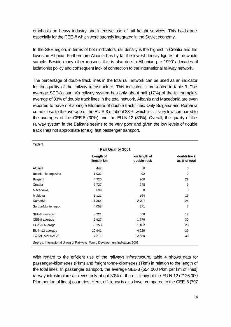
emphasis on heavy industry and intensive use of rail freight services. This holds true especially for the CEE-8 which were strongly integrated in the Soviet economy. In the SEE region, in terms of both indicators, rail density is the highest in Croatia and the lowest in Albania. Furthermore Albania has by far the lowest density figures of the whole sample. Beside many other reasons, this is also due to Albanian pre 1990’s decades of isolationist policy and consequent lack of connection to the international railway network. The percentage of double track lines in the total rail network can be used as an indicator for the quality of the railway infrastructure. This indicator is presented in table 3. The average SEE-8 country’s railway system has only about half (17%) of the full sample’s average of 33% of double track lines in the total network. Albania and Macedonia are even reported to have not a single kilometre of double track lines. Only Bulgaria and Romania come close to the average of the EU-S-3 of about 23%, which is still very low compared to the averages of the CEE-8 (30%) and the EU-N-12 (39%). Overall, the quality of the railway system in the Balkans seems to be very poor and given the low levels of double track lines not appropriate for e.g. fast passenger transport.

Table 3

Rail Quality 2001

Length of km length of double track lines in km double track as % of total

Albania 447 0 0


Bulgaria 4,320 966 22

Croatia 2,727 248 9

Macedonia 699 0 0

Moldova 1,121 164 15

Romania 11,364 2,707 24


SEE-8 average 3,221 556 17

CEE-8 average 5,927 1,776 30

EU-S-3 average 6,353 1,462 23

EU-N-12 average 10,941 4,229 39

TOTAL AVERAGE 7,211 2,380 33


With regard to the efficient use of the railways infrastructure, table 4 shows data for passenger-kilometres (Pkm) and freight tonne-kilometres (Tkm) in relation to the length of the total lines. In passenger transport, the average SEE-8 (654 000 Pkm per km of lines) railway infrastructure achieves only about 30% of the efficiency of the EU-N-12 (2126 000 Pkm per km of lines) countries. Here, efficiency is also lower compared to the CEE-8 (797

15

000 Pkm per km of lines) and the EU-S-3 (1357 000 Pkm per km of lines). The only Balkan country having a higher efficiency in rail passenger transport than e.g. all the CEE-8 is Romania with 965 000 Pkm per km of lines. Bosnia and Herzegovina (52 000 Pkm per km of lines) exhibits by far the lowest value of efficiency in the total sample of countries analysed. In freight transport, the efficiency of the SEE rail infrastructure is somewhat higher (1075 000 Tkm per km of lines) but remains with about 60% of the value for the EU-N-12 (1720 000 Tkm per km of lines) still very low. Only the EU-S-3 (771 000 Tkm per km of lines) have a lower efficiency. The average CEE-8 country outperforms all the others with 2426 000 Tkm per km of lines. The only former Soviet republic within the group of the SEE-8 countries, Moldova (1828 000 Tkm per km of lines) exhibits the highest infrastructure efficiency in the SEE region, though still relatively low compared to other former Soviet republics in the total sample. The highest value has Estonia with 8503 000 Tkm per km of lines. The lowest rail infrastructure efficiency of all countries with regard to freight transport is performed by Albania with only 43 000 Tkm per km of lines.

Table 4

Rail Efficiency 2001

Length of Passenger-km Freight Tonne -km

000 Pkm 000 Freight Tkm

lines in km mn mn per km of lines per km of lines

Albania 447 138 19 309 43

Bosnia-Herzegovina 1,032 53 264 52 256

Bulgaria 4,320 2,990 4904 692 1135

Croatia 2,727 949 2074 348 761

Macedonia 699 133 462 190 661

Moldova 1,121 325 2049 290 1828

Romania 11,364 10,965 15899 965 1399

Serbia-Montenegro 4,058 1,310 2042 323 503

SEE-8 average 3,221 2,108 3464 654 1075

CEE-8 average 5,927 4,725 14379 797 2426

EU-S-3 average 6,353 8,623 4900 1,357 771

EU-N-12 average 10,941 23,257 18816 2,126 1720

TOTAL AVERAGE 7,211 11,601 12362 1,609 1714


Attempting to assess and compare the level of development in infrastructure reform in general and in the railway sector in particular is difficult. The EBRD tries to do that and regularly publishes Infrastructure Transition Indicators for all the transition countries. On a scale ranging from a minimum of 1 to a maximum of 4+, the EBRD tries to evaluate what level of reform, compared to the standards of advanced industrial economies, a given

16

country has achieved in terms of issues such as e.g. liberalisation, privatisation, restructuring, commercialisation, decentralisation or regulation. As can be seen from table 5, with regards to railway sector reform, the average SEE-8 country achieved in 2003 a mark of 2+, which is lower than the average for the CEE-8 of 3. This implies according to the EBRD (2003) that in the countries of SEE some new laws reducing state control over rail operations were passed but this also implies that there still are weak commercial objectives and that there has been only minimal encouragement of private sector involvement. The average mark of 3 for the countries of CEE means that restructuring and commercial orientation were further developed and that inter alia business plans have been designed with clear investment and rehabilitation targets. In this evaluation, Romania was the best SEE performer in 2003, with an indicator value of 4, implying that the railways are now fully commercialised and e.g. separate internal profit centres have been created for passenger and freight. However from the group of SEE and CEE transition countries, only Estonia was able to achieve the maximum of 4+, indicating that a railway law allowing for separation of infrastructure from operations has been passed, that there is private sector participation and that inter alia a rail regulator has been established.

Table 5 Infrastructure Reform – Railways

EBRD infrastructure transition indicators, 2003 1)

Infrastructure reform 2) Railways

Albania 2 2

Bosnia-Herzegovina 2+ 3

Bulgaria 3- 3

Croatia 3- 2+

Macedonia 2 2

Moldova 2 2

Romania 3 4

Serbia-Montenegro 2 2+

SEE-8 average 2+ 2+

CEE-8 average 3 3

Notes: 1) Ranging from minimum 1 to maximum 4+ = standards of advanced industrial economies. -2) Infrastructure includes telecommunications, electric power, water, roads and railways.

Source: EBRD Transition report 2003.

3.2. Road Density, Quality, Efficiency and Reform

In the present section we shed light on the state of the road infrastructure in SEE in the year 2001 by studying the density of the road network, its quality and efficiency, as well as the level of reform development in the road sector in 2003. It has to be said that, compared

17

to the data on the railway sector, road statistics seem to be somewhat less consistent, less accurate and thus also less reliable and comparable. This is probably also due to the different national classification systems of public roads for each country. Table 2 provides us with information on road density. Here the SEE-8 countries are clearly underdeveloped when compared to the other countries in the sample regardless which of the two indicators are used. In terms of the length of roads in kilometres per 1000 km² of area, the average SEE-8 country (587) has only about half of the value for the total average across all the countries analysed of 1102 km per 1000 km². The averages of the countries of the CEE-8 (1265), EU-S-3 (1169) and EU-N-12 (1169) have very similar values close to the total average in this category. When comparing the length of the roads in kilometres with the population in millions of persons, then the SEE-8 (6534) do not perform much better. The average of the EU-S-3 exhibits here the highest density with 14319 km per 1 mn persons, followed by the CEE-8 (12488) and the EU-N-12 (9272). Out of the group of the SEE-8 countries, Romania has the highest road density in terms of both indicators, which are close to the total sample average, with values of 833 and 8852, respectively.

Table 6

Road Density 2001

Length of Density of roads Density of roads roads in km 1) 2) km/'000km² area km/mn persons

Albania 18,000 626 5,743

Bosnia-Herzegovina 22,600 442 5,683

Bulgaria 37,296 336 4,692

Croatia 28,275 500 6,454

Macedonia 12,927 503 6,355

Moldova 12,657 375 3,478

Romania 198,603 833 8,852

Serbia-Montenegro 49,805 487 4,684

SEE-8 average 47,520 587 6,534

CEE-8 average 115,225 1,265 12,488

EU-S-3 average 283,899 1,169 14,319

EU-N-12 average 244,390 1,169 9,272

TOTAL AVERAGE 164,076 1,102 10,017

Notes: 1) Data on the length of roads for Moldova corresponds to the year 1999, for Albania, Austria, France, Germany, Greece, Italy, Netherlands, Portugal, Romania, Serbia and Montenegro, Spain and UK it corresponds to the year 2000 and for Bosnia and Herzegovina to the year 2003. 2) Data for Germany and Portugal is incomplete as there is no information on ‘other roads’ (besides motorways, national and regional roads) available.

Source: World Development Indicators 2003, EU Energy and Transport in Figures 2003, National Statistics, International Union of Railways and wiiw estimates.

18

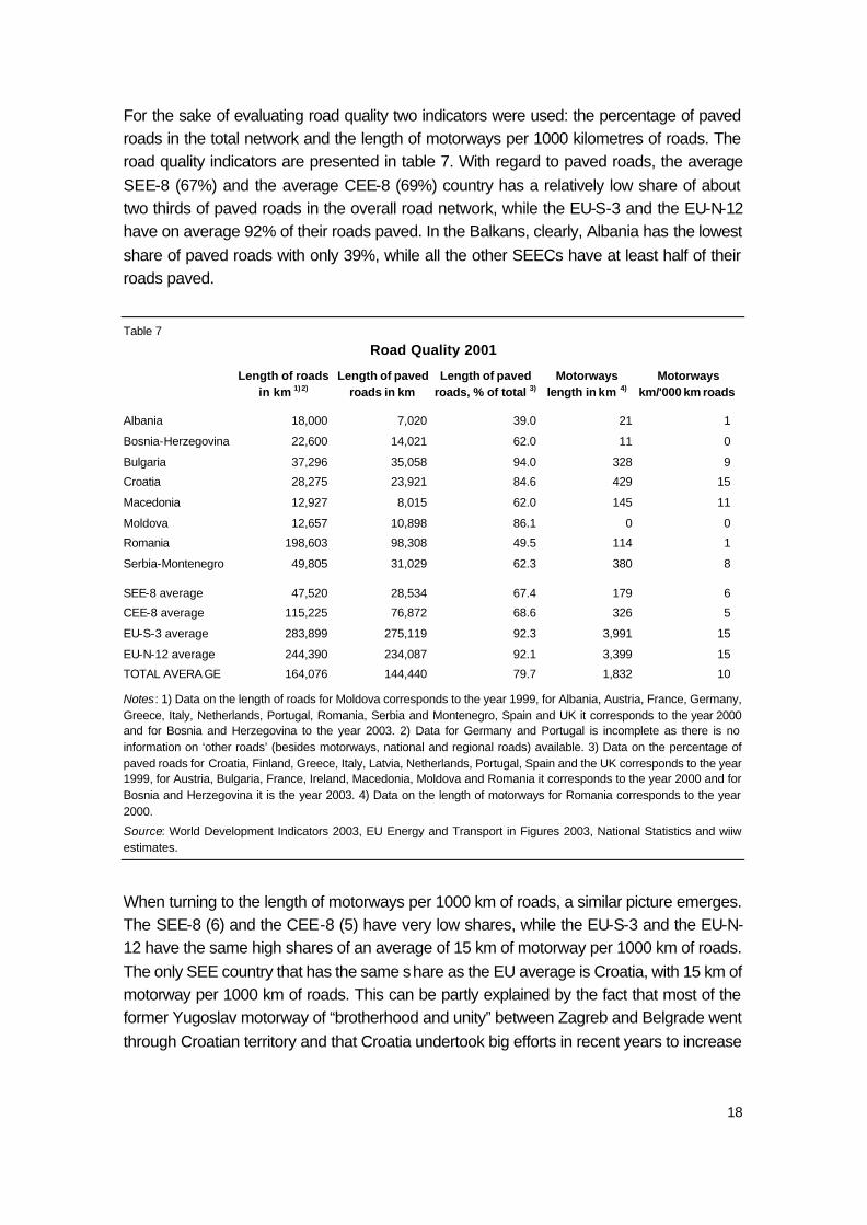
For the sake of evaluating road quality two indicators were used: the percentage of paved roads in the total network and the length of motorways per 1000 kilometres of roads. The road quality indicators are presented in table 7. With regard to paved roads, the average SEE-8 (67%) and the average CEE-8 (69%) country has a relatively low share of about two thirds of paved roads in the overall road network, while the EU-S-3 and the EU-N-12 have on average 92% of their roads paved. In the Balkans, clearly, Albania has the lowest share of paved roads with only 39%, while all the other SEECs have at least half of their roads paved.

Table 7

Road Quality 2001

Length of roads in km 1) 2)

Length of paved roads in km

Length of paved roads, % of total 3)

Motorways length in km 4)

Motorways km/'000 km roads

Albania 18,000 7,020 39.0 21 1

Bosnia-Herzegovina 22,600 14,021 62.0 11 0

Bulgaria 37,296 35,058 94.0 328 9

Croatia 28,275 23,921 84.6 429 15

Macedonia 12,927 8,015 62.0 145 11

Moldova 12,657 10,898 86.1 0 0

Romania 198,603 98,308 49.5 114 1

Serbia-Montenegro 49,805 31,029 62.3 380 8

SEE-8 average 47,520 28,534 67.4 179 6

CEE-8 average 115,225 76,872 68.6 326 5

EU-S-3 average 283,899 275,119 92.3 3,991 15

EU-N-12 average 244,390 234,087 92.1 3,399 15

TOTAL AVERA GE 164,076 144,440 79.7 1,832 10

Notes: 1) Data on the length of roads for Moldova corresponds to the year 1999, for Albania, Austria, France, Germany, Greece, Italy, Netherlands, Portugal, Romania, Serbia and Montenegro, Spain and UK it corresponds to the year 2000 and for Bosnia and Herzegovina to the year 2003. 2) Data for Germany and Portugal is incomplete as there is no information on ‘other roads’ (besides motorways, national and regional roads) available. 3) Data on the percentage of paved roads for Croatia, Finland, Greece, Italy, Latvia, Netherlands, Portugal, Spain and the UK corresponds to the year 1999, for Austria, Bulgaria, France, Ireland, Macedonia, Moldova and Romania it corresponds to the year 2000 and for Bosnia and Herzegovina it is the year 2003. 4) Data on the length of motorways for Romania corresponds to the year 2000.

Source: World Development Indicators 2003, EU Energy and Transport in Figures 2003, National Statistics and wiiw estimates.

When turning to the length of motorways per 1000 km of roads, a similar picture emerges. The SEE-8 (6) and the CEE-8 (5) have very low shares, while the EU-S-3 and the EU-N-12 have the same high shares of an average of 15 km of motorway per 1000 km of roads. The only SEE country that has the same share as the EU average is Croatia, with 15 km of motorway per 1000 km of roads. This can be partly explained by the fact that most of the former Yugoslav motorway of “brotherhood and unity” between Zagreb and Belgrade went through Croatian territory and that Croatia undertook big efforts in recent years to increase

19

its motorway network, especially by connecting the hinterland with the coast. Moldova is the only SEE country without any km of motorway reported. It is arguable whether the few kilometres of motorway reported for Albania and Bosnia and Herzegovina can be really classified as motorways. However there is a new four lane road linking the Albanian capital Tirana with the harbour of Durres and there are some smaller parts of four lane roads in the vicinity of the northwest Bosnian town of Banja Luka and the Bosnian capital of Sarajevo. Trying to develop efficiency indicators for the road infrastructure is more difficult than in the case of railways because data on total passenger-kilometres is missing for most SEE and CEE countries, due to a lack of estimates on passenger-kilometres by private cars. Therefore we shall present the data on passenger-kilometres separately for passenger transport by private cars and by busses and coaches. Table 8 shows the absolute figures of passenger-kilometres for the two modes in addition to the absolute figures of freight tonne-kilometres.

Table 8

Road Efficiency 2001, I

Length of Passenger-km Passenger-km Freight Tonne -km roads in km 1) 2) cars mn 3) buses mn 4) mn 4)

Albania 18,000 5,200 200 2,200

Bosnia-Herzegovina 22,600 . 1,240 290

Bulgaria 37,296 . 15,000 3,300

Croatia 28,275 . 3,500 6,800

Macedonia 12,927 . 800 2,300

Moldova 12,657 . 1,100 600

Romania 198,603 . 7,100 10,600

Serbia-Montenegro 49,805 9,600 5,400 2,900

SEE-8 average 47,520 7,400 4,293 3,624

CEE-8 average 115,225 72,850 9,513 20,950

EU-S-3 average 283,899 159,067 28,567 61,600

EU-N-12 average 244,390 275,208 27,328 80,600

TOTAL AVERAGE 164,076 194,567 16,906 43,503

Notes: 1) Data on the length of roads for Moldova corresponds to the year 1999, for Albania, Austria, France, Germany, Greece, Italy, Netherlands, Portugal, Romania, Serbia and Montenegro, Spain and UK it corresponds to the year 2000 and for Bosnia and Herzegovina to the year 2003. 2) Data for Germany and Portugal is incomplete as there is no information on ‘other roads’ (besides motorways, national and regional roads) available. 3) Due to a lack of data on passeneger-km by cars for several SEE and CEE countries, the average for the SEE-8 is based on the figures for Albania and Serbia and Montenegro only, the CEE-8 average is based only on the figures for 4 countries and the total average only on 21 countries. 4) Data on passenger-km by buses and on freight tonne-km for Bosnia and Herzegovina corresponds to the year 1997 and for Greece it corresponds to the year 1999.

Source: World Development Indicators 2003, EU Energy and Transport in Figures 2003, National Statistics, ECMT Trends in the Transport Sector and wiiw estimates.

20

In table 9 the Pkm and the Tkm are related to the length of the total road network in order to receive efficiency indicators for road infrastructure. Given the fact that there exists only data for Albanian and Serbian Pkm by cars in the SEE-8, comparison with efficiency averages of the other country groups becomes meaningless. However with only 193 000 cars Pkm per km of roads, Serbia and Montenegro exhibits the lowest efficiency rate of the full sample in this category. The average for the EU-S-3 is 560 000 cars Pkm per km of roads and the average of the EU-N-12 is about 1126 000 cars Pkm per km of roads.

Table 9

Road Efficiency 2001, II

Length of 000 Pkm cars 000 Pkm buses 000 Freight Tkm roads in km 1) 2) per km of roads 3) per km of roads 4) per km of roads 4)

Albania 18,000 289 11 122

Bosnia-Herzegovina 22,600 . 55 13

Bulgaria 37,296 . 402 88

Croatia 28,275 . 124 240

Macedonia 12,927 . 62 178

Moldova 12,657 . 87 47

Romania 198,603 . 36 53

Serbia-Montenegro 49,805 193 108 58

SEE-8 average 47,520 156 90 76

CEE-8 average 115,225 632 83 182

EU-S-3 average 283,899 560 101 217

EU-N-12 average 244,390 1,126 112 330

TOTAL AVERAGE 164,076 1,186 103 265

Notes: 1) Data on the length of roads for Moldova corresponds to the year 1999, for Albania, Austria, France, Germany, Greece, Italy, Netherlands, Portugal, Romania, Serbia and Montenegro, Spain and UK it corresponds to the year 2000 and for Bosnia and Herzegovina to the year 2003. 2) Data for Germany and Portugal is incomplete as there is no information on ‘other roads’ (besides motorways, national and regional roads) available. 3) Due to a lack of data on passeneger-km by cars for several SEE and CEE countries, the average for the SEE-8 is based on the figures for Albania and Serbia and Montenegro only, the CEE-8 average is based only on the figures for 4 countries and the total average only on 21 countries. 4) Data on passenger-km by buses and on freight tonne-km for Bosnia and Herzegovina corresponds to the year 1997 and for Greece it corresponds to the year 1999.


In passenger transport by busses and coaches, the average SEE-8 (90 000 Pkm per km of roads) country has a slightly higher infrastructure efficiency as compared to the CEE-8 (83 000 Pkm per km of roads). The EU-N-12 and the EU-S-3 have similar efficiency ratios of 112 000 and 101 000 Pkm per km of roads, respectively. Among the SEECs, Bulgaria is the only country to perform above the whole sample as well as above the EU-N-12 average with 402 000 Pkm per km of roads. On the other hand, Albania has the lowest level of efficiency of all the countries in the sample, with only 11 000 Pkm per km of roads by busses and coaches.

21

Regarding road freight transport, the situation is even worse. The average SEE-8 efficiency is only at about 30% of the total average level of efficiency. A typical Balkan country has only a share of 76 000 Tkm per km of roads, while this indicator is much higher for the CEE-8 (182 000 Tkm per km of roads), the EU-S-3 (217 000 Tkm per km of roads) and especially for the EU-N-12 (330 000 Tkm per km of roads). In this category there is a very high variation. Within the SEECs, Croatia is the only country to have an efficiency close to the total sample average. The country with the lowest efficiency in the Balkans as well as in the full sample is Bosnia and Herzegovina with only 13 000 Tkm per km of roads (however this is a 1997 figure). Interestingly enough, in this case, Albania (122 000 Tkm per km of roads) has a higher road efficiency than the average SEE-8. In table 10 the EBRD infrastructure reform indicators for the road sector in the year 2003 are presented. It can be seen that the average SEE-8 country has a mark of 2+, which is the same degree of reform development as in the CEE-8 (2+). According to the classification defined in EBRD (2003) the mark of 2 indicates the following: there is only a moderate degree of decentralisation and commercialisation, a road agency has been created, road user charges are mostly indirectly related to road use via vehicle and fuel taxes, road construction and maintenance is undertaken primarily by public entities. According to the EBRD road infrastructure transition indicator, Croatia and Romania are reported to have the highest level of reform development among the SEE-8 in 2002, with a mark of 3. In the EBRD classification a mark of 3 stands for a fairly large degree of decentralisation and commercialisation, inter alia including the provision and operation of public roads by private companies under negotiated commercial contracts.

Table 10

Infrastructure Reform – Road EBRD infrastructure transition indicators, 2003 1)

Infrastructure reform 2) Road

Albania 2 2


Bulgaria 3- 2+

Croatia 3- 3

Macedonia 2 2+

Moldova 2 2

Romania 3 3


SEE-8 average 2+ 2+

CEE-8 average 3 2+

Notes: 1) Ranging from minimum 1 to maximum 4+ = standards of advanced industrial economies. - 2) Infrastructure includes telecommunications, electric power, water, roads and railways.


22

3.3. The Core Network

This section shall provide information about the core transport network as defined by the recent Regional Balkans Infrastructure Study (REBIS) on transport (EC 2003) and ongoing, committed and possible new projects in the core network of the region. The REBIS project, which is financed by the EU Commission, aims to develop a regional core network and to identify projects suitable for international co-financing. Unfortunately it is focused only on the so called western Balkan CARDS countries of Albania, Bosnia and Herzegovina, Croatia, Macedonia and Serbia and Montenegro. Bulgaria and Romania are covered by the Trans-European Network (TEN) Invest project, which gives an overview on passed and future investments made in the Trans-European Transport Network (TEN-T) in the enlarged European Union. For the purposes of this study, we shall concentrate on the outcome of the REBIS project. Based on the Pan-European Transport corridors that have been defined at a series of Pan-European Transport conferences, the EU strategic networks in SEE and the Transport Infrastructure Regional Study (TIRS) in the Balkans, REBIS proposed a core network for the region. This core network includes in addition to the Pan-European corridors interconnections between the five national capitals of the region, as well as the “territorial capitals” of Banja Luka, Podgorica and Pristina, the capitals of the neighbouring countries and strategic ports at the Adriatic Sea. Maps 1 and 2 in the appendix, taken from the REBIS study (EC 2003), show the core road and the core rail networks, respectively. The Pan-European corridors are identified by Roman numbers. The Arabic numbers indicate the additionally proposed connections of the core network. The multimodal Pan-European Transport Corridor X shall link the cities Salzburg - Ljubljana - Zagreb - Beograd - Nis - Skopje - Veles - Thessaloniki and includes the branches a: Graz - Maribor – Zagreb, b: Budapest - Novi Sad – Beograd, c: Nis -Sofia (Dmitrovgrad - Istanbul via Corridor IV) and d: Veles - Bitola - Florina - via Egnatia to Igoumenitsa. This is certainly the main transport corridor in the Balkans. However another important North-South connection, which is not included in this map, is the Pan-European Transport Corridor IV going through: Berlin/Nuremberg-Prague-Budapest-Bucuresti-Constanta/Thessaloniki/Istanbul. In the West-East direction, the Pan-European Transport Corridor VIII connects: Durres-Tirana-Skopje-Sofia-Varna. Moreover some of the branches of the Pan-European Transport Corridor V connecting: Venice-Trieste/Koper-Ljubljana-Budapest-Uzgorod-Lviv run through the Balkans. These are branches b: Rijeka-Zagreb-Budapest and c: Ploce-Sarajevo-Osijek-Budapest.

23

Maps 3 and 4 in the appendix show an qualitative assessment of the core road network. The core rode network comprises some 6000 km of primary road, which is only about 5% of the five countries total road network. It becomes evident that almost all of the motorways in the region are concentrated on the main Corridor X, which is more or less identical to the former Yugoslav motorway of “brotherhood and unity”. Also due to the fear of a Warsaw Pact invasion, former Yugoslavia did not have any major transport connections with its eastern neighbours. Also within former Yugoslavia, “geostrategic” interests can help to explain the poor transport connections of e.g. Bosnia and Herzegovina with its neighbours. The military defence of Tito’s “Yugoslav way of socialism” was planned to happen in the Bosnian Mountains. Similar reasons can help to explain the poor connections of Albania with all its neighbouring countries, given Albania’s long history of autarchic dictatorship after World War II. Moreover most parts of the Albanian sections of the core network need complete new pavement. Map 5 in the appendix shows the situation of the railway tracks in the core network. Again, most of the double track lines are on the Corridor X. With the help of quite debatable, high annual GDP growth rate estimates (Albania 6.5%, Bosnia and Herzegovina 4.25%, Croatia 4%, Macedonia 4.25%, Serbia and Montenegro 5%) for the period up to 2025, projections for traffic growth for that period were made for the core network by REBIS. According to this, road traffic will increase by 200-300% and rail traffic by only 60-140%. By having assessed the quality of the core network and estimating average costs to upgrading, REBIS estimated short and long term investment requirements of the core rail and road network. For the short run (2004-2009), the proposed investment amounts to EUR 3.8 bn which is about 0.5% (for Croatia) - 1.4% (for Albania) of the total GDP during that period. Out of this sum, 23% is related to already ongoing projects, 18% to projects already committed and 59% are related to identified new projects. The modal split is 60% for the road and 30% for the rail sector (other investment would fall into air and seaports as well as border crossings). Corridor X and its branches receive 32% of this sum, while 23% falls in the Corridors Vb and Vc. In the longer term, the aim is to upgrade the network to an “acceptable European standard” by 2015. For this period investments are assumed to be around EUR 16.6 bn which ranges from 0.9% of total GDP for Croatia to 3.1% of total GDP for Serbia and Montenegro for that period. The modal split between road and rail investment for this period would be 25% for the roads and 75% for the railways. The website of the EC/World Bank Office for South East Europe (www.seerecon.org) on economic reconstruction and development in South East Europe provides updated figures on the ongoing regional infrastructure projects which are being monitored by the Infrastructure Steering Group (ISG). The current list (as of May 2004) comprises some 51 projects, with a total cost of EUR 4.1 bn. Transport infrastructure (in particular road infrastructure) represents 68% of the overall costs. There it is also possible to download the latest Memorandum of Understanding on the Development of the South East Europe Core Regional Transport Network signed on June 11th 2004.

24

4. SEE Transport Infrastructure and Economic Development This third part of the study shall try to make a synthesis of the former two. The current state of the SEE transport infrastructure shall be put in relation to the level of economic development. Based on the findings of the previous sections, one may summarise by stating that the average SEE-8 country is a poor country with a poor transport infrastructure. Using the terminology of the “Big Push” theory, one would further assume that at least some of these countries are caught in a bad equilibrium. Irrespective of the question of whether infrastructure investment might increase economic growth directly or indirectly, and of which way the causality may operate, the question arises whether, in comparison to other European countries, the countries of Southeastern Europe have enough infrastructural capacity given their current level of economic development. Or, to put it the other way around, whether currently missing transport infrastructure might be a bottleneck for further economic development in the near future. In order to address these issues we estimate a set of simple econometric models which focus on the quantity and quality of the road and railway networks. Our first model seeks to account for the total length of the road network in kilometres per capita of a country i (ROADi) using GDP per capita in PPP (GDPi) and population density (DENSITYi) as explanatory variables. The chosen specification is a log-linear model.

)Ylog(DENSIT)log(GDP)log(ROAD i2i1i ββ ++= c The rationale for our choice of variables is as follows. On average, a given transport infrastructure density should match a given level of economic activity, as a wealthier country should be expected to need more transport infrastructure, while also having more financial means to pay for it. At this stage one would think of using GDP as a measurement of economic activity. However we opt for GDP at PPP as transport infrastructure measured in terms of physical units (length of road network) should be linked to a physical notion of economic activity, not a nominal one. Now comes the issue of country size. For a country of fixed GDP per capita and fixed population, a longer road network should be necessary if the area of the country is larger, giving us a larger length of network per capita. With our specification this would be captured thanks to a lower population density (we expect β2 to be negative). The second model explains the total length of the paved road network in kilometres per capita of a country i (PAVEDi) with the help of the GDP per capita in PPP (GDPi) and the population density (DENSITYi).

25

)Ylog(DENSIT)log(GDP)log(PAVED i2i1i ββ ++= c

We estimated these models on our sample of SEE-8, CEE-8, EU-S-3 and EU-N-12 data, except for Germany and Portugal due to unreliable data for total road network length, for the year 2001. The regression results are as follows and can be seen in detail in the appendix (Table A-11, A-12 and A-13). Overall the estimation results for the first specification seemed satisfactory, with both variables being significant and of the expected signs. A dummy variable for the countries of Southeast Europe was introduced. What happened then was that this dummy variable was negative and significant, but its inclusion into the model rendered the GDP per capita variable insignificant. Of course in the sample used there is a strong correlation between the Southeast Europe dummy variable and GDP per capita. But incredibly if one proxies GDP per capita using the Southeast Europe dummy, one obtains a higher R-squared than with the initial regression. The correct interpretation is as follows: GDP per capita does explain to some extent the length of road network per capita for the sample as a whole. However the most important part of the variance in the dependent variable is between (rather than within) two groups of countries: the Southeast European ones, and the other ones. In sum, being a Southeast European country means having both low GDP per capita and not a lot of road length per capita. But this in itself does not help us to judge whether the current level of infrastructure is somehow below or above what the current GDP levels should imply or require. As a first intuition, one can just add that when comparing the current road network lengths per capita and their corresponding forecasts based on the first regression, one finds most (6 out of 8) Southeast European countries to currently have less than 80% of their forecasted levels, the lowest being Bulgaria with 52% of its forecasted level, and the largest being Moldova with 78% of its forecasted level (Serbia and Montenegro 76%, Macedonia 77%, Bosnia and Herzegovina 69%, Croatia 65%). The 2 other countries are Albania and Romania, respectively 2% and 19% above their forecasts. At this stage we had not taken the quality of roads into account. It was for this reason that we decided to test the second specification, taking this time the total length of paved roads only as the dependent variable. This time the introduction of the Southeast Europe dummy variable yielded an unambiguous result. The dummy variable was negative and significant, while GDP per capita at PPP remained positive and significant. Here the interpretation is clear: GDP per capita at PPP and population density are significant in explaining the total length of paved roads. However Southeast European countries have less paved roads than is implied by their GDP levels and population densities. In other words even without a growth in GDP, the countries of Southeast Europe should, on average, have more paved roads. All of them except for Moldova (29% above the expected level) are below the

26

regression line in the model without the dummy. Here, Albania has only 68% of the paved roads it would be expected to have given its current level of economic development. The values for the other countries are: Bosnia and Herzegovina 70%, Macedonia and Bulgaria 78%, Serbia and Montenegro 79%, Croatia 82%, Romania 94%. In other words our first results indicate that with regards to paved roads, SEE countries have, in comparison with other European countries, a smaller level of total length of paved roads per capita than their current GDP levels would imply. This result is quite a strong one. It means that even without GDP growth, the countries of the region have “insufficient” infrastructure in terms of paved roads. Current trends and forecasts for GDP growth for the region being relatively high, we conclude that significant road infrastructure improvements are necessary if the countries of the region are to reach the levels that they should have according to our specifications. Similar to the above, we have also estimated basic rail infrastructure sector models. The first model seeks to account for the total length of the rail network in kilometres per capita of a country i (RAILi) using GDP per capita in PPP (GDP i) and population density (DENSITYi) as explanatory variables. The chosen specification is a log-linear model.

)Ylog(DENSIT)log(GDP)log(RAIL i2i1i ββ ++= c We estimated the model on our sample of SEE-8, CEE-8, EU-S-3 and EU-N-12 data for the year 2001. The regression results are as follows and can be seen in detail in the appendix (Table A-14 and A-15). This simple model does explain the length of the rail network per capita. However the R² is below 50% and the estimated GDP coefficient is only significant at the 5% level. We then included a dummy variable for the former communist countries (COMMUNISTi), as these countries typically had a strong emphasis on heavy industry and an intensive use of rail freight services. The collapse of these industries left many former communist countries with huge overcapacities in railway infrastructure (as described in the descriptive part above). The new specification is the following.

)COMMUNISTlog()Ylog(DENSIT)log(GDP)log(RAIL i3i2i1i βββ +++= c Now the R² goes up to 66% and all the estimated coefficients are significant at the 1% level. However introducing the SEE dummy variable in the new specification doesn’t yield a significant result. The length of the rail network varies tremendously between Balkan countries, so that there is no significant group effect for the region. Using the estimated coefficients of GDP and DENSITY in the new specification in order to calculate the forecasted levels of rail network infrastructure per capita shows that all the SEE countries are far above their estimated levels, given their GDP and their population density. While

27

Albania is only 32% above the predicted value, Moldova is as much as 315% above (Bosnia and Herzegovina 47%, Macedonia 93%, Croatia 160%, Bulgaria 168%, Serbia and Montenegro 212%, Romania 217%). Thus it can be concluded that the length of the railway network in the Balkans is definitively more than sufficient. Of course this result is just in terms of length. A more detailed analysis would have to account for the quality of these lines, as well as their exact locations within each country. As production patterns shift, it could be that disused lines remain useless, while new lines would in fact be welcome elsewhere. We tried to estimate models on rail infrastructure quality similar to the one on paved roads above. We used data on double track and electrified lines. However, we couldn’t find a convincing setting which could explain these two variables properly. The R² remained far below 50% in both cases. It seems that the indicators we had at our disposal are not necessarily the best indicators for the quality of a railway network. They might rather explain what the rail system is used for (e.g. freight vs. passengers) or what the energy policy of the single country looks like (e.g. whether cheap electricity is available or not). To conclude we can say that our main finding is that even without GDP growth, the countries of the region have “insufficient” infrastructure in terms of quantity and quality of roads, given their current level of economic development. Significant road infrastructure improvements are necessary if the countries of the region are to reach the levels that they should have according to our specifications. In the case of the railway infrastructure rather the opposite seems to be true. The length of the railway network in the Balkans is definitively more than sufficient at the moment. However, this result is just in terms of length. It is difficult to assess the quality of these lines, as well as their strategic locations within the framework of this analysis.

5. Theoretical and Empirical Conclusions The theory of the ‘Big Push’ emphasises that coordinated investment and simultaneous industrialisation of many sectors could move economies from a bad to a good equilibrium. Shared infrastructure could help to make their industrialisation more likely. International empirical evidence on the relationship of infrastructure investment and economic growth is mixed. Although most studies reveal a positive relationship, it is still arguable whether infrastructure investment contributes directly to GDP growth or by raising the productivity of investment in other type of capital. Moreover the question of reverse causality, with an increase in income leading to an increased demand for infrastructure, is still debatable. However a set of international empirical studies point out that, with respect to economic growth it might be more important how well countries use their infrastructure rather than how much of it they have. This underlines the importance of infrastructure quality and efficiency.

28

The analysis of the current state of the Southeast European rail and road transport infrastructure shows that while rail density is close to the European average, road density is significantly below the European average. Moreover rail and road transport infrastructure in the Balkans is of very poor quality compared to the other countries in Europe. Low levels of double track railway lines and only few motorways in the region constrain modern transportation services. The Southeast European countries’ rail and road transport infrastructure has only low levels of efficiency. To sum up, these countries are poor countries with poor infrastructure. In this respect the central question is whether the Southeast European countries have enough infrastructure capacity given their current stage of economic development and whether the poor level of transport infrastructure is a constraint for further economic growth. Our results indicate that e.g. with regards to paved roads, SEE countries have, in comparison with other European countries, a smaller level of total length of paved roads per capita than their current GDP levels would imply. In the case of the railway network rather the opposite holds true. Looking at the maps, one sees that most of the Balkan countries have better transport connections to the EU than with the other countries of the region. This is also a legacy of the cold war and the breakup of former Yugoslavia. Nevertheless the European Union and the International Financial Organisations are engaged in helping the countries of the region to establish a core transport network. International and regional cooperation could help to overcome the inherited infrastructure patterns from decades of regional disintegration.

6. Infrastructure and Borders The argument for “big push” via investments in infrastructure apply perhaps better to longer distances than to shorter ones. This is because these are partly investments in public goods, i.e., in goods with large fixed costs. The longer the distance, the higher the fixed costs. Consequently, higher is the element of the public good and of externalities. Therefore, in a region with small countries, development is sapped to the extent that border impede large infrastructure projects. Conversely, investments in infrastructure lead to significant cross-border cooperation and can lead to increased economic and political integration. This is even more the case with a transit region. Southeast Europe is such a region. Current infrastructure partly testifies to that. With the other part, it testifies to the long history of disintegration due to political reasons. It is this interplay of geography with politics that is of such an importance in the development or lack thereof in this region. With these

29

two statements – that this is a transit region and that its infrastructure is distorted – it would then follow that investments in infrastructure would have positive effects for development and will also have to cut across borders. How would it contribute to development? If it is true that the inherited infrastructure is distorted because of the history of political disintegration, then political normalisation should lead to reallocation of infrastructure that would by itself, without the added “big push” effects, lead to high growth. In addition, if it is true that this is a transit area, then “big push” effects could be expected to exist because, by assumption, lack of adequate infrastructure leads to the existence of unexploited opportunities for trade, investment and production of goods and services. Here, the key problem issue is how to cross borders? The history of disintegration and conflicts has worked for the support for hard borders. Though they may in fact be porous for private businesses, they often prove to be quite hard for public agencies. The recent experience of the Stability Pact, which has been especially active in procuring infrastructure projects, testifies to the fact that those that are regional have hard time being put together and realised. The political economy of this is not simple because it involves three types of actors: private businesses, public budget centres and international (or multilateral) bodies. In a decentralised setting of decision-making, it may be difficult to come up with workable cooperation. Thus, unlike the classical case of institutional failure inherent in the working of the market that was analysed by the theory of the “big push”, there is an institutional failure due to political disintegration that has to be overcome. Clearly, once it is realised that cross-border infrastructure development is beneficial to all involved, these investments will in turn have beneficial effects on regional security and on the rationalisation of the behaviour of the local public agents, i.e., states and other political entities. One reason that inter-state cooperation may be difficult to engineer is the effect that cross-border investments may have on the budgets. Not only some direct sources of public revenues may be lost – e.g., tariffs – but the reallocation of businesses may present various budget centres with a changing tax base. This may be temporary, but still important enough to make it difficult if not impossible for local public authorities to cooperate on common projects. For that reason, the public failure is perhaps more difficult to deal with than the market one, because there is, by assumption, no market solution to this problem. In that circumstance, an outside agent, either private or public, could play a useful role in moving the various local governments to cooperate on common infrastructure projects. The same logic would work for the outside push for faster and more comprehensive reform in the sector of infrastructure services. It is indeed in this sector that public and private

30

partnership (P&PP) play such a crucial role if that partnership is well organised and carried out. The idea beside the P&PP is that public interest should be applied to the investment in the public good while private interest should be relied on to efficiently supply the private goods. For this partnership to work, it is important that proper procedures for competition are put in place. For that to be the case across border, it is necessary to liberalise the services sector in the whole region. In addition, the presence of an international or multilateral actor should induce the local public agents to cooperate not only in infrastructure projects but in the liberalisation of the services sector across borders also. Infrastructure development may have far-reaching consequences for regional and inter-regional cooperation too. Common infrastructure leads to economic and political inter-dependencies. Those, in turn, work for regional investments, which eventually lead to policy inter-dependency. Those would then lead not only to the diminishing significance of the official borders, but also of the policy borders and so-called invisible borders too.

7. Policy Conclusions Investments in infrastructure should have significant effects on the efficient allocation of resources in Southeast Europe. They should also contribute to the high growth rate and faster convergence with the EU. The more important ones cross borders, thus contributing to regional development and security. In addition, they make countries in the region inter-dependent and thus more prone to cooperate. With that, the policy and invisible borders get to play a diminishing role. All that, however, cannot be expected to be generated from within the region alone, an outside push, primarily from the EU, is indispensable to overcome the consequences of the long history of political disintegration.

31

References

Aschauer, D., A. (1997), ‚Do States Optimize? Public Capital and Economic Growth’, Working Paper No. 189, The Jerome Levy Economics Institute, April 1997.

Aschauer, D., A. (1997), ‚Dynamic Output and Employment Effects of Public Capital’, Working Paper No. 191, The Jerome Levy Economics Institute, April 1997.

Aschauer, D., A. (1997), ‚Output and Employment Effects of Public Capital’, Working Paper No. 190, The Jerome Levy Economics Institute, April 1997.

Aschauer, D., A. (1998), ‚Public Capital and Economic Growth: Issues of Quantity, Finance, and Efficiency’, Working Paper No. 233, The Jerome Levy Economics Institute, April 1998.

Aghion, P., Schnakerman, M. (1999), ‘Competition, entry and the social returns to infrastructure in transition economies’, in: Economics of Transition, Volume 7 (1) 1999, pp. 79-101.

Barro, R., J. (1989), ‘A Cross-Country Study of Growth, Saving, and Government’, Working Paper No. 2855, National Bureau of Economic Research, February 1989.

Boatman, K., T., Francois, J.F. (1992), ‘Telecommunications Network Quality and Export Performance’, in: Lofstrom M., D. and Wedemeyer, D., J., eds., Regional Interests and Global Issues: The Challenge of Telecommunications Integration for the Pacific, Pacific Telecommunications Council, pp. 827-831.

Canning, D., Bennathan, E. (2000), ‘The Social Rate of Return on Infrastructure Investments’, paper produced as a part of the World Bank research project ‘Infrastructure and Growth: A Multicountry Panel Study’, July 2000.

Easterly, W., Rebelo, S. (1993), ‘Fiscal Policy and Economic Growth: An Empirical Investigation’, Working Paper No. 4499, National Bureau of Economic Research, October 1993.

EBRD (2003), ‘Transition Report 2003’, European Bank for Reconstruction and Development, 2003.

EC (2003), ‘European Union Energy and Transport in Figures 2003’, European Commission, 2003.

EC (2003), ‘Regional Balkans Infrastructure Study – Transport’, Final Report, European Commission 2000 CARDS Programme, July 2003.

ECMT (2002), ‘Trends in the Transport Sector 1970-2000’, European Conference of Ministers of Transport, 2002.

Francois, J., Wooton, I. (2000), ‘Trade in Inte rnational Transport Services’, Tinbergen Institute Discussion Paper, TI 2000-057/2, Tinbergen Institute, June 2000.

Hulten, C., R. (1996), ‘Infrastructure Capital and Economic Growth: How Well You Use it May Be More Important Than How Much You Have’, Working Paper 5847, National Bureau of Economic Research, December 1996.

Murphy, K., M., Shleifer, A., Vishny, R. (1988), ‘Industrialization and the Big Push’, Working Paper No. 2708, National Bureau of Economic Research, September 1988.

Rosenstein-Rodan, P., N. (1943), ‚Problems of Industrialisation of Eastern and South-Eastern Europe’, in: Economic Journal, LIII, June-September, pp. 202-211.

Sugolov, P., Dodonov, B., Hirschhausen, C. (2002), ‘Infrastructure Policies and Economic Development in East European Transition Countries: First Evidence’, paper for the Annual Conference of the International Society for New Institutional Economics, September 2002.

Vanhoudt, P., Mathä, T., Smid, B. (2000), ‘How productive are capital investments in Europe?’, in: EIB Papers , Volume 5, No.2, European Investment Bank, 2000, pp. 81-106.

32

Appendix Table A-1

Basic Indicators

Area Population Persons per GDP pc km² mn, 2001 km² USD PPP, 2001

Albania 28,748 3.1 109 3,680

Bosnia-Herzegovina 51,129 4.0 78 5,970

Bulgaria 110,912 7.9 72 6,890

Croatia 56,538 4.4 77 9,170

Macedonia 25,713 2.0 79 6,110

Moldova 33,760 3.6 108 2,150

Romania 238,391 22.4 94 5,830

Serbia-Montenegro 102,173 10.6 104 4,250

SEE-8 average 80,921 7.3 90 5,506

Czech Rep. 78,864 10.3 130 14,720

Estonia 45,226 1.4 30 10,170

Hungary 93,030 10.0 108 12,340

Latvia 64,616 2.4 38 7,730

Lithuania 65,300 3.7 57 8,470

Poland 312,685 38.6 124 9,450

Slovak Rep. 49,000 5.4 110 11,960

Slovenia 20,256 2.0 98 17,130

CEE-8 average 91,122 9.2 101 11,496

Greece 131,957 10.0 76 17,440

Portugal 92,082 10.0 109 18,150

Spain 504,782 39.5 78 20,150

EU-S-3 average 242,940 19.8 82 18,580

Austria 83,859 8.1 82 26,730

Belgium 30,514 10.2 336 25,520

Denmark 43,093 5.3 124 29,000

Finland 338,145 5.2 15 24,430

France 547,026 58.9 108 23,990

Germany 356,959 82.0 230 25,350

Ireland 70,283 3.8 54 32,410

Italy 301,225 57.8 192 24,670

Luxembourg 2,586 0.4 169 53,780

Netherlands 41,528 15.9 383 27,190

Sweden 449,964 8.9 20 24,180

UK 244,046 59.8 245 24,160

EU-N-12 average 209,102 26.4 126 28,451

TOTAL AVERAGE 148,851 16.4 110 17,199

Source: International Union of Railways, World Development Indicators 2003 and wiiw estimates.

33

Table A-2 Rail Density 2001

Length of Density of lines Density of lines lines in km km/'000km² area km/mn persons

Albania 447 16 143


Bulgaria 4,320 39 543

Croatia 2,727 48 622

Macedonia 699 27 344

Moldova 1,121 33 308

Romania 11,364 48 507


SEE-8 average 3,221 40 443

Czech Rep. 9,444 120 919

Estonia 967 21 706

Hungary 7,949 85 793

Latvia 2,331 36 958

Lithuania 1,696 26 459

Poland 20,134 64 521

Slovak Rep. 3,662 75 678

Slovenia 1,229 61 618

CEE-8 average 5,927 65 642

Greece 2,377 18 238

Portugal 2,814 31 281

Spain 13,869 27 351

EU-S-3 average 6,353 26 320

Austria 5,780 69 713

Belgium 3,454 113 337

Denmark 2,047 48 384

Finland 5,850 17 1130

France 29,445 54 500

Germany 36,040 101 439

Ireland 1,919 27 507

Italy 16,356 54 283

Luxembourg 274 106 628

Netherlands 2,809 68 177

Sweden 10,920 24 1231

UK 16,397 67 274

EU-N-12 average 10,941 52 415

TOTAL AVERAGE 7,211 48 440


34

Table A-3

Rail Quality 2001

Length of km length of double track lines in km double track as % of total

Albania 447 0 0


Bulgaria 4,320 966 22

Croatia 2,727 248 9

Macedonia 699 0 0

Moldova 1,121 164 15

Romania 11,364 2,707 24


SEE-8 average 3,221 556 17

Czech Rep. 9,444 1,838 19

Estonia 967 104 11

Hungary 7,949 1,292 16

Latvia 2,331 311 13

Lithuania 1,696 531 31

Poland 20,134 8,784 44

Slovak Rep. 3,662 1,020 28

Slovenia 1,229 330 27

CEE-8 average 5,927 1,776 30

Greece 2,377 356 15

Portugal 2,814 497 18

Spain 13,869 3,532 25

EU-S-3 average 6,353 1,462 23

Austria 5,780 1,834 32

Belgium 3,454 2,634 76

Denmark 2,047 907 44

Finland 5,850 507 9

France 29,445 16,090 55

Germany 36,040 17,745 49

Ireland 1,919 496 26

Italy 16,356 6,334 39

Luxembourg 274 140 51

Netherlands 2,809 1,878 67

Sweden 10,920 1,990 18

UK 16,397 196 1

EU-N-12 average 10,941 4,229 39

TOTAL AVERAGE 7,211 2,380 33


35

Table A-4

Rail Efficiency 2001

Length of Passenger-km Freight Tonne -km 000 Pkm 000 Freight Tkm lines in km mn mn per km of lines per km of lines

Albania 447 138 19 309 43

Bosnia-Herzegovina 1,032 53 264 52 256

Bulgaria 4,320 2,990 4904 692 1135

Croatia 2,727 949 2074 348 761

Macedonia 699 133 462 190 661

Moldova 1,121 325 2049 290 1828

Romania 11,364 10,965 15899 965 1399

Serbia-Montenegro 4,058 1,310 2042 323 503

SEE-8 average 3,221 2,108 3464 654 1075

Czech Rep. 9,444 7,262 16557 769 1753

Estonia 967 183 8222 189 8503

Hungary 7,949 7,387 7147 929 899

Latvia 2,331 706 14179 303 6083

Lithuania 1,696 533 7741 314 4564

Poland 20,134 18,208 47656 904 2367

Slovak Rep. 3,662 2,805 10929 766 2984

Slovenia 1,229 715 2600 582 2116

CEE-8 average 5,927 4,725 14379 797 2426

Greece 2,377 1,747 379 735 159

Portugal 2,814 3,692 2138 1,312 760

Spain 13,869 20,431 12184 1,473 879

EU-S-3 average 6,353 8,623 4900 1,357 771

Austria 5,780 8,355 16566 1,445 2866

Belgium 3,454 8,038 7080 2,327 2050

Denmark 2,047 5,548 2068 2,710 1010

Finland 5,850 3,282 9857 561 1685

France 29,445 71,209 50396 2,418 1712

Germany 36,040 73,926 74555 2,051 2069

Ireland 1,919 1,515 516 789 269

Italy 16,356 47,827 21785 2,924 1332

Luxembourg 274 346 585 1,263 2135

Netherlands 2,809 14,392 3834 5,124 1365

Sweden 10,920 5,272 17989 483 1647

UK 16,397 39,377 20561 2,402 1254

EU-N-12 average 10,941 23,257 18816 2,126 1720

TOTAL AVERAGE 7,211 11,601 12362 1,609 1714


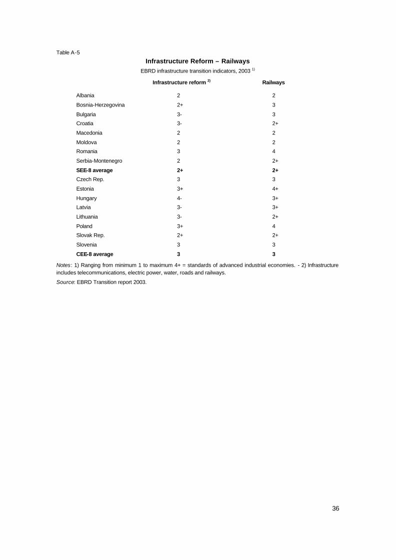
36

Table A-5

Infrastructure Reform – Railways EBRD infrastructure transition indicators, 2003 1)

Infrastructure reform 2) Railways

Albania 2 2


Bulgaria 3- 3

Croatia 3- 2+

Macedonia 2 2

Moldova 2 2

Romania 3 4


SEE-8 average 2+ 2+

Czech Rep. 3 3

Estonia 3+ 4+

Hungary 4- 3+

Latvia 3- 3+

Lithuania 3- 2+

Poland 3+ 4

Slovak Rep. 2+ 2+

Slovenia 3 3

CEE-8 average 3 3

Notes: 1) Ranging from minimum 1 to maximum 4+ = standards of advanced industrial economies. - 2) Infrastructure includes telecommunications, electric power, water, roads and railways.


37

Table A-6

Road Density 2001

Length of Density of roads Density of roads roads in km 1) 2) km/'000km² area km/mn persons

Albania 18,000 626 5,743 Bosnia-Herzegovina 22,600 442 5,683

Bulgaria 37,296 336 4,692

Croatia 28,275 500 6,454

Macedonia 12,927 503 6,355

Moldova 12,657 375 3,478

Romania 198,603 833 8,852

Serbia-Montenegro 49,805 487 4,684

SEE-8 average 47,520 587 6,534 Czech Rep. 127,728 1,620 12,433

Estonia 52,038 1,151 38,012

Hungary 167,839 1,804 16,744

Latvia 69,732 1,079 28,673

Lithuania 76,573 1,173 20,718

Poland 364,697 1,166 9,440

Slovak Rep. 42,956 877 7,955

Slovenia 20,236 999 10,179

CEE-8 average 115,225 1,265 12,488 Greece 116,707 884 11,661

Portugal 72,463 787 7,241

Spain 662,527 1,313 16,787

EU-S-3 average 283,899 1,169 14,319 Austria 132,999 1,586 16,399

Belgium 149,028 4,884 14,541

Denmark 71,622 1,662 13,420

Finland 77,993 231 15,068

France 981,766 1,795 16,671

Germany 230,932 647 2,816

Ireland 92,500 1,316 24,426

Italy 479,688 1,592 8,305

Luxembourg 5,189 2,007 11,901

Netherlands 125,839 3,030 7,910

Sweden 212,961 473 24,004

UK 372,167 1,525 6,228

EU-N-12 average 244,390 1,169 9,272

TOTAL AVERAGE 164,076 1,102 10,017

Notes: 1) Data on the length of roads for Moldova corresponds to the year 1999, for Albania, Austria, France, Germany, Greece, Italy, Netherlands, Portugal, Romania, Serbia and Montenegro, Spain and UK it corresponds to the year 2000 and for Bosnia and Herzegovina to the year 2003. 2) Data for Germany and Portugal is incomplete as there is no information on ‘other roads’ (besides motorways, national and regional roads) available.

Source: World Development Indicators 2003, EU Energy and Transport in Figures 2003, National Statistics, International Union of Railways and wiiw estimates.

38

Table A-7

Road Quality 2001

Length of Length of paved Length of paved Motorways Motorways roads in km 1) 2) roads in km roads, % of total 3) length in km 4) km/'000 km roads

Albania 18,000 7,020 39.0 21 1

Bosnia-Herzegovina 22,600 14,021 62.0 11 0

Bulgaria 37,296 35,058 94.0 328 9

Croatia 28,275 23,921 84.6 429 15

Macedonia 12,927 8,015 62.0 145 11

Moldova 12,657 10,898 86.1 0 0

Romania 198,603 98,308 49.5 114 1

Serbia-Montenegro 49,805 31,029 62.3 380 8

SEE-8 average 47,520 28,534 67.4 179 6

Czech Rep. 127,728 127,728 100.0 517 4

Estonia 52,038 10,251 19.7 94 2

Hungary 167,839 73,346 43.7 448 3

Latvia 69,732 26,917 38.6 0 0

Lithuania 76,573 69,911 91.3 417 5

Poland 364,697 249,088 68.3 399 1

Slovak Rep. 42,956 37,501 87.3 296 7

Slovenia 20,236 20,236 100.0 435 21

CEE-8 average 115,225 76,872 68.6 326 5

Greece 116,707 107,137 91.8 742 6

Portugal 72,463 62,318 86.0 1,659 23

Spain 662,527 655,902 99.0 9,571 14

EU-S-3 average 283,899 275,119 92.3 3,991 15

Austria 132,999 132,999 100.0 1,645 12

Belgium 149,028 116,689 78.3 1,729 12

Denmark 71,622 71,622 100.0 953 13

Finland 77,993 50,305 64.5 602 8

France 981,766 981,766 100.0 9,934 10

Germany 230,932 230,932 100.0 11,786 51

Ireland 92,500 87,043 94.1 125 1

Italy 479,688 479,688 100.0 6,478 14

Luxembourg 5,189 5,189 100.0 115 22

Netherlands 125,839 113,255 90.0 2,291 18

Sweden 212,961 167,387 78.6 1,529 7

UK 372,167 372,167 100.0 3,605 10

EU-N-12 average 244,390 234,087 92.1 3,399 15

TOTAL AVERAGE 164,076 144,440 79.7 1,832 10

Notes : 1) Data on the length of roads for Moldova corresponds to the year 1999, for Albania, Austria, France, Germany, Greece, Italy,

Netherlands, Portugal, Romania, Serbia and Montenegro, Spain and UK it corresponds to the year 2000 and for Bosnia and Herzegovina to the year 2003. 2) Data for Germany and Portugal is incomplete as there is no information on ‘other roads’ (besides motorways, national and regional roads) available. 3) Data on the percentage of paved roads for Croatia, Finland, Greece, Italy, Latvia, Netherlands,

Portugal, Spain and the UK corresponds to the year 1999, for Austria, Bulgaria, France, Ireland, Macedonia, Moldova and Romania it corresponds to the year 2000 and for Bosnia and Herzegovina it is the year 2003. 4) Data on the length of motorways for Romania corresponds to the year 2000.

Source: World Development Indicators 2003, EU Energy and Transport in Figures 2003, National Statistics and wiiw estimates.

39

Table A-8

Road Efficiency 2001, I

Length of Passenger-km Passenger-km Freight Tonne -km roads in km 1) 2) cars mn 3) buses mn 4) mn 4)

Albania 18,000 5,200 200 2,200

Bosnia-Herzegovina 22,600 . 1,240 290

Bulgaria 37,296 . 15,000 3,300

Croatia 28,275 . 3,500 6,800

Macedonia 12,927 . 800 2,300

Moldova 12,657 . 1,100 600

Romania 198,603 . 7,100 10,600

Serbia-Montenegro 49,805 9,600 5,400 2,900

SEE-8 average 47,520 7,400 4,293 3,624

Czech Rep. 127,728 63,400 10,600 37,300

Estonia 52,038 . 2,500 4,700

Hungary 167,839 46,200 18,300 11,800

Latvia 69,732 . 2,300 5,400

Lithuania 76,573 . 1,600 8,300

Poland 364,697 157,700 31,000 74,400

Slovak Rep. 42,956 24,100 8,300 20,200

Slovenia 20,236 . 1,500 5,500

CEE-8 average 115,225 72,850 9,513 20,950

Greece 116,707 81,600 22,000 13,800

Portugal 72,463 89,400 12,000 10,000

Spain 662,527 306,200 51,700 161,000

EU-S-3 average 283,899 159,067 28,567 61,600

Austria 132,999 69,500 13,200 17,600

Belgium 149,028 108,000 12,500 53,200

Denmark 71,622 59,300 9,031 10,900

Finland 77,993 57,000 7,700 26,700

France 981,766 727,600 43,800 189,000

Germany 230,932 705,500 68,700 289,000

Ireland 92,500 34,900 6,300 12,400

Italy 479,688 666,400 95,800 154,800

Luxembourg 5,189 5,200 900 500

Netherlands 125,839 152,000 12,700 31,000

Sweden 212,961 93,100 11,300 30,000

UK 372,167 624,000 46,000 152,100

EU-N-12 average 244,390 275,208 27,328 80,600

TOTAL AVERAGE 164,076 194,567 16,906 43,503

Notes : 1) Data on the length of roads for Moldova corresponds to the year 1999, for Albania, Austria, France, Germany, Greece, Italy, Netherlands, Portugal, Romania, Serbia and Montenegro, Spain and UK it corresponds to the y ear 2000 and for Bosnia and Herzegovina to the year 2003. 2) Data for Germany and Portugal is incomplete as there is no information on ‘other roads’ (besides motorways, national and regional roads) available. 3) Due to a lack of data on passeneger-km by cars for several SEE and CEE countries, the average for the SEE-8 is based on the figures for Albania and Serbia and Montenegro only, the CEE-8 average is based only on the figures for 4 countries and the total average only on 21 countries. 4) Data on passenger-km by buses and on freight tonne-km for Bosnia and Herzegovina corresponds to the year 1997 and for Greece it corresponds to the year 1999.


40

Table A-9

Road Efficiency 2001, II

Length of 000 Pkm cars 000 Pkm buses 000 Freight Tkm roads in km 1) 2) per km of roads 3) per km of roads 4) per km of roads 4)

Albania 18,000 289 11 122

Bosnia-Herzegovina 22,600 . 55 13

Bulgaria 37,296 . 402 88

Croatia 28,275 . 124 240

Macedonia 12,927 . 62 178

Moldova 12,657 . 87 47

Romania 198,603 . 36 53

Serbia-Montenegro 49,805 193 108 58

SEE-8 average 47,520 156 90 76

Czech Rep. 127,728 496 83 292

Estonia 52,038 . 48 90

Hungary 167,839 275 109 70

Latvia 69,732 . 33 77

Lithuania 76,573 . 21 108

Poland 364,697 432 85 204

Slovak Rep. 42,956 561 193 470

Slovenia 20,236 . 74 272

CEE-8 average 115,225 632 83 182

Greece 116,707 699 189 118

Portugal 72,463 1,234 166 138

Spain 662,527 462 78 243

EU-S-3 average 283,899 560 101 217

Austria 132,999 523 99 132

Belgium 149,028 725 84 357

Denmark 71,622 828 126 152

Finland 77,993 731 99 342

France 981,766 741 45 193

Germany 230,932 3,055 297 1,251

Ireland 92,500 377 68 134

Italy 479,688 1,389 200 323

Luxembourg 5,189 1,002 173 96

Netherlands 125,839 1,208 101 246

Sweden 212,961 437 53 141

UK 372,167 1,677 124 409

EU-N-12 average 244,390 1,126 112 330

TOTAL AVERAGE 164,076 1,186 103 265

Notes : 1) Data on the length of roads for Moldova corresponds to the year 1999, for Albania, Austria, France, Germany, Greece, Italy, Netherlands, Portugal, Romania, Serbia and Montenegro, Spain and UK it corresponds to the year 2000 and for Bosnia and Herzegovina to the year 2003. 2) Data for Germany and Portugal is incomplete as there is no information on ‘other roads’ (besides motorways, national and regional roads) available. 3) Due to a lack of data on passeneger-km by cars for several SEE and CEE countries, the average for the SEE-8 is based on the figures for Albania and Serbia and Montenegro only, the CEE-8 average is based only on the figures for 4 countries and the total average only on 21 countries. 4) Data on passenger-km by buses and on freight tonne-km f or Bosnia and Herzegovina corresponds to the year 1997 and for Greece it corresponds to the year 1999.


41

Table A-10

Infrastructure Reform – Road EBRD infrastructure transition indicators, 2003 1)

Infrastructure reform 2) Road

Albania 2 2


Bulgaria 3- 2+

Croatia 3- 3

Macedonia 2 2+

Moldova 2 2

Romania 3 3


SEE-8 average 2+ 2+

Czech Rep. 3 2+

Estonia 3+ 2+

Hungary 4- 3+

Latvia 3- 2+

Lithuania 3- 2+

Poland 3+ 3

Slovak Rep. 2+ 2+

Slovenia 3 3

CEE-8 average 3 2+

Notes: 1) Ranging from minimum 1 to maximum 4+ = standards of advanced industrial economies. -2) Infrastructure includes telecommunications, electric power, water, roads and railways.


42

Table A-11

Explaining the length of roads per capita I Dependent variable

Independent variables logROAD

Constant 6.98

(6.655)***

logGDP 0.457 (4.367)***

logDENSITY -0.447 (-3.997)***

R² 0.541 Adjusted R² 0.505 Number of observations

29

Note. Absolute values of the t statistics are in parentheses. The superscripts *,**, and *** following the t statistics represent a 10, 5, and less than 1% significant level, respectively.

Table A-12

Explaining the length of roads per capita II Dependent variable

Independent variables logROAD

Constant 11.31

(29.03)***

SEE -0.95 (-7.112)***

logDENSITY -0.386 (-4.552)***


29


43

Table A-13

Explaining the length of paved roads per capita Dependent variable

Independent variables logPAVED

Constant 6.874

(5.602)***

logGDP 0.353 (2.787)***

logDENSITY -0.229 (-2.713)***

SEE -0.667 (-3.163)***


29


Table A-14

Explaining the length of rail per capita I

Dependent variable Independent variables logRAIL

Constant 6.239

(6.208)***

logGDP 0.212 (2.085)**

logDENSITY -0.467 (-4.365)***


31


44

Table A-15

Explaining the length of rail per capita II

Dependent variable Independent variables logRAIL

Constant 0.937

(0.643)

logGDP 0.707 (5.067)***

logDENSITY -0.439 (-5.224)***

COMMUNIST 0.892 (4.320)***


31


45

Map 1

Routes and corridors, roads.

Source: EC (2003), ‘Regional Balkans Infrastructure Study – Transport’, Final Report, European Commission 2000 CARDS Programme, July 2003.

46

Map 2

Routes and corridors, railways.


47

Map 3

Road geometry.


48

Map 4

Road condition.


49

Map 5

Present technical condition, railways.


Infrastructural Needs & Economic Development in Southeastern Europe: The Case of Rail and Road...

Documents

Transcript of Infrastructural Needs & Economic Development in Southeastern Europe: The Case of Rail and Road...