Information weighted sampling for detecting rare items in finite populations with a focus on...

arX

iv:1

310.

5821

v1 [

mat

h.PR

] 2

2 O

ct 2

013

Submitted to the Annals of Applied Probability

arXiv: arXiv:0000.0000

INFORMATION WEIGHTED SAMPLING FOR

DETECTING RARE ITEMS IN FINITE POPULATIONS

WITH A FOCUS ON SECURITY

By Andre J. Hoogstrate†,∗ and Chris A.J. Klaassen‡

Netherlands Forensic Institute and Leiden University†

University of Amsterdam‡

Frequently one has to search within a finite population for a singleparticular individual or item with a rare characteristic. Whether anitem possesses the characteristic can only be determined by close in-spection. The availability of additional information about the items inthe population opens the way to a more effective search strategy thanjust random sampling or complete inspection of the population. Wewill assume that the available information allows for the assignmentto all items within the population of a prior probability on whetheror not it possesses the rare characteristic. This is consistent with thepractice of using profiling to select high risk items for inspection. Theobjective is to find the specific item with the minimum number of in-spections. We will determine the optimal search strategies for severalmodels according to the average number of inspections needed to findthe specific item. Using these respective optimal strategies we showthat we can order the numbers of inspections needed for the differ-ent models partially with respect to the usual stochastic ordering.This entails also a partial ordering of the averages of the number ofinspections.

Finally, the use, some discussion, extensions, and examples of theseresults, and conclusions about them are presented.

1. Introduction. This research is motivated by several problems rele-vant to security applications. Examples thereof are the search for a terroristamong a group of passengers, for a container carrying illicit material on avessel entering a port, for a murderer that has left his DNA profile at acrime scene in a small community, etc. In general, one has to search withina finite population for a particular item with a rare characteristic. Only closeinspection will reveal if an item possesses the characteristic or not. Based onprofiling, a relatively quick assessment is obtained on the probability thatan individual item has the rare characteristic. Subsequently, the possibly ex-pensive or intrusive inspection of the high probability individuals or items is

∗Part of the research was funded by the program VIA: Veiligheidsverbetering doorInformation Awareness (Improving Security by Information Awareness).

Primary 62D99, 60E15; secondary 94A20.Keywords and phrases: probability sampling, search, rare events, profiling

1imsart-aap ver. 2011/11/15 file: aap_subm.tex date: December 16, 2013

http://arxiv.org/abs/1310.5821v1

http://www.imstat.org/aap/

http://arxiv.org/abs/arXiv:0000.0000

2 A.J. HOOGSTRATE ET AL.

started. The underlying idea is that this is an economically desirable, logis-tically possible, and hopefully socially acceptable way of improving securityin contrast to purely random checks or inspection of all relevant individuals.

In this research we limit ourselves to the situation where it is certain thatexactly one individual or item with the rare characteristic belongs to thepopulation. This situation was studied earlier by Press [7]. He considered asubset of the models that we have studied in Hoogstrate and Klaassen [4]and that we study in this article. Press’ results and our results in [4] arelimited to the average number of inspections, while we extend these resultshere to the stochastic ordering of the numbers of inspections themselves.Meng [5] and Press [8] extended the results of Press [7] from a population atone checkpoint to a population flowing through a network of airports withmultiple checkpoints. In the present study we use [7] as a starting point, butwe apply an axiomatic approach, thus specifying our assumptions clearly.After introducing our models and assumptions we discuss in subsection 1.3similarities to and differences with [5], [7], and [8].

1.1. Assumptions. For the population the following assumptions hold.

1. Finite Population The population consists of a finite number N ofitems, numbered i = 1, 2, ...., N.

2. Uniqueness One and only one of the items in the population possessesthe characteristic Γ.

3. Prior Probabilities Each item i can be assigned a known probabilitypi > 0 of possessing the characteristic Γ we are searching for, and theseprobabilities add up to 1.

The index of the Γ-item may be viewed as the result of one draw fromthe set {1, 2, . . . , N} with sampling probabilities (p1, p2, . . . , pN ). We know(p1, p2, . . . , pN ), but not the result of the draw, which follows a multinomialdistribution with parameters 1 and (p1, p2, . . . , pN ).For the procedures of inspection we vary the following assumptions.

4. Enumeration Whether or not it is possible to enumerate and orderthe items according to their associated prior probability of possessingcharacteristic Γ. This translates into the issue whether or not one candeterministically control the order in which items will be inspected.

5. Recognition Whether or not recognition of characteristic Γ is per-fect. We introduce the parameter si, 0 < si ≤ 1, i = 1, ..., N, as theprobability of recognizing characteristic Γ when item i is inspected andactually has the characteristic.

imsart-aap ver. 2011/11/15 file: aap_subm.tex date: December 16, 2013

INFORMATION WEIGHTED SAMPLING 3

6. ReplacementWhether or not it is possible to apply sampling withoutreplacement.

7. Memory Whether or not it is possible to use the information that anitem has been selected before, and to use the outcome of this inspec-tion.

Assumptions 4–7 result in 16 different models as listed in Table 1. Proceduresare allowed only if they stop searching once the Γ-item has been found.Formally we put the following two conditions on the search procedures.

8. Stopping Rule Once the Γ-item has been found or when no itemsremain for inspection, no further inspections take place.

9. Finiteness The search procedure terminates after a finite number ofinspections.

Next we introduce the inspection probabilities. These are the probabilitieswithin the models I–P that govern the process that selects items for inspec-tion. We note that these probabilities are called public profile probabilitiesby Press [7].

10. Inspection Probabilities If an inspection takes place, the probabil-ity that item i will be inspected, is qi. We require

∑Ni=1 qi = 1 and

qi > 0, i = 1, . . . , N.

To enable a more detailed analysis we define the following probabilities.

11. Attention The sampling probability that item i comes to the atten-tion of the inspector, is denoted by λi . We require

∑Ni=1 λi = 1 and

λi > 0, i = 1, . . . , N.12. Conditional Inspection Given item i has come to the attention of

the inspector, it has probability πi > 0 of being inspected.

Note that qi, i = 1, . . . , N, result from the two processes described in As-sumptions 10 and 11, and that the probabilities concerned are related by

(1.1) qi =λiπi

∑Nj=1 λjπj

, i = 1, . . . , N.

1.2. Discussion of the Assumptions. In Assumption 3 the probabilitiespi are assumed to be given without error. Of course, in practice this will oftennot be the case. We will not assess the effects of uncertainty in these prob-abilities by estimation here, as it is our objective to find optimal strategiesfirst.



model index A B C D E F G H I J K L M N O P

enumeration y y y y y y y y n n n n n n n nperfect recognition y y y y n n n n y y y y n n n nwith replacement y y n n y y n n y y n n y y n nmemory y n y n y n y n y n y n y n y n

Table 1

An overview of the different models: the authoritarian models A to H, the democratic

models I to P.

Assumption 5 does not allow for false positives. We could enhance themodels by introducing a parameter representing the probability that anitem is incorrectly classified as possessing the specific characteristic Γ whilethis is actually not the case. Such an addition is left for further research.

Note that each item i with pi positive could be the Γ-item, and henceshould not be excluded from inspection under any procedure. Exclusionwould be in conflict with assumption 9. This implies that procedures usinga positive threshold to pi , i = 1, . . . , N, are excluded from our study.

Assumption 10 introduces the probabilities that govern the process forselecting the individuals to be inspected in case enumeration is not possible.When it is possible to enumerate the items, one can decide in which order theitems have to be inspected. In the models without enumeration the order inwhich items are inspected, is random and depends on two processes. First itdepends on the stochastic mechanism that determines in which order itemscome to the point of inspection (Assumption 11), secondly it depends on theprobability with which the item is inspected, once the item has come to thepoint of inspection (Assumption 12). If some properties or characteristics ofthe individuals or items in the population are known, the resulting profilesmay be used in determining the conditional inspection probabilities πi oreven the sampling probabilities λi .Obtaining an estimate for πi is commonlyassociated with the term profiling. The items will be inspected in an orderlysequential fashion but the order in which items are to be inspected, mightbe determined beforehand. Finally, we point out explicitly that we assumethe probabilities pi, qi, si, λi, and πi to be constant over time and to be thesame in repeated trials and for all inspections. In practice, this assumptionwill often only hold by approximation.

1.3. Comparison between Approaches. The most important questionPress raises in [7] is whether actuarial methods will, from a mathemati-cal or probabilistic point of view, deliver the security levels as expected bygovernment. Subsequently he studies a stylized model of reality and obtainsboth expected and surprising results. The analyzed models however are for-



mulated mathematically sloppily, what makes determining their practicalrelevance rather difficult.

In [8] Press analyzes the same kind of model and optimization criterion,the average number of inspections, called secondary checks, necessary tocatch the malfeasor, but for a network of checkpoints and under the extraconstraint of allowing for only M secondary checks. As Meng [5] points outhis equations (4) and (5) are wrong in that they allow probabilities largerthan 1, and Meng derives the correct formulas.

In this setting of a maximum of M secondary checks, as several re-searchers, notably Meng [5], think, the optimization criterion of minimizingthe average number of checks makes hardly any sense anymore. There is al-ways a positive probability that the terrorist, or malfeasor, will go throughundetected. So, they propose to optimize the probabilities qi of being se-lected for inspection such as to minimize the probability of a terrorist goingthrough undetected. Meng [5] analyzes this new optimization criterion un-der the constraint on the number of inspections and obtains some surprisingresults.

In our research we consider all models presented in Table 1.1 without amaximum of M secondary checks and with the mean of the number of sec-ondary checks as the optimization criterion. However, in Models G, H, O,and P the probability might be positive that the Γ-item goes through un-detected. For these models our criterion will be the conditional mean of thenumber of secondary checks, given the Γ-item will be detected. Subsequently,we order all models with their corresponding optimal procedures, thus allow-ing for a balanced decision in choosing the model and procedure appropriatefor the situation at hand. In practice our analysis is relevant when one has awell defined closed population where there is certainty about the existenceof one item or individual having the sought after property and it is necessaryto find that person or item.

2. Analysis. For each of the models we will introduce and analyzeinspection procedures. As performance measure we use the average numberof inspections that these procedures need in order to find the Γ-item. Wherepossible we will minimize these averages. Subsequently, we will study thedistribution function of the random number of inspections needed whenthese procedures are applied and partially order the procedures.

2.1. Authoritarian Models. In this section we analyze procedures forthe models A to H from Table 1, where enumeration and ordering of theitems is possible. We will call these models Authoritarian as in most casesan authoritarian regime will have to be put in place in order to get the



ordering implemented, especially when the items are people. This is in linewith Press [7]. We first analyze the models where besides enumeration andordering, perfect recognition is possible.

2.1.1. Analysis of Models A, B, C, and D. First we consider model A. Aswe can use enumeration, ordering, and perfect recognition, we can proceedby using the assigned prior probabilities pi and inspect without replacement.If at the j-th inspection an item with prior probability p(j) is checked, thenthe average number of inspections for this procedure is

(2.1) µABCD =

N∑

j=1

jp(j) .

If there is an i with p(i) < p(i+1), then µABCD can be made smaller byinterchanging p(i) and p(i+1). Consequently, as our objective is to minimizethe average number of inspections, we follow Press [7] and choose p(1) ≥p(2) ≥ · · · ≥ p(N), the ordered probabilities pi. For the uninformative priorprobabilities pi = 1/N, i = 1, . . . , N, this yields the classical value

(2.2) µABCD =N + 1

2.

Note that under the optimal strategy with p(1) ≥ p(2) ≥ · · · ≥ p(N) theaverage µABCD from (2.1) equals at most (N + 1)/2 from (2.2). This is aninstance of Chebyshev’s algebraic inequality, which may be proved for Nodd by noting that

(2.3)N + 1

2−

N∑

j=1

jp(j) =

N∑

j=1

[

N + 1

2− j

]

[

p(j) − p(N+1

2 )

]

≥ 0

holds since each term in the second sum is nonnegative.For the models A, B, C, and D we note that under the Stopping Rule

8 with or without memory and with or without replacement have no ef-fect. Consequently, the best strategies for these models are the same, andtherefore we have indicated the resulting average with µABCD.

2.1.2. Analysis of Models E and F. In Press [7] an analysis for modelE, with enumeration and stochastic recognition, was carried out under thereference authoritarian screening strategies with stochastic recognition. Toclarify the argument for the optimal strategy as put forward in Press [7],we use conditional probabilities. By Press’ notation si we denote the condi-tional probability of identifying item i at inspection as having characteristic



Γ, given it is the Γ-item. Given that item j has been inspected mj timeswithout having been identified as having characteristic Γ for j = 1, . . . , N,the conditional probability that item i has characteristic Γ and will be iden-tified at inspection, equals

(2.4)pi(1− si)

misi∑N

j=1 pj(1− sj)mj

, i = 1, . . . , N.

Consequently, in order to have the highest probability of identifying the itemwith characteristic Γ at the next inspection, given the inspection history, onehas to inspect item i, if it satisfies

(2.5) pi(1− si)misi = max

j=1,...,Npj(1− sj)

mjsj .

Note that for si = 1, i = 1, . . . , N, (2.4) and (2.5) present an alternative wayto describe the optimal procedure for Models A, B, C, and D. To computethe average number of inspections under this optimal strategy we observethat the order in which the items are to be inspected is completely governedby (2.4) and (2.5) in a deterministic manner as the parameters si and piare assumed known. Denote the order of the items to be inspected by thesequence of numbers tij, where at the tij-th inspection item i is inspectedfor the j-th time. The probability that item i is recognized as the Γ-item atinspection tij, is

(2.6) pi(1− si)j−1si .

Therefore the expected number of inspections under the optimal strategyfor model E equals

(2.7) µEF =

N∑

i=1

∞∑

j=1

tijpi(1− si)j−1si .

Note that in case of perfect recognition (2.7) reduces to

(2.8) µABCD =

N∑

i=1

∞∑

j=1

tijpi0j−1 =

N∑

i=1

ti1pi =

N∑

i=1

ti1p(ti1) =

N∑

j=1

jp(j).

To verify that (2.7) is optimal indeed, we compare time tij with tij+1 = tkℓ.If k = i then ℓ = j + 1 and we do nothing. However, if k 6= i then reversingthe order of these two inspections gives a smaller value for µEF if and onlyif

(2.9) pi(1− si)j−1si − pk(1− sk)

ℓ−1sk < 0.



This implies that at each point in time (2.5) should hold.Note that [12] of Press [7] is equivalent to (2.7) and that [13] of Press [7]

follows by P (NEF = tij) = pi(1− si)j−1si and

(2.10)N∑

i=1

∞∑

j=1

P (NEF = tij) =N∑

i=1

∞∑

j=1

pi(1− si)j−1si = 1.

Here NEF is defined as the number of inspections needed to find the Γ-itemunder the optimal strategy.

For the analysis of procedure F we just observe that as the order in whichthe items are inspected can be determined in advance just as in model E,the optimal strategy and subsequent analysis are the same for model E andF, whence the notation µEF and NEF .

2.1.3. Analysis of Models G and H.Models G and H satisfy the same conditions as Models C and D, ex-

cept for the perfect recognition condition. In fact, Models G and H area generalization of Models C and D, respectively, in the sense that forsi = 1, i = 1, . . . , N, these models are the same. In these four models thereis sampling without replacement, and hence in Models G and H there is apossibility that the Γ-item will not be found. Indeed, the probability theΓ-item will be found equals

∑Ni=1 sipi here, and if this probability is less

than 1, the distribution of the number of inspections needed to identify theΓ-item is defective. In this case it makes sense to take the number of inspec-tions as infinity if the Γ-item has not been identified, and consequently wethen have

(2.11) µGH = ∞.

One might be interested in the conditional expectation of the number ofinspections given the Γ-item will be found. This conditional expectationequals µABCD given in (2.1).

Since the probability that the Γ-item will not be found, equals∑N

i=1(1−si)pi and does not depend on the choice of the qis, we define the optimalstrategy as the same one that minimizes µABCD given in (2.1). Hence itmakes sense to write

(2.12) µGH =

N∑

i=1

sipi

N∑

j=1

jp(j) +

(

1−N∑

i=1

sipi

)

∞

with 0×∞ interpreted as 0.



2.2. Democratic Models. In this section we analyze the six models Ito N. We note that models J and N have been analyzed by Press [7] asdemocratic strategies under perfect recognition and stochastic recognition,respectively.

2.2.1. Analysis of Models I, K, and L. If within the models I, K, or L aninspected item is not the Γ-item, it is not selected again for inspection eitherbecause the model is without replacement (K and L) or because the item isbeing recognized as having had a negative outcome of the inspection before(I). Consequently, these models give rise to the same optimal procedure.

By (I1, I2, . . . , IN ) we denote the random vector of indices that describesin which order the items in the population will be inspected. This randomvector is ruled by the qi from Assumption 10, to wit

(2.13) P (I1 = i1, . . . , IN = iN ) =N∏

j=1

qij

1−∑j−1h=1 qih

.

The conditional expectation of the number of inspections needed, given(I1, I2, . . . , IN ) = (i1, i2, . . . , iN ), equals

(2.14)

N∑

k=1

kpik .

Consequently, the unconditional average number of inspections equals

(2.15) µIKL =∑

(i1,...,iN)

N∑

k=1

kpik

N∏

j=1

qij

1−∑j−1h=1 qih

,

where the first summation is over the collection of N ! vectors (i1, ..., iN ) thatcan be obtained by permutation of (1, . . . , N). Calculation of the optimalq1, ..., qN for this model is an extremely daunting task. However, we notethat the special case of the uniform distribution with qi = 1/N, i = 1, . . . , N,yields µIKL = (N + 1)/2, which is no surprise.

2.2.2. Analysis of Model J. In Model J we have sampling with replace-ment, actually. Let C be the index of the item that has characteristic Γ andlet T be the number of inspections needed to identify the item with char-acteristic Γ. Note that C is random with distribution P (C = i) = pi , i =1, . . . , N, according to Assumption 2. Given C = i, the random variable Thas a geometric distribution with success probability qi , i.e.

(2.16) P (T = j |C = i) = (1− qi)j−1qi ,



and mean

(2.17)∞∑

j=1

j(1 − qi)j−1qi =

1

qi.

Consequently, the average number µJ of inspections needed is the expecta-tion of (2.17) and equals (cf. [3] of Press [7])

(2.18) µJ =

N∑

i=1

piqi.

By the Cauchy-Schwarz inequality we have

(2.19)

(

N∑

i=1

√pi

)2

=

(

N∑

i=1

√pi√qi

√qi

)2

≤N∑

i=1

piqi

N∑

j=1

qj = µJ

with equality if and only if

(2.20) qi =

√pi

∑Nj=1

√pj

, i = 1, . . . , N,

holds. Note that (2.20) yields the optimal strategy.

2.2.3. Analysis of Models M and N. In model N the same conditionshold as in model J. However, there is no perfect recognition. Instead weassume that the probability of recognizing item i as the Γ-item when it isinspected, is given by the probability si. Based on the same reasoning as in(2.16) and (2.17) we get the average number of required inspections, givenC, as 1/(qCsC). Taking the expectation over this C, we obtain (cf. (2.18))

(2.21) µMN =

N∑

i=1

piqisi

.

Minimization as in (2.19) and (2.20) shows that the optimal strategy andminimized value of µMN are given by

(2.22) qi =

√

pi/si∑N

j=1

√

pj/sj, µMN =

(

N∑

i=1

√

pisi

)2

.

For model M we obtain the same results as for model N. At first sightthis is a bit strange, but it is due to the fact that the optimal strategy is



obtained using known pi and si. That means that remembering whethersomebody has been screened already and found not to be the item withcharacteristic Γ, does not give additional information and consequently theoptimal strategy for model N cannot be improved within model M. However,in practice the values of pi and si would have to be estimated and obtaininga negative observation would mean an adjustment in the estimates for piand si.

2.2.4. Analysis of Models O and P.The relationship between Models O and P on the one hand and Models K

and L on the other hand is the same as between Models G and H and ModelsC and D, respectively. They differ in the perfect recognition condition. Inthese models there is sampling without replacement, and the probability theΓ-item will be found equals

∑Ni=1 sipi . If this probability is less than 1, it

makes sense to take the number of inspections as infinity if the Γ-item hasnot been identified.

Like for Models G and H, we define the optimal strategy as the same onethat minimizes µIKL given in (2.15), and we write(2.23)

µOP =N∑

i=1

sipi∑

(i1,...,iN)

N∑

k=1

kpik

N∏

j=1

qij

1−∑j−1h=1 qih

+

(

1−N∑

i=1

sipi

)

∞.

3. Ordering of Models. In the above analysis we introduced severalprocedures minimizing the average number of inspections necessary to findthe Γ-item under varying assumptions on the investigative environment.This left us with the averages

µABCD , µEF , µGH , µIKL , µJ , µMN , µOP ,

which we try to put in increasing order in this section. If one is smaller thanthe other an investigator could try to change the conditions under which onehas to conduct the investigation such that the assumptions of the procedurewith the smaller average number of inspections can be met.

Denote the number of inspections needed by the optimal strategy for eachof the models discussed above by

NABCD , NEF , NGH , NIKL , NJ , NMN , NOP ,

where the subscripts denote the model. These numbers are random variables,which can be ordered partially. We need the following definition.



Definition 3.1. Random variable X is stochastically smaller than ran-dom variable Y , if and only if

P (X ≤ z) ≥ P (Y ≤ z)

holds for all z ∈ R; notation X �st Y.

It is clear that not any pair of random variables can be ordered stochas-tically, but some of the above numbers of inspections can, as stated in ourtheorem.

Theorem 1. Under Assumptions 1–10 the optimal strategies for modelsA–P as defined and analyzed above, give rise to the following partial orderingof the corresponding random numbers of inspections

NABCD �st NEF �st NMN ,(3.1)

NABCD �st NGH �st NOP ,(3.2)

NABCD �st NIKL �st NJ �st NMN ,(3.3)

NIKL �st NOP .(3.4)

Furthermore, the first inequality of (3.1) and of (3.2), the last inequality of(3.3), and (3.4) are equalities if and only if

∑Ni=1 sipi = 1 holds. The second

inequality of (3.2) and the first inequality of (3.3) are equalities if and onlyif p1 = · · · = pN = 1/N holds. The second inequality of (3.1) and of (3.3)are equalities if and only if N = 1 holds.

Finally, NEF is not comparable to NGH , nor to NIKL, NJ , and NOP inthis stochastic ordering, NGH is not comparable to NIKL, NJ , and NNM ,and NOP is not comparable to NJ and NMN .

This result has its consequences for the average numbers of inspections.

Corollary 2. Under the Assumptions 1–10 the models A–P as ana-lyzed above give rise to the following ordering of the average numbers ofinspections corresponding to the optimal strategies

µABCD ≤ µEF ≤ µMN ,

µABCD ≤ µGH ≤ µOP ,

µABCD ≤ µIKL ≤ µJ ≤ µMN ,

µIKL ≤ µOP .



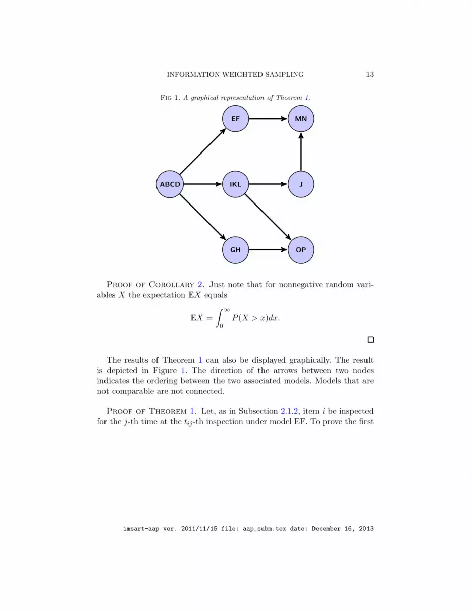
Fig 1. A graphical representation of Theorem 1.

ABCD IKL

EF MN

J

GH OP

Proof of Corollary 2. Just note that for nonnegative random vari-ables X the expectation EX equals

EX =

∫ ∞

0P (X > x)dx.

The results of Theorem 1 can also be displayed graphically. The resultis depicted in Figure 1. The direction of the arrows between two nodesindicates the ordering between the two associated models. Models that arenot comparable are not connected.

Proof of Theorem 1. Let, as in Subsection 2.1.2, item i be inspectedfor the j-th time at the tij-th inspection under model EF. To prove the first



inequality of (3.1) we just note that for any positive integer m

P (NEF ≤ m) =

N∑

i=1

pi

∞∑

j=1

1[tij≤m](1− si)j−1si

=N∑

i=1

pi1[ti1≤m]

∞∑

j=1

1[tij≤m](1− si)j−1si ≤

N∑

i=1

pi1[ti1≤m](3.5)

≤min{m,N}∑

j=1

p(j) = P (NABCD ≤ m)

holds with p(1) ≥ p(2) ≥ · · · ≥ p(N). Note that equalities hold here if and

only if si equals 1 whenever pi is positive, i.e. if and only if∑N

i=1 sipi = 1holds.

Note that under model MN the optimal strategy for model EF as de-scribed in (2.4) and (2.5) cannot be applied since there is no enumeration.This coupling argument shows the second inequality of (3.1), which reducesto an equality if and only if models EF and MN coincide, i.e. for N = 1.

One might call NGH a defective version of NABCD in that inspectionproceeds in exactly the same way, unless because of imperfect recognitionthe Γ-item has not been recognized and hence will never be, in which caseNGH = ∞ holds. This proves the first inequality of (3.2) with equality ifand only if

∑Ni=1 sipi = 1 holds. Similarly, inequality (3.4) and its equality

condition are proved.The first inequality from (3.3) and its condition for equality are proved

in Lemma 3 of the Appendix. Since NGH and NOP are defective versions ofNABCD and NIKL, respectively, this Lemma also proves the second inequal-ity of (3.2) and its equality condition.

Note that under model IKL items that have been checked before, are notchecked again, either because the perfect memory is used or because itemsthat have been checked, are not replaced. Under J these items can still besampled. This coupling argument proves the second inequality from (3.3).Perfect, restricted, or no memory and with or without replacement do notmake a difference here if and only if N = 1.

Finally, the third ordering relation of (3.3) and its equality condition areproved by Lemma 4 of the Appendix.

12 out of the(72

)

= 21 possible pairs of numbers of inspections have beenordered stochastically in (3.1)–(3.4). The other 9 pairs cannot be stochasti-cally ordered, as we will show now. Let B be a Bernoulli random variablewith P (B = 1) = 1 − P (B = 0) =

∑Ni=1 sipi that is independent of all ran-

dom numbers of inspections. Note that NGH has the same distribution as



the defective random variable BNABCD + (1−B)∞. Since inequality (3.1)and the inequalities of (3.3) can be strict, this representation of NGH showsthat it is not comparable to NEF , NIKL, NJ , and NMN stochastically. Byan analogous argument NOP = BNIKL + (1 − B)∞ is not comparable toNJ and NMN .

As Lemma 5 of the Appendix shows, NEF is not comparable to NOP norto NIKL and NJ .

4. Further Explorations.

4.1. Profiling. The interesting question for the models studied here ishow an improvement of the differentiating power of the prior probabilitiespi affects the efficiency. Good discriminatory prior probabilities lead to alimited group of relatively high probability items and a large group of smallprobability items. Obviously the optimal situation across all models is adegenerate prior probability distribution with probability 1 for the Γ-itemand 0 for the other items. The closer one gets to this distribution the better.In practice the prior probabilities consist of probabilities based on availableinformation. Estimating these probabilities using the available informationis often referred to as profiling. The results here open up the possibility totry to balance the costs of collecting additional data in order to improvethe discriminatory power of profiling and the costs of additional inspectionsneeded to find the Γ-item.

4.2. Updating Prior Probabilities. Recall that the random variable Cdenotes the index of the Γ-item. Furthermore, assume information I hascome to the attention of the investigators before the procedure has started.We may update the prior probability pi = P (C = i), using Bayes rule, by

(4.1) P (C = i | I) = P (I |C = i)pi∑N

j=1 P (I |C = j)pj.

4.3. Inspection and Profiling Probabilities. Let us substitute the inspec-tion probabilities from Assumption 10 by the profiling probabilities fromAssumptions 11 and 12 as in (1.1). If we do this in the derived expressionsfor the optimal inspection strategies in (2.20) for model J, we see that theconditional inspection probabilities πi have to satisfy

(4.2) πi =

√pi/λi

∑Nj=1

√pj

N∑

h=1

λhπh , i = 1, . . . , N.



Note that these equations determine the πi up to a constant. Consequently, ifπ1, . . . , πN are optimal, so are cπ1, . . . , cπN for any 0 < c ≤ 1/max1≤j≤N πj.This argument shows that the intensity of actual inspections may be chosenquite freely without influencing NJ or µJ . The same reasoning holds forNMN and µMN .

Finally, we would like to note that (1.1) also shows that if for some i theattention probability λi is relatively high, then the conditional inspectionprobability πi should be chosen relatively small. Consequently, items thatare more likely to come to the attention of the inspectors, like for instancefrequent flyers at airports, should have a smaller probability to be inspected.

4.4. Related and future research. Besides the research of Press [7] thetopic of the present paper has not received much attention yet. In adjacentfields of research more results are available. Our results however are moreor less complementary to these results. Boland et al. [1], [2], [3] in a seriesof papers study stochastic orders of partition and random testing for faultsin software. Some of our models, specifically the models with enumeration,are a limiting case when a partition can contain a single item. Montanaro[6] shows that information about items in an unstructured but enumeratedlist can speed up the search for a single item in quantum search relative toquantum search using no additional information.

Further research should include the situation of an unknown, randomnumber of items with the rare characteristic. These models are highly rel-evant when optimizing security screening applications. The same holds foranalyzing the effects of estimated prior probabilities, or replacing them withconditional probabilities.

5. Examples. To show the relevance and the use of our results we givesome examples and some guidance on how to act in some practical cases. Thegoal is to find the item with the Γ-characteristic as efficiently as possible. Inpractice all kinds of situations can occur and our intention is to choose thebest model to handle the situation. Further applications like fraud detectionetc., are left to the imagination of the reader.

5.1. Example: DNA Screening. In a small village a murder has takenplace. Due to the isolated nature of the village and some other indicationsthe police strongly belief that the murderer is one of the men in the village.The police suggests requesting for a DNA analysis of all these men as therewas DNA found at the scene of the crime. However, DNA analyses taketime and money, and they compromise the privacy of the people involved.So, the strategy should be to take as few DNA samples as possible. What is



the optimal available strategy, assuming that the perpetrator is among themale inhabitants? The police can assign prior probabilities to the men thatindicate how likely it is that they are the murderer. Furthermore, they canalso enumerate the men and order them according to the assigned probabil-ities. So, in this case the best choice is to go for model ABCD, since a DNAmatch might be considered as perfect recognition here.

5.2. Example: Customs. Customs has to check containers transportedby sea for illicit materials like drugs and after 9/11 also for nuclear materials,weapons, explosives, and biological and chemical weapons. Every once anda while customs gets credible information that a container at a certain shipcontains one of these illegal materials. Suppose the ship is carryingN = 5000containers, and that for each of them a risk profile is available so that one canassign prior probabilities pi of containing the illicit material. How to checkthese containers as efficiently as possible? If one could first completely unloadthe ship and set the containers on the dock, then one could use model ABCDif the recognition of the illicit material was perfect. In case of imperfectrecognition one would use model E. If one does not have this possibility, butonly has the possibility to decide whether to check or not when the containerleaves the ship, the preferred model under perfect recognition would be IKL,and model MN otherwise.

5.3. Example: Entrance. The authorities have received information thata certain criminal is trying to escape from the country with a false identityusing a certain plane. How to proceed most efficiently? That is, not disrupt-ing the flight schedule and not aggravating innocent public. In this case ifone assumes that recognition is perfect, one could use model ABCD if onecalls the passengers one by one. Procedures can resume to normal once thecriminal has been found. If one assumes recognition not to be perfect, modelEF could be chosen. Note that everybody has to stay at the gate until thecriminal has been identified, and some individuals will possibly have to beinspected multiple times. Observe that inspecting individuals just as theyenter, i.e. in random order, will be less efficient.

5.4. Example: Robber in Town. Suppose a bank is robbed and the rob-bers get-away car is red. Which model applies? Model J or model IKL? Thedifference? Assuming that every car had an initial probability of being usedfor a robbery, we can now update these prior probabilities using (4.1) toincorporate the information that the car is red. When there is perfect recog-nition one could go for model IKL but more likely for model J. In the caseof stochastic recognition one resides in model MN. The use of model IKL



in practice would need communication and coordination between differentpolicing units.

6. Conclusions. In this paper we introduced a framework of modelsthat can be used to analyze how to find an item of interest in a finitepopulation when the probability of an item of actually being the item ofinterest is assumed known or partially known based on prior information.The results can be used in several ways. First they can give investigatorsand developers of security protocols ideas on how to design the physicalinspections. Secondly they can give a first handle on weighing the costs ofimproving prior information against reduction in costs of more thoroughinspections. Furthermore, the results extend the results of Press [7] in thesense that not only the averages of the numbers of needed inspections forthe different models are ordered but also these random numbers themselves.Finally, for the democratic case of model J our results imply that peopleoften travelling and therefore having a larger probability of coming to theattention of the inspectors should receive a lower conditional probability ofactually getting an inspection according to the optimal inspection strategy.

7. Appendix: Three Lemmata.

Lemma 3. NABCD is stochastically smaller than NIKL, i.e. P (NABCD >m) ≤ P (NIKL > m) holds for all positive integers m, with equality if andonly if p1 = · · · = pN = 1/N holds.

Proof. First consider, with C the index of the Γ-item,

(7.1) P (NIKL > m |C = k) =

N∑

i1=1i1 6=k

fi1

N∑

i2=1i2 6=ki2 6=i1

fi2

N∑

i3=1i3 6=ki3 6=i1i3 6=i2

fi3 · · ·N∑

im=1im 6=kim 6=i1im 6=i2

···im 6=im−1

fim,

with

(7.2) fij =qij

1− qi1 − · · · − qij−1

for j = 2, . . . , N and fi1 = qi1 .



Since the qi’s add up to 1, the last sum in (7.1) equals

(7.3) 1− qk1− qi1 − qi2 − · · · qim−1

.

Addition of (7.1) over k from 1 to ℓ taking into account (7.3) yields

ℓ∑

k=1

P (NIKL > m |C = k)

=N∑

i1=1

N∑

i2=1i2 6=i1

N∑

i3=1i3 6=i1i3 6=i2

· · ·N∑

im−1=1im−1 6=i1im−1 6=i2

···im−1 6=im−2

fi1fi2fi3 · · · fim−1

ℓ∑

k=1k 6=ij

j=1,...,m−1

(

1− qk1− qi1 − qi2 − · · · qim−1

)

,(7.4)

where we have interchanged the summation over k with the summationsover the ij’s. Note that the last sum in (7.4) equals at least(7.5)

ℓ∑

k=1k 6=ij

j=1,...,m−1

1−N∑

k=1k 6=ij

j=1,...,m−1

qk1− qi1 − qi2 − · · · qim−1

≥ ℓ− (m− 1)− 1 = ℓ−m.

Combining (7.4) and (7.5) we obtain

ℓ∑

k=1

P (NIKL > m |C = k)

≥N∑

i1=1

N∑

i2=1i2 6=i1

N∑

i3=1i3 6=i1i3 6=i2

· · ·N∑

im−1=1im−1 6=i1im−1 6=i2

···im−1 6=im−2

fi1fi2fi3 · · · fim−1(ℓ−m)

= ℓ−m.(7.6)

Without loss of generality we may assume that the items in the populationhave been numbered such that

(7.7) p1 ≥ p2 ≥ · · · ≥ pN .



Then, we have

(7.8) P (NABCD > m) =

N∑

k=m+1

P (C = k) =

N∑

k=m+1

pk .

Together with (7.6) and (7.7) this equality yields, with pN+1 = 0,

P (NIKL > m)− P (NABCD > m) =N∑

k=1

{

P (NIKL > m |C = k)− 1[k>m]

}

pk

=

N∑

k=1

N∑

ℓ=k

{

P (NIKL > m |C = k)− 1[k>m]

}

(pℓ − pℓ+1)

=

N∑

ℓ=1

ℓ∑

k=1

(pℓ − pℓ+1){

P (NIKL > m |C = k)− 1[k>m]

}

≥N∑

ℓ=1

(pℓ − pℓ+1)

{

[ℓ−m]+ −ℓ∑

k=1

1[k>m]

}

= 0,(7.9)

where [x]+ equals the maximum of x and 0. Inequality (7.9) proves thestochastic ordering. (7.9) and (7.4)–(7.6) show that NABCD and NIKL havethe same distribution if and only if p1 = · · · = pN holds.

Lemma 4. NJ is stochastically smaller than NMN , i.e. P (NJ ≤ m) ≥P (NMN ≤ m) holds for all positive integers m, with equality if and only if∑N

i=1 sipi = 1 holds.

Proof. We have

P (NJ ≤ m) =

N∑

k=1

P (NJ ≤ m |C = k)P (C = k)

=

N∑

k=1

m∑

ℓ=1

(1− qk)ℓ−1qkpk =

N∑

k=1

1− (1− qk)m

1− (1− qk)qkpk(7.10)

=N∑

k=1

[1− (1− qk)m]pk = 1−

N∑

k=1

(1− qk)mpk .

Similarly, for NMN we have

(7.11) P (NMN ≤ m) = 1−N∑

k=1

(1− skqk)mpk .



This leads to

P (NJ ≤ m)− P (NMN ≤ m) =N∑

k=1

[(1− skqk)m − (1− qk)

m] pk ≥ 0

in view of 0 < sk ≤ 1, which proves the lemma.

Lemma 5. NEF is stochastically not comparable to NOP nor to NIKL

and NJ .

Proof. If both∑N

i−1 sipi = 1 and N > 1 hold and not all pi are equalto 1/N, then Theorem 1 and Corollary 2 imply

(7.12) µEF = µABCD < µIKL < µJ .

However, for N = 1 and s1 < 1 we have

(7.13) µEF =1

s1> 1 = µIKL = µJ .

Inequalities (7.12) and (7.13) show that NEF cannot be stochastically or-dered with respect to NIKL and NJ without additional conditions.

Comparing NEF to NOP we choose

(7.14) pi =2i

N(N + 1), si =

1

i, i = 1, . . . , N.

Now, on the one hand

(7.15) P (NEF < ∞) = 1, P (NOP = ∞) = 1− 2

N + 1

holds and on the other hand (2.5) implies

(7.16) P (NEF = 1) = max1≤j≤N

sjpj =2

N(N + 1)

and the second inequality of (3.3), (7.10), and (2.20) yield

P (NOP = 1) = P (BNIKL + (1−B)∞ = 1)

≥ P (B = 1)P (NJ = 1) = P (B = 1)

N∑

i=1

qipi

=N∑

i=1

sipi

∑Ni=1 pi

√pi

∑Ni=1

√pi

=4

N(N + 1)2

∑Ni=1 i

√i

∑Ni=1

√i.(7.17)



The right hand side of (7.17) is larger than the right hand side of (7.16) ifand only if

(7.18)

∑Ni=1 i

√i

∑Ni=1

√i>

N + 1

2

if and only if

(7.19)N∑

i=1

(

i− N + 1

2

)

(

√i−√

N + 1

2

)

> 0,

which holds for N ≥ 2; Chebyshev’s algebraic inequality. This shows

(7.20) P (NOP = 1) > P (NEF = 1) , N ≥ 2,

which together with (7.15) shows that NEF is stochastically neither largernor smaller than NOP .

Acknowledgements. We thank Cor Veenman and Gert Jacobusse forhelpful discussions.

References.

[1] Boland, P.J., Singh, H., and Cukic, B. (2002), Stochastic orders in partition andrandom testing of software. J. Appl. Probab. 39, 555–565.

[2] Boland, P.J., Singh, H., and Cukic, B. (2003), Comparing partition and randomtesting via majorization and Schur functions. IEEE Trans. Softw. Eng. 29, 88–94.

[3] Boland, P.J., Singh, H., and Cukic, B. (2004), The stochastic precedence orderingwith applications in sampling and testing. J. Appl. Probab. 41, 73–82.

[4] A.J. Hoogstrate & C.A.J. Klaassen (2011). Minimizing the average number of inspec-tions for detecting rare items in finite populations. In N. Memon & D. Zeng (Eds.),European Intelligence and Security Informatics Conference (EISIC), 2011 IEEE Con-ference Proceedings (pp. 203–208). Athens, Greece: IEEEXplore.

[5] X.-L. Meng (2012), Enhanced security checks at airports: minimizing time to detec-tion or probability to escape? Stat 1, 42–52.

[6] A. Montanaro (2010), Quantum search with advice, arXiv:0908.3066v1 [quant-ph].[7] W.H. Press (2009), Strong profiling is not mathematically optimal for discovering

rare malfeasors. Proc Natl Acad Sci USA 106, 1716–1719.[8] W.H. Press (2010), To catch a terrorist: can ethnic profiling work?. Significance 7,

164–167.

Knowledge and Expertise Centre

for Intelligent Data Analysis,

Netherlands Forensic Institute,

Laan van Ypenburg 6,

2497 GB The Hague, The Netherlands,

E-mail: [email protected]

Centre for Terrorism and Counterterrorism,

Campus The Hague, Leiden University,

Kantoren Stichthage,

Koningin Julianaplein 10,

P.O.Box 13228,

2501 EE The Hague, The Netherlands,



mailto:[email protected]



Korteweg-de Vries Institute for Mathematics

University of Amsterdam,

Science Park 904, P.O. Box 94248,

1090 GE Amsterdam, The Netherlands,




Information weighted sampling for detecting rare items in finite populations with a focus on...

Documents

Transcript of Information weighted sampling for detecting rare items in finite populations with a focus on...