INFORMATION TO USERS - ERA - University of Alberta
166
INFORMATION TO USERS This manuscript has been reproduced from the microfilm master. UMI films the text directly from the original or copy submitted. Thus, some thesis and dissertation copies are in typewriter face, while others may be from any type of computer printer. The quality of this reproduction is dependent upon the quality of the copy submitted. Broken or indistinct print, colored or poor quality illustrations and photographs, print bleedthrough, substandard margins, and improper alignment can adversely affect reproduction. In the unlikely event that the author did not send UMI a complete manuscript and there are missing pages, these will be noted. Also, if unauthorized copyright material had to be removed, a note will indicate the deletion. Oversize materials (e.g., maps, drawings, charts) are reproduced by sectioning the original, beginning at the upper left-hand comer and continuing from left to right in equal sections with small overlaps. ProQuest Information and Learning 300 North Zeeb Road, Ann Arbor, Ml 48106-1346 USA 800-521-0600 Reproduced with permission of the copyright owner. Further reproduction prohibited without permission.
-
Upload
khangminh22 -
Category
Documents
-
view
1 -
download
0
Transcript of INFORMATION TO USERS - ERA - University of Alberta

INFORMATION TO USERS
This manuscript has been reproduced from the microfilm master. UMI films
the text directly from the original or copy submitted. Thus, some thesis and
dissertation copies are in typewriter face, while others may be from any type of
computer printer.
The quality of this reproduction is dependent upon the quality o f the
copy submitted. Broken or indistinct print, colored or poor quality illustrations
and photographs, print bleedthrough, substandard margins, and improper
alignment can adversely affect reproduction.
In the unlikely event that the author did not send UMI a complete manuscript
and there are missing pages, these will be noted. Also, if unauthorized
copyright material had to be removed, a note will indicate the deletion.
Oversize materials (e.g., maps, drawings, charts) are reproduced by
sectioning the original, beginning at the upper left-hand comer and continuing
from left to right in equal sections with small overlaps.
ProQuest Information and Learning 300 North Zeeb Road, Ann Arbor, Ml 48106-1346 USA
800-521-0600
Reproduced with permission o f the copyright owner. Further reproduction prohibited w ithout permission.

Reproduced with permission of the copyright owner. Further reproduction prohibited without permission.

University o f Alberta
M A T H E M A T IC A L M O D ELIN G OF L E U K E M IA A N D TU M O R TREATM ENTUSING C O M PETITIO N THEORY
by
Wenxiang L iu
A thesis submitted to the Faculty of Graduate Studies and Research in partial fulfillment o f the requirements for the degree o f Doctor o f Philosophy
in
Applied Mathematics
Department o f Mathematical & Statistical Sciences
Edmonton, Alberta Fall 2005
Reproduced with permission o f the copyright owner. Further reproduction prohibited w ithout permission.

Library and Archives Canada
Published Heritage Branch
395 Wellington Street Ottawa ON K1A 0N4 Canada
Bibliotheque et Archives Canada
Direction du Patrimoine de I'edition
395, rue Wellington Ottawa ON K1A 0N4 Canada
0-494-08682-3
Your file Votre reference ISBN:Our file Notre reference ISBN:
NOTICE:The author has granted a nonexclusive license allowing Library and Archives Canada to reproduce, publish, archive, preserve, conserve, communicate to the public by telecommunication or on the Internet, loan, distribute and sell theses worldwide, for commercial or noncommercial purposes, in microform, paper, electronic and/or any other formats.
AVIS:L'auteur a accorde une licence non. exclusive permettant a la Bibliotheque et Archives Canada de reproduire, publier, archiver, sauvegarder, conserver, transmettre au public par telecommunication ou par ('Internet, preter, distribuer et vendre des theses partout dans le monde, a des fins commerciales ou autres, sur support microforme, papier, electronique et/ou autres formats.
The author retains copyright ownership and moral rights in this thesis. Neither the thesis nor substantial extracts from it may be printed or otherwise reproduced without the author's permission.
L'auteur conserve la propriete du droit d’auteur et des droits moraux qui protege cette these.Ni la these ni des extraits substantiels de celle-ci ne doivent etre imprimes ou autrement reproduits sans son autorisation.
In compliance with the Canadian Privacy Act some supporting forms may have been removed from this thesis.
While these forms may be included in the document page count, their removal does not represent any loss of content from the thesis.
Conformement a la loi canadienne sur la protection de la vie privee, quelques formulaires secondaires ont ete enleves de cette these.
Bien que ces formulaires aient inclus dans la pagination, il n'y aura aucun contenu manquant.
CanadaReproduced with permission o f the copyright owner. Further reproduction prohibited w ithout permission.
This thesis is dedicated to Herb I. Freedman
with whom I had the good fortune to study on my doctorate program, who epitomized research, learning and scholarship, who instilled both the excitement and integrity of the research process, and who unselfishly promoted the scholarship of his
students.
Reproduced with permission of the copyright owner. Further reproduction prohibited w ithout permission.

Abstract
This thesis deals with some mathematical models concerning the treatment of leukemia
and tumors, respectively. The thesis comprises five chapters, the first o f which is an
introductory chapter, and the remaining four each contain a model for either leukemia
or tumor treatment. The proposed models are analyzed for their stabilities and dynamical
behaviors, both analytically and numerically, with biological interpretations.
In chapter two, from the viewpoint o f biological stoichiometry, a mathematical model of
vascular tumor treatment with chemotherapy techniques is proposed utilizing a system of
delayed differential equations. Sufficient criteria are obtained for the uniform persistence
of populations and the extinction of cancer cells. Conditions for the global stabilities
o f the cancer-free equilibrium and the interior equilibrium are obtained. Necessary and
sufficient conditions for Hopf bifurcation to occur is also obtained by using the time delay
as a bifurcation parameter.
Chapter three utilizes a logistic growth model to construct the cancer interactions with
healthy tissue as a competition process and then extends to the diffusion case to model
the spread o f cancer within a site such as leukemia in the bone marrow. The existence,
uniqueness, and boundedness o f the solutions are established by means of a comparison
principle and a monotonicity method. Persistence criteria for the normal cells and cancer
cells are also derived.
With respect to the dynamical progression o f chronic myeloid leukemia, chapter
four utilizes a logistic-like growth model with self-regulated properties to construct the
cytokinetics of cancer and normal cells as a competition process. The stabilities for the
complicated system with one or two delays are fu lly analyzed and necessary and sufficient
conditions for stability switches to occur are obtained.
Reproduced w ith permission o f the copyright owner. Further reproduction prohibited w ithout permission.
Finally, this thesis studies the cycle-specificity o f chemotherapy to the G0 model.
Stabilities of cancer-free equilibria are fully analyzed and conditions for stability switching
and its biological implications are given. Also, necessary and sufficient conditions for Hopf
bifurcation to occur are derived by using the time delay as a bifurcation parameter.
The mathematical techniques involved in the thesis include competition theory,
persistence theory, comparison theory, dissipativity theory, spectrum theory, bifurcation
theory and the complex analysis residual theory.
Reproduced with permission o f the copyright owner. Further reproduction prohibited w ithout permission.

Acknowledgements
First o f all, I would like to express my deep gratitude to my supervisor, Professor Herb I.
Freedman, for his invaluable advice, consistent encouragement and kind assistance since
I first met him by email in China in May, 2001. As a successful educator and a great
father, he lets me understand and learn how to be confident with research work and life.
With careful attention to detail, he gives me every chance to try new things and allow me
freedom to follow my own pursuits in independent study. Under his careful cultivation, my
understanding and abilities would reach a higher level each time after we finished a project
together. I really benefit a lot from his kind guidance and gentle nudging. A word at this
moment is always helpless to express all my gratitude to him during these wonderful four
years I worked with him. His interest and support were instrumental in the process that led
to this final product. I deeply appreciate his invaluable self-giving dedication.
Second, I am grateful to the members o f my dissertation committee, Dr. Gerda de Vries,
Dr. Phil Gordon, Dr. Thomas Hillen and Dr. Joseph So for their role in the completion of
this dissertation. A special thank you goes to Dr. Yang Kuang for taking time out o f his
busy schedules to review and assist with this project.
Finally, my sincere appreciation is extended to the Mathematical & Statistical
Department and the Faculty o f Graduate Studies and Research. This work could not have
been done without their generous financial support. To both bodies, may 1 express my deep
gratitude.
Reproduced with permission o f the copyright owner. Further reproduction prohibited w ithout permission.

Contents
1 Introduction 2
1.1 Mathematical modeling and cancer tre a tm e n t................................................ 2
1.2 Cancer: tumor & leukemogenesis ................................................................... 4
1.3 Mathematical preliminaries: basic definitions and standard theorems . . . . 6
1.3.1 Definitions of basic concepts................................................................ 6
1.3.2 Standard theo rem s............................................................................... 10
1.4 Outline o f thesis................................................................................................... 15
2 A Mathematical Model of Vascular Tumor Treatment by Chemotherapy 17
2.1 Introduction ......................................................................................................... 17
2.2 The m ode l............................................................................................................ 19
2.3 The no treatment case ....................................................................................... 23
2.3.1 Asymptotic behavior and Hopf b ifu rca tio n ...................................... 23
2.4 The continuous treatment c a s e .......................................................................... 39
2.4.1 E q u ilib r ia ............................................................................................... 39
2.4.2 Local stability ...................................................................................... 42
2.4.3 Global s ta b il ity ...................................................................................... 45
2.5 Discussion............................................................................................................ 51
3 A Reaction-Diffusion Model of Leukemia Treatment by Chemotherapy 54
3.1 Introduction ......................................................................................................... 54
3.2 The m ode l............................................................................................................ 56
3.3 The no diffusion ca se .......................................................................................... 58
Reproduced with permission o f the copyright owner. Further reproduction prohibited w ithout permission.

3.3.1 The homogeneous steady s ta tes ........................................................... 59
3.3.2 Local s ta b il i ty ........................................................................................... 61
3.4 The diffusion case................................................................................................. 68
3.4.1 Prelim inaries...............................................................................................68
3.4.2 The analysis of ^o (0 ,0 , ^ _1 A ) .................................................................75
3.4.3 The analysis o f E\ {u\, 0, v ) ..................................................................... 76
3.4.4 The analysis o f £ 2(0, ^ 2, v ) ................................................................. 78
3.5 Numerical re su lts ............................................................................................... 79
3.6 Discussion............................................................................................................ 83
4 A Mathematical Model of Chemotherapy Treatment with Chronic Myeloid
Leukemia 85
4.1 Introduction ......................................................................................................... 85
4.2 The m ode l............................................................................................................ 89
4.3 The no treatment case.............................................................................................94
4.3.1 Linear s ta b il ity ....................................................................................... 95
4.4 The continuous treatment c a s e ............................................................................103
4.5 Numerical examples ........................................................................................... 110
4.5.1 An example without chemotherapy trea tm en t......................................110
4.5.2 An example with chemotherapy treatm ent............................................ I l l
4.6 Discussion............................................................................................................116
5 A Cancer Treatment of Cycle-Specific Chemotherapy to the G0 Model 118
5.1 Introduction........................................................................................................... 118
5.2 The m ode l.............................................................................................................. 122
5.3 Nondimensionalization........................................................................................ 123
5.4 Stability resu lts .................................................................................................... 124
5.4.1 Drug-free model in a non-delay case in the absence o f an immune
response.................................................................................................... 124
5.4.2 Drug-free model when r > 0 in the absence o f an immune response 126
5.4.3 Drug-free model in a non-delay case with immune suppression . . 129
Reproduced w ith permission of the copyright owner. Further reproduction prohibited w ithout permission.
1
5.4.4 Drug-free model when r > 0 with immune suppression...................131
5.4.5 Drug model in a non-delay case with immune suppression 134
5.4.6 Drug model when r > 0 with immune suppression............................ 136
5.5 Hopf bifurcation......................................................................................................138
5.6 Numerical re su lts .................................................................................................. 141
5.7 Discussion...............................................................................................................142
Reproduced with permission o f the copyright owner. Further reproduction prohibited w ithout permission.

Introduction
1.1 Mathematical modeling and cancer treatment
A ll organs of the body are made up o f cells. Bio-medically, each tissue in a person can
be defined as a cellular configuration o f matter, endowed with a unique morphologic,
pathologic, genetic and physiologic parametric configuration. This dynamic parametric
configuration represents the state o f health and well being o f a person. The number and
type of cells in each tissue is highly regulated. However, when this regulatory balance is
altered, a variety of diseases, including cancer, can develop.
Cancers threaten an individual’s life when their growth disrupts the tissues and organs
needed for survival. Basically, there are four major types o f cancer treatments used in an
effort to obtain long-term periods o f disease-free remission. The treatment types include
surgery, radiation therapy, chemotherapy, and immunotherapy. These therapies can be used
either alone or in combination with each other. Depending on location, size and stage of
the tumor, as well as individual overall health, a treatment or treatments w ill be chosen to
treat a cancer patient. Surgery is the oldest form o f cancer treatment and only treats one
particular part of the body. Therefore, people whose cancer has spread to another part of
their body will not always be offered a surgery. Radiation therapy involves using large
2
Reproduced with permission o f the copyright owner. Further reproduction prohibited w ithout permission.

Sec. 1.1 Mathematical modeling and cancer treatment 3
doses of high-energy beams or particles to destroy cancer cells in a specifically targeted
area. Most commonly, localized solid tumors, leukemia and lymphoma are treated by
radiotherapy; for some, it w ill be the only cancer treatment they need, but often, radiation
is used in combination with other treatments, in which radiation shrinks the tumor to make
surgery or chemotherapy more effective. Chemotherapy involves utilizing powerful drugs
to destroy cancer cells and inhibit their growth. Chemotherapy might involve one drug,
or a combination o f two or more drugs, depending on the type o f cancer and its rate of
progression. In order to improve the treatment o f cancer, chemotherapy might be used in
combination with other treatments such as surgery or radiation, to make sure all cancer
cells have been eliminated. Immunotherapy is body’s own natural defenses to fight cancer
and works as the body’s first line o f defense against disease. Generally, white blood cells in
the body can be stimulated in several ways to boost the body’s immune response to cancer,
with little or no effect on healthy tissue. Also, immunotherapy can be used to lessen the
side effects o f other cancer treatments. A ll in all, with the exception of surgery, which relies
mostly on the accuracy of x-rays and other imaging techniques, the other treatments such
as chemotherapy and immunotherapy mainly depend on accurate staging of the tumor, the
dynamical properties o f the tumor, the optimal administration o f the anti-cancer drugs, and
the kinetic interactions among tumor, host and drug.
Clinically, it is observed that every pathological process, including carcinogenesis,
possesses a time evolution profile. Thus, i f the kinetic parameters characterizing a
pathological process such as cancer can be determined accurately, it w ill be possible to
establish quantitative therapeutic criteria depicting the prognosis or outcome of therapy.
When applying therapy, it may disturb and alter the initial pathological parametric
configuration o f the cancer cells. Under such situations, it may be prudent to use
mathematical modeling and analysis to ( 1) make quantitative predictions regarding the
dynamic evolution o f the disease and the region of therapeutic efficacy, and (2) provide
a more rational basis for the design of a drug protocol based on the mathematical relation
between the dynamical variables involved in the progression o f disease, and finally (3)
determine the general prognosis of the cancer based on the initial data and the clinical
parametric configuration of the cancer patient and the pharmacodynamics of the anti-cancer
Reproduced with permission o f the copyright owner. Further reproduction prohibited w ithout permission.

Sec. 1.2 Cancer: tumor & leukemogenesis 4
drug. In short, mathematical models based on biological principles serve to define critical
underlying dynamics and interactions in the complex systems and predict the results of
system perturbations through therapy.
Now with the advent o f modern experimental equipment and the desire to obtain
quantitative therapeutic criteria, computerized mathematical modeling has become an
important part o f clinical cancer research. The use o f computer simulations helps many
physicians design the safest and most efficient treatments in terms o f drug and schedule
choices. The simulations allow both the mathematicians and the medical oncologists to
observe model behavior graphically. In particular, the simulations o f pharmacodynamics
models quantifying drug effects on several target tissues allow physicians to observe
the short/long-term cellular dynamics of specific patients undergoing drug therapy, and
provide them efficient treatments such as per-case choice of drug, drug combinations
and schedules to achieve clinically desired end-points. Mathematical models could
be deterministic or stochastic. Basically, the two approaches describe the same basic
dynamics. Stochastic modeling is used i f there is randomness or uncertainty about the
evolutionary process. But i f there is abundance of experimental kinetic data and established
physiological pathways and mechanisms on a given pathological process, it is possible
to use deterministic modeling techniques. In this thesis, deterministic modeling w ill be
used to describe cancer chemotherapy and immunotherapy and simulate the models under
various parametric configurations and finally completely predict the output of the models
i f the input parameters and initial states o f the model are given.
1.2 Cancer: tumor & leukemogenesis
In simple terms, cancer is a group of more than 100 diseases that develop across time and
involve the uncontrolled growth regulatory mechanisms o f the body.
Cancerous tumor growth can be considered as having an avascular phase and a vascular
phase. During the avascular phase, the tumor is of such a size that the surface to volume
ratio o f the spheroid is adequate for diffusion of nutrients and oxygen, and consequently
there is a rapid exponential growth. During the later stages o f avascular growth, the tumor
growth decelerates and at a certain critical cell number, the growth levels o ff into a plateau
Reproduced with permission o f the copyright owner. Further reproduction prohibited w ithout permission.

Sec. 1.2 Cancer: tum or & leukemogenesis 5
as cellular proliferation ia balanced by cell death, and necrosis due to lack o f oxygen and
nutrients[102]. A state dormancy occurs unless the tumor acquires new blood vessels by
a process called vascularization and tumor angiogenesis. Tumor angiogenesis enables an
aggregate of tumor cells to expand beyond the maximal three dimensional size restraints
imposed by space, nutrients and oxygen diffusion requirements. The primary tumor may
then metastasize into other organs o f the human anatomy forming secondary tumors. After
neo-vascularization the primary tumor may again undergo exponential growth unless it
encounters limitations. Thus realistic tumor growth may be a cascade o f exponential
growths interspaced with deceleratory periods or dormant growth. However many other
realistic growth scenarios are possible such as modeled by Goldman et al[44]. But generally
logistic growth or Gompertz tumor growth profiles are the most frequently used models to
depict tumor growth.
Leukemia is a cancer o f blood cells that originates in the bone marrow, the soft, spongy
inner portion o f certain bones. The cancerous cells in leukemia are the white blood cells
(leukocytes). When a blood cell undergoes a bio-transformation into a malignant cell,
leukemia begins to develop, in which the malignant cells begin to multiply in the marrow,
and as they do so they crowd out the normal blood cells - those that carry oxygen to the
body’s tissues, fight infections, and help wounds heal by clotting the blood [49]. Leukemia
can also spread from the marrow to other parts o f the body, including the lymph nodes,
brain, liver, and spleen.
Blood-cells develop from stem cells in the bone marrow. These primitive cells are
capable o f developing into any kind o f blood cell. Each o f these types of cells has a very
specific job in the functioning o f the body.
A malignant transformation can happen at any stage o f blood cell development. When
leukemia cells result from the transformation, they carry many characteristics of the cell
from which they began. Most leukemia arc either myelogenous leukemia or lymphocytic
leukemia [49|. Physicians also classify leukemia according to whether they are acute or
chronic. In acute leukemia, the malignant cells are blasts that remain very immature and
incapable of performing their immune system functions. The onset o f acute leukemia is
rapid and the number of blasts increases rapidly. Chronic leukemia develop in more mature
Reproduced with permission o f the copyright owner. Further reproduction prohibited w ithout permission.
Sec. 1.3 M athematical preliminaries: basic definitions and standard theorems 6
cells, which can perform some o f their functions but not well. These abnormal cells may
increase at a slower rate than in acute leukemia. As a result, the disease gets worse more
slowly than in acute leukemia.
Researchers have noticed an increasing proportion of younger patients with chronic
myelogenous leukemia (CML) in recent years. Treatment approaches for adult leukemia
may include chemotherapy and immunotherapy. Radiation therapy is sometimes used for
leukemia in the central nervous system ( see [49] for more information about leukemia).
1.3 Mathematical preliminaries: basic definitions and standard theorems
In this section of the introduction we w ill list all useful basic definitions and standard
theorems which w ill be encountered in the forthcoming chapters.
1.3.1 Definitions of basic concepts
In this subsection we present the definitions of some basic concepts and parameters which
w ill later be used in theorems or proofs o f theorems in the forthcoming chapters.
Definition 1: Acyclicity [13 ]
Consider the system
x (t) = F (x) (1.1)
x { t0) Xo ,
where x0 G $tn+, F e C (^ ,5 R n), = {x G 3ln|x< > 0,1 < i < ?i} and »!* = Cm n+
denotes the closure of 5R".
Let M \ and M 2 be any isolated invariant sets on the boundary o f Sft” , denoted by 93?".
Let 7 (3;) denote the orbit o f a point x G 93?" such that
ct'(x) = M i, u(x) = M 2,
respectively the alpha and omega lim it sets of x.
Then M \ is said to be connected or chained to M 2. This is depicted symbolically by
A! 1 —> Mo.
Reproduced with permission o f the copyright owner. Further reproduction prohibited w ithout permission.

Sec. 1.3 M athematical preliminaries: basic definitions and standard theorems 7
A finite sequence M i, M 2, ■ ■ • , M* o f isolated invariant sets o f (1.1) w ill be called a chain
if
M i —> M 2 —> • • • —> M k{M \ —* M i , i f k = 1).
The chain w ill be called a cycle i f M * = M i. I f the dynamics are such that there are no
cycles, system (1.1) is said to be acyclic.
Definition 2: Dissipcitivity [13,40]
Consider system (1.1) and let
x(t) = {S i(f)}?=1.
Then the system describing the evolution o f x (t) is called dissipative i f
lim sup ||x(f)|| < L,l —>co
where L is a positive constant. In particular, it implies that the trajectories o f the system are
asymptotically bounded. In other words, there is a compact neighborhood B e t " such
that for sufficiently large T = T ( t0, xq)
x (t) € B, t > T,
where x (t) is any solution o f system ( 1.1) such that x (t0) = x0 in 5ft+.
For dissipative systems, the existence o f an equilibrium in the interior o f 5ft", denoted by
intS i” , is a consequence o f uniform persistence [12,13].
Definition 3: Hyperbolicity [12,13]
Let E (x 0) € 5ft+ such that F (E (x 0)) = 0 for system ( 1.1). Then E(xo) is a critical point
of system ( 1.1).
The linearization o f (1.1) in the neighborhood of E (x 0) gives the equation
y(t) = D F (E (x 0))y ( 1.2)
y(to) = yo, y e 5ft",
where Je(xu) = D F {E [x 0)) is the Jacobian matrix of the linearization via a Taylor
expression around E ( x q ) . In particular, Je(xq) *s defined asr 0 f, (x) dF\ (x) -I
dx\ 3x„
dFn(x) dFu(x)dx\ dx„
Reproduced with permission o f the copyright owner. Further reproduction prohibited w ithout permission.

Sec. 1.3 Mathematical preliminaries: basic definitions and standard theorems 8
The eigenvalues o f Je {Xo) are defined by the set
° { J e(x0)) = {A|det(JE{xo) - XI) = 0}.
The critical point E (x o) or periodic orbit x = ip(t) is called hyperbolic respectively i f the
eigenvalues corresponding to JE{xa)) or the Floquet exponents for ip(t) are such that they
have nonzero real parts. Furthermore, let cr( J£(lo)) contain n eigenvalues. Then:
( 1) E (x 0) is a hyperbolic saddlepoint i f there exist some A, € o {J E{XQ)) with Re A* > 0
and also some Aj € a(JE X0)) such that ReXj < 0, for i, j e {1 ,2 , ...,n }, but there exist
no Xk such that ReXk = 0.
(2) E (x 0) is a hyperbolic sink i f for all A,- e a {J E(Xo)) we have Re A, < 0, i — 1, 2, ...n.
(3) E (x 0) is a hyperbolic source i f for all Xt 6 <?{JE(X0)), we have Re A, > 0,
i = 1, 2,..., n.
Definition 4: Isolatedness [30]
Consider system (1.1) and let F (x ) be analytic and let-E^a;,) for i 6 {0,1, ..,n } denote
the critical points o f (1.1). E q ( x q ) is said to be isolated i f the Jacobian matrix due to
linearization o f system ( 1.1) in the neighborhood o f E0{x0), denoted by JE„[X0) is such that
•hi{xo) is non-singular.
In the results presented in the forthcoming chapters, isolatedness and acyclicity w ill
be guaranteed by the hyperbolicity and global asymptotical stability requirements for the
critical points in their respective two or three dimensional subspaces.
Definition 5: Persistence [12,13,31,36]
Consider system (1.1) and let
x (t) = { x j ( 0 KU -
Then x,j(t) is said to be persistent i f
X i ( t ) > 0 , t > 0, l im in fz f( f ) > 0.t—‘00
Further, the persistence is said to be uniform, i f
35 > 0, 3 lim in f x ,( i) > 6,t—OO
independent o f initial conditions x, (0).
Reproduced with permission o f the copyright owner. Further reproduction prohibited w ithout permission.
Sec. 1.3 Mathematical preliminaries: basic definitions and standard theorems 9
System (1.1) is said to be (uniformly) persistent i f each component x,, i = 1,2, ,.,n is
(uniformly) persistent.
In particular, persistence o f system (1.1) corresponds to global survival o f all x,-,
i = 1, 2, . . , n, non-persistence corresponds to local extinction o f at least one component.
Definition 6: Permanence [58 ]
System (1.1) is said to be permanent i f there exists a compact region f i0 € mflR" such
that every solution o f system ( 1.1) with nonnegative initial conditions w ill eventually enter
and remain in region f l0-
Clearly, for a dissipative system uniform persistence is equivalent to permanence.
Definition 7: Liapunov functions and negative definiteness[5,39,61,91 ]
Consider system (1.1) such that
F : C(SR") — ft".
Let D be any neighborhood in Then V is a Liapunov function for system (1.1) on D i f
( 1) V £ C l (D ) and bounded below,
(2) K (x ) = 0. where F (x ) = 0, and x is in the interior of D ,
(3) there exists an (5 > 0 such that V'(x) > 0 whenever x e Ds(x ) \x , where
F j( I ') — {x £ D : ||x — x|| < J}.
(4) V’ (x) < 0 along the solution trajectories of system ( 1.1), x G D \ {x } ,
(5) K (x) — oo i f either ||x|| — oo, or x —■- 0D.
Remarks
(i) The requirements (2) and (3) of D cfin tio n 7 imply that V is positive definite.
(ii) For global asymptotic stability, we require V’ (x) < 0.
( iii) I f V and — V are positive definite with respect to x, then x is globally asymptotically
stable.
Now, assume V can he written in the form of
V X ' AX < .-LY..Y >.
where A' (X| - x j /•„ - x .^ .a n d .4(x.x) isa n x n symmetric matrix over!)?, given
Reproduced with permission o f the copyright owner. Further reproduction prohibited w ithout permission.

Sec. 1.3 M athematical preliminaries: basic definitions and standard theorems 10
by the expression
A(x, x ) =an . . . aln
Cln 1 • • • On71
Let Dk denote the sequence of leading principal minors of the matrix A(x, x). In particular,
D i — a n , £>2 — an a i2 021 «22
Oil fl12 Ol3 an ■ d\n
£>3 = 021 &22 fl23 , ..., D n =_ O31 032 033 &n\ •
Theorem 1.3.1 The quadratic form A (x ,x ) and consequently, V = X T A X is negative
definite i f and only i f the following inequalities hold:
A < 0, Do > 0, D 3 < 0, ..., ( -1 )nD n > 0.
Theorem 1.3.2 A necessary and sufficient condition fo r the quadratic form A (x ,x ) to be
negative definite is that a ll the characteristic roots (eigenvalues) o f A(x, x) are negative or
have negative real parts.
1.3.2 Standard theorems
Bendixon 's Negative Criterion/ Bendixon-du Lac [11]
Theorem 1.3.3 Consider the system
x j( t ) = F f x i , x 2)
x i( t ) = F2(x u x2)
on a simply connected domain D C K 2. Suppose:
(1.3)
(i) F \ ,F 2 6 C 1 (D , 3?) such that F \ , F2 have continuous first partial derivatives
on D.
(ii) 1^- + does not change sign on D, and does not vanish identically in any open
subset o f D.
Then there are no nontrivial closed paths (periodic solutions, lim it cycles) in D.
Reproduced with permission of the copyright owner. Further reproduction prohibited without permission.

Sec. 1.3 M athematical preliminaries: basic definitions and standard theorems 11
Theorem 1.3.4 Suppose that,
(i) 3 B (x l ,x 2) e C f D , R ) ,
(H) j ~ [ F i ( x u x 2 ) B ( x u x 2 )} + ■ ^ [ F 2 ( x u x 2 ) B ( x i , X 2 )} does not change sign orvanish
identically on any open subset o f the simply connected domain D.
Then there are no closed paths lying entirely in D.
(Hi) I f E is an annular region contained in D on which ( ii) does not change sign, then
there is at most one lim it cycle in E.
Floc/uet Multipliers Theory [83 ]
Consider the non-autonomous system
x (t) = F (t, x)
x(to) = x0
F ( t + u ,x ) — F ( t ,x ) , (1.4)
where F £ C'1(1R+ x 3?", 5?n), 3?+ = [0, oo), and x ,x 0 € 3Jn.
Let f ..., <j>n{t)) be a given periodic orbit or lim it cycle o f (1.4). Let the
Jacobian matrix of linearization o f (1.4) about ijj be given by
J* = D F ( f ) =
m n m i „
m n i . . . mn= : M (t)
such that is locally integrable.
The Floquet exponents are the eigenvalues o f X (u ) where X ( t) solves
X ( t ) = M { t)X { t) , X {0 ) = I ,
where
* (0 =
A'n • • • A 'ln
A „ i • • • X nn
In general this is a tedious computation and sometimes only estimates are possible, unless
the matrix and consequently X (t ) has some zeros.
Reproduced with permission of the copyright owner. Further reproduction prohibited without permission.

Sec. 1.3 M athematical preliminaries: basic definitions and standard theorems 12
Theorem 1.3.5
x (t) = A (t)x (1.5)
x(to) = zo,
where A (t) = is a locally integrable n x n matrix such that A (t + u ) = A(t). let pi
denote the i l h Floquent multiplier. Then:
(i) A ll solutions x (t) o f (1.5) satisfy x (t) —* 0 as t —► oo i f \p,\ < 1, i = 1, 2,..., n, in
which case x = >p(t) is asymptotically stable in the sense o f Liapunov.
(ii) Some solution o f (1.5) is a nontrivial u-periodic solution i f and only i f p, = 1 fo r
some i € { 1, 2,..., n}.
(Hi) I f however, \pj\ > 1 fo r some j € { 1, 2, ...,n }, then x = i/>(£) is unstable.
Hopf-Andronov-Poincare Bifurcation Theorem [30]
Theorem 1.3.6 Let
x (t) = F (x ,p ) (1.6)
x ( tQ) — x 0,
where p is a bifurcation parameter, x E 5Rn, / i e 91, and F 6 C r (5K" x (K, 5R'!). Suppose:
(i) F 6 C r , r > 2 on some sufficiently large open set D containing the equilibrium,
(a:, /./) = (xq, f iQ) = E,ln, where xo is an isolated critical point o f F (x , p).
( ii) F (x ,p ) = 0 fo r some cur\>e x = x (p ) with x(p ) € N (x a, po), a neighborhood o f
(xQ, p Q) on D.
( iii) The Jacobian matrix dn = D xF {x 0, p 0) has a pa ir o f complex conjugate
eigenvalues A and A such that
A(p) = a (p ) + i(3{p), A(p) G C r ,
where
1. f i(p o ) > 0,
2. a ( / /o) = 0,
3. jTRc\(p,n) = c\'(po) f 0 (transversality criterion) where is asymptotically
stable.
Reproduced with permission of the copyright owner. Further reproduction prohibited without permission.

Sec. 1.3 Mathematical preliminaries: basic definitions and standard theorems 13
(iv) The remaining n — 2 eigenvalues o f = D xF ( xq, po) have nonzero (preferably
negative) real parts.
Then Eft=lil) = (x0, p0) is a bifurcation point o f the equilibrium, x = x0, leading to a
lim it cycle fo r some small values o f p ^ po. I f p > p Q the bifurcation is supercritical and
i f p. < po, then the bifurcation is subcritical. I f the bifurcation is a ll at p = p0, there is
a center around x = xq and infinitely many neutrally stable concentric closed(periodic)
orbits surrounding x = x0.
The Implicit Function Theorem [89,91 ]
Theorem 1.3.7 suppose that U C tfl'1 x 5Rm is an open set and F : U —> 3Rm is a Cr
function fo r some r > 1. Represent a point p € U by p(x, y) with x £ -ft" and y € 5Rm
and the coordinate functions o f F by f , i.e. F = ( f u f 2, ..., f m). Assume that fo r some
i x o, !Jo) € U
( {x 0, y a ) ) l < i , j < r n Ol j j
is an invertible rn x m matrix. Let C — F (x 0, y0) e 5Rm. Then there is an open set V
containing x0, and an open set W containing y0 with V x W C U, and a C r function
h : V —► W such that
h(xo) = i/o, F(x, h (x )) = C, x G V.
Furthermore, fo r each x € V, h(x) is the unique y 6 W such that F (x , y) = C.
The Poincare-Bendixson Theorem [83]
Theorem 1.3.8 Consider the system
x(t) = f ( x ),
where, x e 5R2, / € C 1 (‘l i2,-R2).
Let M be a positively invariant region fo r the vector fie ld o f the system, containing a
fin ite number o f fixed points. Let p € M and consider the uj-limit set o f p denoted by u>(p).
Then one o f the following possibilities holds:
I) u>(p) is a fixed point (critical equilibrium point).
Reproduced with permission o f the copyright owner. Further reproduction prohibited w ithout permission.

Sec. 1.3 M athematical preliminaries: basic definitions and standard theorems 14
2) u(p) is a closed orbit.
3) cj(p) consists o f a fin ite number o f fixed points p \ , ...,pn and orbits 7 with the alpha
lim it set and omega lim it set o f 7 being such that a (7) = pt and uj(7) = pj.
In particular, i f M contains no fixed points, then it contains a lim it cycle.
The Routh-Hurwitz Criterion [3,26]
Consider the autonomous system
x (t) = F (x ), (1.7)
where x 6 F € C(5?n, 3?n). Let A = D F (E (x 0)) be the n x n matrix o f linearization
o f the system around the fixed point E (x 0), leading to the system
y(t) = Ay, 2/(0) = y0.
Consider the characteristic polynomial equation p{A, A) — 0 where
p {\ , A ) = det(A — XI)
Define n matrices as follows
Hi = a\, H<i
n + 01 An' + aoX71' ‘2 + • • + an.
1ai 1 0 '
Oi II a-3 a-2 Ol. 03 a2 . 05 a. 1 a.3
H , =
a\
an
10-2a.,
0aia3
0
a2
ak
ai 1 0 . . 0
II a3 a2 a! . . 0
0 0 0 . • ana 2k- 1 0,2k-2 a 2k- 3 a2fc-4 • ■
where the ( i , j ) term in the matrix H * is
1) a2i - j for 0 < 2i — j < n,
2) 1 for 2 i — j = 0,
3) 0 for 2i < j or 2i > n + j .
Theorem 1.3.9 The eigenvalues o f (1.7) have negative real parts and consequently, the
equilibrium E (x 0) is locally asymptotically stable i f and only i f
det(H j) > 0, (j = 1 ,2 ,...,/:).
Reproduced with permission o f the copyright owner. Further reproduction prohibited w ithout permission.

Sec. 1.4 Outline of thesis 15
In particular fo r n = 2,3,4 the criteria reduce to:
n = 2: a\ > 0, a? > 0.
n = 3: a\ > 0 , , <13 > 0 , a iao > a3.
n = 4 : a\ > 0 , (13 > 0 , a4 > 0 , aiOoa3 > <23 + a ja 4.
1.4 Outline of thesis
The thesis w ill consist o f five chapters in total. Following this introductory chapter w ill
be four chapters, each containing a class o f models to simulate certain specific or general
cancers, including tumor growth and leukemia, together with treatment by chemotherapy.
The idea in modeling w ill be to consider cancer and healthy cells as competing populations
for the bodily resources, and the chemotherapy as acting like a predator on both.
From the viewpoint o f biological stoichiometry, Chapter 2 deals with vascular tumor
growth and its treatment with chemotherapy techniques. Sufficient criteria are obtained
for the uniform persistence o f populations and the extinction of cancer cells. Conditions
for the global stabilities of the cancer-free equilibrium and the interior equilibrium are
obtained. Necessary and sufficient conditions for Hopf bifurcation to occur is also obtained
by using the time delay as a bifurcation parameter. By so doing, we hope to identify criteria
involving combinations of parameters which yield the eradication of the cancer cells or at
least the existence of Hopf bifurcation with stable lim it cycles or o f permanence, which
means in either case that the normal cells w ill persist at some level.
Chapter 3 utilizes a special case (logistic) of the model developed in [75] to study the
cytokinetics of cancer and normal cells under chemotherapy, and extends it to the diffusion
case to model the spread of cancer within a site (such as leukemia in the bone marrow).
The existence, uniqueness, and boundedness of the solutions are established by means of
a comparison principle and a monotonicity method. Persistence criteria for the normal
cells and cancer cells are also derived. Here our results may be interpreted as to a general
chemotherapeutic treatment o f leukemia, with a view to identifying parametric relations
for control of leukemia growth.
In chapter 4, a generalized mathematical model is proposed to give a plausible
explanation of events that lead to the progression o f chronic myeloid leukemia to blast
Reproduced with permission o f the copyright owner. Further reproduction prohibited w ithout permission.

Sec. 1.4 Outline o f thesis 16
crisis. The stabilities for the complicated system with one or two delays are fu lly analyzed
and necessary and sufficient conditions for stability switches to occur are obtained. When
the system remain stable, this corresponds to preservation at some level o f both cancer
and healthy cells. However, when stability switches occur, this could indicate switching
between remission and cancer growth.
Finally, Chapter 5 studies the cycle-specificity of chemotherapy techniques utilizing a
system o f delayed differential equations to take into account the phases o f the cell cycle.
Stabilities o f cancer-free equilibria are fu lly analyzed and conditions for stability switching
and its biological implications are given. Also, necessary and sufficient conditions for Hopf
bifurcation to occur are derived by using the time delay as a bifurcation parameter. Here
again, we hope to identify relations among the parameters that w ill lead to eradication of
the cancer, or at least control on its growth.
Numerical examples are used to illustrate results throughout the thesis.
Reproduced w ith permission o f the copyright owner. Further reproduction prohibited w ithout permission.
A Mathematical Model of Vascular Tumor Treatment by Chemotherapy
2.1 Introduction
Cancer is a multi-stage malignant disease in which certain cells proliferate with disregard
to the regulatory mechanisms that act to regulate the growth o f healthy cells. These
cells then biotransform to stages of greater malignancy, characterized by oncogene
activation/mutation, heterogeneity, invasion and metastasis (8,38,62,77]. In general, such
a cellular proliferation is called neoplasia and hence cancer is sometimes referred to as a
neoplastic disease. The term tumor which denotes swelling is commonly used to refer to
neoplasm, while cancer is a general term for all malignant neoplasms. A malignant tumor
or cancer is a configuration of neoplastic cells in an anatomic organ or tissue such that
these cancer cells differ from healthy cells in histopathologic, morphologic, immunologic
and cytokinetic characteristics 162,861.
Having a cancerous tumor has been widely acknowledged as one o f the most deadly
diseases o f mankind. Studies show cancer cells not only compete with normal cells
for resources, but also compete with each other and against normal cells throughout the
body for the same resources, such as oxygen, nutrients, space, and so on. among which
17
Reproduced with permission o f the copyright owner. Further reproduction prohibited w ithout permission.

Sec. 2.1 Introduction 18
phosphorus is one important resource that cancer and normal cells are competing for
[60]. Phosphorus has been considered as an important element both structurally and
functionally in all organisms. Recent works [10,14,110] show that cancer cells up-regulate
ribosome synthesis, a process which requires large amounts of phosphate. Ribosomes are
the structures where structural proteins are synthesized, and since proteins are the most
abundant macromolecules, the ribosomes constitute the core of the biosynthesis machinery
in all cells and play a significant role in tumor biology [60,105].
Biological stoichiometry is the study of the balance o f energy and multiple chemical
elements in biological systems [100]. The growth rate hypothesis proposes that
ecologically significant variations in the relative requirements o f an organism for C, N
and P are determined by its mass-specific growth rate because o f the heavy demand for
P-rich ribosomal RNA under rapid growth [28]. Two important assumptions o f the growth
rate hypothesis are (1) that there is a positive relationship between rRNA concentration and
specific growth rate, and (2) that the P in rRNA makes up a significant fraction o f the total
P in organisms [105]. Recent numerous experimental data show that P-rich animals are
usually sensitive to the P-content o f their foods. They w ill suffer strong declines in growth
and reproduction when consuming food low in P, which make them vulnerable to irregular
population dynamics and possible extinction in environments that do not provide them with
sufficient P [100].
Biological stoichiometry and the growth rate hypothesis have strong relevance for tumor
biology. The idea of modeling cancer interactions with healthy tissue from the viewpoint
of biological stoichiometry and the growth rate hypothesis was first proposed by Kuang et
al. [60]. However, their work only included a numerical and not an analytical analysis.
It also did not include any treatment. Here we continue their work and incorporate
chemotherapy treatment with the model developed in [60](see [60] for the derivation of
the model) and mathematically explore the effects of treatment on such tumor growth.
Current therapeutic approaches center on destroying individual cancer cells or on slowing
their reproduction. While the approach may be increasingly successful for many cancers
[9], they may be inherently limited in their ability to defeat many forms of cancer [42].
However, by applying a stoichiometric perspective to the modeling, which may better
Reproduced with permission of the copyright owner. Further reproduction prohibited w ithout permission.

Sec. 2.2 The model 19
reflect the multivariate material demands o f populations, we might be better able to design
a drug protocol in favor o f the patient. It is within this context our studies o f treatment for
such tumor growth may be significant.
The organization of this chapter is as follows. In the next section, we develop our model.
In section 2.3 we discuss the invariance of nonnegativity, boundedness o f solutions, nature
o f equilibria, permanence and global stability in the no treatment case. In the section
that follows we look at the continuous treatment case: we discuss the existence, local and
nonlocal stability o f relevant equilibria, and check the effects o f the time delay on the
stability o f solutions. These are done both analytically and numerically.
2.2 The model
The model consists o f three ordinary differential equations and one functional differential
equation, altogether simulating the interactions between the normal cells, parenchyma
(cancerous) cells, blood vessels within the tumor, and chemotherapy agents. Let x(t) and
y(t) be the mass o f healthy and cancer cells, z(t) is the mass o f blood vessels within the
tumor (in [60] z(t) was the number o f blood vessels), and u(t) is the mass of chemotherapy
agents. Then the model is given as
• /jn / ,\t . „ Pc , , , , sX(t) + y(t) + z(t). p ix ( t )u ( t )x ( t ) = x ( t ) [ a m m ( l ,— e~ ) - dx - {a - dx) w ^ -~ ] ~ I
' ‘feflj fell ^1• m r , • Pe v . n r , , , , , M t ) + z(t) p2y(t)u(t)y ( t ) = ^
z(t) =«3 + z{t)
,',(*) = A - [5 + _ £ i£ < tL + + _ 5 i S L ] u (t)a\ + x{t) a2 + y{t) a3 + z(t)
_ g ( z - ay)
yPc = P — (nx + my + nz), (2.1)
with initial conditions
x (0) = x 0 > 0, y(t) = 4>2{0) > 0, — t < 6 < 0, z(0) = z0 > 0, u (0) = u0 > 0.
Reproduced with permission o f the copyright owner. Further reproduction prohibited w ithout permission.

Sec. 2.2 The model 20
Here the chemotherapy might be the combination o f several chemical agents, which
acts like a predator on both healthy and cancer cells. The growth rate o f heathy tissue
decelerates as the masses o f both the healthy and tumor tissue approache kh. A similar
situation does not apply to the tumor. The tumor growth rate is only modified by the
relationship between tumor mass and tumor carrying capacity, kt \ mass o f healthy tissue
has no effect on the tumor. The parameters in the model can be interpreted as follows:
a, b are the maximum per capita rates at which healthy cells and tumor cells proliferate
respectively in a phosphorus-rich environment.
kh, kt are respective carrying capacities of healthy cells and tumor cells.
dx, dy represent the respective constant per capita mortality o f healthy cells and tumor cells,
P i , i — 1 , 2 , 3 are the predation coefficients of u on x, y and
di, i = 1,2,3 determine the rate at which x ,y ,z , in the absence o f competition and
predation, reach carrying capacities.
Ci, i = 1,2,3 represent the combination rates o f the chemotherapy agent with the cells.
Hence they are proportional to pt, i = 1,2,3.
P is the homeostatically regulated total amount of phosphorus within the organ.
m represents the mean amount o f phosphorus (g) per kilogram o f parenchyma cells.
n is the mean amount of phosphorus per kilogram of healthy cells, including both healthy
organ tissue and vascular endothelial cells within the tumor stroma.
A represents the continuous infusion rate of chemotherapy.
£ is the washout rate o f chemotherapy at the site.
r represents the time it takes for vascular endothelial cells to respond to angiogenic growth
factors, divide, degrade their basement membranes, migrate to the site o f growth and mature
into working endothelium.
a is the mass o f cancer cells that one unit of blood vessel can just barely maintain.
y measures the sensitivity o f tumor tissue to the lack o f blood.
A ll constants are positive. To make this model more realistic, we impose certain
inequalities among the parameters. It is well known that cancer cells grow at a much faster
rate than normal cells. The chemotherapy agents must be considerably more effective in
killing cancer cells than in k illing normal cells in order for the treatment to be effective.
Reproduced with permission o f the copyright owner. Further reproduction prohibited w ithout permission.

Sec. 2.2 The model 21
This leads to the inequality:
b > a, p2 » pi.
The growth rate is limited by nutrients and decreases whenever the concentration of
extracellular phosphorus drops below n. The same applies to tumor cells. Therefore, our
analysis throughout this chapter, is simplified by the assumption that
P,n k ,J
Clearly (2.2) implies that
< 1, L > 1. (2.2)
Pe< 1,mkhf
since m > n.
Now by substituting Pe = P — (nx 4- my + nz) into system (2.1)with the assumption
(2.2) and simplifying it, we obtain
PiX{t)i l{t)x ( t ) = x(t)[a0 - a ix {t) - a2y(t) - a:iz { t ) ] -
«i 4- x(t)
2/(0 = 2/(0 [ o - bix(t) - b2y{t) - bzz(t)} -«2 4- 2/(0
tt3 + 2(0
"W = + + <2-3>fii 4" J (0 ^2 4- 2/(0 4* 2(0
with initial conditions
x{0) = x 0 > 0, 2/(0 = 4>2(0) > 0 , - t < 0 < 0 , 5(0) = z0 > 0, u (0) = u0 > 0,
where
<iP , a a — dj mil a — dx a a — dx(>q — , , - «i - 777 4 7 , a2 = — 1--------- , o3 = —— I----- -------;
’i f ' i j >'hJ jnki1 A/, j A /, k/,
and
. bP nb b b — dv nbkt + mfkh{b — dy)<h\ — ; 7 - «i — 7 “ . »2 — 7—; 4--- :— 03 = --------------—— ---------—.m k i j mfk ; , A , , / A , m f k hkt
Throughout this chapter our analysis w ill be based on the simplified system (2.3).
At this point we establish some important properties o f system(2.3).
Reproduced with permission o f the copyright owner. Further reproduction prohibited w ithout permission.
Sec. 2.2 The model 22
Lemma 2.2.1 All solutions with positive initial values remain positive.
Proof. By uniqueness o f solutions, since x = 0 is a solution o f the first equation of (2.3),
no solution with x(t) > 0 at any time t > 0 can become zero in finite time. Similarly, the
same is true for y(t). Since ft(0) = A > 0, no solution u(t) o f (2.3) with u(t) > 0 can
become zero. Using a comparison theory and induction methods, we can prove that z (t)
must remain positive provided that y ( t ) is positive on t > —r,which it is. □
Theorem 2.2.1 System (2.3) is dissipative.
Proof. Since the initial conditions are nonnegative, then so are the solutions. From (2.3),
we havedx dy .. , .— < x(a0 - aix), - ^ < y { b 0 - o 2y).
It follows from standard comparison theory that
lim supx(£) < a f'ao , lint supy(t) < b^1bo.£—+00 +00
Let T be so large that 0 < y(t) < bob^1 for t > T. Then we have
dz ,— < bn o0c — d.z, dt
which then implies, again using a comparison theorem and after some computations, that
Now we have that,
lim sup z(t) < dZ bo boc.t—*00
duT t - A - iu
g iv ing
lim sup«(£) < £ 1A.l-*00
Hence, the region (R = { ( x ,y ,z , u) G R+ : 0 < x < a ^ a o, 0 < y < b^bo, 0 < z <
dz'b^boc, 0 < u < ^_1A } is an attracting invariant region proving the property. □
Reproduced with permission o f the copyright owner. Further reproduction prohibited w ithout permission.
Sec. 2.3 The no treatment case 23
2.3 The no treatment case
Depending on the initial conditions, a trajectory can either converge to an attractor, or
diverge to infinity. In our system the attractor may be an equilibrium, a lim it cycle, or a
higher dimensional subset o f phase space. Knowing the conditions for which we can obtain
all these possibilities enables us to better understand the long term behavior o f our system
that is crucial to the outcome o f therapy. We first determine the type of dynamics that can
arise in the system without the presence o f the drug and then study the case with drugs. The
rationale behind this is to use the information about the drug-free system when designing
chemotherapeutic protocols. When we stop the treatment, we would like the patient to be
’’cured” , or to be inside the basin o f attraction o f the cancer-free fixed points o f this new
drug-free system. It is also o f interest to study how the delay t affects the behavior of
our system and how each element contributes to the overall stability. Here the model is
modified to the form
x(t) — x(t)[a0 - a \x { t) - a2y(t) - a2z(t)]
y{ t ) = 2/(0 [&o - bix(t) - b2y{t) - b3z{t)}
z(t) = cy{t - r ) - dzz(t ) (2.4)
with initial conditions
x(0) - x 0 > 0, y(t) = <p2(6) > o, - T < 9 < 0, 2(0) = zQ > 0.
2.3.1 Asymptotic behavior and Hopf bifurcation
Equilibria
System (2.4) has a trivial equilibrium £ 0(0,0 ,0 ) and a one-dimensional equilibrium
E i(x , 0,0). The two-dimensional equilibrium is E 2(0,y, z). Finally a possible interior
equilibrium is E3(x*, y*, z*).
By solving the algebraic equation with y — z — 0
ao — i i \x { t) = 0,
we obtainaP — nkh fdx
x = a0ax = ------- —— .n o + (a - dx) f \
Reproduced w ith permission o f the copyright owner. Further reproduction prohibited w ithout permission.

Sec. 2.3 The no treatment case 24
Similarly, solving the algebraic system with x = 0
b0 - b2y - b 3z - 0
cy — dzz — 0,
gives
ktdz(bP — mkhfdy)b2 + b2cd, 1 bkt {mdz + nc) + mkhf{b - dy)(c + dz) ’
Again, by solving the system
ao — a\x — a2y — a2z = 0
bo — b\x — b2y — b2z - 0
cy — dzz = 0
c „Z y -
we have
x -
V =
2 2 - P + t )<Jaj d.(a0bi - aib0)d:
(a2bi - (i\b2)d. + (a3fr] - a\b2)c cy"d.
Characteristic equation
In order to determine the stability o f an equilibrium E(x, y, z), we linearize system (2.4)
about E and obtain
w'(t) — Aw(t) + Bw(t, — r) ,
where
w(t) = (x ( t.) ,y ( t) ,z ( t) )T
A =flo — 2a,\X — a2y — (tyz —
—b\y bo - b\X - 2b2y - b3z - b x y0 0 - d .
D =0 0 00 0 00 c 0
Reproduced w ith permission o f the copyright owner. Further reproduction prohibited w ithout permission.
Sec. 2.3 The no treatment case 25
where matrices A and B are computed at the equilibrium under consideration. The stability
is determined by computing the roots o f the characteristic equation
det(A + Be~XT - XI) - 0. (2.5)
Nonpersistence
we say a system is nonpersistent if there is solution (x{t), y(t), z(t)) such that
(x (0), y (0), z(0)) > 0, then either
l im s u p ,^ x(t) = 0, and/or l im s u p ^ ^ y(t) = 0, and/or l im s u p ^ ^ z(t) = 0.
In particular, nonpersistence with respect to cancer means
lim sup,_co y(/) = 0, and/or lim sup 1-00 2(t) = 0.
Theorem 2.3.1 Suppose the interior equilibrium E 2{x*, y*, z*) exists. I f either or both o f
(/') a() < a2y + o3S or
(ii) b0 < bxx,
hold, then system (2.4) is nonpersistent fo r all r > 0, provided that dz(2b2y + b3z - b0) >
cb:iz. Furthermore, i f dz[2b2y + b3z — b0) < cb2z, then system (2.4) is nonpersistent at least
fo r small values o f the time delay.
Proof. Clearly the trivial equilibrium is a hyperbolic saddle point. The characteristic
equation about E\ (x. 0. 0) is given by
(in — 2 <i\.r — A — a2x —o^x 0 b0 — b\x — X 00 ce-Ar —d. - X
= 0.
Hence the eigenvalues are
. _ a P - n f k hdxA| = (i() - 2(i\x = < 0
n f kh _ nbdTkh + bP(a — d,.)
- - " 0 ~ b l X = -------- — — ----------------- ---- - d ym k h [ a + ( a - d x ) J \
A :1 = - < L < 0.
In the case /;() < b|.r. all eigenvalues are negative and E\ is asymptotically stable for all
r > 0. Therefore, a necessary condition for the tumor growth is bQ > b\x, i.e.
P > [b(n - '/ , ) ]_ l[(n - ds)m JkU(ly + {(iiudy - biidfk/,}.
Reproduced with permission o f the copyright owner. Further reproduction prohibited w ithout permission.

Sec. 2.3 The no treatment case 26
Let (i) hold. Evaluating the Jacobian matrix about £ 2(0, y, z), gives
a0 - a2y - a3z J = - b iy
060 - 2b2y - b3z - b 3z
ce~Xr —d.
0 0
Hence, one of the eigenvalues is
A — ao — a2y — a3 z,
which is negative by assumption. The other roots satisfy
A2 - (bo — 2b2y — b3z — dz)A — (b0 — 2b2y — b3z)dz + cb3ze~XT = 0. (2.6)
It follows from Freedman and Rao [34] that equation (2.6) has all roots with negative real
parts for r > 0 i f dz(2b2y + b3z - b0) > cb3z. On the other hand, i f dz(2b2y + b3z - bo) <
cb3z , then E 2 is asymptotically stable for 0 < r < dz(2b2y + b3z — b0)/cb3z.
Corollary 2.3.2 Whenever E2 is stable in the x-clirection, then the interior equilibrium E3
cannot be globally stable fo r system (2.4), at least fo r small time delays.
Proof. It follows from Theorem 2.3.1 that stability o f E 2 implies nonpersistence, at least
for small values of delay. Hence global stability cannot hold as it implies persistence o f the
system under consideration.
Theorem 2.3.1 and Corollary 2.3.2 show that the mature time for vascular endothelial
cells plays an important role in the global survival o f all populations. They demonstrate
that there exists a certain situation in which one o f populations w ill lose the competition
between them and is driven to death with a certain value o f time delay (see Figure 2.1).
Permanence
In this section we shall prove that the instability o f boundary equilibria implies that system
(2.4) is permanent. Thus we prove the open problem in [60]. Before starting our theorem,
we give some definitions.
Let Q. = {(x , y, z) € R+ : 0 < x < a]"1 , 0 < y < 6J 160) 0 < 2 < d^b^boc}. Then it
is easy to show that f i is an attracting invariant region for system (2.4).
Reproduced with permission o f the copyright owner. Further reproduction prohibited w ithout permission.

Sec. 2.3 The no treatment case 27
Trajectories ot Populations in the Absence of Treatment with t= 8 .
05
0.9
08
07
06
04
03
0 2
0 1s '
200 400 600 800 tOOO 1 200 1400 1600
time t (days)
Figure 2.1: A solution for model (2.4) with a = 3 d ay -1 , p — 60 g, f — 0.67, n = 10g/kg, kh = 20 kg, kt = 10 kg, b = 3.01 d ay-1 , dx = l d a y -1 , dy = 0.3 day-1 , m = 20 g/kg, dz = 0.2 day- 1 , c = 0.654 d a y -1 . Here £ 2(0,0.213,0.698) is locally stable at least for t < 8.4. The interior equilibrium £ 3(0.002,0.231,0.698) cannot be globally stable and system (2.4) is nonpersistent at least for r < 8.4.
Definition 1. System (2.4) is said to be uniformly persistent i f there is an rj > 0 (
independent o f initial data) such that every solution (x ( t ) ,y ( t ) ,z ( t ) ) with nonnegative
initial conditions satisfies
lim in f x(t) > 77, l im in f y(t) > rj, lim in f z(t) > rj.t—* OO i —OO £—*00
Definition 2. System (2.4) is said to be permanent i f there exists a compact region
fio € intCl such that every solution o f Eq.(2.4) with nonnegative initial conditions w ill
eventually enter and remain in region D0-
Clearly for a dissipative system uniform persistence is equivalent to permanence.
Theorem 2.3.3 System (2.4) is permanent provided
Since we have uniform boundedness of solutions o f system (2.4), we only need to
show system (2.4) is uniformly persistent. It follows from D e f in i t io n 1 that uniform
persistence means strictly positive solutions are eventually uniformly bounded away from
Reproduced with permission o f the copyright owner. Further reproduction prohibited w ithout permission.
Sec. 2.3 The no treatment case 28
the boundary. To obtain persistence, two techniques have been employed: verifying that
invariant sets in the boundary o f the feasible region are not attractors and constructing
Lyapunov-like functions. We shall analyze the boundary flow following techniques
established in [47]. The basic idea o f proving Theorem 2.3.3 is to show that all dynamics
are trivial on the boundaries o f R3+, that all equilibria are hyperbolic and acyclic, and
that no equilibrium is asymptotically stable. By acyclicity we mean that equilibria which
are connected to other equilibria through a chain o f saddle connectors are not eventually
connected to themselves ( see Bulter, et al.[12] for a formal definition).
For the convenience of description, we first present the uniform persistence theory for
infinite dimensional systems from [47]. Let X be a complete metric space. Suppose that
A"0 is open, dense in X and Ar° c X, X 0 C X , Ao U A 0 = X, X 0 n A 0 = 0. Assume
that S(t) is a C° semigroup on A satisfying
Let Sb(t) = S(t)\xt) and let Ab be the global attractor for Sb{t).
Lemma 2.3.1 Suppose that S(t) satisfies Eq.(2.7) and we have the following:
(i) there is a to > 0 such that S(t) is compact f o r t > f0,
(ii) S(t) is point dissipative in X ,
(Hi) Ab = Uxe/ifiu;(x) is isolated and has an acyclic covering M, where M -
{A /,, A/2, ..., M n},
(iv) W -'lM j) f l A' 0 = 0 fo r i = 1.2 n.
Then X Q is a uniform repellor with respect to X°, i.e. there is an e > 0 such that fo r any
x 6 X°, lim ,_oc, in f d(S(t.)x, Ao) > <. where d is the distance o f S(t).r from A’o.
Now we sketch a proof that the boundary planes o f R \ repel the positive solutions of
system (2.4) uniformly. Let us define
(2.7)
Ci = { (< * .,& ,& ) € C ( [ - r , ()],/?;[) : 0 , (0) = 0, 0 ,(0) = 0,0 £ [- r .O ]}
C , = { ( 0 , ,0 2 ,0 ;,) G C ( [ - t , 0 ],/? '].) : 0 ,(0 ) = 0 ,0 2(0 )0 3(0) ? 0 ,0 e [ - r . O ] }
Ci = { ( 0 i , 0 2, 0 3) G C ( [ - r , 0 ] , R \ ) : 0 ,(0 ) 0 ,0 2(0) = 0 ,0 G [ - r . 0 ] } .
Reproduced w ith permission o f the copyright owner. Further reproduction prohibited w ithout permission.

Sec. 2.3 The no treatment case 29
I f C0 = Ci U C2 U C3 and C° = m fC ([—r, 0], R\_), it suffices to show that there
exists an f 0 > 0 such that for any solution ut o f system (2.4) initiating from C°,
lim «^+0O in f d(ut , C0) > e0- To this end, we verify below that the conditions of Lemma
2.3.1 are satisfied. It is easy to see that C° and Co are positively invariant. Moreover,
conditions (i ) and ( i i ) of Lemma 2.3.1 are clearly satisfied. Thus, we only need to
verify conditions (Hi) and (iv). There are three constant solutions E 0,E\ and E2 in C0,
corresponding, respectively, to x(t) = y(t) = z(t) = 0; x = x ,y ( t ) = z (t) = 0; and
x ( t ) = 0, y(£) = y,z(t) = z(t).
In the following we shall show that i f invariant sets E 0, E\ and E 2 are isolated, then
{E 0, E i ,E 2} is isolated and is an acyclic covering. To do this, we need to prove that any
solution o f system (2.4) initiating from C,: w ill remain in C,, i - 1,2,3, which is easily
shown. It is obvious that Eq is isolated invariant. The proof o f isolated invariance o f E\
and E2 w ill follow easily.
We show that IT’’*(£ ,) f l C° = 0, i = 0,1,2. Taking the case of i = 1 as an example
to show the method, we assume the contrary, i.e. W S(E\) D C° ^ 0. Then there exists a
positive solution (x ( t) ,y ( t) ,z ( t)) o f system (2.4) such that
{x ( t) ,y ( t ) ,z ( t) ) - * ( — ^0.0), a-s t - > + o o . a i
Let to > 0 be sufficiently large such that
— - c0 < x(t) < — + e0, a i aj
- e 0 < z(t) < Co, f o r t > t 0,
where > b is sufficiently small. Then
^ > ,v[^o ~ ~ + to) — b2y — b co}-
Hence, we have
,. . f , . , s 0 1 r(ll «<) ,b \ +63 .lim in f;/(/.) > —r [r - — - ( — — )e0] > 0,
which contradicts lim ,_+co y(t.) = 0. Hence, lK s(vE7]) f l C° = 0. Therefore, we are able to
conclude from Lemma 2.3.1 that Co repels the positive solutions o f system (2.4) uniformly,
and hence the conclusion of Theorem 2.3.3 follows.
Reproduced with permission o f the copyright owner. Further reproduction prohibited w ithout permission.

Sec. 2.3 The no treatment case 30
Theorem 2.3.3 obtains a sufficient condition that guarantees the global survival o f all
populations in the long-time period.
Global stability
Here we consider the problem o f global stability o f the interior equilibrium E$ defined in
the previous section. We use ideas similar to Shukla [95]. However we note that his proof
is incomplete as he did not establish the boundedness of the solutions. For an arbitrary
solution o f (2.4) we define a positive definite function V by
V {x { t ) ,y ( t ) ,z ( t ) ) = x(t) - x * - x ' \ n { x ( t ) / x * )
+a [y( t) - y * - y * In (y { t ) / i / ) }1
+ ^ a b 2 J [y(t -I- s) - y ' f d s
+ j M t ) - - ' ) 2, (2-8)
where a are positive constants to be determined later.
After some algebraic manipulations we obtain that the time derivative o f V along the
Reproduced with permission o f the copyright owner. Further reproduction prohibited w ithout permission.

Sec. 2.3 The no treatment case 31
solutions of (2.4) is given by
V = ( x - x m) ^ + a ( y - i / ) j Q + { z - z * ) z ( t ) + ^b2a [ { y - i f ) 2 - ( y ( t - T ) - y *
= (x ~ x *)(ao ~ axx - a2y - a3z) + a(y - i f ) ( b 0 - b xx - b2y - b3z)
+ {z - z*)(cy(t - r ) - dzz) + ^ b2a[(y - y *)2 - (y(t - r ) - y ’ )2]
= (x - x * ) [ -a i( x - x *) - a2(y - y*) - a3(z - 2*)] + a (y - y * ) [ - 6i(x - x*)
~b2(y - y*) - b3(z - z*)] + ( z - z*)[c(y(t - r ) - y*) - dz(z - z*)]
~ ^ h a [ { y - y*)2 - (y (t - t ) - y*)2}
= - a x(x - x *)2 - ^ b2a(y - i f ) 2 - ^ d z(z - z * f - b2a - c2dZx)(y(t - r ) - y*)
- \ d z[(z - z*) - c d : l (y(t, - r ) - i f ) ) 2
~ { {a 2 + 6ia )(x - x *)(y - i f ) + b3a (y - i f ) ( z - z*) + a3(z - z*)(x - x * )}
= ~ {^o . i{x - x*)2 + (a2 + bxa )(x - x *)(y - y*) + ^b2a(y - i f ) 2}
~ { ^ b 2a(y - i f ) 2 + b3a(y - i f ) ( z - z*) + ^ d : (z - z*)2}
~ { \ dz{z ~ z*? + a3{z - z")(x - x*) + ia x (x - x * )2}
- I ( & 2a - c2dz x)(y(t - r ) - i f ) 2 - | dz[{z - z*) - cd~x{iy{t - t ) - y*)}2.
Clearly, i f
2(a2 + bxa )2 < axb2a
4b\a < b2dz
c2 < b2dza
2 a2 < axdz. (2.9)
Then V < 0, which leads to the following theorem.
Theorem 2.3.4 I f we choose positive a such that (2.9) holds, then the interior equilibrium
E3(:r*, y \ z’ ) fo r system (2.4) is globally asymptotically stable.
Theorem 2.3.4 shows that i f the condition (2.9) is satisfied, the interior equilibrium
E f x * ,y * , z*) w ill be globally asymptotically stable and solutions w ill be eventually
attracted to the interior equilibrium E3, which means the global survival o f all populations
(see Figure 2.2).
Reproduced with permission o f the copyright owner. Further reproduction prohibited w ithout permission.

Sec. 2.3 The no treatment case 32
Trajectories ot Populations in the Absence ot Treatment with Any Delays.s
7
6
5
N
4
X3 — m2
1
00 to 20 30 40 SO 60 70 90 10060
time t (days)
Figure 2.2: A solution for model (2.4) with a = 3 day~l ,p — 1 5 0 # , / = 0 .6 7 ,n = 10 g / k g , kh = 10 k g , kt = 3 k g , b = 6 day~l , dx = dy = 1 day~l , m — 2 0 g / k g , dz = 0.2c/ay- 1 ,c = 0 .08day-1. Here (S .825 ,0 ,0 ) and £ 2 (0 ,1 .677,0.671) are unstable. System (2.4) is permanent and the interior equilibrium jE’3(7.342, 0.714,0.286) is globally asymptotically stable, independent of the delay.
Stability and Hopf bifurcation
As shown in the previous section a stable boundary equilibrium implies Ez{x*,y*,z*)
cannot be globally stable, at least for small r and that the system is nonpersistent for such a
delay. Thus it is o f interest to know if £3 can be locally stable. We now address ourselves
to this question.
Computing the characteristic polynomial (2.5) about E :i, we obtain
H(X) =: P(X) + Q(X)e ^ = X* + P2X2 + p\X + po + (cj\X + go)e = 0, (2.10)
where
Pi = («o ~ 2aia:* - a2y* - «i~*)(5o - V'c* - 262#* - 632*) - d.(d. - p2) - «2^ i i'*})*
Reproduced with permission o f the copyright owner. Further reproduction prohibited w ithout permission.

Sec. 2.3 The no treatment case 33
j >2 — dz — a, o — bo + (2ai + b\)x* + (a2 + 2b2)y* + (aj + 63)2*
Po = dz(pi + cl.{dz — p2))
<7i = cb — 3yr
(Jo = - 0(0^1 + a2b3)x*y*. (2 .11)
Note that when the delay r = 0, equation (2.10) becomes
A3 + p2A2 + (jpi + <71)A 4- Po 4- <Jo = 0. (2.12)
By the Routh-Hurwitz criteria, necessary and sufficient conditions for solutions A to have
negative real parts are
When r / 0, there are many ways in which we can determine if there is a root o f the
characteristic equation (2.10) with a positive real part. Geometric arguments can be used
to establish the stability of an equilibrium, such as those used by Mahaffy in [66], where
the argument principle is used to count the number of zeroes o f the characteristic equation
(2.10) on the right hand side o f the complex plane. However, in this case we w ill resort to
some results by Cooke and van den Driessche in Theorem, 1 o f [18].
They define the function
and analyze the function F(y ) , giving conditions under which equation (2.10) is stable as
a function of r. They also gives conditions under which stability changes may occur as
the delay r is increased and show that in these cases the equilibrium is unstable for large
enough r . In short, they showed: (a) suppose that i f F(y) = 0 has no positive roots, then
i f (2.10) is stable at r = 0 it remans stable for all r > 0, whereas i f it is unstable at r = 0
it remains unstable for all t > 0, (b) i f F(y) = 0 has at least one positive root and each
positive root is simple, then as r increases, stability switches may occur, and there exists a
positive f such that (2.10) is unstable for all r > f , and as r varies from 0 to f , at most a
finite number of stability switches may occur.
Po + (Jo > 0, p 1 + q 1 > 0, p2[p\ + (j\ ) > po + (Jo- (2.13)
F (v ) = \P {iy)\2 - m y ) \ \
Reproduced with permission o f the copyright owner. Further reproduction prohibited w ithout permission.
Sec. 2.3 The no treatment case 34
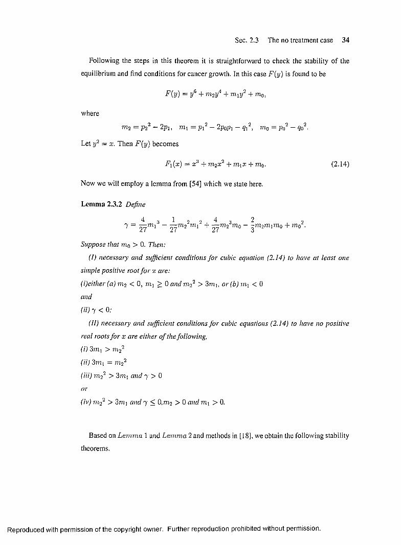
Following the steps in this theorem it is straightforward to check the stability o f the
equilibrium and find conditions for cancer growth. In this case F (y ) is found to be
F(y) = y° + moy4 + rnxy1 + mo,
where
m 2 = p 22 -2 p x , m i = px - 2p0pi - qx2, m0 = p02 - qQ2.
Let y2 = x. Then F (y ) becomes
Fx(x) = x 3 + m 2x2 + m ix + mo. (2.14)
Now we w ill employ a lemma from [54] which we state here.
Lemma 2.3.2 Define
4 O 1 2 9 4 n 2 9
7 = ~ 27m 2 m i “ + 27m 2 W7o “ ^ r n 2m x m 0 + m.0“ .
Suppose that mo > 0. Then:
(I) necessary and sufficient conditions fo r cubic equation (2.14) to have at least one
simple positive root fo r x are:
(i)either (a) m 2 < 0, m j > 0 andm 22 > 3mi, or(b)mx < 0
and
(ii) 7 < 0;
(II) necessary and sufficient conditions fo r cubic equations (2.14) to have no positive
real roots fo r x are either o f the following,
(i) 3m i > m22
(ii) 3??ii = m22
(Hi) m 22 > 3m! and 7 > 0
or
(iv) m 22 > 3mi and 7 < 0,m 2 > 0 and ni\ > 0.
Based on Lemma 1 and Lemma 2 and methods in [18], we obtain the following stability
theorems.
Reproduced with permission o f the copyright owner. Further reproduction prohibited w ithout permission.

Sec. 2.3 The no treatment case 35
Theorem 2.3.5 Suppose that m 22 > 3m i, 7 < 0, m2 > 0 and m\ > 0. Then
H i f Po + (Jo > 0, pi + q\ > 0, p2(p\ + f/i) > po + qo, the stability o f equilibrium £3 is
independent o f delay r and it remains stable fo r all r > 0,
2) i f po + (jo < 0, or p i + qx < 0, o r p2{pi + 91) < Po + (Jo the stability o f equilibrium £3
does not depend on r and it remains unstable fo r all r > 0.
Theorem 2.3.6 Suppose that m 22 > 3m j, 7 > 0. Then
1) i f (2.13) holds, the stability o f equilibrium £3 is independent o f delay r and it remains
stable fo r all r > 0,
2) i f (2.13) does not hold, £3 remains unstable fo r all r > 0.
Theorem 2.3.7 Assume that either (a) m 2 < 0, m\ > 0 and m 2 > 2>m\, or (b) m i < 0
and 7 < 0. Then there exists a positive f such that
1) i f Po + (jo > 0, pi + qx > 0, p2{pi + (j\) > po + (jo, the equilibrium £3 remains stable
fo r 0 < t < f, and becomes unstable fo r all r > f ,
2) i f po + (jo < 0, or pi + (j\ < 0 , or p2{jh + (j\) < po + (Jo, the equilibrium £3 remains
unstable fo r all t > t . As t varies from 0 to t , at most a finite number o f stability switches
may occur.
In cancer chemotherapy, stability switching is a very important issue in the design of a
drug protocol. We must keep in mind that in many cases the drugs can prevent vascular
endothelial precursor cells from continuing through their immigration, maturation into
vascular endothelia cells, thus trapping them at some points, where the cells die from
natural causes. This effect can be interpreted as an increase in the delay r . But as we
have seen here this trapping may have an adverse effects since it may cause a fixed point to
become unstable when it was stable in itia lly (Theorem 2.3.7). On the other hand, the same
properties can be used to the clinicians advantage, i f we are certain that our parameters are
in the stability switching region and the equilibrium is unstable. In this case, it may be
possible to use the same trapping mechanism to stabilize the cancer-free equilibrium.
Theorem 2.3.5-2.3.7 show that there exist stability switches for the interior equilibrium
by taking the time delay a variable parameter, in which a small delay makes the equilibrium
Reproduced with permission o f the copyright owner. Further reproduction prohibited w ithout permission.

Sec. 2.3 The no treatment case 36
stable and the populations grow periodically at the critical value o f the time delay (see
Figure 2.3-2.5).
Now by applying Theorem 1 in [18], it is also straightforward to check for possible
Hopf bifurcations when we increase the delay r . The importance of Hopf bifurcations in
this context is that at the bifurcation point a lim it cycle is formed around the fixed point, thus
resulting in stable periodic solutions. The existence o f periodic solutions is o f significance
in cancer models because it implies that the cancer levels may oscillate around a fixed point
even in the absence o f any treatment. Such a phenomenon has been observed clinically and
is known as ’’Jeff’s Phenomenon” [54]. In this section, we w ill prove that such a Hopf
bifurcation can occur. Here we are interested in the bifurcation o f the coexistence o f three
populations. Hence we consider the characteristic equation (2.10) and rewrite it as
A'5 + />_>A“ + pi A -f po -f (<71A + qo)e *T = 0. (2.15)
Let A = u + iv (u. v 6 /?) and rewrite (2.15) in terms o f its real and imaginary parts as
//'* — 3uv2 + jh (u2 - i'J) + pi u + po - <;“ “T[<yiUsin(i>T) + (qxu + qo) cos(wr)]
3 i r v — i ''1 + 2 jhuv + p\v = c~UT\(i]\ii + ry0)s in (u r) — ryiucos(ur)]. (2.16)
Let f be such that u(f) = 0. Then the above equations reduce to
p>V2 - Po = <husm(vf) + (J o cos(uf)
— f'-‘ + p ii ' = f/osin(rf) — (j\v coa(uf). (2.17)
It follows by taking the sum o f squares that
r/’ + (p>2 - 2pi)r‘ + (in2 - 2JH)1>2 - (] i 2)v2 + Po2 - (Jo2 = o. (2.18)
Suppose that f | is the last positive simple root o f equation (2.18). We now show that with
this value of i'i there is a n such that u ( f | ) ~ 0 and v ( f \ ) — i»i. Given in, equation (2.17)
can be written as
/I cos(ri f'|) + / i sin( -fi f’i ) = C
.4 si11(7"| i ' | ) - II cos(ti ,-'i ) — (2.19)
Reproduced with permission o f the copyright owner. Further reproduction prohibited w ithout permission.

Sec. 2.3 The no treatment case 37
where C2 + D2 = A2 + B 2 = G2, say, where G > 0. The equations
A = Geos a
B = G s in a (2.20)
determine a unique a e [0,27r], With this value of ct, we have
G cos(fiU i) cosa + G s in (fiV i)s inc t = C
Gsii^TyD!) cos a — G co s^U !) sin a = D. (2.21)
Hence
G cos(fii;1 — a) = G, G sin (fiU i - a) = £>. (2.22)
These equations determine fj-Dj - a uniquely in [q/D i, (a + 27r)/i5i]. To apply the Hopf
bifurcation theorem as stated in Marsden & McCracken [68] we state and prove the
following theorem.
Theorem 2.3.8 Suppose that equation (2.18) has at least one simple positive root and vx
is the last such root. Theniv(f\) = iux is a simple root o f equation (2.15) and u ( t ) + iv ( r )
is differentiable with respect to t in a neighborhood o f t = f x.
Proof. To show that i v ( f x) = i v x is a simple root, we investigate equation (2.15)
H (A) = A3 + P2A2 4- pi A -t- po + (<7v A + qo)e ^T — 0.
Any double root A satisfies
H { A) = 0, H { A) = 0,
where
H ( A) = 3A~ + 2p‘iX 4- p i + (<71 - Tqx\ — Tqo)e . (2.23)
Substituting A = iu x and r = f x into (2.15),(2.23) and equating real and imaginary parts if
iv x is a double root, we obtain
p 2 v \ - p o = q \ V \ sin(D1f 1) + <y0 c o s ^ f , )
1>\V\ ~ cos(u ifi) 4- q0sm(vxf x) (2.24)
Reproduced with permission o f the copyright owner. Further reproduction prohibited w ithout permission.

Sec. 2.3 The no treatment case 38
and
3u? - Pi = (tfi - f i r / o j c o s ^ f ] ) + u i f ^ j s i i^ u j f j )
2p2ui = (<]i - figo) sin(ii1f ) + u in t/ i cos(Difi). (2.25)
Now, equation (2.17) can be written as h(vi) = 0, where
h(v) = (p2v2 - po)2 + (piu - v3)2 - q\v2 - q02 (2.26)
h(v) = 2(piv2 - p0)2p2v + 2(piu - v3)(pi - 3u2) - 2 v q 2. (2.27)
By substituting (2.24) and (2.25) into (2.26), (2.27), we obtain
h(v i ) = h(vi) = 0.
It follows that Vi is a double root o f equation(2.26) and that h(v\) = h{v\) = 0, which is
a contradiction since we have assumed that v\ is a simple root o f (2.18). Hence iv\ is a
simple root of equation (2.15), which is an analytic equation. By using the analytic version
of the implicit function theorem(Chow & Hale [16]), we can see that u {t ) + w (t ) is defined
and analytic in a neighborhood of r = f j . The proof is complete! □
Next, to establish Hopf bifurcation at r = f j , we need to verify the transversality
conditiond u ,^ | T = fl^ 0.
By differentiating equations (2.16) with respect to r and setting u = 0 and v = we
obtain
. du. d v , _2 _ vA i — | T = f l - 5 i — |T = f l = p o 'U i s i n ( u i r 1 ) — p \ v \ c o s ( u i T i )
da dvB\ — |r= f, + A x — |T=tl = p 1ii? s in ( ijif i) + po ijicos(ijif1)], (2.28)
where
Ai - pi - 3u2 + fi[<7i cos(i)ifi) - qivi s in (v if i) - <70cos(v ifi)]
B\ = 2p2v\ + f i[ t /0 s in ( t i i f i) - q{vi cos(u ,fI ) - qx s in ^ j f i ) ] .
(2.29)
Reproduced with permission o f the copyright owner. Further reproduction prohibited w ithout permission.

Sec. 2.4 The continuous treatment case 39
Solving for jjif from (2.28) with the help o f (2.17), we have
du _ vf[3vj + 2(p22 - 2pi)vj + Pi2 ~ 2p2po - Qi:dr 1 A i 2 + B i 2
Let z — vf. Then equation (2.18) reduces to
$ (2) = 23 + (p22 - 2 px)z2 + (p i2 - 2p2p0 - q 2)z + po2 - qQ2.
Hence
— = 322 + 2(p22 - 2pi)z + P \ 2 ~ 2p2Po - q 2-
As v\ is the last positive single root o f equation(2.18), then
d<J>
Therefore,du . u? d'i>.
> 0.
(2.30)
dr 1 A 2 + B 2 dz 2 v
We summarize the preceding details in the following theorem.
Theorem 2.3.9 Suppose that (2.18) has at least one simple positive root and v\ is the last
such root. Then a Hopf bifurcation occurs as r passes through f\. On the other hand i f
(2.18) has no positive real roots then the interior equilibrium E* is locally asymptotically
sable fo r all values o f r i f (2.13) holds.
2.4 The continuous treatment case
Here we consider the fu ll model (2.3). Again equilibria are derived and listed. We study
the local stability o f some relevant equilibria by analytical and numerical methods.
2.4.1 Equilibria
In this case, we denote the equilibria by variations on F and again some o f them
are physiologically non-feasible. As in the no treatment case, the trivial equilibrium
F0(0 ,0 ,0,£ -1 A ) always exists. The following equilibria may or may not exist:
Fi(x,0,0,fi), F2(0,y, z ,u) , F z { x \ y \ z \ i L * ) .
Reproduced with permission o f the copyright owner. Further reproduction prohibited w ithout permission.

Sec. 2.4 The continuous treatment case 40
Trajectories of Populations in the Absence of Treatment with t« 1 1 .
200 1200
03S200 400 600 1000 1400
06
1000
yyyyy\/\/\AAA/v\AAAA/\/vv\^s^N-~^^^ -
/Yyyv\AAA/\AA/vwvwwwwW^ —•.—-— ;
time t (days)
Figure 2.3: A solution for model (2.4) with a = 3day~x ,p = 150g . f - 0.67,n = 10 g/kg , k), = 10 kg ,k t = 3 kg ,b = 6 day-1 , dx = dy = 1 day- 1 , m = 20g/kg , d. = 0.2 day"1, c = 0.3 day-1. Here the interior equilibrium E${1.679,0.397,0.5955) is locally stable when the delay r < 12.14.
Trajectories of Populations in the Absence of treatment with t=12 .!4 .
200 300 600
300 600 700 900
w v w w w v w w w v w w w #
iVWWWWWVVWWVVWVWV_l____L_
100 200 3O0 400 500 600 700 MO 900
time t (days)
Figure 2.4: A solution for model (2.4) with a = 3 day-1 ,y = 4O r/, / = 0.67,n = 10 g /kg .kh -- \0 kg .k , — 0kg ,b = 4 day-1 ,d j; = dy = 1 day-1 , m = 15 g /k g ,d . = 0.2 da;/-1 . r — 0.3 da//-1. Here the interior equilibrium En( 1.027,0.06S, 0.102) bifurcates at r - 12.14 and periodic solutions occur.
Reproduced with permission o f the copyright owner. Further reproduction prohibited w ithout permission.

Sec. 2.4 The continuous treatment case 41
Trajectories of Populations in the Absence of Treatment w ithr=l3 .2 .
500 1000 1500 2000 2500 3000
500 1000 1500 2000 2500 3000
1000 1500 2000tim e t (days)
Figure 2.5: A solution for model (2.4) with a = 2>day~l ,p = 150g , / = 0.67,n = 10g /k g ,k h = 10kg ,k t = 3 kg ,b = 6 day~l ,dx = dy = 1 day~l ,m = 20g /k g ,d z — 0.2 day~l ,c = 0.3 day-1. Here the interior equilibrium £ 3(7.679,0.397,0.5955) becomes unstable but approaches to the periodic solutions when r > 12.14.
Here the symbols that are the same as in the no treatment case may have different values.
The equilibrium £1 exists provided that the algebraic system
Piuao — a\x —
ai + x0
A - [£ + - ^ - } u - 0 (2.31)X
has a positive solution. System(2.31) has a positive solution provided that the quadratic
equation
° i ( f + ci )3;2 + (a i« i£ - - a0ci)x + p iA - a0d ^ = 0 (2.32)
has a positive solution. Here ao, aj are defined in the previous section. I f
p i A < a0aj£, (2.33)
then equation (2.32) has a unique positive solution. Necessary and sufficient conditions for
(2.32) to have two positive solutions are
< ao(f + ci)( a ia i£ - a 0£ - a0c 1)2
a0a , £ < p jA <4ai (£ + c i)
(2.34)
Reproduced with permission o f the copyright owner. Further reproduction prohibited w ithout permission.

Sec. 2.4 The continuous treatment case 42
From the above, we have proved the following lemma.
Lemma 2.4.1 I f (2.33) holds, then F\ exists uniquely. I f (2.34) holds, then there exist two
distinct equilibria o f type F\.
Although the other equilibria F2 and F3 may exist, sufficient conditions for their existence
are not easily obtained. In section 2.4.3, we w ill present some numerical examples to
illustrate cases when these equilibria exist.
2.4.2 Local stability
Here the Jacobian matrix around a general equilibrium F ( x , y, z, u) is
—a2x —a$x
M =
an- b iy
0a 22
b - \ t
Pi x fij+X
- h y - d s
0 2 + y
03+a ic in __ aocoti _ 03C3U
(« 1 + x )2 (02+J/)- (as + c)^ 33
where
flu = 0-0 ~ 2a ix — a2y — a$z — —
0 22 = b0 - h x - 2b2y - b3z -
P\a\u(ai + x )2 P2O2U
( 0 2 + y )2t c , C l3; , C2V , C32 a«33 = - ( £ + - ----------1- ---------- h : ---------).
a\ + x a2 + y a3 + z
Analysis o f F0
It is quite easy to get the eigenvalues associated with the trivial equilibrium F0 which are
A<°> = ao > 0
a 2 = b0 > 0
A f = - d . < 0
A f = —£ < 0.
Hence F0 is a hyperbolic saddle point.
Reproduced w ith permission o f the copyright owner. Further reproduction prohibited w ithout permission.

Sec. 2.4 The continuous treatment case 43
Analysis of Fi
In this case, the Jacobian matrix is given by
P1Q1U (ai+z)
M i =
a0 - 2axx - - a 2x0 0
- a 2x - a 3xbo — bix 0
e-Ar —dz—a^cou —a3 c*3'
bxx, A ^ = —d~.
P \ Xai+zo0
~ a \ + x > .(a i+ i)2
Hence two of the eigenvalues are
\ ( D
The other eigenvalues satisfy
a(A) = {A ^ IA 2 - T r{A )A + det(A) = 0, £ = 1,4},
where
A = a ° ^ a l X ( f i i + i )2d \ C \ u
(a i+ x ) -
EliS i+ 2
By the Routh-Hurwitz criteria [19], i f Tr(A ) < 0 and det(A) > 0, then the eigenvalues of
A have negative real parts. I f x > a0/2 a \ , then
Tr(A) = a0 - 2ayx - + g + i r ^ r l < 0(a\ 4- x) d i + X
dct{A) = - f l M L + (2a ,* - „ „ ) ( { + - £ !£ - ) > 0.(aj + x)~ a-i + x
As a result, we have the following lemma.
Lemnia 2.4.2 I f x > a0/2ax, then the real parts o f eigenvalues A,1' and A,^ are negative.
Based on Lemma 2.4.2, we obtain the following theorem.
Theorem 2.4.1 Suppose that x > a.0/2a\ and bo f bxx. I f bo > bpx, then F\ is a
hyperbolic saddle point. On the other hand, i fb 0 < bxx, then F\ is asymptotically stable.
Reproduced with permission o f the copyright owner. Further reproduction prohibited w ithout permission.

Sec. 2.4 The continuous treatment case 44
Analysis of F2
In this case, the Jacobian matrix is given by
M 2 =
A/}? 0 0
- f r i y a4 3) -^32/0 £- \ t —d-
a f 'c i u
- < 2)
-•M g ’- M l ?
where
= a0 - r/2/y - a-.iz - a, l p i it. M ^ 1 = b0 - 2b, y - bAz -r(2) -p2a2u
(a2 + it)2
-I - T - T T : - - — - 7- A/.j.'f = — (£ + r ~ ~ r + r ~ ~ r )w (2) P'1'J w M i'
* W _>I — - : r . .W ; | | — ------— T«•> — #/ (l;t - r ' a2 + y a;j 4 - ;
«2C2» . . ( 2)* (r,.J + / y)'2- i / l : i - (fi3 + £)2-
Hence, one o f the eigenvalues is
\ ( 2 ) - .A, = dr, — a2y — a:iz — a, p\ u.
The other eigenvalues satisfy
A’* -F />.»A* + pi A + pn + ((j\X + r/0) c - Ar = 0,
where
1>2
l> I
1h I
'/I
' / ( I
,/. _ ,u«» - .y<->i i
A/l-j’A / i f - rf,(Aig> 4 A / f f ) - A JS jA /ff - A / ' f A/|;>
( L M ^ M ^ r- A / if )A/.;*>-\/^)
k\!l
- K U n ' i / - A /i;» A /^ .
(2.35)
liquation (2.35) is the characteristic polynomial (2.10) in the previous section with new
coefficient values. Computing »»|. /i/„ and employing the same arguments as before,
we have the following theorems.
Reproduced with permission o f the copyright owner. Further reproduction prohibited w ithout permission.

Sec. 2.4 The continuous treatment case 45
Theorem 2.4.2 Suppose that m 2 > 3mi, 7 < 0, m 2 > 0 and m\ > 0. Then
1) i f Po + Qo > 0, pi + <71 > 0, p2{pi + <71) > po + qo, the stability o f equilibrium
Fo is independent o f delay r and it remains stable fo r all r > 0, provided that a0 <
a2y + a3z 4- a ^ p i i i ,
- ) i f Po + Qo < 0, o rp i + qi < 0 , o rp 2{p\ + Qi) < Po + qo, the stability o f equilibrium Fo
does not depend on r and it remains unstable fo r all r > 0.
Theorem 2.4.3 Assume that either (a) m2 < 0, m\ > 0 and m22 > 2>mh or (b) m\ < 0
and 7 < 0. Then there exists a positive f such that
l ) i fP o + qo > 0, pi + q\ > 0, p2(pi + fji) > po + qo, the equilibrium F2 remains stable
f o r 0 < t < f when a 0 < a 2y + a 3 z + a j" 'p iu , and becomes unstable fo r all r > r,
- ) i f Po + qo < 0, or p i + <71 < 0, or p2{p\ + <?i) < Po + qo, the equilibrium F2 remains
unstable f o r all r > f . As r varies from 0 to f , at most a finite number o f stability switches
may occur.
2.4.3 Global stability
Note that i f Fi is achieved, then healthy cells eventually win the competition with the
cancer cells, which is the most desirable result. F3 represents the coexistence of all four
populations. In this section, we derive criteria for the global stabilities of Fi and F3 with
respect to solutions initiating in in t R‘ ..
Global stab ility o f F\
In in t R‘| we choose the Liapunov function,
V(x{ t ) , y( t ) , z{ t ) , n( t ) ) = x{t ) - x - x \ n{ x { t ) / x ) + a {y(t) + ^ z2{ t )
I f 0 , 1+ j [y{t + s)\2ds + - a 2{u{t) - u)2, (2.36)
Reproduced with permission o f the copyright owner. Further reproduction prohibited w ithout permission.

Sec. 2.4 The continuous treatment case 46
where q j, a2 are positive constants to be determined later. The derivative o f (2.36) along
solutions o f (2.3) is given by
V = (x — a-)[ao — axx — aoy — a^z — J. lUX lai + x
n , , , 'PoUy+ait/[Oo - bix - b2y - b3z - —"
52 + 2/
+ \a \b 2 [y2 ~ (y [ t - r ) ) 2] + z{cy{t - r ) - dzz - PzU~- )I a3 + z
+ a 2{u - u ) [A - (£ + ^a i + x a2 + y a3 + z
After some computing, we obtain
V = - ( a , + an )(x - x ) 2 - a x{ h j2 + a22)y2 - (d: + a33)z2
- ^ M i [{y(t - t ) - c(b2a i )~l z}2 - a 2( f + a.,4)(u - u f
~ { {a 2 + 6 ia i)(a : - x)y + (aX2 + a2Xa 2)(u - u)(x - x) + b3a xyz
+ a 3(x — x )z + au a 2z(u — u) + a\3a 2y{u — -u)}
= + an ) ( x' - ^ ) 2 + (a2 + M i ) ( x - x)y + ^< *1 (^2 + a22)y2}
~ ^3Q l^2^2 a22^ 2 ^3(Xiyz 3 ^ - "*■ ^33)^2}1 1
- { - ( 5. + a33)z2 + aMa 2z{u - u) + - a 2(£ + au )(u - i i ) 2}
- { ^ a 2(^ + aAA)(u - u )2 + (a12 + a2i a 2)(u - i i) ( x - x) + ^ ( a x + a n ) ( i - x )2}
+ a n ) ~ 5')2 + a3(x - x)z + ^ (d z + a33)z2}
1 1 1+ a22)y2 + a\3a 2y{u - i i) + - a 2( f + a44)(u - u)2}
- ^ > 2 fx\[(v{t - t ) - c(52a 1) “ 12]2, (2.37)
where
_ C l\P \U P \ X c2u p2ua l l — j z — , - w - — ;— r , «12 = ~ — ~ a l.'i = z — ;— , ci22 —
(d] + x)(a\ + x) ’ ' ci] + x ' a-2 + 2/ ’ " “ 2 + 2/5iC|U c3u p3u c2 c ix
a2i — TZ— , _w_— ;— r, a]4 — - — ;— O33 — j i — ;— r - - — a,14 =(5] + x)(a,] + x ) 53 + 2 (a3 + z) 2oi]b2 ’ do + x
Reproduced with permission o f the copyright owner. Further reproduction prohibited w ithout permission.

Sec. 2.4 The continuous treatment case 47
Note that we have a 13, a hl,a2i > 0 and
Pi Aan S -T7z— —t t —: au
U “ i + a :)
0-22 < P2A (a20 _1 =: a220
0 “
033 + - — p < p3A(a3£)-1 =: S33.ZQ1O2
Therefore, i f
I963(11 < 4( —62 + a22 )(d ; + a33)
9a2 < 4(a i 4- o \ \ ) ( d z 4- 033)
9a22 < 4a 2(a i + ( i i i) (£ + (144)
c2 < 2 a 162(cL + P 3 A (a 30 _1)
9(a2 4- 6 ia .'i)2 < 4a i( a i 4- a n K -6 2 4- (122)-
Then V < 0, which leads to the following theorem.
Theorem 2.4.4 I f we choose an, <22 such that (3.28) holds, then F x
asymptotically stable (see F igure 2.6).
Global stability of F3
In in t R+ we choose the Liapunov function,
V (x ( t ) ,y ( t ) ,z ( t ) ,u ( t ) ) = x(t) — x* - x * ln (x ( t ) /x * )
+ a [y { t ) - y* - y* In(y{t)/y*)]1 f °
+ ^ a b 2 J [y(t + s ) ~ ly 'fds
+ ^ ( < ) - -*')2
+§(«(<)
(2.38)
is globally
(2.39)
Reproduced with permission o f the copyright owner. Further reproduction prohibited w ithout permission.

Sec. 2.4 The continuous treatment case 48
Trajectories ot Poputatona in the Case ot Tieatment wrth Any Delay*
U{l)
W)
V /»(t)
1
____________ „ .0 » '0 0 ISO 200 2S0 300 » 0 *00
tim et (days)
Figure 2.6: A solution for model (2.3) with a = 3 day~l ,P = COg , f = 0.67,n = 10 g/kg , kh = 10 k g ,k t = 3kg, b = 6 day- 1,dx = dy = 1 day-1 ,m — 20 g /kg , dz =0.2 day~1,c — 0.3 (/ay-1 ,p x — 0.0008 day-1 ,p 2 = 0.08 day-1 ,p3 = 0.09 day-1 ,a j = 2 k g ,a 2 = «3 = 3A;y,ci = 0.0024 day- 1 , C2 = 0.04day-1 ,c3 = 0.03 day- 1 , A = 200 kgday~l , £ = 20 day-1 . Here Fj (2.6015,0,0,9.9887) is globally stable, independent o f delay. The number o f blood vessels drops to zero very fast from the beginning o f the treatment. The initial conditions are x(0) = 1, faiO) — 3, - r < 0 < 0, c(O) = 4, h(0) = 14.
where a is positive constants to be determined later. The derivative of (2.39) along solutions
o f (2.3) is given by
V = (x — J’’ )[«o ~ a \x — ui!J — a 3a —P\11X
a I + x
+ o ( y - - I)\X - b2y - .: -
+ “ J/‘ )2 - ( y ( t - r ) - y * )2]
+ ( ; - z '){cy (t - r ) - dss - '
P2“ !J | (i2 + y
d3 +
+ (« - l/’ )[A - ($ +M vs a i + . r a2 + y «3 + s
Reproduced with permission o f the copyright owner. Further reproduction prohibited w ithout permission.
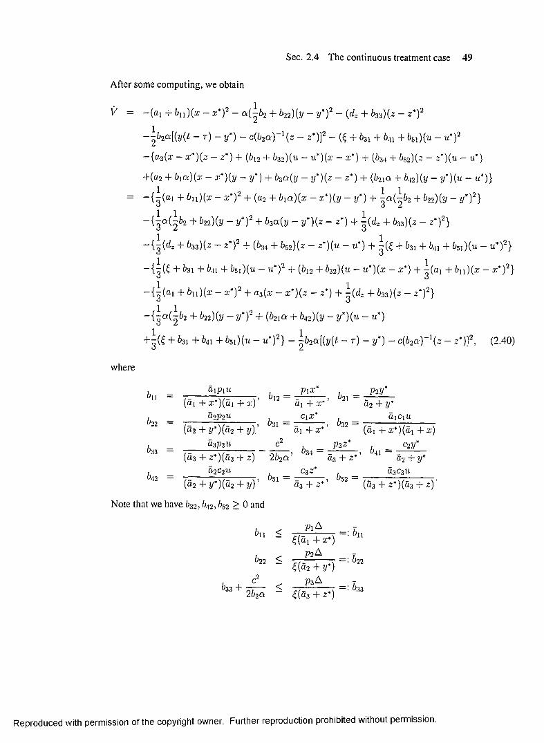
Sec. 2.4 The continuous treatment case 49
After some computing, we obtain
V = ~(ai + bn )(x - x *)2 - a (^b2 + b22)(y - i/ ) 2 - (dz + b33)(z - z*)2
~ \ h2^ [{y { t - r ) - y*) - c(62a )_1(z - z*)]2 - (£ + 631 + 6.u + 651)(ti - u*)2
— {0 3 (2 : — a: )(z — 2*) + (612 + b32)(u — u * ) ( x — x * ) + (634 + b52)(z — z*)(-u — u*)
+(a2 + b,a)(x - a:*)(y - y*) 4- b3a(y - y ') (z - 2*) + (b2\a + 642)(y - y*)(u - u*)}
= + ^ i iX * _ a'*)2 + (fl2 + b ia)(x - x*)(y - y*) + ^ a ( |& 2 + b22){y - i f ) 2}
+ b22){y - y * f + h a { y - y*)(z - z*) + ^ ( 4 + &33)(z - z*)2}
~ { 3 ^ ■*" b3s){z ~ Z )~ + (^34 + b32) [z — z* ) {u ~ U*) + ~ (£ + b31 + 641 + b5i ) ( u — U *) " }
“ { g ^ "I" + ^5 i ) ( ^ ~ u * ) 2 + {bi2 + b32) (u — u * ) ( x — x ’ ) + - ( a j + bn ) (x — x * ) 2}
- { ^ ( “ 1 + bn ) ( x - X * ) 2 + a3(x - x * ) ( z - z*) + ^ ( 4 + 633)(2 - z * )2}
~ { ^ a ( ^ 2 + b22)(y - y * f + (£>21 a + bA2){y - y*)(u - u*)
+ ^ (£ + &31 + h 1 + b5i ) (u - u*)2} - i b2a[{y(t - r ) - y*) - c(b2a)~ l {z - z*)]2, (2.40)
where
222
233
a ip i«i 12 —
Pis* b PiV*(a i + x*)(a i + x) ax + x* ’ 4 + y*
a2p2ubii 1 = ClX* fe -
aiC]U(«2 + y*)(d2 + y) ' ai + x* ’ (a i + x*)(a i + x)
a3p3u c2 £j _ P*Z* c2 v*(a,3 + z:*)(a3 4- z) 2 b2 a ' ’ a3 + z* ’
0<u — ■a2 + y*
a2 c2u1 4 l = C3--* 5 a3 c3u
( 4 + y*)(d 2 + y) 4 + z* ’ “ ( 4 + z * )(4 + z)'
Note that we have b32, £>42, £>52 > 0 and
* . < 5n£(ai + x*)
; P2A _ j22 s e f e T T T ' 1’22
h , + f - < =•2£>2a ^(a3 + z*)
Reproduced with permission o f the copyright owner. Further reproduction prohibited w ithout permission.

Sec. 2.4 The continuous treatment case 50
Trajectories of Populations in the Case of Treatment with Any Delays.
time t (days)
Figure 2.7: A solution for model (2.3) with a — 3 day ' 1 ,P = 150<7, / = 0.67, n = 10g /kg ,k)v - 10 kg , kt = 3 kg , b = 6 day-1 ,dx — dy — 1 day ' 1 , m = 20 g /k g , d . =0.2 day ' 1 ,c = 0.09 day ' 1 ,p x = 0.0005 day - 1 , P2 = 18 day- 1 ,p3 = 2day~l , 0,} = 20 kg, a,2 = a3 = 800/cy,Ci = 0.01 day ' 1 , C2 = 36 c/ay- 1 , c3 = 8 day- 1 , A = 200 kg day ' 1 ,£ = 80 d a y '1. Here the interior equilibrium .F3(7.238,0.9224,0.5,2.4986) is globally stable, independent o f delay. The initial conditions are x(0) = 7.5, $2 (6 ) = 0.5, —r < 0 < 0, 2(0) = 0.3, u(0) = 10.
Therefore, i f
963a < 4 (^ 1 + 22 )(d~ + 633)
< 4 (d: + 633)(£ + 631 + b,xx + ^51)
96?2 < 4(£ + 31 + hu + bs l)(a i + 611)
0a\ < 4(a i + bn)(dz + b33)
0b\xa < 4(—61 + £>22) ( f + ^3i + b4X + 651)
c2£(a3 + z*) < 2 ab2p3A
9(02 + bxo:)~ < 4a(a1 "F S ii)(—bi + b 22).
Then V < 0, which leads to the following theorem.
Theorem 2.4.5 I f we choose a such that (2.41), then the interior equilibrium F3 is globally
asymptotically stable (see F igure 2.7).
Reproduced with permission o f the copyright owner. Further reproduction prohibited w ithout permission.
Sec. 2.5 Discussion 51
2.5 Discussion
From the viewpoint o f biological stoichiometry, this chapter dealt with vascular tumor
growth and its treatment with chemotherapy techniques. In the absence o f treatment, our
model is one of the models in Kuang, et al. [60], in which they formulated over a dozen
plausible models, then performed extensive simulations on all o f them, but they did not give
a complete analytical analysis to the models. Therefore, the difference between our work
and their work is that they mainly focused on numerical simulations and we mostly focused
on analytical analysis. Their extensive simulation work shows that (1) tumor growth and
size are very sensitive to the total amount o f phosphorus more so than tumor birth rate
or death rate is. Phosphorus supply mostly controls and determines a tumor’s ultimate
size; (2) when several tumor cell species coexist in the tumor, the less malignant type
has a high tendency to quickly dominate the tumor and thus push more aggressive tumor
cells to metastasize; (3) the time delay r plays a key role in determining the time for a
tumor to reach a given size more dramatically than changes in some other organ values; (4)
restricting phosphorus in the body damages both the tumor and the healthy organ. However,
selectively lim iting phosphorus only to tumor cells w ill keeping the tumor from reaching a
lethal size.
In our analysis in the case of no treatment, we first studied the model equations with
regard to invariance of nonnegativity, boundedness o f solutions, and the nature o f equilibria.
Comparing their work to ours, one can find their simulations support very well our
theoretical results. The expression o f tumor steady state size ( y and/or y* ) in our analysis
shows that the phosphorus value P does play a clear and prominent role in determining its
value as confirmed by simulations in [60]. Also, one can find from those expressions for
the tumor steady state size that the tumor dies out i f one can increase the tumor’s death rate
(dy) or lower the tumor’s birth rate (b) to certain threshold values. Here we only consider
one type o f parenchyma cells, our analytical results are not comparable in terms of the case
in which several tumor cell species coexist. With respect to the cell maturity time r , our
analysis and simulations show that it not only dramatically determines the time for tumor
cells to reach a given size, but plays an important role in the stabilities of the steady states
and the stability switches for the delay system.
Reproduced with permission o f the copyright owner. Further reproduction prohibited w ithout permission.

Sec. 2.5 Discussion 52
In our analysis in this case, necessary and sufficient conditions for Hopf bifurcation of
the interior equilibrium to occur were obtained by using the time delay as a bifurcation
parameter. Analytically, it is difficult to prove in general whether Hopf bifurcation for
delay systems is supercritical or subcritical. However, we see from Figure 23-2.5 that in
our models, we get supercritical bifurcation.
Sufficient criteria was also obtained for the uniform persistence of populations and the
extinction o f cancer cells. With respect to global stabilities, sufficient conditions were
obtained for the cancer-free equilibria and interior equilibrium. Thus, we solved the open
problem in [60]. It was shown that the system can be permanent but whenever the boundary
equilibrium is stable, the interior equilibrium o f the system cannot be globally stable for at
least small values o f the time delay. Further, in this case, persistence cannot occur at least
for small values o f the time delay. In particular, Thoerem 2.3.5 and 2.3.6 give criteria for
no stability switching and Theorem 2.3.7 for stability switching in the no treatment case.
Theorem 2.4.2 and 2.4.3 give criteria for no stability switching and stability switching,
respectively, in the presence o f continuous treatment case.
Finally, based on all these dynamical behaviors of the drug-free system, a continuous
treatment with chemotherapy was considered. The rationale behind this is to use the
information about the drug-free system to design a drug protocol. When stopping
treatment, we would like the patient to be cured or stay in the stable region o f the new
system. Here, sufficient criteria was obtained for the extinction of cancer cells. Local and
global stabilities o f the cancer-free equilibrium was studied by utilizing spectral theory and
Liapunov functions. It is important to mention that because of the lack of good biological
understanding o f the drug functioning, it is not clear how the drug acts on the normal and
tumor cells. In this chapter, Holling type II function as drug functional response to cells was
proposed to simulate the functional response mathematically. We emphasize that to the best
of our knowledge, the actual functional response to cancer cells by a chemotherapy agent is
not known; but Holling type II is a reasonable starting point based on ecological modeling.
Recent work [59) indicated that a ratio-dependent functional response makes more sense
and fits the data better than Holling type II. In the future, we w ill consider this type of
functional response as a model o f the drug function.
Reproduced with permission o f the copyright owner. Further reproduction prohibited w ithout permission.

Sec. 2.5 Discussion 53
This chapter deals with some aspects o f angiogenesis. We note that this topic is also
modelled in [46] and [96]. However, these papers only model single species growth and
involve partial differential equations. Hence, our results are not comparable.
Since the medical objectives of cancer treatments are to either eliminate the cancer
altogether, or confine cancer cells to a tolerable low level, or at least to terminate the growth
of cancer, we hope that our results w ill suggest how to vary the parameters for those cancer
interactions governed by system (2.1) so as to make the treatment more effective.
Reproduced with permission o f the copyright owner. Further reproduction prohibited w ithout permission.

A Reaction-Diffusion Model of Leukemia Treatment by Chemotherapy
3.1 Introduction
Leukemia is a cancer o f blood cells and can be described as the disorganization of the
hematopoietic system in which a malignant clone o f blood cells acts to impede the growth
of normal hemopoietic tissue. When leukemia develops, the body produces large numbers
of abnormal blood cells. In most types o f leukemias, the abnormal cells are white blood
cells, and they usually look different from normal blood cells, and do not function properly.
Leukemia is either acute or chronic. In acute leukemia, the abnormal blood cells are blasts
that remain very immature and cannot carry out their normal functions. The number o f
blasts increases rapidly, and the disease gets worse quickly. Recent works [69-72] show
that the origins o f acute leukemia can be found in pluripotent stem cells. In the acute
leukemia state a pluripotent stem cell in the bone marrow becomes malignant, proliferates
and displaces normal cells in the marrow. These abnormal cells then fill the blood and the
marrow and produce a malfunction o f the body’s immune system. In chronic leukemia,
some blast cells are present, but in general, these cells are more mature and can carry out
some o f their normal functions. Also, the number o f blasts increases less rapidly than in
54
Reproduced with permission o f the copyright owner. Further reproduction prohibited w ithout permission.

Sec. 3.1 Introduction 55
acute leukemia. As a result, patients with chronic leukemia get worse gradually. However,
without treatment, even the chronic disorders may be fatal [92,93J.
In cancer treatment today, four types of treatment are most commonly used in efforts to
obtain long-term periods o f disease-free remission. These include surgery, radiotherapy,
chemotherapy and immunotherapy. Cancer chemotherapy has demonstrated a definite
capacity for controlling disseminated metastatic cancer and is therefore widely used
[24,37,63,84]. In cancer chemotherapy, anti-neoplastic drugs are designed to selectively
destroy or inhibit the proliferative activity o f cancer cells while the normal cells are affected
to a lesser extent [24,37].
The ultimate role o f mathematical modelling in cancer chemotherapy is to provide a
more rational basis for experimental design o f the anti-cancer drugs and to make qualitative
predictions with regard to the dynamic evolution o f the disease based on the cytokinetic
parameters o f the patient and the drug parametric configuration. The fact that it is
reasonable to view the interaction between normal cells and cancer cells as competitive
is justified in Freedman [30] and Nani and Freedman [75,85]. In [75], a model o f cancer
treatment by chemotherapy was presented and conditions for the boundedness o f solutions
were analyzed. The equilibria and their stabilities, and conditions for the existence o f small
amplitude periodic solutions were also discussed. Persistence and extinction criteria of the
normal cells and cancer cells were also derived. It is well known that the distributions
of populations in general, being heterogeneous, depend not only on time, but also on the
spatial positions in the habitat. For example, leukemia diffuses within the bone marrow and
spread from the marrow to other parts of the body, including the lymph nodes, brain, liver,
and spleen. So it is natural and more precise to study the corresponding P.D.E. problem as
suggested by the authors in [751. For a detailed explanation o f the ecological background
of the problem, the reader is referred to [75]. Motivated by the conception o f persistence
in [12,33,35], we introduce it into this chapter and establish the existence, uniqueness,
boundedness and persistence of the solutions for the mixed boundary condition problem
by means of a comparison principle and a monotonicity method, (see e.g. ,[80,97]). The
main method used in studying the stability o f constant solutions is the spectral analysis of
the linearized operators.
Reproduced with permission o f the copyright owner. Further reproduction prohibited w ithout permission.

Sec. 3.2 The model 56
The idea o f modelling cancer interactions with healthy tissue as a competition process
was first proposed by Gatenby [41]. However, his paper did not consider treatment.
The first paper to incorporate chemotherapy treatment was Nani and Freedman [75]. An
extension to modelling cancer at several sites (metastasis) with chemotherapy treatment
was carried out in [85].
Since normal cells and cancer cells are competing for nutrient and space, we assume
both cancer and normal cells have the same carrying capacity in the model developed in
175] (see [75] for the derivation of the model) and propose a chemotherapy treatment for
the new model. Finally we extend it to the diffusion case to model the spread o f cancer
within a site (such as leukemia in the bone marrow).
The purpose of this chapter is twofold. Mathematically, we compare the dynamics o f our
model in the case o f no diffusion to the diffusion case. Clinically, we hope to derive criteria
on the parameters o f the model which lead to the control o f cancers, and in particular
leukemia, which are simulated by our models.
The organization o f this this chapter is as follows. In section 3.2 we describe the
model. Section 3.3 deals with the no diffusion case, whereas in section 3.4, we analyze
the diffusion case. We conclude with a final section which contains numerical examples to
illustrate our results and a short discussion.
3.2 The model
We take as our model o f leukemia treatment by chemotherapy a system of reaction diffusion
equations where i i \ ( x , t ) represents the density of normal cells, u2 (x , t) the density of
leukemia cells, and i ’( x , t ) the density o f chemotherapy agents in the affected region at
lime / > 0. We view //1 (x, t.) and u2 (x, t) as competing for nutrients, oxygen, etc. and we
think o fr(.r. / ) as a predator capable o f destroying both u\(x, t) and i/2(x, t), but selectively
Reproduced w ith permission o f the copyright owner. Further reproduction prohibited w ithout permission.

Sec. 3.2 The model 57
is more lethal to u2(x, t). The model then takes the form
d \ *T U ] do " f" Uo
r 21ux + u2\
u i + r x2u2
K
C \U \ C2U 2
I f - )
a\ "Tp2 u2v
do + Uo
P\U\V
V
(3.1)
with initial conditions
U l(x ,0 ) = U°(x), U2 (x,0) = 'Uo(x), v(x ,0) = u ° (x ) .
Since this model is used to simulate the interactions between healthy and cancer cells
in the bone marrow (which implies it is a one-dimensional measurable space), and since
these cells migrate from the bone marrow into the bloodstream, we take as our boundary
conditions Albedo (or mixed) boundary conditions of the form with x as one-dimensional
variables in the interval 0 < x < L:
where (u \ ,u \ , v c) is some reference concentration o f the system. (u°(x), u2 (x), v°(x)), is
a smooth initial function in the interval 0 < x < L.
The constants in system(3.1) may be interpreted as follows:
a, , i = 1, 2, are the specific birth rates o f the normal and cancer cells for small densities.
K is the carrying capacity o f cells which could be adequately supported by the environment
in the absence of the competing population.
r 2 1 is a competition coefficient measuring the effects on cancer cells u2 caused by the
presence o f normal cells u x.
r x2 is a competition coefficient measuring the effects on normal cells u x caused by the
presence o f cancer cells u2.
Pi, i = l,2 , are the predation coefficients o f v(x, t) on it,(x, t).
dj, i = 1, 2, determine the rates at which Ui{x,t), in the absence of competition and
predation, reaches the carrying capacity.
A is the infusion rate o f the chemotherapy to the bone marrow.
( - ^ 7 ± 7 i(u i ~ “ i))U = o ,l = 0, ( - ^ ± 7 2(u2-Wo))I
Reproduced with permission o f the copyright owner. Further reproduction prohibited w ithout permission.

Sec. 3.3 The no diffusion case 58
£ is the washout rate for the chemotherapy agent within this region.
Cj, i — 1,2 are the combination rates o f the chemotherapy agent with the cells. Hence they
are proportional to pu i = 1, 2.
A ll constants are positive. To make this model more realistic, we impose certain
inequalities among the parameters. It is well known that leukemia cells grow at a much
faster rate than normal cells, at least in the acute case. Further, i f no treatment is
offered, most o f the time leukemia cells out-compete the normal cells independent o f initial
conditions. Furthermore, the chemotherapy agent must be considerably more effective in
killing leukemia than in killing normal cells in order for the treatment to be effective. These
lead to the following sets o f inequalities:
In addition, there are other inequalities which we w ill list in the next section since they
depend on homogeneous steady state values.
3.3 The no diffusion case
In the case of no diffusion, the model is just a special case o f the main model discussed in
Nani and Freedman [75], and consequently all the results o f [75] apply here. The model
takes the form
q 2 > a u p2 » Vl •
K j d\ + u\r 2i t i i + u2\ P2 U2 V
(3.2)
dv . r c\U\ c2u2 — = A - g + , + —V 1dt ci\ F fl2 + u2
with initial conditions
tti(O) = > 0, t i2(0) = u\ > 0 , v(0) — v° > 0.
From [75], the following two results hold.
Reproduced with permission o f the copyright owner. Further reproduction prohibited w ithout permission.

Sec. 3.3 The no diffusion case 59
1. A ll solutions with positive initial values remain positive.
2. System (3.2) is dissipative.
3.3.1 The homogeneous steady states
From [75], the equilibria in terms o f our given parameters are:
£o(0 ,0,£_ IA ), E i{u u 0, 0), E 2 (0,u 2 ,v), E 3 (u\, u*2, v").
We carry out the analysis o f these steady states, even though it may repeat the analysis in
[75], since our results w ill now be given explicitly in terms o f the parameters.
Note that the trivial steady state £o(0,0,£- 1A ) always exists, and Ei[u \,Q ,v),
E 2 (o, Uo, v), E 3 (u\, U2 , V*) may or may not exist. In particular E \{u \, 0, v) represents the
steady state where leukemia is eliminated, which is the most desirable state. E2(0, u2, v)
represents the case where the leukemia has completely taken over the site. E 3 (u \ , i i2 , v ')
means coexistence, which is only desirable for small numbers o f leukemia cells.
The equilibrium E i(u u 0, v) exists provided that the algebraic system
„ /i V\v<*i(l ~ 77) --------- ;---- = 0 ,A ci\ -f~ ii]
A — £ + - ^ - ] v = 0 (3.3)+ III
has a positive solution ( f t i, v).
This system has a unique positive solution provided
p iA < n ,c i i£ . (3.4)
Necessary and sufficient conditions for (3.3) to have two positive solutions are
+ cj)
. . . , o ^ a ^ - Z v ^ + c ,)]2< o, < 4A '({ + C ) ' ° - 5)
Analogously, E2{0. v) exists provided that the algebraic system
/1 " ‘A Pivq 2(1 - v t ) ------- 7 — = 0a2 + u2
Reproduced with permission o f the copyright owner. Further reproduction prohibited w ithout permission.

Sec. 3.3 The no diffusion case 60
A - K + - ^ - ] u = 0 (3.6)
has a positive solution (fi2> v).
Similar to the analysis o f E\, system (3.6) has a unique positive solution provided
p2A < a2a2£, (3.7)
and exactly two positive solutions i f
£a2 < K (£ + Co)
r n . P2A _ a 2[a2? - K (£ + c2)]2sa2 < ------< -------- Ty , , -— v--------- • ( j . 8)
Q2 4A (£ + c2)
As a result, we have the following theorems.
Theorem 3.3.1 I f (3.4) holds, then E i(u i,0 ,v ) exists uniquely. I f (3.5) holds, then there
exists two distinct equilibria o f type E\ (ui, 0, v).
Theorem 3.3.2 I f (3.7) holds, then E 2 (0, u2, v) exists uniquely. I f (3.8) holds, there exists
two distinct equilibria o f type E2( 0, u2, v).
In the next sections, we w ill analyze both cases when model(3.2) has only one or several
solutions of type £ 1(1) 1,0, v), E2(0, u2, v). Here we have their coordinates. In the case of
more than one solution of each type, we consider just the first solution with the following
coordinates.
- = + c i) - «)£] ± {a j j f l ig - K(£ + c i)]2 - 4 a i/\(5 + c i)(p iA - Oia-iQ}^
2»i(C + ci). _ A(Q'i + u i)
Oh + {£, + ci )ui
- _ t i2\ K (j; + c2) - a2Q\ ± { a 2[a2 - ! < ( £ + Q2)]2 ~ 4a 2 K(Z + c2 )(p2A - a 2a2Q)}^2a 2(£ + c2)
A (a 2 + u2)1; = _
Ol 2 + (£ + C2)»2
Reproduced with permission of the copyright owner. Further reproduction prohibited w ithout permission.

Sec. 3.3 The no diffusion case 61
3.3.2 Local stability
In order to compute the stability o f the various equilibria o f system (3.2), we let M be the
Jacobian matrix about the point (uu u2, v). Then
M =
« i ( l 2 m + r io u ? •v a \ P j V(a i + u i ) 21<
0:2 211X2K
a\c<v(ai+ui)'^
o i r io mK
n ( I _ I2ii£i+2u2 \ _ «2P2»K > (02+U2)2 aoC2V(02+U2)2 - K +
V \ u \
ai+ui P2U2<12+113
ai+ui a2+U2J
Computing M at jE70(0, 0, A ), we get
Mo =
and the eigenvalues are
Q i - p ] A (a 1 ) 1 0 00 a 2 — p2A (a 2£)-1 0
-C iA (a i^ )-1 - c 2A (a 2£)-1
A] — a j — p iA (a ^ ) 1 , A2 — a2 — p2A (a 2£) 1 , A3 = — £.
As a result, we have:
Theorem 3.3.3 I f p \A < a^ai£ or p2A < ct2a2£, then E 0 (0 ,0, £- 1A ) is a hyperbolic
saddle point. I f P \A > a+ai^ and p2A > a 2a2£, then Eo{0,0,£_1A ) is locally
asymptotically stable.
Computing M at E\ (u \ ,0,0), we obtain
n (1 «1P1»“ H 1 K ) (0 1+ui) 2
0 tt2( 1
q\ namK
a \ c \ v(a i+ iii)2
PlUla i+ u i
0_ ( ■ £ + _ £ U h _ )
V1* ' 01+111 >
Hence the eigenvalues are
A2 = q2(1 - K ~ 1r 21ui) - a ^ p i v ,
Reproduced with permission o f the copyright owner. Further reproduction prohibited w ithout permission.

Sec. 3.3 The no diffusion case 62
a(A) = {Ai |A2 - T r(A )X + det(A) = 0, t = 1,3} ,
where
A =a i P l t i P i u \
( a i + u i ) 2 a i + u i
° lcl" „ (C I cl“ l f(aj+tii)2 VS “ ai+ui >
By the Routh-Hurwitz criteria, i f T r{A ) < 0 and det(A) > 0, then the eigenvalues o f A
have negative real parts.
Case 1. u\ > A / 2.
In this case, we have
T r ( A ) = 0 , ( 1A (ai + u\Y - ( £ + ^ p H < 0, di + u\
det(X ) = - [q '!(1 - — ) -A (aj + U\)-
2u u aiPiV CjUj aicjpiuiv
= - a , ( l - ? £ ) ( { +A
ai + i i i ( a ^ r l i )3______P i^iAg________
+ U i 1 (aj + ii i) [a i^ + (£ + aOUi]CiUi
•) + > 0 .
Lemma 3.3.1 lfu,\ > A /2, then the real part o f eigenvalues A], A3 are negative.
Note that in this case we have
A2 = a2( l - I<~l r 2 iU i) - a ^ p fu < a 2( l - ~ ) - a f lp2 V.
As a result, we have the following theorem.
Theorem 3.3.4 Suppose that U\ > A /2 and a 2 7 a 2A - 1r 2i i i i + a^p^v. I f r 2I < 2,
then E i { i i \ , 0 ,v) is locally asymptotically stable provided ct2( l — ^ < af^pru, and
E \{u \, 0,v) becomes unstable provided a2 > a 2A - 1r 2it i i + a j 1p2t). However, / / r 21 > 2,
then E\ (u \ , 0, v) locally asymptotically stable.
Biological implications from Theorem 3.3.4:
(1) The survival of the normal cells depends on the steady state size (u i ) and the
competitive capacity with the cancer cells ( r 2 i ) . Theorem 3.4.4 shows that i f the steady
Reproduced with permission o f the copyright owner. Further reproduction prohibited w ithout permission.

Sec. 3.3 The no diffusion case 63
Trajectories of Populations in the Case of No Diffusion.
3
01
0
30
I
Time t (days)
Figure 3.1: Solutions for model (3.2) with Qi = 0.5day~1 ,a 2 = 1.0duy~l , K =60.0 m(/, 7’i2 = 8, r 2i = l , p i = 0.0008 day*1, p2 = 0.05day~l ,a i = 1.0 mg.a? = 1.0mg,Ci = 0.008day-1 , c2 = 0.5, day*1, A = 100.0 mg day* 1 ,£ — 20 day* 1 \ u i(0 ) =30.0 mg, u2(0) = 0.3 mg, v(0) = 8.0 mg. Here the boundary equilibrium ^(G O .0,0,5.0) is locally stable. The cancer cells in itia lly grow but eventually decrease and are driven to extinction. This is due to the heavy dose o f chemotherapy drugs, which inhibits the proliferative capacities o f the cancer cells and causes damage to the cancer growth.
state size o f the normal cells is greater than the half size o f the carrying capacity (« j >
K / 2), then normal cells may survive the treatment and the body remains healthy. Also, if
the normal cells are more competitive ( r2i > 2), thus inhibiting the proliferative capacities
o f cancer cells, then the normal cells may eventually win the competition (see Figure 3.1),
i.e. i f the stability is global.
(2) The survival o f the cancer cells depends on the growth rate (a2), the competitive
ability of the normal cells (?’2i), and the intensity o f the treatment («2 1p2) applied to the
cancer cells. I f the intensity o f the treatment to the cancer cells is relatively weak (small
value o f «2 'p j) and cancer grows very rapidly (large value o f n2) and the normal cells are
less competitive (7 -2 ] < 2) such that ci2 > o 2/ \ '- l 72ii/ i + a.j'/m u, then the cancer cells
w ill survive the treatment and win the competition with the normal cells. Thus, cancer w ill
accumulate and begin to grow.
Case 2. u\ < K /2 .
Reproduced with permission o f the copyright owner. Further reproduction prohibited w ithout permission.

Sec. 3.3 The no diffusion case 64
In this case we obtain
Theorem 3.3.5 Suppose that u\ < K j2 and Q2 ^ a2/C-1u i + a2 ]p2V. Then E i ( u i ,0,u)
Theorem3.3.5 shows that in the absence o f any treatment (p2 = 0) a necessary condition
for cancer growth is that the competition effect o f the normal cells on the cancer cells is
less than a certain value (since q 2 > a 2r 2i /2 + a2 lp2v implies that r 2i < 2), which is
consistent with the development o f cancer cells in patients. When applying treatment, the
cancer cells w ill also survive the treatment i f the growth rate a 2 is sufficiently large and the
intensity o f treatment is relatively weak (small value o f a2 lp2 ).
Computing M at £'2(0, u2, v), one obtains
becomes unstable i f a 2 > o 2r 21 /2 a2 xp2v and the cancer population begins to grow.
a i ( l - r \ n U '2 \ v \ vI\ ' a i
AT = 027*211*2K
Hence the eigenvalues are
Ai = a i (1 - I< - dj l p iv
a{D) = {A ; |A2 - T r { B )A + det(B ) = 0,* = 2,3} ,
where( I n p n V
(ll 2 + l'< 2 )
" w w _ f e i _ss ih_i((12+U2)2 tS <12+112 J
Similar to the analysis o f E\, we have the following Lemma.
Reproduced with permission o f the copyright owner. Further reproduction prohibited w ithout permission.

Sec. 3.3 The no diffusion case 65
Lemma 3.3.2 Ifiio > K j 2, then the real parts o f eigenvalues \ 2, A3 are negative.
Based on Lemma 3.3.2, we have the following theorem.
Theorem 3.3.6 Suppose that u2 > K [ 2 and a i / a iK ~ xr X2U2 + axxpxv. I f r 12 < 2,
then £ 2(0, u2, v) is locally asymptotically stable provided a i ( l — Lf L) < ax lp xv, and
E 2 (0,u2 ,v) becomes unstable provided a i > a xK ~ xr x2U2 + ax lpxv. However, i f r x2 > 2,
then E2(0, u2, v) locally asymptotically stable.
Biological implications from Theorem 3.3.6:
(1) The survival o f the cancer cells is dependent on the steady state size (U2 ) and the
competitive capacity with the normal cells ( r i2). Theorem3.3.6 demonstrates that i f
the steady state size o f cancer cells is greater than the half size o f the carrying capacity
{u2 > K / 2) and the cancer cells are more competitive and inhibit the growth o f the
normal cells ( r X2 > 2 ), then the cancer cells w ill dominate the normal cells and survive
the treatment (see Figure 3.2).
(2) The survival o f the normal cells depends on the growth rate (a i), the competitive
capacity o f cancer cells ( r x2) and the intensity treatment (a ^ P i) applied to the normal
cells. Theorem. 3.3.6 shows that i f the drug is selectively less lethal to the normal cells
(small value of ax lp x ) and they grow rapidly (large value of aO and the cancer cells are
less competitive (small value o f r ^ ) such that a x > a 1K ~ 1r X2u2 + ax lpxv, then the normal
cells w ill recover their growth and win the competition with the cancer cells (small value
o f ax ypx).
Theorem 3.3.7 Suppose that u.2 < E /2 and a x ^ a xK ~ l r X2 U2 + a ^ p iv . Then
E 2 {0 , U2 ,v) becomes unstable i f a x > a \ r 2 \ / 2 + a~]p xv and the normal cells recover
their growth.
Theorem 3.3.1 shows that in the absence of any treatment (px = 0) a necessary condition
for the normal cells to grow is that the competition effect o f the cancer cells on normal
cells is less than a certain value (since cii > a xr 2 Xl 2 + axxp xv implies that r X2 < 2).
Reproduced with permission o f the copyright owner. Further reproduction prohibited w ithout permission.

Sec. 3.3 The no diffusion case 66
Trajectories of Populations in the Case of No Diffusion.
10 is 30 25 30
10 IS 30 3S
10 IS 30 35Time t (days)
Figure 3.2: Solutions for model (3.2) approach £ 2(0, 60.0,5.0) i f the treatment intensity is weak (small values o f a2- 1p2 and/or £- 1A). Here other parameters and initial conditions are the same as in F igure 3.1 except p2 — 0.01. Figure 3.2 shows that ( 1) the normal cells grow at the beginning due to their large initial size but eventually lose the competition with the cancer cells and decrease to zero due to the weak intensity treatment(small p2), and (2) the cancer cells accumulate persistently at the beginning and take about 20 days to dominate the normal cells. This is due to the weak intensity of the treatment.
Trajectories of Populations in the Case of No Diffusion.
60
15 30 35 30Time t (days)
Figure 3.3: A solution for model (3.2) with a-i = 0.5 day' 60 mg, 7-i 2 80.0 mg, a2
,a 2 — 0.8 day l , I \ = 8.0 day - 1— 0.4,?’2i - 0.3,p i -- 0.0008day ,p2 — a.uaay *,a i -
= 90.0 mg, c\ = 0.008 day-1 , c2 — 0.5 day-1 , A = 100.0 mg day-1 , £ = 20.0day-1 ;w i(0) = 60.0m y,u2(0) = 58.0my,u(0) = 20.0my. Here system (2) is uniformly persistent and the interior equilibrium £ 3(53.0,18.1,5.0) is locally stable. Here also the drug is selectively lethal to the cancer cells and controls it at a lower level than the normal cells
Reproduced with permission o f the copyright owner. Further reproduction prohibited w ithout permission.

Sec. 3.3 The no diffusion case 67
When applying treatment, normal cells w ill also survive the treatment i f its growth rate a x
is sufficiently large and the drug is less lethal to normal cells.
Now we wish to examine criteria for there to be no lim it cycles in the u x — v plane, u2 — v
plane, and the — u2 plane.
In the ux — v plane:
dux ux p iu xv— = Q i U ^ l - — -) -------- —at }\ ci\ U\dv , c i« i .— = A - [£ + — ] ».dt. uj 4" U\
Using Dulac’s negative criterion, we define
n /. \ d r« i + u i , „ u x pxux d ax + u x , C\U\ ,D { u i ,u) = -=— [-----------( Q i U i i l - — ) ----------- v)] + -s-[---------- (A — (^ + ----------- -)
uu i P\u \ A + U\ dv p i^ i a\ + u\_ a x( K — ax) 2 a xu\ ^(a i + r ii) cx
P\K p\I< piux pi '
Clearly, D (u x,v) < 0 for mj, v > 0 i f K < ax. Therefore, i f K < ax, then there are no
periodic solutions in the «j — v plane.
A similar statement holds for the corresponding system in the u2 — v plane, that is, i f
1\ < (i2, then there are no periodic solutions in the u2 - v plane.
Since there is no equilibrium in the u i — u2 plane, there are no periodic solutions in this
plane.
Based on the above results, we may address the question o f an interior equilibrium in
ui - n2- r space by using the techniques in Freedman and Waltman [12,35], and the results
in Butler ct al. [ 12], and obtain the following theorem.
Theorem 3.3.8 Suppose that K < in i! i{n t , a2s 2fi\,2u2}. I f ci\ > a xK ~ l r X2 u2 + a f lp xv
and a 2 > r 2t ft2 + n f lp2 f.\ then system (3.2) is uniformly persistent, and hence
l i . i ( u \ , r ' ) exists.
Theon //i3.3.8 shows that there exists a situation in which all populations w ill eventually
survive the treatment and globally coexist in the long-term run if the environmental carrying
capacity is small enough (see F iyu rc 3.3).
Reproduced with permission o f the copyright owner. Further reproduction prohibited w ithout permission.

Sec. 3.4 The diffusion case. 68
3.4 The diffusion case.
To study the effects o f spatial variations, we first note that the non-uniform diffusive steady
state produces equations that can not be solved in closed form. We therefore consider the
effects o f small space - time perturbations o f the uniform steady states, E 0, E\, Eo, E3.
Before we study the stabilities o f these steady states, we first establish the existence and
uniqueness o f solutions o f system (3.1).
3.4.1 Preliminaries
In this section we introduce the concept o f upper and lower solutions as well as an
existence-comparison theorem, which w ill be very useful to us in establishing the existence,
uniqueness, and boundedness, and even in studying the asymptotic behavior (in some
sense) o f the solutions.
We first consider the more general system
- V 2ut = / l(U i,U 2,U3),
- V 2u2 = / 2O 1, «2, ua),
du-i „ r ,
— - V Ii3 = / 3(u i,U 2,M3), (3.9)
with boundary condition
/?,[»,] = n,(x ) i i i + 8 , ( x ) ^ = /),(x), i - 1,2,3 on <9Q x 5J?+,
and initial condition
11, (x, 0) = »°(.r), z' = 1,2,3 in an open boundary region f2 with smooth boundary <9Q.
Wc assume that a,, /?,, /1, and u” are smooth nonnegative functions with </” 7 0 ,
n, -f 8 , > 0 and that / , is continuously differentiable with respect to its variables for
> 0, i . k - 1,2.3. In addition, we require that / = ( / i , / 2,/s ) is a quasi-monotone
Reproduced with permission o f the copyright owner. Further reproduction prohibited w ithout permission.

Sec. 3.4 The diffusion case. 69
function, i.e.:
< 0 , i = 1,2,3, j = 1,2,3, i ± j ,
for Ui > 0, i = 1, 2,3.
Now, we give the definition of upper and lower solutions.
Definition 3.1 Ordered smooth functions u = (u i ,u 2 ,u3) and u = (u i ,u 2 ,Us) in f I t
are called upper and lower solutions of (3.9) respectively, i f they satisfy the following
inequalities
(•Ui)t - V 2U1 - / i ( u i,u 2,«3) > {lLi)t - V 2Mi - f l { U i , U 2,U3)
(u2)i - V 2u2 - f 2 (Ul,U2 ,U3) > (u2)t - V 2u2 - f 2 {u i ,u 2 ,u3)
(ua)t ~ V 2rZ3 - M u i , u 2 ,u 3) > ( t ^ t - V 2 - M u i , u 2 ,u3)
in Q t .where f l? = Q x (0, T\.
B i[u i} > h i(x) > Bi{uJ[, i = 1,2,3 , on ST ; 0) > u°(x) > u^x , 0), i = 1,2,3,
on , where St = 3 0 x (0, T ], and T < oo but can be arbitrarily large.
Suppose u and u exist. Denote
E = { (u u u2 ,u 3) € & : [ h < U i < p i, i = 1 ,2 ,3}
M i = s u p { ^ - } , i = 1,2,3,2 OUi
where pt = in f(l)06nr ^ ( x , t), pt = sup(a.it)6fJr u^x , t), i = 1, 2,3.
We construct the sequences { u ^ } and { u ^ } with — u and — u as follows:
{u(x ])t - S72u[k) + M iu \k) =
- V 2 + Moi4fc) = M 2u{t l) +
( 4 k))t ~ V 24 fc) + M 34 fc) = + /3(2i(i/c_1),W2,C_1). 4 fc’~1))
- V 2! ^ +
Reproduced with permission o f the copyright owner. Further reproduction prohibited w ithout permission.

Sec. 3.4 The diffusion case. 70
(M2fc))* - V 2 + MzyJf't = M 2 ui,k~l) +
( u f ), - V 2 + = May!?-1' +
and
B i [ u f }] = /ii(x ) = 5 i[u |fc)], i = 1, 2,3, (a:, t) € ST ,
u[k\ x , 0) = u°(x) = u[k\ x , 0), z = 1, 2,3, x 6 Cl.
By using standard techniques (e.g. C. V. Pao [80]), we can establish the following
existence - comparison theorem.
Theorem 3.4.1 For system (3.9), suppose that f = ( f i , f o , h ) is a quasi-monotone
function and there exists a pair o f upper and lower solutions u = (u i .u 2, u2) and
1L — (Hl] i M2j Ma) satisfying Ui < uit i = 1,2,3. Then the sequences {u 1-^ } and { V ^ }
obtained as above converge monotonically from above and below, respectively, to a unique
solution u = (u \ , uo, u3) o f (3.9) such that
u fx , t) < u fx , t) < i i i(x , t), i = 1, 2,3, (x, t) e CIt ■
In view o f Theorem 3.4.1, to obtain the existence and uniqueness o f solutions o f (3.1),
we need only to find a pair of upper and lower solutions of (3.1). We do this as follows by
using an appropriate O.D.E. problem to find upper and lower solutions.
For an upper solution, we study the O.D.E. system
dux u,
du2 .. u2
n =dv~ t = A - 5” -
with initial conditions
u;(0) = Uj = sup?i°(x) > 0,7 = 1,2,3, v(0) = v = sup v°(x) > 0. n n
Then we have
ux(t) = K [ l + I- ^ 1 e - ^ l) - \U i
Reproduced w ith permission o f the copyright owner. Further reproduction prohibited w ithout permission.
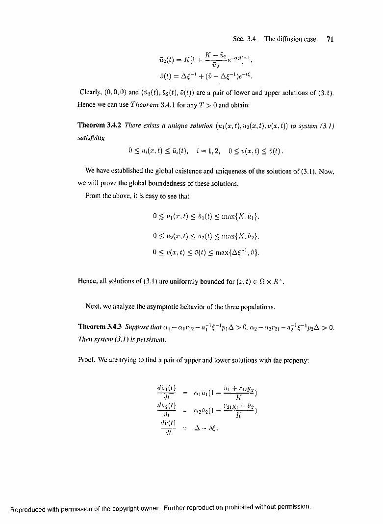
Sec. 3.4 The diffusion case. 71
u2 (t) = K { l + I ^ e - a*t} - \ u 2
v(t) = A £_1 + (v — A £_1)e_t0
Clearly, (0,0,0) and ( M O /M O M O ) area pair o f lower and upper solutions o f (3.1).
Hence we can use Theorem 3.4.1 for any T > 0 and obtain:
Theorem 3.4.2 There exists a unique solution ( ii i (x, t), uo(x, t), v(x, t)) to system (3.1)
satisfying
0 < u,(x, t) < Ui(t), 2 = 1, 2, 0 < v(x, t ) < v ( t ) .
We have established the global existence and uniqueness of the solutions o f (3.1). Now,
we w ill prove the global boundedness o f these solutions.
From the above, it is easy to see that
0 < u\(x.t.) < U. i ( t ) < max{/v. fq },
0 < i/o(x, t.) < il2(t) < m ax{/\, (1-2}.
0 < v(x ,t) < v(t) < m ax{A£_1, i)}.
Hence, all solutions o f (3.1) are uniformly bounded for (x, t.) 6 Q x R+.
Next, we analyze the asymptotic behavior o f the three populations.
Theorem 3.4.3 Suppose that a j — ci j 7’ j2 — A > 0, a 2 - n27'2i ~ c / . j '^ ’ /j^A > 0.
Then system (3.1) is persistent.
Proof. We are trying to lind a pair o f upper and lower solutions with the property:
' / M 0 . » t T r | 2»._,— = — — >f/f/2(0 . ,, r2i >ii + r/._.— “ — — >
'/<■(/),11
A - fr£.
Reproduced with permission o f the copyright owner. Further reproduction prohibited w ithout permission.

Sec. 3.4 The diffusion case. 72
and
d u^ t)dt
du2 {t)dt
dv(t) dt
with initial conditions
Ui{0) = Ui = sup u°(x) > 0, v (0) = v° = supv°(x) > 0,n q
and
M;(0) = u. = in f u°(x) > 0, u(0) = = in f v°(x) > 0,
Here, we take K = maxf/C, Uj}, i = 1, 2 for convenience.
Obviously, (u i ,u 2 ,v) and (u i ,u 2 ,v) are a pair o f lower and upper solutions o f (3.1);
moreover, we have
v{t) = A £-1 + (v° - A £ - 1)e_ie ,
v{t) = A i t + a ^ a K + a ^ c o K ) - '
+[v° - A (£ + a r 1c1/ ra 2- 1c2/ 0 “ 1]e -t(?+a>"lciA'+a2‘C2/<).
Therefore,
lim in f v(t) = A (£ + a7xc \K + a7 1c2A' ) " 1 > 0 ,*oo
lim in fv(:r, t) > lim in fv ( f ) = A(£ + a r 1CiA' + a2 1c2A') -1 > 0.t—* oo i —*oo
Again,
r+\ _ (Ql _ a' i r i 2 — a f Xpiv)ce(cn~cnri2~ni lpiV')t— 1 v / — *— —----------------------------------------------------------------Z ! ------------------------------•>
1 + Q'iA'_1ce(Q1_" ,’'12-ni ,n'^t
where c is a constant. Hence
lim in f u i ( i , f ) > lim in f u ,(a ;,t) = —— Ql?12 y \ ^ > 0 .t - 00 — ( - . o o - 1V ‘ C t \ K ~ X
i = 1, 2 ,
i = 1, 2 .
,, * £ i + r 12A \ _i= ------------^ ---J - O j lp iu xv
, , r 2iA: + u2 _ j= a 2u2( l ------------—---) — a2 po-u2v
= A — [ + aJl CiK + a2l C2K]v,
Reproduced with permission o f the copyright owner. Further reproduction prohibited w ithout permission.
Sec. 3.4 The diffusion case. 73
Similarly, we have
lim m iu 2 {x , t ) > lim in f u0 (x , t ) = — — 0 :2 ,2 1 a- ^—22—. > o.t— oo t—'00 - Ce2K ~ l
The proof is complete. □
Generally, normal and abnormal cells are competing for resources, such as oxygen,
nutrients and space. Cancer cells not only compete with those healthy cells for resources,
but also compete with each other and against healthy cells throughout the body for the same
resources. Therefore, normal cells and cancer cells have different competition effects on
each other (different values o f r 12 and r 21). Theorem 3.4.3 demonstrates that the treatment
and the competition capacities o f both populations play an important role in the persistence
o f the system, and i f one of populations eventually wins the competition, then the system
(3.1) cannot persist.
Now we w ill analyze the stability o f all possible equilibria for system (3.1),
-Eo(O) 0,£- 1A ), E i( u u 0,0), E 2 (0 ,u 2 ,v), E 3 (u*,u*2 ,v*).
By linearizing (3.1) around a uniform steady state E (u cl ,u%,vc), we obtain
du\ d2 u\~ d t = a u (u * - a i2 (u2 — ^ 2 ) + a u ( v ~ yC)
~dt = D 2- ^ - + a2 l {u { - u^) + a2 2 (u2 - u2) + a23(v - vc)
dv 02u~dt = a31 Ul — a 3 2 ( U 2 ~ “ 2) + a33(^ — vc)-
Here the one-dimensional boundary conditions in the interval 0 < x < L are:
( - ^ ± /yi(lh-u'{))\x=o,L = 0, ( ^ ± 72(u 2—u5) ) | x = 0 , l = 0, ( ^ ± J 3( v - v c))\x=0iL = 0.
The above Albedo BCs can be maintained in time by controlling the diffusive flow of u \ ,u 2
and v through the boundaries. For those BCs, (u \ ,u 2 ,v c) remain as the homogeneous
steady state for 0 < 7,- < 00, i = 1, 2,3.
Reproduced with permission o f the copyright owner. Further reproduction prohibited w ithout permission.
Sec. 3.4 The diffusion case. 74
We are looking for stability in the homogeneous steady state by using the linear stability
theory. As usual, we propose for u i ,u 2 and v the perturbed forms:
U\ ( x , t ) = Ui + E\ (x , t )
Uo(x,t) — u l + £ 2 (x ,t)
v (x , t ) = vc + s3 {x,t).
This leads to the following linear system for the small space and time-dependent
perturbations:
8_dt
" £ \ " a n + A ^ 7 “ 12 “ 13&2 - “ 21 “ 22 + Do CLo 3
. “ 3 “ 31 “ 32 “ 33 + D \-£3
1O
l
t
So (3.10)
(3.11)
By linearity, the BCs to be fulfilled by the perturbations at the boundaries are:
dsi\x=0,L~ |x=0,Li i = 1,2,3.
Equations (3.10) constitutes a set o f linear homogeneous equations of first order in time
with constant coefficients. They therefore have solutions of the form:
(3.12)
As the Laplacian is the only operator acting on the space coordinates, we choose its
eigenfunctions in order to investigate the stability o f the system:
^ \ k)(x ) = - h l ^ i x )
= -Pm^2 l\ x )
‘ £ i(x 0 1 £i(x)£2 (X t) — eXt s2 (x)
. £s(x * ) . . £s(x) _
d1
dx22 - ( n ) , \
= — n ~ e \ H ' r ) (3.13)
where k ,m and n are sets o f induces labelling the infinite sets of eigenfunctions and the
minus signs in front of hk,pm and qn takes into account that f t / d x 1 is a dissipative operator
having non-positive eigenvalues. The hk,pm and qn are functions of L, 7,-, i = 1,2,3,
respectively. The applied BCs generate the following equations for the wave vectors:
(h i - 71) sm(h,kL) = 2hkLcos(hkL)
(Pm - 7 2 ) s i n ( P m £ ) = 2 p m L C 0 S ( p m L )
(<7n - 73) sm(qnL) = 2qnL cos(qnL ) ,
Reproduced w ith permission of the copyright owner. Further reproduction prohibited w ithout permission.

Sec. 3.4 The diffusion case. 75
respectively. In order to obtain hk(7 i) ,p m(72) and qn{73), these equations must be solved
numerically.
By substituting Eqs. (3.12) and (3.13) into Eq. (10), we obtain:
(* )C1 «12 ^13(rn )«21 Co «2:j
(n )«3i «:i2 <<,
-Ik)£i£r(m)
*-(«)-a
si‘>=("•)wQ
4 " ’
(3.14)
where
c| * — « ii _ D \h l, 4 J — a22 — Do'p~n, c ^ ] — a.i.j -
This system has nontrivial solutions provided that the following equation is satisfied:
A - c 1,(rn)1 —a
—-«:u
12( m )A — C-2
— 32
-«13“ ^23
A - c , ( « )3
= 0 (3.15)
Depending on the variables A , 7,, a i , j — 1,2,3, the frequency A can be either real
or complex which leads in some particular cases to bifurcations. Therefore, in the following
we w ill consider those situations around each uniform steady state separately based on Eq.
(3.15).
3.4.2 The analysis of £u(0,0. £-1 A)
In this case, = i/f, = 0 and r' ' - £-1 A. Evaluating at this steady state, we obtain
front (3.15) that
A f D\h'l f ■ a \ '/>iA - n 1 0 0I) A - D 2p;n + «.J W 2A - n j 0
" ( 's 1 r2*A A »- />,(/’• + £= 0 .
Hcncc
A| ft, - «, 'p i A - D]h'l
\ 2 ... n , - o . j ' r ' p j A ~ 0 2pi,
Reproduced with permission o f the copyright owner. Further reproduction prohibited w ithout permission.
Sec. 3.4 The diffusion case. 76
As a result, we have the following theorem.
Theorem 3.4.4 For system (3.1), no Turing instability occurs and the diffusion has no
effect on the stability o f the uniform steady state E q(0] 0; £-1 A ) i f a i < A and
a 2 < a2Xt i ' l p2A. However, i f Qj > A + D \h \ o r a 2 > a f 1 ~1p2A + D 2p n,
then E 0(0; 0; £-1 A ) becomes unstable.
Thoerem 3.4.4 shows that with a fixed wave number, a necessary condition for cancer
growth is that a2 should be sufficiently large with a relatively weak intensity treatment
(small a2 lp2), which coincides with our intuition.
3.4.3 The analysis of E \ (ui, 0, v)
Again, in this case, u\ = u h u2 = 0 and vc = v. Evaluating atj at this steady state gives
thatA + D ih l — an
0—flsi
A + D 2P™ — a22 —a32
0 = 0, A + D 2q\ — a33
“ ^13
where
a 12 = — OL\ri2u \K
«2i = 0, a2 2 = (*2(1 — ^21^1I<
Hence
A2 — (J-22 ~ D 2lt% ,
(7(A) = {A, |A2 - T r(A )A + det(A ) = 0, i = 1,3}
where
Reproduced with permission o f the copyright owner. Further reproduction prohibited w ithout permission.

Sec. 3.4 The diffusion case. 77
A = an - D xh \ a13<^31 a 33 —
I f u\ > K /2 , then
and
^11^33 — 013 31 =
, 2*1«n = - a i ( - 7 T “ 1) ~K
aiPiV (ax + u xf
< 0,
a\P\v ^ [ cxu x a xcxp xu xv
I< ( a i+ U i )2 a i + * i ( a i + * i )3,, ^a x cj-ui
= - a i ( i - - r r ) ( S + — ~ r ) +CiUi P iaiA £
I< a i + * i (ax + * i) [a i£ + (£ + « i) * i]> 0 .
Since a33 < 0, we have
T r{A ) = axx + a33 - D xh \ - D 3q\ < 0,
det(A) = D xD 3h \q \ — (a xxD 3q~ + a33D xh \) + (ana33 — a13a3i) > 0.
By the Routh-Hurwitz criteria, we have Re A; < 0, i = 1,3. Note that E x(ux, 0, *) is
locally asymptotically stable i f a.i < a'2.A- 1r 2i * i + a2~ 1p2v in the absence o f diffusion.
Therefore, there no Turing instability occurs under the diffusion case.
Theorem 3.4.5 For system (3.1), suppose that ux > K /2 , ancl a 2 ^ a 2K ~ l r 2xu x +
a2~lp2i) + Then no Turing instability occurs and the diffusion has no effect on the
stability o f the uniform steady state E x(u i , 0, v) provided that a2 < a 2K ~ ] r 2 Xux + a 2~1p2v.
However, i f a 2 > a2I \ ~ l r 2xu x + a f xp2v + D 2jrvl, then E x (ux, 0, v) becomes unstable and
the cancer cells begin to grow and eventually win the competition with the normal cells.
Comparing with Theorem 3.3.4 in the no diffusion case, Theorem 3A.5 shows that the
diffusion has no effect on the stability o f the uniform steady state E x/u x,Q, * ), and there is
no Turing instability to occur in the diffusion case. However, the survival o f populations
w ill also depend on the space along with those factors (see Theorem 3.3.4) included in
the no diffusion case. The simulation o f our models demonstrates that small diffusion does
benefit the survival o f both populations in such a case (see F igure 3.4).
Reproduced with permission of the copyright owner. Further reproduction prohibited w ithout permission.
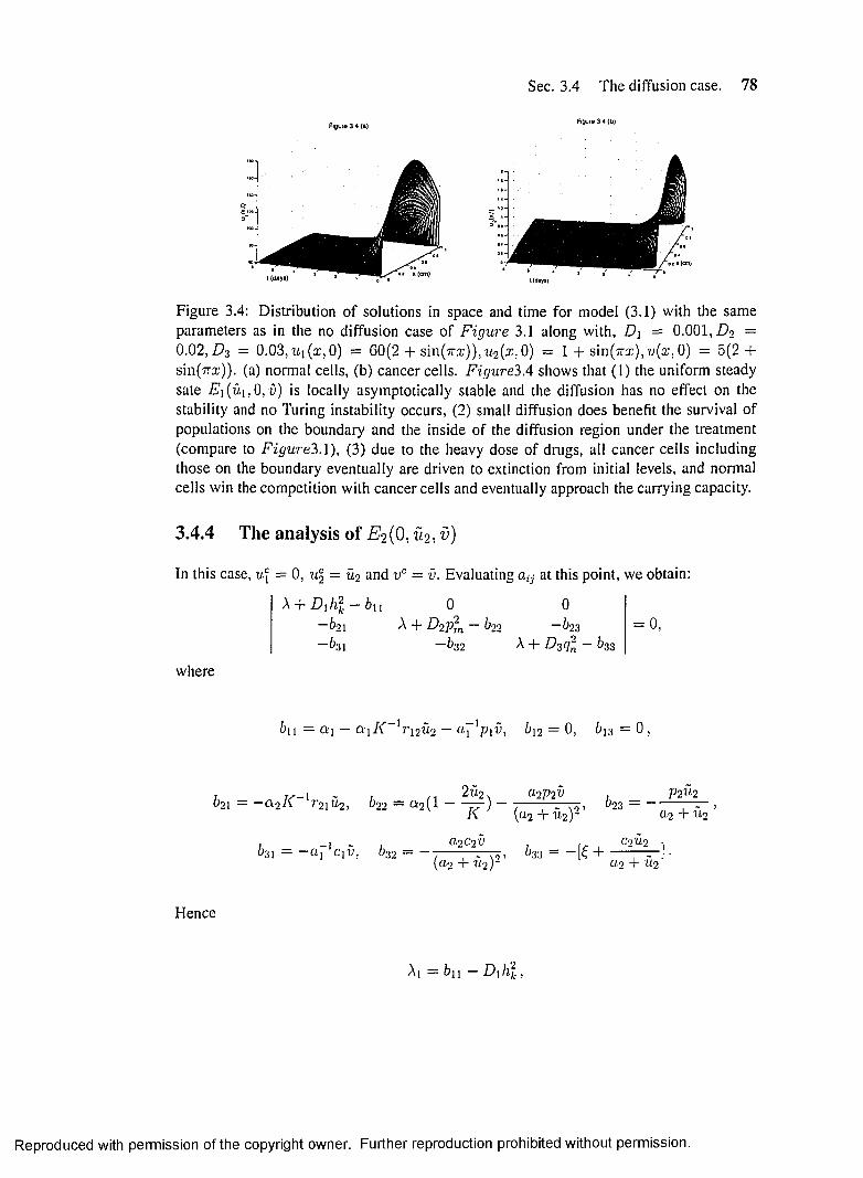
Figure 3 4 (a)
Sec. 3.4 The diffusion case. 78
Figure 3 4 (b)
l(cUyi)
Figure 3.4: Distribution o f solutions in space and time for model (3.1) with the same parameters as in the no diffusion case o f F igure 3.1 along with, D \ = 0.001, Do = 0.02, Z?3 = 0.03, u \(x , 0) = 60(2 + sin(7ra:)),'!i2(3:j 0) = 1 + sin(7rx), v(x, 0) = 5(2 + sin(7nr)). (a) normal cells, (b) cancer cells. F igu re3.4 shows that (1) the uniform steady sate E \(u i,0 , v) is locally asymptotically stable and the diffusion has no effect on the stability and no Turing instability occurs, (2) small diffusion does benefit the survival of populations on the boundary and the inside of the diffusion region under the treatment (compare to F ig u re 3.1), (3) due to the heavy dose o f drugs, all cancer cells including those on the boundary eventually are driven to extinction from initial levels, and normal cells win the competition with cancer cells and eventually approach the carrying capacity.
3.4.4 The analysis of Eo(0,U2,v)
In this case, u\ = 0, u2 = u2 and vc = v. Evaluating ay at this point, we obtain:
A + D [h 2 — 6u — 21 ~&31
0A + Da?m - b22
—h32
0~ b 23
A + D 3ql — b.33
= 0,
where
ci] — a \ I \ r 12w2 '1 2 0, b\3 = 0
2£t2^ 2 1 = — l K V 2 1 U 2 , b32 = Oi 2 ( 1 -------------— ) —
C12P2V
K ' (a2 + u 2)2 ’
, _ -1 - , a,2C2vO31 — —a, C\v, O32 — —
bo2 — ~
(a2 + U2)2
P2 U2
0-2 4" iia
, &33 = - [£ +C2+2 j
C lo + t i n
Hence
X ^ b n - D . h l ,
Reproduced with permission o f the copyright owner. Further reproduction prohibited w ithout permission.

Sec. 3.5 Numerical results 79
o (B ) = {A,-1A2 - T r { B )A + det(B ) = 0, i = 2,3},
where
B = b22 - D2p;n b23 b32 b33 — D 3q2
Similarly, i f u2 > K /2 , then we have
T r(B ) — b22 + 633 — D 2Pm — D 3q2 < 0 ,
de t(B ) = D 2D 3p nq2 — (b22D 3q2 -F b33D 2pjn) + (b22b33 — b32b23) > 0 .
Theorem 3.4.6 For system (3.1), suppose that u2 > K /2 , and a\ f- a xl \ ~ xr x2ii2 +
a \ lVi v + D \h 2k. Then no diffusive instability occurs and the diffusion is harmless to the
stability o f the uniform steady state E2(0,u2,u) provided cii < a xK ~ xr X2u2 + a / lp xv.
However, i f a* > a \K ~ l r X2u2-\-a fxpxv + D \ifk then E2(0 ,ii2,v ) is unstable and the normal
cells w ill eventually win the competition with the cancer cells under the chemotherapy
treatment.
Comparing with Theorem 3.3.6 in the no diffusion case, Theorem 3.4.6 shows that
the diffusion has no effect on the stability of the uniform steady state E2(0. u2, v), and no
Turing instability occurs in the diffusion case. However, the survival of cell populations
w ill also depend on the space along with those factors (see Theorem 3.3.6) included in
the no diffusion case. The simulation o f our models demonstrates that small diffusion docs
benefit the survival o f both cell populations in such a case (see Figure 3.5).
3.5 Numerical results
In order to perforin the numerical simulations of system (3.1) and (3.2). we impose some
conditions based both on the analytical results and on some physiological arguments:
a) o_> > n 1 (cancer cells grow faster than normal cells).
Reproduced with permission o f the copyright owner. Further reproduction prohibited w ithout permission.

Sec. 3.5 Num erical results 80
Figu»o3 5(a) Figuro 3 S (b)
Figure 3.5: Distribution o f solutions in space and time for model (3.1) with the same parameters as in the no diffusion case o f Figure 3.2 along with, D \ = 0.001, Do = 0.02, D 3 = 0.03, u i(x , 0) = 60(2 + sin(7n r)),u2(x, 0) = 1 + sin(Trx), v(x, 0) = 5(2 + sin(7rx)). (a) normal cells, (b) cancer cells. F igure3.5 shows that ( 1) the uniform steady sate E 2(0 ,u2,v ) is locally asymptotically stable and the diffusion has no effect on the stability and no Turing instability occurs, (2) small diffusion does benefit the survival of cell populations on the boundary and the inside of the diffusion region under the treatment (compare to Figure3.2), (3) due to the small dose o f drugs, cancer cells eventually win the competition with normal cells and grow to approach the carrying capacity.
t (dAyt) l(dayi)
Figure 3.6: Distribution of solutions in space and time for model (3.1) with the same parameters as in the no diffusion case of Figure 3.3 along with, D \ = 0.0001, D 2 = 0.002, D 3 = 0.003, u i(x , 0) = 53(2 + sin(7rx)), u2(x, 0) = 18.1(2 + sin(7rx)), v(x, 0) = 5(2 + sin(7rx)). (a) normal cells, (b) cancer cells. F igure 3.6 demonstrates that (1) the normal cells grow and peak at a level which is far higher than that fo r the abnormal cells, which is due to the weakening effects o f cancer inhibition and regeneration o f the normal cells, and (2) the heavy drug dosage ultimately causes damage to regrowth and proliferative capabilities o f the cancer cells, and keeps it at a lower level than that o f normal cells.
Reproduced with permission of the copyright owner. Further reproduction prohibited without permission.

Sec. 3.5 Numerical results 81
b) p2 » p i (the drug is more potent against the cancer cells than against the normal
cells).
c) c2 > > ci (a consequence of the above item).
d) the hypotheses o f Theorems 3.3.1 and 3.3.2 which guarantee the existence of E\ and
E 2 are satisfied.
Also the initial condition is such that: > u° (in general), i.e. the cancer is initially not
too advanced.
In the no diffusion case, F igure 3.1 shows that the boundary equilibrium
E\ (60.0,0,5.0) is locally stable. Initially, the cancer cells grow but eventually decrease
and are driven to extinction. This is due to the heavy dose o f chemotherapy drugs, which
inhibits the proliferative capacities o f the cancer cells and causes damage to the cancer
growth.
In the no diffusion case, F igure 3.2 shows that solutions for model (3.2) approach
E2(0 ,60.0,5.0) i f the treatment intensity is weak (small values of a2~l p2 and/or £-1 A).
Here other parameters and initial conditions are the same as in Figure 3.1 except p2 =
0.01. From F igure 3.2 it is easy to see that (1) the normal cells grow at the beginning
due to their large initial size but eventually lose the competition with the cancer cells and
decrease to zero due to the weak intensity treatment(small p2), and (2) the cancer cells
accumulate persistently at the beginning and take about 20 days to dominate the normal
cells. This is due to the weak intensity o f the treatment. F igu re 3.3 shows that system
(2) is uniformly persistent and the interior equilibrium £ 3(53.0,18.1,5.0) is locally stable.
Here also the drug is selectively lethal to the cancer cells and controls them at a lower level
than the normal cells.
In the presence o f diffusion, F igure 3.4 shows the distribution of solutions in space and
time for model (3.1) with the same parameters as in the no diffusion case o f Figure 3.1
along with, D\ = 0.001, Do = 0.02,1)3 = 0.03, u \{x , 0) = 60(2 + sin(7rx)), u2(x, 0) =
1 + sin(7rx),u(a;, 0) = 5(2 + sin^rc)). From F igure3A we can see that (1) the uniform
steady sate E i(u i,0 , v) is locally asymptotically stable and the diffusion has no effect on
the stability and no Turing instability occurs, (2) small diffusion does benefit the survival
o f populations on the boundary and the inside o f the diffusion region under the treatment
Reproduced with permission of the copyright owner. Further reproduction prohibited without permission.

Sec. 3.5 Numerical results 82
(compare to F i g u r e 3.1), (3) due to the heavy dose of drugs, all cancer cells including those
on the boundary eventually are driven to extinction from initial levels, and normal cells win
the competition with cancer cells and eventually approach the carrying capacity.
In the diffusion case, Figure 3.5 shows the distribution o f solutions in space and time
for model (3.1) with the same parameters as in the no diffusion case of Figure 3.2 along
with, D\ = 0.001, Do = 0.02, £3 — 0 .03,u i(x ,0) = 60(2 + sin(7ra:)), U2 (x, 0) =
1 + sin(7rx), v(x, 0) = 5(2 + sin(7rx)). From F igu re3.5 we can see that ( 1) the uniform
steady sate £ 2(0, u2, v) is locally asymptotically stable and the diffusion has no effect on
the stability and no Turing instability occurs, (2) small diffusion does benefit the survival of
cell populations on the boundary and the inside o f the diffusion region under the treatment
(compare to Figure?).2), (3) due to the small dose of drugs, cancer cells eventually win
the competition with normal cells and grow to approach the carrying capacity. Figure
3.6 shows the distribution o f solutions in space and time for model (3.1) with the same
parameters as in the no diffusion case o f F igure 3.3 along with, D \ — 0.0001, £2 =
0.002, £3 = 0.003, u \(x , 0) = 53(2 + sin(7rx)), ^ ( x , 0) = 18.1(2 + sin(7rx)), v(x, 0) =
5(2 + sin(7rx)).
Finally, in the diffusion case, F i g u r e 3.6 demonstrates that (1) the normal cells grow
and peak at a level which is far higher than that for the abnormal cells, which is due to
the weakening effects of cancer inhibition and regeneration of the normal cells, and (2) the
heavy drug dosage ultimately causes damage to regrowth and proliferative capabilities of
the cancer cells, and keeps it at a lower level than that o f normal cells.
Comparing with T h e o r e m 3.3.4 in the no diffusion case, T h e o r e m Z A . h shows that the
diffusion has no effect on the stability o f the uniform steady state E \ { u \ , 0, v ), and there is
no Turing instability to occur in the diffusion case. However, the survival o f populations
w ill also depend on the space along with those factors (see T h e o r e m 3.3.4) included in
the no diffusion case. The simulation of our models demonstrates that small diffusion does
benefit the survival o f both populations in such a case (see F i g u r e 3.4).
Comparing with T h e o r e m 3.3.6 in the no diffusion case, T h e o r e m 3.4.6 shows that
the diffusion has no effect 011 the stability o f the uniform steady state £ 2(0, u 2, v ) , and no
Turing instability occurs in the diffusion case. However, the survival of cell populations
Reproduced w ith permission of the copyright owner. Further reproduction prohibited w ithout permission.

Sec. 3.6 Discussion 83
will also depend on the space along with those factors (see Theorem 3.3.6) included in
the no diffusion case. The simulation o f our models demonstrates that small diffusion does
benefit the survival of both cell populations in such a case (see F igure 3.5).
3.6 Discussion
The three most important steady states o f our model from a physiological point o f view
are E \.E 2 and E:i. E\ represents a cancer free state, and of course the most desirable
result would be to have E x globally asymptotically stable. E2 represents a state which is
exclusively cancerous and is a lethal state for the individual. E2 represents a state where
normal and cancer cells exist simultaneously.
We are able to obtain analytic criteria for E\ to be locally asymptotic stable, but not
globally stable. Numerically, we can show that i f treated with a heavy dose o f drugs (big
value o f /m), solutions may approach E\ (F igu re 3.1). However, solutions may approach
E2 (F igure 3.2) i f the treatment intensity is weak (small values of and/or £- 'A ),
and may approach E:i (F igure 3.3) i f the treatment intensity is strong (higher values of
h-JVj and/or A). This demonstrates an equi-asymptotical stability in the large for E:i.
Also the region o f stability o f E\ is found numerically to increase with higher treatment
levels. On the other hand, we show that it is possible to choose parameters and initial
values so that solutions o f system (3.1) approach a positive state E.K with the cancer level
small. In a bounded space region, we find numerically that diffusion has no effect on the
stability o f constant solutions and no Turing instability occurs. I f the treatment is strong
enough, then solutions o f system (3.1) approach the uniform steady stale E\ (F igures 3.4)
and the drugs k ill all cancer cells. In the case of a weak intensity treatment, we find normal
cells lose the competition with cancer cells and all cells including those on the boundary
are driven to extinction (Figure 3.5 (a)). However, in such a situation (weak intensity
treatment) cancer cells have the growth advantage over normal cells and eventually win the
competition with all normal cells and approach the carrying capacity eventually (F igure
3.5 (h)). Numerically, it is also possible to choose parameters and initial values so that
solutions of system ( I) approach a positive state E:i with the cancer level small in the
diffusion case (/•'»>;un 3.6) under a reasonable treatment.
Reproduced with permission o f the copyright owner. Further reproduction prohibited w ithout permission.

Sec. 3.6 Discussion 84
In a population system, diffusion or dispersal exists in many instances. However, in some
systems, when diffusions are considered, the stability o f the corresponding ODE systems
may be changed. Hence one o f the purpose of this work is to fully understand just what
features o f reaction-diffusion systems are necessary and sufficient for Turing instabilities
and compare the dynamics o f our model in the case of no diffusion to the diffusion case.
Unfortunately, Turing instability does not occur in the systems considered here. However,
we prove that each uniform steady state is unique for the system and asymptotically stable
in both cases, which means that in this kind of a system, the diffusion does not change
the stability. However, our numerical solutions show that a small diffusion may benefit the
survival o f all cell populations.
Finally, with respect to clinical advantage, we point out how our results may be useful
to leukemia treatment. For those situations in which our models may apply, the theorems
identify which combination o f coefficients, i.e. sufficiently high or low values would lead
to low levels o f cancer, or elimination altogether. It is known [92] that different leukemias
can be treated with various successes ( or failures), and our results may be used to help in
improving the successes (i.e. the rate o f success or length of remission time).
Reproduced with permission o f the copyright owner. Further reproduction prohibited w ithout permission.

A Mathematical Model of Chemotherapy Treatment with Chronic Myeloid Leukemia
4.1 Introduction
Hematopoietic stem cells are generally characterized by three properties: they are capable
o f dividing and renewing themselves for long periods o f time; the process of differentiation
is not complete; and after dividing, each daughter cell either remains a stem cell or proceeds
to a terminal differentiation in order to form different types o f blood cells throughout the
body such as leukocytes (white blood cells), erythrocytes (red blood cells), lymphocytes
and platelets [25]. B and T leukocytes form part o f the immune response and serve
to prevent infections. They travel in the blood stream, but also can pass into tissues
surrounding the circulatory system. Other cells that circulate with the leucocytes, are
erythrocytes which contain hemoglobin for transport o f oxygen throughout the body, and
platelets which participate in the process o f hemostasis(or blood clotting).
Chronic myeloid Ieukemia(CML), also known as granulocytic leukemia, chronic
myelogenous leukemia, and chronic myelocytic leukemia, is a clonal stem cell disorder
that begins as an indolent disease in which the myeloid lineages in the bone marrow and
blood gradually expand. The hallmark o f CM L is the Philadelphia chromosome(22q-)
85
Reproduced with permission o f the copyright owner. Further reproduction prohibited w ithout permission.

Sec. 4.1 Introduction 86
resulted from a reciprocal translocation that also involves chromosome 9. The reciprocal
translocation t (9,22) generates two novel fusion genes: BCR-ABL on the derivative 22q-
chromosome, and ABL-BCR on chromosome 9q+ [22,51]. The ABL gene product is a
protein tyrosine kinase, and the fusion protein BCR-ABL has constitutive kinase activity
that deregulates signal transduction pathways, causing abnormal cell cycling, inhibition
o f apoptosis, and increased proliferation o f immature cells. BCR-ABL is very important
because in patients with CML, the clonal expansion o f hematopoietic stem cells express
this unique fusion gene. Moreover, continued expression of BCR-ABL is required for
sustained proliferation o f leukemic cells [22,43,50,51].
From the view point o f cytokinetics, it is generally believed that CML develops when
a single, pluripotential, hematopoietic stem cell acquires a Ph chromosome carrying the
BCR-ABL gene, which confers on its progeny a proliferative advantage over normal
hematopoietic elements and thus allows the Ph-positive clone gradually to displace residual
normal hematopoiesis [25]. This competitive growth advantage of abnormal stem cells
usually gives rise to a malignant proliferation and subsequently, to the relative dominance
of the abnormal stem cell population. Frequently, the abnormal cells do not differentiate at
a sufficiently high rate to form healthy levels o f white and red blood cells. This results in
anemia and in a weakened immune system, vulnerable to infections [20]. Moreover, CML
stem cells seem to survive longer than their normal counterparts as a result o f defective
apoptotic response to stimuli that would otherwise lead to physiologic cell death.
Dynamically, CML progresses through three phases: the chronic phase, the acceleration
phase, and the acute phase. The mechanisms for the evolution o f the massive hyperplasia
and for the blastic crisis from CML are poorly understood. The most generally accepted
hypothesis proposes that this progression is due to the development o f genetic instability
in the leukemic cells. In particular, the last two phases o f the disease are believed to reflect
different, discrete genetic events. Such events remain undefined as yet, and the causal
significance o f observed genetic aberrations is not clear.
In humans and mice, hematopoietic stem cells are the only normal progenitors that
renew themselves [2,4,23,57,67,73,78,103] and therefore, they are widely considered to
be the only cells in the marrow in which preleukemic changes can accumulate, whether by
Reproduced with permission o f the copyright owner. Further reproduction prohibited w ithout permission.

Sec. 4.1 Introduction 87
genetic or epigenetic means. However, it is also possible that a downstream progenitor
can acquire self-renewal capacity[53,67,81,87,88] and the deregulation of self-renewal
pathways in these progenitors, which are normally tightly regulated in hematopoietic stem
cells [2,23,57,67,73,78,88,103,108] has been recognized as an important step in leukemic
progression. Recent work (Jamieson et al [52]) shows that the progression of CML to blast
crisis is supported by self-renewing leukemic progenitor cells. Unlike normal granulocyte-
macrophage progenitors, CM L granulocyte-macrophage progenitors form self-renewing
myeloid colonies and the progenitor pool from patients with CM L in blast crisis, rather than
the pool o f hematopoietic stem cells, is expanded, generates BCR-ABL and has elevated
levels o f nuclear ^-cantenin as compared with the levels in progenitors from normal
marrow, increasing their proliferative and self-renewal capacity and possibly allowing them
to become leukemic stem cells, thus giving rise to the progression to blast crisis [52], Here,
,/3-cantenin is cytoplasmic protein that has important structural and signaling functions.
Expressing /3-cantenin usually leads to an enhanced ability o f self-renewal of hematopoietic
stem cells. Abnormalities in the regulation o f structural and signaling functions o f 8-
cantenin gives rise to tumorigenesis [52].
Working on the haematopoietic stem cell population (HSC), Mackey [65] proposed a
standard Go model for the cell cycle in order to calculate the steady state parameters
characterizing the HSC populations, such as the differentiation rate, the rate of cell re
entry from Go back into the proliferative phase, and the rate o f apoptosis. The purpose
o f [65] is to understand how the HSC population carries out the cellular production over
the course o f a lifetime and thus the kinetics o f HSC populations. In this chapter, we
work on a downstream compartment, granulocyte-macrophage progenitor compartment in
which we assume that the cells obtain a self-renewal capacity and the progenitor cells
go into a cell cycle with a similar standard G0 model properties as in [65]. Due to the
lack o f better knowledge about the cell kinetics in this compartment, we do not know
what specific function forms the model w ill take in this compartment. Based on the bio
medical work in [521. a general formulation with self-renewal properties is proposed to
mathematically study the dynamical progression o f the disease. Our interest here is to
formulate a plausible explanation o f the transition from the seeming stable chronic phase
Reproduced with permission o f the copyright owner. Further reproduction prohibited w ithout permission.

Sec. 4.1 Introduction 88
to the unstable acceleration phase and ultimately, to the rapidly changing acute phase.
Finally, based on all the qualitative behaviors o f the model, a continuous treatment
for CML is considered. Herein, our model is significantly different from [65] in that
more general functions and treatment are included. The ultimate role o f our mathematical
modelling in cancer treatment is to provide a more rational basis for experimental design
of the anti-cancer drugs and to make qualitative predictions with regard to the dynamic
evolution o f the disease based on the cytokinetic parameters o f the patient and the drug
parametric configuration. In cancer treatment today, four types o f treatment are most
commonly used in efforts to obtain long-term periods o f disease-free remission. These
include surgery, radiotherapy, chemotherapy and immunotherapy. Allogeneic bone marrow
transplantation can cure chronic-phase CML in up to 70 percent of patients, but the use
of this procedure is limited by the toxicity o f the treatment, the risk o f graft-versus-host
disease, and the lack o f suitable donors for many patients. Cancer chemotherapy treatment
now has demonstrated a definite capacity for controlling disseminated metastatic cancer
and is therefore widely used (Dorr and Von Ho [24], Frei [37], Liotta [63], Perry [84]). In
cancer chemotherapy, anti-neoplastic drugs are designed to selectively destroy or inhibit
the proliferative activity o f cancer cells while the normal cells are affected to a lesser
extent (Dorr and Von Ho [24], Frei [37]). Recent studies show that up to 80 percent of
patients enter a period of complete cytogenetic remissions when treated with imatinib
mesylate(called Gleevec), a new ABL-specific tyrosine kinase inhibitor that specifically
blocks the enzymatic action o f the BCR-ABL fusion proteins [45]. The introduction into
clinical practise o f such an inhibitor promises to be a major contribution to the management
of CML and may also prove to be the lead agent that ushers in an era o f success with
molecularly targeted therapy for other leukemias, lymphomas, and cancers. Interferon alfa
therapy also extends survival by one to two years and can reduce the number o f cells with
the Philadelphia chromosome [82]. Combined treatment with interferon alfa and cytarabine
may have further benefits, and many view it as the gold standard of therapy. It is within this
context that our studies o f chronic myeloid leukemia and its corresponding chemotherapy
treatment may be significant.
The organization o f this chapter is as follows. In the next section, we develop our model.
Reproduced with permission o f the copyright owner. Further reproduction prohibited w ithout permission.

Sec. 4.2 The model 89
In section 4.3 we discuss the invariance o f nonnegativity, boundedness of solutions, nature
o f equilibria, and their stabilities in the no treatment case. In the section that follows
we look at the continuous treatment case: we discuss the existence and local stability of
relevant equilibria, and check the effects o f the time delay on the stability of solutions.
These are done both analytically and numerically. In section 4.5 we give some numerical
examples to illustrate our results. Out final section contains a discussion.
4.2 The model
In order to better understand the standard G0 model properties in [65], we make the
following assumptions. The stem cells progress through a multi-staged system. Steps
to model such a population are as follows:
1) The granulocyte-macrophage stem cells constitute a population (compartment G M )
with its own feedback mechanism controlling population size. This means that at any
given time, the population o f stem cells is evaluated and if this population is greater than
a certain threshold, future production w ill be reduced. Conversely, i f the population lies
below the threshold, more cells w ill begin a process o f self-renewal. This mechanism
serves to maintain the stem cell population at some optimal level while smoothing out both
positive and negative perturbations from this level. The process o f self-replication, though,
takes a non-trivial amount of time. Hence, when new cells are entering the system, they are
entering based on slightly outdated information. As such, certain values for the delay most
likely exist which would give rise to an instability in this system leading to blast crisis.
2) When the population size reaches the ’’normal” state (no cells removed from the
population) the cells are in a state o f dormancy with respect to growth, that is, the cells
neither proliferate nor initiate any further cellular differentiation and just remain in their
current compartment.
3) When a number o f cells is removed from the population(at a rate S(N), with N
representing the number of cells) the feedback mechanism triggers an equal number from
the remaining cells.
4) The triggered cells ’ ’emit” a signal which may be interpreted as ’’message received
and understood” .
Reproduced w ith permission o f the copyright owner. Further reproduction prohibited w ithout permission.

Sec. 4.2 The model 90
Cells Reentry into Proliferation a (N )N
Delay
Proliferating Phase Cells
5(N)NGM
Cellular Differentiation
Mortality(a) Resting Phase Cclls(N)
Figure 4.1: Based on F igure 3.6 in Neiman [77], the G M model for cell growth shows how cells may either remain in the G M resting phase, go through a process of self-renewal to reproduce cells, or begin a differentiation process to form different types o f cells.
5) The feedback mechanism ceases to create further cells.
6) The triggered cells begin a self-renewal process (at a rate a(iV))involving four phases:
G i, S, Go, and M phases. Thus the population size is returned to normal.
The stem cell population has, however, the particular characteristics of never in fact
reaching its ’’normal” size (and with a dormancy state for all its cells) due to the existence
o f a continuous removal o f cells from the population by an exogenous mechanism [77].
Therefore, in the physiological steady state o f haemopoiesis a balance should exist, in
which, a physiological mechanism is removing (at a rate 6{N )) a certain proportion o f
stem cells from the stem cell population, and therefore, the positive feedback control for
the population size triggers a similar proportion o f stem cells moving into the cell cycle (at
a rate a(N )). Hence, after a time delay r , two cells re-enter the compartment as a result
o f one cell self-renewing. Some cells w ill die (at a rate a) during this proliferation process.
The model is illustrated in F igure 4.1.
Now let x (t) represent the concentration of normal cells in the G M phase, y {t) the
concentration of leukemia cells, and u(t) the concentration o f chemotherapy agents. The
model then takes the form
x ( t ) = 2 ( 1 - a i) x T, a i ( x r i , y Tl) - x a n ( x , y ) - 5 i x ( t ) - p i ( x ) w ( u )
y { t ) = 2 ( 1 - a2)i jT2a 2( x T2, y T2) - y a 2( x , y ) - 62y(t) - M y ) w ( u )
u ( t ) = A - [7 + y ip,(.r) + T]2P2 ( y ) )w{u) , (4.1)
Reproduced with permission o f the copyright owner. Further reproduction prohibited w ithout permission.

Sec. 4.2 The model 91
with initial conditions
x (t) = cf)\(t) > 0, y(t) = <f>2( t ) > 0, u(0) = u0, t e [—r , 0], r = m aa^r^TT},
where r, and r2 are the delays for the normal and cancer cells, respectively; x Tl = x ( t - T i ) ,
ijv2 = y {t - t 2).
a \,a 2 are the respective cell mortality rates o f normal and abnormal cells in a cell cycle
period.
Q'i i Q2 represent the self-renewal growth rates o f normal and abnormal cells, respectively.
£ i, S2 are the respective differentiation rates.
p i , p2 represent the cell-killing rales per unit agent o f the chemotherapy.
7/1, 7/2 represent the combination rates o f the chemotherapy agents with the cells.
w is the concentration dependent chemotherapy effect.
7 is the loss rate o f poison for chemotherapy agents.
A is the rate o f continuous constant infusion o f chemotherapy agents.
Specifically we assume the following properties for the defined functions.
( / l i ): According to the negative feedback properties for controlling cell population size
and the competing properties between both cell populations, the growth rate is diminished
by increasing the number of either cell population. This leads to the condition
r9 n ,(.r ,;/) ( ) a 2 ( . r . i / ) <)c\ 2 ( j \ y ) ^------ < 0. ----- < 0.-------t < 0. ----- < 0.
(J.r ()ii t).r ()i/
( /! >): Both cell populations should grow if they are very small. Hence
n ,((1.0) > 0. n 2(0,0) > 0.
(A i): It is supposed that there are proliferative limits for each cell population, which
could occupy the space and he adequately supported by the environment in the absence
of the competing cell population. This is tantamount to supposing that there exist h \. l \ 2
such that
„ i( A V o) + a V ^ ± J ! ! o. „.A 0 . K t ) + K , » ^ M< I.r ()u
Reproduced with permission o f the copyright owner. Further reproduction prohibited w ithout permission.
Sec. 4.2 The model 92
(A i): p i(0) = 0 ,p j(x ) > O fo rx > 0, p'2(y) > 0 for y > 0. Further p2{0) > p!(0) due
to the selectivity o f the the chemotherapy agent.
(As): 'tu(O) = 0, w '(u ) > 0. Further lim u_ +00 w (u ) = ui < +oo. The existence o f ui is
due to empirical observations o f the effect o f body enzymes on chemotherapy agents(Agur
et a l.[l], Curt and Collins [21], Shargel and Yu [94]). We assume that the chemotherapy
agent is in itia lly zero at time t = 0.
A t this point we w ill establish two important properties of solutions to system (4.1).
Theorem 4.2.1 A ll solutions o f system (4.1) with positive in itia l values remain positive.
Proof. Since u ( 0) = A > 0, no solution u( t ) of (4.1) with u ( t ) > 0 can become zero. The
nonnegativity o f x ( t ) and y( t ) can be proved by induction. Assume that ( x ( t ) , y ( t ) ) > 0
for t 6 [(n — l ) r , n r ] . Consider the following initial value problem
v i { t ) = - u i ( i ) ( a i ( w i ,U 2 ) + 5i + q i ( v 1) w{ u ) )
v2(t) = - v 2( t ) ( a 2( v i ) v2) + S2 + q2(v 2 ) w( u ) ) , (4.2)
with initial value
v i ( nT ) = x nT, v2( n r ) = y nT, t G [nr, (n + l) r ] .
It is obvious that (u i(t),'u2(0 ) >s nonnegative for (x nT,ynT) > 0. Hence V{{t — r*) > 0.
Now one can look at (4.2) and notice that
2(1 - a i ) r Tlcv i(xT l, y Tl) - x ( t ) a f x , y ) - Six(t) - x ^ q f x ^ w i u ) >
—x(t)a\(x, y) - 5\x(t.) - x( t )qx(x)w(u)\
2(1 - a2)yT2a 2(xT2,yT2) - y( t )a2{x,y) - S2y(t ) - y(t)q2(y)w(u) >
- y { t ) a 2( x , y ) - 5vy( t ) - y ( t ) q2(y) i u(u) ,
where we have setp,(u) = vqi(v). Therefore,
x ( t ) > - v x{ t ) { a \ { v \ , v 2) + 5X + q \ { v \ ) w ( u ) )
y { t ) > - V 2 ( t ) ( a 2( v i , v 2) + 52 + q2(v2) w { u ) ) , t e [ n T , ( n + l ) T } . (4.3)
Reproduced with permission o f the copyright owner. Further reproduction prohibited w ithout permission.

Sec. 4.2 The model 93
It follows that x ( t ) > v \ ( t ) , y( t ) > v2( t ) with initial values V i ( n r ) = x { n r ) , v2{ t i t ) =
y (n r ) . Moreover, the solution of (4.2) is nonnegative because v i ( t i t ) = x (n r ) >
0, Vo(nr ) = y (n r ) > 0. This implies from comparison theory that x( t ) > v i ( t ) , y ( t ) >
v2(t) for t E [n r, (n + l ) r ] . Hence x { t ) > 0, y( t ) > 0. Notice that x ( t ) = 4>\{t) >
y{ t ) = > 0 for all t > 0. It follows that x ( t ) > 0, y ( t ) > 0 for all t > 0.
Theorem 4.2.2 System (4.1) is dissipative provided that there exists M \ > 0, M 2 > 0 such
that \\4>\|| < M i, ||021| < M 2.
Proof. Since the initial conditions are nonnegative, then so are the solutions. From (4.1)
we have
x (t) < 2(1 - a i)x Txa i( x Tl,yTl) - 5xx ( i)
< 2(1 - a O x ^ a ^x ^ .O ) - 5xx {t)
< 2(1 — a i)K \C ii(K i, 0) — 5\x{t),
that is,
i { t ) < £ i - 5 ix ( t ) , ^ = 2(1 - a i ) I < i a i ( K u 0) > 0.
By using the ’ ’variation o f constants” formula for the inequality and standard comparison
theory, we obtain
x (t) < x(to)e-<Sl _t(l 4- — (1 —Si
Passing to the lim it superior in both sides, we get
lim supx(i) < t-oo Si
Similarly, we have
2/(0 < 6 - S2y(t), ^2 = 2(1 - a2)I<2a2{0, I<2) > 0.
Again, with the help o f the ” variation of constants” formula for the inequality and standard
comparison theory, we obtain
lim sup i/(0 < 1 -*—’00 O2
Reproduced with permission of the copyright owner. Further reproduction prohibited w ithout permission.

Sec. 4.3 The no treatment case 94
Note that from (4.1) we have
u(t) < A — 7 w(u)
< A - 7u(f),
which gives
lim sup 'ii(f) < 7 - 1A , 7 = m ax{7rD(u)}, w (u ) — u(t)w (u).t —*oo
Now let M i = m a x {M i,^ i/5 i}. Then the region 5R = { (x ,y ,u ) £ R+ : 0 < x (t) <
M \, 0 < y ( t) < Mo, 0 < u(t) < 7 _1A } is an attracting invariant region proving the
property. □
Model (4.1) is analyzed throughout the remainder o f this chapter. However, before
doing so, we need to consider the interaction o f normal and cancer cells when there is
no treatment. This is done in the next section.
4.3 The no treatment case
In this section we consider the case where there is no treatment for CML, i.e. u = 0 for all
t > 0. Our model then takes the form
x (t) = 2(1 - a i)x n a i{x Tl,y Tl) - x a i(x ,y ) - 5 ix (t)
y(t) = 2(1 - a2)yT2Q2 (xr2,yT2) ~ ya 2 (x ,y ) - S2y(t), (4.4)
with initial conditions
.?;(£) = cj)i(t) > 0, y(t) = fa (t) > 0 , t e [—r , 0].
System (4.4) has a trivial equilibrium £ o(0,0). Two boundary equilibria are E \(x ,0),
E2(0,y), It is easy to prove that they exist uniquely provided that 5\ < ( l-2 a i)a i(0 ,0 )a n d
(S2 < (1 — 2«2)q2(0, 0), respectively. Finally the possible interior equilibrium is E:i (x t ,y ') ,
but sufficient conditions for its existence are not easily obtained. In the final section, we
w ill present some numerical examples to illustrate cases when this equilibrium exists.
Reproduced with permission o f the copyright owner. Further reproduction prohibited w ithout permission.
Sec. 4.3 The no treatment case 95
4.3.1 Linear stability
In order to examine the stability of the boundary steady states, we employ M ikha ilov 's
theorem [29] quoted below.
Theorem 4.3.1 IfQ (z ) has no zeros on the imaginary axis, then Q is stable (i.e. a triv ia l
solution x = 0 to the linear system o f delay differential equations with the characteristic
quasi-polynomial equal to Q is asymptotically stable) i f and only i f A = where
A = A^gfo.+oo)argQ(iu>), i.e. A denotes the change o f argument o f the vector Q {iu )
in the positive direction o f the complex plane as ui increases from 0 to +oo.
First, we linearize system (4.4) about a general point (t>i, v2) and obtain
x (t) - 2(1 - a i)c i(x r, - i>i) + 2(1 - «i)c/i(i/r, - v2) - (cj + 5 i){x - t>i) - dx(y - v2)
The analysis for the steady state w ith x > 0 and y = 0
For the examination o f the stability of E\, we start by looking at the steady state by
where
writing
x = x + A cm
and
U =■ 0 + DvM.
By evaluating < \ . . il, at /*'j. we obtain
We put this system in matrix form and write
- ( ' 'i - rh) 2(1 - - d]2(1 - (i2)c2(’" Xr‘ - (r-2 + S2)
Reproduced with permission of the copyright owner. Further reproduction prohibited w ithout permission.

Sec. 4.3 The no treatment case 96
For stability to exist, the real part of all o f the eigenvalues must be less than or equal to
zero. To solve for the eigenvalues o f the variational matrix, we must solve for the roots of
the characteristic polynomial from the above
D {A) = [A + (Cl + 50 - 2(1 - o 0 c ie "AT1][A + (c2 + 62) - 2(1 - a2)c2e~XTy = 0.
Therefore, we have either
A + (ci + di) — 2(1 — aOci e Ari = 0,
or
A + (c2 + d2) — 2(1 — a2)c2e At2 = 0.
Set Q(X) = A + (c2 + 52) - 2 ( l — a2)c2e "AT2, which determines the stability o f the steady
state y = 0. Then
R —: Re(Q(iuj)) = (c2 + 5 2 ) — 2(1 — a2)c2 cos(cv t 2 )
I = : Im (Q (iu j)) = uj + 2(1 — a2)c2 sin(u;r2).
Let fa u ) denote an argument o f the vector Q{iuj). Then we have
Rcos ( fauj ) ) =
sin(</>(u;)) =
( R 2 + p y / 2 '
I
( R f + p y vAfter substitution, one obtains
cosW (lj)) = & ~ ~ 0 “ s w +0° ’
uj + o(uj)s ill(fauj)) = -r-2 — , 2t u/2 — > 1 as u -» + °°- (tJ2 + o(w2) )1/ ‘!
Thus cjj converges to f a = f + 2/c7t as u j —> + o o , where /c is an integer. The initial angle is
either equal to f a = 7r if c2 + 52 < 2(1 - a2)c2 or to fa, = 0 if c2 + S2 > 2(1 - a2)c2. Let
Reproduced with permission o f the copyright owner. Further reproduction prohibited w ithout permission.

Sec. 4.3 The no treatment case 97
us see when the increment o f 4> is equal to f .
Case 1. Co + S2 < 2(1 - a2)c2.
In this case, Q is unstable when t 2 = 0; when r 2 ^ 0, we have
A {4>) = <f>k - <f>p = + 2kw,
“f" 2 /u7T — — .2 2
* “ 5 -
which contradicts the assumption that /c is an integer. It follows from M ikha ilov 's
theorem that there exists at least one eigenvalue with positive real part and E\ is unstable,
independent o f r 2.
Case 2. c2 + <52 > 2(1 — a2')c2 und |c2 -T S2\ •-> 12(1 — u2)c2|.
In this situation, Q is stable when t 2 = 0; when t 2 ^ 0, we obtain
A (0 ) = (j>k ~ 4>P = | + 2kn,
7T 7T— + 2/C7T — —,
fc = 0.
Note that we have either c2 + 5o > 2(1 — a2)c2 > 0 or c2 + 60 > 0 and 2(1 — a2)c2 < 0
in this case, which shows that Q{iuj) stays in the right-hand complex half-plane( because
Re(Q(iu>)) > 0). Therefore, stability does not depend on r 2.
Case 3. c2 + S2 > 2(1 — a2)c2 and |c2 + 52\ < |2(1 — a2)c2|.
Under this situation, Q is still stable when r 2 = 0; but i f r2 < — 2(i-a2)e2' tlien
Im(Q(iu>)) increases as u> increases from 0 to + 00. Re(Q{ia>)) oscillates between
c 2 + 5 2 — 2 ( l - a 2)c2 and c2+52+ 2 ( l—a2)c2. It is clear from the above that arg(Q(iu>)) —► f
as lv —> +00 and arg(Q(0)) = 0. Therefore, A = -|- When r2 increases, Im(Q(iu>))
starts to oscillate and Q (iu ) may intersect the real axis. We suppose that the point o f
intersection is u such that Re(Q(iu>)) — 0. This implies that cos(< I>t 2 )= 2(f iq ^ c- • The
Reproduced with permission o f the copyright owner. Further reproduction prohibited w ithout permission.

Sec. 4.3 The no treatment case 98
change o f stability occurs for such values of ui and r 2 that Im(Q(iH>)) = 0. Therefore,
Q = { ( 2(1 - ao)c2f - (c2 + £ 2)2} i/2 and f 2 = 3 arccos(2(^ -)cJ .
As a result, we have the following lemma.
Lemma 4.3.1 For system (4.4), the steady state y = 0 is stable (independent o f T o ) i f
c2 + So > 2(1 — a2)c2 and c2 + So + 2(1 — a2)c2 > 0. In the case that c2 + 52 < 2(1 - a2)c2,
there exists at least one eigenvalue with positive real part and y = 0 is unstable. However,
i f c'2 -(- <52 > 2(1 — a2)c2 and c2 + 5o + 2(1 — a2)c2 < 0 , then there is a threshold value
o f the delay, f 2 jmc/j that fo r r2 < f 2, the steady state y = 0 is stable and fo r r2 > To, is
unstable.
Alternatively, we consider the stability o f the steady state x = x which is determined by
the characteristic equation
A 4- (ci 4- 5j) — 2(1 — (i{)c\e *T1 = 0.
Following the same steps as before, we have the following lemma.
Lemma 4.3.2 For system (4.4), the steady state x = x is stable (independent o f T \ ) i f
c\ +£1 > 2 (1 — « i)c i andc\ 4-<5t 4- 2(1 — u ^c i > 0. In the case that cj < 2(1
there exists at least one eigenvalue with positive real part and x = x is unstable. However,
i f C] + > 2(1 — « i)c i and ci + <)t + 2(1 — «])<> < 0 , then there is a threshold value
o f the delay, f \ such that fo r T\ < f l f the steady state x = x is stable and fo r T\ > f \ , is
unstable.
Based on Lemma 4.3.1 and 4.3.2, we obtain the following theorem.
Theorem 4.3.2 For system (4.4), the steady state E\ is stable fo r a ll r,- > 0 i f Cj + S, >
2(1 — Uj)c 1 and r, + <5, + 2(1 — a,)e, > 0, In the case that c.\ + < 2(1 — or
c-2 + So < 2 ( 1 - a2 )co there exists at least one eigenvalue with positive real part and E\ is
unstable. However, i f c, + S, > 2(1 — «,)c, and c, 4- + 2(1 — a,)c, < 0 , then there is a
threshold value o f the delay, t, such that fo r t, < r „ the steady state E\ is stable and fo r
t 1 > ft, or r2 > to is unstable. Here i = 1.2.
Reproduced with permission o f the copyright owner. Further reproduction prohibited w ithout permission.

Sec. 4.3 The no treatment case 99
The analysis for the steady state with x = 0 and y > 0
Now we will examine the steady state £72(0, y). We write
x(t) = 0 + CeXt
and
3/(0 = y + DeXt.
Following exactly as we did for the previous steady state, we find
( XCeXt ^ = ( 2(1 “ ° i)c ie -An — (ci + 50 0 \ ( CeXl \\ ADeXt j \ 2(1 - a2)c2e~Xr2 - d2 2(1 - a2)c2e~XT2 - (c2 + <52) J V DeXt J ’
where we have evaluated the derivatives q , c2, d \ , d2 at the point (0, y) instead o f at (x, 0).
The stability o f the steady state ^ ( 0 , y) is determined by the characteristic equation
[A + (ci + 50 - 2(1 - a O q e - ^ p + (c2 + J2) - 2(1 - a2)c2e~XT2} = 0.
Similarly, we examine different cases for the characteristic equations and obtain the
following theorem.
Theorem 4.3.3 For system (4.4), the steady state E2 is stable fo r a ll r, > 0 provided that
C; + 5i > 2(1 — ai)ci and c< + Si + 2(1 — > 0. When either c\ + < 2(1 — aOq, or
c2 + ()2 < 2(1 — a2)c2 there exists at least one eigenvalue with positive real part and E2 is
unstable. However, in the case that Ci + 5, > 2(1 - a,-)c; and ct + 5, + 2(1 - a,)c, < 0 ,
there is a threshold value o f the delay, f ?- such that fo r r,- < f „ the steady state E2 is stable
and fo r r t > f t, or r2 > f 2 is unstable. Here i = 1,2.
The analysis for the steady state with x > 0 and y > 0
In order to examine the stability o f interior equilibria, we employ the theorem in [99]
stated below.
Theorem 4.3.4 Consider the n-diniensional linear autonomous retarded functional
differential equalion(RFDE)
>o
Reproduced with permission o f the copyright owner. Further reproduction prohibited w ithout permission.

Sec. 4.3 The no treatment case 100
and suppose that there exists a scalar v > 0 such that
fO[ e u0\dr)jk{e)\ < +oo, j, k = 1,..., n,J —oo
where rj{9) is a im x n matrix function on [—oo, 0] o f bounded variation.
The characteristic function assumes the form
r0D {A) = det{X I - f exodn{B)).
J — 00
Let pi > ... > pr > 0 and o\ > ... > a3 > 0 denote the non-negative real zeros o f R
and S respectively, where
R {uj) = R eD (iu ), S(ui) = Im D ( iu ) .
The trivia l solution x = 0 o f the RFDE is exponentially asymptotically stable i f and only
i f
n - 2m,
S(pk) ± 0, k = 1r
^ ( - l ) fcS(7n5(/?fc) = (—1 )mm;l
or
n - 2m + 1,
^ 0, k = 1, ...,s - 1,
R {0) > 0,
Y ^ s g n R io ,) + i ( ( - l ) ‘ + (-1)"*) + ( - l ) " ‘m = 0.s-i
A;=1
We w ill proceed as we did for the other steady states and write
x (t) = x* 4- BeXl
and
y{t) = y* + Cext.
Reproduced with permission o f the copyright owner. Further reproduction prohibited w ithout permission.

Sec. 4.3 The no treatment case 101
Substituting into (4.5) and evaluating cu dit i = 1 , 2 at (x*, y*), we obtain
ABeXt = [2(1 - ax)cxe~Xn - (cx + 6x) \BeXl + [2(1 - ax)die~Xri - dx}CeXt
and
ACeXt = [2(1 - a2)d2e~Xr2 - d2)BeXt + [2(1 - a2)c2e~XT* - (c2 + 62)}Cext.
We put this system in matrix form and write
( AB e xt \ / 2(1 - ax)cxe~Xrx - (Cl + <5i) 2 ( 1 - ax)dxe~XTx - dx \ f B e Xl \V ACext ) V 2(! “ « 2 )d2e~x^ - d2 2 ( 1 - ao)c2e~xT2 - (c2 + S2) J { CeXt J
(4.6)
For stability to exist, the real part of all of the eigenvalues must be less than or equal to
zero. To solve for the eigenvalues of the variational matrix, we must solve for the roots of
the characteristic polynomial from (4 .6 )
D { A) = A2 + mj A + mo + (piA + po)e~XT2 4 - (qx\ + qa)e~Xn + 'yoe~Xn+T2'1 (4.7)
where
m x = ci + c2 + (5j + 52, pi — —2(1 — a2 )c2, qx = —2(1 — ai)ci,
Po — 2(1 — a x) d xd 2 — 2(1 — a2)c2(c x + 5X), m o — ( cx + < 5 i ) ( c 2 + S2) — d xd 2 ,
qo = 2(1 - a 2 ) d xd 2 - 2(1 - a ^ c ^ c o + <52 ) , 7 0 = 4(1 - a x) ( 1 - cl2 ) ( c xc2 - d xd 2 ).
Thus
R ( uj) = —J 1 + mo + P iu sin(r2a;) + qxu> s in ^w )
+ po cos(t2u>) + q0 cos( t xoj) + 70 cos((ri + r 2 )w),
S(u>) = 7 7 7 , + p xu cos(t2uj) + qxu> cos( txu>)
- Po sin(r2w) - qQ s in ^u ;) - 7 0 sin((ri + t2)u ).
For u e (0, + 0 0 ), the following inequalities hold:
|cos(rw)| < 1 , -s in ( ( r ! + t2)cj) > —( r x + t2)u
Reproduced with permission o f the copyright owner. Further reproduction prohibited w ithout permission.

Sec. 4.3 The no treatment case 102
and
sin(ro;) > —0.22rw .
With the help o f them, S can be estimated in the following ways:
S(u) > S~(w) = (m i - |pi| - |<7i| - 0.22|p0|Ti - 0.22|<7O|n ) - |to|(^i + r2))w.
Thus, it follows that if
(b'ol +0 .22 |/;0|)ri + (h'o| + 0.22|<70|)r2 < m x - |pi| - \qx\,
then
S{oj) > S~{u)) > 0, u 6 (0 ,+oo).
On the other hand, since lin ^ ._ +3c R{<jj) = —oo, the number r o f the positive zeros p*. of
R is odd i f /?(()) = mQ + p() + <y0 + ~,() > 0. Hence we have
r
5 ^ ( - l )ksgnS{pk) = - 1 .k= 1
This means that the stability conditions in Theorem 4.3.3 are satisfied.
As a result, we have the following theorem.
Theorem 4.3.5 For system (4.4), the interior equilibrium is exponentially
asymptotically stable i f
m o + p o + ( jo + 70 > 0
( M + 0.22|(/o|)T| + (ho| + 0.22|po|)T2 < (2«i — l)c j + + (2a2 — l )c2 + 2 •
Corollary 4.3.6 For system (4.4), the interior equilibrium is unstable i f
n>o + ]>o + (jo + 7o < 0.
Proof. I f ///o + po + qo + 7o = 0 then D (0) = 0, zero is a root o f the characteristic equation
and D is not stable.i.e. the interior equilibrium £ :1 is unstable. I f m0 + po + qo T 7n < b
then there exists at least one positive real root o f the characteristic equation since
lim D ( h ) - -foe. // € 3?
and D is continuous in [(). t oo). In this case D is not stable either. □
Reproduced with permission o f the copyright owner. Further reproduction prohibited w ithout permission.

Sec. 4.4 The continuous treatm ent case 103
4.4 The continuous treatment case
Here we consider the case where chemotherapy is applied continuously. In this case the
model becomes (4.1) and we rewrite it here as
x { t ) = 2 ( l - a 1)x Tla 1 {xTl,yn ) - x a 1 ( x , y ) - 5 1x ( t ) - p i ( x ) w ( u )
y{t) = 2(1 — a2)yT2Q2(xT12,y r2) — y a 2 {x ,y ) — 5oy(t) — p2 {y)w(u)
u{t) = 5 - [ 7 + ri ip i{x) + T]2p2 (y)]w(u).
The equilibria for system (4.1) are Fq(0 ,0 ,uo), F x( x , 0, u i ) , F2(0 ,£ ,u 2), and F3(£-,y,u),
where un is the positive solution o f w(u) = 7_ l<5, providing it exists.
In order for Fi to exist, the algebraic system
(1 — 2 a i)x a 1(x, 0) — Six — p l (x)w(u) = 0
$ ~ [7 + mPi(z)]w(u) = 0 (4.8)
must have a positive solution. It follows from (4.8) that
dpi (x)(1 — 2 a\)xa.\(x, 0) — =
7 + 7?ipi(a;)'
We write this as <p(x) = ip(x).
Since x = x is an equilibrium in the no treatment case, <p(x) = (1 — 2 a i)x a 1(x, 0) -
Six = 0 and < >(0) = 0, < 0, ip(x) > 0,0 < x < x. Since
i/>(0) = 0, > 0, 1p'{x) > 0 , x > 0, there w ill be a positive intersection o f the
curves ; = tp(x) and z = ip(x) provided ip'(Q) < ip'(0 ) . But 4>'(0) = S'y~1p i l [0) and
i,2'(()) = (1 - 2nv)a i(0 ,0 ) — <$1. Hence we assume that
6p/(0) + 6 n < ~f{l - 2a 1 ) a 1 (0 ,0 ) , (4.9)
which guarantees that Fj exists uniquely. Note that (4.9) also guarantees the existence of
Ei.
Similarly, F> exists i f
< W (0 ) + (527 < 7 '(! ~ 2«2) q 2(0, 0).
Reproduced with permission o f the copyright owner. Further reproduction prohibited w ithout permission.

Sec. 4.4 The continuous treatment case 104
Note that from a biological standpoint, neither F0 nor F2 can occur, since in either case,
there are no healthy cells left(presumably death has occurred).
Before discussing the existence question for F3, the interior equilibrium, we analyze the
stability o f the boundary equilibria. We first linearize system (4.1) about a general point
(u i, vo, v-s) and obtain the variational matrix M o f the form
/ 2(1 — cii)cie Ati — (ci + + £x) 2(1 — a \ ) d \ e At‘ - d x —p x
M = 2(1 — a2)d2e-Ar2 — d2 2(1 — a2)c2e_AT2 — (c2 4- 82 + £2) —p2
V - Z i V i - & V 2 - 7(4.10)
where & = P i ( v i ) w ( v 3 ), = p f v f j w ' ( v 3) , 7 = [7 + r ) \ P i { v x ) + r ) 2 P i ( v 2 ) } w ' ( v f ) and
c t , d i are evaluated at the point ( v x , V2 , v 3 ).
Evaluating the variational matrices M about Fx, we get that
/ 2(1 - a i)c ie -Ari - (a + 5X + £1) 2(1 - ax)dxe~Xn - dx - p x \M x = I 0 2(1 - a2)c2e~Ar2 — (c2 + S2 + £2) 0
V S i V i - & V 2 ~7 /
Hence the eigenvalues satisfy
[A + c2 + 62 + & ~ 2(1 — a2 )c2e-Ar2][A2 + pxA + p0 — (qxA + ?o)e_ATl] — 0,
where
P\ = Ci + 6 1 + £ i + 7) Po — (c i + £i + £ i )7 — F i ^ i ) 9 1 = 2 ( 1 — 0 1 ) 0 !, q0 — 2(1 — a x)cx f.
Note that Q i(A ) = A + c2 + 52 + £> — 2(1 - a2)c2e“ Ar2 = 0 determines the stability of
the steady sate y = 0; while Q2(A) = A2 + pxX + p0 - (qxA + <?o)e_Ari = 0 determines
the stability of both x = x and u = u x. The following lemmas are special cases in [64] and
proved by L iu and Freedman [64].
Lemnia 4.4.1 For system (4.1), the steady state y = 0 is stable fo r all r 2 > 0 i f
2(1 — a2)c2 < c2 + S2 + £2 and 2(1 — a2)c2 + c2 + S2 + £2 > 0 . Assume that 2(1 — a2)c2 >
Reproduced with permission o f the copyright owner. Further reproduction prohibited w ithout permission.

Sec. 4.4 The continuous treatment case 105
Co + S2 + 6 - Then there exists at least one eigenvalue with positive real part and y = 0
becomes unstable. However, i / 2 ( l - a 2)c2 < c2 + <52 + 6 oh^2(1 —a2)c2+co + <52 + C2 < 0,
then there is a threshold value f 2 = arccos( f ) / [ (2( l — a2)c2)2 - (c2 + <52 + 6 ) 2]^.
such that fo r t 2 < r2, y = 0 is stable and fo r r 2 > f 2, is unstable.
Lemma 4.4.2 For system (4.1), suppose that (p \ 2 — 2p0 — q 2 ) 2 < 4(p02 - yo2). Then i f
<h < P\ and {p\ — <7i )2 < 4(p0 — yo), both the steady states x and u = u\ are stable fo r all
T\ > 0; whereas i f q\ > pi, x = x and u = u\ become unstable fo r all T\ > 0. Assume that
{p i2 — 2po — y i2)2 > 4(p02 — yo2) and q 2 + 2p0 - p 2 > 0. Then as T\ increases, stability
switches may occur. There exists a positive f \ such that Q2 W is unstable fo r all 77 > f i.
As T\ varies from 0 to f \ , at most a finite number o f stability switches may occur and Qo{ A)
bifurcates at t x = 77.
Based on Lemma 4.4.1 and 4.4.2, we have the following theorems.
Theorem 4.4.1 For system (4.1), assume that ( p 2 — 2p0 — y i2)2 < 4(p02 — yo2). Then
1 ) the steady state F\ is stable fo r all r, > 0 provided that q\ < p\ and (pi — y i)2 <
4(po ~ yo). 2(1 — a2)c2 < c2 + <52 + 62 and 2(1 — a2)c2 + c2 + 52 + C2 > 0;
2 ) the steady state F\ becomes unstable i f either yi > p\, or 2(1 — a2)c2 > c2 4- S2 + 6 -
Theorem 4.4.2 For system (4.1), suppose that ( p 2 — 2po - y i2)2 > 4(p02 - y02),
y!2 + 2p0 > p i2, 2(1 — a2)c2 < c2 + 52 + £2 and 2(1 - a2)c2 + c2 + So + £2 < 0. Then as
Tj increases, stability switches may occur. There exists f i > 0 such that the steady state F\
is stable fo r Ti < f i and unstable fo r Ti > fi. Further F\ bifurcates at = f i, i — 1,2.
Evaluating the variational matrix M about F2, we obtain that
/ 2 ( 1 - a i)Cie - ^ - { C l+ 5 i + £0 0 0 \Mo — j 2(1 — a2)d2e 2 — d2 2(1 — a2)c2e ^r2 — (c2 + (52 + £2) —y2 J .
\ - 6 m - 6 m - 7 /
Hence the eigenvalues satisfy
[A + ci + + 6 — 2(1 — a i)cie ^Tl][A2 + l\X + lo — (m iA 4- mf)e ,>lT2] = 0,
where
l i = c2 + <52 + £2 + 7 , l0 = (c2 + 6 + 6 ) 7 - M 2 6 m . m i = 2 ( l - a 2)c2, m 0 = 2 ( l - a 2)c27.
Reproduced with permission o f the copyright owner. Further reproduction prohibited w ithout permission.

Sec. 4.4 The continuous treatment case 106
By using the same methods as we did before, we obtain:
Theorem 4.4.3 For system (4.1), assume that ( l \ 2 - 210 - m i2)2 < 4(l0 2 — m 02). Then
1) the steady state F2 is stable fo r all r, > 0 provided that m i < l[ and (l\ - n i l ) 2 <
4(/o — mo), 2(1 — ui)c[ < Ci + <5i + and 2(1 — cii)ci 4- Ci -t- 6 \ + £i > 0;
2 ) the steady state Fo becomes unstable i f either m\ > l x or 2(1 — ai )c\ > Ci + 5\ 4- £i-
Theorem 4.4.4 For system (4.1), suppose that ( lx2 — 2/q — m i2)2 > 4(/o2 — mo2),
m i 2 4- 2/o > I 2, 2(1 — a j)c i < ci 4- <5i 4-£i and 2(1 — a i)c i 4- ci 4- 5i 4- £i < 0 . Then as 77
increases, stability switches may occur. There exists f, > 0 such that the steady state Fo is
stable fo r t, < f, and unstable fo r 77 > 77. Further Fo bifurcates at 77 = 77, i = 1, 2. Here
n = arCc0S( f | ^ ± |L ) / [ ( 2 ( l - a ,)c ,)2 - (c, 4- 5, 4- £ i)2] i
Evaluating the variational matrix M about F3, we obtain that
/ 2 ( 1 - a ,)c ie -An — (c, 4 - ^ 4 - & ) 2(1 - ax) d ie ~ ^ - dx - p x \Ah = j 2(1 — a2 )d2c 2 — do 2(1 — a2 )c2e 2 — (c2 4" S2 4" £2) —F2 J •
\ - £ i rh — 2 72 - 7 /Therefore, the eigenvalues satisfy
e“ A {T' +T2)H(X) = 0 ,
where
H( A) = A V (r,+ri) + A2(A 2eA(T' +T2> + BoeXT2 + C2eXTl) + A(.4ieA(Tl+T2) + B {eXT2
4-C ,cAr‘ 4- D i) 4- 4l0eA(T' +T2) 4- Z?0eAr2 + C0eAT' 4- D 0
D i = 4(1 - «i )( l - < i o ) c i c o — 4(1 - « i ) ( l - a o ) d i d . o
C' 1 = dol)\ — 2(1 — a’2 )1:0 "! — 2(c'i 4- 4'i -f £ i) ( l — u2)c’2
Di = diDo - 2(1 - « i)c j7 — 2(c2 4- S2 4- £2)(1 — «i)ci
.42 = cj •)- rfj 4" £1 4- <’o 4- <2 4- £2 4- 7 , Bo : —2(1 — rti)c], C2 = —2(1 — a2 )c2
.-li = (c| f ri| 7 1 f c2 4- ri) 4- £2 )7 4- (r, 4- <5i 4- £ 1) (c2 4- <52 4- £2 ) — (I\do - //i£i?/i — p2 2>)2:
M l - 4(1 - «0(1 - a2)(<'i<’2 - d\d2y,
Co 2(1 - <ii)di(i i2t,iij\ I- d27 ) - 2(1 - a2 )c2 (p ,£ ,7/i 4- (c, 4- 4- £1)7 )
Bn - 2(1 - u2V/2(//|S2//2 I- d i i ) — 2(1 — «i )ci ( /i2 2//2 4- (c'2 4- 52 + £2)7 )
■4(i - 4 P'2 \ 1 >hdi — //|£|7/i(f'2 -f- (S2 4- £2 ) ~ IH&teic 1 4- ^1 4- £1).
Reproduced with permission o f the copyright owner. Further reproduction prohibited w ithout permission.

Sec. 4 .4 The continuous treatment case 107
Theorem 4.4.5 For system (4. I), suppose that A 0 + B 0 + C0 + D 0 ^ 0. Then a necessary
and sufficient condition fo r all the zeros o f H ( A) to have negative real parts is that
(a) in the interval [ -2 ^ i7 r /( r1 + r 2), 2/c17 r/(r1 + r 2) ] , the function G(y) = Im (H ( iy )) ,
y 6 R , i = \ f — i , has exactly 4fci + 3 zeros , and
(b) the condition F{yn)G'(y0) > 0, where F ( y ) = Re(H(iy)), is satisfied fo r the zeros
2/o in the interval [-2A:i7r/(r1 + r2), k y t t / [ t x + T o ) } , where k i is equal to max(k0, k'0 ), where
k o and k'0 are the smallest integers fo r which
Bk > y/2Ak , k > k 0 ; Bk > V 2 A'k , k > k'0
with
= 7 ^ - y ^ ( l ^ | + | 5 2| + | C , | ) + ^ ± ^ ( | > l 1| + | B 1| + | C 1| + | D 1| ) + ( | 2\ o | + | B o | + | C o | )t ' l T To ) T \ 4- r 2
= + (T1 + 2) IA%| + To\B2\ -4- T! IC2 I) + — - p ^ - ( 2 ( j A 2| 4- \Bo\ + |C2|)
+ (r i + r2)|i4i| 4- t2\Bx\ + T i|C i|) 4--------— (|A i| 4- \BX\ + |Ci|T\ + r2
+ ( t ] + r2)|^lo| + r2|i?o| + t 1|Co| + |A ,|)
and
Bk = k 2 n 2 / T 2 .
Further, i f An + Bn + C’o 4- Do = 0, then / /(A ) is unstable.
Proof. For our polynomial, the functions F(y) and G(y) take the form
F(y) - / / * siii[(-| f- T o ) y \ - //'’{.•l2cos[(r1 4- r2)iy] 4- Z?2 cos(r2;y) + Co c o s ( t i iy)}
-y { .4 ] sin[(Ti + r 2)jy] 4- Bj sin(r2y) + C\ sin(rif/)}
4■/l(lm s[(r| 4- r2)iy] 4- B 0 cos(r2/y) 4- C ocos^y) + D 0,
G(y) i f cos((r1 t T>)y\ - t f {A > sin((ri 4- r2)iy] 4- Z?2sin(r2y) 4- C2sin(ri/y)}
4 y { A \ <:on|(T| 4- r2),iy] 4- B\ cos(r2iy) 4- C, cos(riiy) 4- A }
4 /10sin[(r] 4- r 2)/y] 4- Bns iii(r2y) 4- Cosm{TXy).
Reproduced with permission of the copyright owner. Further reproduction prohibited w ithout permission.

Sec. 4.4 The continuous treatment case 108
We w ill also need G'{y).
G'{y) = y3(r i + r 2) s in [ ( r i + r 2 )y\ + y2{[3 + ( r i + t 2) A 2\ co s [(r i + t 2) i j } + t 2B 2 c o s ( r2y)
+ r 1 C 2 c o s (TXy )} - y{[2A 2 + ( n + t 2) A x] s in [(T i + r 2)y ] + (2B 2 + t 2B x) s in ( r2y)
+ (2 C 2 + r iC i ) s in ( r !y ) } + [ ^ i + ( n + r 2 ) j4 0] cos[(r, + r 2 )y]
+ ( 5 i + t 2B q ) c o s ( r2y) + ( C x + n C 0 ) c o s (r iy ) + Z ? i.
We w ill be using the method described in Bellman and Cooke [ 6 ], Theorems 13.3 and
13.7. The method states that i f there exists a principal term o f the polynomial H(z), then
the character o f zeros of H{z) is determined by the behavior o f H {z ) on the imaginary
axis. Therefore it requires that we verify first i f the principal term $*(Tl+T2) ( defined in [6],
Theorem 13.3) satisfies the condition
4>*(r i+T2\ e + hy) ± 0
for every y in R and some real e. It is easily checked that in our case f)*(T1+T2)(2) =
cos[(tj + t 2 )z], and thus i f we take e = 0, the condition is verified.
Inspection of Theorems 13.3 and 13.7 o f [6] gives in our case the following necessary
and sufficient conditions for the stability o f H ( A):
(1) The function G{y) has exactly 4 (rj + t 2)A; + 3 real zeros in each interval[—2kir, 2kn],
beginning from some k.
(2) For each such zero yo o f F, it follows that
F(yo)G'(yo) > 0.
First o f all, Consider the degenerate case, i.e. A q + B q + Cq + Do — 0. We see that
G(0) = 0, and so F (0) = 0 This means condition (2) can not be satisfied. Hence H ( A) is
unstable.
Now assume that Ao + Bo + Co + Do ^ 0. Let us start with the su f f ic ie n t condition,
and we introduce the following hypotheses:
(3) G(y) has exactly one zero in each of the following intervals:
k _ .2A:7r + 7t/4 2A:7r + 37r/4. k _ .2 kn + 5n/4 2kn + 7n/4.1 TX + T 2 T i + T 2 ” 2 T\ + T2 ’ TX + T 2
Reproduced with permission o f the copyright owner. Further reproduction prohibited w ithout permission.
Sec. 4.4 The continuous treatment case 109
where k > /ct , and G has no other zeros in the interval [2fc7r/(ri + t 2 ),2(A; + 1 )tt/(ti + t 2)].
(4) .F(y) is positive in if ', negative in i f , for k > k \ .
(5) G '(y) > 0 in i f , G '(y) < 0 in i f , for Jfc > A*.
First, we w ill prove that conditions (3)-(5) imply conditions (l)and (2), under the
hypotheses (a) and (b) o f Theorem 4.4.5. Since F is even, G(0) = 0 and G is odd,
it is sufficient when looking at (1) to prove that G has exactly 4 (ri + r 3)/c + 3 zeros in
[—2fc7r,2fc7r] for all k large enough, and looking at (2), to prove that F (y 0 )G'(yQ) > 0 for
the zeros in [—2At7t, 2A;7r].
Proof of (1). We write the interval [—2kn, 2kn] as the union o f [—2fci7r/(r1 +
r2),2A;|7r/(ri + r 2)] and of the intervals [2/7 t/(ti + t 2),2 (/ + l ) 7 r / ( r i + r2)]:^ i < I <
k ( r i + r 2) — 1. By using hypothesis (a) o f Theorem 4.4.5 and condition (3), we count
exactly
4 k \ -t- 3 4- 4 [/i( ti + t 2 ) — / c j ] = 4 (ti + T o ) k \ + 3
zeros in the interval [ - 2 &7T, 2 k i r } .
Proof of (2). This is a direct consequence of conditions (4) and (5). The next step is to
prove that (3)-(5) are true under the conditions o f Theorem 4.4.5. The proof w ill be based
on the fact that the terms involving the factor y3 in F, G, G' dominates the remaining terms
for y sufficiently large. But because of the presence o f cos[(ri + r 2)y], the domination w ill
only take place in intervals in which cos[(ri + r 2)y] is far from zero. On the other hand, we
w ill find a zero in intervals at the extremities o f which c o s [ ( t j + r2)y] takes opposite values
and far from zero values.
Let us take k > k0\ note that the value o f — y3 cos[(rj + r 2)y] is less than - B k / V 2 (resp.
greater than B <./\/2 ) on the left (resp. right) end of / f , while is the upper bound for the
absolute value of the sum of the remaining terms of G(y). The same estimates are true for
/ 2. Moreover, in the set
I r f r , ~(r~ r ' r ’r,l / ( J! 'u 4 ) ,T\ + t 2 t \ + r 2
we have | - y3 cos[(r, + r2)y]| > Bk/y /2.
Reproduced with permission o f the copyright owner. Further reproduction prohibited w ithout permission.

Sec. 4.5 Numerical examples 110
Therefore, G has at least one zero in each of the intervals I \ and Io and has no zero in / ,
k > ko.
A similar argument applied to F shows that F (y ) > 0 in / f and F{y) < 0 in /£, k > k0,
which is (4).
To complete the verification of (3), we have only to prove (5).
Looking at G'(y), we see that it is a combination of the same functions which appear
in F , with other coefficients. Dividing G' by t x + r 2, we can define a new A'k and B k as
before. Thus from the preceding proof, it follows that the condition Bk > \f2A'k , k > k '0 (
for some new constant k'0), ensures that G' w ill stay positive in / f and negative in 1%. This
completes the proof o f (3)-(5).
We now show the necessary condition. Suppose that (a) does not hold. Then since
G{y) is odd, we see that it has less that 4 ( t j + r 2)k + 3 zeros in the interval \-2kii,2kTr] for
each k greater than some value. This in turn implies the instability of H ( A) by condition(l).
Similarly, i f (b) does not hold, then H ( A) is unstable by condition (2). The proof is
complete. □
4.5 Numerical examples
In this section we describe some examples to illustrate some of our results. In the first
example there is no treatment considered and parameter values are chosen to fall within
the very wide confidence intervals offered by several different papers [17,74,90,107]. In
the following example we consider the corresponding treatment with an Michaelis-Menton
type function.
4.5.1 An example without chemotherapy treatment
In this section, the example w ill be of the form
.r{0 = - 1' 1 ~ | , j +)/'. ]■; ~ t | j-.Tfi+.nn j. ~
* ‘ > “ 2(1 - , | ^ , (£ „ ) ' - W ) , (4.11)
where
Reproduced with permission o f the copyright owner. Further reproduction prohibited w ithout permission.

Sec. 4.5 Numerical examples 111
<37, a2 are the apoptosis rates o f normal and abnormal cells, respectively.
A i, Aa are the specific growth rates o f the normal and abnormal cells for small densities.
6 1 , 6 2 are the respective differentiation rates.
A is the proliferative lim it, which relies on the total(normal and abnormal)stem cell
population.
g allows the possibility that the abnormal cells are less sensitive to the standard
proliferative lim it A, than the normal stem cells.
In this example, the normal population has a delay o f 3 days, and the abnormal
population has a delay o f 45 days. It takes about 600 days for abnormal cells to approach the
steady state, and 900 days for healthy cells to be extinct, which means without treatment,
cancer cells w ill win the competition with healthy cells and eventually drive them to
extinction(Figure 4.3). When we increase the abnormal cell cycle time to 70 days, we
observe that the disease grows periodically (F igu re 4.4). However, when the abnormal cell
cycle time goes beyond the critical value, the highly malignant cancer w ill eventually give
rise to blast crisis (F igure 4.5). Also, it is possible to choose parameters and initial values
so that solutions o f system (4.11) approach a positive interior steady state, in which we
observe an indolent cancer where a higher level cancer coexists with normal cells (F igure
4.6). However, when the abnormal cell cycle time increases to 70 days in this situation,
both cell populations still coexist, but grow periodically (F igu re 4.7).
4.5.2 An example with chemotherapy treatment
In this section we consider the chemotherapy treatment with the corresponding model in
section 4.4.1.
X}Xt' XlX(*) x1 + ( £ 5 i l± ! ! h ) 2 1 1 ( 0 x ( t)+ l/ ( t ) )2 1 l + u (£ )
- n N X^ T 2___________ M v ( t ) 712y{ t )u{ t )1 + (£ l2±H LL )2 1 + ( £ W + M il) 2 2 j ^ l + ?i(£)
«(£) = A - [ 7 + Tnx(t) +
(4.12)
Reproduced with permission o f the copyright owner. Further reproduction prohibited w ithout permission.

Sec. 4.5 Numerical examples 112
Trajectories of Populations in the Absence of Treatment.
OAbnormal Cells3
Q.Oa0)o
Normal Cells
500 1500
Time (days)
2500
Figure 4.2: A solution for model (4.12) with a! = 0.1, a2 = 0.05, Aj = A2 = 0.2day~1,5 l = 0.025day~l , <52 = 0.0125day-1 , = 100ml, fa i t ) = 0.1 m l,A = 10 m/, g — 2.
where
771,772 represent the cell-killing coefficients to normal cells and abnormal cells
respectively.
7 is the loss rate o f poison for chemotherapy agents.
A is the rate continuous constant infusion o f chemotherapy agents.
In this example, we consider the chemotherapy treatment to the model (4.11). To make
this model more realistic, we impose certain inequalities among the parameters. It is well
known that i f no treatment is offered, most o f the time leukemia cells out-compete the
normal cells independent o f initial conditions (see F iguresA.lA .l). In order to inhibit
the growth o f cancer cells and finally destroy them, the chemotherapy agent must be
considerably more effective in killing leukemia than in killing normal cells, which means
V2 > > Vi- F igure 4.8 shows that when we apply a higher intensity o f the treatment (larger
values of i j 2 and/or 7 _ 1 A ) , the heavy drug dosage ultimately causes damage to regrowth
and proliferative capabilities o f the cancer cells and eventually drive them to extinction
even with a high initial value of abnormal cells exhibiting an excellent treatment.
Reproduced with permission o f the copyright owner. Further reproduction prohibited w ithout permission.

Sec. 4.5 Numerical examples 113
Trajectories of Populations in the Absence of Treatment.
Abnormal Cells
Normal Cells
1000 2500
T im e (days)
Figure 4.3: A stable steady state with x = 0 and y = y. The parameter values and initial conditions are ai = 0.1 ,a2 = 0.05, Ax = A2 = Q.2day~x,5\ = 0.025day~l ,5o = 0.0125 day-1 ,fa (t) = 14 ml, fa i t ) = 0.1m l, A = 10 rnl,g = 2. Here the normal population has a delay o f 3 days, and the abnormal population has a delay o f 45 days.
Trajectories of Populations in the Absence of Treatment.
Abnormal Cells
COco53CLOCL
a>O
Normal Cells
1000 35002000 T im e (days)
Figure 4.4: A periodic oscillation from the steady state with x = 0 and y = y. Here the parameters and initial conditions are the same as in Figure 4.3 and the normal population has a delay o f 3 days, and the abnormal population has a delay of 70 days.
Reproduced w ith permission o f the copyright owner. Further reproduction prohibited w ithout permission.

Sec. 4.5 Numerical examples 114
Trajectories of Populations in the Absence of Treatm ent.
Abnormal Cells0 .25
a> 20
Normal Cells
soo 2000 2500Tim e (days)
3000 3500
Figure 4.5: An unstable steady state with x = 0 and y = y. Here the parameters initial conditions are the same as in Figure 3 and the normal population has a delay of 3 days, and the abnormal population has a delay o f 72.5 days.
Trajectories of Populations in the Absence of Treatm ent.
Abnormal Cells
10
Normal Cells
2000 2500 3000
Tim e (days)
Figure 4.6: A stable interior solution for model (4.12) with a\ = 0.1, a2 = 0.05, Ai = ():2(lay" \ \ 2 - 0.1 day~ \S l — 0.025day~1,<52 = 0.02c/ay-1 , ^ i ( i ) = 6 m l , ^ ( t ) = 2 ml. A - \ i )m l ,g = 2, Here the normal population has a delay o f 3 days, and the abnormal population has a delay of 30 days.
Reproduced with permission o f the copyright owner. Further reproduction prohibited w ithout permission.

Sec. 4.5 Numerical examples 115
Trajectories of Populations in the Absence of Treatment.
Abnormal Cells
a) io
Normal Ceils
Time (days)
Figure 4.7: A periodic oscillation from the steady state with x = x* and y = y*. Here the parameters and initial conditions are the same as in Figure 4.6 and the normal population has a delay o f 70 days, and the abnormal population has a delay o f 72.5 days.
Trajectories of Populations in the Case of Treatment.
12
10
Normal cells(0co 8re3§•£ 6reO
4
2
Agents
o.250
Time (days)
Figure 4.8: A solution for model (4.13) with the same parameter values, initial conditions and delays as in Figure 4.3, except 771 = 0.0002 day-1 , 772 = 0.04day~\ 7 = S(lay~ \ A = 64 Till clay” 1, fa i t ) = 2 m l,u 0 = 9 ml.
Reproduced with permission o f the copyright owner. Further reproduction prohibited w ithout permission.

Sec. 4.6 Discussion 116
4.6 Discussion
Chronic myeloid leukemia is characterized by the abnormal growth o f relatively mature
myeloid cells. In itia lly in chronic myeloid leukemia, there is a gradual increase in mature,
abnormal myeloid cells in the bone marrow. The number o f leukemic cells increases
slowly at first, which is referred to as the chronic phase, but these cells invariably begin
to increase more rapidly and/or include less mature cells, resulting in the accelerated or
blastic phase. Eventually, the leukemia becomes completely resistant to treatment and the
bone marrow becomes overburdened with large numbers o f immature white blood cells
known as ’ ’blasts” . Generally, the massive hyperplasia is referred to the acceleration phase
and blastic crisis referred to the acute phase.
This chapter is based on the work (Jamieson et al [52]), in which it is shown bio-
medically that the progression o f CM L to blast crisis is supported by self-renewing
leukemic progenitor cells. Our purpose here is to justify this work mathematically and
to try to give a plausible explanation o f the dynamical progression of the disease. We know
that the abnormal cells grow at the expense o f the normal cells. Generally, CM L cells do
not grow faster than normal cells, but they persist longer or divide more often during their
lifetime. A t some point where the abnormal cells outnumber the normal cells, there appears
to be a stable state for a period o f time before it becomes unstable. From a mathematical
modeling perspective, this immediately causes us to search for a slow moving variable. The
time delay needed for a cell to reproduce could be altered by the same mutation that causes
the growth advantage in CML.
In this chapter, we assumed in chronic myeloid leukemia a downstream progenitor
a granulocyte-macrophage progenitor can acquire self-renewal capacity with the same
properties as the standard Go in [65] and the progression of CML to blast crisis is supported
by the self-renewing leukemic progenitor cells. We assumed that the normal and abnormal
cells have different cell cycle times, and cancer cells have a longer cell cycle time than
that o f normal cells. The model described both the normal process and that in chronic
myelogenous leukemia. It demonstrated that the abnormal cell cycle time did give rise to
the oscillatory solutions to the model system and showed how the CM L cells can ultimately
outnumber the normal cells and how this process can be very slow. Compared with the
Reproduced with permission o f the copyright owner. Further reproduction prohibited w ithout permission.

Sec. 4.6 Discussion 117
normal cell cycle time, i f the abnormal cell cycle time is less than a threshold number, the
disease stays stable; when the delay increases beyond the critical number, an oscillatory
instability occurred. A t the critical number, the disease grew periodically. With regard to
the model system, sufficient conditions for the stability of all equilibria for the complicated
system were obtained.
The model should be helpful in designing experiments to better define the abnormalities
o f proliferation in CML. With regard to the cancer chemotherapy, stability switching is a
very important issue in the design of a drug protocol. The results we obtained here can be
used to clinical advantage. I f we are certain that our parameters are in the stability switch
region and the equilibrium is unstable, then in this case it may be possible to stabilize the
cancer-free equilibrium by increasing or decreasing the delay t 2. Moreover, by comparing
the treatment case to the no treatment case, it is easy to see that the chemotherapy agents
did inhibit the growth o f cancer cells and enhanced the recovery o f heathy cells. (Compare
Theorem 4.3.2 to Theorem 4.4.1-4.4.2, and Theorem 4.3.3 to Theorem 4.4.3-4.4.4).
Finally, we note that because of the complexity o f the model system, global stabilities of
the equilibria are very difficult to carry out analytically.
The immune response might also be an obvious place to look for this slowly moving
variable. Other less promising yet reasonable places to look for this variable include the
slow exhaustion of the stem cell niche ( a physical space that stem cells occupy when
receiving growth factors), as well as the idea o f a continuous, though very low, mutation
rate. In the future, we w ill consider and include these factors into our model to study the
development o f chronic myeloid leukemia. Age-structure models might also be a good
modeling approach to study chronic myeloid leukemia. The model considered here is a
general one which includes many special cases. We are aware that models are not the
purposes; they are tools for us to better understand the underlying biological process and
dynamics, and we hope in that sense, they may be o f some use.
Reproduced with permission of the copyright owner. Further reproduction prohibited without permission.

A Cancer Treatment of Cycle-Specific Chemotherapy to the G q Model
5.1 Introduction
The standard G 0 model was developed by Mackey [65], in which he worked on the
haematopoietic stem cell population (HSC) in order to calculate the steady state parameters
characterizing the HSC populations, such as the differentiation rate, the rate o f cell re-entry
from Go back into the proliferative phase, and the rate o f apoptosis. The G 0 model takes
the form:
P{t) = - 7P + p ( N ) N - e - 'IT(3{NT)N r
N (t) = —[/3(N) + 5}N + 2e~JT/3(NT)NT,
where P(t) represents the density of proliferating phase cells, and N(t.), the density of
resting phase cells, r is the time required for a cell to traverse the proliferative phase, and
the resting to proliferative phase. Feedback rate P is taken to be a function of P, N, or
P + N [65].
The purpose o f [65] is to understand how the HSC population carries out the cellular
production over the course o f a lifetime and thus the kinetics of HSC populations. In order
118
Reproduced with permission o f the copyright owner. Further reproduction prohibited w ithout permission.

Sec. 5.1 Introduction 119
to better understand the standard G0 model properties in [65], we describe our modeling
assumptions below for this chapter.
The cell cycle is the process between two cell divisions (or mitosis)[27,56] and at any
time, stem cells may be involved in one of three activities. They may remain ’’resting” in the
so-called G0 stage. In this stage, the cells neither proliferate nor initiate any further cellular
differentiation and just remain in their current compartment. Alternatively, when a proper
stimulus arises, some o f these cells in the G0 stage w ill be ’ ’triggered o f f ’ to enter into a
cell cycle to begin a self-renewal process (at a rate <23) involving four phases. The first,
called the G i phase, is the first ’’gap” (hence the ” G” ) in the reproductive process before
DNA synthesis (5). While in this phase, the cell is busy reproducing cell components that
w ill be required by the daughter cells resulting from the reproductive cell cycle. G1 could
last as long as 48 hours and is the longest phase of the cycle. After Gapl, the cell enters the
synthesis phase and new DNA, as well as a number o f proteins, are synthesized. During
synthesis, the chromosomal DNA is copied into two sister chromatids. This phase may last
between 8 and 20 hours. After synthesis, the cell enters another gap phase, called G2 or
Gap2, during which more proteins are produced, the material used for the cell membrane
is created, and chromosomes are formed by the super-coiling o f the DNA. Finally, the cell
moves on to mitosis (M ), during which the cell w ill actually divide into two daughter cells.
Mitosis is the shortest phase o f all, lasting up to one hour. The duration o f the cell cycle
is very much dependent on the type o f cell and its growth conditions[104]. In general,
each daughter cell is given one o f the two sister chromatids formed earlier during DNA
synthesis. Hence, after a time delay r , two cells re-enter the compartment as a result of
one cell self-renewing. Some cells w ill die (at a rate 5u i = 1,2) during this proliferation
process. This type o f cellular death is called apoptosis. Finally, the third possibility is
that the cells leave a given compartment (at a rate <53) and begin the process of cellular
differentiation. The model is known as the Go model and is illustrated in F igure 5.1.
In cancer treatment today, chemotherapy treatment has demonstrated a definite capacity
for controlling disseminated metastatic cancer and is widely used. Unfortunately, drugs
in cancer chemotherapy k ill normal as well as cancerous cells. Naturally it is desirable
to kill as many cancerous cells as possible while sparing as many normal cells as
Reproduced with permission of the copyright owner. Further reproduction prohibited without permission.

Sec. 5.1 Introduction 120
Resident time
Figure 5.1: The model for cell growth illustrates how a cell may either remain in the G0
resting phase, begin to differentiate into different types o f cells, or reproduce. Reproduction is a four stage process beginning with the Gapl phase(Gi), moving to DNA synthesis(S), the second gap p h a se d ), and finally, mitosis(M).
possible. One way of accomplishing this goal is by taking advantage o f the fact that many
chemotherapeutic drugs are cycle-specific: they only destroy cells in the specific phases of
their cycle. In the cell synchronization method the cancerous cells are first synchronized
by one drug. When nearly all the cancerous cells reach the desirable phase, they are treated
with a second cycle-specific drug. This kills the maximum number o f cancer cells while
sparing large numbers o f normal cells. Some examples o f these types o f drugs are Cytosine
Arabinoside (Ara-C), 5-fluorouracil and Prednisone which work in the G\ and S phases of
the cell-cycle and Vincristine, Paclitaxel and Bleomycin which work in the M phase of
the cell-cycle [56]. Hence the cell is disabled from continuing in the cell cycle, and thus
the drugs stop the cell proliferation and allow a natural death of cells due to the immune
system [104]. The object o f the model in this chapter is to model the effects and interactions
between cancer cells and cells o f the immune system, clearly differentiating between phases
for subsequent treatment with the M phase in the G0 compartment. Taking the cycle-
specificity o f drugs into consideration, it is therefore, very natural to subdivide the cancer
population into its different stages, which w ill make it easier to control and model how the
drug acts on the different stages o f the cell cycle.
Some of the more recent work done with mathematical models of cycle-specific
chemotherapy is by Webb [106]. He develops both linear and nonlinear models of cycle-
specific chemotherapy. The advantage of periods of dose with shorter duration are invested
Reproduced with permission o f the copyright owner. Further reproduction prohibited w ithout permission.

Sec. 5.1 Introduction 121
in the case of the linear model. Another work o f interest is by Birkhead et al. (7] in
which a four-compartment linear system is developed to model the cycling, resistant, and
resting cells. Their results are limited to a few numerical calculations on four specific
types of treatments. Swan[101] also examines cycle-specific chemotherapy in his review
article. Particularly, he concentrates on age-structured models which take into account the
age o f the cells in each compartment o f the cell cycle. He also studies an age-structured
chemotherapeutic model o f acute myeloid leukemia. The fact is that in the above articles
only chemotherapy is considered. Kirschner and Panetta [55] included the immune system
into a mathematical model to study immunotherapy as an alternative to chemotherapy. In
[104] the authors model the cycle-specific chemotherapy that includes the immune system
but excludes the resting stage. In their paper, they study the interaction o f tumor cells and
drug with the immune system and show that the stability o f fixed points may depend on the
delay.
The model we propose is an extension o f the models above, especially, the model
developed by Villasana and Radunskaya [104], However, we find that the model in [104]
is wrong in the development o f one delayed term in the model, which w ill make solutions
of the system negative in positive time. Therefore, we correct their model and include the
immune system and the quiescent stage into the model. The inclusion of the resting phase
into the model in [104] makes it a standard G 0 model developed by Mackey [65]. Here,
we subdivide the population in the G() model into different stages to account for the cyclc-
specificily o f the drugs. The consideration o f a resting compartment is very important and
it is worth exploring in more detail since it is known that the cells in this phase escape
the action o f cycle-specific cytotoxic agents and that approximately only 20 percent o f the
cells are cycling in the normal state [104].
Following the assumptions made in [104] and the additional assumptions made for
the new model, we w ill work on the new model to answer the following questions of
chemotherapy such as: w ill the cancer grow or decay, how w ill the major parameters affect
the outcome, and what is the optimal regimen to deliver the drugs? In this chapter, we
w ill present the new model in section 5.2, and discuss the stability of cancer-free equilibria
with/without immune suppression and/or in the case o f drugs in section 5.4. In section 5.5.
Reproduced with permission o f the copyright owner. Further reproduction prohibited w ithout permission.

Sec. 5.2 The model 122
we study the Hopf bifurcation and finally conclude with numerical results and a discussion.
5.2 The model
We take as our model o f cancer treatment by chemotherapy a system of delayed differential
equations, where x(t) represents the density o f cancer cells during the interphase (namely,
G\ + S + G2) at time t, y(t) is the density o f cancer cells during the mitotic phase at time
t , z(t) is the density o f cancer cells during the resting phase at time t, I ( t ) is the density o f
lymphocytes at time t, and u(t) is the concentration o f chemotherapy drug present at time
t. t is the resident time o f cells in the interphase. The model then takes the form
x(t) = a 3 z(t) - a {x (t) - (<5, + k i l ( t ) ) x ( t )
y(t) = a i x ( t - T ) - ( a 2 + 6 2 + k2 I ( t M t ) - k 4 ( l - e - k ) y ( t )
z(t) = 2 a 2 y(t) — (03 + S3 + k3 I ( t ) )z ( t )
I { t ) = k + + y + - (5.i + c ix (t) + c2y(t) + c3 z { t ) ) I ( t ) - k6( l - e~h7uW)I ( t )
u ( t ) = - r u ( t ) ,
with initial conditions
x (t) = (t) > 0 , t e [~T, 0], y(0) = 2/o > 0, z( 0) = zo > 0 ,7 (0) = 70 > 0 , u(0) = u0 > 0.
The constants in this system may be interpreted as follows:
Sj. i = 1,2.3,4, are the proportions o f natural death or apoptosis o f x, y, z and I for small
densities.
q i represents the rate at which cells flow into the mitosis phase.
Q'2 represents the rate at which cells flow into the resting compartment.
Q.i represents the rate at which cells cycle or reproduce.
<?,, i = 1,2,3, represent losses from encounters o f cancer cells with immune cells
(lymphocytes).
p represents the proportion of the nonlinear growth o f lymphocytes due to stimulus by the
cancer cells.
a determines the speeds at which the lymphocytes, in the absence o f stimulation, reach
Reproduced with permission of the copyright owner. Further reproduction prohibited w ithout permission.

Sec. 5.3 Nondimensionalization 123
their saturation level.
k is the growth rate o f the lymphocytes in the absence o f cancer cells.
hi, i = 1,2,3, are the rates at which lymphocytes destroy the cancer cells in different
phases.
k{, i = 4 ,5,6,7, are the proportions o f chemotherapy drugs which eliminate cancer cells
and lymphocytes.
7 represents the proportion o f decay of the drugs.
A ll constants are positive. The cancer cells reside in the cycle for a certain period of
time t before entering into the resting stage. Thus we have the term x(t - r ) in the system.
With respect to high densities o f drugs, we know that the drug interferes with cancer cells
in mitosis where they die naturally when they fail to complete the cycle. So we assume
that once the drug encounters the cancer cell, the cancer cell is taken out of the cycle and
can no longer proliferate. This is modeled by the term —/c4( l — e~kbU)y , but there are other
curves that describe a similar feature(see [79]). Biologically, this treatment term means
that when no drugs are applied (/c5 = 0), there are no effects on the cancer cell population
since 1 — e~k*u = 0. Further, represents the intensity o f the treatment. In this new
model, we assume that the resting cells are not affected by the drugs but immune cells w ill
attack them. This assumption comes from the fact that faster proliferating cells are more
sensitive to the drugs, while the cells in the resting phase escape the action o f cycle-specific
cytotoxic agents [104]. For other assumptions for the model, the reader is referred to [104].
The purpose of this chapter is to study the cycle-specificity o f chemotherapy, therefore, the
treatment terms are assumed different from the form used in the previous chapters.
Finally, we note that to the best o f our knowledge this is the first model to incorporate
both chemotherapy (u(t)) and immunotherapy ( l ( t )) effects.
5.3 Nondimensionalization
Following similarly as in [104], we nondimensionalize the system and write
- _ t - _ x - _ y - 2 t i u _ 2(^)~ d ^ ' x ~ m ' 7j = W r Z = W > ' w u = u (o )’ s = x (o j’
Reproduced with permission o f the copyright owner. Further reproduction prohibited w ithout permission.

Sec. 5.4 Stability results 124
k\ — /c i/(0), k-}. — ^ /(O ) , k$ — k3 I ( 0 ), k& — k$u(0), k7 — kyu(0 ),
a = a /x n( 0), ci = c iz (0 ), c2 = c2a:(0), c3 = c3z(0), k = k / I ( 0),
where x(0) = y(0) are initial values. By renaming the variables t , x , y , z , I , u to
t, x, y, z, I , u respectively, and the parameter values k, a, kit dj to k, a, kt , Cj respectively,
i — 1 - 7; j = 1 - 3, then all the new parameters and variables do not have dimensions.
Now we w ill work with the non-dimensionalized model from this point on:
x(t) = sa3z(t) — a \x ( t ) — (5\ + k^ I( t ) )x ( t )
y{t) = a }x ( t - T ) - (a 2 + 52 + k 2 I ( t ) ) y { t ) - k i { l - e~kin{t))y{t)
z(t) = 2s_1a 2y(t) - (q3 + S3 + k3 I ( t ) )z { t )
m = k + y + 32 _ (s4+ Clx(t)+ c2y(t)+ c3z(t))i(t) - kG( 1 -
a + [x + y + sz)n u (t) = - 7 u{t),
(5.1)
with initial conditions
x(t) = <t>i{t) > 0 , t E [—r , 0] , 2/(0 ) = y0 > 0 ,z (0 ) = z0 > 0 , / ( 0 ) = J0 > 0 ,u (0 ) = n0 > 0.
5.4 Stability results
We first determine the type of dynamics that can arise in the system without the presence
o f the drug and then study the case with drugs. Hence we begin by analyzing the simplest
case: a drug-free model in a non-delay case in the absence of an immune response.
5.4.1 Drug-free model in a non-delay case in the absence of an immune response
In this subsection, we shall study the drug-free model in a non-delay case without an
immune response. Necessary and sufficient conditions that guarantee the stability of the
cancer-free equilibrium are obtained. Also, a necessary condition for cancer growth is
Reproduced with permission o f the copyright owner. Further reproduction prohibited w ithout permission.
Sec. 5.4 Stability results 125
obtained. In this case the equations are a simple set o f ordinary differential equations:
x(t) = — (q i + + 0 y(t) + sa 2 z(t)
y(t) = <\\x(t) — ( q 2 4- S2 )y{t) + Ox(t)
z(t) = 2s l a 2i/(t) — (a3 + S3)z(t), (5.2)
with initial values
x (0 ) = To. 1/(0) = y0% c(0) = z0.
This is a linear system with the only equilibrium being E 0(0 ,0,0). The Jacobian matrix
about this equilibrium is
— (O | -f ()| ) 0 M l3n l “ (Oa-rfi-j) 0 ,0 2s~1n_> — (o.-i+(5.j)
and the characteristic equation is
A* + i/jA* -r U[A + t i n — 0,
where
a2 — n j -* -y 11 _> -* { *-1)\
<i\ = (ri| -f f>i)(ii2 -f- <f>) -f (o2 + 4,)(a:, + <V|) + (a.-j + rf.i)(oi -f rf|)
(in — (<i 1 -f ( i)(o j + + A;i) — 2n |n 2o:t
-■ 0 |0 2((i.| — (i,|) f (< 11 n 2fS| + ^ i^ ) - (5.3)
Clearly. a>.a 1 are positive and a<(t\ > atl. Uy the Routh-Hurwitz criteria . necessary and
sufficient conditions for A to have negative real pans become a„ > 0.
As a result, we have the following lemma.
Lemma 5.4.1 The cancer free equilibrium /v„ o f system (5.2) is locally asymptotically
stable if and only i f an (I.
Note that (> ( represents the rate at which cells in the resting phase enter into their cell cycles
to reproduce cells, and <Vi is the proportion ol cells which die naturally in the resting phase.
It is easy to see from lam ina 5.4.1 that a necessary condition for the extinction o f all cancer
Reproduced with permission o f the copyright owner. Further reproduction prohibited w ithout permission.

Sec. 5.4 Stability results 126
cells is just that the death rate is greater than the reproduction rate (S3 > a 3, i.e. a0 > 0) in
the resting phase, that is, the control o f the death rate o f cells in the resting compartment is
sufficient to inhibit the growth of cancer.
Based on Lemma 5.4.1, a necessary condition for the cancer growth is a0 < 0, which
implies that the cancer growth rate in the resting phase must exceed its death rate (a3 > S3).
In general, all cancer cells eventually lose their ability to respond to signals to divide or die
1104). Therefore, cancer cells accumulate, competing with normal cells for nutrients and
encroaching on the space and territory o f other cells (thus, o 3 > 53). Lemma 5.4.1 implies
that cancer cells w ill eventually win the competition and begin to grow in the absence of
any treatment.
5.4.2 Drug-free model when r > 0 in the absence of an immune response
In this subsection. We are interested in studying how the conditions for the cancer growth
at extinction are varied for positive values o f the delay r . When we add the effect o f the
dclax in the inodci. we obtain
j ( / ) - T
y ( f ) = - r ) - (<1J V 6, ) > / ( / )
; ( / ) 2.>-'«■ ,./( /)- ( o ; , <U)z(t). (5.4)
Note tlu t sxstem <5 2> in section 5.4.1 corresponds to the special case when r = 0. As
before the only equilibrium of this system is the cancer-free point /Lo((),0,0). For the
ddejsHifiation o f stability in the case o f delayed differential equations, we linearize the
s.irm abt»ut the equilibrium and consider exponential solutions which are characterized
bv the ciccmaloes for exponents o f these solutions, The characteristic equation for this
i>i.ic5ri jibout the equilibtiuin }-1, is given by
I V » <»3 » .*1) (I
-i j j t * \ * < i . » a ,o ;J> 1 < i -
-- > o , it
a iI ) .
with permission o f the copyright owner. Further reproduction prohibited w ithout permission.

Sec. 5.4 Stability results 127
that is,
A3 -4- &2 A2 + aiA + ag + 2aiQ:20!3 — 2qio:2Q!36 = ’. -Pi(A) 4- Qi(A)e = 0,
(5.5)
where ao, a j, 02 are given by (3.5).
There are many ways in which we can determine i f there is a root A o f the characteristic
equation with positive real part. Geometric arguments can be used to establish the stability
o f an equilibrium, such as those used by Mahaffy in [66], where the argument principle is
used to count the number o f zeros of characteristic equation (5.5) on the right hand side of
the complex plane. However, in our case we w ill resort to some results by Cooke and van
den Driessche in Theorem 1 o f [18].
They define the function
F{y) = m y ) ? - \ Q m \ \
and analyze the function F(y), giving conditions under which equation (5.5) is stable as
a function o f r . They also give conditions under which stability changes may occur as
the delay r is increased and show that in these cases the equilibrium is unstable for large
enough r . In short, they showed: (a) Suppose that F(y) = 0 has no positive roots. Then if
(5.5) is stable at r = 0 it remans stable for all r > 0, whereas i f it is unstable at r = 0 it
remains unstable for all r > 0. (b) Suppose that F (y ) = 0 has at least one positive root and
that each positive root is simple. Then as r increases, stability switches may occur. There
exists a positive f such that (5.5) is unstable for all r > f . As r varies from 0 to f , and at
most a finite number o f stability switches may occur.
Following the steps in this theorem it is straightforward to check the stability o f the
equilibrium and find the conditions for cancer growth. In this case F(y) is found to be:
F{y) = VG + m 2y4 + m il/2 + m Q,
where
m 2 = u2 — 2d i,
mi = cii2 — 2a2(a,o + 2a']Q:2a'3))
m 0 = a02 + 4a0a i a'2a'3.
Reproduced with permission o f the copyright owner. Further reproduction prohibited w ithout permission.

Sec. 5.4 Stability results 128
Let y2 = x. Then F( y ) becomes
Fi (x) = x 3 + m2:r2 + m ix + mo- (5.6)
In order to examine the stability of the steady states, we employ a lemma in [54] quoted
here.
Lemma 5.4.2 Define
. 4 3 1 2 2 ^ ^ 9= 27m i ~ 27m2 m i + * m° ~ 3m 2m im 0 + m0 .
Suppose that m 0 > 0. Then:
(I) Necessary and sufficient conditions fo r the cubic equation (5.6) to have at least one
simple positive root fo r x are:
(i)either(a) m 2 < 0, m \ > 0 and m 22 > 3?ni, or (b) m i < 0;
and
(ii) A < 0.
(II) Necessaty and sufficient conditions fo r the cubic equations (5.6) to have no positive
real roots f o r x are either one o f the following,
(i) 3m i > m 22,
(ii) m 22 > 3rni and A > 0 or
(Hi) m 22 > 3m !, A < 0, m 2 > 0 and m i > 0.
Based on Lemmas 1 and 2 and methods found in [18], we obtain the following stability
theorems.
Theorem 5.4.1 For system (5.4), suppose that m22 > 3m i, A < 0, m2 > 0 and m\ > 0.
Then
1) i f uq > 0, the stability o f equilibrium Eq is independent o f delay r and it remains stable
fo r all t > 0,
2) i f a a < 0 and mo > 0, the stability o f equilibrium E q does not depend on r and it
remains unstable fo r all r > 0.
Reproduced with permission o f the copyright owner. Further reproduction prohibited w ithout permission.

Sec. 5.4 Stability results 129
It follows from Lemma 5.4.1 and Theorem 5.4.1 that there is a certain case in which the
condition for cancer growth or extinction w ill remain unchanged even i f we add the delay
in the corresponding model. In such a case, we say the delay is harmless for the stability of
system.
Theorem 5.4.2 For system (5.4), assume that either (a) m2 < 0, m x > 0 and m 22 > 3mh
or (b) 7/i i < 0 and A < 0. Then there exists a positive f such that
(i) i f «o > 0, the cancer-free equilibrium Eq remains stable fo r 0 < r < f , and becomes
unstable fo r all r > f ,
(ii) i f n0 < 0 and m 0 > 0, the cancer-free equilibrium Eq remains unstable fo r 0 < r < t ,
becomes stable when r > f.
Furthermore, in both cases, the ccmcer-free equilibrium wil l become unstable when the
delay gets sufficiently large.
Theorem 5.4.2 shows that stability switches occur in certain situations. In cancer
chemotherapy stability switching is a very important issue in the design o f a drug protocol.
We must keep in mind that in many cases the drugs prevent cells from continuing through
their cell cycle, thus trapping them at some point during interphase, where the cells die
from natural causes. This effect can be interpreted as an increase in the delay r (see (ii) o f
Theorem 4.5.2). Hut as we have seen here this trapping may have adverse effects, since it
may cause the cancer free fixed points to become unstable when they were stable initially
(see (i) o f Theorem 4.5.2). On the other hand, the same properties can be used to the
clinicians advantage, i f we are certain that our parameters are in the stability switch region
and the equilibrium is unstable (see (ii) of Theorem 4.5.2). In this case, it may be possible
to use the same trapping mechanism to stabilize the cancer-free equilibrium.
5.4.3 Drug-free model in a non-delay case with immune suppression
In this subsection. Wo w ill add the effect of immune suppression to study how lymphocytes
w ill change the dynamical behavior of cancer cells when r - 0. New conditions for cancer
growth or extinction that insohe the immune suppression parameter terms w ill be obtained.
Reproduced with permission o f the copyright owner. Further reproduction prohibited w ithout permission.

Sec. 5.4 Stability results 130
When adding immune suppression, the system becomes:
^ (0 = ~ ( Q'i + 8 \)x (t) + sa3 z(t) - k \x ( t ) I ( t )
y{t) = a xx(t) - (a 2 + 6 2 )y(t) - k2 y ( t ) I ( t )
z{t) = 2s~l a 2y ( t ) - (o3 + 53 )z(t) - k3 z ( t ) I ( t )
I { t ) = k + ~ (c ia (t) + c2y ( t ) + c3 z(t) + 6 4 ) I ( t ) . (5.7)
Note that £ i(0 ,0 ,0, k/54) is an equilibrium o f this system with zero cancer level and a
positive immune level. In general, there w ill be other fixed points, but this fixed point is of
particular interest since it represents a caner-free state. The Jacobian matrix about £1 is
(q i + 5\ -j- k \k / 8 n) 0 s a 3 0a i — ( a 2 + ^2 + k2 k / <5j) 0 00 2s- 1a 2 — (a'3 + £3 + k2 k/54) 0
—c\k/5 4 —c2 k/S4 - c 3k/S4 - 6
Clearly, A = —<54 is an eigenvalue and the remaining eigenvalues are given by the solutions
to the characteristic equation
A3 + b2 A2 + b\X + bo = 0, (5.8)
where
b2 = ct] + + q2 + $2 + ci3 + <53 + ~x~{ki + k2 + k:Ao4
bo — (ci’i + + - j — ) ( a (2 + S2 + — )(ct3 + (53 + - j —) — 2aiQ:2a'3a 1 0,1 0,1
= a'lQ2((53 + —r— — Q:3) + (a'3 "F <5.3 + ~7- ")(Q;l Q!20,1 o4
+ a i ( 62 + -=—) + a 2(5i + - j - ) + (5! + - t —) ( 62 + - I —)), (5.9)0,1 o4 0,] 0.1
hi = ( a 1+ 6 1 + - ^ ) ( Q 24-52+ - ^ —)+ (Q 2+ 5 2+ - y - ) ( a 3+ 5 3+ - j —) + ( a 3+ 5 3+ - j - ) ( Q ’i + 5 i + - j - ) .0.) 0,| O4 04 O4 O4
Obviously, b2 ,b\ are positive and and b2 b\ > b0. By the Routh-Hurwitz criteria, necessary
and sufficient conditions for A to have negative real parts become bo > 0.
As a result, we have the following.
Reproduced with permission o f the copyright owner. Further reproduction prohibited w ithout permission.

Sec. 5.4 Stability results 131
Lemma 5.4.3 For system (5.7), the equilibrium E \ is locally asymptotically stable i f and
only i f bo > 0.
Biological implications from Lemma 5.4.3 are given below.
1) Note that a 3 represents the rate at which cells in the resting phase begin to go into their
cell cycles to reproduce, and <53 is the proportion o f the natural death o f cells in the resting
phase. Comparing with Lemma 5.4.1, it is easy to see from Lemma 5.4.3 that a necessary
condition (53 > a 3) for the cancer extinction in the absence of any treatments w ill also
guarantee the extinction o f cancer cells also with the presence o f immune suppression.
2) k represents the growth rate o f lymphocytes, k3 represents the rate at which
lymphocytes destroy the cancer cells in the resting phase, and &i is the the natural death
rate of lymphocytes in the resting compartment. When we include the immune suppression
into the model, we find that it w ill greatly help to inhibit the further growth o f cancer cells
since conditions for cancer extinction easily are obtained (see the first term o f b0).
3) I f lymphocytes are very effective in destroying the cancer cells in the resting phase
(sufficiently high value of k3) with a lower natural death rate (sufficiently small value o f
5.i), then it becomes easy to obtain the condition for extinction of cancer cells (b0 > 0) in
all phases(sufficiently high value o f kk36 f l such that 53 + kk36J 1 > a 3, i.e. b0 > 0).
4) From Lemma 5.4.3, we see that a necessary condition for the cancer growth is bo < 0,
which implies that cancer cells always intend to win the competition with normal cells and
w ill begin to grow(ci3 > 53) without any treatment.
5.4.4 Drug-free model when r > 0 with immune suppression
When we add the effect of the delay in the drug-free model with immune suppression, we
obtain
x (t) = - a \x ( t ) — S\x(t) + sa3z(t) — k \x ( t ) I ( t ) ,
y(t) = a xx (t - r ) - ( q 2 + S2)y(t) - k2y(t)J (t) ,
z(t) = 2s~xa 2y(t) - (a3 + 5 3)z(t) - k3z ( t) I( t ) ,
i [ t ) = k + p l( t ) (x + y + szT _ (c ix (t) + c2y(f) + csz(t) + m t ) (510)a + (x + y + sz J
Reproduced with permission o f the copyright owner. Further reproduction prohibited w ithout permission.

Sec. 5.4 Stability results 132
Again, E\ is an equilibrium and its analysis is similar to the case o f section 5.4.2 though
computations are complicated by more terms. This system has the same equilibria as the
system described in section 5.4.3, but again we focus on the cancer free equilibrium E x.
In the case of a positive delay, the characteristic equation for the linearized equation
about the fixed point E\ is given by:
A + a.'i + <5j + k\k/5.\ 0 —sct3 0—oc\c A + ct2 &2 kok/ 5<\ 0 0
Clearly, A = — 5.) is an eigenvalue and the remaining eigenvalues are given by the solutions
to the characteristic equation
where bQ, bx,b2 are given by (5.9).
Geometric arguments using the argument principle can be used to establish the stability
o f a given fixed point by counting the number o f zeros of H (A) on the right hand side o f the
complex plane[66]. The argument is based on the relative orientation o f H { A) compared to
P2(A) as we traverse a given contour. Unfortunately, the theorem developed in [66| cannot
be used directly in our case because the hypotheses are not satisfied, but the argument can
be modified and we can thereby deduce conditions on the parameter space which ensure
stability. However, these conditions are not easy to satisfy in reality. Therefore, we w ill
apply the same methods as in section 5.4.2 to study the stability.
0c\k/5.\
A + 0 3 + 5'i 4- k 'ik /5.\ 0C3 k /5.1 A + S.\
H ( A) = P2(A) + Q2(A)e-Ar
= A1 + b2\ 2 b\X + + 2q]CV2ci3 — 2ckict2ci3e Ar,
Define
GO/) - IP2('.'/)I'2 - |Q2(0 /)l2.
Then
G(.v) = T n2//' + it] y 2 + n0, (5.11)
Reproduced with permission o f the copyright owner. Further reproduction prohibited w ithout permission.

Sec. 5.4 Stability results 133
where
n2 = b2 - 2bi
n \ = 6 j 2 — 262 (60 + 20*10120:3)
no = 602 + 460O 1O 2O 3.
Let y2 = x. Then G(y) becomes
G \(y ) = x 3 + n2x 2 + n 1x + n0. (5.12)
With the same argument as in Lemma 5.4.2, we have:
Lemma 5.4.4 Define
4 • 1 4 2A = ^ n i 3 - — n 22 m 2 + 2 ^ ^ 2 3 ^ o - g n 2 n i n 0 + n 0 2 .
Suppose that n0 > 0. Then fo r system (5.10)
(I) Necessary and sufficient conditions fo r the cubic equation (5.12) to have at least one
simple positive root fo r x are:
(i) either (a) n2 < 0, rij > 0 and n 22 > 3n;, o r (b )n x < 0
and
(ii) A < 0.
(II) Necessary and sufficient conditions fo r the cubic equations (5.12) to have no positive
real roots fo r x are either,
(i) 3/f 1 > ;<22
(ii) ;i22 > 3>)| and A > 0 or
(Hi) Tb>2 > 3))i, A < 0, ;)2 > 0 and n x > 0 .
Based on Lemmas 5.4.3 and 5.4.4, we obtain the following theorems.
Theorem 5.4.3 For system (5.10), suppose that n22 > 3/? 1, A < 0, n2 > 0 and n x > 0.
Then
I ) i f I I (X) is stable with r — 0 ( i.e. bo > 0), it remains stable fo r a ll r > 0,
Reproduced with permission of the copyright owner. Further reproduction prohibited w ithout permission.

Sec. 5.4 Stability results 134
2) i f H (A) is unstable with t — 0 (i.e. bo < 0) and nQ > 0, it remains unstable fo r all
T > 0.
T h e o r e m 5.4.3 implies that there exists a certain case in which the condition for cancer
growth or extinction o f all cancer cells w ill remain unchanged even i f we add the delay
in the corresponding model with immune suppression. In such a case, we say the delay is
harmless for the stability o f the system.
Theorem 5.4.4 For system (5.10), assume that either (a) n ff < 3ni and A > 0 , or (b)
n i < 0 and A < 0. Then there exists a positive f such that
(i) i f bo > 0, the cancer-free eciuilibrium E\ remains stable fo r 0 < r < t , and becomes
unstable fo r a ll r > f .
(ii) i f b0 < 0 and n0 > 0, the cancer-free equilibrium E\ remains unstable fo r 0 < r < t,
and becomes stable fo r t > f .
Moreover, in both cases, the cancer-free equilibrium w ill become unstable when the delay
becomes sufficiently large.
As mentioned earlier, in the context o f cancer models, stability switching as the delay
is varied is very important since many cycle-phase-specific drugs retain the cells or trap
them in a given phase, thus increasing the time a cell spends in a particular compartment.
This analysis shows that care must be taken when trapping the cells in a compartment since
the ultimate effect may be adverse: the cancer-free fixed point may switch from a stable
equilibrium to an unstable one ( see (i) o f T h e o r e m 5.4.4). This would mean that when
treatment is stopped, the system would not move towards the disease-free state. On the
other hand, it is possible to increase or decrease the resident time during the interphase to
’ ’unlock” a fixed point from its instability and to push it towards the stable range (see (ii)
of T h e o r e m 5.4.4).
5.4.5 Drug model in a non-delay case with immune suppression
Now we shall begin to consider the effect o f drugs in the model along with the immune
suppression when there is no delay, r = 0. We are interested in studying how the conditions
Reproduced with permission o f the copyright owner. Further reproduction prohibited w ithout permission.

Sec. 5.4 Stability results 135
for the cancer growth or extinction are varied when we apply drugs to the model. In this
case the system considered becomes:
== —(Qi + 6\)x(t) + sa3z(t) — k ix ( t ) I ( t )
y(t) = a ix {t) - {a2 + 52)y(t) - k2y ( t ) I ( t ) - k4{ 1 - e_fc=u(i))y(f)
z{t) = 2s~1a 2y(t) - ( a 3 + <53) z ( i ) - k3z ( t) I( t )
/ ( f ) = k + SZ^ n ~ (c ix( t ) 4 - c2y( t ) + c3z(t) + 54) I ( t ) - k6( 1 - e_,C7u(t))ja + (x + y + sz)n
u(t) — —~{u(t).
(5
Under this situation, E 2(0 ,0,0, k /5 ti, 0) ia an equilibrium of this system with zero cancer
and drug levels and a positive immune level. Again, in general there are other fixed points,
but this fixed point is o f particular interest since it represents a cancer and drug-free state.
The Jacobian matrix about E 2 is
( q i + <5 j + k \k / 0 SQ'3 0 0O i — (ci2 + <52 + k2k/5.1) 0 0 00 2.s_ 1 a 2 — ( a 3 + <53 + k3k/5.\) 0 0
—c\k/5,\ —c2k/S<\ —c3k/5,\ - < 5 4 k o k - r k / 6.
0 0 0 0 - 7
Clearly, A = —7, A = — <S4 are two eigenvalues. The remaining eigenvalues are the same
as the solutions to characteristic equation (5.7), that is,
A3 + b2X2 + £>1A + bo = 0,
where n2, n t , n o are given in section 5.4.3. With the same argument as in section 5.4.3, we
have the following lemma.
Lemma 5.4.5 For system (5.13), the cancer-free equilibrium E2 is locally asymptotically
stable i f and only ifb 0 > 0.
Comparing with Lemma 5.4.3 in section 5.4.3, Lemma 5.4.5 shows that the condition for
the extinction of cancer cells in all phases remains the same, which implies that the drug
does not have any effects on the stability o f the cancer-free equilibrium. This is because the
Reproduced with permission o f the copyright owner. Further reproduction prohibited w ithout permission.

Sec. 5.4 Stability results 136
cancer cells in the resting phase escape the action o f the cycle-specific cytotoxic agents, and
the drugs are only cytotoxic to the cells in the mitosis phase. This suggests that the immune
therapy w ill be an optimal treatment to inhibit the growth o f the cancer cells. Therefore,
we have the following.
(i) When we include the immune suppression into the model, it w ill greatly help to
inhibit the further growth o f the cancer cells (see the first term of b0).
(ii) I f lymphocytes are produced at a sufficiently high rate (sufficiently large value of
k ) or are very effective in destroying the cancer cells in the resting phase (sufficiently
high value o f k3) with a lower natural death rate (sufficiently small value of <5.i), then it
becomes to easy to obtain conditions for the extinction o f cancer cells (b0 > 0) in all
phases(sufficiently high value of kk35^1 such that S3 + kk3SJ 1 > q 3, i.e. b0 > 0).
(iii) It follows from Lemma 5.4.5 that a necessary condition for the cancer growth is
bo < 0, which implies that i f lymphocytes lose the ability to recognize these cancer cells,
the cancer cells w ill continue to reproduce at a larger rate and eventually dominate the
normal tissues.
5.4.6 Drug model when r > 0 with immune suppression
When we add the effect o f the delay in the model, we obtain
x (t) = —a.\x{t) — Six(t) -I- sa3z(t) — k \x { t ) I { t)
y ( t ) = a i x (f- ~ T) ~ ( q 2 + S2)y(t) - k2y { t) I{ t ) - fc,(l - e~kiu{t))y(t)
z{t) = 2s~i a2y(t) - (o3 + S3)z(t) - k3z ( t) /( t )
Again E 2 is an equilibrium and its analysis is similar to the case of section 5.4.4. The
system has the same equilibria as the system described in section 5.4.5, but again we focus
on the cancer free equilibrium E2.
In this case, the characteristic equation for the linearized equation about a fixed point E2
is given by:
u, ~r ~ r y t }
u{t) = —7 u(t).
— (c i£ (0 + c2y(t.) + c3z(t) + 5 .i)I(t) — kG( l — e k,uW
(5.
Reproduced with permission of the copyright owner. Further reproduction prohibited w ithout permission.

Sec. 5.4 Stability results 137
A + Qo ~b <52 -b k 2 k / 8 ,\ —2s-1a 2
Cikf $4
0
A -b a 3 -b <53 + k 3 k / ^4c3 k / 6 4
0
—sa 3
00 0 0 0 0 0
0 0
Obviously, A = — <5.|, A = —7 are two eigenvalues. The remaining eigenvalues are given as
the solutions to the characteristic equation
F ( X ) = A 3 + 62A2 + l ) \ \ + + ‘2,Cx.\Cx.2Ol3 — 2 c tiQ 2 0 :3 e _ ^r = 0 ,
where b2, b\, b0 are given in section 5.4.4 and the stability analysis o f the equilibria is same
as H { \) , and thus we state the appropriate theorems here.
Theorem 5,4.5 For system (5.14), suppose that n22 > 3 n j,A < 0 ,n 2 > 0 and m > 0.
Then
1) i f b2bi > no then Eo remains stable fo r a ll r,
2) i f bob 1 < n0 then Eo, it remains unstable fo r all r.
Theorem 5.4.6 For system (5.14), assume that either (a) n2 < 0, n x > 0 and n f1 > 3£lt
or (b) n\ < 0 and A < 0. Then there exists a positive f such that
(i) i f b2bi > bo then the equilibrium Eo remains stable fo r 0 < t < T, and becomes
unstable fo r a ll r > f ,
(ii) i f b2bx < b0 then the equilibrium Eo remains unstable fo r a ll t > ? . As t varies from 0
to f , at most a finite number o f stability switches may occur.
Theorem 5.4.6 shows that there are cases in which we can depend on to design a drug
protocol. I f we are in the stability switching region and the cancer-free equilibrium is
unstable (sec (ii) of Theorem 4.5.6), it may be possible to use the trapping mechanism to
stabilize the cancer-free equilibrium. However, i f we are certain that our parameters are in
the stable region, we may choose a way to inhibit the activities o f the lymphocytes in the
resting phase.
Reproduced with permission o f the copyright owner. Further reproduction prohibited w ithout permission.

5.5 Hopf bifurcation
Sec. 5.5 Hopf bifurcation 138
With the aid o f Theorem 1 in [18], it is also straightforward to check for possible Hopf
bifurcations when we increase the delay r . The importance of Hopf bifurcations in this
context is that at the bifurcation point a lim it cycle is formed around the fixed point, thus
resulting in stable periodic solutions. The existence o f periodic solutions is relevant in
cancer models because it implies that the cancer levels may oscillate around a fixed point
even in the absence of any treatment. Such a phenomenon has been observed clinically
and is known as ’’Jeff’s Phenomenon” [54]. In this section, we w ill prove that such Hopf
bifurcation can occur. Now consider a general characteristic equation
A3 -f- t"2A2 + T\A + tq — sqg = 0. (5.15)
Let A = u + iv,(u, v e R) and rewrite (5.15) in terms o f its real and imaginary parts as
u 3 — 3UV~ + T2{u2 — V2) + T\U + 7’0 = soe_nr cos( v t ) ,
3 u2v — v3 + 2rouv + r \v = —s oe-ur s in ^ r ) . (5.16)
Let f be such that u(t ) = 0. Then The above equations reduce to
—r f o 2 + ro = so cos ( v t )
—v3 + ?’I'D = —sosin(uf). (5.17)
It follows by taking the sum of squares that
D6 + (r22 - 2t’ i)D‘i + (r 2 — 2r2r 0)D2 + r 02 - So2 = 0- (5.18)
Suppose that v\ is the last positive simple root o f equation (5.18). Then with this value
o f v\ (5.17) determine a f \ uniquely such that u {t{) = 0 and v ( f i) = vx. To apply the
Hopf bifurcation theorem as stated in Marsden & McCracken [69] we state and prove the
following theorem.
Theorem 5.5.1 Suppose that equation (5.18) has at least one simple positive root and v\
is the last such root. Then iv ( f i ) = iv i is a simple root o f equation (5.15) and u ( r ) + iv ( r )
is differentiable with respect to r in a neighborhood o f t = f \ .
Reproduced with permission o f the copyright owner. Further reproduction prohibited w ithout permission.

Sec. 5.5 H opf bifurcation 139
Proof. To show that iv {?\) = iv \ is a simple root, equation (5.15) can be written as
/(A ) = 0 where
/(A ) = A3 + t*2A2 + r’jA + tq — Soe ^T. (5.19)
Any double root A satisfies
/(A ) = 0, / ' ( A) = 0,
where
/'(A ) = 3A2 4* 2t*2A + 7*i + TSoe ^T. (5.20)
Substituting A = iv x and r = f t into (5.20) and equating real and imaginary parts i f iv j is
a double root, we obtain
- r 2v 2 + r 0 = socos(uifi)
- v f + r\V\ — — s0 s in ( u i f i ) (5.21)
and
7*1 — 3t;2 = — fiSo cos(77if)
2r2v\ = TiSo s in (t)if). (5.22)
Now, equation (5.17) can be written as F (v \) = 0, where
F (v ) = { - r 2v2 + 7*0)2 + ( - u 3 + n u )2 - (s0)2 (5.23)
F '(v ) = 2(-7*2u2 + r 0)(-27*2i;) + 2 { - v 3 + r iv ) ( - 3 v 2 + t* i). (5.24)
By substituting (5.21) and (5.22) into (5.23), (5.24), we obtain
F(tJ,) = F '(v i) = 0.
Note that v\ is a double root of F {v \) — 0 and that F (v i) = F '(v i) = 0, which is a
contradiction as we have assumed that v\ is a simple root o f (5.18). Hence iv\ is a simple
root o f equation (5.15), which is an analytic equation. By using the analytic version o f
the implicit function theorem (Chow & Hale [16]), we can see u (t ) + iv ( r ) is defined and
analytic in a neighborhood of r = f \ . The proof is complete!
Reproduced with permission o f the copyright owner. Further reproduction prohibited w ithout permission.

Sec. 5.5 Hopf bifurcation 140
Next, to establish Hopf bifurcation at r = t \, we need to verify the transversality
conditiondu.d r 1 ^ ° '
By differentiating equations (5.16) with respect to r and setting u = 0 and v = uIt we
obtain
.du dv. .A - ^ \ r = f i + B — |T = f l = — SqV \ Sin(lliTi)
n du dv. _ .- B — \T=fl + A — |T=fl = So^i cos(uxri)
where
A = r \ - 3vf + s0r i cos(Difi)
B — —2r2vi + s0f i s in (u ifi).
Solving for ^ form (5.24) with the help o f (5.17), we have
du _ Ui[3ui + 2(r22 — 2r f jv f + r 2 — 2r2ro] d ? T=fl " A2 + B 2
Let z — u2 then equation (5.18) reduces to
$ (2) — z3 + (ro2 — 2r i ) 2“ + ( r i “ — 2 t 2 Tq)z + tq~ — so".
Hence
= 2>z~ + 2 (r22 - 2rx)2 + r , 2 - 2r2r 0.
Since v2 is the last positive single root o f equation(5.18), then
> 0.
Therefore,du , vr (/'!>
(5.25)
(5.26)
d r n A2 + B 2 dz 1 We summarize the preceding details in the following theorem.
Theorem 5.5.2 Suppose that (5.18) has at least one simple positive root and v\ is the last
such root. Then a H opf bifurcation occurs as t passes through f \ . On the other hand i f
(5.16) has no positive real roots then the disease free fixed point is locally asymptotically
stable fo r a ll values o f r.
Reproduced with permission o f the copyright owner. Further reproduction prohibited w ithout permission.

5.6 Numerical results
Sec. 5.6 Numerical results 141
In this section, we w ill use the original mathematical model to determine numerical
solutions for the population’s stem cells. To do this, we first find reasonable estimates for
the values o f the parameters from [104], For the abnormal cells, we w ill use the estimates
for the parameters o f r = 14 hr(0 .6 days), o;(0) = y(Q) = 1 x 10⁶ce//s, z(0) = 2 x 10⁶,
Qj = 0.84day~l , ct2 — 0.9day-1 , ct3 = 0.024 day-1 , ^ = O .lld a y -1 , 52 = 0.67day-1 ,
d3 = 0.056 day-1.
The MATLAB simulations in F ig u re 5.2, running with a delay parameter equal 0.6
days show that a cancer population in the absence of an immune suppression decays with
any delays, which implies that the stability of the cancer-free equilibrium E0(0,0,0) is
independent of delays.
Next, we would like to examine the stability switches for cancer growth. Thus we can use
the information about the drug-free model to design a drug protocol. Here we choose the
non-dimensional parameter values set at = 0.84, dj = 0.12, a 2 = 0.9, <52 = 0.32, a 3 =
0.87, <5;t = 0.25. We can use now Theorem 5.4.2 in section 5.4.2 to check the stability of
the cancer-free equilibrium. In this case, cancer cells begin to grow in positive time. The
MATLAB simulations in F igu re 5.3-5.5, running with three different delay parameters
show that a cancer population without any treatment begins to grow with a small delay
below the bifurcation point (about 60 days) and oscillates periodically at the bifurcation
point. They demonstrate that oscillatory instability can be stabilized by increasing the cell
cycle time.
Finally, we now would like to examine the stability o f the steady state with immune
suppression. The immune system is made up of many different types o f cells and each cell
has different functions. Some very important cell types are the lymphocytes. The helper
T cells and the cytotoxic T cells are two subcategories of the T cells which is a subset of
the lymphocytes. In this chapter, we only focus on the cytotoxic T cells as the primary
representation of the immune system given its importance in the fight against cancer. For
more detailed information about the immune system, the reader is referred to [104]. Here
the parameter values o f lymphocytes are chosen from [104,109]. Therefore, we use the
estimates of ;/•(()) — ;/(()) = 7(0) = 1 x 10⁶ cells, .i(O) = 2 x 10°, k\ = fc2 = h — 2.16
Reproduced with permission of the copyright owner. Further reproduction prohibited w ithout permission.

Sec. 5.7 Discussion 142
Trajectories ot Cancer Populations with Delay o) t = 0.6 Days.
Time t (days)
Figure 5.2: A solution for model (5.3) in the absence o f any treatments with a:(0) = y(0) = 1 x 10⁶ cells, 2(0) = 2 x 10⁶ cells, « i = 0.84 day-1, a 2 = 0.9 day-1, 03 — 0.024 day-1, (5i = 0.11 day-1, <52 = 0.67day-1, 83 — 0.056day-1 . Here the cancer-free equilibrium £ 0(0, 0, 0) is stable for any delays, which implies that the stability is independent o f cell cycle duration and cancer populations eventually go extinct in positive time (see Theorem 5.4.1).
x 10- ' cell-1 day-1 , cx = c2 = c3 = 3.42 x 10~10 cell-1 day-1, k = 1.3 x 10⁴ cell day-1,
n = 3, p = 0.3 day-1, a = (0.3 x 10⁶ce(()3, = kc = 0.02 day-1, k5 = k j — 0.03 g-1 ,
64 = 0.04 day-1 , 7 = 0.7 day-1 . u(0) = 4 x 10⁶ g.
With the non-dimensional parameter values set at a i = 0.84, a2 = 0.9, a 3 = 0.87,
h = 0.02, k2 = 0.08, k '3 = 0.02, d - 0.02, c2 - 0.08, c3 = 0.02, 8X = 0.12, S2 = 0.32,
<53 = 0.25, 84 = 0.04 ,a = 0.5, p = 0.2, k — 0.36, we can use Lemma 5.4.3 and Theorem
5.4.3 to check the stability o f the steady states o f the model described in section 5.4.3-5.4.4.
Note that in the case of no immune suppression with these same parameter values, cancer
populations begin to grow eventually. The M ATLAB simulations in F igure 5.6 show
that the lymphocytes eventually inhibit the cancer growth and demonstrate a effectively
treatment,which is consistent very well with our analysis in the models.
5.7 Discussion
In this chapter, we studied the cycle-specificity o f chemotherapy to the G0 model. Now
we can answer the questions we listed at the beginning. In the absence o f any treatments,
Reproduced with permission o f the copyright owner. Further reproduction prohibited w ithout permission.

Sec. 5.7 Discussion 143
l0Trajectories o! Cancer Populations with Delayx=0.6 Days.
I 10*
■ 10*
Time t (days)
Figure 5.3: A solution for model (5.3)in the absence o f treatments with x-(0) = y (0) = 1 x 10⁶ cells, z(0) = 2 x 10⁶ cells, cti = 0.84 d a y '1, a 2 = 0.9 day-1 , ct3 = 0.87 day-1 , di = 0.12 day-1 , 52 = 0.32 day-1 , d3 = 0.25 day-1 . Here the cancer-free equilibrium £ o ( 0 , 0 ,0 ) is unstable, which implies cancer populations begin to grow with a small delay (see 2) of Theorem 5.4.2).
, T /ajectories of Cancer Populations with Delay o ft*60 Days.
»>0*
» 10*
: JJLIJlUJUUUUUUAAAAAAAAAAAAAAAAAAAAAAaaaaaaaaaaa
IIIIIIIIUAAAJIAAAAAAAAAAAAAAAAW W u w w w v w v a
Time t (days)
Figure 5.4: A solution for model (5.3) in the absence of any treatments with the same parameters in F igure 5.3, but with a critical delay. Here the level o f cancer populations begin to oscillate and cancer is in the control by increasing the cell cycle duration to a critical value (see 2) o f Theorem 5.4.2).
Reproduced with permission o f the copyright owner. Further reproduction prohibited w ithout permission.

Sec. 5.7 Discussion 144
f Jrajedorios ol Cancer Populations with Delay olt>60 Days
» 10*
■ L u m a —LJ-
Time t (days)
Figure 5.5: A solution for model (5.3) in the absence o f any treatments with the same parameters in F igure 5.3, but with a big delay. Here we can stabilize the cancer-free equilibrium E 0 by increasing the cell cycle duration and the cancer is in the control(see 2) o f Theorem 5.4.2).
.Trajectories ol Cancer Populations with Delay o! t= 0 6 Days
0 |0< too 200 900 400 S00 000 200 100 MO (000
Timo t (days)
Figure 5.6: A solution for model (5.8) in the case o f immune suppression with the same parameters in Figure 5.3. along with k\ — 0.02,A:2 = 0.08, k% = 0.0'2, C] = 0.02, c2 = 0.08, c:} = 0.02, (i.\ — 0.0-1,« = 0.5, p = 0.2, k = 0.3G. Here the stability of cancer- frce equilibrium is independent o f the parameter delay and it becomes stable under the treatment of immune suppression (Note that the equilibrium is originally unstable without any treatments), which implies the lymphocytes help the body fight and destroy the cancer cells and eventually keep the body healthy(Sce Lenuna5A3 and Theorem 5.4.3).
Reproduced with permission o f the copyright owner. Further reproduction prohibited w ithout permission.

Sec. 5.7 Discussion 145
we see that cancer growth mainly depends on the death rate o f cells in the resting phase
and the reproduction rate at which cells in the resting phase go into the cell cycle (see
Lemma 5.4.1). Cancer w ill begin to grow i f the reproduction rate is greater than the death
rate o f cancer cells in the resting phase, which implies that without any treatment cancer
w ill grow, accumulate and eventually become fatal to the body. Cell cycle duration is
an important factor to give rise to oscillation o f solutions. When including the cell cycle
time into consideration, we determined those situations where the cell cycle time delay
is harmless and in which cases, stability switches occur and thus periodic solutions exist.
Based on all these dynamical behaviors and the critical cell cycle time value we found
here, a better drug protocol may be designed and delivered to treat the disease (see the
Theorems 5.4.2,5.4.4 and 5.4.6).
When disease develops, the immune system is a natural force to fight against the disease.
Taking the immune suppression into account in the model, we showed that it w ill greatly
help to inhibit the growth o f cancer cells (see Lemma 5.4.3), especially, i f the lymphocytes
are rapidly producing and are very effective in combining with cancer cells in order to
destroy them, there is little chance for the cancer cells to reach maturity. Unfortunately,
this may only happen at the beginning o f the disease onset and we may depend on drugs to
inhibit the growth of cancer cells i f the disease gets worse and the lymphocytes lost their
ability to recognize these abnormal cells .
Finally, we consider the application o f drugs to the model. We demonstrated that the
drug does not change the stability o f cancer-free equilibrium compared with other cases
we studied (see Lemma 5.4.4). This is because cancer cells in the resting phase escape
the action of cycle-spccilic cytotoxic agents. However, drugs destroy cells in other phases
and this w ill help to inhibit the further development of the disease. The study of this case
suggests that immune therapy may be a natural and optimal treatment to inhibit the growth
o f cancer cells in order to well control the disease. Also, we observed periodic solutions for
some parameter values through a llo p f bifurcation (see Theorem 5.5.2). Periodic tumors
arise from time to time in patients. The existence of periodic solutions in our system implies
that periodic tumor growth may be uncorrciated with the administration of chemotherapy.
This case is referred to as Jeff’s phenomenon.
Reproduced with permission o f the copyright owner. Further reproduction prohibited w ithout permission.

Sec. 5.7 Discussion 146
Our model presented here is very simple but gives us interesting information about the
dynamics o f the system. The inclusion o f a quiescent phase into consideration does give
us a deep insight into the mechanism of disease development and help us understand how
the resistant population contributes to the eradication o f the disease. Our simulations are
consistent well with the analysis we carried out in the model and the analysis provided a
more rational basis for the design o f anti-cancer drugs based on the mathematical relation
between the dynamical variables involved in the progression o f disease. Here we must
point out there a few features we consider significant that have not been included in our
model. For example the inclusion o f another delay in the cell cycle might be pertinent as
we separate the phases o f the cycle to be more precise about the model action of the drugs
on the different phases, or that these delays may be a function of the drug. The immune
system is a very complicated entity, and in this chapter we have merely touched the surface
o f the interactions and processes involved in the immune system response. A more careful
study and detailed modeling o f the interaction is another avenue o f possible future research.
Reproduced with permission o f the copyright owner. Further reproduction prohibited w ithout permission.

Bibliography
[1] Agur, Z., Arnon, R., Schector, B., Effect o f dosing interval on myelotoxicity and
survival in mice treated by cytarabine, Eur. J. Cancer, 28, 1085-1090, 1992.
[2] Akashi, K., Traver, D., Miyamoto, T., Weissman, I. L., A clonogenic common myeloid
progenitor that gives rise to a ll myeloid lineages, Nature, 404, 193-197, 2000.
[3] Amman, H., Ordinary Differential Equations: Introduction to Nonlinear Analysis,
Walter de Gruyter, Berlin, 209-210, 1990.
[4] Baum, C. M., Weissman, I. L., Tsukamoto, A. S., Buckle, A. M., Peault, B., Isolation
o f a candidate human hematopoietic stem-cell population, Proc. Natl. Acad. Sci.
U.S.A., 89, 2804-2808,1992.
[5] Bellman, R., Introduction to M atrix Analysis, McGraw-Hill, New York, 70-75, 1960.
[6] Bellman, R., Cooke, K. L., Difference-Differential Equations, Academic Press, New
York, 1963.
[7] Birkhead, B.G., Rakin, E.M., Gallivan, S., Dones, L., Rubens, R.D., A mathemtical
model o f the development o f drug resistance to cancer chemotherapy, J. Cancer. Clin.
Oncol. 23(9), 1421-1427, 1987.
[8] Bos, J.L., The ras oncogene fam ily and human carcinogenesis, Mut. Res. 195,255-
271, 1998.
[9] Brenner, H., Long-term survival rates o f cancer patients achieved by the end o f the
20th century: a period analysis, Lancet, 360, 1131-1135, 2002.
147
Reproduced w ith permission of the copyright owner. Further reproduction prohibited w ithout permission.

Bibliography 148
[10] Budde, A. and Grummt, I., p53 represses ribosomal gene transcription. Oncogene,
19, 1119-1124, 1998.
[11] Burton, T.A., Stability and Periodic Solutions o f Ordinary and Functional
Differential Equations, Academic Press, New York, 206-208, 214-260, 1985.
[12] Butler, G.J., Freedman, H.I., Waltman, P., Uniformly persistent systems, Proc. Am.
Math. Soc., 96, 425-430, 1986.
[13] Butler, G.J., Waltman, P.E., Persistence in three-dimensional Lotka-Volterra systems,
Mathl. Comput. Modelling, 10, 13-16, 1988.
[14] Cairns, C.A., White, R.J., p53 is a general repressor o f RNA polymerase I I I
transcription, EMBO, 17,3112-3123, 1998.
[15] Chabner, B.A., Longo, D.L., Cancer Chemotherapy and Biotherapy: Principles and
Practice, Lippincott Williams & Wilkins, Philadelphia, 2001.
[ 16] Chow, S.N., Hale, J.K., Methods o f Bifurcation Theory, Sringer-Verlag, New York,
1982.
[17] Clarkson, B.D., Strife, A., Jerrold, F., Gulati, S., Cytokinetics and Cancer Treatment,
Accomplishments in Oncology, 1998.
[ 18] Cooke, K.L., Van den Driessche, P., On the zeros o f some transcendental equations,
Funkcialaj Ekvacioj, 29, 77-90, 1986.
[19] Coppel, W.A., Stability and Asympotic Behavior o f Differential Equations, D.C.
Heath, Boston, 1965.
[20] Cotran, R. S., Kumar, V., Robbins, S. L., Robbins Pathologic Basis o f Disease, W.B.
Saunders, 1989.
[21] Curt, G. A., Collins, J. M., Clinical pharmacology o f continuos infusional
chemotherapy, Cancer Chemotherapy by Infusion, 2nd Edilion(Lokich, J.J., ed.).
Precept Press, Chicago, 35-42, 1990.
Reproduced with permission of the copyright owner. Further reproduction prohibited w ithout permission.

Bibliography 149
[22] Daley, G. Q., Van Etten, R. A., Baltimore, D., Induction o f chronic myelogenous
leukemia in mice by the P210bcr/abl gene o f the Philadelphia chromosome, Science,
247,824-830, 1990.
[23] Domen, J., Weissman, I. L., Hematopoietic stem cells need two signals to prevent
apoptosis; BCL-2 can provide one o f these, K itl/c-K it signaling the other, J. Exp.
Med., 192, 1707-1718,2000.
[24] Dorr, R.T. and Von Hoff, D.D., Cancer Chemotherapy Handbook, Norwalk,
Connecticut, Appleton and Lange, 1994.
[25] Eavns, C. J., Eaves, A. C., Stem cell kinetics, Baillieres Clin. Haematol., 10,233-257,
1997.
[26] Edelstein-Keshet, L., Mathematical Models in Biology, Random House/Birkhauser,
New York, 233-235, 1988.
[27] Eisen, M.M., Mathematical Models in Cell Biology and Cancer Chemotherapy,
Springer-Verlag, New York, 1979.
[28] Elser, J.J., Sterner, R.W., Gorokhova, E., Fagan, W.F., Markow, T.A., Cotner, J.B.,
Harrison, J.F., Hobbie, S.E., Odell, G.M., Weider,L.J., Biological stoiciometry from
genes to ecosystems, Ecol. Let., 3, 540-550, 2000.
[29] Forys, U., On the Mikhailov criterion and stability o f delay differential equations,
(pending).
[30] Freedman, H.I., Deterministic Mathematical Models in Population Ecology, Marcel
Dekker, New York, 1980.
[31] Freedman, H.I. Global stability in ODE models o f population interactions, Applied
Math. Notes, 13, 9-13, 1988.
[32] Freedman, H.I., Gatica, J.A., A threshold model simulating humoral immune
response to replicating antigens. Math. Biosci., 37, 113-134, 1977.
Reproduced with permission o f the copyright owner. Further reproduction prohibited w ithout permission.

Bibliography 150
[33] Freedman, H.I., Moson, P., Persistence definitions and their connections, Proc.
Amer. Math. Soc., 109, 1025-1033, 1990.
[34] Freedman, H.I., Rao, V.S.H., The trade-off between mutual interference and time lags
in predator-prey systems, Bull. Math. Biol., 45, 991-1004, 1983.
[35] Freedman, H.I., Waltman, P.E., Persistence in models o f three interacting predator-
prey populations, Math. Biosci., 68, 213-231, 1984.
[36] Freedman, H.I., Waltman, P.E., Persistence in a model o f three competitive
populations, Math. Biosci., 73, 89-91, 1985.
[37] Frei, E. I l l , Curative caner chemotherapy, Cancer Res., 45, 6523-6548, 1985.
[38] Gambke, C., Hall, A., Moroni, C., Activation o f Nras oncogene in Acute Myelobastic
Leukemia, Pro. Natl. Acad. Sci. U.S.A., 82, 879-882, 1984.
[39] Gantmacher, F.R., The Theory o f Matrices, Vol. 1, Chelsea Publ. Co., New York,
300-308, 1955.
[40] Gard, T.C., Uniform persistence in multispecies population models, Math. Biosci.,
85, 93-104, 1987.
[41] Gatenby, R.A., Models o f tumor-host interaction as competing populations:
implications fo r tumor biology and treatment, J. Theor. B io l.,176, 447-455, 1995.
[42] Gatenby, R.A., Maini, P.K., Gawlinski, E.T., Analysis o f tumor as an inverse problem
provides a novel theoreticframework fo r understanding tumor biology and therapy,
Appl. Math. Lett., 15, 339-345, 2002.
[43] Gishizky, M. L., Johnson-White, J., Witte, O. N., Efficient transplantation o f BCR-
ABLinduced chronic myelogenous leukemialike syndrome in mice, Proc. Natl. Acad.
Sci. U.S.A, 90, 3755-3759,1993.
[44] Goldman, A.J., Goldie, J.H., A model fo r the resistance o f tumor cells to cancer
chemotherapeutic agents, Math. Biosci., 65, 281-298, 1983.
Reproduced w ith permission o f the copyright owner. Further reproduction prohibited w ithout permission.

Bibliography 151
[45] Goldman, J. M., Melo, J. V., Chronic myeloid leukemia-advances in biology and new
approaches to treatment, N. Engl. J. Med., 349, 1451-1464, 2003.
[46] Gracheva, M.E., Othmer, H.G., A continuum model o f motility in ameboid cells, Bull.
Math. Bio., 66, 167-193, 2004.
[47] Hale, J.K., Waltman, P.E., Persistence in infinite-dimensional systems, SIAM J.
Math. Anal., 20, 388-396, 1989.
[48] Henderson, E.S., Acute leukemia in adults, in: B. Hoogsstraten(Ed.), Hematologic
Malignancies, Springer-Verlag, 1986.
[49] Henderson, E.S., Lister, T.A., Greaves, F.M., Leukemia, Philadelphia, Saunders,
2002.
[50] Huettner, C. S., Zhang, P., Van Etten, R. A., Tenen, D. G., Reversibility o f acute
B-cell leukaemia induced by BCR-ABL1, Nat. Genet., 24, 57-60, 2000.
[51] Jaiswal, S., Traver, D., Miyamoto, T., Akashi, K., Lagasse, E., Weissman, I.
L., Expression o f BCR/ABL and BCL-2 in myeloid progenitors leads to myeloid
leukemias, Proc. Natl. Acad. Sci. U.S.A., 100, 10002-10007, 2003.
[52] Jamieson, H. M. C., Ailles, E. L., Scott, J. D., Muijtjens, M., Jones, C., Zehnder,
J.L., Gotlib, J., L i, K., Manz, M.G., Keating, A., Sawyers, C.L., Weissman, I.L.,
Granulocyte-macrophage progenitors as candidate leukemic stem cells in blast-crisis
CML, N. Engl. J. Med., 351, 657-667, 2004.
[53] Jamieson, C. H. M., Passegue, E., Weissman, I. L., Leukemia and leukemic stem
cells. In: Gage R, (ed.) Stem Cells in the Nervous System: Functional and Clinical
Implications, Springer-Verlag, 157-182, 2004.
[54] Khan, Q.J.A., Greenhalgh, D., H opf bifurcation in epidemic models with a time delay
in vaccination, IM A J. Math. Appl. Med. Biol., 16, 113-142, 1999.
[55] Kirschner, D., Panetta, J., Modeling immunotherapy o f the tumor-immune interation,
J. Math. Biol., 37, 235-252, 1998.
Reproduced with permission o f the copyright owner. Further reproduction prohibited w ithout permission.

Bibliography 152
[56] Knolle, H., Cell Kinetic Modeling and the Chemotherapy o f Cancer, Springer-
Verlag, New York, 1988.
[57] Kondo, M., Wagers, A.J., Manz, M.G., Prohaska S.S., Scherer, D.C., Beilhack, G.F.,
Shizuru, J.A., Weissman, I.L., Biology o f hematopoietic stem cells and progenitors:
implications fo r clinical application, Annu. Rev. Immunol., 21, 759- 806, 2003.
[58] Kuang, Y., Delay Differential Equations with Applications in Population Dynamics,
Acedemic Press, New York, 1993.
[59] Kuang, Y., Beretta, E., Global qualitative analysis o f a ratio-dependent predator-prey
system, J. Math. Biol., 36, 389-406, 1998.
[60] Kuang, Y., Nagy, J.D., Elser, J.J., Biological stoichiometry o f tumor dynamics:
mathematical models and analysis, Disc. Cont. Dyn. Sys. Series B, 4, 221-240,2004.
[61] LaSalle, J.P., The Stability and Control o f Discrete Process, Springer-Verlag, 1-10,
1986.
[62] Levine, A.S., The biology o f human cancer and the development o f a rational basis
fo r treatment, in Cancer Growth and Progression: Fundamental Aspects o f Cancer,
(Goldfarb, R.H. ed.), Kluwer, Boston, 1-22, 1989.
[63] Liotta, L.A., Cancer cell invasion and metastasis, Sci. Am., 266(2), 54-63, 1992.
[64] Liu, W., Freedman, H. I., A mathematical model o f vascular tumor treatment by
chemotherapy. Math. Compt. Modelling, (in press).
[651 Mackey, M.C., Cell kinetic status o f haematopoietic stem cells. Cell Prolif. 34,71 -83,
2001.
[66] Mahaffy, J., A test fo r stability o f linear differential equations, Quart. Appl. Math.,
40, 193-202, 1982.
167] Manz, M. G., Miyamoto, T., Akashi, K., Weissman, I. L., Prospective isolation o f
human clonogenic common myeloid progenitors, Proc. Natl. Acad. Sci. U.S.A., 99,
11872-11877, 2002.
Reproduced with permission o f the copyright owner. Further reproduction prohibited w ithout permission.

Bibliography 153
[68] Marsden, J.E. and McCracken, M., The H opf Bifurcation and its Applications,
Springer-Verlag, New York, 1976.
[69] McCulloch, E.A., Stem cells in normal and leukemia hemopoiesis, Blood, 62, 1-13,
1983.
[70] McCulloch, E.A., The blast cells o f acute myeloblastic leukemia, Clin. Immunol.
News., 9(9), 144-147, 1988.
[71] McCulloch, E.A., Howatson, A.F., Buick, R.N., Minden, M „ Izaguirre, C.A., Acute
myeloblastic leukemia considered as a clonal hemoathy, Blood Cells, 5, 261-268,
1979.
[72] McCulloch, E.A., T ill, J.E., Blast cells in acute myeloblastic leukemia: A model,
Blood cells, 7, 63-67, 1981.
[73] Mikkola, H. K. A., Klintman, J., Yang, H., Hock, H., Schlaeger, T.M., Fujiwara,
Y., Orkin, S.H., Haematopoietic stem cells retain longterm repopulating activity and
multipotency in the absence o f stem-cell leukaemia SCL/tal-1 gene. Nature, 421,547-
51,2003.
[74] Murray, J. D., Mathematical Biology, Springer-Verlag, New York, 1993.
[75] Nani, F.K., Freedman, H.I., A mathematical model o f cancer treatment by
chemotherapy, (pending).
[76] Neiman, B., A Mathematical Model o f Chronic Myelogenous Leukemia, Masters
thesis. University o f Oxford, 2000.
177) Neri, A., Knowles, D.M., Greco, A., McCormick, F., Dalla-Favera, R., Analysis
o f RAS oncogene mutations in human lympoid malignancies, Proc. Natl. Acad. Sci.
U.S.A.. 85, 9268-9272, 1998.
[78] Orkin, S. H., Zon, L. I., Hematopoiesis and stem cells: plasticity versus
developmental heterogeneity, Nat. Immunol., 3, 323-328, 2002.
with permission o f the copyright owner. Further reproduction prohibited w ithout permission.

Bibliography 154
[79] Panetta, J.C., A mathematical model o f periodically pulsed chemotherapy: Tumor
metastasis in a competitive environment, Bull. Math. Biol., 58,425-447, 1996.
[80] Pao, C.V., On nonlinear reaction-diffusion systems, J. Math. Anal. Appl., 87, 165-
198, 1982.
[81] Passegue, E., Jamieson, C. H. M., Ailles, L. E., Weissman, I. L., Normal and leukemic
hematopoiesis: are leukemias a stem cell disorder or a reacquisition o f stem cell
characteristics? Proc. Natl. Acad. Sci. U.S.A., 100, 11842-11849, 2003.
[82] Peggs, K., Mackinnon, S., Imatinib mesylate- the new gold standard fo r treatment o f
chronic myeloid leukemia, N. Engl. J. Med., 348, 1048-1050, 2003.
[83] Perko, L., Differential Equations and Dynamical Systems, Springer-Verlag, New
York, 2001.
[84] Perry, M. C., The Chemotherapy Sourcebook, Williams and Wilkins, Baltimore,
1992.
[85] Pinho, S.T.R., Freedman, H.I., Nani, F.K., A chemotherapy model fo r the treatment
o f cancer with metastasis, Math. Comp. Model., 36, 773-803, 2002.
[86] Pitot, H.C., Fundamentals o f Oncology, Marcel Dekker, New York, 1986.
[87] Reya, T., Duncan, A. W., Ailles, L., Domen,J., Scherer, D.C., Willert, K., Hintz,L.,
Nusse, R., Weissman, I.L., A role fo r Wnt signalling in self-renewal o f hematopoietic
stem cells, Nature, 423, 409-414, 2003.
[88] Reya, T., Morrison, S. J., Clarke, M. F., Weissman, I. L., Stem cells, cancer, and
cancer stem cells, Nature, 414, 105-111, 2001.
[89] Robinson, C., Dynamic Systems: Stability, Symbolic Dynamics and Chaos, CRC
Press, London, 135-137, 1995.
[90] Rosenthal, S., Canellos, G. P., Devita, V. T., Gralnick, H.R., Characteristics o f blast
crisis in chronic granulocytic leukemia, Blood, 49(5), 705-714, 1977.
Reproduced with permission o f the copyright owner. Further reproduction prohibited w ithout permission.

Bibliography 155
[91] Saperstone, S.H., Semidynamical systems in infinite dimensional spaces, Sringer-
Verlag, New York, 78-80,1981.
[92] Schrier, S.L., The leukemias and myeloproliferative disorders, Sci. Am. Med., 8,
1-37, 1994.
[93] Schrier, S.L., Hematopoiesis and red blood cell function, Sci. Am. Med., 5, 2-8,
1988.
[94] Shargel, L., Yu, A. B. C., Applied Biopharmaceutics and Pharmocokinetics, 2nd
Edition, Norwalk, Connecticut, Appleton and Lange, 1990.
[95] Shukla, J., A nonlinear cell population model o f periodic chemotherapy treatment,
In ” Recent Trends in Ordinary Differential Equations, Series in applicable analysis",
Singapore, River Edge, NJ, World Scientific, 1, 569-583, 1992.
[96] Sleeman, B.D., Levine, H.A., Partial differential equations o f chemotaxis and
angiogenesis, Math. Meth. Appl. Sci., 24, 405-426, 2001.
[97] Smoller, J., Shock Waves and Reaction-Diffusion Equations, Springer-Verlag, New
York, 1994.
[98] Spivak, M., Calculus on Manifolds, W.A. Benjamin, New York, 41-45, 1965.
[99] Stepan, G., Retarded Dynamical Systems: Stability and Characteristic Functions,
Longman Scientific k Technical, England, 1989.
[100] Sterner, R.W., Elser, J.J., Ecological Stoichiometiy, Princeton University Press,
Princeton, NJ., 2002.
[101] Swan, G.W., Tumor growth models and cancer chemotherapy, In "Cancer
Modeling", Vol. 83, Chapter 3, (Thompson, J. R. and Brown, B., eds.), Marcel
Dekker, New York, 91-179, 1987.
[102] Thompson, J.R. and Brown, B.W., Cancer Modelling, Marcel Dekker, New York,
1987.
Reproduced with permission o f the copyright owner. Further reproduction prohibited w ithout permission.

Bibliography 156
[103] Uchida, N., Sutton, R.E., Friera, A.M., He, D., Reitsma, M.J., Chang, W.C., Veres,
G., Scollay, R., Weissman, I.L., HIV, but not murine leukemia virus, vectors mediate
high efficiency gene transfer into freshly isolated GO/Gl hitman hematopoietic stem
cells, Proc. Natl. Acad. Sci. U.S.A., 95, 11939-11944, 1998.
[104] Villasana, M., Radunskaya, A ., A delay differential equation model fo r tumor
growth, J. Math. Biol., 47, 270-294, 2003.
[105] Vrede, T., Dobberfuhl, D.R., Kooijman, S., Elser, J.J. , Fundamental connections
among organism C:N:P stoichiometry, macromolecular composition, and growth,
Ecology, 85(5), 1217-1229, 2004.
[106] Webb, G.F., A cell population model o f periodic chemotherapy treatment, In
"Biomedical Modeling and Simulation", Elsevier Science, 83-92, 1992.
] 107] Wichmann, H. E., Loeffler, M., Mathematical Modelling o f Cell Proliferation: Stem
Cell Regulation in Hemopoiesis, CRC Press, Boca Raton, Florida, 1985.
[108] Willert, K., Brown, J. D., Danenberg, E., Duncan, A.W., Weissman, I.L., Reya, T.,
John, R., Yates, III, Nusse, R., Wnt proteins are lipid-modified and can act as stem
cell growth factors. Nature, 423, 448-452, 2003.
[109] Zagury, D., Bernard, J., Jeannesson, P., Thiernesse, N., Cerottini, J.. Studies on
the mechanism ofT-cell mediated lysis at the single effector cell level, J. Immunol.,
123(4), 1604-1609, 1979.
[110] Zhai, W., Comai, L., Repression o f RNA polymerase I transcription by the tumor
suppressorp53, Mol. Cell. Biol., 20, 5930-5938, 2000.
99
Reproduced with permission o f the copyright owner. Further reproduction prohibited w ithout permission.