Information Theory for Data Communications and Processing

Information Theory for Data Com

munications and Processing • Shlom

o Shamai (Shitz) and Abdellatif Zaidi

Information Theory for Data Communications and Processing

Printed Edition of the Special Issue Published in Entropy

www.mdpi.com/journal/entropy

Shlomo Shamai (Shitz) and Abdellatif ZaidiEdited by

Information Theory forData Communications and Processing

Information Theory forData Communications and Processing

Editors

Shlomo Shamai (Shitz)

Abdellatif Zaidi

MDPI • Basel • Beijing •Wuhan • Barcelona • Belgrade •Manchester • Tokyo • Cluj • Tianjin

Editors

Shlomo Shamai (Shitz)

Technion—Israel Institute of

Technology, EE Department

Israel

Abdellatif Zaidi

Institut Gaspard Monge,

Universite Paris-Est

France

Editorial Office

MDPI

St. Alban-Anlage 66

4052 Basel, Switzerland

This is a reprint of articles from the Special Issue published online in the open access journal

Entropy (ISSN 1099-4300) (available at: https://www.mdpi.com/journal/entropy/special issues/

Information Communications).

For citation purposes, cite each article independently as indicated on the article page online and as

indicated below:

LastName, A.A.; LastName, B.B.; LastName, C.C. Article Title. Journal Name Year, Volume Number,

Page Range.

ISBN 978-3-03943-817-4 (Hbk)

ISBN 978-3-03943-818-1 (PDF)

c© 2020 by the authors. Articles in this book are Open Access and distributed under the Creative

Commons Attribution (CC BY) license, which allows users to download, copy and build upon

published articles, as long as the author and publisher are properly credited, which ensures maximum

dissemination and a wider impact of our publications.

The book as a whole is distributed by MDPI under the terms and conditions of the Creative Commons

license CC BY-NC-ND.

Contents

About the Editors . . . . . . . . . . . . . . . . . . . . . . . . . . . . . . . . . . . . . . . . . . . . . . vii

Shlomo Shamai (Shitz) and Abdellatif Zaidi

Information Theory for Data Communications and ProcessingReprinted from: Entropy 2020, 22, 1250, doi:10.3390/e22111250 . . . . . . . . . . . . . . . . . . . . 1

Inaki Estella Aguerri and Abdellatif Zaidi and Shlomo Shamai

On the Information Bottleneck Problems: Models, Connections,Applications and InformationTheoretic ViewsReprinted from: Entropy 2020, 22, 151, doi:10.3390/e22020151 . . . . . . . . . . . . . . . . . . . . . 5

Yigit Ugur, George Arvanitakis and Abdellatif Zaidi

Variational Information Bottleneck for Unsupervised Clustering: Deep Gaussian MixtureEmbeddingReprinted from: Entropy 2020, 22, 213, doi:10.3390/e22020213 . . . . . . . . . . . . . . . . . . . . . 41

Yizhong Wang 1, Li Xie 2, Siyao Zhou 3, Mengzhen Wang 3 and Jun Chen 1,3,*

Asymptotic Rate-Distortion Analysis of Symmetric Remote Gaussian Source Coding:Centralized Encoding vs. Distributed EncodingReprinted from: Entropy 2019, 21, 213, doi:10.3390/e21020213 . . . . . . . . . . . . . . . . . . . . . 57

Andrea Matera, Rahif Kassab, Osvaldo Simeone and Umberto Spagnolini

Non-Orthogonal eMBB-URLLC Radio Access for Cloud Radio Access Networks with AnalogFronthaulingReprinted from: Entropy 2018, 20, 661, doi:10.3390/e20090661 . . . . . . . . . . . . . . . . . . . . . 71

Seok-Hwan Park, Osvaldo Simeone and Shlomo Shamai (Shitz)

Robust Baseband Compression Against Congestion in Packet-Based Fronthaul Networks UsingMultiple Description CodingReprinted from: Entropy 2019, 21, 433, doi:10.3390/e21040433 . . . . . . . . . . . . . . . . . . . . . 99

Alex Dytso, Mario Goldenbaum, H. Vincent Poor and Shlomo Shamai (Shitz)

Amplitude Constrained MIMO Channels: Properties of Optimal Input Distributions andBounds on the Capacity †

Reprinted from: Entropy 2019, 21, 200, doi:10.3390/e21020200 . . . . . . . . . . . . . . . . . . . . . 115

Mohit Thakur and Gerhard Kramer

Quasi-Concavity for Gaussian Multicast Relay ChannelsReprinted from: Entropy 2019, 21, 109, doi:10.3390/e21020109 . . . . . . . . . . . . . . . . . . . . . 149

Borzoo Rassouli, Morteza Varasteh and Deniz Gunduz

Gaussian Multiple Access Channels with One-Bit Quantizer at the Receiver †,‡

Reprinted from: Entropy 2018, 20, 686, doi:10.3390/e20090686 . . . . . . . . . . . . . . . . . . . . . 167

Giuseppe Vettigli, Mingyue Ji, Karthikeyan Shanmugam, Jaime Llorca, Antonia M. Tulino

and Giuseppe Caire

Efficient Algorithms for Coded Multicasting in Heterogeneous Caching NetworksReprinted from: Entropy 2019, 21, 324, doi:10.3390/e21030324 . . . . . . . . . . . . . . . . . . . . . 191

v

Jia Yu, Ye Wang, Shushi Gu, Qinyu Zhang, Siyun Chen and Yalin Zhang

Cross-Entropy Method for Content Placement and User Association in Cache-EnabledCoordinated Ultra-Dense NetworksReprinted from: Entropy 2019, 21, 576, doi:10.3390/e21060576 . . . . . . . . . . . . . . . . . . . . . 223

Chao Tian

Symmetry, Outer Bounds, and Code Constructions: A Computer-Aided Investigation on theFundamental Limits of CachingReprinted from: Entropy 2018, 20, 603, doi:10.3390/e20080603 . . . . . . . . . . . . . . . . . . . . . 241

vi

About the Editors

Shlomo Shamai (Shitz) is with the Viterbi Department of Electrical Engineering, Technion—Israel

Institute of Technology, where he is a Technion Distinguished Professor, and holds the William

Fondiller Chair of Telecommunications. He is an IEEE Life Fellow, a URSI Fellow, a member of the

Israeli Academy of Sciences and Humanities and a foreign member of the US National Academy of

Engineering. He was the recipient of the 2011 Claude E. Shannon Award, the 2014 Rothschild Prize in

Mathematics/Computer Sciences and Engineering, and the 2017 IEEE Richard W. Hamming Medal.

He was also a co-recipient of the 2018 Third Bell Labs Prize for Shaping the Future of Information

and Communications Technology and other awards and recognitions.

Abdellatif Zaidi received his B.S. degree in Electrical Engineering from ENTSTA ParisTech, Paris,

in 2002 and his M. Sc. and Ph.D. degrees in Electrical Engineering from TELECOM ParisTech,

Paris, France, in 2003 and 2006, respectively. From December 2003 to March 2006, he was with

the Communications and Electronics Dept., TELECOM ParisTech, Paris, France, and the Signals and

Systems Lab, CNRS/Suplec, France, pursuing his PhD degree. From May 2006 to September 2010,

he was at Ecole Polytechnique de Louvain, Universite Catholique de Louvain, Belgium, working

as a senior researcher. Dr. Zaidi was a Research Visitor at the University of Notre Dame, Indiana,

USA, during 2007 and 2008, the Technical University of Munich during Summer 2014, and the Ecole

Polytechnique Federale de Lausanne, EFPL, Switzerland. He is currently an Associate Professor at

Universite Paris-Est, France; and with the Mathematics and Algorithmic Sciences Lab, Paris Research

Center, Huawei France. His research interests lie broadly in network information theory and its

interactions with other fields, including communication and coding, statistics, security, and privacy,

as well as learning, with applications for diverse problems of data transmission and compression in

networks. Dr. Zaidi is an IEEE senior member. From 2013 to 2016, he served as an Associate Editor for

the Eurasip Journal on Wireless Communication and Networking (EURASIP JWCN); and, since 2016,

as Associate Editor for the IEEE Transactions on Wireless Communications. He was the recipient of

the French Excellence in Research Award (in 2011); and co-recipient (with Shlomo Shamai (Shitz)) of

the N# Best Paper Award (in 2014).

vii

entropy

Editorial

Information Theory for Data Communicationsand Processing

Shlomo Shamai (Shitz) 1,* and Abdellatif Zaidi 2,*

1 The Viterbi Faculty of Electrical Engineering, Technion—Israel Institute of Technology, Haifa 3200003, Israel2 Institut Gaspard Monge, Université Paris-Est, 05 Boulevard Descartes, Cité Descartes,

77454 Champs sur Marne, France* Correspondence: [email protected] (S.S.); [email protected] (A.Z.)

Received: 20 October 2020; Accepted: 30 October 2020; Published: 3 November 2020

Keywords: information theory; data communications; data processing

This book, composed of the collection of papers that have appeared in the Special Issue of theEntropy journal dedicated to “Information Theory for Data Communications and Processing”, reflects,in its eleven chapters, novel contributions based on the firm basic grounds of information theory.The book chapters [1–11] address timely theoretical and practical aspects that carry both interestingand relevant theoretical contributions, as well as direct implications for modern current and futurecommunications systems.

Information theory has started with the monumental work of Shannon: Shannon, C.E.“A Mathematical Theory of Communications”, Bell System Technical Journal, vol. 27, pp. 379–423,623–656, 1948, and it provided from its very start the mathematical/theoretical framework whichfacilitated addressing information related problems, in all respects: starting with the basic notion ofwhat is information, going through basic features of how to convey information in the best possible wayand how to process it given actual and practical constraints. Shannon himself not only fully realizedthe power of the basic theory he has developed but further in his profound contributions addressedpractical constraints of communications systems, such as bandwidth, possible signaling limits (as peaklimited signals), motivating from the very start to address practical constraints via theoretical tools,see, for example: Jelonek, Z. A comparison of transmission systems, In Proc. Symp. Appl. Commun.Theory, E.E. Dep., Imperial College, Buttenvorths Scientific Press, London, September 1952, pp. 45–81.Shannon has contributed fundamentally also to most relevant aspects as source coding under a fidelity(distortion) measure, finite code lengths (error exponents) as well as network aspects of informationtheory (the multiple-access channel), see: Sloane, N.J.A. and Wyner, A.D., Eds., Collected Papers ofClaude Elwood Shannon. IEEE Press: New York, 1993.

While at its beginning and through the first decades, information theory, as is reflected in the basic1948 work of Shannon, was a mathematical tool that pointed out the best that can be achieved (as channelcapacity for point-to-point communications), which with past technology could not even be imaginedto be approached. Now, the power of information theory is way greater as it is able to theoreticallyaddress network problems and not only point out the limits of communications/signal processing,but with current technology, those limits can, in general, be decently approached. This is classicallydemonstrated by the capacity of the point-to-point Gaussian channel, which is actually achieved withinfractions of dB in signal-to-noise (snr) ratio by advanced coding techniques (Low-Density-Parity-Check,Turbo and Polar codes). In our times, current advanced technology turns information theory into apractical important tool that is capable also to provide basic guidelines how to come close to ultimateoptimal performance.

Modern, current and future communications/processing aspects motivate in fact basic informationtheoretic research for a wide variety of systems for which we yet do not have the ultimate theoretical

Entropy 2020, 22, 1250; doi:10.3390/e22111250 www.mdpi.com/journal/entropy1

Entropy 2020, 22, 1250

solutions (for example a variety of problems in network information theory as the broadcast/interferenceand relay channels, which mostly are yet unsolved in terms of determining capacity regions and thelike). Technologies as 5/6G cellular communications, Internet of Things (IoT), Mobile Edge Networksand others place in center not only features of reliable rates of information measured by the relevantcapacity, and capacity regions, but also notions such as latency vs. reliability, availability of system stateinformation, priority of information, secrecy demands, energy consumption per mobile equipment,sharing of communications resource (time/frequency/space) and the like.

This book focuses on timely and relevant features, and the contributions in the eleven bookchapters [1–11], summarized below, address the information theoretical frameworks that have importantpractical implications.

The basic contributions of this book could be divided into three basic parts:

(1) The first part Chapters [1–5] considers central notions such as the Information Bottleneck,overviewed in the first chapter, pointing out basic connections to a variety of classical informationtheoretic problems, such as remote source coding. This subject covering timely novel informationtheoretic results demonstrates the role information theory plays in current top technology.These chapters, on one hand, provide application to ‘deep learning’, and, on the other, they presentthe basic theoretical framework of future communications systems such as Cloud and FogRadio Access Networks (CRAN, FRAN). The contributions in this part directly address aspectssuch as ultra-reliable low-latency communications, impacts of congestion, and non-orthogonalaccess strategies.

(2) The second part of the contributions in this book Chapters [6–8] addresses classical communicationssystems, point-to-point Multiple-Input-Multiple-Output (MIMO) channels subjected to practicalconstraints, as well as network communications models. Specifically, relay and multiple accesschannels are discussed.

(3) The third part of the contributions of this book Chapters [9–11] focuses mainly on caching, which,for example, is the center component in FRAN. Information theory indeed provides the classicaltool to address network features of caching, as demonstrated in the contributions summarizedbelow (and references therein).

Chapter 1: “On the Information Bottleneck Problems: Models, Connections, Applications andInformation Theoretic Views” provides a tutorial that addresses from an information theoretic viewpointvariants of the information bottleneck problem. It provides an overview emphasizing variational inference,representation learning and presents a broad spectrum of inherent connections to classical informationtheoretic notions such as: remote source-coding, information combining, common reconstruction,the Wyner–Ahlswede–Korner problem and others. The distributed information bottleneck overviewed inthis tutorial sets the theoretical grounds for the uplink CRAN, with oblivious processing.

Chapter 2: “Variational Information Bottleneck for Unsupervised Clustering: Deep GaussianMixture Embedding” develops an unsupervised generative clustering framework that combines thevariational information bottleneck and the Gaussian mixture model. Among other results, this approachthat models the latent space as a mixture of Gaussians generates inference-type algorithms for exactcomputation, and generalizes the so-called evidence lower bound, which is useful in a variety ofunsupervised learning problems.

Chapter 3: “Asymptotic Rate-Distortion Analysis of Symmetric Remote Gaussian Source Coding:Centralized Encoding vs. Distributed Encoding” addresses remote multivariate source coding, which isa CEO problem and, as indicated in Chapter 1, connects directly to the distributed bottleneck problem.The distortion measure considered here is minimum-mean-square-error, which can be connected to thelogarithmic distortion via classical information–estimation relations. Both cases—the distributed andjoint remote source coding (all terminals cooperate)—are studied.

Chapter 4: “Non-Orthogonal eMBB-URLLC Radio Access for Cloud Radio Access Networks withAnalog Fronthauling” provides an information-theoretic perspective of the performance of Ultra-Reliable

2

Entropy 2020, 22, 1250

Low-Latency Communications (URLLC) and enhanced Mobile BroadBand (eMBB) traffic under bothOrthogonal and Non-Orthogonal multiple access procedures. The work here considers CRAN based onthe relaying of radio signals over analog fronthaul links.

Chapter 5: “Robust Baseband Compression against Congestion in Packet-Based FronthaulNetworks Using Multiple Description Coding” also addresses CRAN and considers the practicalscenario when the fronthaul transport network is packet based and it may have a multi-hoparchitecture. The timely information theoretic concepts of multiple description coding are employed,and demonstrated to provide advantageous performance over conventional packet-based multi-routereception or coding.

Chapter 6: “Amplitude Constrained MIMO Channels: Properties of Optimal Input Distributionsand Bounds on the Capacity” studies the classical information theoretic setting where input signalsare subjected to practical constraints, with focus on amplitude constraints. Followed by a survey ofavailable results for Gaussian MIMO channels, which are of direct practical importance, it is shownthat the support of a capacity-achieving input distribution is a small set in both a topological and ameasure theoretical sense. Bounds on the respective capacities are developed and demonstrated to betight in the high amplitude regime (high snr).

Chapter 7: “Quasi-Concavity for Gaussian Multicast Relay Channels” addresses the classicalmodel of a relay channel, which is one of the classical information theoretic problems that are not yetfully solved. This work identifies useful features of quasi-concavity of relevant bounds (as the cut-setbound) that are useful in addressing communications schemes based on relaying.

Chapter 8: “Gaussian Multiple Access Channels with One-Bit Quantizer at the Receiver” investigatesthe practical setting when the received input is sampled and here it employs a zero-threshold one-bitanalogue-to-digital converter. It is shown that the optimal capacity achieving signal distribution is discrete,and bounds on the respective capacity are reported.

Chapter 9: “Efficient Algorithms for Coded Multicasting in Heterogeneous Caching Networks”addresses crucial performance–complexity tradeoffs in a heterogeneous caching network setting,where edge caches with possibly different storage capacities collect multiple content requests thatmay follow distinct demand distributions. The basic known performance-efficient coded multicastingschemes suffer from inherent complexity issues, which makes them impractical. This chapterdemonstrates that the proposed approach provides a compelling step towards the practical achievabilityof the promising multiplicative caching gain in future-generation access networks.

Chapter 10: “Cross-Entropy Method for Content Placement and User Association in Cache-EnabledCoordinated Ultra-Dense Networks” focuses on ultra-dense networks, which play a central role forfuture wireless technologies. In Coordinated Multi-Point-based Ultra-Dense Networks, a greatchallenge is to tradeoff between the gain of network throughput and the degraded backhaullatency, and caching popular files has been identified as a promising method to reduce the backhaultraffic load. This chapter investigated Cross-Entropy methodology for content placement strategiesand user association algorithms for the proactive caching ultra-dense networks, and demonstratesadvantageous performance.

Chapter 11: “Symmetry, Outer Bounds, and Code Constructions: A Computer-Aided Investigationon the Fundamental Limits of Caching” also focuses on caching, which, as mentioned, is a fundamentalprocedure for future efficient networks. Most known analyses and bounds developed are based oninformation theoretic arguments and techniques. This work illustrates how computer-aided methodscan be applied to investigate the fundamental limits of the caching systems, which are significantlydifferent from the conventional analytic approach usually seen in the information theory literature.The methodology discussed and suggested here allows, among other things, to compute performancebounds for multi-user/terminal schemes, which were believed to require unrealistic computation scales.

In closing, one can view all the above three categories of the eleven chapters, in a unified way,as all are relevant to future wireless networks. The massive growth of smart devices and the adventof many new applications dictates not only having better systems, such as coding and modulation

3

Entropy 2020, 22, 1250

on the point-to-point channel, classically characterized by channel capacity, but a change of thenetwork/communications paradigms (as demonstrated for example, by the notions of CRAN andFRAN) and performance measures. New architectures and concepts are a must in current and futurecommunications systems, and information theory provides the basic tools to address these, developingconcepts and results, which actually are not only of essential theoretical value, but are also of directpractical importance. We trust that this book provides a sound glimpse to these aspects.

Funding: This research received no external funding.

Acknowledgments: We express our thanks to the authors of the above contributions, and to the journal Entropyand MDPI for their support during this work.

Conflicts of Interest: The authors declare no conflict of interest.

References

1. Zaidi, A.; Estella-Aguerri, I.; Shamai, S. On the Information Bottleneck Problems: Models, Connections,Applications and Information Theoretic Views. Entropy 2020, 22, 151. [CrossRef]

2. Ugur, Y.; Arvanitakis, G.; Zaidi, A. Variational Information Bottleneck for Unsupervised Clustering:Deep Gaussian Mixture Embedding. Entropy 2020, 22, 213. [CrossRef]

3. Wang, Y.; Xie, L.; Zhou, S.; Wang, M.; Chen, J. Asymptotic Rate-Distortion Analysis of Symmetric RemoteGaussian Source Coding: Centralized Encoding vs. Distributed Encoding. Entropy 2019, 21, 213. [CrossRef]

4. Matera, A.; Kassab, R.; Simeone, O.; Spagnolini, U. Non-Orthogonal eMBB-URLLC Radio Access for CloudRadio Access Networks with Analog Fronthauling. Entropy 2018, 20, 661. [CrossRef]

5. Park, S.-H.; Simeone, O.; Shamai, S. Robust Baseband Compression Against Congestion in Packet-BasedFronthaul Networks Using Multiple Description Coding. Entropy 2019, 21, 433. [CrossRef]

6. Dytso, A.; Goldenbaum, M.; Poor, H.V.; Shamai, S. Amplitude Constrained MIMO Channels: Properties ofOptimal Input Distributions and Bounds on the Capacity. Entropy 2019, 21, 200. [CrossRef]

7. Thakur, M.; Kramer, G. Quasi-Concavity for Gaussian Multicast Relay Channels. Entropy 2019, 21, 109.[CrossRef]

8. Rassouli, B.; Varasteh, M.; Gündüz, D. Gaussian Multiple Access Channels with One-Bit Quantizer at theReceiver. Entropy 2018, 20, 686. [CrossRef]

9. Vettigli, G.; Ji, M.; Shanmugam, K.; Llorca, J.; Tulino, A.M.; Caire, G. Efficient Algorithms for CodedMulticasting in Heterogeneous Caching Networks. Entropy 2019, 21, 324. [CrossRef]

10. Yu, J.; Wang, Y.; Gu, S.; Zhang, Q.; Chen, S.; Zhang, Y. Cross-Entropy Method for Content Placement andUser Association in Cache-Enabled Coordinated Ultra-Dense Networks. Entropy 2019, 21, 576. [CrossRef]

11. Tian, C. Symmetry, Outer Bounds, and Code Constructions: A Computer-Aided Investigation on theFundamental Limits of Caching. Entropy 2018, 20, 603. [CrossRef]

Publisher’s Note: MDPI stays neutral with regard to jurisdictional claims in published maps and institutionalaffiliations.

© 2020 by the authors. Licensee MDPI, Basel, Switzerland. This article is an open accessarticle distributed under the terms and conditions of the Creative Commons Attribution(CC BY) license (http://creativecommons.org/licenses/by/4.0/).

4

entropy

Tutorial

On the Information Bottleneck Problems: Models,Connections, Applications and InformationTheoretic Views

Abdellatif Zaidi 1,2,*, Iñaki Estella-Aguerri 2 and Shlomo Shamai (Shitz) 3

1 Institut d’Électronique et d’Informatique Gaspard-Monge, Université Paris-Est,77454 Champs-sur-Marne, France

2 Mathematics and Algorithmic Sciences Lab, Paris Research Center, Huawei Technologies France,92100 Boulogne-Billancourt, France; [email protected]

3 Technion Institute of Technology, Technion City, Haifa 32000, Israel; [email protected]* Correspondence: [email protected]

Received: 16 October 2019; Accepted: 21 January 2020; Published: 27 January 2020

Abstract: This tutorial paper focuses on the variants of the bottleneck problem taking aninformation theoretic perspective and discusses practical methods to solve it, as well as itsconnection to coding and learning aspects. The intimate connections of this setting to remotesource-coding under logarithmic loss distortion measure, information combining, commonreconstruction, the Wyner–Ahlswede–Korner problem, the efficiency of investment information,as well as, generalization, variational inference, representation learning, autoencoders, and othersare highlighted. We discuss its extension to the distributed information bottleneck problem withemphasis on the Gaussian model and highlight the basic connections to the uplink Cloud RadioAccess Networks (CRAN) with oblivious processing. For this model, the optimal trade-offs betweenrelevance (i.e., information) and complexity (i.e., rates) in the discrete and vector Gaussian frameworksis determined. In the concluding outlook, some interesting problems are mentioned such as thecharacterization of the optimal inputs (“features”) distributions under power limitations maximizingthe “relevance” for the Gaussian information bottleneck, under “complexity” constraints.

Keywords: information bottleneck; rate distortion theory; logarithmic loss; representation learning

1. Introduction

A growing body of works focuses on developing learning rules and algorithms using informationtheoretic approaches (e.g., see [1–6] and references therein). Most relevant to this paper is theInformation Bottleneck (IB) method of Tishby et al. [1], which seeks the right balance between datafit and generalization by using the mutual information as both a cost function and a regularizer.Specifically, IB formulates the problem of extracting the relevant information that some signal X ∈ Xprovides about another one Y ∈ Y that is of interest as that of finding a representation U thatis maximally informative about Y (i.e., large mutual information I(U; Y)) while being minimallyinformative about X (i.e., small mutual information I(U; X)). In the IB framework, I(U; Y) is referredto as the relevance of U and I(U; X) is referred to as the complexity of U, where complexity hereis measured by the minimum description length (or rate) at which the observation is compressed.Accordingly, the performance of learning with the IB method and the optimal mapping of the data arefound by solving the Lagrangian formulation

LIB,∗β ∶= max

PU∣XI(U; Y) − βI(U; X), (1)


Entropy 2020, 22, 151

where PU∣X is a stochastic map that assigns the observation X to a representation U from which Yis inferred and β is the Lagrange multiplier. Several methods, which we detail below, have beenproposed to obtain solutions PU∣X to the IB problem in Equation (4) in several scenarios, e.g., when thedistribution of the sources (X, Y) is perfectly known or only samples from it are available.

The IB approach, as a method to both characterize performance limits as well as to designmapping, has found remarkable applications in supervised and unsupervised learning problems suchas classification, clustering, and prediction. Perhaps key to the analysis and theoretical developmentof the IB method is its elegant connection with information-theoretic rate-distortion problems, as itis now well known that the IB problem is essentially a remote source coding problem [7–9] in whichthe distortion is measured under logarithmic loss. Recent works show that this connection turns outto be useful for a better understanding the fundamental limits of learning problems, including theperformance of deep neural networks (DNN) [10], the emergence of invariance and disentanglement inDNN [11], the minimization of PAC-Bayesian bounds on the test error [11,12], prediction [13,14], or asa generalization of the evidence lower bound (ELBO) used to train variational auto-encoders [15,16],geometric clustering [17], or extracting the Gaussian “part” of a signal [18], among others. Otherconnections that are more intriguing exist also with seemingly unrelated problems such as privacyand hypothesis testing [19–21] or multiterminal networks with oblivious relays [22,23] and non-binaryLDPC code design [24]. More connections with other coding problems such as the problems ofinformation combining and common reconstruction, the Wyner–Ahlswede–Korner problem, and theefficiency of investment information are unveiled and discussed in this tutorial paper, together withextensions to the distributed setting.

The abstract viewpoint of IB also seems instrumental to a better understanding of the so-calledrepresentation learning [25], which is an active research area in machine learning that focuses onidentifying and disentangling the underlying explanatory factors that are hidden in the observed datain an attempt to render learning algorithms less dependent on feature engineering. More specifically,one important question, which is often controversial in statistical learning theory, is the choice of a“good” loss function that measures discrepancies between the true values and their estimated fits.There is however numerical evidence that models that are trained to maximize mutual information,or equivalently minimize the error’s entropy, often outperform ones that are trained using othercriteria such as mean-square error (MSE) and higher-order statistics [26,27]. On this aspect, we alsomention Fisher’s dissertation [28], which contains investigation of the application of informationtheoretic metrics to blind source separation and subspace projection using Renyi’s entropy as well aswhat appears to be the first usage of the now popular Parzen windowing estimator of informationdensities in the context of learning. Although a complete and rigorous justification of the usage ofmutual information as cost function in learning is still awaited, recently, a partial explanation appearedin [29], where the authors showed that under some natural data processing property Shannon’smutual information uniquely quantifies the reduction of prediction risk due to side information.Along the same line of work, Painsky and Wornell [30] showed that, for binary classification problems,by minimizing the logarithmic-loss (log-loss), one actually minimizes an upper bound to any choice ofloss function that is smooth, proper (i.e., unbiased and Fisher consistent), and convex. Perhaps, thisjustifies partially why mutual information (or, equivalently, the corresponding loss function, whichis the log-loss fidelity measure) is widely used in learning theory and has already been adopted inmany algorithms in practice such as the infomax criterion [31], the tree-based algorithm of Quinlan[32], or the well known Chow–Liu algorithm [33] for learning tree graphical models, with variousapplications in genetics [34], image processing [35], computer vision [36], etc. The logarithmic lossmeasure also plays a central role in the theory of prediction [37] (Ch. 09) where it is often referred to asthe self-information loss function, as well as in Bayesian modeling [38] where priors are usually designedto maximize the mutual information between the parameter to be estimated and the observations. Thegoal of learning, however, is not merely to learn model parameters accurately for previously seen data.Rather, in essence, it is the ability to successfully apply rules that are extracted from previously seen

6

Entropy 2020, 22, 151

data to characterize new unseen data. This is often captured through the notion of “generalizationerror”. The generalization capability of a learning algorithm hinges on how sensitive the output of thealgorithm is to modifications of the input dataset, i.e., its stability [39,40]. In the context of deep learning,it can be seen as a measure of how much the algorithm overfits the model parameters to the seen data.In fact, efficient algorithms should strike a good balance between their ability to fit training dataset andthat to generalize well to unseen data. In statistical learning theory [37], such a dilemma is reflectedthrough that the minimization of the “population risk” (or “test error” in the deep learning literature)amounts to the minimization of the sum of the two terms that are generally difficult to minimizesimultaneously, the “empirical risk” on the training data and the generalization error. To preventover-fitting, regularization methods can be employed, which include parameter penalization, noiseinjection, and averaging over multiple models trained with distinct sample sets. Although it is not yetvery well understood how to optimally control model complexity, recent works [41,42] show that thegeneralization error can be upper-bounded using the mutual information between the input datasetand the output of the algorithm. This result actually formalizes the intuition that the less information alearning algorithm extracts from the input dataset the less it is likely to overfit, and justifies, partly, theuse of mutual information also as a regularizer term. The interested reader may refer to [43] whereit is shown that regularizing with mutual information alone does not always capture all desirableproperties of a latent representation. We also point out that there exists an extensive literature onbuilding optimal estimators of information quantities (e.g., entropy, mutual information), as well astheir Matlab/Python implementations, including in the high-dimensional regime (see, e.g., [44–49]and references therein).

This paper provides a review of the information bottleneck method, its classical solutions,and recent advances. In addition, in the paper, we unveil some useful connections with codingproblems such as remote source-coding, information combining, common reconstruction, theWyner–Ahlswede–Korner problem, the efficiency of investment information, CEO source codingunder logarithmic-loss distortion measure, and learning problems such as inference, generalization,and representation learning. Leveraging these connections, we discuss its extension to the distributedinformation bottleneck problem with emphasis on its solutions and the Gaussian model and highlightthe basic connections to the uplink Cloud Radio Access Networks (CRAN) with oblivious processing.For this model, the optimal trade-offs between relevance and complexity in the discrete and vectorGaussian frameworks is determined. In the concluding outlook, some interesting problems arementioned such as the characterization of the optimal inputs distributions under power limitationsmaximizing the “relevance” for the Gaussian information bottleneck under “complexity” constraints.

Notation

Throughout, uppercase letters denote random variables, e.g., X; lowercase letters denoterealizations of random variables, e.g., x; and calligraphic letters denote sets, e.g., X . The cardinalityof a set is denoted by ∣X ∣. For a random variable X with probability mass function (pmf) PX,we use PX(x) = p(x), x ∈ X for short. Boldface uppercase letters denote vectors or matrices,e.g., X, where context should make the distinction clear. For random variables (X1, X2,⋯) anda set of integers K ⊆ N, XK denotes the set of random variables with indices in the set K, i.e.,XK = {Xk ∶ k ∈ K}. If K = ∅, XK = ∅. For k ∈ K, we let XK/k = (X1,⋯, Xk−1, Xk+1,⋯, XK), and assumethat X0 = XK+1 = ∅. In addition, for zero-mean random vectors X and Y, the quantities Σx, Σx,y andΣx∣y denote, respectively, the covariance matrix of the vector X, the covariance matrix of vector (X, Y),and the conditional covariance matrix of X, conditionally on Y, i.e., Σx = E[XXH] Σx,y ∶= E[XYH], andΣx∣y = Σx − Σx,yΣ−1

y Σy,x. Finally, for two probability measures PX and QX on the random variableX ∈ X , the relative entropy or Kullback–Leibler divergence is denoted as DKL(PX∥QX). That is, if PX isabsolutely continuous with respect to QX , PX ≪ QX (i.e., for every x ∈ X , if PX(x) > 0, then QX(x) > 0),DKL(PX∥QX) = EPX [log(PX(X)/QX(X))], otherwise DKL(PX∥QX) = ∞.

7

Entropy 2020, 22, 151

2. The Information Bottleneck Problem

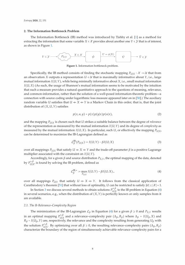
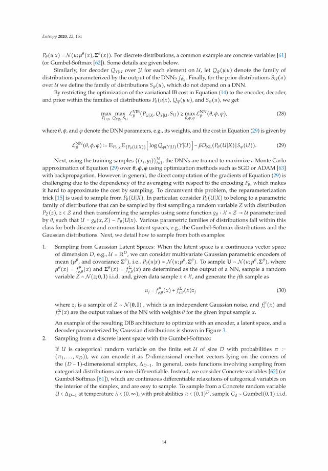
The Information Bottleneck (IB) method was introduced by Tishby et al. [1] as a method forextracting the information that some variable X ∈ X provides about another one Y ∈ Y that is of interest,as shown in Figure 1.

PX|YY ∈ Y φ ψ Y ∈ YX ∈ X U = φ(X)

Figure 1. Information bottleneck problem.

Specifically, the IB method consists of finding the stochastic mapping PU∣X ∶ X → U that froman observation X outputs a representation U ∈ U that is maximally informative about Y, i.e., largemutual information I(U; Y), while being minimally informative about X, i.e., small mutual informationI(U; X) (As such, the usage of Shannon’s mutual information seems to be motivated by the intuitionthat such a measure provides a natural quantitative approach to the questions of meaning, relevance,and common-information, rather than the solution of a well-posed information-theoretic problem—aconnection with source coding under logarithmic loss measure appeared later on in [50].) The auxiliaryrandom variable U satisfies that U −�− X −�−Y is a Markov Chain in this order; that is, that the jointdistribution of (X, U, Y) satisfies

p(x, u, y) = p(x)p(y∣x)p(u∣x), (2)

and the mapping PU∣X is chosen such that U strikes a suitable balance between the degree of relevanceof the representation as measured by the mutual information I(U; Y) and its degree of complexity asmeasured by the mutual information I(U; X). In particular, such U, or effectively the mapping PU∣X ,can be determined to maximize the IB-Lagrangian defined as

LIBβ (PU∣X) ∶= I(U; Y) − βI(U; X) (3)

over all mappings PU∣X that satisfy U −�− X −�−Y and the trade-off parameter β is a positive Lagrangemultiplier associated with the constraint on I(U; Y).

Accordingly, for a given β and source distribution PX,Y, the optimal mapping of the data, denotedby P∗,β

U∣X , is found by solving the IB problem, defined as

LIB,∗β ∶= max

PU∣XI(U; Y) − βI(U; X)., (4)

over all mappings PU∣Y that satisfy U −�− X −�− Y. It follows from the classical application ofCarathéodory’s theorem [51] that without loss of optimality, U can be restricted to satisfy ∣U ∣ ≤ ∣X ∣ + 1.

In Section 3 we discuss several methods to obtain solutions P∗,βU∣X to the IB problem in Equation (4)

in several scenarios, e.g., when the distribution of (X, Y) is perfectly known or only samples from itare available.

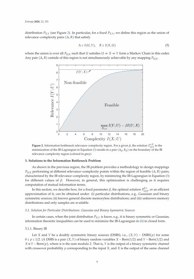
2.1. The Ib Relevance–Complexity Region

The minimization of the IB-Lagrangian Lβ in Equation (4) for a given β ≥ 0 and PX,Y results

in an optimal mapping P∗,βU∣X and a relevance–complexity pair (Δβ, Rβ) where Δβ = I(Uβ, X) and

Rβ = I(Uβ, Y) are, respectively, the relevance and the complexity resulting from generating Uβ with

the solution P∗,βU∣X. By optimizing over all β ≥ 0, the resulting relevance–complexity pairs (Δβ, Rβ)

characterize the boundary of the region of simultaneously achievable relevance–complexity pairs for a

8

Entropy 2020, 22, 151

distribution PX,Y (see Figure 2). In particular, for a fixed PX,Y, we define this region as the union ofrelevance–complexity pairs (Δ, R) that satisfy

Δ ≤ I(U, Y), R ≥ I(X, U) (5)

where the union is over all PU∣X such that U satisfies U −�− X −�−Y form a Markov Chain in this order.Any pair (Δ, R) outside of this region is not simultaneously achievable by any mapping PU∣X .

0 2 4 6 8 10 12 14 16 18 200

1

2

3

4

5

6

7

8

9

Figure 2. Information bottleneck relevance–complexity region. For a given β, the solution P∗,βU∣X to the

minimization of the IB-Lagrangian in Equation (3) results in a pair (Δβ, Rβ) on the boundary of the IBrelevance–complexity region (colored in grey).

3. Solutions to the Information Bottleneck Problem

As shown in the previous region, the IB problem provides a methodology to design mappingsPU∣X performing at different relevance–complexity points within the region of feasible (Δ, R) pairs,characterized by the IB relevance–complexity region, by minimizing the IB-Lagrangian in Equation (3)for different values of β. However, in general, this optimization is challenging as it requirescomputation of mutual information terms.

In this section, we describe how, for a fixed parameter β, the optimal solution Pβ,∗U∣X , or an efficient

approximation of it, can be obtained under: (i) particular distributions, e.g., Gaussian and binarysymmetric sources; (ii) known general discrete memoryless distributions; and (iii) unknown memorydistributions and only samples are available.

3.1. Solution for Particular Distributions: Gaussian and Binary Symmetric Sources

In certain cases, when the joint distribution PX,Y is know, e.g., it is binary symmetric or Gaussian,information theoretic inequalities can be used to minimize the IB-Lagrangian in (4) in closed form.

3.1.1. Binary IB

Let X and Y be a doubly symmetric binary sources (DSBS), i.e., (X, Y) ∼ DSBS(p) for some0 ≤ p ≤ 1/2. (A DSBS is a pair (X, Y) of binary random variables X ∼ Bern(1/2) and Y ∼ Bern(1/2) andX ⊕Y ∼ Bern(p), where ⊕ is the sum modulo 2. That is, Y is the output of a binary symmetric channelwith crossover probability p corresponding to the input X, and X is the output of the same channel

9

Entropy 2020, 22, 151

with input Y.) Then, it can be shown that the optimal U in (4) is such that (X, U) ∼ DSBS(q) for some0 ≤ q ≤ 1. Such a U can be obtained with the mapping PU∣X such that

U = X ⊕ Q, with Q ∼ DSBS(q). (6)

In this case, straightforward algebra leads to that the complexity level is given by

I(U; X) = 1− h2(q), (7)

where, for 0 ≤ x ≤ 1, h2(x) is the entropy of a Bernoulli-(x) source, i.e., h2(x) = −x log2(x) − (1 −x) log2(1− x), and the relevance level is given by

I(U; Y) = 1− h2(p ⋆ q) (8)

where p ⋆ q = p(1− q) + q(1− p). The result extends easily to discrete symmetric mappings Y �→ Xwith binary X (one bit output quantization) and discrete non-binary Y.

3.1.2. Vector Gaussian IB

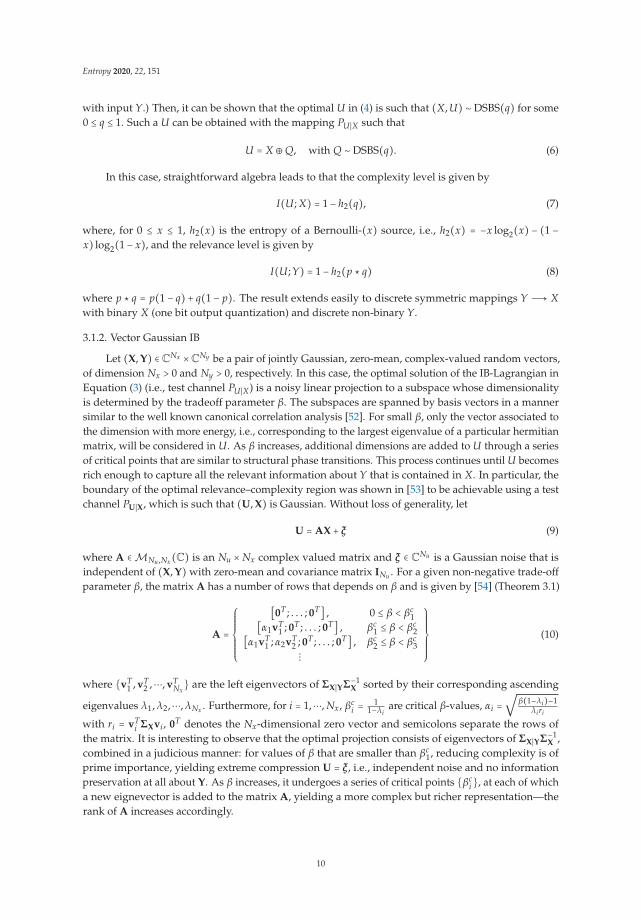
Let (X, Y) ∈ CNx ×CNy be a pair of jointly Gaussian, zero-mean, complex-valued random vectors,of dimension Nx > 0 and Ny > 0, respectively. In this case, the optimal solution of the IB-Lagrangian inEquation (3) (i.e., test channel PU∣X) is a noisy linear projection to a subspace whose dimensionalityis determined by the tradeoff parameter β. The subspaces are spanned by basis vectors in a mannersimilar to the well known canonical correlation analysis [52]. For small β, only the vector associated tothe dimension with more energy, i.e., corresponding to the largest eigenvalue of a particular hermitianmatrix, will be considered in U. As β increases, additional dimensions are added to U through a seriesof critical points that are similar to structural phase transitions. This process continues until U becomesrich enough to capture all the relevant information about Y that is contained in X. In particular, theboundary of the optimal relevance–complexity region was shown in [53] to be achievable using a testchannel PU∣X, which is such that (U, X) is Gaussian. Without loss of generality, let

U = AX + ξ (9)

where A ∈ MNu ,Nx(C) is an Nu × Nx complex valued matrix and ξ ∈ CNu is a Gaussian noise that isindependent of (X, Y) with zero-mean and covariance matrix INu . For a given non-negative trade-offparameter β, the matrix A has a number of rows that depends on β and is given by [54] (Theorem 3.1)

A =

⎧⎪⎪⎪⎪⎪⎪⎨⎪⎪⎪⎪⎪⎪⎩

[0T ; . . . ; 0T] , 0 ≤ β < βc1

[α1vT1 ; 0T ; . . . ; 0T] , βc

1 ≤ β < βc2

[α1vT1 ; α2vT

2 ; 0T ; . . . ; 0T] , βc2 ≤ β < βc

3⋮

⎫⎪⎪⎪⎪⎪⎪⎬⎪⎪⎪⎪⎪⎪⎭

(10)

where {vT1 , vT

2 ,⋯, vTNx

} are the left eigenvectors of ΣX∣YΣ−1X sorted by their corresponding ascending

eigenvalues λ1, λ2,⋯, λNx . Furthermore, for i = 1,⋯, Nx, βci =

11−λi

are critical β-values, αi =√

β(1−λi)−1λiri

with ri = vTi ΣXvi, 0T denotes the Nx-dimensional zero vector and semicolons separate the rows of

the matrix. It is interesting to observe that the optimal projection consists of eigenvectors of ΣX∣YΣ−1X ,

combined in a judicious manner: for values of β that are smaller than βc1, reducing complexity is of

prime importance, yielding extreme compression U = ξ, i.e., independent noise and no informationpreservation at all about Y. As β increases, it undergoes a series of critical points {βc

i}, at each of whicha new eignevector is added to the matrix A, yielding a more complex but richer representation—therank of A increases accordingly.

10

Entropy 2020, 22, 151

For the specific case of scalar Gaussian sources, that is Nx = Ny = 1, e.g., X =√

snrY + N whereN is standard Gaussian with zero-mean and unit variance, the above result simplifies considerably.In this case, let without loss of generality the mapping PU∣X be given by

X =√

aX + Q (11)

where Q is standard Gaussian with zero-mean and variance σ2q . In this case, for I(U; X) = R, we get

I(U; Y) = 12

log(1+ snr) − 12

log(1+ snr exp(−2R)). (12)

3.2. Approximations for Generic Distributions

Next, we present an approach to obtain solutions to the the information bottleneck problem forgeneric distributions, both when this solution is known and when it is unknown. The method consistsin defining a variational (lower) bound on the IB-Lagrangian, which can be optimized more easilythan optimizing the IB-Lagrangian directly.

3.2.1. A Variational Bound

Recall the IB goal of finding a representation U of X that is maximally informative about Y whilebeing concise enough (i.e., bounded I(U; X)). This corresponds to optimizing the IB-Lagrangian

LIBβ (PU∣X) ∶= I(U; Y) − βI(U; X) (13)

where the maximization is over all stochastic mappings PU∣X such that U −�− X −�−Y and ∣U ∣ ≤ ∣X ∣ + 1.In this section, we show that minimizing Equation (13) is equivalent to optimizing the variational cost

LVIBβ (PU∣X , QY∣U , SU) ∶= EPU∣X

[log QY∣U(Y∣U)] − βDKL(PU∣X ∣SU), (14)

where QY∣U(y∣u) is an given stochastic map QY∣U ∶ U → [0, 1] (also referred to as the variationalapproximation of PY∣U or decoder) and SU(u) ∶ U → [0, 1] is a given stochastic map (also referred to asthe variational approximation of PU), and DKL(PU∣X ∣SU) is the relative entropy between PU∣X and SU .

Then, we have the following bound for a any valid PU∣X, i.e., satisfying the Markov Chain inEquation (2),

LIBβ (PU∣X) ≥ LVIB

β (PU∣X , QY∣U , SU), (15)

where the equality holds when QY∣U = PY∣U and SU = PU , i.e., the variational approximationscorrespond to the true value.

In the following, we derive the variational bound. Fix PU∣X (an encoder) and the variationaldecoder approximation QY∣U . The relevance I(U; Y) can be lower-bounded as

I(U; Y) = ⨋u∈U , y∈Y

PU,Y(u, y) logPY∣U(y∣u)

PY(y) dydu (16)

(a)= ⨋u∈U , y∈Y

PU,Y(u, y) logQY∣U(y∣u)

PY(y) dydu + D(PY∥QY ∣U) (17)

(b)≥ ⨋

u∈U , y∈YPU,Y(u, y) log

QY∣U(y∣u)PY(y) dydu (18)

= H(Y) +⨋u∈U , y∈Y

PU,Y(u, y) log QY∣U(y∣u)dydu (19)

(c)≥ ⨋

u∈U , y∈YPU,Y(u, y) log QY∣U(y∣u)dydu (20)

11

Entropy 2020, 22, 151

(d)= ⨋u∈U , x∈X , y∈Y

PX(x)PY∣X(y∣x)PU∣X(u∣x) log QY∣U(y∣u)dxdydu, (21)

where in (a) the term D(PY∥QY ∣U) is the conditional relative entropy between PY and QY, given PU ;(b) holds by the non-negativity of relative entropy; (c) holds by the non-negativity of entropy; and (d)follows using the Markov Chain U −�− X −�−Y.

Similarly, let SU be a given the variational approximation of PU . Then, we get

I(U; X) = ⨋u∈U , x∈X

PU,X(u, x) logPU∣X(u∣x)

PU(u) dxdu (22)

= ⨋u∈U , x∈X


SU(u) dxdu − D(PU∥SU) (23)

≤ ⨋u∈U , x∈X


SU(u) dxdu (24)

where the inequality follows since the relative entropy is non-negative.Combining Equations (21) and (24), we get

I(U; Y) − βI(U; X) ≥ ⨋u∈U , x∈X , y∈Y

PX(x)PY∣X(y∣x)PU∣X(u∣x) log QY∣U(y∣u)dxdydu

− β⨋u∈U , x∈X


SU(u) dxdu. (25)

The use of the variational bound in Equation (14) over the IB-Lagrangian in Equation (13) showssome advantages. First, it allows the derivation of alternating algorithms that allow to obtain a solutionby optimizing over the encoders and decoders. Then, it is easier to obtain an empirical estimate ofEquation (14) by sampling from: (i) the joint distribution PX,Y; (ii) the encoder PU∣X ; and (iii) the priorSU . Additionally, as noted in Equation (15), when evaluated for the optimal decoder QY∣U and prior SU ,the variational bound becomes tight. All this allows obtaining algorithms to obtain good approximatesolutions to the IB problem, as shown next. Further theoretical implications of this variational boundare discussed in [55].

3.2.2. Known Distributions

Using the variational formulation in Equation (14), when the data model is discrete and the jointdistribution PX,Y is known, the IB problem can be solved by using an iterative method that optimizesthe variational IB cost function in Equation (14) alternating over the distributions PU∣X , QY∣U , and SU .In this case, the maximizing distributions PU∣X , QY∣U , and SU can be efficiently found by an alternatingoptimization procedure similar to the expectation-maximization (EM) algorithm [56] and the standardBlahut–Arimoto (BA) method [57]. In particular, a solution PU∣X to the constrained optimizationproblem is determined by the following self-consistent equations, for all (u, x, y) ∈ U ×X ×Y , [1]

PU∣X(u∣x) = PU(u)Z(β, x) exp( − βDKL(PY∣X(⋅∣x)∥PY∣U(⋅∣u))) (26a)

PU(u) = ∑x∈X

PX(x)PU∣X(u∣x) (26b)

PY∣U(y∣u) = ∑x∈X

PY∣X(y∣x)PX∣U(x∣u) (26c)

where PX∣U(x∣u) = PU∣X(u∣x)PX(x)/PU(u) and Z(β, x) is a normalization term. It is shown in [1]that alternating iterations of these equations converges to a solution of the problem for any initialPU∣X . However, by opposition to the standard Blahut–Arimoto algorithm [57,58], which is classicallyused in the computation of rate-distortion functions of discrete memoryless sources for which

12

Entropy 2020, 22, 151

convergence to the optimal solution is guaranteed, convergence here may be to a local optimumonly. If β = 0, the optimization is non-constrained and one can set U = ∅, which yields minimalrelevance and complexity levels. Increasing the value of β steers towards more accurate and morecomplex representations, until U = X in the limit of very large (infinite) values of β for which therelevance reaches its maximal value I(X; Y).

For discrete sources with (small) alphabets, the updating equations described by Equation (26)are relatively easy computationally. However, if the variables X and Y lie in a continuum, solvingthe equations described by Equation (26) is very challenging. In the case in which X and Y are jointmultivariate Gaussian, the problem of finding the optimal representation U is analytically tractablein [53] (see also the related [54,59]), as discussed in Section 3.1.2. Leveraging the optimality of Gaussianmappings PU∣X to restrict the optimization of PU∣X to Gaussian distributions as in Equation (9), allowsreducing the search of update rules to those of the associated parameters, namely covariance matrices.When Y is a deterministic function of X, the IB curve cannot be explored, and other Lagrangians havebeen proposed to tackle this problem [60].

3.3. Unknown Distributions

The main drawback of the solutions presented thus far for the IB principle is that, in the exceptionof small-sized discrete (X, Y) for which iterating Equation (26) converges to an (at least local) solutionand jointly Gaussian (X, Y) for which an explicit analytic solution was found, solving Equation (3)is generally computationally costly, especially for high dimensionality. Another important barrier insolving Equation (3) directly is that IB necessitates knowledge of the joint distribution PX,Y. In thissection, we describe a method to provide an approximate solution to the IB problem in the casein which the joint distribution is unknown and only a give training set of N samples {(xi, yi)}N

i=1is available.

A major step ahead, which widened the range of applications of IB inference for various learningproblems, appeared in [48], where the authors used neural networks to parameterize the variationalinference lower bound in Equation (14) and show that its optimization can be done through the classicand widely used stochastic gradient descendent (SGD). This method, denoted by Variational IB in [48]and detailed below, has allowed handling handle high-dimensional, possibly continuous, data, evenin the case in which the distributions are unknown.

3.3.1. Variational IB

The goal of the variational IB when only samples {(xi, yi)}Ni=1 are available is to solve the IB

problem optimizing an approximation of the cost function. For instance, for a given training set{(xi, yi)}N

i=1, the right hand side of Equation (14) can be approximated as

Llow ≈ 1N

N∑i=1

[⨋u∈U

(PU∣X(u∣xi) log QY∣U(yi∣u) − βPU∣X(u∣xi) logPU∣X(u∣xi)

SU(u) )du] . (27)

However, in general, the direct optimization of this cost is challenging. In the variational IBmethod, this optimization is done by parameterizing the encoding and decoding distributions PU∣X ,QY∣U , and SU that are to optimize using a family of distributions whose parameters are determined byDNNs. This allows us to formulate Equation (14) in terms of the DNN parameters, i.e., its weights, andoptimize it by using the reparameterization trick [15], Monte Carlo sampling, and stochastic gradientdescent (SGD)-type algorithms.

Let Pθ(u∣x) denote the family of encoding probability distributions PU∣X over U for each elementon X , parameterized by the output of a DNN fθ with parameters θ. A common example is the familyof multivariate Gaussian distributions [15], which are parameterized by the mean μθ and covariancematrix Σθ , i.e., γ ∶= (μθ , Σθ). Given an observation X, the values of (μθ(x), Σθ(x)) are determinedby the output of the DNN fθ , whose input is X, and the corresponding family member is given by

13

Entropy 2020, 22, 151

Pθ(u∣x) = N(u; μθ(x), Σθ(x)). For discrete distributions, a common example are concrete variables [61](or Gumbel-Softmax [62]). Some details are given below.

Similarly, for decoder QY∣U over Y for each element on U , let Qψ(y∣u) denote the family ofdistributions parameterized by the output of the DNNs fψk . Finally, for the prior distributions SU(u)over U we define the family of distributions Sϕ(u), which do not depend on a DNN.

By restricting the optimization of the variational IB cost in Equation (14) to the encoder, decoder,and prior within the families of distributions Pθ(u∣x), Qψ(y∣u), and Sϕ(u), we get

maxPU∣X

maxQY∣U ,SU

LVIBβ (PU∣X , QY∣U , SU) ≥ max

θ,φ,ϕLNN

β (θ, φ, ϕ), (28)

where θ, φ, and ϕ denote the DNN parameters, e.g., its weights, and the cost in Equation (29) is given by

LNNβ (θ, φ, ϕ) ∶= EPY,XE{Pθ(U∣X)}[ log Qφ(Y∣U)(Y∣U)] − βDKL(Pθ(U∣X)∥Sϕ(U)). (29)

Next, using the training samples {(xi, yi)}Ni=1, the DNNs are trained to maximize a Monte Carlo

approximation of Equation (29) over θ, φ,ϕ using optimization methods such as SGD or ADAM [63]with backpropagation. However, in general, the direct computation of the gradients of Equation (29) ischallenging due to the dependency of the averaging with respect to the encoding Pθ , which makesit hard to approximate the cost by sampling. To circumvent this problem, the reparameterizationtrick [15] is used to sample from Pθ(U∣X). In particular, consider Pθ(U∣X) to belong to a parametricfamily of distributions that can be sampled by first sampling a random variable Z with distributionPZ(z), z ∈ Z and then transforming the samples using some function gθ ∶ X ×Z → U parameterizedby θ, such that U = gθ(x, Z) ∼ Pθ(U∣x). Various parametric families of distributions fall within thisclass for both discrete and continuous latent spaces, e.g., the Gumbel-Softmax distributions and theGaussian distributions. Next, we detail how to sample from both examples:

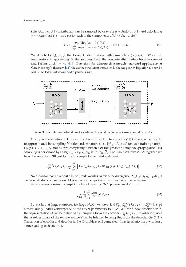
1. Sampling from Gaussian Latent Spaces: When the latent space is a continuous vector spaceof dimension D, e.g., U = RD, we can consider multivariate Gaussian parametric encoders ofmean (μθ , and covariance Σθ), i.e., Pθ(u∣x) = N(u; μθ , Σθ). To sample U ∼ N(u; μθ , Σθ), whereμθ(x) = f μ

e,θ(x) and Σθ(x) = f Σe,θ(x) are determined as the output of a NN, sample a random

variable Z ∼ N(z; 0, I) i.i.d. and, given data sample x ∈ X , and generate the jth sample as

uj = f μe,θ(x) + f Σ

e,θ(x)zj (30)

where zj is a sample of Z ∼ N(0, I) , which is an independent Gaussian noise, and f μe (x) and

f Σe (x) are the output values of the NN with weights θ for the given input sample x.

An example of the resulting DIB architecture to optimize with an encoder, a latent space, and adecoder parameterized by Gaussian distributions is shown in Figure 3.

2. Sampling from a discrete latent space with the Gumbel-Softmax:

If U is categorical random variable on the finite set U of size D with probabilities π ∶=(π1, . . . , πD)), we can encode it as D-dimensional one-hot vectors lying on the corners ofthe (D − 1)-dimensional simplex, ΔD−1. In general, costs functions involving sampling fromcategorical distributions are non-differentiable. Instead, we consider Concrete variables [62] (orGumbel-Softmax [61]), which are continuous differentiable relaxations of categorical variables onthe interior of the simplex, and are easy to sample. To sample from a Concrete random variableU ∈ ΔD−1 at temperature λ ∈ (0,∞), with probabilities π ∈ (0, 1)D, sample Gd ∼ Gumbel(0, 1) i.i.d.

14

Entropy 2020, 22, 151

(The Gumbel(0, 1) distribution can be sampled by drawing u ∼ Uniform(0, 1) and calculatingg = − log(− log(u)). ), and set for each of the components of U = (U1, . . . , UD)

Ud = exp((log(πd + Gd)/λ))∑D

j=1 exp((log(πj + Gj)/λ)), d = 1, . . . , D. (31)

We denote by Qπ,λ(u,x) the Concrete distribution with parameters (π(x), λ). When thetemperature λ approaches 0, the samples from the concrete distribution become one-hotand Pr{limλ→0 Ud} = πd [61]. Note that, for discrete data models, standard application ofCaratheodory’s theorem [64] shows that the latent variables U that appear in Equation (3) can berestricted to be with bounded alphabets size.

Figure 3. Example parametrization of Variational Information Bottleneck using neural networks.

The reparametrization trick transforms the cost function in Equation (29) into one which can beto approximated by sampling M independent samples {um}M

m=1 ∼ Pθ(u∣xi) for each training sample(xi, yi), i = 1, . . . , N and allows computing estimates of the gradient using backpropagation [15].Sampling is performed by using ui,m = gφ(xi, zm) with {zm}M

m=1 i.i.d. sampled from PZ. Altogether, wehave the empirical-DIB cost for the ith sample in the training dataset:

Lempβ,i (θ, φ, ϕ) ∶= 1

M

M∑m=1

[ log Qφ(yi∣ui,m) − βDKL(Pθ(Ui∣xi)∥Qϕ(Ui)))]. (32)

Note that, for many distributions, e.g., multivariate Gaussian, the divergence DKL(Pθ(Ui∣xi)∥Qϕ(Ui))can be evaluated in closed form. Alternatively, an empirical approximation can be considered.

Finally, we maximize the empirical-IB cost over the DNN parameters θ, φ, ϕ as,

maxθ,φ,ϕ

1N

N∑i=1

Lempβ,i (θ, φ,ϕ). (33)

By the law of large numbers, for large N, M, we have 1/N ∑Mi=1 L

empβ,i (θ, φ, ϕ) → LNN

β (θ, φ, ϕ)almost surely. After convergence of the DNN parameters to θ∗, φ∗, ϕ∗, for a new observation X,the representation U can be obtained by sampling from the encoders Pθ∗k

(Uk∣Xk). In addition, notethat a soft estimate of the remote source Y can be inferred by sampling from the decoder Qφ∗(Y∣U).The notion of encoder and decoder in the IB-problem will come clear from its relationship with lossysource coding in Section 4.1.

15

Entropy 2020, 22, 151

4. Connections to Coding Problems

The IB problem is a one-shot coding problem, in the sense that the operations are performedletter-wise. In this section, we consider now the relationship between the IB problem and (asymptotic)coding problem in which the coding operations are performed over blocks of size n, with n assumedto be large and the joint distribution of the data PX,Y is in general assumed to be known a priori.The connections between these problems allow extending results from one setup to another, and toconsider generalizations of the classical IB problem to other setups, e.g., as shown in Section 6.

4.1. Indirect Source Coding under Logarithmic Loss

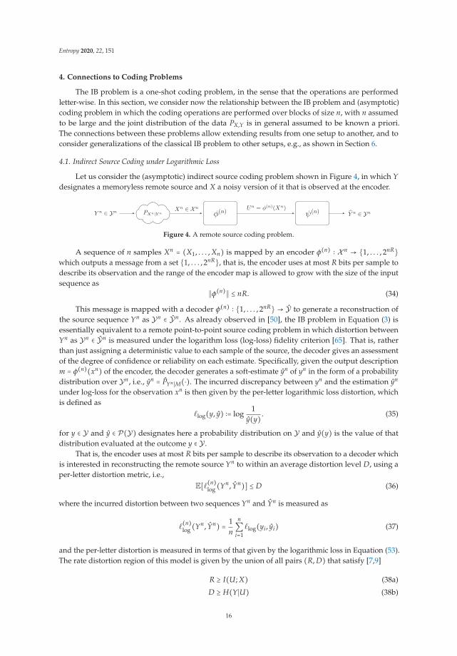
Let us consider the (asymptotic) indirect source coding problem shown in Figure 4, in which Ydesignates a memoryless remote source and X a noisy version of it that is observed at the encoder.

PXn|Y nY n ∈ Yn φ(n) ψ(n) Y n ∈ YnXn ∈ Xn Un = φ(n)(Xn)

Figure 4. A remote source coding problem.

A sequence of n samples Xn = (X1, . . . , Xn) is mapped by an encoder φ(n) ∶ X n → {1, . . . , 2nR}which outputs a message from a set {1, . . . , 2nR}, that is, the encoder uses at most R bits per sample todescribe its observation and the range of the encoder map is allowed to grow with the size of the inputsequence as

∥φ(n)∥ ≤ nR. (34)

This message is mapped with a decoder φ(n) ∶ {1, . . . , 2nR} → Y to generate a reconstruction ofthe source sequence Yn as Yn ∈ Yn. As already observed in [50], the IB problem in Equation (3) isessentially equivalent to a remote point-to-point source coding problem in which distortion betweenYn as Yn ∈ Yn is measured under the logarithm loss (log-loss) fidelity criterion [65]. That is, ratherthan just assigning a deterministic value to each sample of the source, the decoder gives an assessmentof the degree of confidence or reliability on each estimate. Specifically, given the output descriptionm = φ(n)(xn) of the encoder, the decoder generates a soft-estimate yn of yn in the form of a probabilitydistribution over Yn, i.e., yn = PYn ∣M(⋅). The incurred discrepancy between yn and the estimation yn

under log-loss for the observation xn is then given by the per-letter logarithmic loss distortion, whichis defined as

�log(y, y) ∶= log1

y(y) . (35)

for y ∈ Y and y ∈ P(Y) designates here a probability distribution on Y and y(y) is the value of thatdistribution evaluated at the outcome y ∈ Y .

That is, the encoder uses at most R bits per sample to describe its observation to a decoder whichis interested in reconstructing the remote source Yn to within an average distortion level D, using aper-letter distortion metric, i.e.,

E[�(n)log (Yn, Yn)] ≤ D (36)

where the incurred distortion between two sequences Yn and Yn is measured as

�(n)log (Yn, Yn) = 1

n

n∑i=1

�log(yi, yi) (37)

and the per-letter distortion is measured in terms of that given by the logarithmic loss in Equation (53).The rate distortion region of this model is given by the union of all pairs (R, D) that satisfy [7,9]

R ≥ I(U; X) (38a)

D ≥ H(Y∣U) (38b)

16

Entropy 2020, 22, 151

where the union is over all auxiliary random variables U that satisfy that U −�− X −�−Y forms a MarkovChain in this order. Invoking the support lemma [66] (p. 310), it is easy to see that this region is notaltered if one restricts U to satisfy ∣U ∣ ≤ ∣X ∣ + 1. In addition, using the substitution Δ ∶= H(Y) − D, theregion can be written equivalently as the union of all pairs (R, H(Y) −Δ) that satisfy

R ≥ I(U; X) (39a)

Δ ≤ I(U; Y) (39b)

where the union is over all Us with pmf PU∣X that satisfy U −�− X −�−Y, with ∣U ∣ ≤ ∣X ∣ + 1.The boundary of this region is equivalent to the one described by the IB principle in Equation (3)

if solved for all β, and therefore the IB problem is essentially a remote source coding problem in whichthe distortion is measured under the logarithmic loss measure. Note that, operationally, the IB problemis equivalent to that of finding an encoder PU∣X which maps the observation X to a representationU that satisfies the bit rate constraint R and such that U captures enough relevance of Y so that theposterior probability of Y given U satisfies an average distortion constraint.

4.2. Common Reconstruction

Consider the problem of source coding with side information at the decoder, i.e., the wellknown Wyner–Ziv setting [67], with the distortion measured under logarithmic-loss. Specifically, amemoryless source X is to be conveyed lossily to a decoder that observes a statistically correlated sideinformation Y. The encoder uses R bits per sample to describe its observation to the decoder whichwants to reconstruct an estimate of X to within an average distortion level D, where the distortion isevaluated under the log-loss distortion measure. The rate distortion region of this problem is given bythe set of all pairs (R, D) that satisfy

R + D ≥ H(X∣Y). (40)

The optimal coding scheme utilizes standard Wyner–Ziv compression [67] at the encoder and thedecoder map ψ ∶ U ×Y → X is given by

ψ(U, Y) = Pr[X = x∣U, Y] (41)

for which it is easy to see that

E[�log(X, ψ(U, Y))] = H(X∣U, Y). (42)

Now, assume that we constrain the coding in a manner that the encoder is be able to produce anexact copy of the compressed source constructed by the decoder. This requirement, termed commonreconstruction constraint (CR), was introduced and studied by Steinberg [68] for various source codingmodels, including the Wyner–Ziv setup, in the context of a “general distortion measure”. For theWyner–Ziv problem under log-loss measure that is considered in this section, such a CR constraintcauses some rate loss because the reproduction rule in Equation (41) is no longer possible. In fact, itis not difficult to see that under the CR constraint the above region reduces to the set of pairs (R, D)that satisfy

R ≤ I(U; X∣Y) (43a)

D ≥ H(X∣U) (43b)

17

Entropy 2020, 22, 151

for some auxiliary random variable for which U −�− X −�− Y holds. Observe that Equation (43b) isequivalent to I(U; X) ≥ H(X) − D and that, for a given prescribed fidelity level D, the minimum rate isobtained for a description U that achieves the inequality in Equation (43b) with equality, i.e.,

R(D) = minPU∣X ∶ I(U;X)=H(X)−D

I(U; X∣Y). (44)

Because U −�− X −�−Y, we have

I(U; Y) = I(U; X) − I(U; X∣Y). (45)

Under the constraint I(U; X) = H(X) − D, it is easy to see that minimizing I(U; X∣Y) amounts tomaximizing I(U; Y), an aspect which bridges the problem at hand with the IB problem.

In the above, the side information Y is used for binning but not for the estimation at the decoder.If the encoder ignores whether Y is present or not at the decoder side, the benefit of binning isreduced—see the Heegard–Berger model with common reconstruction studied in [69,70].

4.3. Information Combining

Consider again the IB problem. Assume one wishes to find the representation U that maximizesthe relevance I(U; Y) for a given prescribed complexity level, e.g., I(U; X) = R. For this setup, we have

I(X; U, Y) = I(U; X) + I(Y; X) − I(U; Y) (46)

= R + I(Y; X) − I(U; Y) (47)

where the first equality holds since U −�− X −�− Y is a Markov Chain. Maximizing I(U; Y) is thenequivalent to minimizing I(X; U, Y). This is reminiscent of the problem of information combining [71,72],where X can be interpreted as a source information that is conveyed through two channels: the channelPY∣X and the channel PU∣X. The outputs of these two channels are conditionally independent givenX, and they should be processed in a manner such that, when combined, they preserve as muchinformation as possible about X.

4.4. Wyner–Ahlswede–Korner Problem

Here, the two memoryless sources X and Y are encoded separately at rates RX and RY, respectively.A decoder gets the two compressed streams and aims at recovering Y losslessly. This problem wasstudied and solved separately by Wyner [73] and Ahlswede and Körner [74]. For given RX = R, theminimum rate RY that is needed to recover Y losslessly is

R⋆Y(R) = minPU∣X ∶ I(U;X) ≤ R

H(Y∣U). (48)

Thus, we getmax

PU∣X ∶ I(U;X)≤RI(U; Y) = H(Y) − R⋆Y(R),

and therefore, solving the IB problem is equivalent to solving the Wyner–Ahlswede–Korner Problem.

4.5. The Privacy Funnel

Consider again the setting of Figure 4, and let us assume that the pair (Y, X) models data that auser possesses and which have the following properties: the data Y are some sensitive (private) datathat are not meant to be revealed at all, or else not beyond some level Δ; and the data X are non-privateand are meant to be shared with another user (analyst). Because X and Y are correlated, sharing thenon-private data X with the analyst possibly reveals information about Y. For this reason, there is atrade off between the amount of information that the user shares about X and the information that he

18

Entropy 2020, 22, 151

keeps private about Y. The data X are passed through a randomized mapping φ whose purpose is tomake U = φ(X) maximally informative about X while being minimally informative about Y.

The analyst performs an inference attack on the private data Y based on the disclosed informationU. Let � ∶ Y × Y �→ R be an arbitrary loss function with reconstruction alphabet Y that measures thecost of inferring Y after observing U. Given (X, Y) ∼ PX,Y and under the given loss function �, it isnatural to quantify the difference between the prediction losses in predicting Y ∈ Y prior and afterobserving U = φ(X). Let

C(�, P) = infy∈Y

EP[�(Y, y)] − infY(φ(X))

EP[�(Y, Y)] (49)

where y ∈ Y is deterministic and Y(φ(X)) is any measurable function of U = φ(X). The quantityC(�, P) quantifies the reduction in the prediction loss under the loss function � that is due to observingU = φ(X), i.e., the inference cost gain. In [75] (see also [76]), it is shown that that under some mildconditions the inference cost gain C(�, P) as defined by Equation (49) is upper-bounded as

C(�, P) ≤ 2√

2L√

I(U; Y) (50)

where L is a constant. The inequality in Equation (50) holds irrespective to the choice of the lossfunction �, and this justifies the usage of the logarithmic loss function as given by Equation (53) in thecontext of finding a suitable trade off between utility and privacy, since

I(U; Y) = H(Y) − infY(U)

EP[�log(Y, Y)]. (51)

Under the logarithmic loss function, the design of the mapping U = φ(X) should strike a rightbalance between the utility for inferring the non-private data X as measured by the mutual informationI(U; X) and the privacy metric about the private date Y as measured by the mutual informationI(U; Y).

4.6. Efficiency of Investment Information

Let Y model a stock market data and X some correlated information. In [77], Erkip and Coverinvestigated how the description of the correlated information X improves the investment in the stockmarket Y. Specifically, let Δ(C) denote the maximum increase in growth rate when X is described tothe investor at rate C. Erkip and Cover found a single-letter characterization of the incremental growthrate Δ(C). When specialized to the horse race market, this problem is related to the aforementionedsource coding with side information of Wyner [73] and Ahlswede-Körner [74], and, thus, also to theIB problem. The work in [77] provides explicit analytic solutions for two horse race examples, jointlybinary and jointly Gaussian horse races.

5. Connections to Inference and Representation Learning

In this section, we consider the connections of the IB problem with learning, inference andgeneralization, for which, typically, the joint distribution PX,Y of the data is not known and only a setof samples is available.

5.1. Inference Model

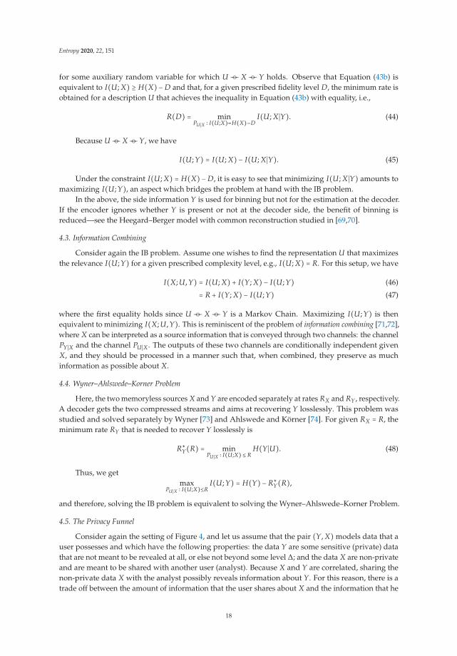
Let a measurable variable X ∈ X and a target variable Y ∈ Y with unknown joint distributionPX,Y be given. In the classic problem of statistical learning, one wishes to infer an accurate predictorof the target variable Y ∈ Y based on observed realizations of X ∈ X . That is, for a given class F ofadmissible predictors ψ ∶ X → Y and a loss function � ∶ Y → Y that measures discrepancies between

19

Entropy 2020, 22, 151

true values and their estimated fits, one aims at finding the mapping ψ ∈ F that minimizes the expected(population) risk

CPX,Y(ψ, �) = EPX,Y [�(Y, ψ(X))]. (52)

An abstract inference model is shown in Figure 5.

PX|YY ∈ Y ψ Y ∈ YX ∈ X

Figure 5. An abstract inference model for learning.

The choice of a “good” loss function �(⋅) is often controversial in statistical learning theory. Thereis however numerical evidence that models that are trained to minimize the error’s entropy oftenoutperform ones that are trained using other criteria such as mean-square error (MSE) and higher-orderstatistics [26,27]. This corresponds to choosing the loss function given by the logarithmic loss, which isdefined as

�log(y, y) ∶= log1

y(y) (53)

for y ∈ Y , where y ∈ P(Y) designates here a probability distribution on Y and y(y) is the value ofthat distribution evaluated at the outcome y ∈ Y . Although a complete and rigorous justificationof the usage of the logarithmic loss as distortion measure in learning is still awaited, recently apartial explanation appeared in [30] where Painsky and Wornell showed that, for binary classificationproblems, by minimizing the logarithmic-loss one actually minimizes an upper bound to any choice ofloss function that is smooth, proper (i.e., unbiased and Fisher consistent), and convex. Along the sameline of work, the authors of [29] showed that under some natural data processing property Shannon’smutual information uniquely quantifies the reduction of prediction risk due to side information.Perhaps, this justifies partially why the logarithmic-loss fidelity measure is widely used in learningtheory and has already been adopted in many algorithms in practice such as the infomax criterion [31],the tree-based algorithm of Quinlan [32], or the well known Chow–Liu algorithm [33] for learningtree graphical models, with various applications in genetics [34], image processing [35], computervision [36], and others. The logarithmic loss measure also plays a central role in the theory ofprediction [37] (Ch. 09), where it is often referred to as the self-information loss function, as wellas in Bayesian modeling [38] where priors are usually designed to maximize the mutual informationbetween the parameter to be estimated and the observations.

When the join distribution PX,Y is known, the optimal predictor and the minimum expected(population) risk can be characterized. Let, for every x ∈ X , ψ(x) = Q(⋅∣x) ∈ P(Y). It is easy to see that

EPX,Y [�log(Y, Q)] = ∑x∈X , y∈Y

PX,Y(x, y) log( 1Q(y∣x)) (54a)

= ∑x∈X , y∈Y

PX,Y(x, y) log( 1PY∣X(y∣x)) + ∑

x∈X , y∈YPX,Y(x, y) log(

PY∣X(y∣x)Q(y∣x) ) (54b)

= H(Y∣X) + D(PY∣X∥Q) (54c)

≥ H(Y∣X) (54d)

with equality iff the predictor is given by the conditional posterior ψ(x) = PY(Y∣X = x). That is, theminimum expected (population) risk is given by

minψ

CPX,Y(ψ, �log) = H(Y∣X). (55)

20

Entropy 2020, 22, 151

If the joint distribution PX,Y is unknown, which is most often the case in practice, the populationrisk as given by Equation (56) cannot be computed directly, and, in the standard approach, one usuallyresorts to choosing the predictor with minimal risk on a training dataset consisting of n labeled samples{(xi, yi)}n

i=1 that are drawn independently from the unknown joint distribution PX,Y. In this case, oneis interested in optimizing the empirical population risk, which for a set of n i.i.d. samples from PX,Y,Dn ∶= {(xi, yi)}n

i=1, is defined as

CPX,Y(ψ, �,Dn) =1n

n∑i=1

�(yi, ψ(xi)). (56)

The difference between the empirical and population risks is normally measured in terms of thegeneralization gap, defined as

genPX,Y(ψ, �,Dn) ∶= CPX,Y(ψ, �log) − CPX,Y(ψ, �,Dn). (57)

5.2. Minimum Description Length

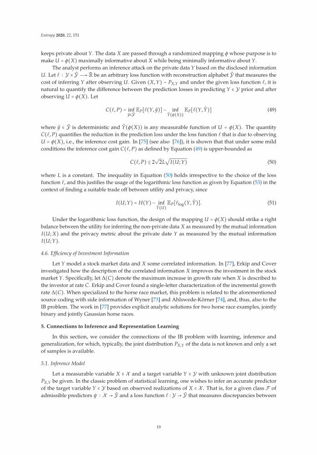
One popular approach to reducing the generalization gap is by restricting the set F of admissiblepredictors to a low-complexity class (or constrained complexity) to prevent over-fitting. One wayto limit the model’s complexity is by restricting the range of the prediction function, as shown inFigure 6. This is the so-called minimum description length complexity measure, often used in thelearning literature to limit the description length of the weights of neural networks [78]. A connectionbetween the use of the minimum description complexity for limiting the description length of theinput encoding and accuracy studied in [79] and with respect to the weight complexity and accuracyis given in [11]. Here, the stochastic mapping φ ∶ X �→ U is a compressor with

∥φ∥ ≤ R (58)

for some prescribed “input-complexity” value R, or equivalently prescribed average description-length.

PX|YY ∈ Y φ ψ Y ∈ YX ∈ X U = φ(X)

Figure 6. Inference problem with constrained model’s complexity.

Minimizing the constrained description length population risk is now equivalent to solving

CPX,Y ,DLC(R) =minφ

EPX,Y [�log(Yn, ψ(Un))] (59)

s.t. ∥φ(Xn)∥ ≤ nR. (60)

It can be shown that this problem takes its minimum value with the choice of ψ(U) = PY∣U and

CPX,Y ,DLC(R) = minPU∣X

H(Y∣U) s.t. R ≥ I(U; X), (61)

The solution to Equation (61) for different values of R is effectively equivalent to the IB-problemin Equation (4). Observe that the right-hand side of Equation (61) is larger for small values of R; it isclear that a good predictor φ should strike a right balance between reducing the model’s complexityand reducing the error’s entropy, or, equivalently, maximizing the mutual information I(U; Y) aboutthe target variable Y.

21

Entropy 2020, 22, 151

5.3. Generalization and Performance Bounds

The IB-problem appears as a relevant problem in fundamental performance limits of learning.In particular, when PX,Y is unknown, and instead n samples i.i.d from PX,Y are available, theoptimization of the empirical risk in Equation (56) leads to a mismatch between the true loss givenby the population risk and the empirical risk. This gap is measured by the generalization gap inEquation (57). Interestingly, the relationship between the true loss and the empirical loss can bebounded (in high probability) in terms of the IB-problem as [80]

CPX,Y(ψ, �log) ≤ CPX,Y(ψ, �,Dn) + genPX,Y(ψ, �,Dn)

= HP(n)X,Y

(Y∣U)01111111111111111111111111112111111111111111111111111113CPX,Y

(ψ,�,Dn)

+ A√

I(P(n)X ; PU∣X) ⋅log n

n+

B√

Λ(PU∣X , PY∣U , PY∣U)√

n+O( log n

n)

011111111111111111111111111111111111111111111111111111111111111111111111111111111111111111111111111111111111111111111111111111111111111111111111111111111111111111111111111111111111111111111111111111111111111111111111111111111121111111111111111111111111111111111111111111111111111111111111111111111111111111111111111111111111111111111111111111111111111111111111111111111111111111111111111111111111111111111111111111111111111111111111111111111111111111113Bound on genPX,Y

(ψ,�,Dn)

where PU∣X and PY∣U are the empirical encoder and decoder and PY∣U is the optimal decoder.

HP(n)X,Y

(Y∣U) and I(P(n)X ; PU∣X) are the empirical loss and the mutual information resulting from the

dataset Dn and Λ(PU∣X, PY∣U , PY∣U) is a function that measures the mismatch between the optimaldecoder and the empirical one.

This bound shows explicitly the trade-off between the empirical relevance and the empiricalcomplexity. The pairs of relevance and complexity simultaneously achievable is precisely characterizedby the IB-problem. Therefore, by designing estimators based on the IB problem, as described inSection 3, one can perform at different regimes of performance, complexity and generalization.

Another interesting connection between learning and the IB-method is the connection of thelogarithmic-loss as metric to common performance metrics in learning:

• The logarithmic-loss gives an upper bound on the probability of miss-classification (accuracy):

εY∣X(QY∣X) ∶= 1−EPXY [QY∣X] ≤ 1− exp(−EPX,Y [�log(Y, QY∣X)])

• The logarithmic-loss is equivalent to maximum likelihood for large n:

− 1n

log PYn ∣Xn(yn∣xn) = − 1n

n∑i=1

log PY∣X(yi∣xi)n→∞�→ EX,Y[− log PY∣X(Y∣X)]

• The true distribution P minimizes the expected logarithmic-loss:

PY∣X = arg minQY∣X

EP log1

QY∣Xand min

QY∣X

E[�log(Y, QY∣X)] = H(Y∣X)

Since for n →∞ the joint distribution PXY can be perfectly learned, the link between these commoncriteria allows the use of the IB-problem to derive asymptotic performance bounds, as well as designcriteria, in most of the learning scenarios of classification, regression, and inference.

5.4. Representation Learning, Elbo and Autoencoders

The performance of machine learning algorithms depends strongly on the choice of datarepresentation (or features) on which they are applied. For that reason, feature engineering, i.e.,the set of all pre-processing operations and transformations applied to data in the aim of making themsupport effective machine learning, is important. However, because it is both data- and task-dependent,such feature-engineering is labor intensive and highlights one of the major weaknesses of currentlearning algorithms: their inability to extract discriminative information from the data themselves

22

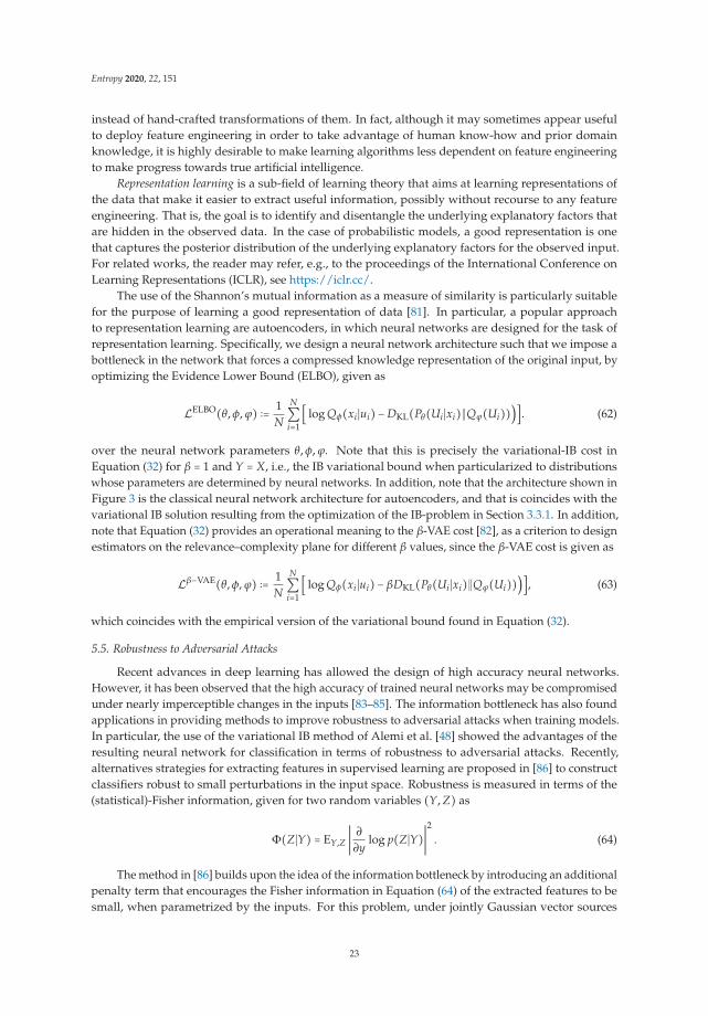
Entropy 2020, 22, 151

instead of hand-crafted transformations of them. In fact, although it may sometimes appear usefulto deploy feature engineering in order to take advantage of human know-how and prior domainknowledge, it is highly desirable to make learning algorithms less dependent on feature engineeringto make progress towards true artificial intelligence.

Representation learning is a sub-field of learning theory that aims at learning representations ofthe data that make it easier to extract useful information, possibly without recourse to any featureengineering. That is, the goal is to identify and disentangle the underlying explanatory factors thatare hidden in the observed data. In the case of probabilistic models, a good representation is onethat captures the posterior distribution of the underlying explanatory factors for the observed input.For related works, the reader may refer, e.g., to the proceedings of the International Conference onLearning Representations (ICLR), see https://iclr.cc/.

The use of the Shannon’s mutual information as a measure of similarity is particularly suitablefor the purpose of learning a good representation of data [81]. In particular, a popular approachto representation learning are autoencoders, in which neural networks are designed for the task ofrepresentation learning. Specifically, we design a neural network architecture such that we impose abottleneck in the network that forces a compressed knowledge representation of the original input, byoptimizing the Evidence Lower Bound (ELBO), given as

LELBO(θ, φ, ϕ) ∶= 1N

N∑i=1

[ log Qφ(xi∣ui) − DKL(Pθ(Ui∣xi)∥Qϕ(Ui)))]. (62)

over the neural network parameters θ, φ, ϕ. Note that this is precisely the variational-IB cost inEquation (32) for β = 1 and Y = X, i.e., the IB variational bound when particularized to distributionswhose parameters are determined by neural networks. In addition, note that the architecture shown inFigure 3 is the classical neural network architecture for autoencoders, and that is coincides with thevariational IB solution resulting from the optimization of the IB-problem in Section 3.3.1. In addition,note that Equation (32) provides an operational meaning to the β-VAE cost [82], as a criterion to designestimators on the relevance–complexity plane for different β values, since the β-VAE cost is given as

Lβ−VAE(θ, φ, ϕ) ∶= 1N

N∑i=1

[ log Qφ(xi∣ui) − βDKL(Pθ(Ui∣xi)∥Qϕ(Ui)))], (63)

which coincides with the empirical version of the variational bound found in Equation (32).

5.5. Robustness to Adversarial Attacks

Recent advances in deep learning has allowed the design of high accuracy neural networks.However, it has been observed that the high accuracy of trained neural networks may be compromisedunder nearly imperceptible changes in the inputs [83–85]. The information bottleneck has also foundapplications in providing methods to improve robustness to adversarial attacks when training models.In particular, the use of the variational IB method of Alemi et al. [48] showed the advantages of theresulting neural network for classification in terms of robustness to adversarial attacks. Recently,alternatives strategies for extracting features in supervised learning are proposed in [86] to constructclassifiers robust to small perturbations in the input space. Robustness is measured in terms of the(statistical)-Fisher information, given for two random variables (Y, Z) as

Φ(Z∣Y) = EY,Z ∣ ∂

∂ylog p(Z∣Y)∣

2

. (64)

The method in [86] builds upon the idea of the information bottleneck by introducing an additionalpenalty term that encourages the Fisher information in Equation (64) of the extracted features to besmall, when parametrized by the inputs. For this problem, under jointly Gaussian vector sources

23

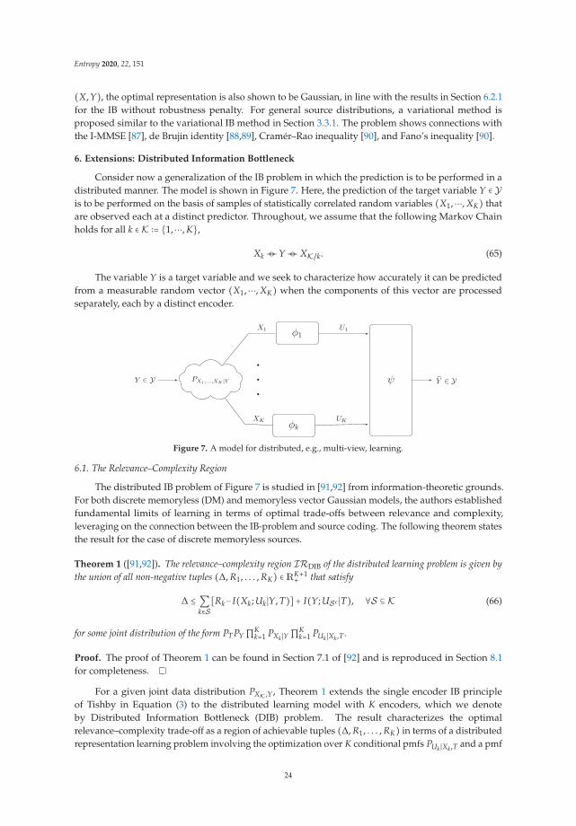
Entropy 2020, 22, 151

(X, Y), the optimal representation is also shown to be Gaussian, in line with the results in Section 6.2.1for the IB without robustness penalty. For general source distributions, a variational method isproposed similar to the variational IB method in Section 3.3.1. The problem shows connections withthe I-MMSE [87], de Brujin identity [88,89], Cramér–Rao inequality [90], and Fano’s inequality [90].

6. Extensions: Distributed Information Bottleneck

Consider now a generalization of the IB problem in which the prediction is to be performed in adistributed manner. The model is shown in Figure 7. Here, the prediction of the target variable Y ∈ Yis to be performed on the basis of samples of statistically correlated random variables (X1,⋯, XK) thatare observed each at a distinct predictor. Throughout, we assume that the following Markov Chainholds for all k ∈ K ∶= {1,⋯, K},

Xk −�−Y −�− XK/k. (65)

The variable Y is a target variable and we seek to characterize how accurately it can be predictedfrom a measurable random vector (X1,⋯, XK) when the components of this vector are processedseparately, each by a distinct encoder.

PX1,...,XK |YY ∈ Y ···

φ1

φk

ψ Y ∈ Y

XK

X1 U1

UK

Figure 7. A model for distributed, e.g., multi-view, learning.

6.1. The Relevance–Complexity Region

The distributed IB problem of Figure 7 is studied in [91,92] from information-theoretic grounds.For both discrete memoryless (DM) and memoryless vector Gaussian models, the authors establishedfundamental limits of learning in terms of optimal trade-offs between relevance and complexity,leveraging on the connection between the IB-problem and source coding. The following theorem statesthe result for the case of discrete memoryless sources.

Theorem 1 ([91,92]). The relevance–complexity region IRDIB of the distributed learning problem is given bythe union of all non-negative tuples (Δ, R1, . . . , RK) ∈ RK+1

+ that satisfy

Δ ≤ ∑k∈S

[Rk−I(Xk; Uk∣Y, T)] + I(Y; USc ∣T), ∀S ⊆ K (66)

for some joint distribution of the form PT PY ∏Kk=1 PXk ∣Y ∏K

k=1 PUk ∣Xk ,T.

Proof. The proof of Theorem 1 can be found in Section 7.1 of [92] and is reproduced in Section 8.1for completeness.

For a given joint data distribution PXK,Y, Theorem 1 extends the single encoder IB principleof Tishby in Equation (3) to the distributed learning model with K encoders, which we denoteby Distributed Information Bottleneck (DIB) problem. The result characterizes the optimalrelevance–complexity trade-off as a region of achievable tuples (Δ, R1, . . . , RK) in terms of a distributedrepresentation learning problem involving the optimization over K conditional pmfs PUk ∣Xk ,T and a pmf

24

Entropy 2020, 22, 151

PT . The pmfs PUk ∣Xk ,T correspond to stochastic encodings of the observation Xk to a latent variable,or representation, Uk which captures the relevant information of Y in observation Xk. Variable Tcorresponds to a time-sharing among different encoding mappings (see, e.g., [51]). For such encoders,the optimal decoder is implicitly given by the conditional pmf of Y from U1, . . . , UK, i.e., PY∣UK,T .

The characterization of the relevance–complexity region can be used to derive a cost function forthe D-IB similarly to the IB-Lagrangian in Equation (3). For simplicity, let us consider the problem ofmaximizing the relevance under a sum-complexity constraint. Let Rsum = ∑K

k=1 Rk and

RIsumDIB ∶={(Δ, Rsum) ∈ R2

+ ∶ ∃(R1, . . . , RK) ∈ RK+ s.t.

K∑k=1

Rk = Rsum and (Δ, R1, . . . , RK) ∈ RIDIB}.

We define the DIB-Lagrangian (under sum-rate) as

Ls(P) ∶= −H(Y∣UK) − sK∑k=1

[H(Y∣Uk) + I(Xk; Uk)]. (67)

The optimization of Equation (67) over the encoders PUk ∣Xk ,T allows obtaining mappings thatperform on the boundary of the relevance–sum complexity region RIsum

DIB . To see that, note that it iseasy to see that the relevance–sum complexity region RIsum

DIB is composed of all the pairs (Δ, Rsum) ∈ R2+

for which Δ ≤ Δ(Rsum, PXK,Y), with

Δ(Rsum, PXK,Y) = maxP

min⎧⎪⎪⎨⎪⎪⎩

I(Y; UK), Rsum −K∑k=1

I(Xk; Uk∣Y)⎫⎪⎪⎬⎪⎪⎭

, (68)

where the maximization is over joint distributions that factorize as PY ∏Kk=1 PXk ∣Y ∏K

k=1 PUk ∣Xk. The pairs

(Δ, Rsum) that lie on the boundary of RIsumDIB can be characterized as given in the following proposition.

Proposition 1. For every pair (Δ, Rsum) ∈ R2+ that lies on the boundary of the region RIsum

DIB , there exists aparameter s ≥ 0 such that (Δ, Rsum) = (Δs, Rs), with

Δs =1

(1+ s) [(1+ sK)H(Y) + sRs +maxP

Ls(P)] , (69)

Rs = I(Y; U∗K) +K∑k=1

[I(Xk; U∗k ) − I(Y; U∗k )], (70)

where P∗ is the set of conditional pmfs P = {PU1∣X1,⋯, PUK ∣XK

} that maximize the cost function in Equation (67).

Proof. The proof of Proposition 1 can be found in Section 7.3 of [92] and is reproduced here inSection 8.2 for completeness.

The optimization of the distributed IB cost function in Equation (67) generalizes the centralizedTishby’s information bottleneck formulation in Equation (3) to the distributed learning setting. Notethat for K = 1 the optimization in Equation (69) reduces to the single encoder cost in Equation (3) witha multiplier s/(1+ s).

6.2. Solutions to the Distributed Information Bottleneck

The methods described in Section 3 can be extended to the distributed information bottleneckcase in order to find the mappings PU1∣X1,T ,⋯, PUK ∣XK ,T in different scenarios.

25

Entropy 2020, 22, 151

6.2.1. Vector Gaussian Model

In this section, we show that for the jointly vector Gaussian data model it is enough to restrictto Gaussian auxiliaries (U1,⋯, UK) in order to exhaust the entire relevance–complexity region.In addition, we provide an explicit analytical expression of this region. Let (X1, . . . , XK, Y) be ajointly vector Gaussian vector that satisfies the Markov Chain in Equation (83). Without loss ofgenerality, let the target variable be a complex-valued, zero-mean multivariate Gaussian Y ∈ Cny withcovariance matrix Σy, i.e., Y ∼ CN(y; 0, Σy), and Xk ∈ Cnk given by

Xk = HkY +Nk, (71)

where Hk ∈ Cnk×ny models the linear model connecting Y to the observation at encoder k and Nk ∈ Cnk

is the noise vector at encoder k, assumed to be Gaussian with zero-mean, covariance matrix Σk, andindependent from all other noises and Y.

For the vector Gaussian model Equation (71), the result of Theorem 1, which can be extendedto continuous sources using standard techniques, characterizes the relevance–complexity region ofthis model. The following theorem characterizes the relevance–complexity region, which we denotehereafter as RIG

DIB. The theorem also shows that in order to exhaust this region it is enough to restrictto no time sharing, i.e., T = ∅ and multivariate Gaussian test channels

Uk = AkXk +Zk ∼ CN(uk; AkXk, Σz,k), (72)

where Ak ∈ Cnk×nk projects Xk and Zk is a zero-mean Gaussian noise with covariance Σz,k.

Theorem 2. For the vector Gaussian data model, the relevance–complexity region RIGDIB is given by the union

of all tuples (Δ, R1, . . . , RL) that satisfy

Δ ≤ ∑k∈S

(Rk + log ∣I −Σ1/2k ΩkΣ

1/2k ∣) + log

EEEEEEEEEEEI + ∑

k∈ScΣ

1/2y H†

kΩkHkΣ1/2y

EEEEEEEEEEE, ∀S ⊆ K,

for some matrices 0 ⪯ Ωk ⪯ Σ−1k .

Proof. The proof of Theorem 2 can be found in Section 7.5 of [92] and is reproduced here in Section 8.4for completeness.

Theorem 2 extends the result of [54,93] on the relevance–complexity trade-off characterization ofthe single-encoder IB problem for jointly Gaussian sources to K encoders. The theorem also shows thatthe optimal test channels PUk ∣Xk

are multivariate Gaussian, as given by Equation (72).Consider the following symmetric distributed scalar Gaussian setting, in which Y ∼ N(0, 1) and

X1 =√

snrY + N1 (73a)

X2 =√

snrY + N2 (73b)

where N1 and N2 are standard Gaussian with zero-mean and unit variance, both independent of Y. Inthis case, for I(U1; X1) = R and I(U; X2) = R, the optimal relevance is

Δ⋆(R, snr) = 12

log(1+ 2snr exp(−4R)( exp(4R) + snr−√

snr2 + (1+ 2snr) exp(4R))). (74)

An easy upper bound on the relevance can be obtained by assuming that X1 and X2 are encodedjointly at rate 2R, to get

Δub(R, snr) = 12

log(1+ 2snr) − 12

log(1+ 2snr exp(−4R)). (75)

26

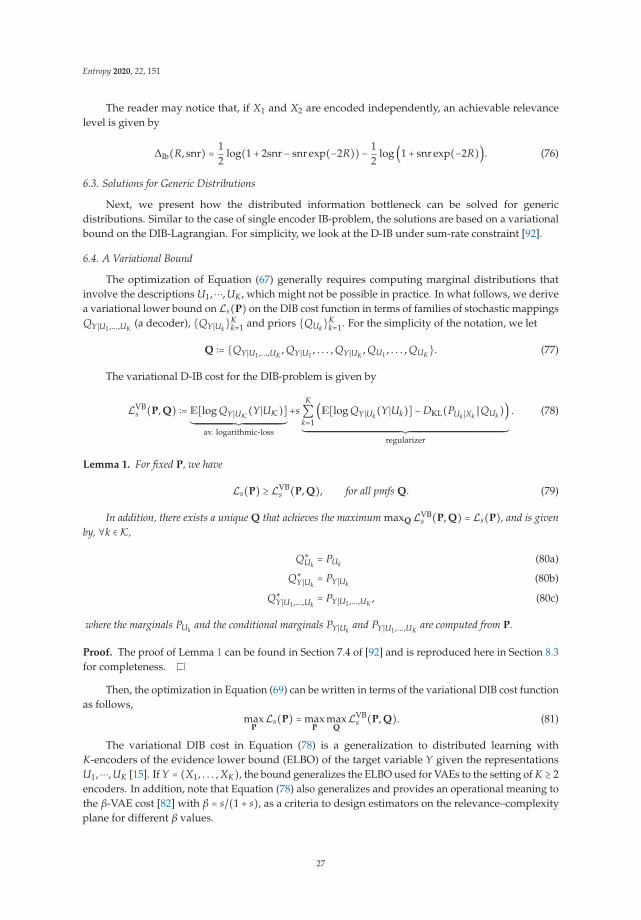
Entropy 2020, 22, 151

The reader may notice that, if X1 and X2 are encoded independently, an achievable relevancelevel is given by

Δlb(R, snr) = 12

log(1+ 2snr− snr exp(−2R)) − 12

log(1+ snr exp(−2R)). (76)

6.3. Solutions for Generic Distributions

Next, we present how the distributed information bottleneck can be solved for genericdistributions. Similar to the case of single encoder IB-problem, the solutions are based on a variationalbound on the DIB-Lagrangian. For simplicity, we look at the D-IB under sum-rate constraint [92].

6.4. A Variational Bound

The optimization of Equation (67) generally requires computing marginal distributions thatinvolve the descriptions U1,⋯, UK, which might not be possible in practice. In what follows, we derivea variational lower bound on Ls(P) on the DIB cost function in terms of families of stochastic mappingsQY∣U1,...,UK

(a decoder), {QY∣Uk}K

k=1 and priors {QUk}Kk=1. For the simplicity of the notation, we let

Q ∶= {QY∣U1,...,UK, QY∣U1

, . . . , QY∣UK, QU1 , . . . , QUK}. (77)

The variational D-IB cost for the DIB-problem is given by

LVBs (P, Q) ∶= E[log QY∣UK(Y∣UK)]

011111111111111111111111111111111111111111111111111111111111111121111111111111111111111111111111111111111111111111111111111111113av. logarithmic-loss

+sK∑k=1

(E[log QY∣Uk(Y∣Uk)] − DKL(PUk ∣Xk

∥QUk))

011111111111111111111111111111111111111111111111111111111111111111111111111111111111111111111111111111111111111111111111111111111111111111111111111111111111121111111111111111111111111111111111111111111111111111111111111111111111111111111111111111111111111111111111111111111111111111111111111111111111111111111111113regularizer

. (78)

Lemma 1. For fixed P, we have

Ls(P) ≥ LVBs (P, Q), for all pmfs Q. (79)

In addition, there exists a unique Q that achieves the maximum maxQ LVBs (P, Q) = Ls(P), and is given

by, ∀k ∈ K,

Q∗Uk= PUk (80a)

Q∗Y∣Uk= PY∣Uk

(80b)

Q∗Y∣U1,...,Uk= PY∣U1,...,UK

, (80c)

where the marginals PUk and the conditional marginals PY∣Ukand PY∣U1,...,UK

are computed from P.

Proof. The proof of Lemma 1 can be found in Section 7.4 of [92] and is reproduced here in Section 8.3for completeness.

Then, the optimization in Equation (69) can be written in terms of the variational DIB cost functionas follows,

maxP

Ls(P) = maxP

maxQ

LVBs (P, Q). (81)

The variational DIB cost in Equation (78) is a generalization to distributed learning withK-encoders of the evidence lower bound (ELBO) of the target variable Y given the representationsU1,⋯, UK [15]. If Y = (X1, . . . , XK), the bound generalizes the ELBO used for VAEs to the setting of K ≥ 2encoders. In addition, note that Equation (78) also generalizes and provides an operational meaning tothe β-VAE cost [82] with β = s/(1+ s), as a criteria to design estimators on the relevance–complexityplane for different β values.

27

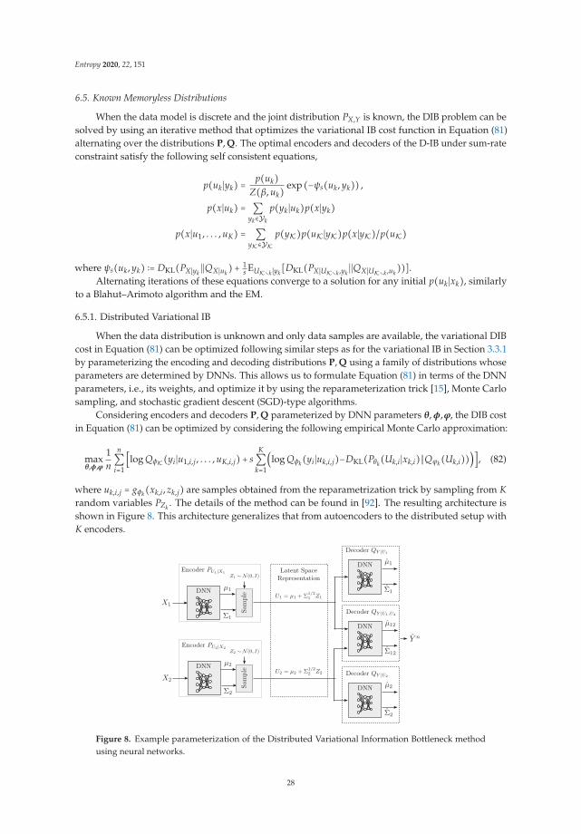
Entropy 2020, 22, 151

6.5. Known Memoryless Distributions

When the data model is discrete and the joint distribution PX,Y is known, the DIB problem can besolved by using an iterative method that optimizes the variational IB cost function in Equation (81)alternating over the distributions P, Q. The optimal encoders and decoders of the D-IB under sum-rateconstraint satisfy the following self consistent equations,

p(uk∣yk) =p(uk)

Z(β, uk)exp (−ψs(uk, yk)) ,

p(x∣uk) = ∑yk∈Yk

p(yk∣uk)p(x∣yk)

p(x∣u1, . . . , uK) = ∑yK∈YK

p(yK)p(uK∣yK)p(x∣yK)/p(uK)

where ψs(uk, yk) ∶= DKL(PX∣yk∣∣QX∣uk

) + 1s EUK∖k ∣yk

[DKL(PX∣UK∖k ,yk∣∣QX∣UK∖k ,uk

))].Alternating iterations of these equations converge to a solution for any initial p(uk∣xk), similarly

to a Blahut–Arimoto algorithm and the EM.

6.5.1. Distributed Variational IB

When the data distribution is unknown and only data samples are available, the variational DIBcost in Equation (81) can be optimized following similar steps as for the variational IB in Section 3.3.1by parameterizing the encoding and decoding distributions P, Q using a family of distributions whoseparameters are determined by DNNs. This allows us to formulate Equation (81) in terms of the DNNparameters, i.e., its weights, and optimize it by using the reparameterization trick [15], Monte Carlosampling, and stochastic gradient descent (SGD)-type algorithms.

Considering encoders and decoders P, Q parameterized by DNN parameters θ, φ,ϕ, the DIB costin Equation (81) can be optimized by considering the following empirical Monte Carlo approximation:

maxθ,φ,ϕ

1n

n∑i=1

[log QφK(yi∣u1,i,j, . . . , uK,i,j) + sK∑k=1

(log Qφk(yi∣uk,i,j)−DKL(Pθk(Uk,i∣xk,i)∥Qϕk(Uk,i)))], (82)

where uk,i,j = gφk(xk,i, zk,j) are samples obtained from the reparametrization trick by sampling from Krandom variables PZk . The details of the method can be found in [92]. The resulting architecture isshown in Figure 8. This architecture generalizes that from autoencoders to the distributed setup withK encoders.

Figure 8. Example parameterization of the Distributed Variational Information Bottleneck methodusing neural networks.

28

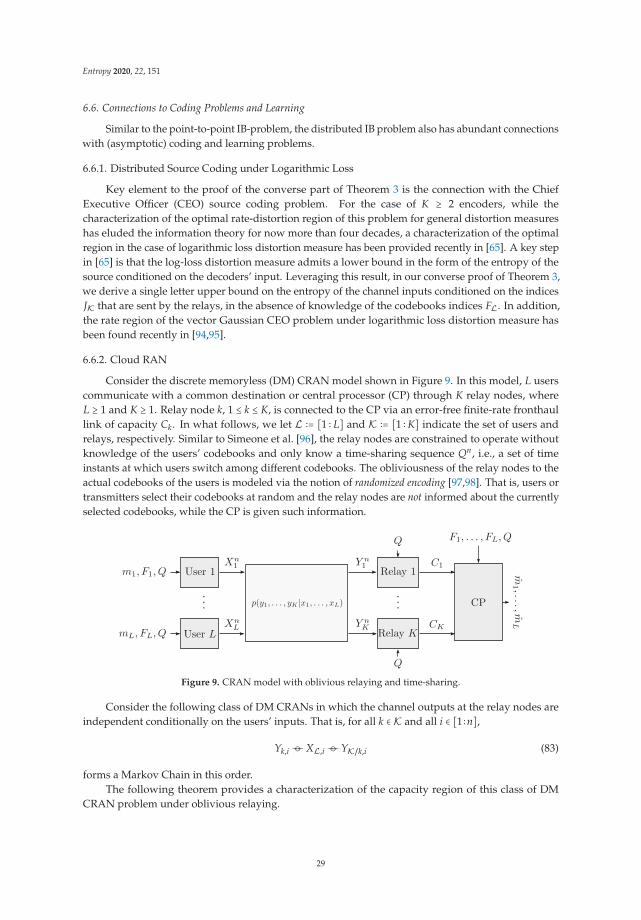
Entropy 2020, 22, 151

6.6. Connections to Coding Problems and Learning

Similar to the point-to-point IB-problem, the distributed IB problem also has abundant connectionswith (asymptotic) coding and learning problems.

6.6.1. Distributed Source Coding under Logarithmic Loss

Key element to the proof of the converse part of Theorem 3 is the connection with the ChiefExecutive Officer (CEO) source coding problem. For the case of K ≥ 2 encoders, while thecharacterization of the optimal rate-distortion region of this problem for general distortion measureshas eluded the information theory for now more than four decades, a characterization of the optimalregion in the case of logarithmic loss distortion measure has been provided recently in [65]. A key stepin [65] is that the log-loss distortion measure admits a lower bound in the form of the entropy of thesource conditioned on the decoders’ input. Leveraging this result, in our converse proof of Theorem 3,we derive a single letter upper bound on the entropy of the channel inputs conditioned on the indicesJK that are sent by the relays, in the absence of knowledge of the codebooks indices FL. In addition,the rate region of the vector Gaussian CEO problem under logarithmic loss distortion measure hasbeen found recently in [94,95].

6.6.2. Cloud RAN

Consider the discrete memoryless (DM) CRAN model shown in Figure 9. In this model, L userscommunicate with a common destination or central processor (CP) through K relay nodes, whereL ≥ 1 and K ≥ 1. Relay node k, 1 ≤ k ≤ K, is connected to the CP via an error-free finite-rate fronthaullink of capacity Ck. In what follows, we let L ∶= [1 ∶ L] and K ∶= [1 ∶K] indicate the set of users andrelays, respectively. Similar to Simeone et al. [96], the relay nodes are constrained to operate withoutknowledge of the users’ codebooks and only know a time-sharing sequence Qn, i.e., a set of timeinstants at which users switch among different codebooks. The obliviousness of the relay nodes to theactual codebooks of the users is modeled via the notion of randomized encoding [97,98]. That is, users ortransmitters select their codebooks at random and the relay nodes are not informed about the currentlyselected codebooks, while the CP is given such information.

Figure 9. CRAN model with oblivious relaying and time-sharing.

Consider the following class of DM CRANs in which the channel outputs at the relay nodes areindependent conditionally on the users’ inputs. That is, for all k ∈ K and all i ∈ [1 ∶n],

Yk,i −�− XL,i −�−YK/k,i (83)

forms a Markov Chain in this order.The following theorem provides a characterization of the capacity region of this class of DM

CRAN problem under oblivious relaying.

29

Entropy 2020, 22, 151

Theorem 3 ([22,23]). For the class of DM CRANs with oblivious relay processing and enabled time-sharingfor which Equation (83) holds, the capacity region C(CK) is given by the union of all rate tuples (R1, . . . , RL)which satisfy

∑t∈T

Rt ≤ ∑s∈S

[Cs − I(Ys; Us∣XL, Q)] + I(XT ; USc ∣XT c , Q),

for all non-empty subsets T ⊆ L and all S ⊆ K, for some joint measure of the form

p(q)L∏l=1

p(xl ∣q)K∏k=1

p(yk∣xL)K∏k=1

p(uk∣yk, q). (84)

The direct part of Theorem 3 can be obtained by a coding scheme in which each relay nodecompresses its channel output by using Wyner–Ziv binning to exploit the correlation with the channeloutputs at the other relays, and forwards the bin index to the CP over its rate-limited link. The CPjointly decodes the compression indices (within the corresponding bins) and the transmitted messages,i.e., Cover-El Gamal compress-and-forward [99] (Theorem 3) with joint decompression and decoding(CF-JD). Alternatively, the rate region of Theorem 3 can also be obtained by a direct application of thenoisy network coding (NNC) scheme of [64] (Theorem 1).

The connection between this problem, source coding and the distributed information bottleneckis discussed in [22,23], particularly in the derivation of the converse part of the theorem. Note also thesimilarity between the resulting capacity region in Theorem 3 and the relevance complexity region ofthe distributed information bottleneck in Theorem 1, despite the significant differences of the setups.

6.6.3. Distributed Inference, ELBO and Multi-View Learning

In many data analytics problems, data are collected from various sources of information orfeature extractors and are intrinsically heterogeneous. For example, an image can be identified byits color or texture features and a document may contain text and images. Conventional machinelearning approaches concatenate all available data into one big row vector (or matrix) on which asuitable algorithm is then applied. Treating different observations as a single source might causeoverfitting and is not physically meaningful because each group of data may have different statisticalproperties. Alternatively, one may partition the data into groups according to samples homogeneity,and each group of data be regarded as a separate view. This paradigm, termed multi-view learning [100],has received growing interest, and various algorithms exist, sometimes under references such asco-training [101–104], multiple kernel learning [104], and subspace learning [105]. By using distinct encodermappings to represent distinct groups of data, and jointly optimizing over all mappings to removeredundancy, multi-view learning offers a degree of flexibility that is not only desirable in practice but isalso likely to result in better learning capability. Actually, as shown in [106], local learning algorithmsproduce fewer errors than global ones. Viewing the problem as that of function approximation, theintuition is that it is usually not easy to find a unique function that holds good predictability propertiesin the entire data space.

Besides, the distributed learning of Figure 7 clearly finds application in all those scenarios inwhich learning is performed collaboratively but distinct learners either only access subsets of the entiredataset (e.g., due to physical constraints) or access independent noisy versions of the entire dataset.

In addition, similar to the single encoder case, the distributed IB also finds applications infundamental performance limits and formulation of cost functions from an operational point of view.One of such examples is the generalization of the commonly used ELBO and given in Equation (62) tothe setup with K views or observations, as formulated in Equation (78). Similarly, from the formulationof the DIB problem, a natural generalization of the classical autoencoders emerge, as given in Figure 8.

30

Entropy 2020, 22, 151

7. Outlook

A variant of the bottleneck problem in which the encoder’s output is constrained in terms of itsentropy, rather than its mutual information with the encoder’s input as done originally in [1], wasconsidered in [107]. The solution of this problem turns out to be a deterministic encoder map asopposed to the stochastic encoder map that is optimal under the IB framework of Tishby et al. [1],which results in a reduction of the algorithm’s complexity. This idea was then used and extended tothe case of available resource (or time) sharing in [108].

In the context of privacy against inference attacks [109], the authors of [75,76] considered a dualof the information bottleneck problem in which X ∈ X represents some private data that are correlatedwith the non-private data Y ∈ Y . A legitimate receiver (analyst) wishes to infer as much information aspossible about the non-private data Y but does not need to infer any information about the privatedata X. Because X and Y are correlated, sharing the non-private data X with the analyst possiblyreveals information about Y. For this reason, there is a trade-off between the amount of informationthat the user shares about X as measured by the mutual information I(U; X) and the information thathe keeps private about Y as measured by the mutual information I(U; Y), where U = φ(X).

Among interesting problems that are left unaddressed in this paper is that of characterizingoptimal input distributions under rate-constrained compression at the relays where, e.g., discretesignaling is already known to sometimes outperform Gaussian signaling for single-user GaussianCRAN [97]. It is conjectured that the optimal input distribution is discrete. Other issues might relateto extensions to continuous time filtered Gaussian channels, in parallel to the regular bottleneckproblem [108], or extensions to settings in which fronthauls may be not available at some radio-units,and that is unknown to the systems. That is, the more radio units are connected to the central unit, thehigher is the rate that could be conveyed over the CRAN uplink [110]. Alternatively, one may considerfinding the worst-case noise under given input distributions, e.g., Gaussian, and rate-constrainedcompression at the relays. Furthermore, there are interesting aspects that address processing constraintsof continuous waveforms, e.g., sampling at a given rate [111,112] with focus on remote logarithmicdistortion [65], which in turn boils down to the distributed bottleneck problem [91,92]. We also mentionfinite-sample size analysis (i.e., finite block length n, which relates to the literature on finite blocklength coding in information theory). Finally, it is interesting to observe that the bottleneck problemrelates to interesting problem when R is not necessarily scaled with the block length n.

8. Proofs

8.1. Proof of Theorem 1

The proof relies on the equivalence of the studied distributed learning problem with theChief-Executive Officer (CEO) problem under logarithmic-loss distortion measure, which was studiedin [65] (Theorem 10). For the K-encoder CEO problem, let us consider K encoding functionsφk ∶ Xk → M(n)

k satisfying nRk ≥ log ∣φk(Xnk )∣ and a decoding function ψ ∶ M(n)

1 ×⋯ ×M(n)K → Yn,

which produces a probabilistic estimate of Y from the outputs of the encoders, i.e., Yn is the set ofdistributions on Y . The quality of the estimation is measured in terms of the average log-loss.

Definition 1. A tuple (D, R1, . . . , RK) is said to be achievable in the K-encoder CEO problem for PXK,Y forwhich the Markov Chain in Equation (83) holds, if there exists a length n, encoders φk for k ∈ K, and a decoderψ, such that

D ≥ E⎡⎢⎢⎢⎢⎣

1n

log1

PYn ∣JK(Yn∣φ1(Xn1 ),⋯, φK(Xn

K))

⎤⎥⎥⎥⎥⎦, (85)

Rk ≥1n

log ∣φk(Xnk )∣ for all k ∈ K. (86)

31

Entropy 2020, 22, 151

The rate-distortion region RDCEO is given by the closure of all achievable tuples (D, R1, . . . , RK).

The following lemma shows that the minimum average logarithmic loss is the conditional entropyof Y given the descriptions. The result is essentially equivalent to [65] (Lemma 1) and it is provided forcompleteness.

Lemma 2. Let us consider PXK,Y and the encoders Jk = φk(Xnk ), k ∈ K and the decoder Yn = ψ(JK). Then,

E[�log(Yn, Yn)] ≥ H(Yn∣JK), (87)

with equality if and only if ψ(JK) = {PYn ∣JK(yn∣JK)}yn∈Yn .

Proof. Let Z ∶= (J1, . . . , JK) be the argument of ψ and P(yn∣z) be a distribution on Yn. We have forZ = z:

E[�log(Yn, Yn)∣Z = z] = ∑yn∈Yn

P(yn∣z) log( 1P(yn∣z)

) (88)

= ∑yn∈Yn

P(yn∣z) log(P(yn∣z)P(yn∣z)

) + H(Yn∣Z = z) (89)

= DKL(P(yn∣z)∥P(yn∣z)) + H(Yn∣Z = z) (90)

≥ H(Yn∣Z = z), (91)

where Equation (91) is due to the non-negativity of the KL divergence and the equality holds if andonly if for P(yn∣z) = P(yn∣z) where P(yn∣z) = Pr{Yn = yn∣Z = z} for all z and yn ∈ Yn. Averaging over Zcompletes the proof.

Essentially, Lemma 2 states that minimizing the average log-loss is equivalent to maximizing

relevance as given by the mutual information I(Yn; ψ(φ1(Xn1 ),⋯, φK(Xn

K))). Formally, the connectionbetween the distributed learning problem under study and the K-encoder CEO problem studied in [65]can be formulated as stated next.

Proposition 2. A tuple (Δ, R1, . . . , RK) ∈ RIDIB if and only if (H(Y) −Δ, R1, . . . , RK) ∈ RDCEO.

Proof. Let the tuple (Δ, R1, . . . , RK) ∈ RIDIB be achievable for some encoders φk. It follows by Lemma 2that, by letting the decoding function ψ(JK) = {PYn ∣JK(yn∣JK)}, we have E[�log(Yn, Yn)∣JK] = H(Yn∣JK),and hence (H(Y)−Δ, R1, . . . , RK) ∈ RDCEO.Conversely, assume the tuple (D, R1, . . . , RK) ∈ RDCEO is achievable. It follows by Lemma 2 thatH(Y) − D ≤ H(Yn) − H(Yn∣JK) = I(Yn; JK), which implies (Δ, R1, . . . , RK) ∈ RIDIB with Δ = H(Y) −D.

The characterization of rate-distortion region RCEO has been established recently in [65] (Theorem10). The proof of the theorem is completed by noting that Proposition 2 implies that the result in [65](Theorem 10) can be applied to characterize the region RIDIB, as given in Theorem 1.

8.2. Proof of Proposition 1

Let P∗ be the maximizing in Equation (69). Then,

(1+ s)Δs = (1+ sK)H(Y) + sRs +Ls(P∗) (92)

= (1+ sK)H(Y) + sRs +⎛⎝−H(Y∣U∗K) − s

K∑k=1

[H(Y∣U∗k ) + I(Xk; U∗k )]⎞⎠

(93)

= (1+ sK)H(Y) + sRs + (−H(Y∣U∗K) − s(Rs − I(Y; U∗K) +KH(Y))) (94)

32

Entropy 2020, 22, 151

= (1+ s)I(Y; U∗K) (95)

≤ (1+ s)Δ(Rs, PXK,Y), (96)

where Equation (94) is due to the definition of Ls(P) in Equation (67); Equation (95) holds since∑K

k=1[I(Xk; U∗k ) + H(Y∣U∗k )] = Rs − I(Y; U∗K) + KH(Y) using Equation (70); and Equation (96) followsby using Equation (68).

Conversely, if P∗ is the solution to the maximization in the function Δ(Rsum, PXK,Y) in Equation(68) such that Δ(Rsum, PXK,Y) = Δs, then Δs ≤ I(Y; U∗K) and Δs ≤ R −∑K

k=1 I(Xk; U∗k ∣Y) and we have, forany s ≥ 0, that

Δ(Rsum, PXK,Y) = Δs (97)

≤ Δs − (Δs − I(Y; U∗K)) − s⎛⎝

Δs − Rsum +K∑k=1

I(Xk; U∗k ∣Y)⎞⎠

(98)

= I(Y; U∗K) − sΔs + sRsum − sK∑k=1

I(Xk; U∗k ∣Y) (99)

= H(Y) − sΔs + sRsum − H(Y∣U∗K) − sK∑k=1

[I(Xk; U∗k ) + H(Y∣U∗k )] + sKH(Y) (100)

≤ H(Y) − sΔs + sRsum +L∗s + sKH(Y) (101)

= H(Y) − sΔs + sRsum + sKH(Y) − ((1+ sK)H(Y) + sRs − (1+ s)Δs) (102)

= Δs + s(Rsum − Rs), (103)

where in Equation (100) we use that ∑Kk=1 I(Xk; Uk∣Y) = −KH(Y) +∑K

k=1 I(Xk; Uk) + H(Y∣Uk). whichfollows by using the Markov Chain Uk −�− Xk −�− Y −�− (XK∖k, UK∖k); Equation (101) follows sinceL∗s is the maximum over all possible distributions P (possibly distinct from the P∗ that maximizesΔ(Rsum, PXK,Y)); and Equation (102) is due to Equation (69). Finally, Equation (103) is valid for anyRsum ≥ 0 and s ≥ 0. Given s, and hence (Δs, Rs), letting R = Rs yields Δ(Rs, PXK,Y) ≤ Δs. Together withEquation (96), this completes the proof of Proposition 1.

8.3. Proof of Lemma 1

Let, for a given random variable Z and z ∈ Z , a stochastic mapping QY∣Z(⋅∣z) be given. It is easyto see that

H(Y∣Z) = E[− log QY∣Z(Y∣Z)] − DKL(PY∣Z∥QY∣Z). (104)

In addition, we have

I(Xk; Uk) = H(Uk) − H(Uk∣Xk) (105)

= DKL(PUk ∣Xk∥QUk) − DKL(PUk∥QUk). (106)

Substituting it into Equation (67), we get

Ls(P) = LVBs (P, Q) + DKL(PY∣UK ∣∣QY∣UK) + s

K∑k=1

(DKL(PY∣Uk∣∣QY∣Uk

) + DKL(PUk ∣∣QUk)) (107)

≥ LVBs (P, Q), (108)

where Equation (108) follows by the non-negativity of relative entropy. In addition, note that theinequality in Equation (108) holds with equality iff Q∗ is given by Equation (80).

33

Entropy 2020, 22, 151


The proof of Theorem 2 relies on deriving an outer bound on the relevance–complexity region, asgiven by Equation (66), and showing that it is achievable with Gaussian pmfs and without time-sharing.In doing so, we use the technique of [89] (Theorem 8), which relies on the de Bruijn identity and theproperties of Fisher information and MMSE.

Lemma 3 ([88,89]). Let (X, Y) be a pair of random vectors with pmf p(x, y). We have

log ∣(πe)J−1(X∣Y)∣ ≤ h(X∣Y) ≤ log ∣(πe)mmse(X∣Y)∣, (109)

where the conditional Fischer information matrix is defined as

J(X∣Y) ∶= E[∇ log p(X∣Y)∇ log p(X∣Y)†] (110)

and the minimum mean square error (MMSE) matrix is

mmse(X∣Y) ∶= E[(X −E[X∣Y])(X −E[X∣Y])†]. (111)

For t ∈ T and fixed ∏Kk=1 p(uk∣xk, t), choose Ωk,t, k = 1, . . . , K satisfying 0 ⪯ Ωk,t ⪯ Σ−1

k such that

mmse(Yk∣X, Uk,t, t) = Σk −ΣkΩk,tΣk. (112)

Note that such Ωk,t exists since 0 ⪯ mmse(Xk∣Y, Uk,t, t) ⪯ Σ−1k , for all t ∈ T , and k ∈ K.

Using Equation (66), we get

I(Xk; Uk∣Y, t) ≥ log ∣Σk∣ − log ∣mmse(Xk∣Y, Uk,t, t)∣

= − log ∣I −Σ1/2k Ωk,tΣ

1/2k ∣, (113)

where the inequality is due to Lemma 3, and Equation (113) is due to Equation (112).In addition, we have

I(Y; USc ,t∣t) ≤ log ∣Σy∣ − log ∣J−1(Y∣USc ,t, t)∣ (114)

= logEEEEEEEEEEE∑

k∈ScΣ

1/2y H†

kΩk,tHkΣ1/2y + I

EEEEEEEEEEE, (115)

where Equation (114) is due to Lemma 3 and Equation (115) is due to to the following equality, whichrelates the MMSE matrix in Equation (112) and the Fisher information, the proof of which follows,

J(Y∣USc ,t, t) = ∑k∈Sc

H†kΩk,tHk +Σ−1

y . (116)

To show Equation (116), we use de Brujin identity to relate the Fisher information with the MMSEas given in the following lemma, the proof of which can be found in [89].

Lemma 4. Let (V1, V2) be a random vector with finite second moments and N∼CN(0, ΣN) independent of(V1, V2). Then,

mmse(V2∣V1, V2 +N) = ΣN −ΣNJ(V2 +N∣V1)ΣN . (117)

From the MMSE of Gaussian random vectors [51],

Y = E[Y∣XSc] +ZSc = ∑k∈Sc

GkXk +ZSc , (118)

34

Entropy 2020, 22, 151

where Gk = Σy∣xSc H†kΣ−1

k and ZSc ∼ CN(0, Σy∣xSc ), and

Σ−1y∣xSc = Σ−1

y + ∑k∈Sc

H†kΣ−1

k Hk. (119)

Note that ZSc is independent of YSc due to the orthogonality principle of the MMSE and itsGaussian distribution. Hence, it is also independent of USc ,q.Thus, we have

mmse⎛⎝ ∑

k∈ScGkXk∣Y, USc ,t, t

⎞⎠= ∑

k∈ScGkmmse (Xk∣Y, USc ,t, t)G†

k (120)

= Σy∣xSc ∑k∈Sc

H†k (Σ−1

k −Ωk)HkΣy∣xSc , (121)

where Equation (120) follows since the cross terms are zero due to the Markov Chain (Uk,t, Xk) −�−Y−�−(UK/k,t, XK/k) (see Appendix V of [89] ); and Equation (121) follows due to Equation (112) and Gk.Finally, we have

J(Y∣USc ,t, t) = Σ−1y∣xSc −Σ−1

y∣xSc mmse⎛⎝ ∑

k∈ScGkXk∣Y, USc ,t, t

⎞⎠

Σ−1y∣xSc (122)

= Σ−1y∣xSc − ∑

k∈ScH†

k (Σ−1k −Ωk,t)Hk (123)

= Σ−1y + ∑

k∈ScH†

kΩk,tHk, (124)

where Equation (122) is due to Lemma 4; Equation (123) is due to Equation (121); and Equation (124)follows due to Equation (119).

Then, averaging over the time sharing random variable T and letting Ωk ∶= ∑t∈T p(t)Ωk,t, we get,using Equation (113),

I(Xk; Uk∣Y, T) ≥ − ∑t∈T

p(t) log ∣I −Σ1/2k Ωk,tΣ

1/2k ∣

≥ − log ∣I −Σ1/2k ΩkΣ

1/2k ∣, (125)

where Equation (125) follows from the concavity of the log-det function and Jensen’s inequality.Similarly, using Equation (115) and Jensen’s Inequality, we have

I(Y; USc ∣T) ≤ logEEEEEEEEEEE∑

k∈ScΣ

1/2y H†

kΩkHkΣ1/2y + I

EEEEEEEEEEE. (126)

The outer bound on RIDIB is obtained by substituting into Equation (66), using Equations (125)and (126), noting that Ωk = ∑t∈T p(t)Ωk,t ⪯ Σ−1

k since 0 ⪯ Ωk,t ⪯ Σ−1k , and taking the union over Ωk

satisfying 0 ⪯ Ωk ⪯ Σ−1k .

Finally, the proof is completed by noting that the outer bound is achieved with T = ∅ andmultivariate Gaussian distributions p∗(uk∣xk, t) = CN(xk, Σ

1/2k (Ωk − I)Σ

1/2k ).

Author Contributions: A.Z., I.E.-A. and S.S.(S.) equally contributed to the published work. All authors haveread and agreed to the published version of the manuscript.

Funding: The work of S. Shamai was supported by the European Union’s Horizon 2020 Research And InnovationProgramme, grant agreement No. 694630, and by the WIN consortium via the Israel minister of economyand science.

35

Entropy 2020, 22, 151

Acknowledgments: The authors would like to thank the anonymous reviewers for the constructive commentsand suggestions, which helped us improve this manuscript.


References

1. Tishby, N.; Pereira, F.; Bialek, W. The information bottleneck method. In Proceedings of the Thirty-SeventhAnnual Allerton Conference on Communication, Control, and Computing, Allerton House, Monticello, IL,USA, 22–24 September 1999; pp. 368–377.

2. Pratt, W.K. Digital Image Processing; John Willey & Sons Inc.: New York, NY, USA, 1991.3. Yu, S.; Principe, J.C. Understanding Autoencoders with Information Theoretic Concepts. arXiv 2018,

arXiv:1804.00057.4. Yu, S.; Jenssen, R.; Principe, J.C. Understanding Convolutional Neural Network Training with Information

Theory. arXiv 2018, arXiv:1804.06537.5. Kong, Y.; Schoenebeck, G. Water from Two Rocks: Maximizing the Mutual Information. arXiv 2018,

arXiv:1802.08887.6. Ugur, Y.; Aguerri, I.E.; Zaidi, A. A generalization of Blahut-Arimoto algorithm to computing rate-distortion

regions of multiterminal source coding under logarithmic loss. In Proceedings of the IEEE InformationTheory Workshop, ITW, Kaohsiung, Taiwan, 6–10 November 2017.

7. Dobrushin, R.L.; Tsybakov, B.S. Information transmission with additional noise. IRE Trans. Inf. Theory 1962,85, 293–304. [CrossRef]

8. Witsenhausen, H.S.; Wyner, A.D. A conditional Entropy Bound for a Pair of Discrete Random Variables.IEEE Trans. Inf. Theory 1975, IT-21, 493–501. [CrossRef]

9. Witsenhausen, H.S. Indirect Rate Distortion Problems. IEEE Trans. Inf. Theory 1980, IT-26, 518–521.[CrossRef]

10. Shwartz-Ziv, R.; Tishby, N. Opening the Black Box of Deep Neural Networks via Information. arXiv 2017,arXiv:1703.00810.

11. Achille, A.; Soatto, S. Emergence of Invariance and Disentangling in Deep Representations. arXiv 2017,arXiv:1706.01350.

12. McAllester, D.A. A PAC-Bayesian Tutorial with a Dropout Bound. arXiv 2013, arXiv:1307.2118.13. Alemi, A.A. Variational Predictive Information Bottleneck. arXiv 2019, arXiv:1910.10831.14. Mukherjee, S. Machine Learning using the Variational Predictive Information Bottleneck with a Validation

Set. arXiv 2019, arXiv:1911.02210.15. Kingma, D.P.; Welling, M. Auto-Encoding Variational Bayes. arXiv 2013, arXiv:1312.6114.16. Mukherjee, S. General Information Bottleneck Objectives and their Applications to Machine Learning.

arXiv 2019, arXiv:1912.06248.17. Strouse, D.; Schwab, D.J. The information bottleneck and geometric clustering. Neural Comput. 2019,

31, 596–612. [CrossRef] [PubMed]18. Painsky, A.; Tishby, N. Gaussian Lower Bound for the Information Bottleneck Limit. J. Mach. Learn.

Res. (JMLR) 2018 18, 7908–7936.19. Kittichokechai, K.; Caire, G. Privacy-constrained remote source coding. In Proceedings of the 2016 IEEE

International Symposium on Information Theory (ISIT), Barcelona, Spain, 10–15 July 2016; pp. 1078–1082.20. Tian, C.; Chen, J. Successive Refinement for Hypothesis Testing and Lossless One-Helper Problem.

IEEE Trans. Inf. Theory 2008, 54, 4666–4681. [CrossRef]21. Sreekumar, S.; Gündüz, D.; Cohen, A. Distributed Hypothesis Testing Under Privacy Constraints. arXiv 2018,

arXiv:1807.02764.22. Aguerri, I.E.; Zaidi, A.; Caire, G.; Shamai (Shitz), S. On the Capacity of Cloud Radio Access Networks with

Oblivious Relaying. In Proceedings of the 2017 IEEE International Symposium on Information Theory (ISIT),Aachen, Germany, 25–30 June 2017; pp. 2068–2072.

23. Aguerri, I.E.; Zaidi, A.; Caire, G.; Shamai (Shitz), S. On the capacity of uplink cloud radio access networkswith oblivious relaying. IEEE Trans. Inf. Theory 2019, 65, 4575–4596. [CrossRef]

36

Entropy 2020, 22, 151

24. Stark, M.; Bauch, G.; Lewandowsky, J.; Saha, S. Decoding of Non-Binary LDPC Codes Using the InformationBottleneck Method. In Proceedings of the ICC 2019-2019 IEEE International Conference on Communications(ICC), Shanghai, China, 20–24 May 2019; pp. 1–6.

25. Bengio, Y.; Courville, A.; Vincent, P. Representation learning: A review and new perspectives. IEEE Trans.Pattern Anal. Mach. Intell. 2013, 35, 1798–1828. [CrossRef]

26. Erdogmus, D. Information Theoretic Learning: Renyi’s Entropy and Its Applications to Adaptive SystemTraining. Ph.D. Thesis, University of Florida Gainesville, Florida, FL, USA, 2002.

27. Principe, J.C.; Euliano, N.R.; Lefebvre, W.C. Neural and Adaptive Systems: Fundamentals Through Simulations;Wiley: New York, NY, USA, 2000; Volume 672.

28. Fisher, J.W. Nonlinear Extensions to the Minumum Average Correlation Energy Filter; University of Florida:Gainesville, FL, USA, 1997.

29. Jiao, J.; Courtade, T.A.; Venkat, K.; Weissman, T. Justification of logarithmic loss via the benefit of sideinformation. IEEE Trans. Inf. Theory 2015, 61, 5357–5365. [CrossRef]

30. Painsky, A.; Wornell, G.W. On the Universality of the Logistic Loss Function. arXiv 2018, arXiv:1805.03804.31. Linsker, R. Self-organization in a perceptual network. Computer 1988, 21, 105–117. [CrossRef]32. Quinlan, J.R. C4. 5: Programs for Machine Learning; Elsevier: Amsterdam, The Netherlands, 2014.33. Chow, C.; Liu, C. Approximating discrete probability distributions with dependence trees. IEEE Trans.

Inf. Theory 1968, 14, 462–467. [CrossRef]34. Olsen, C.; Meyer, P.E.; Bontempi, G. On the impact of entropy estimation on transcriptional regulatory

network inference based on mutual information. EURASIP J. Bioinf. Syst. Biol. 2008, 2009, 308959. [CrossRef]35. Pluim, J.P.; Maintz, J.A.; Viergever, M.A. Mutual-information-based registration of medical images: A survey.

IEEE Trans. Med. Imaging 2003, 22, 986–1004. [CrossRef]36. Viola, P.; Wells, W.M., III. Alignment by maximization of mutual information. Int. J. Comput. Vis. 1997,

24, 137–154. [CrossRef]37. Cesa-Bianchi, N.; Lugosi, G. Prediction, Learning and Games; Cambridge University Press: New York, NY,

USA, 2006.38. Lehmann, E.L.; Casella, G. Theory of Point Estimation; Springer Science & Business Media: Berlin, Germany, 2006.39. Bousquet, O.; Elisseeff, A. Stability and generalization. J. Mach. Learn. Res. 2002, 2, 499–526.40. Shalev-Shwartz, S.; Shamir, O.; Srebro, N.; Sridharan, K. Learnability, stability and uniform convergence.

J. Mach. Learn. Res. 2010, 11, 2635–2670.41. Xu, A.; Raginsky, M. Information-theoretic analysis of generalization capability of learning algorithms.

In Proceedings of the 31st International Conference on Neural Information Processing Systems, Long Beach,CA, USA, 4–9 December 2017; pp. 2521–2530.

42. Russo, D.; Zou, J. How much does your data exploration overfit? Controlling bias via information usage.arXiv 2015, arXiv:1511.05219.

43. Amjad, R.A.; Geiger, B.C. Learning Representations for Neural Network-Based Classification Using theInformation Bottleneck Principle. IEEE Trans. Pattern Anal. Mach. Intell. 2019. [CrossRef]

44. Paninski, L. Estimation of entropy and mutual information. Neural Comput. 2003, 15, 1191–1253. [CrossRef]45. Jiao, J.; Venkat, K.; Han, Y.; Weissman, T. Minimax estimation of functionals of discrete distributions.

IEEE Trans. Inf. Theory 2015, 61, 2835–2885. [CrossRef] [PubMed]46. Valiant, P.; Valiant, G. Estimating the unseen: improved estimators for entropy and other properties.

In Proceedings of the Advances in Neural Information Processing Systems 26 (NIPS 2013), Lake Tahoe, NV,USA, 5–10 December 2013; pp. 2157–2165.

47. Chalk, M.; Marre, O.; Tkacik, G. Relevant sparse codes with variational information bottleneck. arXiv 2016,arXiv:1605.07332.

48. Alemi, A.; Fischer, I.; Dillon, J.; Murphy, K. Deep Variational Information Bottleneck. In Proceedings of theInternational Conference on Learning Representations, ICLR 2017, Toulon, France, 24–26 April 2017.

49. Achille, A.; Soatto, S. Information Dropout: Learning Optimal Representations Through Noisy Computation.IEEE Trans. Pattern Anal. Mach. Intell. 2018, 40, 2897–2905. [CrossRef]

50. Harremoes, P.; Tishby, N. The information bottleneck revisited or how to choose a good distortion measure.In Proceedings of the 2007 IEEE International Symposium on Information Theory, Nice, France, 24–29 June2007; pp. 566–570.

51. Gamal, A.E.; Kim, Y.H. Network Information Theory; Cambridge University Press: Cambridge, UK, 2011.

37

Entropy 2020, 22, 151

52. Hotelling, H. The most predictable criterion. J. Educ. Psycol. 1935, 26, 139–142. [CrossRef]53. Globerson, A.; Tishby, N. On the Optimality of the Gaussian Information Bottleneck Curve; Technical Report;

Hebrew University: Jerusalem, Israel, 2004.54. Chechik, G.; Globerson, A.; Tishby, N.; Weiss, Y. Information Bottleneck for Gaussian Variables. J. Mach.

Learn. Res. 2005, 6, 165–188.55. Wieczorek, A.; Roth, V. On the Difference Between the Information Bottleneck and the Deep Information

Bottleneck. arXiv 2019, arXiv:1912.13480.56. Dempster, A.P.; Laird, N.M.; Rubin, D.B. Maximum likelihood from incomplete data via the EM algorithm.

J. R. Stat. Soc. Ser. B 1977, 39, 1–38.57. Blahut, R. Computation of channel capacity and rate-distortion functions. IEEE Trans. Inf. Theory 1972,

18, 460–473. [CrossRef]58. Arimoto, S. An algorithm for computing the capacity of arbitrary discrete memoryless channels. IEEE Trans.

Inf. Theory 1972, IT-18, 12–20. [CrossRef]59. Winkelbauer, A.; Matz, G. Rate-information-optimal gaussian channel output compression. In Proceedings

of the 48th Annual Conference on Information Sciences and Systems (CISS), Princeton, NJ, USA, 19–21March 2014; pp. 1–5.

60. Gálvez, B.R.; Thobaben, R.; Skoglund, M. The Convex Information Bottleneck Lagrangian. Entropy 2020,20, 98. [CrossRef]

61. Jang, E.; Gu, S.; Poole, B. Categorical Reparameterization with Gumbel-Softmax. arXiv 2017, arXiv:1611.01144.62. Maddison, C.J.; Mnih, A.; Teh, Y.W. The Concrete Distribution: A Continuous Relaxation of Discrete Random

Variables. arXiv2016, arXiv:1611.00712.63. Kingma, D.P.; Ba, J. Adam: A Method for Stochastic Optimization. arXiv 2014, arXiv:1412.6980.64. Lim, S.H.; Kim, Y.H.; Gamal, A.E.; Chung, S.Y. Noisy Network Coding. IEEE Trans. Inf. Theory 2011,

57, 3132–3152. [CrossRef]65. Courtade, T.A.; Weissman, T. Multiterminal source coding under logarithmic loss. IEEE Trans. Inf. Theory

2014, 60, 740–761. [CrossRef]66. Csiszár, I.; Körner, J. Information Theory: Coding Theorems for Discrete Memoryless Systems; Academic Press:

London, UK, 1981.67. Wyner, A.D.; Ziv, J. The rate-distortion function for source coding with side information at the decoder.

IEEE Trans. Inf. Theory 1976, 22, 1–10. [CrossRef]68. Steinberg, Y. Coding and Common Reconstruction. IEEE Trans. Inf. Theory 2009, IT-11, 4995–5010. [CrossRef]69. Benammar, M.; Zaidi, A. Rate-Distortion of a Heegard-Berger Problem with Common Reconstruction

Constraint. In Proceedings of the International Zurich Seminar on Information and Communication,Cambridge, MA, USA, 1–6 July 2016.

70. Benammar, M.; Zaidi, A. Rate-distortion function for a heegard-berger problem with two sources anddegraded reconstruction sets. IEEE Trans. Inf. Theory 2016, 62, 5080–5092. [CrossRef]

71. Sutskover, I.; Shamai, S.; Ziv, J. Extremes of Information Combining. IEEE Trans. Inf. Theory 2005,51, 1313–1325. [CrossRef]

72. Land, I.; Huber, J. Information Combining. Found. Trends Commun. Inf. Theory 2006, 3, 227–230. [CrossRef]73. Wyner, A.D. On source coding with side information at the decoder. IEEE Trans. Inf. Theory 1975, 21, 294–300.

[CrossRef]74. Ahlswede, R.; Korner, J. Source coding with side information and a converse for degraded broadcast

channels. IEEE Trans. Inf. Theory 1975, 21, 629–637. [CrossRef]75. Makhdoumi, A.; Salamatian, S.; Fawaz, N.; Médard, M. From the information bottleneck to the privacy

funnel. In Proceedings of the IEEE Information Theory Workshop, ITW, Hobart, Tasamania, Australia, 2–5November 2014; pp. 501–505.

76. Asoodeh, S.; Diaz, M.; Alajaji, F.; Linder, T. Information Extraction Under Privacy Constraints. IEEE Trans.Inf. Theory 2019, 65, 1512–1534. [CrossRef]

77. Erkip, E.; Cover, T.M. The efficiency of investment information. IEEE Trans. Inf. Theory 1998, 44, 1026–1040.[CrossRef]

78. Hinton, G.E.; van Camp, D. Keeping the Neural Networks Simple by Minimizing the Description Length ofthe Weights. In Proceedings of the Sixth Annual Conference on Computational Learning Theory; ACM: New York,NY, USA, 1993; pp. 5–13.

38

Entropy 2020, 22, 151

79. Gilad-Bachrach, R.; Navot, A.; Tishby, N. An Information Theoretic Tradeoff between Complexityand Accuracy. In Learning Theory and Kernel Machines; Lecture Notes in Computer Science; Springer:Berlin/Heidelberg, Germany, 2003; pp. 595–609.

80. Vera, M.; Piantanida, P.; Vega, L.R. The Role of Information Complexity and Randomization in RepresentationLearning. arXiv 2018, arXiv:1802.05355.

81. Huang, S.L.; Makur, A.; Wornell, G.W.; Zheng, L. On Universal Features for High-Dimensional Learningand Inference. arXiv 2019, arXiv:1911.09105.

82. Higgins, I.; Matthey, L.; Pal, A.; Burgess, C.; Glorot, X.; Botvinick, M.; Mohamed, S.; Lerchner, A. β-VAE:Learning basic visual concepts with a constrained variational framework. In Proceedings of the InternationalConference on Learning Representations, Toulon, France, 24–26 April 2017.

83. Kurakin, A.; Goodfellow, I.; Bengio, S. Adversarial Machine Learning at Scale. arXiv 2016, arXiv:1611.01236.84. Madry, A.; Makelov, A.; Schmidt, L.; Tsipras, D.; Vladu, A. Towards Deep Learning Models Resistant to

Adversarial Attacks. arXiv 2017, arXiv:1706.06083.85. Engstrom, L.; Tran, B.; Tsipras, D.; Schmidt, L.; Madry, A. A rotation and a translation suffice: Fooling cnns

with simple transformations. arXiv 2017, arXiv:1712.02779.86. Pensia, A.; Jog, V.; Loh, P.L. Extracting robust and accurate features via a robust information bottleneck.

arXiv 2019, arXiv:1910.06893.87. Guo, D.; Shamai, S.; Verdu, S. Mutual Information and Minimum Mean-Square Error in Gaussian Channels.

IEEE Trans. Inf. Theory 2005, 51, 1261–1282. [CrossRef]88. Dembo, A.; Cover, T.M.; Thomas, J.A. Information theoretic inequalities. IEEE Trans. Inf. Theory 1991,

37, 1501–1518. [CrossRef]89. Ekrem, E.; Ulukus, S. An Outer Bound for the Vector Gaussian CEO Problem. IEEE Trans. Inf. Theory 2014,

60, 6870–6887. [CrossRef]90. Cover, T.M.; Thomas, J.A. Elements of Information Theory; John Willey & Sons Inc.: New York, NY, USA, 1991.91. Aguerri, I.E.; Zaidi, A. Distributed information bottleneck method for discrete and Gaussian sources.

In Proceedings of the International Zurich Seminar on Information and Communication, IZS, Zurich,Switzerland, 21–23 February 2018.

92. Aguerri, I.E.; Zaidi, A. Distributed Variational Representation Learning. arXiv 2018, arxiv:1807.04193.93. Winkelbauer, A.; Farthofer, S.; Matz, G. The rate-information trade-off for Gaussian vector channels.

In Proceedings of the The 2014 IEEE International Symposium on Information Theory, Honolulu, HI, USA,29 June–4 July 2014; pp. 2849–2853.

94. Ugur, Y.; Aguerri, I.E.; Zaidi, A. Rate region of the vector Gaussian CEO problem under logarithmicloss. In Proceedings of the 2018 IEEE Information Theory Workshop (ITW), Guangzhou, China, 25–29November 2018.

95. Ugur, Y.; Aguerri, I.E.; Zaidi, A. Vector Gaussian CEO Problem under Logarithmic Loss. arXiv 2018,arXiv:1811.03933.

96. Simeone, O.; Erkip, E.; Shamai, S. On Codebook Information for Interference Relay Channels WithOut-of-Band Relaying. IEEE Trans. Inf. Theory 2011, 57, 2880–2888. [CrossRef]

97. Sanderovich, A.; Shamai, S.; Steinberg, Y.; Kramer, G. Communication Via Decentralized Processing.IEEE Tran. Inf. Theory 2008, 54, 3008–3023. [CrossRef]

98. Lapidoth, A.; Narayan, P. Reliable communication under channel uncertainty. IEEE Trans. Inf. Theory 1998,44, 2148–2177. [CrossRef]

99. Cover, T.M.; El Gamal, A. Capacity Theorems for the Relay Channel. IEEE Trans. Inf. Theory 1979, 25, 572–584.[CrossRef]

100. Xu, C.; Tao, D.; Xu, C. A survey on multi-view learning. arXiv 2013, arXiv:1304.5634.101. Blum, A.; Mitchell, T. Combining labeled and unlabeled data with co-training. In Proceedings of the Eleventh

Annual Conference on Computational Learning Theory, Madison, WI, USA, 24–26 July 1998; pp. 92–100.102. Dhillon, P.; Foster, D.P.; Ungar, L.H. Multi-view learning of word embeddings via CCA. In Proceedings

of the 2011 Advances in Neural Information Processing Systems, Granada, Spain, 12–17 December 2011;pp. 199–207.

103. Kumar, A.; Daumé, H. A co-training approach for multi-view spectral clustering. In Proceedings of the28th International Conference on Machine Learning (ICML-11), Bellevue, WA, USA, 28 June–2 July 2011;pp. 393–400.

39

Entropy 2020, 22, 151

104. Gönen, M.; Alpaydın, E. Multiple kernel learning algorithms. J. Mach. Learn. Res. 2011, 12, 2211–2268.105. Jia, Y.; Salzmann, M.; Darrell, T. Factorized latent spaces with structured sparsity. In Proceedings of the

Advances in Neural Information Processing Systems, Brno, Czech, 24–25 June 2010; pp. 982–990.106. Vapnik, V. The Nature of Statistical Learning Theory; Springer Science & Business Media: Berlin, Germany, 2013.107. Strouse, D.J.; Schwab, D.J. The deterministic information bottleneck. Mass. Inst. Tech. Neural Comput. 2017,

26, 1611–1630. [CrossRef] [PubMed]108. Homri, A.; Peleg, M.; Shitz, S.S. Oblivious Fronthaul-Constrained Relay for a Gaussian Channel. IEEE Trans.

Commun. 2018, 66, 5112–5123. [CrossRef]109. du Pin Calmon, F.; Fawaz, N. Privacy against statistical inference. In Proceedings of the 2012 50th Annual

Allerton Conference on Communication, Control, and Computing (Allerton), Monticello, IL, USA, 1–5October 2012.

110. Karasik, R.; Simeone, O.; Shamai, S. Robust Uplink Communications over Fading Channels with VariableBackhaul Connectivity. IEEE Trans. Commun. 2013, 12, 5788–5799.

111. Chen, Y.; Goldsmith, A.J.; Eldar, Y.C. Channel capacity under sub-Nyquist nonuniform sampling. IEEE Trans.Inf. Theory 2014, 60, 4739–4756. [CrossRef]

112. Kipnis, A.; Eldar, Y.C.; Goldsmith, A.J. Analog-to-Digital Compression: A New Paradigm for ConvertingSignals to Bits. IEEE Signal Process. Mag. 2018, 35, 16–39. [CrossRef]

© 2020 by the authors. Licensee MDPI, Basel, Switzerland. This article is an open accessarticle distributed under the terms and conditions of the Creative Commons Attribution(CC BY) license (http://creativecommons.org/licenses/by/4.0/).

40

entropy

Article

Variational Information Bottleneck for UnsupervisedClustering: Deep Gaussian Mixture Embedding

Yigit Ugur 1,2,*, George Arvanitakis 2 and Abdellatif Zaidi 1,*

1 Laboratoire d’informatique Gaspard-Monge, Université Paris-Est, 77454 Champs-sur-Marne, France2 Mathematical and Algorithmic Sciences Lab, Paris Research Center, Huawei Technologies,

92100 Boulogne-Billancourt, France; [email protected]* Correspondence: [email protected] (Y.U.); [email protected] (A.Z.)

Received: 3 December 2019; Accepted: 9 February 2020; Published: 13 February 2020

Abstract: In this paper, we develop an unsupervised generative clustering framework that combinesthe variational information bottleneck and the Gaussian mixture model. Specifically, in our approach,we use the variational information bottleneck method and model the latent space as a mixture ofGaussians. We derive a bound on the cost function of our model that generalizes the EvidenceLower Bound (ELBO) and provide a variational inference type algorithm that allows computingit. In the algorithm, the coders’ mappings are parametrized using neural networks, and the boundis approximated by Markov sampling and optimized with stochastic gradient descent. Numericalresults on real datasets are provided to support the efficiency of our method.

Keywords: clustering; unsupervised learning; Gaussian mixture model; information bottleneck

1. Introduction

Clustering consists of partitioning a given dataset into various groups (clusters) based on somesimilarity metric, such as the Euclidean distance, L1 norm, L2 norm, L∞ norm, the popular logarithmicloss measure, or others. The principle is that each cluster should contain elements of the data thatare closer to each other than to any other element outside that cluster, in the sense of the definedsimilarity measure. If the joint distribution of the clusters and data is not known, one should operateblindly in doing so, i.e., using only the data elements at hand; and the approach is called unsupervisedclustering [1,2]. Unsupervised clustering is perhaps one of the most important tasks of unsupervisedmachine learning algorithms currently, due to a variety of application needs and connections withother problems.

Clustering can be formulated as follows. Consider a dataset that is composed of N samples{xi}N

i=1, which we wish to partition into |C| ≥ 1 clusters. Let C = {1, . . . , |C|} be the set of all possibleclusters and C designate a categorical random variable that lies in C and stands for the index of theactual cluster. If X is a random variable that models elements of the dataset, given that X = xi inducesa probability distribution on C, which the learner should learn, thus mathematically, the problem isthat of estimating the values of the unknown conditional probability PC|X(·|xi) for all elements xi ofthe dataset. The estimates are sometimes referred to as the assignment probabilities.

Examples of unsupervised clustering algorithms include the very popular K-means [3] andExpectation Maximization (EM) [4]. The K-means algorithm partitions the data in a manner thatthe Euclidean distance among the members of each cluster is minimized. With the EM algorithm,the underlying assumption is that the data comprise a mixture of Gaussian samples, namely a GaussianMixture Model (GMM); and one estimates the parameters of each component of the GMM whilesimultaneously associating each data sample with one of those components. Although they offersome advantages in the context of clustering, these algorithms suffer from some strong limitations.For example, it is well known that the K-means is highly sensitive to both the order of the data and


Entropy 2020, 22, 213

scaling; and the obtained accuracy depends strongly on the initial seeds (in addition to that, it does notpredict the number of clusters or K-value). The EM algorithm suffers mainly from slow convergence,especially for high-dimensional data.

Recently, a new approach has emerged that seeks to perform inference on a transformed domain(generally referred to as latent space), not the data itself. The rationale is that because the latent spaceoften has fewer dimensions, it is more convenient computationally to perform inference (clustering) onit rather than on the high-dimensional data directly. A key aspect then is how to design a latent spacethat is amenable to accurate low-complexity unsupervised clustering, i.e., one that preserves onlythose features of the observed high-dimensional data that are useful for clustering while removing allredundant or non-relevant information. Along this line of work, we can mention [5], which utilizedPrincipal Component Analysis (PCA) [6,7] for dimensionality reduction followed by K-means forclustering the obtained reduced dimension data; or [8], which used a combination of PCA andthe EM algorithm. Other works that used alternatives for the linear PCA include kernel PCA [9],which employs PCA in a non-linear fashion to maximize variance in the data.

Thisby’s Information Bottleneck (IB) method [10] formulates the problem of finding a goodrepresentation U that strikes the right balance between capturing all information about the categoricalvariable C that is contained in the observation X and using the most concise representation for it.The IB problem can be written as the following Lagrangian optimization:

minPU|X

I(X; U)− sI(C; U) , (1)

where I(· ; ·) denotes Shannon’s mutual information and s is a Lagrange-type parameter, which controlsthe trade-off between accuracy and regularization. In [11,12], a text clustering algorithm is introducedfor the case in which the joint probability distribution of the input data is known. This textclustering algorithm uses the IB method with an annealing procedure, where the parameter s isincreased gradually. When s → 0, the representation U is designed with the most compact form, i.e.,|U | = 1, which corresponds to the maximum compression. By gradually increasing the parameters, the emphasis on the relevance term I(C; U) increases, and at a critical value of s, the optimizationfocuses on not only the compression, but also the relevance term. To fulfill the demand on the relevanceterm, this results in the cardinality of U bifurcating. This is referred as a phase transition of the system.The further increases in the value of s will cause other phase transitions, hence additional splits of Uuntil it reaches the desired level, e.g., |U | = |C|.

However, in the real-world applications of clustering with large-scale datasets, the joint probabilitydistributions of the datasets are unknown. In practice, the usage of Deep Neural Networks (DNN) forunsupervised clustering of high-dimensional data on a lower dimensional latent space has attractedconsiderable attention, especially with the advent of Autoencoder (AE) learning and the developmentof powerful tools to train them using standard backpropagation techniques [13,14]. Advanced formsinclude Variational Autoencoders (VAE) [13,14], which are generative variants of AE that regularizethe structure of the latent space, and the more general Variational Information Bottleneck (VIB) of [15],which is a technique that is based on the information bottleneck method and seeks a better trade-offbetween accuracy and regularization than VAE via the introduction of a Lagrange-type parameters, which controls that trade-off and whose optimization is similar to deterministic annealing [12] orstochastic relaxation.

In this paper, we develop an unsupervised generative clustering framework that combines VIBand the Gaussian mixture model. Specifically, in our approach, we use the variational informationbottleneck method and model the latent space as a mixture of Gaussians. We derive a bound on the costfunction of our model that generalizes the Evidence Lower Bound (ELBO) and provide a variationalinference type algorithm that allows computing it. In the algorithm, the coders’ mappings areparametrized using Neural Networks (NN), and the bound is approximated by Markov sampling andoptimized with stochastic gradient descent. Furthermore, we show how tuning the hyper-parameter s

42

Entropy 2020, 22, 213

appropriately by gradually increasing its value with iterations (number of epochs) results in a betteraccuracy. Furthermore, the application of our algorithm to the unsupervised clustering of variousdatasets, including the MNIST [16], REUTERS [17], and STL-10 [18], allows a better clustering accuracythan previous state-of-the-art algorithms. For instance, we show that our algorithm performs betterthan the Variational Deep Embedding (VaDE) algorithm of [19], which is based on VAE and performsclustering by maximizing the ELBO. Our algorithm can be seen as a generalization of the VaDE,whose ELBO can be recovered by setting s = 1 in our cost function. In addition, our algorithm alsogeneralizes the VIB of [15], which models the latent space as an isotropic Gaussian, which is generallynot expressive enough for the purpose of unsupervised clustering. Other related works, which are oflesser relevance to the contribution of this paper, are the Deep Embedded Clustering (DEC) of [20] andthe Improved Deep Embedded Clustering (IDEC) of [21,22]. For a detailed survey of clustering withdeep learning, the readers may refer to [23].

To the best of our knowledge, our algorithm performs the best in terms of clustering accuracyby using deep neural networks without any prior knowledge regarding the labels (except the usualassumption that the number of classes is known) compared to the state-of-the-art algorithms of theunsupervised learning category. In order to achieve the outperforming accuracy: (i) we derive a costfunction that contains the IB hyperparameter s that controls optimal trade-offs between the accuracyand regularization of the model; (ii) we use a lower bound approximation for the KL term in thecost function, that does not depend on the clustering assignment probability (note that the clusteringassignment is usually not accurate in the beginning of the training process); and (iii) we tune thehyperparameter s by following an annealing approach that improves both the convergence and theaccuracy of the proposed algorithm.

Throughout this paper, we use the following notation. Uppercase letters are used to denoterandom variables, e.g., X; lowercase letters are used to denote realizations of random variables,e.g., x; and calligraphic letters denote sets, e.g., X . The cardinality of a set X is denoted by|X |. Probability mass functions (pmfs) are denoted by PX(x) = Pr{X = x} and, sometimes,for short, as p(x). Boldface uppercase letters denote vectors or matrices, e.g., X, where contextshould make the distinction clear. We denote the covariance of a zero mean, complex-valued,vector X by Σx = E[XX†], where (·)† indicates the conjugate transpose. For random variables Xand Y, the entropy is denoted as H(X), i.e., H(X) = EPX [− log PX ], and the mutual informationis denoted as I(X; Y), i.e., I(X; Y) = H(X)− H(X|Y) = H(Y)− H(Y|X) = EPX,Y [log PX,Y

PX PY]. Finally,

for two probability measures PX and QX on a random variable X ∈ X , the relative entropy orKullback–Leibler divergence is denoted as DKL(PX‖QX), i.e., DKL(PX‖QX) = EPX [log PX

QX].

2. Proposed Model

In this section, we explain the proposed model, the so-called Variational Information Bottleneckwith Gaussian Mixture Model (VIB-GMM), in which we use the VIB framework and model the latentspace as a GMM. The proposed model is depicted in Figure 1, where the parameters πc, μc, Σc, for allvalues of c ∈ C, are to be optimized jointly with those of the employed NNs as instantiation of thecoders. Furthermore, the assignment probabilities are estimated based on the values of latent spacevectors instead of the observations themselves, i.e., PC|X = QC|U. In the rest of this section, we elaborateon the inference and generative network models for our method.

43

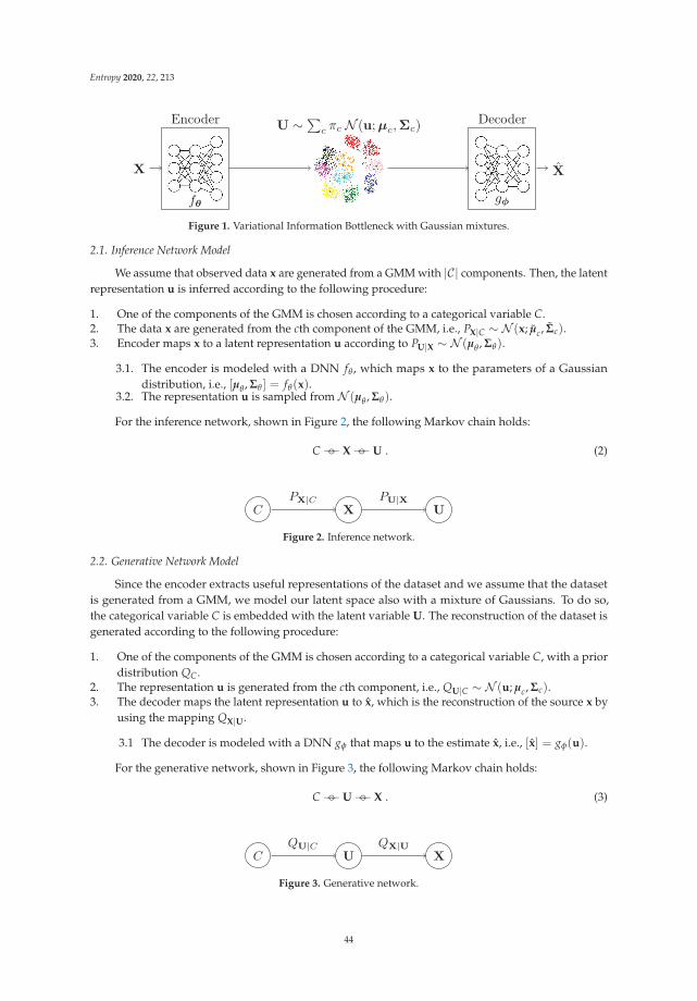
Entropy 2020, 22, 213

Encoder

fθ

Decoder

gφ

U ∼∑c πc N (u;μc,Σc)

X X

Figure 1. Variational Information Bottleneck with Gaussian mixtures.

2.1. Inference Network Model

We assume that observed data x are generated from a GMM with |C| components. Then, the latentrepresentation u is inferred according to the following procedure:

1. One of the components of the GMM is chosen according to a categorical variable C.2. The data x are generated from the cth component of the GMM, i.e., PX|C ∼ N (x; μc, Σc).3. Encoder maps x to a latent representation u according to PU|X ∼ N (μθ , Σθ).

3.1. The encoder is modeled with a DNN fθ , which maps x to the parameters of a Gaussiandistribution, i.e., [μθ , Σθ ] = fθ(x).

3.2. The representation u is sampled from N (μθ , Σθ).

For the inference network, shown in Figure 2, the following Markov chain holds:

C−�− X−�−U . (2)

C X UPX|C PU|X

Figure 2. Inference network.

2.2. Generative Network Model

Since the encoder extracts useful representations of the dataset and we assume that the datasetis generated from a GMM, we model our latent space also with a mixture of Gaussians. To do so,the categorical variable C is embedded with the latent variable U. The reconstruction of the dataset isgenerated according to the following procedure:

1. One of the components of the GMM is chosen according to a categorical variable C, with a priordistribution QC.

2. The representation u is generated from the cth component, i.e., QU|C ∼ N (u; μc, Σc).3. The decoder maps the latent representation u to x, which is the reconstruction of the source x by

using the mapping QX|U.

3.1 The decoder is modeled with a DNN gφ that maps u to the estimate x, i.e., [x] = gφ(u).

For the generative network, shown in Figure 3, the following Markov chain holds:

C−�−U−�− X . (3)

C U XQU|C QX|U

Figure 3. Generative network.

44

Entropy 2020, 22, 213

3. Proposed Method

In this section, we present our clustering method. First, we provide a general cost function for theproblem of the unsupervised clustering that we study here based on the variational IB framework;and we show that it generalizes the ELBO bound developed in [19]. We then parametrize ourmodel using NNs whose parameters are optimized jointly with those of the GMM. Furthermore,we discuss the influence of the hyperparameter s that controls optimal trade-offs between accuracyand regularization.

3.1. Brief Review of Variational Information Bottleneck for Unsupervised Learning

As described in Section 2, the stochastic encoder PU|X maps the observed data x to a representationu. Similarly, the stochastic decoder QX|U assigns an estimate x of x based on the vector u. As perthe IB method [10], a suitable representation U should strike the right balance between capturing allinformation about the categorical variable C that is contained in the observation X and using the mostconcise representation for it. This leads to maximizing the following Lagrange problem:

Ls(P) = I(C; U)− sI(X; U) , (4)

where s ≥ 0 designates the Lagrange multiplier and, for convenience, P denotes the conditionaldistribution PU|X.

Instead of (4), which is not always computable in our unsupervised clustering setting, we find itconvenient to maximize an upper bound of Ls(P) given by:

Ls(P) := I(X; U)− sI(X; U)(a)= H(X)− H(X|U)− s[H(U)− H(U|X)] , (5)

where (a) is due to the definition of mutual information (using the Markov chain C−�− X−�−U, it iseasy to see that Ls(P) ≥ Ls(P) for all values of P). Noting that H(X) is constant with respect to PU|X,maximizing Ls(P) over P is equivalent to maximizing:

L′s(P) : = −H(X|U)− s[H(U)− H(U|X)] (6)

= EPX

[EPU|X [log PX|U + s log PU − s log PU|X]

]. (7)

For a variational distribution QU on U (instead of the unknown PU) and a variational stochasticdecoder QX|U (instead of the unknown optimal decoder PX|U), let Q := {QX|U, QU}. Furthermore, let:

LVBs (P, Q) := EPX

[EPU|X [log QX|U]− sDKL(PU|X‖QU)

]. (8)

Lemma 1. For given P, we have:

LVBs (P, Q) ≤ L′s(P) , for all Q .

In addition, there exists a unique Q that achieves the maximum maxQ LVBs (P, Q) = L′s(P) and is given by:

Q∗X|U = PX|U , Q∗U = PU .

Proof. The proof of Lemma 1 is given in Appendix A.

Using Lemma 1, maximization of (6) can be written in term of the variational IB cost as follows:

maxPL′s(P) = max

Pmax

QLVB

s (P, Q) . (9)

45

Entropy 2020, 22, 213

Next, we develop an algorithm that solves the maximization problem (9), where the encodingmapping PU|X, the decoding mapping QX|U, as well as the prior distribution of the latent spaceQU are optimized jointly.

Remark 1. As we already mentioned in the beginning of this section, the related work [19] performedunsupervised clustering by combining VAE with GMM. Specifically, it maximizes the following ELBO bound:

LVaDE1 := EPX

[EPU|X [log QX|U]− DKL(PC|X‖QC)−EPC|X [DKL(PU|X‖QU|C)]

]. (10)

Let, for an arbitrary non-negative parameter s, LVaDEs be a generalization of the ELBO bound in (10) of [19]

given by:

LVaDEs := EPX

[EPU|X [log QX|U]− sDKL(PC|X‖QC)− sEPC|X [DKL(PU|X‖QU|C)]

]. (11)

Investigating the right-hand side (RHS) of (11), we get:

LVBs (P, Q) = LVaDE

s + sEPX

[EPU|X [DKL(PC|X‖QC|U)]

], (12)

where the equality holds since:

LVaDEs = EPX


](13)

(a)= EPX

[EPU|X [log QX|U]− sDKL(PU|X‖QU)− sEPU|X

[DKL(PC|X‖QC|U)

](14)

(b)= LVB

s (P, Q)− sEPX

[EPU|X

[DKL(PC|X‖QC|U)

]], (15)

where (a) can be obtained by expanding and re-arranging terms under the Markov chain C−�− X−�−U (for adetailed treatment, please look at Appendix B); and (b) follows from the definition of LVB

s (P, Q) in (8).Thus, by the non-negativity of relative entropy, it is clear that LVaDE

s is a lower bound on LVBs (P, Q).

Furthermore, if the variational distribution Q is such that the conditional marginal QC|U is equal to PC|X,the bound is tight since the relative entropy term is zero in this case.

3.2. Proposed Algorithm: VIB-GMM

In order to compute (9), we parametrize the distributions PU|X and QX|U using DNNs. For instance,let the stochastic encoder PU|X be a DNN fθ and the stochastic decoder QX|U be a DNN gφ. That is:

Pθ(u|x) = N (u; μθ , Σθ) , where [μθ , Σθ ] = fθ(x) ,

Qφ(x|u) = gφ(u) = [x] ,(16)

where θ and φ are the weight and bias parameters of the DNNs. Furthermore, the latent space ismodeled as a GMM with |C| components with parameters ψ := {πc, μc, Σc}|C|c=1, i.e.,

Qψ(u) = ∑c

πc N (u; μc, Σc) . (17)

Using the parametrizations above, the optimization of (9) can be rewritten as:

maxθ,φ,ψ

LNNs (θ, φ, ψ) (18)

46

Entropy 2020, 22, 213

where the cost function LNNs (θ, φ, ψ) is given by:

LNNs (θ, φ, ψ) := EPX

[EPθ(U|X)[log Qφ(X|U)]− sDKL(Pθ(U|X)‖Qψ(U))

]. (19)

Then, for given observations of N samples, i.e., {xi}Ni=1, (18) can be approximated in terms of an

empirical cost as follows:

maxθ,φ,ψ

1N

N

∑i=1Lemp

s,i (θ, φ, ψ) , (20)

where Lemps,i (θ, φ, ψ) is the empirical cost for the ith observation xi and given by:

Lemps,i (θ, φ, ψ) = EPθ(Ui |Xi)

[log Qφ(Xi|Ui)]− sDKL(Pθ(Ui|Xi)‖Qψ(Ui)) . (21)

Furthermore, the first term of the RHS of (21) can be computed using Monte Carlo sampling andthe reparametrization trick [13]. In particular, Pθ(u|x) can be sampled by first sampling a randomvariable Z with distribution PZ, i.e., PZ = N (0, I), then transforming the samples using some functionfθ : X ×Z → U , i.e., u = fθ(x, z). Thus,

EPθ(Ui |Xi)[log Qφ(Xi|Ui)] =

1M

M

∑m=1

log q(xi|ui,m), ui,m = μθ,i + Σ12θ,i · εm, εm ∼ N (0, I) ,

where M is the number of samples for the Monte Carlo sampling step.The second term of the RHS of (21) is the KL divergence between a single component multivariate

Gaussian and a Gaussian mixture model with |C| components. An exact closed-form solution for thecalculation of this term does not exist. However, a variational lower bound approximation [24] of itcan be obtained as:

DKL(Pθ(Ui|Xi)‖Qψ(Ui)) = − log|C|∑c=1

πc exp(−DKL(N (μθ,i, Σθ,i)‖N (μc, Σc)

). (22)

In particular, in the specific case in which the covariance matrices are diagonal, i.e., Σθ,i :=diag({σ2

θ,i,j}nuj=1) and Σc := diag({σ2

c,j}nuj=1), with nu denoting the latent space dimension, (22) can

be computed as follows:

DKL(Pθ(Ui|Xi)‖Qψ(Ui))

= − log|C|∑c=1

πc exp(− 1

2

nu

∑j=1

[ (μθ,i,j − μc,j)2

σ2c,j

+ logσ2

c,j

σ2θ,i,j− 1 +

σ2θ,i,j

σ2c,j

]), (23)

where μθ,i,j and σ2θ,i,j are the mean and variance of the ith representation in the jth dimension of the

latent space. Furthermore, μc,j and σ2c,j represent the mean and variance of the cth component of the

GMM in the jth dimension of the latent space.Finally, we train NNs to maximize the cost function (19) over the parameters θ, φ, as well as those

ψ of the GMM. For the training step, we use the ADAM optimization tool [25]. The training procedureis detailed in Algorithm 1.

47

Entropy 2020, 22, 213

Algorithm 1 VIB-GMM algorithm for unsupervised learning.

1: input: Dataset D := {xi}Ni=1, parameter s ≥ 0.

2: output: Optimal DNN weights θ�, φ� and GMM parameters ψ� = {π�c , μ�

c , Σ�c }|C|c=1.

3: initialization Initialize θ, φ, ψ.4: repeat

5: Randomly select b mini-batch samples {xi}bi=1 from D.

6: Draw m random i.i.d samples {zj}mj=1 from PZ.

7: Compute m samples ui,j = fθ(xi, zj)

8: For the selected mini-batch, compute gradients of the empirical cost (20).9: Update θ, φ, ψ using the estimated gradient (e.g., with SGD or ADAM).

10: until convergence of θ, φ, ψ.

Once our model is trained, we assign the given dataset into the clusters. As mentioned in Section 2,we do the assignment from the latent representations, i.e., QC|U = PC|X. Hence, the probability thatthe observed data xi belongs to the cth cluster is computed as follows:

p(c|xi) = q(c|ui) =qψ�(c)qψ�(ui|c)

qψ�(ui)=

π�cN (ui; μ�

c , Σ�c )

∑c π�cN (ui; μ�

c , Σ∗c ), (24)

where � indicates the optimal values of the parameters as found at the end of the training phase.Finally, the right cluster is picked based on the largest assignment probability value.

Remark 2. It is worth mentioning that with the use of the KL approximation as given by (22), our algorithmdoes not require the assumption PC|U = QC|U to hold (which is different from [19]). Furthermore, the algorithmis guaranteed to converge. However, the convergence may be to (only) local minima; and this is due to theproblem (18) being generally non-convex. Related to this aspect, we mention that while without a properpre-training, the accuracy of the VaDE algorithm may not be satisfactory, in our case, the above assumption isonly used in the final assignment after the training phase is completed.

Remark 3. In [26], it is stated that optimizing the original IB problem with the assumption of independentlatent representations amounts to disentangled representations. It is noteworthy that with such an assumption,the computational complexity can be reduced from O(n2

u) to O(nu). Furthermore, as argued in [26],the assumption often results only in some marginal performance loss; and for this reason, it is adopted inmany machine learning applications.

3.3. Effect of the Hyperparameter

As we already mentioned, the hyperparameter s controls the trade-off between the relevanceof the representation U and its complexity. As can be seen from (19) for small values of s, it is thecross-entropy term that dominates, i.e., the algorithm trains the parameters so as to reproduce X asaccurately as possible. For large values of s, however, it is most important for the NN to producean encoded version of X whose distribution matches the prior distribution of the latent space, i.e.,the term DKL(Pθ(U|X)‖Qψ(U)) is nearly zero.

In the beginning of the training process, the GMM components are randomly selected; and so,starting with a large value of the hyperparameter s is likely to steer the solution towards an irrelevantprior. Hence, for the tuning of the hyper-parameter s in practice, it is more efficient to start with a smallvalue of s and gradually increase it with the number of epochs. This has the advantage of avoidingpossible local minima, an aspect that is reminiscent of deterministic annealing [12], where s plays therole of the temperature parameter. The experiments that will be reported in the next section show thatproceeding in the above-described manner for the selection of the parameter s helps in obtaining higher

48

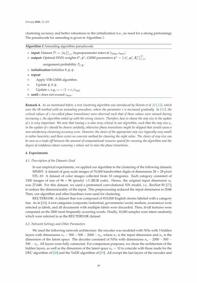
Entropy 2020, 22, 213

clustering accuracy and better robustness to the initialization (i.e., no need for a strong pretraining).The pseudocode for annealing is given in Algorithm 2.

Algorithm 2 Annealing algorithm pseudocode.

1: input: Dataset D := {xi}ni=1, hyperparameter interval [smin, smax].

2: output: Optimal DNN weights θ�, φ�, GMM parameters ψ� = {π�c , μ�

c , Σ�c }|C|c=1,

assignment probability PC|X.

3: initialization Initialize θ, φ, ψ.4: repeat

5: Apply VIB-GMM algorithm.6: Update ψ, θ, φ.7: Update s, e.g., s = (1 + εs)sold.8: until s does not exceed smax.

Remark 4. As we mentioned before, a text clustering algorithm was introduced by Slonim et al. [11,12], whichuses the IB method with an annealing procedure, where the parameter s is increased gradually. In [12], thecritical values of s (so-called phase transitions) were observed such that if these values were missed duringincreasing s, the algorithm ended up with the wrong clusters. Therefore, how to choose the step size in the updateof s is very important. We note that tuning s is also very critical in our algorithm, such that the step size εs

in the update of s should be chosen carefully, otherwise phase transitions might be skipped that would cause anon-satisfactory clustering accuracy score. However, the choice of the appropriate step size (typically very small)is rather heuristic; and there exists no concrete method for choosing the right value. The choice of step size canbe seen as a trade-off between the amount of computational resource spared for running the algorithm and thedegree of confidence about scanning s values not to miss the phase transitions.

4. Experiments

4.1. Description of the Datasets Used

In our empirical experiments, we applied our algorithm to the clustering of the following datasets.MNIST: A dataset of gray-scale images of 70,000 handwritten digits of dimensions 28× 28 pixel.STL-10: A dataset of color images collected from 10 categories. Each category consisted of

1300 images of size of 96 × 96 (pixels) ×3 (RGB code). Hence, the original input dimension nx

was 27,648. For this dataset, we used a pretrained convolutional NN model, i.e., ResNet-50 [27],to reduce the dimensionality of the input. This preprocessing reduced the input dimension to 2048.Then, our algorithm and other baselines were used for clustering.

REUTERS10K: A dataset that was composed of 810,000 English stories labeled with a categorytree. As in [20], 4 root categories (corporate/industrial, government/social, markets, economics) wereselected as labels, and all documents with multiple labels were discarded. Then, tf-idf features werecomputed on the 2000 most frequently occurring words. Finally, 10,000 samples were taken randomly,which were referred to as the REUTERS10K dataset.

4.2. Network Settings and Other Parameters

We used the following network architecture: the encoder was modeled with NNs with 3 hiddenlayers with dimensions nx − 500− 500− 2000− nu, where nx is the input dimension and nu is thedimension of the latent space. The decoder consisted of NNs with dimensions nu − 2000− 500−500− nx. All layers were fully connected. For comparison purposes, we chose the architecture of thehidden layers, as well as the dimension of the latent space nu = 10 to coincide with those made for theDEC algorithm of [20] and the VaDE algorithm of [19]. All except the last layers of the encoder and

49

Entropy 2020, 22, 213

decoder were activated with the ReLU function. For the last (i.e., latent) layer of the encoder, we useda linear activation; and for the last (i.e., output) layer of the decoder, we used the sigmoid function forMNIST and linear activation for the remaining datasets. The batch size was 100, and the variationalbound (20) was maximized by the ADAM optimizer of [25]. The learning rate was initialized with0.002 and decreased gradually every 20 epochs with a decay rate of 0.9 until it reached a small value(0.0005 in our experiments). The reconstruction loss was calculated by using the cross-entropy criterionfor MNIST and the mean squared error function for the other datasets.

4.3. Clustering Accuracy

We evaluated the performance of our algorithm in terms of the so-called unsupervised clusteringAccuracy (ACC), which is a widely used metric in the context of unsupervised learning [23].For comparison purposes, we also present those of algorithms from the previous state-of-the-art.

For each of the aforementioned datasets, we ran our VIB-GMM algorithm for various values of thehyper-parameter s inside an interval [smin, smax], starting from the smaller valuer smin and graduallyincreasing the value of s every nepoch epochs. For the MNIST dataset, we set (smin, smax, nepoch) =

(1, 5, 500); and for the STL-10 dataset and the REUTERS10K dataset, we chose these parameters to be(1, 20, 500) and (1, 5, 100), respectively. The obtained ACC accuracy results are reported in Tables 1and 2. It is important to note that the reported ACC results were obtained by running each algorithmten times. For the case in which there was no pretraining (in [19,20], the DEC and VaDE algorithmswere proposed to be used with pretraining; more specifically, the DNNs were initialized with a stackedautoencoder [28]), Table 1 states the accuracies of the best case run and average case run for theMNIST and STL-10 datasets. It was seen that our algorithm outperformed significantly the DECalgorithm of [20], as well as the VaDE algorithm of [19] and GMM for both the best case run andaverage case run. Besides, in Table 1, the values in parentheses correspond to the standard deviationsof clustering accuracies. As seen, the standard deviation of our algorithm VIB-GMM was lower thanthe VaDE; which could be expounded by the robustness of VIB-GMM to non-pretraining. For thecase in which there was pretraining, Table 2 states the accuracies of the best case run and averagecase run for the MNIST and REUTERS10K datasets. A stacked autoencoder was used to pretrainthe DNNs of the encoder and decoder before running algorithms (DNNs were initialized with thesame weights and biases of [19]). It was seen that our algorithm outperformed significantly the DECalgorithm of [20], as well as the VaDE algorithm of [19] and GMM for both the best case run andaverage case run. The effect of pretraining can be observed comparing Tables 1 and 2 for MNIST.Using a stacked autoencoder prior to running the VaDE and VIB-GMM algorithms resulted in a higheraccuracy, as well as a lower standard deviation of accuracies; therefore, supporting the algorithmswith a stacked autoencoder was beneficial for a more robust system. Finally, for the STL-10 dataset,Figure 4 depicts the evolution of the best case ACC with iterations (number of epochs) for the fourcompared algorithms.

50

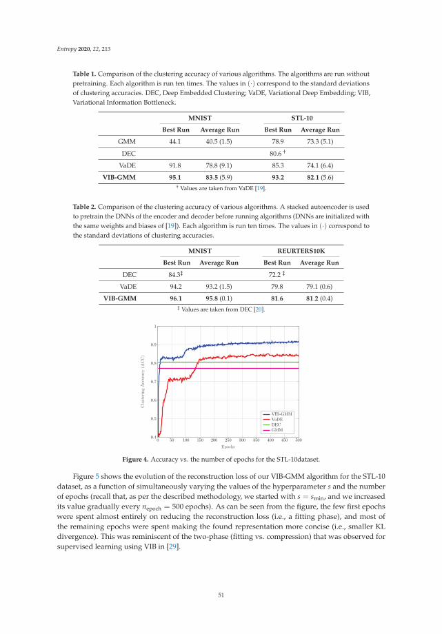
Entropy 2020, 22, 213

Table 1. Comparison of the clustering accuracy of various algorithms. The algorithms are run withoutpretraining. Each algorithm is run ten times. The values in (·) correspond to the standard deviationsof clustering accuracies. DEC, Deep Embedded Clustering; VaDE, Variational Deep Embedding; VIB,Variational Information Bottleneck.

MNIST STL-10

Best Run Average Run Best Run Average Run

GMM 44.1 40.5 (1.5) 78.9 73.3 (5.1)

DEC 80.6 †

VaDE 91.8 78.8 (9.1) 85.3 74.1 (6.4)

VIB-GMM 95.1 83.5 (5.9) 93.2 82.1 (5.6)† Values are taken from VaDE [19].

Table 2. Comparison of the clustering accuracy of various algorithms. A stacked autoencoder is usedto pretrain the DNNs of the encoder and decoder before running algorithms (DNNs are initialized withthe same weights and biases of [19]). Each algorithm is run ten times. The values in (·) correspond tothe standard deviations of clustering accuracies.

MNIST REURTERS10K

Best Run Average Run Best Run Average Run

DEC 84.3‡ 72.2 ‡

VaDE 94.2 93.2 (1.5) 79.8 79.1 (0.6)

VIB-GMM 96.1 95.8 (0.1) 81.6 81.2 (0.4)‡ Values are taken from DEC [20].

0 50 100 150 200 250 300 350 400 450 5000.4

0.5

0.6

0.7

0.8

0.9

1

Epochs

ClusteringAccuracy

(ACC)

VIB-GMMVaDEDECGMM

Figure 4. Accuracy vs. the number of epochs for the STL-10dataset.

Figure 5 shows the evolution of the reconstruction loss of our VIB-GMM algorithm for the STL-10dataset, as a function of simultaneously varying the values of the hyperparameter s and the numberof epochs (recall that, as per the described methodology, we started with s = smin, and we increasedits value gradually every nepoch = 500 epochs). As can be seen from the figure, the few first epochswere spent almost entirely on reducing the reconstruction loss (i.e., a fitting phase), and most ofthe remaining epochs were spent making the found representation more concise (i.e., smaller KLdivergence). This was reminiscent of the two-phase (fitting vs. compression) that was observed forsupervised learning using VIB in [29].

51

Entropy 2020, 22, 213

0 2 4 6 8 10 12 14350

400

450

500

550

600

650

KL Divergence Loss, I(X;U)

ReconstructionLoss

epoch 1 - 10epoch 11 - 20epoch 21 - 50epoch 51 - 100epoch 100 - 500

Figure 5. Information plane for the STL-10 dataset.

Remark 5. For a fair comparison, our algorithm VIB-GMM and the VaDE of [19] were run for the samenumber of epochs, e.g., nepoch. In the VaDE algorithm, the cost function (11) was optimized for a particular valueof hyperparameter s. Instead of running nepoch epochs for s = 1 as in VaDE, we ran nepoch epochs by graduallyincreasing s to optimize the cost (21). In other words, the computational resources were distributed over a rangeof s values. Therefore, the computational complexity of our algorithm and the VaDE was equivalent.

4.4. Visualization on the Latent Space

In this section, we investigate the evolution of the unsupervised clustering of the STL-10 dataseton the latent space using our VIB-GMM algorithm. For this purpose, we found it convenient tovisualize the latent space through application of the t-SNEalgorithm of [30] in order to generatemeaningful representations in a two-dimensional space. Figure 6 shows 4000 randomly chosen latentrepresentations before the start of the training process and respectively after 1, 5, and 500 epochs.The shown points (with a · marker in the figure) represent latent representations of data sampleswhose labels are identical. Colors are used to distinguish between clusters. Crosses (with an x markerin the figure) correspond to the centroids of the clusters. More specifically, Figure 6a shows the initiallatent space before the training process. If the clustering is performed on the initial representations,it allows ACC as small as 10%, i.e., as bad as a random assignment. Figure 6b shows the latent spaceafter one epoch, from which a partition of some of the points starts to be already visible. With fiveepochs, that partitioning is significantly sharper, and the associated clusters can be recognized easily.Observe, however, that the cluster centers seem not to have converged yet. With 500 epochs, the ACCaccuracy of our algorithm reached %91.6, and the clusters and their centroids were neater, as is visiblefrom Figure 6d.

52

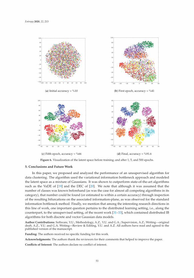
Entropy 2020, 22, 213

−100 −80 −60 −40 −20 0 20 40 60 80 100−100

−80

−60

−40

−20

0

20

40

60

80

100

(a) Initial accuracy = %10

−80 −60 −40 −20 0 20 40 60−80

−60

−40

−20

0

20

40

60

80

100

(b) First epoch, accuracy = %41

−80 −60 −40 −20 0 20 40 60 80−80

−60

−40

−20

0

20

40

60

80

100

(c) Fifth epoch, accuracy = %66

−80 −60 −40 −20 0 20 40 60 80−80

−60

−40

−20

0

20

40

60

80

(d) Final, accuracy = %91.6

Figure 6. Visualization of the latent space before training; and after 1, 5, and 500 epochs.

5. Conclusions and Future Work

In this paper, we proposed and analyzed the performance of an unsupervised algorithm fordata clustering. The algorithm used the variational information bottleneck approach and modeledthe latent space as a mixture of Gaussians. It was shown to outperform state-of-the-art algorithmssuch as the VaDE of [19] and the DEC of [20]. We note that although it was assumed that thenumber of classes was known beforehand (as was the case for almost all competing algorithms in itscategory), that number could be found (or estimated to within a certain accuracy) through inspectionof the resulting bifurcations on the associated information-plane, as was observed for the standardinformation bottleneck method. Finally, we mention that among the interesting research directions inthis line of work, one important question pertains to the distributed learning setting, i.e., along thecounterpart, to the unsupervised setting, of the recent work [31–33], which contained distributed IBalgorithms for both discrete and vector Gaussian data models.

Author Contributions: Software, Y.U.; Methodology, A.Z., Y.U. and G.A.; Supervision, A.Z.; Writing—originaldraft, A.Z., Y.U. and G.A. Writing—Review & Editing, Y.U. and A.Z. All authors have read and agreed to thepublished version of the manuscript.

Funding: The authors received no specific funding for this work.

Acknowledgments: The authors thank the reviewers for their comments that helped to improve the paper.


53

Entropy 2020, 22, 213

(b)= EPX


],

where (a) and (b) follow due to the Markov chain C−�− X−�−U.

References

1. Sculley, D. Web-scale K-means clustering. In Proceedings of the 19th International Conference on WorldWide Web, Raleigh, NC, USA, 26–30 April 2010; pp. 1177–1178.

2. Huang, Z. Extensions to the k-means algorithm for clustering large datasets with categorical values. Data Min.Knowl. Disc. 1998, 2, 283–304. [CrossRef]

3. Hartigan, J.A.; Wong, M.A. Algorithm AS 136: A K-means clustering algorithm. J. R. Stat. Soc. 1979,28, 100–108. [CrossRef]

4. Dempster, A.P.; Laird, N.M.; Rubin, D.B. Maximum likelihood from incomplete data via the EM algorithm.J. R. Stat. Soc. 1977, 39, 1–38.

5. Ding, C.; He, X. K-means clustering via principal component analysis. In Proceedings of the 21st InternationalConference on Machine Learning, Banff, AB, Canada, 4–8 July 2004.

6. Pearson, K. On lines and planes of closest fit to systems of points in space. Philos. Mag. 1901, 2, 559–572.[CrossRef]

7. Wold, S.; Esbensen, K.; Geladi, P. Principal component analysis. Chemom. Intell. Lab. Syst. 1987, 2, 37–52.[CrossRef]

8. Roweis, S. EM algorithms for PCA and SPCA. In Proceedings of the Advances in Neural InformationProcessing Systems 10, Denver, CO, USA, 1–6 December 1997; pp. 626–632.

9. Hofmann, T.; Scholkopf, B.; Smola, A.J. Kernel methods in machine learning. Ann. Stat. 2008, 36, 1171–1220.[CrossRef]

10. Tishby, N.; Pereira, F.C.; Bialek, W. The information bottleneck method. In Proceedings of the 37th AnnualAllerton Conference on Communication, Control and Computing, Monticello, IL, USA, 22–24 September1999; pp. 368–377.

11. Slonim, N.; Tishby, N. Document clustering using word clusters via the information bottleneck method.In Proceedings of the 23rd Annual International ACM SIGIR Conference on Research and Development inInformation Retrieval, Athens, Greece, 24–28 July 2000; pp. 208–215.

12. Slonim, N. The Information Bottleneck: Theory and Applications. Ph.D. Thesis, Hebrew University,Jerusalem, Israel, 2002.

13. Kingma, D.P.; Welling, M. Auto-encoding variational bayes. In Proceedings of the 2nd InternationalConference on Learning Representations, Banff, AB, Canada, 14–16 April 2014.

14. Rezende, D.J.; Mohamed, S.; Wierstra, D. Stochastic backpropagation and approximate inference in deepgenerative models. In Proceedings of the 31st International Conference on Machine Learning, Beijing, China,21–26 June 2014; pp. 1278–1286.

15. Alemi, A.A.; Fischer, I.; Dillon, J.V.; Murphy, K. Deep variational information bottleneck. In Proceedings ofthe 5th International Conference on Learning Representations, Toulon, France, 24–26 April 2017.

16. Lecun, Y.; Bottou, L.; Bengio, Y.; Haffner, P. Gradient-based learning applied to document recognition.Proc. IEEE 1998, 86, 2278–2324. [CrossRef]

17. Lewis, D.D.; Yang, Y.; Rose, T.G.; Li, F. A new benchmark collection for text categorization research. J. Mach.Learn. Res. 2004, 5, 361–397.

18. Coates, A.; Ng, A.; Lee, H. An analysis of single-layer networks in unsupervised feature learning.In Proceedings of the 14th International Conference on Artificial Intelligence and Statistics, Fort Lauderdale,FL, USA, 11–13 April 2011; pp. 215–223.

19. Jiang, Z.; Zheng, Y.; Tan, H.; Tang, B.; Zhou, H. Variational deep embedding: An unsupervised and generativeapproach to clustering. In Proceedings of the 26th International Joint Conference on Artificial Intelligence,Melbourne, Australia, 19–25 August 2017; pp. 1965–1972.

20. Xie, J.; Girshick, R.; Farhadi, A. Unsupervised deep embedding for clustering analysis. In Proceedings of the33rd International Conference on Machine Learning, New York, NY, USA, 19–24 June 2016; pp. 478–487.

55

Entropy 2020, 22, 213

21. Guo, X.; Gao, L.; Liu, X.; Yin, J. Improved deep embedded clustering with local structure preservation.In Proceedings of the 26th International Joint Conference on Artificial Intelligence, Melbourne, Australia,19–25 August 2017; pp. 1753–1759.

22. Dilokthanakul, N.; Mediano, P.A.M.; Garnelo, M.; Lee, M.C.H.; Salimbeni, H.; Arulkumaran, K.;Shanahani, M. Deep unsupervised clustering with Gaussian mixture variational autoencoders. arXiv 2017,arXiv:1611.02648.

23. Min, E.; Guo, X.; Liu, Q.; Zhang, G.; Cui, J.; Long, J. A survey of clustering with deep learning: From theperspective of network architecture. IEEE Access 2018, 6, 39501–39514. [CrossRef]

24. Hershey, J.R.; Olsen, P.A. Approximating the Kullback Leibler divergence between Gaussian mixture models.In Proceedings of the IEEE International Conference on Acoustics, Speech and Signal Processing, Honolulu,HI, USA, 15–20 April 2007; pp. 317–320.

25. Kingma, D.P.; Ba, J. Adam: A method for stochastic optimization. In Proceedings of the 3rd InternationalConference on Learning Representations, San Diego, CA, USA, 7–9 May 2015.

26. Achille, A.; Soatto, S. Information dropout: Learning optimal representations through noisy computation.IEEE Trans. Pattern Anal. Mach. Intell. 2018, 40, 2897–2905. [CrossRef] [PubMed]

27. He, K.; Zhang, X.; Ren, S.; Sun, J. Deep residual learning for image recognition. In Proceedings of the IEEEConference on Computer Vision and Pattern Recognition, Las Vegas, NV, USA, 27–30 June 2016; pp. 770–778.

28. Vincent, P.; Larochelle, H.; Lajoie, I.; Bengio, Y.; Manzagol, P.-A. Stacked denoising autoencoders: Learninguseful representations in a deep network with a local denoising criterion. J. Mach. Learn. Res. 2010,11, 3371–3408.

29. Schwartz-Ziv, R.; Tishby, N. Opening the black box of deep neural networks via information. arXiv 2017,arXiv:1703.00810.

30. van der Maaten, L.; Hinton, G. Visualizing Data using t-SNE. J. Mach. Learn. Res 2008, 9, 2579–2605.31. Estella-Aguerri, I.; Zaidi, A. Distributed variational representation learning. IEEE Trans. Pattern Anal.

Mach. Intell. 2020, in press32. Estella-Aguerri, I.; Zaidi, A. Distributed information bottleneck method for discrete and Gaussian sources.

In Proceedings of the International Zurich Seminar on Information and Communication, Zürich, Switzerland,21–23 February 2018.

33. Zaidi, A.; Estella-Aguerri, I.; Shamai (Shitz), S. On the information bottleneck problems: Models, connections,applications and information theoretic views. Entropy 2020, 22, 151. [CrossRef]

c© 2020 by the authors. Licensee MDPI, Basel, Switzerland. This article is an open accessarticle distributed under the terms and conditions of the Creative Commons Attribution(CC BY) license (http://creativecommons.org/licenses/by/4.0/).

56

entropy

Article

Asymptotic Rate-Distortion Analysis of SymmetricRemote Gaussian Source Coding: CentralizedEncoding vs. Distributed Encoding

Yizhong Wang 1, Li Xie 2, Siyao Zhou 3, Mengzhen Wang 3 and Jun Chen 1,3,*

1 College of Electronic Information and Automation, Tianjin University of Science and Technology,Tianjin 300222, China; [email protected]

2 Department of Electrical System of Launch Vehicle, Institute of Aerospace System Engineering Shanghai,Shanghai Academy of Spaceflight Technology, Shanghai 201109, China; [email protected]

3 Department of Electrical and Computer Engineering, McMaster University, Hamilton, ON L8S 4K1, Canada;[email protected] (S.Z.); [email protected] (M.W.)

* Correspondence: [email protected] or [email protected]; Tel.: +1-905-525-9140 (ext. 20163)

Received: 10 January 2019; Accepted: 20 February 2019; Published: 23 February 2019

Abstract: Consider a symmetric multivariate Gaussian source with � components, which arecorrupted by independent and identically distributed Gaussian noises; these noisy componentsare compressed at a certain rate, and the compressed version is leveraged to reconstruct the sourcesubject to a mean squared error distortion constraint. The rate-distortion analysis is performed fortwo scenarios: centralized encoding (where the noisy source components are jointly compressed) anddistributed encoding (where the noisy source components are separately compressed). It is shown,among other things, that the gap between the rate-distortion functions associated with these twoscenarios admits a simple characterization in the large � limit.

Keywords: CEO problem; mean squared error; multiterminal source coding; rate-distortion; remotesource coding

1. Introduction

Many applications involve collection and transmission of potentially noise-corrupted data. It isoften necessary to compress the collected data to reduce the transmission cost. The remote sourcecoding problem aims to characterize the optimal scheme for such compression and the relevantinformation-theoretic limit. In this work we study a quadratic Gaussian version of the remote sourcecoding problem, where compression is performed on the noise-corrupted components of a symmetricmultivariate Gaussian source. A prescribed mean squared error distortion constraint is imposed onthe reconstruction of the noise-free source components; moreover, it is assumed that the noises acrossdifferent source components are independent and obey the same Gaussian distribution. Two scenariosare considered: centralized encoding (see Figure 1) and distributed encoding (see Figure 2). It is worthnoting that the distributed encoding scenario is closely related to the CEO problem, which has beenstudied extensively [1–18].

The present paper is primarily devoted to the comparison of the rate-distortion functionsassociated with the aforementioned two scenarios. We are particularly interested in understandinghow the rate penalty for distributed encoding (relative to centralized encoding) depends on the targetdistortion as well as the parameters of source and noise models. Although the information-theoreticresults needed for this comparison are available in the literature or can be derived in a relativelystraightforward manner, the relevant expressions are too unwieldy to analyze. For this reason, wefocus on the asymptotic regime where the number of source components, denoted by �, is sufficiently


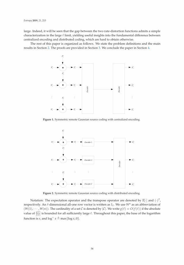
Entropy 2019, 21, 213

large. Indeed, it will be seen that the gap between the two rate-distortion functions admits a simplecharacterization in the large � limit, yielding useful insights into the fundamental difference betweencentralized encoding and distributed coding, which are hard to obtain otherwise.

The rest of this paper is organized as follows. We state the problem definitions and the mainresults in Section 2. The proofs are provided in Section 3. We conclude the paper in Section 4.

Figure 1. Symmetric remote Gaussian source coding with centralized encoding.

Figure 2. Symmetric remote Gaussian source coding with distributed encoding.

Notation: The expectation operator and the transpose operator are denoted by E[·] and (·)T ,respectively. An �-dimensional all-one row vector is written as 1�. We use Wn as an abbreviation of(W(1), · · · , W(n)). The cardinality of a set C is denoted by |C|. We write g(�) = O( f (�)) if the absolutevalue of g(�)

f (�) is bounded for all sufficiently large �. Throughout this paper, the base of the logarithm

function is e, and log+ x � max{log x, 0}.

58

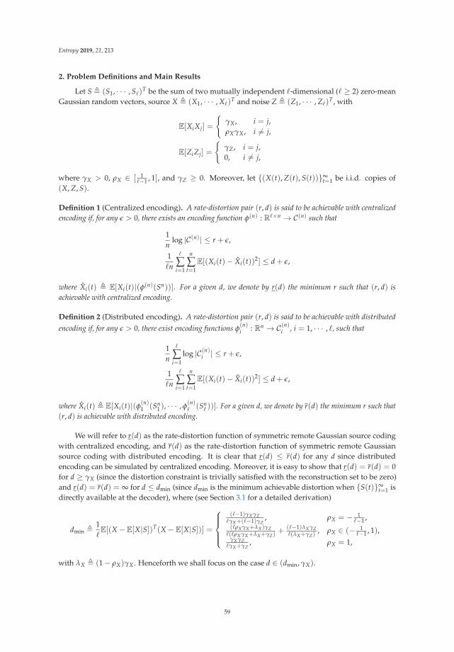
Entropy 2019, 21, 213

2. Problem Definitions and Main Results

Let S � (S1, · · · , S�)T be the sum of two mutually independent �-dimensional (� ≥ 2) zero-mean

Gaussian random vectors, source X � (X1, · · · , X�)T and noise Z � (Z1, · · · , Z�)

T , with

E[XiXj] =

{γX , i = j,ρXγX , i �= j,

E[ZiZj] =

{γZ, i = j,0, i �= j,

where γX > 0, ρX ∈ [ 1�−1 , 1], and γZ ≥ 0. Moreover, let {(X(t), Z(t), S(t))}∞

t=1 be i.i.d. copies of(X, Z, S).

Definition 1 (Centralized encoding). A rate-distortion pair (r, d) is said to be achievable with centralizedencoding if, for any ε > 0, there exists an encoding function φ(n) : R�×n → C(n) such that

1n

log |C(n)| ≤ r + ε,

1�n

�

∑i=1

n

∑t=1

E[(Xi(t)− Xi(t))2] ≤ d + ε,

where Xi(t) � E[Xi(t)|(φ(n)(Sn))]. For a given d, we denote by r(d) the minimum r such that (r, d) isachievable with centralized encoding.

Definition 2 (Distributed encoding). A rate-distortion pair (r, d) is said to be achievable with distributedencoding if, for any ε > 0, there exist encoding functions φ

(n)i : Rn → C(n)i , i = 1, · · · , �, such that

1n

�

∑i=1

log |C(n)i | ≤ r + ε,

1�n

�

∑i=1

n

∑t=1

E[(Xi(t)− Xi(t))2] ≤ d + ε,

where Xi(t) � E[Xi(t)|(φ(n)1 (Sn

1 ), · · · , φ(n)� (Sn

� ))]. For a given d, we denote by r(d) the minimum r such that(r, d) is achievable with distributed encoding.

We will refer to r(d) as the rate-distortion function of symmetric remote Gaussian source codingwith centralized encoding, and r(d) as the rate-distortion function of symmetric remote Gaussiansource coding with distributed encoding. It is clear that r(d) ≤ r(d) for any d since distributedencoding can be simulated by centralized encoding. Moreover, it is easy to show that r(d) = r(d) = 0for d ≥ γX (since the distortion constraint is trivially satisfied with the reconstruction set to be zero)and r(d) = r(d) = ∞ for d ≤ dmin (since dmin is the minimum achievable distortion when {S(t)}∞

t=1 isdirectly available at the decoder), where (see Section 3.1 for a detailed derivation)

dmin � 1�E[(X−E[X|S])T(X−E[X|S])] =

⎧⎪⎪⎨⎪⎪⎩(�−1)γXγZ

�γX+(�−1)γZ, ρX = − 1

�−1 ,(�ρXγX+λX)γZ

�(�ρXγX+λX+γZ)+ (�−1)λXγZ

�(λX+γZ), ρX ∈ (− 1

�−1 , 1),γXγZ

�γX+γZ, ρX = 1,

with λX � (1− ρX)γX . Henceforth we shall focus on the case d ∈ (dmin, γX).

59

Entropy 2019, 21, 213

Lemma 1. For d ∈ (dmin, γX),

r(d) =

⎧⎪⎪⎪⎨⎪⎪⎪⎩�−1

2 log �(�−1)γ2X

(�γX+(�−1)γZ)((�−1)d−γX), ρX = − 1

�−1 ,12 log+ (�ρXγX+λX)

2

(�ρXγX+λX+γZ)ξ+ �−1

2 log+ λ2X

(λX+γZ)ξ, ρX ∈ (− 1

�−1 , 1),12 log �γ2

X(�γX+γZ)d−γXγZ

, ρX = 1,

where

ξ �

⎧⎪⎪⎪⎨⎪⎪⎪⎩d− dmin, d ≤ min{ (�ρXγX+λX)

2

�ρXγX+λX+γZ, λ2

XλX+γZ

}+ dmin,�(d−dmin)

�−1 − (�ρXγX+λX)2

(�−1)(�ρXγX+λX+γZ), d > (�ρXγX+λX)

2

�ρXγX+λX+γZ+ dmin,

�(d− dmin)− (�−1)λ2X

λX+γZ, d >

λ2X

λX+γZ+ dmin.

Proof. See Section 3.1.

The following result can be deduced from ([19] Theorem 1) (see also [11,15]).

Lemma 2. For d ∈ (dmin, γX),

r(d) =12

log�ρXγX + λX + γZ + λQ

λQ+

�− 12

logλX + γZ + λQ

λQ,

where

λQ � −b +√

b2 − 4ac2a

with

a � �(γX − d),

b � (�ρXγX + λX)(λX + 2γZ) + (�− 1)λX(�ρXγX + λX + 2γZ)− �(�ρXγX + 2λX + 2γZ)d,

c � �(�ρXγX + λX + γZ)(λX + γZ)(dmin − d).

The expressions of r(d) and r(d) as shown in Lemmas 1 and 2 are quite complicated, renderingit difficult to make analytical comparisons. Fortunately, they become significantly simplified in theasymptotic regime where � → ∞ (with d fixed). To perform this asymptotic analysis, it is necessaryto restrict attention to the case ρX ∈ [0, 1]; moreover, without loss of generality, we assume d ∈(d(∞)

min, γX), where

d(∞)min � lim

�→∞dmin =

{λXγZ

λX+γZ, ρX ∈ [0, 1),

0, ρX = 1.

Theorem 1 (Centralized encoding).

1. ρX = 0: For d ∈ (d(∞)min, γX),

r(d) =�

2log

γ2X

(γX + γZ)d− γXγZ.

60

Entropy 2019, 21, 213

2. ρX ∈ (0, 1]: For d ∈ (d(∞)min, γX),

r(d) =

⎧⎪⎪⎪⎨⎪⎪⎪⎩�2 log λ2

X(λX+γZ)d−λXγZ

+ 12 log �+ α + O( 1

� ), d < λX ,12 log �+ 1

2 log ρXγX(λX+γZ)

λ2X

+γ2

Z2λ2

X+ O( 1

� ), d = λX ,12 log ρXγX

d−λX+ O( 1

� ), d > λX ,

where

α � 12

logρXγX(λX + γZ)

λ2X

+γ2

Z2((λX + γZ)d− λXγZ)

.


Theorem 2 (Distributed encoding).

1. ρX = 0: For d ∈ (d(∞)min, γX),

r(d) =�

2log

γ2X

(γX + γZ)d− γXγZ.

2. ρX ∈ (0, 1]: For d ∈ (d(∞)min, γX),

r(d) =

⎧⎪⎪⎪⎨⎪⎪⎪⎩�2 log λ2

X(λX+γZ)d−λXγZ

+ 12 log �+ α + O( 1

� ), d < λX ,(λX+γZ)

√�

2λX+ 1

4 log �+ 12 log ρX

1−ρX− (λX+γZ)(λX−ρXγZ)

4ρXλ2X

+ O( 1√�), d = λX ,

12 log ρXγX

d−λX+ (λX+γZ)(γX−d)

2ρXγX(d−λX)+ O( 1

� ), d > λX ,

where

α � 12

logρXγX(λX − d)

λ2X

+(λX + γZ)d2

2(λX − d)((λX + γZ)d− λXγZ).


Remark 1. One can readily recover ([20] Theorem 3) for the case m = 1 (see [20] for the definition of parameterm) and Oohama’s celebrated result for the quadratic Gaussian CEO problem ([3] Corollary 1) by setting γZ = 0and ρX = 1, respectively, in Theorem 2.

The following result is a simple corollary of Theorems 1 and 2.

Corollary 1 (Asymptotic gap).

1. ρX = 0: For d ∈ (d(∞)min, γX),

r(d)− r(d) = 0.

2. ρX ∈ (0, 1]: For d ∈ (d(∞)min, γX),

lim�→∞

r(d)− r(d) = ψ(d) �

⎧⎪⎪⎨⎪⎪⎩12 log λX−d

λX+γZ+ γZ+d

2(λX−d) , d < λX ,

∞, d = λX ,(λX+γZ)(γX−d)

2ρXγX(d−λX), d > λX .

61

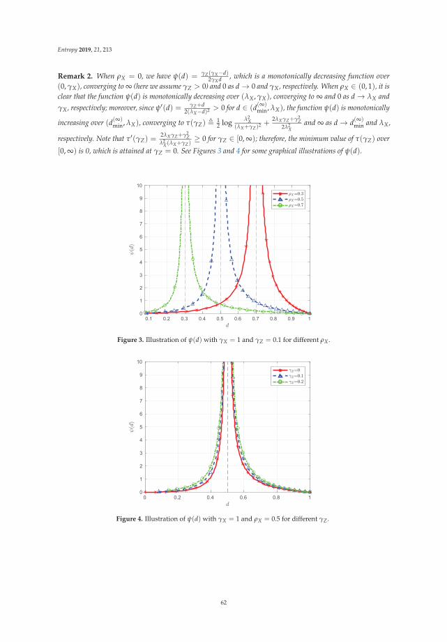
Entropy 2019, 21, 213

Remark 2. When ρX = 0, we have ψ(d) = γZ(γX−d)2γXd , which is a monotonically decreasing function over

(0, γX), converging to ∞ (here we assume γZ > 0) and 0 as d → 0 and γX, respectively. When ρX ∈ (0, 1), it isclear that the function ψ(d) is monotonically decreasing over (λX , γX), converging to ∞ and 0 as d → λX andγX, respectively; moreover, since ψ′(d) = γZ+d

2(λX−d)2 > 0 for d ∈ (d(∞)min, λX), the function ψ(d) is monotonically

increasing over (d(∞)min, λX), converging to τ(γZ) � 1

2 log λ2X

(λX+γZ)2 +2λXγZ+γ2

Z2λ2

Xand ∞ as d → d(∞)

min and λX,

respectively. Note that τ′(γZ) =2λXγZ+γ2

Zλ2

X(λX+γZ)≥ 0 for γZ ∈ [0, ∞); therefore, the minimum value of τ(γZ) over

[0, ∞) is 0, which is attained at γZ = 0. See Figures 3 and 4 for some graphical illustrations of ψ(d).

Figure 3. Illustration of ψ(d) with γX = 1 and γZ = 0.1 for different ρX .

Figure 4. Illustration of ψ(d) with γX = 1 and ρX = 0.5 for different γZ.

62

Entropy 2019, 21, 213

3. Proofs

3.1. Proof of Lemma 1

It is known [21] that r(d) is given by the solution to the following optimization problem:

(P1) minpX|S

I(S; X)

subject to E[(X− X)T(X− X)] ≤ �d,

X ↔ S ↔ X form a Markov chain.

Let X � ΘX, Z � ΘZ, and S � ΘS, where Θ is an arbitrary (real) unitary matrix with the firstrow being 1√

�1�. Since unitary transformations are invertible and preserve the Euclidean norm, we can

write (P1) equivalently as

(P2) minpX|S

I(S; X)

subject to E[(X− X)T(X− X)] ≤ �d,

X ↔ S ↔ X form a Markov chain.

For the same reason, we have

�dmin = E[(X−E[X|S])T(X−E[X|S])]. (1)

Denote the i-th components of X, Z, and S by Xi, Zi, and Si, respectively, i = 1, · · · , �. Clearly,Si = Xi + Zi, i = 1, · · · , �. Moreover, it can be verified that X1, · · · , X�, Z1, · · · , Z� are independentzero-mean Gaussian random variables with

E[(X1)2] = �ρXγX + λX , (2)

E[(Xi)2] = λX , i = 2, · · · , �, (3)

E[(Z1)2] = γZ, i = 1, · · · , �.

Now denote the i-th component of S � E[X|S] by Si, i = 1, · · · , �. We have

Si = E[Xi|Si], i = 1, · · · , �,

and

E[(S1)2] =

{0, ρX = − 1

�−1 ,(�ρXγX+λX)

2

�ρXγX+λX+γZ, ρX ∈ (− 1

�−1 , 1],(4)

E[(Si)2] =

{λ2

XλX+γZ

, ρ ∈ [− 1�−1 , 1),

0, ρX = 1,i = 2, · · · , �. (5)

Note that

E[(X− S)T(X− S)] =�

∑i=1

E[(Xi)2]−

�

∑i=1

E[(Si)2],

63

Entropy 2019, 21, 213

which, together with (1)–(5), proves

dmin =1�E[(X− S)T(X− S)] =

⎧⎪⎪⎨⎪⎪⎩(�−1)γXγZ

�γX+(�−1)γZ, ρX = − 1

�−1 ,(�ρXγX+λX)γZ

�(�ρXγX+λX+γZ)+ (�−1)λXγZ

�(λX+γZ), ρX ∈ (− 1

�−1 , 1),γXγZ

�γX+γZ, ρX = 1.

Clearly, S is determined by S; moreover, for any �-dimensional random vector X jointly distributedwith (X, S) such that X ↔ S ↔ X form a Markov chain, we have

E[(X− X)T(X− X)] = E[(S− X)T(S− X)2] +E[(X− S)T(X− S)2]

= E[(S− X)T(S− X)2] + �dmin.

Therefore, (P2) is equivalent to

(P3) minpX|S

I(S; X)

subject to E[(S− X)T(S− X)] ≤ �(d− dmin).

One can readily complete the proof of Lemma 1 by recognizing that the solution to (P3) is givenby the well-known reverse water-filling formula ([22] Theorem 13.3.3).


Setting ρX = 0 in Lemma 1 gives

r(d) =�

2log

γ2X

(γX + γZ)d− γXγZ

for d ∈ ( γXγZγX+γZ

, γX). Setting ρX = 1 in Lemma 1 gives

r(d) =12

log�2γ2

X�(�γX + γZ)d− γXγZ

for d ∈ ( γXγZ�γX+γZ

, γX); moreover, we have

12

log�2γ2

X�(�γX + γZ)d− γXγZ

=12

logγXd

+ O(1�),

and γXγZ�γX+γZ

→ 0 as �→ ∞.It remains to treat the case ρX ∈ (0, 1). In this case, it can be deduced from Lemma 1 that

r(d) =

⎧⎪⎨⎪⎩12 log (�ρXγX+λX)

2(λX+γZ)

λ2X(�ρXγX+λX+γZ)

+ �2 log λ2

X(λX+γZ)(d−dmin)

, d ∈ (dmin, λ2X

λX+γZ+ dmin],

12 log (�ρXγX+λX)

2(λX+γZ)

(�ρXγX+λX+γZ)(�(λX+γZ)(d−dmin)−(�−1)λ2X)

, d ∈ (λ2

XλX+γZ

+ dmin, γX),

and we have

dmin =(�ρXγX + λX)γZ

�(�ρXγX + λX + γZ)+

(�− 1)λXγZ�(λX + γZ)

=λXγZ

λX + γZ+

ρXγXγ2Z

(�ρXγX + λX + γZ)(λX + γZ)(6)

=λXγZ

λX + γZ+

γ2Z

(λX + γZ)�+ O(

1�2 ). (7)

64

Entropy 2019, 21, 213

Consider the following two subcases separately.

• d ∈ ( λXγZλX+γZ

, λX ]

It can be seen from (6) that dmin is a monotonically decreasing function of � and converges toλXγZ

λX+γZas �→ ∞. Therefore, we have d ∈ (dmin, λ2

XλX+γZ

+ dmin] and consequently

r(d) =12

log(�ρXγX + λX)

2(λX + γZ)

λ2X(�ρXγX + λX + γZ)

+�

2log

λ2X

(λX + γZ)(d− dmin), (8)

when � is sufficiently large. Note that

12


2

�ρXγX + λX + γZ=

12

log �+12

log(ρXγX) + O(1�) (9)

and

12

log(d− dmin) =12

log

(d− λXγZ

λX + γZ− γ2

Z(λX + γZ)�

−O(1�2 )

)(10)

=12

log(λX + γZ)d− λXγZ

λX + γZ− γ2

Z2((λX + γZ)d− λXγZ)�

+ O(1�2 ), (11)

where (10) is due to (7). Substituting (9) and (11) into (8) gives

r(d) =�

2log

λ2X

(λX + γZ)d− λXγZ+

12

log �+12


λ2X

+γ2

Z2((λX + γZ)d− λXγZ)

+ O(1�).

In particular, we have

r(λX) =12

log �+12


λ2X

+γ2

Z2λ2

X+ O(

1�).

• d ∈ (λX , γX)

Since dmin converges to λXγZλX+γZ

as �→ ∞, it follows that d ∈ (λ2

XλX+γZ

+ dmin, γX) and consequently

r(d) =12


2(λX + γZ)

(�ρXγX + λX + γZ)(�(λX + γZ)(d− dmin)− (�− 1)λ2X)

(12)

when � is sufficiently large. One can readily verify that

12


2

(�ρXγX + λX + γZ)(�(λX + γZ)(d− dmin)− (�− 1)λ2X)

=12

logρXγX

(λX + γZ)(d− λX)+ O(

1�). (13)

Substituting (13) into (12) gives

r(d) =12

logρXγX

d− λX+ O(

1�).

65

Entropy 2019, 21, 213

This completes the proof of Theorem 1.


One can readily prove part one of Theorem 2 by setting ρX = 0 in Lemma 2. So only part two ofTheorem 2 remains to be proved. Note that

b = g1�2 + g2�,

c = h1�2 + h2�,

where

g1 � ρXγX(λX − d),

g2 � λ2X + 2γXγZ − 2(λX + γZ)d,

h1 � ρXγX(λX + γZ)(d(∞)min − d),

h2 � ρXγXγ2Z + λXγZ(λX + γZ)− (λX + γZ)

2d.

We shall consider the following three cases separately.

• d < λX

In this case g1 > 0 and consequently

λQ =−b + b

√1− 4ac

b2

2a(14)

when � is sufficiently large. Note that√1− 4ac

b2 = 1− 2acb2 −

2a2c2

b4 + O(1�3 ). (15)


λQ = − cb− ac2

b3 + O(1�2 ). (16)

It is easy to show that

− cb= − h1

g1− g1h2 − g2h1

g21�

+ O(1�2 ), (17)

− ac2

b3 = − (γX − d)h21

g31�

+ O(1�2 ). (18)

Combining (16), (17) and (18) yields

λQ = η1 +η2

�+ O(

1�2 ),

66

Entropy 2019, 21, 213

where

η1 � − h1

g1,

η2 � − g21h2 − g1g2h1 + (γX − d)h2

1g3

1.

Moreover, it can be verified via algebraic manipulations that

η1 =(λX + γZ)d− λXγZ

λX − d,

η2 = − λ2Xd2

(λX − d)3 .

Now we write r(d) equivalently as

r(d) =12


λX + γZ + λQ+

�

2log

λX + γZ + λQ

λQ. (19)

Note that

12


λX + γZ + λQ=

12

log �+12

logρXγX

λX + γZ + η1+ O(

1�)

=12

log �+12


λ2X

+ O(1�) (20)

and

12

logλX + γZ + λQ

λQ

=12

logλX + γZ + η1

η1− (λX + γZ)η2

2(λX + γZ + η1)η1�+ O(

1�2 )

=12

logλ2

X(λX + γZ)d− λXγZ

+(λX + γZ)d2

2(λX − d)((λX + γX)d− λXγZ)�+ O(

1�2 ). (21)

Substituting (20) and (21) into (19) gives

r(d) =�

2log

λ2X

(λX + γZ)d− λXγZ+

12

log �+12


λ2X

+(λX + γZ)d2

2(λX − d)((λX + γX)d− λXγZ)+ O(

1�).

• d = λX

In this case g1 = 0 and consequently

λQ =−g2 +

√g2

2 − 4(γX − λX)(h1�+ h2)

2(γX − λX). (22)

67

Entropy 2019, 21, 213

Note that √g2

2 − 4(γX − λX)(h1�+ h2) =√−4(γX − λX)h1�+ O(

1√�). (23)


λQ = μ1√�+ μ2 + O(

1√�),

where

μ1 �√− h1

γX − λX,

μ2 � − g2

2(γX − λX).

Moreover, it can be verified via algebraic manipulations that

μ1 = λX ,

μ2 =(1− ρX)

2γX − 2ρXγZ2ρX

.

Now we proceed to derive an asymptotic expression of r(d). Note that

12


λX + γZ + λQ=

14

log �+12

logρXγX

μ1+ O(

1√�)

=14

log �+12

logρX

1− ρX+ O(

1√�) (24)

and

12

logλX + γZ + λQ

λQ=

λX + γZ2λQ

− (λX + γZ)2

4λ2Q

+ O(1

�32)

=λX + γZ

2μ1√�− (λX + γZ)(λX + γZ + 2μ2)

4μ21�

+ O(1

�32)

=λX + γZ

2λX√�− (λX + γZ)(λX − ρXγZ)

4ρXλ2X�

+ O(1

�32). (25)


r(λX) =(λX + γZ)

√�

2λX+

14

log �+12

logρX

1− ρX− (λX + γZ)(λX − ρXγZ)

4ρXλ2X

+ O(1√�).

• d > λX

In this case g1 < 0 and consequently

λQ =−b− b

√1− 4ac

b2

2a(26)

68

Entropy 2019, 21, 213

when � is sufficiently large. Note that√1− 4ac

b2 = 1 + O(1�). (27)


λQ = − ba+ O(1). (28)

It is easy to show that

− ba=

ρXγX(d− λX)�

γX − d+ O(1). (29)

Combining (28) and (29) yields

λQ =ρXγX(d− λX)�

γX − d+ O(1).

Now we proceed to derive an asymptotic expression of r(d). Note that

12


λX + γZ + λQ=

12

logρXγX

d− λX+ O(

1�) (30)

and

12

logλX + γZ + λQ

λQ=

λX + γZ2λQ

+ O(1�2 )

=(λX + γZ)(γX − d)

2ρXγX(d− λX)�+ O(

1�2 ). (31)


r(d) =12

logρXγX

d− λX+

(λX + γZ)(γX − d)2ρXγX(d− λX)

+ O(1�).

This completes the proof of Theorem 2.

4. Conclusions

We have studied the problem of symmetric remote Gaussian source coding and made a systematiccomparison of centralized encoding and distributed encoding in terms of the asymptotic rate-distortionperformance. It is of great interest to extend our work by considering more general source andnoise models.

Author Contributions: Conceptualization, Y.W. and J.C.; methodology, Y.W.; validation, L.X., S.Z. and M.W.;formal analysis, L.X., S.Z. and M.W.; investigation, L.X., S.Z. and M.W.; writing—original draft preparation, Y.W.;writing—review and editing, J.C.; supervision, J.C.

Funding: S.Z. was supported in part by the China Scholarship Council.

Acknowledgments: The authors wish to thank the anonymous reviewer for their valuable commentsand suggestions.


69

Entropy 2019, 21, 213

References

1. Berger, T.; Zhang, Z.; Viswanathan, H. The CEO problem. IEEE Trans. Inf. Theory 1996, 42, 887–902.[CrossRef]

2. Viswanathan, H.; Berger, T. The quadratic Gaussian CEO problem. IEEE Trans. Inf. Theory 1997, 43, 1549–1559.[CrossRef]

3. Oohama, Y. The rate-distortion function for the quadratic Gaussian CEO problem. IEEE Trans. Inf. Theory1998, 44, 1057–1070. [CrossRef]

4. Prabhakaran, V.; Tse, D.; Ramchandran, K. Rate region of the quadratic Gaussian CEO problem.In Proceedings of the IEEE International Symposium onInformation Theory, Chicago, IL, USA, 27 June–2July 2004; p. 117.

5. Chen, J.; Zhang, X.; Berger, T.; Wicker, S.B. An upper bound on the sum-rate distortion function and itscorresponding rate allocation schemes for the CEO problem. IEEE J. Sel. Areas Commun. 2004, 22, 977–987.[CrossRef]

6. Oohama, Y. Rate-distortion theory for Gaussian multiterminal source coding systems with several sideinformations at the decoder. IEEE Trans. Inf. Theory 2005, 51, 2577–2593. [CrossRef]

7. Chen, J.; Berger, T. Successive Wyner-Ziv coding scheme and its application to the quadratic Gaussian CEOproblem. IEEE Trans. Inf. Theory 2008, 54, 1586–1603. [CrossRef]

8. Wagner, A.B.; Tavildar, S.; Viswanath, P. Rate region of the quadratic Gaussian two-encoder source-codingproblem. IEEE Trans. Inf. Theory 2008, 54, 1938–1961. [CrossRef]

9. Tavildar, S.; Viswanath, P.; Wagner, A.B. The Gaussian many-help-one distributed source coding problem.IEEE Trans. Inf. Theory 2010, 56, 564–581. [CrossRef]

10. Wang, J.; Chen, J.; Wu, X. On the sum rate of Gaussian multiterminal source coding: New proofs and results.IEEE Trans. Inf. Theory 2010, 56, 3946–3960. [CrossRef]

11. Yang, Y.; Xiong, Z. On the generalized Gaussian CEO problem. IEEE Trans. Inf. Theory 2012, 58, 3350–3372.[CrossRef]

12. Wang, J.; Chen, J. Vector Gaussian two-terminal source coding. IEEE Trans. Inf. Theory 2013, 59, 3693–3708.[CrossRef]

13. Courtade, T.A.; Weissman, T. Multiterminal source coding under logarithmic loss. IEEE Trans. Inf. Theory2014, 60, 740–761. [CrossRef]

14. Wang, J.; Chen, J. Vector Gaussian multiterminal source coding. IEEE Trans. Inf. Theory 2014, 60, 5533–5552.[CrossRef]

15. Oohama, Y. Indirect and direct Gaussian distributed source coding problems. IEEE Trans. Inf. Theory 2014,60, 7506–7539. [CrossRef]

16. Nangir, M.; Asvadi, R.; Ahmadian-Attari, M.; Chen, J. Analysis and code design for the binary CEO problemunder logarithmic loss. IEEE Trans. Commun. 2018, 66, 6003–6014. [CrossRef]

17. Ugur, Y.; Aguerri, I.-E.; Zaidi, A. Vector Gaussian CEO problem under logarithmic loss and applications.arXiv 2018, arXiv:1811.03933.

18. Nangir, M.; Asvadi, R.; Chen, J.; Ahmadian-Attari, M.; Matsumoto, T. Successive Wyner-Ziv coding for thebinary CEO problem under logarithmic loss. arXiv 2018, arXiv:1812.11584.

19. Wang, Y.; Xie, L.; Zhang, X.; Chen, J. Robust distributed compression of symmetrically correlated Gaussiansources. arXiv 2018, arXiv:1807.06799.

20. Chen, J.; Xie, L.; Chang, Y.; Wang, J.; Wang, Y. Generalized Gaussian multiterminal source coding:The symmetric case. arXiv 2017, arXiv:1710.04750.

21. Dobrushin, R.; Tsybakov, B. Information transmission with additional noise. IRE Trans. Inf. Theory 1962, 8,293–304. [CrossRef]

22. Cover, T.; Thomas, J.A. Elements of Information Theory; Wiley: New York, NY, USA, 1991.


70

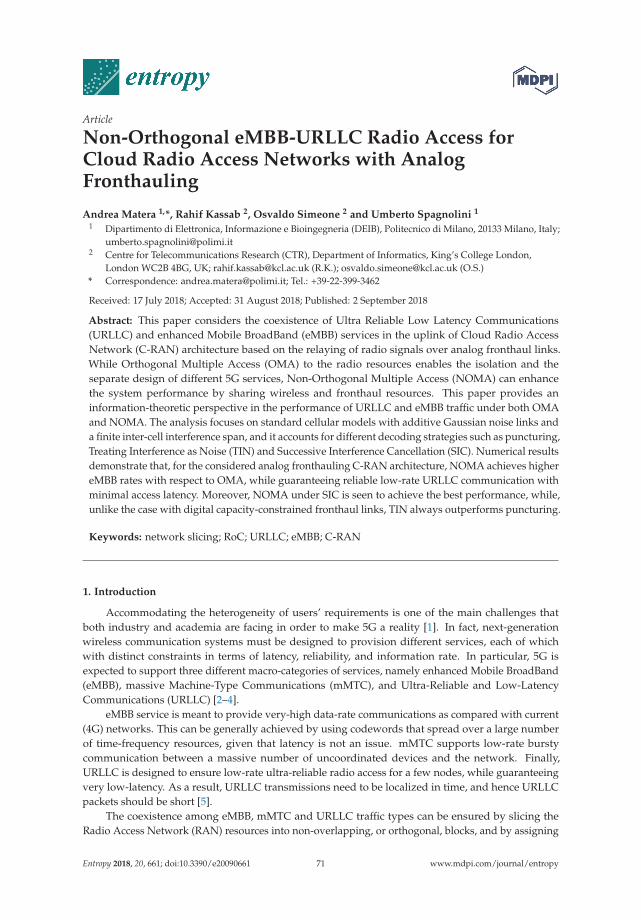
Article

Non-Orthogonal eMBB-URLLC Radio Access forCloud Radio Access Networks with AnalogFronthauling

Andrea Matera 1,*, Rahif Kassab 2, Osvaldo Simeone 2 and Umberto Spagnolini 1

1 Dipartimento di Elettronica, Informazione e Bioingegneria (DEIB), Politecnico di Milano, 20133 Milano, Italy;[email protected]

2 Centre for Telecommunications Research (CTR), Department of Informatics, King’s College London,London WC2B 4BG, UK; [email protected] (R.K.); [email protected] (O.S.)

* Correspondence: [email protected]; Tel.: +39-22-399-3462

Received: 17 July 2018; Accepted: 31 August 2018; Published: 2 September 2018

Abstract: This paper considers the coexistence of Ultra Reliable Low Latency Communications(URLLC) and enhanced Mobile BroadBand (eMBB) services in the uplink of Cloud Radio AccessNetwork (C-RAN) architecture based on the relaying of radio signals over analog fronthaul links.While Orthogonal Multiple Access (OMA) to the radio resources enables the isolation and theseparate design of different 5G services, Non-Orthogonal Multiple Access (NOMA) can enhancethe system performance by sharing wireless and fronthaul resources. This paper provides aninformation-theoretic perspective in the performance of URLLC and eMBB traffic under both OMAand NOMA. The analysis focuses on standard cellular models with additive Gaussian noise links anda finite inter-cell interference span, and it accounts for different decoding strategies such as puncturing,Treating Interference as Noise (TIN) and Successive Interference Cancellation (SIC). Numerical resultsdemonstrate that, for the considered analog fronthauling C-RAN architecture, NOMA achieves highereMBB rates with respect to OMA, while guaranteeing reliable low-rate URLLC communication withminimal access latency. Moreover, NOMA under SIC is seen to achieve the best performance, while,unlike the case with digital capacity-constrained fronthaul links, TIN always outperforms puncturing.

Keywords: network slicing; RoC; URLLC; eMBB; C-RAN

1. Introduction

Accommodating the heterogeneity of users’ requirements is one of the main challenges thatboth industry and academia are facing in order to make 5G a reality [1]. In fact, next-generationwireless communication systems must be designed to provision different services, each of whichwith distinct constraints in terms of latency, reliability, and information rate. In particular, 5G isexpected to support three different macro-categories of services, namely enhanced Mobile BroadBand(eMBB), massive Machine-Type Communications (mMTC), and Ultra-Reliable and Low-LatencyCommunications (URLLC) [2–4].

eMBB service is meant to provide very-high data-rate communications as compared with current(4G) networks. This can be generally achieved by using codewords that spread over a large numberof time-frequency resources, given that latency is not an issue. mMTC supports low-rate burstycommunication between a massive number of uncoordinated devices and the network. Finally,URLLC is designed to ensure low-rate ultra-reliable radio access for a few nodes, while guaranteeingvery low-latency. As a result, URLLC transmissions need to be localized in time, and hence URLLCpackets should be short [5].

The coexistence among eMBB, mMTC and URLLC traffic types can be ensured by slicing theRadio Access Network (RAN) resources into non-overlapping, or orthogonal, blocks, and by assigning


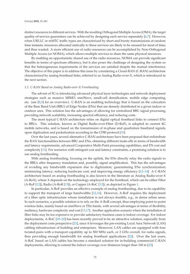
Entropy 2018, 20, 661

distinct resources to different services. With the resulting Orthogonal Multiple Access (OMA), the targetquality-of-service guarantees can be achieved by designing each service separately [6,7]. However,when URLLC or mMTC traffic types are characterized by short and bursty transmissions at randomtime instants, resources allocated statically to these services are likely to be unused for most of time,and thus wasted. A more efficient use of radio resources can be accomplished by Non-OrthogonalMultiple Access (or NOMA), which allows multiple services to share the same physical resources.

By enabling an opportunistic shared use of the radio resources, NOMA can provide significantbenefits in terms of spectrum efficiency, but it also poses the challenge of designing the system sothat the heterogeneous requirements of the services are satisfied despite the mutual interference.The objective of this paper is to address this issue by considering a Cloud-RAN (C-RAN) architecturecharacterized by analog fronthaul links, referred to as Analog Radio-over-X, which is introduced inthe next section.

1.1. C-RAN Based on Analog Radio-over-X Fronthauling

The advent of 5G is introducing advanced physical layer technologies and network deploymentstrategies such as massive MIMO, mmWave, small-cell densification, mobile edge computing,etc. (see [8,9] for an overview). C-RAN is an enabling technology that is based on the colocationof the Base Band Unit (BBU) of Edge Nodes (ENs) that are densely distributed in a given indoor oroutdoor area. This solution has the advantages of allowing for centralized BBU signal processing,providing network scalability, increasing spectral efficiency, and reducing costs.

The most typical C-RAN architecture relies on digital optical fronthaul links to connect ENsto BBUs. This solution, known as Digital Radio-over-Fiber (D-RoF), is adopted in current 4Gmobile networks, and is based on the transmission of in-phase and quadrature baseband signals,upon digitization and packetization according to the CPRI protocol [10].

Over the last years, several alternative C-RAN architectures have been proposed that redistributethe RAN functionalities between BBU and ENs, obtaining different trade-offs in terms of bandwidthand latency requirements, advanced Cooperative Multi-Point processing capabilities, and EN cost andcomplexity [11]. For scenarios with stringent cost and latency constraints, a promising solution is touse analog fronthauling.

With analog fronthauling, focusing on the uplink, the ENs directly relay the radio signals tothe BBUs after frequency translation and, possibly, signal amplification. This has the advantagesof avoiding any bandwidth expansion due to digitization; guaranteeing ENs synchronization;minimizing latency; reducing hardware cost; and improving energy efficiency [12–14]. A C-RANarchitecture based on analog fronthauling is also known in the literature as Analog Radio-over-X(A-RoX), where X depends on the technology employed for the fronthaul, which can be either Fiber(A-RoF [12]), Radio (A-RoR [15]), or Copper (A-RoC [13]), as depicted in Figure 1.

In particular, A-RoF provides an effective example of analog fronthauling, due to its capabilityto support the transport of large bandwidths [12,16]. However, A-RoF requires the deploymentof a fiber optic infrastructure whose installation is not always feasible, e.g., in dense urban areas.In such scenarios, a possible solution is to rely on the A-RoR concept, thus employing point-to-pointwireless links, mainly based on mmWave or THz bands, with several advantages in terms of flexibility,resiliency, hardware complexity and cost [15,17]. Another application scenario where the installation offiber links may be too expensive to provide satisfactory business cases is indoor coverage. For indoordeployments, A-RoC [18–20] has been recently proved to be an attractive solution, especially fromthe deployment costs perspective [21], since it leverages the pre-existing Local Area Network (LAN)cabling infrastructure of building and enterprises. Moreover, LAN cables are equipped with fourtwisted-pairs with a transport capability up to 500 MHz each, or 2 GHz overall, for radio signals,thus providing enough bandwidth for analog fronthaul applications [22]. Over the last years,A-RoC based on LAN cables has become a standard solution for in-building commercial C-RANdeployments, allowing to extend the indoor coverage over distances longer than 100 m [23].

72

Entropy 2018, 20, 661

Figure 1. C-RAN architecture overview for uplink direction: (a) Digital Radio-over-Fiber, (b) AnalogRadio-over-Fiber, (c) Analog Radio-over-Radio, (d) Analog Radio-over-Copper.

In this paper we study the coexistence of URLLC and eMBB services under both OMA andNOMA assuming a C-RAN multi-cell architecture based on analog fronthauling (see Figure 1) byusing information theoretical tools.

1.2. Related Works

The concept of NOMA is well-known from the information theoretic literature [24], and itsapplication to 5G dates back to [25], where authors demonstrated for a single-cell scenario thatsuperimposing multiple users in the same resources achieves superior performance with respectto conventional LTE networks, provided that the resulting interference is properly taken care of.The extension of NOMA to multi-cell networks is presented in [26], which addresses several multi-cellNOMA challenges, including coordinated scheduling, beamforming, and practical implementationissues related to successive interference cancellation.

In contrast with most of the works on NOMA, which deal with homogeneous trafficconditions (see [27] for a recent review), here the focus is on NOMA techniques in the context ofheterogeneous networks, such as the forthcoming 5G wireless systems, as discussed in [28–30].In fact, NOMA represents an attractive solution to meet the distinct requirements of 5G services,as it improves spectral efficiency (eMBB), enables massive device connectivity (mMTC), and allows forlow-transmission latency (URLLC) [31].

In [29] a communication-theoretic model was introduced to investigate the performance trade-offsfor eMBB, mMTC and URLLC services in a single-cell scenario under both OMA and NOMA.This single-cell model has been later extended in [32] to the uplink of a multi-cell C-RAN architecture,in which the BBU communicates with multiple URLLC and eMBB users belonging to different cellsthrough geographically distributed ENs. In the C-RAN system studied in [32], while the URLLCsignals are locally decoded at the ENs due to latency constraints, the eMBB signals are quantized andforwarded over limited-capacity digital fronthaul links to the BBU, where centralized joint decodingis performed.

None of the aforementioned works considers the coexistence of different 5G services in a C-RANarchitecture based on analog fronthaul links which is the focus of this paper.

1.3. Contributions

In this paper we study for the first time the coexistence between URLLC and eMBB services in theuplink of a C-RAN system with analog fronthauling in which the URLLC signals are still decodedlocally at the EN, while the eMBB signals are forwarded to the BBU over analog fronthaul links.

73

Entropy 2018, 20, 661

In particular, the main contributions of this paper are three-fold:

• We extend the uplink C-RAN theoretic model proposed in [32] to the case of analog fronthaul,assuming that the fronthaul links are characterized by multiple, generally interfering, channels thatcarry the received radio signals;

• By leveraging information theoretical tools, we investigate the performance trade-offs betweenURLLC and eMBB services under both OMA and NOMA, by considering different interferencemanagement strategies such as puncturing, considered for the standardization of 5G NewRadio [33,34], Treating Interference as Noise (TIN), and Successive Interference Cancellation (SIC);

• The analysis demonstrates that NOMA allows for higher eMBB information rates with respectto OMA, while guaranteeing a reliable low-rate URLLC communication with minimal accesslatency. Moreover, differently from the case of conventional digital C-RAN architecture basedon limited-capacity fronthaul links [32], in analog C-RAN, TIN always outperforms puncturing,while the best performance is still achieved by NOMA with SIC.

1.4. Organization

The remainder of the paper is organized as follows. The considered system model is introducedin Section 2. Section 3 details the fronthaul signal processing techniques employed to cope withthe impairments of the A-RoC fronthaul links. The eMBB rand URLLC information rates arediscussed in Sections 4 and 5 for OMA and NOMA, respectively. Numerical results are presented inSection 6. And Section 7 concludes the paper.

1.5. Notation

Bold upper- and lower-case letters describe matrices and column vectors, respectively. Letters R,and C refer to real and complex numbers, respectively. We denote matrix inversion, transposition andconjugate transposition as (·)−1 , (·)T , (·)H . Matrix In is an identity matrix of size n and 1n is a columnvector made by n “1s”. Symbol ⊗ denotes the Kronecker operator, vec(·) is the vectorization operator,and E[·] is the statistical expectation. Notation diag(A1, A2, ..., An) denotes a diagonal matrix withelements A1, A2, ..., An on the main diagonal. The Q-function Q(·) is the complementary cumulativedistribution function of the standardized normal random variable, and Q−1(·) is its inverse.

2. System Model

The C-RAN architecture under study is illustrated in Figure 2. In this system, the BBUscommunicate with multiple user equipments (UEs) belonging to M cells through M single-antennaEdge Nodes (ENs). The BBUs are co-located in the so-called BBU pool so that joint processing canbe performed, while the ENs are geographically distributed. In particular, we assume here that cellsare arranged in a line following the conventional circulant Wyner model ([35], Chapter 2), and eachcell contains two single-antenna UEs with different service constraints: one eMBB user and oneURLLC user.

Due to the strict latency constraints of URLLC traffic, the signal for the URLLC UEs is decodedon-site at the EN, while the eMBB signals are forwarded to the BBU through a multi-channel analogfronthaul. In this hybrid cloud-edge architecture, the mobile operator equips the EN with edgecomputing capabilities in order to provision the services required by the URLLC user directly from theEN. Following the A-RoX concept, the end-to-end channel from the eMBB UEs and the BBU pool isassumed to be fully analog: the EN performs only signal amplification and frequency translation tocomply with fronthaul capabilities and forwards the signals to the BBU, where centralized decodingis performed. In practice, as detailed later in the paper (see Sections 4 and 5), we assume thateach EN hosts a digital module, responsible for URLLC signal decoding, and an analog module,responsible for the mapping of received radio signal over the analog fronthauling, which is identifiedas Analog-to-Analog (A/A) mapping.

74

Entropy 2018, 20, 661

1 1 1 1

Figure 2. Model of the uplink of C-RAN system based on Analog Radio-over-Copper (A-RoC) fronthauling.

While the technology used for the analog fronthauling can be either fiber-optics (A-RoF),wireless (A-RoR) or cable (A-RoC), the system model proposed in this paper reflects mainly the lasttwo solutions. Furthermore, we will focus on A-RoC, and we will use the corresponding terminologyto fix the ideas (see Figure 2).

2.1. RAN Model

We consider the same Wyner-type radio access model of [32], which is described in this subsection.The Wyner model is an abstraction of cellular systems that captures one of the main aspects of suchsettings, namely the locality of inter-cell interference. The advantage of employing such a simple modelis the possibility to obtain analytical insights, which is a first mandatory step for the performanceassessment under more realistic operating conditions [35]. As illustrated in Figure 3, the direct channelgain from the eMBB UE and the EN belonging to the same cell is set to one, while the inter-cell eMBBchannel gain is equal to α ∈ [0, 1]. Furthermore, the URLLC UEs have a channel gain equal to β > 0.The URLLC user is assumed to be in the proximity of the EN, and thus it does not interfere with theneighboring cells. The eMBB user, instead, is assumed to be located at the edges of the cell in order toconsider worst-case performance guarantees. As a result, each eMBB user interferes with both left andright neighboring cells, following the standard Wyner model [35]. All channel gains are assumed to beconstant over the considered radio resources shown Figure 3, and known to all UEs and ENs.

U U U

nT

nF

U U U

nT

nF

Figure 3. Time-frequency resource allocation: (a) Orthogonal Multiple Access (OMA) and(b) Non-Orthogonal Multiple Access (NOMA). Downwards arrows denote arrival of URLLC packets.

75

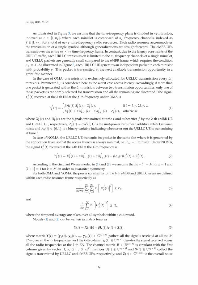
Entropy 2018, 20, 661

As illustrated in Figure 3, we assume that the time-frequency plane is divided in nT minislots,indexed as t ∈ [1, nT ], where each minislot is composed of nF frequency channels, indexed asf ∈ [1, nF], for a total of nFnT time-frequency radio resources. Each radio resource accommodatesthe transmission of a single symbol, although generalizations are straightforward. The eMBB UEstransmit over the entire nF × nT time-frequency frame. In contrast, due to the latency constraints of theURLLC traffic, each URLLC transmission is limited to the nF frequency channels of a single minislot,and URLLC packets are generally small compared to the eMBB frame, which requires the conditionnT � 1. As illustrated in Figure 3, each URLLC UE generates an independent packet in each minislotwith probability q. This packet is transmitted at the next available transmission opportunity in agrant-free manner.

In the case of OMA, one minislot is exclusively allocated for URLLC transmission every LUminislots. Parameter LU is considered here as the worst-case access latency. Accordingly, if more thanone packet is generated within the LU minislots between two transmission opportunities, only one ofthose packets is randomly selected for transmission and all the remaining are discarded. The signalY f

k (t) received at the k-th EN at the f -th frequency under OMA is

Y fk (t) =

{βAk(t)U

fk (t) + Z f

k (t), if t = LU , 2LU , ...

X fk (t) + αX f

k−1(t) + αX fk+1(t) + Z f

k (t), otherwise(1)

where X fk (t) and U f

k (t) are the signals transmitted at time t and subcarrier f by the k-th eMBB UE

and URLLC UE, respectively; Z fk (t) ∼ CN (0, 1) is the unit-power zero-mean additive white Gaussian

noise; and Ak(t) ∈ {0, 1} is a binary variable indicating whether or not the URLLC UE is transmittingat time t.

In case of NOMA, the URLLC UE transmits its packet in the same slot where it is generated bythe application layer, so that the access latency is always minimal, i.e., LU = 1 minislot. Under NOMA,the signal Y f

k (t) received at the k-th EN at the f -th frequency is

Y fk (t) = X f

k (t) + αX fk−1(t) + αX f

k+1(t) + βAk(t)Ufk (t) + Z f

k (t). (2)

According to the circulant Wyner model, in (1) and (2), we assume that [k− 1] = M for k = 1 and[k + 1] = 1 for k = M, in order to guarantee symmetry.

For both OMA and NOMA, the power constraints for the k-th eMBB and URLLC users are definedwithin each radio resource frame respectively as

1nFnT

nT

∑t=1

nF

∑f=1

E

[∣∣∣X fk (t)

∣∣∣2] ≤ PB, (3)

and1

nF

nF

∑f=1

E

[∣∣∣U fk (t)

∣∣∣2] ≤ PU , (4)

where the temporal average are taken over all symbols within a codeword.Models (1) and (2) can be written in matrix form as

Y(t) = X(t)H + βU(t)A(t) + Z(t), (5)

where matrix Y(t) = [y1(t), y2(t), ..., yM(t)] ∈ CnF×M gathers all the signals received at all the MENs over all the nF frequencies, and the k-th column yk(t) ∈ CnF×1 denotes the signal received acrossall the radio frequencies at the k-th EN. The channel matrix H ∈ RM×M is circulant with the firstcolumn given by vector [1, α, 0, ..., 0, α]T ; matrices U(t) ∈ CnF×M and X(t) ∈ CnF×M collect thesignals transmitted by URLLC and eMBB UEs, respectively; and Z(t) ∈ CnF×M is the overall noise

76

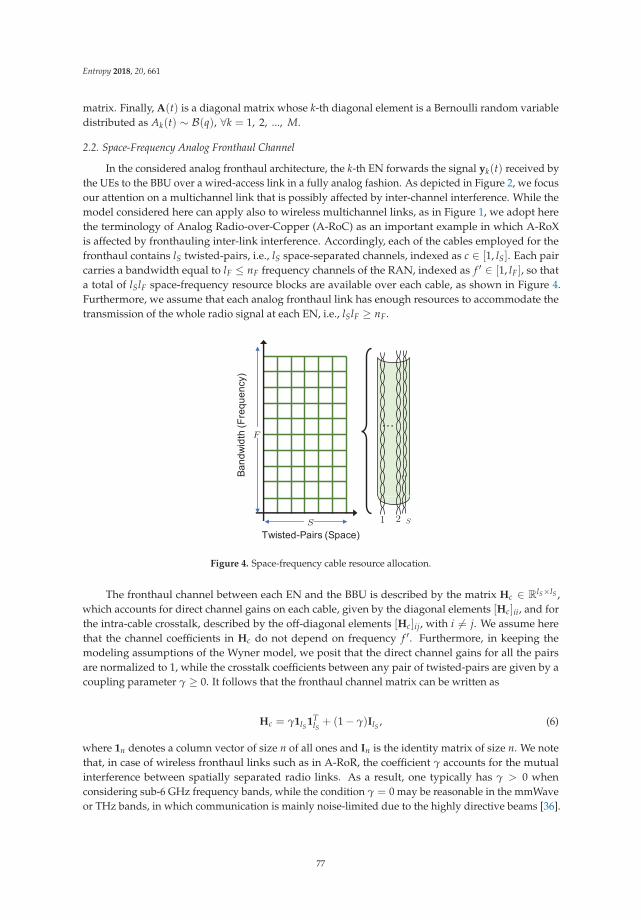
Entropy 2018, 20, 661

matrix. Finally, A(t) is a diagonal matrix whose k-th diagonal element is a Bernoulli random variabledistributed as Ak(t) ∼ B(q), ∀k = 1, 2, ..., M.

2.2. Space-Frequency Analog Fronthaul Channel

In the considered analog fronthaul architecture, the k-th EN forwards the signal yk(t) received bythe UEs to the BBU over a wired-access link in a fully analog fashion. As depicted in Figure 2, we focusour attention on a multichannel link that is possibly affected by inter-channel interference. While themodel considered here can apply also to wireless multichannel links, as in Figure 1, we adopt herethe terminology of Analog Radio-over-Copper (A-RoC) as an important example in which A-RoXis affected by fronthauling inter-link interference. Accordingly, each of the cables employed for thefronthaul contains lS twisted-pairs, i.e., lS space-separated channels, indexed as c ∈ [1, lS]. Each paircarries a bandwidth equal to lF ≤ nF frequency channels of the RAN, indexed as f ′ ∈ [1, lF], so thata total of lSlF space-frequency resource blocks are available over each cable, as shown in Figure 4.Furthermore, we assume that each analog fronthaul link has enough resources to accommodate thetransmission of the whole radio signal at each EN, i.e., lSlF ≥ nF.

S

F

S1 2

Figure 4. Space-frequency cable resource allocation.

The fronthaul channel between each EN and the BBU is described by the matrix Hc ∈ RlS×lS ,which accounts for direct channel gains on each cable, given by the diagonal elements [Hc]ii, and forthe intra-cable crosstalk, described by the off-diagonal elements [Hc]ij, with i �= j. We assume herethat the channel coefficients in Hc do not depend on frequency f ′. Furthermore, in keeping themodeling assumptions of the Wyner model, we posit that the direct channel gains for all the pairsare normalized to 1, while the crosstalk coefficients between any pair of twisted-pairs are given by acoupling parameter γ ≥ 0. It follows that the fronthaul channel matrix can be written as

Hc = γ1lS 1TlS + (1− γ)IlS , (6)

where 1n denotes a column vector of size n of all ones and In is the identity matrix of size n. We notethat, in case of wireless fronthaul links such as in A-RoR, the coefficient γ accounts for the mutualinterference between spatially separated radio links. As a result, one typically has γ > 0 whenconsidering sub-6 GHz frequency bands, while the condition γ = 0 may be reasonable in the mmWaveor THz bands, in which communication is mainly noise-limited due to the highly directive beams [36].

77

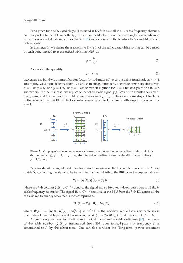
Entropy 2018, 20, 661

For a given time t, the symbols yk(t) received at EN k-th over all the nF radio frequency channelsare transported to the BBU over the lSlF cable resource blocks, where the mapping between radio andcable resources is to be designed (see Section 3.1) and depends on the bandwidth lF available at eachtwisted-pair.

In this regards, we define the fraction μ ∈ [1/lS, 1] of the radio bandwidth nF that can be carriedby each pair, referred to as normalized cable bandwidth, as

μ =lFnF

. (7)

As a result, the quantityη = μ · lS (8)

expresses the bandwidth amplification factor (or redundancy) over the cable fronthaul, as η ≥ 1.To simplify, we assume here that both 1/μ and η are integer numbers. The two extreme situations withμ = 1, or η = lS, and μ = 1/lS, or η = 1, are shown in Figure 5 for lS = 4 twisted-pairs and nF = 8subcarriers. For the first case, one replica of the whole radio signal yk(t) can be transmitted over all ofthe lS pairs, and the bandwidth amplification over cable is η = lS. In the second case, disjoint fractionsof the received bandwidth can be forwarded on each pair and the bandwidth amplification factor isη = 1.

S

nF

S

nF SnFyk( )

= 1 = 1 S

= S = 1

nFyk( )

Figure 5. Mapping of radio resources over cable resources: (a) maximum normalized cable bandwidth(full redundancy), μ = 1, or η = lS; (b) minimal normalized cable bandwidth (no redundancy),μ = 1/lS, or η = 1.

We now detail the signal model for fronthaul transmission. To this end, let us define the lF × lSmatrix Yk containing the signal to be transmitted by the EN k-th to the BBU over the copper cable as

Yk = [y1k(t), y2

k(t), ..., ylSk (t)], (9)

where the k-th column yck(t) ∈ ClF×1 denotes the signal transmitted on twisted-pair c across all the lF

cable frequency resources. The signal Rk ∈ ClF×lS received at the BBU from the k-th EN across all thecable space-frequency resources is then computed as

Rk(t) = Yk(t)Hc + Wk(t), (10)

where Wk(t) = [w1k(t), w2

k(t), ..., wlSk (t)] ∈ ClF×lS is the additive white Gaussian cable noise

uncorrelated over cable pairs and frequencies, i.e., wck(t) ∼ CN (0, IlF ) for all pairs c = 1, 2, ..., lS.

As commonly assumed in wireline communications to control cable radiations [37], the powerof the cable symbol

[yc

k(t)]

f ′ transmitted from ENk over twisted-pair c at frequency f′

isconstrained to Pc by the (short-term: One can also consider the “long-term” power constraint

78

Entropy 2018, 20, 661

n−1T ∑t E[|[yc

k(t)] f ′ |2] ≤ Pc, ∀c ∈ [1, lS], f ′ ∈ [1, lF] with minor modifications to the analysis andfinal results) power constraint

E

[∣∣∣[yck(t)] f ′

∣∣∣2] ≤ Pc ∀c ∈ [1, lS], f ′ ∈ [1, lF], t ∈ [1, nT ]. (11)

In the following, we will omit the time index t, when no confusion arises.

2.3. Performance Metrics

The performance metrics used to evaluate the interaction between eMBB and URLLC services inthe considered A-RoC-based C-RAN architecture are detailed in the following.

2.3.1. eMBB

Capacity enhancement is the main goal of the eMBB service, which is envisioned to provide veryhigh-rate communication to all the UEs. Therefore, for eMBB UEs, we are interested in the per-UE ratedefined as

RB =log2(MB)

nTnF, (12)

where MB is the number of codewords in the codebook of each eMBB UE.

2.3.2. URLLC

Differently from eMBB, URLLC service is mainly focused on low-latency and reliability aspects.Due to the short length of URLLC packets, in order to guarantee ultra reliable communications,we need to ensure that the error probability for each URLLC UE, denoted as Pr[EU ], is bounded by apredefined value εU (typically smaller than 10−3) as

Pr[EU ] ≤ εU . (13)

Concerning latency, we define the maximum access latency LU as the maximum number ofminislots that an URLLC UE has to wait before transmitting a packet. Finally, although rateenhancement is not one of the goals of URLLC service, it is still important to evaluate the per-UEURLLC rate that can be guaranteed while satisfying the aforementioned latency and reliabilityconstraints. Similarly to (12), the per-UE URLLC rate is defined as

RU =log2(MU)

nF, (14)

where MU is the number of URLLC codewords in the codebook used by the URLLC UE for eachinformation packet.

3. Analog Fronthaul Signal Processing

The analog fronthaul links employed in the C-RAN system under study pose several challengesin the system design, which are addressed in this section. Firstly, the radio signal received at eachEN needs to be mapped over the corresponding fronthaul resources in both frequency and spacedimension. Secondly, the signal at the output of each fronthaul link needs to be processed in orderto maximize the Signal-to-Noise Ratio (SNR) for all UE signals. Finally, the power constraints in (11)must be properly enforced. All these requirements are to be addressed by all-analog processing inorder to meet the low-complexity and latency constraints of the analog fronthaul. In the rest of thissection, we discuss each of these problems in turn.

79

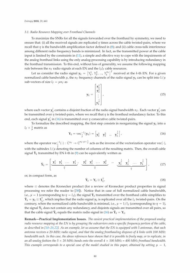
Entropy 2018, 20, 661

3.1. Radio Resource Mapping over Fronthaul Channels

To maximize the SNRs for all the signals forwarded over the fronthaul by symmetry, we need toensure that: (i) all the received signals are replicated η times across the cable twisted-pairs, where werecall that η is the bandwidth amplification factor defined in (8); and (ii) cable cross-talk interferenceamong different radio frequency bands is minimized. In fact, as the transmitted power at the cableinput is limited by the constraints in (11), a simple and effective way to cope with the impairments ofthe analog fronthaul links using the only analog-processing capability is by introducing redundancy inthe fronthaul transmission. To this end, without loss of generality, we assume the following mappingrule between the nF radio signals at each EN and the lSlF cable resources.

Let us consider the radio signal yk =[Y1

k , Y2k , ..., YnF

k]T received at the k-th EN. For a given

normalized cable bandwidth μ, the nF frequency channels of the radio signal yk can be split into 1/μ

sub-vectors of size lF = μnF as

yk =

⎡⎢⎢⎢⎢⎢⎣y1

ky2

k...

y1μ

k

⎤⎥⎥⎥⎥⎥⎦ , (15)

where each vector yjk contains a disjoint fraction of the radio signal bandwidth nF. Each vector y

jk can

be transmitted over η twisted-pairs, where we recall that η is the fronthaul redundancy factor. To thisend, each signal y

jk in (16) is transmitted over η consecutive cable twisted-pairs.

To formalize the described mapping, the first step consists in reorganizing the signal yk into alF × 1

μ matrix as

Yk = vec−11μ

(yk) =[y1

k y2k ... y

1μ

k

], (16)

where the operator vec−11μ

(·) : CnF → CnF ·μ× 1

μ acts as the inverse of the vectorization operator vec(·),with the subindex 1/μ denoting the number of columns of the resulting matrix. Then, the overall cablesignal Yk transmitted by EN k-th in (9) can be equivalently written as

Yk =

⎡⎣ y1k y1

k . . . y1k︸︷︷︸

η

, y2k y2

k . . . y2k︸︷︷︸

η

... y1μ

k y1μ

k . . . y1μ

k︸︷︷︸η

⎤⎦ , (17)

or, in compact form, asYk = Yk ⊗ 1T

η , (18)

where ⊗ denotes the Kronecker product (for a review of Kronecker product properties in signalprocessing we refer the reader to [38]). Notice that in case of full normalized cable bandwidth,i.e., μ = 1 (corresponding to η = lS), the signal Yk transmitted over the fronthaul cable simplifies toYk = yk ⊗ 1T

lS, which implies that the radio signal yk is replicated over all the lS twisted-pairs. On the

contrary, when the normalized cable bandwidth is minimal, i.e., μ = 1/lS (corresponding to η = 1),the signal Yk does not contain any redundancy, and disjoints signals are transmitted over all pairs, sothat the cable signal Yk equals the matrix radio signal in (16) as Yk = Yk.

Remark—Practical Implementation Issues. The easiest practical implementation of the proposed analogradio resource mapping at the EN is by grouping the subcarriers onto a specific frequency portion of the cable,as described in [18–20,22]. As an example, let us assume that the EN is equipped with 5 antennas, that eachantenna receives a 20-MHz radio signal, and that the analog fronthauling disposes of 4 links with 100 MHzbandwidth each. In this case, the above references have shown that it is possible to freely map, or to replicate, inan all-analog fashion the 5 × 20 MHz bands onto the overall 4 × 100 MHz = 400 MHz fronthaul bandwidth.This example corresponds to a special case of the model studied in this paper, obtained by setting μ = 1,

80

Entropy 2018, 20, 661

i.e., the whole radio signal bandwidth received at the ENs is mapped/replicated over the analog fronthauling.More generally, this paper posits the possibility to carry out the fronthaul mapping at a finer granularity, i.e., at asubcarrier level. In this case, filtering operations would in practice be mandatory in order to extract groupsof subcarriers. This operation can be implemented in principle still by analog filters, whose design is left asfuture works.

3.2. Signal Combining at the Fronthaul Output

As discussed, depending on the fronthaul bandwidth, a number η of noisy replicas of the radiosignals received at each EN are relayed to the BBU over η different twisted-pairs. Hence, in orderto maximize the SNRs for all signals, Maximum Ratio Combining (MRC) [39] is applied at the cableoutput as

Rk = RkG, (19)

where Rk ∈ ClF× 1

μ is the signal received at BBU from the k-th EN after the combiner and G ∈ RlS× 1

μ isthe MRC matrix. Under the assumptions here, MRC coincides with equal ratio combining and hencematrix G can be written as

G =1η

(I 1

μ⊗ 1η

). (20)

As an example, in the case of maximum redundancy, i.e., η = lS, the MRC matrix G = l−1S 1lS

combines the analog signals received over all pairs, since they carry the same information signal.On the contrary, in the case of minimal normalized bandwidth μ = 1/lS or η = 1, the matrix G equalsthe identity matrix as G = IlS , since no combining is possible.

The signal rk ∈ CnF received at the BBU from ENk across the nF subcarriers is thus obtained byvectorizing matrix Rk in (19) as

rk = vec(Rk). (21)

The relationship between the signal rk (21) obtained at the output of the combiner and the radioreceived signal yk in (15) is summarized by the block-scheme in Figure 6, and it is

rk = vec[((

vec−11μ

(yk)⊗ 1Tη

)Hc + Wk

)Gk

]. (22)

yk (·)⊗ 1Tηvec−1

1μ

(·) Hc Gk vec(·) rk

YkYk Rk

Wk

Rk

E Analog E processing Digital BB processingAnalog ronthauling BB

Figure 6. Relationship between the signal rk (21) obtained at the output of the combiner and the radioreceived signal yk in (15).

Finally, we collect the overall signal R ∈ CnF×M received at the BBU from all ENs across allfrequencies in the matrix

R = [r1, r2, ..., rM]. (23)

After some algebraic manipulations, it is possible to express Equation (23) in a more compactform, which is reported in the following Lemma 1.

81

Entropy 2018, 20, 661

Lemma 1. In the given C-RAN architecture with analog fronthaul links, for a given bandwidth amplificationfactor η ≥ 1, the signal R ∈ CnF×M received at the BBU from all ENs across all radio frequencies after MRCcan be written as

R =(

Hηc ⊗ IlF

)Y + W, (24)

whereH

ηc = γη1 1

μ1T

1μ+ (1− γ)I 1

μ(25)

is the equivalent fronthaul channel matrix; Y is the signal received at all ENs across all frequency radio channelsin (5); and W = [w1, w2, ..., wM] is the equivalent cable noise at the BBU after MRC, with the k-th columndistributed as wk ∼ CN

(0, 1

η InF

)for all k = 1, 2, ..., M.

Proof. see Appendix A.

To gain some insights, it is useful again to consider the two extreme cases of maximum redundancy,i.e., η = lS, and no redundancy, i.e., η = 1. In the former case, the equivalent channel (25) equalsthe scalar H

ηc = 1 + γ(lS − 1). This demonstrates the effect of transmitting a replica of the whole

radio signal over all pairs. In fact, the useful signal is received at the BBU not only through thedirect path, which has unit gain, but also from the remaining lS − 1 interfering paths, each with gainγ, which constructively contribute to the overall SNR after the combiner. More precisely, it can beobserved that, in case of full redundancy, the SNR of the radio signal Y at the BBU is increased bythe analog fronthaul links by a factor of (1 + γ(lS − 1))2/(1/η) = lS(1 + γ(lS − 1))2. As a result,in this case, for a coupling factor γ > 0, the SNR at the BBU increases with the cube of the numberof fronthaul links lS. In contrast, for μ = 1/lS, the equivalent fronthaul channel reflects the factthat signals forwarded over the different pairs interfere with each other, and is equal to H

ηc = Hc.

The beneficial effect of redundantly transmitting radio signals over different pairs is reflected also in thepower of the noise after the combiner, which is reduced proportionally to the bandwidth amplificationfactor η.

3.3. Fronthaul Power Constraints

To enforce the cable power constraints in (11), it is necessary to scale the radio signal Y in (24) bya factor of λ prior to the transmission over the fronthaul. This is given as

λ =

√Pc

δPB(1 + 2α2) + 1, (26)

where δ is equal to δ =(

1− L−1U

)−1for OMA, accounting for the fact that only LU − 1 minislots are

devoted to the eMBB UE, while it equals δ = 1 for NOMA, since the eMBB transmission spreads overall LU minislots. To simplify the notation, in the following we will account for the gain λ by scalingthe noise over the cable after MRC in Equation (25) accordingly as

wk(t) ∼ CN(

0,1

ηλ2 I

). (27)

4. Orthogonal Multiple Access (OMA)

As described in Section 2.1, under OMA over the radio channel, one minislot every LU isexclusively allocated to URLLC UEs, while eMBB UEs transmit over the remaining minislots. In thisway, URLLC UEs never interfere with eMBB transmissions. If more than one URLLC packet isgenerated at a user between two URLLC transmission opportunities, only one of such packets(randomly selected) is transmitted, while the others are discarded, causing a blockage error. Due tothe latency constraints, URLLC signals are digitized and decoded locally at the ENs, while the

82

Entropy 2018, 20, 661

eMB signals are first mapped over the fronthaul lines, and then analogically forwarded to the BBU,as mathematically summarized in Figure 7. In this section, we derive the expressions for the eMBBand URLLC rates under OMA for a given URLLC access latency LU and, in the case of URLLC, for afixed URLLC target error probability εU .

yk( )Yk( )

YM ( )

Figure 7. Block diagram of the operation of the ENs and BBU for Orthogonal Multiple Access (OMA).A/A stands for Analog-to-Analog.

4.1. URLLC Rate

To evaluate the per-UE URLLC rate under OMA and for a given URLLC target error probabilityεU , we follow the approach in [32], which is reviewed here. URLLC packets are generally short dueto the strict latency constraints, and the maximum achievable rate can be computed by leveragingresults from finite blocklength information theory. To this end, fix a given blocklength nF and URLLCerror decoding probability εD

U . Notice that this probability is different from the general URLLC targeterror probability εU , as detailed later in this section. According to [40], the URLLC rate can be wellapproximated by

RU = log2(1 + β2PU)−√

VnF

Q−1(εDU), (28)

where

V =β2PU

1 + β2PU(29)

is the channel dispersion and Q−1(·) is the inverse Q-function (see Section 1.5).The error probability for URLLC packets is the sum of two contributions. The first represents the

probability that an URLLC packet is discarded due to blockage, given that only one URLLC packet canbe transmitted within the required LU worst-case latency; while the second is the probability that thepacket is transmitted but not successfully decoded. Accordingly, the overall error probability can becomputed as

Pr[EU ] =LU−1

∑n

p(n)n

n + 1+

LU−1

∑n

p(n)1

n + 1εD

U , (30)

where p(n) = Pr[NU(LU) = n] is the distribution of the binomial random variable NU(LU) ∼Bin(LU − 1, q) representing the number of additional packets generated by the URLLC UE during theremaining minislots between two transmission opportunities. The decoding error probability εD

U in(28) can be obtained from the URLLC reliability constraint in (13), i.e., Pr[EU ] = εU .

4.2. eMBB Rate

The eMBB signals received at the ENs are forwarded over the analog fronthaul to the BBU,where centralized digital signal processing and decoding are performed. In the case of OMA, the eMBBsignal is free from URLLC interference, hence signal Y received by all ENs over all radio channels in(5) can be written as

Y = XH + Z. (31)

83

Entropy 2018, 20, 661

By substituting (31) in (24), it is possible to compute the expression for the eMBB per-UE rate underOMA, as shown in Lemma 2. Notice that, unlike the case of URLLC packets, the nFnT blocklength ofeMBB packets allows for the use of standard asymptotic Shannon theory in the computation of eMBBinformation rate.

Lemma 2. In the given C-RAN architecture with analog fronthaul links, for a given bandwidth amplificationfactor η ≥ 1, the eMBB user rate under OMA is given as

RB = μ1− L−1

UM

log(

det(

I + PBR−1zeq HeqHT

eq

)), (32)

where PB = PB

(1− L−1

U

)−1 is the transmission power of eMBB users under OMA, Heq = H⊗H

ηc is the

overall channel matrix comprising both the radio channel H and the equivalent cable channel Hηc defined in

Lemma 1, and Rzeq = IM ⊗Hηc H

ηc +

1λ2η

I Mμ

is the overall wireless plus cable noise at the BBU.

Proof. see Appendix B.

As a first observation, the eMBB rate (32) linearly scales with the normalized bandwidth μ.This shows that a potential performance degradation in terms of spectral efficiency can be incurred inthe presence of fronthaul channels with bandwidth limitations, i.e., with μ < 1. This loss is pronouncedin the presence of significant inter-channel interference, i.e., for large γ. In fact, a large γ increasesthe effective noise power as per expression of matrix Rzeq . It is also important to point out that in theconsidered C-RAN system based on the analog relaying of radio signals, the overall noise at the BBUis no longer white as it accounts both for the white cable noise and the wireless noise, where the latteris correlated when there is some bandwidth redundancy, i.e., when μ ≥ 1/lS or η > 1.

5. Non-Orthogonal Multiple Access (NOMA)

In NOMA, URLLC UEs transmit in the same minislot where the packet is generated, and hencethe access latency is minimal and limited to LU = 1 minislot. However, the URLLC signals mutuallyinterfere with the eMBB transmission, which spans the whole time-frequency resource plane. Due toURLLC latency constraints, the eMBB signals necessarily need to be treated as noise while decodingURLLC packets at the ENs. On the contrary, several strategies can be adapted in order to deal withthe interfering URLLC signal. Beside puncturing, considered for 5G NR standardization [33,34],this work considers two other techniques, namely Treating Interference as Noise (TIN) and SuccessiveInterference Cancellation (SIC), as detailed in the rest of this section.

5.1. URLLC Rate under NOMA

The URLLC per-UE rate for NOMA can be computed by leveraging results from finite blocklengthinformation theory similarly to the OMA case, but accounting for the additional eMBB interference [41].The URLLC per-UE rate under NOMA is thus well approximated by [32]

RU = log2(1 + SU)−√

VnF

Q−1(εDU),

where

SU =β2PU

1 + (1 + 2α2)PB(33)

is the Signal-to-Interference-plus-Noise Ratio (SINR) for the URLLC UE, and the channel dispersion Vis given as

V =SU

1 + SU. (34)

84

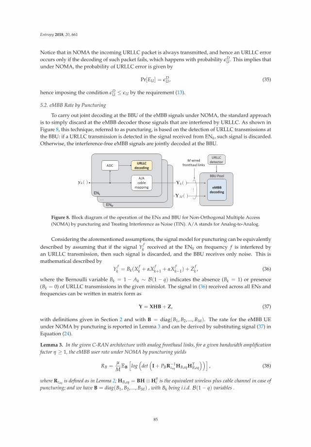
Entropy 2018, 20, 661

Notice that in NOMA the incoming URLLC packet is always transmitted, and hence an URLLC erroroccurs only if the decoding of such packet fails, which happens with probability εD

U . This implies thatunder NOMA, the probability of URLLC error is given by

Pr[EU ] = εDU , (35)

hence imposing the condition εDU ≤ εU by the requirement (13).

5.2. eMBB Rate by Puncturing

To carry out joint decoding at the BBU of the eMBB signals under NOMA, the standard approachis to simply discard at the eMBB decoder those signals that are interfered by URLLC. As shown inFigure 8, this technique, referred to as puncturing, is based on the detection of URLLC transmissions atthe BBU: if a URLLC transmission is detected in the signal received from ENk, such signal is discarded.Otherwise, the interference-free eMBB signals are jointly decoded at the BBU.

yk( ) Yk( )

YM ( )

Figure 8. Block diagram of the operation of the ENs and BBU for Non-Orthogonal Multiple Access(NOMA) by puncturing and Treating Interference as Noise (TIN). A/A stands for Analog-to-Analog.

Considering the aforementioned assumptions, the signal model for puncturing can be equivalentlydescribed by assuming that if the signal Y f

k received at the ENk on frequency f is interfered byan URLLC transmission, then such signal is discarded, and the BBU receives only noise. This ismathematical described by

Y fk = Bk(X f

k + αX fk+1 + αX f

k−1) + Z fk , (36)

where the Bernoulli variable Bk = 1− Ak ∼ B(1− q) indicates the absence (Bk = 1) or presence(Bk = 0) of URLLC transmissions in the given minislot. The signal in (36) received across all ENs andfrequencies can be written in matrix form as

Y = XHB + Z, (37)

with definitions given in Section 2 and with B = diag(B1, B2, ..., BM). The rate for the eMBB UEunder NOMA by puncturing is reported in Lemma 3 and can be derived by substituting signal (37) inEquation (24).

Lemma 3. In the given C-RAN architecture with analog fronthaul links, for a given bandwidth amplificationfactor η ≥ 1, the eMBB user rate under NOMA by puncturing yields

RB =μ

MEB

[log

(det

(I + PBR−1

zeq HB,eqHTB,eq

))], (38)

where Rzeq is defined as in Lemma 2; HB,eq = BH⊗Hηc is the equivalent wireless plus cable channel in case of

puncturing; and we have B = diag(B1, B2, ..., BM) , with Bk being i.i.d. B(1− q) variables .

85

Entropy 2018, 20, 661

Proof. Lemma 3 can be proved by following similar steps as for the proof of Lemma 2 with two minordifferences: (i) the radio channel matrix H is right multiplied by the random matrix B and (ii) thecapacity is computed by averaging over the distribution of B.

Differently from the rate (32) achieved by OMA, under NOMA, the eMBB transmission spreadsover all the minislots, so that there is no scaling factor 1− L−1

U in front of the rate expression (38)to account for the resulting loss in spectral efficiency. In case of NOMA by puncturing, the noisecovariance is exactly as the one in the eMBB OMA rate in Equation (32), since the eMBB signal, if notdiscarded at the BBU, is guaranteed to be URLLC interference-free. The overall rate is computed byaveraging over all the possible realizations of the random matrix B, which left-multiplies the radiochannel matrix H and accounts for the probability that the entire signal is discarded due to an incomingURLLC packet.

In the case of C-RAN with digital limited-capacity fronthaul links, as discussed in [32], it isadvantageous to carry out the operation of detecting and, eventually, discarding the eMBB signal at theENs. In fact, with a digital fronthaul, only the undiscarded minislots can be quantized, hence devotingthe limited fronthaul resources to increase the resolution of interference-free eMBB samples [32].The same does not apply to the analog fronthaul considered here, as signals are directly relayed to theBBU without any digitization.

5.3. eMBB Rate by Treating Interference as Noise

In the case of analog fronthaul, an enhanced strategy to jointly decode the eMBB signals underNOMA at the BBU is to treat the URLLC interfering transmissions as noise at the eMBB decoder,instead of discarding the corresponding minislot as in puncturing. The block diagram is the same asfor puncturing and shown in Figure 8. Accordingly, based on the signals received over the fronthaullinks, the BBU first detects the presence of URLLC transmission so as to properly select the decodingmetric. Then, based on this knowledge, joint decoding is performed by TIN.

Lemma 4. In the given C-RAN architecture with analog fronthaul links, for a given bandwidth amplificationfactor η ≥ 1, the eMBB user rate under NOMA by treating URLLC interference as noise yields

RB =μ

MEA

[log

(det

(I + PBR−1

A,zeqHeqHT

eq

))], (39)

where RA,zeq = Rzeq + β2PU

(A⊗H

ηc H

ηc

)is the overall noise plus URLLC interference at the BBU; matrix A

is as in (5); and matrices Rzeq and Heq are the same as in Lemma 2.

Proof. see Appendix C.

Differently from the two previous cases, in the case of NOMA under TIN, the noise covariancematrix RA,zeq needs to account also for the interfering URLLC transmissions, whose packet arrivalprobability is described by matrix A. The achievable rate is then computed by taking the average overthe random matrix A. This average reflects the long-blocklength transmissions of the eMBB users.

5.4. eMBB Rate by Successive Interference Cancellation

Finally, a more complex receiver architecture can be considered at the BBU, whereby interference iscancelled out from the useful signal. This technique, referred to as Successive Interference Cancellation(SIC), is based on the idea that, if an URLLC signal is successfully decoded at the ENk, it can becancelled from the overall received signal yk prior to the relaying over the cable, so that an ideallyinterference-free eMBB signal is forwarded to the BBU. We also assume that, if the URLLC signal is notsuccessfully decoded, signal yk is discarded.

As a practical note, SIC must be performed in the analog domain, thus complicating the systemdesign. Practical complications are not considered in the analysis here. As shown in Figure 9, if the

86

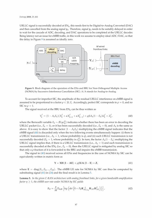
Entropy 2018, 20, 661

URLLC signal is successfully decoded at ENk, this needs first to be Digital-to-Analog Converted (DAC)and then cancelled from the analog signal yk. Therefore, signal yk needs to be suitably delayed in orderto wait for the cascade of ADC, decoding, and DAC operations to be completed at the URLLC decoder.Being latency not an issue for eMBB traffic, in this work we assume to employ ideal ADC/DAC, so thatthe delay in Figure 9 is assumed as ideally zero.

yk( )Yk( )

YM ( )

Figure 9. Block diagram of the operation of the ENs and BBU for Non-Orthogonal Multiple Access(NOMA) by Successive Interference Cancellation (SIC). A/A stands for Analog-to-Analog.

To account for imperfect SIC, the amplitude of the residual URLLC interference on eMBB signal isassumed to be proportional to a factor ρ ∈ [0, 1]. Accordingly, perfect SIC corresponds to ρ = 0, and noSIC to ρ = 1.

The signal received at the BBU from ENk can be thus written as

Y fk = (1− AkEk)(X f

k + αX fk+1 + αX f

k−1) + ρβAk(1− Ek)Ufk + Z f

k , (40)

where the Bernoulli variable Ek ∼ B(qεDU) indicates whether there has been an error in decoding the

URLLC packet (i.e., Ek = 1), or it has been successfully decoded (i.e., Ek = 0), and Ak is the same asabove. It is easy to show that the factor (1− AkEk) multiplying the eMBB signal indicates that theeMBB signal (40) is discarded only when the two following events simultaneously happen: (i) there isa URLLC transmission (i.e., Ak = 1, whose probability is q), and (ii) such URLLC transmission is notsuccessfully decoded (Ek = 1, whose probability is εD

U ). In turn, the factor Ak(1− Ek) multiplying theURLLC signal implies that, if there is a URLLC transmission (i.e., Ak = 1) and such transmission issuccessfully decoded at the ENk (i.e., Ek = 0), then the URLLC signal is mitigated by analog SIC sothat only a ρ-fraction of it is forwarded to the BBU and impairs the eMBB transmission.

The signal in (40) received across all ENs and frequencies in the case of NOMA by SIC can beequivalently written in matrix form as

Y = XH (I−AE) + ρβUA (I− E) + Z, (41)

where E = diag(E1, E2, ..., EM). The eMBB UE rate for NOMA by SIC can thus be computed bysubstituting signal (41) in (24) and the final result is in Lemma 5.

Lemma 5. In the given C-RAN architecture with analog fronthaul links, for a given bandwidth amplificationfactor η ≥ 1, the eMBB user rate under NOMA by SIC yields

RB =μ

MEA,E

[log

(det

(I + PBR−1

AE,zeqHAEHT

AE

))], (42)

87

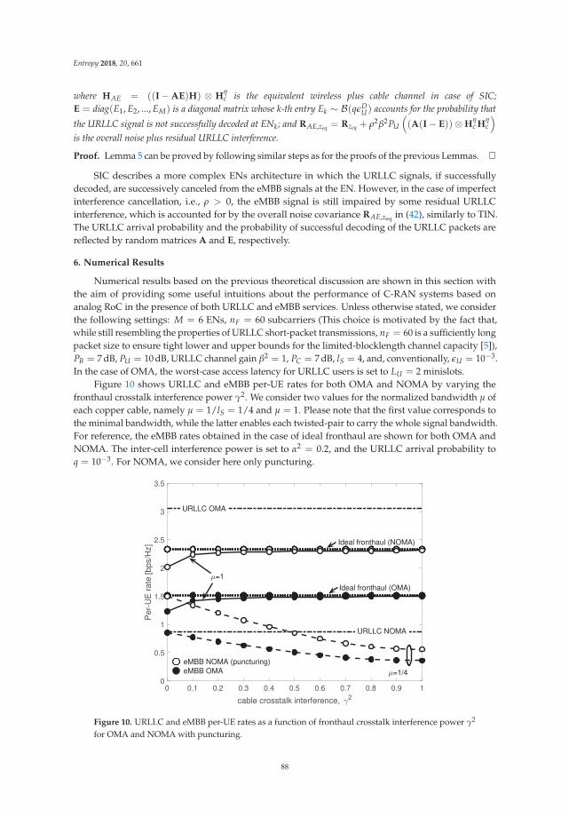
Entropy 2018, 20, 661

where HAE = ((I−AE)H) ⊗ Hηc is the equivalent wireless plus cable channel in case of SIC;

E = diag(E1, E2, ..., EM) is a diagonal matrix whose k-th entry Ek ∼ B(qεDU) accounts for the probability that

the URLLC signal is not successfully decoded at ENk; and RAE,zeq = Rzeq + ρ2β2PU

((A(I− E))⊗H

ηc H

ηc

)is the overall noise plus residual URLLC interference.

Proof. Lemma 5 can be proved by following similar steps as for the proofs of the previous Lemmas.

SIC describes a more complex ENs architecture in which the URLLC signals, if successfullydecoded, are successively canceled from the eMBB signals at the EN. However, in the case of imperfectinterference cancellation, i.e., ρ > 0, the eMBB signal is still impaired by some residual URLLCinterference, which is accounted for by the overall noise covariance RAE,zeq in (42), similarly to TIN.The URLLC arrival probability and the probability of successful decoding of the URLLC packets arereflected by random matrices A and E, respectively.

6. Numerical Results

Numerical results based on the previous theoretical discussion are shown in this section withthe aim of providing some useful intuitions about the performance of C-RAN systems based onanalog RoC in the presence of both URLLC and eMBB services. Unless otherwise stated, we considerthe following settings: M = 6 ENs, nF = 60 subcarriers (This choice is motivated by the fact that,while still resembling the properties of URLLC short-packet transmissions, nF = 60 is a sufficiently longpacket size to ensure tight lower and upper bounds for the limited-blocklength channel capacity [5]),PB = 7 dB, PU = 10 dB, URLLC channel gain β2 = 1, PC = 7 dB, lS = 4, and, conventionally, εU = 10−3.In the case of OMA, the worst-case access latency for URLLC users is set to LU = 2 minislots.

Figure 10 shows URLLC and eMBB per-UE rates for both OMA and NOMA by varying thefronthaul crosstalk interference power γ2. We consider two values for the normalized bandwidth μ ofeach copper cable, namely μ = 1/lS = 1/4 and μ = 1. Please note that the first value corresponds tothe minimal bandwidth, while the latter enables each twisted-pair to carry the whole signal bandwidth.For reference, the eMBB rates obtained in the case of ideal fronthaul are shown for both OMA andNOMA. The inter-cell interference power is set to α2 = 0.2, and the URLLC arrival probability toq = 10−3. For NOMA, we consider here only puncturing.

0 0.1 0.2 0.3 0.4 0.5 0.6 0.7 0.8 0.9 1

cable crosstalk interference, 2

0

0.5

1

1.5

2

2.5

3

3.5

Per

-UE

rat

e [b

ps/H

z]

=1/4

Ideal fronthaul (NOMA)

Ideal fronthaul (OMA)

=1

eMBB NOMA (puncturing)eMBB OMA

URLLC OMA

URLLC NOMA

Figure 10. URLLC and eMBB per-UE rates as a function of fronthaul crosstalk interference power γ2

for OMA and NOMA with puncturing.

88

Entropy 2018, 20, 661

The URLLC rates do not depend on cable crosstalk interference γ2, since URLLC packets aredecoded at the EN and thus never forwarded to the BBU over the fronthaul. Furthermore, with NOMA,the access latency of URLLC is minimum, i.e., LU = 1, while for OMA it equals LU = 2. However,Figure 10 shows that the price to pay for this reduced latency is in terms of transmission rate, which islower than in the OMA case. On the contrary, in the case of eMBB, NOMA allows for a communicationat higher rates than those achieved by OMA, thanks to the larger available bandwidth when q issmall enough.

On the subject of eMBB rates, it is interesting to discuss the interplay between the normalizedcable bandwidth μ and crosstalk power γ2. For μ = 1, the same signal is transmitted over all the lS = 4fronthaul twisted-pairs, and hence the four spatial paths sum coherently over the cable, thus turningcrosstalk into a benefit. Hence, the eMBB rates under both OMA and NOMA increase with γ2 andultimately converge to those achieved over the ideal fronthaul (In this work, we consider the sameinterference gain γ for all fronthaul links. In practice, the performance boost shown in Figure 10for increasing γ and for μ = 1 would still be present, albeit to a different extent dependent on thechannel realization, even if considering complex channel gain. However, this would require the use ofmore complex precoding techniques, such as Tomlinson-Harashima [37], which require an estimateof the fronthaul channel. Since for wired fronthauling the channel is nearly static and time-invariant,channel state information can be easily obtained [42]). For μ = 1/4 instead, disjoint portions of theradio signal are transmitted over different interfering twisted-pairs, and the performance progressivelydecrease with γ2. The leftmost portion of Figure 10 suggests that for mild cable interference, evenwhen the cable bandwidth is small (i.e., μ = 1/4), it is still possible to provide communication withacceptable performance degradation, i.e., with a ≈ 1 bps/Hz loss from the ideal fronthaul case forNOMA, and an even smaller loss for OMA. However, when the cable crosstalk increases, the ratedegradation is severe, and fair performance are achieved only if the cable bandwidth is large enoughto accommodate the redundant transmission of radio signals over all pairs, i.e., μ = 1.

Figure 11 shows URLLC and eMBB rates as a function of the URLLC packet arrival probability q.eMBB rates under OMA are compared with those achieved by NOMA under puncturing, TIN and SIC.We consider here full cable bandwidth availability μ = 1 and γ2 = 1, so that, as in Figure 10, the ratesachieved for both OMA and NOMA for low q (say, q < 10−2) coincide with those achieved over theideal fronthaul. Inter-cell interference is set to α2 = 0.2. As noted in [32], under OMA, when q increases,the probability of an URLLC packet to be dropped due to blockage becomes very high, preventingURLLC transmission from meeting the strict reliability constraints, and results in a vanishing URLLCrate. This is unlike in NOMA, whereby the URLLC rate is not affected by q, and the access latency isminimal, i.e., LU = 1. For eMBB under NOMA, TIN always outperforms puncturing. This is becauseTIN does not discard any received minislot, thus contributing to the overall eMBB rate. The result isin contrast with the conventional digital capacity-constrained fronthaul considered in [32]. In fact,in the latter, for sufficient low q, it is preferable not to waste fronthaul capacity resources by quantizingsamples received in minislots affected by URLLC interference in order to increase the resolution of theinterference-free samples. Additional gains are achieved by SIC, which takes advantages of the highreliability, and thus high probability to be cancelled, of the URLLC signal at the EN.

Implementing SIC in a fully analog fashion is practically not trivial, and there is generally someresidual URLLC interference. The effect of residual interference on the achievable eMBB rate isinvestigated in Figure 12 for q = 0.3, α2 = 0.4, γ2 = 0.5, μ = 1 and for different power of URLLCUE PU . Once again, in case of perfect interference cancellation, i.e., ρ = 0, SIC approaches the idealfronthaul performance, while for more severe values of the residual interference power ρ, the eMBBperformance progressively decreases. Nevertheless, even in the worst-case SIC scenario, i.e., ρ = 1,the achievable rates are never worse than those achieved by TIN irrespective of the value of PU . This isonce again due to the high reliability of URLLC transmission. It is in fact easy to prove that for ρ = 1and low values of εD

U , the SIC eMBB rate in (42) converges to the one of TIN in (39).

89

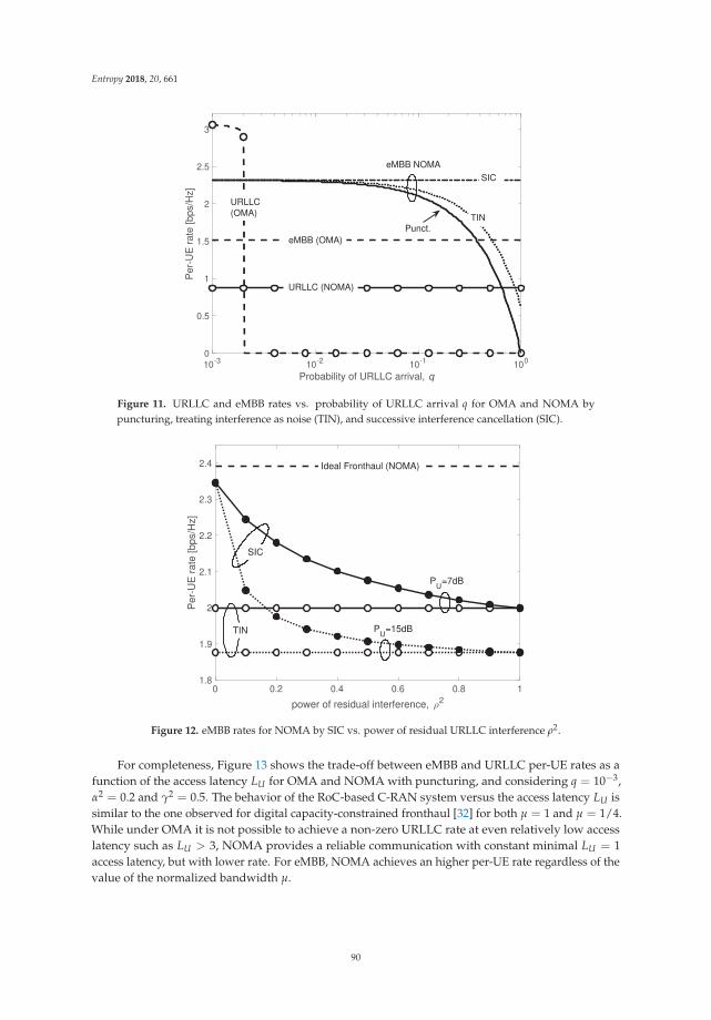
Entropy 2018, 20, 661

10-3 10-2 10-1 100

Probability of URLLC arrival, q

0

0.5

1

1.5

2

2.5

3

Per

-UE

rat

e [b

ps/H

z]

URLLC (NOMA)

eMBB (OMA)

SIC

Punct.

eMBB NOMA

URLLC(OMA) TIN

Figure 11. URLLC and eMBB rates vs. probability of URLLC arrival q for OMA and NOMA bypuncturing, treating interference as noise (TIN), and successive interference cancellation (SIC).

0 0.2 0.4 0.6 0.8 1

power of residual interference, 2

1.8

1.9

2

2.1

2.2

2.3

2.4

Per

-UE

rat

e [b

ps/H

z]

PU

=15dB

PU

=7dB

Ideal Fronthaul (NOMA)

TIN

SIC

Figure 12. eMBB rates for NOMA by SIC vs. power of residual URLLC interference ρ2.

For completeness, Figure 13 shows the trade-off between eMBB and URLLC per-UE rates as afunction of the access latency LU for OMA and NOMA with puncturing, and considering q = 10−3,α2 = 0.2 and γ2 = 0.5. The behavior of the RoC-based C-RAN system versus the access latency LU issimilar to the one observed for digital capacity-constrained fronthaul [32] for both μ = 1 and μ = 1/4.While under OMA it is not possible to achieve a non-zero URLLC rate at even relatively low accesslatency such as LU > 3, NOMA provides a reliable communication with constant minimal LU = 1access latency, but with lower rate. For eMBB, NOMA achieves an higher per-UE rate regardless of thevalue of the normalized bandwidth μ.

90

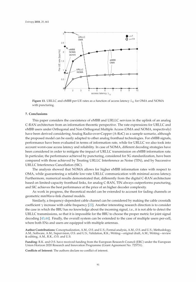
Entropy 2018, 20, 661

1 2 3 4 5 6 7 8 9 10access latency, LU

0

0.5

1

1.5

2

2.5

3

Per

-UE

rat

e [b

ps/H

z]

=1=1/4

eMBBOMA

URLLC NOMA

eMBBNOMA(punct)

URLLCOMA

Figure 13. URLLC and eMBB per-UE rates as a function of access latency LU for OMA and NOMAwith puncturing.

7. Conclusions

This paper considers the coexistence of eMBB and URLLC services in the uplink of an analogC-RAN architecture from an information theoretic perspective. The rate expressions for URLLC andeMBB users under Orthogonal and Non-Orthogonal Multiple Access (OMA and NOMA, respectively)have been derived considering Analog Radio-over-Copper (A-RoC) as a sample scenario, althoughthe proposed model can be easily adapted to other analog fronthaul technologies. For eMBB signals,performance have been evaluated in terms of information rate, while for URLLC we also took intoaccount worst-case access latency and reliability. In case of NOMA, different decoding strategies havebeen considered in order to mitigate the impact of URLLC transmission on eMBB information rate.In particular, the performance achieved by puncturing, considered for 5G standardization, have beencompared with those achieved by Treating URLLC Interference as Noise (TIN), and by SuccessiveURLLC Interference Cancellation (SIC).

The analysis showed that NOMA allows for higher eMBB information rates with respect toOMA, while guaranteeing a reliable low-rate URLLC communication with minimal access latency.Furthermore, numerical results demonstrated that, differently from the digital C-RAN architecturebased on limited-capacity fronthaul links, for analog C-RAN, TIN always outperforms puncturing,and SIC achieves the best performance at the price of an higher decoder complexity.

As work in progress, the theoretical model can be extended to account for fading channels orgeometric mmWave-link channel models.

Similarly, a frequency-dependent cable channel can be considered by making the cable crosstalkcoefficient γ increase with cable frequency [22]. Another interesting research direction is to considerthe case in which the BBU has no knowledge about the incoming signal, i.e., it is not able to detect theURLLC transmissions, so that it is impossible for the BBU to choose the proper metric for joint signaldecoding [43,44]. Finally, the overall system can be extended to the case of multiple users per-cell,where both ENs and users are equipped with multiple antennas.

Author Contributions: Conceptualization, A.M., O.S. and U.S.; Formal analysis, A.M., O.S. and U.S.; Methodology,A.M.; Software, A.M.; Supervision, O.S. and U.S.; Validation, R.K.; Writing—original draft, A.M.; Writing—review& editing, A.M., R.K., O.S. and U.S.

Funding: R.K. and O.S. have received funding from the European Research Council (ERC) under the EuropeanUnion Horizon 2020 Research and Innovation Programme (Grant Agreement No. 725731).


91

Entropy 2018, 20, 661

Appendix A. Proof of Lemma 1

The proof of Lemma 1 is structured in two main steps detailed in the following: (i) MRC at thecable output, (ii) cable signal vectorization.

Appendix A.1. Maximum Ratio Combining at the Cable Output

The signal Rk ∈ ClF× 1

μ after the MRC at the cable output is

Rk = RkG

=(YkHc + Wk

)G,

(A1)

where the definitions of Rk, G, Yk and Hc follow from and (10), (20), (18) and (6), respectively. Thus,Equation (A1) can be rewritten as

Rk =(

Yk ⊗ 1Tη

) (γ1lS 1T

lS + (1− γ)IlS

)G + WkG

= γ(

Yk ⊗ 1Tη

)1lS 1T

lS G︸︷︷︸R′k

+ (1− γ)(

Yk ⊗ 1Tη

)G︸︷︷︸

R′′k

+ WkG︸︷︷︸Wk

, (A2)

where Wk = WkG is the noise post MRC. The first term in (A2) can be rewritten as

R′k =

γ

η

(Yk ⊗ 1T

η

)1lS 1T

lS

(I 1

μ⊗ 1η

)(a)= γ

(Yk ⊗ 1T

η

)1lS 1T

1μ

(b)= γηYk1 1

μ1T

1μ

,

(A3)

where(a)= comes from the fact that 1T

lS

(I 1

μ⊗ 1η

)=

(1T

1μ

⊗ 1Tη

)(I 1

μ⊗ 1η

)= η1T

1μ

due to the

mixed-product property of Kronecker product operator (A⊗ B) (C⊗D) = AC ⊗ BD (see [38],

Chapter 2), and, similarly,(b)= is obtained by

(Yk ⊗ 1T

η

)1lS 1T

1μ

=(

Yk ⊗ 1Tη

)(1 1

μ1T

1μ

⊗ 1η

)= ηYk1 1

μ1T

1μ

.

Using similar arguments, the second term in (A2) simplifies to

R′′k =

1− γ

η

(Yk ⊗ 1T

η

)(I 1

μ⊗ 1η

)= (1− γ)Yk.

(A4)

Finally, substituting (A3) and (A4) in (A2) we obtain

Rk = YkHηc + Wk, (A5)

whereH

ηc = γη1 1

μ1T

1μ+ (1− γ)I 1

μ(A6)

is the equivalent cable channel matrix accounting for the bandwidth amplification factor over cable η,and Yk is the radio signal reorganized in matrix form as in (16).

92

Entropy 2018, 20, 661

Appendix A.2. Cable Signal Vectorization

The vector signal rk ∈ CnF×1 received at the BBU from the k-th EN over all the radio frequencychannels can be obtained by vectorizing matrix Rk in (A5) as

rk = vec(YkHηc + Wk)

=(

Hηc ⊗ IlF

)vec(Yk) + vec(Wk)

=(

Hηc ⊗ IlF

)yk + wk,

(A7)

where yk is the radio signal received at EN k-th. The overall cable noise vector wk can be rewritten as

wk = vec(Wk)

= vec(WkG)

=(

GT ⊗ IlF

)vec(Wk)

=1η

(I 1

μ⊗ 1T

η ⊗ IlF

)wk.

(A8)

It is important to notice that since the cable noise Wk is white Gaussian and uncorrelated overcable pairs (see (10)), wk = vec(Wk) is also white Gaussian distributed as wk ∼ CN (0, IlSlF ). Hence,the covariance Rw of the overall cable noise vector wk yields

Rw = E

[wkwH

k

]=

1η2

(I 1

μ⊗ 1T

η ⊗ IlF

)(I 1

μ⊗ 1T

η ⊗ IlF

)T

(a)=

1η

(I 1

μ⊗ IlF

)=

1η

InF ,

(A9)

where the equality (a) comes again from the mixed-product property of Kronecker product.Equation (A9) shows that the MRC allows to take advantages from the signal redundancy overthe cable, which results in a reduction of the cable noise power by a factor of η.

The proof is completed by gathering the signals rk (A7) received at the BBU from all ENs as

R = [r1, r2, ..., rM]

=(

Hηc ⊗ IlF

)[y1, y2, ..., yM] + [w1, w2, ..., wM]

=(

Hηc ⊗ IlF

)Y + W,

(A10)

where Y is the signal received by all ENs over all radio channels in (5).

Appendix B. Proof of Lemma 2

By substituting signal Y in (31) received by all ENs over all radio channels in case of OMA inEquation (24), we obtain

R =(

Hηc ⊗ IlF

)XH +

(H

ηc ⊗ IlF

)Z + W. (A11)

93

Entropy 2018, 20, 661

To compute the per-UE eMBB rate, a further vectorization is needed, leading to

r = vec(R)

= vec((

Hηc ⊗ IlF

)XH

)+ vec

((H

ηc ⊗ IlF

)Z)+ vec(W)

=(

HT ⊗Hηc ⊗ IlF

)x +

(IM ⊗H

ηc ⊗ IlF

)z + w

= Heqx + zeq,

(A12)

where Heq = HT ⊗ Hηc ⊗ IlF is the overall equivalent channel comprising both cable and radio

channels over all ENs, and zeq =(

IM ⊗Hηc ⊗ IlF

)z + w is the overall noise vector comprising both

the vectorized radio noise z = vec(Z) ∼ CN (0, InF M) and the vectorized cable noise w = vec(W) ∼CN (0, 1

λ2ηInF M), where we recall that the scaling λ is due to the cable power constraints. Hence,

the covariance of the equivalent noise zeq yields

Rzeq = E

[zeqzH

eq

]=

(IM ⊗H

ηc ⊗ IlF

) (IM ⊗H

ηc ⊗ IlF

)H+

1λ2η

InF M

= IM ⊗Hηc H

ηc ⊗ IlF +

1λ2η

InF M.

(A13)

The eMBB per-UE rate under OMA is computed by

RB =(1− L−1

U )

nF MI(r, x)

=(1− L−1

U )

nF Mlog

(det

(I + PBR−1

zeqHeqHT

eq

)),

(A14)

where HeqHTeq = HH⊗H

ηc H

ηc ⊗ IlF . Finally, using the determinant property of the Kronecker product

|A⊗ B| = |A|m |B|n , Equation (A14) simplifies to

RB =lF(1− L−1

U )

nF Mlog

(det

(I + PBR−1

zeqHeqHT

eq

))= μ

1− L−1U

Mlog

(det

(I + PBR−1

zeq HeqHTeq

)),

(A15)

where Heq = H⊗Hηc and Rzeq = IM ⊗H

ηc H

ηc +

1λ2η

I Mμ

, thus concluding the proof.

Appendix C. Proof of Lemma 3

By substituting the signal (5) received at the k-th EN under NOMA into (A10) and by followingsimilar steps as for the proof of Lemma 2, the overall vector signal received at the BBU comprisingboth cable and radio channels over all ENs under NOMA by treating interference as noise yields

r = Heqx + βAequ + zeq, (A16)

where the definitions of Heq and zeq are the same as in (A12), Aeq = A⊗Hηc ⊗ IlF accounts for the

relay of URLLC signal over the cable, and u is the vectorization of the URLLC signal matrix U in (5).Similarly to the proof of Lemma 2, the eMBB per-UE rate under NOMA by treating URLLC interferenceas noise can be computed by

94

Entropy 2018, 20, 661

RB =1

nF MI (r, x |A )

=μ

MEA

[log

(det

(I + PBR−1

A,zeqHeqHT

eq

))] (A17)

where the average is taken over all the possible values of matrix A, PB is the power of the eMBB userunder NOMA and Heq is defined as in (A15). Finally, the covariance RA,zeq of the noise plus URLLCinterference yields

RA,zeq = β2PU AeqATeq + Rzeq ,

where Aeq = A ⊗ Hηc and Rzeq is the same as in (A15). The proof is completed by noticing that

AeqATeq = (A⊗H

ηc )(A⊗H

ηc )

H = A⊗Hηc H

ηc , since matrix A is idempotent and H

ηc symmetric.

References

1. Shafi, M.; Molisch, A.F.; Smith, P.J.; Haustein, T.; Zhu, P.; Silva, P.D.; Tufvesson, F.; Benjebbour, A.;Wunder, G. 5G: A tutorial overview of standards, trials, challenges, deployment, and practice. IEEE J. Sel.Areas Commun. 2017, 35, 1201–1221. [CrossRef]

2. 5G PPP Architecture Working Group. View on 5G Architecture. 2016. Available online:https://5g-ppp.eu/wp-content/uploads/2014/02/5G-PPP-5G-Architecture-WP-July-2016.pdf (accessedon 31 August 2018).

3. Minimum Requirements Related to Technical Performance for IMT-2020 Radio Interface(s). 2017.Available online: https://www.itu.int/dms_pub/itu-r/opb/rep/R-REP-M.2410-2017-PDF-E.pdf (accessedon 31 August 2018).

4. Takeda, F. Study on New Radio (NR) Access Technology—Physical Layer Aspects. 2017. Available online:http://www.tech-invite.com/3m38/tinv-3gpp-38-802.html#e-3-1 (accessed on 31 August 2018).

5. Durisi, G.; Koch, T.; Popovski, P. Toward massive, ultrareliable, and low-latency wireless communicationwith short packets. Proc. IEEE 2016, 104, 1711–1726. [CrossRef]

6. Zhang, H.; Liu, N.; Chu, X.; Long, K.; Aghvami, A.H.; Leung, V.C.M. Network slicing based 5G and futuremobile networks: mobility, resource management, and challenges. IEEE Commun. Mag. 2017, 55, 138–145,[CrossRef]

7. Popovski, P.; Nielsen, J.J.; Stefanovic, C.; de Carvalho, E.; Strom, E.; Trillingsgaard, K.F.; Bana, A.S.;Kim, D.M.; Kotaba, R.; Park, J.; et al. Wireless access for ultra-reliable low-latency communication:Principles and building blocks. IEEE Netw. 2018, 32, 16–23. [CrossRef]

8. Boccardi, F.; Heath, R.W.; Lozano, A.; Marzetta, T.L.; Popovski, P. Five disruptive technology directions for5G. IEEE Commun. Mag. 2014, 52, 74–80. [CrossRef]

9. Wong, V.; Schober, R.; Ng, D.; Wang, L.E. Key Technologies for 5G Wireless Systems; Cambridge UniversityPress: Cambridge, UK, 2017.

10. CPRI Specification V.6.1 (2014-07-01). 2014. Available online: http://www.cpri.info/downloads/CPRI_v_6_1_2014-07-01.pdf (accessed on 31 August 2018).

11. Bartelt, J.; Rost, P.; Wubben, D.; Lessmann, J.; Melis, B.; Fettweis, G. Fronthaul and backhaul requirements offlexibly centralized radio access networks. IEEE Wirel. Commun. 2015, 22, 105–111. [CrossRef]

12. Wake, D.; Nkansah, A.; Gomes, N.J. Radio over fiber link design for next generation wireless systems.J. Lightw. Technol. 2010, 28, 2456–2464. [CrossRef]

13. Gambini, J.; Spagnolini, U. Radio over telephone lines in femtocell systems. In Proceedings of the 21stAnnual IEEE International Symposium on Personal, Indoor and Mobile Radio Communications, Istanbul,Turkey, 26–30 September 2010; pp. 1544–1549.

14. Gambini, J.; Spagnolini, U. Wireless over cable for femtocell systems. IEEE Commun. Mag. 2013, 51, 178–185.[CrossRef]

15. Bartelt, J.; Fettweis, G. Radio-over-radio: I/Q-stream backhauling for cloud-based networks via millimeterwave links. In Proceedings of the 2013 IEEE Globecom Workshops (GC Wkshps), Atlanta, GA, USA,9–13 December 2013; pp. 772–777.

95

Entropy 2018, 20, 661

16. Combi, L.; Gatto, A.; Martinelli, M.; Parolari, P.; Spagnolini, U. Pulse-Width optical modulation for CRANfront-hauling. In Proceedings of the 2015 IEEE Globecom Workshops (GC Wkshps), San Diego, CA, USA,6–10 December 2015; pp. 1–5.

17. Dat, P.T.; Kanno, A.; Yamamoto, N.; Kawanishi, T. 5G transport networks: The need for new technologiesand standards. IEEE Commun. Mag. 2016, 54, 18–26. [CrossRef]

18. Matera, A.; Spagnolini, U. On the optimal Space-Frequency to Frequency mapping in indoor single-pair RoCfronthaul. In Proceedings of the 2017 European Conference on Networks and Communications (EuCNC),Oulu, Finland, 12–15 June 2017; pp. 1–5.

19. Matera, A.; Combi, L.; Naqvi, S.H.R.; Spagnolini, U. Space-frequency to space-frequency for MIMO radioover copper. In Proceedings of the 2017 IEEE International Conference on Communications (ICC), Paris,France, 21–25 May 2017; pp. 1–6.

20. Matera, A.; Spagnolini, U. Analog MIMO-RoC Downlink with SF2SF. IEEE Wirel. Commun. Lett. 2018.[CrossRef]

21. Tonini, F.; Fiorani, M.; Furdek, M.; Raffaelli, C.; Wosinska, L.; Monti, P. Radio and transport planning ofcentralized radio architectures in 5G indoor scenarios. IEEE J. Sel. Areas Commun. 2017, 35, 1837–1848.[CrossRef]

22. Naqvi, S.H.R.; Matera, A.; Combi, L.; Spagnolini, U. On the transport capability of LAN cables in all-analogMIMO-RoC fronthaul. In Proceedings of the 2017 IEEE Wireless Communications and NetworkingConference (WCNC), San Francisco, CA, USA, 19–22 March 2017; pp. 1–6.

23. Lu, C.; Berg, M.; Trojer, E.; Eriksson, P.E.; Laraqui, K.; Tridblad, O.V.; Almeida, H. Connecting the dots:Small cells shape up for high-performance indoor radio. Ericsson Rev. 2014, 91, 38–45. [CrossRef] [PubMed]

24. Cover, T.M.; Thomas, J.A. Elements of Information Theory; John Wiley & Sons: New York, NY, USA, 2012.25. Saito, Y.; Kishiyama, Y.; Benjebbour, A.; Nakamura, T.; Li, A.; Higuchi, K. Non-Orthogonal Multiple Access

(NOMA) for Cellular Future Radio Access. In Proceedings of the 2013 IEEE 77th Vehicular TechnologyConference (VTC Spring), Dresden, Germany, 2–5 June 2013; pp. 1–5.

26. Shin, W.; Vaezi, M.; Lee, B.; Love, D.J.; Lee, J.; Poor, H.V. Non-orthogonal multiple access in multi-cellnetworks: Theory, performance, and practical challenges. IEEE Commun. Mag. 2017, 55, 176–183. [CrossRef]

27. Ding, Z.; Lei, X.; Karagiannidis, G.K.; Schober, R.; Yuan, J.; Bhargava, V.K. A Survey on Non-OrthogonalMultiple Access for 5G Networks: Research Challenges and Future Trends. IEEE J. Sel. Areas Commun. 2017,35, 2181–2195. [CrossRef]

28. Anand, A.; de Veciana, G.; Shakkottai, S. Joint scheduling of URLLC and eMBB traffic in 5G wirelessnetworks. arXiv 2017, arXiv:1712.05344.

29. Popovski, P.; Trillingsgaard, K.F.; Simeone, O.; Durisi, G. 5G Wireless Network Slicing for eMBB, URLLC,and mMTC: A Communication-Theoretic View. arXiv 2018, arXiv:1804.05057.

30. Vaezi, M.; Ding, Z.; Poor, H. Multiple Access Techniques for 5G Wireless Networks and Beyond; Springer:New York, NY, USA, 2018.

31. Dai, L.; Wang, B.; Yuan, Y.; Han, S.; I, C.-L.; Wang, Z. Non-orthogonal multiple access for 5G: solutions,challenges, opportunities, and future research trends. IEEE Commun. Mag. 2015, 53, 74–81. [CrossRef]

32. Kassab, R.; Simeone, O.; Popovski, P. Coexistence of URLLC and eMBB services in the C-RAN Uplink:An Information-Theoretic Study. In Proceedings of the 2018 IEEE Global Communications Conference(GLOBECOM), Abu Dhabi, UAE, 9–13 December 2018, pp. 1–6.

33. Making 5G NR a Reality. 2016. Available online: https://www.qualcomm.com/media/documents/files/whitepaper-making-5g-nr-a-reality.pdf (accessed on 31 August 2018).

34. eMBB and URLLC Multiplexing for NR. R1-1705051. 2017. Available online: https://portal.3gpp.org/ngppapp/CreateTdoc.aspx?mode=view&contributionId=775991 (accessed on 31 August 2018).

35. Simeone, O.; Levy, N.; Sanderovich, A.; Somekh, O.; Zaidel, B.M.; Poor, H.V.; Shamai, S. Cooperativewireless cellular systems: An information-theoretic view. Found. Trends Commun. Inf. Theory 2012, 8, 1–177.[CrossRef]

36. Rappaport, T.S.; Sun, S.; Mayzus, R.; Zhao, H.; Azar, Y.; Wang, K.; Wong, G.N.; Schulz, J.K.; Samimi, M.;Gutierrez, F., Jr. Millimeter wave mobile communications for 5G cellular: It will work! IEEE Access 2013,1, 335–349. [CrossRef]

96

Entropy 2018, 20, 661

37. Hekrdla, M.; Matera, A.; Wang, W.; Wei, D.; Spagnolini, U. Ordered Tomlinson-Harashima Precoding inG.fast Downstream. In Proceedings of the 2015 IEEE Global Communications Conference (GLOBECOM),San Diego, CA, USA, 6–10 December 2015; pp. 1–6.

38. Spagnolini, U. Statistical Signal Processing in Engineering; John Wiley & Sons: New York, NY, USA, 2018.39. Jakes, W.C.; Cox, D.C. Microwave Mobile Communications; John Wiley & Sons: New York, NY, USA, 1994.40. Polyanskiy, Y.; Poor, H.; Verdu, S. Channel Coding Rate in the Finite Blocklength Regime.

IEEE Trans. Inf. Theory 2010, 56, 2307–2359. [CrossRef]41. Scarlett, J.; Tan, V.Y.; Durisi, G. The dispersion of nearest-neighbor decoding for additive non-Gaussian

channels. IEEE Trans. Inf. Theory 2017, 63, 81–92. [CrossRef]42. Zafaruddin, S.; Bergel, I.; Leshem, A. Signal processing for gigabit-rate wireline communications:

An overview of the state of the art and research challenges. IEEE Signal Process. Mag. 2017, 34, 141–164.[CrossRef]

43. Zhang, W. A general framework for transmission with transceiver distortion and some applications.IEEE Trans. Commun. 2012, 60, 384–399. [CrossRef]

44. Merhav, N.; Kaplan, G.; Lapidoth, A.; Shitz, S.S. On information rates for mismatched decoders.IEEE Trans. Inf. Theory 1994, 40, 1953–1967. [CrossRef]


97

entropy

Article

Robust Baseband Compression Against Congestionin Packet-Based Fronthaul Networks Using MultipleDescription Coding

Seok-Hwan Park 1,*, Osvaldo Simeone 2 and Shlomo Shamai (Shitz) 3

1 Division of Electronic Engineering, Chonbuk National University, Jeonju 54896, Korea2 Department of Informatics, King’s College London, London WC2R2NA, UK; [email protected] Department of Electrical Engineering, Technion, Haifa 32000, Israel; [email protected]* Correspondence: [email protected]; Tel.: +82-63-270-2357

Received: 4 February 2019; Accepted: 22 April 2019; Published: 24 April 2019

Abstract: In modern implementations of Cloud Radio Access Network (C-RAN), the fronthaultransport network will often be packet-based and it will have a multi-hop architecture builtwith general-purpose switches using network function virtualization (NFV) and software-definednetworking (SDN). This paper studies the joint design of uplink radio and fronthaul transmissionstrategies for a C-RAN with a packet-based fronthaul network. To make an efficient use of multipleroutes that carry fronthaul packets from remote radio heads (RRHs) to cloud, as an alternative tomore conventional packet-based multi-route reception or coding, a multiple description coding(MDC) strategy is introduced that operates directly at the level of baseband signals. MDC ensuresan improved quality of the signal received at the cloud in conditions of low network congestion,i.e., when more fronthaul packets are received within a tolerated deadline. The advantages of theproposed MDC approach as compared to the traditional path diversity scheme are validated viaextensive numerical results.

Keywords: robust compression; congestion; packet-based fronthaul; multiple description coding;cloud radio access network; broadcast coding; eCPRI

1. Introduction

In a Cloud Radio Access Network (C-RAN) architecture, a cloud unit, or baseband processing unit(BBU), carries out baseband signal processing on behalf of a number of radio units, or remote radioheads (RRHs), that are connected to the cloud through an interface referred to as fronthaul links [1].The C-RAN technology is recognized as one of the dominant architectural solutions for future wirelessnetworks due to the promised reduction in capital and operational expenditures and the capability oflarge-scale interference management [2]. A major challenge of C-RAN deployment is that high-ratebaseband in-phase and quadrature (IQ) samples need to be carried on the fronthaul links of limiteddata rate. The design of signal processing strategies, including fronthaul compression techniques,for C-RAN was widely studied in the literature [3–6].

The mentioned works [3–6] and references therein assume a conventional fronthaul topology,whereby there are dedicated point-to-point fronthaul links from the cloud to each RRH as in CommonPublic Radio Interface (CPRI) specification [7]. However, in modern implementations of C-RAN,as illustrated in Figure 1, the fronthaul transport network will often be packet-based and it will havea multi-hop architecture built with general-purpose switches using network function virtualization(NFV) and software-defined networking (SDN) [8,9]. Packet-based fronthaul network can leverage thewide deployment of Ethernet infrastructure [10].


Entropy 2019, 21, 433

Figure 1. Illustration of the uplink of a Cloud Radio Access Network (C-RAN) with a packet-basedfronthaul transport network.

Packet-based multi-hop networks are subject to congestion and packet losses. The traditionalpath diversity approach repeats the same packet on the multiple routes in order to mitigate theseissues [11,12]. This approach can successfully reduce the packet loss probability at the cost of increasingthe overhead in the fronthaul network. A limitation of these traditional schemes is that, when multiplepackets arrive at the cloud within the tolerated delay, the signal quality utilized for channel decodingat the cloud is the same as if a single packet is received. To make a more efficient use of the multipleroutes, in this paper, we propose a multiple description coding (MDC) scheme that operates directlyon the baseband signals. Thanks to MDC, a better distortion level is obtained as more packets arrive atthe cloud within the deadline. We refer to [13] for an overview and for a discussion on applicationsof MDC. In addition, the work [14] proposed the use of MDC to improve the achievable rate of amulticast cognitive interference channel.

Since, thanks to MDC, the signal quality varies depending on the number of packets arriving atthe cloud, we propose that user equipments (UEs) leverage the broadcast approach in order to enablethe adaptation of the transmission rate to the effective received signal-to-noise ratio (SNR) [15,16].The broadcast approach defines a variable-to-fixed channel code [17] that enables the achievablerate to adapt to the channel state when the latter is known only at the receiving end. The broadcastapproach splits the message of each UE into multiple submessages that are encoded independently,and transmitted as a superposition of the encoded signals. With the proposed MDC-based solution,based on the packets received within a given deadline, the cloud performs successive interferencecancellation (SIC) decoding of the UEs’ submessages with a given order so that the achievable rate canbe adapted to the number of delivered packets. Therefore, the number of received packets determinesthe quality of the channel state known only at the receiver. Related methods were introduced in [18]and [19], where broadcast coding with layered compression [20] was applied to the uplink of C-RANsystems with distributed channel state information [18] and with uncertain fronthaul capacity [19].

More specifically, in this work, we study joint radio and fronthaul transmission for the uplink of aC-RAN with a packet-based fronthaul network. In the system, the uplink received baseband signal ofeach RRH is quantized and compressed producing a bit stream. The output bits are then packetizedand transmitted on the fronthaul network. Following a standard approach to increase robustnessto network losses and random delays (see, e.g., [11,12]), we assume that the packets are sent overmultiple paths towards the cloud as seen in Figure 2. This can be done by using either conventionalpacket-based duplication [11,12] or the proposed MDC approach. The packets may be lost due tonetwork delays or congestion when they are not received within a tolerable fronthaul delay dependenton the application. Based on the packets that have arrived within the delay, the cloud carries outdecompression and channel decoding.

100

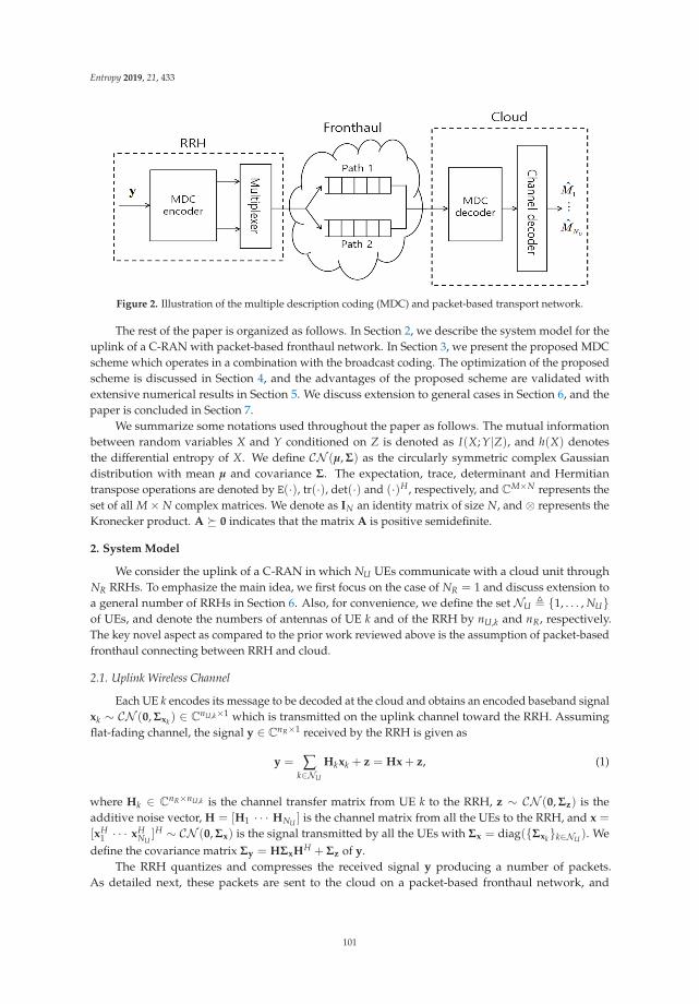
Entropy 2019, 21, 433

Figure 2. Illustration of the multiple description coding (MDC) and packet-based transport network.

The rest of the paper is organized as follows. In Section 2, we describe the system model for theuplink of a C-RAN with packet-based fronthaul network. In Section 3, we present the proposed MDCscheme which operates in a combination with the broadcast coding. The optimization of the proposedscheme is discussed in Section 4, and the advantages of the proposed scheme are validated withextensive numerical results in Section 5. We discuss extension to general cases in Section 6, and thepaper is concluded in Section 7.

We summarize some notations used throughout the paper as follows. The mutual informationbetween random variables X and Y conditioned on Z is denoted as I(X; Y|Z), and h(X) denotesthe differential entropy of X. We define CN (μ, Σ) as the circularly symmetric complex Gaussiandistribution with mean μ and covariance Σ. The expectation, trace, determinant and Hermitiantranspose operations are denoted by E(·), tr(·), det(·) and (·)H , respectively, and CM×N represents theset of all M× N complex matrices. We denote as IN an identity matrix of size N, and ⊗ represents theKronecker product. A � 0 indicates that the matrix A is positive semidefinite.

2. System Model

We consider the uplink of a C-RAN in which NU UEs communicate with a cloud unit throughNR RRHs. To emphasize the main idea, we first focus on the case of NR = 1 and discuss extension toa general number of RRHs in Section 6. Also, for convenience, we define the set NU � {1, . . . , NU}of UEs, and denote the numbers of antennas of UE k and of the RRH by nU,k and nR, respectively.The key novel aspect as compared to the prior work reviewed above is the assumption of packet-basedfronthaul connecting between RRH and cloud.

2.1. Uplink Wireless Channel

Each UE k encodes its message to be decoded at the cloud and obtains an encoded baseband signalxk ∼ CN (0, Σxk ) ∈ CnU,k×1 which is transmitted on the uplink channel toward the RRH. Assumingflat-fading channel, the signal y ∈ CnR×1 received by the RRH is given as

y = ∑k∈NU

Hkxk + z = Hx + z, (1)

where Hk ∈ CnR×nU,k is the channel transfer matrix from UE k to the RRH, z ∼ CN (0, Σz) is theadditive noise vector, H = [H1 · · · HNU ] is the channel matrix from all the UEs to the RRH, and x =

[xH1 · · · xH

NU]H ∼ CN (0, Σx) is the signal transmitted by all the UEs with Σx = diag({Σxk}k∈NU ). We

define the covariance matrix Σy = HΣxHH + Σz of y.The RRH quantizes and compresses the received signal y producing a number of packets.

As detailed next, these packets are sent to the cloud on a packet-based fronthaul network, and

101

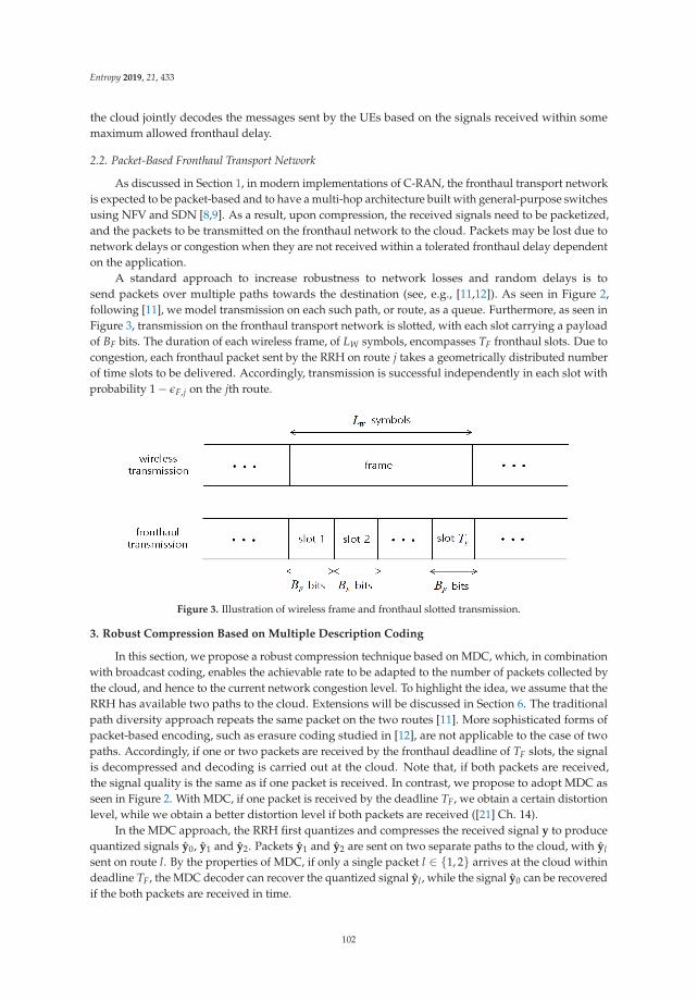
Entropy 2019, 21, 433

the cloud jointly decodes the messages sent by the UEs based on the signals received within somemaximum allowed fronthaul delay.

2.2. Packet-Based Fronthaul Transport Network

As discussed in Section 1, in modern implementations of C-RAN, the fronthaul transport networkis expected to be packet-based and to have a multi-hop architecture built with general-purpose switchesusing NFV and SDN [8,9]. As a result, upon compression, the received signals need to be packetized,and the packets to be transmitted on the fronthaul network to the cloud. Packets may be lost due tonetwork delays or congestion when they are not received within a tolerated fronthaul delay dependenton the application.

A standard approach to increase robustness to network losses and random delays is tosend packets over multiple paths towards the destination (see, e.g., [11,12]). As seen in Figure 2,following [11], we model transmission on each such path, or route, as a queue. Furthermore, as seen inFigure 3, transmission on the fronthaul transport network is slotted, with each slot carrying a payloadof BF bits. The duration of each wireless frame, of LW symbols, encompasses TF fronthaul slots. Due tocongestion, each fronthaul packet sent by the RRH on route j takes a geometrically distributed numberof time slots to be delivered. Accordingly, transmission is successful independently in each slot withprobability 1− εF,j on the jth route.

Figure 3. Illustration of wireless frame and fronthaul slotted transmission.

3. Robust Compression Based on Multiple Description Coding

In this section, we propose a robust compression technique based on MDC, which, in combinationwith broadcast coding, enables the achievable rate to be adapted to the number of packets collected bythe cloud, and hence to the current network congestion level. To highlight the idea, we assume that theRRH has available two paths to the cloud. Extensions will be discussed in Section 6. The traditionalpath diversity approach repeats the same packet on the two routes [11]. More sophisticated forms ofpacket-based encoding, such as erasure coding studied in [12], are not applicable to the case of twopaths. Accordingly, if one or two packets are received by the fronthaul deadline of TF slots, the signalis decompressed and decoding is carried out at the cloud. Note that, if both packets are received,the signal quality is the same as if one packet is received. In contrast, we propose to adopt MDC asseen in Figure 2. With MDC, if one packet is received by the deadline TF, we obtain a certain distortionlevel, while we obtain a better distortion level if both packets are received ([21] Ch. 14).

In the MDC approach, the RRH first quantizes and compresses the received signal y to producequantized signals y0, y1 and y2. Packets y1 and y2 are sent on two separate paths to the cloud, with ylsent on route l. By the properties of MDC, if only a single packet l ∈ {1, 2} arrives at the cloud withindeadline TF, the MDC decoder can recover the quantized signal yl , while the signal y0 can be recoveredif the both packets are received in time.

102

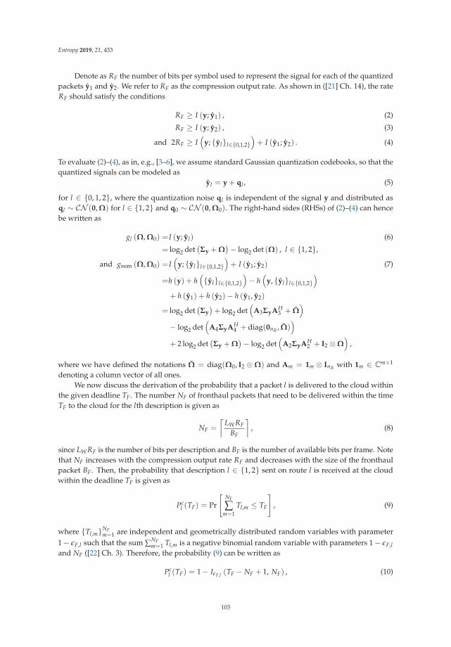
Entropy 2019, 21, 433

Denote as RF the number of bits per symbol used to represent the signal for each of the quantizedpackets y1 and y2. We refer to RF as the compression output rate. As shown in ([21] Ch. 14), the rateRF should satisfy the conditions

RF ≥ I (y; y1) , (2)

RF ≥ I (y; y2) , (3)

and 2RF ≥ I(

y; {yl}l∈{0,1,2})+ I (y1; y2) . (4)

To evaluate (2)–(4), as in, e.g., [3–6], we assume standard Gaussian quantization codebooks, so that thequantized signals can be modeled as

yl = y + ql , (5)

for l ∈ {0, 1, 2}, where the quantization noise ql is independent of the signal y and distributed asql ∼ CN (0, Ω) for l ∈ {1, 2} and q0 ∼ CN (0, Ω0). The right-hand sides (RHSs) of (2)–(4) can hencebe written as

gl (Ω, Ω0) =I (y; yl) (6)

= log2 det(Σy + Ω

)− log2 det (Ω) , l ∈ {1, 2},

and gsum (Ω, Ω0) =I(

y; {yl}l∈{0,1,2})+ I (y1; y2) (7)

=h (y) + h({yl}l∈{0,1,2}

)− h

(y, {yl}l∈{0,1,2}

)+ h (y1) + h (y2)− h (y1, y2)

= log2 det(Σy

)+ log2 det

(A3ΣyAH

3 + Ω)

− log2 det(

A4ΣyAH4 + diag(0nR , Ω)

)+ 2 log2 det

(Σy + Ω

)− log2 det

(A2ΣyAH

2 + I2 ⊗Ω)

,

where we have defined the notations Ω = diag(Ω0, I2 ⊗Ω) and Am = 1m ⊗ InR with 1m ∈ Cm×1

denoting a column vector of all ones.We now discuss the derivation of the probability that a packet l is delivered to the cloud within

the given deadline TF. The number NF of fronthaul packets that need to be delivered within the timeTF to the cloud for the lth description is given as

NF =

⌈LW RF

BF

⌉, (8)

since LW RF is the number of bits per description and BF is the number of available bits per frame. Notethat NF increases with the compression output rate RF and decreases with the size of the fronthaulpacket BF. Then, the probability that description l ∈ {1, 2} sent on route l is received at the cloudwithin the deadline TF is given as

Pcl (TF) = Pr

[NF

∑m=1

Tl,m ≤ TF

], (9)

where {Tl,m}NFm=1 are independent and geometrically distributed random variables with parameter

1− εF,l such that the sum ∑NFm=1 Tl,m is a negative binomial random variable with parameters 1− εF,l

and NF ([22] Ch. 3). Therefore, the probability (9) can be written as

Pcl (TF) = 1− IεF,l (TF − NF + 1, NF) , (10)

103

Entropy 2019, 21, 433

where Ix(a, b) is the regularized incomplete beta function defined as

Ix(a, b) =B(x; a, b)B(1; a, b)

, (11)

with B(x; a, b) =∫ x

0 ta−1(1 − t)b−1dt. For simplicity of notation, we also define the probabilitiesPc

∅(TF) = (1− Pc1(TF))(1− Pc

2(TF)) and Pcall(TF) = Pc

1(TF)Pc2(TF) that no or both descriptions arrive

at the cloud within the deadline.Define as M ∈ {0, 1, 2} the number of descriptions that arrive at the cloud within the given

deadline TF. The probability distribution pM(m) = Pr [M = m] can then be written as

pM(m) =

⎧⎪⎪⎨⎪⎪⎩Pc

∅(TF), m = 0

∑2l=1 Pc

l (TF)(

1− Pcl (TF)

), m = 1

Pcall(TF), m = 2

, (12)

with the notation 1 = 2 and 2 = 1.

Broadcast Coding

With MDC, the quality of the information available at the cloud for decoding the transmittedsignals {xk}k∈NU is determined by the number M of descriptions that arrive at the cloud. Since thestate M ∈ {0, 1, 2} is not known to the UEs, the rate cannot be a priori adapted by the UEs dependingon the congestion level. To handle this issue, we propose that each UE k adopts a broadcast codingstrategy [15–18] as

xk = xk,1 + xk,2, (13)

where the signals xk,1 and xk,2 encode independent messages of UE k, and the decoder at the cloud isrequired to reliably recover only the signals {xk,j}k∈NU with j ≤ m when M = m descriptions arriveat the cloud. We denote the rate of the signal xk,m as Rk,m for k ∈ NU and m ∈ {1, 2}. We make thestandard assumption that the jth signal xk,j of each UE k is distributed as xk,j ∼ CN (0, Pk,jInU,k ), wherethe powers Pk,j need to satisfy the power constraint Pk,1 + Pk,2 = P. Under the described assumption,the covariance matrix Σx of all the transmitted signals x is given as Σx = PInU with nU = ∑k∈NU

nU,k.The signal rm collected at the cloud when M = m descriptions have arrived at the cloud is given as

rm =

⎧⎪⎪⎨⎪⎪⎩0, m = 0

y1, m = 1

y0, m = 2

. (14)

For the case of m = 1, the cloud receives r1 = y1 or r1 = y2. In (14), we set r1 = y1 without loss ofgenerality, since y1 and y2 are statistically equivalent.

When no description arrives at the cloud (i.e., M = 0), the cloud has no information received fromthe RRH, and none of the signals {xk,0, xk,1}k∈NU can be decoded by the cloud. When only a singledescription arrives at the cloud (M = 1), the cloud jointly decodes the first-layer signals {xk,1}k∈NU

based on the received quantized signal r1. Therefore, the achievable sum-rate RΣ,1 = ∑k∈NURk,1 of the

first-layer signals is given as

RΣ,1 = f1 (P, Ω, Ω0) = I (x1; r1) (15)

= log2 det(

HΣxHH + Σz + Ω)− log2 det

(HP2HH + Σz + Ω

),

where we have defined the vector xm = [xH1,m · · · xH

NU ,m]H ∼ CN (0, Pm) that stacks the layer-m signals

of all the UEs, and the notations P = {Pk,j}k∈NU ,j∈{1,2} and Pm = diag({Pk,m}k∈NU ).

104

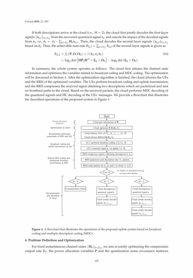
Entropy 2019, 21, 433

If both descriptions arrive at the cloud (i.e., M = 2), the cloud first jointly decodes the first-layersignals {xk,1}k∈NU from the recovered quantized signal r2, and cancels the impact of the decoded signalsfrom r2, i.e., r2 ← r2 − ∑k∈NU

Hkxk,1. Then, the cloud decodes the second-layer signals {xk,2}k∈NU

based on r2. Thus, the achievable sum-rate RΣ,2 = ∑k∈NURk,2 of the second-layer signals is given as

RΣ,2 = f2 (P, Ω, Ω0) = I (x2; r2|x1) (16)

= log2 det(

HP2HH + Σz + Ω0

)− log2 det (Σz + Ω0) .

In summary, the whole system operates as follows. The cloud first obtains the channel stateinformation and optimizes the variables related to broadcast coding and MDC coding. The optimizationwill be discussed in Section 4. After the optimization algorithm is finished, the cloud informs the UEsand the RRH of the optimized variables. The UEs perform broadcast coding and uplink transmission,and the RRH compresses the received signal obtaining two descriptions which are packetized and senton fronthaul paths to the cloud. Based on the received packets, the cloud performs MDC decoding ofthe quantized signals and SIC decoding of the UEs’ messages. We provide a flowchart that illustratesthe described operations of the proposed system in Figure 4.

Figure 4. A flowchart that illustrates the operations of the proposed uplink system based on broadcastcoding and multiple description coding (MDC).

4. Problem Definition and Optimization

For fixed instantaneous channel states {Hk}k∈NU , we aim at jointly optimizing the compressionoutput rate RF, the power allocation variables P and the quantization noise covariance matrices

105

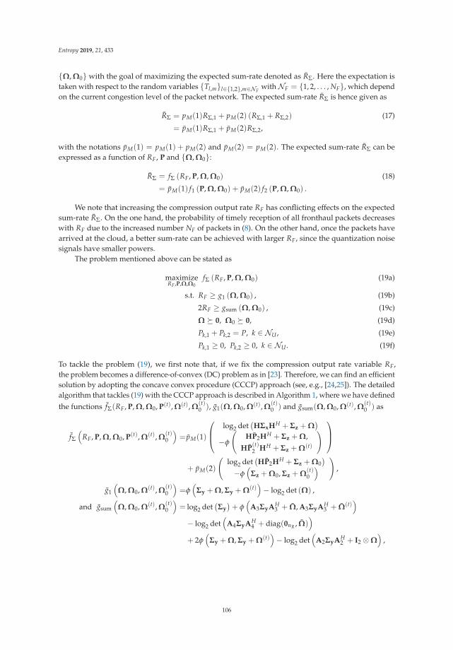
Entropy 2019, 21, 433

{Ω, Ω0} with the goal of maximizing the expected sum-rate denoted as RΣ. Here the expectation istaken with respect to the random variables {Tl,m}l∈{1,2},m∈NF

withNF = {1, 2, . . . , NF}, which dependon the current congestion level of the packet network. The expected sum-rate RΣ is hence given as

RΣ = pM(1)RΣ,1 + pM(2) (RΣ,1 + RΣ,2) (17)

= pM(1)RΣ,1 + pM(2)RΣ,2,

with the notations pM(1) = pM(1) + pM(2) and pM(2) = pM(2). The expected sum-rate RΣ can beexpressed as a function of RF, P and {Ω, Ω0}:

RΣ = fΣ (RF, P, Ω, Ω0) (18)

= pM(1) f1 (P, Ω, Ω0) + pM(2) f2 (P, Ω, Ω0) .

We note that increasing the compression output rate RF has conflicting effects on the expectedsum-rate RΣ. On the one hand, the probability of timely reception of all fronthaul packets decreaseswith RF due to the increased number NF of packets in (8). On the other hand, once the packets havearrived at the cloud, a better sum-rate can be achieved with larger RF, since the quantization noisesignals have smaller powers.

The problem mentioned above can be stated as

maximizeRF ,P,Ω,Ω0

fΣ (RF, P, Ω, Ω0) (19a)

s.t. RF ≥ g1 (Ω, Ω0) , (19b)

2RF ≥ gsum (Ω, Ω0) , (19c)

Ω � 0, Ω0 � 0, (19d)

Pk,1 + Pk,2 = P, k ∈ NU , (19e)

Pk,1 ≥ 0, Pk,2 ≥ 0, k ∈ NU . (19f)

To tackle the problem (19), we first note that, if we fix the compression output rate variable RF,the problem becomes a difference-of-convex (DC) problem as in [23]. Therefore, we can find an efficientsolution by adopting the concave convex procedure (CCCP) approach (see, e.g., [24,25]). The detailedalgorithm that tackles (19) with the CCCP approach is described in Algorithm 1, where we have definedthe functions fΣ(RF, P, Ω, Ω0, P(t), Ω(t), Ω

(t)0 ), g1(Ω, Ω0, Ω(t), Ω

(t)0 ) and gsum(Ω, Ω0, Ω(t), Ω

(t)0 ) as

fΣ

(RF, P, Ω, Ω0, P(t), Ω(t), Ω

(t)0

)= pM(1)

⎛⎜⎝ log2 det(HΣxHH + Σz + Ω

)−φ

(HP2HH + Σz + Ω,

HP(t)2 HH + Σz + Ω(t)

) ⎞⎟⎠+ pM(2)

(log2 det

(HP2HH + Σz + Ω0

)−φ

(Σz + Ω0, Σz + Ω

(t)0

) ),

g1

(Ω, Ω0, Ω(t), Ω

(t)0

)=φ

(Σy + Ω, Σy + Ω(t)

)− log2 det (Ω) ,

and gsum

(Ω, Ω0, Ω(t), Ω

(t)0

)= log2 det

(Σy

)+ φ

(A3ΣyAH

3 + Ω, A3ΣyAH3 + Ω(t)

)− log2 det

(A4ΣyAH

4 + diag(0nR , Ω))

+ 2φ(

Σy + Ω, Σy + Ω(t))− log2 det

(A2ΣyAH

2 + I2 ⊗Ω)

,

106

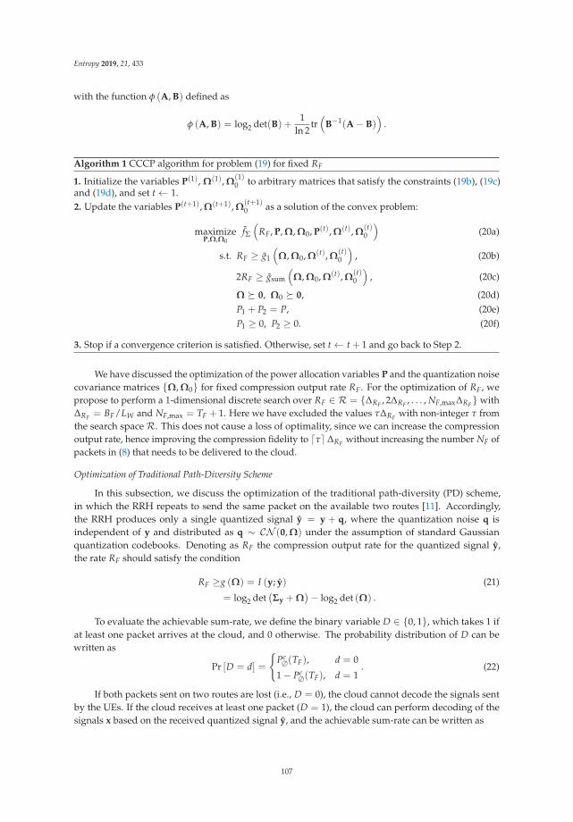
Entropy 2019, 21, 433

with the function φ (A, B) defined as

φ (A, B) = log2 det(B) +1

ln 2tr

(B−1(A− B)

).

Algorithm 1 CCCP algorithm for problem (19) for fixed RF

1. Initialize the variables P(1), Ω(1), Ω(1)0 to arbitrary matrices that satisfy the constraints (19b), (19c)

and (19d), and set t ← 1.2. Update the variables P(t+1), Ω(t+1), Ω

(t+1)0 as a solution of the convex problem:

maximizeP,Ω,Ω0

fΣ

(RF, P, Ω, Ω0, P(t), Ω(t), Ω

(t)0

)(20a)

s.t. RF ≥ g1

(Ω, Ω0, Ω(t), Ω

(t)0

), (20b)

2RF ≥ gsum

(Ω, Ω0, Ω(t), Ω

(t)0

), (20c)

Ω � 0, Ω0 � 0, (20d)P1 + P2 = P, (20e)P1 ≥ 0, P2 ≥ 0. (20f)

3. Stop if a convergence criterion is satisfied. Otherwise, set t ← t + 1 and go back to Step 2.

We have discussed the optimization of the power allocation variables P and the quantization noisecovariance matrices {Ω, Ω0} for fixed compression output rate RF. For the optimization of RF, wepropose to perform a 1-dimensional discrete search over RF ∈ R = {ΔRF , 2ΔRF , . . . , NF,maxΔRF} withΔRF = BF/LW and NF,max = TF + 1. Here we have excluded the values τΔRF with non-integer τ fromthe search space R. This does not cause a loss of optimality, since we can increase the compressionoutput rate, hence improving the compression fidelity to �τ�ΔRF without increasing the number NF ofpackets in (8) that needs to be delivered to the cloud.

Optimization of Traditional Path-Diversity Scheme

In this subsection, we discuss the optimization of the traditional path-diversity (PD) scheme,in which the RRH repeats to send the same packet on the available two routes [11]. Accordingly,the RRH produces only a single quantized signal y = y + q, where the quantization noise q isindependent of y and distributed as q ∼ CN (0, Ω) under the assumption of standard Gaussianquantization codebooks. Denoting as RF the compression output rate for the quantized signal y,the rate RF should satisfy the condition

RF ≥g (Ω) = I (y; y) (21)

= log2 det(Σy + Ω

)− log2 det (Ω) .

To evaluate the achievable sum-rate, we define the binary variable D ∈ {0, 1}, which takes 1 ifat least one packet arrives at the cloud, and 0 otherwise. The probability distribution of D can bewritten as

Pr [D = d] =

{Pc

∅(TF), d = 0

1− Pc∅(TF), d = 1

. (22)

If both packets sent on two routes are lost (i.e., D = 0), the cloud cannot decode the signals sentby the UEs. If the cloud receives at least one packet (D = 1), the cloud can perform decoding of thesignals x based on the received quantized signal y, and the achievable sum-rate can be written as

107

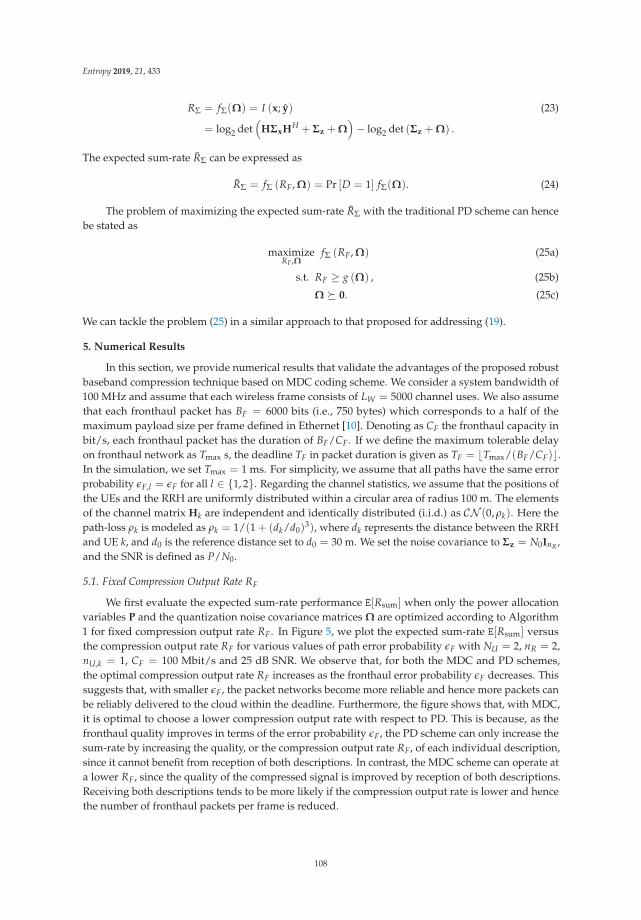
Entropy 2019, 21, 433

RΣ = fΣ(Ω) = I (x; y) (23)

= log2 det(

HΣxHH + Σz + Ω)− log2 det (Σz + Ω) .

The expected sum-rate RΣ can be expressed as

RΣ = fΣ (RF, Ω) = Pr [D = 1] fΣ(Ω). (24)

The problem of maximizing the expected sum-rate RΣ with the traditional PD scheme can hencebe stated as

maximizeRF ,Ω

fΣ (RF, Ω) (25a)

s.t. RF ≥ g (Ω) , (25b)

Ω � 0. (25c)

We can tackle the problem (25) in a similar approach to that proposed for addressing (19).

5. Numerical Results

In this section, we provide numerical results that validate the advantages of the proposed robustbaseband compression technique based on MDC coding scheme. We consider a system bandwidth of100 MHz and assume that each wireless frame consists of LW = 5000 channel uses. We also assumethat each fronthaul packet has BF = 6000 bits (i.e., 750 bytes) which corresponds to a half of themaximum payload size per frame defined in Ethernet [10]. Denoting as CF the fronthaul capacity inbit/s, each fronthaul packet has the duration of BF/CF. If we define the maximum tolerable delayon fronthaul network as Tmax s, the deadline TF in packet duration is given as TF = �Tmax/(BF/CF)�.In the simulation, we set Tmax = 1 ms. For simplicity, we assume that all paths have the same errorprobability εF,l = εF for all l ∈ {1, 2}. Regarding the channel statistics, we assume that the positions ofthe UEs and the RRH are uniformly distributed within a circular area of radius 100 m. The elementsof the channel matrix Hk are independent and identically distributed (i.i.d.) as CN (0, ρk). Here thepath-loss ρk is modeled as ρk = 1/(1 + (dk/d0)

3), where dk represents the distance between the RRHand UE k, and d0 is the reference distance set to d0 = 30 m. We set the noise covariance to Σz = N0InR ,and the SNR is defined as P/N0.

5.1. Fixed Compression Output Rate RF

We first evaluate the expected sum-rate performance E[Rsum] when only the power allocationvariables P and the quantization noise covariance matrices Ω are optimized according to Algorithm1 for fixed compression output rate RF. In Figure 5, we plot the expected sum-rate E[Rsum] versusthe compression output rate RF for various values of path error probability εF with NU = 2, nR = 2,nU,k = 1, CF = 100 Mbit/s and 25 dB SNR. We observe that, for both the MDC and PD schemes,the optimal compression output rate RF increases as the fronthaul error probability εF decreases. Thissuggests that, with smaller εF, the packet networks become more reliable and hence more packets canbe reliably delivered to the cloud within the deadline. Furthermore, the figure shows that, with MDC,it is optimal to choose a lower compression output rate with respect to PD. This is because, as thefronthaul quality improves in terms of the error probability εF, the PD scheme can only increase thesum-rate by increasing the quality, or the compression output rate RF, of each individual description,since it cannot benefit from reception of both descriptions. In contrast, the MDC scheme can operate ata lower RF, since the quality of the compressed signal is improved by reception of both descriptions.Receiving both descriptions tends to be more likely if the compression output rate is lower and hencethe number of fronthaul packets per frame is reduced.

108

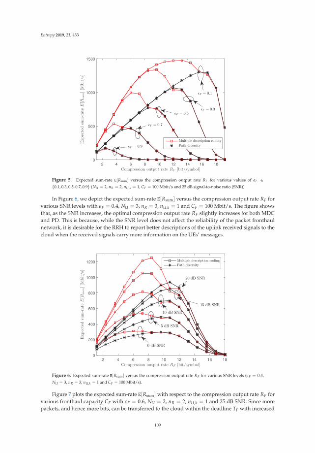
Entropy 2019, 21, 433

2 4 6 8 10 12 14 16 18Compression output rate RF [bit/symbol]

0

500

1000

1500

Expectedsum-rate

E[R

sum][M

bit/s]

Multiple description coding

Path-diversity

εF = 0.1

εF = 0.3εF = 0.5

εF = 0.7

εF = 0.9

Figure 5. Expected sum-rate E[Rsum] versus the compression output rate RF for various values of εF ∈{0.1, 0.3, 0.5, 0.7, 0.9} (NU = 2, nR = 2, nU,k = 1, CF = 100 Mbit/s and 25 dB signal-to-noise ratio (SNR)).

In Figure 6, we depict the expected sum-rate E[Rsum] versus the compression output rate RF forvarious SNR levels with εF = 0.4, NU = 3, nR = 3, nU,k = 1 and CF = 100 Mbit/s. The figure showsthat, as the SNR increases, the optimal compression output rate RF slightly increases for both MDCand PD. This is because, while the SNR level does not affect the reliability of the packet fronthaulnetwork, it is desirable for the RRH to report better descriptions of the uplink received signals to thecloud when the received signals carry more information on the UEs’ messages.

2 4 6 8 10 12 14 16 18Compression output rate RF [bit/symbol]

0

200

400

600

800

1000

1200

Expectedsum-rate

E[R

sum][M

bit/s]

Multiple description codingPath-diversity

0 dB SNR

5 dB SNR

10 dB SNR

15 dB SNR

20 dB SNR

Figure 6. Expected sum-rate E[Rsum] versus the compression output rate RF for various SNR levels (εF = 0.4,

NU = 3, nR = 3, nU,k = 1 and CF = 100 Mbit/s).

Figure 7 plots the expected sum-rate E[Rsum] with respect to the compression output rate RF forvarious fronthaul capacity CF with εF = 0.6, NU = 2, nR = 2, nU,k = 1 and 25 dB SNR. Since morepackets, and hence more bits, can be transferred to the cloud within the deadline TF with increased

109

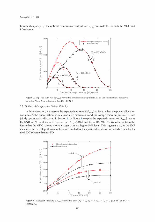
Entropy 2019, 21, 433

fronthaul capacity CF, the optimal compression output rate RF grows with CF for both the MDC andPD schemes.

5 10 15 20 25Compression output rate RF [bit/symbol]

0

500

1000

1500Expectedsum-rate

E[R

sum][M

bit/s]


CF = 200 Mbit/s

CF = 100 Mbit/sCF = 50 Mbit/s

Figure 7. Expected sum-rate E[Rsum] versus the compression output rate RF for various fronthaul capacity CF

(εF = 0.6, NU = 2, nR = 2, nU,k = 1 and 25 dB SNR).

5.2. Optimized Compression Output Rate RF

In this subsection, we present the expected sum-rate E[Rsum] achieved when the power allocationvariables P, the quantization noise covariance matrices Ω and the compression output rate RF arejointly optimized as discussed in Section 4. In Figure 8, we plot the expected sum-rate E[Rsum] versusthe SNR for NU = 3, nR = 3, nU,k = 1, εF ∈ {0.4, 0.6} and CF = 100 Mbit/s. We observe from thefigure that the MDC scheme shows a larger gain at a higher SNR level. This suggests that, as the SNRincreases, the overall performance becomes limited by the quantization distortion which is smaller forthe MDC scheme than for PD.

0 5 10 15 20 25 30Wireless SNR [dB]

200

400

600

800

1000

1200

1400

1600

Expectedsum-rate

E[R

sum][M

bit/s]


εF = 0.4

εF = 0.6

Figure 8. Expected sum-rate E[Rsum] versus the SNR (NU = 3, nR = 3, nU,k = 1, εF ∈ {0.4, 0.6} and CF =

100 Mbit/s).

110

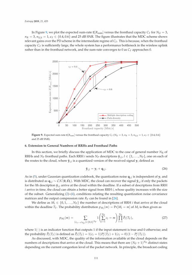
Entropy 2019, 21, 433

In Figure 9, we plot the expected sum-rate E[Rsum] versus the fronthaul capacity CF for NU = 3,nR = 3, nU,k = 1, εF ∈ {0.4, 0.6} and 25 dB SNR. The figure illustrates that the MDC scheme showsrelevant gains over the PD scheme in the intermediate regime of CF. This is because, when the fronthaulcapacity CF is sufficiently large, the whole system has a performance bottleneck in the wireless uplinkrather than in the fronthaul network, and the sum-rate converges to 0 as CF approaches 0.

0 50 100 150 200 250 300 350 400 450 500Fronthaul capacity [Mbit/s]

0

500

1000

1500

2000

2500

Expectedsum-rate

E[R

sum][M

bit/s]

Multiple description coding

Path-diversity

εF = 0.4

εF = 0.6

Figure 9. Expected sum-rate E[Rsum] versus the fronthaul capacity CF (NU = 3, nR = 3, nU,k = 1, εF ∈ {0.4, 0.6}and 25 dB SNR).

6. Extension to General Numbers of RRHs and Fronthaul Paths

In this section, we briefly discuss the application of MDC to the case of general number NR ofRRHs and NP fronthaul paths. Each RRH i sends NP descriptions yi,l , l ∈ {1, . . . , NP}, one on each ofthe routes to the cloud, where yi,l is a quantized version of the received signal yi defined as

yi,l = yi + qi,l . (26)

As in (5), under Gaussian quantization codebook, the quantization noise qi,l is independent of yi andis distributed as qi,l ∼ CN (0, Ωi). With MDC, the cloud can recover the signal yi,l if only the packetsfor the lth description yi,l arrive at the cloud within the deadline. If a subset of descriptions from RRHi arrive in time, the cloud can obtain a better signal from RRH i, whose quality increases with the sizeof the subset. Generalizing (2)–(4), conditions relating the resulting quantization noise covariancematrices and the output compression rate RF can be found in [26].

We define as Mi ∈ {0, 1, . . . , NP} the number of descriptions of RRH i that arrive at the cloudwithin the deadline TF. The probability distribution pMi (m) = Pr[Mi = m] of Mi is then given as

pMi (m) = ∑(c1,...,cNP )∈{0,1}NP

1

(NP

∑l=1

cl = m

)NP

∏l=1

Pl(TF), (27)

where 1(·) is an indicator function that outputs 1 if the input statement is true and 0 otherwise; andthe probability Pl(TF) is defined as Pl(TF) = 1(cl = 1)Pc

l (TF) + 1(cl = 0)(1− Pcl (TF)).

As discussed, with MDC, the quality of the information available at the cloud depends on thenumbers of descriptions that arrive at the cloud. This means that there are (NP + 1)NR distinct statesdepending on the current congestion level of the packet network. In principle, the broadcast coding

111

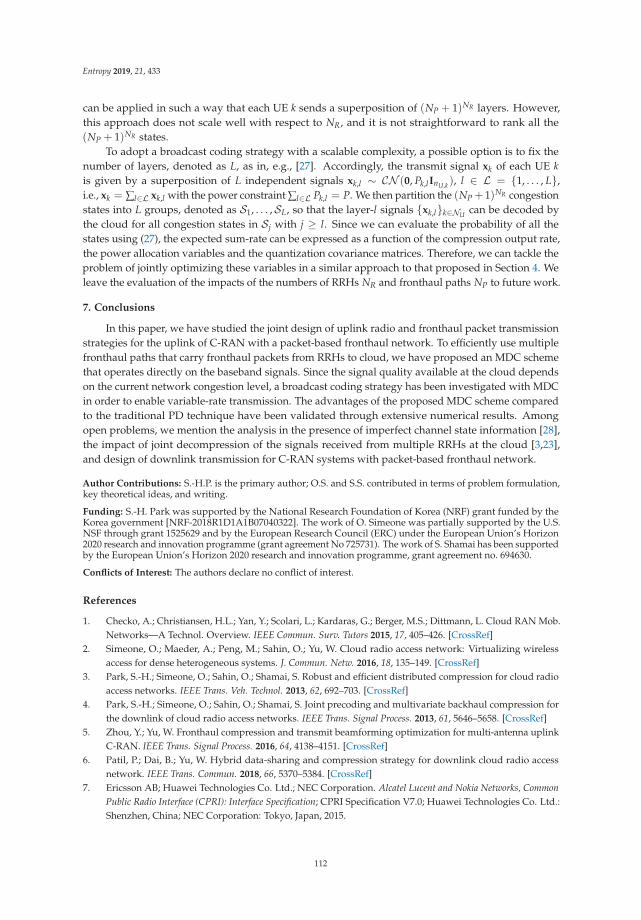
Entropy 2019, 21, 433

can be applied in such a way that each UE k sends a superposition of (NP + 1)NR layers. However,this approach does not scale well with respect to NR, and it is not straightforward to rank all the(NP + 1)NR states.

To adopt a broadcast coding strategy with a scalable complexity, a possible option is to fix thenumber of layers, denoted as L, as in, e.g., [27]. Accordingly, the transmit signal xk of each UE kis given by a superposition of L independent signals xk,l ∼ CN (0, Pk,lInU,k), l ∈ L = {1, . . . , L},i.e., xk = ∑l∈L xk,l with the power constraint ∑l∈L Pk,l = P. We then partition the (NP + 1)NR congestionstates into L groups, denoted as S1, . . . ,SL, so that the layer-l signals {xk,l}k∈NU can be decoded bythe cloud for all congestion states in Sj with j ≥ l. Since we can evaluate the probability of all thestates using (27), the expected sum-rate can be expressed as a function of the compression output rate,the power allocation variables and the quantization covariance matrices. Therefore, we can tackle theproblem of jointly optimizing these variables in a similar approach to that proposed in Section 4. Weleave the evaluation of the impacts of the numbers of RRHs NR and fronthaul paths NP to future work.

7. Conclusions

In this paper, we have studied the joint design of uplink radio and fronthaul packet transmissionstrategies for the uplink of C-RAN with a packet-based fronthaul network. To efficiently use multiplefronthaul paths that carry fronthaul packets from RRHs to cloud, we have proposed an MDC schemethat operates directly on the baseband signals. Since the signal quality available at the cloud dependson the current network congestion level, a broadcast coding strategy has been investigated with MDCin order to enable variable-rate transmission. The advantages of the proposed MDC scheme comparedto the traditional PD technique have been validated through extensive numerical results. Amongopen problems, we mention the analysis in the presence of imperfect channel state information [28],the impact of joint decompression of the signals received from multiple RRHs at the cloud [3,23],and design of downlink transmission for C-RAN systems with packet-based fronthaul network.

Author Contributions: S.-H.P. is the primary author; O.S. and S.S. contributed in terms of problem formulation,key theoretical ideas, and writing.

Funding: S.-H. Park was supported by the National Research Foundation of Korea (NRF) grant funded by theKorea government [NRF-2018R1D1A1B07040322]. The work of O. Simeone was partially supported by the U.S.NSF through grant 1525629 and by the European Research Council (ERC) under the European Union’s Horizon2020 research and innovation programme (grant agreement No 725731). The work of S. Shamai has been supportedby the European Union’s Horizon 2020 research and innovation programme, grant agreement no. 694630.


References

1. Checko, A.; Christiansen, H.L.; Yan, Y.; Scolari, L.; Kardaras, G.; Berger, M.S.; Dittmann, L. Cloud RAN Mob.Networks—A Technol. Overview. IEEE Commun. Surv. Tutors 2015, 17, 405–426. [CrossRef]

2. Simeone, O.; Maeder, A.; Peng, M.; Sahin, O.; Yu, W. Cloud radio access network: Virtualizing wirelessaccess for dense heterogeneous systems. J. Commun. Netw. 2016, 18, 135–149. [CrossRef]

3. Park, S.-H.; Simeone, O.; Sahin, O.; Shamai, S. Robust and efficient distributed compression for cloud radioaccess networks. IEEE Trans. Veh. Technol. 2013, 62, 692–703. [CrossRef]

4. Park, S.-H.; Simeone, O.; Sahin, O.; Shamai, S. Joint precoding and multivariate backhaul compression forthe downlink of cloud radio access networks. IEEE Trans. Signal Process. 2013, 61, 5646–5658. [CrossRef]

5. Zhou, Y.; Yu, W. Fronthaul compression and transmit beamforming optimization for multi-antenna uplinkC-RAN. IEEE Trans. Signal Process. 2016, 64, 4138–4151. [CrossRef]

6. Patil, P.; Dai, B.; Yu, W. Hybrid data-sharing and compression strategy for downlink cloud radio accessnetwork. IEEE Trans. Commun. 2018, 66, 5370–5384. [CrossRef]

7. Ericsson AB; Huawei Technologies Co. Ltd.; NEC Corporation. Alcatel Lucent and Nokia Networks, CommonPublic Radio Interface (CPRI): Interface Specification; CPRI Specification V7.0; Huawei Technologies Co. Ltd.:Shenzhen, China; NEC Corporation: Tokyo, Japan, 2015.

112

Entropy 2019, 21, 433

8. De la Oliva, A.; Hernandez, J.A.; Larrabeiti, D.; Azcorra, A. An overview of the CPRI specification and itsapplication to C-RAN-based LTE scenarios. IEEE Commun. Mag. 2016, 54, 152–159. [CrossRef]

9. Ericsson AB; Huawei Technologies Co. Ltd.; NEC Corporation and Nokia. Common Public Radio Interface:ECPRI Interface Specification. eCPRI Specification V1.0; Huawei Technologies Co. Ltd.: Shenzhen, China;NEC Corporation: Tokyo, Japan, 2017.

10. The Ethernet—A Local Area Network—Data Link Layer and Physical Layer Specifications, Ver. 2.0; The ACMDigital Library: New York, NY, USA, 1982.

11. Alasti, M.; Sayrafian-Pour, K.; Emphremides, A.; Farvardin, N. Multiple description coding in networks withcongestion problem. IEEE Trans. Inf. Theory 2001, 47, 891–902. [CrossRef]

12. Mountaser, G.; Mahmoodi, T.; Simeone, O. Reliable and low-latency fronthaul for tactile internet applications.IEEE J. Sel. Areas Commun. 2018, 36, 2455–2463. [CrossRef]

13. Goyal, V.K. Multiple description coding: Compression meets the network. IEEE Signal Process. Mag. 2001,18, 74–93. [CrossRef]

14. Benammar, M.; Piantanida, P.; Shamai, S. Capacity Results for the Multicast Cognitive Interference Channel.IEEE Trans. Inf. Theory 2017, 63, 4119–4136. [CrossRef]

15. Cover, T.M. Comments on broadcast channels. IEEE Trans. Inf. Theory 1998, 44, 2524–2530. [CrossRef]16. Shamai, S.; Steiner, A. A broadcast approach for a single-user slowly fading MIMO channel. IEEE Trans. Inf.

Theory 2003, 49, 2617–2635. [CrossRef]17. Verdu, S.; Shamai, S. Variable-rate channel capacity. IEEE Trans. Inf. Theory 2010, 56, 2651–2667. [CrossRef]18. Park, S.-H.; Simeone, O.; Sahin, O.; Shamai, S. Robust layered transmission and compression for distributed

uplink reception in cloud radio access networks. IEEE Trans. Veh. Technol. 2014, 63, 204–216. [CrossRef]19. Karasik, R.; Simeone, O.; Shamai, S. Robust Uplink Communications over Fading Channels with Variable

Backhaul Connectivity. IEEE Trans. Wirel. Commun. 2013, 12, 5788–5799. [CrossRef]20. Ng, C.T.K.; Tian, C.; Goldsmith, A.J.; Shamai, S. Minimum Expected Distortion in Gaussian Source Coding

With Fading Side Information. IEEE Trans. Inf. Theory 2012, 58, 5725–5739. [CrossRef]21. Gamal, A.E.; Kim, Y.-H. Network Information Theory; Cambridge University Press: Cambridge, UK, 2011.22. Leon-Garcia, A. Probability and Random Processes for Electrical Engineering; Addison Wesley: Boston, MA,

USA, 1994.23. Park, S.-H.; Simeone, O.; Sahin, O.; Shamai, S. Joint decompression and decoding for cloud radio access

networks. IEEE Signal Process. Lett. 2013, 20, 503–506. [CrossRef]24. Tao, M.; Chen, E.; Zhou, H.; Yu, W. Content-centric sparse multicast beamforming for cache-enabled cloud

RAN. IEEE Trans. Wirel. Commun. 2016, 15, 6118–6131. [CrossRef]25. Park, S.-H.; Simeone, O.; Shamai, S. Joint optimization of cloud and edge processing for fog radio access

networks. IEEE Trans. Wirel. Commun. 2016, 15, 7621–7632. [CrossRef]26. Venkataramani, R.; Kramer G.; Goyal, V.K. Multiple description coding with many channels. IEEE Trans. Inf.

Theory 2003, 49, 2106–2114. [CrossRef]27. Steiner, A.; Shamai, S. Multi-Layer Broadcasting over a Block Fading MIMO Channel. IEEE Trans. Wirel.

Commun. 2007, 6, 3937–3945. [CrossRef]28. Kang, J.; Simeone, O.; Kang, J.; Shamai, S. Joint Signal and Channel State Information Compression for the

Backhaul of Uplink Network MIMO Systems. IEEE Trans. Wirel. Commun. 2014, 13, 1555–1567. [CrossRef]


113

entropy

Article

Amplitude Constrained MIMO Channels: Propertiesof Optimal Input Distributions and Boundson the Capacity †

Alex Dytso 1,*, Mario Goldenbaum 1,*, H. Vincent Poor 1,* and Shlomo Shamai (Shitz) 2,*

1 Department of Electrical Engineering, Princeton University, Princeton, NJ 08544, USA2 Department of Electrical Engineering, Technion-Israel Institute of Technology,

Technion City, Haifa 32000, Israel* Correspondence: [email protected] (A.D.); [email protected] (M.G.);

[email protected] (H.V.P.); [email protected] (S.S.)† Parts of the material in this paper were presented at the 2017 IEEE Global Communications Conference

(Singapore, 4–8 December 2017).

Received: 21 January 2019; Accepted: 13 February 2019; Published: 19 February 2019

Abstract: In this work, the capacity of multiple-input multiple-output channels that are subjectto constraints on the support of the input is studied. The paper consists of two parts. The firstpart focuses on the general structure of capacity-achieving input distributions. Known results aresurveyed and several new results are provided. With regard to the latter, it is shown that the supportof a capacity-achieving input distribution is a small set in both a topological and a measure theoreticalsense. Moreover, explicit conditions on the channel input space and the channel matrix are found suchthat the support of a capacity-achieving input distribution is concentrated on the boundary of theinput space only. The second part of this paper surveys known bounds on the capacity and providesseveral novel upper and lower bounds for channels with arbitrary constraints on the support of thechannel input symbols. As an immediate practical application, the special case of multiple-inputmultiple-output channels with amplitude constraints is considered. The bounds are shown to be withina constant gap to the capacity if the channel matrix is invertible and are tight in the high amplituderegime for arbitrary channel matrices. Moreover, in the regime of high amplitudes, it is shown thatthe capacity scales linearly with the minimum between the number of transmit and receive antennas,similar to the case of average power-constrained inputs.

Keywords: MIMO; channel capacity; amplitude constraint; input distrbution; capacity bounds

1. Introduction

While the capacity of a multiple-input multiple-output (MIMO) channel with an average powerconstraint is well understood [1], there is surprisingly little known about the capacity of the morepractically relevant case in which the channel inputs are subject to amplitude constraints. Shannonwas the first who considered a channel that is constrained in its amplitude [2]. In that paper,he derived corresponding upper and lower bounds and showed that in the low-amplitude regime,the capacity behaves as that of channel with an average power constraint. The next major contributionto this problem was a seminal paper of Smith [3] published in 1971. Smith showed that, for thesingle-input single-output (SISO) Gaussian noise channel with an amplitude-constrained input,the capacity-achieving inputs are discrete with finite support. In [4], this result is extended topeak-power-constrained quadrature Gaussian channels. Using the approach of Shamai [4], it is shownin [5] that the input distribution that achieves the capacity of a MIMO channel with an identity channelmatrix and a Euclidian norm constraint on the input vector is discrete. Even though the optimal input


Entropy 2019, 21, 200

distribution is known to be discrete, very little is known about the number or the optimal positions ofthe corresponding constellation points. To the best of our knowledge, the only case for which the inputdistribution is precisely known is considered in [6], where it is shown for the Gaussian SISO channelwith an amplitude constraint that two point masses are optimal if amplitude values are smaller than1.665 and three for amplitude values of up to 2.786. Finally, it has been shown very recently that thenumber of mass points in the support of the capacity-achieving input distribution of a SISO channel isof the order O(A2) with A the amplitude constraint.

Based on a dual capacity expression, in [7], McKellips derived an upper bound on the capacity ofa SISO channel that is subject to an amplitude constraint. The bound is asymptotically tight; that is,for amplitude values that tend to infinity. By cleverly choosing an auxiliary channel output distributionin the dual capacity expression, the authors of [8] sharpened McKellips’ upper bound and extendedit to parallel MIMO channels with a Euclidian norm constraint on the input. The SISO version ofthe upper bound in [8] has been further sharpened in [9] by yet another choice of auxiliary outputdistribution. In [10], asymptotic lower and upper bounds for a 2× 2 MIMO channel are presented andthe gap between the bounds is specified.

In this work, we make progress on this open problem by deriving several new upper and lowerbounds that hold for channels with arbitrary constraints on the support of the channel input distributionand then apply them to the practically relevant special case of MIMO channels that are subject toamplitude-constraints.

1.1. Contributions and Paper Organization

The remainder of the paper is organized as follows. The problem is stated in Section 2. In Section 3,we study properties of input distributions that achieve the capacity of input-constrained MIMOchannels. The section reviews known results on the structure of optimal input distributions andpresents several new results. In particular, Theorem 3 shows that the support of a capacity-achievinginput distribution must necessarily be a small set both topologically and measure theoretically.Moreover, Theorem 8 characterizes conditions on the channel input space as well as on the channelmatrix such that the support of the optimal input distribution is concentrated on the boundary of thechannel input space.

In Section 4, we derive novel upper and lower bounds on the capacity of a MIMO channelthat is subject to an arbitrary constraint on the support of the input. In particular, three familiesof upper bounds are proposed, which are based on: (i) the maximum entropy principle (see thebound in Theorem 9); (ii) the dual capacity characterization (see the bound in Theorem 10); and (iii)a relationship between mutual information and the minimum mean square error that is known asthe I-MMSE relationship (see the bound in Theorem 11). On the other hand, Section 4 providesthree different lower bounds. The first one is given in Theorem 12 and is based on the entropypower inequality. The second one (see Theorem 13) is based on a generalization of the celebratedOzarow–Wyner bound [11] to the MIMO case. The third upper bound (see Theorem 14) is based onJensen’s inequality and depends on the characteristic function of the channel input distribution.

In Section 5, we evaluate the performance of our bounds by studying MIMO channels withinvertible channel matrices. In particular, Theorem 17 states that our upper and lower bounds arewithin n log2(ρ) bits, where ρ is the packing efficiency and n the number of transmit and receiveantennas. For diagonal channel matrices, it is then shown (see Theorem 18) that the Cartesian productof simple pulse-amplitude modulation (PAM) constellations achieves the capacity to within 1.64n bits.

Section 6 is devoted to MIMO channels with arbitrary channel matrices. It is shown that,in the regime of high amplitudes, similar to the case of average power-constrained channel inputs,the capacity scales linearly with the minimum of the number of transmit and receive antennas.

In Section 7, our upper and lower bounds are applied to the SISO case, which are then comparedwith bounds known from the literature. Finally, Section 8 concludes the paper. Note that parts of theresults in this paper were also published in [12].

116

Entropy 2019, 21, 200

1.2. Notation

Vectors are denoted as bold lowercase letters, random vectors as bold uppercase letters,and matrices as bold uppercase sans serif letters (e.g., x, X, X). For any deterministic vector x ∈ Rn,n ∈ N, we denote the Euclidian norm of x by ‖x‖. For some random X ∈ supp(X) ⊆ Rn and any p > 0,we define

‖X‖p :=(

1nE[‖X‖p]

) 1p, (1)

where supp(X) denotes the support of X. Note that for p ≥ 1, the quantity in Equation (1) definesa norm and for n = 1 we simply have ‖X‖p

p = E[|X|p].The norm of a matrix H ∈ Rn×n is defined as

‖H‖ := supx:x �=0

‖Hx‖‖x‖ ,

whereas Tr(H) is denoting its trace. The n× n identity matrix is represented as In.Let S be a subset of Rn. Then,

Vol(S) :=∫S

dx

denotes its volume. Moreover, the boundary of S is denoted as ∂S .Let R+ := {x ∈ R : x ≥ 0}. We define an n-dimensional ball or radius r ∈ R+ centered at x ∈ Rn

as the setBx(r) := {y ∈ R

n : ‖x− y‖ ≤ r}.

Recall that, for any x ∈ Rn and r ∈ R+,

Vol(Bx(r)

)=

πn2

Γ( n

2 + 1) rn,

where Γ(z) denotes the gamma function.For any matrix H ∈ Rk×n and some S ⊂ Rn, we define

HS := {y ∈ Rk : y = Hx , x ∈ S}.

Note that for an invertible H ∈ Rn×n, we have

Vol(HS) = |det(H)|Vol(S)

with det(H) the determinant of H. We define the maximum and minimum radius of a set S ⊂ Rn thatcontains the origin as

rmax(S) := min{r ∈ R+ : S ⊂ B0(r)},

rmin(S) := max{r ∈ R+ : B0(r) ⊆ S}.

For a given vector a = (a1, . . . , an) ∈ Rn+, we define

Box(a) := {x ∈ Rn : |xi| ≤ ai, i = 1, . . . , n}

and the smallest box containing a given set S ⊂ Rn as

Box(S) := inf{Box(a) : S ⊆ Box(a)},

respectively.

117

Entropy 2019, 21, 200

The entropy of any discrete random object X is denoted as H(X), whereas h(X) (i.e., the differentialentropy) is used whenever X is continuous. The mutual information between two random objects X andY is denoted as I(X; Y) and N (m,C) denotes the multivariate normal distribution with mean vectorm and covariance matrix C. Finally, log+

a (x) := max{loga(x), 0}, for any base a > 0, Q(x), x ∈ R,denotes the Q-function, and δx(y) the Kronecker delta, which is one for x = y and zero otherwise.

2. Problem Statement

Consider a MIMO system with nt ∈ N transmit and nr ∈ N receive antennas. The correspondingnr-dimensional channel output for a single channel use is of the form

Y = HX + Z,

for some fixed channel matrix H ∈ Rnr×nt (considering a real-valued channel model is without loss ofgenerality). Here and hereafter, we assume Z ∼ N (0, Inr ) is independent of the channel input X ∈ Rnt

and H is known to both the transmitter and the receiver.Now, let X ⊂ Rnt be a convex and compact channel input space that contains the origin

(i.e., the length-nt zero vector) and let FX denote the cumulative distribution function of X. As of thewriting of this paper, the capacity

C(X ,H) := maxFX :X∈X

I(X; Y) = maxFX :X∈X

I(X;HX + Z), (2)

of this channel is unknown and we are interested in finding novel lower and upper bounds.Even though most of the results in this paper hold for arbitrary convex and compact X , we aremainly interested in the two important special cases:

(i) per-antenna amplitude constraints, i.e., X = Box(a) for some given a = (A1, . . . , Ant) ∈ Rnt+ ; and

(ii) nt-dimensional amplitude constraint, i.e., X = B0(A) for some given A ∈ R+.

Remark 1. Note that determining the capacity of a MIMO channel with average per-antenna power constraintsis also still an open problem and has been solved for some special cases only [13–17].

3. Properties of an Optimal Input Distribution

Unlike the special cases of real and complex-valued SISO channels (i.e., nt = nr = 1), the structureof the capacity-achieving input distribution, denoted as F�

X, is in general not known. To motivate whyin this paper we are seeking for novel upper and lower bounds on the capacity (Equation (2)) instead oftrying to solve the optimization problem directly, in this section we first summarize properties optimalinput distributions must posses, which demonstrate how complicated the optimization problemactually is. Note that, whereas an optimal input distribution always exists, it does not necessarily needto be unique.

3.1. Necessary and Sufficient Conditions for Optimality

To study properties of an optimal input distribution, we need the notion of a point of increase ofprobability distribution.

Definition 1. (Points of Increase of a Distribution) A point x ∈ Rn, n ∈ N, is said to be a point of increase ofa given probability distribution FX if for any open set A ⊂ Rn containing x, FX(A) > 0.

The following result provides necessary and sufficient conditions for the optimality of a channelinput distribution.

118

Entropy 2019, 21, 200

Theorem 1. Let FX be some given channel input distribution and let E(FX) ⊂ X denote the set of points ofincrease of FX. Then, the following holds:

• FX is capacity-achieving if and only if the Karush–Kuhn–Tucker (KKT) conditions

h(x; FX) ≤ h(HX + Z), x ∈ X , (3a)

h(x; FX) = h(HX + Z), x ∈ E(FX) ⊂ X , (3b)

are satisfied [3,18], where

h(x; FX) := −∫Rnr

1

(2π)nr2

e−‖y−Hx‖2

2 log2(

fY(y))dy

with fY being the probability density of the channel output induced by the channel input X ∼ FX.• FX is unique and symmetric if H is left invertible [18].• FY (i.e., the channel output distribution) is unique [18,19].

3.2. General Structure of Capacity-Achieving Input Distributions

Theorem 1 can be used to find general properties of the support of a capacity-achieving inputdistribution, which we will do in this subsection.

Remark 2. Fully characterizing an input distribution that achieves the capacity of a general MIMO channelwith per-antenna or an nt-dimensional amplitude constraint is still an open problem. To the best of ourknowledge, the only general available for showing that discrete channel inputs are optimal was developed bySmith in [3] for the amplitude and variance-constrained Gaussian SISO channel. Since then, it has been usefulto also characterize the optimal input distribution of several other SISO channels (see, for instance, [4,20–24]).The method relies on the following series of steps:

1. Towards a contradiction, it is assumed that the set of points of increase E(FX) is infinite.2. The assumption in Step 1 is then used to establish a certain property of the function h(x; FX) on the input

space X . For example, by showing that h(x; FX) has an analytic continuation to C. Then, by means of theIdentity Theorem of complex analysis and the Bolzano–Weierstrass Theorem [25], Smith was able to showthat h(x; FX) must be constant.

3. By using either the Fourier or Laplace transform of h(x; FX) together with the property of h(x; FX)

established in Step 2, a new a property of the channel output distribution FY is established. For example,Smith was able to show that FY must be constant.

4. A conclusion out of Step 3 is used to reach a contradiction. The contradiction implies that E(FX) must befinite. For example, to reach a contradiction, Smith was using the fact that the channel output distributionFY results from a convolution with a Gaussian probability density, which cannot be constant.

Remark 3. Under the restriction that the output space, Y , of a Gaussian SISO channel is finite and thechannel input space, X , is subject to an amplitude constraint, Witsenhausen has shown in [26] that thecapacity-achieving input distribution is discrete with the number of mass points bounded as |X | ≤ |Y|.The approach of Witsenhausen, however, does not use the variational technique of Smith and relies on argumentsfrom convex analysis instead.

According to Remark 2, assuming in the MIMO case that E(FX) is of infinite cardinality doesnot help (or at least it is not clear how this assumption should be used) in showing that thecapacity-achieving input distribution is discrete and finite. However, by using the weaker assumptionthat E(FX) contains a non-empty open subset in conjunction with the following version of the IdentityTheorem, we can show that the support of the optimal input distribution is a small set in a certaintopological sense.

119

Entropy 2019, 21, 200

Theorem 2. (Identity Theorem for Real-Analytic Functions [27]) For some n ∈ N let U be a subset of Rn

and f , g : U → R be two real-analytic functions that agree on a set A ⊆ U . Then, f and g agree on Rn if one ofthe following two conditions is satisfied:

(i) A is an open set.(ii) A is a set of positive Lebesgue measure.

Furthermore, for n = 1, it suffices for A to be an arbitrary set with an accumulation point.

We also need the definitions of a dense and a nowhere dense set.

Definition 2. (Dense and Nowhere Dense Sets) A subset A ⊂ X is said to be dense in the set X if everyelement x ∈ X either belongs to A or is an accumulation point of A. A subset A ⊂ X is said to be nowheredense if for every nonempty open subset U ⊂ X , the intersection A∩ U is not dense in U .

With Theorem 2 at our disposal, we are now able to prove the following result on the structure ofthe support of the optimal input distribution.

Theorem 3. The set of points of increase E(F�X) of an optimal input distribution F�

X is a nowhere dense subsetof X that is of Lebesgue measure zero.

Proof. It is not difficult to show that h(x; F�X) is a real-analytic function on Rnt ([18] Proposition 5).

Now, in order to prove the result, we follow a series of steps similar to those outlined in Remark 2.Towards a contradiction, assume that the set of points of increase E(F�

X) of F�X is not a nowhere dense

subset of X . Then, according to Definition 2, there exists an open set U ⊂ X such that E(F�X) ∩ U is

dense in U .By using the KKT condition in Equation (3b), we have that h(x; F�

X) is constant on the intersectionE(F�

X) ∩ U . Thus, as E(F�X) ∩ U is dense in U , it follows by the properties of continuous functions

(real-analytic functions are continuous) that h(x; F�X) is also constant on U . Moreover, as U is an open set,

Theorem 2 implies that h(x; F�X) must also be constant on Rnt . This, however, leads to a contradiction

as h(x; F�X) cannot be constant on all of Rnt , which can be shown by taking the Fourier transform of

h(x; F�X) and solving for the probability density fY(y) of the channel output (the reader is referred to

[3] for details). Therefore, we conclude that E(F�X) is a nowhere dense subset of X .

Showing that E(F�X) has Lebesgue measure zero follows along similar lines by assuming that

E(F�X) is a set of positive measure. Then, Property (ii) of Theorem 2 can be used to conclude that

h(x; F�X) must be zero on all of U . This again leads to a contradiction, which implies that E(F�

X) must beof Lebesgue measure zero.

Remark 4. Note that if X = B0(A) for some A ∈ R+ and h(x; F�X) is orthogonally equivariant (i.e., it only

depends on ‖x‖), then E(F�X) can be written as a union of concentric spheres. That is,

E(F�X) =

⋃jC(Aj) (4)

with C(Aj) := {x ∈ Rnt : ‖x‖ = Aj} for some Aj ∈ R+. To see this, let

g(x) := h(x; F�X)− h(HX + Z)

and observe that if x ∈ E(F�X), then g(x) = 0. Combining this with the symmetry of the function ‖x‖ �→ g(‖x‖),

we have that (We know that it is abuse of notation to use the same letter for the functions x �→ g(x) and ‖x‖ �→g(‖x‖) even if they are different. It is an attempt to say in a compact way that g is orthogonally equivariant.)

∀‖x‖ = ‖y‖ : x ∈ E(F�X)⇒ y ∈ E(F�

X).

120

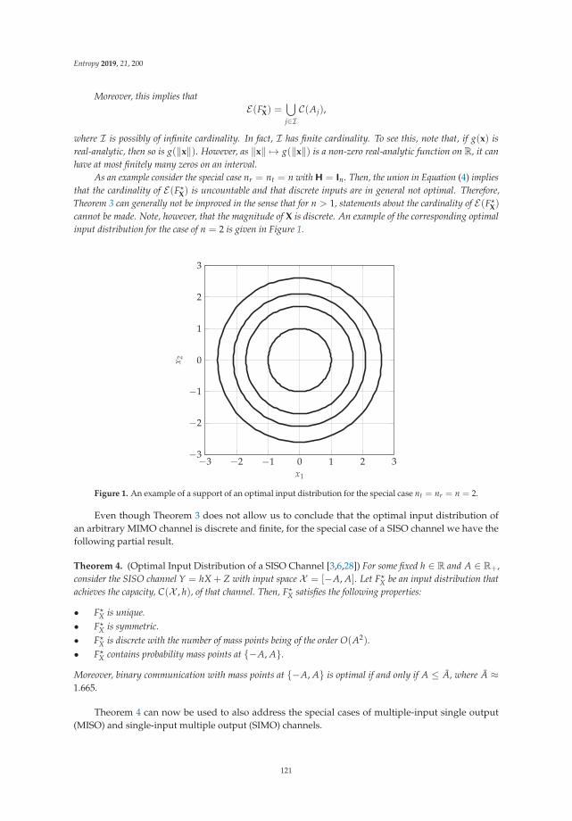
Entropy 2019, 21, 200

Moreover, this implies thatE(F�

X) =⋃j∈IC(Aj),

where I is possibly of infinite cardinality. In fact, I has finite cardinality. To see this, note that, if g(x) isreal-analytic, then so is g(‖x‖). However, as ‖x‖ �→ g(‖x‖) is a non-zero real-analytic function on R, it canhave at most finitely many zeros on an interval.

As an example consider the special case nr = nt = n with H = In. Then, the union in Equation (4) impliesthat the cardinality of E(F�

X) is uncountable and that discrete inputs are in general not optimal. Therefore,Theorem 3 can generally not be improved in the sense that for n > 1, statements about the cardinality of E(F�

X)

cannot be made. Note, however, that the magnitude of X is discrete. An example of the corresponding optimalinput distribution for the case of n = 2 is given in Figure 1.

−3 −2 −1 0 1 2 3−3

−2

−1

0

1

2

3

x1

x 2

Figure 1. An example of a support of an optimal input distribution for the special case nt = nr = n = 2.

Even though Theorem 3 does not allow us to conclude that the optimal input distribution ofan arbitrary MIMO channel is discrete and finite, for the special case of a SISO channel we have thefollowing partial result.

Theorem 4. (Optimal Input Distribution of a SISO Channel [3,6,28]) For some fixed h ∈ R and A ∈ R+,consider the SISO channel Y = hX + Z with input space X = [−A, A]. Let F�

X be an input distribution thatachieves the capacity, C(X , h), of that channel. Then, F�

X satisfies the following properties:

• F�X is unique.

• F�X is symmetric.

• F�X is discrete with the number of mass points being of the order O(A2).

• F�X contains probability mass points at {−A, A}.

Moreover, binary communication with mass points at {−A, A} is optimal if and only if A ≤ A, where A ≈1.665.

Theorem 4 can now be used to also address the special cases of multiple-input single output(MISO) and single-input multiple output (SIMO) channels.

121

Entropy 2019, 21, 200

Theorem 5. Let Y = hTX� + Z be a MISO channel with channel matrix hT ∈ Rnt and some optimal inputX� ∈ X ⊂ Rnt . Then, the distribution of hTX∗ is discrete with finitely many mass points. On the other hand,let Y = hX� + Z be a SIMO channel with channel matrix h ∈ Rnr . Then, the optimal input X� ∈ X ⊂ R hasa discrete distribution with finitely many mass points.

Proof. For the MISO case, the capacity can expressed as

C(X ,hT) = maxFX :X∈X

I(X;hTX + Z)

= maxFX :X∈X

I(hTX;hTX + Z)

= maxFS :S∈hTX

I(S; S + Z)

= maxFS :|S|≤rmax(h

TX )I(S; S + Z). (5)

Using Theorem 5 we have that the maximizing distribution in Equation (5) F�S , where S := hTX,

is discrete with finitely many mass points.For the SIMO case, the channel input distribution is discrete as a SIMO channel can be transformed

into a SISO channel. Thus, let A ∈ R+ be finite. Then, the capacity of the SIMO channel can beexpressed as

C(X ,h) = maxFX :|X|≤A

I(X;hX + Z)

= maxFX :|X|≤A

I(X; ‖h‖X + Z). (6)

Again, it follows from Theorem 5 that the mutual information in Equation (6) is maximizedby a channel input distribution, F�

X, that is discrete with finitely many mass points. This concludesthe proof.

Remark 5. Note that in the MISO case, we do not claim F�X to be discrete with finitely many points. To illustrate

the difficulty, let hT = [1,−1] so that

hTX� = hT

(X�

1X�

2

)= X�

1 − X�2 .

As X�1 and X�

2 can be arbitrarily correlated, we cannot rule out cases in which X�1 = X − D and

X�2 = X− 2D, with D a discrete random variable and X of arbitrary distribution. Clearly the distribution of

X� is not discrete.

Note that in general it can be shown that the capacity-achieving input distribution is discreteif the optimization problem in Equation (2) can be reformulated as an optimization over onedimensional distributions. This, for example, has been done in [5] for parallel channels with a totalamplitude constraint.

3.3. Properties of Capacity-Achieving Input Distributions in the Small (But Not Vanishing) Amplitude Regime

In this subsection, we study properties of capacity-achieving input distribution in the regime ofsmall amplitudes. To that end, we will need the notion of a subharmonic function.

Definition 3. (Subharmonic Function) Let f be a real-valued function that is twice continuously differentiableon an open set G ⊂ Rn. Then, f is subharmonic if ∇2 f ≥ 0 on G, where ∇2 denotes the Laplacian (if f is

twice differentiable, its Laplacian is given by ∇2 f (x1, . . . , xn) = ∑ni=1

∂2 f∂x2

i).

122

Entropy 2019, 21, 200

We use the following Theorem, which states that a subharmonic function always attains itsmaximum on the boundary of its domain.

Theorem 6. (Maximum Principle of Subharmonic Functions [29]) Let G ⊂ Rn be a connected open set.If f : G → R is subharmonic and attains a global maximum in the interior of G, then f is constant on G.

In addition to Theorem 6, we need the following result that has been proven in [30].

Lemma 1. Let the likelihood function of the output of a MIMO channel be defined as

� : Rnr → R , �(y) =fY(y)

1(2π)

nr2

e−‖y‖2

2

and let Ay denote the Hessian matrix of loge(�(y)

). Then, the Laplacian (or the trace of Ay) is given by

∇2 loge(�(y)

)= Tr(Ay) = E

[‖HX‖2|Y = y

]−

∥∥E[HX|Y = y]∥∥2. (7)

Theorem 7. Suppose that r2max(HX ) ≤ log2(e). Then, x �→ h(x; FX) is a subharmonic function for every FX.

Proof. Let FX be arbitrary and observe that

h(x; FX) = −E[log2

(fY(Hx + Z)

)]= −E

[�(Hx + Z)

]−E

[log2

(1

(2π)nr2

e−‖Hx+Z‖2

2

)]

= −E[�(Hx + Z)

]+E

[‖Hx + Z‖2

2

]log2(e) + log2

((2π)

nr2

)= −E

[�(Hx + Z)

]+‖Hx‖2 + nr

2log2(e) + log2

((2π)

nr2

).

With this expression in hand, the Laplacian of h(x; FX) with respect to x can be bounded frombelow as follows:

∇2h(x; FX) = ∇2(−E

[�(Hx + Z)

]+‖Hx‖2 + nr

2log2(e) + log2

((2π)

nr2

))= −E

[∇2�(Hx + Z)

]+∇2 ‖Hx‖2

2log2(e)

(a)= −E

[Tr

(HHTAHx+Z

)]+∇2 ‖Hx‖2

2log2(e)

= −E[Tr

(HHTAHx+Z

)]+ Tr

(HHT) log2(e)

(b)≥ −E

[Tr

(HHT)Tr

(AHx+Z

)]+ Tr

(HHT) log2(e)

= Tr(HHT) (−E[

Tr(AHx+Z)]+ log(e)

)(c)≥ Tr

(HHT) (−r2

max(HX ) + log(e))

, (8)

where (a) follows from Equation (7) and the chain rule for the Hessian; (b) from using thewell-known inequality

Tr(CD)2 ≤ Tr(C)2Tr(D)2

123

Entropy 2019, 21, 200

that holds for C and D positive semi-definite; and (c) from using the inequality

Tr(Ay

)= E

[‖HX‖2|Y = y

]−

∥∥E[HX|Y = y]∥∥2

≤ E[‖HX‖2|Y = y

]≤ r2

max(HX ).

Thus, according to the assumption that r2max(HX ) ≤ log2(e), the right-hand side of Equation (8)

is nonnegative, which proves the result.

Now, knowing that h(x; FX) is a subharmonic function allows us to characterize the support of anoptimal input distribution of a MIMO channel provided that the radius of the channel input space, X ,is sufficiently small.

Theorem 8. Let F�X be a capacity-achieving input distribution and r2

max(HX ) ≤ log2(e). Then, E(F�X) ⊆ ∂X .

Proof. From the KKT conditions in Equation (3), we know that, if x ∈ E(F�X), then x is a maximizer

of h(x; F�X). According to Theorem 7, we also know that h(x; F�

X) is subharmonic. Hence, from theMaximum Principle of Subharmonic Functions (i.e., Theorem 6), it follows E(F�

X) ⊆ ∂X .

Combining Theorem 8 with the observations made in Remark 4 leads to the following corollary.

Corollary 1. Let X = B0(A) and A ≤ 1‖H‖ log2(e). Then,

E(F�X) ⊆ C(A),

where C(A) := {x ∈ Rn : ‖x‖ = A} denotes a sphere of radius A.

We conclude this section by noting that for the special case nt = nr = n with H = In, the exactvalue of A such that E(F�

X) = C(A) has been characterized in terms of an integral equation in [31],which is approximately equal to 1.5

√n.

4. Upper and Lower Bounds on the Capacity

The considerations in the previous section have shown that characterizing the structure ofan optimal channel-input distribution is a challenging question in itself that we could only partiallyanswer. A full characterization, however, is a necessary prerequisite to narrow down the searchspace in Equation (2) to one that is tractable. Except for some special cases (i.e., special choices ofX ), optimizing over the most general space of input distributions that consists of all continuousnt-dimensional probability distributions FX with X ∈ X , is prohibitive (Note that Dytso et al. [32]summarized methods of how to optimize functionals over the space of probability distributions thatare constrained in there support). Thus, up to the writing of this paper, there is little hope in being ableto solve the problem in Equation (2) in full generality so that in this section we are proposing novellower and upper bounds on the capacity C(X ,H). Nevertheless, these bounds will allow us to betterunderstand how the capacity of such MIMO channels behaves.

Towards this end, in Section 4.1, we provide four upper bounds. The first is based on an upperbound on the differential entropy of a random vector that is constraint in its pth moment, the secondand third bounds are based on duality arguments, and the fourth on the relationship between mutualinformation and the minimum mean square error (MMSE), I-MMSE relationship for short, knownfrom [33]. The three lower bounds proposed in Section 4.2, on the other hand, are based on thecelebrated entropy power inequality, a generalization of the Ozarow–Wyner capacity bound takenfrom [11], and on Jensen’s inequality.

124

Entropy 2019, 21, 200

4.1. Upper Bounds

To establish our first upper bound on Equation (2), we need the following result ([11] Th. 1).

Lemma 2. (Maximum Entropy Under pth Moment Constraint) Let n ∈ N and p ∈ (0, ∞) be arbitrary.Then, for any U ∈ Rn such that h(U) < ∞ and ‖U‖p < ∞, we have

h(U) ≤ n log2

(kn,p n

1p ‖U‖p

),

where

kn,p :=

√π e

1p( p

n) 1

p Γ( n

p + 1) 1

n

Γ( n

2 + 1) 1

n.

Theorem 9. (Moment Upper Bound) For any channel input space X and any fixed channel matrix H,we have

C(X ,H) ≤ CM(X ,H) := infp>0

nr log2

(knr ,p

(2πe)12

n1pr ‖x + Z‖p

),

where x ∈ HX is chosen such that ‖x‖ = rmax(HX ).

Proof. Expressing Equation (2) in terms of differential entropies results in

C(X ,H) = maxFX :X∈X

h(HX + Z)− h(Z)

(a)≤ max

FX :X∈Xnr log2

(knr ,p

(2πe)12

n1pr ‖HX + Z‖p

)(b)= nr log2

(knr ,p

(2πe)12

n1pr max

FX :X∈X‖HX + Z‖p

), (9)

where (a) follows from Lemma 2 with the fact that h(Z) = nr2 log2(2πe); and (b) from the monotonicity

of the logarithm.Now, notice that ‖HX+Z‖p is linear in FX and therefore it attains its maximum at an extreme point

of the set FX := {FX : X ∈ X} (i.e., the set of all cumulative distribution functions of X). As a matterof fact [26], the extreme points of FX are given by the set of degenerate distributions on X ; that is,{FX(y) = δx(y), y ∈ X}x∈X . This allows us to conclude

maxFX :X∈X

‖HX + Z‖p = maxx∈X

‖Hx + Z‖p.

Observe that the Euclidian norm is a convex function, which is therefore maximized at theboundary of the set HX . Combining this with Equation (9) and taking the infimum over p > 0completes the proof.

The following Theorem provides two alternative upper bounds that are based on duality arguments.

Theorem 10. (Duality Upper Bounds) For any channel input space X and any fixed channel matrix H

C(X ,H) ≤ CDual,1(X ,H) := log2

(cnr (d) +

Vol(B0(d)

)(2πe)

nr2

), (10)

125

Entropy 2019, 21, 200

where

d := rmax(HX ) , cnr (d) :=nr−1

∑i=1

(nr − 1

i

) Γ(

nr−12

)2

nr2 Γ

( nr2)di,

and

C(X ,H) ≤ CDual,2(X ,H) :=nr

∑i=1

log2

(1 +

2Ai√2πe

), (11)

where a = (A1, . . . , Anr ) such that Box(a) = Box(HX ).

Proof. Using duality bounds, it has been shown in [8] that for any centered n-dimensional ball ofradius r ∈ R+

maxFX :X∈B0(r)

I(X; X + Z) ≤ log2

(cn(r) +

Vol(B0(r)

)(2πe)

n2

), (12)

where cn(r) := ∑n−1i=1 (n−1

i )Γ( n−1

2 )2

n2 Γ( n

2 )ri.

Now, observe that

C(X ,H) = maxFX :X∈X

h(HX + Z)− h(HX + Z|HX)

= maxFX :X∈X

I(HX;HX + Z)

= maxFX :X∈HX

I(X; X + Z) (13)

(a)≤ max

FX :X∈B0(d),d:=rmax(HX )I(X; X + Z)

(b)≤ log2

(cnr (d) +

Vol(B0(d)

)(2πe)

nr2

).

where (a) follows from enlarging the optimization domain; and (b) from using the upper bound inEquation (12). This proves Equation (10).

To show the upper bound in Equation (11), we proceed with an alternative upper boundto Equation (13):

C(X ,H) = maxFX :X∈HX

I(X; X + Z)

(a)≤ max

FX :X∈Box(HX )I(X; X + Z)

(b)≤ max

FX :X∈Box(HX )

nr

∑i=1

I(Xi; Xi + Zi)

(c)=

nr

∑i=1

maxFXi

:|Xi |≤Ai

I(Xi; Xi + Zi)

(d)≤

nr

∑i=1

log2

(1 +

2Ai√2πe

),

where the (in)equalities follow from: (a) enlarging the optimization domain; (b) single-letterizingthe mutual information; (c) choosing individual amplitude constraints (A1, . . . , Anr ) =: a ∈ R

nr+ such

that Box(a) = Box(HX ); and (d) using the upper bound in Equation (12) for n = 1. This concludesthe proof.

126

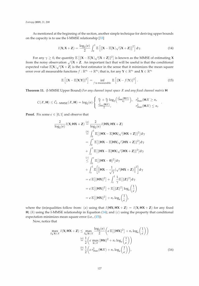
Entropy 2019, 21, 200

As mentioned at the beginning of the section, another simple technique for deriving upper boundson the capacity is to use the I-MMSE relationship [33]

I(X; X + Z) =log2(e)

2

∫ 1

0E

[∥∥X−E[X |√γX + Z]∥∥2

]dγ. (14)

For any γ ≥ 0, the quantity E[‖X−E[X |√γX + Z]‖2] is known as the MMSE of estimating X

from the noisy observation√

γX + Z. An important fact that will be useful is that the conditionalexpected value E[X |√γX + Z] is the best estimator in the sense that it minimizes the mean squareerror over all measurable functions f : Rnr → Rnt ; that is, for any Y ∈ Rnr and X ∈ Rnt

E

[‖X−E[X|Y]‖2

]= inf

f is measurableE

[‖X− f (Y)‖2

]. (15)

Theorem 11. (I-MMSE Upper Bound) For any channel input space X and any fixed channel matrix H

C(X ,H) ≤ CI−MMSE(X ,H) = log2(e)

⎧⎨⎩nr2 + nr

2 log2

(r2max(HX )

nr

), r2

max(HX ≥ nr

r2max(HX )

2 , r2max(HX ) ≤ nr

.

Proof. Fix some ε ∈ [0, 1] and observe that

2log2(e)

I(X;HX + Z)(a)=

2log2(e)

I(HX;HX + Z)

(b)=

∫ 1

0E[‖HX−E[HX|√γHX + Z]‖2]dγ

=∫ ε

0E[‖HX−E[HX|√γHX + Z]‖2]dγ

+∫ 1

εE[‖HX−E[HX|√γHX + Z]‖2]dγ

(c)≤

∫ ε

0E[‖HX− 0‖2]dγ

+∫ 1

εE

[∥∥∥HX− 1√γ(√

γHX + Z)∥∥∥2

]dγ

= εE[‖HX‖2]+ ∫ 1

ε

1γE[‖Z‖2]dγ

= εE[‖HX‖2]+E

[‖Z‖2] loge

(1ε

)= εE

[‖HX‖2]+ nr loge

(1ε

),

where the (in)equalities follow from: (a) using that I(HX;HX + Z) = I(X;HX + Z) for any fixedH; (b) using the I-MMSE relationship in Equation (14); and (c) using the property that conditionalexpectation minimizes mean square error (i.e., (15)).

Now, notice that

maxFX :X∈X

I(X;HX + Z) ≤ maxFX :X∈X

log2(e)2

(εE

[‖HX‖2]+ nr loge

(1ε

))(a)=

12

(ε max

x∈X‖Hx‖2 + nr loge

(1ε

))(b)=

12

(ε r2

max(HX ) + nr loge

(1ε

)), (16)

127

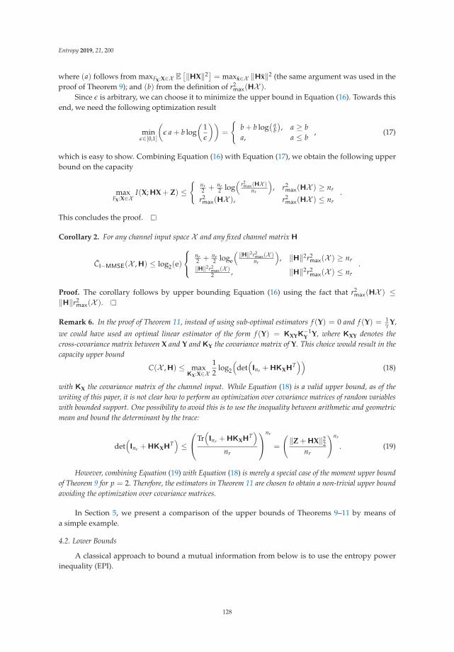
Entropy 2019, 21, 200

where (a) follows from maxFX :X∈X E[‖HX‖2] = maxx∈X ‖Hx‖2 (the same argument was used in the

proof of Theorem 9); and (b) from the definition of r2max(HX ).

Since ε is arbitrary, we can choose it to minimize the upper bound in Equation (16). Towards thisend, we need the following optimization result

minε∈[0,1]

(ε a + b log

(1ε

))=

{b + b log

( ab), a ≥ b

a, a ≤ b, (17)

which is easy to show. Combining Equation (16) with Equation (17), we obtain the following upperbound on the capacity

maxFX :X∈X

I(X;HX + Z) ≤{

nr2 + nr

2 log(

r2max(HX )

nr

), r2

max(HX ) ≥ nr

r2max(HX ), r2

max(HX ) ≤ nr.

This concludes the proof.

Corollary 2. For any channel input space X and any fixed channel matrix H

CI−MMSE(X ,H) ≤ log2(e)

⎧⎨⎩nr2 + nr

2 loge

(‖H‖2r2

max(X )nr

), ‖H‖2r2

max(X ) ≥ nr

‖H‖2r2max(X )2 , ‖H‖2r2

max(X ) ≤ nr

.

Proof. The corollary follows by upper bounding Equation (16) using the fact that r2max(HX ) ≤

‖H‖r2max(X ).

Remark 6. In the proof of Theorem 11, instead of using sub-optimal estimators f (Y) = 0 and f (Y) = 1γ Y,

we could have used an optimal linear estimator of the form f (Y) = KXYK−1Y Y, where KXY denotes the

cross-covariance matrix between X and Y and KY the covariance matrix of Y. This choice would result in thecapacity upper bound

C(X ,H) ≤ maxKX :X∈X

12

log2

(det

(Inr +HKXH

T))

(18)

with KX the covariance matrix of the channel input. While Equation (18) is a valid upper bound, as of thewriting of this paper, it is not clear how to perform an optimization over covariance matrices of random variableswith bounded support. One possibility to avoid this is to use the inequality between arithmetic and geometricmean and bound the determinant by the trace:

det(Inr +HKXH

T)≤

⎛⎝Tr(Inr +HKXH

T)

nr

⎞⎠nr

=

(‖Z +HX‖2

2nr

)nr

. (19)

However, combining Equation (19) with Equation (18) is merely a special case of the moment upper boundof Theorem 9 for p = 2. Therefore, the estimators in Theorem 11 are chosen to obtain a non-trivial upper boundavoiding the optimization over covariance matrices.

In Section 5, we present a comparison of the upper bounds of Theorems 9–11 by means ofa simple example.

4.2. Lower Bounds

A classical approach to bound a mutual information from below is to use the entropy powerinequality (EPI).

128

Entropy 2019, 21, 200

Theorem 12. (EPI Lower Bounds) For any fixed channel matrix H and any channel input space X with X

absolutely continuous, we have

C(X ,H) ≥ CEPI(X ,H) := maxFX :X∈X

nr

2log2

(1 +

22

nr h(HX)

2πe

). (20)

Moreover, if nt = nr = n, H ∈ Rn×n invertible, and X uniformly distributed over X , then

C(X ,H) ≥ CEPI(X ,H) :=n2

log2

(1 +

|det(H)| 2n Vol(X )

2n

2πe

). (21)

Proof. By means of the EPI

22

nr h(HX+Z) ≥ 22

nr h(HX) + 22

nr h(Z),

we conclude

22

nr C(X ,H) ≥ 1 + (2πe)−122

nr maxFX :X∈X

h(HX),

which finalizes the proof of the lower bound in Equation (20).To show the lower bound in Equation (21), all we need is to recall that

h(HX) = h(X) + log2 |det(H)|,

which is maximized for X uniformly distributed over X . However, if X is uniformly drawn from X ,we have

22n h(HX) = Vol(HX )

2n = |det(H)| 2

n Vol(X )2n ,

which completes the proof.

The considerations in Section 3 suggest that a channel input distribution that maximizesEquation (2) might be discrete. Therefore, there is a need for lower bounds that unlike the bounds inTheorem 12 rely on discrete inputs.

Theorem 13. (Ozarow–Wyner Type Lower Bound) Let XD ∈ supp(XD) ⊂ Rnt be a discrete random vectorof finite entropy, g : Rnr → Rnt a measurable function, and p > 0. Furthermore, let Kp be a set of continuousrandom vectors, independent of XD, such that for every U ∈ Kp we have h(U) < ∞, ‖U‖p < ∞, and

supp(U + xi) ∩ supp(U + xj) = ∅ (22)

for all xi, xj ∈ supp(XD), i �= j. Then,

C(X ,H) ≥ COW(X ,H) := [H(XD)− gap]+,

wheregap := inf

U∈Kpg measurable

p>0

(G1,p(U, XD, g) + G2,p(U)

)

with

G1,p(U, XD, g) := nt log2

(‖U + XD − g(Y)‖p

‖U‖p

), (23)

G2,p(U) := nt log2

⎛⎝ knt ,p n1pt ‖U‖p

21nt

h(U)

⎞⎠, (24)

129

Entropy 2019, 21, 200

and knt ,p as defined in Lemma 2, respectively.

Proof. The proof is identical to ([11] Theorem 2). To make the manuscript more self-contained,we repeat it here.

Let U and XD be statistically independent. Then, the mutual information I(XD; Y) can be lowerbounded as

I(XD; Y)(a)≥ I(XD + U; Y)

= h(XD + U)− h(XD + U|Y)(b)= H(XD) + h(U)− h(XD + U|Y). (25)

Here, (a) follows from the data processing inequality as XD + U → XD → Y forms a Markovchain in that order; and (b) from the assumption in Equation (22). By using Lemma 2, we have that thelast term in Equation (25) can be bounded from above as

h(XD + U|Y) ≤ nt log2

(knt ,p n

1pt ‖XD + U− g(Y)‖p

).

Combining this expression with Equation (25) results in

I(XD; Y) ≥ H(XD)−(G1,p(U, XD, g) + G2,p(U)

),

with G1,p and G2,p as defined in Equations (23) and (24), respectively. Maximizing the right-hand sideover all U ∈ Kp, measurable functions g : Rnr → Rnt , and p > 0 provides the bound.

Interestingly, the bound of Theorem 13 holds for arbitrary channels and is therefore not restrictedto MIMO channels. The interested reader is referred to [11] for details.

We conclude the section by providing a lower bound that is based on Jensen’s inequality andholds for arbitrary inputs.

Theorem 14. (Jensen’s Inequality Lower Bound) For any channel input space X and any fixed channelmatrix H, we have

C(X ,H) ≥ CJensen(X ,H) := maxFX :X∈X

log+2

((2e

) nr2

ψ−1(X,H)

)(26)

with

ψ(X,H) := E

[exp

(−‖H(X− X′)‖2

4

)]= E

⎡⎣∣∣∣∣∣φX

(HTZ√

2

)∣∣∣∣∣2⎤⎦ ,

where X′ is an independent copy of X and φX denotes the characteristic function of X.

Proof. To show the lower bound, we follow an approach of Dytso et al. [34]. Note that byJensen’s inequality

h(Y) = −E[log2 fY(Y)] ≥ − log2 E[ fY(Y)] = − log2

∫Rnr

fY(y) fY(y)dy. (27)

Now, evaluating the integral in Equation (27) results in

∫Rnr

fY(y) fY(y)dy =1

(2π)nr

∫Rnr

E

[e−

‖y−HX‖22

]E

[e−

‖y−HX′‖22

]dy

130

Entropy 2019, 21, 200

(a)=

1(2π)nr

E

[∫Rnr

e−‖y−HX‖2+‖y−HX′‖2

2 dy

](b)=

1(2π)nr

E

[e−

‖HX−HX′‖24

∫Rnr

e−‖y−H(X−X′)2 ‖2

dy

](c)=

1

2nr πnr2E

[e−

‖H(X−X′)‖24

], (28)

where (a) follows from the independence of X and X′ and Tonelli’s Theorem ([35] Chapter 5.9);

(b) from completing a square; and (c) from the fact that∫Rnr e−‖y−H(X−X′)

2 ‖2dy =

∫Rnr e−‖y‖2

dy = πnr2 .

Combining Equation (27) with Equation (28) and subtracting h(Z) = nr2 log2(2πe) completes the proof

of the first version of the bound.To show the second version, observe that

E

[e−

‖H(X−X′)‖24

](d)= E

[φH(X−X′)√

2

(Z)]

(e)= E

[φHX√

2(Z)φ−HX′√

2(Z)

]( f )= E

[φX

(HTZ√

2

)φX′

(−HTZ√

2

)](g)= E

[φX

(HTZ√

2

)φX

(−HTZ√

2

)](h)= E

[φX

(HTZ√

2

)φ∗X

(HTZ√

2

)]

= E

⎡⎣∣∣∣∣∣φX

(HTZ√

2

)∣∣∣∣∣2⎤⎦ ,

where (d) follows from Parseval’s identity ([35] Chapter 9.5) by noting that exp(−‖ · ‖2/2)is a characteristic function of Z and φH(X−X′)√

2

(·) is a characteristic function of H(X−X′)√2

; (e) from using

the property that the characteristic function of a sum of random vectors is equal to the product of itscharacteristic functions; ( f ) from using the fact that a characteristic function is a linear transformation;(g) from using that X and X′ have the same characteristic function; and (h) from the fact that thecharacteristic function is Hermitian. This completes the proof.

Remark 7. As is evident from our examples in the following sections, in many cases, the Jensen’s inequalitylower bound of Theorem 14 performs remarkably well. The bound, however, is also useful for MIMO channelsthat are subject to an average power constraint. For example, evaluating Equation (26) with X ∼ N (0,KX)

results in

I(X;HX + Z) ≥ 12

log+2

((2e

)min(nr ,nt)

det(Inr +HKXH

T))

.

Note that this bound is within min(nr ,nt)2 log2

( 2e)

bits of the capacity of the power-constrained channel.

In Section 3, we discuss that the distributions that maximize mutual information in nt-dimensionsare typically singular, which means that they are concentrated on a set of Lebesgue measure zero.Singular distributions generally do not have a probability density, whereas the characteristic functionalways exists. This is why the version of Jensen’s inequality lower bound in Theorem 14 that isbased on the characteristic function of the channel input is especially useful for amplitude-constrainedMIMO channels.

131

Entropy 2019, 21, 200

5. Invertible Channel Matrices

Consider the symmetric case of nt = nr = n antennas with H ∈ Rn×n being invertible. In thissection, we evaluate some of the lower and upper bounds proposed in the previous section for thespecial case of H being also diagonal and then characterize the gap to the capacity for arbitraryinvertible channel matrices.

5.1. Diagonal Channel Matrices

Suppose the channel inputs are subject to per-antenna or an n-dimensional amplitude constraint.Then, the duality upper bound CDual,2(X ,H) of Theorem 10 takes on the following form.

Theorem 15. (Upper Bounds) Let H = diag(h11, . . . , hnn) ∈ Rn×n be fixed. If X = Box(a) for somea = (A1, . . . , An) ∈ Rn

+, then

CDual,2(Box(a),H) =n

∑i=1

log2

(1 +

2|hii|Ai√2πe

). (29)

Moreover, if X = B0(A) for some A ∈ R+, then

CDual,2(B0(A),H) =n

∑i=1

log2

(1 +

2|hii|A√n√

2πe

). (30)

Proof. The bound in Equation (29) immediately follows from Theorem 10 by observing thatBox(HBox(a)) = Box(Ha). The bound in Equation (30) follows from Theorem 10 by the fact that

Box(HB0(A)

)⊂ Box

(HBox

(B0(A)

))= Box(h),

where h := A√n (|h11|, . . . , |hnn|). This concludes the proof.

For an arbitrary channel input spaceX , the EPI lower bound of Theorem 12 and Jensen’s inequalitylower bound of Theorem 14 take on the following form.

Theorem 16. (Lower Bounds) Let H = diag(h11, . . . , hnn) ∈ Rn×n be fixed and X arbitrary. Then,

CJensen(X ,H) = log+2

((2e

) n2 1

ψ(H, b�)

)(31)

with

ψ(H, b�) := minb∈X

n

∏i=1

ϕ(|hii|Bi),

where b := (B1, . . . , Bn) and ϕ : R+ → R+,

ϕ(x) :=1x2

(e−x2 − 1 +

√πx

(1− 2Q(

√2x)

)). (32)

Moreover,

CEPI(X ,H) =n2

log2

(1 + Vol(X )

2n|∏n

i=1 hii|2n

2πe

). (33)

132

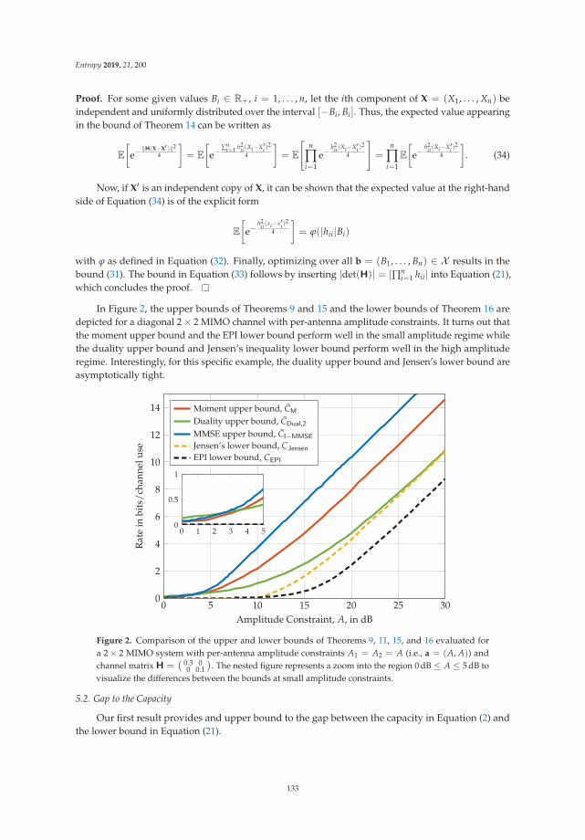
Entropy 2019, 21, 200

Proof. For some given values Bi ∈ R+, i = 1, . . . , n, let the ith component of X = (X1, . . . , Xn) beindependent and uniformly distributed over the interval [−Bi, Bi]. Thus, the expected value appearingin the bound of Theorem 14 can be written as

E

[e−

‖H(X−X′)‖24

]= E

[e−

∑ni=1 h2

ii(Xi−X′i )2

4

]= E

[n

∏i=1

e−h2

ii(Xi−X′i )2

4

]=

n

∏i=1

E

[e−

h2ii(Xi−X′i )

2

4

]. (34)

Now, if X′ is an independent copy of X, it can be shown that the expected value at the right-handside of Equation (34) is of the explicit form

E

[e−

h2ii(xi−x′i )

2

4

]= ϕ(|hii|Bi)

with ϕ as defined in Equation (32). Finally, optimizing over all b = (B1, . . . , Bn) ∈ X results in thebound (31). The bound in Equation (33) follows by inserting |det(H)| = |∏n

i=1 hii| into Equation (21),which concludes the proof.

In Figure 2, the upper bounds of Theorems 9 and 15 and the lower bounds of Theorem 16 aredepicted for a diagonal 2× 2 MIMO channel with per-antenna amplitude constraints. It turns out thatthe moment upper bound and the EPI lower bound perform well in the small amplitude regime whilethe duality upper bound and Jensen’s inequality lower bound perform well in the high amplituderegime. Interestingly, for this specific example, the duality upper bound and Jensen’s lower bound areasymptotically tight.

0 5 10 15 20 25 300

2

4

6

8

10

12

14

Amplitude Constraint, A, in dB

Rat

ein

bits

/ch

anne

luse

Moment upper bound, CM

Duality upper bound, CDual,2

MMSE upper bound, CI−MMSE

Jensen’s lower bound, CJensen

EPI lower bound, CEPI

0 1 2 3 4 50

0.5

1

Figure 2. Comparison of the upper and lower bounds of Theorems 9, 11, 15, and 16 evaluated fora 2× 2 MIMO system with per-antenna amplitude constraints A1 = A2 = A (i.e., a = (A, A)) andchannel matrix H =

(0.3 00 0.1

). The nested figure represents a zoom into the region 0 dB ≤ A ≤ 5 dB to

visualize the differences between the bounds at small amplitude constraints.

5.2. Gap to the Capacity

Our first result provides and upper bound to the gap between the capacity in Equation (2) andthe lower bound in Equation (21).

133

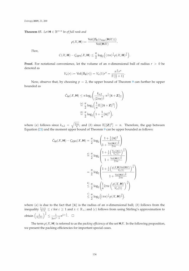
Entropy 2019, 21, 200

Theorem 17. Let H ∈ Rn×n be of full rank and

ρ(X ,H) :=Vol

(B0 (rmax(HX ))

)Vol(HX )

.

Then,C(X ,H)− CEPI(X ,H) ≤ n

2log2

((πn)

1n ρ(X ,H)

2n

).

Proof. For notational convenience, let the volume of an n-dimensional ball of radius r > 0 bedenoted as

Vn(r) := Vol(B0(r)

)= Vn(1)rn =

πn2 rn

Γ( n

2 + 1) .

Now, observe that, by choosing p = 2, the upper bound of Theorem 9 can further be upperbounded as

CM(X ,H) ≤ n log2

(kn,2

(2πe)12

n12 ‖x + Z‖2

)(a)=

n2

log2

(1nE[‖x + Z‖2])

(b)=

n2

log2

(1 +

1n‖x‖2

),

where (a) follows since kn,2 =√

2πen ; and (b) since E[‖Z‖2] = n. Therefore, the gap between

Equation (21) and the moment upper bound of Theorem 9 can be upper bounded as follows:

CM(X ,H)− CEPI(X ,H) =n2

log2

⎛⎝ 1 + 1n‖x‖2

1 + Vol(HX )2n

2πe

⎞⎠a)=

n2

log2

⎛⎜⎜⎝1 + 1n

(Vn(‖x‖)

Vn(1)

) 2n

1 + Vol(HX )2n

2πe

⎞⎟⎟⎠

=n2

log2

⎛⎜⎜⎝1 + 1n

(ρ(X ,H)Vol(HX )

Vn(1)

) 2n

1 + Vol(HX )2n

2πe

⎞⎟⎟⎠b)≤ n

2log2

(1n

2πe(

ρ(X ,H)

Vn(1)

) 2n)

c)≤ n

2log2

((πn)

1n ρ(X ,H)

2n

).

where (a) is due to the fact that ‖x‖ is the radius of an n-dimensional ball; (b) follows from theinequality 1+cx

1+x ≤ c for c ≥ 1 and x ∈ R+; and (c) follows from using Stirling’s approximation to

obtain(

1Vn(1)

) 2n ≤ 1

2eπ1− 1n

n1+ 1n .

The term ρ(X ,H) is referred to as the packing efficiency of the set HX . In the following proposition,we present the packing efficiencies for important special cases.

134

Entropy 2019, 21, 200

Proposition 1. (Packing Efficiencies) Let H ∈ Rn×n be of full rank, A ∈ R+, and a := (A1, . . . , An) ∈Rn+. Then,

ρ(B0(A), In

)= 1, (35)

ρ(B0(A),H

)=

‖H‖n

|det(H)| , (36)

ρ(Box(a), In

)=

πn2

Γ( n

2 + 1) ‖a‖n

∏ni=1 Ai

, (37)

ρ(Box(a),H

)≤ π

n2

Γ( n

2 + 1) ‖H‖n‖a‖n

|det(H)|∏ni=1 Ai

. (38)

Proof. The packing efficiency in Equation (35) follows immediately. Note that

rmax(HB0(A)

)= max

x∈B0(A)‖Hx‖ = ‖H‖A.

Thus, as H is assumed to be invertible, we have Vol(HB0(A)) = |det(H)|Vol(B0(A)),which results in Equation (36). To show Equation (37), observe that

Vol(B0

(rmax

(InBox(a)

)))= Vol

(B0(‖a‖)

)=

πn2

Γ( n

2 + 1)‖a‖n.

The proof of Equation (37) is concluded by observing that Vol(InBox(a)) = ∏ni=1 Ai. Finally,

observe that Box(a) ⊂ B0(‖a‖) implies rmax(HBox(a)) ≤ rmax(HB0(‖a‖)) so that

ρ(H, Box(a)

)≤ Vol

(B0(‖H‖‖a‖)

)Vol

(HBox(a)

) =π

n2

Γ( n

2 + 1) ‖H‖n‖a‖n

|det(H)|∏ni=1 Ai

,

which is the bound in Equation (38).

We conclude this section by characterizing the gap to the capacity when H is diagonal and thechannel input space is the Cartesian product of n PAM constellations. In this context, PAM(N, A)

refers to the set of N ∈ N equidistant PAM-constellation points with amplitude constraint A ∈ R+

(see Figure 3 for an illustration), whereas X ∼ PAM(N, A) means that X is uniformly distributed overPAM(N, A) [11].

Figure 3. Example of a pulse-amplitude modulation constellation with N = 4 points and amplitudeconstraint A (i.e., PAM(4, A)), where Δ := A/(N− 1) denotes half the Euclidean distance between twoadjacent constellation points. In the case N is odd, 0 is a constellation point.

Theorem 18. Let H = diag(h11, . . . , hnn) ∈ Rn×n be fixed and X = (X1, . . . , Xn). Then, if Xi ∼PAM(Ni, Ai), i = 1, . . . , n, for some given a = (A1, . . . , An) ∈ Rn

+, it holds that

CDual,2(Box(a),H)− COW(Box(a),H) ≤ c · n bits, (39)

135

Entropy 2019, 21, 200

where Ni :=⌊

1 + 2Ai |hii |√2πe

⌋and

c := 1 +12

log2

(πe6

)+

12

log2

(1 +

6πe

)≈ 1.64.

Moreover, if Xi ∼ PAM(Ni, A), i = 1, . . . , n, for some given A ∈ R+, it holds that

CDual,2(B0(A),H)− COW(B0(A),H) ≤ c · n bits, (40)

where Ni :=⌊

1 + 2A|hii |√n√

2πe

⌋.

Proof. Since the channel matrix is diagonal, letting the channel input X be such that its elements Xi,i = 1, . . . , n, are independent, we have that

I(X;HX + Z) =n

∑i=1

I(Xi; hiiXi + Zi).

Let Xi ∼ PAM(Ni, Ai) with Ni :=⌊

1 + 2Ai |hii |√2πe

⌋and observe that half the Euclidean distance

between any pair of adjacent points in PAM(Ni, Ai) is equal to Δi := Ai/(Ni − 1) (see Figure 3),i = 1, . . . , n. To lower bound the mutual information I(Xi; hiiXi + Zi), we use the bound of Theorem 13for p = 2 and nt = 1. Thus, for some continuous random variable U that is uniformly distributed overthe interval [−Δi, Δi) and independent of Xi, we have that

I(Xi; hiiXi + Zi) ≥ H(Xi)−12

log2

(πe6

)− 1

2log2

(E[(U + Xi − g(Yi))

2]E[U2]

). (41)

Now, note that the entropy term in Equation (41) can be lower bounded as

H(Xi) = log2

(⌊1 +

2Ai|hii|√2πe

⌋)≥ log2

(1 +

2Ai|hii|√2πe

)+ log2(2), (42)

where we have used that �x� ≥ x2 for every x ≥ 1. On the other hand, the last term in Equation (41)

can be upper bounded by upper bounding its argument as follows:

E[(U + Xi − g(Yi))

2]E[U2]

a)= 1 +

3E[(Xi − g(Yi))

2]Δ2

ib)≤ 1 +

3E[Z2i ](Ni − 1)2

A2i |hii|2

= 1 +3(Ni − 1)2

A2i |hii|2

c)≤ 1 +

3(

2Ai |hii |√2πe

)2

A2i |hii|2

= 1 +6

πe. (43)

where (a) follows from using that Xi and U are independent and E[U2] =Δ2

i3 ; (b) from using the

estimator g(Yi) =1

hiiYi; and (c) from Ni =

⌊1 + 2Ai |hii |√

2πe

⌋≤ 1 + 2Ai |hii |√

2πe. Combining Equations (41), (42),

and (43) results in the gap in (39).The proof of the capacity gap in Equation (40) follows along similar lines, which concludes

the proof.

136

Entropy 2019, 21, 200

We are also able to determine the gap to the capacity for a general invertible channel matrix.

Theorem 19. For any X and any invertible H

C(X ,H)− COW(X ,H) ≤ log2(πn) +n2

log2

(1 + 4n(4 + 4n)

(‖H−1‖2r2

max(HX )

r2min(X )

+n‖H−1‖2

r2min(X )

)).

Proof. Let X be uniformly distributed over a set constructed from an n-dimensional cubic lattice withthe number of points equal to N =

⌊‖x + Z‖n

2⌋, where x ∈ HX is chosen such that ‖x‖ = rmax(HX ),

and scaled such that it is contained in the input space X . Note that the minimum distance betweenpoint in X are given by

dmin

(supp(X)

):=

rmin(X )

N1n

.

Now, we compute the difference between the moment upper bound of Theorem 9 and theOzarow–Wyner lower bound of Theorem 13:

CM(X ,H)− COW(X ,H)(a)≤ log2(‖x + Z‖2)− H(X) + gap

= n log2(‖x + Z‖2)− log2(�‖x + Z‖n2�) + gap

(b)≤ log2(2) + gap, (44)

where (a) follows from Theorem 9 by choosing p = 2; and (b) by using the bound �x� ≥ x2 for x > 1.

The next step in the proof consists in bounding the gap term, which requires to upper bound the termsin Equations (23) and (24) individually. Towards this end, choose p = 2 and let U be a random vectorthat is uniformly distributed over a ball of radius dmin(X). Thus, for (23) it follows

G1,2(U, X, g) = n log2

(‖U + X− g(Y)‖2

‖U‖2

)(a)= n log2

(‖U−H−1Z‖2

‖U‖2

)

=n2

log2

(1 +

‖H−1Z‖22

‖U‖22

)(b)=

n2

log2

(1 +

4(4 + 4n)‖H−1Z‖22

d2min

(supp(X)

) )(c)≤ n

2log2

(1 +

(4 + 4n)‖H−1Z‖22 ‖x + Z‖2

2r2min(X )

)(d)=

n2

log2

(1 +

(4 + 4n)‖H−1Z‖22(r2max(HX ) + n

)r2min(X )

)(e)≤ n

2log2

(1 +

4(4 + 4n)‖H−1‖2‖Z‖22(r2max(HX ) + n

)r2min(X )

)

=n2

log2

(1 +

4(4 + 4n)‖H−1‖2n(r2max(HX ) + n

)r2min(X )

).

137

Entropy 2019, 21, 200

where (a) follows by choosing g(Y) = H−1Y: (b) by using ‖U‖22 = r2

4+2n , where r = dmin(supp(X))2 is

the radius of an n-dimensional ball; (c) from dropping the floor function in the expression for theminimum distance, i.e.,

d−1min

(supp(X)

)=

N1n

rmin(X )=

⌊‖x + Z‖n

2⌋ 1

n

rmin(X )≤ ‖x + Z‖2

rmin(X );

(d) follows by expanding ‖x + Z‖22 using that ‖x‖ = rmax(HX ); and (e) from using the bound

‖H−1Z‖2 ≤ ‖H−1‖‖Z‖2.On the other hand, the term G2,p(U) can be bounded from above as follows ([36] Appendix L):

G2,p(U) = n log2

⎛⎝ kn,p n1p ‖U‖p

21n h(U)

⎞⎠ ≤ n log2

((πn)

1n

).

Combining these two bounds with the one in (44) provides the result.

6. Arbitrary Channel Matrices

For an arbitrary MIMO channel with an average power constraint, it is well known that thecapacity is achieved by a singular value decomposition (SVD) of the channel matrix (i.e., H = UΛVT)along with considering the equivalent channel model

Y = ΛX + Z,

where Y := UTY, X := VTX, and Z := UTZ, respectively.To provide lower bounds for channels with amplitude constraints and SVD precoding, we need

the following lemma.

Lemma 3. For any given orthogonal matrix V ∈ Rnt×nt and constraint vector a = (A1, . . . , Ant) ∈ Rnt+ , there

exists a distribution FX of X such that X = VTX is uniformly distributed over Box(a). Moreover, the componentsX1, . . . , Xnt of X are mutually independent with Xi uniformly distributed over [−Ai, Ai], i = 1, . . . , nt.

Proof. Suppose that X is uniformly distributed over Box(a); that is, the density of X is of the form

fX(x) =1

Vol(Box(a)

) , x ∈ Box(a).

Since V is orthogonal, we have VX = X and by the change of variable Theorem for x ∈ VBox(a)

fX(x) =1

|det(V)| fX(VTx) =

1|det(V)|Vol

(Box(a)

) =1

Vol(Box(a)

) .

Therefore, such a distribution of X exists.

Theorem 20. (Lower Bounds with SVD Precoding) Let H ∈ Rnr×nt be fixed, nmin := min(nr, nt),and X = Box(a) for some a = (A1, . . . , Ant) ∈ R

nt+ . Furthermore, let σi, i = 1, . . . , nmin, be the ith singular

value of H. Then,

CJensen(Box(a),H) = log+2

((2e

) nmin2 1

ψ(H, b�)

)(45)

and

CEPI(Box(a),H) =nmin

2log2

⎛⎝1 +

∣∣∏nmini=1 Aiσi

∣∣ 2nmin

2πe

⎞⎠, (46)

138

Entropy 2019, 21, 200

where

ψ(H, b�) := minb∈Box(a)

nmin

∏i=1

ϕ(σiBi)

with b := (B1, . . . , Bnt) and ϕ as defined in Equation (32).

Proof. Performing the SVD, the expected value in Theorem 14 can be written as

E

[e−

‖H(X−X′)‖24

]= E

[e−

‖UΛVT (X−X′)‖24

]= E

[e−

‖ΛVT (X−X′)‖24

]= E

[e−

‖Λ(X−X′)‖24

].

By Lemma 3, there exists a distribution FX such that the components of X are independent anduniformly distributed. Since Λ is a diagonal matrix, we can use Theorem 16 to arrive at Equation (45).

Note that by Lemma 3 there exists a distribution on X such that X is uniform over Box(a) ⊂ Rnt

and ΛX is uniform over ΛBox(a) ⊂ Rnmin , respectively. Therefore, by the EPI lower bound given inEquation (20), we obtain

CEPI(Box(a),H) =nmin

2log2

⎛⎝1 +2

2nmin

h(ΛX)

2πe

⎞⎠=

nmin

2log2

⎛⎝1 +Vol

(ΛBox(a)

) 2nmin

2πe

⎞⎠=

nmin

2log2

⎛⎝1 +

(∏nmin

i=1 Ai) 2

nmin∣∣∏nmin

i=1 σi∣∣ 2

nmin

2πe

⎞⎠,

which is exactly the expression in Equation (46). This concludes the proof.

Remark 8. Notice that choosing the optimal b for the lower bound in Equation (45) is an amplitude allocationproblem, which is reminiscent of waterfilling in the average power constraint case. It would be interesting tostudy whether the bound in Equation (45) is connected to what is called mercury waterfilling in [37,38].

In Figure 4, the lower bounds of Theorem 20 are compared to the moment upper bound ofTheorem 2 for the special case of a 3× 1 MIMO channel. Similar to the example presented in Figure 2,the EPI lower bound performs well in the low amplitude regime, while Jensen’s inequality lowerbound performs well in the high amplitude regime.

We conclude this section by showing that for an arbitrary channel input space X , in the largeamplitude regime the capacity pre-log is given by min(nr, nt).

Theorem 21. Let X be arbitrary and H ∈ Rnr×nt fixed. Then,

limrmin(X )→∞

C(X ,H)

log2

(1 + 2rmin(X )√

2πe

) = min(nr, nt).

Proof. Notice that there always exists a ∈ Rnt+ and c ∈ R+ such that Box(a) ⊆ X ⊂ cBox(a). Thus,

without loss of generality, we can consider X = Box(a), a = (A, . . . , A), for sufficiently large A ∈ R+.To prove the result, we therefore start with enlarging the constraint set of the bound in Equation (11):

Box(HBox(a)

)⊆ B0

(rmax

(HBox(a)

))⊆ B0

(rmax

(HB0(

√nt A)

))= B0

(rmax

(UΛVTB0(

√nt A)

))

139

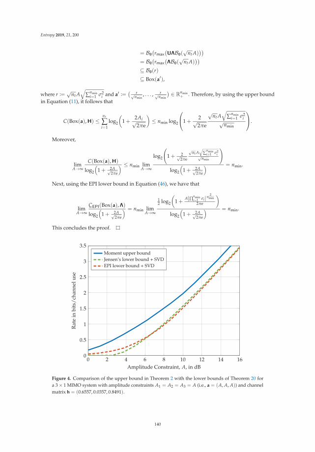
Entropy 2019, 21, 200

= B0

(rmax

(UΛB0(

√nt A)

))= B0

(rmax

(ΛB0(

√nt A)

))⊆ B0(r)

⊆ Box(a′),

where r :=√

nt A√

∑nmini=1 σ2

i and a′ :=( r√

nmin, . . . , r√

nmin

)∈ R

nmin+ . Therefore, by using the upper bound

in Equation (11), it follows that

C(Box(a),H) ≤nr

∑i=1

log2

(1 +

2Ai√2πe

)≤ nmin log2

⎛⎝1 +2√2πe

√nt A

√∑nmin

i=1 σ2i√

nmin

⎞⎠.

Moreover,

limA→∞

C(Box(a),H)

log2

(1 + 2A√

2πe

) ≤ nmin limA→∞

log2

(1 + 2√

2πe

√nt A

√∑

nmini=1 σ2

i√nmin

)log2

(1 + 2A√

2πe

) = nmin.

Next, using the EPI lower bound in Equation (46), we have that

limA→∞

CEPI(Box(a),Λ)

log2

(1 + 2A√

2πe

) = nmin limA→∞

12 log2

(1 +

A|∏nmini=1 σi|

2nmin

2πe

)log2

(1 + 2A√

2πe

) = nmin.


0 2 4 6 8 10 12 14 160

0.5

1

1.5

2

2.5

3

3.5


Rat

ein

bits

/ch

anne

luse

Moment upper boundJensen’s lower bound + SVDEPI lower bound + SVD

Figure 4. Comparison of the upper bound in Theorem 2 with the lower bounds of Theorem 20 fora 3× 1 MIMO system with amplitude constraints A1 = A2 = A3 = A (i.e., a = (A, A, A)) and channelmatrix h = (0.6557, 0.0357, 0.8491).

140

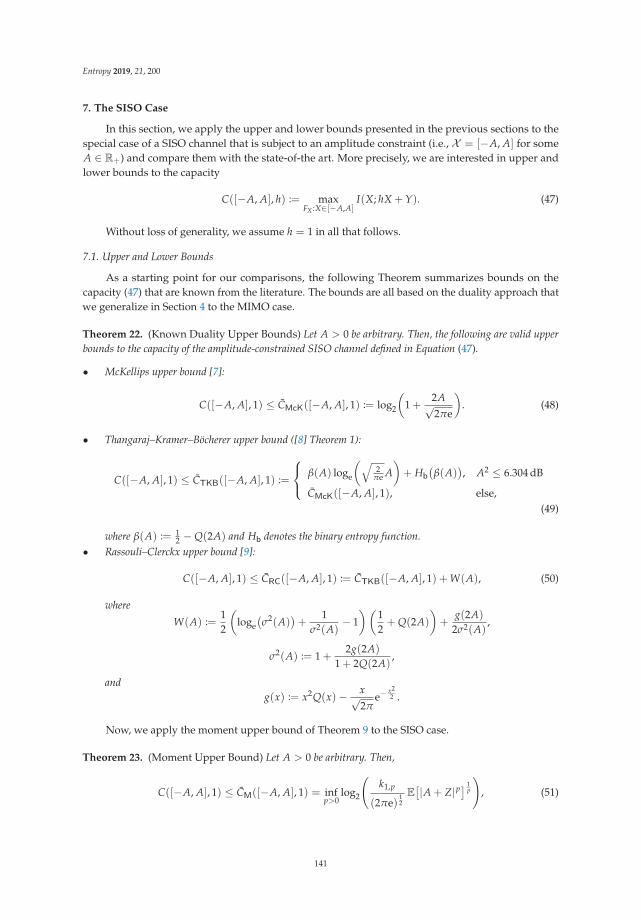
Entropy 2019, 21, 200

7. The SISO Case

In this section, we apply the upper and lower bounds presented in the previous sections to thespecial case of a SISO channel that is subject to an amplitude constraint (i.e., X = [−A, A] for someA ∈ R+) and compare them with the state-of-the art. More precisely, we are interested in upper andlower bounds to the capacity

C([−A, A], h) := maxFX :X∈[−A,A]

I(X; hX + Y). (47)

Without loss of generality, we assume h = 1 in all that follows.

7.1. Upper and Lower Bounds

As a starting point for our comparisons, the following Theorem summarizes bounds on thecapacity (47) that are known from the literature. The bounds are all based on the duality approach thatwe generalize in Section 4 to the MIMO case.

Theorem 22. (Known Duality Upper Bounds) Let A > 0 be arbitrary. Then, the following are valid upperbounds to the capacity of the amplitude-constrained SISO channel defined in Equation (47).

• McKellips upper bound [7]:

C([−A, A], 1) ≤ CMcK([−A, A], 1) := log2

(1 +

2A√2πe

). (48)

• Thangaraj–Kramer–Böcherer upper bound ([8] Theorem 1):

C([−A, A], 1) ≤ CTKB([−A, A], 1) :=

⎧⎨⎩ β(A) loge

(√2

πe A)+ Hb

(β(A)

), A2 ≤ 6.304 dB

CMcK([−A, A], 1), else,(49)

where β(A) := 12 −Q(2A) and Hb denotes the binary entropy function.

• Rassouli–Clerckx upper bound [9]:

C([−A, A], 1) ≤ CRC([−A, A], 1) := CTKB([−A, A], 1) + W(A), (50)

where

W(A) :=12

(loge

(σ2(A)

)+

1σ2(A)

− 1)(

12+ Q(2A)

)+

g(2A)

2σ2(A),

σ2(A) := 1 +2g(2A)

1 + 2Q(2A),

andg(x) := x2Q(x)− x√

2πe−

x22 .

Now, we apply the moment upper bound of Theorem 9 to the SISO case.

Theorem 23. (Moment Upper Bound) Let A > 0 be arbitrary. Then,

C([−A, A], 1) ≤ CM([−A, A], 1) = infp>0

log2

(k1,p

(2πe)12E[|A + Z|p

] 1p

), (51)

141

Entropy 2019, 21, 200

where the expected value is of the explicit form

E[|A + Z|p

]=

2p2 Γ

(p+1

2

)√

π1F1

(− p

2;

12

;−A2

2

)with 1F1(a; b; z) being the confluent hypergeometric function of the first kind ([39] Chapter 13).

Proof. First, note that rmax([−A, A]) = A. Then, by using the expression for the raw absolute momentof a Gaussian distribution given in [40], we have that

maxa∈[0,A]

E[|a + Z|p

]= max

a∈[0,A]

2p2 Γ

(p+1

2

)√

π1F1

(− p

2;

12

;− a2

2

).

The proof is concluded by observing that f (a) := 1F1

(− p

2 ; 12 ;− a2

2

)is an increasing function

in a.

The following theorem establishes the EPI and the Jensen lower bound of Section 4.2 assumingthe channel input symbols are uniformly distributed.

Theorem 24. (Lower Bounds with Uniform Inputs) Let A > 0 be arbitrary and the channel input X beuniformly distributed over [−A, A]. Then,

C([−A, A], 1) ≥ CEPI([−A, A], 1) =12

log2

(1 +

2A2

πe

)(52)

and

C([−A, A], 1) ≥ CJensen([−A, A], 1) = log2

⎛⎝ √2A2

e12

(e−A2 − 1 +

√πA

(1− 2Q

(√2A

)))⎞⎠. (53)

Proof. The lower bound in Equation (52) follows from Theorem 12 by observing that Vol(X ) = 2A.To show the lower bound in Equation (53), consider Theorem 14 and let X and X′ be independent anduniformly distributed over [−A, A]. Then, we have

E

[e−

|X−X′ |24

]=

14A2

∫ A

−A

∫ A

−Ae−

(x−x′)24 dx dx′

=1

A2

(e−A2 − 1 +

√πA

(1− 2Q

(√2A

))),

which concludes the proof.

Restricting the channel inputs to be discrete allows for another set of lower boundson Equation (47).

Theorem 25. (Lower Bounds with Discrete Inputs) Let A > 1 be arbitrary, XB ∈ {−A, A} equally likely,and XD ∼ PAM(N) with N =

⌈1 + A√

2πe

⌉. Then,

C([−A, A], 1) ≥ CBinary([−A, A], 1) := I(XB; XB + Z) (54)

=1

loge(2)

⎛⎝A2 −∫ ∞

−∞

e−y22√

2πloge

(cosh(A2 − Ay)

)dy

⎞⎠ , (55)

142

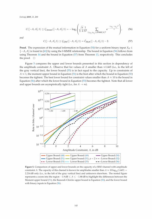
Entropy 2019, 21, 200

C([−A, A], 1) ≥ CJensen([−A, A], 1) = − log2

⎛⎜⎝√e2

1N2 ∑

(xDi,xDj

)∈PAM(N)2

e−(xDi

−xDj)2

4

⎞⎟⎠, (56)

andC([−A, A], 1) ≥ COW([−A, A], 1) = CMcK([−A, A], 1)− 2. (57)

Proof. The expression of the mutual information in Equation (54) for a uniform binary input XB ∈{−A, A} is found in [41] by using the I-MMSE relationship. The bound in Equation (56) follows fromusing Theorem 14 and the bound in Equation (57) from Theorem 13, respectively. This concludesthe proof.

Figure 5 compares the upper and lower bounds presented in this section in dependency ofthe amplitude constraint A. Observe that for values of A smaller than ≈1.665 (i.e., to the left ofthe gray vertical line), the lower bound (55) is in fact equal to the capacity. Up to constraints ofA ≈ 1, the moment upper bound in Equation (51) is the best after which the bound in Equation (50)becomes the tightest. The best lower bound for constraint values smaller than A ≈ 10 is the bound inEquation (56) after which the lower bound in Equation (53) becomes the tightest. Note that all lowerand upper bounds are asymptotically tight (i.e., for A → ∞).

−2 0 2 4 6 8 1010−0.6

10−0.4

10−0.2

100

100.2

100.4

100.6


Rat

ein

bits

/ch

anne

luse

Upper Bound (48) Upper Bound (49) Upper Bound (50)Upper Bound (51) Upper bound (51), p = 2 Lower Bound (52)Lower Bound (53) Lower Bound (55) Lower Bound (56)

−1.90 −1.89 −1.880.250

0.252

0.254

Figure 5. Comparison of upper and lower bounds on the capacity of a SISO channel with amplitudeconstraint A. The capacity of this channel is known for amplitudes smaller than A ≈ 10 log10(1.665) =2.214 dB only (i.e., to the left of the gray vertical line) and unknown elsewhere. The nested figurerepresents a zoom into the region −1.9 dB ≤ A ≤ −1.88 dB to highlight the differences between theMoment upper bound (51), the Rassouli–Clerckx upper bound in Equation (50), and the lower boundwith binary inputs in Equation (56).

143

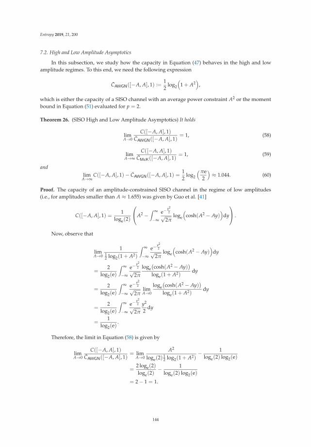
Entropy 2019, 21, 200

7.2. High and Low Amplitude Asymptotics

In this subsection, we study how the capacity in Equation (47) behaves in the high and lowamplitude regimes. To this end, we need the following expression

CAWGN([−A, A], 1) :=12

log2

(1 + A2

),

which is either the capacity of a SISO channel with an average power constraint A2 or the momentbound in Equation (51) evaluated for p = 2.

Theorem 26. (SISO High and Low Amplitude Asymptotics) It holds

limA→0

C([−A, A], 1)CAWGN([−A, A], 1)

= 1, (58)

limA→∞

C([−A, A], 1)CMcK([−A, A], 1)

= 1, (59)

andlim

A→∞C([−A, A], 1)− CAWGN([−A, A], 1) =

12

log2

(πe2

)≈ 1.044. (60)

Proof. The capacity of an amplitude-constrained SISO channel in the regime of low amplitudes(i.e., for amplitudes smaller than A ≈ 1.655) was given by Guo et al. [41]

C([−A, A], 1) =1

loge(2)

⎛⎝A2 −∫ ∞

−∞

e−y22√

2πloge

(cosh(A2 − Ay)

)dy

⎞⎠ .

Now, observe that

limA→0

112 log2(1 + A2)

∫ ∞

−∞

e−y22√

2πloge

(cosh(A2 − Ay)

)dy

=2

log2(e)

∫ ∞

−∞

e−y22√

2π

loge(cosh(A2 − Ay)

)loge(1 + A2)

dy

=2

log2(e)

∫ ∞

−∞

e−y22√

2πlimA→0

loge(cosh(A2 − Ay)

)loge(1 + A2)

dy

=2

log2(e)

∫ ∞

−∞

e−y22√

2π

y2

2dy

=1

log2(e).

Therefore, the limit in Equation (58) is given by

limA→0

C([−A, A], 1)CAWGN([−A, A], 1)

= limA→0

A2

loge(2)12 log2(1 + A2)

− 1loge(2) log2(e)

=2 loge(2)loge(2)

− 1loge(2) log2(e)

= 2− 1 = 1.

144

Entropy 2019, 21, 200

The limit in Equation (59) follows from comparing the EPI lower bound CEPI([−A, A], 1) =12 log2

(1 + 2A2

πe)

in (52) with the McKellips upper bound CMcK([−A, A], 1) = log2(1 + 2A√

2πe

)given in

Equation (48).Finally, to show Equation (60), observe that

limA→∞

C([−A, A], 1)− CAWGN([−A, A], 1) = limA→∞

CMcK([−A, A], 1)− CAWGN([−A, A], 1)

= limA→∞

log2

(1 +

2A√2πe

)− 1

2log2(1 + A2)

=12

log2

(πe2

).


8. Conclusions

In this work, we studied the capacity of MIMO channels with bounded input spaces. Severalnew properties of input distributions that achieve the capacity of such channels have been provided.In particular, it is shown that the support of a capacity-achieving channel input distribution is a setthat is small in a topological and measure theoretical sense. In addition to that, it is shown that, if theradius of the underlying channel input space, X , is small enough, then the support of a correspondingcapacity-achieving input distribution must necessarily be a subset of the boundary of X . As theconsiderations on the input distribution have demonstrated that determining the capacity is a verychallenging problem, we proposed several new upper and lower bounds that are shown to be tight inthe high amplitude regime. An interesting future direction would be to study generalizations of ourtechniques to wireless optical MIMO channels [42] and other channels such as the wiretap channel [43].

Author Contributions: All authors contributed equally to this work.

Funding: This work was supported in part by the U. S. National Science Foundation under Grants CCF-093970and CCF-1513915, by the German Research Foundation (DFG) under Grant GO 2669/1-1, and by the EuropeanUnion’s Horizon 2020 Research And Innovation Programme, grant agreement No. 694630.


References

1. Telatar, I.E. Capacity of multi-antenna Gaussian channels. Eur. Trans. Telecommun. 1999, 10, 585–595.2. Shannon, C. A mathematical theory of communication. Bell Syst. Tech. J. 1948, 27.3. Smith, J.G. The information capacity of amplitude-and variance-constrained scalar Gaussian channels.

Inf. Control 1971, 18, 203–219.4. Shamai (Shitz), S.; Bar-David, I. The capacity of average and peak-power-limited quadrature Gaussian

channels. IEEE Trans. Inf. Theory 1995, 41, 1060–1071.5. Rassouli, B.; Clerckx, B. On the capacity of vector Gaussian channels with bounded inputs. IEEE Trans.

Inf. Theory 2016, 62, 6884–6903.6. Sharma, N.; Shamai (Shitz), S. Transition points in the capacity-achieving distribution for the peak-power

limited AWGN and free-space optical intensity channels. Probl. Inf. Transm. 2010, 46, 283–299.7. McKellips, A.L. Simple tight bounds on capacity for the peak-limited discrete-time channel. In Proceedings

of the 2004 IEEE International Symposium on Information Theory (ISIT), Chicago, IL, USA, 27 June–2 July2004; pp. 348–348.

8. Thangaraj, A.; Kramer, G.; Böcherer, G. Capacity Bounds for Discrete-Time, Amplitude-Constrained,Additive White Gaussian Noise Channels. Available Online: https://arxiv.org/abs/1511.08742 (accessed on15 February 2019).

9. Rassouli, B.; Clerckx, B. An Upper Bound for the Capacity of Amplitude-Constrained Scalar AWGN Channel.IEEE Commun. Lett. 2016, 20, 1924–1926.

145

Entropy 2019, 21, 200

10. ElMoslimany, A.; Duman, T.M. On the Capacity of Multiple-Antenna Systems and Parallel GaussianChannels With Amplitude-Limited Inputs. IEEE Trans. Commun. 2016, 64, 2888–2899.

11. Dytso, A.; Goldenbaum, M.; Poor, H.V.; Shamai (Shitz), S. A Generalized Ozarow-Wyner Capacity Boundwith Applications. In Proceedings of the 2017 IEEE International Symposium on Information Theory (ISIT),Aachen, Germany, 25–30 June 2017; pp. 1058–1062.

12. Dytso, A.; Goldenbaum, M.; Shamai (Shitz), S.; Poor, H.V. Upper and Lower Bounds on the Capacityof Amplitude-Constrained MIMO Channels. In Proceedings of the 2017 IEEE Global CommunicationsConference (GLOBECOM), Singapore, 4–8 December 2017; pp. 1–6.

13. Cao, P.L.; Oechtering, T.J. Optimal transmit strategy for MIMO channels with joint sum and per-antennapower constraints. In Proceedings of the 2017 IEEE International Conference on Acoustics, Speech andSignal Processing (ICASSP), New Orleans, LA, USA, 5–9 March 2017.

14. Loyka, S. The Capacity of Gaussian MIMO Channels Under Total and Per-Antenna Power Constraints.IEEE Trans. Commun. 2017, 65, 1035–1043.

15. Loyka, S. On the Capacity of Gaussian MIMO Channels under the Joint Power Constraints. Available online:https://arxiv.org/abs/1809.00056 (accessed on 15 February 2019).

16. Tuninetti, D. On the capacity of the AWGN MIMO channel under per-antenna power constraints.In Proceedings of the 2014 IEEE International Conference on Communications (ICC), Sydney, NSW, Australia,10–14 June 2014, pp. 2153–2157.

17. Vu, M. MISO capacity with per-antenna power constraint. IEEE Trans. Commun. 2011, 59, 1268–1274.18. Chan, T.H.; Hranilovic, S.; Kschischang, F.R. Capacity-achieving probability measure for conditionally

Gaussian channels with bounded inputs. IEEE Trans. Inf. Theory 2005, 51, 2073–2088.19. Csiszar, I.; Körner, J. Information Theory: Coding Theorems for Discrete Memoryless Systems; Cambridge

University Press: Cambridge, UK, 2011.20. Abou-Faycal, I.C.; Trott, M.D.; Shamai, S. The capacity of discrete-time memoryless Rayleigh-fading channels.

IEEE Trans. Inf. Theory 2001, 47, 1290–1301.21. Fahs, J.; Abou-Faycal, I. On properties of the support of capacity-achieving distributions for additive noise

channel models with input cost constraints. IEEE Trans. Inf. Theory 2018, 64, 1178–1198.22. Gursoy, M.C.; Poor, H.V.; Verdú, S. The noncoherent Rician fading channel-part I: Structure of the

capacity-achieving input. IEEE Trans. Wireless Commun. 2015, 4, 2193–2206.23. Katz, M.; Shamai, S. On the capacity-achieving distribution of the discrete-time noncoherent and partially

coherent AWGN channels. IEEE Trans. Inf. Theory 2004, 50, 2257–2270.24. Ozel, O.; Ekrem, E.; Ulukus, S. Gaussian wiretap channel with amplitude and variance constraints.

IEEE Trans. Inf. Theory 2015, 61, 5553–5563.25. Bak, J.; Newman, D.J. Complex Analysis; Springer Science & Business Media: Berlin, Germany, 2010.26. Witsenhausen, H.S. Some Aspects of Convexity Useful in Information Theory. IEEE Trans. Inf. Theory 1980,

26, 265–271.27. Krantz, S.G.; Parks, H.R. A Primer of Real Analytic Functions; Springer Science & Business Media: New York,

NY, USA, 2002.28. Dytso, A.; Yagli, S.; Poor, H.V.; Shamai (Shitz), S. Capacity Achieving Distribution for the Amplitude

Constrained Additive Gaussian Channel: An Upper Bound on the Number of Mass Points. Available online:https://arxiv.org/abs/1901.03264 (accessed on 15 February 2019).

29. Ransford, T. Potential Theory in the Complex Plane; London Mathematical Society Student Texts; CambridgeUniversity Press: Cambridge, UK, 1995; Volume 28.

30. Hatsell, C.; Nolte, L. Some geometric properties of the likelihood ratio (Corresp.). IEEE Trans. Inf. Theory1971, 17, 616–618.

31. Dytso, A.; Poor, H.V.; Shamai (Shitz), S. On the Capacity of the Peak Power Constrained Vector GaussianChannel: An Estimation Theoretic Perspective. Available online: https://arxiv.org/abs/1804.08524(accessed on 15 February 2019).

32. Dytso, A.; Goldenbaum, M.; Poor, H.V.; Shamai (Shitz), S. When are Discrete Channel InputsOptimal?—Optimization Techniques and Some New Results. In Proceedings of the 2018 Annual Conferenceon Information Sciences and Systems (CISS), Princeton, NJ, USA, 21–23 March 2018; pp. 1–6.

33. Guo, D.; Shamai, S.; Verdú, S. Mutual information and minimum mean-square error in Gaussian channels.IEEE Trans. Inf. Theory 2005, 51, 1261–1282.

146

Entropy 2019, 21, 200

34. Dytso, A.; Tuninetti, D.; Devroye, N. Interference as Noise: Friend or Foe? IEEE Trans. Inf. Theory 2016,62, 3561–3596.

35. Resnick, S.I. A Probability Path; Springer Science & Business Media: New York, NY, USA, 2013.36. Dytso, A.; Bustin, R.; Tuninetti, D.; Devroye, N.; Shamai (Shitz), S.; Poor, H.V. On the Minimum Mean p-th

Error in Gaussian Noise Channels and its Applications. IEEE Trans. Inf. Theory 2018, 64, 2012–2037.37. Lozano, A.; Tulino, A.M.; Verdú, S. Optimum power allocation for parallel Gaussian channels with arbitrary

input distributions. IEEE Trans. Inf. Theory 2006, 52, 3033–3051.38. Pérez-Cruz, F.; Rodrigues, M.R.; Verdú, S. MIMO Gaussian channels with arbitrary inputs: Optimal

precoding and power allocation. IEEE Trans. Inf. Theory 2010, 56, 1070–1084.39. Abramowitz, M.; Stegun, I.A. Handbook of Mathematical Functions with Formulas, Graphs, and Mathematical

Tables, 9th dover printing ed.; Dover Publications: New York, NY, USA, 1964.40. Winkelbauer, A. Moments and Absolute Moments of the Normal Distribution. Available online:

https://arxiv.org/abs/1209.4340 (accessed on 15 February 2019).41. Guo, D.; Wu, Y.; Shamai, S.; Verdú, S. Estimation in Gaussian Noise: Properties of the Minimum Mean-Square

Error. IEEE Trans. Inf. Theory 2011, 57, 2371–2385.42. Moser, S.M.; Mylonakis, M.; Wang, L.; Wigger, M. Asymptotic Capacity Results for MIMO Wireless Optical

Communication. In Proceedings of the 2017 IEEE International Symposium on Information Theory (ISIT),Aachen, Germany, 25–30 June 2017; pp. 536–540.

43. Dytso, A.; Egan, M.; Perlaza, S.; Poor, H.V.; Shamai (Shitz), S. Optimal Inputs for Some Classes of DegradedWiretap Channels. In Proceedings of the 2018 IEEE Information Theory Workshop (ITW), Guangzhou,China, 25–29 November 2018; pp. 1–5.


147

entropy

Article

Quasi-Concavity for Gaussian Multicast RelayChannels

Mohit Thakur 1 and Gerhard Kramer 2,*

1 Independent Researcher, Amalienstr. 49A, 80799 Munich, Germany; [email protected] Institute for Communications Engineering, Technical University of Munich, 80333 Munich, Germany* Correspondence: [email protected]

Received: 6 January 2019; Accepted: 22 January 2019; Published: 24 January 2019

Abstract: Standard upper and lower bounds on the capacity of relay channels are cut-set (CS),decode-forward (DF), and quantize-forward (QF) rates. For real additive white Gaussian noise (AWGN)multicast relay channels with one source node and one relay node, these bounds are shown to bequasi-concave in the receiver signal-to-noise ratios and the squared source-relay correlation coefficient.Furthermore, the CS rates are shown to be quasi-concave in the relay position for a fixed correlationcoefficient, and the DF rates are shown to be quasi-concave in the relay position. The latter propertycharacterizes the optimal relay position when using DF. The results extend to complex AWGN channelswith random phase variations.

Keywords: capacity; decode-forward; multicast; relaying

1. Introduction

A multicast relay channel (MRC) is an information network with a source node, a relay node,and two or more destination nodes, and where one message originating at the source should be receivedreliably at the destinations. We consider additive white Gaussian noise (AWGN) MRCs and showthat certain information rate expressions are quasi-concave in the receiver signal-to-noise ratios (SNRs),the squared source-relay correlation coefficient, and the relay position. In particular, we study cut-set (CS),decode-forward (DF), and quantize-forward (QF) rates. Quasi-concavity suggests that efficient algorithmscan optimize signaling and the relay position. However, the main motivation of this work is not practicality,but simply to provide better understanding of the problem.

Relay positioning has been studied by many authors, with a focus on rate enhancement (e.g., [1,2]),range extension (e.g., [3,4]), and outage probability (e.g., [1,5,6]). We study the problem of placing a relayto maximize the multicast rate by extending results of [7–10]. A preliminary version of this paper withoutproofs appeared in [11]. Our focus is on real alphabet channels. However, our main results also apply tocomplex alphabet channels if there are random phase variations so that beamforming is not useful.

This paper is organized as follows. Section 2 presents the MRC model and reviews the CS, DF, and QFrates. Section 3 develops quasi-concavity results in the squared source-relay correlation coefficient ρ2 andthe channel SNRs. Section 4 introduces a distance dependence for the channel gains and shows that the CSrate is quasi-concave in the relay position when ρ is fixed. We further show that the DF rate is quasi-concavein the relay position. Section 5 illustrates quasi-concavity for one-, two-, and three-dimensional networks,and compares the performance of two DF strategies. Section 6 discusses complex AWGN channels anda sum (source plus relay) power constraint. Section 7 concludes the paper. Appendices A and B reviewuseful results on concavity and quasi-concavity, and prove a few new results.

Entropy 2019, 21, 109; doi:10.3390/e21020109 www.mdpi.com/journal/entropy

149

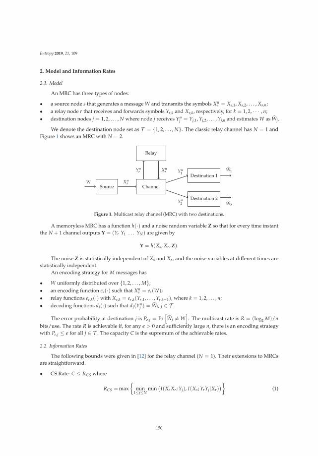
Entropy 2019, 21, 109

2. Model and Information Rates

2.1. Model

An MRC has three types of nodes:

• a source node s that generates a message W and transmits the symbols Xns = Xs,1, Xs,2, . . . , Xs,n;

• a relay node r that receives and forwards symbols Yr,k and Xr,k, respectively, for k = 1, 2, · · · , n;• destination nodes j = 1, 2, . . . , N where node j receives Yn

j = Yj,1, Yj,2, . . . , Yj,n and estimates W as Wj.

We denote the destination node set as T = {1, 2, . . . , N}. The classic relay channel has N = 1 andFigure 1 shows an MRC with N = 2.

WSource

Xns

Channel

Relay

Ynr Xn

rDestination 1

Yn1

W1

Destination 2Yn

2 W2

Figure 1. Multicast relay channel (MRC) with two destinations.

A memoryless MRC has a function h(·) and a noise random variable Z so that for every time instantthe N + 1 channel outputs Y = (Yr Y1 . . . YN) are given by

Y = h(Xs, Xr, Z).

The noise Z is statistically independent of Xs and Xr, and the noise variables at different times arestatistically independent.

An encoding strategy for M messages has

• W uniformly distributed over {1, 2, . . . , M};• an encoding function es(·) such that Xn

s = es(W);• relay functions er,k(·) with Xr,k = er,k(Yr,1, . . . , Yr,k−1), where k = 1, 2, . . . , n;• decoding functions dj(·) such that dj(Yn

j ) = Wj, j ∈ T .

The error probability at destination j is Pe,j = Pr[Wj �= W

]. The multicast rate is R = (log2 M)/n

bits/use. The rate R is achievable if, for any ε > 0 and sufficiently large n, there is an encoding strategywith Pe,j ≤ ε for all j ∈ T . The capacity C is the supremum of the achievable rates.

2.2. Information Rates

The following bounds were given in [12] for the relay channel (N = 1). Their extensions to MRCsare straightforward.

• CS Rate: C ≤ RCS where

RCS =max{

min1≤j≤N

min(

I(XsXr; Yj), I(Xs; YrYj|Xr))}

(1)

150

Entropy 2019, 21, 109

and where the maximization is over all XsXr.• Direct-Transmission (DT) Rate: C ≥ RDT where

RDT = max{ min1≤j≤N

I(Xs; Yj|Xr = x∗)} (2)

and where the maximization is over all x∗ and Xs.• DF Rate: C ≥ RDF where

RDF =max{

min1≤j≤N

min(

I(XsXr; Yj), I(Xs; Yr|Xr))}

(3)

and where the maximization is over all XsXr.• QF Rate: C ≥ RQF where

RQF =max{

min1≤j≤N

min(

I(XsXr; Yj)− I(Yr; Yr|XsXrYj), I(Xs; YrYj|Xr))}

(4)

where Yr is an auxiliary random variable, and where the maximization is over all XsXrYr such that Xs

and Xr are independent and Xs − XrYr − Yr forms a Markov chain.

2.3. Real Alphabet AWGN MRC

The real alphabet AWGN MRC has real channel symbols and

Yr = as,rXs + Zr (5)

Yj = as,jXs + ar,jXr + Zj (6)

where j ∈ T . The as,r, as,j, and ar,j are channel gains between the nodes (see Figure 2). We later relatethese gains to distances between the nodes. The Zr and Zj, j = 1, 2, . . . , N, are independent and identicallydistributed Gaussian random variables with zero mean and unit variance. We may alternatively write (5)and (6) in vector form as

Yj = AjX + Zj (7)

where X = (Xs Xr)T , Yj = (Yr Yj)T , Z = (Zr Zj)

T , and

Aj =

(as,r 0as,j ar,j

). (8)

151

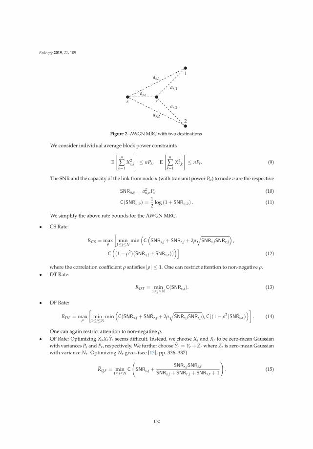
Entropy 2019, 21, 109

s r

1

2

as,r

as,1

as,2

ar,1

ar,2

Figure 2. AWGN MRC with two destinations.

We consider individual average block power constraints

E

[n

∑k=1

X2s,k

]≤ nPs, E

[n

∑k=1

X2r,k

]≤ nPr. (9)

The SNR and the capacity of the link from node u (with transmit power Pu) to node v are the respective

SNRu,v = a2u,vPu (10)

C(SNRu,v) =12

log (1 + SNRu,v) . (11)

We simplify the above rate bounds for the AWGN MRC.

• CS Rate:

RCS = maxρ

[min

1≤j≤Nmin

(C(SNRs,j + SNRr,j + 2ρ

√SNRs,jSNRr,j

),

C((1− ρ2)(SNRs,j + SNRs,r))

)](12)

where the correlation coefficient ρ satisfies |ρ| ≤ 1. One can restrict attention to non-negative ρ.• DT Rate:

RDT = min1≤j≤N

C(SNRs,j). (13)

• DF Rate:

RDF = maxρ

[min

1≤j≤Nmin

(C(SNRs,j + SNRr,j + 2ρ

√SNRs,jSNRr,j),C((1− ρ2)SNRs,r)

)]. (14)

One can again restrict attention to non-negative ρ.• QF Rate: Optimizing XsXrYr seems difficult. Instead, we choose Xs and Xr to be zero-mean Gaussian

with variances Ps and Pr, respectively. We further choose Yr = Yr + Zr where Zr is zero-mean Gaussianwith variance Nr. Optimizing Nr gives (see [13], pp. 336–337)

RQF = min1≤j≤N

C

(SNRs,j +

SNRr,jSNRs,r

SNRs,j + SNRr,j + SNRs,r + 1

). (15)

152

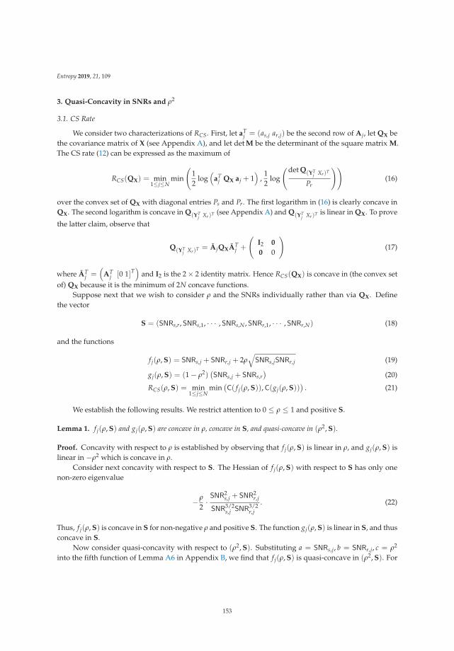
Entropy 2019, 21, 109

3. Quasi-Concavity in SNRs and ρ2

3.1. CS Rate

We consider two characterizations of RCS. First, let aTj = (as,j ar,j) be the second row of Aj, let QX be

the covariance matrix of X (see Appendix A), and let det M be the determinant of the square matrix M.The CS rate (12) can be expressed as the maximum of

RCS(QX) = min1≤j≤N

min

(12

log(

aTj QX aj + 1

),

12

log

(det Q(YTj Xr)T

Pr

))(16)

over the convex set of QX with diagonal entries Ps and Pr. The first logarithm in (16) is clearly concave inQX. The second logarithm is concave in Q(YT

j Xr)T (see Appendix A) and Q(YTj Xr)T is linear in QX. To prove

the latter claim, observe that

Q(YTj Xr)T = AjQXAT

j +

(I2 0

0 0

)(17)

where ATj =

(AT

j [0 1]T)

and I2 is the 2× 2 identity matrix. Hence RCS(QX) is concave in (the convex setof) QX because it is the minimum of 2N concave functions.

Suppose next that we wish to consider ρ and the SNRs individually rather than via QX. Definethe vector

S = (SNRs,r, SNRs,1, · · · , SNRs,N , SNRr,1, · · · , SNRr,N) (18)

and the functions

f j(ρ, S) = SNRs,j + SNRr,j + 2ρ√

SNRs,jSNRr,j (19)

gj(ρ, S) = (1− ρ2)(SNRs,j + SNRs,r

)(20)

RCS(ρ, S) = min1≤j≤N

min(C( f j(ρ, S)),C(gj(ρ, S))

). (21)

We establish the following results. We restrict attention to 0 ≤ ρ ≤ 1 and positive S.

Lemma 1. f j(ρ, S) and gj(ρ, S) are concave in ρ, concave in S, and quasi-concave in (ρ2, S).

Proof. Concavity with respect to ρ is established by observing that f j(ρ, S) is linear in ρ, and gj(ρ, S) islinear in −ρ2 which is concave in ρ.

Consider next concavity with respect to S. The Hessian of f j(ρ, S) with respect to S has only onenon-zero eigenvalue

−ρ

2·SNR2

s,j + SNR2r,j

SNR3/2s,j SNR3/2

r,j

. (22)

Thus, f j(ρ, S) is concave in S for non-negative ρ and positive S. The function gj(ρ, S) is linear in S, and thusconcave in S.

Now consider quasi-concavity with respect to (ρ2, S). Substituting a = SNRs,j, b = SNRr,j, c = ρ2

into the fifth function of Lemma A6 in Appendix B, we find that f j(ρ, S) is quasi-concave in (ρ2, S). For

153

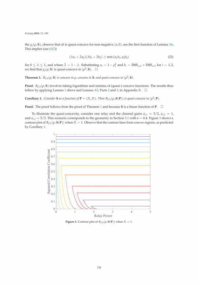
Entropy 2019, 21, 109

the gj(ρ, S), observe that ab is quasi-concave for non-negative (a, b), see the first function of Lemma A6.This implies (see (A7))

(λa1 + λa2)(λb1 + λb2) ≥ min (a1b1, a2b2) (23)

for 0 ≤ λ ≤ 1, and where λ = 1− λ. Substituting ai = 1− ρ2i and bi = SNRs,j,i + SNRs,r,i for i = 1, 2,

we find that gj(ρ, S) is quasi-concave in (ρ2, S).

Theorem 1. RCS(ρ, S) is concave in ρ, concave in S, and quasi-concave in (ρ2, S).

Proof. RCS(ρ, S) involves taking logarithms and minima of (quasi-) concave functions. The results thusfollow by applying Lemma 1 above and Lemma A5, Parts 2 and 3, in Appendix B.

Corollary 1. Consider S as a function of P = (Ps, Pr). Then RCS(ρ, S(P)) is quasi-concave in (ρ2, P).

Proof. The proof follows from the proof of Theorem 1 and because S is a linear function of P.

To illustrate the quasi-concavity, consider one relay and the channel gains as,r = 5/2, as,1 = 1,and ar,1 = 5/3. This scenario corresponds to the geometry in Section 5.1 with r = 0.4. Figure 3 shows acontour plot of RCS(ρ, S(P)) when Ps = 1. Observe that the contour lines form convex regions, as predictedby Corollary 1.

Figure 3. Contour plot of RCS(ρ, S(P)) when Ps = 1.

154

Entropy 2019, 21, 109

3.2. DF Rate

Consider the functions

g∗j (ρ, S) = (1− ρ2)SNRs,r (24)

RDF(ρ, S) = min1≤j≤N

min(C( f j(ρ, S)),C(g∗j (ρ, S))

). (25)

As above, we restrict attention to 0 ≤ ρ ≤ 1 and positive S.

Theorem 2. RDF(ρ, S) is concave in ρ, concave in S, and quasi-concave in (ρ2, S).

Proof. The proof is similar to that of Theorem 1.

Corollary 2. RDF(ρ, S(P)) is quasi-concave in (ρ2, P).

Proof. See the proof of Corollary 1.

3.3. DT Rate

The DT rate (13) is clearly concave in S and P.

3.4. QF Rate

Consider the functions

hj(S) = SNRs,j +SNRr,jSNRs,r

SNRs,j + SNRr,j + SNRs,r + 1(26)

RQF(S) = min1≤j≤N

C(hj(S)). (27)

We establish the following results. We restrict attention to non-negative S.

Lemma 2. hj(S) is quasi-concave in (SNRr,j, SNRs,r).

Proof. Substitute a = SNRr,j, b = SNRs,r, k = SNRs,j + 1 into the second function of Lemma A6 inAppendix B, and apply Lemma A5, Part 1.

Theorem 3. RQF(S) is quasi-concave in S if the SNRs,j, j = 1, 2, . . . , n, are held fixed.

Proof. Apply Lemma 2 above and Lemma A5, Parts 2 and 3, in Appendix B.

4. Quasi-Concavity in Relay Position

Suppose the channel gain for the node pair (i, j) is

ai,j =√

ξi,j

/Dα/2

i,j (28)

155

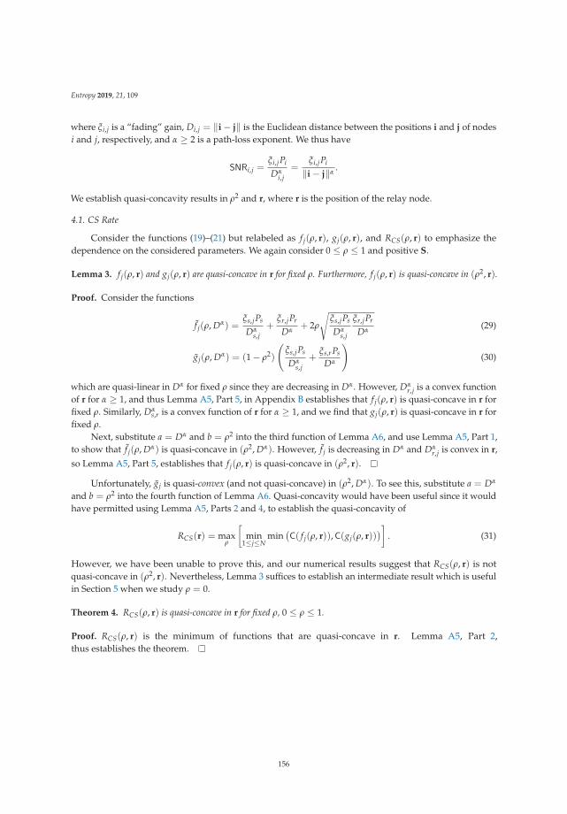
Entropy 2019, 21, 109

where ξi,j is a “fading” gain, Di,j = ‖i− j‖ is the Euclidean distance between the positions i and j of nodesi and j, respectively, and α ≥ 2 is a path-loss exponent. We thus have

SNRi,j =ξi,jPi

Dαi,j

=ξi,jPi

‖i− j‖α.

We establish quasi-concavity results in ρ2 and r, where r is the position of the relay node.

4.1. CS Rate

Consider the functions (19)–(21) but relabeled as f j(ρ, r), gj(ρ, r), and RCS(ρ, r) to emphasize thedependence on the considered parameters. We again consider 0 ≤ ρ ≤ 1 and positive S.

Lemma 3. f j(ρ, r) and gj(ρ, r) are quasi-concave in r for fixed ρ. Furthermore, fj(ρ, r) is quasi-concave in (ρ2, r).

Proof. Consider the functions

f j(ρ, Dα) =ξs,jPs

Dαs,j

+ξr,jPr

Dα+ 2ρ

√ξs,jPs

Dαs,j

ξr,jPr

Dα(29)

gj(ρ, Dα) = (1− ρ2)

(ξs,jPs

Dαs,j

+ξs,rPs

Dα

)(30)

which are quasi-linear in Dα for fixed ρ since they are decreasing in Dα. However, Dαr,j is a convex function

of r for α ≥ 1, and thus Lemma A5, Part 5, in Appendix B establishes that f j(ρ, r) is quasi-concave in r forfixed ρ. Similarly, Dα

s,r is a convex function of r for α ≥ 1, and we find that gj(ρ, r) is quasi-concave in r forfixed ρ.

Next, substitute a = Dα and b = ρ2 into the third function of Lemma A6, and use Lemma A5, Part 1,to show that f j(ρ, Dα) is quasi-concave in (ρ2, Dα). However, f j is decreasing in Dα and Dα

r,j is convex in r,

so Lemma A5, Part 5, establishes that f j(ρ, r) is quasi-concave in (ρ2, r).

Unfortunately, gj is quasi-convex (and not quasi-concave) in (ρ2, Dα). To see this, substitute a = Dα

and b = ρ2 into the fourth function of Lemma A6. Quasi-concavity would have been useful since it wouldhave permitted using Lemma A5, Parts 2 and 4, to establish the quasi-concavity of

RCS(r) = maxρ

[min

1≤j≤Nmin

(C( f j(ρ, r)),C(gj(ρ, r))

)]. (31)

However, we have been unable to prove this, and our numerical results suggest that RCS(ρ, r) is notquasi-concave in (ρ2, r). Nevertheless, Lemma 3 suffices to establish an intermediate result which is usefulin Section 5 when we study ρ = 0.

Theorem 4. RCS(ρ, r) is quasi-concave in r for fixed ρ, 0 ≤ ρ ≤ 1.

Proof. RCS(ρ, r) is the minimum of functions that are quasi-concave in r. Lemma A5, Part 2,thus establishes the theorem.

156

Entropy 2019, 21, 109

4.2. DF Rate

The quasi-convexity of gj(ρ, Dα) relaxes for the DF rate (25). Consider the negative of the fourthfunction of Lemma A6 in Appendix B with k1 = 0:

f (a, b) = (1− b)k2/a. (32)

This function is quasi-linear in (a, b) since both its superlevel and sublevel sets are convex. This resultimplies the following theorem. We again consider the functions (24)–(25) but relabeled as g∗j (ρ, r) andRDF(ρ, r). We further define

g∗j (ρ, Dα) = (1− ρ2)ξs,rPs

Dα(33)

RDF(r) = maxρ

[min

1≤j≤Nmin

(C( f j(ρ, r)),C(g∗j (ρ, r))

)]. (34)

As above, we consider 0 ≤ ρ ≤ 1 and positive S.

Theorem 5. RDF(ρ, r) is quasi-concave in (ρ2, r), and RDF(r) is quasi-concave in r.

Proof. g∗j (ρ, Dα) is quasi-linear in (ρ2, Dα) and decreasing in Dα. Furthermore, Dαs,r is convex in r, and

thus Lemma A5, Part 5, in Appendix B establishes that g∗j (ρ, r) is quasi-concave in (ρ2, r). RDF(ρ, r) istherefore quasi-concave in r, as it is the minimum of quasi-concave functions (see Lemma A5, Part 2).Furthermore, RDF(r) is concave in r by Lemma A5, Part 4.

5. DF Performance

This section presents numerical results for the DF strategy and compares them to results from [7–9].We consider 1-, 2-, and 3-dimensional MRCs with different numbers N of destination nodes. For simplicity,we consider the low SNR or broadband regime where

C(SNR) =12

log(1 + SNR)→ 12SNR. (35)

In other words, we consider the CS and DF rates without the logarithms. This approach is validnot only in the limit of low SNR, but more generally because we proved our quasi-concavity resultswithout taking logarithms. Furthermore, in the low SNR regime the rates of full-duplex and half-duplextransmission are the same under a block power constraint.

We choose Ps = Pr = P = 1, α = 2, and ξu,v = 1 for all node pairs (u, v). We study both coherenttransmission where ρ is optimized and non-coherent transmission with ρ = 0. The rates are in nats/channeluse. Alternatively, suppose we use sync pulses sampled at 2W samples per second, where W is the(one-sided) signal bandwidth. Suppose further that the (one-sided) noise power spectral density is1 Watt/Hz. Then at low SNR the rates in nats/channel use are the same as the rates in nats/sec.

157

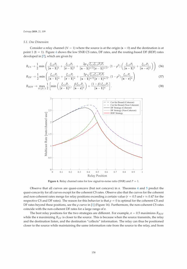
Entropy 2019, 21, 109

5.1. One Dimension

Consider a relay channel (N = 1) where the source is at the origin (s = 0) and the destination is atpoint 1 (1 = 1). Figure 4 shows the low SNR CS rates, DF rates, and the routing-based DF (RDF) ratesdeveloped in [7], which are given by

RCS →12

min

(ξs,1Ps

‖s− 1‖α+

ξr,1Pr

‖r− 1‖α+

2ρ√

ξs,1ξr,1PsPr

‖s− 1‖α/2‖r− 1‖α/2 , (1− ρ2)

(ξs,1Ps

‖s− 1‖α+

ξs,rPs

‖s− r‖α

))(36)

RDF →12

min

(ξs,1Ps

‖s− 1‖α+

ξr,1Pr

‖r− 1‖α+

2ρ√

ξs,1ξr,1PsPr

‖s− 1‖α/2‖r− 1‖α/2 , (1− ρ2)ξs,rPs

‖s− r‖α

)(37)

RRDF → max0≤β≤1

12

[min

(ξr,1Pr

‖r− 1‖α,

β ξs,rPs

‖s− r‖α

)+

(1− β) ξs,1Ps

‖s− 1‖α

]. (38)

Figure 4. Relay channel rates for low signal-to-noise ratio (SNR) and P = 1.

Observe that all curves are quasi-concave (but not concave) in r. Theorems 4 and 5 predict thequasi-concavity for all curves except for the coherent CS rates. Observe also that the curves for the coherentand non-coherent rates merge for relay positions exceeding a certain value (r = 0.5 and r ≈ 0.47 for therespective CS and DF rates). The reason for this behavior is that ρ = 0 is optimal for the coherent CS andDF rates beyond these positions, see the ρ curve in [1] (Figure 16). Furthermore, the non-coherent CS ratescoincide with the non-coherent DF rates for a large range of r.

The best relay positions for the two strategies are different. For example, r = 0.5 maximizes RRDFwhile the r maximizing RDF is closer to the source. This is because when the source transmits, the relayand the destination listen, and the destination “collects” information. The relay can thus be positionedcloser to the source while maintaining the same information rate from the source to the relay, and from

158

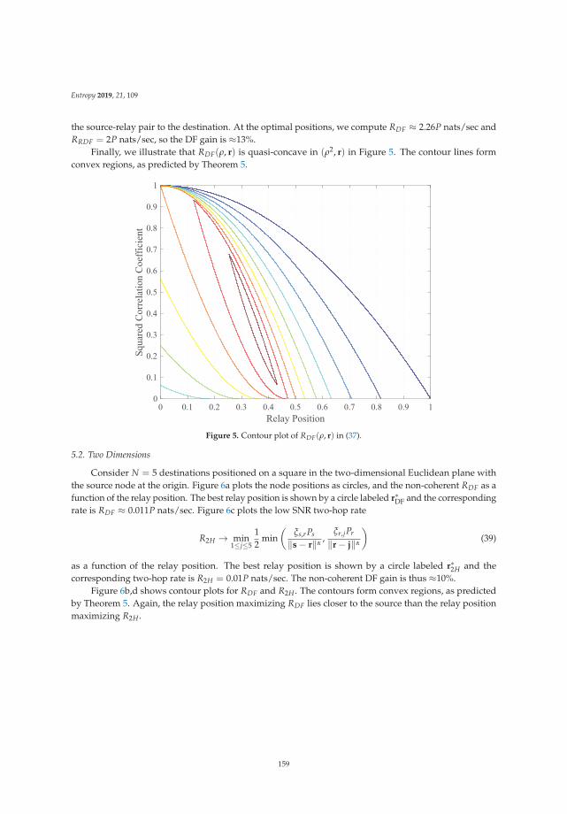
Entropy 2019, 21, 109

the source-relay pair to the destination. At the optimal positions, we compute RDF ≈ 2.26P nats/sec andRRDF = 2P nats/sec, so the DF gain is ≈13%.

Finally, we illustrate that RDF(ρ, r) is quasi-concave in (ρ2, r) in Figure 5. The contour lines formconvex regions, as predicted by Theorem 5.

Figure 5. Contour plot of RDF(ρ, r) in (37).

5.2. Two Dimensions

Consider N = 5 destinations positioned on a square in the two-dimensional Euclidean plane withthe source node at the origin. Figure 6a plots the node positions as circles, and the non-coherent RDF as afunction of the relay position. The best relay position is shown by a circle labeled r∗DF and the correspondingrate is RDF ≈ 0.011P nats/sec. Figure 6c plots the low SNR two-hop rate

R2H → min1≤j≤5

12

min(

ξs,rPs

‖s− r‖α,

ξr,jPr

‖r− j‖α

)(39)

as a function of the relay position. The best relay position is shown by a circle labeled r∗2H and thecorresponding two-hop rate is R2H = 0.01P nats/sec. The non-coherent DF gain is thus ≈10%.

Figure 6b,d shows contour plots for RDF and R2H . The contours form convex regions, as predictedby Theorem 5. Again, the relay position maximizing RDF lies closer to the source than the relay positionmaximizing R2H .

159

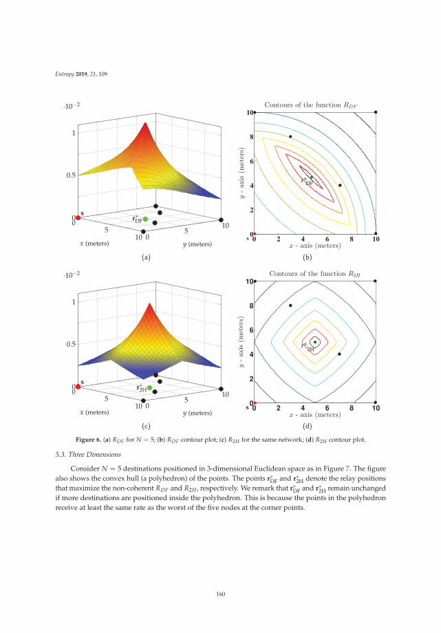
Entropy 2019, 21, 109

05

10 05

100

0.5

1

·10−2

sr∗DF

x (meters) y (meters)

(a)

x - axis (meters)y-ax

is(m

eters)

Contours of the function RDF

0 2 4 6 8 100

2

4

6

8

10

s

r*DF

(b)

05

10 05

100

0.5

1

·10−2

sr∗2H

x (meters) y (meters)

(c)

x - axis (meters)

y-ax

is(m

eters)

Contours of the function R2H

0 2 4 6 8 100

2

4

6

8

10

r*2H

s

(d)

Figure 6. (a) RDF for N = 5; (b) RDF contour plot; (c) R2H for the same network; (d) R2H contour plot.

5.3. Three Dimensions

Consider N = 5 destinations positioned in 3-dimensional Euclidean space as in Figure 7. The figurealso shows the convex hull (a polyhedron) of the points. The points r∗DF and r∗2H denote the relay positionsthat maximize the non-coherent RDF and R2H , respectively. We remark that r∗DF and r∗2H remain unchangedif more destinations are positioned inside the polyhedron. This is because the points in the polyhedronreceive at least the same rate as the worst of the five nodes at the corner points.

160

Entropy 2019, 21, 109

s

1

3

2

4

5

r∗DF

r∗2H

Figure 7. N = 5 destination geometry in three dimensions.

6. Discussion

6.1. Complex AWGN Channels

For complex-alphabet AWGN channels, we could replace (5) and (6) by adding phases φi,j for i = s, rand j = 1, 2, . . . , N as follows:

Yr = as,r ejφs,r Xs + Zr (40)

Yj = as,j ejφs,j Xs + ar,j ejφr,j Xr + Zj (41)

where the noise variables Zr and Zj, j = 1, 2, . . . , N, are independent, identically distributed, circularlysymmetric, complex, Gaussian random variables with zero mean and unit variance. The distancedependence of ai,j can be chosen as in (28) and the phase dependence as

φi,j = 2πDi,j/

λ (42)

where λ = c/ fo is the wavelength, c is the speed of light, and fo is the carrier frequency.For example, the DF rate (14), normalized by the number of real dimensions, is

RDF = maxρ

[min

1≤j≤Nmin

(C(SNRs,j + SNRr,j+

2�{

ρej(φs,j−φr,j)}√

SNRs,jSNRr,j

),C((1− |ρ|2)SNRs,r)

)](43)

where the complex correlation coefficient ρ satisfies 0 ≤ |ρ| ≤ 1. Observe that for a classic relay channel,with N = 1 destination, one can choose ρ to make �

{ρej(φs,1−φr,1)

}real and non-negative, as for real

alphabet AWGN channels. However, for N ≥ 2 one must choose complex ρ in general. Furthermore,the quasi-concavity in r will not be valid in general because the phases φr,j change with r, and we cannotoptimize ρ for each destination node separately. However, we remark that this effect is “local" in the sensethat for large carrier frequencies the phase variations are sensitive to changes in r. A pragmatic approachwould then be to optimize r for non-coherent transmission (ρ = 0) even if beamforming is permitted.Furthermore, if the channel exhibits random phase variations, then the best approach is to choose ρ = 0(see [1], Figure 18) in which case we have quasi-concavity for both the CS and DF rates. Finally, we remark

161

Entropy 2019, 21, 109

that it might be interesting to consider quasi-concavity in the correlation coefficients for problems wherethe source and relay have sufficiently many antennas to overcome the problem outlined above.

6.2. Sum-Power Constraint

For some applications, it is interesting to consider a sum-power constraint

E

[n

∑k=1|X|2s,k + |X|2r,k

]≤ nPT . (44)

As is usually done, we set Pr = PT − Ps and consider Ps, 0 ≤ Ps ≤ PT as a new optimization parameter.One might now hope that RCS(Ps, r) or RDF(Ps, r) are quasi-concave in (Ps, r) for fixed ρ, or at least forρ = 0. Unfortunately, we have found counterexamples that show this is not the case. The rate functions doseem to have interesting properties, however, and these deserve further exploration.

7. Conclusions

Various quasi-concavity results were established for AWGN MRCs. In particular, the CS rates arequasi-concave in the relay position for a fixed correlation coefficient (Theorem 4) and the DF rates arequasi-concave in the relay position (Theorem 5).

Author Contributions: Both authors conceived the problem and solution and wrote the paper.

Funding: This research was funded by the German Ministry of Education and Research in the framework of anAlexander von Humboldt Professorship.

Acknowledgments: The authors thank the reviewers for their comments that helped to improve the paper.

Conflicts of Interest: The authors declare no conflicts of interest.

Appendix A. Covariance Matrices and Concavity

The covariance matrix of a real-valued random column vector V is

QV = E[(V− E [V])(V− E [V])T

]. (A1)

A useful property of covariance matrices is as follows (see [14], p. 684). If Q∗V is a principal minor of QV,

then the following function is concave in QV:

f (QV) = logdet QV

det Q∗V

. (A2)

Appendix B. Concave and Quasi-Concave Functions

We review results on quasi-concavity, and then establish quasi-concavity for several functions.

Appendix B.1. Definitions

Consider the following sets. The domain D f of a real-valued function f : Rn → R is the set ofarguments for which f is defined. The hypograph and hypergraph of f are the respective

H f = {(x, y) |y ≤ f (x)}, H f = {(x, y) |y ≥ f (x)}. (A3)

162

Entropy 2019, 21, 109

The superlevel and sublevel sets of f with respect to β ∈ R are the respective

S f ,β = {x| f (x) ≥ β}, S f ,β = {x| f (x) ≤ β}. (A4)

Concave and quasi-concave functions can be defined via the convexity of these sets. Recall that a setS , S ⊆ Rn, is convex if for any two points x1 and x2 in S and for any λ satisfying 0 ≤ λ ≤ 1 we have

λx1 + λx2 ∈ S (A5)

where λ = 1− λ. Suppose that D f is convex. The function f is concave over D f if and only if its hypographH f is convex. Similarly, f is convex over D f if and only if H f is convex. The function f is quasi-concave overD f if and only if all its superlevel sets are convex, and f is quasi-convex overD f if and only if all its sublevelsets are convex. A function that is quasi-convex and quasi-concave is called quasi-linear. For example, anynon-increasing or non-decreasing function is quasi-linear.

Appendix B.2. Basic Properties

Two properties of concave and quasi-concave functions are as follows; these properties are often usedas the definitions of such functions. Similar properties exist for convex and quasi-convex functions.

Lemma A1. The function f is concave if and only if

f (λx1 + λx2) ≥ λ f (x1) + λ f (x2) (A6)

for all x1 and x2 in D f and for all 0 ≤ λ ≤ 1.

Lemma A2. The function f is quasi-concave if and only if

f (λx1 + λx2) ≥ min( f (x1), f (x2)) (A7)

for all x1 and x2 in D f and for all 0 ≤ λ ≤ 1.

The next two properties assume that f is twice differentiable and that D f is convex. Let H f (x) andB f (x) be the respective Hessian and bordered Hessian of f at x.

Lemma A3. (see [15], Section 3.1.4) f is concave if and only if H f (x) is negative semidefinite for all x ∈ D f .

Lemma A4. (see [16], p. 771) f is quasi-concave on the open and convex setD f if the determinants D2, D3, . . . , Dn

of the respective second to nth leading principal minors of B f (x) satisfy (−1)kDk < 0 for k = 2, 3, . . . , n and for allx ∈ D f .

Appendix B.3. Compositions Preserving Quasi-Concavity

The following compositions preserve quasi-concavity.

Lemma A5. Suppose f and fi, 1 ≤ i ≤ n, are quasi-concave, then so are the functions

1. h = k1 f + k2, where k1 ≥ 0 and k2 ∈ R;2. h = min

1≤i≤nfi;

3. h = g ◦ f where f is quasi-concave and g is non-decreasing;

163

Entropy 2019, 21, 109

4. h(a) = supb∈B f (a, b) where B is a convex set;5. h(a, b) = f (g(a), b) where g is convex and f (a, b) is non-increasing in a for fixed b.

Proof. Properties 1)–4) are standard (see [15], Section 3.4). For property 5), observe that

h(λa1 + λa2, λb1 + λb2)

= f (g(λa1 + λa2), λb1 + λb2)

(a)≥ f (λg(a1) + λg(a2), λb1 + λb2)

(b)≥ min ( f (g(a1), b1), f (g(a2), b2)) (A8)

where (a) follows because g(λa1 + λa2) ≤ λg(a1) + λg(a2) and f (a, b) is non-increasing in a. Step (b)follows because f is quasi-concave.

Appendix B.4. Examples of Quasi-Concave Functions

We establish quasi-concavity for several useful functions.

Lemma A6. The following functions are quasi-concave for x = (a b) with non-negative entries.

1. f (x) = ab2. f (x) = ab

a+b+k for a positive constant k3. f (x) = k1/a + 2

√k2b/a for positive constants k1, k2

4. f (x) = −(1− b)(k1 + k2/a) for positive constants k1, k2, and b ≤ 1

Furthermore, the following function is quasi-concave for x = (a b c) with non-negative entries.

5. f (x) = a + b + 2√

abc

Proof. We consider positive x, and we use bordered Hessians B f (x) and the derivatives Dk of their kthleading principal minors, k = 2, 3, . . . , n. The results extend to non-negative x by using continuity at zerovalues, except for the third and fourth functions where a = 0 makes the functions undefined.

1. We have D2 < 0 and D3 > 0 for

B f (x) =

⎛⎜⎝0 b ab 0 1a 1 0

⎞⎟⎠ .


B f (x) =

⎛⎜⎜⎝0 b(b+k)

(a+b+k)2a(a+k)

(a+b+k)2

b(b+k)(a+b+k)2

−2b(b+k)(a+b+k)3

2ab+(a+b+k)k(a+b+k)3

a(a+k)(a+b+k)2

2ab+(a+b+k)k(a+b+k)3

−2a(a+k)(a+b+k)3

⎞⎟⎟⎠ .

164

Entropy 2019, 21, 109


B f (x) =

⎛⎜⎜⎜⎝0 − k1+

√k2ab

a2

√k2ab

− k1+√

k2aba2

4k1+3√

k2ab2a3 −

√k2

2a3/2√

b√k2ab −

√k2

2a3/2√

b−

√k2

2b3/2√a

⎞⎟⎟⎟⎠ .

4. If b ≤ 1, we have D2 < 0 and D3 > 0 for

B f (x) =

⎛⎜⎝ 0 (1−b)k2a2 k1 +

k2a

(1−b)k2a2 − 2(1−b)k2

a3 − k2a2

k1 +k2a − k2

a2 0

⎞⎟⎠ .

5. We have D2 < 0, D3 > 0 and D4 < 0 for

B f (x) =

⎛⎜⎜⎜⎜⎜⎜⎝0 1 +

√bca 1 +

√acb

√abc

1 +√

bca −

√bc

2a3/212

√c

ab12

√bac

1 +√

acb

12

√c

ab −√

ac2b3/2

12

√abc√

abc

12

√bac

12

√abc −

√ab

2c3/2

⎞⎟⎟⎟⎟⎟⎟⎠ . (A9)

References

1. Kramer, G.; Gastpar, M.; Gupta, P. Cooperative strategies and capacity theorems for relay networks. IEEE Trans.Inf. Theory 2005, 51, 3037–3063. [CrossRef]

2. Lin, B.; Ho, P.-H.; Xie, L.-L.; Shen, X.; Tapolcai, J. Optimal relay station placement in broadband wireless accessnetworks. IEEE Trans. Mob. Comput. 2010, 9, 259–269. [CrossRef]

3. Aggarwal, V.; Bennatan, A.; Calderbank, A. R. Calderbank. On maximizing coverage in Gaussian relay channels.IEEE Trans. Inf. Theory 2009, 55, 2518–2536. [CrossRef]

4. Joshi, G.; Karandikar, A. Optimal relay placement for cellular coverage extension. In Proceedings of theSeventeenth National Conference on Communications, Bangalore, India, 28–30 January 2011; pp. 1196–1200.

5. Lee, J.; Wang, H.; Andrews, J.G.; Hong, D. Outage probability of cognitive relay networks with interferenceconstraints. IEEE Trans. Wirel. Commun. 2011, 10, 390–395. [CrossRef]

6. Chen, X.; Song, S.H.; Letaief, K.B. Relay position optimization improves finite-SNR diversity gain ofdecode-and-forward MIMO relay systems. IEEE Trans. Commun. 2012, 60, 3311–3321. [CrossRef]

7. Thakur, M.; Fawaz, N.; Médard, M. Optimal relay location and power allocation for low-SNR broadcast relaychannels. In Proceedings of the 30th IEEE International Conference on Computer Communications (INFOCOM2011), Shanghai, China, 10–15 April 2011; pp. 2822–2830.

8. Thakur, M.; Fawaz, N.; Médard, M. On the geometry of wireless network multicast in 2-D. In Proceedings of the2011 IEEE International Symposium on Information Theory, Saint Petersburg, Russian, 31 July–5 August 2011;pp. 1628–1632.

9. Thakur, M.; Fawaz, N.; Médard, M. Reducibility of joint relay positioning and flow optimization problem.In Proceedings of the 2012 IEEE International Symposium on Information Theory, Boston, MA, USA,1–6 July 2012; pp. 1117–1121.

10. Thakur, M.; Kramer, G. Relay Positioning for Multicast Relay Networks. In Proceedings of the 2013 IEEEInternational Symposium on Information Theory, Istanbul, Turkey, 7–12 July 2013; pp. 1954–1958.

165

Entropy 2019, 21, 109

11. Thakur, M.; Kramer, G. Quasi-concavity for Gaussian multicast relay channels. In Proceedings of the 2015 IEEEInternational Symposium on Information Theory, Hong Kong, China, 14–19 June 2015; pp. 2867–2869.

12. Cover, T.M.; El Gamal, A. Capacity theorems for the relay channel. IEEE Trans. Inf. Theory 1979, 25, 572–584.[CrossRef]

13. Kramer, G.; Maric, I.; Yates, R.D. Cooperative Communications. Found. Trends Netw. 2006, 1, 271–425. [CrossRef]14. Cover, T.M.; Thomas, J.A. Elements of Information Theory, 2nd ed.; John Wiley & Sons: New York, NY, USA, 2006.15. Boyd, S.; Vandenberghe, L. Convex Optimization; Cambridge University Press: New York, NY, USA, 2004.16. Bazaraa, M.S.; Sherali, H.D.; Shetty, C.M. Nonlinear Programming; Wiley: Hoboken, NJ, USA, 2006

c© 2019 by the authors. Licensee MDPI, Basel, Switzerland. This article is an open accessarticle distributed under the terms and conditions of the Creative Commons Attribution (CCBY) license (http://creativecommons.org/licenses/by/4.0/).

166

entropy

Article

Gaussian Multiple Access Channels with One-BitQuantizer at the Receiver †,‡

Borzoo Rassouli 1,*, Morteza Varasteh 2,* and Deniz Gündüz 2,*

1 School of Computer Science and Electronic Engineering, University of Essex, Colchester CO4 3SQ, UK2 The Intelligent Systems and Networks group of Department of Electrical and Electronics,

Imperial College London, London SW7 2AZ, UK* Correspondence: [email protected] (B.R.); [email protected] (M.V.);

[email protected] (D.G.); Tel.: +44-(0)-207-594-6218 (D.G.)† This paper is an extended version of our paper published in the 2017 IEEE International Symposium on

Information Theory (ISIT), Aachen, Germany, 25–30 June 2017.‡ This work has been carried out when the first author was with the Information Processing and

Communications Laboratory at Imperial College London.

Received: 21 May 2018; Accepted: 5 September 2018; Published: 7 September 2018

Abstract: The capacity region of a two-transmitter Gaussian multiple access channel (MAC) underaverage input power constraints is studied, when the receiver employs a zero-threshold one-bitanalogue-to-digital converter (ADC). It is proven that the input distributions of the two transmittersthat achieve the boundary points of the capacity region are discrete. Based on the position of aboundary point, upper bounds on the number of the mass points of the corresponding distributionsare derived. Furthermore, a lower bound on the sum capacity is proposed that can be achieved bytime division with power control. Finally, inspired by the numerical results, the proposed lowerbound is conjectured to be tight.

Keywords: Gaussian multiple access channel; one-bit quantizer; capacity region

1. Introduction

The energy consumption of an analogue-to-digital converter (ADC) (measured in Joules/sample)grows exponentially with its resolution (in bits/sample) [1,2].When the available power is limited,for example, for mobile devices with limited battery capacity, or for wireless receivers that operateon limited energy harvested from ambient sources [3], the receiver circuitry may be constrained tooperate with low resolution ADCs. The presence of a low-resolution ADC, in particular a one-bit ADCat the receiver, alters the channel characteristics significantly. Such a constraint not only limits thefundamental bounds on the achievable rate, but it also changes the nature of the communication andmodulation schemes approaching these bounds. For example, in a real additive white Gaussian noise(AWGN) channel under an average power constraint on the input, if the receiver is equipped with aK-bin (i.e., log2 K-bit) ADC front end, it is shown in [4] that the capacity-achieving input distributionis discrete with at most K + 1 mass points. This is in contrast with the optimality of the Gaussian inputdistribution when the receiver has infinite resolution.

Especially with the adoption of massive multiple-input multiple-output (MIMO) receiversand the millimetre wave (mmWave) technology enabling communication over large bandwidths,communication systems with limited-resolution receiver front ends are becoming of practicalimportance. Accordingly, there has been a growing research interest in understanding both thefundamental information theoretic limits and the design of practical communication protocols forsystems with finite-resolution ADC front ends. In [5], the authors showed that for a Rayleigh fadingchannel with a one-bit ADC and perfect channel state information at the receiver (CSIR), quadrature


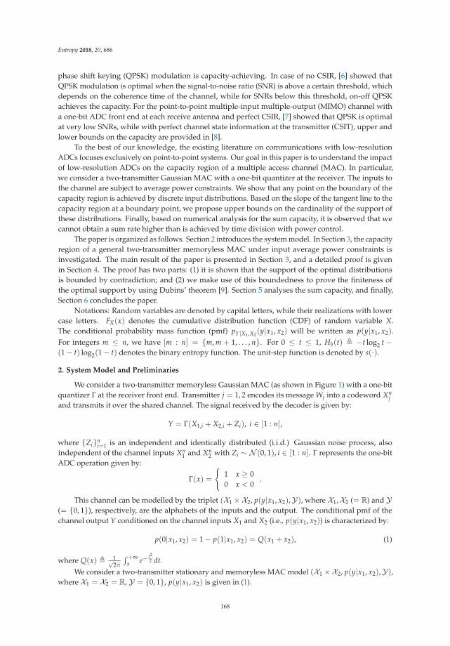
Entropy 2018, 20, 686

phase shift keying (QPSK) modulation is capacity-achieving. In case of no CSIR, [6] showed thatQPSK modulation is optimal when the signal-to-noise ratio (SNR) is above a certain threshold, whichdepends on the coherence time of the channel, while for SNRs below this threshold, on-off QPSKachieves the capacity. For the point-to-point multiple-input multiple-output (MIMO) channel witha one-bit ADC front end at each receive antenna and perfect CSIR, [7] showed that QPSK is optimalat very low SNRs, while with perfect channel state information at the transmitter (CSIT), upper andlower bounds on the capacity are provided in [8].

To the best of our knowledge, the existing literature on communications with low-resolutionADCs focuses exclusively on point-to-point systems. Our goal in this paper is to understand the impactof low-resolution ADCs on the capacity region of a multiple access channel (MAC). In particular,we consider a two-transmitter Gaussian MAC with a one-bit quantizer at the receiver. The inputs tothe channel are subject to average power constraints. We show that any point on the boundary of thecapacity region is achieved by discrete input distributions. Based on the slope of the tangent line to thecapacity region at a boundary point, we propose upper bounds on the cardinality of the support ofthese distributions. Finally, based on numerical analysis for the sum capacity, it is observed that wecannot obtain a sum rate higher than is achieved by time division with power control.

The paper is organized as follows. Section 2 introduces the system model. In Section 3, the capacityregion of a general two-transmitter memoryless MAC under input average power constraints isinvestigated. The main result of the paper is presented in Section 3, and a detailed proof is givenin Section 4. The proof has two parts: (1) it is shown that the support of the optimal distributionsis bounded by contradiction; and (2) we make use of this boundedness to prove the finiteness ofthe optimal support by using Dubins’ theorem [9]. Section 5 analyses the sum capacity, and finally,Section 6 concludes the paper.

Notations: Random variables are denoted by capital letters, while their realizations with lowercase letters. FX(x) denotes the cumulative distribution function (CDF) of random variable X.The conditional probability mass function (pmf) pY|X1,X2

(y|x1, x2) will be written as p(y|x1, x2).For integers m ≤ n, we have [m : n] = {m, m + 1, . . . , n}. For 0 ≤ t ≤ 1, Hb(t) � −t log2 t −(1− t) log2(1− t) denotes the binary entropy function. The unit-step function is denoted by s(·).

2. System Model and Preliminaries

We consider a two-transmitter memoryless Gaussian MAC (as shown in Figure 1) with a one-bitquantizer Γ at the receiver front end. Transmitter j = 1, 2 encodes its message Wj into a codeword Xn

jand transmits it over the shared channel. The signal received by the decoder is given by:

Y = Γ(X1,i + X2,i + Zi), i ∈ [1 : n],

where {Zi}ni=1 is an independent and identically distributed (i.i.d.) Gaussian noise process, also

independent of the channel inputs Xn1 and Xn

2 with Zi ∼ N (0, 1), i ∈ [1 : n]. Γ represents the one-bitADC operation given by:

Γ(x) =

{1 x ≥ 00 x < 0

.

This channel can be modelled by the triplet (X1 ×X2, p(y|x1, x2),Y), where X1,X2 (= R) and Y(= {0, 1}), respectively, are the alphabets of the inputs and the output. The conditional pmf of thechannel output Y conditioned on the channel inputs X1 and X2 (i.e., p(y|x1, x2)) is characterized by:

p(0|x1, x2) = 1− p(1|x1, x2) = Q(x1 + x2), (1)

where Q(x) � 1√2π

∫ +∞x e−

t22 dt.

We consider a two-transmitter stationary and memoryless MAC model (X1 ×X2, p(y|x1, x2),Y),where X1 = X2 = R, Y = {0, 1}, p(y|x1, x2) is given in (1).

168

Entropy 2018, 20, 686

Figure 1. A two-transmitter Gaussian multiple access channel (MAC) with a one-bit analogue-to-digitalconverter (ADC) front end at the receiver.

A (2nR1 , 2nR2 , n) code for this channel consists of (as in [10]):

• two message sets [1 : 2nR1 ] and [1 : 2nR2 ],• two encoders, where encoder j = 1, 2 assigns a codeword xn

j (wj) to each message wj ∈ [1 : 2nRj ], and• a decoder that assigns estimates (w1, w2) ∈ [1 : 2nR1 ]× [1 : 2nR2 ] or an error message to each

received sequence yn.

The stationary property means that the channel does not change over time, while the memorylessproperty indicates that p(yi|xi

1, xi2, yi−1, w1, w2) = p(yi|x1,i, x2,i) for any message pair (w1, w2).

We assume that the message pair (W1, W2) is uniformly distributed over [1 : 2nR1 ]× [1 : 2nR2 ].The average probability of error is defined as:

P(n)e � Pr

{(W1, W2) �= (W1, W2)

}. (2)

Average power constraints are imposed on the channel inputs as:

1n

n

∑i=1

x2j,i(wj) ≤ Pj , ∀wj ∈ [1 : 2nRj ], j ∈ {1, 2}, (3)

where xj,i(wj) denotes the i-th element of the codeword xnj (wj).

A rate pair (R1, R2) is said to be achievable for this channel if there exists a sequence of(2nR1 , 2nR2 , n) codes satisfying the average power constraints (3), such that limn→∞ P(n)

e = 0.The capacity region C (P1, P2) of this channel is the closure of the set of achievable rate pairs (R1, R2).

3. Main Results

Proposition 1. The capacity region C (P1, P2) of a two-transmitter stationary and memoryless MAC withaverage power constraints P1 and P2 is the set of non-negative rate pairs (R1, R2) that satisfy:

R1 ≤ I(X1; Y|X2, U),

R2 ≤ I(X2; Y|X1, U),

R1 + R2 ≤ I(X1, X2; Y|U), (4)

for some FU(u)FX1|U(x1|u)FX2|U(x2|u), such that E[X2j ] ≤ Pj, j = 1, 2. Furthermore, it is sufficient to

consider |U | ≤ 5.

Proof of Proposition 1. The proof is provided in Appendix A.

The main result of this paper is provided in the following theorem. It bounds the cardinality ofthe support set of the capacity-achieving distributions.

Theorem 1. Let J be an arbitrary point on the boundary of the capacity region C (P1, P2) of the memorylessMAC with a one-bit ADC front end (as shown in Figure 1). J is achieved by a distribution in the form of

169

Entropy 2018, 20, 686

FJU(u)FJ

X1|U(x1|u)FJX2|U(x2|u). Furthermore, let lJ be the slope of the line tangent to the capacity region at this

point. For any u ∈ U , the conditional input distributions FJX1|U(x1|u) and FJ

X2|U(x2|u) have at most n1 and n2

points of increase (a point Z is said to be a point of increase of a distribution if for any open set Ω containing Z,we have Pr{Ω} > 0), respectively, where:

(n1, n2) =

⎧⎪⎨⎪⎩(3, 5) lJ < −1(3, 3) lJ = −1(5, 3) lJ > −1

. (5)

Furthermore, this result remains unchanged if the one-bit ADC has a non-zero threshold.

Proof of Theorem 1. The proof is provided in Section 4.

Proposition 1 and Theorem 1 establish upper bounds on the number of mass points of thedistributions that achieve a boundary point. The significance of this result is that once it is known thatthe optimal inputs are discrete with at most a certain number of mass points, the capacity region alongwith the optimal distributions can be obtained via computer programs.

4. Proof of Theorem 1

In order to show that the boundary points of the capacity region are achieved, it is sufficient toshow that the capacity region is a closed set, i.e., it includes all of its limit points.

Let U be a set with |U | ≤ 5 and Ω be defined as:

Ω �{

FU,X1,X2

∣∣ U ∈ U , X1 −U − X2, E[X2j ] ≤ Pj, j = 1, 2

}, (6)

which is the set of all CDFs on the triplet (U, X1, X2), where U is drawn from U , and the Markov chainX1 −U − X2 and the corresponding average power constraints hold.

In Appendix B, it is proven that Ω is a compact set. Since a continuous mapping preservescompactness, the capacity region is compact. Since the capacity region is a subset of R2, it is closedand bounded (note that a subset of Rk is compact if and only if it is closed and bounded [11]).Therefore, any point P on the boundary of the capacity region is achieved by a distribution denoted byFJ

U(u)FJX1|U(x1|u)FJ

X2|U(x2|u).Since the capacity region is a convex space, it can be characterized by its supporting hyperplanes.

In other words, any point on the boundary of the capacity region, denoted by (Rb1, Rb

2), can be written as:

(Rb1, Rb

2) = arg max(R1,R2)∈C (P1,P2)

R1 + λR2,

for some λ ∈ (0, ∞). Here, we have excluded the cases λ = 0 and λ = ∞, where the channel is nota two-transmitter MAC any longer, and boils down to a point-to-point channel, whose capacity isalready known.

Any rate pair (R1, R2) ∈ C (P1, P2) must lie within a pentagon defined by (4) for someFU FX1|U FX2|U that satisfies the power constraints. Therefore, due to the structure of the pentagon, theproblem of finding the boundary points is equivalent to the following maximization problem.

max(R1,R2)∈C (P1,P2)

R1 + λR2 =

{max I(X1; Y|X2, U) + λI(X2; Y|U) 0 < λ ≤ 1max I(X2; Y|X1, U) + λI(X1; Y|U) λ > 1

, (7)

where on the right-hand side (RHS) of (7), the maximizations are over all FU FX1|U FX2|U that satisfy thepower constraints. It is obvious that when λ = 1, the two lines in (7) are the same, which results in thesum capacity.

For any product of distributions FX1 FX2 and the channel in (1), let Iλ be defined as:

170

Entropy 2018, 20, 686

Iλ(FX1 FX2) �{

I(X1; Y|X2) + λI(X2; Y) 0 < λ ≤ 1I(X2; Y|X1) + λI(X1; Y) λ > 1

. (8)

With this definition, (7) can be rewritten as:

max(R1,R2)∈C (P1,P2)

R1 + λR2 = max5

∑i=1

pU(ui)Iλ(FX1|U(x1|ui)FX2|U(x2|ui)),

where the second maximization is over distributions of the form pU(u)FX1|U(x1|u)FX2|U(x2|u),such that:

5

∑i=1

pU(ui)E[X2j |U = ui] ≤ Pj, j = 1, 2.

Proposition 2. For a given FX1 and any λ > 0, Iλ(FX1 FX2) is a concave, continuous and weakly differentiablefunction of FX2 . In the statement of this proposition, FX1 and FX2 could be interchanged.

Proof of Proposition 2. The proof is provided in Appendix C.

Proposition 3. Let P′1, P′2 be two arbitrary non-negative real numbers. For the following problem:

maxFX1 FX2 :

E[X2j ]≤P′j , j=1,2

Iλ(FX1 FX2), (9)

the optimal inputs F∗X1and F∗X2

, which are not unique in general, have the following properties,

(i) The support sets of F∗X1and F∗X2

are bounded subsets of R.(ii) F∗X1

and F∗X2are discrete distributions that have at most n1 and n2 points of increase, respectively, where:

(n1, n2) =

⎧⎪⎨⎪⎩(5, 3) 0 < λ < 1(3, 3) λ = 1(3, 5) λ > 1

.

Proof of Proposition 3. We start with the proof of the first claim. Assume that 0 < λ ≤ 1, and FX2 isgiven. Consider the following optimization problem:

I∗FX2� sup

FX1 :E[X2

1 ]≤P′1

Iλ(FX1 FX2). (10)

Note that I∗FX2< +∞, since for any λ > 0, from (8),

Iλ ≤ (λ + 1)H(Y) ≤ (1 + λ) < +∞.

From Proposition 2, Iλ is a continuous, concave function of FX1 . Furthermore, the set of allCDFs with bounded second moment (here, P′1) is convex and compact. The compactness followsfrom Appendix I in [12], where the only difference is in using Chebyshev’s inequality instead ofMarkov’s inequality. Therefore, the supremum in (10) is achieved by a distribution F∗X1

. Since forany FX1(x) = s(x − x0) with |x0|2 < P′1, we have E[X2

1 ] < P′1, the Lagrangian theorem and theKarush–Kuhn–Tucker conditions state that there exists a θ1 ≥ 0 such that:

I∗FX2= sup

FX1

{Iλ(FX1 FX2)− θ1

(∫x2dFX1(x)− P′1

)}. (11)

171

Entropy 2018, 20, 686

Furthermore, the supremum in (11) is achieved by F∗X1, and:

θ1

(∫x2dF∗X1

(x)− P′1

)= 0. (12)

Lemma 1. The Lagrangian multiplier θ1 is non-zero. From (12), this is equivalent to having E[X21 ] = P′1, i.e.,

the first user transmits with its maximum allowable power (note that this is for λ ≤ 1, as used in Appendix D).

Proof of Lemma 1. In what follows, we prove that a zero Lagrangian multiplier is not possible. Having azero Lagrangian multiplier means the power constraint is inactive. In other words, if θ1 = 0, (10) and (11)imply that:

supFX1

E[X21 ]≤P′1

Iλ(FX1 FX2) = supFX1

Iλ(FX1 FX2). (13)

We prove that (13) does not hold by showing that its left-hand side (LHS) is strictly less than one,while its RHS equals one. The details are provided in Appendix D.

Iλ(FX1 FX2) (0 < λ ≤ 1) can be written as:

Iλ(FX1 FX2) =∫ +∞

−∞

∫ +∞

−∞

1

∑y=0

p(y|x1, x2) logp(y|x1, x2)

[p(y; FX1 FX2)]λ[p(y; FX1 |x2)]1−λ

dFX1(x1)dFX2(x2)

=∫ +∞

−∞iλ(x1; FX1 |FX2)dFX1(x1) (14)

=∫ +∞

−∞iλ(x2; FX2 |FX1)dFX2(x2), (15)

where we have defined:

iλ(x1; FX1 |FX2)�∫ +∞−∞

(D

(p(y|x1, x2)||p(y; FX1 FX2)

)+ (1− λ)∑1

y=0 p(y|x1, x2) logp(y;FX1 FX2 )

p(y;FX1 |x2)

)dFX2(x2), (16)

and:iλ(x2; FX2 |FX1) �

∫ +∞−∞ D

(p(y|x1, x2)||p(y; FX1 FX2)

)dFX1(x1)− (1− λ)D

(p(y; FX1 |x2)||p(y; FX1 FX2)

). (17)

p(y; FX1 FX2) is nothing but the pmf of Y with the emphasis that it has been induced by FX1 and FX2 .Likewise, p(y; FX1 |x2) is the conditional pmf p(y|x2) when X1 is drawn according to FX1 . From (14),iλ(x1; FX1 |FX2) can be considered as the density of Iλ over FX1 when FX2 is given. iλ(x2; FX2 |FX1) canbe interpreted in a similar way.

Note that (11) is an unconstrained optimization problem over the set of all CDFs. Since∫

x2dFX1(x)is linear and weakly differentiable in FX1 , the objective function in (11) is concave and weaklydifferentiable. Hence, a necessary condition for the optimality of F∗X1

is:

∫{iλ(x1; F∗X1

|FX2) + θ1(P′1 − x21)}dFX1(x1) ≤ I∗FX2

, ∀FX1 . (18)

Furthermore, (18) can be verified to be equivalent to:

iλ(x1; F∗X1|FX2) + θ1(P′1 − x2

1) ≤ I∗FX2, ∀x1 ∈ R, (19)

iλ(x1; F∗X1|FX2) + θ1(P′1 − x2

1) = I∗FX2, if x1 is a point of increase of F∗X1

. (20)

The justifications of (18)–(20) are provided in Appendix E.In what follows, we prove that in order to satisfy (20), F∗X1

must have a bounded support byshowing that the LHS of (20) goes to −∞ with x1. The following lemma is useful in the sequel fortaking the limit processes inside the integrals.

172

Entropy 2018, 20, 686

Lemma 2. Let X1 and X2 be two independent random variables satisfying E[X21 ] ≤ P′1 and E[X2

2 ] ≤ P′2,respectively (P′1, P′2 ∈ [0,+∞)). Considering the conditional pmf in (1), the following inequalities hold.∣∣∣∣D (

p(y|x1, x2)||p(y; FX1 FX2)) ∣∣∣∣ ≤ 1− 2 log Q(

√P′1 +

√P′2) (21)

p(y; FX1 |x2) ≥ Q(√

P′1 + |x2|)

(22)∣∣∣∣∣ 1

∑y=0

p(y|x1, x2) logp(y; FX1 FX2)

p(y; FX1 |x2)

∣∣∣∣∣ ≤ −2 log Q(√

P′1 +√

P′2

)− 2 log Q

(√P′1 + |x2|

)(23)

Proof of Lemma 2. The proof is provided in Appendix F.

Note that

limx1→+∞∫ +∞−∞ D

(p(y|x1, x2)||p(y; F∗X1

FX2))

dFX2(x2) =∫ +∞−∞ limx1→+∞ D

(p(y|x1, x2)||p(y; F∗X1

FX2))

dFX2(x2) (24)

= − log pY(1; F∗X1FX2) (25)

≤ − log Q(√

P′1 +√

P′2), (26)

where (24) is due to the Lebesgue dominated convergence theorem [11] and (21), which permit theinterchange of the limit and the integral; (25) is due to the following:

limx1→+∞

D(

p(y|x1, x2)||p(y; F∗X1FX2)

)= lim

x1→+∞

1

∑y=0


p(y; F∗X1FX2)

= − log pY(1; F∗X1FX2),

since p(0|x1, x2) = Q(x1 + x2) goes to zero when x1 → +∞ and pY(y; F∗X1FX2) (y = 0, 1) is bounded

away from zero by (A34) ; (26) is obtained from (A34) in Appendix F. Furthermore,

limx1→+∞∫ +∞−∞ ∑1

y=0 p(y|x1, x2) logp(y;F∗X1

FX2 )

p(y;F∗X1|x2)

dFX2(x2) =∫ +∞−∞ limx1→+∞ ∑1

y=0 p(y|x1, x2) logp(y;F∗X1

FX2 )

p(y;F∗X1|x2)

dFX2(x2) (27)

= log pY(1; F∗X1FX2)−

∫ +∞−∞ log p(1; F∗X1

|x2)dFX2(x2)

< − log Q(√

P′1 +√

P′2)

, (28)

where (27) is due to the Lebesgue dominated convergence theorem along with (23) and (A39) inAppendix F; (28) is from (22) and the convexity of log Q(α +

√t) in t when α ≥ 0 (see Appendix G).

Therefore, from (26) and (28),

limx1→+∞

iλ(x1; F∗X1|FX2) ≤ −(2− λ) log Q(

√P′1 +

√P′2) < +∞. (29)

Using a similar approach, we can also obtain:

limx1→−∞

iλ(x1; F∗X1|FX2) ≤ −(2− λ) log Q(

√P′1 +

√P′2) < +∞. (30)

From (29) and (30) and the fact that θ1 > 0 (see Lemma 1), the LHS of (19) goes to−∞ when |x1| → +∞.Since any point of increase of F∗X1

must satisfy (19) with equality and I∗FX2≥ 0, it is proven that F∗X1

has

a bounded support. Hence, from now on, we assume X1 ∈ [−A1, A2] for some A1, A2 ∈ R (note thatA1 and A2 are determined by the choice of FX2 ).

173

Entropy 2018, 20, 686

Similarly, for a given FX1 , the optimization problem:

I∗FX1= sup

FX2 :E[X2

2 ]≤P′2

Iλ(FX1 FX2),

boils down to the following necessary condition:

iλ(x2; F∗X2|FX1) + θ2(P′2 − x2

2) ≤ I∗FX1, ∀x2 ∈ R, (31)

iλ(x2; F∗X2|FX1) + θ2(P′2 − x2

2) = I∗FX1, if x2 is a point of increase of F∗X2

, (32)

for the optimality of F∗X2. However, there are two main differences between (32) and (20). First is

the difference between iλ and iλ. Second is the fact that we do not claim θ2 to be nonzero, since theapproach used in Lemma 1 cannot be readily applied to θ2. Nonetheless, the boundedness of thesupport of F∗X2

can be proven by inspecting the behaviour of the LHS of (32) when |x2| → +∞.In what follows, i.e., from (33)–(38), we prove that the support of F∗X2

is bounded by showingthat (32) does not hold when |x2| is above a certain threshold. The first term on the LHS of (32) isiλ(x2; F∗X2

|FX1). From (17) and (21), it can be easily verified that:

limx2→+∞

iλ(x2; F∗X2|FX1) = −λ log pY(1; FX1 F∗X2

) ≤ −λ log Q(√

P′1 +√

P′2),

limx2→−∞

iλ(x2; F∗X2|FX1) = −λ log pY(0; FX1 F∗X2

) ≤ −λ log Q(√

P′1 +√

P′2) (33)

From (33), if θ2 > 0, the LHS of (32) goes to −∞ with |x2|, which proves that X∗2 is bounded.For the possible case of θ2 = 0, in order to show that (32) does not hold when |x2| is above a

certain threshold, we rely on the boundedness of X1, i.e., X1 ∈ [−A1, A2]. Then, we prove thatiλ approaches its limit in (33) from below. In other words, there is a real number K such thatiλ(x2; F∗X2

|FX1) < −λ log pY(1; FX1 F∗X2) when x2 > K, and iλ(x2; F∗X2

|FX1) < −λ log pY(0; FX1 F∗X2)

when x2 < −K. This establishes the boundedness of X∗2 . In what follows, we only show the former, i.e.,when x2 → +∞. The latter, i.e., x2 → −∞, follows similarly, and it is omitted for the sake of brevity.

By rewriting iλ, we have:

iλ(x2; F∗X2|FX1) = −λp(1; FX1 |x2) log pY(1; FX1 F∗X2

)

−∫ A2

−A1

Hb(Q(x1 + x2))dFX1(x1) + (1− λ) H(Y|X2 = x2)︸︷︷︸Hb(

∫Q(x1+x2)dFX1 (x1))

− λ p(0; FX1 |x2)︸︷︷︸∫Q(x1+x2)dFX1 (x1)

log pY(0; FX1 F∗X2). (34)

It is obvious that the first term on the RHS of (34) approaches −λ log pY(1; FX1 F∗X2) from below

when x2 → +∞, since p(1; FX1 |x2) ≤ 1. It is also obvious that the remaining terms go to zero whenx2 → +∞. Hence, it is sufficient to show that they approach zero from below, which is proven byusing the following lemma.

Lemma 3. Let X1 be distributed on [−A1, A2] according to FX1(x1). We have:

limx2→+∞

∫ A2−A1

Hb(Q(x1 + x2))dFX1(x1)

Hb

( ∫ A2−A1

Q(x1 + x2)dFX1(x1)

) = 1. (35)

174

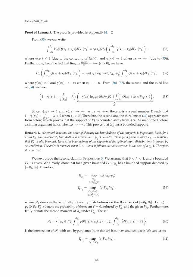
Entropy 2018, 20, 686

Proof of Lemma 3. The proof is provided in Appendix H.

From (35), we can write:

∫ A2

−A1

Hb(Q(x1 + x2))dFX1(x1) = γ(x2)Hb

(∫ A2

−A1

Q(x1 + x2)dFX1(x1)

), (36)

where γ(x2) ≤ 1 (due to the concavity of Hb(·)), and γ(x2) → 1 when x2 → +∞ (due to (35)).Furthermore, from the fact that limx→0

Hb(x)cx = +∞ (c > 0), we have:

Hb

(∫ A2

−A1

Q(x1 + x2)dFX1(x1)

)= −η(x2) log pY(0; FX1 F∗X2

)∫ A2

−A1

Q(x1 + x2)dFX1(x1), (37)

where η(x2) > 0 and η(x2) → +∞ when x2 → +∞. From (36)–(37), the second and the third lineof (34) become:(

1− γ(x2) +λ

η(x2)− λ

)(−η(x2) log pY(0; FX1 F∗X2

)∫ A2

−A1

Q(x1 + x2)dFX1(x1)

)︸︷︷︸

≥0

. (38)

Since γ(x2) → 1 and η(x2) → +∞ as x2 → +∞, there exists a real number K such that1− γ(x2) +

λη(x2)

− λ < 0 when x2 > K. Therefore, the second and the third line of (34) approach zerofrom below, which proves that the support of X∗2 is bounded away from +∞. As mentioned before,a similar argument holds when x2 → −∞. This proves that X∗2 has a bounded support.

Remark 1. We remark here that the order of showing the boundedness of the supports is important. First, for agiven FX2 (not necessarily bounded), it is proven that F∗X1

is bounded. Then, for a given bounded FX1 , it is shownthat F∗X2

is also bounded. Hence, the boundedness of the supports of the optimal input distributions is proven bycontradiction. The order is reversed when λ > 1, and it follows the same steps as in the case of λ ≤ 1. Therefore,it is omitted.

We next prove the second claim in Proposition 3. We assume that 0 < λ < 1, and a boundedFX1 is given. We already know that for a given bounded FX1 , F∗X2

has a bounded support denoted by[−B1, B2]. Therefore,

I∗FX1= sup

FX2 :E[X2

2 ]≤P′2

Iλ(FX1 FX2)

I∗FX1= sup

FX2∈S2:E[X2

2 ]≤P′2

Iλ(FX1 FX2), (39)

where S2 denotes the set of all probability distributions on the Borel sets of [−B1, B2]. Let p∗0 =

pY(0; FX1 F∗X2) denote the probability of the event Y = 0, induced by F∗X2

and the given FX1 . Furthermore,let P∗2 denote the second moment of X2 under F∗X2

. The set:

F2 =

{FX2 ∈ S2|

∫ B2

−B1

p(0|x2)dFX2(x2) = p∗0,∫ B2

−B1

x22dFX2(x2) = P∗2

}(40)

is the intersection of S2 with two hyperplanes (note that S2 is convex and compact). We can write:

I∗FX1= sup

FX2∈F2

Iλ(FX1 FX2). (41)

175

Entropy 2018, 20, 686

Note that having FX2 ∈ F2, the objective function in (41) becomes:

λH(Y)︸︷︷︸constant

+ (1− λ)H(Y|X2)− H(Y|X1, X2)︸︷︷︸linear in FX2

. (42)

Since the linear part is continuous and F2 is compact (The continuity of the linear part followssimilarly the continuity arguments in Appendix C. Note that this compactness is due to the closednessof the intersecting hyperplanes in F2, since a closed subset of a compact set is compact [11].The hyperplanes are closed due to the continuity of x2

2 and p(0|x2) (see (A16)).), the objective functionin (41) attains its maximum at an extreme point of F2, which, by Dubins’ theorem, is a convexcombination of at most three extreme points of S2. Since the extreme points of S2 are the CDFs havingonly one point of increase in [−B1, B2], we conclude that given any bounded FX1 , F∗X2

has at most threemass points.

Now, assume that an arbitrary FX2 is given with at most three mass points denoted by {x2,i}3i=1.

It is already known that the support of F∗X1is bounded, which is denoted by [−A1, A2]. Let S1 denote

the set of all probability distributions on the Borel sets of [−A1, A2]. The set:

F1 =

{FX1 ∈ S1

∣∣∣∣ ∫ A2−A1

p(0|x1, x2,j)dFX1(x1) = p(0; F∗X1|x2,j), j ∈ [1 : 3],

∫ A2−A1

x21dFX1(x1) = P′1

}, (43)

is the intersection of S1 with four hyperplanes. Note that here, since we know θ1 �= 0, the optimalinput attains its maximum power of P′1. In a similar way,

I∗FX2= sup

FX1∈F1

{Iλ(FX1 FX2)

}, (44)

and having FX1 ∈ F1, the objective function in (44) becomes:

Iλ = λH(Y) + (1− λ)3

∑i=1

pX2(x2,i)H(Y|X2 = x2,i)︸︷︷︸constant

−H(Y|X1, X2)︸︷︷︸linear in FX1

(45)

Therefore, given any FX2 with at most three points of increase, F∗X1has at most five mass points.

When λ = 1, the second term on the RHS of (45) disappears, which means that F1 could bereplaced by: {

FX1 ∈ S1|∫ A2

−A1

p(0|x1)dFX1(x1) = p∗0,∫ A2

−A1

x21dFX1(x1) = P′1

},

where p∗0 = pY(0; F∗X1FX2) is the probability of the event Y = 0, which is induced by F∗X1

and the givenFX2 . Since the number of intersecting hyperplanes has been reduced to two, it is concluded that F∗X1has at most three points of increase.

Remark 2. Note that, the order of showing the discreteness of the support sets is also important. First, for agiven bounded FX1 (not necessarily discrete), it is proven that F∗X2

is discrete with at most three mass points.Then, for a given discrete FX2 with at most three mass points, it is shown that F∗X1

is also discrete with at mostfive mass points when λ < 1 and at most three mass points when λ = 1. When λ > 1, the order is reversed,and it follows the same steps as in the case of λ < 1. Therefore, it is omitted.

Remark 3. If X1,X2 are assumed finite initially, similar results can be obtained by using the iterativeoptimization in the previous proof and the approach in Chapter 4, Corollary 3 of [13].

176

Entropy 2018, 20, 686

5. Sum Rate Analysis

In this section, we propose a lower bound on the sum capacity of a MAC in the presence of aone-bit ADC front end at the receiver, which we conjecture to be tight. The sum capacity is given by:

Csum = sup I(X1, X2; Y|U), (46)

where the supremum is over FU FX1|U FX2|U (|U | ≤ 5), such that E[X2j ] ≤ Pj, j = 1, 2. We obtain a

lower bound for the above by considering only those input distributions that are zero-mean per anyrealization of the auxiliary random variable U, i.e., E[Xj|U = u] = 0, ∀u ∈ U , j = 1, 2. Let P′1 and P′2 betwo arbitrary non-negative real numbers. We have:

supFX1 FX2 :

E[X2j ]≤P′j

E[Xj ]=0, j=1,2

I(X1, X2; Y) ≤ supFX :

E[X2]≤P′1+P′2

I(X; Y) (47)

= 1− Hb

(Q

(√P′1 + P′2

))(48)

where in (47), X � X1 + X2, pY|X(0|x) = Q(x); (48) follows from [4] for the point-to-point channel.Therefore, when E[Xj|U = u] = 0, ∀u ∈ U , j = 1, 2, we can write:

I(X1, X2; Y|U) =5

∑i=1

pU(ui)I(X1, X2; Y|U = ui)

≤ 1−5

∑i=1

pU(ui)Hb

(Q

(√E[X2

1 |U = ui] +E[X22 |U = ui]

))≤ 1− Hb

(Q

(√E[X2

1 ] +E[X22 ]

))(49)

≤ 1− Hb

(Q

(√P1 + P2

)), (50)

where (49) is due to the fact that Hb (Q(√

x + y)) is a convex function of (x, y), and (50) follows fromE[X2

j ] ≤ Pj, j = 1, 2.The upper bound in (50) can be achieved by time division with power control as follows.

Let U = {0, 1} and pU(0) = 1− pU(1) = P1P1+P2

. Furthermore, let FX1|U(x|1) = FX2|U(x|0) = s(x),where s(·) is the unit step function, and:

FX1|U(x|0) = FX2|U(x|1) = 12

s(x +√

P1 + P2) +12

s(x−√

P1 + P2).

With this choice of FU FX1|U FX2|U , the upper bound in (50) is achieved. Therefore,

Csum ≥ 1− Hb

(Q

(√P1 + P2

)). (51)

A numerical evaluation of (46) is carried out as follows (the codes that are used forthe numerical simulations are available at https://www.dropbox.com/sh/ndxkjt6h5a0yktu/AAAmfHkuPxe8rMNV1KzFVRgNa?dl=0). Although E[X2

j ] is upper bounded by Pj (j = 1, 2),

the value of E[X2j |U = u] (∀u ∈ U ) has no upper bound and could be any non-negative

real number. However, in our numerical analysis, we further restrict our attention to thecase E[X2

j |U = u] ≤ 20Pj, ∀u ∈ U , j = 1, 2. Obviously, as this upper bound tends to infinity,the approximation becomes more accurate (This further bounding of the conditional second momentsis justified by the fact that the sum capacity is not greater than one, which is due to the one-bit

177

Entropy 2018, 20, 686

quantization at the receiver. As a result, I(X1, X2; Y|U = u) increases at most sublinearly withE[X2

j |U = u], j = 1, 2, while pU(u) needs to decrease at least linearly to satisfy the average power

constraints. Hence, the product pU(u)I(X1, X2; Y|U = u) decreases with E[X2j |U = u] when

E[X2j |U = u] is above a threshold.). Each of the intervals [0, 20P1] and [0, 20P2] are divided into

201 points uniformly, which results in the discrete intervals P110 [0 : 200] and P2

10 [0 : 200], respectively.Afterwards, for any pair (α, β) ∈ P1

10 [0 : 200] × P210 [0 : 200], the following is carried out for input

distributions with at most three mass points.

maxFX1 FX2 :

E[X21 ]≤α,E[X2

2 ]≤β

I(X1, X2; Y) (52)

The results are stored in a 201× 201 matrix accordingly. In the above optimization, the MATLABfunction fmincon is used with three different initial values, and the maximum of these threeexperiments is chosen. Then, the problem boils down to finding proper gains, i.e., the mass probabilitiesof U, that maximize I(X1, X2; Y|U) and satisfy the average power constraints E[X2

j ] ≤ Pj. This is donevia a linear program, which can be efficiently solved by the linprog function in MATLAB. Several caseswere considered, such as (P1, P2) = (1, 1), (P1, P2) = (1, 2), (P1, P2) = (3, 1), etc. In all these cases,the numerical evaluation of (46) leads to the same value as the lower bound in (51). Since the problemis not convex, it is not known whether the numerical results are the global optimum solutions; hence,we leave it as a conjecture that the sum capacity can be achieved by time division with power control.

6. Conclusions

We have studied the capacity region of a two-transmitter Gaussian MAC under average inputpower constraints and one-bit ADC front end at the receiver. We have derived an upper bound onthe cardinality of this auxiliary variable, and proved that the distributions that achieve the boundarypoints of the capacity region are finite and discrete. Finally, a lower bound is proposed on the sumcapacity of this MAC that is achieved by time division with power control. Through numerical analysis,this lower bound is shown to be tight.

178

Entropy 2018, 20, 686

Author Contributions: All three authors contributed to the paper. B.R. derived most of the claims with discussionwith the M.V. and D.G.; The numerical results regarding the sum-rate analysis were obtained by the M.V.; Writingand editing of the paper has been done jointly, and all three authors have read and approved the final manuscript.

Funding: This research was supported in part by the European Research Council (ERC) through Starting GrantBEACON (Agreement No. 677854), by the U.K. Engineering and Physical Sciences Research Council (EPSRC)through the project COPES (EP/N021738/1) and by the British Council Institutional Link Program under GrantNO. 173605884.

Acknowledgments: The authors thank Professor Barbie and Professor Shirokov for their help in showing thepreservation of the Markov chain in the weak convergence of the joint distributions in Appendix B.


Appendix A

The capacity region of the discrete memoryless (DM) MAC with input cost constraints has beenaddressed in Exercise 4.8 of [10]. If the input alphabets are not discrete, the capacity region is still thesame because: (1) the converse remains the same if the inputs are from a continuous alphabet; (2) theregion is achievable by coded time sharing and the discretization procedure (see Remark 3.8 in [10]).Therefore, it is sufficient to show the cardinality bound |U | ≤ 5.

Let P be the set of all product distributions (i.e., of the form FX1(x1)FX2(x2)) on R2. Let g : P →R5 be a vector-valued mapping defined element-wise as:

g1(FX1|U(·|u)FX2|U(·|u)) = I(X1; Y|X2, U = u),

g2(FX1|U(·|u)FX2|U(·|u)) = I(X2; Y|X1, U = u),

g3(FX1|U(·|u)FX2|U(·|u)) = I(X1, X2; Y|U = u),

g4(FX1|U(·|u)FX2|U(·|u)) = E[X21 |U = u],

g5(FX1|U(·|u)FX2|U(·|u)) = E[X22 |U = u]. (A1)

Let G ⊂ R5 be the image of P under the mapping g (i.e., G = g(P)). Given an arbitrary(U, X1, X2) ∼ FU FX1|U FX2|U , we obtain the vector r as:

r1 = I(X1; Y|X2, U) =∫U

I(X1; Y|X2, U = u)dFU(u),

r2 = I(X2; Y|X1, U) =∫U

I(X2; Y|X1, U = u)dFU(u),

r3 = I(X1, X2; Y|U) =∫U

I(X1, X2; Y|U = u)dFU(u),

r4 = E[X21 ] =

∫UE[X2

1 |U = u]dFU(u),

r5 = E[X22 ] =

∫UE[X2

2 |U = u]dFU(u).

Therefore, r is in the convex hull of G ⊂ R5. By Carathéodory’s theorem [9], r can be written as aconvex combination of six (= 5 + 1) or fewer points in G , which states that it is sufficient to consider|U | ≤ 6. Since P is a connected set (P is the product of two connected sets; therefore, it is connected.Each of the sets in this product is connected because of being a convex vector space.) and the mappingg is continuous (this is a direct result of the continuity of the channel transition probability), G is aconnected subset of R5. Therefore, the connectedness of G refines the cardinality of U to |U | ≤ 5.

It is also important to note that for the boundary points of C (P1, P2) that are not sum-rateoptimal, it is sufficient to have |U | ≤ 4. The proof is as follows. Any point on the boundary of thecapacity region that does not maximize R1 + R2 is either of the form (I(X1; Y|X2, U), I(X2; Y|U)) or(I(X1; Y|U), I(X2; Y|X1, U)) for some FU FX1|U FX2|U that satisfies E[X2

j ] ≤ Pj, j = 1, 2. In other words,it is one of the corner points of the corresponding pentagon in (4). As in the proof of Proposition 1,define the mapping g : P → R4, where g1 and g2 are the coordinates of this boundary point

179

Entropy 2018, 20, 686

conditioned on U = u, and g3, g4 are the same as g4 and g5 in (A1), respectively. The sufficiency of|U | ≤ 4 in this case follows similarly.

Appendix B

Since |U | ≤ 5, we assume U = {0, 1, 2, 3, 4} without loss of generality, since what matters in theevaluation of the capacity region is the mass probability of the auxiliary random variable U, not itsactual values.

In order to show the compactness of Ω, we adopt a general form of the approach in [12].First, we show that Ω is tight (a set of probability distributions Θ defined on Rk, i.e., the set of

CDFs FX1,X2,...,Xk , is said to be tight, if for every ε > 0, there is a compact set Kε ⊂ Rk such that [14]:

Pr{(X1, X2, . . . , Xk) ∈ Rk\Kε

}< ε, ∀FX1,X2,...,Xk ∈ Θ.

Choose Tj, j = 1, 2, such that Tj >

√2Pjε . Then, from Chebyshev’s inequality,

Pr{|Xj| > Tj

}≤

Pj

T2j<

ε

2, j = 1, 2. (A2)

Let Kε = [0, 4]× [−T1, T1]× [−T2, T2] ⊂ R3. It is obvious that Kε is a closed and bounded subset of R3

and, therefore, compact. With this choice of Kε, we have:

Pr{(U, X1, X2) ∈ R3\Kε

}≤ Pr{U /∈ [0, 4]}+ Pr{X1 /∈ [−T1, T1]}+ Pr{X2 /∈ [−T2, T2]}< 0 +

ε

2+

ε

2= ε, (A3)

where (A3) is due to (A2). Hence, Ω is tight.From Prokhorov’s theorem [14] (p. 318), a set of probability distributions is tight if and only if

it is relatively sequentially compact (a subset of topological space is relatively compact if its closureis compact). This means that for every sequence of CDFs {Fn} in Ω, there exists a subsequence{Fnk} that is weakly convergent (the weak convergence of {Fn} to F (also shown as Fn(x) w→ F(x)) isequivalent to:

limn→∞

∫R

ψ(x)dFn(x) =∫R

ψ(x)dF(x), (A4)

for all continuous and bounded functions ψ(·) on R. Note that Fn(x) w→ F(x) if and only ifdL(Fn, F) → 0.) to a CDF F0, which is not necessarily in Ω. If we can show that this F0 is alsoan element of Ω, then the proof is complete, since we have shown that Ω is sequentially compact and,therefore, compact (Compactness and sequential compactness are equivalent in metric spaces. Notethat Ω is a metric space with Lévy distance.).

Assume a sequence of distributions {Fn(·, ·, ·)} in Ω that converges weakly to F0(·, ·, ·). In orderto show that this limiting distribution is also in Ω, we need to show that both the average powerconstraints and the Markov chain (X1 −U − X2) are preserved under F0. The preservation of thesecond moment follows similarly to the argument in (Appendix I, [12]). In other words, since x2 iscontinuous and bounded from below, from Theorem 4.4.4 in [15]:∫

x2j d3F0(u, x1, x2) ≤ lim inf

n→∞

∫x2

j d3Fn(u, x1, x2)

≤ Pj, j = 1, 2, (A5)

Therefore, the second moments are preserved under the limiting distribution F0.For the preservation of the Markov chain X1 −U − X2, we need the following proposition.

180

Entropy 2018, 20, 686

Proposition A1. Assume a sequence of distributions {Fn(·, ·)} over the pair of random variables (X, Y) thatconverges weakly to F0(·, ·). Furthermore, assume that Y has a finite support, i.e., Y = {1, 2, . . . , |Y|}.Then, the sequence of conditional distributions (conditioned on Y) converges weakly to the limiting conditionaldistribution (conditioned on Y), i.e.,

Fn(·|y) w→ F0(·|y), ∀y ∈ Y , p0(y) > 0. (A6)

Proof of Proposition A1. The proof is by contradiction. If (A6) is not true, then there exists y′ ∈ Y ,

such that p0(y′) > 0 and Fn(·|y′)��w→F0(·|y′). This means, from the definition of weak convergence, thatthere exists a bounded continuous function of x, denoted by gy′(x), such that:∫

gy′(x)dFn(x|y′)��→∫

gy′(x)dF0(x|y′). (A7)

Let f (x, y) be any bounded continuous function that satisfies:

f (x, y) =

{0 y ∈ Y , y �= y′

gy′(x) y = y′. (A8)

With this choice of f (x, y), we have:∫f (x, y)d2Fn(x, y)��→

∫f (x, y)d2F0(x, y), (A9)

which violates the assumption of the weak convergence of Fn(·, ·) to F0(·, ·). Therefore, (A6) holds.

Since {Fn(·, ·, ·)} in Ω converges weakly to F0(·, ·, ·) and U is finite, from Proposition A1, we have:

Fn(·, ·|u) w→ F0(·, ·|u), ∀u ∈ U , (A10)

where it is obvious that the arguments are x1 and x2. Since Fn ∈ Ω, we have Fn(x1, x2|u) =

Fn(x1|u)Fn(x2|u) ∀u ∈ U . Furthermore, since the convergence of the joint distribution implies theconvergence of the marginals, we have (Theorem 2.7, [16,17]),

F0(x1, x2|u) = F0(x1|u)F0(x2|u) ∀u ∈ U , (A11)

which states that under the limiting distribution F0, the Markov chain X1 − U − X2 is preserved(Alternatively, this could be proven by the lower-semicontinuity of the mutual information as follow:

IF0(X1; X2|U = u) ≤ lim infn→∞

IFn(X1; X2|U = u) (A12)

= 0, ∀u ∈ U , (A13)

where IF denotes the mutual information under distribution F. The last equality is from the conditionalindependence of X1 and X2 given U = u under Fn. Therefore, IF0(X1; X2|U = u) = 0, ∀u ∈ U , whichis equivalent to (A11).). This completes the proof of the compactness of Ω.

Appendix C

Appendix C.1. Concavity

When 0 < λ ≤ 1, we have:

Iλ(FX1 FX2) = λH(Y) + (1− λ)H(Y|X2)− H(Y|X1, X2). (A14)

181

Entropy 2018, 20, 686

For a given FX1 , H(Y) is a concave function of FX2 , while H(Y|X2) and H(Y|X1, X2) are linearin FX2 . Therefore, Iλ is a concave function of FX2 . For a given FX2 , H(Y) and H(Y|X2) are concavefunctions of FX1 , while H(Y|X1, X2) is linear in FX1 . Since (1− λ) ≥ 0, Iλ is a concave function of FX1 .The same reasoning applies to the case λ > 1.

Appendix C.2. Continuity

When λ ≤ 1, the continuity of the three terms on the RHS of (A14) is investigated. Let {FX2,n} bea sequence of distributions, which is weakly convergent to FX2 . For a given FX1 , we have:

limx2→x0

2

p(y; FX1 |x2) = limx2→x0

2

∫Q(x1 + x2)dFX1(x1)

=∫

limx2→x0

2

Q(x1 + x2)dFX1(x1) (A15)

= p(y; FX1 |x02), (A16)

where (A15) is due to the fact that the Q function can be dominated by one, which is an absolutelyintegrable function over FX1 . Therefore, p(y; FX1 |x2) is continuous in x2, and combined with the weakconvergence of {FX2,n}, we can write:

limn→∞

p(y; FX1 FX2,n) = limn→∞

∫p(y; FX1 |x2)dFX2,n(x2)

=∫

p(y; FX1 |x2)dFX2(x2)

= p(y; FX1 FX2).

This allows us to write:

limn→∞

−1

∑y=0

p(y; FX1 FX2,n) log p(y; FX1 FX2,n) = −1

∑y=0

p(y; FX1 FX2) log p(y; FX1 FX2),

which proves the continuity of H(Y) in FX2 . H(Y|X2 = x2) is a bounded (∈ [0, 1]) continuousfunction of x2, since it is a continuous function of p(y; FX1 |x2), and the latter is continuous in x2

(see (A16)). Therefore,

limn→∞

∫H(Y|X2 = x2)dFX2,n(x2) =

∫H(Y|X2 = x2)dFX2(x2),

which proves the continuity of H(Y|X2) in FX2 . In a similar way, it can be verified that∫H(Y|X1 = x1, X2 = x2)dFX1(x1) is a bounded and continuous function of x2, which guarantees the

continuity of H(Y|X1, X2) in FX2 , since:

H(Y|X1, X2) =∫ (∫

H(Y|X1 = x1, X2 = x2)dFX1(x1)

)dFX2(x2) (A17)

Therefore, for a given FX1 , Iλ is a continuous function of FX2 . Exchanging the roles of FX1 and FX2 ,also the case λ > 1 can be addressed similarly, so they are omitted for the sake of brevity.

Appendix C.3. Weak Differentiability

For a given FX1 , the weak derivative of Iλ at F0X2

is given by:

I′λ(FX1 FX2)|F0X2

= limβ→0+

Iλ(FX1((1− β)F0X2

+ βFX2))− Iλ(FX1 F0X2)

β, (A18)

182

Entropy 2018, 20, 686

if the limit exists. It can be verified that:


= limβ→0+

∫iλ(x2; (1− β)F0

X2+ βFX2 |FX1)d((1− β)F0

X2(x2) + βFX2(x2))−

∫iλ(x2; F0

X2|FX1)dF0

X2(x2)

β

=∫

iλ(x2; F0X2|FX1)dFX2(x2)−

∫iλ(x2; F0

X2|FX1)dF0

X2(x2)

=∫

iλ(x2; F0X2|FX1)dFX2(x2)− Iλ(FX1 F0

X2),

where iλ has been defined in (17). In a similar way, for a given FX2 , the weak derivative of Iλ at F0X1

is:


=∫

iλ(x1; F0X1|FX2)dFX1(x1)− Iλ(F0

X1FX2), (A19)

where iλ has been defined in (16). The case λ > 1 can be addressed similarly.

Appendix D

We have:

supFX1 :

E[X21 ]≤P′1

Iλ(FX1 FX2) ≤ supFX1 FX2 :

E[X2j ]≤P′j , j=1,2

Iλ(FX1 FX2)

≤ supFX1 FX2 :

E[X2j ]≤P′j , j=1,2

I(X1, X2; Y) (A20)

≤ supFX1 FX2 :

E[X2j ]≤P′j , j=1,2

H(Y)− infFX1 FX2 :

E[X2j ]≤P′j , j=1,2

H(Y|X1, X2)

= 1− infFX1 FX2 :

E[X2j ]≤P′j , j=1,2

∫ ∫Hb (Q(x1 + x2)) dFX1(x1)dFX2(x2)

= 1− infFX1 FX2 :

E[X2j ]≤P′j , j=1,2

∫ ∫Hb

(Q

(√x2

1 +√

x22

))dFX1(x1)dFX2(x2) (A21)

≤ 1− infFX1 FX2 :

E[X2j ]≤P′j , j=1,2

∫ ∫Q

(√x2

1 +√

x22

)dFX1(x1)dFX2(x2) (A22)

= 1−Q(√

P′1 +√

P′2

)(A23)

< 1, (A24)

where (A20) is from the non-negativity of mutual information and the assumption that 0 < λ ≤ 1;(A21) is justified since the Q function is monotonically decreasing and the sign of the inputs doesnot affect the average power constraints; X1 and X2 can be assumed non-negative (or alternatively

non-positive) without loss of optimality; in (A22), we use the fact that Q(√

x21 +

√x2

2

)≤ 1

2 , and for

t ∈ [0, 12 ], Hb(t) ≥ t; (A23) is based on the convexity and monotonicity of the function Q(

√u +

√v) in

(u, v), which is shown in Appendix G. Therefore, the LHS of (13) is strictly less than one.

183

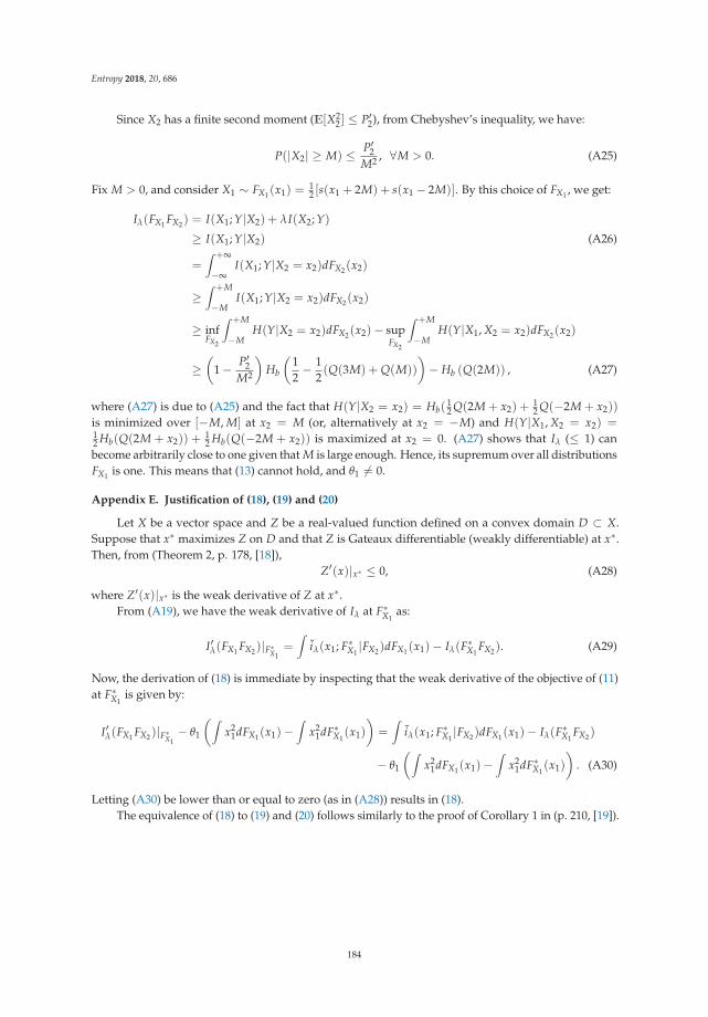
Entropy 2018, 20, 686

Since X2 has a finite second moment (E[X22 ] ≤ P′2), from Chebyshev’s inequality, we have:

P(|X2| ≥ M) ≤ P′2M2 , ∀M > 0. (A25)

Fix M > 0, and consider X1 ∼ FX1(x1) =12 [s(x1 + 2M) + s(x1 − 2M)]. By this choice of FX1 , we get:

Iλ(FX1 FX2) = I(X1; Y|X2) + λI(X2; Y)

≥ I(X1; Y|X2) (A26)

=∫ +∞

−∞I(X1; Y|X2 = x2)dFX2(x2)

≥∫ +M

−MI(X1; Y|X2 = x2)dFX2(x2)

≥ infFX2

∫ +M

−MH(Y|X2 = x2)dFX2(x2)− sup

FX2

∫ +M

−MH(Y|X1, X2 = x2)dFX2(x2)

≥(

1− P′2M2

)Hb

(12− 1

2(Q(3M) + Q(M))

)− Hb (Q(2M)) , (A27)

where (A27) is due to (A25) and the fact that H(Y|X2 = x2) = Hb(12 Q(2M + x2) +

12 Q(−2M + x2))

is minimized over [−M, M] at x2 = M (or, alternatively at x2 = −M) and H(Y|X1, X2 = x2) =12 Hb(Q(2M + x2)) +

12 Hb(Q(−2M + x2)) is maximized at x2 = 0. (A27) shows that Iλ (≤ 1) can

become arbitrarily close to one given that M is large enough. Hence, its supremum over all distributionsFX1 is one. This means that (13) cannot hold, and θ1 �= 0.

Appendix E. Justification of (18), (19) and (20)

Let X be a vector space and Z be a real-valued function defined on a convex domain D ⊂ X.Suppose that x∗ maximizes Z on D and that Z is Gateaux differentiable (weakly differentiable) at x∗.Then, from (Theorem 2, p. 178, [18]),

Z′(x)|x∗ ≤ 0, (A28)

where Z′(x)|x∗ is the weak derivative of Z at x∗.From (A19), we have the weak derivative of Iλ at F∗X1

as:

I′λ(FX1 FX2)|F∗X1=

∫iλ(x1; F∗X1

|FX2)dFX1(x1)− Iλ(F∗X1FX2). (A29)

Now, the derivation of (18) is immediate by inspecting that the weak derivative of the objective of (11)at F∗X1

is given by:

I′λ(FX1 FX2)|F∗X1− θ1

(∫x2

1dFX1(x1)−∫

x21dF∗X1

(x1)

)=

∫iλ(x1; F∗X1

|FX2)dFX1(x1)− Iλ(F∗X1FX2)

− θ1

(∫x2

1dFX1(x1)−∫

x21dF∗X1

(x1)

). (A30)

Letting (A30) be lower than or equal to zero (as in (A28)) results in (18).The equivalence of (18) to (19) and (20) follows similarly to the proof of Corollary 1 in (p. 210, [19]).

184

Entropy 2018, 20, 686

Appendix F

Equation (21) is obtained as follows.∣∣∣∣D(p(y|x1, x2)||p(y; FX1 FX2)

)∣∣∣∣ =∣∣∣∣∣ 1

∑y=0


p(y; FX1 FX2)

∣∣∣∣∣≤

∣∣∣∣H(Y|X1 = x1, X2 = x2)

∣∣∣∣+∣∣∣∣∣ 1

∑y=0

p(y|x1, x2) log p(y; FX1 FX2)

∣∣∣∣∣≤ 1 +

∣∣∣∣∣ 1

∑y=0

log p(y; FX1 FX2)

∣∣∣∣∣ (A31)

= 1−1

∑y=0

log p(y; FX1 FX2)

≤ 1− 2 min{

log pY(0; FX1 FX2), log pY(1; FX1 FX2)

}≤ 1− 2 log Q(

√P′1 +

√P′2) (A32)

< ∞,

where (A31) is due to the fact that the binary entropy function is upper bounded by one. (A32) isjustified as follows.

min{

pY(0; FX1 FX2), pY(1; FX1 FX2)

}≥ inf

FX1 FX2 :E[X2

j ]≤P′j

min{

pY(0; FX1 FX2), pY(1; FX1 FX2)

}

= infFX1 FX2 :

E[X2j ]≤P′j

pY(0; FX1 FX2)

= infFX1 FX2 :

E[X2j ]≤P′j

∫ ∫Q(x1 + x2)dFX1(x1)dFX2(x2)

= infFX1 FX2 :

E[X2j ]≤P′j

∫ ∫Q

(√x2

1 +√

x22

)dFX1(x1)dFX2(x2) (A33)

≥ Q(√

P′1 +√

P′2

), (A34)

where (A34) is based on the convexity and monotonicity of the function Q(√

u +√

v), which is shownin Appendix G.

Equation (22) is obtained as follows.

p(y; FX1 |x2) ≥ min{

p(0; FX1 |x2), p(1; FX1 |x2)

}≥

∫Q (|x1|+ |x2|) dFX1(x1)

=∫

Q(√

x21 + |x2|

)dFX1(x1)

≥ Q(√

P′1 + |x2|)

, (A35)

where (A35) is due to the convexity of Q(α +√

x) in x for α ≥ 0.Equation (23) is obtained as follows.

185

Entropy 2018, 20, 686

∣∣∣∣∑1y=0 p(y|x1, x2) log

p(y;FX1 FX2 )

p(y;FX1 |x2)

∣∣∣∣ ≤ −∑1y=0 p(y|x1, x2) log p(y; FX1 |x2)−∑1

y=0 p(y|x1, x2) log p(y; FX1 FX2)

≤ −1

∑y=0

log p(y; FX1 |x2)−1

∑y=0

log p(y; FX1 FX2) (A36)

≤ −2 log Q(√

P′1 +√

P′2

)− 2 log Q

(√P′1 + |x2|

), (A37)

where (A36) is from p(y|x1, x2) ≤ 1; and (A37) is from (A35) and (A34).Note that (A37) is integrable with respect to FX2 due to the concavity of − log Q(α +

√x) in x for

α ≥ 0 as shown in Appendix G. In other words,

∫ +∞−∞

(−2 log Q

(√P′1 +

√P′2

)− 2 log Q

(√P′1 + |x2|

))dFX2(x2) < −4 log Q

(√P′1 +

√P′2

)(A38)

< +∞. (A39)

Appendix G. Two Convex Functions

Let f (x) = log Q(a +√

x) for x, a ≥ 0. We have,

f ′(x) = − e−(a+

√x)2

2

2√

2πxQ(a +√

x),

and:

f ′′(x) =e−

(a+√

x)22

4x√

2πQ2(a +√

x)

((a +

√x +

1√x)Q(a +

√x)− φ(a +

√x)

), (A40)

where φ(x) = 1√2π

e−x22 . Note that:

(1 + at + t2)Q(a + t) + aφ(a + t) >(

1 + (a + t)2)

Q(a + t) (A41)

> (a + t)φ(a + t), ∀a, t > 0, (A42)

where (A41) and (A42) are, respectively, due to φ(x) > xQ(x) and (1 + x2)Q(x) > xφ(x) (x > 0).Therefore,

(a +√

x +1√x)Q(a +

√x) > φ(a +

√x),

which makes the second derivative in (A40) positive and proves the (strict) convexity of f (x).Let f (u, v) = Q(

√u +

√v) for u, v ≥ 0. By simple differentiation, the Hessian matrix of f is:

H =e−

(√

u+√

v)22√

2π

⎡⎣ 12u√

u +√

u+√

v4u

√u+√

v4√

u√

v√u+√

v4√

u√

v1

2v√

v +√

u+√

v4v

⎤⎦ . (A43)

It can be verified that det(H) > 0 and trace(H) > 0. Therefore, both eigenvalues of H are positive,which makes the matrix positive definite. Hence, Q(

√u +

√v) is (strictly) convex in (u, v).

Appendix H

Let A � max{A1, A2}.

186

Entropy 2018, 20, 686

00

1

12

Hb(·)

Hb (Q(x2 +A))

Hb (Q(x2 −A))

A

C

B

Q(x2 −A)

C = βHb (Q(x2 +A)) + (1− β)Hb (Q(x2 −A))

Q(x2 +A) βQ(x2 +A) + (1− β)Q(x2 −A)

A = Hb

(A∫

−A

Q(x2 + x1)dFX1(x1)

)

B =A∫

−A

Hb (Q(x2 + x1)) dFX1(x1)

Figure A1. The figure depicting (A46) and (A48). Note that in the statement of Lemma 3, x2 → +∞.Hence, we have assumed x2 > A in the figure.

It is obvious that:

Q(x2 + A) ≤∫ A

−AQ(x1 + x2)dFX1(x1) ≤ Q(x2 − A). (A44)

Therefore, we can write:∫ A

−AQ(x1 + x2)dFX1(x1) = βQ(x2 + A) + (1− β)Q(x2 − A), (A45)

for some β ∈ [0, 1]. Note that β is a function of x2. Furthermore, due to the concavity of Hb(·), wehave:

Hb

( ∫ A

−AQ(x1 + x2)dFX1(x1)

)≥

∫ A

−AHb(Q(x1 + x2))dFX1(x1). (A46)

From the fact that:

Hb(x) ≥ Hb(p)− Hb(a)p− a

(x− a) + Hb(a), ∀x ∈ [a, p], ∀a, p ∈ [0, 1](a < p), (A47)

we can also write:

∫ A−A Hb(Q(x1 + x2))dFX1(x1) ≥ Hb(Q(x2−A))−Hb(Q(x2+A))

Q(x2−A)−Q(x2+A)

(∫ A−A Q(x1 + x2)dFX1(x1)−Q(x2 + A)

)+Hb(Q(x2 + A))

= βHb(Q(x2 + A)) + (1− β)Hb(Q(x2 − A)), (A48)

where (A45) and (A47) have been used in (A48). (A46) and (A48) are depicted in Figure A1.From (A45) and (A48), we have:

βHb(Q(x2 + A)) + (1− β)Hb(Q(x2 − A))

Hb

(βQ(x2 + A) + (1− β)Q(x2 − A)

) ≤∫ A−A Hb(Q(x1 + x2))dFX1(x1)

Hb

( ∫ A−A Q(x1 + x2)dFX1(x1)

) ≤ 1. (A49)

187

Entropy 2018, 20, 686

Let:

β∗ � arg minβ

βHb(Q(x2 + A)) + (1− β)Hb(Q(x2 − A))

Hb

(βQ(x2 + A) + (1− β)Q(x2 − A)

) . (A50)

This minimizer satisfies the following equality:

ddβ

⎛⎜⎜⎝ βHb(Q(x2 + A)) + (1− β)Hb(Q(x2 − A))

Hb

(βQ(x2 + A) + (1− β)Q(x2 − A)

)⎞⎟⎟⎠ ∣∣∣∣

β=β∗= 0. (A51)

Therefore, we can write:

βHb(Q(x2 + A)) + (1− β)Hb(Q(x2 − A))

Hb

(βQ(x2 + A) + (1− β)Q(x2 − A)

) ≥ β∗Hb(Q(x2 + A)) + (1− β∗)Hb(Q(x2 − A))

Hb

(β∗Q(x2 + A) + (1− β∗)Q(x2 − A)

) (A52)

=

Hb(Q(x2−A))−Hb(Q(x2+A))Q(x2−A)−Q(x2+A)

H′b

(β∗Q(x2 + A) + (1− β∗)Q(x2 − A)

) (A53)

≥Hb(Q(x2−A))−Hb(Q(x2+A))

Q(x2−A)−Q(x2+A)

H′b(Q(x2 + A)), (A54)

where (A52) is from the definition in (A50); (A53) is from the expansion of (A51), and H′b(t) = log( 1−tt ) is

the derivative of the binary entropy function; (A54) is due to the fact that H′b(t) is a decreasing function.Applying L’Hôspital’s rule multiple times, we obtain:

limx2→+∞

Hb(Q(x2−A))−Hb(Q(x2+A))

Q(x2−A)−Q(x2+A)

H′b(Q(x2+A))= limx2→+∞

Hb(Q(x2−A))

(1− Hb(Q(x2+A))

Hb(Q(x2−A))

)Q(x2−A)

(1− Q(x2+A)

Q(x2−A)

)log( 1−Q(x2+A)

Q(x2+A))

= limx2→+∞− Hb(Q(x2−A))Q(x2−A) log(Q(x2+A))

= limx2→+∞e−

(x2−A)22 log(Q(x2−A))

e−(x2−A)2

2 log(Q(x2+A))+Q(x2−A)Q(x2+A)

e−(x2+A)2

2

= limx2→+∞log(Q(x2−A))

log(Q(x2+A))+1

= limx2→+∞Q(x2+A)eAx2

Q(x2−A)e−Ax2

= 1

(A55)

From (A49), (A54) and (A55), (35) is proven. Note that the boundedness of X1 is crucial in theproof. In other words, the fact that Q(x2 − A)→ 0 as x2 → +∞ is the very result of A < +∞.

References

1. Walden, R.H. Analog-to-digital converter survey and analysis. IEEE J. Sel. Areas Commun. 1999, 17, 539–550.[CrossRef]

2. Murmann, B. ADC Performance Survey. CoRR 2014. Available online: http://web.stanford.edu/~murmann/adcsurvey.html (accessed on 20 May 2018).

3. Gunduz, D.; Stamatiou, K.; Michelusi, N.; Zorzi, M. Designing intelligent energy harvesting communicationsystems. IEEE Comm. Mag. 2014, 52, 210–216. [CrossRef]

188

Entropy 2018, 20, 686

4. Singh, J.; Dabeer, O.; Madhow, U. On the limits of communication with low-precision analog-to-digitalConversion at the Receiver. IEEE Trans. Commun. 2009, 57, 3629–3639. [CrossRef]

5. Krone, S.; Fettweis, G. Fading channels with 1-bit output quantization: Optimal modulation, ergodic capacityand outage probability. In Proceedings of the 2010 IEEE Information Theory Workshop, Dublin, Ireland,30 August–3 September 2010; pp. 1–5.

6. Mezghani, A.; Nossek, J.A. Analysis of Rayleigh-fading channels with 1-bit quantized output. In Proceedingsof the 2008 IEEE International Symposium on Information Theory, Toronto, ON, Canada, 6–11 July 2008.

7. Mezghani, A.; Nossek, J.A. On ultra-wideband MIMO systems with 1-bit quantized outputs: Performanceanalysis and input optimization. In Proceedings of the 2007 IEEE International Symposium on InformationTheory, Nice, France, 24–29 June 2007; pp. 1286–1289.

8. Mo, J.; Heath, R. Capacity analysis of one-bit quantized MIMO systems with transmitter channel stateinformation. IEEE Trans. Signal Process. 2015, 63, 5498–5512. [CrossRef]

9. Witsenhausen, H.S. Some aspects of convexity useful in information theory. IEEE Trans. Inf. Theory 1980, 26,265–271. [CrossRef]

10. El Gamal, A.; Kim, Y.H. Network Information Theory; Cambridge University Press: Cambridge, UK, 2012.11. Rudin, W. Principles of Mathematical Analysis; McGraw-Hill: New York, NY, USA, 1976.12. Abou-Faycal, I.C.; Trott, M.D.; Shamai, S. The capacity of discrete-time memoryless Rayleigh-fading channels.

IEEE Trans. Inf. Theory 2001, 47, 1290–1300. [CrossRef]13. Gallager, R.G. Information Theory and Reliable Communication; Wiley: New York, NY, USA, 1968.14. Shiryaev, A.N. Probability, 2nd ed.; Springer: Berlin, Germany, 1996.15. Chung, K.L. A Course in Probability Theory, 2nd ed.; Academic Press: New York, NY, USA, 1974.16. Billingsley, P. Convergence of Probability Measures, 2nd ed.; Wiley: New York, NY, USA, 1968.17. Sagitov, S. Lecture Notes: Weak Convergence of Probability Measures. Available online: http://www.math.

chalmers.se/~serik/C-space.pdf (accessed on 20 May 2018).18. Luenberger, D. Optimization by Vector Space Methods; Wiley: New York, NY, USA, 1969.19. Smith, J.G. The information capacity of amplitude and variance constrained scalar Gaussian channels.

Inf. Control 1971, 18, 203–219. [CrossRef]


189

entropy

Article

Efficient Algorithms for Coded Multicasting inHeterogeneous Caching Networks

Giuseppe Vettigli 1 , Mingyue Ji 2,*, Karthikeyan Shanmugam 3, Jaime Llorca 4, Antonia M. Tulino 1,4

and Giuseppe Caire 5

1 Department of Electrical Engineering and Information Technology (DIETI), Universitá di Napoli Federico II,80138 Napoli, Italy; [email protected] (G.V.); [email protected] (A.M.T.)

2 Department of Electrical and Computer Engineering (ECE), University of Utah, Salt Lake City, UT 84112, USA3 IBM Research, New York, NY 10598, USA; [email protected] Department of Math and Algorithms, Nokia Bell Labs, Murray Hill, NJ 07738, USA;

[email protected] (J.L.); [email protected] (A.M.T.)5 Faculty of Electrical Engineering and Computer Science (EECS), Technical University of Berlin, 10587 Berlin,

Germany; [email protected]* Correspondence: [email protected]

Received: 14 January 2019; Accepted: 13 March 2019; Published: 25 March 2019

Abstract: Coded multicasting has been shown to be a promising approach to significantly improve theperformance of content delivery networks with multiple caches downstream of a common multicastlink. However, the schemes that have been shown to achieve order-optimal performance require contentitems to be partitioned into several packets that grows exponentially with the number of caches, leadingto codes of exponential complexity that jeopardize their promising performance benefits. In this paper,we address this crucial performance-complexity tradeoff in a heterogeneous caching network setting,where edge caches with possibly different storage capacity collect multiple content requests that mayfollow distinct demand distributions. We extend the asymptotic (in the number of packets per file)analysis of shared link caching networks to heterogeneous network settings, and present novel codedmulticast schemes, based on local graph coloring, that exhibit polynomial-time complexity in all the systemparameters, while preserving the asymptotically proven multiplicative caching gain even for finite filepacketization. We further demonstrate that the packetization order (the number of packets each file issplit into) can be traded-off with the number of requests collected by each cache, while preserving thesame multiplicative caching gain. Simulation results confirm the superiority of the proposed schemesand illustrate the interesting request aggregation vs. packetization order tradeoff within several practicalsettings. Our results provide a compelling step towards the practical achievability of the promisingmultiplicative caching gain in next generation access networks.

Keywords: caching networks; random fractional caching; coded caching; coded multicasting;index coding; finite-length analysis; graph coloring; approximation algorithms

1. Introduction

Recent information-theoretic studies [1–49] have characterized the fundamental limiting performanceof several caching networks of practical relevance, in which throughput scales linearly with cachesize, showing great promise to accommodate the exponential traffic growth experienced in today’scommunication networks [50]. In this context, a caching scheme is defined in terms of two phases: the cache

Entropy 2019, 21, 324; doi:10.3390/e21030324 www.mdpi.com/journal/entropy

191

Entropy 2019, 21, 324

placement phase, which operates at a large time-scale and determines the content to be placed at the networkcaches, and the delivery phase, during which user requests are served from the content caches and sourcesin the network. Some of the network topologies studied include shared link caching networks [1,2,8–14],device-to-device (D2D) caching networks [17–19,33,34], hierarchical caching networks [24], multi-servercaching networks [29], and combination caching networks [36–42].

Consider a network with one source (e.g., base station) having access to m files, and n users(e.g., small-cell base stations or end user devices), each with a cache memory of M files. In [17], the authorsshowed that if the users can communicate between each other via D2D communications, a simpledistributed random caching policy and TDMA-based unicast D2D delivery achieves the order-optimalthroughput Θ

(max{M

m , 1m , 1

n})

whose linear scaling with M when Mn ≥ m exhibits a remarkablemultiplicative caching gain, in the sense that the per-user throughput grows proportionally to thecache size M for fixed library size m, and it is independent of the number of users n in the system.Moreover, in this scheme each user caches entire files without the need for partitioning files into packets,and missing files are delivered via unicast transmissions between neighbor nodes, making it efficientlyimplementable in practice. We recall that order-optimality refers to the fact that the multiplicative gapbetween information-theoretic converse and achievable performance can be bounded by a constant numberwhen m, n → ∞.

In the case that users cannot communicate between each other, but share a multicast link fromthe content source, the authors in [8,9] showed that the use of coded multicasting (also referred to asindex coding [51]) allows achieving the same order-optimal worst-case throughput as in the D2D cachingnetwork. In this case, however, in order to create enough coding opportunities during the delivery phase,requested files are required to be partitioned into a number of packets that grows exponentially with thenumber of users, leading to coding schemes of exponential complexity [8,9,21].

In [10,12], the authors considered the same shared link caching network, but under random demandscharacterized by a probability distribution, and proposed a scheme consisting of random aggregatepopularity (RAP) placement and chromatic number index coding (CIC) delivery, referred to as RAP-CIC,proved to be order-optimal in terms of average throughput. The authors further provided optimalaverage rate scaling laws under Zipf [52] demand distributions, whose analytical characterizationrequired resorting to a polynomial-time approximation of CIC, referred to as greedy constrained coloring(GCC). Using RAP-GCC, the authors further established the regions of the system parameters, in whichmultiplicative caching gains are potentially achievable. While GCC exhibits polynomial complexity inthe number of users and packets, the order-optimal performance guarantee still requires, in general,the packetization order (number of packets per file) to grow exponentially with the number of users,as showed in [21].

It is then key to understand if the promised multiplicative caching gain, shown to be asymptoticallyachievable by the above-referenced schemes, can be preserved in practical settings of finite packetizationorder. In this context, we shall differentiate between coded multicast schemes that assume a deterministicvs. a random cache placement phase. Deterministic placement policies determine where to store filepackets according to a deterministic procedure that takes into account the ID of each packet. In contrast,random placement policies, after determining the number of packets to be cached of each file at eachcache, choose the exact packet IDs uniformly at random. While the increased structure of deterministicplacement policies can be exploited to design more efficient coded multicast algorithms, random placementpolicies are desirable in practice, as they provide increased robustness by requiring less cache configurationchanges under system dynamics.

The seminal work of [21] showed that all previously proposed schemes (based on both deterministicand random cache placement) required exponential packetization, and that under random placement,

192

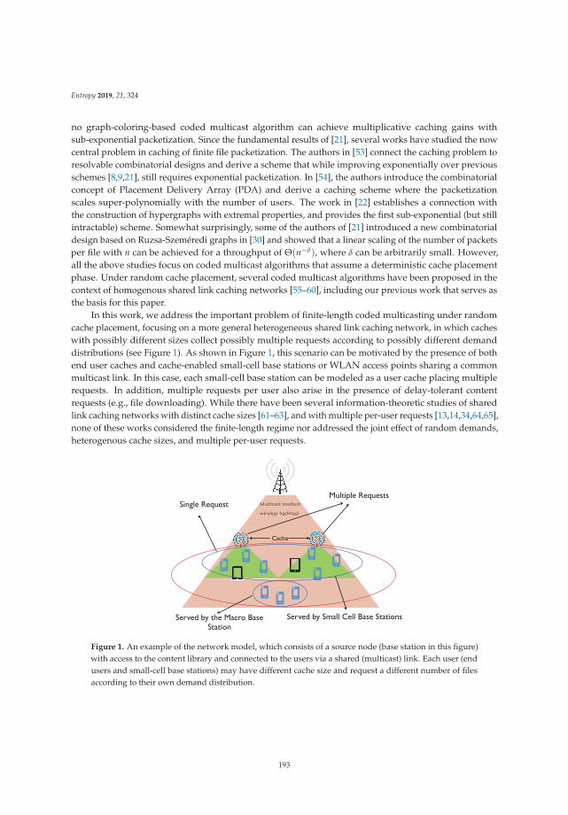
Entropy 2019, 21, 324

no graph-coloring-based coded multicast algorithm can achieve multiplicative caching gains withsub-exponential packetization. Since the fundamental results of [21], several works have studied the nowcentral problem in caching of finite file packetization. The authors in [53] connect the caching problem toresolvable combinatorial designs and derive a scheme that while improving exponentially over previousschemes [8,9,21], still requires exponential packetization. In [54], the authors introduce the combinatorialconcept of Placement Delivery Array (PDA) and derive a caching scheme where the packetizationscales super-polynomially with the number of users. The work in [22] establishes a connection withthe construction of hypergraphs with extremal properties, and provides the first sub-exponential (but stillintractable) scheme. Somewhat surprisingly, some of the authors of [21] introduced a new combinatorialdesign based on Ruzsa-Szeméredi graphs in [30] and showed that a linear scaling of the number of packetsper file with n can be achieved for a throughput of Θ(n−δ), where δ can be arbitrarily small. However,all the above studies focus on coded multicast algorithms that assume a deterministic cache placementphase. Under random cache placement, several coded multicast algorithms have been proposed in thecontext of homogenous shared link caching networks [55–60], including our previous work that serves asthe basis for this paper.

In this work, we address the important problem of finite-length coded multicasting under randomcache placement, focusing on a more general heterogeneous shared link caching network, in which cacheswith possibly different sizes collect possibly multiple requests according to possibly different demanddistributions (see Figure 1). As shown in Figure 1, this scenario can be motivated by the presence of bothend user caches and cache-enabled small-cell base stations or WLAN access points sharing a commonmulticast link. In this case, each small-cell base station can be modeled as a user cache placing multiplerequests. In addition, multiple requests per user also arise in the presence of delay-tolerant contentrequests (e.g., file downloading). While there have been several information-theoretic studies of sharedlink caching networks with distinct cache sizes [61–63], and with multiple per-user requests [13,14,34,64,65],none of these works considered the finite-length regime nor addressed the joint effect of random demands,heterogenous cache sizes, and multiple per-user requests.

wireless backhaulwireless backhaul

Multiple RequestsSingle Request

Cache

Served by the Macro Base Station

Served by Small Cell Base Stations

Figure 1. An example of the network model, which consists of a source node (base station in this figure)with access to the content library and connected to the users via a shared (multicast) link. Each user (endusers and small-cell base stations) may have different cache size and request a different number of filesaccording to their own demand distribution.

193

Entropy 2019, 21, 324

The contributions of this paper are as follows:

1. We provide a generalized model for heterogeneous shared link caching networks, in which userscan have different cache sizes and make different number of requests according to different demanddistributions.

2. We design two novel coded multicast algorithms based on local graph coloring, referred to as GreedyLocal Coloring (GLC) and Hierarchical Greedy Local Coloring (HgLC) that exhibit polynomial-timecomplexity in both the number of caches and the packetization order. In combination with theRandom Aggregate Popularity (RAP) placement policy of [10,12], we show that the overall schemesRAP-GLC and RAP-HgLC are order-optimal in the asymptotic file-length regime.

3. Focusing on the finite-length regime, in which content items can be partitioned into a finite number ofpackets, we show how the general advantage of local graph coloring is especially relevant when thenumber of per-user requests grow. We validate via simulations the superiority of RAP-GLC, especiallywith high number of per-user requests. We then show how RAP-HgLC, with a slight increase inthe polynomial complexity order, further improves the caching gain of RAP-GLC, remarkablyapproaching the multiplicative gain that existing schemes can only guarantee in the asymptoticfile-length regime.

4. We demonstrate that there is a tradeoff between the required packetization order and the numberof requested files per user. In particular, for a given target gain, if the number of requests increases,then the number of packets per file can be reduced, while preserving the target gain. We furtherquantify the regime of per-user requests for which a caching scheme with unit packetizationorder (i.e., a scheme that treats only whole files) is order-optimal. Our analysis illustrates thekey impact of content request aggregation in time and space on caching performance. That is, if edgecaches can wait for collecting multiple requests over time and/or aggregate requests from multipleusers, the same performance can be achieved with lower packetization order, and hence lowercomputational complexity.

The paper is organized as follows. Section 2 introduces the network model and problemformulation. Section 3 describes the construction of coded multicast algorithms using graph coloring,with special focus on the advantages of local graph coloring. Section 4 presents novel polynomial-timelocal-graph-coloring-based coded multicast schemes. Section 5 analyzes the effect of request aggregationon the performance–complexity tradeoff. Section 6 presents simulation results and related discussions.Finally, concluding remarks are given in Section 7.

2. Network Model and Problem Formulation

We consider a caching network formed by a source node with access to a content library,connected to several caching nodes/users via a single shared (multicast) link. Similar to previousworks [8–10,12–14,21,22,30], we define a caching scheme in terms of two phases:

• Placement phase, which operates at a large time-scale and determines the content to be placed at thecaching nodes,

• Delivery phase, during which users requests are served from the content caches and sources inthe network.

However, differently from previous works, we generalize the model to a heterogeneous system inwhich each caching node has a possibly different cache size and requests a possibly different number offiles. A practical example of our setting can be represented by a macro base station connected to severalcache-enabled small-cell base stations, and a number of user devices served either by the macro base

194

Entropy 2019, 21, 324

station or by the small-cell base stations. In this setting, each small cell acts as a super user requestingmultiple files resulting from the requests of the users it serves.

Specifically, the heterogeneous caching network consists of a single source node storing a libraryof files F = {1, . . . , m}, each with entropy F bits, and n user nodes U = {1, . . . , n}, each with a cache ofstorage capacity MuF bits (i.e., each user caches up to Mu files). Each user u can requests Lu (1 ≤ Lu ≤ m)

different files according to its individual request probability distribution. We assume that the library fileshave finite length and consequently a finite packetization order. Our main objective is to design a cachingscheme that minimizes the number of transmissions required to satisfy the demands of all users.

In a homogeneous network setting with infinite packetization order, recent works [8–10,12–14]have shown that it is possible to satisfy a scaling number of users with only a constant number ofmulticast transmissions. The achievable schemes configure user caches with complementary (side)information during the caching phase, such that the resulting coded multicasting opportunities thatarise during the delivery phase can be used to minimize the transmission rate (or load) over the sharedmulticast link. Specifically, reference [12] showed that under Zipf file popularity, a properly optimizedrandom fractional placement policy, referred to as Random Aggregate Popularity (RAP) caching, achievesorder-optimality when combined with a graph-coloring-based coded multicast scheme. Unfortunately,even in the homogenous setting, it was shown in [21] that a central limitation of all previous works is thatthey require infinite packetization order: all existing caching schemes achieve at most a factor of two gainwhen the packetization order is finite.

In this work, inspired by the fundamental throughput-delay-memory tradeoff derived in [21], our goalis to design computationally efficient schemes that provide good performance in the finite packetizationregime. For the caching phase, (1) we restrict our placement policies to the class of random fractionalschemes described in [9,10,12–14], proved to be order-optimal in the homogeneous setting. For the deliveryphase, (2) we focus on the class of graph-coloring-based index coding schemes, and design two novelpolynomial-time algorithms that employ local graph coloring on the (index coding) conflict graph [51].

2.1. Random Fractional Cache Placement

The class of random fractional placement schemes is described as follows:

1. Packetization: Each file is partitioned into B packets of equal-size F/B bits, where the integer B isreferred to as the packetization order. Each packet is represented by a symbol in finite field F2F/B ,where we assume that F/B is large enough.

2. Random Placement: Each user u caches p f ,u MuB packets independently at random from each file f ,where p f ,u is the probability that file f is cached at user u, and satisfies 0 ≤ p f ,u ≤ 1/Mu, ∀ f ∈ Fsuch that ∑m

f=1 p f ,u = 1, ∀u ∈ U .

We introduce a caching distribution matrix P = [p f ,u] ∈ Rm×n+ , where f ∈ F and u ∈ U . Please

note that the number of packets of file f cached at user u, p f ,u MuB, can be directly determined fromthe caching distribution matrix P. As described in [10,12–14], the caching distribution must be properlyoptimized to balance the gains from local cache hits (where requested packets are served by the localcache) and coded multicast opportunities (where requested packets are served by coded transmissionsthat simultaneously satisfy distinct user requests). When this is the case, we refer to the cache placementscheme as Random Aggregate Popularity (RAP) caching (see e.g., [10,12–14]). Given the number of packetsto be cached of a given file, the actual indices of the packets to be cached are chosen uniformly at random,and independently across users. We use Cu, f to denote the set of packets of file f cached at user u andC = {Cu, f } with u ∈ U and f ∈ F to denote the packet-level cache placement realization.

The goal of the placement phase is to configure the user caches to create coding opportunitiesduring the delivery phase that allow serving distinct user requests via common multicast transmissions.

195

Entropy 2019, 21, 324

Compared to deterministic placement [8], random placement schemes allow configuring user caches withlower complexity and increased robustness, i.e., changes in system parameters (e.g., number of users,number files, file popularity) require less changes in users’ cache configurations [12].

Recall that the placement phase operates at a much larger time-scale than the delivery phase,and hence is unaware of the requests in the subsequent delivery rounds. Therefore, the placement phasecan be designed according to the demand distribution, but must be independent of the requests realizations.

2.2. Random Multiple Requests

Each user u ∈ U requests Lu (1 ≤ Lu ≤ m) files independently from other users, followinga probability distribution q f ,u with q f ,u ∈ [0, 1] and ∑m

f=1 q f ,u = 1 (i.e., for each request of user u, file f ischosen with probability q f ,u). We introduce a demand distribution matrix Q = [q f ,u] ∈ R

m×n+ , where f ∈ F

and u ∈ U . In the following, we use W = {Wu, f }, with u ∈ U and f ∈ F , to denote the packet-leveldemand realization where Wu, f denotes the packets of file f requested by user u.

The multiple-request parameters {Lu} have a key operational meaning, in that it captures thepossibility of edge caches to collect requests across time and space. That is, Lu may represent the amountof requests collected over time (given the delay tolerance of some content requests) as well as the amountof requests collected across space from users served by the given edge cache (e.g., when edge caches arelocated at helper nodes or small-cell base stations serving multiple individual users).

2.3. Performance Metric

For given realizations of the random fractional cache placement and the random multiple requests,the goal is to design a delivery scheme that minimizes the rate over the shared multicast link required tosatisfy all user requests. Since one placement phase is followed by an arbitrarily large number of deliveryrounds (each characterized by a new independent request realization), the rate (or load) of the systemrefers only to the delivery phase (i.e., asymptotically the cache placement costs no rate). Furthermore,it makes sense to consider the average rate, where averaging with respect to the users request distributiontakes on the meaning of a time-averaged rate, invoking an ergodicity argument.

At each request round, let F = {f1, f2, · · · , fn} be the demand realization, where fu =

{ f1,u, f2,u, · · · , fLu ,u}, u ∈ U . The source node computes a multicast codeword as a function of the libraryand the demand realization F. We assume that the source node communicates to the user nodes throughan error-free deterministic shared multicast link.

Given the demand realization F, let the total number of bits transmitted by the source node be J(F).We are interested in the average performance of the coded multicast scheme, and hence define the averagerate (or load) as the number of transmitted bits normalized by the file size:

R =E [J(F)]

F, (1)

where the expectation is over the random demand distribution.

3. Graph-Coloring-Based Coded Multicast Delivery

It is important to note that for given cache placement and demand realizations, the delivery phaseof a caching scheme reduces to an index coding problem with a twist. The only difference with theconventional index coding problem introduced in [51] is that the cache information may contain part of(as opposed to entire) requested files, and that users may request multiple (as opposed to single) files.Nevertheless, as in index coding, the problem can still be represented by a conflict graph [10,12–14],where vertices represent requested packets, and an edge between two vertices indicates a conflict, in the

196

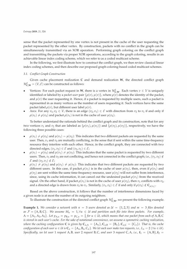
Entropy 2019, 21, 324

sense that the packet represented by one vertex is not present in the cache of the user requesting thepacket represented by the other vertex. By construction, packets with no conflict in the graph can besimultaneously transmitted via an XOR operation. Performing graph coloring on the conflict graphand transmitting the packets via proper XOR operations, according to the graph coloring, results in anachievable linear index coding scheme, which we refer to as a coded multicast scheme.

In the following, we first illustrate how to construct the conflict graph, we then review classical linearindex coding schemes, and then describe our proposed graph-coloring-based coded multicast schemes.

3.1. Conflict Graph Construction

Given cache placement realization C and demand realization W, the directed conflict graphHd

C,W = (V , E) can be constructed as follows:

• Vertices: For each packet request in W, there is a vertex in HdC,W. Each vertex v ∈ V is uniquely

identified or labeled by a packet-user pair {ρ(v), μ(v)}, where ρ(v) denotes the identity of the packet,and μ(v) the user requesting it. Hence, if a packet is requested by multiple users, such a packet isrepresented in as many vertices as the number of users requesting it. Such vertices have the samepacket label ρ(v), but different user label μ(v).

• Arcs: For any v1, v2 ∈ V , there is an edge (v2, v1) ∈ E with direction from v2 to v1 if and only ifρ(v1) �= ρ(v2) and packet ρ(v1) is not in the cache of user μ(v2).

To better understand the rationale behind the conflict graph and its construction, note that for anytwo vertices v1 and v2 that are labeled as {ρ(v1), μ(v1)} and {ρ(v2), μ(v2)}, respectively, we have thefollowing three possible cases:

• ρ(v1) �= ρ(v2) and μ(v1) = μ(v2): This indicates that two different packets are requested by the sameuser. Then, v1 and v2 are mutually conflicting, in the sense that if sent within the same time-frequencyresource they interfere with each other. Hence, in the conflict graph, they are connected with twodirected edges, (v1, v2) ∈ E and (v2, v1) ∈ E ;

• ρ(v1) = ρ(v2) and μ(v1) �= μ(v2): This indicates that the same packet is requested by two differentusers. Then, v1 and v2 are not conflicting, and hence not connected in the conflict graph; i.e., (v1, v2) /∈E and (v2, v1) /∈ E ;

• ρ(v1) �= ρ(v2) and μ(v1) �= μ(v2): This indicates that two different packets are requested by twodifferent users. In this case, if packet ρ(v1) is in the cache of user μ(v2), then, even if ρ(v1) andρ(v2) are sent within the same time-frequency resource, user μ(v2) will not suffer from interference,since, using its cache information, it can cancel out the undesired packet ρ(v1) from the receivedsignal. On the other hand, if packet ρ(v1) is not in the cache of user μ(v2), then v1 conflicts with v2,and a directed edge is drawn from v2 to v1. Similarly, (v1, v2) ∈ E if and only if ρ(v2) /∈ Cμ(v1)

.

Based on the above construction, it follows that the number of interference dimensions faced bya given node is at most the number of its outgoing neighbors.

To illustrate the construction of the directed conflict graphHdC,W, we present the following example.

Example 1. We consider a network with n = 3 users denoted as U = {1, 2, 3} and m = 3 files denotedas F = {A, B, C}. We assume Mu = 1, ∀u ∈ U and partition each file into three packets. For example,A = {A1, A2, A3}. Let pA,u = pB,u = pC,u = 1

3 for u ∈ U , which means that one packet from each of A, B, Cis stored in each user’s cache. For the sake of notational convenience, we assume a symmetric caching realization,where the caching configuration C is given by Cu,A = {Au}, Cu,B = {Bu}, Cu,C = {Cu}). That is, the cacheconfiguration of each user u ∈ U is Cu = {Au, Bu, Cu}. We let each user make two requests, i.e., Lu = 2 (∀u ∈ U ).Specifically, we let user 1 request A, B, user 2 request B, C, and user 3 request C, A, i.e., f1 = {A, B}, f2 =

197

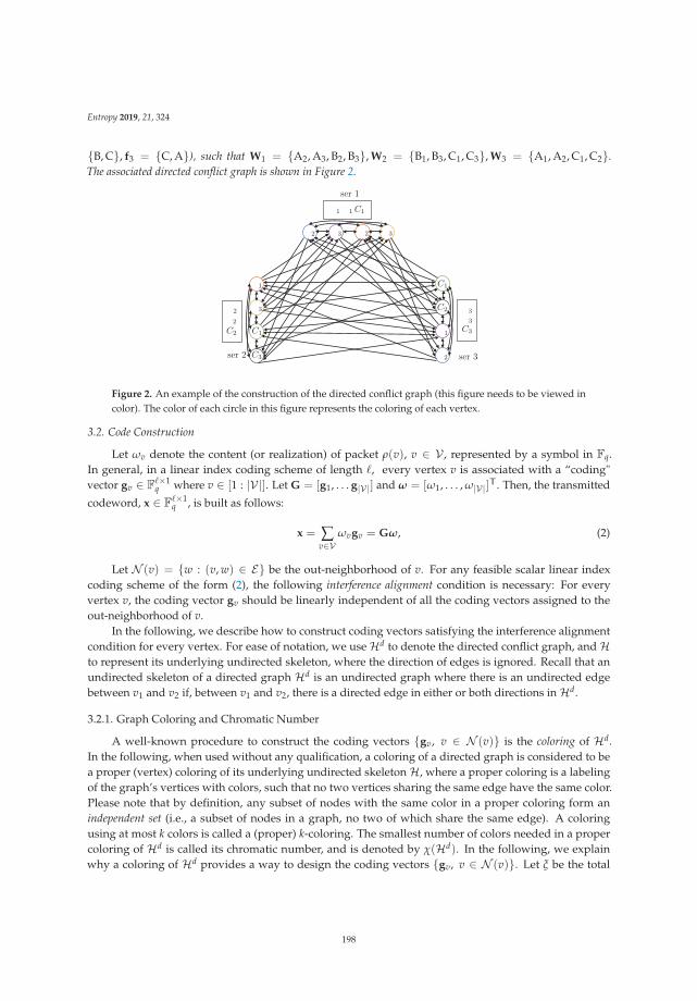
Entropy 2019, 21, 324

{B, C}, f3 = {C, A}), such that W1 = {A2, A3, B2, B3}, W2 = {B1, B3, C1, C3}, W3 = {A1, A2, C1, C2}.The associated directed conflict graph is shown in Figure 2.

2 3 32

3

2

1

C1

C3

C1

C2

1

1 1 C1

C2

2

2 3

3

C3

ser 1

ser 2 ser 3

Figure 2. An example of the construction of the directed conflict graph (this figure needs to be viewed incolor). The color of each circle in this figure represents the coloring of each vertex.

3.2. Code Construction

Let ωv denote the content (or realization) of packet ρ(v), v ∈ V , represented by a symbol in Fq.In general, in a linear index coding scheme of length �, every vertex v is associated with a “coding"vector gv ∈ F

�×1q where v ∈ [1 : |V|]. Let G = [g1, . . . g|V|] and ω = [ω1, . . . , ω|V|]

T. Then, the transmitted

codeword, x ∈ F�×1q , is built as follows:

x = ∑v∈V

ωvgv = Gω, (2)

Let N (v) = {w : (v, w) ∈ E} be the out-neighborhood of v. For any feasible scalar linear indexcoding scheme of the form (2), the following interference alignment condition is necessary: For everyvertex v, the coding vector gv should be linearly independent of all the coding vectors assigned to theout-neighborhood of v.

In the following, we describe how to construct coding vectors satisfying the interference alignmentcondition for every vertex. For ease of notation, we useHd to denote the directed conflict graph, andHto represent its underlying undirected skeleton, where the direction of edges is ignored. Recall that anundirected skeleton of a directed graph Hd is an undirected graph where there is an undirected edgebetween v1 and v2 if, between v1 and v2, there is a directed edge in either or both directions inHd.

3.2.1. Graph Coloring and Chromatic Number

A well-known procedure to construct the coding vectors {gv, v ∈ N (v)} is the coloring of Hd.In the following, when used without any qualification, a coloring of a directed graph is considered to bea proper (vertex) coloring of its underlying undirected skeletonH, where a proper coloring is a labelingof the graph’s vertices with colors, such that no two vertices sharing the same edge have the same color.Please note that by definition, any subset of nodes with the same color in a proper coloring form anindependent set (i.e., a subset of nodes in a graph, no two of which share the same edge). A coloringusing at most k colors is called a (proper) k-coloring. The smallest number of colors needed in a propercoloring of Hd is called its chromatic number, and is denoted by χ(Hd). In the following, we explainwhy a coloring of Hd provides a way to design the coding vectors {gv, v ∈ N (v)}. Let ξ be the total

198

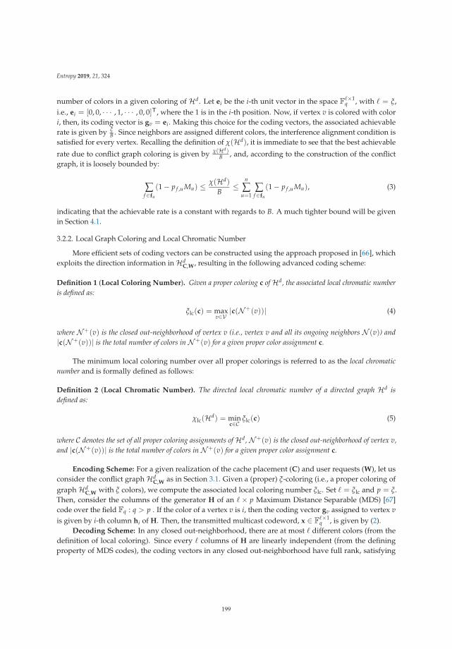
Entropy 2019, 21, 324

number of colors in a given coloring of Hd. Let ei be the i-th unit vector in the space F�×1q , with � = ξ,

i.e., ei = [0, 0, · · · , 1, · · · , 0, 0]T, where the 1 is in the i-th position. Now, if vertex v is colored with colori, then, its coding vector is gv = ei. Making this choice for the coding vectors, the associated achievablerate is given by ξ

B . Since neighbors are assigned different colors, the interference alignment condition issatisfied for every vertex. Recalling the definition of χ(Hd), it is immediate to see that the best achievable

rate due to conflict graph coloring is given by χ(Hd)B , and, according to the construction of the conflict

graph, it is loosely bounded by:

∑f∈fu

(1− p f ,u Mu) ≤χ(Hd)

B≤

n

∑u=1

∑f∈fu

(1− p f ,u Mu), (3)

indicating that the achievable rate is a constant with regards to B. A much tighter bound will be givenin Section 4.1.

3.2.2. Local Graph Coloring and Local Chromatic Number

More efficient sets of coding vectors can be constructed using the approach proposed in [66], whichexploits the direction information inHd

C,W, resulting in the following advanced coding scheme:

Definition 1 (Local Coloring Number). Given a proper coloring c ofHd, the associated local chromatic numberis defined as:

ξlc(c) = maxv∈V

|c(N+(v))| (4)

where N+(v) is the closed out-neighborhood of vertex v (i.e., vertex v and all its ongoing neighbors N (v)) and|c(N+(v))| is the total number of colors in N+(v) for a given proper color assignment c.

The minimum local coloring number over all proper colorings is referred to as the local chromaticnumber and is formally defined as follows:

Definition 2 (Local Chromatic Number). The directed local chromatic number of a directed graph Hd isdefined as:

χlc(Hd) = minc∈C

ξlc(c) (5)

where C denotes the set of all proper coloring assignments ofHd, N+(v) is the closed out-neighborhood of vertex v,and |c(N+(v))| is the total number of colors in N+(v) for a given proper color assignment c.

Encoding Scheme: For a given realization of the cache placement (C) and user requests (W), let usconsider the conflict graphHd

C,W as in Section 3.1. Given a (proper) ξ-coloring (i.e., a proper coloring ofgraph Hd

C,W with ξ colors), we compute the associated local coloring number ξlc. Set � = ξlc and p = ξ.Then, consider the columns of the generator H of an � × p Maximum Distance Separable (MDS) [67]code over the field Fq : q > p . If the color of a vertex v is i, then the coding vector gv assigned to vertex vis given by i-th column hi of H. Then, the transmitted multicast codeword, x ∈ F

�×1q , is given by (2).

Decoding Scheme: In any closed out-neighborhood, there are at most � different colors (from thedefinition of local coloring). Since every � columns of H are linearly independent (from the definingproperty of MDS codes), the coding vectors in any closed out-neighborhood have full rank, satisfying

199

Entropy 2019, 21, 324

the interference alignment condition. The message ωv at vertex v is obtained at user v as follows: (1)Using side information at user v, cancel out message parts corresponding to all vertices outside N+(v),i.e., x′ = x− ∑

u/∈N+(v)ωugu. This is possible because, by the definition of the conflict graphHd, the messages

{ωu}u/∈N+(v) are available as side information at user v and the encoding mechanism is known to all theusers. (2) Find a vector z in the dual space of {gu}u∈N+(v)\{v} such that zTx′ �= 0 (this is possible since gv

is linearly independent of {gu}u∈N+(v)\{v} because of the local chromatic number-based construction).Now, zTx′ = (zTgv)ωv. Therefore, user v recovers its own message. It follows that all users can recover allthe requested packets employing such linear scheme.

Achievable Rate: The coding scheme constructed as described above achieves a rate given by ξlc/B,where B is the number of packets per file.

Example 2. We consider an example shown in Figure 3. First, we assign colors to each vertex such that the totalnumber of colors ξ = 5, and count the local coloring number, which is ξlc = 4. Then, we construct the generatormatrix A of a (ξ = 5, ξlc = 4) MDS code, which is given by

A =

⎛⎜⎜⎜⎜⎜⎝1 0 0 0 1

0 1 0 0 1

0 0 1 0 1

0 0 0 1 1

⎞⎟⎟⎟⎟⎟⎠ . (6)

After that, we assign the columns of A to gv, corresponding from the left to the right to the vertices with thepackets {A2, A3, B2, B1, A1}, as shown in Figure 3. Finally, the transmitted codewords can be generated which arethe rows of the right-hand side of (2)

X(1) = A1 ⊕A2, X(2) = A1 ⊕A3 (7)

X(3) = A1 ⊕ B1, X(4) = A1 ⊕ B2 (8)

where the length of the code is ξlc/B = 4/3 file units. It can be easily verified that every user can decoded its desiredpackets with the cached ones.

1

2

3

3

1

2

⎛⎜⎜⎝1000

⎞⎟⎟⎠

⎛⎜⎜⎝0100

⎞⎟⎟⎠

⎛⎜⎜⎝0100

⎞⎟⎟⎠

⎛⎜⎜⎝0010

⎞⎟⎟⎠

⎛⎜⎜⎝0001

⎞⎟⎟⎠

⎛⎜⎜⎝1111

⎞⎟⎟⎠

Figure 3. An illustration of coded multicast codewords construction based on local coloring (this figureneeds to be viewed in color). The total number of colors is ξ = 5, and the local coloring number is ξlc = 4.

It is immediate to see that the best achievable rate due to local coloring is obtained by computing thelocal chromatic number ofHd

C,W and using its associated coloring to design the coding vectors, yieldinga rate χlc/B. However, note that to compute χlc, we must optimize over all proper colorings to find the

200

Entropy 2019, 21, 324

local chromatic number. As with the chromatic number, this can be cast as an Integer Program and it ishence an NP-hard problem. To overcome this limitation, in Section 4, we propose a greedy approachthat (i) exhibits polynomial-time complexity in all the system parameters, (ii) achieves close to optimalperformance for finite packetization order, and (iii) is asymptotically (i.e., for infinite packetization order)order-optimal.

3.3. Benefits of Local Coloring

Consider the following relation established for general directed graphs in [66]:

χlc(Hd) ≤ χ(Hd) ≤ χlc(Hd)O(log n). (9)

Focusing on the conflict graph of interestHdC,W, the number of vertices can be as large as B ∑u∈U Lu.

It then follows from (9) that the gap between the local chromatic number and the chromatic numbercan be as large as log(B ∑u∈U Lu). Please note that this multiplicative factor grows with the number ofpackets per file B and the number of per-user requests Lu, supporting the extra benefit of local coloringin the multiple-request scenario. In addition, the higher the number of per-user requests, the higherthe directionality of the conflict graph, which is the main factor exploited by local coloring to reducethe achievable rate (see Section 3.2.2), further supporting the suitability of local coloring in increasinglypractical settings where there is some form of spatial or temporal request aggregation.

4. Proposed Algorithms and Performance Analysis

As stated earlier, computing the local chromatic number is NP-hard. To circumvent this challenge,in this section, we propose two greedy coded multicast schemes, which together with the cacheplacement described in Section 2.1, yield the following two caching schemes: Randomized AggregatePopularity-Greedy Local Coloring (RAP-GLC) and Randomized Aggregate Popularity-Hierarchicalgreedy Local Coloring (RAP-HgLC). In both cases, the steps for obtaining the coded multicast scheme areas follow:

i. Given a realization of the cache placement (C) and of the user requests (W), build the conflict graphHd

C,W as in Section 3.1.ii. Use any of the above algorithms (GLC or HgLC) to compute a proper coloring. Let ξ denote the

number of colors used by either of the above algorithms to colorHdC,W. Let ξlc be the associated local

coloring number.iii. Consider a (ξ, ξlc) MDS code and compute the corresponding coded multicast scheme as described in

Section 3.2.2.

4.1. Randomized Aggregate Popularity-Greedy Local Coloring (RAP-GLC)

The RAP-GLC algorithm generalizes the RAP-GCC (Random Aggregate Popularity-GreedyConstrained Coloring) algorithm introduced in [12]. RAP-GCC is a caching scheme based on randomfractional caching for the placement phase and a coded multicast scheme built on greedy-graph-coloring-based linear index coding [51,68] for the delivery phase. RAP-GLC is more general than RAP-GCCin two aspects: (1) conventional coloring is replaced by local coloring to leverage possible gains in themultiple-request scenario, as described in Sections 3.2.1 and 3.3, and (2) RAP-GLC adaptively (dependingon the demand realization) chooses between naive or coded multicasting according to a thresholdparameter, instead of sticking to one of them (as in RAP-GCC).

201

Entropy 2019, 21, 324

4.1.1. RAP-GLC Algorithm Description

The algorithm associates to each vertex v a label or tag, composed of two fieldsi.e., Kv ≡ (TD(v), TC(v)) with TC(v) denoting the subset of users caching the packet associated withvertex v, i.e.,

TC(v)Δ= {u ∈ U : ρ(v) ∈ Cu}, (10)

and TD(v) denoting the subset of users requesting the packet associated with vertex v, i.e.,

TD(v)Δ= {u ∈ U : ρ(v) ∈ Wu}, (11)

which includes the user itself μ(v) who requests ρ(v) and all the others requesting ρ(v). Please note thatthe cardinality of TD(v) indicates the popularity of packet ρ(v). Furthermore, let

Tv = {μ(v)} ∪ TC(v).

Given a vertex v, if the cardinality of TD(v) is higher than a predetermined threshold parametert ∈ {0 · · · , n} i.e., |TD(v)| > t, then all vertices v′ such that ρ(v) = ρ(v′) are colored with the samecolor, leading to a naive multicast transmission scheme. If |TD(v)| ≤ t, then RAP-GLC greedily looks fora maximal set of vertices with the same Tv (Algorithm 1, Line 14) and colors them with the same colorif there is no conflict among the vertices (Algorithm 1, Line 15). The threshold parameter t is subject tooptimization, as described in Section 4.1.2.

Doing this, RAP-GLC computes a valid coloring of the conflict graph H. Finally, the algorithmcomputes its associated local coloring number (Algorithm 1, Line 24). The coding scheme employed isbased on the MDS code described in Section 3.2.1 associated with the above local coloring.

Algorithm 1 RAP-GLC1: Let C = ∅;2: Let c = ∅;3: while V �= ∅ do

4: Pick an arbitrary vertex v in V ; Let I = {v};5: Let V′ = V \ {v};6: if { |TD(v)| > t } then

7: for all v′ ∈ V′ with ρ(v′) = ρ(v) do

8: I = I ∪ v′;9: end for

10: Color all the vertices in I by c /∈ C;11: Let c[I′] = c;12: V = V \ I′.13: else

14: for all v′ ∈ V′ with Tv′ ≡ Tv do

15: if {There is no edge between v′ and I} then

16: I = I ∪ v′;17: end if18: end for19: Color all the vertices in I by c /∈ C;20: Let c[I ] = c;21: V = V \ I .22: end if23: end while24: return the local coloring number maxv∈V |c(N+(v))| and the corresponding color assignment c(N+(v)) for

each v;

202

Entropy 2019, 21, 324

Time Complexity: In Algorithm 1, both the outer while-loop starting at Line 3, and the inner for-loopstarting at Line 6 iterate at most |V| times, and all other operations inside the loops take constant time.Therefore, the complexity of RAP-GLC is O(|V|2) or, equivalently, O(n2B2), since |V| ≤ nB, which ispolynomial in |V| (or n, B).

4.1.2. RAP-GLC Performance Analysis

In the following, we quantify the performance of RAP-GLC in the asymptotic regime when thenumber of users and files is kept constant while the packetization order is sent to infinity. Denotingby E[RRAP−GLC(P, Q, t)] the asymptotic average achievable rate of RAP-GLC for a fixed threshold t,the threshold parameter t is optimized to minimize E[RRAP−GLC(P, Q, t)]. Hence, denoting by RRAP−GLC

the average rate achieved by RAP-GLC with optimized t, i.e.,

RRAP−GLC = mint

E[RRAP−GLC(P, Q, t)],

we have thatRRAP−GLC ≤ min{E[RRAP−GLC(P, Q, n)],E[RRAP−GLC(P, Q, 0)].

Since E[RRAP−GLC(P, Q, 0)] is just the rate achieved via naive multicasting, then, an upperbound on the average asymptotic performance of RAP-GLC can be obtained by upper boundingE[RRAP−GLC(P, Q, n)] which can be obtained by generalizing the asymptotic performance analysisof RAP-GCC derived in [10,12] using conventional graph coloring in the homogeneous shared linkcaching network to the case of using local coloring in the heterogeneous caching network. Specifically,we extend the order-optimality analysis under single per-user requests (L = 1) in the asymptotic regime ofB → ∞ [10,12], to that under multiple L > 1 per-use requests [13,14]. These theoretical results will serveas rate lower bounds for the finite-length performance of our proposed algorithms.

Let L = maxu Lu and order Lu, u ∈ U as a decreasing sequence L[1] ≥ L[2] ≥ L[3], . . . , L[n], where L[i]is the i-th largest Lu and [i] = u for some u ∈ U . It can be seen that L[1] = maxu Lu and L[n] = minu Lu.Let nj = ∑[i] 1{L[i] − j ≥ 0} > 0, where 1 ≤ j ≤ L[1] and 1{·} is the indicator function. Let Unj = {[i] ∈ U :1{L[i] − j ≥ 0}}. In the next theorem, we provide a performance guarantee of the RAP-GLC algorithm.

Theorem 1. For any given m, n, Mu, the random caching distribution P and the random request distribution Q,the average achievable rate of the RAP-GLC algorithm, RRAP−GLC satisfies

RRAP−GLC ≤ min{ψ(P, Q), m− M}, (12)

when B → ∞, where,

m =m

∑f=1

(1−

n

∏u=1

(1− q f ,u

)Lu

), (13)

M =m

∑f=1

(1−

n

∏u=1

(1− q f ,u

)Lu

)min

up f ,u Mu, (14)

ψ(P, Q) =L

∑j=1

n

∑�=1

∑U �⊂Unj

m

∑f=1

∑u∈U �

ρ f ,u,U �λ(u, f ,U �),

203

Entropy 2019, 21, 324

with U � denoting a set of users with cardinality �,

λ(u, fu,U �) = (1− p fu ,u Mu)× ∏k∈U �\{u}

(p fu ,k Mk) ∏k∈U\U �

(1− p fu ,k Mk) (15)

and

ρ f ,u,U �Δ= P( f = arg max

fu∈f(U �)λ(u, fu,U �)),

denoting the probability that f is the file whose p f ,u maximizes the term λ(u, fu,U �) among f(U �) (the set of filesrequested by U �).

Proof. See Appendix A.

Using the explicit expression for RRAP−GLC in Theorem 1, we can optimize the caching distributionfor a wide class of heterogeneous network models to minimize the number of transmissions. We use P∗ todenote the caching distribution that minimizes RRAP−GLC.

Remark 1. For the sake of the numerical evaluation of ψ(q, p), it is worthwhile to note that the probabilities ρ f ,u,U �

can be easily computed as follows. Given the subset of users, U � of cardinality �, let Ju1 , . . . , Ju�denote � i.i.d. random

variables each of them distributed over F with pmf qui , with i = 1, . . . , �. Since λ(u1, Ju1U �), · · · , λ(u�, Ju�,U �)

are i.i.d., the CDF of Y�Δ= max{λ(u1, Ju1 ,U �), · · · , λ(u�, Ju�

,U �)} is given by

P (Y� ≤ y) =�

∏i=1

P

(λ(ui, Jui ,U �) ≤ y

)

=�

∏i=1

⎛⎝ ∑j∈F :λ(ui ,j,U �)≤y

qui ,j

⎞⎠ .

(16)

Hence, it follows that

ρ f ,u,U � = P(Y� = λ(u, f ,U �))

=�

∏i=1

⎛⎝ ∑j∈F :g�(j)≤λ(u, f ,U �)

qui ,j

⎞⎠− �

∏i=1

⎛⎝ ∑j∈F :g�(j)<λ(u, f ,U �)

qui ,j

⎞⎠ ,(17)

which can be easily computed by sorting the values {λ(ui, j,U �) : j ∈ F , ui ∈ U �}.

Nevertheless, as shown in [21], when B is finite or is not exponential in n, the performance ofRAP-GLC can degrade significantly, compromising the promising multiplicative caching gain, although itis already an improved version of RAP-GCC in [12]. This brings us to the other main contribution wherewe propose a new algorithm that preserves the gain due to coded multicasting even when B is finite.

4.2. Randomized Aggregate Popularity-Hierarchical Greedy Local Coloring ( RAP-HgLC) forFinite-Length Packetization

Similarly to RAP-GLC, RAP-HgLC has a predetermined parameter t ∈ {0, · · · , n} that is optimizedto minimize its associated average achievable rate. However, in the RAP-HgLC algorithm, we arrangethe vertices in a hierarchy and use this to design a more careful coloring algorithm. The key idea of

204

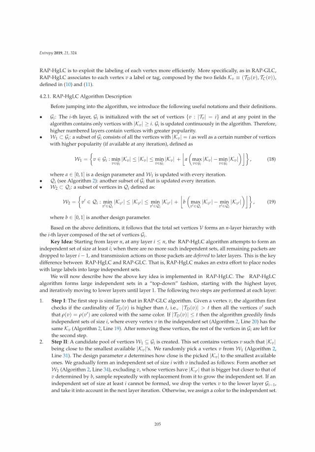
Entropy 2019, 21, 324

RAP-HgLC is to exploit the labeling of each vertex more efficiently. More specifically, as in RAP-GLC,RAP-HgLC associates to each vertex v a label or tag, composed by the two fields Kv ≡ (TD(v), TC(v)),defined in (10) and (11).

4.2.1. RAP-HgLC Algorithm Description

Before jumping into the algorithm, we introduce the following useful notations and their definitions.

• Gi: The i-th layer, Gi is initialized with the set of vertices {v : |Tv| = i} and at any point in thealgorithm contains only vertices with |Kv| ≥ i. Gi is updated continuously in the algorithm. Therefore,higher numbered layers contain vertices with greater popularity.

• W1 ⊂ Gi: a subset of Gi consists of all the vertices with |Kv| = i as well as a certain number of verticeswith higher popularity (if available at any iteration), defined as

W1 =

{v ∈ Gi : min

v∈Gi|Kv| ≤ |Kv| ≤ min

v∈Gi|Kv| +

⌊a(

maxv∈Gi

|Kv| −minv∈Gi

|Kv|)⌋}

, (18)

where a ∈ [0, 1] is a design parameter andW1 is updated with every iteration.• Qi (see Algorithm 2): another subset of Gi that is updated every iteration.• W2 ⊂ Qi: a subset of vertices in Qi defined as:

W2 =

{v′ ∈ Qi : min

v′∈Qi|Kv′ | ≤ |Kv′ | ≤ min

v′∈Qi|Kv′ | +

⌊b(

maxv′∈Qi

|Kv′ | − minv′∈Qi

|Kv′ |)⌋}

, (19)

where b ∈ [0, 1] is another design parameter.

Based on the above definitions, it follows that the total set vertices V forms an n-layer hierarchy withthe i-th layer composed of the set of vertices Gi.

Key Idea: Starting from layer n, at any layer i ≤ n, the RAP-HgLC algorithm attempts to form anindependent set of size at least i; when there are no more such independent sets, all remaining packets aredropped to layer i− 1, and transmission actions on those packets are deferred to later layers. This is the keydifference between RAP-HgLC and RAP-GLC. That is, RAP-HgLC makes an extra effort to place nodeswith large labels into large independent sets.

We will now describe how the above key idea is implemented in RAP-HgLC. The RAP-HgLCalgorithm forms large independent sets in a “top-down” fashion, starting with the highest layer,and iteratively moving to lower layers until layer 1. The following two steps are performed at each layer:

1. Step I: The first step is similar to that in RAP-GLC algorithm. Given a vertex v, the algorithm firstchecks if the cardinality of TD(v) is higher than t, i.e., |TD(v)| > t then all the vertices v′ suchthat ρ(v) = ρ(v′) are colored with the same color. If |TD(v)| ≤ t then the algorithm greedily findsindependent sets of size i, where every vertex v in the independent set (Algorithm 2, Line 20) has thesame Kv (Algorithm 2, Line 19). After removing these vertices, the rest of the vertices in Gi are left forthe second step.

2. Step II: A candidate pool of verticesW1 ⊆ Gi is created. This set contains vertices v such that |Kv|being close to the smallest available |Kv|’s. We randomly pick a vertex v from W1 (Algorithm 2,Line 31). The design parameter a determines how close is the picked |Kv| to the smallest availableones. We gradually form an independent set of size i with v included as follows: Form another setW2 (Algorithm 2, Line 34), excluding v, whose vertices have |Kv′ | that is bigger but closer to that ofv determined by b, sample repeatedly with replacement from it to grow the independent set. If anindependent set of size at least i cannot be formed, we drop the vertex v to the lower layer Gi−1,and take it into account in the next layer iteration. Otherwise, we assign a color to the independent set.

205

Entropy 2019, 21, 324

W1 is repeatedly formed and random sampling fromW1 repeated till every vertex in Gi is droppedor colored.

Algorithm 2 HgLC

1: C = ∅;2: c = ∅;3: choose a ∈ [0, 1]4: choose b ∈ [0, 1]5: for all i = n, n− 1, . . . , 2, 1 do

6: for all v ∈ Gi and |Kv| = i do

7: I = {v};8: Let V′ = V \ {v};9: if { |TD(v)| > t } then

10: for all v′ ∈ V′ with ρ(v′) = ρ(v) do

11: I = I ∪ v′;12: end for13: Color all the vertices in I by c /∈ C;14: Let c[I ] = c;15: for all i = n, n− 1, . . . , 2, 1 do

16: Gi = Gi \ I ;17: end for18: else

19: for all v′ ∈ Gi \ I with Kv′ ≡ Kv do

20: if {There is no edge between v′ and I} then

21: I = I ∪ v′;22: end if23: end for24: if |I| = i then

25: Color all the vertices in I by c /∈ C;26: c[I ] = c, C = C ∪ c;27: Gi = Gi \ I ;28: end if29: end if30: end for31: for all v ∈ Gi with v randomly picked fromW1 ⊂ Gi do

32: I = {v};33: Qi = Gi \ I ;34: for all v′ ∈ Qi with v′ randomly picked fromW2 ⊂ Qi. do

35: if {Kv′ ⊃ Kv } ∩ {No edge between v′ and I} then

36: I = I ∪ v′;37: Qi = Qi \ {v′};38: else

39: Qi = Qi \ {v′};40: end if41: end for42: if |I| ≥ i then

43: Color all the vertices in I by c /∈ C;44: c[I ] = c, C = C ∪ c;45: Gi = Gi \ I ;46: else

47: Gi = Gi \ {v}, Gi−1 = Gi−1 ∪ {v};48: end if49: end for50: end for51: c =LocalSearch(HC,W, c, C);52: return the local coloring number maxv∈V |c(N+(v))| and the corresponding color assignment c(N+(v)) for each v;

206

Entropy 2019, 21, 324

Remark 2. Please note that RAP-GLC goes through the same Step I as RAP-HgLC, and then simply assignsa different color to each remaining uncolored vertex. On the other hand, Step II in RAP-HgLC tries to find furtherindependent sets among the remaining uncolored vertices. It is this extra step that guarantees the performance ofRAP-HgLC to be no worse than that of RAP-GLC.

The RAP-HgLC algorithm, when operating on the i-th layer, always colors at least i vertices with thesame color. Please note that if there are remaining vertices when reaching layer 1, all such vertices will becolored, each with a different color.

To further reduce the required number of colors, we use a function called LocalSearch (Algorithm 2,Line 51), which is described in Algorithm 3. It works in an iterative fashion by replacing the currentsolution with a better one if there exists. It terminates when no better solutions can be found. In particular,the local search algorithm has the purpose of checking the redundancy of each color c ∈ C, to eventuallydecrease the current objective function value |C|. In more detail, the local search computes, iteratively foreach color c ∈ C, the set Jc of all vertices colored with color c, and performs the following steps:

1. For each vertex i ∈ Jc, if there is a color c′ ∈ C, c′ �= c that is not assigned to any adjacent vertexj ∈ Adj(i), then assign vertex i with color c′;

2. Color c is removed from the set C if and only if in the previous step it has been possible to replace cwith some color c′ �= c for all vertices in Jc.

Finally, in Algorithm 2, Line 52, we compute the local coloring number.

Algorithm 3 LocalSearch(HC,W, c, C)

1: for all c ∈ C do

2: Let Jc be the set of vertices whose color is c;3: Let B = ∅;4: Let c = c;5: for all i ∈ Jc do

6: A = ∅;7: for all j ∈ N (i) do

8: A = A∪ c[j];9: if C \ A �= ∅ then

10: c′ is chosen uniformly at random from C \ A;11: c[i] = c′;12: B = B ∪ {i};13: end if14: end for15: if |B| = |Jc| then

16: c = c;17: C = C \ c;18: end if19: end for20: end for21: return c;

To illustrate the RAP-HgLC algorithm, we present the following example.

Example 3. Consider a shared link network with n = 3 users: U = {1, 2, 3}, and m = 3 files: F = {A, B, C}.Each file is partitioned into 4 packets. For example, A = {A1, A2, A3, A4}. For the caching part, let user 1cache {A1, B1, B2, B3, B4, C2}, user 2 cache {A1, A2, A3, A4, B1, C2, C3}, user 3 cache {A1, A2, A3, C1, B2, B3}.Then, let users {1, 2, 3} request files {A, B, C} respectively. Equivalently, user 1 requests A2, A3, A4; user 2

207

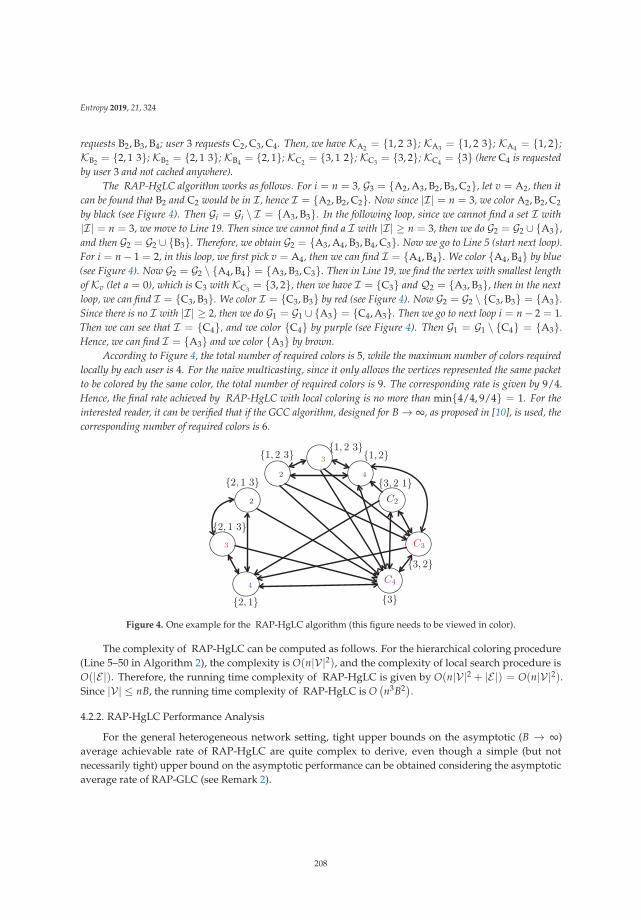
Entropy 2019, 21, 324

requests B2, B3, B4; user 3 requests C2, C3, C4. Then, we have KA2 = {1, 2 3}; KA3 = {1, 2 3}; KA4 = {1, 2};KB2 = {2, 1 3}; KB2 = {2, 1 3}; KB4 = {2, 1}; KC2 = {3, 1 2}; KC3 = {3, 2}; KC4 = {3} (here C4 is requestedby user 3 and not cached anywhere).

The RAP-HgLC algorithm works as follows. For i = n = 3, G3 = {A2, A3, B2, B3, C2}, let v = A2, then itcan be found that B2 and C2 would be in I , hence I = {A2, B2, C2}. Now since |I| = n = 3, we color A2, B2, C2

by black (see Figure 4). Then Gi = Gi \ I = {A3, B3}. In the following loop, since we cannot find a set I with|I| = n = 3, we move to Line 19. Then since we cannot find a I with |I| ≥ n = 3, then we do G2 = G2 ∪ {A3},and then G2 = G2 ∪ {B3}. Therefore, we obtain G2 = {A3, A4, B3, B4, C3}. Now we go to Line 5 (start next loop).For i = n− 1 = 2, in this loop, we first pick v = A4, then we can find I = {A4, B4}. We color {A4, B4} by blue(see Figure 4). Now G2 = G2 \ {A4, B4} = {A3, B3, C3}. Then in Line 19, we find the vertex with smallest lengthof Kv (let a = 0), which is C3 with KC3 = {3, 2}, then we have I = {C3} and Q2 = {A3, B3}, then in the nextloop, we can find I = {C3, B3}. We color I = {C3, B3} by red (see Figure 4). Now G2 = G2 \ {C3, B3} = {A3}.Since there is no I with |I| ≥ 2, then we do G1 = G1 ∪ {A3} = {C4, A3}. Then we go to next loop i = n− 2 = 1.Then we can see that I = {C4}, and we color {C4} by purple (see Figure 4). Then G1 = G1 \ {C4} = {A3}.Hence, we can find I = {A3} and we color {A3} by brown.

According to Figure 4, the total number of required colors is 5, while the maximum number of colors requiredlocally by each user is 4. For the naive multicasting, since it only allows the vertices represented the same packetto be colored by the same color, the total number of required colors is 9. The corresponding rate is given by 9/4.Hence, the final rate achieved by RAP-HgLC with local coloring is no more than min{4/4, 9/4} = 1. For theinterested reader, it can be verified that if the GCC algorithm, designed for B → ∞, as proposed in [10], is used, thecorresponding number of required colors is 6.

2

2 C2

4

4

3 C3

3

C4

{3}

{3, 2}

{2, 1}

{1, 2}{1, 2 3} {1, 2 3}

{2, 1 3}

{2, 1 3}

{3, 2 1}

Figure 4. One example for the RAP-HgLC algorithm (this figure needs to be viewed in color).

The complexity of RAP-HgLC can be computed as follows. For the hierarchical coloring procedure(Line 5–50 in Algorithm 2), the complexity is O(n|V|2), and the complexity of local search procedure isO(|E |). Therefore, the running time complexity of RAP-HgLC is given by O(n|V|2 + |E |) = O(n|V|2).Since |V| ≤ nB, the running time complexity of RAP-HgLC is O

(n3B2).

4.2.2. RAP-HgLC Performance Analysis

For the general heterogeneous network setting, tight upper bounds on the asymptotic (B → ∞)average achievable rate of RAP-HgLC are quite complex to derive, even though a simple (but notnecessarily tight) upper bound on the asymptotic performance can be obtained considering the asymptoticaverage rate of RAP-GLC (see Remark 2).

208

Entropy 2019, 21, 324

Regarding the finite-length regime, in [21] we derived a tight upper bound on the performanceof RAP-HgLC for the simpler case of homogenous networks under worst-case demands. Specifically,the bound in [21], requires B to be O

(( mM)g+2

)(where O hides some poly log terms) to achieve a worst-case

rate of at most ng . This approximately matches a lower bound of O(

( mM)g) derived in the same work for any

coloring algorithm, showing, for the simpler homogenous network setting, the optimality of RAP-HgLCamong all graph-coloring-based algorithms.

For the more complex setting where demands arise from popularity distributions and every userrequests multiple files, the finite-length performance of RAP-HgLC is investigated in Section 6 vianumerical analysis, where we show how the RAP-HgLC is able to recover most of the multiplicativecaching gain even with very moderate packetization order.

5. Tradeoff between Number of Requests and Code Length

As mentioned earlier, in the simpler homogenous scenario, the authors in [21] showed that underworst-case demands, to achieve a gain g over conventional naive multicasting, it is necessary for B togrow exponentially with g. Intuitively, this is because a sufficiently large B is needed to create codedmulticast transmissions that are useful for multiple users. However, when each user makes multiplerequests, the number of requests Lu = L can play a similar role to that of B, such that the requirement forB, and hence the resulting computational complexity can be reduced. For ease of analysis, in this section,we assume that all users place the same number of requests (Lu = L).

In the following, under either worst-case or uniform demands, we show the sufficient conditions onB and L that guarantee achieving a gain g = Mn

m . From this result, we can obtain the regime where B andL are interchangeable (L plays an equivalent role to B). Note that it can be shown that the number of filetransmissions under both worst-case and uniform demands have the same order.

We consider two cases for the range of B: the case of B = 1, and the case of B = ω( m

M). The regime

where 1 < B = O( m

M)

is out of the scope of this paper.When B = 1, the cache placement algorithm becomes scalar uniform cache placement (SUP), in which

each user caches M entire files chosen uniformly at random. For simplicity, we let M be a positive integer.Then, as shown in [14], letting L → ∞ as a function of n, m, M, we obtain the following theorem.

Theorem 2. When B = 1 and M = ω(1), for the shared link caching network with n users, library size m, storagecapacity M, and L distinct per-user requests (nL ≤ m), if (i) M

m ≤ 12 and

L = ω

⎛⎜⎝max

⎧⎪⎨⎪⎩nMm

( mM

)n 1(1− M

m

) ,

⎛⎜⎝ (nM)1

2(1−ε)( mM − 1

) (1−

(1− M

m

)n)⎞⎟⎠⎫⎪⎬⎪⎭

⎞⎟⎠ , (20)

or (ii) Mm ≥ e

1+e and

L = ω

⎛⎜⎝max

⎧⎪⎨⎪⎩(

mm−M

)n,

⎛⎜⎝ (nM)1

2(1−ε)( mM − 1

) (1−

(1− M

m

)n)⎞⎟⎠⎫⎪⎬⎪⎭

⎞⎟⎠ , (21)

where ε is an arbitrarily small number,then, the achievable rate of RAP-GLC is upper bounded by

limn,m→∞

P

(RSUP−GLC ≤ (1 + o(1))min

{L( m

M− 1

), Ln, m−M

})= 1.

209

Entropy 2019, 21, 324

Proof. See Appendix B.

From Theorem 2, we can see that when L and M are large enough, instead of requiring a large B andpacket-level coding, a simpler file-level coding scheme is sufficient to achieve the same order-optimal rate.We remark, however, that the range of the parameter regimes in which this result holds is limited dueto the requirement of a large M and L. Next, we focus on another parameter regime, when B = ω

( mM),

and find the achievable tradeoff between B and L.

Theorem 3. When B = ω( m

M), for the shared link caching network with n users, library size m, storage capacity

M, and L distinct per-user requests (nL ≤ m), if (i) Mm ≤ 1

2 , and

B = ω

⎛⎜⎝max

⎧⎪⎨⎪⎩nMLm

( mM

)n 1(1− M

m

) ,(nM)

12(1−ε)

L( m

M − 1) (

1−(

1− Mm

)n)⎫⎪⎬⎪⎭

⎞⎟⎠ , (22)

or (ii) Mm ≥ e

1+e , and

B = ω

⎛⎜⎝max

⎧⎪⎨⎪⎩ 1L

(m

m−M

)n,

(nM)1

2(1−ε)

L( m

M − 1) (

1−(

1− Mm

)n)⎫⎪⎬⎪⎭

⎞⎟⎠ , (23)

where ε is an arbitrarily small number,Then, the achievable rate of RAP-GLC is upper bounded by

limn,m→∞

P

(RSUP−GLC ≤ (1 + o(1))min

{L( m

M− 1

), Ln, m−M

})= 1. (24)

Proof. See Appendix C.

If we particularize Theorem 1 to the homogenous network setting under uniform demands, we seethat the rate achieved by RAP-GLC is upper bounded by the same expression given in (24). Hence,from Theorem 2, we can see that when L is large enough, instead of requiring a very large B, an intermediatevalue of B = ω

( mM)

is sufficient to achieve the same order-optimal rate. In practice, it is important tofind the right balance and tradeoff between B and L given the remaining system parameters. In Section 6,we show via simulation that a similar tradeoff holds also for RAP-HgLC.

6. Simulations and Discussions

In this section, we numerically evaluate the performance of the two polynomial-time algorithmsdescribed in Section 4, RAP-GLC and RAP-HgLC, in the finite-length regime characterized by the numberof packets per file B.

Recall that the caching distribution P∗ is to be optimized to minimize the number of transmissions.Since the distribution P∗ resulting from minimizing the right-hand side of (12) may not admitan analytically tractable expression in general, in the following numerical results, we restrict the cachingdistribution to take the form of a truncated uniform distribution pu, as described in [12]:

p f ,u =1m u

, f ≤ mu

p f ,u = 0, f ≥ m + 1(25)

210

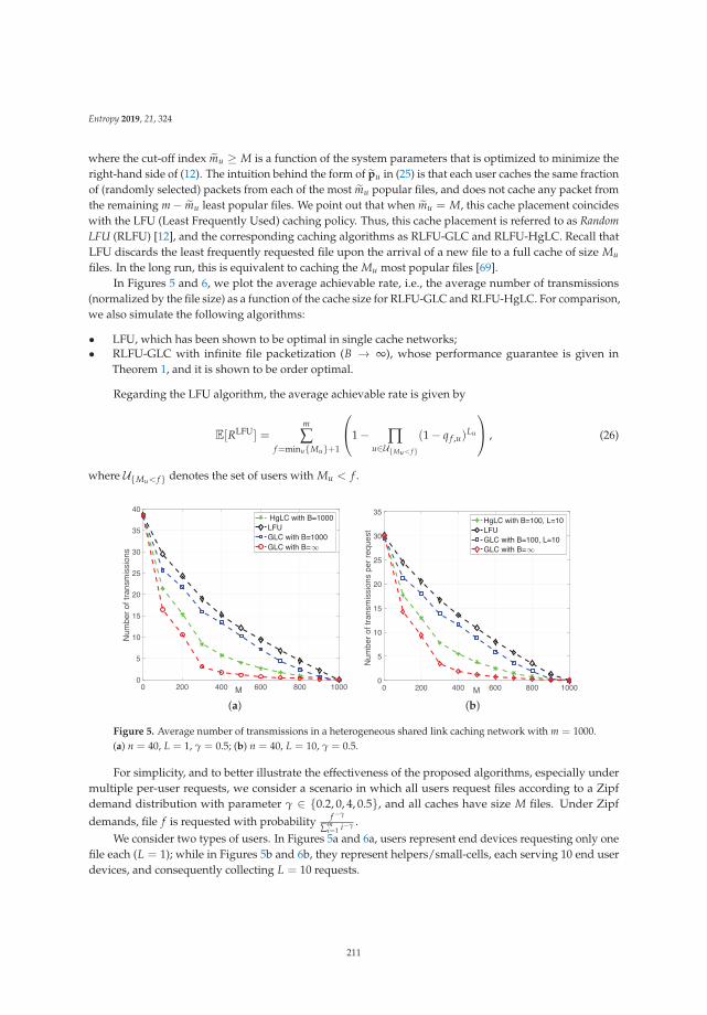
Entropy 2019, 21, 324

where the cut-off index mu ≥ M is a function of the system parameters that is optimized to minimize theright-hand side of (12). The intuition behind the form of pu in (25) is that each user caches the same fractionof (randomly selected) packets from each of the most mu popular files, and does not cache any packet fromthe remaining m− mu least popular files. We point out that when mu = M, this cache placement coincideswith the LFU (Least Frequently Used) caching policy. Thus, this cache placement is referred to as RandomLFU (RLFU) [12], and the corresponding caching algorithms as RLFU-GLC and RLFU-HgLC. Recall thatLFU discards the least frequently requested file upon the arrival of a new file to a full cache of size Mu

files. In the long run, this is equivalent to caching the Mu most popular files [69].In Figures 5 and 6, we plot the average achievable rate, i.e., the average number of transmissions

(normalized by the file size) as a function of the cache size for RLFU-GLC and RLFU-HgLC. For comparison,we also simulate the following algorithms:

• LFU, which has been shown to be optimal in single cache networks;• RLFU-GLC with infinite file packetization (B → ∞), whose performance guarantee is given in

Theorem 1, and it is shown to be order optimal.

Regarding the LFU algorithm, the average achievable rate is given by

E[RLFU] =m

∑f=minu{Mu}+1

⎛⎝1− ∏u∈U{Mu< f }

(1− q f ,u)Lu

⎞⎠ , (26)

where U{Mu< f } denotes the set of users with Mu < f .

0 200 400 600 800 1000M0

5

10

15

20

25

30

35

40

Num

ber

of tr

ansm

issi

ons

HgLC with B=1000LFUGLC with B=1000GLC with B=

(a)

0 200 400 600 800 1000M0

5

10

15

20

25

30

35

Num

ber

of tr

ansm

issi

ons

per

requ

est

HgLC with B=100, L=10LFUGLC with B=100, L=10GLC with B=

(b)

Figure 5. Average number of transmissions in a heterogeneous shared link caching network with m = 1000.(a) n = 40, L = 1, γ = 0.5; (b) n = 40, L = 10, γ = 0.5.

For simplicity, and to better illustrate the effectiveness of the proposed algorithms, especially undermultiple per-user requests, we consider a scenario in which all users request files according to a Zipfdemand distribution with parameter γ ∈ {0.2, 0, 4, 0.5}, and all caches have size M files. Under Zipf

demands, file f is requested with probability f−γ

∑mi=1 i−γ .

We consider two types of users. In Figures 5a and 6a, users represent end devices requesting only onefile each (L = 1); while in Figures 5b and 6b, they represent helpers/small-cells, each serving 10 end userdevices, and consequently collecting L = 10 requests.

211

Entropy 2019, 21, 324

In Figure 5a,b, we fix the total number of users n and the product between L and B (L× B = 1000).Figure 5a plots the average rate for a network with n = 40 users, γ = 0.5, L = 1, and B = 1000.It is immediate to observe the impact of finite packetization on the multiplicative caching gain. In fact,as predicted by the theory (see [21]), the significant caching gain (with respect to LFU) quantified by theasymptotic performance of RAP-GLC (GLC with B = ∞) is completely lost when using RAP-GLC withfinite packetization (GLC with B = 1000). On the other hand, RAP-HgLC remarkably preserves, at theexpense of a slight increase in computational complexity, most of the multiplicative caching gain for thesame value of file packetization. For example, in Figure 5a, if M doubles from M = 200 to M = 400,then the rate achieved by RAP-HgLC reduces from 15 to 5.7. Furthermore, RAP-HgLC can achieve a factorof 3.5 rate reduction from LFU for M = 500. For the same regime, it is straightforward to verify thatneither RAP-GLC nor LFU exhibit this property. Note from Figure 5a that to guarantee a rate of 10,RAP-GLC requires a cache size of M = 500, while RAP-HgLC can reduce the cache size requirement toM = 250, a 2× cache size reduction. Furthermore, while LFU can only provide an additive caching gain,additive and multiplicative gains may show indistinguishable when M is comparable to the library size m.Hence, one needs to pick a reasonably small M ( m

n < M $ m) to observe the multiplicative caching gainof RAP-HgLC.

Figure 5b shows the average rate for a network with n = 40 helpers/small-cells, each serving 10 usersmaking requests according to a Zip distribution with γ = 0.5. Hence, the total number of distinct requestsper helper is up to Lu = 10, ∀u ∈ {1, . . . , 20}. In this case, we assume B = 100 (instead of B = 1000 inFigure 5a). In order to make easier the comparison with Figure 5a, we normalize the achievable rate(number of transmissions) by the file size and the number of requests.

Note from Figure 5a,b that as predicted by Theorem 3, when Lu increases (from Lu = 1 to Lu = 10),almost the same multiplicative caching gain can be achieved with a smaller B (from B = 1000 to B = 100).In fact, from Figure 5a,b, we see that under RAP-HgLC, the average rate per request for B = 100 andL = 10 is almost the same as the average rate per request for B = 1000 and L = 1. This confirms theinteresting tradeoff between B and L established in Theorem 3.

We can observe a similar behavior in Figure 6a,b. Figure 6a plots the average rate for a network withn = 80 users, γ = 0.4, L = 1, and B = 200. RAP-HgLC is able to preserve most of the multiplicativecaching gain for the same values of file packetization. For example, in Figure 6a, if M doubles fromM = 200 to M = 400, then the rate achieved by RAP-HgLC essentially halves from 20 to 10. Furthermore,RAP-HgLC can achieve a factor of 5 rate reduction from LFU for M = 500. Note from Figure 6a that toguarantee a rate of 20, RAP-GLC requires a cache size of M = 500, while RAP-HgLC can reduce the cachesize requirement to M = 200, a 2.5× cache size reduction.

Figure 6b plots the average rate for a network with n = 20 helpers/small-cells, each serving 10 usersmaking requests according to a Zip distribution with γ = 0.2. Hence, the total number of distinct requestsper helper is up to Lu = 10, ∀u ∈ {1, . . . , 20}. In this case, we assume B = 100. Differently from Figure 5b,here we plot the average rate without normalizing it by the number of requests.

Note from Figure 6a,b that, as predicted by Theorem 3, when Lu increases (from Lu = 1 to Lu = 10),almost the same multiplicative caching gain can be achieved with a smaller B (from B = 200 to B = 100).In fact, from Figure 6a,b, we see that under RAP-HgLC , the average rate per request for B = 100 andL = 10 is almost the same as the average rate per request for B = 200 and L = 1. For example, for M = 200,B = 100, and L = 10, the per request average rate achieved by RAP-HgLC is 0.3, while for M = 200 andB = 200, is 0.25. This again confirms the tradeoff between B and L stated in Theorem 3.

212

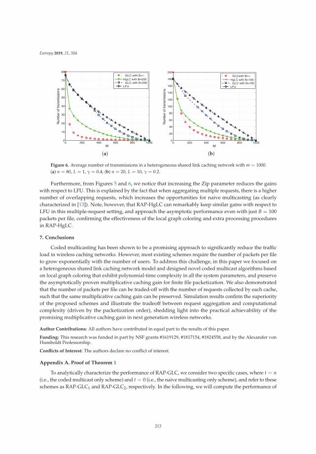
Entropy 2019, 21, 324

0 200 400 600 800 10000

10

20

30

40

50

60

70

80

M

Num

ber o

f tra

nsm

issi

ons

GCLC with B=∞HgLC with B=200GCLC with B=200LFU

G

G

(a)

0 200 400 600 800 10000

20

40

60

80

100

120

140

160

180

200

M

Num

ber o

f tra

nsm

issi

ons

GCLCwith B=∞HgLC with B=100GCLC with B=100LFU

G

G

(b)

Figure 6. Average number of transmissions in a heterogeneous shared link caching network with m = 1000.(a) n = 80, L = 1, γ = 0.4; (b) n = 20, L = 10, γ = 0.2.

Furthermore, from Figures 5 and 6, we notice that increasing the Zip parameter reduces the gainswith respect to LFU. This is explained by the fact that when aggregating multiple requests, there is a highernumber of overlapping requests, which increases the opportunities for naive multicasting (as clearlycharacterized in [13]). Note, however, that RAP-HgLC can remarkably keep similar gains with respect toLFU in this multiple-request setting, and approach the asymptotic performance even with just B = 100packets per file, confirming the effectiveness of the local graph coloring and extra processing proceduresin RAP-HgLC.

7. Conclusions

Coded multicasting has been shown to be a promising approach to significantly reduce the trafficload in wireless caching networks. However, most existing schemes require the number of packets per fileto grow exponentially with the number of users. To address this challenge, in this paper we focused ona heterogeneous shared link caching network model and designed novel coded multicast algorithms basedon local graph coloring that exhibit polynomial-time complexity in all the system parameters, and preservethe asymptotically proven multiplicative caching gain for finite file packetization. We also demonstratedthat the number of packets per file can be traded-off with the number of requests collected by each cache,such that the same multiplicative caching gain can be preserved. Simulation results confirm the superiorityof the proposed schemes and illustrate the tradeoff between request aggregation and computationalcomplexity (driven by the packetization order), shedding light into the practical achievability of thepromising multiplicative caching gain in next generation wireless networks.

Author Contributions: All authors have contributed in equal part to the results of this paper.

Funding: This research was funded in part by NSF grants #1619129, #1817154, #1824558, and by the Alexander vonHumboldt Professorship.


Appendix A. Proof of Theorem 1

To analytically characterize the performance of RAP-GLC, we consider two specific cases, where t = n(i.e., the coded multicast only scheme) and t = 0 (i.e., the naive multicasting only scheme), and refer to theseschemes as RAP-GLC1 and RAP-GLC2, respectively. In the following, we will compute the performance of

213

Entropy 2019, 21, 324

these two cases respectively and take the minimum rate between these two cases. Obviously, this rate canserve as an upper bound of RAP-GLC.

Appendix A.1. Average Total Number of Colors for RAP-GLC1

To compute the average total number of colors provided by RAP-GLC1, we first see that for all v ∈ Iobtained in this algorithm, Tv are identical. Based on Algorithm 1, by construction the independent setsI ⊂ V generated by RAP-GLC1 have the same (unordered) label of users requesting or caching the packets{ρ(v) : v ∈ I}. We shall refer to such unordered label of users as the user label of the independent set.Hence, we count the independent sets by enumerating all possible user labels, and upperbounding howmany independent sets I Algorithm 1 generates for each user label. Consider a user label U � ⊂ U ofsize �, and let I(U �, f, i) the i-th independent set generated by Algorithm 1 with label U � and while letJ (U �, f) = {I(U �, f, i) : ∀i}.

Following Algorithm 1, for each U �, the number of used colors is |J (U �, f)|. Given f, we can see that|J (U �, f)| is a random variable which is a function of C. Let the indicator 1{Tv fu

= U �} denote the eventthat vertex v fu from file fu requested by user u ∈ U � is available in all the users in U � but u and the rest ofthe vertices U \ U �, then 1{Tv fu

= U �} follows a Bernoulli distribution with parameter

λ(u, fu) = (1− p fu ,u Mu) ∏k∈U �\{u}

(p fu ,k Mk) ∏k∈U\U �

(1− p fu ,k Mk) (A1)

such that its expectation is λ(u, fu). Then, we can see that given f , ∑∀v fu1{Tv fu

= U �} = λ(u, fu)B + o(B)with high probability [70]. Thus, as B → ∞, we have that with high probability,

|J (U �, f)| = maxfu∈f(U �)

∑∀v fu

1{Tv fu= U �}

= maxfu∈f(U �)

λ(u, fu)B + o(B),(A2)

where f(U �) represent the set of files requested by U �.Then, by averaging over the demand’s distribution, we obtain that with high probability:

E[χ(HM,W)] ≤ E

⎡⎢⎣ L

∑j=1

n

∑�=1

∑U �⊂Unj

∣∣∣J (U �, f)∣∣∣⎤⎥⎦

=L

∑j=1

n

∑�=1

∑U �⊂Unj

E

[∣∣∣J (U �, f)∣∣∣]

(a)=

L

∑j=1

n

∑�=1

∑U �⊂Unj

E

[max

fu∈f(U �)λ(u, fu)B + o(B)

]

(b)=

L

∑j=1

n

∑�=1

∑U �⊂Unj

m

∑f=1

∑u∈U �

ρ f ,u,U � λ(u, f ) + δ1(B),

(A3)

where (a) is by using (A2) and (b) is obtained by computing the probability that the requested file fu in f(U �)

maximizes λ(u, f ). δ1(B) denotes a smaller order term of ∑Lj=1 ∑n

�=1 ∑U �⊂Unj∑m

f=1 ∑u∈U � ρ f ,u,U �λ(u, f ).

For any U �, we obtain that ∑ f ∑u∈U � ρ f ,u,U � = 1, and ρ f ,u,U � denotes the probability that file f is the file

214

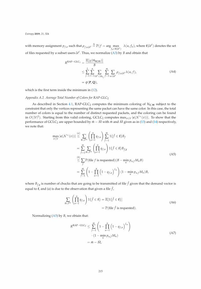
Entropy 2019, 21, 324

with memory assignment p f ,u such that ρ f ,u,U �Δ= P( f = arg max

fu∈f(U �)λ(u, fu), where f(U �) denotes the set

of files requested by a subset users U �. Thus, we normalize (A3) by B and obtain that

RRAP−GLC1 =E[χ(HM,W)]

B

≤L

∑j=1

n

∑�=1

∑U �⊂Unj

m

∑f=1

∑u∈U �

ρ f ,u,U �λ(u, f ),

= ψ(P, Q),

(A4)

which is the first term inside the minimum in (12).

Appendix A.2. Average Total Number of Colors for RAP-GLC2

As described in Section 4.1, RAP-GLC2 computes the minimum coloring of HC,W subject to theconstraint that only the vertices representing the same packet can have the same color. In this case, the totalnumber of colors is equal to the number of distinct requested packets, and the coloring can be foundin O(|V|2). Starting from this valid coloring, GCLC2 computes maxv∈V |c(N+(v))|. To show that theperformance of GCLC2 are upper bounded by m− M with m and M given as in (13) and (14) respectively,we note that:

maxv∈V

|c(N+(v))|(a)≤ ∑

f∈Fn

(n

∏u=1

q f ,u

)m

∑f=1

1{ f ∈ f}Bf

=m

∑f=1

∑f∈Fn

(n

∏u=1

q f ,u

)1{ f ∈ f}Bf ,f

(b)≤ ∑

fP(file f is requested)(B−min

upu, f MuB)

=m

∑f=1

(1−

n

∏u=1

(1− q f ,u

)Lu

)(1−min

upu, f Mu)B,

(A5)

where Bf ,f is number of chucks that are going to be transmitted of file f given that the demand vector is

equal to f, and (a) is due to the observation that given a file f ,

∑f∈Fn

(n

∏u=1

q f ,u

)1{ f ∈ f} = E[1{ f ∈ f}]

= P(file f is requested).

(A6)

Normalizing (A5) by B, we obtain that:

RRAP−GLC2 ≤m

∑f=1

(1−

n

∏u=1

(1− q f ,u

)Lu

)· (1−min

upu, f Mu)

= m− M,

(A7)

215

Entropy 2019, 21, 324

which is the second term inside the minimum in (12).

Appendix B. Proof of Theorem 2

In this section, we prove Theorem 2. Recall that for each U �, the number of used colors is given by|J (U �, f)|, then we have we have |J (U �, f)| = maxu∈U � ∑∀v fu

1{Tv fu= U �}, where f(U �) represent the

set of files requested by U �. In this case, it is clear that

E

⎡⎣ ∑∀v fu

1{Tv fu= U �}

⎤⎦ = L(

Mm

)l−1 (1− M

m

)n−l+1. (A8)

Then let

YlΔ= |J (U �, f)| −E

⎡⎣ ∑∀v fu

1{Tv fu= U �}

⎤⎦ . (A9)

The goal is to find a condition of L such that

|E[Yl ]| = o

(L(

Mm

)l−1 (1− M

m

)n−l+1)

, (A10)

which implies

E

[|J (U �, f)|

]≤ (1 + o(1))L

(Mm

)l−1 (1− M

m

)n−l+1. (A11)

Then following the similar step from Theorem 1 in [12], we can obtain the concentration result shown

in Theorem 2, where we require L = ω

((nM)

12(1−ε)

( mM−1)

(1−(1−M

m )n)

)and ε > 0 is an arbitrarily small number.

To compute |E[Yl ]|, we have

(E[Yl ])2 ≤ E[(Yl)

2]

= E

⎡⎢⎣⎛⎝|J (U �, f)| −E

⎡⎣ ∑∀v fu

1{Tv fu= U �}

⎤⎦⎞⎠2⎤⎥⎦

= E

⎡⎢⎣⎛⎝max

u∈U �

⎛⎝ ∑∀v fu

1{Tv fu= U �} −E

⎡⎣ ∑∀v fu

1{Tv fu= U �}

⎤⎦⎞⎠⎞⎠2⎤⎥⎦

≤ ∑u∈U �

E

⎡⎢⎣⎛⎝ ∑∀v fu

1{Tv fu= U �} −E

⎡⎣ ∑∀v fu

1{Tv fu= U �}

⎤⎦⎞⎠2⎤⎥⎦

= lE

⎡⎢⎣⎛⎝ ∑∀v fu

1{Tv fu= U �} −E

⎡⎣ ∑∀v fu

1{Tv fu= U �}

⎤⎦⎞⎠2⎤⎥⎦

(a)= lL

(Mm

)l−1 (1− M

m

)n−l+1(

1−(

Mm

)l−1 (1− M

m

)n−l+1)+ δ1,

(A12)

216

Entropy 2019, 21, 324

where (a) is because M = ω(1) such that δ1 is a smaller order term compared to the first term in (A12) anduse the variance for the Binomial distribution. Then, we let

(lL

(Mm

)l−1 (1− M

m

)n−l+1(

1−(

Mm

)l−1 (1− M

m

)n−l+1)) 1

2= o

(L(

Mm

)l−1 (1− M

m

)n−l+1)

, (A13)

then, we can obtain

L = ω

⎛⎜⎜⎝ l(

1−(

Mm

)l−1 (1− M

m

)n−l+1)

(Mm

)l−1 (1− M

m

)n−l+1

⎞⎟⎟⎠

= ω

⎛⎜⎜⎝(

1−(

Mm

)l−1 (1− M

m

)n−l+1)

1l

(Mm

)l−1 (1− M

m

)n−l+1

⎞⎟⎟⎠ .

(A14)

For sufficient condition, let

L = ω

⎛⎜⎝ 1

1l

(Mm

)l−1 (1− M

m

)n−l+1

⎞⎟⎠ . (A15)

Do the derivative of s(l) = 1l

(Mm

)l−1 (1− M

m

)n−l+1with respect to l, we obtain

ds(l)dl

=1l

((Mm

)l−1 (1− M

m

)n−l+1log

Mm

− log(

1− Mm

)(Mm

)l−1 (1− M

m

)n−l+1)

− 1l2

(Mm

)l−1 (1− M

m

)n−l+1

=1l

log

(Mm

1− Mm

)(Mm

)l−1 (1− M

m

)n−l+1

− 1l2

(Mm

)l−1 (1− M

m

)n−l+1.

(A16)

• When Mm < 1

2 , then we have ds(l)l < 0. Hence, s(l) is a decreasing function such that the minimum

value of s(l) take place when l = n. Thus, by using (A15), we obtain the sufficient condition isgiven by

L = ω

(n( m

M)n−1

1− Mm

)= ω

⎛⎝nMm

( mM

)n 1(1− M

m

)⎞⎠ . (A17)

217

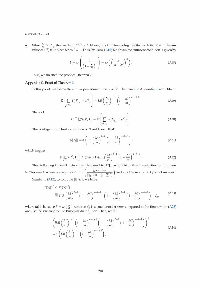
Entropy 2019, 21, 324

• When Mm ≥ e

1+e , then we have ds(l)l > 0. Hence, s(l) is an increasing function such that the minimum

value of s(l) take place when l = 1. Thus, by using (A15) we obtain the sufficient condition is given by

L = ω

⎛⎜⎝ 1(1− M

m

)n

⎞⎟⎠ = ω

((m

m−M

)n). (A18)

Thus, we finished the proof of Theorem 2.

Appendix C. Proof of Theorem 3

In this proof, we follow the similar procedure in the proof of Theorem 2 in Appendix B, and obtain

E

⎡⎣ ∑∀v fu

1{Tv fu= U �}

⎤⎦ = LB(

Mm

)l−1 (1− M

m

)n−l+1. (A19)

Then let

YlΔ= |J (U �, f)| −E

⎡⎣ ∑∀v fu

1{Tv fu= U �}

⎤⎦ . (A20)

The goal again is to find a condition of B and L such that

|E[Yl ]| = o

(LB

(Mm

)l−1 (1− M

m

)n−l+1)

, (A21)

which implies

E

[|J (U �, f)|

]≤ (1 + o(1))LB

(Mm

)l−1 (1− M

m

)n−l+1. (A22)

Then following the similar step from Theorem 1 in [12], we can obtain the concentration result shown

in Theorem 2, where we require LB = ω

((nM)

12(1−ε)

( mM−1)

(1−(1−M

m )n)

)and ε > 0 is an arbitrarily small number.

Similar to (A12), to compute |E[Yl ]|, we have

(E[Yl ])2 ≤ E[(Yl)

2]

(a)= lLB

(Mm

)l−1 (1− M

m

)n−l+1·(

1−(

Mm

)l−1 (1− M

m

)n−l+1)+ δ2,

(A23)

where (a) is because B = ω( m

M)

such that δ2 is a smaller order term compared to the first term in (A23)and use the variance for the Binomial distribution. Then, we let

(lLB

(Mm

)l−1 (1− M

m

)n−l+1(

1−(

Mm

)l−1 (1− M

m

)n−l+1)) 1

2

= o

(LB

(Mm

)l−1 (1− M

m

)n−l+1)

,

(A24)

218

Entropy 2019, 21, 324

then, we can obtain

LB =

(1−

(Mm

)l−1 (1− M

m

)n−l+1)

(Mm

)l−1 (1− M

m

)n−l+1

=

(1−

(Mm

)l−1 (1− M

m

)n−l+1)

1l

(Mm

)l−1 (1− M

m

)n−l+1 .

(A25)

For sufficient condition, let

LB = ω

⎛⎜⎝ 1

1l

(Mm

)l−1 (1− M

m

)n−l+1

⎞⎟⎠ . (A26)

Then following the similar steps as the proof of Theorem 2 in Appendix B, we fished the proofof Theorem 3.

References

1. Shanmugam, K.; Golrezaei, N.; Dimakis, A.; Molisch, A.; Caire, G. FemtoCaching: Wireless Video ContentDelivery through Distributed Caching Helpers. IEEE Trans. Inf. Theory 2013, 59, 8402–8413. [CrossRef]

2. Llorca, J.; Tulino, A.; Guan, K.; Kilper, D. Network-Coded Caching-Aided Multicast for Efficient ContentDelivery. In Proceedings of the 2013 IEEE International Conference on Communications (ICC), Budapest,Hungary, 9–13 June 2013.

3. Fadlallah, Y.; Tulino, A.M.; Barone, D.; Vettigli, G.; Llorca, J.; Gorce, J. Coding for Caching in 5G Networks.IEEE Commun. Mag. 2017, 55, 106–113. [CrossRef]

4. Liu, D.; Chen, B.; Yang, C.; Molisch, A.F. Caching at the wireless edge: Design aspects, challenges, and futuredirections. IEEE Commun. Mag. 2016, 54, 22–28. [CrossRef]

5. Tandon, R.; Simeone, O. Harnessing cloud and edge synergies: Toward an information theory of fog radio accessnetworks. IEEE Commun. Mag. 2016, 54, 44–50. [CrossRef]

6. Maddah-Ali, M.A.; Niesen, U. Coding for caching: Fundamental limits and practical challenges. IEEE Commun. Mag.2016, 54, 23–29. [CrossRef]

7. Paschos, G.; Bastug, E.; Land, I.; Caire, G.; Debbah, M. Wireless caching: Technical misconceptions and businessbarriers. IEEE Commun. Mag. 2016, 54, 16–22. [CrossRef]

8. Maddah-Ali, M.; Niesen, U. Fundamental Limits of Caching. IEEE Trans. Inf. Theory 2014, 60, 2856–2867.[CrossRef]

9. Maddah-Ali, M.; Niesen, U. Decentralized Coded Caching Attains Order-Optimal Memory-Rate Tradeoff.IEEE/ACM Trans. Netw. 2014. [CrossRef]

10. Ji, M.; Tulino, A.; Llorca, J.; Caire, G. On the average performance of caching and coded multicasting withrandom demands. In Proceedings of the 2014 11th International Symposium on Wireless CommunicationsSystems (ISWCS), Barcelona, Spain, 26–29 August 2014; pp. 922–926.

11. Niesen, U.; Maddah-Ali, M.A. Coded Caching With Nonuniform Demands. IEEE Trans. Inf. Theory 2017,63, 1146–1158. [CrossRef]

12. Ji, M.; Tulino, A.M.; Llorca, J.; Caire, G. Order-Optimal Rate of Caching and Coded Multicasting with RandomDemands. IEEE Trans. Inf. Theory 2017, 63, 3923–3949. [CrossRef]

219

Entropy 2019, 21, 324

13. Ji, M.; Tulino, A.; Llorca, J.; Caire, G. Caching and Coded Multicasting: Multiple Groupcast Index Coding.In Proceedings of the 2014 IEEE Global Conference on Signal and Information Processing (GlobalSIP), Atlanta,GA, USA, 3–5 December 2014; pp. 881–885.

14. Ji, M.; Tulino, A.M.; Llorca, J.; Caire, G. Caching-Aided Coded Multicasting with Multiple Random Requests.In Proceedings of the 2015 IEEE Information Theory Workshop (ITW), Jerusalem, Israel, 26 April–1 May 2015; pp. 1–5.

15. Wan, K.; Tuninetti, D.; Piantanida, P. On caching with more users than files. In Proceedings of the 2016IEEE International Symposium on Information Theory (ISIT), Barcelona, Spain, 10–15 July 2016; pp. 135–139.[CrossRef]

16. Wan, K.; Tuninetti, D.; Piantanida, P. On the optimality of uncoded cache placement. In Proceedings of the 2016IEEE Information Theory Workshop (ITW), Cambridge, UK, 11–14 September 2016; pp. 161–165. [CrossRef]

17. Ji, M.; Caire, G.; Molisch, A.F. The Throughput-Outage Tradeoff of Wireless One-Hop Caching Networks.IEEE Trans. Inf. Theory 2015, 61, 6833–6859. [CrossRef]

18. Ji, M.; Caire, G.; Molisch, A.F. Fundamental Limits of Caching in Wireless D2D Networks. IEEE Trans. Inf. Theory2016, 62, 849–869. [CrossRef]

19. Ji, M.; Caire, G.; Molisch, A.F. Wireless Device-to-Device Caching Networks: Basic Principles and SystemPerformance. IEEE J. Sel. Areas Commun. 2016, 34, 176–189. [CrossRef]

20. Cacciapuoti, A.S.; Caleffi, M.; Ji, M.; Llorca, J.; Tulino, A.M. Speeding Up Future Video Distribution viaChannel-Aware Caching-Aided Coded Multicast. IEEE J. Sel. Areas Commun. 2016, 34, 2207–2218. [CrossRef]

21. Shanmugam, K.; Ji, M.; Tulino, A.M.; Llorca, J.; Dimakis, A.G. Finite-Length Analysis of Caching-Aided CodedMulticasting. IEEE Trans. Inf. Theory 2016, 62, 5524–5537. [CrossRef]

22. Shangguan, C.; Zhang, Y.; Ge, G. Centralized Coded Caching Schemes: A Hypergraph Theoretical Approach.IEEE Trans. Inf. Theory 2018, 64, 5755–5766. [CrossRef]

23. Chen, Z. Fundamental limits of caching: Improved bounds for users with small buffers. IET Commun. 2016,10, 2315–2318. [CrossRef]

24. Karamchandani, N.; Niesen, U.; Maddah-Ali, M.A.; Diggavi, S.N. Hierarchical Coded Caching. IEEE Trans.Inf. Theory 2016, 62, 3212–3229. [CrossRef]

25. Pedarsani, R.; Maddah-Ali, M.A.; Niesen, U. Online Coded Caching. IEEE/ACM Trans. Netw. 2016, 24, 836–845.[CrossRef]

26. Sahraei, S.; Gastpar, M. K users caching two files: An improved achievable rate. In Proceedings of the 2016 AnnualConference on Information Science and Systems (CISS), Princeton, NJ, USA, 16–18 March 2016; pp. 620–624.[CrossRef]

27. Wang, C.; Lim, S.H.; Gastpar, M. Information-Theoretic Caching: Sequential Coding for Computing. IEEE Trans.Inf. Theory 2016, 62, 6393–6406. [CrossRef]

28. G., J. Fundamental limits of caching: Improved bounds with coded prefetching. arXiv 2016, arXiv:1612.09071.29. Shariatpanahi, S.P.; Motahari, S.A.; Khalaj, B.H. Multi-Server Coded Caching. IEEE Trans. Inf. Theory 2016,

62, 7253–7271. [CrossRef]30. Shanmugam, K.; Tulino, A.M.; Dimakis, A.G. Coded caching with linear subpacketization is possible using

Ruzsa-Szeméredi graphs. In Proceedings of the 2017 IEEE International Symposium on Information Theory(ISIT), Aachen, Germany, 25–30 June 2017; pp. 1237–1241. [CrossRef]

31. Ghasemi, H.; Ramamoorthy, A. Improved Lower Bounds for Coded Caching. IEEE Trans. Inf. Theory 2017,63, 4388–4413. [CrossRef]

32. Lim, S.H.; Wang, C.; Gastpar, M. Information-Theoretic Caching: The Multi-User Case. IEEE Trans. Inf. Theory2017, 63, 7018–7037. [CrossRef]

33. Jeon, S.; Hong, S.; Ji, M.; Caire, G.; Molisch, A.F. Wireless Multihop Device-to-Device Caching Networks.IEEE Trans. Inf. Theory 2017, 63, 1662–1676. [CrossRef]

34. Sengupta, A.; Tandon, R. Improved Approximation of Storage-Rate Tradeoff for Caching With Multiple Demands.IEEE Trans. Commun. 2017, 65, 1940–1955. [CrossRef]

35. Hachem, J.; Karamchandani, N.; Diggavi, S.N. Coded Caching for Multi-level Popularity and Access. IEEE Trans.Inf. Theory 2017, 63, 3108–3141. [CrossRef]

220

Entropy 2019, 21, 324

36. Ji, M.; Wong, M.F.; Tulino, A.M.; Llorca, J.; Caire, G.; Effros, M.; Langberg, M. On the fundamental limitsof caching in combination networks. In Proceedings of the 2015 IEEE 16th International Workshop onSignal Processing Advances in Wireless Communications (SPAWC), Stockholm, Sweden, 28 June–1 July 2015;pp. 695–699. [CrossRef]

37. Ji, M.; Tulino, A.M.; Llorca, J.; Caire, G. Caching in combination networks. In Proceedings of the 201549th Asilomar Conference on Signals, Systems and Computers, Pacific Grove, CA, USA, 8 November 2015;pp. 1269–1273. [CrossRef]

38. Wan, K.; Ji, M.; Piantanida, P.; Tuninetti, D. Novel outer bounds for combination networks with end-user-caches.In Proceedings of the 2017 IEEE Information Theory Workshop (ITW), Kaohsiung, Taiwan, 6–10 November 2017;pp. 444–448. [CrossRef]

39. Wan, K.; Tuninetti, D.; Ji, M.; Piantanida, P. State-of-the-art in cache-aided combination networks. In Proceedingsof the 2017 51st Asilomar Conference on Signals, Systems, and Computers, Pacific Grove, CA, USA, 29 October–1 November 2017; pp. 641–645. [CrossRef]

40. Wan, K.; Ji, M.; Piantanida, P.; Tuninetti, D. Caching in Combination Networks: Novel Multicast MessageGeneration and Delivery by Leveraging the Network Topology. In Proceedings of the 2018 IEEE InternationalConference on Communications (ICC), Kansas City, MO, USA, 20–24 May 2018; pp. 1–6. [CrossRef]

41. Wan, K.; Jit, M.; Piantanida, P.; Tuninetti, D. On the Benefits of Asymmetric Coded Cache Placement inCombination Networks with End-User Caches. In Proceedings of the 2018 IEEE International Symposium onInformation Theory (ISIT), Vail, CO, USA, 17–22 June 2018; pp. 1550–1554. [CrossRef]

42. Wan, K.; Tuninetti, D.; Ji, M.; Piantanida, P. A Novel Asymmetric Coded Placement in Combination Networkswith End-User Caches. In Proceedings of the 2018 Information Theory and Applications Workshop (ITA),San Diego, CA, USA, 11–16 February 2018; pp. 1–5. [CrossRef]

43. Tian, C.; Chen, J. Caching and Delivery via Interference Elimination. IEEE Trans. Inf. Theory 2018, 64, 1548–1560.[CrossRef]

44. Yu, Q.; Maddah-Ali, M.A.; Avestimehr, A.S. The Exact Rate-Memory Tradeoff for Caching With UncodedPrefetching. IEEE Trans. Inf. Theory 2018, 64, 1281–1296. [CrossRef]

45. Zhang, K.; Tian, C. Fundamental Limits of Coded Caching: From Uncoded Prefetching to Coded Prefetching.IEEE J. Sel. Areas Commun. 2018, 36, 1153–1164. [CrossRef]

46. Wang, C.; Bidokhti, S.S.; Wigger, M. Improved Converses and Gap Results for Coded Caching. IEEE Trans.Inf. Theory 2018, 64, 7051–7062. [CrossRef]

47. Yu, Q.; Maddah-Ali, M.A.; Avestimehr, A.S. Characterizing the Rate-Memory Tradeoff in Cache Networks Withina Factor of 2. IEEE Trans. Inf. Theory 2019, 65, 647–663. [CrossRef]

48. Karat, N.S.; Thomas, A.; Rajan, B.S. Optimal Error Correcting Delivery Scheme for an Optimal Coded CachingScheme with Small Buffers. In Proceedings of the 2018 IEEE International Symposium on Information Theory(ISIT), Vail, CO, USA, 17–22 June 2018; pp. 1710–1714. [CrossRef]

49. Tian, C. Symmetry, Outer Bounds, and Code Constructions: A Computer-Aided Investigation on theFundamental Limits of Caching. Entropy 2018, 20, 603. [CrossRef]

50. Cisco. The Zettabyte Era-Trends and Analysis; Cisco White Paper; Cisco: San Jose, CA, USA, 2013.51. Birk, Y.; Kol, T. Informed-source coding-on-demand (ISCOD) over broadcast channels. In Proceedings of the

Conference on Computer Communications, Seventeenth Annual Joint Conference of the IEEE Computer andCommunications Societies, Gateway to the 21st Century, San Francisco, CA, USA, 29 March–2 April 1998.

52. Breslau, L.; Cao, P.; Fan, L.; Phillips, G.; Shenker, S. Web caching and Zipf-like distributions: Evidence andimplications. In Proceedings of the INFOCOM’99: Conference on Computer Communications, New York,NY, USA, 21–25 March 1999; Volume 1, pp. 126–134.

53. Tang, L.; Ramamoorthy, A. Coded Caching Schemes With Reduced Subpacketization From Linear Block Codes.IEEE Trans. Inf. Theory 2018, 64, 3099–3120. [CrossRef]

54. Yan, Q.; Cheng, M.; Tang, X.; Chen, Q. On the Placement Delivery Array Design for Centralized Coded CachingScheme. IEEE Trans. Inf. Theory 2017, 63, 5821–5833. [CrossRef]

221

Entropy 2019, 21, 324

55. Vettigli, G.; Ji, M.; Tulino, A.M.; Llorca, J.; Festa, P. An efficient coded multicasting scheme preserving themultiplicative caching gain. In Proceedings of the 2015 IEEE Conference on Computer CommunicationsWorkshops (INFOCOM WKSHPS), Hong Kong, China, 26 April–1 May 2015; pp. 251–256. [CrossRef]

56. Ji, M.; Shanmugam, K.; Vettigli, G.; Llorca, J.; Tulino, A.M.; Caire, G. An efficient multiple-groupcast codedmulticasting scheme for finite fractional caching. In Proceedings of the 2015 IEEE International Conference onCommunications (ICC), London, UK, 8–12 June 2015; pp. 3801–3806. [CrossRef]

57. Ramakrishnan, A.; Westphal, C.; Markopoulou, A. An Efficient Delivery Scheme for Coded Caching.In Proceedings of the 2015 27th International Teletraffic Congress, Ghent, Belgium, 8–10 September 2015;pp. 46–54. [CrossRef]

58. Jin, S.; Cui, Y.; Liu, H.; Caire, G. Order-Optimal Decentralized Coded Caching Schemes with Good Performancein Finite File Size Regime. In Proceedings of the 2016 IEEE Global Communications Conference (GLOBECOM),Washington, DC, USA, 4–8 December 2016; pp. 1–7. [CrossRef]

59. Wan, K.; Tuninetti, D.; Piantanida, P. Novel delivery schemes for decentralized coded caching in the finitefile size regime. In Proceedings of the 2017 IEEE International Conference on Communications Workshops(ICC Workshops), Paris, France, 21–25 May 2017; pp. 1183–1188. [CrossRef]

60. Asghari, S.M.; Ouyang, Y.; Nayyar, A.; Avestimehr, A.S. Optimal Coded Multicast in Cache Networks withArbitrary Content Placement. In Proceedings of the 2018 IEEE International Conference on Communications(ICC), Kansas City, MO, USA, 20–24 May 2018; pp. 1–6. [CrossRef]

61. Amiri, M.M.; Yang, Q.; Gündüz, D. Decentralized coded caching with distinct cache capacities. In Proceedingsof the 2016 50th Asilomar Conference on Signals, Systems and Computers, Pacific Grove, CA, USA,6–9 November 2016; pp. 734–738. [CrossRef]

62. Amiri, M.M.; Yang, Q.; Gündüz, D. Decentralized Caching and Coded Delivery With Distinct Cache Capacities.IEEE Trans. Commun. 2017, 65, 4657–4669. [CrossRef]

63. Ibrahim, A.M.; Zewail, A.A.; Yener, A. Centralized Coded Caching with Heterogeneous Cache Sizes.In Proceedings of the 2017 IEEE Wireless Communications and Networking Conference (WCNC), San Francisco,CA, USA, 19–22 March 2017; pp. 1–6. [CrossRef]

64. Wei, Y.; Ulukus, S. Coded caching with multiple file requests. In Proceedings of the 2017 55th Annual AllertonConference on Communication, Control, and Computing (Allerton), Monticello, IL, USA, 3–6 October 2017;pp. 437–442. [CrossRef]

65. Parrinello, E.; Unsal, A.; Elia, P. Fundamental Limits of Caching in Heterogeneous Networks with UncodedPrefetching. arXiv 2018, arXiv:1811.06247.

66. Shanmugam, K.; Dimakis, A.G.; Langberg, M. Local graph coloring and index coding. In Proceedings of the2013 IEEE International Symposium on Information Theory, Istanbul, Turkey, 7–12 July 2013; pp. 1152–1156.[CrossRef]

67. Lin, S.; Costello, D.J. Error Control Coding; Prentice-hall Englewood Cliffs: Upper Saddle River, NJ, USA, 2004;Volume 123.

68. Bar-Yossef, Z.; Birk, Y.; Jayram, T.; Kol, T. Index coding with side information. IEEE Trans. Inf. Theory 2011,57, 1479–1494. [CrossRef]

69. Lee, D.; Noh, S.; Min, S.; Choi, J.; Kim, J.; Cho, Y.; Kim, C. LRFU: A spectrum of policies that subsumes the leastrecently used and least frequently used policies. IEEE Trans. Comput. 2001, 50, 1352–1361.

70. Boucheron, S.; Lugosi, G.; Massart, P. Concentration Inequalities: A Nonasymptotic Theory of Independence;Oxford University Press: Oxford, UK, 2013.

c© 2019 by the authors. Licensee MDPI, Basel, Switzerland. This article is an open accessarticle distributed under the terms and conditions of the Creative Commons Attribution (CCBY) license (http://creativecommons.org/licenses/by/4.0/).

222

entropy

Article

Cross-Entropy Method for Content Placement andUser Association in Cache-Enabled CoordinatedUltra-Dense Networks

Jia Yu 1, Ye Wang 1,2,†, Shushi Gu 1,2,†, Qinyu Zhang 1,2,†, Siyun Chen 1 and Yalin Zhang 3,*

1 Communication Engineering Research Centre, Harbin Institute of Technology (Shenzhen),HIT Campus of University Town of Shenzhen, Shenzhen 518055, China; [email protected] (J.Y.);[email protected] (Y.W.); [email protected] (S.G.); [email protected] (Q.Z.);[email protected] (S.C.)

2 Peng Cheng Laboratory, Shenzhen 518055, China3 School of Electronic and Communication Engineering, Shenzhen Polytechnic, Shenzhen 518055, China* Correspondence: [email protected]; Tel.: +86-0755-2630-2145† These authors contributed equally to this work.

Received: 27 March 2019; Accepted: 1 June 2019; Published: 8 June 2019

Abstract: Due to the high splitting-gain of dense small cells, Ultra-Dense Network (UDN) isregarded as a promising networking technology to achieve high data rate and low latency in 5Gmobile communications. In UDNs, each User Equipment (UE) may receive signals from multipleBase Stations (BSs), which impose severe interference in the networks and in turn motivates thepossibility of using Coordinated Multi-Point (CoMP) transmissions to further enhance networkcapacity. In CoMP-based Ultra-Dense Networks, a great challenge is to tradeoff between the gainof network throughput and the worsening backhaul latency. Caching popular files on BSs has beenidentified as a promising method to reduce the backhaul traffic load. In this paper, we investigatedcontent placement strategies and user association algorithms for the proactive caching ultra densenetworks. The problem has been formulated to maximize network throughput of cell edge UEs underthe consideration of backhaul load, which is a constrained non-convex combinatorial optimizationproblem. To decrease the complexity, the problem is decomposed into two suboptimal problems.We first solved the content placement algorithm based on the cross-entropy (CE) method to minimizethe backhaul load of the network. Then, a user association algorithm based on the CE methodwas employed to pursue larger network throughput of cell edge UEs. Simulation were conductedto validate the performance of the proposed cross-entropy based schemes in terms of networkthroughput and backhaul load. The simulation results show that the proposed cross-entropybased content placement scheme significantly outperform the conventional random and MostPopular Content placement schemes, with with 50% and 20% backhaul load decrease respectively.Furthermore, the proposed cross-entropy based user association scheme can achieve 30% and 23%throughput gain, compared with the conventional N-best, No-CoMP, and Threshold based userassociation schemes.

Keywords: ultra dense network; cross-entropy; proactive caching; user association; CoMP

1. Introduction

Inspired by the development of intelligent terminal such as smart phones, the demand fordata traffic in mobile communication systems is exponentially growing. To cater for this demand,a 1000-fold improvement of capacity per area in the next generation of mobile communication system(5G) compared to 4G is required. An Ultra-Dense Network (UDN) is capable of significantly improving


Entropy 2019, 21, 576

the capacity per area under the limited spectrum resource due to the high splitting-gain of denselylocated small cells and is widely considered as one of the most promising techniques in the coming 5G.It also benefits load balance between Base Stations (BSs) since Small Base Stations (SBSs) can offloaddata traffic of Macro Base Stations (MBSs). Nevertheless, due to the short distance between BSs,the intercell interference in UDNs is severe, therefore making the user experience unsatisfactory.Coordinated Multi-Point (CoMP) transmissions technique is widely studied in academia and theindustry, which can leverage the cooperation of multiple BSs to enhance the signal to interference andnoise ratio (SINR), to counteract intercell interference and to enhance network capacity in UDNs.

Despite remarkable performance gain in network capacity, congestion on backhaul links caused byCoMP risks the mobile communication systems. In order to cooperatively serve users, BSs need to fetchmore files from the Core Network (CN) via backhaul links in a CoMP-employed system, which bringsheavy load to backhaul links between BSs and the CN and probably results in congestion. One wayto alleviate backhaul load is to cache popular files on BSs. When BSs cache files requested by users,it does not need to fetch files from the CN, so the backhaul load can be dramatically reduced. In [1],an architecture based on distributed caching of content in SBSs was presented. Works on proactivecaching in UDNs concentrate on two major issues: Content placement and content distribution.

Content placement focuses on how to distribute popular and hotspot files to the BSs’ cachingunit whose capacity is limited. In [2], an optimal content placement strategy is proposed to maximizethe hit rate. In [3], the problem of content placement is studied to maximize energy efficiency. In [4],an approximation algorithm is proposed to jointly optimize routing and caching policy to maximizethe fraction of requested files cached locally. In [5], a distributed algorithm is proposed to investigatecontent placement and user association jointly. In [6], a content placement strategy is investigatedbased on reinforcement learning. In [7], a content placement strategy is proposed under cooperationschemes of maximum ratio transmission (MRT) and zero-forcing beamforming (ZFBF). In [8], a cachingspace allocation scheme is proposed to improve the hit rate based on the categories of contents and UEs.

Content distribution is the study of how to associate UEs and BSs to improve the hit rate. In [9],the user association problem is modeled as an one-to-many game problem, based on which algorithmis proposed to maximize the average download rate under a given content placement strategy. In [10],an user association algorithm under a given content distribution in a CoMP enabled network isproposed to minimize the backhaul load under a guaranteed rate requirements of UEs. In [11],the content caching and user association schemes are proposed on two different scales: The cachingalgorithm operates in a long time scale and the user association algorithm operates frequently. In [12],user association is investigated to tradeoff between load balancing and backhaul savings in UDN.

To the best of our knowledge, related works on the content placement caching and user associationhave been investigated separately in small-scale networks. We are thus motivated to jointly investigatethe tasks of caching and user association in more realistic large-scale UDNs. The main contributions ofthis paper are summarized as follows.

• The problem of content placement and user association is investigated jointly in large-scalecache-enabled coordinated ultra dense networks. We formulate the problem as a constrainednon-convex combinatorial programming problem to maximize network throughput of cell edgeUEs under the consideration of the backhaul load;

• A two-step heuristic algorithm based on the cross-entropy (CE) method is proposed to solvethe problem: A content placement strategy is first proposed based on cross entropy under theassumption of the conventional N-Best scheme; given the proposed content placement strategy,a user association algorithm is then proposed based on the cross-entropy method. Extensivesimulations are conducted to evaluate the performance of the proposed approach. Simulationsare conducted to validate the performance of the proposed cross-entropy based schemes in termsof network throughput and backhaul load. Simulation results show that the proposed cachingand user association algorithms can reduce backhaul load and improve network throughput ofcell edge UEs simultaneously.

224

Entropy 2019, 21, 576

The rest of this paper is organized as follows. The system model is established in Section 2with some basic assumptions. In Section 3, we formulate the problem and propose the algorithms.In Section 4, simulation results are presented and the system performance is evaluated. Section 5concludes this paper.

2. System Model

2.1. Network

In this paper, we consider a heterogeneous Ultra-Dense Network consisting of NMBS MacroBSs (MBS) and NSBS Small Base Stations (SBS). The Macro BSs are uniformly distributed to providecoverage and to support capacity. The small BSs are randomly distributed within the covering area,following a Poisson Point Process (PPP) with a density of λSBS. Let BΩ = {b|b = 1, 2, · · · , |BΩ|} denotethe set of BSs consisting of both Macro BSs and Small BSs, where |BΩ| = NMBS + NSBS is the totalnumber of BSs.

UEs are randomly distributed following a PPP with density of λU. The set of UEs is denotedby MΩ = {m|m = 1, 2, · · · , |MΩ|}. UEs located at the edges of cells usually suffer from severeintercell interference and low capacity. To reduce the interference and enhance peak data rates ofcell edge users, joint transmission Coordinated Multi-Point (termed as JT CoMP) is considered in thenetwork architecture, which allows multiple BSs in the neighborhood to cooperatively serve a specificUE simultaneously.

The association relationship between UEs, m, and BS, b, is denoted by a bit number xm,b(m ∈MΩ, b ∈ BΩ) defined as:

xm,b =

{1 UE m is associated with BS b0 otherwise

. (1)

Thus, the entire association result between BSs and UEs in the considering network can bepresented by:

X =

⎡⎢⎢⎢⎢⎢⎣x1,1 x1,2 · · · x1,|BΩ|x2,1 x2,2 · · · x2,|BΩ|

......

. . ....

x|MΩ|,1 x|MΩ|,2 · · · x|MΩ|,|BΩ|

⎤⎥⎥⎥⎥⎥⎦ . (2)

The SINR of a specific UE in a downlink transmission can be presented in terms of xm,b as follows,

Γm =

∑b∈BΩ

xm,bPbgm,b

∑b′∈BΩ

(1− xm,b′)Pb′gm,b + σ2 , (3)

where Pb is the transmit power of BS b, gm,b is the channel gain between BS b and UE m, and σ2 isthe variance of additive white Gaussian noise (AWGN). Equation (3) suggests that the more BSs areassociated with UE m, the better service it can obtain. However, the necessary overhead to accomplisha JT CoMP transmission involving too much BSs is unacceptable. Thus, it is better to narrow theassociating BSs of a UE into N BSs in close proximity.

As in 4G LTE and 5G NR (New Radio) wireless standards, resource block (RB) is considered theunit of time and spectrum resource for allocation in this paper. Assume that the bandwidth of each RBis W and the total number of RBs is NRB. Each UE in the network can occupy a part of resource fortransmission. Let βm denote the proportion that the resource assigned to UE m out of all. Then thedata rate of a downlink transmission to UE m can be given by:

Rm = W�βmNRB� log2 (1 + Γm) , (4)

225

Entropy 2019, 21, 576

where �x� is the minimum integer smaller than or equal to x; Γm is defined by Equation (3).Let BΩ

m ⊆ BΩ denote the set consisting of BSs associated with UE m, i.e., BΩm = {b|b ∈

BΩ, and xm,b = 1}. Similarly, let MΩb ⊆ MΩ denote the set consisting of UEs associated with BS

b, i.e., MΩb = {m|m ∈ MΩ, and xm,b = 1}. The resource that BS b can assign to UE m should be no

more than 1|MΩ

b |, where |MΩ

b | represents the total number of UEs associated with BS b. In the case where

JT CoMP is employed, the resource that UE m can be obtained is restricted by the most heavy-loadingBS among those associated with UE m. As a result, the proportion βm can be given by:

βm = min

{1∣∣MΩ

b

∣∣ , b ∈ BΩm

}. (5)

2.2. Caching

UDNs can benefit from caching popular files on BSs in terms of throughput, delay, and traffic loadon backhaul links. It is obvious that the more files cached on BSs, the better performance a networkcan achieve. The cache-enabled heterogeneous UDN we considered in this paper is illustrated asFigure 1. For simplicity, we assume that the files requested by all UEs in the networks are restrictedinto the set of FΩ = { f | f = 1, 2, · · ·, |FΩ|}, and each file is in the same size of Fmax bits. We assumethe popularity of files follows Zipf distribution [13]. Let p f denote the probability mass function ofpopularity random variable F. The probability that file f is requested can be given by:

p f =

(∑|FΩ |f=1 f−γ

)−1

f γ, (6)

where γ is the Shape Factor (SF) indicating the correlation between requests of UEs [13]. It is seenthat the larger the shape factor γ is, the smaller the probability mass function p f would be, the lowerprobability file f is requested out of the caching set FΩ.

Figure 1. System model of caching-enabled Ultra-Dense Network (UDN) with joint transmissionCoordinated Multi-Point (JT CoMP).

Define a caching index vector yb = [yb,1, yb,2, · · · , yb, f , · · · yb,|FΩ |], where yb, f indicates whetherBS b caches file f in the caching set FΩ or not. More specifically,

yb, f =

{1 file f is cached on BS b0 otherwise

. (7)

226

Entropy 2019, 21, 576

Then the File-BS caching matrix can be denoted by:

Y =

⎡⎢⎢⎢⎢⎢⎣y1,1 y1,2 · · · y|BΩ|,|FΩ |y2,1 y2,2 · · · y|BΩ|,|FΩ |

......

. . ....

y|BΩ|,1 y|BΩ|,2 · · · y|BΩ|,|FΩ|

⎤⎥⎥⎥⎥⎥⎦ . (8)

As for UEs, we define a row vector qm = [qm,1, qm,2, · · · , qm, f , · · · ] , where qm, f represents therequest of UE m to file f , i.e.,

qm, f =

{1 file f is requested by UE m0 otherwise

. (9)

Suppose a UE can request one and only one file at each time, then we have ∑ f qm, f = 1, ∀m ∈ MΩ.Then qmyT

b represents whether the file requested by UE m is caching on BS b, where vT representsthe transpose of the vector v.

qmyTb =

{1 file f requested by UE m is on BS b0 otherwise

. (10)

If UE m is associated with BS b (i.e., xm,b = 1), we say that BS b misses a file if file f requested byUE m is not cached in it.

If BSs miss a file, they need to fetch the file from the Core Network (CN). We assume a centralizeddeployment of the considered UDN, where each BS is directly connected to the CN via backhaul links.The backhaul load is defined as the traffic carried by backhaul links between BSs and the CN [14].In the case that BS b misses a file requested by UE m, BS b have to fetch the file from the CN throughthe backhaul link, which aggravates the backhaul load of BS b inevitably. In reality, the capacity ofbackhaul links is usually limited. Congestion occurs when the backhaul load of BS b exceeds thebackhaul capacity Cmax

b .Let Uback represent the increase of backhaul load due to fetching a file from the CN. The backhaul

load caused by UE m can be given by:

Vm = ∑b∈BΩ

m

(1− qmyTb )Uback. (11)

It is obvious that the more files BSs cache (i.e., the less files BSs miss), the less heavier the backhaulload will be.

2.3. Delay

In addition to reducing backhaul load, caching also benefits from reducing the time delay oftransmissions . In this paper, we consider the average time delay of UEs , which consists of two majorparts: Wireless propagation delay and backhaul delay. Let d1 denote the average wireless propagationdelay of a UDN which is related to the size of a file Fmax and the data rate of transmission.

d1 =1

|MΩ| ∑m∈MΩ

Fmax

Rm. (12)

Backhaul delay, denoted by d2, is related to whether the files are hit by the associating BSs ofUEs. Due to joint transmission of CoMP, the backhaul delay for a specific UE m occurs when therequested file is not cached on all its associated BSs. That is, the minimum operation should be

227

Entropy 2019, 21, 576

applied on backhaul delays due to file transmission between the associated BSs and the core network.More specifically, d2 can be represented as follows,

d2 =1

|MΩ| ∑m∈MΩ

⎛⎝min

⎧⎨⎩ Fmax

Uback, ∑

b∈BΩm

(1− qmyTb )

Fmax

Uback

⎫⎬⎭⎞⎠. (13)

As a result, the total time delay of the network is:

D = d1 + d2. (14)

3. Problem Formulation

3.1. Mathematical Formulation

In this paper, we aim to develop the optimal solution of content placement and user associationthat balances network throughput and the backhaul load simultaneously. Considering the fairness ofUEs, the network throughput of cell edge UEs is used as the performance metric. Thus the objectivefunction is a tradeoff between network throughput of cell edge UEs and backhaul load.

maxX,Y

∑m∈MΩ

log10(Rm)− λ∑m∈MΩ Vm

|MΩ| (15)

s.t. C1: 1 ≤ |BΩm | ≤ N, ∀m ∈ MΩ

C2: ∑m

xm,b ≤ NRB, ∀b ∈ BΩ, ∀m ∈ MΩ

C3: ∑m

xm,b(1− qmyTb )Uback ≤ Cmax

b , ∀b ∈ BΩ

where the constraint C1 indicates that a specific UE m should be served by at least one BS, meanwhilethe total number of BSs that cooperatively serve a specific UE should not be more than a given numberN by considering the tradeoff between throughput gain and backhaul load due to the joint transmissionof CoMP; C2 indicates that the total number of RBs allocated to UEs associating with a specific BS islimited to the maximum NRB; C3 indicates that aggregate backhaul load of BS m should not be overthe backhaul capacity Cmax

b .λ ≥ 0 in Equation (15) is a coefficient that influences the balance between network throughput

and backhaul load. A larger λ suggests that we prefer improving network throughput than reducing

backhaul load, and vice versa. Let ∑m∈MΩ log2(R(0)m ) and ∑m∈MΩ V(0)

m

|MΩ| denote sum of logarithm of data

rate and averaged load on backhaul links when λ = 0, respectively. We define λ with ∑m∈MΩ log2(R(0)m )

and ∑m∈MΩ V(0)m

|MΩ| as benchmarks, and then λ can be given by:

λ =∑m∈MΩ log2(R(0)

m )∣∣MΩ

∣∣ μ

∑m∈MΩ V(0)m

. (16)

where μ ∈ [0, 1] is a weight factor used for adjusting λ.The problem in Equation (15) is a constrained non-convex combinatorial optimization problem,

which requires extraordinary high complexity to trace its optimal solution. To obtain a practicalsolution, we decompose the problem into two steps based on the cross-entropy (CE) method. In thispaper, the CE method is chosen because it is a simple, efficient, and general method for solving a greatvariety of estimation and optimization problems, especially NP-hard combinatorial deterministic andstochastic problems [15]. First, we minimize the backhaul load of the system under the assumption ofthe conventional N-Best user association strategy (By N-Best user association strategy, a CoMP UE willassociate with Nmax BSs which have N best SINRs [16]) and propose a content placement algorithm

228

Entropy 2019, 21, 576

based on cross entropy, which is termed as the CPCE algorithm. Subsequently, under the given contentplacement strategy, we propose an user association algorithm based on cross entropy, which is referredto as UACE in the rest of this paper.

3.2. Cross-Entropy Method

The CE method was originally used in the context of rare event simulation [17] and has beenextended as a Monte Carlo method for importance sampling and optimization [17,18].

The principle behind the CE method is to get as close as possible to the optimal importancesampling distribution by using the Kullback-–Leibler (KL) distance as a measure of closeness.By repeatedly updating the Probability Density Function (PDF) of generated samples, the PDF of thesamples can finally converge with the obtained optimal strategy solution [19]. Another method witha similar idea is logarithmic loss distortion measure [20,21], where logarithmic loss is also known ascross-entropy loss. The logarithmic loss distortion measure has been recently used in the study ofDeep Neural Networks (DNNs) to approach an accurate classifier by minimizing the logarithmic loss.It also performs well on tradeoff between complexity and relevance in representation learning [22].

The main steps of the CE method can be depicted as follows:STEP 1: (Encode Strategy Space). Consider a UDN constituted by BΩ BSs, where each BS b is

a decision-making entity. Suppose that each BS b can make a decision out of Nb possible strategies,then the strategy set at BS b can be expressed as Sb = [S1

b , S2b , · · · , SNb

b ]. For a specific decision-makingentity BS b, Si

b is one strategy that belongs to Sb. The strategy set of BΩ BSs entities in a UDN canbe represented as SBΩ = [S1, S2, · · · , S|BΩ |], which is termed as the strategy space of the CE method.Then the samples of the strategy space of the CE method correspond to the strategies at all BSs ina UDN in current iteration.

Let Pb = [Pb,1, Pb,2, · · · , Pb,Nb] denote the probability distribution of sample strategies at BS b.

Let Pb,i denote as the probability of strategy i at a specific BS b. First, Pb,i is initialized to be equalas follows,

Pb,i =1

Nb, and

Nb

∑i=1

Pb,i = 1, (∀i = 1, · · · , Nb). (17)

STEP 2: (Generate Samples According to the Probability). In the second step of the CE method,sufficient strategy samples should be generated according to the given probability distribution.Denote the zth generated sample by A(z) =

[AT

1 (z), AT2 (z), · · · , AT

b (z), · · · , AT|BΩ |(z)

], where Ab(z) is

the subsample set generated by decision-making entity element b. More specifically, the subsampleAb(z) can be represented as:

Ab(z) =[αb,1(z), αb,2(z), · · · , αb,i(z), · · · , αb,Nb

(z)]

, (18)

where αb,i(z) is a binary number. For each Ab(z), only one αb,i(z) is “1” and others are “0”(i.e., ∑Nb

i=1 αb,i = 1), indicating that only one strategy out of all can be selected at each decisionepoch. The probability of subsample Ab is Pb,i ∈ Pb with αb,i = 1 and αb,j = 0(j �= i).

STEP 3: (Performance Evaluation). Fitness values of strategy samples can be calculated accordingto the result of the strategy in the current iteration. Let F(z) denote the fitness value of strategy samplez, which can be expressed as:

F(z) = −∑b

∑m

xmb(1− qmyTb )Uback. (19)

Rearrange F(z) in descending order as F(1) ≥ F(2) · · · F(Z), where Z is the maximum numberof strategy samples. Then calculate the ρ-quantile of the strategy samples in current iteration Fρ and

229

Entropy 2019, 21, 576

weed out the unexpected samples. The samples with fitness value F(i) ≥ Fρ are selected for probabilityupdating in the next iteration.

STEP 4: (Probability Updating). According to samples selected in the performance evaluationstep, the probabilities of each strategy can be updated as follows,

P updateb,i =

Z∑

z=1IF(z)≥Fρ

αb,i(z)

Z∑

z=1IF(z)≥Fρ

, (20)

where I is defined as,

Ix≥y =

{1 if x ≥ y0 others

. (21)

Go back to STEP 2, regenerate the samples based on the updated probability distribution andrepeat STEP 2 to STEP 4.

STEP 5: (Convergence Conditions). The algorithm will come to an end when the fitnessvalue reaches convergence or the algorithm reaches the maximum iteration number set in advance.The cross-entropy method is a global random search procedure, and asymptotical convergence can beachieved to find the optimal solution with probability arbitrarily close to 1 [23,24].

3.3. Content Placement Algorithm Based on the Cross-Entropy Method (CPCE)

Before joining in a network, a specific UE will measure Channel State Information (CSI) andchoose the candidate BSs with the biggest reference signal received power (RSRP). To investigate thecontent placement strategies of BSs, we assume the conventional N-Best scheme for user associationin the first place. BSs in the network are modeled as decision-making entities in the CE method,and feasible content placement candidates are strategies of each entity. The CPCE algorithm can bedepicted as Algorithm 1.

The optimized content placement strategy Y can be given by Algorithm 1, under the assumptionof the N-best user association scheme. User association results can be further optimized with theobtained Y.

Algorithm 1 Content Placement based on CE method (CPCE)

1: User association under N-Best strategy.

2: Generate content placement request samples of UEs qm based on Zipf distribution. Map BSs←→

Decision-making entities in CE method.

3: Map the content placement strategy set←→ Strategies in CE method.

4: Map the sum backhaul load←→ Fitness value in CE method.

5: Execute CPCE.

6: Map the obtained solution into the best content placement strategies of BSs and output Y.

3.4. User Association Algorithm Based on the Cross-Entropy Method (UACE)

By Algorithm 1, we obtain the optimal content placement strategy of each BS under the N-Bestuser association scheme. However, the N-Best user association scheme does not take into account loadbalancing and interference management. Under the obtained content placement result, we can furtheroptimize the user association algorithm.

230

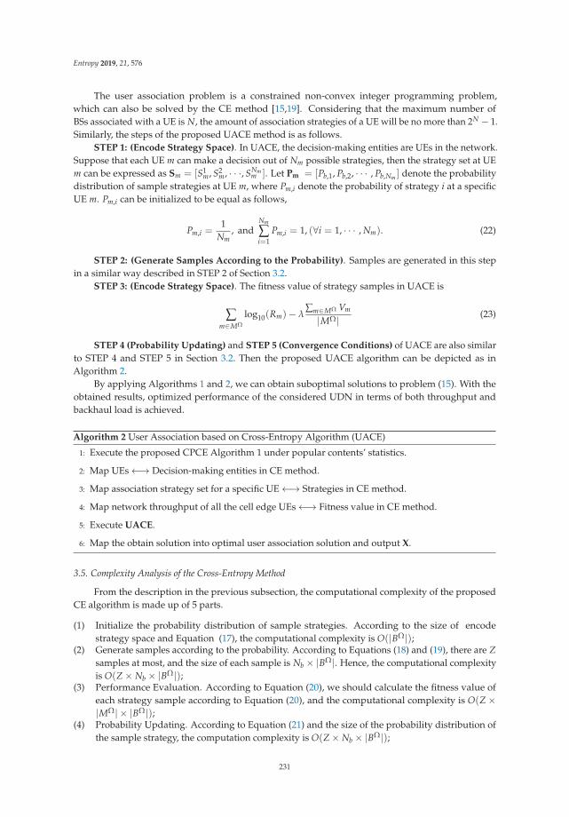
Entropy 2019, 21, 576

The user association problem is a constrained non-convex integer programming problem,which can also be solved by the CE method [15,19]. Considering that the maximum number ofBSs associated with a UE is N, the amount of association strategies of a UE will be no more than 2N − 1.Similarly, the steps of the proposed UACE method is as follows.

STEP 1: (Encode Strategy Space). In UACE, the decision-making entities are UEs in the network.Suppose that each UE m can make a decision out of Nm possible strategies, then the strategy set at UEm can be expressed as Sm = [S1

m, S2m, · · ·, SNm

m ]. Let Pm = [Pb,1, Pb,2, · · · , Pb,Nm ] denote the probabilitydistribution of sample strategies at UE m, where Pm,i denote the probability of strategy i at a specificUE m. Pm,i can be initialized to be equal as follows,

Pm,i =1

Nm, and

Nm

∑i=1

Pm,i = 1, (∀i = 1, · · · , Nm). (22)

STEP 2: (Generate Samples According to the Probability). Samples are generated in this stepin a similar way described in STEP 2 of Section 3.2.

STEP 3: (Encode Strategy Space). The fitness value of strategy samples in UACE is

∑m∈MΩ

log10(Rm)− λ∑m∈MΩ Vm

|MΩ| (23)

STEP 4 (Probability Updating) and STEP 5 (Convergence Conditions) of UACE are also similarto STEP 4 and STEP 5 in Section 3.2. Then the proposed UACE algorithm can be depicted as inAlgorithm 2.

By applying Algorithms 1 and 2, we can obtain suboptimal solutions to problem (15). With theobtained results, optimized performance of the considered UDN in terms of both throughput andbackhaul load is achieved.

Algorithm 2 User Association based on Cross-Entropy Algorithm (UACE)

1: Execute the proposed CPCE Algorithm 1 under popular contents’ statistics.

2: Map UEs←→ Decision-making entities in CE method.

3: Map association strategy set for a specific UE←→ Strategies in CE method.

4: Map network throughput of all the cell edge UEs←→ Fitness value in CE method.

5: Execute UACE.

6: Map the obtain solution into optimal user association solution and output X.

3.5. Complexity Analysis of the Cross-Entropy Method

From the description in the previous subsection, the computational complexity of the proposedCE algorithm is made up of 5 parts.

(1) Initialize the probability distribution of sample strategies. According to the size of encodestrategy space and Equation (17), the computational complexity is O(|BΩ|);

(2) Generate samples according to the probability. According to Equations (18) and (19), there are Zsamples at most, and the size of each sample is Nb × |BΩ|. Hence, the computational complexityis O(Z× Nb × |BΩ|);

(3) Performance Evaluation. According to Equation (20), we should calculate the fitness value ofeach strategy sample according to Equation (20), and the computational complexity is O(Z×|MΩ| × |BΩ|);

(4) Probability Updating. According to Equation (21) and the size of the probability distribution ofthe sample strategy, the computation complexity is O(Z× Nb × |BΩ|);

231

Entropy 2019, 21, 576

(5) Iteration. The proposed algorithm will come to an end when the maximal iteration number V isreached. Hence, the computation complexity is V times the sum of the computation complexityfrom Equations (1)–(4), i.e., O(V × Z× Nb × |MΩ| × |BΩ|).

According to the analysis above, the total computation complexity of the proposed algorithmbased on the CE method is computable in polynomial time.

4. Simulation and Analysis

Extensive simulations are conducted to evaluate the performance of the proposed contentplacement and user association algorithm. In the simulation, 7 MBSs are uniformly distributedin the considered area, while SBSs and UEs randomly drops, the maximum number of BSs that a UEcan be associated is 3 [25]. Major parameter settings are listed in Table 1.

Table 1. Parameters setting.

Parameters Value

Plane of Topology 1.5 × 1.5 km2

Number of MBSs 7Number of SBSs 40Number of UEs 50–200Channel Model WINNER

Transmit Power of MBS 40 WTransmit Power of SBS 2 W

Number of Available RB 100Total Number of Files 20

Backhaul Capacity of MBS 1 GbpsBackhaul Capacity of SBS 100 Mbps

Maximal Number of Caching Files on each BS 10Uback 10 Mbps

N 3

4.1. System Performance under Different Content Placement Schemes

For content placement strategies, we compared the performance of the proposed CECP scheme tothat of random scheme and Most Popular Content (MPC) scheme under different SFs (γ) of popularityof files. Network performance in terms of backhaul load and normalized time delay is shown inFigures 2 and 3 respectively.

When γ = 0.2 , the backhaul load of the proposed CPCE scheme is two-times less than that of theMPC scheme and the random scheme. As the shape factor increases, the backhaul load and time delaydecrease sharply for both the proposed CECP scheme and the MPC scheme. This is because as theshape factor increases, popular files tend to be prone to fewer files, thus more gain can be obtainedby selecting proper caching strategies. When γ becomes larger and larger (γ > 0.2 in the simulation),the backhaul load and time delay of the CPCE scheme are comparable to that of the MPC, being aboutmore than 13 times smaller than the Random scheme as shown in Figures 2 and 3.

232

Entropy 2019, 21, 576

0 0.5 1 1.5 2 2.5

Bac

khau

l Loa

d (b

ps)

×108

0

2

4

6

8

10

12

14

16

Random SchemeMPC SchemeCE Scheme

Figure 2. Backhaul load with different γ (|MΩ| = 200).

0 0.5 1 1.5 2 2.5

Nor

mal

izat

ion

Del

ay

0

0.1

0.2

0.3

0.4

0.5

0.6

0.7

0.8

Random SchemeMPC SchemeCE Scheme

Figure 3. Time delay under different γ (|MΩ| = 200).

4.2. System Performance of CPCE with Different Numbers of UEs

A simulation was also conducted to evaluate the performance of the proposed CPCE schemeunder different network scales with γ = 1. As expected, the proposed CPCE algorithm outperformsthe MPC and random caching scheme in terms of the backhaul load under different scales of thenetwork, as shown in Figure 4. When UEs are sparsely distributed in the network, the backhaul loadof the CPCE scheme is almost ignorable. Even if the number of UEs increases up to 200, the backhaulload of CPCE is still a great deal lower than that of the random scheme and MPC. Figure 5 shows thenormalized time delay of each content placement scheme under different network scales. It is observedthat CPCE can achieve the lowest time delay compared to the MPC and random caching scheme.

233

Entropy 2019, 21, 576

Total Number of users50 100 150 200

Bac

khau

l Loa

d (b

ps)

×108

0

2

4

6

8

10

12

14

RandomMPCCPCE

Figure 4. Backhaul load under different numbers of UEs (γ = 1).

Total Number of users50 100 150 200

Tim

e D

elay

0

0.1

0.2

0.3

0.4

0.5

0.6

0.7

0.8

RandomMPCCPCE

Figure 5. Normalized time delay under different numbers of UEs (γ = 1).

4.3. System Performance of CPCE under Different Storage Capacity of BSs

Figures 6 and 7 show the impact on network performance of the BSs’ different storage capacity. It isclear that the more files that BSs can cache, the more possibility that BSs hit required files. We assumethe total number of files is 20. When the storage capacity of BSs is half of total files, both backhaul loadand time delay of the proposed CPCE is as a third as that of MPC. Even when storage capacity is verylimited (for example, only 1 file can be cached), the backhaul load of CPCE is acceptable, as shownin Figure 6. Meanwhile, as shown in Figure 7, time delay decreases as the storage capacity increases,and the proposed CPCE outperforms the other two.

The performance of Random and MPC comparing with the proposed CPCE in terms of time delayand backhaul load is listed in Table 2.

234

Entropy 2019, 21, 576

Strorage Capacity of SBS1 2 3 4 5 6 7 8 9 10

×108

0

2

4

6

8

10

12

14

16

RandomMPCCPCE

Figure 6. Backhaul load under different storage capacity of BSs (γ = 1).

Strorage Capacity of SBS1 2 3 4 5 6 7 8 9 10

Tim

e D

elay

0

0.1

0.2

0.3

0.4

0.5

0.6

0.7

0.8RandomMPCCPCE

Figure 7. Normalized time delay under different storage capacity of BSs (γ = 1).

Table 2. Comparison of algorithms in terms of delay and backhaul load.

Time Delay Backhaul Load

Random high highMPC low to high low to highCPCE low low

4.4. System Performance of CPCE-UACE under Different Weight Factor

The performance of the entire CPCE-UACE algorithm is evaluated in the simulation and comparedwith N-best, No-CoMP, and Threshold user association schemes. No-CoMP scheme means each UE,no matter where it is located, can be associated only to the BS with the best RSRP. Threshold schemeallows a specific UE to be associated with multiple BSs whose RSRP is better than a given threshold [16].We also assess backhaul load and network throughput of CPCE-UACE algorithm under a differentweight factor μ (increases from 0 to 1 by step of 0.5). Generally speaking, the more BSs each UE in thenetwork can be associated with, the better throughput can be achieved, while heavier the backhaulload will be. Fortunately, the proposed CPCE-UACE algorithm can balance backhaul load and network

235

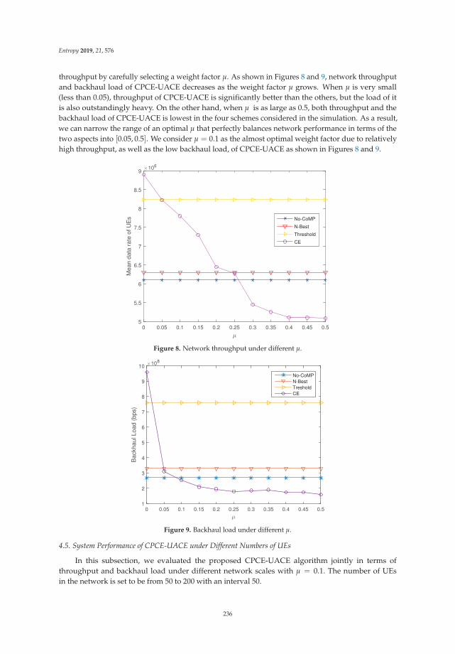
Entropy 2019, 21, 576

throughput by carefully selecting a weight factor μ. As shown in Figures 8 and 9, network throughputand backhaul load of CPCE-UACE decreases as the weight factor μ grows. When μ is very small(less than 0.05), throughput of CPCE-UACE is significantly better than the others, but the load of itis also outstandingly heavy. On the other hand, when μ is as large as 0.5, both throughput and thebackhaul load of CPCE-UACE is lowest in the four schemes considered in the simulation. As a result,we can narrow the range of an optimal μ that perfectly balances network performance in terms of thetwo aspects into [0.05, 0.5]. We consider μ = 0.1 as the almost optimal weight factor due to relativelyhigh throughput, as well as the low backhaul load, of CPCE-UACE as shown in Figures 8 and 9.

0 0.05 0.1 0.15 0.2 0.25 0.3 0.35 0.4 0.45 0.55

5.5

6

6.5

7

7.5

8

8.5

9

Mea

n da

ta r

ate

of U

Es

106

No-CoMP

N-Best

Threshold

CE

Figure 8. Network throughput under different μ.

μ

0 0.05 0.1 0.15 0.2 0.25 0.3 0.35 0.4 0.45 0.5

Bac

khau

l Loa

d (b

ps)

×108

1

2

3

4

5

6

7

8

9

10

No-CoMPN-BestTresholdCE

Figure 9. Backhaul load under different μ.

4.5. System Performance of CPCE-UACE under Different Numbers of UEs

In this subsection, we evaluated the proposed CPCE-UACE algorithm jointly in terms ofthroughput and backhaul load under different network scales with μ = 0.1. The number of UEsin the network is set to be from 50 to 200 with an interval 50.

236

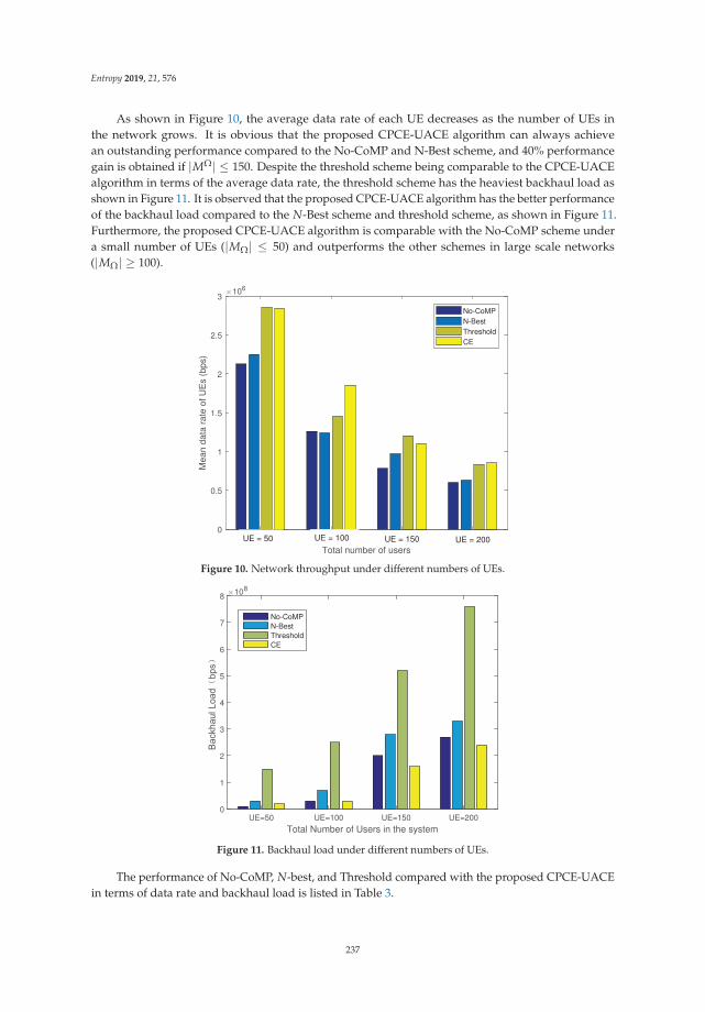
Entropy 2019, 21, 576

As shown in Figure 10, the average data rate of each UE decreases as the number of UEs inthe network grows. It is obvious that the proposed CPCE-UACE algorithm can always achievean outstanding performance compared to the No-CoMP and N-Best scheme, and 40% performancegain is obtained if |MΩ| ≤ 150. Despite the threshold scheme being comparable to the CPCE-UACEalgorithm in terms of the average data rate, the threshold scheme has the heaviest backhaul load asshown in Figure 11. It is observed that the proposed CPCE-UACE algorithm has the better performanceof the backhaul load compared to the N-Best scheme and threshold scheme, as shown in Figure 11.Furthermore, the proposed CPCE-UACE algorithm is comparable with the No-CoMP scheme undera small number of UEs (|MΩ| ≤ 50) and outperforms the other schemes in large scale networks(|MΩ| ≥ 100).

1 2 3 4

Total number of users

0

0.5

1

1.5

2

2.5

3

Mea

n da

ta r

ate

of U

Es

(bps

)

106

No-CoMPN-BestThresholdCE

UE = 50 UE = 100 UE = 150 UE = 200

Figure 10. Network throughput under different numbers of UEs.

Total Number of Users in the systemUE=50 UE=100 UE=150 UE=200

×108

0

1

2

3

4

5

6

7

8

No-CoMPN-BestThresholdCE

Figure 11. Backhaul load under different numbers of UEs.

The performance of No-CoMP, N-best, and Threshold compared with the proposed CPCE-UACEin terms of data rate and backhaul load is listed in Table 3.

237

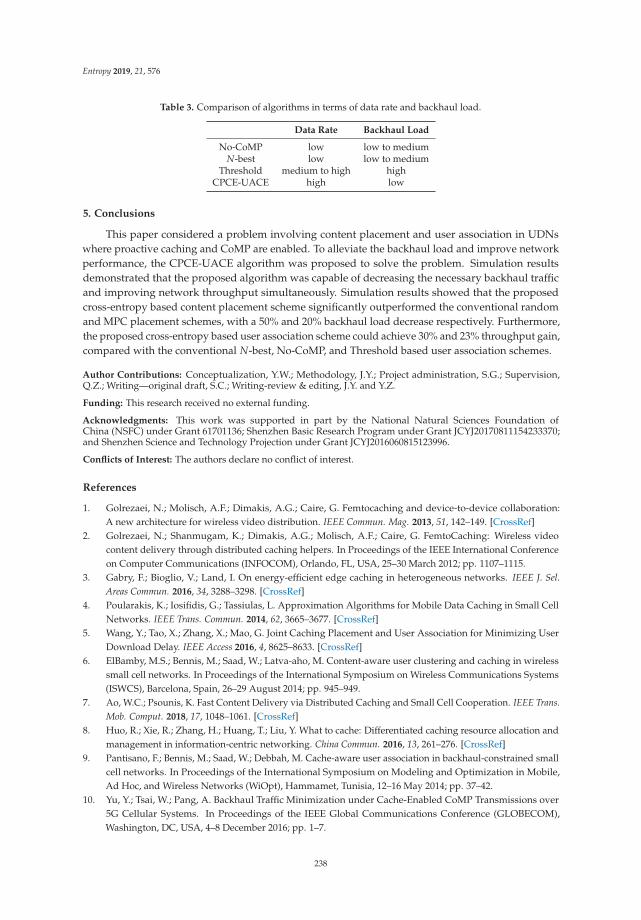
Entropy 2019, 21, 576

Table 3. Comparison of algorithms in terms of data rate and backhaul load.

Data Rate Backhaul Load

No-CoMP low low to mediumN-best low low to medium

Threshold medium to high highCPCE-UACE high low

5. Conclusions

This paper considered a problem involving content placement and user association in UDNswhere proactive caching and CoMP are enabled. To alleviate the backhaul load and improve networkperformance, the CPCE-UACE algorithm was proposed to solve the problem. Simulation resultsdemonstrated that the proposed algorithm was capable of decreasing the necessary backhaul trafficand improving network throughput simultaneously. Simulation results showed that the proposedcross-entropy based content placement scheme significantly outperformed the conventional randomand MPC placement schemes, with a 50% and 20% backhaul load decrease respectively. Furthermore,the proposed cross-entropy based user association scheme could achieve 30% and 23% throughput gain,compared with the conventional N-best, No-CoMP, and Threshold based user association schemes.

Author Contributions: Conceptualization, Y.W.; Methodology, J.Y.; Project administration, S.G.; Supervision,Q.Z.; Writing—original draft, S.C.; Writing-review & editing, J.Y. and Y.Z.

Funding: This research received no external funding.

Acknowledgments: This work was supported in part by the National Natural Sciences Foundation ofChina (NSFC) under Grant 61701136; Shenzhen Basic Research Program under Grant JCYJ20170811154233370;and Shenzhen Science and Technology Projection under Grant JCYJ2016060815123996.


References

1. Golrezaei, N.; Molisch, A.F.; Dimakis, A.G.; Caire, G. Femtocaching and device-to-device collaboration:A new architecture for wireless video distribution. IEEE Commun. Mag. 2013, 51, 142–149. [CrossRef]

2. Golrezaei, N.; Shanmugam, K.; Dimakis, A.G.; Molisch, A.F.; Caire, G. FemtoCaching: Wireless videocontent delivery through distributed caching helpers. In Proceedings of the IEEE International Conferenceon Computer Communications (INFOCOM), Orlando, FL, USA, 25–30 March 2012; pp. 1107–1115.

3. Gabry, F.; Bioglio, V.; Land, I. On energy-efficient edge caching in heterogeneous networks. IEEE J. Sel.Areas Commun. 2016, 34, 3288–3298. [CrossRef]

4. Poularakis, K.; Iosifidis, G.; Tassiulas, L. Approximation Algorithms for Mobile Data Caching in Small CellNetworks. IEEE Trans. Commun. 2014, 62, 3665–3677. [CrossRef]

5. Wang, Y.; Tao, X.; Zhang, X.; Mao, G. Joint Caching Placement and User Association for Minimizing UserDownload Delay. IEEE Access 2016, 4, 8625–8633. [CrossRef]

6. ElBamby, M.S.; Bennis, M.; Saad, W.; Latva-aho, M. Content-aware user clustering and caching in wirelesssmall cell networks. In Proceedings of the International Symposium on Wireless Communications Systems(ISWCS), Barcelona, Spain, 26–29 August 2014; pp. 945–949.

7. Ao, W.C.; Psounis, K. Fast Content Delivery via Distributed Caching and Small Cell Cooperation. IEEE Trans.Mob. Comput. 2018, 17, 1048–1061. [CrossRef]

8. Huo, R.; Xie, R.; Zhang, H.; Huang, T.; Liu, Y. What to cache: Differentiated caching resource allocation andmanagement in information-centric networking. China Commun. 2016, 13, 261–276. [CrossRef]

9. Pantisano, F.; Bennis, M.; Saad, W.; Debbah, M. Cache-aware user association in backhaul-constrained smallcell networks. In Proceedings of the International Symposium on Modeling and Optimization in Mobile,Ad Hoc, and Wireless Networks (WiOpt), Hammamet, Tunisia, 12–16 May 2014; pp. 37–42.

10. Yu, Y.; Tsai, W.; Pang, A. Backhaul Traffic Minimization under Cache-Enabled CoMP Transmissions over5G Cellular Systems. In Proceedings of the IEEE Global Communications Conference (GLOBECOM),Washington, DC, USA, 4–8 December 2016; pp. 1–7.

238

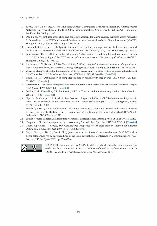
Entropy 2019, 21, 576

11. Kwak, J.; Le, L.B.; Wang, X. Two Time-Scale Content Caching and User Association in 5G HeterogeneousNetworks. In Proceedings of the IEEE Global Communications Conference (GLOBECOM ), Singapore,4–8 December 2017; pp. 1–6.

12. Dai, B.; Yu, W. Joint user association and content placement for Cache-enabled wireless access networks.In Proceedings of the IEEE International Conference on Acoustics, Speech and Signal Processing (ICASSP),Shanghai, China, 20–25 March 2016; pp. 3521–3525.

13. Breslau, L.; Cao, P.; Fan, L.; Phillips, G.; Shenker, S. Web caching and Zipf-like distributions: Evidence andimplications. In Proceedings of the IEEE INFOCOM ’99, New York, NY, USA, 21–25 March 1999; pp. 126–134.

14. Lakshmana, T.R.; Li, J.; Botella, C.; Papadogiannis, A.; Svensson, T. Scheduling for backhaul load reductionin CoMP. In Proceedings of the IEEE Wireless Communications and Networking Conference (WCNC),Shanghai, China, 7–10 April 2013.

15. Rubinstein, R.Y.; Kroese, D.P. The Cross-Entropy Method: A Unified Approach to Combinatorial Optimization,Monte-Carlo Simulation, and Machine Learning; Springer: New York, NY, USA, 2014; ISBN 978-0-387-21240-1.

16. Chen, S.; Zhao, T.; Chen, H.; Lu, Z.; Meng, W. Performance Analysis of Downlink Coordinated MultipointJoint Transmission in Ultra-Dense Networks. IEEE Netw. 2017, 31, 106–114. [CrossRef]

17. Rubinstein, R.Y. Optimization of computer simulation models with rare events. Eur. J. Oper. Res. 1997,99, 89–112. [CrossRef]

18. Rubinstein, R.Y. The cross-entropy method for combinatorial and continuous optimization. Methodol. Comput.Appl. Probab. 1999, 1, 127–190. [CrossRef]

19. De Boer, P.-T.; KroeseShie, D.P.; Rubinstein, M.R.Y. A Tutorial on the cross-entropy Method. Ann. Oper. Res.2005, 134, 19–67. [CrossRef]

20. Ugur, Y.; Estella Aguerri, I.; Zaidi, A. Rate Distortion Region of the Vector CEO Problem under LogarithmicLoss. In Proceedings of the IEEE Information Theory Workshop (ITW 2018), Guangzhou, China,25–29 November 2018.

21. Estella Aguerri, I.; Zaidi, A. Distributed Information Bottleneck Method for Discrete and Gaussian Sources.In Proceedings of the IEEE Int. Zurich Seminar on Information and Communications(IZS 2018), Zürich,Switzerland, 21–23 February 2018.

22. Estella Aguerri, I.; Zaidi, A. Distributed Variational Representation Learning. arXiv 2018, arXiv:1807.04193.23. Margolin, L. On the Convergence of the cross-entropy Method. Ann. Oper. Res. 2005, 134, 201–214. [CrossRef]24. Costa, A.; Owen, J.; Kroese, D.P. Convergence Properties of the cross-entropy Method for Discrete

Optimization. Oper. Res. Lett. 2007, 35, 573–580. [CrossRef]25. Liu, L.; Garcia, V.; Tian, L.; Pan, Z.; Shi, J. Joint clustering and inter-cell resource allocation for CoMP in ultra

dense cellular networks. In Proceedings of the IEEE International Conference on Communications (ICC),London, UK, 8–12 June 2015; pp. 2560–2564.


239

entropy

Article

Symmetry, Outer Bounds, and Code Constructions:A Computer-Aided Investigation on the FundamentalLimits of Caching

Chao Tian

Department of Electrical and Computer Engineering, Texas A&M University, College Station, TX 77843, USA;[email protected]

Received: 26 June 2018; Accepted: 11 August 2018; Published: 13 August 2018

Abstract: We illustrate how computer-aided methods can be used to investigate the fundamentallimits of the caching systems, which are significantly different from the conventional analyticalapproach usually seen in the information theory literature. The linear programming (LP) outerbound of the entropy space serves as the starting point of this approach; however, our effort goessignificantly beyond using it to prove information inequalities. We first identify and formalize thesymmetry structure in the problem, which enables us to show the existence of optimal symmetricsolutions. A symmetry-reduced linear program is then used to identify the boundary of thememory-transmission-rate tradeoff for several small cases, for which we obtain a set of tight outerbounds. General hypotheses on the optimal tradeoff region are formed from these computed data,which are then analytically proven. This leads to a complete characterization of the optimal tradeofffor systems with only two users, and certain partial characterization for systems with only two files.Next, we show that by carefully analyzing the joint entropy structure of the outer bounds for certaincases, a novel code construction can be reverse-engineered, which eventually leads to a general classof codes. Finally, we show that outer bounds can be computed through strategically relaxing the LPin different ways, which can be used to explore the problem computationally. This allows us firstly todeduce generic characteristic of the converse proof, and secondly to compute outer bounds for largerproblem cases, despite the seemingly impossible computation scale.

Keywords: computer-aided analysis; information theory

1. Introduction

We illustrate how computer-aided methods can be used to investigate the fundamental limits ofthe caching systems, which is in clear contrast to the conventional analytical approach usually seen inthe information theory literature. The theoretical foundation of this approach can be traced back to thelinear programming (LP) outer bound of the entropy space [1]. The computer-aided approach has beenpreviously applied in [2–5] on distributed data storage systems to derive various outer bounds, whichin many cases are tight. In this work, we first show that the same general methodology can be tailoredto the caching problem effectively to produce outer bounds in several cases, but more importantly,we show that data obtained through computation can be used in several different manners to deducemeaningful structural understanding of the fundamental limits and optimal code constructions.

The computer-aided investigation and exploration methods we propose are quite general;however, we tackle the caching problem in this work. Caching systems have attracted much researchattention recently. In a nutshell, caching is a data management technique that can alleviate thecommunication burden during peak traffic time or data demand time, by prefetching and prestoringcertain useful content at the users’ local caches. Maddah-Ali and Niesen [6] recently considered theproblem in an information theoretical framework, where the fundamental question is the optimal


Entropy 2018, 20, 603

tradeoff between local cache memory capacity and the content delivery transmission rate. It wasshown in [6] that coding can be very beneficial in this setting, while uncoded solutions suffer asignificant loss. Subsequent works extended it to decentralized caching placements [7], caching withnonuniform demands [8], online caching placements [9], hierarchical caching [10], caching with randomdemands [11], among other things. There have been significant research activities recently [12–21]in both refining the outer bounds and finding stronger codes for caching. Despite these efforts,the fundamental tradeoff had not been fully characterized except for the case with only two usersand two files [6] before our work. This is partly due to the fact that the main focus of the initialinvestigations [6–9] was on systems operating in the regime where the number of files and the numberof users are both large, for which the coded solutions can provide the largest gain over the uncodedcounterpart. However, in many applications, the number of simultaneous data requests can be small,or the collection of users or files need to be divided into subgroups in order to account for variousservice and request inhomogeneities; see, e.g., [8]. More importantly, precise and conclusive resultson such cases with small numbers of users or files can provide significant insights into more generalcases, as we shall show in this work.

In order to utilize the computational tool in this setting, the symmetry structure in the problemneeds be understood and used to reduce the problem to a manageable scale. The symmetry-reducedLP is then used to identify the boundary of the memory-transmission-rate tradeoff for several cases.General hypotheses on the optimal tradeoff region are formed from these data, which are thenanalytically proven. This leads to a complete characterization of the optimal tradeoff for systemswith two users, and certain partial characterization for systems with two files. Next, we show thatby carefully analyzing the joint entropy structure of the outer bounds, a novel code construction canbe reverse-engineered, which eventually leads to a general class of codes. Moreover, data can also beused to show that a certain tradeoff pair is not achievable using linear codes. Finally, we show thatouter bounds can be computed through strategically relaxing the LP in different ways, which can beused to explore the problem computationally. This allows us firstly to deduce generic characteristicof the converse proof, and secondly to compute outer bounds for larger problem cases, despite theseemingly impossible computation scale.

Although some of the tightest bounds and the most conclusive results on the optimalmemory-transmission-rate tradeoff in caching systems are presented in this work, our main focusis in fact to present the generic computer-aided methods that can be used to facilitate informationtheoretic investigations in a practically-important research problem setting. For this purpose, wewill provide the necessary details on the development and the rationale of the proposed techniquesin a semi-tutorial (and thus less concise) manner. The most important contribution of this work isthree methods for the investigation of fundamental limits of information systems: (1) computationaland data-driven converse hypothesis, (2) reverse-engineering optimal codes, and (3) computer-aidedexploration. We believe that these methods are sufficiently general, such that they can be applied toother coding and communication problems, particularly those related to data storage and management.

The rest of the paper is organized as follows. In Section 2, existing results on the caching problemand some background information on the entropy LP framework are reviewed. The symmetry structureof the caching problem is explored in detail in Section 3. In Section 4, we show how the data obtainedthrough computation can be used to form hypotheses, and then analytically prove them. In Section 5,we show that the computed data can also be used to facilitate reverse-engineering new codes, and alsoto prove that a certain memory-transmission-rate pair is not achievable using linear codes. In Section 6,we provide a method to explore the structure of the outer bounds computationally, to obtain insightsinto the problem and derive outer bounds for large problem cases. A few concluding remarks aregiven in Section 7, and technical proofs and some computer-produced proof tables are relegated tothe Appendices A–I .

242

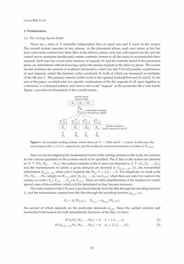
Entropy 2018, 20, 603

2. Preliminaries

2.1. The Caching System Model

There are a total of N mutually independent files of equal size and K users in the system.The overall system operates in two phases: in the placement phase, each user stores in his/herlocal cache some content from these files; in the delivery phase, each user will request one file, and thecentral server transmits (multicasts) certain common content to all the users to accommodate theirrequests. Each user has a local cache memory of capacity M, and the contents stored in the placementphase are determined without knowing a priori the precise requests in the delivery phase. The systemshould minimize the amount of multicast information, which has rate R for all possible combinationsof user requests, under the memory cache constraint M, both of which are measured as multiplesof the file size F. The primary interest of this work is the optimal tradeoff between M and R. In therest of the paper, we shall refer to a specific combination of the file requests of all users together asa demand, or a demand pattern, and reserve the word “request” as the particular file a user needs.Figure 1 provides an illustration of the overall system.

cached contents in users' memory of size

multicasted messagein the delivery phase

central serverhas N=3 files

Figure 1. An example caching system, where there are N = 3 files and K = 4 users. In this case, theusers request files (1, 2, 2, 3), respectively, and the multicast common information is written as X1,2,2,3.

Since we are investigating the fundamental limits of the caching systems in this work, the notationfor the various quantities in the systems needs to be specified. The N files in the system are denotedas W � {W1, W2, . . . , WN}; the cached contents at the K users are denoted as Z � {Z1, Z2, . . . , ZK};and the transmissions to satisfy a given demand are denoted as Xd1,d2,...,dK , i.e., the transmittedinformation Xd1,d2,...,dK when user k requests file Wdk

, k = 1, 2, . . . , K. For simplicity, we shall write(W1, W2, . . . , Wn) simply as W[1:n], and (d1, d2, . . . , dK) as d[1:K]; when there are only two users in thesystem, we write (Xi,1, Xi,2, . . . , Xi,j) as Xi,[1:j]. There are other simplifications of the notation for certainspecial cases of the problem, which will be introduced as they become necessary.

The cache content at the k-th user is produced directly from the files through the encoding functionfk, and the transmission content from the files through the encoding function gd[1:K]

, i.e.,

Zk = fk(W[1:N]), Xd[1:K]= gd[1:K]

(W[1:N]),

the second of which depends on the particular demands d[1:K]. Since the cached contents andtransmitted information are both deterministic functions of the files, we have:

H(ZkW1, W2, . . . , WN) = 0, k = 1, 2, . . . , K, (1)

H(Xd1,d2,...,dK W1, W2, . . . , WN) = 0, dk ∈ {1, 2, . . . , N}. (2)

243

Entropy 2018, 20, 603

It is also clear that:

H(WdkZk, Xd1,d2,...,dK ) = 0, (3)

i.e., the file Wdkis a function of the cached content Zk at user k and the transmitted information when

user k requests Wdk. The memory satisfies the constraint:

M ≥ H(Zi), i ∈ {1, 2, . . . , K}, (4)

and the transmission rate satisfies:

R ≥ H(Xd1,d2,...,dK ), dk ∈ {1, 2, . . . , N}. (5)

Any valid caching code must satisfy the specific set of conditions in (2)–(5). A slight variant of theproblem definition allows vanishing probability of error, i.e., the probability of error asymptoticallyapproaches zero as F goes to infinity; all the outer bounds derived in this work remain valid for thisvariant with appropriate applications of Fano’s inequality [22].

2.2. Known Results on Caching Systems

The first achievability result on this problem was given in [6], which is directly quoted below.

Theorem 1 (Maddah-Ali and Niesen [6]). For N files and K users each with a cache size M ∈{0, N/K, 2N/K, . . . , N},

R = K(1−M/N) ·min{

11 + KM/N

,NK

}(6)

is achievable. For general 0 ≤ M ≤ N, the lower convex envelope of these (M, R) points is achievable.

The first term in the minimization is achieved by the scheme of uncoded placement togetherwith coded transmission [6], while the latter term is by simple uncoded placement and uncodedtransmission. More recently, Yu et al. [19] provided the optimal solution when the placement isrestricted to be uncoded. Chen et al. [15] extended a special scheme for the case N = K = 2 discussedin [6] to the general case N ≤ K, and showed that the tradeoff pair

(1K , N(K−1)

K

)is achievable. There

were also several other notable efforts in attempting to find better binary codes [16–18,21]. Tian andChen [20] proposed a class of codes for N ≤ K, the origin of which will be discussed in more details inSection 5. Gómez-Vilardebó [21] also proposed a new code, which can provide further improvement inthe small cache memory regime. Tradeoff points achieved by the codes in [20] can indeed be optimalin some cases. It is worth noting that while all the schemes [6,15–19,21] are binary codes, the codesin [20] use a more general finite field.

A cut-set outer bound was also given in [6], which is again directly quoted below.

Theorem 2 (Maddah-Ali and Niesen [6]). For N files and K users each with a cache size 0 ≤ M ≤ N,

R ≥ maxs∈{1,2,...,min{N,K}}

(s− sM

�N/s�

). (7)

Several efforts to improve this outer bound have also been reported, which have led to moreaccurate approximation characterizations of the optimal tradeoff [12–14]. However, as mentionedearlier, even for the simplest cases beyond (N, K) = (2, 2), complete characterizations was not availablebefore our work (firstly reported in [23]). In this work, we specifically treat such small problem cases,and attempt to deduce more generic properties and outer bounds from these cases. Some of the most

244

Entropy 2018, 20, 603

recent work [24,25] that were obtained after the publication of our results [23] provide even moreaccurate approximations, the best of which at this point of time is roughly a factor of 2 [24].

2.3. The Basic Linear Programming Framework

The basic linear programing bound on the entropy space was introduced by Yeung [1], whichcan be understood as follows. Consider a total of n discrete random variables (X1, X2, . . . , Xn) with agiven joint distribution. There are a total of 2n − 1 joint entropies, each associated with a non-emptysubset of these random variables. It is known that the entropy function is monotone and submodular,and thus, any valid (2n − 1) dimensional entropy vector must have the properties associated withsuch monotonicity and submodularity, which can be written as a set of inequalities. Yeung showed(see, e.g., [26]) that the minimal sufficient set of such inequalities is the so-called elemental inequalities:

H(Xi{Xk, k �= i}) ≥ 0, i ∈ {1, 2, . . . , n} (8)

I(Xi; Xj{Xk, k ∈ Φ}) ≥ 0, where Φ ⊆ {1, 2, . . . , n} \ {i, j}, i �= j. (9)

The 2n − 1 joint entropy terms can be viewed as the variables in a linear programming (LP)problem, and there is a total of n + (n

2)2n−2 constraints in (8) and (9). In addition to this generic set

of constraints, each specific coding problem will place additional constraints on the joint entropyvalues. These can be viewed as a constraint set of the given problem, although the problem might alsoinduce constraints that are not in this form or even not possible to write in terms of joint entropies.For example, in the caching problem, the set of random variables are {Wi, i = 1, 2, . . . , N} ∪ {Zi, i =1, 2, . . . , K} ∪ {Xd1,d2,...,dK : dk ∈ {1, 2, . . . , N}}, and there is a total of 2N+K+NK − 1 variables in this LP;

the problem-specific constraints are those in (2)–(5), and there are N + K + NK + (N+K+NK

2 )2N+K+NK−2

elemental entropy constraints, which is in fact doubly exponential in the number of users K.

2.4. A Computed-Aided Approach to Find Outer Bounds

In principle, with the aforedescribed constraint set, one can simply convert the outer boundingproblem into an LP (with an objective function R for each fixed M in the caching problem, or moregenerally a linear combination of M and R), and use a generic LP solver to compute it. Unfortunately,despite the effectiveness of modern LP solvers, directly applying this approach on an engineeringproblem is usually not possible, since the scale of the LP is often very large even for simple settings.For example, for the caching problem, when N = 2, K = 4, there are overall 200 million elementalinequalities. The key observation used in [2] to make the problem tractable is that the LP can usually besignificantly reduced, by taking into account the symmetry and the implication relations in the problem.

The details of the reductions can be found in [2], and here, we only provide two examples in thecontext of the caching problem to illustrate the basic idea behind these reductions:

• Assuming the optimal codes are symmetric, which will be defined more precisely later, the jointentropy H(W2, Z3, X2,3,3) should be equal to the joint entropy H(W1, Z2, X1,2,2). This implies thatin the LP, we can represent both quantities using a single variable.

• Because of the relation (3), the joint entropy H(W2, Z3, X2,3,3) should be equal to the joint entropyH(W2, W3, Z3, X2,3,3). This again implies that in the LP, we can represent both quantities using asingle variable.

The reduced primal LP problem is usually significantly smaller, which allows us to find a lowerbound for the tradeoff region for a specific instance with fixed file sizes. Moreover, after identifyingthe region of interest using these computed boundary points, a human-readable proof can also beproduced computationally by invoking the dual of the LP given above. Note a feasible and boundedLP always has a rational optimal solution when all the coefficients are rational, and thus, the boundwill have rational coefficients. More details can again be found in [2]; however, this procedure can beintuitively viewed as follows. Suppose a valid outer bound in the constraint set has the form of:

245

Entropy 2018, 20, 603

∑Φ⊆{1,2,...,n}

αΦ H(Xk, k ∈ Φ) ≥ 0, (10)

then it must be a linear combination of the known inequalities, i.e., (8) and (9), and the problem-specificconstraints, e.g., (2)–(5) for the caching problem. To find a human-readable proof is essentially to finda valid linear combination of these inequalities, and for the conciseness of the proof, the sparsest linearcombination is preferred. By utilizing the LP dual with an additional linear objective, we can findwithin all valid combinations a sparse (but not necessarily the sparsest) one, which can yield a conciseproof of the inequality (10).

It should be noted that in [2], the region of interest was obtained by first finding a set of fine-spacedpoints on the boundary of the outer bound using the reduced LP, and then manually identifying theeffective bounding segments using these boundary points. This task can however be accomplishedmore efficiently using an approach proposed by Lassez and Lassez [27], as pointed out in [28].This prompted the author to implement this part of the computer program using this more efficientapproach. For completeness, the specialization of the Lassez algorithm to the caching problem, which ismuch simplified in this setting, is provided in Appendix A.

The proof found through this approach can be conveniently written in a matrix to list all the linearcombination coefficients, and one can easily produce a chain of inequalities using such a table to obtaina more conventional human-readable proof. This approach of generating human-readable proofs hassubsequently been adopted by other researchers [5,29]. Though we shall present several results thusobtained in this current work in the tabulation form, our main goal is to use these results to present thecomputer-aided approach, and show the effectiveness of our approach.

3. Symmetry in the Caching Problem

The computer-aided approach to derive outer bounds mentioned earlier relies critically on thereduction of the basic entropy LP using symmetry and other problem structures. In this section,we consider the symmetry in the caching problem. Intuitively, if we place the cached contents ina permuted manner at the users, it will lead to a new code that is equivalent to the original one.Similarly, if we reorder the files and apply the same encoding function, the transmissions can also bechanged accordingly to accommodate the requests, which is again an equivalent code. The two typesof symmetries can be combined, and they induce a permutation group on the joint entropies of thesubsets of the random variablesW ∪Z ∪X .

For concreteness, we may specialize to the case (N, K) = (3, 4) in the discussion, and for this case:

W = {W1, W2, W3}, Z = {Z1, Z2, Z3, Z4}, X = {Xd1,d2,d3,d4 : dk ∈ {1, 2, 3}}. (11)

3.1. Symmetry in User Indexing

Let a permutation function be defined as π(·) on the user index set of {1, 2, . . . , K}, which reflects apermuted placement of cached contents Z . Let the inverse of π(·) be denoted as π−1(·), and define thepermutation on a collection of elements as the collection of the elements after permuting each elementindividually. The aforementioned permuted placement of cached contents can be rigorously definedthrough a set of new encoding functions and decoding functions. Given the original encoding functionsfk and gd[1:K]

, the new functions f πk and gπ

d[1:K]associated with a permutation π can be defined as:

Zk � f πk (W[1:N]) � fπ(k)(W[1:N]) = Zπ(k),

Xd[1:K]� gπ

d[1:K](W[1:N]) � gd

π−1([1:K])(W[1:N]) = Xd

π−1([1:K]).

(12)

To see that with these new functions, any demand d([1:K]) can be correctly fulfilled as long as the originalfunctions can fulfill the corresponding reconstruction task, consider the pair ( f π

k (W[1:N]), gπd[1:K]

(W[1:N])),

which should reconstruct Wdk. This pair is equivalent to the pair ( fπ(k)(W[1:N]), gd

π−1([1:K])(W[1:N])), and

246

Entropy 2018, 20, 603

in the demand vector dπ−1([1:K]), the π(k) position is in fact dπ−1(π(k)) = dk, implying that the newcoding functions are indeed valid.

We can alternatively view π(·) as directly inducing a permutation on Z as π(Zk) = Zπ(k), and apermutation on X as:

π(Xd1,d2,...,dK ) = Xdπ−1(1) ,dπ−1(2) ,...,dπ−1(K)

. (13)

For example, the permutation function π(1) = 2, π(2) = 3, π(3) = 1, π(4) = 4 will induce:

(d1, d2, d3, d4)→ (d1, d2, d3, d4) = (d3, d1, d2, d4). (14)

Thus, it will map Z1 to π(Z1) = Z2, but map X1,2,3,2 to X3,1,2,2, X3,2,1,3 to X1,3,2,3, and X1,1,2,2 to X2,1,1,2.With the new coding functions and the permuted random variables defined above, we have the

following relation:

(W π ,Z π ,X π)=(W , π(Z), π(X )), (15)

where the superscript π indicates the random variables induced by the new encoding functions.We call a caching code user-index-symmetric, if for any subsetsWo ⊆ W ,Zo ⊆ Z ,Xo ⊆ X , and

any permutation π, the following relation holds:

H(Wo,Zo,Xo) = H(Wo, π(Zo), π(Xo)). (16)

For example, for such a symmetric code, the entropy H(W2, Z2, X1,2,3,2) under the aforementionedpermutation is equal to H(W2, Z3, X3,1,2,2); note that W2 is a function of (Z2, X1,2,3,2), and after themapping, it is a function of (Z3, X3,1,2,2).

3.2. Symmetry in File Indexing

Let a permutation function be defined as π(·) on the file index set of {1, 2, . . . , N}, which reflectsa renaming of the filesW . This file-renaming operation can be rigorously defined as a permutation ofthe input arguments to the functions fk and gd[1:K]

. Given the original encoding functions fk and gd[1:K],

the new functions f πk and gπ

d[1:K]associated with a permutation π can be defined as:

Zk � f πk (W[1:N]) � fk(Wπ−1([1:N])),

Xd[1:K]� gπ

d[1:K](W[1:N]) � gπ(d[1:K])

(Wπ−1([1:N])).(17)

We first show that the pair ( f πk (W[1:N]), gπ

d[1:K](W[1:N])) can provide reconstruction of Wdk

. This pair

by definition is equivalent to ( fk(Wπ−1([1:N])), gπ(d[1:K])(Wπ−1([1:N]))), where the k-th position of the

demand vector π(d[1:K]) is in fact π(dk). However, because of the permutation in the input arguments,this implies that the π(dk)-th file in the sequence Wπ−1([1:N])) can be reconstructed, which is indeed Wdk

.Alternatively, we can view π(·) as directly inducing a permutation on π(Wk) = Wπ(k), and it also

induces a permutation on X as:

π(Xd1,d2,...,dK ) = Xπ(d1),π(d2),...,π(dK). (18)

For example, the permutation function π(1) = 2, π(2) = 3, π(3) = 1 maps W2 to π(W2) = W3,but maps X1,2,3,2 to X2,3,1,3, X3,2,1,3 to X1,3,2,1, and X1,1,2,2 to X2,2,3,3.

With the new coding functions and the permuted random variables defined above, we have thefollowing equivalence relation:

247

Entropy 2018, 20, 603

(W π ,Z π ,X π) =(

W([1:N]), f[1:k](Wπ−1([1:N])),{

gπ(d[1:K])(Wπ−1([1:N])) : d[1:K] ∈ N K

})d=

(Wπ([1:N]), f[1:k](W[1:N]),

{gπ(d[1:K])

(W[1:N]) : d[1:K] ∈ N K})

= (π(W),Z , π(X )) ,

(19)

where d= indicates equal in distribution, which is due to the the random variables in W being

independently and identically distributed, thus exchangeable.We call a caching code file-index-symmetric, if for any subsetsWo ⊆ W ,Zo ⊆ Z ,Xo ⊆ X , and

any permutation π, the following relation holds:

H(Wo,Zo,Xo) = H(π(Wo),Zo, π(Xo)). (20)

For example, for such a symmetric code, H(W3, Z3, X1,2,3,2) under the aforementioned permutation isequal to H(W1, Z3, X2,3,1,3); note that W3 is a function of (Z3, X1,2,3,2), and after the mapping, W1 is afunction of (Z3, X2,3,1,3).

3.3. Existence of Optimal Symmetric Codes

With the symmetry structure elucidated above, we can now state our first auxiliary result.

Proposition 1. For any caching code, there is a code with the same or smaller caching memory and transmissionrate, which is both user-index-symmetric and file-index-symmetric.

We call a code that is both user-index-symmetric and file-index-symmetric a symmetric code.This proposition implies that there is no loss of generality to consider only symmetric codes. The proofof this proposition relies on a simple space-sharing argument, where a set of base encoding functionsand base decoding function are used to construct a new code. In this new code, each file is partitionedinto a total of N!K! segments, each having the same size as suitable in the base coding functions.The coding functions obtained as in (12) and (17) from the base coding functions using permutations π

and π are used on the i-th segments of all the files to produce random variablesW π·π ∪ Z π·π ∪ X π·π .Consider a set of random variables (Wo ∪ Zo ∪ Xo) in the original code, and denote the same set ofrandom variables in the new code as (W′

o ∪ Z′o ∪ X ′o). We have:

H(W′o ∪ Z′o ∪ X ′o) = ∑

π,πH(W π·π

o ∪ Z π·πo ∪ X π·π

o ) = ∑π,π

H(π(Wo) ∪ π(Zo) ∪ π · π(Xo)), (21)

because of (15) and (19). Similarly, for another pair of permutations (π′, π′), the random variablesπ′(W′

o)∪ π′(Z′o)∪ π′ · π′(X ′o) in the new code will have exactly the same joint entropy value. It is nowclear that the resultant code by space sharing is indeed symmetric, and it has (normalized) memorysizes and a transmission rate no worse than the original one. A similar argument was used in [2]to show, with a more detailed proof, the existence of optimal symmetric solution in regeneratingcodes. In a separate work [30], we investigated the properties of the induced permutation π · π, andparticularly, showed that it is isomorphic to the power group [31]; readers are referred to [30] formore details.

3.4. Demand Types

Even for symmetric codes, the transmissions to satisfy different types of demands may usedifferent rates. For example in the setting N, K = (3, 4), H(X1,2,2,2) may not be equal to H(X1,1,2,2),and H(X1,2,3,2) may not be equal to H(X3,2,3,2). The transmission rate R is then chosen to be themaximum among all cases. This motivates the notion of demand types.

248

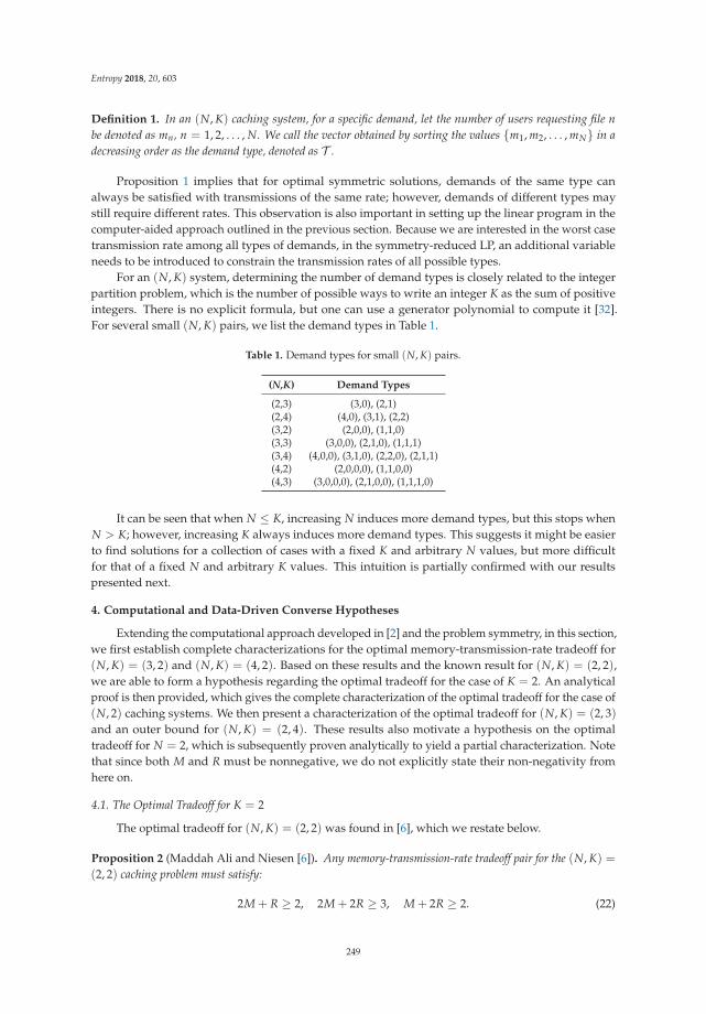
Entropy 2018, 20, 603

Definition 1. In an (N, K) caching system, for a specific demand, let the number of users requesting file nbe denoted as mn, n = 1, 2, . . . , N. We call the vector obtained by sorting the values {m1, m2, . . . , mN} in adecreasing order as the demand type, denoted as T .

Proposition 1 implies that for optimal symmetric solutions, demands of the same type canalways be satisfied with transmissions of the same rate; however, demands of different types maystill require different rates. This observation is also important in setting up the linear program in thecomputer-aided approach outlined in the previous section. Because we are interested in the worst casetransmission rate among all types of demands, in the symmetry-reduced LP, an additional variableneeds to be introduced to constrain the transmission rates of all possible types.

For an (N, K) system, determining the number of demand types is closely related to the integerpartition problem, which is the number of possible ways to write an integer K as the sum of positiveintegers. There is no explicit formula, but one can use a generator polynomial to compute it [32].For several small (N, K) pairs, we list the demand types in Table 1.

Table 1. Demand types for small (N, K) pairs.

(N,K) Demand Types

(2,3) (3,0), (2,1)(2,4) (4,0), (3,1), (2,2)(3,2) (2,0,0), (1,1,0)(3,3) (3,0,0), (2,1,0), (1,1,1)(3,4) (4,0,0), (3,1,0), (2,2,0), (2,1,1)(4,2) (2,0,0,0), (1,1,0,0)(4,3) (3,0,0,0), (2,1,0,0), (1,1,1,0)

It can be seen that when N ≤ K, increasing N induces more demand types, but this stops whenN > K; however, increasing K always induces more demand types. This suggests it might be easierto find solutions for a collection of cases with a fixed K and arbitrary N values, but more difficultfor that of a fixed N and arbitrary K values. This intuition is partially confirmed with our resultspresented next.

4. Computational and Data-Driven Converse Hypotheses

Extending the computational approach developed in [2] and the problem symmetry, in this section,we first establish complete characterizations for the optimal memory-transmission-rate tradeoff for(N, K) = (3, 2) and (N, K) = (4, 2). Based on these results and the known result for (N, K) = (2, 2),we are able to form a hypothesis regarding the optimal tradeoff for the case of K = 2. An analyticalproof is then provided, which gives the complete characterization of the optimal tradeoff for the case of(N, 2) caching systems. We then present a characterization of the optimal tradeoff for (N, K) = (2, 3)and an outer bound for (N, K) = (2, 4). These results also motivate a hypothesis on the optimaltradeoff for N = 2, which is subsequently proven analytically to yield a partial characterization. Notethat since both M and R must be nonnegative, we do not explicitly state their non-negativity fromhere on.

4.1. The Optimal Tradeoff for K = 2

The optimal tradeoff for (N, K) = (2, 2) was found in [6], which we restate below.

Proposition 2 (Maddah Ali and Niesen [6]). Any memory-transmission-rate tradeoff pair for the (N, K) =(2, 2) caching problem must satisfy:

2M + R ≥ 2, 2M + 2R ≥ 3, M + 2R ≥ 2. (22)

249

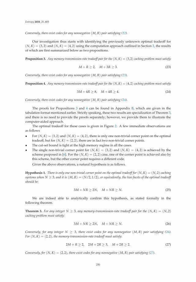
Entropy 2018, 20, 603

Conversely, there exist codes for any nonnegative (M, R) pair satisfying (22).

Our investigation thus starts with identifying the previously unknown optimal tradeoff for(N, K) = (3, 2) and (N, K) = (4, 2) using the computation approach outlined in Section 2, the resultsof which are first summarized below as two propositions.

Proposition 3. Any memory-transmission-rate tradeoff pair for the (N, K) = (3, 2) caching problem must satisfy:

M + R ≥ 2, M + 3R ≥ 3. (23)


Proposition 4. Any memory-transmission-rate tradeoff pair for the (N, K) = (4, 2) caching problem must satisfy:

3M + 4R ≥ 8, M + 4R ≥ 4. (24)


The proofs for Propositions 3 and 4 can be found in Appendix B, which are given in thetabulation format mentioned earlier. Strictly speaking, these two results are specialization of Theorem 3,and there is no need to provide the proofs separately; however, we provide them to illustrate thecomputer-aided approach.

The optimal tradeoff for these cases is given in Figure 2. A few immediate observations areas follows

• For (N, K) = (3, 2) and (N, K) = (4, 2), there is only one non-trivial corner point on the optimaltradeoff, but for (N, K) = (2, 2), there are in fact two non-trivial corner points.

• The cut-set bound is tight at the high memory regime in all the cases.• The single non-trivial corner point for (N, K) = (3, 2) and (N, K) = (4, 2) is achieved by the

scheme proposed in [6]. For the (N, K) = (2, 2) case, one of the corner point is achieved also bythis scheme, but the other corner point requires a different code.

Given the above observations, a natural hypothesis is as follows.

Hypothesis 1. There is only one non-trivial corner point on the optimal tradeoff for (N, K) = (N, 2) cachingsystems when N ≥ 3, and it is (M, R) = (N/2, 1/2), or equivalently, the two facets of the optimal tradeoffshould be:

3M + NR ≥ 2N, M + NR ≥ N. (25)

We are indeed able to analytically confirm this hypothesis, as stated formally in thefollowing theorem.

Theorem 3. For any integer N ≥ 3, any memory-transmission-rate tradeoff pair for the (N, K) = (N, 2)caching problem must satisfy:

3M + NR ≥ 2N, M + NR ≥ N. (26)

Conversely, for any integer N ≥ 3, there exist codes for any nonnegative (M, R) pair satisfying (26).For (N, K) = (2, 2), the memory-transmission-rate tradeoff must satisfy:

2M + R ≥ 2, 2M + 2R ≥ 3, M + 2R ≥ 2. (27)

Conversely, for (N, K) = (2, 2), there exist codes for any nonnegative (M, R) pair satisfying (27).

250

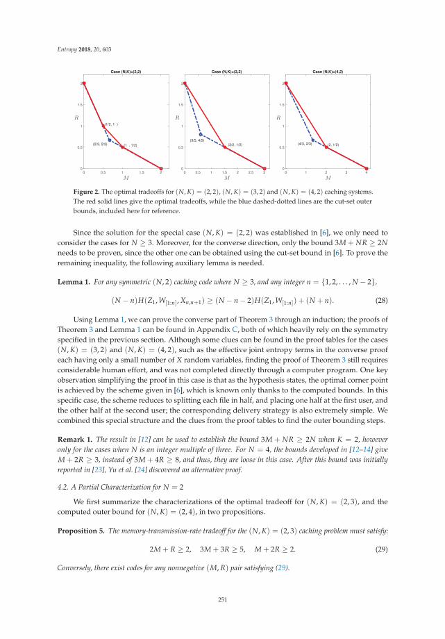
Entropy 2018, 20, 603

0 0.5 1 1.5 2

M

0

0.5

1

1.5

2

R

Case (N,K)=(2,2)

(2/3, 2/3)

(1/2, 1 )

(1 , 1/2)

0 0.5 1 1.5 2 2.5 3

M

0

0.5

1

1.5

2

R

Case (N,K)=(3,2)

(3/5, 4/5)(3/2, 1/2)

0 1 2 3 4

M

0

0.5

1

1.5

2

R

Case (N,K)=(4,2)

(4/3, 2/3) (2, 1/2)

Figure 2. The optimal tradeoffs for (N, K) = (2, 2), (N, K) = (3, 2) and (N, K) = (4, 2) caching systems.The red solid lines give the optimal tradeoffs, while the blue dashed-dotted lines are the cut-set outerbounds, included here for reference.

Since the solution for the special case (N, K) = (2, 2) was established in [6], we only need toconsider the cases for N ≥ 3. Moreover, for the converse direction, only the bound 3M + NR ≥ 2Nneeds to be proven, since the other one can be obtained using the cut-set bound in [6]. To prove theremaining inequality, the following auxiliary lemma is needed.

Lemma 1. For any symmetric (N, 2) caching code where N ≥ 3, and any integer n = {1, 2, . . . , N − 2},

(N − n)H(Z1, W[1:n], Xn,n+1) ≥ (N − n− 2)H(Z1, W[1:n]) + (N + n). (28)

Using Lemma 1, we can prove the converse part of Theorem 3 through an induction; the proofs ofTheorem 3 and Lemma 1 can be found in Appendix C, both of which heavily rely on the symmetryspecified in the previous section. Although some clues can be found in the proof tables for the cases(N, K) = (3, 2) and (N, K) = (4, 2), such as the effective joint entropy terms in the converse proofeach having only a small number of X random variables, finding the proof of Theorem 3 still requiresconsiderable human effort, and was not completed directly through a computer program. One keyobservation simplifying the proof in this case is that as the hypothesis states, the optimal corner pointis achieved by the scheme given in [6], which is known only thanks to the computed bounds. In thisspecific case, the scheme reduces to splitting each file in half, and placing one half at the first user, andthe other half at the second user; the corresponding delivery strategy is also extremely simple. Wecombined this special structure and the clues from the proof tables to find the outer bounding steps.

Remark 1. The result in [12] can be used to establish the bound 3M + NR ≥ 2N when K = 2, howeveronly for the cases when N is an integer multiple of three. For N = 4, the bounds developed in [12–14] giveM + 2R ≥ 3, instead of 3M + 4R ≥ 8, and thus, they are loose in this case. After this bound was initiallyreported in [23], Yu et al. [24] discovered an alternative proof.

4.2. A Partial Characterization for N = 2

We first summarize the characterizations of the optimal tradeoff for (N, K) = (2, 3), and thecomputed outer bound for (N, K) = (2, 4), in two propositions.

Proposition 5. The memory-transmission-rate tradeoff for the (N, K) = (2, 3) caching problem must satisfy:

2M + R ≥ 2, 3M + 3R ≥ 5, M + 2R ≥ 2. (29)


251

Entropy 2018, 20, 603

Proposition 6. The memory-transmission-rate tradeoff for the (N, K) = (2, 4) caching problem must satisfy:

2M + R ≥ 2, 14M + 11R ≥ 20, 9M + 8R ≥ 14, 3M + 3R ≥ 5, 5M + 6R ≥ 9, M + 2R ≥ 2. (30)

For Proposition 5, the only new bound 3M + 3R ≥ 5 is a special case of the more general result ofTheorem 4, and we thus do not provide this proof separately. For Proposition 6, only the second and thethird inequalities need to be proven, since the fourth coincides with a bound in the (2, 3) case, the fifthis a special case of Theorem 4, and the others can be produced from the cut-set bounds. The proofsfor these two inequalities are given in Appendix E. The optimal tradeoff for (N, K) = (2, 2), (2, 3) andthe outer bound for (2, 4) are depicted in Figure 3. A few immediate observations and comments areas follows:

• There are two non-trivial corner points on the outer bounds for (N, K) = (2, 2) and (N, K) = (2, 3),and there are five non-trivial corner points for (N, K) = (2, 4).

• The outer bounds coincide with known inner bounds for (N, K) = (2, 2) and (N, K) = (2, 3), butnot (N, K) = (2, 4). The corner points at R = 1/K (and the corner point (1, 2/3) for (N, K) = (2, 4))are achieved by the scheme given in [6], while the corner points at M = 1/K are achieved by thescheme given in [15]. For (N, K) = (2, 4), two corner points at the intermediate memory regimecannot be achieved by either the scheme in [6] or that in [15].

• The cut-set outer bounds [6] are tight at the highest and lowest memory segments; a new boundfor the second highest memory segment produced by the computer-based method is also tight.

0 0.5 1 1.5 20

0.5

1

1.5

2

(2/3, 2/3)

(1/2, 1 )

(1 , 1/2)

M

R

Case (N,K)=(2,2)

0 0.5 1 1.5 20

0.5

1

1.5

2

(2/3, 2/3)

(1/3, 4/3)

(4/3, 1/3)

M

R

Case (N,K)=(2,3)

0 0.5 1 1.5 20

0.5

1

1.5

2

(2/3, 2/3)

(1/4 , 3/2 )

(6/13, 16/13)

(2/3 , 1 )

(1 , 2/3 )

(3/2 , 1/4 )

M

R

Case (N,K)=(2,4)

Figure 3. The optimal tradeoffs for (N, K) = (2, 2), (N, K) = (2, 3) and computed outer bound(N, K) = (2, 4) caching systems. The red solid lines give the optimal tradeoffs for the first two cases,and the red dotted line gives the computed outer bound (N, K) = (2, 4); the blue dashed-dot lines arethe cut-set outer bounds, and the black dashed line is the inner bound using the scheme in [6,15].

Remark 2. The bounds developed in [12–14] give 2(M + R) ≥ 3 for (N, K) = (2, 3) and (N, K) = (2, 4),instead of 3M + 3R ≥ 5, and thus, they are loose in this case. When specializing the bounds in [24], it matchesProposition 5 for (N, K) = (2, 3), but it is weaker than Proposition 6 for (N, K) = (2, 4).

From the above observations, we can hypothesize that for N = 2, the number of corner pointswill continue to increase as K increases above four, and at the high memory regime, the scheme [6] isoptimal. More precisely, we can establish the following theorem.

Theorem 4. When K ≥ 3 and N = 2, any (M, R) pair must satisfy:

K(K + 1)M + 2(K− 1)KR ≥ 2(K− 1)(K + 2). (31)

252

Entropy 2018, 20, 603

As a consequence, the uncoded-placement-coded-transmission scheme in [6] (with space-sharing) is optimalwhen M ≥ 2(K−2)

K , for the cases with K ≥ 4 and N = 2.

The first line segment at the high memory regime is M + 2R ≥ 2, which is given by the cut-setbound; its intersection with (31) is indeed the first point in:(

2(K− 1)K

,1K

)and

(2(K− 2)

K,

2K− 1

). (32)

The proof of this theorem now boils down to the proof of the bound (31). This requires asophisticated induction, the digest of which is summarized in the following lemma. The symmetry ofthe problem is again heavily utilized throughout the proof of this lemma. For notational simplicity, weuse X→j to denote X1,1,...,1,2,1,...,1, i.e., when the j-th user requests the second file, and all the other usersrequest the first file; we also write a collection of such variables (X→j, X→j+1, . . . , X→k) as X→[j:k].

Lemma 2. For N = 2 and K ≥ 3, the following inequality holds for k ∈ {2, 3, . . . , K− 1}:

(K− k + 1)(K− k + 2)H(Z1, W1, X→[2:k])

≥ [(K− k)(K− k + 1)− 2]H(Z1, W1, X→[2:k−1]) + 2H(W1, X→[2:k−1]) + 2(K− k + 1)H(W1, W2),(33)

where we have taken the convention H(Z1, W1, X→[2:1]) = H(Z1, W1)

The proof of Lemma 2 is given in Appendix F. Theorem 4 can now be proven straightforwardly.

Proof of Theorem 4. We first write the following simple inequalities:

H(Z1) + H(X→2) ≥ H(Z1, X→2) = H(Z1, W1, X→2). (34)

Now, applying Lemma 2 with k = 2 gives:

(K− 1)K[H(Z1) + H(X→2)] ≥ [K2 − 3K]H(Z1, W1) + 2H(W1) + 2(K− 1)H(W1, W2). (35)

Observe that:

H(Z1, W1) = H(W1Z1) + H(Z1) ≥12

H(W1, W2Z1) + H(Z1) =12

H(W1, W2) +12

H(Z1), (36)

where in the first inequality the file index symmetry H(W1Z1) = H(W2Z1) has been used. We cannow continue to write:

(K− 1)K[H(Z1) + H(X→2)] ≥K2 − 3K

2[H(W1, W2) + H(Z1)] + 2H(W1) + 2(K− 1)H(W1, W2), (37)

which has some a common term H(Z1) on both sizes with different coefficients. Removing the commonterm and multiplying both sides by two lead to:

K(K + 1)H(Z1) + 2(K− 1)KH(X→2)

≥ [(K− 2)(K− 1)− 2 + 4(K− 1)]H(W1, W2) + 4H(W1)

= 2K2 + 2K− 4,

(38)

where the equality relies on the assumption that W1 and W2 are independent files of unit size.Taking into consideration the memory and transmission rate constraints (4) and (5) now completesthe proof.

253

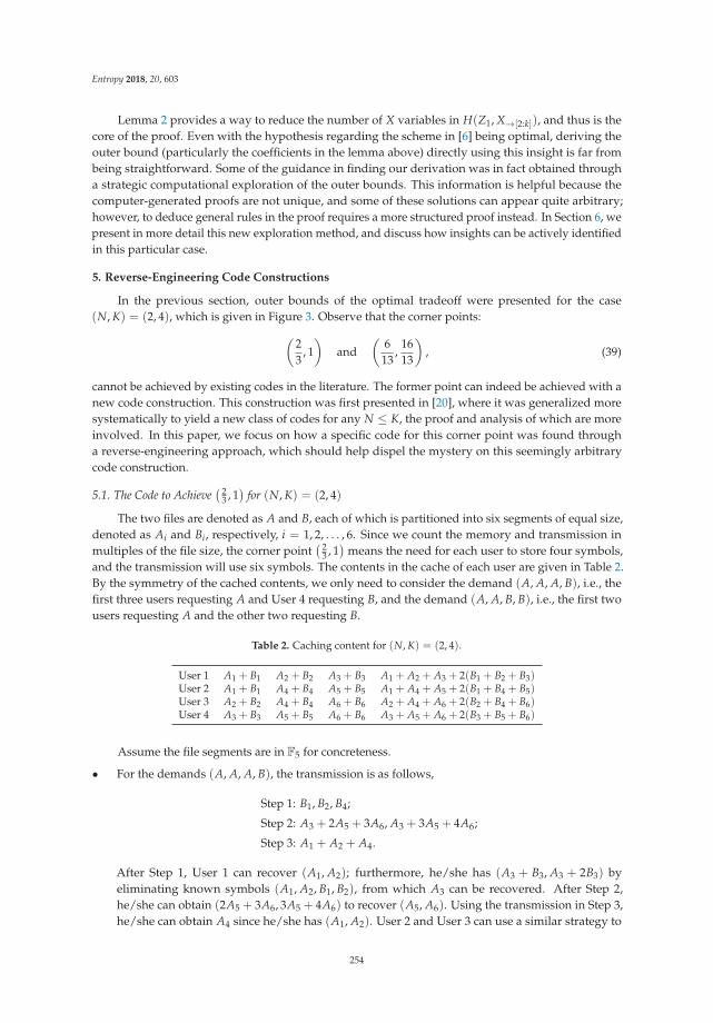
Entropy 2018, 20, 603

Lemma 2 provides a way to reduce the number of X variables in H(Z1, X→[2:k]), and thus is thecore of the proof. Even with the hypothesis regarding the scheme in [6] being optimal, deriving theouter bound (particularly the coefficients in the lemma above) directly using this insight is far frombeing straightforward. Some of the guidance in finding our derivation was in fact obtained througha strategic computational exploration of the outer bounds. This information is helpful because thecomputer-generated proofs are not unique, and some of these solutions can appear quite arbitrary;however, to deduce general rules in the proof requires a more structured proof instead. In Section 6, wepresent in more detail this new exploration method, and discuss how insights can be actively identifiedin this particular case.

5. Reverse-Engineering Code Constructions

In the previous section, outer bounds of the optimal tradeoff were presented for the case(N, K) = (2, 4), which is given in Figure 3. Observe that the corner points:(

23

, 1)

and(

613

,1613

), (39)

cannot be achieved by existing codes in the literature. The former point can indeed be achieved with anew code construction. This construction was first presented in [20], where it was generalized moresystematically to yield a new class of codes for any N ≤ K, the proof and analysis of which are moreinvolved. In this paper, we focus on how a specific code for this corner point was found througha reverse-engineering approach, which should help dispel the mystery on this seemingly arbitrarycode construction.

5.1. The Code to Achieve( 2

3 , 1)

for (N, K) = (2, 4)

The two files are denoted as A and B, each of which is partitioned into six segments of equal size,denoted as Ai and Bi, respectively, i = 1, 2, . . . , 6. Since we count the memory and transmission inmultiples of the file size, the corner point

( 23 , 1

)means the need for each user to store four symbols,

and the transmission will use six symbols. The contents in the cache of each user are given in Table 2.By the symmetry of the cached contents, we only need to consider the demand (A, A, A, B), i.e., thefirst three users requesting A and User 4 requesting B, and the demand (A, A, B, B), i.e., the first twousers requesting A and the other two requesting B.

Table 2. Caching content for (N, K) = (2, 4).

User 1 A1 + B1 A2 + B2 A3 + B3 A1 + A2 + A3 + 2(B1 + B2 + B3)User 2 A1 + B1 A4 + B4 A5 + B5 A1 + A4 + A5 + 2(B1 + B4 + B5)User 3 A2 + B2 A4 + B4 A6 + B6 A2 + A4 + A6 + 2(B2 + B4 + B6)User 4 A3 + B3 A5 + B5 A6 + B6 A3 + A5 + A6 + 2(B3 + B5 + B6)

Assume the file segments are in F5 for concreteness.

• For the demands (A, A, A, B), the transmission is as follows,

Step 1: B1, B2, B4;

Step 2: A3 + 2A5 + 3A6, A3 + 3A5 + 4A6;

Step 3: A1 + A2 + A4.

After Step 1, User 1 can recover (A1, A2); furthermore, he/she has (A3 + B3, A3 + 2B3) byeliminating known symbols (A1, A2, B1, B2), from which A3 can be recovered. After Step 2,he/she can obtain (2A5 + 3A6, 3A5 + 4A6) to recover (A5, A6). Using the transmission in Step 3,he/she can obtain A4 since he/she has (A1, A2). User 2 and User 3 can use a similar strategy to

254

Entropy 2018, 20, 603

reconstruct all file segments in A. User 4 only needs B3, B5, B6 after Step 1, which he/she alreadyhas in his/her cache; however, they are contaminated by file segments from A. Nevertheless,he/she knows A3 + A5 + A6 by recognizing:

(A3 + A5 + A6) = 2 ∑i=3,5,6

(Ai + Bi)− [A3 + A5 + A6 + 2(B3 + B5 + B6)]. (40)

Together with the transmission in Step 2, User 4 has three linearly independent combinationsof (A3, A5, A6). After recovering them, he/she can remove these interferences from the cachedcontent for (B3, B5, B6).

• For the demand (A, A, B, B), we can send:

Step 1: B1, A6;

Step 2: A2 + 2A4, A3 + 2A5, B2 + 2B3, B4 + 2B5.

User 1 has A1, B1, A6 after Step 1, and he/she can also form:

B2 + B3 =[A2 + A3 + 2(B2 + B3)]− (A2 + B2)− (A3 + B3),

and together with B2 + 2B3 in the transmission of Step 2, he/she can recover (B2, B3), andthus A2, A3. He/she still needs (A4, A5), which can be recovered straightforwardly from thetransmission (A2 + 2A4, A3 + 2A5) since he/she already has (A2, A3). Other users can use asimilar strategy to decode their requested files.

5.2. Extracting Information for Reverse-Engineering

It is clear at this point that for this case of (N, K) = (2, 4), the code to achieve this optimal cornerpoint is not straightforward. Next, we discuss a general approach to deduce the code structure fromthe LP solution, which leads to the discovery of the code in our work. The approach is based on thefollowing assumptions: the outer bound is achievable (i.e., tight); moreover, there is a (vector) linearcode that can achieve this performance.

Either of the two assumptions above may not hold in general, and in such a case, our attemptwill not be successful. Nevertheless, though linear codes are known to be insufficient for all networkcoding problems [33], existing results in the literature suggest that vector linear codes are surprisinglyversatile and powerful. Similarly, though it is known that Shannon-type inequalities, which are thebasis for the outer bounds computation, are not sufficient to characterize rate region for all codingproblems [34,35], they are surprisingly powerful, particularly in coding problems with strong symmetrystructures [36,37].

There are essentially two types of information that we can extract from the primal LP and dual LP:

• From the effective information inequalities: since we can produce a readable proof using the dualLP, if a code can achieve this corner point, then the information inequalities in the proof must holdwith equality for the joint entropy values induced by this code, which reveals a set of conditionalindependence relations among random variables induced by this code;

• From the extremal joint entropy values at the corner points: although we are only interested in thetradeoff between the memory and transmission rate, the LP solution can provide the whole set ofjoint entropy values at an extreme point. These values can reveal a set of dependence relationsamong the random variables induced by any code that can achieve this point.

Though the first type of information is important, its translation to code constructions appearsdifficult. On the other hand, the second type of information appears to be more suitable for the purposeof code design, which we adopt next.

One issue that complicates our task is that the entropy values so extracted are not always unique,and sometimes have considerable slacks. For example, for different LP solutions at the same operating

255

Entropy 2018, 20, 603

point of (M, R) =( 2

3 , 1), the joint entropy H(Z1, Z2) can vary between one and 4/3. We can identify

such a slack in any joint entropy in the corner point solutions by considering a regularized primal LP:for a fixed rate value R at the corner point in question as an upper bound, the objective function can beset as:

minimize: H(Z1) + γH(Z1, Z2) (41)

instead of:

minimize: H(Z1), (42)

subject to the same original symmetric LP constraints at the target M. By choosing a small positiveγ value, e.g., γ = 0.0001, we can find the minimum value for H(Z1, Z2) at the same (M, R) point;similarly, by choosing a small negative γ value, we can find the maximum value for H(Z1, Z2) at thesame (M, R) point. Such slacks in the solution add uncertainty to the codes we seek to find and mayindeed imply the existence of multiple code constructions. For the purpose of reverse-engineering thecodes, we focus on the joint entropies that do not have any slacks, i.e., the “stable” joint entropies inthe solution.

5.3. Reverse-Engineering the Code for (N, K) = (2, 4)

With the method outlined above, we identify the following stable joint entropy values in the(N, K) = (2, 4) case for the operating point

( 23 , 1

)listed in Table 3. The values are normalized by

multiplying everything by six. For simplicity, let us assume that each file has six units of information,written as W1 = (A1, A2, . . . , A6) � A and W2 = (B1, B2, . . . , B6) � B, respectively. This is a rich set ofdata, but a few immediate observations are given next.

• The quantities can be categorized into three groups: the first is without any transmission;the second is the quantities involving the transmission to fulfill the demand type (3, 1); and thelast for demand type (2, 2).

• The three quantities H(Z1W1), H(Z1, Z2W1) and H(Z1, Z2, Z3W1) provide the first important clue.The values indicate that for each of the two files, each user should have three units in his/hercache, and the combination of any two users should have five units in their cache, while thecombination of any three users should have all six units in their cache. This strongly suggestsplacing each piece Ai (and Bi) at two users. Since each Zi has four units, but it needs to holdthree units from each of the two files, coded placement (cross files) is thus needed. At this point,we place the corresponding symbols in the caching, but keep the precise linear combinationcoefficients as undetermined.

• The next critical observation is that H(X1,2,2,2W1) = H(X1,1,1,2W1) = H(X1,1,2,2W1) = 3.This implies that the transmission has three units of information on each file alone. However, sincethe operating point dictates that H(X1,2,2,2) = H(X1,1,1,2) = H(X1,1,2,2) = 6, it further implies thatin each transmission, three units are for the linear combinations of W2, and 3 units are for those ofW1; in other words, the linear combinations do not need to mix information from different files.

• Since each transmission only has three units of information from each file, and each user has onlythree units of information from each file, they must be linearly independent of each other.

The observation and deductions are only from the perspective of the joint entropies given inTable 3, without much consideration of the particular coding requirement. For example, in the lastitem discussed above, it is clear that when transmitting the three units of information regarding afile (say file W2), they should be simultaneously useful to other users requesting this file, and to theusers not requesting this file. This intuition then strongly suggests each transmitted linear combinationof W2 should be a subspace of the W2 parts at some users not requesting it. Using these intuitionsas guidance, finding the code becomes straightforward after trial-and-error. In [20], we were able to

256

Entropy 2018, 20, 603

further generalize this special code to a class of codes for any case when N ≤ K; readers are referredto [20] for more details on these codes.

Table 3. Stable joint entropy values at the corner point(

23 , 1

)for (N, K) = (2, 4).

Joint Entropy Computed Value

H(Z1W1) 3H(Z1, Z2W1) 5

H(Z1, Z2, Z3W1) 6

H(X1,2,2,2W1) 3H(Z1, X1,2,2,2W1) 4

H(X1,1,1,2W1) 3H(Z1, X1,1,1,2W1) 4

H(Z1, Z2, X1,1,1,2W1) 5

H(X1,1,2,2W1) 3H(Z1, X1,1,2,2W1) 4

H(Z1, Z2, X1,1,2,2W1) 5

5.4. Disproving Linear-Coding Achievability

The reverse engineering approach may not always be successful, either because the structurerevealed by the data is very difficult to construct explicitly, or because linear codes are not sufficientto achieve this operating point. In some other cases, the determination can be done explicitly. In thesequel, we present an example for (N, K) = (3, 3), which belongs to the latter case. An outer bound for(N, K) = (3, 3) is presented in the next section, and among the corner points, the pair (M, R) = ( 2

3 , 43 )

is the only one that cannot be achieved by existing schemes. Since the outer bound appears quite strong,we may conjecture this pair to be also achievable and attempt to construct a code. Unfortunately,as we shall show next, there does not exist such a (vector) linear code. Before delving into the dataprovided by the LP, readers are encouraged to consider proving directly that this tradeoff point cannotbe achieved by linear codes, which does not appear to be straightforward to the author.

We shall assume each file has 3m symbols in a certain finite field, where m is a positive integer.The LP produces the joint entropy values (in terms of the number of finite field symbols, not inmultiples of file size as in the other sections of the paper) in Table 4 at this corner point, where only theconditional joint entropies relevant to our discussion next are listed. The main idea is to use these jointentropy values to deduce structures of the coding matrices, and then combining these structures withthe coding requirements to reach a contradiction.

Table 4. Stable joint entropy values at the corner point(

23 , 4

3

)for (N, K) = (3, 3).

Joint Entropy Computed Value

H(Z1W1) 2mH(Z1W1, W2) m

H(Z1, Z2W1, W2) 2mH(Z1, Z2, Z3W1, W2) 3m

H(X1,2,3) 4mH(X1,2,3W1) 3m

H(X1,2,3W1, W2) 2m

The first critical observation is that H(Z1W1, W2) = m, and the user-index-symmetry impliesthat H(Z2W1, W2) = H(Z3W1, W2) = m. Moreover H(Z1, Z2, Z3W1, W2) = 3m, from which we canconclude that excluding file W1 and W2, each user stores m linearly independent combinations of thesymbols of file W3, which are also linearly independent among the three users. Similar conclusions

257

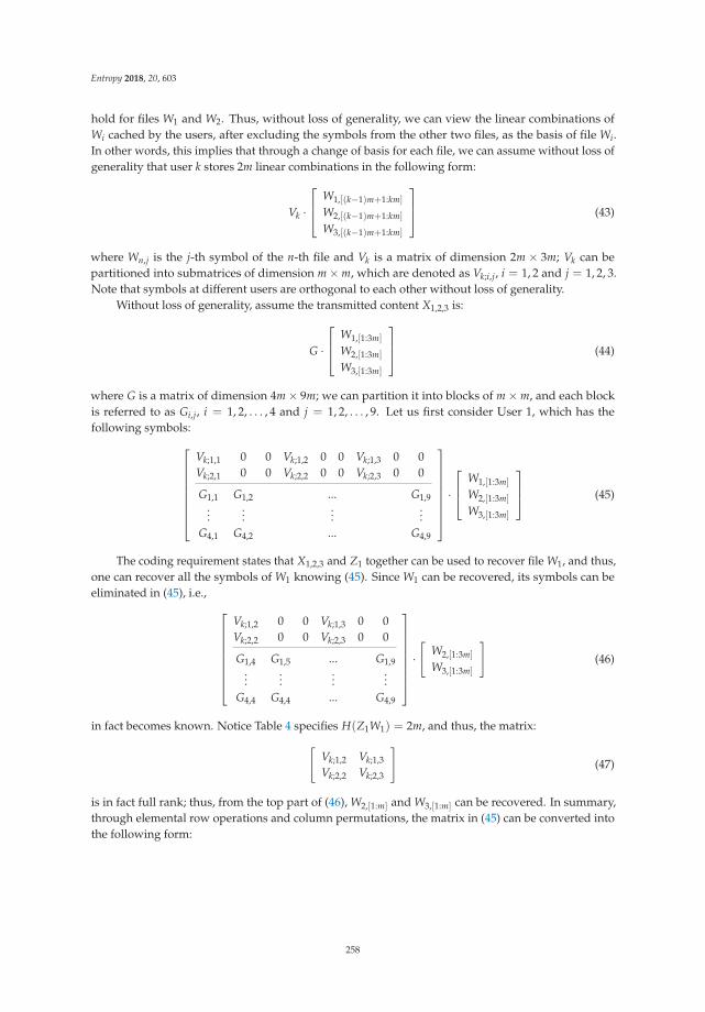
Entropy 2018, 20, 603

hold for files W1 and W2. Thus, without loss of generality, we can view the linear combinations ofWi cached by the users, after excluding the symbols from the other two files, as the basis of file Wi.In other words, this implies that through a change of basis for each file, we can assume without loss ofgenerality that user k stores 2m linear combinations in the following form:

Vk ·

⎡⎢⎣ W1,[(k−1)m+1:km]

W2,[(k−1)m+1:km]

W3,[(k−1)m+1:km]

⎤⎥⎦ (43)

where Wn,j is the j-th symbol of the n-th file and Vk is a matrix of dimension 2m × 3m; Vk can bepartitioned into submatrices of dimension m×m, which are denoted as Vk;i,j, i = 1, 2 and j = 1, 2, 3.Note that symbols at different users are orthogonal to each other without loss of generality.

Without loss of generality, assume the transmitted content X1,2,3 is:

G ·

⎡⎢⎣ W1,[1:3m]

W2,[1:3m]

W3,[1:3m]

⎤⎥⎦ (44)

where G is a matrix of dimension 4m× 9m; we can partition it into blocks of m×m, and each blockis referred to as Gi,j, i = 1, 2, . . . , 4 and j = 1, 2, . . . , 9. Let us first consider User 1, which has thefollowing symbols:⎡⎢⎢⎢⎢⎢⎢⎢⎣

Vk;1,1 0 0 Vk;1,2 0 0 Vk;1,3 0 0Vk;2,1 0 0 Vk;2,2 0 0 Vk;2,3 0 0

G1,1 G1,2 ... G1,9...

......

...G4,1 G4,2 ... G4,9

⎤⎥⎥⎥⎥⎥⎥⎥⎦·

⎡⎢⎣ W1,[1:3m]

W2,[1:3m]

W3,[1:3m]

⎤⎥⎦ (45)

The coding requirement states that X1,2,3 and Z1 together can be used to recover file W1, and thus,one can recover all the symbols of W1 knowing (45). Since W1 can be recovered, its symbols can beeliminated in (45), i.e., ⎡⎢⎢⎢⎢⎢⎢⎢⎣

Vk;1,2 0 0 Vk;1,3 0 0Vk;2,2 0 0 Vk;2,3 0 0

G1,4 G1,5 ... G1,9...

......

...G4,4 G4,4 ... G4,9

⎤⎥⎥⎥⎥⎥⎥⎥⎦·[

W2,[1:3m]

W3,[1:3m]

](46)

in fact becomes known. Notice Table 4 specifies H(Z1W1) = 2m, and thus, the matrix:[Vk;1,2 Vk;1,3Vk;2,2 Vk;2,3

](47)

is in fact full rank; thus, from the top part of (46), W2,[1:m] and W3,[1:m] can be recovered. In summary,through elemental row operations and column permutations, the matrix in (45) can be converted intothe following form:

258

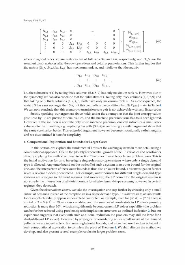
Entropy 2018, 20, 603

⎡⎢⎢⎢⎢⎢⎢⎢⎣

U1,1 U1,2 U1,3 0 ... 0U2,1 U2,2 U2,3 0 ... 0U3,1 U3,2 U3,3 0 ... 0

0 0 0 U4,4 U5,7 0 0 0 00 0 0 U4,4 U5,7 0 0 0 00 0 0 0 0 U6,5 U6,6 U6,8 U6,9

⎤⎥⎥⎥⎥⎥⎥⎥⎦·

⎡⎢⎢⎢⎢⎢⎣W1,[1:3m]

W2,[1:m]

W3,[1:m]

W2,[m+1:3m]

W3,[m+1:3m]

⎤⎥⎥⎥⎥⎥⎦ , (48)

where diagonal block square matrices are of full rank 3m and 2m, respectively, and Ui,j’s are theresultant block matrices after the row operations and column permutations. This further implies thatthe matrix [U6,5, U6,6, U6,8, U6,9] has maximum rank m, and it follows that the matrix:⎡⎢⎣ G1,5 G1,6 G1,8 G1,9

......

......

G4,5 G4,6 G4,8 G4,9

⎤⎥⎦ , (49)

i.e., the submatrix of G by taking thick columns (5, 6, 8, 9) has only maximum rank m. However, due tothe symmetry, we can also conclude that the submatrix of G taking only thick columns (1, 3, 7, 9) andthat taking only thick columns (1, 2, 4, 5) both have only maximum rank m. As a consequence, thematrix G has rank no larger than 3m, but this contradicts the condition that H(X1,2,3) = 4m in Table 4.We can now conclude that this memory-transmission-rate pair is not achievable with any linear codes

Strictly speaking, our argument above holds under the assumption that the joint entropy valuesproduced by LP are precise rational values, and the machine precision issue has thus been ignored.However, if the solution is accurate only up to machine precision, one can introduce a small slackvalue δ into the quantities, e.g., replacing 3m with (3± δ)m, and using a similar argument show thatthe same conclusion holds. This extended argument however becomes notationally rather lengthy,and we thus omitted it here for simplicity.

6. Computational Exploration and Bounds for Larger Cases

In this section, we explore the fundamental limits of the caching systems in more detail using acomputational approach. Due to the (doubly) exponential growth of the LP variables and constraints,directly applying the method outlined in Section 2 becomes infeasible for larger problem cases. This isthe initial motivation for us to investigate single-demand-type systems where only a single demandtype is allowed. Any outer bound on the tradeoff of such a system is an outer bound for the originalone, and the intersection of these outer bounds is thus also an outer bound. This investigation furtherreveals several hidden phenomena. For example, outer bounds for different single-demand-typesystems are stronger in different regimes, and moreover, the LP bound for the original system isnot simply the intersection of all outer bounds for single-demand-type systems; however, in certainregimes, they do match.

Given the observations above, we take the investigation one step further by choosing only a smallsubset of demands instead of the complete set in a single demand type. This allows us to obtain resultsfor cases which initially appear impossible to compute. For example, even for (N, K) = (2, 5), there isa total of 2 + 5 + 25 = 39 random variables, and the number of constraints in LP after symmetryreduction is more than 1011, which is significantly beyond current LP solver capability (the problemcan be further reduced using problem specific implication structures as outlined in Section 2, but ourexperience suggests that even with such additional reduction the problem may still too large for astart-of-the-art LP solver). However, by strategically considering only a small subset of the demandpatterns, we are indeed able to find meaningful outer bounds, and moreover, use the clues obtained insuch computational exploration to complete the proof of Theorem 4. We shall discuss the method wedevelop, and also present several example results for larger problem cases.

259

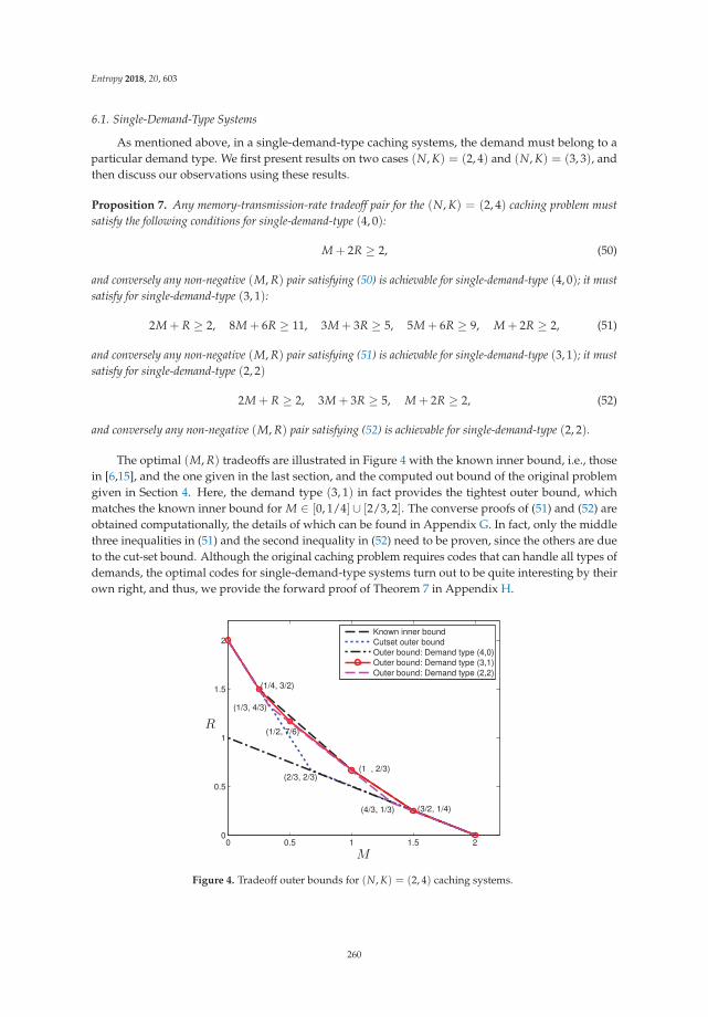
Entropy 2018, 20, 603

6.1. Single-Demand-Type Systems

As mentioned above, in a single-demand-type caching systems, the demand must belong to aparticular demand type. We first present results on two cases (N, K) = (2, 4) and (N, K) = (3, 3), andthen discuss our observations using these results.

Proposition 7. Any memory-transmission-rate tradeoff pair for the (N, K) = (2, 4) caching problem mustsatisfy the following conditions for single-demand-type (4, 0):

M + 2R ≥ 2, (50)

and conversely any non-negative (M, R) pair satisfying (50) is achievable for single-demand-type (4, 0); it mustsatisfy for single-demand-type (3, 1):

2M + R ≥ 2, 8M + 6R ≥ 11, 3M + 3R ≥ 5, 5M + 6R ≥ 9, M + 2R ≥ 2, (51)

and conversely any non-negative (M, R) pair satisfying (51) is achievable for single-demand-type (3, 1); it mustsatisfy for single-demand-type (2, 2)

2M + R ≥ 2, 3M + 3R ≥ 5, M + 2R ≥ 2, (52)

and conversely any non-negative (M, R) pair satisfying (52) is achievable for single-demand-type (2, 2).

The optimal (M, R) tradeoffs are illustrated in Figure 4 with the known inner bound, i.e., thosein [6,15], and the one given in the last section, and the computed out bound of the original problemgiven in Section 4. Here, the demand type (3, 1) in fact provides the tightest outer bound, whichmatches the known inner bound for M ∈ [0, 1/4] ∪ [2/3, 2]. The converse proofs of (51) and (52) areobtained computationally, the details of which can be found in Appendix G. In fact, only the middlethree inequalities in (51) and the second inequality in (52) need to be proven, since the others are dueto the cut-set bound. Although the original caching problem requires codes that can handle all types ofdemands, the optimal codes for single-demand-type systems turn out to be quite interesting by theirown right, and thus, we provide the forward proof of Theorem 7 in Appendix H.

0 0.5 1 1.5 20

0.5

1

1.5

2

(2/3, 2/3)

(1/4, 3/2)

(1/2, 7/6)

(1 , 2/3)

(3/2, 1/4)

(1/3, 4/3)

(4/3, 1/3)

M

R

Known inner boundCutset outer boundOuter bound: Demand type (4,0)Outer bound: Demand type (3,1)Outer bound: Demand type (2,2)

Figure 4. Tradeoff outer bounds for (N, K) = (2, 4) caching systems.

260

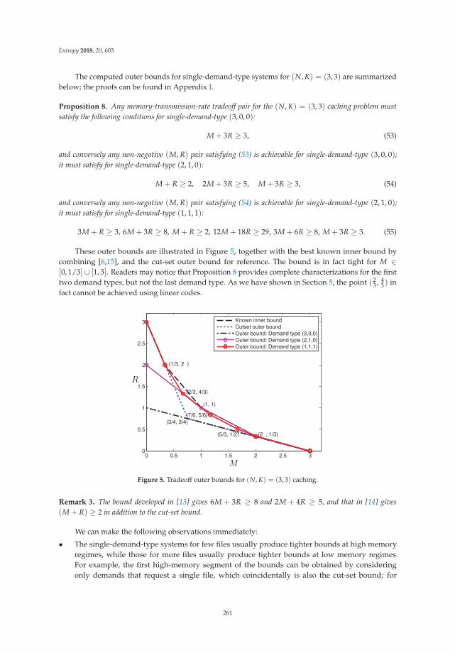
Entropy 2018, 20, 603

The computed outer bounds for single-demand-type systems for (N, K) = (3, 3) are summarizedbelow; the proofs can be found in Appendix I.

Proposition 8. Any memory-transmission-rate tradeoff pair for the (N, K) = (3, 3) caching problem mustsatisfy the following conditions for single-demand-type (3, 0, 0):

M + 3R ≥ 3, (53)

and conversely any non-negative (M, R) pair satisfying (53) is achievable for single-demand-type (3, 0, 0);it must satisfy for single-demand-type (2, 1, 0):

M + R ≥ 2, 2M + 3R ≥ 5, M + 3R ≥ 3, (54)

and conversely any non-negative (M, R) pair satisfying (54) is achievable for single-demand-type (2, 1, 0);it must satisfy for single-demand-type (1, 1, 1):

3M + R ≥ 3, 6M + 3R ≥ 8, M + R ≥ 2, 12M + 18R ≥ 29, 3M + 6R ≥ 8, M + 3R ≥ 3. (55)

These outer bounds are illustrated in Figure 5, together with the best known inner bound bycombining [6,15], and the cut-set outer bound for reference. The bound is in fact tight for M ∈[0, 1/3] ∪ [1, 3]. Readers may notice that Proposition 8 provides complete characterizations for the firsttwo demand types, but not the last demand type. As we have shown in Section 5, the point ( 2

3 , 43 ) in

fact cannot be achieved using linear codes.

0 0.5 1 1.5 2 2.5 30

0.5

1

1.5

2

2.5

3

(1, 1)

(3/4, 3/4)

(1/3, 2 )

(2/3, 4/3)

(7/6, 5/6)

(5/3, 1/2) (2 , 1/3)

M

R

Known inner boundCutset outer boundOuter bound: Demand type (3,0,0)Outer bound: Demand type (2,1,0)Outer bound: Demand type (1,1,1)

Figure 5. Tradeoff outer bounds for (N, K) = (3, 3) caching.

Remark 3. The bound developed in [13] gives 6M + 3R ≥ 8 and 2M + 4R ≥ 5, and that in [14] gives(M + R) ≥ 2 in addition to the cut-set bound.

We can make the following observations immediately:

• The single-demand-type systems for few files usually produce tighter bounds at high memoryregimes, while those for more files usually produce tighter bounds at low memory regimes.For example, the first high-memory segment of the bounds can be obtained by consideringonly demands that request a single file, which coincidentally is also the cut-set bound; for

261

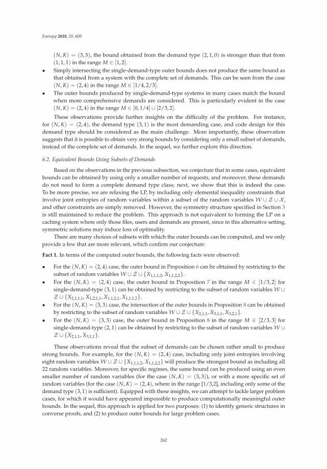
Entropy 2018, 20, 603

(N, K) = (3, 3), the bound obtained from the demand type (2, 1, 0) is stronger than that from(1, 1, 1) in the range M ∈ [1, 2].

• Simply intersecting the single-demand-type outer bounds does not produce the same bound asthat obtained from a system with the complete set of demands. This can be seen from the case(N, K) = (2, 4) in the range M ∈ [1/4, 2/3].

• The outer bounds produced by single-demand-type systems in many cases match the boundwhen more comprehensive demands are considered. This is particularly evident in the case(N, K) = (2, 4) in the range M ∈ [0, 1/4] ∪ [2/3, 2].

These observations provide further insights on the difficulty of the problem. For instance,for (N, K) = (2, 4), the demand type (3, 1) is the most demanding case, and code design for thisdemand type should be considered as the main challenge. More importantly, these observationsuggests that it is possible to obtain very strong bounds by considering only a small subset of demands,instead of the complete set of demands. In the sequel, we further explore this direction.

6.2. Equivalent Bounds Using Subsets of Demands

Based on the observations in the previous subsection, we conjecture that in some cases, equivalentbounds can be obtained by using only a smaller number of requests, and moreover, these demandsdo not need to form a complete demand type class; next, we show that this is indeed the case.To be more precise, we are relaxing the LP, by including only elemental inequality constraints thatinvolve joint entropies of random variables within a subset of the random variables W ∪ Z ∪ X ,and other constraints are simply removed. However, the symmetry structure specified in Section 3is still maintained to reduce the problem. This approach is not equivalent to forming the LP on acaching system where only those files, users and demands are present, since in this alternative setting,symmetric solutions may induce loss of optimality.

There are many choices of subsets with which the outer bounds can be computed, and we onlyprovide a few that are more relevant, which confirm our conjecture:

Fact 1. In terms of the computed outer bounds, the following facts were observed:

• For the (N, K) = (2, 4) case, the outer bound in Proposition 6 can be obtained by restricting to thesubset of random variablesW ∪Z ∪ {X1,1,1,2, X1,1,2,2}.

• For the (N, K) = (2, 4) case, the outer bound in Proposition 7 in the range M ∈ [1/3, 2] forsingle-demand-type (3, 1) can be obtained by restricting to the subset of random variablesW ∪Z ∪ {X2,1,1,1, X1,2,1,1, X1,1,2,1, X1,1,1,2}.

• For the (N, K) = (3, 3) case, the intersection of the outer bounds in Proposition 8 can be obtainedby restricting to the subset of random variablesW ∪Z ∪ {X2,1,1, X3,1,1, X3,2,1}.

• For the (N, K) = (3, 3) case, the outer bound in Proposition 8 in the range M ∈ [2/3, 3] forsingle-demand-type (2, 1) can be obtained by restricting to the subset of random variablesW ∪Z ∪ {X2,1,1, X3,1,1}.

These observations reveal that the subset of demands can be chosen rather small to producestrong bounds. For example, for the (N, K) = (2, 4) case, including only joint entropies involvingeight random variablesW ∪Z ∪ {X1,1,1,2, X1,1,2,2} will produce the strongest bound as including all22 random variables. Moreover, for specific regimes, the same bound can be produced using an evensmaller number of random variables (for the case (N, K) = (3, 3)), or with a more specific set ofrandom variables (for the case (N, K) = (2, 4), where in the range [1/3,2], including only some of thedemand type (3, 1) is sufficient). Equipped with these insights, we can attempt to tackle larger problemcases, for which it would have appeared impossible to produce computationally meaningful outerbounds. In the sequel, this approach is applied for two purposes: (1) to identify generic structures inconverse proofs, and (2) to produce outer bounds for large problem cases.

262

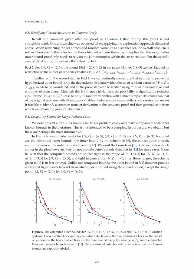
Entropy 2018, 20, 603

6.3. Identifying Generic Structures in Converse Proofs

Recall our comment given after the proof of Theorem 4 that finding this proof is notstraightforward. One critical clue was obtained when applying the exploration approach discussedabove. When restricting the set of included random variables to a smaller set, the overall problem isrelaxed; however, if the outer bound thus obtained remains the same, it implies that the sought-afterouter bound proof only needs to rely on the joint entropies within this restricted set. For the specificcase of (N, K) = (2, 5), we have the following fact.

Fact 2. For (N, K) = (2, 5), the bound 15M + 20R ≥ 28 in the range M ∈ [6/5, 8/5] can be obtained byrestricting to the subset of random variablesW ∪Z ∪ {X2,1,1,1,1, X1,2,1,1,1, X1,1,2,1,1, X1,1,1,2,1, X1,1,1,1,2}.

Together with the second item in Fact 1, we can naturally conjecture that in order to prove thehypothesized outer bound, only the dependence structure within the set of random variablesW ∪Z ∪X→[1:K] needs to be considered, and all the proof steps can be written using mutual information or jointentropies of them alone. Although this is still not a trivial task, the possibility is significantly reduced,e.g., for the (N, K) = (2, 5) case to only 12 random variables, with a much simpler structure than thatof the original problem with 39 random variables. Perhaps more importantly, such a restriction makesit feasible to identify a common route of derivation in the converse proof and then generalize it, fromwhich we obtain the proof of Theorem 4.

6.4. Computing Bounds for Larger Problem Cases

We now present a few outer bounds for larger problem cases, and make comparison with otherknown bounds in the literature. This is not intended to be a complete list of results we obtain, butthese are perhaps the most informative.

In Figure 6, we provide results for (N, K) = (4, 3), (N, K) = (5, 3) and (N, K) = (6, 3). Includedare the computed outer bounds, the inner bound by the scheme in [6], the cut-set outer bounds,and for reference, the outer bounds given in [12]. We omit the bounds in [13,14] to avoid too muchclutter in the plot; however, they do not provide better bounds than that in [12] for these cases. It canbe seen that the computed bounds are in fact tight in the range M ∈ [4/3, 4] for (N, K) = (4, 3),M ∈ [5/3, 5] for (N, K) = (5, 3), and tight in general for (N, K) = (6, 3); in these ranges, the schemegiven in [6] is in fact optimal. Unlike our computed bounds, the outer bound in [12] does not provideadditional tight results beyond those already determined using the cut-set bound, except the singlepoint (M, R) = (2, 1) for (N, K) = (6, 3).

0 1 2 3 40

0.5

1

1.5

2

2.5

3

(4/3, 1 )

(8/3, 1/3)

M

R

Case (N,K)=(4,3)

0 1 2 3 4 50

0.5

1

1.5

2

2.5

3

(5/3 , 1 )

(10/3, 1/3)

M

R

Case (N,K)=(5,3)

0 1 2 3 4 5 60

0.5

1

1.5

2

2.5

3

(2, 1 )

(4, 1/3)

M

R

Case (N,K)=(6,3)

Figure 6. The computed outer bounds for (N, K) = (4, 3), (N, K) = (5, 3) and (N, K) = (6, 3) cachingsystems. The red dotted lines give the computed outer bounds; the blue dashed-dot lines are the cut-setouter bounds; the black dashed lines are the inner bound using the scheme in [6]; and the thin bluelines are the outer bounds given in [12]. Only nontrivial outer bound corner points that match innerbounds are explicitly labeled.

263

Entropy 2018, 20, 603

In Figure 7, we provide results for (N, K) = (3, 4), (N, K) = (3, 5) and (N, K) = (3, 6). Includedare the computed outer bounds, the inner bound by the code in [6] and that in [20], the cut-set outerbound, and for reference, the outer bounds in [12]. The bounds in [13,14] are again omitted. It can beseen that the computed bounds are in fact tight in the range M ∈ [0, 1/4] ∪ [3/2, 3] for (N, K) = (3, 4),M ∈ [0, 1/5] ∪ [6/5, 3] for (N, K) = (3, 5), and M ∈ [0, 1/6] ∪ [3/2, 3] for (N, K) = (3, 6). Generally,in the high memory regime, the scheme given in [6] is in fact optimal, and in the low memory regime,the schemes in [15,20] are optimal. It can be see that the outer bound in [12] does not provide additionaltight results beyond those already determined using the cut-set bound. The bounds given above infact provide grounds and directions for further investigation and hypotheses on the optimal tradeoff,which we are currently exploring.

0 0.5 1 1.5 2 2.5 30

0.5

1

1.5

2

2.5

3

(9/4, 1/4)

(3/2, 2/3)

(1/4, 9/4)

M

R

Case (N,K)=(3,4)

0 0.5 1 1.5 2 2.5 30

0.5

1

1.5

2

2.5

3

(1/5 , 12/5)

(6/5 , 1 )

(9/5 , 1/2 )

(12/5, 1/5 )

M

R

Case (N,K)=(3,5)

0 0.5 1 1.5 2 2.5 30

0.5

1

1.5

2

2.5

3

(1/6, 5/2)

(3/2, 3/4)

(2 , 2/5)

(5/2, 1/6)

M

R

Case (N,K)=(3,6)

Figure 7. The computed outer bounds for (N, K) = (3, 4), (N, K) = (3, 5) and (N, K) = (3, 6) cachingsystems. The red dotted lines give the computed outer bounds; the blue dashed-dot lines are the cut-setouter bounds; the black dashed lines are the inner bound using the scheme in [6,20]; and the thin bluelines are the outer bounds given in [12]. Only nontrivial outer bound corner points that match innerbounds are explicitly labeled.

7. Conclusions

We presented a computer-aided investigation on the fundamental limit of the caching problem,including data-driven hypothesis forming, which leads to several complete or partial characterizationsof the memory-transmission-rate tradeoff, a new code construction reverse-engineered through thecomputed outer bounding data and a computerized exploration approach that can reveal hiddenstructures in the problem and also enables us to find surprisingly strong outer bounds for largerproblem cases.

It is our belief that this work provides strong evidence of the effectiveness of the computer-aidedapproach in the investigation of the fundamental limits of communication, data storage and datamanagement systems. Although at first sight, the exponential growth of the LP problem would preventany possibility of obtaining meaningful results on engineering problems of interest, our experiencein [2,3] and the current work suggest otherwise. By incorporating the structure of the problem, wedevelop more domain-specific tools in such investigations and were able to obtain results that appeardifficult for human experts to obtain directly.

Our effort can be viewed as both data-driven and computational, and thus, more advanceddata analysis and machine learning technique may prove useful. Particularly, the computer-aidedexploration approach is clearly a human-in-the-loop process, which can benefit from more automationbased on reinforcement learning techniques. Moreover, the computed generated proofs may involvea large number of inequalities and joint entropies, and more efficient classification or clustering ofthese inequalities and joint entropies can reduce the human burden in the subsequent analysis. It isour hope that this work can serve as a starting point to introduce more machine intelligence and

264

Entropy 2018, 20, 603

the corresponding computer-aided tools into information theory and communication research inthe future.

Funding: This research was funded in part by the National Science Foundation under Grants CCF-15-26095 andCCF-18-32309.

Acknowledgments: The author wishes to thank Urs Niesen and Vaneet Aggarwal for early discussions, whichpartly motivated this work. He also wishes to thank Jun Chen for several discussions, as well as the insightfulcomments on an early draft. Additionally, the author wishes to thank the authors of [12] for making the sourcecode to compute their proposed outer bounds available online, which was conveniently used to generate some ofthe comparisons.

Conflicts of Interest: The author declares no conflict of interest.

Appendix A. Finding Corner Points of the LP Outer Bounds

Since this is an LP problem, and also due to the problem setting, only the lower hull of the outerbound region between the two quantities M and R is of interest. The general algorithm in [27] isequivalent to the procedure given in Algorithm 1 in this specific setting. In this algorithm, the set Pin the input is the initial extreme points of the tradeoff region, which are trivially known from theproblem setting. The variables and constraints in the LP are given as outlined in Section 2 for a fixed(N, K) pair, which are populated and considered fixed. The output set P is the final computed extremepoints of the outer bound. The algorithm can be intuitively explained as follows: starting with twoknown extreme points, if there are any other corner points, they must lie below the line segmentconnecting these two points, and thus, an LP that minimizes the bounding plane along the direction ofthis line segment must be able to find a lower value; if so, the new point is also an extreme point, andwe can repeat this procedure again.

In the caching problem, the tradeoff is between two quantities M and R. We note here if there aremore than two quantities that need to be considered in the tradeoff, the algorithm is more involved,and we refer the readers to [27,28] for more details on such settings.

Algorithm 1: An algorithm to identify the corner points of the LP outer bound.

Input : N, K, P = {(N, 0), (0, min(N, K))}Output :P

1 n = 2; i = 1;2 while i < n do3 Compute the line segment connecting i-th and (i + 1)-th (M, R) pairs in P , as M + αR = β;4 Set the objective of the LP as M + αR, and solve LP for solution (M∗, R∗) and objective β∗;5 if β∗ < β then6 Insert (M∗, R∗) in P between the i-th and (i + 1)-th (M, R) pairs;7 n = n + 1;8 else9 i = i + 1;

10 end

11 end

Appendix B. Proofs of Proposition 3 and Proposition 4

The proof of Proposition 3 is given in the Tables A1 and A2, and that of Proposition 4 is givenin the Tables A3 and A4. Each row in Tables A2 and A4, except the last rows, are simple and knowninformation inequalities, up to the symmetry defined in Section 3. The last rows in Tables A2 andA4 are the sum of all previous rows, which are the sought-after inequalities, and they are simplythe consequences of the known inequalities summed together. When represented in this form,the correctness of the proof is immediate, since the columns representing quantities not presentin the final bound cancel out each other when being summed together. The rows in Table A2 are

265

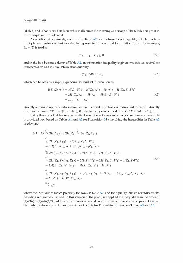
Entropy 2018, 20, 603

labeled, and it has more details in order to illustrate the meaning and usage of the tabulation proof inthe example we provide next.

As mentioned previously, each row in Table A2 is an information inequality, which involvesmultiple joint entropies, but can also be represented in a mutual information form. For example,Row (2) is read as:

2T8 − T4 − T10 ≥ 0, (A1)

and in the last, but one column of Table A2, an information inequality is given, which is an equivalentrepresentation as a mutual information quantity:

I(Z1; Z2W1) ≥ 0, (A2)

which can be seen by simply expanding the mutual information as:

I(Z1; Z2W1) = H(Z1, W1) + H(Z2, W1)− H(W1)− H(Z1, Z2, W1)

= 2H(Z1, W1)− H(W1)− H(Z1, Z2, W1)

= 2T8 − T4 − T10.

(A3)

Directly summing up these information inequalities and canceling out redundant terms will directlyresult in the bound 2R + 2H(Z1)− 4F ≥ 0, which clearly can be used to write 2R + 2M− 4F ≥ 0.

Using these proof tables, one can write down different versions of proofs, and one such exampleis provided next based on Tables A1 and A2 for Proposition 3 by invoking the inequalities in Table A2one by one.

2M + 2R(1)≥ 2H(X1,2) + 2H(Z1)

(3)≥ 2H(Z1, X1,2)

(5)≥ 2H(Z1, X1,2)− 2I(X1,2; Z2Z1, W1)

= 2H(Z1, X1,2, W1)− 2I(X1,2; Z2Z1, W1)

(c)= 2H(Z1, Z2, W1, X1,2) + 2H(Z1, W1)− 2H(Z1, Z2, W1)

(2)≥ 2H(Z1, Z2, W1, X1,2) + 2H(Z1, W1)− 2H(Z1, Z2, W1)− I(Z1; Z2W1)

= 2H(Z1, Z2, W1, X1,2)− H(Z1, Z2, W1) + H(W1)

(4)≥ 2H(Z1, Z2, W1, X1,2)− H(Z1, Z2, W1) + H(W1)− I(X1,2; X1,3Z1, Z2, W1)

= H(W1) + H(W1, W2, W3)

(6,7)≥ 4F,

(A4)

where the inequalities match precisely the rows in Table A2, and the equality labeled (c) indicates thedecoding requirement is used. In this version of the proof, we applied the inequalities in the order of(1)-(3)-(5)-(2)-(4)-(6,7), but this is by no means critical, as any order will yield a valid proof. One cansimilarly produce many different versions of proofs for Proposition 4 based on Tables A3 and A4.

266

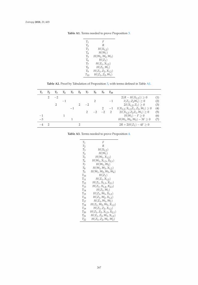
Entropy 2018, 20, 603

Table A1. Terms needed to prove Proposition 3.

T1 FT2 RT3 H(X1,2)T4 H(W1)T5 H(W1, W2, W3)T6 H(Z1)T7 H(Z1, X1,2)T8 H(Z1, W1)T9 H(Z1, Z2, X1,2)T10 H(Z1, Z2, W1)

Table A2. Proof by Tabulation of Proposition 3, with terms defined in Table A1.

T1 T2 T3 T4 T5 T6 T7 T8 T9 T10

2 −2 2(R− H(X1,2)) ≥ 0 (1)−1 2 −1 I(Z1; Z2W1) ≥ 0 (2)

2 2 −2 2I(X1,2; Z1) ≥ 0 (3)−1 2 −1 I(X1,2; X1,3Z1, Z2, W1) ≥ 0 (4)

2 −2 −2 2 2I(X1,2; Z2Z1, W1) ≥ 0 (5)−1 1 H(W1)− F ≥ 0 (6)−3 1 H(W1, W2, W3)− 3F ≥ 0 (7)

−4 2 2 2R + 2H(Z1)− 4F ≥ 0

Table A3. Terms needed to prove Proposition 4.

T1 FT2 RT3 H(X1,2)T4 H(W1)T5 H(W1, X1,2)T6 H(W1, X1,3, X2,1)T7 H(W1, W2)T8 H(W1, W3, X1,2)T9 H(W1, W2, W3, W4)T10 H(Z1)T11 H(Z1, X1,2)T12 H(Z1, X1,3, X2,1)T13 H(Z1, X1,4, X2,3)T14 H(Z1, W1)T15 H(Z1, W3, X1,2)T16 H(Z1, W2, X1,2)T17 H(Z1, W1, W2)T18 H(Z1, W2, W3, X1,2)T19 H(Z1, Z2, X1,2)T20 H(Z1, Z2, X1,3, X2,1)T21 H(Z1, Z2, W3, X1,2)T22 H(Z1, Z2, W1, W2)

267

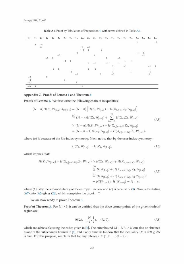
Entropy 2018, 20, 603

Table A4. Proof by Tabulation of Proposition 4, with terms defined in Table A3.

T1 T2 T3 T4 T5 T6 T7 T8 T9 T10 T11 T12 T13 T14 T15 T16 T17 T18 T19 T20 T21 T22

1 −18 −8

8 8 −8−2 4 −2

−1 −1 2−2 4 −2

−2 2 2 −2−1 1 1 −1

2 −2 −2 21 −1 −1 1

−2 2 2 −2−1 1 1 −1

−2 2 −2 2−2 2−2 1−12 3

−16 8 6

Appendix C. Proofs of Lemma 1 and Theorem 3

Proofs of Lemma 1. We first write the following chain of inequalities:

(N − n)H(Z1, W[1:n], Xn,n+1) = (N − n)[

H(Z1, W[1:n]) + H(Xn,n+1Z1, W[1:n])]

(a)= (N − n)H(Z1, W[1:n]) +

N

∑i=n+1

H(Xn,iZ1, W[1:n])

≥ (N − n)H(Z1, W[1:n]) + H(Xn,[n+1:N]Z1, W[1:n])

= (N − n− 1)H(Z1, W[1:n]) + H(Xn,[n+1:N], Z1, W[1:n]),

(A5)

where (a) is because of the file-index-symmetry. Next, notice that by the user-index-symmetry:

H(Z1, W[1:n]) = H(Z2, W[1:n]), (A6)

which implies that:

H(Z1, W[1:n]) + H(Xn,[n+1:N], Z1, W[1:n]) ≥ H(Z2, W[1:n]) + H(Xn,[n+1:N], W[1:n])

(b)≥ H(W[1:n]) + H(Xn,[n+1:N], Z2, W[1:n])

(c)= H(W[1:n]) + H(Xn,[n+1:N], Z2, W[1:N])

= H(W[1:n]) + H(W[1:N]) = N + n,

(A7)

where (b) is by the sub-modularity of the entropy function, and (c) is because of (3). Now, substituting(A7) into (A5) gives (28), which completes the proof.

We are now ready to prove Theorem 3.

Proof of Theorem 3. For N ≥ 3, it can be verified that the three corner points of the given tradeoffregion are:

(0, 2), (N2

,12), (N, 0), (A8)

which are achievable using the codes given in [6]. The outer bound M + NR ≥ N can also be obtainedas one of the cut-set outer bounds in [6], and it only remains to show that the inequality 3M+ NR ≥ 2Nis true. For this purpose, we claim that for any integer n ∈ {1, 2, . . . , N − 2}:

268

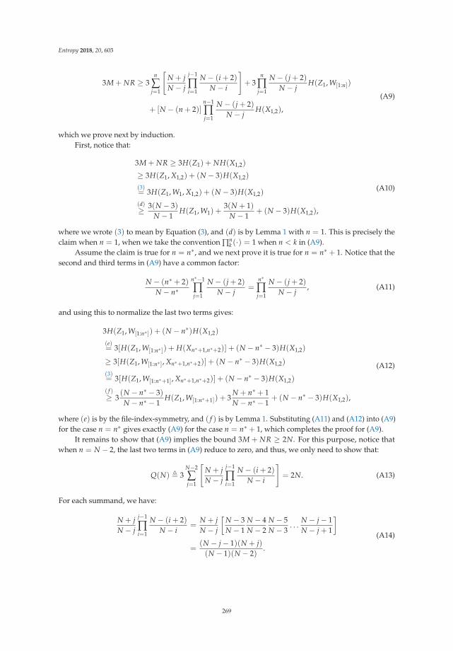
Entropy 2018, 20, 603

3M + NR ≥ 3n

∑j=1

[N + jN − j

j−1

∏i=1

N − (i + 2)N − i

]+ 3

n

∏j=1

N − (j + 2)N − j

H(Z1, W[1:n])

+ [N − (n + 2)]n−1

∏j=1

N − (j + 2)N − j

H(X1,2),

(A9)

which we prove next by induction.First, notice that:

3M + NR ≥ 3H(Z1) + NH(X1,2)

≥ 3H(Z1, X1,2) + (N − 3)H(X1,2)

(3)= 3H(Z1, W1, X1,2) + (N − 3)H(X1,2)

(d)≥ 3(N − 3)

N − 1H(Z1, W1) +

3(N + 1)N − 1

+ (N − 3)H(X1,2),

(A10)

where we wrote (3) to mean by Equation (3), and (d) is by Lemma 1 with n = 1. This is precisely theclaim when n = 1, when we take the convention ∏n

k (·) = 1 when n < k in (A9).Assume the claim is true for n = n∗, and we next prove it is true for n = n∗ + 1. Notice that the

second and third terms in (A9) have a common factor:

N − (n∗ + 2)N − n∗

n∗−1

∏j=1

N − (j + 2)N − j

=n∗

∏j=1

N − (j + 2)N − j

, (A11)

and using this to normalize the last two terms gives:

3H(Z1, W[1:n∗ ]) + (N − n∗)H(X1,2)

(e)= 3[H(Z1, W[1:n∗ ]) + H(Xn∗+1,n∗+2)] + (N − n∗ − 3)H(X1,2)

≥ 3[H(Z1, W[1:n∗ ], Xn∗+1,n∗+2)] + (N − n∗ − 3)H(X1,2)

(3)= 3[H(Z1, W[1:n∗+1], Xn∗+1,n∗+2)] + (N − n∗ − 3)H(X1,2)

( f )≥ 3

(N − n∗ − 3)N − n∗ − 1

H(Z1, W[1:n∗+1]) + 3N + n∗ + 1N − n∗ − 1

+ (N − n∗ − 3)H(X1,2),

(A12)

where (e) is by the file-index-symmetry, and ( f ) is by Lemma 1. Substituting (A11) and (A12) into (A9)for the case n = n∗ gives exactly (A9) for the case n = n∗ + 1, which completes the proof for (A9).

It remains to show that (A9) implies the bound 3M + NR ≥ 2N. For this purpose, notice thatwhen n = N − 2, the last two terms in (A9) reduce to zero, and thus, we only need to show that:

Q(N) � 3N−2

∑j=1

[N + jN − j

j−1

∏i=1

N − (i + 2)N − i

]= 2N. (A13)

For each summand, we have:

N + jN − j

j−1

∏i=1

N − (i + 2)N − i

=N + jN − j

[N − 3N − 1

N − 4N − 2

N − 5N − 3

. . .N − j− 1N − j + 1

]=

(N − j− 1)(N + j)(N − 1)(N − 2)

.

(A14)

269

Entropy 2018, 20, 603

Thus, we have:

Q(N) =3

(N − 1)(N − 2)

N−2

∑j=1

(N − j− 1)(N + j) = 2N,

where we have used the well-known formula for the sum of integer squares. The proof isthus complete.

Appendix D. Proof of Proposition 5

We first consider the achievability, for which only the achievability of the following extremalpoints needs to be shown because of the polytope structure of the region:

(M, R) ∈{(0, 2),

(13

,43

),(

43

,13

), (2, 0)

}. (A15)

Achieving the rate pairs (0, 2) and (2, 0) is trivial. The scheme in [6] can achieve the rate pair(43 , 1

3

). The rate pair

(13 , 4

3

)can be achieved by a scheme given in [15], which is a generalization of a

special scheme given in [6]. To prove the converse, we note first that the cut-set-based approach canprovide all bounds in (29) except

3M + 3R ≥ 5, (A16)

which is a new inequality. As mentioned earlier, this inequality is a special case of Theorem 4 and thereis no need to prove it separately.

Appendix E. Proof of Proposition 6

The inequality 14M+ 11R ≥ 20 is proven using Tables A5 and A6, and the inequality 9M+ 8R ≥ 14is proven using Tables A7 and A8.

Table A5. Terms needed to prove Proposition 6, inequality 14M + 11R ≥ 20.

T1 FT2 RT3 H(X1,1,1,2)T4 H(X1,1,2,2)T5 H(W1)T6 H(W1, X1,1,1,2)T7 H(W1, X1,1,2,2)T8 H(W1, W2)T9 H(Z1)T10 H(Z1, X1,1,1,2)T11 H(Z1, X1,1,2,2)T12 H(Z4, X1,1,1,2)T13 H(Z1, W1)T14 H(Z1, Z2, X1,1,1,2)T15 H(Z1, Z2, X1,1,2,2)T16 H(Z1, Z2, W1)T17 H(Z1, Z2, Z3, X1,1,1,2)T18 H(Z1, Z2, Z3, W1)

270

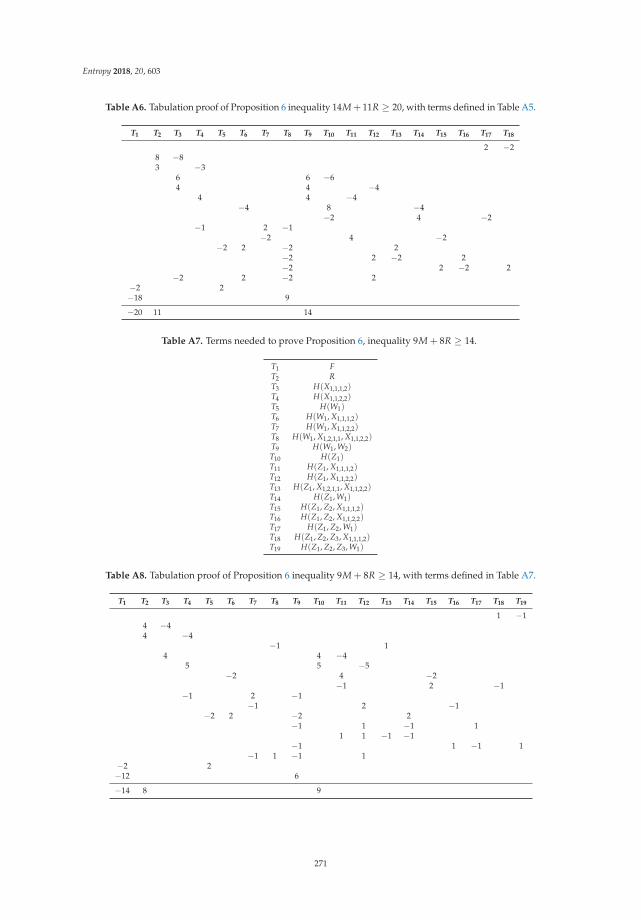
Entropy 2018, 20, 603

Table A6. Tabulation proof of Proposition 6 inequality 14M+ 11R ≥ 20, with terms defined in Table A5.

T1 T2 T3 T4 T5 T6 T7 T8 T9 T10 T11 T12 T13 T14 T15 T16 T17 T18

2 −28 −83 −3

6 6 −64 4 −4

4 4 −4−4 8 −4

−2 4 −2−1 2 −1

−2 4 −2−2 2 −2 2

−2 2 −2 2−2 2 −2 2

−2 2 −2 2−2 2−18 9

−20 11 14


T1 FT2 RT3 H(X1,1,1,2)T4 H(X1,1,2,2)T5 H(W1)T6 H(W1, X1,1,1,2)T7 H(W1, X1,1,2,2)T8 H(W1, X1,2,1,1, X1,1,2,2)T9 H(W1, W2)T10 H(Z1)T11 H(Z1, X1,1,1,2)T12 H(Z1, X1,1,2,2)T13 H(Z1, X1,2,1,1, X1,1,2,2)T14 H(Z1, W1)T15 H(Z1, Z2, X1,1,1,2)T16 H(Z1, Z2, X1,1,2,2)T17 H(Z1, Z2, W1)T18 H(Z1, Z2, Z3, X1,1,1,2)T19 H(Z1, Z2, Z3, W1)

Table A8. Tabulation proof of Proposition 6 inequality 9M + 8R ≥ 14, with terms defined in Table A7.

T1 T2 T3 T4 T5 T6 T7 T8 T9 T10 T11 T12 T13 T14 T15 T16 T17 T18 T19

1 −14 −44 −4

−1 14 4 −4

5 5 −5−2 4 −2

−1 2 −1−1 2 −1

−1 2 −1−2 2 −2 2

−1 1 −1 11 1 −1 −1

−1 1 −1 1−1 1 −1 1

−2 2−12 6

−14 8 9

271

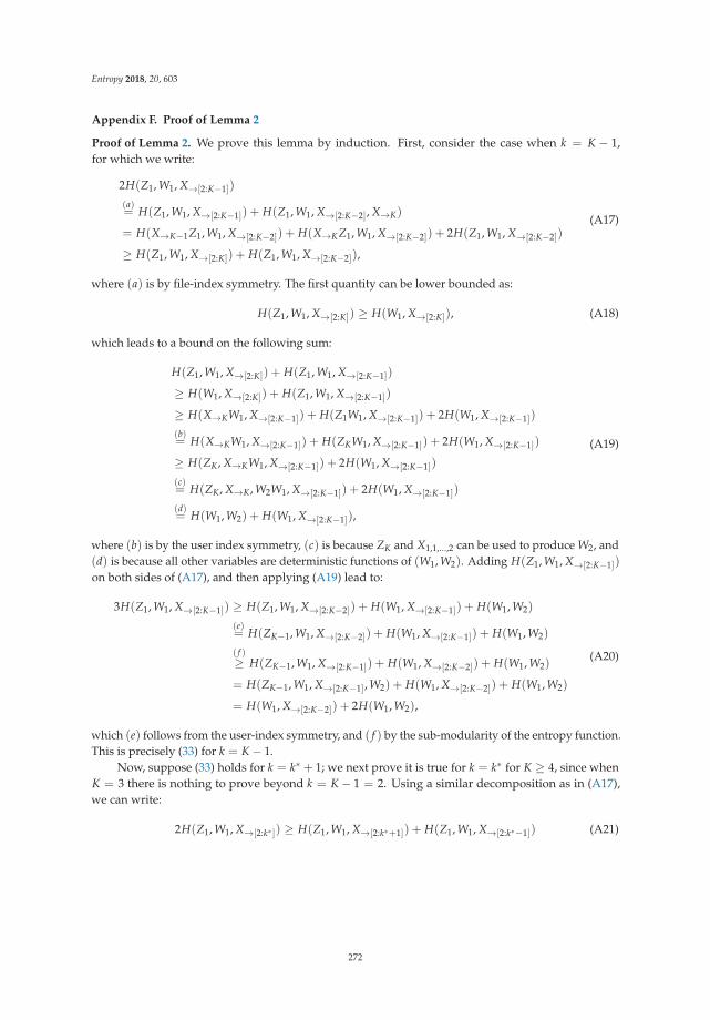
Entropy 2018, 20, 603

Appendix F. Proof of Lemma 2

Proof of Lemma 2. We prove this lemma by induction. First, consider the case when k = K − 1,for which we write:

2H(Z1, W1, X→[2:K−1])

(a)= H(Z1, W1, X→[2:K−1]) + H(Z1, W1, X→[2:K−2], X→K)

= H(X→K−1Z1, W1, X→[2:K−2]) + H(X→KZ1, W1, X→[2:K−2]) + 2H(Z1, W1, X→[2:K−2])

≥ H(Z1, W1, X→[2:K]) + H(Z1, W1, X→[2:K−2]),

(A17)

where (a) is by file-index symmetry. The first quantity can be lower bounded as:

H(Z1, W1, X→[2:K]) ≥ H(W1, X→[2:K]), (A18)

which leads to a bound on the following sum:

H(Z1, W1, X→[2:K]) + H(Z1, W1, X→[2:K−1])

≥ H(W1, X→[2:K]) + H(Z1, W1, X→[2:K−1])

≥ H(X→KW1, X→[2:K−1]) + H(Z1W1, X→[2:K−1]) + 2H(W1, X→[2:K−1])

(b)= H(X→KW1, X→[2:K−1]) + H(ZKW1, X→[2:K−1]) + 2H(W1, X→[2:K−1])

≥ H(ZK, X→KW1, X→[2:K−1]) + 2H(W1, X→[2:K−1])

(c)= H(ZK, X→K, W2W1, X→[2:K−1]) + 2H(W1, X→[2:K−1])

(d)= H(W1, W2) + H(W1, X→[2:K−1]),

(A19)

where (b) is by the user index symmetry, (c) is because ZK and X1,1,...,2 can be used to produce W2, and(d) is because all other variables are deterministic functions of (W1, W2). Adding H(Z1, W1, X→[2:K−1])

on both sides of (A17), and then applying (A19) lead to:

3H(Z1, W1, X→[2:K−1]) ≥ H(Z1, W1, X→[2:K−2]) + H(W1, X→[2:K−1]) + H(W1, W2)

(e)= H(ZK−1, W1, X→[2:K−2]) + H(W1, X→[2:K−1]) + H(W1, W2)

( f )≥ H(ZK−1, W1, X→[2:K−1]) + H(W1, X→[2:K−2]) + H(W1, W2)

= H(ZK−1, W1, X→[2:K−1], W2) + H(W1, X→[2:K−2]) + H(W1, W2)

= H(W1, X→[2:K−2]) + 2H(W1, W2),

(A20)

which (e) follows from the user-index symmetry, and ( f ) by the sub-modularity of the entropy function.This is precisely (33) for k = K− 1.

Now, suppose (33) holds for k = k∗ + 1; we next prove it is true for k = k∗ for K ≥ 4, since whenK = 3 there is nothing to prove beyond k = K − 1 = 2. Using a similar decomposition as in (A17),we can write:

2H(Z1, W1, X→[2:k∗ ]) ≥ H(Z1, W1, X→[2:k∗+1]) + H(Z1, W1, X→[2:k∗−1]) (A21)

272

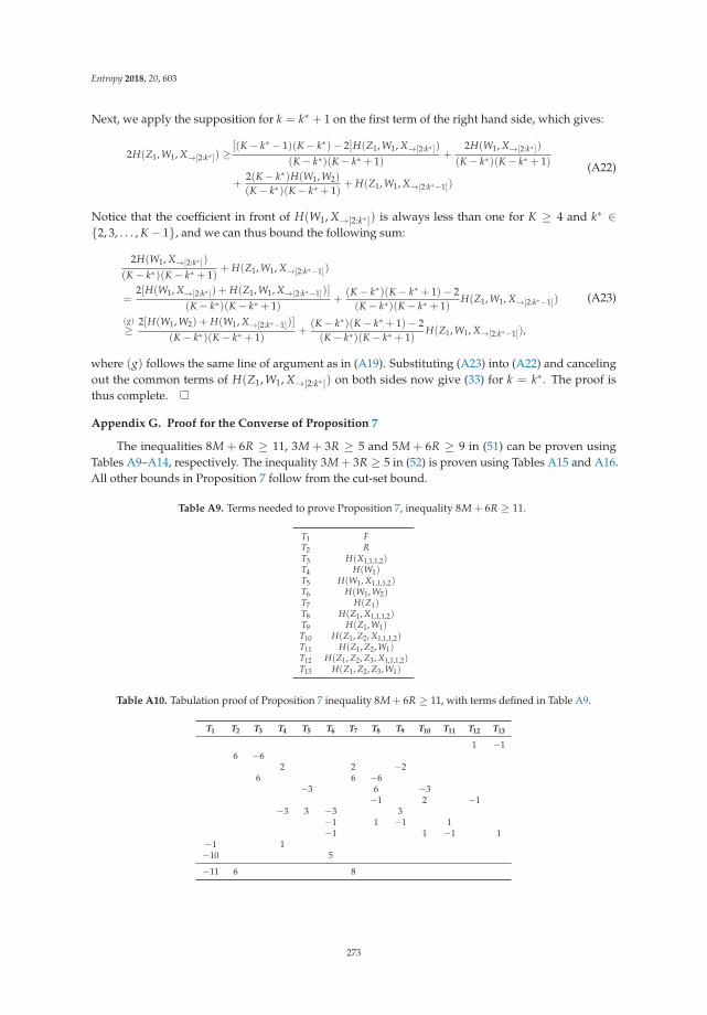
Entropy 2018, 20, 603

Next, we apply the supposition for k = k∗ + 1 on the first term of the right hand side, which gives:

2H(Z1, W1, X→[2:k∗ ]) ≥[(K− k∗ − 1)(K− k∗)− 2]H(Z1, W1, X→[2:k∗ ])

(K− k∗)(K− k∗ + 1)+

2H(W1, X→[2:k∗ ])

(K− k∗)(K− k∗ + 1)

+2(K− k∗)H(W1, W2)

(K− k∗)(K− k∗ + 1)+ H(Z1, W1, X→[2:k∗−1])

(A22)

Notice that the coefficient in front of H(W1, X→[2:k∗ ]) is always less than one for K ≥ 4 and k∗ ∈{2, 3, . . . , K− 1}, and we can thus bound the following sum:

2H(W1, X→[2:k∗ ])

(K− k∗)(K− k∗ + 1)+ H(Z1, W1, X→[2:k∗−1])

=2[H(W1, X→[2:k∗ ]) + H(Z1, W1, X→[2:k∗−1])]

(K− k∗)(K− k∗ + 1)+

(K− k∗)(K− k∗ + 1)− 2(K− k∗)(K− k∗ + 1)

H(Z1, W1, X→[2:k∗−1])

(g)≥

2[H(W1, W2) + H(W1, X→[2:k∗−1])]

(K− k∗)(K− k∗ + 1)+

(K− k∗)(K− k∗ + 1)− 2(K− k∗)(K− k∗ + 1)

H(Z1, W1, X→[2:k∗−1]),

(A23)

where (g) follows the same line of argument as in (A19). Substituting (A23) into (A22) and cancelingout the common terms of H(Z1, W1, X→[2:k∗ ]) on both sides now give (33) for k = k∗. The proof isthus complete.

Appendix G. Proof for the Converse of Proposition 7

The inequalities 8M + 6R ≥ 11, 3M + 3R ≥ 5 and 5M + 6R ≥ 9 in (51) can be proven usingTables A9–A14, respectively. The inequality 3M + 3R ≥ 5 in (52) is proven using Tables A15 and A16.All other bounds in Proposition 7 follow from the cut-set bound.


T1 FT2 RT3 H(X1,1,1,2)T4 H(W1)T5 H(W1, X1,1,1,2)T6 H(W1, W2)T7 H(Z1)T8 H(Z1, X1,1,1,2)T9 H(Z1, W1)T10 H(Z1, Z2, X1,1,1,2)T11 H(Z1, Z2, W1)T12 H(Z1, Z2, Z3, X1,1,1,2)T13 H(Z1, Z2, Z3, W1)


T1 T2 T3 T4 T5 T6 T7 T8 T9 T10 T11 T12 T13

1 −16 −6

2 2 −26 6 −6

−3 6 −3−1 2 −1

−3 3 −3 3−1 1 −1 1−1 1 −1 1

−1 1−10 5

−11 6 8

273

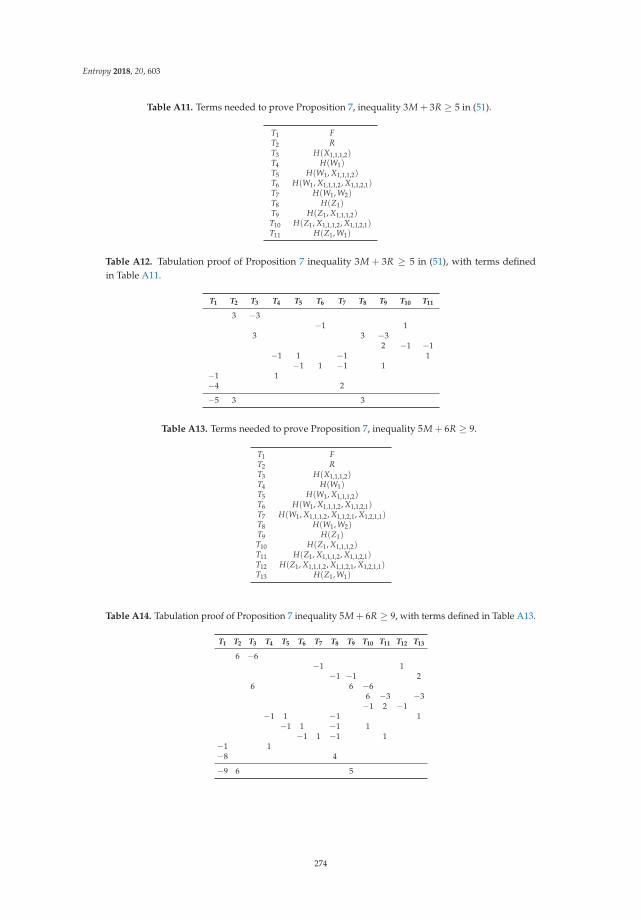
Entropy 2018, 20, 603

Table A11. Terms needed to prove Proposition 7, inequality 3M + 3R ≥ 5 in (51).

T1 FT2 RT3 H(X1,1,1,2)T4 H(W1)T5 H(W1, X1,1,1,2)T6 H(W1, X1,1,1,2, X1,1,2,1)T7 H(W1, W2)T8 H(Z1)T9 H(Z1, X1,1,1,2)T10 H(Z1, X1,1,1,2, X1,1,2,1)T11 H(Z1, W1)

Table A12. Tabulation proof of Proposition 7 inequality 3M + 3R ≥ 5 in (51), with terms definedin Table A11.

T1 T2 T3 T4 T5 T6 T7 T8 T9 T10 T11

3 −3−1 1

3 3 −32 −1 −1

−1 1 −1 1−1 1 −1 1

−1 1−4 2

−5 3 3


T1 FT2 RT3 H(X1,1,1,2)T4 H(W1)T5 H(W1, X1,1,1,2)T6 H(W1, X1,1,1,2, X1,1,2,1)T7 H(W1, X1,1,1,2, X1,1,2,1, X1,2,1,1)T8 H(W1, W2)T9 H(Z1)T10 H(Z1, X1,1,1,2)T11 H(Z1, X1,1,1,2, X1,1,2,1)T12 H(Z1, X1,1,1,2, X1,1,2,1, X1,2,1,1)T13 H(Z1, W1)


T1 T2 T3 T4 T5 T6 T7 T8 T9 T10 T11 T12 T13

6 −6−1 1

−1 −1 26 6 −6

6 −3 −3−1 2 −1

−1 1 −1 1−1 1 −1 1

−1 1 −1 1−1 1−8 4

−9 6 5

274

Entropy 2018, 20, 603


T1 FT2 RT3 H(X1,1,2,2)T4 H(W1)T5 H(W1, X1,1,2,2)T6 H(W1, X1,1,2,2, X1,2,1,2)T7 H(W1, W2)T8 H(Z1)T9 H(Z1, X1,1,2,2)T10 H(Z1, X1,1,2,2, X1,2,1,2)T11 H(Z1, W1)


T1 T2 T3 T4 T5 T6 T7 T8 T9 T10 T11

3 −3−1 1

3 3 −32 −1 −1

−1 1 −1 1−1 1 −1 1

−1 1−4 2

−5 3 3

Appendix H. Proof for the Forward of Proposition 7

Note that the optimal tradeoff for the single demand type (3, 1) system has the followingcorner points:

(M, R) = (0, 2),(

14

,32

),(

12

,76

),(

1,23

),(

32

,14

), (2, 0).

The corner points(1, 2

3)

and(

32 , 1

4

)are achievable using the Maddah-Ali–Niesen scheme [6]. The point(

14 , 3

2

)is achievable by the code given in [15] or [20]. The only remaining corner point of interest is

thus(

12 , 7

6

), in the binary field. This can be achieved by the following strategy in Table A17, where the

first file has six symbols (A1, A2, . . . , A6) and the second file (B1, B2, . . . , B6).

Table A17. Code for the tradeoff point(

12 , 7

6

)for demand type (3, 1) when (N, K) = (2, 4).

User 1 A1 + B1 A2 + B2 A3 + B3User 2 A1 + B1 A4 + B4 A5 + B5User 3 A2 + B2 A4 + B4 A6 + B6User 4 A3 + B3 A5 + B5 A6 + B6

By the symmetry, we only need to consider the demand when the first three users request A andthe last user request B. The server can send the following symbols in this case:

A3, A5, A6, B1, B2, B4, A1 + A2 + A4.

275

Entropy 2018, 20, 603

Let us consider now the single-demand-type (2, 2) system, for which the corner points on theoptimal tradeoff are:

(M, R) = (0, 2),(

13

,43

),(

43

,13

), (2, 0).

Let us denote the first file as (A1, A2, A3), and the second file as (B1, B2, B3), which are in the binaryfield. To achieve the corner point

(13 , 4

3

), we use the caching code in Table A18.


13 , 4

3

)for demand-type (2, 2) when (N, K) = (2, 4).

User 1 A1 + B1User 2 A2 + B2User 3 A3 + B3User 4 A1 + A2 + A3 + B1 + B2 + B3

Again due to the symmetry, we only need to consider the case when the first two users request A,and the other two request B. For this case, the server can send:

B1, B2, A3, A1 + A2 + A3.

For the other corner point(

43 , 1

3

)the following placement in Table A19 can be used. Again for the case

when the first two users request A, and the other two request B, the server can send:

A1 − A3 + B2.


43 , 1

3

)for demand-type (2, 2) when (N, K) = (2, 4).

User 1 A1 A2 B1 B2User 2 A2 A3 B2 B3User 3 A1 A3 B1 B3User 4 A1 + A2 A2 + A3 B1 + B2 B2 + B3

Appendix I. Proof of Proposition 8

The inequalities M + R ≥ 2 and 2M + 3R ≥ 5 in (54) are proven in Tables A20–A23, respectively.The inequalities 6M + 3R ≥ 8, M + R ≥ 2, 12M + 18R ≥ 29 and 3M + 6R ≥ 8 in (55) are provenin Tables A24–A31, respectively. All other bounds in Proposition 8 can be deduced from the cut-setbound, and thus do not need a proof.

Table A20. Terms needed to prove Proposition 8, inequality M + R ≥ 2 in (54).

T1 FT2 RT3 H(X1,1,2)T4 H(W1)T5 H(W2, X1,1,2)T6 H(W1, W2, W3)T7 H(Z1)T8 H(Z3, X1,1,2)T9 H(Z1, W1)T10 H(Z1, W2, X1,1,2)T11 H(Z1, Z3, X1,1,2)T12 H(Z1, Z2, W1)

276

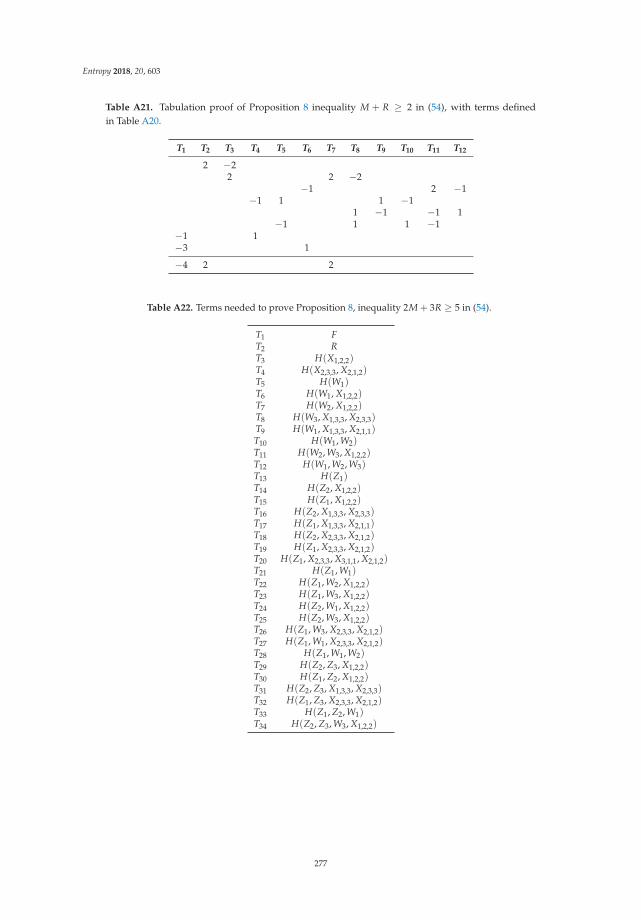
Entropy 2018, 20, 603

Table A21. Tabulation proof of Proposition 8 inequality M + R ≥ 2 in (54), with terms definedin Table A20.

T1 T2 T3 T4 T5 T6 T7 T8 T9 T10 T11 T12

2 −22 2 −2

−1 2 −1−1 1 1 −1

1 −1 −1 1−1 1 1 −1

−1 1−3 1

−4 2 2


T1 FT2 RT3 H(X1,2,2)T4 H(X2,3,3, X2,1,2)T5 H(W1)T6 H(W1, X1,2,2)T7 H(W2, X1,2,2)T8 H(W3, X1,3,3, X2,3,3)T9 H(W1, X1,3,3, X2,1,1)T10 H(W1, W2)T11 H(W2, W3, X1,2,2)T12 H(W1, W2, W3)T13 H(Z1)T14 H(Z2, X1,2,2)T15 H(Z1, X1,2,2)T16 H(Z2, X1,3,3, X2,3,3)T17 H(Z1, X1,3,3, X2,1,1)T18 H(Z2, X2,3,3, X2,1,2)T19 H(Z1, X2,3,3, X2,1,2)T20 H(Z1, X2,3,3, X3,1,1, X2,1,2)T21 H(Z1, W1)T22 H(Z1, W2, X1,2,2)T23 H(Z1, W3, X1,2,2)T24 H(Z2, W1, X1,2,2)T25 H(Z2, W3, X1,2,2)T26 H(Z1, W3, X2,3,3, X2,1,2)T27 H(Z1, W1, X2,3,3, X2,1,2)T28 H(Z1, W1, W2)T29 H(Z2, Z3, X1,2,2)T30 H(Z1, Z2, X1,2,2)T31 H(Z2, Z3, X1,3,3, X2,3,3)T32 H(Z1, Z3, X2,3,3, X2,1,2)T33 H(Z1, Z2, W1)T34 H(Z2, Z3, W3, X1,2,2)

277

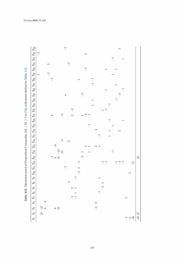
Entropy 2018, 20, 603

Ta

ble

A2

3.

Tabu

lati

onpr

oofo

fPro

posi

tion

8in

equa

lity

2M+

3R≥

5in

(54)

,wit

hte

rms

defin

edin

Tabl

eA

22.

T 1T 2

T 3T 4

T 5T 6

T 7T 8

T 9T 1

0T 1

1T 1

2T 1

3T 1

4T 1

5T 1

6T 1

7T 1

8T 1

9T 2

0T 2

1T 2

2T 2

3T 2

4T 2

5T 2

6T 2

7T 2

8T 2

9T 3

0T 3

1T 3

2T 3

3T 3

4

2−

227−

27 8−

4−

33

−2

4−

28

8−

815

15−

15 12−

6−

6−

36

−3

−3

6−

3−

22

2−

2−

11

1−

1−

33−

33

−3

33

−3

2−

2−

22

11

−1

−1

11

−1−

1−

44

4−

4−

11

1−

1−

33

−3

3−

1−

11

11

1−

1−

1−

11

1−

1−

1−

11

1−

33

−3

3−

11

−1

1−

33

−6

3−

3612

−45

2718

278

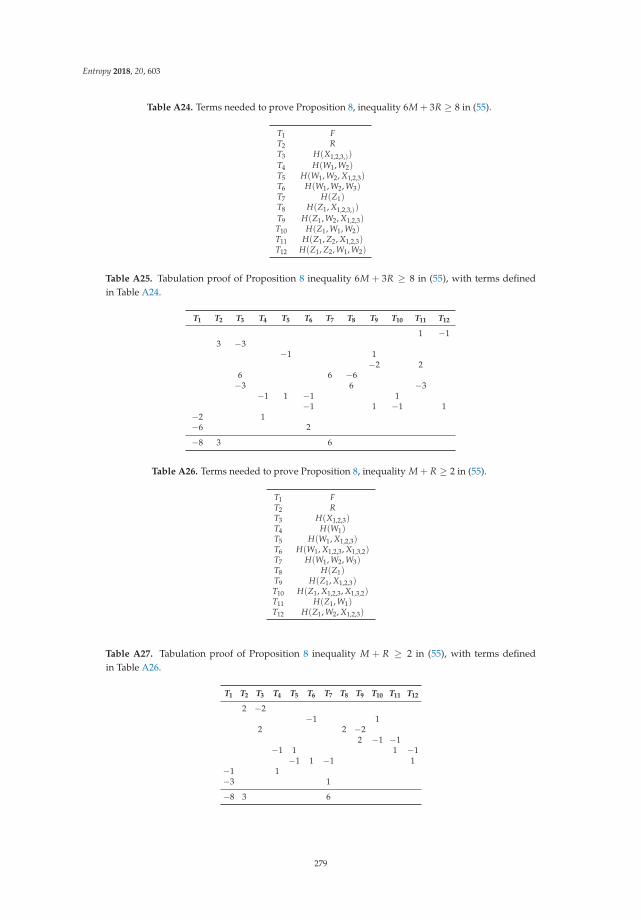
Entropy 2018, 20, 603


T1 FT2 RT3 H(X1,2,3,))

T4 H(W1, W2)T5 H(W1, W2, X1,2,3)T6 H(W1, W2, W3)T7 H(Z1)T8 H(Z1, X1,2,3,))

T9 H(Z1, W2, X1,2,3)T10 H(Z1, W1, W2)T11 H(Z1, Z2, X1,2,3)T12 H(Z1, Z2, W1, W2)


T1 T2 T3 T4 T5 T6 T7 T8 T9 T10 T11 T12

1 −13 −3

−1 1−2 2

6 6 −6−3 6 −3

−1 1 −1 1−1 1 −1 1

−2 1−6 2

−8 3 6

Table A26. Terms needed to prove Proposition 8, inequality M + R ≥ 2 in (55).

T1 FT2 RT3 H(X1,2,3)T4 H(W1)T5 H(W1, X1,2,3)T6 H(W1, X1,2,3, X1,3,2)T7 H(W1, W2, W3)T8 H(Z1)T9 H(Z1, X1,2,3)T10 H(Z1, X1,2,3, X1,3,2)T11 H(Z1, W1)T12 H(Z1, W2, X1,2,3)

Table A27. Tabulation proof of Proposition 8 inequality M + R ≥ 2 in (55), with terms definedin Table A26.

T1 T2 T3 T4 T5 T6 T7 T8 T9 T10 T11 T12

2 −2−1 1

2 2 −22 −1 −1

−1 1 1 −1−1 1 −1 1

−1 1−3 1

−8 3 6

279

Entropy 2018, 20, 603


T1 FT2 RT3 H(X1,2,3)T4 H(X1,2,3, X1,3,2)T5 H(X1,2,3, X1,3,2, X2,1,3)T6 H(W1)T7 H(W1, X1,2,3)T8 H(W2, X1,2,3, X1,3,2)T9 H(W1, W2)T10 H(W1, W2, X1,2,3)T11 H(W1, W2, X1,3,2, X2,1,3)T12 H(W2, W3, X1,2,3, X1,3,2)T13 H(W1, W2, X1,2,3, X1,3,2, X2,1,3)T14 H(W1, W2, W3)T15 H(Z1)T16 H(Z1, X1,2,3)T17 H(Z1, X1,3,2, X2,1,3)T18 H(Z2, X1,2,3, X1,3,2)T19 H(Z1, X1,2,3, X1,3,2)T20 H(Z1, X1,2,3, X1,3,2, X2,1,3)T21 H(Z1, W1)T22 H(Z1, W2, X1,2,3)T23 H(Z1, W2, X1,2,3, X1,3,2)T24 H(Z1, W1, W2)


T1 T2 T3 T4 T5 T6 T7 T8 T9 T10 T11 T12 T13 T14 T15 T16 T17 T18 T19 T20 T21 T22 T23 T24

2 −118 −18

−1 1−3 3

17 17 −17−2 4 −2−3 6 −3

2 −1 −16 −3 −3

−1 2 −1−3 3 3 −3

−1 1 −1 12 −2 −2 2

−3 3 3 −3−1 1 −1 1

2 2 −2 −2−1 1 1 −1

−3 3 −3 3−3 3 −3 3

−3 3−2 1−24 8

−29 18 12

280

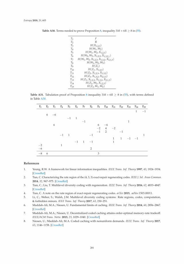
Entropy 2018, 20, 603


T1 FT2 RT3 H(X1,2,3)T4 H(W1, W2)T5 H(W1, W2, X1,2,3)T6 H(W2, W3, X1,2,3, X1,3,2,))

T7 H(W1, W2, X1,2,3, X1,3,2, X2,1,3)T8 H(W1, W2, W3)T9 H(Z1)T10 H(Z1, X1,2,3)T11 H(Z2, X1,2,3, X1,3,2)T12 H(Z1, X1,3,2, X2,1,3)T13 H(Z1, X1,2,3, X1,3,2, X2,1,3)T14 H(Z1, W2, X1,2,3)T15 H(Z1, W1, W2)


T1 T2 T3 T4 T5 T6 T7 T8 T9 T10 T11 T12 T13 T14 T15

1 −16 −6

−1 1−1 1

6 6 −6−2 4 −2−1 2 −1

−1 1 −1 11 1 −1 −1

−1 1 −1 1−2 1−6 2

−8 6 3

References

1. Yeung, R.W. A framework for linear information inequalities. IEEE Trans. Inf. Theory 1997, 43, 1924–1934.[CrossRef]

2. Tian, C. Characterizing the rate region of the (4, 3, 3) exact-repair regenerating codes. IEEE J. Sel. Areas Commun.2014, 32, 967–975. [CrossRef]

3. Tian, C.; Liu, T. Multilevel diversity coding with regeneration. IEEE Trans. Inf. Theory 2016, 62, 4833–4847.[CrossRef]

4. Tian, C. A note on the rate region of exact-repair regenerating codes. arXiv 2015, arXiv:1503.00011.5. Li, C.; Weber, S.; Walsh, J.M. Multilevel diversity coding systems: Rate regions, codes, computation,

& forbidden minors. IEEE Trans. Inf. Theory 2017, 63, 230–251.6. Maddah-Ali, M.A.; Niesen, U. Fundamental limits of caching. IEEE Trans. Inf. Theory 2014, 60, 2856–2867.

[CrossRef]7. Maddah-Ali, M.A.; Niesen, U. Decentralized coded caching attains order-optimal memory-rate tradeoff.

IEEE/ACM Trans. Netw. 2015, 23, 1029–1040. [CrossRef]8. Niesen, U.; Maddah-Ali, M.A. Coded caching with nonuniform demands. IEEE Trans. Inf. Theory 2017,

63, 1146–1158. [CrossRef]

281

Entropy 2018, 20, 603

9. Pedarsani, R.; Maddah-Ali, M.A.; Niesen, U. Online coded caching. IEEE/ACM Trans. Netw. 2016, 24, 836–845.[CrossRef]

10. Karamchandani, N.; Niesen, U.; Maddah-Ali, M.A.; Diggavi, S.N. Hierarchical coded caching. IEEE Trans.Inf. Theory 2016, 62, 3212–3229.

11. Ji, M.; Tulino, A.M.; Llorca, J.; Caire, G. Order-optimal rate of caching and coded multicasting with randomdemands. IEEE Trans. Inf. Theory 2017, 63, 3923–3949.

12. Ghasemi, H.; Ramamoorthy, A. Improved lower bounds for coded caching. IEEE Trans. Inf. Theory 2017,63, 4388–4413. [CrossRef]

13. Sengupta, A.; Tandon, R. Improved approximation of storage-rate tradeoff for caching with multipledemands. IEEE Trans. Commun. 2017, 65, 1940–1955. [CrossRef]

14. Ajaykrishnan, N.; Prem, N.S.; Prabhakaran, V.M.; Vaze, R. Critical database size for effective caching.In Proceedings of the 2015 Twenty First National Conference on Communications (NCC), Mumbai, India,27 February–1 March 2015; pp. 1–6.

15. Chen, Z.; Fan, P.; Letaief, K.B. Fundamental limits of caching: improved bounds for users with smallbuffers. IET Commun. 2016, 10, 2315–2318. [CrossRef]

16. Sahraei, S.; Gastpar, M. K users caching two files: An improved achievable rate. arXiv 2015, arXiv:1512.06682.17. Amiri, M.M.; Gunduz, D. Fundamental limits of caching: Improved delivery rate-cache capacity trade-off.

IEEE Trans. Commun. 2017, 65, 806–815. [CrossRef]18. Wan, K.; Tuninetti, D.; Piantanida, P. On caching with more users than files. arXiv 2016, arXiv:1601.06383.19. Yu, Q.; Maddah-Ali, M.A.; Avestimehr, A.S. The exact rate-memory tradeoff for caching with uncoded

prefetching. IEEE Trans. Inf. Theory 2018, 64, 1281–1296. [CrossRef]20. Tian, C.; Chen, J. Caching and delivery via interference elimination. IEEE Trans. Inf. Theory 2018, 64, 1548–1560.

[CrossRef]21. Gómez-Vilardebó, J. Fundamental limits of caching: Improved rate-memory trade-off with coded

prefetching. IEEE Trans. Commun. 2018. [CrossRef]22. Cover, T.M.; Thomas, J.A. Elements of Information Theory, 1st ed.; Wiley: New York, NY, USA, 1991.23. Tian, C. Symmetry, demand types and outer bounds in caching systems. In Proceedings of the 2016 IEEE

International Symposium on Information Theory (ISIT), Barcelona, Spain, 10–15 July 2016; pp. 825–829.24. Yu, Q.; Maddah-Ali, M.A.; Avestimehr, A.S. Characterizing the rate-memory tradeoff in cache networks

within a factor of 2. arXiv 2017, arXiv:1702.04563.25. Wang, C.Y.; Bidokhti, S.S.; Wigger, M. Improved converses and gap-results for coded caching. arXiv 2017,

arXiv:1702.04834.26. Yeung, R. A First Course in Information Theory; Kluwer Academic Publishers: New York, NY, USA, 2002.27. Lassez, C.; Lassez, J.L. Quantifier Elimination for conjunctions of linear constraints via a convex hull

algorithm. In Symbolic and Numerical Computation for Artificial Intelligence; Donald, B.R., Kapur, D.,Mundy, J.L., Eds.; Academic Press: San Diego, CA, USA, 1992; Chapter 4, pp. 103–1199.

28. Apte, J.; Walsh, J.M. Exploiting symmetry in computing polyhedral bounds on network coding rateregions. In Proceedings of the International Symposium on Network Coding (NetCod), Sydney, Australia,22–24 June 2015; pp. 76–80.

29. Ho, S.W.; Tan, C.W.; Yeung, R.W. Proving and disproving information inequalities. In Proceedings of the2014 IEEE International Symposium on Information Theory (ISIT), Honolulu, HI, USA, 29 June–4 July 2014.

30. Zhang, K.; Tian, C. On the symmetry reduction of information inequalities. IEEE Trans. Commun. 2018,66, 2396–2408. [CrossRef]

31. Harary, F.; Norman, R.Z. Graph Theory as a Mathematical Model in Social Science; University of MichiganPress: Ann Arbor, MI, USA, 1953.

32. Andrews, G.E. The Theory of Partitions; Cambridge University Press: Cambridge, UK, 1976.33. Dougherty, R.; Freiling, C.; Zeger, K. Insufficiency of linear coding in network information flow. IEEE Trans.

Inf. Theory 2005, 51, 2745–2759. [CrossRef]34. Zhang, Z.; Yeung, R.W. A non-Shannon-type conditional inequality of information quantities. IEEE Trans.

Inf. Theory 1997, 43, 1982–1986. [CrossRef]35. Zhang, Z.; Yeung, R.W. On characterization of entropy function via information inequalities. IEEE Trans.

Inf. Theory 1998, 44, 1440–1452. [CrossRef]

282

Entropy 2018, 20, 603

36. Yeung, R.W.; Zhang, Z. On symmetrical multilevel diversity coding. IEEE Trans. Inf. Theory 1999, 45, 609–621.[CrossRef]

37. Tian, C. Latent capacity region: A case study on symmetric broadcast with common messages. IEEE Trans.Inf. Theory 2011, 57, 3273–3285. [CrossRef]

c© 2018 by the author. Licensee MDPI, Basel, Switzerland. This article is an open accessarticle distributed under the terms and conditions of the Creative Commons Attribution(CC BY) license (http://creativecommons.org/licenses/by/4.0/).

283

MDPISt. Alban-Anlage 66

4052 BaselSwitzerland

Tel. +41 61 683 77 34Fax +41 61 302 89 18

www.mdpi.com

Entropy Editorial OfficeE-mail: [email protected]

www.mdpi.com/journal/entropy

MDPI St. Alban-Anlage 66 4052 Basel Switzerland

Tel: +41 61 683 77 34 Fax: +41 61 302 89 18

www.mdpi.com ISBN 978-3-03943-818-1

Information Theory for Data Communications and Processing

Documents

Transcript of Information Theory for Data Communications and Processing