INFORMATION THEORETIC METRICSFOR THE ASSESSMENT OF

DIGITAL IMAGE-TONE RESTORED IMAGES

by

Paul W. Melnychuck

B.S . Rochester Institute o f Technology

(1982)

A thesis s ubmi t t e d in partial fulfillmentof the requirements for the degree ofMaster o f Science in the School o f

Photographic Arts and Sciences in theCollege o f Graphic Arts and Photography

o f the Rochester Institute o f Technology

August, 1984

Signature of the Author Paul W. MelnychuckIma g i ng and Photographic Science Dept .

Ronald FrancisCoordinator , M.S . Degree ProgramAce epted bY--------,.-;;:::-;:;:r<:;-;;;:::;-;:-Mcr-=::;::::;:-====_

College of Graphic Arts and PhotographyRochester Institute of Technology

Rochester, New York

CERTIFICATE OF APPROVAL

M.S . DEGREE THESIS

The M.S . Degree Thesis of Paul W. Melnychuckhas been examined and approved

by the thesis committee as satisfactoryf or the thesis requirement for the

Master of Science degree

Joseph H. AltmanMr. Joseph H. Altman, Thesis Advis or

Peter EngledrumMr. Peter Engledrum

Rodney ShawDr . Rodney Shaw

Date

James R. SullivanMr. Jame s R. Sullivan

ii

THESIS RELEASE PERMISSION FORM

ROCHESTER INSTITUTE OF TECHNOLOGY

COLLEGE OF GRAPHIC ARTS AND PHOTOGRAPHY

Information Theoretic Metrics for the

Title of Thesis

Assessment of Digital Image-Tone Restored Images

Paul W. Melnychuck

I, ,prefer to

be contacted each time a request for reproduction is made.

I can be reached at the following address:

Eastman Kodak Company

Research Laboratories, B-82A

Rochester, New York 14650

Date

<l\rl*.

m

INFORMATION THEORETIC METRICS

FOR THE ASSESSMENT OF

DIGITAL IMAGE-TONE RESTORED IMAGES

by

Paul W. Melnychuck

Submitted to the

Imaging and Photographic Science Department

in partial fulfillment of the requirements

for the Master of Science degree

at the Rochester Institute of Technology

ABSTRACT

Digital image-tone restoration is examined in terms

of information theoretic-based measurements. The metrics

illustrate the relative degree of restorability of a

6-stop underexposure range on Kodak Tri-X pan film. An

image chain model is developed to account for the discrete

nature of sampled images used in digital image processing.

The model includes the major system components (from

object to viewed image) from which the system signal-to-

noise ratio is calculated. Quantization noise and clipping

are treated as signal-dependent, additive noise sources,

and are shown to play a major role in degrading restored

images. Although the eye characteristics are not included

in the calculations, there is some indication that the

logarithm of the information content and the noise equiva

lent number of quanta correlate with the visual perception

of image quality of a restored pictorial image; these

metrics demonstrate their utility in characterizing the

practical limits of an image-tone restoration system.

iv

ACKNOWLEDGEMENTS

This work would not have been possible without

the significant contributions made by a number of kind

individuals, whom I gratefully acknowledge:

Mr. J.H. Altman, for his patience, time and helpful

suggestions in serving as my thesis advisor.

Mr. P.D. Burns, for his helful comments concerning

the Wiener spectrum measurements.

Dr. P. Bunch & crew, for making the WS measurements.

Mr. G. Coutu, for his assistance and software.

Mr. P. Engledrum, for making me think.

Dr. J. DeLorenzo, for interesting discussions.

Dr. R. Francis, for all of his help over the years.

Mr. R.D. Lucitte, for many hours of assistance.

Mr. R. Mergler, for scanning the images.

Mr. S. Muratore, for all of his cooperation in

scanning the images.

Dr. L. Ray, for his programming assistance.

Dr. R. Schaetzing, for the use of his software and

for performing the 2-D FFT.

Dr. R. Shaw, for planting the seed.

Mr. J.R. Sullivan, for watering it.

and the management of the Image Recording Division of the

Kodak Research Laboratories for their support of this work.

v

DEDICATION

This thesis is dedicated to myparents, Walter and Genoveva, mysister, Rosemary, and to those

who have made a profound

influence in my life.

VI

CONTENTS

List of illustrations vii

Introduction 1

Theory 6

Digital Image-Tone Restoration 6

Film Point Gamma 8

Effective Speed Gain 10

Noise Equivalent Quanta (NEQ) 11

System Image Chain Model 15

Quantization Noise and Clipping 18

Information Content 24

Experimental 36

Generation of Images 36

Sensitometry 37

MTF Measurements 38

Wiener Noise Spectrum Measurements 39

Signal Power Spectrum & Probability DensityMeasurement 43

Subjective Assessment of Images 44

Results and Discussion 45

NEQ Measurements 45

Calculation of Quantization Noise and Clipping 50

Information Content Calculations and Images . 55

Conclusions 60

References 61

Vita 65

VII

LIST OF ILLUSTRATIONS

Figure 1. Density remapping functions for Kodak

Tri-X pan film 7

Figure 2. Point gamma available to record a

6-stop scene 9

Figure 3. System image chain model for the

image-tone restoration process 17

Figure 4. Shift in the probability distribution

as a function of exposure 19

Figure 5. Expanded view of the quantization

density increment 20

Figure 6. Output of a system as an addition of

signal plus noise 31

Figure 7. Digital image-tone restoration scheme . 37

Figure 8. Wiener noise spectrum scanning scheme . 42

Figure 9. Sensitometric response of Kodak

Tri-X pan film 46

Figure 10. MTF of Kodak Tri-X pan film for

various degrees of underexposure ... 47

Figure 11. Contrast transfer function at output

stage of system 48

Figure 12. Measured Wiener noise spectrum at

output stage of system 49

Figure 13. Scene probability density distribution. 51

Figure 14. Total quantization noise and clipping

variance 52

Figure 15. Comparison of Weiner spectrum with

quantization + clipping noise 54

Figure 16. Information content for tone restored

images 55

Figure 17. Image-tone restored images, NEQ and I . 57

Figure 18. Log information content and subjective

judgements vs degree of underexposure. . 59

INTRODUCTION

Tone-reproduction concerns mainly the macro-scale charac

teristics, the appearance of comparatively large areas, of

an image. Many methods in tone-reproduction analysis have

been developed, and the literature is extensive ( 1, 2 ) . The

main objective of these methods is to devise criteria to

distinguish between what may be termed"preferred"

and

"failed"

tone-reproduction. Two important factors that

influence the quality of tone-reproduction are the

gradient, or contrast, and the dynamic range, or density

range, of the system. Although these properties can be

changed by a number of ways, this study addresses failed

tone-reproduction as a result of underexposure, or moving

the exposure range of the subject along the film's char

acteristic curve, towards the region where low levels of

light exposure fail to form a developable latent image in

the photographic material. In this region, a considerable

change in exposure produces only slight changes in density,

resulting in severe tone distortion of the underexposed

image; there are fewer distinguishing tones recorded on

the film than were present in the original subject. This

tone-compression produces a rendition on the film that is

too low in contrast ("flat") and the shadow areas lack

detail.

Chemical methods to correct for failed tone- reproduc

tion may involve a posterior intensification treatment of

the developed image, to amplify the image densities to

those which may result in a more preferred tone-reproduced

image. Other chemical methods involve modified developer

formulas called"push-processing"

developers, or simply

increasing the film development time. These techniques

have been well documented by Haist(3). Chemical methods

will yield a slight increase in film emulsion speed of

negative films but with the risk of unwanted enhanced

contrast, increased grain size, and other detrimental

image characteristics.

Digital image processing offers flexibility that

chemical analog techniques cannot afford. Whereas analog

methods are constrained by physical phenomena, digital

methods use mathematical manipulations via computers, and

possess no constraints other than speed and cost.

Tone-scaling is a common digital image processing

technique used to correct failed tone-reproduction, and

can be found in standard texts such as Pratt(4) and

Gonzalez and Wintz(5). Digital image-tone restoration is

atone-

scaling technique which assumes a priori knowledge

of the degree of exposure error (under or overexposure)

for an image, and is used to correct failed tone-reproduc

tion to preferred tone-reproduction, which presumably

would resemble that of a normally exposed image. Tone

restoration differs from other forms of tone-scaling which

are based on perceptual enhancement of the image, or to

produce a desired density value distribution, or histo

gram. Although many applications of these techniques

exist in the literature, the practical limit on the degree

of underexposure that is restorable has not been reported.

The purpose of this work is to describe the performance of

a digital image-tone restoration system with respect to

the relative degree of restorability, in terms of infor

mation theoretic metrics. These measurements will be

compared with the visual assessment of a series of tone-

restored pictorial images. It is not the intent of this

work to maximize the tone restored results, but rather, to

accept the quality of the generated images and simply

construct a model to describe the image quality of the

process which generated the output images.

Attempts to describe the image quality of a spatially

recorded image date back to the early part of the century.

A detailed account of the important advances in image

analysis and evaluation can be found in Shaw(6) or Dainty

and Shaw(7). More recent papers concerning image quality

can be found in refs. 8 to 12. Numerous papers have shown

the applicability ofquantum- limited signal-to-noise

metrics, such as detective quantum efficiency (DQE) and

the noise equivalent number of available quanta (NEQ)

for the evaluation of photographic film, and imaging

systems in general (13). The concept of NEQ provides a

useful measure of image signal-to-noise and can be used as

a metric for the assessment of image quality. Rose(14)

demonstrated this by showing a series of images and the

corresponding number of apparent photons used to record

the image. In addition to describing the efficiency of

radiation detectors, Schade(15) was prominent in estab

lishing the Fourier approach to optical and photographic

image evaluation. Higgins(16) reviewed the factors

relating to image quality and showed the importance of

using a log signal-to-noise metric, which is a form of

information content.* Based on the work of Shannon(17),

early application of information theory by Felgett and

Linfoot(18), Jones (19), and Shaw(20), involved measuring

the information capacity of emulsions, with a constant

signal power spectrum being assumed. Kriss et al . (21)

used a visually weighted information capacity metric to

assess the quality of photographic images. Vendrovsky(22 )

showed that the logarithm of the information content is

linearly related to subjective image quality. More

*I am grateful to Mr. J. R. Sullivan for bringing to my

attention unpublished work on the use of information

content since 1969.

recently, Fales, Huck, and Samms(23) used information

content to assess the performance of image scanners. They

used an assumed signal power spectrum shape and accounted

for degradations such as aliasing and quantization which

are present in digitally generated images.

The following section describes metrics for the

evaluation of image-tone restoration performance. The

theory begins with sensitometric-based metrics, progresses

to signal-to-noise type metrics which include random

fluctuations and deterministic noise sources, and leads to

a derivation of information content.

THEORY

Digital Image-Tone Restoration

The objective of image-tone restoration is to

correct a"failed"

tone-reproduced image, to a"preferred"

tone-reproduced image, via a monotonic remapping of the

image densities. With a priori knowledge of the degree of

exposure error (which is assumed or approximated), a

density remapping function can be derived by selecting,

for each density value in the degraded image, a new

density value resembling a normally exposed image,

according to the D-Log E curve of the recording film. The

gain of the remapping function is then calculated as the

ratio of the desired point gamma to that of the underex

posed point gamma, where the point gamma is the first

derivative of the D-Log E curve at a particular point. A

series of functions can be derived for various degrees of

exposure error, and this is shown in Figure 1 for Kodak

Tri-X pan film. Note that the slope of the remapping

function represents the point gain, or amplification,

applied to the image. For low densities (shadows in the

scene) the gain is high, and gradually approaches a value

of unity towards higher negative densities. Intuitively

this is reasonable, since we know there is very little

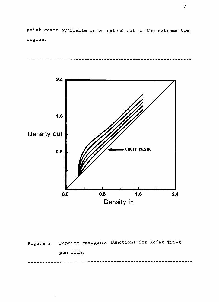
point gamma available as we extend out to the extreme toe

region.

2.4

1.6 -

Density out

0.8

Density in

Figure 1. Density remapping functions for Kodak Tri-X

pan film.

Film Point Gamma

Since image-tone restoration merely involves a

density remapping, a simple first-order metric might be

the point gamma of the remapping function. An evaluation

of the point gamma as a function of exposure before and

after tone restoration could be used to evaluate the

overall success of the restoration; a perfect restoration

would bring back a point gamma which would be identical to

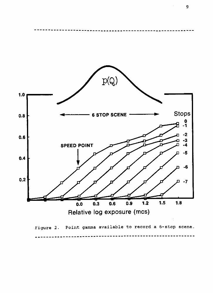
that for the normally exposed case. Figure 2 illustrates

the point gamma as a function of exposure for progressive

degrees of underexposure. The curves are placed so that

the probability density distribution of the scene (in

exposure space) is held fixed, while the curves are

aligned to fall within the scene distribution. Addition

ally, the lowest exposure in the scene occurs 1 stop

beyond the speed point of the film, which is how ANSI

exposure meters are calibrated(24) . For a nominal 6-stop

(1.8 log exposure) input dynamic range, the available

point gamma drops faster at low exposures, illustrating

the effect underexposure has on shadow detail in the

photograph.

0.6 0.9 1.2 1.5

Relative log exposure (mcs)

Figure 2. Point gamma available to record a 6-stop scene

10

Effective Speed Gain

One method used to measure the sensitivity, or

speed, in an imaging system is to measure its response at

a specified density level. The American Standard method

for measuring the speed of black-and-white films is to

determine the exposure, E , corresponding to a density of

0.10 above base plus fog, when the film has been processed

according to specified conditions. The speed is then

computed by the relation

S = 0 . 8/E ( 1 )'m

v '

where E is stated in lux-seconds (meter-candle-seconds).m

v '

A more complete definition of speed and sensitivity is

given by Altman(25). Since the image-tone restoration

process increases the densities in the low exposure, or

shadow region (which is the area on the D-Log E curve

where the speed point, or reference density, is most often

specified) the result is an effective speed increase.

Thus, the success of the image-tone restoration process

can be tracked by measuring the effective exposure index,

E.I., of the original recording film. Additionally, the

E.I. can be used to compare its speed relative to that of

other imaging systems where the speed is expressed in this

11

way. Although numerically there is an effective speed

increase (in the sense that shadow detail is restored), in

practice it is confounded for discrete images by the

non- linear effects of quantization noise due to the

digitization of the density levels. Because of this, the

image may not in general exhibit a complete restoration of

shadow detail. It is important to mention that this

metric gives no indication of the image quality, or the

consequences of extreme tone restoration with respect to

preferred visual quality thresholds. In addition, this

metric is a"DC"

threshold descriptor that does not

describe the micro-characteristics that are important to

image quality.

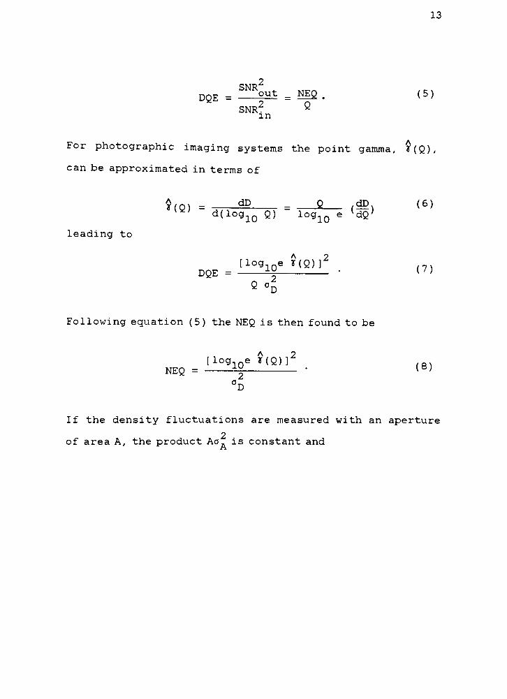
Noise Equivalent Quanta (NEQ)

The performance of a radiation detector (one of which is a

digital image-tone restoration system) can be described in

terms of the signal-to-noise ratio (SNR) associated with

the conversion of Q input quanta to output density, D.

The detective quantum efficiency (DQE) defines the rela

tionship between detector input and output fluctuations,

when expressed in equivalent terms by translating the

input exposure through the system gain:

12

- i- (2)

D

2 2where o and o are the variances of Q and D, respectively

As shown by Shaw(6), the concept of DQE leads to the

possibility of expressing the output SNR of a detector as

the noise-equivalent input, in terms of the noise-

equivalent number of exposure quanta (NEQ). If the mean

exposure, Q (in quanta/area), is assumed to follow Poisson

2statistics, o = Q, and the SNR at the input of the

detector may be defined as

sX =Xf- 2- (3)

^

"()For a practical detector the output SNR will be equivalent

to the lesser number of quanta, NEQ, which defines the

number of quanta an ideal detector would have needed to

yield the same SNR.

SNR2ut= NEQ (4)

The DQE can now be expressed in terms of the NEQ

13

SNR2

DQE = ^ = NiQ. (5)SNR2 2

in

For photographic imaging systems the point gamma, *(Q),

can be approximated in terms of

leading to

$(Q) = -4P = Q dD (6)KV>

d(log1) Q) log10 e{dQ>

[log ey(Q)]2

DQE =* ( ' >

eD

Following equation (5) the NEQ is then found to be

[log e*(Q)]2

NEQ = ^*

D

(8)

If the density fluctuations are measured with an aperture

2of area A, the product AoA is constant and

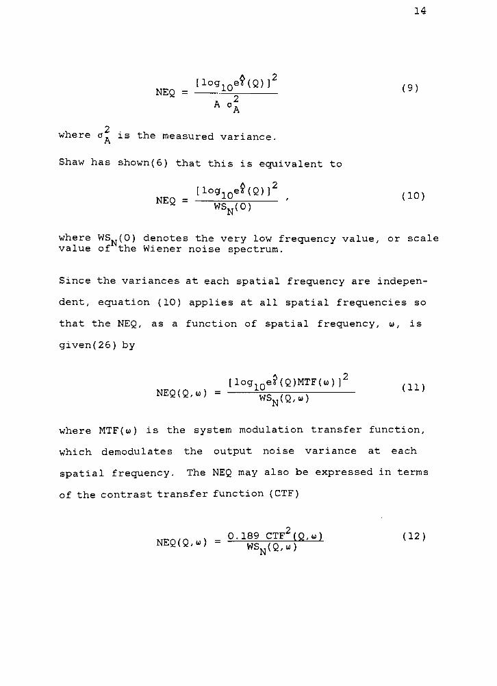
14

[logNEQ =

1U (9)

X2

whereo^

is the measured variance.

Shaw has shown(6) that this is equivalent to

[log-^Q))2

# (10)N*y

wsN(0)

where WS.,(0) denotes the very low frequency value, or scale

value of the Wiener noise spectrum.

Since the variances at each spatial frequency are indepen

dent, equation (10) applies at all spatial frequencies so

that the NEQ, as a function of spatial frequency, w, is

given(26) by

[log

NE^<"> =

ws^Q,.)

( )

where MTF(u) is the system modulation transfer function,

which demodulates the output noise variance at each

spatial frequency. The NEQ may also be expressed in terms

of the contrast transfer function (CTF)

Nmmuv

-

0-189 CTF2(Q,u>) (12)NEQ(Q,u>)

-

WSN(Q,U)

15

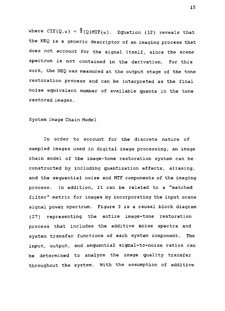
where CTF(Q,W) = $(Q)MTF(w). Equation (12) reveals that

the NEQ is a generic descriptor of an imaging process that

does not account for the signal itself, since the scene

spectrum is not contained in the derivation. For this

work, the NEQ was measured at the output stage of the tone

restoration process and can be interpreted as the final

noise equivalent number of available quanta in the tone

restored images.

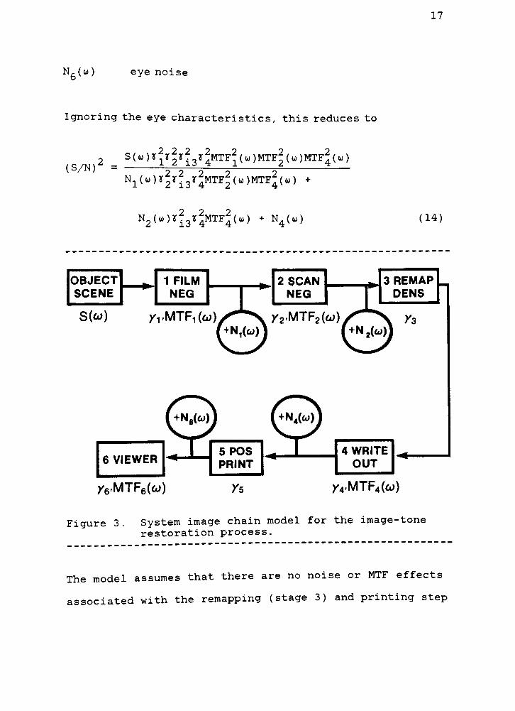
System Image Chain Model

In order to account for the discrete nature of

sampled images used in digital image processing, an image

chain model of the image-tone restoration system can be

constructed by including quantization effects, aliasing,

and the sequential noise and MTF components of the imaging

process. In addition, it can be related to a "matched

filter"

metric for images by incorporating the input scene

signal power spectrum. Figure 3 is a causal block diagram

(27) representing the entire image-tone restoration

process that includes the additive noise spectra and

system transfer functions of each system component. The

input, output, and sequential signal-to-noise ratios can

be determined to analyze the image quality transfer

throughout the system. With the assumption of additive

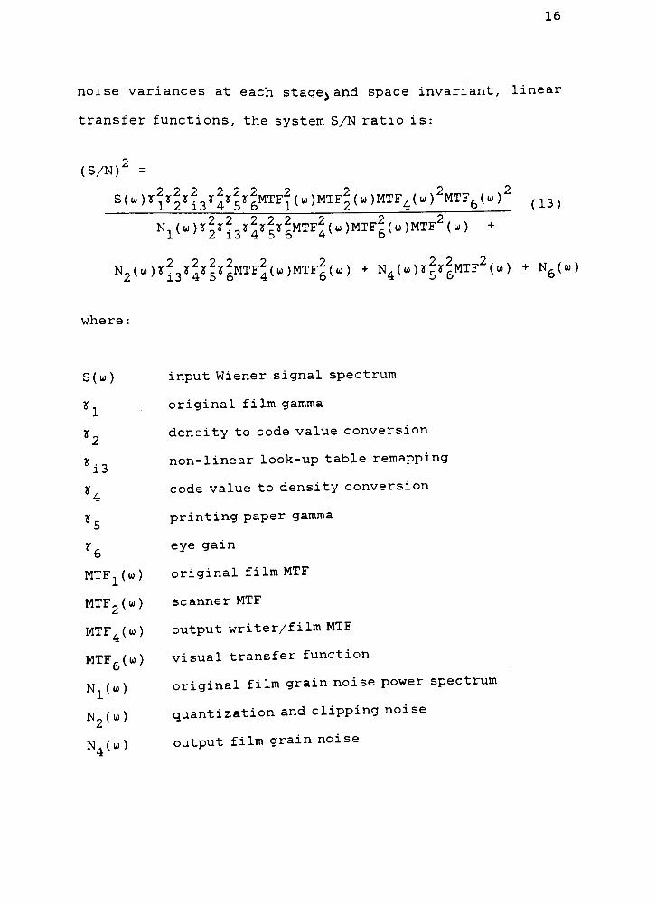
16

noise variances at each stagehand space invariant, linear

transfer functions, the system S/N ratio is:

(S/N)2

=

S(a))Y2y2y23Y2Y2Y2MTF2(u))MTF2(u))MTF4(w)2MTF6(u))2

(13)

N1(u)y2y23y2y2y2MTF2(u)MTF2(w)MTF2(W) +

N2(u.)Y23y2Y2y2MTF2(W)MTF2(W) + N4( u)r2*2MTF2

( u ) + N&(w)

where :

S(w) input Wiener signal spectrum

% original film gamma

r density to code value conversion

2

ynon- linear look-up table remapping

i3

x code value to density conversion

4

Z printing paper gamma

r eye gain

6

MTF-(u) original film MTF

MTF9(w) scanner MTF

MTF (w) output writer/film MTF

MTF,(u) visual transfer function

6

N (w) original film grain noise power spectrum

N (w)quantization and clipping noise

N (w) output film grain noise

17

N6(u) eye noise

Ignoring the eye characteristics, this reduces to

0

S(w)y2y23r2

iJmtf?(u)mtf^(w)mtf5(w)

(S/N) =^

=- -

N1(w)y2y23y2MTF2(W)MTF2(U) +

N2(u)y23y2MTF2(u>) + N4(u) (14)

OBJECT

SCENE

3 REMAP

DENS

y6-MTF6(w) Yb X4.MTF4(cj)

Figure 3. System image chain model for the image-tone

restoration process.

The model assumes that there are no noise or MTF effects

associated with the remapping (stage 3) and printing step

18

(stage 5) and that aliasing and banding artifacts are

negligible. Because the human visual system has been

ignored, the S/N ratio is not a function of the printing

step (stage 5) and the analysis can be performed in terms

of negative densities (stage 4). The first and last noise

terms in the denominator of equation (14) can be directly

measured from the output Wiener noise spectrum of uniform

exposures because N.,(w) and N4(w) are not spatially signal

dependent. If N2(w) is set equal to zero, we are left

with a signal-to-noise ratio that is due solely to the

stochastic nature of the imaging process. The second

noise term takes into account the discrete nature of the

digitization process and allows for a more complete

description of the stochastic and deterministic noise

sources .

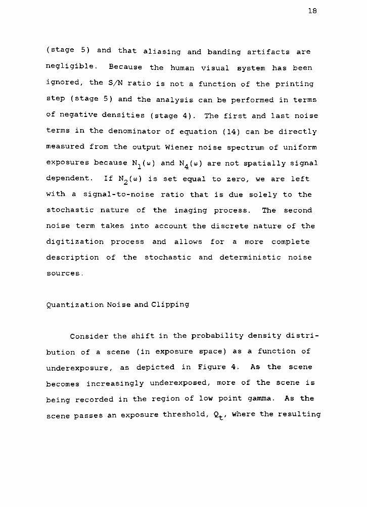
Quantization Noise and Clipping

Consider the shift in the probability density distri

bution of a scene (in exposure space) as a function of

underexposure, as depicted in Figure 4. As the scene

becomes increasingly underexposed, more of the scene is

being recorded in the region of low point gamma. As the

scene passes an exposure threshold, Qt, where the resulting

19

density xt# is the fog density, the scene information is

lost, or truncated. Additionally, there is

D

2.0 3.0 4.0 5.0

log Q (quanta/ /um2)

6.0

Figure 4. Shift in the probability distribution as a

function of exposure

quantization error, which is defined as the mean squared

difference between the true analog density, x., and the

mean quantitized density, x .

, summed over all quantization

increments. The noise, denoted N2 , is considered here as

a combination of quantization noise and amplitude

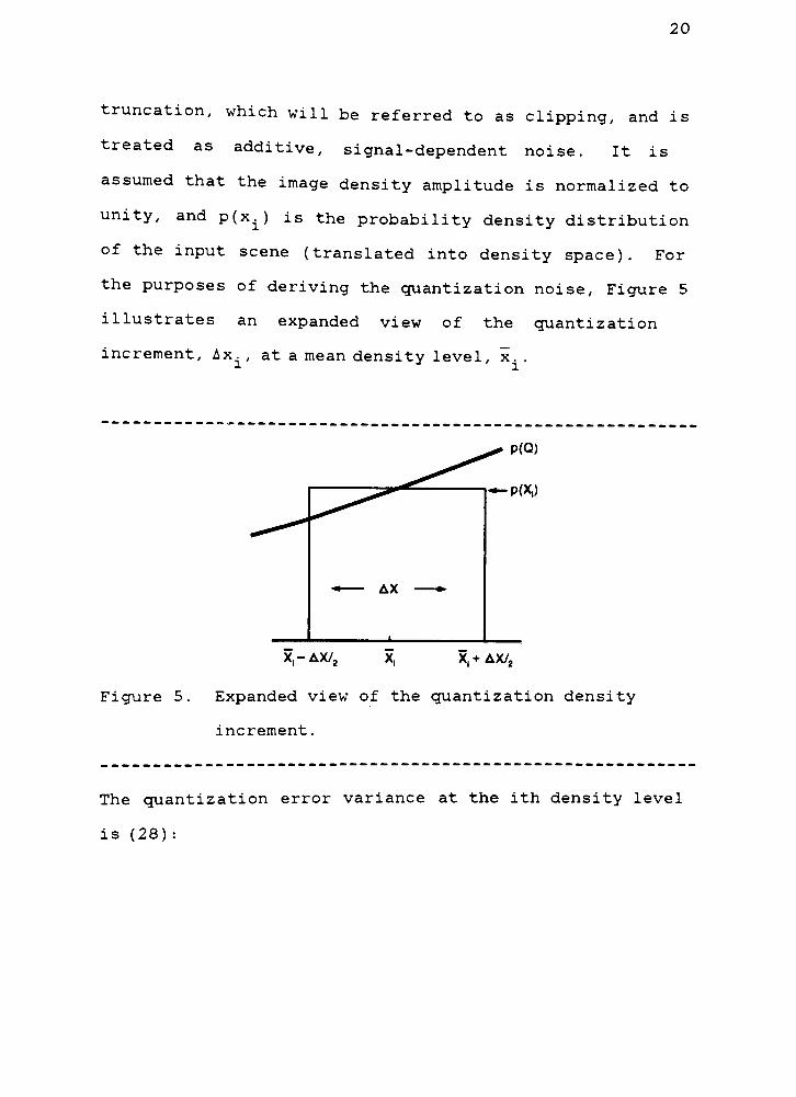
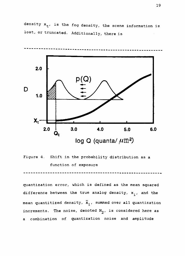
20

truncation, which will be referred to as clipping, and is

treated as additive, signal-dependent noise. It is

assumed that the image density amplitude is normalized to

unity, and p(xi) is the probability density distribution

of the input scene (translated into density space). For

the purposes of deriving the quantization noise, Figure 5

illustrates an expanded view of the quantization

increment, Ax., at a mean density level, x. .

1 J '

l

X-AX/2

Figure 5. Expanded view of the quantization density

increment.

The quantization error variance at the ith density level

is (28) :

21

Xi+

Axi/2

i~ / (X

"

x.)2p(x.,- = / (X. - x. \'Zn(x )dx .

(15)

Xi-AXi/2

If we assume that p(x. ) is constant within the quantization

*

increment, then

Xi+

Axi/2

i=

P<xi> J <xi-

XxVhv d6)) dx

x. -Ax. ._

l 1/2

To facilitate the integration, let u = (x. -

x.), leading

to

"Axi/2

2 - [*

i=P(xi) J

u"du2du d7)

-Axi/2

and, since the function is symmetric

*Note : This Riemman sum approximation is valid only for

small quantization increments.

22

2o .

l2p(x.) y-

Axi/2 (Ax^'

P(xi)(18)

Let the area under p(xi), which is Ax.p(x.), be denoted

Pi, which must sum to unity for all density levels, i.e.,

IPi= 1; then

i

2 <Axi>o .

=

l 12 Pi(19)

The total quantization error variance across all density

levels is found by summing over all i:

2 1 2cj =

-^ I (Ax. )ZP.q 12 .

v i'

l

(20)

If the quantization levels are equally spaced across the

density range, and if we apply a non-linear gain, % .

, the

total error becomes:

2= XAxlf z

p.y2 (21)12 l l

Equation (21) reveals that the quantization error

increases with the square of the gain. This shows that in

23

the limit of extreme tone restoration, the quantization

error becomes a significant degradation term.* Since the

clipped region is lost, and hence, not quantitized, the

clipping error is simply the lost signal itself

c

X.

.*-/ x?P,x<)dx.<22>

and for the discrete case

= l x2P. . (23)1

We now wish to develop a functional form for N(u)

(also denoted N (<*>)), which represents the sum of the

quantization noise power spectrum, N (w), and the clipped

signal power spectrum, N (u). For the case of N (u), the

spectrum shape will be that given by the actual signal

power spectrum, S(u), with a variance given by equation

(23) . The shape of N (w) is difficult to predict, and the

*Note: This will be visually noticeable in the tone re

stored image if the number of quantization levels are

low. The visual effect can be minimized if the number of

levels is increased, or a more efficient coding scheme,

such as differential pulse code modulation (DPCM), is

used(28) .

24

only way of obtaining a reliable function is to measure

it. For the purposes of this work, the shape of N (w) was

assumed to follow S(w), which was measured and fitted to a

function of the form

S() =

A5

a + u

(24)

Derivation of Information Content

In 1927 Hartley first proposed a quantitative measure

whereby the capacities of different systems to transmit

information may be compared. He defined the information

capacity, C, of a system as the logarithm of the number of

distinguishable states the system is capable of transmit

ting. If the logarithm is taken to the base 2, C is the

capacity in terms of the number of binary storage units,

or bits. In 1948 Shannon(29) laid the mathematical

foundation for what has now become the field of information

theory. Although the majority of the literature devoted

to information theory has dealt with communication channels

and the transmission of messages, the tools developed also

apply to imaging systems; a concise treatment of the

information theory approach to imaging systems is given by

Shaw(6). In this section, an abbreviated derivation of

information content is given from an imaging point of

25

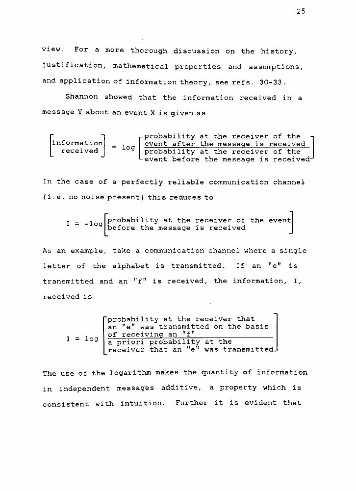
view. For a more thorough discussion on the history,

justification, mathematical properties and assumptions,

and application of information theory, see refs. 30-33.

Shannon showed that the information received in a

message Y about an event X is given as

information

received

= log

probability at the receiver of the

event after the message is received

probability at the receiver of the

event before the message isreceived-

In the case of a perfectly reliable communication channel

(i.e. no noise present) this reduces to

I =-log

probability at the receiver of the event

before the message is received

As an example, take a communication channel where a single

letter of the alphabet is transmitted. If an"e"

is

transmitted and an"f"

is received, the information, I,

received is

I = log

probability at the receiver that

an"e"

was transmitted on the basis

of receiving an"f"

a priori probability at the

receiver that an"e"

was transmitted.

The use of the logarithm makes the quantity of information

in independent messages additive, a property which is

consistent with intuition. Further it is evident that

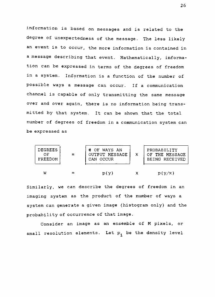
26

information is based on messages and is related to the

degree of unexpectedness of the message. The less likely

an event is to occur, the more information is contained in

a message describing that event. Mathematically, informa

tion can be expressed in terms of the degrees of freedom

in a system. Information is a function of the number of

possible ways a message can occur. If a communication

channel is capable of only transmitting the same message

over and over again, there is no information being trans

mitted by that system. It can be shown that the total

number of degrees of freedom in a communication system can

be expressed as

DEGREES

OF

FREEDOM

W

# OF WAYS AN

OUTPUT MESSAGE

CAN OCCUR

p(y)

PROBABILITY

OF THE MESSAGE

BEING RECEIVED

p ( y/x )

Similarly, we can describe the degrees of freedom in an

imaging system as the product of the number of ways a

system can generate a given image (histogram only) and the

probability of occurrence of that image.

Consider an image as an ensemble of M pixels, or

small resolution elements. Let p. be the density level

27

probability density function (PDF) of the image and Mp .

,

the number of observations, the ith density level, where i

ranges from 1 to n density levels. Further, let f . be the1

probability of observing the true signal value in a single

pixel (it will be shown later that this is the nonzero-mean

PDF of the noise). When f. = 1 for all i, there is no

uncertainty and each of the n density values occurs

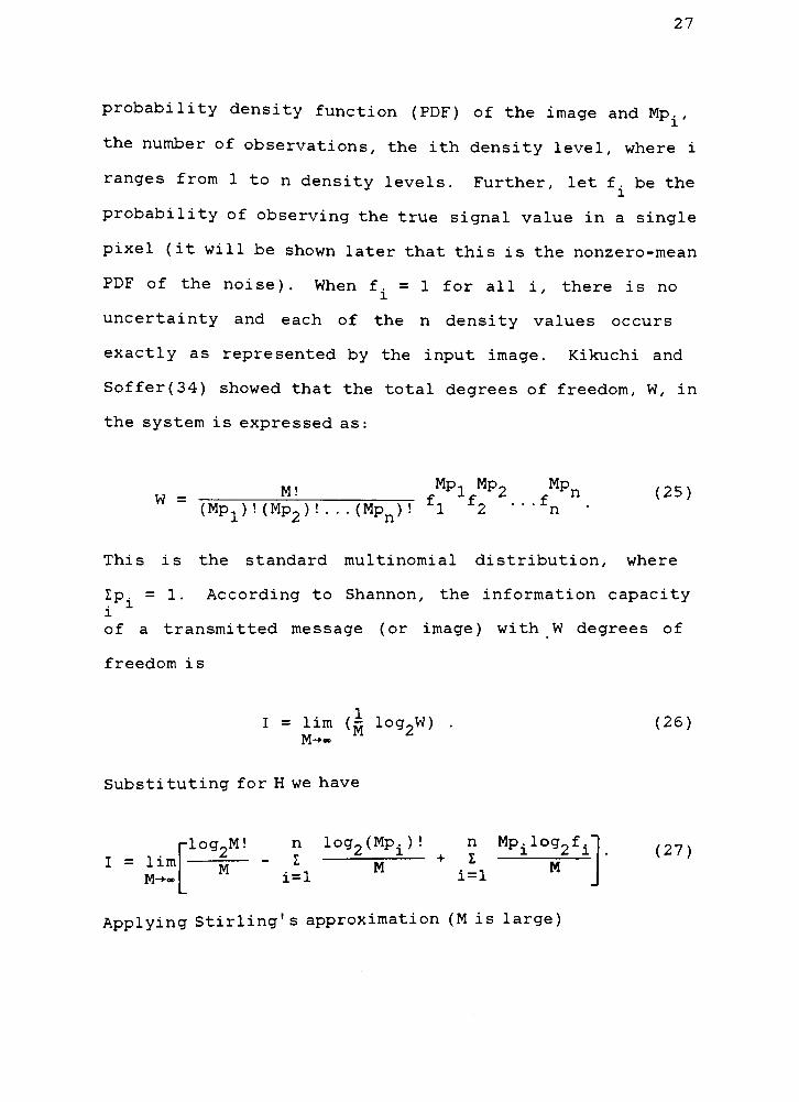
exactly as represented by the input image. Kikuchi and

Soffer(34) showed that the total degrees of freedom, W, in

the system is expressed as:

w-

M! fMPlfMP2 fMPn (25)(MPl)!(Mp2)!...(Mpn)! X X2

' ' '

X '

This is the standard multinomial distribution, where

lp. = 1. According to Shannon, the information capacity

i

of a transmitted message (or image) with W degrees of

freedom is

I = lim (^ log2W) . (26)M-*

Substituting for H we have

-log2M! n log2(Mpi)! n

Mp^og^'

I = lims

IS

+ Ijj

M-+<*> 1=1 1=1

Applying Stirling'sapproximation (M is large)

(27)

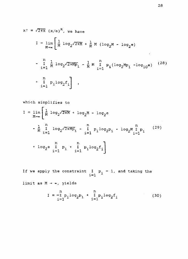
28

x! = /2ttx (x/e)x, we have

I = limM-+--

jj log2/27M + | M ( log2M - log e)

i n"

i = iM 1g2/5i]5!Pi

~

MM.! Pi(log2MPi -log1)e)

(28)

+

J, V92fi] >

which simplifies to

I = lim -

log v'2itM + logM - log_eM-~

|_1J

n n

r; I log /2ttMP. - I p log pi = l

z xi=l

2 ^ 1

n

log9M I pz

i=lx

(29)

+ iog2e

n n "I

Z p. + I p log f

i=l i=l J

If we apply the constraint Z p. = 1, and taking the

limit as M ->

~, yields

n

i=l

n

I = -Z p.log^p. + Z p. log.f

i=l1 z a

i=l2 z 1

(30)

29

The first term in equation (30) is the entropy (or

information) expression given by Shannon's second theorem,

and is analogous to Boltzmann's entropy of a cell in

statistical mechanics. Kikuchi and Soffer stressed that

for a noisy channel, the entropy is given by both terms in

equation (30), and it is this expression that is maximized

in order to determine the most likely distribution for p. .

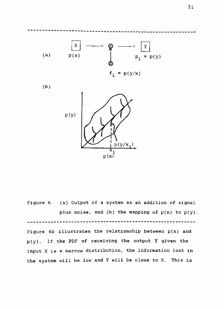
Equation (30) allows the consideration of a communi

cation channel (or imaging system) where an event (or

object) X is received by a message (or image) Y, with the

assumption of signal-independent, additive noise, n; this

is illustrated in Figure 6a. It follows that the PDF of

the signal, p., can be denoted p(y), and the PDF of the

noise, f., be denoted p(y/x) (which is read, "the probabil

ity of the output y, given the input,x"

) . Equation (30)

can now be rewritten as

I(x;y)=-Zp(y)log2p(y)

+ Zp(y ) log2p(y/x) (31)

where I(x;y) is the information in x and y.

This, by definition, is

I(x;y)= l(y)

- Ky/x) (32)

30

and represents the information about x contained in y.

Equation (32) can be interpreted as the information of the

event (or object) minus the information lost in the

channel .

31

(a)

X

P(x)

(b)

p(y)

?> Y

Pi=p(y)

f.1

=p(y/x)

Figure 6. (a) Output of a system as an addition of signal

plus noise, and (b) the mapping of p(x) to p(y)

Figure 6b illustrates the relationship between p(x) and

p(y). If the PDF of receiving the output Y given the

input X is a narrow distribution, the information lost in

the system will be low and Y will be close to X. This is

32

so because p(y/x) represents the noise PDF, and any

differences between p(y/x) and 6(y-x) (a one-to-one

mapping) are due to the PDF of the noise being convolved

with the PDF of the signal, to produce the PDF of Y, which

reduces the amount of information transmitted through the

system. The second term in equation (30) therefore

reduces the degrees of freedom in the system, and thus

does not allow as many possible images to be transmitted.

We can think of a given scene as a sample of an ensemble

of scenes whose probability is the reciprocal of the

degrees of freedom, and the imaging system as an imperfect

channel that will increase the probability of images,

thereby lowering the information content.

We now proceed to determine the most likely PDF for

p(y) and p(y/x), given constraints on the observed vari

ances of the message ( image) and the channel noise and,

CO

/ p(y)dy= 1. Shannon used Lagrangian multipliers and

stated the problem mathematically as

2max p(y)

= / [p(y)logp(y) + Xy p(y) + y p(y)]dy (33)

33

where X and y are normal Lagrangian multipliers. The

condition for this maximum is

-l-logp(y) +Xy2

+ y= 0 . (34)

Solving for p(y) yields

P(y)= OS)

The Lagrangian multipliers can be determined by applying

the constraints

22e"y

/ y2e"Xy

dy =o2

(36)

/ p(y)dy= 1 (37)

leading to

/ x1 (38)

p(y)=

-zzzz: e

?2it o

which shows that the most likely distribution is a

Gaussian. Similarly, p(y/x) is also found to be a

Gaussian. Substitution of p(y) and p(y/x) into (31)

yields

34

Kx,y) =

log2(/li-

0y) + 1-^ - log2(/5i on)- ^^ (39)

which reduces to

2

I(x,y) = 1logA\ (4)

'XSince the output signal Y is considered an addition of X

and N, the variances add, and,

2 ? O

i<*.y>=io,2f^yiic^i +!)- <>

This relationship will hold at each spatial frequency and

since all spatial frequencies are independent

IC = \ J I log2OO 00 }

+

wf^l]-udv

(42)

where IC is now the information content in a unit area.

Fellgett and Linfoot(35) first applied equation 42 to

photographic images. Assuming isotropy, the integral can

be expressed in terms of a radial spatial frequency variable,

/~2 2u = /u + v ,

to yield

35

wc

IC = ir / log_ 1 + -|iL wd<o(43)

02 WSN(W)

where wc is the cutoff frequency.

This is the familiar form of information content which

shows that the information content in an image is related

to the system signal-to-noise ratio. Dainty and Shaw have

shown(36) that equation (43) can be stated in terms of the

NEQ at a given mean exposure value Q

u

c

IC = tt / log,[l + NEQ(Q,u)P(w) ]wdu (44)0

*

where P(w) is the original signal power spectrum in

2exposure space (quanta area) . For this work the SNR

given by equation (14) was used for the integrand in the

information content calculations. Although the theory is

developed for band- limited and not peak- limited systems

(imaging is both) the information content is still a

reasonable metric if one treats the peak-limited, or

clipped, signal as a source of noise; the derivation of

this was discussed earlier.

36

EXPERIMENTAL

The experimental effort has mainly involved the

generation of images via the tone restoration scheme and

measurement of the signal power spectrum and Wiener noise

spectrum, from which the NEQ and information content were

calculated.

Generation of Images

The original negatives were generated on 4x5 Kodak

Tri-X pan film. The negatives were scanned with an

Optronics drum scanner using a 100 ym square aperture,

50 ym square sampling, logarithmic amplifier, and 10 bit

quantization; the data were stored on magnetic tape. The

tone restoration step was performed on the coded density

image via a look-up table of code values derived from

remapping functions of the kind shown in Figure 1.

Following the restoration, the code values were converted

to digital voltage values which modulated an exposing

source via a D/A converter, generating the output density

image. The playback was also done on the Optronics using

the same sampling parameters as in the scan mode, with one

major exception which was that the D/A converter contained

8 rather than 10 bits. The output images were written

37

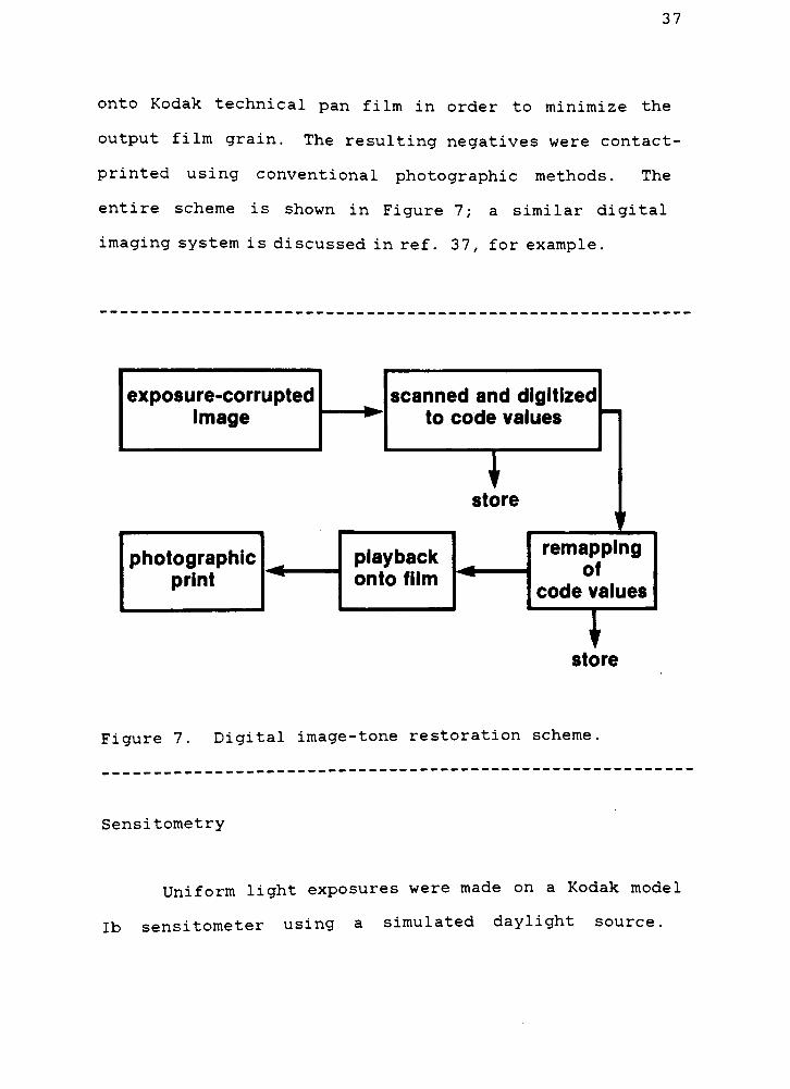
onto Kodak technical pan film in order to minimize the

output film grain. The resulting negatives werecontact-

printed using conventional photographic methods. The

entire scheme is shown in Figure 7; a similar digital

imaging system is discussed in ref . 37, for example.

exposure-corrupted

image

scanned and digitized

to code values

Tstore

photographic

print

playback

onto film

remapping

of

code values

Tstore

Figure 7. Digital image-tone restoration scheme.

Sensitometry

Uniform light exposures were made on a Kodak model

lb sensitometer using a simulated daylight source.

38

Fourteen samples representing the useful density range of

the film were created for Wiener spectrum measurements and

for input into the tone restoration process. The samples

were treated identically to the actual images and were

tone restored to the appropriate levels according to the

desired remapping function for that level of underexposure.

The end product was a series of uniform exposures made on

the playback film for each underexposure case, to allow

for the complete description of the noise as a function of

density and degree of underexposure. The original Tri-X

images were developed in undiluted Kodak developer D-76,

as recommended by the manufacturer. The playback images

were written onto Kodak technical pan film, type 2415, and

were developed in Kodak HC-110 developer, dilution D,

using tray development at room temperature.

MTF Measurements

As described in Figure 3 of the image-chain model,

there are three MTF factors of concern in the system: the

MTF of the original recording film, MTF1# the MTF of the

scanner, MTF2 ,and the MTF of the playback writer, MTF4

(assuming that the MTF of the Kodak technical-pan playback

film is unity across the frequency range of interest

39

here). The MTF of the Kodak Tri-X pan film was measured

at normal, 2, 4, and 6 stops underexposure using the

sine-wave fringe method of Lamberts and Eisen(38). During

scanning, the scanning aperture is generally smeared with

a response envelope (rise, sustain, and decay) across each

pixel; in this work this was approximated by a Dirac delta

function. Additionally, the aperture function is generally

convolved with the sampling lattice, which is represented

by a lattice of delta functions. This results in a MTF in

both the X and Y direction of

MTF(w) = sinc(0. IOOitu) (45)

Wiener Noise Spectrum Measurements

A description of the methods available for measure

ment of the Wiener spectrum for image noise analysis can

be found in Dainty and Shaw(39). The equipment and proce

dure used for Wiener spectrum measurements in this study

are those described by Bunch et al.(40). Here, only a

brief description of the important measurement parameters

follows.

A two-dimensional image density fluctuation, AD(x,y)

existing over an image area (+X, +Y) has a Wiener spectrum

defined by

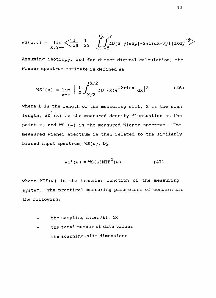
40

(u,v) = lim<X2x ~|y / J AD(x,y)exp[-2ni(ux+vy) ]dxdy

>>

Assuming isotropy, and for direct digital calculation, the

Wiener spectrum estimate is defined as

.

+X/2

wc'/,.\ - i-;L / in'/ \

-2iTix . 2 (46)WS (oo) - lim r? / AD (x)e dx |v '

x' X-ix/2

where L is the length of the measuring slit, X is the scan

length, AD (x) is the measured density fluctuation at the

point x, and WS'(w) is the measured Wiener spectrum. The

measured Wiener spectrum is then related to the similarly

biased input spectrum, WS(io), by

WS'

(w) = WS(u)MTF2(u) (47)

where MTF(w) is the transfer function of the measuring

system. The practical measuring parameters of concern are

the following:

the sampling interval, Ax

the total number of data values

thescanning-slit dimensions

41

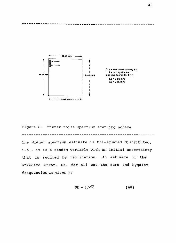
The Wiener noise spectrum measurements were made on a

Perkin-Elmer PDS model 1010A microdensitometer dedicated

to this purpose. Since both contact prints and 8x10 2X

enlargements were to be made (to span the visual bandwidth

assumed to be 10 cycles/mm at IX), a Nyquist frequency of

20 cycles/mm was chosen to be appropriate for viewing. To

help avoid aliasing, this necessitated a scanning aperture

width of 25 ym, or larger; the actual slit dimensions used

were 20x760 ym, which was experimentally convenient.

Figure 8 shows the scanning scheme used in this study. To

synthesize a suitably long scanning slit (in this case 8 x

0.76 mm = 6.08 mm) the original 131,072 transmittance

readings were averaged across 8 physical slits, reducing

the total number of points to 16,384, and the grand mean

of the resulting array was subtracted from each value of

the array. The array was segmented into 64 slices

40.96 mm long and a Wiener spectrum was then computed for

each slice. The Wiener spectrum was the average across

the slices and divided by the aperture function to arrive

at the final Wiener noise spectrum.

42

410.96 mm

48.64 mm

2048 point**

64 roittfi

0.02 x 0.76 mm scanning slit

a x slit synthesis

2.66 mm blocks for FFT

Ax ' 0 02 mm

Ay * 0 76 mm

Figure 8. Wiener noise spectrum scanning scheme

The Wiener spectrum estimate is Chi-squared distributed,

i.e., it is a random variable with an initial uncertainty

that is reduced by replication. An estimate of the

standard error, SE, for all but the zero and Nyquist

frequencies is given by

SE = 1//TT (48)

43

where N is the number of blocks in the data stream.

Because there is one less degree of freedom at the zero

and Nyquist frequencies, the standard error at these

frequencies is/2~

higher than that at all others. For a

128 block stream, the SE's at zero and other frequencies

are 12.5% and 9%, respectively.

Signal Power Spectrum <& Probability Density Measurement

The object scene was assumed to be separable in the X

and Y directions; a 512x512 two-dimensional FFT was

performed on a region of the image (the woman's face) that

was considered the most important in assessing the quality

of the image. Since the separability assumption contra

dicts the isotropic assumption made earlier, and, since

the signal-to-noise ratio was not considered from a

directional standpoint, an average of the zero frequency X

and Y direction signal power spectra was used in the

analysis. This is a reasonable assumption for everyday

scenes and the assumption has very little effect on the

final results.

A code value histogram (linear with exposure) of the

8 bit output 512x512 array was made. Since code value is

equivalent to exposure, the probability density function

44

in code value is equivalent to the probability density

function in exposure.

Subjective Assessment of Images

Thirty observers were asked to assess the relative

image-structure quality of the underexposed and tone

restored images. The instruction given to the observers

was to rate the degree of quality with respect to the

amount of detail present in the woman's face, relative to

that of the first (normally exposed) picture. The

observers were instructed to give their ratings relative

to a value of 100% for the normally exposed image.

45

RESULTS AND DISCUSSION

NEQ Measurements

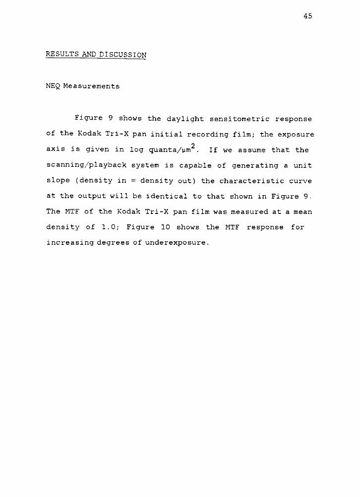
Figure 9 shows the daylight sensitometric response

of the Kodak Tri-X pan initial recording film; the exposure

2axis is given in log quanta/ym . If we assume that the

scanning/playback system is capable of generating a unit

slope (density in = density out) the characteristic curve

at the output will be identical to that shown in Figure 9.

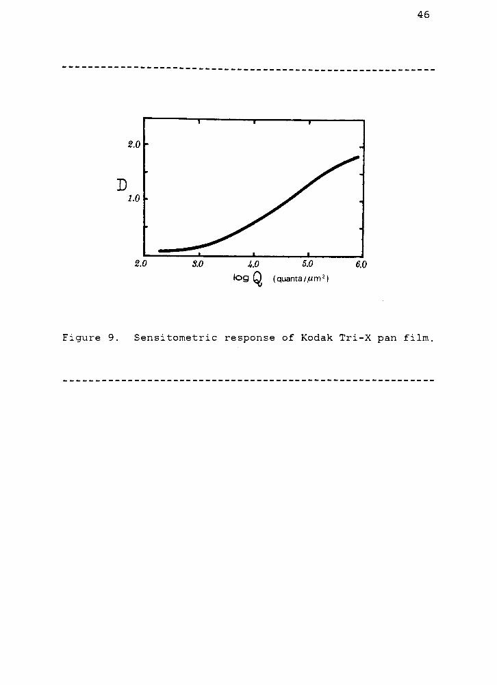
The MTF of the Kodak Tri-X pan film was measured at a mean

density of 1.0; Figure 10 shows the MTF response for

increasing degrees of underexposure.

46

S.O U.O 5.0 6.0

log Q (quanta/,um2)

Figure 9. Sensitometric response of Kodak Tri-X pan film,

47

MTF (%)

150

100

70

50

30

20

10

^

D = 1 [for nc rmal expos jre]

10 20 50 100 200 400

Spatial frequency (cycles/mm)

Figure 10. MTF of Kodak Tri-X pan film for various degrees

of underexposure

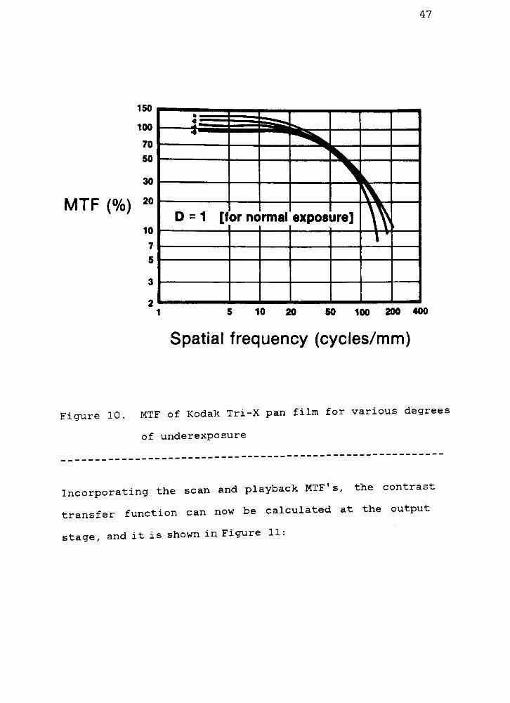
Incorporating the scan and playback MTF's, the contrast

transfer function can now be calculated at the output

stage, and it is shown in Figure 11:

48

1.0,

yMTF

0.6-

0.2-

2.0

Spatial e.o

frequency(cycles/mm) 1(h0

Outp^

dWused*w

Figure 11. Contrast transfer function at output stage of

system

The noise Wiener spectrum at the output stage is given in

Figure 12.

49

60.0 i

D2-/jm*

Spatial 6.0

frequency

(cycles/mm) 10>0

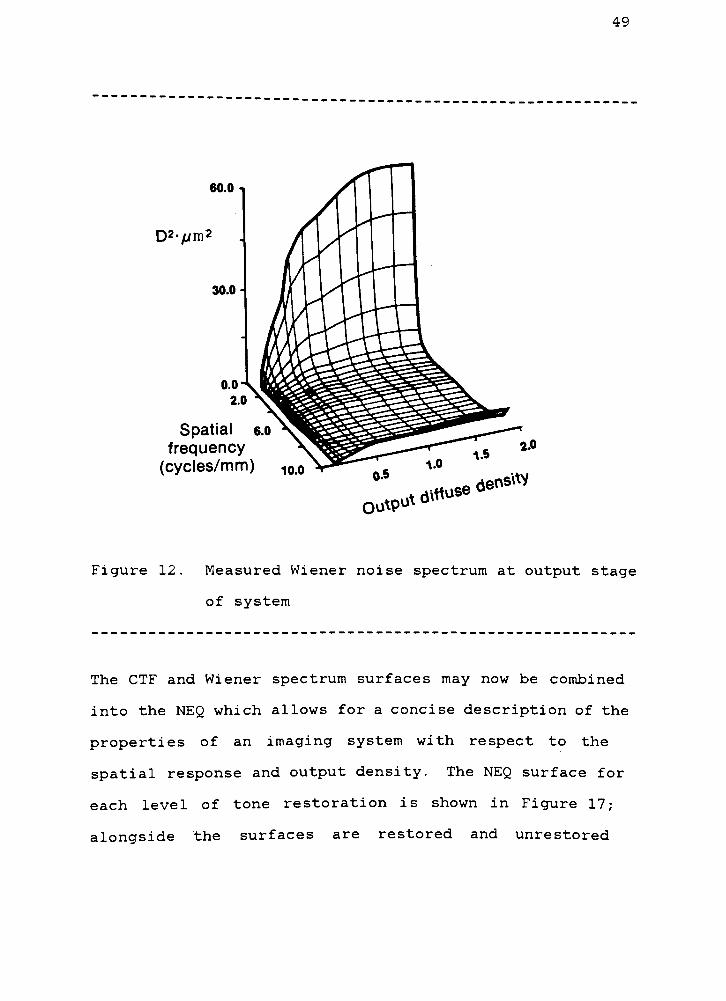
Figure 12. Measured Wiener noise spectrum at output stage

of system

The CTF and Wiener spectrum surfaces may now be combined

into the NEQ which allows for a concise description of the

properties of an imaging system with respect to the

spatial response and output density. The NEQ surface for

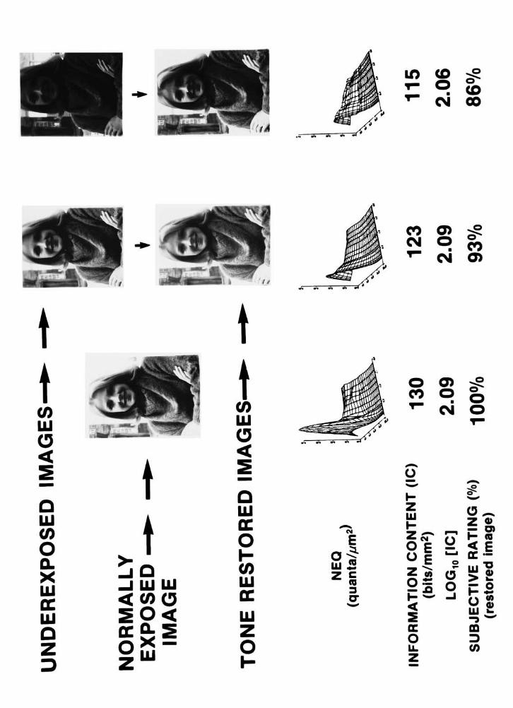
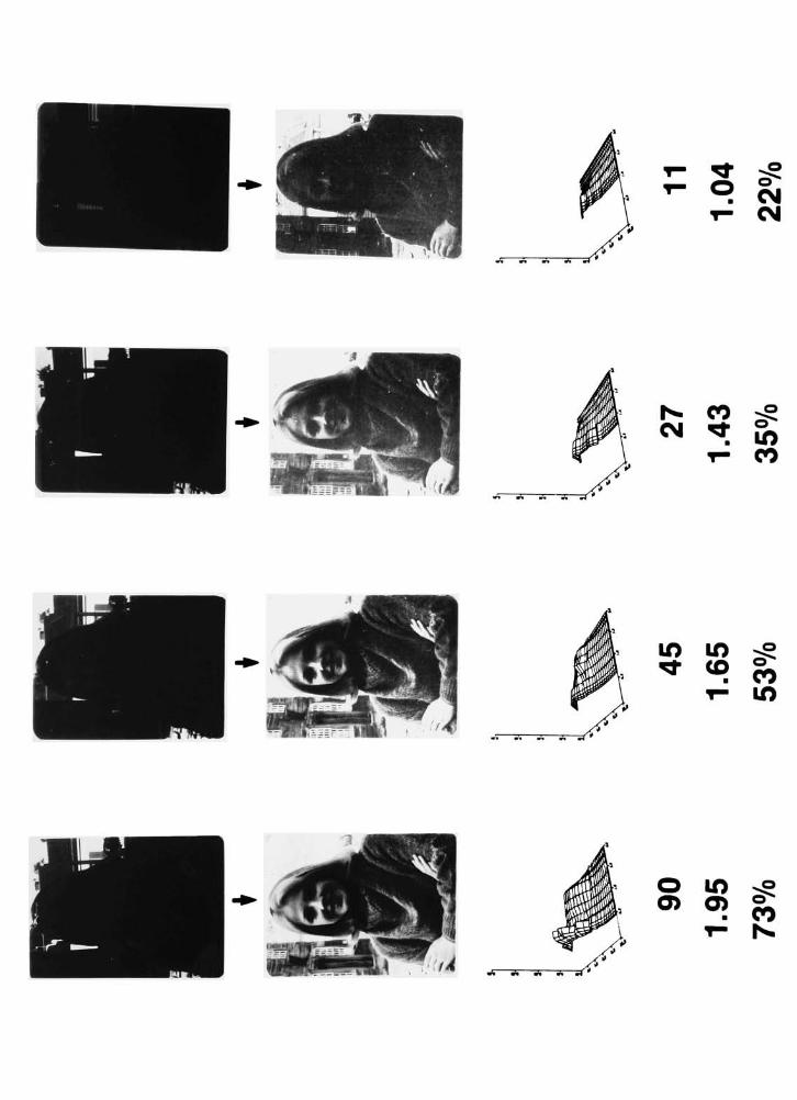
each level of tone restoration is shown in Figure 17;

alongside the surfaces are restored and unrestored

50

images. Note that the trend in the loss of NEQ with

progressive degrees of tone restoration seems to follow

the perceived degradation in image-structure quality of

the tone restored images. Further, the order of magnitude

of the NEQ (a maximum of about 0.04/ym2) is consistent

with what would be expected from a moderate-quality

conventional photographic system, whereas the highest

quality would yield an NEQ approaching 1.0/ym2(41).

Calculation of Quantization Noise and Clipping

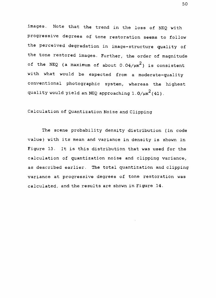
The scene probability density distribution (in code

value) with its mean and variance in density is shown in

Figure 13. It is this distribution that was used for the

calculation of quantization noise and clipping variance,

as described earlier. The total quantization and clipping

variance at progressive degrees of tone restoration was

calculated, and the results are shown in Figure 14.

51

*103 12

10-

8-

MEAN DENSITY = 0.58

DENSITY VARIANCE =0.074

50 100 150

8 Bit code value

200 250

Figure 13. Scene probability density distribution,

52

"C

-3

-4

O QUANTIZATION & CLIPPING....A QUANTIZATION ONLY

Log10D2

-5 CT a

""~X

^

-6

-7III

0 1 2 3 4 5

Underexposure (stops)

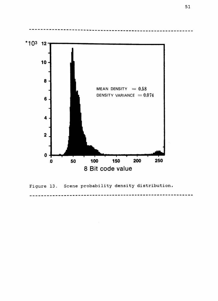
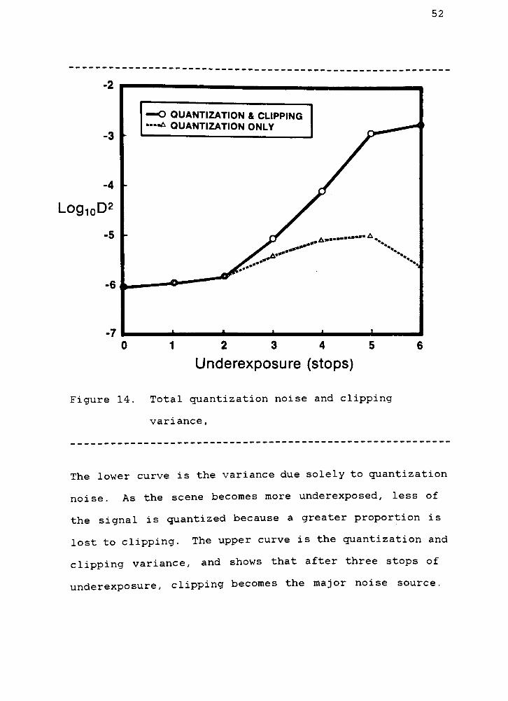
Figure 14. Total quantization noise and clipping

variance.

The lower curve is the variance due solely to quantization

noise. As the scene becomes more underexposed, less of

the signal is quantized because a greater proportion is

lost to clipping. The upper curve is the quantization and

clipping variance, and shows that after three stops of

underexposure, clipping becomes the major noise source.

53

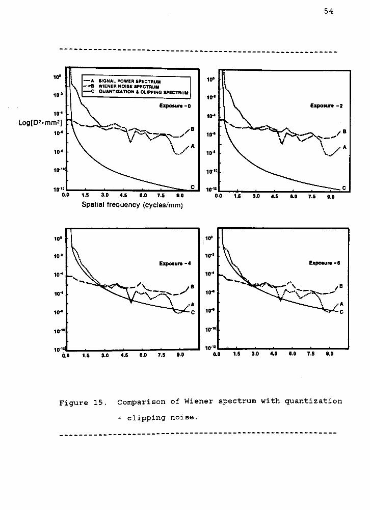
As discussed earlier, Nq+c(w) was assumed to follow the

shape of the measured signal power spectrum, S(w), with

variances given by equations (21) and (23). The calculated

spectrum, Ng+c(w), can now be compared with the measured

Wiener noise spectrum (which is signal independent, and

thus contains no quantization or clipping noise) and with

the measured signal power spectrum of the original scene,

translated into density. For the normally exposed case,

Nq+C(w) has relatively low power compared with the Wiener

noise and signal power spectrum. As we move towards a

greater degree of tone restoration, the quantization and

clipping noise become dominant and as Figure 15 illus

trates, severely reduces the SNR; it is apparent that the

majority of the signal exists below 3 cycles/mm. These

calculated results are consistent with the observed

degradation of quality in the images shown in Figure 17.

It should be emphasized that the low power at high fre

quencies does not mean that the high-frequency information

is unimportant. It simply means that because of low

power, this information is especially vulnerable to the

system noise and can be easily obscured by noise.

54

10"

io-J

io-<

Log[D2mm2]10"*

A SIGNAL POWER SPECTRUMB WIENER NOISE SPECTRUMC QUANTIZATION ft CLIPPING 8PECTRUM

Ex|>oturt-0

1.5 3.0 4.5 6.0 7.5 9.0

Spatial frequency (cycles/mm)

10 i1

10-'

Mr*1\-

lO*

10-* : \ \x

10"" ^^^^10-"

0.0 1.5 .3.0 4.5 6.0 7.5 9.0

10

10'

\ *

Exposure -4

10-"

10-*

k

Mr* ^*--c

10"

lO"12

-

10

io-

Expour -6

Mr*

Mr*

Mr*

10""

10-"

I

6.0 1.5 3.0 4.5 6.0 7.5 9.0 0.0 1.5 3.0 4.5 6.0 7.5 9.0

Figure 15. Comparison of Wiener spectrum with quantization

+ clipping noise.

55

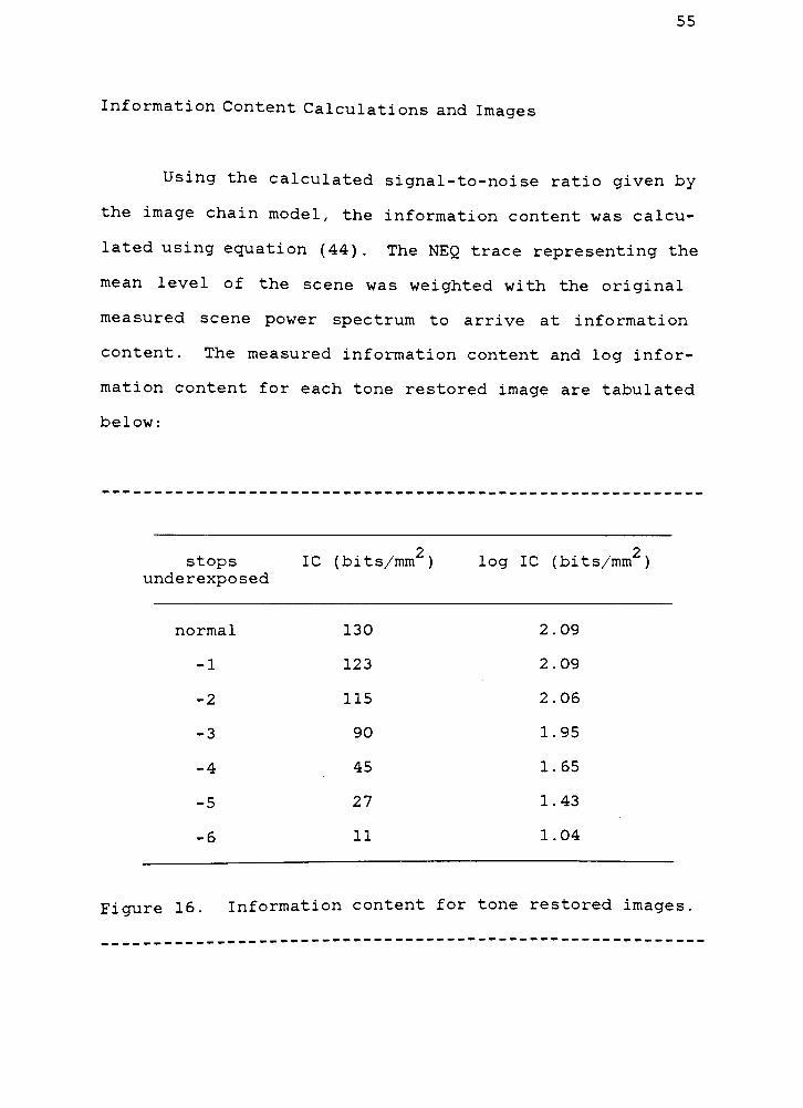
Information Content Calculations and Images

Using the calculated signal-to-noise ratio given by

the image chain model, the information content was calcu

lated using equation (44). The NEQ trace representing the

mean level of the scene was weighted with the original

measured scene power spectrum to arrive at information

content. The measured information content and log infor

mation content for each tone restored image are tabulated

below:

2 2stops IC (bits/mm ) log IC (bits/mm )

underexposed

normal 130 2.09

-1 123 2.09

-2 115 2.06

-3 90 1.95

-4 45 1.65

-5 27 1.43

-6 11 1-04

Figure 16. Information content for tone restored images.

56

These results are shown with the images in Figure 17 and

compared with the visual assessment of underexposed and

tone restored images in Figure 18.

IA <0 ^::

<=> s>r

W 00

t

t(/>

UJ

(3<

5

oLU

(/>

OQ.

XUJ

ccUJ

Q

Z

D

t

t2Qj UJ UJ

< coo20<

OCCLS

Q X

X UJ

t

t

CO O) ^2!

<=>co

r\i o

CO

O)

0)T*

oi OUJ

(5 .^P

*"

<-; s s s 5*

5 o

Q 1- p**^

UJzUJ O^

CC ^s ssO E

5~

O Po

1-

< EH C

',oc -

(0

UJ

cc

UJ

o

(5

O

z

oOLL

is

Hz

S S 3T

9 oii- CM

r^ co -g

* * 5>i- CO

lO IT)

9 CO

o IT) ^o

o> o> g:CO

1- 1^

58

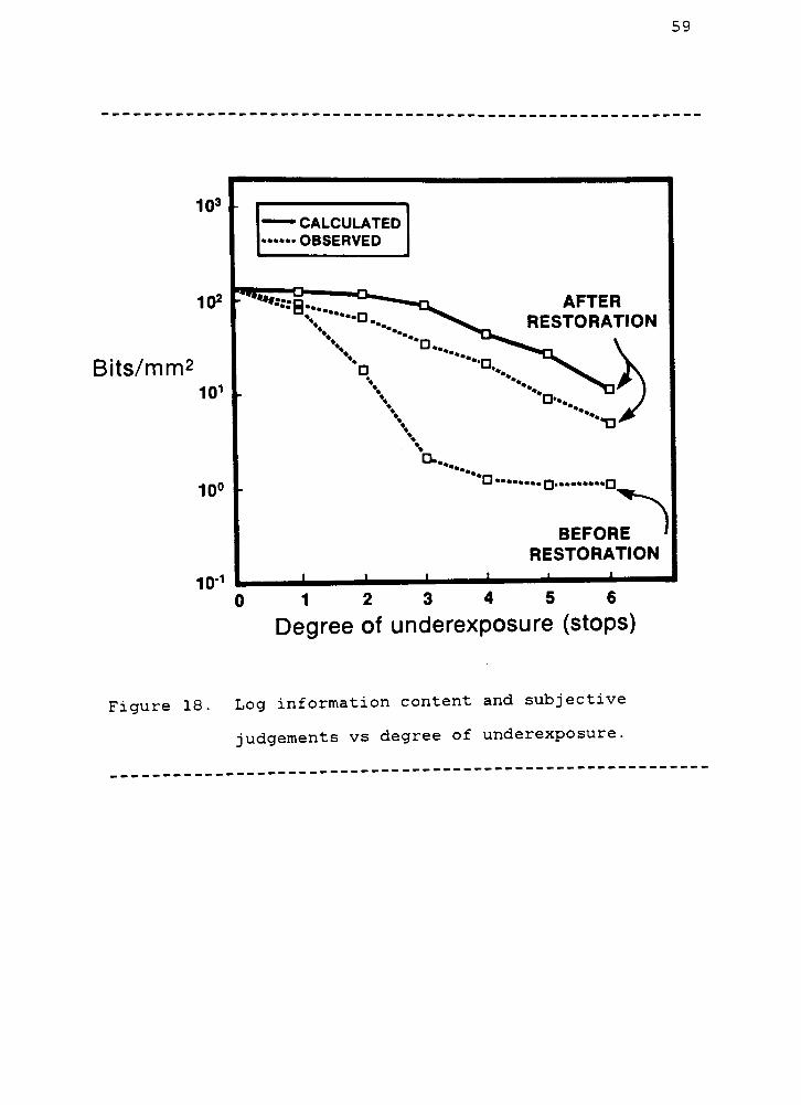
Figure 18 does give some indication that the logarithm of

information content correlates with the visual perception

of image quality in the restored images. It should be

stressed that although the eye perceived an information

gain in the tone restored images (as is illustrated by the

two lower curves), in fact, the actual information content

in a tone restored image is less than or equal to that of

the corresponding underexposed image. This is due to

clipping, sampling, quantization, and playback degradations

as well as the enhanced noise of the original underexposed

image. The reason that the human observer perceives the

restored image as having higher information despite the

increased degradations is that the densities of the

restored images are better matched to the dynamic range

(and contrast sensitivity) of the eye. Since the sensi

tivity of the human visual system was not included in the

model, it was necessary to eliminate this dynamic range

factor by tonally restoring the images so that only the

additional degradations included in the calculations would

limit the perceived quality. If the sampling and playback

system did not introduce degradations, an infinite number

of bits were available, the original recording sensitometry

never had a zero slope, and noise was not present, the

restored images would have the same quality as the normally

exposed image .

59

103

Bits/mm2

CALCULATED

OBSERVED

10"1

AFTER

RESTORATION

BEFORE

RESTORATION

1 2 3 4 5 6

Degree of underexposure (stops)

Figure 18. Log information content and subjective

judgements vs degree of underexposure.

60

CONCLUSIONS

It has been shown that signal-to-noise metrics,

information content and NEQ are useful in characterizing

the performance of an image- tone restoration system. For

discrete sampled images it was necessary to include

degradations such as quantization noise and clipping, as

they were found to be the major source of degradation in

extreme tone restoration cases. The question of a real

effective speed increase obtained by tone restoration was

addressed. Although an effective speed increase is

realized with tone restoration, it is difficult to quantify

because it does not include the effect of quantization.

In the light of the present and future use of photographic

film as an initial recording medium for digital image

processing, the speed alone of a film is not an adequate

measure of a recordingfilms'

s capabilities.

61

REFERENCES

1. CN. Nelsen, in T. H. James, ed., The Theory of the

Photographic Process. Macmillan, New York, 1977,

ch. 19.

2. P. Kowaliski, Applied Photographic Theory, John Wiley

and Sons, New York, 1972, ch. 1.

3. G. Haist, Modern Photographic Processing, Vol. 1 and

2, John Wiley and Sons, New York, 1979.

4. W.K. Pratt, Digital Image Processing, John Wiley

& Sons, New York, 1978, pp. 307-311.

5. R.C. Gonzalez and P. Wintz, Digital Image Processing,

Addison-Wesley, Reading, Mass., 1977, pp. 118-139.

6. R. Shaw, "Evaluating the Efficiency of Imaging

Processes,"

Rep. Prog. Phys . 41: 1103-1155 (1978).

7. J.C. Dainty and R. Shaw, Image Science, Academic Press,

New York, 1974.

8. R. Shaw, ed., Selected Readings in Image Evaluation,

SPSE (1976).

9. R. Shaw, ed. ,Image Analysis and Evaluation,

SPSE Conference, Toronto (1976).

10. P.S. Cheatham, ed. , Image Quality, SPIE Proc,

vol. 310, San Diego (1981).

11. International Congress of Photographic Science Proc,

SPSE, Rochester (1978).

62

12. M. Kriss, in T.H. James, ed., The Theory of the Photo

graphic Process. Macmillan, New York, 1977,

ch. 21.

13. J.C. Dainty and R. Shaw, oc_ cit. , ch. 5.

14. A. Rose, "The Dependence of Image Quality on Quantum

Efficiency in Available LightPhotography,"

in R. Shaw, ed., Image Analysis and Evaluation,

SPSE Proc, Toronto (1976).

15. O.H. Schade, "An Evaluation of Photographic Image

Quality and Resolving Power,"J. Soc. Motion

Pict. Tel. Eng., 73: 81 (1964).

16. G. Higgins, "Image Quality,"

J. Appl . Photogr. Eng. 3:

53-60 (1977).

17. C. Shannon, "A Mathematical Theory ofCommunication,"

Bell Syst. Tech. J. 27: 379 (1948).

18. P.B. Felgett and E.H. Linfoot, "On the Assessment of

OpticalImages,"

Phil. Trans. Roy. Soc. London,

Ser. A 247: 369-407 (1955).

19. R.C. Jones, "The Information Capacity of Photographic

Films,"

J. Opt. Soc. Am. 4 : 799 (1955).

20. R. Shaw, "The Application of Fourier Techniques and

Information Theory to the Assessment of Photo

graphic Image Quality,"Photogr. Sci. Eng. :

281-286 (1962).

63

21. M. Kriss, J. O'Toole, J. Kinard, "Information Capacity

as a Measure of Image Structure Quality of the

Photographic Image,"

(see ref. 6).

22. K.V. Vendrovsky, et aL, "Information Content of B/W

and Color Images,"

ICPS Proc, 1978.

23. C.L. Fales, F.O. Huck, R.W. Samms, "Imaging System

Design for Improved Information Capacity,"

Appl. Opt. , 23: 872-888 (1984).

24. J.H. Altman, in T.H. James, ed. , The Theory of the

Photographic Process, Macmillan, New York, 1977,

pp. 507-509.

25. J.H. Altman, ibid., p. 508.

26. R. Shaw, "Photon Fluctuations, Equivalent Quantum Effic

iency, and the Information Capacity of Photo

graphicImages,"

J. Phot. Sci. ^1: 313-320 (1963).

27. See, for example: G.R. Cooper and CD. McGillem,

Methods of Signal and System Analysis, Holt,

Rinehart, New York, 1967, ch. 8.

28. W.K. Pratt, op^ cit.,p. 142.

29. C. Shannon, op. cit.

30. A.I. Khinchin, Mathematical Foundations of Information

Theory, Dover, New York, 1957.

31. S. Goldman, Information Theory, Prentice-Hall, New

York, 1953.

64

32. P.M. Woodward, Probability and Information Theory

with Applications to Radar, Pergamon Press, Oxford,

1953, ch. 3.

33. B.R. Frieden, Probability, Statistical Optics, and Data

Testing, Springer-Verlag, New York, 1983, ch. 10.

34. R. Kikuchi and B.H. Soffer, "Maximum Entropy Image

Restoration. The EntropyExpression,"

J. Opt. Soc Am. 67: 1656-1665 (1977).y\^

35. P. B. Fellgett and E. H. Linfoot, op. cit.

36. J.C Dainty and R. Shaw, op. cit.,ch. 10.

37. J.E. Boyd, "Digital Image Film GenerationFrom the

Photoscientist'sPerspective,"

J. Appl. Photo. Eng. 8: 15-22 (1982).

38. R.L. Lamberts and F.C. Eisen, "A System for Automated

Evaluation of Modulation Transfer Functions of

PhotographicMaterials,"

J. Appl. Photogr. Eng.

6: 1-8 (1980).

39. J.C. Dainty and R. Shaw, op. cit. ,ch. 8.

40. P.C Bunch, R. Shaw, R.L. Van Metter, "Signal-to Noise

Measurements for a Screen-FilmSystem,"

SPIE Proc, San Diego (1984).

41. J.C Dainty and R. Shaw, oc_ cit.

65

VITA

Paul W. Melnychuck was born in 1960 in Yonkers, New

York, and lived in Mohegan Lake, New York, for most of his

life. In 1978 he attended the Rochester Institute of

Technology and in 1980 received the A.A.S. in Photographic

Science, in 1982 the B.S. in Chemistry, and in 1984 the

M.S. in Imaging and Photographic Science. While at RIT,

Paul was employed with Eastman Kodak Company for three

years as a cooperative education student. Presently, he

is with the Image Analysis Group of the Kodak Research

Laboratories .