Policy ReseaRch WoRking PaPeR 4555

Informal Payments and Moonlighting in Tajikistan’s Health Sector

Andrew DabalenWaly Wane

The World BankEurope and Central Asia Region Poverty Reduction & Economic Management Sector Unit &Development Research GroupHuman Development and Public Services TeamMarch 2008

WPS4555P

ublic

Dis

clos

ure

Aut

horiz

edP

ublic

Dis

clos

ure

Aut

horiz

edP

ublic

Dis

clos

ure

Aut

horiz

edP

ublic

Dis

clos

ure

Aut

horiz

ed

Produced by the Research Support Team

Abstract

The Policy Research Working Paper Series disseminates the findings of work in progress to encourage the exchange of ideas about development issues. An objective of the series is to get the findings out quickly, even if the presentations are less than fully polished. The papers carry the names of the authors and should be cited accordingly. The findings, interpretations, and conclusions expressed in this paper are entirely those of the authors. They do not necessarily represent the views of the International Bank for Reconstruction and Development/World Bank and its affiliated organizations, or those of the Executive Directors of the World Bank or the governments they represent.

Policy ReseaRch WoRking PaPeR 4555

This paper studies the relationship between gender and corruption in the health sector. It uses data collected directly from health workers, during a recent public expenditure tracking survey in Tajikistan’s health sector. Using informal payments as an indicator of corruption, women seem at first significantly less corrupt than men as consistently suggested by the literature. However, once power conferred by position is controlled for, women appear in fact equally likely to take advantage of corruption opportunities as men. Female-headed facilities also are not less likely to experience informal charging than facilities managed by men. However, women are

This paper—a product of ECA PREM and the Human Development and Public Services Team, Development Research Group—is part of a larger effort in the department to understand corruption in public services especially coping strategies health workers adopt such as informal payments and the holding of other jobs outside the facility. Policy Research Working Papers are also posted on the Web at http://econ.worldbank.org. Andrew Dabalen may be contacted at adabalen@worldbank.org and Waly Wane at wwane@worldbank.org.

significantly less aggressive in the amount they extract from patients. The paper provides evidence that workers are more likely to engage in informal charging the farther they fall short of their perceived fair-wage, adding weight to the fair wage-corruption hypothesis. Finally, there is some evidence that health workers who feel that health care should be provided for a fee are more likely to informally charge patients. Contrary to informal charging, moonlighting behavior displays strong gender differences. Women are significantly less likely to work outside the facility on average and across types of health workers.

Informal Payments and Moonlighting in Tajikistan’s Health Sector

Andrew Dabalen, and Waly Wane1

Europe and Central Asia Region, and Development Research Group

The World Bank

Email for Correspondence: adabalen@worldbank.org, wwane@worldbank.org

Keywords: Gender; Corruption; Informal payments; Moonlighting; Health care; Tajikistan; JEL Classification: I10; J20; K42;

1 We would like to thank Couro Kane for her suggestions and support in the earlier stages of this paper. We are also grateful to Logan Brenzel, Elizabeth King, and Steve Knack for very helpful comments on an earlier draft. The findings, interpretations, and conclusions expressed in this paper are those of the authors, and do not necessarily represent the views of the World Bank, its Executive Directors, or the countries they represent.

1

1. Introduction The causes and consequences of corruption are well researched and widely known. There is

ample cross-country empirical evidence that corruption slows growth, reduces public and

private investment (Mauro 1995), and negatively impacts service delivery (World Bank

2004). However, knowledge about what causes individuals to engage in corrupt or illegal

activities is scant. Several determinants of individual corruption have been recently proposed

among which the most stunning and not least controversial is gender. Proponents of this

theory claim that men’s proclivity towards corruption is inherently higher than women’s.

This paper investigates this issue and presents new evidence based on data collected during a

public expenditure tracking survey (PETS) in Tajikistan’s health sector. It shows that women

are no less prone to extorting illegal payments from patients than men once the proper

variables, such as power conferred by position for instance, are controlled for.

Men and women certainly display countless obvious physical and physiological differences.

Attitudinal gender differences have been an active research matter for sociologists and

psychologists for many decades. Although moderate to large differences are acknowledged in

some areas (e.g. sexuality and aggression) men and women display more similarities than

differences (see Hyde, 2005). Economists started to integrate gender in their analysis only

recently and have uncovered interesting gender differences mostly through experiments. This

paper studies two important forms of corruption in the health sector (1) informal charging

and (2) moonlighting. Informal charging is a bribe-taking practice and is clearly classified as

an illegal activity. Moonlighting is a more subtle form of corruption because it is not readily

identified as theft or use of public office for private gain. In fact, moonlighting is a strong

determinant of absenteeism and workers who collect their salary but do not show up at work

can be considered as stealing public money (see Lewis 2006).

The main result of this paper is that with similar power and opportunities, women are equally

likely as men to extract bribes by informally charging patients. However, among doctors and

doctors only, women are less aggressive than men, i.e., they charge smaller amounts. Women

are, on the other hand, significantly less likely to moonlight than men and this holds true

even within positions. Finally the paper shows that there is some evidence for the fair wage-

2

corruption hypothesis but no support for the fair wage-shirking hypothesis. Specifically,

workers whose perceived fair wage is much lower than their actual wage are more likely to

engage in informal charging but they are not more likely to moonlight.

The paper is organized as follows. Section 2 reviews the literature relevant to this paper.

Section 3 describes the Tajikistan PETS data used in the paper and presents summary

statistics. Section 4 states the econometric strategy used to identify the impact of gender on

informal charges and moonlighting. Section 5 presents the results and section 6 concludes.

2. Related Literature

This section reviews two strands of literature to which this paper is linked. We first address

the specific literature of corruption in the health sector before turning to the gender and

corruption literature.

2.1 Corruption in Health

The health sector often ranks among the most corrupt in many developing countries. In a

survey on corruption perceptions in 23 countries the health sector ranked in the top four in

ten countries. The many forms of corruption in the health sector range from the

commercialization of public positions to staff absenteeism (see Lewis 2006). Corruption also

arises at several levels, from the central government to the health facilities including all

intermediary administrative layers. This sub-section focuses on corruption at the front-line

service delivery level.

The most pervasive and studied form of corruption at the point of service delivery is informal

payments. Informal payments can be broadly defined as direct unofficial payments, in-kind

or in cash, from patients to health workers for the latter’s personal benefit. The study of

informal payments poses major challenges, the first of which is measurement. Users are the

most common source of information on informal payments through household surveys and

patients’ exit polls. Unfortunately, users sometimes have a hard time distinguishing between

3

formal fees, legal gifts and illegal payments which render the measurement of informal

payments extremely difficult. Several authors tried to go around this problem by considering

as informal, payments which are made for officially free services (see Chakraborty et al.

2002, Chawla et al. 1998). Some of these payments may sometimes be misclassified as

informal especially in countries where gift-giving is an entrenched cultural practice and

patients voluntarily present the health workers with a gift.2 This paper eschews this difficulty

by collecting the information on informal payments directly from the health workers who are

perfectly able to screen the legal and voluntary from the informal and requested or forced.

The pervasiveness of informal payments in developing and transition economies has attracted

a lot of attention because of their potentially detrimental effects on the health sector. Recent

studies have shown that informal payments reduce access to health for the poor, worsen

health outcomes and reinforce inequities (Killingsworth et al. 1999, Ensor 2004, Falkingham

2004, Gotsadze et al. 2005). Others argue that informal payments act as a barrier to reform

(Killingsworth et al. 1999, Lewis 2000, Thompson and Witter 2000), especially when they

are entrenched and constitute an important source of income for powerful people in the sector

such as doctors (Chawla et al. 1998). Yet, surprisingly others find that informal payments

increase performance measured by the time health staff work in the facility (McPake et al.

1999). This is not necessarily a sign of performance and could well be the opportunity cost of

staying out of the facility in terms of foregone income from informal payments. Given the

importance of informal payments, it is crucial to understand their determinants. The literature

has been heavily focused on the users’ side to answer who pays informal payments. This

paper comes as a complement by looking at the issue from the perspective of the providers

themselves controlling for a wide array of health workers’ characteristics and the

environment in which they operate. The main question this paper intends to address is “do

women take or accept informal payments less often than men?”

A second form of corruption which is of interest in this paper is moonlighting. Akerlof and

Yellen (1990) show theoretically that workers reduce their effort when they perceive to be 2 Recent household surveys make an extra effort to try and distinguish between formal fees, gifts and informal payments. They also try to draw the difference between voluntary and requested payments (e.g. Albania LSMS 2005).

4

paid less than their fair wage. The reduction in effort is proportional to the distance between

the fair and the actual wage. The fair-wage hypothesis may explain both corruption types

considered here: informal payments and moonlighting. As Akerlof and Yellen (1998) state it

“when people do not get what they [think they] deserve, they try to get even.” Akerlof and

Yellen (1990) assume the only instrument at the disposal of the worker to get even is

adjusting the level of her effort. In the health sector and maybe others, however, the worker

has many instruments to get even. She can withdraw effort and work outside of the

workplace, but she can also levy payments on the facility’s clients. Van Rijckeghem and

Weder (2001) show in a cross-country regression framework that relative civil-service pay is

strongly correlated with corruption levels and thereby corroborate the fair-wage and

corruption relationship. Van der Gaag et al. (1989) show using household data from Côte

d’Ivoire and Peru that civil servants’ wage disadvantage is a strong determinant of

moonlighting. This paper tests both the fair-wage corruption and fair-wage shirking or

moonlighting hypotheses. During the survey, the health workers are directly asked what they

consider to be a fair wage for the work they provide.3 Van Rijckeghem and Weder (2001)

use the manufacturing sector’s wage as a comparator for all civil-servants; however, the

salary a worker considers as fair crucially depends on personal circumstances and

haracteristics.

.2 Gender and Corruption

c

2

There is a large literature on gender differences in social preferences, risk-taking behavior

and taste for or reaction to competition.4 For social preferences, the available experimental

evidence offers a mixed picture with many papers showing that women are less selfish, more

altruistic and willing to help others (Eckel and Grossman 1998, Andreoni and Vesterlund

2001, and Seerneels et al. 2005). Other authors however find no differences across genders

(Bolton and Katok 1995, Eckel and Grossman 2001, Croson and Buchan 1999); others still

3 We do not try to assess whether the workers compare themselves to their peers in the facility as Akerlof and Yellen (1990), or in similar health facilities as in Summers (1988), or in the country at large using the manufacturing sector as reference as in Van Rijckeghem and Weder (2001). 4 Croson and Gneezy (2004) provide a nice survey of this literature which mostly consists of experiments such as prisoner dilemma games, dictator games, ultimatum games, or public good provision games.

5

find women to be less altruistic (see references in Croson and Gneezy 2004). The literature

seems more settled in showing that men are more likely to be overconfident than women who

are less willing to enter tournaments and less eager to compete (Barber and Odean 2001, and

Gneezy et al. 2003, and Niederle and Vesterlund 2007). The literature also shows that

women are more averse to risk than men; a finding which is probably driven by the

differences in overconfidence.5 Women also seem to hold the higher moral grounds when it

comes to making ethical decisions in the workplace (Glover et al. 1997, and Reiss and Mitra

998).

a

orld Bank study in Georgia, and individual-level data from the World Values Surveys.

1

Engaging in corruption is certainly an ethical decision though gender differences in

corruption have received little attention from the literature. Two recent seminal papers Dollar

et al. (2001) and Swamy et al. (2001) show that women are less likely to be involved in

bribery, more willing to strongly condemn corrupt behaviors, and that a greater

representation of women in higher executive or legislative public offices reduces countries’

overall corruption levels. Dollar et al. (2001) find in a large cross-section of countries that

greater representation of women in parliament significantly reduces corruption. They control

for important country characteristics that may affect both corruption and women’s

participation in public life such as the level of economic development, or political and civil

freedom. Swamy et al. (2001) use several independent datasets to establish the relationship

between gender and corruption. They uncover a strong correlation (they do not claim

causality) between gender and corruption using macro-data as Dollar et al. (2001), but more

importantly their result is supported by micro-evidence using both firm-level data from

W

Few studies so far dispute the findings of Dollar et al. (2001) and Swamy et al. (2001). A

notable exception is Sung (2003) who argues that increased women’s participation and

reduction in corruption have no causal relationship and both are in fact caused by a fairer

5 See Croson and Gneezy (2004) for references. Although the evidence overwhelmingly supports a higher aversion to risk for women there are important categories of individuals, e.g. managers or professional business persons, for whom women display an equal or even lower aversion to risk than men. Selection issues, whereby more risk-loving women choose these specific jobs may, however, be at play. Most studies also show that gender differences decrease with substantial increases in payoffs. A limited number of studies find no gender differences towards risk.

6

political system. Sung (2003) shows that if one controls for rule of law, freedom of press, and

electoral democracy, then the gender-related variables e.g. percent of women in cabinet,

government, and parliaments do no help explain corruption. This result is in line with

Treisman (2000) who finds that the length of exposure to democracy helps curb corruption.

Mukherjee and Gokcekus (2004) using corruption perceptions of nearly 4,000 public officials

in 90 public sector organizations across six countries show that increasing the proportion of

women in the public sector reduces corruption only up to the point where women are not the

majority. They conclude that corruption in organizations is minimized when genders are

qually represented.

men exert to

ght the negative bias instead of women’s intrinsic higher standard of honesty.

sanctions) if caught. One should expect the presence of risk to have a strong impact on the

e

Recognizing the obvious problems with cross-country studies Duflo and Topalova (2004)

provide further evidence that women care more about public goods, and are less corrupt

using village- and household-level data. They take advantage of a policy with built-in

randomization, whereby one third of Pradhans’ of Gram Panchayatt (GP)6 positions are

reserved for women to provide a gender difference estimate which is less prone to bias. They

show that not only are women Pradhans significantly less likely to be corrupt7 but also

villagers in their GP are less likely to report they had to pay a bribe to access public services

including medical services. However, despite these achievements, villagers are more likely to

be dissatisfied with women Pradhans and poorly rate them. It is very likely that women

Pradhans are aware of such a perception bias against them which may provide them with an

incentive to work harder, refrain from and rein in corruption as much as they can. Duflo and

Topalova (2004) result may therefore merely pick up the additional effort wo

fi

Because of its illegality, corruption is naturally a risky business. Workers who engage in

corrupt activities risk being laid off or punished otherwise (including non-pecuniary

6 A Pradhan is the administrative chief of a Gram Panchayatt (GP) which is a collection of 5 to 15 Indian villages with an average total of 10,000 villagers, see Chattopadhyay and Duflo (2004) for more on the GP system and the reservation policy. 7 It is not clear from DT’s paper how the corruption of Pradhans is measured.

7

willingness to engage in corruption,8 and that impact to vary with the degree of aversion to

risk. Therefore, the results that women are less corrupt than men may merely reflect their

higher (on average) aversion to risk. Eckel and Grossman (2003) for instance find that risk

matters in their experiments because systematic behavioral differences between men and

women tend to vanish with exposure to risk.

To really capture gender differences towards corruption one should either control for

individuals’ aversion to risk, or observe them in a risk-free environment. We argue that

Tajikistan health sector offers such an ideal setting. The accountability vacuum in

Tajikistan’s health sector, one of the most corrupt in the country,9 coupled with a strong

presence of women in the sector as a whole but also in the top positions such as doctors

generate the ideal setting for studying gender differences toward corruption. Indeed, the near-

zero probability of detection and the complete absence of even a threat of sanction create a

breeding ground for all forms of corruption. The ground becomes even more fertile for

corruption when one accounts for the tremendous bargaining power health workers enjoy vis-

à-vis their ill clients. It is in such a risk-free environment where men and women are given

the same opportunities to engage in corruption ceteris paribus that the study of gender

differences is the most promising.

3. Data and Descriptive Analysis

The data used in this paper come from the PETS carried out in Tajikistan’s health sector

during the last two months of 2006. The main objectives of the PETS were to assist the

government in improving the public financial system for the management of health

resources, and improve service delivery, transparency and accountability in the sector. These

8 Abbink et al. (2002) show in an experimental bribery game that the threat of a severe penalty significantly reduces the probability of bribe-giving. Moreover, if the first agents still offers a bribe it is smaller in size and is more likely to be rejected by the second party. Olken (2007) also shows in randomized field experiment in Indonesia than increasing government’s audits reduce corruption. 9 Since 2000, Tajikistan has been consistently ranked amongst the most corrupt countries by several agencies such as Transparency International’s CPI or the Kaufman, Kraay, and Mastruzzi’s Control of Corruption or Voice and Accountability indices. Moreover, the health sector is perceived as the most corrupt sector in Tajikistan according to several public opinion and corruption surveys (see Lewis 2006, Government of Tajikistan 2006).

8

objectives are achieved through a thorough analysis of the flow of public resources in the

sector from the central level to the frontline providers, the final intended beneficiaries. The

PETS therefore collected data from government agencies, local government bodies, and a

nationally representative sample of public health providers.

The sample frame used is a recent census of public providers constructed during the summer

of 2006. There are 316 health facilities in the PETS sample (out of a grand total of 2,559)

selected using a stratified sampling strategy. In addition to a general facility survey, in each

facility seven health workers have been randomly selected for an in-depth interview. For

small facilities with less than seven employees, a take-all strategy has been followed. The

final sample of health workers interviewed is 1,278. Each selected health worker answered

an extensive structured questionnaire covering her work, household, and perception of the

health sector. The questionnaire included a question on the amount of gifts in-kind and other

direct payments from patients the health worker made. It also asked about moonlighting and

the sector in which the health worker held her second job. Finally, to test for the fair wage-

effort theory the health workers were also asked about the salary they thought would be fair

for the job they provide in the facility.

Because informal payments are a sensitive issue in Tajikistan due to their illegal nature the

collection of information was carefully designed. First, the health workers have been firmly

reassured of the confidential nature of the questionnaire’s entire content and that it would be

impossible to identify them. Second, it was made clear that the firm carrying out the survey

was from the private sector and that the data would be the property of the World Bank and

not shared with the survey firm or the government except in aggregate form. Finally, the

question on informal payments came after other questions on health workers’ income sources

including salary and bonuses. Unlike most surveys, however, the question about monthly

average intake from informal payments was asked as directly as possible. The question was

framed in a way that left no ambiguity whatsoever as to what it referred to.10 Fortunately, the

10 The exact question is the following “How much did you receive on average per month from gifts in-kind and other direct payments from patients?” The same question was asked in a similar survey in Chad (see Gauthier and Wane 2005) but failed because of a high refusal rate. It would be interesting to understand under which

9

response rate was quite high with only 87 of the health workers or 6.8 percent refusing to

respond. The health workers agreed to disclose their monthly informal payments intake

probably partly because it is a widespread common knowledge phenomenon and also

because of the sheer lack of accountability in the sector.11 It is unlikely that the omission of

the handful of workers who refused to respond introduce a selection bias. However, we

prefer to check whether they differ in some systematic way from the rest of the sample using

the large set of variables collected during the survey. We regress each observable on a

dummy variable which equals one if the informal payment data is missing. The results are

given in table 7 for the full sample, and the sample without the Gorno-Badakhshan

Autonomous Oblast (GBAO) region. It is mostly the age-related variables that stand out

significant in the regressions. The non-responders are younger, less experienced, and less

likely to be married and have children. They are also more likely to work in GBAO.

However, as we will see later the results are robust to the exclusion of GBAO. These minor

differences do not question the representativeness of our sample.

The paper uses two measures of corruption. First we consider the average monthly intake of

informal payments an individual health worker reports. Informal payments are very hard to

measure from household surveys because the general public has a hard time distinguishing

the legitimate fees from illegal ones. An advantage of the procedure used by the survey is

that health workers’ knowledge in that regard is perfect. They clearly know what is formal

from what is not and therefore we can be confident that we are only capturing informal

payments intended for the personal use of the staff that collects them. Second, we ask the

health workers whether they supply labor outside the facility and the average number of

hours they provide on a weekly basis. Moonlighting is clearly a strong determinant of

absenteeism and one can legitimately think that health workers are in fact “stealing” public

money if it displaces facility work.

circumstances people respond to such direct questions but this is out of the scope of this paper and is left for future research. 11 We found out after the data collection effort that Miller et al. (2000) carried out a qualitative survey with a similar (in spirit) question in four countries (Ukraine, Bulgaria, Slovakia, and Czech Republic). They use data from 1,307 interviews with various public officials such as health workers (292 in the sample), teachers, police officers, customs officials, passport officials, court officials, etc. They found that 89 percent of health workers were willing to confess accepting “money or expensive gifts” from patients.

10

There are a number of caveats to be noted. Since our data on informal charging and

moonlighting is self-reported the results in the subsequent analyses may simply reflect the

willingness to acknowledge corrupt behavior not its true incidence.12 This is even more so

because Tajik health workers operate in a risk-free environment and probably take advantage

of all opportunities to take a bribe or moonlight whereas only a fraction of them truthfully

report that behavior. Second, it is possible that health workers who did admit to informally

charging patients still under-report the amount they extract. Therefore, a scenario where

women are more honest in acknowledging informal charges but less candid in reporting the

amount of their intake is thus possible.

Summary Statistics

The following tables show the variables of interest for the different types of positions health

workers hold and across the regions.

Table 1: Women Presence in Tajikistan’s Health Sector (%)

% FemaleHead Doctor Nurse/Feldsher Administrator Hospital Attendant All

Dushanbe 40.0 42.9 95.8 75.0 100.0 67.2 Sogd 27.9 34.0 85.4 53.2 90.0 66.3 Khatlon 29.4 21.3 80.5 50.0 98.8 64.3 RRS 33.3 38.7 76.5 46.9 100.0 66.1 GBAO 61.3 66.7 100.0 60.0 100.0 86.2

Tajikistan 33.2 33.7 83.9 51.9 97.8 67.3 Source: Authors’ calculations from Tajikistan Health PETS 2006 data Note: Gorno-Badakhshan Autonomous Oblast (GBAO) and Rayon under Republican Subordination (RRS) are regions Table1 presents summary statistics about the presence of women in the health sector. The

sector is dominated by women who constitute 67.3 percent of the overall health workforce.

Women, however, make up only 33.2 percent of the heads of facility and 33.7 percent of the

doctors. GBAO has both the highest proportion of female doctors (2 out of three doctors are

women) and the highest proportion of women-headed facilities with 61.3 percent. Women

12 Swamy et al. (2001) face a similar issue.

11

occupy around 84 percent of the nurse and about half of the administrative positions. The

attendants who are at the bottom of the ladder are almost exclusively women.

Table 2: Prevalence of Informal Payments (%)

Doctor Nurse/Feldsher Administrator Hosp. Att All

Dushanbe 77.1 75.0 50.0 25.0 71.6 Sogd 56.7 52.5 40.4 16.7 48.8 Khatlon 72.2 74.7 46.4 23.8 60.2 RRS 71.0 64.7 37.5 19.0 53.8 GBAO 4.8 4.3 0.0 0.0 2.8

Men 67.8 63.0 40.0 75.0 60.4 Women 55.0 59.0 37.1 17.2 46.8

Tajikistan 63.5 59.6 38.5 18.5 51.2 Source: Authors’ calculations from Tajikistan Health PETS 2006 data Note: Gorno-Badakhshan Autonomous Oblast (GBAO) and Rayon under Republican Subordination (RRS) are regions

Despite female domination, Tajikistan’s health care system is characterized by a high level of

informal charges as shown by table 2. Indeed, more than half the health workers admit to

informally charging patients. The raw averages show a clear gender gap with 60.4 percent of

men reporting informally charging patients compared to 46.8 percent for female workers.

Health workers in Dushanbe, the capital city, are more likely to resort to informal charges

than elsewhere in the country followed by the Khatlon region.

Table 3: Magnitude of Informal Payments [Full Official Salary] (in Somonis per month)

Doctor Nurse/Feldsher Administrator Hosp. Att All

Dushanbe 131.6 [73.9] 59.2 [58.7] 42.5 [73.3] 54.0 [58.3] 95.7 [67.5] Sogd 32.8 [56.7] 16.1 [39.5] 25.9 [49.1] 16.2 [28.0] 22.4 [44.8] Khatlon 64.0 [58.1] 28.9 [43.4] 32.4 [46.3] 8.1 [29.1] 34.1 [44.9] RRS 31.6 [67.0] 22.1 [41.8] 18.0 [52.9] 4.2 [27.8] 20.8 [47.8] GBAO 3.8 [58.7] 1.7 [43.8] 0.0 [43.4] 0.0 [33.0] 1.5 [44.4]

Men 64.4 [60.9] 28.0 [43.8] 24.7 [50.2] 122.5 [53.5] 48.2 [54.8] Women 27.0 [61.7] 21.6 [42.4] 25.4 [46.7] 6.0 [29.2] 19.4 [42.7]

Tajikistan 51.8 [61.20 22.7 [42.7] 25.1 [48.4] 8.6 [29.7] 28.8 [46.6] Source: Authors’ calculations from Tajikistan Health PETS 2006 data Note: Gorno-Badakhshan Autonomous Oblast (GBAO) and Rayon under Republican Subordination (RRS) are regions One would naturally expect the frequency of contact with the patients and the level of

responsibilities in the health facility to be positively correlated with both the prevalence and

intensity of informal charges. For instance, hospital attendants who do not provide care are

probably the least able to extract money from patients, whereas doctors who can refuse to see

patients or oblige them to sustain long waiting times wield more power and therefore can

12

demand or command more. This is confirmed by tables 2 and 3 which show that doctors and

nurses charge more often than the other categories of staff. Doctors also levy a significantly

higher amount, almost twice the national average. Though administrators charge less often

than nurses, they collect a bit more money from informal payments. Hospital attendants

indeed have limited extortion power; they fare best in Khatlon with an average 6.2 somonis a

month and do not have access to this source of income in Dushanbe and GBAO. The average

health worker supplements her income with 28.8 somonis a month from direct charges on the

patients.

Informal payments are important both by their extent and scale. Table 3 shows that the

average monthly intake from informal payments represents 61.8 percent of the sector per

capita monthly wage bill including allowances and other supplements. Doctors in Dushanbe

make almost twice, 1.8 times, their salary from informal payments. Men charge more

aggressively and levy about 2.5 times the amount of informal payments collected by women.

These numbers appear more in line with the reality of corruption than the amounts involved

in experimental studies. It is in fact rare in experiments that the average gain of participants

exceeds $10 which probably may not impact on people’s behavior. Finally, the status of

GBAO is noteworthy. Only 2.8 percent of the health workers and 4.8 percent of the doctors

admit they resort to informal charges for income generation. Also, none of the administrators

or hospital attendants confessed charging patients. Moreover, the average monthly levy in

GBAO is just 1.5 somonis.

Table 4: Probability of Moonlighting (%) Doctor Nurse/Feldsher Administrator Hosp. Att All

Dushanbe 25.7 20.8 25.0 0.0 22.4 Sogd 25.8 19.0 27.7 23.3 22.6 Khatlon 17.6 9.5 17.9 8.8 12.8 RRS 33.9 36.5 34.4 9.5 30.3 GBAO 14.3 2.2 0.0 0.0 3.7

Men 29.4 37.0 31.1 50.0 31.6 Women 12.8 13.0 12.4 9.2 12.1

Tajikistan 23.8 16.9 21.4 10.1 18.5 Source: Authors’ calculations from Tajikistan Health PETS 2006 data Note: Gorno-Badakhshan Autonomous Oblast (GBAO) and Rayon under Republican Subordination (RRS) are regions

13

Around 18.5 percent of the health workers admit that they work outside the facility to

supplement their low income. The highest rate of moonlighting is observed in the RRS with

30.3 percent. Dushanbe where the average health worker earns almost twice the average

wage comes in third place following Sogd. This probably reflects the better outside

opportunities offered in the capital city. Although, GBAO’s health workers have the lowest

wages, only 3.7 percent of them provide labor for pay outside their facility. There is again a

significant gender gap since male workers are more than twice as likely [that is,19.5

percentage points more likely] to supplement their income by working elsewhere than

women. Doctors and administrators also moonlight more when compared to other staff

members.

What kind of labor are moonlighters more likely to perform? The most common activity,

practiced by 53.5 percent of the respondents, is holding of an agricultural job, followed by

the private provision of care done by 23.6 percent of the interviewees. In Dushanbe, 62.5

percent of moonlighters provide care for their private benefit. Some of the health workers are

employed by another private (6.5 percent) or another public (6.5 percent) provider. On

average, the health workers provide 21 hours per week for outside facility activities. Less

than 15 percent of the workers hold two or more jobs outside the facility.

Table 6 presents summary statistics for the variables used in the analysis along with a test of

equality of means between genders. Except for the level of satisfaction, the altruism measure,

and the community characteristics, female health workers differ from their male counterparts

in all other respects. They are less likely to resort to informal charges, engage less often in

outside activities, be in higher proportions in the rural facilities, etc. Will the raw differences

resist to a more complete multivariate analysis?

4. Econometric Specification We will investigate the determinants of the propensity to engage in informal charging and

moonlighting using a simple probit approach. The basic specification for this model is:

)()1Pr( 321

ifccfcifc

ifcifcfcfcifcifc

YZXPOSFAIRPAYFSHFHDFILLACT

εζθηλδγβββα

+′⋅+′⋅+′⋅+′⋅+⋅+⋅++++Φ==

(1)

14

Where Φ is the normal cumulative distribution function, and ILLACTifc denotes whether

health staff i, working in facility f, located in community c has engaged in the relevant

corrupt activity under study i.e. either informal charging or moonlighting. The β’s are our

main coefficients of interest. On the gender-related variables of interest, Fifc is the female

dummy, FHDfc the dummy for female-headed facility, and FSHfc is the proportion of women

in the facility. The other two variables we focus on are FAIRifc which is the ratio between the

perceived fair salary and the actual salary of the health worker, and PAYifc a dummy

indicating whether the health worker thinks that a user fees policy should be in place. POS

represents the vector of dummies for the position (doctor, nurse, or administrative staff) held

by the health worker within the facility to test whether this has any impact on the likelihood

of corruption. We also control for a whole set of individual, Xifc, facility, Yfc, and community,

Zc characteristics. Finally, εifc is the stochastic error term.

The β coefficients capture the various effects of gender on corruption. We expect all of them

to be negative since the literature consistently finds women to be less corrupt, female leaders

to rein in corruption more aggressively, and the share of women in an organization or the

labor force to also lead to reduced levels of corruption.

Opportunities and capacity to extract bribes and moonlight may depend on the position of the

health worker and the environment. Because they treat patients and prescribe drugs, doctors

have more power for extracting payments from patients than, say, hospital attendants whose

position barely affords them the capacity to impose on patients. Any gender effect may be

masked if all women are bunched together. To account for this possibility, the specification

given by equation (1) needs to be slightly changed.

)

()1Pr( 321

ifccfcifcifc

ifcfcfcifcjj

jifc

YZXFAIRPOS

PAYFSHFHDFPOSILLACT

εζθηδλ

γβββα

+′⋅+′⋅+′⋅+⋅+′⋅+

⋅+++⋅⋅+Φ== ∑ (2)

Specification (2) is simply (1) where the gender dummy has been replaced with its

interactions with the different possible positions. The β1 coefficients capture the gender

difference by type of staff. A negative coefficient when interacted with the variable “doctor”

15

would indicate a lower propensity to charge patients for female doctors relative to male

doctors. The results for this specification are given in column 6 for the whole sample and

column 7 when GBAO is excluded in tables 8, 9, 10 and 11.

We used first a probit approach because the decision to engage in corruption is important by

itself. It is also of paramount interest to pin down the determinants of the levels of informal

charges health workers levy on a monthly basis. For that purpose, we will use both a simple

OLS approach and a corner solution models such as the Tobit because of possible clustering

around zero income from informal payments. The basic specifications are thus:

ifccfcifcifc

ifcfcfcifcifc

YZXFAIRPOSPAYFSHFHDFINFAMT

εζθηδλγβββα

+′⋅+′⋅+′⋅+⋅+

′⋅+⋅+++⋅+= 321 (3)

ifccfcifcifc

ifcfcfcifcjj

jifc

YZXFAIRPOS

PAYFSHFHDFPOSINFAMT

εζθηδλ

γβββα

+′⋅+′⋅+′⋅+⋅+′⋅+

⋅+++⋅⋅+= ∑ 321 (4)

INFAMTifc is the amount of income the health worker received from informal payments. In

all the regressions, the standards errors are corrected for clustering at the facility level. We

choose to cluster at such a low level because of the strong possibility of differences in the

tolerance for corruption at the facility level. For instance, in some facilities health workers

may collude and adopt a tacit rule that charging patients is just ok. By contrast, in another it

may be that the head of the facility is a bit more stringent about corruption. One may think

that clustering at the facility level may artificially reduce the size of the standard errors

because of correlations at a higher administrative level. All the regressions have thus been

run with errors clustered at the jamoat level. The results remained essentially unchanged and

we therefore report only the first set of results.

4.1 Control Variables There are number of possible variables that could impact the willingness of health workers to

engage in corrupt practices and are potential confounding factors. We therefore control for a

wide variety of community, facility, household, and individual characteristics.

16

4.1.1 Community Characteristics We control for three important community characteristics the facility is located and the

health worker lives in. We use data from the recent Tajikistan map which combines data

from the 2000 census and the 2003 LSMS. We control for the size of the community by

including the number of households. We control also for the level of development of and

inequality in the community by including the average household’s total consumption per

capita adjusted for regional prices and its Gini coefficient. Socio-economic variables may

impact the willingness and the ability to charge patients. Indeed, one may think that health

workers are less reluctant to charge wealthier people, in part because, the latter are likely

more able to defend themselves against such predatory practices. Which effect dominates is

then an empirical question we tackle next. Moonlighting is more likely in wealthier

communities with more vibrant local economies which increases the opportunity cost of

time. We also control for regional characteristics by including dummy variables for the 5

regions of Tajikistan, using Dushanbe as the reference.

4.1.2 Facility Characteristics

For a fixed supply of patients, the higher the number of health workers in the facility the

more intense the competition for bribe extraction. It could also reduce the likelihood of

asking informal payments because there are more “eyes” that monitor. We therefore control

for the size of the facility. A related variable is the type of the facility. It has been shown by

several studies (see e.g. Lewis 2007) that informal payments are more likely in in-patients

services. This may be due to the frailty of hospitalized patients who come with severe

illnesses which reduce their refusal power and make them more willing to pay for care.

Finally, we introduce a dummy for facilities that operate in rural areas.

4.1.3 Household and Individual Characteristics

The most difficult variables to control for are at the household and individual levels. It is for

instance impossible in cross-country analyses to include these important controls. Even

studies based on firm-level surveys or experimental data rarely include additional

17

characteristics beyond education level. We control for a rich set of variables which are

potentially confounding factors.

At the household level, we introduce a dummy capturing whether the health worker is the

single wage-earner in the household. The presence of another wage earner probably reduces

the pressure to earn more especially through illegal means. We may then expect only-wage-

earners to engage more often in informal charging everything else equal. The same argument

also works for moonlighting.

At the individual level, we control for age because it is widely believed that younger

individuals are more likely to engage in illegal activities. Akerlof (1998) unveils fundamental

differences between married and single men, with the latter more likely to engage in

substance abuse, be crime-victims, and also indulge in criminal activities and be incarcerated.

We introduce a dummy for married health workers to control for these effects. There is less

evidence on the impact of parenthood on the participation in illegal spheres. A recent notable

exception is Folland (2006) who finds that exogenous shocks in an individual’s social capital

such as marriage or a new child change her attitude toward risk and reduces likelihood of

engaging in crime or unhealthy behavior. Corman et al. (2006) on the other hand find that the

birth of a child with a serious health problem increases the father’s likelihood to become or

remain involved in illegal activities. The presence of children creates countervailing

incentives. On one hand, the more children one has the higher the necessary income to make

a decent living, hence the more likely it is for workers to charge patients. On the other hand,

because charging patients is illegal and entails social stigma which one would like to shield

her children from, this plays counter to the first effect and decreases the willingness to

engage in such practices. We therefore control for the number of children.

Finally, we include controls for experience in the health sector, whether the worker is

satisfied working in the facility, her willingness to leave the facility, a dummy indicating

whether her main reason for choosing the health sector was to help others, and a dummy

variable for altruism if she financed the health care needs of non-household members.

18

4.2 Results

4.2.1. Likelihood of Informally Charging Patients

Table 8 presents the results of the probit regressions of informal charging. The controls are

introduced sequentially to better identify the impact of each. The first four columns show that

women are significantly less likely to engage in informal charging than men. The coefficient

is strong and stable at around 10 percent despite controlling for location, community, facility,

and individuals characteristics. The introduction of individual characteristics more than

doubles the explanatory power of the model with the Pseudo R-square jumping to 0.22 in

model 4 up from 0.11 in model 3. This underscores the importance of controlling for

individual characteristics to understand corruption incidence. The female dummy loses

significance as soon as one control for the position of the health worker. Doctors and nurses

are about 20 percent more likely to charge than administrative staff who themselves are 17

percent more likely to resort to informal payments than hospital attendants. It looks therefore,

like it is the power provided by position that matters for engaging in corrupt activity. Indeed

the hypothesis that doctors, nurses and administrators are equally likely to charge patients

informally is strongly rejected (p-value <0.00001). The gender-effect is totally trumped by

the introduction of the staff’s position. To probe this result further, we compare women to

their male peers by replacing the female dummy with its interactions with the various

positions. The results of this new specification are shown in column 6 for the whole sample

and column 7 when GBAO is excluded. The results slightly change with the coefficient on

doctor strengthening in size and precision, whereas the coefficients on nurse and

administrators weaken but remain strong. Doctors are now significantly more likely to

engage in informal charging than nurses by about 10 percentage points. None of the

interaction variables is significant meaning that with equal bargaining power and

opportunities to extract bribes women are just as likely as men to abuse that power for their

personal benefit. We cannot reject the equality of the three interaction terms to zero (the p-

value of the test is 0.59).

19

Contrary to the results obtained by Swamy et al. (2001) for private firms and Duflo and

Topalova (2004) for public administrations, female leadership does not reduce the incidence

of corruption as the female-head dummy coefficient is insignificant in all regressions.

Moreover, the proportion of women in the facility has no impact whatsoever on the

likelihood of informal charging, countering the results obtained by Swamy et al. (2001) and

Dollar et al. (2001) that greater (political) representation of women reduces corruption. To

test the Gokcekus and Mukherjee (2004) proposition of an optimal share of women we

included in all the specifications a quadratic for that variable. The latter is significant in none

of the regressions and leaves essentially unaffected all the results. We then dropped the

quadratic term in the remaining analysis.

The fair wage-corruption hypothesis gains some traction. As a matter of fact the coefficient

on the ratio of fair to actual salary is very strong and stable across all the models. The higher

the distance between the perceived fair salary and the actual remuneration of the health

worker, the more likely she is to informally charge patients. Though the coefficient is small,

the effect is sizeable because at the average (median) level of the ratio, the likelihood of

extracting informal payments increases by 5 percent (4.2 percent). The high incidence of

informal payments combined with the small coefficient on fair-wage corroborates the finding

of Van Rijckeghem and Weder (2001) that to eradicate this practice solely by relying on

salary increase would necessitate an increase in the wage bill beyond the government’s fiscal

capacity. Finally, it is important to note that health workers who believe that user fees should

be instituted are more likely to charge patients. This has important policy implications since

it means that the institution of user fees, which is usually equated to the “formalization” of

informal payments, may in fact reduce the prevalence of such practices. Even though in

several places informal charges and user fees happily co-exist the sheer existence of the latter

may induce health workers to refrain from frequently charging.

Because GBAO look very much like an outlier region in many respects, column 7 replicates

the model in column 6 where the health workers from GBAO have been taken out of the

sample. The results are, however, quite robust to the exclusion of GBAO.

20

4.2.2 Levels of Informal Charges

We now turn to the analysis of the absolute amounts health workers informally charge

patients per month. As table 3 shows, informal payments constitute an important source of

income for health workers. They levy on average 28.8 somonis (median is 5) per month or

60.4% of the monthly average salary. If we condition on actually collecting informal

payments, the average income goes up to 56.3 somonis (median is 30) a month or 1.2 times

the average salary. We first investigate the determinants of the levels of informal payments

collected with a simple OLS and then with a Tobit model because of the many health

workers who report zero income from informal payments.

Although women are equally likely to informally charge patients than men, they seem to

charge much less aggressively. The female dummy is negative and significant across all the

specifications. However, facilities headed by female and the proportion of women in the

facility do not have any significant effect on the level of informal charges. Doctors raise

significantly more money from informal payments than any other group of health workers.

This is reminiscent of the Miller et al. (2000) finding that “tips” such as flowers, and

chocolate went to the nurses whereas doctors received “money and expensive presents”.

Though female doctors seem to charge patients less than their male colleagues, this does not

hold for nurses and administrators. Health workers who think that patients should pay for

care also charge more aggressively. Finally, although fair wage perceptions do not seem to

impact the level of informal charges in the simple OLS regressions, they do matter when one

considers the censored models. The farther the fair wage is from the actual salary, the more

aggressive the health worker becomes in charging patients. The coefficient is, however, not

very robust.

4.2.3 Likelihood of Moonlighting

Finally, we explore the determinants of moonlighting behavior. Unlike informal charging,

there are strong gender differences for moonlighting. Indeed, women are significantly less

likely than men to engage in work outside of the facility or hold a second job. The female

21

dummy coefficient is strong and stable across all the specifications and shows that women

are around 18 percent less likely to moonlight. Contrary to the informal payments model, the

coefficient on the female dummy does not change much after the introduction of all the

controls including all the dummy variables for the worker’s position in the facility. The

position in the facility is not a significant determinant of moonlighting as shown by the

results in column 5. Regressions 1 to 5 show that women are on average significantly less

likely to moonlight. Introducing the interactions effects in model 6, we show that this result

holds even within work categories. We can in fact safely reject the hypothesis that there are

no gender differences in moonlighting across positions (see test 3 with p-value<0.0001).

Women doctors, nurses, and administrators are all significantly less likely to moonlight than

their male colleagues. However, we cannot reject the hypothesis that gender differences in

moonlighting behavior are identical across positions. Therefore, the difference between male

and female doctors is the same as that between men and women nurses. The result that

women are less likely to moonlight may appear surprising given the fact that they are just

equally likely to engage in informal charging if one considers both activities as illegal. One

possible reason for the difference maybe that women supply more hours of labor for

household’s production, a claim our data do not, unfortunately, allow us to evaluate. It is also

noteworthy that there is less moonlighting in female-headed facilities again contrary to the

informal payments models.

Just as informally charging patients, moonlighting can be another way for a worker who

perceives herself as being unfairly remunerated to get even. It is noteworthy that neither the

fair to actual salary ratio nor the recognition that user fees should be imposed impact the

likelihood to moonlight. Therefore, the behavior of Tajik health workers who evolve in a

complete vacuum of accountability with high relative levels of corruption lends support for

the fair wage- corruption hypothesis but does not support the fair wage-shirking hypothesis.

Starting with Conway and Kimmel (1998) the literature shows that moonlighting is often due

to restrictions in hours of labor supplied. Moonlighters would actually like to work more

hours but are permitted to do so in their primary job by their employer. Moonlighting is thus

just an optimal response to this constraint. This theory does not hold for Tajikistan health

22

workers because moonlighters report to work as many hours in the facility than those who do

not hold a second job. It is more likely in this case that the lack of accountability and

oversight drive moonlighting. Krishnan (1990) shows using the second wave of the US

Survey of Income and Program Participation that husbands are less likely to moonlight when

their wives also are in the labor force. We test a similar proposition here by including a

dummy variable for the presence of at least one other wage earner in the health worker’s

household.13 We find that the presence of another wage earner has no significant impact on

moonlighting.

5. Conclusion A large and growing literature strongly and consistently suggests that women are less corrupt

than men. This paper, using a unique dataset on health workers in Tajikistan, shows that with

equal power and equal opportunities, women are in fact just as likely as men to engage in

corrupt activities. The result is obtained in an arguably ideal setting for testing gender

differences towards corruption. Indeed, Tajik health workers operate within a risk-free

environment which features a near-zero probability of corruption detection and no risk of

sanction either through job loss of other non-pecuniary punishment. It is in these kinds of

environments that the willingness to engage in corruption truly manifests itself allowing for

an easier and more precise estimation of its determinants. Contrary to the literature, the paper

also shows that female-headed health facilities experience the same incidence of informal

charging. Although women appear to have the same propensity for extracting informal

payments from patients, they are still shown to be less aggressive than men and collect

smaller amounts. Women are also less likely than men to work outside the facility or hold a

second job.

The paper presents some other interesting findings. For instance it presents evidence that

workers who perceive themselves as unfairly rewarded for their effort will try to get even not

by withdrawing effort but by engaging in corrupt activity if they have the opportunity.

Another noteworthy finding that emerges is that workers who think that patients should get

care for a fee are more likely to charge patients and charge significantly more. This may 13 We do not restrict this other wage earner to be the health worker’s spouse however.

23

serve as a rationale for countries contemplating the institution of a user fees policy in their

health sector to gauge workers’ perception about the gratuity of services.

The well documented low level of women’s representation in legislative bodies and

executive cabinets across the world may partly be due to the fact that women display less

self-confidence and are more reluctant to compete (Barber and Odean 2001, and Niederle and

Vesterlund 2007). Indeed, seats in legislatures are up for grabs through competitive elections.

This constitutes a strong rationale to institute quotas in the name of gender equality as France

did for its legislative bodies or Mexico City and Lima for their police corps. However, based

on the findings of this paper one should not expect the mere institution of such a policy to

cause lower levels of corruption or higher growth. Corruption certainly must be fought using

more conventional means such as carrots and sticks.

24

References Abbink, K., Irlenbusch, B. and Renner, E. 2002. “An experimental bribery game.” Journal of

Law, Economics & Organization, 18(2): 428 – 454.

Akerlof, G. 1998. “Men without children” Economic Journal, 108: 287 – 309.

Akerlof, G. and Yellen, J. L. 1990. “The fair-wage effort hypothesis and unemployment.”

The Quarterly Journal of Economics, 105(2): 255 – 283.

Andreoni, J. and Vesterlund, L. 2001. “Which is the fair sex? Gender differences in

altruism.” The Quarterly Journal of Economics, 116(1): 293–312.

Balabanova, D. and McKee, M. 2003. “Understanding informal payments for health care:

The example of Bulgaria” Health Policy 62: 3 243 – 73.

Barber, B. M. and Odean, T. 2001. “Boys will be boys: Gender, overconfidence, and

common stock investment.” The Quarterly Journal of Economics, vol. 116(1): 261-292.

Belli, P., Gotsadze, G. and Shahriari, H. 2004. “Out-of-pocket and informal payments in

health sector: Evidence from Georgia.” Health Policy, vol. 70(1): 109-123

Bolton, G. and Katok, E. 1995. “An experimental test for gender differences in beneficient

behavior.” Economics Letters, vol. 48: 287-292.

Chattopadhyay, R. and Duflo, E. 2004. “Women as Policy Makers: Evidence from a

randomized policy experiment in India.” Econometrica vol. 72(5): 1409-1443.

Chawla, M., Berman, P. and Kawiorska, D. 1998. “Financing health services in Poland: New

evidence on private expenditures.” Health Economics vol. 7: 337-346.

Conway, K. S. and Kimmel, J. 1998. “Male labor supply estimates and the decision to

moonlight.” Labour Economics vol. 5: 135-166.

Corman, H., Noonan, K., Reichmann, N. E. and Schwartz-Soicher, O. 2006. “Crime and

circumstance: The effects of infant health shock on fathers’ criminal activity.” NBER

Working Paper # 12754.

Croson, R. and Buchan, N. 1999. “Gender and culture: International experimental evidence

from trust games.” Gender and Economic Transactions, vol. 89(2): 386-391.

Croson, R. and Gneezy, U. 2004. “Gender differences in preferences.” Unpublished Working

Paper.

25

Dollar, D., Fisman, R. and Gatti, R. 2001. “Are women really the “fairer” sex? Corruption

and women in government” Journal of Economic Behavior and Organization, vol. 46(4):

423-429.

Duflo, E. and Topalova, P. 2004. “Unappreciated service: Performance, perceptions, and

women leaders in India.” Mimeo MIT.

Eckel, C. and Grossman, P. 1998. “Are women less selfish than men?” Economic Journal,

vol. 108: 726–735.

Eckel, C. and Grossman, P. 2001. “Chivalry and solidarity in ultimatum games.” Economic

Inquiry, vol. 39: 171–188.

Eckel, C. and Grossman, P. 2003. “Differences in economic decisions of men and women:

Experimental evidence.” Handbook of Experimental Economics Results, Eds. C. Plott and

V. Smith, New York, Elsevier, forthcoming.

Ensor, T. 2004. “Informal payments for health care in transition economies.” Social Science

and Medecine, 58(2): 237-246.

Falkingham, J. 2004. “Poverty, out-of-pocket payments and access to health care: Evidence

from Tajikistan.” Social Science and Medicine, 58(2): 247-258.

Folland, S. 2006. “Value of life and behavior toward health risk: An interpretation of social

capital.” Health Economics, 15(2): 159-171.

Gaal, P., Evetovits, T. and McKee, M. 2006. “Informal payment for health care: Evidence

from Hungary.” Health Policy, 77(1): 86-102.

Gauthier, B. and Wane, W. 2005. “Suivi des dépenses publiques à destination dans le secteur

santé au Tchad: Analyse des résultats d’enquête », Mimeo Development Research Group,

The World Bank.

Glover, S. H., Bumpus, M. A., Logan, J. E. and Ciesla, J. R. 1997. “Reexamining the

influence of individual values on ethical decision-making.” Journal of Business Ethics,

vol. 16: 1319-1329.

Gneezy, U., Niderle, M. and Rustichini, A. 2003. “Performance in competitive environments:

Gender differences.” The Quarterly Journal of Economics, vol. 118(3): 1049-1074.

Gotsadze, G., Bennett, S., Ranson, K. and Gzirishvili, D. 2005. “Health care-seeking

behavior and out-of-pocket payments in Tbilisi, Georgia.” Health Policy and Planning,

20(4): 232 - 242.

26

Hyde, J. S. 2005. “The gender similarities hypothesis.” American Psychologist, vol. 60(6):

581-592.

Kaufmann, D., Kraay, A., and Mastruzzi, M. 2003. “Governance matters III: governance

indicators for 1996-2002.” Policy Research Paper 3106.World Bank, Washington, D.C.

Killingsworth, J. R., Hossain, N., Hedrick-Wong, Y., Thomas, S. D., Rahman A. and Begum,

T. 1999. “Unofficial fees in Bangladesh: Price, equity, and organizational issues” Health

Policy and Planning 14: 2 152 – 63.

Krishnan, P. 1990. “The economics of moonlighting: A double self-selection model.” Review

of Economics and Statistics, vol. 72(2): 361-367.

Lewis, M. 2000. “Who is paying for health care in Europe and Central Asia?” Human

Development Sector Unit; Europe and Central Asia Region: The World Bank.

Lewis, M. 2006. “Governance and corruption in public health care systems.” Center for

Global Development, Working Paper 78.

Lewis, M. 2007. “Informal payments and the financing of health care in developing and

transition countries.” Health Affairs, 26(4): 984-997.

Mauro, P. 1995. “Corruption and growth.” The Quarterly Journal of Economics, vol. 110(3):

681-712.

McPake, B., Asiimwe, D., Mwesigye, F., Turinde, A., Ofumbi, M., Ortenblad, L., and

Streefland, P. 1999. “Survival strategies of public health workers in Uganda: Implications

for quality and accessibility of care.” Social Science and Medicine 49: 849 – 865.

Miller, W. L., Grødeland, Å. B. and Koshechkina, T. Y. 2000. “If you pay, we'll operate

immediately.” The Journal of Medical Ethics, vol. 26(5): 305-311.

Mocan, N. 2004. “What determines corruption? International evidence from micro data.”

NBER Working Paper #10460.

Moore, M. 1999. “Mexico City’s stop sign to bribery; to halt corruption, women traffic cops

replace men.” The Washington Post, July 31.

Niederle, M. and Grossman, L. 2007. “Do women shy away from competition? Do men

compete too much?” The Quarterly Journal of Economics, vol. 122(3): 1067-1101.

Olken, B. A. 2007. “Monitoring corruption: Evidence from a field experiment in Indonesia.”

Journal of Political Economy 115 (2): 200-249.

27

Serneels, P., Lindelow, M., Garcia-Montalvo, J., and Barr, A. 2005. “For public service or

money.” World Bank Working Paper #3686.

Sung, H. 2003. “Fairer sex or fairer system? Gender and corruption revisited.” Social Forces,

82(2): 703-723.

Swamy, A., Knack S., Lee Y., and Azfar O. 2001. “Gender and corruption.” Journal of

Development Economics, vol. 64(1): 25-55.

Reiss, M. C. and Mitra, K. 1998. “The Effects of Individual Difference Factors on the

Acceptability of Ethical and Unethical Workplace Behaviors.” Journal of Business

Ethics, vol. 17: 1581-1593.

Summers, L. H. 1988. “Relative wages, efficiency wages, and Keynesian unemployment.”

American Economic Review, vol. 78(2), Papers and Proceedings: 383-388.

Svensson, J. 2003. “Who must pay bribes and how much? Evidence from a cross section of

firms.” The Quarterly Journal of Economics, vol. 118(1): 207-229.

Thompson, R. and Witter, S. 2000. “Informal payments in transitional economies:

implications for health sector reform.” International Journal of Health Planning and

Management 15: 3 169 – 87.

Transparency International. 2006. “Corruption perception index.” Berlin.

Van der Gaag, J., Stelcner, M. and Vijverberg, W. 1989. “Wage Differentials and

Moonlighting by Civil Servants: Evidence from Côte d'Ivoire and Peru” World Bank

Economic Review, vol. 3(1): 67-95.

Van Rijckeghem, C. and Weder, B. 2001. “Bureaucratic corruption and the rate of

temptation: Do wages in the civil service affect corruption, and by how much?” Journal

of Development Economics 65: 307 – 331.

World Bank. 2004. “Making services work for poor people.” World Development Report,

Oxford Press University: New York.

28

Table 5: DATA DESCRIPTION Variable Name Variable Description

INFPAY Dummy for Receipt of Informal Payments INFAMT Average Monthly Amount of Informal Payments Collected MOONL Dummy for Moonlighting FEMALE Dummy for Woman FEMHD Dummy indicating a Female-Headed Facility FEMSHR Proportion of Women in Facility HEALTH WORKER POSITION DOCTOR Dummy indicating Employee is a Doctor FEMDOC Interaction Female x Doctor NURSE Dummy indicating Employee is a Nurse/Feldsher FEMNURSE Interaction Female x Nurse ADMIN Dummy indicating Employee is a Administrator FEMADMIN Interaction Female x Administrator FACILITY CHARACTERISTICS RURAL Dummy indicating Facility is Rural SIZE Number of Health Workers in Facility TYPE Categorical variable for the type of facility (Hospital, Medical House, etc.) SOGD Sogd Region Dummy KHATLON Khatlon Region Dummy RRS Rayons under Republican Subordination Dummy GBAO GBAO Region Dummy HEALTH WORKER CHARACTERISTICS AGE Age of Health Worker AGE2 Age Squared EXPER Experience in the Health Sector EXPER2 Experience Squared MARRIED Dummy for Married NKIDS # of Children WGEARN Dummy indicating there is at Least One Other Wage-Earner in Household FAIR Ratio of Fair over Actual Salary QUIT Dummy indicating the Health Worker Willingness to Leave Facility SATISF Dummy indicating the Health Worker is Satisfied of her Work PAY Dummy indicating the Health Worker thinks Patients Must Pay for Care ALTR Dummy indicating Spending Money for Others’ Health Needs HELPOTH Dummy indicating that Help Others is Reason for Choosing Health Sector COMMUNITY CHARACTERISTICS NHHLDS Number of Households in Community – Census 2000 MCONS Average Household Total Consumption – Census 2000 AGINI Community Consumption Gini Coefficient – Census 2000

29

Table 6: SUMMARY STATISTICS AND COMPARISON OF MEN AND WOMEN

All Health Workers Mean Mean S.D. Median Male Female Difference T-test # Observations 1191 1191 1191 389 802 INFPAY 0.51 0.5 1 0.6 0.47 0.13 4.454*** INFAMT 28.84 71.04 5 48.24 19.43 28.81 6.685*** MOONL 0.18 0.39 0 0.32 0.12 0.2 8.372*** FEMALE 0.67 0.47 1 0 1 FEMHD 0.23 0.42 0 0.07 0.31 -.23 -9.263*** FEMSHR 69.93 20.68 69.23 60.91 74.3 -13.39 -10.996*** DOCTOR 0.27 0.44 0 0.55 0.14 0.41 16.750*** FEMDOC 0.09 0.29 0 0 0.14 NURSE 0.42 0.49 0 0.21 0.53 -0.32 -10.919*** FEMNURSE 0.35 0.48 0 0 0.53 ADMIN 0.16 0.36 0 0.23 0.12 0.11 4.958*** FEMADMIN 0.08 0.27 0 0 0.12 RURAL 0.68 0.47 1 0.63 0.7 -0.07 -2.105*** SIZE 75.98 137.87 19 85.96 71.14 14.82 1.741** SOGD 0.28 0.45 0 0.29 0.27 0.02 0.491 KHATLON 0.39 0.49 0 0.42 0.37 0.05 1.789** RRS 0.19 0.39 0 0.19 0.18 0.01 0.447 GBAO 0.09 0.29 0 0.04 0.12 -0.08 -4.447*** AGE 40.84 9.65 41 42.62 39.98 2.64 4.465*** EXPER 16.92 9.94 16.33 17.82 16.48 1.34 2.194*** SATISF 0.76 0.43 1 0.76 0.76 -0.002 -0.085 ALTR 0.68 0.46 1 0.69 0.68 0.0069 0.240 QUIT 0.54 0.50 1 0.61 0.51 0.1016 3.314*** HELPOTH 0.71 0.45 1 0.77 0.68 0.0929 3.333*** PAY 0.34 0.47 0 0.39 0.31 0.0739 2.535*** MARRIED 0.8 0.4 1 0.98 0.71 0.27 11.192*** NKIDS 3.42 2.15 3 4.2 3.04 1.16 9.025*** WGEARN 0.58 0.49 1 0.48 0.63 -0.15 -5.061*** FAIR 11.84 12.92 8.33 15.93 9.86 6.07 7.8015*** NHHLDS 6703.93 9368.22 2479 7304.54 6412.61 891.9 1.542 MCONS 46.52 14.39 45.16 46.19 46.69 -.495 -0.557 AGINI 0.31 0.02 0.31 0.31 0.31 -.0002 -0.162

30

Table 7: Regression of the Variables on Missing Dummy (=1 if infpay not missing)

Full Sample GBAO Excluded Coef on Samp Robust t-stat Coef on Samp Robust t-stat MOONL -0.047 (1.21) -0.042 (0.95) FEMALE 0.028 (0.59) 0.003 (0.05) FEMHD 0.09 (1.76)* 0.067 (1.33) FEMSHR 2.765 (1.13) -0.552 (0.21) DOCTOR -0.076 (1.76)* -0.108 (2.34)** FEMDOC -0.023 (0.79) -0.045 (1.72)* NURSE 0.026 (0.44) 0.035 (0.53) FEMNURSE 0.036 (0.64) 0.038 (0.61) ADMIN 0.061 (1.32) 0.103 (1.91)* FEMADMIN 0.033 (0.99) 0.05 (1.28) PAY -0.085 (1.66)* -0.111 (2.06)** RURAL 0.094 (1.85)* 0.111 (1.97)** SIZE -24.841 (1.53) -38.514 (3.12)*** SOGD -0.118 (2.80)*** -0.107 (2.16)** KHATLON 0.026 (0.47) 0.087 (1.42) RRS 0.01 (0.22) 0.039 (0.73) GBAO 0.104 (2.35)** -- -- OTHER HOSPITAL -0.041 (1.31) -0.043 (1.25) POLYCLINIC -0.041 (1.67)* -0.054 (2.07)** SUB -0.047 (1.38) -0.024 (0.60) SVA 0.017 (0.42) 0.06 (1.19) FAP 0.137 (2.44)** 0.093 (1.54) OTHER 0.028 (0.88) 0.038 (0.97) AGE -8.542 (8.40)*** -8.59 (7.30)*** EXPER -9.869 (9.92)*** -9.762 (8.50)*** MARRIED -0.202 (3.87)*** -0.206 (3.64)*** NKIDS -1.237 (4.65)*** -1.264 (4.09)*** WGEARN -0.029 (0.52) -0.025 (0.40) QUIT 0.048 (0.80) 0.032 (0.47) SATISF -0.07 (1.28) -0.034 (0.62) ALTR -0.202 (3.54)*** -0.202 (3.16)*** HELPOTH -0.022 (0.44) -0.041 (0.75) NHHLDS -2,347.60 (2.79)*** -2,260.82 (2.31)** MCONS -0.364 (0.25) 0.83 (0.51) AGINI 0.003 (1.05) -0.001 (0.33)

Note: 1. Each line is a regression of the variable listed on the dummy indicating that the information on informal charging is missing because the respondent refused to answer the question and a constant term. 2. Standard errors are clustered at the facility level.

31

Table 8: Probit Regression Results for Informal Charges – Marginal Effects

(1) (2) (3) (4) (5) (6) (7) Female (β1) -0.106*** -0.105*** -0.109*** -0.099** -0.024 (3.09) (3.08) (3.15) (2.51) (0.53) Female head (β2) 0.022 0.021 0.008 -0.017 -0.032 -0.036 -0.026 (0.48) (0.47) (0.15) (0.29) (0.57) (0.62) (0.44) Proportion women (β3) 3.35E-4 -3.9E-4 -0.001 -0.001 -0.001 (0.29) (0.32) (0.76) (0.89) (0.62) Doctor (λ1) 0.375*** 0.407*** 0.382*** (5.22) (5.83) (5.78) Female x Doctor (β11) -0.074 -0.09 (1.10) (1.32) Nurse (λ2) 0.341*** 0.312*** 0.300*** (5.09) (3.68) (3.62) Female x Nurse (β12) 0.043 0.04 (0.58) (0.55) Administrator (λ3) 0.178*** 0.168** 0.161** (2.63) (2.21) (2.20) Female x Admin. (β13) 0.036 0.026 (0.42) (0.31) Fair/Actual Salary 0.005*** 0.005*** 0.005*** 0.005*** (3.35) (3.10) (3.05) (3.10) Patients should pay 0.131*** 0.110** 0.112*** 0.108** (3.19) (2.56) (2.61) (2.53) Location Controls YES YES YES YES YES YES YES Community Controls NO YES YES YES YES YES YES Facility Controls NO NO YES YES YES YES YES Individual Controls NO NO NO YES YES YES YES Position in Facility NO NO NO NO YES YES YES Interaction Effects NO NO NO NO NO YES YES Observations 1191 1191 1191 1191 1191 1191 1082 Pseudo R-squared 0.1 0.1 0.11 0.22 0.24 0.24 0.17 Log Likelihood -741.72 -739.24 -730.39 -646.53 -627.98 -627.18 -615.87 Test 1: λ1=λ2=λ3=0 (p-value) 0.0000 0.0000 0.0000 Test 2: λ1=λ2=λ3 (p-value) 0.0003 0.0017 0.0022 Test 3: β11=β12=β13=0 (p-value) 0.5872 0.4934 Test 4: β11=β12=β13 (p-value) 0.3836 0.3161 Robust z-statistics in parentheses * significant at 10%; ** significant at 5%; *** significant at 1%

Notes: 1. Robust standard errors in parentheses. 2. Location controls are the dummies for the 5 regions of Tajikistan, Sogd, GBAO, Khatlon, and the RRS Dushanbe serves as the reference region. GBAO is not included in regression 7. 3. Community controls are number of households, average household total consumption, and the Gini of consumption. All variables are computed at the jamoat level using the 2002 census. The jamoat is the lowest administrative level; 104 of the 356 jamoats in Tajikistan are included in the survey. 4. Facility controls include the size of the facility, the type of the facility, whether the facility is rural. 5. Individual controls include age, experience in the health sector with their squares, whether the health worker is married and the number of children, the health worker’s satisfaction working in the facility, her willingness to quit the facility, the reason she chose to work in the health sector, whether she used her own money to cater to the health needs of non-members of her household, and whether there is at least one other wage earner in the health worker’s household. Finally we include a dummy for whether the health worker thinks that patients should pay for the care they receive, and the ration between the salary the health worker considers fair and her own salary. 6. Position controls are dummies variables for doctor, nurse/feldsher, and administrative staff. The hospital attendants are the reference category.

32

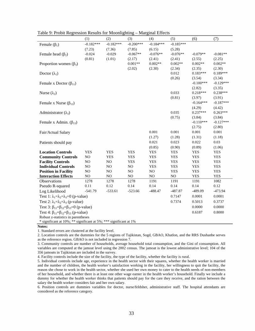
Table 9: Probit Regression Results for Moonlighting – Marginal Effects (1) (2) (3) (4) (5) (6) (7) Female (β1) -0.182*** -0.182*** -0.200*** -0.184*** -0.185*** (7.23) (7.36) (7.85) (6.15) (5.28) Female head (β2) -0.024 -0.029 -0.067** -0.076** -0.076** -0.079** -0.081** (0.81) (1.01) (2.17) (2.41) (2.41) (2.55) (2.25) Proportion women (β3) 0.001** 0.002** 0.002** 0.002** 0.002** (2.02) (2.30) (2.34) (2.35) (2.30) Doctor (λ1) 0.012 0.183*** 0.189*** (0.26) (3.54) (3.34) Female x Doctor (β11) -0.100*** -0.129*** (2.82) (3.35) Nurse (λ2) 0.033 0.218*** 0.238*** (0.81) (3.97) (3.91) Female x Nurse (β12) -0.164*** -0.187*** (4.29) (4.42) Administrator (λ3) 0.035 0.237*** 0.263*** (0.75) (3.84) (3.84) Female x Admin. (β13) -0.110*** -0.127*** (2.75) (2.80) Fair/Actual Salary 0.001 0.001 0.001 0.001 (1.27) (1.28) (1.31) (1.18) Patients should pay 0.021 0.023 0.022 0.03 (0.85) (0.90) (0.89) (1.06) Location Controls YES YES YES YES YES YES YES Community Controls NO YES YES YES YES YES YES Facility Controls NO NO YES YES YES YES YES Individual Controls NO NO NO YES YES YES YES Position in Facility NO NO NO NO YES YES YES Interaction Effects NO NO NO NO NO YES YES Observations 1278 1278 1278 1191 1191 1191 1082 Pseudo R-squared 0.11 0.12 0.14 0.14 0.14 0.14 0.12 Log Likelihood -541.79 -533.61 -523.66 -488.47 -487.87 -489.09 -473.94 Test 1: λ1=λ2=λ3=0 (p-value) 0.7147 0.0001 0.0001 Test 2: λ1=λ2=λ3 (p-value) 0.7374 0.5013 0.3737 Test 3: β11=β12=β13=0 (p-value) 0.0000 0.0000 Test 4: β11=β12=β13 (p-value) 0.6187 0.8000 Robust z-statistics in parentheses * significant at 10%; ** significant at 5%; *** significant at 1%

Notes: 1. Standard errors are clustered at the facility level. 2. Location controls are the dummies for the 5 regions of Tajikistan, Sogd, GBAO, Khatlon, and the RRS Dushanbe serves as the reference region. GBAO is not included in regression 7. 3. Community controls are number of households, average household total consumption, and the Gini of consumption. All variables are computed at the jamoat level using the 2002 census. The jamoat is the lowest administrative level; 104 of the 356 jamoats in Tajikistan are included in the survey. 4. Facility controls include the size of the facility, the type of the facility, whether the facility is rural. 5. Individual controls include age, experience in the health sector with their squares, whether the health worker is married and the number of children, the health worker’s satisfaction working in the facility, her willingness to quit the facility, the reason she chose to work in the health sector, whether she used her own money to cater to the health needs of non-members of her household, and whether there is at least one other wage earner in the health worker’s household. Finally we include a dummy for whether the health worker thinks that patients should pay for the care they receive, and the ration between the salary the health worker considers fair and her own salary. 6. Position controls are dummies variables for doctor, nurse/feldsher, administrative staff. The hospital attendants are considered as the reference category.

33

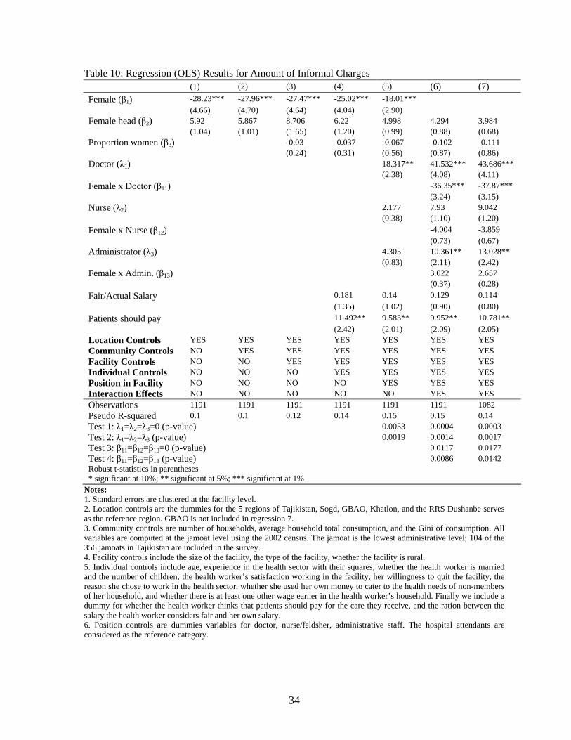
Table 10: Regression (OLS) Results for Amount of Informal Charges (1) (2) (3) (4) (5) (6) (7) Female (β1) -28.23*** -27.96*** -27.47*** -25.02*** -18.01*** (4.66) (4.70) (4.64) (4.04) (2.90) Female head (β2) 5.92 5.867 8.706 6.22 4.998 4.294 3.984 (1.04) (1.01) (1.65) (1.20) (0.99) (0.88) (0.68) Proportion women (β3) -0.03 -0.037 -0.067 -0.102 -0.111 (0.24) (0.31) (0.56) (0.87) (0.86) Doctor (λ1) 18.317** 41.532*** 43.686*** (2.38) (4.08) (4.11) Female x Doctor (β11) -36.35*** -37.87*** (3.24) (3.15) Nurse (λ2) 2.177 7.93 9.042 (0.38) (1.10) (1.20) Female x Nurse (β12) -4.004 -3.859 (0.73) (0.67) Administrator (λ3) 4.305 10.361** 13.028** (0.83) (2.11) (2.42) Female x Admin. (β13) 3.022 2.657 (0.37) (0.28) Fair/Actual Salary 0.181 0.14 0.129 0.114 (1.35) (1.02) (0.90) (0.80) Patients should pay 11.492** 9.583** 9.952** 10.781** (2.42) (2.01) (2.09) (2.05) Location Controls YES YES YES YES YES YES YES Community Controls NO YES YES YES YES YES YES Facility Controls NO NO YES YES YES YES YES Individual Controls NO NO NO YES YES YES YES Position in Facility NO NO NO NO YES YES YES Interaction Effects NO NO NO NO NO YES YES Observations 1191 1191 1191 1191 1191 1191 1082 Pseudo R-squared 0.1 0.1 0.12 0.14 0.15 0.15 0.14 Test 1: λ1=λ2=λ3=0 (p-value) 0.0053 0.0004 0.0003 Test 2: λ1=λ2=λ3 (p-value) 0.0019 0.0014 0.0017 Test 3: β11=β12=β13=0 (p-value) 0.0117 0.0177 Test 4: β11=β12=β13 (p-value) 0.0086 0.0142 Robust t-statistics in parentheses * significant at 10%; ** significant at 5%; *** significant at 1%

Notes: 1. Standard errors are clustered at the facility level. 2. Location controls are the dummies for the 5 regions of Tajikistan, Sogd, GBAO, Khatlon, and the RRS Dushanbe serves as the reference region. GBAO is not included in regression 7. 3. Community controls are number of households, average household total consumption, and the Gini of consumption. All variables are computed at the jamoat level using the 2002 census. The jamoat is the lowest administrative level; 104 of the 356 jamoats in Tajikistan are included in the survey. 4. Facility controls include the size of the facility, the type of the facility, whether the facility is rural. 5. Individual controls include age, experience in the health sector with their squares, whether the health worker is married and the number of children, the health worker’s satisfaction working in the facility, her willingness to quit the facility, the reason she chose to work in the health sector, whether she used her own money to cater to the health needs of non-members of her household, and whether there is at least one other wage earner in the health worker’s household. Finally we include a dummy for whether the health worker thinks that patients should pay for the care they receive, and the ration between the salary the health worker considers fair and her own salary. 6. Position controls are dummies variables for doctor, nurse/feldsher, administrative staff. The hospital attendants are considered as the reference category.

34

35

Table 11: Regression (TOBIT) Results for Amount of Informal Charges – Marginal Effects (1) (2) (3) (4) (5) (6) (7) Female (β1) -30.3*** -29.9*** -29.7*** -29.1*** -16.6** (6.11) (6.03) (5.88) (5.08) (2.55) Female head (β2) 2.253 2.131 2.326 1.513 0.555 0.109 0.466 (1.10) (1.04) (0.98) (0.64) (0.23) (0.05) (0.22) Proportion women (β3) -0.581 -10.061 -17.347 -22.081 -17.450 (0.04) (0.75) (1.29) (1.64) (1.34) Doctor (λ1) 20.40*** 28.52*** 29.13*** (4.70) (6.91) (6.84) Female x Doctor (β11) -4.54*** -4.65*** (3.56) (3.76) Nurse (λ2) 20.81*** 22.14*** 21.63*** (3.42) (2.91) (2.84) Female x Nurse (β12) -0.173 -0.385 (0.03) (0.08) Administrator (λ3) 5.799** 6.617** 6.535** (2.37) (2.84) (2.33) Female x Admin. (β13) 0.638 0.481 (0.41) (0.32) Fair/Actual Salary 5.823** 4.755 4.795 5.056* (1.97) (1.61) (1.63) (1.68)* Patients should pay 9.018*** 7.189*** 7.461*** 7.446*** (3.41) (2.70) (2.81) (2.76) Location Controls YES YES YES YES YES YES YES Community Controls NO YES YES YES YES YES YES Facility Controls NO NO YES YES YES YES YES Individual Controls NO NO NO YES YES YES YES Position in Facility NO NO NO NO YES YES YES Interaction Effects NO NO NO NO NO YES YES Observations 1191 1191 1191 1191 1191 1191 1082 Pseudo R-squared 0.02 0.02 0.03 0.04 0.04 0.04 0.03 Log Likelihood -4009.84 -4008.95 -3996.78 -3945.45 -3933.12 -3929.76 -3903.83 Test 1: λ1=λ2=λ3=0 (p-value) 0.0000 0.0000 0.0000 Test 2: λ1=λ2=λ3 (p-value) 0.0029 0.0000 0.0000 Test 3: β11=β12=β13=0 (p-value) 0.0042 0.0023 Test 4: β11=β12=β13 (p-value) 0.0100 0.0073 Robust t-statistics in parentheses * significant at 10%; ** significant at 5%; *** significant at 1%

Notes: 1. Location controls are the dummies for the 5 regions of Tajikistan, Sogd, GBAO, Khatlon, and the RRS Dushanbe serves as the reference region. GBAO is not included in regression 7. 2. Community controls are number of households, average household total consumption, and the Gini of consumption. All variables are computed at the jamoat level using the 2002 census. The jamoat is the lowest administrative level; 104 of the 356 jamoats in Tajikistan are included in the survey. 3. Facility controls include the size of the facility, the type of the facility, whether the facility is rural. 4. Individual controls include age, experience in the health sector with their squares, whether the health worker is married and the number of children, the health worker’s satisfaction working in the facility, her willingness to quit the facility, the reason she chose to work in the health sector, whether she used her own money to cater to the health needs of non-members of her household, and whether there is at least one other wage earner in the health worker’s household. Finally we include a dummy for whether the health worker thinks that patients should pay for the care they receive, and the ration between the salary the health worker considers fair and her own salary. 5. Position controls are dummies variables for doctor, nurse/feldsher, administrative staff. The hospital attendants are considered as the reference category.