Influence of chemical disorder on the magnetic behaviour and phase diagram of the Fe x Ni 1− x...
6
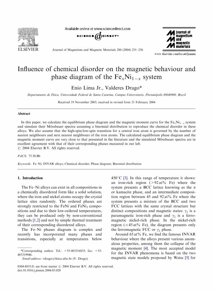
Journal of Magnetism and Magnetic Materials 280 (2004) 251–256 Influence of chemical disorder on the magnetic behaviour and phase diagram of the Fe x Ni 1x system Enio Lima Jr., Valderes Drago* Departamento de F! ısica, Universidade Federal de Santa Catarina, Campus Universitario, Florian ! opolis 88040900, Brazil Received 19 November 2003; received in revised form 21 February 2004 Abstract In this paper, we calculate the equilibrium phase diagram and the magnetic moment curve for the Fe x Ni 1x system and simulate their M. ossbauer spectra assuming a binomial distribution to reproduce the chemical disorder in these alloys. We also assume that the high-spin/low-spin transition for a central iron atom is governed by the number of nearest neighbours and next nearest neighbours of the iron atoms. The calculated equilibrium phase diagram and the magnetic moment curve are very close to that presented in the literature and the simulated M . ossbauer spectra are in excellent agreement with that of their corresponding phases measured in our lab. r 2004 Elsevier B.V. All rights reserved. PACS: 75.50.Bb Keywords: Fe–Ni; INVAR alloys; Chemical disorder; Phase diagram; Binomial distribution 1. Introduction The Fe–Ni alloys can exist in all compositions in a chemically disordered form like a solid solution, where the iron and nickel atoms occupy the crystal lattice sites randomly. The ordered phases are strongly restricted to the FeNi and FeNi 3 compo- sitions and due to their low-ordered temperatures, they can be produced only by non-conventional methods [1,2] and not by simple thermal treatment of their corresponding disordered alloys. The Fe–Ni phases diagram is complex and recently has incorporated many phases and transitions, especially at temperatures below 450 C [3]. In this range of temperature it shows: an iron-rich region (>92 at% Fe) where the system presents a BCC lattice knowing as the a or kamacite phase, and an intermediate composi- tion region between 45 and 92 at% Fe where the system presents a mixture of the BCC and two FCC lattices with the same crystal structure but distinct compositions and magnetic states: g 1 is a paramagnetic iron-rich phase and g 2 is a ferro- magnetic nickel-rich phase. In the nickel-rich region (o45 at% Fe), the diagram presents only the ferromagnetic FCC or g 2 phase. Around 65 at% Fe, we find the famous INVAR behaviour where the alloys present various anom- alous properties, among them the collapse of the magnetic moment [4]. The most accepted model for the INVAR phenomena is based on the two magnetic state models proposed by Weiss [5] for ARTICLE IN PRESS *Corresponding author. Tel.: +55-483316835; fax: +55- 483319946. Email-address: vdrago@fisica.ufsc.br (V. Drago). 0304-8853/$ - see front matter r 2004 Elsevier B.V. All rights reserved. doi:10.1016/j.jmmm.2004.03.020
Transcript of Influence of chemical disorder on the magnetic behaviour and phase diagram of the Fe x Ni 1− x...
ARTICLE IN PRESS
Journal of Magnetism and Magnetic Materials 280 (2004) 251–256
*Corresp
483319946.
Email-a
0304-8853/
doi:10.1016
Influence of chemical disorder on the magnetic behaviour andphase diagram of the FexNi1�x system
Enio Lima Jr., Valderes Drago*
Departamento de F!ısica, Universidade Federal de Santa Catarina, Campus Universitario, Florian !opolis 88040900, Brazil
Received 19 November 2003; received in revised form 21 February 2004
Abstract
In this paper, we calculate the equilibrium phase diagram and the magnetic moment curve for the FexNi1�x system
and simulate their M .ossbauer spectra assuming a binomial distribution to reproduce the chemical disorder in these
alloys. We also assume that the high-spin/low-spin transition for a central iron atom is governed by the number of
nearest neighbours and next nearest neighbours of the iron atoms. The calculated equilibrium phase diagram and the
magnetic moment curve are very close to that presented in the literature and the simulated M .ossbauer spectra are in
excellent agreement with that of their corresponding phases measured in our lab.
r 2004 Elsevier B.V. All rights reserved.
PACS: 75.50.Bb
Keywords: Fe–Ni; INVAR alloys; Chemical disorder; Phase diagram; Binomial distribution
1. Introduction
The Fe–Ni alloys can exist in all compositions ina chemically disordered form like a solid solution,where the iron and nickel atoms occupy the crystallattice sites randomly. The ordered phases arestrongly restricted to the FeNi and FeNi3 compo-sitions and due to their low-ordered temperatures,they can be produced only by non-conventionalmethods [1,2] and not by simple thermal treatmentof their corresponding disordered alloys.
The Fe–Ni phases diagram is complex andrecently has incorporated many phases andtransitions, especially at temperatures below
onding author. Tel.: +55-483316835; fax: +55-
ddress: [email protected] (V. Drago).
$ - see front matter r 2004 Elsevier B.V. All rights reserve
/j.jmmm.2004.03.020
450�C [3]. In this range of temperature it shows:an iron-rich region (>92 at% Fe) where thesystem presents a BCC lattice knowing as the aor kamacite phase, and an intermediate composi-tion region between 45 and 92 at% Fe where thesystem presents a mixture of the BCC and twoFCC lattices with the same crystal structure butdistinct compositions and magnetic states: g1 is aparamagnetic iron-rich phase and g2 is a ferro-magnetic nickel-rich phase. In the nickel-richregion (o45 at% Fe), the diagram presents onlythe ferromagnetic FCC or g2 phase.
Around 65 at% Fe, we find the famous INVARbehaviour where the alloys present various anom-alous properties, among them the collapse of themagnetic moment [4]. The most accepted modelfor the INVAR phenomena is based on the twomagnetic state models proposed by Weiss [5] for
d.
ARTICLE IN PRESS
E. Lima Jr., V. Drago / Journal of Magnetism and Magnetic Materials 280 (2004) 251–256252
the g-Fe: a low magnetic moment state with lowvolume (g1 or LS phase) and a high magneticmoment state with high volume (g2 or HS phase).In this way, the INVAR phenomenon is inter-preted as a spinodal equilibrium between g1 and g2phases. This spinodal equilibrium was incorpo-rated in the phase diagram discussed in the laterparagraph. The transition from the HS to the LSstates was observed in a high pressure M .ossbauerspectroscopy (MS) experiment [6] and accordingto theoretical calculations [7,8] the energy differ-ence between these two states is only 1mRy. Dueto the charge transfer from Ni to Fe atoms, thetransition between the HS and LS states (g2-g1)is determined by the number of nearest neighbours(NN) and next nearest neighbours (NNN) Fearound the central iron atom. Theoretical calcula-tions by Moruzzi [7] have showed that the g2-g1transition depends critically on the valence elec-tron density per atom in the FCC alloy. Specifi-cally, it will occur at the critical concentration of8.6 electrons/atom. For a higher concentration theg2 phase is energetically more stable, and for alower concentration the g1 phase is favoured.
One of the reasons for the complexity of the Fe–Ni phase diagram is that in this system themagnetic energy is comparable with the differencesin the chemical bond energies. The magneticbehaviour of Fe atom is strongly influenced byits neighbourhood and the characteristic chemicaldisorder of FexNi1�x alloys causes enormouschanges in their magnetic properties, and themagnetic state influences the chemical order degreeand its crystalline structure [8,9]. In order tounderstand the complex magnetic behaviour andphase diagram of the Fe–Ni system, it is necessaryto account the chemical disorder and the transitionbetween the low-spin and high-spin states.
Billard and Chamberod [10] used a binomialdistribution for the NN to simulate the chemicaldisorder in the Fe50Ni50 phase. With this proce-dure they could simulate for the first time thecharacteristic asymmetry in the M .ossbauer sextetof this phase. Restrepo et al. [11] extended thebinomial distribution treatment until the NNN tosimulate the chemical disorder in many phases ofthe Fe–Ni system. In another way Sedov andTsigel’nik [12] have had success in simulating the
collapse of the magnetic moment in the INVARregion by using a binomial model taking intoaccount the two spin states known as Weiss’ model[5]. According to these authors, the interaction ofthe Fe atom in the lattice with the NN will play afundamental role in the HS-LS equilibrium.Therefore, models based on a binomial distribu-tion have been used to simulate a chemicaldisorder in Fe–Ni alloys, but always focusing ona particular phenomenon of the Fe–Ni system.
In this work, we propose a model that can giveus the quantities of the g1; g2 and a phases in theFexNi1�x alloys for all the composition range,allowing the construction of a equilibrium phasediagram for this system, and also to simulate theM .ossbauer spectra and the magnetic momentcurve. In this model, we consider that the HS-LS transition is commanded by the central Featom neighbourhood (number of NN and NNNiron) using a binomial distribution to simulate thechemical disorder.
2. Model
We will consider that the FexNi1�x alloys arefully disordered with the Fe and Ni atomsoccupying any site in FCC and BCC lattices. Sowe can write the probability Pðn;mÞ of finding n
NN Fe and m NNN Fe for a central Fe atom in aFexNi1�x alloy with FCC structure by
PFCCðn;mÞ ¼12!6!
ð12� nÞ!n!ð6� mÞ!m!
� ð1� xÞð18�m�nÞxðnþmÞ ð1Þ
and for the FexNi1�x alloy with BCC structure by
PBCCðn;mÞ ¼8!6!
ð8� nÞ!n!ð6� mÞ!m!
� ð1� xÞð14�m�nÞxðnþmÞ: ð2Þ
We assume that the g2-g1 transition occurs atNN Fe=Nc and NNN Fe=Mc: The values ofNc ¼ 8 and Mc ¼ 4 were chosen empiricallybecause they lead to the best results in comparisonwith the experimental data [13]. However, it wasinteresting to note that with these figures (Nc ¼ 8and Mc ¼ 4), the system attains the concentration
ARTICLE IN PRESS
E. Lima Jr., V. Drago / Journal of Magnetism and Magnetic Materials 280 (2004) 251–256 253
of 66.7 at% Fe, being very close to the criticalconcentration of 65 at% Fe, where Moruzzi [7]found the critical density of 8.6 electrons/atom.Based on the FexNi1�x equilibrium phase diagramfounded in the meteoritic samples [3], we willconsider the g-a transition in our approach.Supported by the results of [14] we also assumedthat the superior limit for the local Fe concentra-tion in the FCC g-phase is 75 at% Fe. In this way,we introduce a cutting parameter for the g-atransition at N 0
c ¼ 9: In this case, we do notconsider the NNN atoms since we believe that theNN atoms play the fundamental role in thisstructural transition. Based on these critical(Nc ¼ 8 and Mc ¼ 4) and cutting (N 0
c ¼ 9) num-bers we adopted the following expressions tocalculate the percentages of the g2ðPg2Þ; g1ðPg1 Þand a(Pa) phases in the FexNi1�x alloys:
Pg2 ¼Xn¼Nc�1
n¼0
Xm¼6
m¼0
PFCCðn;mÞ þXMc
m¼0
PFCCðNc;mÞ; ð3Þ
Pg1 ¼X6
m¼Mc¼4
PFCCð8;mÞ; ð4Þ
Pa ¼ 1� Pg1 � Pg2 : ð5Þ
For the Pg1 calculation, we assume that thecritical numbers Nc ¼ 8 and Mc ¼ 4 (where thetransition g2-g1 takes place) are the initial valuesfor n and m in Eq. (4). However, the cuttingnumber for n is N 0
c ¼ 9 (g-a transition), so weonly sum over the m index (from m ¼ Mc up to 6)and consider n ¼ Nc ¼ 8 to calculate Pg1 inEq. (4).
With respect to the magnetic properties, weconsider the magnetic moment of the iron atomsequal to 2.8 mB in the g2 phase, 0.2 mB in g1 phaseand 2.2 mB in a phase. Assuming that the Nimagnetic moment is 0.6 mB and that it does notvary with the alloy composition, we can write thefollowing expressions in order to calculate themean total magnetic moment for the FexNi1�x
alloys:
mTOTAL ¼Pg2 ð2:8x þ ð1� xÞ0:6Þ
þ Pg1ð0:2x þ ð1� xÞ0:6Þ
þ Pað2:2x þ ð1� xÞ0:6Þ: ð6Þ
for the FCC phase:
mg ¼ ðPg2 ð2:8x þ ð1� xÞ0:6Þ
þ ðPg1ð0:2x þ ð1� xÞ0:6ÞÞ=ðPg2 þ Pg1Þ ð7Þ
and for the BCC phase:
ma ¼ ð2:2x þ ð1� xÞ0:6Þ: ð8Þ
The elementary M .ossbauer spectrum for BCCa-Fe can be written like a sum of six Lorentzians:
f ðvÞ ¼X6
i¼1
Ii
1þ ½ðv � IS� ðAiH7DÞÞ=G2; ð9Þ
where H is the hyperfine field, IS the isomeric shift,Dð¼ 2eÞ the quadrupolar splitting (+ for i ¼ 1 or 6and � for i ¼ 2; 3, 4 and 5), G the half widthat half height of the Lorentzian peak and Ii
the relative intensity of the i peak (I3 ¼ I4; I5 ¼I2 ¼ 2I3; I6 ¼ I1 ¼ 3I3). The constants Ai havethe values of A6 ¼ �A1 ¼ 0:16147mm/s/kOe,A5 ¼ �A2 ¼ 0:09344mm/s/kOe and A4 ¼ �A3 ¼0:002541mm/s/kOe, see Ref. [10].
A general M .ossbauer spectrum for the FexNi1�x
alloys will be the sum of g1; g2 and a phasessubspectra: the g1 phase will be taken as a singleline (i ¼ 1) with G ¼ 0:30mm/s andIS=�0.12mm/s (in relation to metallic iron). Thus,it can be described by the following expression:
fg1ðvÞ ¼Ig1
1þ ½ðv � ð�0:12ÞÞ=0:302: ð10Þ
The a phase kamacite subspectrum can bereproduced by a sextet (i ¼ 6) with IS=0.00mm/s, D ¼ 0:00mm/s, G ¼ 0:30mm/s and H ¼ 336 kOeand the expression to faðvÞ is
faðvÞ ¼X6
i¼1
Ii
1þ ½ðv � ð336AiÞÞ=0:302: ð11Þ
To calculate the g2 contribution to the MSspectrum, we have used an expression similar tothat one evaluated in Ref. [10], where the authorsconsider that the g2 sextet is formed by the sum ofall sextets generated by a binomial distribution used
ARTICLE IN PRESS
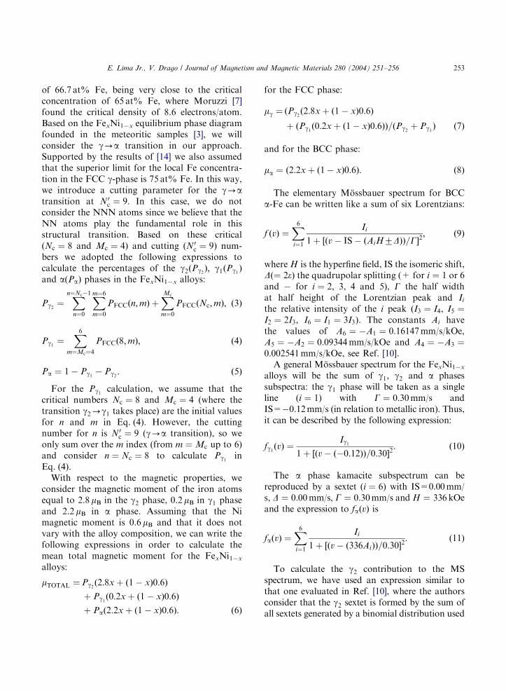
Fig. 1. (a) Phase percentage of g2(&), g1(� ) and a(n)
calculated by Eqs. (3)–(5), respectively, with Nc ¼ 8; Mc ¼ 4
and N 0c ¼ 9; (b) equilibrium phase diagram that we obtained
from our results; and (c) equilibrium phase diagram presented
in Ref. [15].
E. Lima Jr., V. Drago / Journal of Magnetism and Magnetic Materials 280 (2004) 251–256254
to simulate chemical disorder:
fg2 ðvÞ ¼XNc
n¼0
PFCCðnÞ
�X6
i¼1
IiðnÞ
1þ ðv � ðAiH0 þ Aih1ðn � ðnxÞÞÞÞ=GðnÞ� �2;
ð12Þ
where the first sum goes until Nc ¼ 8; H0 is theaverage value from the distribution of hyperfinefields produced by the presence of several neigh-bourhoods of the iron atoms in this phase and h1 isa constant=�1kOe. In this expression Ii and G arefunction of n [10].
The contribution of each phase for theM .ossbauer spectra will be proportional to itsquantity in the alloy. Thus, the final expression forthe M .ossbauer spectrum of the FexNi1�x will be
f ðvÞ ¼ Pg2 fg2 ðvÞ þ Pg1 fg1ðvÞ þ Pa faðvÞ: ð13Þ
3. Results and discussion
In Fig. 1(a), we show the results of thecalculations for g1(� ), g2(&) and a(n) quantitiesagainst the iron content. In this plot, we can seebetween 0 and 40 at% Fe the presence of only theg2 phase. After 40 at% Fe the quantity of thisphase begins to decrease, attaining zero for 90 at%Fe. In another way, the a phase percentage startsto grow up in 40 at% Fe becoming the only phasefor alloys around 90 at% Fe. The g1 curve has adifferent behaviour. The g1 quantity starts to growup in 40 at% Fe, reaching a maximum of 11% in65 at% Fe. After this value it starts to fall,returning to zero in 90 at% Fe. Thus, we foundthe three phases coexisting between 40 and 90 at%Fe. This result seems to indicate that the equili-brium between g1 and g2 phases in the INVARcomposition region occurs due to the naturalchemical disorder of the system. The g1 percentagein the system reaches its maximum at x ¼ 0:65;exactly the composition where, according toMoruzzi [7], the HS-LS transition occurs andthe electron valence density reaches 8.6 electrons/atom. This fact strongly suggests that the observedcollapse in the magnetic moment for compositions
around 65 at% Fe is connected with the maximumin the volume fraction of the g1 phase.
Based on these results, we have constructed anequilibrium phase diagram in bar form, as shownin Fig. 1(b). Then it is compared with the diagramfounded in Ref. [15] (see Fig. 1(c)); we can observethat both are very similar. In fact, the biggestdiscrepancy is on the borderline between the three-phase coexistence region and the FCC ferromag-netic phase. In our diagram, this line is found in40 at% Fe, while in Fig. 1(c) it is found in 30 at%Fe. This difference is possibly related with the factthat our calculations consider that the alloys arefully disordered, that is, there is no possibility ofclustering process. The presence of the orderedFeNi3 leaves to an extension of this border tolower Fe concentration in the diagram, as shownin Fig. 1(c).
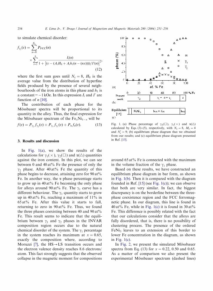
In Fig. 2, we present the simulated M .ossbauerspectra from Eq. (13) for x ¼ 0:22; 0.50 and 0.65.As a matter of comparison we also present theexperimental M .ossbauer spectrum (dashed lines)
ARTICLE IN PRESS
Fig. 2. Left side: simulated (solid line) and right side:
experimental (dashed line) MS spectra for the (a) Fe22Ni78,
(b) Fe50Ni50 and (c) Fe65Ni35 alloys.
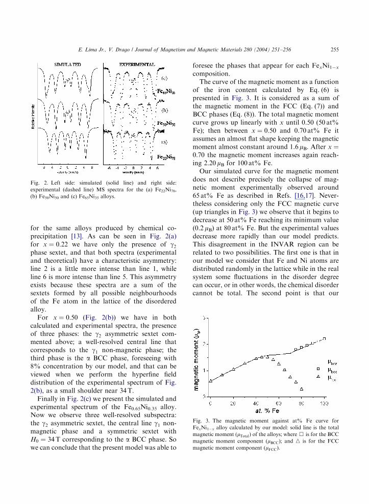
Fig. 3. The magnetic moment against at% Fe curve for
FexNi1�x alloy calculated by our model: solid line is the total
magnetic moment (mTotal) of the alloys; where & is for the BCC
magnetic moment component (mBCC); and n is for the FCC
magnetic moment component (mFCC).
E. Lima Jr., V. Drago / Journal of Magnetism and Magnetic Materials 280 (2004) 251–256 255
for the same alloys produced by chemical co-precipitation [13]. As can be seen in Fig. 2(a)for x ¼ 0:22 we have only the presence of g2phase sextet, and that both spectra (experimentaland theoretical) have a characteristic asymmetry:line 2 is a little more intense than line 1, whileline 6 is more intense than line 5. This asymmetryexists because these spectra are a sum of thesextets formed by all possible neighbourhoodsof the Fe atom in the lattice of the disorderedalloy.
For x ¼ 0:50 (Fig. 2(b)) we have in bothcalculated and experimental spectra, the presenceof three phases: the g2 asymmetric sextet com-mented above; a well-resolved central line thatcorresponds to the g1 non-magnetic phase; thethird phase is the a BCC phase, foreseeing with8% concentration by our model, and that can beviewed when we perform the hyperfine fielddistribution of the experimental spectrum of Fig.2(b), as a small shoulder near 34T.
Finally in Fig. 2(c) we present the simulated andexperimental spectrum of the Fe0.65Ni0.35 alloy.Now we observe three well-resolved subspectra:the g2 asymmetric sextet, the central line g1 non-magnetic phase and a symmetric sextet withH0 ¼ 34T corresponding to the a BCC phase. Sowe can conclude that the present model was able to
foresee the phases that appear for each FexNi1�x
composition.The curve of the magnetic moment as a function
of the iron content calculated by Eq. (6) ispresented in Fig. 3. It is considered as a sum ofthe magnetic moment in the FCC (Eq. (7)) andBCC phases (Eq. (8)). The total magnetic momentcurve grows up linearly with x until 0.50 (50 at%Fe); then between x ¼ 0:50 and 0.70 at% Fe itassumes an almost flat shape keeping the magneticmoment almost constant around 1.6 mB. After x ¼0:70 the magnetic moment increases again reach-ing 2.20 mB for 100 at% Fe.
Our simulated curve for the magnetic momentdoes not describe precisely the collapse of mag-netic moment experimentally observed around65 at% Fe as described in Refs. [16,17]. Never-theless considering only the FCC magnetic curve(up triangles in Fig. 3) we observe that it begins todecrease at 50 at% Fe reaching its minimum value(0.2 mB) at 80 at% Fe. But the experimental valuesdecrease more rapidly than our model predicts.This disagreement in the INVAR region can berelated to two possibilities. The first one is that inour model we consider that Fe and Ni atoms aredistributed randomly in the lattice while in the realsystem some fluctuations in the disorder degreecan occur, or in other words, the chemical disordercannot be total. The second point is that our
ARTICLE IN PRESS
E. Lima Jr., V. Drago / Journal of Magnetism and Magnetic Materials 280 (2004) 251–256256
model considered the existence of only two (HSand LS) magnetic-ordered spin states in the FCCalloys, but the presence of disordered spin states inthe INVAR region of the Fe–Ni system is knowfrom Refs. [9,17]. The non-collinear spin statesare supposed to have intermediate energyvalues (that is between the HS and LS values)and could be responsible for a much more drasticdecrease in the magnetic moment curve around65 at% Fe.
4. Conclusions
We have proposed a model based on a binomialdistribution to simulate the chemical disorder inthe FexNi1�x system that incorporates a criticaldependence of the high-spin-low-spin transitioncommanded by the central iron atom neighbour-hood. It permitted to calculate the equilibriumphase diagram, to simulate the MS spectra and themagnetic moment curve in all the concentrationrange. The simulated MS spectra compare quitewell with the measured ones, but the collapse inthe magnetic moment is not so marked as observedin literature, which is attributed to the presence ofdisordered spin phases not considered in ourmodel. The model predicts that the INVARphenomena are related to the maximum in the g1FCC low-spin phase concentration.
Acknowledgements
We would like to thank the financial support ofthe Brazilian agencies CAPES and CNPq.
References
[1] E. Lima Jr., V. Drago, P.F.P. Fichtner, P.H. Domingues,
Solid State Commun. 128 (2003) 345.
[2] E. Lima Jr., V. Drago, Phys. Status Solidi A 187 (2001) 119.
[3] C.W. Yang, D.B. Williams, J.I. Goldstein, J. Phase
Equilib. 17 (1996) 522.
[4] H. Rechenberg, Hyper. Interact. 54 (1990) 683.
[5] R.J. Weiss, Proc. Phys. Soc. 82 (1963) 281.
[6] M.M. Abd-Elmeguid, Nucl. Instrum. Methods B 76 (1993)
159.
[7] V.L. Moruzzi, Phys. Rev. B 41 (1990) 6939.
[8] M. Schr .oter, H. Ebert, H. Akai, P. Entel, E. Hoffmann,
G.G. Reddy, Phys. Rev. B 52 (1995) 188.
[9] M.Z. Dang, D.G. Rancourt, Phys. Rev. B 53 (1996) 2291.
[10] L. Billard, A. Chamberod, Solid State Commun. 17 (1975)
113.
[11] J. Restrepo, G.A. P!erez Alc!azar, A. Boh !orquez, J. Appl.
Phys. 81 (1997) 4101.
[12] V.L. Sedov, O. Tsigel’nik, J. Magn. Magn. Mater. 183
(1998) 117.
[13] E. Lima Jr., V. Drago, J. Cardoso de Lima, P.F.P.
Fichtner, J. Alloy. Comp., submitted.
[14] R.B. Scorzelli, J. Danon, Phys. Scr. 32 (1985) 143.
[15] L.B. Hong, B. Fultz, J. Appl. Phys. 79 (1996) 3946.
[16] M. van Schilfgaarde, I.A. Abrikosov, B. Johansson,
Nature 400 (1999) 46.
[17] M. Matsushita, S. Endo, K. Miura, F. Ono, J. Magn.
Magn. Mater. 265 (2003) 352.