Swansea University E-Theses _________________________________________________________________________

Industrial case study-driven innovative optimised engineering

design.

Morgan, Heather Dawn

How to cite: _________________________________________________________________________ Morgan, Heather Dawn (2015) Industrial case study-driven innovative optimised engineering design.. thesis,

Swansea University.

http://cronfa.swan.ac.uk/Record/cronfa42659

Use policy: _________________________________________________________________________ This item is brought to you by Swansea University. Any person downloading material is agreeing to abide by the terms

of the repository licence: copies of full text items may be used or reproduced in any format or medium, without prior

permission for personal research or study, educational or non-commercial purposes only. The copyright for any work

remains with the original author unless otherwise specified. The full-text must not be sold in any format or medium

without the formal permission of the copyright holder. Permission for multiple reproductions should be obtained from

the original author.

Authors are personally responsible for adhering to copyright and publisher restrictions when uploading content to the

repository.

Please link to the metadata record in the Swansea University repository, Cronfa (link given in the citation reference

above.)

http://www.swansea.ac.uk/library/researchsupport/ris-support/

Industrial Case Study-Driven

Innovative Optimised

Engineering Design

Heather Dawn Morgan

Submitted to Swansea University in fulfilm ent o f the requirements for the Degree o f Doctor of Engineering

Swansea University

ProQuest Number: 10805435

All rights reserved

INFORMATION TO ALL USERS The quality of this reproduction is dependent upon the quality of the copy submitted.

In the unlikely event that the author did not send a com p le te manuscript and there are missing pages, these will be noted. Also, if material had to be removed,

a note will indicate the deletion.

uestProQuest 10805435

Published by ProQuest LLC(2018). Copyright of the Dissertation is held by the Author.

All rights reserved.This work is protected against unauthorized copying under Title 17, United States C ode

Microform Edition © ProQuest LLC.

ProQuest LLC.789 East Eisenhower Parkway

P.O. Box 1346 Ann Arbor, Ml 48106- 1346

Abstract

Optimisation research is a vast and comprehensive field of study in academia, but its application to complex real life problems is much more limited. This thesis presents an exploration into the use of optimisation in the weight reduction problems of three industrial case studies. The work sought to find robust and practical solutions that could be exploited in the current commercial environment.

The three case studies comprised the housing of a vertical axis wind turbine, a titanium jet engine lifting bracket and a casing for an aircraft cargo release system. The latter two were to be built using additive layer manufacture, while the housing, w ith in itia lly no prescribed manufacturing method, was required to conform to British Standards for design.

Based on commercially available optimisation and analysis packages e.g. Altair Optistruct, ANSYS, Microsoft Excel and MatLab, methodologies were developed to enable solutions to be found with in realistic time-scales, Techniques to improve computational efficiency using the Kreisselmeier Steinhauser functions were also investigated.

Good weight reduction was achieved in all cases. For the housing, a trend showing the relationship between the overall size of the housing and the material requirement was also developed. Extensive data for the lifting bracket was retrieved and analysed from a crowd-sourced design challenge. This highlighted important elements of design for additive layer manufacture and also gave an indication of the efficacy of different optimisation algorithms. The casing design methodology obtained simplified the material selection for the design. Build orientation software was developed to exploit the advantages of additive layer manufacture.

The initial objective to solve the optimisation problems for all three case studies was accomplished using topology and size optimisation w ith both gradient-based and evolutionary methods. Data analysis and optimisation increased design capability for additive layer manufacture build and orientation.

Table of Contents

Chapter 1: Introduction................................................................................... 11.1 M otivation........................................................................................................ 1

1.2 Objectives.........................................................................................................2

1.3 Thesis Layout...................................................................................................3

Chapter 2: Literature Review......................................................................... 52.1 Engineering Design.........................................................................................5

2.2 Optimisation.....................................................................................................8

2.2.1 The Standard Optimisation Problem....................................................8

2.2.2 Karush-Kuhn-Tucker (KKT]................................................................ 11

2.3 Structural Optim isation................................................................................12

2.4 Topology Optim isation................................................................................ 13

2.4.1 Design Problem Formulation...............................................................14

2.4.2 Solution Methodology...........................................................................16

2.4.3 Important Issues arising from the Solution Method..........................21

2.4.4 Solution Methods for Topology Optim isation................................... 31

2.5 Size Optim isation..........................................................................................42

2.6 Use of Commercial Software....................................................................... 44

2.7 Research Novelty...........................................................................................47

Chapter 3: Case Study 1 - Design of a Vertical Axis Wind TurbineHousing 48

3.1 In troduction.................................................................................................. 48

3.2 Background................................................................................................... 49

3.3 Company Requirements...............................................................................51

3.3.1 Road........................................................................................................ 52

3.3.2 R a il..........................................................................................................52

3.4 Structural Optim isation...............................................................................53

3.4.1 Topology Optimisation.........................................................................54

3.4.2 Size Optimisation.................................................................................. 69

3.5 Conforming to BS 5950-1:2000...................................................................91

3.5.1 Ultimate L im it States............................................................................ 92

3.5.2 Serviceability Lim it States.................................................................101

3.5.3 Results of BS 5950 Conformity Check.............................................. 101

3.6 Robust Methodology for Housing Design................................................ 104

3.6.1 Size Optimisation................................................................................ 105

3.6.2 Conformity to BS 5950....................................................................... 108

3.7 Results of Size Optimisation & Standards Check.................................... 108

3.7.1 Continuous...........................................................................................108

3.7.2 Discrete & Standards Check...............................................................I l l

3.8 Material Costing Trends.............................................................................112

3.9 Concluding Remarks...................................................................................112

Chapter 4: Constraints Aggregation............................................................ 1144.1 Motivation for Constraints Aggregation...................................................114

4.2 Benchmarking: Planar Trusses..................................................................114

4.2.1 Ten Bar Truss...................................................................................... 114

4.2.2 Results o f the 10 Bar Truss Optim isation........................................ 116

4.2.3 200-Bar Plane Truss...........................................................................121

4.3 Constraints Aggregation in Optistruct: The VAWT Space frame 126

4.3.1 Case A - KMS defined by Optistruct's Internal Equations.............. 127

4.3.2 Case B - KMS Using HyperMath........................................................ 135

4.3.3 Case C - KMS Using HyperStudy....................................................... 136

4.3.4 Case D - KMS Using MatLab............................................................... 137

4.3.5 Summary of results............................................................................. 137

4.4 Discussion.................................................................................................... 139

4.4.1 Different Optimisation Solvers.......................................................... 139

4.4.2 Added Complexity...............................................................................140

4.4.3 Previous Successful Applications of KMS......................................... 141

4.5 Conclusions.................................................................................................145

Chapter 5: Case Study 2 - The General Electric Challenge - Designing forAdditive Manufacture.......................................................................................146

5.1 In troduction...............................................................................................146

5.2 The GE Design Challenge.......................................................................... 146

5.3 Setting the Challenge in Context.............................................................. 149

5.3.1 Additive Layer Manufacturing........................................................... 149

5.3.2 T itian ium ..............................................................................................153

5.3.3 Design by Crowdsourcing.................................................................. 154

5.3.4 Designing for ALM : Topology Optimisation.................................... 156

5.3.5 Factors of Safety...................................................................................156

5.3.6 Element Selection................................................................................157

5.3.7 Mesh Sensitivity Testing.....................................................................158

5.3.8 Topology Optimisation....................................................................... 159

5.4 Interpreting the Topology Optimisation Results...................................167

5.5 Other Challenge Entries - Statistical Analysis........................................171

5.5.1 Descriptive Statistics...........................................................................171

5.5.2 Observations w ith Future Application............................................. 178

5.5.3 Build orientation..................................................................................186

5.6 Crowdsourcing and the GE Challenge......................................................197

5.6.1 The Company......................................................................................197

5.6.2 The Individual.....................................................................................198

5.7 Conclusions.................................................................................................198

Chapter 6: Optimisation of the Build Orientation to Minimise SupportVolume in ALM.................................................................................................. 200

6.1 In troduction...............................................................................................200

6.2 Background................................................................................................200

6.3 The Optimisation A lgorithm ..................................................................... 203

6.4 Testing the Model....................................................................................... 206

6.4.1 Cylindrical Half Pipe...........................................................................206

6.4.2 GE Challenge Bracket Design - Alexis V2.........................................211

6.4.3 W inning Entry - GE Challenge Jet Engine Bracket Design.............214

6.5 Improving the Build Orientation Software............................................. 215

6 .6 Conclusions..................................................................................................216

Chapter 7: Case Study 3 - Design of Release System Casing for ALM... 2177.1 In troduction ................................................................................................ 217

7.2 ALM: for Steels and A lum inium ................................................................ 218

7.2.1 Stainless Steel - 316L......................................................................... 219

7.2.2 Stainless Steel - 17-4PH....................................................................220

7.2.3 Aluminium - ALSIlOMg.....................................................................222

7.3 The Design Problem...................................................................................222

7.4 Design Approach........................................................................................ 224

7.4.1 Topology Optimisation.......................................................................226

7.4.2 Geometric Interpretation of the Topology......................................232

7.4.3 Incorporating a Faraday Cage...........................................................238

7.5 Optimising Build O rientation....................................................................243

7.5.1 Part A .................................................................................................... 243

7.5.2 Part B.................................................................................................... 245

7.6 Validation w ith Manufactured Part.......................................................... 247

7.7 Conclusions..................................................................................................252

Chapter 8: Concluding Remarks................................................................ 2538.1 Achievements and Conclusions................................................................253

8.1.1 Case Study 1: The design of a housing for a novel VAWT...............253

8.1.2 Case Study 2: GE Challenge - Titanium Bracket Design................255

8.1.3 Case Study 3: Design of Release System for ALM............................256

8.2 Recommendations for Future W ork 258

Appendix A: Global Starting Points used in Optistruct for VAWT HousingSize Optimisation..............................................................................................260Appendix B: Abbreviated input file for Continuous Optimisation inOptistruct for VAWT Housing, 22m, one diameter height model............. 262Appendix C: Commercially Available Standard Circular Hollow Sections,(Class 3 ) .............................................................................................................. 273Appendix D: Table of Compressive Strength pc for Hot Finished HollowSections - S355 Grade.......................................................................................277Appendix E: Nodal Forces for the 10m x ID VAWT Housing Model 279Appendix F: Further Investigation into the differences between modeltype A & B in Chapter 3........................................................................... .. ......285Appendix G: Design Variables Groupings for 200-bar truss example inChapter 4 ............................................................................................................ 289Appendix H: Matlab Code for Nonlinear Constraint Optimisation usingfmincon with Optistruct................................................................................... 291Appendix I: List of References relating to Kreisselmeier Steinhauserfunctions used in the meta-analysis of section 4.4.3...................................298Appendix): MatLab Script - SupportCalc.m................................................ 306Appendix K: MatLab Script - OppTotalSupportVol.nl................................. 312Appendix L: MatLab Script - VOTSVol_RinTriA.m....................................... 321

Acknowledgements

I wish to express my appreciation to my supervisors, Professor Johann

Sienz, Dr Antonio Gil and Dr David Bould for their help and guidance

throughout the Engineering Doctorate programme.

My particular thanks are extended to the College of Engineering for

facilitating this course of study financially and enabling me to integrate my

work and studies together. Also to the Advanced Sustainable

Manufacturing Technologies (ASTUTE] project for allowing me to use the

case studies for this research and for my colleagues in ASTUTE for both

moral and technical support.

As a person w ith few original ideas I express my gratitude to my Heavenly

Father for the concept of the build orientation software. This can only

have been inspiration. I would never have thought of it myself. Thank

you.

And lastly, a word of thanks to my parents, Joy & Haydn Morgan; they

established a home where education was always valued and this has

formed a foundation for discovery and learning that has persisted

throughout my life.

Table of Figures

Figure 2-1: Traditional "Waterfall" Approach to Product Design........................... 5

Figure 2-2: Schematic of Concurrent or Simultaneous Engineering showing

interaction at multiple stages of the design process................................................6

Figure 2-3: The cost of change in Engineering Design [7 ]....................................... 7

Figure 2-4: Typical Stages in Concept Product development.................................. 8

Figure 2-5: Function of one variable showing local and global m in im a..............10

Figure 2-6: Topology Optimisation of a Cantilever Beam showing intermediate

values or "grey" areas of the density variable [2 3 ]............................................... 16

Figure 2-7: The General Flow of Computation for a Gradient-Based Topology

Optimisation [2 6 ]....................................................................................................... 17

Figure 2-8: Example of checkerboard pattern in the solution of a cantilever

beam problem [2 8 ].................................................................................................... 2 1

Figure 2-9: Topology Optimisation of a simply supported beam showing mesh

dependency [2 2 ] .........................................................................................................2 2

Figure 2-10: Illustration of the Density Filter [31 ].................................................23

Figure 2-11: An Example of the Kreisselmeier Steinhauser Function in 2-D...28

Figure 2-12: Level set representations [8 5 ].......................................................... 37

Figure 2-13: Representation of the of the Phase Field function........................... 38

Figure 3-1: The Cross-Flow Energy Company VAWT [136 ]................................. 48

Figure 3-2: Proposed Housing for Vertical Axis Wind Turbine............................ 49

Figure 3-3: Plan view of VAWT showing w indflow and pressure zones around

an operational turbine [136]..................................................................................... 50

Figure 3-4: Model set up for the topology optim isation........................................ 56

Figure 3-5: Plan view of VAWT showing housing orientation for load case n l35

....................................................................................................................................... 57

Figure 3-6: Plan view of VAWT housing showing the distribution of pressures

for loadcase n l3 5 ....................................................................................................... 58

Figure 3-7: Topology Optimisation of VAWT housing comparing effect of

material properties on element densities................................................................60

Figure 3-8: Topology optimisation of steel housing showing element density >

0.009 for in itia l material fraction of a] 0.005 and b] 0.001.................................. 62

Figure 3-9: Plan View of Optimised Housing for in itia l material fraction of a)

0.005 and b] 0.001..................................................................................................... 62

Figure 3-10: Convergence curves for topology optimisation w ith repeat pattern

.......................................................................................................................................65

Figure 3-11: Contour plots for the optimised VAWT housing at iteration 16: a)

for displacement and b] element stress...................................................................6 6

Figure 3-12: Contour plots for the optimised VAWT housing at iteration 21: a]

for displacement and b) element stress...................................................................6 6

Figure 3-13: Result of Topology Optimisation of Complete Housing w ith pattern

repeat in nine sections............................................................................................... 6 8

Figure 3-14: Top view of Optimised Solution......................................................... 6 8

Figure 3-15: 22m x ID Proposed Space Frame Structure for VAWT Housing ....69

Figure 3-16: Plan view of 22m x ID Space Frame showing 14 members around

perimeter and 11 bracing members (rigid elements om itted].............................70

Figure 3-17: Detail of the roof at the Kansai International Airport, Osaka, Japan

showing circular hollow sections............................................................................. 71

Figure 3-18: PBARL Tube element showing cross sectional dimensions 72

Figure 3-19 Examples of Buckling Behaviour in Beams and Columns................73

Figure 3-20: The behaviour of the 41 starting points for the continuous size

optimisation of the 22m x ID housing space frame...............................................84

Figure 3-21: Convergence curves for best optimum (D-X] for 22m x ID housing

....................................................................................................................................... 84

Figure 3-22: Example of the Variation in the Design Variables as the Size

Optimisation Converges.............................................................................................85

Figure 3-23: Dimensions of each member from the Continuous Size

Optimisation Solution.................................................................................................8 6

Figure 3-24: Members allocated to standard sections - Comparison through the

height levels of the housing.......................................................................................89

Figure 3-25 Convergence curves for Discrete Size Optim isation.........................90

Figure 3-26: Illustration of a] a non-sway and b] a sway-sensitive structure 92

Figure 3-27: Variation in Bending Moments........................................................... 99

Figure 3-28: Flowchart for Optimisation Procedure........................................... 104

Figure 3-29: Memory Requirement and CPU time for each Housing Design.... 106

Figure 3-30: Variation in optimised mass trends according to VAWT heights 112

Figure 4-1: Ten Bar truss layout showing node and bar num bering.................115

Figure 4-2: Variation in a) Optimised result and b] CPU Time according to in itia l

starting points for three different algorithms.......................................................117

Figure 4-3: Convergence Curve for Optimisation of 10 bar truss using Active Set

Algorithm in MatLab script......................................................................................118

Figure 4-4: Optimal Solution of 10 bar Truss showing cross sectional areas of

circular bars...............................................................................................................118

Figure 4-5: Layout of 200-bar Truss...................................................................... 122

Figure 4-6: Comparison of MatLab Optimisation of 200-bar truss w ith the work

of Arora and Gorvil [166 ]........................................................................................ 123

Figure 4-7: Convergence curve for KMS aggregated 200-bar truss w ith in itia l

values of 2 x l0 3m2 and scalar m ultip lie r = 5 0 ......................................................124

Figure 4-8: Comparison of the CPU breakdown in the Optistruct Modules w ith

and w ithout the KMS functions...............................................................................132

Figure 4-9: Most Violated Constraints at each iteration of the VAWT housing

Optimisation - No Combining of Constraints........................................................133

Figure 4-10 Most Violated Constraints when Constraints Aggregation is applied

to the Stress Constraints.......................................................................................... 133

Figure 4-11 Comparison of CPU time w ithout Constraint Screening for VAWT

Housing Size Optimisation.......................................................................................135

Figure 4-12: Types of Optimisation used in Research Papers Using KMS

functions.....................................................................................................................141

Figure 4-13 Frequency distribution of sample of KMS published papers.........142

Figure 4-14: Origins of the KMS papers using Multiobjective Optimisation.....144

Figure 5-1: Example of a lifting bracket in s itu ..................................................... 147

Figure 5-2: Original Design Envelope for Engine Bracket [184]........................ 147

Figure 5-3: Four Load Conditions Specified by GE [184].................................... 148

Figure 5-4: The role of Crowdsourcing in the Production Cycle........................ 155

Figure 5-5: Mesh Sensitivity Analysis Results for the GE Bracket Original Design

w ithout optim isation................................................................................................ 158

Figure 5-6: Jet Engine Bracket w ith 5.7xl(H m mesh shown..............................160

Figure 5-7: Basic Set Up for Topology Optimisation (mesh om itted ]................161

Figure 5-8: Convergence Curve for the Topology Optimisation of the GE Bracket

162

Figure 5-9: Topology Optimisation Solution showing variation in Element

Densities, a] A ll densities b] A ll densities above 0.011......................................162

Figure 5-10: Topology Optimisation of Lifting Bracket.......................................164

Figure 5-11: von Mises' Stress Distribution in Optimised Structure................. 165

Figure 5-12: A sample of the intermediate results in the topology optimisation

of the GE bracket.......................................................................................................166

Figure 5-13: CAD Interpretation of Topology Optimisation using surfaces 168

Figure 5-14: FEA Analysis of CAD design of bracket under the four loadcases 169

Figure 5-15: Design based on Topology Optimisation. Weight is 32% or original

bracket....................................................................................................................... 170

Figure 5-16: Variation in average weight over competition period.................. 174

Figure 5-17: Example of Entries w ith only two bolt holes..................................174

Figure 5-18: Complexity of design compared to weight reduction....................175

Figure 5-19: The four main categories of design submitted............................... 176

Figure 5-20: Frequency Distribution of the four main design types................. 177

Figure 5-21: Principal Vectors shown on a "Butterfly" type design.................. 177

Figure 5-22: Example o f a "Flat Design" Bracket showing vector principal

stresses under loadcase 4, the Moment.................................................................178

Figure 5-23: Comparison of designs......................................................................182

Figure 5-24: Overlay of Result of Topological Optimisation on Design [ v i i i ] ... 183

Figure 5-25: Topology Optimisation w ith Loadcase 1 only applied.................. 184

Figure 5-26: Overlay of Topological Optimisation on Compact Design 185

Figure 5-27: Example of support material required for building one of the

components...............................................................................................................187

Figure 5-28: Cross section of Area Support in AutoFAB..................................... 187

Figure 5-29: Variation of Support Material required according to build

orientation and design vo lum e...............................................................................188

Figure 5-30: Relationship between Support Volume and Build Time for a single

je t bracket part at different orientations............................................................... 189

Figure 5-31: Variation in Build Time w ith Volume of Parts w ith Support 189

Figure 5-32: Areas requiring Support During ALM build identified by AutoFAB

software...................................................................................................................... 190

Figure 5-33: Vertical Cross Section through bracket design of Figure 5 -32 191

Figure 5-34: Flow Chart for MatLab script SupportCalc......................................192

Figure 5-35: Single triangular surface from the stl file showing angle to the base

p la te ............................................................................................................................ 192

Figure 5-36: Illustration of Support Volume calculated from projection of

triangle to build plate................................................................................................193

Figure 5-37: SupportCalc Result showing areas where support material is

required...................................................................................................................... 195

Figure 5-38: Relationship between Support Material predicted by AutoFAB and

SupportCalc scrip t.....................................................................................................196

Figure 6-1: Staircasing effect in ALM build caused by adjacent layers of

material of height 'h '................................................................................................. 2 0 1

Figure 6-2: Flowchart fo r OppTotalSupportVol.m...............................................204

Figure 6-3: Half a cylindrical p ipe...........................................................................206

Figure 6-4: Optimised solution for half pipe (yellow] compared to original

orientation (cyan].....................................................................................................209

Figure 6-5: Optimised solution of half pipe showing areas requiring support in

orange. Original (cyan], Optimised orientation (ye llow ].....................................209

Figure 6 -6 : Convergence Curve for Optimisation of Cylindrical Half Pipe -

starting point A ..........................................................................................................210

Figure 6-7 Rendering of GE Bracket Design V2 by Alexis....................................211

Figure 6 -8 : Optimised solution for bracket (yellow] compared to original

orientation (cyan].....................................................................................................213

Figure 6-9: Brackets of Figure 6 - 8 viewed from below w ith areas requiring

support highlighted (orange]..................................................................................213

Figure 6-10: W inning Bracket Design of the GE Challenge................................. 214

Figure 6-11 T im e taken to find global optimised build orientation solutions for

different geometries................................................................................................. 215

Figure 7-1 Current Release system design shown in s itu ....................................218

Figure 7-2: Release System Module showing in terio r components - catch in

open position............................................................................................................. 223

Figure 7-3: Casing B design domain showning filled bolt holes.........................227

Figure 7-4 von Mises Stress Distrubution across the w idth of the Cargo Strap

228

Figure 7-5: FEA model o f casing showing loads and constraints, only the

meshing of the non-design material is shown for greater clarity...................... 229

Figure 7-6: Convergence curves for Topology Optimisation of Aluminium Casing

.....................................................................................................................................230

Figure 7-7: Topology Optisation for Aluminium Casing......................................231

Figure 7-8 von Mises' Stress of the Topological Optimisation............................232

Figure 7-9: Set Up of Bar m odel............................................................................. 233

Figure 7-10: Convergence Curves for Beam Optimisation..................................234

Figure 7-11: Evolution of Design Variables throughout Size Optimisation.....235

Figure 7-12: Comparison of support material required for ALM build of a

circular structure, an ellipse w ith major axis vertical and an inverted teardrop

.....................................................................................................................................236

Figure 7-13: a)Plot of Required Support Volume of circle and ellipse w ith the

same area moment of inertia at a range of rotational angles as shown in b] ...237

Figure 7-14: CAD Interpretation of the Topology Optim isation........................ 237

Figure 7-15: Final casing design showing integrated skin and beam structure

..................................................................................................................................... 238

Figure 7-16: Stress contours from Linear Static Analysis of Optimised Casing

under 45kN lo ad .......................................................................................................239

Figure 7-17: Comparison o f Aluminium Casing Designs, showing mass and

stages in new casing development b] & c ]............................................................ 240

Figure 7-18: Two Halves of Release System Casing.............................................243

Figure 7-19: Convergence Curve for optimisation of Part A............................... 244

Figure 7-20: Optimal Build orientation for Part A found w ith

"OppTotalSupportVol" script, a) Original orientation b) Optimum................... 245

Figure 7-21: Suitable Angle o f build for Part B of Casing.................................... 246

Figure 7-22: Predicted Optimal Build orientation for Part B found w ith

'OppTotalSupportVol' script shown in AutoFAB software w ith support attached

..................................................................................................................................... 247

Figure 7-23: ALM bu ilt Casing parts, 248

Figure 7-24: ALM Part B affixed to base w ith Support material still attached. 248

Figure 7-25: Geometry of Part A position on stl of Support Material from

Manufacture...............................................................................................................249

Figure 7-26: Examples of Surface Roughness in Part A where Support Volumes

were attached............................................................................................................249

Figure 7-27: Support Requirements for Part A using AutoFAB.........................250

Figure F-0-1: Comparison of the global search size optimised solutions found

using model types A and B ...................................................................................... 286

Figure F-0-2: Comparison of firs t 20 iterations of starting point 11 for models

type A and B...............................................................................................................287

Figure F-0-3: The “most violated" contraints for the firs t 20 iterations of a)

model type A and b) model type B..........................................................................288

Nomenclature

Abbreviations

22m x ID A turbine housing w ith diameter of 22 m and height of 1 diameter

ALM Additive Layer Manufacture

ARSM Adaptive Response Surface Method

BESO Bi-directional Structural Optimisation

CAD Computer Aided Design

CFD Computational Fluid Dynamics

C-FEC Cross-Flow Energy Company

CHS tubular beams w ith circular hollow cross sections

CONLIN Convex Linearisation

CS Crowdsourcing

DMLS Direct Metal Laser Sintering

EP Evolutionary Programming

ESO Evolutionary Structural Optimisation

ES Evolutionary Strategies

FEA Finite Element Analysis

GA Genetic Algorithm

GE General Electric

HAWT Horizontal Axis W ind Turbine

HIP Hot iso-static heating cycle

HRC Rockwell C-scale hardness

IH in-house

KKT Karush-Kuhn Tucker

KMS Kreisselmeier Steinhauser functions

LCA Life cycle analysis

LD longitudinal bu ilt ALM part, longest dimension perpendicular to

build direction

MFD Method o f Feasible Directions

MMA Method of Moving Asymptotes

n30 a loadcase for the turbine housing when the housing is positioned

at -30° from the vertical (see Figure 3-5)

NHF Notional Horizontal Force

p90 a loadcase for the turbine housing when the housing is positioned

at +90° from the vertical (see Figure 3-5)

RAMP Rational Approximation of Material Properties

SA Simulating Annealing

SIMP Solid Isotropic Microstructure w ith Penalisation

SLM Selective Laser Melting

SMD Shaped Metal Deposition

SORA Sequential Optimisation and Reliability Assessment

SQP Sequential Quadratic Programming

STL stereo-lithography file form

TD transverse bu ilt ALM part, largest dimension in line w ith build

direction

TIG Tungsten Inert Gas welding

TYS tensile yield strength

UTS Ultimate Tensile Strength

VAWT Vertical Axis W ind Turbine

Roman Symbols

a.i cross sectional area of bars in optimisation

A cross sectional area of tubes in British Standard calculations

Av shear area

B area of base triangle in support structure calculation

dTop displacement of the VAWT turbine at the top and centre

D upper lim it for dTop, which is dependent on turbine height

D0 outer diameter of tubular section

DVi design variables for size optim isation

E Young's modulus

f ( x ) objective function for the design variable set x

F vector of external forces

Fc compressive force

Fcr critical load for member buckling

Ft axial tension

Fv Shear Force

g (x ) in the level set method a function that influences hole development

gi (x ) inequality constraints for the design variable set x

9maxi®) maximum of the set of stress values

h height of a storey of a building or structure

hi ( * ) equality constraints for the design variable set x

H hessian matrix

I Area Moment of Inertia

k scalar m ultip lier for the Kreisselmeier Steinhauser functions

k* parameter in buckling theory that denotes the type of fixing used at

column ends

K global stiffness matrix

K° element stiffness matrix

KK{cr) the p-norm function

KS(a) Kriesselmeier Steinhauser function

li or L length of bars

L(x,X ) Lagrangian function

lb lower bound on a design variable

Le effective length of a column

m * equivalent bending moment

m j mass of individual elements

mx equivalent uniform moment factor about the major axis

my equivalent uniform moment factor about the m inor axis

M reference number of the largest section used in the discrete size

optim isation

Mc moment capacity

Mmax maximum moment in the member

Mx moment about the major axis

My moment about the minor axis

Mcx moment capacity about the major axis

Mcy moment capacity about the m inor axis

N number of elements

p p-norm parameter

pc compressive strength

py design strength of the circular hollow section

Pt tension capacity

Pv shear capacity

q SIMP penalization parameter

r * radius of gyration

77 radii o f circles

77 inner radius of tubular member

r0 outer radius of tubular member

s SIMP penalization parameter

S plastic or plastic section modulus

Sef f effective plastic modulus

Sv plastic modulus for the shear area

t time

Ti discrete values for design variables

Th wall thickness of a tubular member

U displacement vector

ub upper bound of a design variable

U0J}t transformation matrix

171 element volumes

Vi vertices of triangles in stl files

V Volume

V0 volume of the design domain

Vopt inverse of the transformation m atrix Uopt

wk weighting factor used in density filtering

w transverse displacement in a buckled column

x the vector of design variables, x i, X2,.. ..,xn

x iL lower bound on the component of x

x iv upper bound on the component of x

z un it normal vector

z0 in itia l value o f the of the unit normal vector in the build orientation

optimisation

Zj height component of vertex Vi

Z section or elastic modulus

Greek Symbols

a angle of rotation about the x-axis

/? angle o f rotation about the y-axis

Y angle of rotation about the z-axis

8l notional horizontal displacement of the lower storey due to the

notional horizontal force

Sy notional horizontal displacement of the upper storey due to the

notional horizontal force

5ft the boundary of the domain ft

e a small positive value

£ lim it on dimensions for circular hollow sections, V p y)

£f strain to failure

A* slenderness ratio

At Lagrangian Multipliers

Acr sway mode elastic critical load factor

Pi Karush Kuhn Tucker Multipliers

p reduction factor for calculating moment capacity w ith high shear

forces

f strip thickness of the boundary region in the Phase Field Method

p density of material

p{pc) density variable w ith components pt

stress values for individual elements

amaxFEA maximum stress value in the component found by fin ite element

analysis

aY yield strength of a material

0 the phase field function

<h(x) level set function

<Pm ax maximum of the relative displacement between storeys of a

building

to weighting parameter used in the level set method

ft design domain

Chapter 1: Introduction

Summary: This chapter gives an introduction to the work o f the thesis. The

background and motivation o f the research are presented together w ith the main

objectives. A b rie f synopsis o f the thesis layout is also included.

1.1 Motivation

Optimisation is commonly used in the modern design process to increase the

efficiency, cost effectiveness or innovation of a component or process. This can

give a greater competitive edge in the commercial market, improving pro fit

margins and time to market. Since the early 1980s numerical optimisation

techniques have begun to replace the more expensive experimental testing

regimes used for design in previous eras. The academic literature continues to

be flooded w ith new algorithms and approaches for optimisation, but much of

the published research tests the procedures only on standard benchmarking

problems or compares the performance w ith other sim ilar functions. The

application of optimisation research to complex real life problems is much more

limited.

This thesis presents an exploration into the use of optim isation techniques as a

solution for three industrial based problems. In this context it has been

im portant not only to exploit the current research developments but also to

establish methods and approaches that ensured robust and dependable designs,

f it for manufacture. This may take the form of conforming to nationally

prescribed design standards e.g. Euro-codes or British Standards, or ensuring

that the designs fu lly utilise the advantages of the manufacturing process.

W ith an increasing world consciousness of the detrimental impact of carbon

consumption alternative energy sources are being developed on a much greater

scale. Novel manufacturing techniques are being exploited more commercially

and these changes require a fresh approach to design and its application.

Reducing the time and resource usage in manufacture often brings energy

savings and the conservation of costly raw materials. These numeric techniques

for optimised design can bring major savings in both cost and time by reducing

1

the weight of a component, for example, or automating a stage of the

manufacturing process. This can have a significant impact on reducing the time

taken to develop a new idea into a marketable product ready for sale.

Optimisation techniques also allow a new freedom in design, helping the

designer to explore new horizons. New, and not necessarily more complex

options, may be found in the design space that may not have been identified

under more traditional approaches. This can be particularly beneficial when

using some of the more novel manufacturing techniques like Additive Layer

Manufacturing [ALM) where freedom in the construction can be augmented by

freedom in the design by optimisation.

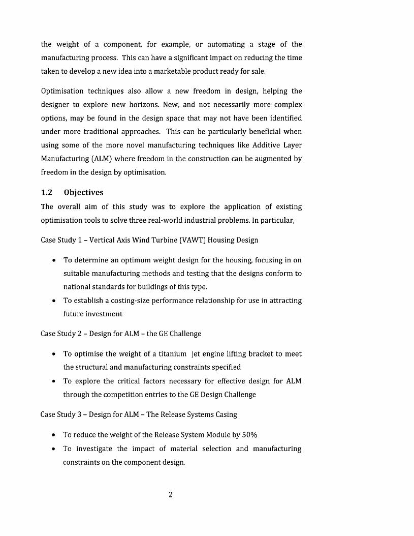
1.2 Objectives

The overall aim of this study was to explore the application of existing

optimisation tools to solve three real-world industrial problems. In particular,

Case Study 1 - Vertical Axis Wind Turbine [VAWT) Housing Design

• To determine an optimum weight design for the housing, focusing in on

suitable manufacturing methods and testing that the designs conform to

national standards for buildings of this type.

• To establish a costing-size performance relationship for use in attracting

future investment

Case Study 2 - Design for ALM - the GE Challenge

• To optimise the weight of a titanium jet engine lifting bracket to meet

the structural and manufacturing constraints specified

• To explore the critical factors necessary for effective design for ALM

through the competition entries to the GE Design Challenge

Case Study 3 - Design for ALM - The Release Systems Casing

• To reduce the weight of the Release System Module by 50%

• To investigate the impact of material selection and manufacturing

constraints on the component design.

2

The w ork o f the three case studies was not only to provide beneficial outcomes

for the companies involved but also to broaden the existing knowledge in the

area of optimised design w ith particular focus on establishing robust solutions

and methodologies.

1.3 Thesis Layout

Chapter 2 of this thesis w ill look in some detail at the place of optimisation in

the design process as observed from the recently published literature. It w ill

reflect on some of the benefits and issues relating to different optimisation

algorithms. It is beyond the scope of this work to consider all the various

algorithms that have been researched. The chapter gives a general overview of

optimisation and looks in detail at some of the most commonly used algorithms

together w ith those used in later chapters. A number of comprehensive review

papers are available [1-3] that address these topics in greater detail.

The remainder of the thesis falls into two distinct parts. Part 1 focusses on the

first Case Study, the design of a housing for a novel vertical axis w ind turbine

design. The problem and the development of the optimised solution are

discussed in Chapter 3. The objective of this work was to determine costing

trends based on minimising the weight of the structure as part of the process of

securing future investment for the turbine. Since this solution was required for

eventual construction the design needed to conform to national building

standards. Chapter 4 investigates the opportunities to improve the

computational efficiency of the methods developed in Chapter 3. Detailed

discussion is presented of the use of the Kreisselmeier Steinhauser functions for

this purpose.

Part 2 incorporates the two remaining case studies, both of these address the

design of components using ALM. The first, in Chapter 5 originated from a

crowdsourcing design challenge issued by General Electric for a je t engine

bracket. The chapter discusses the opportunities for design w ith optim isation

for ALM build and presents some of the changes in design perspective that need

to be made w ith ALM. Chapter 6 explores the optimisation of the build

orientation to minimise the support volume requirement w ith ALM and

3

software that has been developed. Some of the entries from the design

challenge have been used to test the efficacy of the software. Here it can be

seen that optim isation techniques can be applied not only to component design

but also in bringing improvements to the efficiency of the manufacturing

process.

Chapter 7 examines the design of an aerospace component where the company

were assessing ALM as a possible manufacturing method. The investigation

formed part o f the ir undertaking to secure new orders in the aerospace market.

In addition to the optimised design this Case Study considers the complex

relationship between material selection, manufacturing process and design

methodology. Parts of the component have been manufactured and so partial

validation of the design has also been reported.

The final chapter draws together the conclusions from this w ork and considers

the ir implication for present and future work.

4

Chapter 2: L iterature Review

Summary: This chapter gives an overview o f existing optimisation methods with

particu la r focus on topology and size optimisation and their use in commercial

software

2.1 Engineering Design

The trad itiona l approach to the design o f a component, or modification to a

process, has been a "w a te rfa ll” o r serial procedure. The outcomes of each task

or stage o f the design "flow ing ” in to the next and w ith each phase fu lly complete

before the next one was begun (see Figure 2-1). There are however d ifficulties

w ith this. e.g. some phases may impose constraints that restrict future stages, or

cause conflicts that may increase waste, or add additional costs in development

[4]. Innovation in early stages may be diluted by later stage requirements [5].

Typically the development costs were high and the project time long [6] w ith

this approach.

Figure 2-1: T ra d itio n a l "W ate rfa ll” Approach to Product Design

Since the 1990s the concept o f concurrent or simultaneous engineering has

been exploited in many sectors o f industry. Under this regime phases of the

development overlap o r progress in parallel and there is greater collaboration

O n - p ,

ProductPlanning

De sign Review

Proto­type

PilotProduction

■Mass

Production

5

between departments involved in the d ifferent stages of the design chain

(Figure 2-2). This has led to better co-ordination, w ith downstream issues

being addressed and feedback provided earlier in the process. Chapman and

Pinfold [7] showed w ith the bar chart o f Figure 2-3 how the cost o f changes in

design increases steeply the fu rthe r through the process the changes are made.

The early in tervention characteristic of Concurrent Engineering can bring

significant savings in development costs. The use of this approach generally

leads to reduced tim e to m arket and improved p ro fit margins as the companies

are able to meet customers' requirem ents in a more tim e ly manner and ahead

of the ir com petitors [8].

Concept

MassProduct

ion

ProductPlanning

ProductDevelop­

mentPilot

Production

Proto­type

Figure 2-2: Schematic o f Concurrent o r Simultaneous Engineering show ing

in te rac tion at m u ltip le stages o f the design process

Concurrent Engineering is not always the best approach. Many authors have

highlighted lim ita tions in this methodology, namely, some downstream

processes like mould fabrication may be highly dependent on the final design of

the component and would prove costly if progressed before the design was

finalised [6]. Some designs become increasingly and unexpectedly complex as

6

the project progresses and so it becomes more d ifficu lt to manage d ifferent

stages simultaneously [9].

10,000

Concept Eng'g Detail Tooling Production

Figure 2-3: The cost o f change in Engineering Design [7]

The w ork o f this thesis focussed on the early concept phase of design but also

considered the impact o f some of the la ter phases, such as the manufacturing

constraints and the costing o f the structures.

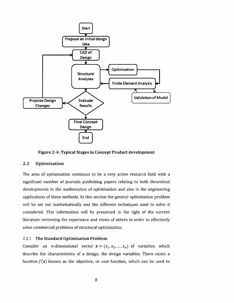
Figure 2-4 shows a flow chart o f the typical stages and tools used in developing a

detailed concept design. The process begins w ith a new idea, or some change to

an old design. The in itia l design is formalised in to a CAD geometry and then

analysed using structura l analysis tools, e.g. optim isation techniques and fin ite

element models. O ptim isation methods a llow optim al feasible solutions to be

found w ithou t having to search through all the possible solutions. These w ill be

discussed at length in the fo llow ing sections.

Ideally these models would be validated using test data, but this may not be

available at this stage of the development. The evaluation o f the results

assesses the su itab ility o f the design against previously defined crite ria e.g. the

impact o f the design on the re liab ility , accuracy, m anufacturab ility and costing

o f the components together w ith the structura l assessments. Modifications are

proposed and changes made to the CAD and the cycle is repeated un til the

design appears satisfactory at this early stage.

7

Validation of ModelEvaluateResults

End

Start

CAD of Design

Optimisation

Final Concept Design

Propose Design Changes

Finite Element Analysis

Propose an initial design Idea

StructuralAnalyses

Figure 2-4: Typical Stages in Concept Product development

2.2 Optimisation

The area of optim isation continues to be a very active research field w ith a

significant number of journals publishing papers relating to both theoretical

developments in the mathematics of optimisation and also in the engineering

applications of these methods. In this section the general optimisation problem

w ill be set out mathematically and the different techniques used to solve it

considered. This information w ill be presented in the light of the current

literature reviewing the experience and views of others in order to effectively

solve commercial problems of structural optimisation.

2.2.1 The Standard Optimisation Problem

Consider an n-dimensional vector x = (x1,x 2, ■■.,*„) ° f variables which

describe the characteristics of a design, the design variables. There exists a

function f ( x ) known as the objective, or cost function, which can be used to

8

classify the design, to indicate the goodness of the design. The generalised

optim isation problem seeks to minimise this objective function

min / ( * ) = f ( x Xlx 2, 2- l

subject to equality constraints, in this case p of them

h j{x ) = hj (x1,x 2, . = 0; j = 1 top,

2-2p < n

and m inequality constraints

9 i(x ) = 9 i ( x i , x 2, . . . ,xn) < 0; i = 1 to m 2.3

and

< xk < x ku, k = l t o n

where xkL and xku are the smallest and largest permissible values of the xk

respectively [10,11].

The functions / ( * ) and gt(x ) can be linear or non-linear in the design variable

x. Some design problems do not have any constraints whether equality or

inequality. Different solution approaches are used in each case, though

unconstrained optimisation problems occur infrequently in practical

engineering design. The design variables, xk are generally considered to be

continuous but problems can be solved where the design variables are discrete.

An example of this would be the number of wind turbines that w ill f it into a

predefined area. This can only take integer values making the design variable

discrete.

A des ign*is said to be acceptable or feasible if it satisfies all the design

constraints. In order to determine i f the design is optimal it must satisfy the

necessary and sufficient conditions set out in section 2.2.2 below.

The design may be a local or a global minimum. This can be seen clearly for a

function of one variable shown in Figure 2-5, but is more formally expressed:

9

A fu n c t io n /(x ) o f n variables has a global m inim um at x* i f the value o f the

function a tx* is less than or equal to the value of the function at any point x in

the set o f feasible solutions, i.e.

f ( x * ) < f ( x ) V feasible x 2-4

The m inim a is local i f equation 2-4 holds for all x in a small neighbourhood

[12].

y

Global minima

Local m inima

a c

Figure 2-5: Function o f one variab le showing local and global m inim a

Over the range a < x < b the global m inim a is clearly identifiable in Figure 2-5

however since the behaviour o f the function cannot be determ ined outside this

range it is not possible to claim that it is the global m in im um for all x . If the

function were convex then any local m inim a found would be the global minima.

A function is convex if and only if the Hessian m atrix H of the function is

positive definite, i.e.

10

H =d2f

dxLdXj; i = 1, ...,n j = 1, ...,n

and

H > 0

In Figure 2-5 the function is convex over the interval c < x < b.

2.2.2 Karush-Kuhn-Tucker (KKT)

There are certain necessary and sufficient conditions that have been proven to

ensure that a local optimal solution can be found. These are known as the

Karush-Kuhn Tucker (KKT) conditions.

A function known as the Lagrangian can be defined such that

v

2-6

K I I I

L{x, X) = f { x ) + Xjh jix) + ^ Higtix)7 = 1 i = l

Xj and fa are called the Lagrangian and KKT multipliers respectively.

Then x is a minimum if and only if there exists a unique set of constants such

that

1. VxL(x,A ,n) = 0 2-7

where the V denotes the partial derivative of the function w ith respect to each

of the variables x t. Also

2. H i> 0 f o r i = 1, ...,m 2-Q

3. = 0 f o r i = 1, ...,m 2-9

4. ^ ( x ) < 0 f o r i = 1, ...,m 2_10

5. h j(x ) = 0 f o r j = 1, ...,p 2 1 1

11

These conditions are sufficient only i f the functions f ( x ) and g t(x) are

continuously differentiable and convex and the functions hj(x) are linear w ith

vector x being a regular po in t1.

In most real-life problems there is not enough information known about the

functions to determine whether they satisfy these sufficiency conditions but

generally condition 1 (Equation 2-7] is used to locate the minima as w ill be seen

in later sections.

This generalised form of the optim isation problem can be applied to any field of

problem-solving e.g. finance, transportation and operational research. Once the

problem is formulated in this way the optim isation techniques described

throughout this chapter can be used to solve the problem independent of the

design application. The focus however, w ill be solely in the area of the

optimisation of structures.

2.3 Structural Optimisation

Much of the early research on structural optimisation focussed on sizing

problems, e.g. optimising truss cross-sections or plate thicknesses. For size

optimisation the domain o f the problem is fixed and remains so throughout the

optimisation.

This w ork progressed further to include problems that sought to identify the

optimal boundary for the structure under consideration, e.g. finding the shape

of an aircraft wing that minimised drag. This is known as shape optimisation.

In these types of problem the shape of the domain does not remain constant but

the topology2 remains the same throughout the optimisation.

Both of the above approaches fix the in itia l topology and so it is possible that

the optimal obtained is not the "best" result. To overcome this, a th ird approach

called topology optimisation has been developed. This is sometimes called

1A feasible point is regular when the gradients o f the constraints at that point are linearly independent, i.e. no two gradients are parallel to each other2 Topology: a mathematical term used to relate classes o f shapes where any shape in one class can be transformed into any other shape in that class without tearing or ripping e.g. a circle and a square are in the same class and thus have the same topology, whereas an annulus and a circle do not.

12

layout optim isation [13] and provides solutions to problems of optimising the

configuration of members and joints in a space-frame structure for example.

More generally the method determines the optimum position of material and

"holes" in both two and three dimensional structures w ithout having to

predetermine the boundary of the structure artificially. Topological

optimisation can be seen as a pre-processing tool for shape and size

optimisation.

In summary there are three main classes of structural optimisation:

1. Topology - an optimised shape and material distribution for a structure

can be determined w ith in a given domain.

2. Size - where the shape of the structure is fixed but the thickness of a

sheet for example, or cross section of a beam can be optimised.

3. Shape - the outer boundary of the product is optimised

Sigmund[14] refers to a 4th class of optimisation - material optimisation, but in

this review this has been included as part of topology optimisation as any

material can be considered to be a structure on a microstructural level. Only

topology and size optim isation w ill be discussed in this literature review as

shape optim isation techniques have not been used in the case studies that form

the main body of this thesis.

2.4 Topology Optimisation

Topology optim isation is now used extensively to optimise weight and

performance in the automotive and aerospace industries, but also in a wide

range of other applications [15], for example, to design a new material w ith a

negative Poisson's Ratio i.e. one that expands laterally when pulled along the

length [16]. It has been a very active area of research w ith engineers and

mathematicians seeking to refine and exploit new methods and approaches.

The first paper published on topology optimisation was by an Australian

Inventor, Anthony G.M. Michell [17] in 1904 who optimised the layout of trusses

to minimise weight. The analytical methods used by Michell worked only for

13

relatively simple load cases. As optimisation problems have become more

complex computer-based solutions have been used extensively. The firs t such

method was proposed by Bendsoe and Kikuchi[18] in 1988 where shape

optimisation problems were transformed to material d istribution problems by

using a material made up of two distinct parts - substance and void. This was

known as the Homogenisation method. This approach has since been developed

much further and this w ill be discussed in detail in section 2.4.1. Since this time

there has been a large body of research undertaken in all aspects of topology

optimisation. There have been a number of comprehensive review papers

detailing the historic background and development of methodologies [1, 2, 19-

21]. This section w ill focus on the most popular techniques which have been

used in industrial applications, particularly those available in commercial

software, but firs t the formulation of the general topology optimisation problem

w ill be set out.

2.4.1 Design Problem Form ula tion

The general topology optim isation problem based on linear static analysis can

be expresses as:

find the distribution of material that minimises an objective function, f ( x )

subject to a volume constraint g0(x) ^ 0 and possibly m other constraints

g i(x ) < 0 i = 1, ...,m.

The material distribution is described by the density variable p{x) that can take

values 0 (representing a void) or 1 (solid material) at any point over the design

domain O. W ritten mathematically this takes the form

min: / ( p , U),2-12p

subject to: K(p)U = F (p) 2-13

9o(P>U) = [ p ( U ) d V - V 0 < 0 Jn

2-14

• g i ( p , U ) < 0, i = 1, ...,m 2-15

14

; p ( f/) — 0 or 1, V x £ Q 2-16

where U is the displacement vector, K is the global stiffness matrix, F the

vector of known external forces, V is the volume and V0 is the volume of the

design domain H [1, 22].

Typically this problem is solved by discretising the domain H into a large

number of finite elements (say N). The density variable is assumed to be a

constant w ith in each element of the domain. The problem can then be

expressed as

m in :/(p , U),p 2-17

subject to: K(p)U = F (p ) 2-18

N

: do(p>u) = ^ p j V j - v0 < oj =i

: 9 i ( p ,U ) < 0, i = 1, ...,m

: Pj = 0 or 1, y == 1,...,

2-19

2-20

2-21

where pj and v; are the density and volume of the elements respectively.

The problem in this form lacks solutions in general [22] as decreasing the mesh

size enables more holes to be introduced which w ill, of course reduce the value

o f / ( p ) ad infinitum . By modifying the problem so that p; becomes a continuous

variable, solutions can be found. So equation 2-21 becomes

0 < e < pj < 1 V j = 1,..., N 2_22

and e is a small positive value chosen to prevent any one element disappearing

completely which would require the domain to be remeshed and cause

singularity of the stiffness matrix.

Approaching the problem in this way enables solutions to be found more easily

using gradient based techniques but the results include elements which take

15

interm ediate values o f the density, known as grey areas (Figure 2-6) and these

have no physical in terpre ta tion when designing w ith trad itiona l materials.

10.14

0.12

Elem ent 0.08 density

0.06

0.04

0.02Figure 2-6: Topology O ptim isation o f a Cantilever Beam showing

in te rm ed ia te values or "grey" areas o f the density variab le [23]

Bendsoe & Sigmund [24] have shown how this can be represented when using

composite materials. This thesis w ill not focus on composite optim isation but

w ill use methods that have been developed to m inim ise the grey areas ensuring

a clear prediction of where material is need in the optim ised structure.

2.4.2 Solution Methodology

Before describing some of these solution methods in detail a schematic for

topology optim isation w ill be discussed to c larify the steps in the process.

Figure 2-7 shows a flow chart o f a typical gradient-based topology optim isation

problem.

In itia lisa tion : The firs t step requires the setting up of the geometry together

w ith the loadings and the density d is tribu tion , p.

Finite Element Analysis: The optim isation loop begins by using FE analysis to

solve the equ ilib rium equation 2-18.

Sensitiv ity Analysis: The next step, the sensitiv ity analysis calculates the

partia l derivatives of the objective function w ith respect to the design variables.

This analysis provides essential in form ation on the gradients of the functions

and determines the d irection the optim iser must take in order to move towards

16

the minimum value of the function. The analysis can be calculated w ith

numerical or analytical methods, the former tend to be easy to implement but

less accurate and computationally expensive [11]. Many researchers use one of

two analytical methods, the Direct method or the Adjoint method which w ill be

described in detail in sections 2.4.2.1 and 2.4.2.2. A detailed review of the

different methods can be found in the paper by Tortorelli and Michaleris[25].

No

Converged?

Yes

Initialisation

Final Topology

Sensitivity Analysis

FilteringTechnique

Finite Element Analysis

Optimisation (update design variables)

Figure 2-7: The General Flow of Computation fo r a Gradient-Based

Topology Optimisation [26]

2.4.2.1 The D irect Method

For any of the responses gi(p, t /) in equations 2-19 and 2-20 by the chain rule

dg i (x*) = dgt ( x \ U ( * " ) ) d9 i {x ' ,U{x*)) dUjxT)dxj dxj "** d(J ' dxj 2-23

17

f o r i = Q,...,m a n d j = 1, . . . . ,N

at a design vector x* which has N components

From the equilibrium equation

KU = F 2-24

where K is the stiffness matrix and F the vector of forces. This can be

differentiated w ith respect to x to give

dxj dxj dxj 2-25

And so

, dU (** ) dF {x *) d K {x *) , x K(x*) a = a -------

dxi dxj 2-26

or

dxj= K - ' t x * )

dF (x*) dK(x*)dxj dxj

U{x*) 2-27

If K (x*) , the inverse of the stiffness matrix has already been computed in the

dU{x*~)fin ite element analysis then the calculated value of — from equation 2-27

0 X j

can be back substituted into equation 2-23 to obtain the derivative of each of

the responses, This back substitution must be made for each of the Ndxj

design variables and so works best i f there are relatively few design variables.

2.4.2.2 The A d jo in t Method

3U{x*)In the Adjoint method — is eliminated from equation 2-23 using a Lagrange

u X j

m ultip lie r method where

A (x*)) = 9i(x' , I /O * ) ) - A jO *)[K ’0 * M * * ) - F O *)] 2 -28

where A is an arb itrary m+1 dimensional vector

18

Differentiating equation 2-28

d L i(x \A ) _ dg i(x * ,U (x * )) dg i(x*,U (x*)) dU(x*)dxj dxj

dAi(x*)dxj

dU

[K(x*)U (x*) - Fix*)]

dXi

- Adx *)dK(x*) , , , J U ( x * ) dF(x*)

U{x*) + K(x*)dXi Ox; dxj

2-29

It should be noted that from the equilibrium equation the firs t bracket in the

above equation is zero as is the second bracket from equation 2-26 so

dLj(x*,X) _ dgjjx*)dxj dXj 2-30

i dAiRearranging equation 2-29 and eliminating the — term givesdx i

d l t e ' . X ) _ dg i { x ' ,V ( x ' ) )dXi

+

dxj

dU(x*)

- A d x * )d K ( x * ) . dF{x*)

U(x ) -

dxjdg i ( x ' ,U (x ' ) )

dU- Kr (x*)Adx*)

2-31

and K r denotes the transpose of if.

Since A is arbitrary, it can be chosen by solving equation 2-32 below to

eliminate the co-efficient of the termdx;

K T(x*)Adx*) =_ d g i {x*,U{x*))

dU 2-32

So equation 2-31 becomes

19

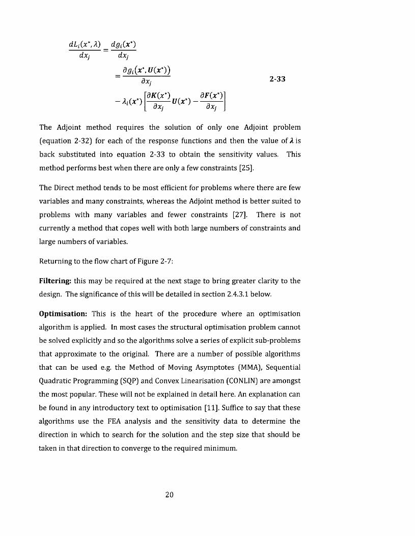
dLi (x* ,X) d g t { x *)

dxj dxj

dgi ( x \ U { x * ) )dxj 2-33

dK{x*) dF(x*)U ( x * ) ~

dxj dxj

The Adjoint method requires the solution of only one Adjoint problem

(equation 2-32) for each o f the response functions and then the value of A is

back substituted into equation 2-33 to obtain the sensitivity values. This

method performs best when there are only a few constraints [25].

The Direct method tends to be most efficient for problems where there are few

variables and many constraints, whereas the Adjoint method is better suited to

problems w ith many variables and fewer constraints [27]. There is not

currently a method that copes well w ith both large numbers of constraints and

large numbers of variables.

Returning to the flow chart o f Figure 2-7:

Filtering: this may be required at the next stage to bring greater clarity to the

design. The significance of this w ill be detailed in section 2.4.3.1 below.

Optimisation: This is the heart of the procedure where an optimisation

algorithm is applied. In most cases the structural optim isation problem cannot

be solved explicitly and so the algorithms solve a series of explicit sub-problems

that approximate to the original. There are a number of possible algorithms

that can be used e.g. the Method of Moving Asymptotes (MMA), Sequential

Quadratic Programming (SQP) and Convex Linearisation (CONLIN) are amongst

the most popular. These w ill not be explained in detail here. An explanation can

be found in any introductory text to optimisation [11]. Suffice to say that these

algorithms use the FEA analysis and the sensitivity data to determine the

direction in which to search for the solution and the step size that should be

taken in that direction to converge to the required minimum.

20

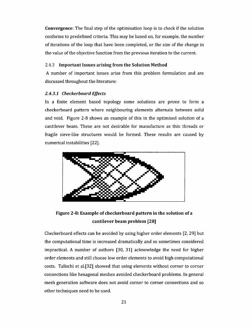
Convergence: The final step of the optimisation loop is to check if the solution

conforms to predefined criteria. This may be based on, for example, the number

of iterations of the loop that have been completed, or the size of the change in

the value of the objective function from the previous iteration to the current.

2.4.3 Important Issues arising from the Solution Method

A number of im portant issues arise from this problem formulation and are

discussed throughout the literature:

2.4.3.1 Checkerboard Effects

In a finite element based topology some solutions are prone to form a

checkerboard pattern where neighbouring elements alternate between solid

and void. Figure 2-8 shows an example of this in the optimised solution of a

cantilever beam. These are not desirable for manufacture as thin threads or

fragile sieve-like structures would be formed. These results are caused by

numerical instabilities [2 2 ].

Figure 2-8: Example of checkerboard pattern in the solution of a

cantilever beam problem [28]

Checkerboard effects can be avoided by using higher order elements [2, 29] but

the computational time is increased dramatically and so sometimes considered

impractical. A number of authors [30, 31] acknowledge the need for higher

order elements and still choose low order elements to avoid high computational

costs. Talischi et al.[32] showed that using elements w ithout corner to corner

connections like hexagonal meshes avoided checkerboard problems. In general

mesh generation software does not avoid corner to corner connections and so

other techniques need to be used.

21

2.4.3.2 Mesh Dependency

It has been found that unless additional steps are taken topology optimisation

results are dependent on the number of fin ite elements chosen for the domain.

Figure 2-9 shows an example of this w ith a simply supported beam [22]. The

topology optimised result of (b) was calculated using 600 elements while the

result in (c] used 5,400 elements. The result is clearly more detailed in (c) than

in [b] and shows a higher order of complexity.

r

t _________________

(C)

Figure 2-9: Topology Optimisation of a simply supported beam showing

mesh dependency [22]

Several methods have been proposed in the literature to correct this feature;

these are known as restriction methods. Three main classes of these have been

identified [20, 33], but other methods exist which are either sim ilar in approach

or further developments of the same:

1. Filter method - These are the most popular due to their ease of

implementation and efficiency

i. Density filte r - each element density is redefined as a

weighted average of the densities in the neighbourhood of

22

that element. The size of the neighbourhood is independent of

the size of the mesh [33-35].

Finite element mesh

Design variable e___

Design variable/:

Figure 2-10: Illustration of the Density Filter [31]

An example of a density filte r [30] is shown in Figure 2-10.

The filte r has been defined as

l w kpkPe II wk

2-34and wk = r°—-

ro

The density of the design variable e becomes a weighted

average of the densities of the elements that lie w ith in a circle

centered at e w ith mesh independent radius, r0. In this

example the weighting factor wk > 0 are defined as a cone

filter, decreasing linearly as the neighbouring nodes near the

edge of the circle. The weighting factors are zero outside the

circle. This filte r smooths the jagged edges of the design and

the mesh independent radius ensures that the solution is

more robust. The technique adds no additional constraints to

the problem.

ii. Sensitivity filters [22] are similar to density filtering but as the

name suggests average sensitivities over a fixed size

neighbourhood. In itia lly seen as an heuristic method w ithout

23

physical justification, a recent paper by Sigmund & Maute [36]

has shown its equivalence to other optim isation approaches.

Both i & ii above create a grey porous region between solids

and voids in the result. The w idth of this region depends on

the filte r size. To minimise this effect the region size and

influence of the filte r is generally reduced as the optim isation

process progresses, but this can cause problems w ith the

mesh dependency effect

2. Constraint Methods - these are more difficu lt to use as they require

tuning of a constraint value and increase the number of constraints

and therefore the computational time. Among these are:

a. Perimeter Control Method [37, 38] which lim its the number of

holes in the solution by lim iting the inner and outer

perimeters

b. Local [39] and Global [29, 40] Gradient Control. Controlling

the gradient locally forces the distance between voids to take

a fixed minimum length but this unfortunately introduces a

large number of additional constraints. A single constraint

can be applied but the choice of a suitable value is d ifficu lt and

problem specific.

Other constraint methods include Regularised Penalisation, Integral

Filtering Method, Wavelet Parameterization, Phase-field approaches

and Level Set methods and many others which have been reviewed

by Deaton and Grandhi [1]

Most of the techniques used to deal w ith mesh dependency can overcome the

checkerboard instabilities at the same time [2 2 ],

2A.3.3 The Objective Function: Stiffness vs Strength

The objective function / in equation 2-17 can take a variety of forms, the most

common of which is compliance. M inimising the compliance in the optimisation

problems finds structures w ith the greatest stiffness. Compliance problems are

24

often solved w ith a volume constraint to creature the maximum stiffness w ith a

known and generally reduced volume [19, 21].

Often in optim isation problems the desired final volume is not a known quantity

and so using the compliance as the objective function tends to require a number

of iterations before a satisfactory solution can be found. In many applications

especially automotive and aeronautical engineering the aim is to design the

lightest components possible. This is true of all the case studies discussed in the

remaining chapters and so only, optimisation problems which minimise mass

w ill be considered and not compliance problems. Equation 2-17 therefore

becomes

iv

2-35j =i

where m.j is the mass of the individual elements.

W ith a mass objective function it is necessary to include some measure of

material stress w ith in the constraints of the problem to ensure that the

structure is sufficiently strong and resilient under the external loadings. In this

case the stress constraints can be written as

o~i < aY V i = 1, ...,N 2-36

where 07 are the stresses of the individual elements and oy is a prescribed

upper lim it for the yield strength of the material. The von Mises' stress is often

used by engineers and designers for the elemental stress as it has proved to be a

reliable measure to establish failure criteria. Other inequality constraints may

also be used in this m inimum mass problem such as displacement and buckling

constraints.

Some issues relating to the use of stress constraints w ill be discussed in the

following section. It is im portant to observe at this stage that using compliance

as the objective function and a volume constraint can give a very different result

to the problem w ith an objective function of mass with stress constraints. The

stiffest structure is not necessarily the same as the strongest [41-44]. Some

25

more recent w ork [45] has looked at m inimising the weight w ith constraints on

both stiffness and stress w ith some success when tested on benchmarking

applications.

Other examples of suitable objective functions include the stress itself,

frequency, displacements, buckling etc.

2.4.3A Stress Constraints

The inclusion of stress constraints in the problem gives rise to three significant

challenges that have to be addressed:

1. In the discrete formulation of the optimisation problem [equations 2-17

- 2 -2 1 ] the stress constraints are precisely defined when p equals either

0 or 1 , but when the problem has been modified for p to be continuous

[equation 2 -2 2 ) stress levels are not defined for the intermediate values.

A number of authors [31, 43, 46] have used a power law to express the

stress w ith in the range, i.e.

a (Pi) = Pi^Y 2-37

This is generally used in conjunction w ith the Solid Isotropic

Microstructure w ith Penalization [SIMP) approach which w ill be

discussed at length in section 0 . q is called the penalisation parameter.

A typical value for q is 3 [24]. Le et al.[30] used q =1. Bruggi and Duysinx

[45] claim that they achieve better results when q is less than the SIMP

penalisation parameter s , taking a value of 2.8 for q when s =3.

2. Stress "singularities". This phenomena was first identified in the layout

optimisation of truss structures by Sved & Ginos [47] where convergence

problems were encountered as some of the bars of the truss reached

small values. It was found that as both the force and the area in a region

tended to zero the stress became undefined and not zero as expected.

Later work observed the same condition in continuous topology

optimisation [42] and Duysinx and Bendsoe [43] proposed a relaxation

method to modify the stress constraint known as the "e-constraint

relaxation" approach where

26

o - aY)p < e2 2-38

0 < e2 < pmin < p < 1 2-39

This enables the density variable to tend to zero in the optimisation

w ithout the loss of the design domain and the subsequent extreme local

stress value. The solution is obtained by solving a sequence of

optimisations problems w ith decreasing e values w ith the results of one

step being used as the starting point for the next. Many authors have

used this approach w ith some variations [41,48, 49]

Svanberg & Werme [50] used a sequential integer programming method

to solve the discrete 0-1 stress constrained problem directly. The issues

of stress singularities and penalisation did not need to be addressed w ith

this technique.

3. Stress is a "local" quantity and so when using finite element techniques

the stress must be constrained at each element of the domain. This gives

rise to many times more constraints when compared to the compliance

problem and is computationally more expensive. One of the first authors

to tackle this issue for continuous domains was Yang & Chen [42] in

1996. They looked at reducing the local stress constraints down to a

single global stress value and using this stress as the objective function

subject to a constraint on material usage. Two different global functions

were used:-

a. Kriesselmeier-Steinhauser (KMS][51]. This has taken a number

of forms in the literature, but the definition shown here is the one

used by Wrenn [52] which avoids the numerical difficulties that

can occur when calculating the exponential of large numbers.

N

9 max) 2-40i = 1

where gi(cr) are the stress values at each N finite elements and

9max is the maximum value of this set of stresses. The parameter

k is a scalar m ultip lie r which typically takes values in the range 5-

27

200. A number o f authors recommend k = 50 to be a reasonable

value [27,52-54].

Illustration o f KMS Constraints Aggregation in 2D

6

-2

-4

4m KMS k = l

KMS k=50

“ ” Obj Fn

Constrl

Constr2

-6-4 -2 0 4

X

Figure 2-11: An Example o f the Kre isselm eier Steinhauser Function in 2-D

Figure 2-11 illustrates the KMS functions for a function o f one

independent variable w ith one linear and one non-linear

constraint. The KMS function combines the two constraints

giving a single continuous constra int for the optim isation

problem. The insert to the figure shows how the function changes

w ith changing k. The higher the value o f k the more closely the

KMS function follows the vertices of the constraint curves.

Raspanti et al.[53] developed the basic properties o f the KMS

function. The most pertinent o f which are summarised below

i] KS(o ,k ) > m a x (^ O ) ) 2_41

ii] hm KS(p, k) = m a x ^ O ) ) 2 42

hi) KS(a, k 2) > K S t o . k J

iv ] KS(a, k) is convex if and only if all constraintsare convex

28

Equations 2-41 and 2-42 show the KMS functions are always an

overestimate of the maximum of the constraints and the function

w ill return a positive value if one or more of the constraints is

violated. Equation 2-43 is a statement of the behaviour shown in

the insert of Figure 2-11 that the KMS function more closely

follows the constraints as k increases. The last property shows

that the KMS does not alter the convexity of the original problem.

It is possible that the feasible region defined by the KMS function

may not contain the true optima. Poon and Martins [27] overcame

this by using an adaptive KMS function where the value of k was

increased as the solution approached the intersection of two or

more constraints. Their results showed that the method achieved

a more accurate optimum but the computational time was greater

than for the standard KMS function.

The KMS function w ill be discussed further in Chapter 4 where

the function was used to investigate the efficiency of computation

of a size optim isation w ith a large number of stress constraints.

b. A function proposed by Park [55] known as the p-norm

i

As p -> oo the function has the property

lim KK(a) = max crp -> oo i 2-46

Duysinx et al.[44] used two global measures for the stress

constraint based on the p-norm, called the q-norm and the q-

mean where they incorporated the relaxation technique w ith in

the constraints to avoid the singularity issues. Qiu and Li [46]

29

claimed that the KMS function was better than the p-norm in

being adapted for use w ith optimisation algorithms because it is a

smoother function.

c. A th ird and the simplest of the constraints aggregations methods

is to take only the most violated of the constraints, i.e.

m a x (^ O )) 2 4 ?

The major d ifficu lty w ith this approach [27] is that for a

continuum problem it is not differentiable and for a discrete

problem the search direction for the algorithm is determined by

considering only the most violated constraint. This usually leads

to the violation of another and different constraint in the next

iteration. Many algorithms find this type of problem difficu lt to

solve.

Some authors [31, 43, 45, 56] observe that although these global

approaches are effective in problems that are free from localised stress

concentrations they are not sufficiently robust to effectively work w ith

these high peak values. An alternative technique is to take a clustered

approach [31] where stress points are grouped and one stress constraint

is applied to each group. This increases the computational cost but

improves the control of the stress. This is sometimes called blocking

aggregation [57] or regional stress measure [30]. A variation of this is

found in the "constraints screening" approach used in A lta ir Optistruct

[58] where a subset [usually 20] of the most violated constraints are

taken to be representative of the whole optimisation problem. This

reduces the computational time but does not affect the overall direction

of the optim isation problem. The practical impact of constraints

screening w ill be discussed in some detail in chapters 3 and 4.

Pausing here to summarise what has been learnt so far. For a linear static

optim isation problem using finite element methods to minimise mass the

following system of equations must be solved

30

N

min n i j P j 2 -4 87 = 1

subject to : K(p)U = F(p) 2-49

: O j< a Y V j = l , . . . ,N 2 . 50

: gi ( f i ,U)< 0 i = 1, ...,m 2-51

: 0 < £ < p;- < 1 V j = l , . . . ,N 2-52

Steps must be taken to ensure that the solution

i) includes filtering techniques to avoid mesh dependent solutions.

These may also correct checkerboard effects, but if not, higher order

elements can be used to reduce the problem but at a high

computational cost.

ii) accounts accurately for stress singularities.

iii) defines stress for all values of the density variable and

iv) may employ constraints aggregation to improve computational

efficiency.

The following sections look in detail at some of the most commonly used and

effective methods for solving this optimisation problem.

2.4.4 Solution Methods fo r Topology Optim isation

Several comprehensive surveys of literature have provided an overview of the

available approaches to topology optimisation. Deaton & Grandhi [1] focus on

methods that have been used successfully in commercial applications while a

more academic review has been recently compiled by Sigmund [2]. The breadth

of the latter is far beyond the scope of this work and so this section w ill fo llow

the approach of the Deaton and Grandhi review looking particularly at those

methods that have been used to solve industrial problems. The techniques can

be grouped together in four main groupings: density-based, hard and soft kill,

boundary variation and stochastic methods.

31

2.4.4.1 Density-based methods

Solid Isotropic Microstructure with Penalization (SIMP)

One method of solution that has been used extensively throughout the

literature is the SIMP or power law method. It was first proposed by Bendsoe in

1989 [59] though not called SIMP until 1992 [60], The objective of the method

is to introduce a penalisation function to eliminate those areas that take

intermediate values of density to create a clearer "black and white"/solid-void

design. The stiffness m atrix is modified so that

N

*(/> ) = 2 .53i=1

where K° is the element stiffness m atrix for the solid material and 5 is the

penalisation parameter.

The value of 3 is often recommended fo r s [24], which is in line w ith point 1 in

section 2.4.3.4 above and which Duysinx & Bendsoe [43] showed was also

consistent w ith the physics of the problem. Other single values have been used

successfully [61] but it has also been shown in work by Rozvany [62], and

Dadalau [63] that the so-called "continuation approach" where s is in itia lly set

to 1 and then gradually increased throughout the optimisation to 5 (say)

increases the likelihood of converging to the global minimum.

One of the main advantages of the SIMP method is that it is easy to implement.

Rozvany [21] advocates that the SIMP method usually finds the correct global

optimum when the problem is convex (e.g. compliance) and the penalty factor is

gradually increased from 1, however SIMP has been applied to many highly

complex non-convex problems and though the global optimum cannot be

guaranteed in these problems but it does find improved solutions.

SIMP is used extensively in commercial software e.g. A lta ir Optistruct [58] and

applied to a wide range of industrial applications from micro-grippers for

carbon nanotubes [64] to aircraft wings [65].

32

At zero density, SIMP has zero sensitivity. Stolpe and Svanberg [66] proposed

the Rational Approximation of Material Properties [RAMP) to avoid this

problem where

and s is the penalisation parameter.

This method has not been taken up as comprehensively as SIMP but evidence in

the literature shows that it has been applied to recent industrial problems w ith

some success, e.g. hearing aid design [67] and thermal masonry bricks [68].

Bruns [69] modified the SIMP method by introducing a penalisation function

based on the hyperbolic sinusoidal functions. This is known as the SINH

[pronounced "cinch") method and penalised the volume constraint and not the

objective function. This approach was found to produce a better "black and

white" solution.

Only 11 papers appeared over the last year referencing Bruns' SINH method

and in all cases the method was not employed in industrial research or in any

commercial software.

2A.4.2 Hard and Soft K i l l Methods

Another group are known as the "hard-kill" or "soft-kill" methods [70] which

solve the discrete problem and remove or "k ill" the superfluous elements. The

"soft-kill" methods reduce the unwanted elements down to weak or soft

material. The firs t of these methods was the Evolutionary Structural

Optimisation proposed by Xie & Stevens [71].

Evolutionary Structural Optimisation (ESO)

The basic concept o f the approach is that by removing redundant material from

a structure the remaining materials moved towards the optimum, e.g. when

considering the FE stress analysis, under-stressed elements are removed based

on some predetermined rejection criteria and then the analysis is rerun w ith

the new structure and so on. The method uses discrete variables w ith the

N

2-54

33

choice of rejection criteria being heuristic, based on experience, and problem

dependent. The stiffness matrix for ESO is simply

N

2.55i

where pe {0 ,l}

The main advantages of the method are the sim plicity w ith which it can be

integrated w ith commercial analysis software to obtain solutions and that the

result is clearly defined w ithout any "grey" areas [1], One of the main

disadvantages of ESO is that once material has been removed it cannot be

replaced and so an extension of ESO was developed called Bi-directional

Evolutionary Structural Optimisation (BESO) [72].

Bi-directional Structural Optimisation (BESO)

In this method the design space begins w ith a kernel structure, e.g. the

minimum space that w ill carry the load. Elements can then be either added to

overstressed regions or removed from under-stressed areas determined by a

rejection and inclusion rationale respectively.

Both ESO & BESO have come under significant criticism [21, 22] for failure to

address issues of mathematical rigour such as convergence and mesh

dependency. The method has been modified and extended over time [73] to

suppress checkerboard effects and maintain boundary conditions [74]; and

w ith an added penalisation parameter to improve convergence and application

to m ultiple materials [75]. The changes to the method have converted it to a

"soft-kill" technique where redundant material never completely disappears but

becomes soft or weak, i.e. barely adding to the stiffness of the structure. Huang

& Xie in a recent review [76] acknowledged some of the lim itations of the

method and its d ifficu lty in solving some specific problems but they also

reiterated the more recent developments [75] that have increased its

performance.

34

The examples in the literature most often have the objective function as mean

compliance w ith a volume constraint and the restriction criteria applied to the

stresses or the strains. Other constraints have been difficult to include because

the discrete nature of the problem means that sensitivities could not be

obtained by differentiation and were chosen heuristically. Huang & Xie [76]

added a displacement constraint to the problem by establishing a sensitivity

number to rank the sensitivities. This has been further developed by Zuo et

al.[77] who added frequency constraints. Sigmund [2] considers that BESO in its

current formulation should be considered only as a discrete update version of

SIMP and not a separate approach in its own right. It is true that the methods of

filtering are sim ilar to those used in density-based algorithms and a power law

(w ith s =3) is used to compute the discrete gradients.

Some of the industrial applications where ESO/BESO has been used include the

verification of historic architectural design [78] and also for new building

designs in Japan and Italy [79].

2A.4.3 Boundary Variation Methods

These methods are very distinct from the methods described in the previous

two sections because they use the boundary of the design space rather than the

material d istribution and so are closely linked to shape optimisation. They

differ from shape optimisation however in that void regions can be created,

merged or eliminated which is much more akin to topology optimisation. There

are two main techniques in this area of boundary variation methods: Level set

and phase field.

Level set

The Level Set method was firs t introduced by Osher and Sethian [80] and has

since been used for a large range of applications, but was firs t applied to

structural optimisation in 2000 [81]. There has been much research activity in

the intervening years and this work has recently been reviewed by van Dijk et

al.[82].

35

The method finds a local m inimum for an optimisation problem by using the

level set function O which defines a structural boundary over a fixed domain

f l as follows

0 (x ) < = 0i f x ED.

i f x e SD 2 - 5 6

i f x £ n

where x is any point in the design domain, and SD is the boundary of H or the

zero level contour.

This function is illustrated in Figure 2-12 where the plane cutting through the

3D curves defines a domain, in this case consisting of two circles w ith two

circular boundaries.

The following evolution equation is used to update the level-set function and

hence the structure

d®(x, t) d *— f t — * - « * ( * ) 2-57

Where t is time, g(x ) is a scalar field over the design domain and a) is a positive

dxparameter which weights the influence of g. known as the speed or velocity

function moves the interface along the domain w ith respect to some merit

function determined by the optimisation.

The formulation of the level set problem shown in equation 2-57 is based on the

work of Challis [83] and g is used to influence the development of new holes in

the structure. Hole nucleation is an issue w ith this method particularly for 2D

problems and a number of different approaches have been presented in the

literature [2, 84], but a discussion of the merits of these is outside the scope of

this review.

36

n

rrw vK n

Cp(x)<0

b) 3D level set surfacea) 2D boundary at zero

level set

Figure 2-12: Level set representations [85]

The main advantages of using the level set method is that the boundaries are

clearly defined at each ite ra tion and it effectively handles both shape and

topology optim isation sim ultaneously and w ithou t the difficulties that arise

from grey areas [86] nor the extensive post-processing required w ith density-

based solvers [1]. The solutions also do not suffer from the checkerboard effect

[84].

Phase-field method

O rig inally developed to describe the transition from one material phase to

another, e.g. solid to liquid, the phase fie ld method was first applied to topology

optim isation in 2003 by Bourdin and Chambolle [87, 88].

The phase field function 0 is specified over the design domain f l that is

composed of two phases A and B which are represented by the values a and /?

as shown in Figure 2-13. The boundary region between the two phases is a

continuously varying th in strip o f thickness <f and the boundary itse lf is known

as the diffuse interface. In a s im ila r manner to the level set method the interface

is moved w ith respect to tim e to solve the optim isation problem.

37

Phase B

Phase A

Phase A

Phase B

aEdge of diffuse interface region

Center of diffuse interface region Diffuse interface

Figure 2-13: Representation of the of the Phase Field function

in a) 2D and b) ID [89]

2 A A A Stochastic Methods

In some structural engineering problems gradient data is either not available or

extremely d ifficu lt to compute, this has led to a large group of stochastic

optimisation techniques to be developed based on methods of probability and

randomness. The techniques have been reviewed in a number of recent papers

[90, 91]. New methods are being introduced w ith great frequency but only

those which have been applied extensively w ill be reviewed here. The

algorithms have been inspired by other branches of science and so the following

sections have been divided in this way.

Evolutionary Methods

Evolutionary approaches group together a series of modern search techniques

that mimic the processes of evolution and natural selection in order to solve

optim isation problems. The vocabulary is clearly borrowed from genetics and

evolutionary theory w ith parameters like population, individuals, parents and

offspring being used to identify sets of solutions and the ir modification towards

an optimum. A typical evolutionary algorithm takes the following form:-

1. Choose a current set of solutions, known as the population [usually

randomly but sometimes from a previously known set of solutions)

2. Evaluate all members of the population according to a fitness value

chosen for the problem. A fitness value is a measure of perceived

performance

38

While the term ination condition (e.g. a predetermined number of

generations or a suitable optimal value of the fitness function] is not

satisfied

a. Select individual(s) in the population to be parent(s) - based on

the fitness scores (better fitness of parents is assumed to create

children w ith higher fitness]. These parents form the first

generation.

b. Create new individuals by applying variation operators to the

copies of parent(s]

c. Evaluate new individuals

d. Replace some or all of the individuals in the current population

w ith the new individuals

The use o f random selection and probability w ith in the methods gives rise to

final solutions that are not dependent upon the in itia l conditions. They search

from one population of solutions to another rather than from individual to

individual and use only information about the objective function, not its

derivatives.

Some of the major benefits of using these techniques include [92]

• Little, if any prio r knowledge is required of the search space

• Excellent search capability due to the efficient sampling from the space

• Effective at avoiding local minima

• Robust across a wide range of problems

• Provide m ultiple good solutions

• Able to locate the region of the global optimum solution

The main disadvantage is that the method has not been proven to show better

mathematical convergence than for gradient based approaches and the

optim isation tends to be much slower [93], requiring significantly more

iterations to converge to a solution.

39

The three main evolutionary techniques are Evolutionary Strategies (ES],

Genetic Algorithm (GA) and Evolutionary Programming (EP)

These were firs t used for structural optimisation by Hoeffler et al. [94] in 1973.

They used a combination of evolutionary algorithms and linear programming to

optimise the position of joints in a truss structure. A review of the use of

Evolutionary methods can be found in a paper by Kicinger et al.[95]

Physical Algorithms

The physical models' main commonality is that they all draw the ir inspiration

from physical laws. The Harmony Search Method [96] mimics the behaviour

of musical harmonies. The optimisation searches for the most aesthetically

pleasing solution through a random process of memory and pitch adjustments.

Simulating Annealing (SA) [97] imitates the annealing process used in

manufacture of metals. In the annealing process metal is heated and gradually

cooled to create the correct crystalline structure in the material. The SA

algorithms search for improved solutions w ith in a predetermined

neighbourhood. The distinction w ith this method and its parallel to the

practical process of annealing is that using a temperature factor the objective

function may increase in the process thus avoiding local m inima and enabling

slower "cooling" to achieve better, more global minima.

Another method known as the Tabu Search [98] exploits the idea in human

behaviour of some actions being forbidden. The algorithm searches the design

space but applies conditions that "forbid" the search to move to points that have

already been recently visited at least for the next few more steps of the

algorithm.

The benefits of the physical algorithms like all stochastic methods is that their

capacity to break away from local minima and so find better, more global

solutions. The probabilistic nature of the algorithms however, tends to lead to

unreliability in convergence.

40

Nature Inspired Algorithms

Since the 1990s there has been an explosion of algorithms based on the

behaviours observed in the natural world. The first of these was Ant Colony

Optimisation [99]. The algorithm was inspired by the movements of ants

searching for food. Ants leave a pheromone tra il as they walk and they are

more like ly to fo llow a tra il where there is a higher level of pheromone deposits.

Pheromones evaporate i f a tra il is not used for a long time. The algorithm

mimics these behaviours by moving each ant from one state to another. For any

ant the probability o f moving from one position to the next depends on the

attractiveness o f the move, the shortest distance and the tra il level of the move,

a measure sim ilar to pheromone level.

The Particle Swarm algorithm has been inspired by the social interaction of

schools of fish or flocks of birds. It was developed by Eberhart and Kennedy

[100] in 1995. A population of particles is randomly generated and each is

assigned position and velocity. Each particle is influenced by its neighbour.

Similar algorithms have been based on different aspects of bee [101-105], bat

[106], frog [107]and bacterial [108] behaviour.

The nature inspired algorithms have often proved effective when applied to

specific problems fo r which they were designed. It is their flexib ility and

versatility in application to different problem types that makes them

particularly useful [91].

Direct Search Methods

In addition to the above there are a large group of direct search methods that

also do not use the gradient information directly for the optimisation. These

include

■ Directional Direct search

■ Simplex gradient methods

■ Trust region methods [109]

■ Response Surface Methods [110]

■ Cutting plane method [111]

41

■ Branch and Bound method [112]

A number of review papers discuss the developments made in this area [3,113].

Evolutionary algorithms are the most commonly used non-gradient methods in

structural optim isation [91] w ith the Genetic Algorithm being most extensively

applied. The GA w ill be described in more detail here and the reader is

refferred back to the review papers of section 2.4A.4 for further literature on

the other methods in this category

Genetic Algorithm (GA)

GA was firs t proposed by John Henry Holland [114] of the University of

Michigan. The main distinction in GA is that the prim ary approach to

generating new children is "cross-over" or recombination. Two parents give

rise to two children by a portion of the characteristics of one parent crossing

over to the other. This is sim ilar to the chromosome exchange in normal human

reproduction. Mutation is also included in GA, but plays a lesser role. GA is

more likely to find global minima than other evolutionary algorithms but tends

to be slow.

GA has been applied to topology optim isation but has not flourished.

Checkerboard effects can occur because of the stochastic search method used

inherent in the algorithm and the computational time is extremely costly [115].

Some success has been achieved in linking ESO/BESO w ith GA [116], though

the papers only show the algorithm tested on bench-marking problems. There

is a lack of application of GA to real-life large scale topology optimisation

problems [115].

It w ill be seen in later sections that stochastic methods provide greater

versatility in size optimisation where the problem has fewer design variables

e.g. one per truss such as cross sectional area, and a discrete design space.

2.5 Size Optimisation

In structural optimisation the m ajority of the size optimisation problems have

discrete design variables, e.g. finding the appropriate beam sections that can be

used to form a stable truss or frame, choosing plate thicknesses from standard

42

sections. The minimum mass problem for a truss structure w ith stress

constraints for example becomes

where p is the density of the material, lj are the lengths of the individual bars or

beams, aj are the cross sectional areas of the bars that w ill be dependent upon

selected dimensions, x} . These depend on the specific geometry of the beams

As has been shown before the stress levels in every finite element w ill be

constrained below the yield lim it. In this case M w ill be the product of the

number of bars and the number of finite elements per bar

and the Xj can only be selected from a set of discrete values

The early work on these problems used combinatorial algorithms such as the

“cutting plane" approach [111] and "branch and bound" method [112].

There is very little evidence that the cutting plane method in its original form is

being used today for structural optimisation. Some use of a hybrid of the cutting

plane and the branch and bound method called the branch and cut has met w ith

some success [117,118].

The branch and bound method tends to be slow and requires large

computational effort. Salajegheh & Vanderplaats [119] have shown its use in a

continuous optimisation for shape and size in trusses w ith approximate

functions and then used the branch and bound method to optimise the discrete

solution. The use of approximations in the functions reduced the time taken to

convergence.

T

mmX 2-58

subject to: K (x )U = F(U) 2-59

Gk < ay V k = 1, . . . . ,M 2-60

and Xj G {Ta, ....,Tq} 2-61

43

In more recent papers authors have used branch and bound searches in

conjunction w ith other methodologies to improve the likelihood of finding a

global optimum e.g. Achtziger and Stolpe used a sequence of quadratic sub

programs [120] while Nema et al.[121] combined Particle Swarm w ith Branch

and Bound.

Saka & Geem [122] have published a recent survey of the literature on the

design o f steel frame structures. They show that all of the stochastic methods

described in section 2.4.4.4 have been applied to the problems of size

optimisation for steel frames and give a number of examples where structures

have been designed to either British [123] or American [124] building

standards indicating that the methods are robust and applicable to real-world

applications. The stochastic approaches have a greater likelihood of finding the

global minima and because of the relatively smaller number of design variables

in the size problems, are more competitive in terms of computational costs.

Some researchers are now taking advantage of parallel computing techniques to

improve efficiency [124,125].

The Case Studies that form the main body of this thesis are all problems posed

by commercial companies and thus there has been a tight deadline to obtain the

results. For this reason commercially available optimisation software has been

used which it is acknowledged comes w ith both advantages and disadvantages.

These w ill be brie fly highlighted in the following section.

2.6 Use of Commercial Software

When carrying out industrial-based engineering design the timescales for

obtaining results tends to be shorter than for academic research. This is one of

the main reasons for using commercial software for optimisation, but there are

many more benefits in doing so e.g.

• They are generally easy to use w ith a pre-processing Graphic User

Interface (GUI] to enable speedy problem set-up and integral post­

processing for solution visualisation and graphing. Thomas et al.[126]

highlight that many users of optim isation software come from an

analysis background and so the commercial software has been designed

44

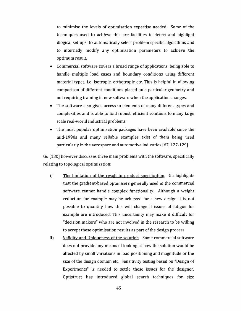
to minimise the levels of optimisation expertise needed. Some of the

techniques used to achieve this are facilities to detect and highlight

illogical set ups, to automatically select problem specific algorithms and

to internally modify any optimisation parameters to achieve the

optimum result.

• Commercial software covers a broad range of applications, being able to

handle multiple load cases and boundary conditions using different

material types, i.e. isotropic, orthotropic etc. This is helpful in allowing

comparison of different conditions placed on a particular geometry and

not requiring training in new software when the application changes.

• The software also gives access to elements of many different types and

complexities and is able to find robust, efficient solutions to many large

scale real-world industrial problems.

• The most popular optimisation packages have been available since the

mid-1990s and many reliable examples exist of them being used

particularly in the aerospace and automotive industries [67,127-129].

Gu [130] however discusses three main problems w ith the software, specifically

relating to topological optimisation:

i] The lim itation o f the result to product specification. Gu highlights

that the gradient-based optimisers generally used in the commercial

software cannot handle complex functionality. Although a weight

reduction for example may be achieved for a new design it is not

possible to quantify how this w ill change if issues of fatigue for

example are introduced. This uncertainty may make it d ifficu lt for

"decision makers" who are not involved in the research to be w illing

to accept these optimisation results as part of the design process

ii) Valid ity and Uniqueness of the solution. Some commercial software

does not provide any means of looking at how the solution would be

affected by small variations in load positioning and magnitude or the

size o f the design domain etc. Sensitivity testing based on "Design of

Experiments" is needed to settle these issues for the designer.

Optistruct has introduced global search techniques for size

45

optim isation in version 11.0 upwards to avoid convergence to a local

minimum, but the solutions found by these methods cannot

guarantee a global optimum and in fact in an industrial application

this may not matter as long as a satisfactory cost saving is made in

material or time [131]

iii) Manufacturabiltv. Although manufacturing constraints have now

been including in some packages, e.g. draw direction [132], m inimum

member size and extrusion constraints, it may not be possible to

manufacture the part as proposed using conventional methods. This

issue w ill be discussed further in the case studies where

manufacturability w ill be incorporated w ith in the constraints of Case

Study 1 (chapter 3] and the advanced manufacturing technique of

additive layer manufacture w ill be discussed to show its

com patibility w ith topological optimisation (chapters 5-6).

In addition to this some of the measures taken in the software to facilitate

their use can be debilitating. Typically the details of the internal parameters

being used are not transparent or accessible and so it is difficu lt to see

exactly what is happening. In order to run the problems w ith low

computation time often methods of approximation are used and adaptations

being made that are not always visible to the user.

Three of the current commercial packages in use are Optistruct [58], TOSCA

[133] and GENESIS [134]. Optimisation capability is also available in

commercial analysis packages like ANSYS, ABAQUS, MSC.Nastran and MatLab.

Both GENESIS and Optistruct have an integral analysis package; Optistruct can

also be interfaced w ith other analysis packages. TOSCA is solely an optim iser

but can w ork in conjunction w ith ABAQUS, ANSYS and MSC.Nastran. In all cases

it appears that the commercial software use SIMP or some variant of it as the

solution approach [1] though TOSCA originally used ESO [21]

The author has been unable to find any literature that makes comparisons

between packages. Le et al. [30] compared the results from different authors of

a topology optimisation of the standard L-beam. An Optistruct solution is

46

included in this comparison which does not produce a result that eliminates the

stress singularity at the vertex. Only limited information is available on the

parameters used to obtain this result In general those authors who comment in

any detail about individual software packages tend to be employed by the

company licensing the software [126] [132,135].

For the optimisation w ork o f this thesis Alta ir Optistruct 11.0 has been used

predominantly because it is the preferred package for many of the major

aerospace manufacturers in the UK and also licencing was readily available in

Swansea University.

2.7 Research Novelty

The major novelty of the research of this thesis is two-fold: Firstly to solve real

commercial problems that arose from manufacturing companies in Wales by

applying optim isation tools and techniques. The solutions found needed to be

resilient and obtained w ith in commercial time scales. Secondly, build ing upon

the understanding gained from the published data, develop tools and design

techniques that would exploit the benefits of additive layer manufacture when

used in a commercial environment.

47

Chapter 3: Case Study 1 - Design of a Vertical Axis W ind

Turb ine Housing

Summary: An industria l Case Study exploring the design to British Standards o f a

housing fo r a vertical axis w ind turbine using modern commercially available

optim isation techniques. Trend data on material-size costing was established. The

research was presented at a conference in Hungary in 2013.

3.1 In tro d u c tio n

Figure 3-1: The Cross-Flow Energy Company VAWT [136]

The Cross-Flow Energy Company (C-FEC) [136] had previously designed, b u ilt

and perform ed w ind tunnel tests on a 1.6m diam eter prototype for the vertical

axis w ind turb ine (VAWT) shown in Figure 3-1. The company now wished to

develop the product fu rthe r and establish costings for a full scale turbine.

The focus o f this Case Study forms part o f that development w ork to design the

housing fo r this structure, the opaque shape shown in Figure 3-2. The housing

position can be adjusted and under normal operating conditions it would be

positioned on the turb ine perim eter not only to avoid interference w ith the

incoming w ind, but also to enhance the a irflow to the blades through the

aerodynamic shape o f its surface. When the project began the exact

construction method for the housing had yet to be determined. The material,

48

position ing and geometry needed to be selected for maximum strength while

m in im ising w eight and thereby material cost.

The Case Study used a series o f numerical and optim isation techniques to

determ ine a suitable manufacturing method and design. Solutions were found

for a range o f sizes o f the VAWT to obtain costing trends.

Figure 3-2: Proposed Housing for Vertical Axis Wind Turb ine

3.2 B a ckg ro und

The use o f w ind energy to provide an environmentally friendly source of

e lectric ity has continued to increase throughout the world. In Europe alone

over the last 12 years the annual installation of w ind power has increased from

3.2 GW in 2000 to 11.9 GW in 2012, a compound annual growth of 11.6% [137].

There are tw o main categories o f w ind turbine, vertical axis (VAWT) and

horizontal axis (HAWT). The earliest w indm ills were VAWTs w ith the ir axis of

ro ta tion at righ t angles to the ground. These were used for high torque

applications such as w ater pum ping and grinding grain. As turb ine design

continued to develop and e lectric ity generation became a greater p r io r ity more

money was invested in HAWTs as they have greater efficiency (~40-50% ) in

converting w ind energy to electrical power under open and steady w ind

conditions[138]. Recent interest has returned to VAWT development as they

typ ically function w e ll in less favourable w ind conditions, e.g. urban

environm ents or more turbu lent flow. In addition VAWTs are usually om ni­

49

directional, enabling them to capture the w ind independent o f the w ind

direction. They generally have fewer moving parts than HAWTs making them

more reliable and easier to maintain.

The C-FEC turb ine is a Darrieus style VAWT, the cross section o f the blades have

an aerofoil design and the turb ine is pulled around the central shaft using

aerodynamic drag. The "S-shape" housing shown in w hite in Figure 3-3 was

developed from the results o f numerous Computational Fluid Dynamic (CFD)

calculations tha t have been undertaken on the system [139, 140].

Housing

Figure 3-3: Plan view o f VAWT showing w ind flo w and pressure zones

around an opera tiona l tu rb ine [136]

The housing acts as a shield and brings three main benefits

i) It creates a pressure gradient draw ing w ind through the turb ine core,

w ith a high pressure zone at the turb ine ingress and low at the egress

ii) The w ind drives the ro to r blades p rim a rily due to drag, but also lif t at

higher speeds

iii) It protects the ro to r blades from the oncoming w ind flow preventing

them resisting the ro tation

The housing is positioned according to w ind direction to optim ise these effects.

The company claim efficiencies o f up to 38% [136].

In order to be able to bring this turb ine to m arket a complex costing exercise

has been undertaken by the company to determ ine the most cost effective

50

design and manufacture of the housing. The precise requirements of the

company are set out in the following section.

3.3 Company Requirements

The C-FEC turbine used a cantilever type housing which formed the backbone

or frame of the entire blade assembly. The structural objectives of the housing

given by the company are as follows:

1. The housing should offer high bending strength under tip loads and

stiffness

2. The housing should withstand ambient and internal pressure loads

3. The housing should be easy to assemble and light enough to be

transported to remote locations

4. The housing construction should not allow any local deformation which

could cause the structure to come into contact w ith the blades

5. The structure should be produced at minimal cost

It should be noted that the housing does not bear the weight o f the rotor, all the

vertical load rests on the lower bearing.

In order to satisfy these objectives the following considerations needed to be

included in the analysis:

a. Any optimisation of the design must include constraints on strength and

stiffness of the structure and bending/buckling loads. The company was

able to quantify acceptable levels for most of these parameters.

b. Pressure loading needed to be determined under ambient and "worst case"

conditions. Fortunately CFD studies had already been carried out on the

turbine [139,140] and so pressure data around the perimeter of the housing

was available for seven different load-cases.

c. A t this stage the most suitable method of manufacture had not been

determined. It was intended that most of the construction should take place

in the factory and only minimal fabrication, requiring a semi-skilled

workforce, would take place at the final location. The lim iting factor in

51

sizing the prefabricated parts was found to be the load size that could be

transported.

Optimising the mass of the total structure helped to reduce the cost of

transportation, but there were other lim itations on the shape and size of the

sections that needed to be considered in order to move the housing to its

final location. The following sub-sections consider the size and weight

restrictions in the UK and the EU only.

3.3.1 Road

The maximum dimensions for a vehicle carrying a load by road in the UK is 3m

wide and 18.75m length. The gross weight of the vehicle must be no more than

44 tonnes. If any of these lim its are exceeded the police must be notified and

the vehicle may have to be escorted [141].

There are no maximum height lim its on vehicles in the UK, though typically

motorway bridges are bu ilt at 5.03m and EU motorway bridges are set at 4m.

In the EU, the maximum w idth is also 3m w ith a maximum length of 24m,

though vehicle combinations are subject to turning tests before this length can

be approved [142]. The maximum weight is approximately 40 tonnes for

vehicles forming part of a vehicle combination. The maximum height is set at

4m [143].

3.3.2 Rail

The maximum physical dimensions of railway vehicles and their loads is called

the loading gauge and is dependent upon the characteristics of the

infrastructure of the route such as bridges, tunnels and station platforms along

the route[144]. Much of the core network o f the UK is W8 loading gauge,

meaning that containers of no more than 8'6" (2.55m] height can be carried on

standard rail wagons [145]. The standard ISO container is 12.2m * 2.7m * 2.4m

w ith a payload weight of approximately 28 tonnes and 33 m3 internal capacity.

Transportation by Inland waterways was not considered due to the lim ited

availability of craft suitable for freight. It has also been assumed that

52

transportation of C-FEC VAWT components by ship would be restricted by the

road and rail lim itations unless the manufacturing facility was based at a port.

This therefore gives additional constraints on the housing design in that the

prefabricated sections should have a maximum width of 3m and any structure

w ider than 2.4m would have to be transported by road. The maximum weight

lim it for the section would have to be in the range 28-44 tonnes.

Returning to the remaining company requirements:

d. The local deformations would be handled by part a. above

e. The cost of manufacture or assembly was not included in this study only the

cost of the materials.

The objectives of the study were therefore three fold:

1. To use structural analysis and optimisation techniques to determine the

optimum design for the housing structure

2. To validate by developing a robust methodology to produce a design that

conformed to British Standards.

3. To apply these techniques to a range of housing sizes in order to predict

the most cost effective size for future construction.

These objectives w ill be addressed in detail in the following four sections.

Results w ill be included w ith in each section as the results of each step informed

the direction chosen for the subsequent steps.

3.4 Structural Optimisation

The optim isation problem was to minimise the total mass for the housing

subject to the following constraints:

i. The stress levels must remain w ith in the elastic lim it of the material.

ii. The permissible displacement at the top of the housing was lim ited

according to height (recommended values were supplied by the

company)

iii. No buckling in any component of the structure was permitted

iv. The optimised design must satisfy British Standards BS 5950-1:2000

[146].

53

The first step in determining the most appropriate method of manufacture was

to consider a topology optim isation of the housing.

3.4.1 Topology O ptim isation

The minimum mass problem for topology optimisation as discussed in Chapter

2 was

m j P j 3-17 = 1

JV

subject to : ^ P jK ° U = F(p);= i

Oj < ay Vy = 1, ...,N

3-2

3-3

: d-Top — D 2_4

• o < c < pj < i v y = l , . . . , i v g _ 5

Topology optim isation was carried out w ith A lta ir Optistruct which uses the

SIMP method, p j is the density variable for each of the N fin ite elements and

takes values between 0 and 1. This is not to be confused w ith the actual density

of the material. m; is the mass of the element and s the penalisation

parameter. Equation 3-2 shows the SIMP formulation of the equilibrium

equation.

Equation 3-3 provides a stress constraint on every element w ith an upper lim it

of oY, the yield strength. The stress constraint on the von Mises' stress was

applied over the whole design domain. Some authors have developed methods

that cater for unequal compressive and tensile stress lim its [44] but in this

problem it has been assumed that the compressive and tensile yield strength

were the same and so a single lim it of the yield strength was sufficient.

Equation 3-4 constrains the displacement at the top centre of the turbine, the

position at which the housing is connected to the central axis of the VAWT [see

54

Figure 3-4]. The upper lim it for this constraint D is a constant value based on

the height of the housing.

Buckling constraints cannot be applied in this topology optimisation problem.

When using 3D elements critical buckling modes are likely to appear in areas of

low density. Any buckling constraint on such a model would prevent further

removal of material and so impede the optimisation [147]. Buckling constraints

can be applied when optim ising stiffening ribs for shell structures provided the

thickness of the base shell is non-zero.

Constraints linked to the British Standards were not applied until later.

3.4.1.1 Set-Up fo r F inite Element Analysis

The firs t of the housing sizes to be investigated was 22m high w ith a 22m

diameter. This w ill be abbreviated to 22m x ID throughout the te x t A diagram

of the model is shown in Figure 3-4. The housing was optimised as a whole; the

outer boundary of the structure being already defined formed the boundary of

the domain. First order solid elements were used to discretise the domain, a

m ixture of hexahedral and pentahedral elements, totalling 146,700. Some

analysis was carried out using second order elements also w ith a view to

m inimising any checkerboard effects [29]. The results were very sim ilar to the

model w ith firs t order elements but w ith considerably longer CPU time. The

model w ith the firs t order elements used just over one hour of CPU time to

converge while the second order element model took more than 18 hours. The

maximum RAM required was 490 MB for firs t order compared to 2341 MB for

second. Only firs t order elements were used in the subsequent analyses.

The connecting plates at the top and bottom of the housing were not modelled.

A single rigid element connected the "Top Node" on the central axis of the

turbine to all nodes on the top surface of the housing. In the figure only two of

the components of the rigid element are shown for clarity. The top layer of

elements in the housing was not included in the optimisation to ensure that

there would be a robust structure to which the top plate could be fixed. A ll the

base nodes o f the housing were fixed in all six degrees of freedom.

55

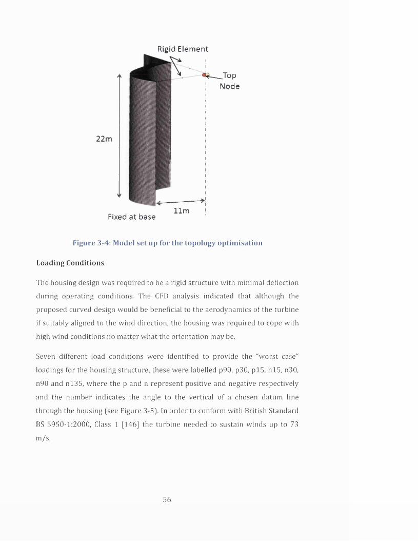
Rigid Element

4 f—_Top Node

11mFixed at base

Figure 3-4: Model set up fo r the topology op tim isa tion

Loading Conditions

The housing design was required to be a rig id structure w ith m inim al deflection

during operating conditions. The CFD analysis indicated that although the

proposed curved design would be beneficial to the aerodynamics o f the turbine

if suitably aligned to the w ind direction, the housing was required to cope w ith

high w ind conditions no m atter w hat the orienta tion may be.

Seven d ifferent load conditions were identified to provide the "w orst case"

loadings for the housing structure, these were labelled p90, p30, p l5 , n l5 , n30,

n90 and n l3 5 , where the p and n represent positive and negative respectively

and the num ber indicates the angle to the vertical o f a chosen datum line

through the housing (see Figure 3-5). In order to conform w ith British Standard

BS 5950-1:2000, Class 1 [146] the turb ine needed to sustain w inds up to 73

m/s.

56

0 °

Turbine

Housing

Figure 3-5: Plan view o f VAWT showing housing orien ta tion fo r load case

n l35

The CFD analysis generated w ind pressure values on the surface of the housing

for each of the seven load cases together w ith the load created by the ro to r at

the top of the structure for each case. Figure 3-6 shows the pressure

d is tribu tion that was applied around the perim eter of the housing. The data

shown is fo r loadcase n l3 5 . The figure also shows the applied loads at the "top

node". These pressures were assumed to be constant in the vertical d irection

despite the significant height o f some of the structures. Following discussions

w ith the company a 10% safety factor was applied to all the load values. All

geometry and elements have been removed from this figure for greater clarity.

Self-weight was applied to each of the load cases using the standard

acceleration due to gravity of 9.81 m s 1. The gravity was a vector load and so

was proportiona l to the element density in the topology optim isation and

updated at every iteration.

This s im plified approach was considered to be sufficiently accurate for this

in itia l costing study.

Wind Direction

57

Figure 3-6: Plan view o f VAWT housing show ing the d is tr ib u tio n o f

pressures forloadcase n l3 5

M ateria l P roperties

In order to carry out the fin ite element analysis the material properties of

Young's modulus, Poisson's ra tio and density were needed in the model.

Although the material for manufacture had not yet been determined in itia l

values fo r a standard structura l steel grade were used. These are shown in

Table 3-1

Selecting the material in this way enabled the upper lim it on the stress

constra int oY to be quantified. This value is also shown in Table 3-1. The

optim isation was repeated w ith a lum in ium properties for comparison.

The remaining constraint, the upper lim it on the top node displacement, D was

specified by the company. For the 22m x ID housing this was 0.45m total

displacement.

58

Table 3-1: Material and Mechanical Properties

Material

Young's

modulus

(GPa)

Poisson's

ratio

Density

(kg/m3)

Tensile

Yield

Strength

(MPa)

Steel 210 0.3 7900 300

Aluminium 69 0.33 2700 270

3.4.1.2 Sensitivity Analysis and F ilte ring

The sensitivity analysis for all topology optimisation in Optistruct used the

Adjoint method automatically w ith no option for adjustment. This topology

optimisation w ith its large number of stress constraints, one for every element

is not ideal for this approach but neither is the Direct method if it could have

been selected as there are a large number of design variables in this problem

also.

No filtering methods have been used at this stage for either control of

checkerboard effects or mesh dependency.

The penalization factor was set to 3 for this model w ith solid elements.

3.4.1.3 Optim isation A lgorithm s and Convergence

The optimisation algorithm was selected automatically from several

possibilities

• Optimality criteria method [148]

• Convex approximation method [11]

• Method of feasible directions[149]

• Sequential quadratic programming [11]

• Advanced approximations [58]

The software did not report the algorithm that had been selected. Later

versions of the Optistruct, e.g. version 13.0, indicated that the default

59

optim isation a lgorithm was the Method of Feasible Directions [150], but it was

not clear i f that was the case in version 11.0.

The convergence tolerance, the ratio o f two consecutive objective function

values, was set to 0.005 or 0.5%.

3.4.1.4 In it ia l Topology Optim isation Results

The topology optim isation converged in 17 iterations for the "Steel” housing in

3673 s CPU time (~1 hour]. The convergence curve decreased m onotonically to

the solution and the stress constra int was inactive throughout the optim isation.

Figure 3-7 shows the results o f the topology optim isation w ith both the steel

and a lum in ium material properties. Both pictures show the iso-p lot for element

densities > 0.1. This was the highest value for which e ither o f the results

showed a structure that created a connection w ith the top plate [see figure b)].

The results were not radically d iffe ren t from one another but neither o f them

suggested a design that would be realistic to manufacture. The alum inium

design took an additional 6 ite ra tions (CPU time = 4936 s) to converge and

again the stress constraint was inactive throughout.

a) Steel M a te r ia l P roperties b) A lu m in iu m M a te r ia l Properties

Figure 3-7: Topology O ptim isation o f VAWT housing com paring effect o f

m ateria l p roperties on elem ent densities

The rem ainder of this w ork was undertaken using only the steel properties as

steel is cheaper than alum inium (£290 per tonne for steel compared to £1290

60

for aluminium [151]), a readily available material and these in itia l results were

not dramatically d ifferent

3.4.1.5 In it ia l Conditions

The results of Figure 3-7 were obtained using an in itia l material fraction of 0.9.

i.e. the element density was set to 0.9 for all elements at the start. According to

section 2.4.1 of the literature review the minimum permissible volume fraction

for the elements was 0.01 to prevent singularities in the stiffness matrix,

however for this model it was found that the problem converged to a feasible

solution w ith lower values. Figure 3-8 shows the iso-plots for element densities

>0.009 for two different in itia l material fractions, 0.005 and 0.001 respectively.

The results provide a clearer indication of a possible design for the structure

than those shown in Figure 3-7 a) and w ith the lower of the two in itia l material

fractions (Figure 3-8 b] there are a greater number of connections to both the

top and bottom plates of the structure, suggesting more stability in the design.

Figure 3-9 shows the plan views for the same structures. The top and bottom

plates have been removed for greater clarity. In both cases it can be seen that

material is not required around the whole perimeter, but where shown is

composed of large sheets that stretch almost the full height of the housing.

These sheets are interconnected in Figure 3-8 b) and Figure 3-9 b) at the central

point for much of its height, but the other supports that connect one edge to the

other only occur in the top 25% of the height. A structure composed of the

large sheets indicated in the design would not be difficult to manufacture but

very d ifficu lt to transport and assemble on site. Further work was required to

find a more acceptable design to match the rem it of the project.

61

£l*m ert 0« ny ii*s® *itM y)|-100DE<00f-88SUE01f t - 7 789E-01

M-6G63E-0I■-5578E -01f t - 4 472EOI

fc s s— 1 156E-01 — 50006-03 ■ >(0 re-ufl M ai • 1 OOOE OO 2D 1 8 9 * iVWi = 6CB0e-O3 ! 30 <9850

Bftlu* C)

Figure 3-8: Topology op tim isa tion o f steel housing show ing elem ent

density > 0.009 fo r in it ia l m ate ria l fraction o f a) 0.005 and b) 0.001

i t C nn i(t« jiD .M 4y) Rwuit

■8 890601 ■7 7 * 6 0 1

f - 5 560601 f t - 4 450601 * - 3 340601 — 2 330601

— 1 120601 — 1 000603■ ttc r n j &M». = 10006*00

Figure 3-9: Plan View o f Optim ised Housing fo r in it ia l m a te ria l fraction o f

a) 0.005 and b) 0.001

62

3.4.1.6 M inim um Member Size

A filtering technique was introduced where the minimum member size was

constrained to be no smaller than a fixed diameter. This automatically

introduced a control on the checkerboard effect. Zhou et al. [39] described the

method which constrained the slope of the density. It was incorporated into

version 3.5 of Optistruct in 1999 and it has been assumed that this is the

approach that continues to be used in the software. Ideally the minimum

member size should be no less than three times the average element size. The

algorithm used the distance between adjacent nodes to prevent voids forming

immediately next to an element w ith density 1. The penalisation factor took an

in itia l value of 3 when the minimum member size was used and this was

increased to 4 for the second iterative phase to ensure clear member definition.

At the th ird iterative phase the factor was relaxed in order to achieve a discrete

solution [39].

The values chosen for the m inimum member size diameter was 0.5443m [the

value chosen by the software, by default based on the average element size].

W ith an in itia l material fraction of 0.001 the problem converged in 28 iterations

and there was very little change from the structure shown in Figure 3-8 b)

above.

It should be noted at this stage that the mesh used for this problem was not

especially dense. The elements on the periphery were approximately 0.2m in

w idth and height. A smaller mesh size might well have enabled a solution to be

found using these minimum member sizes, however although generating a new

mesh would have been simple the application of the pressures around the

periphery was highly labour intensive and so other options were pursued

before resorting to remeshing.

3.4.1.7 Transport and M anufacturing Constraints

In addition to the structural constraints, as previously mentioned, the ease of

manufacture and transportation needed to be considered. Section 3.3 showed

that both these factors could be accommodated by lim iting the size of the

63

structure to be transported to no more than 3m wide and between 28 and 44

tonnes in weight.

The housing height was therefore divided into 9 equal transportable sections

each 2.42m high w ith the layer of elements at the top of the housing set as non­

design material as before. A pattern repetition was applied to the structure by

setting the stress constraint to the base section w ith no minimum member

restriction and linking the optimisation of every other section to this base

section. The displacement constraints and loadcases were as before. No scaling

was applied to the sections at this stage as it was assumed that any variations

would be fine-tuned in a later sizing optimisation.

The penalisation factor began at 3 when the pattern repetition was used and

increased to 4 in the second iterative phase and relaxed in the th ird and final

phase to obtain a more discrete solution.

3.4.1.8 Repeat Pattern Results

The repeat pattern optimisation converged to a feasible solution in 63 iterations

w ith CPU time of 14,226 s, the objective function reduced from 795 x l03 kg3 to

248x l03kg, a reduction of 69%. Several parameters were updated automatically

by the software, namely a minimum member size of 0.5443 was applied

together w ith a global control on the checkerboard effect. Also the material

in itia l volume fraction was set to 0.1.

Figure 3-10 shows the change in mass as the iterations progress. The maximum

violations are also shown though the scale on the prim ary vertical axis has been

lim ited to 900% to enable the changes in both curves to be seen clearly. The

maximum constraints violation value is 6550% at iteration 16 and 1642% at

iteration 43 so these do not appear on the graph.

3 All mass values quoted are calculated based on the variable density of the elements and reflect the behaviour of the objective function and not the final mass of the structure when manufactured to this design

64

(uj) )U3iua3e|ds;Q |e*ox

o

o

o

(%) }U je j)suo3 XE|/M

*8 (e0T x 3>|) sseW

The figure also shows the total displacement for loadcase n30. This loadcase

took the highest values o f displacement for the seven loadcases though all

followed a s im ila r pattern. The total displacement of the top node firs t

exceeded the upper bound of the constraints (0.45m) at ite ra tion 16. Figure

3-11 a) shows a contour p lo t o f the displacement at ite ra tion 16 fo r loadcase

n30. It can be seen that the structure is grossly misshapen at this stage in the

optim isation and this is reflected in the very high maximum stress value of

4.1GPa (see Figure 3-11 b). In Figure 3-10, where crosses denote that the stress

constra int was active, the firs t occurrence of this is seen at ite ra tion 16.

Contour Plot Displacement(Mag) Analysis system— 1 175E+01

r - 1 044E+OI

F* 9 137E+00

7 832E+O0

- - 6 527E+00

6 -5 .2 2 1 E-KB

* -3 9 1 6 E + 0 0

— 2 611E+00— 1 305E+00

— 0 OOOE+OO ■ No result Max = 1 175E+01 Grids 134146 Min = 0.OOOE+OO Grids 533

Contour Plot Element Stresses Analysis system — 4.087E+09

■ -3 .6 3 3 E + 0 9

[■ 3.179E+09

2.725E+09

* - 2 .2 7 1 E+09

£ —1.817E+09

* — 1.362E+09

— 9.083E+08

— 4.542E+08

— O.OOOE+OO ■ No result Max = 4 087E+09 3D 168466 Min = 0 OOOE+OO 2D 18956

Figure 3-11: Contour p lo ts fo r the optim ised VAWT housing at ite ra tion

16: a) fo r d isplacem ent and b) elem ent stress

Contour Plot Displacement(Mag) Analysis system — 9.763E-01

8.678E-01

g - 7 593E-01

I —6 509E-01

* —5.424E-01

j j —4 339E-01

! * —3.254E-01

— 2.170E-01

— 1 085E-01

— OOOOE+OO ■ No result Max = 9.763E-01 Grids 120730 Min = O.OOOE-HDO Grids 533

pofr-eeoihrssac^Ji

- IS3PLO!

L-2IKJ6C1

-ilfDPCOD

Contour Plot Element Stresses Analysis system — 4 363E+08

•7^~3.878E+08

■T-3.394E+08

■ —2.909E+03

* —2 424E+08

£ - 1 939E +08

* —1.454E+08

— 9.696E+07

— 4.848E+07

— 9 058E+02 ■ No result Max = 4 363E+08 3D 168517 Min = 9 058E +02 3D 153225

Figure 3-12: Contour p lo ts fo r the optim ised VAWT housing at ite ra tion

2 1 : a) fo r d isplacem ent and b) elem ent stress

66

The mass was gradually increased after iteration 16, strengthening the

structure and bringing the displacement back into conformity by iteration 2 1 .

Figure 3-12 a) and b] show the same view of the VAWT housing as Figure 3-11.

The displacements and element stresses are much reduced throughout the

structure. The maximum stress value was now 436 MPa.

A smaller peak in the displacement began at iteration 43 and again the mass

increase was seen to bring the displacement back within the required bounds.

It can be seen that spikes in the stress occurred when the displacement first

peaked in both cases, and this was resolved as the displacement constraint came

under control. However, the stress constraint became active again at iteration

51 and continued to be so for the remaining iterations even when the

optim isation had satisfied the convergence criteria. An element-wise stress

constraint applied in the size optimisation would ensure that the stresses would

remain w ith in the elastic lim it of the material.

Figure 3-13 shows the result of the optimisation viewed from the side for

element density 0.1 and above. The optimisation indicated that a space frame

structure would satisfy the design requirements for the housing. Figure 3-14

shows the view from the top for the optimised solution. The rigid elements

have been removed for greater clarity. The figure shows that the space frame is

predicted over approximately 50% of the periphery of the structure w ith only a

single "wall" connecting the outer and inner radii. In some areas there are

complete voids for the whole height of the structure. In order to manufacture a

stable housing additional material would, of course need to be added in these

areas not only to link the housing to the whole of the top plate but also to

provide a framework to apply a lightweight non-loadbearing skin that would be

needed to maintain the required aerodynamic shape.

67

Contour PlotElement Densities(Density)

E1 OOOE+OO 0 900E-01 7 0OOE-O1 6 700E-01

« - 5 600E-01 I - 4 500E-01 * —3 4GJE-01 1-2 300E-01 1 - 1 200E-01 ®-1 OOO E-02Max = 1 OOOE+OO 2D 18956 Min = 1 000E-02 3D 101724

Model info. 1Result C /Users/Dawn/Documents/ASTUTE/PROJECTS/C-FEC/Topological/Jan 2014/Full_Housing_rep_pat_9_parts_GNo-Jan_SW_des h3d

Design Iteration 63 Frame 64

Figure 3-13: Result o f Topology O ptim isation o f Complete Housing w ith

pa tte rn repeat in nine sections

* b— x

Figure 3-14: Top v iew o f Optim ised Solution

The prediction o f a space frame for such a structure is not a radical idea.

Typically this would be the type of design that would be implemented if using

conventional design techniques, however by using mathematical optim isation

the a lgorithm has been able to search through a very large design space and

68

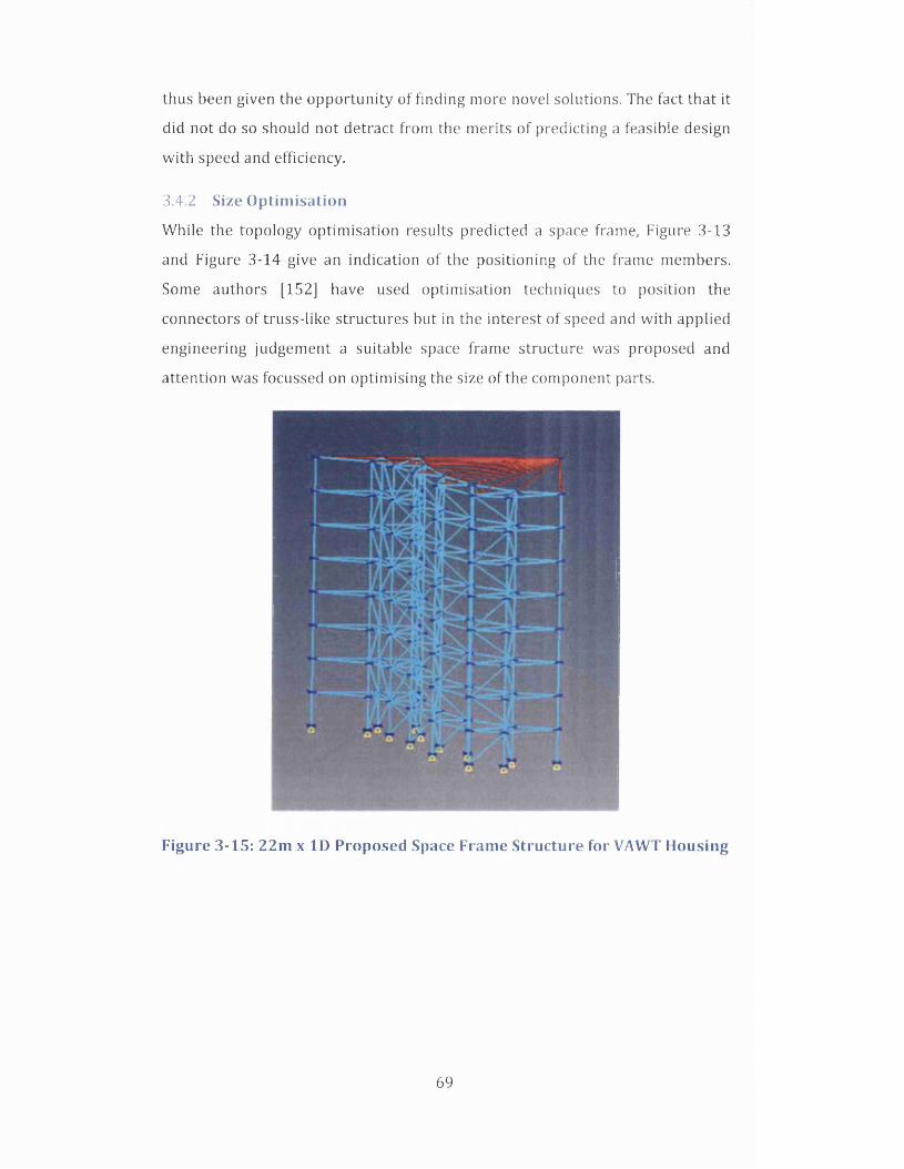
thus been given the oppo rtun ity o f finding more novel solutions. The fact that it

did not do so should not detract from the merits o f predicting a feasible design

w ith speed and efficiency.

3.4.2 Size O ptim isation

W hile the topology optim isation results predicted a space frame, Figure 3-13

and Figure 3-14 give an indication of the positioning of the frame members.

Some authors [152] have used optim isation techniques to position the

connectors o f truss-like structures but in the interest of speed and w ith applied

engineering judgement a suitable space frame structure was proposed and

attention was focussed on optim ising the size of the component parts.

Figure 3-15: 22m x ID Proposed Space Frame Structure fo r VAWT Housing

69

Figure 3-16: Plan v iew o f 22m x ID Space Frame showing 14 members

around pe rim e te r and 1 1 bracing m embers (rig id elements om itted)

Figure 3-15 shows the 22m x ID housing sp lit into eight s im ila r sections each

2.75m high which satisfied the transportation requirements. Each of these

sections consisted o f 50 ind iv idua l members:-

• 14 horizontals around the perim eter to approxim ately define the outer

shape while m aintain ing a practicable member length ( see Figure 3-16)

• 14 verticals connecting into the jo ints o f the horizontals

• 22 diagonal bracing members, 11 shown in Figure 3-16 in the horizontal

plane to ensure adequate stiffness and 11 s im ila r members supporting

the verticals.

A total o f 400 members formed the 22m x ID structure. The odd numbered

transportable sections had exactly the same configuration as one another and

the even sections were a m irro r image of them for greater stability.

The elements shown in red in Figure 3-15 is the rig id element s im ilar to that

used in the topology optim isation to d is tribute the loads on the centre line o f

the turb ine to the top surface of the housing.

3.4.2.1 Set Up fo r Finite Element Analysis

The steel material properties shown in Table 3-1 were used for the structura l

members and the material was assumed to be linear isotropic w ith tem perature

independent properties. C ircular Hollow Sections (CHS) were chosen for all the

beams. CHS are often used for large space frame structures (see Figure 3-17)

70

and this decision ensured that the o rienta tion of the member cross sections d d

not have to be considered in the design.

Figure 3-17: Detail o f the ro o f at the Kansai In te rna tiona l A irp o rt, Osaka,

Japan show ing c ircu la r ho llow sections

O ptistruct offered a num ber o f beam and bar elements fo r structura l analysis.

PBARL elements were chosen for the ir s im plic ity. They were 2-D simple bar

elements connected between tw o nodes which were defined using only the

dimensions of the cross section, i.e. inputs o f inertia and torsional stiffness were

not required. The nodes have six degrees o f freedom. Beams defined using

PBARL have a uniform cross section along th e ir length. The CHS or tube section

was defined by only two dimensions, the inner and outer radius, r0 and r,

respectively, as shown in Figure 3-18.

Each member was divided in to 12 PBARL elements to ensure suffic ient accuracy

for buckling analysis, g iving a total o f 4,800 elements.

The same seven load cases used in the topology optim isation were applied to

the housing though in this case the w ind pressures were converted to nodal

forces and applied to the jo in ts on the periphery o f the structure. The loads from

the ro to r for each load case were also applied to the top node (see Figure 3-4]

71

and a rig id element used to transfer this load to the jo in ts on the top of the

housing. A ll load cases included self weight.

Figure 3-18: PBARL Tube elem ent showing cross sectional dimensions

An additional load case fo r linear buckling was incorporated to enable the

optim isation problem to be constrained for buckling in this phase. The nodes

on the base plane of the housing were constrained in all six degrees of freedom.

It is w orth setting out some clear defin itions o f buckling at this stage to avoid

any confusion in the focus and lim ita tions of this optim isation. There are at least

three types o f buckling tha t can occur when an axial force is applied to a

member in compression:

i) Member Buckling - the beam or column becomes distorted along the

long itud ina l axis o f the bar (see Figure 3-19 a)). The wavelength of

the buckling is o f the same order as the member’s length.

ii) Local Buckling o r Crippling - local collapse due to the thinness o f the

walls o f a member. The wavelength is o f the order o f the cross

sectional dimensions (see Figure 3-19 b)).

i) Global Buckling - the d is tortion of the structure as a whole. It may becaused by the fa ilure o f ind iv idual members, instabilities in the jo ints or the accumulated second order effects o f the members. The wavelength of the buckling is of the order o f the height o f the whole structure.

72

p p

i 1 Circular Hollow Sections

Buckling in

u WebBuckling^

FlangeBuckling

a) Member Buckling b) Local Buckling

Figure 3-19 Examples of Buckling Behaviour in Beams and Columns

Local buckling can be avoided by careful selection of the section sizes of the

members. This w ill be discussed further in section 3.4.2.5.

In each case, the buckling occurs not because of the failure of the material itse lf

but because of the geometric instability of the column or beam. For a long th in

column subject to an axial compressive force, buckling occurs long before the

normal stress reaches the strength of the column material.

The governing equation for slender columns under elastic stability conditions

w ith pinned ends is

where w is the transverse displacement of the buckled column, x the vertical

distance along the column, Fc the compressive force and E and / the Young's

modulus and area moment of inertia respectively.

This differential equation has solutions of the form

w (x) = A sin(mx) + Bcos(mx) 3-7

p

where m 2 = —. From the boundary conditions w (0) = w (L) = 0, then B = EI

0 and

Asin(m L) = 0 3-8

73

where L is the length of the beam. Equation 3-8 has non-trivial solutions when

mL = nn, where n is a positive integer. These are known as the modes of

buckling.

The lowest load that results in buckling of the column, known as the critical

load, Fcr occurs when n = 1 and

E ln 2Fc f = - p - 3-9

Or more generally

F _ gfa2 3-10cr k ’ 2L2

where k* depends on the type of end fixings of the columns. This formula is

applicable to linear elastic buckling only, which is the approach used in this

study.

3.4.2.2 Design Variables

In itia lly the design variables for the problem were taken to be the inner and

outer radii for each member to match the dimensions specified for the definition

of the PBARL element. The User Guide for Optistruct [58] indicated that the

software would ensure that r 0 — r j would always be positive. However, some

ambiguities in the results led to further investigation and it was understood that

although the software checked that this difference was positive at the end of the

calculations, it did not guarantee that it would remain so during the analysis.

The final model therefore used inner radius, r } and wall thickness, Th as the

design variables for each member. The lower bound on the thickness prevented

the wall disappearing. The element dimensions were linked using the following

relationships:

Design V ar iab le 1 j = Thj = r0j — rtj 3 -11

Design V ariab le 2j = r/; 3-12

V members j = 1, ...,400

74

The same design variable was applied to every element of a member to ensure a

uniform cross section throughout the length.

3A.2.3 Optim isation using Standard Sections

As discussed in chapter 2 most problems of size optimisation for truss

structures use discrete design variables and often non-gradient based

optimisation approaches. Optistruct does have facility for discrete size

optimisation but since standard commercially available sections are not

produced in every combination of outer diameter and wall thickness then the

problem set-up becomes increasingly complex.

This can be illustrated from the data of Table 3-2 below where a sample of 13

standard circular hollow sections is shown. For an outer diameter of 33.7mm

the sections can be supplied in four different wall thicknesses (3mm, 3.2mm,

3.6mm and 4mm), whereas for an outer diameter of 21.3mm only one wall

thickness (3.2mm) is available. The design variables of wall thickness and outer

radius for each member in the structure would have to be linked together and

allowed to step between a discrete set of over 150 values.

An alternative two stage approach was chosen to give greater simplicity and

clarity in the size optimisation. Firstly a continuous optimisation, the

dimensions being able to take any value over a continuous range and then

secondly, based on the results of the size optimisation appropriate sizes where

chosen from the standard sections.

75

Table 3-2: Sample of Commercially Available Standard Circular Hollow

Sections

Name

OuterDiameter

D0(m)

WallThicknes

sTh(m)

Area

(m2)

Area Moment of

Inertia/

Cm4)

No.

21.3x3.2CHS

0.0213 0.0032 182xl0-6 7680 x lO 121

26.9x3.2CHS

0.0269 0.0032 238x10-6 1 7 x l0 92

33.7x3.0CHS

0.0337 0.003 289x10-6 344 x lO 103

33.7x3.2CHS

0.0337 0.0032 307x10-6 36x10-94

33.7x3.6CHS

0.0337 0.0036 340 x lO -6 391 x lO 105

48.3x2.5CHS

0.0483 0.0025 360x10-6 946 x lO 106

42.4x3.0CHS

0.0424 0.003 371x10-6 725 x lO -10 7

33.7x4.0CHS

0.0337 0.004 373 xlO -6 419 x lO 108

42.4x3.2CHS

0.0424 0.0032 394x10-6 762 x lO 10 9

48.3x3.0CHS

0.0483 0.003 427x10-6 l l x l O 81 0

42.4x3.6CHS

0.0424 0.0036 439 xlO -6 833 x lO 101 1

48.3x3.2CHS

0.0483 0.0032 453 xlO -6 116x10-91 2

60.3x2.5CHS

0.0603 0.0025 454x10-6 1 9 x l0 -8 13

3.4.2A Continuous Size Optim isation

The continuous size optimisation problem could be expressed as:

400

min mass = np ^ lj [(r /;- + T h j)2 — r/y] 3-13;= i

where lj are the lengths of the beams, multiplied by the cross sectional area and

density p to obtain the mass

76

subject to : -3 0 0 MPa < ak < 300 MPa

3-14f o r k = 1, ...,4800

where the ok are the max signed4 von Mises' stress for every element

: dTop < 0.45m 3 _1 5

the total displacement is constrained on the top node

: buckling eigenvalues > 1 3-16

0.003m < Thj < 0.5m 3-17

0.01m < r j j < 0.5m

the upper and lower bounds on the design variables.

Equation 3-16 constrains the structure to prevent the buckling of any member.

The buckling analysis is solved using the Lanczos method and the eigenvalues

found give the factor by which the pre-buckled state of stress must be

multiplied to produce buckling in the element. This analysis was applied to all

seven loadcases.

Again the validation w ith British Standards was to be carried out at a later stage.

Using multiple starting points a global search algorithm was included in the

optimisation. The method used 20 different in itia l conditions across the design

space to increase the likelihood of finding the best solution. The design variables

were split into ten equal groupings and these groups were assigned different

in itia l conditions at each starting point. The global search was carried out w ith

two different sets of conditions, one where the extremes of the bounds were

included in the in itia l conditions and one where they were not, giving 39

different in itia l conditions for the search (both methods use the average of the

upper and lower bounds as the firs t starting point]. The details of the starting

point used are shown in Appendix A.

4 The signed von Mises stress indicate the direction o f the largest principle stress and thus show whether the member is in tension or compression.

11

The choice o f algorithm used for this optimisation was not visible in the

software. A concatenated and annotated version of the input file for the 22m x

ID continuous size optim isation can be found in Appendix B.

3.4.2.5 Discrete Size Optim isation

It would not be practicable to manufacture the housing from sections w ith

individually unique dimensions and so it was necessary to i] use standard

sections which were readily available for purchase and ii] lim it the number of

different sections used in order to facilitate the construction process and

minimize costs.

It was agreed w ith the company that a maximum of 12 different standard

sections would be used. Table 3-2 shows a sample of appropriate commercially

available standard circular hollow sections. The sections were selected so that

ITh < 2 ' w ^ ere D0 *s the outer diameter of the tube, Th the wall

thickness and e2 = ^ ^ / p w ith py the design strength for a circular hollow

section. These parameters w ill be discussed in some detail in section 3.5.1.2.

This ensured that the chosen members were not prone to local buckling [146]

and gave a total of 154 commercially available sections ranging from 0.0213 -

0.6m outer diameter by 0.0032-0.05m wall thickness. The complete list of the

154 suitable sections can be found in Appendix C.

The solver in Microsoft Excel was used to perform the optimisation. The steps

taken in the procedure are briefly described below:

1. The lis t of standard CHS sections were ordered firs tly by cross-sectional

area and then by area moment of inertia. From lowest to highest in both

cases. These were number consecutively as shown in Table 3-2 .

2. The member sizes from the optimum result found by the continuous size

optimisation of section 3.4.2.4. were set out in a spreadsheet. A standard

section number from the ordered list was assigned to each member. This

number was chosen as the firs t section in the lis t where both the cross

sectional area and the area moment of inertia were at least as high as the

78

continuous solution. This reduced the 400 continuous sections down to a

total of 89 different standard section sizes for the 22m x ID structure.

3. A random sample of twelve sections was chosen from the lis t of 154

where the maximum number was no greater than the maximum section

found in part 2 above.

4. Then a new optimisation was set up in the spreadsheet as follows

400

min mass = lj[D%j - (Doj - 2Th j)2] 3 _1 9

; ' = i

where the outer diameters D0j and the wall thicknesses, Thj for each of

the standard sections were obtained from the look up table of standard

sections, lj were the member lengths as before.

The design variables DVt were 12 different standard sections in itia lly

chosen at random. These were identified by integer only and subject to

the following constraint

1 < DVi < DVi+1 < M < 1543-20

V i = 1 , . . . ,1 2

where M was the number of the maximum section from part 2. This was

intended to keep the total mass in the discrete size optimisation close to the

continuous result. The constraint also ensured that all the design variables

formed an ordered lis t o f valid sections.

5. The sections for the 400 members could now only be chosen from the

random 1 2 sections based once more on area and area moment of inertia

and this gave a new calculated value for the total mass.

6 . The built-in optimisation Solver in Microsoft Excel was used to minimize

this mass by modifying the twelve sections chosen and allocating the

members accordingly. The Solver offered three different approaches for

the optimisation

i) Simplex Method [153] for linear programming

ii) Generalized Reduced Gradient Method [154] for non-linear

programming of smooth functions and

79

i i i] Evolutionary technique for non-linear non smooth functions.

The discrete optimisation of the housing members was non-linear and unlikely

to be smooth and so the Evolutionary option was used.

The Evolutionary Solver was described as using "a combination of genetic and

evolutionary algorithms, tabu and scatter search methods and classical

optimisation methods" [155]. Flystra et al. [156] presented details of the

Microsoft Excel Solver in 1998, but at that stage the Evolutionary Solver was not

included. The solver has continued to be developed over time because in a

previous version of the user guide no mention was made of either Tabu or

Scatter Search methods.

A population size of 100 was used to enable a good exploration of the whole design

space. The solver always retains at least one copy of the previous best value when

a new evolution is begun. A mutation rate of 0.075 was used to create diversity in

the population. The convergence ratio was 0.0001.

The evolutionary methods are non-gradient based approaches and so have no

capacity to assess whether an optimum is global or not. Repeated application of the

solver can produce improvements in the result, but the decision to stop the search

will generally be based subjectively on the available time to find a solution, for

example, and the degree of improvement made in each case.

3.4.2.6 Testing the Discrete Optim isation aga inst the Optim isation

Criteria

The optimisation of the above section worked on the basis that i f the cross

sectional area and area moment of inertia were at least as large as the

continuous result then the structure would be sufficiently strong and resistant

to bending. This approach however did not take any account of the impact of

these changes on the load path and thus the stress, displacement and buckling

conditions of the structure. It was therefore necessary to carry out a final

analysis of the housing w ith the members set to the results of the discrete size

80

optimisation and ensure that the solution was still feasible, i.e. all the

constraints were still satisfied.

3.4.2.7 Results o f Size Optim isation

Continuous Size Optimisation

Figure 3-20 shows the in itia l and the final or optimised mass for each of the 41

starting points. A logarithmic scale has been used on the y-axis to give greater

clarity for the lower values. The first point, NG [Not Global] was not part of

either of the global search groupings. For this model the initial values for all the

design variables were the lower bounds, i.e. 0.003 for the wall thicknesses and

0.01 for the inner radii. These conditions were also the starting point for B-X.

Starting points A and A-X also had the same in itia l conditions and the same final

mass. A total of 39 different starting points were therefore used.

The starting points A to T were the global search where the initial values did not

use the upper and lower bounds of the range directly and A-X to T-X are those

for which they did [see appendix A]. All the starting points A to T gave feasible

solutions w ith the final mass lying in the range 26.53 - 40.44 x 103 kg. The

average of the iterations was 15.25 w ith standard deviation of 4.6. The graph

shows that the starting points A-X to T-X which used the extremes of the range

had much more erratic behaviour. Only 12 of the 20 starting points gave

feasible solutions. The feasible solutions ranged from 24.64 - 24.94 x 103 kg

w ith the number of iterations higher in nearly all cases, averaging 46.08 w ith a

standard deviation of 24.95. The best solution however was found by using the

extremities of the bounds from starting point D-X an optimised mass of 24.64 x

103 kg obtained after 69 iterations.

The starting conditions for D-X were as follows i] all the inner radii were set to

their lower bound 0.01m ii]W all thicknesses were set to the upper bound 0.5m

for all but members 161-240 which took the lower bound 0.003m.

The members were numbered sequentially from the base w ith members 1-50 in

the lowest level and 51-100 in the second and so on. These initial conditions

would therefore form very sturdy components in levels 1-3 and some of the

81

uprights of level 4 but very slender members in most of levels 4 & 5 w ith

heavier components on top.

Figure 3-21 shows the convergence curve for D-X together w ith the maximum

constraints violations. The in itia l mass took a fa irly high value and the

optim iser began by changing the design variables which brought a reduction in

both the objective function and the violations. Also shown on the graph are

dotted lines that represent the stress and displacement violations. The

displacement violation shows the number of loadcases for which the

displacement was greater than the maximum value. In itia lly this was for four of

the seven loadcases but it gradually reduced and by iteration ten the

displacement constraint was satisfied for all the loadcases and remained so

throughout the optimisation. The software recorded the most violated stress

constraints up to a maximum of 2 0 and for the firs t 2 1 iterations 2 0 stress

violations were present. This quickly fell to zero by iteration 23 but rose again

to ten by the following. The stress values continued to oscillate until iteration

46 and then gradually reduced until complete convergence was achieved. No

buckling modes were found throughout this optim isation which was somewhat

surprising considering the fine members that existed in the mid sections during

the early iterations. It was assumed that the load path was able to move though

more robust members while maintaining low levels of compression in the

slender bars.

A sample of eight members were chosen from the housing. Member 1 was a

vertical member in the lowest section on the inner radius of the housing. The

other seven members lay in the same position but at each o f the seven

transportable sections above. The upper graph of Figure 3-22 shows the inner

radii for these eight members and the lower graph shows the variation in the

wall thickness.

The lower graph clearly shows that in itia lly the wall thickness of the member

w ith the highest number (8 ) and therefore nearest to the top of the housing

reducing in line w ith the mass which enabled the displacement constraint to

become inviolate. The lowest members remain constant in radius and wall

thickness until iteration 2 1 but then the significant reduction in wall thickness

82

for DVs 1-3 matched the sharp reduction in the mass. The inner radius of the

top-most member remained virtually constant throughout at the m inimum

bound, while a sim ilar trend was seen for most of the mid-level members where

the wall thickness was in itia lly set at its minimum value. While this is only a

sample of the data, the development of the housing design, as illustrated by

these design variables, does seem to be logical.

83

s u o jie ja ) ; jo o fj

_i i ■

X

XX•

X

♦

x - ix-sx-yx-ox-dx-oX-N

X-lAI

X-T

x-xx-rX-|

X-H

X -9

x-dX - 3

x- ax-ox-gx-v1syod0N

1AI

1 >1 r

5 iz

H

0d3a

ogvON

(E0I K 3>() sseiAl

a>£re

£0)urea(/5OX)s'(753O

JS

X£CNcma

<4-!osore(/}

aoa>N‘175t/j3O3C+33Oua

j=4-1u

£(/J

4>4c‘oaOX)3'X3ure

a>ssou30>re33O)

X!O)33

E-6CN100OJu3OX)

suoi}e|Oj/\ss3J)9/|dsiQ

<2-(35

(% ) ;u je j}s u o 3 xe|/yj

*8 (£0T x 3>J) sseirtj

-C

(w)ssau>p!im|e/v\

Figure 3-23 shows the dimensions o f the ind iv idual members from the best

solution. It is d ifficu lt to get an overall p icture from just looking at the inner

radii and wall thickness data as the optim iser appears to have strengthened

some members by increasing the radii while increasing the wall thickness in

others. The cross sectional area graph gives some reassurance as there is a

clear ind ication that the cross sections were larger at the base and decreased as

the member num ber and therefore position up the housing increased

suggesting good s tab ility and ease o f manufacture. There appears to be some

cyclical effects in both the wall thickness and the cross sectional area graphs, for

example there is a member which has a noticeably large cross section at

member num ber one and s im ila rly the member 50 and 100 which sit on the

levels above are also larger than the ir neighbours but d im in ish w ith height. This

indicated that the structure has been strengthened through the height in some

regions only.

Inner Radius (m)

$

4 00t ♦♦

■o S u * *

I 0.02 ---- ---------------

♦ «► “ j F ♦ A ♦ ♦ ♦ ♦ .! i f %

50 100 150 200 250 300 350 Member No.

400

W all Thickness (m)

0 SO 100 150 200 250 BOO 350 400

Member No.

Cross Sectional Area

0 50 100 150 200 250 300 350 400

Member No.

Figure 3-23: Dimensions o f each m ember from the Continuous Size

O ptim isation Solution.

86

Converting to Nearest Standard Section

Each of the structural members was assigned a standard section based on the

maximum of the cross sectional area and the area moment of inertia. This

increased the mass of the structure from 24.64 x 103 kg to 25.43 x 103 kg, a 3%

increase, w ith a total of 89 different sections. These are shown in upper graph of

Figure 3-24 w ith the members at the different height levels in the housing

plotted in different colours. The structural members have been numbered

according to the ir position in the structure so that the same member in different

levels has the same member number on the graph. Members 1-14 are all the

vertical members, 15-25 the vertical bracing members, 26-39 the horizontals

and 40-50 the horizontal bracings. The graph shows that the verticals have the

highest standard section numbers [see Appendix C) indicating the strongest

sections. There is a general decrease in member section number as the member

number increases showing the need for less strength in the horizontal planes

than in the vertical.

Discrete Size Optimisation

The lower graph of Figure 3-24 shows the same bars after the discrete

optimisation into only 12 standard sections. The total mass of the structure was

increased by 26% from the topology optimisation to 30.95xl03 kg.

The weight increased in two distinct ways, firstly by raising the lowest

permissible section size and secondly by increasing the number of members

taking the maximum size. In the upper graph the maximum section was only

used in the base level, but in the lower graph some members even up to level

four require this size. It can also be seen that there is now greater uniform ity of

size in horizontal members which w ill make the structure less complex to

manufacture.

Figure 3-25 shows the convergence behavior of the algorithm used in the Excel

Solver to optimise the 400 members of the VAWT housing into 12 different

standard sections. The data represents a total 266 trials and almost 4900 sub­

problems. The in itia l conditions were 130,120,110, 100, 80,14,12, 10, 8 , 6 , 4,

2 for the twelve standard sections though due to the random nature of the

87

solver the optim isation was not repeatable unless a random seed was chosen,

which was not the case in this solution. The upper value of 130 was fixed.

The objective function, known as the incumbent, changed very rapidly w ith in

the firs t 20 or so trials. The uneven intervals between the incumbent values

indicate the different numbers of sub-problems needed to find a better value of

the incumbent. It is difficu lt to detect any particular trends in this data, partially

because the number of members assigned to each section has not been recorded

and also because of the probabilistic nature of the process.

The static analysis of the Excel Solver result identified 23 of the 400 members

violating the optim isation constraints. In each case these members were

increased to the next section in the lis t of 1 2 chosen until a feasible solution was

achieved. Unfortunately one of the lowest verticals which already was assigned

the maximum section size from the continuous size optimisation violated the

constraints and so a new maximum had to be chosen and this increased the size

of six other members which were already conforming to the constraint

conditions. This change to just over 7% of the members brought the total mass

up to 34.56 x 103 kg, an increase of 40% over the continuous optimisation

result, which was much higher than expected. A second attempt using the Excel

solver w ith the maximum section size set at 132 found an optimum of 31.45 x

103 kg which when checked against the optimisation constraints required 25

members to be adjusted and gave only a marginally better result of 34.03 x 103

kg, an increase of 38%. These were the results taken forward to the next stage.

88

• C O

• •0 •© • m

• o o-CO •

• o a n *

H----

• • • :jaqujnfij uojv^ss pjepueis

<N m m

ss ©>

<v>

<u>

©>

CD• o 0 o o

a00)Nto01 4->ou .u<o

ja q iu n N UOIV33S p je p u e *s

OJDc

"to2o

£<u

- 2w

oto

"3>a;

.2 f"53£0)-C• w

J3OX)2Ou-C•w2otoucoa

E0

u1tos

_o' 5u1)to

CO■acCOCOOw

■ao>■MCOCJ

_o

«toua>

. 2EOJ

rfCN

1ro0)u2 OX)

oo

(£0T x 3>l) sseIAJ - lu a q u in o u iCN O 0 0 UO CN

jaqiun^j uojjoas p jep u e is

3.5 Conforming to BS 5950-1:2000

The design of space frame structures such as the Wind Turbine Housing comes

under the guidance of British Standard BS 5950-1:2000 "Structural Use of

Steelwork in Building, Part 1: Code of practice for design -Rolled and welded

sections [146]. In keeping w ith most UK codes of practice, BS 5950 adopts a

"L im it State" approach to design. "A Lim it State is a condition beyond which the

structure would become less than completely fit for its intended use" [157].

These states can be divided into two main groups:

i] Ultimate L im it State

This is an assessment of the factors that could cause the structure to collapse

and includes

• Stability, including overturning and sway

• Strength, including yielding, rupture, buckling, forming a mechanism

• Fatigue fracture

• Brittle fracture

• Structural integrity, which includes any accidental damage

ii) Serviceability L im it State

An assessment of the design under normal working conditions and includes

• Deflection

• W ind Induced Oscillation

• Durability

• Vibration

This section w ill seek to validate the optimised design of the VAWT against each

of the lim it states.

For the C-FEC housing, continuous design has been chosen for the design

method since it has been assumed that for elastic analysis the welded joints are

assumed to have sufficient rotational stiffness to resist the moments resulting

91

from the analysis (see section 2.1.2.3. in [146]) and first order linear static

analysis has been undertaken.

3.5.1 Ultimate Limit States

3.5.1.1 S tab ility

It has been assumed that the foundations for the structure would be sufficiently

robust to prevent the housing overturning, lifting off its seating or sliding in any

way and so the only factors to consider in terms of stability are sway and

buckling (both member and local).

3.5.1.1.1.1 Sway

In common design practice it is easier to assess the stability of individual

members separately from the overall stability of a structure. This is valid only if

the structure itself is not subject to large inter-storey displacement as shown in

Figure 3-26b). This is called a sway or sway-sensitive structure. The horizontal

movement of the structure as a whole can induce additional moments in the

members and so it is not possible to assess the stabilities of the members

independently.

b)a

Figure 3-26: Illustration of a) a non-sway and b) a sway-sensitive structure

Non sway frames (Figure 3-26 a)) can be analysed using first-order linear

elastic methods whereas sway frames may require second-order

techniques[146].

92

For a clad structure like the VAWT housing, as long as no account is taken of the

stiffening effects of the wall panels, it can be classed as non-sway provided the

sway mode elastic critical load factor Acr of the frame under Notional Horizontal

Force (NHF) only5 satisfies the following condition:

where _ h

2 0 0 (pmax 3 - 2 2

1 8 jj—^ Lw ith h as the height of the storey and <pmax = — ~— , the maximum of the

relative displacements of the storeys. 6V and 8h are the notional horizontal

displacements of the upper and lower levels of the storey due to the NHF.

All structures where Acr < 10 are classed as sway-sensitive and the Standard

recommends three possible methods for addressing the secondary effects of the

forces and moments for an elastic analysis. One of these, the Effective Length

method was the one chosen for this analysis because in all cases Acr > 4 and so

this was suitable to use w ith linear static analysis

3.5.1.2 Strength

There were a number of factors to consider concerning the strength of the

individual members and thus the strength of the structure as a whole. The

relevant equations and definitions from the British Standard are highlighted in

this section together w ith the assumptions made.

Cross Section Classification

The Standard defines lim iting dimensions for different classes of members

dependent upon the type of cross section used. Table 3-3 gives the lim its on the

dimensions for CHSs, where D0 is the outer diameter of the section, Th is the

wall thickness, and£ = p ^ / p y) , w ith p y being the design strength. The

5 The Standard recommends the Notional Horizontal Force to be 0.5% o f any vertical load being applied in both horizontal directions at each storey. In the Case Study, the only vertical load is due to the self-weight o f the structure.

93

design strength is generally taken to be equal to the yield strength but for CHS

there is a dependency on wall thickness and this is shown in Table 3-4 below.

The Standard gives data for three different steel grades, but analysis for this

Case Study has used grade S355 only, which most closely matches the material

properties used in the topology and size optimisation.

Table 3-3: Limits on the Classes of Circular Hollow Sections

ClassLimiting Value, D0/T h less

than or equal to

Number Name brief description

Compression

due to

bending

Axial

Compression

1 Plastic

w ith plastic hinge

rotation capacity 40c2

Not

Applicable

2 Compact

w ith plastic moment

capacity 50c2

3Semi-

Compact

where stress at the

extreme

compression fibre

can reach the design

140c2 80c2

4 Slender

allowances must be

made for the effects

of buckling

>140e2

94

Table 3-4: Variation in Design Strength Value with Thickness for steel

grade S355

Steel Grade

Thickness less

than or equal to

mm

Design

Strength py

MPa

S 355

16 355

40 345

63 335

80 325

1 0 0 315

150 295

Buckling checks

Using the inequality lim its of Table 3-3 member dimensions should be selected

to ensure that the sections are class 3 and below to avoid the slender sections

that are prone to buckling i.e.

Do 9— < 80s 3-23

This is the lower of the two lim its for class 3 members and thus w ill give a more

conservative design. For CHSs the beam is equally resistant to buckling in all

directions. The Standard advises ([146] section 4.3.6} that a separate check for

lateral-torsional resistance is not needed for CHSs.

Shear Capacity

The shear force Fv should be no greater than the shear capacity Pv which is

defined as

Pv — 0.6pyAv 3-24

95

Where Av is the shear area which can be taken to be 0.6 of the cross sectional

area for circular hollow sections, i.e.

Pv = 0.36pyn(DoTh — Th2) 2 2 5

Moment Capacity

When determining the moment capacity the Standard proposes different

conditions dependent on the levels of the shear force and the class of the

member.

For Low Shear (Fv < 0 .6Pv)

For class 1 & 2 members, the Moment Capacity is

For class 3

Mc PyS

M c = PyZ

OT M c P y ^ e f f

3-26

3-27

where Z is the section or elastic modulus defined in equation 3-30 below

Where S is the plastic or plastic section modulus given as

S =Dq ~ (D0 - 277i):

3-28

And Sef f , the effective plastic modulus, which for circular hollow sections is

defined as

Se f f — Z + 1.485

\140

Do t

,T h !

(213

\ P y

0.5

- 1 ( S - Z ) 3-29

And Z the section or elastic modulus

96

_ n [D j - (D0 - 277Q4] 32D0 3-30

Formulae 3-28 -3-30 apply specifically to circular hollow sections.

For High Shear (Fv > 0.6Pv)

For class 1 & 2 members, the moment capacity is

3-31

And for class 3

Mc = py Z - ^ / 1 5

3-32

or Mc — Py [*$e//

Where 5V is the plastic modulus for the shear area Av and the reduction factor

Interaction Expressions for members with Combined Moments and Axial

Force

The members must be considered separately in this case according to whether

the axial forces show them to be in tension or compression. Circular hollow

sections have to be classified separately for axial compression and for bending

(see Table 3-3}, but in this assessment the most conservative case <

8 0 f2 has been used, as mentioned above.

Members in tension

The cross section capacity for these members must be checked at those

locations where the moments and axial force are the largest. By the simplified

3-33

97

method ([146] section 4.8.2.2), the following relationship must be satisfied for

tension members w ith moments

where Ft is the axial tension, Mcx the moment capacity about the major axis,

Mcy the moment capacity about the m inor axis, Mx the moment about the major

axis, My the moment about the m inor axis and Pt the tension capacity.

For CHS, Mcx = Mcy = Mc and Pt = pyA

Normally the net area is used here to take into consideration any material loss

due to bolt holes etc. If it is assumed at this stage that welded joints w ill be used

w ith no loss of material then the net area can be taken as A, the cross-sectional

area.

With the section being axisymmetric the Standard recommends using the

expression

which gives a tighter lim it on the design.

Members in compression

Using a sim ilar approach to that used for the tensile members, the cross

sectional capacity is checked where the moments and axial forces take the

highest values. For CHS w ith no bolt holes (gross area = A ), the compressive

member must also satisfy the above expression w ith Ft replaced by Fc , the

compressive axial force but in addition to this the member buckling resistance

must also be checked.

For members w ith moments in both axes, the expression for interactive

buckling gives

3-34

3-35

98

where mx is the equivalent uniform moment factor about the major axis, my is

the equivalent uniform moment factor about the minor axis and pc is the

compressive strength.

The equivalent bending moment factors are calculated as follows

where Mmax is the maximum moment in the member, M24 the maximum in the

central half of the section and M2 and M4 are the values at the two quarter

points and M3 is the value of the moment at the centre.

If M2, M3 and M4 all lie on the same side of the axis as shown in Figure 3-27 a),

the ir values are taken as positive. If they lie both sides of the axis Figure 3-27 b]

the side leading to the larger value of m* is taken as the positive side.

m = maxm ax m ax 3-37

a) All Bending Moments have same sign

b) Bending Moments with both positive and negative values

Figure 3-27: Variation in Bending Moments

The compressive strength pc is dependent upon the design strength py and the

slenderness ratio A* for a particular steel grade according to type of section

used. A table of values for hot finished hollow sections and grade S355 can be

found in Appendix D. The slenderness A* is calculated from the radius of

gyration

r/A

and

3-38

where LE is the effective length of the column.

Effective length Method

For sway sensitive frames, w ith Xcr> 4, the effective length of each member has

been calculated using the elastic critical load factor The in-plane effective

length is given by

where Fc is the compressive force, E the Young's modulus and /, the area

moment of inertia.

Xcr can be calculated using second order elastic analysis but it is equally

effective to use the sway mode elastic critical factor found in section 3.5.1.1.1.1

above, whichever method is used only a single value of Xcr is calculated for the

whole structure. To prevent an unrealistic result where a large value of Acrfrom

a single member is applied to all members a modification of this expression has

been used where

for k*, the effective length constant. Since the housing structure uses braced

frames then a value of k * = 2 has been used.

3-39

Le = min k*L, 3-40

100

3.5.1.3 Fatigue fra c tu re

Section 2.4.3 of the Standard states that

"Fatigue need not be considered unless a structure or element is subject to

numerous significant fluctuations of stress. Stress changes due to normal

fluctuations in w ind loading need not be considered"

Only static steady state conditions are being used in this analysis and so fatigue

w ill not be included in the checks.

3.5.1.4 B ritt le fra c tu re

Provided a steel quality of sufficient toughness6 is chosen for the design, brittle

fracture need not be considered in the design.

3.5.2 Serviceability L im it States

The performance of the structure under normal operation was not considered

in this prelim inary design except for the inclusion of the permissible deflection

lim it of the top central node that was supplied by the company.

Safety factors have already been accommodated in the loads predicted by the

CFD analysis.

3.5.3 Results o f BS 5950 C onform ity Check

Once the optimised discrete solution had been achieved for the 22m x ID

housing, the structure was checked against the British Standard BS 5950:1-

2000 using the Effective Length method described above. The check on the 400

members was simply set up in a spreadsheet to test the various inequalities

required by the standard.

The details of the relevant Lim it States are summaries in the Table 3-5 below.

No changes to any of the member sizes were needed to enable the structure to

conform to the Standard.

It is im portant to note here that neither the gradient-based method of the

continuous optimisation nor the evolutionary methods of the discrete

6 The ability to withstand shock loading, to absorb and distribute both applied stresses and strains within the material.

101

optimisation are guaranteed to find the global minima of this problem.

However, using global search methods in the continuous optimisation and

repeated application of the evolutionary algorithm in the discrete optimisation

w ith variation in population size, mutation rate and the lim it on the maximum

sub-problems has established a degree of confidence that the solutions found

were the best of the local minima that were identified.

The British Standards check has provided additional evidence that these results

were not only mathematically sound but also feasible in terms of structural

safety. Issues of complexity and cost of construction, i.e. the practicality of

jo ining the different section sizes has not been considered.

102

Tabl

e 3-5

S

umm

ary

of re

sults

fo

r 22

m x

ID VA

WT

Hou

sing

co

nfor

min

g to

BS

5950

:1-2

000

0c

3.6 Robust Methodology for Housing Design

As a result of effectively optimising a design for the 22m x ID housing a

methodology had been developed for designing to British Standards which

could be applied to housings of other proportions. Figure 3-28 shows the

flowchart for this approach.

Bestm in im a

No

Yes

No

Yes

in form s to O pt..

Conforms V t o B.S.y

TopologicalOptimisation

Increase section size

ContinuousOptimisation

DiscreteOptimisation

Identify members that violate

Identify members that do not conform

Check Discrete Solution conforms to BS5950

Test Discrete Solution satisfied Optimisation criteria

Optimal Solution Found

Figure 3-28: Flowchart for Optimisation Procedure

The flowchart includes two feedback loops; one after the discrete size

optimisation to check that the resulting solution conforms to the optimisation

criteria and secondly at the Standards check. Both these loops allow for

adjustment to be made to the section sizes of any one member to ensure

conformity to the criteria specified for the optimum structure.

104

It was assumed that the space frame design would be suitable for all the

housing sizes and so the topology optimisation was not repeated for the

different dimensions.

In consultation w ith C-FEC, a range of housing sizes for optimisation was

determined as shown in Table 3-6.

Table 3-6: Range of Housing Dimensions to be Optimised

o HeightQfl 1.5Ceaa

1 DiameterDiameters

2 Diameters

10m V V V

22m V V" V

28m V V'

As the project progressed it became clear that the higher structures (2

diameters) were no longer needed. Additional data for 0.5 diameter height and

other interim values was included to enable trends to be established in the

optimised volume according to height and diameter.

3.6.1 Size Optimisation

All the 10 m and 22 m diameter structures had the same arrangement of the 50

members in each transportable section as described for the ID height, though

the height and number of sections was different. The 28 m housings had 20

instead of 14 beams around the perimeter to avoid the use of very long beams.

Corresponding verticals and bracing members were connected to each joint.

Circular hollow sections continued to be used in all designs w ith the same

element types described in section 3.4.2.1 w ith 12 elements per member

independent of length. A summary of the parameters for each housing model is

shown in

Table 3-7.

The design variables were inner radius and wall thickness in all cases w ith the

same bounds used in the 21m xlD structure. The constraints on stress,

105

displacement o f the top nodes, and buckling were applied to each structure. The

bounds on the signed von Mises stress remained at ±300 MPa for all designs.

The upper bound on the total displacement o f the top centre o f the housing

varied w ith height. The values used are also shown in

Table 3-7. The low er bound on the buckling eigenvalue remained at 1 to prevent

member buckling in all cases. The seven loadcases identified from the CFD were

applied together w ith self-weight. The loads were dependent on the

dimensions. Appendix E shows values fo r 10m x ID housing.

M ultip le starting point global search techniques were used to give 39 unique

in itia l conditions for the design variables.

3.6.1.1 Memory Usage and Calculation Time

As the numbers o f design variables in the model increased the models required

significantly more RAM and correspondingly longer com putational tim e to

reach convergence as shown in Figure 3-29 below.

35

30

S 25IDJ 2 0

21510

5

0

A■

■ // A

■

A - * •

t ' ..........ft---------o ---- -------— ........T" ---0.5 1.5

6.E+05

5.E+05

4.E+05 $ (/>3.E+05 p

2.E+05 ?CLu

0.E+00

• 10m RAM

▲ 22m RAM

■ 28m RAM

O 10m CPU

A 22m CPU

□ 28m CPU

Height in Multiples of Diameter

Figure 3-29: Memory Requirem ent and CPU tim e fo r each Housing Design

The 28m x 1.5D model failed to run in O ptistruct completely because the

problem had both a large num ber o f design variables and constraints. The

upper lim it for the design variables m ultip lied by the num ber o f responses in

Optistruct was 232- l (2,147,483,647) and the same lim it in the 28m 1.5D model

was almost 70% greater than this.

106

Tabl

e 3-7

Su

mm

ary

of Ho

usin

g M

odel

Par

amet

ers

App

lied

Forc

ed

7lo

adca

ses

vary

ing

with

dim

ensi

ons,

self-

wei

ght

incl

uded

Con

stra

ints

Buc

klin

g

Eige

nval

ue

> 1

Dis

plac

emen

t

(m)

0.1

02

0.15

30.

205

0.30

70.

225

0.33

80.

450.

675

0.28

60.

401

0.57

30.

859

Stre

ss

(MP

a)

300

No.

of

Des

ign

Varia

bles

20

0

300

400 009 400 009 800

12

00

740

110

3614

80

I2

22

0

No

of

tran

spor

tabl

e

sect

ions

CN CO vO CO

1 I

1 12 LO 1

0

1 15

No.

of

mem

bers

10

0

150

20

0

300

20

0

300

400 009 370

518

740

11

10

Hei

ght

a in 7.5

10 15 11

16.5

22 33 14

9‘6T 28 42

(in

diam

eter

s)

0.5D

0.75

DID 1.5D

0.5D

0.75

DID 1.5D

aso

0.7D ID

cis

t

Hou

sing

Dia

met

er

10

m

22

m

28m

ZUT

By default the software used "Constraints Screening". This method was

discussed in detail in chapter 2 where only a finite set of the highest violated or

active constraints were considered in the sensitivity analysis. By using the

representative set only a lim ited number of gradient values needed to be

calculated at each iteration which gave a large saving in the computational

expense. When constraint screening was active Optistruct calculated 15 modes

of buckling. In an effort to obtain a workable model for the 28m x 1.5D model

constraint screening was removed and the number of buckling modes reduced

to one. This model was also too large for the software to optimise and the

retained responses increased by a factor o f approximately two. Redefining the

stress response based on the elements and not the properties of the members

created a model that would run. The new model required relatively little

memory (1.052 GB). Similar models were set up for all the other dimensions

and all required memory of approximately 1 GB.

Using the lowest values for each structure from the continuous size

optimisation the Evolutionary Solver in Microsoft Excel 2010 was used to

optimise the selection of no more than 1 2 different standard sections from

which to build the structure. The procedure included 20 runs of the software to

ensure that little or no further improvement could be made to the mass.

The resulting members were tested for feasibility w ith a single analysis run in

Optistruct. Adjustments in section sizes were made as required.

3.6.2 C onform ity to BS 5950

The structures from the size optim isation were assessed in exactly the same

way as the 22m x ID structure to ensure conformity to Standards. No

modification to the methodology was required for the different sized housings.

3.7 Results of Size Optimisation & Standards Check

3.7.1 Continuous

Two types or methods of continuous size operation were carried out on the 12

structures of

Table 3-7:-

108

Model Type A

i) Constraints screening used by default

ii) Stress responses defined by property. It is clear from the results that

a different calculation approach was used in the software depending

on the choice made in this selection, but there was insufficient

transparency or access to the model code to identify the differences

iii) 15 modes of buckling were calculated by default

Model Type B

i) Constraints Screening was turned off

ii) Stress responses defined by element

iii) Only 1 mode of buckling calculated by default

The results of this works are summarised in Table 3-8.

The benefits of using method B were that the models used relatively little

memory ~1 GB RAM, whereas method A models memory requirement

increased from 1 to 34 GB RAM as the housing size increased. Type B models

also ran more quickly.

For the 22 and 28 m structures it was very difficu lt to obtain a feasible solution

w ith the in itia l conditions set at the lower bound of the range, the analysis in

each case came to a halt because over three consecutive iterations there was

only a small change in the objective function but still responses violated the

optimisation constraints. Modifications to the convergence tolerance and the

move lim it for the size optim isation failed to improve the convergence.

In all cases, however the optima found w ith method B were larger than w ith

method A. This was true even when global search methods were applied to

each method. The best solutions found w ith method B range from 29 - 134%

higher than the best solution found w ith method A. The numbers in bold in

Table 3-8 are the lowest values of mass found for each housing. All occur using

method A and it can be seen that there is no clear pattern linking the in itia l

109

conditions to the "best" optim um . Certainly the type A model is most effective,

though less com putationally efficient.

Table 3-8: Results o f Continuous Size O ptim isation - Comparison o f Model

Type A and B

Model Type A B

In it ia l ConditionsLower

bound

Global

Search

Global

Search

inc lud ing

extremes

o f range

Lower

bound

Global

Search

Global

Search

inc lud ing

extremes

o f range

Housing

D iam eter

(m)

Height

(M u ltip les o f

D iam eter)

Mass (kgx lO 3)

10

0.5 0.58 0.55 0.56 1.23 0.87 0.71

0.75 1.34 1.26 1.3 2.68 2.17 1.8

1 2.32 2.47 2.38 4.84 3.98 3.92

1.5 5.98 6.79 6.23 18.43 8.08 11.54

22

0.5 4.51 5.23 4.72

Did

not

conv

erge

to

a fea

sibl

e

solu

tion

12.12 10.55

0.75 12.92 13.3 11.06 23.81 45.55

1 28.84 26.53 24.64 43.12 105.23

1.5 62.62 74.12 86.31 118.1 191.62

28

0.5 8.92 10.9 8.91 19.58 21.39

0.7 26.66 22.74 17.36 40.4 56.18

1 63.52 55.31 52.66 90.7 180

1.5 Too large fo r Optistruct 263 898

It is w orth noting here that the application o f model type B does not necessarily

give poorer solutions fo r every optim isation problem. Appendix F presents a

small study to h ighlight the differences in behaviour for models A & B using a

sim pler structure.

110

3.7.2 Discrete & Standards Check

In most cases only a very small number of members needed to be adjusted to

satisfy the feasibility and Standards checks of the housings. In one case, the 22m

x 1.5D structure, one o f the members was at the largest standard structure size

and s till violated the stress constraint of the optimisation. A custom made

section would need to be used in this housing.

Table 3-9 shows the final results for the range of housings investigated. The

table compares the results of the continuous size optimisation w ith those o f the

discrete conforming to BS 5950. Reducing the number of different members

down to no more than 1 2 standard sections increased the total tonnage by

between 5% and 34%. In most cases for any one housing diameter the greater

the tonnage the larger the increase once the section numbers are reduced.

Table 3-9: Comparison of Conforming Discrete and Continuous Size

Optimisation Results - Model A only

Optimised Mass (kgxlO3)

Housing

Diameter

Cm)

Height

(multiples

of

Diameter)

Continuous

Discrete &

Standard

Checked

Percentage

Increase

1 0

0.5 0.55 0.61 1 1 %

0.75 1.26 1.49 18%

1 2.32 2 .6 8 16%

1.5 5.98 7.81 31%

2 2

0.5 4.51 5.2 15%

0.75 11.06 1 1 .6 6 5%

1 24.64 30.95 26%

1.5 62.62 84.01 34%

28

0.5 8.91 10.31 16%

0.7 17.36 20.49 18%

1 52.66 66.48 2 0 %

111

3.8 Material Costing Trends

The results o f the optim ised designs conform ing to BS 5950 are shown in the

graph o f Figure 3-30. Trend lines have been fitted to the data from each housing

diameter. Second order polynom ial give an excellent f it (R2>0.99 in all cases). It

should be noted that the results have not been combined for all the structures to

find a single re lationship as the 10 m and 22 m both had 14 members around

the perim eter whereas the 28 m had 20 members.

y = 58.985X2 - 38.288X + 8.9427 R2 = 0.9986

100

90

80

- 70CD y = 204.8x2- 194.86x + 56.54

R2 = 1

y = 5.7891X2 - 4.4444x + 1.4345 R2 = 0.999

0.5 0 .75 1.25 1.5

Height (m ultip lesof d iam eter)

♦ 10m ■ 22m ▲ 28m

Figure 3-30: V a ria tion in optim ised mass trends according to VAWT

heights

This graph now provides the in form ation required to establish material costing

estimations based on the housing size.

3.9 Concluding Remarks

This chapter has illustra ted how structura l analysis and design optim isation

techniques e.g. topology, continuous and discrete size optim isation using

gradient based and evolu tionary algorithm s have been used to find not only an

optim ised design fo r a housing structure for a VAWT but also determ ined a

suitable m anufacturing method. The techniques have been extended to

establish a robust methodology that ensured that all designs satisfied the

appropriate B ritish Standard fo r such a structure using no more than 12

112

different standard section sizes. This methodology has been applied to 11

different housing sizes to enable trends to establish the most cost effective sizes

for future construction.

The novelty of this w ork is in the application to of these optimisation algorithms

and techniques to real-world complex problems and validating the results to

show that they are not only mathematically sound but structurally safe.

This w ork has been presented at the International Conference on "Design,

Fabrication and Economy of Metal Structures" in Miskolc, Hungary in April 2013

[158].

Attempts to improve the computational efficiency of this approach failed to find

sufficiently optimal solutions. The next chapter w ill look in some detail at the

use of constraints aggregation in an attempt to improve the speed of solution for

the optimisation o f this problem.

113

Chapter 4: Constraints Aggregation

Summary: This chapter explores several methods o f constraints aggregation to

improve computational efficiency o f the optimisation process. The Kreisselmeier

Steinhauserfunction has been investigated in detail with particular application to

the VAWT housing problem o f Case Study 1.

4.1 Motivation for Constraints Aggregation

When working w ith large optimisation problems there is a high computational

expenditure in time and memory usage. It has been seen in the w ork of Case

Study 1, that for the largest of the structures, 28m x ID (1480 design variables

and 124,334 constraints] took 28 days to solve the continuous size optim isation

and required 34 GB of RAM. Any actions that could be taken to improve the

efficiency of this computation would be greatly beneficial particularly when

working on industrial problems w ith commercial timescales. Constraints

aggregation offers one such technique by combining a number of the constraints

in the problem and thus reducing the computational requirements. Section

2.4.3.4 discussed the relative merits of the different approaches to constraints

aggregation in the light of the current literature.

This chapter w ill look in itia lly at the improvements that can be made in

computation efficiency to the benchmarking problems of the 1 0 and 2 0 0 bar

plane truss and then apply the lessons learnt to the A lta ir Optistruct

environment to enable the complex geometry of the VAWT housing of chapter 3

to be maintained while improving the performance of the optimisation.

4.2 Benchmarking: Planar Trusses

4.2.1 Ten Bar Truss

The simple ten bar truss size optim isation problem has been used extensively

throughout the literature to test the valid ity of a variety of optim isation

algorithms for both discrete and continuous optimisation [159, 160]. Figure

4-1 shows the truss layout w ith the node [bold] and bar (ita lic ] numbering used

in the model.

114

Bars 1-6 were 9.144m in length and bars 7-10, 12.932m. The truss was made of

a lum inium solid rods w ith a Young's modulus of 69 GPa, Poisson's ra tio o f 0.33

and density o f 2700 k g /m 3. The truss was fixed at nodes 5 and 6 and a load, F of

4.45kN was applied downwards at nodes 2 and 4. [161]

10

F F

Figure 4-1: Ten Bar truss layout showing node and bar num bering

The optim isation problem was to m inim ise the mass while constraining the von

Mises stresses in each bar to w ith in the ir elastic lim it o f 172MPa and restric ting

the displacement on node 2 to 0.0508m in the downward direction.

Expressed mathematically,

min mass =

subject to : —172MPa < ak < 172 MPa

4-2for k= 1,...,10

d2 > —0.0508m ^ g

1.29x10~4m 2 < a, < 1 .2 9 x l0 _1m 2

where the at are the cross-sectional areas for each bar. These were used as the

design variables. l t are the bar lengths and p the material density. The effect of

g ravity on the bars was not included in this analysis.

115

The optimisation problem was solved using MatLab R2012a. The script used

had previously been developed by Dr Hean Lee [C. H. Lee, personal

communication, 7th December 2012}. The optimisation function used in MatLab

for constrained optimisation problems was fmincon, The function is a gradient

based optim iser and has a choice of one of the following four algorithms:

a} Trust Region Reflective [109]

b} Active Set [162]

c] In terior Point [163] and

d) Sequential Quadratic Programming [SQP} [11]

The Trust Region Reflective algorithm required the user to supply gradient

values for the objective functions and constraints and since these were not

readily available for this problem this algorithm was not used. Multiple starting

points w ith algorithms b]-d) were investigated in itially, to obtain the best

minimum. Constraints aggregation techniques were then applied to the

problem.

4.2.2 Results o f the 10 Bar Truss O ptim isation

The graphs of Figure 4-2 show the results of the optimisation using the three

algorithms. A number of different in itia l conditions [A-O} were used for the

cross sectional area of the bars. Conditions E-0 were the firs t 11 options used by

Optistruct in the previous chapter [see Appendix A}. The in itia l conditions p rio r

to these on the graph were selected by varying some of the algorithm-specific

parameters to determine the best options.

Figure 4-2 a] shows that the Active Set algorithm achieved the same optimal

solutions of 2,295 kg for all the starting points, the CPU time taken to converge

to the solution ranged from 1.22 to 2.21 s w ith a standard deviation of 0.23 s.

The times were recorded w ith the computer running on a "selective startup"

where only the system services were loaded and the only application running

was MatLab. The CPU times shown in the graph are averages over ten repeats of

each optimisation w ith the same starting point. The solution w ith the fastest

time was in itia l condition B [all cross sectional areas at 0.0129 m 2 and forward

finite difference estimation of the derivatives} which converged in 37 iterations.

116

• Active Set O Interior Point * SQP

J? 20000-CDO

•5 15000 §"S 10000 i-------------------------------o --------------------* —</) WE♦= 5000n 0

0A B C D E F G H I J K L M N O

a) Different Initial Conditions

• Active Set O Interior Point a SQP

2.S

0 <1)- 1.5 . •01E

• •

; 1> r \ O0.5 0

0A B C D E F G H I J K L M N O

b ) Different Initial Conditions

Figure 4-2: V aria tion in a) Optim ised result and b) CPU Time according to

in it ia l s ta rting points fo r three d iffe ren t algorithm s

The convergence curves are shown in Figure 4-3. In itia lly the constraints are

not violated significantly un til the 5th iteration but the algorithm continues to

search for values o f the cross sectional areas that w ill give improved mass. The

higher values of the vio lations are reflected in the adjustments seen in the

objective function. The optim isation converged after 448 function evaluations

when the constraints v io la tion was only 1.2xlO n .

117

^ 4000S 3800£ 3600 ro1 3400 c 3200 tS 3000i 2800" 2600'€ 2400 a151 2200 O

2000

------ Obj Fun.

------Constr. Viol.\ f

\ A-

\ F\ »»

\ 1*\ i ‘

\ i ‘1 1 n

ti »■ j ■ r

i \ i / i t S\ l / vi — —------ r - '— —— ------

0 10 20Ite ra tio n s

30

0.07

0.06V)C

0.05 -2 ro

0.04 |

0.03 1(TJL -

0.02 ? 0.0 1 5

0

40

Figure 4-3: Convergence Curve fo r O ptim isation o f 10 bar truss using

Active Set A lgo rithm in MatLab scrip t

The optim al solution took the form shown in Figure 4-4. Bars 2, 5, 6 and 10

were shown to be redundant. The figure is labelled w ith the cross sectional area

of each of the remaining bars and gives a visual indication o f the ir relative

thicknesses. The optim ised w eight was only 0.3% low er than tha t quoted by

Haug and Arora [159] w ith the same configuration and cross sectional area of

the bars w ith in +0.0003 m2.

0.02 m2

0.014 m0.005 m

0.014 m

0.015 m2 0.01 m

F F

Figure 4-4: Optimal Solution o f 10 bar Truss showing cross sectional areas

o f c ircu la r bars

118

Only a few feasible solutions were found w ith the Interior Point and SQP

algorithms across the 15 different start points and these spanned a large range.

For point H the SQP algorithm achieved the 2,295 kg solution in 1.67s but the

lowest of the other solutions was approximately 60% higher than the Active Set

solution though found in significantly quicker times (see Figure 4-2b)). The best

solutions for each algorithm are summarised in Table 4-1.

Table 4-1: Summary of the results for the "best optima" with the three

algorithms used in MatLab for the 10 bar truss

AlgorithmBest Optimum

(Weight - kg)

No. of

Iterations

CPU Time

(s)

Starting

Point

Active Set 2295 37 1 .2 2 B

Interior

Point3645 9 0.55 A

SQP 2295 39 1.67 H

Using the more consistent Active Set algorithm and starting point B, the three

constraint aggregation methods discussed in Chapter 2, namely maximum

stress, p-norm and Kreisselmeier Steinhauser functions, were applied to the

stress constraints of this problem. See section 2.4.3.4 for a detailed explanation.

i] Maximum Stress Value only - The same minimum weight o f 2,295

kg was found in 37 iterations and CPU time of 1.28s, 0.06s slower

than the non-aggregated problem.

ii] P-norm - a new minimum of 2260 kg (~1.5% less than the reference

and w ith the same relative configuration as Figure 4-4) was found in

40 iterations w ith 1.32s CPU time average. The parameter p was

varied from 1 to lx lO 6. The lower values of p gave a lower

convergence time of 1.27s which is still higher than the reference.

iii] Kreisselmeier Steinhauser functions - the new minimum of 2,260

kg was found in approximately 1.34s and 40 iterations w ith values of

the parameter k = 1, 50,100,200.

119

The forward difference method was used for the sensitivity analysis in the

above results though a sim ilar pattern was seen when the central difference

method was applied though the times were approximately 25% longer due to an

additional backward calculation for each derivative. These results show no

improvement when the constraints aggregation methods were used. In fact the

increased times are shown to be statistically significant when a two-sample t-

test assuming unequal variances was applied to 10 repeats of the data (p<0.05).

The same benchmarking problem was used by Chang [164] coupling the KMS

functions w ith the Optimality Criteria method to improve computational

efficiency. His results were 53% slower when using KMS in this problem, though

he added both constraints aggregation and changed the optim iser from his

reference case.

A number of authors [11, 54, 165] indicate that the use of fin ite difference

derivatives are computationally expensive and prone to errors however they

are used extensively in commercial software because of the ir ease of

implementation. Akgun et al.[54] compared the use of the Kreisselmeier

Steinhauser function w ith both the Adjoint and Direct methods for sensitivity

calculations. Application o f the KMS gave a reduction in CPU time in all cases but

the Direct method was more efficient for problems w ith a small number of

loadcases. The Adjoint method was significantly better as the complexity of the

problem increased. This fits well w ith the understanding of the Adjoint method

as the method best suited to problems w ith many variables and few constraints.

The number o f constraints having been reduced by the application of the KMS

functions. The paper used three different test cases for size optimisation; a 108-

bar truss and two w ing/a ircra ft models. In the light of this research there may

be two main reasons why no improvement was seen in the example above,

firstly because finite difference methods have been used for the sensitivity

analysis and secondly the problem was not sufficiently complex to see any

major change. A second more complex plane truss size optim isation problem

was then investigated to further explore the impact of constraint aggregation

methods.

120

4.2.3 200-Bar Plane Truss

The 200 bar plane truss problem has been used in a number of papers [166,

167]. The layout of the truss is shown in Figure 4-5 together w ith the critical

dimensions and the numbering of the 200 bars and 77 nodes connecting them.

The structure was constrained in all 6 degrees of freedom at nodes 76 and 77.

Three loadcases were applied:-

i] 4,448 N load applied in the positive x direction on the left hand edge

nodes 1, 6,15, 20, 29, 34, 43, 48, 57, 62 and 71.

ii] 44,482 N acting in the negative y direction on nodes 1, 2, 3, 4, 5, 6 , 8 ,

10 ,12 ,14 ,15 ,16 ,17 ,18 ,19 71, 72, 73, 74, 75.

ii i] Loads i] and ii] acting together.

The material used had a Young's modulus of 207GPa and density, 7833 kg /m 3.

The size optim isation of the structure took the form:

min mass = Yii=i aiPh 4 . 1;

subject to:

- 2 0 7MPa < Ojk < 207MPa 4 _6

j= 1,...,3 and k = l, 200

6ASxlO~5m < a.i

Where j accounts for the three loadcases. In this example only a constraint on

the member stresses was included together w ith a lower bound value on the

cross sectional area of each beam. The 200 bars were divided into 96 groups

shown in Appendix G, reducing the number of design variables required in the

problem.

The MatLab script from the 10-bar truss problem was adapted to include the

new geometry and the three load case. The Active Set algorithm was used as

before together w ith forward difference sensitivity analysis. The starting point

for the optim isation for all design variables was set at the lower bound of

6 .4 5 x l0 5m.

121

The solution converged sm oothly in 19 iterations to an optim al weight o f

3387kg using 53.9s CPU time. This result compared favourably w ith the w ork o f

Arora and Govil [166] who achieved a m in im um weight o f 3396kg. Figure 4-6

compares the optim ised cross sectional area fo r each of the 96 design variables

in both cases. It is clear that the resulting truss configuration is the same and

the cross sections are very s im ila r in magnitude.

6.096m< >

9.144m

Figure 4-5: Layout o f 200-bar Truss

122

0.0045

0.004

~ 0.0035<NEre 0.003 a;

^ 0.0025 c

0.002a£ 0.0015 o^ 0.001

0.0005

0

0

♦ Arora & Govil 1977

□ MatLab Script Optimisation

-o-

□JS- n

a®

A f r8-a-

— f t -

20 40 60

Design Variable Groups

80 100

Figure 4-6: Comparison o f MatLab O ptim isation o f 200-bar truss w ith the

w o rk o f Arora and Gorvil [166]

The same methods of constraints aggregation were applied to the 200-bar truss

optim isation as discussed in section 4.2.2 above. A range of starting points and

values of the scalar m u ltip lie r were investigated to find the fastest solution to

the best optim um . These best results are summarized in Table 4-2 w ith a

comparison to the orig inal solution. W ithout exception none of the aggregation

techniques improved the efficiency o f the optim isation. The max aggregation

took the longest time though converged closest to the reference minima. The

KMS function was 29 times slower and found a slightly higher optimum. The

convergence to the KMS solution was in itia lly very erratic. An example of this

can be seen in Figure 4-7 w ith a starting point of 2 x l0 '3m2 and the scalar

m u ltip lie r set at 50. Although all members started at large cross sectional areas

the optim iser brought all the areas down to low values before taking an

oscillating, though increasing route to the optima. Increasing the values o f the

scalar m u ltip lie r increased the number of iterations required while reducing the

value below 50 generally converged to a higher optimum.

123

Table 4-2 Summary o f Constraints Aggregation Results fo r 200-bar Plane

Truss

MatLab

scrip t using

fm incon

Constraints aggregation

MAX p-norm KMS

Starting Point fo r

a ll design variab les

(m 2)

0.645x 10'5 6.45x lO-4 2 x l0 3 2 x l0 -3

scalar m u lt ip lie r N /A N /A 800 50

Ite ra tions 19 931 459 619

Function Counts 1,942 92,537 45,177 60,601

O ptim ised Solution

(kg)3387 3389 3401 3398

CPU Tim e (s) 54 2311 1185 1575

16000

14000 — ■Objective Function -M a s s (k g )20

12000— M ax. Constraints Violations

10000

8000

6000

4000

2000

100 200 300

Ite ra tio n s

400 500 600

Figure 4-7: Convergence curve fo r KMS aggregated 200-bar truss w ith

in it ia l values o f 2x10 3m 2 and scalar m u lt ip lie r = 50

124

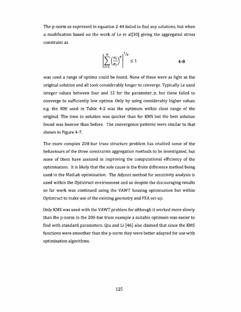
The p-norm as expressed in equation 2-44 failed to find any solutions, but when

a modification based on the work of Le et al[30] giving the aggregated stress

constraint as

was used a range of optima could be found. None of these were as light as the

original solution and all took considerably longer to converge. Typically Le used

integer values between four and 12 for the parameter, p, but these failed to

converge to sufficiently low optima. Only by using considerably higher values

e.g. the 800 used in Table 4-2 was the optimum w ith in close range of the

original. The time to solution was quicker than for KMS but the best solution

found was heavier than before. The convergence patterns were sim ilar to that

shown in Figure 4-7.

The more complex 200-bar truss structure problem has enabled some of the

behaviours of the three constraints aggregation methods to be investigated, but

none of them have assisted in improving the computational efficiency of the

optimisation. It is likely that the sole cause is the finite difference method being

used in the MatLab optimisation. The Adjoint method for sensitivity analysis is

used w ith in the Optistruct environment and so despite the discouraging results

so far w ork was continued using the VAWT housing optimisation but w ith in

Optistruct to make use of the existing geometry and FEA set-up.

Only KMS was used w ith the VAWT problem for although it worked more slowly

than the p-norm in the 2 0 0 -bar truss example a suitable optimum was easier to

find w ith standard parameters. Qiu and Li [46] also claimed that since the KMS

functions were smoother than the p-norm they were better adapted for use w ith

optimisation algorithms.

N Vp

4-8

125

4.3 Constraints Aggregation in Optistruct: The VAWT Space frame

The original optimisation for the C-FEC VAWT Housing was undertaken using

A lta ir Optistruct 11.0. In order to avoid repetition of work that was very time

consuming and that had already been found to be satisfactory, i.e. the setting up

of the geometry, finite element modelling and the main components of

optimisation. These were all maintained in Optistruct and the KMS functions

were applied w ith in the software. The continued use of Optistruct also enabled

an immediate and clear comparison of the results of the KMS optim isation w ith

the original results of chapter 3.

The KMS function was used to aggregate the individual stress constraints into a

single constraint. The efficacy of the KMS function was investigated using four

different approaches.

A. Internal equations in Optistruct

B. HyperMath - a numerical computing environment which forms part of

Optistruct that enabled the KMS functions to be calculated external to

Optistruct. This was sim ilar in functionality to MatLab

C. HyperStudy - a solver-neutral design study tool integrated into the A lta ir

suite. It facilitates design of experiments and optimisation studies and

thus brought the optim isation and the KMS calculations away from

Optistruct

D. MatLab optimisation function fmincon w ith Optistruct being used fo r the

finite element analysis only

These techniques enabled different stages in the optimisation process to be

addressed in different ways in order to find the most effective procedure for

applying the constraints aggregation while maintaining the geometry and

meshing in Optistruct. These methods are summarised in Table 4-3.

The smallest of the C-FEC VAWT housing model designs was used for this

investigation, 10m diameter by 0.5 diameter height (10m x 0.5D). As described

previously the housing was a space-frame structure comprising 1 0 0 circular

hollow sectioned steel bars. The housing was fixed at the base and attached to a

central node at the top by a s tiff flat support. Seven different loadcases were

126

included in the model. All the details of the boundary conditions and material

properties fo r this structure can be found in Chapter 3.

Table 4-3 Summary o f the Four Approaches used for app ly ing the

Constraints Aggregation

Methods of Approach

case A case B case C case D

O ptis truct -

In te rna l HyperMath HyperStudy MatLab

Equations

Geometry,COCOO)uoua.

Meshing &

Finite ElementOptistruct O ptistruct

c_oVP Analysis O ptistruct OptistructCO

sO ptim isation &

VPCLo

Sensitivity

QJJC4->

AnalysisHyperStudy

MatLabcCO

Method of KMS O ptistruct - (fm incon)<L>ro

4-1function Internal HyperMath

COdefinition Equations

Displacement, Stress and Buckling constraints were used in the optim isation as

before. The in itia l values for the design variables were taken to be 0.01m for

each of the inner radii and 0.003 for the wall thickness.

4.3.1 Case A - KMS de fined by O p tis truc t's In te rn a l Equations

The methodology for each o f the four approaches was in itia lly set up using a 10

bar truss model to check that the form at and syntax were being used correctly.

The bars in this case were A lum inium circular hollow sections. The objective

function o f the size optim isation was to minim ise the mass subject to

constraints on displacement and stress as in section 4.2 above. An additional

constra int on buckling was included together w ith self-weight to better reflect

the conditions of the VAWT housing optim isation. The in itia l values o f the

127

design variables are shown in columns B & C of Table 4-4. The best minimum

was found w ith these conditions when the truss was optimised using a global

search approach and no constraint aggregation.

The model w ith the KMS function {k = 50) converged to 2352 kg in 17 iterations

w ith and w ithout constraints aggregation. The inner radii and wall thicknesses

were exactly the same in both cases w ith the same predicted shape for the

optimised truss as shown in Figure 4-4. The optimised truss dimensions are

shown in columns D & E of Table 4-4. The cross sectional areas are also similar

to those in Figure 4-4 though the bars would be stronger as circular hollow

sections have a greater Moment of Inertia than solid bars for the same cross

sectional area. This would enable the structure to withstand the additional

resistance to buckling and the effects of gravity.

Table 4-4 Values of 10 bar Truss Design Variables with and without

Constraints Aggregation

A B C D E F

Bar

No.

Initial Values of

Design Variables

Optimised Va

(same with and wit!

ues

lout KMS)

Inner

Radius

Cm)

Wall

Thickness

(m)

Inner

Radius

(m)

Wall

Thickness

(m)

Cross -

sectional

Area

(m ^

1 0.09167 0.08583 0.060 0.041 0 .0 2 1

2 0.09167 0.08583 0 .0 1 1 0.008 0 .0 0 1

3 0.4183 0.08583 0.192 0.013 0.016

4 0.4183 0.08583 0.164 0.009 0 .0 1 0

5 0.4183 0.08583 0 .0 1 0 0.003 0 .0 0 0

6 0.4183 0.08583 0.023 0.004 0 .0 0 1

7 0.09167 0.08583 0.024 0 .0 2 2 0.005

8 0.09167 0.08583 0.146 0.015 0.014

9 0.09167 0.4172 0 .0 2 0 0.049 0.014

10 0.09167 0.4172 0.018 0.007 0 .0 0 1

128

An in itia l comparison of the truss optimisation w ith and w ithout constraints

aggregations showed that the time taken to reach the optima was 7% lower for

the KMS model than for the original (1.49s compared w ith 1.61). Repeated runs

of the model converged to the same optimum; however there was a marked

variation in the CPU time under both conditions. Data from 20 runs were

generated for optimisation both w ith and w ithout constraints aggregation. A

two-sample t-test assuming unequal variances on data showed no statistical

significance between the CPU times under the different conditions. The one­

tailed p-value was ~0.3 while the two tailed p-value~0.6 indicating that the use

of KMS functions made no measurable difference to the computational time for

better or worse.

Applying the same approach to the VAWT housing model found a sim ilar

optimum weight (568 kg) when using KMS functions and without, although w ith

fewer iterations (12 compared to 15).

Repeated calculations of the same structure not only generated different CPU

times but also achieved different feasible solutions. Without any combining of

the constraints 80% of the results gave a minimum mass of 568 kg in 15

iterations. The remaining 20% stopped at a higher feasible solution of 597 kg in

only 10 iterations. A total of 20 solutions were considered. Personal

correspondence w ith A lta ir (S. Patten, Altair, Technical Support, 23rd May 2014)

suggested that this was like ly to be caused by rounding off differences in the

eigenvalues. These differences are completely negligible in the analysis but can

accumulate in an optimisation run. This issue has been resolved in v l2 .0 of

Optistruct.

Similarly when the KMS functions were applied approximately 65% of the runs

found the 568 kg solution in 12 iterations while the remainder converged to a

higher minimum of 576 kg in 15 iterations. Comparing only those solutions that

converged to the best m inimum of 568 kg, the average CPU time w ithout

aggregation was 141 s while the average w ith aggregation was 865 s, more than

six times slower. These results are summarised in Table 4-5.

129

Incorporating the KMS function into the model has increased the number of

responses w ith in Optistruct [see Table 4-5). This value of 336 is the product of

the number of loadcases (7), the number of stress values per member [24) and

the number of equations [2). The KMS constraint was set up using two

equations, one to calculate the maximum of the stress constraints and the other,

the KMS equation 2-40 above, which accessed the firs t equation. Two equations

gave greater clarity in the input file. When the KMS equation was reduced to a

single equation to halve the number of equation responses a reduction in CPU

time was observed but the optimum found was higher than before [576 kg).

Some data was available on the breakdown of the CPU time amongst the

different modules of the software. A comparison of these times w ith and

w ithout constraints aggregation is shown in Figure 4-8 for the VAWT housing

optimisation. No detailed information is available w ith regard to the

functionality of the individual modules w ith in the software. The User Guide for

Optistruct 11.0 [58] states that

"OptiStruct uses an iterative procedure known as the local approximation method to solve the optimization problem. This method determines the solution o f the optimization problem using the following steps:1. Analysis o f the physical problem using fin ite elements.2. Convergence test; whether or not the convergence is achieved.3. Response screening to retain potentially active responses fo r the current iteration.4. Design sensitivity analysis fo r retained responses.5. Optimization o f an explicit approximate problem formulated using the sensitivity information. Back to 1."

It would appear from the figure that the increased time occurred in steps 4 & 5

above.

130

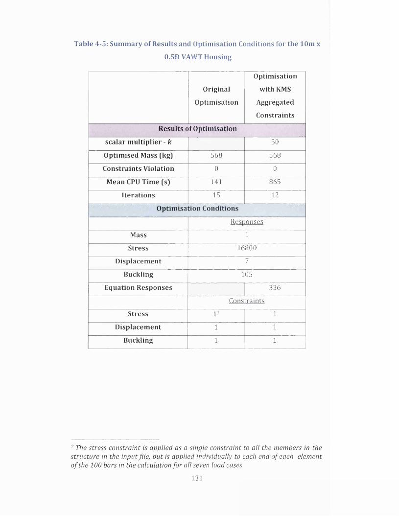
Table 4-5: Summary o f Results and O ptim isation Conditions fo r the 10m x

0.5D VAWT Housing

O riginal

O ptim isation

O ptim isation

w ith KMS

Aggregated

Constraints

Results o f O ptim isation

scalar m u lt ip lie r - k 50

Optim ised Mass (kg) 568 568

Constraints V io la tion 0 0

Mean CPU Time (s) 141 865

Ite ra tions 15 12

O ptim isation Conditions

Responses

Mass 1

Stress 16800

Displacement 7

Buckling 105

Equation Responses 336

Constraints

Stress l 7 1

Displacement 1 1

Buckling 1 1

7 The stress constraint is applied as a single constraint to a ll the members in the structure in the input file , but is applied individually to each end o f each element o f the 100 bars in the calculation fo r a ll seven load cases

131

800

700

600

¥ 500LOa>E 400 i—

2 300 u

200

100

0

■ Original Optimisation

■ with KMS ConstraintsAggregation (rho=50)

Q<

rHQCCl­u jocCL.

n 1 i 1 r

OocCl­u jQCCl.

UU J

X OuO

unonU JQCf—on

Cuon oc

uon

QC

i 1 ro a_ on

oQCQ_

HonXU Jon

Ou

XOQCC uCU<

1 I Ion cu

II £ ?

M odu les of th e Solver

Figure 4-8: Comparison o f the CPU breakdown in the O ptis truct Modules

w ith and w ith o u t the KMS functions

"SENSIT” which is presumed to deal w ith the sensitiv ity analysis has a 20%

higher CPU time w ith constraints aggregation than w ithout. O ptistruct can use

e ither the Direct or Adjo in t methods for sensitiv ity analysis w ith size

optim isation but no indication is given in the output data to as to which method

has been used. It would have been hoped that the Adjo in t method would have

been employed w ith the KMS as the number o f constraints has been

dram atically reduced and that this would bring an im provem ent in this tim e but

this is not evident. The tim e in the "APPROX” module dominates, the difference

being 23 times greater when constraints aggregation was used but there is

insuffic ient documentation to determ ine exactly what is happening here. S im ilar

trends were seen when KMS was expressed as a single equation.

132

N o C o n s t r a i n t s A g g r e g a t i o n

20

15

10

5 5

V)Cou-o<D

o■>

0 i nl i r— i i I I I I 1 I I I 1 T 1

0 1 2 3 4 5 6 7 8 9 10 11 12 13 14 15Iterations

■ Stress ■D isplacem ent ■ Buckling

Figure 4-9: Most V iolated Constraints at each ite ra tion o f the VAWT

housing O ptim isation - No Combining o f Constraints

W i t h C o n s t r a i n t s A g g r e g a t i o n

■*->C

'2 15

<3 10~o0)13 5 o >

i

i

i iV, u o5

I 1 1 1 1 1 1 ! 1 1 1 10 1 2 3 4 5 6 7 8 9 10 11 12

Iterations

■ Stress ■ Displacement ■ Buckling ■ KMS Responses

Figure 4-10 Most V iolated Constraints when Constraints Aggregation is

applied to the Stress Constraints

Closer inspection o f the constraints v io la tion in the models show that except at

ite ra tion zero the buckling constraints were the most violated. Figure 4-9 and

133

4

Figure 4-10 show the 20 most violated constraints at each iteration for the

VAWT housing w ith and w ithout constraints aggregation respectively. Since

Constraints Screening is used in both of these models then these are the active

constraints upon which the sensitivity analysis is tested. Since the buckling

constraints dominate both of these graphs this may be one of the reasons why

aggregated stress constraints bring very little improvement to the sensitivity

analysis.

An optimisation using higher in itia l conditions was investigated. This created a

structure where none of the constraints were violated for the early iterations

but once the mass became sufficiently low it was the buckling constraints that

dominated the most violated group once more.

4.3.1.1 Constraints Screening

As mentioned in section 2.4.3.4 Constraints Screening is used in Optistruct as a

method of improving the computational efficiency. In order to isolate the impact

of the two different techniques Constraint Screening was removed and the

optimisation was run again w ith and w ithout constraints aggregation.

When constraints screening was removed the solution converged to a higher

feasible solution. In this case an optimal mass of 1042kg in 37 iterations w ith a

CPU time of 424s, almost double the weight of the best design and three times

the time taken to find it. Applying the KMS functions converged to a higher

optimum of 1081 kg in 34 iterations and took 1820s to converge. The results of

chapter 3 also showed higher optima when constraints screening was

suspended.

These results show as before that the inclusion of constraints screening enabled

the optimisation algorithm to find the lower optima and so was incorporated in

all models in the remainder of this study.

What can be seen from the breakdown of the CPU time shown in Figure 4-11 is

that w ith Constraints Screening turned off the application of the KMS functions

did reduce the time spent in the "SENSIT" module compared to Constraints

Screening Off but w ithout Constraints Aggregation. This is consistent w ith fewer

constraints reducing the sensitivity calculations, however in both cases this time

134

far exceeded the time taken when Constraints Screening was employed. Once

more, however the time in the "APPROX” module dominated the CPU time when

the KMS functions were used.

1800

1600

1400

- 1 2 0 0 <D- 1 0 0 0 Ei= 800Xu 600

400

200

0

uM odules of th e Solver

Figure 4-11 Comparison o f CPU tim e w ith ou t Constraint Screening fo r

VAWT Housing Size Optim isation

4.3.2 Case B - KMS Using HyperMath

In an a ttem pt to reduce the number of responses and thus the computational

tim e HyperMath was introduced to move the KMS calculation outside of

Optistruct. This enabled the 336 equation responses above to be reduced to

168 external responses.

For the 10 bar truss the KMS constrained model achieved the same optim um in

17 iterations. This was consistent throughout 20 repetitions o f the

optim isation. An average time of 1.99 s was recorded, 64% higher than the

■ Constraints Screening On■ Constraints Screening Off■ Constraints Screening Off with KMS

u

i "r1 " i - i i i i i i i r i i i i i

<Cl . —

ocC L

OccCL­U JccCl.

xuUJXo

ccU J> —ioon

ononoci—on

Q .on oc

uon

13oCUJ>2n

h— © Z Q .cc on C L £

on2UJon

xOocC LC L<

onf—=™i

Xon

Xon

oc =

135

original optim isation in Optistruct. This increase was shown to be statistically

significant using the two sample t-test.

The time taken to optimise using the KMS constraints for the VAWT housing

was eight times higher than the base case optimisation and the time taken in the

'APPROX' module dominated the CPU time being 29 times higher. In this case

the model converged to the 568 kg optimum which is the same as the original

but in fewer iterations (12 instead of 15).

These results show that reducing the responses did not improve the

computational efficiency of the problem, in fact introducing HyperMath into the

process appears to have compounded the problems.

4.3.3 Case C - KMS Using HyperStudy

The use of HyperStudy enabled both the Optimisation and the sensitivity

analysis to be removed from w ith in Optistruct in the expectation that this would

give greater clarity and control over the techniques being used. HyperStudy

extracted the required responses from the results of an Optistruct analysis and

enabled the optim isation problem w ith the required design variables, responses

and constraints to be set up externally. The design variables were taken as the

inner radii and wall thickness for each o f truss members. Buckling,

displacement, mass and stress constraints were identified. This gave a total of

123 responses as only one stress value was available for each of the elements

and only 1 buckling response, the maximum of the eigenvalues was used for the

whole structure.

For the 10 bar truss the best optimised mass obtained using this approach and

before applying the KMS function was 2600 kg, 11% higher than the Optistruct

solution. This solution was obtained using the Sequential Quadratic

Programming (SQP) algorithm w ith in itia l conditions for all the design variables

set to the upper bound of 0.5m. Although HyperStudy does not have the facility

to m onitor the associated CPU times the optimiser was visibly many orders of

magnitude slower than w ith Optistruct.

When applying the KMS functions the model failed to run in less than 10

iterations. The software bu ilt up to using 100GB of working memory and so

136

crashed when it reached the lim it of the hardware. It was difficult to see how

this could be avoided when all that had been done was to express the KMS

response as a function of the stress variables in accordance w ith equation 2-40.

This approach was not therefore applied to the VAWT housing model.

4.3.4 Case D - KMS Using MatLab

The final method studied was the use of functions in MatLab for optimisation of

the structures and aggregation of the constraints. Fmincon has been used to

minimise the constrained nonlinear function. The MatLab code can be found in

Appendix H. The use of MatLab for this problem allowed greater transparency

and control over the optimisation. The best optimum found for the 10 bar truss

before the constraints were aggregated was 3804kg, which was 62% higher

than the optimum found by Optistruct alone. The CPU time was 433s. 96% of

this time was taken up in the FEanalysis function which was a single line of code

that called up RADIOSS in Optistruct to run the FE analysis only. The algorithm

used for this optimisation was the Interior Point algorithm, the Active Set

algorithm that had proved so reliable in section 4.2.1 found only an optimum

that was almost twice as heavy again. Despite not finding the best optimum a

KMS function was applied to the stress constraints and the new optimum was

obtained in 552s but unfortunately it was not even as good as the previous

value and the design maintained all ten members of the truss, 1 -6 at a cross

sectional area of 0.016m2 and 7-10 at 0.12m2. This new optimum mass was

4166 kg. This approach was not applied to the VAWT housing model because

of the mediocrity of the results shown.

4.3.5 Summary o f results

The results of all four approaches are summarised in Table 4-6, showing the

numerical results and a short precis of the outcomes.

137

Table 4-6: Summary o f the results o f the four methods investigated fo r

KMS Constraints Aggregation

Methods of Approach

Case A Case B Case C Case D

O p tis tru c t -

In te rn a l H ype rM a th H yperS tudy M atLab

Equations

w /o8 With With w/o With w /o With

KMS KMS KMS KMS KMS KMS KMS

Optimum

(k g )2352 2352 2352 2600 No

result

3804 4166

Iterations 17 17 17 51 7 8

i/it/i3uE-

Av. CPU

Time (s)1.17 1.15 1.99

Not monitored

by the software433 552

lmreJ3

Higher optimabest

co

*13re

’ao

c0)E-

no significant

improvement

64% greater

in CPU time

usage

found in

significantly

slower time. No

Solution with

KMS

Optimum

62% higher

and longer

CPU time

< Optimum

(k g )568 568 568

0X3Iterations 15 12 12

C"c/33OXH

Av. CPU

Time (s)141 865 1572

Not investigatedNot

investiaated£< Same> CPU time 6

times higher

optimum

but 11 times

longer

8 w /o - w ithout

138

4.4 Discussion

The results of this w ork have been unexpectedly disappointing, much has been

w ritten about the efficacy of constraints aggregation but in none of the

examples or the methods of approach have there been any significant indicators

that improvements have been made. This section w ill highlight some possible

areas which may have been the cause of the difficulties in this particular

application and then provide an overview of the published research in other

areas where the application of KMS has been shown to be successful.

4.4.1 D iffe ren t O ptim isation Solvers

In each of the optimisation packages used a choice of different algorithms were

available. Table 4-7 shows these options and indicates the commonality

between them.

As has been highlighted by Chinneck [168] in non-linear optimisation problems

using different algorithms for the same problem even w ith the same in itia l

conditions w ill not necessarily lead to the same optimum solution. This has

been clearly illustrated in the work of this section. The five algorithms used in

Optistruct were automatically selected and no indication was given as to which

algorithm was used in this version of the software.

Consistency was not found even w ith the same solver. The only algorithm

common to all of the software packages used was Sequential Quadratic

Programming (SQP}. In MatLab for the 10 bar truss the SQP algorithm could

find no feasible solution, while in Optistruct when this method was selected

manually the model failed after five iterations. As mentioned in section 4.3.3 the

HyperStudy solution was obtained using the SQP algorithm but was 11% higher

than the best optima.

Similar concerns arise over the methods used for sensitivity analysis. It is clear

that the Adjoint method should be the preferred option to minimise the CPU

time but only finite difference methods were available w ith in the solvers of

HyperStudy and MatLab. It is unclear i f the Adjoint method was consistently

used in the Optistruct only and HyperMath (Cases A & B} solutions.

139

Table 4-7: O ptim isation A lgorithm s available in the Software

Available

O ptim isa tion A lgorithm sO ptis truct/H yperM ath HyperStudy MatLab

O ptim ality Criteria Method •

Convex Approxim ation

Method•

Method of Feasible

D irections (MFD)• •

Sequential Quadratic

Program ming (SQP)• • •

Advanced Approxim ations •

Adaptive Response Surface

Method (ARSM) [110]•

Genetic A lgorithm s •

Sequential Optim isation and

R eliab ility Assessment

(SORA) [169]

•

ARSM based SORA •

Trust Region Reflective •

Active Set •

In te rio r Point •

4.4.2 Added Complexity

In all cases the addition of the KMS functions appeared to add additional

com plexity to the problem. Additional responses created by the equations

w hether in ternal or external had an impact on the CPU tim e not only for the

sens itiv ity analysis but more significantly on the approxim ation methods being

used. In HyperStudy this also impacted on the storage capacity needed to solve

the problem.

In the MatLab application it was evident that the time taken to call O ptistruct for

the FEA analysis dominated the CPU time and so any improvements in the

140

processing time caused by the constraints aggregation was overshadowed by

the file handling process. This may also have been a con tribu to ry factor w ith

the HyperStudy method, but the software was not su ffic ien tly transparent to

identify this.

4.4.3 Previous Successful Applications o f KMS

A meta-analysis o f 65 papers where the KMS functions have been applied has

been undertaken. The papers span the period 1988 to 2014, the m a jo rity o f

which have appeared in peer-reviewed journals, but 9% o f them come from

conference proceedings since 2012 to ensure that the most recent research was

represented. Details o f the papers are listed in Appendix I.

Figure 4-12 shows the main type of optim isation problem being addressed in

this lite ra ture. The pie chart shows that more than half o f the papers consider

m ulti-objective optim isation w ith topology and shape optim isation the next

most common. This trend can be seen throughout the time period of the sample

as shown in the frequency d is tribu tion of Figure 4-13.

LocationTopology^

22%1%

Size6%

M ulti­objective

52%

Shape12%

Process___

5% None. 2%

Figure 4-12: Types o f O ptim isation used in Research Papers Using KMS

functions

141

>2 5 0)3O’2! 4

■ Location

■ Process

□ Topology

M u ltio b jec tiv e □ None

Shape □ Size

Ih in mo o c n t H O r M r o ^ - L D U D r ^ o o c n o ^ - i r ^ n n ^ - L n u D r ^M o o a i o i o i o i o i o i o a t c n m o o o o o o o o - . _ c n c n c n c n a i c n c r i c n c n c n c n c n o o o o o o o o o o o o o o o

H H H H H H H H H H H H f M r M r M ( N f M ( N ( N r M ( N I N ( N ( N ( N r M ( N

Year

Figure 4-13 Frequency d is tr ib u tio n o f sample o f KMS published papers

4.4.3.1 Size Optim isation

Only three papers were found where size optim isation was the main objective,

two o f which have already been referenced in this chapter. One, the paper by

Chang [164] already referred to in section 4.2.2 showed results where the

com putational tim e increased five-fo ld for the 10 bar truss when KMS functions

were used however the author had changed the optim isation algorithm at the

same tim e as in troducing the KMS function so the ind iv idua l effects o f the two

in terventions could not be identified. The second from Akgun et al.[54] showed

that the benefits o f the KMS aggregation were most prevalent when the

application used the A djo in t method for sensitiv ity analysis and the problem

was complex, e.g. a large num ber o f load cases. A more recent paper by Poon

and Martins [27] proposed an adaptive KMS approach for aggregating the stress

constraints fo r the w eight reduction o f a w ing structure composed of tubu la r

elements w ith the design variables being the diameters of the tubes. The KMS

142

was adapted by modifying the k parameter as the solution approached the

optimum. The researchers used an active-set SQP-based optimiser w ith a semi-

analytic Adjoint method for the sensitivity analysis. The partial derivatives of

the Adjoint analysis were computed using the complex-step method. The

adaptive KMS function reduced the computational time of the optimisation by a

th ird and came w ith in 0.2% of the reference solution. Using the standard KMS

aggregation the time saving was greater but the solution less accurate.

4A.3.2 Shape Optim isation

Small variations in shape can give extreme changes in the stress measures when

a Shape Optimisation is undertaken. In the papers reviewed, e.g. [170-172],

typically the KMS functions have been used to obtain a single representative

measure that reflects the global stress of the structure. This prevents the

solution being adversely affected by the large fluctuations in stress by providing

a function that is both continuous and differentiable. This focus appears to have

been more critical than the aggregation of constraints for computational cost

savings. The KMS functions were chosen for sim ilar reasons in the process

optimisation papers [173, 174]. Where stated most authors used the Adjoint

method for sensitivity analysis in the shape optimisation, Breitenberger et

al.[175] did use the finite difference method.

4.4.3.3 Topology Optim isation

The topology optimisation papers, e.g. [43, 176, 177], aggregated the stress

constraints in the standard way to minimise the number of constraints and thus

speed up the computation. Paris et al.[57] observed that there was some lack of

strictness in the constraints when all were combined into a single inequality and

so they improved the accuracy of their results by aggregating the constraints

into several blocks rather than a single stress function, while still maintaining

some of the computational cost savings in both time and storage. Typically in

topology optimisation buckling is not included as a constraint and so unlike the

results of section 4.3.1 the most violated constraints w ill be those that have

been aggregated by the KMS functions.

143

4.4.3.4 M ulti-ob jective / M u lti-D isc ip lina ry Optim isation

The pie-chart o f Figure 4-14 shows the affilia tions of the authors who have used

the KMS function in m ulti-objective and m u lti-d isc ip linary optim isation to

ensure that the data is not imbalanced by repetitive publishing of s im ila r

research. 50% of these, a total o f 17 papers originated from the Department of

Mechanical and Aerospace Engineering at Arizona State University. The papers

chosen span almost 20 years from 1993 [178] to 2011 [179] but the application

of the KMS functions appears to be very s im ila r throughout. Both the

constraints and objective functions in m u ltid isc ip lina ry optim isation were

combined. In some of this lite ra ture the aggregated objective functions have

been weighted [180] to enable the designer to emphasize specific design

objectives over others w hile s till being able to express the complex constraints

in terms of simple continuous and differentiable functions.

University of Michigan ^ 6% Virginia

■ ^ 7 —— PolytechnicV 6%

NASA12%Arizona

StateUniversity

50%Others

26%

Figure 4-14: O rigins o f the KMS papers using M ultiob jective O ptim isation

144

The NASA papers were mostly published in the late 1980s and early 1990s by

Sobieszczanski-Sobieski [181] and his colleagues, while the remaining sectors of

the pie represent 1 or 2 papers from different Universities throughout the world

right up to 2014. In nearly all cases the KMS has been used to aggregate the

constraints and objective functions [182, 183]. Where specified the Adjoint

method has been used for sensitivity analysis.

4.5 Conclusions

Analysis of the available literature on the use of Kreisselmeier Steinhauser

functions shows that this approach is most likely to be successful when the

Adjoint method is used for sensitivity analysis. Most often these functions are

used not only to agglomerate the optimisation constraints but also to make use

of other beneficial characteristics of the function, i.e. continuity and

differentiability, to facilitate a smoother convergence to the optimal solution.

Applying the KMS functions to the problem of Case Study 1 while maintaining

the structural geometry and mesh w ith in Optistruct has increased the

complexity of the problem w ith all approaches whether by increasing

responses, applying alternative algorithms and sensitivity analysis or just in the

speed of interface between different software. Applying KMS functions in this

way does not provide a quicker route to the solution. The method of

Constraints Screening already a part of Optistruct appears to effectively find

good solutions in optimal time.

145

Chapter 5: Case Study 2 - The General Electric Challenge - Designing for Additive Manufacture

Summary: Using the entries to a recent design challenge sponsored by General

Electric this chapter explores some o f the critica l factors necessary in designing fo r

ALM.

5.1 Introduction

In June 2013 General Electric [GE) launched a design challenge for additive

layer manufacture [ALM) on the GrabCAD website [184]. The challenge was to

redesign an existing titanium lifting bracket for a jet aircraft engine in order to

minimise the weight. The reasons for considering this challenge as a Case Study

in this Engineering Doctorate are two-fold: firstly, as a means for personal

development to improve the skills and understanding necessary when

designing components for ALM. Secondly, since the format of the challenge was

an open crowdsourcing competition this provided free access to both the

geometry and image files of all of the entries. This is the area of greatest novelty

in this study, the analysis of a large dataset of designs for ALM. Approximately

700 entries were submitted to the competition and it was expected that this

would provide a rich source of data to inform future ALM design.

This chapter w ill in itia lly consider the details of the GE challenge and then

present the current thinking from the literature on various aspects of the

problem. The author's own optimisation design w ork w ill then be presented

and discussed and this w ill be followed by a statistical analysis o f the other

entries to the competition. The chapter w ill conclude w ith a discussion of the

trends observed in the data and some of the issues that these raise in the design.

The major findings o f this w ork w ill be applied to the final Case Study of this

thesis [see Chapter 7:).

5.2 The GE Design Challenge

As previously mentioned the GE design challenge was the redesign of a jet

engine lifting bracket made from titanium [see Figure 5-1). The bracket was to

be produced by Direct Metal Laser Sintering [DMLS).

146

Figure 5-1: Example o f a lift in g bracket in situ

Clevis Arms

Bolt holes

Figure 5-2: O rig ina l Design Envelope fo r Engine Bracket [184]

The design envelope for the bracket as shown in Figure 5-2 was precisely

specified. The current bracket shows four asymmetric holes for bo lting the part

to the engine and two parallel clevis arms w ith holes for the insertion o f the

clevis pin from the crane attachment mechanism. The maximum dimensions o f

the bracket were 0.174m, 0.092m and 0.153m for w id th , depth and height

respectively. The total mass was 1.938 kg. The bolts used were 0.375-24

147

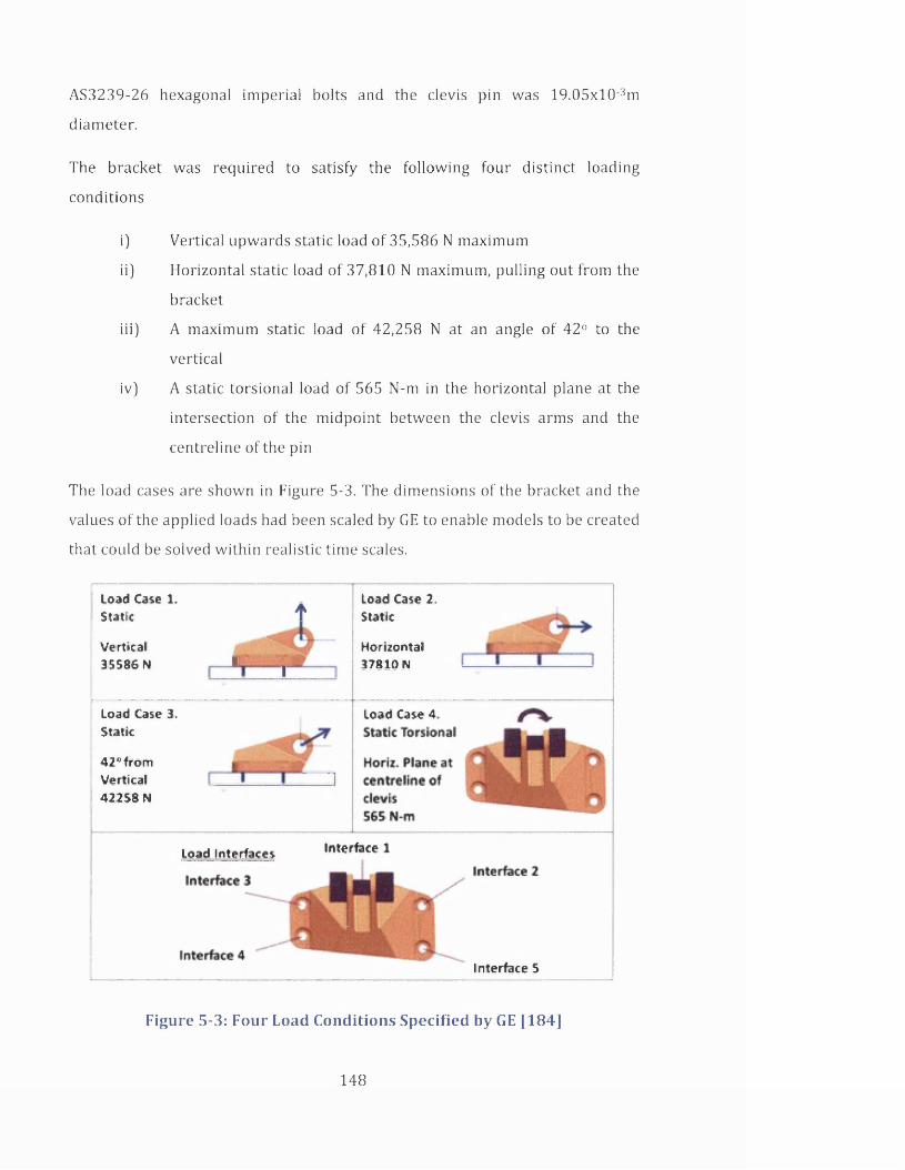
AS3239-26 hexagonal im peria l bolts and the clevis pin was 1 9 .0 5 x l0 3m

diameter.

The bracket was required to satisfy the fo llow ing four d is tinct loading

conditions

i) Vertical upwards static load o f 35,586 N maximum

ii) Horizontal static load of 37,810 N maximum, pulling out from the

bracket

iii) A maximum static load of 42,258 N at an angle o f 42° to the

vertical

iv) A static torsional load of 565 N-m in the horizontal plane at the

intersection o f the m idpoin t between the clevis arms and the

centreline of the pin

The load cases are shown in Figure 5-3. The dimensions o f the bracket and the

values o f the applied loads had been scaled by GE to enable models to be created

that could be solved w ith in realistic tim e scales.

1Load Case 1.Static t

Vertical35586 N 1 -|b

Load Case 2. Static

Horizontal 37810 N

Load Case 3.Static

42*^001Vertical i 4 2 2 5 8 N

Load Case 4,

load Interfaces Interface 1

f

Interface 5

Figure 5-3: Four Load Conditions Specified by GE [184]

148

The material grade for the component was titanium Ti-6A1-4V w ith Young's

modulus 110 GPa, Poisson's ratio, 0.31 and density 4430 kg/m 3. The maximum

permissible yield strength was 903 MPa. The minimum feature size permitted in

the final design was 1.27 x 1 0 3 m.

It was recommended that the bolts and the clevis pin should be considered to be

in fin ite ly s tiff and to ensure a fair comparison of the resulting designs. ANSYS

software was stated to be the simulation tool of choice by GE.

The competition itself was to be divided into two distinct stages. An in itia l

phase where all entries would be analysed and evaluated using simulation tools

and then a second phase where the top ten entries from phase one would be

bu ilt using ALM and tested under the specified loading conditions. Prizes were

awarded for the best ten of phase one and the best eight in phase two.

5.3 Setting the Challenge in Context

There are a number of areas relating to this design that remain quite

specialised, not only in the methods of manufacture and the material but also

the tools that are available to assist in optimising the structure. The following

section w ill detail the findings of a review of the current literature in these areas

to inform the approach taken in addressing the design problem.

5.3.1 A dd itive Layer M anufacturing

Additive layer manufacturing techniques have been available in various forms

since the late 1980s. Working directly from a 3D CAD of a part a solid

component can be bu ilt up in thin slices, layer by layer. Parts can be fabricated

in polymers, ceramics, paper or metals. In metal working a wide range of

techniques have been developed, most of which use either wire or metal

powders as the raw material and apply a selective energy source to form the

solid as required. W ith the powder-based technologies, e.g. DMLS, also known

as Selective Laser Melting (SLM), metal powders are solidified only where

needed in the component leaving the unused powder to be easily removed at

the end of the process. UV light (Direct Light Processing), Electron Beams

(Electron Beam Melting) and lasers (Selective Laser Sintering, for example)

have all been used to melt and solidify the source material. Shaped Metal

149

Deposition (SMD), a w ire based additive manufacturing technique deposits

welding w ire layer by layer on a base plate, the part is fabricated using tungsten

inert gas [TIG] welding. The processes are carried out in an inert atmosphere to

prevent oxidation. A detailed description of these processes w ill not be included

in this thesis, an excellent description can be found in reference [185] but some

discussion w ill follow on the advantages and disadvantages of the technology.

Over the last decades mass production of metal components has mostly

migrated to the Third W orld due to lower labour costs and taxes, and the ease of

access to raw materials. Developed countries have needed to focus on creating

high value customised components to remain competitive [186]. ALM

techniques have provided a means of accomplishing this and they have a

number o f advantages over traditional manufacturing methods:

i] Time and Cost Savings. W ith the component being made directly from the

CAD design there is a large reduction in the time taken to bring an in itia l

design to market and also a capital cost saving in tooling etc. [186] in terms

of manufacturing time only. Generally the build time w ith ALM is longer than

for a machined component and so energy consumption tends to be greater

however, a Life Cycle Analysis (LCA) carried out by Serres et al.[187]

showed that the total environmental impact for an ALM part was about 70%

of the impact of a machined part. Serres' study looked at an aerospace part

made of Ti-6A1-4V. In general for aerospace components weight reduction

and the subsequent fuel savings have such a large impact on the long term

energy consumption that manufacturing costs become insignificant.

ii) W ithout having to consider tool access or the need for part removal from

moulds etc. there can be much greater flexibility in the design and build of

the part. Complex and intricate designs can be developed. These fabrication

techniques have fewer lim itations and increased complexity does not

necessarily add to the cost o f manufacture. For example, ALM enables

lightweight lattice structures to be easily included in the component which

creates a part which has a high degree of rig id ity and low density while still

enabling easy removal of the powder [188].

150

ii i] Since material is added and not subtracted w ith these techniques then there

is considerably less waste. This has been estimated to be as much as 80%

less [187]. W ith most ALM technologies the majority of the powder which

has not been fused may be recycled [186] giving significant material savings

over conventional techniques. W ith Ti-6A1-4V powder there can be some

oxygen pick up at high temperatures and this can reduce the volumes

available for recycling [188].

There are some issues however w ith this technology:

a] Material and Geometric properties. Typically an as-built ALM component

does have some directional variation in mechanical properties according to

the orientation of the build [189]. Material densities as high as the wrought

product can be achieved w ith sufficiently slow scan speeds and high laser

power. Surface roughness too has been shown to be dependent on build

direction [190], though the greatest roughness variation was seen where

support material had been attached. The accuracy of the build may also be

problematic, issues w ith shrinkage and warping [191], non-cylindricity of

parts [192] can cause difficulties particularly when the ALM component

must f it w ith an existing part.

b) Support material. Additional material to support the component during the

build is required for a number of reasons:-

i. To act as scaffolding structures for large overhangs. Features that

are inclined at a relatively small angle to the horizontal are not self-

supporting and so additional structures must be added temporarily

to the design to hold the feature in place until the solidification

occurs. The required angle at which this is needed varies according

to the process used but tends to be in a range below 40-50°.

ii. To prevent curling and warping of overhangs due to residual

stresses

iii. To reduce high temperature gradients during processing by

conduction to the base-plate .

These structures require additional material to be used which is usually

wasted as it cannot be recycled easily [193]. Additional time and costs are

151

incurred in the building of the component and in the removal of the supports

after processing. The removal is often a manual process and requires some

constraint in the design to enable access for hand tools etc. As mentioned

above it may also serve to increase the surface roughness at the point of

attachment to the part.

A number of authors have proposed methods of designing to completely

avoid the need for support structures [193-195] but these techniques are in

the ir infancy and have only been tested on 2D structures in the literature.

Leary et al. [194] describe a method that modifies the design to form

structures w ith sufficiently steep angles to avoid using supports and then

suggests that these features could be removed at post processing. In this

way the time saving and the majority of the material saving has been

achieved in the build and only a lim ited amount of extra time would be

needed in the post processing. Serphos [195] incorporated a restriction on

the permissible angle of overhanging areas w ith in a topology optimisation.

Three different approaches are considered; a multiple objective, a global

constraint and a density filtering method. Although the results from a 2D

benchmarking validation for all three methods showed some promise

further development work was proposed to identify the most appropriate

parameters required in the optimisations and to avoid instabilities in

convergence.

c) Powder removal. The most notable capability of ALM is its capacity to

manufacture lightweight and hollow structures. However, careful design is

necessary to ensure that any unused powder in internal cavities can be

easily removed otherwise the planned weight saving w ill not be realised

[188]. Inefficient removal of the powder not only wastes the raw materials

but also serves as a potential environmental hazard by the spread of metallic

powders.

d] All these factors require designers to modify their thinking when designing

for ALM. Change in any form is not always easily accommodated.

152

5.3.2 T itian ium

Titanium and its alloys are used extensively in the aerospace industry because

of the ir high strength, low density and high corrosion resistance. The material is

also biocompatible and so is commonly used for medical implants. The weight

savings possible by using ALM for manufacture are particularly pertinent for

titanium components as the production of titanium from its raw material

consumes high levels of energy. A recent cradle-to-grave LCA by Norgate et

al.[196] showed titanium to have a gross energy requirement of 361 MJ/kg,

more than 15 times that of steel. Titanium is also difficu lt to machine [197] and

so ALM manufacture can be particularly favourable for titanium components.

Most commercial, wrought Ti-6A1-4V products have a UTS of ~lGPa and

elongation of 14%. The hardness, measured as Rockwell C-scale hardness (HRC)

is around 38 [198]. M urr et al.[198] measured tensile strengths as high as 1.45

GPa and elongations ranging from 4 - 25% in samples made by EBM or SLM in

the ir "as built" condition. The range of hardness values was 37 - 54 for these

samples. All samples were measured in the build [or z] direction in this study.

Vilaro et al.[199] measured mechanical properties of samples built in two

different orientations; Longitudinal (LD), least height w ith the fewest layers and

Transverse (TD), the sample length was in line w ith build direction. In both

cases the UTS and yield strengths were well above the properties for wrought

material w ith the LD sample higher than the TD. The ductility measurements

were much lower than the wrought material however; the LD value was 7.6%

which far exceeded the TD value of 1.7%. Young's modulus values of ~105 GPa

were quoted in this paper though no comment was made about how these had

been measured. The results were sim ilar for both LD and TD samples. As

mentioned in section 5.2 a typical value of Young's modulus for wrought

titanium is 110 GPa.

The high energy input and fast solidification rates of the ALM process cause the

microstructure of titanium and its alloys built using these techniques to be out-

of equilibrium. It is therefore necessary for components to be heat treated to

achieve mechanical properties sim ilar to the conventional material. Leuders et

al.[2 0 0 ] showed that heat treatment not only reduced the residual stresses in

153

SLM bu ilt parts but modified the microstructure so that the breaking elongation

increased to w ith in acceptable levels. Heating the samples reduced the UTS

from 1080 MPa in the as-built case down to 945 MPa after a treatment of 1050°

C for 2 hours in a vacuum, but this was still w ith in an acceptable range for Ti-

6A1-4V. High-cycle fatigue testing showed that the number of cycles to failure

increased w ith increased heating but was not comparable w ith conventional Ti-

6A1-4V until a hot isostatic pressing (HIP) cycle was applied. The application of

heat modified the microstructure but the pressure was necessary to reduce the

pores typically found in SLM bu ilt material.

5.3.3 Design by Crowdsourcing

Another interesting facet of this challenge was the use of open crowdsourcing

(CS) approach to solicit the designs. The word "crowdsourcing" was firs t coined

in 2006 [2 0 1 ] though the practise was used much earlier than this, e.g. public

logo and photograph competitions, both forms of crowdsourcing, were run early

in the 1900s.

Crowdsourcing has been defined as

"... the act o f a company or institution taking a function once performed by employees and outsourcing i t to an undefined (andgenerally large) network o f people in the form o f an open call"[202].

Sometimes crowdsourcing uses competitions w ith financial rewards to

incentivise participation but often organisations engage volunteers in large

crowdsourcing projects, e.g. currently over 1 2 0 , 0 0 0 volunteers are engaged in

indexing worldw ide genealogical records [203]. Crowds may need to have

specific skills, but this is not always the case, the value to the client may lie in

the volume of information acquired rather than in the contribution of a single

individual, e.g. data from supermarket loyalty cards.

It is clear that in conjunction w ith the internet CS provides a method of

accessing individuals over a large geographical area and potentially from a

diverse group. Referring back to design approaches discussed in Chapter 2 CS

can be seen as a variation on the Concurrent Engineering model where input

external to the organisation comes in at the concept stage and this may or may

154

not already be informed by experience in other areas o f the production cycle

(see Figure 5-4).

s aMass

Product­ion

ProductPlanning

Product Develop­

ment WPilot

Production

DesignReview

Proto y?type y

Figure 5-4: The ro le o f Crowdsourcing in the Production Cycle

There are a num ber o f risks for organisations when taking the CS approach. The

uptake on the call may be lim ited or the quality o f the submissions poor. Early

perceptions of the crowd were somewhat negative, considering them to be

merely amateurs or hobbyists though some recent publications [204] have

shown that this is generally not the case. The response may be large and

significant additional resources may need to be employed by the client in the

evaluation process. Careful planning is required to clearly define the client's

requirem ents w hile removing all company-specific details. Integration of CS

w ith existing staff must be managed carefully to avoid alienation.

Recent studies indicate that individuals engaged in R & D in the future are much

more like ly to be freelance contractors than have long-term careers w ith one

company [205]. Crowdsourcing enables individuals to showcase the ir w ork to

155

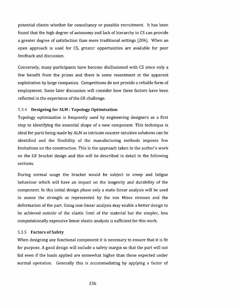
potential clients whether for consultancy or possible recruitment. It has been

found that the high degree of autonomy and lack of hierarchy in CS can provide

a greater degree of satisfaction than more traditional settings [206]. When an

open approach is used for CS, greater opportunities are available for peer

feedback and discussion.

Conversely, many participants have become disillusioned w ith CS since only a

few benefit from the prizes and there is some resentment at the apparent

exploitation by large companies. Competitions do not provide a reliable form of

employment. Some later discussion w ill consider how these factors have been

reflected in the experience of the GE challenge.

5.3.4 Designing for ALM : Topology Optimisation

Topology optimisation is frequently used by engineering designers as a firs t

step to identifying the essential shape of a new component. This technique is

ideal for parts being made by ALM as intricate counter-intuitive solutions can be

identified and the flex ib ility of the manufacturing methods imposes few

lim itations on the construction. This is the approach taken in the author's w ork

on the GE bracket design and this w ill be described in detail in the following

sections.

During normal usage the bracket would be subject to creep and fatigue

behaviour which w ill have an impact on the longevity and durab ility of the

component. In this in itia l design phase only a static linear analysis w ill be used

to assess the strength as represented by the von Mises stresses and the

deformation of the part. Using non-linear analysis may enable a better design to

be achieved outside of the elastic lim it of the material but the simpler, less

computationally expensive linear elastic analysis is sufficient for this work.

5.3.5 Factors of Safety

When designing any functional component it is necessary to ensure that it is f it

for purpose. A good design w ill include a safety margin so that the part w ill not

fail even if the loads applied are somewhat higher than those expected under

normal operation. Generally this is accommodating by applying a factor of

156

safety to the design. There are several approaches to this but the definition that

w ill be adopted in this thesis for a structural part is

F a ilu re stressF a c to r o f S a fe ty = —— —-------------- t- *

W ork ing stress

In practice to maintain the structure w ith in the elastic region in the linear static

analysis this general becomes

(7yF a c to r o f S a fe ty = ------------ - 2

GmaxFEA

Where <sY is the yield strength of the material and c7maxFEA s the maximum

stress in the component found by the FEA analysis [207]. Topology

Optimisation for GE Challenge

Based on the understanding gained from the current literature an in itia l

topology optimisation was undertaken for the GE Engine bracket design using

A lta ir Optistruct 11.0. Optistruct was chosen as it allowed all four loadcases to

be applied to the model simultaneously.

5.3.6 Element Selection

The elements used in this study were in itia lly 10-noded tetrahedral.

Tetrahedral elements were used prim arily because of the ease w ith which the

mesh can be generated for complex shapes. For stress dominated problems like

the GE bracket the 10-noded quadratic tetrahedral elements are more accurate

than the 4-noded linear tetrahedral and better able to adapt to the curved

surfaces [208]. As mentioned in the literature review of Chapter 2 (section

2.4.3.1) the use of higher order elements helps to avoid checkerboard effects in

the optimisations. The 10-noded elements were of course, more

computationally expensive.

157

5.3.7 Mesh Sensitiv ity Testing

180~ 1 7 0(0| 160 — 150 jjj 140 £ 130

s i 120 2 110 § 100 > 90

80

No. of Elements

4.E-05

3.E-05

2.E-05CL

l.E-05

0.E+00

No. of Elements

LC 1 LC 2 LC 3 LC 4

Figure 5-5: Mesh Sensitiv ity Analysis Results fo r the GE Bracket O riginal

Design w ith o u t op tim isa tion

A mesh sensitiv ity analysis was carried out to ensure that the solution found in

the FEA was mesh independent. As the bolts and the surface to which the

bracket would be fixed were considered to be rig id bodies the bracket was

constrained over the whole o f the base surface and also at four annular surfaces

158

where the bolt heads would contact the bracket. An alternative constraint

method would have been to fix the in terio r surfaces of the bolt holes instead of

the base however this approach was found to give stress singularities caused by

the FEA method. Figure 5-5 show the trends in both the von Mises stresses and

the maximum displacement for mesh sizes from 3xl0 3 to 4.5xl0 4m. These

results were derived from a structural analysis of the original bracket of Figure

5-2 and are shown for all four load cases. The von Mises stresses were plotted at

a different fixed point on the geometry for each loadcase. The location was

chosen because of the occurrence of high stress levels and remained fixed as the

mesh density was varied.

5.3.8 Topology O ptim isation

The minimum mass problem of Chapter 2 [equations 2-47) was solved for the

titanium bracket using the SIMP method in A ltair Optistruct 11.0.

N

m m V mjPy 5 . 3

; ' = i

N

subject to : ^ ^ p fK ? U = F(p)i= 1

\ O j < o Y Vy = 1, ...,N 5 _5

: 0 < e < < p j < 1 Vy = 1, ...,N 5 6

N is the number of finite elements in the geometric domain. For this

optimisation an element size of 5.7x10 4m was chosen which as mentioned in

section 5.3.7 above was the smallest element size where the rigid element for

the clevis pin could connect to every node on the circumferential surfaces of the

clevis pin hole. The element size of 5 .7x l0 '4m gave a value of 2,478,178

elements for N [see Figure 5-6)

Ideally a mesh size o f 4.2xl0 4m would have been preferred. This would have

allowed at least three elements w ith in the specified minimum member size of

1.27xl0 3m ensuring greater accuracy. However not only would this mesh not

allow accurate fixing o f the clevis pin element it also created a mesh w ith over

159

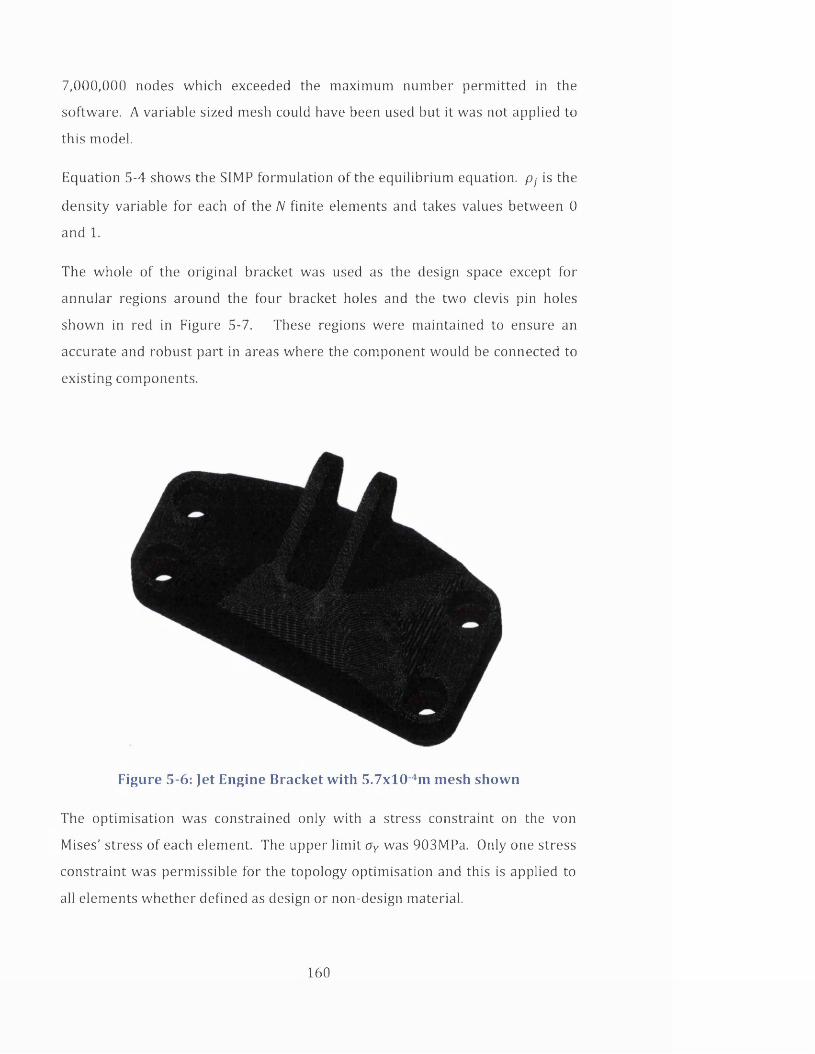
7,000,000 nodes which exceeded the maximum number perm itted in the

software. A variable sized mesh could have been used but it was not applied to

this model.

Equation 5-4 shows the SIMP form ulation o f the equ ilib rium equation. p7 is the

density variable fo r each of the N fin ite elements and takes values between 0

and 1.

The whole o f the orig inal bracket was used as the design space except for

annular regions around the four bracket holes and the two clevis pin holes

shown in red in Figure 5-7. These regions were maintained to ensure an

accurate and robust part in areas where the component would be connected to

existing components.

Figure 5-6: Jet Engine Bracket w ith 5.7x10 4m mesh shown

The optim isation was constrained only w ith a stress constraint on the von

Mises' stress o f each element. The upper lim it ay was 903MPa. Only one stress

constra in t was perm issible for the topology optim isation and this is applied to

all elements w hether defined as design or non-design material.

160

The component was optim ised for all four load cases w ith the inner surface of

the four bolt holes constrained to represent the fixing of the bracket to the je t

engine. This was not the same as in the mesh sensitiv ity analysis above for two

reasons: firs tly constrain ing the bolt holes was considered more representative

o f real conditions and any stress singularities caused by boundary geometry

could be elim inated in subsequent design iterations and secondly, only

im practical optim isation solutions were found w ith the base fixed. The designs

generated w ith a fixed base formed only vertical prongs between the clevis

brackets and the base w ith no material connecting to the bolt holes.

Vjy Clevis Pin represented by / Rigid elementInterior surfaces

of bolt holes fixed

Non-design Material

Figure 5-7: Basic Set Up fo r Topology O ptim isation (mesh om itted)

The optim isation converged in 37 iterations to a mass of 0.148 kg, 7.2% of the

orig inal mass. Figure 5-8 shows the convergence curve for the optim isation

which is v irtu a lly monotonic. The constraints vio lation remained at zero at

every iteration, though the stress constraint was either active or violated from

ite ra tion four to the end.

161

Iteration No

Figure 5-8: Convergence Curve fo r the Topology O ptim isation o f the GE

Bracket

Contour Plot Element Densitiesi Simple Average w -1 OOOE+OO

E8 900E 01 7 800E-01 6 700E-01 5 600E-01 4.500E-01 3 400E 01

— 2 300E-01— 1 200E-01— 1 OOOE02 ■ Mo result Max = 1 OOOE+OO Grids 296255 Min = I OOOE-C2 Gnds 825859

Figure 5-9: Topology O ptim isation Solution show ing va ria tion in Element

Densities, a) A ll densities b) A ll densities above 0.011

The optim ised component is shown in Figure 5-9. The variations in the density

gives very litt le useful in form ation when all density values are displayed as in

Figure 5-9 a), but increasing the low er threshold on densities to 0.011 (Figure

5-9 b)) reveals the essential areas where material is required for structura l

strength. Figure 5-10 shows several views of the optim ised bracker for density

values of 0.3 and above. Using the OSSmooth functiona lity in O ptistruct an FEA

of this structure was undertaken. The component was remeshed to 499,552

162

elements and the same loading conditions and constraints applied. Figure 5-11

shows the von Mises's stresses throughout the component for each of the four

load cases. The pictures on the left (a, c, e, g] display all the stress values

whereas the pictures on the right (b,d,f,h) show only those areas where the

stress levels are above the tensile yield strength (TYS) of the material, 903 MPa.

The highest values arise in loadcase 1 where the maximum von Mises stress is

3064 MPa and this occurs at a very small junction on the cross piece between

the clevis pin brackets. The component would need to be strengthened in this

area for manufacture so the high value at this point is not an issue. More

concerning are the high values in loadcases 1, 3 & 4 where high stress levels

exist at the junction of the clevis arms w ith the top surface of the bracket. These

are over 1500 MPa. The built-in intelligence in the Optistruct software

generally ignores boundary violations, working on the assumption that these

issues can be removed w ith subsequent shape optimisation at the boundaries.

In this design it is not possible to change the boundary at the surface as any

modifications would move the bracket outside of the design domain.

The maximum deformation in these parts is or the order of 1.3 x 1 0 3 m or less

which are acceptable for a part of this size.

163

Contour Ptot Model info I \EngD\Tetra 10 ■ GE bracket\The finished Topol • 10 nodedVTOP_057mmMESH_MinM_10-noded_rst033_des h3dElement Densrties(Density) Result I \EngO\Tetra 10 - GE bracke!\The finished Topol - 10 noded\TOP 057mmMESH MmM 10-noded rst033 des h3d

E, 000E*° - - - De- |t-aion37890® > ! Frame 47 0QOE-O1

w—6.700E-01 M-5.600E-01 1 —4.500E-01 • - 3 400E-01 i - 2 300E-Gt 1-1 200E-01

1 000E-Q2

Max = 1 OOOE+OO 30 3860381 Min = 1 000E 02 3D 3412973

Plan V ie w

Rear V ie w

Figure 5-10: Topology O ptim isation o f L ifting Bracket

164

Contour Plot Element Stresses A nalysis system

E2 539E*OS

2 .257E K B 1 975E409

•H -1 633E-H39

1.411E-KJ9

1 129E-KJ9

•3.4o4E-*08

•5.643E*06

•2 821E*06

•0 000E *00

Max = 2 539E+09 3D 000122 Min = 0.OOOE+OO3 0 1923689

Loadcase 1

Contour Plot E lement Stresses A n a lys is system

E2 296E-KB

2.G42E+09

1 787E-t09

— 1 632E-*09

1 27b t - to y

1.021E <09

7.659E-*OB 5 tO6E-tO0

2 653E-tOB

O.OOOE-KB

Max = 2-298E-*C9 3 0 5759325 Min =■ 0000E-*CC 3D 1923669

Loadcase 3

w

f)\ \

Contour Plot Element Stresses Ana lys is system

[ 2271E -K B

2016E -K B

I 766E-tC9

j - 1 514E-«09

1262E-r09

1 009E-t09

7 569E<C8

5 046E+C8

•2.523E+C6

OQOOE-tCC

Max = 2-271E<09 3D 5BO306D Mm = O.OCOE+OO 3D 1923689

Loadcase 4 \

h)

' i v v

Figure 5-11: von Mises' Stress D is tribu tion in Optim ised S tructure

On the le ft - a ll values, on the right, on ly values >903 MPa, the TYS

The development o f the optim isation is illustrated by a sample of the iterative

solutions shown in Figure 5-12. All structures are for material density 0.3 and

Loadcase 2Contour Plot Element Stresses Analysis system

E4 092E +09

3 638E+09

3.183E+09

— 2 728E+09

2 274E+09

1 819E+09

1 364E+09

9 094E +08

4 547E+O0 0 OOOE+OO

165

above. As early as itera tion 3 the optim isation shows that no material is

required below the clevis pin bracket. W ith in another five iterations four

d is tinct legs have been identified and the plate between the clevis pin supports

is already being eroded. By itera tion 20 the solution is already very close to the

final design, only small adjustments occurred w ith in the rem aining 17

iterations. This suggests that the final solution was well established by the

optim isation and not the cause of some last m inute change from a more robust

structura l design.

I te ra t ion 3 Itera t ion 8

Itera t ion 20 Itera t ion 30

Figure 5-12: A sample o f the in te rm ed ia te results in the topology

op tim isa tion o f the GE bracket.

The dram atic reduction in mass for the bracket is very prom ising but in its

current form the design does not have sufficient in teg rity to be practical and

there are a num ber o f areas where the predicted von Mises' stress far exceed

the elastic lim it of the material. Further w ork is required to bring this concept

design in to conform ity.

166

5.4 In te rp re t in g the T op o lo gy O p tim is a tio n Results

There are now CAD/Optimisation packages on the market, e.g. 3-maticSTL[209],

OSSmooth in A lta ir Hyperworks, capable of creating geometry directly from the

optimised solution but their use generally leads to a component w ith a non­

smooth appearance caused by the large number of surfaces it detects. This may

be acceptable for parts hidden after assembly but is unlikely to be so for a "state

of the art" je t engine. Some interpretation of the design was therefore required

in moving from the topological result to a workable geometry. Some digital

sculpting packages are available on the market, e.g. Freeform from Geomagic

[210], Sculptris [211] and Meshmixer[212] from Autodesk. Some manipulation

of stl files formed from the optimised geometry is also possible. Very little

information is available on relative merits of the different techniques [213]. The

work of this case study was lim ited by commercial timescales and so the

optimisation was interpreted using the more traditional approach of CAD

software.

Taking the output from the topology optimisation a bracket design was

developed using CATIA V5. In itia lly the topology optimisation was imported as a

stereo lithography or stl file and attempts were made to generate the shape

using surface recognition techniques, however this proved to be highly labour-

intensive and so instead the design was modelled from scratch using the stl

shape as a guide. Figure 5-13 shows the resulting design together w ith an FEA

analysis of the part in Figure 5-14 for the four loadcases. The properties used in

the analysis were assumed to be isotropic. The design in its current form

weighted 0.365 kg, 18.8% of the original mass. Unfortunately it can be seen that

von Mises' stress values above 903 MPa were present in all four loadcases but

particularly evident in loadcases 1 and 2. The stress concentrations in loadcase

2 were able to be reduced by strengthening the front spars, but attempts at

redesigning the areas around the rear bolt holes and the junctions of the spars

and surfaces failed to eliminate the high values.

167

Plan V iew

Isometric View

R earV iew Side View

Figure 5-13: CAD In te rp re ta tio n o f Topology O ptim isation using surfaces

Hector Levatti, a s truc tu ra l engineer w o rk in g in a s im ila r fie ld in Swansea

U n ivers ity [214] developed a num ber o f CAD models based on the same

topology op tim isa tion . The lightest o f these designs is shown in Figure

5-15. The bracket is 32% o f the o rig ina l weight. A fin ite elem ent analysis

o f the bracket using ANSYS W orkbench 14.0 gave a m axim um von Mises

stress o f 891 MPa w ith a to ta l de form ation o f 0.00052m. These values

occurred in the vertica l loadcase and gave a safety factor o f 1.01. A range

o f values o f safety factors no rm a lly used in the aerospace in dus try have

been quoted th roughou t the lite ra tu re 1.15-1.25 [207], 1.5[215, 216], 1.4-

3.0 [217]. The GE challenge did no t specify a suitab le value.

Table 5-1 summarises the designs described up to this point.

168

Figure 5-15: Design based on Topology O ptim isation. W eight is 32% or

o rig ina l b racket

Table 5-1: Comparison o f Development in the Bracket O ptim isation

M aximum

Deform ation

( 1 0 5m)

M axim um

von Mises Stress

(MPa)

Percentage o f

o rig ina l weight

Original 3.93 407 100%

Topology Optimised 130 >1500 7.2%

CAD in terpreta tion 170 >1900 18.8%

Hector Levatti's Design 52 891 32%

Considerable time was expended to fine tune this part to meet the design

crite ria w h ile m in im ising the weight. An a lternative approach could have been

to use shape optim isation in conjunction w ith topology optim isation but since

the author has no experience in shape optim isation the manual CAD route was

preferred to achieve a 'clean' design more quickly.

170

It was considered that the availability of the challenge designs provided a

unique opportunity to investigate different solutions to this problem w ithout

expending the additional time, effort or innovation to produce new geometries.

The following sections w ill therefore report an analysis of the challenge entries

as a whole and assess their suitability for ALM manufacture. The objective here

was to identify the common factors found in the best designs and show how

these can be applied in the future to the manufacture by ALM of different

components and mechanisms.

5.5 Other Challenge Entries - Statistical Analysis

The GE challenge was launched on the GrabCAD platform on 12th June 2013 for

approximately two months. By using the GrabCAD website the designs

submitted were open to public scrutiny throughout the submission period and

many of them remain accessible to date. Some designers took advantage o f this,

submitting designs throughout the development period to solicit feedback and

in some cases assistance w ith FEA analysis and CAD rendering. Many of the

designers submitted more than one entry.

5.5.1 Descrip tive Statistics

Approximately 700 entries were submitted by 320 designers from 56 different

countries. The mass reduction achieved ranged from 7-96% of the original

bracket weight w ith approximately 70% of the entries having a mass of 40% or

less. Approximately 10% of the entries were repeats or had no CAD files and so

a statistical analysis was carried out on the remaining 617 entries.

Figure 5-16 shows the average weight of the entries that were submitted on any

particular day. As expected there was a downward trend in the average

showing that the entries improved as the competition moved towards the

closing date. The error bars shown on the graph give the range of weights

submitted and it was surprising to see that some very heavy designs (~90%

original weight) were submitted even during the final few days.

Close inspection of the designs showed that 54% failed to fit w ith in the original

design domain and so were discarded from further analysis. Some designers

showed that four bolting positions were not necessary to create a bracket that

171

satisfied the design criteria and submitted a design w ith only two (see Figure

5-17). These designs were also discarded for not conforming to the design

envelope. The remaining 281 entries s till retained some w ith very low weights.

The weight range was between 10 and 96% of the original and 79% of these had

a weight o f 40% or less.

In seeking to identify some measure of the intricacy of the designs, the number

of surfaces was recorded for each part as the geometry was opened in

Solidworks. The available literature describes a number of different approaches

that have been used to measure the complexity of geometry. Some early w ork

by Forrest [218] considered complexity in terms of three components:

geometric complexity (lines, planes surfaces etc), combinatorial complexity

(components, edges and faces) and dimensional or embedded complexity (i.e.

2D or 3D geometries). More recent work by Rossignac [219] identified the

following five alternate measures of complexity:

1 ) algebraic complexity, measured by the degree of the polynomials needed

to represent the shapes;

2 ) topological complexity, which measured the number of non-manifold

singularities like holes or self-intersections;

3) morphological complexity, a measure of smoothness and feature size;

4) combinatorial complexity, the measure of vertex count in polygon

meshes and

5) representational complexity, based on the storage size of the compressed

model.

The main driver in this work was in defining and if possible, reducing the

complexity of 3D shapes to lower the cost of transmission and storage of digital

models. Saleem et al. [220] highlighted that while each o f these measures

captured a distinct characteristic of shape complexity it was difficult to see how

they could be combined to give a single quantitative measure particularly as

topological complexity gave a qualitative result. He proposed a method of visual

complexity where 2D images of 3D shapes were compared for sim ilarities and

the more sim ilarities found the lower the complexity attributed to the 3D shape.

172

Other approaches have been proposed, e.g. Sukumar et al. [221] who measured

variation in curvature of part surfaces, Valentan et al. [222] used the number of

triangles in the stl file of a model together w ith the model surfaces and volume

to assess shape complexity for ALM.

For this study the measure of complexity most closely followed the Forrest

approach and since all the models were 3-dimensional and formed only a single

component then the complexity measure was purely geometrical. It was also

readily available, a not insignificant concern when collecting data for almost 300

parts. It must be noted however that this is not a particularly robust measure as

the number of surfaces w ill be influenced by the software used to prepare the

geometry and also the construction steps taken.

Figure 5-18 shows that in fact there appears to be no link between this

complexity measure and the weight reduction achieved. The designers who

achieved less than 12% of the original created parts that ranged from 301 to

963 surfaces [average 531 and standard deviation 238].

Structural analysis of the 40 lightest designs using ANSYS Workbench 15.0

found only three designs w ith von Mises stresses less than the Tensile Yield

Strength in all four loadcases. More than 60% of these brackets had problems

w ith either the geometry importing into the FEA or failed to mesh when using a

mesh size of 0.00042m. No extra time was spent trying to f it a mesh to these

components as it was considered that the information gleaned would not help

significantly when applied to other components designed for ALM.

173

oOMoo"o

orsl00"O

■O

VEjD3 -------

of N

o

op<D$a;ao

<D><

co00 SO EC i -o 3° £rsl otH <y

*■> 10 OoONjO

OCM

O

ontHO

V.O v P nP v P v p

S O ' o ' o ' o 'O Q Q O o 00 ^ (N

ujeiuop |euj3iJO jo d ite iu a jad

T3O‘C0)aso

a>aEouua>o-uJC.2 f"o$CJoxreuOJ>rec

C0'*3_re'ure>NDrH1L0QJ3Mu.

^ 100%

"Sb ^ O

£ o%uQj 10 100 1000 10000 100000Q-

No. of Surfaces in the CAD Geometry (log scale)

Figure 5-18: Com plexity o f design compared to weight reduction

The m a jo rity o f the designs could be classified in to four main categories (see

Figure 5-19) :

i) An "Open Mouth" design (Figure 5-19a), the concave surface from the

underside gives large angles from the base suggesting that low levels of

support m aterial would be needed in the ALM process. There were many

designs o f this type w ith the lowest at 10% of the original weight.

ii) A pocketed design (Figure 5-19b). The boundary o f the original domain

was clearly s till v isible but material had been excavated through the

planes. This design spanned the whole w eight range, but the lowest

weight was 12%.

iii) Flat designs (Figure 5-19c). The clevis pin support was perpendicular to

the upper surface. Some of these designs had large flat bases which

would require support material across the whole base area depending on

build orientation. M inim um weight 10%

iv) A "B utte rfly" design (Figure 5-19d). Smooth concave surfaces between

the clevis pin holes and the bolt holes achieved a pleasing aesthetic

design. The low angles at the base however, would require support

during manufacture. The m inim um weight achieved was 19%. Lighter

175

designs of this type were subm itted but these did not f it w ith in the

orig inal design envelope.

Figure 5-19: The four m ain categories o f design subm itted

Some of the designs f it into more than one of these categories. Figure 5-20

shows the frequency d is tribu tion o f the four main types o f design. Only five of

the 76 brackets w ith a weight o f 20% of less were of the bu tte rfly type. Figure

5-21 shows that the principal vector stresses o f loadcase 1 pulling upwards

draw the clevis pin bracket together. Designs o f low er w eight of this type were

submitted but each had included additional material between the clevis pin

brackets to strengthen them making the design invalid as the material lay

outside of the design envelope.

176

140

i

Open M outh

■ pocketed

■ Flat

■ Butterf ly

0-20% 21-40% 41-60% 61-80%

Percentage of original volum e

81-100%

Figure 5-20: Frequency D is tribu tion o f the four m ain design types

0.000

BrlClVertVector Principal Strejs Type; Vector Principal Stren U nit Pa Time; 112/01/2014 09:17

| Maximum Pnncipal

| Middle Principal

| Minimum Pnncipal

0.050

Figure 5-21: P rinc ipa l Vectors shown on a "B u tte rfly " type design

w ith loadcase 1

The eight pocketed designs in this grouping all consisted of hollow

compartments, some were completely enclosed which prevented powder

removal and many had large flat in te rio r surfaces which may require support

177

which could not be removed. This issue has been discussed in some detail in

section 5.5.3.

The perpendicular angle at the interface o f the clevis pin bracket in the flat

designs tended to be effective in all but loadcase four, the moment. The lim ited

material at the base of the arms o f the bracket tended to focus the principal

stresses at the clevis pin holes themselves (see Figure 5-22} which could not be

strengthened fu rthe r w ith in the lim its o f the design envelope. The designer of

the bracket shown in Figure 5-22 had managed to keep the maximum stresses

w ith in the TYS w ith a weight reduction down to 17% of the original.

I P M * ,m ofr\

0 | UtdS* A

sst principa l resses at is pin holes

Figure 5-22: Example o f a "F lat Design” B racket show ing vector p rinc ipa l

stresses under loadcase 4, the Moment

5.5.2 Observations w ith Future A pp lica tion

5.5.2.1 Topology Optim isation - varia tion in software

A large num ber o f the entries to the GE Challenge were based on an in itia l

topological optim isation. Nine designers specified e ither the software or

a lgorithm used to achieve these results. Table 5-2 shows a comparison of these

designs w ith the percentage w eight achieved, the type o f bracket produced and

178

a measure o f the complexity of the design indicated by the number of surfaces in

the CAD.

It can be seen that the majority of the designs were of type a], the "Open Mouth"

hollow design, though three of these also had a partial flat base. The resulting

entries spanned a large weight range (13-61%). Type d) was not predicted by

any of the algorithms.

The optim isation option in ANSYS is currently a beta version [223]. It is

understood that the element type used is not currently supported and so it was

considered as a reliable alternative approach. Designs (i) and (ix) in Table 5-2

both used ANSYS but the results were very different as were the final weight

reductions. It would appear that different boundary conditions have been

applied in the optimisation. ANSYS assigns non-design material to all areas

where the boundary conditions are applied. It would appear that in design (ix)

fixed constraints were applied to the whole of the base whereas only the bolt

holes were fixed in design (i).

The weight reduction of 85% in design (ii) was excellent. The bracket was very

sim ilar to design (i), an open mouth design but w ith four limbs. The designer

quoted a safety factor of 2 for this component. The algorithm reported was the

level set method. None of the commercially available optimisation packages

appear to use this technique, most of the research papers in this area do not

specify how the codes were set up, though there is some use of FEMLAB [224]

and MatLab [83]. In many cases the efficacy o f the algorithm is demonstrated

only against 2D problems [8 6 ].

Design (iii) used the same optim iser as Optistruct but in "Solid Thinking Inspire"

This package has a simplified GUI to provide fast results for industrial designers.

The functionality is more lim ited than Optistruct. The designer of ( iii) provided

additional documentation to show the development of his design and the figures

indicated that his optim isation is more closely aligned to some of the earlier

iterations of the in-house (IH) solution (Section 5.3.8).

179

Tabl

e 5-2

D

etai

ls

of N

ine

Des

igns

w

here

To

polo

gy

Opt

imis

atio

n wa

s sp

ecifi

ed

in the

GE

C

halle

nge

e.HP'35cuQ

tt

<W OX

—"aEou

5—t <D -Cl

32

COro

LDODOO'oLD DO

a>a>>H

3CC

t: ojro nj 52 a _g

O'JSOJO «*-■5 °

3CMuO

CO LD OD Oro oro

EJSu->uoOlD

ros_34->U3U

4-1OD>>UroCo

OODUco’•iC3

-2 SO *43> CL UJ o

LOroro-ao_c

LOroropo4->>C/JCojoou

'5b_ooCLoH

au ODrc£ OD

4 £ 2o <

OD

OJO35cISf-i3o

ODU

OD2 )O'<CQ<

oH

C L )L h3

Cu

<V o

Figure 5-23: Comparison o f designs

a) an early ite ra tion o f the in-house so lu tion using O p tis truc t (Section

5.3.8), b) design ( ii i) o f Table 5-2 and c) design (ix ) o f Table 5-2

Figure 5-23 a) shows the material d is tribu tion of itera tion 6 o f the 1H solution,

the shape is very s im ila r to that o f design (iii) shown in b) above and also c),

which is design (v iii) o f Table 5-2. This suggests that the optim isation packages

used failed to find the best optim um and stopped at a heavier local m inim um .

ABAQUS was used to optim ise design iv). The topology optim isation in the most

recent version of the ABAQUS software, 6.14 supports two algorithms, a general

and a condition-based. Quoting from the ABAQUS Analysis User Guide

"General topology optim ization uses an algorithm tha t adjusts the density and stiffness o f the design variables while trying to satisfy the objective function and the constraints. The general a lgorithm is partly described in Bendspe and Sigmund (2003). In contrast, condition-based topology optim ization uses a more efficient algorithm tha t uses the strain energy and the stresses a t the nodes as input data and does not need to calculate the local stiffness o f the design variables. The condition-based algorithm was developed a t the University o f Karlsruhe, Germany and is described in Bakhtiary (1996). "[228]

The 2003 book by Bendsoe and Sigmund [229] deals m ain ly w ith gradient

based d is tribu tion methods and the paper by Bakhtiary et al.[230] presents a

182

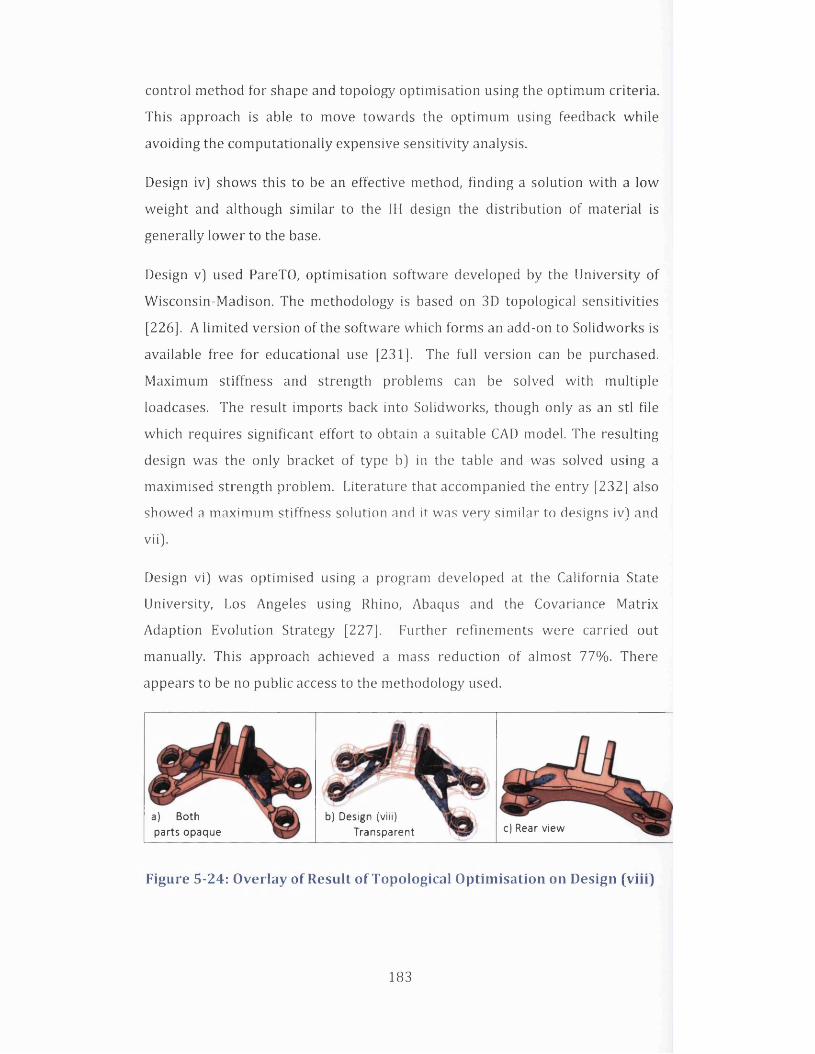
control method for shape and topology optim isation using the optim um criteria .

This approach is able to move towards the optim um using feedback w hile

avoiding the com putationally expensive sensitiv ity analysis.

Design iv) shows this to be an effective method, find ing a solution w ith a low

weight and although s im ila r to the IH design the d is tribu tion of material is

generally low er to the base.

Design v) used PareTO, optim isation software developed by the University of

Wisconsin-Madison. The methodology is based on 3D topological sensitivities

[226]. A lim ited version of the software which forms an add-on to Solidworks is

available free for educational use [231]. The fu ll version can be purchased.

Maximum stiffness and strength problems can be solved w ith m ultip le

loadcases. The result im ports back into Solidworks, though only as an stl file

which requires significant e ffo rt to obtain a suitable CAD model. The resulting

design was the only bracket o f type b) in the table and was solved using a

maximised strength problem. Literature that accompanied the entry [232] also

showed a m aximum stiffness solution and it was very s im ila r to designs iv) and

vii).

Design vi) was optim ised using a program developed at the California State

University, Los Angeles using Rhino, Abaqus and the Covariance M atrix

Adaption Evolution Strategy [227]. Further refinements were carried out

manually. This approach achieved a mass reduction of almost 77%. There

appears to be no public access to the methodology used.

a) Both parts opaque

b) Design (viii) Transparent c) Rear view

Figure 5-24: Overlay o f Result o f Topological O ptim isation on Design (v iii)

183

The designer o f design [v ii) stated that it was topology optim ised and designed

w ith the product design software CREO [233]. Topology optim isation does not

appear to be part o f the CREO suite currently. No fu rther details were given.

Figure 5-24 shows the topological results o f Figure 5-10 overlaid on design [v ii).

The diagrams show an excellent f it and w hile the design satisfies all the loading

conditions the w eight reduction is 71%, 3% less than Figure 5-15. The main

differences in the tw o designs were that the addition o f a partia lly fla t base

ensured low stress values at the bo lt holes, the fron t 'lim bs' have been made

finer together w ith a ho llow rear section below the clevis pin brackets. When

examining the topology optim isation in Optistruct w ith each of the loadcases

applied separately the resulting design fo r loadcase 1 only [see Figure 5-25)

showed a s im ila r partia l base at the rear o f the bracket.

Jrt Enynt 'cfowyr 0«1

j

Figure 5-25: Topology O ptim isa tion w ith Loadcase 1 only applied

Element Densities>0.5

The rear sections o f design [v ii) are ho llow but unfortunate ly no holes o r gaps

have been included to enable the loose powder to be removed and so the

calculated w eight loss is in fact incorrect.

Amongst the other entries there are many that appear to be developed from

topology optim isation and in all cases the upper surfaces are low er than the 1H

solution. The low er top surface has reduced the high stress levels at the clevis

pin interface and reduced the overall weight. A good example o f this is shown in

184

Figure 5-26. This is not one of the designs specified in Table 5-2 but one of the

finalists from Phase I and follows the shape of the topological optim isations.

Unlike design (v ii) the fla t base has not been included and the stress

concentration at the bo lt hole was minimised by constructing a fa irly robust leg

that extended horizon ta lly from the bolt-hole surface at the base. A weight of

18% was achieved w ith this bracket even though the geometry was not

complex.

a) Top View b) Front View c) Rear View

Figure 5-26: Overlay o f Topological O ptim isation on Compact Design

These observations are not sufficient to draw any firm conclusions about the

relative m erits o f the d iffe rent optim isation software, but there are some

observations w o rthy o f note:

• Boundary conditions need to be carefully assigned. The final solution is

heavily dependent on the boundary conditions used.

• Some algorithm s may not find the best optimum, the solution may

converge early to local m inimum. Modification of the available

convergence parameters may enable a ligh ter solution to be found.

• The design must allow for any loose powder to be freed from hollow

sections. These areas may be problematic for a number of reasons and

this w ill be discussed fu rthe r in the fo llow ing section.

185

5.5.3 Build orientation

5.5.3.1 O rientation o f parts fo r effic ient Additive Layer M anufacturing

Taking the geometry data from a sample of 18 of the valid entries in itia lly and

using Marcam Engineering AutoFAB software for a Renishaw AM250 Selective

Laser Melting machine an investigation was carried out to determine the factors

critical to building the components.

The parts were considered w ith two different orientations, m inimum footprin t

and minimum height. Data was collected on the volumes of the support material

and the part, the number of layers or slices to be built. A 50x l0 6m slice

thickness was used in this study. Time to build was also provided though data

on the total build cost was not assessed. The cost of materials was dependent on

the part and support volume required, but no assessment of the cost of the

machine usage has been made either in terms of energy or manpower.

Figure 5-27 shows an image of the support material (light grey) of a component

(orange) relative to the x-y plane. The image is displayed at every 8 th layer for

speed of processing. The AutoFAB software offers a number of options for

applying support material, e.g. line, point, area and transverse and longitudinal

angled. The part is displayed showing w ith three different colours regions

where support is required: dark blue for the bottom surface; light blue for

sloped surfaces and orange-yellow when an undercut surface requires support

In this study only area supports have been used. The area is filled w ith spaced

strips of support material (Figure 5-28). The dimensions of both the support

strips and the spacing can be specified in the software together w ith the angle of

the hatching. Support around the perimeter of the area can also be chosen. The

defaults of 1 mm and 2 mm for strips and spacing respectively, were used in this

work.

186

Figure 5-27: Example o f support m ateria l requ ired fo r bu ild ing one o f the

components

1mm Supports

2mm Gap

Figure 5-28: Cross section o f Area Support in AutoFAB

The results o f the study failed to show any relationship between the volume of

the support m aterial needed and the part orientation (see Figure 5-29). The

same was true fo r the num ber o f slices. A fu rthe r study was undertaken

187

focusing on a single part and looking at rotations at 10° intervals about the x

and y-axes respectively between 0° and 180°.

1.4E-04

*£ 1.2E-04

V 1.0E-04

| 8.0E-05

> 6.0E-05 +■>° 4.0E-05

□ 2.0E-05

0.0E+00

-

♦ Least Height

□ Least Footprint

O.OE+OO 5.0E-05 1.0E-04

Part Volume (m 3)

1.5E-04

Figure 5-29: V aria tion o f Support M ateria l requ ired according to bu ild

o rien ta tion and design volume

The analysis o f the data highlighted, as expected, that the number o f slices

needed to build the part was d irectly p roportional to the height o f the part, but

neither o f these parameters showed any linear re lationship to the build time.

The build time was found however, to have a linear correlation w ith the support

volume (R2 = 0.96 for the x-rotations and 0.78 for the rotations about the y-axis)

as shown in Figure 5-30. This trend is a reflection o f the build tim e actually

being dependent on the num ber o f slices and the cross-sectional area of the part

at each slice, including support. The sum of the product o f the cross-sectional

areas w ith the slice thickness approximates to the total volume.

A s im ila r trend (see Figure 5-31) was seen in the data from the 18 d ifferent

bracket designs. The trend-lines show that the support volume related more

closely to the build time than the part volume itself.

188

140

130

100CO

h-

0.0E+00 5.0E-05 1.0E-04 Support Volum e (m 3)

1.5E-04

□ rotation about x-axis o rotation about y-axis

Figure 5-30: Relationship between Support Volume and Build Tim e foi a

single je t bracket pa rt at d iffe ren t o rien ta tions

160 A

R2 = 0.62140

120 7 X

100

R2 = 0.75* 80

60

40

20 4 -

0.0E+00 5.0E-05 1.0E-04

Volume (m 3)

1.5E-04 2.0E-C4

□ Total ♦P a rt a Support

Figure 5-31: V aria tion in Bu ild Time w ith Volume o f Parts w ith Suppot

Although the AutoFAB software indicated those areas where support needei to

be added to the geometry the supports themselves had to be applied manudly.

189

In some cases where there were hollow sections the software identified the area

as needing support but some of these surfaces were not completely visible and

so could not be selected. This is illustrated in Figure 5-32. The AutoFAB

software has indicated that support is needed across the flat base (ligh t blue

area), though this w ill be o f a m inim al thickness (~0.004m ) and also in the

upper arch of the clevis pin holes (shown in orange), however it can also be seen

through the two small holes in the base that in te r io r surfaces also require

support and it is not possible to view the extent o f this.

Figure 5-33 shows a vertical section through the same bracket. The in te r io r of

the hollow cavity has large areas parallel to the base plate and so all these

surfaces would require support if the part were to be b u ilt in this orientation. Of

course, even if it were possible to add support in these areas they would be

impossible to remove after fabrication w ithou t damaging the part.

Support material neededin blue and orange area

Figure 5-32: Areas re q u irin g Support During ALM bu ild id en tified by

AutoFAB software

190

Figure 5-33: Vertica l Cross Section through bracket design o f Figure 5-32

5.5.3.2 Support Volume Calculation

A MatLab scrip t (see Appendix J), "SupportCalc.m" was w ritte n to calculate the

total support volume required by the part based on the inclination of all

surfaces visible or hidden. It is im portant to note here that the calculated

support volume for both the AutoFAB software and SupportCalc take into

consideration only geometric factors and are not able to assess the need for

additional support based on the in ternal stresses generated during the build nor

the requirem ent fo r heat dissipation.

The flow of logic for SupportCalc is shown in Figure 5-34. The scrip t reads the

geometry in the form of an stl file. The stl file represents the surfaces o f the

geometry in terms o f non-overlapping triangu lar faces. The co-ordinates and

order o f the vertices of the triangles are obtained as well as the normal vectors

for each face. Testing the angle o f the normal for each face relative to the

build ing base plate identifies those areas o f the part that require support. The

angle (p, shown in Figure 5-35 chosen tends to be in the range 30-50° and it

dependent on the ALM process and equipment being used. The Renishaw

AM250 recommends 45° and so this has been the value taken in the calculation.

191

Read .stl file

Detect surface« p °

Iden tify enclosed regions

Calculate Required Support Volume

Provides vertex, face and face norm al data

Surfaces that require support during build

Surfaces where the support doesn 't need to

extend to the base

Figure 5-34: Flow Chart fo r MatLab scrip t SupportCalc

Base plate

Triangular surface

Figure 5-35: Single tria n g u la r surface from the stl file show ing angle to the

base plate

For each o f the triangles where (p is less than 45° the volume o f support

required was obtained from the irregu la r triangu la r prism formed as the

triangle was projected perpendicular to the base plate (see Figure 5-36]. The

192

t h r e e v e r t i c e s V i g i v e t h e c o - o r d i n a t e s f o r t h e c a l c u l a t i o n o f t h e b a s e a r e a B a n d

t h e v e r t i c a l h e i g h t s z\ f o r i = 1,2,3.

Figure 5-36: I llu s tra tio n o f Support Volume calculated from pro jection o f

triang le to bu ild plate

The volume o f the prism [234] is

For some surfaces other sections o f the component lie w ith in its field o f v iew of

the base and so it is suffic ient to have support only from the surface to the next

feature. Ideally it would be preferable to minim ise the locations where this

happens as the in terim supports require more post-processing effort. An

example of where these types o f support are needed can be seen at the clevis

hole pins o f Figure 5-27 where the support for the top o f the hole only extends

to the base o f the hole and not the base plate. This calculation is carried out

using a bu ilt- in "inpolygon" function in MatLab. The software tests the centroid

o f each o f the triangles that need support to see if it lies w ith in the perim eter of

any of the triangles below. The support volume height is then reduced to the

distance from the centroid to centroid of the triangle below. The total support

volume takes account o f these changes in the calculation.

5-7

193

Figure 5-37 shows a surface plot generated by SupportCalc. The surfaces in cyan

require support to the base. Ideally the orientation of the build should be chosen

to minimise this area to reduce the degree of post processing required. The

surfaces shown in red in Figure 5-37 only require support to the next feature

below. The component shown is the same as in Figure 5-32. The in terior upper

surfaces of the clevis pin holes can be seen to require support, as expected. Any

circular part lying in a plane perpendicular to the base plate requires some

support. The mapping shows however that there is a large area of in terio r

surfaces that need support that were not visible in AutoFAB.

This raises some important issues. W ith the AutoFAB software support can be

applied in enclosed areas using the available sectioning tools in the software but

since these in te rio r regions allow no tooling access the supports could not be

removed at post processing and so the weight saving predicted for this part

would not be achieved. In addition, if supports were inserted in the space this

would change the structural behaviour of this part and modify the stress

distribution when the bracket was under load. Such redistribution may enable

material to be removed from other locations, modifying the design and once

more reducing the weight. W ith this in mind it would be beneficial to include

the support requirements as part of the early design decisions, for example as a

constraint in the topology optimisation, however the problem is extremely

complex as support volumes depend on the build orientation and this too would

need to be incorporated for these manufacturing constraints to be valid. The

next chapter seeks to partially address some of these issues by looking to

optimise the orientation to minimise the support volume. A more robust

inclusion of manufacturing constraints would make an excellent study for future

work.

194

In terior hidden surfaces

Upper surfaces o f clevis pin holes

Lower surfaces supported from the x-y plane

x-a*is

Figure 5-37: SupportCalc Resuit showing areas where support m ate ria l is

required

Figure 5-38 shows a comparison of the support volume required fo r ALM as

predicted by the AutoFAB software and the MatLab sc rip t SupportCalc. The

data was created using a num ber o f the titan ium bracket designs together w ith

some geom etrically s im pler shapes. The graph shows a strong corre lation

between the tw o sets o f figures showing the SupportCalc values being ~3 times

higher than the AutoFAB. The AutoFAB supports are not completely dense,

typ ica lly 1mm support strands are separated by 2mm gaps which fits well w ith

the gradient o f the trend line being approxim ately one th ird.

195

ol/lCO<

P r e d ic t e d S u p p o r t V o lu m e ( m 3)

1.2E-04

1.0E-04

8.0E-05

6.0E-05

o 4.0E-05

2.0E-05

0.0E+00

y = 0.331x + 0.000 R2 = 0.962

0.0E+00 1.0E-04 2.0E-04

SupportCalc

3.0E-04

Figure 5-38: Relationship between Support M ateria l predicted by AutoFAB

and SupportCalc scrip t

There is some known loss of accuracy in the scrip t calculations:

i) The triangu lar surfaces generated by the CAD software used to

produce the stl file give an approxim ation to any curved surfaces. The

degree of e rro r can be reduced by increasing the resolution o f the file

when created.

ii) A very s im plistic approach has been used to test whether the support

should extend to the base of the build o r only to the next feature of

the part below. The scrip t used an "inpolygon" function to determine

if the centroid o f the face lies w ith in the triangle o f any of the surfaces

at a low er height. There are many like ly configurations where the

centroid may indeed lie w ith in the low er triangle but the upper

triangle may only partia lly overlap the one below or vice versa in

which case the volume calculation would be in error. Testing all the

possible options would add considerably to the computational time

and so have not been included. The accuracy can be improved by

using a more a more un ifo rm mesh.

196

Despite this the support volume predictions are considered more than adequate

for purpose.

Finally, the impact o f the crowdsourcing approach on the design competition

w ill be discussed not only for the company's perspective but also for the

individuals involved.

5.6 C ro w d s o u rc in g a n d th e GE Challenge

5.6.1 The Company

There were a number o f benefits that are apparent from this analysis:

i) Cost - where recorded the time spent on the design ranged from 40-

160 hours. Taking the lower of these values as typical the entries

represent a total of 700 working weeks or 14 man years. If it is

assumed that the cost for setting up the challenge was sim ilar to the

prize money (-$30,000) then the client paid just over $2 an hour for

the designs, less than a th ird of the US statutory m inimum wage. This

figure did not include the cost of the equipment or software licences

used which were contributed by the participants. The company also

benefitted from ownership of all the Intellectual Property according

to the GrabCAD agreement[184]

The high number of entries to the competition may have required

greater than expected resources in the assessment stage. There is no

information in this area. All press releases indicate that the company

was delighted w ith the outcome [235, 236].

ii) Sustainability - the designers came from 56 different countries,

approximately a quarter of them were from the USA w ith the next

highest group (11%) from India. GE was able to access expertise

from a large geographical area w ith no additional costs or impact on

the environment.

iii) Q ua lity - 27% of those for whom there was data available identified

themselves as University/College students. The m ajority of the

remainder were engineers or designers predominantly mechanical or

industrial designer. Some of these operated their own companies or

197

consultancies. Where levels of experience were indicated a number of

people were shown to have 10 years or more experience. It would

appear that the crowd accessed through GrabCAD was sufficiently

skilled to provide quality entries and it was likely that they brought

not only design but other area of manufacturing expertise to the

concept.

5.6.2 The Ind iv idua l

It was difficu lt to assess the overall benefits to the individuals from the GE

challenge aside from the financial remuneration to the winners [$30,000 shared

amongst 10 finalists). Certainly there were individuals who were able to

showcase the ir skills and in some cases their areas o f research interest [226].

Difficulties have arisen w ith this challenge. The original deadline was extended

as the GrabCAD community pushed for the precise details of the analysis

approach to be used during the judging phase. Some discontent has been

expressed over the choice of w inning entries in Phase I and the lack of feedback

provided by GE, though the company was under no obligation to provide further

information.

No data was available to assess the impact that this approach had on existing

employees o f the Company and how this w ork was integrated into the existing

design strategies.

5.7 C onclusions

The GE challenge for the design o f a lightweight je t engine bracket has proved to

be fertile ground in highlighting a number of critical factors essential in the

design of components for construction using ALM. It has shown that:

i) Topology optim isation is an excellent tool for generating concept

designs for ALM which incorporate intricacy and freedom of

manufacture, however

a. Care must be taken in defining the boundary conditions.

Solutions can be dramatically different depending on the fixed

supports and the optim isation software used.

198

III

b. Software w ith higher functionality increases the likelihood of

finding global minima w ith improved structural performance.

ii] Attempts to reflect every feature of the topology optim isation in the

geometric design may not give the best results. Complexity does not

necessarily lead to the most effective designs.

ii i] Hollow structures provide an excellent means of reducing component

weight, however

a. openings must be incorporated into the design to enable powder

removal after construction

b. all enclosed surfaces must either be self-supporting to avoid the

need for permanent support structures in bounded areas or

greater care must be taken in the early stages to more fully design

for manufacture.

iv] The time and therefore the cost of building components are

dependent on the total volume of the part including the support

volume. Generally by the time of the build the part volume is fixed to

meet structural strength requirements and so only the support

volume can be minimised by changing the orientation of the build.

The crowdsourcing approach provided a large volume of good quality entries

which proved beneficial to the company. Future challenges would need to be

more carefully managed to keep individual designers engaged.

199

Chapter 6: Optimisation of the Build Orientation to Minimise

Support Volume in ALM

Summary: Build orientation optim isation software has been developed and tested

to reduce the volume o f support m ateria l needed during manufacture.

6.1 Introduction

The objective of this chapter was to find a way of minimising the volume of

support material by optim ising the orientation of the part during the build. This

not only reduced waste but provided an effective and consistent approach even,

for inexperienced users to orient the component during the build.

Software was developed using MatLab and an unconstrained optimisation

algorithm to search the different rotations of the part and identify the

configuration w ith the least requirement for support volume. The algorithm

was gradient based and so multiple starting points have been used to identify a

global minima. The efficacy of the algorithm is illustrated w ith three different

case studies o f increasing complexity.

6.2 Background

Additive Layer Manufacture [ALM) has been discussed in some detail in

previous chapter [see section 5.3.1). Refinements to the process to improve

production efficiency and accuracy have been studied in some detail over the

past 20 years both in polymer and metal manufacture [237-240]. The majority

of the published research has focussed on plastic technologies but although the

work of this chapter is aimed at optimising the performance of metallic

processes e.g. Selective Laser Melting [SLM) and Direct Metal Laser Sintering

[DMLS), it w ill firs t consider some of the lessons learnt from other processes

and materials.

The w ork of Phatak and Pande [241] is typical in this area. They identified five

distinct parameters for Fused Deposition Modeling [FDM) in a multi-objective

optimisation, namely;

• surface roughness

• in te rio r material

200

• the volume of the support structure

• contact surface area

• build height.

The surface roughness measure used was the degree o f "staircasing" present in

any particular orientation. Adjacent layers create a non-smooth stepping effect

when building an inclined plane (see Figure 6-1). In FDM the layer thickness, h

is of the order of 200pm, at least four times the thickness typical of SLM. A

number of authors [242-244] use adaptive slicing to reduce this effect, using

th inner layers in more critical areas. Adaptive slicing is not readily available in

all ALM technologies and although it may be effective when building a single

part it becomes increasingly complex for multiple parts bu ilt simultaneously.

Figure 6-1: Staircasing effect in ALM build caused by adjacent layers of

material of height'h'

In metal ALM, staircasing may not be the dominant factor in terms of roughness.

Maximum powder particle diameter can be larger than the layer thickness, (e.g.

60pm powder compared to 50pm slice thickness) and so entrainment at the

surface of partia lly sintered powder may have a greater impact than staircasing

[245]. Most commonly, metal ALM parts are manufactured for the aerospace

and medical industries and so it is accepted that post-processing w ill be

necessary to meet the stringent design requirements. The as-built surface

roughness is therefore, less critical.

The freedom to reduce in te rio r material or simply hollow out a component is

more applicable to plastic parts than metals. Metal parts tend to be more

201

strength critical and so material removal cannot be undertaken w ithout

considering the structural in tegrity o f the component.

As previously discussed, support material is need to act as scaffolding for

overhanging features of design, as a heat sink increasing the conduction from

the melt-pool to the substrate [246] and the reduction in distortions caused by

residual stress [247]. The area where the support contacts the part tends to

show high roughness values, but this too can be reduced at post processing.

Changing the part orientation to reduce the support volume may increase the

build height and therefore the time taken to manufacture. Some authors [239,

240] have undertaken complex multi-objective optimisation to find solutions

that allow for both the impact o f surface roughness, part orientation and build

height. In the data available to the author it is not clear that there is a significant

correlation between build height and manufacturing time. Thus from the factors

considered by Phatak and Pande [241] the optimisation of support volume

remains one of the most critical factors for improving the efficiency of metallic

ALM processing.

Section 5.3.1 b) discussed the w ork of a number of authors who have proposed

methods of designing to minimise support in 2D structures. Strano et al [248]

optimised the support volume for 3D structures by calculating the support at

every 5° rotational angle about the x and y axes and then choose the lowest

value. This technique was also used w ith polymer ALM by Masood et al. [249].

This systematic approach may not find the most optimum orientation w ith 5°

resolution, particularly for very complex structures and increasing the

resolutions can make the problem very time consuming.

This chapter w ill present an alternative approach for optim ising the part

orientation to minimise the support structure only. Using an unconstrained

optimisation algorithm in MatLab inexperienced operators can find the most

effective positioning of parts for ALM build. The novelty of this approach it can

be applied to three dimensional geometries and has potential for greater

accuracy than other methods found in the literature.

202

6.3 The Optimisation Algorithm

In order to determine the optimum orientation for building the part while

m inimising the support material SupportCalc was further developed to

incorporate an optim isation function in MatLab.

The optimisation problem was unconstrained and could be simply stated as:

m i m f ( z ) = Tota l Support Volume ^

where the design variable, z is the normal of the base plane of the build. The

code for the program "OppTotalSupportVol.m" can be found in Appendix K and

the w ork flow is shown in Figure 6-2.

The vertices, faces and normal values for the part geometry were read from the

stl file. These vectors and co-ordinates assumed that the x-y plane was the base

plate for the build. The vector z0, the in itia l estimate for the design variable was

the normal vector for the new base plate. A new orthogonal co-ordinate system

was generated from z0 and the co-ordinates and surface normals from the stl

file were transformed to determine their new position of the part relative to the

new base plate. Effectively what was happening was that the stl of the part was

being rotated while maintaining the x-y plane as the base plate. In order to

ensure that the base plate did not cut through the rotated part the lowest

vertical point was detected and the part was translated to ensure all portions

were above the plane. Following the flow of Figure 5-34 the surfaces needing

support were identified and the volume of support material was calculated

making allowance for those surfaces where the support extended only to the

next feature.

203

A p p ly

O p t im is a t io n A lg o r i th m

( fm in u n c )

to m in im is e th e

t o ta l s u p p o r t v o lu m e

re q u ire d

N oC o n v e rg e d ?

Yes

R ead

.s tI f i le

D e te c t s u r fa c e

<Cp°

Id e n t i f y e n c lo s e d

re g io n s

C a lc u la te R e q u ire d

S u p p o r t V o lu m e

C h o o s e in i t ia l b ase

p la n e z0 fo r b u i ld

T ra n s fo rm

c o -o rd in a te s & s u r fa c e

n o rm a ls t o r o ta te p a r t

Figure 6-2: Flowchart for OppTotalSupportVol.m

Using the unconstrained optim isation function fminunc in MatLab the value of

the design variable continued to be modified until the total support volume

converged to a minimum. No information was available on the behaviour of the

gradients of this problem and so fminunc defaulted to a line search algorithm

[162], The final design variable vector was generated, which was now the

204

surface normal of the optimum plane together w ith the minimum point. These

two factors defined the new plane precisely and thus the optimum build

position of the part. The transformation matrix, JJopt was also output which

converted the original orientation to this optimum one.

Since the transformations here preserved all vector lengths then the inverse of

the transformation matrix was equal to its transpose, ( Uovt) , which was called

Vopt. This could be expressed as the product of the three rotations about the x,

y, and z axes w ith angles a, p and y respectively, i.e.

Vopt =

/cosy — siny 0 \ / c o s / ? 0 s in j? \ / i o 0 \I s iny cosy O il 0 1 0 ) I 0 cos a —sin a )\ 0 0 1 / V — sin /? 0 co s /? /Vo sin a cos a /

/cosy cos /? cosy sin /? sin a - s iny cos a cosy sin /? cos a + s iny sin cr = I s iny cos/? sin y sin /? sin a + cosy cos a sin y sin /? cos a — cosy sin a

V — sin/? cos/? sin a cos/? cos a s6-

And comparing terms

P = -s in 1(Vopt3'l ) 6-4

where the subscripts denote the row and column location of the term of the Vopt

matrix and — sin /? = s in (—/?) V p. There are two possible solutions to this

equation in the range (—n, n ) since sin /? = sin(7r — /?)

a = tan - l V,opt 3 , 2

V,Opts 3 J6-5

y = tan 1V,opt2,iV,opt 1(iJ 6-6

provided cos /? =£ 0. In MatLab the atan2 function was used for both equations

6-5 and 6 - 6 as this automatically determined the appropriate quadrant for the

angles.

If p = ± then cos p = 0 , this created what is known as a "gimbal link" and a

and/becam e linked, the individual rotations were not independent of each

other. It was not possible to find solutions for each angle only either (a + y) or

(a — y) depending on the sign o f p, but since the rotation y around the z axis

did not impact on the support volume y could be set to 0 and solutions for a

found. The output from the script gave all the angles together w ith the plane

unit normal and the plot of the optimised part. This was sufficient to orientate

the part in the ALM machine.

The line search is a gradient based method and so a global solution could not be

guaranteed in this optimisation. Multiple starting points were therefore used to

search for the best optimum.

6.4 Testing the Model

6.4.1 C ylindrica l H a lf Pipe

Initial tests on the optimisation algorithm were undertaken using a simple

geometry of half a cylindrical pipe [see Figure 6-3]. The pipe was 0.06m long

w ith an outer diameter of -O .lrn and wall thickness of 0.0145m and consisted

of only 6 surfaces. The stl file for the pipe had 252 triangular faces. An in itia l

calculation of the support required in the orientation shown was 9.9 x 10 5 m3.

Figure 6-3: Half a cylindrical pipe

Eight different in itia l values were generated for the starting points for the

optimisation. The numbers were chosen randomly, but the sign of the

206

components were allocated so that each of the starting vectors lay in a different

quadrant of the of the co-ordinate system

Table 6-1 shows the eight starting points (A-H) for the global search

optimisation. Using starting point A the optimisation algorithm found the best

solution to the problem w ith the total support material of 0.007 x 10 5 m3. The

optimised plane had unit normal [0 ,1 ,0 .0 0 2 ] which is the x-z plane to 2 decimal

places. The orientation of the optimised part is shown in yellow in Figure 6-4

together w ith the original part in cyan. The optimiser has successfully chosen

the best orientation. Figure 6-5 shows a rotation of the optimised result where

the orange regions indicate the areas requiring support. The relative positions

of the two pipes is different in Figure 6-4 and Figure 6-5 this is because the

orthogonal axes to the plane normal are chosen randomly. This has no impact

on the support volume or the plane orientation Starting point D also found the

same optimal orientation w ith twice the volume of support material, though in

both cases the value is very small and can be taken as zero w ith in the numerical

accuracy of the problem.

It should be noted that another low value was found from starting point E. The

optimised plane in this case was [0 ,-1, 0] to 1 decimal place. This is again the x-

z plane but w ith the normal facing in the opposite direction. Effectively this is

showing that when the pipe is turned upside down there is also an optimum

solution.

207

Tabl

e 6-

1: R

esul

ts

of the

O

ptim

isat

ion

of the

ha

lf pi

pe

with

ei

ght

diffe

rent

sta

rting

po

ints

Rot

atio

nal

angl

es

abou

t

the

axes

(only

the

an

gle

of lo

wes

t

mag

nitu

de

show

n) 119

129

160

11

1 96

134

59 LO

ea. o o -24 o o -23

44 42

«

06

os- -46 06 o

1 49 o -60

optim

ised

su

rface

un

it

norm

al z

X

0.0

02

0.64

31

-0.6

383

OOo 0

.01

1

-0.6

024

-0.7

156

-0.3

714

— tH

-0.7

657

-0.6

564

t-H tHi

0.69

64o

-0.6

487

•P4 o o

IZO

fO O o

0.38

99

-0.6

985

-0.6

643

Opt

imis

ed

Sup

port

Vol

ume

10

’5 m

3

9.9

r>oo6 1.

62

2.33

0.01

3

0.03

5

1.17 1.6

2.79

Func

tion

Cou

nts

orig

inal

orie

ntat

ion

152

108

160 00

T—i 176

252 o

00 280

S U 0 I} B J 9 } I vO CO t-H 00 CN rH H

initi

al v

alue

of

surfa

ce

norm

al

*0

X

Z6

0I0

0.97

67

-0.7

733

0.99

43

0.31

73

-0.7

34

-0.8

155

-0.4

154

—

8X980

-0.5

533

0.79

56

0.94

99

-0.7

458

-0.0

62

0.19

04

-0.7

465

0.23

48

0.76

72

0.48

71

-0.7

964

-0.3

086 980S

0

-0.8

071

-0.7

503

I

< CO u Q w b o X

00oCN

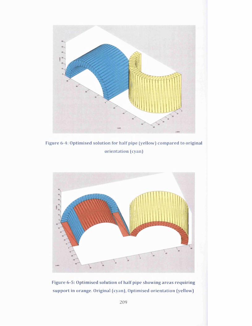
Figure 6-4: O ptim ised so lu tion fo r ha lf pipe (ye llow ) compared to o rig ina l

o rien ta tion (cyan)

Figure 6-5: O ptim ised so lu tion o f ha lf pipe show ing areas requ iring

support in orange. O rig ina l (cyan), Optim ised o rie n ta tio n (ye llow )

209

The convergence curve for starting point A is shown in Figure 6-6. The graph

shows the objective function values fo r iterations 0-6 and the num ber of

function calculations executed in the optim isation. The convergence progressed

sm oothly to a local m inim um . The graph shows that 99% of the reduction in the

objective function was achieved in the firs t 5 iterations and required only 40

function calculations. The rem aining ite ra tion took a fu rther 112 function

counts. A s im ila r pattern was seen in all the starting points o f Table 6-1. In this

simple model the tim e taken to converge was very small (~20s), but if these

additional calculations could be shown to be unnecessary then efficiency

savings could be made w ith more complex geometries.

<yEo>

+■>

oaa□to■cotsc□L L

<y>tJ<uIdO

20000

16000

ar* 12000 E<T\

2S 8000

4000

Ite ra tio n s

• •50 100

Function Counts

150

Figure 6 -6 : Convergence Curve fo r O ptim isation o f Cylindrica l H a lf Pipe -

s ta rting po in t A

Checks were made to determ ine the sensitiv ity of the term ination tolerance on

both the function value (TolFun) and the design variable (TolX). The default

values were 10 6 in both cases. Increasing the TolFun to 0.6 did not reduce the

number o f function calculations required but all values above this reduced the

function counts but failed to achieve the best optim um . Sim ilar results were

210

observed w ith TolX only here the critical value was around 5 x l0 3. No

im provem ent was able to be made to the efficiency of the optim isation in this

way.

6.4.2 GE Challenge Bracket Design - Alexis V2

The second example used to test the optim isation scrip t was one of the ten

finalists from the GE challenge entered by a French designer, Alexis [250]. The

w eight achieved w ith this design was 18% of the original. The design is shown

in Figure 6-7 and was composed of 110 surfaces which generated 6208

triangu la r faces in the stl file. Table 6-2 shows the results o f the optim isation

under the eight d iffe ren t starting vectors A-H.

Figure 6-7 Rendering o f GE Bracket Design V2 by Alexis

The best solution w ith an optim ised support volume of 2 .2 3 x l0 '5m3 was found

w ith starting po in t D [see Figure 6-8 and Figure 6-9) . Using the AutoFAB

software and m anually applying the support volume where indicated gave a

volume of 3 .1 x l0 5m3 and 5 .1 1 x l0 '5m3 for the least height and least foo tp rin t

orientations respectively. These are at the less dense volume and so d iv id ing by

the p ropo rtiona lity factor, 0.331 from Figure 5-38 gives comparative values of

9 .3 7 x l0 '5 and 15.44xl0~5. The optim ised result gives a 76% reduction in

support volume over the best o f these two orientations.

211

Table 6-2: Optimisation results for Alexis Bracket Design using global

starting pointsIte

ratio

ns

Func

tion

Cou

nts Optimised

Support

Volume

1 0 '5 m3

Optimised

surface un it normal z

Rotational

angles about

the axes (only

the angle o f

lowest

magnitude

shown)

i j k a P

original

orientation6.89

A 2 236 5.4 0.0328 0.4752 0.8793 28 -2

B 1 80 16.28 -0.0441 -0.3535 0.9344 - 2 1 2.5

C 1 184 10.29 0.667 0.6022 -0.4388 54 -42

D 2 260 2.22 0.041 0.762 0.6463 50 -2

E 1 8 8 7.65 -0.1126 -0.9032 0.4142 -65 6

F 1 276 11.79 0.5772 -0.0806 -0.8126 -6 -35

G 1 180 6.39 -0.6919 0.1635 -0.7033 13 44

H 2 288 5.4 0.0176 -0.5632 -0.8261 -34 -1

212

Figure 6 -8 : Optim ised so lu tion fo r bracket (ye llow ) compared to o rig ina l

o rien ta tion (cyan)

axis

x axis

z

Figure 6-9: Brackets o f Figure 6 - 8 viewed from below w ith areas requ iring

support h igh lighted (orange)

213

6.4.3 W in n in g E n try - GE Challenge Jet Engine B racke t Design

The w inn ing design was subm itted by an Indonesian designer, M Arie

Kurniawan [251]. He entered three designs, the lightest o f which, at 17% of the

orig inal is shown in Figure 6-10 below. The design consisted o f 805 surfaces

w ith 84,486 triangles in the stl file. The designer had positioned the part in the

geometry file so that the volume of support required was only 9.37 x 1 0 14 m 3.

The MatLab scrip t was in itia lly tested w ith this model to see if it would

converge to this optim um orientation. It was found that because of the large

quantity o f surfaces in the file the tim e taken to find a solution from a single

starting po in t was in excess o f four weeks elapsed time. Further checks w ith this

software were not made as w ith these levels o f com putational inefficiency the

software would not make a practical tool for complex models.

A breakdown o f the in terna l time allocation fo r the scrip t showed that the bu ilt-

in "inpolygon" function dominated the running tim e of the software (~75% ).

This was the function that detected the existence o f in terim support features

and was essential to the volume calculation and so could not be avoided at this

stage. Further w o rk was undertaken to improve the computational efficiency of

the software.

Figure 6-10: W inn ing Bracket Design o f the GE Challenge

214

6.5 Im proving the Build O rientation Software

The optim isation code was rew ritten to increase the use o f m atrix and vector

operations and to m inim ise loop-based processes. This reduced the length of

the code but did not m arkedly increase the speed. Improvements in

com putational efficiency were made only when an alternative approach for the

in terim surface detection, i.e. the inpolygon function, was identified.

The new method was developed from an " intersection o f a ray w ith a triangle"

a lgorithm proposed by Dan Sunday [252]. Taking only the triangles that needed

support, the centroid was projected onto all o f the triangles that lay below it.

The position vector o f this projected point was then expressed param etrica lly in

terms of the tw o vectors formed by the sides of the low er triangle. It was then

not d ifficu lt to determ ine whether the position vector extended beyond the

triangle or lay w ith in i t , thus identify ing suitable support surfaces.

14000

12000

10000

2 8000 <uI 6000

4000

2000

0 •

5,000 10,000 15,000 20,000No. of triangular surfaces in stl file

Figure 6 - l l :T im e taken to Find global optim ised bu ild o rien ta tion

so lutions fo r d iffe ren t geometries

The new code VOTSVol_RinTriA.m can be found in Appendix L and when tested

on a num ber o f d iffe rent models was found to be approxim ately 30 times faster

than the previous software. Figure 6-11 shows the tim e taken to find the best

215

orientation of a series of parts m inimising the support volume. The data is

plotted as a function o f the number of triangular surfaces formed in the stl file

for the component The graph shows a strong positive correlation w ith a linear

correlation coefficient of R2=0.76; A power law relationship o f the form y=Axb

gave a much higher correlation, R2=0.95. In reality the time is more closely

related to the number of downward facing surfaces in any orientation which

cannot be predicted easily from the in itia l file. The graph, however, does give a

good indication of the expected time to solution.

6.6 Conclusions

An optimisation program, ''OppTotalSupportVol" has been developed to identify

the best orientation of the part to minimise the support volume. This software

has been tested on two different components of increasing complexity and

found to be effective though computationally slow particularly when geometries

are complex and the stl file contains many triangular faces.

The code has been further vectorised and a new approach used for interim

surface detection. This has increased the speed to solution by a factor of 30

creating a much more practical tool for m inimisation of support volume during

the ALM build.

216

Chapter 7: Case Study 3 - Design of Release System Casing for

ALM

Summary: Applying the design lessons learnt from Case Study 2, the casing o f an

a irc ra ft cargo release system has been optimised. The methodology included

m ateria l selection o f both conventional and ALM b u ilt metals. A pa rtia l validation

o f the orientation software was explored using data from the ALM bu ilt casing.

7.1 Introduction

The th ird industrial Case Study of this thesis looks at the weight optimisation

and material selection for the design of an aerial delivery release mechanism.

The design methodology is sim ilar to Case Study two, however there are a

number of areas in which this w ork adds to the body of knowledge, namely; the

part is more complex in its design requirements, it offers opportunity for

investigating alternative materials for ALM build and the part itself has been

professionally bu ilt which enabled partial validation of the design and build

predictions.

The work originated from a collaborative project between ASTUTE of Swansea

University, Airborne Systems Ltd [253], Renishaw pic [254] and Sandvik-Osprey

Ltd [255]. Airborne Systems manufacture the module and wished to assess the

suitability of ALM for making the parts. Renishaw build ALM machines and

Sandvik-Osprey manufacture the metal alloy powders used in ALM. The

components were trad itionally made by Computer Numerical Control (CNC)

machining. The release system has been developed for sale to a large aircraft

manufacturer and to be able to be competitive in the market it must not only

meet optimum weight requirements but also Airbus' stringent safety standards.

The design w ork of this chapter w ill not take the product to a final design

specification but w ill develop a concept design and test its suitab ility for ALM.

The current component is shown in the insert o f Figure 7-1. Large cargo loads

are secured to the floor o f an aircraft using webbing straps. One end of the strap

is fixed directly to the floor and the other attached via the release system

mechanism. The strapping is wrapped around a catch in the release system

217

which is then hooked in to the floor plate. When the cargo is to be ejected from

the plane the catch is e lectronically activated and the straps are loosened

releasing the load. The objective o f this study was not only to ensure that the

ALM b u ilt part should be suffic iently robust to w ithstand the operational

loading conditions but tha t the new design should have a weight reduction of

50% over the existing design.

Webbingstraps

Figure 7-1 C urrent Release system design shown in s itu

7.2 ALM: fo r Steels and A lu m in iu m

Section 5.3 discussed the current understanding of ALM design and

manufacture but w ith particu la r reference to titan ium . This section w ill look at

the published research re lating to additive manufacture o f a lum inium and

stainless steel components. Only lite ra ture using SLM as the m anufacturing

method w ill be discussed.

In a recent article, Hunt et al. [256] highlighted that any alloy w ith good

w e ldab ility is a good candidate for use w ith ALM technologies. He also indicated

the therm al stresses developed in the ALM processes were p roportiona l to the

Young's modulus, therm al expansion coefficient and the tem perature difference

218

at the heating surface. Choosing alloys w ith good thermal shock resistance

avoids cracking, but also good dimensional stability is desirable and this is

dependent upon the thermal conductivity of the alloy as well as the thermal

expansion coefficient. Renishaw lists 316L, 17-4PH and AlSilOMg as suitable

materials for use w ith the ir AM250 SLM equipment as well as titanium, cobalt

chrome and Inconel grades [257]. 316L performs poorly according to Hunt's

performance indicators but can be used provided process parameters are

chosen so that high thermal stresses are avoided during the build. 316L has

1 0 0 % austenitic microstructure but all other alloys require precipitation

hardening heat treatments at post processing to improve the uniform ity of the

microstructure.

7.2.1 Stainless Steel - 3 16L

A number of authors have investigated the mechanical properties and

microstructure of 316L stainless bu ilt using SLM [258-262]. In all cases the

tensile yield strength was found to be significantly higher than for wrought

material. Mertens et al. [259] quoted values of between 450 and 540 MPa for the

tensile yield strength compared to 220-270MPa [258] for wrought 316L and

UTS values between 565 and 660 MPa (520-680 MPa for wrought). The

breaking elongation, values were less than half the wrought values o f 40-

45%. Shifeng et al. [260], Tolosa et al. [258] and Riemer et al. [261] all measured

elongations in the as-built condition comparable or better than the traditionally

processed material. It is not clear why these results were so different, though in

Mertens test specimens, a greater volume fraction of defects "e.g lack of melting"

in the microstructure of the vertical samples was noted. Mertens also observed

larger austenite grains in the z-direction, whereas Reimer attributed the good

performance of the material to the "very fine substructures present in the as-

bu ilt microstructure", which suggests that the samples were of very different

quality. Some details of the processing parameters used in the build are

available in both these papers [259, 261] however the lis t is not sufficiently

comprehensive for a direct comparison. The Reimer samples were built w ith a

smaller layer thickness than Merten (30pm compared to 60pm) but w ithout a

219

clear understanding of the all the other contributory factors it is d ifficu lt to

determine is this is the cause of the finer substructure in the as-built samples.

In all cases, the researchers identified that the properties showed a dependency

on build direction. The lowest values were always found in samples tested in

the vertical build direction. Spieriengs et al. [262] quoted values of 5 and 15%

difference between the vertical and horizontal build directions. None of the

authors have published Young's modulus values for this material.

7.2.2 Stainless Steel - 17-4PH

Stainless Steel 17-4PH alloy is a high strength steel w ith a moderate level of

corrosion resistance. It is typically used in the aerospace and high tech

industries [263]. The mechanical properties are optimised by using a heat

treatment that causes the copper in the alloy to precipitate into the martensitic

microstructure. Although a number of authors have investigated the behaviour

of 17-4PH bu ilt using ALM techniques, there is only lim ited numerical data on

the mechanical properties of the resulting parts. Many authors have [263-265]

investigated closely the microstructure of the alloy under different conditions

but have given measurements of hardness, magnetism[263] and porosity [265]

only. The data from the three papers w ith mechanical properties are

summarised in Table 7-1 together w ith the results o f in-house measurements

obtained at Swansea University.

As expected, where tensile data was measured for "as bu ilt" samples, the yield

strength was significantly lower than for conventionally manufactured 17-4PH

and showed anisotropy according to build direction. Facchini et al. [266]

measured UTS values as high as 1300 MPa but their samples had undergone a

"stress re lie f' heating cycle of 600°C for 2hr, the results not being dissim ilar to

M urr et al. [264] whose samples had been aged for lh o u r at 482°C. The in-

house measurements w ith no post processing showed anisotropic UTS values

approximately 30% lower than conventionally manufactured 17-4PH.

Certainly, the data available lacks consistency, but does indicate that heat

treatment brings greater un ifo rm ity not only in the tensile properties but also in

the Young's modulus and Poisson's ratio as has been seen w ith other metals.

220

Tabl

e 7-

1: S

umm

ary

of M

echa

nica

l P

rope

ries

for

Sta

inle

ss

Stee

l 17

-4PH

fro

m th

e L

itera

ture

Add

ition

al I

nfo

rma

tion

soln

. an

neal

& ag

ed, 4

82°C

, 1

hr

incl

. a

stre

ss

relie

f he

atin

g cy

cle

of 60

0°C

for

2 h

r

aged

, 48

2°C

for

1 hr

anne

aled

at

1350

°C,

solu

tion

heat

ed

1050

°C,

deep

fro

zen

and

aged

, 48

0°C

for

1 h

r

+

VC

T—IV'

~ 'S' Q

"oLr-j

1120

°C

for

4 hr

at

100

MP

a

Str

ain

to

failu

re,

£F (%

) N7% 8.3% 10%A

X

28%

UT

S(M

Pa) N

1450

1370

(V)

861

992

AX

1300

696

866

Yiel

d st

ren

gth

(MP

a)

N

1380

1190

ovoI -1

05

0

1240

415

550

AX

009 ovO

? -11

70

531

575

Poi

sson

's

ratio

Noncc

| 0.2

54 __0.

31A

X

vOvOCNJc i

You

ng's

mod

ulus

(GP

a)

N >ro

o jU">t HI

187

196 30

4

196

AX

199

273

Pro

cess

as b

uilt

as bu

ilt

& ag

ed

as b

uilt

as bu

ilt &

heat

trea

ted

Conv

. M

an.

&

1190

0 [2

69]

as b

uilt

& H

IPin

g

Ref

eren

ce

Facc

hini

et

al. [

266]

Mur

r et

al.[2

64]

Spi

erin

gs

et

al. [2

67]

in-h

ouse

C

herr

y

[268

]

7.2.3 A lum in ium - ALSIlOMg

The light-weight corrosion resistant aluminium alloys are ideal for aerospace

components in terms of weight reduction though they lack the strength of the

stainless steels w ith tensile yield strengths in the order of 275 MPa and UTS of

310MPa for conventionally bu ilt material andfy = 2 - 3.5%. Vilaro et al. [270]

obtained sim ilar properties in the as-built ALM samples w ith some anisotropy

according to build direction. The UTS and £f values were typical higher in the x-

y plane and this was more marked in the results presented by Kempen et al.

[271] where increases of approximately 25% were observed in the UTS and

60% in £f. No research was evident into the effect of aging on A1SI10 ALM bu ilt

samples. Only reference [271] refers to Young's modulus and this was found to

be of the same order as for conventionally manufactured aluminium (68±3 GPa

compared to 71GPa).

Titanium has not been considered for these components as it would increase

the cost considerably and make the mechanism less competitive in the

commercial market.

The same issues relating to design for ALM build as discussed in section 5.3.1

are applicable w ith different material selection, namely:

i] Support Material

a. Must be minimised to ensure material and build time savings

b. Supports should not be needed w ith in enclosed hollow spaces

ii] Powder removal - hollow structures must be designed to ensure

unused powder can be removed

iii] Designers may need to develop new design approaches free from the

constraints of traditional manufacturing techniques but better suited

to the flex ib ility of ALM.

7.3 The Design Problem

The current release system module consists of an aluminium casing connected

by a hook to the aircraft floor w ith a catch mechanism for connection to the

222

strapping. The approximate casing dimensions are 0.178m x 0.127m x 0.064m

w ith a m in im um wall thickness of 0.01m. The hook which is an “ off-the-shelf'

design extends approxim ate ly 0.145m beyond the casing. Figure 7-2 (i) shows

the component w ith the hook attached. Figure 7-2 (ii) shows the in te rio r parts

w ith the two parts o f the casing transparent and the hook removed. The catch is

shown in the open position. Stainless steel pins connect the hook, the catch arm,

latch and the release pin to the casing.

Release Pin

Dowel Pin

Solenoid Rod

Catch| Solenoid |

Switch Block

Casing BoltsHook Pin

Electronic Connector

Figure 7-2: Release System Module showing in te r io r components - catch

in open position

As mentioned previously the mechanism is operated electronically. The signal

through the electrical connector causes the solenoid rod to retract liberating the

latch. The release pin and catch arm are under tension from the strap and so

the movement in the latch allows the strap to pull free o f the release modu e.

223

The component has been designed to withstand a functional load of 45kN.

Under these conditions the stress levels w ith in the material would be w ith in the

tensile yield strength and any deformation would remain elastic. The maximum

structural load determined by the part manufacturers was 60kN, plastic

deformation may occur at these levels but the component would remain intact

as the maximum stress would be less than the ultimate tensile strength for the

material.

The total weight for the module was 3.445 kg. Table 7-2 gives a breakdown of

the main parts of the mechanism. The greater part of the mass was taken up by

the two parts of the casing which combine to approximately 55% of the overall

weight. The greatest weight saving would thus be achieved by minimising the

mass of the case. The remainder of this chapter w ill focus on optimising the

mass of the casing. It w ill exploit techniques learnt from the previous chapters

and consider the suitablilty of using different materials and optimising the

positioning of the build. The final design has been manufactured using ALM and

this has enabled a partial validation of the design from a manufacturing

perspective. No testing was been carried w ith in the timescale of this study to

validate the component in terms of strength or durability.

7.4 Design Approach

The casing design needed to be more than just structurally sound; there were

additional constraints on the design:

i] The electronics needed to be protected from electromagnetic

radiation and moisture

ii) The casing needed to be sufficiently robust to withstand the shocks

and impacts of everyday use in a relatively harsh environment

Both the above points indicated that some form of complete cage needed to

surround the internal workings of the device. To achieve this, the design

process was undertaken in three distinct phases:

1. Topology Optimisation to determine the fundamental shape to ensure

structural robustness

2. Interpret as a simple CAD geometry

224

3. Ensure the final design incorporated a Faraday Cage

Table 7-2: W eight o f Release System Module sp lit in to its com ponent parts

Q uantity Item M ateria lMass

(kg)

Total

Mass

(kg)

%

Weight

1 Casing A Alum inium 0.99 0.99 28.72

1 Casing B Alum inium 0.91 0.91 26.53

1 Hook

Stainless

Steel

0.34 0.34 9.83

1 Catch Arm 0.33 0.33 9.62

1 Release Pin 0.203 0.203 5.83

1 Solenoid 0.16 0.16 4.61

4 Casing Bolts 0.02 0.08 2.21

1 Solenoid Rod 0.07 0.07 2.03

2 Dowel Pin 0.035 0.07 2.03

1 latch 0.065 0.065 1.89

1 Hook Pin 0.05 0.05 1.43

-

Other

Components

each less than

1% of weight

various - 0.182 5.2

TOTAL 3.45 1 0 0

The fo llow ing sections w ill describe each of these stages in detail. The

results shown are fo r an alum inium casing and the results are presented

w ith in each section since the decisions made at any one stage have infcrmed

the design developments in the fo llow ing stages. Isotropic properties for

trad itiona lly produced material were used in itia lly and these are shov/n for

the three materials used in Table 7-3 below.

225

Table 7-3 Material Properties used in the design analysis and optimisation

Material GradeDensity

(kg/m 3)

Poisson’s

ratio

Young's

modulus

(GPa)

Tensile

yield

strength

(MPa)

Aluminium AlSilO(Mg) 2670 0.33 70 245

Stainless

Steel

316L

7810 0.3

2 0 0 190

174-PH 196 1240

7.4.1 Topology Optimisation

A simplified model of the casing was set up combining the two halves of the

original design. Most of the bolt and pin holes were eliminated. The holes

for the dowels of the catch arm and release pin and the locator holes for the

hook pin were maintained. All but one of the internal cavities of the casing

were preserved to allow space for the electronic components. The geometry

was modified to fill the region close to the switch block where there was a

large empty space. By reducing the restrictions on the volume in this way

there was greater potential for the best optimum to be found in the design

space. These features are illustrated in Figure 7-3 where half the design

domain is shown on the side of casing B.

226

Catch Dowel locations

Additional M aterial added To increase design space

Bolt holes filled

Hook pin location

Figure 7-3: Casing B design domain showning filled bo lt holes

and m odified sw itch block cavity

The load to the module was applied along the cargo straps and this was

transm itted to the casing via the catch and dowel pins. Figure 7-4 illustrates

that although a uniform load may be applied at one end of a length o f

strapping, the d is tribu tion becomes more parabolic even over a short length.

The von Mises stress varia tion o f Figure 7-4 compares the values across the

w id th of a 0.1m length o f strapping near each of the ends. The data was

derived from a simple 2D shell model developed in Hyperworks 11.0. The

strap was fixed at one end and a 60 kN load d istributed un ifo rm ly along the

other. Material properties for a car seatbelt were used, namely Young's

modulus, 20 GPa, density 1080 kg /m 3 [272], Poisson’s ratio, 0.3. The strap

dimensions were 0.044m w id th and 0.0012m thickness.

227

1.8E+09At free end within 0.0005m of applied load position At fixed end

1.7E+09

1.6E+09

™ 1.5E+09

1.4E+09

£ 1.3E+09

■<= 1.2E+09

o 1.1E+09

1.0E+09

9.0E+08

8.0E+080.01 0.02 0.03Distance across Cargo Strap (m )

0.04

Figure 7-4 von Mises Stress D is trubu tion across the w id th o f the Cargo

Strap

The fixed end curve shown in the graph would be typical of the force

d is tribu tion on the catch release pin.

W ith the casing volume being modelled w ithou t any o f the other

components included in the design space, such variations in loading could

not be taken into account and so the application of the load has been

sim p lified9. This was achieved by applying the structura l load o f 60kN at the

hook pin end of the casing. The hook pin was represented by a rigid

element. The casing was fixed at the holes where the catch dowels would

have been located (see Figure 7-5). Linear static analysis only was used in

the modelling. This together w ith the s im plified loading leads to a

conservative design, but this was considered acceptable at this concept

phase.

9 No account has been taken o f any angular application o f the strap load nor "bunching" tha t can sometimes occur. The inline loading was taken as the worst case.

228

Inse rt show ing C onstra in ts on all

nodes on the in te rio r surfaces o f the catch pin holes

Figure 7-5: FEA model o f casing showing loads and constra in ts, only the

meshing o f the non-design m ateria l is shown fo r greater c la rity

The topology optim isation was undertaken using A lta ir O ptistruct 11.0. Annular

regions around the release arm dowels, the hook pin holes and other areas

where critica l components needed to be located, e.g. the solenoid pin, were

designated as non-design material, as shown in Figure 7-5. An element size of

0.001m was chosen after a mesh convergence study; this gave a total of

approxim ately two m illion 4-noded tetrahedral elements in the design space.

The design variables were the material densities o f the discretised elements of

the FEA analysis. The objective function was to m inim ise the mass (equation

2-48). A stress constra in t was applied to the whole design space to maintain the

structure w ith in a maximum von Mises' stress less than the yie ld strength of

280 MPa for 6082 T6 A lum in ium Alloy. It is possible fo r h igher stress levels than

these to occur in the final topology as the stress constra in t is applied to both

design and non-design material and yet no m odifications can be made to the

non-design m ateria l in the optim isation. A m inim um member size (1.24 x 10_

3m) was selected to ensure a more cleanly defined solution w ith confidence in

its m anufacturab ility by ALM.

229

7.4.1.1 O ptim isation Results

The optim isation converged m onotonically to a feasible design in 38

iterations w ith a m in im um mass of 0.1764 kg, a reduction of 91% (see

Figure 7-6). The stress constra in t remained active from ite ra tion three to the

end but was not violated. The only o ther ind icator o f the development o f the

optim ised structure is the compliance which is also shown in Figure 7-6. The

compliance increased as expected w ith the reduction in the mass showing

that the structure became less s tiff as the weight reduced. The compliance

curves also indicated the three phase change in the penalisation (see section

3.4.1.6), where the factor was adjusted each tim e the convergence ratio was

satisfied on two consecutive iterations. The factor changed at iterations 20

and 28.

cot5c=>LL<U>tJ<uin'O

2.01.81.61.41.21.00.80.60.40.20.0 — i—

10

♦ ♦ ♦

• Mass

♦ Compliance

20Ite ra tio n s

30

18161412108

6

42

0

40

a>ucTOQ.Eou

Figure 7-6: Convergence curves fo r Topology O ptim isa tion o f A lum in ium

Casing

The result o f the topology optim isation for the A lum in ium A lloy is shown in

Figure 7-7. The structure is shown for all elements w ith element density

>0.2. It is assumed that elements w ith density values less than 0.2 do not

contribute substantia lly to load bearing.

230

Non Design

M aterial

Figure 7-7: Topology O ptisation fo r A lum in ium Casing

show ing all elements w ith density >0 .2

An analysis o f this structure using RADIOSS in A lta ir Hyperworks 11.0

showed a very small maximum deflection of 4.24 x 10 4 m and maximum

stress of 619 MPa, well above the tensile yield strength of the material.

Structures based on higher or low er element density thresholds showed

higher maximum stress values. Figure 7-8a shows the stress d istribution

throughout the structure for the 0.2 density threshold, w ith Figure 7-8b

h ighlighting those areas where the levels exceeded the elastic lim it. Seme of

the high values appear because of singularities in the FEA analysis caused by

non-smooth edges in the boundary o f the mesh. This is true o f the h ghest

value o f 619 MPa which occurred in an element of the dowel pin support at

the base of the figure, an area that is not like ly to experience high stress

levels in reality. A ll the stresses above 500 MPa appear to be caused by

singularities. Higher levels in the region of 300-500MPa are apparent at the

jo in ts o f the cross pieces w ith the uprights this constitutes 0.85% of the total

nodes, a small p roportion of the whole structure, but may prove critical

locally. Further design modifications were needed to reduce these stress

concentrations.

231

ftesoh C /UswsJDawrn/Documef' ^Com out PlocElement Sltetses (2D 1 atT/korVnea) Anelyti* fty^twm

E6 186E*08$497E*<»

4 81OE*O0-4 1736*08 -3 4366 *09 -2 749E*0B -20626*03 -1 3746 H»-6 8726 *07 -0 0006*0)

M *. * 6 1866*06 X 3639941 Mm = 00006*0) X 1399639

Figure 7-8 von Mises' Stress o f the Topological O ptim isation

- A1 60kN 0.2 Element Density

The solution achieved w ith topology optim isation could easily be manufactured

using ALM, but the results indicated that it was possible to s im plify the

geometry to a series o f un ifo rm beams or bars to satisfy the structura l

requirements. This was undertaken to ensure the CAD geometry was as simple a

structure as possible.

7.4.2 Geometric In te rp re ta tion o f the Topology

In order to s im p lify the topology optim isation results, a beam model was

constructed and a simple size optim isation undertaken to determ ine suitable

uniform dimensions for the structure. The structure was composed of 1-D bar

elements as described in section 3.4.2 w ith solid c ircu lar cross sections.

232

Figure 7-9: Set Up o f Bar model

Figure 7-9 shows a representation of the model. The structure was assumed to

be m irrored in the XZ plane and so only 6 d ifferent beam sizes needed to be

determined. A rig id element shown in black in Figure 7-9 represented the hook

pin to which the load o f 60kN was applied. The fo llow ing size optim isation was

carried out on the structure using A lta ir O ptistruct 11.0

m in : Mass = np I tiji]i - i j =i

7-1

subject to: ok < 280 MPa,

= 1 ,..,6 7-2

0.001m < rk < 0.05 m k = 1, ...,6 7-3

where p is the density o f the alum inium. The firs t term of equation 7-1 is the

volume of the eight uprigh t beams and the second term is the volume of the two

cross beams. ok are the von Mises' stresses for each of the beams and each of

the radii rk lie w ith in the range 0.001m to 0.05m. This gave a suffic iently large

design domain to enable the a lgorithm to fine optim al solutions. A global search

optim isation was undertaken w ith 20 d iffe rent starting points selected from the

range o f the rk.

The best solution achieved a mass o f 0.1765 kg in seven iterations (see Figure

7-10). This is almost exactly the same mass as achieved by the topology

optim isation. Much of the w eight reduction was gained in the firs t iteration, but

fu rthe r adjustments were needed to bring the maximum constraints vio la tion

w ith in acceptable levels. Figure 7-11 shows the changes in each of the design

variables w ith each iteration. A fte r ite ra tion tw o the only major changes

occurred in DV2and DV5, the upper supports and the cross-piece on the solenoid

side respectively. The strengthening of the upper support appeared to be

critica l in bringing the constra int vio lations into conform ity. The optim ised

beam radii are shown below in Table 7-4.

~ 0 .62J> 0.5I/)ro^ 0 .4

.1 0.3t;c^ 0.2 LL.QJ

0.1

go.o

♦A ♦ Mass/ \ -

/ \t \

/ \ ----- Max Constraints -

Violation/ \/ \ -

/ ♦ ♦ * \ ♦ ♦ ♦ <►/ N -

/ x-i------------1— "" "* r ^ ——

3 4Iterations

50 *

< ° !o

30 >in+■>C

20 2

io Qro

Figure 7-10: Convergence Curves fo r Beam O ptim isation

234

-Oro>_ro>c.5®'in0)O

O.OIO *

0.009

0.008

0.007

0.006

0.005

0.004

0.003

0.002

\V- \ \\ \

*

---------------____

-----------

0

A ,\ /a

h -------“A*----------4-

— i------------------------ 1—

3 4Iterations

- DV1

- ♦ - DV2

DVB

DV4

- e - DV5

- A - DV6

Figure 7-11: Evo lution o f Design Variables th roughout Size O ptim isation

Table 7-4: O ptim ised Solution fo r Beam Model o f A lum in ium Casing

Beam

No.Beam Description

Optim ised

Radius (m)

Optim ised Solid

C ircu lar Cross

Sectional Area o f

Beams (x lO 5m2)

1 Uprights (Solenoid side) 0.0055 9.5

2 Top Supports (Solenoid Side) 0.0078 19.1

3Top Supports (Switch Block

side)0.0052 8.5

4 Uprights (Switch Block side) 0.0052 8.5

5 Cross Piece (Solenoid side) 0.0059 10.9

6Cross Piece (Switch Block

side)0.0025 1.96

The maximum deform ation o f the structure was only 6.4 x 10~4m, whi.e the

maximum stress coincided w ith the elastic lim it of the material as constrained.

This beam model was suffic ient to satisfy the structura l requirem ents of the

design and re la tive ly simple to in te rp re t as a workable geometry, however it

235

would not satisfy the Faraday cage requirem ents and so the design brought

together two integrated parts, firs t the structura l fram ework and then a skin to

enclose all the component parts.

Beams 1-4 were modified to be sem i-circular beams w ith the same area

moment of inertia as the sections o f Table 7-4. The change in cross section was

chosen to s im plify the interface between the skin and the flat surface o f the

beam w hile m aintain ing the same structura l in tegrity. The principal stress in all

the vertical members was tensile and a linear static analysis of both structures

showed an increase in the maximum deform ation o f only 0 .0 7 x l0 _4m and a 13%

reduction in the maximum von Mises stress. Similarly, beams 5 and 6, both

under compression were converted to ellipses. Using ellipses increased the

like lihood of using less support material in the build as can be seen in Figure

7-12 and Figure 7-13.

S u p p o rt v o lu m e

Figure 7-12: Comparison o f support m ate ria l requ ired fo r ALM bu ild o f a

c ircu la r s tructure, an ellipse w ith m ajor axis ve rtica l and an inverted

teardrop

The support required fo r the circle is independent o f orientation, whereas fo r an

ellipse it is a function o f the angle o f ro ta tion as shown in Figure 7-13. For more

than half of the angles the volume of support needed for an e llip tica l shape is

considerably low er than for a circle, the m in im um occurring when the major

axis is vertical, i.e. a rotational angle o f 90° in Figure 7-13 a). The th ird shape of

Figure 7-12, an inverted tear-drop requires no support in the orientation shown

but the sharp edge could have been structura lly problem atic if used fo r the

cross pieces.

236

2.00E-03

1.50E-03

_ 1.00E-03

5.00E-04

O.OOE+OO — i---------------- 1-------- 1------------1-------------i------------ 1--------------------------i------------i

0 10 20 30 40 50 60 70 80 90

Angle of rotation (deg.)

Angle of — 1---------

ro tation \ ____

| Minor 's J / axis

1

b)

Figure 7-13: a)P lot o f Required Support Volume o f c irc le and ellipse w ith

the same area m om ent o f in e rtia at a range o f ro ta tiona l angles as shown

in b )

Figure 7-14 shows a 3D CAD in terpre ta tion of the beam optim isation. The

existing parts have been located inside the structure w ith all but the electrical

connector in its orig inal position. Some m odifications to the design were

required to the enable the components to fit but linear static analysis was

carried out at every stage to ensure the design met the structura l requirements.

This modelling w ork was carried out using the higher load requirements of

60kN.

Figure 7-14: CAD In te rp re ta tio n o f the Topology O ptim isation

237

7.4.3 Inco rpo ra ting a Faraday Cage

In consultation w ith the company a simple 0.003m skin was designed on the

in te rio r o f the beam structure and formed to closely contain all the in te rio r

parts. The skin and the beams were completely integrated and the final design

is shown from three d iffe rent views in Figure 7-15. The total mass of this casing

was 0.745kg, 39 % o f the orig inal design.

View from Above

View from Below

Figure 7-15: Final casing design show ing in tegra ted skin and beam

structu re

It was assumed that as the design was developed w ith the 60kN structura l load

then this would provide suffic ient margin o f safety when the 45kN functional

load was applied. This proved not to be the case. It appeared that plastic

deform ation occurred even when the low er load was applied. The details o f the

casing o f Figure 7-15 have been included here as this was the component that

was manufactured and has been discussed in some detail in sections 7.5 and 7.6.

The beam size optim isation was repeated using the 45kN load w ith a 163MPa

stress constraint. This allowed for a safety factor o f 1.5. The detailed casing

design required additional material in the areas o f the hook pin and the dowel

holes to bring the casing w ith in the desired stress levels. Figure 7-16 shows the

stress d is tribu tion o f the AlSilO optim ised casing design under 45kN load. The

238

maximum stress was 180 MPa giving a safety factor o f 1.36. The maximum

displacement was 1 .1 4 x l0 4m. Applying the 60kN load to this design increased

the maximum stress to 190MPa (Safety factor of 1.63 w ith respect to the UTS of

310MPa) and the displacement to 1 .6 2 x l0 4m. This casing mass has increased to

0.771kg, 41% of the original, s till well w ith in the 50% reduction in itia lly

specified. The new design is compared to the original in Figure 7-17 a) & c) w ith

Figure 7-17 b] showing the interm ediate stage in the design of the structura l

frame. The mass of each is also shown for comparison.

A: S U tk StructuralEquivalent StressType: Equivalent (von-Mises) Stress U n it Pa Time: I14/11/2014 15:12

Figure 7-16: Stress contours from Linear Static Analysis o f Optim ised

A sim ila r design process was undertaken using the properties of the two

stainless steel grades, 316L and 17-4 PH. For the 316L the m inim um mass

found in the beam optim isation was 0.807kg. The actual structura l frame would

be heavier than this as it included connectors for the hook pin and the dowels

for the release pin arm etc. The 0.003m th ick skin would have approxim ately

the same volume as the AlSilO casing as it had to surround all the same

components and so a llow ing for the difference in density this would give a mass

y

i— | 1.7984*8 M «“ L5986e8- 1.3988*8- L 199*8- 9.9927*7

7.9949*7 5.9971*7 3.9993*7 2.0015*7 37450 Min

Casing under 45kN load

239

of approxim ately 1.336kg. The total mass o f the 316L casing would be at least

2.143 which was greater than the original. A th inner skin m ight be considered

for the d iffe ren t m ateria l types but the main function o f the skin is to protect the

in ternal components from impact and puncture damage. An assessment o f those

behaviours was not w ith in the scope of this study.

Figure 7-17: Comparison o f A lum in ium Casing Designs, show ing mass and

stages in new casing developm ent b) & c)

The 17-4PH stainless steel w ith its higher tensile yie ld strength enabled a finer

beam structure to be developed than fo r the a lum inium though the weight was

2% higher. The addition of the 3mm skin to this design once more exceeded the

orig inal case weight.

In-house measurements o f ALM manufactured 17-4PH showed anisotropic

properties in both the Poisson's ratio and the tensile yield strength, though the

Young's modulus was found to be isotropic. Designing w ith anisotropic

properties would have required the build orienta tion to be determ ined p rio r to

design and even then it would be un like ly that every part o f the casing would be

positioned to take advantage of the best material properties. One possible

approach was to assume that the material had o rtho trop ic properties. To

undertake an analysis w ith this assumption required the values o f the shear

modulus to be known and these values had not been measured nor were there

c) O ptim ised Casing Design

a) Original Casing

b) Structural Fram ew ork <&

1.897 kg 0.314 kg 0.771 kg

240

any indicators o f suitable values in the lite ra ture. This approach was not

pursued.

Additional data collected from ALM bu ilt HIPed samples (four hours at 1120° C

w ith 100 MPa pressure], gave isotropic properties w ith the Poisson's ratio and

Young's modulus s im ila r to the conventionally manufactured material. The

stress contours in the design remained the same, but as the tensile yield

strength fo r the ALM HIPed material was 44% o f w rought 17-4PH this required

a much more robust structura l frame. The in itia l size optim isation for the beams

predicted a mass tw ice as heavy for this m aterial as for the conventional, even

w ith a global search. Detailed design using these properties was not carried

through as it was assumed that the skin would have approxim ately the same

mass and thus the overall w eight would once more exceed the weight o f the

present casing. These results are summarised in Table 7-5.

The results of this section have shown that the only feasible material for gaining

a w eight saving, of those investigated, in the manufacture o f the casing is the

A lum in ium AlSilOMg alloy. The saving here has reduced the mass down to 41%

o f the original, well below the 50% target weight. This design, however has

assumed all the fle x ib ility o f ALM manufacture while using the material

properties of conventionally manufactured material. The lite ra ture [270, 271,

273] indicated that s im ila r material properties could be achieved w ith the ALM

b u ilt a nd /o r aged AlSilOMg. The in-house measured material properties for

ALM b u ilt Stainless Steel showed a dramatic reduction in the tensile yield

strength compared to the trad itiona lly manufactured material and very litt le

im provem ent was seen once the samples were HIPed, which was not

comparable to the lite ra ture. Data is not yet available in-house for ALM bu ilt

a n d /o r HIPed AlSilOMg to confirm if the assumptions made for this material are

correct.

241

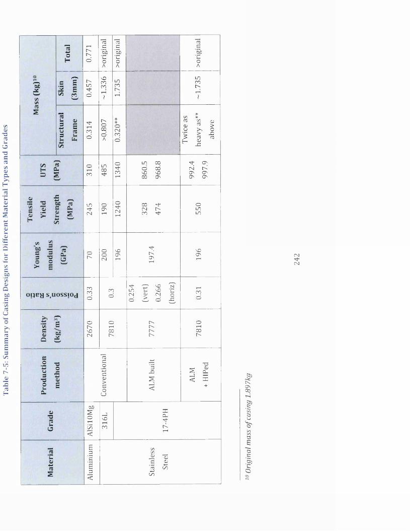
Tabl

e 7-

5: S

umm

ary

of Ca

sing

Des

igns

fo

r D

iffer

ent

Mat

eria

l Ty

pes

and

Gra

des

oT—<r->M

&

C/iC/1TO

£

Tot

al

0.77

1

rec‘5b'uoA

rec‘5b'u,OA >

orig

inal

Ski

n

(3m

m)

IXLD

O

nDcoCOr-H

I

LOCOXt-H -1

.73

5

Str

uct

ura

l

Fra

me

0.31

4 XoCOoA 0.

320*

*

Twic

e as

heav

y as

**

abov

e

UTS

(MP

a)

310 u*>

0 0

1340

860.

5

968.

8

992.

4

997.

9

Ten

sile

Yie

ld

Str

engt

h

(MP

a)

245

190

1240 0 0 *3* CX X

CO 550

You

ng's

mod

ulus

(GP

a) oX 20

0

196

------

'

197.

4

196

o ije y s .uoss io j 0.33 CO

o 0.25

4

(ver

t)

0.26

6

(hor

iz)

0.31

Den

sity

(kg

/m3)

2670

7810

7777

7810

Pro

duct

ion

met

hod

Con

vent

iona

l

ALM

bu

ilt

ALM

+ H

IPed

Gra

de

AlS

ilOM

g

316L

17-4

PH

Ma

teri

al

Alu

min

ium

Sta

inle

ss

Ste

el

5 sIXON00

OS).c53CSu

e/jonC3

XJCM

CS.C

!§)o

7.5 Optimising Build Orientation

In order to enable the electronic components and other parts to be assembled

inside the casing it was necessary fo r it to be sp lit into two separate parts. The

d ivision was made before the part was b u ilt on the ALM. Figure 7-18 shows the

two parts, A and B. The parts would be bolted together on assembly but the

holes fo r the bolts have not been included in the design. Greater precision

would be achieved i f the supports were d rilled out at post processing. The hole

for the electrical connector has also been om itted for the same reason.

Supports for bolts

Part A: Solenoid side Part B: Connector side

Figure 7-18: Two Halves o f Release System Casing

These parts have been manufactured by Renishaw on an AM250 SLM machine

using ALSIlOMg alloy. Data has been provided by the company showing the

orienta tion o f the parts fo r the build and the positioning of the support material.

In the fo llow ing sections this in form ation w ill be compared w ith the results o f

the optim isation code developed for Case Study 2 and applied to these parts.

7.5.1 Part A

Part A had a mass of 0.392 kg and a high resolution stl file o f the geometry was

composed of 11,372 triangu la r faces. Using the "OppTotalSupportVol.m"

software of chapter 5 and the m ultip le starting po in t shown in Table 6-1, the

best o rientation found had a support volume of 3 8 .7 x l0 '6m3 of fu lly dense

243

support. The optim isation algorithm converged to this solution in eight

iterations after 252 function evaluations w ith starting po in t C. The convergence

curve is shown in Figure 7-19. Iteration zero (the firs t red circle] gave an

objective function value of 7 5 .6 x l0 '6m3, which dropped to 40.I x l0 ’6m3 after 48

function counts and seven iterations. The optim isation took a long tim e to stop

though the final ite ra tion brought a fu rthe r reduction of 3.5% in the remaining

200 functions counts.

8.0E-5

7.5E-5

■5 7.0E-5

X 6.5E-5-•-Ite ra tions

6.0E-5

5.5E-5

5.0E-5

g 4.5E-55§ 4.0E-5

3.5E-550 200 250 300100 150

No. of Function Counts

Figure 7-19: Convergence Curve fo r op tim isa tion o f Part A

Figure 7-20 compares the optim al orienta tion for part A (in ye llow ] w ith the

orig inal position ing (cyan]. The ro tational plane had un it normal (0.6913,

0.2586, -0.6747] and formed angles o f -21° and 224° about the x and y axes

respectively.

These angles were applied to the geometry in the Renishaw AutoFAB software

and the predicted support volume was 3 .1 8 x l0 '6m3. The ra tio o f AutoFAB

prediction to OppTotalSupportVol was 0.082 significantly low er than the ratio

o f 0.331 shown in figure 5-35 and fu rthe r removed from the one th ird that

would have been expected (see Figure 5-28] . It could be seen visually that

fewer surfaces indicated the need fo r support w ith the AutoFAB software than

244

in the solution above. It was not clear w hy this should be the case. The

estimated build time for the part was 19 hours and 48 minutes.

b)

•20100

y-axi:-150x-axis

Figure 7-20: O ptim al Bu ild o rien ta tion fo r Part A found w ith

"O ppTotalSupportVol" scrip t, a) O rig ina l o rien ta tion b) O ptim um

7.5.2 Part B

Part B had a mass of 0.353kg and the stl file was made up o f 19,068 faces. On

firs t inspection this part appeared more favourable in design than part A in

using m inim al support m aterial as the rear hat surface followed the angle of the

structura l support (see Figure 7-2 la ) This suggested that as long as the whole

part was b u ilt at an incline of approxim ately 45° to the horizonta l no support

material would be needed over the large fla t areas (Figure 7-21b). If the

inclined angle were much less than this, support would need to be introduced

for the base walls and in ternal parallel surfaces. The fla t surfaces o f the four bolt

holes would require support in this position. Their combined area was very

small but in fact w ith greater forethought these surfaces too could have been

x-axis

245

designed parallel to the support as they would u ltim ate ly be removed when the

bo lt holes were drilled. The round bulbous cap at the top of casing required

support no m atter what the angle o f orientation. If the part was inverted but

the incline remained the same additional material would be required as the

walls along the sp lit line would all require support.

W ith the optim isation software the best orientation found gave a support

volume of 2 5 x l0 '6m3 of fu lly dense support (starting point B). The ro tation

angles for this position were -32°, -50° about the x and y axes respectively. The

un it normal vector for the rotated surface was (-0.7697, -0.3382, 0.5415). This

rotated part is shown in Figure 7-22 in the AutoFAB software w ith the support

material attached. This was not the expected orientation shown in Figure 7-21,

the addition o f a ro tation about the x axis only served to increase the volume of

support needed.

a. Rearview of Part B split line walls

boltholes

Structural su pp o rt'

rear fla t surface b. Possible Build Orientation

Figure 7-21: Suitable Angle o f bu ild fo r Part B o f Casing

246

I

z

X

Figure 7-22: Predicted O ptim al Build o rien ta tion fo r Part B found w ith

'O ppTotalSupportVol' scrip t shown in AutoFAB software w ith support

attached

The support volume calculated by AutoFAB software was 3.65xlO ‘6mT The

ra tio o f AutoFAB prediction to OppTotalSupportVol was 0.146 more thar. half

the expected value of 0.331. The estimated build time for part was 18 hours and

15 minutes.

7.6 V a lid a t io n w ith M a n u fa c tu re d P a rt

Both parts o f the casing were manufactured using sim ilar stl files to those used

in the sections above (see Figure 7-23). The parts were bu ilt by Renshaw using

AlS ilOMg powder on a 400 W laser SLM machine. Stl files o f the support

material used was supplied by Rensihaw once the build had been completed

together w ith a photo o f part B w ith the support still attached (Figure 7-24).

This has enabled the build orienta tion to be determined and using the Swansea

University ALM equipm ent an assessment of build times and support mass has

been generated for comparison w ith the data predictions of section 7.5.

247

Figure 7-23: ALM b u ilt Casing parts

Figure 7-24: ALM Part B affixed to base w ith Support m ate ria l s t ill

attached

A side view o f the geometry taken from the stl file for the support for part A is

shown in Figure 7-25 (in turquoise). The geometry o f the part has been

superimposed onto the support. A t an angle o f 45° the support was shown to

connect to the surfaces o f the bolt holes, the base o f the catch connectors and

also some areas at the low er end of the rear surface. Close inspection o f the

manufactured part indicated increased roughness in these areas which would

confirm that the positioning was correct, e.g. Figure 7-26. In Figure 7-25 it can

248

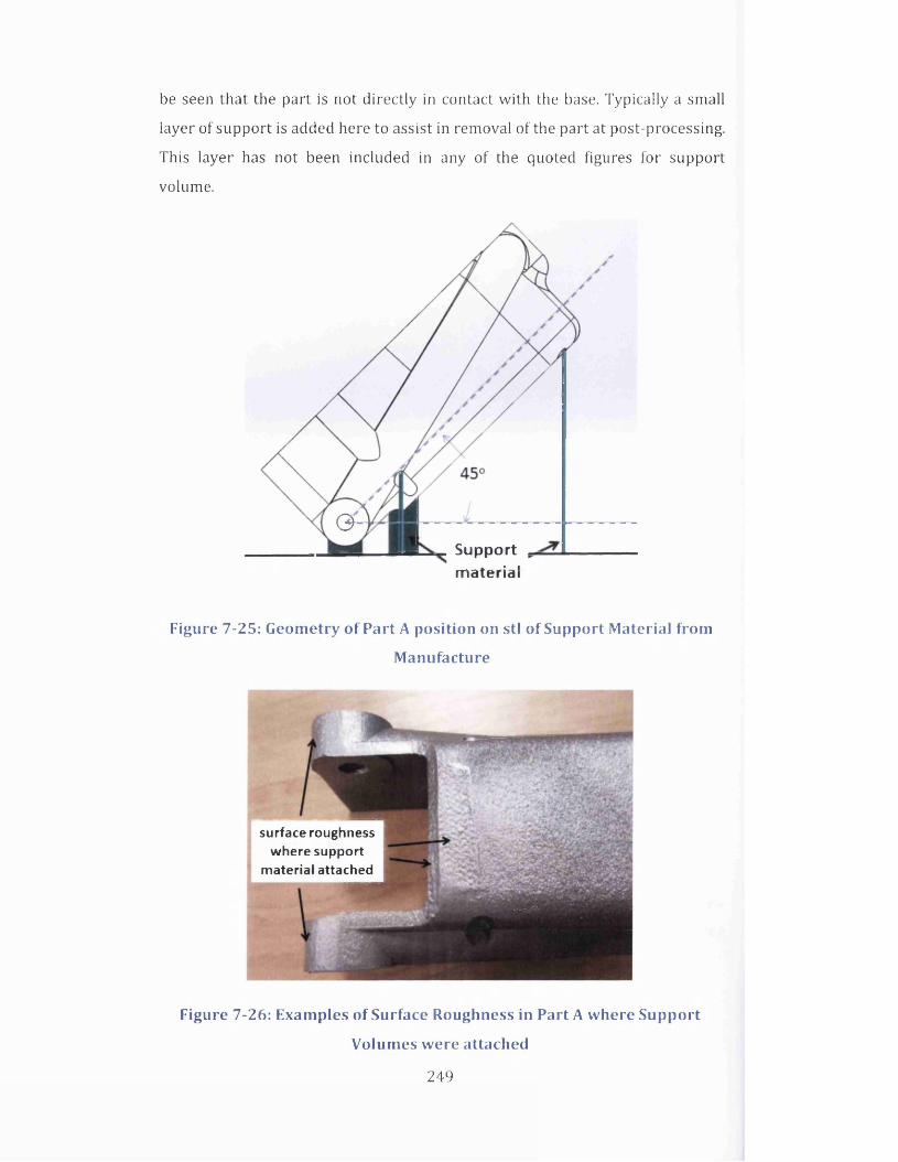
be seen that the part is not d irectly in contact w ith the base. Typically a small

layer of support is added here to assist in removal o f the part at post-processing.

This layer has not been included in any o f the quoted figures for support

volume.

0-

Supportmateriai

Figure 7-25: Geometry o f Part A position on stl o f Support M ateria l from

M anufacture

surface roughness where support

material attached

Figure 7-26: Examples o f Surface Roughness in Part A where Support

Volumes were attached

249

a. Side view of Part A b. Interior view of Part A

c. Rear view at 45.0001° incline about y axis

Figure 7-27: Support Requirem ents fo r Part A using AutoFAB

This angle o f orientation was used w ith the AutoFAB software to calculate the

volume of support used. The areas indicated by the stl (Figure 7-25) were

chosen though the software did not indicate that the support was needed in an

area as w ide as the stl showed in the low er surface (see Figure 7-27a). Looking

at the underside of the part in this orientation (Figure 7-27b) showed an

additional blue area in need of support but this could not be selected. The

orange areas in this view also require support material but the stl does not

250

indicate any support was used here. For these reasons it is believed tha: the

prediction of support volume used here was an under estimate. Small changes

in the angle o f inclination did not offer a better match to the stl. An add itona l

ro tation o f 0.0001° indicated tha t the whole of the rear face would need support

(Figure 7-27c], while a s im ila r reduction in the angle required support f t r the

whole o f the base surface shown in Figure 7-27b and the base walls.

Using only the selection shown in Figure 7-27a, AutoFAB predicted a support

volume o f 1 .9 6 x l0 _6m3 w ith a build time of 18 hours and 59 minutes.

Figure 7-24 shows part B s till attached to the build plate w ith the support

material attached to the part. It can be seen that the support extended to the

cap as expected, but not to the surface of the bolt holes. Support was also

required along the edge between the holes for the catch dowels. This

arrangement was achieved on the AM250 using a ro tation of -46° about t ie y-

axis only. The support volume was 3 .4 5 x l0 _6m3 w ith a build time of 18 tours

and 24 minutes predicted by AutoFAB. The software did indicate that support

was required at the bo lt and dowel holes but it was not applied in these areis.

Table 7-6: Comparison o f Support Volume Predictions w ith Manufactured

Volumes

Best

optim um

using

MatLab

scrip t

AutoFAB

using Best

MatLab

orien ta tion

using

Renishaw

orien ta tion

percentage

im p roven en t

by Renisliaw

Support Volume (x lO 6m 3)

Part A 38.72 3.18 1.9611 38%

Part B 25 3.65 3.45 5%

Time to bu ild (h r)

Part A 19.8 18.98 4%

Part B 18.25 18.4 -1%

11 known under-estimate

251

Table 7-6 gives a comparison between the support volume required using the

best orientation found using the MatLab script and estimate of the support

volume used when the manufactured part was built; comparison of build times

are also shown. For both parts the MatLab script did not find the best

orientation, though for part B the Renishaw orientation has only made a 5%

improvement on the support volume. The build time w ith the MatLab script

orientation is in fact marginally quicker.

It has been noted above that for part A the manufacturer has chosen not to

apply support in all the areas indicated by the software therefore the 38%

increase is not a valid comparison for validating the MatLab script.

7.7 Conclusions

This chapter has shown that using a design approach that included a series of

optim isation techniques it has been possible to:

a} Successfully reduce the weight of the casing by more than 50% while

still achieving a safety factor of 1.3

b] Establish a design methodology that has been robust enough to

investigate the design using different material properties, whether

conventionally or ALM bu ilt

c] Make a sw ift assessment of the different materials w ithout having to

undertake a complete redesign

d] Demonstrate that AlSilO Mg was the most suitable material w ith

which to manufacture the lighter casing.

Also the build orientation software although effective w ith the casing designs in

finding optimum orientations, the predicted volumes were not as good as those

selected by the professional engineers w ith expertise in this field.

These results indicate the potential for future work in this area, namely

i) To further develop the software to incorporate some of the

knowledge base of the manufacturers

ii] Investigate the material properties of ALM bu ilt and heat treated AlSilO to validate the assessment of the new casing design

252

Chapter 8: Concluding Remarks

Summary : This ch ap te r completes the ma in body o f the thesis by

sum m ar is ing the achievements , conclusions and recommendat ions f o r

f u t u r e w o rk

The aim of this thesis was to explore optimisation and develop robust

methodologies to use w ith these techniques as a solution to real complex

industrial based problems. This was not to be merely as an academic exercise

but to provide sound approaches that conform to industrial standards and can

take full advantage of the chosen manufacturing methods. This concluding

chapter summarises the achievements that have been made through this

research, discusses the implications of this work and some limitations. It also

considers how these findings could be further developed.

8.1 Achievements and Conclusions

The previous chapters have shown in detail that optimisation techniques have

been identified and used to solve real-world problems and the success of this

research is outlined below.

8.1.1 Case Study 1: The design o f a housing fo r a novel VAWT

• An optimal design for the housing of a new design of Vertical Axis Wind

Turbine has been identified. This has also enabled an appropriate

manufacturing method to be identified.

The design was a space frame which is not radical for this type of structure,

however by using mathematical optimisation, the algorithm has been able to

search through a very large design space and thus been given the opportunity of

finding more novel solutions. The fact that it did not do so should not detract

from the merits of predicting a feasible design w ith speed and efficiency.

• A reliable, consistent methodology has been established. This enabled

the design to conform to British Standard BS:5950 when bu ilt w ith no

more than 1 2 different standard sections.

253

Checking the design against British Standards showed that the design

methodology was trustworthy as only a lim ited number of member sizes

needed to be modified to conform in each case. Restricting the number of

sections sizes permissible and the use of standard sections, improved the

manufacturability of the structure and would add to the cost reduction, though

this has not been quantified in the research.

• The design method has been applied to 11 different housing sizes to

establish a cost-size performance relationship for use in attracting

investment for construction and further development.

Each design followed approximately the same layout of beams and columns and

so the data is lim ited to this particular design and cannot be used generically,

however it met the objectives for the Company. The lateral w ind loads were

applied w ith no variation in height, this work could be further enhanced by

applying non-uniform w ind loads, particularly for the higher structures for

which this would be more realistic.

• The Kreisselmeier Steinhauser (KMS] functions have been tested in

conjunction w ith A lta ir Optistruct in an attempt to improve the

computational efficiency. The functions aggregate the constraints in the

optimisation. It has been shown that the approach does not reduce the

time to find a convergent solution. The constraints screening already

incorporated in Optistruct appears to be effective in finding good

solutions in optimal tim e , at least for the problems considered.

Other authors have seen improvements w ith the KMS function, particularly

when the p parameter was modified as the solution approached the optimum or

the continuity and differentiab ility of the KMS functions have been used to full

advantage. The latter was most often used in shape optimisation problems

where small changes in shape can lead to large fluctuations in stress and the

KMS function was effective here in smoothing out these large variations. The

decision to save time by keeping the geometry in Optistruct increased the

complexity of the problem at every attempt. Setting up the geometry however,

254

in another environment would have been very time consuming and may well

have counteracted any time gains made by the constraints aggregation.

8.1.2 Case Study 2: GE Challenge - T itan ium Bracket Design

• A crowdsourcing design competition has been systematically

investigated. The solutions to the problem have been studied as well as

the tools used and the feedback provided. The strengths and weaknesses

of this approach have also been explored not only for the sponsoring

company but also for the individuals who participated.

The General Electric design challenge provided an excellent example of how

innovative solutions can be achieved through an open crowdsourcing

competition. All subsequent press releases indicate that the company

considered the venture to be successful. The lack of promised feedback caused

much discontent amongst the competitors which would make this a d ifficult

approach to sustain. Certainly this work has shown that this approach can

deliver innovative solutions to design problems, though it is d ifficu lt to assess

the cost effectiveness for the company and w ith only a lim ited reward system

this must be carefully managed to keep designers engaged.

• A number o f highly practical critical factors have been identified. These

can be used immediately to inform the designer in designing for additive

layer manufacture and build.

It has been seen that topology optimisation is an excellent tool for ALM design;

however care must be taken when applying boundary conditions as this has a

major impact on the optimised solution obtained. Not all commercial software is

equally effective. Some of the commercial packages that are easiest to use have

not always found the best local minima. The form of the topology optim isation is

often more helpful than the detail; efforts to capture every feature tends to be

time-consuming and may over complicate the design .

It is well known that all hollow features need holes to allow for unused powder

to be removed at post processing, but more critical is the need for all the

surfaces o f enclosed spaces to be self-supporting. Support volume cannot be

applied to enclosed spaces nor removed at post processing.

255

It has been shown that time and cost to build depends on total volume. Once the

part has been designed to meet structural requirements the cost becomes a

function of the support volume only and it is essential to also minimise the

support volume in the design to make the most o f the advantages of additive

layer manufacture.

• A software tool has been developed to minimise support material volume

in ALM manufacture. This has been tested on models of increasing

complexity w ith favourable results.

The software has proved quite effective for the examples of this case study but

because it tests the orientation of every triangular surface in the geometry

stereo-lithography (stl] file of the model, the time to solution increases w ith

geometric complexity. It would be possible to use a coarser stl file as an in itia l

assessment of orientation, though the finer stl file would still be required for the

ALM build to avoid any stepping in the surfaces of the final component. The

software code has been modified to achieve greater computational efficiency.

8.1.3 Case Study 3: Design o f Release System fo r ALM

• In the th ird Case Study, the required weight reduction of 50% for the

Release System Casing was comfortably achieved using AlSilO Mg.

The casing was successfully manufactured using additive layer w ith only m inor

modifications required. The support material volume needed was less than

predicted. In all the case studies, finite element analysis has been used to assess

the structural valid ity of the components. It is im portant not to lose sight of the

fact that in using the FEA method simplification have been made to the

boundary conditions and the behaviour of the connecting parts and so the

solution is only an approximation to the structural behaviour of the component.

The major shortcoming of this w ork is that there is no data available to validate

these models. Structural testing of these components would enhance this work

considerably. In the meantime, since the designs are considered to be at the

concept stage, and safety factors were incorporating into the design, the linear

static FEA analysis has been considered sufficient.

256

• The methodology has been established for the casing design. This has

provided an easy assessment approach for testing different materials for

this redesign. These materials included ALM bu ilt and post processed

ALM material.

Since the design was effectively a beam model merged w ith a th in cage, it was

clear in most cases to see even at the beam model stage the design would be

heavier than the original. There would of course be a threshold in the material

properties where the topology optimisation would no longer indicate a beam

structure for the optimised solution, making the methodology ineffective. This

seems unlikely in the range of properties of metals. The design would need to

be reassessed from the start for less conventional materials.

• Orientation software to minimise support volume has been validated

against the manufactured part.

The support is only based on the geometry of the part. No consideration of

support for residual stresses or for heat dissipation has been incorporated. The

bu ilt part has also highlighted areas where the manufacturer has chosen to om it

support material and has still achieved an acceptable quality in the final part.

Despite these lim itations the software does provide a useful tool for those w ith

lim ited expertise.

Overall this work has shown that it has been possible to find suitable

optim isation tools which have enabled workable solutions to be found for some

commercial problems. Not all tools have proved to be successful, e.g. the KMS

functions in conjunction w ith Optistruct did not improve computational

efficiency in Case Study 1. Certainly it has been demonstrated that working w ith

a range of appropriate techniques can prove beneficial. Also the same approach

may be valid in very different applications, e.g. size modelling of beams was

used for the very large VAWT housing model but also for the structural frame of

the release system casing.

The increased understanding gained from the study of the geometries design for

ALM may not have been universally ground-breaking but it has helped to

257

inform the case studies of this thesis and w ill continue to do so for the author in

the future.

8.2 Recommendations for Future W ork

Though significant progress has been made in providing robust solutions to

these problems, there are still several unfinished topics that could provide

further benefits.

• The beam and column layout of the VAWT housing design were chosen

using engineering judgement and to complete the w ork w ith in

commercially determined timescales. An additional optim isation step

could have been included at that stage using methods to position the

joints between the different members. This research would be of value

to see if additional weight savings could be made by using a less

standardised layout. The inclusion of manufacturing constraints in the

optimisation of structures would also be beneficial in the practical design

of these large industrial structures.

• An interesting area of research would be to introduce and m onitor an

interdisciplinary crowdsourcing challenge w ith in a university. Perhaps,

the design of a component or process that would have relevance in

medical or social care and yet would require scientific or engineering

input for a robust design. Certainly, this would require a change of m ind­

set in many areas, but could in itia lly be launched at a student level where

m ultidisciplinary research could be highly beneficial and this would help

to gradually draw in some of the academics. Harvard Medical School

[274] successfully used sim ilar methods of open innovation to invite

ideas for the cure of Type 1 diabetes and then brought together new

diverse interdisciplinary teams in the workplace to generate the grant

proposals to fund the most innovative of these ideas.

• Further research in the area of ALM bu ilt AlSilO Mg is essential. The data

available is lim ited and shows large variation in the results. Robust data

258

is needed to establish confidence in future components designed w ith

this material.

• In conjunction w ith w ork on the fundamental physics of the ALM process

the orientation software could be expanded to incorporate supports to

control heat and residual stress. “High fidelity" models for heat and

stress calculations would need to be investigated in itially, but then it may

then be possible to develop a lower level simplified model as an

approximation that could form the basis of a multi-objective

optim isation incorporating support for the three factors of geometry,

stress and temperature.

• W orking in conjunction w ith the manufacturers the software could be

developed further to incorporate more of the producer's expertise and

provide a more effective optimisation tool that could be used by the

novice but still provide excellent results.

259

App

endi

x A:

G

loba

l St

artin

g Po

ints

us

ed

in O

ptis

truc

t fo

r VA

WT

Hou

sing

Si

ze

Op

tim

isat

ion

Key

to Ta

ble:

20 U u . U . u u u

19 u u . u . U u Q

18

u u . b U u Q

17 u u U u . u . u

16 u u u u . t u u

15 u u u u . u . Q

14 u u u u . u . Q

13 u u u u . u u

C/J

12 u u u u . u u

s■ Mo

CL.

11 u u u u. u Q

M lr j

■ M 10 u u u Urn « Q

re*->in O ' u u u u u . u

0 0 u u u u u . u

u u u u u . Q

vD u u u u u . O

LO u u u u u u

r t - u u u u u U J

CO u u u u u Q

CNI u u u u u Q

tH < < < < < CQ

s a j q e i J B A

u S i s a a

oo p

t-H

81

-1

60

16

1-

24

0

24

1-

32

0 oo

1T - 1CNIr o 4

01

-4

80

s d n o j g H CNI CO LD

n p e y J 9 U U J

i v a c m

ovOCNI

20 U Q Q Q c

5c33

1 C"-03 c5

c5

t--33

E--33■dE- dE—3

1 < E- 3

O'rH Q u u Q c5

c33

c-33

c5

c5

.£f-5

■£E-•cE-33

dE-33

dE-3

00rH Q Q Q u c5

c3 £~3 c5

C5

-cE- -dE-5

■dE-3dE-3

E-33

rH u u u u c5

c5

c3C"3s

c-033

•c-E--33

5-33E-33

E-33

dE-33

nOtH UJ

°Q Q c3 c3 C"

5c-Q C~os

■cE--33

•dE--33

■dE-3dE-3

dE-3

inrH Q u u Q c5

c5

cs

c-Q c-QxiE- «E-

5

■dE-33

E-33dE-3

re-rH Q Q Q u c5

c3 c5

c-Q c-Q3

-Ct--3 E--3-dE-3

dE-3—E-33

rorH Q u Q u c3 c3 c3c-03s

C-Q-j--E--33

E--3■dE-33

dE-3 33

c/5CNIrH Q Q u Q c c

5c

3c-03 c

5

■cE--33

E-5

■dE-3dE-33

dE-3

coCl.

rHrH w w Q Q C"3 c

5c3

c-03 c5

-cE-x:E--33

■dE-33

dE-3dE-3

OX)c• p.4-1u

OrH u Q u u c5

c5

c3c--C3 c

S■iSE--3

•c _ E- -3 3

dE-3—

dE-33f—.

33

re■Mt/5 0> Q u Q Q c5

c3 c5

c-Qc-C3

3

~ -5T E- -3 3

■eE-3E-33

dE-3dE-3

CO Q Q u u c3 c5

c-03—c

5C-033

-cE--33X!E-3

dE-.3dE-33

E-33

u u Q u c3 c5

C3—Jc

5 -cT3t- - fr-1

d3~3

d3"3

dE-33

NO u Q u Q c3 c3 C3 c c-033

•cf--3

P33

dE-3d

33dE-3

in u u u Q c

5

C"5

c

3

c-03 CS

—E --33

c s :E--33

‘ S T E- 3 3

dE-3dE-3

t J" u Q Q u c

5

c

5

c3 c

5

c

S

■ ~E--33

XTE-33

dE-3d " E- 3 3

dE-33

co Q u u u c

5c

5c3 c

5c

5-cE-

5«E-3

d-E-33

d _ E- 3 3

dE-33

CNJ Q O Q Q c c5

c5

c5

c-3JSE-

5*E-3

dE-3dE»3

dE-3

rH 00 QO QQ QQ < < < < < QQ QQ QQ QQ QQ

s a jq e i je AONOin

onENO

oCN

ooCO oCOoNO

on)-CNI

oCNICO

oonJ-

oCONf

0NOm

ONO

OCMh-

OOCO

uSisaat-H00

t-HNOin

r H

NO

r HCMC-r H r H

COr HNOr H

r H

CMr H

CNICOr H

Or H

COn)-

r HNOLO

r H

''t'NO

r H

CNIE'­

sdno jg 00 ON or H

r H CM CO Nh in NO CO ON er;r H

S's a iD p iq jnpe^ jauuj SS9Uq3iqi IJBM

3W3H1X3 IV a c m

Appendix B: Abbreviated input file for Continuous

Optimisation in Optistruct for VAWT Housing, 22m, one

diameter height model

$$$$ Optistruct Input Deck Generated by HyperMesh Version : 11.0.0.47 $$ Generated using HyperMesh-Optistruct Template Version : 11.0.0.47 $$$$ Template: optistruct $$$$$$ optistruct $TITLE = C-FEC VAWT Housing - 22m 1 Diameter in SI UNITSFORMAT H3DFORMAT OUTPUT2DISPLACEMENT(OPTI) = ALLELFORCE(OPTI] =ALLGPFORCE(OPTF) = ALLSTRESS(OPTI,VON] = YES$$ - $$$ Case Control Cards $$$ - - - - $ $$$$ OBJECTIVES Data $$$$HMNAME OBJECTIVES $DESOBJ(MIN)=l$$HMNAME LOADSTEP $SUBCASE 1 SPC= 8

LOAD = 11DESSUB = 4

$$HMNAME LOADSTEP $SUBCASE 2 SPC= 8

LOAD = 12DESSUB = 5

$$HMNAME LOADSTEP 3"loadstep p l5 "

1 objective

l"loadstep p90"

2"loadstep p30"

262

$SUBCASE 3 SPC = 8

LOAD = 13DESSUB = 6

$$HMNAME LOADSTEP $SUBCASE 4 SPC = 8

LOAD = 14DESSUB = 7

$$HMNAME LOADSTEP $SUBCASE 5 SPC= 8

LOAD = 15DESSUB = 8

$$HMNAME LOADSTEP $SUBCASE 6

SPC= 8

LOAD = 16DESSUB = 9

$$HMNAME LOADSTEP $SUBCASE 7 SPC= 8

LOAD = 17DESSUB = 10

$$HMNAME LOADSTEP $SUBCASE 8

SPC = 8

METHOD(STRUCTURE) STATSUB = 1DESSUB = 11

$$HMNAME LOADSTEP $SUBCASE 9 SPC = 8

METHOD(STRUCTURE) STATSUB = 2DESSUB = 12

4"loadstep n l5 " 1

5"loadstep n30" 1

6 "loadstep n90" 1

7"loadstep n l35 '' 1

8"Bucklingp90" 4

9

9"Buckling p30" 4

263

$$HMNAME LOADSTEP $SUBCASE 10 SPC= 8

METHOD[STRUCTURE] = STATSUB = 3DESSUB = 13

$$HMNAME LOADSTEP $SUBCASE 11 SPC = 8

METHOD(STRUCTURE) = STATSUB = 4DESSUB = 14

$$HMNAME LOADSTEP $SUBCASE 12 SPC = 8

METHOD(STRUCTURE) = STATSUB = 5DESSUB = 15

$$HMNAME LOADSTEP $SUBCASE 13 SPC = 8

METHOD(STRUCTURE) = STATSUB = 6

DESSUB = 16$$HMNAME LOADSTEP $SUBCASE 14 SPC = 8

METHOD(STRUCTURE) = STATSUB = 7DESSUB = 17

10"Buckling pl5" 4

9

lr 'B u c k lin g n l5 " 4

9

12"Buckling n30" 4

9

13"Buckling n90" 4

9

14"Buckling n l3 5 " 4

$$$$ HYPERMESH TAGS $$$$BEGIN TAGS $$END TAGS $BEGIN BULK $$$$ Stacking Information for Ply-Based Composite Definition

264

$$$$HMNAME OPTICONTROLS l"optistruct_opticontrol" $DOPTPRM DESMAX 200 GBUCK 1

$HMNAME DESVARS 1RI1 DESVAR 1 RI10.01 0.01 0.5$HMNAME DESVARS 2RI2 DESVAR 2 RI20.01 0.01 0.5] the above 2 lines repeated fo r each inner radius design variable DESVAR 426 Thl0.003 0.003 0.5$HMNAME DESVARS 427Th2 DESVAR 427 Th20.003 0.003 0.5$HMNAME DESVARS 428Th3] the above 2 lines repeated fo r each wall thickness design variable$HMNAME DVPRELS 1 rROlDVPREL11 PBARL 1DIM1 0.0+ 1 1.0 426 1.0$HMNAME DVPRELS 2 rR02DVPREL12 PBARL 2DIM1 0.0+ 2 1.0 427 1.0] 3 line repeat fo r each Outer Radius (DIM1) design variable relationship $HMNAME DVPRELS 426 rR IlDVPREL1426 PBARL 1DIM2 0.0+ 1 1.0$HMNAME DVPRELS 427 rRI2DVPREL1427 PBARL 2DIM2 0.0+ 2 1.0] 3 line repeat fo r each Inner Radius (DIM2J design variable relationship $$$$ OPTIRESPONSES Data $$DRESP1 1 Volume VOLUMEDRESP1 2 DisplaceDISP TXYZ 19071DRESP1 3 Stress STRESS PBARL SVMAX 15 + 16 17 18 19 20 21 22 23+ and so on un til 425 DRESP1 4 BucklingLAMA 1$$$$ OPTICONSTRAINTS Data $$$$HMNAME OPTICONSTRAINTS $DCONSTR 1 2 0.45$$HMNAME OPTICONSTRAINTS $

IDisplacement

2Stress

265

DCONSTR 2 3-3.0+8 3.0+8$$HMNAME OPTICONSTRAINTS 3buckling $DCONSTR 3 41.0DCONADD 4 1 2

DCONADD 5 1 2

DCONADD 6 1 2

DCONADD 7 1 2

DCONADD 8 1 2

DCONADD 9 1 2

DCONADD 1 0 1 2

DCONADD 11 3DCONADD 1 2 3DCONADD 13 3DCONADD 14 3DCONADD 15 3DCONADD 16 3DCONADD 17 3$$$$ DESVARG Data $$$$$$ GRID Data $$GRID 1 0 0 1 -7.752797.8378910.0GRID 1 0 0 2 -4.7354 9.928 0.0GRID 1003 -0.863 10.965650.0GRID 1004 2.4276 10.7284 0.0GRID 1005 5.8695 9.3026 0.0GRID 1006 7.82845 7.82845 0.0GRID 1007 9.95495 9.95495 0.0GRID 1008 13.6639113.663910.0GRID 1009 9.6005 11.497150.0GRID 1 0 1 0 7.542 11.172150.0GRID 1 0 1 1 4.77812511.694720.0GRID 1 0 1 2 0.9321 13.135150.0GRID 1013 -3.1958 13.244350.0GRID 1014 -5.5776511.726850.0GRID 2 0 0 1 -7.752797.8378912.75GRID 2 0 0 2 -4.7354 9.928 2.75GRID 2003 -0.863 10.965652.75GRID 2004 2.4276 10.7284 2.75GRID 2005 5.8695 9.3026 2.75GRID 2006 7.82845 7.82845 2.75GRID 2007 9.95495 9.95495 2.75GRID 2008 13.6639113.663912.75GRID 2009 9.6005 11.497152.75GRID 2 0 1 0 7.542 11.172152.75

266

GRID 2 0 1 1 4.77812511.694722.75GRID 2 0 1 2 0.9321 13.135152.75GRID 2013 -3.1958 13.244352.75GRID 2014 -5.5776511.726852.75GRID 3001 -7.752797.8378915.5GRID 3002 -4.7354 9.928 5.5GRID 3003 -0.863 10.965655.5GRID 3004 2.4276 10.7284 5.5GRID 3005 5.8695 9.3026 5.5GRID 3006 7.82845 7.82845 5.5GRID 3007 9.95495 9.95495 5.5GRID 3008 13.6639113.663915.5GRID 3009 9.6005 11.497155.5GRID 3010 7.542 11.172155.5GRID 3011 4.77812511.694725.5GRID 3012 0.9321 13.135155.5GRID 3013 -3.1958 13.244355.5GRID 3014 -5.5776511.726855.5GRID 4001 -7.752797.8378918.25GRID 4002 -4.7354 9.928 8.25GRID 4003 -0.863 10.965658.25GRID 4004 2.4276 10.7284 8.25GRID 4005 5.8695 9.3026 8.25GRID 4006 7.82845 7.82845 8.25GRID 4007 9.95495 9.95495 8.25GRID 4008 13.6639113.663918.25GRID 4009 9.6005 11.497158.25GRID 4010 7.542 11.172158.25GRID 4011 4.77812511.694728.25GRID 4012 0.9321 13.135158.25GRID 4013 -3.1958 13.244358.25GRID 4014 -5.5776511.726858.25GRID 5001 -7.752797.83789111.0GRID 5002 -4.7354 9.928 11.0GRID 5003 -0.863 10.9656511.0GRID 5004 2.4276 10.7284 11.0GRID 5005 5.8695 9.3026 11.0GRID 5006 7.82845 7.82845 11.0GRID 5007 9.95495 9.95495 11.0GRID 5008 13.6639113.6639111.0GRID 5009 9.6005 11.4971511.0GRID 5010 7.542 11.1721511.0GRID 5011 4.77812511.6947211.0GRID 5012 0.9321 13.1351511.0GRID 5013 -3.1958 13.2443511.0GRID 5014 -5.5776511.7268511.0GRID 6001 -7.752797.83789113.75GRID 6002 -4.7354 9.928 13.75GRID 6003 -0.863 10.9656513.75

267

GRID 6004 2.4276 10.7284 13.75GRID 6005 5.8695 9.3026 13.75GRID 6006 7.82845 7.82845 13.75GRID 6007 9.95495 9.95495 13.75GRID 6008 13.6639113.6639113.75GRID 6009 9.6005 11.4971513.75GRID 6010 7.542 11.1721513.75GRID 6011 4.77812511.6947213.75GRID 6012 0.9321 13.1351513.75GRID 6013 -3.1958 13.2443513.75GRID 6014 -5.5776511.7268513.75GRID 7001 -7.752797.83789116.5GRID 7002 -4.7354 9.928 16.5GRID 7003 -0.863 10.9656516.5GRID 7004 2.4276 10.7284 16.5GRID 7005 5.8695 9.3026 16.5GRID 7006 7.82845 7.82845 16.5GRID 7007 9.95495 9.95495 16.5GRID 7008 13.6639113.6639116.5GRID 7009 9.6005 11.4971516.5GRID 7010 7.542 11.1721516.5GRID 7011 4.77812511.6947216.5GRID 7012 0.9321 13.1351516.5GRID 7013 -3.1958 13.2443516.5GRID 7014 -5.5776511.7268516.5GRID 8001 -7.752797.83789119.25GRID 8002 -4.7354 9.928 19.25GRID 8003 -0.863 10.9656519.25GRID 8004 2.4276 10.7284 19.25GRID 8005 5.8695 9.3026 19.25GRID 8006 7.82845 7.82845 19.25GRID 8007 9.95495 9.95495 19.25GRID 8008 13.6639113.6639119.25GRID 8009 9.6005 11.4971519.25GRID 8010 7.542 11.1721519.25GRID 8011 4.77812511.6947219.25GRID 8012 0.9321 13.1351519.25GRID 8013 -3.1958 13.2443519.25GRID 8014 -5.5776511.7268519.25GRID 9001 -7.752797.83789122.0GRID 9002 -4.7354 9.928 22.0GRID 9003 -0.863 10.9656522.0GRID 9004 2.4276 10.7284 22.0GRID 9005 5.8695 9.3026 22.0GRID 9006 7.82845 7.82845 22.0GRID 9007 9.95495 9.95495 22.0GRID 9008 13.6639113.6639122.0GRID 9009 9.6005 11.4971522.0GRID 9010 7.542 11.1721522.0

268

GRID 9011 4.77812511.6947222.0GRID 9012 0.9321 13.1351522.0GRID 9013 -3.1958 13.2443522.0GRID 9014 -5.5776511.7268522.0GRID 19071 -0.0003 -0.0001822.0These are the co-ordinates o f the connecting nodes and then there are a ll the ether nodes which are set up as the members are meshed $$$$ SPOINT Data $$$HMNAME BEAMSECTCOLS l"a u to ln $HMNAME BEAMSECTCOLS 2"auto_std_hb_cor $HMNAME BEAMSECTS $ 1 l"op ti_ tube.l"$ 2 0 49 01.0 1.0 0.0 0.0 0.0$ 0 .0 1

$HMNAME BEAMSECTS BEAMSECTIONSTANDARD 7 2 OTube$HMNAME BEAMSECTS BEAMSECTIONSTANDARD PARAMETERS 0.250.25 0.25$HMNAME BEAMSECTS BEAMSECTIONSTANDARD PARAMETERS 0.5 0.50.5$HMNAME BEAMSECTS END $HMNAME BEAMSECTS $ 2 l"opti_tube.2 "$ 2 0 49 01.0 1.0 0.0 0.0 0.0$ 0 .0 1

$HMNAME BEAMSECTS BEAMSECTIONSTANDARD 7 2 OTube$HMNAME BEAMSECTS BEAMSECTIONSTANDARD PARAMETERS 0.250.25 0.25$HMNAME BEAMSECTS BEAMSECTIONSTANDARD PARAMETERS 0.5 0.50.5$HMNAME BEAMSECTS END] the above 8 lines are repeated fo r each o f the beam members $$ RBE2 Elements - Multiple dependent nodes $RBE2 9631 19071 123456 9001 9002 9003 9004 9005+ 9006 9007 9008 9009 9010 9011 9012 9013+ 9014$$HMMOVE 426 $ 9631$$$ CBAR Elements $CBAR 9632 15 1001 190721.0 0.0 0.0] These are the elements generated by the line meshing $

269

$HMMOVE 15 $ 9632THRU 9643$$$HMMOVE 16 $ 9644THRU 9655$$7 above 4 lines are repeated they move the generated elements into the

] appropriate collector$$$$---- - - $$$ HyperMesh name and color information for generic components $$$.................................................................................................... —-$$HMNAME COMP l 'T r l "$HWCOLOR COMP 1 7$$HMNAME COMP 2"Tr2"$HWCOLOR COMP 2 7$7 above 3 lines are repeated to name and select a colour fo r the collectors $HMDPRP$ 9632THRU 12799 14564THRU 15391 15400THRU 15403$ 15392THRU 15399 15404THRU 15895 14276THRU 14563$ 14264THRU 14275$$HWBEAMSEC PBARLASSOC 1 1$$$$ PBARL Data $$$HMNAME PROP l " p l " 3$HWCOLOR PROP 1 49$HMBEAMSEC PBARLASSOC 1 426PBARL 1 1 TUBE ++ 0.5 0.25$HWBEAMSEC PBARLASSOC 2 2$$$HMNAME PROP 2"p2" 3$HWCOLOR PROP 2 49$HMBEAMSEC PBARLASSOC 2 427PBARL 2 1 TUBE ++ 0.5 0.257 above 6 lines repeated to assign properties to each o f the PBARL tubes $$$$ MAT1 Data $$$HMNAME MAT l"Steel" "MAT1"$HWCOLOR MAT 1 5MAT1 12.1+11 0.3 7900.0

270

$$$$-- - - $$$ HyperMesh Commands for loadcollectors name and color information $$$ - $$HMNAME LOADCOL 1"P90"$HWCOLOR LOADCOL 1 5$$] repeated fo r the remaining 6 load cases and the constraints load collector $$$$ LOAD cards $$$HMNAME LOADCOL Il"p90+G "$HWCOLOR LOADCOL 11 53$$LOAD 111.0 1.0 1 1.0 10$] repeated fo r the remaining 6 loadcases with g ravity $$$ EIGRL cards $$$HMNAME LOADCOL 9"Buckling"$HWCOLOR LOADCOL 9 25EIGRL 90.0 1 MAX$$$$ SPC Data $$SPC 8 1 0 0 1 1234560.0SPC 8 1 0 0 2 1234560.0SPC 8 1003 1234560.0SPC 8 1004 1234560.0SPC 8 1005 1234560.0SPC 8 1006 1234560.0SPC 8 1007 1234560.0SPC 8 1008 1234560.0SPC 8 1009 1234560.0SPC 8 1 0 1 0 1234560.0SPC 8 1 0 1 1 1234560.0SPC 8 1 0 1 2 1234560.0SPC 8 1013 1234560.0SPC 8 1014 1234560.0$$$HMNAME1LOADCOL 10'$HWCOLOR LOADCOL 10 48$$GRAV 10 09.81 0.0 0.0 -1.0$$$ $$$$ FORCE Data

271

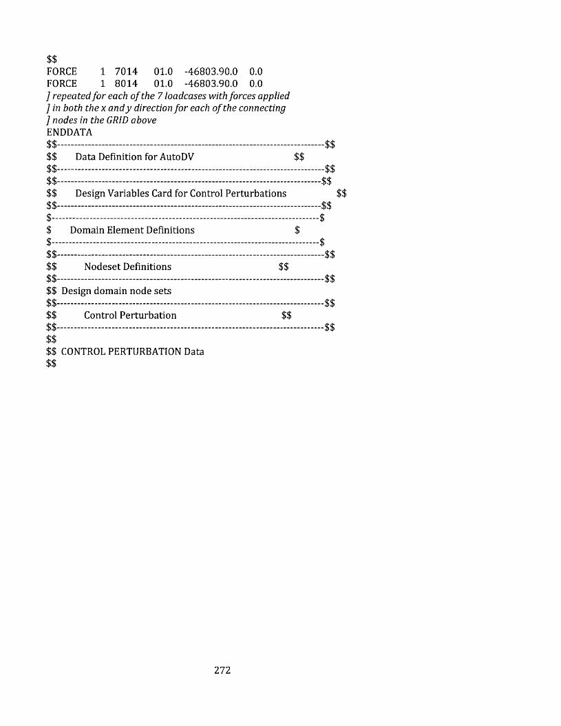
$$FORCE 1 7014 01.0 -46803.90.0 0.0FORCE 1 8014 01.0 -46803.90.0 0.0] repeated fo r each o f the 7 loadcases with forces applied ] in both the x andy direction fo r each o f the connecting ] nodes in the GRID above ENDDATA$$ - $$$$ Data Definition for AutoDV $$$$ - $$$$-.....- -..................................................................................... $$$$ Design Variables Card for Control Perturbations $$$$---- - $$$ $$ Domain Element Definitions $$ $$$.................................................. $$$$ Nodeset Definitions $$$$- -- - $$$$ Design domain node sets$$ - - - - $$$$ Control Perturbation $$$$ -............................................................................................... $$$$$$ CONTROL PERTURBATION Data $$

272

Appendix C: Commercially Available Standard Circular

Hollow Sections, (Class 3)

Name

OuterD iam eter

D0(m)

W allThickness

Th(m)

Area

(m ^

Area Moment o f Ine rtia

/(m4l

No.

21.3x3.2 CHS 0.0213 0.0032 1.82E-04 7.68E-09 1

26.9x3.2 CHS 0.0269 0.0032 2.38E-04 1.70E-08 2

33.7x3.0 CHS 0.0337 0.003 2.89E-04 3.44E-08 333.7x3.2 CHS 0.0337 0.0032 3.07E-04 3.60E-08 433.7x3.6 CHS 0.0337 0.0036 3.40E-04 3.91E-08 542.4x3.0 CHS 0.0424 0.003 3.71E-04 7.25E-08 6

33.7x4.0 CHS 0.0337 0.004 3.73E-04 4.19E-08 742.4x3.2 CHS 0.0424 0.0032 3.94E-04 7.62E-08 8

48.3x3.0 CHS 0.0483 0.003 4.27E-04 1.10E-07 942.4x3.6 CHS 0.0424 0.0036 4.39E-04 8.33E-08 1 0

48.3x3.2 CHS 0.0483 0.0032 4.53E-04 1.16E-07 1 1

42.4x4.0 CHS 0.0424 0.004 4.83E-04 8.99E-08 1 2

48.3x3.6 CHS 0.0483 0.0036 5.06E-04 1.27E-07 1360.3x3.0 CHS 0.0603 0.003 5.40E-04 2.22E-07 1448.3x4.0 CHS 0.0483 0.004 5.57E-04 1.38E-07 1560.3x3.2 CHS 0.0603 0.0032 5.74E-04 2.35E-07 1660.3x3.6 CHS 0.0603 0.0036 6.41E-04 2.59E-07 1748.3x5.0 CHS 0.0483 0.005 6.80E-04 1.62E-07 1876.1x3.0 CHS 0.0761 0.003 6.89E-04 4.61E-07 1960.3x4.0 CHS 0.0603 0.004 7.07E-04 2.82E-07 2 0

76.1x3.2 CHS 0.0761 0.0032 7.33E-04 4.88E-07 2 1

88.9x3.0 CHS 0.0889 0.003 8.10E-04 7.48E-07 2 2

76.1x3.6 CHS 0.0761 0.0036 8.20E-04 5.40E-07 2388.9x3.2 CHS 0.0889 0.0032 8.62E-04 7.92E-07 2460.3x5.0 CHS 0.0603 0.005 8.69E-04 3.35E-07 2576.1x4.0 CHS 0.0761 0.004 9.06E-04 5.91E-07 2688.9x3.6 CHS 0.0889 0.0036 9.65E-04 8.79E-07 27114.3x3.0 CHS 0.1143 0.003 1.05E-03 1.63E-06 2888.9x4.0 CHS 0.0889 0.004 1.07E-03 9.63E-07 2976.1x5.0 CHS 0.0761 0.005 1.12E-03 7.09E-07 30114.3x3.2 CHS 0.1143 0.0032 1.12E-03 1.72E-06 31114.3x3.6 CHS 0.1143 0.0036 1.25E-03 1.92E-06 3276.1x6.0 CHS 0.0761 0.006 1.32E-03 8.18E-07 3388.9x5.0 CHS 0.0889 0.005 1.32E-03 1.16E-06 34139.7x3.2 CHS 0.1397 0.0032 1.37E-03 3.20E-06 3576.1x6.3 CHS 0.0761 0.0063 1.38E-03 8.48E-07 36114.3x4.0 CHS 0.1143 0.004 1.39E-03 2.11E-06 37

273

Name

OuterD iam eter

D0(m)

W allThickness

Th(m )

Area

(m 2)

Area M om ent o f In e rtia

/M

No.

139.7x3.6 CHS 0.1397 0.0036 1.54E-03 3.57E-06 3888.9x6.0 CHS 0.0889 0.006 1.56E-03 1.35E-06 3988.9x6.3 CHS 0.0889 0.0063 1.63E-03 1.40E-06 40168.3x3.2 CHS 0.1683 0.0032 1.66E-03 5.66E-06 41139.7x4.0 CHS 0.1397 0.004 1.71E-03 3.93E-06 42114.3x5.0 CHS 0.1143 0.005 1.72E-03 2.57E-06 43168.3x3.6 CHS 0.1683 0.0036 1.86E-03 6.32E-06 44114.3x6.0 CHS 0.1143 0.006 2.04E-03 3.00E-06 45168.3x4.0 CHS 0.1683 0.004 2.06E-03 6.97E-06 46139.7x5.0 CHS 0.1397 0.005 2.12E-03 4.81E-06 47114.3x6.3 CHS 0.1143 0.0063 2.14E-03 3.13E-06 48139.7x6.0 CHS 0.1397 0.006 2.52E-03 5.64E-06 49168.3x5.0 CHS 0.1683 0.005 2.57E-03 8.56E-06 50139.7x6.3 CHS 0.1397 0.0063 2.64E-03 5.89E-06 51193.7x5.0 CHS 0.1937 0.005 2.96E-03 1.32E-05 52168.3x6.0 CHS 0.1683 0.006 3.06E-03 1.01E-05 53168.3x6.3 CHS 0.1683 0.0063 3.21E-03 1.05E-05 54139.7x8.0 CHS 0.1397 0.008 3.31E-03 7.20E-06 55219.1x5.0 CHS 0.2191 0.005 3.36E-03 1.93E-05 56193.7x6.0 CHS 0.1937 0.006 3.54E-03 1.56E-05 57193.7x6.3 CHS 0.1937 0.0063 3.71E-03 1.63E-05 58244.5x5.0 CHS 0.2445 0.005 3.76E-03 2.70E-05 59219.1x6.0 CHS 0.2191 0.006 4.02E-03 2.28E-05 60168.3x8.0 CHS 0.1683 0.008 4.03E-03 1.30E-05 61139.7x10.0 CHS 0.1397 0 .0 1 4.07E-03 8.62E-06 62219.1x6.3 CHS 0.2191 0.0063 4.21E-03 2.39E-05 63273x5.0 CHS 0.273 0.005 4.21E-03 3.78E-05 64244.5x6.0 CHS 0.2445 0.006 4.50E-03 3.20E-05 65193.7x8.0 CHS 0.1937 0.008 4.67E-03 2.02E-05 6 6

244.5x6.3 CHS 0.2445 0.0063 4.71E-03 3.35E-05 67168.3x10.0 CHS 0.1683 0 .0 1 4.97E-03 1.56E-05 6 8

273x6.0 CHS 0.273 0.006 5.03E-03 4.49E-05 69273x6.3 CHS 0.273 0.0063 5.28E-03 4.70E-05 70219.1x8.0 CHS 0.2191 0.008 5.31E-03 2.96E-05 71193.7x10.0 CHS 0.1937 0 .0 1 5.77E-03 2.44E-05 72168.3x12.0 CHS 0.1683 0 .0 1 2 5.89E-03 1.81E-05 73244.5x8.0 CHS 0.2445 0.008 5.94E-03 4.16E-05 74323.9x6.0 CHS 0.3239 0.006 5.99E-03 7.57E-05 75168.3x12.5 CHS 0.1683 0.0125 6.12E-03 1.87E-05 76323.9x6.3 CHS 0.3239 0.0063 6.29E-03 7.93E-05 77219.1x10.0 CHS 0.2191 0 .0 1 6.57E-03 3.60E-05 78273x8.0 CHS 0.273 0.008 6.66E-03 5.85E-05 79

274

Name

OuterD iam eter

D0(m )

W allThickness

Th(m)

Area

(m 2)

Area M om ent o f Ine rtia

/fm *)

No.

193.7x12.0 CHS 0.1937 0 .0 1 2 6.85E-03 2.84E-05 80355.6x6.3 CHS 0.3556 0.0063 6.91E-03 1.06E-04 81193.7x12.5 CHS 0.1937 0.0125 7.12E-03 2.93E-05 82244.5x10.0 CHS 0.2445 0 .0 1 7.37E-03 5.07E-05 83219.1x12.0 CHS 0.2191 0 .0 1 2 7.81E-03 4.20E-05 84323.9x8.0 CHS 0.3239 0.008 7.94E-03 9.91E-05 85219.1x12.5 CHS 0.2191 0.0125 8.11E-03 4.35E-05 8 6

273x10.0 CHS 0.273 0 .0 1 8.26E-03 7.15E-05 87355.6x8.0 CHS 0.3556 0.008 8.74E-03 1.32E-04 8 8

244.5x12.0 CHS 0.2445 0 .0 1 2 8.77E-03 5.94E-05 89193.7x16.0 CHS 0.1937 0.016 8.93E-03 3.55E-05 90244.5x12.5 CHS 0.2445 0.0125 9.11E-03 6.15E-05 91273x12.0 CHS 0.273 0 .0 1 2 9.84E-03 8.40E-05 92323.9x10.0 CHS 0.3239 0 .0 1 9.86E-03 1.22E-04 93406.4x8.0 CHS 0.4064 0.008 1.00E-02 1.99E-04 94219.1x16.0 CHS 0.2191 0.016 1.02E-02 5.30E-05 95273x12.5 CHS 0.273 0.0125 1.02E-02 8.70E-05 96355.6x10.0 CHS 0.3556 0 .0 1 1.09E-02 1.62E-04 97457x8.0 CHS 0.457 0.008 1.13E-02 2.85E-04 98244.5x16.0 CHS 0.2445 0.016 1.15E-02 7.53E-05 99323.9x12.0 CHS 0.3239 0 .0 1 2 1.18E-02 1.43E-04 1 0 0

323.9x12.5 CHS 0.3239 0.0125 1.22E-02 1.49E-04 1 0 1

219.1x20.0 CHS 0.2191 0 .0 2 1.25E-02 6.26E-05 1 0 2

406.4x10.0 CHS 0.4064 0 .0 1 1.25E-02 2.45E-04 103273x16.0 CHS 0.273 0.016 1.29E-02 1.07E-04 104355.6x12.0 CHS 0.3556 0 .0 1 2 1.30E-02 1.91E-04 105355.6x12.5 CHS 0.3556 0.0125 1.35E-02 1.99E-04 106457x10.0 CHS 0.457 0 .0 1 1.40E-02 3.51E-04 107244.5x20.0 CHS 0.2445 0 .0 2 1.41E-02 8.96E-05 108406.4x12.0 CHS 0.4064 0 .0 1 2 1.49E-02 2.89E-04 109323.9x16.0 CHS 0.3239 0.016 1.55E-02 1.84E-04 1 1 0

406.4x12.5 CHS 0.4064 0.0125 1.55E-02 3.00E-04 1 1 1

508x10.0 CHS 0.508 0 .0 1 1.56E-02 4.85E-04 1 1 2

273x20.0 CHS 0.273 0 .0 2 1.59E-02 1.28E-04 113457x12.0 CHS 0.457 0 .0 1 2 1.68E-02 4.16E-04 114355.6x16.0 CHS 0.3556 0.016 1.71E-02 2.47E-04 115244.5x25.0 CHS 0.2445 0.025 1.72E-02 1.05E-04 116457x12.5 CHS 0.457 0.0125 1.75E-02 4.31E-04 117508x12.0 CHS 0.508 0 .0 1 2 1.87E-02 5.75E-04 118323.9x20.0 CHS 0.3239 0 .0 2 1.91E-02 2.21E-04 119273x25.0 CHS 0.273 0.025 1.95E-02 1.51E-04 1 2 0

508x12.5 CHS 0.508 0.0125 1.95E-02 5.98E-04 1 2 1

275

Name

O uterD iam eter

D0(m)

W allThickness

Th(m)

Area

(m 2)

Area M oment o f Ine rtia

/(m 4)

No.

406.4x16.0 CHS 0.4064 0.016 1.96E-02 3.75E-04 1 2 2

355.6x20.0 CHS 0.3556 0 .0 2 2.11E-02 2.98E-04 123457x16.0 CHS 0.457 0.016 2.22E-02 5.40E-04 124323.9x25.0 CHS 0.3239 0.025 2.35E-02 2.64E-04 125406.4x20.0 CHS 0.4064 0 .0 2 2.43E-02 4.54E-04 126508x16.0 CHS 0.508 0.016 2.47E-02 7.49E-04 127355.6x25.0 CHS 0.3556 0.025 2.60E-02 3.57E-04 128457x20.0 CHS 0.457 0 .0 2 2.75E-02 6.57E-04 129406.4x25.0 CHS 0.4064 0.025 3.00E-02 5.47E-04 130508x20.0 CHS 0.508 0 .0 2 3.07E-02 9.14E-04 131457x25.0 CHS 0.457 0.025 3.39E-02 7.94E-04 132559x20.0 CHS 0.559 0 .0 2 3.39E-02 1.23E-03 133610x20.0 CHS 0.61 0 .0 2 3.71E-02 1.62E-03 134406.4x32.0 CHS 0.4064 0.032 3.76E-02 6.64E-04 135508x25.0 CHS 0.508 0.025 3.79E-02 1.11E-03 136660x20.0 CHS 0 .6 6 0 .0 2 4.02E-02 2.06E-03 137559x25.0 CHS 0.559 0.025 4.19E-02 1.50E-03 138457x32.0 CHS 0.457 0.032 4.27E-02 9.70E-04 139610x25.0 CHS 0.61 0.025 4.59E-02 1.97E-03 140508x32.0 CHS 0.508 0.032 4.79E-02 1.36E-03 141660x25.0 CHS 0 .6 6 0.025 4.99E-02 2.52E-03 142457x40.0 CHS 0.457 0.04 5.24E-02 1.15E-03 143559x32.0 CHS 0.559 0.032 5.30E-02 1.85E-03 144610x32.0 CHS 0.61 0.032 5.81E-02 2.43E-03 145508x40.0 CHS 0.508 0.04 5.88E-02 1.62E-03 146660x32.0 CHS 0 .6 6 0.032 6.31E-02 3.12E-03 147559x40.0 CHS 0.559 0.04 6.52E-02 2.21E-03 148610x40.0 CHS 0.61 0.04 7.16E-02 2.92E-03 149508x50.0 CHS 0.508 0.05 7.19E-02 1.91E-03 150660x40.0 CHS 0 .6 6 0.04 7.79E-02 3.76E-03 151559x50.0 CHS 0.559 0.05 8.00E-02 2.61E-03 152610x50.0 CHS 0.61 0.05 8.80E-02 3.48E-03 153660x50.0 CHS 0 .6 6 0.05 9.58E-02 4.49E-03 154

276

Appendix D: Table of Compressive Strength p c for Hot

Finished Hollow Sections - S355 Grade

XDesign Strength py (N/mm2)

S355315 325 335 345 355

15 315 325 335 345 35520 312 322 332 342 35125 309 318 328 338 34730 305 315 324 333 34335 301 310 320 329 33840 296 305 315 324 33342 294 303 312 321 33044 292 301 310 319 32746 290 299 307 316 32548 288 296 305 313 32250 285 293 302 310 31852 282 291 299 307 31554 279 287 295 303 31156 276 284 292 300 30758 273 281 288 295 30360 269 277 284 291 29862 266 273 280 286 29364 262 268 275 281 28866 257 264 270 276 28268 253 259 265 270 27670 248 254 259 265 27072 243 248 253 258 26374 238 243 247 252 25676 232 237 241 245 24978 227 231 235 239 24280 2 2 1 225 229 232 23582 215 219 2 2 2 225 22884 209 213 216 219 2 2 1

86 204 207 209 2 1 2 21488 198 2 0 0 203 205 20890 192 195 197 199 2 0 1

92 186 189 191 193 19494 181 183 185 187 18896 175 177 179 181 18298 170 172 173 175 176

100 165 167 168 169 171102 160 161 163 164 165104 155 156 158 159 160106 150 152 153 154 155

277

XDesign Strength py (N/mm2)

S355315 325 335 345 355

108 146 147 148 149 150110 142 143 144 144 145112 137 138 139 140 141114 133 134 135 136 136116 129 130 131 132 132118 126 126 127 128 128120 1 2 2 123 123 124 125122 119 119 1 2 0 1 2 0 1 2 1

124 115 116 116 117 117126 1 1 2 113 113 114 114128 109 109 1 1 0 1 1 0 1 1 1

130 106 106 107 107 108135 99 99 1 0 0 1 0 0 1 0 1

140 93 93 93 94 94145 87 87 87 8 8 8 8

150 82 82 82 82 83155 77 77 77 77 78160 72 72 73 73 73165 6 8 6 8 69 69 69170 64 65 65 65 65175 61 61 61 61 62180 58 58 58 58 58185 55 55 55 55 55190 52 52 52 53 53195 50 50 50 50 50200 47 47 47 48 48210 43 43 43 43 43220 39 39 40 40 40230 36 36 36 36 36240 33 33 33 33 33250 31 31 31 31 31260 28 29 29 29 29270 26 27 27 27 27280 25 25 25 25 25290 23 23 23 23 23300 2 2 2 2 2 2 2 2 2 2

310 2 0 2 0 2 0 2 0 2 0

320 19 19 19 19 19330 18 18 18 18 18340 17 17 17 17 17350 16 16 16 16 16

278

Appe

ndix

E:

Noda

l Fo

rces

fo

r the

10m

x

ID VA

WT

Hous

ing

Mod

el

nl3

5

b 3838

.2

-119

9

-489

.2

-737

.4

-210

4

15.6

26

5215

.4

6046

.3

3610

.5

3432

.7

00 ^ 00

“xb -8

140

735.

53

38.7

55

-187

.5

-147

6

-295

8

-527

3

-497

7

-153

3

307.

88

1941

. |

1

o>»

b 5175

.5

5368

.8

6107

.5

6018

.3

4561

.8

-376

.1

-449

0

553.

78

4913

4660

in

00O'c

‘xb -7

023

-231

7

-721

.4

1363

.4

2316

.5

2860

.9

4528

.8

997.

58

-203

3

366.

65

2617

.2

©b 51

57.

230

10.

761

72.

161

97.

330

32.

6

-144

0

-314

5

1035

.4

4506

.3

3945

.7

4821

.8

ros

Xb -9

657

-715

.8

-711

.3

1403

.7

1074

.2

1029

.6

3173

.6

360.

44

-185

2

255.

8 CO

LD

">»b 27

95.

3

1471

2284

3708

.7

2483

.4

-101

2

-320

2

-118

2

1192

.3 Z

8006 23

41.

5

C"xb -4

472

-621

.8

-175

.8

972.

28

1008

.3

1244

.3

3233

.9

1624

-523

.6 9Z6‘69 79

7.3

3

in►»b -5

809

-620

9

-432

9

-391

5

-301

2

-345

5

-631

1

-528

41

-271

0

-326

6

-267

1a

“xb 61

87.

832

66.

252

4.7

4 Lfj00 -1

593

|

1499

.4

6369

.2

4750

.2

946.

71

-180

.6

-690

.4

o">>b -6

133

1048

1

1106

6

1143

9

-810

2

1 -2

871

1 -264

0 LDOl -4

227

-452

1 o00"T

COa‘xb 58

33.

8

4755

1274

.8

-264

2

-389

3

-607

.2 6S

99

Z 3044

.9

1589

.2

-269

.7

-138

5

oO 'a

V,b -1

413

1118

4

1192

0

1270

5

-878

8

-360

3

-435

1

-665

0

-621

0

-574

9

-685

7 '

“xb -3

283

5127

.9

1312

.7

-293

0

-416

3

89.1

74

4390

.6

4902

.1

2498

.8

CN

COi -202

0 '

Coo

rdin

ates

N o o o o © o o o o o o

3.56

07

4.54

05

4.97

88

4.90

37

4.29

69

3.53

44

4.52

50

6.20

79

5.22

60

5.07

83

5.37

88

X

-3.5

28

-2.0

93

00i_no 0.

975

42.

556

43.

524

2

4.52

5

6.17

33

4.36

38

3.42

82

1.98

21

iItI'if.!

r

279

inro

>>b

1412

3

1915

5

1366

3

7676

.4

-239

9

-978

.4

-147

5

-420

9

31.2

52

1043

1

1209

3

7221 £S

989

1223

8

T—1G

‘xb 1701

.1

-593

8

1500

3

1628

014

71.

177

.50

9

-375

-295

3

-591

6

1054

6

-995

3

-306

5

615.

77

3882

.1

©O'G

V,b

2118

5

2174

1

8795

.2

1035

1

1073

8

1221

5

1203

7

9123

.7

-752

.3

-898

0

1107

.6

9826

9319

.9

1639

1

"xb 2367

.3

-364

1

-959

5

1404

7

-463

5

-144

3

2726

.8

4633

5721

.8

9057

.6

1995

.2

-406

6 CM

00 5234

.3

©>»b 81

24.

4

1175

4

1142

5

1031

4

6021

.4

1234

4

1239

5

6065

.2

-288

0

-629

1

2070

.8

9012

.5

7891

.4

9643

.6

MS3

“xb 1063

.6

-410

1

1404

2

1931

4

-143

2

-142

3

2807

.4

2148

.4

2059

.2

6347

.1

720.

88

-370

3

511.

6

2857

.5

inV»b 13

120

1913

3

1002

1

5590

.5

2942

.1

4568

7417

.4

4966

.8

-202

4

-640

5

-236

5

2384

.6

1801

.6

4682

.9

s‘xb 94

3.9

9

-517

7

-954

2

-894

5

-124

4

-351

.6

1944

.6

2016

.7

2488

.7

6467

.9

3248

.1

-104

7 00

1594

.7

in">>b 54

1.3

465

2.4

3

-260

2

1161

8

1241

7

-865

8

-782

9

-602

5

-691

1

1262

1

1056

9

-542

1

-653

2

-534

2

&‘xb

-263

.9

490.

05

4009

.5

1237

6

6532

.5

1049

.5

-169

1

-318

6

2998

.7

1273

8

9500

.5

1893

.4

-361

.3

-138

1

oVb

o00O'1 -5

159

-377

1

1226

7

2096

2

2213

3 r-'.■ 00

CM CM 16

204

-574

1

-527

9 coCM001 -8

455

-904

3

-968

0

P0a

“xb

-892

.9

1564

.4

4261

.2

1166

8

9509

.9

2549

.6

-528

4 00o-r- -121

4

5331

.9

6089

.8

3178

.3

-539

.5

-277

0

oO'a

">>b -539

8 9V196

T—11 00 t"- ^

VO -282

7

2236

8

2384

1

2540

9

1757

6

-720

6 tHOC-V001 1330

0

1241

9

1149

9

1371

5

Xb -134

3

-214

1 0000001 -656

6

1025

6

2625

.4

-586

1

-832

7

178.

35

8781

.2

9804

.1

4997

.7

-734

.3

-403

9

C/JN o o o 2.

5

2.5

2.5

2.5

2.5

2.5

2.5

2.5

2.5

2.5

2.5

a>+Jrts• N•au

>»

5.93

71

5.98

62

5.26

06

3.56

07

4.54

05

COO'- „ q-s 00

4.90

37

4.29

69

3.53

44

4.52

50

6.20

79

5.22

60

5.07

83

5.37

88

oou X

0.52

9

-1.5

6

-2.5

96

-3.5

28

-2.0

93

-0.4

58

0.97

54

2.55

64

3.52

42

4.52

5

6.17

33

4.36

38

3.42

82

1.98

21

o00CM

nl3

5b

2824

6

3831

0

2732

7

7676

.4

-239

9

CO

-147

5

-420

9

31.2

52

1043

1

1209

3

7221

6865

.3

1223

8

“xb 3402

.2

1187

6

3000

5

1628

014

71.

177

.50

9

-375

-295

3

-591

6

1054

6

-995

3

-306

5

615.

77

3882

.1

oONS3

b

4236

9

4348

2

1759

0

1035

1

1073

8

1221

5

1203

7

9123

.7

-752

.3

-898

0

1107

.6

9826

9319

.9

1639

1

Xb 4734

.5

-728

2

1919

0

1404

7

-463

5

-144

3

2726

.8

4633

5721

.8

9057

.6

1995

.2

-406

6

733.

29

5234

.3

©

V >b

1624

9

2350

8

2285

0

1031

4

6021

.4

1234

4

1239

5

6065

.2

-288

0

-629

1

2070

.8

9012

.5

7891

.4

9643

.6

roG

"xb 2127

.3

-820

2

2808

4

1931

4

-143

2

-142

3

2807

.4

2148

.4

2059

.2

6347

.1

720.

88

-370

3

511.

6

2857

.5

in

v >b

2624

0

3826

7

2004

3

5590

.5

2942

.1

COlOinrh1 74

17.

449

66.

8

-202

4

-640

5

-236

5

2384

.6 9

I08X

4682

. 1

9

G‘xb

00 00 00 T—1 10

354

1908

4

-894

5

-124

4

-351

.6

1944

.6 L

'910Z 2488

.7

6467

.9

3248

.1 o

i 139.

85

1594

.7

in

V>b 1082

.7

1304

.9

-520

5

1161

8

1241

7 00ino00 -7

829

-602

5

-691

1

1262

1

1056

9

-542

1

-653

2

-534

2a

‘xb

-527

.8 T1086 80

19.

1

1237

6

6532

.5

1049

.5

-169

1

-318

6

2998

.7

1273

8

9500

.5

1893

.4

-361

.3

-138

1

o">>b -9

960

1031

7

-754

2

1226

7

2096

2

2213

3

2287

7

1620

4

-574

1

-527

9

-820

9

-845

5

-904

3i

-968

0

COo .

"xb -178

6

3128

.9

8522

.4

1166

8

9509

.9

2549

.6

-528

4

ao

1 -121

4

5331

.9

6089

.8

3178

.3

-539

.5

-277

0

oONa

V .b

1079

719

22.

9

1342

4

-282

7

2236

8

2384

1

2540

9

1757

6

-720

6

-870

1

1330

0

1241

9

1149

9

1371

5

“xb -268

6

-428

1

1776

7

-656

6

1025

6

2625

.4

-586

1

-832

7

178.

35

8781

.2 CO

O ' 4997

.7

-734

.3

-403

9

Coo

rdin

ates

N 2.5

2.5

2.5 in in in in in in in in in in m

>>

5.93

71 Z

986'S 5.26

06

3.56

07

4.54

05

4.97

88

4.90

37

4.29

69

3.53

44

4.52

50

6.20

79

5.22

60

5.07

83

5.37

88

X

0.52

9

-1.5

6

-2.5

96

-3.5

28

-2.0

93

-0.4

58

0.97

54

2.55

64

3.52

42

4.52

5

6.17

33

4.36

38

3.42

82

1.98

21

1f tm

V,a

2824

6

3831

0

2732

7

7676

.4

-239

9 00O '1 -1

475

-420

9

31.2

52

1043

1

1209

3

7221

6865

.3

1223

8

c“xa 34

02.

2

1187

6

3000

5

1628

014

71.

177

.50

9

-375

-295

3

-591

6

1054

6

-995

3

-306

5

615.

77

3882

.1

oV.a

4236

9

4348

2

1759

0

1035

1

1073

8

1221

5

1203

7

9123

.7

-752

.3

-898

0

1107

.6

9826

9319

.9

1639

1

ss“xa 47

34.

5

-728

2

1919

0

1404

7

-463

5

-144

3

2726

.8

4633

5721

.8

9057

.6 Z

S66X

-406

6

733.

29

5234

.3

o“> »a

1624

9

2350

8

2285

0

1031

4

6021

.4

1234

4

1239

5

6065

.2

o0000CM -6

291

2070

.8

9012

.5

7891

.4

9643

.6

COfl“xa 21

27.

3

-820

2 00 ■ o00CM 19

314

-143

2

-142

3

2807

.4

2148

.4

2059

.2

6347

.1

720.

88

-370

3 9‘TTS 2857

.5

in

V>a

2624

0

3826

7

2004

3

5590

.5

2942

.1

4568

7417

.4

4966

.8

-202

4

-640

5

-236

5

2384

.6

rH

00t-H 46

82.

9

c“xa

00 00 00 T—1 10

354

1908

4

-894

5

-124

4

-351

.6

1944

.6

2016

.7

2488

.7

6467

.9

3248

.1

-104

7

139.

85

1594

.7

LO

">>a 1082

.7

1304

.9

-520

5

1161

8

1241

7

-865

8

-782

9

-602

5

-691

1

1262

1

1056

9

-542

1

-653

2

-534

2

a"xa

1

-527

.8

980.

11

8019

.1

1237

6

6532

.5

1049

.5

-169

1

-318

6

2998

.7

1273

8

9500

.5

1893

.4

-361

.3

-138

1

oa -9

960

1031

7

-754

2

1226

7

2096

2

2213

3

■ 00 CM CM 16

204

-574

1

-527

9

-820

9

-845

5

-904

3 oCOVOO '

COa

“xa -178

6

3128

.9

8522

.4

1166

8

9509

.9

2549

.6

-528

4

-778

7

-121

4

5331

.9

6089

.8

3178

.3

-539

.5

-277

0

oO 'a

V,a 1079

719

22.

9

1342

4

-282

7

2236

8

2384

1

2540

9

1757

6

-720

6

-870

1

1330

0

1241

9

1149

9

1371

5

Xa -268

6

-428

1

1776

7

-656

6

1025

6

2625

.4

-586

1

-832

7

178.

35

8781

.2

9804

.1

4997

.7

-734

.3

-403

9

V)N LD LD LD 7.

5

7.5

7.5

7.5

7.5

7.5

7.5

7.5

7.5

7.5

7.5

0>rec

T3s-l

>>

5.93

71

5.98

62

5.26

06

3.56

07

4.54

05

4.97

88

4.90

37

4.29

69

3.53

44

4.52

50

6.20

79

5.22

60

5.07

83

5.37

88

OOu

X

0.52

9

-1.5

6

-2.5

96

-3.5

28

-2.0

93

-0.4

58

0.97

54

2.55

64

3.52

42

4.52

5

6.17

33

4.36

38

3.42

82

1.98

21

CM00CM

inCOrHd

b

2824

6

3831

0

2732

7

3838

.2

-119

9

-489

.2

-737

.4

-210

4

15.6

26

5215

.4

6046

.3

3610

.5

3432

.7

6118

.8

‘xb 3402

.2

1187

6

3000

5

-814

0

735.

53

38.7

55

LDCOt-H -1

476

-295

8

-527

3

-497

7

-153

3 cq00oCO 19

41.

1

©O'e

V>b

4236

9

4348

2

1759

0

5175

.5

5368

.8

6107

.5

6018

.3

4561

.8

-376

.1

-449

0

553.

78

4913

4660

8195

.5

‘xb 4734

.5

-728

2

1919

0

-702

3

-231

7

-721

.4

1363

.4

2316

.5

2860

.9

4528

.8

997.

58

-203

3

366.

65

2617

.2

©b

1624

9I 23

508

2285

0

5157

.2

3010

.7

6172

.1

6197

.3

3032

.6

-144

0

-314

5

1035

.4

4506

.3

3945

.7

rH£ 00 00

COd

‘xb 2127

.3

-820

2

2808

4

-965

7

-715

.8

-711

.3

1403

.7

1074

.2 9

’6Z0I 31

73.

636

0.4

4

-185

2

255.

8 003 ^rH

inV,b

2624

0

3826

7

2004

3

2795

.3

1471 00CMCM

00

CO 2483

.4

-101

2

-320

2

-118

2

1192

.3 Z

8006 2341

.5

c‘xb 18

88

1035

4

1908

4

-447

2 00t-HCMVO -1

75.8

972.

28

1008

.3

1244

.3

3233

.9

1624

-523

.6

69.9

26

797.

33

mVb 10

82.

713

04.

9

-520

5

-580

9

-620

9

-432

9

-391

5

-301

2

-345

5

-631

1

-528

4

-271

0l

-326

6

-267

1a

‘xb

-527

.8 I1086

I•6108 61

87.

832

66.

252

4.7

4 iri001 -1

593

1499

.4

6369

.2

4750

.2

946.

71

-180

.6

-690

.4

oV,b -9

960

1031

7

-754

2

-613

3

1048

1

| 110

66

1143

9

-810

2

-287

1

-264

0

-410

5

-422

7

-452

1

-484

0

COa

“xb -178

6

3128

.9

8522

.4

5833

.8

4755

1274

.8

-264

2

-389

3

-607

.2

2665

.9

3044

.9

1589

.2

-269

.7

-138

5

o©a

Vb

1079

719

22.

9

1342

4

-141

3

1118

4

1192

0

1270

5 0000c00 -3

603

-435

1

-665

0

-621

0

-574

9

-685

7

“xb -268

6

-428

1

1776

7

-328

3

5127

.9

1312

.7

-293

0

-416

3

89.1

74

4390

.6

4902

.1

2498

.8

-367

.2

-202

0

Coo

rdin

ates

N 7.5

7.5

7.5

1

OrH OrH orH Ot-H

Ot-H

Ot-H

OrH orH OrH OrH OrH

>>

5.93

71 Z

986‘S 5.26

06

3.56

07

4.54

05

00 „ o> 00

4.90

37

4.29

69

3.53

44

4.52

50

6.20

79

5.22

60

5.07

83

5.37

88

X

0.52

9

-1.5

6

-2.5

96

-3.5

28

-2.0

93

00LDo 0.

975

42.

556

43.

524

2

4.52

5

6.17

33

4.36

38

3.42

82

1.98

21

283

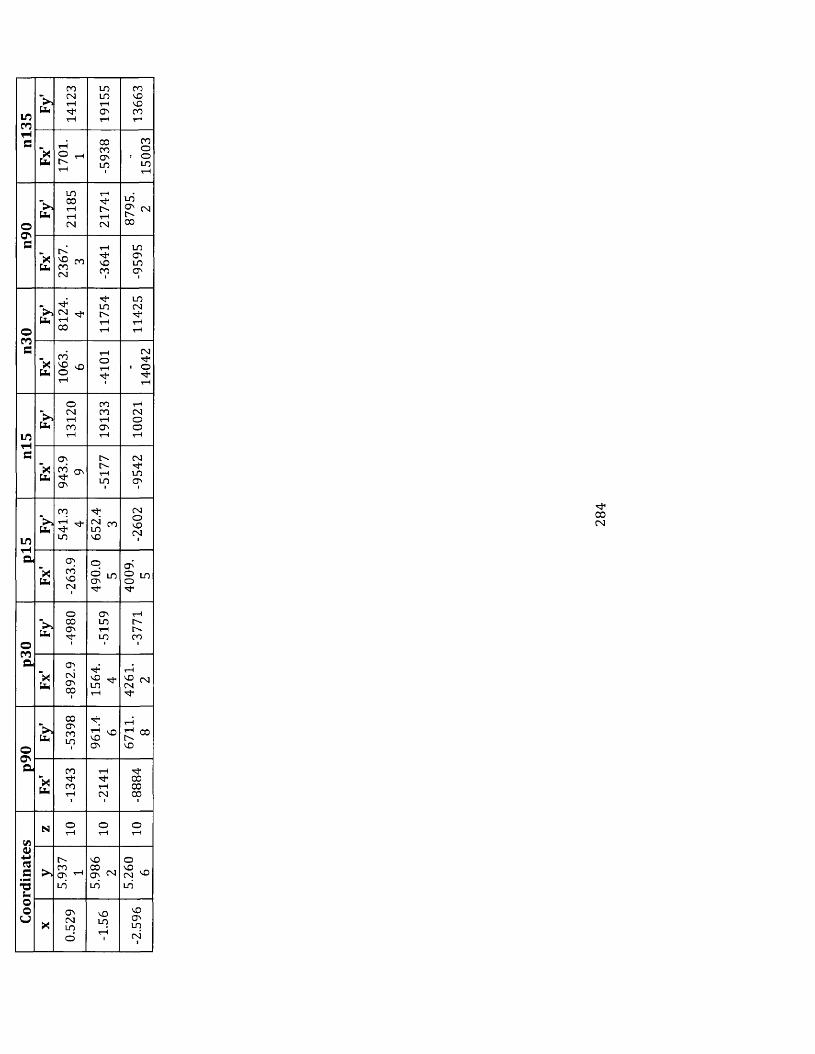
nl3

5

b

1412

3

1915

5

1366

3"xb 17

01.

1

-593

8

1500

3

oO 's

"►»b

2118

5

2174

1

8795

.2

"xb CM -364

1

-959

5

©V,b 81

24.

4

1175

4

1142

5

COc

"xb

98901 -4

101

1404

2

un

"►»b

1312

0

1913

3

1002

1

£3“xb 94

3.9

9

-517

7

-954

2

inrHa

v»b 541.

34

652.

43

-260

2

‘xb

-263

.9

490.

05

4009

.5

o>>b -4

980

-515

9

-377

1

ma

‘xb

-892

.9

1564

.4

4261

.2

o©a

“>»b -539

8 9V

I96 6711

.8

‘xb -134

3

-214

1 00COCO1

Coo

rdin

ates

N OrH orH orH

>»

5.93

71 Z

986S

5.26

06

X

0.52

9

-1.5

6

-2.5

96

00CN

Appendix F: Further Investigation into the differences

between model type A & B in Chapter 3

As detailed in section 3.7.1 two methods of continuous size optimisation were

carried out on the VAWT housing. They were:

Model Type A. where

i] Constraints screening was used by default

ii] Stress responses were defined by property and

iii] 15 modes of buckling were calculated by default

and Model Type B

i] Constraints screening was turned off

ii] Stress responses were defined by element and

iii] Only one mode of buckling was calculated by default

In order to gain further insight into the implications of making these changes to

the optim isation problem some further study on a simple model were

undertaken. This investigation used a ten bar planar truss w ith both of the

above model types.

The structure used was sim ilar to that described in section 4.2.1, though for this

application circular hollow sections were used instead of solid rods to more

closely match the size optim isation of the VAWT housing. The truss

optimisation was subject to stress and displacement constraints as before, but

also a buckling constraint on each member (see equation 3-16] and self-weight.

A global search method using 20 starting points was used for each of the

methods above. It was also found that unlike the VAWT housing model o f

Chapter 3 it was possible to define stress responses either by element or by

property and exactly the same results were found w ith each, i.e. Type A as

described above converged to the same 20 solutions as Type A w ith the stresses

defined by element. The same was true of the two Type B models. It seems likely

that w ith the VAWT housing optimisation there exists an upper lim it on the

285

number of properties values that can be selected in the Optistruct software. No

further w ork has been undertaken to determine this threshold.

11000 _10000

9000 8000 7000 6000 5000 4000 3000 2 0 0 0

ai/it/iro

"O<vi/i

o.O ¥ * x

0

a)

1 0

Starting Point15

* — ¥

2 0

60 50

tog 4 0 S 30

| 2 0

1 0

0

b)

x * » %

o 1 0

Starting Point15 2 0

X Type A #TypeB

Figure F-0-1: Comparison of the global search size optimised solutions

found using model types A and B

Figure F-0-1 a] compares the feasible solutions found w ith 20 different starting

points for model types A and B. The best global solution found was a mass of

2347kg at starting point 12 for type A and unlike the VAWT housing models a

lower optimum of 2324kg was found w ith model type B from starting point 13.

In about 75% of the starting points the solutions found by the two methods are

w ith in +10% of the other. Some extremes can be seen, e.g. starting point 11,

286

where the mass found by the type B model was more than four times as heavy

as the structure found using model type A.

Figure F-0-1 b) shows the num ber o f iterations required at each starting point

fo r the models to reach convergence. In the m a jo rity o f cases more iterative

steps were required by model type B than A. A closer analysis o f the

convergence curves o f starting point 11 sheds fu rthe r ligh t on this behaviour

(see Figure F-0-2). The two methods show the same trend in the objective

function up to and including iteration 3. At this po in t the type A model

increased the mass o f the structure whereas the type B model reduced it

in it ia lly and then gradually increased the function to eventually converge at

very high solution.

- * ♦ - Type A - ♦ - Type B

cots ~

2 (T»

O

80,000

70.000

60.000

50.000

40.000

30.000

2 0 .0 0 0

10,000

0 I — i— i— i— i— i— i— i— i— i— i— i— i— i— i— i— i— i— i— i0 1 2 3 4 5 6 7 8 9 10 11 12 13 14 15 16 17 18 19 20

Iteration No.

Figure F-0-2: Comparison o f f irs t 20 ite ra tions o f s ta rtin g po in t 11 for

models type A and B

A depiction o f the num ber o f the "most violated" constraints is shown in Figure

F-0-3 fo r the firs t 20 itera tions o f both models. It can be seen that fo r im de l

type A (Figure F-0-3 a)) all 15 modes of buckling were vio lated at itera tion two

as well as the displacement constraint. For model type B, w ith the constraints

screening o ff only a single mode of buckling was calculated and so only one

buckling v io la tion was identified (Figure F-0-3 b)). Model B was not able to

detect the true severity o f the vio lations because o f the single buckling mode

287

and so did not respond as effectively as model A. The same pattern can be seen

a t iterations 3-5 and 9. The more comprehensive in form ation available on

b uckling to model A enabled a convergent solution to be found in 17 iterations,

w h ile model B converged to the higher solution after 52 iterations.

-o

1614

<u15 12" 5 ain> C 10♦ *8 2

«-» 82 i/i

g 60 u

4oz 2

a )0

16T J 14V15 12-5 ^> £ 108 * 8

§ 64o

2 20

0 1

EJ Displacement

■ Buckling

\ m

1______ _____________________ |

I I ■

3 4 5 6 7 8 9I ! "1

10 11 12 13 14 15 16 17 18 19 20

Z Displacement

■ Buckling

b) 8 9 10 11 12 13 14 15 16 17 18 19 20Iteration No.

Figure F-0-3: The "m ost v io la ted ” contra in ts fo r the First 20 ite ra tions o f a)

model type A and b) m odel type B

For this 10 bar planar truss problem the "m ost vio lated" constraints were

p redom inantly buckling for all 20 starting points. The effects o f the stress

constraints on the optim isation were secondary to both buckling and

displacement violations. The influence o f tu rn ing the constraints screening on

o r o ff therefore, fo r this particu lar problem, had very litt le influence on the 240

stress constraints. As has been discussed above it was the associated buckling

mode calculation tha t had a bigger impact. This behavior is therefore problem

specific. For an optim isation problem where the vio la tion o f the stress

constraints dom inated it would be expected tha t the convergence would be

slower if constraints screening were removed as a greater num ber o f stress

calculations would have to be retained.

288

Appe

ndix

G:

Des

ign

Varia

bles

G

roup

ings

fo

r 20

0-ba

r tru

ss

exam

ple

in Ch

apte

r 4

Mem

ber

No.

146

153,

156

154,

155

1 57,

169

158,

168

159,

167

160,

166

161,

165

162,

164

163

vOI St-H

inI St-H

CNI SrHt-HI St-H

Gro

up

No.

73 74 75 76 77 78 79

08 81 82 83

Mem

ber

No.

102,

114

103,

113

104,

112

1 05,

111

106,

110

107,

109

108

115,

118

116,

117

119,

131

120,

130

Gro

up

No.

49

OS 51 5 2 53 54 55 56 57 58 59

Mem

ber

No.

46,5

2

47,5

1 oLDCO 49

57,5

8,61

,62

59,6

0

64,7

6 inI S

invO 66,7

4

67,7

3

68,7

2

Gro

up

No.

25 26 27 28 29 30 31 32 33 34 35

Mem

ber

No.

t-H

roCM t-H

in 6,16

7,15

8,14

9,13

10

,12 rHrH

18,2

5,56

,63,

94,1

01,1

32,

139,

170,

177

19,2

0,23

,24

Gro

up

No.

rH CM ro in vO IS CO O ' 10 11

289

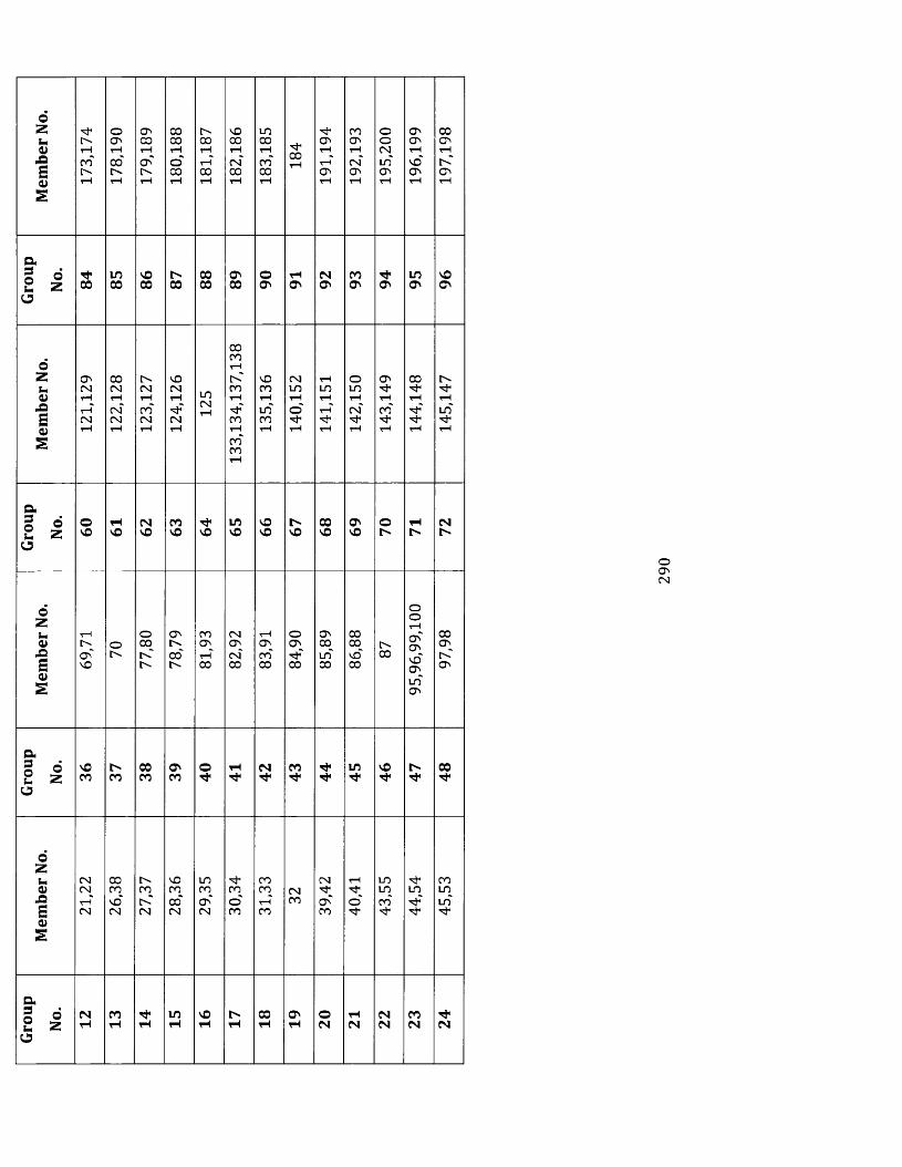
Mem

ber

No.

173,

174

178,

190

179,

189

180,

188

181,

187

182,

186

183,

185

184

191,

194

192,

193

195,

200

196,

199

197,

198

Gro

up

No.

84 in00

98 87 0000 89

06 91 92 93 94 95

96

Mem

ber

No.

121,

129

122,

128

123,

127

124,

126

125

0 0COT—1rCCOt-H

COt-Hco'COT—1

135,

136

140,

152

141,

151

142,

150

143,

149

144,

148

145,

147

Gro

up

No. 09 61 62 63 64 65

99 67

89 69 70 71 72

Mem

ber

No.

69,7

1

70

77,8

0

78,7

9

81,9

3

82,9

2

83,9

1

84,9

0

85,8

9

86,8

8

0 0

95,9

6,99

,100

97,9

8

Gro

up

No.

36 37 38 39 40 41 42 43 44 45 46 47 00

Mem

ber

No.

21,2

2

26,3

8

27,3

7

28,3

6

29,3

5

30,3

4

31,3

3

32

39,4

2

40,4

1

43,5

5

44,5

4

45,5

3

Gro

up

No.

12 13 14 15 16 17 18 19 20 21 22 23 24

oCNI

u3u

aox

eouc

W )

'55=5

CO

+ 305C/5

aO

eflu■MC/3Co

uueaOJc

'fio

2u

ao

T 3O

u

J 3

J2cc

SX

■ p N

T 3COaa<

ic o+3 <U G C.23 '-C.§ §■4—* S-a 43 o 3II Vi

GT G G O

< 2 +3

e S.2 X3 +-> ag °3 ' P<4_ 0 s" o '

Vi^OJ435

‘ u05>c

mCU O) T3 -C u- 4-> o

>> 4—*43 33GO)44054-JCO

« 05t 3 G OJD CL> C ^

■c ° 2 £ ’5 ° £ s - .£ 2

03Q

C/305CQ

• - t rG ojo aQJ O

£ T3a in

H

rS'-

C/3G O

G u O 03 u. G .O 03

44u

2

t 3 2 2 *

> o o?5 cu .— 3-

03 203 Vi

CC O

Vi

03C03

5 2 7 2C/3 >

2 t■ s «£ - •> G*= £ M u

"c/3 P<D 0 s

Qcu43

c/3CU . „

2 £’*"' 2 2 > OS ' 0303 a CG o4_J ^4

.5 G3 S-i 44

«& s

GO

2GOcu

2

CNo 't-H

C/30)GO*LO

oIIoX

LOCOp<4—LO0 0

o '<4-4LOCO

p ^<4—iLOCOpH '<4-4LOCOpP '<4-4LO000 s< -iLO00po '<4-4LOCOpP "<4—ILOCO

<4—cLO00pO '<4_LO00

COp<4—1LO00p<4—1LOCOp<4-4LOCOp<4-4LO0 0

p ^<4-4LO00pp '<4-4LOCOpo '<4-4LO0 0

LOCOr~r-

Vi4—4c’gu4-4c/3GOu3-iGCUc

oGP

G3crcu3-oG

G

r.a c.

II

COoo

t-HooCOooot-Hoc ac ooo

t-Hoc i

c oooot-HOOCOooCOt-HOoCOoo

t-HooCOooot-HOO

COooc qt-HOOCOOo

t-HooCOoo<ot-Hoo

T3GGO

433-4CUaaG

iT CT II CU CU

< 43 < 43

LOC3LOoLOoLO'oLOo’LO*oLOoLO'oLOoLO*©LOoLO*oLO*o’L0*oLOoLOoLOoLO*c >

LO*oLO*

© S§ " O 43

© G

3' g0 a1uo

’ Ccu

B434—*

oCUD

X4-4oa

< .

2 a

£ V ®*p 03 w-

a "c/3 ° 00 Gp fc

4->o

ao

291

g_o'GOhCDonOJwc/5CUOh

oooCN

DJD_U

"£ CNhG+-> O ^GO G(50 3

<Oh

3g CL,CD Oh

OJ3 Go OhOh 3a QQX23 G00

0)GOG

OOh

a .

uoo

G

GO

u

G<bcu>

w. I

<§>x f3XTcrQJXI&O)

<xT<o '>1c 'o

’■GJ33u13u

3

gGOuG

3£G'x

CDx:-McGO3 on

GonOh 3cu Oh

XS LO3 LOcu OJGcu 3X3+-> DCj>,3ocn.a3-t->GOO

" 5o '

0)

cGds

33 £

cu $ O diS ■§

O h

as . - +-»>—> as"O T3<G cu G o

o S(U I; aj<G >, >£ £ «CL a) G ii > £a 7i a

onon3

3 ^x ro

* 2 U rHon t+_ £ o

G 5/5 G </J

O 0/0 . 2 <->U ^G u,5 ^ ^

CNcooCN T—ICNonCTJCNt-H

CNCOoCNrH

G CN3 00 .3 O'

3 CN£ H3 ^

< 3

>>£■HonG0)33

o '

OOoCN

ox:Oh

CNOCN

(3J0c :O)

CN<

3<UOh

<1 3G_o

Gu<uLO

oOh

u

o

■'FT— I

o"F' Ft-H

O

■F1rHO

CN<

CNo '

CDa_3O>

3 r> *" O'St'S

fid

= fo

pen(

'Bas

ic

Dat

a',

'a');

%

open

a

file

for

outp

ut

cuG

X4—>o

<uGG

X4->O

Xi03X

XroX

fcUOG

cuo_Gc/3G

Xo3X

Xnj

Gv /£cu X cu-M03

X X X

03G03X

IX

GuE-*s-,

IIII 1X3 II o'a? ^S 5/3a S

£oib>__<CNCUXoG

oDJOGX

c Q o ^■m G1=1 u<U G CC QCU ^ CJ to 03

.S2 D Q ^ cu Ci^ c j<U 4->■r rt^ b<u hPd C/311 11

V© <u0 s J_

X,C/3

X

CUooG

x 1 u - 7 <u CQ X

1 X03 bX w o c

X OJ

15 £ ™rt 11 x X Q N X X -~^ 52 c£

xC/3

CU.W>

XC/3

XroooCN

XGO

XCNU

X X3£ cb CU

X X XC/3 g C/3 CO

i i ? S I f ^ m 0" r cn & u X oE 11 2 73-l_> C/3 G X

GL-HS-,03

X

II £ii s

Go * ’£ofe<UC>GCDOfXOjoc

2uGQQcu><u

QCUDGXcoGCD£

a o^ H G X £ O03 O Q G”vf 7 . iXcu G - , co QQ X . 1 XS - X

O . 03 X X w O G lo

CU

<UCC

OSCJ X X ■b X Xc/3 45 ^ II11 2 Ji bcu o<q r ■ o 4

b x £

<U.00

CU.00

X£

3

33

-3■Mo

-Q3

—3

tn3£3

-O

—3

C/0

35 -

Hs-.3

- 3

O

O'CN

mro

Q+23aC/5-l-JOJ

t|_ cII0 , t 3 £ C£ j CD

r - * \ 3Q 3+j

3 3o

£v___ ! 'S T3

CNQ4_>

C/5+ - i £ 5-h

■)-j 33 +-»

5-iC/5II £

M-m11 3 > 3a , -33 M C/1

O£■M II

C/5WCQ £

3O)£3

* 3,3u3CDS_

£C/5CDC/5C/5CDS-H•Mt/2

3O>CD>3

3cC

C/5 Q - <DC/5 Eon W 3 i_

C/0

3Q

C/5S-HCDC/5

-- D

CNt-H 3v—/ CJ

C/5 5-io ■>-J£ ^5CD II N 1)II F2

S — > 2

H0 -iOo3

3 >CQ|

3 S n <D O^ 3

CD8 a f > ?

iS <2 *H.11

o B >-cn +5 ^

CNCN

C/5

.C/5

. t3 3

_3-Q 3 O

3* rvi „ \ , 3* cn) C/5 £ 5 ^-- f \ j 4_i 3 -M>> th 3 ^* - • • .30 H ! i(D H ^ 3 'T '> || II ^0 c lqj 11 a u z r3 -* £ 11 ^c/d s_ j-> cr

<L = <2v O

» . > ■ *CD

Q

+j

H—i3C/5o

OV

3O

U5—33

_ 3

3O

\ r Nf Nr0 s* c-T*'*

33O '<uJ-.3CU3i

oo3

aC/5

- a

CNCUT30 31

00oLDoo

CN

00cu

CO

>sOQ

CNcu

CNCNr - tCO115-

, P

CN CN

CN t-H

c n 3 CO S CN £ >H II O

CT ll CQ IIS'

cu G cu u

s>I00cu

coIII

c<2*E—cuOo3

I

"o 'JHcc

E(U

I f >4-h

CU 3t u •—cu C/54-> 33 oT 3O h V5

D I3(U

4—*C/5 E

x7 T C/5>4-1 (U3 bOO 3

3Tju X3 u

>H "5

<_> .v“ 3 'a.CQ OJ u3 pg JO co

2o

"s

cuooc

J tf 'cu3

OQI

u,3JO

O

b 03

X3CUU,u,

.O

G

£CU

3o>cuu,CUc/53

. . CJ r -r CU“u o

bJD3

cu33TOc3

>>CUOCJ

££HCUoO3

lXu3

00I

u3JOO

XS

33O hO

T3

£,(U

n :fV>

££

cuOo3

X 1u3CQJ332

o

33O h

£IIX

e£.3

coHCJwcoS<UJCQ>4—Oc

'5bcuXo

4-1

3£o

XT3335-

295

c'CD.

T 3C

vO

vOCTvCN

s- uQJ cu-G Gl-4-1 4-»O oG c03 03 -t-»

T 3nJ T 303

C/3S-cu-4-1u

sCUu, CU

S_u’C

0s --"\t-H

O' 033-h03

cu£

jGt-H

t-HjG,

.GUo■u

3G1G

~s- t-H “s-. C OGcu-i-i p . cu-4-1 -i-» CUV._J 4-1 .G

6S-H-M 1 ■4—1to ’a cu

0) CN ra3 00 cuIP £ 2° o '

cuT“H g rH -pO'

0) CN

F-hCuOoc

CQI

s~03XO

03ujO

X 3SX_o0J

301

Bcu

U - i

cuoo£

I

u3CQ

!l_03X2O

c V_1c'x

CNc V_•<cX+

■SX. aOJ

<u

5-i C<u•ti <+*C LDx odId vP T3 o 'M-hrH Ln

“w °P

“ c/5T3 no

,<D •-=-

c ^01 73 U x: c/s j—•

J_ ) <4—I

x £_ 0) cT3 -m

5 O i^ 'ga>

L-J L-M <u v£jC/3 -M^ 'c +-1 3 C c/5 U 3 M u o c£ 1 ° §

o ' c/3

72 ^S 72sS E . ii i 0) / Nc c 72 z?# ‘tJ £ Ex ss ^£} U t i t l iii <u a>r v T 3 c/5 Cfl a C O O

O) Tj u

CNIN

C/5

C05WCX

03XC/3

T33U

o}iX)C

?c3

oXCU a.

r j 0J_ 4_JX. A

297

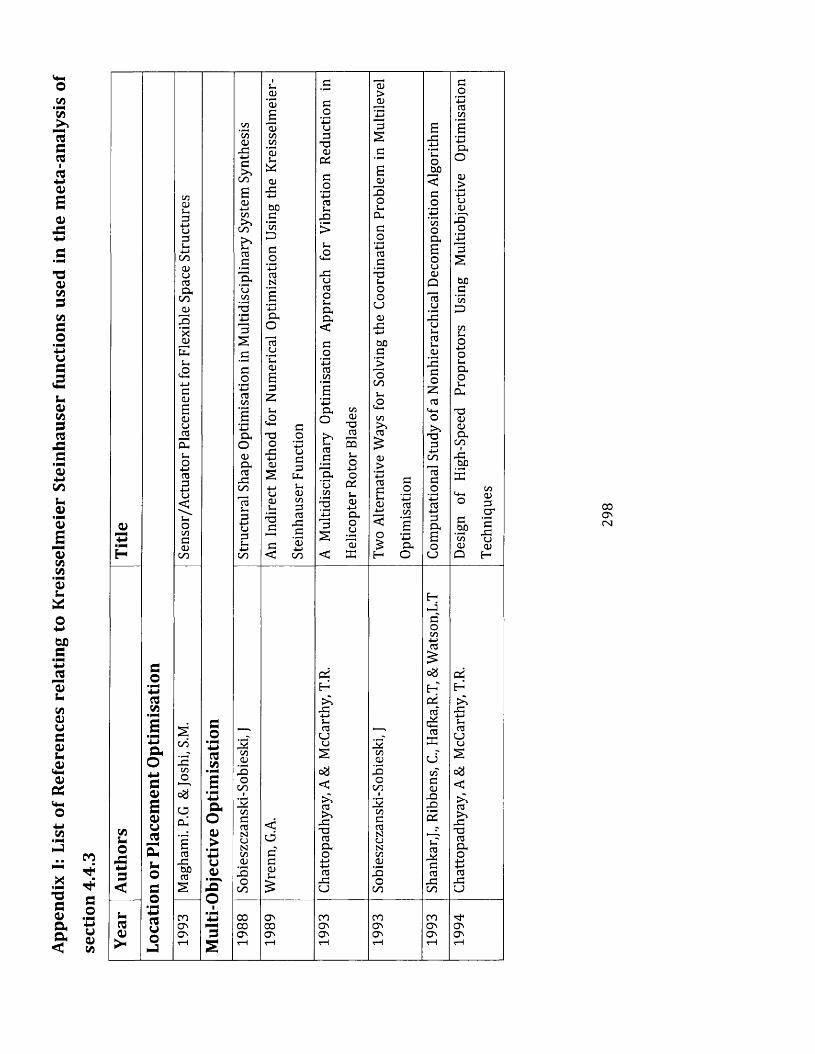
Appe

ndix

I:

List

of

Refe

renc

es

rela

ting

to K

reis

selm

eier

St

einh

ause

r fu

nctio

ns

used

in

the

met

a-an

alys

is

of

sect

ion

4.4.

3

0)

H

t/3uOX4-*3<

3O3VJ

ao■Mf l0)£O)uiS£s-o3O

-M

uonJ

coCDS-i34->u

(-14—*coCDuasCD

co(D

u>O

4—>0334->CJ<s_oto3(DCO

COIS

COO

aal

Sas

pbJD03

3O■■4-M

C/3

ao.>ua>' £o

COCD

p4—I3>,

C/3

a>4-> CO >,co5-, OS 3

CDoCDCD03

pCO

*03S-h34-> CJ35-h 4->CO

CDCOCO

'cDS-H

CDP4->

OJD3'coP3op03N

Oho_cjpCDS32S-H

PO

X-i->a>

CJCDS-H

p

o<

c_op

c j

33

t uS-H(DCO33PC'54->C/D

3OPu3PCD023OP3UP

PCJ3OUiCDCD<3OP3co

CDO CDPJHsD-o■4—*o02UCD

4->CDOu

'a;P

C2

H>>P+->s-3

CJcj

C#

<3>,PP3CDO

4->4->3PCJ

<D

PODh

cu3OP3CPuOOCJ<DP4->

CUD3

OCOu ,

£CO>>3

O P£ O hH O

sp■4-JPoCUD<3OPcoOCDSoUCDQ13upuS-H3S-HCD

P3O23

t(-HO>>P3

4-*CO

133_o

piS3CDEoCJ

E-p3“O

o #

H02of£3PCJto3CD

pp5s-3

P33PCO

CDoCD>PCJCD

PO

3sCUD3coPCOS-ho4->o5-HCDOS-H

CU

PCDCDCD

COi

PCUD

3COcoCDO

02HP4-J5-H3

CJCJ

0#<3

PP3CDOP3PCJ

CD3O '

3PCJCDH

00

CN

H

PCUCUa

COI

a00

COCm

O4-J0Cm1

aocm

a

3M

cocuQOJa

4—>

5-H

£CUCm3PCUUOCm

a

co

P303

- f r

mQ03

4-»CO

CO

- 23oCm

CU<CUCJ303

eC m

£Cm

CUa

003

a3Ocj

a >a4->

003

"33

33.3 -MM Cm

aO3<

3

-S2’3Cm

CJ

aocu>

pcjcu33

O

CU3CT3

3 3ucuH003

3CU33

<PCU

4->

- 23E

CO

CO3Cm

34->CJ3Cm4—*CO4-13CUoocu4->

< £

ao3

.5 P"co3

Q4->3cu

a

Cm

aCUCm

3X3cuUOc-a3O

OaEoCJcu

Q3>cu

cuPras

C m

o4->O

ac*cu

4->aou

3P

300coCUT3cu

334->

C m

£CUCm

3X !CUcjOCma3o

aO

cuCm

34-1CJ3Cm

4->CO

OCm4->3O

CJ

0 3

3 m3O

CJ

COCm

o4->033

4-JCJ<CJ

u0 )

3oNCU

a33

CO

s03cuCQXoCQcu4->COOa£oCJ003P034-*oa

003

33

03<uaCm

£CUCm

3”3(Uc jOCma3o

ao(U>PCJcu^

ao

03C |_

O

4-J3cuEa

jO3>cuQ

<u4-J

3a<u

oao

c j

3_ o

P033E

3<u

Qcu0 0

Pw

JU

3oCma

>>CO

cu33

003

oCO

Cm

o00

3<

30P03CO

1paO

03cu3a

CO

3300

aO

0 03

Cm

o4-Joa

03-2a3oCJ

a03CmCJCm

< <

w

co3 C O . 2

ao

<Ua03

33CO

cu_ >pCJ<U

S 'o

3

033OCJ0 03P03O

J

- 2' E m

003p<UPco3OCJ

COS-Io

■MP

<

3cuPP03

o 3

a

> ;334->Cm

3CJCJ

0 3

<> ;

> ,33p03aoP03

33CJ

wCJ> ,

Scucu

CO

<03>>

33P03aoP03

33CJ

_ap" 30 003a

a

H

>>33+->Cm

03CJc j

S

>>03> ,

33P03ao

4->4-J03

33CJ

wc j> ,

- 23cu

CO

<03

33P03aoP03

33CJ

CO

N4-J

’ S0 0cpa

<03>>

33P03ao4-J4-J03

33CJ

aCO

.230

CO1

aCO303NuNCO

23o

CO

o 3

a0 03

03a

>»3>»

ap3aoP3

aCJ

a

> ;a4-JCm

3CJCJ

3Cm

3a3

CO

o 3

X

e300cuN<

3PO

aCO

S-I

OSo c

LD

o c

LDOc<Jc

LDO '

coO '

COacoc

29

9

03>

3p

05

CJOJP

03>

JU

>NS-05P

CO03

x s

b05

re<4-1oc

cuXcus-

C/3P

± J

X3

2

3oCO

3303

’ c jCO

W)’co03

d u

E

05S-HCJ i s

X

C

Xi s‘Dj

Q

X 3o

c j

CUD<X3

an

d 32

s-p

H32

re-SP7)

03>Os-

C O) s-C/305 S-H O) DX

3XC/303

X3

03DU

C/51

XCUD

03U,P

Xa

3

cupS '

a

_033

< 2

O)

. 2

a

1U.

E

S-H

2

2 £CJo £

0CJ

13 <

03S-i

s Uh X X 03 re

5-o■l-J

£

03

DU c j03

H

£ u03

H

re

Xs-

X 303uo

oDcS4-J

H

S-

X 503CJO

CO’ co

3DS

p_ oX05

_N

<4—OPo4U

po+JreN

reE-CO03

a

S-HDU

re_ oX

<4-1 on03

s- < f-H re (H s- reo DU P N E 2 N

po

P. S '

PO

I T

XDU

o|+J

’■HDU

o

reo

EX

X E X DU 'P DU05

_N Xcu03

as_Nrn

_>x

03>

OP

03>

03_N O

res H E CO

cXCJ M u E . S 3

4-J CD 4-J 03 . £ , ’co 0) X ’ coDU

O_C DU

o0 0 x 1

o

O)Q X s

o

DUO

03Q

b31 f < b

iX b

1b b

05 05 as S3 re re 03re o C u o D5 c re _ c _C

2§

X 2 23 , 03 3 , CO

O3 , 3 , 3 ,

u 4-J u 3 X 3 " u X5 u ’ uCO on oo e a ,

£

03 CO 03 CO CO

QJ i sO

i s< ■

CJ£0 p

i sCJc re

i s i sX DU ‘X o 05 CUD 03 bJD ’X X

x■ PNH

3

2

Eo

u 2

£03

C/5

u03

Q

XC

DQ

’co03

Q

3

2

Xre

w

’ co03

Qre

2

3

2

2 <c A

on 05 <05 > , < < < 2

X J X >>-S , X re >> > >"o5DCS

05 05 >» 05 03 CODU >N X 03O X T 3 X X X

o 2 4-J x s 05 X 3 X5 03t ! 05 DU 05 re S '

DtS 05 DU O DU DX DiSX o 4-J o o

E-< CJ 4-J4-J

4-J05 4-J

4-J4-J4-J

> ;C-|

o # 05X

XCJ

reX

reX <

4-J£- 2 C J

o 3CJ C J

05 - X o 3 c # 05CJ 2u

2

<

C/3as

X.as,’ S 'DiS

<DC

£P^

COre

X

<DtS

> ,s-P^

2

COre

0 3re

Xx s05DUOt l

as> ,

X !2 '

2

’ S 'PC

2 ~’ S 'DCS

03XCJ

C/5U

X 305 ‘X

DUcn C/5 C/5

oJ 3

DUO4-J is

CO05

X3

C/5

re

CO05

X5

C/5

re

C/5

re■M3

4-J05

05CUD • S , • S , - b b

X 05 'as 3 ’ re 3 3< CJ Oh DCS H DC H E -1

5 - I ' '* 0 0 0 0 05 o o CN]cd 0 5 O ' Q5 0 5 o o o0 ) CJ3 O '1 0 5 0 5 o o o

> ▼H T—1 T—I rH CN] CN] CN]

axsJ2scupx(-1reE-C/3asCjXScuoo

C J

XSS3054->aCUCJreocj4 -Jreo>105XXOOQCUDP

05CUD.£'c/3XPoXasC/3

CUOCUDp

iEbasP

P

2

CUX JO

cocoCUpXcj2E-_u’u4-Jcu£05s-iasCu05

5-CUCUDP

3Oa:

tucubP

1/3C/3CU

5

XCU

E£

2

CN5ooCNS

ooro

QJx

H

oDU£ocj03>XDUrexs<d

X03DU£reQ

03>c/5COrecu

DUO

xsreret>o.£3xo

S-I03DOS303coCOrecureS-Ho

re03£035-3cr03CD

reS-H

XH

£re£

S303£03

_S-H

recr03CDreDOCO03Q

£rere>,xo$-03<3cj

Xures-cuDO_c'coXS3_o

XreCO

a ,0

1s-<

03DOrereQ_033uCO

reox03COreCQ0)DOre+->c/5

XUreS-H

cj

03reDO

Xretu

reo2034-J

XCJ

xrereCO03S-Hrerex 1on4-JCOre03

DOS3>o

coreX

CJo4-JC/5

3CJ

XC J5-HreS-H03

S3_ocorerea,xCJcoOreXcj

oreb3cu

DUoDOS3

03X22C U

s-2xoX4 -J0324 -Jre'o^

DOc"co3

DOre

S3OcoS-H03DUreCO

£ £DUO

s-rtre

x re reCO S-Hre DU co

X s-du reu £X 32 >3 E

2 u

s-re03_re

3o2X23 ,reoCJreDOre3XreDO303a

oaoE-

3£xDUO

reDO

asxo03DOre£rearererexreoCJ

S-H

2

cuoS3DO303Q<

XrerereDOCO03a

DUo5>sS-Hrere

reuCO■03DOS-Hre

reoxreS-H03DUO

S-HODUcorereS-H

E-1

re

DUO

03X

XDOX X

oDU

</JUo

pC4-»X

rexXreDUo4-J4->reXCJo3

CU2

x"DO5-HreXS3S-HO X E-h

DODOreNo3

QQre "oxCSJ

033oreCQ

re>»xXreDUo

4-J4-JreXCJc3cJorex

xs-re

S-,03x303Qo3

<Xreo£reaefs-T03XS-Hrecj

_re'£reDUre

' £re

o?j

dre£S303

OJ>-

CN

DOa

x05o

222

£re03

XreXre03

0303CU

C/5

£re2Grere

CJre-Oreo

x03recu03DO05

£05

Q03reDO

X05Cu

Xre05

COre_ox2re£reoCu

_re

' o

x<XDOreore

XE -

re_oX05N

CUO

coCO03Uore

CU

£05re> ,

Q

reoX05DO03reDODO<

05rerecoreoCJ

reDO

'co03

Q

0)CJore

CU

3

£xcuo

05rer ecoreoCJ

oco

orer ereo

c j03>

X03re

Cu3Xo

co05Cu

COX

03re

H ,COI

DC03r e. 2're05>

'reHDOreXc jrererecoreo

ure

2xc j05OreCUCU<reoxosN

CUore<

CO

£2xore

CU

reox03N

CUo03CU05

XC/5X03

OC/5

3CJ

're03

£rez

re03

£03CJ

2B uCO

QXre05COCO03rer eC/5

£re

£x05

OreDOCO03

Q

X03£

£'reE-D0re

3X

CO03rerereurere

03XC/5

CUo

reoX05

X

c j're

03

£ o

DO Cu O X 2 Z

CO03U

2 <4—Irere

C/5inCQ

COCO03rer emre

203rerer eCJrere

03Xi n<reoreDO'co03

Q

£re

2■0303re

DU

3£xcu

o

Viuo

- C■M3

<

rea ;

XovsVi

aoO

2

x05X

XX05CUOt iOSXCJ

C/5

£re05

Xo

CJ

o're

X

cn

oCN

C_ o+3c tVi

aoViViuore

Oh

X

re03COCO03

XU

C/5

o 3

re23b03

£

DU

X

OQ

0 50 5O '

E-Xre'03DO03

£

o 3

c j

>»03reoo

DC

CNOoCN

coXre05

Xu

CO

oCN

Xo■ PH

x

Vi

aoa>ax

m

xre'05

'&C#

X

DOre05

oCN

E-£rere

x05

C/5

< 3

£05DO03N

<

05XO

XC/5

0 0O'0 5

re03rexc jre

o 3

X

X

re03DOre

QQ

re03DOre03Xre034->3reQQ

cn

oCN

rexo 3

05XO

£xC/5

05rerex03reo

>«

CO

oCN

CNOcn

Tit

le

Para

met

er

Free

Sh

ape

and

Thic

knes

s O

ptim

isat

ion

Con

side

ring

Stre

ss

Res

pons

e

Con

stra

ined

O

ptim

izat

ion

of Na

celle

Sh

apes

in

Eule

r Flo

w Us

ing

Sem

i-

anal

ytic

al S

ensi

tivity

A

naly

sis

Hig

h-Fi

delit

y A

eros

truc

tura

l De

sign

Opt

imiz

atio

n of

a Su

pers

onic

B

usin

ess

Jet

S3o■ Nc«C/3■ PNS'5a

An

Opt

imal

ity

Crit

eria

Ba

sed

Met

hod

for

Dis

cret

e De

sign

Opt

imis

atio

n

taki

ng

into

Acc

ount

Bui

ldab

ility

C

onst

rain

ts

Opt

imal

ity

Crit

eria

M

etho

ds

Using

K-S

Fu

nctio

ns

1 Effi

cien

t st

ruct

ural

op

timiz

atio

n for

m

ultip

le

load

case

s us

ing

Adj

oint

| sen

sitiv

ities

An

Adap

tive

Appr

oach

to

Con

stra

int

Agg

rega

tion

usin

g A

djoi

nt

Sen

sitiv

ity

Ana

lysi

s

£O£C/3

abao6jo

Some

As

pect

s of

the

Gen

esis

of S

truct

ures

Au

tho

rs

Arn

out,

S, Fi

rl, M

. &

Ble

tzin

ger,

K.U.

Lam

bert,

P.A

, Le

cord

ix,

J.L.

& B

raib

ant,

V.

Mar

tins,

J.R

.R.A

, A

lons

o, J

,J, &

Reu

ther

, J.J

.i i 1

Sch

even

els,

M,

McG

inn,

S,

Rol

vink

, A.

& C

oend

ers,

J- CHAN

G,

K.J.

Akg

un,

MA;

Haf

tka,

RT;

Wu,

KC;

Wal

sh,

JL;

Gar

celo

n, J

H

Poon

, N.

M.

K.&

Mar

tins,

J. R

. R.

A.

Mle

jnek

, H.

P.

Ou CN LD o •'f CN t-H o CNT—1 cn o a> T—1 cn O o O'a> o o N O cn O o o cn> CM T—1 CN C/5 CN t-H CN CN H tH

303

cdcla3

X!C/3

T3g03

GOPG

P4->005

03£pCLo

X!u03OOhaCL

<to

PO)cuG'5bG

w

c<

00C

*3_Gi£

CLO

&ooCLO

H

GOP03C_)aCL<a)>Po£o■MG<

CLo>*ooo'oCLO

T3CDto03

OQtotooOh

•4—*C/3

C/3

03UO—3

COCUOh

G4->c_>GOh

4->C/3

£GGGPGO

U

CLO

53o'oCLO

H

03Oh

4—*COGO

CD

GPJOO

o3GCJO

P

toCDOh

G4->CJGOh

4->on

G

CLo

oO co CL G O O

H CD

£GG0^

QG00G

toCDtoG

UT3GOP

a ,

CLo

o'oCLOE-1GOh

G4->uGOh

4-»C/3

CDG_crGpuCDE-GOPG00CDOh

0000<

CLO

oCLOE-

GOh

4->COGO

CDcoCOCDOh

GOPG00<DOh

0000<MuO

DQ on

o' o'0- _0-’£CD CD

4-1 4->to COG GCD CDo3 o#p PCO to'G G_G _G3 3GO

GO

'o 'oCD CD

CL CL

g' g'a GP POh Oh

G G> >G G2 2PC ■Pto COP P

Pa

M. G —4

CL 2

GOh

4—*COGO

CDcoCO<DOh

GCD

£CD>OOh

CL£

£JDpoOh

CLGOPGco

CLo

p5T3GGcoOh

GCL

C/3Oh

G<D

_G

1G

CD00

_G’coDGOPGto

O ho4—1P00

Xo

CQ00G

C/33-o■*-»3<uftaj

DCOh'CD

PuG£OhOh

Puono3CL

XP"CDG"o7CD

CO CJ3 O '

CDT3GG

PG

PC_Jo3

DC00GG

><

oO0303

CDG~CD

PCJo3

DC00GG

>*

0303

CDOCO

T3GCD

CDo3

X_Gto> ,G

Q

000 30 3

DCGGGCLGLC

06CQon

’ £G

oCNJ

oCO

Viuo■M3

Sm

V

OSc jo

nJ

a,O

60

oaoE-S-H

£T3O434->CUsd_o'3rebi30)s-,fcuDW)<

T3<UUC03,CCCUd<

Mt)2)C03S*Jo3

bfidos

Od

cooCM

doucoCOcus-

doT3(UCO03CQ

T3O43•M<U

CO

5-icudcucuu

r 03 tl—IS-,cu

£ '3•C3 cjcu cli

O 03bX)

63 -So'ocuoH

< J3

cos03cuDQ

cu

OCU

BOu

03cu03d

S03JJ

■J3 CCUo63ocuoH

' r e

‘C<u-Mr e

a

cudcrCO

3

oCN

COdoCJ>,ud<udCTcu£dcu.£Pcu

di 43 d .13

305

co o'vP

Hn

CflU•Muoaa3

5 / 5

s-uc/i32CS■Mrt

x• PNT3SOaa<

f-V"'

CU s P 733 O' t*_ vO<s (S'2 NO

oCJ ^

! *a, np ss o' Un >gS _ O '

O ^CU s P a, o'3on154->oE-E3oX3cjC.3

CD

eJ3O>■4—*uocucucsCO154-4O4-4cu ,

£ ■cu 24-4 ■—ias a £ ^■s ss j u < 2 W> ^ .£ Q- u

S3

>,o03S-,S3uu03

Xcu4->5-,cu>33c j03CU

(D S-i > 2 £ ^ a SPe G£ 03

.a 32 £ 3 ~c jT3 cu ro CU ' o

r ' <u

rN

S-ic jon3303-J+-J032

T3T3

CU3-’3crcu5-4

•B £ DQCJ++03

_3O >Co03 CU co

2 JD

QO ■— x3

o 33 > 03

0 s*

33OX)’5333

j= « " ISg X)ccs 75£ c oo o-Q .a« o£ ^ O) cu

33 33£ £ro ® rc

a o ^3 CO v Pco S— o 'a ; 2 ^d CJ Np

034— vOU.33 nP5 - o '

a ^B £§ ^tuD vp33

T3CU

£5-<U

S-,O

CU$-.03CU334->

CO

CQ

bX)£3

2c j<U33cj2Oo>—3ocuZCU334-45-i O

o ^■a ^cu p SG o'TO sOX3 o'"4-Jrl °s ^E ^£ J

(U qs-o 0s

Ou,-Mccuu

o' -O 0s 'P 0s N? ■M 0sS— p

O O '

on po'

CO

15a5—ioC3X3£303coajcjEcu>CO — Icuu ^ 03 ,_, *M“l <1) 4->xs — 03C ^ 33 33 ^

_ S-, COP 03 3 £ 3 CJ

.3 3 <d

H - '---- ' ^

j T3 'P co 03 <U OJ 33 i

CU

S iO

S°o ' NpO ' 'Po ' 'Po ' o ' 'po ' 'po ' 'Po ' 'Po ' o ' 'Po ' 'Po 'o ' o ' 'Po ' N°o ' 'Po ' o ' o ' -pos' 'Po ' o ' 'Po ' -po 'o ' o ' 'po ' o ' 'po ' O ' o ' o ' o ' O ' o ' -po '

i j nj£ So «2.£ 03 w u, X)

x<U ?

334—>roCUin

CQ<- JE—< 1ITS 3333O 1

4-4 <uo 713S3 Cl—i

CO CU33CU 4->

——OCC3 4-4cu 33334—i

4-403Ct_ CU"d S3S3 Cl—

S3 CUo 33

<4_ 4->4-4O33

MU1U

- CU~co CUN po '

COO■“ 4-4cu a>733 S-i

CLh S33__ , CO— j cuS-IO 33S-4 _ -S-i

CU

£CU■Mo3 3

co

3*3uCU33cjXJ3303j>NS3O■a03cuu

CC cu

COS3cu ^Ou^ O T3

^ srA »-io> U.

c u CU

33(U CUo S2 cu co

CO

03

£uoS3o3

COCUus_cu>incucjCt—Io+->_cco

00 ^.S &

X 33 3(U

I

u.oUiu.cu4->CO

£3' i5-ioS-i

CU Xccu

c o4->C’£

T 3 .3 3

<G - Q

X 3030)

,S -i

VOOon

X3<uS-i

’£ cr <u 03 <u £

'o > 4->s- o cu cu3tun<u4->

f S3 JS33u03CJ

CN

s-h*co

CNc nI$-1

*co

S-H*roS+t— \cnCN

uc j

,03U—I

43c j0303S-i

£c/30ODCH2wcg

-£23c j

"reu

03_GT3u01oc j

0'o3-i4->GCUu0)c j

.H3

co to CO

* * * CO CO CO

H N CO

CO CO CO

> > + +

,43, CO

^ 6 G ^>>— I C/303 o N 3-

O) NC/3

rH CN CO CN CN CN

* * * CO CO CO

s s sH H ( N CO

tH U <-3 Uo

Norv«

OS

ES-hoG60G

C_)<u

43u> ,X4->j-OC lO,GC/3

T303<UG

to0)CJ

L-hS-hGCO

43CJ

>>

_oO

CGcuc j

osX

COs-T

*CO

CNi3-i

*CO

CNS-T*

CO

CNi3-h

*CO

COa>cuS-,boa>

oG

cuco co

03 Xos

3- 43C ^ G u£ cG .> u4-1 G 03 co 60 CU G60 Gn G

T3 : G ' ns

3-hGO

- “ 60

O « 60

■G GJ— C8

COG8 O^ CUG O O 00

4*uaj43u-P

T3GCU r-N

3-h

O g .JL §■5- G O C/3

13 G o

C/3 E -1

COCN

CO

II 43S-H U

S S

“bo _ - G5—t-5 £o gdcu 3 60 cj T3 03 W X

LOCOs-T

5—1

oc g<ucjre

IX

COs-T*

CO

CN

CO

CNs-T

*CO

CN■3-h

*CO

- : botH 4 4 -

CO_J>I

/— \ CN S-T

* CO

*CO

S '+

CNs-T

*CO

sI

CN

CO

X5 CN— r~\ I

2 3 *uG O O - >

*LDf t

< GO

'— ' LDG

s i_ ii k° x a-V XCO CU 60^ Ev i Cv3c re Go

coCN "J 1 G s-i O* "G CO O'—1 <g> CU

60 SG S-i

60 43£ w03 " CL

43bo

C/34-4GCU

X£<

CO3-T

o',11 II s_G ©

C/3 U0 03

E-* is

1 ^Q C/3

CUXtncuu

t l —I3-iGto> ,G03Qi3-h03CU3-h 03QJ C/3 f 03 42 4D

G : CU

X i -5 0 3 T3o g

N? N?Np vO c-v"* rv**

307

COs-T

CJVf—1

cn

CN* * cn cn

> > t- i cn

* * cn cn

V Vr —\ r—~ rH CNCN CNi i

*cn cn '_> >

II ur s.0

*

O).G-Mo>»

• ' G

sOe* 1

r T ^1 s-T 00 v—/ cu CJ ZZ

X £ ^ cG ^ O U 00 .52

JZ O J- > a S3 G bO■|| .sZ u O OJA ^ Z cjlI I vO

o '

S-ijQO

CJCUu03

a

cns-T*

cnCN■S-i*cn

CNs-T*

cnCN1

S-<*cn

• ■• v

z£ O

-2 o3 _g o3w Vflj II

110 0 r—\ C tH03 '— * a Z

cnCZjU a ; A cn ^ X

UOJ

J-tG

00s_03cuZ

S-iG

onoE- 1

QvO-iS-iG

onS-i03cuZ

M -

t 3 •_ .

2 -1 33 O O - 0 0 ^

S-I*cn

-u 0- O * 33

£ .< 3> O)^ 00rC -Q£ w03 "a

00 - ' g00 cu

.2 b t i <z> zz +->bO G ■re <u

T3GCU T5

§ "G

s-O■MCJreS-i4-*

G>G

on*cn

S-i*cnX+cn

S- 4->•#* S-Hc n o> a

X ^cn ^CN -M

1 S—is-i O* a 00 e£> ^^ on

re o CQ E? re "<U £

^ aB |s-i G o on2 1 ^ a -m

~ P o _<u on E-1 ^

cu

00ocn

o>-t-1 ^ ^ S - 4-1o s-ia 2 a Ohg a

G ! on13

on

■§ a

CU 00 03

O P H :=

'— ’ '■— ■' V >a a in „ .52 .52 '>< o r e r e r t

oE-

xlab

el('x

-axi

s');

yl

abel

('y-a

xis'

);

zlab

el('z

-axi

s');

vi

ew([-

135

35])

;

T3G0)s-

T3 03 <U 06

_ ] H on4->cO)■MG0 c j

5-HCUXOSOJs_1

cu03

OCNCN

CO QJ£ w> g c 5 gC_J X!

c jCQ X <*E-1 X < >

s_CU £M g£ U G x i

cC x

wU-NII oX . C/3QJ

u x

n n ii ix > 2

s->OCu■MUcuU.S-,oc jGT3GCUs_

. CQ ^ <£ ® 3V H/■—' <c 2 2

■5 ^CO OC fcoj a

Hco: >, ■ S-h

^ G 03 XP X

G

CUT 303CU

X!

CUBOUG

OS-,CUXl6GGa)X4->00G&'c jcuOhC/3

s_CU00cu

GO-aC/3

BCU+J

o00

a>x

CNm-i->_G3

00 T—I 00

XGCU

CNrox0) c opC/3GGG GCU S-i GN* .

“ It-h O00 5/5 O DC/3 M -h CJ

P +-> Gt G I i

« « e# # c

GcjcuG.*II

00cuuGCu

XHC/3cG

- i - jGXO

G-MGT3OG3GCUS-HGC +3

v / C/3

3 m■§ 3•§ ° H73 II <2, 11 sCO C/3 “ ,03 aj ^riCJ u ^G G 5Cu tu

I s5 3£ 3

. . G3 faJ- G

-fa£ £ X Gcu

309

roco'0)u

. - CQ^ CxB SI =LD '—CO 2

S 2

ro.S' /----\to «y~ QJcj to TO qj CX ua £c 6* j2

2 2as cts

2 2

E— tx > 2

COa;cjas[X£3TOVT3

.h as o ojII *

T3 £TO 2 cu OG a) £ x3 > e >

Xo

u N a j ^ > > < ,

to x £ «

CSl >*><X QJ

X X CJ >

X !c o u XQj xj CO 4-1QJ <U

X X

N> -X ,

XQJ4-1XQJ>

X5x

OtHro

toQJX > .

X I o u o

qj a j x X

tuo CUD OJO OJO.£ .£ .£ .5S ' s s S’□ u "u uQJ OJ QJ QJ O h O h OX O h co to co to co co co co QJ QJ QJ QJ3 3 3 3 TO TO TO TO > > > > C O C O

.2 .2 .2 .2co ’co ’ co COu u u ‘u a j a j q j q j x x x xO h O h O h O h

QJ QJ QJ QJ bO W ) QO M C C C G

’ co ’co ’ to "co qj a j qj a jQJ QJ QJ QJ X X X XX X X X H H E- H

CU +

r> TO2 - ^T 5 Q j • 'oj e HCO 2 I

o ? o § * 1/5

O o +£ S d^ II II

o ' O ' O ' O ' Cj ' O ' - h h . f h

CM

CM

COTOUQJO h

£

f—' r—\ r— \‘ qj ~QJ ‘ qj

CUD tuoC a a

’ co Ico CO

c— t— \ r -^M ' vO 0 0CM roro LOtH CM roX X XQJ QJ QJU CJ CJTO TO TOX X X

0 v__/ X JX X XCO CO COTO TO TOU CJ CJQJ QJ QJO h O O h> . >> >>X X XII II II

t-H CM ro> > >

m>CM>

0) QJ

x X 3 3 o o X xs

c >

QJX

QJCJ

,0 !Cl_iQJ

X4-1

XeTOcoQJUXXQJ>5:QJCQJCOQJ

X

QJXQJ

X£XTOOQJXTObJD

COCOXCJ

^QJ

OrH

c j +> XX TO

QJCTO G

t x COX

QJ OCUD IIX

_TO T 5

v pO '

OG

T3C

G*o n

T3JO

>

vlnd

2 =

vlnd

l +

3 -

CN]T3e

> rH

CM"C5C

,5 c c> c cv J v j

> u, 2

+T3nj

CDCeSscii

T3ns<DpeSac ^ c

CD

T3C<D

311

x p

O>4-4Uoaa3

5 2

4-4o

Haa

01

c-u

C/3pfire

j4-4re

£

£x

■ac0)aa<

q j

G3oG 0so #N vOv— J O '

O ^ > $

£ ^ s ^O h vPd 0 s

00 °o

5-o d „ d c G00

'rt4-Jo

HGO

'Xrfs>

G xP

Vp S- 0s TO

TO toU—I 1 ’—1o s- w 0) c ■*-> S «3 £TO 4_» s-

o 'o '

oXJT3Gro

Goon xpG ^.2 ^ 4 -4 s Pro o'J— vP 04 O'

- 3 ^

x-1

G o S i d

to q: -G

dgCO £

sc

S i

s-O

4-4on04G304

-G

xprfx

O o ' E-i "5r ndd O '

o ^.11. Sn o 'o ' x P

04

E ^S-I 4-4OJ

on G O 'gfj O'xP 04 o '

‘C ^4_>04 xC

£ ~ o

M S ,G o '° ^ XJ xo04 O 'on xP (O ^

on xp■ •—1 r-?x

Q J 0

xj .£° Z4-4 C T

4-1 04d 5 - 1 U -CU 04

-O > CO > —3 XJ +J -TO CO ■=S 5

xpO 'O d O 'a ^3

03 <5 c_O G O

’■3g

- ^ co o'<-> ?§

xp xp xp xpi-vx rxx nX rox

onTo£S-oG

T 3GTO onon 4-404 onu X

' 3s- 0)04 04> "30|—on04 4-4

u on. TO r-~s * ’

04 4-4X J TOG GC -G

CG > ,4-4

5- onO4-4 TO

G u04 04

" 3 3 J GC -H — ‘ u" 3on

X3TO

x po '04

-G0)s-

4-4 4 ^ f— 'X3 C/5

~ 0 4TO G * 304 O U-,U T 3 044—1 04on on oG

TO X—-4Cu -Q 4-4on

04

rod

CQ<-JE—1 <G , -T Oo4_i a;§ s

- - % 0 ) " :3 O

C t_ 4->

04 -C I— 4—4■Xj COU -c d

xS 3 c u-3 QJO -GoG 4-4te ,>x

u04d

04 Qj U

•SyO > , 0 S^O s O N.Or s,>

o s-U aes .2 xP vPj i n> rv>

x p x p Hx f4x X 0)

O' I

Cu 3 on04

-Q

d

B044-»Ocon

4—4

onu04

-Cu-T3eCO

3 o

xsCO04 s-04

onC04dO

xp

S - O Q O t?t ° 3 t

P " , q j p" -Mr? on

s- j-4

C04O StP Q4

XSG04

c04

TO£s -OC

03 on04 _u "3 s_ 04 >on"04U,TOo4->c

r-Zi onJo s

• S w

z *II

00c ^•S sO

.£ gTO3 .£<e £

on2 II

. S— i— iG >

CMt-Hro

'fr fr if‘A >, c,M bp bp‘u ’C ’C o o o

GTO> ,u

TOG

'S d'Co04

-C

od

OJCUs_,tuocu

XS

oc5oo '

cuCuOcass-oc4->uoacu3C/3

XSajcuc4->asxajCJ

<4—S-Hcscn0>x ■ -4-> t »CUD '“Ia c g o 'O N X cn cn II^ £

S-H

oCJ0)CJas

ros-T*

rocn■S-H

*ro

P'Ss-T

*rocn

ro

XS J -

2 -1 3 O O

as£S-iOa0J>

XastUDOJcCUDC‘Caj

‘cococj

-£r>co

cu cn 03

XS

OJcjasu—S-Hcsco

C l_

OCUCUDSCas

rH x -CUD'

ros-T

S-H*cnpsi - J

1 cc s- o* x ro ° Lu cj

S > OJCUD

tH -g Xii +3 wS-H 03 S-H CUo

tuo cuo § .£ isX ^ CUD C

■— aj

LO

S-Io

'oCJQJOas

U h

S-I■*rocn

ro

CNs-T*

roCNiS-I

*ro

roCN

-13 ■-

rt LO 2 rHcs oO H

-M ituo - - c tuo QJ

C h

03

V* _LJ

V M O .Sf

X£<

JL ac > «~ ^ tUOX xS id CJ

3COhOJbXD

rQ CO

_ C/D X 4-JbXD C

i—i £QJ Xu £ 03 C

Cx- <XCQJ

CUOajX4—>t3JDC

X5-H034->CO

OJcOJX

OJtuoc03XCJ4->

"co

XcoOJo

.a s

cu>

XJSTS

S-H4-J5-, 03a,OJx

4-J

CUOc

N-w S -w v O v OX ^ ^ o' ^C v p vO --P(U ^ o '

C vp vOCJ o' o' o'

v- ' > — Xas - r1 Sg E-5 cc -2ns ^2 £° & U ct_0) £ > ^ J* _|_iOJc 0 XOJ 4-J

■6 ° ^ C/3tUD XC 05

■r xX ctUO 03

vO sOo' c ' vP -Po' o'vO v P0s o'

-2"CU i 2 o

Q opL , o4 -J ^oj - 'co J£>M gQ «° § II £fi *

x £CU ■o

oCNOJ

XIOJ x■cu

3 3 - ' CJ

£: ^ ■ - o o x H H O

313

00<u

_C5

>X5CU

T—■I CO

C/5Cid o

> 'p o

CU oCU CSJ

00 ^ cu u3 §

3 .S73 . £M <4-1

^ IIN

IIXS

CCS£

X !OJ

CO r—

£S- —I§ Iid o' c c

V—/ wa aon .on

X - 3

Oon

T 5OJon

CUoQJ

- c4-J4-Josd*5Oon3 QJ

054-0

£o

2

24-05-hoCU CU0 3 ^ 00

1 B ^^ o c£ .S

CQ

X 5SdQJ

05OJUh

-5D

S-H05

dducn

OS

QJdd

0 s o ' 0 sXJ05

0 s 0 s o 'OJS-H

C O ''Po '

v °O ' o '

C 'J_lCUc£! £ 1 II cu 'O 73

yn _c.S £

Oh05Cu

4->aQJaoO h

£ocjcn

cuoQJ X.

^ r >2o 4-> O+J 05 * cn P ^ ’73 H™ G X

§ $ ' 05 QJ

£ c Oh QJ O cn

T 3 ^CiC K-J d J• 5 > ,'—‘ 4->j j cuQJ CtxD F c r qj

ii .S2j id ^

^ sdQJ

O _J4-> V /

■£ £ os C

4-> 4->OS S-H

T3 ■M u cnQJ '— '

£ ! » ■id cn - r s_

C U 4-1cn cn

£ s- O C

X Sd™ c aj£ > *-• CJu 4 -J . S

' p QJ QJ

JU - 5 - 5

^ ^ Np

sd’5b'Co — ■>Q-) CO CO

’S CO co"H v ' U _ J3 cn on r o oO u u

^ 2 QJ QJ on N N Sd 05S-H

CO

d33O

XQJ>05

-CJ4-Joncs£

*CO+

QJ3CJo

XCNs-

4-Jcn

II

cu cu.II4-> O O s_■nO I ,1 oO ' - J U > O-H

CU O

^ D ' c2 g - g

CU sd° l ^— ■ cnP, °> oj c N■n 1J,4-J >>.CU >'o >

QJ > Sd

oc j0) u03G

oo s

*ro

toV__1>

3 $NG CVZ

s— toO* £, I V■MG

-MG

O O CL)^ 1 V G> t— \ IIII ro N

o to G

rH c n

to to15150) <D G G II

>,. IX

G Gto > ' £ ° £ O h

GO

li ;> Q) G G G^ c o o o 13to QJ . Ct- G ^G 0) -ao cOG <u

Go

ro

B 2ro VtH

B S »- e o

ro

OX)'Co

GO> '

oG

c G0)

tooju

t*—X5QJ

GO0)

-C

N:

U*roCNiS-*ro

QJGI— \

CNs-T

*roCNiS-

*ro

s-*roCN r

T3 : G ' 05L-

GO

- ' bflJ*S - x:

+-! co

W> - ' G bJO qj

. ~ G s-^ 4 -O £O M

<-> JOJ CJD

X3 G

QJCJra

G

rn_G"5

S-i01ou

vO O0s S-^ G•vP OJ O '- CJ

0 ) CL) C J U

OS-Gu u

CQ X OJ ■ «

S- -M O CQ

^ £ Q 0s

05G

rogCJ QJ£ vE3 CO

1 S03 CL)

CJ N

* 4

ro ro ro

t—i cn ro

* * * ro ro ro> > >^ ^ QJ 0) QJG G G+ + +

th cn ro

* * * ro ro roW

^ $ QJ QJ QJ

G G G + + +

t 1 I S I \th cn roCN CN CNi i i *" *" *" ro ro row vi i £ 0) 0) 0) G G G

t-h c n ro

CJ CJ CJ^ J J j,E G G G 5 - 0 0 0 o

315

o <o A o o '

-agcu

O'

CQ

BOh

OgCUD3

Sucu3

oj

>.3■MS-hoaO h3On

TOQJQJg

onQJ0J

(4—1S-H3on

3u

3uOJ

3u-p0s-Pr - N

onQJQJOhCDaj

T3

J2 M cq re

Oh

o'ocjajuCQtu

ro

CQ

Oh

o cQJ

£ CCQCUDQJccuog

OJ J~*

re ^ X CM3 u on *

«+-, ro o '—>- JDC £ 3 QJ CQ C

Oh

QJ

'(Agou>?

’co

QJ

W>sdCQ

o'-n j o’ J

2 ™ UJ 0- 3 * CL, fO

oCJ

roOh'

ro

Oh*CVQCN 7 1

Oh*ro

to: 3 ‘ CQ

Oh

3O

-_C D

CN1Oh*

rodn >1/1 •>' X £ o g

a ro

X oDh O h

00 E- 1

Oh

Oa C2a £3 rH CO Vre

ovr— \roOh''_4c I£cusd

LO

1V

XOhJUCUDsdre

X 3a ^a) 3 3 u CUD 4-Jh P re a

cuo . ~ sdLh ■43-2 3 O W)^ JQJ QJcuo u

to re W tu

sd

£ XS *"3 C jOJ >

I I '< 3

t-H CN CN JOh < .* 3ro '— ' <■—1 on > on.J 0£ £4? s

4----- < Ohro otH c

h *0- LO

ro dV OJ-J uc CQ M £ £ <

QJ-3QJ0_>304-H

Oh3onre

A on ro —'

. - QJv d s-i QJ

cj « 521 -3 05-J X x> 3 cu o K> -3

II 4-Jo+h CJ L 1) 3 3 3 3 c /d c j r eO vO

H O ' O '

- 1' CN rK>1

ro

*ro

QJcn c, - 4— •,

0X 4 rH u , CN

*ro >

QJ X / 3 CJ' N. f t ' rH O

I -

jP 77ro , - ;1 L -J

^ X '* Wqj a3 o

OJ34-J 4—1O>>3re33

on o '

5 #_0 vO -I—,

r v *Ox , >ro >'X QJu co! 11 O X

'—' r-1N O

- CN tuo 3 -3 >,

' h i> 3

I I

oOT—Iro

ro

u

5 5 ^ 03 op QJ o 3

3 3 c£jCJO on

S £ n^ cuo IIU 3 4— QJ CQ r H

,. c |‘ 7 o t : u A 3 3

, Oh y re '— 4 C QJ

u l s *O.Q Jl. ro v s- J Uh 3

oil ^ ^ S ^ eS■c 2 «J z Q

0- —1O

T3Ccu T 5

Ccu

t :

3 ioo t:£ ° E -: a

uoQ*cuu03

OU03OJS-H

<£ 3 o on&■ nj ■a o, -m c q o

cu c/3 H xsficu

03DJD<=3

034-J<uhQ03“

OS ^C/3<U O C/3

W> OJ 2c n aj< II NT 3 03 ||c a 1,3cu 'g w o . ■£

cu X 3 < CQ

ro4-1cuo

ro

> ' & ^ i D 03

^CQ £. S O SC/3 CO -q 03 < c/3II II of— ■» I— ' cj

^ C O II tH tH ^>■— ' >■— ‘ 03 03 03 4-*4-J 4-J QJCU CU QQ

CQ CQ cj

cuCQCJ

o gro'v_/4-JCUO

£T3CC/303

CM03

4-JCU

CQu

^ C M

1 ro ^

cuCQ- 5 "C/3ou

O h

O

> 'v_IX 5a

03x :cu

oo o

e xo

03x lcu

OShCcu

03hCCU

OSx:cu

< < < <

03

03

££03

< CQ C ^ ^ cu cu cu .52 xitfl w w x n3^ -3 -a 'x

C/3 C/3 t/30) ;><; W) £ Cu i

£ r *N

d) 03J2 03 ^ T3

317

t NI 1 CULO >

^ ^ 5in T3 r CO C ?t-h g

V ' a o ^ 1/3 s- — 5 o a U ^

U ^ O Ccu

> »l-ln3c

2> 'fj-T

c_o'•£3uG3

- JHon

: >, ■ u

^ gco .a £ ^ ^ co

U -4- J C J CU s-i5 -.ouc

T3COcut -

CO

c _op

CO

£s-,

£ _G

S -i O ) T3

X ra5/5 aj OQ X!

<u

tU > Z

<- J -*-'

V H -E' a

SoP u

W) o Cc fc “

JH QJ

■ - ■ <

X!

oS-I<U

x£3GCU

X4->CUD

_ C

ST’Gcucuto5 -,<UCIOa

CNC OXCUGD CcoGGGCO<US-iCO

00

Go

Xco

£CU

4-J

o00

<uX

CNCO4->a

jg

C OT—I00

coCOc uCUc u

T-l O 1100 ^ CO

c o O CU

4- J 4- J CO>> 2 °Q £ £^ > o s

co<UCJCO

th£G

JHXG

XE—1 on_G

c o4-1CO

T OOZ~c04->CO

XoG

XG<U5 -i

-g ° H^ II <CO CO -11 u ^CJ CJ 1 CO CO ! th u« ■:

M !c g ;v P ^ o ' X

00 T—ICO

cS -iG

4- J

E -aGcu

COCOCUu

• - G(X,

G Ecu G

uo00 'S2

G2

ii IIH th

rorq in <v c j mOS 03X <->f i x fi c o

*c 2 11 ro f i,Z Z aj as rt q£

> Z

u NU N >< >42 £ x £1> ' 03

5 x j. oiC 03 03 4->C 4 -1 > t -S- O) O CL) TP > C > fi ^ 0) o PO £ U ■- ro .h c> - f i<4-1 <4-1 C/3 -4-J0) CU OJ cu

xz xz - f i xz00 00 DO DO G C fi G& S S Su 'G ‘G ’G0)0)03 0)CL fin DL fin in in in in in m in in O) 03 03 03 P 3 D 3 03 03 ro 03 > > > >

in03CJ onos 03Xs

4->

- f ifi Ofi LOV m

T fi 4-403 0303 CJcfiS

J9<4—I- f ifi CJ

g 03X

3£

- Po '

c c o o G C O O

U CJ CJ CJ a> +O) 03 0) 0> -H3 - S _ J _ S-, > > ^03

03fin On CL CL pD

C C fi c

03 03 03 03S_ s - U S-I

E—1 E—■ E—1 E— E—1

fi 1 cm 2 O '3 ^ LO t-H

CN

m03u03CL*

r_—sr—\ /—<*0) jQ3 "OJ'do tuo OJOG _G c

J/3 'c73 C/3/--~v ,-G,

MP 00CM ro pro LOT—1 CM ro—44-4 4-4 4-403 03 03CJ CJ CJ03 03 03<4-1 <4-i <4-1v_/ <_/4-4 4-4 4-4C/3 C/3 mOS 03 03CJ CJ U03 03 03X Oh CL>. >3 >>4-J 4-4 4-JII II II

T—( CN ro> > >

ro>

CN>

03 03

3 3fi fi O O TP X5

fi >

03-C

03CJ

p<4—I03

- f i4-4" f iC03

in03CJ

Ps-03>£03G03m03

XZ

03S-,03sz£4-*fio03ufi.5PX

C/3GO+4c j03

Cfi tHou +

> TPTP OS

0)G03 DC

f iX f i

u03

f ifiDJO IIS-i

p£0 TP

o '-G

G

ro+

TPfiro >

CMTPG

CMTPG

TPG

> >

319

oCNcn

CNTJG

T3G>II

+T3a<ua:£

« cT303

, . cu'77' ^ 0^

? ? S c Bfc' 2

GG

T3GCU

TDCaj

cu

E<u

HS3

03i

'o></5HO>

i

uuV3-Q

J

t s

£JX

■PX- aaa>aa

<

0 s*

0 s x<S-I

<s4-JUhasG

n s j ■ —<o'- -H

as ns'C o 5-1 w cu

C 4-*§ 2 _ E5 t:c o .Si a S- cu O G4_ i C/2

5/3 Coj E -a cs22 B

XGas

"cocoGO

XasS-cu

X

'xo '

O 'O ' N° O '•'v o 'p o ' P o ' PO 'o ' PO ' o '

o '

O 'pO 'o 'p o '

o 'p o '

O 'o '"SO '

XJ P QJ O '

3 73 ^5 o ° o

C/1Gocucu

'C4-J<uBocutUDGO

/ — N

JJ2 o ' EQJrp

.CO -MQJ

po '

IIII

X

X o '!—a j

4-J 5 3 o ' II O4->

<po '

-MQJ

toQJ 0

GQJ p

o 'IIII 3 2

‘ uHc

O '

O '

X J

04-J

U-

’ 3o '

G3

C/D

" 5 bG

.ro

po '

( S '

IIIIII

X

XCO

5^1po 'po '

4-JG

’ u

QJG

X

M -,O

G

’ PH

G

po '

o '

IIIIII

QJX4-40

>po '

uC/D

CU

XO

X J > ,po '

IIII X

roC/DE -

po '- 0 X

as - 3as

CCpo 'w O

IIII

QJUh0>

c £po '

X4-Jas ’ 3

Gu to

QJto

's To '

O ' cIIIIII

4-JCOUh

GO

" P

'po'o'

S

PO '

X

po '

u

pO '

G

o '

o 'po '

00 )

II

Po '

G

Po '

uG

po' PO ' O '

Po '

Po' po '

tl-HO

Po '

Po '

c E O 'po ' o ' o' po' p

o 'S-HG po' po'

asBs-OG

XSGasC/2<UU‘-PS -CU>CO<ucuJ5<4—iXG

X X I

rocuj/sCQ<XE— - < a j

s ap I—u o

C/2

, , * ’QJ 4-J

73 fJJ <4- X►, ^ S-. 0203 M G u cu

X '— ' Uxs p as o' cuUh

73 O X -Mcu XI - 1 4-J

■5 03 u-i G

X J " 3G ^3 QJ

. 0 X

c/iGO

XSCUc/2as

X

G U- QJ

'—' w s*“ . sP c/ 2

— O' O4—A 4-J

“ - QJ QJ D OS Ucn ’x 311 .- . C/2

QJX

G

C/2X

CUcu

Xu

XGas

j>»GO

XJascuS-h

cu

G<uGO

S-i OUh _ '

fe ■§QJ

'O r—\o ' x'

Xr — Uh r—^O S-H

QJ

X

S-HUh

<4-1 V— J

OS-HS-HQJ

V _ J

GQJ G

4-JCO

i SG£ B

QJS-I0

IIto S-I

■T* S-H

CO4-J.G’ 3AII

004-J.G_ 3

<4-TG

xs"

Xas0,Uh

asEU,OG

<3

rf'

> .uasG

bJD‘uO>5?‘Co

\s. oc »=-•QJ ^

CUD 7- •— 'P u o '0 p 1---- 1 O '

QJtsJDGasS-iO

s-0 G G 3 to

XJQJQJG4- *

- as G X ro>1 to CU QJe u .5 ,asas b G S5 b q j

' £ x o ^ cu g>

■fi | G

1 .2f>- - _c j_G co OsP yO IIo ' o ' G

G£XGasGa

> bdiCUD -E

■E -gO +jII 03> G

32

1

cuc

i S' H -

73go

os—<QJ-G

iuOg4->

’£d

cn4->c

OcxtuD

_ Gd

I -03

■MC/3

00

cxo0 )

X !■i—i

OJOG

'■Ms-,03

QJG03

QJ 6 0 G OS

-G u4-J~G

O 0 3C/3 Q J

^ Js£ ^O J ^c 73 ^OJ c >-c 5 x4—> i iO S -iO G t !4- J ^ 03Q J £ > G ^

■p CO Gnj w O

' S o ?s-i 4-j U;-u> UU Q J03 >

°* £_TO V- B c6 0 QJ— 4 3

*-* ££U -1COG o3S-H

£S-H

£C/1G03^H4-JOJ

-G4-*oC/3

S-Hocxa3

CO734-Jo

H

o s££03ao 3

054-JO JCQos'-GCX

~ O + V3

-rt G-d .2

bOS

OC/3cvj

60 03 ro 03 003G>, H Gtuo OS

- oo ' o '-O vO

o -' o ' o ' nv O v O v O " O '" O " ' 0 s O

N sO yO vO 'O Np -*p_I 0s 0s 0s 0s 0s 0s•p

g o -3 4- » - ■>c o c o

I "* -w C

00 _?g *C0 3 S ' /

g 3 3 qj iG iG CX CX Oh

P O OH ' J v j

S G G 4->

r o r of ' v

dI

s DLO O '

dT— I

0 0

d

vO

O'd r o r o LO LDd

iCMr ^V O l >dcm O'orHd o oT— IvO

.G co o d

O hn r C O r o ^

. 5 c of -1 C MS-H •03 O

C/3

<4-h U -h O

CO II O h CO

r oi > -d

iCMvO Od

ivO 0 0 oLOd r o[M rH

r odo oLO

di

vO00or od

iC O

O NO'dO'O '

c s >d

vOO'C 'H

d

_ 'LO S-.rH QJ4-J

I1-1d

LO03

VO D hH cnt^s 2? 5d

■ 4-J uro c G

roo o roLO Qh

tuD 1d G <•4—1i ’■D ®

in s-LO ro cnrH0 0

4-Joo G

_ o

di

< do

‘dCX

rH Oro i d

oO ' O '

cd

■QJ

T—1d

cn

O ' d

cxon ~G

rorHIM 0 0

Ci__jC-H4-J

'__ jQh

cnG Qh

o r - l a CO O oCO II ’C II d Hd d cx o cx

i cn N o

cn : OJ

g ’S-'SH QJ rH QJ >

4-Ji -d Cn N

‘ ^ ^ « gCD > ^ D2 .G c x u

t j p > >< .2, £ 7?O -G QJ 'r'H O P ®

Godcxo

o "N

2 juG3G

03

£

ro S-hcG Od & x aQJ 3

£ s4 £ e 2

s-ocxcx3

C O734->o

H

C nCM

3u

QJ

£J O

O > 4—JXocxcx3

O O

73

CM

£3G

QJG

_ ro

c x3 3QJ4->ro4-Jo5-H

O r HH o o ^ Z

JL <r H v— j C O C X 2 .2 < 3 3

C M00Z<v_/CXi n

C MC Mr o

xP

CX° E- QJ I ~X > +->j-i +j

XE—1

03 Xo E ° c*os on1 <u H 3*3 03

03PP

X~03PS-iXI

S-I03Xu

cuonoo

O2

rv*

§ £ cxo£ o

f

T3' ^ X X P '—'I *p Pi cu g

P<D

°_ «g x^ B £

G03Qi

4-JPppoPi£ocj

p ci03 B re ^X S i

P to X ^4-J

i t sCO £ 3 t h

vP .11 o'

_P

XPoXp>OSX■McoP£

CN

cn+CZ3

OXpoXCNS-i

S-Io

ro ^ th ^5

^ D Pc2 p

COp_pre>x

p

cuopX

reBs_OPXPreCOpc j

’PS-Ip>"re.£ boo re

° IP o

*("p m £ 6<2 £p c 2 re" S—j i i“i

P4-J03_pXU,01OPN

4-JCOP

£OPX

pp-2cx>>iXp>o

Xre

S-,rePi

puXCl—i

XPco

P,OP

X

ocuN prv*

pp>. I

">-Si-1"Co

^ jy d\ ° 5 ii H >

XP vO vO P o ' o '

£ sV £

5 a£ pg £

J .00

P oM *

cn ^ O II > p

* ' ^ p p p p

p cn p '—' w H£O h v*T ^re x5- C

-55 oo pXT I.£ iiX ^ £ 2 re p cu CQ

xpX

rt4-JPOQ o

O'

CN 4Jre p

tu mDQ P

p OX IIp reS i PTO CJre p

reUB

rn COf— \

pre

P o o c nO p tH

OX

’■Mj 3

Xr e

'__ iH

p o4-J >

03 CO >> r~-\

03 t4-i X CNX O X tHCX Si p C—J

<PX p

n £Xpre

£pp

CnPX

x"CNP

X p P r euJQ

4-J

PX

r eCJp

4-Jrei ire

" r e p o pX X G o

£ pre

j 3'o

£03

c nI11

o p CO O 11 ||

re S-ire -£

reX t-H

CO p 0 0 CU H3-M

CO Sip

p’co <

CDCQ

X X tu r | ,4-J 4-J r e b' PO ' O ' o ' 3 0)

323

Cu-

CT'

o CNO ' rH

E-1>T 3CNGG

4-JCO

T—ICO4->cu CQ g

aO)

^ CO £ £

„ CO ° co CO

£ -Q

. § - oCO S

o ' CO

CJo

oG

OJ-G

O '

CN COCfl CO O)

4- > m O) 0) CE4CQ CQ ^v—* '—' O CO CO Xo o urc j u g ;

CNCO

4 -JCU

CQ^coOu

co ro__ ro ro'V / V /E- H > >H (M 5co co cu■*-* +-» r n O U wCQ CQ onv—> v—t o

1/1 W MO O <T u u 2

ECOtoo

_><"g-t->COEcu-G

CMCO

4-JCUCQooOu

CN CN CN CMro ro'

oco

- a c g oCOCO G4-> —cu O„ Q CO

- r ^CO S_-G CO Q , 75

3 i iCO b OCU G

' "G l CO

T3 TO ™ CN CM 5

r * fy

H>- a "CMGCO

b nccobnG

G G CO ™

CU co <U

o -C

G CO II II rH CMco co X! -Ga, o.

<U

GE EG< < a

Jo oH 4Q- 4—»'or' O CU _Q CO

■-HT3 ^

rH CM G GE ££ EG G

a orH CM'G G

4-J 4-JCU CU CQ CQrH CM'G G

S i 4 3 .

cx Qh£7cn

II II Qh CXrH CM . i . i CC CQ T3 T3

N

5 SGa < g

G - N™ t : as ovP Qh U - —o £

”© ^ £ 3H-. L_o ”_U CM

g

O £

5o ' CM u - cO

'=T r n s P - o ' CM ti— cO O S i^ -9 * ^ <

o G

H—i G r— s

O GTH tH ' P G *0,o ' 4 -J ^- - CU - -2 CQ 5 nCi— —J' Xh "rt CU ^ Oh CC O -G O GV J o 1__ 4 • —t | _ f t l + H ' -----

rr G ^ h G co OJ ^ ^ —

c Q . Q h (U tCT v £ r u

X4-J>>GG

EEG

Cj OI

CUC o0 0_G

T3GGO

Q.O<U

-G

GcocuG

<4—co>>G

^ fE n-n cu E § ^3 cu -E

; o ><H '—4 cu£ t U 7rn CO

^ £ - 2 Eoj O u! Dh

GG

3

2>txTGO

CMro

o c i j cu

vP - ^ 4-J

s p CJ vO d ' C o 'vO s p

3 o '

%%

%

func

tion

that

rea

ds

STL

file

CO

OO

Hon>■»S-,03303

Bu 3otu

4-Ju0J5-h L-ouc

OO03

II II> z

QJ oJ 0 3 03

. . OJOQ -C< QJ

V H ^ ^ < O-^ S E

^ ¥ IM O jjjjc f c "<u s

l-QJ

- 3B33OJ

- 34-Jbo3

uOJO h1 /1

uOJbOQJ

CNroT3QJ3

_W)' E / 333303QJl_>03

00

QJ

S-,QJts03

Bo

4-J

BOJQJC / 3

_4-J

" sO

0 3C / 3

eQJ4-J

o00

QJ- 3

CNCO4-J3

J 3

r - ' i

0 0 T—I 00

co03uOJa

&

oo •—> co ^ o QJ

0 33QJ

■tr* 03 tin- 6 e

COQJu03

OL,

s33

-Q3

- JHoo_33

4-J3

0 3OZ

re0 3o3

0303QJ

QQ

CO CO rQJ QJ ^U u Ire a3 i6 E >I § '

cn

T33QJ

coQJCJ

. 03 t—\ tc3 S

LO >---- '00 2

2 2

M II H tin

cn ' l«----1C/3 po

QJ i U COre qj

IX , CJ3 3 3 tu3 6* 3 £LcS z z03 3z z> z

COQJCJ03

U hre333V

0 3. reo QJ

II OST3 3re 3aj 3

od QJ33re 133 £

COOJ4-J> ,

X5OLOVi

J3ureNr /“ >*

325

u N§ R s S £s a £ .5Z, P x03 X S-I qj OJ

CU OJ 4 -J U> b r .0 3s ~ „ ~

*-■ S-H QJO <D X 3 >c > cQJ h j OU £ U

. 0 3

0)XS X

~ .b J"’oj 2 "2C/3 4-> fiOJ OJ O J OJ

jz x i - f i - f i

03

c/3tuD bO OJD bJD cj_C _fi _C _fi '+3^ ^ fi'u u u 'G ifq j QJ QJ O) ^d d d d ■ - . „ . .. . , QJC/3 C/3 C/3 C/3 r—> t—\ t—\ t—> £C/3 C/3 C/3 C/3QJ Q J QJ QJ

3 3 3 3

"os 73 "to 2> > > > -00 -00 ^ Mf i c e f i ^ ^ c r c S cnO O O O N ^ CO 00 ^ O -qj’c75 ’c75 "Ui c7j

/■— s t—\ t— >

j u 'a ; JU2 ) tsc 'Hbc _ fi _c

J/3 in C/3

r “ ~\ r -Z, 0,N« \D 00c n r o

PO u ot-H CM r ov__ ) v__ J4-J 4-J 4-JOJ CU cuU u CJ03 ,03 03<j- i <4-1 <4-1

<__ >V__ ! v— J■4-J 4-* 4-JC/3 C/3 V i03 03 03CJ CJ CJCU CU OJa, d d> . > > > ,

4-J 4-J 4-J

II II IIt-H CN r o> > >

cuC/3CU

H H H H £ „ „ i i i * ^ „ o E 11 £ n c ' S f i................................... cu _ , i i II M * 5 e cc j G , _ . C || 0 s " — p C > JG ^

s P vO vO vO vO H N f l! T—I CN CO ^ G w _ <— J V—J^ ^ ^ ^ ^ <4-c > > > > os C h > > J> 2

t-H

+,— , t-Ht-H i

i cnT3fi +

C t-HX 3

* fir o >

II IIt-H C NX S T3fi> *>

fi,—, , ^ 2U U □ U QJ + 2 j 2 ] r o £3 ^ 5° ^QJ QJ QJ CU +-> _ , 4-> ^ . J N , > >H s ■ ; /— t t-H fL"u U s- c- > , ^ 3 c u V ^ V ^ V ? 1 , 0 ) q h . > -—a a a a p f i ^ qj cu oj cm - 2 u + , n ^Q J Q J D ( U ’ a [ y ; - . , i 2 y ^ - > ^ S T j ' n , /— < 2 _^ ’bb"3b'bb53g,H^ ' r ! >^ / ^ ^ ' c >Ti j ' i d T3 ^ c + c S >. s . E . s . s 3 i o ? J S s s s v > o l (S s 5 i

QJ QJ QJ Q J f i * , ■ — , ^ U U U - S O J s Z d ^a j D O J c U n ^ + y p - c u c u c u ^ T i p , 3^ ^ ^ ^ ^ U P h ^ txO oj ^ i i i i ' - - - "

•F - e - c - c £ m E I, ^ > , > , > , x s g : r So i i " " ■ a t s t j

t- H

+XS03CU

ccc3fi3fiII

T303<U

CCcfipp T3 T3

C fi

326

3OJ

££ou

LHUo4-»ucu>

II ,__ s II 4-JII 3 II 3II > II XII N II CLIIIIII

V__4 IIIIII

CLo

II 2 || uIIII

DQJ

IIII

oo>

II > II QJII II II XII 11

4-J5-I II X11

11 o II ■11 II Cl II

ii LO1 Cl j tH

3 11II OO II XII II QJII 73

4-J II UOII o II XIIII

E-h IIII

4-Jo

II 3 II CM

o 'O

P ' Po '

'Po '

o 'u3 o '

'Oo '

o' 2 ' Po '

v pO '

£x4-J

' C

Si e

2 S.QJ r v’Eb 3C C/Jrt s_

' E £

^ *

■S x im +-'ro —■ccQJ

X

3to£J3

ISx

QJU

*4—u3</5

roC/JQJuQJX

QJX

SP ro

'P 'P N ? oN o ' oN 3 QJv P v P v P 0s 0s O''P 'P 'PO' O' O'

3O

PuOJs-

X

QJ

£rom

QJX

o3

OJS -roN

X3roCLB4->

CUD3

3uQJXu

CL£

r---- \r H

N

minO

f—\r HC O

C O S-i x"v___/ uX >■___/

eS-Hr o3 3 S-i

r oS-H

3m IIII QJ CLD h ££ X

S>- M

o 3

N

o4 -J

" r o3OCUDOX4 -*!—io5-IO

4-JUQJ>

N

X3ro> !

o4-»

7 33oCUDOX4-J5-iouO

4-JUQJ>

r v *

x—4 / 1

£ £ ss-1 S-I0 ^ 03 m 3

O ^

>> u XII II II

O*E-1D

c/jQJ

73>X

5 -01ou

I

£QJ3

Vi-4>> > * X X o ' o '

327

^ COf—' \OJ

™ vsrH CQ •Jh ns * cu co hV ?i /—ir~\ r—\CM COn r r &CO >

co

03C-5uoou

OJciS'aixcu>o

XI03

c / 3

4-1Uh0 3a.

s_a(/)C

03s-4-1CUX

E-1DN°CV-

CO CO

Q CN CO2 O O x 2 2O fi t i n U h D CQ C£ c/3 X D * co co co * * V CO CO

3-H oj CO

O Z.oZ

£ x

rv"*

N

c3CUUh

C /3CficuxCrfx

XU-01ocj

”2"oUh

o2IXDei3CO CO * * CO CO

§ CNCJ Xn \ O

2

CN CO CN CN

, 0 3 X

£ OSco__ ^

CO p

V c

3CO*CO

O2xdSD

C / 3a>OJUhW)cuX

0 3 —

OJC/3o 3

0 3 X

£ P

OJ U-4> £J 1 I—1

GO

X uOJxu

^ “ 03 X 0 J 3 ^4-> QJ Cjo c ^Q< W) tUDS .s sQ u- <000 OJ s O■o T3 ^OJ V3Jl fi P o /—3

> 'e O w § CO OJ t-Hu s P V— I CO O ' * M—i r~\UhQ CO

XCJ

CO CO

I XCO OJ CN CN X ■ ** COco vt - /

m* 't oCO c x

Q'— ' LO Q Tfs i

03 >

£ ^ sO IIO'' U

C/3 C/3 * * CO CO II

> —1 ‘ Uh£

XL x5 o t &h Jx v x -2 cu A OJ M 3

sP CO -7Hn f i O^ . _ r ™ 0 3 CJ

^ cfi o3

co

X co * '—> cn >

V * ?/— > CN

f ? r r coCO >> OJ I C/3

CN QQ3-H CO I aj* Jfi cn <>V i f ^> j cn

* CXH U<2 cjiP C2CO C_3

rH LO + O3-H '—'4-J C/3

II 5G4->C Q CQ O

CO CJ QJ ' — *Uh C/3 < 2

XO)XajQJsfiC/3

-I—> UhoQ h

Q hQC/3

OJUhOJX

OJC/303XQJX

oUh

4->CQJC_JOJXochUhO4->CJQJ>aX

00CJCO

<J\'■LDC/32

C/3

XEfiQJ

4_> T3 2u r clO QJ OJQh ” N Oh CO Q c/3

r““ie—> ^^ W o ClD^ 4X

1 o xO u Xa r 5

00lo4-1oH

> II11 'IT

> <5

II X Ofi XQ Q Q

XX

cuc

-2a ,GCD£o

tn bD<U G

'g

V i C

v 'C. BrG >» O0 3 r t >

«u clT2 £ ~_C G /~>

oA

-CbJD•5343<d

434-»

CDGCD

43£

£OG0)

434->

<d4->0 3

_G

r-~>* £ O ^II CDII . cnT 1

1/3Qj 2ir z

-G p£ II p II C/3

<H<Q

CNI

O 2 ■—1 OG03P

CD 00 CJ *

ros on(4—I V I5 *cn 'p ' G ^ 0 3 r H

| §cfl h4

* r t f4—• 0343 3 u 00 0 3 *(D COo ^

CNCNIO2Ju ,03Pon*CO

> >

CM1O2> -3Oh03Pon*on

T-H Gh —n CM CD I

<cH <

I Q

C? O g " 2

<E-jco ® <3

S ^ Q

T3G . . . .

<3 ti, 'u '^3 *r~ < p l^ IQ on

CO Lf3^ v HO H■•-> / o « <> £bJD <G Q

II

O2Jou03Pon*m> > >

t—\ ‘■PCN onCNi CNi

O

3uo ’re2 2 u>-3 J aj(i, 04 u03 03 GD T3QJon on* *on on o

_* ■4—*>■ >i ouCN on CD

O o ' N2 2 Vi-3 i-3 CD04 04 u03 03 GD O CDT ,on in CD* * U - ion on <4—I

> -5

LT3

OO

<H<Q

<H<Qr —s00

CN

on 2 C/3G

vb g

^ s5 @ <Q

<E-<QV__/CDN

V iCDGO

^ 03

5O II

5 h4-> <J °1 03 ii P

< Q

CMX03E-<0352 '

CQCDGCD

43£V i

£Og

bJOC+30 3G

03^3 3 cu 00 Nt H V i

o £T3 E-1 M <

00 Q

cn

<H <B TT3 'T? G 5-T

H < Q

< 2 Sc IQ 03

><2

E-1<QII

03

C o CD G

_ O —3 pTf CJ • - CD

CN V i ' 5—cO CD

on +32 .SII vPw ^ Ji

E-<s JO03 CD

4 35 Vic d CDc/T '3bCDG

G2G ‘g■M

© CD CN

G434-1 S '<4_o vO

X >1 vP/V i

4 3_1_ G05

<HT

CD <’ ^

3 q _V IC 00cn v b

o £

a j4—1

<N 4-J HV i

G4^ <4-> Q

V iCD 4«3

'_!4-1G o oO QJ

43 -aii

03 u

0s P

329

<U QJ

>< ><

02 QJ

C /2 U J

In w

fG QO C /2

Oroco

func

tion

[] =

Pat

chin

g_G

raph

[v,n

,col

our]

% Pl

ots

the

surf

aces

m=s

ize(

n,l);

ou<uuGix.

5-1*COC\i

CO

S-.*COr \ iiS-I

*CO

*COojIs-,

*CO

onCU<u5-tuOa>

T3

ra'H-ajC/5

,12 G03 X 5

B os-. +-*o cuc y<U vlS > £OJO 'Or cu o G OJ OJO '3 d G GX «CU v P T3 0s’3GO 'X

« II^ S-H ^ £ .SP O

-Cu•M03Dh

G3 : G' 03S-.GO- ~ 00 X3 -

ojo. ' G£ £ o Mu 13OJO u

T3 03 W Uh

in

CUDGQJX-

00

COs-7

g'v_iG

O

do'

s-oucuuGOn

COs-7

*rncsi■S_*CO

CvJ5-7

*cpcsii5-i

*CO

T3GG5-.GO00

in

co

G i f ' )

° X v a.cn £s-7 13X5 X/ G G G

XOn<U"SoGG

JOo C_J cuojo u

G 3 G W tu

OJD - " G OD <u G 5-.• G 4-»-C -mOJO GJ "a> XI

B<

<u xOJO G

.52 1/3 ’x 'xG 03

xsGCU

G

incoinco

6 ^ ’ojin -Q

■G G

X N rH

X

CU CU-s ^iS iS 3^ 'n

* T3.Si c> cu

331

References

1. Deaton, J. and R. Grandhi, A survey o f structural and multidisciplinary continuum topology optimization: post 2000. Structural and Multidisciplinary Optimization, 2013: p. 1-38.

2. Sigmund, 0. and K. Maute, Topology optimization approaches. Structural and Multidisciplinary Optimization, 2013: p. 1-25.

3. Rios, L. and N. Sahinidis, Derivative-free optimization: a review o f algorithms and comparison o f software implementations. Journal of Global Optimization, 2013. 56(3): p. 1247-1293.

4. AitSahlia, F., E. Johnson, and P. Will, Is concurrent engineering always a sensible proposition? Engineering Management, IEEE Transactions on, 1995. 42(2): p. 166-170.

5. Johnson, S., Where Good Ideas Come From: The Seven Patterns o f Innovation. 2010: Penguin Books.

6. Jun, L., Q. Yanjun, and C. Wentian, Managing the Concurrent Execution of Dependent Product Development Stages. Engineering Management, IEEE Transactions on, 2012. 59(1): p. 104-114.

7. Chapman, C.B. and M. Pinfold, Design engineering—a need to rethink the solution using knowledge based engineering. Knowledge-Based Systems, 1999. 12(5-6): p. 257-267.

8. Koufteros, X., M. Vonderembse, and W. Doll, Concurrent engineering and its consequences. Journal of Operations Management, 2001.19(1): p. 97-115.

9. Le, H.N., D.C. Wynn, and P.J. Clarkson, Impacts o f concurrency, iteration, design review, and problem complexity on design project lead time and error generation. Concurrent Engineering, 2012. 20(1): p. 55-67.

10. Arora, J., Introduction to Optimum Design. 2004, Burlington, MA, USA: Academic Press.

11. Christensen, P.W. and A. Klarbring, An Introduction to Structural Optimization. Solid Mechanics and Its Application, ed. G.M.L. Gladwell. Vol. 153. 2009: Springer.

12. Arora, J.S., Introduction to Optimum Design. Third Edition ed. 2012: Academic Press.

13. Shape and layout optimization o f structural systems and optimality criteria methods. International Centre for Mechanical Sciences., ed. G.I.N. Rozvany. 1992, Springer: Wien.

14. Sigmund, O., Topology Optimization: A Tool fo r the Tailoring o f Structures and Materials. Philisophical Transactions of the Royal Society of London - Series A,2000. 358(1765): p. 211-227.

15. Bendsoe, M.P., et al., Topology Optimization - broadening the areas o f application. Control and Cyberbetics, 2005. 34(1).

16. Sigmund, O. and S. Torquato, Design o f materials with extreme thermal expansion using a three-phase topology optimization method. Journal of the Mechanics and Physics of Solids, 1997. 45(6): p. 1037-1067.

17. Michell, A.G.M., LVIII. The limits o f economy o f m aterial in frame-structures. Philosophical Magazine Series 6,1904. 8(47): p. 589-597.

18. Bendsoe, M.P. and N. Kikuchi, Generating Optimal Topologies in Structural Design Using a Homogenization Method. Computer Methods in Applied Mechanics and Engineering, 1988. 71: p. 197-224.

19. Eschenauer, H.A. and N. Olhoff, Topology Optimization o f Continuum Structures - A Review. Applied Mech Rev (NEED THIS IN FULL), 2001. 54(4): p. 331-389.

332

20. Bendsoe, M.P. and O. Sigmund, Topology Optimization, Theory, Methods and Applications. 2004, Berlin: Springer-Verlag.

21. Rozvany, G., A critical review o f established methods o f structural topology optimization. Structural and Multidisciplinary Optimization, 2009. 37(3): p. 217-237.

22. Sigmund, O. and J. Petersson, Numerical instabilities in topology optimization: A survey on procedures dealing with checkerboards, mesh-dependencies and local minima. Structural and Multidisciplinary Optimization, 1998.16(1): p. 68-75.

23. Kutylowski, R., B. Rasiak, and M. Szwechlowicz, Topology optimisation as a tool fo r obtaining a multimaterial structure. Archives of Civil and Mechanical Engineering, 2011.11(2): p. 391-409.

24. Bendsoe, M.P. and S. O., M aterial Interpolation Schemes in Topology Optimization. Archive of Applied Mechanics, 1999. 69: p. 635-654.

25. Tortorelli, D.A. and P. Michaleris, Design sensitivity analysis: Overview and review. Inverse Problems in Engineering, 1994.1(1): p. 71-105.

26. Wang, S., E.d. Sturler, and G.H. Paulino, Large-scale topology optimization using preconditioned Krylov subspace methods with recycling. International Journal for Numerical Methods in Engineering, 2007. 69(12): p. 2441-2468.

27. Poon, N. and J. Martins, An adaptive approach to constraint aggregation using adjoint sensitivity analysis. Structural and Multidisciplinary Optimization, 2007. 34(1): p. 61-73.

28. Poulsen, T.A., Topology optimization in wavelet space. International Journal for Numerical Methods in Engineering, 2002. 53(3): p. 567-582.

29. Petersson, J. and O. Sigmund, Slope constrained topology optimization. International Journal for Numerical Methods in Engineering, 1998. 41(8): p. 1417- 1434.

30. Le, C., et a!., Stress-based topology optimization fo r continua. Structural and Multidisciplinary Optimization, 2010. 41(4): p. 605-620.

31. Holmberg, E., B. Torstenfelt, and A. Klarbring, Stress constrained topology optimization. Structural and Multidisciplinary Optimization, 2013. 48(1): p. 33-47.

32. Talischi, C., G. Paulino, and C. Le, Honeycomb Wachspress finite elements for structural topology optimization. Structural and Multidisciplinary Optimization, 2009. 37(6): p. 569-583.

33. Sigmund, O., Morphology-based black and white filters fo r topology optimization. Structural and Multidisciplinary Optimization, 2007. 33(4): p. 401-424.

34. Bourdin, B., Filters in topology optimization. International Journal for Numerical Methods in Engineering, 2001. 50(9): p. 2143-2158.

35. Bruns, T.E. and D.A. Tortorelli, Topology optimization o f non-linear elastic structures and compliant mechanisms. Computer methods in Applied Mechanics and Engineering, 2001.190(26-27): p. 3443-3459.

36. Sigmund, O. and K. Maute, Sensitivity filtering from a continuum mechanics perspective. Structural and Multidisciplinary Optimization, 2012. 46(4): p. 471-475.

37. Haber, R.B., C.S. Jog, and M.P. Bendstfe, A new approach to variable-topology shape design using a constraint on perimeter. Structural and Multidisciplinary Optimization, 1996.11(1): p. 1-12.

38. Ambrosio, L. and G. Buttazzo, An optimal design problem with perimeter penalization. Calculus of Variations and Partial Differential Equations, 1993. 1(1): p. 55-69.

39. Zhou, M., Y.K. Shyy, and H.L. Thomas, Checkerboard and minimum member size control in topology optimization. Structural and Multidisciplinary Optimization, 2001. 21(2): p. 152-158.

40. Borrvall, T., Topology optimization o f elastic continua using restriction. Archives of Computational Methods in Engineering, 2001. 8(4): p. 351-385.

333

41. Pereira, J.T., E.A. Fancello, and C.S. Barcellos, Topology optimization o f continuum structures with material failure constraints. Structural and Multidisciplinary Optimization, 2004. 26(1-2): p. 50-66.

42. Yang, RJ. and CJ. Chen, Stress-based topology optimization. Structural and Multidisciplinary Optimization, 1996.12(2): p. 98-105.

43. Duysinx, P. and M.P. Bendspe, Topology optimization o f continuum structures with local stress constraints. International Journal for Numerical Methods in Engineering, 1998. 43(8): p. 1453-1478.

44. Duysinx, P., et al., Topology and generalized shape optimization: Why stress constraints are so important? Int. J. Simul. Multidisci. Des. Optim., 2008. 2(4): p. 253-258.

45. Bruggi, M. and P. Duysinx, Topology optimization fo r minimum weight with compliance and stress constraints. Structural and Multidisciplinary Optimization, 2012. 46(3): p. 369-384.

46. Qiu, G. and X. Li, A note on the derivation o f global stress constraints. Structural and Multidisciplinary Optimization, 2010.40(1): p. 625-628.

47. Sved, G. and Z. Ginos, Structural optimization under multiple loading. International Journal of Mechanical Sciences, 1968.10(10): p. 803-805.

48. Bruggi, M. and P. Venini, A mixed FEM approach to stress-constrained topology optimization. International Journal for Numerical Methods in Engineering, 2008. 73(12): p. 1693-1714.

49. Guilherme, C.E.M. and J.S.O. Fonseca, eds. Topology Optimization o f Continuum Structures with e-relaxed Stress Constraints. Solid Mechanics in Brazil, ed. M. Alver and H.S. da Costa Mattos. Vol. 1. 2007, Brazilliam Society of Mechanical Sciences and Engineering. 239-250.

50. Svanberg, K. and M. Werme, Sequential integer programming methods fo r stress constrained topology optimization. Structural and Multidisciplinary Optimization, 2007. 34(4): p. 277-299.

51. Kreisselmeier, G. and R. Steinhauser. Systematic Control Design by Optimizing a Vector Performance Index, in International Federation o f Active Controls Syposium on Computer-Aided Design o f Control Systems. 1979. Zurich, Switzerland.

52. Wrenn, G.A., An Indirect Method fo r Numerical Optimization Using the Kreisselmeier-Steinhauser Function. 1989, NASA.

53. Raspanti, C.G., J.A. Bandoni, and L.T. Biegler, New strategies fo r flexibility analysis and design under uncertainty. Computers &amp; Chemical Engineering, 2000. 24(9- 10): p. 2193-2209.

54. Akgun, M.A., et a I., Efficient structural optimization fo r multiple load cases using adjoint sensitivities. Aiaa Journal, 2001. 39(3): p. 511-516.

55. Park, Y.K., Extensions o f optimal layout design using the homogenization method. 1995: University of Michigan.

56. Bruggi, M., On an alternative approach to stress constraints relaxation in topology optimization. Structural and Multidisciplinary Optimization, 2008. 36(2): p. 125-141.

57. Paris, J., et al., Block aggregation o f stress constraints in topology optimization of structures. Advances in Engineering Software, 2010. 41(3): p. 433-441.

58. Altair Hyperworks. OptiStruct 11.0 User Guide. 2011 1 Sep 2011]; Available from: http://www.altairhyperworks.co.uk/.

59. Bendspe, M.P., Optimal shape design as a material distribution problem. Structural and Multidisciplinary Optimization, 1989.1(4): p. 193-202.

60. Rozvany, G.I.N., M. Zhou, and T. Birker, Generalized shape optimization without homogenization. Structural and Multidisciplinary Optimization, 1992. 4(3): p. 250-252.

334

61. Hsu, W. and I.M.Y. Woon, Current research in the conceptual design o f mechanica products. Computer-Aided Design, 1998. 30(5): p. 377-389.

62. Rozvany, G.I.N., Aims, scope, methods, history and unified terminology o f computer aided topology optimization in structural mechanics. Structural anc Multidisciplinary Optimization, 2001. 21(2): p. 90-108.

63. Dadalau, A., A. Hafla, and A. Verl, A new adaptive penalization scheme fo r topology optimization. Production Engineering, 2009. 3(4-5): p. 427-434.

64. Sardan, O., et al., Rapid prototyping o f nanotube-based devices using topology optimized microgrippers. Nanotechnology, 2008.19(49): p. 495503.

65. James, K.A., GJ. Kennedy, and J.R.R.A. Martins, Concurrent aerostructural topology optimization o f a wing box. Computers & Structures, 2014.134(0): p. 1-17.

66. Stolpe, M. and K. Svanberg, An alternative interpolation scheme fo r minimurr compliance topology optimization. Structural and Multidisciplinary Optimization 2001. 22(2): p. 116-124.

67. Spndergaard, M.B. and C.B.W. Pedersen, Applied topology optimization o f vibro acoustic hearing instrument models. Journal of Sound and Vibration, 2014. 333(3) p. 683-692.

68. Bruggi, M. and A. Taliercio, Design o f masonry blocks with enhancec thermomechanical performances by topology optimization. Construction anc Building Materials, 2013. 48(0): p. 424-433.

69. Bruns, T.E., A reevaluation o f the SIMP method with filtering and an alternative form ulation fo r solid-void topology optimization. Structural and Multidisciplinary Optimization, 2005. 30(6): p. 428-436.

70. Sienz, J. and E. Hinton, Reliable structural optimization with error estimation adaptivity and robust sensitivity analysis. Computers & Structures, 1997. 64(1-4): p 31-63.

71. Xie, Y.M. and G.P. Steven, A simple evolutionary procedure fo r structura optimization. Computers & Structures, 1993. 49(5): p. 885-896.

72. Querin, O.M. and G.P. Steven, Evolutionary Structural Optimisation (ESO) using c bidirectional algorithm. Engineering Computations, 1998. 15(8): p. 1031-1048.

73. Li, Q., G.P. Steven, and Y.M. Xie, A simple checkerboard suppression algorithm foi evolutionary structural optimization. Structural and Multidisciplinary Optimization2001. 22(3): p. 230-239.

74. Huang, X. and Y.M. Xie, A new look a t ESO and BESO optimization methods Structural and Multidisciplinary Optimization, 2008. 35(1): p. 89-92.

75. Huang, X. and Y.M. Xie, Bi-directional evolutionary topology optimization oj continuum structures with one or multiple materials. Computational Mechanics 2009.43(3): p. 393-401.

76. Huang, X. and Y.-M. Xie, A further review o f ESO type methods fo r topology optimization. Structural and Multidisciplinary Optimization, 2010. 41(5): p. 671-683

77. Zuo, I., Y. Xie, and X. Huang, Evolutionary Topology Optimization o f Structures witt Multiple Displacement and Frequency Constraints. Advances in Structura Engineering, 2012.15(2): p. 359-372.

78. Burry, J., et al., Dynamical structural modeling A collaborative design exploration International Journal of Architectural Computing, 2005. 3(1): p. 27-42.

79. Ohmori, H., Computational Morhogenesis, Its Current State and Possibility fo r the Future. International Journal of Space Structures, 2011. 26(3).

80. Osher, S. and J.A. Sethian, Fronts propagating with curvature-dependent speed Algorithms based on Hamilton-Jacobi formulations. Journal of Computationa Physics, 1988. 79(1): p. 12-49.

335

81. Sethian, J.A. and A. Wiegmann, Structural Boundary Design via Level Set and Immersed Interface Methods. Journal of Computational Physics, 2000. 163(2): p. 489-528.

82. Dijk, N.P., et al., Level-set methods fo r structural topology optimization: a review. Structural and Multidisciplinary Optimization, 2013. 48(3): p. 437-472.

83. Challis, V., A discrete level-set topology optimization code written in Matlab. Structural and Multidisciplinary Optimization, 2010. 41(3): p. 453-464.

84. Dunning, P.D. and H. Alicia Kim, A new hole insertion method fo r level set based structural topology optimization. International Journal for Numerical Methods in Engineering, 2013. 93(1): p. 118-134.

85. Luo, Z., et al., Structural shape and topology optimization using a meshless Galerkin level set method. International Journal for Numerical Methods in Engineering, 2012. 90(3): p. 369-389.

86. Guo, X., et al., Stress-related topology optimization via level set approach. Computer methods in Applied Mechanics and Engineering, 2011. 200(47-48): p. 3439-3452.

87. Bourdin, B. and A. Chambolle, Design-dependent loads in topology optimization. ESAIM. Control, Optimisation and Calculus of Variations, 2003. 9: p. 19-48.

88. Bourdin, B. and A. Chambolle, The Phase-Field Method in Optimal Design, in IUTAM Symposium on Topological Design Optimization o f Structures, Machines and Materials, M. Bends0e, N. Olhoff, and 0. Sigmund, Editors. 2006, Springer Netherlands, p. 207-215.

89. Takezawa, A., S. Nishiwaki, and M. Kitamura, Shape and topology optimization based on the phase fie ld method and sensitivity analysis. Journal of Computational Physics, 2010. 229(7): p. 2697-2718.

90. Boussai'd, I., J. Lepagnot, and P. Siarry, A survey on optimization metaheuristics. Information Sciences, 2013. 237(0): p. 82-117.

91. Hare, W., J. Nutini, and S. Tesfamariam, A survey o f non-gradient optimization methods in structural engineering. Advances in Engineering Software, 2013. 59(0): p. 19-28.

92. Parmee, I.C., Exploring the Design Potential o f Evolutionary Search, Exploration and Optimisation, in Evolutionary Design by Computers, P.J. Bentley, Editor. 1999, Academic Press: London.

93. Garcia-Lopez, N.P., et al., A hybrid topology optimization methodology combining simulated annealing and SIMP. Computers & Structures, 2011. 89(15-16): p. 1512- 1522.

94. Hoeffler, A., U. Leysser, and J. Wiedeman. Optimsation o f the Layout o f Trusses Combining Strategies Based on Michell's Theorem and on the Biological Principles o f Evolution, in AGARD Second Synposium on Structural Optimisation. 1973. Milan, Italy.

95. Kicinger, R., T. Arciszewski, and K.D. Jong, Evolutionary computation and structural design: A survey o f the state-of-the-art. Computers &amp; Structures, 2005. 83(23- 24): p. 1943-1978.

96. Zong Woo Geem, Joong Hoon Kim, and G.V. Loganathan, A New Heuristic Optimization Algorithm: Harmony Search. SIMULATION, 2001. 76(2): p. 60-68.

97. Kirkpatrick, S., C.D. Gelatt, and M.P. Vecchi, Optimisation by Simulated Annealing. Science, 1983. 220(4598): p. 671-680.

98. Glover, F., Tabu Search - Part 1. ORSA Journal on Computing, 1989. 1(3): p. 190-206.

99. Dorigo, M., G. Di Caro, and L.M. Gambardella, Ant Algorithms fo r Discrete Optimization. Artifial Life, 1999. 5: p. 137-172.

100. Kennedy, J. and R. Eberhart, Particle Swarm Optimization. 1995.

336

101. Abbass, H.A. MBO: marriage in honey bees optimization-a Haplometrosis polygynous swarming approach, in Evolutionary Computation, 2001. Proceedings o f the 2001 Congress on. 2001.

102. Yang, X.-S., Engineering Optimizations via Nature-Inspired Virtual Bee Algorithmsm - Artificial Intelligence and Knowledge Engineering Applications: A Bioinspired Approach, J. Mira and J. Alvarez, Editors. 2005, Springer Berlin / Heidelberg, p. 317- 323.

103. Wedde, H.R. and M. Farooq. The wisdom o f the hive applied to mobile ad-hoc networks, in Swarm Intelligence Symposium, 2005. SIS 2005. Proceedings 2005 IEEE. 2005.

104. Pham, D.T., et a I., The Bees Algorithm - A Novel Tool fo r Complex Optimisation Problems. Intelligent Productions Machines and Systems, 2006.

105. Karaboga, D., et al., A comprehensive survey: artificial bee colony (ABC) algorithm and applications. Artificial Intelligence Review, 2012: p. 1-37.

106. Gandomi, A., et al., Bat algorithm fo r constrained optimization tasks. Neural Computing & Applications: p. 1-17.

107. Eusuff, M., K. Lansey, and F. Pasha, Shuffled frog-leaping algorithm: a memetic meta-heuristic fo r discrete optimization. Engineering Optimization, 2006. 38(2): p. 129-154.

108. Passino, K.M., Biomimicry of bacterial foraging fo r distributed optimization and control. Control Systems, IEEE, 2002. 22(3): p. 52-67.

109. Yuan, Y.X. A Review o f Trust Region Algorithms fo r Optimization, in ICM99: 4th International Congress on Industrial and Applied Mathematics. 2000. Oxford: Oxford Univeristy Press.

110. Wang, G.G., Z. Dong, and P. Aitchison, Adaptive Response Surface Method - A Global Optimization Scheme fo r Computation-Intensive Design Problems. Engineering Optimization, 2001. 33(6): p. 707-734.

111. Toakley, A., Optimum Design Using Available Sections. Proceedings of the American Society of Civil Engineering, Journal of Structural Div, 1968. 94(ST5): p. 1219-1241.

112. Reinschmidt, K., F., Discrete Structural Optimisation. Proceedings of the American Society of Civil Engineers, Journal of Structural Division, 1971. 97(1): p. 133-156.

113. Kolda, T., R. Lewis, and V. Torczon, Optimization by Direct Search: New Perspectives on Some Classical and Modern Methods. SIAM Review, 2003. 45(3): p. 385-482.

114. Holland, J.H., Adaptation in Natural and Artificial Systems. 1975, Ann Arbor: University of Michigan Press.

115. Roy, R., S. Hinduja, and R. Teti, Recent advances in engineering design optimisation: Challenges and future trends. CIRP Annals - Manufacturing Technology, 2008. 57(2): p. 697-715.

116. Zuo, Z.H., Y.M. Xie, and X. Huang, Combining genetic algorithms with BESO for topology optimization. Structural and Multidisciplinary Optimization, 2009. 38(5): p. 511-523.

117. Bollapragada, S., O. Ghattas, and J.N. Hooker, Optimal Design o f Truss Structures by Logic-Based Branch and Cut. Operations Research, 2001. 49(1): p. 42-51.

118. Stolpe, M. and M. Bendsde, Global optima fo r the Zhou-Rozvany problem. Structural and Multidisciplinary Optimization, 2011. 43(2): p. 151-164.

119. Salajegheh, E. and G.N. Vanderplaats, Optimum design o f trusses with discrete sizing and shape variables. Structural and Multidisciplinary Optimization, 1993. 6(2): p. 79-85.

120. Achtziger, W. and M. Stolpe, Global optimization o f truss topology with discrete bar areas—Part II: Implementation and numerical results. Computational Optimization and Applications, 2009. 44(2): p. 315-341.

337

121. Nema, S., et al.; A Hybrid Particle Swarm Branch-and-Bound (HPB) Optimizer fo r Mixed Discrete Nonlinear Programming. Systems, Man and Cybernetics, Part A: Systems and Humans, IEEE Transactions on, 2008. 38(6): p. 1411-1424.

122. Saka, M.P. and Z.W. Geem, Mathem atical and Metaheuristic Applications in Design Optimization o f Steel Frame Structures: An Extensive Review. Mathematical Problems in Engineering, 2013. 2013.

123. Saka, M.P., Optimum design o f steel sway frames to BS5950 using harmony search algorithm. Journal of Constructional Steel Research, 2009. 65(1): p. 36-43.

124. Hasangebi, O., et al., Optimum design o f high-rise steel buildings using an evolution strategy integrated parallel algorithm. Computers & Structures, 2011. 89(21-22): p. 2037-2051.

125. Paris, J., et al., Parallel computing in topology optimization o f structures with stress constraints. Computers & Structures, 2013.125(0): p. 62-73.

126. Thomas, H., M. Zhou, and U. Schramm, Issues o f commercial optimization software development. Structural and Multidisciplinary Optimization, 2002. 23(2): p. 97-110.

127. Sudin, M.N., et al., Topology Optimization in Automotive Brake Pedal Design. International Journal of Engineering and Technology, 2014. 6(1): p. 398-402.

128. Muneiah, T., E. Bhaskar, and C.V. Rajesh, Design and Developemnt o f Aircraft Droop Nose Ribs by Using Optistruct. International Journal of Advanced Engineering Research and Studies, 2014. 3(4): p. 18-21.

129. Ide, T., et al., Structural optimization methods and techniques to design light and efficient automatic transmission o f vehicles with low radiated noise. Structural and Multidisciplinary Optimization, 2014: p. 1-14.

130. Gu, W. On Challenges and Solutions o f Topology Optimization fo r Aerospace Structural Design, in 10th World Congress on Structural and Multidisciplinary Optimization. 2013. Orlando, Florida, U.S.A.

131. Rozvany, G.I.N., A critical review o f established methods o f structural topology optimization. Structural and Multidisciplinary Optimization, 2009. 37(3): p. 217-237.

132. Schramm, U. and M. Zhou, Recent Developments in the Commercial Implementation o f Topology Optimization, in IUTAM Symposium on Topological Design Optimization o f Structures, Machines and Materials, M.P. Bendspe, INI. Olhoff, and O. Sigmund, Editors. 2006, Springer Netherlands, p. 239-248.

133. TOSCA Structure. [cited 2014 13 Jan]; Available from: http://www.fe- design.de/en/products/.

134. GENESIS: Software fo r Structural Analysis and Optimization, [cited 2014 13th Jan]; Available from: http://www.vrand.com/Genesis.html.

135. Pedersen, C.W. and P. Allinger, Industrial Implementation and Applications o f Topology Optimization and Future Needs, in IUTAM Symposium on Topological Design Optimization o f Structures, Machines and Materials, M. Bendsde, N. Olhoff, and O. Sigmund, Editors. 2006, Springer Netherlands, p. 229-238.

136. C-fec. C-fec. 2012 1st September 2011]; Available from: http://www.c-fec.com/.137. European Wind Energy Association, Wind in power - 2012 European Statistics. 2013.138. Eriksson, S., H. Bernhoff, and M. Leijon, Evaluation o f different turbine concepts fo r

wind power. Renewable and Sustainable Energy Reviews, 2008. 12(5): p. 1419- 1434.

139. Rolland, S., et al., Simulations technique fo r the design o f a vertical axis wind turbine device with experimental validation. Applied Energy, 2013. 111(0): p. 1195- 1203.

140. Rolland, S.A., et al., Benchmark experiments fo r simulations o f a vertical axis wind turbine. Applied Energy, 2013.111(0): p. 1183-1194.

141. Department of Transport. Notification requirements fo r large or heavy loads. 2011[cited 2011 30th June]; Available from:

338

http://www2.dft.gov.uk/pgr/roadsafety/drs/drivingforwork/largeorheavyloads/backgroundanddefinitions.html.

142. European Commission, European Best Practice Guidelines fo r Abnormal Road Transports, D.G.f.E.a. Transport, Editor.

143. European Commission, Council Directive 96/53/EC. 1996.144. Network Rail. Loading Gauge. [cited 2011 27th July]; Available from:

http://www.networkrail.co.uk/browse%20documents/rus%20documents/route%2 0utilisation%20strategies/great%20western/great%20western%20rus%20baseline %20information/03.%20infrastructure/loading%20gauge/loading%20gauge.pdf.

145. Network Rail. Loading Gauge M ap. [cited 2011 27th July]; Available from: http://www.networkrail.co.uk/browse%20documents/rus%20documents/route%2 0utilisation%20strategies/great%20western/great%20western%20rus%20baseline %20information/03.%20infrastructure/loading%20gauge/loading%20gauge%20ma p.pdf.

146. British Standard, Structural Use o f Steelwork in Building, in Part 1: Code o f practice fo r design o f rolled and welded sections. 2000.

147. Zhou, M., Topology Optimization fo r Shell Structures with Linear Buckling Responses, in 6th World Congress o f Computaiona! Mechanics. 2004: Beijing, China.

148. Zhou, M. and R.T. Haftka, A comparison o f optimality criteria methods fo r stress and displacement constraints. Computer methods in Applied Mechanics and Engineering, 1995.124(3): p. 253-271.

149. Zoutendijk, G., Methods o f feasible directions. A study in linear and non - linear programming. 1960, [s.n.]: Amsterdam [etc.].

150. Altair Hyperworks. OptiStruct 13.0 User Guide. 2013 22 May 2015]; Available from: http://www.altairhyperworks.co.uk/.

151. London Metal Exchange. Metals 2014 [cited 2014 12th November]; Available from: http://www.lme.com/metals/.

152. Wang, D., W.H. Zhang, and J.S. Jiang, Combined shape and sizing optimization o f truss structures. Computational Mechanics, 2002. 29(4): p. 307-312.

153. Dantzig, G.B., The Basic George B. Dantzig, ed. R.W. Cottle. 2003, Standford, California: Stanford University Press.

154. Lasdon, L.S., et al., Design and Testing o f a Generalized Reduced Gradient Code for Nonlinear Programming. ACM Transactions on Mathematical Software, 1978. 4(1): p. 34-50.

155. Frontline Solvers Inc. Frontline Solvers - User Guide - Version 2014. 2014 31 Jan2014]; Available from:http://www.solver.com/system/files/access/FrontlineSolversUserGuide.pdf.

156. Fylstra, D., et al., Design and Use o f the Microsoft Excel Solver. Interfaces, 1998. 28(5): p. 29-55.

157. Nethercot, D., A, Limit States Design o f Structural Steel. Third ed. 2001, London: Spon Press.

158. Morgan, H.D., et al., Design and Optimisation o f a Vertical Axis Wind Turbine Housing to Standards, in Design, Fabrication and Economy o f M eta l Structures - InternationalConference Proceedings 2013, Miskolc, Hungary, April 24-26, 2013, K. Jarmai and J. Farkas, Editors. 2013, Springer.

159. Haug, E.J. and J.S. Arora, Applied Optimal Design. 1979: Wiley-lnterscience.160. Eskander, H., A. Sadollah, and A. Bahreininejad, Weight Optimization o f Truss

Structures using W ater Cycle Algorithm. International Journal of Optimization in Civil Engineering, 2013. 3(1): p. 115-129.

161. Cai, J. and G. Thierauf, A parallel evolution strategy fo r solving discrete structural optimization. Advances in Engineering Software, 1996. 27(1-2): p. 91-96.

339

162. Fletcher, R., Practical Methods o f Optimization. 2nd Edition ed. 1987, New York, NY, USA: Wiley.

163. Karmarkar, N., A new polynomial-time algorithm fo r linear programming. Combinatorica, 1984. 4(4): p. 373-395.

164. Chang, K.J., OPTIMALITY CRITERIA METHODS USING K-S FUNCTIONS. Structural Optimization, 1992. 4(3-4): p. 213-217.

165. Kirsch, U., Efficient Sensitivity Analysis fo r Structural Optimization. Computer methods in Applied Mechanics and Engineering, 1994.117: p. 143-156.

166. Arora, J.S. and A.K. Govil, An Efficient M ethod fo r Optimal Structural Design by Substructuring. Computers & Structures, 1977. 7(4): p. 507-515.

167. Thierauf, G. and J. Cai, Parallelization o f the Evolution Strategy fo r Discrete Structural Optimization Problems. Computer-Aided Civil and Infrastructure Engineering, 1998. 13: p. 23-30.

168. Chinneck, J.W., Practical Optimization:A Gentle Introduction. 2012.169. Du, X. and W. Chen, Sequential Optimization and Reliability Assessment Method fo r

Efficient Probabilistic Design. Journal of Mechanical Design, Transactions of the ASME, 2004. 126(2): p. 225-233.

170. Arnout, S., M. Firl, and K.-U. Bletzinger, Parameter free shape and thickness optimisation considering stress response. Structural and Multidisciplinary Optimization, 2012. 45(6): p. 801-814.

171. Shintani, K. and H. Azegami, Construction method o f the cost function fo r the minimax shape optimization problem. JSIAM Letters, 2013. 5: p. 61-64.

172. Lambert, P.A., J.L. Lecordix, and V. Braibant, Constrained optimization o f nacelle shapes in Euler flow using semianalytical sensitivity analysis. Structural Optimization, 1995.10(3-4): p. 239-246.

173. Rooney, W.C. and L.T. Biegler, Optimal process design with model param eter uncertainty and process variability. AlChE Journal, 2003. 49(2): p. 438-449.

174. Richards, A. Fast model predictive control with soft constraints, in Control Conference (ECC), 2013 European. 2013.

175. Breitenberger, M., K.-U. Bletzinger, and R. Wuchner. Isogeometric Layout Optimisation o f Shell Structures Using Trimmed NURBS Surfaces, in 10th World Congress on Structural and Multidisciplinary Optimisation. 2013. Orlando, Florida, USA.

176. Paris, J., et al., Topology optimization o f continuum structures with local and global stress constraints. Structural and Multidisciplinary Optimization, 2009. 39(4): p. 419-437.

177. Blasques, J.P. and M. Stolpe, M ulti-m aterial topology optimization o f laminated composite beam cross sections. Composite Structures, 2012. 94(11): p. 3278-3289.

178. Chattopadhyay, A. and T.R. McCarthy, MULTIDISCIPLINARY OPTIMIZATION AND DESIGN VARIABLE SENSITIVITY OF HELICOPTER ROTOR BLADES USING A COMPOSITE BOX BEAM MODEL. Composites Engineering, 1993. 3(7-8): p. 585-599.

179. Luo, C. and A. Chattopadhyay, Prediction o f fatigue crack initial stage based on a multiscale damage criterion. International Journal of Fatigue, 2011. 33(3): p. 403- 413.

180. Rajadas, J.N., R.A. Jury, and A. Chattopadhyay, Enhanced multiobjective optimization technique fo r multidisciplinary design. Engineering Optimization, 2000. 33(1): p. 113-133.

181. Sobieszczanski-Sobieski, J., Structural Shape Optimization in Multidisciplinary System Synthesis, in Structural Optimization, G.I.N. Rozvany and B.L. Karihaloo, Editors. 1988, Springer Netherlands, p. 331-338.

340

182. Kenway, G.K.W. and J.R.R.A. Martins, Multipoint High-Fidelity Aerostructural Optimization o f a Transport Aircraft Configuration. Journal of Aircraft, 2014. 51(1): p. 144-160.

183. James, K.A. and H. Waisman, Failure mitigation in optimal topology design using a coupled nonlinear continuum damage model. Computer methods in Applied Mechanics and Engineering, 2014. 268(0): p. 614-631.

184. GrabCAD. GE Jet Engine Bracket Challenge. 2013 [cited 2013 20th June]; Available from: https://grabcad.com/challenges/ge-jet-engine-bracket-challenge.

185. Vayre, B., F. Vignat, and F. Villeneuve, Metallic additive manufacturing: state-of- the-art review and prospects. Mechanics & Industry, 2012.13(02): p. 89-96.

186. Petrovic, V., et al., Additive layered manufacturing: sectors o f industrial applicaton shown through case studies. International Journal of Production Research, 20L1. 49(4): p. 1061-1079.

187. Serres, N., et al., Environmental comparison o f MESO-CLAD® process a id conventional machining implementing life cycle assessment. Journal of Cleaner Production, 2011.19(9-10): p. 1117-1124.

188. Vayre, B., F. Vignat, and F. Villeneuve, Identification on Some Design Fey Parameters fo r Additive Manufacturing: Application on Electron Beam Melting. Procedia CIRP, 2013. 7(0): p. 264-269.

189. Baufeld, B., E. Brandi, and 0. van der Biest, Wire based additive layer manufacturing: Comparison o f microstructure and mechanical properties o fT i-6 A I- 4V components fabricated by laser-beam deposition and shaped m etal deposition. Journal of Materials Processing Technology, 2011. 211(6): p. 1146-1158.

190. Cooper, D.E., et al., Additive Manufacturing fo r product improvement a t Red Bull Technology. Materials & Design, 2012. 41(0): p. 226-230.

191. Paul, R., S. Anand, and F. Gerner, Effect o f Thermal Deformation on Part Errors in M eta l Powder Based Additive Manufacturing Processes. Journal of Manufacturng Science and Engineering, 2014.136(3): p. 031009-031009.

192. Paul, R. and S. Anand, Optimal part orientation in Rapid Manufacturing processor achieving geometric tolerances. Journal of Manufacturing Systems, 2011. 30(4): p. 214-222.

193. Brackett, D., I. Ashcroft, and R. Hague, Topology Optimization fo r Additve Manufacturing, in 22nd Annual International Solid Freeform Fabricaton Symposium. 2011: Austin, Texas.

194. Leary, M., et al., Optimal Topology fo r Additive Manufacture: A method fo r enablng additive manufacture o f support-free optimal structures. Materials & Design, (0).

195. Serphos, M.R., Incorporating AM-specific Manufacturing Constraints into Topology Optimization, in Department o f Precision and Microsystems Engineering. 2014, University of Delft: Delft.

196. Norgate, T.E., S. Jahanshahi, and W.J. Rankin, Assessing the environmental impact of m etal production processes. Journal of Cleaner Production, 2007. 15(8-9): p. 838-848.

197. Baufeld, B., Effect o f deposition parameters on mechanical properties o f shaped m etal deposition parts. Proceedings of the Institution of Mechanical Engineers, Part B: Journal of Engineering Manufacture, 2012. 226(1): p. 126-136.

198. Murr, L.E., et al., Microstructure and mechanical behavior o f Ti-6A I-4Vproducedby rapid-layer manufacturing, fo r biomedical applications. Journal of the Mechani:al Behavior of Biomedical Materials, 2009. 2(1): p. 20-32.

199. Vilaro, T., C. Colin, and J.D. Bartout, As-Fabricated and Heat-Treated Microstructures o f the Ti-6AI-4V Alloy Processed by Selective Laser Melting. Metallurgical and Materials Transactions A, 2011. 42(10): p. 3190-3199.

341

200. Leuders, S., et al., On the mechanical behaviour o f titanium alloy TiAI6V4manufactured by selective laser melting: Fatigue resistance and crack growthperformance. International Journal of Fatigue, 2013. 48(0): p. 300-307.

201. Howe, J., The Rise o f Crowdsourcing, in Wired. 2006.202. Howe, J. Crowdsourcing: Why the power o f the crowd is driving the future o f

business. 2006 [cited 2013 27th Sept]; Available from: http://crowdsourcing.typepad.com/cs/2006/06/crowdsourcing_a.html.

203. Indexing Makes Records Free and Searchable. 2013 [cited 2013 11th October]; Available from: https://familysearch.org/indexing/.

204. Brabham, D.C., The Myth o f Amateur Crowds. Information, Communication & Society, 2012.15(3).

205. Farrington, T., C. Crews, and J. Blenkle, IRI 2038: Envisioning the Future o f R&D. Research Technology management, 2013. 56(1): p. 58-59.

206. Schenk, E. and C. Guittard, Towards a Characterization o f Crowdsourcing. Journal of Innovation Economics & Management, 2011.1(7): p. 93-107.

207. Frantziskonis, G.N., Essentials o f the Mechanics o f Materials. Second ed. 2013, Lancaster, Pennsylvania, USA: DEStech Publishers Inc.

208. Cheung, Y.K., S.H. Lo, and A.Y.T. Leung, Finite Element Implementation. 1996: Blackwell Science Ltd.

209. Materialise. 3-m atic STL. [cited 2014 7th August]; Available from: http://software.materialise.com/3-maticSTL.

210. Geomagic. Geomagic Freeform. 2015 [cited 2015 1st June]; Available from: http://www.geomagic.com/en/products/freeform/overview/.

211. Pixologic. Sculptris. 2015 [cited 2015 1st June]; Available from: http://pixologic.com/sculptris/.

212. Autodesk. Meshmixer. 2015 [cited 2015 1st June]; Available from: http://meshmixer.com/.

213. Parrott, A.M., An Evaluation o f Digital Methods in Reverse Engineering Using Selected Medical Applications, in Faculty o f Engineering. 2004, University of Witwatersrand: Johannesburg.

214. Levatti, H., et al. Computational Methodology fo r Optimal Design o f Additive Layer Manufactured Turbine Bracket, in International Conference o f Sustainable Design & Manufacturing. 2014. Cardiff, Wales, UK.

215. Zhu, T.L., A reliability-based safety factor fo r aircraft composite structures. Computers & Structures, 1993. 48(4): p. 745-748.

216. Acar, E., A. Kale, and R.T. Haftka, Comparing Effectiveness o f Measures that Improve Aircraft Structural Safety. Journal of Aerospace Engineering, 2007. 20(3).

217. Pluvinage, G. and C. Schmitt, Probabilistic Approach o f Safety Factor from Failure Assessment Diagram, in Numerical Methods fo r Reliability and Safety Assessment,S. Kadry and A. El Hami, Editors. 2015, Springer International Publishing, p. 549-577.

218. Forrest, A.R., ed. Computational Geometry - Achievements and Problems. Computer Aided Geometric Design, ed. B. R.E. and R.F. Riesenfeld. 1974.

219. Rossignac, J., Shape complexity. The Visual Computer, 2005. 21(12): p. 985-996.220. Saleem, W., et al., On visual complexity o f 3D shapes. Computers & Graphics, 2011.

35(3): p. 580-585.221. Sukumar, S., et al. Shape Measure fo r Identifying Perceptually Informative Parts o f

3D Objects, in 3D Data Processing, Visualization, and Transmission, Third International Symposium on. 2006.

222. Valentan, B., et al., Development o f a Part-Complexity Evaluation Model fo r Application in Additive Fabrication Technologies. 2012, 2012.57(10).

223. Carman, E. How I can access the module o f the Shape Optimization in Ansys 14?2013 [cited 2014 10th October]; Available from:

342

https://www.linkedin.com/groups/How-l-can-access-module- 114265.S.5792412255245053952.

224. Liu, Z., J.G. Korvink, and R. Huang, Structure topology optimization: fully couplec level set method via FEMLAB. Structural and Multidisciplinary Optimization, 2005. 29(6): p. 407-417.

225. Wang, M.Y., X. Wang, and D. Guo, A level set method fo r structural topology optimization. Computer methods in Applied Mechanics and Engineering, 2003. 192: p. 227-246.

226. Suresh, K., Efficient generation o f large-scale pareto-optimal topologies. Structural and Multidisciplinary Optimization, 2013. 47(1): p. 49-61.

227. Hansen, N. and A. Ostermeier. Adapting arbitrary normal mutation distributions in evolution strategies, in Evolutionary Computation, 1996., Proceedings o f IEEE International Conference on. 1996.

228. Abaqus Analysis User's Guide 6.14. 2014 [cited 2014 10th November]; Available from: http://50.16.176.52/v6.14/books/usb/default.htm.

229. Bendsoe, M.P. and 0. Sigmund, Topological Optimization, in Theory, Methods ano Applications. 2003, Springer: Berlin.

230. Bakhtiary, N., et al., A New Approach fo r Sizing, Shape and Topology Optimisation, in 1996 SAE International Congress and Exposition. 1996: Detroit, Michigan, USA.

231. College of Engineering University of Wisconsin-Madison. ERSL - PareTOWorks 2004 [cited 2014 10th November]; Available from: www.ersl.wisc.edu.

232. Suresh, K. UW MadisomOptimized Design. 2013 [cited 2013 9th August]; Available from: https://grabcad.com/library/uw-madison-optimized-design-l/files.

233. PTC Creo. 2014 [cited 2014 12th November]; Available from: http://creo.ptc.com/.234. Irvine, D. Volume o f Irregular Triangular Prism. 2011 [cited 2014 3rd October];

Available from: http://darrenirvine.blogspot.co.uk/2011/10/volume-of-irregular- triangular-prism.html.

235. GE Reports. Jet Engine Bracket from Indonesia Wins 3D Printing Challenge. 2013 [cited 2014 26th Sept]; Available from:http://www.gereports.com/post/77131235083/jet-engine-bracket-from-indonesia- wins-3d-printing.

236. General Electric. GE Unveils the Ten Global Finalists fo r its Open Innovation Jet Engine Bracket Design Quest. 2013 [cited 2014 26th September]; Available from: http://www.genewscenter.com/Press-Releases/GE-Unveils-the-Ten-Global- Finalists-for-its-Open-lnnovation-Jet-Engine-Bracket-Design-Quest-42a9.aspx.

237. Alexander, P., S. Allen, and D. Dutta, Part orientation and build cost determination in layered manufacturing. Computer-Aided Design, 1998. 30(5): p. 343-356.

238. Canellidis, V., J. Giannatsis, and V. Dedoussis, Genetic-algorithm-based multi­objective optimization o f the build orientation in stereolithography. The International Journal of Advanced Manufacturing Technology, 2009. 45(7-8): p. 714-730.

239. Padhye, N. and K. Deb, Multi-objective optimisation and multi-criteria decision making in SLS using evolutionary approaches. Rapid Prototyping Journal, 2011. 17(6): p. 458-478.

240. Pandey, P.M., K. Thrimurthulu, and N. Venkata Reddy, Optimal part deposition orientation in FDM by using a multicriteria genetic algorithm. International Journal of Production Research, 2004. 42(19): p. 4069-4089.

241. Phatak, A.M. and S.S. Pande, Optimum part orientation in Rapid Prototyping using genetic algorithm. Journal of Manufacturing Systems, 2012. 31(4): p. 395-402.

242. Verma, A., S. Tyagi, and K. Yang, Modeling and optimization o f direct m etal laser sintering process. The International Journal of Advanced Manufacturing Technology, 2015. 77(5-8): p. 847-860.

343

243. Singhal, S.K., P.K. Jain, and P.M. Pandey, Adaptive Slicing fo r SLS Prototyping. Computer-Aided Design and Applications, 2008. 5(1-4): p. 412-423.

244. Panhalkar, N., R. Paul, and S. Anand, Increasing Part Accuracy in Additive Manufacturing Processes Using a k-d Tree Based Clustered Adaptive Layering. Journal of Manufacturing Science and Engineering, 2014.136(6): p. 061017-061017.

245. Strano, G., et al., Surface roughness analysis, modelling and prediction in selective laser melting. Journal of Materials Processing Technology, 2013. 213(4): p. 589-597.

246. Kruth, J.-P., et al. Feedback Control o f Selective Laser Melting, in 3rd International Conference on Advanced Research in Virtual and Rapid Prototyping. 2007. Leira, Portugal.

247. Wang, D., et al., Research on the fabricating quality optimization o f the overhanging surface in SLM process. The International Journal of Advanced Manufacturing Technology, 2013. 65(9-12): p. 1471-1484.

248. Strano, G., et al., A new approach to the design and optimisation o f support structures in additive manufacturing. The International Journal of Advanced Manufacturing Technology, 2013. 66(9-12): p. 1247-1254.

249. Masood, S.H., W. Rattanawong, and P. lovenitti, A generic algorithm fo r a best part orientation system fo r complex parts in rapid prototyping. Journal of Materials Processing Technology, 2003.139(1-3): p. 110-116.

250. Alexis. GE je t engine bracket V2. [cited 2013 8 August]; Available from: https://grabcad.com/library/ge-jet-engine-bracket-v2-2.

251. Kurniawan, M.A. M Kurniawan GE Jet Engine Bracket Version 1.2. [cited 2013 9 August]; Available from: https://grabcad.com/library/m-kurniawan-ge-jet-engine- bracket-version-1-2-1.

252. Sunday, D. Intersections o f Rays and Triangles (3D). 2012 [cited 2014 6th Dec]; Available from: http://geomalgorithms.com/a06-_intersect-2.html.

253. Airborne Systems, [cited 2014 19th August]; Available from: http://www.airborne- sys.com/.

254. Renishaw pic. [cited 2014 19th August]; Available from:http://www.renishaw.com/en/renishaw-enhancing-efficiency-in-manufacturing- and-healthcare--1030.

255. Sandvik-Osprey Ltd. [cited 2014 19th August]; Available from:http://www.smt.sandvik.com/en/products/osprey-ce-alloys-and-metal-powders/.

256. Hunt, J., F. Derguti, and I. Todd, Selection o f steels suitable fo r additive layer manufacturing. Ironmaking & Steelmaking, 2014. 41(4): p. 254-256.

257. Renishaw pic. A M 250 laser melting (m etal 3D printing) machine. 2014 [cited 2014 2nd September]; Available from: http://www.renishaw.com/en/15253.aspx.

258. Tolosa, I., et al., Study o f mechanical properties ofAISI 316 stainless steel processed by "selective laser melting", following different manufacturing strategies. The International Journal of Advanced Manufacturing Technology, 2010. 51(5-8): p. 639-647.

259. Mertens, A., et al., Microstructures and Mechanical Properties o f Stainless Steel AISI 316L Processed by Selective Laser Melting. Materials Science Forum, 2014. 783-786: p. 898-903.

260. Shifeng, W., et al., Effect o f molten pool boundaries on the mechanical properties o f selective laser melting parts. Journal of Materials Processing Technology, 2014. 214(11): p. 2660-2667.

261. Riemer, A., et al., On the fatigue crack growth behavior in 316L stainless steel manufactured by selective laser melting. Engineering Fracture Mechanics, 2014. 120(0): p. 15-25.

262. Spierings, A.B., et al. Production o f functional parts using SLM - Opportunities and limitations, in Innovative Developments in Virtual and Physical Prototyping -

344

Proceedings o f the 5th International Conference on Advanced Research and Rapid Prototyping. 2012.

263. Jerrard, P.G.E., L. Hao, and K.E. Evans, Experimental investigation into selective laser

melting o f austenitic and martensitic stainless steel pow der mixtures. Proceedings o f the Institu tion o f Mechanical Engineers, Part B: Journal o f Engineering M anufacture, 2009. 223(11): p. 1409-1416.

264. M urr, L.E., et al., Microstructures and Properties o f 17-4 PH Stainless Steel Fabricated by Selective Laser Melting. Journal o f M aterials Research and Technology, 2012. 1(3): p. 167-177.

265. Gu, H., et a I. Influences o f Energy Density on Porosity and Microstructure o f Selective Laser M elted 17-4PH Stainless Steel, in 24th Annual International Solid Freeform Fabrication Symposium. 2013. Austin, Texas, USA.

266. Facchini, L., et al., M etastab le Austenite in 1 7 -4 Precipitation-Hardening Stainless Steel Produced by Selective Laser Melting. Advanced Engineering Materials, 2010. 12(3): p. 184-188.

267. Spierings, A.B., K. Wegener, and G. Levy. Designing M a te ria l Properties Locally withAdditive M anufacturing Technology SLM in 23rd Annual International SolidFreeform Fabrication Symposium. 2012. Austin, Texas, USA.

268. Cherry, J., Mechanical Properties o f ALM built 17-4PH Stainless Steel with and w ithout HIPing. 2014, Swansea University: Swansea.

269. ATI. Stainless Steel AL 17-4 Precipitation Hardening Alloy: Technical D ata BlueSheet. [cited 2014 17th O ctober]; Available from :h ttp ://w w w .spec ia ltystee lsupp ly.com /brochure/17-4-techn ica l-da ta .pdf.

270. Vilaro, T., S. Abed, and W. Knapp. Direct M anufacturing o f Technical Parts UsingSelective Laser M elting: Example o f Autom otive Application, in 12th EuropeanForum on Rapid Prototyping. 2008. Paris, France.

271. Kempen, K., e t al., M echanical Properties o f AISilOM g Produced by Selective Laser Melting. Physics Procedia, 2012. 39(0): p. 439-446.

272. Mao, V., Finite Element Analysis o f Passenger M ultip le Belt Restraint Configurations, in School o f Biomedical Engineering and Sciences. 2010, Wake Forest University: W inston-Salem, North Carolina, USA.

273. Kempen, K., e t al., Processing A ISilOMg by selective laser melting: param eter optimisation and m ateria l characterisation. M ateria ls Science and Technology, 2014. 0(0): p. 1743284714Y.0000000702.

274. Guinan, E., K.J. Boudreau, and K.R. Lakhani, Experiments in Open Innovation a t Harvard M edical School. MIT Sloan m anagement Review, 2013. 54(3).

345