ECONOMIC STUDIES

DEPARTMENT OF ECONOMICS SCHOOL OF BUSINESS, ECONOMICS AND LAW

UNIVERSITY OF GOTHENBURG 175

________________________

Individual Preferences, Choices, and Risk Perceptions - Survey Based Evidence

Elina Lampi

Logotyp

University of Gothenburg

ISBN 91-85169-34-X ISBN 978-91-85169-34-4

ISSN 1651-4289 print ISSN 1651-4297 online

Printed in Sweden

Geson, Kungsbacka 2008

To the loving memory of my parents, Klaus and Kaarina

iii

Abstract

Paper 1 investigates how birth order and having siblings affect positional concerns in

terms of success at work and of income. We find that only-children are the most

positional, but that number of siblings increases the concern for their position among

those who grew up together with siblings. Furthermore, people whose parents often

compared them with their siblings have stronger positional concerns in general.

Paper 2 analyzes whether an introduction of an entrance fee affects visitor

composition at a Swedish state-funded museum, namely the Museum of World

Culture. We conducted two surveys in order to collect information about the visitors’

socio-economic backgrounds, one before and one after the introduction of the

entrance fee. While the entrance was still free, we asked visitors about their

willingness to pay (WTP) for a visit, using the Contingent Valuation (CV) method.

The results of the CV survey show that several target group visitors that the museum

wishes to reach are less likely to visit the museum even at a very low fee level. By

comparing the CV results and the observed post-introduction change in visitor

composition, we conclude that CV does predict a majority of the changes

successfully.

In Paper 3 we use a choice experiment to study whether Swedish Environmental

Protection Agency (EPA) administrator preferences regarding improvements in

environmental quality differ from citizen preferences. The EPA administrators were

asked to choose the alternatives they would recommend as a policy, while the citizens

were asked to act as private persons. We find that the attribute rankings and the WTP

levels for particular attributes differ between the two groups. We also find that

ecological sustainability is more important for the administrators than the preferences

of ordinary people regarding changes in environmental quality.

iv

Paper 4 analyzes the marginal willingness to pay (MWTP) for changes in noise levels

related to changes in the volume of take-offs and landings at a city airport in

Stockholm, by using a choice experiment. When estimating MWTP for different times

of the day and days of the week, we find that these vary with temporal dimensions:

mornings and evenings have higher values.

Paper 5 investigates whether women have correct perceptions about the age-related

risk of female infertility, whether the perceptions of the personal and the general risk

in the own age group differ, and if so, which factors can explain the difference. The

results show that women overestimate the general risks for women older than 34, and

that mothers in general have a too optimistic picture of their own fertility while non-

mothers do not.

Paper 6 analyzes from which channels of information women get information about

the general risks of age-related female infertility and how the different channels of

information affect women’s risk perceptions. We find that media reaches women of

all ages, while only about one-fourth have received information from the health care

system. Furthermore, information from friends and relatives makes women more

likely to overestimate the risks. Since women are most interested in receiving

information from the health care system, we argue that system authorities should

inform women earlier than what is being done today.

Keywords: administrators, aircraft, airports, birth order, choice experiment, citizens, environmental policy, female infertility, free entrance, general risk, health care, information, media, museum, natural experiment, noise, only-child, optimistic bias, personal risk, positional concern, relative income, siblings, stated preferences, visitor composition. JEL Classification: D12, D31, D61, D63, D81, D83, H41, I10, J13, Q51, Q58, Z11 Contact information: Department of Economics, University of Gothenburg, Box 640, SE-40530 Göteborg, Sweden. Tel: + 46 31 7861393 e-mail: elina.lampi@economics.gu.se

v

Preface

When my father died at the end of my first year as a PhD student, I decided to

dedicate my thesis to him. He was always my biggest supporter, encouraging me in

whatever I decided to do. At the time when I was working with dance he recorded all

dance performances shown on Finnish TV and saved dance articles from newspapers

so that I could follow the dance life in Finland while living in Stockholm. When I

changed my career he began discussing economics with me. He was very happy when

I became a PhD student, somehow finishing his own dream. Isä, I have your licentiate

theses in chemistry from 1961, typed with a typewriter, in my bookcase. It is a black

bound book, a lot bigger and thicker than this small yellow soft-covered book. Isä, I

promise, this thesis is for real and it’s for you. I know that you would have been both

happy and proud to see it.

That my loving mother passed away only a few months ago is very difficult for me.

All these years you followed my studies as a PhD candidate. As a mother of three,

you nodded in agreement when I told you about the paper by Katarina and I about

siblings and birth order. And as a cultural person you liked that Matilda and I wrote

about a museum. I wanted so dearly to share this experience with you as I have

always shared everything else. Dear Äiti, I know how you would have looked on the

day I defend my thesis; you would have been very nervous on my behalf, but still

enjoyed of the atmosphere. Äiti, this thesis is also for you. I miss you so much!

When I was forced to change my career I thought I would never find an occupation I

would love as much as I loved dancing. Despite the hard working conditions, lots of

training, little money, and never-ending grant applications, the moments of freedom

and creativity when you are dancing are difficult to replace. However, I have found

that working with research can also be creative and highly rewarding as well as that I

still write a lot of grant applications to be able to send out surveys…. It is a real

privilege to have a job where you are able to investigate and try to find answers to the

questions you want to know more about. That there are so many different interesting

research questions might partly explain why I have written my articles about such a

variety of issues. Moreover, I have always been interested in human behavior and

vi

preferences in areas where no register data exists, which explains why my thesis

consists of five different surveys.

Several people have helped me throughout the work on this thesis. First of all I want

to thank my two supervisors, Katarina Nordblom and Peter Martinsson. Katarina has

always been there for me, taking time for my questions, supporting me, and reading

my papers. You have simply been great! In addition to reading and commenting on

my papers, Peter has taught me many different kinds of tests and stated preference

methods, forcing me to be careful in my research. I am a persistent person and

certainly may not always have listened to the two of you, but thank you for trying! I

also like to thank all my co-authors: Fredrik Carlsson, Mitesh Kataria, Peter

Martinsson, Katarina Nordblom, and Matilda Orth. I have not only learned a lot from

working with all of you, I have also had great fun along the way. My papers have also

been greatly improved by the comments by Håkan Eggert, Olof Johansson Stenman,

Åsa Löfgren, Katarina Steen Carlsson, Nils-Olov Ståhlhammar, Maria Vredin-

Johansson, and several seminar participants at the department. I also want to thank my

teachers at Södertörn University College, where I received my undergraduate degree:

Magnus Arnek, Stig Blomskog, and Karl-Markus Modén. It is thanks to your support

I kept studying economics. Thanks also to Runar Brännlund who was my supervisor

during my first year as a PhD student at Umeå University as well as Lennart Flood

and Roger Wahlberg for help with econometrics here in Gothenburg. Many thanks

also to Elisabeth Földi, Gerd Georgsson, Eva-Lena Neth-Johansson and Jeanette

Saldjoughi for all your help and for being the great persons you are.

There are also two other persons I would like to especially thank. Professor Sakari

Orava in Finland and Dr. Johan Träff in Stockholm. Thank you for not giving up but

finding what causes the pain. You have helped me a lot, making it possible for me to

better concentrate on my work.

Life at the department would not have been the same without my friends who make

me feel that Gothenburg is my home: Anders Boman, Olof Drakenberg, Anders

Ekbom, Gustav Hansson, Marcela Ibanéz, Innocent Kabenga, Annika Lindskog, Åsa

Löfgren, Florin Maican, Carl Mellström, Andreea Mitrut, Matilda Orth, Ping Qin,

vii

Daniel Slunge, Björn Sund, Sven Tengstam, Precious Zikhali, and Anna Widerberg.

Thank you for the lunches, the laughter and the many discussions.

And to my dear friends outside the department, most of them in Stockholm and

Finland: I am both happy and privileged to have you guys as my friends. Thank you

for keeping in touch all these years, first when I moved from Finland to Sweden and

then from Stockholm to Gothenburg. I also miss my sister Minna and my brother

Hannu and their families, even if I don’t feel that you really are as far away as you

really are geographically. Finally, Figge, the finest person I know: Thank you for

sharing your life with me and thanks especially for “vapaapäivistä” – they gave me

energy to work with my thesis.

Elina Lampi

Göteborg, April 2008

viii

Summary of the thesis

”Economists have long been hostile to subjective data. Caution is prudent, but

hostility is not warranted. The empirical evidence cited in this article shows that, by

and large, persons respond informatively to questions eliciting probabilistic

expectations for personally significant events. We have learned for me to recommend,

with some confidence, that economists should abandon their antipathy to

measurement of expectations. The unattractive alternative to measurement is to make

unsubstantiated assumptions.” (Manski, 2004)

This thesis consists of six articles. They can be divided into four different areas of

economics: behavioral economics, cultural economics, environmental economics, and

health economics. All six papers are based on survey data, and three use stated

preferences methods such as Contingent Valuation and Choice Experiments.

Paper 1:

Money and success – Sibling and birth-order effects on positional concerns

This paper utilizes unique Swedish survey data to increase our understanding of the

extent to which birth order and other family variables affect a person’s positional

concerns. By positional concern we mean the concern that people have with their own

position compared to that of others in terms of, e.g., income, successfulness, and

consumption of certain goods. We analyze whether positional concerns differ

depending on whether the issue at hand is relative income or relative successfulness.

We have three reference groups, namely parents, siblings, and friends, and analyze

whether positional concerns differ depending on the reference group. We are able to

distinguish between biological, adoptive, and half- and step-siblings and between

siblings one lived with and others. Most previous sibling studies have used register

data about current households; we have not found any other study that controls for

growing up in these kinds of “new families.”

Our results show that although people are generally not very concerned about relative

income or relative successfulness at work, there are variations in the degree of

positional concern depending on the reference group and on the issue at hand:

positional concern is the strongest in relation to friends, and the weakest in relation to

ix

siblings. We also found that only-children and those who did not live with their

siblings have the strongest positional concerns. For those who grew up with siblings,

the number of siblings increases positional concern regardless of reference group.

Moreover, a person cares substantially more about relative position if he/she perceives

that he/she was compared with siblings during childhood. Except for the family and

sibling effects, we found that both education and income strongly affect positional

concerns, which is in line with previous research (see, e.g., McBride, 2001, and

Kingdon and Knight, 2007). Moreover, we found a very strong age effect: the

younger respondents are far more positional than the older ones.

Paper 2: Who visits the museums? A comparison between stated preferences and observed

effects of entrance fees

All public museums in Sweden have policy directives from the Swedish government

to reach more visitors and especially those who rarely visit museums (Swedish

Government, 1996). A similar policy document exists for example in the UK

(Falconer and Blair, 2003). The Swedish public funded museums offered free

admission for a few years until January 1st, 2007, when due to a change in government

regime, the free entrance for adults was abolished. Each museum was permitted to

decide over its fee levels, while the policy directives to reach certain target groups

remained.

The first objective of this study is to investigate whether one of the public free-

entrance museums, namely the Museum of World Culture in Sweden, is able to follow

the government directive to attract target visitors after introducing an entrance fee.

While entrance to the museum was still free, we conducted a survey to collect

information about visitor characteristics and used the Contingent Valuation (CV)

method to measure visitors’ willingness to pay (WTP) for a visit to the museum.

Using the results we can predict possible changes in visitor composition at several

potential fee levels. The second objective is to evaluate what actually happened after

the introduction of the fee. We therefore conducted another survey to obtain

information about socio-economic characteristics of those who actually ended up

paying the entrance fee to the museum. The third objective is to test the validity of the

CV method in the context of a cultural good. We do that by investigating whether the

x

predicted changes in visitor composition based on the results of the CV survey differ

from the actual changes observed after the introduction of the entrance fee.

The findings of the CV survey predict that an introduction of even a low entrance fee

(40 SEK) should result in that men, immigrants, those who live in suburb areas, and

visitors with low income should become less likely to visit the museum. The validity

test of the CV method shows that a majority of the changes in visitor composition

were correctly predicted. Our type of quasi-public good, a museum visit, seems very

appropriate for the CV method in terms of the degree to which correct predictions are

made. As free entrance reforms and various policy objectives exist in several

countries, the conclusions of the present paper are of interest in a broader international

context, especially for cultural policy makers.

Paper 3:

Do EPA administrators recommend environmental policies that citizens want?

Very little attention is given in economics to whether the policy recommendations of

those who work with policy and management of the environment relate to citizen

preferences. There is also a lack of knowledge regarding similarities and differences

between citizens and administrators in terms of willingness to pay (WTP) for

environmental improvements. In Sweden, just as in many other countries, the

Environmental Protection Agency (EPA) is one of the main responsible authorities in

managing environmental resources, and hence plays a crucial role in determining

environmental policy. The main objective of this paper is to investigate whether

administrators at the Swedish EPA recommend environmental policies that the

citizens prefer. This is done by conducting two identical choice experiments (CEs):

one on a random sample of Swedish citizens and one on a random sample of EPA

administrators. The citizens were asked to choose their preferred environmental

policy, and the EPA administrators were asked to choose which policy they would

recommend. The CE concerns two of the environmental objectives in Sweden: a

Balanced Marine Environment and Clean Air. The main purpose of these objectives is

to provide a framework for obtaining a sustainable environment (SEPA, 2006).1 We

also investigate on what grounds administrators make their policy recommendations 1 In Sweden, there are 16 so-called environmental quality objectives, adopted by the Swedish Parliament in 1999 and 2005.

xi

and whether they feel that certain people should have more to say when deciding on

environmental policy.

We found that the rankings of attributes by citizens and EPA administrators are not

the same. We also found significant differences in the levels of WTP for particular

attributes. The administrators’ motives for their CE choices show that ecological

sustainability is more important than the preferences of ordinary people regarding

changes in environmental quality. A majority of the administrators have also a

paternalistic approach; they think that individuals with environmental education

should have more say in shaping environmental policy in Sweden than other groups in

society.

Paper 4:

The marginal values of noise disturbance from air traffic: does the time of the day

matter?

Wherever an airport is located, residents nearby will be disturbed, and whenever an

airport expands, the disturbance and the number of people disturbed will increase.

How residents perceive disturbance from air traffic is therefore an important issue for

decisions regarding both the location and the size of airports. In this paper we focus

on noise damages from air traffic that can vary with the time of the day and the day of

the week. We use a choice experiment (CE) to estimate the welfare effects via

changes in the number of take-offs and landings at Bromma Airport, a city-center

airport in Sweden. Since there has been a discussion on both an increase and a

decrease in the size of the airport, two separate versions of the CE were designed: one

describing an increase in the number of landings and take-offs and another describing

a decrease. Moreover, half of the choice sets concern the stated situation during

weekdays and the other half during weekends.

We found for both versions of the survey that a large share of the respondents do not

seem to want a change in the number of take-offs and landings at the airport.

However, people are sensitive to noise, and the time of the day does matter. Some of

the residents living close to the airport have a significant willingness to pay (WTP) for

a decrease in the number of aircraft movements in mornings and evenings. Women

and those who do not use the airport are less likely to want to increase the number of

xii

take-offs and landings and more likely to want to decrease them compared to men and

households where someone flies from the airport on a regular basis.

Paper 5:

Age-related risk of female infertility: A comparison between perceived personal and

general risks

Women’s desire to have children has not changed during the last decades, while the

average age of first-time mothers has increased steadily in several Western countries

(Council of Europe, 2004). This hints that women may believe that the risk of not

becoming pregnant is lower than it really is. We approach this issue by investigating

(1) whether women have correct perceptions of the age-related risk of female

infertility, (2) whether the perceptions of the personal and the general risk in the own

age group differ, and if so, (3) what factors can explain this difference. In order to

answer the objectives, the respondents were asked to estimate the average risks for

women in four different age groups (20-24, 25-29, 30-34, and 35-40 years) of not

becoming pregnant during a one-year period despite regular unprotected sexual

intercourse. The respondents were also asked whether they have children, whether

(and if so when) they would like to have a/another biological child, and how

important they perceive being fertile is, regardless of whether they want to have

children or not.

The results show that Swedish women are well aware of the risk levels for young

women but clearly overestimate the risks for women older than 34. We also found that

a large majority of mothers, regardless of age, believe they are at lower risk than an

average same-age woman, while childless women do not. Hence, there is an

optimistic bias among mothers, even if we account for the fact that mothers generally

have a lower than average risk than non-mothers. It also seems that risk perceptions of

infertility are affected by psychological factors; a woman who perceives that being

fertile per se is important is also more likely to perceive that she is more fertile than

other same-age women. We also found that a woman who does not want to have

(more) children is more likely to believe that her own risk is lower than average

compared to a woman who does want (more) children.

xiii

Paper 6:

What do friends and the media tell us? How different information channels affect

women’s risk perceptions of age-related female infertility

A woman’s risk of not being able to become pregnant increases with age. Since no

available medical test can tell a woman her personal risk, it is important for women to

have knowledge about the general risk levels of age-related female infertility and how

they change with age. One interesting question is therefore how women obtain

information about this risk and how the different information channels affect their risk

perceptions. A biased risk perception is undesirable for a woman who wishes to

become pregnant; overestimation creates an unnecessary worry and underestimation

may result in serious disappointments if it becomes difficult to become pregnant.

The objectives of this paper are to investigate: (1) from what sources women receive

information about the general risks of age-related female infertility, (2) how different

information channels affect risk perception, and (3) who would like to have more

information, and from what source(s)? We also tested the effect of media information:

does a peak in the media coverage of the general risks of age-related female infertility

affect women’s risk perceptions? This was possible because only two days before our

survey had been planned to be mailed out, Swedish newspapers reported that

university students in Sweden have overly optimistic perceptions of women’s chances

of becoming pregnant, especially women 35 years or older. If there is such an effect,

then those who answered the questionnaire directly after the large media coverage

should have stated higher risks than those who received the questionnaire two months

later.

The results show that the media reaches women of all ages, but that more of the older

women receive information from the health care system than younger women do. We

also found that those who receive information from the media are more likely to state

correct risks. On the other hand, both reading articles in magazines about women who

became pregnant in their late 30s and information coming from friends and relatives

make women more likely to overestimate the risks. Moreover, we found effects of the

peak in media coverage on people’s risk perceptions, although the effects are not

always significant.

xiv

Although the empirical evidence in this paper comes from Sweden, the risks of age-

related infertility concern all women and our results are therefore of general interest.

The results can for example be useful for health care systems in other countries to

reflect on who they give information to and whether they reach those with biased risk

perceptions.

References

Council of Europe (2004), Demographic year book 2004, http://www.coe.int/t/e/social_cohesion/population/demographic_year_book/2004_Edition/RAP2004%20Note%20synth+%20INTRO%20E.asp#TopOfPage.

Falconer, P. K., and S. Blair (2003), The Governance of Museums: a study of admission charges policy in the UK, Public Policy and Administration, 18 (2), 71-88.

Kingdon G. and J. Knight (2007), Community, comparison and subjective well-being in a divided society, Journal of Economic Behavior & Organization, 64, 69-90.

Manski C. F. (2004), Measuring expectations, Econometrica, 72 (5), 1329-1376. McBride M. (2001), Relative-income effects on subjective well-being in the cross-

section, Journal of Economic Behavior & Organization, 45, 251-278. SEPA (2006), Sweden’s 16 Environmental Objectives, Swedish Environmental

Protection Agency, April 2006. Swedish Government (1996), Government bill 1996/97:3; Kulturutskottets

betänkande 1996/97:krU 1.

xv

Contents Abstract Preface Summary of the thesis Paper 1: Money and success – Sibling and birth-order effects on positional

concerns

1. Introduction

2. Design of survey

3. Results

3.1. Descriptive statistics of background variables

3.2. Descriptive statistics of the responses on positional concerns

3.3. Positional concern in relation to parents and friends, full sample

3.4. Positional concern in relation to siblings, sub sample

3.5. Birth order and sibling comparison during childhood

3.6. Comparisons between siblings, effects on all reference groups

4. Conclusions

References

Appendix A

Appendix B

Appendix C

Paper 2: Who visits the museums? A comparison between stated preferences and

observed effects of entrance fees

1. Introduction

2. The Museum of World Culture

3. The Survey

4. Results

4.1. Results before the entrance fee was introduced

4.2. What actually happened after the introduction of the entrance fee?

4.3. Validity of the CV results

5. Conclusions

References

Appendix A

xvi

Paper 3: Do EPA administrators recommend environmental policies that citizens

want?

1. Introduction

2. The choice experiment

3. Econometric model

4. Results

4.1. The choice experiment

4.2. The motives and opinions of the EPA administrators

5. Conclusions

References

Paper 4: The marginal values of noise disturbance from air traffic: does the time

of the day matter?

1. Introduction

2. Description of Bromma Airport

3. Design of the choice experiment

4. Results

5. Discussions and conclusions

Appendix A

References

Paper 5: Age-related risk of female infertility: A comparison between perceived

personal and general risks

1. Introduction

2. Facts of infertility and the actual risk levels

3. The survey and survey design

4. Results

4.1. Descriptive statistics

4.2. Perceptions of the general and personal risks of age-related female infertility

4.3. Comparison between stated personal and general risks for other same age

women

4.4. Factors behind the difference between the stated general and personal risks

5. Conclusions and discussion

References

xvii

Appendix A

Paper 6: What do friends and the media tell us? How different information

channels affect women’s risk perceptions of age-related female infertility

1. Introduction

2. The survey and survey design

3. Results

3.1. Descriptive statistics

3.2. From which sources do women receive information about the general risks of

age-related female infertility?

3.3. Stated risks and how different information channels affect women’s risk

perception

3.4. Who wants to have more information and from what source?

4. Conclusions and discussion

References

Appendix A

Paper I

1

Money and success –

Sibling and birth-order effects on

positional concerns*

Elina Lampi and Katarina Nordblom¤

Abstract

Survey data is used to investigate how birth order and having siblings affect positional con-cerns in terms of success at work and of income. We find that only-children are the most con-cerned with relative position, but that number of siblings increases the concern among those who grew up together with siblings. Furthermore, people whose parents often compared them with their siblings have stronger positional concerns in general. We find differences depend-ing on whether the issue is relative income or relative successfulness, and that people gener-ally have stronger positional concern in relation to friends, but less so in relation to parents and least in relation to siblings. We also find that younger respondents are far more concerned with relative position than older in all studied situations.

Keywords: birth order, positional concern, only child, relative income, siblings.

JEL Classification: D31, D63

* The paper has benefited from comments by Fredrik Carlsson, Olof Johansson-Stenman, Peter Martinsson, and Andreea Mitrut and from seminar participants at the University of Gothenburg and the Second Nordic Workshop in Behavioural and Experimental Economics, 2007. Generous financial support from the Royal Swedish Acad-emy of Sciences, the Helge Ax:son Johnson Foundation, and the Wilhelm and Martina Lundgren Foundation is gratefully acknowledged. ¤ Department of Economics, University of Gothenburg, P.O. Box 640, SE 405 30 Göteborg, Sweden; Phone: +46 31 786 00 00; e-mail: Elina.Lampi@economics.gu.se or Katarina.Nordblom@economics.gu.se

2

1. Introduction This paper utilizes unique Swedish survey data to increase our understanding of the extent to

which birth order and other family variables affect a person’s positional concerns in terms of

income and successfulness at work. By positional concern we mean the concern that people

have with their own position compared to that of others in terms of e.g. income, successful-

ness, and consumption of certain goods. Ever since the seminal work by Easterlin (1974),

many studies have indicated that relative issues affect people’s well-being and are therefore

important to investigate.1 Yet, almost no work has been done to understand what in our back-

grounds and childhood can explain the existence of positional concern. To our knowledge,

this is the first study that links the potential effects of family variables, such as birth order and

being the only child, to positional preferences.

Most of us have a sense that our siblings (or absence of siblings) affect us throughout our

lives. From popular media we have for instance heard that if you are the oldest child you are

orderly and likely to become a leader. One might also think that an only- child, who during

childhood was always used to being the foremost (never surpassed by any brothers or sisters)

would be eager to be more successful than others also as an adult, while a youngest child, who

through his/her entire upbringing could not achieve as much as the older siblings, would not

be equally concerned with relative position. Sulloway claims in a highly debated article from

1996 that first-borns are more conscientious than later-borns, and later-borns are more agree-

able and extraverted, while Freese et al. (1999) find very small differences between first-borns

and later-borns on social attitudes. However, Saroglou and Fiasse, (2003) argue that it is im-

portant to distinguish between middle-borns and the youngest, and not simply regard them

both as later-borns.2 Moreover, Beck et al. (2006) find in a within-family study that first-

borns score higher on dominance and later-borns on sociability. Blake (1991) investigates

whether only-children and others raised in small families are less social, more egocentric,

and/or more goal-oriented but concludes that this is not the case. There are also quite a few

studies that have found that birth order and/or family size affect educational and wage level.3

1 See e.g., Frank (1985a), Easterlin (1995), Solnick and Hemenway (1998), McBride (2001), Johansson-Stenman et al. (2002), Alpizar et al. (2005), Ferrer-i-Carbonell (2005), Torgler et al. (2006), and Carlsson et al. (2007). 2 They find that last- and first-borns are similar in conscientiousness, religion, and educational achievement, while middle-borns are less conscientious, less religious, and have lower school performance. 3 Hanushek (1992) finds that first-borns have better educational attainment, because being a first-born increases the likelihood of coming from a small family. Black et al. (2005) and Kantarevich and Mechoulan (2006) ex-plain it with birth order rather than with family size. Booth and Kee (2008) find that both family size and birth

3

We specifically analyze how birth order and the presence or absence of siblings affect posi-

tional concerns. Thanks to our survey data, we can also check whether different siblings have

different impacts on preferences, e.g. we make a distinction between the siblings one grew up

with and those one did not grow up with, and we also analyze whether growing up with step-

and half-siblings matters for positional concern. Since most previous sibling studies have used

register data, this is, as far as we know, the first study that controls for growing up in these

kinds of “new families.”

Previous research has pointed to the importance of sibship sex composition,4 so we examine

whether gender-composition also affects positional concerns. According to Tesser (1980), a

person’s self-esteem is threatened by sibling comparison; the closer in age two siblings are

and the better one performs compared to the other, the more the friction increases between

them. It is also possible that comparisons between siblings enhance the degree of positional

concern, so we analyze whether people who feel that their parents used to compare them with

their siblings care more about their relative position than others.

Although most previous studies on positional concerns have focused on comparisons with

“people in general,” Kingdon and Knight (2007) found that a person can have several refer-

ence groups,5 and Frank (1985b) argues that people compare themselves with those they

compete with for important resources. We regard three specific reference groups, namely par-

ents, siblings, and friends, and analyze whether positional concerns differ depending on the

reference group and on the issue at hand. Moreover, Solnick and Hemenway (2005) find that

positional concern varies widely across issues. Therefore, we do not consider relative income

to be the only measure of position, but also look at relative successfulness at work, something

that has not been done before.

order matter for educational attainment, while Kessler (1991) finds no effects of either birth order or family size on wage level. 4 Kidwell (1982) finds that middle-born males have lower self-esteem but that being a sole brother among sisters clearly increases it; Argys et al. (2006) find that for smoking, drinking alcohol or belonging to a gang, younger brothers are more affected by their oldest sibling if this is a girl; Butcher and Case (1994) show that women who have grown up with only brothers have received more education than women with only sisters, while the sex composition of siblings does not affect men’s education. Kaestner (1997) finds that those who grew up with sisters received more education. 5 E.g., one’s own past, family members, others with similar characteristics, and people at one’s workplace.

4

The notion of positional concern has important policy implications since it affects, e.g., opti-

mal taxation and optimal public goods provision.6 According to Fisher and Torgler (2006),

positional concern per se is undesirable because people with lower income perceive frustra-

tion over not being able to keep up with the Joneses, which may decrease trust in society.

Relative status seeking also affects wage formation (Agell and Lundborg, 1995, 2003) and

labor-force participation (Neumark and Postelwait, 1998).7 Our paper shows that childhood

matters for people’s relative concerns for work related issues. The results can therefore in-

crease knowledge about what affects people’s educational and occupational choices. The remainder of this paper is organized as follows. Section 2 describes the design of our sur-

vey. Section 3 reports the descriptive statistics and empirical results from the analyses. We

study the positional concerns both descriptively depending on birth order and in regressions

where we first analyze the whole sample and then the sub-sample of respondents who were

brought up together with siblings. In this section we also investigate whether the degree to

which a person perceives having been compared with siblings is affected by the person’s birth

order. Finally, Section 4 concludes the paper.

6 Boskin and Sheshinski (1978), Oswald (1983), Persson (1995), Ireland (2001), and Aronsson and Johansson-Stenman (2008) all study the effects on optimal taxation and Ng (1987) those on public goods provision. 7 Neumark and Postlewaite (1998) find that a woman’s labor-market decision depends on the labor-market status of her sisters and on the relative income of her sisters and their spouses; if a woman’s spouse earns less than her sister’s, and the sister is non-working, the woman is more likely to join the labor force in order to achieve a higher family income than her sister.

5

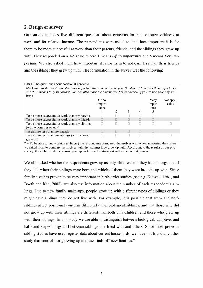
2. Design of survey Our survey includes five different questions about concerns for relative successfulness at

work and for relative income. The respondents were asked to state how important it is for

them to be more successful at work than their parents, friends, and the siblings they grew up

with. They responded on a 1-5 scale, where 1 means Of no importance and 5 means Very im-

portant. We also asked them how important it is for them to not earn less than their friends

and the siblings they grew up with. The formulation in the survey was the following:

Box 1. The questions about positional concerns.

Mark the box that best describes how important the statement is to you. Number “1” means Of no importance and “ 5” means Very important. You can also mark the alternative Not applicable if you do not have any sib-lings.

Of no impor-tance

Very impor-

tant

Not appli-cable

1 2 3 4 5 To be more successful at work than my parents To be more successful at work than my friends To be more successful at work than my siblings (with whom I grew up)*

To earn no less than my friends To earn no less than my siblings (with whom I grew up)

* = To be able to know which sibling(s) the respondents compared themselves with when answering the survey, we asked them to compare themselves with the siblings they grew up with. According to the results of our pilot survey, the siblings who a person grew up with have the strongest influence on that person.

We also asked whether the respondents grew up as only-children or if they had siblings, and if

they did, when their siblings were born and which of them they were brought up with. Since

family size has proven to be very important in birth-order studies (see e.g. Kidwell, 1981, and

Booth and Kee, 2008), we also use information about the number of each respondent’s sib-

lings. Due to new family make-ups, people grow up with different types of siblings or they

might have siblings they do not live with. For example, it is possible that step- and half-

siblings affect positional concerns differently than biological siblings, and that those who did

not grow up with their siblings are different than both only-children and those who grew up

with their siblings. In this study we are able to distinguish between biological, adoptive, and

half- and step-siblings and between siblings one lived with and others. Since most previous

sibling studies have used register data about current households, we have not found any other

study that controls for growing up in these kinds of “new families.”

6

We then asked for the respondents’ subjective perception of their birth order, i.e. whether they

feel like an oldest-, a middle-, or an only-child, etc. Thus, our questions give information

about birth order in three different ways: (1) by including all the siblings a respondent had as

a child, (2) by including only the siblings he/she shared at least half his/her childhood with,

and (3) his/her subjective perception of his/her birth order. We also tested which of (1) and (2)

that corresponds best to (3). We find that the distribution of those a person grew up with (re-

gardless of whether the siblings were biological or not) corresponds better to his/her subjec-

tive perception than to the distribution of all the siblings he/she had, or to the narrower defini-

tion of including biological and adopted siblings only. In this paper we therefore define sib-

lings as the siblings with whom a person shared at least half of his/her childhood.

In order to disentangle birth-order effects from other family effects, we asked the respondents

about several family-specific characteristics such as economic standard during childhood, and

whether their parents lived together at least until the respondent turned 15. These are both

factors that affect a person’s childhood and possibly positional concern. To control for

whether one’s parents lived together is also important for us since we want to distinguish the

effect of living with step- and half-siblings from the effect of broken families. The question of

birth-order effects is closely related to that of the mother’s age; the youngest children tend to

have older mothers than the oldest children. While the oldest child in a family might receive

more parental attention, the standard of living is often better for the youngest child. This

might boost the effects of being born last and underestimate the effects of being a first-born

(Kantarevic and Mechoulan, 2006). We therefore also asked for the age of each respondent’s

mother.

In addition to several questions about socio-economic characteristics, we included a number

of subjective questions related to childhood and family. For example, we asked whether the

respondents think they have been affected by their birth order or by being an only-child. Since

we believe that comparison during childhood increases positional concern, we also asked the

respondents whether they perceive that their parents compared them with their siblings during

childhood. The question read:8

8 In order to not affect the answers to the positional concern questions, the comparison question was placed two pages and several questions before the positional concern questions.

7

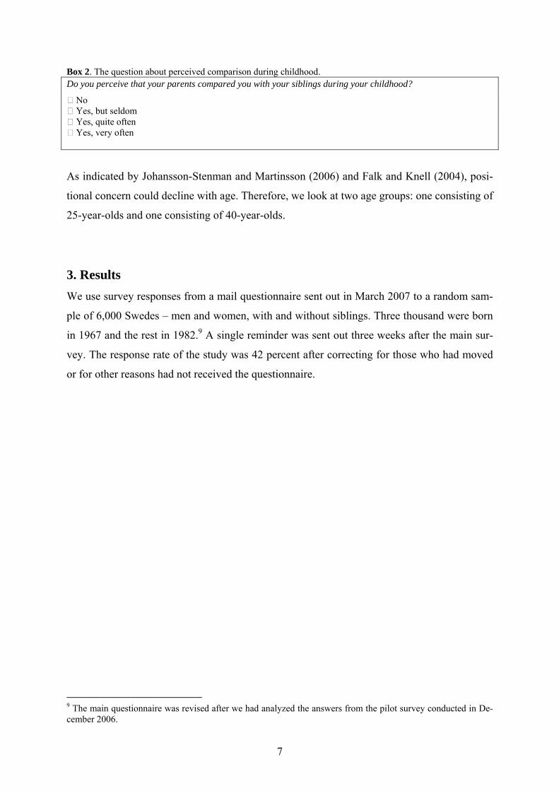
Box 2. The question about perceived comparison during childhood. Do you perceive that your parents compared you with your siblings during your childhood?

No Yes, but seldom Yes, quite often Yes, very often

As indicated by Johansson-Stenman and Martinsson (2006) and Falk and Knell (2004), posi-

tional concern could decline with age. Therefore, we look at two age groups: one consisting of

25-year-olds and one consisting of 40-year-olds.

3. Results We use survey responses from a mail questionnaire sent out in March 2007 to a random sam-

ple of 6,000 Swedes – men and women, with and without siblings. Three thousand were born

in 1967 and the rest in 1982.9 A single reminder was sent out three weeks after the main sur-

vey. The response rate of the study was 42 percent after correcting for those who had moved

or for other reasons had not received the questionnaire.

9 The main questionnaire was revised after we had analyzed the answers from the pilot survey conducted in De-cember 2006.

8

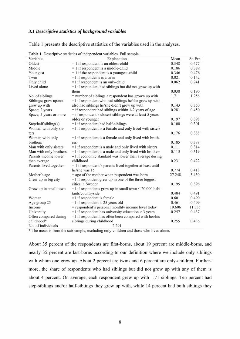
3.1 Descriptive statistics of background variables Table 1 presents the descriptive statistics of the variables used in the analyses. Table 1. Descriptive statistics of independent variables. Full sample. Variable Explanation Mean St. Err. Oldest = 1 if respondent is an oldest-child 0.348 0.477 Middle = 1 if respondent is a middle-child 0.186 0.389 Youngest = 1 if the respondent is a youngest-child 0.346 0.476 Twin =1 if respondents is a twin 0.021 0.142 Only child =1 if respondent is an only-child 0.062 0.241 Lived alone =1 if respondent had siblings but did not grow up with

them 0.038 0.190 No. of siblings = number of siblings a respondent has grown up with 1.711 1.256 Siblings; grew up/not grew up with

=1 if respondent who had siblings he/she grew up with also had siblings he/she didn’t grow up with 0.143 0.350

Space; 2 years = if respondent had siblings within 1-2 years of age 0.281 0.450 Space; 5 years or more = if respondent‘s closest siblings were at least 5 years

older or younger 0.197 0.398 Step/half sibling(s) =1 if respondent had half-siblings 0.100 0.301 Woman with only sis-ters

=1 if respondent is a female and only lived with sisters 0.176 0.388

Woman with only brothers

=1 if respondent is a female and only lived with broth-ers 0.185 0.388

Man with only sisters =1 if respondent is a male and only lived with sisters 0.111 0.314 Man with only brothers =1 if respondent is a male and only lived with brothers 0.115 0.319 Parents income lower than average

=1 if economic standard was lower than average during childhood 0.231 0.422

Parents lived together = 1 if respondent’s parents lived together at least until he/she was 15 0.774 0.418

Mother’s age = age of the mother when respondent was born 27.248 5.430 Grew up in big city =1 if respondent grew up in one of the three biggest

cities in Sweden 0.195 0.396 Grew up in small town =1 if respondents grew up in small town ≤ 20,000 habi-

tants/countryside 0.404 0.491 Woman =1 if respondent is female 0.601 0.490 Age group 25 =1 if respondent is 25 years old 0.461 0.499 Income = respondent’s personal monthly income level today 19.606 11.335 University =1 if respondent has university education > 3 years 0.257 0.437 Often compared during childhood*

=1 if respondent has often been compared with her/his siblings during childhood 0.255 0.436

No. of individuals 2,291 * The mean is from the sub sample, excluding only-children and those who lived alone.

About 35 percent of the respondents are first-borns, about 19 percent are middle-borns, and

nearly 35 percent are last-borns according to our definition where we include only siblings

with whom one grew up. About 2 percent are twins and 6 percent are only-children. Further-

more, the share of respondents who had siblings but did not grow up with any of them is

about 4 percent. On average, each respondent grew up with 1.71 siblings. Ten percent had

step-siblings and/or half-siblings they grew up with, while 14 percent had both siblings they

9

grew up with and siblings they did not grow up with.10 Finally, because we are interested in

whether sibling comparison affects positional concern, it is interesting that nearly 26 percent

of the respondents who grew up with siblings perceive that their parents quite or very often

compared them with their siblings. When comparing the descriptive statistics of the respon-

dents with national statistics, we find that in terms of the share of respondents with university

education, this study corresponds very well with the national level shares (Statistics Sweden

2007).11 However, the share of women is significantly higher in our study (namely 60 per-

cent), and the net response rate is slightly higher for the older cohort than for the younger.

Unfortunately, there are no statistics available regarding the shares of first-/middle-/last-borns

and only-children born in 1967 and 1985; we are therefore not able to test whether our shares

of the different birth orders are representative or not. However, the shares of first- and last-

borns are about equal in our sample.

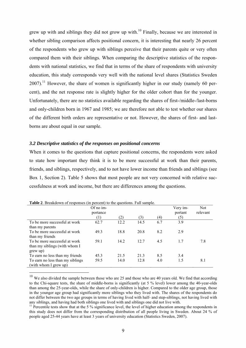
3.2 Descriptive statistics of the responses on positional concerns

When it comes to the questions that capture positional concerns, the respondents were asked

to state how important they think it is to be more successful at work than their parents,

friends, and siblings, respectively, and to not have lower income than friends and siblings (see

Box 1, Section 2). Table 5 shows that most people are not very concerned with relative suc-

cessfulness at work and income, but there are differences among the questions.

Table 2. Breakdown of responses (in percent) to the questions. Full sample. Of no im-

portance (1)

(2)

(3)

(4)

Very im-portant

(5)

Not relevant

To be more successful at work than my parents

62.7 12.2 14.5 6.7 3.9

To be more successful at work than my friends

49.3 18.8 20.8 8.2 2.9

To be more successful at work than my siblings (with whom I grew up)

59.1 14.2 12.7 4.5 1.7 7.8

To earn no less than my friends 45.3 21.5 21.3 8.5 3.4 To earn no less than my siblings (with whom I grew up)

59.5 14.0 12.8 4.0 1.5 8.1

10 We also divided the sample between those who are 25 and those who are 40 years old. We find that according to the Chi-square tests, the share of middle-borns is significantly (at 5 % level) lower among the 40-year-olds than among the 25-year-olds, while the share of only-children is higher. Compared to the older age group, those in the younger age group had significantly more siblings who they lived with. The shares of the respondents do not differ between the two age groups in terms of having lived with half- and step-siblings, not having lived with any siblings, and having had both siblings one lived with and siblings one did not live with. 11 Percentile tests show that at the 5 % significance level, the level of higher education among the respondents in this study does not differ from the corresponding distribution of all people living in Sweden. About 24 % of people aged 25-44 years have at least 3 years of university education (Statistics Sweden, 2007).

10

Solnick and Hemenway (2005) find that people are positional in different respects, and that

no-one in their sample was altogether positional or non-positional. In our sample, three per-

cent stated “of no importance” for all questions, and only a handful stated “very important”

for all questions. The distributions of the responses are statistically different among the ques-

tions according to the Chi-square tests. We also find rather low correlations between ques-

tions (Appendix A presents a correlation matrix). However, the correlations are higher con-

cerning the same reference group than concerning the same relative issue, and the strongest

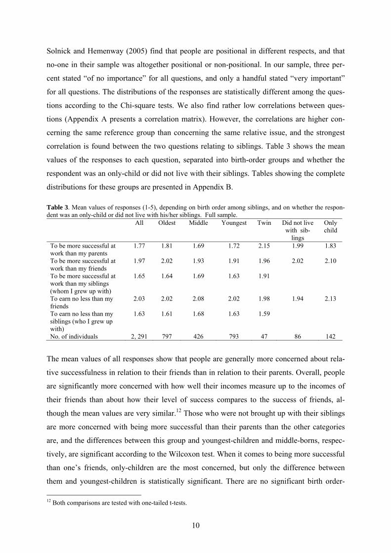
correlation is found between the two questions relating to siblings. Table 3 shows the mean

values of the responses to each question, separated into birth-order groups and whether the

respondent was an only-child or did not live with their siblings. Tables showing the complete

distributions for these groups are presented in Appendix B. Table 3. Mean values of responses (1-5), depending on birth order among siblings, and on whether the respon-dent was an only-child or did not live with his/her siblings. Full sample.

All Oldest Middle Youngest Twin Did not live with sib-

lings

Only child

To be more successful at work than my parents

1.77 1.81 1.69 1.72 2.15 1.99 1.83

To be more successful at work than my friends

1.97 2.02 1.93 1.91 1.96 2.02 2.10

To be more successful at work than my siblings (whom I grew up with)

1.65 1.64 1.69 1.63 1.91

To earn no less than my friends

2.03 2.02 2.08 2.02 1.98 1.94 2.13

To earn no less than my siblings (who I grew up with)

1.63 1.61 1.68 1.63 1.59

No. of individuals 2, 291 797 426 793 47 86 142

The mean values of all responses show that people are generally more concerned about rela-

tive successfulness in relation to their friends than in relation to their parents. Overall, people

are significantly more concerned with how well their incomes measure up to the incomes of

their friends than about how their level of success compares to the success of friends, al-

though the mean values are very similar.12 Those who were not brought up with their siblings

are more concerned with being more successful than their parents than the other categories

are, and the differences between this group and youngest-children and middle-borns, respec-

tively, are significant according to the Wilcoxon test. When it comes to being more successful

than one’s friends, only-children are the most concerned, but only the difference between

them and youngest-children is statistically significant. There are no significant birth order-

12 Both comparisons are tested with one-tailed t-tests.

11

related differences in positional concern in relation to siblings with one exception: Twins are

more concerned with relative success than others, but since they are so few, the result should

be interpreted with care. People with siblings are significantly less positional in relation to

their brothers and sisters than in relation to parents and friends.13 This could either be com-

pletely true or could reflect that it is not really acceptable to be positional in relation to sib-

lings.

3.3 Positional concern in relation to parents and friends, full sample

So far, we have only looked at descriptive statistics on positional concerns. To be able to see

whether the differences in positional concern due to birth order prevail when we control for a

number of family and socio-economic variables, we turn to a regression analysis. In this sec-

tion, we analyze positional concerns in relation to parents and friends. Table 4 presents the

results of least square regressions of relative success at work and relative income for the full

sample.14 In the next section and in Table 5, we present results of OLS regressions for a rela-

tive comparison with siblings for the sub-sample of those who grew up together with siblings.

In all the OLSs, the standard errors are White-heteroskedasticity adjusted.

13 According to a one-tailed t-test. 14 The questions were also investigated with ordered probit. The signs and significance of the coefficient of OLS and ordered probit do not differ substantially between these models. In the next section we show the OLS results, which allow us to compare the coefficients between the different regressions.

12

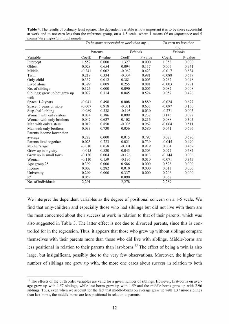
Table 4. The results of ordinary least square. The dependent variable is how important it is to be more successful at work and to not earn less than the reference group, on a 1-5 scale, where 1 means Of no importance and 5 means Very important. Full sample. To be more successful at work than my… To earn no less than

my… Parents Friends Friends Variable Coeff. P-value Coeff. P-value Coeff. P-value Intercept 1.552 0.000 1.327 0.000 1.358 0.000 Oldest 0.028 0.654 0.094 0.117 0.005 0.941 Middle -0.241 0.002 -0.062 0.423 -0.017 0.834 Twin 0.219 0.334 -0.004 0.981 -0.088 0.639 Only-child 0.337 0.012 0.381 0.005 0.262 0.048 Lived alone 0.399 0.009 0.255 0.081 -0.003 0.981 No. of siblings 0.126 0.000 0.090 0.005 0.082 0.008 Siblings; grew up/not grew up with

0.077

0.314

0.045

0.524

0.057

0.426

Space; 1-2 years -0.041 0.498 0.008 0.889 -0.024 0.677 Space; 5 years or more -0.007 0.918 -0.031 0.633 -0.097 0.150 Step-/half-sibling -0.089 0.338 -0.195 0.030 -0.271 0.003 Woman with only sisters 0.074 0.386 0.099 0.232 0.145 0.087 Woman with only brothers 0.042 0.637 0.102 0.216 0.088 0.305 Man with only sisters 0.019 0.850 -0.005 0.962 -0.064 0.511 Man with only brothers 0.033 0.730 0.056 0.580 0.041 0.696 Parents income lower than average 0.282 0.000 0.015 0.797 0.025 0.670 Parents lived together 0.025 0.723 0.021 0.739 -0.045 0.490 Mother’s age -0.010 0.058 -0.001 0.919 0.004 0.469 Grew up in big city -0.015 0.830 0.043 0.503 0.027 0.684 Grew up in small town -0.150 0.004 -0.126 0.013 -0.144 0.006 Woman -0.110 0.159 -0.196 0.010 -0.071 0.345 Age group 25 0.399 0.000 0.586 0.000 0.528 0.000 Income 0.003 0.282 0.010 0.000 0.013 0.000 University 0.209 0.000 0.337 0.000 0.206 0.000 R2 0.059 0.090 0.068 No. of individuals 2,291

2,278 2,289

We interpret the dependent variables as the degree of positional concern on a 1-5 scale. We

find that only-children and especially those who had siblings but did not live with them are

the most concerned about their success at work in relation to that of their parents, which was

also suggested in Table 3. The latter effect is not due to divorced parents, since this is con-

trolled for in the regression. Thus, it appears that those who grew up without siblings compare

themselves with their parents more than those who did live with siblings. Middle-borns are

less positional in relation to their parents than last-borns.15 The effect of being a twin is also

large, but insignificant, possibly due to the very few observations. Moreover, the higher the

number of siblings one grew up with, the more one cares about success in relation to both

15 The effects of the birth order variables are valid for a given number of siblings. However, first-borns on aver-age grew up with 1.57 siblings, while last-borns grew up with 1.59 and the middle-borns grew up with 2.96 siblings. Thus, even when we account for the fact that middle-borns on average grew up with 1.37 more siblings than last-borns, the middle-borns are less positional in relation to parents.

13

parents and friends. That the number of siblings increases positional concern is in line with

the results by Johansson-Stenman et al. (2002).

When it comes to the importance of being more successful than friends, only-children distin-

guish themselves as by far the most positional. Also those who did not live with their siblings

perceive it to be important to be more successful than friends, although less so than only-

children. Oldest children are also more positional than youngest children, but the effect is

insignificant.16 On the other hand, those who grew up with step- or half-siblings are signifi-

cantly less concerned about position relative to their friends, both in terms of successfulness

and income; however, the effect in terms of income is the largest. Kantarevic and Mechoulan

(2006) do not find any effects of half-siblings when studying education but contrary to us,

they do not distinguish whether a respondent has lived together with his/her half sibling(s) or

not. We, however, find that half- and step-siblings really have an effect on positional concern

if one grew up with them.

The results regarding the importance of not earning less than friends show once again that

only-children care more about relative position than others, but the more siblings a person

grew up with the more he/she cares about his/her income relative to that of friends. Conse-

quently, all regressions show that only-children distinguish themselves as those who care the

most about relative issues. Thus, not having siblings is more important for positional concern

than birth order per se. A woman who lived with only sisters is clearly more concerned about

not earning less than her friends compared to women who lived with only brothers or with

both brothers and sisters. When dividing the sample into the two age groups, some differences

become apparent:17 Only-children have substantially stronger positional concerns in the older

age group than in the younger. Moreover, having grown up with step- and/or half-siblings

reduces positional concerns in both age groups, but when the reference group is friends the

reduction is insignificant for the older age group.

If the parents had a lower than average income during a respondent’s childhood, he/she is

more eager to surpass them, which could be interpreted at least partly as an income effect 16 The p-value is 0.117. However, there is a birth order effect of being the oldest sibling. When dividing the sample between the two age groups we find that an oldest sibling is significantly and substantially more con-cerned about his/her success relative to friends than a last-born is (the value of the coefficient is 0.184 and p-value is 0.020) among 40-year-old respondents. On the other hand, there is no oldest-child effect among the 25-year-olds (p-value is 0.967). 17 The results are not presented, but are available on request.

14

(successfulness and income are likely to be correlated) and not necessarily as a pure relative

comparison effect. On the other hand, the age of one’s mother decreases positional concern in

relation to parents. Thus, a larger age gap between a child and her mother decreases the level

of relative comparison. As pointed out by Kanarevic and Mechoulan (2006), there could be a

positive correlation between the mother’s age and economic standard, which might bias the

results. However, this is not the case in our study.18

In addition to the birth order and other family related results, there are some other interesting

findings. The 25-year-old respondents are more positional than the 40-year-olds regardless of

what is compared and of the reference group. We actually find that respondent age is the most

important variable in terms of explaining differences in positional concern. This effect is es-

pecially large in terms of friends, i.e. friends are a much more important reference groups for

young adults than for those who are older. Previous literature also indicates that age affects

positional concern: Falk and Knell (2004) find a negative but insignificant effect of age on

positional concern and according to Johansson-Stenman and Martinsson (2006), age affects

own status concern negatively. However, we cannot be certain whether it is mainly an age or

a cohort effect.19

Furthermore, McBride (2001) and Kingdon and Knight (2007) find that relative income is

more important for people with high income than for low-income earners, while we find that

people with higher incomes perceive both income and successfulness in relation to friends and

siblings to be important, but not in relation to parents. Thus, also here the reference group

matters. People who grew up in small places are generally less positional than others, while

those with university education have stronger positional concerns than others, two effects that

are stable across all regressions. Although the sign of the coefficient “Woman” is negative in

all regressions, women are only significantly less positional than men in terms of being more

successful than their friends. Johansson-Stenman et al. (2002) and Alpizar et al. (2005) find

women to be more positional than men. However, Solnick and Hemenway (2005) do not find

any significant difference between men and women in terms of positional concerns.

18 We do not find significant correlation between mother’s age and economic standard during childhood. More-over, excluding one or both of the variables has no effect on the signs and significance of the other, which im-plies that we should not have this kind of problem in our study. 19 To be able to distinguish the age effect from the cohort effect we need to do a follow up study after 15 years. It would be interesting to investigate whether people born in 1982 will have stronger positional concern when they turn 40 than those born in 1967 currently have.

15

According to the birth-order literature, first-borns are likely to have higher levels of education

and income (see e.g. Hanushek, 1992; Black et al., 2005; Kantarevic and Mechoulan, 2006,

and Booth and Kee, 2008). Thus, the variables capturing whether a respondent has a univer-

sity education and/or a higher income might include indirect effects of the birth-order vari-

ables. We test this by re-estimating all the regressions without the income and university vari-

ables, and the coefficient of the variable “oldest” increases slightly. However, the effect on

positional concerns of being the oldest sibling is still far smaller than the effects of being an

only-child or a person who had siblings but did not grow up with them.

Summarizing the results, we see that birth order and being an only-child affect positional con-

cerns differently depending on the issue and the reference group, which is in line with the

results by Solnick and Hemenway (2005) who find that positional concern varies widely

across issues. The socio-economic variables are on the other hand very stable across the re-

gressions. Our results give a very clear picture that only-children and those who did not live

with their siblings care more about relative issues than others. However, Table C1 in Appen-

dix C shows that only-children perceive that they are affected by birth order/being an only-

child the least. Our finding that only-children care the most about both relative successfulness

and relative income indicates that they are affected more by growing up without siblings than

they believe.

3.4 Positional concern in relation to siblings, sub sample

We are also interested in positional concern in relation to siblings. Table 3 suggests that peo-

ple with siblings are the least concerned about their position in relation to their sisters and

brothers and that there are no significant birth-order differences in this regard. Moreover, as

mentioned before, while envy and rivalry among siblings are common, it might be less com-

mon to admit to. We therefore want to investigate whether people care about successfulness

and income in relation to the siblings they grew up with, and whether the fact that parents

often compared their children affects positional concern. Table 5 shows the results of two

least square models where only respondents who grew up with siblings are included. Also

here, the dependent variable is the 1-5 scale, where five means very important.

16

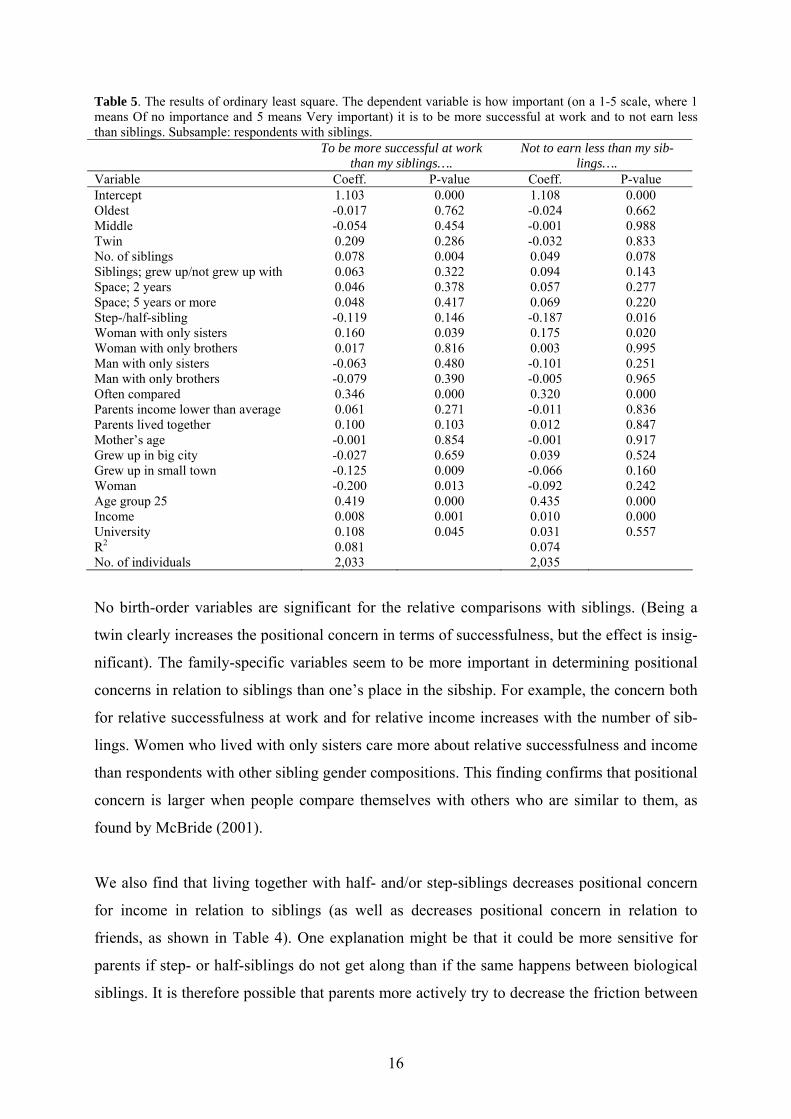
Table 5. The results of ordinary least square. The dependent variable is how important (on a 1-5 scale, where 1 means Of no importance and 5 means Very important) it is to be more successful at work and to not earn less than siblings. Subsample: respondents with siblings. To be more successful at work

than my siblings…. Not to earn less than my sib-

lings…. Variable Coeff. P-value Coeff. P-value Intercept 1.103 0.000 1.108 0.000 Oldest -0.017 0.762 -0.024 0.662 Middle -0.054 0.454 -0.001 0.988 Twin 0.209 0.286 -0.032 0.833 No. of siblings 0.078 0.004 0.049 0.078 Siblings; grew up/not grew up with 0.063 0.322 0.094 0.143 Space; 2 years 0.046 0.378 0.057 0.277 Space; 5 years or more 0.048 0.417 0.069 0.220 Step-/half-sibling -0.119 0.146 -0.187 0.016 Woman with only sisters 0.160 0.039 0.175 0.020 Woman with only brothers 0.017 0.816 0.003 0.995 Man with only sisters -0.063 0.480 -0.101 0.251 Man with only brothers -0.079 0.390 -0.005 0.965 Often compared 0.346 0.000 0.320 0.000 Parents income lower than average 0.061 0.271 -0.011 0.836 Parents lived together 0.100 0.103 0.012 0.847 Mother’s age -0.001 0.854 -0.001 0.917 Grew up in big city -0.027 0.659 0.039 0.524 Grew up in small town -0.125 0.009 -0.066 0.160 Woman -0.200 0.013 -0.092 0.242 Age group 25 0.419 0.000 0.435 0.000 Income 0.008 0.001 0.010 0.000 University 0.108 0.045 0.031 0.557 R2 0.081 0.074 No. of individuals 2,033 2,035

No birth-order variables are significant for the relative comparisons with siblings. (Being a

twin clearly increases the positional concern in terms of successfulness, but the effect is insig-

nificant). The family-specific variables seem to be more important in determining positional

concerns in relation to siblings than one’s place in the sibship. For example, the concern both

for relative successfulness at work and for relative income increases with the number of sib-

lings. Women who lived with only sisters care more about relative successfulness and income

than respondents with other sibling gender compositions. This finding confirms that positional

concern is larger when people compare themselves with others who are similar to them, as

found by McBride (2001).

We also find that living together with half- and/or step-siblings decreases positional concern

for income in relation to siblings (as well as decreases positional concern in relation to

friends, as shown in Table 4). One explanation might be that it could be more sensitive for

parents if step- or half-siblings do not get along than if the same happens between biological

siblings. It is therefore possible that parents more actively try to decrease the friction between

17

step- or half-siblings, leading to less positional concerns between them. The perception of

often being compared with one’s siblings increases positional concerns substantially in both

regressions. The coefficients capturing this effect are very large and highly significant. Con-

sequently, the birth-order variables are not important in explaining the relative comparison

with siblings. Rather the characteristics of the sibship, such as the number of siblings, their

gender composition, and especially whether a respondent perceives that he/she has often been

compared with his/her siblings, are of greater importance. This result partly differs from those

found for positional concern in relation to parents and friends. Thus, people do not only differ

in positional concerns in relation to a reference group, these concerns also have different de-

terminants for different reference groups.

In addition to the birth-order and family-related results, we find that people with higher in-

come care more about both income and successfulness in relation to their siblings, compared

to people with lower income. And as before, the younger respondents perceive both relativity

issues to be far more important than the older respondents do.

3.5 Birth order and sibling comparison during childhood

Table 5 shows that parental comparison between siblings clearly increases positional concerns

among siblings. It is therefore of interest to investigate what makes respondents perceive that

they were often compared with their siblings by their parents during childhood, and whether

there are differences in this perception depending on birth order. To analyze this we use a

binary probit model, where the dependent variable is one if a respondent stated that his/her

parents quite or very often compared him/her with siblings (The question in Box 2). Those

who are only-children and those who did not grow up with their siblings are excluded from

this analysis. Table 6 shows the results.

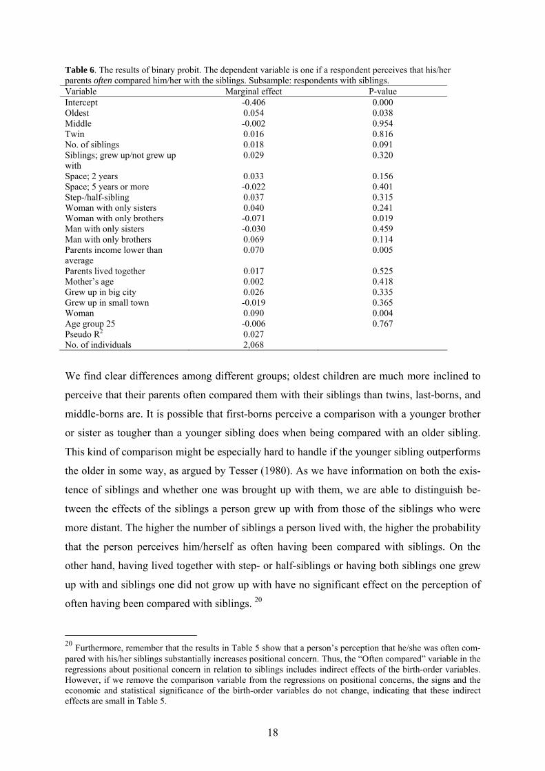
18

Table 6. The results of binary probit. The dependent variable is one if a respondent perceives that his/her parents often compared him/her with the siblings. Subsample: respondents with siblings. Variable Marginal effect P-value Intercept -0.406 0.000 Oldest 0.054 0.038 Middle -0.002 0.954 Twin 0.016 0.816 No. of siblings 0.018 0.091 Siblings; grew up/not grew up with

0.029 0.320

Space; 2 years 0.033 0.156 Space; 5 years or more -0.022 0.401 Step-/half-sibling 0.037 0.315 Woman with only sisters 0.040 0.241 Woman with only brothers -0.071 0.019 Man with only sisters -0.030 0.459 Man with only brothers 0.069 0.114 Parents income lower than average

0.070 0.005

Parents lived together 0.017 0.525 Mother’s age 0.002 0.418 Grew up in big city 0.026 0.335 Grew up in small town -0.019 0.365 Woman 0.090 0.004 Age group 25 -0.006 0.767 Pseudo R2 0.027 No. of individuals 2,068

We find clear differences among different groups; oldest children are much more inclined to

perceive that their parents often compared them with their siblings than twins, last-borns, and

middle-borns are. It is possible that first-borns perceive a comparison with a younger brother

or sister as tougher than a younger sibling does when being compared with an older sibling.

This kind of comparison might be especially hard to handle if the younger sibling outperforms

the older in some way, as argued by Tesser (1980). As we have information on both the exis-

tence of siblings and whether one was brought up with them, we are able to distinguish be-

tween the effects of the siblings a person grew up with from those of the siblings who were

more distant. The higher the number of siblings a person lived with, the higher the probability

that the person perceives him/herself as often having been compared with siblings. On the

other hand, having lived together with step- or half-siblings or having both siblings one grew

up with and siblings one did not grow up with have no significant effect on the perception of

often having been compared with siblings. 20

20 Furthermore, remember that the results in Table 5 show that a person’s perception that he/she was often com-pared with his/her siblings substantially increases positional concern. Thus, the “Often compared” variable in the regressions about positional concern in relation to siblings includes indirect effects of the birth-order variables. However, if we remove the comparison variable from the regressions on positional concerns, the signs and the economic and statistical significance of the birth-order variables do not change, indicating that these indirect effects are small in Table 5.

19

Women and those who experienced a below-average economic standard during childhood are

more likely to perceive that they often used to be compared with their siblings. These effects

are quite large; 9 and 7 percentage points respectively. Interestingly, there are no significant

differences between the two age groups of respondents; the feeling of having been compared

during childhood does not seem to decline with age. Finally, whether a person perceives to

have been compared with his/her siblings is affected by the sibship sex composition. Women

who lived with only brothers are less likely to perceive that they were compared with their

brothers than women who (also) grew up with sisters. Similarly, the sign of the marginal ef-

fect capturing males who lived with only sisters is negative, although the marginal effect is

insignificant, indicating that people of unique gender in a sibship are less likely to perceive

that they were often compared with their siblings during childhood. This is also confirmed by

the fact that the signs of the marginal effects representing women and men who grew up only

with same-gender siblings are positive, although insignificant.

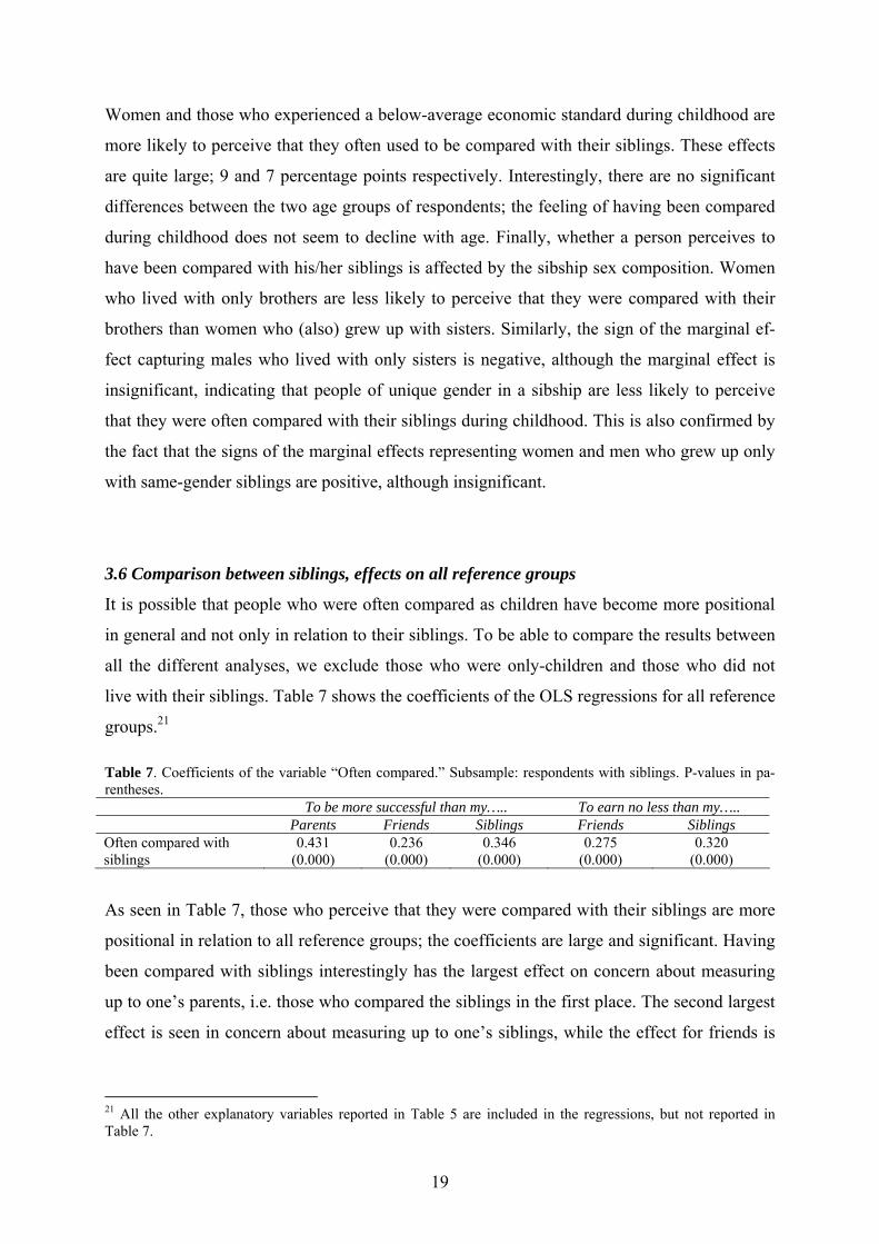
3.6 Comparison between siblings, effects on all reference groups

It is possible that people who were often compared as children have become more positional

in general and not only in relation to their siblings. To be able to compare the results between

all the different analyses, we exclude those who were only-children and those who did not

live with their siblings. Table 7 shows the coefficients of the OLS regressions for all reference

groups.21 Table 7. Coefficients of the variable “Often compared.” Subsample: respondents with siblings. P-values in pa-rentheses. To be more successful than my….. To earn no less than my….. Parents Friends Siblings Friends Siblings Often compared with siblings

0.431 (0.000)

0.236 (0.000)

0.346 (0.000)

0.275 (0.000)

0.320 (0.000)

As seen in Table 7, those who perceive that they were compared with their siblings are more

positional in relation to all reference groups; the coefficients are large and significant. Having

been compared with siblings interestingly has the largest effect on concern about measuring

up to one’s parents, i.e. those who compared the siblings in the first place. The second largest

effect is seen in concern about measuring up to one’s siblings, while the effect for friends is

21 All the other explanatory variables reported in Table 5 are included in the regressions, but not reported in Table 7.

20

slightly smaller. Thus, if parents compare their children, it has lasting effects and makes the

children more positional in general but mainly in relation to their family members.

One could think that those who were often compared with their siblings during childhood not

only care more about relative issues but are also more successful and have higher income in

absolute terms. If so, comparing siblings might be positive and push children to better

achievements. We therefore compare the mean personal income of these respondents with the

mean personal income level of those who were not compared often and find an interesting

result: Those who perceive that they were often compared with their siblings have signifi-

cantly lower income (at the 5 % significance level) than those who perceive that they were not

compared often. Moreover, the shares of respondents with at least three years of university

education do not significantly differ between those who perceive that they were compared

often and those who do not.22

4. Conclusions By using a survey method, the aim of this paper was to investigate whether having siblings

and birth order affect positional concern and whether this concern varies with issue and refer-

ence group. We study the importance of income and successfulness at work relative to three

different reference groups, namely parents, friends, and siblings, and conclude that family and

background variables are indeed important determinants of positional concern. Although peo-

ple are generally not very concerned about relative income or relative successfulness at work,

there are variations in the degree of positional concern depending on the reference group and

on the issue at hand: positional concern is the strongest in relation to friends, and the weakest

in relation to siblings.

This study has four strong main results. First, only-children and those who lived without their

siblings have the strongest positional concern. Thus, birth order itself has less of an effect

than whether one shared childhood with siblings. One possible explanation is that only-

children have more pressure to live up to their parents’ expectations than people with siblings

and that they were always the “best” child in the family and were never outperformed by any

siblings. However, we also found that only-children are the least likely to perceive themselves 22 The income comparison is tested by using a t-test, while the education comparison is done with a Chi-square test.

21

to be affected by birth order/being an only child. However, the results of this study show that

they really are more affected by growing up without siblings than they think. As mentioned in

the introduction, Blake (1991) finds that only-children are not significantly less social, more

egocentric, and/or more goal-oriented than those with siblings but we find that they definitely

have stronger positional concerns. Second, for those who grew up with siblings, the number

of siblings increases positional concern regardless of reference group. Third, a person cares

substantially more about relative position if that person perceives that he/she was compared

with siblings during childhood. This effect is both large and highly significant in relation to

all reference groups, indicating that how parents treat their children has long lasting effects on

the children. Finally, positional concern in relation to siblings depends more on sibship com-

position than on birth order. For example women who only grew up with sisters are more po-

sitional in this context than women who (also) grew up with brothers are.

We also found that it is important in a birth-order study to control for all types of siblings.

Having lived together with half- or step-siblings decreases positional concern in general. Ha-

nushek (1992) argues that first-borns achieve better at school than later-borns because they

are more likely to come from small families. However, this study clearly shows that although

only-children, first-borns, and those who had siblings but were not raised with them all come

from small families, they generally do not have equal positional concerns and should there-

fore be analyzed separately.

Except for the family and sibling effects, we found that both education and income strongly

affect positional concerns, which is in line with previous research (see e.g. McBride, 2001,

and Kingdon and Knight, 2007). Moreover, we found a very strong age effect: the 25-year-

olds are far more positional than the 40-year-olds regardless of reference group and whether

the issue is relative success or relative income. This indicates that positional concerns are

strong when people are young adults and then decreases with age. Alternatively, it could be a

cohort effect that people born at the end of the 1960s are less concerned with relative issues

than people born in the beginning of the 1980s. Hence, an important task for future research is

to further investigate the age and cohort effects on positional concern.

In summary, we have found that the childhood years matter for how much a person cares

about relative income and relative successfulness. The family environment in which a child

lives and how the parents treat him/her do affect the strength of his/her positional concern as

22

an adult. This might in turn affect educational and work-related choices, as well as how peo-

ple as adults deal with comparisons with others. In this study, we asked the respondents to

compare themselves with their parents, friends, and siblings, i.e. people close to them. Further

research is needed to investigate whether the results are similar when other, more distant, ref-

erence groups are used.

23

References

Agell J. and P. Lundborg (1995), Theories of pay and unemployment: Survey evidence from Swedish manufacturing firms, Scandinavian Journal of Economics, 97 (2), 295-307.

Agell J. and P. Lundborg (2003), Survey evidence on wage rigidity and unemployment: Swe-den in 1990s, Scandinavian Journal of Economics, 105 (1), 15-29.

Alpizar F., F. Carlsson and O. Johansson-Stenman (2005), How much do we care about abso-lute versus relative income and consumption?, Journal of Economic Behavior & Or-ganization. 56, 405-421.

Argys L. M., D. I. Rees, S. L. Averett and B. Witoonchart (2006), Birth order and risky ado-lescent behaviour, Economic Inquiry, 44 (2), 215-233.

Aronsson T. and O. Johansson-Stenman (2008), When the Joneses’ consumption hurts: Opti-mal public good provision and nonlinear income taxation, Journal of Public Economics, forthcoming.

Beck, E., Burnet, K. and J. Vosper (2006), Birth-order effects on facets of extraversion, Per-sonality and Individual Differences, 40, 953-959.

Black. S., P. Devereux and K. Salvanes (2005), The more the merrier? The effect of family size and birth order on children’s education, Quarterly Journal of Economics, 120 (2), 669-700.

Blake J. (1991), Number of siblings and personality, Family Planning Perspectives, 23 (6), 272-274.

Booth A. and H. Joo Kee (2008), Birth order matters: The effect of family size and birth order on educational attainment, Journal of Population Economics, forthcoming.

Boskin M. J. and E. Sheshinski (1978), Optimal redistributive taxation when individual wel-fare depends upon relative income, Quarterly Journal of Economics, 92, 589-601.

Butcher K. F. and A. Case (1994), The effect of sibling sex composition on women’s educa-tion and earnings, Quarterly Journal of Economics, CIX (3), 531-563.

Carlsson F., O. Johansson-Stenman and P. Martinsson (2007), Do you enjoy having more than others? Survey evidence of positional goods, Economica, 74, 586-598.

Easterlin R. A. (1974), Does economic growth improve the human lot? in Paul A. David and Melwin W. Reder, eds., Nations and Households in Economic Growth: Essays in hon-our of Moses Abramovitz, New York: Academic Press.

Easterlin R. A. (1995), Will raising incomes of all increase the happiness of all?, Journal of Economic Behavior and Organization. 27, 35-47.

Falk A. and M. Knell (2004), Choosing the Joneses: Endogenous goals and reference stan-dards, Scandinavian Journal of Economics,106 (3), 417-435.

Fischer J. A. V. and B. Torgler (2006), Does envy destroy social fundamentals? The impact of relative income position on social capital, Working Paper, Fondazione Eni Enrico Mat-tei.

Frank R. H. (1985a), The demand for Unobservable and other nonpositional goods, The American Economic Review, 75 (1), 101-116.

Frank R. H. (1985b), Choosing the right bond. Human behaviour and the quest for status, Oxford University Press, New York.

Freese J., B. Powell and L. Carr Steelman (1999), Rebel without a cause or effect: Birth order and social attitudes, American Sociological Review, 64 (2), 207-231.

Ferrer-i-Carbonell A. (2005), Income and well-being: an empirical analysis of the comparison income effect, Journal of Public Economics, 89, 997-1019.

Hanushek E. A. (1992), The trade-off between child quantity and quality, The Journal of Po-litical Economy, 100 (1), 84-117.

Ireland N. J. (2001), Optimal income tax in the presence of status effects, Journal of Public Economics, 81,193-212.

24

Johansson-Stenman O., F. Carlsson and D. Daruvala (2002), Measuring future grandparents’ preferences for equality and relative standing, The Economic Journal, 112, 362-383.

Johansson-Stenman O. and P. Martinsson (2006), Honestly, why are you driving a BMW?, Journal of Economic Behavior and Orgainazation, 60, 129-146.

Kaestner R. (1997), Are brothers really better? Sibling sex composition and educational achievements revisited, The Journal of Human Resources, 32 (2), 250-284.

Kantarevic J. and S. Mechoulan (2006), Birth order, educational attainment and earnings, an investigation using the PSID, The Journal of Human Resources, XLI (4), 755-777.

Kessler D. (1991), Birth order, family size, and achievement: Family structure and wage de-termination, Journal of Labour Economics. 9 (4), 413-426.

Kidwell J. S. (1981), Number of siblings, siblings spacing, sex, and birth order: Their effects on perceived parent-adolescent relationship, Journal of Marriage and Family, 43 (2), 315-332.

Kidwell J. S. (1982), The neglected Birth order: Middle-borns, Journal of Marriage and the Family, 44 (1), 225-235.

Kingdon G. and J. Knight (2007), Community, comparison and subjective well-being in a divided society, Journal of Economic Behavior & Organization, 64, 69-90.

McBride M. (2001), Relative-income effects on subjective well-being in the cross-section, Journal of Economic Behavior & Organization, 45, 251-278.

Neumark D. and A. Postlewaite (1998), Relative income concerns and the rise in married women’s employment, Journal of Public Economics, 70, 157-183.

Ng Y. K. (1987), Relative income effects and the appropriate level of public expenditure, Ox-ford Economic papers, 39, 293-300.

Oswald A. (1983), Altruism, jealousy and the theory of optimal non-linear taxation, Journal of Public Economics, 20, 77-87.

Persson M. (1995), Why are taxes so high in egalitarian societies? Scandinavian Journal of Economics, 97, 569-580.

Saroglou V. and L. Fiasse (2003), Birth order, personality, and religion: a study among young adults from a three-siblings family, Personality and Individual differences, 35, 19-29.

Solnick S. and D. Hemenway (1998), Is more always better?: A survey on positional con-cerns, Journal of Economic Behavior & Organization, 37, 373-383.

Solnick S. and D. Hemenway (2005), Are positional concerns stronger in some domains than in others?, The American Economic Review, 95 (2), 147-151.

Statistics Sweden (2007), Swedish population 1 January 2007, 16-74 years of age, by level of education, sex, age, and born in Sweden/foreign born, homepage: http://www.scb.se/statistik/UF/UF0506/2007A01/Tab1e.xls. Attached January 2008

Sulloway F. J. (1996), Born to Rebel: Birth Order, Family Dynamics, and Creative Lives. New York. Pantheon.

Tesser A. (1980), Self-esteem maintenance in family dynamics, Journal of Personality and Social Psychology, 39 (1), 77-91.

Torgler B., S. L. Schmidt and B. S. Frey (2006), The power of positional concerns: A panel analysis. Working Paper No. 2006-19. Center for Research in Economics, Management, and the Arts.

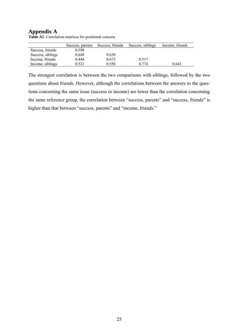
25

Appendix A Table A1. Correlation matrices for positional concern

The strongest correlation is between the two comparisons with siblings, followed by the two

questions about friends. However, although the correlations between the answers to the ques-

tions concerning the same issue (success or income) are lower than the correlation concerning

the same reference group, the correlation between “success, parents” and “success, friends” is

higher than that between “success, parents” and “income, friends.”

Success, parents Success, friends Success, siblings Income, friends Success, friends 0.598 Success, siblings 0.640 0.630 Income, friends 0.444 0.673 0.517 Income, siblings 0.521 0.550 0.774 0.641

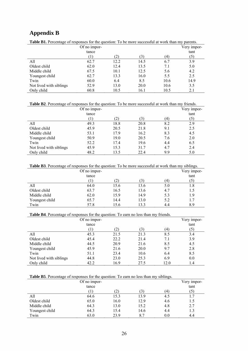
26

Appendix B Table B1. Percentage of responses for the question: To be more successful at work than my parents.

Of no impor-tance (1)

(2)

(3)

(4)

Very impor-tant (5)

All 62.7 12.2 14.5 6.7 3.9 Oldest child 62.0 12.4 13.5 7.1 5.0 Middle child 67.5 10.1 12.5 5.6 4.2 Youngest child 62.7 13.3 16.0 5.5 2.5 Twin 60.0 6.4 8.5 10.6 14.9 Not lived with siblings 52.9 13.0 20.0 10.6 3.5 Only child 60.8 10.5 16.1 10.5 2.1 Table B2. Percentage of responses for the question: To be more successful at work than my friends.

Of no impor-tance (1)

(2)

(3)

(4)

Very impor-tant (5)

All 49.3 18.8 20.8 8.2 2.9 Oldest child 45.9 20.5 21.8 9.1 2.5 Middle child 53.1 17.9 16.2 8.3 4.5 Youngest child 50.9 19.0 20.5 7.6 2.0 Twin 52.2 17.4 19.6 4.4 6.5 Not lived with siblings 45.9 15.3 31.7 4.7 2.4 Only child 48.2 13.5 22.4 9.9 5.0 Table B3. Percentage of responses for the question: To be more successful at work than my siblings.

Of no impor-tance (1)

(2)

(3)

(4)

Very impor-tant (5)

All 64.0 15.6 13.6 5.0 1.8 Oldest child 63.7 16.5 13.6 4.7 1.5 Middle child 62.0 15.9 14.9 5.3 1.9 Youngest child 65.7 14.4 13.0 5.2 1.7 Twin 57.8 15.6 13.3 4.4 8.9 Table B4. Percentage of responses for the question: To earn no less than my friends.

Of no impor-tance (1)

(2)

(3)

(4)

Very impor-tant (5)

All 45.3 21.5 21.3 8.5 3.4 Oldest child 45.4 22.2 21.4 7.1 3.9 Middle child 44.5 20.9 21.6 8.5 4.5 Youngest child 45.9 21.6 20.0 9.7 2.8 Twin 51.1 23.4 10.6 6.4 8.5 Not lived with siblings 44.8 23.0 25.3 6.9 0.0 Only child 42.2 16.9 27.5 12.0 1.4 Table B5. Percentage of responses for the question: To earn no less than my siblings.

Of no impor-tance (1)

(2)

(3)

(4)

Very impor-tant (5)

All 64.6 15.3 13.9 4.5 1.7 Oldest child 65.0 16.0 12.9 4.6 1.5 Middle child 64.3 13.0 15.2 4.8 2.7 Youngest child 64.3 15.4 14.6 4.4 1.3 Twin 63.0 23.9 8.7 0.0 4.4

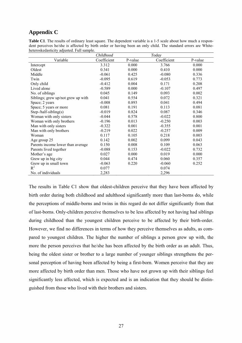
27

Appendix C Table C1. The results of ordinary least square. The dependent variable is a 1-5 scale about how much a respon-dent perceives he/she is affected by birth order or having been an only child. The standard errors are White-heteroskedasticity adjusted. Full sample. Childhood Today

Variable Coefficient P-value Coefficient P-value Intercept 3.312 0.000 3.766 0.000 Oldest 0.341 0.000 0.410 0.000 Middle -0.061 0.425 -0.080 0.336 Twin -0.095 0.619 -0.053 0.773 Only child -0.412 0.004 0.171 0.208 Lived alone -0.589 0.000 -0.107 0.497 No. of siblings 0.045 0.149 0.093 0.002 Siblings; grew up/not grew up with 0.041 0.554 0.072 0.321 Space; 2 years -0.008 0.893 0.041 0.494 Space; 5 years or more 0.081 0.191 0.113 0.081 Step-/half-sibling(s) -0.019 0.824 0.087 0.346 Woman with only sisters -0.044 0.578 -0.022 0.800 Woman with only brothers -0.196 0.013 -0.250 0.003 Man with only sisters -0.322 0.001 -0.355 0.001 Man with only brothers -0.219 0.022 -0.257 0.009 Woman 0.117 0.105 0.218 0.003 Age group 25 0.142 0.002 0.099 0.043 Parents income lower than average 0.150 0.008 0.109 0.063 Parents lived together -0.088 0.153 -0.022 0.732 Mother’s age 0.027 0.000 0.019 0.000 Grew up in big city 0.044 0.474 0.060 0.357 Grew up in small town -0.063 0.220 -0.060 0.252 R2 0.077 0.074 No. of individuals 2,283 2,296

The results in Table C1 show that oldest-children perceive that they have been affected by

birth order during both childhood and adulthood significantly more than last-borns do, while

the perceptions of middle-borns and twins in this regard do not differ significantly from that

of last-borns. Only-children perceive themselves to be less affected by not having had siblings

during childhood than the youngest children perceive to be affected by their birth-order.

However, we find no differences in terms of how they perceive themselves as adults, as com-

pared to youngest children. The higher the number of siblings a person grew up with, the

more the person perceives that he/she has been affected by the birth order as an adult. Thus,

being the oldest sister or brother to a large number of younger siblings strengthens the per-

sonal perception of having been affected by being a first-born. Women perceive that they are

more affected by birth order than men. Those who have not grown up with their siblings feel

significantly less affected, which is expected and is an indication that they should be distin-

guished from those who lived with their brothers and sisters.

Paper II

1

Who visits the museums?

A comparison between stated preferences and observed

effects of entrance fees

Elina Lampi* and Matilda Orth**

Abstract

This study investigates whether the introduction of an entrance fee affects visitor composition at a state funded museum in Sweden. While entrance to the museum was still free, we conducted a survey to collect information about visitor characteristics and used the Contingent Valuation (CV) method to measure visitors’ willingness to pay (WTP) for a visit. The results of the CV survey show that several target group visitors that the museum has policy directives to reach are less likely to visit the museum even at a very low fee level. Additionally, we conducted another survey after the introduction of the fee. Thus, we have a unique opportunity to test the validity of CV in the context of a cultural good. The comparison between the CV results and the observed change in visitor composition after the introduction of the fee implies that CV does predict a majority of the changes successfully.

Keywords: free entrance, visitor composition, museum, natural experiment, stated

preferences.

JEL Classification: D12, H41, Z11

* Department of Economics, University of Gothenburg, Box 640, SE 405 30 Göteborg, Sweden; Ph. +46 31 78613 93; e-mail: Elina.Lampi@economics.gu.se. ** Department of Economics, University of Gothenburg, Box 640, SE 405 30 Göteborg, Sweden; Ph. +46 31 78659 84; e-mail: Matilda.Orth@economics.gu.se This paper has benefited from comments by Fredrik Carlsson, Olof Johansson Stenman, Peter Martinsson, Katarina Nordblom and seminar participants at the University of Gothenburg. Generous financial support from the Wilhelm and Martina Lundgren Foundation is gratefully acknowledged. We also wish to thank Anna Mighetto, Anna Boman and Linda Söderqvist for help with carrying out the survey at the museum.

2

1. Introduction A highly debated issue in many countries is whether or not publicly financed museums

should offer free entrance. Many of the public museums in Britain and Ireland started doing

this in 2001, while Sweden did in 2004-2005 at 19 state funded museums (Swedish Art

Council, 2006).1 As a result, several of the Swedish museums included in the reform more

than doubled their number of visitors (Swedish Art Council, 2006), in line with previous

experiences of free entrance reforms.2 However, there is still a lack of knowledge regarding

the effects of free entrance on visitor composition (Falconer and Blair, 2003).

All public museums in Sweden have policy directives from the Swedish government to reach

more visitors and especially those who rarely visit museums (Swedish Government, 1996).

These visitors are men, young people, immigrants, people who live in the suburbs, people

with low levels of education, and people with low income (Museum of World Culture,

2004b; Swedish Art Council, 2006). A similar policy document exists for example in the UK

(Falconer and Blair, 2003).3 The Swedish free entrance reform was only in effect for a couple

of years. Due to a change in government regime, the reform was abolished in January 1st,

2007 for adults, while children and adolescents younger than 20 continue to get in free to the

museum. While each museum was permitted to decide over its fee levels, the policy

directives to reach certain target groups remained. At the same time, the government grants to

the 19 public museums decreased by 43 million SEK per year (Swedish Government, 2006).4

This policy change was controversial and is still highly debated.

The purpose of the present study consists of three parts: The first objective is to investigate

whether a public free entrance museum, namely the Museum of World Culture in Sweden, is

able to follow the government directive to attract target visitors after introducing an entrance

fee. While entrance to the museum was still free, we conducted a survey to collect

information about visitor characteristics and used the Contingent Valuation (CV) method to

1 Other countries in Europe that have introduced free entrance at public museums during the last five years are among others France, Hungary, Germany, and Denmark (Swedish Art Council, 2006). 2 The total number of visitors in all 19 museums included in the free entrance reform increased by 84 percent during 2005 compared to 2004 (Swedish Art Council, 2008). 3 The U.K. government has promoted the free access to museums because they believe that free entrance is consistent with their “access and social inclusion” objectives, i.e. to have museum visitors from all social groups (Falconer and Blair, 2003). 4 6.98 SEK = 1 USD (2006-12-01).

3

measure visitors’ willingness to pay (WTP) for a visit to the museum.5 Using these results we

can predict possible changes in visitor composition in general, and in the target groups in

particular, at several potential fee levels. The second objective is to evaluate what actually

happened after the introduction of the fee. We therefore conducted another survey to obtain

information about socio-economic characteristics of those who actually ended up paying the

entrance fee to the museum. We then evaluate how the introduction of the entrance fee

influenced the ability of the museum to follow the policy directives imposed by the

government. The third objective is to test the validity of the CV method in the context of a

cultural good. We do that by investigating whether and if so to what extent the predicted

changes in visitor composition based on the results of the CV survey differ from the actual

changes observed after the introduction of the entrance fee.

The present study contributes to the existing literature in the following ways: Since an

entrance fee was introduced in reality, we act on the unique opportunity to conduct surveys

both before and after the museum began charging an entrance fee. Thus, we use both a

natural experiment and stated preferences to investigate changes in visitor composition and to

test the validity of the CV method.6 Moreover, as far as we know, the present study is the first

to analyze visitor composition at museums and relate them to governmental policy directives.

As free entrance reforms and various policy objectives exist in several countries (Swedish Art

Council, 2006; Falconer and Blair, 2003), the results of the present paper are of interest in an

international context, especially for cultural policy makers in other countries.

Several previous studies have used the CV method to investigate WTP for maintaining a

museum (Santagata and Signorello, 2000; Sanz et al., 2003; Thomo, 2004). These studies

focus on both visitors and non-visitors, while we focus only on visitors. A number of other

studies have investigated both the benefits and the drawbacks of having a museum entrance

fee financed by public funds. One argument for free entrance is that in the absence of

congestion, the marginal cost of an additional visitor is zero for a public good (Willis, 2003).

On the other hand, O’Hagan (1995) and Bailey and Falconer (1998) claim that marginal cost

is zero only in the short run. Another argument often presented in support of free entrance is

5 The Contingent Valuation method is a stated preference method where the respondents are asked to state their WTP for a specific (most often public) good. For more information about the CV method, see Mitchell and Carson (1989). 6 A number of studies compare the results of revealed preferences studies on for example visits to national parks with stated preference surveys, but these are often travel cost surveys (Carson et al., 1996). Furthermore, they have not had the unique opportunity to conduct a stated preference survey before an actual price change.

4

that it makes the socio-economic composition of visitors more heterogeneous. However,

according to O’Hagan (1995) and the Department of Culture, Media and Sport in U.K.

(1997), a large majority of those who visit museums with no fee are people from the highest

socio-economic group. This means that people with lower income finance the maintenance

and services of museums they very seldom visit. Moreover, O’Hagan (1995) also argues that

it is a myth that museums with free entrance have visitors from all income groups and that the

entrance fee is not the reason why people from lower income groups attend museums less

often, while Anderson (1998) finds that museums that charge for entrance lose visitors. On

the other hand, Bailey and Falconer (1998) discuss that entrance fees can actually increase

access to museums. Revenues from fees may for example be used to increase opening hours

or the quality of exhibitions.7

The findings of the CV survey predict that an introduction of even a low entrance fee (40

SEK) should result in that four out of the six target groups included in the government

directive are less likely to visit the museum. The findings from our second survey, carried out

after the introduction of the entrance fee, confirm a majority of the predicted changes.

Moreover, the validity test of the CV method shows that the method is successful in capturing

changes in visitor composition for a quasi-public good such as a museum visit.

The rest of the paper is structured as follows. The Museum of World Culture is presented in

Section 2, followed by a description of the surveys in Section 3. Section 4 shows empirical

results before and after the introduction of the entrance fee and the results of the validity test

of the CV method. Section 5 concludes the paper.

7 There are also other studies about museums investigating pricing rules for entry fees (see e.g. Frey, 1994), whether it is profitable to have an additional free day at a museum (Steiner, 1997), and how much “value for the money” people get from visiting a museum (Ashworth and Johnson, 2006).

5

2. The Museum of World Culture The Museum of World Culture, located in Gothenburg, Sweden, is one of 19 state funded

museums and one of four National Museums of World Culture in Sweden. The opening date

was January 1st, 2005 and from the start it was set to offer free entrance. According to policy

directives, the Museum of World Culture should try to reach people who do not visit

museums frequently, namely men, young people, first and second generation immigrants,

people living in the suburbs, people with lower levels of education, and people with low

income (Museum of World Culture, 2004a and 2004b). Five different surveys at the museum

report a mean visitor age of 41 and that 61 percent of the visitors are women, 87 percent were

born in Sweden, 41 percent live in the city center of Gothenburg, 60 percent have a university

degree, 55 percent have a job, and 25 percent are students (Exquiro Market Research, 2006).

The Museum of World Culture is one of the museums that introduced an entrance fee on

January 1st, 2007. The fee was decided at 40 SEK (about 7 USD at the time of the survey) for

visitors older than 19 and gave access to the museum for the whole year. It is worth noting

that the fee level of 40 SEK is low compared to other activities; for example, a movie ticket

costs twice as much. In addition, the museum kept admission free on Wednesday evenings

between 5p.m. and 9p.m.8 Since the museum had no entrance fee when it opened, it is

particularly appropriate for analyzing the effects of introducing a fee, since visitors are then

less likely to have preconceived thoughts (caused by previous fee levels) that may affect their

WTP.

3. The Survey We conducted two surveys at the museum in order to evaluate whether the visitor

composition changed after the introduction of the entrance fee. The first survey was carried

out during the fall of 2006 while entrance was still free. The second was done during the

spring of 2007 after the introduction of the fee. The first survey collected information about

visitor characteristics and WTP for a visit, using the CV method. When the good is familiar

(as we believe a museum visit is to a person who actually visits the museum), the CV method

is appropriate to use (Mitchell and Carson, 1989).

8 The museum decided to keep Wednesday evenings free after we had already conducted our study. Therefore, our follow-up study was conducted only on days with an entrance fee.

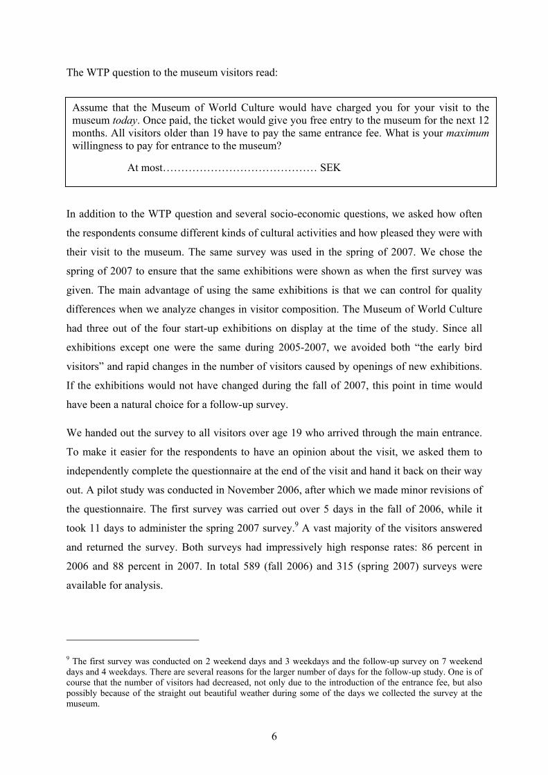
6

The WTP question to the museum visitors read:

In addition to the WTP question and several socio-economic questions, we asked how often

the respondents consume different kinds of cultural activities and how pleased they were with

their visit to the museum. The same survey was used in the spring of 2007. We chose the

spring of 2007 to ensure that the same exhibitions were shown as when the first survey was

given. The main advantage of using the same exhibitions is that we can control for quality

differences when we analyze changes in visitor composition. The Museum of World Culture

had three out of the four start-up exhibitions on display at the time of the study. Since all

exhibitions except one were the same during 2005-2007, we avoided both “the early bird

visitors” and rapid changes in the number of visitors caused by openings of new exhibitions.

If the exhibitions would not have changed during the fall of 2007, this point in time would

have been a natural choice for a follow-up survey.

We handed out the survey to all visitors over age 19 who arrived through the main entrance.

To make it easier for the respondents to have an opinion about the visit, we asked them to

independently complete the questionnaire at the end of the visit and hand it back on their way

out. A pilot study was conducted in November 2006, after which we made minor revisions of

the questionnaire. The first survey was carried out over 5 days in the fall of 2006, while it

took 11 days to administer the spring 2007 survey.9 A vast majority of the visitors answered

and returned the survey. Both surveys had impressively high response rates: 86 percent in

2006 and 88 percent in 2007. In total 589 (fall 2006) and 315 (spring 2007) surveys were

available for analysis.

9 The first survey was conducted on 2 weekend days and 3 weekdays and the follow-up survey on 7 weekend days and 4 weekdays. There are several reasons for the larger number of days for the follow-up study. One is of course that the number of visitors had decreased, not only due to the introduction of the entrance fee, but also possibly because of the straight out beautiful weather during some of the days we collected the survey at the museum.

Assume that the Museum of World Culture would have charged you for your visit to the museum today. Once paid, the ticket would give you free entry to the museum for the next 12 months. All visitors older than 19 have to pay the same entrance fee. What is your maximum willingness to pay for entrance to the museum?

At most…………………………………… SEK

7

There are several ways to ask the WTP question. Two of the most common are to ask each

respondent to state her/his maximum WTP (open-ended format) or to ask each respondent

whether her/his WTP is at least as high as the bid suggested by a researcher (closed-ended

format). The question used in our survey was open-ended. An important advantage of open-

ended questions is that they result in much more information than closed-ended questions.

There are, however, some arguments against using open-ended questions because the

situation of paying for a public good often is uncommon for a respondent. The open-ended

format also tends to lead to a large number of no and protest zero responses (Mitchell and

Carson, 1989) and it is argued not to be incentive-compatible (Carson and Groves, 2007).

It has been argued that people are willing to pay more when the WTP question is

hypothetical, i.e. when the respondents do not really have to pay anything for their visit.

According to Balistreri et al. (2001), Loomis et al. (2001), and Brown et al. (2001), the CV

method overestimates the actual WTP, leading to a hypothetical bias.10 On the other hand,

Carson et al. (1996) show that CV estimates are slightly smaller than revealed preference

estimates when it comes to quasi-public goods such as visits to national parks or recreational

fishing tours. Moreover, Kriström (1993), Balistreri et al. (2001), and Brown et al. (2001) all

show that open-ended hypothetical questions produce estimates closer to actual payments

than closed-ended questions do. An additional way to decrease the existence of the possible

hypothetical bias is to use a “cheap talk script” (Cummings and Taylor, 1999). In such a

script, people are reminded that it is easy to be willing to pay for a good when they do not

really have to pay anything. Respondents are then encouraged to act as if they really would

have to pay the amount they state as their maximum WTP. In order to reduce a possible

hypothetic bias, our questionnaire therefore included a cheap talk script before the WTP

question (the WTP question, the follow-up question, and the cheap talk script are all

presented in Appendix A).

10 The goods to be valued in the studies were an insurance policy (Balisteri et al., 2001), an art print (Loomis et al., 2001), and a public environmental good (removal of roads in Grand Canyon National Park).

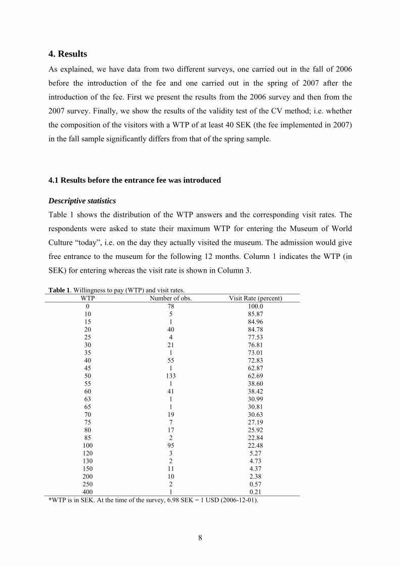
8

4. Results As explained, we have data from two different surveys, one carried out in the fall of 2006

before the introduction of the fee and one carried out in the spring of 2007 after the

introduction of the fee. First we present the results from the 2006 survey and then from the

2007 survey. Finally, we show the results of the validity test of the CV method; i.e. whether

the composition of the visitors with a WTP of at least 40 SEK (the fee implemented in 2007)

in the fall sample significantly differs from that of the spring sample.

4.1 Results before the entrance fee was introduced

Descriptive statistics

Table 1 shows the distribution of the WTP answers and the corresponding visit rates. The

respondents were asked to state their maximum WTP for entering the Museum of World

Culture “today”, i.e. on the day they actually visited the museum. The admission would give

free entrance to the museum for the following 12 months. Column 1 indicates the WTP (in

SEK) for entering whereas the visit rate is shown in Column 3.

Table 1. Willingness to pay (WTP) and visit rates. WTP Number of obs. Visit Rate (percent)

0 78 100.0 10 5 85.87 15 1 84.96 20 40 84.78 25 4 77.53 30 21 76.81 35 1 73.01 40 55 72.83 45 1 62.87 50 133 62.69 55 1 38.60 60 41 38.42 63 1 30.99 65 1 30.81 70 19 30.63 75 7 27.19 80 17 25.92 85 2 22.84

100 95 22.48 120 3 5.27 130 2 4.73 150 11 4.37 200 10 2.38 250 2 0.57 400 1 0.21

*WTP is in SEK. At the time of the survey, 6.98 SEK = 1 USD (2006-12-01).

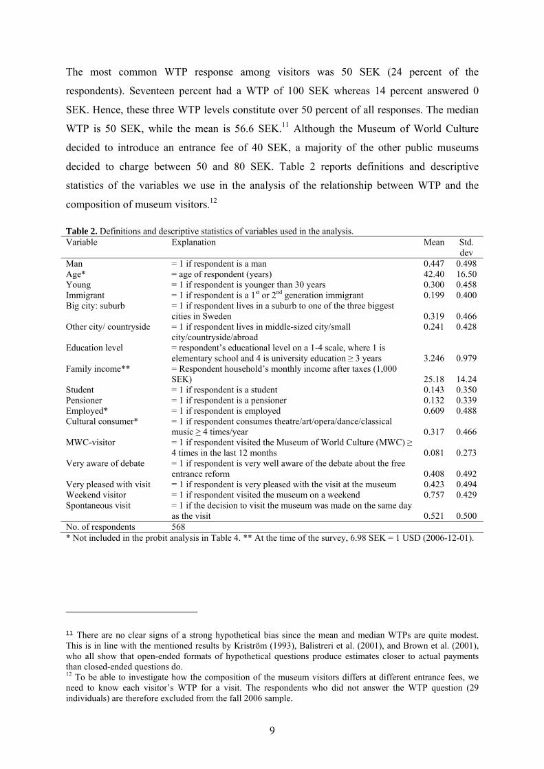
9

The most common WTP response among visitors was 50 SEK (24 percent of the

respondents). Seventeen percent had a WTP of 100 SEK whereas 14 percent answered 0

SEK. Hence, these three WTP levels constitute over 50 percent of all responses. The median

WTP is 50 SEK, while the mean is 56.6 SEK.11 Although the Museum of World Culture

decided to introduce an entrance fee of 40 SEK, a majority of the other public museums

decided to charge between 50 and 80 SEK. Table 2 reports definitions and descriptive

statistics of the variables we use in the analysis of the relationship between WTP and the

composition of museum visitors.12

Table 2. Definitions and descriptive statistics of variables used in the analysis. Variable Explanation Mean Std.

dev Man = 1 if respondent is a man 0.447 0.498 Age* = age of respondent (years) 42.40 16.50 Young = 1 if respondent is younger than 30 years 0.300 0.458 Immigrant = 1 if respondent is a 1st or 2nd generation immigrant 0.199 0.400 Big city: suburb = 1 if respondent lives in a suburb to one of the three biggest

cities in Sweden 0.319 0.466 Other city/ countryside = 1 if respondent lives in middle-sized city/small

city/countryside/abroad 0.241

0.428

Education level = respondent’s educational level on a 1-4 scale, where 1 is

elementary school and 4 is university education ≥ 3 years 3.246 0.979 Family income** = Respondent household’s monthly income after taxes (1,000

SEK) 25.18 14.24 Student = 1 if respondent is a student 0.143 0.350 Pensioner = 1 if respondent is a pensioner 0.132 0.339 Employed* = 1 if respondent is employed 0.609 0.488 Cultural consumer* = 1 if respondent consumes theatre/art/opera/dance/classical

music ≥ 4 times/year 0.317 0.466 MWC-visitor = 1 if respondent visited the Museum of World Culture (MWC) ≥

4 times in the last 12 months 0.081 0.273 Very aware of debate = 1 if respondent is very well aware of the debate about the free

entrance reform 0.408 0.492 Very pleased with visit = 1 if respondent is very pleased with the visit at the museum 0.423 0.494 Weekend visitor = 1 if respondent visited the museum on a weekend 0.757 0.429 Spontaneous visit = 1 if the decision to visit the museum was made on the same day

as the visit 0.521 0.500 No. of respondents 568 * Not included in the probit analysis in Table 4. ** At the time of the survey, 6.98 SEK = 1 USD (2006-12-01).

11 There are no clear signs of a strong hypothetical bias since the mean and median WTPs are quite modest. This is in line with the mentioned results by Kriström (1993), Balistreri et al. (2001), and Brown et al. (2001), who all show that open-ended formats of hypothetical questions produce estimates closer to actual payments than closed-ended questions do. 12 To be able to investigate how the composition of the museum visitors differs at different entrance fees, we need to know each visitor’s WTP for a visit. The respondents who did not answer the WTP question (29 individuals) are therefore excluded from the fall 2006 sample.

10

Table 2 shows that about 55 percent of the respondents were women. The mean age of all

respondents was 42 years,13 and 30 percent were younger than 30. Twenty percent were first

or second generation immigrants. Thirty-two percent lived in suburb areas close to one of the

three biggest cities, 24 percent in middle sized cities, small cities, at the countryside, or

abroad, while the remaining 44 percent lived in big city centers. About 14 percent were

students, and 13 percent pensioners. Moreover, 32 percent were frequent consumers of

culture, while only 8 percent were regular visitors at the Museum of World Culture.

Interestingly, over 40 percent were very well aware of the debate about the free entrance

reform. We also measured how pleased the respondents were about their visit to the museum.

On a 1-5 scale where five means very pleased, 42 percent chose the highest alternative.

Finally, 76 percent of the respondents visited the museum either on a Saturday or a Sunday,

indicating that the museum has more visitors on the weekends than on weekdays.

By comparing the descriptive statistics of the respondents with the national statistics, we find

that the share of the respondents who are women, and share with university education are

significantly higher in this study than in Sweden as a whole (Statistics Sweden, 2007).14

However, the share of respondents who are women, share with university education, share

who are employed, and share who live in a big city center, as well as the mean age of the

respondents, are very close to the levels found in five previous surveys conducted by Exquiro

Market Research (2006) on visitors at the Museum of World Culture. All comparisons are

tested with the bootstrapping method.15 These statistics confirm the argument by O´Hagan

(1995) and by the Department of Culture, Media and Sport in U.K. (1997) that a majority of

museum visitors are from higher socio-economic groups.

13 Respondents 19 years and younger had free access to the museum both before and after the museum introduced the entrance fee. We therefore exclude this age group from the study. This of course increases the mean age of the visitors participating in our study. 14 About 24 % of people aged 20-74 years have at least 3 years of university education (Statistics Sweden, 2007). 15 The mean age of visitors at the Museum of World Culture is 41, 61 % are women, 60 % have a university degree, 55 % are employed, and 41 % lives in the inner city of Gothenburg (Exquiro Market Research, 2006). One thousand samples were bootstrapped by randomly drawing observations with replacement as many times as there are observations in the original sample. The differences between the means are calculated 1000 times for each variable. By using the percentile method and the 95 % confidence interval, it can be shown whether the means significantly differ from each other at the 5 % significance level. The advantage of the percentile method is that it makes no assumptions of the underlying distribution (Efron and Tibshirani, 1998).

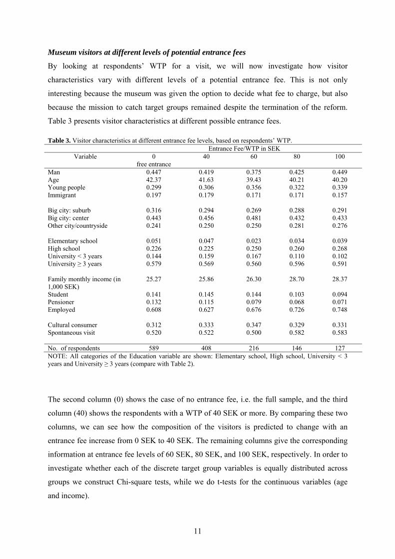
11

Museum visitors at different levels of potential entrance fees

By looking at respondents’ WTP for a visit, we will now investigate how visitor

characteristics vary with different levels of a potential entrance fee. This is not only

interesting because the museum was given the option to decide what fee to charge, but also

because the mission to catch target groups remained despite the termination of the reform.

Table 3 presents visitor characteristics at different possible entrance fees.

Table 3. Visitor characteristics at different entrance fee levels, based on respondents’ WTP.

NOTE: All categories of the Education variable are shown: Elementary school, High school, University < 3 years and University ≥ 3 years (compare with Table 2).

The second column (0) shows the case of no entrance fee, i.e. the full sample, and the third

column (40) shows the respondents with a WTP of 40 SEK or more. By comparing these two

columns, we can see how the composition of the visitors is predicted to change with an

entrance fee increase from 0 SEK to 40 SEK. The remaining columns give the corresponding

information at entrance fee levels of 60 SEK, 80 SEK, and 100 SEK, respectively. In order to

investigate whether each of the discrete target group variables is equally distributed across

groups we construct Chi-square tests, while we do t-tests for the continuous variables (age

and income).

Entrance Fee/WTP in SEK Variable 0

free entrance 40 60 80 100

Man 0.447 0.419 0.375 0.425 0.449 Age 42.37 41.63 39.43 40.21 40.20 Young people 0.299 0.306 0.356 0.322 0.339 Immigrant 0.197 0.179 0.171 0.171 0.157 Big city: suburb 0.316 0.294 0.269 0.288 0.291 Big city: center 0.443 0.456 0.481 0.432 0.433 Other city/countryside 0.241 0.250 0.250 0.281 0.276 Elementary school 0.051 0.047 0.023 0.034 0.039 High school 0.226 0.225 0.250 0.260 0.268 University < 3 years 0.144 0.159 0.167 0.110 0.102 University ≥ 3 years 0.579 0.569 0.560 0.596 0.591 Family monthly income (in 1,000 SEK)

25.27 25.86 26.30 28.70 28.37

Student 0.141 0.145 0.144 0.103 0.094 Pensioner 0.132 0.115 0.079 0.068 0.071 Employed 0.608 0.627 0.676 0.726 0.748 Cultural consumer 0.312 0.333 0.347 0.329 0.331 Spontaneous visit 0.520 0.522 0.500 0.582 0.583 No. of respondents 589 408 216 146 127

12

Comparing with the full sample (free entrance), we observe some general trends as the fee

increases. Setting the fee at 40 SEK rather than at 0 SEK should result in a significant

decrease in the share of visitors who are men, share who are immigrants, and share who are

pensioners. Increasing the fee to 60 SEK is predicted to reduce the share of visitors who are

men and/or share who are pensioners, while the share of visitors who are young should

increase. Finally, a fee of 80 or 100 SEK should reduce the share of visitors who are students

and share who are pensioners significantly, but increase the share who are employed. Overall

we thus find that the shares of the visitors who belong to the target groups can be expected to

decrease, although the changes should be small in magnitude, when the entrance fee

increases. On the other hand, “cultural consumers,” i.e. those who regularly consume cultural

activities other than museums, are not sensitive to the level of the entrance fee: There are no

significant changes in their shares at any suggested fee level.

To be able to see whether the changes in visitor composition due to different fee levels (based

on WTP) prevail when we control for a number of other variables we now turn to a

regression analysis. We estimate five probit regressions and the results are shown in Table

4.16 The dependent variable is equal to one if a respondent would visits the museum at the

given entrance fee level. The levels are 40, 60, 80, and 100 SEK respectively. In addition, it

is of particular interest to investigate the group of visitors who are not willing to visit the

museum at any entrance fee level. Therefore, the dependent variable in the first regression in

Table 4 is equal to one if the visitor has a zero WTP.

16 The probit model allows us to investigate what affects the composition of the museum visitors at different WTP levels, including those with a zero WTP.

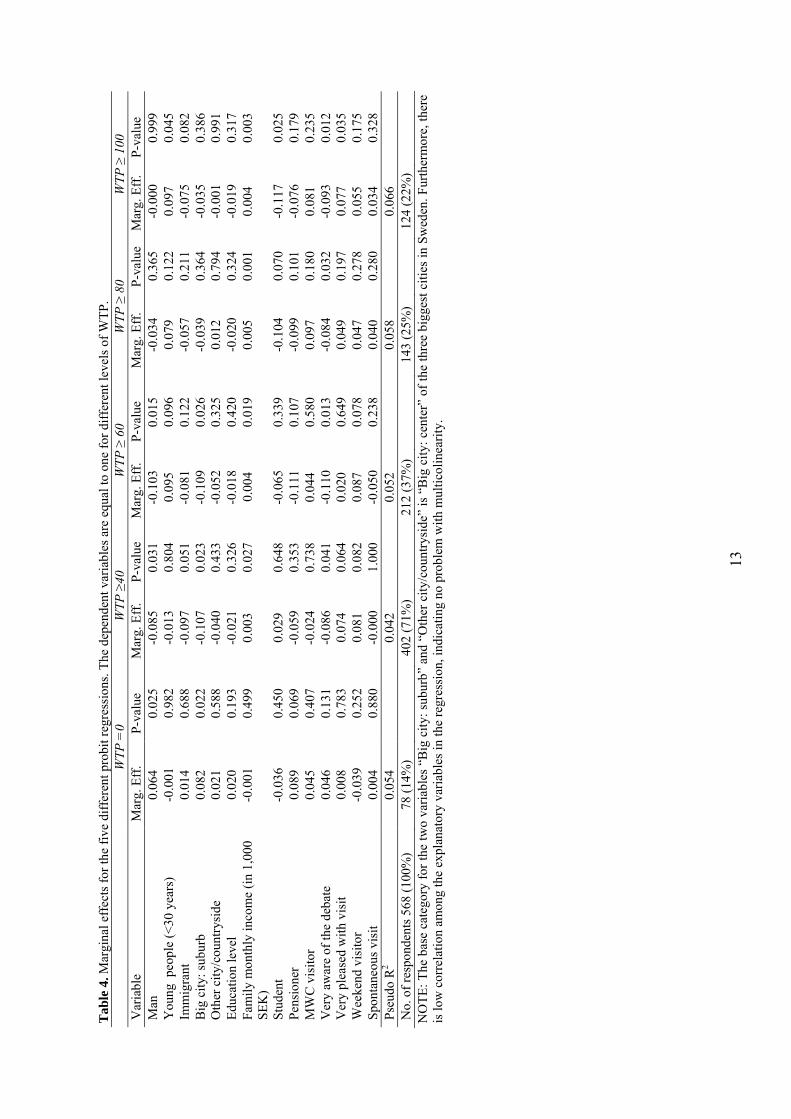
13

Tab

le 4

. Mar

gina

l eff

ects

for t

he fi

ve d

iffer

ent p

robi

t reg

ress

ions

. The

dep

ende

nt v

aria

bles

are

equ

al to

one

for d

iffer

ent l

evel

s of W

TP.

W

TP =

0 W

TP ≥

40

WTP

≥ 6

0 W

TP ≥

80

WTP

≥ 1

00

Var

iabl

e M

arg.

Eff

. P-

valu

e M

arg.

Eff

. P-

valu

e M

arg.

Eff

. P-

valu

e M

arg.

Eff

. P-

valu

e M

arg.

Eff

. P-

valu

e M

an

0.06

4 0.

025

-0.0

85

0.03

1 -0

.103

0.

015

-0.0

34

0.36

5 -0

.000

0.

999

You

ng p

eopl

e (<

30 y

ears

) -0

.001

0.

982

-0.0

13

0.80

4 0.

095

0.09

6 0.

079

0.12

2 0.

097

0.04

5 Im

mig

rant

0.

014

0.68

8 -0

.097

0.

051

-0.0

81

0.12

2 -0

.057

0.

211

-0.0

75

0.08

2 B

ig c

ity: s

ubur

b 0.

082

0.02

2 -0

.107

0.

023

-0.1

09

0.02

6 -0

.039

0.

364

-0.0

35

0.38

6 O

ther

city

/cou

ntry

side

0.

021

0.58

8 -0

.040

0.

433

-0.0

52

0.32

5 0.

012

0.79

4 -0

.001

0.

991

Educ

atio

n le

vel

0.02

0 0.

193

-0.0

21

0.32

6 -0

.018

0.

420

-0.0

20

0.32

4 -0

.019

0.

317

Fam

ily m

onth

ly in

com

e (in

1,0

00

SEK

) -0

.001

0.

499

0.00

3 0.

027

0

.004

0.

019

0.00

5 0.

001

0.00

4 0.

003

Stud

ent

-0.0

36

0.45

0 0.

029

0.64

8 -0

.065

0.

339

-0.1

04

0.07

0 -0

.117

0.

025

Pens

ione

r 0.

089

0.06

9 -0

.059

0.

353

-0.1

11

0.10

7 -0

.099

0.

101

-0.0

76

0.17

9 M

WC

vis

itor

0.04

5 0.

407

-0.0

24

0.73

8 0.

044

0.58

0 0.

097

0.18

0 0.

081

0.23

5 V

ery

awar

e of

the

deba

te

0.04

6 0.

131

-0.0

86

0.04

1 -0

.110

0.

013

-0.0

84

0.03

2 -0

.093

0.

012

Ver

y pl

ease

d w

ith v

isit

0.00

8 0.

783

0.07

4 0.

064

0.02

0 0.

649

0.04

9 0.

197

0.07

7 0.

035

Wee

kend

vis

itor

-0.0

39

0.25

2 0.

081

0.08

2 0.

087

0.07

8 0.

047

0.27

8 0.

055

0.17

5 Sp

onta

neou

s vis

it 0.

004

0.88

0 -0

.000

1.

000

-0.0

50

0.23

8 0.

040

0.28

0 0.

034

0.32

8 Ps

eudo

R2

0.05

4

0.04

2

0.05

2

0.05

8

0.06

6

No.

of r

espo

nden

ts 5

68 (1

00%

) 78

(14%

)

402

(71%

)

212

(37%

)

143

(25%

)

124

(22%

)

NO

TE: T

he b

ase

cate

gory

for t

he tw

o va

riabl

es “

Big

city

: sub

urb”

and

“O

ther

city

/cou

ntry

side

” is

“B

ig c

ity: c

ente

r” o

f the

thre

e bi

gges

t citi

es in

Sw

eden

. Fur

ther

mor

e, th

ere

is lo

w c

orre

latio

n am

ong

the

expl

anat

ory

varia

bles

in th

e re

gres

sion

, ind

icat

ing

no p

robl

em w

ith m

ultic

olin

earit

y.

14

The results in Table 4 show that men, pensioners, and those living in the suburbs are

significantly more likely to have a zero WTP for a visit. Hence, the museum might lose

people from these visitor groups when it starts charging for entrance, regardless of the fee

level. Since a majority of the visitors participating in this study live either in the city center of

Gothenburg or in one of its suburbs, it is clear that the WTP differs depending on where in

Gothenburg they live.17 Respondents who are very aware of the debate about the free

entrance reform seem more likely to have a zero WTP for a visit.18

If we then look at the probit models for the various entrance fees, we find two main effects:

the parameter estimate of income is positive and significant in all cases, and the coefficient of

“Very aware of the debate” is also significant in all cases, but negative. Thus, those with a

higher income are more likely to visit the museum at all fee levels, while those who are well

aware of the debate about whether the free entrance reform should continue are less likely.

Comparing our results with the policy directives given to the Museum of World Culture, we

find that men, immigrants, people who live in the suburbs, and those with lower income (four

out of the six target groups) are less likely to visit the museum even at a very low fee level

(40 SEK). The largest effect is whether a respondent lives in a suburb, which decreases the

probability of visiting the museum by about 11 percentage points. On the other hand, we do

not find any significant effect of age or education at that fee level. Thus, the museum is less

likely to lose visitors from the remaining two target groups: people who are young and people

with lower levels of education.

For the next fee level (60 SEK), the probability of visiting decreases if the respondent is a

man or lives in a suburb, while the opposite is found for young people and weekend visitors.

The fee level of 80 SEK seems to be too high for students and pensioners, while young

people and those who were very pleased with their visit19 would still be likely to visit even

17 About 40 out of the 44 percent of visitors who are included in the variable Big city: Center live in Gothenburg. Similarly, 30 of the 32 percent of visitors who are included in the variable Big city: Suburb live in Gothenburg. 18 The p-value is 0.131. However, this does not have to mean that they do not value the museum at all. One explanation might instead be that the zero WTP expresses their opinion against the government’s plan to stop the free entrance reform. We therefore also asked those with a zero WTP the reason for stating zero. About 11 percent answered that they think it is wrong to charge for access to the Museum of World Culture, while only about two percent said that the reason was either that the exhibitions at the museum were of bad quality or that they had already seen the exhibitions before.

19 We also investigate what makes a visitor very pleased with her/his visit using a probit model (not reported here), where the dependent variable is one if the visitor was very satisfied. We find that those who visited the

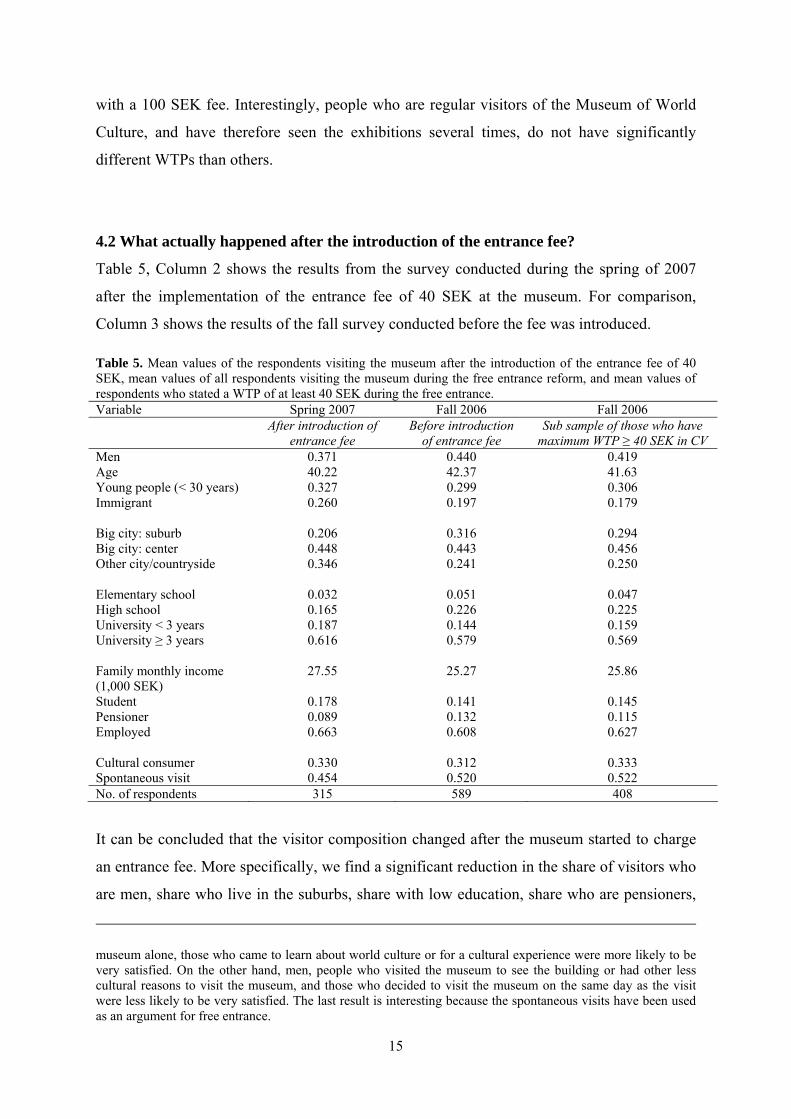
15

with a 100 SEK fee. Interestingly, people who are regular visitors of the Museum of World

Culture, and have therefore seen the exhibitions several times, do not have significantly

different WTPs than others.

4.2 What actually happened after the introduction of the entrance fee?

Table 5, Column 2 shows the results from the survey conducted during the spring of 2007

after the implementation of the entrance fee of 40 SEK at the museum. For comparison,

Column 3 shows the results of the fall survey conducted before the fee was introduced.

Table 5. Mean values of the respondents visiting the museum after the introduction of the entrance fee of 40 SEK, mean values of all respondents visiting the museum during the free entrance reform, and mean values of respondents who stated a WTP of at least 40 SEK during the free entrance. Variable Spring 2007 Fall 2006 Fall 2006 After introduction of

entrance fee Before introduction

of entrance fee Sub sample of those who have

maximum WTP ≥ 40 SEK in CV Men 0.371 0.440 0.419 Age 40.22 42.37 41.63 Young people (< 30 years) 0.327 0.299 0.306 Immigrant 0.260 0.197 0.179 Big city: suburb 0.206 0.316 0.294 Big city: center 0.448 0.443 0.456 Other city/countryside 0.346 0.241 0.250 Elementary school 0.032 0.051 0.047 High school 0.165 0.226 0.225 University < 3 years 0.187 0.144 0.159 University ≥ 3 years 0.616 0.579 0.569 Family monthly income (1,000 SEK)

27.55 25.27 25.86

Student 0.178 0.141 0.145 Pensioner 0.089 0.132 0.115 Employed 0.663 0.608 0.627 Cultural consumer 0.330 0.312 0.333 Spontaneous visit 0.454 0.520 0.522 No. of respondents 315 589 408

It can be concluded that the visitor composition changed after the museum started to charge

an entrance fee. More specifically, we find a significant reduction in the share of visitors who

are men, share who live in the suburbs, share with low education, share who are pensioners,

museum alone, those who came to learn about world culture or for a cultural experience were more likely to be very satisfied. On the other hand, men, people who visited the museum to see the building or had other less cultural reasons to visit the museum, and those who decided to visit the museum on the same day as the visit were less likely to be very satisfied. The last result is interesting because the spontaneous visits have been used as an argument for free entrance.

16

and share who decided to visit the museum on the day of the visit. The results also show a

significant increase in the share of visitors who are immigrants and/or employed, while the

average age decreased.20 Hence, we observe clear changes in the museum’s target groups

after the introduction of the entrance fee, while the share of the “cultural consumers” is the

same. We can thus conclude that the Museum of World Culture has problems following the

policy directives to reach some of the target groups after the introduction of an entrance fee,

while those who are habitual consumers of different cultural activities seem to visit the

museum regardless of the fee. It is, however, worth noting that the museum did not lose

visitors from all target groups, e.g. immigrants. In addition to the loss in target groups, the

total entrance fee revenues during 2007 were about 30 percent below the government

requirement that the museum was given after the entrance fee reform was abolished.

Moreover, revenues from the museum shop decreased with the introduction of the entrance

fee (National Museums of World Culture, 2008).

4.3 Validity of the CV results

In order to test the validity of the CV method, we compare the results from the spring sample,

i.e. those who visited the museum after the introduction of the entrance fee (40 SEK), with

the sub sample of fall visitors with a maximum WTP of at least 40 SEK. Hence, by

comparing the mean values in Columns 2 and 4 in Table 5, we can test whether the CV

correctly predicts the changes in visitor composition that are due to the change from no

entrance fee to an entrance fee of 40 SEK.21 All the comparisons between the discrete

variables are done using the Chi-Square tests, while we use t-tests for the continuous

variables (age and income).

We find that the shares consisting of men, young people, students, pensioners, employed

people, and cultural consumers do not significantly differ between the sub sample from the

fall and the spring sample after the introduction of the entrance fee. Similarly, the CV

20 For the discrete variables, we construct Chi-square tests for equal distribution across groups while we do t-test for the continuous variables (age and income). 21 Several previous studies have compared stated preferences with actual payments in an experimental design (e.g. Carson et al., 1996; Balistreri et al., 2001; Loomis et al., 2001; Brown et al., 2001). However, as far as we know, the present study is the first to use a natural experiment (i.e. an exogenous change) to validate the CV method.

17

predictions of mean age22 and mean income do not significantly differ between the samples.

However, contrary to the prediction of the CV method, the share of visitors who were

immigrants was significantly larger after the introduction of the entrance fee. Investigating

the first and second generation immigrants separately, we find that only the share of the

visitors who were first generation immigrants increased, while the share of the visitors who

were second generation immigrants decreased, which is in line with the prediction. The Chi-

Square test for all three areas of residence simultaneously is significant, indicating that the

areas of residence significantly differ between the two samples. That the share of visitors who

live in the suburbs decreased even more than predicted is problematic for the museum, which

has policy objectives to reach this group. On the other hand, it is positive for the museum that

people living in small/middle sized towns or in the countryside visit the museum more than

the CV method predicted. The results related to education show that there are no significant

differences in the distribution of the education levels in total before and after the entrance fee

was introduced. Separate tests for the different levels of education show, however, that the

CV method underestimated the decrease in the share of visitors with only high school

education. Finally, spontaneous visits decreased more than predicted as well. 23

Summarizing the comparison between predicted and actual shares, we find that the CV

method successfully predicted changes in visitor composition for nearly all the target groups.

However, the method overestimated the decline in one of the museum’s main target groups

(immigrants), while it underestimated the decline in another important target group (those

who live in the suburbs).

22 The p-value for mean age is 0.116. 23 According to the museum’s visitor data, the museum lost 22 % of its visitors after the entrance fee was introduced, while we predicted a decrease by 28 %. However, these figures should be interpreted with care. The data from the museum counts all individuals who passed through the entrance door: those younger than 20, museum workers, people visiting only the restaurant, and people participating in a conference arranged in the museum’s meeting hall. Thus, we are not able to compare the number of actual visitors before and after the entrance fee was introduced.

18

5. Conclusions The issue of free entrance to museums is currently being debated in many countries.

However, whether the composition of visitors changes as a result of free entrance is still an

open question. In the present study we investigated changes in visitor composition associated

with an introduction of an entrance fee to a state funded museum in Sweden. The motivation

for the study was a recent policy change that brought an end to a reform of free entrance at 19

Swedish state funded museums. The museums were allowed to design their own entrance

fees, while they at the same time had government directives to particularly catch visitors who

rarely attend museums, i.e. men, young people, immigrants, people who live in the suburbs,

people with low levels of education, and people with low income. We conducted two surveys

in order to collect information about the visitors’ socio-economic backgrounds, one before

and one after the introduction of the entrance fee. While the entrance was still free, we asked

visitors about their willingness to pay (WTP) for a visit, using the Contingent Valuation (CV)

method. We then compared the results of the CV survey with the actual change in visitor

composition caused by the fee. We thus had an opportunity to do a unique test of the validity

of the CV, which, as far as we know, has never been done in a similar way before.

The results of the CV, based on a representative sample of museum visitors, indicate that

men, immigrants, those who live in suburb areas, and visitors with low income should

become less likely to visit the museum after an implementation of a 40 SEK. Hence, we did

find a clear effect already at this low fee level. On the other hand, we also found that young

visitors are not sensitive to the fee level and that education has no significant effect on a

person’s WTP for a visit. Our results are strengthened by our very high response rates (almost

90 %). The validity test of the CV method shows that a majority of the changes in visitor

composition were correctly predicted. Since the museum had the same exhibitions before and

after the introduction of the fee (thus no exhibitions were new), our findings are robust to

quality differences. Hence, the CV method is rather successful in measuring what will

actually happen after a change in entrance fee and can therefore be an interesting method to

use for many museums. Our type of quasi-public good, a museum visit, seems very

appropriate for the CV method in terms of the degree to which correct predictions are made.

Applications to other cultural goods such as visits to theatres or dance performances should

therefore be of interest for future research. We are nevertheless careful in generalizing to

what extent CV is successful in predicting changes in visitor composition for non-cultural

goods.

19

The empirical results of the present study are important considering the government

directives given to the museum that we study. The conclusion that targeted individuals are

less likely to visit the museum already at a low entrance fee level emphasizes that these

groups are price sensitive. Consequently, charging for entrance does affect who visits the

museum. Moreover, the fact that an entrance fee is charged at all seems more central for the

composition of visitors than the actual level of the fee. We conclude that although the

composition of museum visitors were not evenly distributed across different socio-economics

groups during the years of free entrance, the distribution became even more skewed after the

introduction of the fee. Thus, abolishing the free entrance reform makes it even harder to

follow the policy directive regarding target groups. This partly contradicts the findings by

O’Hagan (1995), who claims that the entrance fee is not the reason why people from lower

income groups attend museums less often. As free entrance reforms and various policy

objectives exist in several countries, the conclusions of the present paper are of interest in an

international context, especially for cultural policy makers in other countries. In line with our

methodological contribution, we suggest that future research touch upon further evidence of

stated preferences that are linked to an exogenous change.

20

References

Anderson R. G. W. (1998), Is charging economic?”, Journal of Cultural Economics, 22, 179-187

Ashworth, J., and P. Johnson (2006), Source of “Value for Money” for Museum Visitors: Some Survey Evidence, Journal of Cultural Economics, 20, 67-83.

Bailey S. J. and P. Falconer (1998), Charging for admission to museums and galleries: A framework for analyzing the impact on access, Journal of Cultural Economics, 22, 167-177.

Balistreri E., G. McClelland, G. Poe and W. Schule (2001), Can hypothetical questions reveal true values? A laboratory comparison of dichotomous choice and open-ended contingent valuation with auction values”, Environmental and Resource Economics, 18, 275-292.

Brown T. C., P. A. Champ, R. C. Bishop and D. W. McCollum (2001), Which response format reveals the truth about donations to a public good? Land Economics, 72 (2), 152-166.

Carson R. T., N. E. Flores, K. M. Martin and, J.L Wright (1996), Contingent valuation and revealed preference methodologies: Comparing the estimates for quasi-public goods, Land Economics, 72 (1), 80-99.

Carson R. T. and T. Groves (2007), Incentive and informational properties of preference questions, Environmental and Resource Economics, 37, 181-210.

Cummings R. G. and L. O. Taylor (1999), Unbiased value estimates for environmental goods: A cheap talk design for the contingent valuation method, The American Economic Review, 89 (3), 649-665.

Department of Culture, Media and Sport in U.K (1997), Review of access to national museums and galleries, Press release DCMS 155/97, 8Th December 1997.

Efron B. and R. J. Tibshirani (1998), An introduction to the Bootstrap, Chapman & Hall/CRC, U.S.A, 1998, p. 55.

Exquiro Market Research (2006), Statens Museer för Världskultur- Publikundersökningar på Etnografiska museet, Medelhavsmuseet, Världskulturmuseet och Östasiatiska Museet, sommaren 2006.

Falconer, P. K., and S. Blair (2003), The Governance of Museums: a study of admission charges policy in the UK, Public Policy and Administration, 18 (2), 71-88.

Frey B. S. (1994), Cultural economics and museum behavior, Scottish Journal of Political Economy 41 (3), 325-335.

Kriström B. (1993), Comparing continuous and discrete contingent valuation questions, Environmental and Resource Economics, 3, 63-71.

Loomis J., T. Brown, B. Lucero and G. Peterson (2001), Improving validity experiments of contingent valuation methods: Results of efforts to reduce the disparity of hypothetical and actual willingness to pay, Land Economics, 72 (4), 450-461.

Mitchell R. C. and R. T. Carson (1989), Using surveys to value public goods, the contingent valuation method, Resources for the Future, Washington D.C., 1989.

Museum of World Culture (2004a), Annual report for 2003, homepage: http://www.varldskulturmuseet.se/content/1/c4/35/14/c1747dbdc49c.pdf Attached 2008-03-11.

Museum of World Culture (2004b), Två inledning av målgrupper för Världskulturmuseet: Utdrag ut kommunikationsplattfrom från 2004.

National Museums of World Culture (2008), Annual report 2007, http://www.smvk.se/content/1/c4/01/47/Arsredovisning_2007_SMVK.pdf Attached 2008-03-11.

21

O’Hagan J. W. (1995), National museums: To charge or not to charge?, Journal of Cultural Economics, 19, 33-47.

Santagata, W., and G. Signorello (2000), Contingent Valuation of a Cultural Public Good and Policy Design: The Case of “Napoli Musei Aperti, Journal of Cultural Economics, 24, 181-204.

Sanz J. Á., L. C. Herrero and A. M. Bedate (2003), Contingent valuation and semiparametric methods: A case study of the National Museum of Sculpture in Valladolid, Spain, Journal of Cultural Economics, 27, 241-257.

Statistics Sweden (2007), Swedish population 1 January 2007, 16-74 years of age, by level of education, sex, age, and born in Sweden/foreign born, homepage: http://www.scb.se/statistik/UF/UF0506/2007A01/Tab1e.xls. Attached January 2008.

Steiner, F. (1997), Optimal Pricing of Museum Admission, Journal of Cultural Economics, 21, 307-333.

Swedish Art Council (2006), Fri entré till museer, Report from the Swedish Art Council in August 2006.

Swedish Art Council (2008), Besöksutveckling för museer 2007” KUR 2008/1. Swedish Government (1996), Government bill 1996/97:3; Kulturutskottets betänkande

1996/97:krU 1. Swedish Government (2006), Press release from the Government 16th October 2006,

Homepage; www.regeringen.se/sb/d/7277/a/71130. Thomo, T. (2004), Economic value of a local museum: Factors of willingness-to-pay, Journal

of Socio-Economics, 33, 229-240. Willis, K. G. (2003), Pricing Public Parks, Journal of Environmental Planning and

Management, 46(1), 3-17.

22

Appendix A

The willingness to pay question used in the questionnaire

Question 16. Assume that the Museum of World Culture would have charged you for your visit to the museum today. Once paid, the ticket would give you free entry to the museum for the next 12 months. All visitors older than 19 have to pay the same entrance fee. What is your maximum willingness to pay for entrance to the museum?

At most…………………………………… SEK

If you answered 0 SEK, please explain why you are not willing to pay for admission to the museum? (Several alternatives are possible)

□ The exhibitions are not good enough

□ I can not afford to pay

□ I have seen the exhibitions before

□ I believe it is wrong to charge for access to the Museum of World Culture

□ Other: ……………………………………….

Experience from previous studies shows that people claim to be willing to pay more when answering a hypothetical question in a questionnaire than what they actually would pay in real life. One possible reason for this might be that it is easy to be generous when the payment is not charged in reality. Another reason might be that people do not realize effect the payment would have on their household budgets.

Paper III

1

Do EPA administrators recommend environmental

policies that citizens want?

Fredrik Carlsson a, Mitesh Kataria b, Elina Lampic

Abstract

We investigate whether Swedish Environmental Protection Agency (EPA) administrator preferences regarding improvements in environmental quality differ from citizen preferences. The scope and significance of the possible difference are assessed by conducting identical choice experiments (CE) on a random sample of Swedish citizens and a random sample of administrators working at the Swedish EPA. The experiment concerns two environmental quality objectives: a Balanced Marine Environment and Clean Air. The EPA administrators were asked to choose the alternatives they would recommend as a policy, while the citizens were asked to act as private persons. We find that the rankings of attributes differ between the two groups, and that there are significant differences in the willingness to pay (WTP) for particular attributes. EPA administrators have a higher WTP for five out of the seven attributes, and in some cases the difference is not only significant but also substantial. We also asked the administrators to motivate their CE choices, and the main motive was ecological sustainability. Keywords: Choice experiment, environmental policy, administrators, citizens. JEL Classification: D61, Q51, Q58

Acknowledgments: We have received valuable comments from Peter Martinsson, Katarina Nordblom, Maria Vredin-Johansson, and seminar participants at University of Gothenburg. We also wish to thank Maria Ohlman for help with carrying out the survey at the Swedish EPA. Financial support from Swedish Environmental Protection Agency and from Sida to the Environmental Economics Unit at the University of Gothenburg is gratefully acknowledged. a Department of Economics, University of Gothenburg, Box 640, SE-40530 Göteborg, Sweden. Tel: + 46 31 7864174, e-mail: fredrik.carlsson@economics.gu.se b Mitesh Kataria: National Environmental Research Institute, University of Aarhus, Frederiksborgvej 399, PB 358, DK-4000 Roskilde, Denmark Tel: +45 4630 1887, e-mail: mika@dmu.dk c Department of Economics, University of Gothenburg, Box 640, SE-40530 Göteborg, Sweden. Tel: + 46 31 7861393 e-mail: elina.lampi@economics.gu.se

2

1. Introduction Many people have an attitude of distrust towards politicians and administrators (bureaucrats)

responsible for public policy. Part of this distrust could be related to uncertainty about

whether administrators serve their own self-interest or act in the interest of the public.1

Another explanation for this distrust is that politicians and administrators are considered to be

distanced from people in general, creating policies and making decisions that are not in line

with the desires of citizens. However, it can be argued that certain policies in fact should be

paternalistic and to some extent ignore the preference of the general public (O’Donoghue and

Rabin, 2003; Johansson-Stenman, 2008). For example, the fact that people working with

environmental management have more information about environmental problems than the

public may justify paternalistic behavior to some degree. According to studies in psychology,

decision makers in the public sector have preferences that are similar to those of the general

public when it comes to policies for the reduction of greenhouse gases, while decision makers

in the private sector have preferences that are different (Nilsson et al., 2004; Nilsson and Biel,

2008). Moreover, the decisions of those who work in the public sector are based on their

private norms regarding environmental values (Nilsson et al., 2004).2 von Borgstede et al.

(2007) show that also individual professional roles in an organization, regardless of whether

the organization is private or public, matter for the acceptance of climate policy measures.

Environmental managers, planners, and economists all have different patterns of acceptance;

environmental managers are significantly more willing to accept high-cost measures than both

planners and economists.

However, very little attention is given in economics to how the policy recommendations of

those who work with policy and management of the environment relate to citizen

preferences.3 There is also a lack of knowledge regarding similarities and differences between

1 This viewpoint is a central element in public choice theory (Mueller, 2003); for example Niskanen (1971) where the bureaucrat is described as a budget-maximizer, and Brennan and Buchanan (1980) where politicians and bureaucrats collaborate and try to maximize the size of the public sector. 2 Ordinary citizens might also act as a policy maker when answering a stated preference survey. According to Nyborg (2000), people have multiple preference orderings. A respondent might take the social point of view, i.e. applying social rather than her/his personal preferences, when answering a stated preference study. This might especially be the case if the good to be valued is ethically complex, such as endangered species. On the other hand, people in general are also reluctant to tax increases (Gemmell et al., 2004; Hammar et al., 2006), which might affect their willingness to pay for a public good like environmental quality. 3 In political science, there has been an increased interest in the behavior of administrators ever since Lipsky (1980). In economics, citizen juries and participatory tools have been used as environmental valuation methods or complements to stated preference methods (Davis and Whittington, 1998; Kenyon et al., 2001). However, these are methods where citizens discuss and make decisions in groups, and not a comparison between decision makers and citizens.

3

citizens and administrators in terms of willingness to pay (WTP) for environmental

improvements. The only studies in economics that we are aware of that touches upon a similar

issue are Alberini et al. (2006) and Colombo et al. (2007). 4 Alberini et al. (2006) looked at how

well the preferences of public officials and other stakeholders match those of the public. The

preferences of the public were estimated using choice experiment (CE) and rating tasks while the

preferences of public officials and other stakeholders were obtained using rating and ranking

tasks. Similarities as well as sharp dissimilarities in preferences between the groups were found.

Colombo et al. (2007) looked at possible differences between citizen and expert preferences.

They used a CE to obtain citizen preferences, and the Analytic Hierarchy Process method5 to

obtain expert preferences, and found similar attribute rankings in the two groups.

In Sweden, just as in many other countries, the Environmental Protection Agency (EPA) is

one of the main responsible authorities in managing environmental resources, and hence plays

a crucial role in determining environmental policy.6 The main objective of this paper is to

investigate whether administrators at the Swedish EPA recommend environmental policies

that the citizens prefer. This is done by conducting two identical CEs one on a random sample

of Swedish citizens and one on a random sample of EPA administrators. The CE concerns

two of the environmental objectives in Sweden: a Balanced Marine Environment and Clean

Air (these are explained in the next section). One advantage of our approach is that by using

the same method (CE) and a very similar survey for both groups, we can make a clean test of

whether the preferences differ. Moreover, since we are interested in preferences for several

various aspects of these two environmental objectives the CE method is most appropriate

considering the objectives .7

The citizens were asked to choose their preferred environmental policy, and the EPA

administrators were asked to choose which policy they would recommend. The choices made

can be used to estimate the WTP for various measures to improve environmental quality. By

comparing the WTPs for the two groups, we can assess whether or not the choices of the

4 The goods valued in the studies were a reuse of “Arsenale”, an underutilized site (previously used by the Italian Navy) located in the city of Venice in Italy (Alberini et al., 2006), and “Public Rights of Way” that provide rights of passage over property to those other than owners (Colombo et al., 2007). 5 A method designed for using expert judgments to represent citizen preferences. Experts are asked to compare attributes on a scale; see Colombo et al. (2007) and Saaty (1980). 6 As in other countries, the people working at the EPA are public servants and not politically appointed. 7 In a CE respondents make repeated choices between alternatives. The alternatives are described by a number of attributes, and the levels of the attributes are varied among the choice sets. For overviews on the CE method, see for example Alpizar et al. (2003) and Louviere et al. (2000).

4

administrators are in line with the preferences of the citizens. We also investigate on what

grounds administrators make their policy recommendations and whether they feel that some

people should have more to say when deciding on environmental policy. We also asked them

to rate their perceived trustworthiness of the results of stated preference studies. As Lipsky

(1980) argues, “Policy implementation in the end comes down to the people who actually

implement it.” Thus, the opinions of administrators about different environmental issues

might affect environmental policy decisions.

2. The choice experiment In Sweden, there are 16 so-called environmental quality objectives, adopted by the Swedish

Parliament in 1999 and 2005. The main purpose of these objectives is to provide a framework

for obtaining a sustainable environment. Another purpose is to define the quality of the

environment, natural resources, and cultural resources in Sweden, and to be able to measure

the change in environmental quality over time. The objectives are designed to, among other

things, promote human health, safeguard biodiversity and the natural environment, and

preserve the cultural heritage. The objectives should be reached within one generation, i.e. by

the year 2020 (SEPA, 2006). The Environmental Objectives Council has the overall

responsibility for coordinating the goals of and monitoring the actions taken by different

governmental bodies in different sectors. Every year the council publishes a progress report.

In this paper we look at two of the environmental quality objectives: a Balanced Marine

Environment and Clean Air. The Swedish EPA is the public agency that has the main

responsibility for these two objectives. The overall goal of the Balanced Marine Environment

objective reads: “The North Sea and the Baltic Sea must have a sustainable productive

capacity, and biological diversity must be preserved. Coasts and archipelagos must be

characterized by a high degree of biological diversity and a wealth of recreational, natural,

and cultural assets. Industry, recreation, and other utilization of the seas, coasts, and

archipelagos must be compatible with the promotion of sustainable development. Particularly

valuable areas must be protected against encroachment and other disturbance” (SEPA, 2006).

The overall goal of the Clean Air objective reads: “The air must be clean enough not to

represent a risk to human health or to animals, plants, or cultural assets” (SEPA, 2006).

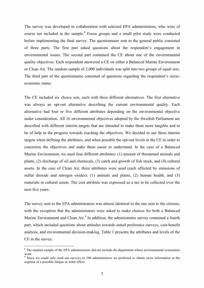
5

The survey was developed in collaboration with selected EPA administrators, who were of

course not included in the sample.8 Focus groups and a small pilot study were conducted

before implementing the final survey. The questionnaire sent to the general public consisted

of three parts. The first part asked questions about the respondent’s engagement in

environmental issues. The second part contained the CE about one of the environmental

quality objectives. Each respondent answered a CE on either a Balanced Marine Environment

or Clean Air. The random sample of 2,000 individuals was split into two groups of equal size.

The third part of the questionnaire consisted of questions regarding the respondent’s socio-

economic status.

The CE included six choice sets, each with three different alternatives. The first alternative

was always an opt-out alternative describing the current environmental quality. Each

alternative had four or five different attributes depending on the environmental objective

under consideration. All 16 environmental objectives adopted by the Swedish Parliament are

described with different interim targets that are intended to make them more tangible and to

be of help in the progress towards reaching the objectives. We decided to use these interim

targets when defining the attributes, and when possible the opt-out levels in the CE in order to

concretize the objectives and make them easier to understand. In the case of a Balanced

Marine Environment, we used four different attributes: (1) amount of threatened animals and

plants, (2) discharge of oil and chemicals, (3) catch and growth of fish stock, and (4) cultural

assets. In the case of Clean Air, three attributes were used (each affected by emissions of

sulfur dioxide and nitrogen oxides): (1) animals and plants, (2) human health, and (3)

materials in cultural assets. The cost attribute was expressed as a tax to be collected over the

next five years.

The survey sent to the EPA administrators was almost identical to the one sent to the citizens,

with the exception that the administrators were asked to make choices for both a Balanced

Marine Environment and Clean Air.9 In addition, the administrator survey contained a fourth

part, which included questions about attitudes towards stated preference surveys, cost-benefit

analysis, and environmental decision-making. Table 1 presents the attributes and levels of the

CE in the survey. 8 The random sample of the EPA administrators did not include the department where environmental economists work. 9 Since we could only send out surveys to 100 administrators we preferred to obtain more information at the expense of a possible fatigue or order effect.

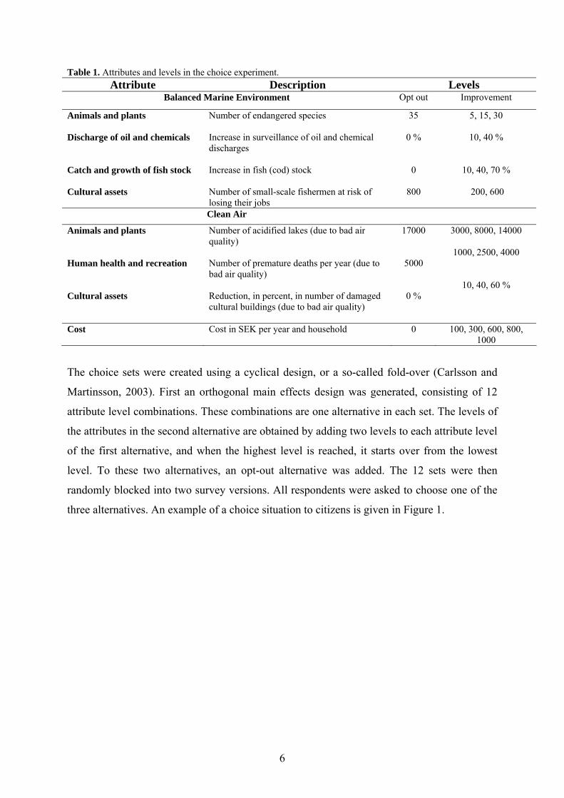
6

Table 1. Attributes and levels in the choice experiment. Attribute Description Levels

Balanced Marine Environment Opt out Improvement

Animals and plants Discharge of oil and chemicals Catch and growth of fish stock Cultural assets

Number of endangered species Increase in surveillance of oil and chemical discharges Increase in fish (cod) stock Number of small-scale fishermen at risk of losing their jobs

35

0 %

0

800

5, 15, 30

10, 40 %

10, 40, 70 %

200, 600

Clean Air

Animals and plants Human health and recreation Cultural assets

Number of acidified lakes (due to bad air quality) Number of premature deaths per year (due to bad air quality) Reduction, in percent, in number of damaged cultural buildings (due to bad air quality)

17000

5000

0 %

3000, 8000, 14000

1000, 2500, 4000

10, 40, 60 %

Cost Cost in SEK per year and household 0 100, 300, 600, 800, 1000

The choice sets were created using a cyclical design, or a so-called fold-over (Carlsson and

Martinsson, 2003). First an orthogonal main effects design was generated, consisting of 12

attribute level combinations. These combinations are one alternative in each set. The levels of

the attributes in the second alternative are obtained by adding two levels to each attribute level

of the first alternative, and when the highest level is reached, it starts over from the lowest

level. To these two alternatives, an opt-out alternative was added. The 12 sets were then

randomly blocked into two survey versions. All respondents were asked to choose one of the

three alternatives. An example of a choice situation to citizens is given in Figure 1.

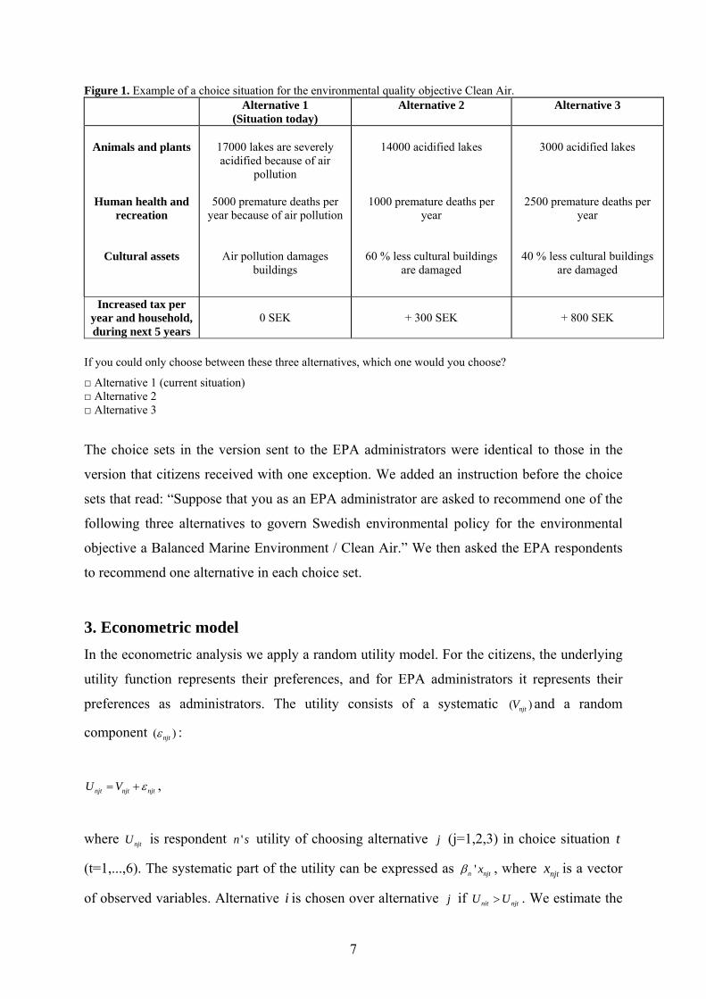
7

Figure 1. Example of a choice situation for the environmental quality objective Clean Air. Alternative 1

(Situation today) Alternative 2 Alternative 3

Animals and plants

Human health and recreation

Cultural assets

17000 lakes are severely acidified because of air

pollution

5000 premature deaths per year because of air pollution

Air pollution damages buildings

14000 acidified lakes

1000 premature deaths per year

60 % less cultural buildings are damaged

3000 acidified lakes

2500 premature deaths per year

40 % less cultural buildings are damaged

Increased tax per year and household, during next 5 years

0 SEK

+ 300 SEK

+ 800 SEK

If you could only choose between these three alternatives, which one would you choose?

□ Alternative 1 (current situation) □ Alternative 2 □ Alternative 3

The choice sets in the version sent to the EPA administrators were identical to those in the

version that citizens received with one exception. We added an instruction before the choice

sets that read: “Suppose that you as an EPA administrator are asked to recommend one of the

following three alternatives to govern Swedish environmental policy for the environmental

objective a Balanced Marine Environment / Clean Air.” We then asked the EPA respondents

to recommend one alternative in each choice set.

3. Econometric model In the econometric analysis we apply a random utility model. For the citizens, the underlying

utility function represents their preferences, and for EPA administrators it represents their

preferences as administrators. The utility consists of a systematic ( )njtV and a random

component ( )njtε :

njt njt njtU V ε= + ,

where njtU is respondent 'n s utility of choosing alternative j (j=1,2,3) in choice situation t

(t=1,...,6). The systematic part of the utility can be expressed as 'n njtxβ , where njtx is a vector

of observed variables. Alternative i is chosen over alternative j if nit njtU U> . We estimate the

8

models with a random parameter logit model. We include an alternative specific constant for

the opt-out alternative and assume that all attribute parameters other than the cost parameter

are normally distributed. Since we have repeated observations, we assume that the parameters

are constant across choice sets for a given respondent. The models are estimated with Nlogit

4.0 using simulated maximum likelihood with Halton draws with 500 replications. See Train

(2003) for details on simulated maximum likelihood. We decided not to include any socio-

economic characteristics and use the same model specification for both subsamples.10

4. Results For the general public, we use survey responses from a mail questionnaire sent out in June

2007 to a random sample of 2,000 men and women aged 18-75, selected from the Swedish

census registry. One thousand questionnaires were sent out for each objective, and the

respondents received a single reminder three weeks after the main survey. In total 648

individuals returned the questionnaire, of which 306 (a Balanced Marine Environment) and

310 (Clean Air) were available for analysis due to non-responses to various questions.11 For

the administrators, we use survey responses from a mail questionnaire sent out in September

2007 to a random sample of 100 EPA administrators. A single reminder was sent out two

weeks after the main survey. In total 59 administrators returned the questionnaire, of which 58

were available for analysis.12 Comparing the descriptive statistics of the citizens with the

national statistics, we find that the mean age of the citizens (48.8 years) in our sample does

not significantly differ from the mean age at the national level. However, the shares of women

and of those who have at least three years of university education are significantly higher in

our citizens sample than in the population as a whole (Statistics Sweden, 2007).13 In the

econometric analysis we therefore have to test whether this overrepresentation affects the

results.

10 The mean WTPs for the citizens do not differ to any large extent if we include socio-economic characteristics. The EPA administrators were asked to make their choices as recommendations for environmental policy, so their socioeconomic characteristics should not affect their choices to any great extent. 11 The response rate is 33 percent, corrected for those who had moved or for other reasons had not received the questionnaire. 12 The response rate is 62 percent, corrected for those who had changed jobs or were on parental or sick leave. 13 One thousand samples were bootstrapped by randomly drawing observations with replacement as many times as there are observations in the original sample. By using the percentile method and a 95 % confidence interval, it can be shown whether the means significantly differ from each other at the 5 % significance level.

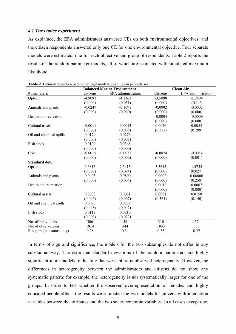
9

4.1 The choice experiment

As explained, the EPA administrators answered CEs on both environmental objectives, and

the citizen respondents answered only one CE for one environmental objective. Four separate

models were estimated, one for each objective and group of respondents. Table 2 reports the

results of the random parameter models, all of which are estimated with simulated maximum

likelihood. Table 2. Estimated random parameter logit models, p-values in parentheses. Balanced Marine Environment Clean Air Parameters Citizens EPA administrators Citizens EPA administrators Opt-out -4.9097

(0.000) -4.1363 (0.051)

-3.5098 (0.000)

-1.2404 (0.143

Animals and plants -0.0247 (0.000)

-0.1091 (0.000)

-0.0002 (0.000)

-0.0002 (0.000)

Health and recreation

-0.0004 (0.000)

-0.0009 (0.000)

Cultural assets -0.0011 (0.000)

-0.0013 (0.095)

0.0026 (0.332)

0.0054 (0.299)

Oil and chemical spills 0.0179 (0.000)

0.0276 (0.005)

Fish stock 0.0109 (0.000)

0.0368 (0.000)

Cost -0.0015 (0.000)

-0.0031 (0.000)

-0.0024 (0.000)

-0.0014 (0.001)

Standard dev. Opt-out 6.6813

(0.000) 2.3415 (0.094)

3.5613 (0.000)

1.4755 (0.027)

Animals and plants 0.0403 (0.000)

0.0809 (0.004)

0.0002 (0.000)

0.00006 (0.258)

Health and recreation

0.0012 (0.000)

0.0007 (0.000)

Cultural assets 0.0008 (0.046)

0.0031 (0.007)

0.0081 (0.364)

0.0150 (0.140)

Oil and chemical spills 0.0075 (0.448)

0.0286 (0.042)

Fish stock 0.0118 (0.000)

0.0210 (0.027)

No. of individuals 306 58 310 57 No. of observations 1814 344 1843 338 R-square (constants only) 0.28 0.34 0.33 0.27

In terms of sign and significance, the models for the two subsamples do not differ in any

substantial way. The estimated standard deviations of the random parameters are highly

significant in all models, indicating that we capture unobserved heterogeneity. However, the

differences in heterogeneity between the administrators and citizens do not show any

systematic pattern: for example, the heterogeneity is not systematically larger for one of the

groups. In order to test whether the observed overrepresentation of females and highly

educated people affects the results we estimated the two models for citizens with interaction

variables between the attributes and the two socio-economic variables. In all cases except one,

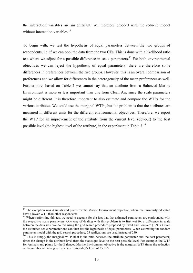
10

the interaction variables are insignificant. We therefore proceed with the reduced model

without interaction variables.14

To begin with, we test the hypothesis of equal parameters between the two groups of

respondents, i.e. if we can pool the data from the two CEs. This is done with a likelihood ratio

test where we adjust for a possible difference in scale parameters.15 For both environmental

objectives we can reject the hypothesis of equal parameters; there are therefore some

differences in preferences between the two groups. However, this is an overall comparison of

preferences and we allow for differences in the heterogeneity of the mean preferences as well.

Furthermore, based on Table 2 we cannot say that an attribute from a Balanced Marine

Environment is more or less important than one from Clean Air, since the scale parameters

might be different. It is therefore important to also estimate and compare the WTPs for the

various attributes. We could use the marginal WTPs, but the problem is that the attributes are

measured in different units for the different environmental objectives. Therefore, we report

the WTP for an improvement of the attribute from the current level (opt-out) to the best

possible level (the highest level of the attribute) in the experiment in Table 3.16

14 The exception was Animals and plants for the Marine Environment objective, where the university educated have a lower WTP than other respondents. 15 When performing this test we need to account for the fact that the estimated parameters are confounded with the respective scale parameters. One way of dealing with this problem is to first test for a difference in scale between the data sets. We do this using the grid search procedure proposed by Swait and Louivere (1993). Given the estimated scale parameter one can then test the hypothesis of equal parameters. When estimating the random parameter model with the grid search procedure, 25 replications are used instead of 250. 16 This is simply the marginal WTP (that is the ratio between the attribute parameter and the cost parameter) times the change in the attribute level from the status quo level to the best possible level. For example, the WTP for Animals and plants for the Balanced Marine Environment objective is the marginal WTP times the reduction of the number of endangered species from today’s level of 35 to 5.

11

Table 3. Mean WTP in SEK for attributes, standard errors in parentheses. Results of t-tests of equal mean WTP between citizens and administrators, p-values in parentheses. Balanced Marine Environment Clean Air Citizens EPA

administrators Diff. (%)

t-test (p-value)

Citizens EPA administrators

Diff. (%)

t-test (p-value)

Animals and plants*

510 (99)

1068 (202)

109 % 2.481 (0.013)

961 (115)

1771 (521)

84% 1.52 (0.129)

Health and recreation*

710 (142)

2560 (794)

261% 2.295 (0.022)

Cultural assets*

437 (70)

240 (131)

- 45% 1.323 (0.186)

66 (67)

229 (225 )

247% 0.692 (0.489)

Oil and chemical spills

492 (67)

361 (108)

- 27% 1.038 (0.299)

Fish stock 525 (83)

840 (148)

60% 1.856 (0.063)

* In order to express the values in WTP terms we simply change the sign of the parameters with a negative sign in Table 2 (Animals and plants and Health and recreation, and Cultural assets for the Balanced Marine Environment objective).

The WTP estimates of both the citizens and the EPA administrators are significant for all

attributes except Cultural assets for the Clean Air objective. For the given improvements of

the attributes, we can also compare the ranking of the attributes. The rankings (in terms of the

WTP estimates) are actually a little bit different. For the Balanced Marine Environment

objective citizens rank Fish stock highest, and then Animals and plants, while the

administrators have the opposite ranking for these two attributes. However, the levels of the

WTPs do not statistically differ among the attributes for the citizens.17 Therefore, the

administrators have a clearer ranking of the attributes in the objective Balanced Marine

Environment objective than what the citizens have. For the Clean Air objective, the rankings

are also different. Citizens have the highest WTP for the Animals and plants attribute, while

administrators have the highest WTP for the Health and recreation. Both groups rank the

Cultural assets attribute as the least important for both objectives.18

However, simply comparing the ordering of the attributes with respect to the magnitude of

WTP does not give much information. Table 3 therefore also reports the results of a two-sided

t-test of equal mean WTP between citizens and administrators. Using a two-sided t-test for the

Balanced Marine Environment objective, the difference in WTP between the citizens and the

EPA administrators is significant at the 10% level for Animals and plants and Fish stock. The

administrators have a higher WTP than the citizens for decreasing the amount of endangered 17 Using two-sided t-tests we cannot reject the hypothesis of equality for any of the WTP comparisons for citizens. For administrators, the WTP for Animals and plants and Fish stock is significantly different from the WTP of the other two attributes. 18 For citizens, the WTP for Cultural assets is significantly lower than the WTP for the two other attributes. For administrators, the WTPs for the three attributes are all statistically different from each other.

12

animals and plants and for increasing the fish stock. For Clean Air, the difference in WTP is

significant at the 5% level for one of the attributes: Health and recreation. Hence, when the

difference in WTP is significant, the administrator WTP is always larger than the citizen

WTP. There is also a large difference for Cultural assets in the Clean Air objective; however,

the difference is not statistically significant, which is explained by the large standard errors

for this attribute. Table 3 also reports the difference in percent between administrator WTP

and citizen WTP; a positive difference means that the administrator WTP is larger than the

citizen WTP. The difference varies between -27 percent and +261 percent.

EPA administrators have a higher WTP than citizens for five out of the seven attributes, and

in some cases the difference is not only significant but also substantial. Although both citizens

and EPA administrators have a high WTP for endangered animals and plants living in the

marine environment, the administrator WTP is twice as high as the citizen WTP. Similarly,

the administrator WTP for better air quality, in terms of improved health, is over three times

the WTP of the citizens. That administrators working with environmental issues have a higher

WTP for measures improving environmental quality is in line with the results of von

Borgstede et al. (2007). Moreover, it is possible that those citizens who answered the

questionnaire are more interested in environmental issues than those who did not participate

in the study. If this is the case, the differences in the sizes of administrator and citizen WTPs

should be even larger than what we found here.

Thus, if we were to use the administrator preferences for policy management, resources would

be allocated differently than if we had used the citizen preferences. Note that these are the

conditional WTPs, i.e. we do not use the alternative specific constant for the opt-out

alternative. Since fewer EPA administrators choose the opt-out, any difference in WTP would

be even larger if we considered the alternative specific constant. None of the EPA

administrators chose the opt-out alternative in all choice situations, while 8 percent of the

citizens did.

4.2 The motives and opinions of the EPA administrators

As said before, the personal views of EPA administrators on how decisions regarding

environmental projects should be made are likely to affect the extent to which economic

information is incorporated into the environmental decision-making process. In the survey we

asked the EPA administrators to motivate their CE choices. A majority (55 percent) chose the

13

alternatives they perceived as necessary for ecological sustainability, while about one-third

chose the alternatives they believed would be appreciated the most by future generations.19

Only 16 percent answered that they chose alternatives they believed to be preferred by people

living today. In other words, administrators put a heavy weight on the long-run development

of environmental quality, and ecological aspects were more important than how ordinary

people view the changes, when the administrators made their choices in the experiment.

Bromley (1990) made similar conclusions in a critical discussion of the main-stream

economist perception of economic efficiency, arguing that the past 40 years of observations of

public decisions indicate that the public sector is not especially convinced of the efficiency

advice offered by economists.

We also asked the administrators to state whether they perceive that some people should have

more say than others when deciding on Swedish environmental policy. They were allowed to

choose among various interest and professional groups such as biologists/ecologists,

environmental economists, experts in political science, sociologists, politicians, and people

who are especially affected by the environmental problem in question. Forty-one percent of

the EPA administrators think that biologists/ecologists should have more say than others,

while about 18 percent believe that environmental economists should. This indicates that a

majority of the administrators believe that persons with environmental education know what

the best environmental management is. However, about 12 percent of the EPA administrators

answered that people who are especially affected by the problem should have the most say,

while 15 percent believe that no group should have more say than others. Thus, although the

EPA should consider the perspective of the citizens in the decision making process (SEPA,

2004), our results suggest that making decisions in line with citizen preferences is not

generally of high priority.

Finally, the administrators were asked to rate their perceived trustworthiness of the results of

stated preference studies on a 1-5 scale (1 meaning Not trustworthy at all and 5 meaning Very

trustworthy). Although about 90 percent of the EPA administrators had heard about stated

preference studies, they responded that they do not believe in them: About 40 percent stated

that these methods are not trustworthy and no one feels that they are very trustworthy. This

could affect their willingness to incorporate economic information into the final policy

19 This is in line with the experiences of one of the authors, as a former Swedish EPA employee. Ecological sustainability and the future generation perspective are very strong objectives in the management.

14

decision. On the other hand, a large majority (79 percent) have a positive view of using cost-

benefit analyses as a basis for decision making in environmental problems. This is however

partly in conflict with the fact that the EPA administrators do not trust stated preference

studies. Stated preference studies constitute the most commonly used method to capture the

benefit side in cost-benefit analyses.20

5. Conclusions In Sweden, just as in many other countries, the EPA is one of the main responsible authorities

for managing environmental resources. Consequently, it plays an important role in

determining environmental policies. The main interest of this paper was to investigate

whether citizen preferences regarding environmental quality differ from the preferences of

those engaged in environmental management. This was done by conducting the same choice

experiment on a random sample of Swedish households and on a random sample of

administrators working at the Swedish EPA. For the environmental objective in question, the

EPA administrators were told to choose the alternative they would recommend to govern

Swedish environmental policy. We found that the rankings of attributes by citizens and EPA

administrators are not the same. These results are not in line with Nilsson et al. (2004) who

found that the preferences of the general public and decision makers working in the public

sector do not differ with respect to support for programs aimed to improve environmental

quality. Colombo et al. (2007) also found that citizens and decision makers rank

environmental attributes in a similar fashion. However, they are more in line with the study by

Alberini et al. (2006) who found both similarities and dissimilarities between the general

public and official/stakeholder preferences. Clearly, the results are contextual, but our

advantages are that we use the same preference elicitation method for both groups and that the

EPA is the public agency that is responsible for the two environmental objectives.21 We also

found significant differences in the levels of WTP for particular attributes. For example, for

the attribute Animals and plants in the Balanced Marine Environment objective, the EPA

administrator WTP is more than twice as large as the citizen WTP. For the Clean Air

objective, the administrator WTP for better health is more than three times the citizen WTP.

These differences are found despite the choice experiment being generic in the sense that not

20 According to Samakovlis and Vredin Johansson (2005) the quality of cost-benefit analysis done by several Swedish public authorities is not good enough and authorities should use cost-benefit analysis more often. 21 Alberini et al. (2006) and Colombo et al. (2007) use different elicitation methods and both Alberini et al. (2006) and Nilsson et al. (2004) sample administrators at a wide range of public agencies.

15

all citizens have personal experiences of marine environments or live in large cities with

particularly bad air quality.

These differences between administrators and citizens can have two effects. First,

administrators are likely to make different priorities than citizens for a given amount of

resources. Second, administrators are likely to argue for a larger share of the resources to be

spent on environmental quality compared to what the citizens would argue for. The

administrators’ motives for their CE choices show that ecological sustainability is more

important than the preferences of ordinary people regarding changes in environmental quality.

A majority of the administrators have a paternalistic approach; they think that individuals with

environmental education should have more say in shaping environmental policy in Sweden

than other groups in society. Although EPA administrators have more information about the

environmental quality objectives than what citizens have,22 a paternalistic point of view is in

strong contrast to how economic theory and many economists advocate that environmental

resources should be managed. It might also increase potential distrust among citizens towards

those who are responsible for the environmental policies and management.

This is to our knowledge the first study that compares decision makers and citizen preferences

for environmental quality using the same methodology. Clearly, more studies of this kind are

needed.

22 They of course have more information since they work with these issues daily. Moreover, they are more educated than the average person, and many of them have a degree in natural sciences.

16

References

Alberini, A., A. Longo and P. Riganti (2006), Using surveys to compare the public’s and decisionmakers’ preferences for urban regeneration: The Venice Arsenale, Working Paper, Fondazione Eni Enrico Mattei.

Alpizar, F., F. Carlsson and P. Martinsson (2003), Using choice experiments for non-market valuation, Economic Issues 8, 83-110.

von Borgstede C., M. Zannakis and L. J. Lundqvist (2007), Organizational culture, professional norms and local implementation of national climate policy, in From Kyoto to the Town Hall, (Eds.) L. J. Lundqvist and A. Biel, Earthscan, London.

Brennan, G. and J. Buchanan (1980), The Power to Tax: Analytical Foundations of a Fiscal Constitution, Cambridge University Press, Cambridge.

Bromely, W (1990), The ideology of efficiency: Searching for a theory of policy analysis, Journal of Environmental Economics and Management 19, 86 – 107.

Carlsson, F. and P. Martinsson (2003), Design techniques for stated preference methods in health economics, Health Economics 12, 281-294.

Colombo S., A. Angus, J. Morris, D. J. Parson, M. Brawn, K. Stacey and N. Hanley (2007), A comparison of citizen and “expert” preferences using an attribute-based approach to choice, Working Paper, Cranfield University, UK.

Davis, J. and D. Whittington (1998), Participatory research for development projects: A comparison of the community meeting and household survey techniques, Economic Development and Cultural Change 47, 73-94.

Gemmell N., O. Morrissey and A. Pinar (2004), Tax perceptions and preferences over tax structure in the United Kingdom, The Economic Journal, 114, 117-138.

Hammar H., S. C. Jagers and K. Nordblom (2006) What explains attitudes towards tax levels? A multi-tax comparison, Working paper, University of Gothenburg.

Johansson-Stenman, O. (2008), Mad cows, terrorism and junk food: Should public policy reflect subjective or objective risk?, Journal of Health Economics, forthcoming.

Kenyon, W., N. Hanley and C. Nevin (2001), Citizens’ juries: an aid to environmental valuation, Environment and Planning C 19, 557-566.

Lipsky, M. (1980), Street-level Bureaucracy. Dilemmas of the Individual in Public Services. New York: Russell Sage Foundation.

Louviere, J.J, D.A. Hensher and J.U.D. Swait (2000), Stated Choice Methods: Analysis and Applications, Cambridge University Press, Cambridge.

Mueller, D. (2003) Public Choice III, Cambridge University Press, Cambridge. Nilsson A., C. von Borgstede and A. Biel (2004), Willingness to accept climate change

strategies: The effect of values and norms, Journal of Environmental Psychology, 24, 267-277.

Nilsson A. and A. Biel (2008), Acceptance of climate change policy measures: Role framing and value guidance, Working Paper, Department of Psychology, University of Gothenburg.

Niskanen, W. (1971), Bureaucracy and Representative Government, Aldine-Atherton, Chicago.

Nyborg K. (2000), Homo economicus and homo politicus: interpretation and aggregation of environmental values, Journal of Economic Behavior & Organization, Vol. 42, 305-322.

O’Donoghue, T. and M. Rabin (2003), Studying optimal paternalism, illustrated by a model of sin taxes, American Economic Review (Papers and proceedings) 93, 186-191.

SEPA (2004), Ekonomiska konsekvensanalyser i myndighetens miljöarbete - förslag till förbättringar, Report 5398, July 2004.

17

SEPA (2006), Sweden’s 16 Environmental Objectives, Swedish Environmental Protection Agency, April 2006.

Saaty, T. (1980) The Analytical Hierarchy Process. McGraw-Hill, New York. Samakovlis, E. and M. Vredin Johansson (2005), Samhällsekonomiskt underlag till

miljöpolitiken: brister och förbättringar, Ekonomisk Debatt 7/2005, 39-39. Statistics Sweden (2007), Swedish Population 1 January 2007, Accessed at homepage:

www.scb.se February 2008. Swait, J. and J. Louviere (1993), The role of the scale parameter in the estimation and

comparison of multinomial logit models, Journal of Marketing Research 30: 305-314. Train, K (2003), Discrete Choice Methods with Simulation. Cambridge University Press, New

York.

Paper IV

www.elsevier.com/locate/trd

Transportation Research Part D 9 (2004) 373–385

The marginal values of noise disturbance from air traffic:does the time of the day matter?

Fredrik Carlsson a, Elina Lampi b,*, Peter Martinsson c

a Department of Economics, Goteborg University, SE-405 30 Goteborg, Swedenb Department of Economics, Umea University, SE-901 87 Umea, Sweden

c Department of Economics, Goteborg University, SE-405 30 Goteborg, Sweden

Abstract

This paper analyzes the marginal willingness to pay for changes in noise levels related to changes in the

volume of flight movements at a city airport in Stockholm, Sweden, by using a choice experiment. When

estimating marginal willingness to pay for different times of the day and days of the week, we find that thesevary with the temporal dimensions: mornings and evenings have higher marginal values. Interestingly, a

substantial proportion of the respondents prefer no changes in the current noise level. The paper concludes

with a policy discussion related to incentive-based pricing.

� 2004 Elsevier Ltd. All rights reserved.

Keywords: Choice experiment; Discrete choice; Aircraft; Noise; Airports

1. Introduction

Air traffic is now starting to pick up after September 11, and is expected to grow in the nearfuture. One important issue linked to growth is the location and the size of airports. Whereveran airport is located, residents nearby will be disturbed, and whenever an airport expands, the dis-turbance and the number of people disturbed will increase. How residents perceive disturbance

1361-9209/$ - see front matter � 2004 Elsevier Ltd. All rights reserved.

doi:10.1016/j.trd.2004.07.002

* Corresponding author.

E-mail address: elina.lampi@econ.umu.se (E. Lampi).

374 F. Carlsson et al. / Transportation Research Part D 9 (2004) 373–385

from air traffic, and the welfare losses linked to this, is therefore an important issue for decisionsregarding both the location and the size of airports. Furthermore, the aviation sector is currentlymoving away from a command-and-control type of environmental regulation with engine stand-ards and a phasing out of engine types towards implementation of incentive-based pricing systems(Carlsson, 2003; Morrell and Lu, 2001). This is in line with the European Union (2001) recom-mendation of increased use of incentive-based pricing in the transport sector.A successful environmental regulation of externalities requires information about the marginal

damage. In this paper we focus on noise damages from air traffic. Noise externalities are ratherdifferent from other types of externalities caused by air traffic because the marginal damagecan vary with the time of the day and the day of the week, which is, for example, different fromexternalities caused by air pollution. For example, the external damage of one night-flight is pre-sumably more damaging than the same flight made during the day. There are also findings sug-gesting that noise from air traffic is considered more disturbing than the equivalent noisedisturbance from road traffic (Naturvardsverket, 2001).There are few studies on the aggregated marginal damage from air traffic noise. The majority of

work has applied a hedonic pricing approach (Levesque, 1994; Uyeno et al., 1993; Penningtonet al., 1990), but there are also studies using stated preference methods (Feitelson et al.,1996) 1. There are two main problems with hedonic pricing studies: it is difficult to estimate wel-fare measures from them, at least if one wants to obtain generic values of attributes (Haab andMcConnell, 2002), and it is almost impossible to estimate welfare measures for changes in noisefrom air traffic at different days of the week, as well as at different times of the day.Here a choice experiment is used to estimate the welfare effects via changes in the number of

take-offs and landings at a city-center airport in Stockholm, Sweden. 2 In a choice experiment,respondents are presented with a hypothetical situation, in our case that the number of landingsand take-offs at Bromma Airport will either increase or decrease depending on the survey versionassigned to them. The respondents are then asked to choose the preferred alternative among sev-eral alternatives in each choice set presented, and normally they are asked to perform a sequenceof choices containing 5–15 choice sets. In the case of an increase they would be compensated,while for a decrease there would be an extra payment. In our experiment the attributes relateto the number of take-offs and landings in one hour at different times of the day. Moreover, halfof the choice sets concern the stated situation during working days and half during weekends. Thestrength of a stated preference method is that we can estimate the welfare changes for changes inthe number of take-offs and landings at levels which do not exist today. It also provides us witheasily interpretable results.

2. Description of Bromma Airport

The study analyzes the aircraft noise from Bromma Airport. The airport is located in Stock-holm and is Sweden�s third largest in terms of the number of flight movements and the second

1 Nelson (2004) offers a recent overview and meta-analysis of the relationship between airport noise and hedonic

property values.2 See for example Alpizar et al. (2003) and Louviere et al. (2000) for overviews of choice experiments.

F. Carlsson et al. / Transportation Research Part D 9 (2004) 373–385 375

largest for domestic flights. It is located near highly population areas being only 8 km from Stock-holm city center. The environmental regulations for Bromma Airport are stricter than for airportslocated further away from the city centers (Luftfartsverket, 2002). Aircraft operations are com-pletely banned during the night; operations being allowed only 7 am–10 pm on weekdays,9 am–5 pm on Saturdays and 10 am–8 pm on Sundays. There is a limit on aircraft noise of89 EPN decibels. 3 There is also a maximal weight limit for aircraft of 50,000 kg, and take-offsand landings per year are restricted to 65,000.The existence and the size of Bromma Airport have been frequently debated. The current reg-

ulations and volume of air traffic at Bromma Airport are an outcome of a political process, whichhas evolved over many years. The latest agreement between the City Council, which is the su-preme decision making body of the City of Stockholm, and the Swedish Civil Aviation Adminis-tration states that Bromma Airport will be shut down by the end of 2011 (Luftfartsverket, 2003).The majority of the City Council wants to use the area to build a new residential area after theairport has been shut down. Building a new residential area will, however, result in other effectson the current residents such as increased road traffic and possibly changes in housing prices. Onthe other hand, some of those in opposition do not want the airport closed. The future of the air-port is a widely debated topic and people living close to the airport often have, for natural rea-sons, strong opinions about the existence of the airport (Blomqvist et al., 2000).Kristrom (1997) reports the results from a contingent valuation study on the size of Bromma

Airport in 1993. This has a bearing on methodological development since the spike models areintroduced. This type of model allows a proportion of the respondents to have a zero willing-ness-to-pay in a closed-ended contingent valuation survey, which is not the case when using ordi-nary parametric models such as a probit model. An expansion in the size of the airport wasdescribed as beneficial to local business and a decrease as yielding environmental benefits. Theconstruction of the survey allowed Kristrom to discover that slightly more than 70% are indiffer-ent between an increase and a decrease in the size of the airport. Kristrom reports these individ-uals as having a no willingness to pay for a change and thus these respondents do not see theairport as a major environmental problem.

3. Design of the choice experiment

There are small differences in noise levels among the types of aircrafts using Bromma Airport(Luftfartsverket, 2002). 4 It is likely, however, that the marginal damage caused by take-offs andlandings varies with time of the day and with the day of the week. Therefore we specify the flightmovements in the choice experiment to be the number of take-offs and landings by time of day(early mornings, mornings, afternoons and evenings) and by day of the week (weekdays andweekends). Furthermore, since there has been a discussion on both an increase and a decrease

3 EPNL, Effective Perceived Noise Level, is a value of certification for every type of aircraft when they take off or

land.4 The different types of aircrafts operating at Bromma Airport have a maximum noise level between 78 and 83 dB (A)

when landing. The maximum noise level is between 75 and 83 dB (A) when taking off.

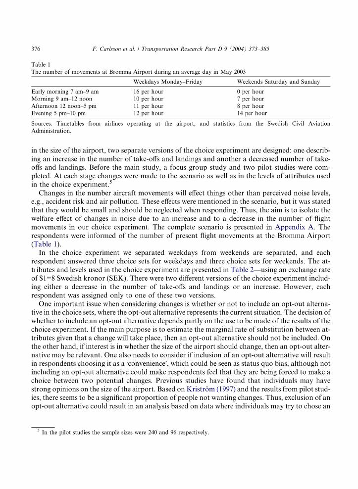
Table 1

The number of movements at Bromma Airport during an average day in May 2003

Weekdays Monday–Friday Weekends Saturday and Sunday

Early morning 7 am–9 am 16 per hour 0 per hour

Morning 9 am–12 noon 10 per hour 7 per hour

Afternoon 12 noon–5 pm 11 per hour 8 per hour

Evening 5 pm–10 pm 12 per hour 14 per hour

Sources: Timetables from airlines operating at the airport, and statistics from the Swedish Civil Aviation

Administration.

376 F. Carlsson et al. / Transportation Research Part D 9 (2004) 373–385

in the size of the airport, two separate versions of the choice experiment are designed: one describ-ing an increase in the number of take-offs and landings and another a decreased number of take-offs and landings. Before the main study, a focus group study and two pilot studies were com-pleted. At each stage changes were made to the scenario as well as in the levels of attributes usedin the choice experiment.5

Changes in the number aircraft movements will effect things other than perceived noise levels,e.g., accident risk and air pollution. These effects were mentioned in the scenario, but it was statedthat they would be small and should be neglected when responding. Thus, the aim is to isolate thewelfare effect of changes in noise due to an increase and to a decrease in the number of flightmovements in our choice experiment. The complete scenario is presented in Appendix A. Therespondents were informed of the number of present flight movements at the Bromma Airport(Table 1).In the choice experiment we separated weekdays from weekends are separated, and each

respondent answered three choice sets for weekdays and three choice sets for weekends. The at-tributes and levels used in the choice experiment are presented in Table 2––using an exchange rateof $1=8 Swedish kronor (SEK). There were two different versions of the choice experiment includ-ing either a decrease in the number of take-offs and landings or an increase. However, eachrespondent was assigned only to one of these two versions.One important issue when considering changes is whether or not to include an opt-out alterna-

tive in the choice sets, where the opt-out alternative represents the current situation. The decision ofwhether to include an opt-out alternative depends partly on the use to be made of the results of thechoice experiment. If the main purpose is to estimate the marginal rate of substitution between at-tributes given that a change will take place, then an opt-out alternative should not be included. Onthe other hand, if interest is in whether the size of the airport should change, then an opt-out alter-native may be relevant. One also needs to consider if inclusion of an opt-out alternative will resultin respondents choosing it as a �convenience�, which could be seen as status quo bias, although notincluding an opt-out alternative could make respondents feel that they are being forced to make achoice between two potential changes. Previous studies have found that individuals may havestrong opinions on the size of the airport. Based on Kristrom (1997) and the results from pilot stud-ies, there seems to be a significant proportion of people not wanting changes. Thus, exclusion of anopt-out alternative could result in an analysis based on data where individuals may try to chose an

5 In the pilot studies the sample sizes were 240 and 96 respectively.

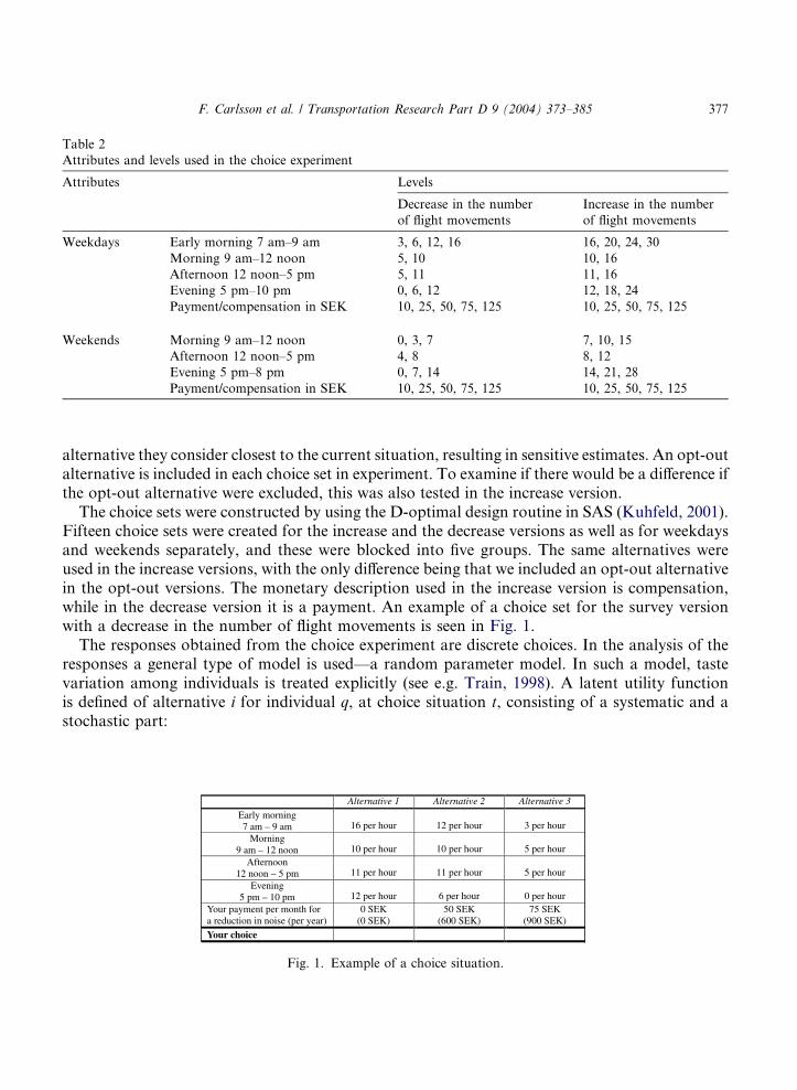
Table 2

Attributes and levels used in the choice experiment

Attributes Levels

Decrease in the number

of flight movements

Increase in the number

of flight movements

Weekdays Early morning 7 am–9 am 3, 6, 12, 16 16, 20, 24, 30

Morning 9 am–12 noon 5, 10 10, 16

Afternoon 12 noon–5 pm 5, 11 11, 16

Evening 5 pm–10 pm 0, 6, 12 12, 18, 24

Payment/compensation in SEK 10, 25, 50, 75, 125 10, 25, 50, 75, 125

Weekends Morning 9 am–12 noon 0, 3, 7 7, 10, 15

Afternoon 12 noon–5 pm 4, 8 8, 12

Evening 5 pm–8 pm 0, 7, 14 14, 21, 28

Payment/compensation in SEK 10, 25, 50, 75, 125 10, 25, 50, 75, 125

F. Carlsson et al. / Transportation Research Part D 9 (2004) 373–385 377

alternative they consider closest to the current situation, resulting in sensitive estimates. An opt-outalternative is included in each choice set in experiment. To examine if there would be a difference ifthe opt-out alternative were excluded, this was also tested in the increase version.The choice sets were constructed by using the D-optimal design routine in SAS (Kuhfeld, 2001).

Fifteen choice sets were created for the increase and the decrease versions as well as for weekdaysand weekends separately, and these were blocked into five groups. The same alternatives wereused in the increase versions, with the only difference being that we included an opt-out alternativein the opt-out versions. The monetary description used in the increase version is compensation,while in the decrease version it is a payment. An example of a choice set for the survey versionwith a decrease in the number of flight movements is seen in Fig. 1.The responses obtained from the choice experiment are discrete choices. In the analysis of the

responses a general type of model is used––a random parameter model. In such a model, tastevariation among individuals is treated explicitly (see e.g. Train, 1998). A latent utility functionis defined of alternative i for individual q, at choice situation t, consisting of a systematic and astochastic part:

Alternative 1 Alternative 2 Alternative 3

Early morning7 am – 9 am 16 per hour 12 per hour 3 per hour

Morning9 am – 12 noon 10 per hour 10 per hour 5 per hour

Afternoon12 noon – 5 pm 11 per hour 11 per hour 5 per hour

Evening5 pm – 10 pm 12 per hour 6 per hour 0 per hour

Your payment per month for a reduction in noise (per year)

0 SEK(0 SEK)

50 SEK(600 SEK)

75 SEK(900 SEK)

Your choice

Fig. 1. Example of a choice situation.

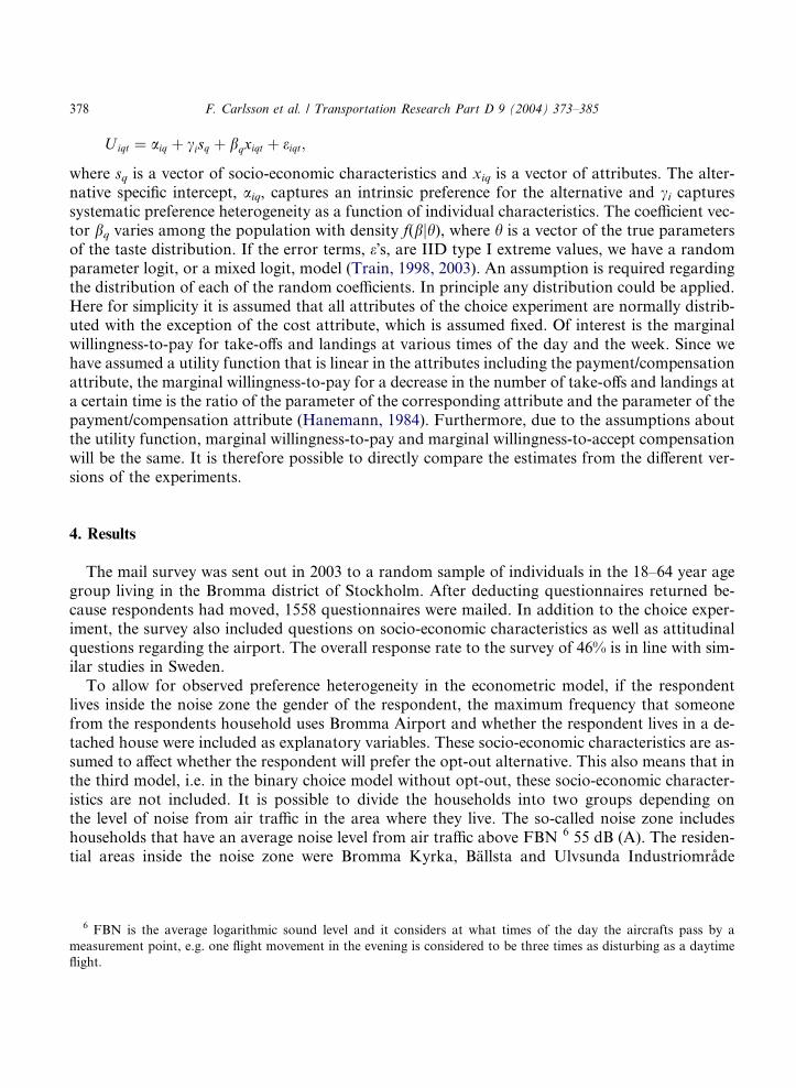
6 F

measu

flight.

378 F. Carlsson et al. / Transportation Research Part D 9 (2004) 373–385

Uiqt ¼ aiq þ cisq þ bqxiqt þ eiqt;

where sq is a vector of socio-economic characteristics and xiq is a vector of attributes. The alter-native specific intercept, aiq, captures an intrinsic preference for the alternative and ci capturessystematic preference heterogeneity as a function of individual characteristics. The coefficient vec-tor bq varies among the population with density f(bjh), where h is a vector of the true parametersof the taste distribution. If the error terms, e�s, are IID type I extreme values, we have a randomparameter logit, or a mixed logit, model (Train, 1998, 2003). An assumption is required regardingthe distribution of each of the random coefficients. In principle any distribution could be applied.Here for simplicity it is assumed that all attributes of the choice experiment are normally distrib-uted with the exception of the cost attribute, which is assumed fixed. Of interest is the marginalwillingness-to-pay for take-offs and landings at various times of the day and the week. Since wehave assumed a utility function that is linear in the attributes including the payment/compensationattribute, the marginal willingness-to-pay for a decrease in the number of take-offs and landings ata certain time is the ratio of the parameter of the corresponding attribute and the parameter of thepayment/compensation attribute (Hanemann, 1984). Furthermore, due to the assumptions aboutthe utility function, marginal willingness-to-pay and marginal willingness-to-accept compensationwill be the same. It is therefore possible to directly compare the estimates from the different ver-sions of the experiments.

4. Results

The mail survey was sent out in 2003 to a random sample of individuals in the 18–64 year agegroup living in the Bromma district of Stockholm. After deducting questionnaires returned be-cause respondents had moved, 1558 questionnaires were mailed. In addition to the choice exper-iment, the survey also included questions on socio-economic characteristics as well as attitudinalquestions regarding the airport. The overall response rate to the survey of 46% is in line with sim-ilar studies in Sweden.To allow for observed preference heterogeneity in the econometric model, if the respondent

lives inside the noise zone the gender of the respondent, the maximum frequency that someonefrom the respondents household uses Bromma Airport and whether the respondent lives in a de-tached house were included as explanatory variables. These socio-economic characteristics are as-sumed to affect whether the respondent will prefer the opt-out alternative. This also means that inthe third model, i.e. in the binary choice model without opt-out, these socio-economic character-istics are not included. It is possible to divide the households into two groups depending onthe level of noise from air traffic in the area where they live. The so-called noise zone includeshouseholds that have an average noise level from air traffic above FBN 6 55 dB (A). The residen-tial areas inside the noise zone were Bromma Kyrka, Ballsta and Ulvsunda Industriomrade

BN is the average logarithmic sound level and it considers at what times of the day the aircrafts pass by a

rement point, e.g. one flight movement in the evening is considered to be three times as disturbing as a daytime

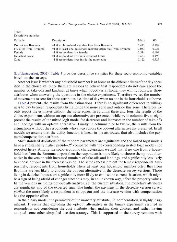
Table 3

Descriptive statistics

Variable Description Mean SD

Do not use Bromma =1 if no household member flies from Bromma 0.471 0.499

Fly often from Bromma =1 if at least one household member often flies from Bromma 0.053 0.224

Female =1 if respondent is a female 0.544 0.499

Detached house =1 if respondent lives in a detached house 0.453 0.498

Zone =1 if respondent lives inside the noise zone 0.122 0.327

F. Carlsson et al. / Transportation Research Part D 9 (2004) 373–385 379

(Luftfartsverket, 2002). Table 3 provides descriptive statistics for these socio-economic variablesbased on the surveys.Another issue is whether any household member is at home at the different times of the day spec-

ified in the choice set. Since there are reasons to believe that respondents do not care about thenumber of take-offs and landings at times when nobody is at home, they will not consider thoseattributes when answering the questions in the choice experiment. Therefore we set the numberof movements to zero for those attributes, i.e. time of day when no one in the household is at home.Table 4 presents the results from the estimations. There is no significant differences in willing-

ness to pay between respondents living inside the noise zone and outside this zone. Therefore weonly report the estimates without the noise zones. In columns three and four, the results of thechoice experiments without an opt-out alternative are presented, while we in columns five to eightpresent the results of the mixed logit model for decreases and increases in the number of take-offsand landings with an opt-out alternative. Finally, in columns nine to twelve, the results from theestimations without the respondents who always chose the opt-out alternative are presented. In allmodels we assume that the utility function is linear in the attributes, that also includes the pay-ment/compensation attribute.Most standard deviations of the random parameters are significant and the mixed logit models

have a substantially higher pseudo-R2 compared with the corresponding nested logit model (notreported here). Among the socio-economic characteristics, we find that if no one from a house-hold flies from the Bromma airport then the respondent is more likely to choose the opt-out alter-native in the version with increased numbers of take-offs and landings, and significantly less likelyto choose opt-out in the decrease version. The same effect is present for female respondents. Sur-prisingly, respondents from households where at least one household member often flies fromBromma are less likely to choose the opt-out alternative in the decrease survey versions. Thoseliving in detached houses are significantly more likely to choose the current situation, which mightbe a sign of being afraid of changes since this may, in an unknown way, affect the property values.In the versions including opt-out alternatives, i.e. the current situation, the monetary attributesare significant and of the expected sign. The higher the payment in the decrease version ceterisparibus the more likely a respondent is to opt-out and the increase version with compensationhas the opposite effect.In the binary model, the parameter of the monetary attribute, i.e. compensation, is highly insig-

nificant. It seems that excluding the opt-out alternative in the binary experiment resulted inrespondents not considering the cost attribute when making their choices, and rather havingadopted some other simplified decision strategy. This is supported in the survey versions with

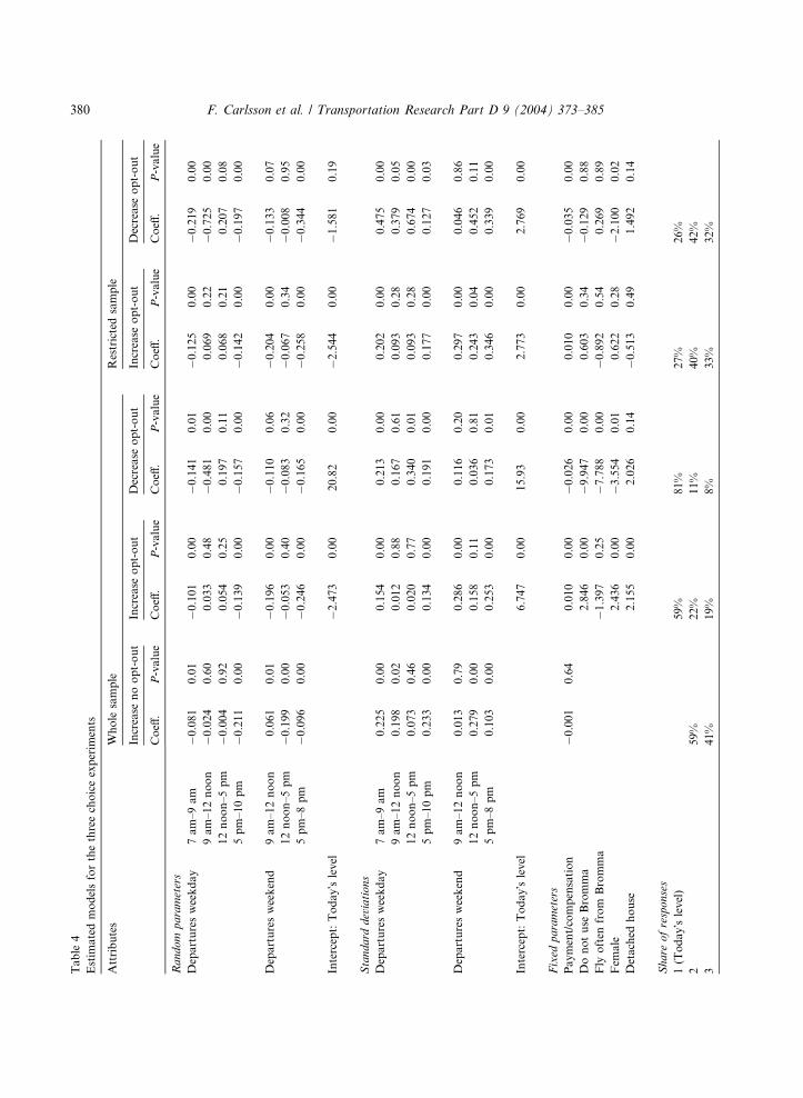
Table4

Estimatedmodelsforthethreechoiceexperiments

Attributes

Wholesample

Restrictedsample

Increasenoopt-out

Increaseopt-out

Decreaseopt-out

Increaseopt-out

Decreaseopt-out

Coeff.

P-value

Coeff.

P-value

Coeff.

P-value

Coeff.

P-value

Coeff.

P-value

Random

parameters

Departuresweekday

7am–9am

�0.081

0.01

�0.101

0.00

�0.141

0.01

�0.125

0.00

�0.219

0.00

9am–12noon

�0.024

0.60

0.033

0.48

�0.481

0.00

0.069

0.22

�0.725

0.00

12noon–5pm

�0.004

0.92

0.054

0.25

0.197

0.11

0.068

0.21

0.207

0.08

5pm–10pm

�0.211

0.00

�0.139

0.00

�0.157

0.00

�0.142

0.00

�0.197

0.00

Departuresweekend

9am–12noon

0.061

0.01

�0.196

0.00

�0.110

0.06

�0.204

0.00

�0.133

0.07

12noon–5pm

�0.199

0.00

�0.053

0.40

�0.083

0.32

�0.067

0.34

�0.008

0.95

5pm–8pm

�0.096

0.00

�0.246

0.00

�0.165

0.00

�0.258

0.00

�0.344

0.00

Intercept:Today�slevel

�2.473

0.00

20.82

0.00

�2.544

0.00

�1.581

0.19

Standard

deviations

Departuresweekday

7am–9am

0.225

0.00

0.154

0.00

0.213

0.00

0.202

0.00

0.475

0.00

9am–12noon

0.198

0.02

0.012

0.88

0.167

0.61

0.093

0.28

0.379

0.05

12noon–5pm

0.073

0.46

0.020

0.77

0.340

0.01

0.093

0.28

0.674

0.00

5pm–10pm

0.233

0.00

0.134

0.00

0.191

0.00

0.177

0.00

0.127

0.03

Departuresweekend

9am–12noon

0.013

0.79

0.286

0.00

0.116

0.20

0.297

0.00

0.046

0.86

12noon–5pm

0.279

0.00

0.158

0.11

0.036

0.81

0.243

0.04

0.452

0.11

5pm–8pm

0.103

0.00

0.253

0.00

0.173

0.01

0.346

0.00

0.339

0.00

Intercept:Today�slevel

6.747

0.00

15.93

0.00

2.773

0.00

2.769

0.00

Fixed

parameters

Payment/compensation

�0.001

0.64

0.010

0.00

�0.026

0.00

0.010

0.00

�0.035

0.00

DonotuseBromma

2.846

0.00

�9.947

0.00

0.603

0.34

�0.129

0.88

Flyoften

fromBromma

�1.397

0.25

�7.788

0.00

�0.892

0.54

0.269

0.89

Fem

ale

2.436

0.00

�3.554

0.01

0.622

0.28

�2.100

0.02

Detached

house

2.155

0.00

2.026

0.14

�0.513

0.49

1.492

0.14

Share

ofresponses

1(Today�slevel)

59%

81%

27%

26%

259%

22%

11%

40%

42%

341%

19%

8%

33%

32%

380 F. Carlsson et al. / Transportation Research Part D 9 (2004) 373–385

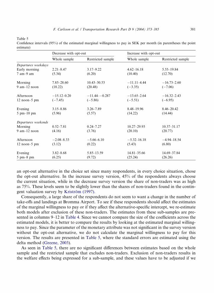
Table 5

Confidence intervals (95%) of the estimated marginal willingness to pay in SEK per month (in parentheses the point

estimate)

Decrease with opt-out Increase with opt-out

Whole sample Restricted sample Whole sample Restricted sample

Departures weekdays

Early morning 2.21–8.47 3.17–9.22 4.62–16.18 5.55–19.84

7 am–9 am (5.34) (6.20) (10.40) (12.70)

Morning 7.85–28.60 10.43–30.53 �11.11–4.44 �16.73–2.609 am–12 noon (18.22) (20.48) (�3.35) (�7.06)

Afternoon �15.12–0.20 �11.44–�0.287 �13.65–2.64 �16.32–2.4312 noon–5 pm (�7.45) (�5.86) (�5.51) (�6.95)

Evening 3.15–8.86 3.26–7.89 8.48–19.96 8.46–20.42

5 pm–10 pm (5.96) (5.57) (14.22) (14.44)

Departures weekends

Morning 0.52–7.81 0.24–7.27 10.27–29.93 10.37–31.17

9 am–12 noon (4.16) (3.76) (20.10) (20.77)

Afternoon �2.08–8.33 �5.66–6.10 �5.32–16.18 �4.94–18.5412 noon–5 pm (3.12) (0.22) (5.43) (6.80)

Evening 3.82–8.68 5.85–13.59 14.81–35.66 14.69–37.84

5 pm–8 pm (6.25) (9.72) (25.24) (26.26)

F. Carlsson et al. / Transportation Research Part D 9 (2004) 373–385 381

an opt-out alternative in the choice set since many respondents, in every choice situation, chosethe opt-out alternative. In the increase survey version, 45% of the respondents always choosethe current situation, while in the decrease survey version the share of non-traders was as highas 75%. These levels seem to be slightly lower than the shares of non-traders found in the contin-gent valuation survey by Kristrom (1997).Consequently, a large share of the respondents do not seem to want a change in the number of

take-offs and landings at Bromma Airport. To see if these respondents should affect the estimatesof the marginal willingness to pay or if they affect the alternative-specific intercept, we re-estimateboth models after exclusion of these non-traders. The estimates from these sub-samples are pre-sented in columns 9–12 in Table 4. Since we cannot compare the size of the coefficients across theestimated models, it is better to compare the results by looking at the estimated marginal willing-ness to pay. Since the parameter of the monetary attribute was not significant in the survey versionwithout the opt-out alternative, we do not calculate the marginal willingness to pay for thisversion. The results are presented in Table 5, where the standard errors are estimated using thedelta method (Greene, 2003).As seen in Table 5, there are no significant differences between estimates based on the whole

sample and the restricted sample that excludes non-traders. Exclusion of non-traders results inthe welfare effects being expressed for a sub-sample, and these values have to be adjusted if we

382 F. Carlsson et al. / Transportation Research Part D 9 (2004) 373–385

want to obtain values for the whole population. In turn this implies that one cannot use theseestimates directly for a welfare evaluation since the marginal willingness-to-pay is zero, or evennegative, for some respondents. In general the estimated marginal willingness to pay is higherfor the increase version with one exception: departures in the morning during weekdays. It isdifficult to know why this time of the day would be the exception. The major disturbancesaccording to our estimates are during the mornings and the evenings both for weekdaysand weekends. If we focus on the increase survey version, the marginal willingness to pay isabout 10 SEK per month for take-offs or landings in the early mornings during weekdaysand about 20 SEK in the mornings during weekends. Moreover, the willingness to pay is evenhigher in the evenings.

5. Discussions and conclusions

This paper provides some empirical evidence about the marginal willingness to pay for changesin noise from air traffic related to changes in aircraft movements at Bromma Airport. A substan-tial proportion of those surveyed favored the current situation in all choice sets, both in the in-crease (45%) and in the decrease (75%) versions. These figures are not surprising given thatKristrom (1997) found in a contingent valuation value survey that more than 70% were non-trad-ers. A high proportion of non-traders may also indicate that other, non-standard economic as-pects are important. There is also a tendency for a larger proportion of non-traders, and alower marginal willingness-to-pay in the decrease version. This is in line with evidence suggestingdivergence between willingness-to-pay and willingness-to-accept, that is particularly large for non-market goods (Horowitz and McConnell, 2002). One explanation is an endowment effect wherebyrespondents are reluctant to pay money for an improvement (Kahneman et al., 1990). Moreover,Kahneman et al. (1999) argue responses in surveys are more likely to be expressive than to rep-resent a value. In addition to psychological explanations, the size of Bromma Airport is a resultof past political debates, and hence individuals have at least indirectly affected the size of theairport.A large proportion of people are satisfied with the current level of flight operations at the air-

port and are not prepared to trade off any change for monetary compensation or payments. Thereare restrictions on aircraft noise levels and the weights of the aircrafts allowed to take off and landand it is a relatively quiet airport despite its size.However, people are sensitive to noise and the time of day matters. Some of the residents in the

Bromma area show a significant willingness-to-pay for a decrease in the number of aircraft move-ments in the morning and evening throughout the week. At the same time, many respondents arenot willing to pay anything for a change in the number of departures.

Acknowledgments

Financial support from the Swedish Agency for Innovation Systems (VINNOVA) and theSwedish Civil Aviation Administration is gratefully acknowledged. We have received valuable

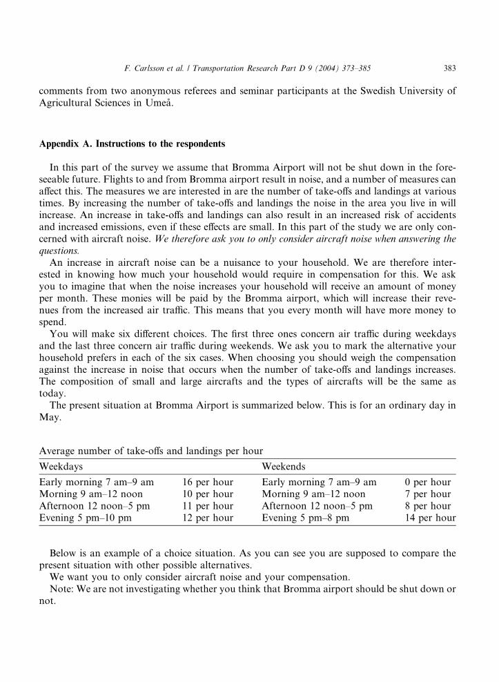
F. Carlsson et al. / Transportation Research Part D 9 (2004) 373–385 383

comments from two anonymous referees and seminar participants at the Swedish University ofAgricultural Sciences in Umea.

Appendix A. Instructions to the respondents

In this part of the survey we assume that Bromma Airport will not be shut down in the fore-seeable future. Flights to and from Bromma airport result in noise, and a number of measures canaffect this. The measures we are interested in are the number of take-offs and landings at varioustimes. By increasing the number of take-offs and landings the noise in the area you live in willincrease. An increase in take-offs and landings can also result in an increased risk of accidentsand increased emissions, even if these effects are small. In this part of the study we are only con-cerned with aircraft noise. We therefore ask you to only consider aircraft noise when answering thequestions.

An increase in aircraft noise can be a nuisance to your household. We are therefore inter-ested in knowing how much your household would require in compensation for this. We askyou to imagine that when the noise increases your household will receive an amount of moneyper month. These monies will be paid by the Bromma airport, which will increase their reve-nues from the increased air traffic. This means that you every month will have more money tospend.You will make six different choices. The first three ones concern air traffic during weekdays

and the last three concern air traffic during weekends. We ask you to mark the alternative yourhousehold prefers in each of the six cases. When choosing you should weigh the compensationagainst the increase in noise that occurs when the number of take-offs and landings increases.The composition of small and large aircrafts and the types of aircrafts will be the same astoday.The present situation at Bromma Airport is summarized below. This is for an ordinary day in

May.

Average number of take-offs and landings per hour

Weekdays Weekends

Early morning 7 am–9 am 16 per hour Early morning 7 am–9 am 0 per hourMorning 9 am–12 noon 10 per hour Morning 9 am–12 noon 7 per hourAfternoon 12 noon–5 pm 11 per hour Afternoon 12 noon–5 pm 8 per hourEvening 5 pm–10 pm 12 per hour Evening 5 pm–8 pm 14 per hour

Below is an example of a choice situation. As you can see you are supposed to compare thepresent situation with other possible alternatives.We want you to only consider aircraft noise and your compensation.Note: We are not investigating whether you think that Bromma airport should be shut down or

not.

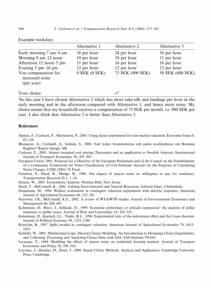
Example weekdays

Alternative 1 Alternative 2 Alternative 3

Early morning 7 am–9 am 16 per hour 24 per hour 16 per hourMorning 9 am–12 noon 10 per hour 10 per hour 11 per hourAfternoon 12 noon–5 pm 11 per hour 16 per hour 16 per hourEvening 5 pm–10 pm 12 per hour 12 per hour 12 per hourYou compensation forincreased noise(per year)

0 SEK (0 SEK) 75 SEK (900 SEK) 50 SEK (600 SEK)

Your choice ·aaIn this case I have chosen Alternative 2 which has more take-offs and landings per hour in theearly morning and in the afternoon compared with Alternative 1, and hence more noise. Mychoice means that my household receives a compensation of 75 SEK per month, i.e. 900 SEK peryear. I also think that Alternative 2 is better than Alternative 3.

384 F. Carlsson et al. / Transportation Research Part D 9 (2004) 373–385

References

Alpizar, F., Carlsson, F., Martinsson, P., 2003. Using choice experiments for non-market valuation. Economic Issues 8,

83–110.

Blomqvist, A., Carlstedt, A., Scheele, S., 2000. Vad tycker brommaborna och andra stockholmare om Bromma

flygplats? Report Inergia AB.

Carlsson, F., 2003. Airport marginal cost pricing: Discussion and an application to Swedish Airports. International

Journal of Transport Economics 30, 283–303.

European Union, 2001. Proposal for a Directive of the European Parliament and of the Council on the Establishment

of a Community Framework for Noise Classification of Civil Subsonic Aircraft for the Purposes of Calculating

Noise Charges. COM (2001) 74 Final.

Feitelson, E., Hurd, R., Mudge, R., 1996. The impact of airport noise on willingness to pay for residences.

Transportation Research D 1, 1–14.

Greene, W., 2003. Econometric Analysis. Prentice Hall, New Jersey.

Haab, T., McConnell, K., 2002. Valuing Environmental and Natural Resources. Edward Elgar, Cheltenham.

Hanemann, M., 1984. Welfare evaluations in contingent valuation experiments with discrete responses. American

Journal of Agricultural Economics 66, 332–341.

Horowitz, J.K., McConnell, K.E., 2002. A review of WTA/WTP studies. Journal of Environmental Economics and

Management 44, 426–447.

Kahneman, D., Ritov, I., Schkade, D., 1999. Economic preferences or attitude expressions? An analysis of dollar

responses to public issues. Journal of Risk and Uncertainty 19, 203–235.

Kahneman, D., Knetsch, J.L., Thaler, R.L., 1990. Experimental tests of the endowment effect and the Coase theorem.

Journal of Political Economy 98, 1325–1348.

Kristrom, B., 1997. Spike models in contingent valuation. American Journal of Agricultural Economics 79, 1013–

1023.

Kuhfeld, W., 2001. Multinomial Logit, Discrete Choice Modeling. An Introduction to Designing Choice Experiments,

and Collecting, Processing and Analyzing Choice Data with SAS. SAS Institute TS-643.

Levesque, T., 1994. Modeling the effects of airport noise on residential housing markets. Journal of Transport

Economics and Policy 28, 199–210.

Louviere, J., Hensher, D., Swait, J., 2000. Stated Choice Methods. Analysis and Application. Cambridge University

Press, Cambridge.

F. Carlsson et al. / Transportation Research Part D 9 (2004) 373–385 385

Luftfartsverket, 2002. Miljorapport 2001 Stockholm-Bromma flygplats. Norrkoping, Luftfartsverket.

Luftfartsverket, 2003. Miljorapport 2002 Stockholm-Bromma flygplats. Norrkoping, Luftfartsverket.

Morrell, P., Lu, C.H.Y., 2001. Aircraft noise social cost and charge mechanisms––a case study of Amsterdam Airport

Schiphol. Transportation Research D 5, 305–320.

Naturvardsverket, 2001. Riktvarden for trafikbuller vid nyanlaggning eller vasentlig ombyggnad av infrastuktur,

forslag till utveckling av definitioner. Dnr 540-355-01 Rv, Naturvardsverket, Stockholm.

Nelson, J.P., 2004. Meta-analysis of airport noise and hedonic property values. Journal of Transport Economics and

Policy 38, 1–28.

Pennington, G., Topham, N., Ward, R., 1990. Aircraft noise and residential property values adjacent to Manchester

international airport. Journal of Transport Economics and Policy 24, 49–59.

Train, K., 1998. Recreation demand models with taste differences over people. Land Economics 74, 230–239.

Train, K., 2003. Discrete Choice Methods with Simulation. Cambridge University Press, New York.

Uyeno, D., Hamilton, S., Biggs, A., 1993. Density of residential land use and the impact of airport noise. Journal of

Transport Economics and Policy 27, 3–18.

Paper V

1

Age-related risk of female infertility: A comparison

between perceived personal and general risks

Elina LampiA

Abstract

Based on a survey of a random sample of Swedish females aged 20-40 this paper investigates: (1) whether women have correct perception of the age-related risk of female infertility, (2) whether the perceptions of the personal risk and the general risk in the own age group differ, and if so, (3) what factors can explain this difference. The results show that Swedish women do know that the likelihood of being infertile increases with age, while they clearly overestimate the general risks for women older than 34. The results also show that mothers have a too optimistic picture of their own fertility, while non-mothers have not. Several factors that explain differences between the stated personal and general risks are discussed. Keywords: personal risk, general risk, female infertility, optimistic bias JEL Classification: D81, I10, J13

Financial support from the Iris Foundation is gratefully acknowledged. The author would like to thank Fredrik Carlsson, Lennart Flood, Olof Johansson-Stenman, Åsa Löfgren, Peter Martinsson, Katarina Nordblom, Katarina Steen Carlsson, Sven Tengstam and seminar participants at University of Gothenburg and at the IAREP/SABE 2006 for many useful comments. A Department of Economics, University of Gothenburg, Box 640, SE 405 30 Göteborg, Sweden, Ph. +46 31 7861393, e-mail: elina.lampi@economics.gu.se.

2

1. Introduction The mean age of first-time mothers has been increasing steadily during the last three decades

in Western countries. In Europe, the highest average age of first-time mothers is found in San

Marino (30.4 years) followed by the Netherlands, Spain, and Sweden (29 years) (Council of

Europe, 2004). This means that the average age of Swedish first-time mothers is now more

than five years higher than 30 years ago (Statistics Sweden, 2005). However, neither the

desire to have children nor the number of children couples want to have has changed during

the last decades (Statistics Sweden, 2001; Lampic et al., 2006), meaning that the outcome of

not becoming pregnant can be assumed to be highly negative for many women. Since the

average age of first-time mothers has been increasing, it is possible that women believe that

the risk of not becoming pregnant is lower than it really is. This was actually found in a

public health study by Lampic et al. (2006), who showed that female and male university

students in Sweden underestimate the general risks of age-related female infertility.1

Infertility is defined as a state where a healthy couple of childbearing age does not use any

type of contraceptive and tries to become pregnant, but does not become pregnant during a

period of 12 months (Infomedica, 2004). It is worth noting that this risk is very individual and

that there is currently no medical test that can investigate the true risk level of infertility in a

specific woman. Some women can easily become pregnant at age 40, while others are

involuntarily childless already at 25 (Infomedica, 2004). An awareness of the infertility risks

is also important because infertility treatments are costly. And more importantly, the current

assisted reproduction technologies cannot totally compensate for the natural age-related

decline in fertility (Leridon, 2004). On the other hand, according to Menken (1985) the age-

related infertility has not increased over time but the problem receives today more attention

than before among both the health care and couples who want to have a child.

We approach the issue of infertility by investigating (1) whether women have correct

perception of the age-related risk of female infertility, (2) whether the perceptions of the

personal risk and the general risk in the own age group differ, and if so, (3) what factors can

explain this difference. Thus, the present study contributes to the existing literature in the

following ways: As far as we know, this study is the first to analyze the relative risk

1 Many previous studies have examined the influence of different economic factors on number of births (Becker, 1981; Heckman and Walker, 1990; Hoem, 2000; Löfström, 2003; Adserá, 2004; Björklund, 2006), while others have looked at the timing of births (Gustafsson and Wetzels, 2000; Martin, 2000 and Gustafsson, 2001 and 2005). The article by Lampic et al. (2006) is the only study we are aware of that investigates women’s risk perception about female age-related infertility.

3

perception in the context of the risk of age-related female infertility, and to study reasons why

women’s risk perceptions might differ between personal and general risk of infertility.

Moreover, there is lack of knowledge about how aware women are about the risk levels.

It is well known that estimation of risk is difficult and several studies have found that people

do not have correct perceptions about risks. Two often reported biases are that small

probabilities are overestimated while large probabilities are underestimated, and that more

sensational risks are easily exaggerated while estimates of more ordinary risks tend to be too

low (Slovic et al., 2000a. See Benjamin et al., 2001 for counterarguments about

underestimation of general risks for the own age group). For example, Black et al., (1995)

report that 40 to 50 year old women highly overestimate their probability of dying of breast

cancer. The risk of age-related female infertility is neither small nor large and it is not

sensational either, but the possible risk of not becoming pregnant may still be a highly

sensitive issue for many women. However, although people are less aware of the magnitude

of the risks, they generally are well aware of the relative risk of different activities (van der

Pligt, 1996). Thus we hypothesize that: Women between 20 and 40 years of age are aware

that the risk of female infertility increases with age, but they do not have a correct perception

of the magnitude of this general risk at different ages.

It is known that people often state lower risks for themselves than for other individuals

(Sjöberg and Fromm, 2001; Sjöberg, 2002). According to van der Pligt (1996), people may

experience that they have more control over their personal risk than the general risk. The

more a person experiences that she has control, the greater the deviation between the

perceived personal and general risks. This positive self-image, i.e. that people think they are

better than others, is also well documented (Svenson 1981; Taylor and Brown 1988; Santos-

Pinto and Sobel, 2005). Explanations found in the literature include that people in general

overestimate their abilities, that a positive self-image increases happiness, and that a personal

experience can both increase and decrease the feeling of personal invulnerability. That people

tend to see themselves as less vulnerable to most kinds of risks compared to other people is

called “optimistic bias”.2 Thus, an optimistic bias is not dependent on actual risk levels, but

2 This definition comes from van der Pligt (1996). Another name for the optimistic bias is “unrealistic optimism” (Weinstein 1980). Moreover, when the person they compare themselves with becomes less abstract (such as a “sibling” or “your closest friend”), people usually rate themselves and the other person as equally vulnerable (Perloff and Fetzer, 1986).

4

instead refers to a person’s perception of her own risk relative to her perception of other

people’s risk levels. We therefore hypothesize that: Women perceive themselves as less

vulnerable to the risk of age-related infertility than other women their age.

It is not sufficient to only investigate whether the risk perception differs between stated

personal and general risks. It is as important to study what explains the potential differences.

Especially older women and mothers may have private information that helps them make

more correct predictions of their own risk of infertility. If mothers really have a lower than

average personal risk, then stating a lower personal than general risk can’t be defined as a

bias. On the other hand, people who have no experience of a particular negative life event

tend to be more positive than others considering this event (Perloff and Fetzer, 1986;

Weistein, 1987; Slovic et al., 2000b). Weinstein found that those who believe that they are at

a lower risk than others think that if the problem has not yet occurred it is unlikely to appear

in the future. He also claims that this behaviour is not limited to any particular age, sex or

education. In the case of infertility, a woman who has become pregnant easily before has a

positive personal experience and may therefore think that she is more fertile than other

women her age. Moreover, the more important people consider an attribute, the more they

perceive that they have it (Dunning et al., 1991). Therefore, it is possible that the more

important it is for a woman to be fertile per se and/or have a child, the more likely she might

perceive that she is able to become pregnant. We hypothesize that: The difference between the

stated personal and general risk depends on a woman’s own previous experience of

becoming pregnant, on how important she perceives of being fertile per se, and on whether

she wants to have children.

The best way to investigate women’s risk perceptions is to ask them, which is why this study

uses a survey method where 1,800 questionnaires were mailed out to a random sample of 20-

40 year old women living in Sweden. The respondents were asked to estimate the average

risks of female infertility for women in four different age groups (20-24, 25-29, 30-34 and

35-40 years). They were also asked to estimate their own personal risk of infertility.

The remainder of this paper is organized as follows. Section 2 presents facts of infertility and

the actual risk levels of age-related infertility, and Section 3 describes the survey and its

design. Section 4 reports the descriptive statistics and the empirical results from the analyses

of the three hypotheses, while Section 5 discusses the results and concludes the paper.

5

2. Facts of infertility and the actual risk levels The risks used as ‘actual’ risks of age-affected infertility in this paper are estimates based on

age-specific pregnancy rates with natural insemination in modern populations, where the

infertility risk levels are collected by interviewing over 7,600 women in the U.S. The

interviews are performed by the National Survey of Family Growth (NSFG) and collected in

2002.3 According to the 2002 study the infertility risk is 7 % for 20-24 year old women,4 11

% for 25-29 year old women, 17 % for 30-34 year old women and 23 % for 35-40 year old

women (Chandra et al, 2005). Data from retrospective surveys such as the NSFG are seen as

being most trustworthy even if it may be difficult for a woman to remember exactly when she

began trying to become pregnant (Högberg, 1998).5 A European study in which infertility

levels are in line with the levels of NSFG surveys is ‘Netherlands Fertility and Family

Survey’ from 1998. It shows that 14-20 % of the women under 30 years and about 21-23 %

of women aged 30 and older did not become pregnant within 12 months (Steenhof and de

Jong, 2001). The reason for using the risk estimates from the NSFG 2002 survey and, not

from the Netherlands survey, is that the NSFG survey has been conducted six times during

the 1973-2002 period and the infertility levels are nearly the same in all of the NSFG surveys,

indicating robustness. Another reason is that the NSFG survey is well documented, has a high

response rate among women (80 %) and it separates among women who are sterilized, who

have tried to become pregnant longer than 3 years, who are fecund but for whom a pregnancy

3 The NSFG survey measures the infertility rates of women who had not become pregnant during the 12 months (or more) proceeding the time of the interview. Surgically sterilised couples are excluded from the survey. There are some possible sources of estimation bias in the NSFG survey. Their assumption that all couples using contraceptives are fertile may decrease the overall estimate of infertility, and it is also possible that couples choosing to be sterilized have a higher than average fertility rate, boosting the NSFG overall estimate since this group was excluded from their study. 4 The youngest age-group in the 2002 survey is very large (15-29 years) and it also includes 15-19 year old women, who we perceived to be far too young to participate in this study. Therefore we divide the age groups according to the NSFG 1976 survey, i.e. 20-24, 25-29, 30-34 and 35-40 years. We also use the risk for 20-24 year old women from the NSFG 1976 survey. The risks in the 2002 survey are 11 % for 15-29 year old women, 17 % for 30-34 year old women, 23 % for 35-40 year old women, while they in the 1976 survey are 7 % for 20-24 year old women, 11 % for 25-29 year old women, 16 % for 30-34 year old women, and 23 % for 35-40 year old women, i.e. very similar levels (National Center for Health Statistics, 1987). 5 The other two ways to measure infertility risks are: age-specific pregnancy rates in natural populations (populations where contraception and abortion are not allowed or used) and age-specific pregnancy rates with artificial insemination in modern populations. The major disadvantage of studies done in natural populations is that the type of data is hard to compare with more modern data, while artificial insemination ends up boosting infertility rates and is therefore often criticized since the probability of becoming pregnant artificially is much smaller compared to using unprotected intercourses (See e.g. Bongaarts, 1982). A study of artificially inseminated women reports that 26-27 % of women 30 or younger, 39 % of women aged 31-35, and 46 % of women aged 36-40 did not become pregnant within a one-year period. (Schwartz and Mayaux 1982). A study by Tietze (1957) reports the shares of natural population (Hutterites) from the first half of 20th century: 3 % of women aged 20-24 were permanently infertile, while the corresponding shares of women aged 25-29, 30-34 and 35-39 years were 5.3 %, 9.0 % and 22 %.

6

is dangerous, and those who are infertile according to the definition of infertility (Chandra et

al., 2005). However, the Netherlands survey has the advantage of reporting risk levels of both

first and second pregnancies. Therefore, we use the results of the Netherlands survey when

analyzing the second hypothesis of this study.

3. The survey and survey design In order to answer the first hypothesis (whether women have correct perception of the age-

related risk of female infertility) the respondents were asked to estimate the average risks,

expressed in percents, for women in four different age groups (20-24, 25-29, 30-34 and 35-40

years) of not becoming pregnant during a one-year period despite regular unprotected sexual

intercourse. All questions were open-ended. For example, the question about the general risk

for the age group 20-24 stated in the questionnaire read:

Question 1. I believe that the average risk for a 20-24 year old woman of not becoming

pregnant during a time period of one year is……………………………….%

The other questions about general risks were identical with the example above, but the age

group was different in each case. (The scenario and all the risk questions are included in the

Appendix). The respondents were also asked to estimate their own risk of infertility. The

corresponding question for measuring respondents’ personal risk perception read:

Question 5. Imagine that you want to try to become pregnant. How great, do you believe, is

your personal risk of not becoming pregnant during a time period of one

year?..........................%

The second hypothesis (whether the perceptions of the personal risk and the general risk in

the own age group differ from each other) is tested by comparing the stated personal risks

with the general risks that the respondents stated for their own age groups, and not by

comparing the stated risks with any available actual risks. It is also worth noting that the

woman in her own age group to whom the respondents were asked to state the risk of

infertility for might be either a mother or a woman without children. In order to make this

comparison as strict as possible, the question about the personal risk immediately followed

7

the questions about the general risks on the same page in the questionnaire. To be able to

answer the third hypothesis (which factors can explain the possible difference between the

stated personal and general risks), and since we hypothesize that the women’s risk

perceptions depend on their own previous experiences of becoming pregnant and whether

they want to have a/another child or not, the respondents were asked whether they had

children and whether (and if so when) they would like to have a/another biological child.

Moreover, the importance of being fertile per se might also affect the risk perception. If

important, it is possible that a woman states lower risks than those who perceive it less

important. Therefore, we also asked the respondents how important they perceive being

fertile is, regardless if they want to have children or not.

The survey (1,800 questionnaires) was sent out by mail to a random sample of women 20-40

year old women in November 2005 in Sweden. Postcards were sent out as a single reminder

10 days after the final questionnaires had been mailed out. Because infertility may be a

sensitive issue for many, the respondents were kept completely anonymous.6

4. Results

4.1 Descriptive statistics

The overall response rate was 47 percent after adjusting for those who had moved. Because

the main objective of the paper is to compare the stated personal and general risks,

respondents who did not answer the risk questions (17 individuals), sterilized women (12

individuals), and the respondents who misunderstood the question about personal risk (9

individuals) are excluded from the analysis.7 It is likely that several persons reported the

chance of becoming pregnant instead of the risk of not becoming pregnant, i.e. the claimed

risks clearly decreased with increasing age. The respondents who confused the chance to and

6 The first pilot survey consisted of 45 questionnaires e-mailed in October 2004 to a sample of women aged 20 to 40. The resulting revised questionnaire was tested by a focus group, and then a second pilot study was performed, consisting of 200 questionnaires sent out in October 2005 by regular mail to a random sample of 20 to 40 year old women living in Sweden. The questionnaire was again revised based on the comments and the results of the second pilot study. 7 The most common misunderstanding was that a pregnant woman stated 100 % as her personal risk of infertility. She was logically thinking that it is not possible for her to become pregnant one more time during the next 12 months but her personal risk is certainly not 100 %. Sterilized women were excluded in the NSFG 2002 survey as well.

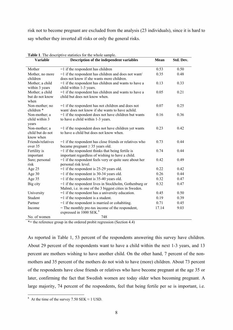
8

risk not to become pregnant are excluded from the analysis (23 individuals), since it is hard to

say whether they inverted all risks or only the general risks.

Table 1. The descriptive statistics for the whole sample. Variable

Description of the independent variables

Mean

Std. Dev.

Mother =1 if the respondent has children 0.53 0.50 Mother, no more children

=1 if the respondent has children and does not want/ does not know if she wants more children.

0.35 0.48

Mother; a child within 3 years

=1 if the respondent has children and wants to have a child within 1-3 years.

0.13 0.33

Mother; a child but do not know when

=1 if the respondent has children and wants to have a child but does not know when.

0.05 0.21

Non-mother; no children *

=1 if the respondent has not children and does not want/ does not know if she wants to have achild.

0.07 0.25

Non-mother; a child within 3 years

=1 if the respondent does not have children but wants to have a child within 1-3 years.

0.16 0.36

Non-mother; a child but do not know when

=1 if the respondent does not have children yet wants to have a child but does not know when.

0.23 0.42

Friends/relatives over 35

=1 if the respondent has close friends or relatives who became pregnant ≥ 35 years old.

0.73 0.44

Fertility is important

=1 if the respondent thinks that being fertile is important regardless of wishing to have a child.

0.74 0.44

Sure; personal risk

=1 if the respondent feels very or quite sure about her personal risk level.

0.42 0.49

Age 25 =1 if the respondent is 25-29 years old. 0.22 0.42 Age 30 =1 if the respondent is 30-34 years old. 0.26 0.44 Age 35 =1 if the respondent is 35-40 years old. 0.32 0.47 Big city =1 if the respondent lives in Stockholm, Gothenburg or

Malmö, i.e. in one of the 3 biggest cities in Sweden. 0.32 0.47

University =1 if the respondent has a university education. 0.45 0.50 Student =1 if the respondent is a student. 0.19 0.39 Partner =1 if the respondent is married or cohabiting. 0.71 0.45 Income = The monthly pre-tax income of the respondent,

expressed in 1000 SEK.8 17.14 9.03

No. of women 748 *= the reference group in the ordered probit regression (Section 4.4)

As reported in Table 1, 53 percent of the respondents answering this survey have children.

About 29 percent of the respondents want to have a child within the next 1-3 years, and 13

percent are mothers wishing to have another child. On the other hand, 7 percent of the non-

mothers and 35 percent of the mothers do not wish to have (more) children. About 73 percent

of the respondents have close friends or relatives who have become pregnant at the age 35 or

later, confirming the fact that Swedish women are today older when becoming pregnant. A

large majority, 74 percent of the respondents, feel that being fertile per se is important, i.e.

8 At the time of the survey 7.50 SEK ≈ 1 USD.

9

regardless of whether they wish to have a child (children) or not. Furthermore, 42 percent of

the women feel quite sure or very sure about their personal risk levels. When comparing the

descriptive statistics of the respondents with the national statistics, we find that the numbers

of respondents in each age group correspond well with the shares of women of these ages

living in Sweden.9 Similarly, in terms of the share of women who have children, it is the same

in this study as at the national level (Statistics Sweden, 2002).10 However, the share of

respondents with a university education is significantly higher in this study than in Sweden as

a whole (Statistics Sweden, 2004). We tested whether this overrepresentation affects the

stated risks or not, which was not the case. We therefore proceed with the whole sample. The

three hypotheses presented in the introduction will now be investigated one by one.

4.2 Perceptions of the general and personal risks of age-related female infertility

The first hypothesis is: Women between 20 and 40 years of age are aware that the risk of

female infertility increases with age, but they do not have a correct perception of the

magnitude of this general risk at different ages.

The answers to the general risk questions are used to investigate whether women are aware of

the relationship between age and infertility. Table 2 reports the mean and median stated

general and personal risk levels for the four age groups (20-24, 25-29, 30-34 and 35-40

years). Since it is highly plausible that the perceptions of women with and without children

differ, the stated risks are reported separately for mothers and non-mothers. Furthermore,

since the reported infertility distributions are skewed, both the mean and median values are

reported and commented on. The actual risks according to the NSFG 2002 survey are also

reported in the table.

9 The differences between the means are bootstrapped 1000 times for each variable. By using the percentile method and the 95 % confidence interval, it can be shown whether the means significantly differ from each other at the 5 % significance level. (The 95 % confidence interval is created by calculating relevant percentiles, which in this case are the 2.5th and 97.5th percentiles. These make the lower and upper bounds for the 95 % confidence interval). It should be noted that the advantage of the percentile method is that it makes no assumption about the underlying distribution (Efron and Tibshirani, 1998). 10 About 80 % of 35-40 year old women living in Sweden have children younger than 18 years (Statistics of Sweden, 2002), while 80 % of the respondents in the sample aged 35-40 have children. About 41 % of women aged 20-44 years in Sweden have university education (Statistics Sweden, 2004).

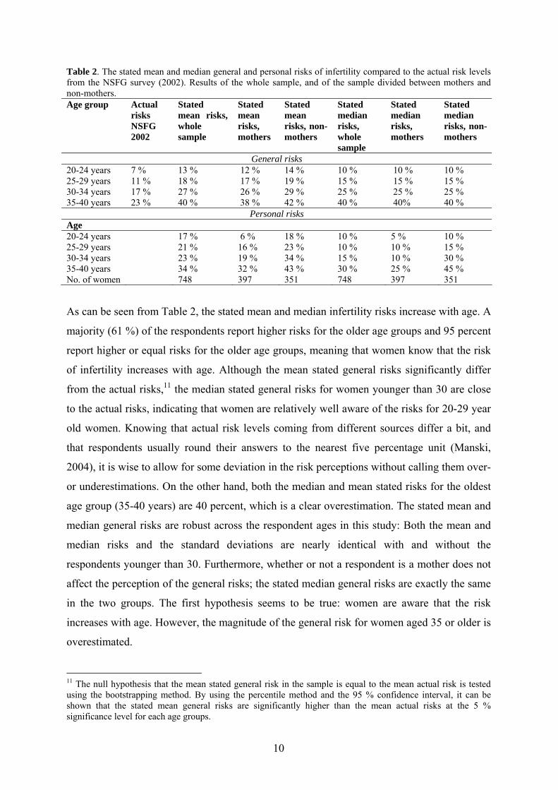
10

Table 2. The stated mean and median general and personal risks of infertility compared to the actual risk levels from the NSFG survey (2002). Results of the whole sample, and of the sample divided between mothers and non-mothers. Age group Actual

risks NSFG 2002

Stated mean risks, whole sample

Stated mean risks, mothers

Stated mean risks, non-mothers

Stated median risks, whole sample

Stated median risks, mothers

Stated median risks, non-mothers

General risks 20-24 years 7 % 13 % 12 % 14 % 10 % 10 % 10 % 25-29 years 11 % 18 % 17 % 19 % 15 % 15 % 15 % 30-34 years 17 % 27 % 26 % 29 % 25 % 25 % 25 % 35-40 years 23 % 40 % 38 % 42 % 40 % 40% 40 %

Personal risks Age 20-24 years 17 % 6 % 18 % 10 % 5 % 10 % 25-29 years 21 % 16 % 23 % 10 % 10 % 15 % 30-34 years 23 % 19 % 34 % 15 % 10 % 30 % 35-40 years 34 % 32 % 43 % 30 % 25 % 45 % No. of women 748 397 351 748 397 351

As can be seen from Table 2, the stated mean and median infertility risks increase with age. A

majority (61 %) of the respondents report higher risks for the older age groups and 95 percent

report higher or equal risks for the older age groups, meaning that women know that the risk

of infertility increases with age. Although the mean stated general risks significantly differ

from the actual risks,11 the median stated general risks for women younger than 30 are close

to the actual risks, indicating that women are relatively well aware of the risks for 20-29 year

old women. Knowing that actual risk levels coming from different sources differ a bit, and

that respondents usually round their answers to the nearest five percentage unit (Manski,

2004), it is wise to allow for some deviation in the risk perceptions without calling them over-

or underestimations. On the other hand, both the median and mean stated risks for the oldest

age group (35-40 years) are 40 percent, which is a clear overestimation. The stated mean and

median general risks are robust across the respondent ages in this study: Both the mean and

median risks and the standard deviations are nearly identical with and without the

respondents younger than 30. Furthermore, whether or not a respondent is a mother does not

affect the perception of the general risks; the stated median general risks are exactly the same

in the two groups. The first hypothesis seems to be true: women are aware that the risk

increases with age. However, the magnitude of the general risk for women aged 35 or older is

overestimated.

11 The null hypothesis that the mean stated general risk in the sample is equal to the mean actual risk is tested using the bootstrapping method. By using the percentile method and the 95 % confidence interval, it can be shown that the stated mean general risks are significantly higher than the mean actual risks at the 5 % significance level for each age groups.

11

At a first glance, these results seem totally opposite to those by Lampic et al. (2006), who

found that female and male university students in Sweden underestimated the general risks of

age-related female infertility. One explanation to the deviation is that the risk levels they

consider as actual are much higher than the levels used in this study.12 Another reason might

be that their sample consists only of young students. However, when comparing the stated

general risk levels in the Lampic et al. study with the stated mean general risks in this study

and only including female students, the results confirm the fact that women to a high extent

overestimate the age-related risks of infertility. Actually, a larger and, not smaller, share of

the female students in the Lampic et al study overestimated the risks compared to both the

actual risk levels used in their study and the actual risk levels according to NSFG survey

200213

While the stated mean and median general risks are nearly the same regardless of whether the

respondent is a mother or not, the stated personal risks are quite different. Mothers state

significantly lower personal risk levels compared to childless respondents.14 It is possible that

the non-mothers older than 29 have personal experience of difficulties of becoming pregnant,

which could partly explain why they state higher personal risks. However, it is more difficult

to explain why childless women aged younger than 30 (which constitute 71 % of the non-

mothers) state significantly higher personal risks as well. Therefore, we in the next section

investigate further the difference between stated personal and general risks.

12 They use 21-30 % as the actual risk level for women at the age of 25-30 years and 41-50 % for women at the age of 35-40 years. 13 The study by Lampic et. al. (2006) included 222 and this study 147 female students. 26 % of the female students in the Lampic et al. study stated risks higher than 30 % for women at the age group 25-30 years, while only 9 % of respondents in this study did the same. Similarly, 46 % of the respondents in the study of Lampic et al. stated risks higher than 50 % for the women in the age group 35-40 years, while the corresponding share of the respondents in this study is 15 %. 14 The difference between the mean stated personal risks for mothers and women without children are tested as before with the percentile method. The results show that the mean stated personal risks of the non-mothers are significantly higher than those of the mothers at the 5 % significance level for all age groups.

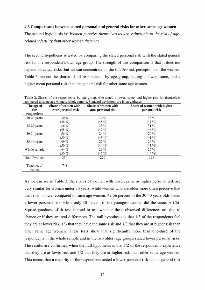
12

4.3 Comparisons between stated personal and general risks for other same age women

The second hypothesis is: Women perceive themselves as less vulnerable to the risk of age-

related infertility than other women their age.

The second hypothesis is tested by comparing the stated personal risk with the stated general

risk for the respondent’s own age group. The strength of this comparison is that it does not

depend on actual risks, but we can concentrate on the relative risk perceptions of the women.

Table 3 reports the shares of all respondents, by age group, stating a lower, same, and a

higher mean personal risk than the general risk for other same age women.

Table 3. Shares of the respondents, by age group, who stated a lower, same, and higher risk for themselves compared to same age women, whole sample. Standard deviations are in parentheses.

The age of the

respondent

Share of women with lower personal risk

Share of women with same personal risk

Share of women with higher personal risk

20-24 years 30 % (46 %)

37 % (48 %)

33 % (47 %)

25-29 years 36 % (48 %)

33 % (47 %)

31 % (46 %)

30-34 years 56 % (50 %)

24 % (43 %)

20 % (41 %)

35-40 years 49 % (50 %)

27 % (44 %)

24 % (43 %)

Whole sample 44 % (50 %)

29 % (46 %)

27 % (44 %)

No. of women

330 220 198

Total no. of women

748

As we can see in Table 3, the shares of women with lower, same or higher personal risk are

very similar for women under 30 years, while women who are older more often perceive that

their risk is lower compared to same age women: 49-56 percent of the 30-40 years olds stated

a lower personal risk, while only 30 percent of the youngest women did the same. A Chi-

Square goodness-of-fit test is used to test whether these observed differences are due to

chance or if they are real differences. The null hypothesis is that 1/3 of the respondents feel

they are at lower risk, 1/3 that they have the same risk and 1/3 that they are at higher risk than

other same age women. These tests show that significantly more than one-third of the

respondents in the whole sample and in the two oldest age groups stated lower personal risks.

The results are confirmed when the null hypothesis is that 1/2 of the respondents experience

that they are at lower risk and 1/2 that they are at higher risk than other same age women.

This means that a majority of the respondents stated a lower personal risk than a general risk

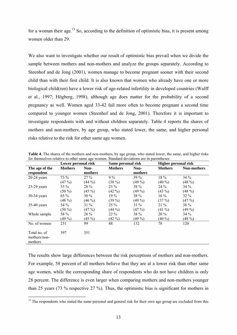
13

for a woman their age.15 So, according to the definition of optimistic bias, it is present among

women older than 29.

We also want to investigate whether our result of optimistic bias prevail when we divide the

sample between mothers and non-mothers and analyze the groups separately. According to

Steenhof and de Jong (2001), women manage to become pregnant sooner with their second

child than with their first child. It is also known that women who already have one or more

biological child(ren) have a lower risk of age-related infertility in developed countries (Wulff

et al., 1997; Högberg, 1998), although age does matter for the probability of a second

pregnancy as well. Women aged 33-42 fail more often to become pregnant a second time

compared to younger women (Steenhof and de Jong, 2001). Therefore it is important to

investigate respondents with and without children separately. Table 4 reports the shares of

mothers and non-mothers, by age group, who stated lower, the same, and higher personal

risks relative to the risk for other same age women.

Table 4. The shares of the mothers and non-mothers, by age group, who stated lower, the same, and higher risks for themselves relative to other same age women. Standard deviations are in parentheses Lower personal risk Same personal risk Higher personal risk The age of the respondent

Mothers Non-mothers

Mothers Non-mothers

Mothers Non-mothers

20-24 years 73 % (47 %)

27 % (44 %)

9 % (30 %)

39 % (49 %)

18 % (40 %)

34 % (48 %)

25-29 years 53 % (50 %)

28 % (45 %)

23 % (42 %)

38 % (49 %)

24 % (43 %)

34 % (48 %)

30-34 years 65 % (48 %)

30 % (46 %)

19 % (39 %)

38 % (49 %)

16 % (37 %)

32 % (47 %)

35-40 years 54 % (50 %)

31 % (47 %)

25 % (44 %)

31 % (47 %)

21 % (41 %)

38 % (49 %)

Whole sample 58 % (49 %)

28 % (45 %)

22 % (42 %)

38 % (49 %)

20 % (40 %)

34 % (48 %)

No. of women

231 99 88 132 78 120

Total no. of mothers/non-mothers

397 351

The results show large differences between the risk perceptions of mothers and non-mothers.

For example, 58 percent of all mothers believe that they are at a lower risk than other same

age women, while the corresponding share of respondents who do not have children is only

28 percent. The difference is even larger when comparing mothers and non-mothers younger

than 25 years (73 % respective 27 %). Thus, the optimistic bias is significant for mothers in

15 The respondents who stated the same personal and general risk for their own age group are excluded from this

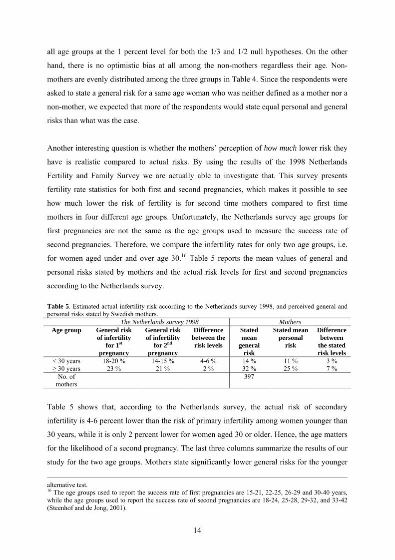
14

all age groups at the 1 percent level for both the 1/3 and 1/2 null hypotheses. On the other

hand, there is no optimistic bias at all among the non-mothers regardless their age. Non-

mothers are evenly distributed among the three groups in Table 4. Since the respondents were

asked to state a general risk for a same age woman who was neither defined as a mother nor a

non-mother, we expected that more of the respondents would state equal personal and general

risks than what was the case.

Another interesting question is whether the mothers’ perception of how much lower risk they

have is realistic compared to actual risks. By using the results of the 1998 Netherlands

Fertility and Family Survey we are actually able to investigate that. This survey presents

fertility rate statistics for both first and second pregnancies, which makes it possible to see

how much lower the risk of fertility is for second time mothers compared to first time

mothers in four different age groups. Unfortunately, the Netherlands survey age groups for

first pregnancies are not the same as the age groups used to measure the success rate of

second pregnancies. Therefore, we compare the infertility rates for only two age groups, i.e.

for women aged under and over age 30.16 Table 5 reports the mean values of general and

personal risks stated by mothers and the actual risk levels for first and second pregnancies

according to the Netherlands survey. Table 5. Estimated actual infertility risk according to the Netherlands survey 1998, and perceived general and personal risks stated by Swedish mothers.

The Netherlands survey 1998 Mothers Age group General risk

of infertility for 1st

pregnancy

General risk of infertility

for 2nd pregnancy

Difference between the risk levels

Stated mean

general risk

Stated mean personal

risk

Difference between

the stated risk levels

< 30 years 18-20 % 14-15 % 4-6 % 14 % 11 % 3 % ≥ 30 years 23 % 21 % 2 % 32 % 25 % 7 %

No. of mothers

397

Table 5 shows that, according to the Netherlands survey, the actual risk of secondary

infertility is 4-6 percent lower than the risk of primary infertility among women younger than

30 years, while it is only 2 percent lower for women aged 30 or older. Hence, the age matters

for the likelihood of a second pregnancy. The last three columns summarize the results of our

study for the two age groups. Mothers state significantly lower general risks for the younger

alternative test. 16 The age groups used to report the success rate of first pregnancies are 15-21, 22-25, 26-29 and 30-40 years, while the age groups used to report the success rate of second pregnancies are 18-24, 25-28, 29-32, and 33-42 (Steenhof and de Jong, 2001).

15

age group and significantly higher risks for the older age group compared to the risk levels of

the Netherlands survey. However, our main interest is the difference between the stated

general and personal risks. The results show that mothers state 7 percent lower mean personal

than general risks for women older than 30, while the difference between the risks for first

and second pregnancies according to the Netherlands study is only 2 percent. Thus, mothers,

aged 30 and older, have a too optimistic picture of how much easier it is to become pregnant

the second time compared to the first time.17 This finding is in line with the results by Perloff

and Fetzer, 1986, Weistein, 1987, and Slovic et al., 2000b. People who have no experience of

a particular negative life event tend to be more positive than others considering this event.

4.4 Factors behind the difference between the stated general and personal risks

The third hypothesis is: The difference between the stated personal and general risk depends

on a woman’s own previous experience of becoming pregnant, on how important she

perceives of being fertile per se, and on whether she wants to have children.

To be able to see what affects the probabilities that the stated personal risks differs from the

stated general risks for same age women, the respondents are divided into three different

groups. In the analysis we use an ordered probit model, where the dependent variable is

whether the respondents state a lower, equal, or higher personal risk than their stated general

risks for other same age women. Table 6 shows the marginal effects of the ordered probit

model.

17 Whether the deviation in stated risk levels in this study (7 %) significantly differs from the deviation between first and second pregnancies according to the Netherlands study (2 %) is tested as before with the percentile method. The results show that the difference is significant at 5 % significance level. Moreover, the general risk of infertility for the first pregnancy according to the Netherlands study and the general risk of infertility in our study are not the same. The average woman that the respondents were asked to state the general risk for could either be a mother or a childless woman. This risk is comparable to the weighted average of the risks for first and second pregnancies according to the Netherlands study. Therefore, the difference between the risk for first and second pregnancies would be even lower for the Netherlands study, which strengthens our results even more.

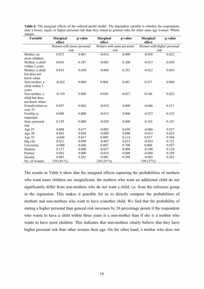
16

Table 6. The marginal effects of the ordered probit model. The dependent variable is whether the respondents state a lower, equal, or higher personal risk than they stated as general risks for other same age women. Whole sample.

Variable Marginal effect

p-value Marginal effect

p-value Marginal effect

p-value

Women with lower personal risk

Women with same personal risk

Women with higher personal risk

Mother, no more children

0.072 0.001 -0.016 0.000 -0.056 0.422

Mother; a child within 3 years

0.016 0.387 -0.003 0.300 -0.013 0.850

Mother; a child but does not know when

0.015 0.430 -0.004 0.353 -0.012 0.863

Non-mother; a child within 3 years

-0.262 0.000 0.004 0.681 0.257 0.000

Non mother; a child but does not know when

-0.159 0.000 0.020 0.027 0.140 0.025

Friends/relatives over 35

0.057 0.002 -0.010 0.000 -0.046 0.517

Fertility is important

0.088 0.000 -0.015 0.000 -0.073 0.325

Sure; personal risk

0.129 0.000 -0.028 0.000 -0.101 0.167

Age 25 0.008 0.677 -0.002 0.650 -0.006 0.927 Age 30 0.043 0.020 -0.009 0.000 -0.033 0.625 Age 35 -0.046 0.017 0.009 0.114 0.037 0.568 Big city 0.031 0.098 -0.007 0.015 -0.024 0.723 University -0.008 0.686 0.002 0.708 0.006 0.927 Student 0.137 0.000 -0.037 0.000 -0.100 0.154 Partner 0.082 0.000 -0.014 0.000 -0.068 0.358 Income 0.003 0.281 -0.001 0.288 -0.002 0.263 No. of women 330 (44 %) 220 (29 %) 198 (27%)

The results in Table 6 show that the marginal effects capturing the probabilities of mothers

who want more children are insignificant; the mothers who want an additional child do not

significantly differ from non-mothers who do not want a child, i.e. from the reference group

in the regression. This makes it possible for us to directly compare the probabilities of

mothers and non-mothers who want to have a/another child. We find that the probability of

stating a higher personal than general risk increases by 26 percentage points if the respondent

who wants to have a child within three years is a non-mother than if she is a mother who

wants to have more children. This indicates that non-mothers clearly believe that they have

higher personal risk than other women their age. On the other hand, a mother who does not

17

want to have more children is more likely to state a lower personal than general risk than all

other women.18

From a policy point of view the interesting group is women who want to have a/another child,

but from the risk perception point of view it is an interesting result that women who do not

want (more) children perceive that they are at lower risk than others. It is difficult to have

medical explanations for why a non-mother who is pleased to live without children would

have a lower risk than a non-mother who wants to become pregnant. Unless the non-mothers

who do not want to have a child (7 % of the sample) are those who know that they have

difficulties to become pregnant. If so, these women’s wish to remain childless might be a

reaction to their higher than an average risk of infertility, indicating an endogeneity problem.

This argument is however less plausible for the mothers (35 % of the sample) who do not

want to have more children. A better explanation for why these mothers stated a lower

personal than general risk is that they are pleased with the number of children they already

have. Thus, it is even more difficult to explain in medical terms why a mother who does not

want to have more children should have lower risk than a mother who wants to become

pregnant. One explanation is that these women’s risk perception is affected by their decision

of not trying to become pregnant

We also find some other interesting results. Respondents with close friends or relatives who

have become pregnant at the age of 35 or later are more likely to state a risk that is lower than

the risk they state for other same age women. Thus, positive experiences of persons close to

one do matter.19 Furthermore, the probability of stating a lower personal than general risk

increases by 9 percentage points if a respondent feels that being fertile per se is important to

her, regardless of whether she wants to have (more) children or not.

Summarizing the results of the third hypothesis, it seems that, in line with our hypothesis, a

woman’s own previous positive experience of becoming pregnant does matter for her risk

perception. Mothers are more likely to state lower personal than general risks compared to

18 The respondents who do not know if they want to have (more) children are also included in the variables: mother; no more children and in the reference group non -mother; no child. The others responded that they were very or quite sure about wishing to have (more) children. 19 According to Kohler (2000) individual’s fertility behavior depends also on the fertility behavior of other individuals in society. Although Kohler discusses the number of births, which is somewhat different, the message is the same. Social interactions do matter for a woman’s fertility behavior, her timing of births and/or her perceptions of the risk of infertility.

18

non-mothers who want to become pregnant. Moreover and contrary to our hypothesis, a wish

to have a child does not decrease the perception of the personal risk level; it instead increases

it among all women. A possible explanation might be that, according to Weber (1994), people

are sensitive to the consequences of making a misjudgement of a quantity they are asked to

estimate. The more negative the outcome, the greater the cost of a wrong decision due to the

underestimation. And the outcome of not becoming pregnant is likely to be assumed to be

highly negative for many women who want to have a child. Finally, if a woman perceives that

being fertile is important per se she also more likely believes that she has a lower risk than

other same age women. This result is in line with Dunning et al. (1991), who found that the

more important people consider an attribute the more they perceive that they have it.

5. Conclusions and discussion The desire of having children has not changed during the last decades, while the average age

of first-time mothers has increased steadily in several Western countries (Council of Europe,

2004). Therefore, this study, based on a random representative sample of Swedish females

20-40 years of age, attempts to find out whether women are aware of the magnitudes of age

related infertility risks. Both the individuality of the risk and the fact that the actual risk levels

might differ depending on the used estimation method make the risk levels more difficult to

state. Even if it can be hard to interpret the results of this study as exact risk levels, the trend

is clear. Swedish women are well aware of the risk levels for young women but they clearly

overestimate the risks for women older than 34. There are several potential reasons why

women overestimate the general risks for women over 34 years. Firstly, the age of 30 is often

described as ‘critical’ (Steenhof and de Jong, 2001). Other studies indicate that the female

age-related infertility increases somewhat before age 30 and then significantly more so after

the age of 35 (Leridon, 2004; Infomedica, 2004). One very reasonable explanation for the

overestimation of the risks is therefore that information about the ages 30 or 35 as being

‘critical’ has reached the respondents, making them believe that the risks are even higher than

they actually are.

A further objective of this paper was to investigate whether an individual’s perceptions of

personal risk and general risk differ from each other. We found that a large majority of

mothers, regardless their age, believe to be at a lower risk than an average same-age woman,

19

while the childless women do not. Hence, there is an optimistic bias among mothers, even if

we account for the fact that mothers generally have a lower than average risk than non-

mothers. Moreover, we found that mothers aged 30 and older have a too optimistic picture of

how much easier it is to become pregnant the second time compared to the first time, which

strengthens further our result about optimistic bias among mothers. These findings are also in

line with the articles by Perloff and Fetzer (1986), Weinstein (1987) and Slovic et al. (2000b):

People who have no experience from a negative life event tend to be more positive than

others. It is also very unlikely that a majority of all childless women aged 20-40 really have

higher than average risks of age-related infertility, especially among those 71 percent of the

respondents without children who are younger than 30.

Consequently, the results of this study highlight several facts that are interesting from a

policy point of view: Women are quite well aware of the general risks of infertility; they do

not believe that that the risks are lower than they are. Moreover, perceptions of the general

risks do not differ between women who have children and childless women. On the other

hand, we found large difference in the risk perceptions between general and personal risks

among mothers who in general have too optimistic picture about their own fertility level.

Thus, even if mothers are aware of the general risk levels they do not believe that the risks

apply to themselves, which naturally makes it harder to inform mothers about the risk. How

correct a woman’s risk perception is, matters also for other women’s risk perceptions.

According to Coleman (1993) and Lampi (2007), interpersonal information channels as

friends and relatives affect the general risk perception, especially when information based on

the experiences of peers is concerned to be very credible (Tonn et al.,1990). This means that

women, regardless whether they are mothers or not and whether they want to become

pregnant or not, spread information (correct or incorrect) from the risk of age-related

infertility to other women.

Finally, it seems that risk perceptions of infertility are also affected by psychological factors;

a woman who perceives that being fertile per se is important is also more likely to perceive

that she is more fertile than other same-age women. Moreover, the exposure to the risk of

infertility is possible to avoid if a woman does not want to become pregnant: We found that a

woman who does not want to have (more) children is more likely to believe that her own risk

is lower than average compared to a woman who wants (more) children. Further research is

20

needed to determine whether non-exposure to a risk can explain why people perceive

themselves as less vulnerable to the risk in terms of risks other than the one studied here.

21

References

Adserà A. (2004), Changing fertility rates in developed countries. The impact of labour market institutions, Journal of Population Economics, 17, 17-43.

Becker G. S. (1981), A treatise on the family, Harvard University Press, Cambridge, Massachusetts, 1981.

Benjamin D. K., W. R. Dougan and D. Buschena (2001), Individuals´ estimates of the risk of death: Part II- New evidence, Journal of Risk and Uncertainty, 22 (1), 35-57.

Björklund A. (2006), Does family police affect fertility, Lessons from Sweden?, Journal of Population Economics, 19, 3-24.

Black W.C, R. F. Nease Jr, and A. N. Tosteson (1995), Perceptions of breast cancer risk and screening effectiveness in women younger than 50 years of age, Journal of the National Cancer Institute 17; 87 (10), 720-731.

Bongaarts J. (1982), “Infertility after age 30: A false alarm”, Family Planning Perspectives, 14 (2), 75-78.

Chandra A., GM Martinez, WD Mosher, JC Abma, and J. Jones (2005), Fertility, family planning, and reproductive health of U.S. women: Data from the 2002 National Survey of Family Growth, U.S. Department of Health and Human Services 23 (25), National Center for Health Statistics.

Coleman C-L. (1993), The influence of mass media and interpersonal communication on societal and personal risk judgements, Communication Research, 20 (4), 611-628.

Council of Europe (2004), Demographic year book 2004, http://www.coe.int/t/e/social_cohesion/population/demographic_year_book/2004_Edition/RAP2004%20Note%20synth+%20INTRO%20E.asp#TopOfPage.

Dunning D., M. Perie and A. L. Story (1991), Self-serving prototypes of social categories, Journal of Personality and Social Psychology, 61 (6), 957-968.

Efron B. and R. J. Tibshirani (1998), An introduction to the Bootsrap, Chapman & Hall/CRC, U.S.A, 1998, p. 55.

Gustafsson S. and C. Wetzels (2000), Optimal age at first birth: Germany, Great Britain, the Netherlands and Sweden In Gustafsson Siv and Daniéle Meulders (eds.), Gender and the Labour Market, Econometric Evidence of Obstacles to Achieving Gender Equality, London: MacMillan Press Ltd. 2000.

Gustafsson S. (2001), Optimal age at motherhood. Theoretical and empirical considerations on postponement of maternity in Europe, Journal of Population Economics, 14, 225-247.

Gustafsson S. (2005), Having kids later. Economic analyses for industrialized countries, Review of Economics of the Household, 3, 5-16

Heckman J. and J. Walker (1990), The relationship between wages and income and the timing and spacing of births: Evidence from Swedish longitudinal data, Econometrica 58, 1411-1441.

Hoem B. (2000), Entry into motherhood in Sweden: the influence of economic factors on the rise and fall in fertility, 1986-1997, Demographic Research, 2 (4).

Högber U. (1998), Epidemiologska synpunkter på fekunditet och infertilitet In: Ofrivillig barnlöshet, N-O. Sjöberg (ed.), Rapport nr: 37, Arbets- och Rferensgruppen för Ofrivillig Barnlöshet 1998.

Infomedica (2004), homepage www.infomedica.se/artikel.asp?CategoryID=11729 Kohler H-P. (2000), Social interactions and fluctuations in birth rates, Population Studies, 54

(2), 223-237. Lampi E. (2007), What do friends and media tell us? How different information channels affect women’s risk perceptions of age-related female infertility. Working paper, University of Gothenburg.

22

Lampic C., A. Skoog Svanberg, P. Karlström and T. Tyden (2006), Fertility awareness, intentions concerning childbearing, and attitudes toward parenthood among female and male academics, Human Reproduction, 21 (2), 558-564.

Leridon H. (2004), Can assisted reproduction technology compensate for the natural decline in fertility with age? A model assessment, Human Reproduction, 19 (7), 1548-1553.

Löfström Å. (2003), Att lillan kom till jorden…..Barnafödande och konjunktur under det sena 1900-talet, Working Paper, Department of Economics, Umeå University, Umeå 2003

Manski C. F. (2004), Measuring expectations, Econometrica, 72 (5), 1329-1376. Martin S. P. (2000), Diverging fertility among U.S. women who delay childbearing,

Demography, 37 (4), 523-533. Menken J. (1985), Age and fertility: How late can you wait?, Demography, 22 (4), 469-483. National Center for Health Statistics, W. D. Mosher and W. F. Pratt (1987), Fecundity,

infertility, and reproductive health in the United States, 1982, Vital and Health Statistics Series 23 (14). DHHS Pub No (PHS) 87-1990 U.S., Public Health Service Washington U.S., Government Printing Office, May 1987.

Perloff L.S. and B.K. Fetzer (1986), Self-other judgements and perceived vulnerability to victimization, Journal of Personality and Social Psychology, 50 (3), 502-510.

Santos-Pinto L. and J. Sobel (2005), A model of positive self-image in subjective assessments, The American Economic Review, 95 (5), 1386-1402.

Schwartz D. and MJ. Mayaux (1982), Female fecundity as a function of age: results of artificial insemination in 2193 nulliparous women with azoospermic husbands. Federation CECOS., New England Journal of Medicin, 306 (7), 404-406.

Sjöberg L. and J. Fromm (2001), Information technology risks as seen by the public, Risk Analysis, 21 (3), 427-441.

Sjöberg L. (2002), Risk, politik och näringsliv, working paper, Center for Risk Research, Stockholm School of Economics.

Slovic P., B. Fischhoff and S. Lichtenstein (2000a), Rating the Risks In: P. Slovic (ed.) The Perception of Risk, Earthscan Publications Ltd, London ans Sterling 2000.

Slovic P., B. Fischhoff and S. Lichtenstein (2000b), Accident probabilities and seat belt usage: A psychological perspective In: P. Slovic (ed.) The Perception of Risk, Earthscan Publications Ltd, London ans Sterling 2000.

Statistics Sweden (2001), Varför föds det så få barn? Resultat av en enkätundersökning om vad som påverkar beslutet att få barn. Demografiska rapporter 2001:1.

Statistics Sweden (2002), Pappa och barn, VälfärdsBulletinen, No. 4. Statistics Sweden (2005), Medelåldern vid första barnets födelse 1970-2004, homepage

http://www.scb.se/templates/tableOrChart____142439.asp. Attached, 2008-04-01. Statistics Sweden (2004), “Population aged 16-74 by level of education, sex and age 2004”,

homepage: http://www.scb.se/templates/Product____9577.asp. Attached 2006-09-01.

Steenhof L. and A. de Jong (2001): In fecundity: a result of postponed childbearing?, Statistics Netherlands, Department of Population.

Svenson O. (1981), Are we less risky and more skilful than our fellow drivers? Acta Psychologica, 47 (2), 143-148.

Taylor S. E. and J. D. Brown (1988), Illusion and well-being: A social psychological perspective in mental health, Psychological Bulletin, 103 (2), 193-210.

Tietze C. (1957), Reproductive span and rate of reproduction among Hutterite women”, Fertility and Sterility, 8 (1), 89-97.

Tonn B. E., C. B. Travis, R. T. Goeltz and R. H. Phillippi (1990), Knowledge-based representations of risk beliefs, Risk Analysis, 10 (1), 169-184.

23

van der Pligt J. (1996), Risk perception and self-protective behavior, European Psychologist, 1 (1), 34-43.

Weber E.U. (1994), From subjective probabilities to decision weights: The effect of asymmetric loss functions on the evaluation of uncertain outcomes and events, Psychological Bulletin, 115 (2), 228-242.

Weinstein N. D. (1980), Unrealistic optimism about future life events, Journal of Personality and Social Psychology, 39 (5), 806-820.

Weinstein N. D. (1987), Unrealistic optimism about susceptibility to health problems: conclusion from a community-wide sample, Journal of Behavioural Medicine, 10 (5), 481-500.

Wulff M., U. Högberg and H. Stenlund (1997), Infertility in an industrial setting: a population-based study from Northern Sweden, Acta Obstet Gynecol Scand. 76 (7), 673-679.

24

Appendix A Part 2 – Questions about the age-related risk of female infertility Nowadays, we establish families later in life than previous generations did. The average age of Swedish first-time mothers is now 29 years, which is up five years from 30 years ago. Age affects the fertility of a woman, even if fertility is a very individual issue. Infertility is defined as when a woman regularly tries to but does not become pregnant without medical assistance during a period of one year. Although, it is possible that she becomes pregnant after for example three years, with or without medical assistance. While infertility can be due to several reasons, this study investigates only how age affects female infertility. Questions 1-4 below are about women of different ages. Imagine that these women try to become pregnant and that their partners are perfectly fertile. I want to know what you believe the risk of age-related infertility is for a woman in every age group. Question 5 is about what you believe your own risk is. The number you state as a percentage rate in questions 1-4 indicates the number of women out of 100 in that age group who will not become pregnant in a one year period without medical assistance, despite trying regularly. Answer the questions even if you feel unsure about the percentage rates. For this study, it is important to find out what you believe the risks are. You can always go back and change your answers if you like. Question 1. I believe that the average risk for a 20-24 year old woman of not becoming pregnant during a time period of one year is……………………………….% Question 2. I believe that the average risk for a 25-29 year old woman of not becoming pregnant during a time period of one year is……………………………….% Question 3. I believe that the average risk for a 30-34 year old woman of not becoming pregnant during a time period of one year is……………………………….% Question 4. I believe that the average risk for a 35-40year old woman of not becoming pregnant during a time period of one year is……………………………….% Note: Question 5 below is about you personally. Question 5. Imagine that you want to try to become pregnant. How great, do you believe, is your personal risk of not becoming pregnant during a time period of one year?..........................% Space for your own comments……………………………………………………………….. ………………………………………………………………………………………………………………………………………………………………………………………………………………………………………………………………………………………………....................................................................................................................................................................

Paper VI

1

What do friends and the media tell us?

How different information channels affect women’s risk

perceptions of age-related female infertility

Elina LampiA

Abstract

Based on a survey given to a random sample of Swedish 20-40 year old females, this paper

investigates through which channels women receive information about the general risk levels

of age-related female infertility and how the different channels affect women’s perceptions of

the risk. We find that the media reach women of all ages, while only about one woman in four

has received information from the health care system. We also found that what peers say and

do strongly affect women’s risk perceptions: The respondents who had obtained information

from friends and relatives were more likely to state too high risks, while a woman with close

friends or relatives who became pregnant at age 35 or older was more likely to have a correct

perception of the risks. Since women are most interested in receiving information from the

health care system, we argue that health care workers should inform women earlier than what

happens today.

Keywords: Information, Media, Health care, Infertility, General risk.

JEL Classification: D81, D83, I10, J13

Financial support from the Iris Foundation is gratefully acknowledged. The author would like to thank Fredrik Carlsson, Lennart Flood, Olof Johansson-Stenman, Åsa Löfgren, Peter Martinsson, Katarina Nordblom, Katarina Steen Carlsson, Maria Vredin-Johansson, Roger Wahlberg, and seminar participants at the University of Gothenburg for many useful comments. A Department of Economics, School of Business, Economics and Law, University of Gothenburg, Box 640, SE 405 30 Göteborg, Sweden, Ph. +46 31 7861393, e-mail: elina.lampi@economics.gu.se. .

2

1. Introduction A woman’s risk of not being able to become pregnant increases with age. Since no available

medical test is able to reveal a woman’s personal risk, it is important for a woman to have

knowledge about the general risk levels and how they change with age. Interesting issues

therefore include how women obtain information about this risk of age-related female

infertility and how the different information channels affect their risk perceptions. Infertility

is defined as a state where a healthy couple of childbearing age tries to but does not manage

to become pregnant within a 12-month period without using any type of contraceptive. Thus,

infertility does not indicate sterility but instead highlights a group of individuals having

trouble becoming pregnant and who may need medical assistance (Infomedica, 2004). A

biased risk perception is undesirable for a woman who wishes to become pregnant;

overestimation creates an unnecessary worry and underestimation may result in serious

disappointments if it becomes difficult to become pregnant. Moreover, to be able to plan the

timing of births together with other important life decisions such as education etc., it is

important for a woman to be aware of how the risk increases with age. Thus, it is not

sufficient to know the general risk level for the own age group only. Another reason why it is

important for women to have knowledge about the changes in risk due to increasing age is as

shown in this paper: Women are themselves information spreaders when they talk with their

peers about the risks.

The objectives of this paper are to investigate: (1) from what sources women receive

information about the general risks of age-related female infertility, (2) how different

information channels affect risk perception, and (3) who would like to have more

information, and from what source(s)? To be able to address these objectives, 2,000

questionnaires were mailed out to a random sample of 20-40 year old women living in

Sweden. The respondents were asked to identify from which sources they had obtained

information and from where they would like to receive more information. They were also

asked to estimate the general risks of female infertility for four different age groups (20-24,

25-29, 30-34, and 35-40 years).

According to Weaver and Wakshlag (1986), personal experiences have the strongest impact

on a person’s beliefs, followed by information from peers, and then all other information

channels. A woman may have personal experience of pregnancy and/or of trying to become

3

pregnant, which gives her some kind of perception of the infertility risks, both on a personal

and a general level. Women might also be affected by information they get through both

formal and informal channels, e.g., from the health care system, different media sources,

and/or discussions with friends and relatives. A woman’s risk perception might also be

influenced by the ages at which her close friends and relatives became pregnant. The degree

to which information is adopted by people depends on how credible they think the source of

the information is (Wiegman and Gutteling, 1995). According to Tonn et al. (1990),

information based on the experiences of peers is considered to be especially credible.

How the media affects risk perception is a debated issue. Some studies have shown that the

media makes people aware of risks (see for example Wiegman and Gutteling, 1995), and

Kasperson et al., (2003) found that high media coverage alone does not increase perceived

risks. Several previous studies have reported that experiences of peers affect people more

than the mass media does (McAlister, 1987; Rogers, 1987; Tonn et al., 1990; Chang and

Kinnucan, 1991; Wåhlberg and Sjöberg, 2000)1, and if the object of the risk is straight out

feared, rumors within peer groups may be a significant element in forming people’s

perceptions (Kasperson et al., 1988). However, the information women receive might not be

correct. Incorrect information has an opportunity cost since it may crowd out more correct

information in a person’s mind. It is therefore important to investigate how different

information channels affect risk perceptions of age-related infertility.

Furthermore, infertility is a sensitive issue and we know that people react differently to

information. Increasing the amount of information for individuals not wanting it increases

their stress levels and causes anxiety, while extra information reduces the stress of individuals

who are information seekers (Miller and Mangan, 1983). Some people may choose to totally

ignore the information if it is seen as too negative (Bénabou and Tirole, 2002). We therefore

ask: who wishes to be informed about the risks, and from which sources do they want

information. We then compare these sources with the sources they actually receive

information from.

1 According to McAlister (1987) and Rogers (1987), it is well-known that the mass media channels are effective in creating awareness but that peers are often the most influential in an individual’s decision to adopt or reject new information and to change or not change her behavior. According to Tonn et al. (1990), personal experience and/or communications may be needed to make knowledge relevant for a person.

4

We also include a test of media information that investigates whether a peak in the media

coverage of the general risks of age-related female infertility affects women’s risk

perceptions. This was possible for us to do since only two days before the survey had been

planned to be mailed out, several major newspapers in Sweden published articles based on

the public health study by Lampic et al., (2006). Newspapers reported the findings that female

and male university students in Sweden have overly optimistic perceptions of women’s

chances of becoming pregnant, especially for women age 35 and older. Headlines such as

“Swedish students at risk for childlessness – both men and women overestimate fertility after

age 35” (Svenska Dagbladet, 2005) and “Swedish students know too little about fertility –

both men and women overestimate the possibilities to have a child after 35 and researchers

warn that the consequences might be involuntary childlessness” (Göteborgs Posten, 2005)

were common. However, these articles did not say anything about the actual risk levels. To be

able to see whether these kinds of articles affect women’s risk perceptions, 200 of the 2,000

questionnaires were not sent out with the others but instead to another random sample of

women two months later. This way of testing is in line with several previous studies about

how media affects risk perceptions; see for example Soumerai et al., (1992) on how media

can play a central role in decreasing the use of aspirin among children. Similarly, several

studies have shown that negative health risk information from the media has significant

effects on food demand (Chang and Kinnucan, 1991; Burton and Young, 1996; Verbeke and

Ward, 2001)2.

The remainder of this paper is organized as follows. Section 2 describes the survey, its

design, and the actual risk levels used in this study. Section 3 reports the descriptive statistics

and the empirical results from the analyses associated with the objectives of this paper.

Finally, Section 4 discusses the results and concludes the paper.

2 According to Chang and Kinnucan (1991), information about the connection between blood cholesterol and dietary fats decreased the consumption of butter in Canada. They also found that an industry advertising campaign increased the demand for butter. According to Verbeke and Ward (2001), negative information about meat decreases the consumption of meat and affects what kind of meat people want to buy.

5

2. The survey and survey design In order to investigate the objectives of this study, the respondents were asked to estimate the

risks of female infertility3 for four different age groups (20-24, 25-29, 30-34, and 35-40

years). The part of the survey containing the scenario and all four risk questions are included

in the Appendix. As an example, we show the question about the general risk for the 20-24

age group4:

Question 1. I believe that the average risk for a 20-24 year old woman of not becoming

pregnant during a time period of one year is……………………………….%

Furthermore, the respondents were asked whether they had received information about the

risks of age-related female infertility and whether they would like to get more information.

They were also asked to identify from what sources they had obtained information and from

where they would like to receive more information. The questionnaire also included questions

about whether the respondent wished to become pregnant (and if so, when). Since the subject

of infertility may be sensitive to many, the respondents were completely anonymous.

The survey was mailed out in two rounds to a random sample of 20-40 year old women living

in Sweden.5 The first 1,800 questionnaires were sent out in November 2005, and the

remaining 200 in January 2006. The overall response rate was 47 percent. The reason for

sending out some of the questionnaires in January was that only one day before the survey

had been planned to be mailed out in November, several major newspapers in Sweden

published articles based on the public health study by Lampic et al. (2006) about how male

and female university students in Sweden underestimate the age-related decline in female

fertility, especially among women aged 35 or older. We saw this as a good opportunity to test

whether articles of this kind could affect women’s risk perceptions. If there is such an effect,

then those who answered the questionnaire directly after the large media coverage should

have stated higher risks than those who received the questionnaire two months later.

3 Meaning not becoming pregnant despite regular unprotected intercourse during a one-year period. 4 The respondents were also asked to state what they believe their personal risk to be. The stated personal risks are however not the objective of this paper. For a discussion on how the stated personal and general risk perceptions differ, see Lampi (2006). 5 The first pilot survey consisted of 45 questionnaires sent out by e-mail in October 2004 to a non-random sample of 20-40 year old women. The resulting revised questionnaire was tested on a focus group, and then a second pilot study was carried out, where 200 questionnaires were sent out in October 2005 by regular mail to a

6

Postcards were sent out to all respondents as a single reminder 10 days after the

questionnaires (in both November and January).

The ”actual” risks of age-related infertility used in this paper are estimates based on age-

specific pregnancy rates with unprotected intercourse for modern populations.6 The infertility

risk levels are collected through interviews performed by the National Survey of Family

Growth (NSFG) in 2002 in the U.S.7 According to the 2002 study (including over 7,600

women), the infertility risk is 7 % for 20-24 year old women, 11 % for 25-29 year old

women, 17 % for 30-34 year old women and 23 % for 35-40 year old women (Chandra et al,

2005).8 Infertility risks collected from retrospective surveys such as the NSFG are seen as the

most trustworthy even if it may be difficult for a woman to remember exactly when she began

trying to become pregnant (Högberg, 1998). The NSFG surveys have been conducted six

times during the 1973-2002 period and the infertility levels are nearly the same in all of the

NSFG surveys, indicating robustness.

random sample of 20-40 year old women living in Sweden. The questionnaire was again revised based on the comments and results of the second pilot study. 6 The two other ways to measure infertility risks are: age-specific pregnancy rates in natural populations (populations where contraception and abortion are not allowed or used) and age-specific pregnancy rates with artificial insemination in modern populations. The major disadvantage of studies done in natural populations is that the type of data is hard to compare with more modern data, while artificial insemination ends up boosting infertility rates and is therefore often criticized since the probability of becoming pregnant artificially is much smaller compared to using the natural method (see e.g., Bongaarts, 1982). A study of artificially inseminated women reports that 26-27 % of women 30 or younger, 39 % of women aged 31-35, and 46 % of women aged 36-40 did not become pregnant within a one-year period (Schwartz and Mayaux 1982). A study by Tietze (1957) reports the shares of a natural population (Hutterites) who were infertile in the first half of the 20th century: 3 % of women aged 20-24 were permanently infertile, while the corresponding shares of women aged 25-29, 30-34, and 35-39 years were 5.3 %, 9.0 %, and 22 %. 7 The NSFG survey measures the infertility rates of women who had not become pregnant despite not using contraceptives, during the 12 months proceeding or earlier the time of the interview; i.e. according to the official definition of infertility. Surgically sterilized couples are excluded from the survey. 8 The risk levels for women aged 20-24 are taken from the NSFG survey from 1976. The reason for using values from the 1976 survey is that contrary to subsequent surveys, it does not include women younger than 20 (who we perceive as too young to answer our questions). Moreover, the youngest age group in the 2002 survey is 15-29 year old women, while the youngest age interval is divided into two age groups (20-24) and (25-29) in the 1976 survey. The risk levels for the NSFG 1976 survey are 7 % for 20-24 year old women, 11 % for 25-29 year old women, 16 % for 30-34 year old women and 23 % for 35-40 year old women, which are very similar to the 2002 results (National Center for Health Statistics, 1987).

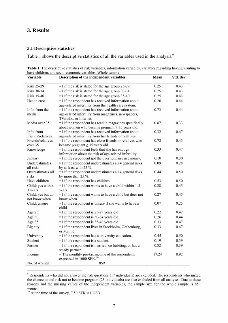
7

3. Results

3.1 Descriptive statistics

Table 1 shows the descriptive statistics of all the variables used in the analysis.9 Table 1. The descriptive statistics of risk variables, information variables, variables regarding having/wanting to have children, and socio-economic variables. Whole sample Variable

Description of the independent variables

Mean

Std. dev.

Risk 25-29 =1 if the risk is stated for the age group 25-29. 0.25 0.43 Risk 30-34 =1 if the risk is stated for the age group 30-34. 0.25 0.43 Risk 35-40 =1 if the risk is stated for the age group 35-40. 0.25 0.43 Health care =1 if the respondent has received information about

age-related infertility from the health care system. 0.26 0.44

Info. from the media

=1 if the respondent has received information about age-related infertility from magazines, newspapers, TV/radio, or Internet.

0.73 0.44

Media over 35 =1 if the respondent has read in magazines specifically about women who became pregnant ≥ 35 years old.

0.87 0.33

Info. from friends/relatives

=1 if the respondent has received information about age-related infertility from her friends or relatives.

0.32 0.47

Friends/relatives over 35

=1 if the respondent has close friends or relatives who became pregnant ≥ 35 years old.

0.72 0.45

Knowledge =1 if the respondent feels that she has enough information about the risk of age-related infertility.

0.33 0.47

January =1 if the respondent got the questionnaire in January. 0.10 0.30 Underestimates all risks

=1 if the respondent underestimates all 4 general risks by at least with 25 %.

0.09 0.28

Overestimates all risks

=1 if the respondent underestimates all 4 general risks by more than 25 %.

0.44 0.50

Have children =1 if the respondent has children. 0.53 0.50 Child; yes within 3 years

=1 if the respondent wants to have a child within 1-3 years.

0.28 0.45

Child; yes but do not know when

=1 if the respondent wants to have a child but does not know when.

0.27 0.45

Child; unsure =1 if the respondent is unsure if she wants to have a child.

0.07 0.25

Age 25 =1 if the respondent is 25-29 years old. 0.22 0.42 Age 30 =1 if the respondent is 30-34 years old. 0.26 0.44 Age 35 =1 if the respondent is 35-40 years old. 0.33 0.47 Big city =1 if the respondent lives in Stockholm, Gothenburg,

or Malmö. 0.33 0.47

University =1 if the respondent has a university education. 0.45 0.50 Student =1 if the respondent is a student. 0.19 0.39 Partner =1 if the respondent is married, co-habiting, or has a

steady partner. 0.82 0.39

Income = The monthly pre-tax income of the respondent, expressed in 1000 SEK.10

17.24 8.92

No. of women 859

9 Respondents who did not answer the risk questions (17 individuals) are excluded. The respondents who mixed the chance to and risk not to become pregnant (23 individuals) are also excluded from all analyses. Due to these reasons and the missing values of the independent variables, the sample size for the whole sample is 859 women. 10 At the time of the survey, 7.50 SEK ≈ 1 USD.

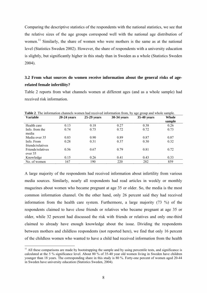
8

Comparing the descriptive statistics of the respondents with the national statistics, we see that

the relative sizes of the age groups correspond well with the national age distribution of

women.11 Similarly, the share of women who were mothers is the same as at the national

level (Statistics Sweden 2002). However, the share of respondents with a university education

is slightly, but significantly higher in this study than in Sweden as a whole (Statistics Sweden

2004).

3.2 From what sources do women receive information about the general risks of age-

related female infertility?

Table 2 reports from what channels women at different ages (and as a whole sample) had

received risk information.

Table 2. The information channels women had received information from, by age group and whole sample. Variable 20-24 years 25-29 years 30-34 years 35-40 years Whole

sample Health care 0.13 0.18 0.27 0.38 0.26 Info. from the media

0.74 0.75 0.72 0.72 0.73

Media over 35 0.83 0.90 0.89 0.87 0.87 Info. From friends/relatives

0.28 0.31 0.37 0.30 0.32

Friends/relatives over 35

0.56 0.67 0.79 0.81 0.72

Knowledge 0.15 0.26 0.41 0.43 0.33 No. of women 167 190 220 282 859

A large majority of the respondents had received information about infertility from various

media sources. Similarly, nearly all respondents had read articles in weekly or monthly

magazines about women who became pregnant at age 35 or older. So, the media is the most

common information channel. On the other hand, only 26 percent said they had received

information from the health care system. Furthermore, a large majority (73 %) of the

respondents claimed to have close friends or relatives who became pregnant at age 35 or

older, while 32 percent had discussed the risk with friends or relatives and only one-third

claimed to already have enough knowledge about the issue. Dividing the respondents

between mothers and childless respondents (not reported here), we find that only 16 percent

of the childless women who wanted to have a child had received information from the health

11 All these comparisons are made by bootstrapping the sample and by using percentile tests, and significance is calculated at the 5 % significance level. About 80 % of 35-40 year old women living in Sweden have children younger than 18 years. The corresponding share in this study is 80 %. Forty-one percent of women aged 20-44 in Sweden have university education (Statistics Sweden, 2004).

9

care system, while 34 percent of the mothers had, a difference which is significant at the one

percent level according to a Chi-square test. A larger share of the mothers had friends who

became pregnant at age 35 or older, while all other information channels reached about equal

shares of mothers and women without children.12

We also find that the media reaches women of all ages. On the other hand, the share of

women who had received information from the health care system increases substantially

with age. The results also show that women in the 30-40 age group more often perceive that

they have enough knowledge about the risks than women in the 20-29 age group.13 We are

therefore in the next section going to investigate whether the older women have more correct

risk perceptions than the younger.

12 These results are available upon request. 13 A difference that is significant according to a Chi-square test at the 1 % significance level.

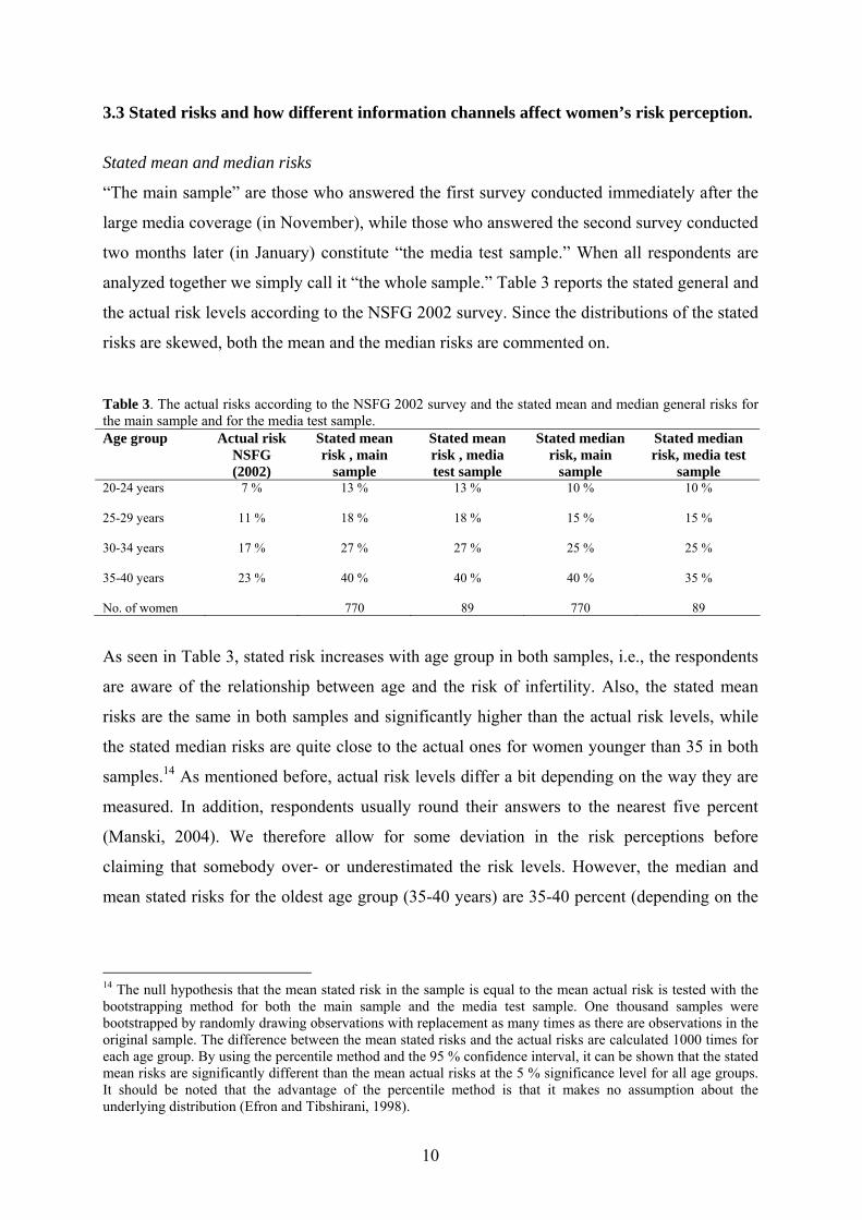
10

3.3 Stated risks and how different information channels affect women’s risk perception.

Stated mean and median risks

“The main sample” are those who answered the first survey conducted immediately after the

large media coverage (in November), while those who answered the second survey conducted

two months later (in January) constitute “the media test sample.” When all respondents are

analyzed together we simply call it “the whole sample.” Table 3 reports the stated general and

the actual risk levels according to the NSFG 2002 survey. Since the distributions of the stated

risks are skewed, both the mean and the median risks are commented on. Table 3. The actual risks according to the NSFG 2002 survey and the stated mean and median general risks for the main sample and for the media test sample. Age group Actual risk

NSFG (2002)

Stated mean risk , main

sample

Stated mean risk , media test sample

Stated median risk, main

sample

Stated median risk, media test

sample 20-24 years 7 % 13 %

13 % 10 % 10 %

25-29 years 11 % 18 %

18 % 15 % 15 %

30-34 years 17 % 27 %

27 % 25 % 25 %

35-40 years 23 % 40 %

40 % 40 % 35 %

No. of women 770 89 770 89

As seen in Table 3, stated risk increases with age group in both samples, i.e., the respondents

are aware of the relationship between age and the risk of infertility. Also, the stated mean

risks are the same in both samples and significantly higher than the actual risk levels, while

the stated median risks are quite close to the actual ones for women younger than 35 in both

samples.14 As mentioned before, actual risk levels differ a bit depending on the way they are

measured. In addition, respondents usually round their answers to the nearest five percent

(Manski, 2004). We therefore allow for some deviation in the risk perceptions before

claiming that somebody over- or underestimated the risk levels. However, the median and

mean stated risks for the oldest age group (35-40 years) are 35-40 percent (depending on the

14 The null hypothesis that the mean stated risk in the sample is equal to the mean actual risk is tested with the bootstrapping method for both the main sample and the media test sample. One thousand samples were bootstrapped by randomly drawing observations with replacement as many times as there are observations in the original sample. The difference between the mean stated risks and the actual risks are calculated 1000 times for each age group. By using the percentile method and the 95 % confidence interval, it can be shown that the stated mean risks are significantly different than the mean actual risks at the 5 % significance level for all age groups. It should be noted that the advantage of the percentile method is that it makes no assumption about the underlying distribution (Efron and Tibshirani, 1998).

11

sample), which clearly is an overestimation.15 Respondent age has no significant effect on the

stated risk levels; they are about the same with and without the respondents younger than 30.

To find out whether the large media coverage immediately before our main survey was sent

out had any effect on the stated risks, we compare the stated risks of the main and the media

test samples and find the mean risks to be the same. However, the stated median risk for the

oldest age group (35-40 years) is 5 percentage points lower in the media test sample. That the

newspaper articles especially highlighted (sometimes already in the introduction) the age of

35 as a threshold after which a woman’s fertility begins to take a sharper decline might have

increased the stated median risk levels in the main sample for the oldest age group (35-40

years). However, although the difference is substantial it is not significant.16

How the different information channels affect the perception of female infertility risks Table 4 reports the results of the multinomial logit model, which analyzes how the different

channels of information affect whether the stated risks are estimated correctly or whether they

are under- or overestimated. The stated risks for the four age groups are strongly correlated

and it is likely that there is unobservable heterogeneity among the respondents. Therefore, the

data is pooled and standard errors are corrected for clustering.17 Each respondent stated risk

levels of infertility for women in the four age groups. Since a same respondent may

overestimate, underestimate, and/or give correct risk estimates when estimating these risks,

all conceivable combinations are in principle possible. Therefore, it is better to investigate

whether the stated risk is underestimated, correct, or overestimated, instead of whether a

respondent stated correct or biased risks. Moreover, there is always some uncertainty about

the correct risk levels, so we allow for a deviation of ± 25 percent in the “correct” risk

estimation. To be able to examine how the information channels affect the probability of

estimating the risks correctly, the dependent variable consists of risks divided into three

15 The median risks in both samples remain the same if we exclude the highest stated risks (top 10 % of both samples), indicating that the median risks are robust. We excluded risks that are larger than 40 % for the 20-24 age group, 50 % for the 25-30 age group, 60 % for the 30-34 age group, and 70 % for the 35-40 age group. 16 The difference is tested both by a Wilcoxon rank sum test and a Chi-square test corrected for continuity (see Siegel and Castellan, 1988). 17 The correlations between the risks stated for the four age groups are between 0.39 and 0.84. The highest correlations are between the risks stated for the two youngest age groups (0.82) and between the two oldest age groups (0.84). Furthermore, there is no strong correlation among the explanatory variables in the regression.

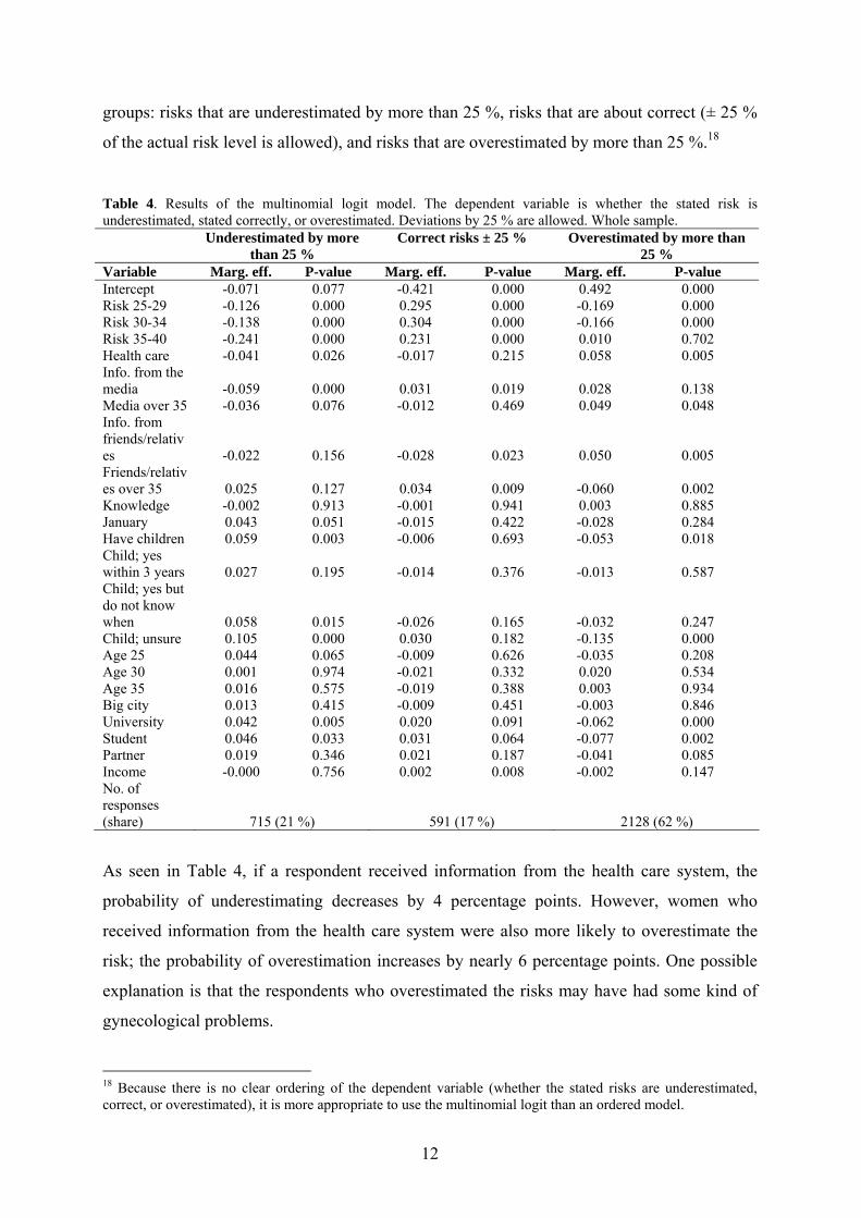
12

groups: risks that are underestimated by more than 25 %, risks that are about correct (± 25 %

of the actual risk level is allowed), and risks that are overestimated by more than 25 %.18 Table 4. Results of the multinomial logit model. The dependent variable is whether the stated risk is underestimated, stated correctly, or overestimated. Deviations by 25 % are allowed. Whole sample.

Underestimated by more than 25 %

Correct risks ± 25 % Overestimated by more than 25 %

Variable Marg. eff. P-value Marg. eff. P-value Marg. eff. P-value Intercept -0.071 0.077 -0.421 0.000 0.492 0.000 Risk 25-29 -0.126 0.000 0.295 0.000 -0.169 0.000 Risk 30-34 -0.138 0.000 0.304 0.000 -0.166 0.000 Risk 35-40 -0.241 0.000 0.231 0.000 0.010 0.702 Health care -0.041 0.026 -0.017 0.215 0.058 0.005 Info. from the media -0.059 0.000 0.031 0.019 0.028 0.138 Media over 35 -0.036 0.076 -0.012 0.469 0.049 0.048 Info. from friends/relatives -0.022 0.156 -0.028 0.023 0.050 0.005 Friends/relatives over 35 0.025 0.127 0.034 0.009 -0.060 0.002 Knowledge -0.002 0.913 -0.001 0.941 0.003 0.885 January 0.043 0.051 -0.015 0.422 -0.028 0.284 Have children 0.059 0.003 -0.006 0.693 -0.053 0.018 Child; yes within 3 years 0.027 0.195 -0.014 0.376 -0.013 0.587 Child; yes but do not know when 0.058 0.015 -0.026 0.165 -0.032 0.247 Child; unsure 0.105 0.000 0.030 0.182 -0.135 0.000 Age 25 0.044 0.065 -0.009 0.626 -0.035 0.208 Age 30 0.001 0.974 -0.021 0.332 0.020 0.534 Age 35 0.016 0.575 -0.019 0.388 0.003 0.934 Big city 0.013 0.415 -0.009 0.451 -0.003 0.846 University 0.042 0.005 0.020 0.091 -0.062 0.000 Student 0.046 0.033 0.031 0.064 -0.077 0.002 Partner 0.019 0.346 0.021 0.187 -0.041 0.085 Income -0.000 0.756 0.002 0.008 -0.002 0.147 No. of responses (share) 715 (21 %) 591 (17 %) 2128 (62 %)

As seen in Table 4, if a respondent received information from the health care system, the

probability of underestimating decreases by 4 percentage points. However, women who

received information from the health care system were also more likely to overestimate the

risk; the probability of overestimation increases by nearly 6 percentage points. One possible

explanation is that the respondents who overestimated the risks may have had some kind of

gynecological problems.

18 Because there is no clear ordering of the dependent variable (whether the stated risks are underestimated, correct, or overestimated), it is more appropriate to use the multinomial logit than an ordered model.

13

Keeping in mind that the media is the most common information channel, it is important to

study how they affect risk perceptions. We find that women who had received information

from the media were more likely to state a correct risk, but that respondents who had read

articles in the magazines about women who became pregnant at age 35 or older were more

likely to overestimate the risks. In addition, the results of our media test are in line with our

expectations that respondents in the test sample were more likely to state lower risks than

those in the main sample (who received the questionnaire immediately after the large media

coverage).

What peers say and do affect risk perceptions. The respondents who had obtained information

from friends and relatives were more likely to state too high risks. However, a woman with

close friends or relatives who became pregnant at age 35 or older was more likely to have a

correct perception of the risks. Comparing the effects of the media and friends/relatives, we

see that the magnitudes of the effects are nearly the same in the case when the risks are

almost correctly estimated, but the signs are the opposite. Information from the media is thus

better for the risk perception than information from friends and relatives. Another interesting

result is that mothers and respondents who wanted (possibly again) to become pregnant later

in life, but did not know when, were more likely to underestimate the risks.

As a sensitivity analysis we estimated the same multinomial logit model again, but this time

allowing a 50 percent deviation from the actual risk levels when classifying the responses.19

The results show that articles in magazines about women who became pregnant in their late

30s no longer affect the probabilities of overestimating the risks significantly. Moreover,

information from the health care system no longer decreases the probability of

underestimation significantly. The results of how women are affected by their peers are more

robust: There are no changes in significance or in signs of the marginal effects that capture

that women had received information from friends/relatives or that a woman had close

friends/relatives who became pregnant at age 35 or older. However, the effects of peers are

even larger when we allow for a 50 percent deviation from the actual risk levels; the sizes of

the marginal effects are doubled. Finally, our media test gives the same result: Women who

completed the questionnaire two months later were more likely to underestimate the risks

19 The results are available upon request.

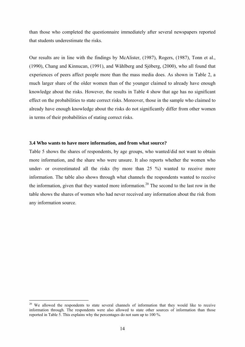
14

than those who completed the questionnaire immediately after several newspapers reported

that students underestimate the risks.

Our results are in line with the findings by McAlister, (1987), Rogers, (1987), Tonn et al.,

(1990), Chang and Kinnucan, (1991), and Wåhlberg and Sjöberg, (2000), who all found that

experiences of peers affect people more than the mass media does. As shown in Table 2, a

much larger share of the older women than of the younger claimed to already have enough

knowledge about the risks. However, the results in Table 4 show that age has no significant

effect on the probabilities to state correct risks. Moreover, those in the sample who claimed to

already have enough knowledge about the risks do not significantly differ from other women

in terms of their probabilities of stating correct risks.

3.4 Who wants to have more information, and from what source?

Table 5 shows the shares of respondents, by age groups, who wanted/did not want to obtain

more information, and the share who were unsure. It also reports whether the women who

under- or overestimated all the risks (by more than 25 %) wanted to receive more

information. The table also shows through what channels the respondents wanted to receive

the information, given that they wanted more information.20 The second to the last row in the

table shows the shares of women who had never received any information about the risk from

any information source.

20 We allowed the respondents to state several channels of information that they would like to receive information through. The respondents were also allowed to state other sources of information than those reported in Table 5. This explains why the percentages do not sum up to 100 %.

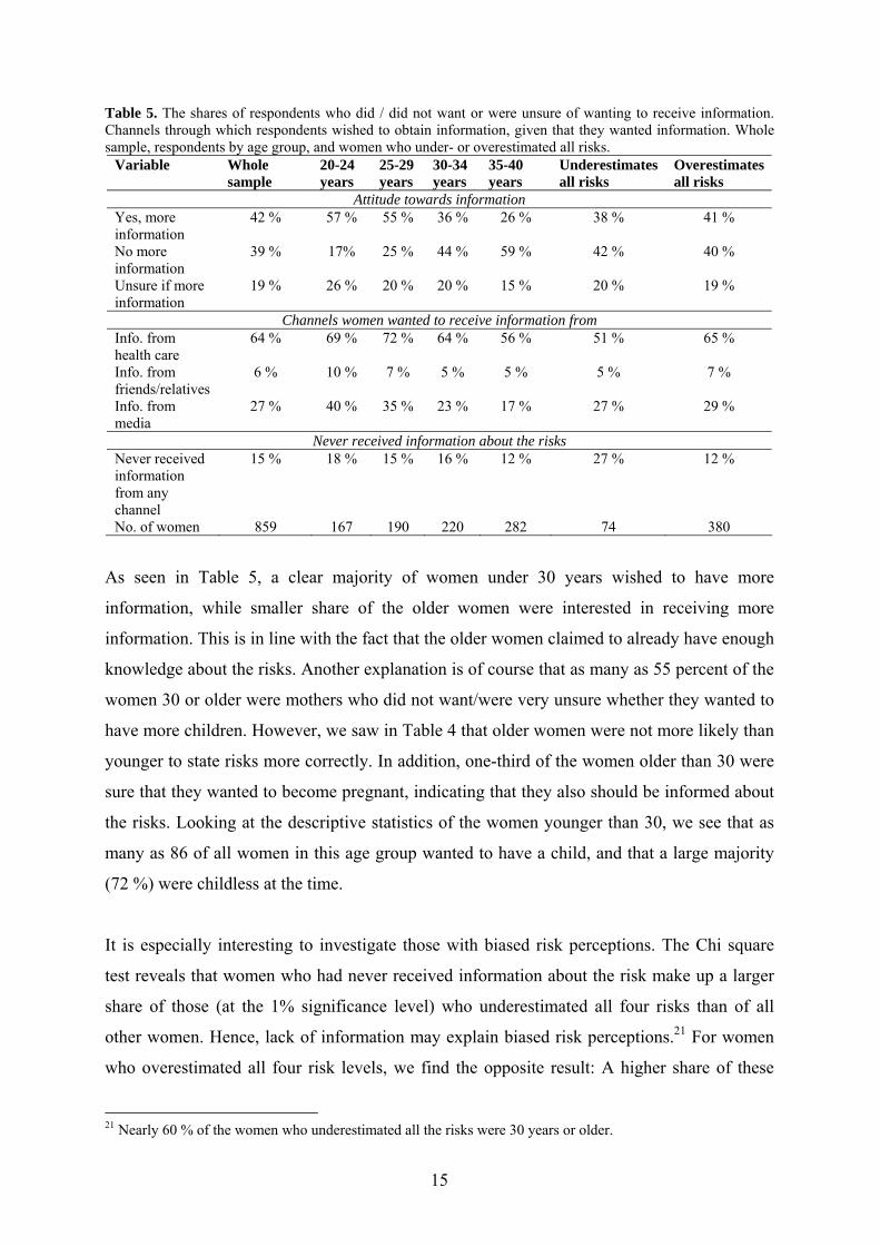
15

Table 5. The shares of respondents who did / did not want or were unsure of wanting to receive information. Channels through which respondents wished to obtain information, given that they wanted information. Whole sample, respondents by age group, and women who under- or overestimated all risks.

Variable Whole sample

20-24 years

25-29 years

30-34 years

35-40 years

Underestimates all risks

Overestimates all risks

Attitude towards information Yes, more information

42 % 57 % 55 % 36 % 26 % 38 % 41 %

No more information

39 % 17% 25 % 44 % 59 % 42 % 40 %

Unsure if more information

19 % 26 % 20 % 20 % 15 % 20 % 19 %

Channels women wanted to receive information from Info. from health care

64 % 69 % 72 % 64 % 56 % 51 % 65 %

Info. from friends/relatives

6 % 10 % 7 % 5 % 5 % 5 % 7 %

Info. from media

27 % 40 % 35 % 23 % 17 % 27 % 29 %

Never received information about the risks Never received information from any channel

15 % 18 % 15 % 16 % 12 % 27 % 12 %

No. of women 859 167 190 220 282 74 380

As seen in Table 5, a clear majority of women under 30 years wished to have more

information, while smaller share of the older women were interested in receiving more

information. This is in line with the fact that the older women claimed to already have enough

knowledge about the risks. Another explanation is of course that as many as 55 percent of the

women 30 or older were mothers who did not want/were very unsure whether they wanted to

have more children. However, we saw in Table 4 that older women were not more likely than

younger to state risks more correctly. In addition, one-third of the women older than 30 were

sure that they wanted to become pregnant, indicating that they also should be informed about

the risks. Looking at the descriptive statistics of the women younger than 30, we see that as

many as 86 of all women in this age group wanted to have a child, and that a large majority

(72 %) were childless at the time.

It is especially interesting to investigate those with biased risk perceptions. The Chi square

test reveals that women who had never received information about the risk make up a larger

share of those (at the 1% significance level) who underestimated all four risks than of all

other women. Hence, lack of information may explain biased risk perceptions.21 For women

who overestimated all four risk levels, we find the opposite result: A higher share of these

21 Nearly 60 % of the women who underestimated all the risks were 30 years or older.

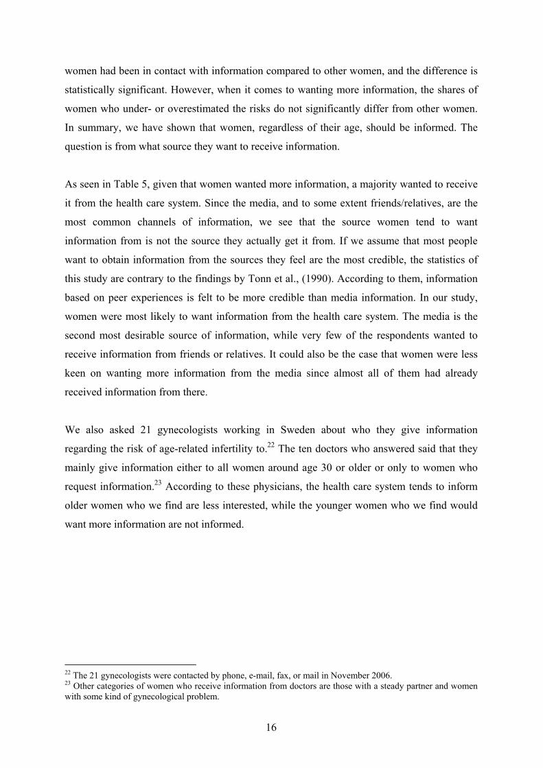
16

women had been in contact with information compared to other women, and the difference is

statistically significant. However, when it comes to wanting more information, the shares of

women who under- or overestimated the risks do not significantly differ from other women.

In summary, we have shown that women, regardless of their age, should be informed. The

question is from what source they want to receive information.

As seen in Table 5, given that women wanted more information, a majority wanted to receive

it from the health care system. Since the media, and to some extent friends/relatives, are the

most common channels of information, we see that the source women tend to want

information from is not the source they actually get it from. If we assume that most people

want to obtain information from the sources they feel are the most credible, the statistics of

this study are contrary to the findings by Tonn et al., (1990). According to them, information

based on peer experiences is felt to be more credible than media information. In our study,

women were most likely to want information from the health care system. The media is the

second most desirable source of information, while very few of the respondents wanted to

receive information from friends or relatives. It could also be the case that women were less

keen on wanting more information from the media since almost all of them had already

received information from there.

We also asked 21 gynecologists working in Sweden about who they give information

regarding the risk of age-related infertility to.22 The ten doctors who answered said that they

mainly give information either to all women around age 30 or older or only to women who

request information.23 According to these physicians, the health care system tends to inform

older women who we find are less interested, while the younger women who we find would

want more information are not informed.

22 The 21 gynecologists were contacted by phone, e-mail, fax, or mail in November 2006. 23 Other categories of women who receive information from doctors are those with a steady partner and women with some kind of gynecological problem.

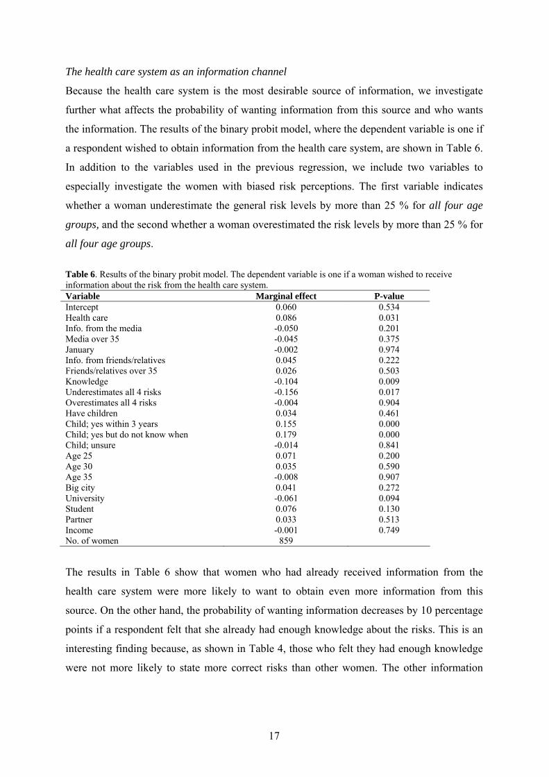
17

The health care system as an information channel

Because the health care system is the most desirable source of information, we investigate

further what affects the probability of wanting information from this source and who wants

the information. The results of the binary probit model, where the dependent variable is one if

a respondent wished to obtain information from the health care system, are shown in Table 6.

In addition to the variables used in the previous regression, we include two variables to

especially investigate the women with biased risk perceptions. The first variable indicates

whether a woman underestimate the general risk levels by more than 25 % for all four age

groups, and the second whether a woman overestimated the risk levels by more than 25 % for

all four age groups.

Table 6. Results of the binary probit model. The dependent variable is one if a woman wished to receive information about the risk from the health care system. Variable Marginal effect P-value Intercept 0.060 0.534 Health care 0.086 0.031 Info. from the media -0.050 0.201 Media over 35 -0.045 0.375 January -0.002 0.974 Info. from friends/relatives 0.045 0.222 Friends/relatives over 35 0.026 0.503 Knowledge -0.104 0.009 Underestimates all 4 risks -0.156 0.017 Overestimates all 4 risks -0.004 0.904 Have children 0.034 0.461 Child; yes within 3 years 0.155 0.000 Child; yes but do not know when 0.179 0.000 Child; unsure -0.014 0.841 Age 25 0.071 0.200 Age 30 0.035 0.590 Age 35 -0.008 0.907 Big city 0.041 0.272 University -0.061 0.094 Student 0.076 0.130 Partner 0.033 0.513 Income -0.001 0.749 No. of women 859

The results in Table 6 show that women who had already received information from the

health care system were more likely to want to obtain even more information from this

source. On the other hand, the probability of wanting information decreases by 10 percentage

points if a respondent felt that she already had enough knowledge about the risks. This is an

interesting finding because, as shown in Table 4, those who felt they had enough knowledge

were not more likely to state more correct risks than other women. The other information

18

variables have no significant effect on the probabilities of wanting information from the

health care system.

Women who underestimated the risk levels for all age groups by more than 25 percent were

less likely to want to receive more information from the health care system. The effect is

large; the probability of wanting information decreases by 16 percentage points. The stated

mean risk levels of these respondents are also substantially lower than those of the whole

sample,24 showing that the risk perceptions of these women are clearly biased. As mentioned

before, the shares of women who underestimated all risks do not significantly differ from the

shares of other women when we look at who wants to receive more information. However,

they are obviously less likely to receive information from the health care system. One

explanation might be that it is more sensitive to receive information from a personal source,

such as physicians. However, underestimation of the risks might be undesirable, especially

since a majority (56 %) of the women who clearly underestimated all risks were sure that they

would like to have a child. Women who overestimated the risks for all age groups do not

significantly differ from those who had just about correct risk perceptions when we look at

who wanted more information from the health care system.

Women who wanted to become pregnant were more likely to want to receive information

from the health care system. The probabilities increase by 16-18 percentage points. However,

women of different ages do not significantly differ from each other when it comes to wanting

to have information from the health care system.

4. Conclusions and discussion This paper is based on a survey of a random and representative sample of Swedish females

aged 20 to 40, and investigates: (1) from what sources women receive information about the

general risks of age-related female infertility, (2) how different information channels affect

women’s perceptions of the risks, and (3) who would like to have more information, and from

what source(s)?

24 The stated mean levels of the risks are 3, 4, 6, and 10 % for the four age groups. The corresponding median risks are 3, 5, 6, and 10 %.

19

The results show that the media reaches women of all ages, while the share of women who

have already received information from the health care system differs among the age groups.

The older the woman, the more likely it is that she has received information from the health

care system. This is in line with what the gynecologists we asked said: the health care system

usually informs women around 30 and older, which is in sharp contrast to the fact that a large

majority of the younger women (under 30) want more information from the health care

system.

Women who have received information from the media are more likely to state correct risks.

On the other hand, reading articles in magazines about women who became pregnant in their

late 30s increases the probability of overestimation. One possible explanation is that several

studies report that female age-related infertility increases only a little before age 30 but more

rapidly after age 35 (Leridon, 2004; Infomedica, 2004). Therefore, it is possible that

magazines spread information highlighting the ages 30 and 35 as ”critical,” making women

believe that the risks are higher than they actually are. If overestimation creates unnecessary

worry, women should also have other information sources.

Only about one-third of the respondents had discussed this risk with their friends or relatives,

but as the results clearly show, friends and relatives are an important source of information

that does affect women’s risk perceptions. However, the information from friends and

relatives seems to generally be incorrect, making female recipients more likely to

overestimate the risks. One possible explanation is that people tend to mainly discuss

problems and difficult pregnancies, leading to overestimations of the risks. On the other hand,

the probability of stating correct risks increases if a woman has close friends or relatives who

became pregnant at 35 or older. These findings are also in line with previous research;

experiences of peers affect people more than the mass media (McAlister, 1987; Rogers, 1987;

Tonn et al., 1990; Chang and Kinnucan, 1991; Wåhlberg and Sjöberg, 2000).

Moreover, we found that the stated median risk level for women aged 35-40 was clearly

higher in the survey mailed out immediately after the media coverage than in the one carried

out two months later, but the difference was not significant. Those who answered our second

survey were more likely to underestimate the risks than those who answered the first survey,

a result that is in line with our expectations. Thus, we find effects of the large media coverage

on people’s risk perceptions, although the effects are not always significant. It is also possible

20

that the effect of the increased media coverage lasted longer than two months, which could

explain why the median and mean risks for the 35-40 age group were overestimated by both

samples. Furthermore, we do not know whether the respondents actually read the articles in

the Swedish newspapers in November 2005.

Our study points to three dilemmas that the Swedish health care system should want to direct

attention to: (1) Only 26 percent of our respondents had obtained information from the health

care system, while a majority wished they had. (2) Although large majority of the women

who are younger than 30 want information from the health care system, the health care

system tends to rather inform older women. Although we must remember that the issue of

infertility might be sensitive for many women (which makes informing more difficult), we

argue that it is important to reach women earlier since a majority of the younger women want

to have a child later on but do not know when. (3) A larger share of women who

underestimated the risk levels for all four age groups had not been in contact with any kind of

information compared to other women. These women were however less likely to wish to

receive information from the health care system, although a majority of them would like to

have a child. In addition, if the health care system succeeds in informing women, it will affect

women themselves as information channels; women can then give more correct information

about the risks to their friends and relatives. Since the media is found to be the most common

source of information, it should be an efficient channel for the health care system to use when

informing women about the risks.

Although the empirical evidence in this paper comes from Sweden, the risks of age-related

infertility concern all women, and our results are therefore of more general interest. It is very

likely that the media reaches women in most countries, while the roles and practices of the

health care systems might differ among countries. However, the results of this study can be

useful for health care systems in other countries to reflect on who they give information to

and whether they reach those with biased risk perceptions. Moreover, the health care systems

should be aware that women receive biased information, especially from their friends and

relatives, and that this can cause unnecessary worry or serious disappointments if it becomes

difficult for a woman to become pregnant.

21

References

Bénabou R. and J. Tirole (2002), “Self-confidence and personal motivation”, The Quarterly Journal of Economics, 117 (3), 871-915.

Bongaarts J. (1982), “Infertility after age 30: A false alarm”, Family Planning Perspectives, 14 (2), 75-78.

Burton M. and T. Young (1996), “The impact of BSE on the demand for beef and other meats in Great Britain”, Applied Economics, 28, 687-693.

Chang H-S, and H. W. Kinnucan (1991), “Advertising, information, and product quality: The case of butter”, American Journal of Agricultural Economics, 73, 1195-1203.

Chandra A., GM Martinez, WD Mosher, JC Abma, and J. Jones (2005), Fertility, family planning, and reproductive health of U.S. women: Data from the 2002 National Survey of Family Growth, U.S. Department of Health and Human Services 23 (25), National Center for Health Statistics.

Efron B. and R. J. Tibshirani (1998), An introduction to the Bootstrap, Chapman & Hall/CRC, U.S.A, 1998, p. 55.

Göteborgs Posten (2005), Studenter riskerar bli barnlösa, 2005-11-16, Attached 2008-03-26 Högber U. (1998), “Epidemiologska synpunkter på fekunditet och infertilitet” In: Ofrivillig

barnlöshet, N-O. Sjöberg (ed.), Rapport nr: 37, Arbets- och Rferensgruppen för Ofrivillig Barnlöshet 1998.

Infomedica (2004), homepage: www.infomedica.se/artikel.asp?CategoryID=11729 Kasperson R. E, O. Renn, P. Slovic, H. S. Brown, J. Emel, R. Goble, J. X. Kasperson and S.

Ratick, (1988), ”The social amplification of risk: A conceptual framework”, Risk Analysis, 8 (2), 177-187.

Kasperson J. X., R. E. Kasperson, N. Pidegon, and P. Slovic (2003), ”The social amplification of risk: assessing fifteen years of research and theory” In: The Social Amplification of Risk, Pidgeon N., R. E. Kasperson and P. Slovic (eds.), Cambridge University Press, UK.

Lampi (2006), Age-related risk of female infertility: A comparison between stated general and personal risks, Working Paper, Revised version April 2008, University of Gothenburg.

Lampic C., A. Skoog Svanberg, P. Karlström and T. Tyden (2006), “Fertility awareness, intentions concerning childbearing, and attitudes toward parenthood among female and male academics”, Human Reproduction, 21 (2), 558-564.

Leridon H. (2004), Can assisted reproduction technology compensate for the natural decline in fertility with age? A model assessment, Human Reproduction, 19 (7), 1548-1553.

Manski C. F. (2004), Measuring expectations, Econometrica, 72 (5), 1329-1376. McAlister A., (1987), “Social learning theory and preventive behaviour” In: Weinstein (Ed.)

Taking Care: Understanding and encouraging self-protective behaviour, Cambridge University Press, USA, 1987.

Miller S. and C. Mangan (1983), “Interacting effects of information and coping style in adapting to gynecologic stress: Should the doctor tell all?”, Journal of Personality and Social Psychology, 45 (1), 223-236.

National Center for Health Statistics, W. D. Mosher and W. F. Pratt (1987), Fecundity, infertility, and reproductive health in the United States, 1982, Vital and Health Statistics Series 23 (14). DHHS Pub No (PHS) 87-1990 U.S., Public Health Service Washington U.S., Government Printing Office, May 1987.

Rogers E. M. (1987), “The diffusion of innovations perspective”, In: Weinstein (Ed.) Taking Care: Understanding and encouraging self-protective behaviour, Cambridge University Press, USA, 1987.

22

Schwartz D. and MJ. Mayaux (1982), “Female fecundity as a function of age: results of artificial insemination in 2193 nulliparous women with azoospermic husbands. Federation CECOS.”, New England Journal of Medicin, 306 (7), 404-406.

Siegel S. and J. Castellan (1988), Nonparametric statistics for the behavioural sciences, McGraw-Hill Book Company, Singapore, 1988.

Soumerai S.B., D. Ross-Degnan and J. S. Kahn (1992), “Effects of professional and media warnings about the association between aspirin use in children and Reye’s syndrome”, The Milbank Quarterly, 70 (1), 155-182.

Statistics of Sweden (2002), “Pappa och barn”, VälfärdsBulletinen, No. 4, homepage: http://www.scb.se/Grupp/allmant/_dokument/A05ST0204_08.pdf.

Statistics Sweden (2004), Statistics Sweden (2004), “Population aged 16-74 by level of education, sex and age 2004”, homepage: http://www.scb.se/templates/Product____9577.asp.

Svenska Dagbladet (2005), Studenter överskattar fertilitet-riskerar barnlöshet, 17th November 2005, www.svd.se/nyheter/inrikes/artikel_478537.svd, Attached Mars 2008. Tietze C. (1957) “Reproductive span and rate of reproduction among Hutterite women”,

Fertility and Sterility, 8 (1), 89-97. Tonn B. E., C. B. Travis, R. T. Goeltz and R. H. Phillippi, (1990), “Knowledge-based

representations of risk beliefs”, Risk Analysis, 10 (1), 169-184. Weaver J. and J. Wakshlag (1986), “Perceived vulnerability to crime, criminal victimization

experience, and television viewing”, Journal of Broadcasting and Electronic Media, 30 (2), 141-158.

Verbeke W. and R. W. Ward (2001), “A fresh meat almost ideal demand system incorporating negative TV press and advertising impact”, Agricultural Economics, 25, 359-374.

Wiegman O. and J. M. Gutteling (1995), “Risk appraisal and risk communication: Some empirical data from the Netherlands reviewed”, Basic and Applied Social Psychology, 16 (1&2), 227-249.

Wåhlberg A. AF. and L. Sjöberg, (2000), “Risk perception and the media”, Journal of Risk Research, 3 (1), 31-50.

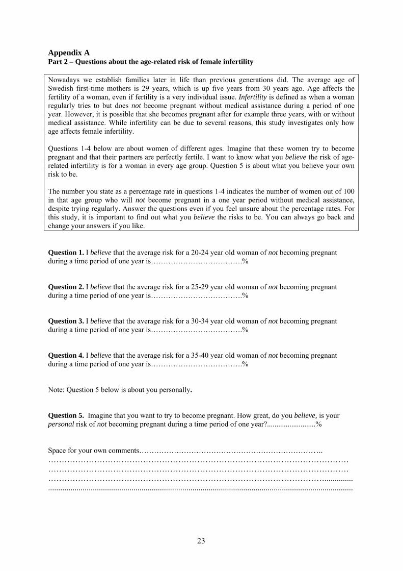
23

Appendix A Part 2 – Questions about the age-related risk of female infertility Nowadays we establish families later in life than previous generations did. The average age of Swedish first-time mothers is 29 years, which is up five years from 30 years ago. Age affects the fertility of a woman, even if fertility is a very individual issue. Infertility is defined as when a woman regularly tries to but does not become pregnant without medical assistance during a period of one year. However, it is possible that she becomes pregnant after for example three years, with or without medical assistance. While infertility can be due to several reasons, this study investigates only how age affects female infertility. Questions 1-4 below are about women of different ages. Imagine that these women try to become pregnant and that their partners are perfectly fertile. I want to know what you believe the risk of age-related infertility is for a woman in every age group. Question 5 is about what you believe your own risk to be. The number you state as a percentage rate in questions 1-4 indicates the number of women out of 100 in that age group who will not become pregnant in a one year period without medical assistance, despite trying regularly. Answer the questions even if you feel unsure about the percentage rates. For this study, it is important to find out what you believe the risks to be. You can always go back and change your answers if you like. Question 1. I believe that the average risk for a 20-24 year old woman of not becoming pregnant during a time period of one year is……………………………….% Question 2. I believe that the average risk for a 25-29 year old woman of not becoming pregnant during a time period of one year is……………………………….% Question 3. I believe that the average risk for a 30-34 year old woman of not becoming pregnant during a time period of one year is……………………………….% Question 4. I believe that the average risk for a 35-40 year old woman of not becoming pregnant during a time period of one year is……………………………….% Note: Question 5 below is about you personally. Question 5. Imagine that you want to try to become pregnant. How great, do you believe, is your personal risk of not becoming pregnant during a time period of one year?..........................% Space for your own comments……………………………………………………………….. ………………………………………………………………………………………………………………………………………………………………………………………………………………………………………………………………………………………………....................................................................................................................................................................

Previous doctoral theses in the Department of Economics, Göteborg. Avhandlingar publicerade innan serien Ekonomiska Studier startades: Östman, Hugo (1911), Norrlands ekonomiska utveckling Moritz, Marcus (1911), Den svenska tobaksindustrien Sundbom, I. (1933), Prisbildning och ändamålsenlighet Gerhard, I. (1948), Problem rörande Sveriges utrikeshandel 1936/38 Hegeland, Hugo (1951), The Quantity Theory of Money Mattsson, Bengt (1970), Cost-Benefit analys Rosengren, Björn (1975), Valutareglering och nationell ekonomisk politik Hjalmarsson, Lennart (1975), Studies in a Dynamic Theory of Production and its Applications Örtendahl, Per-Anders (1975), Substitutionsaspekter på produktionsprocessen vid massaframställning Anderson, Arne M. (1976), Produktion, kapacitet och kostnader vid ett helautomatiskt emballageglasbruk Ohlsson, Olle (1976), Substitution och odelbarheter i produktionsprocessen vid massaframställning Gunnarsson, Jan (1976), Produktionssystem och tätortshierarki – om sambandet mellan rumslig och ekonomisk struktur Köstner, Evert (1976), Optimal allokering av tid mellan utbildning och arbete Wigren, Rune (1976), Analys av regionala effektivitetsskillnader inom industribranscher Wästlund, Jan (1976), Skattning och analys av regionala effektivitetsskillnader inom industribranscher Flöjstad, Gunnar (1976), Studies in Distortions, Trade and Allocation Problems Sandelin, Bo (1977), Prisutveckling och kapitalvinster på bostadsfastigheter Dahlberg, Lars (1977), Empirical Studies in Public Planning Lönnroth, Johan (1977), Marxism som matematisk ekonomi Johansson, Börje (1978), Contributions to Sequential Analysis of Oligopolistic Competition Ekonomiska Studier, utgivna av Nationalekonomiska institutionen vid Göteborgs Universitet. Nr 1 och 4 var inte doktorsavhandlingar. (The contributions to the department

series ’Ekonomiska Studier’ where no. 1 and 4 were no doctoral theses): 2. Ambjörn, Erik (1959), Svenskt importberoende 1926-1956: en ekonomisk-

statistisk kartläggning med kommentarer 3. Landgren, K-G. (1960), Den ”Nya ekonomien” i Sverige: J.M. Keynes, E.

Wigfors och utecklingen 1927-39 5. Bigsten, Arne (1979), Regional Inequality and Development: A Case Study of

Kenya 6. Andersson, Lars (1979), Statens styrning av de kommunala budgetarnas struktur

(Central Government Influence on the Structure of the Municipal Budget) 7. Gustafsson, Björn (1979), Inkomst- och uppväxtförhållanden (Income and

Family Background) 8. Granholm, Arne (1981), Interregional Planning Models for the Allocation of

Private and Public Investments

9. Lundborg, Per (1982), Trade Policy and Development: Income Distributional Effects in the Less Developed Countries of the US and EEC Policies for Agricultural Commodities

10. Juås, Birgitta (1982), Värdering av risken för personskador. En jämförande studie av implicita och explicita värden. (Valuation of Personal Injuries. A comparison of Explicit and Implicit Values)

11. Bergendahl, Per-Anders (1982), Energi och ekonomi - tillämpningar av input-output analys (Energy and the Economy - Applications of Input-Output Analysis)

12. Blomström, Magnus (1983), Foreign Investment, Technical Efficiency and Structural Change - Evidence from the Mexican Manufacturing Industry

13. Larsson, Lars-Göran (1983), Comparative Statics on the Basis of Optimization Methods

14. Persson, Håkan (1983), Theory and Applications of Multisectoral Growth Models

15. Sterner, Thomas (1986), Energy Use in Mexican Industry. 16. Flood, Lennart (1986), On the Application of Time Use and Expenditure

Allocation Models. 17. Schuller, Bernd-Joachim (1986), Ekonomi och kriminalitet - en empirisk

undersökning av brottsligheten i Sverige (Economics of crime - an empirical analysis of crime in Sweden)

18. Walfridson, Bo (1987), Dynamic Models of Factor Demand. An Application to Swedish Industry.

19. Stålhammar, Nils-Olov (1987), Strukturomvandling, företagsbeteende och förväntningsbildning inom den svenska tillverkningsindustrin (Structural Change, Firm Behaviour and Expectation Formation in Swedish Manufactury)

20. Anxo, Dominique (1988), Sysselsättningseffekter av en allmän arbetstidsför-kortning (Employment effects of a general shortage of the working time)

21. Mbelle, Ammon (1988), Foreign Exchange and Industrial Development: A Study of Tanzania.

22. Ongaro, Wilfred (1988), Adoption of New Farming Technology: A Case Study of Maize Production in Western Kenya.

23. Zejan, Mario (1988), Studies in the Behavior of Swedish Multinationals. 24. Görling, Anders (1988), Ekonomisk tillväxt och miljö. Förorenings-struktur och

ekonomiska effekter av olika miljövårdsprogram. (Economic Growth and Environment. Pollution Structure and Economic Effects of Some Environmental Programs).

25. Aguilar, Renato (1988), Efficiency in Production: Theory and an Application on Kenyan Smallholders.

26. Kayizzi-Mugerwa, Steve (1988), External Shocks and Adjustment in Zambia.

27. Bornmalm-Jardelöw, Gunilla (1988), Högre utbildning och arbetsmarknad (Higher Education and the Labour Market)

28. Tansini, Ruben (1989), Technology Transfer: Dairy Industries in Sweden and Uruguay.

29. Andersson, Irene (1989), Familjebeskattning, konsumtion och arbetsutbud - En ekonometrisk analys av löne- och inkomstelasticiteter samt policysimuleringar för svenska hushåll (Family Taxation, Consumption and Labour Supply - An Econometric Analysis of Wage and Income Elasticities and Policy Simulations for Swedish Households)

30. Henrekson, Magnus (1990), An Economic Analysis of Swedish Government Expenditure

31. Sjöö, Boo (1990), Monetary Policy in a Continuous Time Dynamic Model for Sweden

32. Rosén, Åsa (1991), Contributions to the Theory of Labour Contracts. 33. Loureiro, Joao M. de Matos (1992), Foreign Exchange Intervention,

Sterilization and Credibility in the EMS: An Empirical Study 34. Irandoust, Manuchehr (1993), Essays on the Behavior and Performance of

the Car Industry 35. Tasiran, Ali Cevat (1993), Wage and Income Effects on the Timing and

Spacing of Births in Sweden and the United States 36. Milopoulos, Christos (1993), Investment Behaviour under Uncertainty: An

Econometric Analysis of Swedish Panel Data 37. Andersson, Per-Åke (1993), Labour Market Structure in a Controlled Economy:

The Case of Zambia 38. Storrie, Donald W. (1993), The Anatomy of a Large Swedish Plant Closure 39. Semboja, Haji Hatibu Haji (1993), Energy and Development in Kenya 40. Makonnen, Negatu (1993), Labor Supply and the Distribution of Economic

Well-Being: A Case Study of Lesotho 41. Julin, Eva (1993), Structural Change in Rural Kenya 42. Durevall, Dick (1993), Essays on Chronic Inflation: The Brazilian Experience 43. Veiderpass, Ann (1993), Swedish Retail Electricity Distribution: A Non-

Parametric Approach to Efficiency and Productivity Change 44. Odeck, James (1993), Measuring Productivity Growth and Efficiency with

Data Envelopment Analysis: An Application on the Norwegian Road Sector 45. Mwenda, Abraham (1993), Credit Rationing and Investment Behaviour under

Market Imperfections: Evidence from Commercial Agriculture in Zambia 46. Mlambo, Kupukile (1993), Total Factor Productivity Growth: An Empirical

Analysis of Zimbabwe's Manufacturing Sector Based on Factor Demand Modelling 47. Ndung'u, Njuguna (1993), Dynamics of the Inflationary Process in Kenya 48. Modén, Karl-Markus (1993), Tax Incentives of Corporate Mergers and

Foreign Direct Investments 49. Franzén, Mikael (1994), Gasoline Demand - A Comparison of Models 50. Heshmati, Almas (1994), Estimating Technical Efficiency, Productivity Growth

And Selectivity Bias Using Rotating Panel Data: An Application to Swedish Agriculture

51. Salas, Osvaldo (1994), Efficiency and Productivity Change: A Micro Data Case Study of the Colombian Cement Industry

52. Bjurek, Hans (1994), Essays on Efficiency and Productivity Change with Applications to Public Service Production

53. Cabezas Vega, Luis (1994), Factor Substitution, Capacity Utilization and Total Factor Productivity Growth in the Peruvian Manufacturing Industry

54. Katz, Katarina (1994), Gender Differentiation and Discrimination. A Study of Soviet Wages

55. Asal, Maher (1995), Real Exchange Rate Determination and the Adjustment Process: An Empirical Study in the Cases of Sweden and Egypt

56. Kjulin, Urban (1995), Economic Perspectives on Child Care 57. Andersson, Göran (1995), Volatility Forecasting and Efficiency of the Swedish

Call Options Market 58. Forteza, Alvaro (1996), Credibility, Inflation and Incentive Distortions in the

Welfare State 59. Locking, Håkan (1996), Essays on Swedish Wage Formation 60. Välilä, Timo (1996), Essays on the Credibility of Central Bank Independence 61. Yilma, Mulugeta (1996), Measuring Smallholder Efficiency: Ugandan Coffee

and Food-Crop Production 62. Mabugu, Ramos E. (1996), Tax Policy Analysis in Zimbabwe Applying General

Equilibrium Models 63. Johansson, Olof (1996), Welfare, Externalities, and Taxation; Theory and Some

Road Transport Applications. 64. Chitiga, Margaret (1996), Computable General Equilibrium Analysis of Income

Distribution Policies in Zimbabwe 65. Leander, Per (1996), Foreign Exchange Market Behavior Expectations and

Chaos 66. Hansen, Jörgen (1997), Essays on Earnings and Labor Supply 67. Cotfas, Mihai (1997), Essays on Productivity and Efficiency in the Romanian

Cement Industry 68. Horgby, Per-Johan (1997), Essays on Sharing, Management and Evaluation of

Health Risks 69. Nafar, Nosratollah (1997), Efficiency and Productivity in Iranian Manufacturing

Industries 70. Zheng, Jinghai (1997), Essays on Industrial Structure, Technical Change,

Employment Adjustment, and Technical Efficiency 71. Isaksson, Anders (1997), Essays on Financial Liberalisation in Developing

Countries: Capital mobility, price stability, and savings 72. Gerdin, Anders (1997), On Productivity and Growth in Kenya, 1964-94 73. Sharifi, Alimorad (1998), The Electricity Supply Industry in Iran: Organization,

performance and future development 74. Zamanian, Max (1997), Methods for Mutual Fund Portfolio Evaluation: An

application to the Swedish market 75. Manda, Damiano Kulundu (1997), Labour Supply, Returns to Education, and

the Effect of Firm Size on Wages: The case of Kenya 76. Holmén, Martin (1998), Essays on Corporate Acquisitions and Stock Market

Introductions

77. Pan, Kelvin (1998), Essays on Enforcement in Money and Banking 78. Rogat, Jorge (1998), The Value of Improved Air Quality in Santiago de Chile 79. Peterson, Stefan (1998), Essays on Large Shareholders and Corporate Control 80. Belhaj, Mohammed (1998), Energy, Transportation and Urban Environment in

Africa: The Case of Rabat-Salé, Morocco 81. Mekonnen, Alemu (1998), Rural Energy and Afforestation: Case Studies from

Ethiopia 82. Johansson, Anders (1998), Empirical Essays on Financial and Real Investment

Behavior 83. Köhlin, Gunnar (1998), The Value of Social Forestry in Orissa, India 84. Levin, Jörgen (1998), Structural Adjustment and Poverty: The Case of Kenya 85. Ncube, Mkhululi (1998), Analysis of Employment Behaviour in Zimbabwe 86. Mwansa, Ladslous (1998), Determinants of Inflation in Zambia 87. Agnarsson, Sveinn (1998), Of Men and Machines: Essays in Applied Labour and

Production Economics 88. Kadenge, Phineas (1998), Essays on Macroeconomic Adjustment in Zimbabwe:

Inflation, Money Demand, and the Real Exchange Rate 89. Nyman, Håkan (1998), An Economic Analysis of Lone Motherhood in Sweden 90. Carlsson, Fredrik (1999), Essays on Externalities and Transport 91. Johansson, Mats (1999), Empirical Studies of Income Distribution 92. Alemu, Tekie (1999), Land Tenure and Soil Conservation: Evidence from

Ethiopia 93. Lundvall, Karl (1999), Essays on Manufacturing Production in a Developing

Economy: Kenya 1992-94 94. Zhang, Jianhua (1999), Essays on Emerging Market Finance 95. Mlima, Aziz Ponary (1999), Four Essays on Efficiency and Productivity in

Swedish Banking 96. Davidsen, Björn-Ivar (2000), Bidrag til den økonomisk-metodologiske

tenkningen (Contributions to the Economic Methodological Thinking) 97. Ericson, Peter (2000), Essays on Labor Supply 98. Söderbom, Måns (2000), Investment in African Manufacturing: A

Microeconomic Analysis 99. Höglund, Lena (2000), Essays on Environmental Regulation with Applications

to Sweden 100. Olsson, Ola (2000), Perspectives on Knowledge and Growth 101. Meuller, Lars (2000), Essays on Money and Credit 102. Österberg, Torun (2000), Economic Perspectives on Immigrants and

Intergenerational Transmissions 103. Kalinda Mkenda, Beatrice (2001), Essays on Purchasing Power Parity,

RealExchange Rate, and Optimum Currency Areas 104. Nerhagen, Lena (2001), Travel Demand and Value of Time - Towards an

Understanding of Individuals Choice Behavior

105. Mkenda, Adolf (2001), Fishery Resources and Welfare in Rural Zanzibar 106. Eggert, Håkan (2001), Essays on Fisheries Economics 107. Andrén, Daniela (2001), Work, Sickness, Earnings, and Early Exits from the

Labor Market. An Empirical Analysis Using Swedish Longitudinal Data 108. Nivorozhkin, Eugene (2001), Essays on Capital Structure 109. Hammar, Henrik (2001), Essays on Policy Instruments: Applications to Smoking

and the Environment 110. Nannyonjo, Justine (2002), Financial Sector Reforms in Uganda (1990-2000):

Interest Rate Spreads, Market Structure, Bank Performance and Monetary Policy 111. Wu, Hong (2002), Essays on Insurance Economics 112. Linde-Rahr, Martin (2002), Household Economics of Agriculture and Forestry

in Rural Vienam 113. Maneschiöld, Per-Ola (2002), Essays on Exchange Rates and Central Bank

Credibility 114. Andrén, Thomas (2002), Essays on Training, Welfare and Labor Supply 115. Granér, Mats (2002), Essays on Trade and Productivity: Case Studies of

Manufacturing in Chile and Kenya 116. Jaldell, Henrik (2002), Essays on the Performance of Fire and Rescue Services 117. Alpizar, Francisco, R. (2002), Essays on Environmental Policy-Making in

Developing Countries: Applications to Costa Rica 118. Wahlberg, Roger (2002), Essays on Discrimination, Welfare and Labor Supply 119. Piculescu, Violeta (2002), Studies on the Post-Communist Transition 120. Pylkkänen, Elina (2003), Studies on Household Labor Supply and Home

Production 121. Löfgren, Åsa (2003), Environmental Taxation – Empirical and Theoretical

Applications 122. Ivaschenko, Oleksiy (2003), Essays on Poverty, Income Inequality and Health in

Transition Economies 123. Lundström, Susanna (2003), On Institutions, Economic Growth and the

Environment 124. Wambugu, Anthony (2003), Essays on Earnings and Human Capital in Kenya 125. Adler, Johan (2003), Aspects of Macroeconomic Saving 126. Erlandsson, Mattias (2003), On Monetary Integration and Macroeconomic

Policy 127. Brink, Anna (2003), On the Political Economy of Municipality Break-Ups 128. Ljungwall, Christer (2003), Essays on China’s Economic Performance During

the Reform Period 129. Chifamba, Ronald (2003), Analysis of Mining Investments in Zimbabwe 130. Muchapondwa, Edwin (2003), The Economics of Community-Based Wildlife

Conservation in Zimbabwe 131. Hammes, Klaus (2003), Essays on Capital Structure and Trade Financing 132. Abou-Ali, Hala (2003), Water and Health in Egypt: An Empirical Analysis 133. Simatele, Munacinga (2004), Financial Sector Reforms and Monetary Policy in

Zambia 134. Tezic, Kerem (2004), Essays on Immigrants’ Economic Integration 135. INSTÄLLD

136. Gjirja, Matilda (2004), Efficiency and Productivity in Swedish Banking 137. Andersson, Jessica (2004), Welfare Environment and Tourism in Developing

Countries 138. Chen, Yinghong (2004), Essays on Voting Power, Corporate Governance and

Capital Structure 139. Yesuf, Mahmud (2004), Risk, Time and Land Management under Market

Imperfections: Applications to Ethiopia 140. Kateregga, Eseza (2005), Essays on the Infestation of Lake Victoria by the Water

Hyacinth 141. Edvardsen, Dag Fjeld (2004), Four Essays on the Measurement of Productive

Efficiency 142. Lidén, Erik (2005), Essays on Information and Conflicts of Interest in Stock

Recommendations 143. Dieden, Sten (2005), Income Generation in the African and Coloured Population

– Three Essays on the Origins of Household Incomes in South Africa 144. Eliasson, Marcus (2005), Individual and Family Consequences of Involuntary

Job Loss 145. Mahmud, Minhaj (2005), Measuring Trust and the Value of Statistical Lives:

Evidence from Bangladesh 146. Lokina, Razack Bakari (2005), Efficiency, Risk and Regulation Compliance:

Applications to Lake Victoria Fisheries in Tanzania 147. Jussila Hammes, Johanna (2005), Essays on the Political Economy of Land Use

Change 148. Nyangena, Wilfred (2006), Essays on Soil Conservation, Social Capital and

Technology Adoption 149. Nivorozhkin, Anton (2006), Essays on Unemployment Duration and Programme

Evaluation 150. Sandén, Klas (2006), Essays on the Skill Premium 151. Deng, Daniel (2006), Three Essays on Electricity Spot and Financial Derivative

Prices at the Nordic Power Exchange 152. Gebreeyesus, Mulu (2006), Essays on Firm Turnover, Growth, and Investment

Behavior in Ethiopian Manufacturing 153. Islam, Nizamul Md. (2006), Essays on Labor Supply and Poverty: A

Microeconometric Application 154. Kjaer, Mats (2006), Pricing of Some Path-Dependent Options on Equities and

Commodities 155. Shimeles, Abebe (2006), Essays on Poverty, Risk and Consumption Dynamics in

Ethiopia 156. Larsson, Jan (2006), Four Essays on Technology, Productivity and Environment 157. Congdon Fors, Heather (2006), Essays in Institutional and Development

Economics 158. Akpalu, Wisdom (2006), Essays on Economics of Natural Resource Management

and Experiments 159. Daruvala, Dinky (2006), Experimental Studies on Risk, Inequality and Relative

Standing 160. García, Jorge (2007), Essays on Asymmetric Information and Environmental

Regulation through Disclosure

161. Bezabih, Mintewab (2007), Essays on Land Lease Markets, Productivity, Biodiversity, and Environmental Variability

162. Visser, Martine (2007), Fairness, Reciprocity and Inequality: Experimental Evidence from South Africa

163. Holm, Louise (2007), A Non-Stationary Perspective on the European and Swedish Business Cycle

164. Herbertsson, Alexander (2007), Pricing Portfolio Credit Derivatives 165. Johansson, Anders C. (2007), Essays in Empirical Finance: Volatility,

Interdependencies, and Risk in Emerging Markets 166. Ibáñez Díaz, Marcela (2007), Social Dilemmas: The Role of Incentives, Norms

and Institutions 167. Ekbom, Anders (2007), Economic Analysis of Soil Capital, Land Use and

Agricultural Production in Kenya 168. Sjöberg, Pål (2007), Essays on Performance and Growth in Swedish Banking 169. Palma Aguirre, Grisha Alexis (2008), Explaining Earnings and Income

Inequality in Chile 170. Akay, Alpaslan (2008), Essays on Microeconometrics and Immigrant

Assimilation 171. Carlsson, Evert (2008), After Work – Investing for Retirement 172. Munshi, Farzana (2008), Essays on Globalization and Occupational Wages 173. Tsakas, Elias (2008), Essays on Epistemology and Evolutionary Game Theory 174. Erlandzon, Karl (2008), Retirement Planning: Portfolio Choice for Long-Term

Investors 175. Lampi, Elina (2008), Individual Preferences, Choices, and Risk Perceptions –

Survey Based Evidence