ECONOMIC STUDIES

DEPARTMENT OF ECONOMICS SCHOOL OF BUSINESS, ECONOMICS AND LAW

UNIVERSITY OF GOTHENBURG 232

________________________

Incentives and Forest Reform: Evidence from China

Yuanyuan Yi

ISBN 978-91-88199-19-5 (printed) ISBN 978-91-88199-20-1 (pdf) ISSN 1651-4289 (printed) ISSN 1651-4297 (online)

Printed in Sweden,

Gothenburg University 2017

In loving memory of my fatherTo my mother and my daughter, Yingzhuo

Acknowledgements

First and foremost I wish to thank my supervisors Gunnar Kohlin and Fredrik Carlsson at

the University of Gothenburg, and my advisor Jintao Xu at Peking University. They have

supported me not only by their expertise, inspiration, and enthusiasm in environmental and

natural resource economics, but also their guidance, advice and encouragement in many aspects

throughout the writing of this thesis.

I gratefully acknowledge the generous financial and capacity building support from the

Swedish International Development Cooperation Agency (Sida) at the Environmental Eco-

nomics Unit at the University of Gothenburg. I would also like to express my enormous

gratitude to the Environment for Development Initiative (EfD) and the Richard C. Malmstens

Foundation for their financial support.

Cyndi Berck is highly appreciated for her expertise in editing and publication manage-

ment. Her advice and comments on the entire thesis and her help in clarifying my language

have been indispensable. I want to especially thank Yonas Alem and Jessica Coria for their

thorough reviews and constructive comments. I would like to express my deep appreciation to

Hakan Eggert, Erik Hjalmarsson, Randi Hjalmarsson, Martin Holmen, Mitesh Kataria, Elina

Lampi, Asa Lofgren, Ola Olsson, Johan Stennek, Thomas Sterner, and Mans Soderbom at the

University of Gothenburg. I would also like to extend my sincere gratitude to Peter Berck at

UC Berkeley, Allen Blackman at the Inter-American Development Bank, Martin Dufwenberg

at the University of Arizona, Pamela Jagger at the University of North Carolina at Chapel

Hill, Billy Pizer at Duke University, Elizabeth Robinson at University of Reading, Andy White

at the Rights and Resources Group, Runsheng Yin at Michigen State University, and William

F. Hyde.

Heartfelt thanks to Wolfgang Habla. He has been not only a brilliant co-author, but has

shared with me his generosity and admirable research attitude.

I warmly acknowledge all my classmates and friends for their deep understanding of the

papers in my thesis and their very useful comments in my seminars. I equally appreciate my

colleagues at the department for their encouragement and moral support.

A special thanks to my family. They are the most precious fortune to me and have blessed

me with a life of joy in research.

Yuanyuan YiGothenburg, May 2017

Contents

Acknowledgments i

1 Introduction 1Collective forests and household management . . . . . . . . . . . . . . . . . . . . . . . 2State-owned forests and state forest enterprieses . . . . . . . . . . . . . . . . . . . . . 4Policy implications . . . . . . . . . . . . . . . . . . . . . . . . . . . . . . . . . . . . . . 5References . . . . . . . . . . . . . . . . . . . . . . . . . . . . . . . . . . . . . . . . . . . 7

2 Forest Devolution Reform in China: A Trigger for Investment or Deforestation?Introduction . . . . . . . . . . . . . . . . . . . . . . . . . . . . . . . . . . . . . . . . . . 1Evidence of devolution and forest conditions . . . . . . . . . . . . . . . . . . . . . . . . 3The Chinese Collective Forest Tenure Reform . . . . . . . . . . . . . . . . . . . . . . . 5Data and descriptive statistics . . . . . . . . . . . . . . . . . . . . . . . . . . . . . . . . 7Empirical strategy . . . . . . . . . . . . . . . . . . . . . . . . . . . . . . . . . . . . . . 12Results . . . . . . . . . . . . . . . . . . . . . . . . . . . . . . . . . . . . . . . . . . . . . 15Conclusion . . . . . . . . . . . . . . . . . . . . . . . . . . . . . . . . . . . . . . . . . . 20References . . . . . . . . . . . . . . . . . . . . . . . . . . . . . . . . . . . . . . . . . . . 21Figures and tables . . . . . . . . . . . . . . . . . . . . . . . . . . . . . . . . . . . . . . 27

3 Allocative Efficiency or Agglomeration? The Emergence of Forestland Rental Mar-kets and the Forest Devolution Reform in China

Introduction . . . . . . . . . . . . . . . . . . . . . . . . . . . . . . . . . . . . . . . . . . 1Studies on agricultural land rental markets and efficiency . . . . . . . . . . . . . . . . 3China’s forest devolution reform and emerging forestland rental markets . . . . . . . . 5A conceptual model of forestland rental market participation . . . . . . . . . . . . . . 7Testable hypotheses and empirical strategy . . . . . . . . . . . . . . . . . . . . . . . . 8Data . . . . . . . . . . . . . . . . . . . . . . . . . . . . . . . . . . . . . . . . . . . . . . 14Results . . . . . . . . . . . . . . . . . . . . . . . . . . . . . . . . . . . . . . . . . . . . . 17Conclusion . . . . . . . . . . . . . . . . . . . . . . . . . . . . . . . . . . . . . . . . . . 23References . . . . . . . . . . . . . . . . . . . . . . . . . . . . . . . . . . . . . . . . . . . 24Figures and tables . . . . . . . . . . . . . . . . . . . . . . . . . . . . . . . . . . . . . . 29

4 Managerial Incentives for Environmental Protection in Chinese-Style FederalismIntroduction . . . . . . . . . . . . . . . . . . . . . . . . . . . . . . . . . . . . . . . . . . 1Background . . . . . . . . . . . . . . . . . . . . . . . . . . . . . . . . . . . . . . . . . . 4Theoretical framework . . . . . . . . . . . . . . . . . . . . . . . . . . . . . . . . . . . . 7Empirical strategy . . . . . . . . . . . . . . . . . . . . . . . . . . . . . . . . . . . . . . 11Data . . . . . . . . . . . . . . . . . . . . . . . . . . . . . . . . . . . . . . . . . . . . . . 15Econometric results . . . . . . . . . . . . . . . . . . . . . . . . . . . . . . . . . . . . . . 20Conclusion . . . . . . . . . . . . . . . . . . . . . . . . . . . . . . . . . . . . . . . . . . 24References . . . . . . . . . . . . . . . . . . . . . . . . . . . . . . . . . . . . . . . . . . . 25Figures and tables . . . . . . . . . . . . . . . . . . . . . . . . . . . . . . . . . . . . . . 29

1 Introduction

In the past two decades, the world’s forests had a net loss of 129 million hectares,

though the rate of forest loss is declining (FAO, 2015). An increasing number of devel-

oping countries have recognized local ownership and control over forests. Meanwhile,

governments adopted forest tenure reforms by devolving control of forests to (indige-

nous) community management, or by a further step, to household management. And

some governments maintain their forests as public. By 2015, 76 percent of the world’s

total forests of 3,999 million hectares were under public ownership and less than 20

percent were under private ownership. The existence of such reforms, legislation or

regulations, however, is not always coupled with effective enforcement and forest con-

servation (FAO, 2015; RRI, 2014). Meanwhile, governments in general, in spite of

concerns with environmental protection and climate change mitigation, are more fo-

cused on economic development, food security and political stability. The overriding

concerns of sustainability, efficiency and distribution in forest devolution reforms and

forest management systems have never been higher.

China, as one of the world’s recent “economic development miracles”, has a total

forestland area of over 208 million hectares as of 2014, and is ranked fifth in terms

of percentage of the world’s total (FAO, 2015). China’s forests are categorized into

two ownership types: village collective-owned and state-owned. The collective forests

consist of 60 percent of the national forest area and 32 percent of the forest stock

volume; the state forests account for 40 percent of the national forest area and 68

percent of the forest stock (State Forestry Administration, 2011).

In this context, the thesis explores the extent and depth of recognition of rights to

forest land and resources in the two types of forest in China, and investigates the rela-

tionship between managerial incentives and associated environmental outcomes. The

first two chapters focus on collective forests and evaluate the impacts of the devolution

of forest tenure rights from villages to households. The third chapter shows how the

institutional setting for state-owned forests, in which the actual forest manager is an

agent to two principals – the central government and jurisdictional (local) government –

leads to deforestation. The findings show that devolution of forest rights to households

improves households’ investment and the efficiency of forestland reallocation among

households, as well as household welfare and forest biomass. With respect to state-

owned forests, however, the research shows that forests are being depleted because local

governments strongly incentivize the forest manager to maximize revenue, while the

1

central government provides only limited incentives to protect the environment. These

findings contribute substantially to the knowledge base for the forest policy sector.

2 Collective Forests and Household Management

Whether devolution (decentralization) brings about deforestation is a question that is

ceaselessly asked. An increasing number of countries have devolved forests to the com-

munity level in forest-rich areas of Asia, Africa, and Latin America, where more than

27 countries had the total forest area under local community management increased

from 383 million hectares to 511 million hectares in 2002-2013 (RRI, 2014). A large

body of literature has been devoted to studying the effect of this step of devolution on

forest conditions, but the findings are inconclusive (e.g., Kaimowitz et al., 1998; Foster

et al., 2002; Baland et al., 2010; Coleman and Fleischman, 2012). A key question, then,

is whether to take a further step, by devolving forest management to the household

level. China made an early move.

Given the history of unsuccessful village collective management, a wave of forest de-

volution reform was announced soon after the millennium, starting in Fujian province,

and featuring the devolution of forest management rights to households. The main

measures include reallocation of village collectively-owned forestland, formal acknowl-

edgement of household property rights to these forest plots, in particular by forest-

land certificates with legalized tenure terms, and encouragement of forestland transfer

(rental) markets. This was very successful and encouraged the central government

to implement a few more pilots starting in 2003 (State Council, 2003) and finally to

promulgate the policy document “Collective Forest Tenure Reform in the Southern

Collective Forest Areas in China” in 2008. This promulgation reflects both the recog-

nition by the benefits of devolution by the highest legislation and the extent and the

depth of the government’s ambition to devolve forest tenure rights. During that pe-

riod, any decision and implementation of the reform required village-level democratic

consensus.

The Collective Forest Tenure Reform in China is the most extensive devolution of

communal forests to households ever seen. By 2008, the reform had devolved 62 million

hectares of the total 100 million hectares of the forests from collective ownership to

individual households (Xu et al., 2010). The reform has involved 600 million people

in rural areas in more than twenty provinces of China (State Forestry Administration,

2

2011).

My Chapter I, Forest Devolution Reform in China: A Trigger for Investment

or Deforestation? (single authored), evaluates the impact of the Collective Forest

Tenure Reform on households’ investment in forestland. I also investigate the effect

of household management on forest resource conditions. Specifically, the investment

analysis is based on a panel dataset of a two-round survey of 3,000 households in

eight provinces before and after the implementation of the forest devolution reform.

The identification strategy exploits the variations in villages’ decisions to select the

reform and in households’ forest investment across time. Using a difference-in-difference

propensity score matching model, I find that the devolution reform resulted in more

investment per area unit of a forest plot, in terms of annual labor input days and value

of silvicultural treatments. The analysis on resource conditions is based on satellite

imagery on forest cover and vegetation during 2001-2012. At the county level, where

more forestland is under household management, improved forest conditions are found

soon after the reform. As the channels for the investment effect, I investigate the

following two: (i) the effect of tenure security, i.e., holding a forestland certificate

and (ii) the reallocation effect from obtaining more forestland during reform. The

effects of devolution and improved tenure on increased private investment and resource

conditions provide evidence that well-defined and protected property (tenure) rights

for households offer an effective alternative to common-pool resources management in

small-scale forestry in China.

In Chapter II, Allocative Efficiency or Agglomeration? The Emergence of Forest-

land Rental Markets and the Forest Devolution Reform in China (single authored),

I focus on the emerging forestland rental markets. I investigate whether the devo-

lution reform of forestland to household management had an effect on allocative ef-

ficiency and household welfare through households’ participation in forestland rental

markets. Using a household panel dataset from three Chinese provinces, I find that the

emerging forestland rental markets improved allocative efficiency, using an indicator of

factor equalization. Based on multinomial logit model estimates for households that

chose among renting out their forestland, renting in forestland, and not participat-

ing in the rental market, I find that, with the reform, forestland is transferred (rented)

from forestland-rich, labor-constrained households to forestland-constrained, labor-rich

households. I also find that forestland is transferred to households with higher levels of

productivity in forestry. I do not find any evidence for agglomeration of forestland to

3

households that were already land-rich, nor to wealthier or politically powerful house-

holds. Furthermore, I compare the differences in welfare between the no-renters and

renting households of similar characteristics, based on a propensity score matching ap-

proach. I find participation in forestland rental markets increases household per-capita

income and decreases the likelihood of having an income below the poverty line.

3 State-owned Forests and State Forest Enterprises

The state-owned forest sector presents a different system from that in the villages’ col-

lective forests. In the state forest areas, forests are owned by the state (i.e., the central

government on behalf of the state). These forests are managed by state-owned forest

enterprises (SFEs). A manager of an SFE has obligations to the central government

on sustainable use of forests. Meanwhile, he or she also signs a contract with the ju-

risdictional sub-national government on revenue sharing and other societal goals such

as job creation, payment of pension benefits, provision of schooling and health care.

In the past thirty years, China’s annual growth rate of gross domestic product

(GDP) was remarkable, at almost 10 percent. However, the fast speed of economic

growth has come at a tremendous cost to the environment, with inefficient, excessive

resource use and high levles of pollution (Liu and Diamond, 2008). In this process,

state-owned enterprises inextricably make an enormous contribution, given that 80

percent of the total national value of gross industrial output came from state-owned

enterprises by the end of the 1970s and they accounted for 70 percent of the total

national assets (NBSC, 1999). During the current decade, state-owned enterprises still

account for 40 percent of the total national assets (NBSC, 2015).

The fast rate of GDP growth has been attributed to the so-called Chinese-style

federalism (Montinola et al., 1995; Xu, 2011). A key feature of this type of federalism

is that it combines fiscal decentralization with performance-based personnel control.

The decentralization of fiscal authority, combined with a fiscal transfer system, allows

regional governments (provincial, municipal, county and township level governments)

to have primary control over economic issues, including firms in their jurisdiction,

while the central government typically owns natural resources and possesses the right

to set pollution targets. In this system, short-term economic growth is rewarded with

promotions of the eligible people at each level of the political hierarchy; by contrast,

longer-term environmental issues such as resource degradation and pollution do not

4

negatively affect the likelihood of being promoted.

In Chapter III, Managerial Incentives for Environmental Protection in Chinese-

Style Federalism (with Wolfgang Habla and Jintao Xu), we explain the strategic con-

sequences of a manager of an SFE in this context, as an agent who faces two principals

– the jurisdictional sub-national government that is in charge of the state-owned en-

terprise, and the State Forestry Administration on behalf of the central government,

which is the owner of the forests that the agent manages. Career concerns by managers

of state-owned enterprises that manage natural resources, and asymmetric information

between managers and their superiors regarding the enterprises’ environmental perfor-

mance, are sources of environmental degradation. As well as needing to meet ecological

targets imposed by the national government, a manager wants to be promoted into the

ranks of the sub-national government. We develop three hypotheses based on a the-

oretical model with two principals and one agent. We then empirically test these

hypotheses for the case of China’s northeastern state-owned forests, combining satel-

lite imagery data on deforestation with economic survey data. Our findings suggest

that managers of state-forest enterprises that have a larger area are more difficult to

monitor with respect to ecological targets, log more timber, and are more likely to

deforest. The same holds true for managers who share a larger percentage of profits

with the local government. We find that the latter increases the likelihood that the

managers will get promoted.

4 Policy Implications

The results of this thesis have important policy implications along at least three di-

mensions. First, the two papers on the Chinese second-order devolution reinforce the

importance of focusing on the quality of resource management reforms. The quality of

reforms depends on deepening the recognition of tenure rights, as well as the in-depth

knowledge of a great number of factors that determine individual managerial incentives,

so that managers of devolved forest will not “fell and run”. The effects of devolution

and improved tenure on increased private investment and short-run forest conditions

enhance our understanding that the effectiveness of devolution relies on well-defined

and protected property rights for households. Emerging forestland rental markets are

facilitating forestland allocation among households. The households that need more

forestland, and that manage forests efficiently, rent in more land. A long-run, compre-

5

hensive effect on sustainable forest management will benefit from policy efforts that

intensify tenure rights – in particular, transferability rights to more households – and

that strengthen the protection of tenure rights and households’ perception of tenure

security.

Second and more specifically to China, although the results in Chapter II alleviate

concerns about agglomeration of forestland to wealthy or powerful households or those

already are large landholders, follow-up policies should still be vigilant on fighting con-

solidation to households of these kinds in the long run. Yet, agglomeration to more

efficient users is not bad. In particular, rapid urbanization and transformation from

rural to urban economic activities have demanded more rural-to-urban labor migration.

More and easier factor mobilization is required. In this case, strengthening local insti-

tutions to improve farmers’ access to factor resources and credit is necessary to address

these considerable constraints. In parallel, policies to improve rural households’ knowl-

edge and skills in forest management, and to help build transparent, well-functioning

forestland exchange platforms/markets that are easily accessible by villagers, could

reduce transaction costs and encourage forestland rental market development.

Finally, the findings about the lack of managerial incentives to protect the environ-

ment call for systematic change. The scale of China’s forests already makes it difficult

for national or regional environmental authorities to measure and monitor forest de-

pletion; an additional challenge comes from the fact that forest managers and local

governments have a mutual interest in maximizing revenue from forests. The latter

worsens the problem of deforestation even more, because of local governments’ “protec-

tive umbrella” effect. Policy suggestions are directed toward making the measurement

of forest activities easier – for example, by using monitoring technologies such as real-

time satellite imagery. More systematic solutions include transferring authority over

forests to local governments and basing promotions on the performance of environmen-

tal protection as well as revenue generation, or designing contracts for SFE managers

that make their interests compatible with both the local governments and the central

or regional environmental authority.

To reiterate, as of 2015, the world’s total forests still have 76 percent under gov-

ernmental ownership (FAO, 2015). Potential policy reforms, when it comes to forest

management, can be both bottom-up and top-down. In addition, there are a number

of potential steps from well-functioning government management to individual or pri-

vate or household management. Increasing evidence reveals a great deal of interest in

6

reform by the customary owners of their land and resources in African, Latin Amer-

ican, and Southeastern Asian countries where deforestation is still problematic. It is

my hope that this thesis – and the data and analyses – will make a small contribution

to increased awareness of this global trend of devolution, and to our understanding of

policy options for effective natural resource management.

References

[1] Baland, J.-M., P. Bardhan, S. Das, and D. Mookherjee. 2010. Forests to the people:

decentralization and forest degradation in the Indian Himalayas. World Develop-

ment 38 (11): 1642-1656.

[2] Coleman, E. A. and F. D. Fleischman. 2012. Comparing forest decentralization and

local institutional change in Bolivia, Kenya, Mexico, and Uganda. World Develop-

ment 40 (4): 836-849.

[3] FAO. 2015. Global Forest Resources Assessment 2015. Food and Agriculture Orga-

nization of the United Nations, Rome, 2015.

[4] Foster A.D., M. R. Rosenzweig, and J.R. Behrman. 2002. Population Growth, In-

come Growth and Deforestation: Management of Village Common Land in India.

University of Pennsylvania.

[5] Kaimovitz, D., C. Vallejos, P. B. Pacheco, and R. Lopez. 1998. Municipal govern-

ments and forest management in lowland Bolivia. The Journal of Environment and

Development 7 (1): 45-59.

[6] Liu, J. and J. Diamond. 2008. Revolutionizing China’s environmental protection.

Science 319 (5859): 37-8.

[7] Meyfroidt, P. and E. F. Lambin. 2008a. Forest transition in Vietnam and its envi-

ronmental impacts. Global Change Biology 14 (6): 1319-1336.

[8] Meyfroidt, P. and E. F. Lambin. 2008b. The causes of the reforestation in Vietnam.

Land Use Policy 25 (2): 182-197.

[9] Montinola, Gabriella, Yingyi Qian, and Barry R. Weingast. 1995. Federalism, Chi-

nese style: the political basis for economic success in China. World Politics 48 (01):

50-81.

7

[10] Nagendra, H., S. Pareeth, S. Bhawna, C. M. Schweik, and K. R. Adhikari. 2008.

Forest fragmentation and regrowth in an institutional mosaic of community, gov-

ernment and private ownership in Nepal. Landscape Ecology 23 (1): 41-54.

[11] National Bureau of Statistics of China (NBSC). 1999, 2015. China Statistical Year-

book 2015. China Statistics Press, Beijing, China (2015).

[12] Rights and Resources Initiative. 2014. What Future for Reform? Progress and

Slowdown in Forest Tenure Reform since 2002. Washington, D.C. 2014.

[13] State Council, P.R. China. 2003. Document No. 9: The Resolution on the Devel-

opment of Forestry. Beijing.

[14] State Forestry Administration, P.R. China. 2011. Forest Resource Statistics of

China. (Beijing, China).

[15] Xu, Chenggang. 2011. The fundamental institutions of China’s reforms and devel-

opment. Journal of Economic Literature 49 (4): 1076-1151.

[16] Xu, Jintao, Andy White, and Uma Lele. 2010. China’s Forest Tenure Reforms:

Impacts and Implications for Choice, Conservation, and Climate Change. Rights

and Resources Initiative. Washington, D.C., USA

8

Chapter I

Forest Devolution Reform in China:

A Trigger for Investment or Deforestation?*

Yuanyuan Yi�1

1Department of Economics, University of Gothenburg, Sweden

Abstract

I investigate whether and how the devolution of forestland to households in Chinatriggered investment in forestland, and its effect on forest resource conditions. The in-vestment analysis is based on a panel dataset of a two-round survey of 3,000 householdsin eight provinces before and after the implementation of the forest devolution reform,while the analysis on resource conditions is based on satellite imagery on forest cover andvegetation during 2001-2012. Using a difference-in-difference propensity score matchingmodel, I find that the devolution reform resulted in more investment, in terms of annuallabor input days and value of silvicultural treatments per area unit. At the county level,more forestland under household management is found to improve forest conditions dur-ing the time period studied. I also investigate the investment effect through two channels:(i) the effect of tenure security, i.e., holding a forestland certificate and (ii) the reallocationeffect from obtaining more forestland resources. The effects of devolution and improvedtenure on increased private investment and resource conditions provide evidence thatwell-defined and protected property rights for households offer an effective alternative tocommon-pool resources management in small-scale forestry in China.

JEL Classification: O13, Q23, Q24, Q58

Keywords: forest devolution; household management; forest investment; deforestation;China

*I am grateful to Yonas Alem, Peter Berck, Allen Blackman, Fredrik Carlsson, Martin Dufwenberg, HakanEggert, Pamela Jagger, Gunnar Kohlin, Billy Pizer, Thomas Sterner, Jintao Xu, and seminar participants atthe University of Gothenburg for valuable comments and suggestions. I also acknowledge generous financialsupport from the following organizations: the Ford Foundation, the National Science Foundation of China(NSFC), State Forestry Administration of China, Richard C Malmstens Foundation and the Swedish Inter-national Development Cooperation Agency (Sida) at the Environmental Economics Unit at the University ofGothenburg and the World Bank PROFOR project.

�Vasagatan 1, SE-405 30 Gothenburg, Sweden, Email: yuanyuan.yi@economics.gu.se

1 Introduction

Devolution of forestland management and its implications for deforestation have con-

cerned both economists and policy-makers for a long time. Devolution means a transfer

of the control over a resource from the central government to lower levels such as com-

munities or households. First-order devolution in forest management means transferring

full responsibility for state forests to local collective management, while second-order

devolution means a transfer to household management. The overall question is whether

or not devolution of authority over natural resources is an efficient policy. Many propo-

nents argue that devolution to communities or households is a good idea because they

have better knowledge of local conditions and the unique characteristics of the resource.

In addition, internalizing protection costs and reducing transaction costs increase ef-

ficiency (Baland and Platteau, 1996; Agrawal and Ribot, 1999; Whitaker and Time,

2001; Kelleher and Yackee 2004; Hyde, 2015). Yet, one main concern with devolution

is that recipients of devolved rights might simply cut down the forest for short-run

profit. There are also concerns about equality and distribution of welfare, in that local

actors may be ill-equipped and lack capabilities to respond to local needs (Kenyon and

Kincaid, 1991; Peterson, 1996) or the poorest residents may not benefit from devolu-

tion. The literature provides no consistency in empirical findings regarding the effects

of forest devolution on user investments and forest conditions and focuses mostly on

forest devolution of the first-order. For example, in a selection of Asian and African

countries as well as South America, positive evidence is found by Kohlin and Amacher

(2005), Engel and Palmer (2006), Bray et al. (2008), Qin and Xu (2013), Holden et

al. (2013a, 2013b), Yi et al. (2014), and Xie et al. (2016), and inconclusive findings

are found by, e.g., Kaimowitz et al. (1998), Baland et al. (2010), and Coleman and

Fleischman (2012).

In this study, my interest is to empirically evaluate the second-order devolution

of forest management. This has been in place in rural China since 2003 through the

Chinese Collective Forest Tenure Reform (State Council, 2003). This devolution reform

allows villages to reallocate village-owned forestland to rural households’ management

and certifies the households’ rights. The expectation has been that a local forest owner’s

decision would incorporate long-term forest returns so that investment in forestland is

incentivized, rather than clear-cutting trees and changing land use to a less sustainable

use.1 The incentives influencing the land-use decisions by households are crucial for

the outcome of forest cover and quality. With devolved forestland and secure tenure,

1 In this study, I use “owners” to represent those who possess tenure rights during the contract period.I do not distinguish between the concepts of property rights and tenure rights, because in China all land isowned collectively or by the country as a whole, while management/tenure rights are guaranteed by China’sProperty Law.

1

forest owners could: 1) conserve the standing forests by waiting and not harvesting,

2) invest in the forestland by undertaking silvicultural treatments such as thinning

and gap-filling, and 3) replant trees after harvest. All of these are examples of forest

investments. However, if owners are uncertain of the long-term stability of the reform,

they could immediately reap the “windfall” timber benefits of the mature forest stand

and convert it into other land uses such as cropland, or even abandon the land.

I provide a microeconomic perspective on the impact of second-order devolution

on a forest owner’s propensity to invest or deforest, and forest growth or decline as a

consequence. This reform was implemented by formally devolving forestland to house-

hold management, issuing forestland certificates, and reallocating more village-owned

forestland to households. I use two rounds of survey data from 2,940 randomly selected

households in eight Chinese provinces from south to north, covering the period 2000-

2010. I analyze a total of 10,860 forest plots managed by farmer households. They are

located in 258 villages, where the village committees decided on whether and how to

implement second-order devolution. To assess the devolution effect on investment, the

forest plots are divided into the treated group and the control group. The control group

comprises forest plots with no reform before 2010, and the treated group comprises the

plots reformed between 2006 and 2010. The reform is not completely exogenous to

the villages, the forest plots, or the households, because villages self-selected into the

reform and made many decisions related to implementation.

I adopt a difference-in-difference matching approach based on propensity scores.

This approach controls for the fact that villages self-selected into the reform, and for

the pre-existing observed and unobservable heterogeneity between the treated and the

control groups of forest plots, to identify the average treatment effect of the devolution

reform on investment. Investment is measured by days of labor input and annual silvi-

cultural investments (in Chinese Yuan, or CNY) for per area unit of each plot. I find

a large and statistically significant effect of forest devolution on both labor input and

value of investment. Next, I match the satellite MODIS land cover and the Enhanced

Vegetation Index (EVI) data with the 44 counties involved in the surveys. By instru-

mented fixed effects (FE-IV) models, I find short-run positive impacts of devolution on

forest cover and forest quality. In addition, I investigate two channels through which the

devolution reform triggered investment, i.e., the tenure security effect (through holding

a forestland certificate) and the reallocation effect of obtaining more forestland during

the reform.

The remainder of the paper is structured as follows. Section 2 reviews the literature

on forest devolution and identifies main problems of the mixed findings in previous

studies. Section 3 introduces the history of forest management institutions in China,

and generates two main hypotheses to test. Section 4 describes the data and Section 5

2

presents the empirical strategy to test the hypotheses. Section 6 discusses the results

and the final section concludes.

2 Evidence of Devolution and Forest Conditions

An increasing number of countries have adopted first-order devolution in forest man-

agement. In Asia, these include India (Somanathan, 1991; Agrawal, 2001; Foster et

al., 2002; Kohlin and Amacher, 2005; Behera and Engel, 2006), Indonesia (Engel and

Palmer, 2006), Vietnam (Meyfroidt and Lambin, 2008a; Meyfroidt and Lambin, 2008b),

Nepal (Nagendra et al., 2008), and the Philippines (Dalmacio et al., 2000). In Africa,

these include Uganda (Coleman and Fleischman, 2012), Tanzania (Meshack et al.,

2006; Robinson and Lokina, 2011); in Latin America, Mexico (Antinori and Rausser,

2007; Bray et al., 2008), Bolivia (Kaimowitz et al., 1998; Andersson 2004; Coleman and

Fleischman, 2012) and others (Lynch and Talbott, 1995; Andersson 2004; Agrawal et

al, 2008). However, the effects of such first-order devolution on whether forest is more

sustainably managed are inconclusive in the literature.

For example, in Bolivia, where forest management was devolved to local municipal

governments in the mid-1990s, some studies find no evidence that either the forest

or indigenous people benefited from devolution (Kaimowitz et al., 1998; Coleman and

Fleischman, 2012). Other studies find that effective forest devolution depends on the

connectivity amongst actors and local politicians’ interests in forestry (Andersson,

2004; Andersson et al., 2006). Palmer and Engel (2007) investigated logging and forest

cover in forest-dependent communities in Indonesia before and after decentralization in

1999. They found logging significantly increased, but they did not evaluate the effect on

forest quality. Foster and Rosenzweig (2003) and Baland et al. (2010) both investigated

Indian communities but the results are different. Foster and Rosenzweig (2003) used

national census data and 1971-99 satellite images and found that the effect of common

ownership is positive on forest area and negative on biomass. Baland et al. (2010)

found community forest management leads to no improvements in either forest area or

biomass. Coleman and Fleischman (2012) assessed the effects of forest devolution on

forest conditions in Bolivia, Kenya, Mexico, and Uganda, and found that community

management was effective only in Mexico, with insignificant impact in the others.

Given the inconclusive effectiveness of the first-order forest devolution, a key issue

is whether to take a further step, by devolving forest management to the household

level. A large body of research has provided evidence on the success of second-order

devolution of agricultural land ownership, tenure or use; see, for example, Holden et

al., 2013a; Jacoby et al., 2002; Feder et al., 1988; Bandiera, 2007; Rozelle and Swin-

3

nen, 2004; Goldstein and Udry, 2008. Though the success of the devolution reforms in

cropland tenure or titling is not universal, lessons include how the establishment and

maintenance of land use rights are arranged (Besley, 1995; Carter and Olinto, 2003;

and Deininger and Jin, 2006). Moreover, the devolution of agricultural land in China

in 1978 doubled agricultural productivity in a period as short as six years and led to a

five-fold increase in rural household income in real terms in two decades (NBS, 2014).

Little evidence exists on second-order forest devolution and its effect on forest cover,

and that evidence points in different directions. For example, Meyfroidt and Lambin

(2008a, 2008b) found in Vietnam that first-order devolution of forestland before 1994

had no effect on forest regrowth, but second-order devolution post-1994 was positive

and statistically significant. Nagendra (2007) qualitatively studied a portion of Nepal’s

Chitwan Valley district and compared forest changes among community, government

and private ownership, using Landsat satellite-image data for 1989 and 2000. Com-

munity forests were found more stable than the other two, and the privately owned

forestland was cleared or had fragmented forests.

There are several reasons for the inconclusive findings. First of all, many papers

are case studies, or studies with small sample size and a narrow geographical focus.

Second, reforms are often endogenous to local circumstances and devolution tends

to emerge when local forests become degraded (Baland et al., 2010). This in turn

brings about a greater level of forest improvement than in previously less-degraded

forests.2 Third, except for satellite imagery data, regional-level or subjective estimates

on forest conditions may suffer from systematic measurement error and inconsistencies

in definitions across contexts, or extrapolations from outdated surveys, or other dubious

estimation techniques (Rudel et al., 2005). The fourth reason lies in the lack of focus

on individual behavior. The regional outcome is an aggregation of behaviors at the

micro level. Any variation among the following could affect the impact of devolution

on good forest management: the actors involved in the devolution process and their new

powers, the powers and resources transferred, the accountability of local authorities,

the amount of information, financial and human resources, and the degree of public

participation (Agrawal and Ribot, 1999; Etoungou, 2003; Andersson, 2004; Andersson

et al., 2006; Ribot and Agrawal, 2006).

More recently, studying the same forest devolution reform that is of interest in this

paper, Qin and Xu (2013), Holden et al (2013b), Yi et al. (2014), Huang (2015) and Xie

et al. (2016) documented the reform’s effectiveness in increasing owner investment and

village-level forestation. However, these studies rely on regional data and most of them

2 In the cases where financial aid is available, this positive effect can be expected to be very significant,because this is usually a companion to devolution to communities and local governments, with the purpose ofprotecting forests.

4

focus only on Fujian province. My paper uses a panel dataset of comprehensive, two-

round household and village surveys in eight provinces from south to north China. The

data allows me to address the aforementioned problems. To my knowledge, this paper

is the first study analyzing forest-plot-level panel data from a large-scale household

survey to evaluate the impacts of a second-order forest devolution reform in terms

of private investment and resource conditions. It will provide evidence on how well-

defined and protected property rights for households can be an effective alternative to

common-pool resources management.

3 The Chinese Collective Forest Tenure Reform

The collective forest tenure reform that I study in this paper is the most extensive

devolution of communal forests to households ever seen. By 2008, the reform had

devolved 62 million hectares of the total 100 million hectares of forests from collective

village ownership to individual households (Xu et al., 2010). The reform has involved

600 million people in rural areas in more than twenty provinces of China (State Forestry

Administration, 2011). In this section, I review the background to this reform, and the

features of the reform compared to earlier institutional changes in forest management

in this context.

Since 1954, when all private forests were collectivized, China’s collective forests have

undergone a number of tenure system reforms. What followed in the early 1960s was

returning trees around homesteads to individual households’ control. In the early 1980s,

inspired by the successful Household Responsibility System reform, which contracted

agricultural land to households in the late 1970s, the tenure rights of collectively owned

forests were allowed to be devolved to villagers within the village communities on a large

scale. This is known as the “Three Fixes” policy, in the policy document “Resolution on

Issues Concerning Forest Protection and Development”, announced by the State Council

of China in 1981.

By 1986, roughly 60-70 percent of collectively owned forests was under household

management (Xu et al., 2010). The “Three Fixes” had three characteristics – the

forests were still under collective ownership, there was a lack of clearly defined borders

and use rights, and the implementation was uneven. Excessive timber harvest and

extensive deforestation were perceived as rampant outcomes, especially in association

with the Chinese government’s attempts to liberalize trade control in the mid-1980s. By

1987, the government increased its control over forest management again, along with

a logging quota system. In the 1990s, villages took back forestland from households

and put it under collective control. In the meantime, some forestland was subject to

5

market transactions through, for example, auction of use rights. This marketization

process created opportunities for large-scale private forest management, but the large

poor rural population could not afford to participate in this market and still had no

full property rights to claim returns from the community forests (Hyde et al., 2003).

Soon after the millennium, a new wave of forest tenure reform was initiated in

Fujian province. This time, the focus was on devolution of forest management rights

to households. The main features of the devolution were reallocation of village col-

lectively owned forestland to households, and formal acknowledgement of household

tenure rights to these forest plots. This was very successful and encouraged the cen-

tral government to implement a few other pilot cases starting in 2003 (State Council,

2003). The reform spread to other provinces quickly, and was finally promulgated by

the central government in the policy document “Collective Forest Tenure Reform in the

Southern Collective Forest Areas in China” in 2008.

This round of forest devolution had the following features. First, based on votes

in the village – via village assembly or representative meetings – the village commit-

tee decided on the implementation of forest reallocation. Second, ambitious measures

were adopted to strengthen tenure security. Forestland certificates for each forest plot,

with clearly specified contract terms, were issued to owners. For instance, the tenure

for plots previously called “family plots” was given a clear duration in this round of

reform, ranging from 30 to 70 years, and some of these plots received certificates with

a “long-term” contract duration. The terms specified in the certificates were more

complete compared to the earlier, simpler contracts. Furthermore, the new certificates

often extended the rights to include production and harvest decisions, such as rights to

convert forestland to cropland, select tree or plant species, interchange different forest

types, harvest non-timber forest products, and even abandon plots, as well as transfer-

ability rights to other villagers or outsiders, and the right to use forestland as collateral.

Third, forestland rental/transfers markets were encouraged in the new devolution re-

form. The rights to transfer forestland to people within or even outside villages, and to

mortgage forestland as collateral, were acknowledged, which was unprecedented. The

transferability rights and rental markets are expected to mobilize production factors

and also to provide incentives for owners to invest in forestland in order to transfer it

with a higher price.

With these features, the devolution reform aimed to incentivize forest owners to

make long-term decisions on forestland uses. According to the policy documents, the

expectations included increases in investment and reforestation. Investment can take

one of the following forms: (i) waiting a longer period before harvesting,3 or (ii) un-

3 Waiting for a longer period before harvesting is regarded as an investing behavior in an asset withexpectation of future interest.

6

dertaking silvicultural treatments, such as thinning trees and reforesting after harvest.

Such investments protect the forest and foster forest growth. As discussed earlier, the

opposite could also occur, where households would reap the “windfall” timber benefits

of the mature forest stand and convert it into other land uses, such as cropland, or

even abandon the land.

Given the mixed evidence in the literature on the impacts of devolution in other

countries, and the past challenges in devolving forest management in China, I am

interested in analyzing the impact of the collective forest tenure reform in terms of

investment and forest quality. In order to assess these outcomes of the reform, I will

test the following hypotheses:

Hypothesis 1 . Forest investment increases due to the devolution reform.

Hypothesis 1a . The devolution reform increases forest investment through enhanced

tenure security.

Hypothesis 1b. The devolution reform increases forest investment through reallocation of

forestland. That is, households that receive more forestland during the reform conduct

more forest investment per area unit.

Hypothesis 2 . More forestland devolved to household management contributes to better

forest conditions.

4 Data and Descriptive Statistics

The data used in this study come from two sources. Data regarding forest invest-

ments come from a unique, comprehensive two-round survey of households and vil-

lages in eight Chinese provinces, conducted by the Environmental Economics Program

in China, based at Peking University. After a pilot survey in two counties in Fujian, the

first-round survey was conducted in 45 other counties during the period from March

2006 to August 2007. These counties are located in eight provinces: Fujian, Jiangxi,

Zhejiang, Anhui, Hunan, Liaoning, Shandong, and Yunnan. A stratified random sam-

pling rule was applied to survey 10-20 households in each of the 258 villages from 128

townships in the 45 counties. The second-round survey, in 2011, revisited the same

households. Figure 1 depicts the distribution and survey time of the samples.4

In each round, a household level questionnaire collected information on the past

year on forestland management practices for each forest plot, as well as households’

farming activities, with costs and outputs, and non-farm work and income. Village

4 Two counties in Fujian province were selected for pilot surveys in March 2006, so in the second roundof survey they were not followed up. The pilot samples are thus excluded from the analysis in this paper. Intotal, 45 counties were included in the analysis. In the second survey, some observations are missing becausethe houshold representative could not be surveyed due to temporary absence such as being in the hospital, orbusy at work, or long-term absence because of migration or death, etc.

7

leaders were asked about the decision-making and implementation of the Collective

Forest Tenure Reform and the community socio-economic characteristics during the

period 2000-2010.

< Figure 1 here >

To measure forest conditions, i.e., forest cover rate and forest quality, the second

data source is spatial data – the MODIS land cover (MOD12Q1) and the Enhanced

Vegetation Index (EVI) data (in MOD13Q1) from satellite images of NASA’s Terra

spacecraft. The data provides spatial resolution up to 250 meters and covers the period

from 2001 to 2012. I match them for the 45 counties with two year lags to the survey,

i.e., in 2002, 2007, and 2012, to allow for the forest management decisions to be better

captured in the satellite images.5 Figures 2 and 3 illustrate the changes in forest cover

and EVI of China as an overview from the satellite.

< Figures 2 and 3 here >

Variable Definitions and Descriptive Statistics

I drop the forest plots that were already reformed in 2005, because of no data about

them prior to the reform. The samples in the pilot survey are also excluded because

they were not followed-up. In order to compare the investment change in the reformed

forest plots with those not reformed, I divide the sample into control and treated

groups: the control refers to forest plots with no reform before 2010, and the treated

group includes the plots reformed between 2006 and 2010. Table 1 summarizes the

investment and reform variables for each group and period.

< Table 1 here >

Forest investment is represented by yearly days of labor input in taking care of the

forestland and the CNY value of other investments such as silvicultural treatments

or/and regeneration efforts. The reformed forest plots have higher levels of investment

in 2010, in both per-plot and per-mu terms.6 The difference seems to exist as early

as 2005, but not to the same level as in 2010. Interestingly, in 2010 a larger share

of plots have positive investment in the treatment group compared with the control

5 Huang (2015) evaluated the same reform’s effect on forest conditions using village shapefiles. In theirstudy, half of the village maps were not available, so the author created buffers based on the coordinates ofvillage centers and village land areas. In this paper, I use the administrative county maps to improve theaccuracy and variation in forest cover and quality.

6 Mu is an area unit used in rural China, with 1 mu equal to 1/15 hectare.

8

group, while the opposite was true in 2005, suggesting a positive effect of the reform

on investment.

In the treated group, 58 percent of the plots received their forestland certificates

and 72 percent were in households that obtained more forestland during the reform.

Whether a household received a certificate was due to administrative time and financial

constraints, and variations in resource endowments. I also observe that 27 percent of the

plots in the control group were rented in, so that their households’ access to forestland

increased, too.

< Table 2 here >

Table 2 lists the characteristic variables of households, forest plots and villages that

affect investment incentives. The mean values of demographic characteristics such as

household size, household head’s age, gender, and education are not different between

the two groups in either period. However, differences exist in other household, plot,

and village characteristics between the treated and control groups. The differences

indicate a methodological concern that the pre-treatment differences should be taken

into account, and also suggest differences in characteristics that may correlate with a

village selecting the reform, households’ incentives to invest, and the consequences for

forests.

In general, the treated group has wealthier households than the control group, given

by their higher livestock value, per capita income, and value of house(s). Furthermore,

these households have easier access to credit by closer distance to a local bank, and

better connections to village leadership. The forest plots in the treated group are lo-

cated farther from households’ homes and from the closest paved main road, and are

larger in size, with flatter slope and worse irrigation conditions, less timber and more

so-called “economic” forests such as fruit trees and medicine plantations. The resource

status of the stands looked similar in 2005 in the control and treated groups, i.e.,

3.94, implying near-mature forests. In 2010, the reformed forest plots looked better,

with 4.17, meaning closer to maturity, than 3.85 in the comparison group. So, if better

forestland is reformed first, this fact rather than the reform could drive the change in

investments. Therefore, I control for these factors in the identification.

Importantly, harvesting activities reflect how forest owners realize their property (or

tenure) rights, even though they may harvest due to poor tenure in the short run. In

2005, around 7 percent of the forest plots were harvested. In 2010, almost 20 percent

of the plots were harvested, with a higher percentage in the treated group than in

the control group. Harvest with improved tenure should differ from harvest because of

poor tenure (e.g., insecurity), in that the former would be carried out with regeneration

efforts, such as replanting trees or nurturing the harvested plots. I will look at this by

9

comparing the difference in investment between harvested and non-harvested plots in

the treated group, and the difference in investment in the harvested plots between the

treated and the control groups.

In addition, in parallel with the influence of harvest on investment incentives and

forest outcomes, there is a small number of forest plots with a special role. These are

the forest plots involved in the Sloping Land Conversion Program (SLCP), which are 5

percent of the sample.7 These plots were converted from cropland to forestland, based

on households’ decisions. They accepted governmental payment and in return promised

to protect and not harvest the standing trees. Although the SLCP is independent of

the forest tenure reform, I take into account any spillover effect to the new round of

devolution reform with respect to reform decisions and household investment.

At the village level, population, income, and commercial timber price increased over

time, as well as average precipitation and the number of households with telephones (an

indicator of development). The labor market became more developed, as measured by

the percentage of labor engaging in off-farm work. The overall changes in the economy

are relevant to the increased interest in forestry, possibly driving a village to reform.

In contrast to the control group, the villages that implemented the reform are

located in somewhat more remote areas, farther from paved roads and from the closest

county center. In those respects, they were less developed, but they grew quickly, as

indicated by the population having telephones and the increasing timber prices. They

were larger in size (in terms of the total number of households), had higher per capita

income, and were endowed with more forestland. By contrast, the villages that decided

not to reform had a smaller share of forestland, and households already managed over 80

percent of the forestland in 2005, though without legal acknowledgement. Also, villages

with a less developed labor market, in terms of a smaller proportion of off-farm labor

out of the total labor force, were more likely to select the reform; specifically, less than

30 percent of labor was engaged in off-farm work in the reform villages, compared to

61 percent in villages with no reform.

< Table 3 here >

For the county-level analysis on forest conditions, Table 3 reports the summary

statistics of the variables of interest for the years 2000, 2005 and 2010. From the

National Geomatics Center of China, I obtain the 44 administrative maps for the 45

7 The Sloping Land Conversion Program in China is one of the first and most ambitious payment forecosystem services programs in China (Bennett, 2008). The program started in 1999. It encourages farmersto convert cropland to forests and uses a public payment scheme. The farmer households participating in thisprogram are obliged to take care of the converted forests and are limited in harvest.

10

counties involved in our survey.8 Forest conditions are computed using the MODIS

products data of 2002, 2007 and 2012. I use two dependent variables – one for forest

cover and one for forest quality.

The forest cover indicator includes evergreen (deciduous) needle leaf (broad leaf)

forests and mixed forests, as defined in the IGBP classification of land cover types in the

standard MODIS product MCD12Q1, at 500 meter spatial resolution in a sinusoidal

projection. The dependent variable, forest cover, is the percentage of land in a county

that is covered by forests, and it is observed to rise in this 10-year period, from 32 to

38 percent.

The forest quality variable is the average value of the vegetation index for each pixel

in the polygon that represents a county region, using the Enhanced Vegetation Index

(EVI) at 250 meter resolution in the MOD13Q1 product data. Overall, I observe a rise

in vegetation indices from 2002 to 2007, and then a decline to a level lower than in the

beginning in 2012.

The county socio-economic variables are generated as the county mean of the sur-

veyed villages weighted by village land area out of the county total. The representa-

tiveness of this approach is justified by the stratified randomness of sampling at each

level of the survey. The degree of forest devolution in one county is measured by the

percentage of area of forestland managed by households. This percentage increased

from 36 to over 43 in the study period. In addition to the institutional dimension –

forest devolution – I take the following factors of economic and social development into

account: per capita income, commercial timber price, daily labor wage, average village

size, and population having telephones.

Finally, the weather data come from the China Meteorological Data Sharing Service

System (CMDSSS) on daily precipitation and temperature.9 Matching with the closest

weather station recorded by the CMDSSS, I compute for each county the annual rainfall

average and its variability. For temperature, because of its nonlinear effect on plants

(Schlenker and Roberts, 2009), I use two aggregates for trees: the effective growing-

degree days of 0-35 degrees Celsius (GDD) and the harmful degree days of >35 degree

Celsius (HDD).10 In this decade, effective GDD is stable but the rainfall average and

variation and the HDD all increased. For example, the average precipitation increased

by 20 percent, from 37.4 mm to 44.9 mm during 2000-2010.

8 In total, 44 counties are matched, because two counties (Taierzhuang and Shanting Districts) belongedto the same polygon as one county in Zaozhuang City of Shandong province.

9 http://data.cma.cn/10 GDD is a measure of effective cumulative heat for days with 0-35 degree Celsius ( ◦C). GDD =∑Ni Ti,a − Ti,base, where Ti,a is the daily average temperature for day i, and Ti,base is the base tem-

perature below which vegetation ceases to be biologically active (here, 0 ◦C is selected for trees). HDD mea-sures harmful cumulative heat for the days with temperature higher than 35 ◦C, calculated by HDD =∑N

i (Ti,max − 35 ◦C)/Ti,max, where Ti,max is maximum temperature for day i.

11

5 Empirical Strategy

5.1 Estimating the Impact of Devolution on Forest Investment

To test Hypothesis 1, I estimate the impact of the forest devolution reform on own-

ers’ investments in forestland. As a natural experiment, a valid measure of impact

evaluation should compare outcomes in the plots that received the reform to what the

outcomes would have been if there were no reform. But two challenges exist in the iden-

tification of such an impact. One is that the counterfactuals are unobservable, while

a difference-in-difference estimator compares the outcomes based on observable differ-

ences. The other challenge is induced by unobserved characteristics that drive targets

to self-select into the experiment and also correlate with the outcome of interest, thus

biasing the impact estimate even if the pre-experiment characteristics are controlled

for (Heckman, 1990; Heckman et al., 1998; Heckman and Navarro-Lozano, 2004).

Because villages self-selected into the reform, village resource endowments and

socio-economic development might drive these reform decisions and also correlate with

households’ incentives to invest. However, the fact that the panel data consist of both

a control group with no reform and a treated group before and after the reform allows

me to apply the difference-in-difference propensity score matching approach. With this

approach, I first construct a plausible comparison group by matching the reformed

plots with similar non-reformed ones, based on a rich set of covariates. The covariates

include the plot-, household- and village-level characteristics that potentially influence

reform status and investment incentives. Second, taking advantage of the panel data

setting, changes in investments before and after the reform in the treated group are

compared to the change in investments in the sample of controls between periods. This

process removes possible unobserved time-constant differences between the treated and

the control group (Heckman et al., 1998; Heckman and Navarro-Lozano, 2004). These

differences include household risk and time preferences that are believed to be stable

in the long run and may influence incentives for forest investment.

For this approach, I follow the procedures formalized in Heckman et al. (1997, 1998),

Smith and Todd (2001, 2005), and Gilligan and Hoddinott (2007), and estimate the

average impact of the treatment on the treated (ATT) with the panel dataset:

ATT = E(∆|X,D = 1)

= E(Y 1 − Y 0|X,D = 1)

= E(Y 1|X,D = 1)− E(Y 0|X,D = 1)

= E(Y 1t − Y 1

τ |Xτ , D = 1)− E(Y 0t − Y 0

τ |Xτ , D = 1). (1)

12

where the superscripts 1 and 0 stand for “treatment” status, with 1 if the village

adopted the reform between 2006 and 2010, and 0 if the village did not adopt the

Reform by 2010. Y 1 = Y 1t − Y 1

τ is the outcome, i.e., change in investment, from

2005 (τ ) to 2010 (t), of a forest plot receiving the reform between 2006 and 2010,

and Y 0 = Y 0t − Y 0

τ is the change in investment if the forest plot did not receive the

reform. Investment (Y ) is measured by annual, per-mu labor days or the CNY value of

silvicultural investment conducted on each plot. Xτ is a vector of covariates, including

forest plot, household and village characteristics. D is an indicator that an observation

is in the “treatment” group, equal to 1 if in the treated group and 0 if in the control

group.

Because only Y 1 or Y 0 can be observed for each observation, E(Y 0t −Y 0

τ |Xτ , D =

1) is not observable. The propensity score matching method allows me to match a

number of similar non-treated to the treated, and to estimate the counterfactual out-

come for the treated observations (Rosenbaum and Rubin, 1983). To match, I let

p(Xτ ) = Pr(D = 1|Xτ ) be the probability of a forest plot being in the treated group,

so that a reform recipient plot is statistically matched to a group of non-reformed forest

plots with similar values of p(Xτ ). To put it differently, the propensity scores, p(Xτ ),

are obtained as the fitted values from estimating the likelihood of receiving the reform,

by using a probit model that includes pre-reform observable characteristics, Xτ . Xτ in-

clude potential determinants of a village selecting the reform and factors affecting forest

investment. Based on the propensity scores, I match the treatment and control obser-

vations using kernel-based matching (KBM), which matches all treated observations

with a weighted average of all controls. The weights in KBM are inversely proportional

to the distance between the propensity scores of treated and control groups. Then, the

average of the differences of each matched pair is computed as ATT . The standard

errors for the impact are estimated by a bootstrap strategy.

The validity of this approach stands on two assumptions: the “conditional mean in-

dependence” (CIA) and common support condition. The former requires that E(Y 0|X,D = 1) = E(Y 0|X,D = 0), implying that, conditional on the covariates, the obser-

vations in the control group have the same mean outcomes as the treated observations

would have had if they had not been treated. The latter condition, 0 < p(Xτ ) < 1,

requires that valid matches of p(Xτ ) can be found for all values of Xτ .

Next, in order to test Hypotheses 1a and 1b, regarding how the reform triggered

investment through tenure security and through reallocation, I estimate two separate

treatment effects of the reform, interacted with improved tenure security and with re-

allocation, respectively. In other words, I regard a household’s perception of security of

tenure over a specific forest plot due to the reform as one treatment, and a household

receiving more forestland during the reform as another treatment. As discussed in Sec-

13

tion 3, the tenure security effect may occur because the household received a forestland

certificate or formal acknowledgement of tenure rights. In addition, households could

receive more forestland from the administrative reallocation by village committees or

from the forestland rental markets that have been encouraged by the reform. Invest-

ments are therefore expected to be incentivized because of increased access to more

production assets, and through stronger tenure security and resulting gains-from-trade

(Deacon, 1994; Mendelsohn, 1994; Besley, 1995).

5.2 Estimating the Effect of Devolution on Forest Conditions

To test Hypothesis 2, I assess the impact of devolution on forest cover and quality in

a reduced-form regression model:

Fit = α+ θ1sit + θ2Pit + θ3Vit + ωi + µt + εit. (2)

where Fit is forest cover or EVI index of county i at time t; sit, extent of forest

devolution, i.e., percentage of forest under household management, see Table 3; and

Pit and Vit, respectively, are vectors of prices of input factors (e.g., timber price and

off-farm labor wage) and observed geographical and socio-economic characteristics.

These factors drive forest degradation through economic and population growth, and

agricultural expansion, that increase the demand for forest products. In spite of this,

forest could rehabilitate and increase in area and quality via increased output price

because of forest scarcity and/or reduced agricultural expansion, due to increased labor

moving to off-farm work (Foster and Rosenzweig, 2003; Rudel, 1998; Rudel et al., 2005).

ωi represent the unobservable, time-invariant factors; µt is year trends, and εit is the

error term.

The extent of forest devolution, sit, may be endogenous because some unobservable

factors in the error term, εit, may correlate with both sit and Fit. These factors may be

time-constant or varying. Let me take the exogenous geographical conditions first, as

in ωi. Their influences can be controlled by panel fixed effects (FE) models, assuming

there are permanent differences, such as soil conditions, between villages adopting and

not adopting the reform. However, some other unobservable, time-varying influences

cannot be removed by FE estimations. They stem from historical resource changes and

regional socio-economic development and structure. Such influences – including the

regional reliance on forestry, forestland productivity or ability factors, and villagers’

overall bargaining power in calling for the reform – could lead to the variation in

reform implementation amongst villages and counties. To put it simply, these factors

explain why a region is endowed with better institutions and more sustainable resource

14

management. Omitting them in FE estimations would result in biased point estimates.

Therefore, I use 2SLS fixed effects (FE-IV) estimators. The following instrumental

variables (IVs) are used: average and standard deviation of rainfall, the helpful and

harmful cumulative heat measures (GDD and HDD), and the population share with

telephones. Weather conditions may correlate with the general environment for forestry

and forestland productivity. A larger population with telephones suggests better infor-

mation access and social development, so that villagers may have stronger bargaining

power in calling for the reform and thus more forest may be devolved.11 Therefore, the

IVs are relevant (Cov(IV, s) 6= 0), and in the meantime they do not directly affect

forest cover, fulfilling the exclusion restriction (Cov(IV, εit) = 0). In addition, because

vegetation depends on weather conditions as trees grow, I remove the weather variables

from the excluded instruments and include them in the second-stage estimation.

6 Results

The empirical results of impact evaluation involve two sets of estimations: the matching

difference-in-difference estimators of the investment effect of the reform, and the fixed-

effects estimators of the impact of devolution on forest cover and quality.

6.1 The Investment Effect of the Forest Devolution Reform

The impact analysis of the reform is preceded by a specification of the propensity scores

for the treatment variables used to match the treatment recipients and non-recipients.

I analyze three treatments specifically: the reform and its two possible triggers, which

are the enhanced tenure security effect and the forestland reallocation effect. A probit

model is regressed on a broad set of covariates (for 2005) for each treatment variable to

predict the probability of being treated, the results of which are presented in Table 4.

The selection of the covariates is based on the desirability of over-parameterizing the

probit model for the best possible match, conditional on factors highly associated with

the treatment variable and the outcome. Also, the individual parameter estimates from

the model should not possess a causal interpretation, but only association (Heckman

and Navarro-Lozano, 2004; Lee, 2013).

< Table 4 here >

By a series of t-tests on the covariates across the treated and control groups, I check

that the CIA condition is satisfied and the groups are well balanced. Figure 4 distributes

11 Access to the phone grid can also be an indicator of cohesion and political clout, which would affecttenure reform.

15

the propensity scores between the treated and control observations for each treatment.

Each figure shows that the common support condition is well satisfied by the substantial

overlap of the density distributions of the estimated propensity scores for the treated

and control groups. On the propensity to be treated, the significant coefficients provide

evidence that the reform decisions are associated with socio-economic development and

natural conditions in a village, as well as plot and household characteristics. Column 2

shows that, as expected, receiving a forestland certificate and a higher score of perceived

tenure rights are significantly and positively associated with more secure perception

of ownership of a forest plot.12 In Column 3, the significant estimates suggest that,

in addition to village selection into the reform, household characteristics such as work

experience in a forestry department, as well as plot conditions, correlate with the

likelihood of receiving more forestland during the reform.

< Figure 4 here >

Given the proper matches based on the distribution of the propensity scores, the

effect of the reform and its two triggers on forest owner’s investment is estimated with

a KBM algorithm with 0.01 bandwidth. Table 5 reports the estimates of the average

impacts of the reform on investments (in Columns 1-3). As in Equation (1), the level

of investment, in terms of annual per-mu labor-days or CNY value of silvicultural

investment, is Y 1 = ln(Y 12010/Y

12005) for the treated forest plots and Y 0 = ln(Y 0

2010/Y02005)

for the control plots. The results reveal a large and statistically significant effect of

the reform on forestland owners’ investment, both in terms of labor input and value

of investments. Investments increase over time in both the treated and the control

groups, but the increase in the treated group is higher. The ATT estimates for the

reform treatment, 0.119 and 0.328, imply that the reform increases both labor inputs

and investment in a forest plot. The effect is equivalent to a 13 percent increase in the

ratio of average forest labor investment in the reformed plots to that in the matched

non-reformed plots over this period, and a 39 percent increase in the CNY value of

investment in the reformed plots compared to the controls. These findings support

Hypothesis 1.

< Table 5 here >

In Columns 2 and 3, the ATT estimates represent strong average impact of the re-

form through enhanced tenure security and through more forestland reallocated. Lack

of protection for ownership (or tenure) is a common problem in developing countries

12 The nine tenure rights are: production rights such as converting forestland to cropland, selecting treeor plant species, interchanging different forest types and different land use purposes, using non-timber forestproducts, and gains-from-trade rights such as forestland transfers, inheritance, and mortgaging.

16

that jeopardizes the incentives of landowners to invest. Many economists see security as

a prerequisite to successful forest investment (Deacon, 1994; Mendelsohn, 1994; Besley,

1995). In addition to legal acknowledgement of private tenure and rights, the Chinese

forest devolution reform issued forestland certificates, which strengthened tenure se-

curity as perceived by forestland owners, as found in Column 2 of Table 4. Evidently

supporting Hypothesis 1a, the statistically significant estimates (0.348 and 0.526) sug-

gest that perception of security of future ownership encourages a 42 percent increase

in labor input and a 69 percent increase in the CNY value of investment.

Besides the devolution of ownership and improved tenure, the reform encourages

reallocation of village-owned forestland to households and participation in forestland

rental markets. Increased access to production assets enables a household to conduct

more investment. In Column 3, the ATT estimates show that the reform’s reallocation

effect is sizable too: 0.246 (0.294), implying a 28 percent (34 percent) increase in the

labor (value) of investment on a forest plot where its owner received more forestland

during the reform than if it had not been received, supporting Hypothesis 1b.

Further Exploration: Forest Investment as Regeneration Efforts after Harvest

As discussed previously, the right to harvest empowers owners to realize their rights to

claim returns on investment. There also exists opposition to forest devolution, with the

fear that harvest would be conducted without regeneration efforts such as nurturing

and replanting. Due to this concern, I check whether harvesting brought about forest

investment in reformed forest plots (Column 4 of Table 5). The investment variables

(labor input and CNY value of investment) allow us to check this because they are

aggregated, excluding those associated with harvesting activities. The labor and other

investments associated with harvesting are more often regarded as harvest costs. By

contrast, for the variable, an investment increase in plots where harvest was carried

out in the study period reflects post-harvest regeneration efforts or investments. So, I

also compare the difference in investment in the harvested plots between the treated

and the control groups (Column 5).

First of all, as shown in Columns 2 and 3 of Table 4, previous harvests do not un-

dermine households’ perception of tenure security, but may encourage them to acquire

more forestland. On the other hand, harvest activities on the reformed plots are an

outcome of self-selection, where an owner may invest more because he or she wants to

harvest, given the perception of tenure security and other household and resource char-

acteristics. So, I use harvest as a treatment variable and the same set of covariates for

the first-stage propensity estimation and then report the second-stage ATT estimates

in Column 4 of Table 5. The ATT estimates show that the difference in investment in-

17

crease between the devolved plots harvested and the matched, devolved non-harvested

plots is statistically significant. The increase in labor input will be 8 percent higher on a

forest plot after harvest than if no harvest activities were undertaken, and the value of

investment will be 35 percent higher. These findings alleviate the concern that harvest

would be carried out without regeneration efforts on devolved forestland. Furthermore,

in Column 5, the estimated difference in investment between the matched pairs of har-

vested plots with the reform and the harvested plots with no reform is negative for

labor and positive for investment value, though statistically insignificant.13

6.2 Forest Devolution and Forest Conditions

In light of the evidence supporting Hypotheses 1, 1a and 1b, devolution of forest man-

agement to households increases forest investment, including regeneration efforts. As a

result, reduced deforestation and better forest outcomes can be anticipated. Table 6 re-

ports the FE and FE-IV estimation results of Equation (2), on the impact of devolution

on forest cover and forest quality (EVI). Columns 1-2 and 4-5 are FE estimators, where

year trends are included in Columns 2 and 5. Adding the year dummies influences the

estimate of devolution on forest volume change, as expected, as forest foliage naturally

grows with time in all regions. Following the earlier discussion on the endogeneity of

the degree of devolution, the variable of percentage of household-managed forestland

in the FE-IV estimates in Columns 3 and 6 are instrumented separately for forest cover

and EVI. The first-stage results are reported in the last column. The significant coef-

ficient of the population share having telephones and the strong F -statistic satisfy the

condition that the selected instruments are correlated with the endogenous variable.

The Sargan test cannot reject the null that all instruments are uncorrelated with the

error term, satisfying the exclusion restriction.

< Table 6 here >

The FE estimates in Columns 2 and 4 suggest that all forestland devolved to house-

hold management from communal management will lead to an increase of 23 percentage

points in forest cover, and of 6 percentage points in vegetation volume, ceteris paribus.

This effect indicates that households of the average levels of characteristics in the sam-

ples, in the case of obtaining 100 hectares of forestland, will enlarge the regional forest

cover by 23 hectares of forest. By waiting a longer period before harvesting, they will

13 I also employ a simple probit model to investigate the factors that explain why a forest plot had noinvestment after harvest. I find plots with stronger tenure rights, greater household wealth and credit access,and less time spent on off-farm work, are more likely to have post-harvest investment. Plot characteristics seemto drive post-harvest investment, e.g., plots with fruit trees are more likely to have post-harvest investmentthan those with timber trees. The results are not reported in the paper but are available upon request.

18

also improve forest conditions by undertaking more silvicultural treatments; as an ex-

pected result, forest volume will be improved, with a 6 percentage point increase in

vegetation index values.

The difference in the FE versus FE-IV estimates suggests a downward bias of the

FE estimates of devolution’s impact on forest conditions. The FE-IV estimate of the

devolution variable in Column 3 of Table 6 indicates that full devolution from com-

pletely collective management will lead to a 51.8 percentage points increase in forest

cover. Vegetation will have an increase of 7 percentage points from the mean level. In

other words, taking the 2010 sample mean of devolution rate (0.431, in Table 3) for

example, an increase in devolution by one standard deviation (0.194) will lead to an

increase in forest cover by 0.100 (or 26.7 percent of the mean level of forest cover, 0.377)

and an increase in vegetation by 0.014 (or 5.7 percent of the mean indexed vegetation,

0.245). These findings support Hypothesis 2 by suggesting a short-term impact of forest

devolution on forest cover and quality, given that the variables of forest conditions are

measured in two years.

I acknowledge that the devolution effects on forest conditions are identified only

for forestland under household management, instead of the overall marginal effect of

the new round of reform. Household management in the studied area comes from two

sources – the new round of devolution reform and the earlier Sloping Land Conversion

Program.14 I also recognize that the forest cover and EVI are constructed as averages

of the pixels inside a county and do not exclude urban land; therefore, the estimates

may be taken as a lower bound effect on forest conditions.

I also find interesting evidence on economic development and forest increase in area.

Economic growth would be expected to bring about forest decline due to increased

demand for forest products, but would also promote tree-planting because of forest

scarcity (Rudel, 1998; Foster and Rosenzweig, 2003; Rudel et al., 2005). I find, on

the one hand, that timber price increases would drive more deforestation to supply

more timber products and thus reduce forest cover, but the effect is nonlinear. On

the other hand, income growth increases forest cover and the increasing effect slows

down as income grows higher, though the marginal effect estimated by both the FE

and FE-IV models is trivial. A high labor wage attracts rural labor to engage more

in off-farm work; thus, less labor would be spent on enlarging forest cover and taking

14 Due to data availability, I cannot exclude the influences on forest increase of the Sloping Land Conver-sion Program starting from 1999, which compensated farm households that converted agricultural land intoforest plots and refrained from cutting standing trees before they are mature. Some counties, in particular inShandong province, followed the devolution trend by allowing villages to devolve forest plots with ecologicalforests, with the aim of encouraging better forest management by devolution. In these two cases, the ownersof forest plots promise not to cut the standing trees, at least before the trees are mature. Though the earlierinvestment analysis controlled for the SLCP effect, the estimates of household management effect on forestconditions would encompass the SLCP’s contribution to forest increase.

19

care of forests, and, as a result, forests would decline in both area and quality. Thus,

I do not find similar evidence as in Rudel et al. (2005) that the labor market moves

rural labor from agricultural expansion by a higher wage, which eases the pressures on

forests, allowing for their spontaneous regeneration.

7 Conclusion

In spite of natural disasters, forest degradation is more often caused by human activities

such as cattle ranching, logging, mining and oil extraction, construction of dams and

roads, and so on. Population and economic growth have been identified as two main

underlying driving factors of forest decline by a number of regional and country-level

studies, e.g., Rudel (1998) and Rudel et al. (2005), Barbier and Burgess (2001a, 2001b),

Foster and Rosenzweig (2003), and Coleman and Fleischman (2012). Weak institutions

and market failures due to non-existing prices for forest goods or services and bad

policies also contribute to forest degradation. For instance, centralized land ownership,

thence poorly defined or non-existing ownership and land tenure arrangements, are the

institutional factors of governance weakness leading to forest declines (Ostrom, 1990;

Deacon 1994; Mendelsohn, 1994).

The trends encouraging privatization and devolving collaborative resource manage-

ment emerged from the concern about the prediction of the tragedy of the commons by

Garrett Hardin (1968). Ostrom (1990) contributed to collective action and common-

pool-resources institutions with her famous eight design principles. Practically, the

findings on the first-order devolution effect on forest conditions are largely mixed in

the existing literature. The second-order devolution, to household management, has

undeniably improved the welfare of the local population compared to the previous sys-

tem of collective management of forestland in China (Xu et al., forthcoming). China

started devolution due to previously weak institutional management of public assets,

where non-cooperation and forest degradation were generally observed under collective

management.

This paper provides evidence of the positive effects in terms of investment and for-

est cover of the Chinese second-order devolution, implying that private management of

forests can be an alternative to common-pool resource management. I studied house-

holds’ behaviors as responses to the devolution of forestland management. I combined

repeated household surveys and satellite imagery data. The econometric results indi-

cate that privatizing forest management to households triggered more investment, and

had a positive impact on forest conditions. But we have to also keep in mind that there

does not exist a unique institutional arrangement that fits all. For China, the success of

20

forestland devolution can to a large degree be attributed to the reallocation of forest-

land and improved tenure security. By reallocation of forestland, farmers’ access to

resources and production factors is improved. With forestland certificates being issued

to farmer households, the contract terms are clearly specified. Ownership security is

strengthened to a degree unprecedented in China, which guarantees the right to claim

future returns on investments. Moreover, private ownership of forests has a longer his-

tory in industrial countries, where private property rights have been well protected by

institutions and rules of law. For developing countries, the path to forest transitions

from deforestation and degradation is still long.

References

[1] Agrawal, A. 2001. State formation in community spaces? Decentralization of control

over forests in the Kumaon Himalaya, India. The Journal of Asian Studies 60 (01):

9-40.

[2] Agrawal, A. and J.C. Ribot. 1999. Accountability in decentralization: a framework

with South Asian and West African cases. Journal of Developing Areas 33: 473-502.

[3] Agrawal, A., A. Chhatre, and R. Hardin. 2008. Changing governance of the world’s

forests. Science, 320 (5882): 1460-1462.

[4] Andersson, K. P. 2004. Who talks with whom? The role of repeated interactions in

decentralized forest governance. World Development 32 (2): 233-249.

[5] Andersson, K.P., C.C. Gibson, and F. Lehoucq. 2006. Municipal politics and forest

governance: comparative analysis of decentralization in Bolivia and Guatemala.

World Development 34 (3): 576-595.

[6] Antinori, C. and G. Rausser. 2007. Collective choice and community forestry man-

agement in Mexico: an empirical analysis. The Journal of Development Studies 43 (3):

512-536.

[7] Baland, J. M., and J. P. Platteau. 1996. Halting Environmental Degradation. Is There

a Role for Rural Communities? Oxford: Oxford University Press.

[8] Baland, J.-M., P. Bardhan, S. Das, and D. Mookherjee. 2010. Forests to the people:

decentralization and forest degradation in the Indian Himalayas. World Development

38 (11): 1642-1656.

[9] Bandiera, O. 2007. Land tenure, investment incentives, and the choice of techniques:

evidence from Nicaragua. World Bank Economic Review 21 (3): 487-508.

21

[10] Barbier, E. B. and J. C. Burgess. 2001a. Tropical deforestation, tenure insecurity,

and unsustainability. Forest Science 47 (4): 497-509.

[11] Barbier, E. B. and J. C. Burgess. 2001b. The economics of tropical deforestation.

Journal of Economic Surveys 15 (3): 413-433.

[12] Behera, B. and S. Engel. 2006. Institutional analysis of evolution of joint forest

management in India: a new institutional economics approach. Forest Policy and

Economics 8 (4): 350-362.

[13] Bennett, M. T. 2008. China’s sloping land conversion program: institutional inno-

vation or business as usual? Ecological Economics 65 (4): 699-711.

[14] Besley, T. 1995. Property rights and investment incentives: theory and evidence

from Ghana. Journal of Political Economy 103 (5):903-37.

[15] Bray, D.B., E. Duran, V. H. Ramos, J-F. Mas, A. Velazquez, R. B. McNab, D.

Barry, and J. Radachowsky. 2008. Tropical deforestation, community forests, and

protected areas in the Maya Forest. Ecology and Society 13 (2).

[16] Carter, M., and P. Olinto. 2003. Getting institutions “right” for whom? Credit

constraints and the impact of property rights on the quantity and composition of

investment. American Journal of Agricultural Economics 85 (1): 173-186.

[17] Channan, S., K. Collins, and W. R. Emanuel. 2014. Global mosaics of the stan-

dard MODIS land cover type data. University of Maryland and the Pacific Northwest

National Laboratory, College Park, Maryland, USA.

[18] Coleman, E. A. and F. D. Fleischman. 2012. Comparing forest decentralization

and local institutional change in Bolivia, Kenya, Mexico, and Uganda. World De-

velopment 40 (4): 836-849.

[19] Dalmacio, M. V., E. S. Guiang, B. R. Harker, and W. F. Hyde. 2000. Secure forest

tenure, community management, and deforestation: a Philippine policy application.

In Economics of Forestry and Rural Development: An Empirical Introduction from Asia.

The University of Michigan Press.

[20] Deacon, R. T. 1994. Deforestation and the rule of law in a cross-section of countries.

Land Economics 70 (4): 414-430.

[21] Deininger, K., and S. Jin. 2006. Tenure security and land-related investment: evi-

dence from Ethiopia. European Economics Review 50 (2006): 1245-1277.

22

[22] Engel, S., and C. Palmer. 2006. Who owns the right? The determinants of commu-

nity benefits from logging in Indonesia. Forest Policy and Economics 8 (4): 434-446.

[23] Feder, G., Y. Chalamwong, T. Onchan, and C. Hongladarom (Eds.). 1988. Land

Policies and Farm Productivity in Thailand. Baltimore and London: Johns Hopkins

University Press.

[24] Foster, A. D., and M. R. Rosenzweig. 2003. Economic growth and the rise of

forests. The Quarterly Journal of Economics 118 (2): 601-637.

[25] Foster A.D., M. R. Rosenzweig, and J.R. Behrman. 2002. Population Growth, In-

come Growth and Deforestation: Management of Village Common Land in India. Uni-

versity of Pennsylvania.

[26] Friedl, M. A., D. Sulla-Menashe, B. Tan, A. Schneider, N. Ramankutty, A. Sibley,

and X. Huang. 2010. MODIS collection 5 global land cover: algorithm refinements

and characterization of new datasets. Remote Sensing of Environment 114 (1): 168-

182.

[27] Gilligan, D. O. and J. Hoddinott. 2007. Is there persistence in the impact of

emergency food aid? Evidence on consumption, food security, and assets in rural

Ethiopia. American Journal of Agricultural Economics 89 (2): 225-242.

[28] Goldstein, M. and C. Urdy. 2008. The profits of power: land rights and agricultural

investment in Ghana. Journal of Political Economy 116 (6): 980-1022.

[29] Hardin, Garrett. 1968. The tragedy of the commons. Science 162 (3859): 1243-48.

[30] Heckman, J.J. 1990. Varieties of selection bias. American Economic Review 80: 313-

318.

[31] Heckman, J. J., H. Ichimura, J. Smith, and P. Todd. 1997. Matching as an econo-

metric evaluation estimator: evidence from evaluating a job training programme.

The Review of Economic Studies 64 (4): 605-654.

[32] Heckman, J. J., H. Ichimura, J. Smith, and P. Todd. 1998. Characterizing selection

bias using experimental data (No. w6699). National Bureau of Economic Research.

[33] Heckman, J. and S. Navarro-Lozano. 2004. Using matching, instrumental variables,

and control functions to estimate economic choice models. Review of Economics and

Statistics 86 (1): 30-57.

23

[34] Holden, S. T., K. Otsuka, and K. Deininger. 2013a. Land Tenure Reform in Asia

and Africa: Assessing Impacts on Poverty and Natural Resource Management. Palgrave

Macmillan.

[35] Holden, S. T., Y. Yi, X. Jiang and J. Xu. 2013b. Tenure security and investment

effects of forest tenure reform in China, in Holden, S., Otsuka, K., and Deininger,

K. (eds), Land Tenure Reform in Asia and Africa. pp. 256-282. Palgrave Macmillan.

[36] Huang, Zhumei. 2015. Forest Tenure Reform and Its Impact on Forest Growth. Mas-

ter’s Thesis (in Chinese), College of Environment Science and Engineering, Peking

University.

[37] Hyde, W.F., B. Belcher and J. Xu (Eds.). 2003. China’s Forests: Global Lessons from

Market Reforms. Washington, D.C.: Resources for the Future Press.

[38] Hyde, William F. 2015. Whereabouts devolution and collective forest manage-

ment? Working paper, presented at the International Conference on New Frontiers

of Forest Economics (NeFFE), Peking University, Beijing, China, August 17-23,

2015.

[39] Jacoby, H. G., G. Li, S. Rozelle. 2002. Hazards of expropriation: tenure insecurity

and investment in rural China. American Economic Review 92 (5): 1420-47.

[40] Kaimovitz, D., C. Vallejos, P. B. Pacheco, and R. Lopez. 1998. Municipal govern-

ments and forest management in lowland Bolivia. The Journal of Environment and

Development 7 (1): 45-59.

[41] Kelleher, C. A. and S. W. Yackee. 2004. An empirical assessment of devolution’s

policy impact. Policy Studies Journal 32 (2): 253-270.

[42] Kenyon, D. A., and J. Kincaid (Eds.). 1991. Competition Among States and Local

Governments: Efficiency and Equity in American Federalism. Washington, DC: Urban

Institute Press.

[43] Kohlin, G. and G. S. Amacher. 2005. Welfare implications of community forest

plantations in developing countries: the Orissa social forestry project. American

Journal of Agricultural Economics 87 (4): 855-869.

[44] Lee, W. 2013. Propensity score matching and variations on the balancing tests.

Empirical Economics 44 (1): 47-80.

[45] Lynch, O. J. and K. Talbott. 1995. Balancing Acts: Community-Based Forest Man-

agement and National Law in Asia and the Pacific. World Resources Institute.

24

[46] Mendelsohn, R. 1994. Property rights and tropical deforestation. Oxford Economic

Papers Vol. 46: 750-756.

[47] Meshack, C. K., B. Ahdikari, N. Doggart, and J. C. Lovett. 2006. Transaction

costs of community-based forest management: Empirical evidence from Tanzania.

African Journal of Ecology 44 (4): 468-477.

[48] Meyfroidt, P. and E. F. Lambin. 2008a. Forest transition in Vietnam and its

environmental impacts. Global Change Biology 14 (6): 1319-1336.

[49] Meyfroidt, P. and E. F. Lambin. 2008b. The causes of the reforestation in Vietnam.

Land Use Policy 25 (2): 182-197.

[50] Nagendra, H., S. Pareeth, S. Bhawna, C. M. Schweik, K. R. Adhikari. 2008. Forest

fragmentation and regrowth in an institutional mosaic of community, government

and private ownership in Nepal. Landscape Ecology 23 (1): 41-54.

[51] National Bureau of Statistics of the People’s Republic of China (NBS). 2014. China

Statistical Yearbook 2014, China Statistics Press.

[52] Ostrom, E. 1990. Governing the Commons: The Evolution of Institutions for Collective

Action. Cambridge: Cambridge University Press.

[53] Peterson, P. 1996. The Price of Federalism. Washington, DC: Brookings Institution

Press.

[54] Qin, P., and J. Xu. 2013. Forest land rights, tenure types, and farmers’ invest-

ment incentives in China: an empirical study of Fujian Province. China Agricultural

Economics Review 5 (1): 154-170.

[55] Robinson, E. J., and R. B. Lokina. 2011. Efficiency, enforcement and revenue trade-

offs in participatory forest management: an example from Tanzania. Environment

and Development Economics 1-19.

[56] Rosenbaum, P., and D.B. Rubin. 1983. The central role of the propensity score in

observational studies for causal effects. Biometrika 70: 41-55.

[57] Rozelle, S. and J.F.M. Swinnen. 2004. Success and failure of reform: insights from

the transition of agriculture. Journal of Economic Literature 42 (2): 404-56.

[58] Rudel, T. 1998. Is there a forest transition? Deforestation, reforestation, and de-

velopment. Rural Sociology 63 (4): 533-552.

25

[59] Rudel, T. K., O. T. Coomes, E. Moran, F. Achard, A. Angelsen, J. Xu and E.

Lambin. 2005. Forest transitions: towards a global understanding of land use change.

Global Environmental Change 15 (1): 23-31.

[60] Schlenker, Wolfram and Michael J. Roberts. 2009. Nonlinear temperature effects

indicate severe damages to U.S. crop yields under climate change. Proceedings of the

National Academy of Sciences of the United States of America 106 (37): 15594-98.

[61] Smith, J. A. and P. E. Todd. 2001. Reconciling conflicting evidence on the per-

formance of propensity-score matching methods. The American Economic Review 91

(2): 112-118.

[62] Smith, J. A. and P. E. Todd. 2005. Does matching overcome LaLonde’s critique

of nonexperimental estimators? Journal of Econometrics 125 (1): 305-353.

[63] Somanathan, E. 1991. Deforestation, property rights and incentives in the Central

Himalayas. Economic and Political Weekly 26: 37-46.

[64] State Council, P.R. China. 2003. Document No. 9: The Resolution on the Development

of Forestry. Beijing.

[65] State Forestry Administration, P.R. China. 2011. Forest Resource Statistics of China.

(Beijing, China).

[66] Whitaker, I. P. and V. Time. 2001. Devolution and welfare: the social and legal

implications of state inequalities for welfare reform in the United States. Social

Justice 28 (1 (83)): 76-90.

[67] Xie, L., P. Berck, and J. Xu. 2016. The effect on forestation of the collective forest

tenure reform in China. China Economic Review 38: 116-129.

[68] Xu, J., K. Deininger, and W. Hyde. Forthcoming (Eds.). China’s Collective Forests:

Global Lessons from Tenure Reform. Washington: World Bank.

[69] Xu, Jintao, Andy White, and Uma Lele. 2010. China’s Forest Tenure Reforms: Im-

pacts and Implications for Choice, Conservation, and Climate Change. Rights and Re-

sources Initiative, Washington, D.C.

[70] Yi, Y., G. Kohlin, and J. Xu. 2014. Property rights, tenure security and forest

investment incentives: evidence from China’s Collective Forest Tenure Reform. En-

vironment and Development Economics 19: pp 48-73.

26

Figure 1: Distribution of survey samples.

Survey Time Province County Township Village Household Forest plots

March-April 2006 Fujian 8 23 46 419 1385June 2011 8 24 46 281 1013

May 2006 Jiangxi 5 15 30 279 884March 2011 5 15 30 195 771

Oct-Nov 2006 Zhejiang 6 18 34 299 1339July 2011 6 18 35 286 1739

April 2007 Anhui 5 15 30 283 1067July 2011 5 15 30 249 1526

April 2007 Hunan 5 15 27 105 105May-June 2011 5 15 29 202 689

May-June 2007 Liaoning 5 15 29 263 642July 2011 5 14 28 254 756

May-June 2007 Shandong 5 15 30 263 482August 2011 5 15 30 236 573

August 2007 Yunnan 6 12 30 485 1391August 2011 6 12 30 502 1942

1st round Total 45 128 256 2396 72952nd round 45 128 258 2205 9009

Notes: The figures in the table exclude the two counties surveyed as pilots in Fujian province,because they were not followed up in the second round of surveys, nor are the pilots includedin the analysis. The increase in the number of villages was because some administrative villagessplit during the research period. Other missing samples were due to temporary absence, such asbeing in a hospital, being at work, migration or death, etc. The first round survey skipped over2006 and 2007 due to the unavailability of financial resources.

27

Figure 2: Forest cover in China, 2002-2012.

(a) Forest cover in 2002

(b) Forest cover in 2007

(c) Forest cover in 2012

Source: Channan et al. (2014); Friedl et al. (2010) − MODIS land cover type data

28

Figure 3: Trend in the Enhanced Vegetation Index (EVI), China, 2002-2012.

(a) EVI in 2002

(b) EVI in 2007

(c) EVI in 2012

Source: Channan et al. (2014); Friedl et al. (2010) − MODIS land cover data on EVI

29

Figure 4: Propensity score distribution and common support fordifference-in-difference propensity score matching estimation.

Notes: “Reformed (Treated) 2005-2010”, indicated by the red bars, means theobservations in the treated group that have a suitable comparison in the “No-Reform

(Control)” – the blue bars. “Treated: Off support”, indicated by the green bars,means the observations in the treated group that do not have a suitable comparison.

30

Table 1: Summary statistics for investment and reform measures

2005 2010Control Treated Control Treated

Labor input, daysLabor input on plot (days)∗ 13.89 20.10 11.53 19.89

(29.89) (38.23) (17.51) (41.38)Labor input per mu (days)∗ 5.54 7.25 5.95 7.99

(9.13) (11.73) (9.63) (13.62)If labor input is nonzero (1 if >0; 0 if otherwise) 0.547 0.491 0.414 0.461

(0.498) (0.500) (0.493) (0.499)Value of investment, CNY

Value of investment on plot (CNY)∗ 725.49 698.79 549.80 855.87(1650.99) (1484.64) (1444.26) (1855.36)

Value of investment per mu (CNY)∗ 166.29 170.94 213.45 342.00(251.82) (234.94) (386.44) (709.47)

If investment is nonzero (1 if >0; 0 otherwise) 0.308 0.271 0.285 0.290(0.462) (0.444) (0.452) (0.454)

Reform dummy, 1=yes, 0=no 0 0 0 1(0) (0) (0) (0)

Received Forestland Certificate, 1=yes, 0=no 0 0 0 0.581(0) (0) (0) (0.493)

Obtained more forestland, 1=yes, 0=no 0 0 0.271 0.722(0) (0) (0.445) (0.448)

Number of observations 406 4229 649 5854

Notes: * The values are sample means among plots with nonzero labor input and nonzero investment,respectively. Mu is a land area unit used in rural China, with 1 mu equal to 1/15 hectare. The controlgroup is defined as the forest plots with no reform in the village before 2010; the treated group includesforest plots where the village selected the reform between 2006 and 2010. The table summarizes differencesin investments between the two groups of forest plots.

31

Table 2: Sample mean: household, forest plot, and village characteristics

2005 2010Control Treated Control Treated

Household characteristicsHousehold size 4.877 4.342 4.143 4.249Gender of household head (1=male, 0=female) 0.953 0.966 0.959 0.951Age of household head 51.61 48.97 53.21 52.23Household head education, years 5.488 5.971 5.550 5.890Household head is Communist (1=yes, 0=no) 0.155 0.208 0.251 0.213Household head is village leader (1=yes, 0=no) 0.0788 0.102 0.0647 0.0699Work experience in forestry department (1=yes, 0=no) 0.00739 0.0175 0.0709 0.0687Credit access (distance to local bank, km) 9.713 8.414 15.50 11.48Per-labor nonfarm work days 108.4 103.1 112.9 112.7Per capita cropland size (in mu) 1.849 2.113 1.709 1.636Household livestock value (CNY) 789.3 1,585 1,491 3,970Per capita income (CNY) 5,820 6,595 9,770 12,038House value (10,000 CNY) 4.443 4.923 12.35 13.77

Forest plot characteristicsForest plot size, mu a 4.191 10.42 4.495 8.381Distance to home, km 0.971 1.862 0.987 1.769Distance to main road, km 1.271 1.593 0.804 1.194Irrigation condition, 1-4 b 3.246 3.579 2.928 3.301Slope (1: <25◦; 2: 25-45◦; 3: >45◦) 2.151 1.595 2.066 1.520Sloping Land Conversion Program (1=yes, 0=no) 0.0123 0.0419 0.0139 0.0516Timber forest (1=yes, 0=no) 0.727 0.452 0.750 0.648Economic forest (1=yes, 0=no) 0.0985 0.167 0.106 0.293Bamboo forest (1=yes, 0=no) 0.0911 0.106 0.159 0.125Current resource status (1-6) c 3.946 3.945 3.849 4.175If harvested (1=yes, 0=no) 0.0813 0.0641 0.173 0.190Bundle of rights score, 0-9 d 6.628 6.088 5.581 5.676Perception of ownership risk (1=secure) 0.919 0.955 0.871 0.953

Village characteristicsVillage distance to paved road, km 0.610 6.914 0.277 1.487Village distance to closet county center, km 26.64 36.32 30.85 35.58Village total forestland area, ha 5,043 16,685 5,241 18,004Village forestland area share 0.561 0.709 0.572 0.703Proportion of village forest managed by household 0.869 0.804 0.836 0.769Village total population 1,278 1,503 1,082 1,601Village size, number of households 283.2 383.7 276.6 425.5Village average per capita income (CNY) 2,146 2,588 3,467 3,859Proportion of households having telephone 0.779 0.724 0.871 0.930Development of labor market (Off-farm labor/total) 0.311 0.292 0.610 0.257Commercial timber price, CNY 500 422 580 579Precipitation: annual average, mm 36.87 35.32 39.81 44.29Precipitation: standard deviation, mm 113.4 93.33 111.6 108.3Effective cumulative heat, 0-35◦C 6,101 5,871 5,953 6,014Harmful cumulative heat, >35◦C 8.137 4.472 8.859 5.037Number of observations 406 4229 649 5854

Notes: a: 1 mu =1/15 hectare.b: Irrigation condition takes four values: 1 means the best and 4 means no irrigation.c: Current resource takes 6 values, 1 if scattered trees, 2 if very young trees, 3 if young trees, 4 if near-matureforest, 5 if mature or old forest, and 6 if bamboo, or other “economic” forest such as fruit trees and medicineplantations.d: The rights scores are summed from the nine rights: production rights such as converting forestland tocropland, selecting tree or plant species, interchanging different forest types and different land use purposes,using non-timber forest products; and gains-from-trade rights such as forestland transfers, inheritance, andmortgaging.

32

Table 3: Summary statistics of forest conditions and county characteristics

2000 2005 2010Mean Std. Dev. Mean Std. Dev. Mean Std. Dev.

Forest cover in 2 years 0.321 0.239 0.355 0.252 0.377 0.257Forest quality (EVI) in 2 years 0.261 0.156 0.266 0.159 0.245 0.147Proportion of village forest of household management * 0.359 0.195 0.418 0.201 0.431 0.194Per capita income, CNY * 1,217 695.0 1,592 1,044 2,372 1,469Commercial timber price, CNY * 193.8 102.4 256.4 123.5 523.9 601.3Forestland as percentage of village land area * 0.150 0.102 0.154 0.102 0.162 0.105Labor daily wage, CNY * 19.95 10.76 27.75 15.57 44.40 26.40Average village population * 865.5 607.2 902.7 662.4 974.2 698.4Household size * 2.426 1.134 2.374 1.124 2.296 1.010Population share with telephone * 0.186 0.114 0.455 0.202 0.595 0.245Precipitation: annual average, mm 37.44 11.86 38.40 11.84 44.90 15.25Precipitation: standard deviation, mm 100.3 25.28 109.4 34.10 118.0 30.63Growing degree-days (GDD, 0-35◦C) 6,036 1,174 6,098 1,191 6,141 1,241Harmful degree-days (HDD, >35◦C) 2.861 3.072 5.396 5.566 6.241 6.527Number of observations 44 44 44

Notes: Forest cover includes evergreen (and deciduous) needle leaf (and broad leaf) forests and mixed forests, as defined in theIGBP classification of land cover types in the standard MODIS product MCD12Q1. Forest quality is computed as the averagevalue of the Enhanced Vegetation Index (EVI) in the MOD13Q1 product data for each county, and the values are divided by1000 for scaling purpose.*: Variables are generated as mean of sample villages for each county.

33

Table 4: Probit estimates of the propensity to treatment

Treatment 1 Treatment 2 Treatment 3Reform Security Reallocation

Log village population 0.229*** 0.268*** 0.131*(0.081) (0.073) (0.068)

Log village average income 0.174 0.165 -0.134(0.221) (0.171) (0.170)

Proportion of households having telephone 2.946*** 2.721*** 2.375***(0.835) (0.577) (0.732)

Development of labor market (Off-farm labor/total) -1.269*** -0.541 -1.277***(0.406) (0.343) (0.339)

Log village total forestland area 0.006 0.004 -0.002(0.045) (0.040) (0.039)

Proportion of village forest managed by household -0.567* -0.630*** -0.070(0.307) (0.225) (0.227)

Log distance to closet county, km 0.017 -0.015 0.009(0.119) (0.085) (0.089)

Log timber price 0.142 -0.047 -0.007(0.158) (0.121) (0.119)

Precipitation: annual average, mm 0.026*** 0.012* 0.025***(0.009) (0.007) (0.007)

Precipitation: standard deviation, mm -0.001 -0.002 -0.002(0.005) (0.004) (0.003)

Effective cumulative heat, 0-35◦C 0.000*** 0.000*** 0.000**(0.000) (0.000) (0.000)

Harmful cumulative heat, >35◦C -0.033 -0.039** -0.008(0.022) (0.018) (0.018)

Log household size -0.395*** -0.376*** -0.071(0.110) (0.108) (0.132)

Gender of household head (1=male, 0=female) -0.204* -0.028 -0.274**(0.113) (0.181) (0.138)

Household head age 0.880*** 0.637*** 0.408***(0.133) (0.134) (0.133)

Household head education years 0.141** 0.133** 0.040(0.059) (0.053) (0.062)

Household head is Communist (1=yes, 0=no) -0.262*** -0.209*** -0.228***(0.075) (0.074) (0.088)

Household head is village leader (1=yes, 0=no) -0.272*** -0.125 -0.188*(0.089) (0.095) (0.102)

Work experience in forestry department (1=yes, 0=no) 0.669*** 0.365*** 0.600***(0.158) (0.123) (0.140)

Log per-labor nonfarm work days -0.068 -0.054 -0.005(0.052) (0.040) (0.052)

Log per-capita cropland size 0.046 0.056 0.073(0.094) (0.065) (0.091)

Log household livestock value 0.071*** 0.052*** 0.055***(0.011) (0.011) (0.009)

Log per-capita income 0.173*** 0.129*** 0.135***(0.031) (0.029) (0.028)

Log house value 0.251*** 0.154*** 0.187***(0.037) (0.032) (0.035)

Log distance to local bank 0.018 0.073 0.015(0.092) (0.067) (0.072)

Log distance to home 0.071 0.026 0.053(0.065) (0.061) (0.069)

continued on next page

34

Table 4 continued

Log distance to main road -0.205*** -0.235*** -0.202***(0.056) (0.055) (0.063)

Irrigation condition -0.118*** -0.108*** -0.107***(0.026) (0.024) (0.024)

Slope (1: <25◦; 2: 25-45◦; 3: >45◦) -0.087** 0.009 -0.044(0.037) (0.032) (0.039)

Sloping Land Conversion Program plot (1=yes, 0=no) -0.032 -0.165 0.001(0.115) (0.110) (0.108)

Timber forest (1=yes, 0=no) 0.267*** 0.129* 0.158***(0.075) (0.068) (0.055)

Economic forest (1=yes, 0=no) 0.355*** 0.170** 0.264***(0.100) (0.086) (0.077)

Current resource status 0.005 -0.016 -0.003(0.027) (0.021) (0.022)

If harvested (1=yes, 0=no) 0.407*** 0.311*** 0.277***(0.088) (0.078) (0.080)

Bundle of rights score, 0-9 -0.006 -0.038*** -0.008(0.014) (0.014) (0.012)

Perception of ownership risk (1=secure; 0 otherwise) 0.803*** 2.169*** 0.512***(0.183) (0.225) (0.171)

Receiving forestland certificate 1.861***(0.134)

Observations 10,860 10,860 10,860Log Lik -4310 -3486 -5121Pseudo R-squared 0.427 0.536 0.292

Notes: The probit models regress on all village and household variables of 2005. Robust standarderrors in parentheses. Significance is denoted: *** p<0.01, ** p<0.05, * p<0.1

35

Table 5: DID estimates of the impact of the Reform on forestland owner investment

(1) (2) (3) (4) (5)Treatment 1 Treatment 2 Treatment 3 Reformed: Harvested:

Harvest vs. Reform vs.The Reform Tenure Security Reallocation No harvest No reform

Labor input per mu, daysAverage in the treated 0.492 0.514 0.581 0.508 0.449Average in the control 0.373 0.166 0.335 0.427 0.470Difference in average outcomes (ATT) 0.119* 0.348*** 0.246*** 0.081* -0.020

(0.070) (0.043) (0.038) (0.045) (0.122)Value of investment per mu, CNYAverage in the treated 0.942 0.977 1.065 1.058 0.988Average in the control 0.614 0.450 0.771 0.76 0.812Difference in average outcomes (ATT) 0.328*** 0.526*** 0.294*** 0.298*** 0.176

(0.117) (0.100) (0.077) (0.082) (0.247)

Notes: Column 4 reports the ATT estimates of post-harvest investment in the reformed plots, by comparing the difference ininvestment between the matched, harvested plots and non-harvested plots using the treated group. Column 5 reports the ATTestimates of the reform’s effect on investment if harvested, by comparing the difference in investment between the matchedpairs of harvested plots with the reform and the harvested plots with no reform. Standard errors of the ATT estimates are inparentheses, bootstrapped using 200 replications. Significance is denoted: *** p<0.01, ** p<0.05, * p<0.1.

36

Table 6: Devolution impact on forest conditions (FE and FE-IV estimators)

Forest Cover Forest Quality (EVI) IV 1st Stage(1) FE (2) FE (3) FE-IV (4) FE (5) FE (6) FE-IV % devolved

Proportion of household-managed forestland 0.243*** 0.233*** 0.518*** 0.061** 0.025 0.070*(0.053) (0.058) (0.125) (0.023) (0.024) (0.041)

Household size -0.022 -0.018 -0.010 0.023** 0.025** 0.023** 0.045(0.025) (0.025) (0.027) (0.011) (0.010) (0.010) (0.051)

Commercial timber price -0.750* -0.831** -0.427 -0.016 0.014 -0.014 -1.094(0.405) (0.407) (0.430) (0.178) (0.164) (0.162) (0.792)

Timber price squared 2.661** 2.892** 2.308* 0.130 0.080 0.137 1.899(1.268) (1.271) (1.363) (0.556) (0.513) (0.508) (2.481)

Labor daily wage -0.001 -0.001 -0.002** -0.000 -0.000 -0.000 0.003*(0.001) (0.001) (0.001) (0.000) (0.000) (0.000) (0.002)

Labor wage squared 0.000 0.000 0.000 -0.000 0.000 -0.000 -0.000(0.000) (0.000) (0.000) (0.000) (0.000) (0.000) (0.000)

Average village population -0.000 -0.000 0.000 0.000 0.000 0.000 0.000(0.000) (0.000) (0.000) (0.000) (0.000) (0.000) (0.000)

Population squared 0.000 0.000 0.000 -0.000 -0.000 -0.000 -0.000(0.000) (0.000) (0.000) (0.000) (0.000) (0.000) (0.000)

Per capita income 0.000*** 0.000 0.000*** -0.000 -0.000 -0.000 -0.000***(0.000) (0.000) (0.000) (0.000) (0.000) (0.000) (0.000)

Per capita income squared -0.000** -0.000 -0.000*** 0.000 0.000 0.000 0.000(0.000) (0.000) (0.000) (0.000) (0.000) (0.000) (0.000)

Forestland share -0.039 -0.086 -0.574 -0.257* -0.234* -0.273** 1.280**(0.294) (0.295) (0.380) (0.129) (0.119) (0.134) (0.542)

Rainfall: average 0.001 0.001 -0.001 -0.000 -0.001 0.001(0.001) (0.001) (0.000) (0.000) (0.000) (0.002)

Rainfall: variation 0.000 0.000 0.000 -0.000 0.000 0.000(0.000) (0.000) (0.000) (0.000) (0.000) (0.001)

GDD 0.000 -0.000 -0.000*** -0.000*** -0.000*** -0.000(0.000) (0.000) (0.000) (0.000) (0.000) (0.000)

HDD 0.003* 0.002 0.001 0.000 0.001* -0.004(0.002) (0.002) (0.001) (0.001) (0.001) (0.003)

Population share with telephone 0.014 0.011** 0.342***(0.013) (0.005) (0.068)

Year trends NO YES NO NO YES NO NOObservations 132 132 132 132 132 132 132R-squared 0.574 0.588 0.380 0.445 0.547 0.444 0.540IV validity (LM -statistic) 26.15 22.77 25.49Sargan statistic P -value 0.2518 / /

Notes: Instrumented: Proportion of forestland devolved to household management. Excluded instruments: population share possessing telephones,for both forest cover and EVI estimation (Column 3 and 6); average and deviation of precipitation, effective and harmful cumulative heat variables(GDD and HDD) are instrumented only in Column 3. Results of the first stage are reported in the last column.The LM -statistic of IV(s) rejects the null hypothesis that excluded instruments are orthogonal, implying the instruments are relevant. Theoveridentification test on multiple instruments in Column 3 (Sargan statistic) cannot reject the joint null that all instruments are valid, i.e.,uncorrelated with the error term, and that the excluded instruments are correctly excluded from the estimated equation.Standard errors are in parentheses, bootstrapped with 100 replications. Significance is denoted: *** p<0.01, ** p<0.05, * p<0.1.

37

Chapter II

Allocative Efficiency or Agglomeration?

The Emergence of Forestland Rental Markets and the Forest

Devolution Reform in China*

Yuanyuan Yi�1

1Department of Economics, University of Gothenburg, Sweden

Abstract

This paper evaluates whether the devolution reform of forestland to household man-agement had an effect on allocative efficiency and household welfare through partici-pation in forestland rental markets. Using a household panel dataset from three Chi-nese provinces, I find that the emerging forestland rental markets improved allocativeefficiency in terms of factor equalization. With the reform, forestland is transferred toforestland-constrained and labor-rich households, and to households with higher levelsof productivity in forestry. I do not find any support for agglomeration of forestland toland-richer, wealthier, larger or powerful households. Participation in forestland rentalmarkets increases household per-capita income and decreases the likelihood of having anincome below the poverty line.

JEL Classification: D61, O12, Q15, Q23

Keywords: allocative efficiency, household welfare, forestland rental markets, collectiveforest tenure reform, China

*I am grateful to Yonas Alem, Fredrik Carlsson, Hakan Eggert, Wolfgang Habla, Elina Lampi, MiteshKataria, Gunnar Kohlin, Elizabeth Robinson, Thomas Sterner, Jintao Xu, and seminar participants at theUniversity of Gothenburg for valuable comments and suggestions. I also acknowledge generous financial supportfrom the following organizations: the Ford Foundation, the National Science Foundation of China (NSFC),State Forestry Administration of China, Richard C Malmstens Foundation, Swedish International DevelopmentCooperation Agency (Sida) at the Environmental Economics Unit at the University of Gothenburg and theWorld Bank PROFOR project.

�Vasagatan 1, SE-405 30 Gothenburg, Sweden, Email: yuanyuan.yi@economics.gu.se

1 Introduction

Land reform, by means of changing land tenure arrangements, is an institutional in-

strument for reallocation of factors of production to and among farm households. Prop-

erty (tenure) rights are an important precondition for economic growth (North, 1981;

Barro, 1991; Besley, 1995). In China, the Household Responsibility System (HRS) in

1978 successfully transformed collectively owned agricultural land to household tenure.

Following that reform, agricultural production increased by 225 percent in six years and

rural household income increased five-fold in real terms by 2000 (NBS, China, 2014).

Following the success of the HRS reform, in the early 2000s the Collective Forest Tenure

Reform started to formally devolve forestland owned by village collectives to individual

households (hereinafter, the Reform). As in earlier land reforms, the Reform applied

an egalitarian rule to reallocate forestland on a per capita basis, leading to concerns

that fragmented and small operational sizes of forest plots might result (Wen, 1989).

As an attempt to address potential problems in fragmentation of land, the Reform en-

courages forestland rental markets by giving formal transfer rights to the households to

which forestland was devolved, with the aims of sustainable management of collective

forests and growth of forestry productivity and household income.1 The reform also al-

located more forestland to household management and improved tenure security. The

combination of increased land resources under private management, secure tenure, and

transfer rights, in the presence of heterogeneity in managerial ability, allows households

to maximize the value of forestland by providing both willing out-renters and in-renters

for land markets (Zimmerman and Carter, 1999).

In light of Besley (1995)’s seminal work on the link between investment and property

rights, a land owner with property rights is incentivized to invest more when given

transfer rights, which makes it easier to rent (or sell) land. Earlier in Chapter I of this

thesis, I investigated the impact on investment when households obtained tenure rights

to forestland. The objectives of this chapter are to explore whether the Reform also

encouraged forestland rental markets to emerge and improved the allocative efficiency

of forestland; and to assess the impact of renting on household welfare. More productive

farmers are expected to rent in forestland, and less productive farmers to rent it out.

In case of an equal level of managerial ability, households with a larger area of forest

are expected to be willing to rent out, and those in the opposite situation to rent

in. In addition, farmers may use forestland as collateral, making it easier to obtain

credit for investment purposes. Opportunity costs are important to rural households;

those who rent out forestland due to relatively lower ability in forest management and

1 The overall objectives were stated in the State Council’s announcement of “The Promotion of the Collec-tive Forest Tenure Reform” on June 8, 2008. (http://www.gov.cn/jrzg/2008-07/14/content_1044403.htm)

1

higher ability in off-farm jobs would be able to obtain more income through engaging

in off-farm work. Hence, participating in the rental market could improve household

welfare and meanwhile, facilitate rural structural transformation by shifting rural labor

to nonagricultural sectors.

This is the first study that uses empirical data to assess the performance of forest-

land markets in a context where forest management is individualized. The Reform

involved two-thirds of the total forestland area of China (i.e., 62 million hectares of

the total 100 million hectares) and 70 million rural households, though forestland mar-

kets are thin (Xu et al., 2010; Siikamaki et al., 2015). In the literature on agricultural

land use and rental markets, small operational size is likely to affect investment incen-

tives and sustainable management (Rozelle et al., 2002). Inefficiency in land markets

concerns both policy makers and development economists, in that small farmers and

land-scarce or landless workers tend to be rationed out, so that land is agglomerated

into the hands of richer and more powerful people, or those who already are large

landowners (Otsuka, 2007). In addition, rapid growth of off-farm industries is fostering

rural-urban labor migration, which calls for a flexible system for facilitating factor and

resource reallocation. Farm households in places like rural China could benefit from a

land rental system, not only through optimizing factors allocation, but also by holding

forestland as a safety-net asset. Forestland is different from farmland in that standing

trees store wealth, require less intensive labor, and are subject to a greater extent of

uncertainty and production risk because forests growth takes a longer time than crops

on farmland. As a unique model of forest devolution – private management accom-

panied by forestland markets – the lessons of China will provide options for effective

common-pool resources management in other contexts.

The analysis uses a panel dataset of 1,192 randomly surveyed households in three

Chinese provinces: Fujian, Jiangxi, and Yunnan. These provinces were the earliest

adopters of the forest devolution reform, and data is available as a panel with two

waves. The data include households’ farming and non-farming work and income, in

particular forestland management activities in 2005 and 2010; villages’ socio-economic

characteristics, resources, and natural conditions; and whether, when and how the Re-

form was implemented in 2000, 2005 and 2010. Controlling for the fact that village

characteristics correlate with the adoption of the forest devolution reform, I exam-

ine the determinants of forestland rental participation, i.e., how a household chooses

among rent-in, rent-out, and no-rent. I focus on two factors: a household’s endowment

of forestland per unit of labor and managerial ability in forestry. The managerial abil-

ity is obtained as a composite residual term from a Cobb-Douglas forestry production

function for each household. A multinomial logit model is applied on the determinants

of forestland rental participation. I then analyze the welfare effects of rental partici-

2

pation in terms of income and poverty by propensity score matching (PSM) methods

because the renting decision is not random.

I find positive effects of forestland rental market participation on household factor

equalization, income and poverty reduction, suggesting efficiency and household welfare

improvement. Forestland is transferred from land-rich, labor-constrained households to

households with relatively abundant labor and less forestland and to more productive

households. Little evidence is found for agglomeration in forestland to richer house-

holds, households that already have large landholdings, or more politically powerful

households. Consequently, participation in forestland rental markets increases house-

hold per-capita income and reduces the likelihood of absolute poverty. The results are

highly consistent with alternative estimation procedures (multinomial logit and tobit

models and PSM with a number of matching algorithms).

The rest of this article is structured as follows. Section 2 reviews a selection of the

literature related to allocative efficiency, rural land institutions, and land rental/sales

markets. Section 3 introduces the background and emerging forestland rental markets

in China. Section 4 discusses a conceptual model, followed by four testable hypotheses

and the associated methodological approach in Section 5. Section 6 describes the data,

and the next section presents the estimation results. Finally, I conclude with policy

implications in Section 8.

2 Studies on Agricultural Land Rental Markets and Efficiency

This chapter focuses on the performance of forestland rental markets with regard to al-

locative efficiency and rural household welfare. Standard economic theory started with

very strong assumptions – an identical, constant-returns-to-scale production function

for all households, with clearly defined and perfectly functioning markets – says that

the initial resource endowment should not be important for allocative efficiency (Bliss

and Stern, 1982; Feder, 1985; Bardhan and Urdy, 1999; Deininger 2003). Under these

assumptions, managerial ability does not differ, land-labor ratios will be efficiently al-

located across farm households, and output per factor unit will be optimized. However,

these assumptions are often not fulfilled in reality, and, particularly in developing coun-

tries, the outcome of a rental market could be that land or other forms of resources are

prevalently captured by a small group of people. Moreover, parts of the markets might

be imperfect or missing, due to the presence of transaction costs such as lack of access

to credit.

Imperfect land rental markets and transaction costs have long been recognized in

the literature. In addition to unclear ownership, one main source of transaction costs

3

arises from asymmetric information between renting partners in the process of making

transactions. Such costs might include searching, bargaining, enforcing bargains, and

monitoring tenants (Alston et al., 1984; Otsuka and Hayami, 1988; Carter and Yao,

2002; Holden et al., 2009; Kimura et al., 2011). Another type of transaction costs

include varying degrees of regulation on land transfer rights, which result in missing and

imperfect labor, credit and insurance, and land markets (Skoufias, 1995; Deininger and

Jin, 2005; Pender and Fafchamps, 2006; Deininger et al. 2008).2 The overall conclusion

is that these costs cause the discrepancy between optimal and actual transactions,

and the latter systematically agglomerate land to wealthier, land-rich, or powerful

households (Deininger and Jin, 2008).

Empirical evidence on the performance of rental markets is mainly about farmland,

with a considerable variation in geographical and cultural conditions, and with mixed

findings. For example, the following studies found evidence for inefficient farmland

markets: Andre and Platteau (1998) in Rwanda, Zimmerman and Carter (1999) in

Burkina Faso, and Deininger et al. (2011) and Holden et al. (2011) in Ethiopia. The

others, such as Migot-Adholla et al. (1994) in Ghana, Gavian and Fafchamps (1996)

in Niger, Yamano et al. (2009) and Jin and Jayne (2013) in Kenya, Lunduka et al.

(2009) in Malawi, Deininger and Mpuga (2009) and Nkonya et al. (2009) in Uganda,

Deininger et al. (2008) in India, Deininger and Jin (2008) in Vietnam, and Carter and

Yao (2002), Deininger and Jin (2005), and Kimura et al. (2011) in China, found that

farmland markets equilibrate factor ratios among households. A key factor determining

rental participation is, according to many studies, transaction costs.

Forestland markets differ from farmland markets in a number of aspects. First

of all, the nature of forests means longer-term uncertainty, and the public benefits

provided by standing trees mean that forest plots often are undervalued. Moreover,

relatively larger land size, compared to farmland, requires a considerable amount of

rental payment. Because of these two facts, cash constraints and credit access would be

associated with imperfect forestland rental markets, raising the costs of rental contracts

of forestland and thus reducing households’ willingness to rent. On the other hand,

forestland functions as a safety-net asset, with standing trees which store wealth with

merely a small amount of labor, so that renting-out makes it easier for rural labor to

engage in off-farm work while still enjoying the benefits of owning the forestland. Given

all these features and the large scale of the Reform3, this study adds to the literature

2 Pender and Fafchamps (2006) find that transaction costs do not necessarily affect rental market partici-pation and efficiency in a negative way in Ethiopia.

3 In Chapter I of the thesis, a review was presented in Section 3. According to government statistics, thereform had devolved 62 million hectares of the 100 million hectares of forests from village-owned to householdtenure, involving 600 million people in rural areas in more than twenty provinces of China (Xu et al., 2010;State Forestry Administration, 2011).

4

as one of the first empirical evaluations of forestland markets in terms of determinants

of participation and consequences on household welfare.

3 China’s Forest Devolution Reform and Emerging Forestland

Rental Markets

China’s forestland tenure system started to reform as early as 1954. However, it under-

went privatization and collectivization, revoking privatization and then redistributing

forestland through contracts to households in the late 1980s and 1990s (Xu et al.,

2010). By the end of the 1990s, all the forestland in southern collective forest areas was

legally owned by village collectives. The success of the agricultural HRS reform in the

late 1980s provided lessons for improving agricultural productivity and the welfare of

the rural population, and for the introduction of devolution of forestland management

to rural households. Eventually, since the beginning of the 2000s, village committees,

on the basis of majority voting in village assemblies or representative meetings, decided

on whether to implement the reform.4 In mid-2003, a state council resolution (Docu-

ment No. 9, The Resolution on the Development of Forestry) was issued, formally calling

for deeper reform in the collective and state forest sectors.

In villages adopting the Reform, the village committees decided on whether and

how much of the village-owned forestland to devolve to household management by

means of administrative reallocation. Measures were taken to strengthen and secure

tenure rights. These included formally documenting rights in production, transferability

and use as collateral, and issuance of forestland certificates. Besides forest devolution,

together with local institutional support on land value assessment, for example, efforts

have been directed toward reducing transaction costs in the forestland transfer market,

with the hope of encouraging rental transactions.

Land reforms by the Chinese government are based on egalitarian rules for equity

purposes. The administrative reallocation of forestland is not an exception. Land was

thus distributed amongst village members on a per capita basis. Earlier studies have

shown that this type of reallocation results in land fragmentation and small house-

hold operational size (e.g., Wen, 1989). Small-scale management dis-incentivizes land

investment because of the low level of expected returns. Fragmentation hampers ac-

quisition of timely information about markets because of the large cost of acquiring

4 The village committee is the lowest administrative organization in China, elected by member householdsin both administrative and natural villages. (Natural villages mean villages in place for a long period asvillage clusters, which trace their history back in time to at least before 1949. Administrative villages refer toa structural integration of neighboring villages during the early Mao years, and comprise two or more naturalvillages.) Village committee membership ranges from 3 to 7 people, as required by China’s Organic Law ofVillagers Committees.

5

information relative to the small quantity of goods produced on a small plot. Therefore,

the egalitarianism in land (re)allocation has been subject to problems of inefficiency

and high transaction costs. In addition, attributed to concentrated power in the hands

of village leaders, it may create rent-seeking opportunities and preferences for friends

and relatives (Rozelle et al., 2002; Deininger and Jin, 2005). Moreover, forest fragmen-

tation concerns enviornmental scientists due to potential negative impacts on forest

quality such as biodiversity (Hill et al., 2011). With an aim to address fragmentation

concerns, the Reform was designed to also encourage forestland holders to participate

voluntarily in the land rental market. The main purpose in this paper is to explore

how the recipients of devolved rights to forestland respond in reallocating forestland

among themselves.

The rural population in collective forest areas lives on agricultural, forestry, and

livestock production, as well as off-farm income. Their heterogeneous skills in (forest)

land management and off-farm occupations call for a flexible system that optimizes the

allocation of resources and factors. In China, the rapid growth of off-farm industries has

induced rural-to-urban labor migration, resulting in a need to reallocate land resources

among rural households (Deininger et al., 2014). Well-functioning land rental markets

bring land to more productive users, and allow owners working off-farm to continue

enjoying the benefits of owning land (Otsuka and Hayami, 1988; Jin and Deininger,

2009).

Agricultural land rental transactions increased nationwide following the HRS re-

form, with 2.3 percent of the total number of households renting out in 1992. By 2013,

the total rented area of agricultural land accounted for 26 percent of agricultural land

in the nation. Still, compared to other developing countries, this number is very low

(Otsuka, 2007; Deininger and Jin, 2005). In the meantime, along with the recent forest

devolution reform, forestland rental transactions are emerging among households. The

three provinces studied in this paper – Fujian, Jiangxi and Yunnan – were among the

earliest adopting the Reform. In these provinces, the percentage of households engaged

in the forestland rental market increased from 4 percent in 2005 to 12 percent in 2010,

as shown in Table 1.

< Table 1 here >

Forestland rental participation increased over the period: the percentage of house-

holds renting in forestland increased from 2.1 to more than 7 in 2005-2010; the more

than threefold increase mainly comes from households that were affected by the Reform

during the study period. The percentage of households renting out forestland increased

from 2.9 to 5.5 in the same period. Pre-rental, households affected by the Reform had a

larger mean area of forestland compared to non-Reform households. Among households

6

not subject to the Reform, 4.4 percent had informal forestland transfers in 2005, im-

plying lax regulation in some villages. When villages implemented the Reform, former

informal rental contracts for forestland, if still valid, were presented to the leaseholders

and tenants for their re-assessment of whether to rent again or keep the forestland for

own use. So, the 4.42 percent of the non-reform households who rented out in 2005

do not necessarily appear among the 5.58 percent of the rent-out households with the

Reform in 2010. In addition, compared to the non-reformed households, the reformed

households had a larger area of forestland rented-in, and their rented-in forest plots

accounted for a larger proportion of the endowment level of forestland.

4 A Conceptual Model of Forestland Rental Market Partici-

pation

A representative household in the study area is endowed with some size of forestland

area (A), family labor (L), managerial ability (α), household characteristics such as

risk preferences (ρ), and credit and cash constraints (C). Other household characteris-

tics (H) include age and years of education of the household head, who is usually the

decision-maker in a rural household, as well as the household head’s professional knowl-

edge of forestry. In household forestry, the optimal size of the operational forestland

area, A∗, is a function of the household’s forestry managerial ability (α), its character-

istics (A,L,ρ,C,H), and village-level exogenous factors (V ), such as natural and social

endowments, market access, precipitation and temperature. The household’s utility is

maximized when the difference between the household’s actual and desired land size is

minimized.

This utility maximization can be achieved through rental market participation,

taking transaction costs into account. When a forestland rental market exists but there

are transaction costs (T ), the household decides to participate in the rental market

based on the rental payment and opportunity cost of rental participation (R), e.g.,

potential income from managing cropland, off-farm work, and livestock. That is, the

household finds itself in one of the three rental states:

Rent-out (A∗ < A) if MB(A) + εi ≤ R− T out;

No-rent (A∗ = A) if R− T out < MB(A) + εi < R+ T in;

Rent-in (A∗ > A) if MB(A) + εi ≥ R+ T in.

(1)

where MB(A) + εi stands for the marginal benefit or marginal value of the forest and

non-forest production of managing an additional area unit of forestland. The marginal

7

returns are evaluated at the level of forestland endowment, and depend on α,ρ,C,R,T,H

and V. εi is an error term containing non-observable factors and is assumed to follow

a standard normal distribution.

One type of transaction cost arises from imperfect factor markets, resulting in credit

constraints for some households. Firstly, the lack of finance for rental payments, and,

secondly, the possibility that wealthier farmers will have the opportunity to monopolize

land, greatly impede market transactions in rural areas of developing countries, as in

Skoufias (1995), Rozelle et al. (2002), Deininger and Jin (2005), and Deininger et al.

(2008). Rozelle et al. (2002), Deininger and Jin (2005) and Deininger et al. (2008)

also found that varying degrees of regulation on land transfer rights result in high

transaction costs that reduce the efficiency of land rental markets. Deininger and Jin

(2005) developed a model for transaction costs affecting rental decisions, so I follow

them to denote T in and T out as the transaction costs associated with rent-in and rent-

out transactions. In the study area, the rights to rent forestland to any other villagers

and to any outsiders, the right to use a forest plot as collateral, and the right to change

forest type, i.e., among timber, fruit, bamboo, and other types of trees, vary across

villages.

In the forest tenure reform in China, a household’s ownership of one specific forest

plot is guaranteed for 30 to 70 years, and in some cases even longer (“long term” or

“forever”). The length of ownership is clearly specified in the forestland certificate for

each forest plot. Thus, a rental contract for any forest plot can be as long as the length

of the ownership. Besides the security brought by a certificate, the household’s attitude

towards production risk and future ownership risk, reflected by the perception of risk

of losing the plot, factors into the household’s willingness to participate in the rental

market. In addition, a cash-constrained household, with cropland size too small to meet

its own consumption needs, may rent out some forestland to obtain some cash.

5 Testable Hypotheses and Empirical Strategy

According to the conceptual model, a rural household’s decision to rent in, rent out, or

do neither, and the implications of its decisions for allocative efficiency, are driven by

factor endowment and managerial ability in forestry, ceteris paribus. To improve the un-

derstanding of the Reform’s impact on forestland rental markets and the determinants

and welfare effects of household participation, I am interested in testing four hypothe-

ses, as follows. I take three steps in the empirical analysis. The identification strategies

are explained later in this section, taking into account the factors of ownership and

tenure security, policy restrictions on transfer rights, and market access.

8

Hypothesis 1 . The forest devolution reform improves allocative efficiency through forest-

land rental markets, which contribute to the equalization of forestland-labor ratios among rural

households. In other words, forestland is transferred from households with less labor and

more forestland to households with more labor and less forestland, holding other factors

constant.5

Hypothesis 2 . Forestland rental markets improve allocative efficiency by transferring

forestland from less productive to more productive households.

Hypothesis 3 . Rental market participation has a positive income effect on rent-in house-

holds through higher production value in forestry, and on rent-out households through more

income from off-farm work.

Hypothesis 4 . Rental market participation has a positive impact on poverty alleviation.

That is, participating in forestland rental market reduces the likelihood of household

per capita income falling below the absolute poverty line.

5.1 Household Forestry Production and Managerial Ability

First, I estimate a measure of a household’s managerial ability in forestry, which is not

directly observable. To obtain the measure, for each household, I compute an annual

incremental value of household forestry production – the value of marginal benefit of

leaving the trees to grow for an extra year – from standing timber, economic forests

(including fruit trees, herbal medicine and seedling nursery plantations), or bamboo

forests on each forest plot,6 and then aggregate a Cobb-Douglas forestry incremental

5 A focus on equalization of factor ratios is warranted if the quality of factor inputs are homogenous or atleast similar. While this is commonly assumed, I try to keep closer to reality by controlling for households’different quality of labor (managerial skill). This means that equalization of forestland-labor ratios is onlyan indication of allocative efficiency. In agriculture it is therefore more common to analyze changes in actualproductivity. But in my case it is too early after the reform to analyze that (particularly for timber outputs).Given earlier research and an assumption of not too different within-household managerial skill in land andlabor (in agricultural production, e.g., Gavian and Fafchamps, 1996; Deininger and Jin, 2005), I thereforefocus on forestland-labor ratios.

6 This value of marginal benefit of leaving the standing trees to grow for an extra year is computed ina manner similar to the decision to invest the stumpage for an interest return: for timber forest, the self-estimated standing timber volume is multiplied by the village-reported timber price and annual interest rate;for economic forests – fruit trees, herbal plantations, etc. – it is the annual production value; and for bambooforest, the value is a summation of annual production value of bamboo shoots and the bamboo fiber volumetimes output price and interest rate. I acknowledge that this value function differs from the forest valuationfunction in which the (discounted) present value of forest rent is maximized based on a decision of optimalrotation in the long run. One major issue is the unavailability of precise data from the surveys on optimal(or household perceived optimal) rotation years for all the tree species. So the current measure for forest plotproductivity, by using the annual incremental value, is not able to evaluate a longer-term impact of the foresttenure reform on forest (forestry) productivity. In addition, it is still too early for us to assess that, due tothe lack of knowledge about the recently planted trees – the rotation decisions and long-run uncertainty, forexample. So this paper is devoted to the short-term effects on the responses of forestland owners, how theyadapt to improved tenure and transfer rights in small-scale forest management, and whether their responseswould imply more efficient forest production overall.

9

value function for a household i in village j at time t, as in Equation (2).

logyijt = γ1logLijt +γ2logAijt +γ3logKijt +γ4Xijt +ηt +ϑj +ϑjt +µi + εijt. (2)

where yijt, Lijt, Aijt, and Kijt are, respectively, annual incremental value of household

forestry production, family labor, total forestland area, and value of inputs. Xijt is a

set of household control variables (ρ,C,R,H) that could potentially affect households’

forestry production. Time trend (ηt), province and village fixed effects (ϑj) and village

year effects (ϑjt) are controlled for. ϑjt is expected to also capture a few particular

events. First, some provinces and villages were affected by the 2008 global financial

crisis, and these effects might have lasted until 2010. Second, in the year when villages

implemented the Reform, there might have been some immediate effects encouraging

efforts in production.

Equation (2) is estimated by a household-level fixed effects linear regression (FE)

model on a two-period panel dataset. I obtain the measure of forestry managerial abil-

ity, αi, as the composite term of the time-invariant constant (µi) and the stochastic

error (εijt): αi = µi + ˆεijt. Including the latter takes into account the randomness of,

for example, weather and social influences in the productivity of a piece of land with

standing trees, which is a feature of the measurement of total factor forestry produc-

tivity. Therefore, the measure of αi differs from several previous studies of agricultural

land that use only the household fixed effect µi (Deininger and Mpuga, 2009; Jin and

Deininger, 2009; Jin and Jayne, 2013; Chamberlin and Ricker-Gilbert, 2016).

5.2 Determinants of Forestland Rental Market Participation

In the next step, I use the derived estimate of total factor forestry productivity, α,

as an explanatory variable in a model of the determinants of forestland rental market

participation in Equation (3):

τijt = δ1αi + δ2(A

L)ijt + δ3FTRjt + δ4Tijt + δ5Xijt + δ6Vjt + εijt. (3)

τijt < 0 when A∗ < A (so the household rents out forestland), τijt > 0 when A∗ > A

(so the household rents in forestland), and τijt = 0 when A∗ = A (so the household

does not rent). I will treat τijt in the following two ways. First, I use a categorical

response of τijt ∈ {0, 1, 2} to indicate {Rent out, No rent, Rent in}, with the category

0 representing a case when A∗ < A, category 1 representing a case when A∗ = A,

and category 2 representing a case when A∗ > A. Second, τijt also can be continuous,

meaning the difference between the desired and the endowed forestland, A∗− A, which

is the amount of rented area. The three variables – the household’s managerial ability

10

in forestry (αi), the pre-rental area of forestland per unit of labor ((AL

)ijt), and the

length of time with the Reform (FTRjt) – allow me to test Hypotheses 1 and 2 by the

signs and marginal effects of the coefficients δ1∼3.

FTRjt estimates the Reform’s effect in encouraging rental transactions. An imme-

diate effect is expected to be an increase in (AL

)ijt once a village decided to reform

and reallocate some its forestland. Furthermore, forestland rental participation might

increase over time with the Reform.7 To identify the effect of the Reform, potential

endogeneity has to be addressed, because the reform decision, driven by village natural

endowments and socio-economic characteristics, may also correlate with households’

willingness to rent forestland. In particular, the villages with more forestland involved

in informal transfers may be more likely to reform. I define FTRjt = zjξ′+υjt, where

zj includes a vector of village characteristics before the Reform (zj0) and in the current

period (zjt). εijt = βυjt + eijt leads to a biased estimate of the Reform’s effect on

forestland rental participation, i.e., δ3 in Equation (3). I use the control function (CF)

approach to correct the selection bias. Then, Equation (3) is adjusted to:

τijt = δ1αi + δ2(A

L)ijt + δ3FTRjt + δ4Tijt + δ5Xijt + δ6Vjt + βυjt + eijt. (4)

and υjt = ˆFTRjt − zj ξ′ as a first-stage step to estimate Equation (4). The two

main advantages of using the CF approach are that (1) the null of the endogeneity

of FTRjt can be tested simply by the statistical significance of the parameter β and

(2) the average partial effects are easy to compute when Equation (4) is estimated by

a nonlinear (and multinomial response) model (Petrin and Train, 2006; Wooldridge,

2010).

In interpreting αi and its parameter estimate δ1, I follow several other studies such

as Jin and Jayne (2013), and acknowledge that αi also captures some other things that

do not vary with time, for example, soil quality. Soil quality of plots with standing

trees is believed to be even more stable, that is, time-invariant, than that of plots with

crops. Given the assumption that a household is more likely to rent out (forest) land

with lower soil quality than to maintain such land for its own use, δ1 is more likely to

be downward biased than to over-estimate the effect of productivity on renting in or

out forest plots.

Xijt is the same set of household-level factors as in Equation (2), including percep-

tions of risk (ρ), cash constraints and credit access and ability to obtain credit (C),

opportunity costs of managing more forest (R) (reflected by cropland size, income

7 For example, it takes time to arrange forestland transfers; to obtain professional services, such as theassessment of the value of land with standing trees, which is important for establishing market rates; and todevelop information platforms. Further, owners’ confidence in tenure security may take time to develop.

11

from off-farm work, and livestock production value), and other household characteris-

tics (H): household head’s gender, age, education, political connections, and experience

working in a forestry department.

Tijt is a vector of variables representing transaction costs affecting rental decisions.

Two examples in the vector include holding a forestland certificate, which guarantees

the security of tenure rights, and the perceived rights to change forest types, to transfer

forestland to other villagers and outsiders, and to mortgage forestland, which are based

on policy regulations. More forestland transactions at an earlier time may imply better-

functioning markets and lower transaction costs. Other village-level characteristics in

Vjt include demographic and resource endowment, and distances to cement-paved road,

to closest county center, and to local bank. Precipitation and temperature are controlled

for because they are important for forest growth.

Equation (4) is estimated by multinomial logit regressions on farmers’ choices among

rent-in, rent-out, and no-rent, using the same two-period panel data. I also unravel the

determinants of the extent of rental participation by random effects tobit models,

where the dependent variables are continuous – the amount of area and the percentage

of forestland rented-out (rented-in) compared to the pre-rental level. Tobit estimators

allow us to account for the corner solution for a large number of households that do

not participate in the forestland rental market. The results of the binary response of

rent-out (rent-in) estimated by probit models are similar to the results of multinomial

logit models and are not reported in the paper. Standard errors are bootstrapped for

models, including the two estimates αi and υjt that are generated from the two-step

estimation process.

5.3 Welfare Impacts of Forestland Rental Market Participation

The third step of the empirical analysis is to quantify the impact of rental partici-

pation on household welfare, in terms of income and income distribution, in order to

test Hypotheses 3 and 4. I estimate a set of models on the average treatment effect

of rental participation on a set of welfare indicators: i) a household’s per capita in-

come; ii) household’s income share from off-farm work; iii) household’s income share

from forestry; and iv) probability of income falling below the poverty line. The treat-

ment, a household’s renting-in (renting-out) forestland (Di in Equations (5) and (6)) is

not randomly assigned. Some factors driving households to self-select to renting may

also correlate with their welfare outcomes. Propensity score matching (PSM) methods

correct the self-selection bias so as to identify the causal impact of renting, based on

the observable pre-treatment differences between the treated and the control groups. I

elaborate the conceptual foundation and procedure of the PSM method as follows.

12

Following Becerril and Abdulai (2010), a random utility framework is used to model

the difference between the utility from renting (in or out) (U1) and the utility from

not renting (U0), defined by a latent variable, D∗i . Di is observed as households’ actual

forestland rental behavior given a set of observable household and forestland charac-

teristics (Zi) according to the decision function (5):

D∗i = g(Zi) + ui, Di =

1 if D∗i = U1 − U0 ≥ 0

0 if D∗i = U1 − U0 < 0. (5)

BecauseDi is by self-selection instead of random assignment, I use the following welfare

Equation (6) to illustrate how PSM is carried out to identify the average renting effects:

Ii = p(Zi) + θDi + σi. (6)

where Ii refers to one of the aforementioned welfare indicators. p(Zi) = Pr[Di = 1 |Zi] = F{h(Zi)} and F{·} can be normal or logistic cumulative distribution; σi is

a normal error term. As suggested by Rosenbaum and Rubin (1983), counterfactual

situations for those who rented (i.e., the treated, ifDi = 1) will be statistically matched

with those who did not rent (i.e., the control,Di = 0) and who had the same probability

of assignment to the treatment, p(Zi). Conditional on the propensity score, p(Zi), the

coefficient of rental participation θ, will be unbiased and estimated as the average

treatment effect on the treated (ATT). The average welfare effect of forestland rental

participation is given by Equation (7):

θ = ATT = E{E[Ii1 | Di = 1, p(Zi)]− E[Ii0 | Di = 0, p(Zi)] | Di = 1}. (7)

The estimation of the treatment effects using propensity score matching requires two

assumptions. First, the Conditional Independence Assumption (CIA) assumes that, for

a given set of covariates, participation is independent of potential outcomes. Second is

the condition that the ATT is only defined within the region of common support. The

propensity scores, p(Zi) are conditional on a vector of observable pre-treatment char-

acteristics, suggesting that the selection of the Zi covariates is crucial for the matching.

My selection of Zi includes all the observed covariates determining a household’s forest-

land rental status, as used in the estimation of Equation (4).

The last step is to match the “neighbors” of a rent-in (or rent-out) household with

a propensity score very close to the propensity scores of the no-rent households. I

apply the most commonly used matching methods: the nearest neighbor (NNM) and

the kernel-based (KBM) matching. The NNM and KBM differ in that the former

13

matches each treated observation with the control observation that has the closest

propensity score. The latter matches all treated observations with a weighted average

of all controls. The weights in KBM are inversely proportional to the distance between

the propensity scores of treated and control groups. Then, the average of the differences

of each matched pair is computed as the ATT (θ).

6 Data

I use a two-period panel dataset from over 1,000 randomly surveyed households in

three Chinese provinces: Fujian, Jiangxi, and Yunnan. The survey team, from the

Environmental Economics Program in China at Peking University, collected household

data on demographic and social-economic characteristics, labor allocation, agricultural

production, forest management activities at plot level, income and assets, basic social

relationships, and (forest) land use practices and rights, in the years 2005 and 2010.

The village-level data is for three years (2000, 2005 and 2010) and covers natural and

resource endowments, socio-economic characteristics, and whether, when, and how the

Reform was implemented in the village. The survey is nationally representative, in

eight provinces with collective forests from the south to north of China. In 2006, 10-20

households were selected in one village in each county following a stratified random

sampling rule, and were revisited in 2011. The three provinces are included in this

study because the surveys in the other five did not ask about rent-in and rent-out of

forestland plots in 2005. More importantly, the provinces included were the earliest to

adopt the Reform, and thereby provide a better understanding of the emergence and

evolution of forestland rental markets.

The analysis focuses on the 1,192 and 967 households who were interviewed in

106 villages in the two waves, respectively.8 This gives an attrition rate of 19 percent.

The variables used in the analysis are defined in Tables 2 and 3, for the surveyed

households in reformed and non-reformed villages in both periods and their village

characteristics in 2000-2010. The Reform had been implemented in 58 percent of the

households in 2005 and 98 percent in 2010. As Table 2 shows, sizeable differences exist

between the reformed and non-reformed households in landholdings, tenure rights,

and ownership security. Households in reformed places had a larger average size of

per labor forestland as an endowment than in non-reformed places (18 vs. 12 and

17 vs. 5 mu in 2005 and 2010, respectively). In general, households with the Reform

8 The first wave surveyed 480, 300, and 600 households in Fujian, Jiangxi and Yunnan respectively (1,380in total). In the second wave, 325, 228, and 528 households were available to be re-surveyed (1,081 in total).The sample size for the analysis comes to 1,192 and 967 excluding observations with missing and bad qualitydata. The reason for attrition is that the respondent was not available. I believe this is not systematic andwill not affect the analysis. My reasoning is discussed below.

14

perceived stronger rights to change forest type and to transfer forestland within and

outside the village. The households receiving forestland certificates in reformed places

increased from 19 to 65 percent during 2005-2010, while the 2005 non-reform households

already perceived that they were secure about the risk of ownership/production. Other

household characteristics will be discussed later in Table 4 with regard to different

rental participation status.

< Table 2 here >

Table 3 reports the village characteristics of social, economic, geographic and weather

conditions during 2000-2010. Among the sampled villages, 4 villages where forestland

accounted for 90 percent of the total land area, decided, in a spontaneous and informal

way, to reform in 2000 and devolved 43 percent of their collective forests to house-

holds. In 2005, when the central government officially announced its encouragement to

proceed with the Reform, 73 villages followed. Villages with better forest endowment,

in terms of larger size and percentage of the village total land area, seem to be the

first-movers of reform. Also, the Reform was more likely to be selected by villages with

smaller population size and fewer households, those with higher average income, and

those facing a higher price of commercial timber. By 2010, the 105 reformed villages

had devolved on average 62 percent of the collective forests to households. The higher

percentage of forestland transfers in reformed villages suggests better rental markets

in villages with the Reform than in those without in 2000 (10 vs. 5 percent), 2005 (8

vs. 2 percent) and 2010 (almost 10 percent vs. 0).

< Table 3 here >

Weather data on rainfall and temperature is obtained from the China Meteorolog-

ical Data Sharing Service System (CMDSSS). The CMDSSS records daily minimum,

maximum and average temperatures, precipitation, and solar radiation in 820 weather

stations (with exact coordinates) distributed across all of China. Using village center

coordinates taken by the survey team with GPS devices, I match each village with

the closest weather station. As shown in the bottom of Table 3, I calculate average

and standard deviation of annual precipitation. Because temperature effects are non-

linear, a higher level of effective cumulative heat (0-35 degree Celsius, ◦C) is good for

plants, whilst the influence by harmful cumulative heat (>35 degree Celsius, ◦C) is

the opposite (Schlenker and Roberts, 2009). The reformed villages had higher average

rainfall and rainfall variation, as well as higher levels of both heat measures, than the

non-reformed at all times.

To illustrate the extent to which the hypotheses on forestland markets are borne

out, Table 4 presents key variables by household’s forestland rental status – rent-in,

15

rent-out, or no-rent – and by reform status and time. On average, in both 2005 and

2010, the rent-in households with the Reform were endowed with a smaller area of

forestland per unit of labor (17.61 and 12.88 mu) and the households who rented out

had a larger endowment (38.15 and 43.34 mu). Among the non-reformed households, the

gap is bigger, with 79.76 mu of forests in rent-out households and only 6 mu of forests

in rent-in households in 2005. In 2010, none of the 18 sampled households in the only

non-reformed village rented any forestland. The comparison between the endowed level

and the currently managed level of forestland per unit of labor among the three groups

suggests that rental participation decreases the gap in landholdings. Furthermore, this

gap is smaller in households with the Reform than in those without. In 2010, the

gap almost disappeared, when each member of the family available for labor managed

about 34 mu of forestland in both rent-in and rent-out households. These facts imply

a direction in which forestland markets transferred land from households richer in per

labor forest-landholdings to those with less forestland per labor unit.

< Table 4 here >

The rent-in households had the highest value of investment in forestry, compared

with the rent-out and no-rent households. As expected, the annual value of all forest

and non-forest products on plots is higher than that of the no-rent or the rent-out

households. Labor work time in off-farm jobs does not differ much by rental status.

Off-farm income was the highest in the rent-out households and the lowest in the

rent-in households in 2005, but in 2010 the rent-in households surpassed those renting

out. The difference in per capita income suggests a higher level of income achieved by

households who participated in forestland rental markets than by the no-renters.

I also observe that forestland is transferred from households with older heads to

those with younger heads. The renters had easier credit access (by the distance to

closest local bank) and stronger ability to obtain credit than the no-renters had.9 The

other variables, such as regulations on forestland use and transfer rights, do not differ

in a meaningful way, except that the rent-in households perceived stronger rights to

mortgage forestland to obtain loans. Note that the rent-in households are never the

richest, nor are the rent-out households the poorest, based on values of house and

livestock, for example. Further, the household head’s Communist Party membership

and village committee service do not indicate a consistent difference among the three

rental states. So, forestland agglomeration into the hands of wealthy and powerful

people should not be a major concern based on the descriptive evidence so far. The

9 Ability to obtain credit is measured by the answer to whether a surveyed household could successfullyborrow 500 CNY within one week’s time. 500 CNY is roughly the wage income of two weeks of off-farm workin rural areas in the three provinces.

16

next section exploits econometric methods to control for endogeneity and other factors

affecting rental decisions, and examines the agglomeration or the allocative efficiency

effect in household forestry via rental markets.

Potential Attrition Bias

The second wave survey lost 225 observations (19 percent attrition) because of house-

hold heads’ temporary absences for business, sickness, or migration. Concerns exist

about potential attrition bias if the reasons that households were not re-surveyed are

non-random exist with respect to their forestland rental market participation. To cor-

rect the bias, I use the inverse probability weighting (IPW) method introduced in

Wooldridge (2010, p. 837). I first estimate a household’s probability of being re-surveyed

on their first-period observable characteristics (Pri,2010 = Φ(Xi,2005)), and then use the

inverse predicted probabilities as weights (IPWi = 1/Pri,2010) for each variable of 2010

in the estimation of Equation (4). The coefficient estimates from the IPWs-adjusted

specifications do not differ much from the basic results, suggesting that attrition bias

should not be a major concern, so I report the main results in which IPWs are not

included.

7 Results

In this section, I present results for three sets of regressions: first, a Cobb-Douglas pro-

duction function of household forestry, via a household FE model, aiming to derive the

measure of forestry productivity; second, the multinomial logit and tobit models on de-

terminants of forestland rental participation, with implications for allocative efficiency

and agglomeration concerns; and, finally, the welfare impacts of renting forestland,

estimated by the PSM method.

7.1 Household Forestry Productivity

Table 5 presents the FE estimates of the Cobb-Douglas production function. Results

indicate that the annual incremental value of household forestry is significantly higher

in households with larger forest landholding, higher value of investment, easier access

to credit (with shorter distance to local bank), farther distance from urban popula-

tion pressure (with longer distance to closest county center), and higher product price

17

(proxied by commercial timber price, due to unavailable prices for all products).10

Lower average and higher variation of rainfall, more days with temperature between 0

and 35 ◦C, and less days warmer than 35 ◦C are statistically significantly related to a

higher level of forestry production.

< Table 5 here >

As discussed previously, I use the time-invariant and the stochastic terms from these

results as a measure of forestry productivity: αi = µi + ˆεijt for each household i. The

distribution of household forestry productivity is plotted in Figure 1. Overall, household

forestry productivity shows a normal distribution in all subsamples of provinces in

each year, but with various degrees of dispersion in different provinces and times.

Active rental markets and better factors mobility are believed to contribute to a more

concentrated normal distribution of managerial ability towards a zero mean; however,

more spikes and larger dispersion of the distribution of productivity would be due to

inactive land rental markets and less off-farm or migration opportunities, which impede

factors mobility. Similar to what Deininger and Jin (2005) found for household farming

ability, a more dispersed productivity distribution is found in Yunnan than in the other

two provinces due to less-developed factor markets.

< Figure 1 here >

7.2 Forestland Rental Market Participation and Allocative Efficiency

Table 6a reports the estimation results on the determinants of forestland rental market

participation (Equation (4)). I apply multinomial logit models with three rental states:

rent-out, no-rent, and rent-in (the reference case is no-rent), with standard errors clus-

tered at the household level. I estimate them firstly on pooled data (in column-set 1)

and then for 2005 and 2010 samples separately (in column-sets 2 and 3). The results

include the two generated regressors – αi representing the household forestry produc-

tivity and υjt representing the endogeneity of reform selectivity to rental participation,

with p-values based on 200 iterations of bootstrapping the standard errors. Omitting

υjt and then also αi yields results very similar to other coefficient estimates (not shown

and available upon request), indicating robustness to the addition. The coefficient of

υjt is statistically significant, and the model corrects the estimation bias of the reform’s

time effect.10 The quadratic terms of family labor, forestland area and input value are added to investigate the non-

linearity of scale and investment increments, as well as that of education and price of timber. None of thequadratic terms has significant coefficients. The coefficient of the quadratic term of endowed forest landholdingsis negative, suggesting the returns to scale could be diminishing. Results are available upon request.

18

< Table 6a here >

The coefficient estimates in Table 6a are consistent with previous literature in agri-

cultural land rental markets regarding the implications for welfare, in terms of allocative

or productive efficiency (e.g., Deininger and Mpuga, 2009; Jin and Deininger, 2009; Jin

and Jayne, 2013). In all specifications, household pre-rental, per-labor forestland has

a positive and statistically significant effect on the likelihood of renting out, and a

negative and significant effect on the likelihood of renting in. Stated otherwise, holding

other factors equal, households with a larger amount of forestland per unit of labor

are more likely to rent out, and those with a smaller amount of forestland per unit of

labor are more likely to rent in. The forestry productivity variable has positive and

statistically significant coefficients in all “rent-in” columns, suggesting that relatively

productive households are more likely to rent in forestland. A longer period with the

Reform in place increases the likelihood of renting in forestland, and, for 2005, increases

the likelihood of renting out. The findings support Hypotheses 1 and 2 that, via forest-

land rental markets, the forest devolution reform improves allocative efficiency. The

other covariates that significantly explain the variation in forestland rental partici-

pation have the expected signs. Their marginal effects are evaluated at the sample

means and presented in Table 6b, on the likelihood of rent-out, no-rent, and rent-in,

respectively.

Holding other factors constant, for a household where per labor forestland is 100

percent higher than the average (of 15 mu), the probability of the household renting

out some forestland will be 2.2 percentage points higher; the likelihood of renting in

will decrease by 1.9 percentage points. Given that the average percentage of renting-

out households is 7 and that of renting-in households is 5.4 (in 2010), the effects are

sizeable – about one-third. Hypothesis 1 is supported by the evidence that rental mar-

kets transfer forestland from the forestland-rich, labor-constrained households to the

labor-rich, forestland-constraint households. This points toward the equalization of

forestland-labor ratios among households. An increase in productivity, from the bot-

tom to the top in the sampled households, is estimated to increase the likelihood to

rent in by 9.5 percentage points. Households with younger (older) heads are more likely

to rent-in (rent-out), and they rent in more forestland, implying a net transfer from

less able to more able households. These findings suggest a productive efficiency effect

through the forestland rental market that transfers forestland from less productive to

more productive households, supporting Hypothesis 2.

< Table 6b here >

To examine the extent of rental participation – the determinants of amount and

19

percentage of rented forestland relative to the endowment level, I employ random effect

tobit models. Results for renting-in and renting-out are presented in Table 7. The

negative (positive) coefficients of the per-labor forest landholding, accompanied by the

positive (negative) coefficients of household forestry productivity in the area rented in

(rented out) are evidence of the allocative efficiency effect of these rental markets.

Little evidence is found on agglomeration in forestland to a specific kind of land-

holders, by either the size of household landholdings, political connections, or wealth.

Political connections such as membership in the Communist Party or village commit-

tee, or work experience in forestry departments, have no statistically significant impact

on rental market participation. An exception is that members of village committees

were less likely to rent forests out in 2005. Households with a higher asset value of,

e.g., houses, are more likely to rent in forests. But this does not necessarily mean ag-

glomeration to the rich, because there is no significant effect suggesting that poorer

households are more likely to rent out.

< Table 7 here >

In addition to forest landholdings and owner productivity, I find that access to

credit and ability to obtain credit affect forestland rental participation, as expected.

Households with a shorter distance to local banks are more likely to participate in

forestland rentals. Softened credit constraints, i.e., ease of borrowing 500 CNY within

a week, increases the likelihood of forest rental transactions (in Tables 6a and 6b), but

there is no significant effect on rental amount (in Table 7). As a tenure security effect,

households’ stronger perception of secure ownership or rights to production is found

to significantly encourage renting in forestland in 2005, while those perceiving a bigger

chance of losing plots were more likely to rent out.

Timber price, as the proxy variable for the price of forest products, indicates the

value of a forest plot on rental markets. A price increase would drive the market

supply up; thus, more rental transactions would be anticipated. As expected, I find

the likelihood and magnitude of renting out, and the area rented in, increasing with

an increase in timber price. Another important factor that would make the expected

returns to land differ is a restriction on forestland use – the right that allows owners

to change forest type amongst timber, bamboo, and economic forests.11 This right

enables owners to rationalize their use in order to maximize the profits from a forest

plot. Controlling for the right does not affect the driving effects of factor endowment

and productivity. Nevertheless, this right seems to have an encouraging effect on renting

in, as shown by the positive signs.

11 It is usually forbidden to change forestland to other uses, such as cropland or for construction. In placeswith this right, any restrictions on harvest would be non-binding.

20

A household’s opportunity costs in view of agricultural and livestock production

and off-farm work do not have a statistically significant impact on rental participation.

Note that households with a smaller amount of per capita cropland tend to rent out

some forestland (significantly in 2005), probably due to cash constraints and the need

to fulfill their own consumption of food. As Table 7 shows, households with greater

per-capita cropland are more likely to rent in a larger amount of forestland, indicating

the complementarity of agricultural and forestry production. This is also supported by

the evidence that renting in and renting out are more likely in villages with a larger

share of cropland.

One more year with the Reform is estimated to increase the rent-in likelihood

by 2.7 percentage points, and also the likelihood to rent out in 2005. Apart from

the effect of perceived tenure security, other sources of transaction costs related to

rental markets, such as regulations, earlier transactions and forestland certificates, have

little statistical power. An exception is that the right to mortgage forestland is found

to encourage renting in (for 2005) and a stronger transfer right (the ability to rent

forestland to outsiders) encourages renting out (in 2010). Finally, households in villages

with a larger area of forests are more likely to rent. Larger population and social-

economic development, represented by average income, percentage of population having

telephones, and development of off-farm labor markets, entail high pressures on forests,

and are found to discourage households from participating in rental markets. Weather

conditions, on which forests are very dependent for growth, affect rental participation

in a significant way. Households are more likely to rent out forestland, and to rent

out a greater amount of forestland, in places with lower average rainfall and greater

variation, and are more likely to rent in where rainfall is higher on average but varies

less and where there are more days between 0 and 35 degrees Celsius.

7.3 Impact of Forestland Rental Participation on Household Welfare

Table 8 shows the differences in the main welfare indicators between the no-renters

(Column A), the rent-in households (Column C), the rent-out households (Column

D), and the households rented (Column B). Compared to the no-renters, the rent-in

and rent-out households have higher annual per capita income, ranging from 1,930

to 2,448 CNY, and more than 10 percent lower probability of income falling below

the absolute poverty line. The poverty line is defined as 2000 CNY for 2005 and 2300

CNY for 2010, in accordance with the World Bank’s global poverty standard, i.e., 1.25

Purchasing-Power-Parity (PPP) U.S. dollars a day in 2005. Households participating

in forestland rental markets have more off-farm income than the no-rent households, by

1,766-2,758 CNY a year. The difference in products value of per-mu forestland does not

21

significantly differ by rental status. This suggests that the average forestry productivity

of the incumbent managers is satisfactory. In support of this point of view, I also find

that, compared to the no-renters, the rent-out households have 6 percent less income

from forestry production, and this difference is statistically significant.

< Table 8 here >

In the light of the significant mean differences in welfare indicators, I undertake the

following procedures to identify average treatment effects for each treatment – renting

(including either rent-in or rent-out), rent-in and rent-out separately. The propensity

to be treated, i.e., p(Zi), is estimated on the basis of the observables from the earlier

results on rental market participation.12 In the estimation of a treatment effect, I use

a common support, assuming the treated and the control are distributed in the same

domain. Figure 2 provides a visual inspection of the density of the distribution of

the estimated propensity scores for the treated group and the control group, for each

treatment. The substantial overlap in the distribution of the propensity scores for each

treatment indicates that the common support condition is satisfied.

< Figure 2 here >

Table 9 presents the estimates of the average treatment effect of rental participation,

rent-in and rent-out, using the Epanechnikov kernel estimator (KBM) with a bandwidth

of 0.06. Standard errors of the estimated ATT are bootstrapped with 200 replications.

For sensitivity analysis, other matching algorithms, of KBM with bandwidth 0.1, and

nearest neighbor matching (NNM) with 1, 5 and 10 neighbors, are also applied and

produce similar results (not shown and available upon request).

Renting in forestland could increase household income through forestry production,

and renting out land could release labor for greater engagement in off-farm work. As

expected, participation in forestland rental markets has a positive impact on household

annual per-capita income, of more than 1,500 CNY, and reduces the probability of

income falling below the poverty line, by 9 percentage points, for either renting in

or renting out forestland. These results support Hypotheses 3 and 4 – namely, rental

market participation has positive impacts on household income and poverty alleviation.

I find that renting out forestland leads to higher off-farm incomes, with an average

treatment effect of 1,646 CNY a year, and 7 percent more income from off-farm work.

12 The logit models for propensity scores have Pseudo-R2 values of 0.133, 0.177 and 0.183. These values aresimilar to the levels in recent literature using the PSM strategy, e.g., Becerril and Abdulai, 2010; Kassie etal., 2011. By contrast, significant parameter estimates (t-test) or goodness-of-fit measures like Pseudo-R2 canbe misleading (Heckman and Navarro-Lozano, 2004; Lee, 2013). They only show association and are used tobalance the observed distribution of covariates across the treated and the control groups, in order to providegood matches for the estimation of ATT .

22

The findings lend support to my contention that renting out forestland enables family

labor to engage better in off-farm jobs, given that off-farm working days per household

labor do not differ across rental status, as observed in Table 4.

Renting in forestland seems not to increase forestry production value in a statis-

tically significant way. Renting out forestland significantly reduces household forestry

production, by an average value of 78 CNY per mu, and reduces income from forestry

by almost 5 percent, compared to the case if the household does not rent out. Results

indicate that the no-rent households are doing well as forest managers, so that they

are willing to maintain the forestland for their own use rather than rent it out.

< Table 9 here >

8 Conclusion

I analyzed panel survey data and found that, through allowing more productive house-

holds to access forestland and equalize factor ratios, rental markets improve allocative

efficiency and household welfare. The number of transactions of forestland transfers

is still very small compared to the rental transactions in agricultural land. Obviously,

the devolution in agricultural land to households started twenty years earlier than the

devolution in forest management. With the experiences and lessons from agriculture,

policy makers anticipate the same efficiency gains as were achieved with forestland

markets.

The main findings include the importance of factor endowment and managerial

ability, which determine productivity in forestry, in driving the direction of resource

allocation. Policies should improve rural households’ knowledge and skills in forest

management, and should facilitate more productive individuals in obtaining their op-

timal operational size of forestland. Transparent, well-functioning land exchange plat-

forms/markets have been put in place at the municipal level by the Chinese central

government. Policies that promote the inclusion of forestland in these markets and the

extension of such exchange platforms to counties and communities could encourage

forestland rental market development.

I also propose that policies should be devoted to address constraints and strengthen

local institutions to improve farmers’ access to factor resources and credit. Effective

efforts should include securing property rights to forestland. I find, and so have previous

studies, that households’ perceptions on property rights (or tenure security) drive their

decisions on management and transfer. However, in 2010, seven years after the formal

announcement of the Collective Forest Tenure Reform, only two-thirds of households

had received forestland certificates in the earliest reformed provinces.

23

Finally, the current low participation rate in forestland rental markets implies po-

tential for a future market. Although no evidence was found of agglomeration of forest-

land to larger, wealthier, or more powerful landholders, follow-up policies should still

be vigilant on avoiding consolidation among such households. On the contrary, forest-

land agglomeration to more efficient users is not bad, especially in the context where

the growth of rural migration would demand reallocation of factor resources in rural

areas. Given the results that rental participation enables households to better engage

in off-farm work, forestland could provide a household not only with a safety-net asset

but also with improved off-farm ability. From an integrative perspective, a shift of labor

to the manufacturing and service industries may play an underpinning role in fostering

the structural transformation of rural development in China.

References

[1] Alston, J. Lee, Samar K. Datta, and Jeffery B. Nugent. 1984. Tenancy choice in a

competitive framework with transaction costs. Journal of Political Economy 92 (6):

1121-33.

[2] Andre, Catherine, and Jean-Philippe Platteau. 1998. Land relations under unbear-

able stress: Rwanda caught in the Malthusian trap. Journal of Economic Behavior

and Organization 34 (1): 1-47.

[3] Bardhan, Pranab K., and Chris Udry. 1999. Development Microeconomics. Oxford,

UK: Oxford University Press.

[4] Barro, Robert J. 1991. Economic growth in a cross section of countries. Quarterly

Journal of Economics 106 (2): 407-43.

[5] Becerril, J. and A. Abdulai. 2010. The impact of improved maize varieties on

poverty in Mexico: a propensity score-matching approach. World Development 38

(7): 1024-1035.

[6] Besley, Timothy. 1995. Property rights and investment incentives: theory and evi-

dence from Ghana. Journal of Political Economy 103 (5): 903-37.

[7] Bliss, C.J. and N.H. Stern. 1982. Palanpur: The Economy of an Indian Village. Oxford,

UK: Clarendon Press

[8] Carter, M.R., and Yang Yao. 2002. Local versus global separability in agricultural

household models: the factor price equalization effect of land transfer rights. Amer-

ican Journal of Agricultural Economics 84 (3): 702-715.

24

[9] Chamberlin J, and J. Ricker-Gilbert. 2016. Participation in rural land rental mar-

kets in Sub-Saharan Africa: who benefits and by how much? Evidence from Malawi

and Zambia. American Journal of Agricultural Economics 98 (5): 1507-1528.

[10] Deininger, K. 2003. Land Policy for Growth and Poverty Reduction. World Bank

Policy Research Report, World Bank and Oxford University Press.

[11] Deininger, K., D.A. Ali and T. Alemu. 2011. Impacts of land certification on tenure

security, investment, and land market participation: evidence from Ethiopia. Land

Economics 87 (2): 312-334.

[12] Deininger, K., and Songqing Jin. 2005. The potential of land rental markets in

the process of economic development: evidence from China. Journal of Development

Economics 78: 241-270.

[13] Deininger, K. and S. Jin. 2008. Land sales and rental markets in transition: evi-

dence from rural Vietnam. Oxford Bulletin of Economics and Statistics (70): 67-101.

[14] Deininger, Klaus, Songqing Jin, and Hari K. Nagarajan. 2008. Efficiency and eq-

uity impacts of rural land market restrictions: evidence from India. European Eco-

nomic Review 52 (5): 892-18.

[15] Deininger, K., S. Jin, F. Xia, and J. Huang. 2014. Moving off the farm: land insti-

tutions to facilitate structural transformation and agricultural productivity growth

in China. World Development 59: 505-520.

[16] Deininger, K., and Paul Mpuga. 2009. Land markets in Uganda: what is their

impact and who benefits? In The Emergence of Land Markets in Africa, eds. Stein

T. Holden, Keijiro Otsuka, and Frank M. Place, pp. 131-158. Washington, DC:

Resources for the Future.

[17] Feder, Gershon. 1985. The relationship between farm size and farm productivity:

the role of family labor, supervision and credit constraints. Journal of Development

Economics 18 (2-3): 297-313.

[18] Gavian, S. and Marcel Fafchamps. 1996. Land tenure and allocative efficiency in

Niger. American Journal of Agricultural Economics 78 (2): 460-471.

[19] Holden, S.T., K. Deininger and H. Ghebru. 2011. Tenure insecurity, gender, low-

cost land certification and land rental market participation in Ethiopia. The Journal

of Development Studies 47 (1): 31-47.

25

[20] Heckman, J. and S. Navarro-Lozano. 2004. Using matching, instrumental variables,

and control functions to estimate economic choice models. Review of Economics and

Statistics 86 (1): 30-57.

[21] Hill, J.K., M.A. Gray, C.V. Khen, S. Benedick, N. Tawatao and K.C. Hamer. 2011.

Ecological impacts of tropical forest fragmentation: how consistent are patterns in

species richness and nestedness? Philosophical Transactions of the Royal Society of

London B: Biological Sciences, 366 (1582): 3265-3276.

[22] Holden, Stein T., and Keijiro Otsuka. 2014. The roles of land tenure reforms and

land markets in the context of population growth and land use intensification in

Africa. Food Policy 48: 88-97.

[23] Holden, S.T., K. Otsuka and F. Place (eds). 2009. The Emergence of Land Markets

in Africa: Impacts on Poverty, Equity, and Efficiency. Washington, DC: Resources for

the Future.

[24] Jin, S., and K. Deininger. 2009. Land rental markets in the process of rural struc-

tural transformation: productivity and equity impacts from China. Journal of Com-

parative Economics 37 (4): 629-46.

[25] Jin, Songqing and T.S. Jayne. 2013. Land rental markets in Kenya: implications for

efficiency, equity, household income, and poverty. Land Economics, 89 (2): 246-271.

[26] Kassie, M., B. Shiferaw, and G. Muricho. 2011. Agricultural technology, crop in-

come, and poverty alleviation in Uganda. World Development 39 (10): 1784-1795.

[27] Kimura, S., K. Otsuka, T. Sonobe, and S. Rozelle. 2011. Efficiency of land allo-

cation through tenancy markets: evidence from China. Economic Development and

Cultural Change 59 (3): 485-510.

[28] Lee, W. 2013. Propensity score matching and variations on the balancing tests.

Empirical Economics 44(1): 47-80.

[29] Lunduka, R., S.T. Holden, and R. Øygard. 2009. Land rental market participation

and tenure security in Malawi. In The Emergence of Land Markets in Africa: Impacts

on Poverty, Equity and Efficiency, Chapter 6, eds. S.T. Holden, K. Otsuka, and F.M.

Place, 112-30. Washington DC: Resources for the Future Press.

[30] Migot-Adholla, S.E., G. Benneh, F. Place, S. Atsu. 1994. Land, Security of Tenure,

and Productivity in Ghana. J.W. Bruce, S.E. Migot-Adholla (Eds.), Searching for

land tenure security in Africa, Kendall/Hunt, Dubuque, Iowa (1994), pp. 169-98.

26

[31] National Bureau of Statistics of the People’s Republic of China (NBS). 2014. China

Statistical Yearbook 2014, China Statistics Press.

[32] Nkonya, Ephraim, John Pender, Samuel Benin, and Edward Kato. 2009. Land

rental markets and land management: Evidence from Uganda. In The Emergence of

Land Markets in Africa, eds. Stein T. Holden, Keijiro Otsuka, and Frank M. Place,

238-253. Washington, DC: Resources for the Future.

[33] North, Douglass C. 1981. Structure and Change in Economic History. New York:

Norton, 1981.

[34] Otusuka, K., 2007. Efficiency and equity effects of land markets, in Evenson, R.,

and Pingali, P. (eds.), Handbook of Agricultural Economics, 3: 2671-2703.

[35] Otsuka, K., and Y. Hayami. 1988. Theories of share tenancy: a critical survey.

Economic Development and Cultural Change 37 (1): 31-68.

[36] Pender, John, and Marcel Fafchamps. 2006. Land lease markets and agricultural

efficiency in Ethiopia. Journal of African Economies 15 (2): 251-84.

[37] Petrin, A. and K. Train. 2006. Control function corrections for omitted attributes

in differentiated product markets. Quantitative Marketing and Economics.

[38] Rosenbaum, P. R. and D. B. Rubin. 1983. The central role of the propensity score

in observational studies for causal effects. Biometrika 70 (1): 41-55.

[39] Rozelle, S., L. Brandt, L. Guo, J. Huang. 2002. Land rights in China: facts, fictions,

and issues. China Journal 47 (1): 67-97.

[40] Schlenker, Wolfram and Michael J. Roberts. 2009. Nonlinear temperature effects

indicate severe damages to U.S. crop yields under climate change. Proceedings of the

National Academy of Sciences of the United States of America 106 (37): 15594-98.

[41] State Forestry Administration, P.R. China. 2011. Forest Resource Statistics of China.

(Beijing, China).

[42] Siikamaki, J., Y. Ji, and J. Xu. 2015. Post-reform forestland markets in China.

Land Economics 91 (2): 211-234.

[43] Skoufias, Emmanuel. 1995. Household Resources, transaction costs, and adjust-

ment through land tenancy. Land Economics 71 (1): 42-56.

[44] Wen, G. J. 1989. The Current Land Tenure System and Its Impact on Long Term

Performance of Farming Sector: The Case of Modern China. (Doctoral dissertation,

University of Chicago, Department of Economics).

27

[45] Wooldridge, Jeffrey M. 2010. Econometric Analysis of Cross Section and Panel Data.

Cambridge, MA: MIT Press.

[46] Xu, Jintao, Andy White, and Uma Lele. 2010. China’s Forest Tenure Reforms: Im-

pacts and Implications for Choice, Conservation, and Climate Change. Rights and Re-

sources Initiative. Washington D.C., USA.

[47] Yamano, Takashi, Frank M. Place, Wilfred Nyangena, Juliet Wanjiku, and Keijiro

Otsuka. 2009. Efficiency and equity impacts of land markets in Kenya. In The

Emergence of Land Markets in Africa, eds. Stein T. Holden, Keijiro Otsuka, and

Frank M. Place, pp. 93-111. Washington, DC: Resources for the Future.

[48] Zimmerman F. J., and M. R. Carter. 1999. A dynamic option value for institutional

change: marketable property rights in the Sahel. American Journal of Agricultural

Economics 81 (2): 467-478.

28

Figure 1: Distribution of household forestry productivity in three provinces

Notes: The graphs depict kernel density estimates of the distribution of households’forestry productivity as predicted from the household fixed-effects Cobb-Douglas

forestry production functions.

29

Figure 2: Propensity score distribution and common supportfor propensity score estimation

(a) Rental Participation

(b) Rent-in

(c) Rent-out

Notes: For each of the three treatments: “rental participation” in (a), “rent-in” in (b),and “rent-out” in (c), all treated observations have common support. That is, all the“Treated” observations, i.e., each of the 180 rental participating households, each of

the 93 renting-in households, and each of the 87 renting-out households, has asuitable comparison.

30

Table 1: Emerging forestland rental market, sample mean, by reform and time

2005 2010No- With- No- With-

All Reform Reform All Reform Reform

Total forestland area (mu)*, endowment 48.99 36.59 57.89 52.21 12.43 52.97% of households renting-in 2.10 1.41 2.59 7.03 0 7.17% of households renting-out 2.85 4.42 1.73 5.48 0 5.58Rented-in forestland, area (mu)* 0.854 0.274 1.269 4.229 0 4.309Rented-out forestland, area (mu)* 2.070 4.189 0.549 2.146 0 2.186Rented-in forestland, % to endowment 1.18 0.673 1.54 4.10 0 4.17Rented-out forestland, % to endowment 1.32 1.84 0.942 1.99 0 2.03

Notes: * 1 mu=1/15 hectare.Author’s computation based on representative survey data of 2005 and 2010 in Fujian, Jiangxi andYunnan provinces of China, conducted by the Environmental Economics Program of China at PekingUniversity, China.

31

Table 2: Household characteristics by reform and time (Mean)

2005 2010No- With- No- With-

All Reform Reform All Reform Reform

Demographic characteristics:Number of household members 4.758 4.721 4.784 4.851 5.611 4.837Number of labor equivalents 3.398 3.239 3.512 3.347 3.556 3.344Household head age (years) 47.74 44.70 49.91 50.82 54.67 50.75Household head gender (1=male, 0=female) 0.949 0.920 0.970 0.946 0.667 0.952Household head is Communist (1 if yes, 0 if no) 0.153 0.114 0.180 0.174 0.111 0.175Household head is village leader (1 if yes, 0 if no 0.0629 0.0562 0.0677 0.0558 0 0.0569Average education (years) 5.280 5.029 5.460 5.557 6.897 5.531Work experience in forestry department (1=yes, 0=never) 0.0201 0.0141 0.0245 0.0496 0 0.0506Forestland, cropland, assets and incomes:Mu of forestland per labor 16.13 12.47 18.75 17.24 5.331 17.46Mu of forest endowed to household 48.99 36.59 57.89 52.21 12.43 52.97Capital investment in forestry (CNY) 647.9 796.7 541.1 1,353 706.7 1,365Annual value of forestry production (CNY) 3,851 1,356 5,642 859.9 6.624 876.1Mu of cropland per capita 1.644 2.037 1.361 1.931 0.552 1.957Off-farm work days per labor 106.7 78.24 127.2 110.9 139.9 110.3Total off-farm income (CNY) 12,257 8,197 15,171 25,879 28,067 25,838Total livestock value (CNY) 1,358 2,450 574.7 3,829 343.3 3,895Total house value (10,000 CNY) 3.379 3.244 3.476 11.48 44.69 10.85Income per capita (CNY) 4,134 3,109 4,870 8,772 7,256 8,801Risk perception, credit constraint, and restriction on forestland:Holding a forestland certificate (1 if yes, 0 if no) 0.110 0 0.189 0.635 0 0.647Ability to obtain credita 0.787 0.772 0.797 0.948 1 0.947Credit access (distance to local bank, km) 8.209 10.63 6.475 9.165 0.311 9.333Perception of ownership/production riskb 0.690 0.951 0.504 0.931 0.889 0.932Right to change forest type (1 if yes, 0 if no) 0.878 0.867 0.885 0.807 0.556 0.811Right to transfer forestland within village 0.693 0.645 0.727 0.687 0.500 0.690Right to transfer forestland to outsiders 0.617 0.581 0.642 0.609 0.333 0.614Right to mortgage forestland 0.430 0.406 0.447 0.309 0.361 0.308Number of observations 1192 498 694 967 18 949

Notes: 1 mu=1/15 hectare.a Ability to obtain credit measures household ability to obtain credit, with value equal to 1 if they can successfully borrow 500CNY within a week, 0 if not.b 1 if secure, 0.5 if unsure or do not know, 0 if insecure.

32

Table 3: Villages characteristics by reform and time (Mean)

2000 2005 2010No- With- No- With- No- With-

Reform Reform Reform Reform Reform Reform

Length of period with the Reform (years) 0 1 0 2.195 0 6.581Number of households in village 349.3 152.5 536.4 300.1 867 413.3Population 1,504 642.8 2,457 1,224 2,471 1,650Average per capita income (CNY) 1,640 2,800 1,290 2,374 3,213 3,022Distance to paved road (km) 0.601 0 1.517 0.0629 0 0.541Distance to closest county center (km) 36.08 65.75 39.76 36.08 0 35.03Population share possessing telephones 0.286 0.497 0.583 0.751 1 0.928Development of labor marketa 0.185 0.0724 0.211 0.284 0.731 0.301Village cropland area share 0.111 0.0512 0.121 0.0884 0.0434 0.125Village forestland area share 0.700 0.904 0.751 0.715 0.957 0.654Village total forestland area (mu) 15,587 21,185 23,092 13,267 10,080 16,420Proportion of household-managed forestland areab 0.525 0.427 0.546 0.608 0.00645 0.617Proportion of forestland involved in transfers 0.0556 0.105 0.0159 0.0793 0 0.0958Commercial timber price (10,000 CNY) 0.0269 0.0310 0.0406 0.0469 0.0208 0.0816Annual precipitation: average (mm) 44.32 45.24 32.63 50.35 27.12 51.03Annual precipitation: standard deviation (mm) 107.2 107.3 81.10 137.1 70.90 125.5Effective cumulative heat, 0-35◦C, GDDc 6,687 7,606 6,403 6,962 5,281 6,888Harmful cumulative heat, >35◦C, HDDc 2.794 6.352 0.00701 6.544 0 5.580Number of villages 102 4 29 77 1 105

Source: Author’s computation based on representative survey data of 2005 and 2010 in Fujian, Jiangxi and Yunnanprovinces of China, conducted by the Environmental Economics Program of China at Peking University, China; thevillage-level data on 2000 is recalled. Weather data is obtained from the China Meteorological Data Sharing ServiceSystem (CMDSSS).Notes: a Development of labor market is measured by the ratio of number of off-farm workers to the total labor force invillage.b In 2000, the variable refers to the ratio of forestland area accessed by households over the village total forest area.c Effective cumulative heat, or growing degree days (GDD), is a generated measure of days with 0-35◦C. Harmfulcumulative heat, or harmful degree days (HDD), is generated for days with temperature higher than 35◦C. GDD =∑N

i Ti,a − Tbase, where Ti,a is the daily average temperature for day i, and Tbase is the base temperature below which

vegetation ceases to be biologically active (here we select 0◦C for trees). HDD =∑N

i (Ti,max − 35◦C)/Ti,max, whereTi,max is maximum temperature for day i.

33

Tab

le4:

Hou

sehol

dch

arac

teri

stic

sby

renta

lan

dre

form

stat

us

in20

05

and

201

0(M

ean)

2005

2010

No-R

eform

Wit

h-R

eform

No-R

eform

Wit

h-R

eform

Ren

t-ou

tN

o-re

nt

Ren

t-in

Ren

t-out

No-

rent

Ren

t-in

No-

rent

Ren

t-ou

tN

o-re

nt

Ren

t-in

Demogra

phic

chara

cteristics:

Num

ber

ofhou

sehol

dm

emb

ers

5.36

44.

695

4.4

294.

750

4.810

3.83

35.

611

4.60

44.

836

5.02

9N

um

ber

ofla

bor

equiv

alen

ts3.

955

3.21

32.

714

3.83

33.

526

2.77

83.

556

3.28

33.

326

3.60

3H

ouse

hol

dhea

dage

(yea

rs)

45.7

344

.67

43.5

751.

8350

.09

42.2

254

.67

53.6

750

.68

49.3

5H

ouse

hol

dhea

dgen

der

(1=

yes,

0=nev

er)

0.90

90.

921

0.85

71

0.96

81

0.66

70.

887

0.95

40.

971

Hou

sehol

dhea

dis

Com

munis

t(1

=yes

,0=

nev

er)

0.182

0.11

10.

143

0.08

330.

182

0.16

70.

111

0.18

90.

171

0.20

6H

ouse

hold

hea

dis

villa

ge

lead

er(1

=yes

,0=

nev

er)

00.

0576

0.14

30

0.0

708

00

0.05

660.

0531

0.10

3A

vera

ge

educa

tion

(yea

rs)

6.28

44.

988

3.89

76.

093

5.44

55.

581

6.89

74.

896

5.54

65.

844

Wor

kex

per

ience

info

rest

rydep

artm

ent

(1=

yes,

0=nev

er)

0.04

55

0.01

070.

143

00.

0256

00

0.07

550.

0471

0.07

35Forestland,cro

pland,assets,and

inco

mes:

Mu

offo

rest

land

per

lab

or,

endow

ed79.

76

9.41

26.

224

38.1

518.

4317

.61

5.33

143

.34

16.1

812

.88

Mu

offo

rest

land

per

lab

or,

curr

entl

ym

anag

ed44.

67

9.41

213

.18

28.

0718

.43

35.7

25.

331

33.3

116

.18

34.6

4C

apit

alin

ves

tmen

tin

fore

stry

(CN

Y)

481.

080

3.2

1,35

352

551

5.8

1,48

770

6.7

819.

11,

265

3,00

5A

nnual

valu

eof

fore

stry

pro

duct

ion

(CN

Y)

69.4

71,

272

11,0

142,

486

5,56

910,

436

6.62

491

5.8

732.

62,

593

Mu

ofcr

opla

nd

per

capit

a2.4

33

1.995

3.64

10.7

891.

370

1.43

20.

552

1.47

32.

034

1.39

3O

ff-f

arm

wor

kday

sp

erla

bor

75.7

378

.41

74.8

811

0.1

127.

911

2.9

139.

911

1.5

109.

212

3.4

Tot

aloff

-farm

inco

me

(CN

Y)

13,9

65

7,973

5,09

727,

278

15,0

42

11,8

4728

,067

29,7

2624

,565

38,3

10T

otal

live

stock

valu

e(C

NY

)1,

907

2,48

91,

509

300.8

592.

011

8.9

343.

32,

807

4,11

82,

037

Tot

alhou

seva

lue

(10,

000

CN

Y)

3.725

3.251

1.29

42.

563

3.51

22.

749

44.6

910

.98

10.2

118

.53

Inco

me

per

capit

a(C

NY

)4,

478

3,03

73,

679

8,087

4,80

05,

306

7,25

69,

340

8,63

210

,443

Riskperception,credit

constra

int,

and

restriction

on

forestland:

Hol

din

ga

fore

stla

nd

cert

ifica

te(1

ifye

s,0

ifno)

00

00.

167

0.18

50.

333

00.

811

0.64

40.

559

Abilit

yto

obta

incr

edita

0.90

90.

762

10.

833

0.79

40.

889

11

0.94

20.

971

Cre

dit

acce

ss(d

ista

nce

tolo

cal

bank,

km

)3.

159

10.9

710

.79

4.208

6.47

87.

861

0.31

17.

323

9.72

16.

168

Per

cepti

onof

owner

ship

/pro

duct

ion

risk

b0.

886

0.95

31

0.500

0.50

40.

500

0.88

90.

943

0.93

00.

941

Rig

ht

toch

ange

fore

stty

pe

(1if

yes,

0if

no)

0.773

0.870

10.

833

0.88

90.

778

0.55

60.

755

0.81

00.

868

Rig

ht

totr

ansf

erfo

rest

land

wit

hin

villa

ge

0.273

0.66

30.

643

0.854

0.72

60.

667

0.50

00.

689

0.68

30.

787

Rig

ht

totr

ansf

erfo

rest

land

toou

tsid

ers

0.250

0.598

0.50

00.

688

0.64

20.

611

0.33

30.

660

0.60

30.

706

Rig

ht

tom

ort

gag

efo

rest

land

0.114

0.416

0.6

430.

500

0.4

420.

583

0.36

10.

236

0.30

50.

397

Len

gth

ofp

erio

dw

ith

the

Ref

orm

(yea

rs)

00

02.

667

2.19

72.

833

06.

245

6.01

06.

941

Pro

por

tion

offo

rest

land

invo

lved

intr

ansf

ers

in20

000.

0146

0.01

530.

0447

0.16

30.

0702

0.06

140.

0585

0.07

900.

0684

0.10

4N

um

ber

ofob

serv

atio

ns

22

469

712

664

1818

5382

868

Not

e:In

2010

,n

on

eof

the

18sa

mp

led

hou

seh

old

sin

the

non

-ref

orm

edvil

lage

rente

dan

yfo

rest

lan

d.

1m

u=

1/1

5h

ecta

re.

aA

bil

ity

toob

tain

cred

itm

easu

res

hou

seh

old

abil

ity

toob

tain

cred

it,

wit

hva

lue

equ

alto

1if

they

can

succ

essf

ull

yb

orro

w50

0C

NY

wit

hin

aw

eek,

0if

not

.b

1if

secu

re,

0.5

ifu

nsu

reor

do

not

kn

ow,

0if

inse

cure

.

34

Table 5: Household forestry: Cobb-Douglas production function (FE estimates)

Coefficient Std.Err. (P -value)

Log labor equivalents 0.139 (0.343)Log forestland endowment (mu) 0.225 (0.120)*Log value of investment in forestry (CNY) 0.180 (0.0412)***Log household head age (years) 0.807 (0.731)Household head gender (1=yes, 0=never) -0.261 (0.427)Household head is Communist (1=yes, 0=never) -0.184 (0.549)Household head is village leader (1=yes, 0=never) 0.417 (0.379)Average education (years) 0.0346 (0.0779)Work experience in forestry department (1=yes, 0=never) 0.141 (0.555)Log cropland per capita (mu) 0.160 (0.251)Log off-farm work days per labor 0.109 (0.0508)**Log total livestock value (CNY) 0.00103 (0.0278)Log total house value (10,000 CNY) 0.182 (0.114)Holding a forestland certificate (1 if yes, 0 if no) 0.191 (0.308)Ability to obtain credit (1=can borrow 500 CNY in a week) 0.0568 (0.286)Perception of ownership/production risk (1 if secure) 0.467 (0.492)Log distance to local bank (km) -0.748 (0.121)***Log distance to closest county (km) 0.769 (0.0692)***Log timber price (CNY) 0.263 (0.105)**Annual precipitation: average (mm) -0.236 (0.0325)***Annual precipitation: standard deviation (mm) 0.064 (0.00706)***Effective cumulative heat, 0-35◦C, GDD 0.00239 (0.00134)*Harmful cumulative heat, >35◦C, HDD -0.0595 (0.0205)***

R-squared 0.394Number of households 1,266Number of observations 2,155

Notes: Table shows coefficient estimates from household fixed effects regression. The dependent variableis log of the annual incremental value of forestry. Model includes year, province year and village yeardummies (not shown). Standard errors are robust to clustering at the village level. Significance isdenoted by *** p<0.01, ** p<0.05, * p<0.1.

35

Table 6a: Determinants of forestland rental market participation(Multinomial Logit Model estimates)

(1) Full sample (2) 2005 samples (3) 2010 samplesRent-out Rent-in Rent-out Rent-in Rent-out Rent-in

α (forestry productivity) 0.017 0.172*** -0.063 0.214** 0.058 0.195***(0.051) (0.054) (0.082) (0.100) (0.070) (0.060)

Log forestland endowment 0.609*** -0.524*** 0.673*** -0.579** 0.471*** -0.573***(0.132) (0.186) (0.196) (0.281) (0.167) (0.173)

Log household head age 0.019* -0.027** 0.016 -0.064*** 0.023 -0.017(0.011) (0.012) (0.023) (0.023) (0.014) (0.016)

Household head gender (1=male) -0.501 0.043 1.073 -0.940 -0.775 0.616(1.155) (2.010) (0.894) (0.853) (0.537) (0.730)

Household head is Communist (1=yes) 0.023 -0.229 -0.203 0.560 0.258 -0.347(0.396) (0.428) (0.568) (0.715) (0.445) (0.421)

Household head is village leader (1=yes) -0.514 0.354 -13.887*** -1.224 -0.227 0.774(3.004) (0.467) (0.555) (1.335) (0.802) (0.561)

Average education (years) -0.120 0.024 0.054 0.026 -0.227*** 0.048(0.074) (0.063) (0.146) (0.111) (0.072) (0.072)

Work experience in forestry department (1 if yes) 0.152 0.361 0.252 0.638 -0.019 0.199(0.637) (1.293) (0.880) (1.161) (0.688) (0.544)

Log cropland per capita -0.370 -0.152 -1.314** 0.548 -0.218 -0.161(0.303) (0.305) (0.627) (0.597) (0.282) (0.324)

Log off-farm work days per labor 0.076 -0.019 0.025 -0.013 0.106 -0.034(0.084) (0.075) (0.120) (0.140) (0.096) (0.087)

Log total livestock value 0.017 -0.014 0.117* 0.001 -0.026 -0.025(0.042) (0.041) (0.070) (0.090) (0.048) (0.045)

Log timber price 0.638** 0.304 0.572 0.196 0.557** 0.231(0.281) (0.267) (0.471) (0.533) (0.248) (0.269)

Right to change forest type (1 if yes) -0.185 0.138 0.370 0.170 -0.277 0.380(0.331) (0.412) (0.518) (0.719) (0.380) (0.472)

Log total house value 0.029 0.276* -0.346 -0.172 0.184 0.382**(0.158) (0.164) (0.281) (0.384) (0.170) (0.164)

Ability to obtain credit 0.982 0.630 0.023 1.156* 14.963*** -0.109(2.416) (2.855) (0.721) (0.699) (0.651) (0.875)

Credit access (km to local bank, log) -0.593*** -0.680*** -1.516* -0.794** -0.559* -0.735***(0.212) (0.214) (0.839) (0.398) (0.295) (0.225)

Risk perception (1=secure) -0.950 1.687 -4.689*** 28.410*** -0.100 1.433(0.836) (1.294) (1.393) (2.515) (0.747) (1.069)

Holding a forestland certificate (1 if yes) 0.546 0.360 -1.052 0.274 0.758 0.374(0.437) (0.370) (1.107) (0.644) (0.480) (0.372)

Right to transfer forestland within village -0.706 -0.211 0.099 -0.687 -1.304 -0.060(3.241) (0.572) (1.031) (0.997) (0.676) (0.593)

Right to transfer forestland to outsiders 0.605 0.024 -0.111 0.217 1.165* 0.161(3.209) (0.525) (1.055) (0.907) (0.705) (0.529)

Right to mortgage forestland -0.081 0.343 0.138 1.087** 0.036 0.128(0.321) (0.290) (0.547) (0.515) (0.432) (0.315)

Earlier transfers in village (%) 0.154 0.028 3.542 -1.557 -0.602 0.269(1.070) (1.032) (2.183) (3.142) (1.171) (0.963)

Distance to paved road (km, log) -0.086 0.184 -1.327 0.216 0.103 0.203(0.217) (0.276) (0.826) (0.667) (0.224) (0.250)

Distance to closest county center (km, log) -0.057 -0.482* -0.690 0.336 0.263 -0.581**(0.217) (0.249) (0.446) (0.647) (0.304) (0.269)

continued on next page

36

Table 6a continued

Village total forestland area (mu, log) 0.428* 0.613*** 0.859 1.132*** 0.326 0.757***(0.226) (0.229) (0.615) (0.422) (0.210) (0.245)

Village cropland area share (%) 4.194*** 2.915* 11.975** 5.070 2.766** 3.212***(1.557) (1.644) (5.191) (3.689) (1.253) (1.235)

Log number of households in village -0.808 -1.023 -4.088 -4.603*** -2.104 0.183(1.552) (1.088) (3.110) (1.413) (2.339) (1.377)

Log village population 0.329 -0.242 2.584 3.373 1.417 -1.621(1.512) (0.980) (2.826) (1.362) (2.378) (1.285)

Log village average pc income (CNY) -0.890 -1.259** -2.504*** 0.163 -1.143 -1.593***(0.560) (0.584) (0.906) (1.301) (0.739) (0.516)

Village income growth 0.149 -0.236 -1.125 -1.699 0.482 0.042(1.019) (0.774) (1.048) (1.064) (0.485) (0.685)

Population share possessing telephones -2.201 -3.767*** -4.589 -0.578 -2.436 -4.244***(1.390) (1.452) (3.051) (3.519) (1.739) (1.342)

Development of labor market (%) -1.200 -0.439 -3.572* -0.956 -0.754 -0.998(1.301) (1.005) (1.835) (3.583) (1.897) (1.119)

Annual precipitation: average (mm) -0.140*** 0.019 -0.265*** 0.335** -0.126*** -0.008(0.042) (0.054) (0.097) (0.136) (0.048) (0.046)

Annual precipitation: standard deviation (mm) 0.036*** -0.007 0.035 -0.091** 0.040** 0.003(0.013) (0.014) (0.036) (0.041) (0.016) (0.014)

Effective cumulative heat (days 0-35◦C) -0.000 0.001** -0.000 0.002*** 0.000 0.001**(0.000) (0.000) (0.001) (0.001) (0.000) (0.000)

Harmful cumulative heat (days >35◦C) -0.036 -0.016 -0.155 -0.072 -0.021 -0.011(0.032) (0.040) (0.095) (0.089) (0.044) (0.048)

Length of period with the Reform (years) 0.251 0.805** 1.644** 0.531 -0.192 0.685**(0.320) (0.314) (0.678) (0.690) (0.363) (0.279)

υjt (Reform selectivity) -0.223 -0.578** -1.190** -0.533 0.088 -0.461*(0.251) (0.263) (0.492) (0.574) (0.307) (0.241)

Number of observations 2,151 2,151 1,187 1,187 964 964Log Lik -567.5 -567.5 -171.4 -171.4 -339.6 -339.6Pseudo R-squared 0.230 0.230 0.367 0.367 0.236 0.236

Notes: The first-stage regression of length of period with the Reform is on a set of village characteristics for 2000 and a set inthe current year. F -statistic reports 57.92, and adjusted R-squared is 62%. Second-stage MNL regressions include year trends,province fixed effects and province year effects (not shown because of insignificance). Robust standard errors are in parentheses,using a bootstrapped method with 200 iterations in model 1, and household-clusters adjusted in models 2 and 3. Significance isdenoted: *** p<0.01, ** p<0.05, * p<0.1.

37

Tab

le6b

:D

eter

min

ants

offo

rest

land

renta

lm

arke

tpart

icip

atio

n(M

arg

inal

effec

tsfr

omM

ult

inom

ial

Logi

tM

odel

,D

elta

-met

hod)

Rent-out

No-rent

Rent-out

dy/dx

Std

.E

rr.

dy/dx

Std

.E

rr.

dy/dx

Std

.E

rr.

α(f

ore

stry

pro

duct

ivit

y)

0.029

0.1

68-0

.618*

**

0.23

60.5

88***

0.168

Fore

stla

nd

endow

men

t(m

u,

1%)

2.1

59**

*0.3

94-0

.262

0.6

74-1

.896*

**

0.5

55

House

hol

dhea

dag

e(y

ears

)0.0

70*

0.03

60.

025

0.0

57-0

.095

**

0.0

45

Ave

rage

educa

tion

(yea

rs)

-0.4

15*

0.2

370.3

110.

310

0.10

30.2

11

Tota

lhou

seva

lue

(1%

)0.

054

0.461

-0.9

970.6

540.9

44*

*0.4

66

Abilit

yto

obta

incr

edit

(0−

1)3.2

47*

1.8

67-5

.254

**2.

500

2.008

1.92

5C

redit

acc

ess

(km

loca

lbank,

1%fa

rther

)-1

.912

***

0.632

4.1

53**

*0.

885

-2.2

40*

**

0.6

51

Ris

kp

erce

pti

on(0

−1)

-3.5

09*

2.024

-2.4

404.1

145.

949*

3.5

99

Tim

ber

pri

ce(1

%)

2.12

6**

0.8

34-3

.067

***

1.1

36

0.9

410.

769

Villa

ge

tota

lfo

rest

land

are

a(m

u,

1%)

1.361

*0.

664

-3.4

00***

1.00

12.

038

***

0.70

7V

illa

ge

crop

land

are

ash

are

(%,

0−

1)13.

825*

**

3.885

-23.

164*

**6.

161

9.33

8**

3.69

6E

arlier

tran

sfer

sin

villa

ge(%

,0−

1)0.5

222.9

54-0

.595

4.01

40.0

732.

989

Villa

ge

aver

age

pc

inco

me

(1%

)-2

.831*

1.63

37.

014

***

2.1

83-4

.183

***

1.49

2D

ista

nce

tocl

oses

tco

unty

(km

,1%

)-0

.118

0.6

551.

766

*0.

950

-1.6

48*

*0.

691

Pop

ula

tion

share

poss

essi

ng

tele

phon

es(%

,0−

1)-6

.895*

3.826

19.4

83***

5.51

6-1

2.5

88***

4.02

0A

nnual

pre

cipit

atio

n:

aver

age

(mm

)-0

.479

***

0.125

0.3

92**

0.184

0.0

87

0.146

Annual

pre

cipit

atio

n:

standar

ddev

iati

on(m

m)

0.124

***

0.04

1-0

.093*

0.0

53-0

.031

0.0

37

Eff

ecti

vecu

mula

tive

hea

t(d

ays

0-35

◦ C)

-0.0

01

0.001

-0.0

020.0

01

0.0

03***

0.00

1L

engt

hof

per

iod

wit

hth

eR

efor

m(y

ears

)0.7

260.

939

-3.4

52***

1.282

2.72

6***

0.9

01

Not

es:

Table

show

sm

argi

nal

effec

tsof

ase

lect

ion

ofva

riab

les

eval

uat

edat

sam

ple

mea

ns,

base

don

the

esti

mati

on

resu

lts

ofm

od

el1

inta

ble

6a.

Del

ta-m

eth

od

isu

sed

for

com

pu

tati

on.

Sig

nifi

can

ceis

den

oted

:**

*p<

0.01

,**

p<

0.0

5,

*p<

0.1.

38

Table 7: Determinants of forestland rent-in and rent-out (Random Effect Tobit Model)

Area % of EndowmentRented-out Rented-in Rented-out Rented-in

α (forestry productivity) -7.346 9.698** -0.030 0.053**(5.502) (3.775) (0.022) (0.024)

Log forestland endowment 100.460*** -45.187*** 0.270*** -0.440***(13.156) (10.906) (0.055) (0.073)

Log household head age 0.591 -2.754*** 0.003 -0.015**(1.142) (0.947) (0.005) (0.006)

Household head gender -19.290 19.454 -0.177 0.110(46.567) (56.747) (0.184) (0.346)

Household head is Communist -18.995 2.018 -0.042 0.062(33.916) (25.083) (0.139) (0.160)

Household head is village leader 14.301 7.446 -0.240 0.079(53.989) (35.224) (0.250) (0.221)

Average education years 3.201 5.434 -0.017 0.011(6.464) (4.650) (0.026) (0.029)

Work experience in forestry department -64.985 44.009 -0.237 0.143(55.705) (39.048) (0.239) (0.254)

Log cropland per capita -39.573 30.966* -0.257** 0.152(28.189) (18.200) (0.119) (0.116)

Log off-farm work days per labor -4.093 -2.088 0.007 -0.000(6.405) (5.089) (0.027) (0.032)

Log total livestock value 7.083* 0.467 0.022 0.006(3.725) (3.059) (0.015) (0.019)

Log timber price 207.751 78.108* 0.853 0.530**(170.712) (43.815) (0.539) (0.266)

Right to change forest type -13.210 24.213 -0.109 0.109(30.223) (26.143) (0.119) (0.160)

Total house value -1.703 11.930 -0.029 0.041(13.416) (9.442) (0.054) (0.060)

Ability to obtain credit 38.435 19.397 0.244 0.297(46.191) (34.202) (0.189) (0.222)

Credit access (km to local bank, log) 30.106 -60.184 0.378 -0.434(80.594) (55.697) (0.293) (0.340)

Risk perception -182.293*** 106.762 -0.618** 0.533(65.340) (71.560) (0.268) (0.434)

Holding a forestland certificate -23.710 39.042 -0.013 0.161(45.903) (25.472) (0.172) (0.162)

Right to transfer forestland within village -6.160 -33.379 -0.104 -0.262(47.162) (39.701) (0.197) (0.241)

Right to transfer forestland to outsiders 40.768 40.259 0.167 0.180(46.920) (35.783) (0.197) (0.221)

Right to mortgage forestland -8.161 26.027 0.004 0.141(28.406) (19.667) (0.114) (0.122)

continued on next page

39

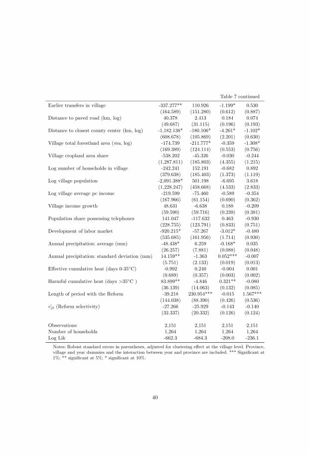
Table 7 continued

Earlier transfers in village -337.277** 110.926 -1.199* 0.530(164.589) (151.280) (0.612) (0.887)

Distance to paved road (km, log) 40.378 2.413 0.184 0.074(49.687) (31.115) (0.196) (0.193)

Distance to closest county center (km, log) -1,182.138* -180.106* -4.261* -1.102*(608.678) (105.869) (2.201) (0.630)

Village total forestland area (mu, log) -174.739 -211.777* -0.359 -1.308*(169.389) (124.114) (0.553) (0.756)

Village cropland area share -538.202 -45.326 -0.030 -0.244(1,287.811) (185.803) (4.355) (1.215)

Log number of households in village -242.241 152.191 -0.682 0.892(379.638) (185.403) (1.373) (1.119)

Log village population -2,091.388* 501.198 -6.695 3.618(1,228.247) (458.668) (4.533) (2.833)

Log village average pc income -219.599 -75.460 -0.589 -0.354(167.966) (61.154) (0.690) (0.362)

Village income growth 48.631 -6.638 0.188 -0.209(59.590) (59.716) (0.239) (0.381)

Population share possessing telephones 141.047 -117.632 0.463 -0.930(228.755) (123.791) (0.833) (0.751)

Development of labor market -920.215* -57.267 -3.012* -0.480(535.685) (161.956) (1.714) (0.930)

Annual precipitation: average (mm) -48.438* 6.259 -0.168* 0.035(26.257) (7.881) (0.088) (0.048)

Annual precipitation: standard deviation (mm) 14.159** -1.363 0.052*** -0.007(5.751) (2.133) (0.019) (0.013)

Effective cumulative heat (days 0-35◦C) -0.992 0.240 -0.004 0.001(0.689) (0.357) (0.003) (0.002)

Harmful cumulative heat (days >35◦C ) 83.899** -4.846 0.321** -0.080(36.139) (14.063) (0.132) (0.085)

Length of period with the Reform -39.218 230.954*** -0.015 1.567***(144.038) (88.390) (0.426) (0.536)

υjt (Reform selectivity) -27.266 -25.929 -0.143 -0.140(32.337) (20.332) (0.126) (0.124)

Observations 2,151 2,151 2,151 2,151Number of households 1,264 1,264 1,264 1,264Log Lik -662.3 -684.3 -208.0 -236.1

Notes: Robust standard errors in parentheses, adjusted for clustering effect at the village level. Province,village and year dummies and the interaction between year and province are included. *** Significant at1%; ** significant at 5%; * significant at 10%.

40

Table

8:D

iffer

ence

sin

wel

fare

indic

ator

sac

ross

no-

rent,

rent-

in,

rent-

out

hou

sehold

s(S

am

ple

mea

n)

No-

rent

Ren

tin

gR

ent-

inR

ent-

out

hou

seh

old

sh

ouse

hol

ds

Diff

ere

nce

hou

seh

old

sD

iffere

nce

hou

seh

old

sD

iffere

nce

Var

iab

le(A

)(B

)(B

-A)

(c)

(C-A

)(D

)(D

-A)

Per

cap

ita

inco

me,

CN

Y60

07.6

8455

.224

47.6

***

8939

.529

31.9

***

7937

.419

29.8

**P

over

ty:

like

lih

ood

un

der

pov

erty

lin

e0.

305

0.15

6-0

.149

***

0.12

9-0

.176

***

0.18

4-0

.117

**O

ff-f

arm

inco

me

per

cap

ita,

CN

Y34

95.5

5773

.722

78.2

***

6253

.327

57.8

***

5261

1765

.5**

*O

ff-f

arm

inco

me

shar

e0.

514

0.56

80.

054

**0.

572

0.05

8*

0.56

40.

05F

ores

try

pro

du

ctio

n,

CN

Y/m

u16

2.4

92.6

-69.

817

1.9

9.5

7.7

-154

.7F

ores

try

pro

du

ctio

nsh

are

0.10

10.

07-0

.031

**0.

098

-0.0

030.

04-0

.061

***

Nu

mb

erof

obse

rvat

ion

s19

7918

093

87

Not

es:

Auth

or’s

own

com

puta

tion.

Colu

mn

(B)

incl

udes

both

the

rent-

inhouse

hol

ds

and

rent-

out

house

hold

s.P

over

tyline

isdefi

ned

as

2000

CN

Yfo

r20

05an

d23

00

CN

Yfo

r201

0,in

acc

ordan

cew

ith

the

1.2

5P

urc

hasi

ng-P

ower

-Pari

ty(P

PP

)U

.S.

dollar

sa

day

in200

5as

the

Worl

dB

ank’s

glob

alp

over

tyst

andar

d.

Sig

nifi

cance

isden

ote

d:

***

p<

0.0

1,

**

p<

0.05

,*

p<

0.1

.

41

Tab

le9:

Wel

fare

effec

tsof

fore

stla

nd

renta

lpar

tici

pat

ion,

PSM

esti

mate

s

Avera

ge

Tre

atm

ent

Eff

ects

(ATT,θ

)W

elfa

rein

dic

ator

Ren

tin

gS

td.

Err

.R

ent-

inS

td.

Err

.R

ent-

ou

tS

td.

Err

.

Inco

me

per

capit

a153

8.36

(657

.10)

**13

18.9

1(9

73.

18)

1849

.48

(986

.91)

*A

bso

lute

pov

erty

-0.0

93(0

.027)

***

-0.0

93

(0.0

40)

**-0

.088

(0.0

51)

*O

ff-f

arm

inco

me

per

cap

ita

144

5.30

(600

.73)

**14

23.2

1(9

74.9

4)16

45.8

7(8

12.3

7)**

Pro

port

ion

ofin

com

efr

omoff

-far

m0.0

35(0

.028)

0.02

7(0

.040

)0.

070

(0.0

40)

*F

ores

try

incr

emen

tal

valu

ep

erm

u1.

47(7

8.25)

76.

86(1

50.7

2)-7

7.85

(16.

57)

***

Pro

port

ion

ofin

com

efr

omfo

rest

ry-0

.020

(0.0

14)

0.02

0(0

.023

)-0

.047

(0.0

22)

**

Not

es:

Tab

lere

por

tsre

sult

sof

aver

age

trea

tmen

teff

ect

inth

etr

eate

d(A

TT

)u

sin

gth

em

atch

ing

algo

rith

m−

the

Ep

anec

hn

ikov

kern

eles

tim

ator

(KB

M)

wit

hb

and

wid

ths

0.06

.S

tan

dard

erro

rs,

inp

aren

thes

es,

are

boot

stra

pp

edw

ith

200

iter

atio

ns.

Sig

nifi

can

ceis

den

ote

d:

***

p<

0.01,

**p<

0.05,

*p<

0.1

.

42

Chapter III

Managerial Incentives for Environmental Protection in

Chinese-Style Federalism*

Yuanyuan Yi�1, Wolfgang Habla�2 and Jintao Xu§3

1Department of Economics, University of Gothenburg, Sweden2Center for European Economic Research (ZEW), Mannheim, Germany

3National School of Development, Peking University, China

Abstract

China’s fast economic growth has come at the expense of environmental quality andthe degradation of natural resources such as forests. In this paper, we identify careerconcerns by managers of state-owned enterprises that manage natural resources, andasymmetric information between managers and their superiors regarding the enterprises’environmental performance, as sources of environmental degradation. A manager of suchan enterprise is the agent of two principals: national and sub-national governments. Aswell as needing to meet ecological targets imposed by the national government, a managerwants to be promoted into the ranks of the sub-national government. We develop threehypotheses based on a theoretical model with two principals and one agent. We thenempirically test these hypotheses for the case of China’s northeastern state-owned forests,combining satellite imagery data on deforestation with economic survey data. Our findingssuggest that managers of state forests that have a larger area and volume, and are thusmore difficult to monitor with respect to ecological targets, log more timber and are morelikely to deforest. The same holds true for managers who share a larger percentage ofprofits with the local government. In turn, we find that sharing more revenue with thelocal government increases the likelihood of getting promoted.

JEL Classification: H77, O13, O44, Q23, Q56

Keywords: managerial incentives; environmental protection; deforestation; state-ownedforests; state-owned enterprises; Chinese-style federalism; two-principal, one-agent model

*We thank Peter Berck, Fredrik Carlsson, Jessica Coria, Gunnar Kohlin, Thomas Sterner and seminarparticipants at the University of Gothenburg for valuable comments and suggestions. We also acknowledgegenerous financial support from the following organizations: the Ford Foundation, FORMAS through theresearch program Human Cooperation to Manage Natural Resources (COMMONS), the National ScienceFoundation of China (NSFC), the International Institute of Applied Systems Analysis (IIASA), the SwedishInternational Development Cooperation Agency (Sida) through the Environmental Economics Unit at theUniversity of Gothenburg, the State Forestry Administration of China, and the World Bank PROFOR project.

�Vasagatan 1, SE-405 30 Gothenburg, Sweden, Email: yuanyuan.yi@economics.gu.se�L7 1, DE-68161 Mannheim, Germany, Email: habla@zew.de§No.5 Yiheyuan Rd., Beijing 100871, China, Email: xujt@pku.edu.cn

1 Introduction

China’s remarkable economic growth has come at a tremendous cost to the environ-

ment, with inefficient, excessive resource use and high levels of pollution (Liu and

Diamond, 2008). The growth and environmental consequences are closely linked to

so-called Chinese-style federalism (Montinola et al., 1995; Xu, 2011). A key feature

of this type of federalism is that it combines fiscal decentralization with performance-

based personnel control. The decentralization of fiscal authority and a fiscal transfer

system allow regional governments (provincial, municipal, county and township level

governments) to have primary control over economic issues, including firms in their ju-

risdiction, while the central government typically owns natural resources (through var-

ious agencies) and sets pollution targets. In this system, short-term economic growth

is rewarded with promotions; by contrast, longer-term environmental issues such as

resource degradation and pollution do not negatively affect the likelihood of being

promoted.

In this paper, we argue that a systematic cause for the neglect of the environment

is the fact that authority over the environment lies with the central government, while

local governments are interested in economic performance and use this as the basis for

promoting managers of state-owned enterprises (SOEs) to local government positions.

During the economic reforms of the 1970s and 1980s, SOE ownership was decentral-

ized from the central to sub-national governments at all levels. SOEs have enormous

importance to local governments: they provide public goods such as schools and hospi-

tals, and they are also a considerable source of revenue. In addition to tax payments,

the managers of SOEs can transfer part of their profits to the local government to

increase their chances to be promoted into the ranks of the local government. At the

same time, SOEs are monitored by central government agencies in terms of their en-

vironmental performance. For instance, the Ministry of Environmental Protection is

in charge of environmental regulation and its enforcement. Responsibility for natural

resources is with the Ministry of Land Resources, the Ministry of Water Resources,

and the State Forestry Administration (SFA). If managers are found to fail to meet

ecological targets, they can be fined. Although the central government authorities have

sub-level bureaus responsible for the enforcement of their respective ecological targets,

these local bureaus are not superior to local governments but work independently.

Overall, the managers’ incentives to protect the environment seem to be outweighed

by their career concerns.

We focus on state-owned forest enterprises (SFEs), which are owned by local govern-

ments but whose forests are owned and monitored by the central government through

the SFA. In this context, the difficulty of monitoring the SFEs’ and their managers’ en-

1

vironmental performance is due in part to the size and volume of the managed forests.

We interpret the complex relationship between an SFE manager, the local government

and the SFA as a two-principal, one-agent framework, in which the SFA has only limited

information on the manager’s environmental performance and the manager cares about

being promoted. Establishing a simple political career concern model with asymmetric

information, we derive three hypotheses. First, a larger degree of asymmetric informa-

tion between the SFA and the SFE, as measured by the forest area and volume, as well

as the area and volume share of the natural forest, increases the amount of logging and

thus leads to more deforestation. The reason that these variables are correlated with

the degree of asymmetric information between the SFA and the SFE is that it is more

difficult, and also more costly, to conduct inspections in larger forest areas and in areas

with more forest in terms of volume. Furthermore, in natural forests, the application

of selective logging makes it harder to detect whether too much cutting has been done.

Second, if a manager transfers a higher percentage of profits to the local government,

the logged volume increases (or decreases) and thus induces more (or less) deforesta-

tion. The intuition for why this effect is ambiguous in sign is that, on the one hand, a

higher transfer rate directly increases a manager’s chances of getting a promotion (an

assumption we confirm with the next hypothesis), which makes cutting more attractive

to the manager. On the other hand, if a manager transfers a higher percentage to the

local government, cutting can be reduced. This will, of course, decrease profits but the

corresponding drop in the chance to get promoted is offset by the higher transfer rate.

Third, the likelihood of an SFE manager getting promoted increases with the share

of profits transferred to the local government as well as with the absolute amount of

transferred profits. The last hypothesis sets out to test the assumptions that we have

made in the theoretical model.

Using data on state-owned forest enterprises (SFEs) in Northeast China over the

period 1980-2009 and combining it with satellite imagery data on vegetation growth

as a measure of deforestation, we test these hypotheses. We find support for the first

hypothesis and show that the logged volume increases with a higher rate of transfers

from the SFE to the local government (second hypothesis). Finally, we find evidence in

support of the first part of the third hypothesis (that the share of profits is a determi-

nant of a manager’s likelihood of getting promoted) but not in support of the second

part (that the absolute amount of transferred profits has a significant and positive

effect on this likelihood). Our results suggest that the information asymmetry with the

SFA is exploited by SFE managers and that higher transfers to local governments go

hand in hand with more deforestation. On the other hand, our findings also suggest

that it is rational for SFE managers to transfer a higher percentage of profits to the

SFE’s owner – the local government – as this does indeed increase their likelihood of

2

getting promoted.

This paper highlights the managerial incentive problem regarding environmental

protection in this Chinese-style fiscal federalism. It aims to explain how, in such

Chinese-style federalism, the SOE managers lack incentives to protect the environ-

ment. The paper draws extensively on the growing literature on managerial incentives

and their impact on performance and societal welfare (e.g., Besley and Coate, 1997,

2003; Acemoglu and Johnson, 2005; Xu, 2011). It also draws on the Chinese fiscal

federalism literature (Qian and Xu, 1993; Lin and Liu, 2000; Maskin et al., 2000; Jin

et al., 2005; Xu, 2011), in that career concerns not only motivate government officials

to compete among each other but also motivate the managers of SOEs to over-harvest

resources or to over-pollute.

The impact of fiscal federalism on economic growth has been studied intensively,

but not sufficiently with respect to the impact on environmental quality and resources.

Zhang et al. (2011) study this relationship for China, using provincial data on carbon

emissions from 1998 to 2008. They find that pollution is positively correlated with

fiscal decentralization. Li and Chan (2016) compare firms of different ownership types

and find that SOEs spend less on pollution abatement, but they do not find different

environmental consequences among SOEs and private or foreign-funded firms. Indeed,

the incentives that SOE managers face are very similar to those in Western corporations

(Murphy and Zimmerman, 1993; Weisbach, 1988). The most closely related paper

is Groves et al. (1995), who show that local governments rely mostly on economic

performance criteria for the selection of SOE managers.

Overall, we add to the large body of literature on managerial incentives and a vari-

ety of principal-agent models (e.g., Tirole, 1986; Thomas and Worrall, 1990; Holmstrom

and Milgrom, 1991, 1994; Fehr and Schmidt, 2004; Ward and Filatotchev, 2010; Dela-

cote et al., 2014) with a dual-principal, one-agent model with asymmetric information

between one principal and the agent, with the agent possessing information that one

of the two principals does not have.

The paper proceeds as follows. Section 2 introduces Chinese-style federalism, the

importance of state-owned enterprises, the system of environmental authority, and the

implications for the state forest sector. Our empirical analysis is grounded on this sec-

tor. In Section 3, we outline a simple theoretical framework that captures the complex

relationship between an SFE manager, his jurisdictional government and the SFA (we

use male gender because all managers in our surveyed SFEs are males). Section 4

formalizes testable hypotheses based on the theoretical predictions and specifies econo-

metric models. Section 5 describes the construction of the data sets and Section 6

presents the econometric results. Section 7 concludes.

3

2 Background

In the following sections, we explain the features of “Chinese-style” federalism, the

importance of state-owned enterprises, the system of the environmental policy-making

and enforcement, and the implications for the state forest sector.

2.1 Chinese-style Federalism

China’s economic reforms, which began in 1978, transformed China from a highly

centralized to a decentralized, market-oriented economy (Montinola et al., 1995; Xu,

2011). In the 1980s, authority over jurisdictional economies was decentralized to local

governments. In this process, sub-national governments – at provincial, prefecture,

county and township levels – were endowed with control rights over land, firms, financial

resources, energy, raw materials, etc. At the same time, all sub-national governments

obtained full fiscal autonomy, which secured tax revenues from “grabbing-hand” upper-

level governments.1 Based on this autonomy, a fiscal transfer system was established

which allows each sub-national government to contract with the next higher level.2

The decentralization in China is different from other countries for two reasons. First,

typical elements of Western federalism are absent: the protection of individual rights;

strong and explicit constitutional foundations; political freedom; and the right of rep-

resentation and democratization (Montinola et al., 1995; Qian and Weingast, 1997; Xu,

2011). Second, despite decentralization in economic terms, there is strong political cen-

tralization by means of personnel control. Through control over promotion decisions,

the central government provides provincial officials with incentives to adhere to cen-

trally proclaimed goals but, also, because promotion decisions are taken mainly based

on economic performance, with incentives to compete as if they were in a tournament.

However, as we will argue below, personnel control applies not only to officials but also

to the managers of state-owned enterprises, who can be promoted into the ranks of

local government officials. It has been argued that this “Chinese-style” federalism is

one of the key determinants of China’s economic success (Qian and Weingast, 1997).

1 This stands in stark contrast to some post-Soviet Eastern European countries, in which the centralauthorities retained discretionary authority over the firms’ profits and bailed out firms with deficits; seeMontinola et al., 1997.

2 The fiscal contract system (1980-1993) and revenue assignment system (since 1994) allow each sub-national government to contract with the next level up. They decide on the remittance amount (or share) oftax and revenue for a certain number of years. The lower level keeps the rest and enjoys sole discretion toallocate the retained revenues (World Bank, 1993).

4

2.2 Importance of State-Owned Enterprises

State-owned enterprises (SOEs) have played an important role in China’s development.

By the end of the 1970s, SOEs accounted for 80 percent of the total national value of

gross industrial output (NBSC, 1999). In 1998, SOEs managed almost 70 percent of

the total national assets, and in the 2010s this number is still at 40 percent (NBSC,

2015).

The SOEs were initially established to fulfill development and construction needs,

such as the production of timber, coal, cement and steel, agricultural machinery, au-

tomobiles and tractors (Xu and Zhuang, 1998). Managers were initially appointed by

government officials of, e.g., industrial bureaus. Prior to the economic reforms in 1978,

the central and regional planning commissions controlled the entire industrial system.

Managers of the SOEs had to follow the orders of the (upper level) political leaders

and to provide services to the government (Groves et al., 1995). Because the areas

in which the SOEs were located were sparsely populated, the SOEs were also obliged

to supply social services, such as housing and schooling, health and child care, and

pension benefits, to employed families.

In the 1980s, enterprise reforms, accompanied by various price and market reforms,

introduced material incentives for SOE management. Simultaneously, SOE ownership

was decentralized from the central to sub-national governments at all levels. Managerial

contracts now commit the managers to specific performance targets, such as profitabil-

ity. After transferring taxes and an agreed-upon share of profits to the local government

(which is prescribed for the duration of the contract), managers enjoy extensive auton-

omy in using the retained profits for firm investments and capacity expansion (Nolan

and Wang, 1999). They may also transfer more than the contractually required amount

to the local government in order to signal their ability. We will, later on, assume that

the managers can freely choose the amount to transfer. The contracts effectively link

managers’ rewards and careers to firm performance. The contracts generally have a

duration of three or five years (Groves et al., 1995).

SOEs have enormous importance to local governments: they provide public goods

such as schools and hospitals, and they are also a considerable source of revenue.

Nevertheless, SOEs often are very pollution-intensive and depleting natural resources,

because they mostly belong to the industrial sectors of iron and steel, machinery con-

struction, mining, automotive, and manufacturing, as well as the processing of wood,

leather and chemical products.

5

2.3 Environmental Protection: Authority and Enforcement

This section reviews the system of environmental authority and enforcement in which

SOEs operate. First of all, the enviornmetnal legal framework is well-developed in

China, including 22 laws and over 44 regulations, 500 standards and more than 600

other legal documents addressing pollution control, natural resource protection and

environmental regulation of consumer products.3 As mentioned in the introduction, the

authority regarding the environment lies with the central government and is delegated

to several distinct ministries. The Ministry of Environmental Protection (MEP) is

in charge of environmental regulation, while the Ministry of Land Resources (MLR),

Ministry of Water Resources (MWR) and State Forestry Administration (SFA) are

in charge of natural resources, which are mostly owned by the central government.

Their sub-level bureaus are designed to work independently and undertake monitoring

and inspection activities to make sure that SOEs and other firms comply with the

environmental regulations.

In the National Pollutant Discharge Reporting and Registration Program, as an

example, each firm reports its input uses of raw materials, its pollutant discharges,

and its environmental management. Using the self-reported data, local environmental

protection bureaus aggregate the data and submit it to the MEP to compile a national

pollution register. In reality, monitoring is very incomplete, and few environmental

agencies have accurate data on firms’ actual emissions and use of natural resources

or raw materials. Likewise, in the Pollutant Discharge Standard, the pollution charges

on 65 kinds of water pollutants and 44 kinds of air pollutants (MEP, 2003) are set

by the central government (i.e., the MEP), but, in practice, the actual payments by

enterprises are limited, not only by difficulties in measurement and monitoring, but

also by the “protective umbrella” of local governments (OECD, 2009).4

2.4 Implications for the State Forest Sector

This section introduces the empirical context of our analysis: the state-owned forest

sector and its SOEs. State forests make up 42 percent of China’s total forest area and

68 percent of the total national forest stock.5 Since the 1950s, 135 SFEs have been

3 See, for example, the website of the Department of Policies, Laws and Regulations, Ministry of Environ-mental Protection, P.R. China: http://zfs.mep.gov.cn/.

4 According to anecdotal evidences, except for a small number of severe violations against criminal law, thesub-bureaus seldom disclose enforcement decisions. It also seems that they often go with the local governments’preferences regarding the trade-off between development and environment (Lo et al., 2006).

5 Chinese forests, which are the fifth largest in area world-wide (208 million hectares), account for merely 22percent of the total land area, which is below the 30.8 percent global average (FAO, 2016). They are unevenlydistributed, with the majority located in the South (about 68 million ha) and 43 million hectares located inthe Northeast, 83 percent of which are natural forests (Xu, 2013), in which no sowing or planting is allowed.

6

established to meet the growing demand for timber in China’s development process.

The SFEs manage the forest-rich regions in the Northeast, Northwest and Southwest,

and their main business is timber extraction.

Before the reforms of the 1980s, the SFEs, like other SOEs, were under the control

of the central government, specifically, the Ministry of Forestry. With the economic

reforms in the 1990s, the ownership of the SFEs was devolved to sub-national govern-

ments, which were given great autonomy in appointing managers and making financial

and production decisions.6 In 1998, the Ministry of Forestry was downgraded to be-

come the SFA, which still maintains authority in forest governance on behalf of the

central government. The SFA thereby represents the central government as the for-

est owner. The monitoring bodies of the SFA are State Forest Resource Monitoring

Offices (SFRMOs) for timber production and forest protection; they also implement

the national forest policies. For example, the Forest Law from the mid-1980s required

reforestation after commercial harvest, and a logging ban associated with the Natural

Forest Protection Program (NFPP) was introduced in 1998 (Xu, 2013).

The managers of SFEs have commitments to the SFA in terms of sustainable use of

forests and commitments to their jurisdictional governments based on contracts that

specify revenue-sharing and social obligations. They are, of course, free to over-fulfill

these targets to please the local government. The goals written in the contracts –

profitability, job creation, payment of pension benefits and provision of other social

benefits, and profit-sharing – are relatively easy to monitor. By contrast, the ecological

targets on forest protection are more difficult to measure and do not affect human

welfare immediately; the impact of over-harvesting on forest degradation is cumulative

and takes a longer time. SFE managers are thus reasonable in prioritizing economic

performance over natural resource protection, leading to over-harvesting and forest

degradation (Xu et al., 2004).

3 Theoretical Framework

As described in the previous section, the management and monitoring of Chinese state-

owned forests involves a complex interplay of three actors: the SFA, the local govern-

ments, and the SFEs, represented by their managers. The managers have career con-

cerns and care about being promoted, while they also have to make sure that ecological

targets imposed by the SFA are not violated (at least not by too much) - else, they will

be fined. We interpret this complex relationship as a two-principal, one-agent relation-

ship, with the principals being the SFA and the local government, and the agent being

6 The SFEs were mainly devolved to provincial governments, and also to prefecture- and county-levelgovernments.

7

the manager of an SFE. We will argue that one of the principals (the SFA) can only

imperfectly observe the agent’s effort with respect to meeting the ecological target,

while the other one (the local government) decides upon his promotion.

In what follows, we characterize the relationship between a representative SFE

(through its manager), the SFA and a representative local government. In particular,

we describe the SFA’s and local government’s objectives and interests, and then turn

to the description of the manager’s payoffs and maximization problem. We take the

agent’s contract as given and will not characterize the optimal contract here. This

would be beyond the scope of this paper.

3.1 SFA and Local Governments

As the owner of all state forests, the central government through the SFA wants to

ensure that the forests are able to fulfill their ecological functions. Therefore, it sets an

upper limit to the total allowable harvested volume, x. Let X be each SFE’s overall

forest volume. Then X − x is the protected volume, which may not be logged. We

assume that SFEs always log a volume x which is at least as large as x, i.e., the “cap”

on legally logged forest is binding. To enforce this cap, the SFA or its sub-bureaus

make monitoring visits in each SFE. However, due to the large area of the forests and

the huge administrative cost that a complete inspection would require, the monitoring

technology is imperfect. We assume that the SFA only receives the signal xs about the

total logged volume (where the superscript “s” stands for signal):

xs = µ(x) + ε , ε ∼ N (0, σ2) . (1)

µ is assumed to be twice continuously differentiable and strictly concave, and ε is

normally distributed with mean zero and variance σ2.

The massive floods of the Yangtze River, the Nen River, the Songhua River and

the Pearl River in the summer of 1998 convinced the SFA to implement the Natural

Forest Protection Program (NFPP). The main policy instrument of this program is a

logging ban on most commercial logging in order to increase the capacity of the forests

to absorb rainwater. However, logging is still allowed in plantation forests and for forest

tending. To compensate the SFEs for the logging ban and the associated reduced profit,

the SFA supports them with an annual transfer of T .

The local government gets twofold benefits from the SFE’s gross profit πG. First, it

receives corporate income tax payments, which we model as a profit tax. These amount

to τπG, where 0 < τ < 1 is the tax rate. Second, it receives an additional share of

the profit as a transfer from the SFE, amounting to γπG, where 0 ≤ γ ≤ 1. Whereas

8

the tax rate is exogenously given for the SFE, the transferred amount can be chosen

by the SFE through its manager.7

3.2 SFEs and Managers

Each SFE cuts a volume x of timber and sells at the exogenously given price P . Cutting

costs are C(x), with C′(x), C′′(x) > 0. The profits, net of taxes and net of the transfer

T received from the SFA for offsetting the financial implications of the logging ban after

1998, are given by:

π = (1− τ )πG + T , (2)

where gross profit is πG = Px − C(x). From these profits, transfers to the local

government can be made, and social welfare benefits G > 0 to residents in the local

communities of an SFE must be provided. The latter consist of unemployment benefits,

health insurance, etc., and are exogenously given in our model. After transfers, taxes

and the provision of social welfare benefits, the remaining profits have to satisfy:

(1− γ)π −G ≥ 0 . (3)

In other words, the transfer to the local government cannot be set so high that this

inequality is violated, i.e., γ is always strictly smaller than unity.

The manager earns a fixed wage w. Beyond that, he may be promoted into the

ranks of local government officials based on economic achievements, and may also be

fined for failing to meet ecological targets. If promoted, the agent receives economic

benefits from the time of being promoted until retirement (and possibly beyond). The

net present value of a promotion (compared to the earnings profile of continuing to work

as a manager) equals b. We model the likelihood of being promoted as a continuous

variable which depends on the amount of transfers that are voluntarily handed over to

the local government. Either a higher share γ or a higher profit π (or both) will thus

increase the agent’s likelihood of receiving a promotion. The likelihood reads:8

Pr(b) = 1− e−γπ ∈ [0, 1) . (4)

If fined, the agent will suffer an income loss equal to f . The likelihood of being

caught cheating upon the ecological target positively depends on the deviation of the

7 Before the manager signs a contract for a certain number of years, individual targets for the transfersare negotiated. We conjecture that managers have an incentive to over-fulfill their targets and strategicallynegotiate lower targets in order to be able to demonstrate their good performance.

8 This specification of the probability function is chosen to analytically separate the variance componentof the signal in the agent’s payoff function.

9

signal from the ecological target, xs − x, and is equal to

Pr(f) = 1− e−(xs−x) ∈ [0, 1) . (5)

The manager chooses the share of π transferred to the local government, i.e., τ , and

the logged volume, x (where we assume that x ≥ x always holds), so as to maximize

his payoff

EU = E[w + b(1− e−γπ)− f(1− ex−xs)] . (6)

Plugging in (1) and considering that E[ekε

]= e

k2σ2

2 for any constant k when ε ∼N (0, σ2), expected utility can be written as:

EU = w + b(1− e−γπ)− f(1− ex−µ(x)−σ2

2 ) . (7)

The first-order conditions with respect to γ and x read as follows:

bπe−γπ > 0 , (8)

bγ(1− τ )[P − C′(x)]e−γπ − fµ′(x)ex−µ(x)−σ2

2 = 0 , (9)

which implies P − C′(x) > 0 at the optimum.

The first condition is never fulfilled with equality. Instead, a corner solution is

chosen, i.e., γ is chosen as high as possible so that equation (3) is still satisfied. The

agent thus does not gain from transferring less to the local government than π − G,

which increases his chances of getting a promotion. The second condition trades off the

marginal benefits of cutting more timber (first term in equation (9)) with the marginal

costs of doing so (second term). The marginal benefits are the increased likelihood of

receiving a promotion because profits have increased. At the same time, the agent runs

a higher risk of being fined because the likelihood of being detected cheating increases

with cutting (marginal costs).

In general, it cannot be shown that the maximization problem is concave for all pa-

rameter constellations. We assume that it is concave for empirically relevant parameter

constellations.

Applying the implicit function theorem to equation (9), we derive the following

10

comparative statics results:

∂x

∂x=fµ′(x)ex−µ(x)−σ2

2

Γ> 0 , (10)

∂x

∂T=bγ2(1− τ )[P − C′(x)]e−γπ

Γ< 0 , (11)

∂x

∂b=−γ(1− τ )[P − C′(x)]e−γπ

Γ> 0 , (12)

∂x

∂f=µ′(x)ex−µ(x)−σ2

2

Γ< 0 , (13)

∂x

∂σx=−fσµ′(x)ex−µ(x)−σ2

2

Γ> 0 , (14)

∂x

∂γ= −b(1− τ )[P − C′(x)]e−γπ [1− γπ]

ΓR 0 , (15)

where Γ ≡ ∂2EU/∂x2 < 0 by the assumed concavity of the maximization problem.

The interpretation of the comparative statics goes as follows: A marginal increase

in the ecological target x increases the amount of logged timber due to the less binding

constraint. If the transfer T from the SFA to the SFE marginally increases, the manager

cuts less timber because he can maintain the same or a similar level of profits with

less logging. Therefore, ceteris paribus, less logging does not decrease the manager’s

likelihood of getting a promotion. Marginally increasing b or marginally decreasing f

has qualitatively the same effect: more timber will be cut.

If the signal with respect to x becomes more blurred, i.e., σ marginally increases,

the agent can cut more without having to fear that he will be caught with a higher

probability. Interestingly, if the transfer rate γ goes up, the reaction of x is ambiguous

in sign. On the one hand, a higher γ directly increases the marginal benefits of cutting

more forest because a higher transfer of funds to the local government, given a certain

profit, increases the likelihood of being promoted. For this reason, the agent would like

to cut more. On the other hand, profits can be decreased by cutting less trees while

still having the same probability of being promoted due to a higher γ. Therefore, the

agent would like to cut less.

4 Empirical Strategy

In this section, we state our hypotheses based on the predictions from the theoretical

model and lay out our empirical strategy to test them. We will test the hypotheses

with a focus on the northeastern state-owned forests in China.

11

4.1 Hypotheses

We base our empirical analysis on the following hypotheses, with two of the predictions

coming from the comparative statics results above.

Hypothesis 1: Logging and asymmetric information .

A larger degree of asymmetric information between the SFA and the SFE, as measured by the

forest area and volume as well as the area and volume share of the natural forest, increases

the amount of logging and thus leads to more deforestation.

This hypothesis is in line with equation (14). The idea is that the larger the SFE’s

forest area and volume, the harder and more costly it is for the SFA and its sub-level

bureaus to monitor that SFE’s logging activities. This claim is also backed by the

literature on public harvesting and concession contracts, as well as anecdotal evidence

on Chinese SFEs (Poore, 1993; Gray, 2002; Palmer, 2000; Johnson, 2002; Xu et al.,

2004). SFEs with larger areas of forests, especially natural forests, can more easily hide

their operations from SFA inspectors, including logging beyond the specified quotas.

Furthermore, in natural forests, in which no sowing or planting is allowed, it is less

obvious how much cutting was actually done. The reason for this is that natural forests

are usually less regular in their structure than plantation forests, and inspection of

selective logging in mostly natural forests is useless, because largely intact canopy will

not look very different from selectively logged canopy when viewed by the human eye

from some distance.

Hypothesis 2.1: Logging and voluntary transfers: positive correlation .

If a higher percentage of profit is transferred to the local government, the manager of an SFE

increases the logged volume x and thus induces more deforestation.

Hypothesis 2.2: Logging and voluntary transfers: negative correlation .

If a higher percentage of profit is transferred to the local government, the manager of an SFE

decreases the logged volume x and thus induces less deforestation.

The above two hypotheses are obviously related. While the first one corresponds to

equation (15) being positive, the second one corresponds to the same equation being

negative. Because the theory does not give a clear prediction regarding the sign of this

effect, we split the hypothesis into two sub-hypotheses.

Hypothesis 3.1: Likelihood of being promoted and share of profits transferred

to local government .

The likelihood of an SFE manager getting promoted increases with the share of profits trans-

ferred to the local government, i.e., ∂Pr(b)∂γ

> 0.

Hypothesis 3.2: Likelihood of being promoted and absolute amount of profits

transferred to local government .

The likelihood of an SFE manager getting promoted increases with the absolute amount of

12

transferred profits, i.e., ∂Pr(b)∂π

> 0.

The last two hypotheses come from our assumption about the probability function

of getting promoted. We want to test whether the share and the absolute amount

of transferred profits matter for the likelihood of promotion. In contrast to the other

hypotheses, this will shed light on the other side of the coin: how managers’ economic

and environmental performance is actually evaluated by the SFEs’ owners, the local

governments.

4.2 The Role of Asymmetric Information in Deforestation

The first hypothesis is tested by estimating a simple reduced form relationship between

information asymmetry and deforestation:

H = f(θ,V) + u, (16)

where H is deforestation or the rate of change in forest vegetation from one year to

the next, respectively. θ represents the difficulty of measuring the manager’s effort and

thus the degree of asymmetric information between the SFA and the SFE (σ in the

theory part). As discussed previously, as proxy variables for this asymmetry, we take

the total forest area as well as the total forest stock volume, and area and volume

shares of natural forest.

V denotes control variables that affect H, and u is a disturbance term. The vector

V contains, first, the characteristics of natural forests, including their area and volume

shares, because they constitute an important part of the total forests managed by an

SFE. Given their more diversified ecosystem services, natural forests face more restric-

tions on cutting; in fact, higher demands are placed on the protection of natural forests

because of their ecological importance. Second, the vector contains the afforested area,

including areas newly afforested and reforested in the current year and their shares of

the total forest land area. We include the latter variable because future vegetation will

differ by the various levels of afforestation and post-harvest reforestation. Third, we

include SFE characteristics such as population density and employee structure, that is,

the ratio of employees to supported laid-off and retired people. Fourth, we control for

manager characteristics because a manager takes actions that affect the enterprise’s

productivity and thus the forest stock. This includes manager age, education, and

managerial experience. In addition, regional demographics and economic factors are

included in V , such as population and GDP, ecological pressure from agricultural and

urban populations, influences from the non-farming sector, and the timber price. We

also control for whether the previous manager was promoted, and whether he defor-

13

ested, as well as the interaction term of these two.

We employ a linear panel fixed effects model to estimate equation (16), controlling

for year trends, fixed and year effects related to upper bureaus. The panel fixed effects

model allows us to capture the influence of time-invariant factors. One such important

factor is historical importance, measured by the contributions to social and economic

development, which might give some SFEs greater bargaining power, so that its logging

activities have low probabilities of punishment. The year dummy variables control for

weather changes and, in particular, for the influence of, for example, a drought year

on the vegetation values. The upper bureau fixed and year effects enable us to capture

time-varying factors, including changes in technology and equipment efficiency at the

upper level bureaus. The upper level bureaus of the SFEs belonged to the central

government prior to the economic reform and served as a government body which

allocated tasks and provided equipment to the SFEs. With the economic reform, many

SFEs have been delegated to the local government while their upper level bureaus

still serve as their parent enterprises. These upper level bureaus are not the same

sub-bureaus that are responsible for monitoring and inspection of the forests, as we

introduced in Section 2.

4.3 Political Career Interest and Environmental Protection Effort

We test the remaining two sub-hypotheses by exploring the determinants of a manager’s

promotion into the ranks of local or upper level governments. We focus on whether or

not sub-national governments in charge of selecting firm managers were driven by

both environmental protection effort and the voluntary transfer of profits. We estimate the

relationship between various characteristics of the incumbent manager of an SFE and

his fate when his tenure as the manager was at an end (i.e., at the end of his current

managerial contract):

Pr[Y = 1|z, V ] = Φ(α+ β′z + δ′V). (17)

The dependent variable is the likelihood of an SFE manager being promoted to the

local (or upper level) government. Φ is a standard normal cumulative distribution func-

tion. z denotes the decision variables of each SFE manager – the percentage of profits

transferred, natural logs of the transferred amount, yearly average and aggregated

transfers, and environmental protection efforts, i.e., the total afforestation area and

the area in proportion to the total forest land area. V is a vector of manager personal

and SFE characteristics, as discussed for equation (16). α, β and δ are parameters to

be estimated.

14

In the V -vector, a manager’s age, education, and expertise in management seem to

be important evaluation criteria, in addition to political loyalty (Li and Zhou, 2005).

Expertise is correlated with the manager’s economic performance and political loyalty

is reflected by the share of profits transferred to the local government. We also control

for the manager’s number of years to retirement and for his education in the estimation

of equation (17).

Table 1 provides the definitions of all variables used in the estimation. The variables

in the vector V are characteristics that may also influence H and Pr[Y = 1] when we

estimate the equations (16) and (17), respectively. Data sources, summary statistics,

and estimation methods are described in the next section.

< Table 1 here >

5 Data

The data used for analysis comes from the economic survey data measuring various

characteristics of 24 randomly surveyed SFEs and their respective managers, which are

combined with satellite data measuring vegetation as a measure of deforestation.

5.1 Satellite Data Set

Given the difficulty of obtaining truthful reporting of deforestation by SFEs (Alford and

Shen, 1998; Brandt and Zhu, 2000), we develop an independent measure of deforestation

by using satellite imagery from two NASA satellite sensors – the AVHRR sensor carried

on the Polar Orbiting Environmental Satellites (POES) and the MODIS sensor on

board the Terra and Aqua satellites (Tucker et al., 2010; NASA LP DAAC, 2015). In

particular, we combine the Normalized Differentiated Vegetation Index (NDVI) (1981-

2002) and the Enhanced Vegetation Index (EVI) (2003-2009) to construct an annual

measure of forest quality and quantity for each year. Using this measure, we are able

to encompass both legal and illegal logging undertaken in the SFEs.9

The NDVI is the ratio of the difference in reflectance of sunlight, ρ, between the

near-infrared (NIR) and red bands (visible radiation), divided by the sum of near-

infrared and red band radiation (Tucker 1980; Sellers 1985; Sellers et al., 1994):

NDV I =ρNIR − ρREDρNIR + ρRED

. (18)

9 Illegal logging includes both over-harvesting by the SFE itself and unlawful logging of forests, by therural population, for example. An SFE is responsible for both within its management area.

15

Calculations of NDVI for a given pixel result in a number ranging from −1 to +1.

No green leaves results in a value close to zero, while a value close to +1 indicates the

highest possible density of green leaves. In other words, unhealthy or sparse vegetation

implies low values of NDVI, and healthy or abundant vegetation implies high values of

NDVI.

We obtain a generalized annual measure of the state of the forest in the area of an

SFE by taking the mean value of the vegetation index over all pixels of size 250 by

250 meters from 1981 to 2009. Deforestation is then measured as a negative annual

rate of change in vegetation values. The latter measure of deforestation differs from

Burgess et al. (2012) in that we assess the forest change observed at an SFE average,

while they treat a pixel inside a village as being deforested if 90% of the area is cleared.

Thus, their method captures only large-scale changes such as observed clear-cutting.

Selective logging, by contrast, changes the forest canopy moderately and is not captured

in their estimates. Given that selective logging is a reasonable logging method and is

usually adopted by forest managers over medium and large scales of forests, the average

measure of forest change in our study will provide an objective estimate of an SFE

manager’s environmental performance.

Due to data availability, we combine the NDVI data with EVI data after 2002.

EVI is an optimized vegetation index. It accounts for and reduces background and

atmospheric noise. It is also more responsive to canopy structural variations, canopy

type, plant physiognomy, and canopy architecture (Huete et al., 2002). In contrast to

the NDVI, the EVI is computed according to the following equation:

EV I = 2.5× ρNIR − ρREDρNIR + 6ρRED − 7.5ρBLUE + L

. (19)

where ρΛ, Λ ∈ (NIR,RED,BLUE), is atmospherically-corrected or partially atmosphere-

corrected surface reflectance, and L is the canopy background adjustment, which ad-

dresses non-linear, differential NIR and red radiant transfers through the canopy.

The final outputs of forest change data are values of vegetation index rescaled to

be bounded between -1 and 1 for each pixel and averaged over all pixels for each

SFE. We match the pixels with the maps of areas of the 24 SFEs that were surveyed;

the description is in the next section. As for the years available in the survey data,

vegetation change refers to the year pairs 1980-81, 1985-86, 1990-91, 1995-96, 2000-01,

2004-05 and 2008-09. Thus, the switch from NDVI to EVI in 2003 does not cause any

data inconsistencies in our forest change measures because we do not compare NDVI

data with EVI data – only NDVI with NDVI data and EVI with EVI data. Figure

1 illustrates the study area – maps of the 24 SFEs. Figure 2 codes the pixels with

vegetation indices in Northeast China in the study period.

16

< Figures 1 and 2 here >

5.2 Economic Survey Data Set for State Forest Enterprises

Our data on 24 SFEs in Northeast China comes from a survey conducted by the Envi-

ronmental Economics Program in China (EEPC) at Peking University. The northeast-

ern state forests are located in three provinces (Heilongjiang, Inner Mongolia and Jilin)

and are managed by 84 SFEs in total. These SFEs played an important role in the

old industrial base in this area and contributed to China’s growth by providing more

than half of the national timber production in the past five decades. However, this

enormous contribution to social and economic development has come at the expense

of environmental degradation. By the beginning of the 2000s, 60 out of the 84 SFEs

had almost depleted their mature forests (Xu, 2013).

To study the institutional system of state forest management and provide a roadmap

for feasible reform, EEPC researchers conducted surveys in 24 randomly selected SFEs.

The first wave survey was conducted from June to October 2005, and in summer 2009

the SFEs were revisited, and the earlier process of data collection was repeated. For each

SFE, data was collected for the period 1980-2008 on logging and reforestation activities,

employment structure, income and expenditure, and investments in other assets. The

data on forest resources and the SFEs’ social services, tax payments and transfers

to local jurisdictional governments, as well as on the timber price, was provided by

provincial forestry authorities (the sub-level bureaus of the SFA).

In addition to the average values of our constructed vegetation indices – the annual

rate of change between two consecutive years and the deforestation dummy – Table 2

reports the mean values of socio-economic variables for the SFEs and the counties in

which the SFEs are located, as well as the SFE managers’ characteristics, during the

period 1980-2008. The availability of data on the transferred amount of profits allows

us to have nine observations in 1980, 13 in 1985, 15 in 1990, and around 20 for the

remaining years. Overall, the observed SFEs reported a stable total land area but forest

stock volumes fluctuated by more than 10 percent in the 1990s and the early 2000s. An

annual deforestation rate of three to five percent was observed in 1990, 2000 and 2004

(which means that the rates of change in vegetation index values were negative in the

following years). In each year, at least one to four SFEs over-harvested their forests,

as shown by negative rates of change in vegetation value, and this figure rises to ten in

1990 and even more in 2000 and 2004.

In our sample, natural forests account for more than half of the forests in each

SFE. They decrease in volume on average over time, while plantation forests increase

in both area and volume. Following Xu et al. (2004), we use areas of forest land and of

17

natural forest, and area and volume shares of natural forest, as proxies for the degree

of asymmetric information between the SFA and the SFEs. Natural forests also differ

from plantation forests in their growth rates. Plantation forests are used for timber

production, and therefore fast-growing tree species are planted. Depending on climatic

conditions, natural forests grow at an annual rate of about two to three percent in the

SFE-managed areas. Natural and plantation forests also provide different ecological

functions. Estimating equations (16) and (17), we control for the growth of natural

forests in addition to their area and volume, also as a percentage of total forest.

As discussed earlier, the transfer of profits to jurisdictional local governments is

unique to China. The percentage of profits transferred, the absolute amount, and the

amount of timber production may signal the SFE manager’s ability. They are also sup-

posed to be among the evaluation criteria for his economic performance. We do not

focus on tax payments due to the fact that these are exogenously set. The transferred

amount of profits is subject to the manager’s decision, and we are interested in investi-

gating how the transfer decision determines a manager’s political career at the end of

his tenure as manager. The transferred amount ranges from 10 to 800 million CNY; as

a share of the SFEs’ disposable profit, the transfer ranges from less than ten percent

to as high as 90 percent. Timber production was very high in the beginning and de-

creased over time, with an average of 357,463 cubic meters in 1980, and dropped by 40

percent in 1995 to 215,827 cubic meters; after the implementation of the NFPP, there

was soon another 38 percent decrease, to 133,502 cubic meters in 2000, suggesting that

the logging ban was effective. Nevertheless, during the period with the logging ban,

the average timber production of the SFEs was still over 110,000 cubic meters in the

2000s. Because timber production is self-reported data and may be subject to mea-

surement error and reporting fraud, our econometric estimations do not include this

variable. Similar reasoning applies to the total harvested volume. Apart from transfers,

the yearly afforestation area, both in absolute amount and as a percentage of the total

land area, may serve as a signal for an SFE manager’s effort in forest conservation.

These two variables are observed to have an average decrease over time.

In addition to the above variables, a manager’s personal characteristics are impor-

tant. The average age of the managers is less than 50 years, varying from 34 to 60

years. The retirement age in China is 65 for males, and we conjecture that the proba-

bility of being promoted and hence the logging and transfer decisions may differ when

approaching this age. Therefore, we control for the number of years for an incumbent

manager until retirement age. We observe that the number of managers with higher

education significantly increased over the sample period, and all the observed managers

have a college education in the 2000s. Managerial experience, i.e., the number of years

as the manager of an SFE, is about 3.5 years on average, varying from one to 13 years.

18

For each manager, the promotion status is valued 1 if he was promoted to an upper

political position in a local or higher government after the tenure as manager was at an

end. For promoted managers observed in two or more periods, we recode their earlier

promotion status into 0 and leave only their last period of promotion equal to 1. In

each observed year except 2008, one to two thirds of the managers of the northeastern

state-owned forests were promoted at a later time.

Other variables that are important and may drive deforestation come from social

and economic pressures to harvest forests (Hyde et al., 1996; Amacher et al., 1998;

Rozelle et al., 1998; Rozelle and Huang, 2000; Foster and Rosenzweig, 2003). The

sources of these pressures include SFE population and social welfare payments (be-

cause laid-off and retired employees are required to be supported by the SFE)10, the

regional endowment with land and the share of agricultural population, urban pop-

ulation, population growth, income growth, and changes in the timber price. Among

these factors, SFE and local county population experienced first an overall increasing

and then a decreasing trend (since the late 1990s), while population density at SFEs

has kept rising. The social welfare payments by SFEs become less over time, as indi-

cated by the increasing ratio of employees to supported laid-off and retired persons.

The timber price during the period experienced an increasingly rising trend, due to

the booming timber markets and forest resource scarcity. At the regional level, pop-

ulation and GDP in counties increased, and the urban populations exhibited only a

slight decline. Agricultural population density was high in the 1990s and the local non-

farming sector experienced small fluctuations. The growth of agricultural and urban

populations may drive deforestation due to an increased need for agricultural land and

higher demand for forest products. The development of the non-farming sector, e.g.,

the manufacturing industries, may influence forest change directly through the growth

in processing related to forest and non-forest products, and indirectly by contributing

to regional economic growth. Therefore, we control for the variations in these factors

in the econometric estimations.

In total, we have a sample size of 24 (SFEs) for the seven year pairs for which we have

vegetation data, which yields 168. From this sample, we have to drop 54 observations

because of missing data on the transfers to the local government. We proceed with a

sample of 114 SFEs.

< Table 2 here >10 The economic reform in China in the 1990s brought about a number of laid-off employees in state-owned

enterprises, some of whom receive a monthly allowance for subsistence, paid by the SOEs. The retired workersare also supported by the SOEs.

19

6 Econometric Results

In this section, we present the econometric results of the examination of the previously

stated hypotheses regarding the impact of the information asymmetry on deforestation

and the role of personal interests in pursuing a future political career.

6.1 Deforestation and Information Asymmetry

Table 3 presents the estimation results of fixed-effects linear models on equation (16).

The dependent variable in Columns 1 and 2 is the rate of change of the vegetation index;

in Column 3, the dependent variable is the deforestation dummy. Column 1 focuses on

how the rate of change is affected by various measures of asymmetric information with

respect to monitoring by the central government, which is associated with different sizes

of the forests managed by an SFE. The models control for an SFE’s (natural) resource

structure, for managerial and regional characteristics, for last year’s vegetation value

and for the previous manager’s performance, as well as for year trends and upper

bureau fixed and year effects. The parameter estimates do not have statistical power

and are not reported.11

In support of Hypothesis 1, we find that the coefficients of the total forest land

area, the forest volume and the area share of natural forests are statistically significant

in Columns 1 and 2, and the total forest land area is also significant in Column 3. For

Columns 1 and 2, an increase in the information asymmetry as measured by our three

proxies leads to a smaller rate of change in the vegetation. This smaller rate implies

that the vegetation grows less on average, and the rate might even become negative

or more negative, indicating more logging activities and, as a result, deforestation.

Taking the marginal effect (-0.301) of the total forest land area on the rate of vegetation

change in Column 2 as an example, an SFE with a one percent larger area of forest land

compared to the average (256,200 ha) will have a 30.1 percent decrease from the average

rate of vegetation change in the following year (0.0183). This effect suggests that an

average-sized SFE being given a 10 percent larger area will experience a decrease of 5.5

percentage points in the average rate of change in vegetation, or an annual deforestation

rate of 3.7 percent in this area next year. This is a sizable effect in destroying forests.

Similar correlations hold for the other two asymmetric information proxies. If we only

look at SFEs that experience deforestation (Column 3), then deforestation is more

likely to happen in an SFE with larger forest land area, ceteris paribus. This lends

strong support to our Hypothesis 1, and is in line with findings by Xu et al. (2004).

In Columns 2 and 3, we add the variable of the percentage of profits transferred

11 The complete results are available upon request.

20

by the SFEs to the jurisdictional sub-national governments. The parameter estimate

of the variable does not have statistical power in explaining the variation in the rate

of change of the vegetation index in Column 2. However, it is statistically significant

at the 5 percent level when we look at the binary variable deforestation as the de-

pendent variable in Column 3. Column 3 is estimated by a linear probability model

with SFE fixed effects. The parameter estimate (0.963) implies that, when evaluated

at the avearge, an SFE manager whose transfer rate to the local government increases

by one standard deviation (0.288) leads to a stronger likelihood of having an overall

negative rate of change of the vegetation in his area by 0.277. This effect is equivalent

as 58 percent of the mean deforesatation rate (0.474). This finding provides support

for Hypothesis 2.1 but not for Hypothesis 2.2. While a higher transfer rate does, on

average, increase logging, it makes it more likely that forests are being degraded.

< Table 3 here >

6.2 Political Career Interest and Environmental Protection

The above analysis assumes that the jurisdictional sub-national governments are hap-

pier with more transfers and thus are more likely to promote the responsible manager

into the ranks of a government official. We now examine the determinants of an SFE

manager’s probability of getting a promotion to sub-national governments as a result

of these transfers, which we interpret as a better political relationship. Table 4 reports

the maximum likelihood estimation results of a probit model on equation (17) on the

promotion status of the incumbent SFE managers in the observed years.12 To allow

for heterogeneity across observations and control for SFE fixed effects across years, we

estimate the probit model with the SFE dummy variables and with the robust standard

errors option – adjusted at SFE level.

While no detailed evidence is available on how the local governments evaluate

and select SFE managers, we conjecture that a manager’s evaluation may depend

on multiple-year averages of transfers or cumulative performance rather than simply

on annual performance. In Table 4, the first three columns report the results of regres-

sions with the percentage of SFE profits transferred to local government, controlling in

Columns 1-3 for different variables that signal the manager’s performance and ability:

the natural log of the total transferred amount in the current observational year, the

multiple-year average transfer and the aggregated amount of the transfer. By doing

this, the effect of past performance is incorporated into the analysis of the determi-

12 A manager who had a tenure for five years or longer appears at least twice in our observations. This iswhy we control for the number of years in office as a proxy for managerial experience.

21

nants of personnel promotion. Column 4 computes the marginal effects of a selection

of coefficients in Column 1 at sample means.

Consistent with Hypothesis 3.1, the percentage of transferred profits has a positive

impact on the probability of being promoted. The sign of the coefficient is positive and

significant at the 5 percent level in all columns. Moreover, the marginal effect of the

percentage of profits shared with the local government on a manager’s promotion prob-

ability is reasonably large. When evaluated at the mean of the independent variables,

it is 0.941, suggesting that, when an average-level manager increases the transfer rate

by one standard deviation (0.29) from the mean (0.288), his probability of promotion

will increase by 0.273 or 66 percent of the average promotion probability (0.412).

We do not find evidence supporting a positive relationship between the amount of

transferred profits and the probability of promotion and thus we reject Hypothesis 3.2.

For this, we consider current year and past average and cumulative transfers of the same

incumbent manager. In Columns 1 and 2, the coefficients of the transferred amount

are insignificant and have ambiguous signs; in Column 3, the cumulative amount has

a negative impact on the promotion probability at the 10 percent level of statistical

significance. One plausible interpretation for this result is that a bigger cumulative

amount, aggregated from past performance, would signify larger quantities of logging

and potentially cause trouble for the manager from environmental authorities. Overall,

this suggests that it is not the absolute amount of transfer that matters for the promo-

tion decision but rather the transfer rate. No matter the size of the cake, a manager

who hands over a larger share of the cake is more likely to get promoted. It seems that

the transfer rate is a better signal to the local government of the manager’s ability

than the absolute amount of the transfer.

Interestingly, an SFE manager’s efforts in environmental protection – measured

by the yearly afforestation area (log) and its share of the total forest land area – do

not have a positive effect on promotion as one might expect. First, a larger afforested

area has no significant effect in increasing an SFE manager’s promotion probability,

given the statistically insignificant coefficient in all columns. Second, however, in the

cases where the afforested area accounts for more than three percent of the total SFE

forest land area (sample mean), a standard deviation (seven percent) increase in the

total afforested and reforested area as a share of the total forest land area decreases

the probability of promotion for the manager by 0.296 or 71 percent of the average

promotion probability. It seems that afforestation and reforestation are not appreciated

by the manager’s superiors – on the contrary, more afforestation/reforestation may be

a bad signal to the local government because it shows that there must have been a lot

of deforestation previously.

Additionally, the point estimates are not influenced by adding manager character-

22

istics and the importance of the SFE, which is why we only report the table with all

controls. For the importance of an SFE, we consider the management scale in terms

of land area and population and the volume share of its natural forests. With these

variables controlled for, the regressions take into account various scales, where some

managers just need to do a little and can be easily promoted because the scale de-

termines the importance of the position of the SFE in the local economy and society.

Total land area and natural forest volume have the positive and significant impact on

promotion that we expected. Other economic and environmental efforts of the manager

equal, a manager with a one percent larger area than the average is more likely to be

promoted, by 3.3 percentage points (8 percent of the mean promotion probability of

0.412). Similarly, if the natural forest volume as a share of the total forest volume is

one percentage point higher than the average, the manager’s promotion is increased by

6 percentage points (15 percent of the mean probability of 0.412).

Among the manager characteristics of age, education and managerial experience,

we find that the younger a manager is, the more likely he is to get a promotion. This

effect is significant at the one percent level. The marginal effect of this is, however,

small in absolute value. Given that the mean age of the managers is 48, the mean num-

ber of years to the retirement age of 65 is 17 years. One year less from this mean (17)

increases his promotion likelihood by 0.072, or 17 percent of the average probability of

promotion. This result is consistent with other studies on political promotion of person-

nel from the local level of governments in China, e.g., Li and Zhou (2005). Equally or

more important than the incumbent manager’s own characteristics is the performance

of his predecessor, which has a significant impact on his promotion probability. In

particular, the promotion of one’s predecessor significantly decreases one’s promotion

probability, at the one percent level in all three columns of Table 4. The marginal effect

of the predecessor’s promotion on the incumbent manager’s promotion is -0.857. This

number means that, if the predecessor was promoted, this may raise the standard for

the incumbent manager to be promoted. It might become harder for the subsequent

manager to outperform his predecessor if the latter got promoted. By contrast, the

predecessor’s environmental performance in terms of deforestation, and the condition

that the predecessor both deforested and was promoted, do not always influence the

incumbent manager’s promotion probability in a statistically significant way, except in

Column 1. One plausible interpretation for this result is that earlier deforestation may

impede the incumbent’s performance due to the lack of resources available for logging;

however, a manager’s efficiency, especially in difficult situations like this, could also be

valued highly and considered in sub-national governments’ evaluation criteria.

In summary, our empirical findings lend support to the notion that: 1) an SFE

manager (the agent) utilizes the information asymmetry with the central government

23

(principal 1) to over-use natural resources; and 2), he satisfies the jurisdictional sub-

national government (principal 2) with a higher percentage of profits, which indeed

benefits his personal political career.

< Table 4 here >

7 Conclusion

In this paper, we identify a new channel through which natural resources such as

forest stocks get degraded. We establish a theoretical model to show that, in this two-

principal, one-agent relationship, managers of state forest enterprises take advantage

of the asymmetric information between the SFE and the SFA to increase logging and

thereby maximize profits and further their own careers. Their jurisdictional local gov-

ernments are driven by their own economic and career concerns. The principal-agent

relationship between the local government and the SFE manager drives the latter to

share a larger proportion of his profit cake with the former. This might even add to

the difficulty for the other principal – the SFA – to monitor its target if the local

government is able to protect an SFE from the SFA’s influence, which is suggested by

anecdotal evidence, as reported in Xu et al. (2004). For both the local government and

the SFE manager, environmental degradation plays a minor role because authority over

the environment does not lie with the local governments and the SFA has difficulties

in monitoring the exact amount of logged forest.

Our empirical analysis focuses on the state-owned forests in northeastern China,

using economic survey data and satellite imagery. We find that the rate of forest change

decreases and the likelihood of deforestation increases with the scale of forests, due to

the difficulty of measuring and monitoring. We also find that a larger share of the cake

to local government positively impacts the likelihood of deforestation. Futhermore, we

find that it is the share of the cake, not the size of the cake or the environmental protec-

tion effort, that determines an SFE manager’s political promotion. We suggest that the

degree of information asymmetry can be reduced through better monitoring technolo-

gies such as real-time satellite imagery, by transferring authority over forests to local

governments, which will then also be in charge of conservation, or simply by designing

incentive-compatible contracts for SFE managers with both of their principals.

Our theoretical model not only applies to the two-principal, one-agent relationship

in the state forestry sector but also to other sectors, e.g., the industrial SOEs which

have emissions as a by-product of output. In that case, x needs to be interpreted as

output, which is normalized in such a way that one unit of output causes one unit of

emissions, and thus x is the maximum permissible level of emissions. However, it is

24

more difficult to develop an objective measure of emissions because satellites cannot

capture a factory’s emissions.

References

[1] Acemoglu, Daron, and Simon Johnson. 2005. Unbundling institutions. Journal of PoliticalEconomy 113 (5): 949-95.

[2] Alford, W. P. and Y. Shen. 1997. Limits of the law in addressing China’s environmentaldilemma. Stanford Environmental Law Journal 16: 125-150.

[3] Amacher, G., W. Cruz, D. Grebner, and W. Hyde. 1998. Environmental motivation formigration: population pressure, poverty, and deforestation in the Philippines. Land Eco-nomics 74 (1): 92-101.

[4] Besley, T. and S. Coate. 1997. An economic model of representative democracy. TheQuarterly Journal of Economics 112 (1): 85-114.

[5] Besley, T. and S. Coate. 2003. Centralized versus decentralized provision of local publicgoods: a political economy approach. Journal of Public Economics 112 (1): 85-114.

[6] Brandt, L., and X. Zhu. 2000. Redistribution in a decentralized economy: growth andinflation in China under reform. Journal of Political Economy 108 (2): 422-439.

[7] Burgess, R., M. Hansen, B. A. Olken, P. Potapov, and S. Sieber. 2012. The politicaleconomy of deforestation in the tropics. The Quarterly Journal of Economics 127 (4):1707-1754.

[8] Delacote, P., A. Dragicevic,, and S. Garcia. 2014. Principal-agent relationship in re-source management, multiple principals and spatial dynamics (No. 2014-10). Laboratoired’Economie Forestiere, AgroParisTech-INRA.

[9] Fehr, E. and K. M. Schmidt. 2004. Fairness and Incentives in a Multi-task Principal-AgentModel. Scandinavian Journal of Economics 106 (3): 453-474.

[10] Food and Agriculture Organization of the United Nations (FAO). 2016. Global ForestResources Assessment 2015: How Are the World’s Forests Changing? Second edition.FAO, Rome.

[11] Foster, A.D., and M.R. Rosenzweig. 2003. Economic growth and the rise of forests. TheQuarterly Journal of Economics 118 (2): 601-637.

[12] Gray, J. A., 2002. Forest Concession Policies and Revenue Systems: Country Experienceand Policy Changes for Sustainable Tropical Forestry (Vol. 522). World Bank Publica-tions.

[13] Groves, T., Y. Hong, J. McMillan, and B. Naughton. 1995. China’s evolving manageriallabor market. Journal of Political Economy, 103 (4): 873-892.

25

[14] Holmstrom, B. and P. Milgrom. 1991. Multitask principal-agent analyses: incentive con-tracts, asset ownership, and job design. Journal of Law, Economics, and Organization 7:24-52.

[15] Holmstrom, B. and P. Milgrom. 1994. The firm as an incentive system. The AmericanEconomic Review 84 (4): 972-991.

[16] Huete, A., K. Didan, T. Miura, E. P. Rodriguez, X. Gao, L. G. Ferreira. 2002. Overviewof the radiometric and biophysical performance of the MODIS vegetation indices. RemoteSensing of Environment 83 (2002): 195-213.

[17] Hyde, W. F., G. S. Amacher, and W. Magrath. 1996. Deforestation and forest land use:theory, evidence, and policy implications. The World Bank Research Observer 11 (2):223-248.

[18] Jin, Hehui, Yingyi Qian, and Barry Weingast. 2005. Regional decentralization and fiscalincentives: federalism, Chinese style. Journal of Public Economics 89 (9-10): 1719-1742.

[19] Johnson, S. 2002. Documenting the undocumented. Tropical Forest Update 12 (1): 6-14.

[20] Li X., and C.G.W. Chan. 2016. Who pollutes? Ownership type and environmental per-formance of Chinese firms. Journal of Contemporary China 25 (98): 248-263.

[21] Li, H. and L.-A. Zhou. 2005. Political turnover and economic performance: the incentiverole of personnel control in China. Journal of Public Economics 89 (9-10): 1743-1762.

[22] Lin, Justin Yifu, and Zhiqiang Liu. 2000. Fiscal decentralization and economic growthin China. Economic Development and Cultural Change 49 (1): 1-21.

[23] Liu, J. and J. Diamond. 2008. Revolutionizing China’s environmental protection. Science319 (5859): 37-8.

[24] Lo, C.W.-H., G.E. Fryxell, and W.W.-H. Wong. 2006. Effective regulations with lit-tle effect? The antecedents of the perceptions of environmental officials on enforcementeffectiveness in China. Environmental Management 38: 388-410.

[25] Maskin, Eric, Yingyi Qian, and Chenggang Xu. 2000. Incentives, information, and orga-nizational form. The Review of Economic Studies 67 (2): 359-378.

[26] Ministry of Environmental Protection (MEP), P.R. China. 2003. Measures for the Ad-ministration of the Charging Rates for Pollutant Discharge Fees [in Chinese]. (Ministryof Environmental Protection, P.R. China, 2003-07-01). http://zfs.mep.gov.cn/

[27] Montinola, Gabriella, Yingyi Qian, and Barry R. Weingast. 1995. Federalism, Chinesestyle: the political basis for economic success in China. World Politics 48 (01): 50-81.

[28] Murphy, K., and J. Zimmerman. 1993. Financial performance surrounding CEOturnover. Journal of Accounting and Economics 16: 273-315.

[29] NASA LP DAAC. 2015. Vegetation Indices 16-Day L3 Global 250m: MOD13Q1. NASAEOSDIS Land Processes DAAC, USGS Earth Resources Observation and Science (EROS)Center, Sioux Falls, South Dakota https://lpdaac.usgs.gov.

26

[30] National Bureau of Statistics of China (NBSC). 1999, 2011, 2015. China Statistical Year-book, 2015. China Statistics Press, Beijing, China (2015)

[31] Nolan, P. and X. Wang. 1999. Beyond privatization: institutional innovation and growthin China’s large state-owned enterprises. World Development 27 (1): 169-200.

[32] OECD. 2009. Ensuring Environmental Compliance: Trends and Good Practices. Organ-isation for Economic Co-operation and Development. ISBN: 9789264059580. Released:15/06/2009.

[33] Palmer, C. 2001. The extent and causes of illegal logging: an analysis of a major causeof tropical deforestation in Indonesia. CSERGE working paper, Economics Department,University College London.

[34] Poore, E. 1993. The sustainable management of tropical forests: the issues. In: Rietber-gen, E. (Ed.), The Earthscan Reader in Tropical Forestry. Earthscan Publications Ltd,London.

[35] Qian, Y. and B. R. Weingast. 1997. Federalism as a commitment to preserving marketincentives. The Journal of Economic Perspectives 11 (4): 83-92.

[36] Qian, Y. and C. Xu. 1993. Why China’s economic reforms differ: the M-form hierarchyand entry/expansion of the non-state sector. Economics of Transition 1 (2): 135-170.

[37] Rozelle, S.,H. Albers, L. Guo, V. Benziger. 1998. Forest resources under economic reformin China. China Information 13: 106-125.

[38] Rozelle, S. and J. Huang. 2000. China: From Afforestation to Poverty Alleviation andNatural Forest Management, World Bank Publications.

[39] Sellers, P.J. 1985. Canopy reflectance, photosynthesis, and transpiration. InternationalJournal of Remote Sensing 6 (8): 1335-1372.

[40] Sellers, P. J., S. O. Los, C. J. Tucker, C. O. Justice, G. J. Collatz, and D. A. Randall.1994. A global 1 degree by 1 degree NDVI data set for climate studies. Part 2: the adjust-ment of the NDVI and generation of global fields of terrestrial biophysical parameters.International Journal of Remote Sensing 15: 3519-3546.

[41] Thomas, J. and T. Worrall. 1990. Income fluctuation and asymmetric information: anexample of a repeated principal-agent problem. Journal of Economic Theory 51 (2): 367-390.

[42] Tirole, J. 1986. Hierarchies and bureaucracies: on the role of collusion in organizations.Journal of Law, Economics, and Organization 2 (2): 181-214.

[43] Tucker, C.J. 1980. Remote sensing of leaf water content in the near infrared. RemoteSensing of Environment 10: 23-32.

[44] Tucker, C.J., J. Pinzon, M. Brown, and GIMMS/GSFC/NASA. 2010. ISLSCP II GIMMSMonthly NDVI, 1981-2002. In Hall, Forrest G., G. Collatz, B. Meeson, S. Los, E. Brown de

27

Colstoun, and D. Landis (eds.). ISLSCP Initiative II Collection. Data set. Available on-line [http://daac.ornl.gov/] from Oak Ridge National Laboratory Distributed ActiveArchive Center, Oak Ridge, Tennessee, U.S.A.

[45] Ward D. and I. Filatotchev. 2010. Principal-principal-agency relationships and the roleof external governance. Managerial and Decision Economics 31 (4): 249-261.

[46] Weisbach, M. 1988. Outside directors and CEO turnover. Journal of Financial Eco-nomics 20 (1-2): 431-460.

[47] World Bank. 1993. China: Budgetary Policy and Intergovernmental Fiscal Relations.Report No. 11094-CHA. Washington, D.C.

[48] Xu, Chenggang. 2011. The fundamental institutions of China’s reforms and development.Journal of Economic Literature 49 (4): 1076-1151.

[49] Xu, Chenggang, and Juzhong Zhuang. 1998. Why China grew: the role of decentraliza-tion. In Emerging from Communism: Lessons from Russia, China, and Eastern Europe,ed. Peter Boone, Stanislaw Gomulka, and Richard Layard, 183-212. Cambridge and Lon-don: MIT Press.

[50] Xu, Jintao. 2013. State Forest Reform in Northeast China: Issues and Options. PROFORWorking Paper. World Bank. Washington DC: Program on Forests (PROFOR).

[51] Xu, Jintao, Ran Tao, and Gregory S. Amacher. 2004. An empirical analysis of China’sstate-owned forests. Forest Policy and Economics 6 (3) (2004): 379-390.

[52] Zhang, K. Z., J. Wang, and X. Y. Cui. 2011. Fiscal decentralization and environmentalpollution: from the perspective of carbon emission [in Chinese]. China Industrial Eco-nomics 10: 008.

28

Figure 1: The study area: maps of 24 SFEs

29

Figure 2: Forest change in Northeast China, 1981-2009

(a) NDVI 1981 (b) NDVI 1986

(c) NDVI 1991 (d) NDVI 1996

(e) NDVI 2001 (f) EVI 2001

(g) EVI 2005 (h) EVI 2009

Data sources: Tucker et al., 2010; NASA LP DAAC, 2015

30

Tab

le1:

Defi

nit

ions

of

vari

able

s

Var

iab

le:

Defi

nit

ion

and

un

itof

mea

sure

men

t

Measu

reof

defo

rest

ati

on

:A

nnu

alra

teof

chan

geof

vege

tati

on

ind

exA

nnu

al

rate

ofch

an

geof

ND

VI/

EV

Iva

lues

for

anS

FE

-man

aged

fore

stla

nd

area

Def

ores

tati

onB

inary

,=

1if

neg

ativ

eannu

al

rate

ofch

ange

of

veg

etat

ion

ind

ex,

=0

oth

erw

ise

Diffi

cu

lty

inevalu

ati

ng

the

SFA

’sta

rget:

Tot

alfo

rest

lan

dar

eaT

ota

lfo

rest

lan

dar

eam

an

aged

by

anS

FE

(ha)

Tot

alfo

rest

volu

me

Tot

alfo

rest

livin

gst

ock

volu

me

man

age

dby

anS

FE

(100

0m

3)

Are

ash

are

ofn

atu

ral

fore

stN

atu

ral

fore

stare

aas

ash

are

ofth

eto

tal

lan

dar

eain

an

SF

EV

olu

me

shar

eof

nat

ura

lfo

rest

Nat

ura

lfo

rest

volu

me

as

ash

are

ofth

eto

tal

fore

stli

vin

gst

ock

volu

me

inan

SF

EA

rea

share

ofp

lanta

tion

fore

stP

lanta

tion

fore

star

eaas

ash

are

of

the

tota

lla

nd

are

ain

an

SF

EV

olu

me

shar

eof

pla

nta

tion

fore

stP

lanta

tion

fore

stvo

lum

eas

ash

are

ofth

eto

tal

fore

stli

vin

gst

ock

volu

me

inan

SF

EP

rofi

tstr

an

sfer

red

tolo

cal

gove

rnm

ent

Am

ou

nt

of

anS

FE

’sp

rofi

tstr

ansf

erre

dto

the

juri

sdic

tion

al

gove

rnm

ent

(100

00C

NY

)P

rop

ort

ion

ofp

rofi

tstr

ansf

erre

dP

erce

nta

ge

ofan

SF

E’s

pro

fits

tran

sfer

red

toth

eju

risd

icti

onal

gov

ern

men

tC

ontr

ol

vari

ab

les:

An

nu

al

grow

thra

teof

nat

ura

lfo

rest

volu

me

Ave

rage

annu

algro

wth

rate

of

tim

ber

vol

um

ein

nat

ura

lfo

rest

sof

an

SF

ES

har

eof

year

lyaff

ore

stat

ion

area

Tot

alaff

ores

ted

an

dre

fore

sted

area

at

tim

et

as

ash

are

of

tota

lfo

rest

lan

dare

ain

anS

FE

Log

ofye

arly

affor

esta

tion

area

Nat

ura

llo

gof

yearl

yaff

ore

stati

on

area

(ha)

Pop

ula

tion

Pop

ula

tion

size

of

anS

FE

Pop

ula

tion

den

sity

Per

son

sp

erh

ecta

rein

anS

FE

Rat

ioof

emp

loye

esto

the

sup

por

ted

laid

-off

and

reti

red

Rati

oof

the

nu

mb

erof

emp

loyee

sto

the

nu

mb

erof

supp

orte

dla

id-o

ffan

dre

tire

dp

erso

ns

Cou

nty

pop

ula

tion

Tot

al

pop

ula

tion

size

inth

eco

unty

wh

ere

anS

FE

islo

cate

dC

ounty

GD

Pp

erca

pit

aA

nnu

alG

DP

inth

eco

unty

wh

ere

an

SF

Eis

loca

ted

(CN

Y)

Cou

nty

urb

anp

op

ula

tion

shar

eU

rban

pop

ula

tion

as

ash

are

of

tota

lp

opu

lati

on

inth

eco

unty

wh

ere

an

SF

Eis

loca

ted

Cou

nty

agri

cult

ura

lp

opu

lati

ond

ensi

tyA

gri

cult

ura

lp

opu

lati

ond

ensi

tyin

the

county

wh

ere

anS

FE

islo

cate

d(p

erso

ns

per

ha)

Cou

nty

non

-agr

icu

ltura

lG

DP

shar

eN

on-a

gric

ult

ura

lG

DP

asa

share

of

tota

lG

DP

inth

eco

unty

wh

ere

an

SF

Eis

loca

ted

Tim

ber

pri

ceT

imb

erp

rice

(1000

CN

Yp

erm

3)

Man

ager

chara

cte

rist

ics:

Age

Cu

rren

tag

eof

the

incu

mb

ent

man

age

rof

an

SF

E(y

ears

)E

du

cati

onE

duca

tion

ofth

eS

FE

man

ager

(1if

coll

ege,

0if

low

er)

Man

ager

ial

exp

erie

nce

Nu

mb

erof

year

sb

ein

gan

SF

Em

anag

erP

rom

oti

onat

the

end

ofcu

rren

tm

anag

eria

lco

ntr

act

Man

age

rb

ein

gp

rom

ote

dto

gov

ern

men

tp

osi

tion

(1=

yes,

0=n

o)P

rom

oti

onof

pre

vio

us

man

ager

Wh

eth

erth

ep

revio

us

man

ager

was

pro

mote

dto

loca

lgo

vern

men

t(1

=ye

s,0=

no)

Not

es:

1.S

FA

:S

tate

Fore

stry

Ad

min

istr

atio

nof

P.R

.C

hin

a.

2.S

FE

s:st

ate

fore

sten

terp

rise

s.3.

Lai

d-o

ffre

fers

toth

ela

id-o

ffw

ork

ers

inan

SF

Ew

ho

rece

ive

am

onth

lyal

low

ance

for

subsi

sten

cep

aid

by

the

SF

E.

31

Tab

le2:

Sum

mar

yst

ati

stic

sof

SF

Es

and

counti

es(m

eans)

Full

By

year

sam

ple

1980

1985

1990

199

52000

2004

200

8

Measu

reof

defo

rest

ati

on

:N

DV

I(E

VI

from

2003)

0.662

n/a

0.7

25

0.7

53

0.7

730.7

39

0.5

12

0.5

16

ND

VI

inth

enex

tyea

r(E

VI

from

200

3)0.

670

0.7

25

0.7

32

0.7

65

0.764

0.7

61

0.5

20

0.5

00A

nnual

rate

ofch

ange,

vege

tati

on

index

0.0

183

0.0

912

0.0

483

-0.0

405

0.0251

-0.0

448

-0.0

509

0.1

49

Def

ores

tati

on0.4

740

0.1

11

0.3

08

0.667

0.2

11

0.9

47

0.8

09

0D

ifficu

lty

inevalu

ati

ng

the

SFA

’sta

rget:

Tot

alfo

rest

land

are

a256,2

00248,8

53

252,0

37

242,0

41274,7

46

235,

894

259,

685

272,4

71

Tot

alfo

rest

stock

20,

026

22,6

69

20,4

28

18,4

2220,2

03

17,3

68

19,1

73

23,

365

Are

ash

are

of

nat

ura

lfo

rest

0.671

0.6

65

0.6

42

0.6

32

0.6

60

0.6

71

0.6

82

0.7

25V

olum

esh

are

ofnat

ura

lfo

rest

0.855

0.9

00

0.8

97

0.8

91

0.8

79

0.8

30

0.8

02

0.8

32A

rea

shar

eof

pla

nta

tion

fore

st0.1

34

0.0

684

0.0

738

0.1

030.1

41

0.175

0.1

75

0.1

41

Vol

um

esh

are

ofpla

nta

tion

fore

st0.0

937

0.0

191

0.0

457

0.0

552

0.0

639

0.1

29

0.1

50

0.1

26P

rofits

tran

sfer

red

tolo

cal

gove

rnm

ent

2,1

90

516.7

925.6

1,686

3,6

11

2,3

42

2,9

65

1,7

96

Pro

por

tion

of

pro

fits

transf

erre

d0.2

88

0.3

01

0.2

950.

334

0.4

91

0.2

28

0.2

910.0

807

Contr

ol

vari

ab

les:

Annual

grow

thra

teof

natu

ral

fore

stvo

lum

e0.0

276

0.0

231

0.0

220

0.0

267

0.0

285

0.0

330

0.0

316

0.0

236

Shar

eof

year

lyaff

ore

stat

ion

are

a0.0

300

0.0

515

0.0

454

0.0452

0.0

440

0.0

249

0.0

130

0.0

0593

Yea

rly

affor

esta

tion

area

5,4

66

11,6

58

7,7

238,0

75

7,8

12

4,1

61

2,1

30

1,3

59

Pop

ula

tion

36,7

81

35,9

41

37,5

69

38,0

12

40,1

0536,5

80

33,4

7736

,163

Pop

ula

tion

den

sity

0.194

0.1

73

0.2

03

0.1

97

0.1

92

0.1

94

0.1

81

0.2

12R

atio

ofem

plo

yees

toth

ela

id-o

ffand

reti

red

0.6

87

0.1

01

0.2

08

0.3

24

0.3

93

0.7

75

1.0

571.4

11

Cou

nty

popula

tion

345,

142

233,9

54244,9

95

442,

822

522,1

22

397,

232

271,

976

235,2

29

Cou

nty

GD

Pp

erca

pit

a7,8

84

1,0

74

1,7

581,

945

4,5

81

8,3

39

15,6

63

14,

591

Cou

nty

urb

anp

opula

tion

share

0.6

54

0.6

58

0.6

770.

605

0.6

45

0.6

71

0.6

920.6

24

Cou

nty

agr

icult

ura

lp

opula

tion

den

sity

0.6

87

0.5

01

0.4

401.

184

0.9

13

0.8

80

0.4

02

0.4

36

Cou

nty

non

-agr

icult

ura

lG

DP

share

0.3

59

0.4

34

0.3

930.4

820.3

86

0.2

92

0.3

02

0.3

01

Tim

ber

pri

ce0.4

54

0.0

177

0.0

369

0.0

845

0.190

0.4

69

0.8

42

1.0

92

Man

ager

chara

cte

rist

ics:

Age

48.

03

49.2

245.5

447.0

750.

05

46.7

447.1

050.3

3E

duca

tion

0.825

0.2

22

0.6

92

0.8

00

0.6

84

11

1M

anag

eria

lex

per

ience

3.509

1.2

22

1.7

69

4.8

00

3.6

32

3.0

53

2.9

52

5.8

33P

rom

otio

nat

the

end

ofcu

rren

tm

anager

ial

contr

act

0.4

12

0.3

33

0.615

0.6

67

0.4

74

0.5

790.

286

0.1

11

Pro

mot

ion

of

pre

vio

us

manag

er0.5

710

n/a

0.2

31

0.6

67

0.8

42

0.5

79

0.6

67

0.3

33

Nu

mb

er

of

ob

serv

ati

on

s:114

913

15

19

19

21

18

Not

es:

1.SFA

:Sta

teF

ores

try

Adm

inis

trat

ion

ofP

.R.

Chin

a.2.

SF

E:

stat

efo

rest

ente

rpri

se.

3.

Lai

d-o

ffre

fers

toth

ela

id-o

ffw

orke

rsin

anSF

Ew

ho

rece

ive

am

onth

lyallow

ance

for

subsi

sten

cepaid

by

the

SF

E.

Sourc

es:

Auth

or’s

com

puta

tion

from

SF

Esu

rvey

dat

a,an

dsa

tellit

eim

age

data

(Car

roll

etal

.,20

03;

Tuck

eret

al.,

201

0;N

ASA

LP

DA

AC

,201

5).

32

Table 3: SFE fixed-effects (FE) estimates: information asymmetry and deforestation

1 2 3Dep. Var.: Rate of vegetation change, t+ 1 Deforestation

Proportion of profits transferred (γt) -0.023 0.963**(0.053) (0.386)

Log of total forest land area -0.292* -0.301* 1.881*(0.144) (0.148) (1.070)

Log of forest stock volume -0.106** -0.104** 0.102(0.048) (0.049) (0.358)

Area share of natural forest -0.577*** -0.551*** 1.696(0.156) (0.169) (1.223)

Volume share of natural forest 0.139 0.144 -0.466(0.155) (0.158) (1.145)

Log of vegetation index value at t− 1 YES YES YESSFE characteristics YES YES YESCounty characteristics YES YES YESManager characteristics YES YES YESPromotion of previous manager YES YES YESPromotion of previous manager × He deforested YES YES YESUpper bureau fixed and year effects YES YES YESYear trends YES YES YESObservations 105 105 105R-squared 0.953 0.953 0.916

Notes: The dependent variable in Models 1 and 2 is the rate of vegetation index change at t+1. The dependentvariable in Model 3 is binary, with value 1 meaning deforestation given a negative rate of vegetation indexchange at t + 1. SFE characteristics include annual growth rate of natural forest volume, log area of newlyafforested forest and as a percentage of total forest area, population density at SFE, and ratio of employees tothe supported laid-off and retired people. County characteristics include population, GDP per capita, urbanpopulation share, agricultural population density, non-agricultural GDP share, and timber price. Managercharacteristics include age, education level, and managerial experience. Standard errors are in parentheses.Significance is denoted as: * significant at 10%; ** significant at 5%; *** significant at 1%.We lose 9 observations (from 114 in total) because we included NDVI values that are lagged by one yearand these are not available prior to 1980.

33

Table 4: Probit estimates: determinants of an SFE manager’s political promotion

Dep. Var.: Promotion (1=yes, 0=no) 1 2 3 4

Proportion of profits transferred (γt) 2.388** 2.861** 2.904** 0.941**(1.084) (1.245) (1.324) (0.423)

Log amount of transferred profits 0.146(0.409)

Log amount of yearly average transfer -0.430(0.358)

Log amount of aggregated tranfer -0.505*(0.297)

Log of yearly afforestation area 0.232 0.240 0.245(0.232) (0.225) (0.224)

Share of yearly afforestation area over the total -10.724* -15.930** -17.143** -4.228*(5.920) (7.089) (7.167) (2.366)

Log of total forest land area 8.337* 10.134** 10.378** 3.287*(4.652) (4.487) (4.713) (1.809)

Share of natural forest volume over the total 15.431** 11.148* 10.286 6.084**(7.195) (6.529) (6.726) (2.746)

Log of population 0.276 0.408 0.386(0.432) (0.434) (0.416)

Population share of the county total 0.098 -0.291 -0.366(1.790) (1.958) (1.955)

Manager education -0.312 -0.400 -0.434(0.924) (0.909) (1.046)

Managerial experience 0.032 -0.039 0.096(0.112) (0.100) (0.166)

Number of years to retirement (i.e., 65 for males in China) 0.182*** 0.203** 0.203** 0.072***(0.069) (0.081) (0.087) (0.027)

Promotion of previous manager (1 if yes, 0 otherwise) -2.174*** -2.072*** -2.124*** -0.857***(0.629) (0.757) (0.799) (0.243)

Deforestation by previous manager (1 if yes, 0 otherwise) -1.942** -1.555 -1.526 -0.766**(0.819) (0.962) (0.983) (0.321)

Promotion of previous manager × He deforested 1.736* 1.538 1.556 0.684*(0.993) (1.072) (1.148) (0.388)

Observations 105 105 105SFE Fixed-effects YES YES YESPseudo R2 0.486 0.500 0.508

Notes: The dependent variable is whether the incumbent manager is promoted to a government position at the endof the current managerial contract.Robust standard errors in parentheses are clustered at the SFE level. The significance levels of 1%, 5% and 10% arenoted by ***, ** and *.Column 4 reports the marginal effects computed at sample means for Column 1.

34

Previous doctoral theses in the Department of Economics, Gothenburg Avhandlingar publicerade innan serien Ekonomiska Studier startades (Theses published before the series Ekonomiska Studier was started): Östman, Hugo (1911), Norrlands ekonomiska utveckling Moritz, Marcus (1911), Den svenska tobaksindustrien Sundbom, I. (1933), Prisbildning och ändamålsenlighet Gerhard, I. (1948), Problem rörande Sveriges utrikeshandel 1936/38 Hegeland, Hugo (1951), The Quantity Theory of Money Mattsson, Bengt (1970), Cost-Benefit analys Rosengren, Björn (1975), Valutareglering och nationell ekonomisk politik Hjalmarsson, Lennart (1975), Studies in a Dynamic Theory of Production and its Applications Örtendahl, Per-Anders (1975), Substitutionsaspekter på produktionsprocessen vid massaframställning Anderson, Arne M. (1976), Produktion, kapacitet och kostnader vid ett helautomatiskt emballageglasbruk Ohlsson, Olle (1976), Substitution och odelbarheter i produktionsprocessen vid massaframställning Gunnarsson, Jan (1976), Produktionssystem och tätortshierarki – om sambandet mellan rumslig och ekonomisk struktur Köstner, Evert (1976), Optimal allokering av tid mellan utbildning och arbete Wigren, Rune (1976), Analys av regionala effektivitetsskillnader inom industribranscher Wästlund, Jan (1976), Skattning och analys av regionala effektivitetsskillnader inom industribranscher Flöjstad, Gunnar (1976), Studies in Distortions, Trade and Allocation Problems Sandelin, Bo (1977), Prisutveckling och kapitalvinster på bostadsfastigheter Dahlberg, Lars (1977), Empirical Studies in Public Planning Lönnroth, Johan (1977), Marxism som matematisk ekonomi Johansson, Börje (1978), Contributions to Sequential Analysis of Oligopolistic Competition Ekonomiska Studier, utgivna av Nationalekonomiska institutionen vid Göteborgs Universitet. Nr 1 och 4 var inte doktorsavhandlingar. (The contributions to the department series ’Ekonomiska Studier’ where no. 1 and 4 were no doctoral theses): 2. Ambjörn, Erik (1959), Svenskt importberoende 1926-1956: en ekonomisk-

statistisk kartläggning med kommentarer 3. Landgren, K-G. (1960), Den ”Nya ekonomien” i Sverige: J.M. Keynes, E.

Wigfors och utecklingen 1927-39 5. Bigsten, Arne (1979), Regional Inequality and Development: A Case Study of

Kenya 6. Andersson, Lars (1979), Statens styrning av de kommunala budgetarnas struktur

(Central Government Influence on the Structure of the Municipal Budget) 7. Gustafsson, Björn (1979), Inkomst- och uppväxtförhållanden (Income and

Family Background) 8. Granholm, Arne (1981), Interregional Planning Models for the Allocation of

Private and Public Investments 9. Lundborg, Per (1982), Trade Policy and Development: Income Distributional

Effects in the Less Developed Countries of the US and EEC Policies for Agricultural Commodities

10. Juås, Birgitta (1982), Värdering av risken för personskador. En jämförande studie av implicita och explicita värden. (Valuation of Personal Injuries. A comparison of Explicit and Implicit Values)

11. Bergendahl, Per-Anders (1982), Energi och ekonomi - tillämpningar av input-output analys (Energy and the Economy - Applications of Input-Output Analysis)

12. Blomström, Magnus (1983), Foreign Investment, Technical Efficiency and Structural Change - Evidence from the Mexican Manufacturing Industry

13. Larsson, Lars-Göran (1983), Comparative Statics on the Basis of Optimization Methods

14. Persson, Håkan (1983), Theory and Applications of Multisectoral Growth Models

15. Sterner, Thomas (1986), Energy Use in Mexican Industry. 16. Flood, Lennart (1986), On the Application of Time Use and Expenditure

Allocation Models. 17. Schuller, Bernd-Joachim (1986), Ekonomi och kriminalitet - en empirisk

undersökning av brottsligheten i Sverige (Economics of crime - an empirical analysis of crime in Sweden)

18. Walfridson, Bo (1987), Dynamic Models of Factor Demand. An Application to Swedish Industry.

19. Stålhammar, Nils-Olov (1987), Strukturomvandling, företagsbeteende och förväntningsbildning inom den svenska tillverkningsindustrin (Structural Change, Firm Behaviour and Expectation Formation in Swedish Manufactury)

20. Anxo, Dominique (1988), Sysselsättningseffekter av en allmän arbetstidsför-kortning (Employment effects of a general shortage of the working time)

21. Mbelle, Ammon (1988), Foreign Exchange and Industrial Development: A Study of Tanzania.

22. Ongaro, Wilfred (1988), Adoption of New Farming Technology: A Case Study of Maize Production in Western Kenya.

23. Zejan, Mario (1988), Studies in the Behavior of Swedish Multinationals. 24. Görling, Anders (1988), Ekonomisk tillväxt och miljö. Förorenings-struktur och

ekonomiska effekter av olika miljövårdsprogram. (Economic Growth and Environment. Pollution Structure and Economic Effects of Some Environmental Programs).

25. Aguilar, Renato (1988), Efficiency in Production: Theory and an Application on Kenyan Smallholders.

26. Kayizzi-Mugerwa, Steve (1988), External Shocks and Adjustment in Zambia. 27. Bornmalm-Jardelöw, Gunilla (1988), Högre utbildning och arbetsmarknad

(Higher Education and the Labour Market) 28. Tansini, Ruben (1989), Technology Transfer: Dairy Industries in Sweden and

Uruguay. 29. Andersson, Irene (1989), Familjebeskattning, konsumtion och arbetsutbud - En

ekonometrisk analys av löne- och inkomstelasticiteter samt policysimuleringar för svenska hushåll (Family Taxation, Consumption and Labour Supply - An Econometric Analysis of Wage and Income Elasticities and Policy Simulations for

Swedish Households) 30. Henrekson, Magnus (1990), An Economic Analysis of Swedish Government

Expenditure 31. Sjöö, Boo (1990), Monetary Policy in a Continuous Time Dynamic Model for

Sweden 32. Rosén, Åsa (1991), Contributions to the Theory of Labour Contracts. 33. Loureiro, Joao M. de Matos (1992), Foreign Exchange Intervention, Sterilization

and Credibility in the EMS: An Empirical Study 34. Irandoust, Manuchehr (1993), Essays on the Behavior and Performance of

the Car Industry 35. Tasiran, Ali Cevat (1993), Wage and Income Effects on the Timing and

Spacing of Births in Sweden and the United States 36. Milopoulos, Christos (1993), Investment Behaviour under Uncertainty: An

Econometric Analysis of Swedish Panel Data 37. Andersson, Per-Åke (1993), Labour Market Structure in a Controlled Economy:

The Case of Zambia 38. Storrie, Donald W. (1993), The Anatomy of a Large Swedish Plant Closure 39. Semboja, Haji Hatibu Haji (1993), Energy and Development in Kenya 40. Makonnen, Negatu (1993), Labor Supply and the Distribution of Economic

Well-Being: A Case Study of Lesotho 41. Julin, Eva (1993), Structural Change in Rural Kenya 42. Durevall, Dick (1993), Essays on Chronic Inflation: The Brazilian Experience 43. Veiderpass, Ann (1993), Swedish Retail Electricity Distribution: A Non-

Parametric Approach to Efficiency and Productivity Change 44. Odeck, James (1993), Measuring Productivity Growth and Efficiency with

Data Envelopment Analysis: An Application on the Norwegian Road Sector 45. Mwenda, Abraham (1993), Credit Rationing and Investment Behaviour under

Market Imperfections: Evidence from Commercial Agriculture in Zambia 46. Mlambo, Kupukile (1993), Total Factor Productivity Growth: An Empirical

Analysis of Zimbabwe's Manufacturing Sector Based on Factor Demand Modelling 47. Ndung'u, Njuguna (1993), Dynamics of the Inflationary Process in Kenya 48. Modén, Karl-Markus (1993), Tax Incentives of Corporate Mergers and

Foreign Direct Investments 49. Franzén, Mikael (1994), Gasoline Demand - A Comparison of Models 50. Heshmati, Almas (1994), Estimating Technical Efficiency, Productivity Growth

And Selectivity Bias Using Rotating Panel Data: An Application to Swedish Agriculture

51. Salas, Osvaldo (1994), Efficiency and Productivity Change: A Micro Data Case Study of the Colombian Cement Industry

52. Bjurek, Hans (1994), Essays on Efficiency and Productivity Change with Applications to Public Service Production

53. Cabezas Vega, Luis (1994), Factor Substitution, Capacity Utilization and Total Factor Productivity Growth in the Peruvian Manufacturing Industry

54. Katz, Katarina (1994), Gender Differentiation and Discrimination. A Study of Soviet Wages

55. Asal, Maher (1995), Real Exchange Rate Determination and the Adjustment Process: An Empirical Study in the Cases of Sweden and Egypt

56. Kjulin, Urban (1995), Economic Perspectives on Child Care 57. Andersson, Göran (1995), Volatility Forecasting and Efficiency of the Swedish

Call Options Market 58. Forteza, Alvaro (1996), Credibility, Inflation and Incentive Distortions in the

Welfare State 59. Locking, Håkan (1996), Essays on Swedish Wage Formation 60. Välilä, Timo (1996), Essays on the Credibility of Central Bank Independence 61. Yilma, Mulugeta (1996), Measuring Smallholder Efficiency: Ugandan Coffee

and Food-Crop Production 62. Mabugu, Ramos E. (1996), Tax Policy Analysis in Zimbabwe Applying General

Equilibrium Models 63. Johansson, Olof (1996), Welfare, Externalities, and Taxation; Theory and Some

Road Transport Applications. 64. Chitiga, Margaret (1996), Computable General Equilibrium Analysis of Income

Distribution Policies in Zimbabwe 65. Leander, Per (1996), Foreign Exchange Market Behavior Expectations and

Chaos 66. Hansen, Jörgen (1997), Essays on Earnings and Labor Supply 67. Cotfas, Mihai (1997), Essays on Productivity and Efficiency in the Romanian

Cement Industry 68. Horgby, Per-Johan (1997), Essays on Sharing, Management and Evaluation of

Health Risks 69. Nafar, Nosratollah (1997), Efficiency and Productivity in Iranian Manufacturing

Industries 70. Zheng, Jinghai (1997), Essays on Industrial Structure, Technical Change,

Employment Adjustment, and Technical Efficiency 71. Isaksson, Anders (1997), Essays on Financial Liberalisation in Developing

Countries: Capital mobility, price stability, and savings 72. Gerdin, Anders (1997), On Productivity and Growth in Kenya, 1964-94 73. Sharifi, Alimorad (1998), The Electricity Supply Industry in Iran: Organization,

performance and future development 74. Zamanian, Max (1997), Methods for Mutual Fund Portfolio Evaluation: An

application to the Swedish market 75. Manda, Damiano Kulundu (1997), Labour Supply, Returns to Education, and

the Effect of Firm Size on Wages: The case of Kenya 76. Holmén, Martin (1998), Essays on Corporate Acquisitions and Stock Market

Introductions 77. Pan, Kelvin (1998), Essays on Enforcement in Money and Banking 78. Rogat, Jorge (1998), The Value of Improved Air Quality in Santiago de Chile 79. Peterson, Stefan (1998), Essays on Large Shareholders and Corporate Control 80. Belhaj, Mohammed (1998), Energy, Transportation and Urban Environment in

Africa: The Case of Rabat-Salé, Morocco 81. Mekonnen, Alemu (1998), Rural Energy and Afforestation: Case Studies from

Ethiopia 82. Johansson, Anders (1998), Empirical Essays on Financial and Real Investment

Behavior 83. Köhlin, Gunnar (1998), The Value of Social Forestry in Orissa, India 84. Levin, Jörgen (1998), Structural Adjustment and Poverty: The Case of Kenya

85. Ncube, Mkhululi (1998), Analysis of Employment Behaviour in Zimbabwe 86. Mwansa, Ladslous (1998), Determinants of Inflation in Zambia 87. Agnarsson, Sveinn (1998), Of Men and Machines: Essays in Applied Labour and

Production Economics 88. Kadenge, Phineas (1998), Essays on Macroeconomic Adjustment in Zimbabwe:

Inflation, Money Demand, and the Real Exchange Rate 89. Nyman, Håkan (1998), An Economic Analysis of Lone Motherhood in Sweden 90. Carlsson, Fredrik (1999), Essays on Externalities and Transport 91. Johansson, Mats (1999), Empirical Studies of Income Distribution 92. Alemu, Tekie (1999), Land Tenure and Soil Conservation: Evidence from

Ethiopia 93. Lundvall, Karl (1999), Essays on Manufacturing Production in a Developing

Economy: Kenya 1992-94 94. Zhang, Jianhua (1999), Essays on Emerging Market Finance 95. Mlima, Aziz Ponary (1999), Four Essays on Efficiency and Productivity in

Swedish Banking 96. Davidsen, Björn-Ivar (2000), Bidrag til den økonomisk-metodologiske

tenkningen (Contributions to the Economic Methodological Thinking) 97. Ericson, Peter (2000), Essays on Labor Supply 98. Söderbom, Måns (2000), Investment in African Manufacturing: A

Microeconomic Analysis 99. Höglund, Lena (2000), Essays on Environmental Regulation with Applications

to Sweden 100. Olsson, Ola (2000), Perspectives on Knowledge and Growth 101. Meuller, Lars (2000), Essays on Money and Credit 102. Österberg, Torun (2000), Economic Perspectives on Immigrants and

Intergenerational Transmissions 103. Kalinda Mkenda, Beatrice (2001), Essays on Purchasing Power Parity,

RealExchange Rate, and Optimum Currency Areas 104. Nerhagen, Lena (2001), Travel Demand and Value of Time - Towards an

Understanding of Individuals Choice Behavior 105. Mkenda, Adolf (2001), Fishery Resources and Welfare in Rural Zanzibar 106. Eggert, Håkan (2001), Essays on Fisheries Economics 107. Andrén, Daniela (2001), Work, Sickness, Earnings, and Early Exits from the

Labor Market. An Empirical Analysis Using Swedish Longitudinal Data 108. Nivorozhkin, Eugene (2001), Essays on Capital Structure 109. Hammar, Henrik (2001), Essays on Policy Instruments: Applications to Smoking

and the Environment 110. Nannyonjo, Justine (2002), Financial Sector Reforms in Uganda (1990-2000):

Interest Rate Spreads, Market Structure, Bank Performance and Monetary Policy 111. Wu, Hong (2002), Essays on Insurance Economics 112. Linde-Rahr, Martin (2002), Household Economics of Agriculture and Forestry

in Rural Vienam 113. Maneschiöld, Per-Ola (2002), Essays on Exchange Rates and Central Bank

Credibility 114. Andrén, Thomas (2002), Essays on Training, Welfare and Labor Supply 115. Granér, Mats (2002), Essays on Trade and Productivity: Case Studies of

Manufacturing in Chile and Kenya 116. Jaldell, Henrik (2002), Essays on the Performance of Fire and Rescue Services 117. Alpizar, Francisco, R. (2002), Essays on Environmental Policy-Making in

Developing Countries: Applications to Costa Rica 118. Wahlberg, Roger (2002), Essays on Discrimination, Welfare and Labor Supply 119. Piculescu, Violeta (2002), Studies on the Post-Communist Transition 120. Pylkkänen, Elina (2003), Studies on Household Labor Supply and Home

Production 121. Löfgren, Åsa (2003), Environmental Taxation – Empirical and Theoretical

Applications 122. Ivaschenko, Oleksiy (2003), Essays on Poverty, Income Inequality and Health in

Transition Economies 123. Lundström, Susanna (2003), On Institutions, Economic Growth and the

Environment 124. Wambugu, Anthony (2003), Essays on Earnings and Human Capital in Kenya 125. Adler, Johan (2003), Aspects of Macroeconomic Saving 126. Erlandsson, Mattias (2003), On Monetary Integration and Macroeconomic

Policy 127. Brink, Anna (2003), On the Political Economy of Municipality Break-Ups 128. Ljungwall, Christer (2003), Essays on China’s Economic Performance During

the Reform Period 129. Chifamba, Ronald (2003), Analysis of Mining Investments in Zimbabwe 130. Muchapondwa, Edwin (2003), The Economics of Community-Based Wildlife

Conservation in Zimbabwe 131. Hammes, Klaus (2003), Essays on Capital Structure and Trade Financing 132. Abou-Ali, Hala (2003), Water and Health in Egypt: An Empirical Analysis 133. Simatele, Munacinga (2004), Financial Sector Reforms and Monetary Policy in

Zambia 134. Tezic, Kerem (2004), Essays on Immigrants’ Economic Integration 135. INSTÄLLD 136. Gjirja, Matilda (2004), Efficiency and Productivity in Swedish Banking 137. Andersson, Jessica (2004), Welfare Environment and Tourism in Developing

Countries 138. Chen, Yinghong (2004), Essays on Voting Power, Corporate Governance and

Capital Structure 139. Yesuf, Mahmud (2004), Risk, Time and Land Management under Market

Imperfections: Applications to Ethiopia 140. Kateregga, Eseza (2005), Essays on the Infestation of Lake Victoria by the Water

Hyacinth 141. Edvardsen, Dag Fjeld (2004), Four Essays on the Measurement of Productive

Efficiency 142. Lidén, Erik (2005), Essays on Information and Conflicts of Interest in Stock

Recommendations 143. Dieden, Sten (2005), Income Generation in the African and Coloured Population

– Three Essays on the Origins of Household Incomes in South Africa 144. Eliasson, Marcus (2005), Individual and Family Consequences of Involuntary

Job Loss 145. Mahmud, Minhaj (2005), Measuring Trust and the Value of Statistical Lives:

Evidence from Bangladesh 146. Lokina, Razack Bakari (2005), Efficiency, Risk and Regulation Compliance:

Applications to Lake Victoria Fisheries in Tanzania 147. Jussila Hammes, Johanna (2005), Essays on the Political Economy of Land Use

Change 148. Nyangena, Wilfred (2006), Essays on Soil Conservation, Social Capital and

Technology Adoption 149. Nivorozhkin, Anton (2006), Essays on Unemployment Duration and Programme

Evaluation 150. Sandén, Klas (2006), Essays on the Skill Premium 151. Deng, Daniel (2006), Three Essays on Electricity Spot and Financial Derivative

Prices at the Nordic Power Exchange 152. Gebreeyesus, Mulu (2006), Essays on Firm Turnover, Growth, and Investment

Behavior in Ethiopian Manufacturing 153. Islam, Nizamul Md. (2006), Essays on Labor Supply and Poverty: A

Microeconometric Application 154. Kjaer, Mats (2006), Pricing of Some Path-Dependent Options on Equities and

Commodities 155. Shimeles, Abebe (2006), Essays on Poverty, Risk and Consumption Dynamics in

Ethiopia 156. Larsson, Jan (2006), Four Essays on Technology, Productivity and Environment 157. Congdon Fors, Heather (2006), Essays in Institutional and Development

Economics 158. Akpalu, Wisdom (2006), Essays on Economics of Natural Resource Management

and Experiments 159. Daruvala, Dinky (2006), Experimental Studies on Risk, Inequality and Relative

Standing 160. García, Jorge (2007), Essays on Asymmetric Information and Environmental

Regulation through Disclosure 161. Bezabih, Mintewab (2007), Essays on Land Lease Markets, Productivity,

Biodiversity, and Environmental Variability 162. Visser, Martine (2007), Fairness, Reciprocity and Inequality: Experimental

Evidence from South Africa 163. Holm, Louise (2007), A Non-Stationary Perspective on the European and

Swedish Business Cycle 164. Herbertsson, Alexander (2007), Pricing Portfolio Credit Derivatives 165. Johansson, Anders C. (2007), Essays in Empirical Finance: Volatility,

Interdependencies, and Risk in Emerging Markets 166. Ibáñez Díaz, Marcela (2007), Social Dilemmas: The Role of Incentives, Norms

and Institutions 167. Ekbom, Anders (2007), Economic Analysis of Soil Capital, Land Use and

Agricultural Production in Kenya 168. Sjöberg, Pål (2007), Essays on Performance and Growth in Swedish Banking 169. Palma Aguirre, Grisha Alexis (2008), Explaining Earnings and Income

Inequality in Chile 170. Akay, Alpaslan (2008), Essays on Microeconometrics and Immigrant

Assimilation 171. Carlsson, Evert (2008), After Work – Investing for Retirement

172. Munshi, Farzana (2008), Essays on Globalization and Occupational Wages 173. Tsakas, Elias (2008), Essays on Epistemology and Evolutionary Game Theory 174. Erlandzon, Karl (2008), Retirement Planning: Portfolio Choice for Long-Term

Investors 175. Lampi, Elina (2008), Individual Preferences, Choices, and Risk Perceptions –

Survey Based Evidence 176. Mitrut, Andreea (2008), Four Essays on Interhousehold Transfers and

Institutions in Post-Communist Romania 177. Hansson, Gustav (2008), Essays on Social Distance, Institutions, and Economic

Growth 178. Zikhali, Precious (2008), Land Reform, Trust and Natural Resource Management

in Africa 179. Tengstam, Sven (2008), Essays on Smallholder Diversification, Industry Location, Debt Relief, and Disability and Utility 180. Boman, Anders (2009), Geographic Labour Mobility – Causes and Consequences 181. Qin, Ping (2009), Risk, Relative Standing and Property Rights: Rural Household

Decision-Making in China 182. Wei, Jiegen (2009), Essays in Climate Change and Forest Management 183. Belu, Constantin (2009), Essays on Efficiency Measurement and Corporate

Social Responsibility 184. Ahlerup, Pelle (2009), Essays on Conflict, Institutions, and Ethnic Diversity 185. Quiroga, Miguel (2009), Microeconomic Policy for Development: Essays on

Trade and Environment, Poverty and Education 186. Zerfu, Daniel (2010), Essays on Institutions and Economic Outcomes 187. Wollbrant, Conny (2010), Self-Control and Altruism 188. Villegas Palacio, Clara (2010), Formal and Informal Regulations: Enforcement

and Compliance 189. Maican, Florin (2010), Essays in Industry Dynamics on Imperfectly Competitive

Markets 190. Jakobsson, Niklas (2010), Laws, Attitudes and Public Policy 191. Manescu, Cristiana (2010), Economic Implications of Corporate Social

Responsibility and Responsible Investments 192. He, Haoran (2010), Environmental and Behavioral Economics – Applications to

China 193. Andersson, Fredrik W. (2011), Essays on Social Comparison 194. Isaksson, Ann-Sofie (2011), Essays on Institutions, Inequality and Development 195. Pham, Khanh Nam (2011), Prosocial Behavior, Social Interaction and

Development: Experimental Evidence from Vietnam 196. Lindskog, Annika (2011), Essays on Economic Behaviour: HIV/AIDS,

Schooling, and Inequality 197. Kotsadam, Andreas (2011), Gender, Work, and Attitudes 198. Alem, Yonas (2011), Essays on Shocks, Welfare, and Poverty Dynamics:

Microeconometric Evidence from Ethiopia 199. Köksal-Ayhan, Miyase Yesim (2011), Parallel Trade, Reference Pricing and

Competition in the Pharmaceutical Market: Theory and Evidence 200. Vondolia, Godwin Kofi (2011), Essays on Natural Resource Economics 201. Widerberg, Anna (2011), Essays on Energy and Climate Policy – Green

Certificates, Emissions Trading and Electricity Prices

202. Siba, Eyerusalem (2011), Essays on Industrial Development and Political Economy of Africa

203. Orth, Matilda (2012), Entry, Competition and Productivity in Retail 204. Nerman, Måns (2012), Essays on Development: Household Income, Education,

and Female Participation and Representation 205. Wicks, Rick (2012), The Place of Conventional Economics in a World with

Communities and Social Goods 206. Sato, Yoshihiro (2012), Dynamic Investment Models, Employment Generation

and Productivity – Evidence from Swedish Data 207. Valsecchi, Michele (2012), Essays in Political Economy of Development 208. Teklewold Belayneh, Hailemariam (2012), Essays on the Economics of

Sustainable Agricultural Technologies in Ethiopia 209. Wagura Ndiritu, Simon (2013), Essays on Gender Issues, Food Security, and

Technology Adoption in East Africa 210. Ruist, Joakim (2013), Immigration, Work, and Welfare 211. Nordén, Anna (2013), Essays on Behavioral Economics and Policies for

Provision of Ecosystem Services 212. Yang, Xiaojun (2013), Household Decision Making, Time Preferences, and

Positional Concern: Experimental Evidence from Rural China 213. Bonilla Londoño, Jorge Alexander (2013), Essays on the Economics of Air

Quality Control 214. Mohlin, Kristina (2013), Essays on Environmental Taxation and Climate Policy 215. Medhin, Haileselassie (2013), The Poor and Their Neighbors: Essays on

Behavioral and Experimental Economics 216. Andersson, Lisa (2013), Essays on Development and Experimental Economics:

Migration, Discrimination and Positional Concerns 217. Weng, Qian (2014), Essays on Team Cooperation and Firm Performance 218. Zhang, Xiao-Bing (2015), Cooperation and Paradoxes in Climate Economics 219. Jaime Torres, Monica Marcela (2015) Essays on Behavioral Economics and

Policy Design 220. Bejenariu, Simona (2015) Determinants of Health Capital at Birth: Evidence

from Policy Interventions 221. Nguyen, Van Diem (2015) Essays on Takeovers and Executive Compensation 222. Tolonen, Anja (2015) Mining Booms in Africa and Local Welfare Effects: Labor

Markets, Women’s Empowerment and Criminality 223. Hassen, Sied (2015) On the Adoption and Dis-adoption of Household Energy and Farm Technologies 224. Moursli, Mohamed-Reda (2015) Corporate Governance and the Design of Board of Directors 225. Borcan, Oana (2015) Economic Determinants and Consequences of Political

Institutions 226. Ruhinduka, Remidius Denis (2015) Essays on Field Experiments and Impact

Evaluation 227. Persson, Emil (2016) Essays on Behavioral and Experimental Economics,

Cooperation, Emotions and Health. 228. Martinangeli, Andrea (2017) Bitter divisions: inequality, identity and

cooperation

229. Björk, Lisa (2017) Essays on Behavioral Economics and Fisheries: Coordination and Cooperation

230. Chegere, Martin Julius (2017) Post-Harvest Losses, Intimate Partner Violence and Food Security in Tanzania 231. Villalobos-Fiatt, Laura (2017) Essays on forest conservation policies, weather and school attendance 232. Yi, Yuanyuan (2017) Incentives and Forest Reform: Evidence from China