Atmos. Chem. Phys., 7, 3385–3398, 2007www.atmos-chem-phys.net/7/3385/2007/© Author(s) 2007. This work is licensedunder a Creative Commons License.

AtmosphericChemistry

and Physics

Including the sub-grid scale plume rise of vegetation fires in lowresolution atmospheric transport models

S. R. Freitas1, K. M. Longo1, R. Chatfield2, D. Latham3, M. A. F. Silva Dias1,7, M. O. Andreae4, E. Prins5,J. C. Santos6, R. Gielow1, and J. A. Carvalho Jr.8

1Center for Weather Forecasting and Climate Studies, INPE, Cachoeira Paulista, Brazil2NASA Ames Research Center, Moffet Field, USA3USDA Forest Service, Montana, USA4Max Planck Institute for Chemistry, Mainz, Germany5UW-Madison Cooperative Institute for Meteorological Satellite Studies, Madison, WI, USA6Laboratorio de Combustao e Propulsao, INPE, Cachoeira Paulista, Brazil7Department of Atmospheric Sciences, University of Sao Paulo, Brazil8FEG/UNESP, Guaratingueta, SP, Brazil

Received: 30 October 2006 – Published in Atmos. Chem. Phys. Discuss.: 17 November 2006Revised: 5 June 2007 – Accepted: 20 June 2007 – Published: 2 July 2007

Abstract. We describe and begin to evaluate a parameteriza-tion to include the vertical transport of hot gases and particlesemitted from biomass burning in low resolution atmospheric-chemistry transport models. This sub-grid transport mech-anism is simulated by embedding a 1-D cloud-resolvingmodel with appropriate lower boundary conditions in eachcolumn of the 3-D host model. Through assimilation ofremote sensing fire products, we recognize which columnshave fires. Using a land use dataset appropriate fire proper-ties are selected. The host model provides the environmen-tal conditions, allowing the plume rise to be simulated ex-plicitly. The derived height of the plume is then used in thesource emission field of the host model to determine the ef-fective injection height, releasing the material emitted duringthe flaming phase at this height. Model results are comparedwith CO aircraft profiles from an Amazon basin field cam-paign and with satellite data, showing the huge impact thatthis mechanism has on model performance. We also showthe relative role of each main vertical transport mechanisms,shallow and deep moist convection and the pyro-convection(dry or moist) induced by vegetation fires, on the distributionof biomass burning CO emissions in the troposphere.

Correspondence to:S. R. Freitas(sfreitas@cptec.inpe.br)

1 Introduction

The high concentrations of aerosol particles and trace gasesobserved in the Amazon and Central Brazilian atmosphereduring the dry season are associated with intense anthro-pogenic biomass burning activity (vegetation fires,Andreae,1991). Most of the particles are in the fine particle fraction ofthe size distribution, which can remain in the atmosphere forapproximately a week (Kaufman, 1995; Reid et al., 2005). Inaddition to aerosol particles, biomass burning produces wa-ter vapor and carbon dioxide (CO2), and is a major sourceof other compounds such as carbon monoxide (CO), volatileorganic compounds, nitrogen oxides (NOx=NO+NO2) andorganic halogen compounds. In the presence of abundant so-lar radiation and high concentrations of NOx, the oxidationof CO and hydrocarbons typically causes ozone (O3) forma-tion.

In spite of the continuous increase in computing power,we are still far from the capability of running atmosphericmodels, whether including chemistry or not, that take into ac-count explicitly all relevant motion scales. Therefore, currentatmospheric chemistry models use several types of parame-terizations in order to include the sub-grid processes to re-solve the mass continuity equation of the transported species.The most common sub-grid transport parameterizations in-clude diffusion in the boundary layer and convective trans-port associated with moist convection. However, for biomass

Published by Copernicus Publications on behalf of the European Geosciences Union.

3386 S. R. Freitas et al.: Including the plume rise of vegetation fires

burning emissions the strong updrafts associated with the ini-tial buoyancy can have a huge impact on tracer distributionthrough a direct and rapid transport into the free troposphereas well as the stratosphere (Fromm et al., 2000; Fromm andServranckx, 2003; Jost et al., 2004; Rosenfeld et al., 2007).This mechanism cannot be resolved explicitly by the currentlarge-scale models and it is frequently ignored. However,Li-ousse et al.(1996) in their global model studies of carbona-ceous aerosols, showed that the predicted concentrations inremote areas are extremely dependent on the height of injec-tion of the aerosols, among others factors.Chatfield and De-lany (1990) andPoppe et al.(1998) demonstrated that due tothe nonlinearity of ozone production, the rate of ozone for-mation is influenced by atmospheric dilution and transport.Consequently, the plume rise mechanism plays an importantrole. In the absence of this mechanism, the pyrogenic emis-sions often are released at the surface in the model, or ver-tically distributed in an arbitrary way (Turquety et al., 2007)or using some empirical relationship between the injectionheight and fire intensity (Lavoue et al., 2000; Wang et al,2006).

Several authors presented work on numerical simulationof smoke transport associated with urban, wildland and slashfires. Penner et al.(1986) performed simulations of smokedistribution above large fires using a compressible and non-hydrostatic model including water vapor condensation. Theauthors found that the height of smoke depends on the envi-ronmental conditions (stability, the amount the water vaporand the wind speeds), as well as the heat flux. Similar re-sults were also found bySmall and Heikes(1988). However,for small fires (radius<1 km)Heikes et al.(1990) found thatthe plume rise is mostly controlled by total heat release (theheat flux spatially integrated) and by the entrainment of en-vironmental air into the plume.Trentmann et al.(2002, here-after T2002) applied the ATHAM plume model successfullyto simulate the dynamical evolution of the plume from theQuinault prescribed fire on the Pacific Coast of WashingtonState (USA). The fire burned 19.4 ha with maximum convec-tive heat flux around 3 GW. The ATHAM model reproducedquite well the injection height (250–600 m above the surfacein a stable maritime influenced flow) and the horizontal ex-tent of the plume (∼4 km). More recently,Luderer et al.(2006) andTrentmann et al.(2006) used the ATHAM modelto perform 3-D simulations and sensitivity studies on thesmoke injection into the lower stratosphere by the Chisholmforest fire in Canada in May 2001. Coupled atmosphere-firemodels have been proposed by several authors (Clark et al.,1996; Grishin, 1996; Clark et al., 2003) and include detailedinteraction between the atmosphere and combusting mate-rial. However, these models have the enormous task of tak-ing into account all the relevant spatial scales, which span sixto seven orders of magnitude (Clark et al., 2003).

From the observational point of view,Carvalho et al.(1995) measured air temperature above a tropical rainforestclearing fire experiment in Brazil. The authors burned an area

of 1 ha and the flaming phase lasted about 2 h. The maximumtemperatures recorded by three radiation-shielded thermo-couples installed at the levels 8, 12 and 20 m above groundlevel (AGL) were about 328–333 K during the flaming com-bustion, only 20–25 K warmer than the environmental air.Using the carbon flux estimated by the authors, the meanheat flux from the fires was about 28 kW m−2. Riggan et al.(2004) describe temperature, vertical velocity, sensible heatand radiative fluxes, among other properties in plumes fromtypical vegetation fires on September 1992 in Brazil, usingremote sensing. Airborne measurements at 200 m a.g.l. inthe main plume from fires burning tropical savanna showedvertical velocities up to 5 m s−1 and potential air tempera-ture as much as 4 K greater than that of the environmentalair. The estimated plume area was 59 ha, encompassing aninstantaneous total sensible heat flux around 0.87 GW, andthe plume extended through the 1.6 km depth of the plane-tary boundary layer (PBL). For the Serra do Maranhao fire(involving grassland, cerrado and gallery forests) the pri-mary plume extended through a depth of 4.3 km, producinga capping cumulus that peaked at an altitude of 5.1 km. At1.3 km a.g.l. the plume area was estimated as 43 ha and thetotal sensible heat flux around 1.4 GW. In addition, airbornemeasurements were done within plumes from fires burningslashed tropical forest in Maraba, also in Brazil. This caseshowed strong vertical velocity with a peak of 15.4 m s−1

and potential air temperature as much as 2.4 K greater thanin the ambient air at 526 m a.g.l. The estimated plume areawas 93 ha with a total of 6.7 GW of sensible heat flux. Thisplume was also capped by a deep cumulus.

In this paper we describe the implementation of the plumerise sub-grid scale transport term in the Coupled Aerosol andTracer Transport model to the Brazilian developments on theRegional Atmospheric Modeling System (CATT-BRAMS,Freitas et al., 2005) 3-D atmospheric transport model. Thistransport mechanism is simulated by embedding a 1-D cloud-resolving model, with appropriate lower boundary condi-tions, in each column of CATT-BRAMS, the host model.The paper is organized as follows. In Sect. 2, the methodol-ogy is described. Numerical sensitivity studies are discussedin Sect. 3. Section 4 explores model results for the Quin-ault prescribed fire. The CATT-BRAMS model simulationsfor 2002 are introduced and comparisons of model resultswith aircraft CO profiles from the SMOCC 2002 (SmokeAerosols, Clouds, Rainfall and Climate) and CO data re-trieved by the “Measurements of Pollution in the Tropo-sphere” (MOPITT) instrument, onboard the Earth ObservingSystem (EOS)/Terra satellite, are presented in Sect. 5. Ourconclusions are discussed in Sect. 6.

2 Methodology

Biomass burning emits hot gases and particles which aretransported upward with the positive buoyancy of the fire.

Atmos. Chem. Phys., 7, 3385–3398, 2007 www.atmos-chem-phys.net/7/3385/2007/

S. R. Freitas et al.: Including the plume rise of vegetation fires 3387

Due to radiative cooling and the efficient heat transport byconvection, there is a rapid decay of temperature above thefire area. Also, the interaction between the smoke and the en-vironment produces eddies that entrain colder environmentalair into the smoke plume, which dilutes the plume and re-duces buoyancy. The dominant characteristic is a strong up-ward flow with an only moderate temperature excess aboveambient. The final height that the plume reaches is controlledby the thermodynamic stability of the atmospheric environ-ment and the surface heat flux release from the fire. More-over, if water vapor is allowed to condense, the additionalbuoyancy gained from latent heat release plays an impor-tant role in determining the effective injection height of theplume. However, in presence of strong horizontal wind, itmight enhance the lateral entrainment and even prevent theplume to reach the condensation level, particularly for smallfires, impacting the injection height. The plume rise mecha-nism may have a strong impact on pollutant dispersion sincein the free troposphere with its higher wind speeds, the pol-lutants are advected faster away from the source region withhigher wind speeds, especially outside the equatorial trop-ics. Removal processes are also more efficient in the PBL;when the pollutants are transported to the free tropospheretheir residence time increases (Chatfield and Delany, 1990).

The plume rise associated with the biomass burning isexplicitly simulated using a simple one-dimensional time-dependent entrainment plume model originally developed byLatham(1994). A simple 1-D model that provides reason-able estimates of parameters needed is required, otherwisethe embedded model might easily require more computertime than the 3-D host model. The governing equations arebased on the first law of thermodynamics, the vertical equa-tion of motion (Simpson and Wiggert, 1969), and continuityequations for the water phases. Equations (1) to (5) introducethe 1-D cloud-resolving model (CRM) designed for this task:

∂w

∂t+ w

∂w

∂z=

1

1 + γgB −

2α

Rw2

+∂

∂z

(Km

∂w

∂z

)(1)

∂T

∂t+ w

∂T

∂z= −w

g

cp

−2α

R|w| (T − Te)

+∂

∂z

(KT

∂T

∂z

)+

(∂T

∂t

)microphysics

(2)

∂rv

∂t+ w

∂rv

∂z= −

2α

R|w| (rv − rve)

+∂

∂z

(KT

∂rv

∂z

)+

(∂rv

∂t

)microphysics

(3)

∂rc

∂t+ w

∂rc

∂z= −

2α

R|w| rc

+∂

∂z

(KT

∂rc

∂z

)+

(∂rc

∂t

)microphysics

(4)

∂rice,rain

∂t+ w

∂rice,rain

∂z= −

2α

R|w| rice,rain

+∂

∂z

(KT

∂rice,rain

∂z

)+

(∂rice,rain

∂t

)microphysics

+ sedimice,rain (5)

Herew, T , rv, rc, rrain, rice are the vertical velocity, airtemperature, water vapor, cloud, rain and ice mixing ratios,respectively, and are associated with in-cloud air parcels. En-trainment of environmental air is taken to be proportional tothe vertical velocity in the cloud, and the entrainment coef-ficient is based on the traditional formulation 2αR−1 whereR stands for the radius of the plume andα=0.1. In Eq. (1) γ

is 0.5 and was introduced to compensate for the neglect ofnon-hydrostatic pressure perturbations (Simpson and Wig-gert, 1969), g is the acceleration due the gravity andB isthe buoyancy term related to the difference of temperaturebetween the in-cloud air parcel and its environment and in-cludes the downward drag of condensate water. In Eqs. (2)and (3) the indexe stands for the environmental value.cp

is the specific heat at constant pressure. Cloud microphysi-cal calculations are based on theKessler(1969) parameter-ization for accretion and include ice formation according toOgura and Takahashi(1971). Autoconversion is performedfollowing theBerry (1967) formulation. In our case, the ini-tial number concentration of cloud condensation nuclei is de-fined as 105 cm−3, as described inAndreae et al.(2004) forpyro-cumulonimbus clouds. These parameterizations pro-vide the microphysical tendencies terms of Eqs. (2) to (5).Sedimentation calculation for ice and rain is performed us-ing the terminal velocity given byKessler(1969) andOguraand Takahashi(1971). Scalar fields are advected using aforward–upstream scheme of second-order, with flux lim-iters to preserve positive definiteness, while for wind a stan-dard leapfrog-type scheme is used (Tremback et al., 1987).Km andKT are the eddy coefficients for the diffusivity ofmomentum and heat, respectively. They are based on theSmagorinsky(1963) scheme and include corrections for theinfluence of the Brunt-Vaisala frequency (Hill , 1974) andRichardson number (Lilly , 1962).

The lower boundary condition is based on a virtual sourceof buoyancy placed below the model surface (Turner, 1973;Latham, 1994). The buoyancy generated by this source isobtained from the convective energy fluxE and the plumeradius, for which values are derived in the following way.For each grid column, all fires are aggregated into three cat-egories (forest, woody savanna, and grassland) by mergingthe fire location with the land use dataset. For each cate-gory, two heat fluxes (lower and upper limits) are definedaccording to Table 1 (Freitas et al., 2006, reproduced herefor convenience) and using theMcCarter and Broido(1965)factor (0.55) to convert heat flux into convective energy. Theradius of plume is estimated by the fire size. The remote

www.atmos-chem-phys.net/7/3385/2007/ Atmos. Chem. Phys., 7, 3385–3398, 2007

3388 S. R. Freitas et al.: Including the plume rise of vegetation fires

Table 1. Lower and upper bounds for the heat flux (kW m−2) and fraction of biomass consumed in the flaming phase (Freitas et al., 2006).

Biome type Lower boundkW m−2

Upper boundkW m−2

Flaming phase consumption

Tropical forest 30. 80. 45%Woody savanna – cerrado 4.4 23. 75%

Grassland – pasture – cropland 3.3 97%

Fig. 1. Fire size distribution as estimated by the WFABBA algo-rithm for the months July to November, 2002. The fire size intervalis 2.5 ha.

sensing fire product GOES-8 WFABBA (Wild Fire Auto-mated Biomass Burning Algorithm,Prins et al., 1998) is usedto provide the fire location and the instantaneous fire size foreach non-saturated and non-cloudy fire pixel, where it is pos-sible to retrieve sub-pixel fire characteristics. The area of thefire is defined from the simple mean of the instantaneous size,as estimated by WFABBA, of all fires that belong to thesame category. Figure1 shows the fire size distribution for 5months of the burning season (July to November) of 2002, inwhich 600 652 fires were analyzed using 2.5 ha as the size in-terval. About 28% of the fires have instantaneous size lowerthan 2.5 ha and for 75% of the detected fires, the size is lowerthan 20 ha. The mean value of entire distribution is 12.8 hawith standard deviation of 14.7 ha. This mean value is usedwhen a specific fire count has not valid information about theinstantaneous fire size. With the selected convective energyflux and plume radius the buoyancy fluxF is calculated usingthe following expression (Viegas, 1998)

F =g<

cppe

ER2 (6)

where< is the ideal gas constant andpe is the ambient sur-face pressure. Once the buoyancy flux is determined, it pro-vides the vertical velocity (w0) and the temperature excess(T0−Te,0) for the air parcels at the surface according to (Mor-ton et al., 1956; Latham, 1994)

w0 =5

6α

(0.9αF

zv

)1/3

(7)

1ρ0

ρe,0=

5

6α

F

g

z−5/3v

(0.9αF)1/3(8)

T0 =Te,0

1 −1ρ0ρe,0

(9)

wherezv=(5/

6)α−1R is the virtual boundary height, and

1ρ0 is the density difference between in-cloud air parcelsand environmental air at the surface. The surface water va-por excess is calculated from the burnt biomass using 0.5 kgH2O per kg dry fuel as emission factor for water (Byram,1959). The rate by which biomass is consumed (kg m−2 s−1)

is given by hC−1 (Alexander, 1982) where h is the heatflux (Table 1), andC is the combustion coefficient, whichwas estimated as 19.3 MJ kg−1 for Amazon forest (J. C. San-tos, 2005, personal communication) and 15.5 MJ kg−1 for sa-vanna (Griffin and Friedel, 1984).

The upper boundary condition is defined by a Rayleighfriction layer with 60 s timescale, which relaxes wind andtemperature toward the undisturbed reference state values.We adopt the Arakawa-C grid and the model grid space reso-lution is 100 m with top at 20 km height. The model timestepis dynamically calculated following the Courant-Friedrich-Lewy stability criterion, not exceeding 5 s. The microphysicsis resolved with time splitting (1/3 of dynamic timestep). Theheating rate increases linearly in time from 0 to its prescribedvalue at time equal to 300 s. Typically, the steady state isreached within 50 min, this number being the upper limit ofthe time integration. The final rise of the plume is determinedby the height which the vertical velocity of the in-cloud airparcel is less than 1 m s−1.

The 1-D plume model is embedded in each column of the3-D host model. In this technique, the 3-D model feedsthe plume model with the environmental conditions. Since

Atmos. Chem. Phys., 7, 3385–3398, 2007 www.atmos-chem-phys.net/7/3385/2007/

S. R. Freitas et al.: Including the plume rise of vegetation fires 3389

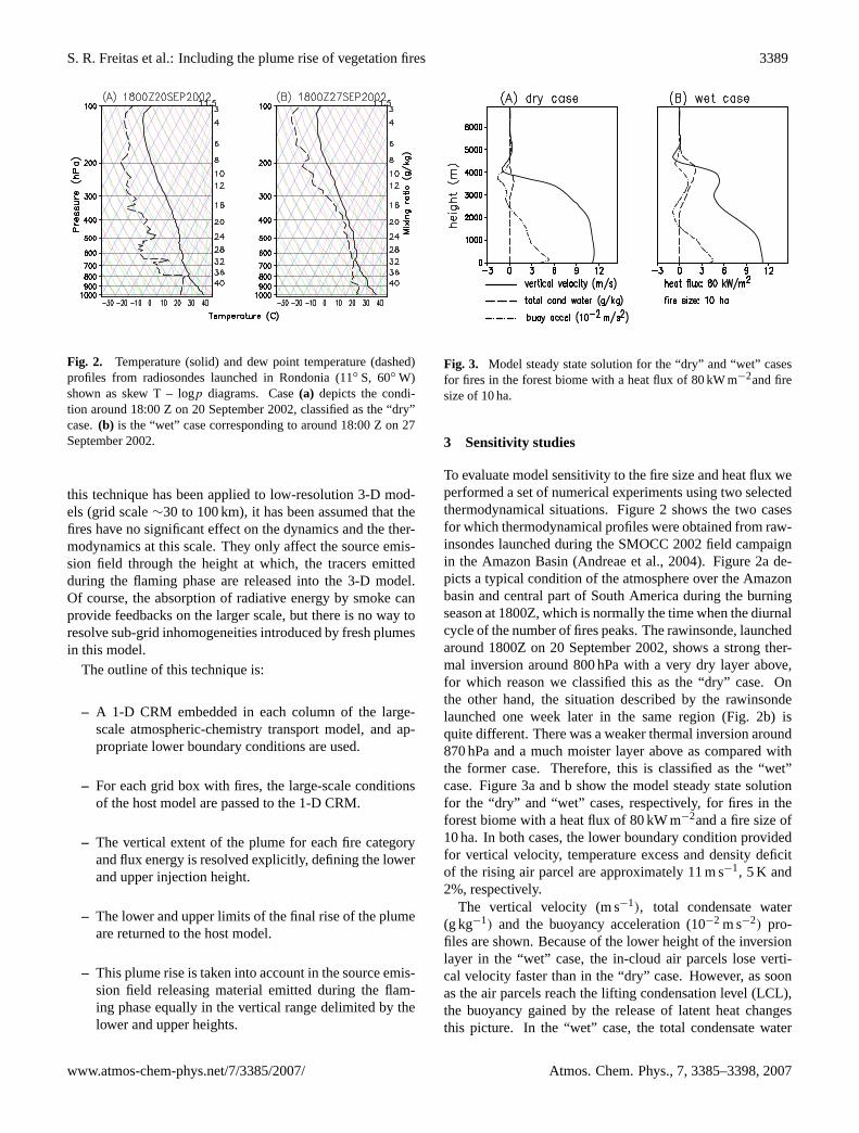
Fig. 2. Temperature (solid) and dew point temperature (dashed)profiles from radiosondes launched in Rondonia (11◦ S, 60◦ W)shown as skew T – logp diagrams. Case(a) depicts the condi-tion around 18:00 Z on 20 September 2002, classified as the “dry”case.(b) is the “wet” case corresponding to around 18:00 Z on 27September 2002.

this technique has been applied to low-resolution 3-D mod-els (grid scale∼30 to 100 km), it has been assumed that thefires have no significant effect on the dynamics and the ther-modynamics at this scale. They only affect the source emis-sion field through the height at which, the tracers emittedduring the flaming phase are released into the 3-D model.Of course, the absorption of radiative energy by smoke canprovide feedbacks on the larger scale, but there is no way toresolve sub-grid inhomogeneities introduced by fresh plumesin this model.

The outline of this technique is:

– A 1-D CRM embedded in each column of the large-scale atmospheric-chemistry transport model, and ap-propriate lower boundary conditions are used.

– For each grid box with fires, the large-scale conditionsof the host model are passed to the 1-D CRM.

– The vertical extent of the plume for each fire categoryand flux energy is resolved explicitly, defining the lowerand upper injection height.

– The lower and upper limits of the final rise of the plumeare returned to the host model.

– This plume rise is taken into account in the source emis-sion field releasing material emitted during the flam-ing phase equally in the vertical range delimited by thelower and upper heights.

Fig. 3. Model steady state solution for the “dry” and “wet” casesfor fires in the forest biome with a heat flux of 80 kW m−2and firesize of 10 ha.

3 Sensitivity studies

To evaluate model sensitivity to the fire size and heat flux weperformed a set of numerical experiments using two selectedthermodynamical situations. Figure2 shows the two casesfor which thermodynamical profiles were obtained from raw-insondes launched during the SMOCC 2002 field campaignin the Amazon Basin (Andreae et al., 2004). Figure2a de-picts a typical condition of the atmosphere over the Amazonbasin and central part of South America during the burningseason at 1800Z, which is normally the time when the diurnalcycle of the number of fires peaks. The rawinsonde, launchedaround 1800Z on 20 September 2002, shows a strong ther-mal inversion around 800 hPa with a very dry layer above,for which reason we classified this as the “dry” case. Onthe other hand, the situation described by the rawinsondelaunched one week later in the same region (Fig.2b) isquite different. There was a weaker thermal inversion around870 hPa and a much moister layer above as compared withthe former case. Therefore, this is classified as the “wet”case. Figure3a and b show the model steady state solutionfor the “dry” and “wet” cases, respectively, for fires in theforest biome with a heat flux of 80 kW m−2and a fire size of10 ha. In both cases, the lower boundary condition providedfor vertical velocity, temperature excess and density deficitof the rising air parcel are approximately 11 m s−1, 5 K and2%, respectively.

The vertical velocity (m s−1), total condensate water(g kg−1) and the buoyancy acceleration (10−2 m s−2) pro-files are shown. Because of the lower height of the inversionlayer in the “wet” case, the in-cloud air parcels lose verti-cal velocity faster than in the “dry” case. However, as soonas the air parcels reach the lifting condensation level (LCL),the buoyancy gained by the release of latent heat changesthis picture. In the “wet” case, the total condensate water

www.atmos-chem-phys.net/7/3385/2007/ Atmos. Chem. Phys., 7, 3385–3398, 2007

3390 S. R. Freitas et al.: Including the plume rise of vegetation fires

(B)Heat Flux (kW/m2)

0

2

4

6

8

10

0.1 1 10 100 1000Fire size (ha)

Hei

gh

t (k

m) 1

51020305080160

(A)Heat Flux (kW/m2)

0

2

4

6

8

10

0.1 1 10 100 1000Fire size (ha)

Hei

gh

t (k

m) 1

51020305080160

Fig. 4. Effective height (km above surface) reached by plumes from fires with size spanning from 0.1 to 200 ha and heat flux from 1 to160 kW m−2 for the “dry” (a) and “wet” (b) thermodynamical situations. The horizontal axis uses a log scale.

Fig. 5. 1-D plume rise model results for the Quinault prescribedfire. (a) Ambient air temperature (◦C) depicting the strong inver-sion between 300 and 600 m.(b) Steady state profile of the verticalvelocity (m/s).

is greater, as the environmental air entrained by the lateraleddies are much moister, and generates positive buoyancyacceleration, which does not occur in the “dry” case. Thisimposes a higher plume rise (by about 500 m) above the in-version for the wet case. Figure4 shows the calculation ofthe final height of the plume as a function of the fire size andheat flux for the “dry” (A) and “wet” (B) cases. Results withfire size spanning from 0.1 to 200 ha and heat flux from 1to 160 kW m−2 are shown. For the “dry” case (Fig.4a), themodel results follow a smooth function with the fire size andheat flux. The results range between 2 and 7.5 km. For a fixedfire size, the variation range of height is 0.5 to 1.5 km. Fora fixed heat flux, this range is around 3 to 5 km. However,the “wet” case (Fig.4b) shows a remarkably different be-havior, with discontinuities at the LCL and effective heightsspanning from 1.3 to 10 km. This case points out the hugeimpact of water phase change in the dynamics of the plume.Another important characteristic to observe in the model re-sults for the effective heights is the weak sensitivity to the

heat flux over the range we have estimated (Table 1). Forthe “dry” case, it is possible to express the effective height interms of the heat flux as height=a(heatflux)b, with a=2.5 km,b=0.1 and the correlation coefficient (R2) 0.98 for a fire sizeof 10 ha. This dependence is weaker than that obtained byManins(1985) in a stably stratified environment wherea andb were estimated as 1.43 km and 0.25, respectively. The re-sults for the “dry case” are also consistent with the findingsof Heikes et al.(1990), who used a 2-D model applied toslash fires in the Pacific Northwest (USA) under Septemberweather conditions. For fire sizes of 20, 38 and 78 ha anda heat flux of about 75 kW m−2, the maximum altitudes ofplume rise were 2.5, 3.2 and 4.7 km, respectively.

4 The Quinault fire case

This section explores the model’s performance in simulat-ing the plume rise evolution associated with the Quinaultprescribed fire, already introduced in Sect. 1. This fire oc-curred on 21 September 1994, and it is a very well docu-mented case (T2002 and references therein). According toT2002, the fire lasted a few hours and the maximum esti-mated heat flux was around 28 kW m−2. The height reachedby the plume of smoke was around 600 m, being transportedhorizontally out over the Pacific Ocean. The ambient atmo-sphere was characterized by a strong temperature inversionbetween 300 and 600 m, very low relative humidity (less than40%), and nearly calm wind. To verify the 1-D plume modelintroduced here, it was set up with the above heat flux, a firesize of 19.4 ha, and 20 m grid spacing resolution. The ambi-ent conditions were based on data shown in Fig. 3 of T2002.Figure5a shows the ambient air temperature, depicting thestrong inversion referred to above. The model result for thesteady state vertical velocity is shown in Fig.5b. The ver-tical velocity of the plume is strongly reduced above 300 m,which reaches a maximum height of about 600 m, consis-tent with the observations and the ATHAM model results.Unfortunately, T2002 did not present any plume dynamic

Atmos. Chem. Phys., 7, 3385–3398, 2007 www.atmos-chem-phys.net/7/3385/2007/

S. R. Freitas et al.: Including the plume rise of vegetation fires 3391

Fig. 6. 1-D plume rise model results for the forest and savanna biomes. The figures show the steady state for the equivalent potentialtemperature(a, d); vertical velocity(b, e) and total condensate water(c, f) for forest and savanna, respectively. Also for each biome, theresults for the upper (solid and black color) and lower bounds (long dash and grey color) of heat flux are shown. Thicker and dark lines showthe equivalent potential temperature of the ambient.

characteristics simulated by the ATHAM model and so wecould not perform more comparisons between the two mod-els. More thoughful comparisons with the ATHAM resultswill appear in a forthcoming paper.

5 Model results and validation using 2002 dry seasondata

The 3-D host model used in this study is CATT-BRAMS.BRAMS is based on the Regional Atmospheric ModelingSystem, RAMS, (Walko et al., 2000) version 5 with sev-eral new functionalities and parameterizations. RAMS is anumerical model designed to simulate atmospheric circula-tion at many scales. RAMS solves the fully compressiblenon-hydrostatic equations described byTripoli and Cotton(1982), and is equipped with a multiple grid nesting schemethat allows the model equations to be solved simultaneouslyon any number of interacting computational meshes of dif-ferent spatial resolutions. BRAMS features used in this sim-ulation include an ensemble version of deep and shallow cu-mulus schemes based on the mass flux approach (Grell and

Devenyi, 2002) and soil moisture initialization data (Gevaerdand Freitas, 2006). CATT is a system designed to simu-late and study the transport and processes associated withbiomass burning emissions. It is an Eulerian transport modelfully coupled to the BRAMS. The tracer transport simula-tion is made simultaneously, or “on-line”, with the atmo-spheric state evolution. The parameterized sub-grid trans-port includes diffusion in the PBL with a turbulent kineticenergy (TKE) closure. The sub-grid tracer transport by shal-low and deep moist convection, which is fully consistent withthe convective parameterization, is also taken into account.

Model simulations for the 2002 dry season were per-formed, and model results were compared with observationaldata. The model configuration used 2 grids: a coarse gridwith 140 km horizontal resolution covering the South Amer-ican and African continents, and a nested grid with a hor-izontal resolution of 35 km, covering only South America.The vertical resolution for both grids was between 150 and850 m, with the top of the model at 23 km (42 vertical levels).The integration time was 135 days, starting at 00:00 Z on 15July 2002. For atmospheric initial and boundary conditions,

www.atmos-chem-phys.net/7/3385/2007/ Atmos. Chem. Phys., 7, 3385–3398, 2007

3392 S. R. Freitas et al.: Including the plume rise of vegetation fires

Fig. 7. Diurnal cycle of the(a) equivalent potential temperature,(b) source emission with the plume rise mechanism, the time evolution ofthe CO concentration profile for a source emission(c) without this mechanism and(d) with it.

the 6 hourly T126 analysis fields from Center for WeatherForecasting and Climate Studies (CPTEC), Brazil, was usedthrough a nudging type of four-dimensional data assimila-tion (Davies, 1983) . For most investigations, two tracerswere simulated, carbon monoxide (COPR) emitted by a 3-D source that includes the plume rise mechanism, and car-bon monoxide (CONOPR), without this mechanism, with allthe emissions released in the first model level. The sametotal mass was emitted for both tracers and they were initial-ized with the same background values. The total amount ofbiomass burning emissions was calculated using the Brazil-ian Fire Emission Model (BFEMO,Freitas et al., 2005).BFEMO emission approach uses detailed information aboutemission factors, aboveground biomass density and combus-tion factors for South America biomes as well as fire counts,derived by remote sensing, to determine location and timingof emission. One basic approximation assumed is the firesize retrieved by remote sensing as burnt area to provide anestimation of the amount of biomass consumed by the fire.To determine the type of biome burning and its space andtime distribution, the1/2-hourly WF ABBA fire product wasmerged with 1 km resolution land-use data. The fraction ofCO emitted during the flaming and smoldering phases wasestimated using Table 1. Due to the large number of fires andin spite of the fire aggregation procedure, the computational

costs required to run this system calling the 1-D plume risemodel at each 3-D host model timestep is highly prohibitive.For that reason, we compute and update the effective injec-tion layer only once every hour. Sensitivity tests, not shown,demonstrated good agreement of model results with thoseobtained by calling the plume rise model at each timestep ofthe host model.

An example of the results from the plume rise model em-bedded in CATT-BRAMS is shown in Fig.6a–f. The figuresshow the steady state for the equivalent potential temperature(A, D); vertical velocity (B, E) and total condensate water (C,F) for forest and savanna biomes and a fire size of 20 ha at18:00 Z on 20 September 2002, respectively. Also for eachbiome, the results for the upper and lower bounds of heatflux, according to Table 1, are shown. In this case, the plumerise dynamics for fires burning forest with heat flux of 80and 30 kW m−2 are similar and define a thin layer of less than1 km for the effective injection height. On the other hand, thedynamic evolution in the savanna is very different. With thelower bound value for the heat flux, the plume cannot passthrough the stable layer to reach the LCL. Penetration doesoccur with the upper bound heat flux value for savanna fires,and results in a 3 km thick injection layer during the flamingphase.

Atmos. Chem. Phys., 7, 3385–3398, 2007 www.atmos-chem-phys.net/7/3385/2007/

S. R. Freitas et al.: Including the plume rise of vegetation fires 3393

The Fig.7 describes the effect of the diurnal cycle of atmo-spheric stability on the effective injection height for a typicalgrid box with simultaneous fires in savanna and tropical for-est. The Fig.7a shows the ambient equivalent potential tem-perature between 0 and 10 km above the local surface; localtime is 4 h less than UTC. The low level warming resultingfrom the surface fluxes driven by solar radiation, and the in-version layer just above 6 km can be seen. The time evolu-tion of the source emission associated with the plume risemechanism is shown in Fig.7b. During the night, the atmo-spheric stability limits the plume rise to an elevation of 2 kmwith a 1.5 km layer thickness. In the afternoon, however, theplume extends upward, reaching a height of 8 km. The upperand denser layer is associated with the forest fires, while thelower, broader, and less dense layer corresponds to the sa-vanna fires, as expected. The effect of the plume rise mecha-nism on the vertical distribution of emissions is demonstratedin Fig.7c and d. The diurnal cycle of CO emitted by a sourcethat does not include the plume rise, CONOPR, is shownin Fig. 7c, while in Fig. 7d the tracer COPR is presented,which includes this mechanism. Without the plume rise, theCO distribution is shallow and limited to the PBL. The COdistribution of Fig.7d appears to be more realistic, with thePBL polluted by emissions from the smoldering phase andthe lower and mid troposphere polluted by emissions fromthe flaming phase. An example of the spatial distribution ofthe CO source emission (with the plume rise mechanism) isgiven by Fig.8, using model results from the coarse grid. Itshows a vertical cross section of CO inputs at 18:00 Z on 2September 2002 along latitude 5.4◦ S. The longitude rangeincludes the South American and African continents. Thehigher and thinner layers of emission in South America areclearly associated with forest fires. In Africa, most fires atthis latitude are burning biomes like savanna, which producebroader and lower injection layers, as discussed previously.Model comparison of the horizontal distribution of CO at500 hPa with AIRS CO data and two lower tropospheric COprofiles from the SMOCC field campaign were shown inFre-itas et al.(2006). The comparison with the AIRS CO demon-strated the huge improvement in model performance close tothe sources, as well as in the simulation of long range trans-port, when the plume rise mechanism was included. In thenext sections, we show more comparisons with SMOCC COdata in the lower troposphere and with MOPITT CO data inthe whole vertical retrieval domain of this product.

5.1 Model comparison with SMOCC 2002 CO airbornemeasurements

Comparisons of simulated CO profiles in the PBL andlower troposphere with observed data were performed usingSMOCC campaign airborne measurements (Andreae et al.,2004). The airborne part of SMOCC took place in the Ama-zon Basin during September and October of 2002. Car-bon monoxide (CO) measurements during SMOCC were ob-

Fig. 8. An example of a vertical cross section of CO source emis-sion on 18:00 Z on 2 September 2002 at latitude 5.4◦ S. The longi-tude range includes the South American and African continents.

tained on the INPE Bandeirante aircraft using an Aero-Laser(AL5002) instrument operating at 1 Hz. The measurementaccuracy is better than±5%; details can be found in (Guyonet al., 2005). The typical maximum altitude reached by theSMOCC aircraft was 5 km. Haze layers resulting from thedetrainment of smoke from convective clouds were visuallyobserved at this height level and also well above the aircraftceiling altitude during almost all flights in the dry season.The role of the plume rise mechanism on CO simulationsis shown in this section using five special CO tracers andthe observed SMOCC CO data. The general mass continuityequation for tracers solved in the CATT-BRAMS model is

∂s

∂t=

(∂s

∂t

)adv︸ ︷︷ ︸

I

+

(∂s

∂t

)PBLdiff︸ ︷︷ ︸

II

+

(∂s

∂t

)deepconv︸ ︷︷ ︸

III

+

(∂s

∂t

)shallowconv︸ ︷︷ ︸

IV

+ Q︸︷︷︸V

, (10)

where s is the grid box mean tracer mixing ratio, I repre-sents the 3-D resolved transport term (advection by the meanwind), II is the sub-grid scale diffusion in the PBL, III andIV are the sub-grid transport by deep and shallow convectionand, finally, V is the source term which may or may not in-clude the plume rise mechanism. In this case the simulationwas carried out with five CO tracers according to the follow-ing specifications. Three tracers named COAD, COSH andCODP did not include the plume rise mechanism, with thetotal CO mass (term V) released into the model layer closestto the surface. The transport processes for the tracer COADincluded only the terms I and II. COSH included processesI, II and IV, while CODP used I, II and III. Another two

www.atmos-chem-phys.net/7/3385/2007/ Atmos. Chem. Phys., 7, 3385–3398, 2007

3394 S. R. Freitas et al.: Including the plume rise of vegetation fires

Fig. 9. Comparison between CO (ppb) observed during SMOCCflights 01 and 10 (black solid line represents the mean while thetwo long dashed lines show the standard deviation range) and modelresults. See text for definitions.

Fig. 10. Comparison between CO (ppb) observed during SMOCCflights 11 and 21 (black solid line represents the mean while thetwo long dashed lines show the standard deviation range) and modelresults. See text for definitions.

tracers (named COPR and COALL) included the plume risemechanism, with the smoldering fraction of the total emis-sion released in the first model layer and the flaming fractionreleased at the effective injection height provided by the 1-D plume rise model (term V). The mixing ratio of COPRwas obtained using only the transport terms I and II, whileCOALL included all I, II, III and IV transport mechanisms.

Figures9, 10and11show comparisons for several flights.The mean and standard deviations (STD) of the observed COprofiles are shown; note that STD represents the actual vari-ability of the concentrations, not the measurement error. Forflight 01 (Fig. 9a) the observed CO profile shows a meanconcentration of around 750 ppb from the surface to 2000 m,decreasing to ca. 400 ppb at 3200 m, the maximum heightfor this flight. The model results for COAD, COSH and

Fig. 11. Comparison between CO (ppb) observed during SMOCCflights 22 and 25 (black solid line represents the mean while thetwo long dashed lines show the standard deviation range) and modelresults. See text for definitions.

CODP over-predict CO, especially above the PBL. COPRand COALL agree very well with observations in the first2 km, and the results from the COALL model are closest tothe observed mean. Flight 10 (Fig.9b) showed strong COvariability in the first 1.2 km as a result of numerous localfires that injected their plumes in the boundary layer. PBLconcentrations outside of these plumes were not well sam-pled, but ranged around 600–800 ppb. In this case, the COPRand COALL model results underestimate the mean observedconcentrations below 1 km, but agree well with the regionalPBL background of 600–800 ppb. Obviously, the model wasnot able to capture the very local fire plumes that were in-tercepted by the aircraft. It also seems that the model sim-ulates a very high and well mixed PBL in this case, whichdoes not agree well with the observed boundary layer heightof about 1300–1400 m. Probably, boundary layer develop-ment was suppressed regionally because of the very densesmoke over the study region (Longo et al., 2006), howeverthe sampling condition might be also considered. COAD,COSH, and COPR appear to agree well with observationsbelow 1 km and show greater disagreement above this level.The better agreement of these models at low levels is some-what fortuitous, as it results from a combination of an over-estimate in boundary layer thickness and an overestimate inthe fraction of the smoke injected into the PBL. For flight 11(Fig. 10a) the observed CO again shows a high variability in-side the PBL (<1.5 km) associated with local plumes, whichcannot be resolved by the model. Above the PBL and below3 km there was relatively clean layer, with only a minor hazelayer with about 300 ppb CO. However, above 3 km CO startsto increase with height, reaching around 350 ppb at about4.5 km. Model COPR and COALL agree very well withthe observed CO profile, being inside the variability rangein the PBL, and following very closely the CO distribution

Atmos. Chem. Phys., 7, 3385–3398, 2007 www.atmos-chem-phys.net/7/3385/2007/

S. R. Freitas et al.: Including the plume rise of vegetation fires 3395

Fig. 12. Comparison between the mean CO (ppb) observed duringSMOCC flights 01, 10, 11, 22, 24 and 25 (black solid line) and themean of model results. See text for definitions.

in the lower troposphere. Models COAD, COSH and CODPover-predict CO in the PBL, and simulate too clean a lowertroposphere. Flights 21, 22 and 25 (Fig.10b, Fig. 11a, b)also show better performance for COALL and COPR whencomparing with COAD, COSH and CODP results. Fig.12presents the mean CO observed during SMOCC flights 01,10, 11, 22, 24 and 25, and the mean of model results up toan elevation of 10.8 km. From near the surface up to 4.5 km,the vertical range of aircraft measurements, the results fromthe COPR and COALL models show the best agreementwith observations. Above 4.5 km, the COAD, COSH andCODP model results are noticeably different from COPR andCOALL. The next section discusses the model results includ-ing also this range of troposphere.

5.2 Model comparisons with MOPITT CO data

The role of the plume rise mechanism in CO simulations in-cluding the mid and upper-troposphere is shown in this sec-tion, using the five CO tracers that were already introducedin Sect. 5.1 and MOPITT data for October 2002. The MO-PITT data used here comprise the tropospheric CO mixingratio (ppb) retrievals for 7 pressure levels, from the surfaceto 150 hPa (Deeter et al., 2003). Because the MOPITT dataproduct shows large horizontal areas without valid data, themodel results and MOPITT data were time-averaged overthe month of October, and area-averaged over the domainbounded by 25◦ S and the Equator, 72◦ W and 45◦ W, theprimary region disturbed by the biomass burning activitiesin South America. Figure13a shows the comparison be-tween CO retrieved by MOPITT and model results after ap-

Fig. 13. Comparison between CO (ppb) retrieved by MOPITT(black lines) and model results with(a) and without(b) the aver-aging kernel and a priori data<50%. See text for definitions.

plying the averaging kernel and a priori data<50%. Becausethe application of the MOPITT averaging kernels changesthe original model results, the unmodified model results areshown in Fig.13b to clarify the role of the different transportmechanisms described in the previous section. Model results(Fig.13a) for the tracer COAD show large disagreement withMOPITT CO and the reason is clearly seen in Fig.13b: thetotal lack of any sub-grid scale convective transport resultsin a heavily polluted PBL and a very clean free troposphereabove. Including shallow convection transport (COSH) pro-duces only small changes in the results, consistent with whatcan be expected. Deep convection transport (CODP) yieldsmore realistic upper troposphere CO simulations, but is notadequate for the correct description of CO in the PBL andlower troposphere. The plume rise mechanism (COPR) pro-vides much better results for CO in the PBL and the lowerand middle troposphere. However, only when all three mainvertical transport mechanisms – shallow and deep moist con-vection and the pyro-convection (dry or moist) induced byvegetation fires – are included, optimal agreement with theMOPITT CO retrieval is obtained in our comparisons.

6 Conclusions

We have shown the usefulness of including the sub-grid scaletransport associated with convection resulting from the ini-tial strong buoyancy of gases/aerosols emitted during veg-etation fires. Comparison of the results from the completemodel with observed CO and with modeled CO withoutthe plume rise mechanism demonstrated clearly the impor-tance of this mechanism on the simulation of CO across thewhole troposphere, including the PBL. Without the plumerise mechanism, the simulated free troposphere over theAmazon basin during the burning season is very clean, whilethe CO in the PBL is overestimated, a characteristic which

www.atmos-chem-phys.net/7/3385/2007/ Atmos. Chem. Phys., 7, 3385–3398, 2007

3396 S. R. Freitas et al.: Including the plume rise of vegetation fires

is not in agreement with observed and remote sensing de-rived data. Including deep and shallow moist convection andpyro-convection lets the model results come to much closeragreement with locally observed or remotely retrieved COmeasurements.

The uncertainty in the injection height associated with theuncertainty of the fire size and heat flux are expected to notaffect significatively the smoke distribution in the 3-D modelbecause it is typically of the order of 1–3 vertical layers ofthe 3-D transport model at that levels (above boundary layer,the thickness of model vertical layers increases from 400 to850 meters), This in particularly true for a typical dry seasonsituation like that one showed at Fig.2 (A). On the other side,it is important to emphasize that the plume rise model sensi-tivity to the environmental thermodynamic is much more sig-nificant, like showed at Fig.7 (B), and, so, it fully justify thechoose for an “on-line” and coupled approach of the plumerise model with the 3-D transport model. The methodologypresented here provides a powerful and feasible approach toinclude this mechanism in low resolution atmospheric trans-port models. The low sensitivity of the final rise of the plumeto the heat flux from the fire is an important and desirable fea-ture of the parameterization. Future work will estimate thisflux directly from the fire radiative energy obtained by re-mote sensing. The fire size is another important fire propertyneeded by the model, which may be also provided by remotesensing.

Acknowledgements.We acknowledge partial support of this workby NASA Headquarters (NRA-03-OES-02 and NRA-02-OES-06)and CNPq (305059/2005-0). This work was carried out withinthe framework of the project “Monitoramento de emissoes dequeimadas e avaliacao das observacoes de qualidade do ar emTres Lagoas – MS” in collaboration with CENPES/Petrobras; theLBA Smoke, Aerosols, Clouds, Rainfall, and Climate (SMOCC)project (funded by the Environmental and Climate Program of theEuropean Commission under contract No. EVK2-CT-2001-00110-SMOCC and by the Max Planck Society), and Radiation, Cloud,and Climate Interactions in the Amazon during the DRY-TO-WETTransition Season (RACCI) project (funded by FAPESP andInstituto do Milenio/LBA/CNPq/MCT).

Edited by: Y. Balkanski

References

Alexander, M. E.: Calculating and interpreting forest fires intensi-ties, Can. J. Bot., 60, 349–357, 1982.

Andreae, M.: Biomass burning: its history, use and distributionand its impact on environmental quality and global climate, in:Global Biomass Burning: Atmospheric, Climatic and BiosphericImplications, edited by: Levine, J. S., MIT Press, Cambridge,Mass., pp. 3–21, 1991.

Andreae, M., Rosenfeld, D., Artaxo, P., Costa, A., Frank, G.,Longo, K. M., and Silva Dias, M A. F.: Smoking rain cloudsover the Amazon, Science, 303, 1342–1345, 2004.

Berry, E. X.: Modification of the warm rain process, Preprints, 1stNatl. Conf. on Weather Modification, Am. Meteorol. Soc., Al-bany, NY, 81–88, 1968.

Byram, G. M.: Combustion of forest fires, in: Forest Fire Controland Use, edited by: Davis, K. P., McGraw-Hill, New York, 1959.

Carvalho Jr., J. A., Santos, J. M., Santos, J. C., Leitao, M.,and Niguchi, N.: A tropical rainforest clearing experiment bybiomass burning in the Manaus region, Atmos. Environ., 29,2301–2309, 1995.

Chatfield, R. B., and Delany, A. C.: Convection links biomass burn-ing to increased tropical ozone: However, models will tend tooverpredict O3, J. Geophys. Res., 95, 18 473–18 488, 1990.

Clark, T. L., Jenkins, M. A., Coen, J. and Packham, D.: A coupledatmosphere-fire model: Convective feedback on fire-line dynam-ics, J. Appl. Meteorol., 35, 875–901, 1996.

Clark, T. L., Griffiths, M., Reeder, M. J. and Latham, D.: Numeri-cal simulations of grassland fires in the Northern Territory, Aus-tralia: A new subgrid-scale fire parameterization, J. Geophys.Res., 108(D18), 4589, doi:10.1029/2002JD003349, 2003.

Davies, H. C.: Limitations of some common lateral boundaryschemes used in regional NWP models, Mon. Wea. Rev., 111,1002–1012, 1983.

Deeter, M. N., Emmons, L. K., Francis, G. L., Edwards, D. P., Gille,J. C., Warner, J. X., Khattatov, B., Ziskin, D., Lamarque, J.-F.,Ho, S.-P., Yudin, V., Atti, J.-L., Packman, D., Chen, J., Mao, D.,Drummond, J. R.: Operational carbon monoxide retrieval algo-rithm and selected results for the MOPITT instrument, J. Geo-phys. Res., 108(D14), 4399, doi:10.1029/2002JD003186, 2003.

Freitas, S. R., Longo, K. M., Silva Dias, M., Silva Dias, P., Chat-field, R., Prins, E., Artaxo, P., Grell, G., and Recuero, F.: Moni-toring the transport of biomass burning emissions in South Amer-ica, Environmental Fluid Mechanics, doi:10.1007/s10652-005-0243-7, 5(1–2), 135–167, 2005.

Freitas, S. R., Longo, K. M., and Andreae, M. O.: Impact of includ-ing the plume rise of vegetation fires in numerical simulationsof associated atmospheric pollutants, Geophys. Res. Lett., 33,L17808, doi:10.1029/2006GL026608, 2006.

Fromm, M., Alfred, J., Hoppel, K., Hornstein, J., Bevilacqua, R.,Shettle, E., Servranckx, R., Li, Z., and Stocks, B.: Observa-tions of boreal forest fire smoke in the stratosphere by POAMIII, SAGE II, and lidar in 1998, Geophys. Res. Lett., 27, 1407–1410, 2000.

Fromm, M. and Servranckx, R.: Transport of forest fire smokeabove the tropopause by supercell convection, Geophys. Res.Lett., 30, 1542, doi:10.1029/2002GL016820, 2003.

Gevaerd, R. and Freitas, S. R.: Estimativa operacional da umidadedo solo para iniciacao de modelos de previsao numerica da at-mosfera. Parte I: Descricao da metodologia e validacao, RevistaBrasileira de Meteorologia, 21(3), 1–15, 2006.

Grell, G. and Devenyi, D.: A generalized approach to pa-rameterizing convection combining ensemble and dataassimilation techniques, Geophys. Res. Lett., 29(14),doi:10.1029/2002GL015311, 2002.

Griffin, G. F. and Friedel, M. H.: Effects in fire in Central Aus-tralia rangelands. I – Fire and fuel characteristics and change inherbage and nutrients, Aust. J. Ecol., 9, 381–393, 1984.

Grishin, A. M.: Mathematical modelling of forest fires, in: Firein Ecosystems of Boreal Eurasia, edited by: Goldammer, J. G.and Furyaev, V. V., Kluwer Acad., Norwell, Mass., pp. 285–302,

Atmos. Chem. Phys., 7, 3385–3398, 2007 www.atmos-chem-phys.net/7/3385/2007/

S. R. Freitas et al.: Including the plume rise of vegetation fires 3397

1996.Guyon, P., Frank, G. P., Welling, M., Chand, D., Artaxo, P., Rizzo,

L., Nishioka, G., Kolle, O., Fritsch, H., Silva Dias, M. A. F.,Gatti, L. V., Cordova, A. M., and Andreae, M. O.: Airbornemeasurements of trace gases and aerosol particle emissions frombiomass burning in Amazonia, Atmos. Chem. Phys., 5, 2989–3002, 2005,http://www.atmos-chem-phys.net/5/2989/2005/.

Heikes, L., Ransohoff, L., and Small, R.: Numerical simulation ofsmall area fires, Atmos. Environ., 24A, 297–307, 1990

Hill, G. E.: Factors controlling the size and spacing of cumulusclouds as revealed by numerical experiments, J. Atmos. Sci., 31,646–673, 1974.

Jost, H., Drdla, K., Stohl, A., et al.: In-situ observations of mid-latitude forest fire plumes deep in the stratosphere, Geophys. Res.Lett., 31, L11101, doi:10.1029/2003GL019253, 2004.

Kaufman, Y.: Remote sensing of direct and indirect aerosol forcing,in: Aerosol Forcing of Climate, edited by: Charlson, R. J. andHeintzenberg, J., John Wiley & Sons Ltd, Chichester, 297–332,1995.

Kessler, E.: On the distribution and continuity of water substance inatmospheric circulation models, Meteor. Monographs, 10, Am.Meteorol. Soc. Boston, MA, 1969.

Latham, D.: PLUMP: A one-dimensional plume predictor andcloud model for fire and smoke managers, General TechnicalReport INT-GTR-314, Intermountain Research Station, USDAForest Service, Nov, 1994.

Lavoue, D., Liousse, C., Cachier, H., Stocks, B. J., and Goldammer,J. G.: Modeling of carbonaceous particles emitted by boreal andtemperate wildfires at northern latitudes, J. Geophys. Res., 105,26 871–26 890, 2000.

Lilly, D. K.: On the numerical simulation of buoyant convection,Tellus, XIV, 2, 148–172, 1962.

Liousse, C., Penner, J. E., Chuang, C., Walton, J. J., Eddleman,H., and Cachier, H.: A global three-dimensional model studyof carbonaceous aerosols, J. Geophys. Res., 101(D14), 19 411–19 432, 1996.

Longo, K. M., Freitas, S. R., Silva Dias, M., Silva Dias, P.: Numer-ical modelling of the biomass-burning aerosol direct radiativeeffects on the thermodynamics structure of the atmosphere andconvective precipitation. In: International Conference on South-ern Hemisphere Meteorology and Oceanography (ICSHMO), 8.,Foz do Iguacu, Proceedings, Sao Jose dos Campos: INPE, CD-ROM, ISBN 85-17-00023-4, p. 283–289, 2006.

Luderer, G., Trentmann, J., Winterrath, T., Textor, C., Herzog, M.,Graf, H.-F., and Andreae, M. O.: Modeling of biomass smokeinjection into the lower stratosphere by a large forest fire (Part II):sensitivity studies, Atmos. Chem. Phys., 6, 5261–5277, 2006,http://www.atmos-chem-phys.net/6/5261/2006/.

Manins, P. C.: Cloud heights and stratospheric injections from athermonuclear war, Atmos. Environ., 19, 1245–1255, 1985.

McCarter, R. and Broido, A.: Radiative and convective energy fromwood crib fires, Pyrodinamics, 2, 65–85, 1965.

Morton, R., Taylor, G., and Turner, J.: Turbulent gravitational con-vection from maintained and instantaneous sources, Proc. Roy.Soc. A, 234, 1–23, 1956.

Ogura, Y. and Takahashi, T.: Numerical simulation of the life cycleof a thunderstorm cell, Mon. Wea. Rev., 99, 895–911, 1971.

Penner, J. E., Haselman Jr., L. C., and Edwards, L. L.: Smoke-

plume distribution above large-scale fires: Implications for simu-lations of “Nuclear Winter”, J. Clim. Appl. Meteorol., 25, 1434–1444, 1986.

Poppe, D., Koppmann, R., and Rudolph, J.: Ozone formationin biomass burning plumes: Influence of atmospheric dilution,Geophys. Res. Lett., 25, 3823–3826, 1998.

Prins, E., Feltz, J., Menzel, W., and Ward, D.: An overview ofGOES-8 diurnal fire and smoke results for SCAR-B and 1995 fireseason in South America, J. Geophys. Res., 103(D24), 31 821–31 835, 1998.

Reid, J. S., Koppmann, R., Eck, T. F., and Eleuterio, D. P.: A reviewof biomass burning emissions part II: intensive physical proper-ties of biomass burning particles, Atmos. Chem. Phys., 5, 799–825, 2005,http://www.atmos-chem-phys.net/5/799/2005/.

Riggan, P., Tissell, R., Lockwood, R., Brass, J., Pereira, J., Miranda,H., Miranda, A., Campos, T., and Higgins, R.: Remote measure-ment of energy and carbon flux from wildfires in Brazil, Ecol.Appl., 14, 3, 855–872, 2004.

Rosenfeld, D., Fromm, M., Trentmann, J., Luderer, G., Andreae,M. O., and Servranckx, R.: The Chisholm firestorm: observedmicrostructure, precipitation and lightning activity of a pyro-cumulonimbus, Atmos. Chem. Phys., 7, 645–659, 2007,http://www.atmos-chem-phys.net/7/645/2007/.

Simpson, J. and Wiggert, S.: Models of precipitating cumulus tow-ers, Mon. Wea. Rev., 97, 471–489, 1969.

Smagorinsky, J.: General circulation experiments with the primitiveequations. Part I, The basic experiment, Mon. Wea. Rev., 91, 99–164, 1963.

Small, R.D. and Heikes, K.: Early cloud formation by large areafires, J. Appl. Meteorol., 27, 654–663, 1988.

Trentmann J., Andreae, M. O., Graf, H.-F., Hobbs, P. V., Ottmar,R. D., and Trautmann, T.: Simulation of a biomass-burningplume: Comparison of model results with observations, J. Geo-phys. Res., 107(D2), 4013, doi:10.1029/2001JD000410, 2002.

Trentmann, J., Luderer, G., Winterrath, T., Fromm, M., Servranckx,R., Textor, C., Herzog, M., Graf, H.-F., and Andreae, M. O.:Modeling of biomass smoke injection into the lower stratosphereby a large forest fire (Part I): reference simulation, Atmos. Chem.Phys., 6, 5247–5260, 2006,http://www.atmos-chem-phys.net/6/5247/2006/.

Tremback, C., Powell, J., Cotton, W., and Pielke, R.: The forwardin time upstream advection scheme: Extension to higher orders,Mon. Wea. Rev., 115, 540–555, 1987.

Tripoli, G. and Cotton, W.: The Colorado State University three-dimensional cloud-mesoscale model. Part I: General theoreticalframework and sensitivity experiments, J. Res. Atmos., 16, 185–219, 1982.

Turner, J. S.: Buoyancy effects in fluids, Cambridge Univ. Press,Cambridge, 368 pp., 1973.

Turquety, S., Logan, J., Jacob, D., Hudman, R., Leung, F., Heald,C., Yantosca, R., Wu, S., Emmons, L., Edwards, D., and Sachse,G.: Inventory of boreal fire emissions for North America in 2004:the importance of peat burning and pyro-convective injection,J. Geophys. Res., 112, D12S03, doi:10.1029/2006JD007281,2007.

Viegas, D. X.: Convective processes in forest fires, in: BuoyantConvection in Geophysical Flows, edited by: Plate, E. J., Fe-dorovich, E. E., Viegas, D. X., and Wyngaard, J. C., Kluwer Aca-

www.atmos-chem-phys.net/7/3385/2007/ Atmos. Chem. Phys., 7, 3385–3398, 2007

3398 S. R. Freitas et al.: Including the plume rise of vegetation fires

demic Publishers, AA Dordrecht, The Netherlands, pp. 401–420,1998.

Walko, R., Band, L., Baron, J., Kittel, F., Lammers, R., Lee, T.,Ojima, D., Pielke, R., Taylor, C., Tague, C., Tremback, C., andVidale, P.: Coupled atmosphere-biophysics-hydrology modelsfor environmental modeling, J. Appl. Meteorol., 39, 6, 931–944,2000.

Wang, J., Christopher, S. A., Nair, U. S., Reid, J. S., Prins, E. M.,Szykman, J., and Hand, J. L.: Mesoscale modeling of CentralAmerican smoke transport to the United States: 1. “Top-down”assessment of emission strength and diurnal variation impacts,J. Geophys. Res., 111, D05S17, doi:10.1029/2005JD006416,2006.

Atmos. Chem. Phys., 7, 3385–3398, 2007 www.atmos-chem-phys.net/7/3385/2007/