Conservation planning for connectivity across marine, freshwater, and terrestrial realms

RESEARCH ARTICLE
Improving the Use of Species DistributionModels in Conservation Planning andManagement under Climate ChangeLuciana L. Porfirio1*, Rebecca M. B. Harris2, Edward C. Lefroy3, Sonia Hugh1,Susan F. Gould4, Greg Lee2, Nathaniel L. Bindoff2,5,6, Brendan Mackey4
1. Fenner School of Environment and Society, College of Medicine, Biology and Environment, AustralianNational University, Canberra, Australian Capital Territory, Australia, 2. Antarctic Climate & EcosystemsCooperative Research Centre, Hobart, Tasmania, Australia, 3. Centre for the Environment, University ofTasmania, Hobart, Tasmania, Australia, 4. Griffith Climate Change Response Program, Griffith University,Gold Coast, Queensland, Australia, 5. Australia Research Council, Centre of Excellence in Climate SystemScience, Hobart, Tasmania, Australia, 6. The Commonwealth Scientific and Industrial Research Organisation,Oceans & Atmosphere Flagship, Hobart, Tasmania, Australia
Abstract
Choice of variables, climate models and emissions scenarios all influence the
results of species distribution models under future climatic conditions. However, an
overview of applied studies suggests that the uncertainty associated with these
factors is not always appropriately incorporated or even considered. We examine
the effects of choice of variables, climate models and emissions scenarios can
have on future species distribution models using two endangered species: one a
short-lived invertebrate species (Ptunarra Brown Butterfly), and the other a long-
lived paleo-endemic tree species (King Billy Pine). We show the range in projected
distributions that result from different variable selection, climate models and
emissions scenarios. The extent to which results are affected by these choices
depends on the characteristics of the species modelled, but they all have the
potential to substantially alter conclusions about the impacts of climate change. We
discuss implications for conservation planning and management, and provide
recommendations to conservation practitioners on variable selection and
accommodating uncertainty when using future climate projections in species
distribution models.
OPEN ACCESS
Citation: Porfirio LL, Harris RMB, Lefroy EC, HughS, Gould SF, et al. (2014) Improving the Use ofSpecies Distribution Models in ConservationPlanning and Management under ClimateChange. PLoS ONE 9(11): e113749. doi:10.1371/journal.pone.0113749
Editor: Lalit Kumar, University of New England,Australia
Received: September 17, 2014
Accepted: October 29, 2014
Published: November 24, 2014
Copyright: � 2014 Porfirio et al. This is anopen-access article distributed under the terms ofthe Creative Commons Attribution License, whichpermits unrestricted use, distribution, andreproduction in any medium, provided the originalauthor and source are credited.
Data Availability: The authors confirm that all dataunderlying the findings are fully available withoutrestriction. The modelled projections are availablethrough the Tasmanian Partnership for AdvancedComputing (TPAC) portal (https://dl.tpac.org.au/tpacportal/). The literature review data weresubmitted as a database in the supplementaryinformant ion, as a ZIP file.
Funding: This research is an output from theLandscapes and Policy Research Hub. The hub issupported through funding from the AustralianGovernment’s National Environmental ResearchProgramme and involves researchers from theUniversity of Tasmania (UTAS), The AustralianNational University (ANU), Murdoch University, theAntarctic Climate and Ecosystems CooperativeResearch Centre (ACE CRC), Griffith Universityand Charles Sturt University (CSU). The fundershad no role in study design, data collection andanalysis, decision to publish, or preparation of themanuscript.
Competing Interests: The authors have declaredthat no competing interests exist.
PLOS ONE | DOI:10.1371/journal.pone.0113749 November 24, 2014 1 / 21

Introduction
Species distribution models (SDMs) are one of the most important tools currently
available to assess the potential impacts of climate change on species [1]. They are
commonly used to project potential future changes in the geographic ranges of
species [2,3], estimate extinction rates [4,5], examine the efficacy of existing
reserve systems [6,7] and prioritise biodiversity conservation efforts [8,9].
However, a range of factors influence the results of SDMs under future climatic
conditions, including the choice of statistical model, variable selection, climate
model range and emissions scenarios [10,11,12].While many of these issues have
been highlighted in the scientific literature (for example,
[13,14,15,16,17,18,19,20,21,22]), less attention has been given to providing
explanations and practical solutions to assist conservation planners and managers
apply the results of SDMs. Yet these issues contribute to cascading uncertainty
that makes decisions based on modelled future projections very challenging.
The emphasis of much ecological research in this area has been the validation of
statistical models [11,23,24,25], and the development of ensemble approaches to
represent the range in SDM outputs [10,19,23,26,27,28,29,30,31,32,33,34,35,36].
Ensemble approaches produce multiple distribution maps that require
summarising before interpretation is possible. Several methods have been
suggested to achieve this and deal with the errors and uncertainties of different
statistical models [37]. These include representing the central tendency with
median or mean values; highlighting spatial extents within which either one or all
models show suitable habitat; presenting the degree of model agreement with
frequency histograms; or probabilistic forecasting when large numbers of models
are used [37]. However, while ensemble-based statistical methods may be
appropriate to deal with errors and uncertainties between models, they may not
always be the best way to summarise projected habitat ranges in SDMs due to the
influence of differences in variable selection, climate model range and emissions
scenarios.
Global climate models (GCMs) and emissions scenarios represent a range of
plausible futures [38,39]. They are not intended to provide accurate predictions
regarding the future state of the climate system at any given point in time, but to
establish the envelope that future climate could conceivably occupy. For this
reason, important information may be lost if an ensemble of GCMs are
summarised inappropriately. For example, presenting a multi-model mean
provides a ‘central estimate’ of the projections obtained under a particular
selection of GCMs and does not consider the variability represented by different
climate models and/or emissions scenarios.
In this paper, we assess the literature in relation to SDM projections in applied
ecological studies and evaluate the extent to which uncertainties attributable to
selection of climatic variables and GCMs are addressed. Some uncertainty is not
taken into account with SDMs, the classic example is the physiological response of
plants and animals to an atmosphere with elevated CO2 concentrations. In this
paper the uncertainty from changing concentrations of CO2 in the atmosphere
Species Distribution Models and Climate Change for Land Managers
PLOS ONE | DOI:10.1371/journal.pone.0113749 November 24, 2014 2 / 21

cannot be addressed and thus these results assume a constant atmospheric
concentration for a given emissions scenario. Informed by the findings of our
literature review, we explore the influence of the choice of climatic variables and
approaches to assimilating multiple SDMs based on a range of climate models and
emissions scenarios using two threatened species from Tasmania, Australia, as
case studies. We conclude with recommendations on the use of SDMs for
conservation planners and managers.
Common approaches to SDM in applied ecology
To gain an overview of how SDMs are being used in applied studies of species
distributions under climate change, we searched for articles in the ISI Web of
Science database (http://www.webofknowledge.com) from 1982 to 2013, where
the phrases ‘bioclimatic’ and ‘climate change’ occurred in the title, abstract or
author’s keywords. In SDM literature, it has become common practice in
ecological studies to refer to climatic variables derived from spatial interpolation
of long-term mean monthly data as ‘bioclimatic’ variables [40]. The aim of this
overview was to provide a substantive sample of relevant literature rather than
being a systematic review of all the literature and available databases. The search
yielded 562 records, which we refined by selecting articles that contained the
words ‘niche’ or ‘habitat’, resulting in a total of 221 publications (the list of
reviewed articles can be found at: http://www.mendeley.com/groups/3315561/
bioclim-review/papers/). Since we focused on applied studies, review articles were
omitted. A total of 163 articles had constructed SDMs for current or future
terrestrial species distributions. From each article, we analysed information
relating to predictor variables used in the SDM, the taxa, the scale and location of
the study region, and how future climate projections were used. Data from the
review were analysed using R [41].
Most of the reviewed articles focused on Europe (,30%), North America
(,17%), Africa (,12%), South America (,11%), Australia and Oceania
(,10%), with a small fraction on Asia (,3%). Note that the sum of fractions is
,100% because some articles were methodological and did not include case
studies. The majority of studies (58%) were carried out at the regional scale (e.g.
geographic extent >10000 km2 ,continental), 14% were at the continental scale,
and just over 10% of the articles reported studies at scales of either ,10 km2 or
between 1000 km2 to 10000 km2. A small proportion of articles (,2%) carried
out SDMs at the global scale. SDMs were used to study the potential impacts of
climate change on the distributions of a wide range of taxa, including birds
(,43%), reptiles and amphibians (,32%), plants (,19%), invertebrates (,12%)
and mammals (,10%) with some articles modelling more than one taxon.
From the reviewed literature, we identified three common approaches to
variable selection. The first common approach uses all available bioclimatic
variables without justification. The BIOCLIM software, a sub-package of
ANUCLIM [42] provides 35 variables, while WORLDCLIM [43] provides a subset
of 19 bioclimatic variables. The second common approach reduces the number of
Species Distribution Models and Climate Change for Land Managers
PLOS ONE | DOI:10.1371/journal.pone.0113749 November 24, 2014 3 / 21

bioclimatic and biophysical covariates to account for colinearity. The third selects
variables based on ecological knowledge. Typically, the third involved assuming a
causal relationship between a climatic variable and a theoretical or empirically
established understanding of a species’ eco-physiology, life history traits, patterns
of movement, reproductive cycle or habitat requirements. Often the assumed
causal relationship was general, such as the relationship between growing degrees
days and biological growth rates [44]. A total of 119 distinct variables were used in
the reviewed articles (see Figure S1) the most common being mean annual
precipitation and mean annual temperature used by 43% and 37% of the articles,
respectively.
Diagnostic statistics regarding performance of SDMs were reported by 55% of
the articles. The most commonly used statistics to assess the performance of
SDMs were the area under the receiver operating curve (AUC), Akaike
information criterion (AIC), Bayesian information criterion (BIC), Kappa and R2.
We found three approaches were commonly used to summarise the outputs of
SDMs: (1) model mean tendency; (2) model agreement; and (3) the bounding box
[23].
About 10% of the reviewed papers provided justification for the selection of
GCM. About 40% of the reviewed articles used two or more GCMs with one or
two emissions scenarios. Only seven articles [19,45,46,47,48,49,50] used more
than 10 GCMs and acknowledged variability in these inputs. Each of these seven
articles focused on testing SDM methods, rather than applying SDMs to practical
conservation problems. The review database can be found in File S2.
Material and Methods
We used two contrasting species as case studies to examine the issues related to
variable selection and GCMs that commonly arise when modelling future species
distributions for applied conservation: the King Billy Pine (Athrotaxis
selaginoides); and the Ptunarra Brown Butterfly (Oreixenica ptunarra). King Billy
Pine is a long-lived paleo-endemic tree that grows at altitudes of 600 m to
1100 m. In contrast, the Ptunarra Brown Butterfly is a short-lived species, which is
active for three to four weeks in late February to April, at altitudes from 200 m to
1200 m. These species are endemic to Tasmania, Australia, and have been listed as
endangered under the Environment Protection and Biodiversity Conservation Act
1999. We conducted SDM experiments to examine the range in projected
distribution due to (a) the three common approaches to variable selection
identified in the review and (b) the three different ways of accounting for the
range in SDM results from using multiple GCMs and emissions scenarios.
Species Distribution Models
Presence data for the species were downloaded from the online database Atlas of
Living Australia (http://collections.ala.org.au/public) and databases of the state
Species Distribution Models and Climate Change for Land Managers
PLOS ONE | DOI:10.1371/journal.pone.0113749 November 24, 2014 4 / 21

conservation agency, the Department of Primary Industries, Parks, Water and
Environment (DPIPWE, https://www.naturalvaluesatlas.tas.gov.au/). There were
212 unique observations for the Ptunarra Brown Butterfly from 1949 to 2007; and
672 observations for The King Billy Pine from the period 1847 to 2005.
The MaxEnt model [51] was used to model the suitability of future climate for
each species. While there are several other methods for modelling species
distributions (e.g. generalised linear models, boosted regression trees, mechanistic
models and ensemble techniques), we used MaxEnt because it is not
computationally expensive, is widely used in applied ecological studies by
government agencies and research organisations, and has been shown to perform
well in comparison to several other models when there are relatively few presence
records available [52]. We did not use an ensemble approach because, as noted,
that issue has been extensively investigated and our focus here is on tools that are
usable by conservation planners and managers who generally do not have access
to the high computing capacity needed for ensemble modelling. We used R [41]
to run MaxEnt, with fifteen replicate runs calculated by cross-validation using
30% of the data and default values for all other parameters (iterations5500,
convergence threshold50.00001, and regularization value51). Results are
presented as the relative probability of occurrence, with suitable climate identified
where this value is greater than 0.5 [53].
Three MaxEnt models, that represent the three common approaches to variable
selection, were run for the two species using different sets of bioclimatic predictor
variables. The first model used all available variables (see Table A1 in File S1). The
second model used principal component analysis (PCA) to identify a subset of
available bioclimatic variables that are not strongly correlated (R2,0.6). The third
model used expert knowledge of the target species to identify subsets of
bioclimatic variables. The available bioclimatic variables represent annual trends
(e.g. mean annual temperature and precipitation), seasonal trends (e.g. annual
range in temperature or precipitation), and extreme or limiting environmental
factors (e.g. temperature of the coldest and warmest month, precipitation for
wettest or driest quarters). Model 1 used the most commonly used set of variables,
based on the literature review, comprising 35 variables provided by BIOCLIM.
These BIOCLIM variables defined the baseline climate.
Model 2 used a subset of uncorrelated bioclimatic variables selected using PCA
that explained more than 90% of the variance. For the Ptunarra Brown Butterfly,
the variables were: temperature seasonality (coefficient of variation, hereafter cv);
maximum temperature warmest period; and mean temperature driest quarter and
annual precipitation. For the King Billy Pine, the variables were: annual mean
temperature: temperature seasonality (cv); temperature annual range; annual
precipitation; annual mean radiation; radiation seasonality (cv); annual mean
moisture index; and highest period moisture index.
Model 3 used variables chosen by experts based on knowledge of the species’ life
cycle. For the Ptunarra Brown Butterfly the selected bioclimatic variables were:
March minimum temperature; April minimum temperature; annual minimum
temperature; radiation with rainfall for April; and annual rainfall (Dr Peter
Species Distribution Models and Climate Change for Land Managers
PLOS ONE | DOI:10.1371/journal.pone.0113749 November 24, 2014 5 / 21

McQuillan and Dr Phil Bell pers. comm.). For the King Billy Pine the selected
bioclimatic variables were: maximum temperature warmest period; minimum
temperature of coldest period; mean temperature warmest quarter; mean
temperature coldest quarter; annual precipitation; precipitation driest period;
annual mean moisture index; lowest period moisture index; and mean moisture
index lowest quarter (Dr Jennie Whinam and Ms Louise Gilfedder pers. comm.).
We only used bioclimatic variables rather than other physical environmental or
vegetation habitat variables in the model in order to provide an indication of
changing climatic suitability assuming all else remains equal. Model performance
was assessed using the area under the receiver operating Curve (AUC) and the
information criteria Akaike information criteria (AIC), corrected Akaike (AICc),
and Bayesian information criteria (BIC) calculated using ENMTools [54]. These
tests can be used as an objective measure of model performance and provide
guidance where there are large differences between models. The degree to which
novel climate conditions are encountered is assessed with the ‘multivariate
similarity surface’ (MESS) output from MaxEnt. The MESS shows similarity
between each point in future projections to conditions observed during model
training. In addition, similarity between the outputs for the future projections
based on Model 2 for the species was quantified using the I similarity statistic [54].
The I statistic calculates pair-wise similarity between two probability distributions
obtained, in this case from MaxEnt, where values close to zero represent
distributions with no geographic overlap, and values close to one represent similar
distributions. We used SigDiff from the R package SDMTools [55] to compute
significant differences between pairs of maps, using the distribution for the
current climate as a reference [56,57].
We consulted land managers and decision makers from the Australian
Department of the Environment, the Tasmanian Department of Primary
Industries, Parks, Water and Environment (DPIPWE), Natural Resource
Management (NRM) groups and local government to ask how uncertainty in
SDM outputs could be represented to better inform conservation management
and prioritisation (see File S1 for further detail on these consultations).
Future Climate Projections
Future climate projections were derived from six global climate models that were
dynamically downscaled to a resolution of 0.1˚(,10 km) across Tasmania using a
regional climate model (Harris et al. 2014). Downscaling was undertaken by the
Climate Futures for Tasmania project using CSIRO’s Conformal Cubic
Atmospheric Model (CCAM). Details of the CCAM model can be found in [58],
and the modelled projections are available through the Tasmanian Partnership for
Advanced Computing (TPAC) portal (https://dl.tpac.org.au/tpacportal/).
The six global climate models (GCMs) used are available from the CMIP3
archive [59]: GFDL-CM2.0; GFDL-CM2.1; CSIRO Mk3.5; MIROC3.2 (medres);
and UKMO-HadCM3. Each of the six GCMs was run under both the SRES A2
and B1 emissions scenarios to represent high and low emissions scenarios
Species Distribution Models and Climate Change for Land Managers
PLOS ONE | DOI:10.1371/journal.pone.0113749 November 24, 2014 6 / 21

respectively. These models are a reasonable representation of the range of the
precipitation and temperature projections for south-eastern Australia indicated in
the full set of GCMs from the CMIP3 archive. Results from three of these GCMs
are presented in Section 3.1.2 as described below, and results from the six GCMs
are used in Section 3.2.
Climate data were spatially interpolated to a grid cell resolution of 0.01˚(,1 km) using the ANUCLIM 6.1 package [42]. A digital elevation model (DEM)
of 0.01˚ (,1 km) was used as input into ANUCLIM 6.1 [42]. The DEM was
aggregated from the 30 seconds (,30 m) NASA Shuttle Radar Topographic
Mission (SRTM) DEM (http://srtm.csi.org) to 0.01˚ using R [41].
Grids representing the difference in Tmax, Tmin, precipitation and evaporation
at the pixel level were calculated for each of the six downscaled GCMs, for each
month within each of three future time slices, relative to the baselines used in
ANUCLIM (1976–2005 and 1970–1995 for evaporation). Future time slices are
represented by mean values associated with the 30-year periods: 2010 to 2039,
2040 to 2069 and 2070 to 2099. Monthly mean values and bioclimatic variables
were then calculated for the future periods.
Monthly mean values for Tmax, Tmin, precipitation and evaporation for the
baseline climate, used to project current species suitable climate, were generated
using the MNTHCLIM sub-package in ANUCLIM 6.1, and the 35 bioclimatic
variables based on these outputs were generated by BIOCLIM.
Species Distribution Models for future climate
As noted above, for each of the case-study species, three SDMs were calculated for
baseline (e.g. current) climate conditions using each of the three different
approaches to variable selection (Models 1 to 3). We then assessed the results
using statistical metrics (AIC and BIC) and feedback from our species experts. We
used outputs from all six available GCMs under both CO2 emission scenarios (A2
and B1) to calculate future climate SDMs for the two species, that is, 12 SDMs for
each species giving a total of 24.
We decided that Model 2 (variable selection based on PCA) was the most
accurate. We then used the outputs from Model 2 to compare the three
commonly used approaches to summarising the output from multiple SDMs
based on future climate (model mean tendency, model agreement and the
bounding box).
Mapped projections are presented here for those SDMs that were based on
three of the GCMs (UKMO-HadCM3, GFDL-CM2.0, and MIROC3.2 (medres))
under each CO2 emissions scenario (A2 and B1). These three GCMs were selected
because they are representative of the range in projected conditions. In Tasmania,
UKMO-HadCM3 is wetter than the mean of all models considered in the CMIP3
archive, GFLD-CM2.0 is drier, and MIROC3.2 (medres) is closer to the mean of
all models (see IPCC AR4 Chapter 11 supplemental figure 18, http://www.ipcc.ch/
graphics/ar4-wg1/jpg/fig-11-18-sm.jpg) [60].
Species Distribution Models and Climate Change for Land Managers
PLOS ONE | DOI:10.1371/journal.pone.0113749 November 24, 2014 7 / 21
Results
Species Distribution Models
The effect of variable choice
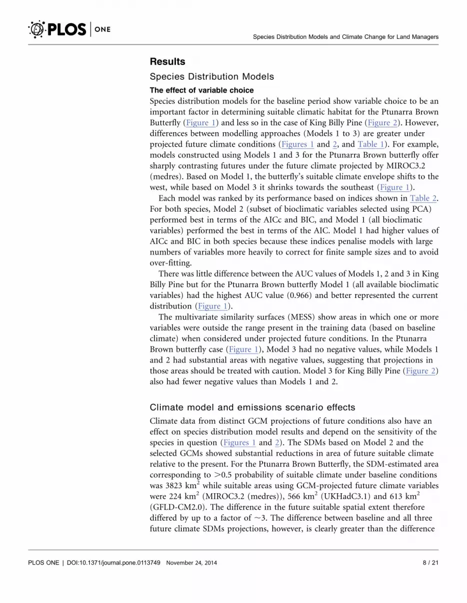
Species distribution models for the baseline period show variable choice to be an
important factor in determining suitable climatic habitat for the Ptunarra Brown
Butterfly (Figure 1) and less so in the case of King Billy Pine (Figure 2). However,
differences between modelling approaches (Models 1 to 3) are greater under
projected future climate conditions (Figures 1 and 2, and Table 1). For example,
models constructed using Models 1 and 3 for the Ptunarra Brown butterfly offer
sharply contrasting futures under the future climate projected by MIROC3.2
(medres). Based on Model 1, the butterfly’s suitable climate envelope shifts to the
west, while based on Model 3 it shrinks towards the southeast (Figure 1).
Each model was ranked by its performance based on indices shown in Table 2.
For both species, Model 2 (subset of bioclimatic variables selected using PCA)
performed best in terms of the AICc and BIC, and Model 1 (all bioclimatic
variables) performed the best in terms of the AIC. Model 1 had higher values of
AICc and BIC in both species because these indices penalise models with large
numbers of variables more heavily to correct for finite sample sizes and to avoid
over-fitting.
There was little difference between the AUC values of Models 1, 2 and 3 in King
Billy Pine but for the Ptunarra Brown butterfly Model 1 (all available bioclimatic
variables) had the highest AUC value (0.966) and better represented the current
distribution (Figure 1).
The multivariate similarity surfaces (MESS) show areas in which one or more
variables were outside the range present in the training data (based on baseline
climate) when considered under projected future conditions. In the Ptunarra
Brown butterfly case (Figure 1), Model 3 had no negative values, while Models 1
and 2 had substantial areas with negative values, suggesting that projections in
those areas should be treated with caution. Model 3 for King Billy Pine (Figure 2)
also had fewer negative values than Models 1 and 2.
Climate model and emissions scenario effects
Climate data from distinct GCM projections of future conditions also have an
effect on species distribution model results and depend on the sensitivity of the
species in question (Figures 1 and 2). The SDMs based on Model 2 and the
selected GCMs showed substantial reductions in area of future suitable climate
relative to the present. For the Ptunarra Brown Butterfly, the SDM-estimated area
corresponding to .0.5 probability of suitable climate under baseline conditions
was 3823 km2 while suitable areas using GCM-projected future climate variables
were 224 km2 (MIROC3.2 (medres)), 566 km2 (UKHadC3.1) and 613 km2
(GFLD-CM2.0). The difference in the future suitable spatial extent therefore
differed by up to a factor of ,3. The difference between baseline and all three
future climate SDMs projections, however, is clearly greater than the difference
Species Distribution Models and Climate Change for Land Managers
PLOS ONE | DOI:10.1371/journal.pone.0113749 November 24, 2014 8 / 21
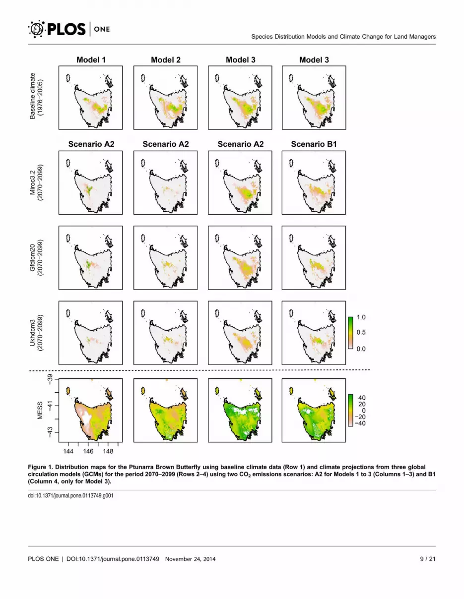
Figure 1. Distribution maps for the Ptunarra Brown Butterfly using baseline climate data (Row 1) and climate projections from three globalcirculation models (GCMs) for the period 2070–2099 (Rows 2–4) using two CO2 emissions scenarios: A2 for Models 1 to 3 (Columns 1–3) and B1(Column 4, only for Model 3).
doi:10.1371/journal.pone.0113749.g001
Species Distribution Models and Climate Change for Land Managers
PLOS ONE | DOI:10.1371/journal.pone.0113749 November 24, 2014 9 / 21
Figure 2. Distribution maps for King Billy Pine using baseline climate data (Row 1) and climate projections from three global circulation models(GCMs) for the period 2070–2099 (Rows 2–4) using two CO2 emissions scenarios: A2 for Models 1 to 3 (Columns 1–3) and B1 (Column 4, only forModel 3).
doi:10.1371/journal.pone.0113749.g002
Species Distribution Models and Climate Change for Land Managers
PLOS ONE | DOI:10.1371/journal.pone.0113749 November 24, 2014 10 / 21

between that arising from the three GCMs. For King Billy Pine, the corresponding
areas for Model 2 were 3806 km2, 134 km2 (MIROC3.2 (medres)), 154 km2
(UKHadC3.1) and 150 km2 (GFLD-CM2.0) (see Table A2 in File S1); a
comparable level of projected reduction from the baseline but with less difference
between GCMs.
Choice of future emissions scenario also affected the results of the SDMs
(Model 3 in Figures 2 and 3). The A2 emissions scenario results in reduced areas
of potential suitable climate compared to the lower B1 emissions scenario and this
was the case for both species (see also Figures S4 and S5). The I similarity statistic
showed SDM predictions based on output from GCMs using A2 (higher)
emissions scenarios to be substantially different from B1 in relation to baseline
predicted suitable areas. Lower values of I found in SDMs derived from the A2
scenario represent higher degrees of difference relative to baseline SDMs
(Table 3). Similarly, the difference maps present a substantial loss in suitable
climate when baseline SDM are compared to the future projections for the A2
emissions scenario using Model 2 (the difference maps in Figures S2 and S3).
These results, while not surprising given the strong association between emissions
and rising temperature, highlight the importance of explicit recognition of
Table 1. Variables identified as important in determining species distribution.
Variable Importance
Ptunarra Brown Butterfly King Billy Pine
Model 1 Mean temperature driest quarter (33%); minimumtemperature coldest period (28%); radiation warmestquarter (7.7%); radiation seasonality (7%); highest periodradiation (5%); radiation coldest quarter (3%)
Mean temperature wettest quarter (22.0%); radiation coldest quarter(16.1%); lowest period moisture index (10.4%); mean temperaturewarmest quarter (6.3%); temperature seasonality (4%); meanmoisture index lowest quarter (3.8%); radiation seasonality (3.6%)
Model 2 Mean temperature driest quarter (53.8%); temperatureseasonality (28.3%); annual precipitation (10.5%);maximum temperature warmest period (7.4%)
Annual mean temperature (49.5%), annual mean radiation (17%);radiation seasonality (12%); annual precipitation (8.2%); temperatureseasonality (4.9%); annual mean moisture index (4.8%); temperatureannual range (3.3%); highest period moisture index (0.2%)
Model 3 April minimum temperature (46%); radiation with rainfallApril (22%); March minimum temperature (16%); annualrainfall (12%); annual minimum temperature (4%)
Mean temperature warmest quarter (36.8%); mean annual precipita-tion (14.2%); lowest period moisture index (13.1%); mean tempera-ture coldest quarter (12%); precipitation driest period (8.2%); annualmean moisture index (5.1%); mean moisture index lowest quarter(4.2%); minimum temperature coldest period (3.9%); maximumtemperature warmest period (2.5%)
doi:10.1371/journal.pone.0113749.t001
Table 2. Statistical model selection indices.
Ptunarra Brown Butterfly King Billy Pine
Model 1 Model 2 Model 3 Model 1 Model 2 Model 3
AIC 3996.30 4000.22 4142.47 7074.82 7174.78 7302.27
AICc 4568.30 4078.51 4311.20 7280.61 7233.80 7367.39
BIC 4474.30 4245.25 4472.34 7678.87 7538.00 7681.28
AUC 0.97 0.94 0.93 0.95 0.94 0.93
Best performance for each model shown in bold.
doi:10.1371/journal.pone.0113749.t002
Species Distribution Models and Climate Change for Land Managers
PLOS ONE | DOI:10.1371/journal.pone.0113749 November 24, 2014 11 / 21

emissions scenario in all SDM construction for any species with potential
temperature dependence. They also point to the potential benefits to biodiversity
of immediate climate change mitigation (Warren et al. 2013).
The effect of different approaches to summarising multiple
species distribution models
Maps showing the spatial effect of the three approaches for summarising multiple
SDMs are shown in Figure 3. Of particular interest is the model agreement map.
While the total geographic area of suitable climate is comparable between the
different future projections, they are not geographically coincident.
Figure 3. Alternative summaries for multiple species distribution models. Maps are model summaries for the Ptunarra Brown Butterfly (left) and KingBilly Pine (right) using models based on six GCM inputs; means and standard deviations (Row 1); spatial extents where at least one model indicates suitablehabitat (Row 2); agreement between models, where at least one model predicted suitability above 0.5 (Row 3); model agreement overlayed on the baselinedistribution for the species (Row 4).
doi:10.1371/journal.pone.0113749.g003
Table 3. The I similarity statistic for future projections of suitable climatic habitat for 2070–2099 using Model 2 in relation to the baseline predicted habitat forthe species.
UKHadC3.1 GFDL-CM2.1 Miroc2.0 (medres)
A2 B1 A2 B1 A2 B1
Ptunarra Brown 0.551 0.656 0.531 0.651 0.547 0.720
King Billy Pine 0.513 0.543 0.735 0.855 0.711 0.848
Values range from zero (no distribution overlap) to one (identical distributions). A2 values show reduced similarity in every instance.
doi:10.1371/journal.pone.0113749.t003
Species Distribution Models and Climate Change for Land Managers
PLOS ONE | DOI:10.1371/journal.pone.0113749 November 24, 2014 12 / 21

Discussion
Common approaches to modelling future species distributions in applied
ecological studies do not always represent the uncertainty associated with variable
selection and the influence of the range in future climate projections and
emissions scenarios. Using two species as case studies, we have shown that these
uncertainties can affect the results of SDMs.
Ignoring the uncertainty associated with modelling future distributions may
lead to over-confidence in single maps of future distributions, with consequences
for conservation planning. The literature review revealed that both choice of
variables and representation of future climate, by using a range of GCMs, are
frequently opportunistic for SDMs in applied ecological studies. Using all
available bioclimatic variables, instead of a tailored selection, increases the
possibility of over-fitting species distribution models, and may lead to an over-
estimate of range reduction and the likelihood of a forecasted extinction under
climate change [16].
The importance of variable selection in determining the output of SDM
depends on the characteristics of the species modelled. For example, variable
selection may be less important for long-lived sedentary plant species such as the
King Billy Pine but can be very important for mobile species with specific
biological characteristics or requirements, such as the Ptunarra Brown Butterfly.
For the butterfly, inclusion of different variables in the model led to widely
divergent projected futures for end-of-century, ranging from close to no locations
with a suitable climate [61] to maintenance of the current range.
Biological knowledge of the species can help in choosing variables amenable to
ecological interpretation. Ideally, modellers, species experts and conservation
practitioners should work as a team to build the SDM, interpret results and
consider conservation management responses. However, such interdisciplinary
exercises are uncommon and often little is known of the species’ biology and
ecology as they relate to climatic factors. In these cases, a range of statistical
diagnostics can provide some guidance as to relative model performance, but
there is no objective method for identifying the ‘best’ SDM when projecting into
the future. Statistical methods of model selection alone are not sufficient to accept
or reject a model, as different performance indices (e.g. AUC, AIC, BIC) can give
conflicting rankings [62]. Furthermore, statistical models are a measure of
internal model performance, not a measure of ecological validity.
The accuracy with which the current distribution is represented by a SDM is an
important consideration. However, an accurate fit with current distributions does
not guarantee that the prediction of future potential distribution will be accurate.
The underlying statistical relationship between the climatic variables and the
distribution of the species may change due to, for example, nonlinear functional
responses of the species or indirect impacts such as an altered fire regime.
Considering the extent to which a SDM is attempting to project into novel
climatic conditions is also an important consideration in model evaluation.
Predicted potential distribution maps with large areas in which one or more
Species Distribution Models and Climate Change for Land Managers
PLOS ONE | DOI:10.1371/journal.pone.0113749 November 24, 2014 13 / 21

climate variables were outside the range present in the data used to train the SDM
should be treated with caution.
In contrast to variable selection, the range in outputs from climate models and
emissions scenarios are not species dependent and will always need to be
documented when modelling future distributions. We caution against using an
ensemble mean of projected climate variables as input into an SDM, for several
reasons. First, each global climate model represents one plausible future among
many. The Coupled Model Intercomparison Project Phase 5 (CMIP5) now
includes more than 50 climate models. Although there are several quantitative
model ‘skill scores’ that can be calculated for particular variables and features of
the models, different models tend to perform well on some metrics and poorly on
others. As a result, the IPCC avoids ranking models, and treats each equally (IPCC
2007, 2013). While multi-model GCM ensembles at large spatial scales have been
shown to agree better with observations of present-day climate than single models
for a range of variables [63,64], this is not always the case at smaller scales,
including the continental scale [65]. Considering multiple GCMs is therefore
essential to capture the range of plausible projections. Further, the ensemble mean
may not coincide with any of the climate model’s projections but create a novel
future climate that is merely a statistical derivative. And finally, using a multi-
model GCM ensemble may not be the best approach for risk assessment in
conservation planning, where considering the ‘best’ and ‘worst’ case scenarios may
be a more useful framework in which to make decisions [61,66].
Multiple SDMs need to be run using a range of climate models and emissions
scenarios as input. This approach produces a range of species distribution maps
(12 for each species in our case study) which need to be assessed and combined in
a useful way to help inform decision-making. The method used to combine the
maps (e.g. taking the mean, the median, the bounding box or the minimum
overlap of the different models) will influence interpretation of the results. This
can have consequences where conservation effort is deployed across the landscape
since both extent and location of projected suitable climate will differ between
GCMs. Over-confidence in a single map risks the possibility that conservation
investments are applied to areas that do not support the target species under
future climate. Ongoing monitoring is essential to track changes as the species
responds to changing climatic conditions. Using a map of an ensemble mean
produces a future that was not projected by any single model. Adding all areas
projected to be suitable (the bounding box) will be the most optimistic outlook,
while only concentrating on areas where all models agree will provide the smallest
estimate of future suitability.
The managers we consulted found that the most informative summary was the
map showing the agreement between the models (pixels where all models agree a
potential suitability above a threshold of 0.5) in addition to the current
distribution as projected by the SDM that used baseline climate data. This was
considered a low-risk option to highlight priority areas for biodiversity
conservation in areas that currently support a target species or community.
Species Distribution Models and Climate Change for Land Managers
PLOS ONE | DOI:10.1371/journal.pone.0113749 November 24, 2014 14 / 21

One aspect of uncertainty in modelling future species distribution not
illustrated here is that associated with the choice of SDM. Different statistical
models have been shown to have a large influence on the results of SDMs and an
ensemble approach is increasingly being used to account for the range in statistical
models [10,37]. However, the main purpose of this paper was to illustrate the
effect that choice of variable, climate model and emissions scenario can have on
Figure 4. Decision tree to guide the application of SDMs under future climate to conservationmanagement.
doi:10.1371/journal.pone.0113749.g004
Species Distribution Models and Climate Change for Land Managers
PLOS ONE | DOI:10.1371/journal.pone.0113749 November 24, 2014 15 / 21

the results of SDMs for future climatic conditions. We propose a protocol for
conservation planners and managers that summarises our recommendations for
using SDM under future climate projections in applied ecological studies
(Figure 4).
Our study highlighted that the relative change in the projected suitable climate
envelope for the species is an important factor to consider. Our SDMs, based on
climate variables, show that projections for the King Billy Pine are more
consistent, and more consistently under threat, when viewed as relative change. A
general hypothesis based on our results is that species with strong temperature
dependencies are more strongly influenced by choice of emissions scenarios. If the
future climate projections of the GCMs diverge, so will the SDMs, while if the
climatic factor were not influential in the baseline model, the effect may be
inconsequential. However, there is a threshold below which relative change is not
important because, for example, the projected areas may not be of sufficient
extent to support the species in any case. It is also important to note that our
models, and SDM models generally, do not account for any of the other major
threat to species such as habitat loss. All of these points emphasise that correct
interpretation of a SDM outcome requires rigorous understanding of the inputs
used in its development.
Conclusions
Species distribution models are useful tools for, among other things, informing
the conservation management of wildlife and their habitats under a rapidly
changing climate. They can provide decision makers with information about the
likely degree of change in a species climatic domain and geographic distribution.
However, the uncertainty associated with their estimation needs to be
documented and understood if their output is to be effectively applied. Systematic
conservation planning can draw on this information, together with ongoing field
monitoring of target species to track changes as they occur, providing the
foundation for adaptive management in response to emerging circumstances.
Supporting Information
Figure S1. The proportion of variables used in the revised literature.
doi:10.1371/journal.pone.0113749.s001 (TIF)
Figure S2. Distribution maps of significant difference (SD) between the current
prediction of suitable habitat for Ptunarra Brown (PB) based on baseline climate,
and the future projections, based on 30 Model 2 (M2, PCA selection of bioclimatic
variables). The difference maps showed when the distribution predicted
significantly more (+ve) or less suitable habitat (2ve) (SD>0.975 or SD#0.025,
respectively) and where there was no significant (ns) difference between models.
doi:10.1371/journal.pone.0113749.s002 (TIF)
Species Distribution Models and Climate Change for Land Managers
PLOS ONE | DOI:10.1371/journal.pone.0113749 November 24, 2014 16 / 21

Figure S3. Distribution maps of significant difference (SD) between the current
prediction of suitable habitat for King Billy Pine (KB) based on baseline climate,
and the future projections based on Model 2 (M2, PCA selection of bioclimatic
variables). The difference maps showed when the distribution predicted
significantly more (+ve) or less suitable habitat (2ve) (SD>0.975 or SD#0.025,
respectively) and where there was no significant (ns) difference between models.
doi:10.1371/journal.pone.0113749.s003 (TIF)
Figure S4. Differences in annual mean temperature and annual rain within the
current distribution of the Ptunarra Brwon Butterfly. Where the box spans the
interquartile range, the segment inside the box 45 shows the median and whiskers
above and below the box show the locations of the minimum and maximum
values; the circles represent outliers.
doi:10.1371/journal.pone.0113749.s004 (TIF)
Figure S5. Differences in annual mean temperature and annual rain within the
current distribution of the King Billy Pine. Where the box spans the interquartile
range, the segment inside the box shows the median and whiskers above and
below the box show the locations of the minimum and maximum values; the
circles represent outliers.
doi:10.1371/journal.pone.0113749.s005 (TIF)
File S1. Table A1, List of bioclimatic variables used in the SDM for Orexeinica
ptunarra and Athrotaxis selaginoides. Subset of variable using a PCA is denoted
by ‘PCA’ and the subset selection made by experts is denoted by ‘x’. The
Orexeinica ptunarra’s experts selected monthly variables. Table A2, The area
predicted to be climatically suitable for the species based on the current and future
climate projections. Pixels for the Ptunarra Brown Butterfly and the King Billy
Pine that with a value0.5 or more were considered as ‘suitable’. The areas are
shown in km2 for Models 1 to 3 based on the SRES scenario A2, and only for
Model 3 based on SRES scenario B1. Maps were projected to 25 World Geodetic
System 1984, Universal Transverse Mercator coordinate system Zone 55 South.
doi:10.1371/journal.pone.0113749.s006 (PDF)
File S2.
doi:10.1371/journal.pone.0113749.s007 (ZIP)
Acknowledgments
Dr Peter McQuillan (UTAS) and Dr Phil Bell (DPIPWE) guided our choice of
variables for the Ptunarra Brown Butterfly and Dr Jenni Whinam (DPIPWE) and
Ms Louise Gilfedder (DPIPWE) provided expert opinion on the King Billy Pine.
Mr Tomas Remenyi (UTAS) helped with R code and Ms Lauren Carter (ANU)
assisted with the figures.
Species Distribution Models and Climate Change for Land Managers
PLOS ONE | DOI:10.1371/journal.pone.0113749 November 24, 2014 17 / 21

Author ContributionsConceived and designed the experiments: LLP RMBH. Performed the
experiments: LLP RMBH SH GL. Analyzed the data: LLP RMBH SH GL BM ECL.
Contributed reagents/materials/analysis tools: LLP RMBH SH GL BM SFG ECL
NLB. Wrote the paper: LLP RMBH GL BM.
References
1. Wiens JA, Stralberg D, Jongsomjit D, Howell CA, Snyder MA (2009) Niches, models, and climatechange: Assessing the assumptions and uncertainties. Proceedings of the National Academy ofSciences of the United States of America 106: 19729–19736.
2. Barrows CW, Rotenberry JT, Allen MF (2010) Assessing sensitivity to climate change and droughtvariability of a sand dune endemic lizard. Biological Conservation 143: 731–736.
3. Gritti ES, Smith B, Sykes MT (2006) Vulnerability of Mediterranean Basin ecosystems to climatechange and invasion by exotic plant species. Journal of Biogeography 33: 145–157.
4. Williams SE, Bolitho EE, Fox S (2003) Climate Change in Australian Tropical Rainforests: AnImpending Environmental Catastrophe. Proceedings: Biological Sciences 270: 1887–1892.
5. Thomas CD, Cameron A, Green RE, Bakkenes M, Beaumont LJ, et al. (2004) Extinction risk fromclimate change. Nature 427: 145–148.
6. Araujo MB, Cabeza M, Thuiller W, Hannah L, Williams PH (2004) Would climate change drive speciesout of reserves? An assessment of existing reserve-selection methods. Global Change Biology 10:1618–1626.
7. Tellez-Valdes O, Davila-Aranda P (2003) Protected areas and climate change: A case study of the cactiin the Tehuacan-Cuicatlan biosphere reserve, Mexico. Conservation Biology 17: 846–853.
8. Pyke CR, Andelman SJ, Midgley G (2005) Identifying priority areas for bioclimatic representation underclimate change: a case study for Proteaceae in the Cape Floristic Region, South Africa. BiologicalConservation 125: 1–9.
9. Pyke CR, Fischer DT (2005) Selection of bioclimatically representative biological reserve systemsunder climate change. Biological Conservation 121: 429–441.
10. Diniz-Filho JAF, Mauricio Bini L, Fernando Rangel T, Loyola RD, Hof C, et al. (2009) Partitioning andmapping uncertainties in ensembles of forecasts of species turnover under climate change. Ecography32: 897–906.
11. Araujo MB, Whittaker RJ, Ladle RJ, Erhard M (2005) Reducing uncertainty in projections of extinctionrisk from climate change. Global Ecology and Biogeography 14: 529–538.
12. Thuiller W (2004) Patterns and uncertainties of species’ range shifts under climate change. GlobalChange Biology 10: 2020–2027.
13. Pearson RG, Thuiller W, Araujo MB, Martinez-Meyer E, Brotons L, et al. (2006) Model-baseduncertainty in species range prediction. Journal of Biogeography 33: 1704–1711.
14. Buisson L, Thuiller W, Casajus N, Lek S, Grenouillet G (2010) Uncertainty in ensemble forecasting ofspecies distribution. Global Change Biology 16: 1145–1157.
15. Cheaib A, Badeau V, Boe J, Chuine I, Delire C, et al. (2012) Climate change impacts on tree ranges:model intercomparison facilitates understanding and quantification of uncertainty. Ecology Letters 15:533–544.
16. Beaumont LJ, Hughes L, Poulsen M (2005) Predicting species distributions: use of climaticparameters in BIOCLIM and its impact on predictions of species’ current and future distributions.Ecological Modelling 186: 250–269.
17. Synes NW, Osborne PE (2011) Choice of predictor variables as a source of uncertainty in continental-scale species distribution modelling under climate change. Global Ecology and Biogeography 20: 904–914.
Species Distribution Models and Climate Change for Land Managers
PLOS ONE | DOI:10.1371/journal.pone.0113749 November 24, 2014 18 / 21

18. Braunisch V, Coppes J, Arlettaz R, Suchant R, Schmid H, et al. (2013) Selecting from correlatedclimate variables: a major source of uncertainty for predicting species distributions under climate change.Ecography 36: 971–983.
19. Garcia RA, Burgess ND, Cabeza M, Rahbek C, Araujo MB (2012) Exploring consensus in 21stcentury projections of climatically suitable areas for African vertebrates. Global Change Biology 18:1253–1269.
20. Beaumont LJ, Hughes L, Pitman AJ (2008) Why is the choice of future climate scenarios for speciesdistribution modelling important? Ecology Letters 11: 1135–1146.
21. Kriticos D, Brown J, Maywald G, Sutherst R, Adkins S, et al. A population model of Acacia nilotica: a toolfor exploring weed management and the effects of climate change; 1999. International RangelandCongress, Inc. pp. 870–872.
22. Shabani F, Kumar L, Taylor S (2012) Climate change impacts on the future distribution of date palms: amodeling exercise using CLIMEX. PloS one 7: e48021.
23. Araujo MB, New M (2007) Ensemble forecasting of species distributions. Trends in Ecology & Evolution22: 42–47.
24. Elith J, Graham CH, Anderson RP, Dudık M, Ferrier S, et al. (2006) Novel methods improve predictionof species’ distributions from occurrence data. Ecography 29: 129–151.
25. Pearson RG, Thuiller W, Araujo MB, Martinez-Meyer E, Brotons L, et al. (2006) Model-baseduncertainty in species range prediction. Journal of Biogeography 33: 1704–1711.
26. Carpenter SR, Mooney HA, Agard J, Capistrano D, DeFries RS, et al. (2009) Science for managingecosystem services: Beyond the Millennium Ecosystem Assessment. Proceedings of the NationalAcademy of Sciences of the United States of America 106: 1305–1312.
27. Flower A, Murdock TQ, Taylor SW, Zwiers FW (2013) Using an ensemble of downscaled climatemodel projections to assess impacts of climate change on the potential distribution of spruce andDouglas-fir forests in British Columbia. Environmental Science & Policy 26: 63–74.
28. Grenouillet G, Buisson L, Casajus N, Lek S (2011) Ensemble modelling of species distribution: theeffects of geographical and environmental ranges. Ecography 34: 9–17.
29. Huntley B, Collingham YC, Willis SG, Green RE (2008) Potential Impacts of Climatic Change onEuropean Breeding Birds. Plos One 3.
30. Li YP, Ye W, Wang M, Yan XD (2009) Climate change and drought: a risk assessment of crop-yieldimpacts. Climate Research 39: 31–46.
31. Marmion M, Parviainen M, Luoto M, Heikkinen RK, Thuiller W (2009) Evaluation of consensusmethods in predictive species distribution modelling. Diversity and Distributions 15: 59–69.
32. Pie MR, Meyer ALS, Firkowski CR, Ribeiro LF, Bornschein MR (2013) Understanding themechanisms underlying the distribution of microendemic montane frogs (Brachycephalus spp.,Terrarana: Brachycephalidae) in the Brazilian Atlantic Rainforest. Ecological Modelling 250: 165–176.
33. Thuiller W, Lafourcade B, Engler R, Araujo MB (2009) BIOMOD – a platform for ensemble forecastingof species distributions. Ecography 32: 369–373.
34. Hamby D (1994) A review of techniques for parameter sensitivity analysis of environmental models.Environmental monitoring and assessment 32: 135–154.
35. Johnson CJ, Gillingham MP (2008) Sensitivity of species-distribution models to error, bias, and modeldesign: an application to resource selection functions for woodland caribou. Ecological Modelling 213:143–155.
36. Shabani F, Kumar L (2014) Sensitivity Analysis of CLIMEX Parameters in Modeling PotentialDistribution of Phoenix dactylifera L. PloS one 9: e94867.
37. Araujo MB, New M (2007) Ensemble forecasting of species distributions. Trends in Ecology & Evolution22: 42–47.
38. Rosentrater LD (2010) Representing and using scenarios for responding to climate change. WileyInterdisciplinary Reviews-Climate Change 1: 253–259.
Species Distribution Models and Climate Change for Land Managers
PLOS ONE | DOI:10.1371/journal.pone.0113749 November 24, 2014 19 / 21
39. Weaver CP, Lempert RJ, Brown C, Hall JA, Revell D, et al. (2013) Improving the contribution ofclimate model information to decision making: the value and demands of robust decision frameworks.Wiley Interdisciplinary Reviews: Climate Change 4: 39–60.
40. Booth TH, Nix HA, Busby JR, Hutchinson MF (2014) bioclim: the first species distribution modellingpackage, its early applications and relevance to most current MaxEnt studies. Diversity and Distributions20: 1–9.
41. R Development Core Team (2005) R: A language and environment for statistical computing, referenceindex version 3.0.0. In:, Computing RFfS, , editor. Available: http://wwwR-projectorg. Viena, Austria.
42. Xu T, Hutchinson MF (2011) ANUCLIM Version 6.1. Canberra: Fenner School of Environment andSociety, Australian National University.
43. Hijmans R, Cameron S, Parra J, Jones P, Jarvis A (2004) The WorldClim interpolated global terrestrialclimate surfaces. Version 1.3.
44. Yang G-J, Gemperli A, Vounatsou P, Tanner M, Zhou X-N, et al. (2006) A growing degree-days basedtime-series analysis for prediction of Schistosoma japonicum transmission in Jiangsu province, China.The American journal of tropical medicine and hygiene 75: 549–555.
45. Bradley BA (2009) Regional analysis of the impacts of climate change on cheatgrass invasion showspotential risk and opportunity. Global Change Biology 15: 196–208.
46. Bradley BA (2010) Assessing ecosystem threats from global and regional change: hierarchicalmodeling of risk to sagebrush ecosystems from climate change, land use and invasive species inNevada, USA. Ecography 33: 198–208.
47. Bradley BA, Oppenheimer M, Wilcove DS (2009) Climate change and plant invasions: restorationopportunities ahead? Global Change Biology 15: 1511–1521.
48. Bradley BA, Wilcove DS (2009) When Invasive Plants Disappear: Transformative RestorationPossibilities in the Western United States Resulting from Climate Change. Restoration Ecology 17: 715–721.
49. Bradley BA, Wilcove DS, Oppenheimer M (2010) Climate change increases risk of plant invasion inthe Eastern United States. Biological Invasions 12: 1855–1872.
50. Lawler JJ, Shafer SL, Blaustein AR (2010) Projected Climate Impacts for the Amphibians of theWestern Hemisphere. Conservation Biology 24: 38–50.
51. Phillips SJ, Anderson RP, Schapire RE (2006) Maximum entropy modeling of species geographicdistributions. Ecological Modelling 190: 231–259.
52. Elith J, Leathwick JR (2009) Species Distribution Models: Ecological Explanation and PredictionAcross Space and Time. Annual Review of Ecology Evolution and Systematics. pp. 677–697.
53. Phillips SJ, Dudık M (2008) Modeling of species distributions with Maxent: new extensions and acomprehensive evaluation. Ecography 31: 161–175.
54. Warren DL, Glor RE, Turelli M (2010) ENMTools: a toolbox for comparative studies of environmentalniche models. Ecography 33: 607–611.
55. VanDerWal J, Falconi L, Januchowski S, Shoo L, Storlie C (2011) SDMTools: Species distributionmodelling tools: Tools for processing data associated with species distribution modelling exercises.R package version 1.
56. Bateman BL, VanDerWal J, Williams SE, Johnson CN (2012) Biotic interactions influence theprojected distribution of a specialist mammal under climate change. Diversity and Distributions 18: 861–872.
57. Januchowski S, Pressey R, VanDerWal J, Edwards A (2010) Characterizing errors in digital elevationmodels and estimating the financial costs of accuracy. International Journal of Geographical InformationScience 24: 1327–1347.
58. Corney SP, Katzfey JJ, McGregor JL, Grose MR, Bennett JC, et al. (2010) Climate Futures forTasmania: climate modelling technical report. Hobart, Tasmania. Available: http://www.dpac.tas.gov.au/divisions/climatechange/adapting/climate_futures/climate_futures_for_tasmania_reports: AntarcticClimate & Ecosystems Cooperative Research Centre.
59. Meehl GA, Covey C, Delworth T, Latif M, McAvaney B, et al. (2007) The WCRP CMIP3 multimodeldataset - A new era in climate change research. Bulletin of the American Meteorological Society 88
Species Distribution Models and Climate Change for Land Managers
PLOS ONE | DOI:10.1371/journal.pone.0113749 November 24, 2014 20 / 21

60. IPCC (2007) Climate Change 2007: The Physical Science Basis. Contribution of Working Group I to theFourth Assessment Report of the Intergovernmental Panel on Climate Change. Cambridge UniversityPress, Cambridge, United Kingdom and New York, NY, USA.
61. Harris RMB, Porfirio LL, Hugh S, Lee G, Bindoff NL, et al. (2013) To Be Or Not to Be? Variableselection can change the projected fate of a threatened species under future climate. EcologicalManagement & Restoration 14: n/a-n/a.
62. Burnham KP, Anderson DR (2002) Model Selection and Multi-model Inference: A Practical Information-Theoretic Approach: Springer-Verlag.
63. Murphy JM, Sexton DMH, Barnett DN, Jones GS, Webb MJ, et al. (2004) Quantification of modellinguncertainties in a large ensemble of climate change simulations. Nature 430: 768–772.
64. Reichler T, Kim J (2008) How well do coupled models simulate today’s climate? Bulletin of the AmericanMeteorological Society 89: 303-+.
65. Fordham DA, Wigley TML, Brook BW (2011) Multi-model climate projections for biodiversity riskassessments. Ecological Applications 21: 3317–3331.
66. Harris RMB, Grose MR, Lee G, Bindoff NL, Porfirio LL, et al. (2014) Climate projections forecologists. Wiley Interdisciplinary Reviews: Climate Change: n/a-n/a.
Species Distribution Models and Climate Change for Land Managers
PLOS ONE | DOI:10.1371/journal.pone.0113749 November 24, 2014 21 / 21
Copyright © 2022 FDOKUMEN