ISSN:

Journal of Biodiversity & Endangered Species

The International Open AccessJournal of Biodiversity & Endangered Species

Executive Editors

Dr. Masahiro KatoNational Museum of Nature and Science HerbariumJapan

This article was originally published in a journal by OMICS Publishing Group, and the attached copy is provided by OMICS

Publishing Group for the author’s benefit and for the benefit of the author’s institution, for commercial/research/educational use including without limitation use in instruction at your institution, sending it to specific colleagues that you know, and providing a copy to your institution’s administrator.

All other uses, reproduction and distribution, including without limitation commercial reprints, selling or licensing copies or access, or posting on open internet sites, your personal or institution’s website or repository, are requested to cite properly.

Available online at: OMICS Publishing Group (www.omicsonline.org)

Digital Object Identifier: http://dx.doi.org/10.4172/jbes.1000107

Volume 1 • Issue 2 • 1000107J Biodivers Endanger SpeciesISSN: JBES an open access journal

Research Article Open Access

Biodiversity & Endangered SpeciesLuque et al., J Biodivers Endanger Species 2013, 1:2

http://dx.doi.org/10.4172/jbes.1000107

Keywords: Biodiversity conservation; Hazel Grouse; Landscape structure; Habitat suitability models; Management decision

IntroductionWithin the current context of rapid landscape change [1-5], habitat

loss is widely regarded as a major factor contributing to the decline of biodiversity [6-11]. Alpine ecosystems have been less modified by human activities than other lowland ecosystems. Nevertheless, current pressures of tourism and other forms of development in mountain areas, are significantly changing landscape structure due to growing human pressures over the last decades [12-13]. Such subtle changes in the landscape matrix is increasingly making habitat unsuitable for many life form, especially for specialist’s species habitats [14-16]. Therefore, we face the challenge to monitor not just changes in natural systems but also the impact of these changes on the health and persistence of the species that depend on these environments. At present, still ecologists, conservation practitioners, and managers require modern specific tools essential for an effective landscape planning to face the increasing threats to biodiversity [17]. In order to reintroduce and rehabilitate the threatened species and to understand environmental and landscape determination of species distribution [18-21], a detailed knowledge about spatial distribution of their potential habitat [22] is a crucial challenge for planning biological conservation priorities [23-28].

Species distribution models SDMs [29] have shown great potential to help achieve conservation goals by refiningour knowledge of species distribution [30]. SDMs are referred as habitat suitability models [22]. These niche models identify areas that are ecologically suitable for the presence of species [22,29,31]. Extensive use of SDMs has broad important applications to support management decisions with regard to biodiversity [29,32-34]. Many examples can be cited that have made such an extensive use of different applications using SDMs approaches, for assessing global impacts, prioritizing or targeting areas for protected

status, assessing threats to those areas, predicting distribution in unsurveyed areas and designing reserves [35-42].

These models are created on the bases of statistical relationships between landscape or/and environmental characteristics and species data [43]. Actually, the species location information from specimen records and other source are widely available due to the development of digital databases for natural history collection [44]. Hence, SDMs provide an alternative approach that can help extend the usefulness of direct observation and improve interpretation and understanding of species distributions [29]. Many methods are used to fit SDMs that may be more or less applicable depending on the type of biological and environmental data available, the species of interest and the aim of the model. Using presence/absence species data is very popular to model species distribution [43, 45-46]. Nevertheless, the rarity and heterogeneity of scarce or endangered species limit the use of these conventional methods to model their habitats. The rarity and low reliability of absence data also limit the use of this method [47-48]. Therefore, new methods have been developed to improve prediction of species distribution from presence data only [32,40,49], which are often

*Corresponding author: S. Luque, Mountain Ecosystem Unit, National Research Institute of Science and Technology for Environment and Agriculture, France, E-mail: Sandra. luque@irstea. fr

Received May 17, 2013; Accepted July 26, 2013; Published August 01, 2013

Citation: Adra W, Delcros P, Luque S (2013) Landscape Structure Indicators as a Key Feature in Habitat Selection: an Operational Approach to Conservation Planning. J Biodivers Endanger Species 1:107. doi:10.4172/jbes.1000107

Copyright: © 2013 Luque S, et al. This is an open-access article distributed under the terms of the Creative Commons Attribution License, which permits unrestricted use, distribution, and reproduction in any medium, provided the original author and source are credited.

AbstractLandscape structure is a key factor for biodiversity conservation. We assessed the potential role of landscape-

related habitat structure on Hazel Grouse (Tetrastesbonasia) by recording the occurrence of the species. Hazel Grouse is a widely recognized endangered species, because of the habitat loss as a direct consequence of land use change that is jeopardizing the species survival. The aim of this study is to provide a method based on habitat suitability modelling to explore and analyse hazel grouse- landscape structure and its relation to key habitat features. We evaluated landscape factors and critical threshold for monitoring the species, in order to assess the predictive power of models based on field surveys, ancillary information and high resolution infrared aerial photographs. We tested Maximum Entropy (MaxEnt) algorithm, in order to predict the distribution of Hazel Grouse species, in the complex mountain landscape within the study site. This presence-only modelling method has showed numerous advantages over many other approaches. It is based on a function that links the fitness of individuals to their environment. Our results were highly consistent with field knowledge, showing that habitat modelling generated using spatial statistics and GIS can effectively help in the characterization of habitat requirements and the localization of the species suitable habitat. We found also that key drivers of Hazel Grouse distribution are not only environmental factors, in particular linked to elevation in mountain areas, but also landscape heterogeneity is a key feature. Hence, conservation of this species will require land management practices that maintain heterogeneous landscape; in particular small forest openings are essential for the species. The approach developed seem to be a promising operational tool for local and regional managers interested in species monitoring and management within the long term.

Landscape Structure Indicators as a Key Feature in Habitat Selection: an Operational Approach to Conservation PlanningAdra W1, Delcros P2 and Luque S2*1Tichreen University, Department of Forestry and Ecology, Faculty of Agronomie, Lattakia, Syrie2IRSTEA, Mountain Ecosystem Unit, National Research Institute of Science and Technology for Environment and Agriculture, France. 2 rue de la Papéterie, BP 76, 38402 Saint-Martin-d’Hères Cedex, France

Citation: Adra W, Delcros P, Luque S (2013) Landscape Structure Indicators as a Key Feature in Habitat Selection: an Operational Approach to Conservation Planning. J Biodivers Endanger Species 1:107. doi:10.4172/jbes.1000107

Page 2 of 10

Volume 1 • Issue 2 • 1000107J Biodivers Endanger SpeciesISSN: JBES an open access journal

valuable resources [41]. This approach is particularly useful to model rare species and species with low detectability.

Some species can be useful indicators for determining the quality of ecosystems or for developing management strategies to restore and conserve biodiversity [24,50-51]. Hazel Grouse (Tetrastes bonasia) is considered as habitat specialist [52-53], and its indicator function makes it a suitable flagship species to promote the conservation of its habitat and biodiversity in general [54-56]. It has been listed in Appendix I of European Birds Directive (CEE/79/409) and in Appendices I, II, IV and V of the Habitat Directive of the European Union. Thus, at the large scale, the conservation of forest habitats in the Alps contributes significantly to the viability, of Hazel Grouse and other habitat specialists or threatened species. Even though its critical population decline has been documented [52,56], Hazel Grouse is not yet taken into account as a target species within a conservation objective. Despite that, habitat modification is the principal cause of decline for Hazel Grouse because it creates unsuitable landscape structure that affects critical habitat characteristics [57-58]. As a result, within this work we attemptto answer questions raised by Hazel Grouse conservation targets that should be considered within the strategy of the CBD towards 2020 [59]. The problem with current distribution data of Hazel Grouse and for other threatened and endangered species is that they are sparse and clustered making it difficult to model their suitable habitat distribution using commonly used modeling approaches. We then introduce an innovative operational approach to support conservation and management decisions by using a method that responds well when only small number of occurrence records exists. The aims of this study are (i) to identify the spatial distribution of Hazel Grouse in order to provide insights for conservation planning (highlighting the specific areas of high habitat suitability) (ii) to evaluate the effect of current landscape composition and structure on Hazel Grouse distribution and (iii) to derive key habitat features for protected areas having different status that can provide useful information for practical recommendation and management guidelines.

Hazel Grouse is a cryptic species with discrete behaviour, and therefore difficult to detect, only presence modelling methods seem to be appropriate to model its habitat quality as a function of both environmental and landscape variables in particular in complex mountain landscapes. We used a maximum entropy algorithm available in MaxEnt, designed specifically for species distribution models [49,60]. This method is known to have a highest predictive performance compared to others, in particular when applying “presence-only” species occurrence data [40,61-62].

MethodsStudy area

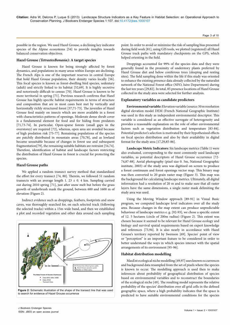
The study site is a land dominated by forest. This forestland is an anchor in the heart of a Regional Natural Park (Chartreuse) with arising objectives of sustainable development and conservation, including a Natura 2000 site. Nevertheless, the area is located in the middle of an axe between Grenoble and Chambery, two important urban centres in the Alps facing an accelerating suburban sprawl. In addition the area is undergoing an important tourism development associated to relatively small ski resorts in winter and other sports like VTT in summer. These activities constitute an important income for a region that is losing traditional activities but increases the impact and pressures for the flora and fauna. Our study was confined to the State Forest of Grand Chartreuse within an area of 6637 hectares (Figure 1), of a complex landscape mosaic (Lat. 45°23’20” N Long 5°47’47” E).

The site is part of “the state forest of the Grand Chartreuse”, located at the heart of the massif of the same name. Following the objectives of the European Habitat Directive, a sustainable forest management is within the agenda of the Park, in tandem with a participatory approach launched with local actors to maintain the area biodiversity. Forestry activities are still important but with aims to balance conservation actions. There is also a plan for the creation of a biological reserve on the site that is nowadays a Natura 2000 area. In this regard, there are regional interests to develop appropriate legislative, financial and contractual instruments towards a better implementation of conservation actions.

The physical framework

Elevation within the study area ranges from 400 to 2000 m. The mountainous area is covered mainly by coniferous forest stands including also open land, expose rocky areas and other open habitats such as pastures and meadows. The dominant tree species are Fir (Abiesalba), Spruce (Piceaabies) and Beech (Fagussylvatica). These dominant species form a complex forest landscape matrixof a typically mixed beech-fir-spruce, with variations in the proportions of the dominant species depending on elevation. Beech is dominant at lower elevations (below 600 m), while fir, beech and spruce are mixed in the mountain range (600–1200 m). Spruce becomes dominant in the subalpine range above 1200 m. The area is managed by the National Forest Office (NFO) of the French Isere Department.

The Natural Park of Chartreuse forests is committed to maintaining biodiversity as it has been selected as a reintroduction area for certain species and is part of the Alps hot spot for European biodiversity [63]. More than any other in the French Alps, the massif of Chartreuse is committed to the maintenance of its forests[64]. The monks from Chartreuse, started their activities during the 11th century, the Church of Saint-Hugues county and recently the seat of the Natural Regional Park of Chartre use provided to these forests a particular patrimonial value that historically helped on the protection of the forests [65-67]. These forests that were part of the church patrimonial value, benefited throughout the centuries of a particular protection status. During the nineteenth century, however, the use of forests becomes more important [65]. Consequently, these alpine ecosystems are nowadays rapidly changing on structure due to the presence of a ski resort in mid-mountain and several other related tourist attractions that jeopardize conservation objectives[13]. Protecting this natural and cultural landscape against degradation and pressures of any kind is the great challenge for biodiversity conservation targets which demands sound scientific analysis based on data and information [68]. In particular an adaptive management that can respond to increasing economic demands while still planning for conservation objectives it should be

The State Forest of ‘Grand Chartreuse’

Hazel Grouse point locations

0 0.5 1 2 3Kilometers

N

Grenoble

Legend

IsereDepartment

N

Figure 1: Study area in the French Alps

Citation: Adra W, Delcros P, Luque S (2013) Landscape Structure Indicators as a Key Feature in Habitat Selection: an Operational Approach to Conservation Planning. J Biodivers Endanger Species 1:107. doi:10.4172/jbes.1000107

Page 3 of 10

Volume 1 • Issue 2 • 1000107J Biodivers Endanger SpeciesISSN: JBES an open access journal

possible in the region. We used Hazel Grouse, a declining key indicator species of the Alpine ecosystems [54] to provide insights towards balanced conservation objectives.

Hazel Grouse (TetrastesBonasia): A target species

Hazel Grouse is known for being strongly affected by forest dynamics, and populations in many areas within Europe are declining. The French Alps is one of the important reserves in central Europe that hold Hazel Grouse population, their density varies locally [56]. This focal species is known as forest-dwelling bird species,  sedentary (adult) and strictly linked to its habitat [52,69]. It is highly secretive and notoriously difficult to census [70]. Hazel Grouse is known to be more territorial in spring [71]. Previous research confirms that Hazel Grouse has highly-specific habitat requirements in terms of structure and composition that are in most cases best met by vertically and horizontally richly structured forest [57,71-73]. The juveniles of Hazel Grouse feed mainly on insects which are more available in a forest with characteristics patterns of openings. Moderate dense shrub cover is a fundamental element for food and for hiding from predators [71,73-74]. In particular, Open-sparse forests (small gaps in the overstorey) are required [72], whereas, open area are avoided because of high predation risk [75-77]. Remaining populations of the species are patchily distributed in mountain areas [70,78], and as lowland became unsuitable because of changes in forest use and subsequent fragmentation[79], the remaining suitable habitats are restraint [54,74]. Therefore, identification of habitat and landscape factors restricting the distribution of Hazel Grouse in forest is crucial for protecting the species.

Hazel Grouse paths

We applied a random transect survey method that standardized the effort for every transect [74, 80]. Therein, we followed 51 random transects with an average length 1. 23 ± 0. 4 km. Sampling carried out during 2010 spring [71], just after snow melt but before the grass growth of underbrush mask the ground, between 600 and 1600 m of elevation (Figure 2).

Indirect evidence such as droppings, feathers, footprints and snow caves, was thoroughly searched for, on each selected track (following the selected tracks) within a 15m wide band, and then we established a plot and recorded vegetation and other data around each sampling

point. In order to avoid or minimize the risk of sampling bias presented during field work [81], using GIS tools, we plotted (registered) all Hazel Grouse track paths with mandatory checkpoints on the GPS, which helped orienting in the field.

Droppings accounted for 99% of the species data and they were generally found in the proximity of understory plants preferred by Hazel Grouse diet and below coniferous trees (sleeping and resting sites). The field sampling done within the life if this study was oriented to enhance the existing presence data already collected by the naturalist network of the National Forest office (NFO, Isère Department) during the last ten years [29,82]. In total, 85 presence locations of Hazel Grouse collected in the study area were selected for further analysis.

Explanatory variables as candidate predictors

Environmental variable: Elevation variable (source: 50 m resolution digital elevation model DEM (French National Geographic Institute) was used in this study as independent environmental descriptor. This variable is considered as an effective surrogate of heterogeneity and provides a reasonable explanation on the role of other environmental factors such as vegetation distribution and temperature [83-84]. Potential predictor’s selection is motivated by their hypothesized effects on focal species distribution and also by their availability in digital format for the study area [17,29,85-86].

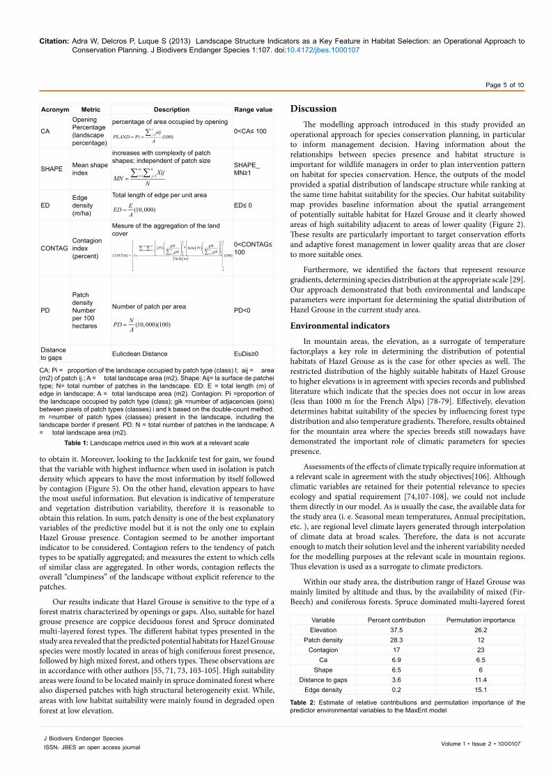
Landscape Metric Indicators: Six landscape metrics (Table 1) were also evaluated, corresponding to the most commonly used landscape variables, as potential descriptors of Hazel Grouse occurrence [72-74,87-88]. Aerial photography (pixel size 0. 5m, National Geographic institute, 2003) of the study area was digitized on screen to produce a forest continuum and forest openings vector map. This binary map was then converted to 20 grain raster map (Figure 3). This map was the background for calculating landscape metrics. Ultimately, all digital information had a resolution of 20 m and to make sure that all raster layers have the same dimensions, a single raster mask delimiting the study area was used.

Using the Moving Window approach [89-91] in Visual Basic program, we computed landscape level indicators over all the study area. Because changes in the map extent can produce unpredictable behaviour of landscape metrics e. g. [92-93], we chose a specific extent of 12. 5 hectares (circle of 200m radius) (Figure 2). This extent was chosen because it seemed to be relevant for Hazel Grouse ecology and biology and survival spatial requirements based on expert knowledge and references [73,94]. It is also nearly in accordance with Hazel Grouse‘s territory reported by Swenson [69]. Species’ point of view or “perception” is an important feature to be considered in order to better understand the ways in which species interact with the spatial arrangements of its environment [95-96].

Habitat distribution modelling

MaxEnt ecological niche modelling [49,97] uses known occurrences and background data resampled from the set of pixels where the species is known to occur. The modelling approach is used then to make inferences about probability of geographical distribution of species based on environmental variables and to reconstruct the boundaries of the ecological niche [49]. The resulting model represents the relative probability of the species’ distribution over all grid cells in the defined geographic space, where a high probability indicates that the space is predicted to have suitable environmental conditions for the species

N

200m

15m

0 1 2 4Kilometers

The State Forest of Grande Chartreuse

Data-NFO-after 2000Data-2010Transect lines

Transet line (Hazel grouse path) Hazel Grouse presence point Buffer of 200m radius

Figure 2: Schematic illustration of the shape of the transect line that was used to search for evidence of Hazel Grouse occurrence

Citation: Adra W, Delcros P, Luque S (2013) Landscape Structure Indicators as a Key Feature in Habitat Selection: an Operational Approach to Conservation Planning. J Biodivers Endanger Species 1:107. doi:10.4172/jbes.1000107

Page 4 of 10

Volume 1 • Issue 2 • 1000107J Biodivers Endanger SpeciesISSN: JBES an open access journal

[41,49]. This algorithm has been shown to perform well even with scarce and noisy presence data subsets collected by different researchers and methodologies [29,40]. The model can easily be updated with new specific occurrences for the target species.

We used MaxEnt software because of its strong attributes such as its algorithm constraints predicted species ranges and thus reduces and avoids commission error that could lead to erroneous conservation decisions[41, 98,99]. It can investigate variable importance through jacknife procedure, in which model performance is assessed based on its ability to predict the single locality that is excluded from the ‘training’ dataset [99]. It permits to show relative suitability rather than the occurrence probability [100]. Globally its properties have several implications for how it should be used in this study [41,86]. We used default setting [60], except for iteration number; we executed 100 replicated model runs. We configured the machine-learning algorithm to use 80% of the species records for training dataset and 20% for testing the model [101]. We determined the heuristic of the relative contribution of each variable to species’ distribution. MaxEnt estimates the importance of variables’ contribution, representing the percentage of the variable contribution to the model based on path selected for a particular run. In addition, the permutation importance values were obtained by changing the predictors’ value between presence and background points and evaluating how that affects the AUC value.

Model evaluation and threshold selection

The Model quality was evaluated based on the Area Under Curve (AUC) value [39,97,101] as it is part of MaxEnt output [49]. High AUC value indicates a high capacity of models to discriminate the presence and absence species [39,102]. We compared AUC values for 100 models replicates, and chose the best model (the model with ROC value closet to 1). According to Phillips et al [60] and Pearson and Dudik [99], we used a fixed threshold to reject only the lowest 10% of possible predicted values at each run. This threshold value, based on a logistic threshold of 10 percentile training presence, was used to reclassify our model (binary building reclassifying).

ResultsModel prediction analysis

The prediction map of the potential distribution of Hazel Grouseas a function of suitable habitat distribution (Figure 4) shows that the potential habitat with high suitability thresholds were distributed in the

higher elevations of the state forest of Grand Chartreuse (Table 2). The highest MaxEnt scores were located in the mountainous areas located above 1000 m.

The model was highly successful in highlighting areas that could potentially harbour this rare species as well as undersampled areas with suitable environment conditions. With 10 percentile threshold (0. 24), 61 % of the analysed study area classified as a potential habitat for Hazel Grouse.

Using three arbitrarily defined probability classes, the high suitability class showedonly 1%, while medium suitabilityscore60% and low or null suitability39%. Areas with a probability of presence greater than 70% were considered to be areas of high habitat suitability [39-40]. Thus, most of the areas fall under medium and low suitability classes, while high habitat suitability was restricted only to about 1% of the whole study area, providing evidence for territorial resources for Hazel Grouse species.

The most relevant variables

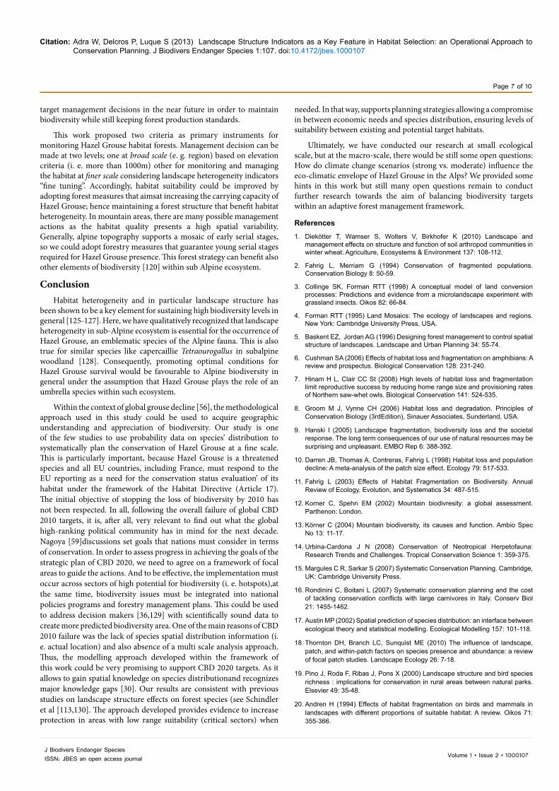
The best model calibration test for Hazel Grouse yielded satisfactory results (AUC train=0. 77 and AUC test= 1). AUC scores indicate a good to high discriminative capacity between predicted presence and absence [39]. The omission rate was null at the minimum training presence threshold. Among input variables elevation was the most influential and contributed37. 5% to MaxEnt model. Landscape layers contributed 62. 5% to the habitat model of species of which patch density 28. 3% had maximum contribution and 17% for contagion (Table 2).

Considering the permutation importance, elevation had also the maximum influence on the habitat model and contributed to 26. 2% while contagion and patch density together contributed to 35% (Table2). It seems to be more pertinent to consider variables importance choice, because it allows overcoming correlations issues between indicators as it depends on the final MaxEnt model results and not on the path used

N

0 1 2 4Kilometers

The State Forest of Grande ChartreuseForest / Forest opening map

ForestForest openingsOther (including NF)

Figure 3: Hazel Grouse Background binary Forest /Non Forest map

N

0 1 2 4Kilometers

High : 1

Low : 0

Hazel grouse predicted presenceValue

Figure 4: Result of MaxEnt model for Hazel Grouse, with 10 percentile training presence threshold. Red: high probability of occurrence (Potential habitat distribution of Hazel Grouse species)

Citation: Adra W, Delcros P, Luque S (2013) Landscape Structure Indicators as a Key Feature in Habitat Selection: an Operational Approach to Conservation Planning. J Biodivers Endanger Species 1:107. doi:10.4172/jbes.1000107

Page 5 of 10

Volume 1 • Issue 2 • 1000107J Biodivers Endanger SpeciesISSN: JBES an open access journal

to obtain it. Moreover, looking to the Jackknife test for gain, we found that the variable with highest influence when used in isolation is patch density which appears to have the most information by itself followed by contagion (Figure 5). On the other hand, elevation appears to have the most useful information. But elevation is indicative of temperature and vegetation distribution variability, therefore it is reasonable to obtain this relation. In sum, patch density is one of the best explanatory variables of the predictive model but it is not the only one to explain Hazel Grouse presence. Contagion seemed to be another important indicator to be considered. Contagion refers to the tendency of patch types to be spatially aggregated; and measures the extent to which cells of similar class are aggregated. In other words, contagion reflects the overall “clumpiness” of the landscape without explicit reference to the patches.

Our results indicate that Hazel Grouse is sensitive to the type of a forest matrix characterized by openings or gaps. Also, suitable for hazel grouse presence are coppice deciduous forest and Spruce dominated multi-layered forest types. The different habitat types presented in the study area revealed that the predicted potential habitats for Hazel Grouse species were mostly located in areas of high coniferous forest presence, followed by high mixed forest, and others types. These observations are in accordance with other authors [55, 71, 73, 103-105]. High suitability areas were found to be located mainly in spruce dominated forest where also dispersed patches with high structural heterogeneity exist. While, areas with low habitat suitability were mainly found in degraded open forest at low elevation.

DiscussionThe modelling approach introduced in this study provided an

operational approach for species conservation planning, in particular to inform management decision. Having information about the relationships between species presence and habitat structure is important for wildlife managers in order to plan intervention pattern on habitat for species conservation. Hence, the outputs of the model provided a spatial distribution of landscape structure while ranking at the same time habitat suitability for the species. Our habitat suitability map provides baseline information about the spatial arrangement of potentially suitable habitat for Hazel Grouse and it clearly showed areas of high suitability adjacent to areas of lower quality (Figure 2). These results are particularly important to target conservation efforts and adaptive forest management in lower quality areas that are closer to more suitable ones.

Furthermore, we identified the factors that represent resource gradients, determining species distribution at the appropriate scale [29]. Our approach demonstrated that both environmental and landscape parameters were important for determining the spatial distribution of Hazel Grouse in the current study area.

Environmental indicators

In mountain areas, the elevation, as a surrogate of temperature factor,plays a key role in determining the distribution of potential habitats of Hazel Grouse as is the case for other species as well. The restricted distribution of the highly suitable habitats of Hazel Grouse to higher elevations is in agreement with species records and published literature which indicate that the species does not occur in low areas (less than 1000 m for the French Alps) [78-79]. Effectively, elevation determines habitat suitability of the species by influencing forest type distribution and also temperature gradients. Therefore, results obtained for the mountain area where the species breeds still nowadays have demonstrated the important role of climatic parameters for species presence.

Assessments of the effects of climate typically require information at a relevant scale in agreement with the study objectives[106]. Although climatic variables are retained for their potential relevance to species ecology and spatial requirement [74,107-108], we could not include them directly in our model. As is usually the case, the available data for the study area (i. e. Seasonal mean temperatures, Annual precipitation, etc. ), are regional level climate layers generated through interpolation of climate data at broad scales. Therefore, the data is not accurate enough to match their solution level and the inherent variability needed for the modelling purposes at the relevant scale in mountain regions. Thus elevation is used as a surrogate to climate predictors.

Within our study area, the distribution range of Hazel Grouse was mainly limited by altitude and thus, by the availability of mixed (Fir-Beech) and coniferous forests. Spruce dominated multi-layered forest

Acronym Metric Description Range value

CA

Opening Percentage (landscape percentage)

percentage of area occupied by opening

1 (100)n

jaij

PLAND PiA== =

∑ 0<CA≤ 100

SHAPE Mean shape index

increases with complexity of patch shapes; independent of patch size

1 1

m n

i jXij

MNN

= ==∑ ∑

SHAPE_MN≥1

EDEdge density (m/ha)

Total length of edge per unit area

(10,000)EEDA

=ED≤ 0

CONTAGContagion index (percent)

Mesure of the aggregation of the land cover

( ) ( )

( )

1 1

1 1

* ln ln

1 (100)2ln ln

m mm mi kk k

gik gikPi Pigik gik

CONTAGm

= =

= =

= +

∑ ∑∑ ∑

0<CONTAG≤ 100

PD

Patch density Number per 100 hectares

Number of patch per area

(10,000)(100)NPDA

=

PD<0

Distance to gaps Eulicdean Distance EuDis≥0

CA: Pi = proportion of the landscape occupied by patch type (class) I; aij = area (m2) of patch ij.; A = total landscape area (m2). Shape: Aij= la surface de patchei type; N= total number of patches in the landscape. ED: E = total length (m) of edge in landscape; A = total landscape area (m2). Contagion: Pi =proportion of the landscape occupied by patch type (class); gik =number of adjacencies (joins) between pixels of patch types (classes) i and k based on the double-count method. m =number of patch types (classes) present in the landscape, including the landscape border if present. PD: N = total number of patches in the landscape; A = total landscape area (m2).

Table 1: Landscape metrics used in this work at a relevant scale

Variable Percent contribution Permutation importanceElevation 37.5 26.2

Patch density 28.3 12Contagion 17 23

Ca 6.9 6.5Shape 6.5 6

Distance to gaps 3.6 11.4Edge density 0.2 15.1

Table 2: Estimate of relative contributions and permutation importance of the predictor environmental variables to the MaxEnt model

Citation: Adra W, Delcros P, Luque S (2013) Landscape Structure Indicators as a Key Feature in Habitat Selection: an Operational Approach to Conservation Planning. J Biodivers Endanger Species 1:107. doi:10.4172/jbes.1000107

Page 6 of 10

Volume 1 • Issue 2 • 1000107J Biodivers Endanger SpeciesISSN: JBES an open access journal

with a deciduous feature is restricted to areas at high altitude and it is considered as representative of Hazel Grouse living conditions in the Alps Mountains [69,72,74]. This can be explained by the feeding regime (winter habitat selection) [70,74], as the food resources are restricted and difficult to access in winter. The same stands for refuge places from preys that are limited. That is why mixed forests are increasingly used in winter [109-110], where a favourable combination of food and cover [52,71,105] can be found. Likewise, species reproduction is affected by severe weather conditions or climate changes [107], because the females are greatly dependant on exogenous nutrient and energy sources for clutch formation and adverse weather or late winter can reduce the foraging time due to rain and wet vegetation and thus decrease the reproductive success [111].

How do landscape features influence Hazel Grouse occurrence in mountain forest?

The type of data to describe predictors used in SDMs and also the need to rely on surrogates are critical issues[29]. For biodiversity estimations and monitoring, landscape metrics are highly informative and capable of interpretation [112]. Therefore, they are largely used for monitoring at different scales [113] and they have to play a considerable role in biodiversity analysis and assessment especially in local studies of species distribution (see Walz [114]. Our results confirm that Hazel Grouse habitat quality is determined by forest land scape spatial structure descriptors. In this sense the modelling tool used can be promisingly useful for assessment studies at different landscape scales and to provide a set of replicable indicators.

Habitat heterogeneity is often illustrated by spatial descriptors of the habitat [115-116] and it is characterized by several landscape indicators such as contagion, patch density and edge density [117-120]. Landscape heterogeneity features are considered as main drivers (surrogates) of habitat quality, thus of Hazel Grouse occurrence, as it was previously documented[72,74,88,121], but not explicitly tested. The present study demonstrates that contagion and patch density indices influence significantly the probability of Hazel Grouse occurrence. Nevertheless, variable contributions should be interpreted with caution when the predictor variables are correlated [122]. Therefore, the model wasre-evaluated on the bases of the permuted data; the resulting drop in training (AUC)allowed to demonstrate that edge density is more important to explain the species presence than PD. While, results from MaxEnt permutation importance indicates that the model depends heavily on contagion as a variable that reflects the degree of habitat heterogeneity. Some variables such as edge density and distance to

gaps have poorly contributed in the predicted habitat suitability map (Table2), but this can be explained because they are highly correlated with contagion [117-119,122].

Nevertheless, it must be noted that Hazel grouse is sensitive to a forest gap width and consequently preferred not to venture far from forest cover, however, it sometimes crossed gaps as large as 1km [123]. During the breeding season, openings provide important localized sources for the species in terms of food, and preferred habitat structure. Evidence suggests that such resources are more abundant, visible and accessible in forests gaps, highlighting the role of these structural features on the landscape [74,124]. Besides that, juveniles of Hazel Grouse feed mainly on insects, more available also in forests gaps. In addition, Hazel Grouse may be attracted by openings because of increased cover in lower levels which offer protection from predators. Our results suggest that the presence of gaps enhanced the presence and movement of this forest bird.

As a result, our study supports the importance of landscape structure indicators for predicting Hazel Grouse habitat quality that is introduced by heterogeneity which implies increasing, somehow, the amount of forest edge and dispersed forest gaps. These key structural forest features, improve the quality of Hazel Grouse habitat throughout a higher supply of food and refuge resources [71,73]. Eventually, our results indicate that our study area is representative of the livelihood conditions of Hazel Grouse in mountain areas and in particular in the Alps; therefore, we have to stress here the importance of the landscape structure for species suitable habitat management.

Usefulness of habitat model as an operational tool for conservation in Chartreuse Natural Park

Systematic conservation planning requires information on the spatial distribution of biodiversity. Forest managers and conservationists benefit greatly from understanding species habitat requirements and determining priority conservation needs. But in some cases, in particular in mountain areas the accessibility is difficult therefore obtaining the needed species data is costly and time consuming. Considering the difficulties in accessing some part of Chartreuse forests (i. e. rocky crests and valleys of very difficult access) [67], targeting efforts to areas of high probability of species occurrence will increase the success of future field excursions. In the current study, prioritization is based upon projected distributions generated by niche modelling of Hazel Grouse occurrence data collected from surveys in the State Forest of Grand Chartreuse. Our fitted model in this study suggests insights for further planning perspectives in favour to Hazel Grouse species as it allows defining potentially suitable areas and discovering new areas over relative coarse geographical scale. Prioritization results highlight also areas that warrant attention for future field surveys.

Comparing the actual forest management plan over the study area with our habitat suitability map, we found that 73% of the forest production sectors defined in the forest management plan represent suitable habitat for hazel grouse species (NOF Isère, management plan, 2002 – 2017). Accordingly, we assume that it could be relevant to keep the actual management strategy which seems to match the indicator species habitat preference. However, any increase in production or changes on the actual management will have a direct impact on biodiversity. At present forest management is not selective for a particular species habitat. As an example we remarked that the Natura 2000 site within the study area does not correspond to high habitat quality for hazel grouse. In that sense the model results can support to

Without variable

With only variable

With all variables

0.5 1.0 1.5 2.0 2.5 3.0 3.5 4.0 4.5

test gain

Env

ironm

enta

l Var

iabl

e

Ca

Contagion

Distance to gaps

Edge density

Elevation

Patch density

Shape

Jancknife of test gain for Tetraste Bonasia

Figure 5: Result of jackknife test for evaluating the relative contribution of the predictor’s variables to the habitat model of Hazel Grouse. The per cent of contribution of each variable to the model represented by the red bar and corresponding values may be found on the left axis

Citation: Adra W, Delcros P, Luque S (2013) Landscape Structure Indicators as a Key Feature in Habitat Selection: an Operational Approach to Conservation Planning. J Biodivers Endanger Species 1:107. doi:10.4172/jbes.1000107

Page 7 of 10

Volume 1 • Issue 2 • 1000107J Biodivers Endanger SpeciesISSN: JBES an open access journal

target management decisions in the near future in order to maintain biodiversity while still keeping forest production standards.

This work proposed two criteria as primary instruments for monitoring Hazel Grouse habitat forests. Management decision can be made at two levels; one at broad scale (e. g. region) based on elevation criteria (i. e. more than 1000m) other for monitoring and managing the habitat at finer scale considering landscape heterogeneity indicators “fine tuning”. Accordingly, habitat suitability could be improved by adopting forest measures that aimsat increasing the carrying capacity of Hazel Grouse; hence maintaining a forest structure that benefit habitat heterogeneity. In mountain areas, there are many possible management actions as the habitat quality presents a high spatial variability. Generally, alpine topography supports a mosaic of early serial stages, so we could adopt forestry measures that guarantee young serial stages required for Hazel Grouse presence. This forest strategy can benefit also other elements of biodiversity [120] within sub Alpine ecosystem.

Conclusion Habitat heterogeneity and in particular landscape structure has

been shown to be a key element for sustaining high biodiversity levels in general [125-127]. Here, we have qualitatively recognized that landscape heterogeneity in sub-Alpine ecosystem is essential for the occurrence of Hazel Grouse, an emblematic species of the Alpine fauna. This is also true for similar species like capercaillie Tetraourogallus in subalpine woodland [128]. Consequently, promoting optimal conditions for Hazel Grouse survival would be favourable to Alpine biodiversity in general under the assumption that Hazel Grouse plays the role of an umbrella species within such ecosystem.

Within the context of global grouse decline [56], the methodological approach used in this study could be used to acquire geographic understanding and appreciation of biodiversity. Our study is one of the few studies to use probability data on species’ distribution to systematically plan the conservation of Hazel Grouse at a fine scale. This is particularly important, because Hazel Grouse is a threatened species and all EU countries, including France, must respond to the EU reporting as a need for the conservation status evaluation’ of its habitat under the framework of the Habitat Directive (Article 17). The initial objective of stopping the loss of biodiversity by 2010 has not been respected. In all, following the overall failure of global CBD 2010 targets, it is, after all, very relevant to find out what the global high-ranking political community has in mind for the next decade. Nagoya [59]discussions set goals that nations must consider in terms of conservation. In order to assess progress in achieving the goals of the strategic plan of CBD 2020, we need to agree on a framework of focal areas to guide the actions. And to be effective, the implementation must occur across sectors of high potential for biodiversity (i. e. hotspots),at the same time, biodiversity issues must be integrated into national policies programs and forestry management plans. This could be used to address decision makers [36,129] with scientifically sound data to create more predicted biodiversity area. One of the main reasons of CBD 2010 failure was the lack of species spatial distribution information (i. e. actual location) and also absence of a multi scale analysis approach. Thus, the modelling approach developed within the framework of this work could be very promising to support CBD 2020 targets. As it allows to gain spatial knowledge on species distributionand recognizes major knowledge gaps [30]. Our results are consistent with previous studies on landscape structure effects on forest species (see Schindler et al [113,130]. The approach developed provides evidence to increase protection in areas with low range suitability (critical sectors) when

needed. In that way, supports planning strategies allowing a compromise in between economic needs and species distribution, ensuring levels of suitability between existing and potential target habitats.

Ultimately, we have conducted our research at small ecological scale, but at the macro-scale, there would be still some open questions: How do climate change scenarios (strong vs. moderate) influence the eco-climatic envelope of Hazel Grouse in the Alps? We provided some hints in this work but still many open questions remain to conduct further research towards the aim of balancing biodiversity targets within an adaptive forest management framework.

References

1. Diekötter T, Wamser S, Wolters V, Birkhofer K (2010) Landscape and management effects on structure and function of soil arthropod communities in winter wheat. Agriculture, Ecosystems & Environment 137: 108-112.

2. Fahrig L, Merriam G (1994) Conservation of fragmented populations. Conservation Biology 8: 50-59.

3. Collinge SK, Forman RTT (1998) A conceptual model of land conversion processes: Predictions and evidence from a microlandscape experiment with grassland insects. Oikos 82: 66-84.

4. Forman RTT (1995) Land Mosaics: The ecology of landscapes and regions. New York: Cambridge University Press, USA.

5. Baskent EZ, Jordan AG (1996) Designing forest management to control spatial structure of landscapes. Landscape and Urban Planning 34: 55-74.

6. Cushman SA (2006) Effects of habitat loss and fragmentation on amphibians: A review and prospectus. Biological Conservation 128: 231-240.

7. Hinam H L, Clair CC St (2008) High levels of habitat loss and fragmentation limit reproductive success by reducing home range size and provisioning rates of Northern saw-whet owls. Biological Conservation 141: 524-535.

8. Groom M J, Vynne CH (2006) Habitat loss and degradation. Principles of Conservation Biology (3rdEdition), Sinauer Associates, Sunderland, USA.

9. Hanski I (2005) Landscape fragmentation, biodiversity loss and the societal response. The long term consequences of our use of natural resources may be surprising and unpleasant. EMBO Rep 6: 388-392.

10. Darren JB, Thomas A, Contreras, Fahrig L (1998) Habitat loss and population decline: A meta-analysis of the patch size effect. Ecology 79: 517-533.

11. Fahrig L (2003) Effects of Habitat Fragmentation on Biodiversity. Annual Review of Ecology, Evolution, and Systematics 34: 487-515.

12. Korner C, Spehn EM (2002) Mountain biodivresity: a global assessment. Parthenon: London.

13. Körner C (2004) Mountain biodiversity, its causes and function. Ambio Spec No 13: 11-17.

14. Urbina-Cardona J N (2008) Conservation of Neotropical Herpetofauna: Research Trends and Challenges. Tropical Conservation Science 1: 359-375.

15. Margules C R, Sarkar S (2007) Systematic Conservation Planning. Cambridge, UK: Cambridge University Press.

16. Rondinini C, Boitani L (2007) Systematic conservation planning and the cost of tackling conservation conflicts with large carnivores in Italy. Conserv Biol 21: 1455-1462.

17. Austin MP (2002) Spatial prediction of species distribution: an interface between ecological theory and statistical modelling. Ecological Modelling 157: 101-118.

18. Thornton DH, Branch LC, Sunquist ME (2010) The influence of landscape, patch, and within-patch factors on species presence and abundance: a review of focal patch studies. Landscape Ecology 26: 7-18.

19. Pino J, Roda F, Ribas J, Pons X (2000) Landscape structure and bird species richness : implications for conservation in rural areas between natural parks. Elsevier 49: 35-48.

20. Andren H (1994) Effects of habitat fragmentation on birds and mammals in landscapes with different proportions of suitable habitat: A review. Oikos 71: 355-366.

Citation: Adra W, Delcros P, Luque S (2013) Landscape Structure Indicators as a Key Feature in Habitat Selection: an Operational Approach to Conservation Planning. J Biodivers Endanger Species 1:107. doi:10.4172/jbes.1000107

Page 8 of 10

Volume 1 • Issue 2 • 1000107J Biodivers Endanger SpeciesISSN: JBES an open access journal

21. Hurlbert AH, Haskell JP (2003) The effect of energy and seasonality on avian species richness and community composition. Am Nat 161: 83-97.

22. Hirzel AH, Lay GLe (2008) Habitat suitability modelling and niche theory. Journal of Applied Ecology 45: 1372-1381.

23. Songer M, Delion M, Biggs A, Huang Q (2012) Modeling Impacts of Climate Change on Giant Panda Habitat. International Journal of Ecology.

24. Carroll C, Noss R, Paquet P (2001) Carnivores as focal species for conservation planning in the rocky region. Ecological Applications 11: 961-980.

25. Manton GM, Angelstam P, Mikusiniski G (2005) Modelling habitat suitability for deciduous forest focal species - a sensitivity analysis using differnt satellite land cover data. Landscape Ecology 20: 827-839.

26. Lindenmayer DB, Margules RC, Botkin DB (2000) Indicators of Biodiversity for Ecologically Sustainable Forest Management. Conservation Biology 14: 941-950.

27. Myers N, Mittermeier RA, Mittermeier CG, da Fonseca GA, Kent J (2000) Biodiversity hotspots for conservation priorities. Nature 403: 853-858.

28. Kharouba MH, Nadeau JL, Young E, Kerr JT (2008) Using species distribution models to effectively conserve biodiversity into the future. Biodibersity 9: 39-46.

29. Franklin J (2009) Mapping spcies Distribution: Spatial Inference and Prediction (Ecology, Biodiversity and Conservation) Saint Diego State. Cambridge University Press.

30. Jetz W, McPherson JM, Guralnick RP (2012) Integrating biodiversity distribution knowledge: toward a global map of life. Trends Ecol Evol 27: 151-159.

31. Soberon J, Peterson AT (2005) Interpretation of models of fundamental ecological niches and species distribution areas. Biodiversity Informatics 2: 1-10.

32. Baldwin RA (2009) Use of Maximum Entropy Modeling in Wildlife Research. Entropy 11: 854-866.

33. Pawar S, Koo MS, Kelley C, Ahmed MF, Choudhury S, Sarkar S (2007) Conservation assessment and prioritization of areas in Northeast India: priorities for amphibians and reptiles. Biological Conservation 136: 346-361.

34. Barbosa AM, Real R, Vargas JM (2010) Use of coarse-resolution models of species’ distributions to guide local conservation inferences. Conserv Biol 24: 1378-1387.

35. Thuiller W (2003) BIOMOD – optimizing predictions of species distributions and projecting potential future shifts under global change. Globale Change Biology 9: 1353-1362.

36. Cabeza M, Araújo MB, Wilson RJ, Thomas CD, Cowley MJR, et al (2004) Combining probabilities of occurrence with spatial reserve design. Journal of Applied Ecology 41: 252-262.

37. Ferrier S (2002) Mapping spatial pattern in biodiversity for regional conservation planning: where to from here? Syst Biol 51: 331-363.

38. Martínez-Meyer E, Townsend AP, Hargrove WW (2004) Ecological niches as stable distributional constraints on mammal species, with implications for Pleistocene extinctions and climate change projections for biodiversity. Global Ecology and Biogeography 13: 305-314.

39. Pearce J, Ferrier S (2000) Evaluating the predictive performance of habitat models developed using logistic regression. Ecological Modelling 133: 225-245.

40. Elith J, Graham CH, Anderson RP, Dudik MS, Ferrier S, et al (2006) Novel methods improve prediction of species distributions from occurrence data. Ecography 29: 129-151.

41. Elith J, Phillips SJ, Hastie T, Dudík M, Chee, EnY, et al (2011) A statistical explanation of MaxEnt for ecologists. Diversity and Distributions 17: 43-57.

42. Araùjo MB, Williams PH (2000) Selecting areas for species persistence using occurrence data. Biological Conservation 96: 331-345.

43. Guisan A, Zimmermann NE (2000) Predictive habitat distribution models in ecology. Ecological Modelling 135: 147-186.

44. Graham CH, Ferrier S, Huettman F, Moritz C, Peterson AT (2004) New developments in museum-based informatics and applications in biodiversity analysis. Trends Ecol Evol 19: 497-503.

45. Hastie TJ, Tibshirani R (1990) Generalized Additive (Chapman & Hall/CRC Monographs on Statistics & Applied Probability). London,UK.

46. Zaniewski AE, Lehamann A, Overton JMcC (2002) Predicting species spatail distributions using presence- only data: a case study of native new Zealand ferns. Ecological Modelling 157: 261-280.

47. Hirzel AH, Haussez J, Chessel D, Perrin N (2002) Ecological-Niche Factor Analysis: How to compute habitat suitability maps without absence data? Ecology 7: 2027-2036.

48. Jiménez-Valverde A, Lobo JM, Hortal J (2008) Not as good as they seem: the importance of concepts in species distribution modelling. Diversity and Distributions 14: 885-890.

49. Phillips SJ, Anderson RP, Schapire RE (2006) Maximum entropy modeling of species geographic distributions. Ecological Modelling 190: 231-259.

50. Patthey P, Signorell N, Rotelli L, Arlettaz R (2012) Vegetation structural and compositional heterogeneity as a key feature in Alpine black grouse microhabitat selection: conservation management implications. European Journal of Wildlife Research 58: 59-70.

51. Lambeck RJ (1997) Focal Species: A Multi-Species Umbrella for Nature Conservation. Conservation Biology 11: 849-856.

52. Swenson JE, Danielsen J (1991) Status and conservation of hazel grouse in Europe. Ornic Scandinavica 22: 297-298.

53. Swenson JE, Angelstam P (1993) Habitat separation by sympatric forest grouse in Fennoscandia in relation to boreal forest succession. Canadian Journal of Zoology 7: 1303–1310.

54. Storch I (2007) Grouse Status survey and conservation actionplan 2006-2010. IUCN, the world feasant association.

55. Jansson G, Angelstam P, Aberg J, Swenson JE (2004) Management targets for the conservation of Hazel Grouse in boreal landscape. Ecolo Bull 51: 259-264.

56. Storch I (2000) Conservation status and threats to grouse worldwide: an overview. Wildlife Biology 6: 195-204.

57. Longru J, He HS, Yufei Z, Rencang B, Keping S (2010) Assessing the effects of management alternatives on habitat suitability in a forested landscape of northeastern China. Environ Manage 45: 1191-1200.

58. Angelstam P, Roberge J, Lohmus MA, Bergmanis M, Brazaitis G, et al. (2004) Habitat modelling as a tool for landscape-scale conservation–a review of parameters for focal forest birds. Ecologicla Bulletine 51: 427-453.

59. Nagoya (2010) Report of the tenth meeting of the conference of the parties to the convention on bioligical diversity. Conference of the parties to the convention of biological diversity, UNEP.

60. Phillips SJ, Dudik M (2008) Modeling of species distributions with Maxent: new extensions and a comperhensive evaluation. Ecography 31: 161-175.

61. Pearson RG (2007) Species’distribution modeling for conservation educators and practitioners. Synthesis, in American Museum of Natural History.

62. Ortega-huerta MA, Peterson AT (2008) Modeling ecological niches and prediction geographic distributions: a test of six presence-only methods. Revistamexicana de Biodiversidad 79: 205-216.

63. Gardet P, Bailly J, Sube F (2009) Projet de reintroduction du Bouquetin des Alpes dans la reserve naturelle national des hautes de Chartreuse, in Parc naturel régional de Chartreuse.

64. Blache J (1931) The mass of the Grande Chartreuse and Vercore, in tom: Human IIgeographie. University of Grenoble: Grenoble 514.

65. Mauz I, Malavieille D, Micheels C, Perret J, Messad S (1996) Enjeux socio-économiques et capacité d’adaptation des stations de moyenne montagne: Analyse d’un échantillon de trois stations. Cemagref, Unité : Développement des Territoires Montagnards Grenoble 82.

66. Chevallier P, Couailhac MJ (1983) The adminstration of water and forests in the department del’Isère nineteenth sciècle: sauvgarde reconstitustion and heritage. University of Social Sciences Grenible 99.

67. Brossier J (1954) Chartreuse mountains: descriptive leaflet. Water and Forest.

68. IMBC (2008) Biodiversity Conservation and Management for Enhanced Ecosystem Services: Responding to the Challenges of Global Change, in International Mountain Biodiversity Conference 92.

69. Swenson JE (1993) The Importance of Alder to Hazel Grouse in Fennoscandian Boreal Forest: Evidence from Four Levels of Scale. Ecography 16: 37-46.

Citation: Adra W, Delcros P, Luque S (2013) Landscape Structure Indicators as a Key Feature in Habitat Selection: an Operational Approach to Conservation Planning. J Biodivers Endanger Species 1:107. doi:10.4172/jbes.1000107

Page 9 of 10

Volume 1 • Issue 2 • 1000107J Biodivers Endanger SpeciesISSN: JBES an open access journal

70. Sachot S, Perrinn N, Neet C (2003) Winter habitat selection by two sympatric forest grouse in western Switzerland: implication for conservation. Biological Conservation 112: 373-382.

71. Swenson JE (1995) The habitat requirements of hazel grouse. Proceedings on the international symposium on Grouse 6: 155-159.

72. Mathys L, Zimmermann NE, Zibindes N, Suter W (2006) Identifying habitat suitability for hazel grouse (Bonasa bonasia) at the landscape scale. WildI. Biol 12: 357-366.

73. Müller D, Schröder B, Müller J (2009) Modelling habitat selection of cryptic hazel Grouse Bonasa Bonasia in montane forest. Journal Ornithology 6: 20.

74. Schäublin S, Bollmann K (2011) Winter habitat selection and conservation of Hazel Grouse (Bonasa bonasia) in mountain forests. Journal of Ornithology 152: 179-192.

75. Åberg J, Jansson G, Swenson JE, Angelstam P (1995) The effect of matrix on the occurrence of hazel grouse (Bonasa bonasia) in isolated habitat fragments. Oecologia 103: 265-269.

76. Saari L, Aberg J, Swenson JE (1998) Factors Influencing the Dynamics of Occurrence of the Hazel Grouse in Fine-Grained managed Landscape. Consevation Biology 12: 586-592.

77. Montadert M, Klaus S (2011) Hazel grouse in open landscapes. Newsletter of theWPA/BirdLife/Species Survival Commission Grouse Specialist Group 2011: 13-20.

78. Bernard-Laurent A, Magnani Y (1994) Status, trends and factors limiting populations of hazel grouse (Bonasabonasia) in France: literature review. Game Wildlife, Game Wildi 11: 5-40.

79. Magnani Y (1993) The Hazel Grouse Bonasabonasia in France: territorial status and evolution. Technical Report, ONC, Alps resort NordSévrier 16.

80. Cushman SA, Raphael MG, Ruggiero LF, Shirk AS, Wasserman T, et al. (2011) Limiting factors and landscape connectivity: the American marten in the Rocky Mountains. Landscape ecology 26: 1137-1149.

81. Thomas DL, Taylor EJ (1990) Study Designs and tests For Comparing Resource use and availability. Journal Wildlife Management 54: 322-330.

82. Kremen C, Cameron A, Moilanen A, Phillips SJ, Thomas CD, et al. (2008) Aligning Conservation Priorities Across Taxa in Madagascar with High-Resolution Planning Tools. Science 320: 222-226.

83. Kumar S, Stohlgren TJ, Chong GW (2006) Spatial heterogeneity influences native and nonnative plant species richness. Ecology 87: 3186-3199.

84. Stage AR, Salas C (2007) Interactions of Elevation, Aspect, and Slope in Models of Forest Species: Composition and Productivity. Forest Sci 53: 486-492.

85. Manly BF, McDonald L, Thomas LD, McDonald LT, L, Erickson WP (2002) Resource Selection by Animals: Statistical Design and Analysis for Field Studies. (2nd ed), Kluwer Acadiemic Publishers, Netherlands.

86. Elith J, Leathwick JR (2009) Species Distribution Models: Ecological Explanation and Prediction Across Space and Time. Annual Review of Ecology Evolution and Systematics 40: 677-697.

87. Aberg J, Jansson G, Swenson JE, Mikusinski G (2000) Difficulties in detecting habitat selection by animals in generally suitable areas. Wildlife Biology 6: 89-99.

88. Kajtoch L, Zmihorski M, Bonczar Z (2012) Hazel Grouse occurrence in fragmented forests: habitat quantity and configuration is more important than quality. Eur J Forest Res 131 : 1783-1795.

89. Dale RT, Dixon P, Fortin M, Legendre JP, Myers D, et al. (2002) Conceptual and mathematical relationships among methods for spatial analysis. Ecography 25: 558-577.

90. Li-guang LI, Xing-yuan HE, Xiu-zhen LI, Qing-chun W, Yong-hua Z (2005) Comparison of two approaches for detecting the depth of edge influence on vegetation diversity in the arid valley of southwestern China. Journal of Forestry Research. 16: 105-108.

91. Krummel JR, Gardner RH, Sugihara G, O ‘Neill RV, Coleman PR (1987) Landscape Patterns in a Disturbed Environment. Oikos 48: 321-324

92. Wu J, Shen W, Sun W, Tueller PT (2002) Empirical patterns of the effects of changing scale on landscape metrics. Landscape Ecol 17: 761-782.

93. Wu J (2004) Effects of changing scale on landscape pattern analysis: scaling relations. Landscape Ecol 19: 125-138.

94. Lieser M, Eisfeld D, Mann S (1995) Evaluation of Hazel Grouse habitat in the Black Forest (southern Germany) and implications for habitat managment. The International Grouse Symposium 106-110.

95. Seoane SS, Baudry J (2002) Scale dependence of spatial patterns and cartography on the detection of landscape change: relationships with species’ perception. Ecography 25: 499-511.

96. Addicott JF, Aho JM, Antolin MF, Padilla DK, Richardson JS, et al. (1987) Ecological neighborhoods: scaling environmental patterns. Oikos 49: 340-346.

97. Phillips SJ, Dudík M, Elith J, Graham CH, Lehmann A, et al. (2009) Sample selection bias and presence-only distribution models: implications for background and pseudo-absence data. Ecol Appl 19: 181-197.

98. Urbina-Cardona JN, Loyola RD (2008) Applying niche-based models to predict endangered-hylid potential distributions: are neotropical protected areas effective enough? Tropical Conservation Science 1: 417-445.

99. Pearson RG, Raxworthy CJ, Nakamura M, Peterson T (2007) Predicting species distributions from small numbers of occurrence records: a test case using cryptic geckos in Madagascar. Journal of Biogeography 34: 102-117.

100. Anderson RP, Lew D, Peterson AT (2003) Evaluating predictive models of species’ distributions: criteria for selecting optimal models. Ecol Model 162: 211-232.

101. Fielding AH, Belle JF (1997) A review of methods for the assessment of prediction errors in conservation presence/absence models. Environ Conserv 24 : 38-49.

102. Thuiller W, Richardson DM, PyŠEk P, Midgley GF, Hughes GO, et al. (2005) Niche-based modelling as a tool for predicting the risk of alien plant invasions at a global scale. Glob Change Biol 11: 2234-2250.

103. Rhim SJ, Son SH (2009) Natal dispersal of hazel grouse Bonasa bonasia in relation to habitat in a temperate forest of South Korea. Forest Ecol Manag 258: 1055-1058.

104. Rhim JS (2010) Spring-season social organization of the Hazel Grouse (Bonasa bonasia) in relation to habitat type in temperate forests of South Korea. Ornis Fennica 87: 160-167.

105. Åberg J, Swenson JE, Angelstam P (2003) The habitat requirements of hazel grouse (Bonasa bonasia) in managed boreal forest and applicability of forest stand descriptions as a tool to identify suitable patches. Forest Ecol Manag 175: 437-444.

106. Fox F (2004) Combining Weather Data for a Dataset Sufficient for Generating High-Resolution Weather Prediction Models. Journal of Young Investigators 10.

107. Swenson JE, Saari L, Bonczar Z (1994) Effects of weather on Hazel Grouse reproduction: an allometric perspective. Journal of avian biology 25: 8-14.

108. Rhim SJ, Lee WS (2004) Seasonal changes in territorial behaviour of hazel grouse (Bonasa bonasia) in a temperate forest of South Korea. Ornitho 145: 31–34.

109. Rhim SJ, Lee WS (2002) Characteristic of saisonal movement of hazel grouse (Bonasa bonasia) in temperate forest. Journal of Forestry Research 13: 131-134.

110. Swenson JE, Andreev AV, Drovetskii SV (1995) Factors shaping winter social organization in hazel grouse Bonasa bonasia: A comparative study in the eastern and western Palearctic. Journal of Avian Biology, 26: 4-12.

111. Klaus S (2007) A33-years of hazel grouse Bonasa bonasia in bohemain forest, sumava, Czech Republic: effects of weather on density in autumn. Wildlife Biol 13: 105-108.

112. Feest A, Aldred TD, Jedamzik K (2010) Biodiversity quality: A paradigm for biodiversity. Ecological Indicators 10: 1077-1082.

113. Schindler S, Poirazidis K, Wrbka T (2008) Towards a core set of landscape metrics for biodiversity assessments: A case study from Dadia National Park, Greece. Ecological Indicators 8: 502-514.

114. Walz U (2011) Landscape structure, landscape metrics and biodiversity. Living reviews in landscape research.

115. Gustafson EJ (1998) Quantifying Landscape spatial Pattern: What Is the State of the Art? Ecosystems 1: 143-156.

Citation: Adra W, Delcros P, Luque S (2013) Landscape Structure Indicators as a Key Feature in Habitat Selection: an Operational Approach to Conservation Planning. J Biodivers Endanger Species 1:107. doi:10.4172/jbes.1000107

Page 10 of 10

Volume 1 • Issue 2 • 1000107J Biodivers Endanger SpeciesISSN: JBES an open access journal

116. Burel F, Baudry J (2003) Landscape Ecology Concepts, Methods, and Applications. Science Publishers.

117. Riitters KH, O’Neill RV, Wickham JD, Jones KB (1996) A note on contagion indices for landscape analysis. Landscape Ecol 11: 197-202.

118. Li H, Reynolds JF (1993) A new contagion index to quantify spatial patterns of landscapes. Landscape Ecol 8: 155-162.

119. McGarigal K, Marks BJ (1995) Fragstats - Spatial Pattern Analyseis Program for Qauntifing Lanscape Structure. General Technical Report.

120. Kati V, Poirazidis K, Dufr M, Halley J, Korakis MGS, et al. (2010) Towards the use of ecological heterogeneity to design reserve networks: a case study from Dadia National Park, Greece. Biodiversity & Conservation 19: 1585-1597.

121. Öhman K, Edenius L, MikusiÅ ski G (2011) Optimizing spatial habitat suitability and timber revenue in long-term forest planning. Canadian Journal of Forest Research 41: 543-551.

122. Li H, Wu J (2004) Use and misuse of landscape indices. Landscape Ecology 19: 389-399.

123. Montadert M, Léonard P (2006) Post-juvenile dispersal of Hazel Grouse Bonasa bonasia in an expanding population of the southeastern French Alps. International Journal of Avian Science 148: 1-13.

124. Blake JG, Hoppes WG (1986) Influence of resource abundance on use of tree-fall gaps by birds in an isolated woodlot. Department of Ecology,Ethology and Evolution 103:328-340.

125. Kati V, Poirazidis K, Dufrêne M, Halley J, Korakis G, et al. (2010) Towards the use of ecological heterogeneity to design reserve networks: a case study from Dadia National Park, Greece. Biodiversity and Conservation 19: 1585-1597.

126. Tews J, Brose U, Grimm V, Tielbörger K, Wichmann MC, et al. (2004) Animal species diversity driven by habitat heterogeneity/diversity: the importance of keystone structures. J Biogeogr 31: 79-92.

127. Fahrig L, Baudry J, Brotons L, Burel FG, Crist TO, et al. (2011) Functional landscape heterogeneity and animal biodiversity in agricultural landscapes. Ecol Lett 14: 101-112.

128. Suter W, Graf RF, Hess R (2002) Capercaillie (Tetrao urogallus) and avian biodiversity: Testing the umbrella-species concept. 16

129. Wilson K, Pressey RL, Newton A, Burgman M, Possingham H, et al. (2005) Measuring and incorporating vulnerability into conservation planning. Environ Manage 35: 527-543.

130. Schindler S, Von Wehrden H, Poirazidis K, Wrbka T, Kati V (2012) Multiscale performance of landscape metrics as indicators of species richness of plants, insects and vertebrates. Ecological Indicators 31: 41-48.

Submit your next manuscript and get advantages of OMICS Group submissionsUnique features:

• Userfriendly/feasiblewebsite-translationofyourpaperto50world’sleadinglanguages• AudioVersionofpublishedpaper• Digitalarticlestoshareandexplore

Special features:

• 250OpenAccessJournals• 20,000editorialteam• 21daysrapidreviewprocess• Qualityandquickeditorial,reviewandpublicationprocessing• IndexingatPubMed(partial),Scopus,EBSCO,IndexCopernicusandGoogleScholaretc• SharingOption:SocialNetworkingEnabled• Authors,ReviewersandEditorsrewardedwithonlineScientificCredits• Betterdiscountforyoursubsequentarticles

Submityourmanuscriptat:http://www.omicsonline.org/submission

Citation: Adra W, Delcros P, Luque S (2013) Landscape Structure Indicators as a Key Feature in Habitat Selection: an Operational Approach to Conservation Planning. J Biodivers Endanger Species 1:107. doi:10.4172/jbes.1000107